Embed Size (px)
Citation preview
arX
iv:1
910.
0095
4v1
[m
ath.
RA
] 2
Oct
201
9
NILPOTENT VARIETIES OF SOME
FINITE DIMENSIONAL RESTRICTED
LIE ALGEBRAS
A thesis submitted to the University of Manchester
for the degree of Doctor of Philosophy
in the Faculty of Science and Engineering
2019
Cong Chen
School of Natural Sciences
Department of Mathematics
Contents
Abstract 4
Declaration 5
Copyright Statement 6
Acknowledgements 7
1 Introduction 8
1.1 Restricted Lie algebras . . . . . . . . . . . . . . . . . . . . . . . . . . . 8
1.2 p-envelopes . . . . . . . . . . . . . . . . . . . . . . . . . . . . . . . . . 12
1.3 Gradations and standard filtrations . . . . . . . . . . . . . . . . . . . . 13
1.4 Graded Lie algebras of Cartan type . . . . . . . . . . . . . . . . . . . . 15
1.5 Nilpotent varieties . . . . . . . . . . . . . . . . . . . . . . . . . . . . . 27
1.6 Some useful theorems . . . . . . . . . . . . . . . . . . . . . . . . . . . . 38
1.7 Overview of results . . . . . . . . . . . . . . . . . . . . . . . . . . . . . 41
2 Reduction of Premet’s conjecture to the semisimple case 44
3 Nipotent varieties of some semisimple restricted Lie algebras 48
3.1 Socle involves sl2 . . . . . . . . . . . . . . . . . . . . . . . . . . . . . . 48
3.2 Socle involves S . . . . . . . . . . . . . . . . . . . . . . . . . . . . . . . 59
3.2.1 Nilpotent elements of D . . . . . . . . . . . . . . . . . . . . . . 63
3.2.2 Nilpotent elements of L . . . . . . . . . . . . . . . . . . . . . . 84
3.2.3 The irreducibility of N (L) . . . . . . . . . . . . . . . . . . . . . 98
4 The nilpotent variety of W (1;n)p is irreducible 104
2
4.1 Preliminaries . . . . . . . . . . . . . . . . . . . . . . . . . . . . . . . . 105
4.1.1 W (1;n) and W (1;n)p . . . . . . . . . . . . . . . . . . . . . . . . 105
4.1.2 The automorphism group G . . . . . . . . . . . . . . . . . . . . 107
4.2 The variety N . . . . . . . . . . . . . . . . . . . . . . . . . . . . . . . . 109
4.2.1 Some elements in N . . . . . . . . . . . . . . . . . . . . . . . . 109
4.2.2 An irreducible component of N . . . . . . . . . . . . . . . . . . 127
4.2.3 The irreducibility of N . . . . . . . . . . . . . . . . . . . . . . . 131
Bibliography 140
Word count 23,388
3
The University of Manchester
Cong ChenDoctor of PhilosophyNilpotent varieties of some finite dimensional restricted Lie algebrasOctober 3, 2019
In the late 1980s, A. Premet conjectured that the variety of nilpotent elements of anyfinite dimensional restricted Lie algebra over an algebraically closed field of charac-teristic p > 0 is irreducible. This conjecture remains open, but it is known to holdfor a large class of simple restricted Lie algebras, e.g. for Lie algebras of connectedalgebraic groups, and for Cartan series W,S and H .
In this thesis we start by proving that Premet’s conjecture can be reduced to thesemisimple case. The proof is straightforward. However, the reduction of the semisim-ple case to the simple case is very non-trivial in prime characteristic as semisimple Liealgebras are not always direct sums of simple ideals. Then we consider some semisim-ple restricted Lie algebras. Under the assumption that p > 2, we prove that Premet’sconjecture holds for the semisimple restricted Lie algebra whose socle involves the spe-cial linear Lie algebra sl2 tensored by the truncated polynomial ring k[X ]/(Xp). Thenwe extend this example to the semisimple restricted Lie algebra whose socle involvesS ⊗O(m; 1), where S is any simple restricted Lie algebra such that adS = DerS andits nilpotent variety N (S) is irreducible, and O(m; 1) = k[X1, . . . , Xm]/(X
p1 , . . . , X
pm)
is the truncated polynomial ring in m ≥ 2 variables.In the final chapter we assume that p > 3. We confirm Premet’s conjecture for
the minimal p-envelope W (1;n)p of the Zassenhaus algebra W (1;n) for all n ∈ N≥2.This is the main result of the research paper [3] which was published in the Journalof Algebra and Its Applications.
4

Declaration
No portion of the work referred to in the thesis has beensubmitted in support of an application for another degreeor qualification of this or any other university or otherinstitute of learning.
5
Copyright Statement
i. The author of this thesis (including any appendices and/or schedules to this thesis)owns certain copyright or related rights in it (the “Copyright”) and s/he has givenThe University of Manchester certain rights to use such Copyright, including foradministrative purposes.
ii. Copies of this thesis, either in full or in extracts and whether in hard or electroniccopy, may be made only in accordance with the Copyright, Designs and PatentsAct 1988 (as amended) and regulations issued under it or, where appropriate, in ac-cordance with licensing agreements which the University has from time to time.Thispage must form part of any such copies made.
iii. The ownership of certain Copyright, patents, designs, trade marks and other intel-lectual property (the “Intellectual Property”) and any reproductions of copyrightworks in the thesis, for example graphs and tables (“Reproductions”), which maybe described in this thesis, may not be owned by the author and may be owned bythird parties. Such Intellectual Property and Reproductions cannot and must notbe made available for use without the prior written permission of the owner(s) ofthe relevant Intellectual Property and/or Reproductions.
iv. Further information on the conditions under which disclosure, publication and com-mercialisation of this thesis, the Copyright and any Intellectual Property and/or Re-productions described in it may take place is available in the University IP Policy (seehttp://documents.manchester.ac.uk/DocuInfo.aspx?DocID=487), in any relevant-Thesis restriction declarations deposited in the University Library, The UniversityLibrary’s regulations (see http://www.manchester.ac.uk/library/aboutus/regulations)and in The University’s Policy on Presentation of Theses.
6
Acknowledgements
I would like to thank Professor Alexander Premet for his knowledge and guidance
during my research. I feel lucky to have such a supervisor who always promptly
answers my questions, generously shares ideas with me, and patiently explains maths
in great detail to me. Thanks for giving me the freedom to choose a project that I
like. Thanks for helping me to prepare a research paper and guiding me through the
publication process. Overall, it has been my great pleasure to be his student and my
PhD life is enjoyable.
I would also like to thank Dr Rudolf Tange and Professor Mike Prest for their
extremely useful comments to help me improving an earlier version of the thesis.
Thanks to Professor Helmut Strade for giving me a copy of the textbook Simple
Lie Algebras over Fields of Positive Characteristic.
Thanks to the University of Manchester for awarding me a scholarship to support
my research. Thanks to the School of Mathematics for providing me a nice working
environment. Thanks for the support from all friendly staff and students at Alan
Turing Building.
To my parents, thank you for providing me the opportunity to study in the UK.
Without your constant support, I would not have been gone this far.
7
Chapter 1
Introduction
The theory of modular Lie algebras begins with E. Witt who discovered a new non-
classical simple Lie algebra W (1; 1) sometime before 1937. It is now called the Witt
algebra. Then H. Zassenhaus generalized the Witt algebra and got a new Lie algebra
W (1;n), called the Zassenhaus algebra. In 1937, N. Jacobson introduced the concept
of “restricted Lie algebras”. Later, more nonclassical Lie algebras were constructed.
In this introductory chapter we first review some basic concepts in the theory of
modular Lie algebras. Then we explain the construction process of a class of nonclas-
sical Lie algebras, namely the Lie algebras of Cartan type. In the end, we introduce
Premet’s conjecture on the variety of nilpotent elements of any finite dimensional re-
stricted Lie algebra over an algebraically closed field of characteristic p > 0. We shall
discuss what have been done so far.
Throughout the thesis we assume that all Lie algebras are finite dimensional, and
k is an algebraically closed field of characteristic p > 0 (unless otherwise specified).
We denote by k∗ the multiplicative group of k. We denote by Fp the finite field with p
elements. We denote by N0 the set of all nonnegative integers, i.e. N0 = 0, 1, 2, . . ..
1.1 Restricted Lie algebras
Let us first introduce the notion of restricted Lie algebras.
Definition 1.1.1. [12, Definition 4, Sec. 7, Chap. V; 31, Sec. 2.1, Chap. 2] Let g be
a Lie algebra over k. A mapping [p] : g → g, x 7→ x[p] is called a [p]-th power map if
it satisfies
8

1.1. Restricted Lie algebras
1. ad x[p] = (ad x)p,
2. (λx)[p] = λpx[p],
3. (x+ y)[p] = x[p] + y[p] +∑p−1
i=1 si(x, y), where the terms si(x, y) ∈ g are such that
(ad(tx+ y))p−1(x) =
p−1∑
i=1
isi(x, y)ti−1
for all x, y ∈ g, λ ∈ k and t a variable. The pair (g, [p]) is referred to as a
restricted Lie algebra.
The third condition in the definition is known as Jacobson’s formula for p-th powers.
A more general form of this formula is given by
Lemma 1.1.1. [30, Lemma 1.1.1] Let (g, [p]) be a restricted Lie algebra over k. Then
for all x1, . . . , xm ∈ g, the following holds:
( m∑
i=1
xi
)[p]n
=
m∑
i=1
x[p]n
i +
n−1∑
l=0
v[p]l
l ,
where vl is a linear combination of commutators in xi, 1 ≤ i ≤ m. By Jacobi identity,
we can rearrange each vl so that vl is in the span of [wt, [wt−1, [. . . , [w2, [w1, w0] . . . ],
where t = pn−l − 1 and each wj, 0 ≤ j ≤ t, is equal to some xi, 1 ≤ i ≤ m.
Let us give some examples of restricted Lie algebras.
Example 1.1.1. 1. Any associative algebra A over k is a Lie algebra with the Lie
bracket given by [x, y] := xy − yx for all x, y ∈ A. Denote this Lie algebra by
A(−). Then A(−) is a restricted Lie algebra with the [p]-th power map given by
x 7→ xp for all x ∈ A; see [31, Sec. 2.1, Chap. 2] for details. In particular, if
A = Matn(k), the algebra of n × n matrices with entries in k, then the general
linear Lie algebra gln(k) := Matn(k)(−) is a restricted Lie algebra.
2. Let A be any algebra over k (not necessarily associative). The derivation algebra
DerA is a restricted Lie algebra with the [p]-th power map given by D 7→ Dp for
all D ∈ DerA; see [12, Sec. 7, Chap. V] for details. As an example, the Lie alge-
bra g of an algebraic k-group G is a restricted Lie algebra as g is identified with
the subalgebra of left invariant derivations of k[G]; see [10, Sec. 9.1, Chap. III].
9
1.1. Restricted Lie algebras
If a [p]-th power map exists on a Lie algebra g, we may ask how many different
[p]-th power maps there are. It turns out that
Lemma 1.1.2. [31, Proposition 2.1, Sec. 2.2, Chap. 2] In a restricted Lie algebra
(g, [p]), every [p]-th power map is of the form x 7→ x[p] + f(x), where f is a map of g
into its centre z(g) satisfying f(λx+ y) = λpf(x) + f(y) for all x, y ∈ g, λ ∈ k.
An immediate corollary is that
Corollary 1.1.1. [31, Corollary 2.2, Sec. 2.2, Chap. 2] If a Lie algebra g is centreless,
then g has at most one [p]-th power map.
Definition 1.1.2. [31, Sec. 2.1, Chap. 2] Let (g, [p]) be a restricted Lie algebra over
k. A subalgebra (respectively an ideal) S of g is called a p-subalgebra (respectively a
p-ideal) if x[p] ∈ S for all x ∈ S.
Examples of p-ideals include the centre z(g) and the radical Rad g. Moreover, if I
and J are p-ideals of g, then so are I + J , I ∩ J , and (I + J)/J ∼= I/(I ∩ J).
Note that if I is a p-ideal of g, then the quotient Lie algebra g/I carries a natural
[p]-th power map given by (x+ I)[p] := x[p] + I for all x ∈ g; see [31, Proposition 1.4,
Sec. 2.1, Chap. 2].
Definition 1.1.3. [31, p. 65] Let S be a subset of a restricted Lie algebra (g, [p]).
(i) The intersection of all p-subalgebras of g containing S, denoted Sp, is a p-
subalgebra of g and is referred to as the p-subalgebra generated by S in g. Note
that Sp is the smallest p-subalgebra of g containing S.
(ii) Let i ∈ N0. The image of S under the iterated application of the [p]-th power
map, denoted S [p]i, is defined by
S [p]i := x[p]i
| x ∈ S.
Let us give an explicit characterization of Sp in the following case.
Lemma 1.1.3. [31, Proposition 1.3(1), Sec. 2.1, Chap. 2] Let (g, [p]) be a restricted
Lie algebra over k, and let H be a subalgebra of g with basis ej | j ∈ J. Then the
p-subalgebra of g generated by H is given by
Hp =∑
i≥0
〈H [p]i〉 =∑
j∈J,i≥0
ke[p]i
j .
10
1.1. Restricted Lie algebras
Definition 1.1.4. [31, Sec. 2.3, Chap. 2] Let (g, [p]) be a restricted Lie algebra over k.
An element x ∈ g is called semisimple (or p-semisimple) if x ∈ (kx[p])p =∑
i≥1 kx[p]i.
If x[p] = x, then x is called toral.
Lemma 1.1.4. [31, Proposition 3.3, Sec. 2.3, Chap. 2] Let (g, [p]) be a restricted Lie
algebra over k. Then the following statements hold:
(i) If x is toral, then x is semisimple.
(ii) If x and y are semisimple and [x, y] = 0, then x+ y is semisimple.
(iii) If x is semisimple, then x[p]i
is semisimple for every i ∈ N. Moreover, y is
semisimple for every y ∈ (kx)p.
Definition 1.1.5. [31, Sec. 2.4, Chap. 2] Let (g, [p]) be a restricted Lie algebra over
k. A subalgebra t ⊂ g is called a torus if t is an abelian p-subalgebra of g consisting
of semisimple elements.
Lemma 1.1.5. [31, Theorem 3.6(1), Sec. 2.3, Chap. 2] Let (g, [p]) be a restricted Lie
algebra over k. Then any torus in g has a basis consisting of toral elements.
Definition 1.1.6. [30, Notation 1.2.5] Let (g, [p]) be a restricted Lie algebra over k.
Set
MT(g) := maxdim t | t is a torus of g,
the maximal dimension of tori in g.
Lemma 1.1.6. [30, Lemma 1.2.6(2)] Let (g, [p]) be a restricted Lie algebra over k and
let I be a p-ideal of g. Then the following holds:
MT(g) = MT(g/I) + MT(I).
Note that in a restricted Lie algebra (g, [p]), Cartan subalgebras can be described
by maximal tori.
Definition 1.1.7. [31, Sec. 1.3, Chap. 1] Let L be a Lie algebra over k (not necessarily
restricted). The lower central series of L is the sequence of ideals of L defined as
follows: L1 = L, Li+1 = [L, Li] for i ≥ 1. Then
L = L1 ⊇ L2 ⊇ · · · ⊇ Ln ⊇ . . .
We say that L is nilpotent if Lm = 0 for some m ∈ N.
11
1.2. p-envelopes
Definition 1.1.8. [31, Sec. 1.4, Chap. 1] Let L be a Lie algebra over k (not necessarily
restricted). A subalgebra h of L is called a Cartan subalgebra if it is nilpotent and
equal to its own normalizer, i.e.
h = NL(h) =: x ∈ L | [x, h] ∈ h for all h ∈ h.
Theorem 1.1.1. [31, Theorem 4.1, Sec. 2.4, Chap. 2] Let (g, [p]) be a restricted Lie
algebra over k. Let h be a subalgebra of g. The following statements are equivalent:
(i) h is a Cartan subalgebra.
(ii) There exists a maximal torus t in g such that h = cg(t), the centralizer of t in g.
Definition 1.1.9. [31, Sec. 2.1, Chap. 2] Let (g, [p]) be a restricted Lie algebra over
k. An element x ∈ g is called nilpotent (or p-nilpotent) if there is n ∈ N such that
x[p]n
= 0 .
We denote by N (g) the variety of all nilpotent elements in g. It is well known that
N (g) is a Zariski closed, conical subset of g.
Theorem 1.1.2 (Jordan-Chevalley Decomposition [31, Theorem 3.5, Chap. 2]).
Let (g, [p]) be a restricted Lie algebra over k. For any x ∈ g, there exist a unique
semisimple element xs ∈ g and a unique nilpotent element xn ∈ g such that x = xs+xn
and [xs, xn] = 0.
It follows from the above theorem that g = N (g) if and only if MT(g) = 0.
1.2 p-envelopes
Let L be a Lie algebra over k. It is useful to embed L into a restricted Lie algebra.
Definition 1.2.1. [31, Sec. 2.5, Chap. 2] Let L be a Lie algebra over k. A triple
(L, [p], i) consisting of a restricted Lie algebra (L, [p]) and a Lie algebra homomorphism
i : L→ L is called a p-envelope of L if i is injective and the p-subalgebra generated by
i(L), denoted (i(L))p, coincides with L.
We often identify L with i(L) ⊂ L. Let us review some properties of p-envelopes.
12
1.3. Gradations and standard filtrations
Theorem 1.2.1. [30, Theorem 1.1.7] Let (L1, [p]1, i1) and (L2, [p]2, i2) be two
p-envelopes of L. Then there exists an isomorphism ψ of restricted Lie algebras
ψ : L1/z(L1)∼−→ L2/z(L2)
such that ψ π1 i1 = π2 i2, where π1 : L1 → L1/z(L1) and π2 : L2 → L2/z(L2) are
the canonical homomorphisms of restricted Lie algebras.
Definition 1.2.2. [31, Sec. 2.5, Chap. 2] A p-envelope (L, [p], i) of L is called minimal
if z(L) ⊂ z(i(L)).
Theorem 1.2.2. [30, Theorem 1.1.6 and Corollary 1.1.8; 31, Theorem 5.8, Sec. 2.5,
Chap. 2]
(i) If (L, [p], i) is a p-envelope of L, then there exists a minimal p-envelope (H, [p]1, i1)
of L and an ideal J ⊂ z(L) such that L = H ⊕ J and i1 = i (i.e. H ⊂ L).
(ii) Any two minimal p-envelopes of L are isomorphic as ordinary Lie algebras.
(iii) Suppose L is semisimple. Then every minimal p-envelope of L is semisimple,
and all minimal p-envelopes of L are isomorphic as restricted Lie algebras.
Remark 1.2.1. [30, p. 22; 31, p. 97] If L is semisimple, then we can easily describe its
minimal p-envelope. Since L is semisimple, there is an embedding L ∼= adL → DerL
via the adjoint representation. Then the minimal p-envelope of L is the p-subalgebra
of DerL generated by adL, i.e. (adL)p. To compute (adL)p, we often identify L with
adL.
1.3 Gradations and standard filtrations
Definition 1.3.1. [31, Sec. 3.2, Chap. 3] Let L be a Lie algebra over k. A Z-grading
of L is a collection of subspaces (Li)i∈Z such that
(i) L =⊕
i∈Z Li and
(ii) [Li, Lj ] ⊂ Li+j for all i, j ∈ Z.
If there exist r, s ∈ Z such that L =⊕s
−r Li, then r (respectively s) is called the depth
(respectively height) of this gradation.
13
1.3. Gradations and standard filtrations
Note that L0 is a Lie subalgebra of L and each subspace Li obtains an L0-module
structure via the adjoint representation.
Definition 1.3.2. [31, Sec. 3.2, Chap. 3] Let (g, [p]) be a restricted Lie algebra over
k. A gradation (gi)i∈Z of g is called restricted if g[p]i ⊂ gpi for all i ∈ Z.
Definition 1.3.3. [31, Sec. 1.9, Chap. 1] Let L be a Lie algebra over k. A descending
filtration of L is a collection of subspaces (L(i))i∈Z such that
(i) L(i) ⊃ L(j) if i ≤ j.
(ii) [L(i), L(j)] ⊂ L(i+j) for all i, j ∈ Z.
A filtration is called separating if ∩i∈ZL(i) = 0 and exhaustive if ∪i∈ZL(i) = L. The
notion of ascending filtration is defined similarly.
It is common to use descending filtrations for Lie algebras. Note that L(0) is a
Lie subalgebra of L and each subspace L(i) obtains an L(0)-module structure via the
adjoint representation. If the filtration is exhaustive, then ∩i∈ZL(i) is an ideal of L. If
in addition that L is simple, then either L(i) = L for all i, or the filtration is separating;
see [31, p. 100]. By a result of Weisfeiler [35], we can define standard filtrations.
Definition 1.3.4. [24, Sec. 2.4; 30, Definition 3.5.1] Let L be a Lie algebra over k
and L(0) be a maximal subalgebra of L. Let L(−1) be an L(0)-invariant subspace of L
which contains L(0). Moreover, assume that L(−1)/L(0) is an irreducible L(0)-module.
Set
L(i+1) := x ∈ L(i) | [x, L(−1)] ⊂ L(i), i ≥ 0,
L(−i−1) := [L(−i), L(−1)] + L(−i), i ≥ 1.
The sequence of subspaces (L(i))i∈Z defines a standard filtration on L.
Since L(0) is a maximal subalgebra of L this filtration is exhaustive. If L is simple,
then this filtration is separating. So there are s1 > 0 and s2 ≥ 0 such that
L = L(−s1) ⊃ · · · ⊃ L(0) ⊃ · · · ⊃ L(s2+1) = (0). (1.1)
Theorem 1.3.1. [31, Theorem 1.3, Sec. 3.1, Chap. 3] Let L be a simple Lie algebra
over an algebraically closed field of characteristic p > 3. If there is x ∈ L such that
(ad x)p−1 = 0, then there exists a standard filtration as above (1.1).
14
1.4. Graded Lie algebras of Cartan type
It was proved by A. Premet that such x 6= 0 with (adx)p−1 = 0 always exists
in simple Lie algebras over algebraically closed fields of characteristic p > 3; see [17,
Theorem 1] . Hence they admit a standard filtration.
We can define restricted filtrations in a similar way.
Definition 1.3.5. [31, Sec. 3.1, Chap. 3] Let (g, [p]) be a restricted Lie algebra over
k. A filtration (g(i))i∈Z of g is called restricted if g[p](i) ⊂ g(pi) for all i ∈ Z.
It is useful to note the interrelation between gradations and filtrations; see [31,
Sec. 3.3, Chap. 3]. Given any Z-graded Lie algebra L =⊕
i∈Z Li, set L(j) :=⊕
i≥j Li.
Then this Z-grading induces a filtration on L. Conversely, suppose L has a descending
filtration (L(i))i∈Z. We can define the graded Lie algebra grL associated with L. Put
Lj := L(j)/L(j+1) for all j ∈ Z. Then grL :=⊕
j∈Z Lj . The Lie bracket in grL is given
by
[x+ L(j+1), y + L(l+1)] := [x, y] + L(j+l+1)
for all x ∈ L(j) and y ∈ L(l).
1.4 Graded Lie algebras of Cartan type
In a series of papers, A. Premet and H. Strade have completed the classification of
finite dimensional simple modular Lie algebras and proved the following:
Theorem 1.4.1 (Classification Theorem [25, Theorem 1.1]).
Any finite dimensional simple Lie algebra over an algebraically closed field of charac-
teristic p > 3 is of classical, Cartan or Melikian type.
The classical simple modular Lie algebras include both classical simple (modulo its
centre for slmp) and exceptional Lie algebras over C. They were constructed using a
Chevalley basis by reduction modulo p [4]. The Melikian algebrasM(m,n) depend on
two parametersm,n ∈ N, and they only occur in characteristic 5 [16]. The Lie algebras
of Cartan type provide a large class of nonclassical simple Lie algebras. They are
finite dimensional modular analogues of the four families Witt, special, Hamiltonian,
contact of infinite dimensional complex Lie algebras. Their construction was motivated
by Cartan’s work on pseudogroups. The formal power series algebras over C were
15
1.4. Graded Lie algebras of Cartan type
replaced by divided power algebras over k; see [14] and [15]. Our work relates to Lie
algebras of Cartan type, particularly the general Cartan type Lie algebras. So let us
give a detailed description of these Lie algebras. All definitions and theorems can be
found in [1], [30] and [31].
Notation 1.4.1. [30, Sec. 2.1, Chap. 2; 31, Sec. 3.5, Chap. 3] Let Nm0 denote the set
of all m-tuples of nonnegative integers. For a = (a1, . . . , am), b = (b1, . . . , bm) ∈ Nm0 ,
we write
x(ai)i :=
1
ai!xaii , x(a) :=
m∏
i=1
x(ai)i ,
(
a+ b
b
)
:=m∏
i=1
(
ai + bibi
)
, a! :=m∏
i=1
ai!,
|a| :=m∑
i=1
ai.
Definition 1.4.1. [30, Sec. 2.1, Chap. 2] Let O(m) denote the commutative associa-
tive algebra with unit element over k defined by generators x(r)i , 1 ≤ i ≤ m, r ≥ 0, and
relations
x(0)i = 1, x
(r)i x
(s)i =
(
r + s
r
)
x(r+s)i , 1 ≤ i ≤ m, r, s ≥ 0.
Then x(a) | a ∈ Nm0 forms a basis of O(m), and O(m) is called the divided power
algebra.
For simplicity, we write x(1)i as xi. Some results on binomial coefficients may be
useful.
Lemma 1.4.1. [30, Lemma 2.1.2(1)] For a, b ∈ N, let a =∑
i≥0 aipi, b =
∑
i≥0 bipi,
0 ≤ ai, bi ≤ p− 1, be the p-adic expansions of a and b. Then the following congruence
holds:
(
a
b
)
≡∏
i≥0
(
aibi
)
(mod p).
Sketch of proof. Let a and b be as in the lemma. Let Y be a variable. Note that
for any integer n such that 1 ≤ n ≤ p− 1,
(
p
n
)
≡ 0 (mod p).
16
1.4. Graded Lie algebras of Cartan type
Hence
(1 + Y )p ≡ 1 + Y p (mod p).
In general, one can show by induction that for any i ≥ 1,
(1 + Y )pi
≡ 1 + Y pi (mod p).
Consider (1 + Y )a and expand it over Z, we get
(1 + Y )a =∏
i≥0
(1 + Y )aipi
≡∏
i≥0
(1 + Y pi)ai (mod p).
Compare the coefficients of Y b on both sides, we get(
a
b
)
≡∏
i≥0
(
aibi
)
(mod p).
This completes the sketch of proof.
Applying the above result, we can prove that
Corollary 1.4.1. Let r ∈ N be such that r ≥ 2 and 1 ≤ s ≤ r − 1. Then for any
0 ≤ i ≤ ps − 1, the following congruence holds:(
pr − ps + i
pr − ps
)
≡ 1 (mod p).
Proof. Let r ∈ N be such that r ≥ 2 and 1 ≤ s ≤ r − 1. Then the p-adic expansion
of pr − ps is
pr − ps =r−1∑
j=s
(p− 1)pj. (1.2)
Since 0 ≤ i ≤ ps − 1 and the p-adic expansion of ps − 1 is ps − 1 =∑s−1
j=0(p− 1)pj, it
follows that the p-adic expansion of i is
i =
s−1∑
j=0
ajpj , (1.3)
where 0 ≤ aj ≤ p − 1 and 0 ≤∑s−1
j=0 aj ≤ s(p − 1). By (1.2) and (1.3), the p-adic
expansion of pr − ps + i is
pr − ps + i =
s−1∑
j=0
ajpj +
r−1∑
j=s
(p− 1)pj .
It follows from Lemma 1.4.1 that(
pr − ps + i
pr − ps
)
≡s−1∏
j=0
(
aj0
)
·r−1∏
j=s
(
p− 1
p− 1
)
(mod p) = 1 (mod p).
This completes the proof.
17
1.4. Graded Lie algebras of Cartan type
Note that there is a Z-grading on O(m) given by O(m)i := spanx(a) | |a| = i.
Hence O(m) =⊕∞
i=0O(m)i. Put O(m)(j) :=⊕
i≥j O(m)i. Then this Z-grading
induces a descending filtration on O(m), called the standard filtration.
Definition 1.4.2. [30, Definition 2.1.1] A system of divided powers on O(m)(1) is a
sequence of maps
γr : O(m)(1) → O(m), f 7→ f (r) ∈ O(m),
where r ≥ 0, satisfying
(i) f (0) = 1, f (r) ∈ O(m)(1) for all f ∈ O(m)(1), r > 0,
(ii) f (1) = f for all f ∈ O(m)(1),
(iii) f (r)f (s) = (r+s)!r!s!
f (r+s) for all f ∈ O(m)(1), r, s ≥ 0,
(iv) (f + g)(r) =∑r
l=0 f(l)g(r−l) for all f, g ∈ O(m)(1), r ≥ 0,
(v) (fg)(r) = f rg(r) for all f ∈ O(m), g ∈ O(m)(1), r ≥ 0,
(vi) (f (s))(r) = (rs)!r!(s!)r
f (rs) for all f ∈ O(m)(1), r ≥ 0, s > 0.
Definition 1.4.3. [30, Definition 2.1.1(2)] A derivation D of O(m) is called special
if D(f (r)) = f (r−1)D(f) for all f ∈ O(m)(1) and r > 0.
For 1 ≤ i ≤ m, set ǫi = (δi1, . . . , δim). Let ∂i denote the ith partial derivative
defined by ∂i(x(a)) = x(a−ǫi) if ai > 0 and 0 otherwise; see [31, p. 132]. We denote by
W (m) the set of all special derivations of O(m). This is a Lie subalgebra of DerO(m)
and it obtains an O(m)-module structure via (fD)(g) := fD(g) for all f, g ∈ O(m)
and D ∈ W (m). Since each D ∈ W (m) is uniquely determined by its effects on
x1, . . . , xm, the Lie algebra W (m) is a free O(m)-module of rank m generated by
the partial derivatives ∂1, . . . , ∂m; see [30, Proposition 2.1.4]. By [31, Lemma 2.1(1),
Sec. 4.2, Chap. 4], we know that for any f, g ∈ O(m) and D,E ∈ W (m),
[fD, gE] = fD(g)E − gE(f)D + fg[D,E]. (1.4)
Since x(a) ∂i | a ∈ Nm0 , 1 ≤ i ≤ m forms a basis for W (m) and [∂i, ∂j ] = 0 for any
1 ≤ i, j ≤ m, it follows from (1.4) that the Lie bracket in W (m) is given by
[x(a) ∂i, x(b) ∂j ] =
(
a + b− ǫia
)
x(a+b−ǫi) ∂j −
(
a+ b− ǫjb
)
x(a+b−ǫj) ∂i . (1.5)
18
1.4. Graded Lie algebras of Cartan type
Note that W (m) inherits a grading and descending filtration from O(m):
W (m)i :=
m⊕
j=1
O(m)i+1 ∂j , W (m)(i) :=
m⊕
j=1
O(m)(i+1) ∂j
for i ≥ −1. Both are called standard.
For any m-tuple n := (n1, . . . , nm) ∈ Nm, define
O(m;n) := spanx(a) | 0 ≤ ai < pni.
It is easy to see that O(m;n) is a subalgebra of O(m) invariant under ∂i for all
1 ≤ i ≤ m. Moreover, dimO(m;n) = p|n|. The general Cartan type Lie algebra
W (m;n) is the Lie subalgebra of W (m) which normalizes O(m;n). Since O(m;n) is
a subalgebra of O(m), the grading and filtration on O(m;n) induce a grading and
filtration on W (m;n):
W (m;n)i :=m⊕
j=1
O(m;n)i+1 ∂j, W (m;n)(i) :=m⊕
j=1
O(m;n)(i+1) ∂j (1.6)
for i ≥ −1. In particular,
W (m;n) =
s⊕
i=−1
W (m;n)i,
where s = (∑m
i=1 pni)−m− 1; see [31, Proposition 2.2(3), Sec. 4.2, Chap. 4].
Theorem 1.4.2. [31, Proposition 5.9, Sec. 3.5, Chap. 3; Proposition 2.2 and Theorem
2.4, Sec. 4.2, Chap. 4]
(i) W (m;n) is a free O(m;n)-module with basis ∂1, . . . , ∂m.
(ii) The set x(a) ∂i | 0 ≤ ai < pni, 1 ≤ i ≤ m forms a basis for W (m;n). Hence
dimW (m;n) = mp|n|.
(iii) W (m;n) is simple unless m = 1 and p = 2.
(iv) W (m;n) is a subalgebra of the restricted Lie algebra DerO(m;n).
(v) W (m;n) is restricted if and only if n = (1, . . . , 1), and in that case D[p] = Dp
for all D ∈ W (m;n) and the gradation is restricted.
19

1.4. Graded Lie algebras of Cartan type
We refer to the Lie algebras W (m) or W (m;n) as Lie algebras of Witt type. In
Chapter 3 we will spell out W (m; 1) in more details. By [31, Lemma 2.1(3), Sec. 4.2,
Chap. 4], we know that O(m; 1) is isomorphic to the truncated polynomial ring
k[X1, . . . , Xm]/(Xp1 , . . . , X
pm) in m variables. Hence W (m; 1) ∼= DerO(m; 1), and it
is called the mth Jacobson-Witt algebra. In Chapter 4 we will study the Zassenhaus
algebra W (1;n). Note that if char k = p > 2 and n = 1, then W (1;n) coincides with
the Witt algebra W (1; 1), a simple and restricted Lie algebra. If char k = p > 2 and
n ≥ 2, then W (1;n) provides the first example of a simple, non-restricted Lie algebra.
In this case it is useful to consider its minimal p-envelope.
Let us determine the minimal p-envelope of the simple, non-restricted Witt algebra
W (m;n). Since W (m;n) is simple, it follows from Theorem 1.2.2(iii) that all its
minimal p-envelopes are isomorphic as restricted Lie algebras. Moreover, there is an
embedding W (m;n) ∼= adW (m;n) → DerW (m;n) via the adjoint representation.
By Remark 1.2.1, the minimal p-envelope of W (m;n), denoted W (m;n)[p], is the
p-subalgebra (adW (m;n))p of DerW (m;n) generated by adW (m;n), i.e.
W (m;n) ∼= adW (m;n) → W (m;n)[p] = (adW (m;n))p → DerW (m;n);
see Definition 1.1.3 and Lemma 1.1.3 for notations. In [30, Sec. 7.1 and 7.2], H. Strade
computed W (m;n)[p]. He first proved the following:
Theorem 1.4.3. [30, Theorems 7.1.2(1)]
DerW (m;n) ∼= W (m;n) +
m∑
i=1
∑
0<ji<ni
k ∂pji
i .
The isomorphism is given by the adjoint representation, W (m;n) ∼= adW (m;n) →
DerW (m;n).
Then H. Strade computed W (m;n)[p] = (adW (m;n))p. He identified W (m;n)
with adW (m;n). By Theorem 1.4.2(iv), we know that W (m;n) is a subalgebra of
the restricted Lie algebra DerO(m;n). So instead of computing the p-subalgebra
(adW (m;n))p of DerW (m;n) generated by adW (m;n), H. Strade computed the p-
subalgebra (W (m;n))p of DerO(m;n) generated by W (m;n). By Definition 1.1.3 and
Lemma 1.1.3,
(W (m;n))p =∑
i≥0
〈W (m;n)pi
〉,
20
1.4. Graded Lie algebras of Cartan type
where W (m;n)pi
:= Dpi |D ∈ W (m;n) is the image of W (m;n) under the iterated
application of the [p]-th power map of DerO(m;n). H. Strade first observed that
Lemma 1.4.2. [30, Lemma 7.1.1(3)] W (m;n)(0) is a restricted Lie subalgebra of
DerO(m;n).
It follows that W (m;n)[p] = (adW (m;n))p contains W (m;n) and all iterated p-th
powers of the partial derivatives ∂1, . . . , ∂m. Applying Theorem 1.4.3, we get
Theorem 1.4.4. [30, Theorem 7.2.2(1)] The minimal p-envelope W (m;n)[p] of
W (m;n) in DerW (m;n) is given by
W (m;n)[p] = W (m;n) +
m∑
i=1
∑
0<ji<ni
k ∂pji
i .
Since W (m;n) is the Lie subalgebra of W (m), the Lie bracket in W (m;n) is given
by (1.5). By (1.4), we have that for any 1 ≤ i, j ≤ m, 0 < r < ni and 0 ≤ ai < pni,
the brackets [∂pr
i , x(a) ∂j ] = x(a−p
rǫi) ∂j if ai ≥ pr and 0 otherwise.
It remains to describe special, Hamiltonian and contact Lie algebras of Cartan
type. Consider the divergence map
div : W (m;n)→ O(m;n)
m∑
i=1
fi ∂i 7→m∑
i=1
∂i(fi).
It is easy to check that div([D,E]) = D(div(E))−E(div(D)) for all D,E ∈ W (m;n).
As a result, the set
S(m;n) :=
D ∈ W (m;n) | div(D) = 0
(1.7)
is a Lie subalgebra of W (m;n) [31, Lemma 3.1, Sec. 4.3, Chap. 4]. It is not simple.
But its derived subalgebra S(m;n)(1) is simple. We refer to the Lie algebra S(m;n)(1)
as the simple special Lie algebra of Cartan type. More generally, S(m;n) or S(m;n)(1)
is referred to as a special Cartan type Lie algebra.
Let us describe the structure of S(m;n)(1) in more detail. Define
Di,j : O(m;n)→W (m;n)
f 7→ ∂j(f) ∂i− ∂i(f) ∂j
21

1.4. Graded Lie algebras of Cartan type
Theorem 1.4.5. [31, Lemma 3.2, Proposition 3.3, Theorems 3.5 and 3.7, Sec. 4.3,
Chap. 4] Suppose m ≥ 3.
(i) Di,j is a linear map of degree −2 satisfying Di,i = 0 and Di,j = −Dj,i for all
1 ≤ i, j ≤ m.
(ii) Di,j(O(m;n)) ⊂ S(m;n) for all 1 ≤ i, j ≤ m.
(iii) S(m;n)(1) is the subalgebra of S(m;n) generated by
Di,j(x(a)) | 0 ≤ al < pnl for 1 ≤ l ≤ m and 1 ≤ i < j ≤ m
.
(iv) S(m;n)(1) is a simple Lie algebra of dimension (m− 1)(p∑m
i=1 ni − 1).
(v) S(m;n)(1) is a graded subalgebra of W (m;n), i.e.
S(m;n)(1) =
s1⊕
i=−1
(S(m;n)(1))i,
where s1 = (∑m
i=1 pni)−m− 2 and (S(m;n)(1))i = S(m;n)(1) ∩W (m;n)i.
(vi) S(m;n)(1) is restricted if and only if n = (1, . . . , 1), and in that case S(m;n)(1)
is a p-subalgebra of W (m;n) with restricted gradation.
Alternatively, we can define special Lie algebras of Cartan type using differential
forms on O(m;n); see [24, Sec. 3.2] and [30, Sec. 4.2]. Set
Ω0(m;n) := O(m;n), Ω1(m;n) := HomO(m;n)(W (m;n),O(m;n)).
Then Ω1(m;n) admits an O(m;n)-module structure via
(fα)(D) := fα(D) for all f ∈ O(m;n), α ∈ Ω1(m;n), D ∈ W (m;n),
and a W (m;n)-module structure via
(Dα)(E) = D(α(E))− α([D,E]) for all D,E ∈ W (m;n), α ∈ Ω1(m;n).
Since W (m;n) is a free O(m;n)-module with basis ∂1, . . . , ∂m, every α ∈ Ω1(m;n) is
determined by its effects on ∂1, . . . , ∂m. It is easy to check that α =∑m
i=1 α(∂i)dxi.
This implies that Ω1(m;n) is a free O(m;n)-module with basis dx1, . . . , dxm.
22
1.4. Graded Lie algebras of Cartan type
Define d : Ω0(m;n)→ Ω1(m;n) by df(D) = D(f) for all f ∈ O(m;n),
D ∈ W (m;n). Then d is a homomorphism of W (m;n)-modules. Set
Ωr(m;n) :=r∧
Ω1(m;n),
the r-fold exterior power algebra over O(m;n). It is a free O(m;n)-module with basis
dxi1 ∧ · · · ∧ dxir | 1 ≤ i1 < · · · < ir ≤ m. Let
Ω(m;n) :=⊕
1≤r≤m
Ωr(m;n).
Then elements of Ω(m;n) are called differential forms on O(m;n). We can extend the
above linear operator d to Ω(m;n) by setting
d(α1 ∧ α2) := d(α1) ∧ α2 + (−1)deg(α1)α1 ∧ d(α2)
for all α1, α2 ∈ Ω(m;n). Then d is a linear operator of degree 1 satisfying
d2(α) = 0, D(dα) = dD(α), d(fα) = (df) ∧ α + fd(α), D(df) = dD(f)
for all f ∈ O(m;n), D ∈ W (m;n), α ∈ Ω(m;n). Note that D(fα) = (Df)α + fD(α)
for every D ∈ W (m;n). Hence D extends to a derivation of Ω(m;n).
Recall the volume form
ωS := dx1 ∧ · · · ∧ dxm, m ≥ 3.
Then
D ∈ W (m;n) |D(ωS) = 0
coincides with S(m;n) (1.7); see [31, p. 161]. The simple special Lie algebra of Cartan
type is the derived subalgebra of S(m;n).
Suppose now char k = p > 2 and m = 2r ≥ 2. The Hamiltonian form
ωH :=
r∑
i=1
dxi ∧ dxi+r, m = 2r ≥ 2
gives rise to a Lie subalgebra
H(2r;n) :=
D ∈ W (2r;n) |D(ωH) = 0
(1.8)
23
1.4. Graded Lie algebras of Cartan type
ofW (2r;n). The second derived subalgebraH(2r;n)(2) is simple. We refer toH(2r;n)(2)
as the simple Hamiltonian Lie algebra of Cartan type. More generally, H(2r;n) or
H(2r;n)(2) is a Hamiltonian Cartan type Lie algebra.
Alternatively, we can define H(2r;n) using a linear map. Let us first introduce
some notations. Set
σ(j) :=
1 if 1 ≤ j ≤ r,
−1 if r < j ≤ 2r,
(1.9)
j′ :=
j + r if 1 ≤ j ≤ r,
j − r if r < j ≤ 2r.
(1.10)
Consider the set
D =
2r∑
i=1
fi ∂i ∈ W (2r;n) | σ(i) ∂j′(fi) = σ(j) ∂i′(fj), 1 ≤ i, j ≤ 2r
.
One can check that this is equivalent to H(2r;n) (1.8). To describe H(2r;n)(2), we
define
DH : O(2r;n)→W (2r;n)
f 7→2r∑
i=1
σ(i) ∂i(f) ∂i′ .
Denote the image ofDH by H(2r;n). Note that H(2r;n) is a proper subset ofH(2r;n).
Indeed derivations x(pnj−1)j ∂j′ for 1 ≤ j ≤ 2r lie in H(2r;n), but do not lie in H(2r;n);
see [31, p. 163].
Theorem 1.4.6. [31, Lemma 4.1, Proposition 4.4 and Theorem 4.5, Sec. 4.4, Chap. 4]
(i) DH is a linear map of degree −2 with KerDH = k.
(ii) [DH(f), DH(g)] = DH(DH(f)(g)) for all f, g ∈ O(2r;n).
(iii) H(2r;n)(1) ⊆ H(2r;n).
(iv) H(2r;n)(2) is a simple Lie algebra with basis
DH(x(a)) | (0, . . . , 0) < a < (pn1 − 1, . . . , pn2r − 1)
.
Hence dimH(2r;n)(2) = p∑2r
i=1ni − 2.
24

1.4. Graded Lie algebras of Cartan type
(v) H(2r;n)(2) is a graded subalgebra of W (2r;n), i.e.
H(2r;n)(2) =
s2⊕
i=−1
(H(2r;n)(2))i,
where s2 = (∑2r
i=1 pni)− 2r − 3 and (H(2r;n)(2))i = H(2r;n)(2) ∩W (2r;n)i.
(vi) H(2r;n)(2) is restricted if and only if n = (1, . . . , 1), and in that case H(2r;n)(2)
is a p-subalgebra of W (2r;n) with restricted gradation.
Remark 1.4.1. [31, p. 168] Note that DH defines a Lie bracket on O(2r;n). For any
f, g ∈ O(2r;n), define
f, g :=2r∑
i=1
σ(i) ∂i(f) ∂i′(g) = DH(f)(g).
It follows from Theorem 1.4.6 that (O(2r;n), , ) is a Lie algebra with centre k, and
(O(2r;n)/k)(1) ∼= H(2r;n)(2); see [1, p. 54]. The Lie bracket , is referred to as the
Poisson bracket.
Suppose char k = p > 2 and m = 2r + 1 ≥ 3. Consider the contact form
ωK := dxm +r
∑
i=1
(xidxi+r − xi+rdxi), m = 2r + 1 ≥ 3.
Set
D ∈ W (2r + 1;n) |D(ωK) ∈ O(2r + 1;n)ωK
. (1.11)
This gives a Lie subalgebra of W (2r + 1;n), denoted K(2r + 1;n), called the contact
Cartan type Lie algebra. The derived subalgebra K(2r + 1;n)(1) is simple.
Similarly, we can describe the structure of K(2r + 1;n) using a linear map. Let
σ(j) and j′ be as in (1.9) and (1.10). Define
DK : O(2r + 1;n)→W (2r + 1;n)
f 7→2r∑
j=1
(
σ(j) ∂j(f) + xj′ ∂2r+1(f))
∂j′
+(
2f −2r∑
j=1
xj ∂j(f))
∂2r+1 .
Then the imageDK(O(2r+1;n)) gives a Lie subalgebra ofW (2r+1;n) which coincides
with K(2r + 1;n) (1.11); see [30, p. 189].
25
1.4. Graded Lie algebras of Cartan type
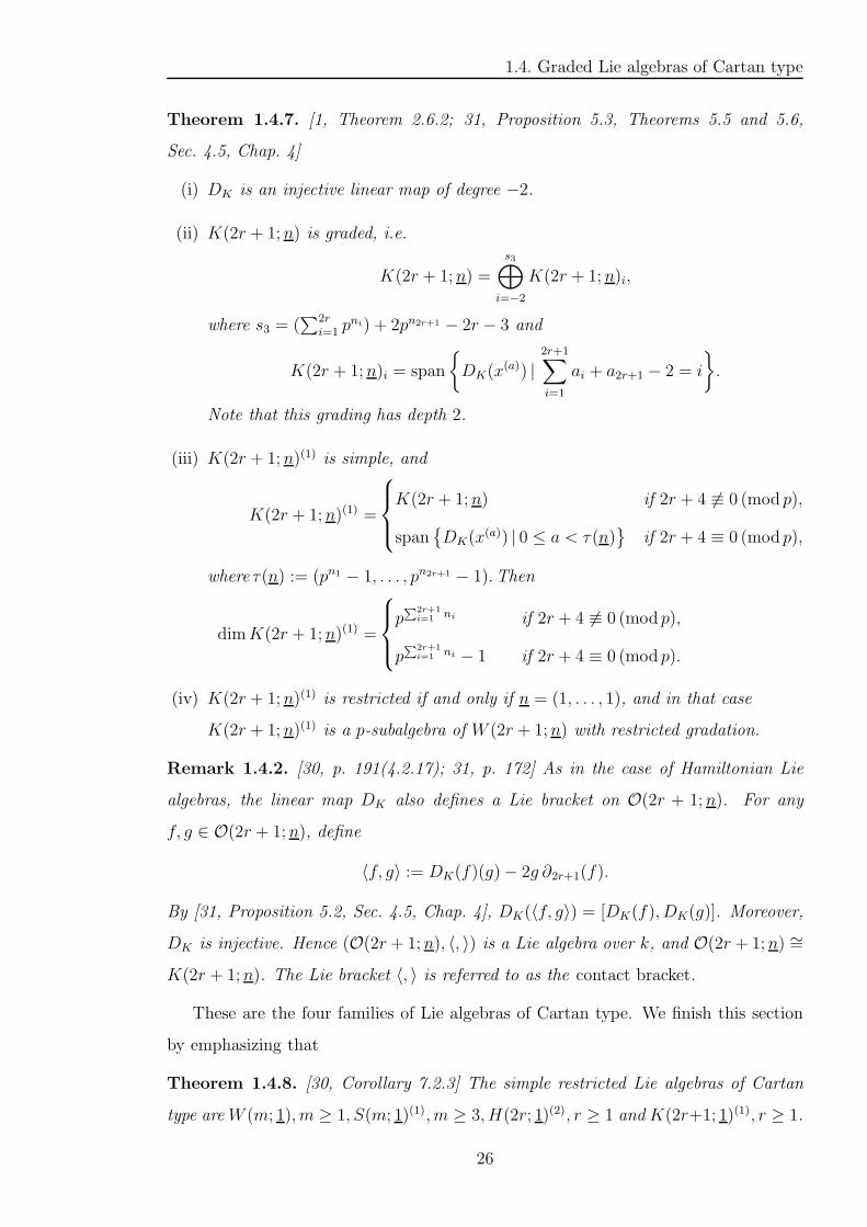
Theorem 1.4.7. [1, Theorem 2.6.2; 31, Proposition 5.3, Theorems 5.5 and 5.6,
Sec. 4.5, Chap. 4]
(i) DK is an injective linear map of degree −2.
(ii) K(2r + 1;n) is graded, i.e.
K(2r + 1;n) =
s3⊕
i=−2
K(2r + 1;n)i,
where s3 = (∑2r
i=1 pni) + 2pn2r+1 − 2r − 3 and
K(2r + 1;n)i = span
DK(x(a)) |
2r+1∑
i=1
ai + a2r+1 − 2 = i
.
Note that this grading has depth 2.
(iii) K(2r + 1;n)(1) is simple, and
K(2r + 1;n)(1) =
K(2r + 1;n) if 2r + 4 6≡ 0 (mod p),
span
DK(x(a)) | 0 ≤ a < τ(n)
if 2r + 4 ≡ 0 (mod p),
where τ(n) := (pn1 − 1, . . . , pn2r+1 − 1).Then
dimK(2r + 1;n)(1) =
p∑2r+1
i=1ni if 2r + 4 6≡ 0 (mod p),
p∑2r+1
i=1ni − 1 if 2r + 4 ≡ 0 (mod p).
(iv) K(2r + 1;n)(1) is restricted if and only if n = (1, . . . , 1), and in that case
K(2r + 1;n)(1) is a p-subalgebra of W (2r + 1;n) with restricted gradation.
Remark 1.4.2. [30, p. 191(4.2.17); 31, p. 172] As in the case of Hamiltonian Lie
algebras, the linear map DK also defines a Lie bracket on O(2r + 1;n). For any
f, g ∈ O(2r + 1;n), define
〈f, g〉 := DK(f)(g)− 2g ∂2r+1(f).
By [31, Proposition 5.2, Sec. 4.5, Chap. 4], DK(〈f, g〉) = [DK(f), DK(g)]. Moreover,
DK is injective. Hence (O(2r + 1;n), 〈, 〉) is a Lie algebra over k, and O(2r + 1;n) ∼=
K(2r + 1;n). The Lie bracket 〈, 〉 is referred to as the contact bracket.
These are the four families of Lie algebras of Cartan type. We finish this section
by emphasizing that
Theorem 1.4.8. [30, Corollary 7.2.3] The simple restricted Lie algebras of Cartan
type areW (m; 1), m ≥ 1, S(m; 1)(1), m ≥ 3, H(2r; 1)(2), r ≥ 1 and K(2r+1; 1)(1), r ≥ 1.
26
1.5. Nilpotent varieties
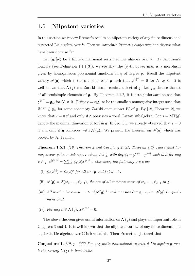
1.5 Nilpotent varieties
In this section we review Premet’s results on nilpotent variety of any finite dimensional
restricted Lie algebra over k. Then we introduce Premet’s conjecture and discuss what
have been done so far.
Let (g, [p]) be a finite dimensional restricted Lie algebra over k. By Jacobson’s
formula (see Definition 1.1.1(3)), we see that the [p]-th power map is a morphism
given by homogeneous polynomial functions on g of degree p. Recall the nilpotent
variety N (g) which is the set of all x ∈ g such that x[p]N
= 0 for N ≫ 0. It is
well known that N (g) is a Zariski closed, conical subset of g. Let gss denote the set
of all semisimple elements of g. By Theorem 1.1.2, it is straightforward to see that
g[p]N
= gss for N ≫ 0. Define e = e(g) to be the smallest nonnegative integer such that
W [p]e ⊆ gss for some nonempty Zariski open subset W of g. By [18, Theorem 2], we
know that e = 0 if and only if g possesses a toral Cartan subalgebra. Let s = MT(g)
denote the maximal dimension of tori in g. In Sec. 1.1, we already observed that s = 0
if and only if g coincides with N (g). We present the theorem on N (g) which was
proved by A. Premet.
Theorem 1.5.1. [19, Theorem 2 and Corollary 2; 21, Theorem 4.2] There exist ho-
mogeneous polynomials ψ0, . . . , ψs−1 ∈ k[g] with deg ψi = pe+s− pe+i such that for any
x ∈ g, x[p]e+s
=∑s−1
i=0 ψi(x)x[p]e+i
. Moreover, the following are true:
(i) ψi(x[p]) = ψi(x)
p for all x ∈ g and i ≤ s− 1.
(ii) N (g) = Z(ψ0, . . . , ψs−1), the set of all common zeros of ψ0, . . . , ψs−1 in g.
(iii) All irreducible components of N (g) have dimension dim g−s, i.e. N (g) is equidi-
mensional.
(iv) For any x ∈ N (g), x[p]e+s
= 0.
The above theorem gives useful information onN (g) and plays an important role in
Chapters 3 and 4. It is well known that the nilpotent variety of any finite dimensional
algebraic Lie algebra over C is irreducible. Then Premet conjectured that
Conjecture 1. [19, p. 563] For any finite dimensional restricted Lie algebra g over
k the variety N (g) is irreducible.
27
1.5. Nilpotent varieties
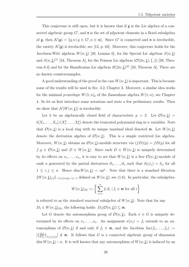
This conjecture is still open, but it is known that if g is the Lie algebra of a con-
nected algebraic group G′, and n is the set of nilpotent elements in a Borel subalgebra
of g, then N (g) = g.n | g ∈ G′, n ∈ n. Since G′ is connected and n is irreducible,
the variety N (g) is irreducible; see [13, p. 64]. Moreover, this conjecture holds for the
Jacobson-Witt algebras W (n; 1) [20, Lemma 6], for the Special Lie algebras S(n; 1)
and S(n; 1)(1) [34, Theorem A], for the Poisson Lie algebras (O(2n; 1), , ) [29, Theo-
rem 6.4] and for the Hamiltonian Lie algebras H(2n; 1)(2) [33, Theorem A]. There are
no known counterexamples.
A good understanding of the proof in the caseW (n; 1) is important. This is because
some of the results will be used in Sec. 3.2, Chapter 3. Moreover, a similar idea works
for the minimal p-envelope W (1;n)p of the Zassenhaus algebra W (1;n); see Chapter
4. So let us first introduce some notations and state a few preliminary results. Then
we show that N (W (n; 1)) is irreducible.
Let k be an algebraically closed field of characteristic p > 2. Let O(n; 1) =
k[X1, . . . , Xn]/(Xp1 , . . . , X
pn) denote the truncated polynomial ring in n variables. Note
that O(n; 1) is a local ring with its unique maximal ideal denoted m. Let W (n; 1)
denote the derivation algebra of O(n; 1). This is a simple restricted Lie algebra.
Moreover, W (n; 1) obtains an O(n; 1)-module structure via (fD)(g) = fD(g) for all
f, g ∈ O(n; 1) and D ∈ W (n; 1). Since each D ∈ W (n; 1) is uniquely determined
by its effects on x1, . . . , xn, it is easy to see that W (n; 1) is a free O(n; 1)-module of
rank n generated by the partial derivatives ∂1, . . . , ∂n such that ∂i(xj) = δij for all
1 ≤ i, j ≤ n. Hence dimW (n; 1) = npn. Note that there is a standard filtration
W (n; 1)(i)−1≤i≤m(p−1)−1 defined on W (n; 1); see (1.6). In particular, the subalgebra
W (n; 1)(0) :=
n∑
i=1
fi ∂i | fi ∈ m for all i
is referred to as the standard maximal subalgebra of W (n; 1). Note that for any
D1 ∈ W (n; 1)(0), the following holds: D1(O(n; 1)) ⊆ m.
Let G denote the automorphism group of O(n; 1). Each σ ∈ G is uniquely de-
termined by its effects on x1, . . . , xn. An assignment σ(xi) = fi extends to an au-
tomorphism of O(n; 1) if and only if fi ∈ m, and the Jacobian Jac(f1, . . . , fn) :=∣
∣
(
∂ fi∂ xj
)
1≤i,j≤n
∣
∣ /∈ m. It follows that G is a connected algebraic group of dimension
dimW (n; 1)−n. It is well known that any automorphism of W (n; 1) is induced by an
28
1.5. Nilpotent varieties
automorphism of O(n; 1) via the rule Dσ = σ D σ−1 for all σ ∈ G and D ∈ W (n; 1).
So we can identify G with the automorphism group of W (n; 1). Note that for any
f ∈ O(n; 1), D ∈ W (n; 1) and σ ∈ G,
(fD)σ = fσDσ, (1.12)
where fσ = f(σ(x1), . . . , σ(xn)); see [20, p. 154]. It follows from (1.12) that if
D1 =∑n
i=1 gi ∂i is an element of W (n; 1), then
Dσ1 =
n∑
i, j=1
gσi
(
∂i(
σ−1(xj))
)σ
∂j ; (1.13)
see [7, Sec. 3]. Note also that G respects the standard filtration of W (n; 1).
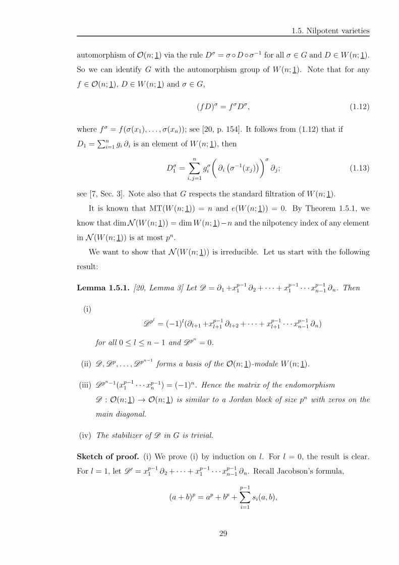
It is known that MT(W (n; 1)) = n and e(W (n; 1)) = 0. By Theorem 1.5.1, we
know that dimN (W (n; 1)) = dimW (n; 1)−n and the nilpotency index of any element
in N (W (n; 1)) is at most pn.
We want to show that N (W (n; 1)) is irreducible. Let us start with the following
result:
Lemma 1.5.1. [20, Lemma 3] Let D = ∂1+xp−11 ∂2+ · · ·+ xp−1
1 · · ·xp−1n−1 ∂n. Then
(i)
Dpl = (−1)l(∂l+1+x
p−1l+1 ∂l+2+ · · ·+ xp−1
l+1 · · ·xp−1n−1 ∂n)
for all 0 ≤ l ≤ n− 1 and Dpn = 0.
(ii) D ,Dp, . . . ,Dpn−1
forms a basis of the O(n; 1)-module W (n; 1).
(iii) Dpn−1(xp−11 · · ·xp−1
n ) = (−1)n. Hence the matrix of the endomorphism
D : O(n; 1) → O(n; 1) is similar to a Jordan block of size pn with zeros on the
main diagonal.
(iv) The stabilizer of D in G is trivial.
Sketch of proof. (i) We prove (i) by induction on l. For l = 0, the result is clear.
For l = 1, let D ′ = xp−11 ∂2+ · · ·+ xp−1
1 · · ·xp−1n−1 ∂n. Recall Jacobson’s formula,
(a + b)p = ap + bp +
p−1∑
i=1
si(a, b),
29
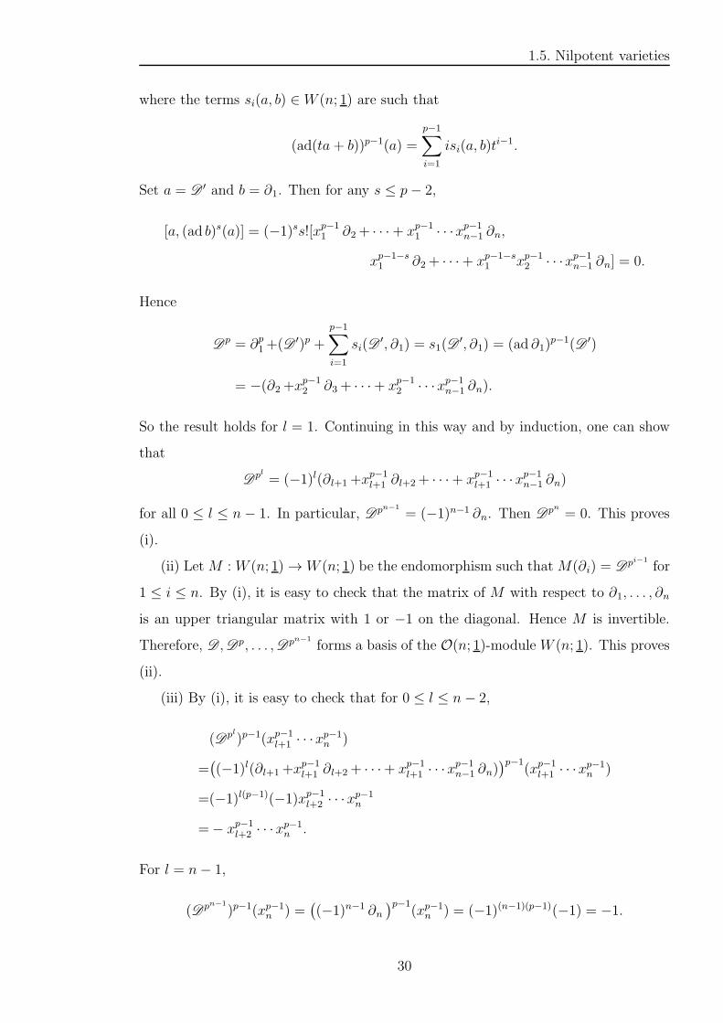
1.5. Nilpotent varieties
where the terms si(a, b) ∈ W (n; 1) are such that
(ad(ta + b))p−1(a) =
p−1∑
i=1
isi(a, b)ti−1.
Set a = D ′ and b = ∂1. Then for any s ≤ p− 2,
[a, (ad b)s(a)] = (−1)ss![xp−11 ∂2+ · · ·+ xp−1
1 · · ·xp−1n−1 ∂n,
xp−1−s1 ∂2+ · · ·+ xp−1−s
1 xp−12 · · ·xp−1
n−1 ∂n] = 0.
Hence
Dp = ∂p1+(D ′)p +
p−1∑
i=1
si(D′, ∂1) = s1(D
′, ∂1) = (ad ∂1)p−1(D ′)
= −(∂2+xp−12 ∂3+ · · ·+ xp−1
2 · · ·xp−1n−1 ∂n).
So the result holds for l = 1. Continuing in this way and by induction, one can show
that
Dpl = (−1)l(∂l+1+x
p−1l+1 ∂l+2+ · · ·+ xp−1
l+1 · · ·xp−1n−1 ∂n)
for all 0 ≤ l ≤ n− 1. In particular, Dpn−1
= (−1)n−1 ∂n. Then Dpn = 0. This proves
(i).
(ii) LetM : W (n; 1)→W (n; 1) be the endomorphism such thatM(∂i) = Dpi−1
for
1 ≤ i ≤ n. By (i), it is easy to check that the matrix of M with respect to ∂1, . . . , ∂n
is an upper triangular matrix with 1 or −1 on the diagonal. Hence M is invertible.
Therefore, D ,Dp, . . . ,Dpn−1
forms a basis of the O(n; 1)-module W (n; 1). This proves
(ii).
(iii) By (i), it is easy to check that for 0 ≤ l ≤ n− 2,
(Dpl)p−1(xp−1l+1 · · ·x
p−1n )
=(
(−1)l(∂l+1+xp−1l+1 ∂l+2+ · · ·+ xp−1
l+1 · · ·xp−1n−1 ∂n)
)p−1(xp−1
l+1 · · ·xp−1n )
=(−1)l(p−1)(−1)xp−1l+2 · · ·x
p−1n
=− xp−1l+2 · · ·x
p−1n .
For l = n− 1,
(Dpn−1
)p−1(xp−1n ) =
(
(−1)n−1 ∂n)p−1
(xp−1n ) = (−1)(n−1)(p−1)(−1) = −1.
30
1.5. Nilpotent varieties
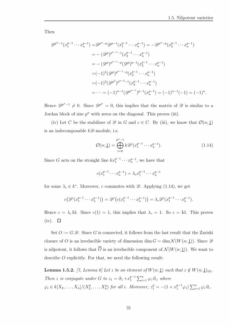
Then
Dpn−1(xp−1
1 · · ·xp−1n ) =D
pn−pDp−1(xp−1
1 · · ·xp−1n ) = −D
pn−p(xp−12 · · ·xp−1
n )
=− (Dp)pn−1−1(xp−1
2 · · ·xp−1n )
=− (Dp)pn−1−p(Dp)p−1(xp−1
2 · · ·xp−1n )
=(−1)2(Dp)pn−1−p(xp−1
3 · · ·xp−1n )
=(−1)2(Dp2)pn−2−1(xp−1
3 · · ·xp−1n )
= · · · = (−1)n−1(Dpn−1
)p−1(xp−1n ) = (−1)n−1(−1) = (−1)n.
Hence Dpn−1 6= 0. Since Dpn = 0, this implies that the matrix of D is similar to a
Jordan block of size pn with zeros on the diagonal. This proves (iii).
(iv) Let C be the stabilizer of D in G and c ∈ C. By (iii), we know that O(n; 1)
is an indecomposable kD-module, i.e.
O(n; 1) =
pn−1⊕
i=0
kD i(xp−11 · · ·xp−1
n ). (1.14)
Since G acts on the straight line kxp−11 · · ·xp−1
n , we have that
c(xp−11 · · ·xp−1
n ) = λcxp−11 · · ·xp−1
n
for some λc ∈ k∗. Moreover, c commutes with D . Applying (1.14), we get
c(
Di(xp−1
1 · · ·xp−1n )
)
= Di(
c(xp−11 · · ·xp−1
n ))
= λcDi(xp−1
1 · · ·xp−1n ).
Hence c = λc Id. Since c(1) = 1, this implies that λc = 1. So c = Id. This proves
(iv).
Set O := G.D . Since G is connected, it follows from the last result that the Zariski
closure of O is an irreducible variety of dimension dimG = dimN (W (n; 1)). Since D
is nilpotent, it follows that O is an irreducible component of N (W (n; 1)). We want to
describe O explicitly. For that, we need the following result:
Lemma 1.5.2. [7, Lemma 6] Let z be an element of W (n; 1) such that z /∈ W (n; 1)(0).
Then z is conjugate under G to z1 = ∂1 +xp−11
∑n
i=1 ϕi ∂i, where
ϕi ∈ k[X2, . . . , Xn]/(Xp2 , . . . , X
pn) for all i. Moreover, zp1 = −(1 + xp−1
1 ϕ1)∑n
i=1 ϕi ∂i.
31

1.5. Nilpotent varieties
Sketch of proof. In [7, Sec. 3], S. P. Demushkin used the convention that for any
D ∈ W (n; 1) and Φ ∈ G, DΦ = Φ−1 D Φ. Our convention is that DΦ = ΦD Φ−1.
So we need to slightly modify his proof.
Let z =∑n
i=1 fi ∂i be an element of W (n; 1) such that z /∈ W (n; 1)(0). Then
fµ(0, . . . , 0) 6= 0 for some 1 ≤ µ ≤ n. If µ 6= 1, then we show that z is conjugate under
G to∑n
i=1 fi ∂i with f1(0, . . . , 0) 6= 0. Let Φ ∈ G be such that Φ(x1) = xµ,Φ(xµ) = x1
and Φ(xj) = xj for j 6= 1, µ. Then Φ−1(x1) = xµ,Φ−1(xµ) = x1 and Φ−1(xj) = xj for
j 6= 1, µ. By (1.13),
zΦ =n
∑
i, j=1
fΦi
(
∂i(
Φ−1(xj))
)Φ
∂j = fΦµ ∂1+f
Φ1 ∂µ+
∑
i 6=1, µ
fΦi ∂i .
Since fΦµ (0, . . . , 0) = fµ(0, . . . , 0) 6= 0, we may assume from the beginning that
z =∑n
i=1 fi ∂i with f1(0, . . . , 0) 6= 0.
Let Φ2 ∈ G be such that Φ2(x1) = f1(0, . . . , 0)x1 and Φ2(xj) = xj for 2 ≤ j ≤ n.
Then Φ−12 (x1) = f−1
1 (0, . . . , 0)x1 and Φ−12 (xj) = xj for 2 ≤ j ≤ n. Applying Φ2 to z,
we get
zΦ2 =n
∑
i, j=1
fΦ2
i
(
∂i(
Φ−12 (xj)
)
)Φ2
∂j = fΦ2
1 f−11 (0, . . . , 0) ∂1+
n∑
i=2
fΦ2
i ∂i .
Since fΦ2
1 (0, . . . , 0) = f1(0, . . . , 0), we may assume from the beginning that
z =∑n
i=1 fi ∂i with f1(0, . . . , 0) = 1.
Let Φ3 ∈ G be such that Φ3(x1) = x1 and Φ3(xj) = xj + αjx1, where αj =
fj(0 . . . , 0) for 2 ≤ j ≤ n. Then Φ−13 (x1) = x1 and Φ−1
3 (xj) = xj −αjx1 for 2 ≤ j ≤ n.
Applying Φ3 to z, we get
zΦ3 =n
∑
i, j=1
fΦ3
i
(
∂i(
Φ−13 (xj)
)
)Φ3
∂j = fΦ3
1 ∂1+n
∑
i=2
(fΦ3
i − αifΦ3
1 ) ∂i .
Hence we may assume from the beginning that z =∑n
i=1 fi ∂i with f1(0, . . . , 0) = 1
and fi(0, . . . , 0) = 0 for all 2 ≤ i ≤ n. Then we can write
f1 = 1 +
m(p−1)∑
l=1
f1,l and fi =
m(p−1)∑
l=1
fi,l (1.15)
for some f1,l, fi,l ∈ m with deg f1,l = deg fi,l = l. Let Φ4 ∈ G be such that Φ−14 (xj) =
xj+gj for 1 ≤ j ≤ n, where gj are elements of m with the same degree ν ≥ 2. Applying
32

1.5. Nilpotent varieties
Φ4 to z, we get
zΦ4 =
n∑
i, j=1
fΦ4
i
(
∂i(
Φ−14 (xj)
)
)Φ4
∂j =
n∑
i, j=1
fΦ4
i
(
∂i(
xj + gj)
)Φ4
∂j . (1.16)
Substituting (1.15) into (1.16) and expanding out, we get
zΦ4 ≡n
∑
i=1
(
fi + ∂1(gi))
∂i (modW (n; 1)(ν−1)).
Since fi(0, . . . , 0) = δi1, we can rewrite the above as
zΦ4 ≡ ∂1+(
f1 − 1 + ∂1(g1))
∂1+n
∑
i=2
(
fi + ∂1(gi))
∂i (modW (n; 1)(ν−1)),
where f1− 1 + ∂1(g1), fi + ∂1(gi) ∈ m with degrees strictly less than ν. It follows that
z is conjugate under G to
z1 = ∂1+xp−11
n∑
i=1
ϕi ∂i,
where ϕi ∈ k[X2, . . . , Xn]/(Xp2 , . . . , X
pn).
It remains to show that zp1 = −(1 + xp−11 ϕ1)
∑n
i=1 ϕi ∂i. Note that
z1(x1) = 1 + xp−11 ϕ1,
z21(x1) = (p− 1)xp−21 ϕ1,
. . .
zη1(x1) = (p− 1) · · · (p− η + 1)xp−η1 ϕ1 for 2 ≤ η ≤ p− 1, and
zp1(x1) = (p− 1)!(1 + xp−11 ϕ1)ϕ1 = −(1 + xp−1
1 ϕ1)ϕ1.
Similarly, one can show that zp1(xi) = −(1 + xp−11 ϕ1)ϕi for 2 ≤ i ≤ n. Hence
zp1 = −(1 + xp−11 ϕ1)
n∑
i=1
ϕi ∂i .
This completes the sketch of proof.
Recall that D = ∂1+xp−11 ∂2 + · · ·+x
p−11 · · ·xp−1
n−1 ∂n. We can now describe O = G.D
as:
Lemma 1.5.3. [20, Lemma 4]
O =
D ∈ N (W (n; 1)) |Dpn−1
6∈ W (n; 1)(0)
.
33
1.5. Nilpotent varieties
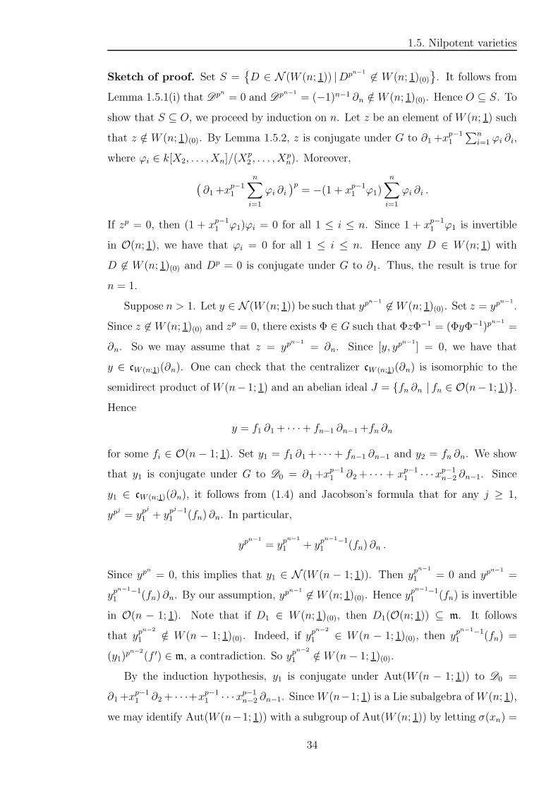
Sketch of proof. Set S =
D ∈ N (W (n; 1)) |Dpn−1
6∈ W (n; 1)(0)
. It follows from
Lemma 1.5.1(i) that Dpn = 0 and Dpn−1
= (−1)n−1 ∂n /∈ W (n; 1)(0). Hence O ⊆ S. To
show that S ⊆ O, we proceed by induction on n. Let z be an element of W (n; 1) such
that z /∈ W (n; 1)(0). By Lemma 1.5.2, z is conjugate under G to ∂1+xp−11
∑n
i=1 ϕi ∂i,
where ϕi ∈ k[X2, . . . , Xn]/(Xp2 , . . . , X
pn). Moreover,
(
∂1+xp−11
n∑
i=1
ϕi ∂i)p
= −(1 + xp−11 ϕ1)
n∑
i=1
ϕi ∂i .
If zp = 0, then (1 + xp−11 ϕ1)ϕi = 0 for all 1 ≤ i ≤ n. Since 1 + xp−1
1 ϕ1 is invertible
in O(n; 1), we have that ϕi = 0 for all 1 ≤ i ≤ n. Hence any D ∈ W (n; 1) with
D 6∈ W (n; 1)(0) and Dp = 0 is conjugate under G to ∂1. Thus, the result is true for
n = 1.
Suppose n > 1. Let y ∈ N (W (n; 1)) be such that ypn−1
6∈ W (n; 1)(0). Set z = ypn−1
.
Since z 6∈ W (n; 1)(0) and zp = 0, there exists Φ ∈ G such that ΦzΦ−1 = (ΦyΦ−1)p
n−1
=
∂n. So we may assume that z = ypn−1
= ∂n. Since [y, ypn−1
] = 0, we have that
y ∈ cW (n;1)(∂n). One can check that the centralizer cW (n;1)(∂n) is isomorphic to the
semidirect product of W (n− 1; 1) and an abelian ideal J = fn ∂n | fn ∈ O(n− 1; 1).
Hence
y = f1 ∂1+ · · ·+ fn−1 ∂n−1+fn ∂n
for some fi ∈ O(n − 1; 1). Set y1 = f1 ∂1+ · · ·+ fn−1 ∂n−1 and y2 = fn ∂n. We show
that y1 is conjugate under G to D0 = ∂1+xp−11 ∂2+ · · · + xp−1
1 · · ·xp−1n−2 ∂n−1. Since
y1 ∈ cW (n;1)(∂n), it follows from (1.4) and Jacobson’s formula that for any j ≥ 1,
ypj
= ypj
1 + ypj−1
1 (fn) ∂n. In particular,
ypn−1
= ypn−1
1 + ypn−1−1
1 (fn) ∂n .
Since ypn
= 0, this implies that y1 ∈ N (W (n − 1; 1)). Then ypn−1
1 = 0 and ypn−1
=
ypn−1−1
1 (fn) ∂n. By our assumption, ypn−1
6∈ W (n; 1)(0). Hence ypn−1−11 (fn) is invertible
in O(n − 1; 1). Note that if D1 ∈ W (n; 1)(0), then D1(O(n; 1)) ⊆ m. It follows
that ypn−2
1 /∈ W (n − 1; 1)(0). Indeed, if ypn−2
1 ∈ W (n − 1; 1)(0), then ypn−1−1
1 (fn) =
(y1)pn−2
(f ′) ∈ m, a contradiction. So ypn−2
1 /∈ W (n− 1; 1)(0).
By the induction hypothesis, y1 is conjugate under Aut(W (n − 1; 1)) to D0 =
∂1+xp−11 ∂2+ · · ·+x
p−11 · · ·xp−1
n−2 ∂n−1. Since W (n−1; 1) is a Lie subalgebra ofW (n; 1),
we may identify Aut(W (n−1; 1)) with a subgroup of Aut(W (n; 1)) by letting σ(xn) =
34
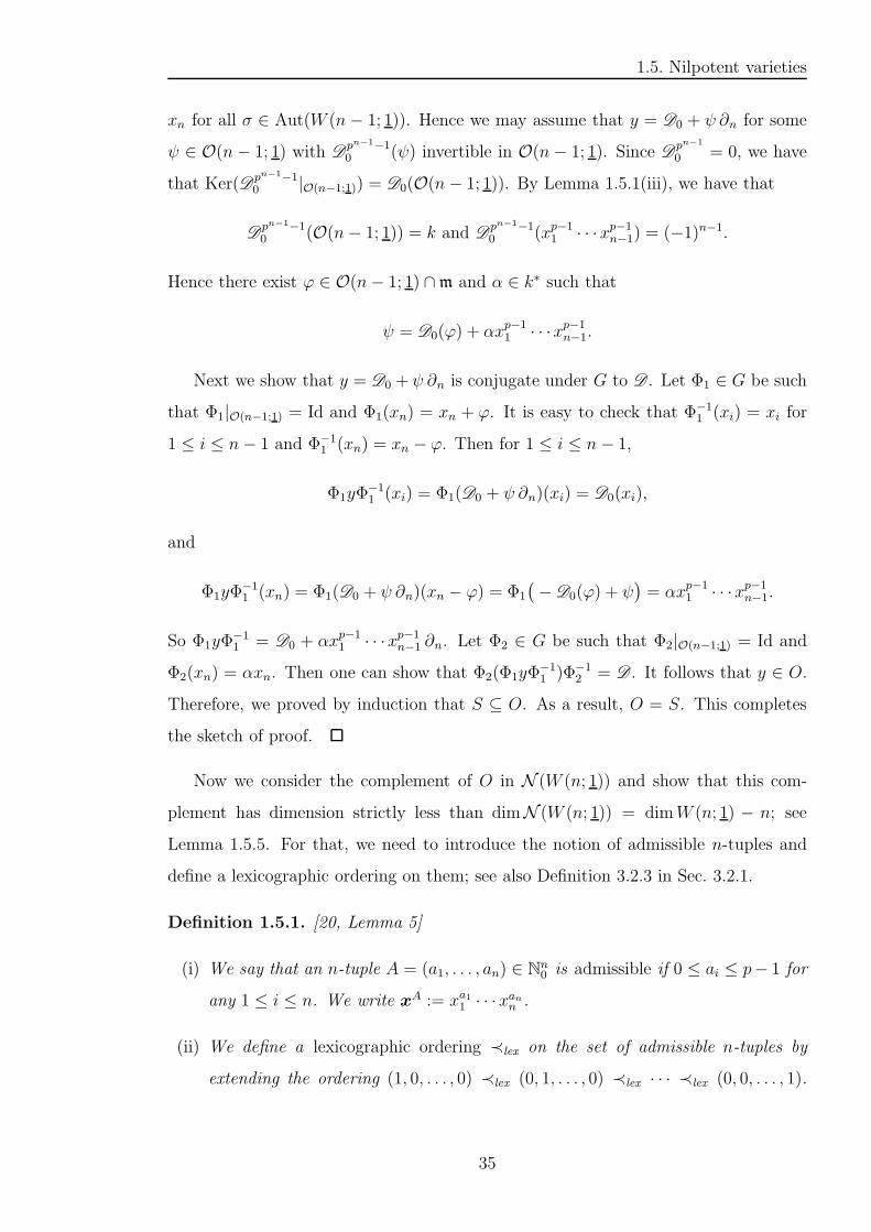
1.5. Nilpotent varieties
xn for all σ ∈ Aut(W (n− 1; 1)). Hence we may assume that y = D0 + ψ ∂n for some
ψ ∈ O(n − 1; 1) with Dpn−1−10 (ψ) invertible in O(n− 1; 1). Since D
pn−1
0 = 0, we have
that Ker(Dpn−1−10 |O(n−1;1)) = D0(O(n− 1; 1)). By Lemma 1.5.1(iii), we have that
Dpn−1−10 (O(n− 1; 1)) = k and D
pn−1−10 (xp−1
1 · · ·xp−1n−1) = (−1)n−1.
Hence there exist ϕ ∈ O(n− 1; 1) ∩m and α ∈ k∗ such that
ψ = D0(ϕ) + αxp−11 · · ·xp−1
n−1.
Next we show that y = D0 + ψ ∂n is conjugate under G to D . Let Φ1 ∈ G be such
that Φ1|O(n−1;1) = Id and Φ1(xn) = xn + ϕ. It is easy to check that Φ−11 (xi) = xi for
1 ≤ i ≤ n− 1 and Φ−11 (xn) = xn − ϕ. Then for 1 ≤ i ≤ n− 1,
Φ1yΦ−11 (xi) = Φ1(D0 + ψ ∂n)(xi) = D0(xi),
and
Φ1yΦ−11 (xn) = Φ1(D0 + ψ ∂n)(xn − ϕ) = Φ1
(
−D0(ϕ) + ψ)
= αxp−11 · · ·xp−1
n−1.
So Φ1yΦ−11 = D0 + αxp−1
1 · · ·xp−1n−1 ∂n. Let Φ2 ∈ G be such that Φ2|O(n−1;1) = Id and
Φ2(xn) = αxn. Then one can show that Φ2(Φ1yΦ−11 )Φ−1
2 = D . It follows that y ∈ O.
Therefore, we proved by induction that S ⊆ O. As a result, O = S. This completes
the sketch of proof.
Now we consider the complement of O in N (W (n; 1)) and show that this com-
plement has dimension strictly less than dimN (W (n; 1)) = dimW (n; 1) − n; see
Lemma 1.5.5. For that, we need to introduce the notion of admissible n-tuples and
define a lexicographic ordering on them; see also Definition 3.2.3 in Sec. 3.2.1.
Definition 1.5.1. [20, Lemma 5]
(i) We say that an n-tuple A = (a1, . . . , an) ∈ Nn0 is admissible if 0 ≤ ai ≤ p− 1 for
any 1 ≤ i ≤ n. We write xA := xa11 · · ·x
ann .
(ii) We define a lexicographic ordering ≺lex on the set of admissible n-tuples by
extending the ordering (1, 0, . . . , 0) ≺lex (0, 1, . . . , 0) ≺lex · · · ≺lex (0, 0, . . . , 1).
35
1.5. Nilpotent varieties
Explicitly, for any two non-equal admissible n-tuples A = (a1, . . . , an) and A′ =
(a′1, . . . , a′n),
A = (a1, . . . , an) ≺lex (a′1, . . . , a
′n) = A′ if and only if ai < a′i,
where i is the largest number in 1, . . . , n for which ai 6= a′i.
Lemma 1.5.4. [20, Lemma 5] The action of D = ∂1+xp−11 ∂2+ · · ·+ xp−1
1 · · ·xp−1n−1 ∂n
on O(n; 1) is compatible with the lexicographic ordering ≺lex defined in Definition 1.5.1.
Explicitly, for any admissible n-tuple A 6= (0, . . . , 0), we have that D(xA) = λAxA′
,
where λA ∈ k∗ and A′ ≺lex A. It follows from the explicit formulas for A′ in the proof
that if B and C are admissible n-tuples such that B,C 6= (0, . . . , 0) and B ≺lex C,
then B′ ≺lex C′.
Sketch of proof. Let A = (a1, . . . , an) 6= (0, . . . , 0) be any admissible n-tuple. We
first show that D(xA) = λAxA′
, where λA ∈ k∗ and A′ ≺lex A. If a1 ≥ 1, then
D(xA) = a1xa1−11 xa22 · · ·x
ann = a1x
A′
,
where A′ = (a1 − 1, a2, . . . , an). It is easy to see that
A′ = (a1 − 1, a2, . . . , an) ≺lex (a1, . . . , an) = A.
If a1 = · · · = as−1 = 0 and as ≥ 1, then
D(xA) = asxp−11 xp−1
2 · · ·xp−1s−1x
as−1s x
as+1
s+1 · · ·xann = asx
A′
,
where A′ = (p− 1, . . . , p− 1, as − 1, as+1, . . . , an). It is easy to see that
A′ = (p− 1, . . . , p− 1, as − 1, as+1, . . . , an) ≺lex (0, . . . , 0, as, as+1, . . . , an) = A.
Hence D(xA) = λAxA′
for some λA ∈ k∗ and A′ ≺lex A. If A′ 6= (0, . . . , 0), then
applying D to xA′
, we get D(xA′
) = λA′xA′′
, where λA′ ∈ k∗ and A′′ ≺lex A′. It follows
from the explicit formulas for A′ that if B and C are admissible n-tuples such that
B,C 6= (0, . . . , 0) and B ≺lex C, then B′ ≺lex C
′. Hence the action of D is compatible
with the lexicographic ordering ≺lex. This completes the sketch of proof.
Lemma 1.5.5. [20, Lemma 5] Set
N0 :=
D ∈ N (W (n; 1)) |Dpn−1
∈ W (n; 1)(0)
.
Then
dimN0 < dimW (n; 1)− n.
36
1.5. Nilpotent varieties
Sketch of proof. By Theorem 1.6.8, it is enough to construct an (n+1)-dimensional
subspace V in W (n; 1) such that V ∩ N0 = 0. Set V := Tn ⊕ kD , where Tn
is a maximal torus in W (n; 1) with basis x1 ∂1, . . . , xn ∂n, and D is the nilpotent
element in Lemma 1.5.1. We show that V ∩ N0 = 0. Suppose the contrary, i.e.
V ∩ N0 6= 0. Then t + D ∈ N0 for some 0 6= t ∈ Tn. Note that for any admissible
n-tuple A = (a1, . . . , an), the straight line kxA is invariant under Tn and corresponds
to the weight c1θ1 + · · · + cnθn, where θ1, . . . , θn is a basis of T ∗n dual to the basis
x1 ∂1, . . . , xn ∂n and ci ≡ ci (mod p). By Lemma 1.5.4, we know the action of D on
O(n; 1) is compatible with the lexicographic ordering ≺lex. Hence for the admissible
n-tuple δ = (p− 1, . . . , p− 1), we have that
(t+ D)pn−1(xδ) = D
pn−1(xδ) +∑
A≻lex(0,...,0)
λAxA for some λA ∈ k
∗.
By Lemma 1.5.1(iii), Dpn−1(xδ) = (−1)n. Hence (t + D)pn−1(xδ) is invertible in
O(n; 1). But t + D ∈ N0 by our assumption. Hence (t + D)pn−1 ∈ W (n; 1)(0). Note
that if D1 ∈ W (n; 1)(0), then D1(O(n; 1)) ⊆ m. In particular, (t + D)pn−1(xδ) ∈ m,
which is not invertible. This is a contradiction. Hence V ∩ N0 = 0. Applying
Theorem 1.6.8, we get the desired result. This completes the sketch of proof.
We are now ready to prove that
Theorem 1.5.2. [20, Lemma 6] The variety N (W (n; 1)) is irreducible.
Sketch of proof. By Theorem 1.5.1, we know that N (W (n; 1)) is equidimensional of
dimension dimW (n; 1)−n. By Lemma 1.5.1, we know that O = G.D is an irreducible
component of N (W (n; 1)). Let Z1, . . . , Zt be pairwise distinct irreducible components
of N (W (n; 1)), and set Z1 = O. Suppose t ≥ 2. Observe that Z2 ∩ O = ∅. Hence
Z2 ⊆ N (W (n; 1)) \O = N0; see Lemma 1.5.3. Then
dimW (n; 1)− n = dimZ2 ≤ dimN0 < dimW (n; 1)− n
by Lemma 1.5.5. This is a contradiction. Hence t = 1 and N (W (n; 1)) is irreducible.
This completes the sketch of proof.
By a similar argument, the nilpotent variety of S(n; 1) (respectively S(n; 1)(1))
is proved to be irreducible. By Remark 1.4.1, we see that the Poisson Lie algebra
37
1.6. Some useful theorems
(O(2n; 1), , ) is closely related to H(2n; 1)(2). In fact, (O(2n; 1)/k)(1) ∼= H(2n; 1)(2).
So the proof for H(2n; 1)(2) relies heavily on Skryabin’s work for (O(2n; 1), , ); see
[29, Lemma 1.5 and Theorem 6.4].
1.6 Some useful theorems
We present three Block’s theorems which will be used in Chapter 3. The first one
is useful for part (b) of the sketch proof of Theorem 3.2.2 which characterizes all
regular elements of the mth Jacobson Witt algebra W (m; 1). Let us begin with some
definitions.
Definition 1.6.1. [2, p. 433] Let B be a ring (not necessarily associative or has
a unit element). A derivation of B is an additive mapping d : B → B such that
d(ab) = d(a)b + ad(b) for all a, b ∈ B. Let D be a set of derivations of B. By a
D-ideal of B we mean an ideal of B which is invariant under D. The ring B is called
D-simple ( d-simple if D consists of a single derivation d) if B2 6= 0 and if B has no
proper D-ideals. Also B is called differentiably simple if it is D-simple for some set
of derivations D of B, and hence for the set of all derivations of B.
Note that the above definitions are also used for algebras over a ring C and the
derivations are assumed to be C-linear. Suppose B is a differentiably simple commu-
tative associative ring. At characteristic 0, B is an integral domain. In particular, if
B has a minimal ideal then B is a field; see [2, Sec. 4, p. 441]. Now suppose B has
prime characteristic. The following theorem determines B:
Theorem 1.6.1. [2, Theorem 4.1] Let B be a differentiably simple commutative as-
sociative ring of prime characteristic p, and let R = x ∈ B | xp = 0. If Rx = 0 for
some x 6= 0 in B (this will hold, e.g. if B has a minimal ideal), then there is a subfield
E of B and an r ≥ 0 such that B ∼= O(r; 1) as E-algebras. Here E may be taken to
be any maximal subfield of B containing the subfield F of differential constants (i.e.
elements of B which are annihilated by all derivations).
The second theorem describes the derivation algebra of a Lie algebra in the follow-
ing form:
38

1.6. Some useful theorems
Theorem 1.6.2. [30, Corollary 3.3.4] Let S be a finite dimensional simple algebra
such that S2 6= (0). Then
Der(
S ⊗O(m;n))
=(
(DerS)⊗O(m;n))
⋊(
IdS ⊗DerO(m;n))
∼=(
(DerS)⊗O(m′; 1))
⋊(
IdS ⊗W (m′; 1))
for some m′ ∈ N.
The last line follows from the fact that considered just as an algebra, O(m;n) is
isomorphic to the truncated polynomial ring O(m′; 1) in m′ = n1+ · · ·+nm variables;
see [30, p. 64]. Hence DerO(m;n) ∼= DerO(m′; 1) =W (m′; 1).
The third theorem describes the structure of any finite dimensional semisimple Lie
algebras. Recall the socle of a finite dimensional semisimple Lie algebra L, denoted
Soc(L), is the direct sum ⊕jIj of minimal ideals Ij of L. In particular, these ideals Ij
are irreducible L-modules.
Theorem 1.6.3. [2, Theorem 9.3; 30, Corollary 3.3.6] Let L be a finite dimensional
semisimple Lie algebra. Then there are simple Lie algebras Si and truncated polynomial
rings O(mi; 1) such that Soc(L) =⊕t
i=1 Si ⊗ O(mi; 1) and L acts faithfully on it.
Moreover,
t⊕
i=1
Si ⊗O(mi; 1) ⊂ L ⊂t
⊕
i=1
(
(DerSi)⊗O(mi; 1))
⋊(
IdSi⊗W (mi; 1)
)
.
We will see in Chapter 2 that Premet’s conjecture can be reduced to the case where
the Lie algebra is semisimple. The above theorem leads us to the study of nilpotent
varieties for a particular class of semisimple restricted Lie algebras, namely the ones
that are sandwiched betweent
⊕
i=1
Si ⊗O(mi; 1)
andt
⊕
i=1
(
(DerSi)⊗O(mi; 1))
⋊(
IdSi⊗W (mi; 1)
)
.
We finish this section with some useful theorems from algebraic geometry.
Definition 1.6.2. [9, p. 91, 3.7] A morphism ψ : V →W of affine varieties is called
dominant if the image ψ(V ) is dense in W , i.e. ψ(V ) =W .
39
1.6. Some useful theorems
Given any morphism of irreducible affine varieties, proving directly its dominance
may be difficult. However, we can show its differential map is surjective. More pre-
cisely,
Theorem 1.6.4 (Differential Criterion for Dominance [8, Proposition 1.4.15]).
Let ψ : V → W be a morphism of irreducible affine varieties. Let v be a smooth
point in V such that ψ(v) is a smooth point in W . If the differential of ψ at v,
dvψ : TvV → Tψ(v)W , is surjective, then the morphism ψ is dominant.
Once we know that a morphism is dominant, we can get a nonempty open set from
the image of the morphism. Specifically,
Theorem 1.6.5. [8, Corollary 2.2.8] Let ψ : V → W be a dominant morphism of
irreducible affine varieties. Then the image of any nonempty open subset U ⊆ V
contains a nonempty open subset of W .
Finally, we present some theorems on dimensions. The first two relate to the
dimension of fibres.
Theorem 1.6.6. [6, Sec. 4.4, Chap. 2, II; 28, Theorem 1.25] Let ψ : V → W be a
dominant morphism of irreducible varieties. Suppose that dim V = m and dimW = n.
Then m ≥ n, and
(i) dimF ≥ m− n for any w ∈ W and for any component F of the fibre ψ−1(w);
(ii) there exists a nonempty open subset U ⊂ W such that dimψ−1(u) = m − n for
all u ∈ U .
Theorem 1.6.7 (Chevalley’s Semi-continuity Theorem [6, Sec. 4.5, Chap. 2, II]).
Let ψ : V →W be a morphism of affine varieties. Then for every r ∈ N0, the set
Vr =
v ∈ V | dimψ−1(ψ(v)) ≥ r
is Zariski closed in V .
The last theorem in this section relates to the dimension of intersections in An.
Theorem 1.6.8 (Affine Dimension Theorem [9, Proposition 7.1, Chap. I]).
Let V,W be varieties of dimensions r, s in An. Then every irreducible component U
of V ∩W has dimension ≥ r + s− n.
40
1.7. Overview of results
1.7 Overview of results
Chapter 2. Let k be an algebraically closed field of characteristic p > 0. We start with
Premet’s conjecture which states that the nilpotent variety of any finite dimensional
restricted Lie algebra over k is irreducible. We prove that this conjecture can be
reduced to the semisimple case.
Theorem 1 (see Theorem 2.0.1). Let (g, [p]) be a finite dimensional restricted Lie
algebra over k. Let Rad g denote the radical of g. Then N (g) is irreducible if and only
if N (g/Radg) is irreducible.
The proof is done by induction on dim g and it relies on a result from algebraic
geometry (see Lemma 2.0.1). Since semisimple Lie algebras are not always direct sums
of simple ideals in prime characteristic, the reduction of Premet’s conjecture to the
simple case is very non-trivial.
Chapter 3. We start to look at a particular class of semisimple restricted Lie
algebras and verify Premet’s conjecture in that case.
By Theorem 1.6.3, we know that any finite dimensional semisimple Lie algebra is
sandwiched betweent
⊕
i=1
Si ⊗O(mi; 1)
andt
⊕
i=1
(
(DerSi)⊗O(mi; 1))
⋊(
IdSi⊗W (mi; 1)
)
for some simple Lie algebras Si and truncated polynomial rings O(mi; 1) with
DerO(mi; 1) = W (mi; 1). Thus, to verify Premet’s conjecture, we begin with the
simplest example, g = (sl2 ⊗O(1; 1))⋊ (Idsl2 ⊗k ∂), where sl2 is the special linear Lie
algebra, O(1; 1) is the truncated polynomial ring k[X ]/(Xp), and ∂ = ddx
which acts
on sl2 ⊗O(1; 1) in the natural way. We assume further that char k = p > 2. So sl2 is
a simple restricted Lie algebra over k with all its derivations inner. We prove that the
maximal dimension of tori in g is 1, and the nilpotency index of any element in N (g)
is at most p2. It follows from Theorem 1.5.1 that dimN (g) = 3p. After gathering
these pieces of information, we are ready to prove that
Theorem 2 (see Theorem 3.1.1). The variety N (g) is irreducible.
41
1.7. Overview of results
We will see that the argument in the proof is quite general. It works if we replace
sl2 by any Lie algebra g2 = Lie(G2), where G2 is a reductive algebraic group. Then
we extend the example g to the semisimple restricted Lie algebra
L := (S ⊗O(m; 1))⋊ (IdS ⊗D),
where S is a simple restricted Lie algebra over k such that adS = DerS and N (S)
is irreducible, O(m; 1) = k[X1, . . . , Xm]/(Xp1 , . . . , X
pm) is the truncated polynomial
ring in m ≥ 2 variables, and D is a restricted transitive subalgebra of W (m; 1) =
DerO(m; 1) such that N (D) is irreducible. We split our study on N (L) into three
sections. In the first section, we study nilpotent elements of D. Then we study
nilpotent elements of L and carry out some calculations using Lemma 1.1.1. We
finally prove that
Theorem 3 (see Theorem 3.2.3). The variety N (L) is irreducible.
As a remark, we see from the above that Premet’s conjecture holds for
t⊕
i=1
(Si ⊗O(mi; 1))⋊ (IdSi⊗Di),
where each Si is a simple restricted Lie algebra over k such that adSi = DerSi
and N (Si) is irreducible, O(mi; 1) are truncated polynomial rings, and each Di is
a restricted transitive subalgebra of W (mi; 1) = DerO(mi; 1) such that N (Di) is
irreducible.
Chapter 4. This is our final chapter. It corresponds to a paper [3] of the author
which was published in the Journal of Algebra and Its Applications. We assume that
char k = p > 3 and n ∈ N≥2. Then the Zassenhaus algebra, denoted L = W (1;n),
provides the first example of a simple, non-restricted Lie algebra. We can embed L
into its minimal p-envelope Lp = W (1;n)p. This restricted Lie algebra is semisimple.
By [37, Theorem 4.8(i)], the variety N (L) := N (Lp)∩L is reducible. So investigating
the variety N (Lp) becomes critical.
Let N denote the nilpotent variety of Lp. We split our study on N into three
sections. In the first section, we focus on nilpotent elements of Lp and carry out some
calculations using Jacobson’s formula. This work enables us to identify an irreducible
component Nreg of N . Moreover, we can explicitly describe it as:
42
1.7. Overview of results
Proposition 1 (see Proposition 4.2.1 and Lemma 4.2.7).
Nreg = G.(∂+k ∂p+ · · ·+ k ∂pn−1
),
where G = Aut(Lp).
In the final section, we show that the complement of Nreg in N , denoted Nsing,
has dimNsing < dimN . The proof is similar to Premet’s proof for the Jacobson-Witt
algebra W (n; 1); see Lemma 1.5.5. But we have to construct a new subspace V of Lp
such that dimV = n + 1 and V ∩ Nsing = 0; see Proposition 4.2.2. Combining all
these results, we are able to prove the last theorem in the thesis:
Theorem 4 (see Theorem 4.2.1). The variety N = N (Lp) coincides with the Zariski
closure of
Nreg = G.(∂+k ∂p+ · · ·+ k ∂pn−1
)
and hence is irreducible.
43
Chapter 2
Reduction of Premet’s conjecture
to the semisimple case
Let (g, [p]) be a finite dimensional restricted Lie algebra over k. Recall Premet’s
conjecture which states that the variety N (g) = x ∈ g | x[p]N
= 0 for N ≫ 0 is
irreducible. In this short chapter we show that this conjecture can be reduced to the
case where g is semisimple. For that, we need the following result from algebraic
geometry. It gives a criterion for a variety to be irreducible.
Lemma 2.0.1. Let ψ : X → Y be a surjective morphism of algebraic varieties such
that
(i) Y is irreducible,
(ii) all fibres of ψ are irreducible and have the same dimension d, and
(iii) X is equidimensional.
Then X is irreducible.
Proof. Let X = X1 ∪ · · · ∪ Xt be the decomposition of X into pairwise distinct
irreducible components Xi. Suppose t ≥ 2. Then for any y ∈ Y ,
ψ−1(y) =t⋃
i=1
(
ψ−1(y) ∩Xi
)
.
Since ψ−1(y) is irreducible, we have that ψ−1(y) = ψ−1(y) ∩Xi for some i.
44
For every i, define Oi := Xi \⋃
j 6=i(Xi ∩Xj). Then Oi is a nonempty open subset
of Xi. If y ∈ ψ(Oi), then the fibre ψ−1(y) is not contained in ψ−1(y) ∩ Xj for every
j 6= i. Hence for any y ∈ ψ(Oi),
ψ−1(y) = ψ−1(y) ∩Xi. (2.1)
Next we show that there is a unique irreducible component Xj of X such that
Y = ψ(Xj). Since ψ is surjective, we have that Y =⋃ti=1 ψ(Xi). But Y is irreducible,
so that Y = ψ(Xj) for some j. By definition of Oj, we also have that Y = ψ(Oj),
i.e. ψ(Oj) is dense in Y . Thus, ψ(Oj) contains a nonempty open subset Z of Y .
By (2.1), we have that for any y ∈ Z, ψ−1(y) = ψ−1(y) ∩ Xj. This means that if
i 6= j, then Xi \ (Xi∩Xj) ⊆ ψ−1(Y \Z). As a result, Xi = Xi \ (Xi ∩Xj) is contained
in ψ−1(Y \ Z). This implies that ψ(Xi) 6= Y for every i 6= j. So there is a unique
irreducible component Xj of X such that Y = ψ(Xj).
We now show that for every i, dimXi = dimψ(Xi) + d. Consider the restriction
of ψ to Xi, ψ : Xi → ψ(Xi). By Theorem 1.6.6, there exists a nonempty open subset
U ⊂ ψ(Xi) such that for every y ∈ U ,
dimXi = dimψ(Xi) + dim(ψ−1(y) ∩Xi).
Since U ∩ ψ(Oi) 6= ∅, then (2.1) implies that for every i,
dimXi = dimψ(Xi) + d. (2.2)
By the previous argument, we know that there is a unique Xj that dominates Y .
So if i 6= j, then ψ(Xi) is a proper subset of Y . This and (2.2) imply that
dimXi = dimψ(Xi) + d < dimY + d = dimψ(Xj) + d = dimXj .
But this contradicts the fact that X is equidimensional. Hence t = 1 and X is
irreducible. This completes the proof.
Theorem 2.0.1. Let (g, [p]) be a finite dimensional restricted Lie algebra over k. We
denote by Rad g the radical of g. Then Conjecture 1 can be reduced to the case where g
is semisimple. Explicitly, N (g) is irreducible if and only if N (g/Radg) is irreducible.
Proof. We proceed by induction on dim g. If dim g = 0 or 1, the result is trivially true.
Suppose dim g > 1 and “N (g) is irreducible if and only if N (g/Radg) is irreducible”
45

holds for all g of dimension less than m. Let dim g = m. If g is semisimple, then there
is nothing to prove. If g is not semisimple, i.e. Rad g 6= 0, then there exists a nonzero
abelian ideal. Let R be such a p-ideal.
Case 1 . If R contains a non-nilpotent element, say y, then it follows fromTheo-
rem 1.1.2 that there exist a unique semisimple element ys ∈ g and a unique nilpotent
element yn ∈ g such that y = ys + yn and [ys, yn] = 0. Since y is non-nilpotent, then
ys 6= 0. Replace y by its semisimple part ys. We show that y[p]N
lies in the centre z(g)
for N ≫ 0. Indeed, since R is a p-ideal we have that [y[p]N
, g] ⊆ R. Moreover, R is
abelian, then [y[p]N
, [y[p]N
, g]] = 0. Since y is semisimple, so is y[p]N
by Lemma 1.1.4(iii).
This implies that [y[p]N
, g] = 0. Hence y[p]N
∈ z(g) and z(g) 6= 0.
Let z(g) = zs⊕
zn, where zs is a subalgebra with a one-to-one [p]-th power map and
zn is the subspace in z(g) consisting of nilpotent elements of z(g). By above, we already
know that y[p]N
∈ zs and so zs 6= 0. We prove that the canonical homomorphism
ψ : g → g/zs, x 7→ x + zs induces a bijective morphism ψ : N (g) → N (g/zs). If
x + zs ∈ N (g/zs), then x[p]N
∈ zs for N ≫ 0. Since the [p]-th power map on zs is
one-to-one, there exists z ∈ zs such that x[p]N
= z[p]N
. Since z is an element of zs, it
commutes with x. As a result, (x− z)[p]N
= 0. This implies that x− z ∈ N (g). So the
morphism ψ is surjective. For injectivity, suppose ψ(x) = ψ(y) for some x, y ∈ N (g).
Then y = x+ z1 for some z1 ∈ zs. Since x and y are nilpotent, then for N ≫ 0 we get
0 = y[p]N
= (x+ z1)[p]N = x[p]
N
+ z[p]N
1 = z[p]N
1 .
Since the [p]-th power map on zs is one-to-one, we have that z1 = 0 and so y = x.
Therefore, the morphism ψ is bijective. Next we claim that N (g) is irreducible if and
only if N (g/zs) is irreducible. The “if” part is trivial because surjective morphism
preserves irreducibility. For the “only if” part, suppose N (g/zs) is irreducible. By
Theorem 1.5.1(iii), we know that N (g) is equidimensional. Since ψ is bijective, it
follows that all fibres of ψ are single points. Applying Lemma 2.0.1 with d = 0 we get
N (g) is irreducible.
Case 2 . If R is contained in N (g), then we may assume that R[p]r = 0 for some
r ∈ N. Note that the canonical homomorphism ψ : g→ g/R, x 7→ x = x+R induces
a surjective mapping ψ : N (g) → N (g/R). We show that N (g) is irreducible if and
only if N (g/R) is irreducible. The “if” part is trivial. For the “only if” part, suppose
N (g/R) is irreducible. We show that N (g) = ψ−1(
N (g/R))
, i.e. x is nilpotent in g if
46
and only if x+ R is nilpotent in g/R. By Jacobson’s formula and that R is a p-ideal
of g, we have that for any v ∈ R,
(x+ v)[p] = x[p] + v1 for some v1 ∈ R.
By Jacobson’s formula again, we have that
(x+ v)[p]N
= x[p]N
+ vN for some vN ∈ R.
If x ∈ N (g), then we can choose N sufficiently large so that (x + v)[p]N
= 0. Hence
x + v ∈ N (g/R). Conversely, if x + R ∈ N (g/R), then for N ≫ 0, x[p]N
∈ R.
By our assumption, R[p]r = 0. Hence x[p]N+r
= 0 and so x ∈ N (g). Therefore,
for any x ∈ N (g/R), the fibre ψ−1(x) consists of elements of the form x + R. But
x+R ∼= R as an affine space, we conclude that all fibres of ψ are irreducible and have
the same dimension. It follows from Theorem 1.5.1(iii) and Lemma 2.0.1 that N (g) is
irreducible.
To sum up, if Rad g 6= 0, then there exists an abelian p-ideal A, i.e. A = zs or
A = R with R[p]r = 0 for some r ∈ N. We proved that N (g) is irreducible if and only if
N (g/A) is irreducible. Since dim(g/A) < dim g, the induction hypothesis implies that
N (g/A) is irreducible if and only ifN(
(g/A)/Rad(g/A))
∼= N (g/Radg) is irreducible.
Therefore, we proved that N (g) is irreducible if and only if N (g/Rad g) is irreducible.
This completes the proof.
It is natural to ask if we could reduce Premet’s conjecture to the simple case.
Unfortunately, this is very non-trivial in prime characteristic as semisimple Lie algebras
are not always direct sums of simple ideals. Hence to prove Premet’s conjecture, we
shall focus on the semisimple case.
47
Chapter 3
Nipotent varieties of some
semisimple restricted Lie algebras
In this chapter, we assume that char k = p > 2. We prove Premet’s conjecture
holds for a class of semisimple restricted Lie algebras whose socle involves any simple
restricted Lie algebra with all its derivations inner. We start with the semisimple
restricted Lie algebra whose socle involves sl2 tensored by the truncated polynomial
ring k[X ]/(Xp). Then we extend it to the semisimple restricted Lie algebra whose
socle involves S ⊗ O(m; 1), where S is any simple restricted Lie algebra such that
adS = DerS and N (S) is irreducible, and O(m; 1) = k[X1, . . . , Xm]/(Xp1 , . . . , X
pm) is
the truncated polynomial ring in m ≥ 2 variables.
3.1 Socle involves sl2
By Block’s theorem (Theorem 1.6.3) on finite dimensional semisimple Lie algebras, the
first example (perhaps the easiest one) we shall consider is (sl2⊗O(1; 1))⋊(Idsl2 ⊗k ∂)1.
Let k be an algebraically closed field of characteristic p > 2. Recall the special linear
Lie algebra sl2 of 2× 2 matrices with trace 0, and its standard basis
e =
0 1
0 0
, f =
0 0
1 0
, h =
1 0
0 −1
1This problem was introduced by A. Premet in the workshop Lie Theory and Representation
Theory in Pisa, Italy, January-February 2015. In [23], A. Premet and D. I. Stewart studied semisimplerestricted Lie subalgebras of this type (referred to as exotic semidirect products) in the Lie algebrag1 = Lie(G1), where G1 is a simple algebraic group of exceptional type over k.
48

3.1. Socle involves sl2
such that
[e, f ] = h, [h, e] = 2e, [h, f ] = −2f.
Since p > 2, we know that sl2 is simple and all its derivations are inner [27, Sec. 5,
Chap. V]. By Example 1.1.1 and Corollary 1.1.1, we know that sl2 is a restricted Lie
algebra with the unique [p]-th power map given by p-th power of matrices. An easy
calculation shows that ep = f p = 0 and hp = h. Hence e, f are nilpotent and h is
toral.
Let O(1; 1) denote the p-dimensional truncated polynomial ring k[X ]/(Xp). We
write x for the image of X in O(1; 1). Note that O(1; 1) is a local ring. Let m denote
its unique maximal ideal. For every g ∈ O(1; 1), gp = g(0)p. Then gp = 0 for all
g ∈ m.
Consider the algebra sl2 ⊗ O(1; 1). The restricted Lie algebra structure on sl2
induces a restricted Lie algebra structure on sl2 ⊗O(1; 1). Explicitly, the Lie bracket
is given by
[y ⊗ g1, z ⊗ g2] := [y, z]⊗ g1g2,
and the [p]-th power map is given by
(y ⊗ g1)[p] := yp ⊗ gp1
for all y ⊗ g1, z ⊗ g2 ∈ sl2 ⊗O(1; 1). Note that dim(sl2 ⊗O(1; 1)) = 3p.
Let W (1; 1) denote the derivation algebra of O(1; 1). It is known as the Witt
algebra. By Theorem 1.4.2 and Example 1.1.1, we know that W (1; 1) is a simple
restricted Lie algebra with the [p]-th power map given byD[p] = Dp for allD ∈ W (1; 1).
Moreover, W (1; 1) is a free O(1; 1)-module of rank 1 generated by ∂ = ddx. Note
that ∂ acts on sl2 ⊗ O(1; 1) by differentiating truncated polynomials in O(1; 1), i.e.
∂(y ⊗ g) = y ⊗ ∂(g) for all y ⊗ g ∈ sl2 ⊗O(1; 1).
Let g := (sl2 ⊗O(1; 1))⋊ (Idsl2 ⊗k ∂). To ease notation we identify Idsl2 ⊗k ∂ with
k ∂. It is easy to check that g is a (3p+1)-dimensional Lie algebra with the Lie bracket
defined in the natural way:
[y ⊗ g, ∂] := −y ⊗ ∂(g)
for all y⊗ g ∈ sl2⊗O(1; 1). By Theorem 1.6.2, we see that g embeds in the restricted
Lie algebra Der(sl2⊗O(1; 1)) =(
sl2⊗O(1; 1))
⋊(
Idsl2 ⊗W (1; 1))
. Then g is restricted
49
3.1. Socle involves sl2
with the [p]-th power map given by p-th power of derivations. Note that ∂p = 0. Let
us look at the structure of g in more detail.
Lemma 3.1.1. (i) [g, g] = sl2 ⊗O(1; 1) which is not semisimple.
(ii) sl2 ⊗O(1; 1) is the unique minimal ideal of g.
(iii) The maximal dimension of tori in sl2 ⊗O(1; 1) is 1, i.e. MT(sl2 ⊗O(1; 1)) = 1.
(iv) All irreducible components of N (sl2 ⊗O(1; 1)) have dimension 3p− 1.
Proof. (i) Write sl2 ⊗ O(1; 1) = (sl2 ⊗ 1) ⊕ (sl2 ⊗ m). Since sl2 is simple, it is easy
to check that [sl2 ⊗ O(1; 1), sl2 ⊗ O(1; 1)] = sl2 ⊗ O(1; 1). As sl2 ⊗ O(1; 1) is a Lie
subalgebra of g, we have that sl2 ⊗O(1; 1) = [sl2 ⊗O(1; 1), sl2 ⊗O(1; 1)] ⊆ [g, g]. On
the other hand,
[y ⊗ g1 + λ1 ∂, z ⊗ g2 + λ2 ∂] = [y, z]⊗ g1g2 + λ1z ⊗ ∂(g2)− λ2y ⊗ ∂(g1)
for all y, z ∈ sl2, g1, g2 ∈ O(1; 1) and λ1, λ2 ∈ k. Clearly, this is an element of
sl2 ⊗O(1; 1). Hence [g, g] ⊆ sl2 ⊗O(1; 1). As a result, [g, g] = sl2 ⊗O(1; 1).
Now suppose sl2 ⊗ O(1; 1) is semisimple. This means the only abelian ideal in
sl2 ⊗ O(1; 1) is the zero ideal. Since sl2 is simple, any ideal I of sl2 ⊗O(1; 1) has the
form sl2⊗J for some ideal J of O(1; 1). Take J = (xp−1), the principal ideal generated
by xp−1 in O(1; 1). Then we find a nonzero ideal I = sl2⊗ (xp−1) in sl2⊗O(1; 1) such
that [I, I] = 0, a contradiction. Hence sl2⊗O(1; 1) is not semisimple. This proves (i).
(ii) Observe that if w = y⊗g1+λ1 ∂ is an element of g such that [w, z⊗g2] = 0 for
all z ⊗ g2 in sl2 ⊗O(1; 1), then we must have that either y = 0 or g1 = 0, and λ1 = 0.
As a result, w = 0. This shows that g acts faithfully on sl2 ⊗ O(1; 1) via the adjoint
representation, and embeds sl2⊗O(1; 1) into its derivation algebra Der(sl2⊗O(1; 1)).
Hence for any nonzero ideal J of g we must have that [J, sl2 ⊗ O(1; 1)] 6= 0. In
particular, for any minimal ideal I of g, [I, sl2 ⊗ O(1; 1)] 6= 0. By (i) of this lemma,
sl2 ⊗ O(1; 1) is an ideal of g, so is [I, sl2 ⊗ O(1; 1)]. Since [I, sl2 ⊗ O(1; 1)] ⊆ I,
the minimality of I implies that [I, sl2 ⊗ O(1; 1)] = I. As I = [I, sl2 ⊗ O(1; 1)] ⊆
I ∩ (sl2 ⊗O(1; 1)), we have that I ⊆ sl2 ⊗O(1; 1).
Let v be any nonzero element of I. Since I ⊆ sl2 ⊗ O(1; 1), we can write v =
y ⊗ (a0 + a1x+ · · ·+ ajxj + · · ·+ ap−1x
p−1) for some 0 6= y ∈ sl2 and aj ∈ k∗. Then
(ad ∂)j(v) = y ⊗ (j!aj + xg3)
50

3.1. Socle involves sl2
for some g3 ∈ O(1; 1). This shows that I ∩ (sl2 ⊗ 1) 6= 0. By the simplicity of sl2,
we have that sl2 ⊗ 1 ⊂ I. Now consider the adjoint endomorphisms from sl2 ⊗ x to
sl2⊗ 1, one can deduce that sl2⊗ x ⊂ I. Continuing in this way and by induction, we
get sl2 ⊗ xl ⊂ I for all 0 ≤ l ≤ p− 1. Hence I = sl2 ⊗O(1; 1). This proves (ii).
(iii) Since any element y⊗g in sl2⊗m satisfies (y⊗g)p = 0, it follows that sl2⊗m is a
p-ideal of sl2⊗O(1; 1) consisting of nilpotent elements. As a results, MT(sl2⊗m) = 0.
By Lemma 1.1.6, we have that MT(sl2⊗O(1; 1)) = MT(sl2⊗ 1). It is known that the
maximal dimension of tori in sl2 is 1. Hence MT(sl2 ⊗O(1; 1)) = 1. This proves (iii).
(iv) By Theorem 1.5.1 and (iii) of this lemma, we know that all irreducible compo-
nents ofN (sl2⊗O(1; 1)) have dimension dim(sl2⊗O(1; 1))−MT(sl2⊗O(1; 1)) = 3p−1.
This proves (iv).
Before we are going to prove a similar result for g, we need to construct some
automorphisms of g.
Lemma 3.1.2. Let y⊗ q be an element of sl2⊗O(1; 1). For any σ ∈ Aut(sl2), define
σ(y ⊗ q) := σ(y)⊗ q. Then σ extends to an automorphism of g.
Proof. We first show that σ extends to an automorphism of sl2 ⊗ O(1; 1). For any
y1 ⊗ g1, y2 ⊗ g2 ∈ sl2 ⊗O(1; 1), we have that
σ([y1 ⊗ g1, y2 ⊗ g2]) = σ([y1, y2]⊗ g1g2) = [σ(y1), σ(y2)]⊗ g1g2.
On the other hand,
[σ(y1 ⊗ g1), σ(y2 ⊗ g2)] = [σ(y1)⊗ g1, σ(y2)⊗ g2] = [σ(y1), σ(y2)]⊗ g1g2.
Hence σ is an automorphism of sl2⊗O(1; 1). Then it induces an automorphism of the
derivation algebra
Der(sl2 ⊗O(1; 1)) =(
sl2 ⊗O(1; 1))
⋊(
Idsl2 ⊗W (1; 1))
via conjugation. Note that g ⊂ Der(sl2⊗O(1; 1)). It remains to check σ ∂ σ−1. For
any y1 ⊗ g1 ∈ sl2 ⊗O(1; 1), we have that
σ ∂ σ−1(y1 ⊗ g1) = σ ∂(
σ−1(y1)⊗ g1)
= σ(
σ−1(y1)⊗ ∂(g1))
= σσ−1(y1)⊗ ∂(g1)
= y1 ⊗ ∂(g1).
51
3.1. Socle involves sl2
Thus, σ ∂ σ−1 = ∂. As a result, σ preserves g and it extends to an automorphism
of g. This completes the proof.
Lemma 3.1.3. Let u = y⊗g be an element of sl2⊗m. Then exp(adu) is an automor-
phism of g. Similarly, if v = z ⊗ q is an element of N (sl2)⊗ O(1; 1), then exp(ad v)
is an automorphism of g.
Proof. For any u = y⊗ g ∈ sl2⊗m, we first show that exp(adu) is an automorphism
of sl2⊗O(1; 1). Suppose that L is a Lie algebra over k and D ∈ DerL satisfies Dp = 0.
In order to show that exp(D) =∑p−1
i=01i!Di is an automorphism of L it suffices to show
that∑
0≤i,j≤p, i+j≥p
1
i!j![Di(w1), D
j(w2)] = 0
for all w1, w2 ∈ L. Note that ad u with u above is a derivation of sl2⊗O(1; 1) such that
(ad u)p = ad up = ad(yp ⊗ gp) = 0; see Definition 1.1.1(1). Set D = adu = ad(y ⊗ g).
Then for any w1 = y1 ⊗ g1 and w2 = y2 ⊗ g2 in sl2 ⊗O(1; 1), we have that
Di(w1) = (ad y)i(y1)⊗ gig1, and
Dj(w2) = (ad y)j(y2)⊗ gjg2.
Hence
∑
0≤i,j≤p, i+j≥p
1
i!j![Di(w1), D
j(w2)]
=∑
0≤i,j≤p, i+j≥p
1
i!j![(ad y)i(y1), (ad y)
j(y2)]⊗ gi+jg1g2.
Since g ∈ m and i+ j ≥ p, we have that gi+j = 0. As a result,
∑
0≤i,j≤p, i+j≥p
1
i!j![Di(w1), D
j(w2)] = 0.
Therefore, exp(adu) is an automorphism of sl2 ⊗ O(1; 1). Then it induces an auto-
morphism of the derivation algebra
Der(sl2 ⊗O(1; 1)) =(
sl2 ⊗O(1; 1))
⋊(
Idsl2 ⊗W (1; 1))
via conjugation. Note that
g = (sl2 ⊗O(1; 1))⋊ k ∂ ⊂ Der(sl2 ⊗O(1; 1)).
52
3.1. Socle involves sl2
To conclude that exp(ad u) is an automorphism of g, we need to check that exp(ad u)
preserves g, i.e. exp(adu) ∂ exp(ad(−u)) ∈ g. Recall that u = y⊗ g ∈ sl2 ⊗m. We
show that for any y1 ⊗ g1 ∈ sl2 ⊗O(1; 1),
(
exp(ad(y ⊗ g)) ∂ exp(ad(−y ⊗ g))
)
(y1 ⊗ g1)
=y1 ⊗ ∂(g1)−(
ad(
y ⊗ ∂(g)))
(y1 ⊗ g1)−(
ad(
yp ⊗ gp−1 ∂(g)))
(y1 ⊗ g1).
(3.1)
We first compute ∂ exp(ad(−y ⊗ g))(y1 ⊗ g1). Then we apply exp(ad(y ⊗ g)) to it.
We will use the following in our computations:
(i) Since ∂ is a derivation of O(1; 1), we have that ∂(gig1) = gi ∂(g1) + igi−1 ∂(g)g1
for all 0 ≤ i ≤ p− 1.
(ii) exp(ad(y ⊗ g)) exp(ad(−y ⊗ g)) = Id.
(iii) Since g ∈ m, we have that gp = 0.
(iv) (p− 1)! ≡ −1(mod p).
Let us compute ∂ exp(ad(−y ⊗ g))(y1 ⊗ g1).
∂ exp(ad(−y ⊗ g))(y1 ⊗ g1)
= ∂
( p−1∑
i=0
1
i!(ad(−y))i(y1)⊗ g
ig1
)
=
p−1∑
i=0
1
i!(ad(−y))i(y1)⊗
(
gi ∂(g1) + igi−1 ∂(g)g1
)
(by (i))
= exp(ad(−y ⊗ g))(y1 ⊗ ∂(g1)) +
( p−1∑
i=1
1
i!(ad(−y))i(y1)⊗ ig
i−1 ∂(g)g1
)
=exp(ad(−y ⊗ g))(y1 ⊗ ∂(g1)) +
( p−1∑
i=1
1
(i− 1)!(ad(−y))i(y1)⊗ g
i−1 ∂(g)g1
)
=exp(ad(−y ⊗ g))(y1 ⊗ ∂(g1))
+
(
ad(−y ⊗ ∂(g))
p−1∑
i=1
1
(i− 1)!(ad(−y ⊗ g))i−1
)
(y1 ⊗ g1)
= exp(ad(−y ⊗ g))(y1 ⊗ ∂(g1))
+
(
ad(−y ⊗ ∂(g))
(
exp(ad(−y ⊗ g))−1
(p− 1)!(ad(−y ⊗ g))p−1
))
(y1 ⊗ g1).
53
3.1. Socle involves sl2
Applying exp(ad(y ⊗ g)) to the above, we get(
exp(ad(y ⊗ g)) ∂ exp(ad(−y ⊗ g))
)
(y1 ⊗ g1)
=y1 ⊗ ∂(g1)
+
(
ad(−y ⊗ ∂(g))
(
Id−( 1
(p− 1)!(ad(−y ⊗ g))p−1
)
exp(ad(y ⊗ g))
))
(y1 ⊗ g1)
(by (ii))
=y1 ⊗ ∂(g1) +
(
ad(−y ⊗ ∂(g))
(
Id+(ad(−y ⊗ g))p−1
))
(y1 ⊗ g1) (by (iii) and (iv))
=y1 ⊗ ∂(g1) +
(
ad(−y ⊗ ∂(g)) + (ad(−y ⊗ ∂(g))(ad(−y ⊗ g))p−1
)
(y1 ⊗ g1)
=y1 ⊗ ∂(g1) +(
ad(−y ⊗ ∂(g)))
(y1 ⊗ g1) + (ad(−y ⊗ ∂(g))(ad(−y ⊗ g))p−1(y1 ⊗ g1)
=y1 ⊗ ∂(g1)−(
ad(y ⊗ ∂(g)))
(y1 ⊗ g1) + (−1)p(ad y)p(y1)⊗ gp−1 ∂(g)(g1)
=y1 ⊗ ∂(g1)−(
ad(
y ⊗ ∂(g)))
(y1 ⊗ g1)−(
ad(
yp ⊗ gp−1 ∂(g)))
(y1 ⊗ g1).
The last line follows from Definition 1.1.1(1) that (ad y)p = ad yp. Hence we get (3.1)
as desired. It follows that
exp(ad(y ⊗ g)) ∂ exp(ad(−y ⊗ g))
= ∂− ad(
y ⊗ ∂(g))
− ad(
yp ⊗ gp−1 ∂(g))
= ∂−y ⊗ ∂(g)− yp ⊗ gp−1 ∂(g).
(3.2)
The last line follows from that sl2 ∼= ad(sl2) via the adjoint representation and hence
we may identify y ⊗ ∂(g) (respectively yp ⊗ gp−1 ∂(g)) with its image ad(
y ⊗ ∂(g))
(respectively ad(
yp⊗gp−1 ∂(g))
) in gl(sl2⊗O(1; 1)) under ad. As a result, we see that
exp(ad(y ⊗ g)) ∂ exp(ad(−y ⊗ g)) ∈ g. Therefore, exp(ad(y ⊗ g)) preserves g and
it is an automorphism of g.
Now let v = z ⊗ q be an element of N (sl2) ⊗ O(1; 1). Note that sl2 contains a
self-centralizing maximal torus, namely kh. Hence e(sl2) = 0. Also, MT(sl2) = 1. It
follows from Theorem 1.5.1 that any nilpotent element z of sl2 satisfies zp = 0. As a
result, ad v is a derivation of sl2⊗O(1; 1) such that (ad v)p = ad vp = ad(zp⊗ qp) = 0.
Since (ad z)p = 0, one can show similarly that exp(ad v) is an automorphism of
sl2 ⊗O(1; 1). Then it induces an automorphism of the derivation algebra
Der(sl2 ⊗O(1; 1)) via conjugation. By (3.2), we have that
exp(ad(z ⊗ q)) ∂ exp(ad(−z ⊗ q)) = ∂−z ⊗ ∂(q) ∈ g.
54

3.1. Socle involves sl2
Hence exp(ad(z ⊗ q)) preserves g and it is an automorphism of g. This completes the
proof.
Lemma 3.1.4. (i) g is semisimple.
(ii) The maximal dimension of tori in g equals MT(sl2 ⊗O(1; 1)) which is 1.
(iii) Let gss denote the set of all semisimple elements of g. Then
1 = e(g) := min
r ∈ Z≥0 |Wpr ⊆ gss for some nonempty Zariski open W ⊂ g
.
(iv) All irreducible components of N (g) have dimension 3p.
(v) Any a ∈ N (g) satisfies ap2
= 0.
Proof. (i) By Lemma 3.1.1(ii), if g is not semisimple, then any nonzero abelian
p-ideal would have to contain the unique minimal ideal sl2⊗O(1; 1). But sl2⊗O(1; 1)
is nonabelian, we get a contradiction. This proves (i).
(ii) Since sl2 ⊗ O(1; 1) is a p-ideal of g and ∂p = 0, it follows from Lemma 1.1.6
and Lemma 3.1.1(iii) that MT(g) = MT(sl2 ⊗ O(1; 1)) + MT(k ∂) = 1 + 0 = 1. This
proves (ii).
(iii) By Lemma 3.1.3, we know that exp(t ad(z ⊗ q)) is an automorphism of g
for any t ∈ k and z ⊗ q ∈ N (sl2) ⊗ O(1; 1). Let G denote the group generated by
these exp(t ad(z ⊗ q)). Then G is a connected algebraic group. Consider the set
G.(h ⊗ O(1; 1)∗ ⋊ k ∂). Here O(1; 1)∗ denotes the set of all invertible elements of
O(1; 1). We want to show that this set contains a nonempty Zariski open subset of g.
This can be done by showing that the morphism
θ : G× (h⊗O(1; 1)⋊ k ∂)→ g
(g, v) 7→ g(v)
is dominant. Consider the differential of θ at (1G, h⊗ 1)
(dθ)(1G,h⊗1) : Lie(G)⊕ (h⊗O(1; 1)⋊ k ∂)→ g
(X, Y ) 7→ [X, h⊗ 1] + Y.
It is easy to see that Im((dθ)(1G,h⊗1)) contains h⊗O(1; 1)⋊k ∂ and [Lie(G), h⊗1]. Since
exp(t ad(e⊗q)) is in G for any t ∈ k and q ∈ O(1; 1), we have that e⊗O(1; 1) ⊂ Lie(G).
55
3.1. Socle involves sl2
Here we identify sl2 ⊗ O(1; 1) with its image in gl(sl2 ⊗ O(1; 1)) under ad. By our
assumption, p > 2. So
[e⊗O(1; 1), h⊗ 1] = −2e⊗O(1; 1) ⊂ [Lie(G), h⊗ 1].
Similarly, one can show that f ⊗ O(1; 1) ⊂ [Lie(G), h ⊗ 1]. Hence Im((dθ)(1G,h⊗1))
contains h⊗O(1; 1)⋊k ∂+e⊗O(1; 1)+f⊗O(1; 1) which is g. Thus, Im((dθ)(1G,h⊗1)) =
g and so (dθ)(1G,h⊗1) is surjective. It follows from Theorem 1.6.4 that the morphism θ
is dominant.
Note that for any g =∑p−1
i=0 aixi ∈ O(1, 1) and λ ∈ k,
(h⊗ g + λ ∂)p = h⊗ (ap0 − λp−1ap−1)
by Jacobson’s formula. It follows that there is a nonempty Zariski open subset U0 =
h⊗O(1, 1)∗⋊k ∂ in h⊗O(1, 1)⋊k ∂ consisting of elements u0 such that up0 is semisimple.
By Theorem 1.6.5, G.U0 contains a nonempty Zariski open subset U of g. We have
that up ∈ gss for all u ∈ U . Therefore, e(g) ≤ 1. If e(g) = 0, then it follows from the
definition of e(g) that gss contains a nonempty Zariski open subset V of g. Then there
is an element v ∈ V \ sl2⊗O(1, 1) such that v ∈ span
vpi
| i ≥ 1
. This is impossible
as wpi
∈ sl2 ⊗O(1, 1) for all w ∈ g. Hence e(g) = 1. This proves (iii).
(iv) By (ii) of this lemma and Theorem 1.5.1, all irreducible components of N (g)
have dimension dim g−MT(g) = 3p. This proves (iv).
(v) By Theorem 1.5.1 and the fact that e(g) = 1 = MT(g), we have that ap2
= 0
for all a ∈ N (g). This proves (v).
We need another result which shows that applying suitable automorphisms of g,
some nilpotent elements of g can be reduced to a nice form.
Lemma 3.1.5. Let a = λ ∂+v be an element of g, where λ ∈ k∗ and v ∈ sl2⊗O(1; 1).
Then there exist automorphisms of g such that a is conjugate to a′ = λ ∂+v′, where
v′ ∈ sl2 ⊗ mp−1. Moreover, if a is nilpotent, then v′ = b ⊗ xp−1 for some b ∈ N (sl2)
(possibly 0).
Proof. Let a = λ ∂+v be an element of g, where λ ∈ k∗ and v ∈ sl2 ⊗ O(1; 1).
Suppose v = z1 ⊗∑p−1
i=0 aixi for some z1 ∈ sl2 and ai ∈ k. By Lemma 3.1.3, we
know that exp(ad(y ⊗ g)) with y ⊗ g ∈ sl2 ⊗ m is an automorphism of g. Let H
56

3.1. Socle involves sl2
denote the subgroup of Aut(g) generated by these exp(ad(y ⊗ g)). Then H is a
connected algebraic group. We show that choosing suitable element y ⊗ g ∈ sl2 ⊗ m,(
exp(ad(y⊗g)))
(a) = λ ∂+v1 for some v1 ∈ sl2⊗m. If a0 = 0, then a is of the desired
form and there is nothing to do. Suppose a0 6= 0. By (3.2),
(
exp(ad(y ⊗ g)))
(a) = exp(ad(y ⊗ g)) λ ∂ exp(ad(−y ⊗ g)) +(
exp(ad(y ⊗ g)))
(v)
=λ ∂−λy ⊗ ∂(g)− λyp ⊗ gp−1 ∂(g)
+ z1 ⊗
p−1∑
i=0
aixi +
p−1∑
j=1
1
j!(ad y)j(z1)⊗ g
j
p−1∑
i=0
aixi.
Choose y = z1/λ ∈ sl2 and g = a0x ∈ m. Then
−λy ⊗ ∂(g) + z1 ⊗ a0 = −z1 ⊗ a0 + z1 ⊗ a0 = 0,
−λyp ⊗ gp−1 ∂(g) = −λyp ⊗ ap0xp−1,
andp−1∑
j=1
1
j!(ad y)j(z1)⊗ g
j
p−1∑
i=0
aixi = 0.
Hence
(
exp(ad(y ⊗ g)))
(a) = λ ∂−λyp ⊗ ap0xp−1 + z1 ⊗
p−1∑
i=1
aixi.
Since −λyp ⊗ ap0xp−1 + z1 ⊗
∑p−1i=1 aix
i ∈ sl2 ⊗ m, we see that(
exp(ad(y ⊗ g)))
(a) =
λ ∂+v1 for some v1 ∈ sl2 ⊗ m. Continuing in this way and by induction we get a is
conjugate under H to λ ∂+vp−2 for some vp−2 ∈ sl2 ⊗mp−2. Suppose
vp−2 = zp−2 ⊗ (ap−2xp−2 + ap−1x
p−1)
for some zp−2 ∈ sl2 and ap−2, ap−1 ∈ k. If ap−2 = 0, then vp−2 ∈ sl2 ⊗ mp−1 and there
is nothing to do. Suppose ap−2 6= 0. Then for any exp(ad(y ⊗ g)) ∈ H , we have that
(
exp(ad(y ⊗ g)))
(λ ∂+vp−2)
= exp(ad(y ⊗ g)) λ ∂ exp(ad(−y ⊗ g)) +(
exp(ad(y ⊗ g)))
(vp−2)
=λ ∂−λy ⊗ ∂(g)− λyp ⊗ gp−1 ∂(g)
+ zp−2 ⊗ (ap−2xp−2 + ap−1x
p−1) +
p−1∑
j=1
1
j!(ad y)j(zp−2)⊗ g
j(ap−2xp−2 + ap−1x
p−1).
57
3.1. Socle involves sl2
Choose y = zp−2/λ ∈ sl2 and g = ap−2xp−1/(p− 1) ∈ m. Then
−λy ⊗ ∂(g) + zp−2 ⊗ ap−2xp−2 = −zp−2 ⊗ ap−2x
p−2 + zp−2 ⊗ ap−2xp−2 = 0.
Moreover, −λyp ⊗ gp−1 ∂(g) = 0, and
p−1∑
j=1
1
j!(ad y)j(zp−2)⊗ g
j(ap−2xp−2 + ap−1x
p−1) = 0.
Hence(
exp(ad(y ⊗ g)))
(λ ∂+vp−2) = λ ∂+zp−2 ⊗ ap−1xp−1.
Therefore, we proved that if a = λ ∂+v ∈ g with λ ∈ k∗ and v ∈ sl2 ⊗O(1; 1), then a
is conjugate under H to a′ = λ ∂+v′, where v′ ∈ sl2 ⊗mp−1.
By above, we may assume that a = λ ∂+b ⊗ xp−1 for some λ ∈ k∗ and b ∈ sl2.
If a is nilpotent, then Lemma 3.1.4(v) implies that ap2
= 0. By Jacobson’s formula,
ap = (p − 1)!λp−1b. So ap2
= 0 implies that bp = 0. As a result, b ∈ N (sl2). This
completes the proof.
We are now ready to prove that
Theorem 3.1.1. The variety N (g) is irreducible.
Proof. Let X be any irreducible component of N (g). Put X0 := X ∩ (sl2 ⊗O(1; 1)).
Then X0 ⊂ N (sl2⊗O(1; 1)). By Lemma 3.1.1(iv) and Lemma 3.1.4(iv), we have that
dimN (sl2 ⊗O(1; 1)) = 3p− 1 and dimX = 3p. It follows that X0 is a proper Zariski
closed subset of X . Then the complement X \X0 is Zariski open and nonempty in X .
As a result, X equals the Zariski closure of X \X0.
Let us describe X\X0 explicitly. If a ∈ X\X0, then a = λ ∂+v for some λ ∈ k∗ and
v ∈ sl2⊗O(1; 1). By Lemma 3.1.5, we know that there exists a subgroup H of Aut(g)
generated by all exp(ad u) with u ∈ sl2⊗m such that a is H-conjugate to λ ∂+b⊗xp−1
for some b ∈ N (sl2) (possibly 0). Since dimH = dimLie(H) = dim(sl2⊗m) = 3(p−1),
X\X0 is not contained in the union ofH.(λ ∂). As a result, there are some λ ∂+b⊗xp−1
with b 6= 0 in X \X0.
Let G = Aut(sl2)H . Note that H is a normal subgroup of G and G ⊂ Aut(g)
is connected. Moreover, it is known that all nonzero nilpotent elements of sl2 are
conjugate under Aut(sl2). By Lemma 3.1.2, we know that Aut(sl2) fixes ∂. Hence any
58
3.2. Socle involves S
a ∈ X \X0 is conjugate under G to λ ∂+µe⊗ xp−1 for some λ ∈ k∗ and µ ∈ k. This
shows that X \X0 ⊆ G.(λ ∂+µe⊗ xp−1 | λ ∈ k∗, µ ∈ k). It is clear that G.(λ ∂+µe⊗
xp−1 | λ ∈ k∗, µ ∈ k) ⊆ X \X0. Thus X \X0 = G.(λ ∂+µe⊗xp−1 | λ ∈ k∗, µ ∈ k). This
quasi-affine variety is the image of a morphism from the irreducible variety G×k∗×k,
hence X \X0 is irreducible.
The above result holds for any irreducible component X of N (g) and shows that
X \X0 is independent of the choice of X . Therefore, there is only one X and so N (g)
is irreducible. This completes the proof.
Remark 3.1.1. 1. We see that the above proof relies heavily on the structure and
automorphisms of g, and Premet’s theorem on N (g) (Theorem 1.5.1). Since we
are familiar with the special linear Lie algebra sl2 and the truncated polynomial
ring O(1; 1), it is easy to do calculations using Jacobson’s formula and construct
such a proof. But for other semisimple restricted Lie algebras with little known
structural information, it may be more difficult to verify Premet’s conjecture.
2. Another useful thing to point out is that the above proof works if we replace sl2
by any Lie algebra g2 = Lie(G2), where G2 is a reductive algebraic group. This
is because
(i) g2 is a restricted Lie algebra by Example 1.1.1, so is (g2 ⊗O(1; 1))⋊ k ∂.
(ii) One can show similarly that MT(g2⊗O(1; 1)) = MT(
(g2⊗O(1; 1))⋊k ∂)
.
Hence dimN (g2 ⊗O(1; 1)) < dimN(
(g2 ⊗O(1; 1))⋊ k ∂)
.
(iii) We know that N (g2) is irreducible and it is the Zariski closure of a single
nilpotent G2-orbit. Hence all nonzero nilpotent elements of g2 are conjugate
under G2; see [13, Theorem 1, Sec. 2.8 and Sec. 6.3-6.4].
3.2 Socle involves S
We would like to extend the previous example by replacing O(1; 1) with the trun-
cated polynomial ring O(m; 1) in m variables. Then we need to replace ∂. A recent
result proved by A. Premet and D. I. Stewart shows that ∂ is one of the representa-
tives of transitive subalgebras of the derivation algebra DerO(1; 1) under the action
59
3.2. Socle involves S
of Aut(O(1; 1)); see [23, Lemma 2.1]. This suggests that a transitive subalgebra of
DerO(m; 1) will do the job. Let us properly explain the set up.
Assume that k is an algebraically closed field of characteristic p > 2. Suppose
m ≥ 2. Let O(m; 1) = k[X1, . . . , Xm]/(Xp1 , . . . , X
pm) denote the truncated polynomial
ring in m variables. We write xi for the image of Xi in O(m; 1). Note that O(m; 1)
is a local ring with dimO(m; 1) = pm. The degree function on the polynomial ring
k[X1, . . . , Xm] induces a grading on O(m; 1). For each i ∈ N0, set
O(m; 1)i := f ∈ O(m; 1) | deg f = i. (3.3)
Then O(m; 1) =⊕m(p−1)
i=0 O(m; 1)i. For each j ∈ N0, set
O(m; 1)(j) :=⊕
i≥j
O(m; 1)i = f ∈ O(m; 1) | deg f ≥ j.
Then the Z-grading on O(m; 1) induces a descending filtration on O(m; 1). Note that
each O(m; 1)(j) is an ideal of O(m; 1). If j > m(p − 1), then O(m; 1)(j) = 0. The
unique maximal ideal of O(m; 1), denoted m, is O(m; 1)(1). Since f p = f(0)p for any
f ∈ O(m; 1), we have that f p = 0 for all f ∈ m.
LetW (m; 1) denote the derivation algebra ofO(m; 1). It is called themth Jacobson-
Witt algebra. By Theorem 1.4.2, this restricted Lie algebra is simple. Note that any
derivation D of O(m; 1) is uniquely determined by its effects on x1, . . . , xm. It is easy
to see thatW (m; 1) is a free O(m; 1)-module of rankm generated by the partial deriva-
tives ∂1, . . . , ∂m such that ∂i(xj) = δij for all 1 ≤ i, j ≤ m. Hence dimW (m; 1) = mpm.
Put
W (m; 1)l :=
m∑
i=1
O(m; 1)l+1 ∂i (3.4)
for −1 ≤ l ≤ m(p − 1) − 1. Then the Z-grading on O(m; 1) induces a Z-grading on
W (m; 1), i.e.
W (m; 1) = W (m; 1)−1 ⊕W (m; 1)0 ⊕ · · · ⊕W (m; 1)m(p−1)−1.
Note that W (m; 1)−1 =∑m
i=1 k ∂i. Similarly, put
W (m; 1)(l) :=
m∑
i=1
O(m; 1)(l+1) ∂i (3.5)
60
3.2. Socle involves S
for −1 ≤ l ≤ m(p−1)−1. Then the natural filtration on O(m; 1) induces a descending
filtration on W (m; 1), i.e.
W (m; 1) = W (m; 1)(−1) ⊃W (m; 1)(0) ⊃ · · · ⊃W (m; 1)(m(p−1)−1) ⊃ 0.
It is called the standard filtration; see Definition 1.3.4. Note that each W (m; 1)(l) is a
Lie subalgebra ofW (m; 1). The subalgebraW (m; 1)(0) =∑m
i=1m ∂i is often referred to
as the standard maximal subalgebra ofW (m; 1). This is because it can be characterized
as the unique proper subalgebra of smallest codimension inW (m; 1). By Lemma 1.4.2,
we know that W (m; 1)(0) is a restricted subalgebra of W (m; 1). Moreover, for any
D1 ∈ W (m; 1)(0), it is easy to check that D1(O(m; 1)) ⊆ m. It is also easy to see that
W (m; 1)(1) =∑m
i=1m2 ∂i is the nilradical of W (m; 1)(0).
A restricted subalgebra Q′ of W (m; 1) is called transitive if it does not preserve
any proper nonzero ideals of O(m; 1). Equivalently, Q′ +W (m; 1)(0) = W (m; 1); see
[23, Sec. 2.1] and [30, Definition 2.3.1].
Let G denote the automorphism group of O(m; 1). Each σ ∈ G is uniquely de-
termined by its effects on x1, . . . , xm. An assignment σ(xi) = fi extends to an au-
tomorphism of O(m; 1) if and only if fi ∈ m, and the Jacobian Jac(f1, . . . , fm) :=∣
∣
(
∂ fi∂ xj
)
1≤i,j≤m
∣
∣ /∈ m. It follows that G is a connected algebraic group of dimension
mpm − m. By [11, Theorem 10], every automorphism of W (m; 1) is induced by a
unique automorphism of O(m; 1) via the rule Dσ = σ D σ−1 for all σ ∈ G and
D ∈ W (m; 1). So we can identify G with the automorphism group of W (m; 1). Note
that for any f ∈ O(m; 1), D ∈ W (m; 1) and σ ∈ G,
(fD)σ = fσDσ,
where fσ = f(σ(x1), . . . , σ(xm)); see (1.12) in Sec. 1.5. It follows that if D2 =∑m
i=1 gi ∂i ∈ W (m; 1), then
Dσ2 =
m∑
i, j=1
gσi
(
∂i(
σ−1(xj))
)σ
∂j ;
see (1.13) in Sec. 1.5. Note also that G respects the standard filtration of W (m; 1),
and Lie(G) =W (m; 1)(0).
Let us introduce the Lie algebra that we are going to work with. Let D be any
restricted transitive subalgebra of W (m; 1) such that N (D) is irreducible. Let S be
61
3.2. Socle involves S
any simple restricted Lie algebra over k such that all its derivations are inner. We
assume further that N (S) is irreducible. It is natural to form the semidirect product
L := (S ⊗O(m; 1))⋊ (IdS ⊗D).
Then L is known to be a semisimple restricted Lie algebra over k; see also [23, Sec. 2.1].
To ease notation we identify IdS ⊗D with D.
Let us explain the reason that we assumed that D is a transitive subalgebra of
W (m; 1). Note that if D is not transitive, then O(m; 1) contains a proper nonzero
D-invariant ideal, say n. Since O(m; 1) is a local ring, this ideal is contained in the
maximal ideal m of O(m; 1). Hence f p = 0 for all f ∈ n. Now consider S⊗n, a nonzero
subspace of L. Since O(m; 1)n ⊆ n, we have that [S ⊗O(m; 1), S ⊗ n] ⊆ S ⊗ n. Since
n is D-invariant, it follows that S ⊗ n is a nonzero ideal of L consisting of nilpotent
elements of L. Hence L is not semisimple and we are not interested in such L in this
chapter. Therefore, for L to be semisimple, it is necessary that D is transitive. This is
the reason that we assumed that D is transitive when we introduced the Lie algebra
L.
We want to prove Theorem 3.2.3 which states that the variety N (L) is irreducible.
We will consider the surjective morphism ψ : N (L)→ N (D) and need some prelimi-
nary results. Let us outline these results in each section.
In Sec. 3.2.1 we consider nilpotent elements of D. Since D is a restricted transitive
subalgebra of W (m; 1), there exists d ∈ D such that d /∈ W (m; 1)(0). If d is also
nilpotent, then we show that d is conjugate under G = Aut(W (m; 1)) to an element in
a nice form. For that, we need a few results. Thanks to Lemma 1.5.2 in Sec. 1.5 and
Lemma 3.2.1 which state that any z ∈ W (m; 1) such that z /∈ W (m; 1)(0) is conjugate
under G to an element in a nice form. Then we show that any such nilpotent element
z is conjugate under G to d0 + u, where d0 = ∂1+xp−11 ∂2+ · · ·+ xp−1
1 · · ·xp−1s−1 ∂s with
1 ≤ s ≤ m, u ∈ (I ∂1+ · · ·+I ∂m)∩W (m; 1)(p−1) and I is the ideal ofO(m; 1) generated
by xs+1, . . . , xm; see Lemma 3.2.7 for notations. For the proof, we need Theorem 3.2.2
which was proved by A. Premet in [22]. Then we show that (d0+u)ps ∈ W (m; 1)(0); see
Lemma 3.2.8. We show in Lemma 3.2.9 that any d ∈ N (D) such that d /∈ W (m; 1)(0)
is conjugate under G to d0+u. Moreover, dps
∈ W (m; 1)(0) by Lemma 3.2.8. We shall
denote d0 + u ∈ N (D) by z.
62
3.2. Socle involves S
Next we define a monomial ordering DegLex on O(m; 1); see Definition 3.2.4. Then
we consider the subspace
M = I + z(m),
where m is the maximal ideal of O(m; 1), I is the ideal of O(m; 1) generated by
xs+1, . . . , xm with s ≥ 1, and z = d0 + u as above. We show M has the property that
M ⊕ kxp−11 · · ·xp−1
s = O(m; 1); see Lemma 3.2.10 and Lemma 3.2.11.
In Sec. 3.2.2 we consider nilpotent elements of L. Let D′ =∑m(p−1)
i=0 si ⊗ fi + d
be an element of L, where si ∈ S, fi ∈ O(m; 1) with deg fi = i, and d ∈ N (D)
with d ∈ W (m; 1)(0). In Lemma 3.2.12, we compute p-th powers of D′ and show that
D′ ∈ N (L) if and only if s0 ∈ N (S).
We want to prove a similar result for the element D =∑m(p−1)
i=0 si ⊗ fi + z of L,
where si ∈ S, fi ∈ O(m; 1) with deg fi = i, and z = d0 + u ∈ N (D) as above. We first
construct some automorphisms of L, i.e. we show that exp(ad(s⊗f)) with s⊗f ∈ S⊗m
is an automorphism of L; see Lemma 3.2.13. Let H denote the subgroup of Aut(L)
generated by these exp(ad(s ⊗ f)). Then we show that D =∑m(p−1)
i=0 si ⊗ fi + z is
conjugate under H to
D1 = s′0 ⊗ xp−11 · · ·xp−1
s + v′ + z,
where s′0 ∈ S (possibly 0), v′ ∈ S⊗I, I is the ideal ofO(m; 1) generated by xs+1, . . . , xm
with s ≥ 1, and z = d0 + u ∈ N (D) as above; see Lemma 3.2.14. Then D is nilpotent
if and only if D1 is nilpotent. In Lemma 3.2.15, we show that D1 ∈ N (L) if and only
if s′0 ∈ N (S).
In Sec. 3.2.3, we prove that the variety N (L) is irreducible.
3.2.1 Nilpotent elements of D
Since D is a restricted transitive subalgebra ofW (m; 1), there are elements in D which
are not inW (m; 1)(0). In this section we consider these elements. If they are nilpotent,
we show that they are conjugate under G = Aut(W (m; 1)) to an element in a nice
form; see Lemma 3.2.9. For that, we start with elements of W (m; 1) which are not in
W (m; 1)(0).
63
3.2. Socle involves S
Lemma 3.2.1. [20, p. 154, line 17] Let z be an element of W (m; 1) such that
z /∈ W (m; 1)(0). Then there exists an 1 ≤ s ≤ m such that z is conjugate under G to
s∑
i=1
xp−11 · · ·xp−1
i−1 (1 + xp−1i ψi) ∂i+x
p−11 · · ·xp−1
s
m∑
i=s+1
ψi ∂i,
where ψi ∈ k[Xi+1, . . . , Xm]/(Xpi+1, . . . , X
pm) for 1 ≤ i ≤ s and ψi ∈ mm−s, the maximal
ideal of k[Xs+1, . . . , Xm]/(Xps+1, . . . , X
pm), for s+ 1 ≤ i ≤ m.
Sketch of proof. Recall that if σ ∈ G and D =∑m
i=1 gi ∂i ∈ W (m; 1), then
Dσ = σ D σ−1 =
m∑
i, j=1
gσi(
∂i(σ−1(xj))
)σ∂j , (3.6)
where gσi = gi(σ(x1), . . . , σ(xm)); see (1.12) and (1.13) in Sec. 1.5.
Let z be an element of W (m; 1) such that z /∈ W (m; 1)(0). By Lemma 1.5.2, there
exists Φ1 ∈ G such that
zΦ1 = ∂1+xp−11
m∑
i=1
ϕi ∂i = (1 + xp−11 ϕ1) ∂1+x
p−11
m∑
i=2
ϕi ∂i,
where ϕi ∈ k[X2, . . . , Xm]/(Xp2 , . . . , X
pm) for all 1 ≤ i ≤ m. Set z2 =
∑mi=2 ϕi ∂i.
If z2 ∈ W (m; 1)(0), then we find an s = 1 such that zΦ1 is of the desired form. If
z2 /∈ W (m; 1)(0), then Lemma 1.5.2 implies that there exists Φ2 ∈ G such that
zΦ2
2 = (1 + xp−12 ϕ′
2) ∂2+xp−12
m∑
i=3
ϕ′i ∂i,
where ϕ′i ∈ k[X3, . . . , Xm]/(X
p3 , . . . , X
pm) for all 2 ≤ i ≤ m. Here we may assume that
Φ2(x1) = x1 and Φ2(xj) ∈ k[X2, . . . , Xm]/(Xp2 , . . . , X
pm) ∩ m, i.e. the intersection of
k[X2, . . . , Xm]/(Xp2 , . . . , X
pm) with the maximal ideal m of O(m; 1), for 2 ≤ j ≤ m. By
(3.6), it is easy to check that
zΦ1Φ2 = (zΦ1)Φ2 = (1 + xp−11 ϕΦ2
1 ) ∂1 +xp−11 (1 + xp−1
2 ϕ′2) ∂2+x
p−11 xp−1
2
m∑
i=3
ϕ′i ∂i .
Set z3 =∑m
i=3 ϕ′i ∂i. If z3 ∈ W (m; 1)(0), then we find an s = 2 such that zΦ1Φ2 is of the
desired form. If z3 /∈ W (m; 1)(0), then Lemma 1.5.2 implies that there exists Φ3 ∈ G
such that
zΦ3
3 = (1 + xp−13 ϕ′′
3) ∂3+xp−13
m∑
i=4
ϕ′′i ∂i,
64
3.2. Socle involves S
where ϕ′′i ∈ k[X4, . . . , Xm]/(X
p4 , . . . , X
pm) for all 3 ≤ i ≤ m. Here we may assume
that Φ3(x1) = x1, Φ3(x2) = x2 and Φ3(xj) ∈ k[X3, . . . , Xm]/(Xp3 , . . . , X
pm) ∩ m for
3 ≤ j ≤ m. By (3.6), it is easy to check that
zΦ1Φ2Φ3 = (zΦ1Φ2)Φ3 =(1 + xp−11 (ϕΦ2
1 )Φ3) ∂1+xp−11 (1 + xp−1
2 (ϕ′2)
Φ3) ∂2
+ xp−11 xp−1
2 (1 + xp−13 ϕ′′
3) ∂3+xp−11 xp−1
2 xp−13
m∑
i=4
ϕ′′i ∂i .
Continue doing the above process until we find an 1 ≤ s ≤ m and Φ1, . . . ,Φs ∈ G such
that
zΦ1Φ2Φ3...Φs =(1 + xp−11 ψ1) ∂1+x
p−11 (1 + xp−1
2 ψ2) ∂2+xp−11 xp−1
2 (1 + xp−13 ψ3) ∂3+ . . .
+ xp−11 · · ·xp−1
s−1(1 + xp−1s ψs) ∂s+x
p−11 · · ·xp−1
s
m∑
i=s+1
ψi ∂i
=
s∑
i=1
xp−11 · · ·xp−1
i−1 (1 + xp−1i ψi) ∂i+x
p−11 · · ·xp−1
s
m∑
i=s+1
ψi ∂i,
where ψi ∈ k[Xi+1, . . . , Xm]/(Xpi+1, . . . , X
pm) for 1 ≤ i ≤ s and ψi ∈ mm−s, the maximal
ideal of k[Xs+1, . . . , Xm]/(Xps+1, . . . , X
pm), for s+ 1 ≤ i ≤ m. Note that if s = m, then
the above process shows that z is G-conjugate to∑m
i=1 xp−11 · · ·xp−1
i−1 (1 + xp−1i ψi) ∂i,
where ψi ∈ k[Xi+1, . . . , Xm]/(Xpi+1, . . . , X
pm) for 1 ≤ i ≤ m. Note that ψm = 0. This
completes the sketch of proof.
Next we assume that z is a nilpotent element ofW (m; 1) such that z /∈ W (m; 1)(0).
We want to prove that z is conjugate under G to an element in a nicer form; see
Lemma 3.2.7. For that, we need Theorem 3.2.2 which was proved by A. Premet
in [22]. This theorem characterizes all regular elements of W (m; 1). To state that
theorem, we need to introduce some notations used in [22, Sec. 2 and 3]. Then we
state a few preliminary results and give a sketch proof of that theorem.
Let g be any finite dimensional restricted Lie algebra over k. Given x ∈ g, let
g0x denote the set of all y ∈ g for which (ad x)N(y) = 0, where N ≫ 0. It is known
that g0x is a restricted subalgebra of g containing the centralizer cg(x). Define rk(g) :=
minx∈g dim g0x. We say that x ∈ g is regular if its centralizer cg(x) has the smallest
possible dimension. Note that dim g0x = rk(g) if and only if x is regular and in this
case g0x is a Cartan subalgebra of minimal dimension in g. It is known that the set of
all regular elements of g is Zariski open in g. We consider the restricted Lie algebra
W (m; 1). In [20], A. Premet proved that
65

3.2. Socle involves S
Lemma 3.2.2. [20, Lemma 9] The set of singular elements of N (W (m; 1)) coincides
with
N0 = D1 ∈ N (W (m; 1)) | Dpm−1
1 ∈ W (m; 1)(0);
see also Lemma 1.5.5.
In [22], A. Premet characterized all regular elements of W (m; 1). The following
result on tori will be used in part (a) of the proof.
Theorem 3.2.1. [30, Theorem 7.5.1] Let t ⊂ W (m; 1) be a torus and set t0 :=
t∩W (m; 1)(0). Let t1, . . . , ts be toral elements of t linearly independent (mod t0). Then
there exists Φ ∈ G = Aut(W (m; 1)) such that Φ(ti) = (1 + xi) ∂i for 1 ≤ i ≤ s and
Φ(t0) ⊂∑m
i=s+1 kxi ∂i.
Let t be any torus in W (m; 1). We denote by (ttor)∗ the set of all linear functions
α : t → k such that α(t) ∈ Fp for all toral elements t ∈ t. It is known that (ttor)∗ is
an Fp-form of the dual space t∗ with Card((ttor)∗) = pl, where l = dim t. Note that
O(m; 1) is tautologically a W (m; 1)-module. Then O(m; 1) decomposes as
O(m; 1) =⊕
λ∈t∗ O(m; 1)λ, where
O(m; 1)λ = f ∈ O(m; 1) | t.f = λ(t)f for all t ∈ t.
If O(m; 1)λ 6= 0, then we say that λ ∈ t∗ is a weight of O(m; 1) with respect to t
or a t-weight. We denote the set of all t-weights of O(m; 1) by Λ(O(m; 1)). Note that
Λ(O(m; 1)) ⊆ (ttor)∗.
Lemma 3.2.3. [22, Lemma 1] Let t be an r-dimensional torus in W (m; 1). Then
Λ(O(m; 1)) = (ttor)∗ and dimO(m; 1)λ = pm−r for all λ ∈ Λ(O(m; 1)).
Next we consider a particular torus tD which is defined as follows: for any D ∈
W (m; 1), there exist a unique semisimple element Ds and a unique nilpotent element
Dn such that D = Ds + Dn and [Ds,Dn] = 0; see Theorem 1.1.2. Let tD denote the
torus ofW (m; 1) generated by the semisimple part Ds of D. For any D ∈ W (m; 1), we
also know that there exist homogeneous polynomials ϕ0, . . . , ϕm−1 in k[W (m; 1)] with
deg ϕi = pm − pi such that Dpm
+∑m−1
i=0 ϕi(D)Dpi
= 0; see Theorem 1.5.1. Define
r = r(D) := min0 ≤ i ≤ m− 1 |ϕi(D) 6= 0 for D /∈ N (W (m; 1)), and
r = r(D) := m for D ∈ N (W (m; 1)).(3.7)
Then the following hold:
66
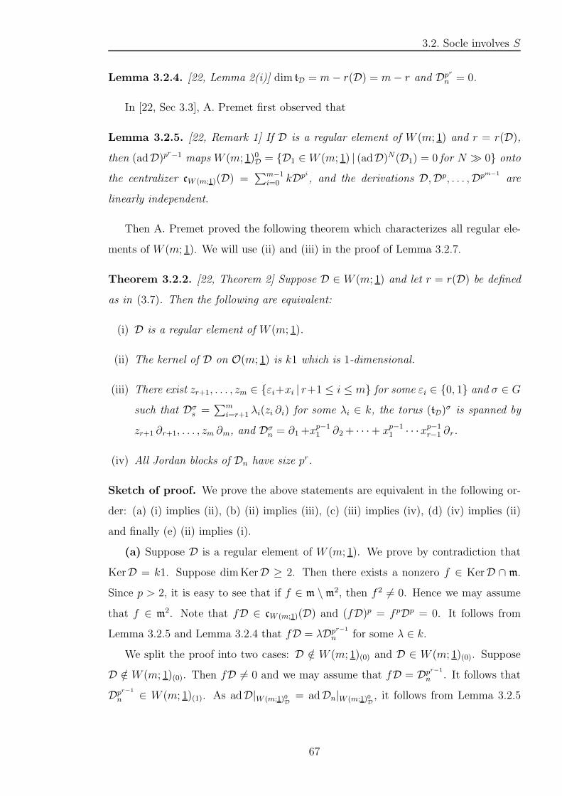
3.2. Socle involves S
Lemma 3.2.4. [22, Lemma 2(i)] dim tD = m− r(D) = m− r and Dpr
n = 0.
In [22, Sec 3.3], A. Premet first observed that
Lemma 3.2.5. [22, Remark 1] If D is a regular element of W (m; 1) and r = r(D),
then (adD)pr−1 maps W (m; 1)0D = D1 ∈ W (m; 1) | (adD)N(D1) = 0 for N ≫ 0 onto
the centralizer cW (m;1)(D) =∑m−1
i=0 kDpi
, and the derivations D,Dp, . . . ,Dpm−1
are
linearly independent.
Then A. Premet proved the following theorem which characterizes all regular ele-
ments of W (m; 1). We will use (ii) and (iii) in the proof of Lemma 3.2.7.
Theorem 3.2.2. [22, Theorem 2] Suppose D ∈ W (m; 1) and let r = r(D) be defined
as in (3.7). Then the following are equivalent:
(i) D is a regular element of W (m; 1).
(ii) The kernel of D on O(m; 1) is k1 which is 1-dimensional.
(iii) There exist zr+1, . . . , zm ∈ εi+xi | r+1 ≤ i ≤ m for some εi ∈ 0, 1 and σ ∈ G
such that Dσs =∑m
i=r+1 λi(zi ∂i) for some λi ∈ k, the torus (tD)σ is spanned by
zr+1 ∂r+1, . . . , zm ∂m, and Dσn = ∂1+xp−11 ∂2+ · · ·+ xp−1
1 · · ·xp−1r−1 ∂r.
(iv) All Jordan blocks of Dn have size pr.
Sketch of proof. We prove the above statements are equivalent in the following or-
der: (a) (i) implies (ii), (b) (ii) implies (iii), (c) (iii) implies (iv), (d) (iv) implies (ii)
and finally (e) (ii) implies (i).
(a) Suppose D is a regular element of W (m; 1). We prove by contradiction that
KerD = k1. Suppose dimKerD ≥ 2. Then there exists a nonzero f ∈ KerD ∩ m.
Since p > 2, it is easy to see that if f ∈ m \ m2, then f 2 6= 0. Hence we may assume
that f ∈ m2. Note that fD ∈ cW (m;1)(D) and (fD)p = f pDp = 0. It follows from
Lemma 3.2.5 and Lemma 3.2.4 that fD = λDpr−1
n for some λ ∈ k.
We split the proof into two cases: D /∈ W (m; 1)(0) and D ∈ W (m; 1)(0). Suppose
D /∈ W (m; 1)(0). Then fD 6= 0 and we may assume that fD = Dpr−1
n . It follows that
Dpr−1
n ∈ W (m; 1)(1). As adD|W (m;1)0D= adDn|W (m;1)0
D, it follows from Lemma 3.2.5
67

3.2. Socle involves S
that there exists some y ∈ W (m; 1)0D such that (adDn)pr−1(y) = D. Since p > 2, we
have that
D =(adDpr−1
n )p−1((adDn)pr−1−1(y))
∈[W (m; 1)(1), [W (m; 1)(1),W (m; 1)]] ⊆W (m; 1)(1).(3.8)
This contradicts our assumption that D /∈ W (m; 1)(0). So this case cannot occur.
Suppose D ∈ W (m; 1)(0). By Theorem 3.2.1, we may assume that tD ⊆ Tm, where
Tm is a maximal torus in W (m; 1) with basis x1 ∂1, . . . , xm ∂m. Let θ1, . . . , θm be
the corresponding dual basis in T ∗m. Let νi denote the restriction of θi to tD. Let ad−1
denote the representation of W (m; 1)0 in gl(W (m; 1)−1) induced by the adjoint action
of W (m; 1)0 to W (m; 1)−1; see (3.4) for the Z-grading on W (m; 1). Then the set of
tD-weights on W (m; 1)−1 coincides with Λ := −ν1, . . . ,−νm. By Lemma 3.2.4, we
know that dim tD = m− r. Since Λ spans t∗D, we have that Card(Λ) ≥ m− r.
For ν ∈ Λ, set η(ν) := dimW (m; 1)ν−1. Then η(ν) ≥ 1 and∑
ν∈Λη(ν) = m. Set
η := maxν∈Λ η(ν). Then one can show that
η ≤ r + 1. (3.9)
Write Dn =∑
i≥0Dn,i, where Dn,i ∈ W (m; 1)i; see (3.4) for notations. Since tD ⊆ Tm,
we have that Dn,i ∈ cW (m;1)(tD) for all i. In particular, each weight space W (m; 1)ν−1
is invariant under ad−1(Dn,0). As Dn is nilpotent, we get
(ad−1(Dn,0))η = 0. (3.10)
SinceW (m; 1)(1) is a p-ideal ofW (m; 1)(0), then one can show using Jacobson’s formula
that
DpK
n −DpK
n,0 ∈ W (m; 1)(1) (3.11)
for all K ≥ 0.
Suppose r ≥ 2. Then one can show that pr−1 ≥ r + 1. By (3.9) and (3.10),
we have that ad−1(Dpr−1
n,0 ) = 0. Since ad−1 is a faithful representation of W (m; 1)0,
we get Dpr−1
n,0 = 0. By (3.11), we get Dpr−1
n ∈ W (m; 1)(1). Applying (3.8), we get
D ∈ W (m; 1)(1). In particular, D is nilpotent. By our assumption, D is regular. This
contradicts Lemma 3.2.2.
Suppose r = 1. Then Card(Λ) = m−1 orm. If Card(Λ) = m, then∑
ν∈Λη(ν) = m
implies that η = 1. By (3.10), we have that ad−1(Dn,0) = 0. This again gives that
68
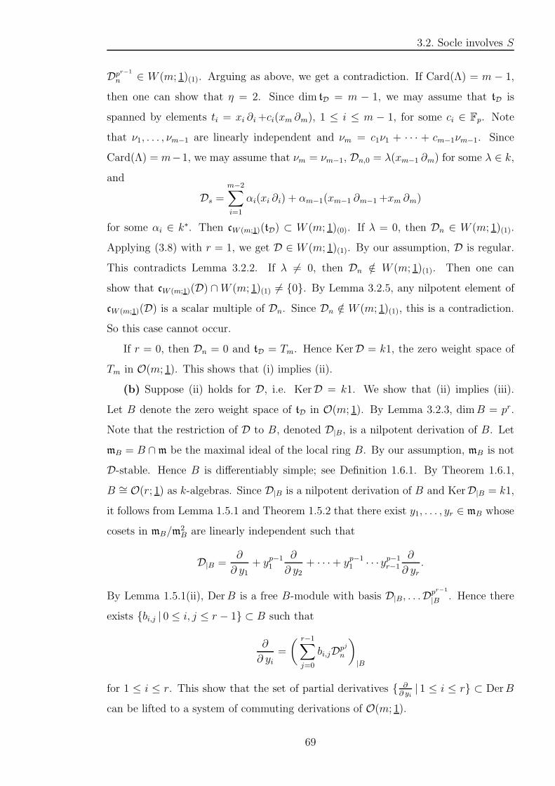
3.2. Socle involves S
Dpr−1
n ∈ W (m; 1)(1). Arguing as above, we get a contradiction. If Card(Λ) = m − 1,
then one can show that η = 2. Since dim tD = m − 1, we may assume that tD is
spanned by elements ti = xi ∂i+ci(xm ∂m), 1 ≤ i ≤ m − 1, for some ci ∈ Fp. Note
that ν1, . . . , νm−1 are linearly independent and νm = c1ν1 + · · · + cm−1νm−1. Since
Card(Λ) = m−1, we may assume that νm = νm−1, Dn,0 = λ(xm−1 ∂m) for some λ ∈ k,
and
Ds =m−2∑
i=1
αi(xi ∂i) + αm−1(xm−1 ∂m−1+xm ∂m)
for some αi ∈ k∗. Then cW (m;1)(tD) ⊂ W (m; 1)(0). If λ = 0, then Dn ∈ W (m; 1)(1).
Applying (3.8) with r = 1, we get D ∈ W (m; 1)(1). By our assumption, D is regular.
This contradicts Lemma 3.2.2. If λ 6= 0, then Dn /∈ W (m; 1)(1). Then one can
show that cW (m;1)(D) ∩W (m; 1)(1) 6= 0. By Lemma 3.2.5, any nilpotent element of
cW (m;1)(D) is a scalar multiple of Dn. Since Dn /∈ W (m; 1)(1), this is a contradiction.
So this case cannot occur.
If r = 0, then Dn = 0 and tD = Tm. Hence KerD = k1, the zero weight space of
Tm in O(m; 1). This shows that (i) implies (ii).
(b) Suppose (ii) holds for D, i.e. KerD = k1. We show that (ii) implies (iii).
Let B denote the zero weight space of tD in O(m; 1). By Lemma 3.2.3, dimB = pr.
Note that the restriction of D to B, denoted D|B, is a nilpotent derivation of B. Let
mB = B ∩m be the maximal ideal of the local ring B. By our assumption, mB is not
D-stable. Hence B is differentiably simple; see Definition 1.6.1. By Theorem 1.6.1,
B ∼= O(r; 1) as k-algebras. Since D|B is a nilpotent derivation of B and KerD|B = k1,
it follows from Lemma 1.5.1 and Theorem 1.5.2 that there exist y1, . . . , yr ∈ mB whose
cosets in mB/m2B are linearly independent such that
D|B =∂
∂ y1+ yp−1
1
∂
∂ y2+ · · ·+ yp−1
1 · · · yp−1r−1
∂
∂ yr.
By Lemma 1.5.1(ii), DerB is a free B-module with basis D|B, . . .Dpr−1
|B . Hence there
exists bi,j | 0 ≤ i, j ≤ r − 1 ⊂ B such that
∂
∂ yi=
( r−1∑
j=0
bi,jDpj
n
)
|B
for 1 ≤ i ≤ r. This show that the set of partial derivatives ∂∂ yi| 1 ≤ i ≤ r ⊂ DerB
can be lifted to a system of commuting derivations of O(m; 1).
69
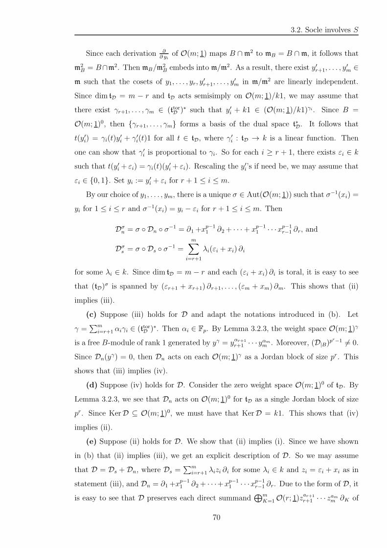
3.2. Socle involves S
Since each derivation ∂∂ yi
of O(m; 1) maps B ∩m2 to mB = B ∩m, it follows that
m2B = B∩m2. Then mB/m
2B embeds into m/m2. As a result, there exist y′r+1, . . . , y
′m ∈
m such that the cosets of y1, . . . , yr, y′r+1, . . . , y
′m in m/m2 are linearly independent.
Since dim tD = m − r and tD acts semisimply on O(m; 1)/k1, we may assume that
there exist γr+1, . . . , γm ∈ (ttorD )∗ such that y′i + k1 ∈ (O(m; 1)/k1)γi. Since B =
O(m; 1)0, then γr+1, . . . , γm forms a basis of the dual space t∗D. It follows that
t(y′i) = γi(t)y′i + γ′i(t)1 for all t ∈ tD, where γ
′i : tD → k is a linear function. Then
one can show that γ′i is proportional to γi. So for each i ≥ r + 1, there exists εi ∈ k
such that t(y′i+ εi) = γi(t)(y′i+ εi). Rescaling the y′i’s if need be, we may assume that
εi ∈ 0, 1. Set yi := y′i + εi for r + 1 ≤ i ≤ m.
By our choice of y1, . . . , ym, there is a unique σ ∈ Aut(O(m; 1)) such that σ−1(xi) =
yi for 1 ≤ i ≤ r and σ−1(xi) = yi − εi for r + 1 ≤ i ≤ m. Then
Dσn = σ Dn σ−1 = ∂1+x
p−11 ∂2+ · · ·+ xp−1
1 · · ·xp−1r−1 ∂r, and
Dσs = σ Ds σ−1 =
m∑
i=r+1
λi(εi + xi) ∂i
for some λi ∈ k. Since dim tD = m − r and each (εi + xi) ∂i is toral, it is easy to see
that (tD)σ is spanned by (εr+1 + xr+1) ∂r+1, . . . , (εm + xm) ∂m. This shows that (ii)
implies (iii).
(c) Suppose (iii) holds for D and adapt the notations introduced in (b). Let
γ =∑m
i=r+1 αiγi ∈ (ttorD )∗. Then αi ∈ Fp. By Lemma 3.2.3, the weight space O(m; 1)γ
is a free B-module of rank 1 generated by yγ = yαr+1
r+1 · · · yαmm . Moreover, (D|B)
pr−1 6= 0.
Since Dn(yγ) = 0, then Dn acts on each O(m; 1)γ as a Jordan block of size pr. This
shows that (iii) implies (iv).
(d) Suppose (iv) holds for D. Consider the zero weight space O(m; 1)0 of tD. By
Lemma 3.2.3, we see that Dn acts on O(m; 1)0 for tD as a single Jordan block of size
pr. Since KerD ⊆ O(m; 1)0, we must have that KerD = k1. This shows that (iv)
implies (ii).
(e) Suppose (ii) holds for D. We show that (ii) implies (i). Since we have shown
in (b) that (ii) implies (iii), we get an explicit description of D. So we may assume
that D = Ds + Dn, where Ds =∑m
i=r+1 λizi ∂i for some λi ∈ k and zi = εi + xi as in
statement (iii), and Dn = ∂1+xp−11 ∂2+ · · ·+x
p−11 · · ·xp−1
r−1 ∂r. Due to the form of D, it
is easy to see that D preserves each direct summand⊕m
K=1O(r; 1)zar+1
r+1 · · · zamm ∂K of
70
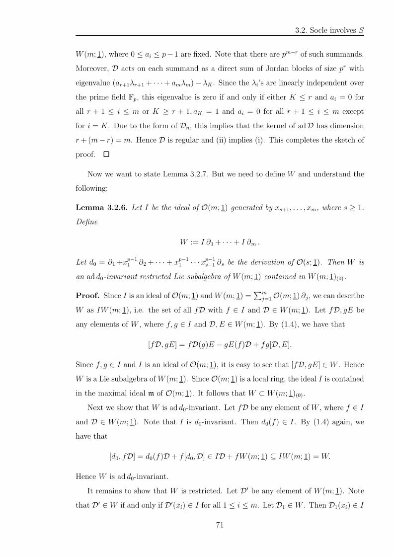
3.2. Socle involves S
W (m; 1), where 0 ≤ ai ≤ p−1 are fixed. Note that there are pm−r of such summands.
Moreover, D acts on each summand as a direct sum of Jordan blocks of size pr with
eigenvalue (ar+1λr+1 + · · ·+ amλm)− λK . Since the λi’s are linearly independent over
the prime field Fp, this eigenvalue is zero if and only if either K ≤ r and ai = 0 for
all r + 1 ≤ i ≤ m or K ≥ r + 1, aK = 1 and ai = 0 for all r + 1 ≤ i ≤ m except
for i = K. Due to the form of Dn, this implies that the kernel of adD has dimension
r+ (m− r) = m. Hence D is regular and (ii) implies (i). This completes the sketch of
proof.
Now we want to state Lemma 3.2.7. But we need to define W and understand the
following:
Lemma 3.2.6. Let I be the ideal of O(m; 1) generated by xs+1, . . . , xm, where s ≥ 1.
Define
W := I ∂1+ · · ·+ I ∂m .
Let d0 = ∂1+xp−11 ∂2+ · · · + xp−1
1 · · ·xp−1s−1 ∂s be the derivation of O(s; 1). Then W is
an ad d0-invariant restricted Lie subalgebra of W (m; 1) contained in W (m; 1)(0).
Proof. Since I is an ideal ofO(m; 1) andW (m; 1) =∑m
j=1O(m; 1) ∂j, we can describe
W as IW (m; 1), i.e. the set of all fD with f ∈ I and D ∈ W (m; 1). Let fD, gE be
any elements of W , where f, g ∈ I and D, E ∈ W (m; 1). By (1.4), we have that
[fD, gE] = fD(g)E − gE(f)D + fg[D, E].
Since f, g ∈ I and I is an ideal of O(m; 1), it is easy to see that [fD, gE] ∈ W . Hence
W is a Lie subalgebra ofW (m; 1). Since O(m; 1) is a local ring, the ideal I is contained
in the maximal ideal m of O(m; 1). It follows that W ⊂W (m; 1)(0).
Next we show thatW is ad d0-invariant. Let fD be any element ofW , where f ∈ I
and D ∈ W (m; 1). Note that I is d0-invariant. Then d0(f) ∈ I. By (1.4) again, we
have that
[d0, fD] = d0(f)D + f [d0,D] ∈ ID + fW (m; 1) ⊆ IW (m; 1) = W.
Hence W is ad d0-invariant.
It remains to show that W is restricted. Let D′ be any element of W (m; 1). Note
that D′ ∈ W if and only if D′(xi) ∈ I for all 1 ≤ i ≤ m. Let D1 ∈ W . Then D1(xi) ∈ I
71
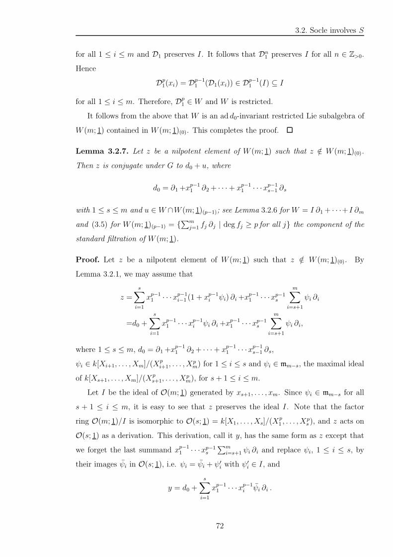
3.2. Socle involves S
for all 1 ≤ i ≤ m and D1 preserves I. It follows that Dn1 preserves I for all n ∈ Z>0.
Hence
Dp1(xi) = Dp−11 (D1(xi)) ∈ D
p−11 (I) ⊆ I
for all 1 ≤ i ≤ m. Therefore, Dp1 ∈ W and W is restricted.
It follows from the above that W is an ad d0-invariant restricted Lie subalgebra of
W (m; 1) contained in W (m; 1)(0). This completes the proof.
Lemma 3.2.7. Let z be a nilpotent element of W (m; 1) such that z /∈ W (m; 1)(0).
Then z is conjugate under G to d0 + u, where
d0 = ∂1+xp−11 ∂2+ · · ·+ xp−1
1 · · ·xp−1s−1 ∂s
with 1 ≤ s ≤ m and u ∈ W ∩W (m; 1)(p−1); see Lemma 3.2.6 for W = I ∂1+ · · ·+I ∂m
and (3.5) for W (m; 1)(p−1) = ∑m
j=1 fj ∂j | deg fj ≥ p for all j the component of the
standard filtration of W (m; 1).
Proof. Let z be a nilpotent element of W (m; 1) such that z /∈ W (m; 1)(0). By
Lemma 3.2.1, we may assume that
z =
s∑
i=1
xp−11 · · ·xp−1
i−1 (1 + xp−1i ψi) ∂i+x
p−11 · · ·xp−1
s
m∑
i=s+1
ψi ∂i
=d0 +s
∑
i=1
xp−11 · · ·xp−1
i ψi ∂i+xp−11 · · ·xp−1
s
m∑
i=s+1
ψi ∂i,
where 1 ≤ s ≤ m, d0 = ∂1+xp−11 ∂2+ · · ·+ xp−1
1 · · ·xp−1s−1 ∂s,
ψi ∈ k[Xi+1, . . . , Xm]/(Xpi+1, . . . , X
pm) for 1 ≤ i ≤ s and ψi ∈ mm−s, the maximal ideal
of k[Xs+1, . . . , Xm]/(Xps+1, . . . , X
pm), for s+ 1 ≤ i ≤ m.
Let I be the ideal of O(m; 1) generated by xs+1, . . . , xm. Since ψi ∈ mm−s for all
s + 1 ≤ i ≤ m, it is easy to see that z preserves the ideal I. Note that the factor
ring O(m; 1)/I is isomorphic to O(s; 1) = k[X1, . . . , Xs]/(Xp1 , . . . , X
ps ), and z acts on
O(s; 1) as a derivation. This derivation, call it y, has the same form as z except that
we forget the last summand xp−11 · · ·xp−1
s
∑m
i=s+1 ψi ∂i and replace ψi, 1 ≤ i ≤ s, by
their images ψi in O(s; 1), i.e. ψi = ψi + ψ′i with ψ
′i ∈ I, and
y = d0 +s
∑
i=1
xp−11 · · ·xp−1
i ψi ∂i .
72

3.2. Socle involves S
Note also that
s∑
i=1
xp−11 · · ·xp−1
i ψ′i ∂i+x
p−11 · · ·xp−1
s
m∑
i=s+1
ψi ∂i ∈ W (m; 1)(p−1). (3.12)
We show that the kernel of y on O(s; 1) is 1-dimensional, i.e. Ker y = k1. Suppose
the contrary. Then there exists a nonzero f ∈ Ker y with f(0) = 0. We want to show
that y(f) 6= 0. Hence we get a contradiction. Note that f is a linear combination
of monomials xA = xa11 · · ·x
ass , where 0 ≤ ai ≤ p − 1 and
∑s
i=1 ai > 0. We want
to look at the “smallest” monomial involved in f . Note that the standard degree of
monomials is not a good choice. This is because y = d0 +∑s
i=1 xp−11 · · ·xp−1
i ψi ∂i and
applying d0 = ∂1+xp−11 ∂2+ · · ·+x
p−11 · · ·xp−1
s−1 ∂s to xA in f , the standard degree either
decreases or increases; see (3.15) and (3.16) below. So it is difficult to compare d0(xA)
with(∑s
i=1 xp−11 · · ·xp−1
i ψi ∂i)
(xA) and the effects of y on the other monomials in f .
This means that we cannot easily deduce that y(f) 6= 0. Hence we are going to use
a monomial ordering introduced later; see Definition 3.2.42. Let xA′′
= xa′′11 · · ·x
a′′ss be
any monomial in O(s; 1). Define the | |p-degree of xA′′
by
|A′′|p :=s
∑
i=1
a′′i pi−1 = a′′1 + a′′2p+ · · ·+ a′′sp
s−1,
i.e. the p-adic expansion of nonnegative integers with digits a′′i . It is known that for a
fixed prime number p, every nonnegative integer has a unique p-adic expansion. Hence
for l = 0, 1, . . . , ps− 1, there is a unique xA′′
∈ O(s; 1) with |A′′|p = l. Note that if the
product of two monomials is nonzero, then the | |p-degree of this product is given by
the sum of | |p-degrees of the monomials; see Remark 3.2.2(iii) and (iv)(a) later.
Consider d0 = ∂1+xp−11 ∂2+ · · ·+ xp−1
1 · · ·xp−1s−1 ∂s in y. By Lemma 3.2.10 later, we
know that applying d0 to any xA in f , we get
d0(xA) = αxA
′
, (3.13)
where 1 ≤ α ≤ p− 1 and xA′
∈ O(s; 1) with |A′|p = |A|p − 1.
Consider∑s
i=1 xp−11 · · ·xp−1
i ψi ∂i in y. We first show that all nonzero summands
in∑s
i=1 xp−11 · · ·xp−1
i ψi ∂i have positive | |p-degrees. Since ψi ∈ O(s; 1), it is a linear
2Note that this monomial ordering was defined after we have proved this lemma. Due to the formsof d0 and u, we defined the | |p-degree of monomials as in Definition 3.2.4; see Example 3.2.1(2) and(3) later for the reasons. Here we are working with the subring O(s; 1) of O(m; 1) and the | |p-degreeis the first part
∑s
i=1a′′i p
i−1.
73
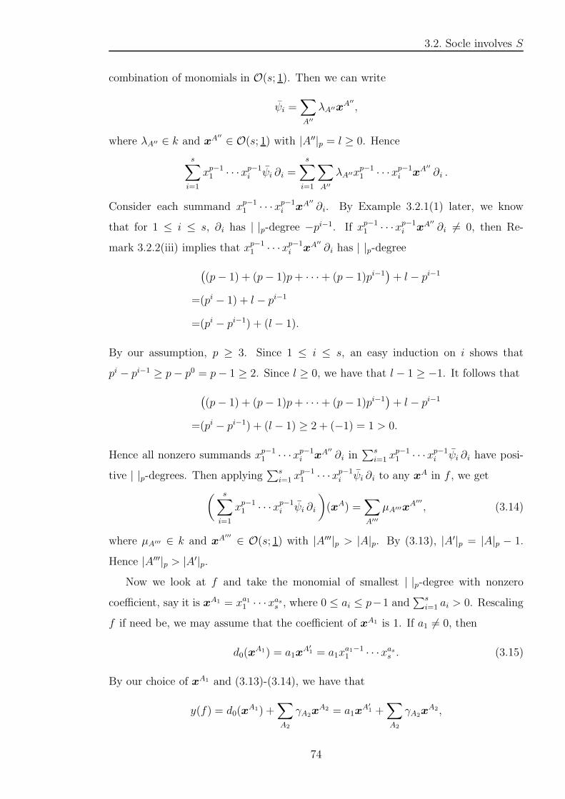
3.2. Socle involves S
combination of monomials in O(s; 1). Then we can write
ψi =∑
A′′
λA′′xA′′
,
where λA′′ ∈ k and xA′′
∈ O(s; 1) with |A′′|p = l ≥ 0. Hence
s∑
i=1
xp−11 · · ·xp−1
i ψi ∂i =
s∑
i=1
∑
A′′
λA′′xp−11 · · ·xp−1
i xA′′
∂i .
Consider each summand xp−11 · · ·xp−1
i xA′′
∂i. By Example 3.2.1(1) later, we know
that for 1 ≤ i ≤ s, ∂i has | |p-degree −pi−1. If xp−11 · · ·xp−1
i xA′′
∂i 6= 0, then Re-
mark 3.2.2(iii) implies that xp−11 · · ·xp−1
i xA′′
∂i has | |p-degree
(
(p− 1) + (p− 1)p+ · · ·+ (p− 1)pi−1)
+ l − pi−1
=(pi − 1) + l − pi−1
=(pi − pi−1) + (l − 1).
By our assumption, p ≥ 3. Since 1 ≤ i ≤ s, an easy induction on i shows that
pi − pi−1 ≥ p− p0 = p− 1 ≥ 2. Since l ≥ 0, we have that l − 1 ≥ −1. It follows that
(
(p− 1) + (p− 1)p+ · · ·+ (p− 1)pi−1)
+ l − pi−1
=(pi − pi−1) + (l − 1) ≥ 2 + (−1) = 1 > 0.
Hence all nonzero summands xp−11 · · ·xp−1
i xA′′
∂i in∑s
i=1 xp−11 · · ·xp−1
i ψi ∂i have posi-
tive | |p-degrees. Then applying∑s
i=1 xp−11 · · ·xp−1
i ψi ∂i to any xA in f , we get
( s∑
i=1
xp−11 · · ·xp−1
i ψi ∂i
)
(xA) =∑
A′′′
µA′′′xA′′′
, (3.14)
where µA′′′ ∈ k and xA′′′
∈ O(s; 1) with |A′′′|p > |A|p. By (3.13), |A′|p = |A|p − 1.
Hence |A′′′|p > |A′|p.
Now we look at f and take the monomial of smallest | |p-degree with nonzero
coefficient, say it is xA1 = xa11 · · ·xass , where 0 ≤ ai ≤ p−1 and
∑s
i=1 ai > 0. Rescaling
f if need be, we may assume that the coefficient of xA1 is 1. If a1 6= 0, then
d0(xA1) = a1x
A′1 = a1x
a1−11 · · ·xass . (3.15)
By our choice of xA1 and (3.13)-(3.14), we have that
y(f) = d0(xA1) +
∑
A2
γA2xA2 = a1x
A′1 +
∑
A2
γA2xA2,
74
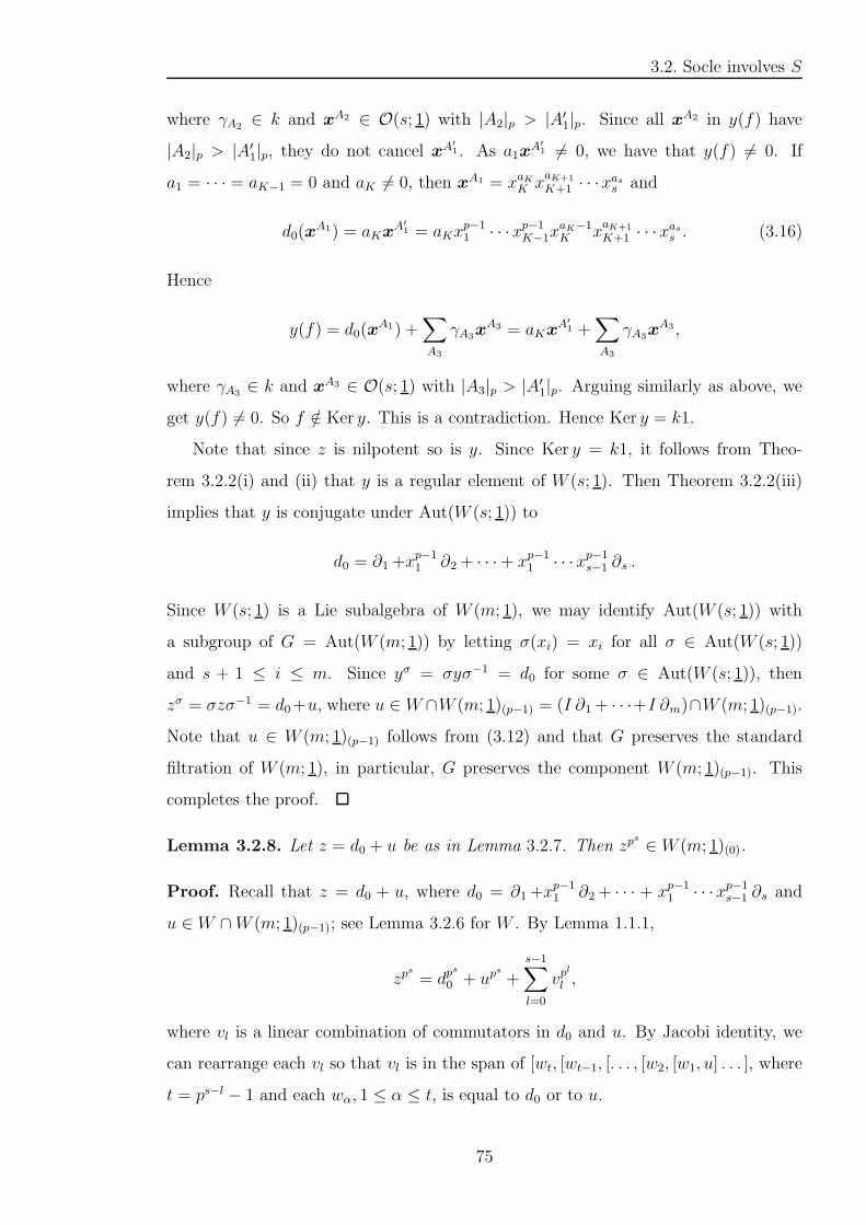
3.2. Socle involves S
where γA2∈ k and x
A2 ∈ O(s; 1) with |A2|p > |A′1|p. Since all xA2 in y(f) have
|A2|p > |A′1|p, they do not cancel xA
′1. As a1x
A′1 6= 0, we have that y(f) 6= 0. If
a1 = · · · = aK−1 = 0 and aK 6= 0, then xA1 = xaKK x
aK+1
K+1 · · ·xass and
d0(xA1) = aKx
A′1 = aKx
p−11 · · ·xp−1
K−1xaK−1K x
aK+1
K+1 · · ·xass . (3.16)
Hence
y(f) = d0(xA1) +
∑
A3
γA3xA3 = aKx
A′1 +
∑
A3
γA3xA3 ,
where γA3∈ k and x
A3 ∈ O(s; 1) with |A3|p > |A′1|p. Arguing similarly as above, we
get y(f) 6= 0. So f /∈ Ker y. This is a contradiction. Hence Ker y = k1.
Note that since z is nilpotent so is y. Since Ker y = k1, it follows from Theo-
rem 3.2.2(i) and (ii) that y is a regular element of W (s; 1). Then Theorem 3.2.2(iii)
implies that y is conjugate under Aut(W (s; 1)) to
d0 = ∂1+xp−11 ∂2+ · · ·+ xp−1
1 · · ·xp−1s−1 ∂s .
Since W (s; 1) is a Lie subalgebra of W (m; 1), we may identify Aut(W (s; 1)) with
a subgroup of G = Aut(W (m; 1)) by letting σ(xi) = xi for all σ ∈ Aut(W (s; 1))
and s + 1 ≤ i ≤ m. Since yσ = σyσ−1 = d0 for some σ ∈ Aut(W (s; 1)), then
zσ = σzσ−1 = d0+u, where u ∈ W ∩W (m; 1)(p−1) = (I ∂1+ · · ·+I ∂m)∩W (m; 1)(p−1).
Note that u ∈ W (m; 1)(p−1) follows from (3.12) and that G preserves the standard
filtration of W (m; 1), in particular, G preserves the component W (m; 1)(p−1). This
completes the proof.
Lemma 3.2.8. Let z = d0 + u be as in Lemma 3.2.7. Then zps
∈ W (m; 1)(0).
Proof. Recall that z = d0 + u, where d0 = ∂1+xp−11 ∂2+ · · · + xp−1
1 · · ·xp−1s−1 ∂s and
u ∈ W ∩W (m; 1)(p−1); see Lemma 3.2.6 for W . By Lemma 1.1.1,
zps
= dps
0 + ups
+s−1∑
l=0
vpl
l ,
where vl is a linear combination of commutators in d0 and u. By Jacobi identity, we
can rearrange each vl so that vl is in the span of [wt, [wt−1, [. . . , [w2, [w1, u] . . . ], where
t = ps−l − 1 and each wα, 1 ≤ α ≤ t, is equal to d0 or to u.
75

3.2. Socle involves S
We show that [wt, [wt−1, [. . . , [w2, [w1, u] . . . ] ∈ W and so vl ∈ W . By Lemma 3.2.6,
W is an ad d0-invariant restricted Lie subalgebra of W (m; 1) contained in W (m; 1)(0).
Since u ∈ W , it follows that [d0, u] ∈ W . It is clear that [u, u] = 0 ∈ W . This
shows that [w1, u] ∈ W . Consider w2. If w2 = d0, then by the same reason, we get
[d0, [d0, u]] ∈ W . If w2 = u, then W is a Lie subalgebra of W (m; 1) implies that
[u, [d0, u]] ∈ W . This shows that [w2, [w1, u]] ∈ W . Continuing in this way and using
the same reasons, we get [wt, [wt−1, [. . . , [w2, [w1, u] . . . ] ∈ W and so vl ∈ W for all
0 ≤ l ≤ s − 1. Since W is a restricted Lie subalgebra of W (m; 1), we have that
vpl
l ∈ W for all 1 ≤ l ≤ s − 1. Hence∑s−1
l=0 vpl
l ∈ W ⊂ W (m; 1)(0). Similarly, since
u ∈ W and W is restricted, we have that ups
∈ W ⊂ W (m; 1)(0). By Lemma 1.5.1(i),
we know that dps
0 = 0. Hence
zps
= ups
+s−1∑
l=0
vpl
l ∈ W (m; 1)(0).
This completes the proof.
Now we consider the restricted transitive subalgebra D of W (m; 1) and show the
last two results hold for any d ∈ N (D) such that d /∈ W (m; 1)(0).
Lemma 3.2.9. Let d be any element of N (D) such that d /∈ W (m; 1)(0). Then d is
conjugate under G to d0 + u, where d0 + u is the element in Lemma 3.2.7. Moreover,
dps
∈ W (m; 1)(0).
Proof. Let d be any element of N (D) such that d /∈ W (m; 1)(0). By Lemma 3.2.7, we
know that d is conjugate under G to d0 + u. Here we want to point out that the use
of the group action does not suppose that D or N (D) is G-stable, it is only used to
bring elements of N (D) to a nice form. Since d is conjugate under G to d0 + u, there
exists σ ∈ G such that d = σ(d0 + u)σ−1. Then
dps
=(
σ(d0 + u)σ−1)ps
= σ(d0 + u)ps
σ−1.
By Lemma 3.2.8, (d0 + u)ps
∈ W (m; 1)(0). Since σ ∈ G, it preserves the standard
filtration of W (m; 1). Hence dps
∈ W (m; 1)(0). This completes the proof.
Remark 3.2.1. Let us denote d0+u ∈ N (D) by z. Note that zps
∈ W (m; 1)(0) implies
that zps
preserves the maximal ideal m of O(m; 1). This will be used in the proof of
Lemma 3.2.15; see step 2.
76

3.2. Socle involves S
Define
M := I + z(m)
to be the subspace of O(m; 1), where m is the maximal ideal of O(m; 1), I is the ideal
of O(m; 1) generated by xs+1, . . . , xm with s ≥ 1, and z = d0+u as in Lemma 3.2.7. We
are aiming for Lemma 3.2.11 which showsM has the property thatM⊕kxp−11 · · ·xp−1
s =
O(m; 1). To prove that result, we need to consider the image of m under z = d0 + u.
In the proof of Lemma 3.2.7, we have seen that applying d0 to any monomial in m, the
standard degree of monomials either decreases or increases. It is difficult to get much
useful information. Therefore, we need to define a monomial ordering on O(m; 1). Let
us first recall the definitions of total ordering and monomial ordering.
Definition 3.2.1. [5, p. 55] A binary relation ≤ is a total ordering on a set X if the
following hold for all a, b, c ∈ X:
(i) Antisymmetry: if a ≤ b and b ≤ a, then a = b.
(ii) Transitivity: if a ≤ b and b ≤ c, then a ≤ c.
(iii) Comparability: either a ≤ b or b ≤ a.
Consider the polynomial ring k[X1, . . . , Xm]. Note that there is a natural bijection
between Zm≥0 and the set of monomials in k[X1, . . . , Xm] given by
(α1, . . . , αm)←→ xα1
1 · · ·xαm
m ,
and addition in Zm≥0 corresponds to multiplication of monomials in k[X1, . . . , Xm]. So
if ≺ is an ordering on Zm≥0, then it gives an ordering on monomials: if (α1, . . . , αm) ≺
(β1, . . . , βm), then xα1
1 · · ·xαmm ≺ xβ11 · · ·x
βmm . Recall that
Definition 3.2.2. [5, Definition 1, Sec. 2 and Corollary 6, Sec. 4, Chap. 2] A mono-
mial ordering on k[X1, . . . , Xm] is a relation ≺ on Zm≥0, or equivalently, a relation ≺
on the set of monomials xα1
1 · · ·xαmm , (α1, . . . , αm) ∈ Zm≥0, satisfying:
(i) ≺ is a total ordering on Zm≥0.
(ii) If (α1, . . . , αm) ≺ (β1, . . . , βm) and (γ1, . . . , γm) ∈ Zm≥0, then
(α1 + γ1, . . . , αm + γm) ≺ (β1 + γ1, . . . , βm + γm).
77
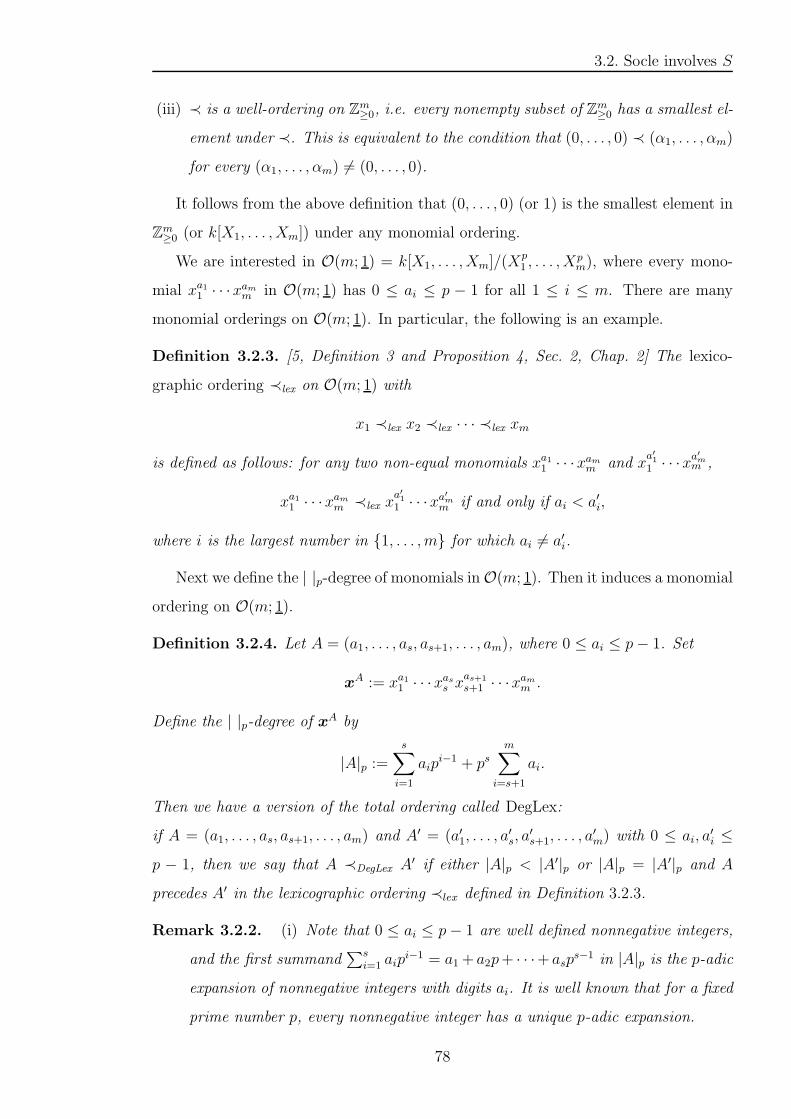
3.2. Socle involves S
(iii) ≺ is a well-ordering on Zm≥0, i.e. every nonempty subset of Zm≥0 has a smallest el-
ement under ≺. This is equivalent to the condition that (0, . . . , 0) ≺ (α1, . . . , αm)
for every (α1, . . . , αm) 6= (0, . . . , 0).
It follows from the above definition that (0, . . . , 0) (or 1) is the smallest element in
Zm≥0 (or k[X1, . . . , Xm]) under any monomial ordering.
We are interested in O(m; 1) = k[X1, . . . , Xm]/(Xp1 , . . . , X
pm), where every mono-
mial xa11 · · ·xamm in O(m; 1) has 0 ≤ ai ≤ p − 1 for all 1 ≤ i ≤ m. There are many
monomial orderings on O(m; 1). In particular, the following is an example.
Definition 3.2.3. [5, Definition 3 and Proposition 4, Sec. 2, Chap. 2] The lexico-
graphic ordering ≺lex on O(m; 1) with
x1 ≺lex x2 ≺lex · · · ≺lex xm
is defined as follows: for any two non-equal monomials xa11 · · ·xamm and x
a′1
1 · · ·xa′mm ,
xa11 · · ·xamm ≺lex x
a′1
1 · · ·xa′mm if and only if ai < a′i,
where i is the largest number in 1, . . . , m for which ai 6= a′i.
Next we define the | |p-degree of monomials inO(m; 1). Then it induces a monomial
ordering on O(m; 1).
Definition 3.2.4. Let A = (a1, . . . , as, as+1, . . . , am), where 0 ≤ ai ≤ p− 1. Set
xA := xa11 · · ·x
ass x
as+1
s+1 · · ·xamm .
Define the | |p-degree of xA by
|A|p :=s
∑
i=1
aipi−1 + ps
m∑
i=s+1
ai.
Then we have a version of the total ordering called DegLex:
if A = (a1, . . . , as, as+1, . . . , am) and A′ = (a′1, . . . , a′s, a
′s+1, . . . , a
′m) with 0 ≤ ai, a
′i ≤
p − 1, then we say that A ≺DegLex A′ if either |A|p < |A′|p or |A|p = |A′|p and A
precedes A′ in the lexicographic ordering ≺lex defined in Definition 3.2.3.
Remark 3.2.2. (i) Note that 0 ≤ ai ≤ p− 1 are well defined nonnegative integers,
and the first summand∑s
i=1 aipi−1 = a1+ a2p+ · · ·+ asp
s−1 in |A|p is the p-adic
expansion of nonnegative integers with digits ai. It is well known that for a fixed
prime number p, every nonnegative integer has a unique p-adic expansion.
78
3.2. Socle involves S
(ii) It is easy to check that DegLex is a monomial ordering on O(m; 1). Moreover,
we see that DegLex first orders monomials by the | |p-degree, then it uses the
lexicographic ordering to break ties.
(iii) Let xA and xA′
be any monomials in O(m; 1). If xAxA′
= xA′′
6= 0, i.e. all expo-
nents of x1, . . . , xm are strictly less than p, then it follows from Definition 3.2.4
that
|A′′|p = |A|p + |A′|p.
(iv) Let xA = xa11 · · ·xass x
as+1
s+1 · · ·xamm be any monomial in O(m; 1). Then
|A|p = a1 + a2p + · · ·+ asps−1 + ps
m∑
i=s+1
ai.
Let
Q0 = (p− 1) + (p− 1)p+ · · ·+ (p− 1)ps−1 = ps − 1,
and
Q = Q0 + ps((m− s)(p− 1)).
(a) If 0 ≤ |A|p ≤ Q0, then we must have that∑m
i=s+1 ai = 0. Indeed, if∑m
i=s+1 ai ≥ 1, then |A|p ≥ ps > Q0, a contradiction. Hence xA = xa11 · · ·xass
with |A|p = a1 + a2p + · · ·+ asps−1. By (i), we know that for a fixed prime
p, the p-adic expansion of any nonnegative integer is unique. Hence for
l = 0, 1, . . . , Q0, there is a unique monomial xA = xa11 · · ·xass with |A|p = l.
(b) If ps = Q0 + 1 ≤ |A|p ≤ Q, then 1 ≤∑m
i=s+1 ai ≤ (m − s)(p − 1) and
0 ≤∑s
i=1 ai ≤ s(p−1) by (a). Note that in this case, we could have distinct
monomials with the same | |p-degree and such monomials are easy to con-
struct. We could simply fix a1, . . . , as and choose as+1, . . . , am so that they
have the same∑m
i=s+1 ai. For example, the monomials xp−11 · · ·xp−1
s xs+1
and xp−11 · · ·xp−1
s xs+2 have the same | |p-degree which is Q0 + ps. By Defi-
nition 3.2.3, we have that xp−11 · · ·xp−1
s xs+1 ≺lex xp−11 · · ·xp−1
s xs+2.
(v) Let us describe O(m; 1) using the | |p-degree. Keeping in mind the numbers Q0
and Q introduced in (iv). Since O(m; 1) is spanned by monomials
xA = xa11 · · ·x
amm , 0 ≤ ai ≤ p− 1,
79
3.2. Socle involves S
we can describe O(m; 1) as
O(m; 1) = spanxA | 0 ≤ |A|p ≤ Q.
Let I be the ideal of O(m; 1) generated by xs+1, . . . , xm, where s ≥ 1. Let f be
any polynomial in O(m; 1). Then f is a linear combination of monomials xA in
O(m; 1). Since O(m; 1) = I ⊕ O(s; 1), these monomials xA are either in I or
in O(s; 1). If xA ∈ I, then A = (a1, . . . , as, as+1, . . . , am), where 0 ≤∑s
i=1 ai ≤
s(p− 1) and 1 ≤∑m
i=s+1 ai ≤ (m − s)(p− 1). It follows that ps ≤ |A|p ≤ Q. If
xA /∈ I, i.e. x
A ∈ O(s; 1), then A = (a1, . . . , as, 0, . . . , 0), where 0 ≤∑s
i=1 ai ≤
s(p− 1). It follows that 0 ≤ |A|p ≤ Q0. By (iv)(a), we can write f as
f =
Q0∑
l=0
λAlxAl + g,
where λAl∈ k, xAl = xa11 · · ·x
ass ∈ O(s; 1) with |Al|p = l, and g ∈ I. We will
come back to this in Lemma 3.2.14, Sec. 3.2.2.
To get familiar with the | |p-degree defined in Definition 3.2.4, let us look at some
examples. Moreover, we want to explain the reason that we define | |p-degree as |A|p =∑s
i=1 aipi−1 + ps
∑mi=s+1 ai. Initially, we want to compute z(xA), where z = d0 + u
and xA is any monomial in the maximal ideal m of O(m; 1). Due to the form of d0,
the standard degree of monomials is not useful. Hence we want to define a monomial
ordering so that d0 decreases the “degree” of the monomial, i.e. | |p-degree, whereas
u increases the | |p-degree of the monomial; see Example 3.2.1(2) and (3) below. As
a result, z(xA) is nonzero. Then we want to use these results to show the subspace
M = I + z(m) has the property that M ⊕ kxp−11 · · ·xp−1
s = O(m; 1). But later we
realize there is an alternative way to prove this and we only need to do computations
for d0; see Lemma 3.2.10 and Lemma 3.2.11. However, the | |p-degree of monomials is
still useful for the proof of Lemma 3.2.14 as we may lost of control if we are using the
standard degree of monomials.
Example 3.2.1. (1) Let xA = xa11 · · ·xass x
as+1
s+1 · · ·xamm ∈ O(m; 1). Let
|A| := a1 + · · ·+ as + as+1 + · · ·+ am
be the standard degree of xA. Suppose |A| > 0. Consider the partial derivatives
∂1, . . . , ∂m. Note that for 1 ≤ j ≤ m, if aj 6= 0, then
∂j(xA) = ajx
a11 · · ·x
aj−1j · · ·xamm .
80
3.2. Socle involves S
Hence the degree of ∂j with respect to the standard degree of monomials is −1.
Consider the | |p-degree. Since
|A|p = a1 + a2p+ · · ·+ ajpj−1 + · · ·+ asp
s−1 + psm∑
j=s+1
aj ,
we see that for 1 ≤ j ≤ s, the degree of ∂j with respect to | |p is −pj−1, and for
s+ 1 ≤ j ≤ m, the degree of ∂j with respect to | |p is −ps.
(2) Consider xA(xi ∂j), where xA ∈ O(m; 1) with |A| > 0, s+ 1 ≤ i ≤ m and
1 ≤ j ≤ m. Suppose xAxi 6= 0. By (1), we know that the degree of xA(xi ∂j) with
respect to the standard degree of monomials is
|A|+ (1− 1) = |A| > 0.
Consider the | |p-degree. By Remark 3.2.2(iii) and (1), we know that for 1 ≤ j ≤ s,
the degree of xA(xi ∂j) with respect to | |p is
|A|p + (ps − pj−1).
Since |A| > 0, we have that |A|p > 0. Since 1 ≤ j ≤ s, we have that ps−pj−1 > 0.
Hence |A|p + (ps − pj−1) > 0. By (1) again, we know that for s+ 1 ≤ j ≤ m, the
degree of xA(xi ∂j) with respect to | |p is
|A|p + (ps − ps) = |A|p,
which is positive, too. Recall that u ∈ (∑m
j=1 I ∂j) ∩W (m; 1)(p−1), where I is the
ideal of O(m; 1) generated by xs+1, . . . , xm with s ≥ 1, and
W (m; 1)(p−1) =
m∑
j=1
fj ∂j | deg fj ≥ p for all j
.
Then u is a linear combination of xA(xi ∂j), where xAxi, s + 1 ≤ i ≤ m, is a
monomial in I with p ≤ |A|+ 1 ≤ m(p− 1), and 1 ≤ j ≤ m. By above, we know
that each xA(xi ∂j) has degree |A| with respect to the standard degree of monomials.
Hence applying xA(xi ∂j) to any x
A′
= xa′1
1 · · ·xa′mm ∈ m with a′j 6= 0, the standard
degree increases by |A| ≥ p− 1, and the | |p-degree increases by at least |A|p > 0.
Since xAxi ∈ I and I is an ideal of O(m; 1), it follows that
(
xA(xi ∂j)
)
(xA′
) ∈ I
and so
u(xA′
) =∑
A′′
λA′′xA′′
,
81
3.2. Socle involves S
where λA′′ ∈ k and xA′′
∈ I with p − 1 ≤ |A| = |A′′| − |A′| ≤ m(p − 1) − 1 and
|A′′|p − |A′|p ≥ |A|p > 0.
(3) Consider xp−11 · · ·xp−1
r−1 ∂r, where 1 ≤ r ≤ s. By (1), the degree of xp−11 · · ·xp−1
r−1 ∂r
with respect to | |p is
(
(p− 1) + (p− 1)p+ · · ·+ (p− 1)pr−2)
− pr−1 = (pr−1 − 1)− pr−1 = −1.
Since d0 = ∂1+xp−11 ∂2+ · · · + xp−1
1 · · ·xp−1s−1 ∂s and each summand has | |p-degree
−1, it follows that d0 has | |p-degree −1.
Now we consider the action of z = d0+u on the maximal ideal m of O(m; 1). Note
that m = ms⊕I, where ms is the maximal ideal of O(s; 1) and I is the ideal of O(m; 1)
generated by xs+1, . . . , xm with s ≥ 1. Since d0 = ∂1+xp−11 ∂2+ · · ·+ xp−1
1 · · ·xp−1s−1 ∂s
is a derivation of O(s; 1), we first consider d0(ms).
Lemma 3.2.10. Let d0 = ∂1+xp−11 ∂2+ · · · + xp−1
1 · · ·xp−1s−1 ∂s be the derivation of
O(s; 1). Let ms be the maximal ideal of O(s; 1). Let xA1 = xarr x
ar+1
r+1 · · ·xass be any
monomial in ms, where 1 ≤ r ≤ s is the smallest index such that 1 ≤ ar ≤ p− 1, and
0 ≤ ai ≤ p− 1 for r + 1 ≤ i ≤ s. Then
d0(xA1) = arx
A2 = arxp−11 · · ·xp−1
r−1xar−1r x
ar+1
r+1 · · ·xass
with |A2|p = |A1|p−1. Hence d0(ms) is spanned by all monomials xA2 ∈ O(s; 1) except
xp−11 · · ·xp−1
s . In particular, dim d0(ms) = ps − 1.
Proof. Let xA1 = xarr x
ar+1
r+1 · · ·xass be any monomial in ms, where 1 ≤ r ≤ s is the
smallest index such that 1 ≤ ar ≤ p− 1, and 0 ≤ ai ≤ p− 1 for r + 1 ≤ i ≤ s. Since
d0 = ∂1+xp−11 ∂2+ · · ·+ xp−1
1 · · ·xp−1r−1 ∂r +x
p−11 · · ·xp−1
r ∂r+1+ · · ·+ xp−11 · · ·xp−1
s−1 ∂s,
we have that
d0(xA1) = arx
p−11 · · ·xp−1
r−1xar−1r x
ar+1
r+1 · · ·xass = arx
A2 .
Since 0 ≤ ar−1 ≤ p−2 < p−1, we see that xA2 6= xp−11 · · ·xp−1
s . By Example 3.2.1(3),
we know that the degree of d0 with respect to | |p is −1. Hence |A2|p = |A1|p − 1. By
Lemma 1.5.1(iii), we know that d0 acts on O(s; 1) as a single Jordan block of size ps
82
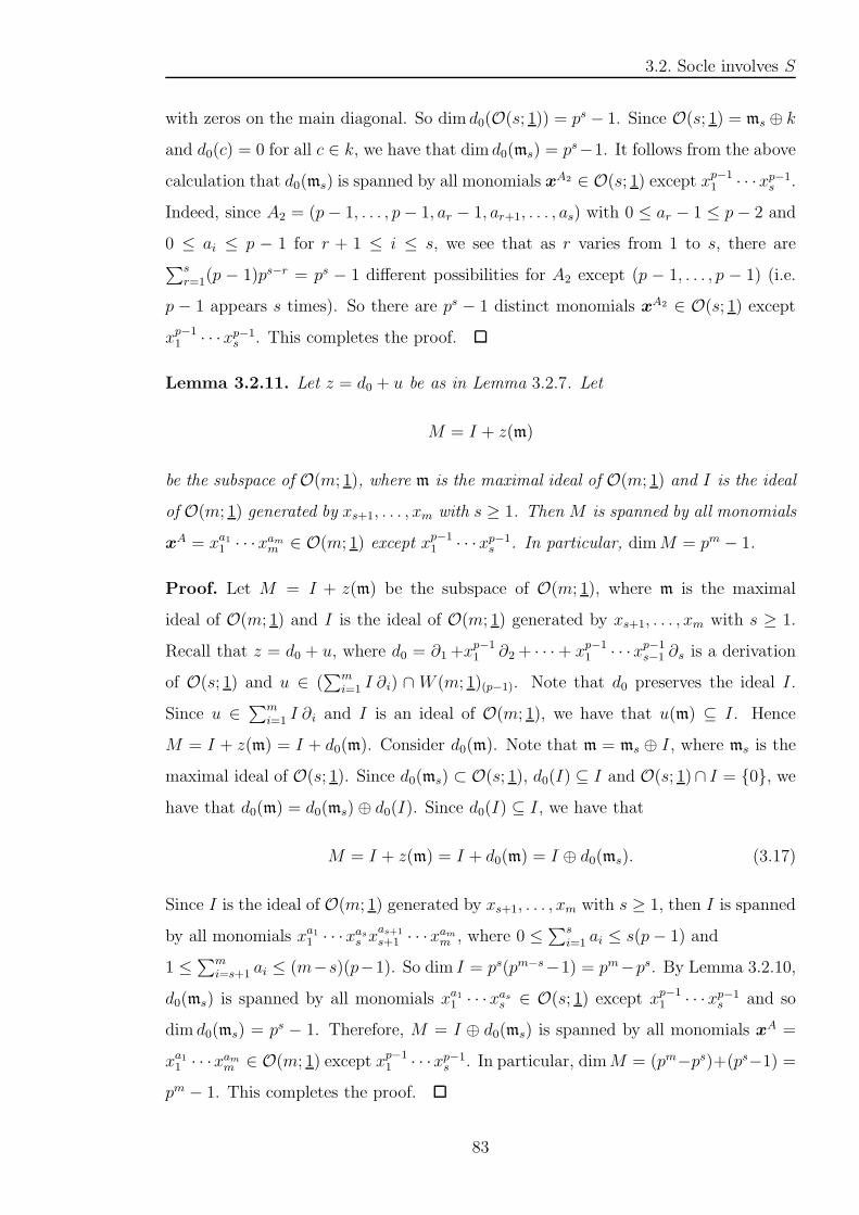
3.2. Socle involves S
with zeros on the main diagonal. So dim d0(O(s; 1)) = ps − 1. Since O(s; 1) = ms ⊕ k
and d0(c) = 0 for all c ∈ k, we have that dim d0(ms) = ps−1. It follows from the above
calculation that d0(ms) is spanned by all monomials xA2 ∈ O(s; 1) except xp−11 · · ·xp−1
s .
Indeed, since A2 = (p− 1, . . . , p− 1, ar − 1, ar+1, . . . , as) with 0 ≤ ar − 1 ≤ p− 2 and
0 ≤ ai ≤ p − 1 for r + 1 ≤ i ≤ s, we see that as r varies from 1 to s, there are∑s
r=1(p − 1)ps−r = ps − 1 different possibilities for A2 except (p − 1, . . . , p − 1) (i.e.
p − 1 appears s times). So there are ps − 1 distinct monomials xA2 ∈ O(s; 1) except
xp−11 · · ·xp−1
s . This completes the proof.
Lemma 3.2.11. Let z = d0 + u be as in Lemma 3.2.7. Let
M = I + z(m)
be the subspace of O(m; 1), where m is the maximal ideal of O(m; 1) and I is the ideal
of O(m; 1) generated by xs+1, . . . , xm with s ≥ 1. Then M is spanned by all monomials
xA = xa11 · · ·x
amm ∈ O(m; 1) except xp−1
1 · · ·xp−1s . In particular, dimM = pm − 1.
Proof. Let M = I + z(m) be the subspace of O(m; 1), where m is the maximal
ideal of O(m; 1) and I is the ideal of O(m; 1) generated by xs+1, . . . , xm with s ≥ 1.
Recall that z = d0 + u, where d0 = ∂1+xp−11 ∂2+ · · ·+ xp−1
1 · · ·xp−1s−1 ∂s is a derivation
of O(s; 1) and u ∈ (∑m
i=1 I ∂i) ∩ W (m; 1)(p−1). Note that d0 preserves the ideal I.
Since u ∈∑m
i=1 I ∂i and I is an ideal of O(m; 1), we have that u(m) ⊆ I. Hence
M = I + z(m) = I + d0(m). Consider d0(m). Note that m = ms ⊕ I, where ms is the
maximal ideal of O(s; 1). Since d0(ms) ⊂ O(s; 1), d0(I) ⊆ I and O(s; 1)∩ I = 0, we
have that d0(m) = d0(ms)⊕ d0(I). Since d0(I) ⊆ I, we have that
M = I + z(m) = I + d0(m) = I ⊕ d0(ms). (3.17)
Since I is the ideal of O(m; 1) generated by xs+1, . . . , xm with s ≥ 1, then I is spanned
by all monomials xa11 · · ·xass x
as+1
s+1 · · ·xamm , where 0 ≤
∑s
i=1 ai ≤ s(p− 1) and
1 ≤∑m
i=s+1 ai ≤ (m−s)(p−1). So dim I = ps(pm−s−1) = pm−ps. By Lemma 3.2.10,
d0(ms) is spanned by all monomials xa11 · · ·xass ∈ O(s; 1) except xp−1
1 · · ·xp−1s and so
dim d0(ms) = ps − 1. Therefore, M = I ⊕ d0(ms) is spanned by all monomials xA =
xa11 · · ·xamm ∈ O(m; 1) except xp−1
1 · · ·xp−1s . In particular, dimM = (pm−ps)+(ps−1) =
pm − 1. This completes the proof.
83
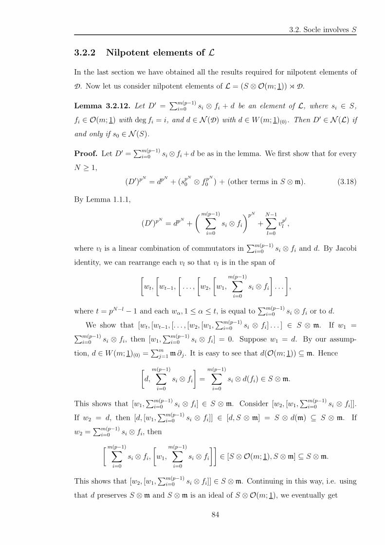
3.2. Socle involves S
3.2.2 Nilpotent elements of L
In the last section we have obtained all the results required for nilpotent elements of
D. Now let us consider nilpotent elements of L = (S ⊗O(m; 1))⋊ D.
Lemma 3.2.12. Let D′ =∑m(p−1)
i=0 si ⊗ fi + d be an element of L, where si ∈ S,
fi ∈ O(m; 1) with deg fi = i, and d ∈ N (D) with d ∈ W (m; 1)(0). Then D′ ∈ N (L) if
and only if s0 ∈ N (S).
Proof. Let D′ =∑m(p−1)
i=0 si⊗ fi+ d be as in the lemma. We first show that for every
N ≥ 1,
(D′)pN
= dpN
+ (spN
0 ⊗ fpN
0 ) + (other terms in S ⊗m). (3.18)
By Lemma 1.1.1,
(D′)pN
= dpN
+
(m(p−1)∑
i=0
si ⊗ fi
)pN
+N−1∑
l=0
vpl
l ,
where vl is a linear combination of commutators in∑m(p−1)
i=0 si ⊗ fi and d. By Jacobi
identity, we can rearrange each vl so that vl is in the span of
[
wt,
[
wt−1,
[
. . . ,
[
w2,
[
w1,
m(p−1)∑
i=0
si ⊗ fi
]
. . .
]
,
where t = pN−l − 1 and each wα, 1 ≤ α ≤ t, is equal to∑m(p−1)
i=0 si ⊗ fi or to d.
We show that [wt, [wt−1, [. . . , [w2, [w1,∑m(p−1)
i=0 si ⊗ fi] . . . ] ∈ S ⊗ m. If w1 =∑m(p−1)
i=0 si ⊗ fi, then [w1,∑m(p−1)
i=0 si ⊗ fi] = 0. Suppose w1 = d. By our assump-
tion, d ∈ W (m; 1)(0) =∑m
j=1m ∂j. It is easy to see that d(O(m; 1)) ⊆ m. Hence
[
d,
m(p−1)∑
i=0
si ⊗ fi
]
=
m(p−1)∑
i=0
si ⊗ d(fi) ∈ S ⊗m.
This shows that [w1,∑m(p−1)
i=0 si ⊗ fi] ∈ S ⊗ m. Consider [w2, [w1,∑m(p−1)
i=0 si ⊗ fi]].
If w2 = d, then [d, [w1,∑m(p−1)
i=0 si ⊗ fi]] ∈ [d, S ⊗ m] = S ⊗ d(m) ⊆ S ⊗ m. If
w2 =∑m(p−1)
i=0 si ⊗ fi, then
[m(p−1)∑
i=0
si ⊗ fi,
[
w1,
m(p−1)∑
i=0
si ⊗ fi
]]
∈ [S ⊗O(m; 1), S ⊗m] ⊆ S ⊗m.
This shows that [w2, [w1,∑m(p−1)
i=0 si ⊗ fi]] ∈ S ⊗m. Continuing in this way, i.e. using
that d preserves S ⊗m and S ⊗m is an ideal of S ⊗O(m; 1), we eventually get
84
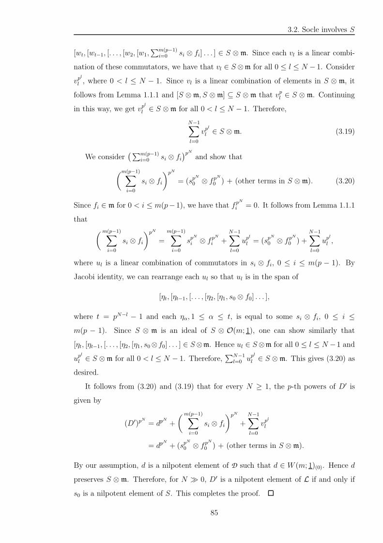
3.2. Socle involves S
[wt, [wt−1, [. . . , [w2, [w1,∑m(p−1)
i=0 si ⊗ fi] . . . ] ∈ S ⊗ m. Since each vl is a linear combi-
nation of these commutators, we have that vl ∈ S⊗m for all 0 ≤ l ≤ N − 1. Consider
vpl
l , where 0 < l ≤ N − 1. Since vl is a linear combination of elements in S ⊗ m, it
follows from Lemma 1.1.1 and [S ⊗ m, S ⊗m] ⊆ S ⊗ m that vpl ∈ S ⊗ m. Continuing
in this way, we get vpl
l ∈ S ⊗m for all 0 < l ≤ N − 1. Therefore,
N−1∑
l=0
vpl
l ∈ S ⊗m. (3.19)
We consider(∑m(p−1)
i=0 si ⊗ fi)pN
and show that
(m(p−1)∑
i=0
si ⊗ fi
)pN
= (spN
0 ⊗ fpN
0 ) + (other terms in S ⊗m). (3.20)
Since fi ∈ m for 0 < i ≤ m(p−1), we have that f pN
i = 0. It follows from Lemma 1.1.1
that
(m(p−1)∑
i=0
si ⊗ fi
)pN
=
m(p−1)∑
i=0
spN
i ⊗ fpN
i +
N−1∑
l=0
upl
l = (spN
0 ⊗ fpN
0 ) +
N−1∑
l=0
upl
l ,
where ul is a linear combination of commutators in si ⊗ fi, 0 ≤ i ≤ m(p − 1). By
Jacobi identity, we can rearrange each ul so that ul is in the span of
[ηt, [ηt−1, [. . . , [η2, [η1, s0 ⊗ f0] . . . ],
where t = pN−l − 1 and each ηα, 1 ≤ α ≤ t, is equal to some si ⊗ fi, 0 ≤ i ≤
m(p − 1). Since S ⊗ m is an ideal of S ⊗ O(m; 1), one can show similarly that
[ηt, [ηt−1, [. . . , [η2, [η1, s0⊗f0] . . . ] ∈ S⊗m. Hence ul ∈ S⊗m for all 0 ≤ l ≤ N −1 and
upl
l ∈ S ⊗m for all 0 < l ≤ N − 1. Therefore,∑N−1
l=0 upl
l ∈ S ⊗m. This gives (3.20) as
desired.
It follows from (3.20) and (3.19) that for every N ≥ 1, the p-th powers of D′ is
given by
(D′)pN
= dpN
+
(m(p−1)∑
i=0
si ⊗ fi
)pN
+
N−1∑
l=0
vpl
l
= dpN
+ (spN
0 ⊗ fpN
0 ) + (other terms in S ⊗m).
By our assumption, d is a nilpotent element of D such that d ∈ W (m; 1)(0). Hence d
preserves S ⊗ m. Therefore, for N ≫ 0, D′ is a nilpotent element of L if and only if
s0 is a nilpotent element of S. This completes the proof.
85

3.2. Socle involves S
Next we consider elements of the form D =∑m(p−1)
i=0 si ⊗ fi + z, where si ∈ S,
fi ∈ O(m; 1) with deg fi = i, and z = d0 + u ∈ N (D) as in Lemma 3.2.7. We first
construct some automorphisms of L; see Lemma 3.2.13. Then we show that D can be
reduced to an element in a nice form; see Lemma 3.2.14.
Lemma 3.2.13. Let s ⊗ f be an element of S ⊗ m. Then exp(ad(s ⊗ f)) is an
automorphism of L.
Proof. The proof is similar to Lemma 3.1.3 in Sec. 3.1. Let s ⊗ f be an element of
S ⊗m. We first show that exp(ad(s⊗ f)) is an automorphism of S ⊗O(m; 1). Since
f ∈ m, we have that f p = 0. Hence (ad(s ⊗ f))p = ad(sp ⊗ f p) = 0. Moreover, it is
easy to check that for any w1, w2 ∈ S ⊗O(m; 1),
∑
0≤i,j≤p, i+j≥p
1
i!j!
[
(ad(s⊗ f))i(w1), (ad(s⊗ f))j(w2)
]
= 0.
Hence exp(ad(s ⊗ f)) is an automorphism of S ⊗ O(m; 1). Then it induces an auto-
morphism of the derivation algebra
Der(S ⊗O(m; 1)) =(
S ⊗O(m; 1))
⋊(
IdS ⊗W (m; 1))
via conjugation. Note that
L = (S ⊗O(m; 1))⋊ D ⊂ Der(S ⊗O(m; 1)).
To conclude that exp(ad(s ⊗ f)) is an automorphism of L, we need to check that
exp(ad(s⊗ f)) preserves L. Explicitly, we need to show that for any d1 ∈ D,
exp(ad(s ⊗ f)) d1 exp(ad(−s ⊗ f)) ∈ L. In the proof of Lemma 3.1.3 (see (3.2)),
we did a similar computation. By the same computational method and the following
reasons:
(i) d1 is a derivation of O(m; 1),
(ii) exp(ad(s⊗ f)) exp(ad(−s⊗ f)) = Id,
(iii) f p = 0,
(iv) (p− 1)! ≡ −1(mod p), and
(v) S ∼= adS via the adjoint representation and hence we may identify S ⊗O(m; 1)
with its image in gl(S ⊗O(m; 1)) under ad,
86
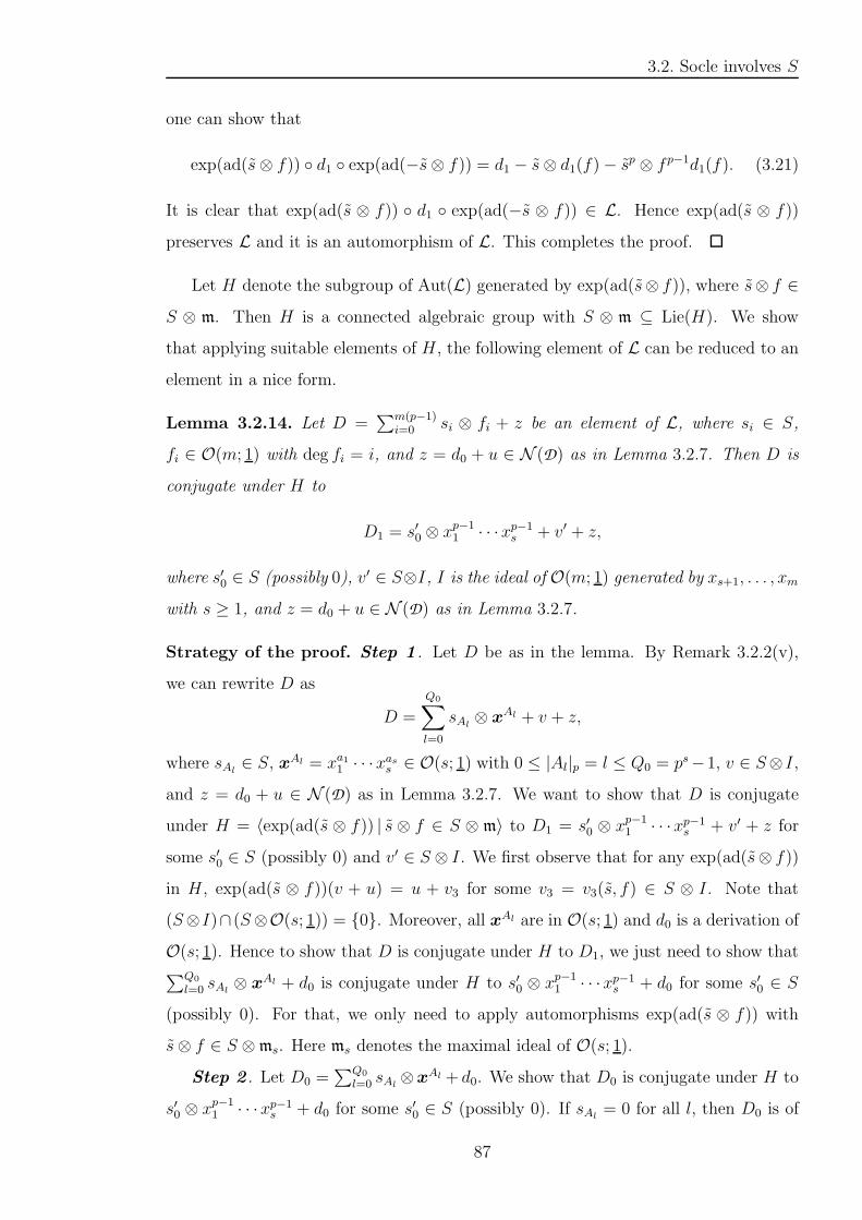
3.2. Socle involves S
one can show that
exp(ad(s⊗ f)) d1 exp(ad(−s⊗ f)) = d1 − s⊗ d1(f)− sp ⊗ f p−1d1(f). (3.21)
It is clear that exp(ad(s ⊗ f)) d1 exp(ad(−s ⊗ f)) ∈ L. Hence exp(ad(s ⊗ f))
preserves L and it is an automorphism of L. This completes the proof.
Let H denote the subgroup of Aut(L) generated by exp(ad(s⊗ f)), where s⊗ f ∈
S ⊗ m. Then H is a connected algebraic group with S ⊗ m ⊆ Lie(H). We show
that applying suitable elements of H , the following element of L can be reduced to an
element in a nice form.
Lemma 3.2.14. Let D =∑m(p−1)
i=0 si ⊗ fi + z be an element of L, where si ∈ S,
fi ∈ O(m; 1) with deg fi = i, and z = d0 + u ∈ N (D) as in Lemma 3.2.7. Then D is
conjugate under H to
D1 = s′0 ⊗ xp−11 · · ·xp−1
s + v′ + z,
where s′0 ∈ S (possibly 0), v′ ∈ S⊗I, I is the ideal of O(m; 1) generated by xs+1, . . . , xm
with s ≥ 1, and z = d0 + u ∈ N (D) as in Lemma 3.2.7.
Strategy of the proof. Step 1 . Let D be as in the lemma. By Remark 3.2.2(v),
we can rewrite D as
D =
Q0∑
l=0
sAl⊗ x
Al + v + z,
where sAl∈ S, xAl = xa11 · · ·x
ass ∈ O(s; 1) with 0 ≤ |Al|p = l ≤ Q0 = ps−1, v ∈ S⊗ I,
and z = d0 + u ∈ N (D) as in Lemma 3.2.7. We want to show that D is conjugate
under H = 〈exp(ad(s ⊗ f)) | s ⊗ f ∈ S ⊗ m〉 to D1 = s′0 ⊗ xp−11 · · ·xp−1
s + v′ + z for
some s′0 ∈ S (possibly 0) and v′ ∈ S ⊗ I. We first observe that for any exp(ad(s⊗ f))
in H , exp(ad(s ⊗ f))(v + u) = u + v3 for some v3 = v3(s, f) ∈ S ⊗ I. Note that
(S⊗I)∩ (S⊗O(s; 1)) = 0. Moreover, all xAl are in O(s; 1) and d0 is a derivation of
O(s; 1). Hence to show that D is conjugate under H to D1, we just need to show that∑Q0
l=0 sAl⊗ x
Al + d0 is conjugate under H to s′0 ⊗ xp−11 · · ·xp−1
s + d0 for some s′0 ∈ S
(possibly 0). For that, we only need to apply automorphisms exp(ad(s ⊗ f)) with
s⊗ f ∈ S ⊗ms. Here ms denotes the maximal ideal of O(s; 1).
Step 2 . Let D0 =∑Q0
l=0 sAl⊗x
Al + d0. We show that D0 is conjugate under H to
s′0 ⊗ xp−11 · · ·xp−1
s + d0 for some s′0 ∈ S (possibly 0). If sAl= 0 for all l, then D0 is of
87
3.2. Socle involves S
the desired form. If not all sAlare zero, then we look at xAl ’s with sAl
6= 0 and take
the one with the smallest | |p-degree, say it is xAK with |AK |p = K. Then
D0 =
Q0∑
l=K
sAl⊗ x
Al + d0.
If xAK = xp−11 · · ·xp−1
s , then |AK |p = K = Q0 and D0 is of the desired form. If xAK =
xa11 · · ·xass 6= xp−1
1 · · ·xp−1s , then 0 ≤ |AK |p = K < Q0 and there exist 0 ≤ ai < p − 1
for some 1 ≤ i ≤ s. Let 1 ≤ r ≤ s be the smallest index such that 0 ≤ ar < p − 1.
Then xAK = xp−1
1 . . . xp−1r−1x
arr x
ar+1
r+1 · · ·xass . Let f = x
AK = xar+1r x
ar+1
r+1 · · ·xass ∈ ms and
s = (ar +1)−1sAK∈ S. It follows from Lemma 3.2.10 that applying exp(ad(s⊗ f)) to
D0, we may assume that
D0 =
Q0∑
l=K+1
s′Al⊗ x
Al + d0,
where s′Al∈ S, xAl = xa11 · · ·x
ass ∈ O(s; 1) with |Al|p = l. Continue doing the above
until we get D0 is conjugate under H to s′0⊗xp−11 · · ·xp−1
s +d0 for some s′0 ∈ S (possibly
0). It follows that D is conjugate under H to D1.
Proof. Step 1 . Let D =∑m(p−1)
i=0 si ⊗ fi + z be as in the lemma. Let I be the ideal
of O(m; 1) generated by xs+1, . . . , xm, where s ≥ 1. Since fi ∈ O(m; 1), it follows from
Remark 3.2.2(v) that we can write
fi =
Q0∑
l=0
λAl,ixAl + gi,
where λAl,i ∈ k, xAl = xa11 · · ·x
ass ∈ O(s; 1) with 0 ≤ |Al|p = l ≤ Q0 = ps − 1, and
gi ∈ I. Then we can rewrite D as
D =
Q0∑
l=0
sAl⊗ x
Al + v + z, (3.22)
where sAl∈ S, xAl = xa11 · · ·x
ass ∈ O(s; 1) with 0 ≤ |Al|p = l ≤ Q0 = ps−1, v ∈ S⊗ I,
and z = d0 + u ∈ N (D) as in Lemma 3.2.7. We want to show that D is conjugate
under H = 〈exp(ad(s ⊗ f)) | s ⊗ f ∈ S ⊗ m〉 to D1 = s′0 ⊗ xp−11 · · ·xp−1
s + v′ + z for
some s′0 ∈ S (possibly 0) and v′ ∈ S ⊗ I. We claim that this problem can be reduced
to show that∑Q0
l=0 sAl⊗ x
Al + d0 is conjugate under H to s′0 ⊗ xp−11 · · ·xp−1
s + d0 for
some s′0 ∈ S (possibly 0). Take D as in (3.22) and let exp(ad(s⊗ f)) be any element
88
3.2. Socle involves S
in H . By Lemma 3.2.13 (see (3.21)),
exp(ad(s⊗ f))(D) = exp(ad(s⊗ f))
( Q0∑
l=0
sAl⊗ x
Al + d0
)
+ exp(ad(s⊗ f))(v + u)
=
Q0∑
l=0
sAl⊗ x
Al +
p−1∑
j=1
Q0∑
l=0
1
j!(ad s)j(sAl
)⊗ f jxAl
+ d0 − s⊗ d0(f)− sp ⊗ f p−1d0(f) + exp(ad(s⊗ f))(v + u).
We show that exp(ad(s⊗ f))(v + u) = u+ v3 for some v3 = v3(s, f) ∈ S ⊗ I. Since I
is an ideal of O(m; 1), this implies that S ⊗ I is an ideal of S ⊗O(m; 1). Hence S ⊗ I
is stabilized by all exp(ad(s⊗ f)) in H . In particular, exp(ad(s⊗ f))(v) = v1 for some
v1 = v1(s, f) ∈ S ⊗ I. By Lemma 3.2.13 (see (3.21)) again,
exp(ad(s⊗ f))(u) = u− s⊗ u(f)− sp ⊗ f p−1u(f).
Since u ∈ (I ∂1+ · · · + I ∂m), we have that u(m) ⊆ I. In particular, u(f) ∈ I.
Hence exp(ad(s ⊗ f))(u) = u + v2 for some v2 = v2(s, f) ∈ S ⊗ I. It follows that
exp(ad(s ⊗ f))(v + u) = u + v3 for some v3 = v3(s, f) = v1(s, f) + v2(s, f) ∈ S ⊗ I.
Hence for any exp(ad(s⊗ f)) ∈ H ,
exp(ad(s⊗ f))(D) = exp(ad(s⊗ f))
( Q0∑
l=0
sAl⊗ x
Al + d0
)
+ (u+ v3)
=
Q0∑
l=0
sAl⊗ x
Al +
p−1∑
j=1
Q0∑
l=0
1
j!(ad s)j(sAl
)⊗ f jxAl
+ d0 − s⊗ d0(f)− sp ⊗ f p−1d0(f) + (u+ v3).
Applying another element exp(ad(s1 ⊗ f ′)) ∈ H to the above, we still get
exp(ad(s1 ⊗ f ′))(u + v3) = u + v4 for some v4 = v4(s1, f′) ∈ S ⊗ I. Note that
(S ⊗ I) ∩ (S ⊗O(s; 1)) = 0. Moreover, all xAl are in O(s; 1) and d0 is a derivation
of O(s; 1). Hence to show that D =∑Q0
l=0 sAl⊗ x
Al + v + d0 + u is H-conjugate to
D1 = s′0⊗ xp−11 · · ·xp−1
s + v′ + d0 + u, we just need to show that∑Q0
l=0 sAl⊗x
Al + d0 is
H-conjugate to s′0⊗xp−11 · · ·xp−1
s +d0. For that, we only need to apply automorphisms
exp(ad(s⊗f)) with s⊗f ∈ S⊗ms and do computations in O(s; 1) and W (s; 1). Here
ms denotes the maximal ideal of O(s; 1).
Step 2 . Let D0 =∑Q0
l=0 sAl⊗ x
Al + d0. We show that D0 is H-conjugate to
s′0 ⊗ xp−11 · · ·xp−1
s + d0 for some s′0 ∈ S (possibly 0). If sAl= 0 for all l, then D0 is of
89
3.2. Socle involves S
the desired form. If not all sAlare zero, then we look at xAl ’s with sAl
6= 0 and take
the one with the smallest | |p-degree, say it is xAK with |AK |p = K. Then
D0 =
Q0∑
l=K
sAl⊗ x
Al + d0.
If xAK = xp−1
1 · · ·xp−1s , then |AK |p = K = Q0 and D0 is of the desired form. If
xAK 6= xp−1
1 · · ·xp−1s , then 0 ≤ |AK |p = K < Q0 and we need to apply exp(ad(s⊗ f))
to D0 and clear sAK⊗ x
AK . By Lemma 3.2.13 (see (3.21)), we know that for any
exp(ad(s⊗ f)) ∈ H ,
exp(ad(s⊗ f))(D0) =
Q0∑
l=K
sAl⊗ x
Al +
p−1∑
j=1
Q0∑
l=K
1
j!(ad s)j(sAl
)⊗ f jxAl
+ d0 − s⊗ d0(f)− sp ⊗ f p−1d0(f).
(3.23)
Let AK = (a1, . . . , as). Since xAK 6= xp−1
1 · · ·xp−1s , there exist 0 ≤ ai < p− 1 for some
1 ≤ i ≤ s. Note that if |AK |p = 0, then ai = 0 for all 1 ≤ i ≤ s. Let 1 ≤ r ≤ s be the
smallest index such that 0 ≤ ar < p− 1. Then
xAK = xp−1
1 . . . xp−1r−1x
arr x
ar+1
r+1 · · ·xass .
Let f = xAK = xar+1
r xar+1
r+1 · · ·xass ∈ ms. By Lemma 3.2.10,
d0(f) = d0(xAK ) = (ar + 1)xAK
with |AK |p = |AK |p − 1. Let s = (ar + 1)−1sAK∈ S. Substituting s and f into (3.23),
we get
exp(ad(s⊗ f))(D0) =
Q0∑
l=K+1
sAl⊗ x
Al
+
p−1∑
j=1
Q0∑
l=K+1
1
j!(ar + 1)−j(ad sAK
)j(sAl)⊗ (xAK)jxAl
+ d0 − (ar + 1)−p+1spAK⊗ (xAK )p−1
xAK .
(3.24)
We want to show that exp(ad(s⊗ f))(D0) =∑Q0
l=K+1 s′Al⊗x
Al + d0, where s′Al∈ S
and xAl = xa11 · · ·x
ass ∈ O(s; 1) with |Al|p = l. Look at the second and the last
summands in (3.24). Since xAK ∈ ms and ms is an ideal of O(s; 1), we see that
these two summands are in S ⊗ms. This implies that every nonzero monomial xA in
90
3.2. Socle involves S
these two summands has |A|p ≤ Q0. Moreover, we show that every nonzero monomial
xA in these two summands has |A|p > K + 1. We start with the second summand.
By Remark 3.2.2(iii), we know that for any monomials xA′
and xA′′
in O(s; 1), if
xA′
xA′′
= xA′′′
6= 0, then |A′′′|p = |A′|p+ |A
′′|p. Consider (xAK )j, where 1 ≤ j ≤ p−1.
By our choice, xAK ∈ ms with |AK |p = |AK |p+1 = K +1. Hence for 2 ≤ j ≤ p− 1, if
(xAK )j 6= 0, then (xAK )j ∈ ms with | |p-degree j|AK |p ≥ 2(K + 1) > K +1. Now look
at (xAK)jxAl in the second summand. Since l ≥ K + 1 ≥ 1, every monomial xAl is
in ms and has |Al|p = l ≥ K + 1. If (xAK )jxAl 6= 0, then (xAK)jxAl is in ms and has
| |p-degree j|AK |p + |Al|p ≥ |AK |p + |Al|p ≥ (K + 1) + (K + 1) > K + 1.
Look at (xAK )p−1xAK in the last summand. By above, if (xAK )p−1 6= 0, then
(xAK )p−1 is in ms and has | |p-degree > K + 1. Note that xAK ∈ O(s; 1) and has
|AK |p = K ≥ 0. So if (xAK )p−1xAK 6= 0, then (xAK )p−1
xAK is in ms and has | |p-
degree (p− 1)|AK |p + |AK |p > (K + 1) +K ≥ K + 1.
Hence every nonzero monomial xA in the second and the last summands hasK+1 <
|A|p ≤ Q0. Therefore, applying exp(ad(s⊗ f)) to D0, we may assume that
D0 =
Q0∑
l=K+1
s′Al⊗ x
Al + d0
for some s′Al∈ S and x
Al = xa11 · · ·xass ∈ O(s; 1) with |Al|p = l.
Now look at D0 and repeat the above process, i.e. take xAl with the smallest
| |p-degree for which s′Al6= 0. If Al = (a1, . . . , as) = (p − 1, . . . , p − 1), then D0 is of
the desired form. If not, then applying a similar automorphism exp(ad(s⊗ f)) to D0
and clear s′Al⊗ x
Al. Continuing in this way, we eventually get D0 is H-conjugate to
s′0 ⊗ xp−11 · · ·xp−1
s + d0 for some s′0 ∈ S (possibly 0). Therefore, D = D0 + v + u is
H-conjugate to D1 = s′0 ⊗ xp−11 · · ·xp−1
s + d0 + v′ + u for some s′0 ∈ S (possibly 0) and
v′ ∈ S ⊗ I. This completes the proof.
Lemma 3.2.15. Let D1 = s′0 ⊗ xp−11 · · ·xp−1
s + v′ + z be an element of L, where
s′0 ∈ S, v′ ∈ S⊗ I, I is the ideal of O(m; 1) generated by xs+1, . . . , xm with s ≥ 1, and
z = d0 + u ∈ N (D) as in Lemma 3.2.7. Then D1 ∈ N (L) if and only if s′0 ∈ N (S).
Strategy of the proof. This is a computational proof with the following key steps:
Step 1 . Let D1 = s′0 ⊗ xp−11 · · ·xp−1
s + v′ + z be as in the lemma. We show that
Dps
1 = zps
+ (s′0 ⊗ (−1)s) + (other terms in S ⊗m).
91
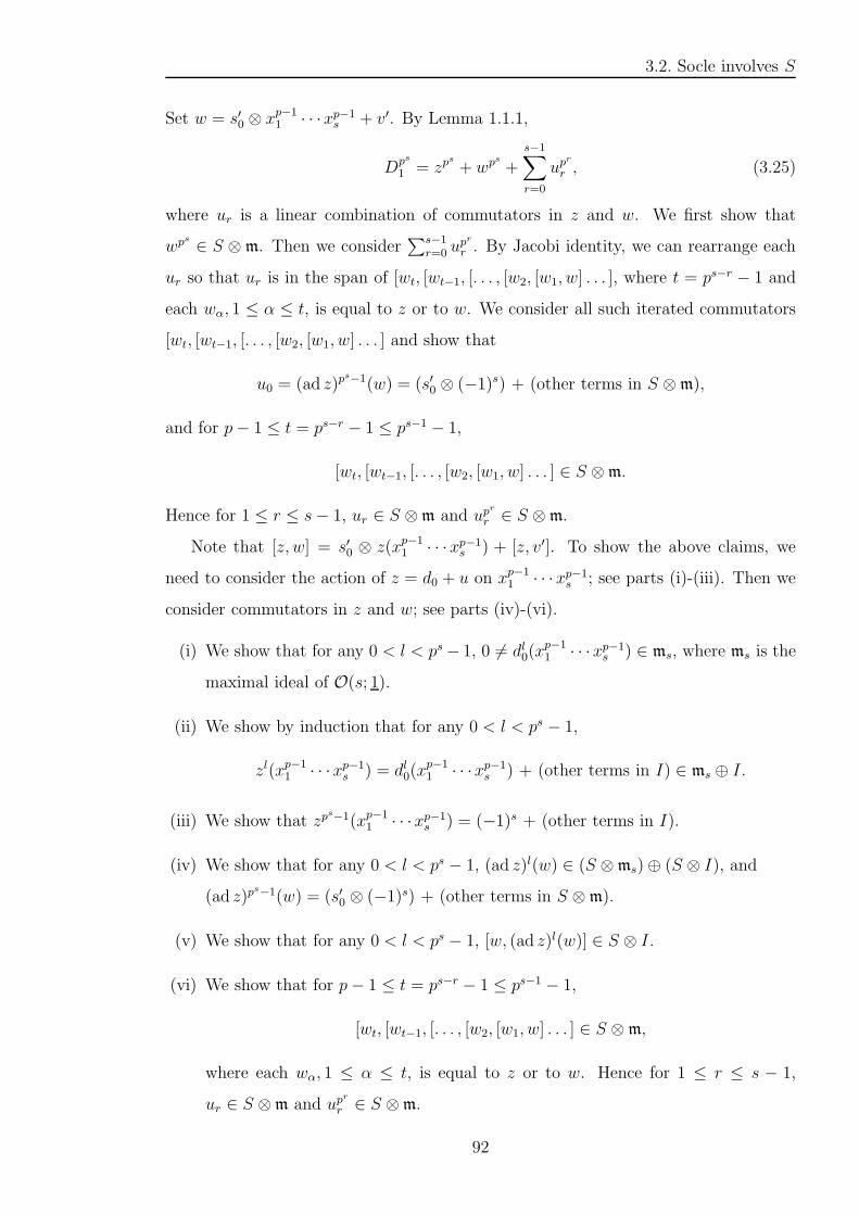
3.2. Socle involves S
Set w = s′0 ⊗ xp−11 · · ·xp−1
s + v′. By Lemma 1.1.1,
Dps
1 = zps
+ wps
+s−1∑
r=0
upr
r , (3.25)
where ur is a linear combination of commutators in z and w. We first show that
wps
∈ S ⊗ m. Then we consider∑s−1
r=0 upr
r . By Jacobi identity, we can rearrange each
ur so that ur is in the span of [wt, [wt−1, [. . . , [w2, [w1, w] . . . ], where t = ps−r − 1 and
each wα, 1 ≤ α ≤ t, is equal to z or to w. We consider all such iterated commutators
[wt, [wt−1, [. . . , [w2, [w1, w] . . . ] and show that
u0 = (ad z)ps−1(w) = (s′0 ⊗ (−1)s) + (other terms in S ⊗m),
and for p− 1 ≤ t = ps−r − 1 ≤ ps−1 − 1,
[wt, [wt−1, [. . . , [w2, [w1, w] . . . ] ∈ S ⊗m.
Hence for 1 ≤ r ≤ s− 1, ur ∈ S ⊗m and upr
r ∈ S ⊗m.
Note that [z, w] = s′0 ⊗ z(xp−11 · · ·xp−1
s ) + [z, v′]. To show the above claims, we
need to consider the action of z = d0 + u on xp−11 · · ·xp−1
s ; see parts (i)-(iii). Then we
consider commutators in z and w; see parts (iv)-(vi).
(i) We show that for any 0 < l < ps− 1, 0 6= dl0(xp−11 · · ·xp−1
s ) ∈ ms, where ms is the
maximal ideal of O(s; 1).
(ii) We show by induction that for any 0 < l < ps − 1,
zl(xp−11 · · ·xp−1
s ) = dl0(xp−11 · · ·xp−1
s ) + (other terms in I) ∈ ms ⊕ I.
(iii) We show that zps−1(xp−1
1 · · ·xp−1s ) = (−1)s + (other terms in I).
(iv) We show that for any 0 < l < ps − 1, (ad z)l(w) ∈ (S ⊗ms)⊕ (S ⊗ I), and
(ad z)ps−1(w) = (s′0 ⊗ (−1)s) + (other terms in S ⊗m).
(v) We show that for any 0 < l < ps − 1, [w, (ad z)l(w)] ∈ S ⊗ I.
(vi) We show that for p− 1 ≤ t = ps−r − 1 ≤ ps−1 − 1,
[wt, [wt−1, [. . . , [w2, [w1, w] . . . ] ∈ S ⊗m,
where each wα, 1 ≤ α ≤ t, is equal to z or to w. Hence for 1 ≤ r ≤ s − 1,
ur ∈ S ⊗m and upr
r ∈ S ⊗m.
92
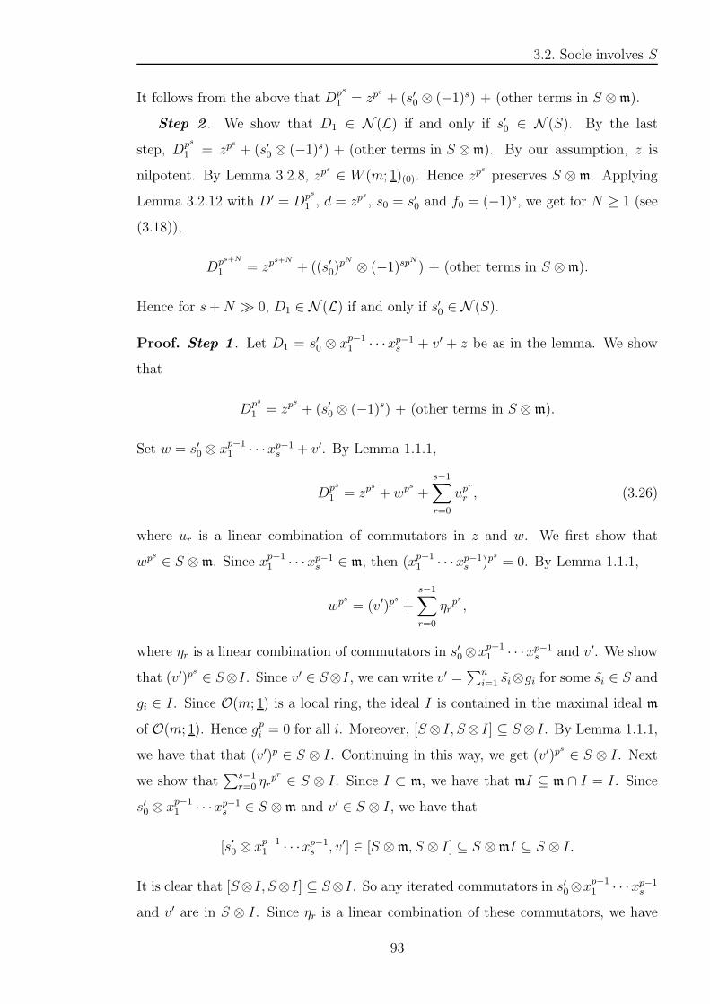
3.2. Socle involves S
It follows from the above that Dps
1 = zps
+ (s′0 ⊗ (−1)s) + (other terms in S ⊗m).
Step 2 . We show that D1 ∈ N (L) if and only if s′0 ∈ N (S). By the last
step, Dps
1 = zps
+ (s′0 ⊗ (−1)s) + (other terms in S ⊗m). By our assumption, z is
nilpotent. By Lemma 3.2.8, zps
∈ W (m; 1)(0). Hence zps
preserves S ⊗ m. Applying
Lemma 3.2.12 with D′ = Dps
1 , d = zps
, s0 = s′0 and f0 = (−1)s, we get for N ≥ 1 (see
(3.18)),
Dps+N
1 = zps+N
+ ((s′0)pN ⊗ (−1)sp
N
) + (other terms in S ⊗m).
Hence for s+N ≫ 0, D1 ∈ N (L) if and only if s′0 ∈ N (S).
Proof. Step 1 . Let D1 = s′0 ⊗ xp−11 · · ·xp−1
s + v′ + z be as in the lemma. We show
that
Dps
1 = zps
+ (s′0 ⊗ (−1)s) + (other terms in S ⊗m).
Set w = s′0 ⊗ xp−11 · · ·xp−1
s + v′. By Lemma 1.1.1,
Dps
1 = zps
+ wps
+
s−1∑
r=0
upr
r , (3.26)
where ur is a linear combination of commutators in z and w. We first show that
wps
∈ S ⊗m. Since xp−11 · · ·xp−1
s ∈ m, then (xp−11 · · ·xp−1
s )ps
= 0. By Lemma 1.1.1,
wps
= (v′)ps
+
s−1∑
r=0
ηrpr ,
where ηr is a linear combination of commutators in s′0⊗xp−11 · · ·xp−1
s and v′. We show
that (v′)ps
∈ S⊗I. Since v′ ∈ S⊗I, we can write v′ =∑n
i=1 si⊗gi for some si ∈ S and
gi ∈ I. Since O(m; 1) is a local ring, the ideal I is contained in the maximal ideal m
of O(m; 1). Hence gpi = 0 for all i. Moreover, [S⊗ I, S⊗ I] ⊆ S⊗ I. By Lemma 1.1.1,
we have that that (v′)p ∈ S ⊗ I. Continuing in this way, we get (v′)ps
∈ S ⊗ I. Next
we show that∑s−1
r=0 ηrpr ∈ S ⊗ I. Since I ⊂ m, we have that mI ⊆ m ∩ I = I. Since
s′0 ⊗ xp−11 · · ·xp−1
s ∈ S ⊗m and v′ ∈ S ⊗ I, we have that
[s′0 ⊗ xp−11 · · ·xp−1
s , v′] ∈ [S ⊗m, S ⊗ I] ⊆ S ⊗mI ⊆ S ⊗ I.
It is clear that [S⊗I, S⊗I] ⊆ S⊗I. So any iterated commutators in s′0⊗xp−11 · · ·xp−1
s
and v′ are in S ⊗ I. Since ηr is a linear combination of these commutators, we have
93
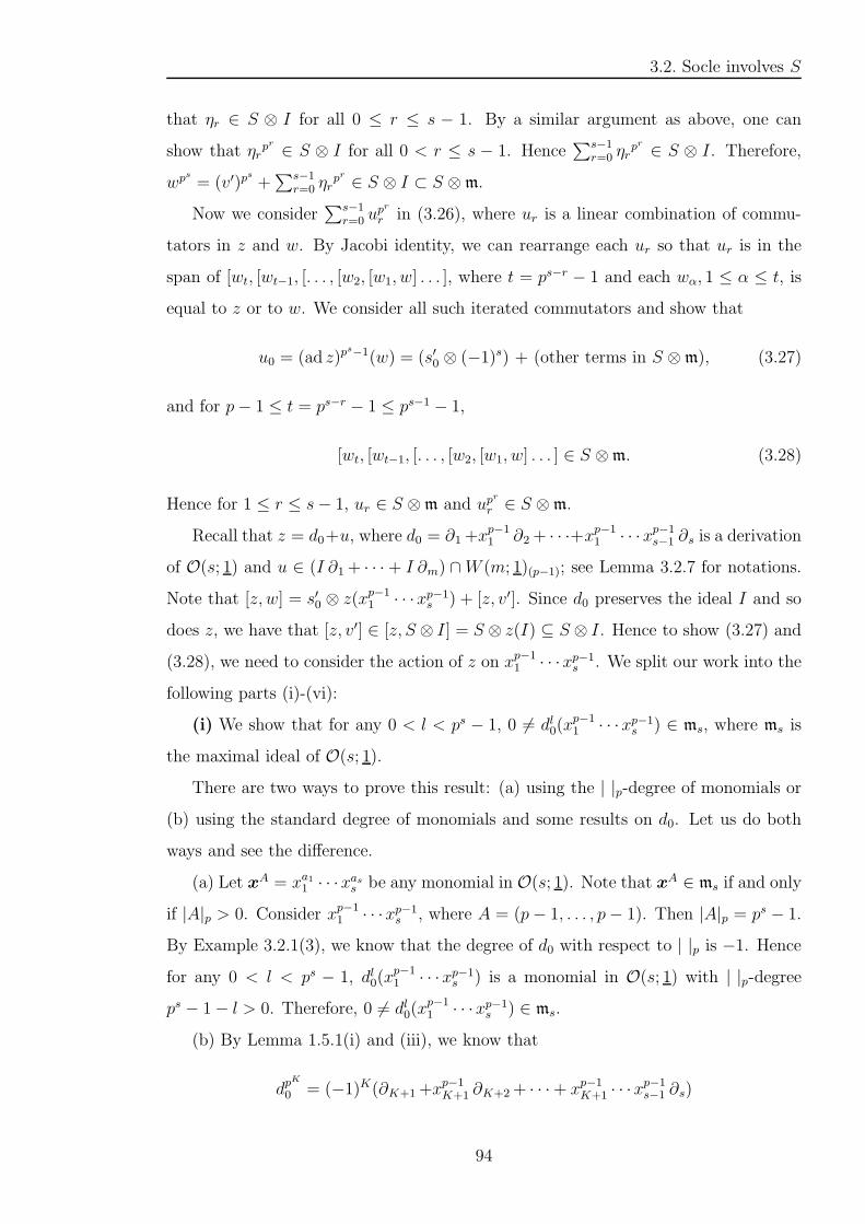
3.2. Socle involves S
that ηr ∈ S ⊗ I for all 0 ≤ r ≤ s − 1. By a similar argument as above, one can
show that ηrpr ∈ S ⊗ I for all 0 < r ≤ s − 1. Hence
∑s−1r=0 ηr
pr ∈ S ⊗ I. Therefore,
wps
= (v′)ps
+∑s−1
r=0 ηrpr ∈ S ⊗ I ⊂ S ⊗m.
Now we consider∑s−1
r=0 upr
r in (3.26), where ur is a linear combination of commu-
tators in z and w. By Jacobi identity, we can rearrange each ur so that ur is in the
span of [wt, [wt−1, [. . . , [w2, [w1, w] . . . ], where t = ps−r − 1 and each wα, 1 ≤ α ≤ t, is
equal to z or to w. We consider all such iterated commutators and show that
u0 = (ad z)ps−1(w) = (s′0 ⊗ (−1)s) + (other terms in S ⊗m), (3.27)
and for p− 1 ≤ t = ps−r − 1 ≤ ps−1 − 1,
[wt, [wt−1, [. . . , [w2, [w1, w] . . . ] ∈ S ⊗m. (3.28)
Hence for 1 ≤ r ≤ s− 1, ur ∈ S ⊗m and upr
r ∈ S ⊗m.
Recall that z = d0+u, where d0 = ∂1+xp−11 ∂2+ · · ·+x
p−11 · · ·xp−1
s−1 ∂s is a derivation
of O(s; 1) and u ∈ (I ∂1+ · · ·+ I ∂m) ∩W (m; 1)(p−1); see Lemma 3.2.7 for notations.
Note that [z, w] = s′0 ⊗ z(xp−11 · · ·xp−1
s ) + [z, v′]. Since d0 preserves the ideal I and so
does z, we have that [z, v′] ∈ [z, S ⊗ I] = S ⊗ z(I) ⊆ S ⊗ I. Hence to show (3.27) and
(3.28), we need to consider the action of z on xp−11 · · ·xp−1
s . We split our work into the
following parts (i)-(vi):
(i) We show that for any 0 < l < ps − 1, 0 6= dl0(xp−11 · · ·xp−1
s ) ∈ ms, where ms is
the maximal ideal of O(s; 1).
There are two ways to prove this result: (a) using the | |p-degree of monomials or
(b) using the standard degree of monomials and some results on d0. Let us do both
ways and see the difference.
(a) Let xA = xa11 · · ·xass be any monomial in O(s; 1). Note that xA ∈ ms if and only
if |A|p > 0. Consider xp−11 · · ·xp−1
s , where A = (p− 1, . . . , p− 1). Then |A|p = ps − 1.
By Example 3.2.1(3), we know that the degree of d0 with respect to | |p is −1. Hence
for any 0 < l < ps − 1, dl0(xp−11 · · ·xp−1
s ) is a monomial in O(s; 1) with | |p-degree
ps − 1− l > 0. Therefore, 0 6= dl0(xp−11 · · ·xp−1
s ) ∈ ms.
(b) By Lemma 1.5.1(i) and (iii), we know that
dpK
0 = (−1)K(∂K+1+xp−1K+1 ∂K+2+ · · ·+ xp−1
K+1 · · ·xp−1s−1 ∂s)
94
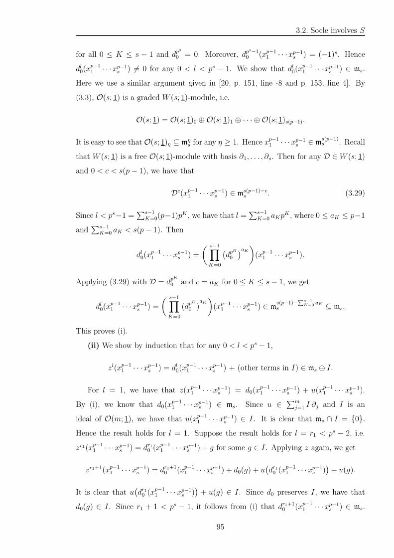
3.2. Socle involves S
for all 0 ≤ K ≤ s − 1 and dps
0 = 0. Moreover, dps−1
0 (xp−11 · · ·xp−1
s ) = (−1)s. Hence
dl0(xp−11 · · ·xp−1
s ) 6= 0 for any 0 < l < ps − 1. We show that dl0(xp−11 · · ·xp−1
s ) ∈ ms.
Here we use a similar argument given in [20, p. 151, line -8 and p. 153, line 4]. By
(3.3), O(s; 1) is a graded W (s; 1)-module, i.e.
O(s; 1) = O(s; 1)0 ⊕O(s; 1)1 ⊕ · · · ⊕ O(s; 1)s(p−1).
It is easy to see that O(s; 1)η ⊆ mηs for any η ≥ 1. Hence xp−1
1 · · ·xp−1s ∈ m
s(p−1)s . Recall
that W (s; 1) is a free O(s; 1)-module with basis ∂1, . . . , ∂s. Then for any D ∈ W (s; 1)
and 0 < c < s(p− 1), we have that
Dc(xp−11 · · ·xp−1
s ) ∈ ms(p−1)−cs . (3.29)
Since l < ps−1 =∑s−1
K=0(p−1)pK , we have that l =
∑s−1K=0 aKp
K , where 0 ≤ aK ≤ p−1
and∑s−1
K=0 aK < s(p− 1). Then
dl0(xp−11 · · ·xp−1
s ) =
( s−1∏
K=0
(
dpK
0
)aK)
(xp−11 · · ·xp−1
s ).
Applying (3.29) with D = dpK
0 and c = aK for 0 ≤ K ≤ s− 1, we get
dl0(xp−11 · · ·xp−1
s ) =
( s−1∏
K=0
(dpK
0 )aK
)
(xp−11 · · ·xp−1
s ) ∈ ms(p−1)−
∑s−1
K=0aK
s ⊆ ms.
This proves (i).
(ii) We show by induction that for any 0 < l < ps − 1,
zl(xp−11 · · ·xp−1
s ) = dl0(xp−11 · · ·xp−1
s ) + (other terms in I) ∈ ms ⊕ I.
For l = 1, we have that z(xp−11 · · ·xp−1
s ) = d0(xp−11 · · ·xp−1
s ) + u(xp−11 · · ·xp−1
s ).
By (i), we know that d0(xp−11 · · ·xp−1
s ) ∈ ms. Since u ∈∑m
j=1 I ∂j and I is an
ideal of O(m; 1), we have that u(xp−11 · · ·xp−1
s ) ∈ I. It is clear that ms ∩ I = 0.
Hence the result holds for l = 1. Suppose the result holds for l = r1 < ps − 2, i.e.
zr1(xp−11 · · ·xp−1
s ) = dr10 (xp−11 · · ·xp−1
s ) + g for some g ∈ I. Applying z again, we get
zr1+1(xp−11 · · ·xp−1
s ) = dr1+10 (xp−1
1 · · ·xp−1s ) + d0(g) + u
(
dr10 (xp−11 · · ·xp−1
s ))
+ u(g).
It is clear that u(
dr10 (xp−11 · · ·xp−1
s ))
+ u(g) ∈ I. Since d0 preserves I, we have that
d0(g) ∈ I. Since r1 + 1 < ps − 1, it follows from (i) that dr1+10 (xp−1
1 · · ·xp−1s ) ∈ ms.
95
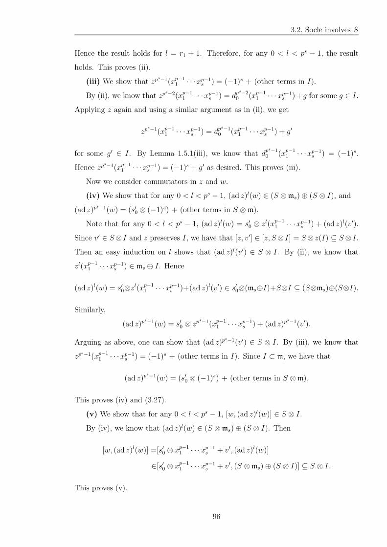
3.2. Socle involves S
Hence the result holds for l = r1 + 1. Therefore, for any 0 < l < ps − 1, the result
holds. This proves (ii).
(iii) We show that zps−1(xp−1
1 · · ·xp−1s ) = (−1)s + (other terms in I).
By (ii), we know that zps−2(xp−1
1 · · ·xp−1s ) = dp
s−20 (xp−1
1 · · ·xp−1s )+g for some g ∈ I.
Applying z again and using a similar argument as in (ii), we get
zps−1(xp−1
1 · · ·xp−1s ) = dp
s−10 (xp−1
1 · · ·xp−1s ) + g′
for some g′ ∈ I. By Lemma 1.5.1(iii), we know that dps−1
0 (xp−11 · · ·xp−1
s ) = (−1)s.
Hence zps−1(xp−1
1 · · ·xp−1s ) = (−1)s + g′ as desired. This proves (iii).
Now we consider commutators in z and w.
(iv) We show that for any 0 < l < ps − 1, (ad z)l(w) ∈ (S ⊗ms)⊕ (S ⊗ I), and
(ad z)ps−1(w) = (s′0 ⊗ (−1)s) + (other terms in S ⊗m).
Note that for any 0 < l < ps − 1, (ad z)l(w) = s′0 ⊗ zl(xp−1
1 · · ·xp−1s ) + (ad z)l(v′).
Since v′ ∈ S⊗ I and z preserves I, we have that [z, v′] ∈ [z, S⊗ I] = S⊗ z(I) ⊆ S⊗ I.
Then an easy induction on l shows that (ad z)l(v′) ∈ S ⊗ I. By (ii), we know that
zl(xp−11 · · ·xp−1
s ) ∈ ms ⊕ I. Hence
(ad z)l(w) = s′0⊗zl(xp−1
1 · · ·xp−1s )+(ad z)l(v′) ∈ s′0⊗(ms⊕I)+S⊗I ⊆ (S⊗ms)⊕(S⊗I).
Similarly,
(ad z)ps−1(w) = s′0 ⊗ z
ps−1(xp−11 · · ·xp−1
s ) + (ad z)ps−1(v′).
Arguing as above, one can show that (ad z)ps−1(v′) ∈ S ⊗ I. By (iii), we know that
zps−1(xp−1
1 · · ·xp−1s ) = (−1)s + (other terms in I). Since I ⊂ m, we have that
(ad z)ps−1(w) = (s′0 ⊗ (−1)s) + (other terms in S ⊗m).
This proves (iv) and (3.27).
(v) We show that for any 0 < l < ps − 1, [w, (ad z)l(w)] ∈ S ⊗ I.
By (iv), we know that (ad z)l(w) ∈ (S ⊗ms)⊕ (S ⊗ I). Then
[w, (ad z)l(w)] =[s′0 ⊗ xp−11 · · ·xp−1
s + v′, (ad z)l(w)]
∈[s′0 ⊗ xp−11 · · ·xp−1
s + v′, (S ⊗ms)⊕ (S ⊗ I)] ⊆ S ⊗ I.
This proves (v).
96
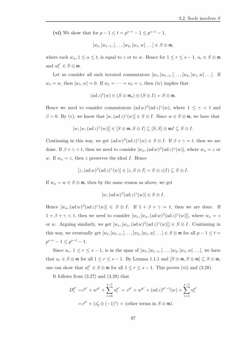
3.2. Socle involves S
(vi) We show that for p− 1 ≤ t = ps−r − 1 ≤ ps−1 − 1,
[wt, [wt−1, [. . . , [w2, [w1, w] . . . ] ∈ S ⊗m,
where each wα, 1 ≤ α ≤ t, is equal to z or to w. Hence for 1 ≤ r ≤ s− 1, ur ∈ S ⊗m
and upr
r ∈ S ⊗m.
Let us consider all such iterated commutators [wt, [wt−1, [. . . , [w2, [w1, w] . . . ]. If
w1 = w, then [w1, w] = 0. If w1 = · · · = wt = z, then (iv) implies that
(ad z)t(w) ∈ (S ⊗ms)⊕ (S ⊗ I) = S ⊗m.
Hence we need to consider commutators (adw)β(ad z)γ(w), where 1 ≤ γ < t and
β > 0. By (v), we know that [w, (ad z)γ(w)] ∈ S ⊗ I. Since w ∈ S ⊗m, we have that
[w, [w, (ad z)γ(w)]] ∈ [S ⊗m, S ⊗ I] ⊆ [S, S]⊗mI ⊆ S ⊗ I.
Continuing in this way, we get (adw)β(ad z)γ(w) ∈ S ⊗ I. If β + γ = t, then we are
done. If β + γ < t, then we need to consider [wα, (adw)β(ad z)γ(w)], where wα = z or
w. If wα = z, then z preserves the ideal I. Hence
[z, (adw)β(ad z)γ(w)] ∈ [z, S ⊗ I] = S ⊗ z(I) ⊆ S ⊗ I.
If wα = w ∈ S ⊗m, then by the same reason as above, we get
[w, (adw)β(ad z)γ(w)] ∈ S ⊗ I.
Hence [wα, (adw)β(ad z)γ(w)] ∈ S ⊗ I. If 1 + β + γ = t, then we are done. If
1 + β + γ < t, then we need to consider [wν , [wα, (adw)β(ad z)γ(w)]], where wν = z
or w. Arguing similarly, we get [wν , [wα, (adw)β(ad z)γ(w)]] ∈ S ⊗ I. Continuing in
this way, we eventually get [wt, [wt−1, [. . . , [w2, [w1, w] . . . ] ∈ S ⊗m for all p− 1 ≤ t =
ps−r − 1 ≤ ps−1 − 1.
Since ur, 1 ≤ r ≤ s − 1, is in the span of [wt, [wt−1, [. . . , [w2, [w1, w] . . . ], we have
that ur ∈ S ⊗m for all 1 ≤ r ≤ s− 1. By Lemma 1.1.1 and [S ⊗m, S ⊗m] ⊆ S ⊗m,
one can show that upr
r ∈ S ⊗m for all 1 ≤ r ≤ s− 1. This proves (vi) and (3.28).
It follows from (3.27) and (3.28) that
Dps
1 =zps
+ wps
+s−1∑
r=0
upr
r = zps
+ wps
+ (ad z)ps−1(w) +
s−1∑
r=1
upr
r
=zps
+ (s′0 ⊗ (−1)s) + (other terms in S ⊗m).
97
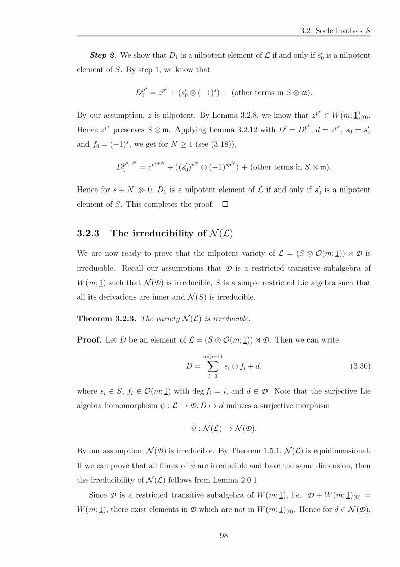
3.2. Socle involves S
Step 2 . We show that D1 is a nilpotent element of L if and only if s′0 is a nilpotent
element of S. By step 1, we know that
Dps
1 = zps
+ (s′0 ⊗ (−1)s) + (other terms in S ⊗m).
By our assumption, z is nilpotent. By Lemma 3.2.8, we know that zps
∈ W (m; 1)(0).
Hence zps
preserves S ⊗m. Applying Lemma 3.2.12 with D′ = Dps
1 , d = zps
, s0 = s′0
and f0 = (−1)s, we get for N ≥ 1 (see (3.18)),
Dps+N
1 = zps+N
+ ((s′0)pN ⊗ (−1)sp
N
) + (other terms in S ⊗m).
Hence for s + N ≫ 0, D1 is a nilpotent element of L if and only if s′0 is a nilpotent
element of S. This completes the proof.
3.2.3 The irreducibility of N (L)
We are now ready to prove that the nilpotent variety of L = (S ⊗ O(m; 1)) ⋊ D is
irreducible. Recall our assumptions that D is a restricted transitive subalgebra of
W (m; 1) such that N (D) is irreducible, S is a simple restricted Lie algebra such that
all its derivations are inner and N (S) is irreducible.
Theorem 3.2.3. The variety N (L) is irreducible.
Proof. Let D be an element of L = (S ⊗O(m; 1))⋊ D. Then we can write
D =
m(p−1)∑
i=0
si ⊗ fi + d, (3.30)
where si ∈ S, fi ∈ O(m; 1) with deg fi = i, and d ∈ D. Note that the surjective Lie
algebra homomorphism ψ : L → D, D 7→ d induces a surjective morphism
ψ : N (L)→ N (D).
By our assumption, N (D) is irreducible. By Theorem 1.5.1, N (L) is equidimensional.
If we can prove that all fibres of ψ are irreducible and have the same dimension, then
the irreducibility of N (L) follows from Lemma 2.0.1.
Since D is a restricted transitive subalgebra of W (m; 1), i.e. D + W (m; 1)(0) =
W (m; 1), there exist elements in D which are not in W (m; 1)(0). Hence for d ∈ N (D),
98
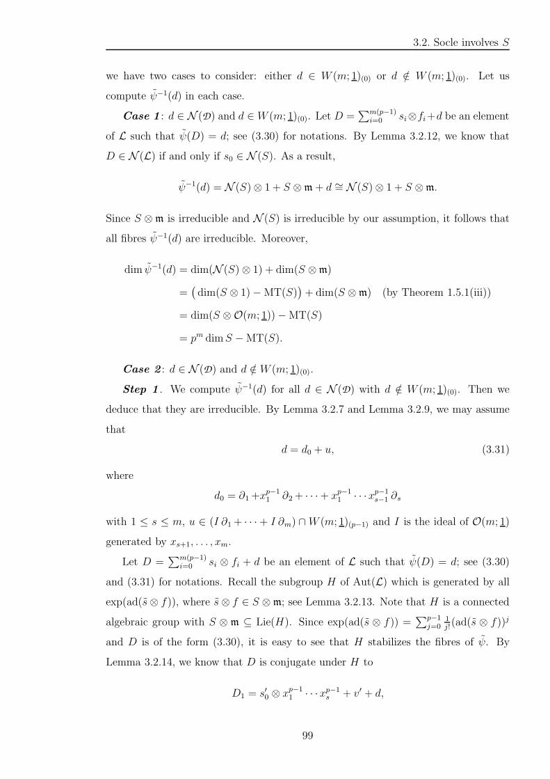
3.2. Socle involves S
we have two cases to consider: either d ∈ W (m; 1)(0) or d /∈ W (m; 1)(0). Let us
compute ψ−1(d) in each case.
Case 1 : d ∈ N (D) and d ∈ W (m; 1)(0). Let D =∑m(p−1)
i=0 si⊗fi+d be an element
of L such that ψ(D) = d; see (3.30) for notations. By Lemma 3.2.12, we know that
D ∈ N (L) if and only if s0 ∈ N (S). As a result,
ψ−1(d) = N (S)⊗ 1 + S ⊗m+ d ∼= N (S)⊗ 1 + S ⊗m.
Since S ⊗m is irreducible and N (S) is irreducible by our assumption, it follows that
all fibres ψ−1(d) are irreducible. Moreover,
dim ψ−1(d) = dim(N (S)⊗ 1) + dim(S ⊗m)
=(
dim(S ⊗ 1)−MT(S))
+ dim(S ⊗m) (by Theorem 1.5.1(iii))
= dim(S ⊗O(m; 1))−MT(S)
= pm dimS −MT(S).
Case 2 : d ∈ N (D) and d /∈ W (m; 1)(0).
Step 1 . We compute ψ−1(d) for all d ∈ N (D) with d /∈ W (m; 1)(0). Then we
deduce that they are irreducible. By Lemma 3.2.7 and Lemma 3.2.9, we may assume
that
d = d0 + u, (3.31)
where
d0 = ∂1+xp−11 ∂2+ · · ·+ xp−1
1 · · ·xp−1s−1 ∂s
with 1 ≤ s ≤ m, u ∈ (I ∂1+ · · ·+ I ∂m) ∩W (m; 1)(p−1) and I is the ideal of O(m; 1)
generated by xs+1, . . . , xm.
Let D =∑m(p−1)
i=0 si ⊗ fi + d be an element of L such that ψ(D) = d; see (3.30)
and (3.31) for notations. Recall the subgroup H of Aut(L) which is generated by all
exp(ad(s⊗ f)), where s⊗ f ∈ S ⊗m; see Lemma 3.2.13. Note that H is a connected
algebraic group with S ⊗ m ⊆ Lie(H). Since exp(ad(s ⊗ f)) =∑p−1
j=01j!(ad(s ⊗ f))j
and D is of the form (3.30), it is easy to see that H stabilizes the fibres of ψ. By
Lemma 3.2.14, we know that D is conjugate under H to
D1 = s′0 ⊗ xp−11 · · ·xp−1
s + v′ + d,
99
3.2. Socle involves S
where s′0 ∈ S (possibly 0), v′ ∈ S⊗ I and d = d0+u as in (3.31). Then D is nilpotent
if and only if D1 is nilpotent. By Lemma 3.2.15, we know that D1 ∈ N (L) if and only
if s′0 ∈ N (S). Hence all fibres of ψ have the form
H.(
N (S)⊗ xp−11 · · ·xp−1
s + S ⊗ I + d)
∼= H.(
N (S)⊗ xp−11 · · ·xp−1
s + S ⊗ I)
.
Since H is connected, N (S) and S ⊗ I are irreducible, it follows that all fibres ψ−1(d)
are irreducible.
Step 2 . We show that all fibres of ψ have the same dimension. By case 1, we
know that dim ψ−1(d) = pm dimS −MT(S) for all d ∈ N (D) with d ∈ W (m; 1)(0). In
particular,
dim ψ−1(0) = pm dimS −MT(S). (3.32)
To finish the proof we just need to show that
dim ψ−1(d) = dim ψ−1(0)
for all d ∈ N (D) with d /∈ W (m; 1)(0).
Step 2(i). We first show that
dim ψ−1(0) ≥ dim ψ−1(d)
for all d ∈ N (D) with d /∈ W (m; 1)(0). Suppose the contrary, i.e. dim ψ−1(0) <
dim ψ−1(d) for some d ∈ N (D) with d /∈ W (m; 1)(0). By Theorem 1.6.7, the set
W1 =
x ∈ N (L) | dim ψ−1(ψ(x)) ≥ r
is Zariski closed in N (L) for every r ∈ N0. We now take r = dim ψ−1(0) + 1. If W1
is empty, then we are done. If W1 is nonempty, then it contains w + d ∈ N (L) with
w ∈ S ⊗m such that dim ψ−1(ψ(w + d)) ≥ r. Note that for all λ ∈ k∗,
ψ(λ(w + d)) = λψ(w + d).
Then
ψ−1(
ψ(λ(w + d)))
= λψ−1(
ψ(w + d))
.
So W1 is k∗-stable. Since W1 is Zariski closed, it contains 0. But this contradicts our
choice of r. As a result,
dim ψ−1(0) ≥ dim ψ−1(d) (3.33)
100
3.2. Socle involves S
for all d ∈ N (D) with d /∈ W (m; 1)(0).
Step 2(ii). Next we show that
dim ψ−1(0) ≤ dim ψ−1(d)
for all d ∈ N (D) with d /∈ W (m; 1)(0). Consider the morphism
θ : H ×(
N (S)⊗ xp−11 · · ·xp−1
s + S ⊗ I + d)
→ ψ−1(d)
(h,D1) 7→ h(D1).
By the work in step 1, we know that any point in the fibre ψ−1(d) has the form
θ(
h, s′0 ⊗ xp−11 · · ·xp−1
s + v′ + d)
for some h ∈ H, s′0 ∈ N (S) and v′ ∈ S⊗ I. As H acts on the fibre it preserves smooth
points. Hence we may assume that h = 1. Instead of computing dim ψ−1(d) which
is difficult, we can compute the differential of θ at a smooth point of the fibre with
h = 1. Since N (S) is irreducible, the set of smooth points in N (S) is nonempty. Let
s′0 be a smooth point of N (S). Then dimTs′0(N (S)) = dimN (S). Take
D1 = s′0 ⊗ xp−11 · · ·xp−1
s + v′ + d ∈ ψ−1(d).
Then the differential of θ at (1, D1) is
(dθ)(1,D1) : Lie(H)⊕(
Ts′0(N (S))⊗ xp−1
1 · · ·xp−1s + S ⊗ I
)
→ TD1(ψ−1(d))
(X, Y ) 7→ [X,D1] + Y.
Since D1 is a smooth point, this implies that dimTD1(ψ−1(d)) = dim ψ−1(d). In order
to show that dim ψ−1(0) ≤ dim ψ−1(d), we just need to show that
dim ψ−1(0) ≤ dimTD1(ψ−1(d)).
It is clear that
Ts′0(N (S))⊗ xp−1
1 · · ·xp−1s + S ⊗ I ⊆ Im((dθ)(1,D1)). (3.34)
Moreover, [Lie(H), D1] ⊆ Im((dθ)(1,D1)). Since S ⊗m ⊆ Lie(H), we have that
[S ⊗m, D1] = [S ⊗m, s′0 ⊗ xp−11 · · ·xp−1
s + v′ + d] ⊆ Im((dθ)(1,D1)) (3.35)
Observe (3.34) and (3.35) carefully. We see that Im((dθ)(1,D1)) contains the follow-
ing subspaces:
101
3.2. Socle involves S
(1) Ts′0(N (S))⊗ xp−1
1 · · ·xp−1s which has dimension equal to dimN (S).
(2) S ⊗ I.
(3) [S ⊗m, s′0 ⊗ xp−11 · · ·xp−1
s + v′ + d].
Look at the last two subspaces. Note that m = ms⊕ I, where ms is the maximal ideal
of O(s; 1). Moreover, mI ⊆ I. Since S ⊗ I is in Im((dθ)(1,D1)),
[S ⊗m, s′0 ⊗ xp−11 · · ·xp−1
s ] = [S ⊗ (ms ⊕ I), s′0 ⊗ x
p−11 · · ·xp−1
s ] ⊆ S ⊗ I,
and
[S ⊗m, v′] ⊆ [S ⊗m, S ⊗ I] ⊆ S ⊗mI ⊆ S ⊗ I,
we see that Im((dθ)(1,D1)) contains
S ⊗ I + [S ⊗m, s′0 ⊗ xp−11 · · ·xp−1
s + v′ + d]
=S ⊗ I + [S ⊗m, d]
=S ⊗ I + S ⊗ d(m).
Recall (3.31) that d = d0 + u, where d0 = ∂1+xp−11 ∂2+ · · · + xp−1
1 · · ·xp−1s−1 ∂s is a
derivation of O(s; 1) and u ∈ (I ∂1+ · · ·+ I ∂m) ∩W (m; 1)(p−1). Since u(m) ⊆ I, we
have that S⊗ I +S⊗ d(m) = S⊗ I +S⊗ d0(m). Since m = ms⊕ I, d0(ms) ⊂ O(s; 1),
d0(I) ⊆ I and O(s; 1)∩I = 0, we have that d0(m) = d0(ms)⊕d0(I). Since d0(I) ⊆ I,
we have that
S⊗I+S⊗d(m) = S⊗I+S⊗d0(m) = (S⊗I)⊕(S⊗d0(ms)) ∼= S⊗(I⊕d0(ms)). (3.36)
By Lemma 3.2.11 (see (3.17)), we know the subspaceM = I+d(m) = I⊕d0(ms) has the
property thatM⊕kxp−11 · · ·xp−1
s = O(m; 1). By (3.36), we see that the sum of the last
two subspaces equals S ⊗M . This subspace of dimension (pm − 1) dimS is contained
in Im((dθ)(1,D1)) and the complement of the first subspace Ts′0(N (S))⊗ xp−1
1 · · ·xp−1s .
Therefore,
dim Im((dθ)(1,D1)) ≥ dim(Ts′0(N (S))⊗ xp−1
1 · · ·xp−1s ) + dim(S ⊗M)
= dimN (S) + (pm − 1) dimS
= (dimS −MT(S)) + (pm − 1) dimS
= pm dimS −MT(S)
= dim ψ−1(0) (see (3.32)).
102
3.2. Socle involves S
Since Im((dθ)(1,D1)) ⊆ TD1(ψ−1(d)) we have that
dim ψ−1(0) ≤ dimTD1(ψ−1(d)) = dim ψ−1(d). (3.37)
It follows from (3.33) and (3.37) that all fibres of ψ have the same dimension.
By case 1 and 2, we see that all fibres of ψ are irreducible and have the same
dimension. Hence N (L) is irreducible by Lemma 2.0.1. This completes the proof.
Remark 3.2.3. 1. We verified Premet’s conjecture for a class of semisimple re-
stricted Lie algebras L = (S ⊗ O(m; 1)) ⋊ D under the assumptions that S is a
simple restricted Lie algebra over k with adS = DerS and N (S) is irreducible,
D is a restricted transitive subalgebra of W (m; 1) with N (D) is irreducible.
2. A similar argument works for⊕t
i=1(Si ⊗O(mi; 1))⋊ (IdSi⊗Di), where
(i) each Si is a simple restricted Lie algebra such that adSi = DerSi and N (Si)
is irreducible, and
(ii) each Di is a restricted transitive subalgebra of W (mi; 1) such that N (Di) is
irreducible.
3. There are further cases to consider such as adS ( DerS and other semisimple
restricted Lie algebras which are not of the form given in Theorem 1.6.3. It is
unclear to the author how to tackle these problems.
103
Chapter 4
The nilpotent variety of W (1;n)p is
irreducible
In this chapter we assume that k is an algebraically closed field of characteristic p > 3,
and n ∈ N≥2. We are interested in the minimal p-envelope W (1;n)p of the Zassen-
haus algebra W (1;n). This restricted Lie algebra is semisimple. Recent studies have
shown that the variety N (W (1;n)) := N (W (1;n)p) ∩W (1;n) is reducible [37, The-
orem 4.8(i)]. So investigating the variety N (W (1;n)p) becomes critical for verifying
Premet’s conjecture. Note that this chapter contains the main result of the research
paper [3] written by the author of this thesis.
This chapter is organized as follows. We first recall some basic results on W (1;n)
andW (1;n)p. Then we study some nilpotent elements ofW (1;n)p and identify an irre-
ducible component of N (W (1;n)p). Finally, we prove that N (W (1;n)p) is irreducible.
The proof is similar to Premet’s proof for the Jacobson-Witt algebraW (n; 1); see The-
orem 1.5.2. But the (n + 1)-dimensional subspace V used in W (n; 1) has no obvious
analogue for W (1;n)p. Therefore, a new V is constructed using the original definition
of W (1;n) due to H. Zassenhaus. In general, constructing analogues of V for the min-
imal p-envelopes of W (n;m), where m = (m1, . . . , mn) and mi > 1 for some i, would
enable one to check Premet’s conjecture for this class of restricted Lie algebras.
104
4.1. Preliminaries
4.1 Preliminaries
4.1.1 W (1;n) and W (1;n)p
Let k be an algebraically closed field of characteristic p > 3 and n ∈ N. The divided
power algebra O(1;n) has a k-basis x(a) = 1a!xa | 0 ≤ a ≤ pn− 1, and the product in
O(1;n) is given by x(a)x(b) =(
a+ba
)
x(a+b) if 0 ≤ a+ b ≤ pn − 1 and 0 otherwise. In the
following, we write x(1) as x. It is straightforward to see that O(1;n) is a local algebra
with the unique maximal ideal m spanned by all x(a) such that a ≥ 1. A system of
divided powers is defined on m, f 7→ f (r) ∈ O(1;n), where r ≥ 0; see Definition 1.4.2.
A derivation D of O(1;n) is called special if D(x(a)) = x(a−1)D(x) for 1 ≤ a ≤ pn−1
and 0 otherwise; see Definition 1.4.3. The set of all special derivations of O(1;n)
forms a Lie subalgebra of DerO(1;n) denoted L =W (1;n) and called the Zassenhaus
algebra. When n = 1, L coincides with the Witt algebra W (1; 1) := DerO(1; 1),
a simple and restricted Lie algebra. When n ≥ 2, L provides the first example of a
simple, non-restricted Lie algebra; see Theorem 1.4.2. From now on, we always assume
that n ≥ 2.
The Zassenhaus algebra L admits an O(1;n)-module structure via (fD)(x) =
fD(x) for all f ∈ O(1;n) and D ∈ L. Since each D ∈ L is uniquely determined by
its effect on x, it is easy to see that L is a free O(1;n)-module of rank 1 generated
by the special derivation ∂ such that ∂(x(a)) = x(a−1) if 1 ≤ a ≤ pn − 1 and 0
otherwise; see Theorem 1.4.2. Hence the Lie bracket in L is given by [x(i) ∂, x(j) ∂] =((
i+j−1i
)
−(
i+j−1j
))
x(i+j−1) ∂ if 1 ≤ i+ j ≤ pn and 0 otherwise; see formula (1.4).
There is a Z-grading on L, i.e. L =⊕pn−2
i=−1 kdi with di := x(i+1)∂. Put L(i) :=⊕pn−2
j≥i kdj for −1 ≤ i ≤ pn − 2. Then this Z-grading induces a natural filtration
L = L(−1) ⊃ L(0) ⊃ L(1) ⊃ · · · ⊃ L(pn−2) ⊃ 0 (4.1)
on L. It is known that for i ≥ 0,
dpi =
di, if i = 0,
dpi, if i = pt − 1 for some 1 ≤ t ≤ n− 1,
0, otherwise.
(4.2)
In particular, L(0) is a restricted Lie subalgebra of DerO(1;n) and L(1) = nil (L(0));
see [37, p. 3]. We show that this implies that all nonzero tori in L(0) have dimension 1.
105
4.1. Preliminaries
Consider the surjective map π : L(0) ։ L(0)/L(1). Let t be any nonzero torus in L(0).
Let π|t be the restriction of π to t. Then Ker π|t ⊂ L(1). Since L(1) is a nilpotent p-ideal
of L(0), we have that Ker π|t = 0. Hence any nonzero torus t in L(0) has dimension 1;
see [32, Sec. 2]. As an example, kd0 = kx ∂ is a 1-dimensional torus in L(0).
Note that the Zassenhaus algebra L has another presentation. Let q = pn and let
Fq ⊂ k be the set of all roots of xq−x = 0. This is a finite field with q elements. Then
L has a k-basis eα |α ∈ Fq with the Lie bracket given by [eα, eβ] = (β − α)eα+β [30,
Theorem 7.6.3(1)]. We will use this presentation in Sec. 4.2.3.
It is also useful to mention that there is an embedding from L into the Jacobson-
Witt algebra W (n; 1); see [37, Lemma 3.1 and Proposition 4.3]. Recall that W (n; 1) is
the derivation algebra of O(n; 1), where O(n; 1) = k[X1, . . . , Xn]/(Xp1 , . . . , X
pn) is the
truncated polynomial ring in n variables. For each 1 ≤ i ≤ n, we write xi for the image
of Xi in O(n; 1). Note that W (n; 1) is a free O(n; 1)-module of rank n generated by
the partial derivatives ∂1, . . . , ∂n such that ∂i(xj) = δij for all 1 ≤ i, j ≤ n; see Sec. 1.5
for details. The Zassenhaus algebra L is the set of all special derivations of the divided
power algebra O(1;n). Note that O(1;n) has a k-basis x(a) | 0 ≤ a ≤ pn − 1. For
each 0 ≤ a ≤ pn − 1, let a =∑n−1
K=0 aKpK , 0 ≤ aK ≤ p− 1, be the p-adic expansion of
a. Define
φ : O(1;n)→ O(n; 1)
x(a) 7→n∏
i=1
xai−1
i
ai−1!;
(4.3)
see [37, (3.1.1)]. Then φ is an algebra isomorphism and it induces the following Lie
algebra isomorphism:
ϕ : DerO(1;n)∼−→ W (n; 1) = DerO(n; 1)
D 7→ ϕ(D),(4.4)
where (ϕ(D))(u) = φ(
D(φ−1(u)))
for all u ∈ O(n; 1). Moreover, ϕ(Dp) = ϕ(D)p for
all D ∈ DerO(1;n); see [37, (3.1.2)]. Since L is a Lie subalgebra of DerO(1;n), the
above ϕ induces an embedding
ι = ϕ|L : L → W (n; 1); (4.5)
see [37, (4.3.2)]. More precisely, ι is induced by φ defined in (4.3). By a direct
106
4.1. Preliminaries
computation, we have that
ι(∂) = D1 = ∂1+n−1∑
l=1
(−1)lxp−11 · · ·xp−1
l ∂l+1 .
Note that D1 has a similar expression to D in Lemma 1.5.1. We will use the above
embedding ι in the sketch proof of Lemma 4.2.2.
Let Lp = W (1;n)p denote the p-envelope of L ∼= adL in DerL. This semisimple
restricted Lie algebra is referred to as the minimal p-envelope of L; see Remark 1.2.1.
By Theorem 1.4.4, we have that Lp = L +∑n−1
i=1 k∂pi . Here we identify L with
adL ⊂ DerL and regard ∂pn
as 0. Then dimLp = pn + (n− 1). By formula (1.4), we
have that for any 1 ≤ i ≤ n−1 and 0 ≤ a ≤ pn−1, the brackets [∂pi
, x(a) ∂] = x(a−pi) ∂
if a ≥ pi and 0 otherwise.
Let N denote the variety of nilpotent elements in Lp. It is well known that N is
Zariski closed in Lp. One should note that the maximal dimension of toral subalgebras
in Lp equals n [30, Theorem 7.6.3(2)]. Moreover, Lp possesses a toral Cartan subalge-
bra; see [19, p. 555]. Hence the set of all semisimple elements of Lp is Zariski dense in
Lp; see [18, Theorem 2]. It follows from these facts and Theorem 1.5.1 that there exist
nonzero homogeneous polynomial functions ϕ0, . . . , ϕn−1 on Lp such that N coincides
with the set of all common zeros of ϕ0, . . . , ϕn−1. The variety N is equidimensional of
dimension pn − 1. Furthermore, any D ∈ N satisfies
Dpn
= 0. (4.6)
4.1.2 The automorphism group G
An automorphism Φ of O(1;n) is called admissible if Φ(f (r)) = Φ(f)(r) for all f ∈ m
and r ≥ 0. By [36, Lemma 8], this is equivalent to the condition that Φ(x(pj)) =
Φ(x)(pj ) for any 1 ≤ j ≤ n−1. Let G denote the group of all admissible automorphisms
of O(1;n). It is well known that G is a connected algebraic group, and each Φ ∈ G
is uniquely determined by its effect on x. By [36, Theorem 2], an assignment Φ(x) :=∑pn−1
i=1 αix(i) with αi ∈ k such that α1 6= 0 and αpj = 0 for 1 ≤ j ≤ n−1 extends to an
admissible automorphism of O(1;n). Conversely, if Φ is an admissible automorphism
of O(1;n), then Φ(x) has to be of this form. Hence dimG = pn − n.
Any automorphism of the Zassenhaus algebra L is induced by a unique admissible
107
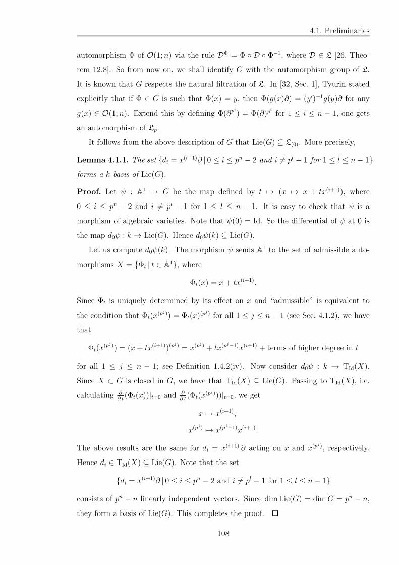
4.1. Preliminaries
automorphism Φ of O(1;n) via the rule DΦ = Φ D Φ−1, where D ∈ L [26, Theo-
rem 12.8]. So from now on, we shall identify G with the automorphism group of L.
It is known that G respects the natural filtration of L. In [32, Sec. 1], Tyurin stated
explicitly that if Φ ∈ G is such that Φ(x) = y, then Φ(g(x)∂) = (y′)−1g(y)∂ for any
g(x) ∈ O(1;n). Extend this by defining Φ(∂pi
) = Φ(∂)pi
for 1 ≤ i ≤ n − 1, one gets
an automorphism of Lp.
It follows from the above description of G that Lie(G) ⊆ L(0). More precisely,
Lemma 4.1.1. The set di = x(i+1)∂ | 0 ≤ i ≤ pn − 2 and i 6= pl − 1 for 1 ≤ l ≤ n− 1
forms a k-basis of Lie(G).
Proof. Let ψ : A1 → G be the map defined by t 7→ (x 7→ x + tx(i+1)), where
0 ≤ i ≤ pn − 2 and i 6= pl − 1 for 1 ≤ l ≤ n − 1. It is easy to check that ψ is a
morphism of algebraic varieties. Note that ψ(0) = Id. So the differential of ψ at 0 is
the map d0ψ : k → Lie(G). Hence d0ψ(k) ⊆ Lie(G).
Let us compute d0ψ(k). The morphism ψ sends A1 to the set of admissible auto-
morphisms X = Φt | t ∈ A1, where
Φt(x) = x+ tx(i+1).
Since Φt is uniquely determined by its effect on x and “admissible” is equivalent to
the condition that Φt(x(pj)) = Φt(x)
(pj) for all 1 ≤ j ≤ n− 1 (see Sec. 4.1.2), we have
that
Φt(x(pj)) = (x+ tx(i+1))(p
j) = x(pj) + tx(p
j−1)x(i+1) + terms of higher degree in t
for all 1 ≤ j ≤ n − 1; see Definition 1.4.2(iv). Now consider d0ψ : k → TId(X).
Since X ⊂ G is closed in G, we have that TId(X) ⊆ Lie(G). Passing to TId(X), i.e.
calculating ∂∂ t(Φt(x))|t=0 and ∂
∂ t(Φt(x
(pj)))|t=0, we get
x 7→ x(i+1),
x(pj) 7→ x(p
j−1)x(i+1).
The above results are the same for di = x(i+1) ∂ acting on x and x(pj), respectively.
Hence di ∈ TId(X) ⊆ Lie(G). Note that the set
di = x(i+1)∂ | 0 ≤ i ≤ pn − 2 and i 6= pl − 1 for 1 ≤ l ≤ n− 1
consists of pn − n linearly independent vectors. Since dimLie(G) = dimG = pn − n,
they form a basis of Lie(G). This completes the proof.
108
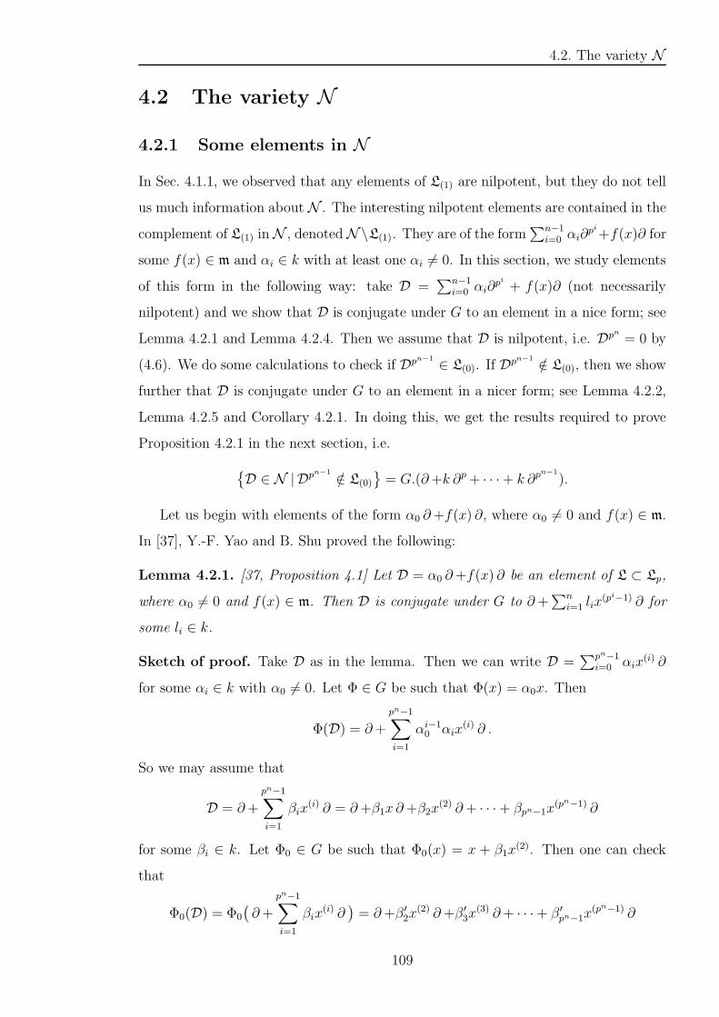
4.2. The variety N
4.2 The variety N
4.2.1 Some elements in N
In Sec. 4.1.1, we observed that any elements of L(1) are nilpotent, but they do not tell
us much information about N . The interesting nilpotent elements are contained in the
complement of L(1) inN , denotedN\L(1). They are of the form∑n−1
i=0 αi∂pi+f(x)∂ for
some f(x) ∈ m and αi ∈ k with at least one αi 6= 0. In this section, we study elements
of this form in the following way: take D =∑n−1
i=0 αi∂pi + f(x)∂ (not necessarily
nilpotent) and we show that D is conjugate under G to an element in a nice form; see
Lemma 4.2.1 and Lemma 4.2.4. Then we assume that D is nilpotent, i.e. Dpn
= 0 by
(4.6). We do some calculations to check if Dpn−1
∈ L(0). If Dpn−1
/∈ L(0), then we show
further that D is conjugate under G to an element in a nicer form; see Lemma 4.2.2,
Lemma 4.2.5 and Corollary 4.2.1. In doing this, we get the results required to prove
Proposition 4.2.1 in the next section, i.e.
D ∈ N |Dpn−1
/∈ L(0)
= G.(∂+k ∂p+ · · ·+ k ∂pn−1
).
Let us begin with elements of the form α0 ∂+f(x) ∂, where α0 6= 0 and f(x) ∈ m.
In [37], Y.-F. Yao and B. Shu proved the following:
Lemma 4.2.1. [37, Proposition 4.1] Let D = α0 ∂+f(x) ∂ be an element of L ⊂ Lp,
where α0 6= 0 and f(x) ∈ m. Then D is conjugate under G to ∂+∑n
i=1 lix(pi−1) ∂ for
some li ∈ k.
Sketch of proof. Take D as in the lemma. Then we can write D =∑pn−1
i=0 αix(i) ∂
for some αi ∈ k with α0 6= 0. Let Φ ∈ G be such that Φ(x) = α0x. Then
Φ(D) = ∂+
pn−1∑
i=1
αi−10 αix
(i) ∂ .
So we may assume that
D = ∂+
pn−1∑
i=1
βix(i) ∂ = ∂+β1x ∂+β2x
(2) ∂+ · · ·+ βpn−1x(pn−1) ∂
for some βi ∈ k. Let Φ0 ∈ G be such that Φ0(x) = x + β1x(2). Then one can check
that
Φ0(D) = Φ0
(
∂+
pn−1∑
i=1
βix(i) ∂
)
= ∂+β ′2x
(2) ∂+β ′3x
(3) ∂+ · · ·+ β ′pn−1x
(pn−1) ∂
109
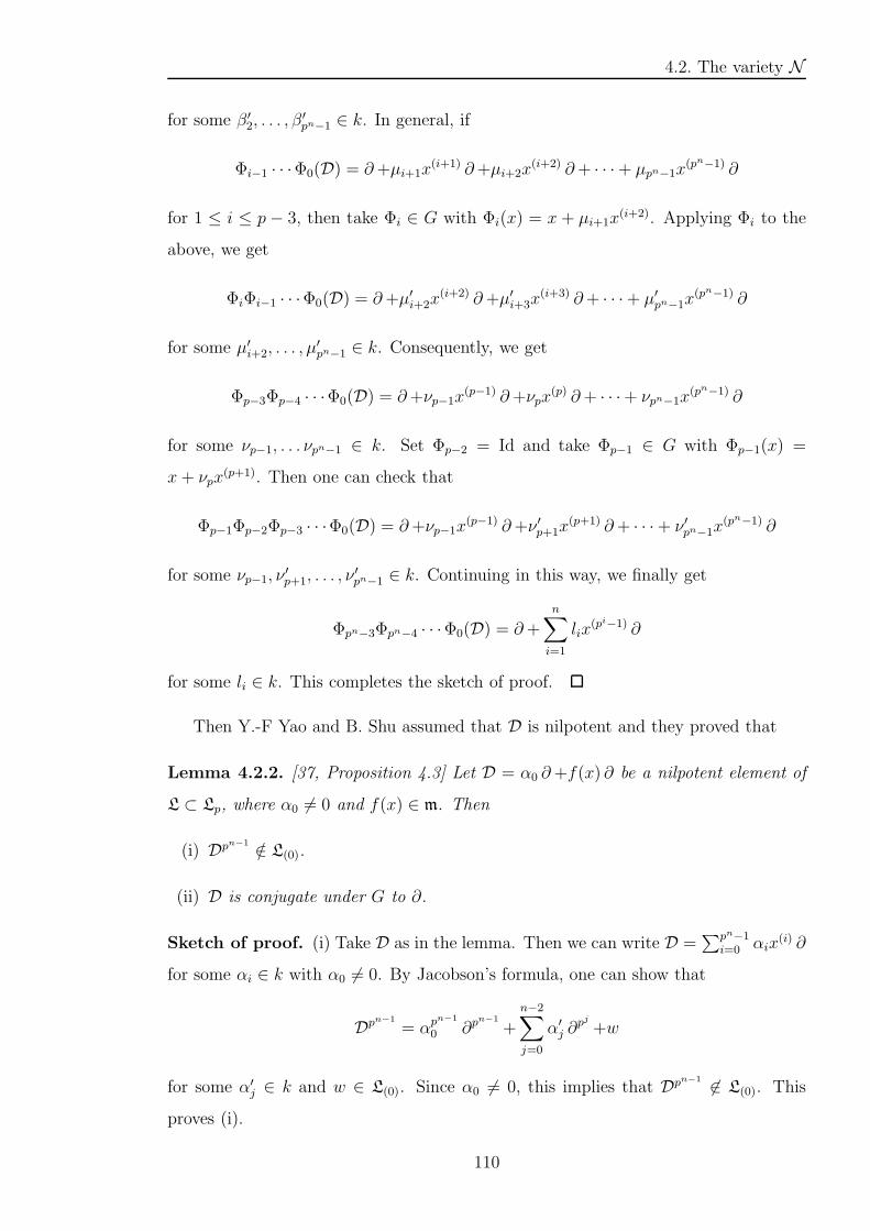
4.2. The variety N
for some β ′2, . . . , β
′pn−1 ∈ k. In general, if
Φi−1 · · ·Φ0(D) = ∂+µi+1x(i+1) ∂+µi+2x
(i+2) ∂+ · · ·+ µpn−1x(pn−1) ∂
for 1 ≤ i ≤ p− 3, then take Φi ∈ G with Φi(x) = x + µi+1x(i+2). Applying Φi to the
above, we get
ΦiΦi−1 · · ·Φ0(D) = ∂+µ′i+2x
(i+2) ∂+µ′i+3x
(i+3) ∂+ · · ·+ µ′pn−1x
(pn−1) ∂
for some µ′i+2, . . . , µ
′pn−1 ∈ k. Consequently, we get
Φp−3Φp−4 · · ·Φ0(D) = ∂+νp−1x(p−1) ∂+νpx
(p) ∂+ · · ·+ νpn−1x(pn−1) ∂
for some νp−1, . . . νpn−1 ∈ k. Set Φp−2 = Id and take Φp−1 ∈ G with Φp−1(x) =
x+ νpx(p+1). Then one can check that
Φp−1Φp−2Φp−3 · · ·Φ0(D) = ∂+νp−1x(p−1) ∂+ν ′p+1x
(p+1) ∂+ · · ·+ ν ′pn−1x(pn−1) ∂
for some νp−1, ν′p+1, . . . , ν
′pn−1 ∈ k. Continuing in this way, we finally get
Φpn−3Φpn−4 · · ·Φ0(D) = ∂+n
∑
i=1
lix(pi−1) ∂
for some li ∈ k. This completes the sketch of proof.
Then Y.-F Yao and B. Shu assumed that D is nilpotent and they proved that
Lemma 4.2.2. [37, Proposition 4.3] Let D = α0 ∂+f(x) ∂ be a nilpotent element of
L ⊂ Lp, where α0 6= 0 and f(x) ∈ m. Then
(i) Dpn−1
/∈ L(0).
(ii) D is conjugate under G to ∂.
Sketch of proof. (i) Take D as in the lemma. Then we can write D =∑pn−1
i=0 αix(i) ∂
for some αi ∈ k with α0 6= 0. By Jacobson’s formula, one can show that
Dpn−1
= αpn−1
0 ∂pn−1
+
n−2∑
j=0
α′j ∂
pj +w
for some α′j ∈ k and w ∈ L(0). Since α0 6= 0, this implies that Dp
n−1
6∈ L(0). This
proves (i).
110
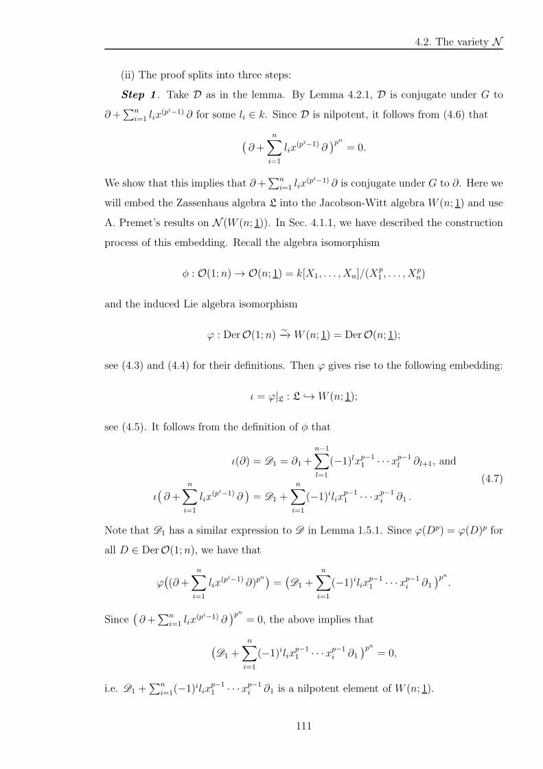
4.2. The variety N
(ii) The proof splits into three steps:
Step 1 . Take D as in the lemma. By Lemma 4.2.1, D is conjugate under G to
∂+∑n
i=1 lix(pi−1) ∂ for some li ∈ k. Since D is nilpotent, it follows from (4.6) that
(
∂+n
∑
i=1
lix(pi−1) ∂
)pn
= 0.
We show that this implies that ∂+∑n
i=1 lix(pi−1) ∂ is conjugate under G to ∂. Here we
will embed the Zassenhaus algebra L into the Jacobson-Witt algebra W (n; 1) and use
A. Premet’s results on N (W (n; 1)). In Sec. 4.1.1, we have described the construction
process of this embedding. Recall the algebra isomorphism
φ : O(1;n)→ O(n; 1) = k[X1, . . . , Xn]/(Xp1 , . . . , X
pn)
and the induced Lie algebra isomorphism
ϕ : DerO(1;n)∼−→ W (n; 1) = DerO(n; 1);
see (4.3) and (4.4) for their definitions. Then ϕ gives rise to the following embedding:
ι = ϕ|L : L → W (n; 1);
see (4.5). It follows from the definition of φ that
ι(∂) = D1 = ∂1+
n−1∑
l=1
(−1)lxp−11 · · ·xp−1
l ∂l+1, and
ι(
∂+
n∑
i=1
lix(pi−1) ∂
)
= D1 +
n∑
i=1
(−1)ilixp−11 · · ·xp−1
i ∂1 .
(4.7)
Note that D1 has a similar expression to D in Lemma 1.5.1. Since ϕ(Dp) = ϕ(D)p for
all D ∈ DerO(1;n), we have that
ϕ(
(∂+n
∑
i=1
lix(pi−1) ∂)p
n)
=(
D1 +n
∑
i=1
(−1)ilixp−11 · · ·xp−1
i ∂1)pn
.
Since(
∂+∑n
i=1 lix(pi−1) ∂
)pn
= 0, the above implies that
(
D1 +
n∑
i=1
(−1)ilixp−11 · · ·xp−1
i ∂1)pn
= 0,
i.e. D1 +∑n
i=1(−1)ilix
p−11 · · ·xp−1
i ∂1 is a nilpotent element of W (n; 1).
111
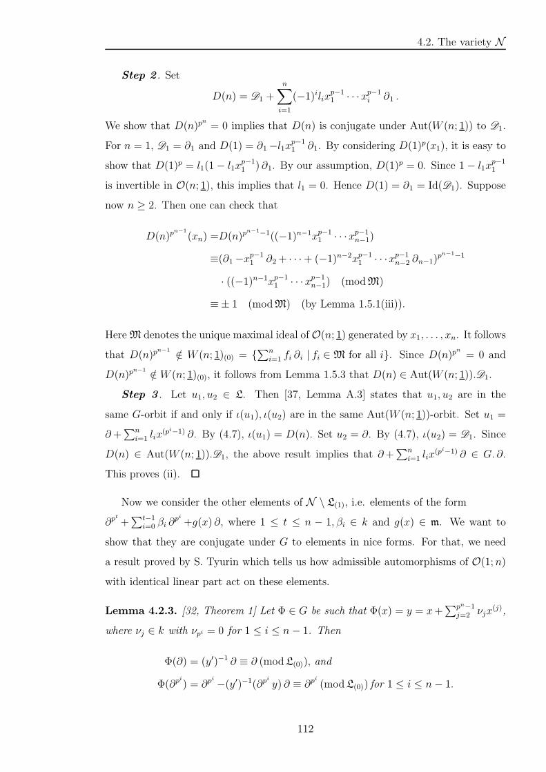
4.2. The variety N
Step 2 . Set
D(n) = D1 +
n∑
i=1
(−1)ilixp−11 · · ·xp−1
i ∂1 .
We show that D(n)pn
= 0 implies that D(n) is conjugate under Aut(W (n; 1)) to D1.
For n = 1, D1 = ∂1 and D(1) = ∂1−l1xp−11 ∂1. By considering D(1)p(x1), it is easy to
show that D(1)p = l1(1− l1xp−11 ) ∂1. By our assumption, D(1)p = 0. Since 1 − l1x
p−11
is invertible in O(n; 1), this implies that l1 = 0. Hence D(1) = ∂1 = Id(D1). Suppose
now n ≥ 2. Then one can check that
D(n)pn−1
(xn) =D(n)pn−1−1((−1)n−1xp−1
1 · · ·xp−1n−1)
≡(∂1−xp−11 ∂2+ · · ·+ (−1)n−2xp−1
1 · · ·xp−1n−2 ∂n−1)
pn−1−1
· ((−1)n−1xp−11 · · ·xp−1
n−1) (modM)
≡± 1 (modM) (by Lemma 1.5.1(iii)).
HereM denotes the unique maximal ideal ofO(n; 1) generated by x1, . . . , xn. It follows
that D(n)pn−1
/∈ W (n; 1)(0) = ∑n
i=1 fi ∂i | fi ∈M for all i. Since D(n)pn
= 0 and
D(n)pn−1
/∈ W (n; 1)(0), it follows from Lemma 1.5.3 that D(n) ∈ Aut(W (n; 1)).D1.
Step 3 . Let u1, u2 ∈ L. Then [37, Lemma A.3] states that u1, u2 are in the
same G-orbit if and only if ι(u1), ι(u2) are in the same Aut(W (n; 1))-orbit. Set u1 =
∂+∑n
i=1 lix(pi−1) ∂. By (4.7), ι(u1) = D(n). Set u2 = ∂. By (4.7), ι(u2) = D1. Since
D(n) ∈ Aut(W (n; 1)).D1, the above result implies that ∂+∑n
i=1 lix(pi−1) ∂ ∈ G. ∂.
This proves (ii).
Now we consider the other elements of N \ L(1), i.e. elements of the form
∂pt
+∑t−1
i=0 βi ∂pi +g(x) ∂, where 1 ≤ t ≤ n − 1, βi ∈ k and g(x) ∈ m. We want to
show that they are conjugate under G to elements in nice forms. For that, we need
a result proved by S. Tyurin which tells us how admissible automorphisms of O(1;n)
with identical linear part act on these elements.
Lemma 4.2.3. [32, Theorem 1] Let Φ ∈ G be such that Φ(x) = y = x+∑pn−1
j=2 νjx(j),
where νj ∈ k with νpi = 0 for 1 ≤ i ≤ n− 1. Then
Φ(∂) = (y′)−1 ∂ ≡ ∂ (modL(0)), and
Φ(∂pi
) = ∂pi
−(y′)−1(∂pi
y) ∂ ≡ ∂pi
(modL(0)) for 1 ≤ i ≤ n− 1.
112

4.2. The variety N
Hence for any D = ∂pt
+∑t−1
i=0 βi∂pi + g(x)∂ ∈ Lp with 1 ≤ t ≤ n − 1, βi ∈ k and
g(x) ∈ m,
Φ(D) = ∂pt
+t−1∑
i=1
βi∂pi + (y′)−1
(
β0 + Φ(g(x))−t−1∑
i=1
βi∂piy − ∂p
t
y
)
∂.
Sketch of proof. Recall from Sec. 4.1.2 that if Φ is any admissible automorphism of
O(1;n) with Φ(x) = y (not necessarily with identical linear part), then
Φ(q(x) ∂) = (y′)−1Φ(q(x))∂ for any q(x) ∈ O(1;n), (4.8)
and
Φ(∂pi
) = Φ(∂)pi
for 1 ≤ i ≤ n− 1. (4.9)
In this lemma, we only consider admissible automorphisms of O(1;n) with identical
linear part, i.e. Φ ∈ G with Φ(x) = y = x +∑pn−1
j=2 νjx(j), where νj ∈ k with
νpi = 0 for 1 ≤ i ≤ n − 1. By (4.8), we have that Φ(∂) = (y′)−1 ∂. We show that
Φ(∂) ≡ ∂ (modL(0)). This is equivalent to show that
(y′)−1 ∂− ∂ ∈ L(0). (4.10)
Note that y′ = 1+∑pn−1
j=2 νjx(j−1) which is invertible in O(1;n). Since L(0) is invariant
under multiplication of invertible elements of O(1;n), we can multiply both sides of
(4.10) by y′ and show that (1− y′) ∂ ∈ L(0). This is clearly true. Hence
Φ(∂) = (y′)−1 ∂ ≡ ∂ (modL(0)).
It remains to compute Φ(∂pi
) for 1 ≤ i ≤ n−1. Since Φ(∂) ≡ ∂ (modL(0)), we may
write Φ(∂) = ∂+φ0(x) ∂ for some φ0(x) ∈ m. By (4.9), Φ(∂p) = Φ(∂)p. By Jacobson’s
formula (Definition 1.1.1(3)) and the fact that L(0) is a restricted Lie subalgebra of
DerO(1;n), we get Φ(∂p) = ∂p+φ1(x) ∂ for some φ1(x) ∈ O(1;n). Since ∂p x = 0, it
follows that
0 = Φ(∂p x) = Φ(∂p)y = (∂p+φ1(x) ∂)y = ∂p y + φ1(x)y′.
Hence φ1(x) = −(y′)−1(∂p y) and so Φ(∂p) = ∂p−(y′)−1(∂p y) ∂. We show that Φ(∂p) ≡
∂p (modL(0)). This is equivalent to show that −(y′)−1(∂p y) ∂ ∈ L(0). By the same
reason as above, we can multiply both sides by −y′ and show that (∂p y) ∂ ∈ L(0). Due
to the form of y, i.e. νp = 0, this is clearly true. Hence
Φ(∂p) = ∂p−(y′)−1(∂p y) ∂ ≡ ∂p (modL(0)).
113

4.2. The variety N
In a similar way, one can show that
Φ(∂pi
) = ∂pi
−(y′)−1(∂pi
y) ∂ ≡ ∂pi
(modL(0)) for 2 ≤ i ≤ n− 1.
Let D = ∂pt
+∑t−1
i=0 βi∂pi + g(x)∂ be an element of Lp, where 1 ≤ t ≤ n− 1, βi ∈ k
and g(x) ∈ m. It follows from (4.8) and the above that
Φ(D) = ∂pt
+t−1∑
i=1
βi∂pi + (y′)−1
(
β0 + Φ(g(x))−t−1∑
i=1
βi∂piy − ∂p
t
y
)
∂.
This completes the sketch of proof.
Lemma 4.2.4. [32, Theorem 1] Let D = ∂pt
+∑t−1
i=0 βi∂pi + g(x)∂ be an element of
Lp, where 1 ≤ t ≤ n− 1, βi ∈ k and g(x) ∈ m. Then D is conjugate under G to
∂pt
+
t−1∑
i=0
βi∂pi + x(p
n−pt)h(x)∂
for some h(x) =∑pt−1
η=0 µηx(η) with µη ∈ k.
Strategy of the proof. The proof splits into two parts. The first part (a) was proved
by S. Tyurin; see [32, Theorem 1, p. 68, line -8]. The second part (b) follows from (a)
and Corollary 1.4.1. Explicitly, we prove the following:
(a) Take D as in the lemma. We show that for 1 ≤ j ≤ pn − pt − 1, if g(x) ∂ ≡
γjx(j) ∂ (modL(j)) for some γj ∈ k and Φj ∈ G is such that Φj(x) = yj = x+ γjx
(pt+j),
then
Φj(D) ≡ ∂pt
+
t−1∑
i=0
βi ∂pi (modL(j)).
We start with j = 1 and continue checking the above equivalence until we get D is
conjugate under G to
∂pt
+t−1∑
i=0
βi ∂pi (modL(pn−pt−1)).
(b) By part (a), we may assume that
D = ∂pt
+t−1∑
i=0
βi∂pi +
pt−1∑
η=0
µηx(pn−pt+η) ∂
for some µη ∈ k. Note that for any 0 ≤ η ≤ pt − 1,
x(pn−pt)x(η) =
(
pn − pt + η
pn − pt
)
x(pn−pt+η).
114
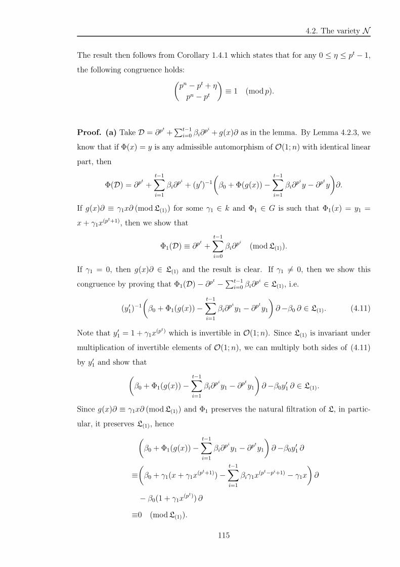
4.2. The variety N
The result then follows from Corollary 1.4.1 which states that for any 0 ≤ η ≤ pt − 1,
the following congruence holds:(
pn − pt + η
pn − pt
)
≡ 1 (mod p).
Proof. (a) Take D = ∂pt
+∑t−1
i=0 βi∂pi + g(x)∂ as in the lemma. By Lemma 4.2.3, we
know that if Φ(x) = y is any admissible automorphism of O(1;n) with identical linear
part, then
Φ(D) = ∂pt
+
t−1∑
i=1
βi∂pi + (y′)−1
(
β0 + Φ(g(x))−t−1∑
i=1
βi∂piy − ∂p
t
y
)
∂.
If g(x)∂ ≡ γ1x∂ (modL(1)) for some γ1 ∈ k and Φ1 ∈ G is such that Φ1(x) = y1 =
x+ γ1x(pt+1), then we show that
Φ1(D) ≡ ∂pt
+t−1∑
i=0
βi∂pi (modL(1)).
If γ1 = 0, then g(x)∂ ∈ L(1) and the result is clear. If γ1 6= 0, then we show this
congruence by proving that Φ1(D)− ∂pt
−∑t−1
i=0 βi∂pi ∈ L(1), i.e.
(y′1)−1
(
β0 + Φ1(g(x))−t−1∑
i=1
βi∂piy1 − ∂
pty1
)
∂−β0 ∂ ∈ L(1). (4.11)
Note that y′1 = 1 + γ1x(pt) which is invertible in O(1;n). Since L(1) is invariant under
multiplication of invertible elements of O(1;n), we can multiply both sides of (4.11)
by y′1 and show that
(
β0 + Φ1(g(x))−t−1∑
i=1
βi∂piy1 − ∂
pty1
)
∂−β0y′1 ∂ ∈ L(1).
Since g(x)∂ ≡ γ1x∂ (modL(1)) and Φ1 preserves the natural filtration of L, in partic-
ular, it preserves L(1), hence
(
β0 + Φ1(g(x))−t−1∑
i=1
βi∂piy1 − ∂
pty1
)
∂−β0y′1 ∂
≡
(
β0 + γ1(x+ γ1x(pt+1))−
t−1∑
i=1
βiγ1x(pt−pi+1) − γ1x
)
∂
− β0(1 + γ1x(pt)) ∂
≡0 (modL(1)).
115
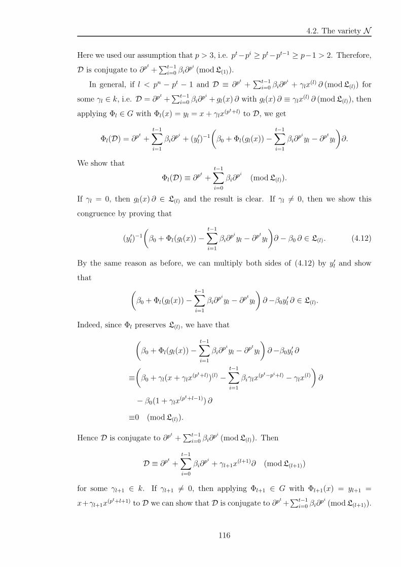
4.2. The variety N
Here we used our assumption that p > 3, i.e. pt−pi ≥ pt−pt−1 ≥ p−1 > 2. Therefore,
D is conjugate to ∂pt
+∑t−1
i=0 βi∂pi (modL(1)).
In general, if l < pn − pt − 1 and D ≡ ∂pt
+∑t−1
i=0 βi∂pi + γlx
(l) ∂ (modL(l)) for
some γl ∈ k, i.e. D = ∂pt
+∑t−1
i=0 βi∂pi + gl(x) ∂ with gl(x) ∂ ≡ γlx
(l) ∂ (modL(l)), then
applying Φl ∈ G with Φl(x) = yl = x+ γlx(pt+l) to D, we get
Φl(D) = ∂pt
+t−1∑
i=1
βi∂pi + (y′l)
−1
(
β0 + Φl(gl(x))−t−1∑
i=1
βi∂piyl − ∂
ptyl
)
∂.
We show that
Φl(D) ≡ ∂pt
+t−1∑
i=0
βi∂pi (modL(l)).
If γl = 0, then gl(x) ∂ ∈ L(l) and the result is clear. If γl 6= 0, then we show this
congruence by proving that
(y′l)−1
(
β0 + Φl(gl(x))−t−1∑
i=1
βi∂piyl − ∂
ptyl
)
∂ − β0 ∂ ∈ L(l). (4.12)
By the same reason as before, we can multiply both sides of (4.12) by y′l and show
that
(
β0 + Φl(gl(x))−t−1∑
i=1
βi∂piyl − ∂
ptyl
)
∂−β0y′l ∂ ∈ L(l).
Indeed, since Φl preserves L(l), we have that
(
β0 + Φl(gl(x))−t−1∑
i=1
βi∂piyl − ∂
ptyl
)
∂−β0y′l ∂
≡
(
β0 + γl(x+ γlx(pt+l))(l) −
t−1∑
i=1
βiγlx(pt−pi+l) − γlx
(l)
)
∂
− β0(1 + γlx(pt+l−1)) ∂
≡0 (modL(l)).
Hence D is conjugate to ∂pt
+∑t−1
i=0 βi∂pi (modL(l)). Then
D ≡ ∂pt
+t−1∑
i=0
βi∂pi + γl+1x
(l+1)∂ (modL(l+1))
for some γl+1 ∈ k. If γl+1 6= 0, then applying Φl+1 ∈ G with Φl+1(x) = yl+1 =
x+γl+1x(pt+l+1) to D we can show that D is conjugate to ∂p
t
+∑t−1
i=0 βi∂pi (modL(l+1)).
116
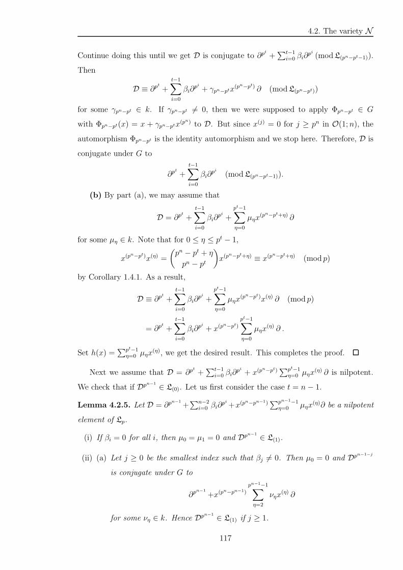
4.2. The variety N
Continue doing this until we get D is conjugate to ∂pt
+∑t−1
i=0 βi∂pi (modL(pn−pt−1)).
Then
D ≡ ∂pt
+
t−1∑
i=0
βi∂pi + γpn−ptx
(pn−pt) ∂ (modL(pn−pt))
for some γpn−pt ∈ k. If γpn−pt 6= 0, then we were supposed to apply Φpn−pt ∈ G
with Φpn−pt(x) = x + γpn−ptx(pn) to D. But since x(j) = 0 for j ≥ pn in O(1;n), the
automorphism Φpn−pt is the identity automorphism and we stop here. Therefore, D is
conjugate under G to
∂pt
+t−1∑
i=0
βi∂pi (modL(pn−pt−1)).
(b) By part (a), we may assume that
D = ∂pt
+t−1∑
i=0
βi∂pi +
pt−1∑
η=0
µηx(pn−pt+η) ∂
for some µη ∈ k. Note that for 0 ≤ η ≤ pt − 1,
x(pn−pt)x(η) =
(
pn − pt + η
pn − pt
)
x(pn−pt+η) ≡ x(p
n−pt+η) (mod p)
by Corollary 1.4.1. As a result,
D ≡ ∂pt
+
t−1∑
i=0
βi∂pi +
pt−1∑
η=0
µηx(pn−pt)x(η) ∂ (mod p)
= ∂pt
+t−1∑
i=0
βi∂pi + x(p
n−pt)
pt−1∑
η=0
µηx(η) ∂ .
Set h(x) =∑pt−1
η=0 µηx(η), we get the desired result. This completes the proof.
Next we assume that D = ∂pt
+∑t−1
i=0 βi∂pi + x(p
n−pt)∑pt−1
η=0 µηx(η) ∂ is nilpotent.
We check that if Dpn−1
∈ L(0). Let us first consider the case t = n− 1.
Lemma 4.2.5. Let D = ∂pn−1
+∑n−2
i=0 βi∂pi +x(p
n−pn−1)∑pn−1−1
η=0 µηx(η)∂ be a nilpotent
element of Lp.
(i) If βi = 0 for all i, then µ0 = µ1 = 0 and Dpn−1
∈ L(1).
(ii) (a) Let j ≥ 0 be the smallest index such that βj 6= 0. Then µ0 = 0 and Dpn−1−j
is conjugate under G to
∂pn−1
+x(pn−pn−1)
pn−1−1∑
η=2
νηx(η) ∂
for some νη ∈ k. Hence Dpn−1
∈ L(1) if j ≥ 1.
117

4.2. The variety N
(b) In particular, if β0 6= 0, then Dpn−1
is conjugate under G to ∂pn−1
. Hence
D = ∂pn−1
+∑n−2
i=0 γi ∂pi for some γi ∈ k with γ0 6= 0.
The proof is long as it involves many calculations. Let us first explain the strategy
of the proof.
Strategy of the proof. This is a computational proof and the following steps are
crucial:
Step 1 . Take D = ∂pn−1
+∑n−2
i=0 βi∂pi+x(p
n−pn−1)∑pn−1−1
η=0 µηx(η)∂ as in the lemma.
Since D is nilpotent, then Dpn
= 0 by (4.6). We first calculate Dp which will be used
in step 2. Set D1 = x(pn−pn−1)
∑pn−1−1η=0 µηx
(η)∂ and D2 = ∂pn−1
+∑n−2
i=0 βi∂pi . By
Jacobson’s formula,
Dp =n−2∑
i=0
βpi ∂pi+1
+ (adD2)p−1(D1) + µ(1)x
(pn−1)∂
for some µ(1) ∈ k; see (4.14) in the proof.
Step 2 . We consider the scalars βi in the following two cases and prove statements
(i) and (ii) in the lemma.
Step 2(i). Suppose βi = 0 for all i. Then D = ∂pn−1
+ x(pn−pn−1)
∑pn−1−1η=0 µηx
(η)∂.
We show that µ0 = µ1 = 0 and Dpn−1
∈ L(1). By the calculation in step 1, we have
that Dp =∑pn−1−1
η=0 µηx(η) ∂+µ(1)x
(pn−1)∂; see (4.15). We show that if µ0 6= 0, then
Dpn
6= 0, a contradiction. Hence µ0 = 0. Similarly, we show that µ1 = 0. As a result,
Dp ∈ L(1). Since L(1) is restricted, we get Dpn−1
∈ L(1) as desired.
Step 2(ii)(a). Let j ≥ 0 be the smallest index such that βj 6= 0, and let l be the
largest index such that βl 6= 0, i.e. 0 ≤ j ≤ l ≤ n− 2 and
D = ∂pn−1
+
l∑
i=j
βi∂pi + x(p
n−pn−1)
pn−1−1∑
η=0
µηx(η)∂.
We show that µ0 = 0 and Dpn−1−j
is conjugate under G to
∂pn−1
+x(pn−pn−1)
pn−1−1∑
η=2
νηx(η) ∂
for some νη ∈ k. Let us start with the special case j = l. We prove by induction that
for any 1 ≤ r ≤ n− 1− j, Dpr
is conjugate under G to
∂pj+r
+ βpr−1
0,(1) ∂pr−1
+x(pn−pj+r)
pj+r−1∑
η=0
µη,(r)x(η) ∂
118
4.2. The variety N
for some β0,(1) ∈ k∗µ0 and µη,(r) ∈ k. Here we will use Jacobson’s formula and
Lemma 4.2.4. In particular, Dpn−1−j
is conjugate under G to
∂pn−1
+ βpn−2−j
0,(1) ∂pn−2−j
+x(pn−pn−1)
pn−1−1∑
η=0
µη,(n−1−j)x(η) ∂;
see (4.16). Then we calculate Dpn
and use Dpn
= 0 to show that β0,(1) = µ0 = 0 and
µ0,(n−1−j) = µ1,(n−1−j) = 0. This gives the desired result in this case.
For the general case, j < l, one can show similarly that Dpn−1−j
is conjugate under
G to
∂pn−1
+ λ ∂pn−2−j
+
n−3−j∑
i=0
λi ∂pi +x(p
n−pn−1)
pn−1−1∑
η=0
νηx(η) ∂
for some λ ∈ k∗µ0 and λi, νη ∈ k; see (4.18). Then we show similarly that Dpn
= 0
implies that λ = µ0 = 0, λi = 0 for 0 ≤ i ≤ n− 3− j and ν0 = ν1 = 0. This gives the
desired result.
Suppose now j ≥ 1. We show that (∂pn−1
+x(pn−pn−1)
∑pn−1−1η=2 νηx
(η) ∂)p ∈ L(1); see
(4.19). Since Dpn−1−j
is conjugate under G to ∂pn−1
+x(pn−pn−1)
∑pn−1−1η=2 νηx
(η) ∂ and
G preserves L(1), we have that Dpn−j
∈ L(1). As L(1) is restricted, we get Dpn−1
∈ L(1)
as desired.
Step 2(ii)(b). Suppose β0 6= 0. By step 2(ii)(a), Dpn−1
is conjugate under G to
∂pn−1
+x(pn−pn−1)
∑pn−1−1η=2 νηx
(η) ∂ for some νη ∈ k. We show that Dpn
= 0 implies that
νη = 0 for all η. Hence Dpn−1
is conjugate to ∂pn−1
. Then we find an expression for D.
Let
S :=
D ∈(
∂pn−1
+n−2∑
i=1
k ∂pi
+L)
∩N |Dpn−1
is conjugate under G to ∂pn−1
.
Note that S is a subset of the centralizer cLp(∂p
n−1
). Then we consider elements of
cLp(∂p
n−1
) and show that any D in S has the form D = ∂pn−1
+∑n−2
i=0 γi ∂pi for some
γi ∈ k with γ0 6= 0.
Proof. Step 1 . Let D = ∂pn−1
+∑n−2
i=0 βi∂pi + x(p
n−pn−1)∑pn−1−1
η=0 µηx(η)∂ be a nilpo-
tent element of Lp. Then Dpn
= 0 by (4.6). Let us first calculate Dp. Recall Jacobson’s
formula,
(D1 +D2)p = Dp1 +D
p2 +
p−1∑
i=1
si(D1,D2) (4.13)
119
4.2. The variety N
for all D1,D2 ∈ Lp, and si(D1,D2) can be computed by the formula
ad(tD1 +D2)p−1(D1) =
p−1∑
i=1
isi(D1,D2)ti−1,
where t is a variable. Set
D1 = x(pn−pn−1)
pn−1−1∑
η=0
µηx(η)∂
and
D2 = ∂pn−1
+n−2∑
i=0
βi∂pi .
We first show that Dp1 = 0. By Corollary 1.4.1, x(pn−pn−1)x(η) ≡ x(p
n−pn−1+η) (mod p).
Then D1 =∑pn−1−1
η=0 µηx(pn−pn−1+η)∂. By Lemma 1.1.1,
Dp1 =
pn−1−1∑
η=0
(
µηx(pn−pn−1+η)∂
)p+ w,
where w is a linear combination of commutators in µηx(pn−pn−1+η)∂, 0 ≤ η ≤ pn−1− 1.
By Jacobi identity, we can rearrange w so that w is in the span of commutators
[wp−1, [wp−2, [. . . , [w2, [w1, w0] . . . ], where each wν , 0 ≤ ν ≤ p− 1, is equal to some
µηx(pn−pn−1+η)∂, 0 ≤ η ≤ pn−1 − 1. We show that such iterated commutator equals 0
and so w = 0. Recall (4.1) the natural filtration L(α)α≥−1 of L, where L(α) = 0 for
all α > pn−2. Since 0 ≤ η ≤ pn−1−1, we have that µηx(pn−pn−1+η)∂ ∈ L(pn−pn−1−1) for
all η. Then [wp−1, [wp−2, [. . . , [w2, [w1, w0] . . . ] ∈ L(p(pn−pn−1−1)) by Definition 1.3.3(ii).
We show that L(p(pn−pn−1−1)) = 0, i.e. p(pn − pn−1 − 1) > pn − 2. Note that
p(pn − pn−1 − 1) > pn − 2 ⇐⇒ pn+1 − pn − p > pn − 2 ⇐⇒ pn+1 − p+ 2 > 2pn.
We consider the p-adic expansions of these two numbers. By our assumption, p > 3.
Then p− 1 > 2. So 2pn+0pn−1 + · · ·+0p+0 is the p-adic expansion of 2pn. By (1.2)
in Corollary 1.4.1, the p-adic expansion of pn+1 − p+ 2 is
pn+1 − p+ 2 =n
∑
j′=1
(p− 1)pj′
+ 2 = (p− 1)pn + (p− 1)pn−1 + · · ·+ (p− 1)p+ 2.
Since p − 1 > 2, it is clear that pn+1 − p + 2 > 2pn. Hence L(p(pn−pn−1−1)) = 0 and
so [wp−1, [wp−2, [. . . , [w2, [w1, w0] . . . ] = 0. As a result, w = 0. By (4.2), we have that(
µηx(pn−pn−1+η)∂
)p= 0 for all 0 ≤ η ≤ pn−1 − 1. Therefore, Dp1 = 0.
120
4.2. The variety N
By Lemma 1.1.1 again, we get Dp2 =∑n−2
i=0 βpi ∂
pi+1
. By (4.1) the natural filtration
of L, we have that for any 1 ≤ s ≤ p− 2,
[D1, (adD2)s(D1)] ∈ [L(pn−pn−1−1),L(pn−(s+1)pn−1−1)]
⊆ [L(pn−pn−1−1),L(pn−1−1)]
⊆ L(pn−2) = spanx(pn−1)∂.
This last term will appear if and only if s = p− 2. So
Dp =n−2∑
i=0
βpi ∂pi+1
+ (adD2)p−1(D1) + µ(1)x
(pn−1)∂ (4.14)
for some µ(1) ∈ k.
Step 2 . We consider the scalars βi in the following two cases.
Step 2(i). If βi = 0 for all i, then D2 = ∂pn−1
. By (4.14),
Dp = (ad ∂pn−1
)p−1(D1) + µ(1)x(pn−1)∂.
Since ∂pn−1
is a derivation of L and ∂pn−1
(∑pn−1−1
η=0 µηx(η)) = 0, we have that
Dp =
pn−1−1∑
η=0
µηx(η) ∂+µ(1)x
(pn−1)∂. (4.15)
If µ0 6= 0, then Dp ≡ µ0∂ (modL(0)). By Lemma 1.1.1,
Dpn
≡ µpn−1
0 ∂pn−1
+n−2∑
i=0
µ′i ∂
pi (modL(0))
for some µ′i ∈ k. As µ0 6= 0, this implies that Dp
n
6≡ 0 (modL(0)) and so it is not
equal to 0. This contradicts that D is nilpotent. Hence µ0 = 0. Similarly, if µ1 6= 0
then Dp ≡ µ1x∂ (modL(1)). But Dpn ≡ µp
n−1
1 x∂ 6≡ 0 (modL(1)), a contradiction. Thus
µ1 = 0. Therefore, Dp is an element of L(1). Since L(1) is restricted we have that
Dpn−1
∈ L(1). This proves (i).
Step 2(ii)(a). Let j ≥ 0 be the smallest index such that βj 6= 0, and let l be the
largest index such that βl 6= 0, i.e. 0 ≤ j ≤ l ≤ n− 2 and
D = ∂pn−1
+l
∑
i=j
βi∂pi + x(p
n−pn−1)
pn−1−1∑
η=0
µηx(η)∂.
We first consider the special case j = l, i.e.
D = ∂pn−1
+ βj∂pj + x(p
n−pn−1)
pn−1−1∑
η=0
µηx(η)∂.
121
4.2. The variety N
We prove by induction that for any 1 ≤ r ≤ n− 1− j, Dpr
is conjugate under G to
∂pj+r
+ βpr−1
0,(1) ∂pr−1
+x(pn−pj+r)
pj+r−1∑
η=0
µη,(r)x(η) ∂
for some β0,(1) ∈ k∗µ0 and µη,(r) ∈ k. For r = 1, the previous calculation (4.14) gives
Dp = βpj ∂pj+1
+ ad(
∂pn−1
+ βj∂pj)p−1
(
x(pn−pn−1)
pn−1−1∑
η=0
µηx(η)∂
)
+ µ(1)x(pn−1)∂.
Note that
ad
(
∂pn−1
+ βj∂pj)p−1(
x(pn−pn−1)
pn−1−1∑
η=0
µηx(η)∂
)
=ad
( p−1∑
m=0
(−1)mβp−1−mj ∂mp
n−1+(p−1−m)pj)( pn−1−1
∑
η=0
µηx(pn−pn−1+η)∂
)
=
pn−1−1∑
η=0
µηx(η)∂ − βj
pn−1−1∑
η=0
µηx(pn−1−pj+η)∂ + . . .
+ βp−1j
pn−1−1∑
η=0
µηx(pn−pn−1−(p−1)pj+η)∂.
The above result can be rewritten as µ0 ∂+g(x) ∂ for some g(x) ∈ m. Hence
Dp = βpj ∂pj+1
+ µ0 ∂+g(x) ∂+µ(1)x(pn−1)∂.
Then the automorphism Φ(x) = αx with αpj+1
= βpj reduces Dp to the form
Dp = ∂pj+1
+ β0,(1) ∂+f1(x) ∂,
where β0,(1) ∈ k∗µ0 and f1(x) ∈ m. Then Lemma 4.2.4 implies that Dp is conjugate
under G to
∂pj+1
+ β0,(1) ∂+x(pn−pj+1)
pj+1−1∑
η=0
µη,(1)x(η) ∂
for some µη,(1) ∈ k. Thus, the result is true for r = 1. Suppose the result is true for
r = K − 1 < n− 1− j, i.e. DpK−1
is conjugate under G to
∂pj+K−1
+ βpK−2
0,(1) ∂pK−2
+x(pn−pj+K−1)
pj+K−1−1∑
η=0
µη,(K−1)x(η) ∂
122
4.2. The variety N
for some β0,(1) ∈ k∗µ0 and µη,(K−1) ∈ k. Let us calculate DpK
. Set
D1 = x(pn−pj+K−1)
pj+K−1−1∑
η=0
µη,(K−1)x(η) ∂
and
D2 = ∂pj+K−1
+ βpK−2
0,(1) ∂pK−2
in the Jacobson’s formula (4.13). Then Dp1 ∈ L(1) and Dp2 = ∂p
j+K
+ βpK−1
0,(1) ∂pK−1
. By
(4.1) the natural filtration of L, we have that
(adD2)p−1(D1) ∈ L(pn−pj+K−1) ⊆ L(1).
Similarly, for any 1 ≤ s ≤ p− 2,
[D1, (adD2)s(D1)] ∈ [L(pn−pj+K−1−1),L(pn−(s+1)pj+K−1−1)]
⊆ [L(1),L(pn−(s+1)pj+K−1−1)]
⊆ L(pn−(s+1)pj+K−1),
⊆ L(pn−(p−1)pj+K−1),
⊆ L(pn−(p−1)pn−2) (since j +K − 1 ≤ n− 2)
⊆ L(1).
Hence DpK
= ∂pj+K
+ βpK−1
0,(1) ∂pK−1
+fK(x) ∂ for some fK(x) ∈ m with fK(x) ∂ ∈ L(1).
By Lemma 4.2.4, DpK
is conjugate under G to
∂pj+K
+ βpK−1
0,(1) ∂pK−1
+x(pn−pj+K)
pj+K−1∑
η=0
µη,(K)x(η) ∂
for some µη,(K) ∈ k, i.e. the result is true for r = K. Therefore, we proved by induction
that for any 1 ≤ r ≤ n− 1− j, Dpr
is conjugate under G to
∂pj+r
+ βpr−1
0,(1) ∂pr−1
+x(pn−pj+r)
pj+r−1∑
η=0
µη,(r)x(η) ∂
for some β0,(1) ∈ k∗µ0 and µη,(r) ∈ k. In particular, Dpn−1−j
is conjugate under G to
∂pn−1
+ βpn−2−j
0,(1) ∂pn−2−j
+x(pn−pn−1)
pn−1−1∑
η=0
µη,(n−1−j)x(η) ∂ . (4.16)
123

4.2. The variety N
By Jacobson’s formula,
Dpn−j
= βpn−1−j
0,(1) ∂pn−1−j
+
pn−1−1∑
η=0
µη,(n−1−j)x(η) ∂+fn−j(x) ∂+µ(n−j)x
(pn−1) ∂ (4.17)
for some fn−j(x) ∂ ∈ L(1) and µ(n−j) ∈ k. Then
Dpn
≡ βpn−1
0,(1) ∂pn−1
+µpj
0,(n−1−j) ∂pj +
j−1∑
i=0
µ′′i ∂
pi (modL(0))
for some µ′′i ∈ k. But D
pn = 0, this implies that β0,(1) = 0. Since β0,(1) ∈ k∗µ0, we have
that µ0 = 0. We must also have that µ0,(n−1−j) = 0 and µ′′i = 0 for all i. Substituting
these into (4.17), we get
Dpn−j
=
pn−1−1∑
η=1
µη,(n−1−j)x(η) ∂+fn−j(x) ∂+µ(n−j)x
(pn−1) ∂
≡ µ1,(n−1−j)x ∂ (modL(1)).
Then one can show similarly that µ1,(n−1−j) = 0. Hence Dpn−1−j
(4.16) is conjugate
under G to
∂pn−1
+ x(pn−pn−1)
pn−1−1∑
η=2
µη,(n−1−j)x(η) ∂ .
If j < l, i.e. D = ∂pn−1
+∑l
i=j βi∂pi + x(p
n−pn−1)∑pn−1−1
η=0 µηx(η)∂, then one can
show similarly that Dpn−1−j
is conjugate under G to
∂pn−1
+ λ ∂pn−2−j
+
n−3−j∑
i=0
λi ∂pi +x(p
n−pn−1)
pn−1−1∑
η=0
νηx(η) ∂ (4.18)
for some λ ∈ k∗µ0 and λi, νη ∈ k. Then by the same arguments as above, one can
show that λ = µ0 = 0, λi = 0 for 0 ≤ i ≤ n − 3 − j and ν0 = ν1 = 0. As a result,
Dpn−1−j
is conjugate under G to
∂pn−1
+ x(pn−pn−1)
pn−1−1∑
η=2
νηx(η)∂.
Suppose now j ≥ 1. By a similar calculation as in (4.14) and (4.15), we get
(
∂pn−1
+ x(pn−pn−1)
pn−1−1∑
η=2
νηx(η)∂
)p=
pn−1−1∑
η=2
νηx(η)∂ + µ(n−j)x
(pn−1) ∂ (4.19)
124

4.2. The variety N
for some µ(n−j) ∈ k. This is an element of L(1). Since Dpn−1−j
is conjugate under G
to ∂pn−1
+ x(pn−pn−1)
∑pn−1−1η=2 νηx
(η)∂ and G preserves L(1), we have that Dpn−j
∈ L(1).
As L(1) is restricted, we have that Dpn−1
∈ L(1). This proves (ii)(a).
Step 2(ii)(b). If β0 6= 0, then (ii)(a) implies that Dpn−1
is conjugate under G to
∂pn−1
+ x(pn−pn−1)
pn−1−1∑
η=2
νηx(η) ∂
for some νη ∈ k. If q is the smallest index such that νq 6= 0, then
Dpn
=
pn−1−1∑
η=q
νηx(η) ∂+µ(n)x
(pn−1) ∂
for some µ(n) ∈ k. As νq 6= 0, this implies that Dpn
6= 0, a contradiction. Hence νη = 0
for all η. Therefore, we are interested in the set
S :=
D ∈(
∂pn−1
+
n−2∑
i=1
k ∂pi
+L)
∩N |Dpn−1
is conjugate under G to ∂pn−1
.
Since [D,Dpn−1
] = 0, the above set S is a subset of the centralizer cLp(∂p
n−1
). It is easy
to verify that cLp(∂p
n−1
) is spanned by ∂pn−1
and W (1, n− 1)p. Since W (1, n− 1)p is a
restricted Lie subalgebra of Lp, we may regard the automorphism group ofW (1, n−1)p
as a subgroup of G. Let D = ∂pn−1
+∑n−2
i=1 γi ∂pi +v be an element of cLp
(∂pn−1
), where
γi ∈ k and v ∈ W (1, n− 1). If v = 0, then Dpn−1
= 0 which is not conjugate to ∂pn−1
.
So v 6= 0. If v 6∈ W (1, n− 1)(0), then v = γ0 ∂ for some γ0 6= 0. It is easy to see that
Dpn−1
is conjugate under G to ∂pn−1
. If v ∈ W (1, n− 1)(0), then v =∑pn−1−1
i=1 λix(i) ∂
with λi 6= 0 for some i. It follows from Lemma 4.2.4 that D is conjugate under G to
∂pn−1
+n−2∑
i=1
γi ∂pi +x(p
n−pn−1)
pn−1−1∑
η=0
λ′ηx(η) ∂
for some λ′η ∈ k. If γi = 0 for all i, then (i) of this lemma implies that Dpn−1
∈ L(1)
which is not conjugate to ∂pn−1
. Similarly, if j ≥ 1 is the smallest index such that
γj 6= 0, then (ii)(a) of this lemma implies thatDpn−1
∈ L(1) which is again not conjugate
to ∂pn−1
. Therefore, the set S consists of elements of the form D = ∂pn−1
+∑n−2
i=0 γi ∂pi,
where γi ∈ k with γ0 6= 0. This proves (ii)(b).
We see that the last proof involves calculations using Jacobson’s formula and ap-
plications of Lemma 4.2.4. The only property of D that we used is Dpn
= 0. Hence
125

4.2. The variety N
using the same arguments, we can prove a very similar result for nilpotent elements
∂pm
+∑m−1
i=0 αi∂pi + x(p
n−pm)∑pm−1
η=0 µηx(η) ∂, where 1 ≤ m ≤ n− 2.
Corollary 4.2.1. Let E = ∂pm
+∑m−1
i=0 αi∂pi +x(p
n−pm)∑pm−1
η=0 µηx(η) ∂ with 1 ≤ m ≤
n− 2 be a nilpotent element of Lp.
(i) If αi = 0 for all i, then Epn−1
∈ L(1).
(ii) (a) Let q ≥ 0 be the smallest index such that αq 6= 0. Then Epn−1−q
is conjugate
under G to
∂pn−1
+x(pn−pn−1)
pn−1−1∑
η=2
νηx(η) ∂
for some νη ∈ k. Hence Epn−1
∈ L(1) if q ≥ 1.
(b) In particular, if α0 6= 0, then Epn−1
is conjugate under G to ∂pn−1
. Hence
E = ∂pm
+∑m−1
i=0 γi ∂pi for some γi ∈ k with γ0 6= 0.
Strategy of the proof. By a similar argument as in step 2(ii)(a) of Lemma 4.2.5,
one can show that Epn−1−m
is conjugate under G to
D1 = ∂pn−1
+m−1∑
i=0
αpn−1−m
i ∂pi+n−1−m
+x(pn−pn−1)
pn−1−1∑
η=0
µη,(n−1−m)x(η) ∂
for some µη,(n−1−m) ∈ k. Note that D1 has a similar expression to D in Lemma 4.2.5.
Applying that lemma to D1, we get most of the desired results. The other results such
as showing that Epn−1
∈ L(1) in (i) and finding an expression for E in (ii)(b) follow
from the same arguments as in the proof of that lemma.
Proof. Take E = ∂pm
+∑m−1
i=0 αi∂pi + x(p
n−pm)∑pm−1
η=0 µηx(η) ∂ as in the corollary. By
a similar argument as in step 2(ii)(a) of Lemma 4.2.5, i.e. using induction on r, one
can show that for any 1 ≤ r ≤ n− 1−m, Epr is conjugate under G to
∂pm+r
+m−1∑
i=0
αpr
i ∂pi+r
+x(pn−pm+r)
pm+r−1∑
η=0
µη,(r)x(η) ∂
for some µη,(r) ∈ k. In particular, Epn−1−m
is conjugate under G to
D1 = ∂pn−1
+m−1∑
i=0
αpn−1−m
i ∂pi+n−1−m
+x(pn−pn−1)
pn−1−1∑
η=0
µη,(n−1−m)x(η) ∂ .
126
4.2. The variety N
Note that D1 has a similar expression to D in Lemma 4.2.5. Since E is nilpotent, we
have that Epn = 0 by (4.6). As Epn−1−m
is conjugate under G to D1, this implies that
Dpm+1
1 = 0.
(i) Suppose αi = 0 for all i. Applying Lemma 4.2.5(i) to D1, we get µ0,(n−1−m) =
µ1,(n−1−m) = 0. Then (4.15) in step 2(i) of Lemma 4.2.5 gives
Dp1 =
pn−1−1∑
η=2
µη,(n−1−m)x(η) ∂+µ(1)x
(pn−1)∂
for some µ(1) ∈ k. Hence Dp1 ∈ L(1). Since G preserves L(1), we have that E
pn−m
∈ L(1).
As L(1) is restricted, we have that Epn−1
∈ L(1). This proves (i).
(ii)(a) Let q ≥ 0 be the smallest index such that αq 6= 0. Then Epn−1−m
is conjugate
under G to
D1 = ∂pn−1
+
m−1∑
i=q
αpn−1−m
i ∂pi+n−1−m
+x(pn−pn−1)
pn−1−1∑
η=0
µη,(n−1−m)x(η) ∂ .
Applying Lemma 4.2.5(ii)(a) to D1, we get µ0,(n−1−m) = 0 and Dpm−q
1 is conjugate
under G to
∂pn−1
+x(pn−pn−1)
pn−1−1∑
η=2
νηx(η) ∂
for some νη ∈ k. Hence (Epn−1−m
)pm−q
= Epn−1−q
is conjugate under G to the above
element. It follows from Lemma 4.2.5(ii)(a) that Epn−1
∈ L(1) if q ≥ 1. This proves
(ii)(a).
(b) If α0 6= 0, then it follows from the above and Lemma 4.2.5(ii)(b) that Epn−1
is
conjugate under G to ∂pn−1
. Here we used that Epn = 0. By the same arguments as
in step 2(ii)(b) of Lemma 4.2.5, one can show that E = ∂pm
+∑m−1
i=0 γi ∂pi for some
γi ∈ k with γ0 6= 0. This proves (ii)(b).
4.2.2 An irreducible component of N
The results in the last section enable us to prove the following:
Proposition 4.2.1. Define Nreg :=
D ∈ N |Dpn−1
/∈ L(0)
. Then
Nreg = G.(∂+k ∂p+ · · ·+ k ∂pn−1
).
127
4.2. The variety N
Proof. Since (∂+∑n−1
i=1 αi ∂pi)p
n
= 0 and (∂+∑n−1
i=1 αi ∂pi)p
n−1
= ∂pn−1
, this shows
that any elements which are conjugate under G to ∂+∑n−1
i=1 αi ∂pi are contained
in Nreg. So G.(∂+k ∂p+ · · · + k ∂pn−1
) ⊆ Nreg. To show that Nreg is a subset of
G.(∂+k ∂p+ · · · + k ∂pn−1
), we observe that if D1 ∈ L(1), then D1 is nilpotent and
Dpn−1
1 ∈ L(1) ⊂ L(0). Hence D1 6∈ Nreg. As a result, Nreg ⊆ N \ L(1).
Let D ∈ Nreg. Note that elements of N \ L(1) have the form
n−1∑
i=0
αi∂pi + f(x)∂,
where f(x) ∈ m and αi ∈ k with at least one αi 6= 0. If α0 6= 0 and αi = 0 for all
i ≥ 1, then (α0 ∂+f(x) ∂)pn−1
6∈ L(0) by Lemma 4.2.2(i). Hence α0 ∂+f(x) ∂ ∈ Nreg.
Take D to be such an element. It follows from Lemma 4.2.2(ii) that D is conjugate
under G to ∂. Thus D ∈ G.(∂+k ∂p+ · · ·+ k ∂pn−1
) in this case.
For the other elements of N \L(1), let 1 ≤ t ≤ n− 1 be the largest index such that
αt 6= 0, i.e. we consider elements of the form∑t
i=0 αi∂pi + f(x)∂. Let Φ ∈ G be such
that Φ(x) = αx, where αpt
= αt. Then Φ reduces∑t
i=0 αi∂pi + f(x)∂ to
∂pt
+
t−1∑
i=0
βi∂pi + g(x) ∂
for some βi ∈ k∗αi and g(x) ∈ m. By Lemma 4.2.4, ∂pt
+∑t−1
i=0 βi∂pi + g(x) ∂ is
conjugate under G to
∂pt
+t−1∑
i=0
βi∂pi + x(p
n−pt)
pt−1∑
η=0
µηx(η) ∂
for some µη ∈ k. If βi = 0 for all i, then Lemma 4.2.5 and Corollary 4.2.1(i) imply
that(
∂pt
+x(pn−pt)
pt−1∑
η=0
µηx(η) ∂
)pn−1
∈ L(1) ⊂ L(0),
and so elements of this form are not in Nreg. Now let j ≥ 1 be the smallest index such
that βj 6= 0. Then Lemma 4.2.5 and Corollary 4.2.1(ii)(a) imply that
(
∂pt
+
t−1∑
i=j
βi∂pi + x(p
n−pt)
pt−1∑
η=0
µηx(η) ∂
)pn−1
∈ L(1) ⊂ L(0),
and so elements of this form are not in Nreg. But if β0 6= 0, then it is easy to see that
(
∂pt
+
t−1∑
i=0
βi∂pi + x(p
n−pt)
pt−1∑
η=0
µηx(η) ∂
)pn−1
6∈ L(0),
128
4.2. The variety N
and so elements of this form are in Nreg. Take D to be such an element. It follows from
Lemma 4.2.5 and Corollary 4.2.1(ii)(b) that D = ∂pt
+∑t−1
i=0 γi ∂pi for some γi ∈ k with
γ0 6= 0. Let Φ1 ∈ G be such that Φ1(x) = γ0x. Applying Φ1 to D, we get Φ1(D) =
∂+∑t−1
i=1 γ′i ∂
pi +(γ0)−pt ∂p
t
for some γ′i ∈ k∗γi. Hence D ∈ G.(∂+k ∂
p+ · · ·+ k ∂pn−1
)
in this case. Since we have exhausted all elements ofNreg, this completes the proof.
Before we proceed to show that the Zariski closure of Nreg is an irreducible com-
ponent of N , we need the following results:
Lemma 4.2.6. Let D = ∂+∑n−1
i=1 λi ∂pi with λi ∈ k and denote by cL(D) (respectively
cLp(D)) the centralizer of D in L (respectively Lp). Then
(i) cL(D) = span∂.
(ii) cLp(D) = span∂, ∂p, . . . , ∂p
n−1
.
(iii) cL(D) ∩ Lie(G) = 0.
Proof. (i) Clearly, span∂ ⊆ cL(D). Since (adD)pn−1 6= 0 and (adD)p
n
= 0, the
theory of canonical Jordan normal form says that there exists a basis B of L such that
the matrix of adD with respect to B is a single Jordan block of size pn with zeros on the
main diagonal. Hence the matrix of adD has rank pn−1. This implies that Ker(adD)
has dimension 1. By definition, Ker(adD) = cL(D). Hence cL(D) = span∂.
(ii) It is clear that span∂, ∂p, . . . , ∂pn−1
⊆ cLp(D). Suppose v ∈ cLp
(D). Then
we can write v =∑n−1
i=0 αi ∂pi +v1 for some v1 ∈ L(0). Since
∑n−1i=0 αi ∂
pi ∈ cLp(D), we
must have that v1 ∈ cLp(D). By (i), the centralizer of D in L is k ∂ which is not in
L(0). Hence v1 = 0 and cLp(D) = span∂, ∂p, . . . , ∂p
n−1
.
(iii) It follows from (i) and Lemma 4.1.1. This completes the proof.
Lemma 4.2.7. The Zariski closure of Nreg is an irreducible component of N .
Proof. By Proposition 4.2.1, it suffices to show that the Zariski closure of
G.(∂+k ∂p+ · · ·+ k ∂pn−1
) is an irreducible component of N . Set
X = ∂+X0,
where X0 = k ∂p+ · · · + k ∂pn−1
. Note that X ∼= X0∼= An−1. So X is irreducible.
Moreover, G is a connected algebraic group and so G.X is an irreducible variety
129
4.2. The variety N
contained in N . Hence dimG.X ≤ dimN . If dimG.X ≥ dimN , then we get the
desired result.
Define Ψ to be the morphism
Ψ : G×X → G.X
(g,D) 7→ g.D
Since G.X is dense in G.X , it contains smooth points of G.X . As the set of smooth
points is G-invariant, there exists D ∈ X such that Ψ(1,D) = D is a smooth point in
G.X . We may assume that D = ∂+∑n−1
i=1 λi ∂pi for some λi ∈ k. Then TD(X) = X0
and the differential of Ψ at the smooth point (1,D) is the map
(dΨ)(1,D) : Lie(G)⊕X0 → TD(G.X)
(Y, Z) 7→ [Y,D] + Z.
Since dimTD(G.X) = dimG.X, it is enough to show that dimTD(G.X) ≥ dimN =
pn − 1. This can be done by showing that (dΨ)(1,D) is injective. By Lemma 4.1.1,
we know that any Y ∈ Lie(G) has the form Y =∑pn−1
j=1 µjx(j) ∂, where µj ∈ k with
µpl = 0 for all 1 ≤ l ≤ n− 1. By (1.4),
[Y,D] =
[ pn−1∑
j=1
µjx(j) ∂, ∂+
n−1∑
i=1
λi ∂pi]
= −
pn−1∑
j=1
µjx(j−1) ∂−
n−1∑
i=1
pn−1∑
j=pi+1
λiµjx(j−pi) ∂ .
Hence [Y,D] ∈ L for all Y ∈ Lie(G). As L ∩X0 = 0, we have that
Ker((dΨ)(1,D)) ∼= cLie(G)(D).
By Lemma 4.2.6(iii), cLie(G)(D) = 0. Hence Ker((dΨ)(1,D)) = 0 and (dΨ)(1,D) is
injective. As a result,
dimTD(G.X) ≥ dim Im((dΨ)(1,D))
= dimLie(G) + dimX0
= (pn − n) + (n− 1) = pn − 1 = dimN .
This completes the proof.
130
4.2. The variety N
4.2.3 The irreducibility of N
Our goal is to prove the irreducibility of the variety N . To achieve this, we need the
following result:
Proposition 4.2.2. Define Nsing := N \ Nreg =
D ∈ N |Dpn−1
∈ L(0)
. Then
dimNsing < dimN .
Clearly, Nsing is Zariski closed inN . To prove this proposition, we need to construct
an (n + 1)-dimensional subspace V in Lp such that V ∩ Nsing = 0. Then the
result follows from Theorem 1.6.8; see Lemma 1.5.5 for a similar proof. The way
V is constructed relies on the original definition of L due to H. Zassenhaus and the
following lemmas. Recall that L has a k-basis eα |α ∈ Fq with the Lie bracket given
by [eα, eβ] = (β − α)eα+β . Here Fq ⊂ k is a finite field with q = pn elements. The
multiplicative group F∗q of Fq is cyclic of order pn − 1 with generator ξ; see Sec. 4.1.1
for detail. Since L is simple, it follows from Theorem 1.2.2(iii) that all its minimal p-
envelopes are isomorphic as restricted Lie algebras. Moreover, L ∼= adL via the adjoint
representation. It follows from Remark 1.2.1 that the minimal p-envelope Lp = (adL)p
is the p-subalgebra of DerL generated by adL. We identify L with adL. Since L is a
subalgebra of the restricted Lie algebra DerO(1;n) and eα |α ∈ Fq is a basis of L,
it follows from Lemma 1.1.3 that
Lp =∑
α∈Fq,i≥0
kepi
α , (4.20)
i.e. Lp consists of all iterated p-th powers of eα and L.
Lemma 4.2.8. (i) Let σ ∈ GL(L) be such that σ(eα) := ξ−1eξα for any α ∈ Fq.
Then σ is a diagonalizable automorphism of L.
(ii) Let σ be as in (i). Define σ(epi
α ) := ξ−pi
epi
ξα for any i ≥ 1 and α ∈ Fq. Then σ
extends to an automorphism of Lp.
Proof. (i) By definition,
[σ(eα), σ(eβ)] = [ξ−1eξα, ξ−1eξβ] = ξ−2(ξβ − ξα)eξα+ξβ = ξ−1(β − α)eξ(α+β)
= σ([eα, eβ])
131
4.2. The variety N
for any α, β ∈ Fq. So the endomorphism σ is an automorphism of L. Since ξpn−1 = 1,
we have that σpn−1 = Id. As k is an algebraically closed field, the automorphism σ is
diagonalizable. This proves (i).
(ii) Define σ(epi
α ) := ξ−pi
epi
ξα for any i ≥ 1 and α ∈ Fq. We show that σ extends to
an automorphism of Lp. By definition,
[σ(epi
α ), σ(epj
β )] = [ξ−pi
epi
ξα, ξ−pjep
j
ξβ]
for any i, j ≥ 1 and α, β ∈ Fq. On the other hand, it follows from Definition 1.1.1(1)
that
[epi
α , epj
β ] = −(ad eα)pi−1 (ad eβ)
pj(eα).
Since σ is an automorphism of L such that σ(eα) = ξ−1eξα for any α ∈ Fq, we have
that
σ[epi
α , epj
β ] = σ(
− (ad eα)pi−1 (ad eβ)
pj(eα))
= −ξ−pi
ξ−pj
(ad eξα)pi−1 (ad eξβ)
pj (eξα)
= [ξ−pi
epi
ξα, ξ−pjep
j
ξβ]
= [σ(epi
α ), σ(epj
β )].
Hence σ extends to an automorphism of Lp. This proves (ii).
Note that [e0, eβ] = βeβ for any β ∈ Fq. So ad e0 is a semisimple endomorphism of
L. Since adL ∼= L, then e0 generates a torus under the [p]-th power map.
Lemma 4.2.9. Let T denote the p-envelope (ke0)p in Lp. Then T is an n-dimensional
torus of Lp such that T ∩ L = ke0.
Proof. Let T denote the p-envelope (ke0)p in Lp. Then T =∑
i≥0 kepi
0 is the p-
subalgebra of Lp generated by ke0; see Definition 1.1.3 and Lemma 1.1.3. We first
show that T is a torus of Lp. By Definition 1.1.1(1),
[epi
0 , epj
0 ] = −(ad e0)pi−1 (ad e0)
pj(e0) = 0
for any i, j ≥ 0. Hence T is an abelian p-subalgebra of Lp. Then we show that T
consists of semisimple elements. By Lemma 1.1.4(iii), it is enough to show that e0 is
semisimple. By Lemma 4.2.8, we know that σ acts on T as
σ(epi
0 ) = ξ−pi
epi
0 (4.21)
132
4.2. The variety N
for all i ≥ 0. Since ξpn−1 = 1, we see that ξ−1, ξ−p, . . . , ξ−p
n−1
are the eigenvalues
of σ on T . Moreover, σ(e0) = ξ−1e0 and σ(epn
0 ) = ξ−pn
epn
0 = ξ−1epn
0 . So e0 and epn
0
correspond to the same eigenvalue ξ−1 and they are in the same eigenspace. We show
that e0 and epn
0 are linearly dependent with e0 = epn
0 . Recall that for any α, β ∈ Fq,
the Lie bracket of L is given by [eα, eβ] = (β−α)eα+β. Then for any α ∈ Fq and i > 0,
we have that
[e0 − epn
0 , epi
α ] = [e0, epi
α ]− [epn
0 , epi
α ]
= −(ad eα)pi(e0) + (ad e0)
pn−1 (ad eα)pi(e0)
= 0 + 0 = 0.
Similarly, for any α ∈ Fq and i = 0, we have that
[e0 − epn
0 , eα] = [e0, eα]− (ad e0)pn(eα) = αeα − α
pneα = αeα − αeα = 0.
We show the above calculations imply that e0 − epn
0 ∈ z(Lp). By (4.20), the minimal
p-envelope Lp of L is given by Lp =∑
α∈Fq,i≥0 kepi
α , i.e. Lp consists of all iterated p-th
powers of eα and L. It follows from the above calculations that e0− epn
0 ∈ z(Lp). Since
L is simple, it follows from Theorem 1.2.2(iii) that Lp is semisimple. Since z(Lp) is
an abelian p-ideal of Lp, we must have that z(Lp) = 0. As a result, e0 = epn
0 . This
implies that e0 is semisimple. By Lemma 1.1.4(iii), epi
0 is semisimple for every i ≥ 1
and t is semisimple for every t ∈ (ke0)p = T . Hence T is an abelian p-subalgebra of
Lp consisting of semisimple elements, i.e. T is a torus of Lp.
Next we show that dimk T = n. Since e0 = epn
0 , this implies that the [p]-th
power map on T is periodic, i.e. epi
0 = epn+i
0 for all i ≥ 0. Hence any t ∈ T has
the form t =∑n−1
i=0 µiepi
0 for some µi ∈ k. Thus e0, ep0, . . . , e
pn−1
0 spans T . More-
over, it follows from (4.21) that the eigenvectors e0, ep0, . . . , e
pn−1
0 correspond to dis-
tinct eigenvalues ξ−1, ξ−p, . . . , ξ−pn−1
. Hence they are linearly independent. Therefore,
e0, ep0, . . . , e
pn−1
0 is a basis for T and dimk T = n.
It remains to show that T ∩ L = ke0. Note that e0 /∈ L(0). Indeed, if e0 ∈ L(0),
then T is contained in L(0) as L(0) is restricted. But this contradicts that any nonzero
torus of L(0) has dimension 1; see (4.2) in Sec. 4.1.1. Therefore, e0 /∈ L(0). Since e0 is
semisimple, we may assume that e0 = ∂+z0 for some 0 6= z0 ∈ L(0). Let us compute
epi
0 for 1 ≤ i ≤ n − 1. By Jacobson’s formula, ep0 = ∂p+α1,0 ∂+z1 for some α1,0 ∈ k
133
4.2. The variety N
and 0 6= z1 ∈ L(0) (otherwise ep0 is nilpotent). Continue doing this, one can show that
for 1 ≤ i ≤ n− 1,
epi
0 = ∂pi
+
i−1∑
j=0
αi,j ∂pj +zi
for some αi,j ∈ k and 0 6= zi ∈ L(0) (otherwise epi
0 is nilpotent). It is clear that epi
0 /∈ L
for all 1 ≤ i ≤ n− 1. Hence T ∩ L = ke0. This completes the proof.
Remark 4.2.1. It follows from Lemma 4.2.8 and the last proof that epi
0 with i ≥ 0
satisfies the following:
(i) σ(epi
0 ) = ξ−pi
epi
0 for all i ≥ 0.
(ii) epi
0 is semisimple with epi
0 = epn+i
0 for all i ≥ 0.
(iii) e0 is an element of L = L(−1) such that e0 /∈ L(0). Hence for any 0 ≤ i ≤ n− 1,
we may assume that
epi
0 = ∂pi
+
i−1∑
j=0
αi,j ∂pj +zi
for some αi,j ∈ k and 0 6= zi ∈ L(0). Note that epi
0 /∈ L for all 1 ≤ i ≤
n − 1. Moreover, e0, ep0, . . . , e
pn−1
0 forms a basis for the n-dimensional torus
T = (ke0)p.
Since we have proved in Lemma 4.2.8 that σ is an automorphism of L, then it
preserves the natural filtration L(i)i≥−1 of L. Moreover, we can prove the following:
Lemma 4.2.10. For −1 ≤ i ≤ pn−2, the automorphism σ acts on each 1-dimensional
vector space L(i)/L(i+1) as ξi Id.
Proof. We prove this result by induction on i. For i = −1, consider the surjective
map π−1 : L(−1) ։ L(−1)/L(0). By Remark 4.2.1(iii), we know that e0 is an element of
L(−1) such that e0 /∈ L(0). Then the vector space L(−1)/L(0) is spanned by π(e0). This
implies that σ acts on L(−1)/L(0) as ξ−1 Id. Hence the result holds for i = −1.
Suppose the result holds for −1 ≤ i = j ≤ pn−3, i.e. σ acts on L(j)/L(j+1) as ξj Id.
We want to show the result holds for i = j+1 ≤ pn−2, i.e. σ acts on L(j+1)/L(j+2) as
ξj+1 Id. Since L = L(0) + ke0 and [L,L(i+1)] = L(i), we have that [e0,L(i+1)] * L(i+1).
So we can find for each i ∈ 0, . . . , pn − 2 a ui ∈ L(i) such that [e0, ui] /∈ L(i). By
writing ui as a sum of σ-eigenvectors corresponding to the same eigenvalue, we see
134
4.2. The variety N
that we may assume that each ui is a σ-eigenvector corresponding to an eigenvalue,
say λi. Then
σ[e0, ui] = [σ(e0), σ(ui)] = [ξ−1e0, λiui] = ξ−1λi[e0, ui].
So ξ−1λi is the eigenvalue of σ on L(i−1)/L(i). Since i ∈ 0, . . . , pn − 2, then i − 1 ∈
−1, . . . , pn − 3. By the induction hypothesis, σ acts on L(i−1)/L(i) as ξi−1 Id. So
we must have that ξ−1λi = ξi−1 and hence λi = ξi. Now consider the surjective map
πi : L(i) ։ L(i)/L(i+1). Since ui ∈ L(i) is such that [e0, ui] /∈ L(i), i.e. ui /∈ L(i+1), then
the vector space L(i)/L(i+1) is spanned by πi(ui). It follows that σ acts on L(i)/L(i+1)
as ξi Id. Therefore, we proved by induction that for −1 ≤ i ≤ pn − 2, σ acts on each
1-dimensional vector space L(i)/L(i+1) as ξi Id. This completes the proof.
Lemma 4.2.11. Let u denote the element u0 in the last proof. Then ku is a 1-
dimensional torus in L(0).
Proof. Recall from the last proof that u ∈ L(0) is such that [e0, u] /∈ L(0). Moreover,
u is a σ-eigenvector corresponding to the eigenvalue ξ0 = 1, i.e. σ(u) = u. We
want to show that ku is a 1-dimensional torus in L(0). We first show that u is not
nilpotent. Note that u /∈ L(1). Indeed, if u ∈ L(1), then Remark 4.2.1(iii) implies
that [e0, u] ∈ [L(−1),L(1)] ⊆ L(0). But this contradicts that [e0, u] /∈ L(0). Hence
u ∈ L(0) is such that u /∈ L(1). If u is nilpotent, then L(0) would be p-nilpotent. But
this contradicts (4.2). Hence u is not nilpotent. Next we show that up is a multiple
of u. Since u ∈ L(0) and L(0) is restricted, we have that up ∈ L(0). Since σ is an
automorphism of the restricted Lie algebra L(0), we have that σ(up) = σ(u)p = up. So
up is σ-fixed. By Lemma 4.2.10, the eigenvalues of σ on L(0) are ξ0 = 1, ξ, . . . , ξp
n−3
and ξpn−2 = ξ−1, and they all have multiplicity 1. Since both u and up are σ-fixed, it
follows that up is a multiple of u. Therefore, ku is a 1-dimensional torus in L(0). This
completes the proof.
Let us summarize what we know so far.
Remark 4.2.2. It follows from Lemma 4.2.10 that
(i) the eigenvalues of σ on L = span∂, x ∂, x(2) ∂, . . . , x(pn−2) ∂, x(p
n−1) ∂ are ξ−1,
ξ0 = 1, ξ, . . . , ξpn−3 and ξp
n−2 = ξ−1. All have multiplicity 1 except ξ−1 which has
multiplicity 2;
135
4.2. The variety N
(ii) the eigenvalues of σ on L(0) = spanx ∂, x(2) ∂, . . . , x(pn−2) ∂, x(p
n−1) ∂ are ξ0 =
1, ξ, . . . , ξpn−3 and ξp
n−2 = ξ−1. All have multiplicity 1;
(iii) the eigenspace L[i] := D ∈ L | σ(D) = ξiD corresponding to the eigenvalue ξi,
where 0 ≤ i ≤ pn−3, has dimension 1. In particular, the eigenspace L[0] = ku is
a 1-dimensional torus in L(0); see Lemma 4.2.11. Since any torus in a restricted
Lie algebra has a basis consisting of toral elements (see Lemma 1.1.5), we may
assume that u is toral, i.e. up = u;
(iv) the eigenspace L[−1] = spane0, v | v ∈ L(pn−2) and it has dimension 2; see Re-
mark 4.2.1(i) and (iii).
We are now ready to prove Proposition 4.2.2 which states that
Nsing := N \ Nreg =
D ∈ N |Dpn−1
∈ L(0)
has dimNsing < dimN .
Proof of Proposition 4.2.2. Recall the n-dimensional torus T =∑n−1
i=0 kepi
0 in Lp
and the 1-dimensional torus ku in L(0); see Lemma 4.2.9 and Lemma 4.2.11. Put
V := T ⊕ ku. We want to show that V ∩ Nsing = 0. Then the result follows from
Theorem 1.6.8. Suppose for contradiction that V ∩Nsing 6= 0. Then take a nonzero
element y in V ∩Nsing, we can write
y =
n−1∑
i=0
λiepi
0 + µu
for some λi, µ ∈ k with at least one λi 6= 0.
Case 1 . Suppose λ0 6= 0. We want to show this implies that ypn−1
/∈ L(0). But
y ∈ Nsing by our assumption, this contradicts the definition of Nsing.
By Lemma 1.1.1 and the facts that epn
0 = e0 and up = u (see Remark 4.2.1(ii) and
Remark 4.2.2(iii)), we have that
ypn−1
=
( n−1∑
i=0
λiepi
0 + µu
)pn−1
=λpn−1
0 epn−1
0 + λpn−1
n−1 epn−2
0 + λpn−1
n−2 epn−3
0 + · · ·+ λpn−1
2 ep0 + λpn−1
1 e0
+ µpn−1
u+n−2∑
r=0
upr
r ,
(4.22)
where ur is a linear combination of commutators in u and epi
0 , 0 ≤ i ≤ n − 1. We
show that ur ∈ L for all 0 ≤ r ≤ n − 2. By Lemma 4.2.11, u ∈ L(0) ⊂ L. By Re-
mark 4.2.1(iii), for any 0 ≤ i ≤ n−1, we may assume that epi
0 = ∂pi
+∑i−1
j=0 αi,j ∂pj +zi
136
4.2. The variety N
for some αi,j ∈ k and 0 6= zi ∈ L(0). So e0 ∈ L is such that e0 /∈ L(0) and for
1 ≤ i ≤ n − 1, epi
0 ∈ Lp is such that epi
0 /∈ L. Since L is an ideal in Lp and the ∂pi
,
0 ≤ i ≤ n − 1, commute amongst each other, it follows immediately that ur ∈ L for
all 0 ≤ r ≤ n− 2.
Next we show that∑n−2
r=0 upr
r ∈ k ∂pn−2
+k ∂pn−3
+ · · ·+k ∂p+L. By Theorem 1.4.2,
L = spanx(γ) ∂ | 0 ≤ γ ≤ pn − 1 is a subalgebra of the restricted Lie algebra
DerO(1;n). By Definition 1.1.3(ii), Lpr
:= Dpr
| D ∈ L. Since ur ∈ L for all
0 ≤ r ≤ n− 2, we have that upr
r ∈ Lpr
. Hence∑n−2
r=0 upr
r ∈∑n−2
r=0 Lpr . By Lemma 1.1.3
and the fact that L(0) ⊂ L is a restricted subalgebra of DerO(1;n), we get
n−2∑
r=0
Lpr
= k ∂pn−2
+k ∂pn−3
+ · · ·+ k ∂p+L.
Hence∑n−2
r=0 upr
r ∈ k ∂pn−2
+k ∂pn−3
+ · · ·+ k ∂p+L as desired.
Now look at µpn−1
u in (4.22). Since u ∈ L(0), it follows from the above that we can
write
µpn−1
u+n−2∑
r=0
upr
r =n−2∑
i=0
λ′i ∂pi +z
for some λ′i ∈ k and z ∈ L(0). Substituting this and epi
0 = ∂pi
+∑i−1
j=0 αi,j ∂pj +zi
(0 ≤ i ≤ n− 1) into (4.22), we get
ypn−1
= λpn−1
0 ∂pn−1
+n−2∑
i=0
λ′′i ∂pi +z (4.23)
for some λ′′i ∈ k and z ∈ L(0). Since λ0 6= 0, this shows that ypn−1
/∈ L(0). But
y ∈ Nsing =
D ∈ N |Dpn−1
∈ L(0)
, this contradicts the definition of Nsing.
Case 2 . Suppose now λ0 = 0 and let 1 ≤ s ≤ n−1 be the largest index such that
λs 6= 0. Then
y =
s∑
i=1
λiepi
0 + µu.
We want to show this implies that yp2n−s−1
6= 0. But y ∈ Nsing, in particular, y is
nilpotent with ypn
= 0. As 2n− s− 1 ≥ n, this contradicts that y is nilpotent.
By Lemma 1.1.1 and the facts that epn
0 = e0 and up = u (see Remark 4.2.1(ii) and
Remark 4.2.2(iii)), we have that
ypn−s
= λpn−s
s e0 + λpn−s
s−1 epn−1
0 + λpn−s
s−2 epn−2
0 + · · ·+ λpn−s
1 epn−s+1
0 + µpn−s
u+n−s−1∑
l=0
vpl
l ,
137
4.2. The variety N
where vl is a linear combination of commutators in u and epi
0 , 1 ≤ i ≤ s. By Jacobi
identity, we can rearrange each vl so that vl is in the span of [wt, [wt−1, [. . . , [w1, u] . . . ],
where t = pn−s−l − 1 and each wν, 1 ≤ ν ≤ t, is equal to u or to some epi
0 , 1 ≤ i ≤ s.
Arguing similarly as in case 1, one can show that [wt, [wt−1, [. . . , [w1, u] . . . ] ∈ L.
More precisely, we show that [wt, [wt−1, [. . . , [w1, u] . . . ] ∈ L(0). Since σ(u) = u and
σ(epi
0 ) = ξ−pi
epi
0 for 1 ≤ i ≤ s (see Remark 4.2.1(i) and Remark 4.2.2(iii)), the σ-
eigenvalue of each such iterated commutator is ξ−a, where
1 < p ≤ a ≤ tps = pn−l − ps ≤ pn − p < pn − 2.
So this eigenvalue is not equal to ξ−1. Then [wt, [wt−1, [. . . , [w1, u] . . . ] ∈ L(0)\L(pn−2) ⊂
L(0); see Remark 4.2.2. Hence vl ∈ L(0). Since L(0) is restricted, we have that vpl
l ∈ L(0)
and so∑n−s−1
l=0 vpl
l ∈ L(0). Therefore,
ypn−s
= λpn−s
s e0 + γn−1epn−1
0 + γn−2epn−2
0 + · · ·+ γn−s+1epn−s+1
0 + f1
for some γi ∈ k, λs 6= 0 and f1 ∈ L(0). Note that ypn−s
has a similar expression to y in
case 1. By Lemma 1.1.1 and a similar argument as in case 1, one can show that
(ypn−s
)pn−1
= yp2n−s−1
= λp2n−s−1
s ∂pn−1
+
n−2∑
i=0
γ′i ∂pi +f
for some γ′i ∈ k and f ∈ L(0); see (4.23). Since λs 6= 0, this shows that yp2n−s−1
6= 0.
But y ∈ Nsing, in particular, y is nilpotent and ypn
= 0 by (4.6). Since 2n− s− 1 ≥ n,
the above contradicts that y is nilpotent. Therefore, we proved by contradiction that
V ∩ Nsing = 0. Then the result follows from Theorem 1.6.8. This completes the
proof.
Theorem 4.2.1. The variety N coincides with the Zariski closure of
Nreg = G.(∂+k ∂p+ · · ·+ k ∂pn−1
)
and hence is irreducible.
Proof. By Theorem 1.5.1, we know that the varietyN is equidimensional of dimension
pn − 1. The ideal defining N is homogeneous, hence any irreducible component of N
contains 0. It follows from Lemma 4.2.7 that the Zariski closure ofNreg is an irreducible
component of N . Let Z1, . . . , Zt be pairwise distinct irreducible components of N , and
138
4.2. The variety N
set Z1 = Nreg. Suppose t ≥ 2. Then Z2\Z1 is contained inNsing, which is Zariski closed
in N with dimNsing < dimN by Proposition 4.2.2. Since Z2 \ Z1 = Z2 \ (Z1 ∩ Z2),
this set is Zariski dense in Z2. Then its closure Z2 is also contained in Nsing, i.e.
dimZ2 = dimN ≤ dimNsing. This is a contradiction. Hence t = 1 and the variety N
is irreducible. This completes the proof.
139
Bibliography
[1] G. Benkart, T. Gregory and A. Premet, The recognition theorem for graded Lie
algebras in prime characteristic, Mem. Amer. Math. Soc. 197 (920), 2009.
[2] R. E. Block, Determination of the differentiably simple rings with a minimal ideal,
Ann. of Math., Vol. 90, No. 3 (1969) 433–459.
[3] C. Chen, The nilpotent variety of W (1;n)p is irreducible, Jour-
nal of Algebra and Its Applications, Vol. 18, No. 3 (2019),
http://dx.doi.org/10.1142/S0219498819500567, arXiv preprint (2017),
arXiv:1707.02881v3 [math.RA].
[4] C. Chevalley, Sur certains groupes simples, Tohoku Math. J. 7 (1955) 14–66
(French).
[5] D. A. Cox, J. Little and D. Oshea, Ideals, Varieties, and Algorithms, An In-
troduction to Computational Algebraic Geometry and Commutative Algebra, 4th
edn., Undergraduate Texts in Mathematics, (Springer International Publishing
Switzerland, 2015).
[6] V. I. Danilov and V. V. Shokurov, Algebraic Geometry I: Algebraic Curves, Al-
gebraic Manifolds and Schemes, ed. I. Shafarevich, translated from Russian by
D. Coray, V. N. Shokurov, Encyclopaedia of Mathematical Sciences, Vol. 23,
(Springer-Verlag Berlin Heidelberg, 1994).
[7] S. P. Demushkin, Cartan subalgebras of simple Lie p-algebrasWn and Sn, Sibirsk.
Mat. Zh. 11 (1970) 310–325 (Russian); Siberian Math. J. 11 (1970) (English
translation).
140

BIBLIOGRAPHY
[8] M. Geck, An Introduction to Algebraic Geometry and Algebraic Groups, Oxford
Graduate Texts in Mathematics, Vol. 10 (OUP Oxford, 2013).
[9] R. Hartshorne, Algebraic Geometry, Graduate Texts in Mathematics, Vol. 52
(Springer-Verlag New York, 1977).
[10] J. E. Humphreys, Linear Algebraic Groups, Graduate Texts in Mathematics, Vol.
21 (Springer-Verlag New York, 1975).
[11] N. Jacobson, Classes of restricted Lie algebras of characteristic p. II., Duke Math.
J. 10 (1943) 107–121.
[12] N. Jacobson, Lie Algebras, (Dover Publications, Inc., New York, 1979).
[13] J. Jantzen, Nilpotent Orbits in Representation Theory, in Lie Theory: Lie Alge-
bras and Representations, eds. J.-P. Anker, B. Orsted, Progress in Mathematics,
Vol. 228 (Birkhauser Boston, Boston, MA, 2004), pp. 1–211.
[14] A. I. Kostrikin and I. R. Shafarevich, Cartan pseudogroups and Lie p-algebras,
Dokl. Akad. Nauk SSSR 168 (1966) 740–742 (Russian); Soviet Math. Dokl. 7
(1966) 715–718 (English translation).
[15] A. I. Kostrikin and I. R. Shafarevich, Graded Lie algebras of finite characteristics,
Izv. Akad. Nauk SSSR Ser. Mat. 33 (1969) 251–322 (Russian); Math. USSR Izv.
3(1) (1969) 237–304 (English translation).
[16] G. M. Melikian, On simple Lie algebras of characteristic 5, Uspekhi Mat. Nauk
35 (1980) 203–204 (Russian).
[17] A. Premet, Lie algebras without strong degeneration, Mat. Sb. 129(1) (1986)
140–153 (Russian); Math. USSR Sb. 57(1) (1987) 151–164 (English translation).
[18] A. Premet, On Cartan subalgebras of Lie p-algebras, Izv. Akad. Nauk SSSR Ser.
Mat. 50(4) (1986) 788–800 (Russian); Math. USSR Izv. 29(1) (1987) 145–157
(English translation).
[19] A. Premet, Regular Cartan subalgebras and nilpotent elements in restricted Lie al-
gebras, Mat. Sb. 180(4) (1989) 542–557 (Russian); Math. USSR Sb. 66(2) (1990)
555–570 (English translation).
141

BIBLIOGRAPHY
[20] A. Premet, The theorem on restriction of invariants, and nilpotent elements in
Wn, Mat. Sb. 182(5) (1991) 746–773 (Russian); Math. USSR Sb. 73(1) (1992)
135–159 (English translation).
[21] A. Premet, Nilpotent commuting varieties of reductive Lie algebras, Invent. Math.
154(3) (2003) 653–683.
[22] A. Premet, Regular derivations of truncated polynomial rings, Contemp. Math.
652 (2015) 123–139, Amer. Math. Soc., Providence, RI.
[23] A. Premet and D. I. Stewart, Classification of the maximal subalgebras of ex-
ceptional Lie algebras over fields of good characteristic, arXiv preprint (2017),
arXiv:1711.06988v2 [math.RA].
[24] A. Premet and H. Strade, Classification of finite dimensional simple Lie algebras
in prime characteristics, Contemp. Math. 413 (2006) 185–214, Amer. Math. Soc.,
Providence, RI.
[25] A. Premet and H. Strade, Simple Lie algebras of small characteristic VI. Com-
pletion of the classification, J. Algebra 320 (2008) 3559–3604.
[26] R. Ree, On generalized Witt algebras, Trans. Amer. Math. Soc. 83 (1956) 510–
546.
[27] G. B. Seligman, Modular Lie Algebras, (Springer-Verlag Berlin Heidelberg, 1967).
[28] I. R. Shafarevich, Basic Algebraic Geometry 1: Varieties in Projective Space,
3rd edn., translated from the 2007 Russian edition and with notes by M. Reid
(Springer-Verlag Berlin Heidelberg, 2013).
[29] S. Skryabin, Invariant polynomial functions on the Poisson algebra in character-
istic p, J. Algebra 256 (2002) 146–179.
[30] H. Strade, Simple Lie Algebras over Fields of Positive Characteristic I: Structure
Theory, 2nd edn., De Gruyter Expositions in Mathematics, Vol. 38 (Walter de
Gruyter & Co., Berlin, 2017).
142

BIBLIOGRAPHY
[31] H. Strade and R. Farnsteiner, Modular Lie Algebras and their Representations,
Monographs and Textbooks in Pure and Applied Mathematics, Vol. 116 (Marcel
Dekker, New York, 1988).
[32] S. A. Tyurin, Classification of tori in the Zassenhaus algebra, Izv. Vyssh. Uchebn.
Zaved. Mat. 2 (1998) 69–76 (Russian); Russian Math. (Iz. VUZ) 42(2) (1998)
66-73 (English translation).
[33] J. Wei, The nilpotent variety and invariant polynomial functions in the Hamilto-
nian algebra, arXiv preprint (2014), arXiv:1401.6532v1 [math.RT].
[34] J. Wei, H. Chang and X. Lu, The variety of nilpotent elements and invariant
polynomial functions on the special algebra Sn, Forum Math. 27(3) (2015) 1689-
1715.
[35] B. Ju. Weisfeiler, Infinite dimensional filtered Lie algebras and their connection
with graded Lie algebras, Funktsional. Anal. i Prilozen. 2(1) (1968) 94-95 (Rus-
sian).
[36] R. Wilson, Classification of generalized Witt algebras over algebraically closed
fields, Trans. Amer. Math. Soc. 153 (1971) 191-210.
[37] Y.-F. Yao and B. Shu, Nilpotent orbits of certain simple Lie algebras over trun-
cated polynomial rings, J. Algebra 458 (2016) 1-20.
143


