Embed Size (px)
Citation preview
Fundamentals of Biomechanics
Nihat ÖzkayaDawn LegerDavid Goldsheyder Margareta Nordin
Equilibrium, Motion, and Deformation
Fourth Edition

Fundamentals of BiomechanicsEquilibrium, Motion, and Deformation
Fourth Edition
Fundamentals of BiomechanicsEquilibrium, Motion, and Deformation
Fourth Edition
Nihat Ozkaya David GoldsheyderMargareta Nordin
Project Editor: Dawn Leger
Nihat OzkayaDeceased (1956–1998)
Dawn LegerNew York University Medical CenterNew York, NY, USA
David GoldsheyderNew York University Medical CenterNew York, NY, USA
Margareta NordinNew York University Medical CenterNew York, NY, USA
ISBN 978-3-319-44737-7 ISBN 978-3-319-44738-4 (eBook)DOI 10.1007/978-3-319-44738-4
Library of Congress Control Number: 2016950199
# Springer International Publishing Switzerland 2017, corrected publication 2018This work is subject to copyright. All rights are reserved by the Publisher, whether the whole or part ofthe material is concerned, specifically the rights of translation, reprinting, reuse of illustrations,recitation, broadcasting, reproduction on microfilms or in any other physical way, and transmissionor information storage and retrieval, electronic adaptation, computer software, or by similar ordissimilar methodology now known or hereafter developed.The use of general descriptive names, registered names, trademarks, service marks, etc. in thispublication does not imply, even in the absence of a specific statement, that such names are exemptfrom the relevant protective laws and regulations and therefore free for general use.The publisher, the authors and the editors are safe to assume that the advice and information in thisbook are believed to be true and accurate at the date of publication. Neither the publisher nor theauthors or the editors give a warranty, express or implied, with respect to the material containedherein or for any errors or omissions that may have been made.
Printed on acid-free paper
This Springer imprint is published by Springer NatureThe registered company is Springer International Publishing AGThe registered company address is: Gewerbestrasse 11, 6330 Cham, Switzerland
Foreword
Biomechanics is a discipline utilized by different groups ofprofessionals. It is a required basic science for orthopedicsurgeons, neurosurgeons, osteopaths, physiatrists, rheuma-tologists, physical and occupational therapists, chiropractors,athletic trainers and beyond. These medical and paramedicalspecialists usually do not have a strong mathematics and phys-ics background. Biomechanics must be presented to theseprofessionals in a rather nonmathematical way so that theymay learn the concepts of mechanics without a rigorous mathe-matical approach.
On the other hand, many engineers work in fields in whichbiomechanics plays a significant role. Human factors engineer-ing, ergonomics, biomechanics research, and prostheticresearch and development all require that the engineers work-ing in the field have a strong knowledge of biomechanics. Theyare equipped to learn biomechanics through a rigorous mathe-matical approach. Classical textbooks in the engineering fieldsdo not approach the biological side of biomechanics.
Fundamentals of Biomechanics (Fourth Edition) approaches bio-mechanics through a rigorous mathematical standpoint whileemphasizing the biological side. This book will be very usefulfor engineers studying biomechanics and for medical specialistsenrolled in courses who desire a more intensive study of bio-mechanics and are equipped through previous study of mathe-matics to develop a deeper comprehension of engineering as itapplies to the human body.
Significant progress has been made in the field of biomechanicsduring the last few decades. Solid knowledge and understand-ing of biomechanical concepts, principles, assessment methods,and tools are essential components of the study for clinicians,researchers, and practitioners in their efforts to prevent muscu-loskeletal disorders and improve patient care that will reducerelated disability when they do occur.
This work was prepared in a combined clinical setting at theNew York University Hospital for Joint Diseases OrthopedicInstitute and teaching setting within the Program of
v
Ergonomics and Biomechanics at the Graduate School of Artsand Science, New York University. The authors of this volumehave the unique experience of teaching biomechanics in a clini-cal setting to professionals from diverse backgrounds. Thiswork reflects their many years of classroom teaching, rehabili-tation treatment, and practical and research experience.
Fundamentals of Biomechanics has been translated into threelanguages (Greek, Japanese, and, coming soon, Italian) andhas contributed to many discussions in the field to advancebiomechanical knowledge.
Victor Frankel, M.D., Ph.D., K.N.O. (retired)Department of Orthopedic Surgery
New York UniversityNew York, NY, USA
vi Foreword
Preface
Biomechanics is an exciting and fascinating specialty with thegoal of better understanding the musculoskeletal system toenable the development of methods to prevent problems or toimprove treatment of patients.
Biomechanics has increasingly become an interdisciplinaryfield where engineers, physicists, computer scientists,biologists, and material scientists work together to supportphysicians, sports scientists, ergonomists, and physiotherapistsand many other professionals.
This book Fundamentals of Biomechanics summarizes the basicsof mechanics, both static and dynamics including kinematicsand kinetics. The book introduces vectors and moments, apply-ing them with many simple examples, which are essential todetermine quantitatively or at least estimate loads acting duringdifferent situations or exercises on bones and joints. Joints andbones are mostly stabilized by their associated ligaments andmuscles and therefore such calculations also require knowledgeof the complex anatomy. Creativity is also needed to simplifythese often complicated scenarios to reduce the parameters forthe free body diagrams that can be used to develop theequations that can be solved. This book presents the conceptsand explains in detail examples for the elbow, the shoulder, thespinal column, the neck, the lumbar spine, the hip and the knee,as well as the ankle joint. The reader however should also beaware that results from such calculations should be validatedwith available in vivo studies because muscle forces are oftennot known and the simplifications may be too strong.
The book also explains stress and strain relations, which cancause the failure of structures. The differences between themechanical properties of hard and soft biological tissues arepresented. The beauty of biomechanics is that mechanics canbe applied to biological tissues to explain healing or degenera-tive processes. This knowledge is important to better under-stand what happens on the cellular level of these tissues and toexplain remodeling processes in these structures. In order tomove deeper into biological applications other books may also
vii
be recommended; some of these can be found in the suggestedreadings following specific chapters. This book may also serveas reference when notations or definitions or units are not clear.
One of the most important unique features that should beemphasized is the fact that each chapter contains exerciseproblems and detailed solutions that help to practice theconcepts via many examples. Therefore this book should notonly be recommended to students but also to professors whoteach biomechanics. People from other disciplines like “nor-mal” engineers or physicists are often asked to teach biome-chanics for example to physiotherapists. For theseprofessionals, this book may serve as a valuable source fortheir own preparation.
Dr. Hans-Joachim Wilke, Ph.D.Institute of Orthopaedic Research and Biomechanics
Trauma Research Center UlmUniversity Hospital Ulm
Ulm, Germany
viii Preface
Contents
Chapter 1 Introduction 11.1 Mechanics / 31.2 Biomechanics / 51.3 Basic Concepts / 61.4 Newton’s Laws / 61.5 Dimensional Analysis / 71.6 Systems of Units / 91.7 Conversion of Units / 111.8 Mathematics / 121.9 Scalars and Vectors / 131.10 Modeling and Approximations / 131.11 Generalized Procedure / 141.12 Scope of the Text / 141.13 Notation / 15References, Suggested Reading, and OtherResources / 16
Chapter 2 Force Vector 212.1 Definition of Force / 232.2 Properties of Force as a Vector Quantity / 232.3 Dimension and Units of Force / 232.4 Force Systems / 242.5 External and Internal Forces / 242.6 Normal and Tangential Forces / 252.7 Tensile and Compressive Force / 252.8 Coplanar Forces / 252.9 Collinear Forces / 262.10 Concurrent Forces / 262.11 Parallel Force / 262.12 Gravitational Force or Weight / 262.13 Distributed Force Systems and Pressure / 272.14 Frictional Forces / 292.15 Exercise Problems / 31
Chapter 3 Moment and Torque Vectors 373.1 Definitions of Moment and Torque Vectors / 393.2 Magnitude of Moment / 393.3 Direction of Moment / 393.4 Dimension and Units of Moment / 40
ix
3.5 Some Fine Points About the Moment Vector / 413.6 The Net or Resultant Moment / 423.7 The Couple and Couple-Moment / 473.8 Translation of Forces / 473.9 Moment as a Vector Product / 483.10 Exercise Problems / 53
Chapter 4 Statics: Systems in Equilibrium 614.1 Overview / 634.2 Newton’s Laws of Mechanics / 634.3 Conditions for Equilibrium / 654.4 Free-Body Diagrams / 674.5 Procedure to Analyze Systems in Equilibrium / 684.6 Notes Concerning the Equilibrium Equations / 694.7 Constraints and Reactions / 714.8 Simply Supported Structures / 714.9 Cable-Pulley Systems and Traction Devices / 784.10 Built-In Structures / 804.11 Systems Involving Friction / 864.12 Center of Gravity Determination / 884.13 Exercise Problems / 93
Chapter 5 Applications of Statics to Biomechanics 1015.1 Skeletal Joints / 1035.2 Skeletal Muscles / 1045.3 Basic Considerations / 1055.4 Basic Assumptions and Limitations / 1065.5 Mechanics of the Elbow / 1075.6 Mechanics of the Shoulder / 1125.7 Mechanics of the Spinal Column / 1165.8 Mechanics of the Hip / 1215.9 Mechanics of the Knee / 1285.10 Mechanics of the Ankle / 1335.11 Exercise Problems / 135References / 139
Chapter 6 Introduction to Dynamics 1416.1 Dynamics / 1436.2 Kinematics and Kinetics / 1436.3 Linear, Angular, and General Motions / 1446.4 Distance and Displacement / 1456.5 Speed and Velocity / 1456.6 Acceleration / 1456.7 Inertia and Momentum / 1466.8 Degree of Freedom / 1466.9 Particle Concept / 1466.10 Reference Frames and Coordinate Systems / 1476.11 Prerequisites for Dynamic Analysis / 1476.12 Topics to Be Covered / 147
x Contents
Chapter 7 Linear Kinematics 1497.1 Uniaxial Motion / 1517.2 Position, Displacement, Velocity,
and Acceleration / 1517.3 Dimensions and Units / 1537.4 Measured and Derived Quantities / 1547.5 Uniaxial Motion with Constant Acceleration / 1557.6 Examples of Uniaxial Motion / 1577.7 Biaxial Motion / 1637.8 Position, Velocity, and Acceleration Vectors / 1637.9 Biaxial Motion with Constant Acceleration / 1667.10 Projectile Motion / 1677.11 Applications to Athletics / 1707.12 Exercise Problems / 175
Chapter 8 Linear Kinetics 1798.1 Overview / 1818.2 Equations of Motion / 1818.3 Special Cases of Translational Motion / 183
8.3.1 Force Is Constant / 183
8.3.2 Force Is a Function of Time / 184
8.3.3 Force Is a Function of Displacement / 1848.4 Procedure for Problem Solving in Kinetics / 1858.5 Work and Energy Methods / 1878.6 Mechanical Work / 188
8.6.1 Work Done by a Constant Force / 188
8.6.2 Work Done by a Varying Force / 189
8.6.3 Work as a Scalar Product / 1898.7 Mechanical Energy / 190
8.7.1 Potential Energy / 190
8.7.2 Kinetic Energy / 1918.8 Work–Energy Theorem / 1918.9 Conservation of Energy Principle / 1918.10 Dimension and Units of Work and Energy / 1928.11 Power / 1928.12 Applications of Energy Methods / 1938.13 Exercise Problems / 198
Chapter 9 Angular Kinematics 2039.1 Polar Coordinates / 2059.2 Angular Position and Displacement / 2059.3 Angular Velocity / 2069.4 Angular Acceleration / 2069.5 Dimensions and Units / 2079.6 Definitions of Basic Concepts / 2089.7 Rotational Motion About a Fixed Axis / 2179.8 Relationships Between Linear and Angular
Quantities / 2189.9 Uniform Circular Motion / 2199.10 Rotational Motion with Constant Acceleration / 2199.11 Relative Motion / 220
Contents xi
9.12 Linkage Systems / 2229.13 Exercise Problems / 226
Chapter 10 Angular Kinetics 23110.1 Kinetics of Angular Motion / 23310.2 Torque and Angular Acceleration / 23910.3 Mass Moment of Inertia / 24010.4 Parallel-Axis Theorem / 24210.5 Radius of Gyration / 24210.6 Segmental Motion Analysis / 24310.7 Rotational Kinetic Energy / 24710.8 Angular Work and Power / 24810.9 Exercise Problems / 250
Chapter 11 Impulse and Momentum 25311.1 Introduction / 25511.2 Linear Momentum and Impulse / 25511.3 Applications of the Impulse-Momentum
Method / 25711.4 Conservation of Linear Momentum / 26411.5 Impact and Collisions / 26411.6 One-Dimensional Collisions / 265
11.6.1 Perfectly Inelastic Collision / 266
11.6.2 Perfectly Elastic Collision / 267
11.6.3 Elastoplastic Collision / 26811.7 Two-Dimensional Collisions / 27011.8 Angular Impulse and Momentum / 27311.9 Summary of Basic Equations / 27411.10 Kinetics of Rigid Bodies in Plane Motion / 27511.11 Exercise Problems / 276
Chapter 12 Introduction to Deformable BodyMechanics 279
12.1 Overview / 28112.2 Applied Forces and Deformations / 28212.3 Internal Forces and Moments / 28212.4 Stress and Strain / 28312.5 General Procedure / 28412.6 Mathematics Involved / 28512.7 Topics to Be Covered / 285
Suggested Reading / 286
Chapter 13 Stress and Strain 28713.1 Basic Loading Configurations / 28913.2 Uniaxial Tension Test / 28913.3 Load-Elongation Diagrams / 29013.4 Simple Stress / 29113.5 Simple Strain / 29213.6 Stress–Strain Diagrams / 294
xii Contents
13.7 Elastic Deformations / 29513.8 Hooke’s Law / 29713.9 Plastic Deformations / 29713.10 Necking / 29813.11 Work and Strain Energy / 29913.12 Strain Hardening / 29913.13 Hysteresis Loop / 29913.14 Properties Based on Stress–Strain Diagrams / 30013.15 Idealized Models of Material Behavior / 30013.16 Mechanical Properties of Materials / 30113.17 Example Problems / 30213.18 Exercise Problems / 309
Chapter 14 Multiaxial Deformations and StressAnalyses 317
14.1 Poisson’s Ratio / 31914.2 Biaxial and Triaxial Stresses / 32014.3 Stress Transformation / 32514.4 Principal Stresses / 32614.5 Mohr’s Circle / 32714.6 Failure Theories / 33014.7 Allowable Stress and Factor of Safety / 33214.8 Factors Affecting the Strength of Materials / 33314.9 Fatigue and Endurance / 33414.10 Stress Concentration / 33514.11 Torsion / 33714.12 Bending / 34414.13 Combined Loading / 35414.14 Exercise Problems / 356
Chapter 15 Mechanical Properties of BiologicalTissues 361
15.1 Viscoelasticity / 36315.2 Analogies Based on Springs and Dashpots / 36415.3 Empirical Models of Viscoelasticity / 365
15.3.1 Kelvin-Voight Model / 365
15.3.2 Maxwell Model / 366
15.3.3 Standard Solid Model / 36715.4 Time-Dependent Material Response / 36815.5 Comparison of Elasticity and Viscoelasticity / 36915.6 Common Characteristics of Biological Tissues / 37115.7 Biomechanics of Bone / 373
15.7.1 Composition of Bone / 373
15.7.2 Mechanical Properties of Bone / 374
15.7.3 Structural Integrity of Bone / 376
15.7.4 Bone Fractures / 37715.8 Tendons and Ligaments / 37815.9 Skeletal Muscles / 37915.10 Articular Cartilage / 38115.11 Discussion / 38215.12 Exercise Problems / 383
Contents xiii
Erratum to: Fundamentals of Biomechanics:Equilibrium, Motion, and Deformation E1
Appendix A: Plane Geometry 389A.1 Angles / 391A.2 Triangles / 391A.3 Law of Sines / 392A.4 Law of Cosine / 392A.5 The Right Triangle / 392A.6 Pythagorean Theorem / 392A.7 Sine, Cosine, and Tangent / 393A.8 Inverse Sine, Cosine, and Tangent / 394A.9 Exercise Problems / 397
Appendix B: Vector Algebra 401B.1 Definitions / 403B.2 Notation / 403B.3 Multiplication of a Vector by a Scalar / 404B.4 Negative Vector / 404B.5 Addition of Vectors: Graphical Methods / 404B.6 Subtraction of Vectors / 405B.7 Addition of More Than Two Vectors / 405B.8 Projection of Vectors / 406B.9 Resolution of Vectors / 406B.10 Unit Vectors / 407B.11 Rectangular Coordinates / 407B.12 Addition of Vectors: Trigonometric Method / 409B.13 Three-Dimensional Components of Vectors / 414B.14 Dot (Scalar) Product of Vectors / 415B.15 Cross (Vector) Product of Vectors / 416B.16 Exercise Problems / 419
Appendix C: Calculus 423C.1 Functions / 425
C.1.1 Constant Functions / 426
C.1.2 Power Functions / 426
C.1.3 Linear Functions / 428
C.1.4 Quadratic Functions / 428
C.1.5 Polynomial Functions / 429
C.1.6 Trigonometric Functions / 429
C.1.7 Exponential and Logarithmic Functions / 431C.2 The Derivative / 432
C.2.1 Derivatives of Basic Functions / 432
C.2.2 The Constant Multiple Rule / 433
C.2.3 The Sum Rule / 434
C.2.4 The Product Rule / 435
C.2.5 The Quotient Rule / 435
C.2.6 The Chain Rule / 436
C.2.7 Implicit Differentiation / 438
C.2.8 Higher Derivatives / 438
xiv Contents

C.3 The Integral / 439
C.3.1 Properties of Indefinite Integrals / 441
C.3.2 Properties of Definite Integrals / 442
C.3.3 Methods of Integration / 444C.4 Trigonometric Identities / 445C.5 The Quadratic Formula / 446C.6 Exercise Problems / 447
Index 449
The original version of this book was revised. An erratum to this book can befound at https://doi.org/10.1007/978-3-319-44738-4_16
Contents xv
Chapter 1
Introduction
1.1 Mechanics / 3
1.2 Biomechanics / 5
1.3 Basic Concepts / 6
1.4 Newton’s Laws / 6
1.5 Dimensional Analysis / 7
1.6 Systems of Units / 9
1.7 Conversion of Units / 11
1.8 Mathematics / 12
1.9 Scalars and Vectors / 13
1.10 Modeling and Approximations / 13
1.11 Generalized Procedure / 14
1.12 Scope of the Text / 14
1.13 Notation / 15
References, Suggested Reading, and Other Resources / 16
I. Suggested Reading / 16
II. Advanced Topics in Biomechanics and Bioengineering / 17
III. Books About Physics and Engineering Mechanics / 18
IV. Books About Deformable Body Mechanics, Mechanicsof Materials, and Resistance of Materials / 18
V. Biomechanics Societies / 18
VI. Biomechanics Journals / 19
VII. Biomechanics-Related Graduate Programsin the United States / 19
# Springer International Publishing Switzerland 2017N. Ozkaya et al., Fundamentals of Biomechanics, DOI 10.1007/978-3-319-44738-4_1
1

1.1 Mechanics
Mechanics is a branch of physics that is concerned with themotion and deformation of bodies that are acted on by mechan-ical disturbances called forces. Mechanics is the oldest of allphysical sciences, dating back to the times of Archimedes(287–212 BC). Galileo (1564–1642) and Newton (1642–1727)were the most prominent contributors to this field. Galileomade the first fundamental analyses and experiments indynamics, and Newton formulated the laws of motion andgravity.
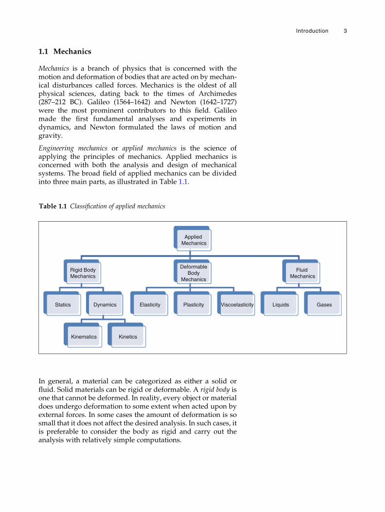
Engineering mechanics or applied mechanics is the science ofapplying the principles of mechanics. Applied mechanics isconcerned with both the analysis and design of mechanicalsystems. The broad field of applied mechanics can be dividedinto three main parts, as illustrated in Table 1.1.
In general, a material can be categorized as either a solid orfluid. Solid materials can be rigid or deformable. A rigid body isone that cannot be deformed. In reality, every object or materialdoes undergo deformation to some extent when acted upon byexternal forces. In some cases the amount of deformation is sosmall that it does not affect the desired analysis. In such cases, itis preferable to consider the body as rigid and carry out theanalysis with relatively simple computations.
Table 1.1 Classification of applied mechanics
Statics
Rigid BodyMechanics
Dynamics
Kinematics Kinetics
Elasticity
Applied Mechanics
DeformableBody
Mechanics
Plasticity Viscoelasticity
Fluid Mechanics
Liquids Gases
Introduction 3
Statics is the study of forces on rigid bodies at rest or movingwith a constant velocity. Dynamics deals with bodies in motion.Kinematics is a branch of dynamics that deals with the geometryand time-dependent aspects of motion without considering theforces causing the motion. Kinetics is based on kinematics, and itincludes the effects of forces and masses in the analysis.
Statics and dynamics are devoted primarily to the study of theexternal effects of forces on rigid bodies, bodies for which thedeformation (change in shape) can be neglected. On the otherhand, the mechanics of deformable bodies deals with the relationsbetween externally applied loads and their internal effects onbodies. This field of appliedmechanics does not assume that thebodies of interest are rigid, but considers the true nature of theirmaterial properties. The mechanics of deformable bodies hasstrong ties with the field of material science which deals withthe atomic and molecular structure of materials. The principlesof deformable body mechanics have important applications inthe design of structures and machine elements. In general,analyses in deformable body mechanics are more complex ascompared to the analyses required in rigid body mechanics.
The mechanics of deformable bodies is the field that isconcerned with the deformability of objects. Deformable bodymechanics is subdivided into the mechanics of elastic, plastic,and viscoelastic materials, respectively. An elastic body isdefined as one in which all deformations are recoverable uponremoval of external forces. This feature of some materials caneasily be visualized by observing a spring or a rubber band. Ifyou gently stretch (deform) a spring and then release it (removethe applied force), it will resume its original (undeformed) sizeand shape. A plastic body, on the other hand, undergoes perma-nent (unrecoverable) deformations. One can observe this behav-ior again by using a spring. Apply a large force on a spring so asto stretch the spring extensively, and then release it. The springwill bounce back, but there may be an increase in its length. Thisincrease illustrates the extent of plastic deformation in thespring. Note that depending on the extent and duration ofapplied forces, a material may exhibit elastic or elastoplasticbehavior as in the case of the spring.
To explain viscoelasticity, wemust first define what is known asa fluid. In general, materials are classified as either solid or fluid.When an external force is applied to a solid body, the body willdeform to a certain extent. The continuous application of thesame force will not necessarily deform the solid body continu-ously. On the other hand, a continuously applied force on afluid body will cause a continuous deformation (flow). Viscosityis a fluid property which is a quantitative measure of resistanceto flow. In nature there are some materials that have both fluidand solid properties. The term viscoelastic is used to refer to the
4 Fundamentals of Biomechanics
mechanical properties of such materials. Many biologicalmaterials exhibit viscoelastic properties.
The third part of applied mechanics is fluid mechanics. Thisincludes the mechanics of liquids and the mechanics of gases.
Note that the distinctions between the various areas of appliedmechanics are not sharp. For example, viscoelasticity simulta-neously utilizes the principles of fluid and solid mechanics.
1.2 Biomechanics
In general, biomechanics is concerned with the application ofclassical mechanics to various biological problems. Biomechanicscombines the field of engineering mechanics with the fields ofbiology and physiology. Basically, biomechanics is concernedwith the human body. In biomechanics, the principles ofmechanics are applied to the conception, design, development,and analysis of equipment and systems in biology and medi-cine. In essence, biomechanics is a multidisciplinary scienceconcerned with the application of mechanical principles to thehuman body in motion and at rest.
Although biomechanics is a relatively young and dynamic field,its history can be traced back to the fifteenth century, whenLeonardo da Vinci (1452–1519) noted the significance ofmechanics in his biological studies. As a result of contributionsof researchers in the fields of biology, medicine, basic sciences,and engineering, the interdisciplinary field of biomechanics hasbeen growing steadily in the last five decades.
The development of the field of biomechanics has improved ourunderstanding of many things, including normal and patholog-ical situations, mechanics of neuromuscular control, mechanicsof blood flow in the microcirculation, mechanics of air flow inthe lung, and mechanics of growth and form. It has contributedto the development of medical diagnostic and treatmentprocedures. It has provided the means for designing andmanufacturing medical equipment, devices, and instruments,assistive technology devices for people with disabilities, andartificial replacements and implants. It has suggested the meansfor improving human performance in the workplace and inathletic competition.
Different aspects of biomechanics utilize different concepts andmethods of applied mechanics. For example, the principles ofstatics are applied to determine the magnitude and nature offorces involved in various joints and muscles of the musculo-skeletal system. The principles of dynamics are utilized formotion description and have many applications in sportsmechanics. The principles of the mechanics of deformable
Introduction 5
bodies provide the necessary tools for developing the field andconstitutive equations for biological materials and systems,which in turn are used to evaluate their functional behaviorunder different conditions. The principles of fluid mechanicsare used to investigate the blood flow in the human circulatorysystem and air flow in the lung.
It is the aim of this textbook to expose the reader to theprinciples and applications of biomechanics. For this purpose,the basic tools and principles will first be introduced. Next,systematic and comprehensive applications of these principleswill be carried out with many solved example problems. Atten-tion will be focused on the applications of statics, dynamics, andthe mechanics of deformable bodies (i.e., solid mechanics). Alimited study of fluid mechanics and its applications in biome-chanics will be provided as well.
1.3 Basic Concepts
Engineering mechanics is based on Newtonian mechanics inwhich the basic concepts are length, time, and mass. These areabsolute concepts because they are independent of each other.Length is a concept for describing size quantitatively. Time is aconcept for ordering the flow of events. Mass is the property ofall matter and is the quantitative measure of inertia. Inertia is theresistance to the change in motion of matter. Inertia can also bedefined as the ability of a body to maintain its state of rest oruniform motion.
Other important concepts in mechanics are not absolute butderived from the basic concepts. These include force, momentor torque, velocity, acceleration, work, energy, power, impulse,momentum, stress, and strain. Force can be defined in manyways, such as mechanical disturbance or load. Force is theaction of one body on another. It is the force applied on abody which causes the body to move, deform, or both. Momentor torque is the quantitative measure of the rotational, bendingor twisting action of a force applied on a body. Velocity isdefined as the time rate of change of position. The time rate ofincrease of velocity, on the other hand, is termed acceleration.Detailed descriptions of these and other relevant concepts willbe provided in subsequent chapters.
1.4 Newton’s Laws
The entire field of mechanics rests on a few basic laws. Amongthese, the laws of mechanics introduced by Sir Isaac Newtonform the basis for analyses in statics and dynamics.
6 Fundamentals of Biomechanics
Newton’s first law states that a body that is originally at rest willremain at rest, or a body in motion will move in a straight linewith constant velocity, if the net force acting upon the body iszero. In analyzing this law, we must pay extra attention to anumber of key words. The term “rest” implies no motion. Forexample, a book lying on a desk is said to be at rest. To be able toexplain the concept of “net force” fully, we need to introducevector algebra (see Chap. 2). The net force simply refers to thecombined effect of all forces acting on a body. If the net forceacting on a body is zero, it does not necessarily mean that thereare no forces acting on the body. For example, there may be twoequal and opposite forces applied on a body so that the com-bined effect of the two forces on the body is zero, assuming thatthe body is rigid. Note that if a body is either at rest or movingin a straight line with a constant velocity, then the body is saidto be in equilibrium. Therefore, the first law states that if the netforce acting on a body is zero, then the body is in equilibrium.
Newton’s second law states that a body with a net force acting onit will accelerate in the direction of that force, and that themagnitude of the acceleration will be directly proportional tothe magnitude of the net force and inversely proportional to themass of the body. The important terms in the statement of thesecond law are “magnitude” and “direction,” and they will beexplained in detail in Chap. 2, within the context of vectoralgebra.
Newton’s third law states that to every action there is always anequal reaction, and that the forces of action and reactionbetween interacting bodies are equal in magnitude, oppositein direction, and have the same line of action. This law can besimplified by saying that if you push a body, the body will pushyou back. This law has important applications in constructingfree-body diagrams of components constituting large systems.The free-body diagram of a component of a structure is one inwhich the surrounding parts of the structure are replaced byequivalent forces. It is an effective aid to study the forcesinvolved in the structure.
Newton’s laws will be explained in detail in subsequentchapters, and they will be utilized extensively throughoutthis text.
1.5 Dimensional Analysis
The term “dimension” has several uses in mechanics. It is usedto describe space, as for example while referring toone-dimensional, two-dimensional, or three-dimensionalsituations. Dimension is also used to denote the nature ofquantities. Every measurable quantity has a dimension and a
Introduction 7
unit associated with it. Dimension is a general description of aquantity, whereas unit is associated with a system of units (seeSect. 1.6). Whether a distance is measured in meters or feet, it isa distance. We say that its dimension is “length.” Whether aflow of events is measured in seconds, minutes, hours, or evendays, it is a point of time when a specific event began and thenended. So we say its dimension is “time.”
There are two sets of dimensions. Primary, or basic, dimensionsare those associated with the basic concepts of mechanics. Inthis text, we shall use capital letters L, T, and M to specify theprimary dimensions length, time, and mass, respectively. Weshall use square brackets to denote the dimensions of physicalquantities. The basic dimensions are:
LENGTH½ � ¼ LTIME½ � ¼ TMASS½ � ¼ M
Secondary dimensions are associated with dependent conceptsthat are derived from basic concepts. For example, the area ofa rectangle can be calculated by multiplying its width andlength, both of which have the dimension of length. Therefore,the dimension of area is:
AREA½ � ¼ LENGTH½ � LENGTH½ � ¼ LL ¼ L2
By definition, velocity is the time rate of change of relativeposition. Change of the relative position is measured in termsof length units. Therefore, the dimension of velocity is:
VELOCITY½ � ¼ POSITION½ �TIME½ � ¼ L
T
The secondary dimensional quantities are established as a con-sequence of certain natural laws. If we know the definition of aphysical quantity, we can easily determine the dimension ofthat quantity in terms of basic dimensions. If the dimension of aphysical quantity is known, then the units of that quantity indifferent systems of units can easily be determined as well.Furthermore, the validity of an equation relating a number ofphysical quantities can be verified by analyzing the dimensionsof terms forming the equation or formula. In this regard, the lawof dimensional homogeneity imposes restrictions on the formula-tion of such relations. To explain this law, consider the follow-ing arbitrary equation:
Z ¼ aX þ bY þ c
For this equation to be dimensionally homogeneous, everygrouping in the equation must have the same dimensionalrepresentation. In other words, if Z refers to a quantity whosedimension is length, then products aX and bY, and quantity
8 Fundamentals of Biomechanics
cmust all have the dimension of length. The numerical equalitybetween both sides of the equation must also be maintained forall systems of units.
1.6 Systems of Units
There have been a number of different systems of units adoptedin different parts of the world. For example, there is the Britishgravitational or foot–pound–second system, the Gaussian (met-ric absolute) or centimeter–gram–second (c–g–s) system, andthe metric gravitational or meter–kilogram–second (mks) sys-tem. The lack of a universal standard in units of measure oftencauses confusion.
In 1960, an International Conference on Weights and Measureswas held to bring an order to the confusion surrounding theunits of measure. Based on the metric system, this conferenceadopted a system called Le Systeme International d’Unites inFrench, which is abbreviated as SI. In English, it is known asthe International System of Units. Today, nearly the entireworld is either using this modernized metric system orcommitted to its adoption. In the International System ofUnits, the units of length, time, and mass are meter (m), second(s), and kilogram (kg), respectively.
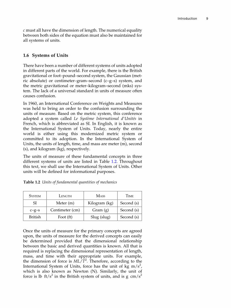
The units of measure of these fundamental concepts in threedifferent systems of units are listed in Table 1.2. Throughoutthis text, we shall use the International System of Units. Otherunits will be defined for informational purposes.
Once the units of measure for the primary concepts are agreedupon, the units of measure for the derived concepts can easilybe determined provided that the dimensional relationshipbetween the basic and derived quantities is known. All that isrequired is replacing the dimensional representation of length,mass, and time with their appropriate units. For example,the dimension of force is ML/T2. Therefore, according to theInternational System of Units, force has the unit of kg m/s2,which is also known as Newton (N). Similarly, the unit offorce is lb ft/s2 in the British system of units, and is g cm/s2
Table 1.2 Units of fundamental quantities of mechanics
SYSTEM LENGTH MASS TIME
SI Meter (m) Kilogram (kg) Second (s)
c–g–s Centimeter (cm) Gram (g) Second (s)
British Foot (ft) Slug (slug) Second (s)
Introduction 9
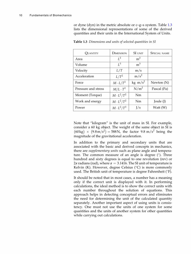
or dyne (dyn) in the metric absolute or c–g–s system. Table 1.3lists the dimensional representations of some of the derivedquantities and their units in the International System of Units.
Note that “kilogram” is the unit of mass in SI. For example,consider a 60 kg object. The weight of the same object in SI is
60kg� � � 9:8m=s2
� � ¼ 588N, the factor 9.8 m/s2 being the
magnitude of the gravitational acceleration.
In addition to the primary and secondary units that areassociated with the basic and derived concepts in mechanics,there are supplementary units such as plane angle and tempera-ture. The common measure of an angle is degree (�). Threehundred and sixty degrees is equal to one revolution (rev) or2π radians (rad), where π ¼ 3.1416. The SI unit of temperature isKelvin (K). However, degree Celsius (�C) is more commonlyused. The British unit of temperature is degree Fahrenheit (�F).
It should be noted that in most cases, a number has a meaningonly if the correct unit is displayed with it. In performingcalculations, the ideal method is to show the correct units witheach number throughout the solution of equations. Thisapproach helps in detecting conceptual errors and eliminatesthe need for determining the unit of the calculated quantityseparately. Another important aspect of using units is consis-tency. One must not use the units of one system for somequantities and the units of another system for other quantitieswhile carrying out calculations.
Table 1.3 Dimensions and units of selected quantities in SI
QUANTITY DIMENSION SI UNIT SPECIAL NAME
Area L2 m2
Volume L3 m3
Velocity L/T m/s
Acceleration L=T2 m/s2
Force M � L=T2 kg m/s2 Newton (N)
Pressure and stress M=L � T2 N/m2 Pascal (Pa)
Moment (Torque) M � L2=T2 Nm
Work and energy M � L2=T2 Nm Joule (J)
Power M � L2=T3 J/s Watt (W)
10 Fundamentals of Biomechanics
1.7 Conversion of Units
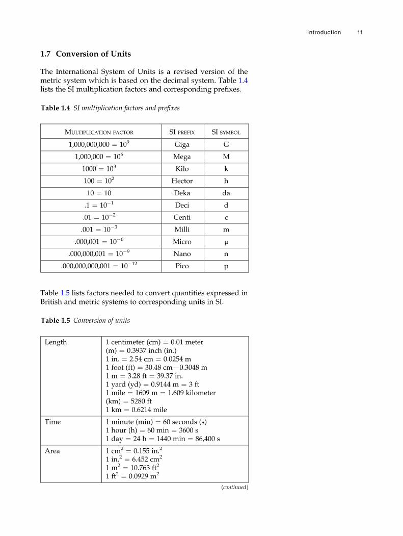
The International System of Units is a revised version of themetric system which is based on the decimal system. Table 1.4lists the SI multiplication factors and corresponding prefixes.
Table 1.5 lists factors needed to convert quantities expressed inBritish and metric systems to corresponding units in SI.
Table 1.4 SI multiplication factors and prefixes
MULTIPLICATION FACTOR SI PREFIX SI SYMBOL
1,000,000,000 ¼ 109 Giga G
1,000,000 ¼ 106 Mega M
1000 ¼ 103 Kilo k
100 ¼ 102 Hector h
10 ¼ 10 Deka da
.1 ¼ 10�1 Deci d
.01 ¼ 10�2 Centi c
.001 ¼ 10�3 Milli m
.000,001 ¼ 10�6 Micro μ
.000,000,001 ¼ 10�9 Nano n
.000,000,000,001 ¼ 10�12 Pico p
Table 1.5 Conversion of units
Length 1 centimeter (cm) ¼ 0.01 meter(m) ¼ 0.3937 inch (in.)1 in. ¼ 2.54 cm ¼ 0.0254 m1 foot (ft) ¼ 30.48 cm—0.3048 m1 m ¼ 3.28 ft ¼ 39.37 in.1 yard (yd) ¼ 0.9144 m ¼ 3 ft1 mile ¼ 1609 m ¼ 1.609 kilometer(km) ¼ 5280 ft1 km ¼ 0.6214 mile
Time 1 minute (min) ¼ 60 seconds (s)1 hour (h) ¼ 60 min ¼ 3600 s1 day ¼ 24 h ¼ 1440 min ¼ 86,400 s
Area 1 cm2 ¼ 0.155 in.2
1 in.2 ¼ 6.452 cm2
1 m2 ¼ 10.763 ft2
1 ft2 ¼ 0.0929 m2
(continued)
Introduction 11
1.8 Mathematics
The applications of biomechanics require some knowledge ofmathematics. These include simple geometry, properties of theright triangle, basic algebra, differentiation, and integration.The appendices that follow the last chapter contain a summaryof the mathematical tools and techniques needed to carry outthe calculations in this book. The reader may find it useful toexamine them now, and review them later when those conceptsare needed. In subsequent chapters throughout the text, the
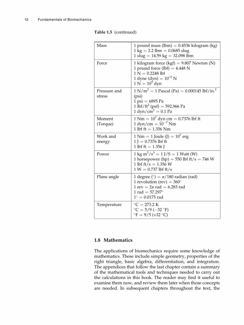
Table 1.5 (continued)
Mass 1 pound mass (lbm) ¼ 0.4536 kilogram (kg)1 kg ¼ 2.2 lbm ¼ 0.0685 slug1 slug ¼ 14.59 kg ¼ 32.098 lbm
Force 1 kilogram force (kgf) ¼ 9.807 Newton (N)1 pound force (lbf) ¼ 4.448 N1 N ¼ 0.2248 lbf1 dyne (dyn) ¼ 10–5 N1 N ¼ 105 dyn
Pressure andstress
1 N/m2 ¼ 1 Pascal (Pa) ¼ 0.000145 lbf/in.2
(psi)1 psi ¼ 6895 Pa1 lbf/ft2 (psf) ¼ 592,966 Pa1 dyn/cm2 ¼ 0.1 Pa
Moment(Torque)
1 Nm ¼ 107 dyn cm ¼ 0.7376 lbf ft1 dyn/cm ¼ 10�7 Nm1 lbf ft ¼ 1.356 Nm
Work andenergy
1 Nm ¼ 1 Joule (J) ¼ 107 erg1 J ¼ 0.7376 lbf ft1 lbf ft ¼ 1.356 J
Power 1 kg m2/s3 ¼ 1 J/S ¼ 1 Watt (W)1 horsepower (hp) ¼ 550 lbf ft/s ¼ 746 W1 lbf ft/s ¼ 1.356 W1 W ¼ 0.737 lbf ft/s
Plane angle 1 degree (�) ¼ π/180 radian (rad)1 revolution (rev) ¼ 360�
1 rev ¼ 2π rad ¼ 6.283 rad1 rad ¼ 57.297�
1� ¼ 0.0175 rad
Temperature �C ¼ 273.2 K�C ¼ 5/9 (�32 �F)�F ¼ 9/5 (+32 �C)
12 Fundamentals of Biomechanics
mathematics required will be reviewed and the correspondingappendix will be indicated.
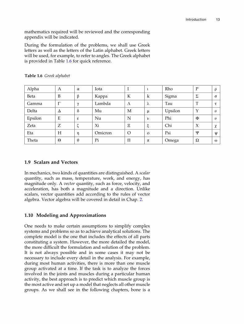
During the formulation of the problems, we shall use Greekletters as well as the letters of the Latin alphabet. Greek letterswill be used, for example, to refer to angles. The Greek alphabetis provided in Table 1.6 for quick reference.
1.9 Scalars and Vectors
In mechanics, two kinds of quantities are distinguished. A scalarquantity, such as mass, temperature, work, and energy, hasmagnitude only. A vector quantity, such as force, velocity, andacceleration, has both a magnitude and a direction. Unlikescalars, vector quantities add according to the rules of vectoralgebra. Vector algebra will be covered in detail in Chap. 2.
1.10 Modeling and Approximations
One needs to make certain assumptions to simplify complexsystems and problems so as to achieve analytical solutions. Thecomplete model is the one that includes the effects of all partsconstituting a system. However, the more detailed the model,the more difficult the formulation and solution of the problem.It is not always possible and in some cases it may not benecessary to include every detail in the analysis. For example,during most human activities, there is more than one musclegroup activated at a time. If the task is to analyze the forcesinvolved in the joints and muscles during a particular humanactivity, the best approach is to predict which muscle group isthe most active and set up amodel that neglects all other musclegroups. As we shall see in the following chapters, bone is a
Table 1.6 Greek alphabet
Alpha A α Iota I ι Rho P ρ
Beta B β Kappa K k Sigma Σ σ
Gamma Γ γ Lambda Λ λ Tau T τ
Delta Δ δ Mu M μ Upsilon Y υ
Epsilon E ε Nu N ν Phi Φ υ
Zeta Z ζ Xi Ξ ξ Chi X χ
Eta H η Omicron O o Psi Ψ ψ
Theta Θ θ Pi Π π Omega Ω ω
Introduction 13
deformable body. If the forces involved are relatively small,then the bone can be treated as a rigid body. This approachmay help to reduce the complexity of the problem underconsideration.
In general, it is always best to begin with a simple basic modelthat represents the system. Gradually, the model can beexpanded on the basis of experience gained and the resultsobtained from simpler models. The guiding principle is tomake simplifications that are consistent with the required accu-racy of the results. In this way, the researcher can set up amodelthat is simple enough to analyze and exhibit satisfactorily thephenomena under consideration. The more we learn, the moredetailed our analysis can become.
1.11 Generalized Procedure
The general method of solving problems in biomechanics maybe outlined as follows:
1. Select the system of interest.2. Postulate the characteristics of the system.3. Simplify the system by making proper approximations.
Explicitly state important assumptions.4. Form an analogy between the human body parts and basic
mechanical elements.5. Construct a mechanical model of the system.6. Apply principles of mechanics to formulate the problem.7. Solve the problem for the unknowns.8. Compare the results with the behavior of the actual system.
This may involve tests and experiments.9. If satisfactory agreement is not achieved, steps 3 through
7 must be repeated by considering different assumptionsand a new model of the system.
1.12 Scope of the Text
Courses in biomechanics are taught within a wide variety ofacademic programs to students with quite differentbackgrounds and different levels of preparation coming fromvarious disciplines of engineering as well as other academicdisciplines. This text is prepared to provide a teaching andlearning tool primarily to health care professionals who areseeking a graduate degree in biomechanics but have limitedbackgrounds in calculus, physics, and engineering mechanics.
14 Fundamentals of Biomechanics
This text can also be a useful reference for undergraduate bio-medical, biomechanical, or bioengineering programs.
This text is divided into three parts. The first part (Chaps. 1through 5, and Appendices A and B) will introduce the basicconcepts of mechanics including force and moment vectors,provide the mathematical tools (geometry, algebra, and vectoralgebra) so that complete definitions of these concepts can begiven, explain the procedure for analyzing the systems at “staticequilibrium,” and apply this procedure to analyze simplemechanical systems and the forces involved at various musclesand joints of the human musculoskeletal system. It should benoted here that the topics covered in the first part of this text areprerequisites for both parts two and three.
The second part of the text (Chaps. 6 through 11) is devoted to“dynamic” analyses. The concepts introduced in the secondpart are position, velocity and acceleration vectors, work,energy, power, impulse, and momentum. Also provided inthe second part are the techniques for kinetic and kinematicanalyses of systems undergoing translational and rotationalmotions. These techniques are applied for human motionanalyses of various sports activities.
The last section of the text (Chaps. 12 through 15) provides thetechniques for analyzing the “deformation” characteristics ofmaterials under different load conditions. For this purpose, theconcepts of stress and strain are defined. Classifications ofmaterials based on their stress–strain diagrams are given. Theconcepts of elasticity, plasticity, and viscoelasticity are alsointroduced and explained. Topics such as torsion, bending,fatigue, endurance, and factors affecting the strength ofmaterials are provided. The emphasis is placed uponapplications to orthopaedic biomechanics.
1.13 Notation
While preparing this text, special attention was given to theconsistent use of notation. Important terms are italicizedwhere they are defined or described (such as, force is definedas load or mechanical disturbance). Symbols for quantities arealso italicized (for example, m for mass). Units are not italicized(for example, kg for kilogram). Underlined letters are used torefer to vector quantities (for example, force vector F). Sectionsand subsections marked with a star (�) are considered optional.In other words, the reader can omit a section or subsectionmarked with a star without losing the continuity of the topicscovered in the text.
Introduction 15
References, Suggested Reading, and Other Resources1
I. Suggested Reading
Adams, M.A., Bogduk, N., Burton, K., Dolan, P., 2012. The Biomechanics of BackPain. 3rd Edition. London, Churchill Livingstone.
Arus, E., 2012. Biomechanics of Human Motion: Applications in the Martial Arts.Bosa Roca, CRC Press Inc.
Benzel, E.C., 2015. Biomechanics of Spine Stabilization. New York, Thieme Medi-cal Publishers Inc.
Bartlett, R., 2014. Introduction to Sports Biomechanics: Analyzing Human Move-ment Patterns. 3rd Edition. London, Routledge International Handbooks.
Bartlett, R., Bussey, M., 2012. Sports Biomechanics: Reducing Injury Risk andImproving Sports Performance. 2nd Edition. London, Routledge InternationalHandbooks.
Blazevich, A.J., 2010. Sports Biomechanics. The Basics: Optimizing Human Perfor-mance. 2nd Ed. A & C Black Publishers Ltd.
Crowe, S.A., Visentin, P., Gongbing Shan., 2014. Biomechanics of Bi-DirectionalBicycle Pedaling. Aachen, Shaker Verlag GmbH.
Doblare, M., Merodio, J., Ma Goicolea Ruigomez, J., 2015. Biomechanics. Ramsey,EOLSS Publishers Co Ltd.
Doyle, B., Miller, K., Wittek, A., Nielsen, P.M.F., 2014. Computational Biomechan-ics for Medicine: Fundamental Science and Patient-Specific Applications.New York, Springer-Verlag New York Inc.
Doyle, B., Miller, K., Wittek, A., Nielsen, P.M.F., 2015. Computational Biomechan-ics for Medicine: New Approaches and New Applications. Cham, Springer-International-Publishing-AG.
Ethier, R.C., Simmons, C.A., 2012. Introductory Biomechanics: From Cells toOrganisms. Cambridge, Cambridge University Press.
Flanagan, S.P., 2013. Biomechanics: A Case-based Approach. Sudbury, Jones andBartlett Publishers, Inc.
Fleisig, G.S., Young-Hoo Kwon, 2013. The Biomechanics of Batting, Swinging, andHitting. London, Routledge International Handbooks.
Freivalds, A., 2014. Biomechanics of the Upper Limbs: Mechanics, Modeling andMusculoskeletal Injuries. 2nd Edition. Bosa Roca, CRC Press Inc.
Gerhard Silber, G., Then, C., 2013. Preventive Biomechanics. Berlin, Springer-Verlag Berlin and Heidelberg GmbH & Co. K.
Hall, S.J., 2014. Basic Biomechanics. London, McGraw Hill Higher Education.Hamill, J., Knutzen, K.M., Derrick, T.D., 2014. Biomechanical Basis of Human
Movement. Philadelphia, Lippincott Williams and Wilkins.Holzapfel, G.A., Kuhl, E., 2013. Computer Models in Biomechanics. Dordrecht,
Springer.Huston, R.L., 2013. Fundamentals of Biomechanics. Bosa Roca, CRC Press Inc.Huttner, B., 2013. Biomechanical Analysis Methods for Substitute Voice Produc-
tion. Aachen, Shaker Verlag GmbH.Kerr, A., 2010. Introductory Biomechanics. Elsevier Health Sciences, UK.Kieser, J., Taylor, M., Carr, D., 2012. Forensic Biomechanics. New York, JohnWiley
& Sons Inc.Knudson, D.V., 2012. Fundamentals of Biomechanics. 2nd Edition. New York,
Springer-Verlag New York Inc.LeVeau, B.F., 2010. Biomechanics of Human Motion: Basics and Beyond for the
Health Professions. Thorofare, NJ. SLACK Incorporated.Luo Qi, 2015. Biomechanics and Sports Engineering. Bosa Roca, CRC Press Inc.
1We believe that this text is a self-sufficient teaching and learning tool. Whilepreparing it, we utilized the information provided from many sources, someof which are listed below. Note, however, that it is not our intention to promotethese publications, or to suggest that these are the only texts availableon the subject matter. The field of biomechanics has been growing very rapidly.There are many other sources of readily available information, including scientificjournals presenting peer-reviewed research articles in biomechanics.
16 Fundamentals of Biomechanics
McGinnis, P., 2013. Biomechanics of Sport and Exercise. 3rd Edition. Champaign,Human Kinetics Publishers.
McLester, J., Peter St. Pierre, P.St., 2010. Applied Biomechanics: Concepts andConnections. CA. Brooks/Cole.
Ming Zhang., Yubo Fan., 2014. Computational Biomechanics of the Musculoskele-tal System. Bosa Roca, CRC Press Inc.
Mohammed Rafiq Abdul Kadir, 2013. Computational Biomechanics of the HipJoint. Berlin, Springer-Verlag Berlin and Heidelberg GmbH & Co. K.
Morin, J.-B., Samozino, P., 2015. Biomechanics of Training and Testing: InnovativeConcepts and Simple Field Methods. Cham, Springer-International-Publish-ing-AG.
Peterson, D.R., Bronzino, J.D,. 2014. Biomechanics: Principles and Practices. BosaRoca, CRC Press Inc.
Richards, J., 2015. The Complete Textbook of Biomechanics. London, ChurchillLivingstone.
Sanders, R., 2012. Sport Biomechanics into Coaching Practice. Chichester, JohnWiley & Sons Ltd.
Shahbaz S. Malik, Sheraz S. Malik, 2015. Orthopaedic Biomechanics Made Easy.Cambridge, Cambridge University Press.
Tanaka, M., Wada, S., Nakamura, M., 2012. Computational Biomechanics: Theoret-ical Background and Biological/Biomedical Problems. Tokyo, Springer Verlag.
Tien Tua Dao, Marie-Christine Ho Ba Tho., 2014. Biomechanics of the Musculo-skeletal System: Modeling of Data Uncertainty and Knowledge. London, ISTELtd and John Wiley & Sons Inc.
Vogel, S., 2013. Comparative Biomechanics: Life’s Physical World. New Jersey,Princeton University Press.
Winkelstein, B.A., 2015. Orthopaedic Biomechanics. Bosa Roca, CRC Press Inc.Youlian Hong., Bartlett, R., 2010. Routledge Handbook of Biomechanics and
Human Movement Science. London, Routledge International Handbooks.Zatsiorsky, V.M., Prilutsky, B.I., 2012. Biomechanics of Skeletal Muscles. Cham-
paign, Human Kinetics Publishers.
II. Advanced Topics in Biomechanics and Bioengineering
Devasahayam, S.R., 2013. Signals and Systems in Biomedical Engineering: SignalProcessing and Physiological Systems Modeling. 3rd Edition. Springer.
Jiyuan Tu, Kiao Inthavong, Kelvin Kian LoongWong, 2015. Computational Hemo-dynamics: Theory, Modelling and Applications. Springer.
Johnson, M., Ethier, C.R., 2013. Problems for Biomedical Fluid Mechanics andTransport Phenomena. Cambridge University Press.
Kenedi, R., 2013. Advances in Biomedical Engineering. Academic Press.King, M.R., Mody, N.A., 2010. Numerical and Statistical Methods for Bioengineer-
ing: Applications in MATLAB. Cambridge University Press.Miftahof, M.R.N., Hong Gil Nam, 2010. Mathematical Foundations and Biome-
chanics of the Digestive System. Cambridge University Press.Miftahof, M.R.N., Kamm, R.D, 2011. Cytoskeletal Mechanics. Models and
Measurements in Cell Mechanics. Cambridge University Press (Texts in Bio-medical Engineering).
Northrop, R.B., 2010. Signals and Systems Analysis in Biomedical Engineering.2nd Edition. CRC Press.
Pruitt, L.A., Chakravartula, A.M., 2011. Mechanics of Biomaterials. FundamentalPrinciples for Implant Design. Cambridge University Press (Texts in Biomedi-cal Engineering).
Saha, P.K., Maulik, U., Basu, S., 2014. Advanced Computational Approaches toBiomedical Engineering. Springer Berlin Heidelberg.
Saltzman, M.W., 2015. Biomedical Engineering: Bridging Medicine and Technol-ogy. 2nd Edition. Cambridge University Press (Texts in BiomedicalEngineering).
Suvranu De, S., Guilak, F., Mofrad, M.R.K., 2009. Computational Modeling inBiomechanics. Springer.
Williams, D., 2014. Essential Biomaterials Science. Cambridge University Press(Texts in Biomedical Engineering).
Introduction 17
III. Books About Physics and Engineering Mechanics
Bhattacharya, D.K., Bhaskaran, A., 2010. Engineering Physics. Oxford UniversityPress.
Chin-Teh Sun Zhihe Jin, 2011. Fracture Mechanics. Academic Press.Harrison, H., Nettleton, T., 2012. Principles of Engineering Mechanics. 2nd Edi-
tion. Elsevier.Gross, D., Hauger, W., Schr€oder, J., Wall, W.A., Rajapakse, N., 2013. Engineering
Mechanics: Statics. Springer.Hibbeler, R. C., 2012. EngineeringMechanics: Dynamics. 13th Edition. Prentice Hall.Jain, S.D., 2010. Engineering Physics. Universities Press.Khare, P., Swarup, A., 2009. Engineering Physics: Fundamentals & Modern
Applications. Jones & Bartlett Learning.Knight, R.D., 2012. Physics for Scientists and Engineers: Modern Physics Plus
Mastering Physics. 3rd Edition. Addison-Wesley.Kumar, K.I., 2011. Engineering Mechanics. McGraw-Hill Education (India) Pvt
Limited.Morrison, J., 2009. Modern Physics for Scientists and Engineers. Academic Press.Plesha, M., Gray, G., Costanzo, F., 2012. Engineering Mechanics: Statics. McGraw-
Hill.Shankar, R., 2014. Fundamentals of Physics: Mechanics, Relativity, and Thermo-
dynamics. Yale University Press.Verma, N.K., 2013. Physics for Engineers. PHI Learning Pvt. Ltd.
IV. Books About Deformable Body Mechanics, Mechanicsof Materials, and Resistance of Materials
Beer, F. Jr., Johnston, R.E., DeWolf, J., Mazurek, D., 2014. Mechanics of Materials.McGraw-Hill Science.
Farag, M.M., 2013. Resistance of Materials: Materials and Process Selection forEngineering Design, 3rd Edition. Bosa Roca, CRC Press Inc.
Francois, D., Pineau, A., Zaoui, A., 2013. Mechanical Behavior of Materials: Frac-ture Mechanics and Damage. Springer.
Ghavami, P., 2015. Mechanics of Materials: An Introduction to Engineering Tech-nology. Springer.
Martin, B.R., Burr, D.B., Sharkey, N.A., 2010. Skeletal Tissue Mechanics.New York, Springer-Verlag New York Inc.
Philpot, T.A., 2012. Mechanics of Materials: An Integrated Learning System, 3rdEdition. Hoboken, Wiley.
Pruitt, L.A., Chakravartula, A.M., 2012. Mechanics of Biomaterials: FundamentalPrinciples for Implant Design. Cambridge, Cambridge University Press.
Riley, W.F., 2006. Mechanics of Materials. John Wiley and Sons.Rubenstein, D., Yin Wei., Frame, M., 2011. Biofluid Mechanics: An Introduction to
Fluid Mechanics, Macrocirculation, and Microcirculation. San Diego, Aca-demic Press Inc.
V. Biomechanics Societies
Bulgarian Society of Biomechanics: http://www.imbm.bas.bg/biomechanics/index.php/societies
Czech Society of Biomechanics: http://www.csbiomech.cz/index.php/en/Danish Society of Biomechanics: http://www.danskbiomekaniskselskab.dk/European Society of Biomechanics: http://esbiomech.org/French Society of Biomechanics: http://www.biomecanique.org/Hellenic Society of Biomechanics: http://www.elembio.gr/index.php/el/International Society of Biomechanics: https://isbweb.org/International Society of Biomechanics in Sports: http://www.isbs.org/Polish Society of Biomechanics: http://www.biomechanics.pl/Portuguese Society of Biomechanics: http://www.spbiomecanica.com/The British Association of Sport and Exercise Sciences: http://www.bases.org.uk/
18 Fundamentals of Biomechanics
VI. Biomechanics Journals
Applied Bionics and Biomechanics: http://www.hindawi.com/journals/abb/Clinical Biomechanics: http://www.clinbiomech.com/International Journal of Experimental and Computational Biomechanics: http://
www.journal-data.com/journal/international-journal-of-experimental-and-computational-biomechanics.html
Journal of Biomechanics: http://www.jbiomech.com/Journal of Applied Biomechanics: http://journals.humankinetics.com/about-jabJournal of Biomechanical Engineering: http://biomechanical.asmedigitalcollection.
asme.org/journal.aspxJournal of Biomechanical Science and Engineering: http://jbse.org/Journal of Dental Biomechanics: http://www.journal-data.com/journal/journal-
of-dental-biomechanics.htmlSports Biomechanics: http://www.isbs.org/journal.html
VII. Biomechanics-Related Graduate Programsin the United States2
Boston University. Department of Biomedical Engineering: http://www.bu.edu/dbin/bme/
University of California Berkeley. Department of Bioengineering: http://bioegrad.berkeley.edu/
Carnegie Mellon. Department of Biomedical Engineering: http://www.bme.cmu.edu/
Columbia University. Department of Biomedical Engineering: http://www.bme.columbia.edu/index.html
Cornell University. Department of Biomedical Engineering: http://www.bme.cornell.edu/
Duke University. Biomedical Engineering: http://www.bme.duke.edu/grads/Harvard University. School of Public Health. Occupational Biomechanics and
Ergonomics Laboratory: http://www.hsph.harvard.edu/ergonomics/Johns Hopkins University. The Whitaker Institute. Department of Biomedical
Engineering: http://www.bme.jhu.edu/University of Michigan. Center for Ergonomics: http://www.engin.umich.edu/
dept/ioe/C4E/MIT. Center for Biomedical Engineering: http://web.mit.edu/afs/athena.mit.
edu/org/c/cbe/www/University of North Carolina at Chapel Hill. Biomedical Engineering: http://
www.bme.unc.edu/academics/grad.htmlNew Jersey Institute of Technology. Department of Biomedical Engineering:
http://biomedical.njit.edu/index.phpNew York University. Graduate School of Arts and Science. Environmental Health
Sciences-Ergonomics and Biomechanics Program: http://oioc.med.nyu.edu/education/masters-program
Ohio State University. Department of Biomedical Engineering: http://www.bme.ohio-state.edu/bmeweb3/
Stanford University. Department of Bioengineering: http://bioengineering.stanford.edu/education/ms.html
Syracuse University. Department of Biomedical Engineering: http://www.lcs.syr.edu/academic/biochem_engineering/index.aspx
Yale University. Department of Biomedical Engineering: http://www.eng.yale.edu/content/DPBiomedicalEngineering.asp
2 For complete list of biomechanics-related Graduate Programs in the UnitedStates, visit the website of The American Society of Biomechanics, http://www.asbweb.org/.
Introduction 19
Chapter 2
Force Vector
2.1 Definition of Force / 23
2.2 Properties of Force as a Vector Quantity / 23
2.3 Dimension and Units of Force / 23
2.4 Force Systems / 24
2.5 External and Internal Forces / 24
2.6 Normal and Tangential Forces / 25
2.7 Tensile and Compressive Force / 25
2.8 Coplanar Forces / 25
2.9 Collinear Forces / 26
2.10 Concurrent Forces / 26
2.11 Parallel Force / 26
2.12 Gravitational Force or Weight / 26
2.13 Distributed Force Systems and Pressure / 27
2.14 Frictional Forces / 29
2.15 Exercise Problems / 31
The original version of this chapter was revised. An erratum to this chapter can befound at https://doi.org/10.1007/978-3-319-44738-4_16
# Springer International Publishing Switzerland 2017N. Ozkaya et al., Fundamentals of Biomechanics, DOI 10.1007/978-3-319-44738-4_2
21

2.1 Definition of Force
Force may be defined as mechanical disturbance or load. Whenyou pull or push an object, you apply a force to it. You also exerta force when you throw or kick a ball. In all of these cases, theforce is associated with the result of muscular activity. Forcesacting on an object can deform, change its state of motion, orboth. Although forces cause motion, it does not necessarilyfollow that force is always associated with motion. For example,a person sitting on a chair applies his/her weight on the chair,and yet the chair remains stationary. There are relatively fewbasic laws that govern the relationship between force andmotion. These laws will be discussed in detail in later chapters.
2.2 Properties of Force as a Vector Quantity
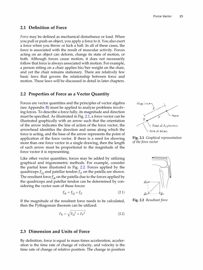
Forces are vector quantities and the principles of vector algebra(see Appendix B) must be applied to analyze problems involv-ing forces. To describe a force fully, its magnitude and directionmust be specified. As illustrated in Fig. 2.1, a force vector can beillustrated graphically with an arrow such that the orientationof the arrow indicates the line of action of the force vector, thearrowhead identifies the direction and sense along which theforce is acting, and the base of the arrow represents the point ofapplication of the force vector. If there is a need for showingmore than one force vector in a single drawing, then the lengthof each arrow must be proportional to the magnitude of theforce vector it is representing.
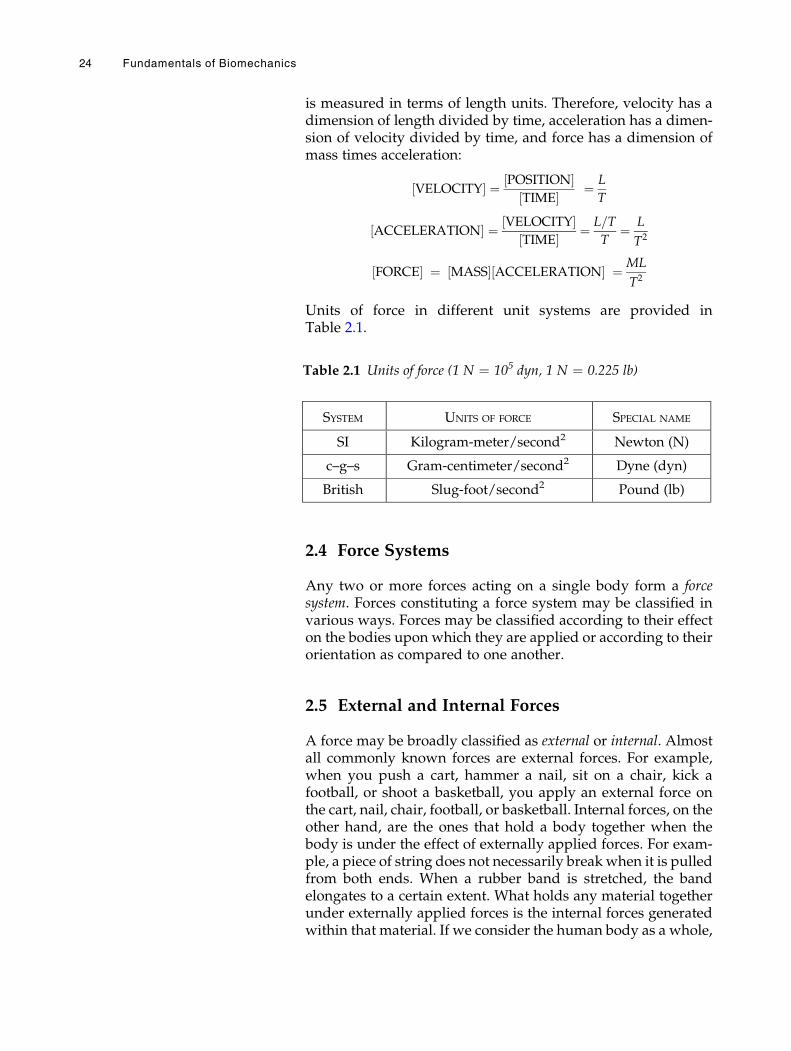
Like other vector quantities, forces may be added by utilizinggraphical and trigonometric methods. For example, considerthe partial knee illustrated in Fig. 2.2. Forces applied by thequadriceps FQ and patellar tendon FP on the patella are shown.
The resultant forceFR on the patella due to the forces applied bythe quadriceps and patellar tendon can be determined by con-sidering the vector sum of these forces:
FR ¼ FQ þ FP ð2:1Þ
If the magnitude of the resultant force needs to be calculated,then the Pythagorean theorem can be utilized:
FR ¼ffiffiffiffiffiffiffiffiffiffiffiffiffiffiffiffiffiffiffiffiffiffi
FQ2 þ FP
2q
ð2:2Þ
2.3 Dimension and Units of Force
By definition, force is equal to mass times acceleration, acceler-ation is the time rate of change of velocity, and velocity is thetime rate of change of relative position. The change in position
Fig. 2.1 Graphical representationof the force vector
Fig. 2.2 Resultant force
Force Vector 23
is measured in terms of length units. Therefore, velocity has adimension of length divided by time, acceleration has a dimen-sion of velocity divided by time, and force has a dimension ofmass times acceleration:
VELOCITY½ � ¼ POSITION½ �TIME½ � ¼ L
T
ACCELERATION½ � ¼ VELOCITY½ �TIME½ � ¼ L=T
T¼ L
T2
FORCE½ � ¼ MASS½ � ACCELERATION½ � ¼ ML
T2
Units of force in different unit systems are provided inTable 2.1.
2.4 Force Systems
Any two or more forces acting on a single body form a forcesystem. Forces constituting a force system may be classified invarious ways. Forces may be classified according to their effecton the bodies upon which they are applied or according to theirorientation as compared to one another.
2.5 External and Internal Forces
A force may be broadly classified as external or internal. Almostall commonly known forces are external forces. For example,when you push a cart, hammer a nail, sit on a chair, kick afootball, or shoot a basketball, you apply an external force onthe cart, nail, chair, football, or basketball. Internal forces, on theother hand, are the ones that hold a body together when thebody is under the effect of externally applied forces. For exam-ple, a piece of string does not necessarily break when it is pulledfrom both ends. When a rubber band is stretched, the bandelongates to a certain extent. What holds any material togetherunder externally applied forces is the internal forces generatedwithin that material. If we consider the human body as a whole,
Table 2.1 Units of force (1 N ¼ 105 dyn, 1 N ¼ 0.225 lb)
SYSTEM UNITS OF FORCE SPECIAL NAME
SI Kilogram-meter/second2 Newton (N)
c–g–s Gram-centimeter/second2 Dyne (dyn)
British Slug-foot/second2 Pound (lb)
24 Fundamentals of Biomechanics
then the forces generated by muscle contractions are also inter-nal forces. The significance and details of internal forces will bestudied by introducing the concept of “stress” in later chapters.
2.6 Normal and Tangential Forces
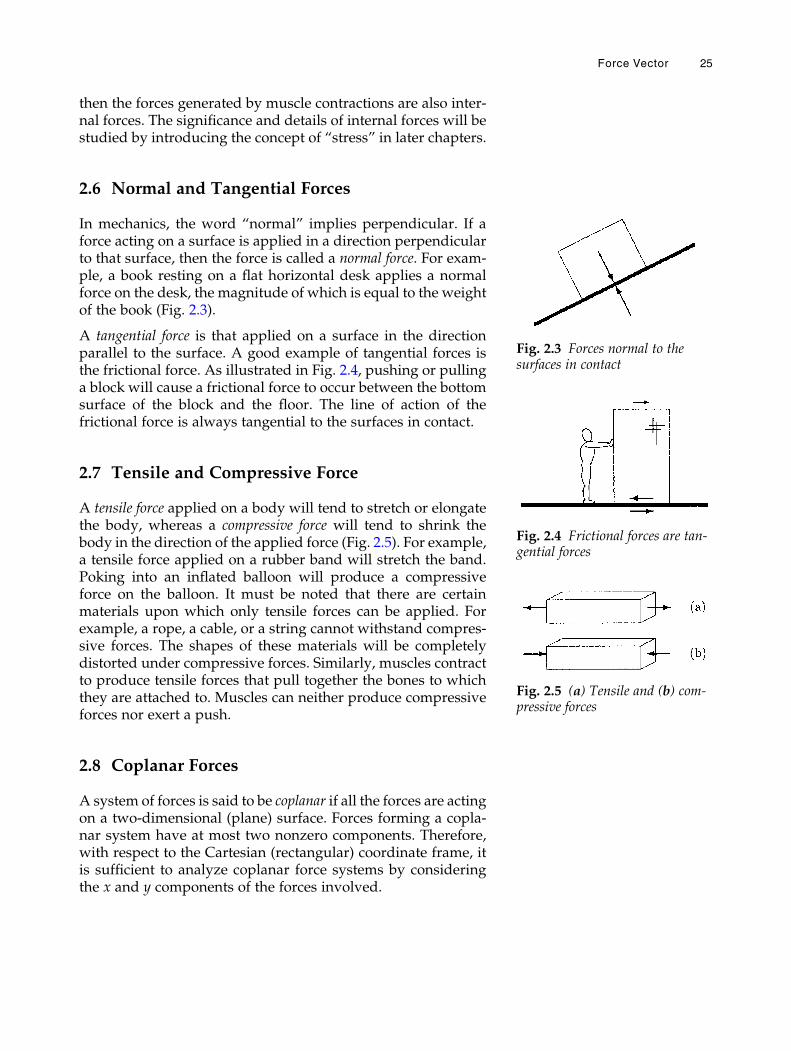
In mechanics, the word “normal” implies perpendicular. If aforce acting on a surface is applied in a direction perpendicularto that surface, then the force is called a normal force. For exam-ple, a book resting on a flat horizontal desk applies a normalforce on the desk, the magnitude of which is equal to the weightof the book (Fig. 2.3).
A tangential force is that applied on a surface in the directionparallel to the surface. A good example of tangential forces isthe frictional force. As illustrated in Fig. 2.4, pushing or pullinga block will cause a frictional force to occur between the bottomsurface of the block and the floor. The line of action of thefrictional force is always tangential to the surfaces in contact.
2.7 Tensile and Compressive Force
A tensile force applied on a body will tend to stretch or elongatethe body, whereas a compressive force will tend to shrink thebody in the direction of the applied force (Fig. 2.5). For example,a tensile force applied on a rubber band will stretch the band.Poking into an inflated balloon will produce a compressiveforce on the balloon. It must be noted that there are certainmaterials upon which only tensile forces can be applied. Forexample, a rope, a cable, or a string cannot withstand compres-sive forces. The shapes of these materials will be completelydistorted under compressive forces. Similarly, muscles contractto produce tensile forces that pull together the bones to whichthey are attached to. Muscles can neither produce compressiveforces nor exert a push.
2.8 Coplanar Forces
A system of forces is said to be coplanar if all the forces are actingon a two-dimensional (plane) surface. Forces forming a copla-nar system have at most two nonzero components. Therefore,with respect to the Cartesian (rectangular) coordinate frame, itis sufficient to analyze coplanar force systems by consideringthe x and y components of the forces involved.
Fig. 2.3 Forces normal to thesurfaces in contact
Fig. 2.4 Frictional forces are tan-gential forces
Fig. 2.5 (a) Tensile and (b) com-pressive forces
Force Vector 25
2.9 Collinear Forces
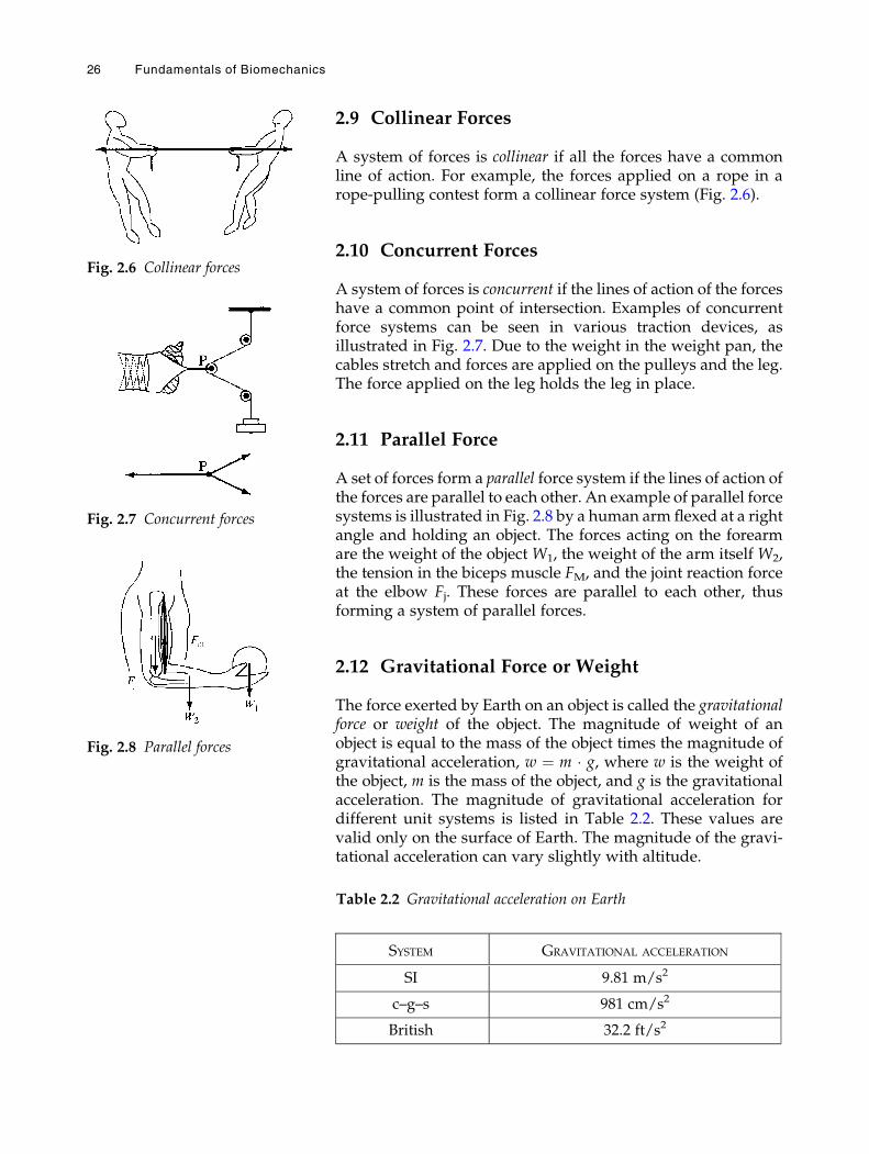
A system of forces is collinear if all the forces have a commonline of action. For example, the forces applied on a rope in arope-pulling contest form a collinear force system (Fig. 2.6).
2.10 Concurrent Forces
A system of forces is concurrent if the lines of action of the forceshave a common point of intersection. Examples of concurrentforce systems can be seen in various traction devices, asillustrated in Fig. 2.7. Due to the weight in the weight pan, thecables stretch and forces are applied on the pulleys and the leg.The force applied on the leg holds the leg in place.
2.11 Parallel Force
A set of forces form a parallel force system if the lines of action ofthe forces are parallel to each other. An example of parallel forcesystems is illustrated in Fig. 2.8 by a human arm flexed at a rightangle and holding an object. The forces acting on the forearmare the weight of the object W1, the weight of the arm itself W2,the tension in the biceps muscle FM, and the joint reaction forceat the elbow Fj. These forces are parallel to each other, thusforming a system of parallel forces.
2.12 Gravitational Force or Weight
The force exerted by Earth on an object is called the gravitationalforce or weight of the object. The magnitude of weight of anobject is equal to the mass of the object times the magnitude ofgravitational acceleration, w ¼ m � g, where w is the weight ofthe object, m is the mass of the object, and g is the gravitationalacceleration. The magnitude of gravitational acceleration fordifferent unit systems is listed in Table 2.2. These values arevalid only on the surface of Earth. The magnitude of the gravi-tational acceleration can vary slightly with altitude.
Fig. 2.7 Concurrent forces
Fig. 2.8 Parallel forces
Fig. 2.6 Collinear forces
Table 2.2 Gravitational acceleration on Earth
SYSTEM GRAVITATIONAL ACCELERATION
SI 9.81 m/s2
c–g–s 981 cm/s2
British 32.2 ft/s2
26 Fundamentals of Biomechanics
For our applications, we shall assume g to be a constant.
The terms mass and weight are often confused with oneanother. Mass is a property of a body. Weight is the force ofgravity acting on the mass of the body. A body has the samemass on Earth and on the moon. However, the weight of a bodyis about six times as much on Earth as on the moon, because themagnitude of the gravitational acceleration on the moon isabout one-sixth of what it is on Earth. Therefore, a 10 kg masson Earth weighs about 98 N on Earth, while it weighs about17 N on the moon.
Like force, acceleration is a vector quantity. The direction ofgravitational acceleration and gravitational force vectors isalways toward the center of Earth, or always vertically down-ward. The force of gravity acts on an object at all times. If wedrop an object from a height, it is the force of gravity that willpull the object downward.
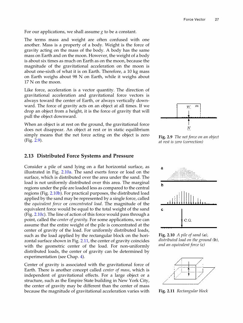
When an object is at rest on the ground, the gravitational forcedoes not disappear. An object at rest or in static equilibriumsimply means that the net force acting on the object is zero(Fig. 2.9).
2.13 Distributed Force Systems and Pressure
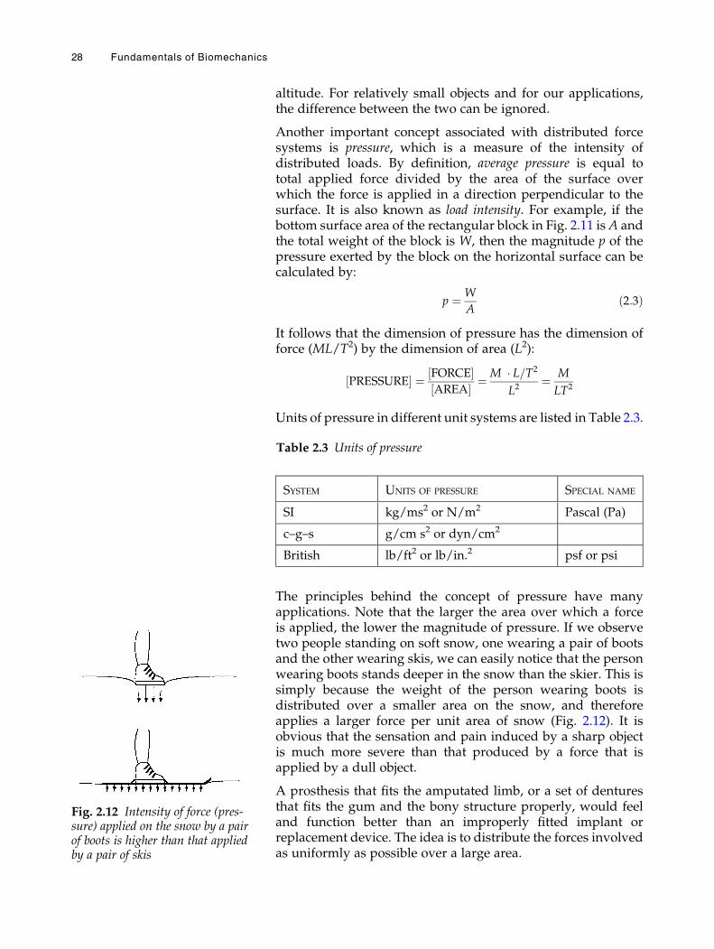
Consider a pile of sand lying on a flat horizontal surface, asillustrated in Fig. 2.10a. The sand exerts force or load on thesurface, which is distributed over the area under the sand. Theload is not uniformly distributed over this area. The marginalregions under the pile are loaded less as compared to the centralregions (Fig. 2.10b). For practical purposes, the distributed loadapplied by the sand may be represented by a single force, calledthe equivalent force or concentrated load. The magnitude of theequivalent force would be equal to the total weight of the sand(Fig. 2.10c). The line of action of this force would pass through apoint, called the center of gravity. For some applications, we canassume that the entire weight of the pile is concentrated at thecenter of gravity of the load. For uniformly distributed loads,such as the load applied by the rectangular block on the hori-zontal surface shown in Fig. 2.11, the center of gravity coincideswith the geometric center of the load. For non-uniformlydistributed loads, the center of gravity can be determined byexperimentation (see Chap. 4).
Center of gravity is associated with the gravitational force ofEarth. There is another concept called center of mass, which isindependent of gravitational effects. For a large object or astructure, such as the Empire State building in New York City,the center of gravity may be different than the center of massbecause the magnitude of gravitational acceleration varies with
Fig. 2.9 The net force on an objectat rest is zero (correction)
Fig. 2.10 A pile of sand (a),distributed load on the ground (b),and an equivalent force (c)
Fig. 2.11 Rectangular block
Force Vector 27
altitude. For relatively small objects and for our applications,the difference between the two can be ignored.
Another important concept associated with distributed forcesystems is pressure, which is a measure of the intensity ofdistributed loads. By definition, average pressure is equal tototal applied force divided by the area of the surface overwhich the force is applied in a direction perpendicular to thesurface. It is also known as load intensity. For example, if thebottom surface area of the rectangular block in Fig. 2.11 isA andthe total weight of the block is W, then the magnitude p of thepressure exerted by the block on the horizontal surface can becalculated by:
p ¼ W
Að2:3Þ
It follows that the dimension of pressure has the dimension offorce (ML/T2) by the dimension of area (L2):
PRESSURE½ � ¼ FORCE½ �AREA½ � ¼ M � L=T2
L2¼ M
LT2
Units of pressure in different unit systems are listed in Table 2.3.
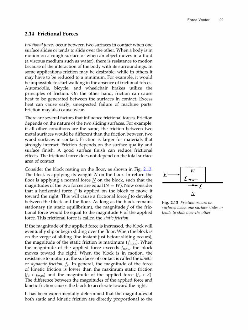
The principles behind the concept of pressure have manyapplications. Note that the larger the area over which a forceis applied, the lower the magnitude of pressure. If we observetwo people standing on soft snow, one wearing a pair of bootsand the other wearing skis, we can easily notice that the personwearing boots stands deeper in the snow than the skier. This issimply because the weight of the person wearing boots isdistributed over a smaller area on the snow, and thereforeapplies a larger force per unit area of snow (Fig. 2.12). It isobvious that the sensation and pain induced by a sharp objectis much more severe than that produced by a force that isapplied by a dull object.
A prosthesis that fits the amputated limb, or a set of denturesthat fits the gum and the bony structure properly, would feeland function better than an improperly fitted implant orreplacement device. The idea is to distribute the forces involvedas uniformly as possible over a large area.
Table 2.3 Units of pressure
SYSTEM UNITS OF PRESSURE SPECIAL NAME
SI kg/ms2 or N/m2 Pascal (Pa)
c–g–s g/cm s2 or dyn/cm2
British lb/ft2 or lb/in.2 psf or psi
Fig. 2.12 Intensity of force (pres-sure) applied on the snow by a pairof boots is higher than that appliedby a pair of skis
28 Fundamentals of Biomechanics
2.14 Frictional Forces
Frictional forces occur between two surfaces in contact when onesurface slides or tends to slide over the other. When a body is inmotion on a rough surface or when an object moves in a fluid(a viscous medium such as water), there is resistance to motionbecause of the interaction of the body with its surroundings. Insome applications friction may be desirable, while in others itmay have to be reduced to a minimum. For example, it wouldbe impossible to start walking in the absence of frictional forces.Automobile, bicycle, and wheelchair brakes utilize theprinciples of friction. On the other hand, friction can causeheat to be generated between the surfaces in contact. Excessheat can cause early, unexpected failure of machine parts.Friction may also cause wear.
There are several factors that influence frictional forces. Frictiondepends on the nature of the two sliding surfaces. For example,if all other conditions are the same, the friction between twometal surfaces would be different than the friction between twowood surfaces in contact. Friction is larger for materials thatstrongly interact. Friction depends on the surface quality andsurface finish. A good surface finish can reduce frictionaleffects. The frictional force does not depend on the total surfacearea of contact.
Consider the block resting on the floor, as shown in Fig. 2.13.The block is applying its weight W on the floor. In return thefloor is applying a normal force N on the block, such that themagnitudes of the two forces are equal (N ¼ W). Now considerthat a horizontal force F is applied on the block to move ittoward the right. This will cause a frictional force f to developbetween the block and the floor. As long as the block remainsstationary (in static equilibrium), the magnitude f of the fric-tional force would be equal to the magnitude F of the appliedforce. This frictional force is called the static friction.
If the magnitude of the applied force is increased, the block willeventually slip or begin sliding over the floor. When the block ison the verge of sliding (the instant just before sliding occurs),the magnitude of the static friction is maximum ( fmax). Whenthe magnitude of the applied force exceeds fmax, the blockmoves toward the right. When the block is in motion, theresistance to motion at the surfaces of contact is called the kineticor dynamic friction, fk. In general, the magnitude of the forceof kinetic friction is lower than the maximum static friction(fk < fmax) and the magnitude of the applied force (fk < F).The difference between the magnitudes of the applied force andkinetic friction causes the block to accelerate toward the right.
It has been experimentally determined that the magnitudes ofboth static and kinetic friction are directly proportional to the
Fig. 2.13 Friction occurs onsurfaces when one surface slides ortends to slide over the other
Force Vector 29
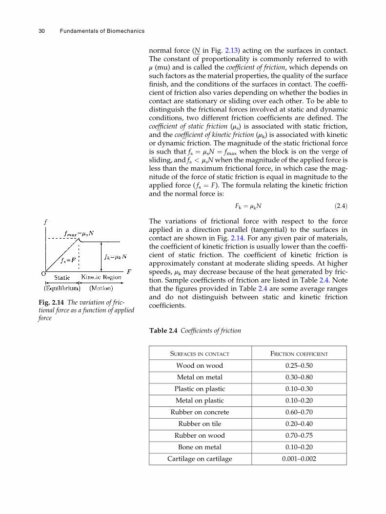
normal force (N in Fig. 2.13) acting on the surfaces in contact.The constant of proportionality is commonly referred to withμ (mu) and is called the coefficient of friction, which depends onsuch factors as the material properties, the quality of the surfacefinish, and the conditions of the surfaces in contact. The coeffi-cient of friction also varies depending on whether the bodies incontact are stationary or sliding over each other. To be able todistinguish the frictional forces involved at static and dynamicconditions, two different friction coefficients are defined. Thecoefficient of static friction (μs) is associated with static friction,and the coefficient of kinetic friction (μk) is associated with kineticor dynamic friction. The magnitude of the static frictional forceis such that fs ¼ μsN ¼ fmax when the block is on the verge ofsliding, and fs < μsNwhen themagnitude of the applied force isless than the maximum frictional force, in which case the mag-nitude of the force of static friction is equal in magnitude to theapplied force ( fs ¼ F). The formula relating the kinetic frictionand the normal force is:
Fk ¼ μkN ð2:4Þ
The variations of frictional force with respect to the forceapplied in a direction parallel (tangential) to the surfaces incontact are shown in Fig. 2.14. For any given pair of materials,the coefficient of kinetic friction is usually lower than the coeffi-cient of static friction. The coefficient of kinetic friction isapproximately constant at moderate sliding speeds. At higherspeeds, μk may decrease because of the heat generated by fric-tion. Sample coefficients of friction are listed in Table 2.4. Notethat the figures provided in Table 2.4 are some average rangesand do not distinguish between static and kinetic frictioncoefficients.Fig. 2.14 The variation of fric-
tional force as a function of appliedforce
Table 2.4 Coefficients of friction
SURFACES IN CONTACT FRICTION COEFFICIENT
Wood on wood 0.25–0.50
Metal on metal 0.30–0.80
Plastic on plastic 0.10–0.30
Metal on plastic 0.10–0.20
Rubber on concrete 0.60–0.70
Rubber on tile 0.20–0.40
Rubber on wood 0.70–0.75
Bone on metal 0.10–0.20
Cartilage on cartilage 0.001–0.002
30 Fundamentals of Biomechanics
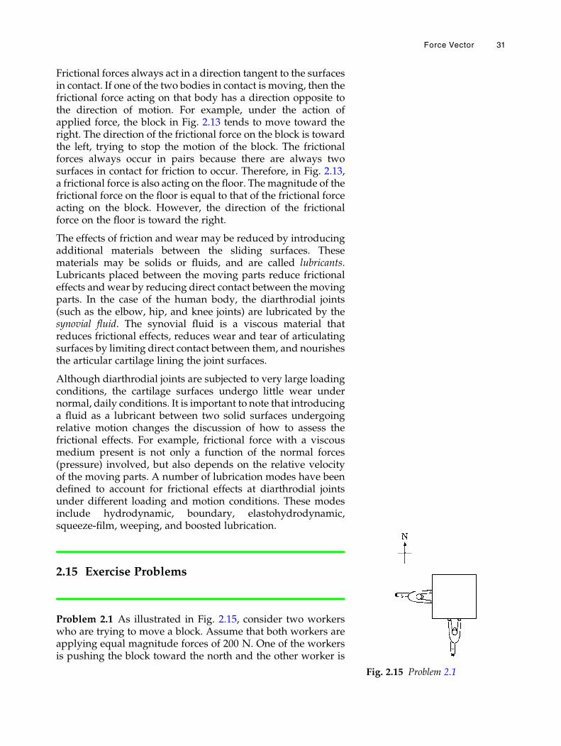
Frictional forces always act in a direction tangent to the surfacesin contact. If one of the two bodies in contact is moving, then thefrictional force acting on that body has a direction opposite tothe direction of motion. For example, under the action ofapplied force, the block in Fig. 2.13 tends to move toward theright. The direction of the frictional force on the block is towardthe left, trying to stop the motion of the block. The frictionalforces always occur in pairs because there are always twosurfaces in contact for friction to occur. Therefore, in Fig. 2.13,a frictional force is also acting on the floor. Themagnitude of thefrictional force on the floor is equal to that of the frictional forceacting on the block. However, the direction of the frictionalforce on the floor is toward the right.
The effects of friction and wear may be reduced by introducingadditional materials between the sliding surfaces. Thesematerials may be solids or fluids, and are called lubricants.Lubricants placed between the moving parts reduce frictionaleffects and wear by reducing direct contact between the movingparts. In the case of the human body, the diarthrodial joints(such as the elbow, hip, and knee joints) are lubricated by thesynovial fluid. The synovial fluid is a viscous material thatreduces frictional effects, reduces wear and tear of articulatingsurfaces by limiting direct contact between them, and nourishesthe articular cartilage lining the joint surfaces.
Although diarthrodial joints are subjected to very large loadingconditions, the cartilage surfaces undergo little wear undernormal, daily conditions. It is important to note that introducinga fluid as a lubricant between two solid surfaces undergoingrelative motion changes the discussion of how to assess thefrictional effects. For example, frictional force with a viscousmedium present is not only a function of the normal forces(pressure) involved, but also depends on the relative velocityof the moving parts. A number of lubrication modes have beendefined to account for frictional effects at diarthrodial jointsunder different loading and motion conditions. These modesinclude hydrodynamic, boundary, elastohydrodynamic,squeeze-film, weeping, and boosted lubrication.
2.15 Exercise Problems
Problem 2.1 As illustrated in Fig. 2.15, consider two workerswho are trying to move a block. Assume that both workers areapplying equal magnitude forces of 200 N. One of the workersis pushing the block toward the north and the other worker is
Fig. 2.15 Problem 2.1
Force Vector 31
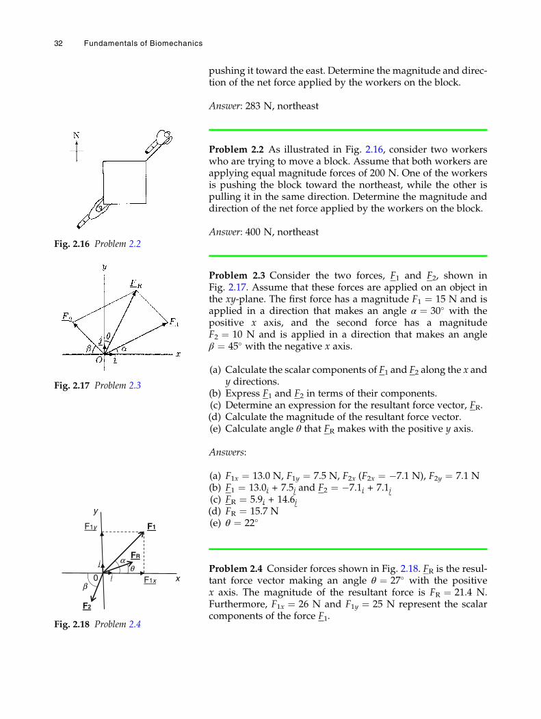
pushing it toward the east. Determine the magnitude and direc-tion of the net force applied by the workers on the block.
Answer: 283 N, northeast
Problem 2.2 As illustrated in Fig. 2.16, consider two workerswho are trying to move a block. Assume that both workers areapplying equal magnitude forces of 200 N. One of the workersis pushing the block toward the northeast, while the other ispulling it in the same direction. Determine the magnitude anddirection of the net force applied by the workers on the block.
Answer: 400 N, northeast
Problem 2.3 Consider the two forces, F1 and F2, shown inFig. 2.17. Assume that these forces are applied on an object inthe xy-plane. The first force has a magnitude F1 ¼ 15 N and isapplied in a direction that makes an angle α ¼ 30� with thepositive x axis, and the second force has a magnitudeF2 ¼ 10 N and is applied in a direction that makes an angleβ ¼ 45� with the negative x axis.
(a) Calculate the scalar components of F1 and F2 along the x andy directions.
(b) Express F1 and F2 in terms of their components.(c) Determine an expression for the resultant force vector, FR.(d) Calculate the magnitude of the resultant force vector.(e) Calculate angle θ that FR makes with the positive y axis.
Answers:
(a) F1x ¼ 13.0 N, F1y ¼ 7.5 N, F2x (F2x ¼ �7.1 N), F2y ¼ 7.1 N(b) F1 ¼ 13.0i + 7.5j and F2 ¼ �7.1i + 7.1j(c) FR ¼ 5.9i + 14.6j(d) FR ¼ 15.7 N(e) θ ¼ 22�
Problem 2.4 Consider forces shown in Fig. 2.18. FR is the resul-tant force vector making an angle θ ¼ 27� with the positivex axis. The magnitude of the resultant force is FR ¼ 21.4 N.Furthermore, F1x ¼ 26 N and F1y ¼ 25 N represent the scalarcomponents of the force F1.
Fig. 2.16 Problem 2.2
Fig. 2.17 Problem 2.3
F1y
xb
aq
y
0
F1
FR
F1x
j
i
F2
Fig. 2.18 Problem 2.4
32 Fundamentals of Biomechanics
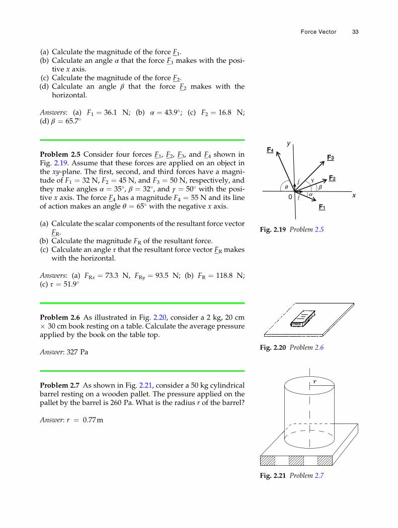
(a) Calculate the magnitude of the force F1.(b) Calculate an angle α that the force F1 makes with the posi-
tive x axis.(c) Calculate the magnitude of the force F2.(d) Calculate an angle β that the force F2 makes with the
horizontal.
Answers: (a) F1 ¼ 36.1 N; (b) α ¼ 43.9�; (c) F2 ¼ 16.8 N;(d) β ¼ 65.7�
Problem 2.5 Consider four forces F1, F2, F3, and F4 shown inFig. 2.19. Assume that these forces are applied on an object inthe xy-plane. The first, second, and third forces have a magni-tude of F1 ¼ 32 N, F2 ¼ 45 N, and F3 ¼ 50 N, respectively, andthey make angles α ¼ 35�, β ¼ 32�, and γ ¼ 50� with the posi-tive x axis. The force F4 has a magnitude F4 ¼ 55 N and its lineof action makes an angle θ ¼ 65� with the negative x axis.
(a) Calculate the scalar components of the resultant force vectorFR.
(b) Calculate the magnitude FR of the resultant force.(c) Calculate an angle τ that the resultant force vector FR makes
with the horizontal.
Answers: (a) FRx ¼ 73.3 N, FRy ¼ 93.5 N; (b) FR ¼ 118.8 N;(c) τ ¼ 51.9�
Problem 2.6 As illustrated in Fig. 2.20, consider a 2 kg, 20 cm� 30 cm book resting on a table. Calculate the average pressureapplied by the book on the table top.
Answer: 327 Pa
Problem 2.7 As shown in Fig. 2.21, consider a 50 kg cylindricalbarrel resting on a wooden pallet. The pressure applied on thepallet by the barrel is 260 Pa. What is the radius r of the barrel?
Answer: r ¼ 0:77m
aq b
y
x0
F3
j
i
F4
F1
F2
Fig. 2.19 Problem 2.5
Fig. 2.20 Problem 2.6
Fig. 2.21 Problem 2.7
Force Vector 33
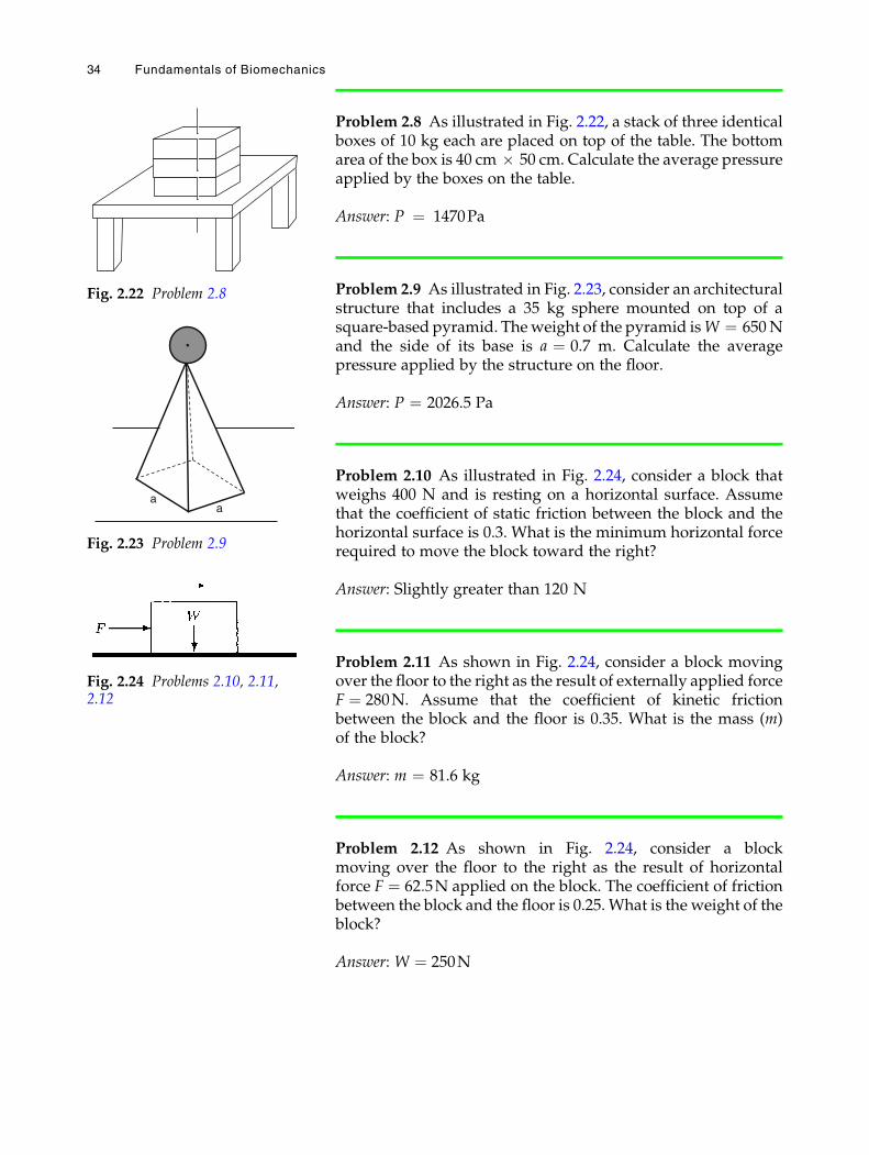
Problem 2.8 As illustrated in Fig. 2.22, a stack of three identicalboxes of 10 kg each are placed on top of the table. The bottomarea of the box is 40 cm � 50 cm. Calculate the average pressureapplied by the boxes on the table.
Answer: P ¼ 1470Pa
Problem 2.9 As illustrated in Fig. 2.23, consider an architecturalstructure that includes a 35 kg sphere mounted on top of asquare-based pyramid. Theweight of the pyramid isW ¼ 650Nand the side of its base is a ¼ 0.7 m. Calculate the averagepressure applied by the structure on the floor.
Answer: P ¼ 2026.5 Pa
Problem 2.10 As illustrated in Fig. 2.24, consider a block thatweighs 400 N and is resting on a horizontal surface. Assumethat the coefficient of static friction between the block and thehorizontal surface is 0.3. What is the minimum horizontal forcerequired to move the block toward the right?
Answer: Slightly greater than 120 N
Problem 2.11 As shown in Fig. 2.24, consider a block movingover the floor to the right as the result of externally applied forceF ¼ 280N. Assume that the coefficient of kinetic frictionbetween the block and the floor is 0.35. What is the mass (m)of the block?
Answer: m ¼ 81.6 kg
Problem 2.12 As shown in Fig. 2.24, consider a blockmoving over the floor to the right as the result of horizontalforce F ¼ 62:5N applied on the block. The coefficient of frictionbetween the block and the floor is 0.25. What is the weight of theblock?
Answer: W ¼ 250N
Fig. 2.22 Problem 2.8
aa
Fig. 2.23 Problem 2.9
Fig. 2.24 Problems 2.10, 2.11,2.12
34 Fundamentals of Biomechanics
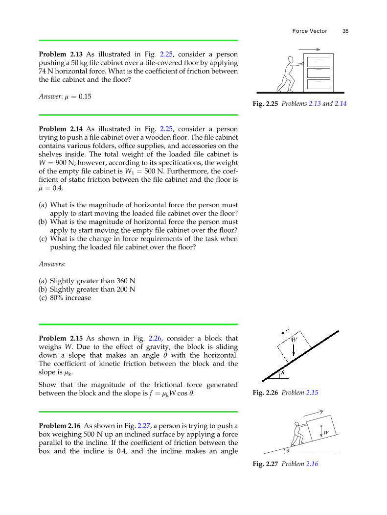
Problem 2.13 As illustrated in Fig. 2.25, consider a personpushing a 50 kg file cabinet over a tile-covered floor by applying74 N horizontal force. What is the coefficient of friction betweenthe file cabinet and the floor?
Answer: μ ¼ 0.15
Problem 2.14 As illustrated in Fig. 2.25, consider a persontrying to push a file cabinet over a wooden floor. The file cabinetcontains various folders, office supplies, and accessories on theshelves inside. The total weight of the loaded file cabinet isW ¼ 900 N; however, according to its specifications, the weightof the empty file cabinet is W1 ¼ 500 N. Furthermore, the coef-ficient of static friction between the file cabinet and the floor isμ ¼ 0.4.
(a) What is the magnitude of horizontal force the person mustapply to start moving the loaded file cabinet over the floor?
(b) What is the magnitude of horizontal force the person mustapply to start moving the empty file cabinet over the floor?
(c) What is the change in force requirements of the task whenpushing the loaded file cabinet over the floor?
Answers:
(a) Slightly greater than 360 N(b) Slightly greater than 200 N(c) 80% increase
Problem 2.15 As shown in Fig. 2.26, consider a block thatweighs W. Due to the effect of gravity, the block is slidingdown a slope that makes an angle θ with the horizontal.The coefficient of kinetic friction between the block and theslope is μk.
Show that the magnitude of the frictional force generatedbetween the block and the slope is f ¼ μkW cos θ.
Problem 2.16 As shown in Fig. 2.27, a person is trying to push abox weighing 500 N up an inclined surface by applying a forceparallel to the incline. If the coefficient of friction between thebox and the incline is 0.4, and the incline makes an angle
Fig. 2.25 Problems 2.13 and 2.14
Fig. 2.26 Problem 2.15
W
Fig. 2.27 Problem 2.16
Force Vector 35
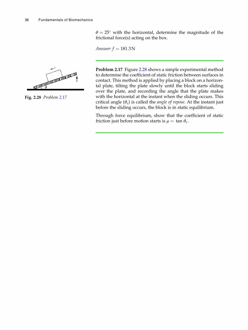
θ ¼ 25� with the horizontal, determine the magnitude of thefrictional force(s) acting on the box.
Answer: f ¼ 181:3N
Problem 2.17 Figure 2.28 shows a simple experimental methodto determine the coefficient of static friction between surfaces incontact. This method is applied by placing a block on a horizon-tal plate, tilting the plate slowly until the block starts slidingover the plate, and recording the angle that the plate makeswith the horizontal at the instant when the sliding occurs. Thiscritical angle (θc) is called the angle of repose. At the instant justbefore the sliding occurs, the block is in static equilibrium.
Through force equilibrium, show that the coefficient of staticfriction just before motion starts is μ ¼ tan θc.
Fig. 2.28 Problem 2.17
36 Fundamentals of Biomechanics
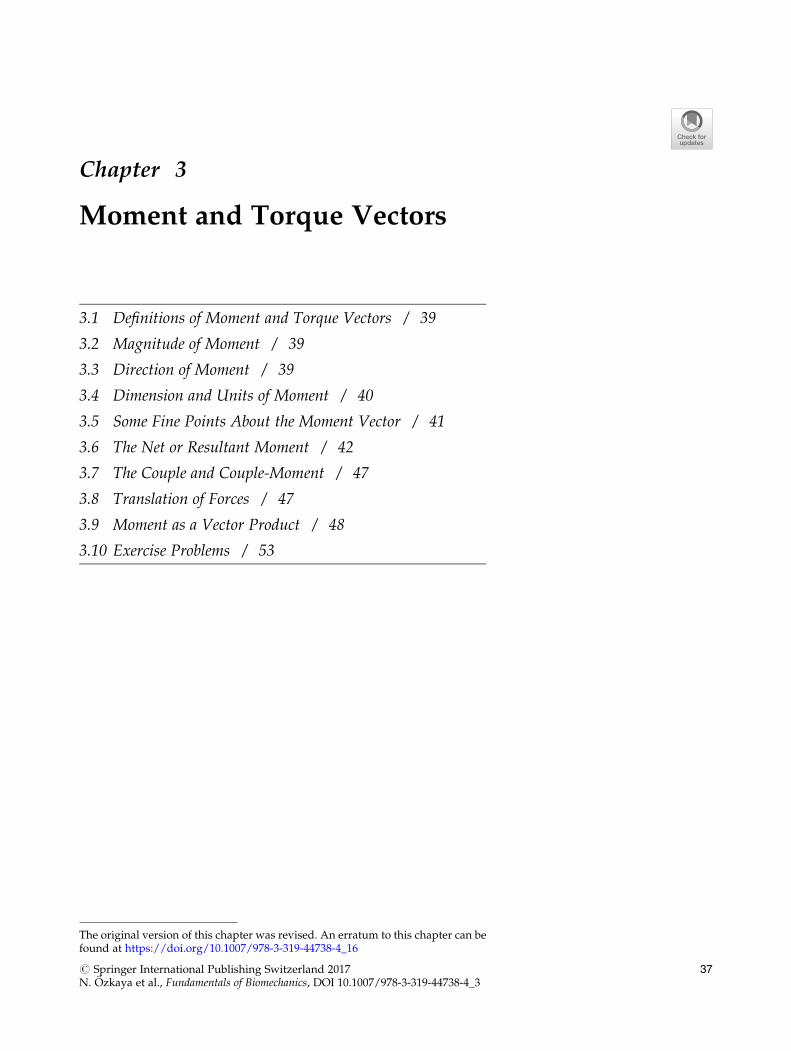
Chapter 3
Moment and Torque Vectors
3.1 Definitions of Moment and Torque Vectors / 39
3.2 Magnitude of Moment / 39
3.3 Direction of Moment / 39
3.4 Dimension and Units of Moment / 40
3.5 Some Fine Points About the Moment Vector / 41
3.6 The Net or Resultant Moment / 42
3.7 The Couple and Couple-Moment / 47
3.8 Translation of Forces / 47
3.9 Moment as a Vector Product / 48
3.10 Exercise Problems / 53
The original version of this chapter was revised. An erratum to this chapter can befound at https://doi.org/10.1007/978-3-319-44738-4_16
# Springer International Publishing Switzerland 2017N. Ozkaya et al., Fundamentals of Biomechanics, DOI 10.1007/978-3-319-44738-4_3
37

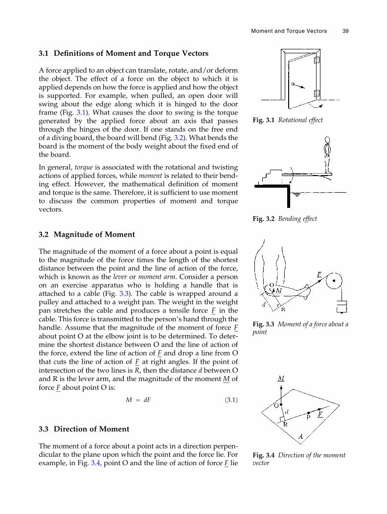
3.1 Definitions of Moment and Torque Vectors
A force applied to an object can translate, rotate, and/or deformthe object. The effect of a force on the object to which it isapplied depends on how the force is applied and how the objectis supported. For example, when pulled, an open door willswing about the edge along which it is hinged to the doorframe (Fig. 3.1). What causes the door to swing is the torquegenerated by the applied force about an axis that passesthrough the hinges of the door. If one stands on the free endof a diving board, the board will bend (Fig. 3.2). What bends theboard is the moment of the body weight about the fixed end ofthe board.
In general, torque is associated with the rotational and twistingactions of applied forces, while moment is related to their bend-ing effect. However, the mathematical definition of momentand torque is the same. Therefore, it is sufficient to use momentto discuss the common properties of moment and torquevectors.
3.2 Magnitude of Moment
The magnitude of the moment of a force about a point is equalto the magnitude of the force times the length of the shortestdistance between the point and the line of action of the force,which is known as the lever or moment arm. Consider a personon an exercise apparatus who is holding a handle that isattached to a cable (Fig. 3.3). The cable is wrapped around apulley and attached to a weight pan. The weight in the weightpan stretches the cable and produces a tensile force F in thecable. This force is transmitted to the person’s hand through thehandle. Assume that the magnitude of the moment of force Fabout point O at the elbow joint is to be determined. To deter-mine the shortest distance between O and the line of action ofthe force, extend the line of action of F and drop a line from Othat cuts the line of action of F at right angles. If the point ofintersection of the two lines is R, then the distance d between Oand R is the lever arm, and the magnitude of the moment M offorce F about point O is:
M ¼ dF ð3:1Þ
3.3 Direction of Moment
The moment of a force about a point acts in a direction perpen-dicular to the plane upon which the point and the force lie. Forexample, in Fig. 3.4, point O and the line of action of force F lie
Fig. 3.1 Rotational effect
Fig. 3.2 Bending effect
Fig. 3.3 Moment of a force about apoint
Fig. 3.4 Direction of the momentvector
Moment and Torque Vectors 39
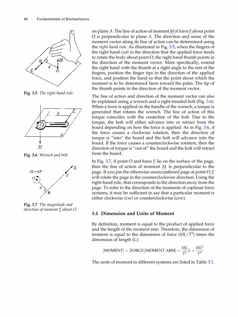
on planeA. The line of action of momentMof forceFabout pointO is perpendicular to plane A. The direction and sense of themoment vector along its line of action can be determined usingthe right-hand rule. As illustrated in Fig. 3.5, when the fingers ofthe right hand curl in the direction that the applied force tendsto rotate the body about point O, the right hand thumb points inthe direction of the moment vector. More specifically, extendthe right hand with the thumb at a right angle to the rest of thefingers, position the finger tips in the direction of the appliedforce, and position the hand so that the point about which themoment is to be determined faces toward the palm. The tip ofthe thumb points in the direction of the moment vector.
The line of action and direction of the moment vector can alsobe explained using a wrench and a right-treaded bolt (Fig. 3.6).When a force is applied on the handle of the wrench, a torque isgenerated that rotates the wrench. The line of action of thistorque coincides with the centerline of the bolt. Due to thetorque, the bolt will either advance into or retract from theboard depending on how the force is applied. As in Fig. 3.6, ifthe force causes a clockwise rotation, then the direction oftorque is “into” the board and the bolt will advance into theboard. If the force causes a counterclockwise rotation, then thedirection of torque is “out of” the board and the bolt will retractfrom the board.
In Fig. 3.7, if point O and force F lie on the surface of the page,then the line of action of moment M is perpendicular to thepage. If you pin the otherwise unencumbered page at point O,Fwill rotate the page in the counterclockwise direction. Using theright-hand rule, that corresponds to the direction away from thepage. To refer to the direction of the moments of coplanar forcesystems, it may be sufficient to say that a particular moment iseither clockwise (cw) or counterclockwise (ccw).
3.4 Dimension and Units of Moment
By definition, moment is equal to the product of applied forceand the length of the moment arm. Therefore, the dimension ofmoment is equal to the dimension of force (ML/T2) times thedimension of length (L):
MOMENT½ � ¼ FORCE½ � MOMENT ARM½ � ¼ ML
T2L ¼ ML2
T2
The units of moment in different systems are listed in Table 3.1.
Fig. 3.5 The right-hand rule
Fig. 3.6 Wrench and bolt
Fig. 3.7 The magnitude anddirection of moment F about O
40 Fundamentals of Biomechanics
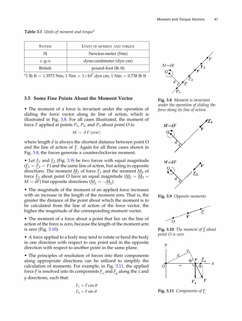
3.5 Some Fine Points About the Moment Vector
• The moment of a force is invariant under the operation ofsliding the force vector along its line of action, which isillustrated in Fig. 3.8. For all cases illustrated, the moment offorce F applied at points P1, P2, and P3 about point O is:
M ¼ d F ccwð Þ
where length d is always the shortest distance between point Oand the line of action of F. Again for all three cases shown inFig. 3.8, the forces generate a counterclockwise moment.
• Let F1 and F2 (Fig. 3.9) be two forces with equal magnitude(F1 ¼ F2 ¼ F) and the same line of action, but acting in oppositedirections. The moment M1 of force F1 and the moment M2 offorce F2 about point O have an equal magnitude (M1 ¼ M2 ¼M ¼ dF) but opposite directions (M1 ¼ �M2).
• The magnitude of the moment of an applied force increaseswith an increase in the length of the moment arm. That is, thegreater the distance of the point about which the moment is tobe calculated from the line of action of the force vector, thehigher the magnitude of the corresponding moment vector.
• The moment of a force about a point that lies on the line ofaction of the force is zero, because the length of the moment armis zero (Fig. 3.10).
• A force applied to a bodymay tend to rotate or bend the bodyin one direction with respect to one point and in the oppositedirection with respect to another point in the same plane.
• The principles of resolution of forces into their componentsalong appropriate directions can be utilized to simplify thecalculation of moments. For example, in Fig. 3.11, the appliedforce F is resolved into its components Fx and Fy along the x and
y directions, such that:
Fx ¼ F cos θ
Fy ¼ F sin θ
Fig. 3.8 Moment is invariantunder the operation of sliding theforce along its line of action
Fig. 3.9 Opposite moments
Fig. 3.10 The moment of F aboutpoint O is zero
Table 3.1 Units of moment and torquea
SYSTEM UNITS OF MOMENT AND TORQUE
SI Newton-meter (Nm)
c–g–s dyne-centimeter (dyn cm)
British pound-foot (lb ft)
a1 lb ft ¼ 1.3573 Nm; 1 Nm ¼ 1�107 dyn cm; 1 Nm ¼ 0.738 lb ft
Fig. 3.11 Components of F
Moment and Torque Vectors 41
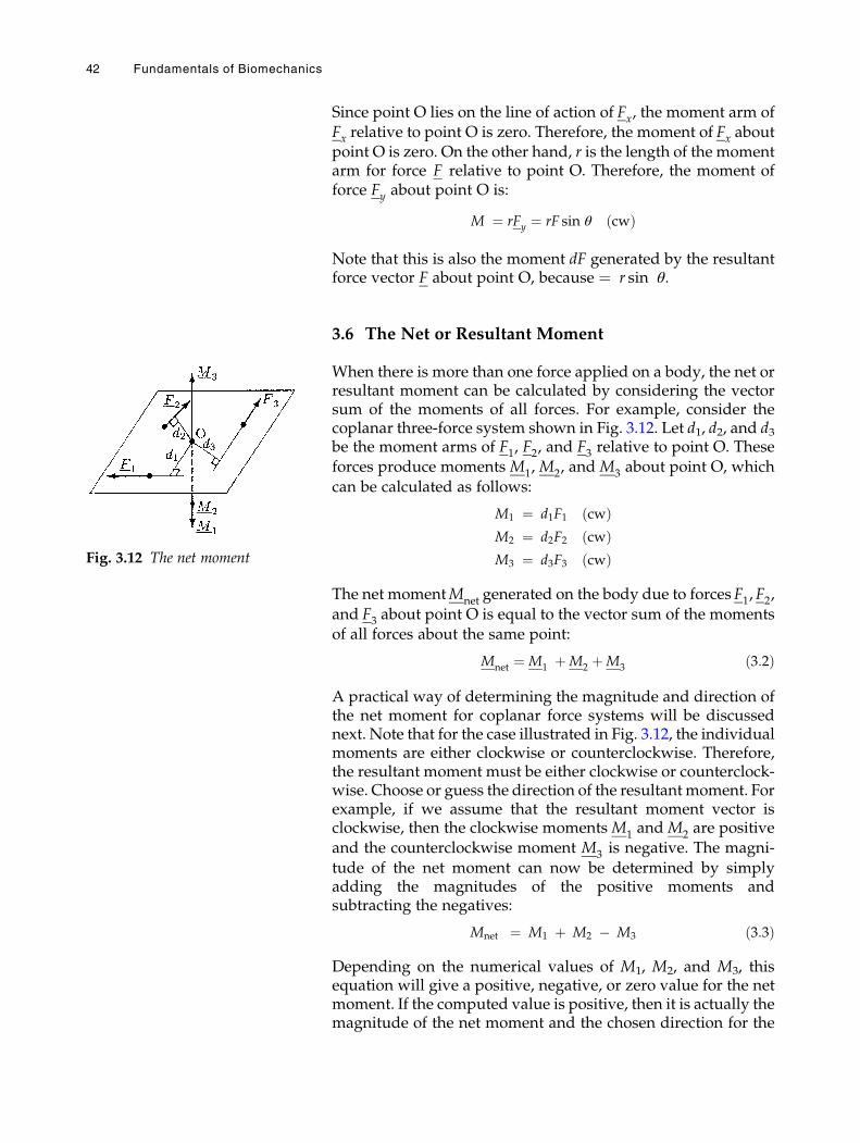
Since point O lies on the line of action of Fx, the moment arm ofFx relative to point O is zero. Therefore, the moment of Fx aboutpoint O is zero. On the other hand, r is the length of the momentarm for force F relative to point O. Therefore, the moment offorce Fy about point O is:
M ¼ rFy ¼ rF sin θ cwð Þ
Note that this is also the moment dF generated by the resultantforce vector F about point O, because ¼ r sin θ.
3.6 The Net or Resultant Moment
When there is more than one force applied on a body, the net orresultant moment can be calculated by considering the vectorsum of the moments of all forces. For example, consider thecoplanar three-force system shown in Fig. 3.12. Let d1, d2, and d3be the moment arms of F1, F2, and F3 relative to point O. Theseforces produce moments M1, M2, and M3 about point O, which
can be calculated as follows:
M1 ¼ d1F1 cwð ÞM2 ¼ d2F2 cwð ÞM3 ¼ d3F3 cwð Þ
The net momentMnet generated on the body due to forces F1, F2,
and F3 about point O is equal to the vector sum of the momentsof all forces about the same point:
Mnet ¼ M1 þM2 þM3 ð3:2Þ
A practical way of determining the magnitude and direction ofthe net moment for coplanar force systems will be discussednext. Note that for the case illustrated in Fig. 3.12, the individualmoments are either clockwise or counterclockwise. Therefore,the resultant moment must be either clockwise or counterclock-wise. Choose or guess the direction of the resultant moment. Forexample, if we assume that the resultant moment vector isclockwise, then the clockwise momentsM1 and M2 are positiveand the counterclockwise moment M3 is negative. The magni-
tude of the net moment can now be determined by simplyadding the magnitudes of the positive moments andsubtracting the negatives:
Mnet ¼ M1 þ M2 � M3 ð3:3Þ
Depending on the numerical values of M1, M2, and M3, thisequation will give a positive, negative, or zero value for the netmoment. If the computed value is positive, then it is actually themagnitude of the net moment and the chosen direction for the
Fig. 3.12 The net moment
42 Fundamentals of Biomechanics
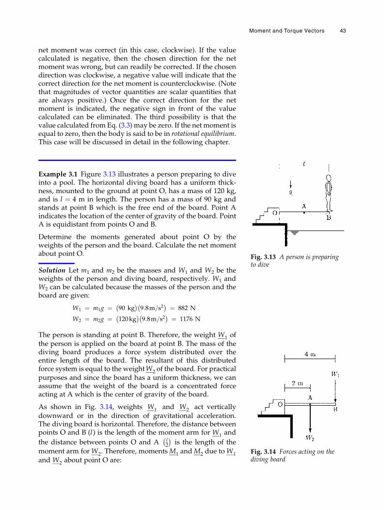
net moment was correct (in this case, clockwise). If the valuecalculated is negative, then the chosen direction for the netmoment was wrong, but can readily be corrected. If the chosendirection was clockwise, a negative value will indicate that thecorrect direction for the net moment is counterclockwise. (Notethat magnitudes of vector quantities are scalar quantities thatare always positive.) Once the correct direction for the netmoment is indicated, the negative sign in front of the valuecalculated can be eliminated. The third possibility is that thevalue calculated from Eq. (3.3) may be zero. If the net moment isequal to zero, then the body is said to be in rotational equilibrium.This case will be discussed in detail in the following chapter.
Example 3.1 Figure 3.13 illustrates a person preparing to diveinto a pool. The horizontal diving board has a uniform thick-ness, mounted to the ground at point O, has a mass of 120 kg,and is l ¼ 4 m in length. The person has a mass of 90 kg andstands at point B which is the free end of the board. Point Aindicates the location of the center of gravity of the board. PointA is equidistant from points O and B.
Determine the moments generated about point O by theweights of the person and the board. Calculate the net momentabout point O.
Solution Let m1 and m2 be the masses and W1 and W2 be theweights of the person and diving board, respectively. W1 andW2 can be calculated because the masses of the person and theboard are given:
W1 ¼ m1g ¼ 90 kg� �
9:8m=s2� � ¼ 882 N
W2 ¼ m2g ¼ 120kg� �
9:8m=s2� � ¼ 1176 N
The person is standing at point B. Therefore, the weight W1 ofthe person is applied on the board at point B. The mass of thediving board produces a force system distributed over theentire length of the board. The resultant of this distributedforce system is equal to the weightW2 of the board. For practicalpurposes and since the board has a uniform thickness, we canassume that the weight of the board is a concentrated forceacting at A which is the center of gravity of the board.
As shown in Fig. 3.14, weights W1 and W2 act verticallydownward or in the direction of gravitational acceleration.The diving board is horizontal. Therefore, the distance betweenpoints O and B (l) is the length of the moment arm for W1 and
the distance between points O and A l2
� �is the length of the
moment arm forW2. Therefore, momentsM1 andM2 due toW1
and W2 about point O are:
Fig. 3.13 A person is preparingto dive
Fig. 3.14 Forces acting on thediving board
Moment and Torque Vectors 43
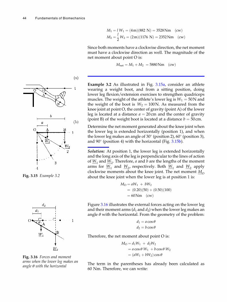
M1 ¼ l W1 ¼ 4mð Þ 882 Nð Þ ¼ 3528Nm cwð ÞM2 ¼ l
2W2 ¼ 2mð Þ 1176 Nð Þ ¼ 2352Nm cwð Þ
Since both moments have a clockwise direction, the net momentmust have a clockwise direction as well. The magnitude of thenet moment about point O is:
Mnet ¼ M1 þM2 ¼ 5880Nm cwð Þ
Example 3.2 As illustrated in Fig. 3.15a, consider an athletewearing a weight boot, and from a sitting position, doinglower leg flexion/extension exercises to strengthen quadricepsmuscles. The weight of the athlete’s lower leg isW1 ¼ 50N andthe weight of the boot is W2 ¼ 100N. As measured from theknee joint at point O, the center of gravity (point A) of the lowerleg is located at a distance a ¼ 20cm and the center of gravity(point B) of the weight boot is located at a distance b ¼ 50cm.
Determine the net moment generated about the knee joint whenthe lower leg is extended horizontally (position 1), and whenthe lower leg makes an angle of 30� (position 2), 60� (position 3),and 90� (position 4) with the horizontal (Fig. 3.15b).
Solution: At position 1, the lower leg is extended horizontallyand the long axis of the leg is perpendicular to the lines of actionofW1 andW2. Therefore, a and b are the lengths of the momentarms for W1 and W2, respectively. Both W1 and W2 applyclockwise moments about the knee joint. The net moment MO
about the knee joint when the lower leg is at position 1 is:
MO ¼ aW1 þ bW2
¼ 0:20ð Þ 50ð Þ þ 0:50ð Þ 100ð Þ¼ 60Nm cwð Þ
Figure 3.16 illustrates the external forces acting on the lower legand their moment arms (d1 and d2) when the lower leg makes anangle θ with the horizontal. From the geometry of the problem:
d1 ¼ a cos θ
d2 ¼ b cos θ
Therefore, the net moment about point O is:
MO ¼ d1W1 þ d2W2
¼ a cos θ W1 þ b cos θ W2
¼ aW1 þ bW2ð Þ cos θ
The term in the parentheses has already been calculated as60 Nm. Therefore, we can write:
Fig. 3.15 Example 3.2
Fig. 3.16 Forces and momentarms when the lower leg makes anangle θ with the horizontal
44 Fundamentals of Biomechanics
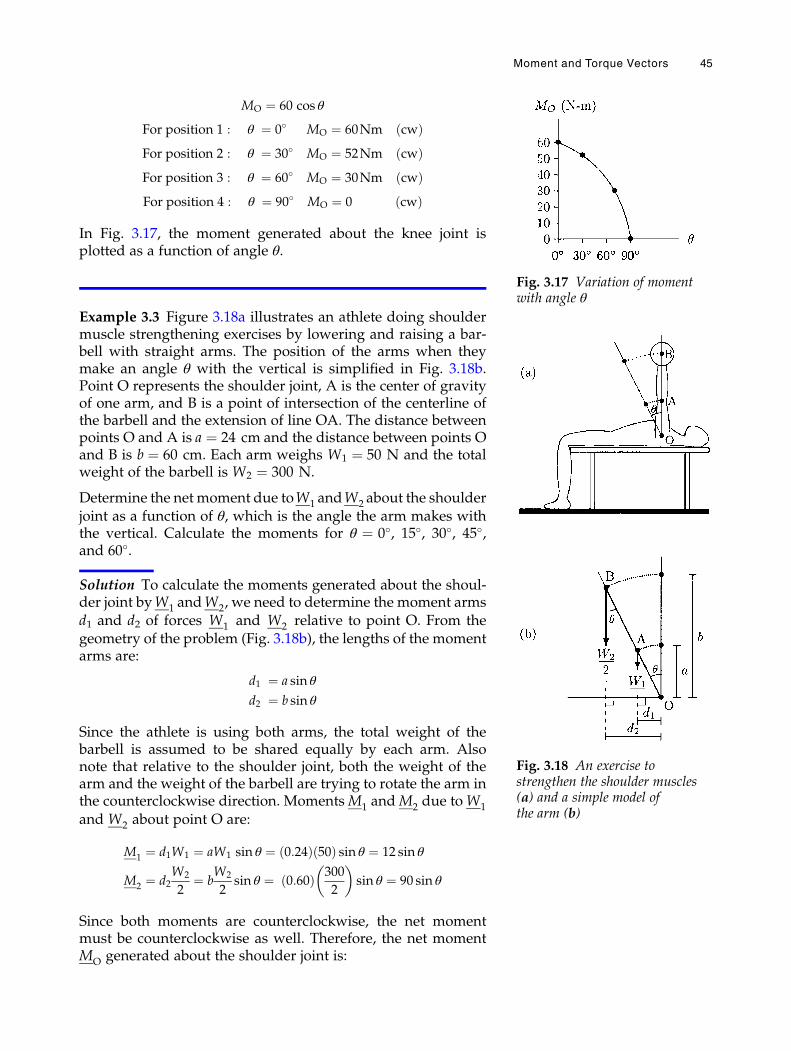
MO ¼ 60 cos θ
For position 1 : θ ¼ 0� MO ¼ 60Nm cwð ÞFor position 2 : θ ¼ 30� MO ¼ 52Nm cwð ÞFor position 3 : θ ¼ 60� MO ¼ 30Nm cwð ÞFor position 4 : θ ¼ 90� MO ¼ 0 cwð Þ
In Fig. 3.17, the moment generated about the knee joint isplotted as a function of angle θ.
Example 3.3 Figure 3.18a illustrates an athlete doing shouldermuscle strengthening exercises by lowering and raising a bar-bell with straight arms. The position of the arms when theymake an angle θ with the vertical is simplified in Fig. 3.18b.Point O represents the shoulder joint, A is the center of gravityof one arm, and B is a point of intersection of the centerline ofthe barbell and the extension of line OA. The distance betweenpoints O and A is a ¼ 24 cm and the distance between points Oand B is b ¼ 60 cm. Each arm weighs W1 ¼ 50 N and the totalweight of the barbell is W2 ¼ 300 N.
Determine the net moment due toW1 andW2 about the shoulderjoint as a function of θ, which is the angle the arm makes withthe vertical. Calculate the moments for θ ¼ 0�, 15�, 30�, 45�,and 60�.
Solution To calculate the moments generated about the shoul-der joint byW1 andW2, we need to determine the moment armsd1 and d2 of forces W1 and W2 relative to point O. From thegeometry of the problem (Fig. 3.18b), the lengths of the momentarms are:
d1 ¼ a sin θ
d2 ¼ b sin θ
Since the athlete is using both arms, the total weight of thebarbell is assumed to be shared equally by each arm. Alsonote that relative to the shoulder joint, both the weight of thearm and the weight of the barbell are trying to rotate the arm inthe counterclockwise direction. MomentsM1 andM2 due toW1
and W2 about point O are:
M1 ¼ d1W1 ¼ aW1 sin θ ¼ 0:24ð Þ 50ð Þ sin θ ¼ 12 sin θ
M2 ¼ d2W2
2¼ b
W2
2sin θ ¼ 0:60ð Þ 300
2
� �sin θ ¼ 90 sin θ
Since both moments are counterclockwise, the net momentmust be counterclockwise as well. Therefore, the net momentMO generated about the shoulder joint is:
Fig. 3.17 Variation of momentwith angle θ
Fig. 3.18 An exercise tostrengthen the shoulder muscles(a) and a simple model ofthe arm (b)
Moment and Torque Vectors 45
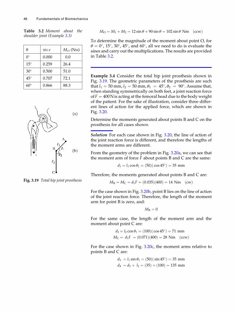
MO ¼ M1 þM2 ¼ 12 sin θ þ 90 sin θ ¼ 102 sin θ Nm ccwð Þ
To determine the magnitude of the moment about point O, forθ ¼ 0�, 15�, 30�, 45�, and 60�, all we need to do is evaluate thesines and carry out the multiplications. The results are providedin Table 3.2.
Example 3.4 Consider the total hip joint prosthesis shown inFig. 3.19. The geometric parameters of the prosthesis are suchthat l1 ¼ 50 mm, l2 ¼ 50 mm, θ1 ¼ 45�, θ2 ¼ 90�. Assume that,when standing symmetrically on both feet, a joint reaction forceofF ¼ 400Nis acting at the femoral head due to the bodyweightof the patient. For the sake of illustration, consider three differ-ent lines of action for the applied force, which are shown inFig. 3.20.
Determine the moments generated about points B and C on theprosthesis for all cases shown.
Solution For each case shown in Fig. 3.20, the line of action ofthe joint reaction force is different, and therefore the lengths ofthe moment arms are different.
From the geometry of the problem in Fig. 3.20a, we can see thatthe moment arm of force F about points B and C are the same:
d1 ¼ l1 cos θ1 ¼ 50ð Þ cos 45�ð Þ ¼ 35 mm
Therefore, the moments generated about points B and C are:
MB ¼ MC ¼ d1F ¼ 0:035ð Þ 400ð Þ ¼ 14 Nm cwð Þ
For the case shown in Fig. 3.20b, point B lies on the line of actionof the joint reaction force. Therefore, the length of the momentarm for point B is zero, and:
MB ¼ 0
For the same case, the length of the moment arm and themoment about point C are:
d2 ¼ l2 cos θ1 ¼ 100ð Þ cos 45�ð Þ ¼ 71 mm
MC ¼ d1F ¼ 0:071ð Þ 400ð Þ ¼ 28 Nm ccwð Þ
For the case shown in Fig. 3.20c, the moment arms relative topoints B and C are:
d3 ¼ l1 sin θ1 ¼ 50ð Þ sin 45�ð Þ ¼ 35 mm
d4 ¼ d3 þ l2 ¼ 35ð Þ þ 100ð Þ ¼ 135 mm
Table 3.2 Moment about theshoulder joint (Example 3.3)
θ SIN θ MO (NM)
0� 0.000 0.0
15� 0.259 26.4
30� 0.500 51.0
45� 0.707 72.1
60� 0.866 88.3
Fig. 3.19 Total hip joint prosthesis
46 Fundamentals of Biomechanics
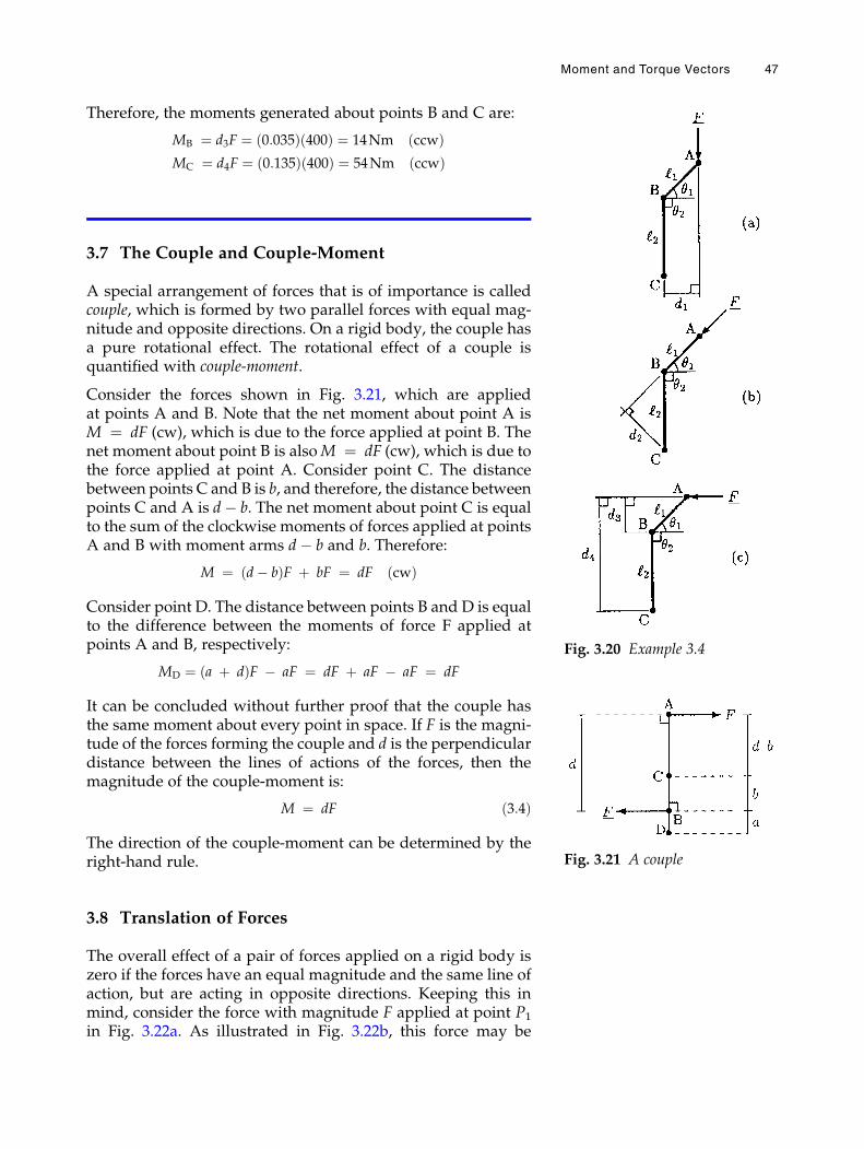
Therefore, the moments generated about points B and C are:
MB ¼ d3F ¼ 0:035ð Þ 400ð Þ ¼ 14Nm ccwð ÞMC ¼ d4F ¼ 0:135ð Þ 400ð Þ ¼ 54Nm ccwð Þ
3.7 The Couple and Couple-Moment
A special arrangement of forces that is of importance is calledcouple, which is formed by two parallel forces with equal mag-nitude and opposite directions. On a rigid body, the couple hasa pure rotational effect. The rotational effect of a couple isquantified with couple-moment.
Consider the forces shown in Fig. 3.21, which are appliedat points A and B. Note that the net moment about point A isM ¼ dF (cw), which is due to the force applied at point B. Thenet moment about point B is alsoM ¼ dF (cw), which is due tothe force applied at point A. Consider point C. The distancebetween points C and B is b, and therefore, the distance betweenpoints C and A is d� b. The net moment about point C is equalto the sum of the clockwise moments of forces applied at pointsA and B with moment arms d� b and b. Therefore:
M ¼ d� bð ÞF þ bF ¼ dF cwð Þ
Consider point D. The distance between points B and D is equalto the difference between the moments of force F applied atpoints A and B, respectively:
MD ¼ a þ dð ÞF � aF ¼ dF þ aF � aF ¼ dF
It can be concluded without further proof that the couple hasthe same moment about every point in space. If F is the magni-tude of the forces forming the couple and d is the perpendiculardistance between the lines of actions of the forces, then themagnitude of the couple-moment is:
M ¼ dF ð3:4Þ
The direction of the couple-moment can be determined by theright-hand rule.
3.8 Translation of Forces
The overall effect of a pair of forces applied on a rigid body iszero if the forces have an equal magnitude and the same line ofaction, but are acting in opposite directions. Keeping this inmind, consider the force with magnitude F applied at point P1
in Fig. 3.22a. As illustrated in Fig. 3.22b, this force may be
Fig. 3.20 Example 3.4
Fig. 3.21 A couple
Moment and Torque Vectors 47
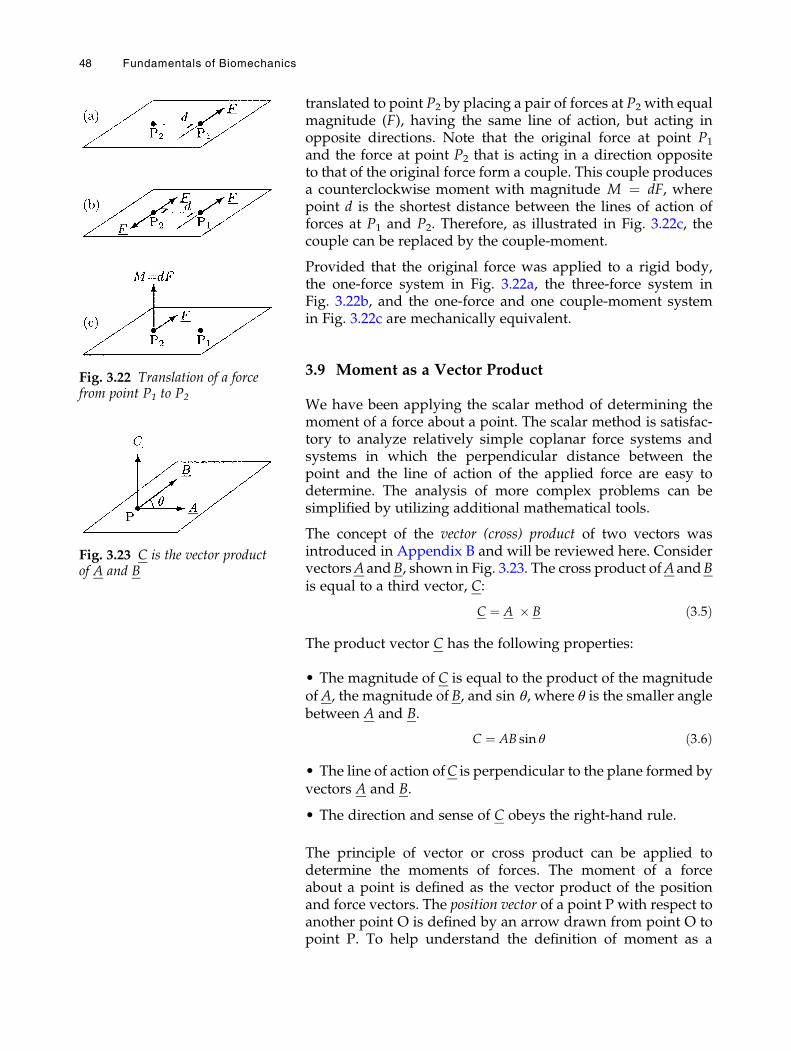
translated to point P2 by placing a pair of forces at P2 with equalmagnitude (F), having the same line of action, but acting inopposite directions. Note that the original force at point P1
and the force at point P2 that is acting in a direction oppositeto that of the original force form a couple. This couple producesa counterclockwise moment with magnitude M ¼ dF, wherepoint d is the shortest distance between the lines of action offorces at P1 and P2. Therefore, as illustrated in Fig. 3.22c, thecouple can be replaced by the couple-moment.
Provided that the original force was applied to a rigid body,the one-force system in Fig. 3.22a, the three-force system inFig. 3.22b, and the one-force and one couple-moment systemin Fig. 3.22c are mechanically equivalent.
3.9 Moment as a Vector Product
We have been applying the scalar method of determining themoment of a force about a point. The scalar method is satisfac-tory to analyze relatively simple coplanar force systems andsystems in which the perpendicular distance between thepoint and the line of action of the applied force are easy todetermine. The analysis of more complex problems can besimplified by utilizing additional mathematical tools.
The concept of the vector (cross) product of two vectors wasintroduced in Appendix B and will be reviewed here. ConsidervectorsA andB, shown in Fig. 3.23. The cross product ofA andBis equal to a third vector, C:
C ¼ A � B ð3:5Þ
The product vector C has the following properties:
• The magnitude of C is equal to the product of the magnitudeofA, the magnitude of B, and sin θ, where θ is the smaller anglebetween A and B.
C ¼ AB sin θ ð3:6Þ
• The line of action ofC is perpendicular to the plane formed byvectors A and B.
• The direction and sense of C obeys the right-hand rule.
The principle of vector or cross product can be applied todetermine the moments of forces. The moment of a forceabout a point is defined as the vector product of the positionand force vectors. The position vector of a point P with respect toanother point O is defined by an arrow drawn from point O topoint P. To help understand the definition of moment as a
Fig. 3.22 Translation of a forcefrom point P1 to P2
Fig. 3.23 C is the vector productof A and B
48 Fundamentals of Biomechanics

vector product, consider Fig. 3.24. Force F acts in the xy-planeand has a point of application at point P. Force F can beexpressed in terms of its components Fx and Fy along thex and y directions:
F ¼ Fxiþ Fyj ð3:7Þ
The position vector of point P with respect to point O isrepresented by vector r, which can be written in terms of itscomponents:
r ¼ rxiþ ryj ð3:8Þ
The components rx and ry of the position vector are simply thex and y coordinates of point P as measured from point O.
The moment of force F about point O is equal to the vectorproduct of the position vector r and force vector F:
M ¼ r� F ð3:9Þ
Using Eqs. (3.7) and (3.8), Eq. (3.9) can alternatively bewritten as:
M¼ rxiþ ryj� �
� Fxiþ Fyj� �
¼ rxFx i� i� �þ ryFy i� j
� �þ ryFx j� i
� �þ ryFy j� j
� � ð3:10Þ
Recall that i� j ¼ j� j ¼ 0 since the angle that a unit vector
makes with itself is zero, and sin 0� ¼ 0. i� j ¼ k because the
angle between the positive x axis and the positive y axis is 90�
ð sin 90� ¼ 1Þ. On the other hand, j� i ¼ �k. For the last two
cases, the product is either in the positive z (counterclockwise orout of the page) or negative z (clockwise or into the page)direction. z and unit vector k designate the direction perpen-dicular to the xy-plane (Fig. 3.25). Now, Eq. (3.10) can besimplified as:
M ¼ rxFy � ryFx� �
k ð3:11Þ
To show that the definition of moment as the vector product ofthe position and force vectors is consistent with the scalarmethod of finding the moment, consider the simple caseillustrated in Fig. 3.26. The force vectorF is acting in the positivey direction and its line of action is d distance away from pointO. Applying the scalar method, the moment about point O is:
M ¼ dF cwwð Þ ð3:12Þ
Fig. 3.24 The moment about O isM ¼ r � F
Fig. 3.25 The right-hand ruleapplies to Cartesian coordinatedirections as well
Fig. 3.26 M ¼ dF (ccw)
Moment and Torque Vectors 49
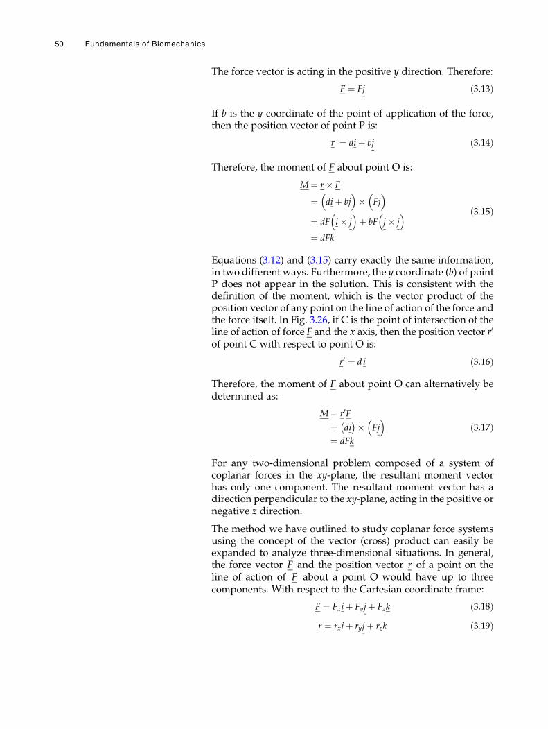
The force vector is acting in the positive y direction. Therefore:
F ¼ Fj ð3:13Þ
If b is the y coordinate of the point of application of the force,then the position vector of point P is:
r ¼ diþ bj ð3:14Þ
Therefore, the moment of F about point O is:
M¼ r� F
¼ diþ bj� �
� Fj� �
¼ dF i� j� �
þ bF j� j� �
¼ dFk
ð3:15Þ
Equations (3.12) and (3.15) carry exactly the same information,in two different ways. Furthermore, the y coordinate (b) of pointP does not appear in the solution. This is consistent with thedefinition of the moment, which is the vector product of theposition vector of any point on the line of action of the force andthe force itself. In Fig. 3.26, if C is the point of intersection of theline of action of force F and the x axis, then the position vector r0
of point C with respect to point O is:
r0 ¼ d i ð3:16Þ
Therefore, the moment of F about point O can alternatively bedetermined as:
M¼ r0F
¼ di� �� Fj
� �¼ dFk
ð3:17Þ
For any two-dimensional problem composed of a system ofcoplanar forces in the xy-plane, the resultant moment vectorhas only one component. The resultant moment vector has adirection perpendicular to the xy-plane, acting in the positive ornegative z direction.
The method we have outlined to study coplanar force systemsusing the concept of the vector (cross) product can easily beexpanded to analyze three-dimensional situations. In general,the force vector F and the position vector r of a point on theline of action of F about a point O would have up to threecomponents. With respect to the Cartesian coordinate frame:
F ¼ Fxiþ Fyjþ Fzk ð3:18Þr ¼ rxiþ ryjþ rzk ð3:19Þ
50 Fundamentals of Biomechanics
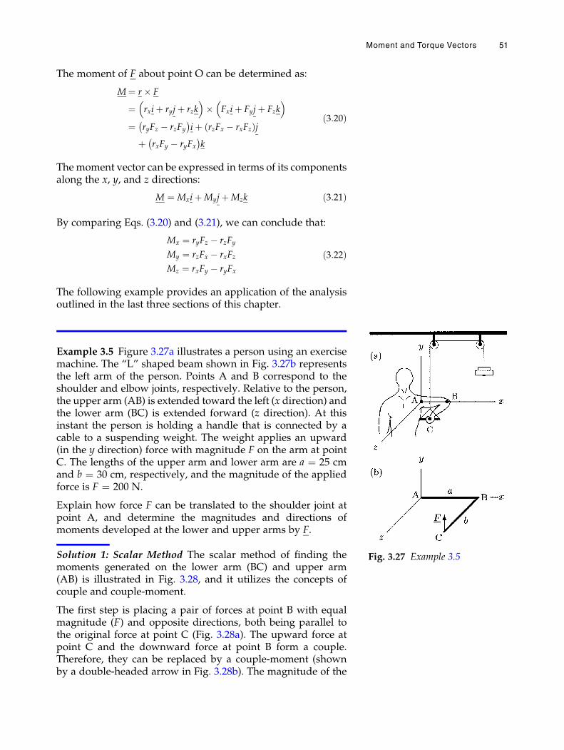
The moment of F about point O can be determined as:
M¼ r� F
¼ rxiþ ryjþ rzk� �
� Fxiþ Fyjþ Fzk� �
¼ ryFz � rzFy� �
iþ rzFx � rxFzð Þjþ rxFy � ryFx� �
k
ð3:20Þ
Themoment vector can be expressed in terms of its componentsalong the x, y, and z directions:
M ¼ MxiþMyjþMzk ð3:21Þ
By comparing Eqs. (3.20) and (3.21), we can conclude that:
Mx ¼ ryFz � rzFy
My ¼ rzFx � rxFz
Mz ¼ rxFy � ryFx
ð3:22Þ
The following example provides an application of the analysisoutlined in the last three sections of this chapter.
Example 3.5 Figure 3.27a illustrates a person using an exercisemachine. The “L” shaped beam shown in Fig. 3.27b representsthe left arm of the person. Points A and B correspond to theshoulder and elbow joints, respectively. Relative to the person,the upper arm (AB) is extended toward the left (x direction) andthe lower arm (BC) is extended forward (z direction). At thisinstant the person is holding a handle that is connected by acable to a suspending weight. The weight applies an upward(in the y direction) force with magnitude F on the arm at pointC. The lengths of the upper arm and lower arm are a ¼ 25 cmand b ¼ 30 cm, respectively, and the magnitude of the appliedforce is F ¼ 200 N.
Explain how force F can be translated to the shoulder joint atpoint A, and determine the magnitudes and directions ofmoments developed at the lower and upper arms by F.
Solution 1: Scalar Method The scalar method of finding themoments generated on the lower arm (BC) and upper arm(AB) is illustrated in Fig. 3.28, and it utilizes the concepts ofcouple and couple-moment.
The first step is placing a pair of forces at point B with equalmagnitude (F) and opposite directions, both being parallel tothe original force at point C (Fig. 3.28a). The upward force atpoint C and the downward force at point B form a couple.Therefore, they can be replaced by a couple-moment (shownby a double-headed arrow in Fig. 3.28b). The magnitude of the
Fig. 3.27 Example 3.5
Moment and Torque Vectors 51
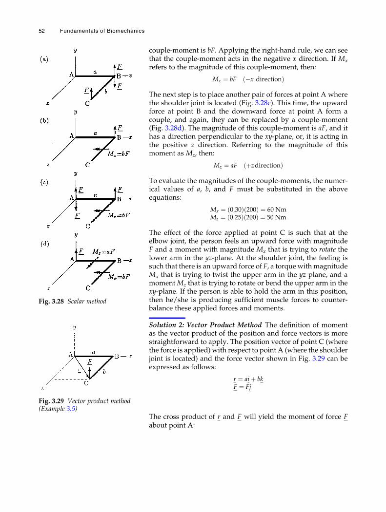
couple-moment is bF. Applying the right-hand rule, we can seethat the couple-moment acts in the negative x direction. If Mx
refers to the magnitude of this couple-moment, then:
Mx ¼ bF �x directionð Þ
The next step is to place another pair of forces at point A wherethe shoulder joint is located (Fig. 3.28c). This time, the upwardforce at point B and the downward force at point A form acouple, and again, they can be replaced by a couple-moment(Fig. 3.28d). The magnitude of this couple-moment is aF, and ithas a direction perpendicular to the xy-plane, or, it is acting inthe positive z direction. Referring to the magnitude of thismoment as Mz, then:
Mz ¼ aF þzdirectionð Þ
To evaluate the magnitudes of the couple-moments, the numer-ical values of a, b, and F must be substituted in the aboveequations:
Mx ¼ 0:30ð Þ 200ð Þ ¼ 60 NmMz ¼ 0:25ð Þ 200ð Þ ¼ 50 Nm
The effect of the force applied at point C is such that at theelbow joint, the person feels an upward force with magnitudeF and a moment with magnitude Mx that is trying to rotate thelower arm in the yz-plane. At the shoulder joint, the feeling issuch that there is an upward force of F, a torquewithmagnitudeMx that is trying to twist the upper arm in the yz-plane, and amomentMz that is trying to rotate or bend the upper arm in thexy-plane. If the person is able to hold the arm in this position,then he/she is producing sufficient muscle forces to counter-balance these applied forces and moments.
Solution 2: Vector Product Method The definition of momentas the vector product of the position and force vectors is morestraightforward to apply. The position vector of point C (wherethe force is applied) with respect to point A (where the shoulderjoint is located) and the force vector shown in Fig. 3.29 can beexpressed as follows:
r ¼ aiþ bkF ¼ Fj
The cross product of r and F will yield the moment of force Fabout point A:
Fig. 3.28 Scalar method
Fig. 3.29 Vector product method(Example 3.5)
52 Fundamentals of Biomechanics
M¼ r� F
¼ aiþ bk� �� Fj
� �
¼ aF i� j� �
þ bF k� j� �
¼ aFk� bFi
¼ 0:25ð Þ 200ð Þk� 0:30ð Þ 200ð Þi¼ 50k� 60i
The negative sign in front of 60 i indicates that the x componentof the moment vector is acting in the negative x direction.Furthermore, there is no component associated with the unitvector j, which implies that the y component of the moment
vector is zero. Therefore, the moment about point A has thefollowing components:
Mx ¼ 60 Nm �x directionð ÞMy ¼ 0
Mz ¼ 50 Nm þz directionð Þ
These results are consistent with those obtained using the scalarmethod.
3.10 Exercise Problems
Problem 3.1 As illustrated in Fig. 3.6, assume a worker isapplying a force F to tighten a right-treaded bolt by using awrench. As the result of the applied force the bolt is advancinginto the metal plate. The recommended torque for the bolt isMrec 80 Nm. Furthermore, the length of the wrench handle isd ¼ 25 cm.
(a) Calculate the magnitude of the force requited to completethe task.
(b) How can the task be modified to decrease its forcerequirements by 50%?
Answers: (a) F ¼ 320 N; (b) by increasing the length of thewrench handle (d ¼ 50 cm)
Problem 3.2 As illustrated in Fig. 3.13, consider a diver of 88 kgmass standing on the free end of a horizontal diving board atpoint B, preparing for a jump. The diving board has a uniform
Moment and Torque Vectors 53
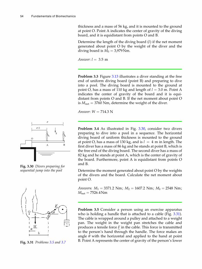
thickness and a mass of 56 kg, and it is mounted to the groundat point O. Point A indicates the center of gravity of the divingboard, and it is equidistant from points O and B.
Determine the length of the diving board (l) if the net momentgenerated about point O by the weight of the diver and thediving board is M0 ¼ 3,979Nm.
Answer: l ¼ 3:5 m
Problem 3.3 Figure 3.13 illustrates a diver standing at the freeend of uniform diving board (point B) and preparing to diveinto a pool. The diving board is mounted to the ground atpoint O, has a mass of 110 kg and length of l ¼ 3.0 m. Point Aindicates the center of gravity of the board and it is equi-distant from points O and B. If the net moment about point Ois Mnet ¼ 3760 Nm, determine the weight of the diver.
Answer: W ¼ 714.3 N
Problem 3.4 As illustrated in Fig. 3.30, consider two diverspreparing to dive into a pool in a sequence. The horizontaldiving board of uniform thickness is mounted to the groundat point O, has a mass of 130 kg, and is l ¼ 4 m in length. Thefirst diver has a mass of 86 kg and he stands at point B, which isthe free end of the diving board. The second diver has a mass of82 kg and he stands at point A, which is the center of gravity ofthe board. Furthermore, point A is equidistant from points Oand B.
Determine the moment generated about point O by the weightsof the divers and the board. Calculate the net moment aboutpoint O.
Answers: M1 ¼ 3371:2 Nm; M2 ¼ 1607:2 Nm; Mb ¼ 2548 Nm;Mnet ¼ 7526:4Nm
Problem 3.5 Consider a person using an exercise apparatuswho is holding a handle that is attached to a cable (Fig. 3.31).The cable is wrapped around a pulley and attached to a weightpan. The weight in the weight pan stretches the cable andproduces a tensile force F in the cable. This force is transmittedto the person’s hand through the handle. The force makes anangle θ with the horizontal and applied to the hand at pointB. Point A represents the center of gravity of the person’s lower
A
O
B
/2
g
Fig. 3.30 Divers preparing forsequential jump into the pool
Fig. 3.31 Problems 3.5 and 3.7
54 Fundamentals of Biomechanics
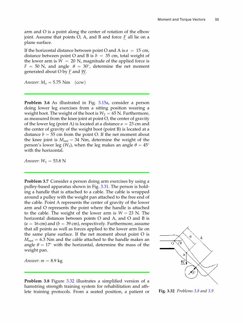
arm and O is a point along the center of rotation of the elbowjoint. Assume that points O, A, and B and force F all lie on aplane surface.
If the horizontal distance between point O and A is a ¼ 15 cm,distance between point O and B is b ¼ 35 cm, total weight ofthe lower arm is W ¼ 20 N, magnitude of the applied force isF ¼ 50 N, and angle θ ¼ 30�, determine the net momentgenerated about O by F and W.
Answer: Mo ¼ 5:75 Nm ccwð Þ
Problem 3.6 As illustrated in Fig. 3.15a, consider a persondoing lower leg exercises from a sitting position wearing aweight boot. The weight of the boot isW2 ¼ 65 N. Furthermore,as measured from the knee joint at point O, the center of gravityof the lower leg (point A) is located at a distance a ¼ 23 cm andthe center of gravity of the weight boot (point B) is located at adistance b ¼ 55 cm from the point O. If the net moment aboutthe knee joint is Mnet ¼ 34 Nm, determine the weight of theperson’s lower leg (W1), when the leg makes an angle θ ¼ 45�
with the horizontal.
Answer: W1 ¼ 53.8 N
Problem 3.7 Consider a person doing arm exercises by using apulley-based apparatus shown in Fig. 3.31. The person is hold-ing a handle that is attached to a cable. The cable is wrappedaround a pulley with the weight pan attached to the free end ofthe cable. Point A represents the center of gravity of the lowerarm and O represents the point where the handle is attachedto the cable. The weight of the lower arm is W ¼ 23 N. Thehorizontal distances between points O and A, and O and B is(a ¼ 16 cm) and (b ¼ 39 cm), respectively. Furthermore, assumethat all points as well as forces applied to the lower arm lie onthe same plane surface. If the net moment about point O isMnet ¼ 6.3 Nm and the cable attached to the handle makes anangle θ ¼ 17� with the horizontal, determine the mass of theweight pan.
Answer: m ¼ 8.9 kg
Problem 3.8 Figure 3.32 illustrates a simplified version of ahamstring strength training system for rehabilitation and ath-lete training protocols. From a seated position, a patient or Fig. 3.32 Problems 3.8 and 3.9
Moment and Torque Vectors 55

athlete flexes the lower leg against a set resistance providedthrough a cylindrical pad that is attached to a load. For theposition illustrated, the lower leg makes an angle θ with thehorizontal. Point O represents the knee joint, point A is the centerof gravity of the lower leg,W is the total weight of the lower leg,F is the magnitude of the force applied by the pad on the lowerleg in a direction perpendicular to the long axis of the lower leg,a is the distance between points O and A, and b is the distancebetween point O and the line of action of F measured along thelong axis of the lower leg.
(a) Determine an expression for the net moment about O due toforces W and F.
(b) If a ¼ 20 cm, b ¼ 40 cm, θ ¼ 30�, W ¼ 60 N, andF ¼ 200 N, calculate the net moment about O.
Answers: (a) MO ¼ bF � aW cos θ (b) MO ¼ 69:6 Nm ccwð Þ
Problem 3.9 As illustrated in Fig. 3.32, consider an athleteperforming lower leg exercises from a seated position tostrengthen hamstring muscles by using a special training sys-tem. The training system provides a set resistance to the legthrough a cylindrical pad attached to the load while leg flexing.Point O represents the knee joint, point A is the center of gravityof the lower leg, W is the weight of the lower leg, θ defines anangle that the long axis of the lower leg makes with the hori-zontal, and MO is the net moment about point O by forcesapplied to the leg.
(a) If a ¼ 0.23 m, b ¼ 0.45 m, θ ¼ 45�, W ¼ 65 N, and MO
¼ 86.14 Nm, determine the magnitude of the set resistance(F).
(b) Considering the same position of the lower leg, calculate thenet moment about point O when the set resistance isincreased by 10 N.
Answer: (a) F ¼ 215 N; (b) MO ¼ 90.64 Nm
Problem 3.10 As illustrated in Fig. 3.33, consider an athleteperforming flexion/extension exercises of the lower arm tostrengthen the biceps muscles. The athlete is holding the weightofW1 ¼ 150 N in his hand, and the weight of his lower arm isW2 ¼ 20 N. As measured from the elbow joint at point O, thecenter of gravity of the lower arm (point A) is located at adistance a ¼ 7:5 cm and the center of gravity of the weightheld in the hand is located at a distance b ¼ 32 cm.
AO
a
b
w2 w1
B
Fig. 3.33 An athlete performinglower arm exercises
56 Fundamentals of Biomechanics
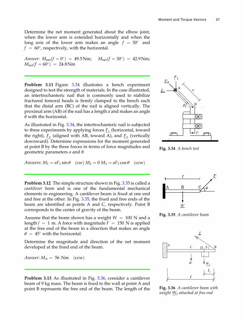
Determine the net moment generated about the elbow joint,when the lower arm is extended horizontally and when thelong axis of the lower arm makes an angle f ¼ 30� andf ¼ 60�, respectively, with the horizontal.
Answer: Mnet f ¼ 0�ð Þ ¼ 49:5Nm; Mnet f ¼ 30�ð Þ ¼ 42:9Nm;Mnet f ¼ 60�ð Þ ¼ 24:8Nm
Problem 3.11 Figure 3.34 illustrates a bench experimentdesigned to test the strength of materials. In the case illustrated,an intertrochanteric nail that is commonly used to stabilizefractured femoral heads is firmly clamped to the bench suchthat the distal arm (BC) of the nail is aligned vertically. Theproximal arm (AB) of the nail has a length a andmakes an angleθ with the horizontal.
As illustrated in Fig. 3.34, the intertrochanteric nail is subjectedto three experiments by applying forces F1 (horizontal, towardthe right), F2 (aligned with AB, toward A), and F3 (verticallydownward). Determine expressions for the moment generatedat point B by the three forces in terms of force magnitudes andgeometric parameters a and θ.
Answers: M1 ¼ aF1 sin θ cwð Þ M2 ¼ 0 M3 ¼ aF3 cos θ ccwð Þ
Problem 3.12 The simple structure shown in Fig. 3.35 is called acantilever beam and is one of the fundamental mechanicalelements in engineering. A cantilever beam is fixed at one endand free at the other. In Fig. 3.35, the fixed and free ends of thebeam are identified as points A and C, respectively. Point Bcorresponds to the center of gravity of the beam.
Assume that the beam shown has a weight W ¼ 100 N and alength l ¼ 1 m. A force with magnitude F ¼ 150 N is appliedat the free end of the beam in a direction that makes an angleθ ¼ 45� with the horizontal.
Determine the magnitude and direction of the net momentdeveloped at the fixed end of the beam.
Answer: MA ¼ 56 Nm ccwð Þ
Problem 3.13 As illustrated in Fig. 3.36, consider a cantileverbeam of 9 kg mass. The beam is fixed to the wall at point A andpoint B represents the free end of the beam. The length of the
Fig. 3.34 A bench test
Fig. 3.35 A cantilever beam
W W1
A C D Bβ
F
Fig. 3.36 A cantilever beam withweight W1 attached at free end
Moment and Torque Vectors 57
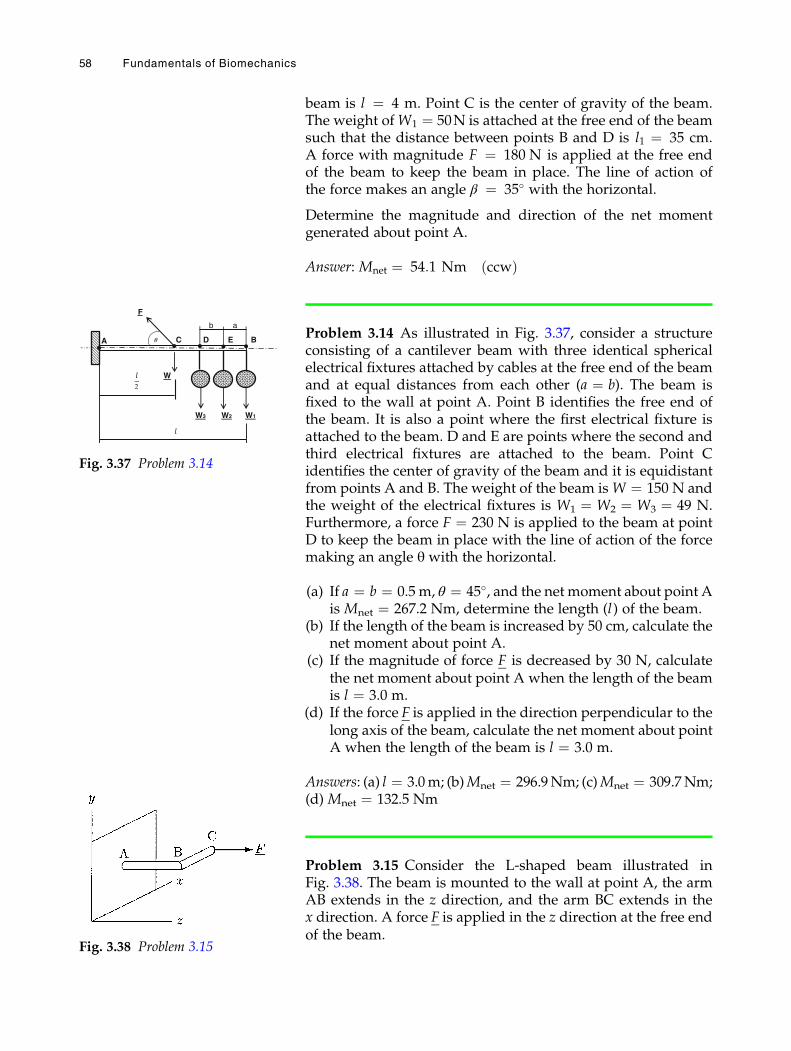
beam is l ¼ 4 m. Point C is the center of gravity of the beam.The weight ofW1 ¼ 50N is attached at the free end of the beamsuch that the distance between points B and D is l1 ¼ 35 cm.A force with magnitude F ¼ 180 N is applied at the free endof the beam to keep the beam in place. The line of action ofthe force makes an angle β ¼ 35� with the horizontal.
Determine the magnitude and direction of the net momentgenerated about point A.
Answer: Mnet ¼ 54:1 Nm ccwð Þ
Problem 3.14 As illustrated in Fig. 3.37, consider a structureconsisting of a cantilever beam with three identical sphericalelectrical fixtures attached by cables at the free end of the beamand at equal distances from each other (a ¼ b). The beam isfixed to the wall at point A. Point B identifies the free end ofthe beam. It is also a point where the first electrical fixture isattached to the beam. D and E are points where the second andthird electrical fixtures are attached to the beam. Point Cidentifies the center of gravity of the beam and it is equidistantfrom points A and B. The weight of the beam isW ¼ 150 N andthe weight of the electrical fixtures is W1 ¼ W2 ¼ W3 ¼ 49 N.Furthermore, a force F ¼ 230 N is applied to the beam at pointD to keep the beam in place with the line of action of the forcemaking an angle θ with the horizontal.
(a) If a ¼ b ¼ 0.5 m, θ ¼ 45�, and the net moment about point Ais Mnet ¼ 267.2 Nm, determine the length (l) of the beam.
(b) If the length of the beam is increased by 50 cm, calculate thenet moment about point A.
(c) If the magnitude of force F is decreased by 30 N, calculatethe net moment about point A when the length of the beamis l ¼ 3.0 m.
(d) If the force F is applied in the direction perpendicular to thelong axis of the beam, calculate the net moment about pointA when the length of the beam is l ¼ 3.0 m.
Answers: (a) l ¼ 3.0m; (b)Mnet ¼ 296.9Nm; (c)Mnet ¼ 309.7Nm;(d) Mnet ¼ 132.5 Nm
Problem 3.15 Consider the L-shaped beam illustrated inFig. 3.38. The beam is mounted to the wall at point A, the armAB extends in the z direction, and the arm BC extends in thex direction. A force F is applied in the z direction at the free endof the beam.
F
a
W3
W
W1W2
A C D E B
b
q
2
Fig. 3.37 Problem 3.14
Fig. 3.38 Problem 3.15
58 Fundamentals of Biomechanics
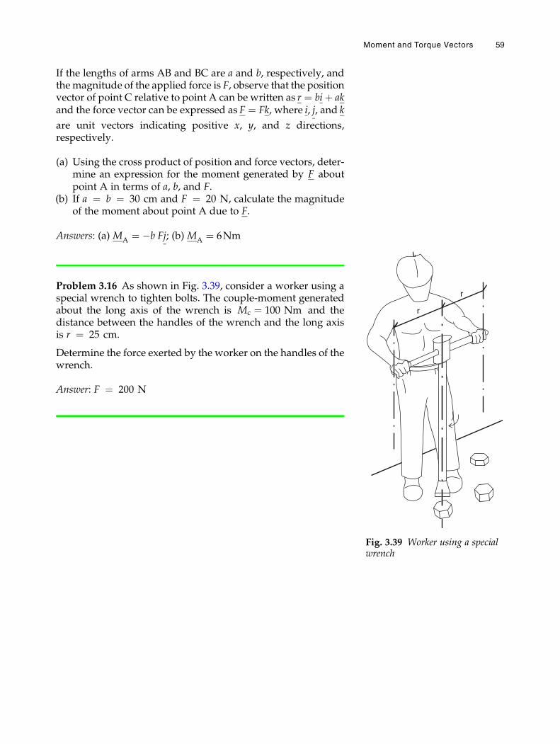
If the lengths of arms AB and BC are a and b, respectively, andthemagnitude of the applied force is F, observe that the positionvector of point C relative to point A can be written as r ¼ biþ akand the force vector can be expressed as F ¼ Fk, where i, j, and k
are unit vectors indicating positive x, y, and z directions,respectively.
(a) Using the cross product of position and force vectors, deter-mine an expression for the moment generated by F aboutpoint A in terms of a, b, and F.
(b) If a ¼ b ¼ 30 cm and F ¼ 20 N, calculate the magnitudeof the moment about point A due to F.
Answers: (a) MA ¼ �b Fj; (b) MA ¼ 6Nm
Problem 3.16 As shown in Fig. 3.39, consider a worker using aspecial wrench to tighten bolts. The couple-moment generatedabout the long axis of the wrench is Mc ¼ 100 Nm and thedistance between the handles of the wrench and the long axisis r ¼ 25 cm.
Determine the force exerted by the worker on the handles of thewrench.
Answer: F ¼ 200 N
r
r
Fig. 3.39 Worker using a specialwrench
Moment and Torque Vectors 59
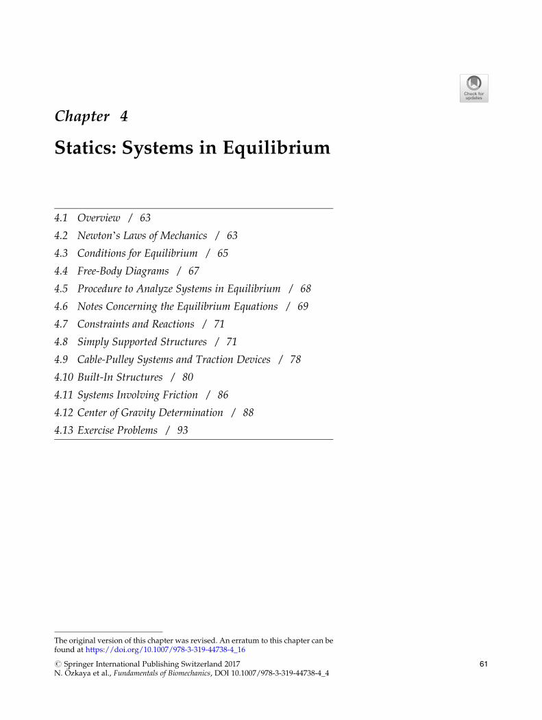
Chapter 4
Statics: Systems in Equilibrium
4.1 Overview / 63
4.2 Newton’s Laws of Mechanics / 63
4.3 Conditions for Equilibrium / 65
4.4 Free-Body Diagrams / 67
4.5 Procedure to Analyze Systems in Equilibrium / 68
4.6 Notes Concerning the Equilibrium Equations / 69
4.7 Constraints and Reactions / 71
4.8 Simply Supported Structures / 71
4.9 Cable-Pulley Systems and Traction Devices / 78
4.10 Built-In Structures / 80
4.11 Systems Involving Friction / 86
4.12 Center of Gravity Determination / 88
4.13 Exercise Problems / 93
The original version of this chapter was revised. An erratum to this chapter can befound at https://doi.org/10.1007/978-3-319-44738-4_16
# Springer International Publishing Switzerland 2017N. Ozkaya et al., Fundamentals of Biomechanics, DOI 10.1007/978-3-319-44738-4_4
61

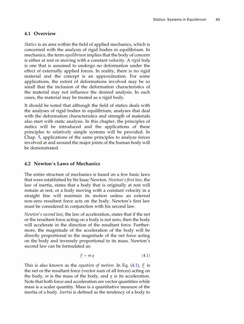
4.1 Overview
Statics is an area within the field of applied mechanics, which isconcerned with the analysis of rigid bodies in equilibrium. Inmechanics, the term equilibrium implies that the body of concernis either at rest or moving with a constant velocity. A rigid bodyis one that is assumed to undergo no deformation under theeffect of externally applied forces. In reality, there is no rigidmaterial and the concept is an approximation. For someapplications, the extent of deformations involved may be sosmall that the inclusion of the deformation characteristics ofthe material may not influence the desired analysis. In suchcases, the material may be treated as a rigid body.
It should be noted that although the field of statics deals withthe analyses of rigid bodies in equilibrium, analyses that dealwith the deformation characteristics and strength of materialsalso start with static analysis. In this chapter, the principles ofstatics will be introduced and the applications of theseprinciples to relatively simple systems will be provided. InChap. 5, applications of the same principles to analyze forcesinvolved at and around the major joints of the human body willbe demonstrated.
4.2 Newton’s Laws of Mechanics
The entire structure of mechanics is based on a few basic lawsthat were established by Sir Isaac Newton.Newton’s first law, thelaw of inertia, states that a body that is originally at rest willremain at rest, or a body moving with a constant velocity in astraight line will maintain its motion unless an externalnon-zero resultant force acts on the body. Newton’s first lawmust be considered in conjunction with his second law.
Newton’s second law, the law of acceleration, states that if the netor the resultant force acting on a body is not zero, then the bodywill accelerate in the direction of the resultant force. Further-more, the magnitude of the acceleration of the body will bedirectly proportional to the magnitude of the net force actingon the body and inversely proportional to its mass. Newton’ssecond law can be formulated as:
F ¼ m a ð4:1Þ
This is also known as the equation of motion. In Eq. (4.1), F isthe net or the resultant force (vector sum of all forces) acting onthe body, m is the mass of the body, and a is its acceleration.Note that both force and acceleration are vector quantities whilemass is a scalar quantity. Mass is a quantitative measure of theinertia of a body. Inertia is defined as the tendency of a body to
Statics: Systems in Equilibrium 63
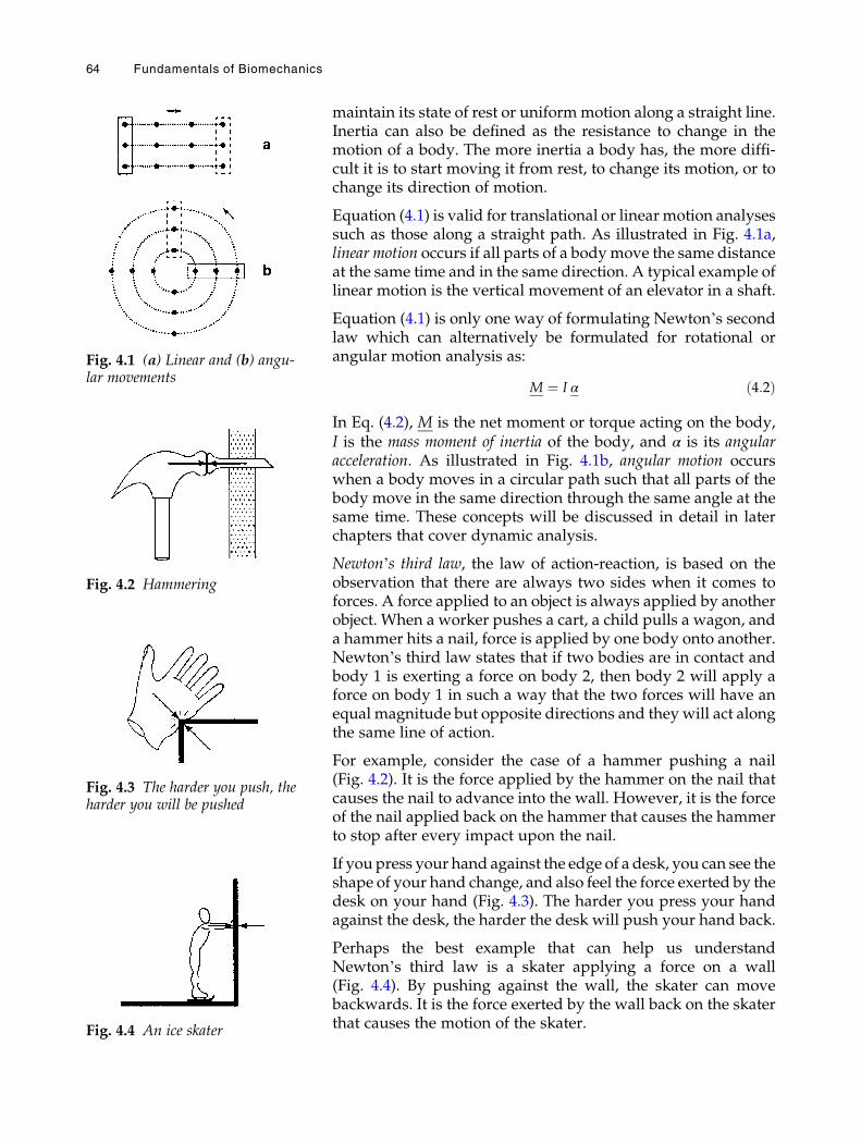
maintain its state of rest or uniformmotion along a straight line.Inertia can also be defined as the resistance to change in themotion of a body. The more inertia a body has, the more diffi-cult it is to start moving it from rest, to change its motion, or tochange its direction of motion.
Equation (4.1) is valid for translational or linear motion analysessuch as those along a straight path. As illustrated in Fig. 4.1a,linear motion occurs if all parts of a bodymove the same distanceat the same time and in the same direction. A typical example oflinear motion is the vertical movement of an elevator in a shaft.
Equation (4.1) is only one way of formulating Newton’s secondlaw which can alternatively be formulated for rotational orangular motion analysis as:
M ¼ I α ð4:2Þ
In Eq. (4.2), M is the net moment or torque acting on the body,I is the mass moment of inertia of the body, and α is its angularacceleration. As illustrated in Fig. 4.1b, angular motion occurswhen a body moves in a circular path such that all parts of thebody move in the same direction through the same angle at thesame time. These concepts will be discussed in detail in laterchapters that cover dynamic analysis.
Newton’s third law, the law of action-reaction, is based on theobservation that there are always two sides when it comes toforces. A force applied to an object is always applied by anotherobject. When a worker pushes a cart, a child pulls a wagon, anda hammer hits a nail, force is applied by one body onto another.Newton’s third law states that if two bodies are in contact andbody 1 is exerting a force on body 2, then body 2 will apply aforce on body 1 in such a way that the two forces will have anequal magnitude but opposite directions and they will act alongthe same line of action.
For example, consider the case of a hammer pushing a nail(Fig. 4.2). It is the force applied by the hammer on the nail thatcauses the nail to advance into the wall. However, it is the forceof the nail applied back on the hammer that causes the hammerto stop after every impact upon the nail.
If you press your hand against the edge of a desk, you can see theshape of your hand change, and also feel the force exerted by thedesk on your hand (Fig. 4.3). The harder you press your handagainst the desk, the harder the desk will push your hand back.
Perhaps the best example that can help us understandNewton’s third law is a skater applying a force on a wall(Fig. 4.4). By pushing against the wall, the skater can movebackwards. It is the force exerted by the wall back on the skaterthat causes the motion of the skater.
Fig. 4.1 (a) Linear and (b) angu-lar movements
Fig. 4.2 Hammering
Fig. 4.3 The harder you push, theharder you will be pushed
Fig. 4.4 An ice skater
64 Fundamentals of Biomechanics
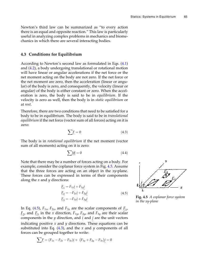
Newton’s third law can be summarized as “to every actionthere is an equal and opposite reaction.” This law is particularlyuseful in analyzing complex problems in mechanics and biome-chanics in which there are several interacting bodies.
4.3 Conditions for Equilibrium
According to Newton’s second law as formulated in Eqs. (4.1)and (4.2), a body undergoing translational or rotational motionwill have linear or angular accelerations if the net force or thenet moment acting on the body are not zero. If the net force orthe net moment are zero, then the acceleration (linear or angu-lar) of the body is zero, and consequently, the velocity (linear orangular) of the body is either constant or zero. When the accel-eration is zero, the body is said to be in equilibrium. If thevelocity is zero as well, then the body is in static equilibrium orat rest.
Therefore, there are two conditions that need to be satisfied for abody to be in equilibrium. The body is said to be in translationalequilibrium if the net force (vector sum of all forces) acting on it iszero: X
F ¼ 0 ð4:3Þ
The body is in rotational equilibrium if the net moment (vectorsum of all moments) acting on it is zero:X
M ¼ 0 ð4:4Þ
Note that there may be a number of forces acting on a body. Forexample, consider the coplanar force system in Fig. 4.5. Assumethat the three forces are acting on an object in the xy-plane.These forces can be expressed in terms of their componentsalong the x and y directions:
F1 ¼ F1xiþ F1yj
F2 ¼ �F2xiþ F2yj
F3 ¼ �F3xiþ F3yj
ð4:5Þ
In Eq. (4.5), F1x, F2x, and F3x are the scalar components of F1,F2, and F3 in the x direction, F1y, F2y, and F3y are their scalarcomponents in the y direction, and i and j are the unit vectors
indicating positive x and y directions. These equations can besubstituted into Eq. (4.3), and the x and y components of allforces can be grouped together to write:X
F ¼ F1x � F2x � F3xð Þiþ F1y þ F2y � F3x� �
j ¼ 0
Fig. 4.5 A coplanar force systemin the xy-plane
Statics: Systems in Equilibrium 65
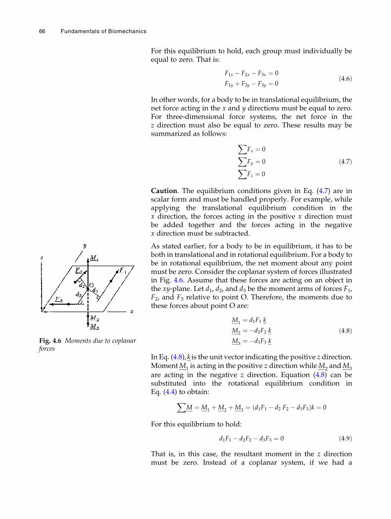
For this equilibrium to hold, each group must individually beequal to zero. That is:
F1x � F2x � F3x ¼ 0
F1y þ F2y � F3y ¼ 0ð4:6Þ
In other words, for a body to be in translational equilibrium, thenet force acting in the x and y directions must be equal to zero.For three-dimensional force systems, the net force in thez direction must also be equal to zero. These results may besummarized as follows:
XFx ¼ 0XFy ¼ 0XFz ¼ 0
ð4:7Þ
Caution. The equilibrium conditions given in Eq. (4.7) are inscalar form and must be handled properly. For example, whileapplying the translational equilibrium condition in thex direction, the forces acting in the positive x direction mustbe added together and the forces acting in the negativex direction must be subtracted.
As stated earlier, for a body to be in equilibrium, it has to beboth in translational and in rotational equilibrium. For a body tobe in rotational equilibrium, the net moment about any pointmust be zero. Consider the coplanar system of forces illustratedin Fig. 4.6. Assume that these forces are acting on an object inthe xy-plane. Let d1, d2, and d3 be the moment arms of forces F1,F2, and F3 relative to point O. Therefore, the moments due tothese forces about point O are:
M1 ¼ d1F1 k
M2 ¼ �d2F2 kM3 ¼ �d3F3 k
ð4:8Þ
In Eq. (4.8),k is the unit vector indicating the positive z direction.MomentM1 is acting in the positive z direction whileM2 andM3
are acting in the negative z direction. Equation (4.8) can besubstituted into the rotational equilibrium condition inEq. (4.4) to obtain:
XM ¼M1 þM2 þM3 ¼ d1F1 � d2 F2 � d3F3ð Þk ¼ 0
For this equilibrium to hold:
d1F1 � d2F2 � d3F3 ¼ 0 ð4:9Þ
That is, in this case, the resultant moment in the z directionmust be zero. Instead of a coplanar system, if we had a
Fig. 4.6 Moments due to coplanarforces
66 Fundamentals of Biomechanics
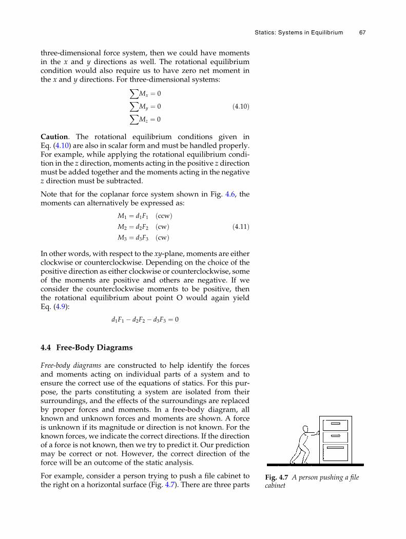
three-dimensional force system, then we could have momentsin the x and y directions as well. The rotational equilibriumcondition would also require us to have zero net moment inthe x and y directions. For three-dimensional systems:X
Mx ¼ 0XMy ¼ 0XMz ¼ 0
ð4:10Þ
Caution. The rotational equilibrium conditions given inEq. (4.10) are also in scalar form and must be handled properly.For example, while applying the rotational equilibrium condi-tion in the z direction, moments acting in the positive z directionmust be added together and the moments acting in the negativez direction must be subtracted.
Note that for the coplanar force system shown in Fig. 4.6, themoments can alternatively be expressed as:
M1 ¼ d1F1 ccwð ÞM2 ¼ d2F2 cwð ÞM3 ¼ d3F3 cwð Þ
ð4:11Þ
In other words, with respect to the xy-plane, moments are eitherclockwise or counterclockwise. Depending on the choice of thepositive direction as either clockwise or counterclockwise, someof the moments are positive and others are negative. If weconsider the counterclockwise moments to be positive, thenthe rotational equilibrium about point O would again yieldEq. (4.9):
d1F1 � d2F2 � d3F3 ¼ 0
4.4 Free-Body Diagrams
Free-body diagrams are constructed to help identify the forcesand moments acting on individual parts of a system and toensure the correct use of the equations of statics. For this pur-pose, the parts constituting a system are isolated from theirsurroundings, and the effects of the surroundings are replacedby proper forces and moments. In a free-body diagram, allknown and unknown forces and moments are shown. A forceis unknown if its magnitude or direction is not known. For theknown forces, we indicate the correct directions. If the directionof a force is not known, then we try to predict it. Our predictionmay be correct or not. However, the correct direction of theforce will be an outcome of the static analysis.
For example, consider a person trying to push a file cabinet tothe right on a horizontal surface (Fig. 4.7). There are three parts
Fig. 4.7 A person pushing a filecabinet
Statics: Systems in Equilibrium 67
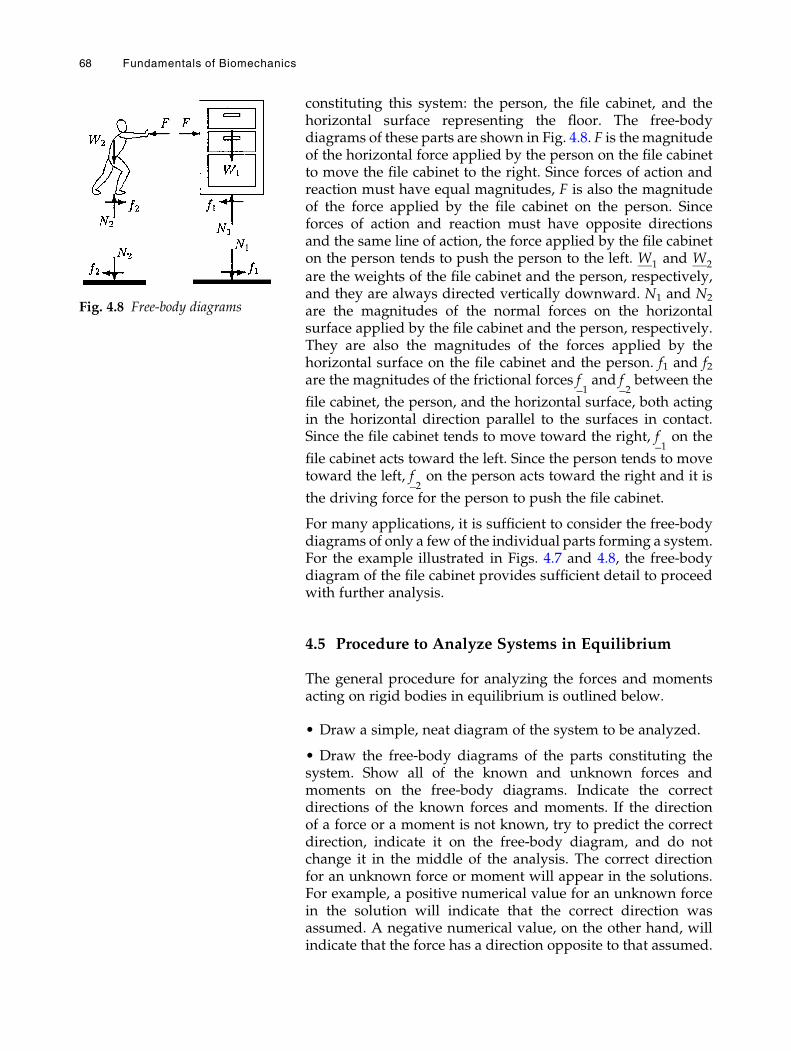
constituting this system: the person, the file cabinet, and thehorizontal surface representing the floor. The free-bodydiagrams of these parts are shown in Fig. 4.8. F is the magnitudeof the horizontal force applied by the person on the file cabinetto move the file cabinet to the right. Since forces of action andreaction must have equal magnitudes, F is also the magnitudeof the force applied by the file cabinet on the person. Sinceforces of action and reaction must have opposite directionsand the same line of action, the force applied by the file cabineton the person tends to push the person to the left. W1 and W2
are the weights of the file cabinet and the person, respectively,and they are always directed vertically downward. N1 and N2
are the magnitudes of the normal forces on the horizontalsurface applied by the file cabinet and the person, respectively.They are also the magnitudes of the forces applied by thehorizontal surface on the file cabinet and the person. f1 and f2are the magnitudes of the frictional forces f
1and f
2between the
file cabinet, the person, and the horizontal surface, both actingin the horizontal direction parallel to the surfaces in contact.Since the file cabinet tends to move toward the right, f
1on the
file cabinet acts toward the left. Since the person tends to movetoward the left, f
2on the person acts toward the right and it is
the driving force for the person to push the file cabinet.
For many applications, it is sufficient to consider the free-bodydiagrams of only a few of the individual parts forming a system.For the example illustrated in Figs. 4.7 and 4.8, the free-bodydiagram of the file cabinet provides sufficient detail to proceedwith further analysis.
4.5 Procedure to Analyze Systems in Equilibrium
The general procedure for analyzing the forces and momentsacting on rigid bodies in equilibrium is outlined below.
• Draw a simple, neat diagram of the system to be analyzed.
• Draw the free-body diagrams of the parts constituting thesystem. Show all of the known and unknown forces andmoments on the free-body diagrams. Indicate the correctdirections of the known forces and moments. If the directionof a force or a moment is not known, try to predict the correctdirection, indicate it on the free-body diagram, and do notchange it in the middle of the analysis. The correct directionfor an unknown force or moment will appear in the solutions.For example, a positive numerical value for an unknown forcein the solution will indicate that the correct direction wasassumed. A negative numerical value, on the other hand, willindicate that the force has a direction opposite to that assumed.
Fig. 4.8 Free-body diagrams
68 Fundamentals of Biomechanics
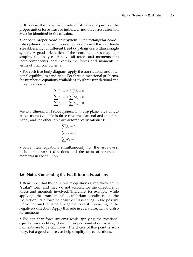
In this case, the force magnitude must be made positive, theproper unit of force must be indicated, and the correct directionmust be identified in the solution.
• Adopt a proper coordinate system. If the rectangular coordi-nate system (x, y, z) will be used, one can orient the coordinateaxes differently for different free-body diagrams within a singlesystem. A good orientation of the coordinate axes may helpsimplify the analyses. Resolve all forces and moments intotheir components, and express the forces and moments interms of their components.
• For each free-body diagram, apply the translational and rota-tional equilibrium conditions. For three-dimensional problems,the number of equations available is six (three translational andthree rotational): X
Fx ¼ 0X
Mx ¼ 0XFy ¼ 0
XMy ¼ 0X
Fz ¼ 0X
Mz ¼ 0
For two-dimensional force systems in the xy-plane, the numberof equations available is three (two translational and one rota-tional, and the other three are automatically satisfied):X
Fx ¼ 0XFy ¼ 0XMz ¼ 0
• Solve these equations simultaneously for the unknowns.Include the correct directions and the units of forces andmoments in the solution.
4.6 Notes Concerning the Equilibrium Equations
• Remember that the equilibrium equations given above are in“scalar” form and they do not account for the directions offorces and moments involved. Therefore, for example, whileapplying the translational equilibrium condition in thex direction, let a force be positive if it is acting in the positivex direction and let it be a negative force if it is acting in thenegative x direction. Apply this rule in every direction and alsofor moments.
• For coplanar force systems while applying the rotationalequilibrium condition, choose a proper point about which allmoments are to be calculated. The choice of this point is arbi-trary, but a good choice can help simplify the calculations.
Statics: Systems in Equilibrium 69
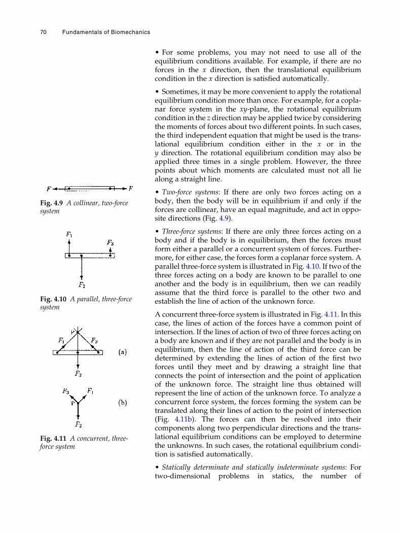
• For some problems, you may not need to use all of theequilibrium conditions available. For example, if there are noforces in the x direction, then the translational equilibriumcondition in the x direction is satisfied automatically.
• Sometimes, it may be more convenient to apply the rotationalequilibrium condition more than once. For example, for a copla-nar force system in the xy-plane, the rotational equilibriumcondition in the z directionmay be applied twice by consideringthe moments of forces about two different points. In such cases,the third independent equation that might be used is the trans-lational equilibrium condition either in the x or in they direction. The rotational equilibrium condition may also beapplied three times in a single problem. However, the threepoints about which moments are calculated must not all liealong a straight line.
• Two-force systems: If there are only two forces acting on abody, then the body will be in equilibrium if and only if theforces are collinear, have an equal magnitude, and act in oppo-site directions (Fig. 4.9).
• Three-force systems: If there are only three forces acting on abody and if the body is in equilibrium, then the forces mustform either a parallel or a concurrent system of forces. Further-more, for either case, the forces form a coplanar force system. Aparallel three-force system is illustrated in Fig. 4.10. If two of thethree forces acting on a body are known to be parallel to oneanother and the body is in equilibrium, then we can readilyassume that the third force is parallel to the other two andestablish the line of action of the unknown force.
A concurrent three-force system is illustrated in Fig. 4.11. In thiscase, the lines of action of the forces have a common point ofintersection. If the lines of action of two of three forces acting ona body are known and if they are not parallel and the body is inequilibrium, then the line of action of the third force can bedetermined by extending the lines of action of the first twoforces until they meet and by drawing a straight line thatconnects the point of intersection and the point of applicationof the unknown force. The straight line thus obtained willrepresent the line of action of the unknown force. To analyze aconcurrent force system, the forces forming the system can betranslated along their lines of action to the point of intersection(Fig. 4.11b). The forces can then be resolved into theircomponents along two perpendicular directions and the trans-lational equilibrium conditions can be employed to determinethe unknowns. In such cases, the rotational equilibrium condi-tion is satisfied automatically.
• Statically determinate and statically indeterminate systems: Fortwo-dimensional problems in statics, the number of
Fig. 4.9 A collinear, two-forcesystem
Fig. 4.10 A parallel, three-forcesystem
Fig. 4.11 A concurrent, three-force system
70 Fundamentals of Biomechanics
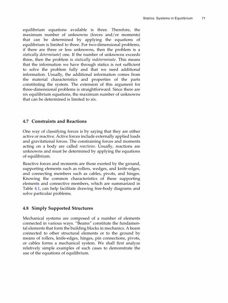
equilibrium equations available is three. Therefore, themaximum number of unknowns (forces and/or moments)that can be determined by applying the equations ofequilibrium is limited to three. For two-dimensional problems,if there are three or less unknowns, then the problem is astatically determinate} one. If the number of unknowns exceedsthree, then the problem is statically indeterminate. This meansthat the information we have through statics is not sufficientto solve the problem fully and that we need additionalinformation. Usually, the additional information comes fromthe material characteristics and properties of the partsconstituting the system. The extension of this argument forthree-dimensional problems is straightforward. Since there aresix equilibrium equations, the maximum number of unknownsthat can be determined is limited to six.
4.7 Constraints and Reactions
One way of classifying forces is by saying that they are eitheractive or reactive. Active forces include externally applied loadsand gravitational forces. The constraining forces and momentsacting on a body are called reactions. Usually, reactions areunknowns and must be determined by applying the equationsof equilibrium.
Reactive forces and moments are those exerted by the ground,supporting elements such as rollers, wedges, and knife-edges,and connecting members such as cables, pivots, and hinges.Knowing the common characteristics of these supportingelements and connective members, which are summarized inTable 4.1, can help facilitate drawing free-body diagrams andsolve particular problems.
4.8 Simply Supported Structures
Mechanical systems are composed of a number of elementsconnected in various ways. “Beams” constitute the fundamen-tal elements that form the building blocks in mechanics. A beamconnected to other structural elements or to the ground bymeans of rollers, knife-edges, hinges, pin connections, pivots,or cables forms a mechanical system. We shall first analyzerelatively simple examples of such cases to demonstrate theuse of the equations of equilibrium.
Statics: Systems in Equilibrium 71
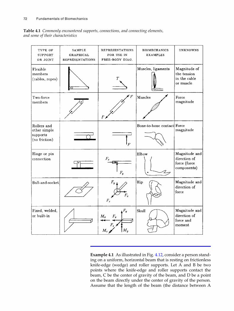
Example 4.1 As illustrated in Fig. 4.12, consider a person stand-ing on a uniform, horizontal beam that is resting on frictionlessknife-edge (wedge) and roller supports. Let A and B be twopoints where the knife-edge and roller supports contact thebeam, C be the center of gravity of the beam, and D be a pointon the beam directly under the center of gravity of the person.Assume that the length of the beam (the distance between A
Table 4.1 Commonly encountered supports, connections, and connecting elements,and some of their characteristics
72 Fundamentals of Biomechanics
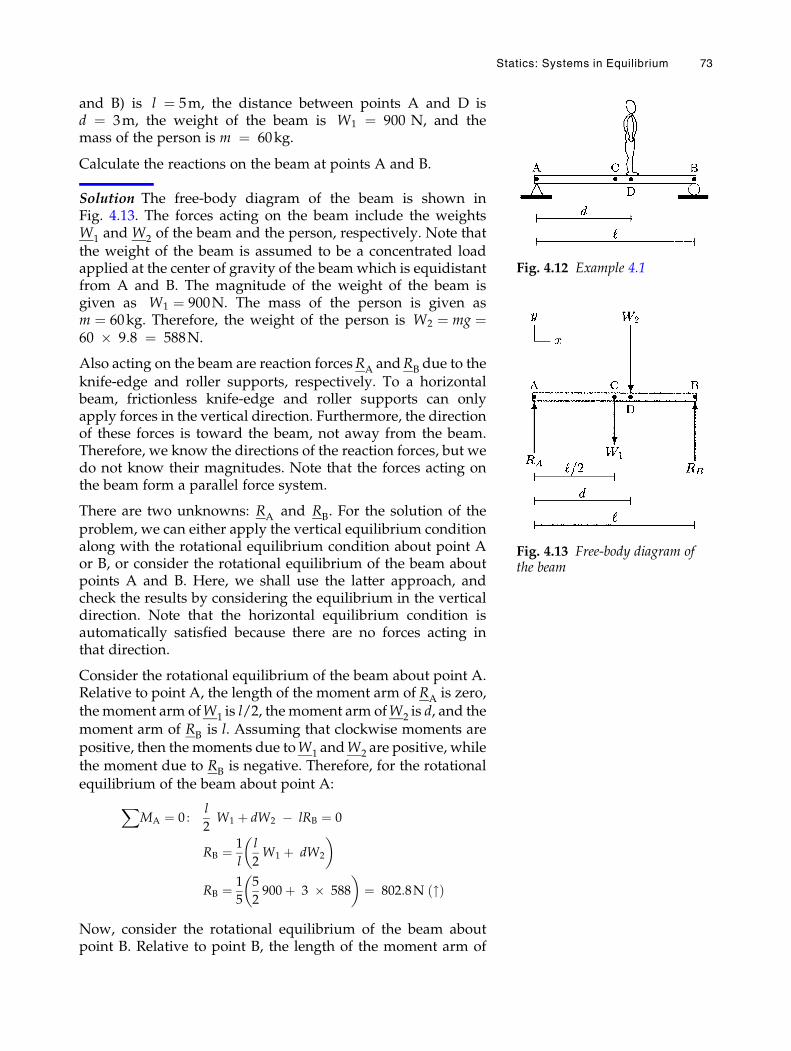
and B) is l ¼ 5m, the distance between points A and D isd ¼ 3m, the weight of the beam is W1 ¼ 900 N, and themass of the person is m ¼ 60kg.
Calculate the reactions on the beam at points A and B.
Solution The free-body diagram of the beam is shown inFig. 4.13. The forces acting on the beam include the weightsW1 and W2 of the beam and the person, respectively. Note thatthe weight of the beam is assumed to be a concentrated loadapplied at the center of gravity of the beamwhich is equidistantfrom A and B. The magnitude of the weight of the beam isgiven as W1 ¼ 900N. The mass of the person is given asm ¼ 60kg. Therefore, the weight of the person is W2 ¼ mg ¼60 � 9:8 ¼ 588N.
Also acting on the beam are reaction forcesRA andRB due to theknife-edge and roller supports, respectively. To a horizontalbeam, frictionless knife-edge and roller supports can onlyapply forces in the vertical direction. Furthermore, the directionof these forces is toward the beam, not away from the beam.Therefore, we know the directions of the reaction forces, but wedo not know their magnitudes. Note that the forces acting onthe beam form a parallel force system.
There are two unknowns: RA and RB. For the solution of theproblem, we can either apply the vertical equilibrium conditionalong with the rotational equilibrium condition about point Aor B, or consider the rotational equilibrium of the beam aboutpoints A and B. Here, we shall use the latter approach, andcheck the results by considering the equilibrium in the verticaldirection. Note that the horizontal equilibrium condition isautomatically satisfied because there are no forces acting inthat direction.
Consider the rotational equilibrium of the beam about point A.Relative to point A, the length of the moment arm of RA is zero,the moment arm ofW1 is l/2, the moment arm ofW2 is d, and themoment arm of RB is l. Assuming that clockwise moments arepositive, then the moments due toW1 andW2 are positive, whilethe moment due to RB is negative. Therefore, for the rotationalequilibrium of the beam about point A:
XMA ¼ 0 :
l
2W1 þ dW2 � lRB ¼ 0
RB ¼ 1
l
l
2W1 þ dW2
� �
RB ¼ 1
5
5
2900þ 3 � 588
� �¼ 802:8N "ð Þ
Now, consider the rotational equilibrium of the beam aboutpoint B. Relative to point B, the length of the moment arm of
Fig. 4.12 Example 4.1
Fig. 4.13 Free-body diagram ofthe beam
Statics: Systems in Equilibrium 73
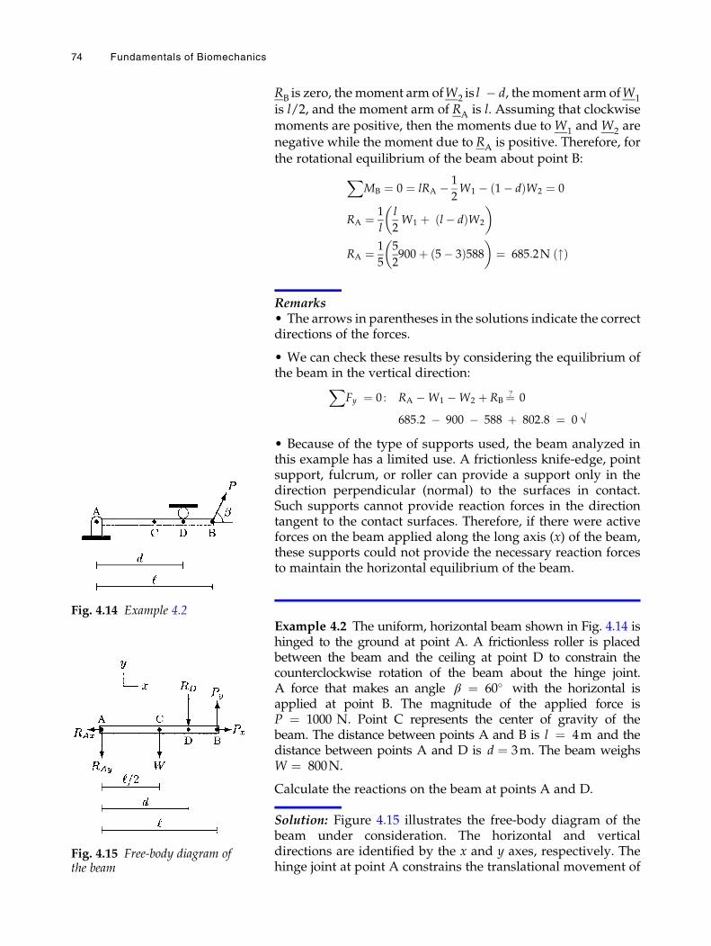
RB is zero, the moment arm ofW2 is l � d, themoment arm ofW1
is l/2, and the moment arm of RA is l. Assuming that clockwisemoments are positive, then the moments due toW1 andW2 arenegative while the moment due to RA is positive. Therefore, forthe rotational equilibrium of the beam about point B:
XMB ¼ 0 ¼ lRA � 1
2W1 � 1� dð ÞW2 ¼ 0
RA ¼ 1
l
l
2W1 þ l� dð ÞW2
� �
RA ¼ 1
5
5
2900þ 5� 3ð Þ588
� �¼ 685:2N "ð Þ
Remarks• The arrows in parentheses in the solutions indicate the correctdirections of the forces.
• We can check these results by considering the equilibrium ofthe beam in the vertical direction:X
Fy ¼ 0 : RA �W1 �W2 þ RB¼? 0
685:2 � 900 � 588 þ 802:8 ¼ 0 √
• Because of the type of supports used, the beam analyzed inthis example has a limited use. A frictionless knife-edge, pointsupport, fulcrum, or roller can provide a support only in thedirection perpendicular (normal) to the surfaces in contact.Such supports cannot provide reaction forces in the directiontangent to the contact surfaces. Therefore, if there were activeforces on the beam applied along the long axis (x) of the beam,these supports could not provide the necessary reaction forcesto maintain the horizontal equilibrium of the beam.
Example 4.2 The uniform, horizontal beam shown in Fig. 4.14 ishinged to the ground at point A. A frictionless roller is placedbetween the beam and the ceiling at point D to constrain thecounterclockwise rotation of the beam about the hinge joint.A force that makes an angle β ¼ 60� with the horizontal isapplied at point B. The magnitude of the applied force isP ¼ 1000 N. Point C represents the center of gravity of thebeam. The distance between points A and B is l ¼ 4m and thedistance between points A and D is d ¼ 3m. The beam weighsW ¼ 800N.
Calculate the reactions on the beam at points A and D.
Solution: Figure 4.15 illustrates the free-body diagram of thebeam under consideration. The horizontal and verticaldirections are identified by the x and y axes, respectively. Thehinge joint at point A constrains the translational movement of
Fig. 4.14 Example 4.2
Fig. 4.15 Free-body diagram ofthe beam
74 Fundamentals of Biomechanics
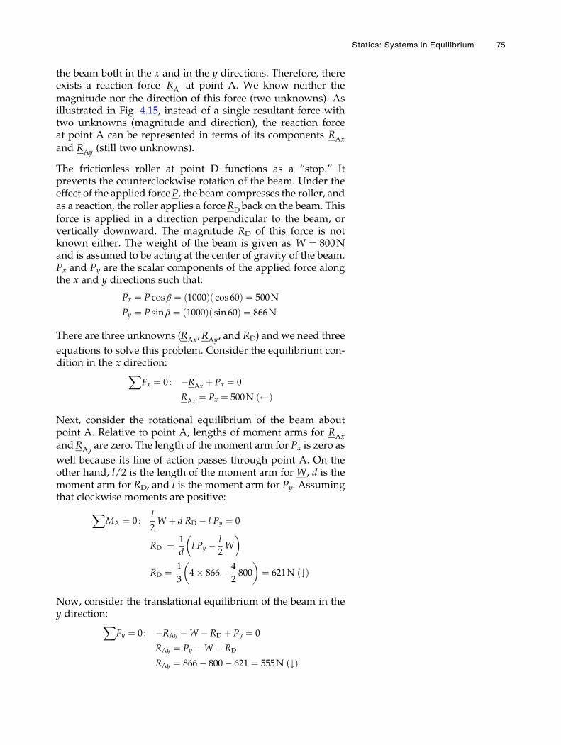
the beam both in the x and in the y directions. Therefore, thereexists a reaction force RA at point A. We know neither themagnitude nor the direction of this force (two unknowns). Asillustrated in Fig. 4.15, instead of a single resultant force withtwo unknowns (magnitude and direction), the reaction forceat point A can be represented in terms of its components RAx
and RAy (still two unknowns).
The frictionless roller at point D functions as a “stop.” Itprevents the counterclockwise rotation of the beam. Under theeffect of the applied forceP, the beam compresses the roller, andas a reaction, the roller applies a forceRD back on the beam. Thisforce is applied in a direction perpendicular to the beam, orvertically downward. The magnitude RD of this force is notknown either. The weight of the beam is given as W ¼ 800Nand is assumed to be acting at the center of gravity of the beam.Px and Py are the scalar components of the applied force alongthe x and y directions such that:
Px ¼ P cos β ¼ 1000ð Þ cos 60ð Þ ¼ 500N
Py ¼ P sin β ¼ 1000ð Þ sin 60ð Þ ¼ 866N
There are three unknowns (RAx,RAy, and RD) and we need three
equations to solve this problem. Consider the equilibrium con-dition in the x direction:X
Fx ¼ 0 : �RAx þ Px ¼ 0
RAx ¼ Px ¼ 500N ð Þ
Next, consider the rotational equilibrium of the beam aboutpoint A. Relative to point A, lengths of moment arms for RAx
andRAy are zero. The length of the moment arm for Px is zero as
well because its line of action passes through point A. On theother hand, l/2 is the length of the moment arm for W, d is themoment arm for RD, and l is the moment arm for Py. Assumingthat clockwise moments are positive:
XMA ¼ 0 :
l
2W þ d RD � l Py ¼ 0
RD ¼ 1
dl Py � l
2W
� �
RD ¼ 1
34� 866� 4
2800
� �¼ 621N #ð Þ
Now, consider the translational equilibrium of the beam in they direction:X
Fy ¼ 0 : �RAy �W � RD þ Py ¼ 0
RAy ¼ Py �W � RD
RAy ¼ 866� 800� 621 ¼ 555N #ð Þ
Statics: Systems in Equilibrium 75
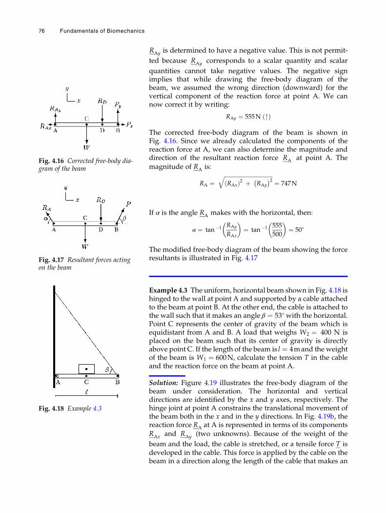
RAy is determined to have a negative value. This is not permit-
ted because RAy corresponds to a scalar quantity and scalar
quantities cannot take negative values. The negative signimplies that while drawing the free-body diagram of thebeam, we assumed the wrong direction (downward) for thevertical component of the reaction force at point A. We cannow correct it by writing:
RAy ¼ 555N "ð Þ
The corrected free-body diagram of the beam is shown inFig. 4.16. Since we already calculated the components of thereaction force at A, we can also determine the magnitude anddirection of the resultant reaction force RA at point A. Themagnitude of RA is:
RA ¼ffiffiffiffiffiffiffiffiffiffiffiffiffiffiffiffiffiffiffiffiffiffiffiffiffiffiffiffiffiffiffiffiffiffiffiffiRAxð Þ2 þ RAy
� �2q¼ 747N
If α is the angle RA makes with the horizontal, then:
α ¼ tan �1RAy
RAx
� �¼ tan �1
555
500
� �¼ 50�
The modified free-body diagram of the beam showing the forceresultants is illustrated in Fig. 4.17
Example 4.3 The uniform, horizontal beam shown in Fig. 4.18 ishinged to the wall at point A and supported by a cable attachedto the beam at point B. At the other end, the cable is attached tothe wall such that it makes an angle β ¼ 53�with the horizontal.Point C represents the center of gravity of the beam which isequidistant from A and B. A load that weighs W2 ¼ 400 N isplaced on the beam such that its center of gravity is directlyabove point C. If the length of the beam is l ¼ 4mand the weightof the beam is W1 ¼ 600N, calculate the tension T in the cableand the reaction force on the beam at point A.
Solution: Figure 4.19 illustrates the free-body diagram of thebeam under consideration. The horizontal and verticaldirections are identified by the x and y axes, respectively. Thehinge joint at point A constrains the translational movement ofthe beam both in the x and in the y directions. In Fig. 4.19b, thereaction force RA at A is represented in terms of its componentsRAx and RAy (two unknowns). Because of the weight of the
beam and the load, the cable is stretched, or a tensile force T isdeveloped in the cable. This force is applied by the cable on thebeam in a direction along the length of the cable that makes an
Fig. 4.16 Corrected free-body dia-gram of the beam
Fig. 4.17 Resultant forces actingon the beam
Fig. 4.18 Example 4.3
76 Fundamentals of Biomechanics
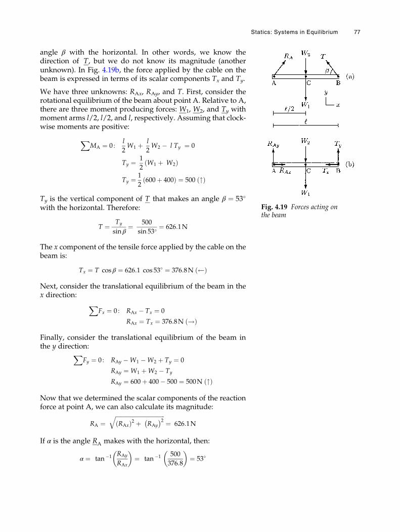
angle β with the horizontal. In other words, we know thedirection of T, but we do not know its magnitude (anotherunknown). In Fig. 4.19b, the force applied by the cable on thebeam is expressed in terms of its scalar components Tx and Ty.
We have three unknowns: RAx, RAy, and T. First, consider therotational equilibrium of the beam about point A. Relative to A,there are three moment producing forces: W1, W2, and Ty withmoment arms l/2, l/2, and l, respectively. Assuming that clock-wise moments are positive:
XMA ¼ 0 :
l
2W1 þ l
2W2 � l Ty ¼ 0
Ty ¼ 1
2W1 þ W2ð Þ
Ty ¼ 1
2600þ 400ð Þ ¼ 500 "ð Þ
Ty is the vertical component of T that makes an angle β ¼ 53�
with the horizontal. Therefore:
T ¼ Ty
sin β¼ 500
sin 53�¼ 626:1N
The x component of the tensile force applied by the cable on thebeam is:
Tx ¼ T cos β ¼ 626:1 cos 53� ¼ 376:8N ð Þ
Next, consider the translational equilibrium of the beam in thex direction:
XFx ¼ 0 : RAx � Tx ¼ 0
RAx ¼ Tx ¼ 376:8N !ð Þ
Finally, consider the translational equilibrium of the beam inthe y direction:X
Fy ¼ 0 : RAy �W1 �W2 þ Ty ¼ 0
RAy ¼W1 þW2 � Ty
RAy ¼ 600þ 400� 500 ¼ 500N "ð Þ
Now that we determined the scalar components of the reactionforce at point A, we can also calculate its magnitude:
RA ¼ffiffiffiffiffiffiffiffiffiffiffiffiffiffiffiffiffiffiffiffiffiffiffiffiffiffiffiffiffiffiffiffiffiffiffiRAxð Þ2 þ RAy
� �2q¼ 626:1N
If α is the angle RA makes with the horizontal, then:
α ¼ tan �1RAy
RAx
� �¼ tan �1
500
376:8
� �¼ 53�
Fig. 4.19 Forces acting onthe beam
Statics: Systems in Equilibrium 77
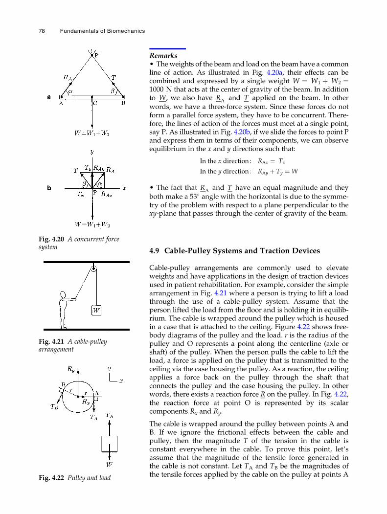
Remarks• Theweights of the beam and load on the beam have a commonline of action. As illustrated in Fig. 4.20a, their effects can becombined and expressed by a single weight W ¼ W1 þ W2 ¼1000 N that acts at the center of gravity of the beam. In additionto W, we also have RA and T applied on the beam. In otherwords, we have a three-force system. Since these forces do notform a parallel force system, they have to be concurrent. There-fore, the lines of action of the forces must meet at a single point,say P. As illustrated in Fig. 4.20b, if we slide the forces to point Pand express them in terms of their components, we can observeequilibrium in the x and y directions such that:
In the x direction : RAx ¼ Tx
In the y direction : RAy þ Ty ¼W
• The fact that RA and T have an equal magnitude and theyboth make a 53� angle with the horizontal is due to the symme-try of the problem with respect to a plane perpendicular to thexy-plane that passes through the center of gravity of the beam.
4.9 Cable-Pulley Systems and Traction Devices
Cable-pulley arrangements are commonly used to elevateweights and have applications in the design of traction devicesused in patient rehabilitation. For example, consider the simplearrangement in Fig. 4.21 where a person is trying to lift a loadthrough the use of a cable-pulley system. Assume that theperson lifted the load from the floor and is holding it in equilib-rium. The cable is wrapped around the pulley which is housedin a case that is attached to the ceiling. Figure 4.22 shows free-body diagrams of the pulley and the load. r is the radius of thepulley and O represents a point along the centerline (axle orshaft) of the pulley. When the person pulls the cable to lift theload, a force is applied on the pulley that is transmitted to theceiling via the case housing the pulley. As a reaction, the ceilingapplies a force back on the pulley through the shaft thatconnects the pulley and the case housing the pulley. In otherwords, there exists a reaction force R on the pulley. In Fig. 4.22,the reaction force at point O is represented by its scalarcomponents Rx and Ry.
The cable is wrapped around the pulley between points A andB. If we ignore the frictional effects between the cable andpulley, then the magnitude T of the tension in the cable isconstant everywhere in the cable. To prove this point, let’sassume that the magnitude of the tensile force generated inthe cable is not constant. Let TA and TB be the magnitudes ofthe tensile forces applied by the cable on the pulley at points A
Fig. 4.21 A cable-pulleyarrangement
Fig. 4.20 A concurrent forcesystem
Fig. 4.22 Pulley and load
78 Fundamentals of Biomechanics
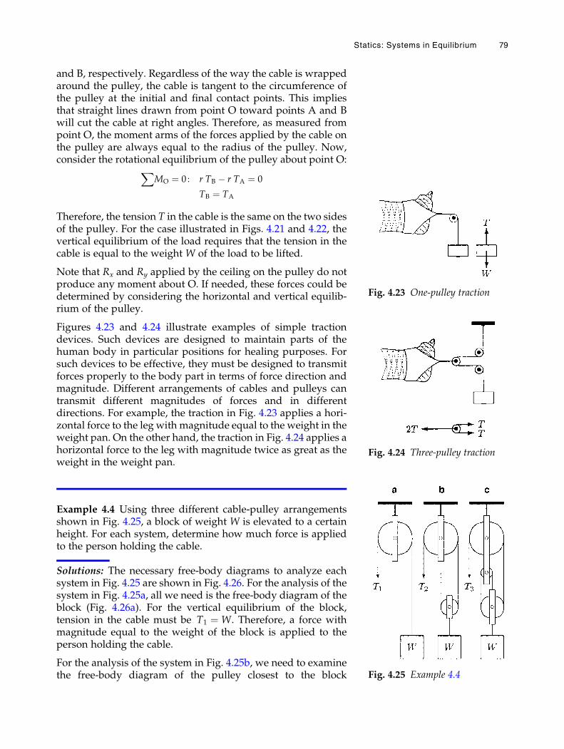
and B, respectively. Regardless of the way the cable is wrappedaround the pulley, the cable is tangent to the circumference ofthe pulley at the initial and final contact points. This impliesthat straight lines drawn from point O toward points A and Bwill cut the cable at right angles. Therefore, as measured frompoint O, the moment arms of the forces applied by the cable onthe pulley are always equal to the radius of the pulley. Now,consider the rotational equilibrium of the pulley about point O:X
MO ¼ 0 : r TB � r TA ¼ 0
TB ¼ TA
Therefore, the tension T in the cable is the same on the two sidesof the pulley. For the case illustrated in Figs. 4.21 and 4.22, thevertical equilibrium of the load requires that the tension in thecable is equal to the weight W of the load to be lifted.
Note that Rx and Ry applied by the ceiling on the pulley do notproduce any moment about O. If needed, these forces could bedetermined by considering the horizontal and vertical equilib-rium of the pulley.
Figures 4.23 and 4.24 illustrate examples of simple tractiondevices. Such devices are designed to maintain parts of thehuman body in particular positions for healing purposes. Forsuch devices to be effective, they must be designed to transmitforces properly to the body part in terms of force direction andmagnitude. Different arrangements of cables and pulleys cantransmit different magnitudes of forces and in differentdirections. For example, the traction in Fig. 4.23 applies a hori-zontal force to the leg with magnitude equal to the weight in theweight pan. On the other hand, the traction in Fig. 4.24 applies ahorizontal force to the leg with magnitude twice as great as theweight in the weight pan.
Example 4.4 Using three different cable-pulley arrangementsshown in Fig. 4.25, a block of weight W is elevated to a certainheight. For each system, determine how much force is appliedto the person holding the cable.
Solutions: The necessary free-body diagrams to analyze eachsystem in Fig. 4.25 are shown in Fig. 4.26. For the analysis of thesystem in Fig. 4.25a, all we need is the free-body diagram of theblock (Fig. 4.26a). For the vertical equilibrium of the block,tension in the cable must be T1 ¼W. Therefore, a force withmagnitude equal to the weight of the block is applied to theperson holding the cable.
For the analysis of the system in Fig. 4.25b, we need to examinethe free-body diagram of the pulley closest to the block
Fig. 4.23 One-pulley traction
Fig. 4.24 Three-pulley traction
Fig. 4.25 Example 4.4
Statics: Systems in Equilibrium 79
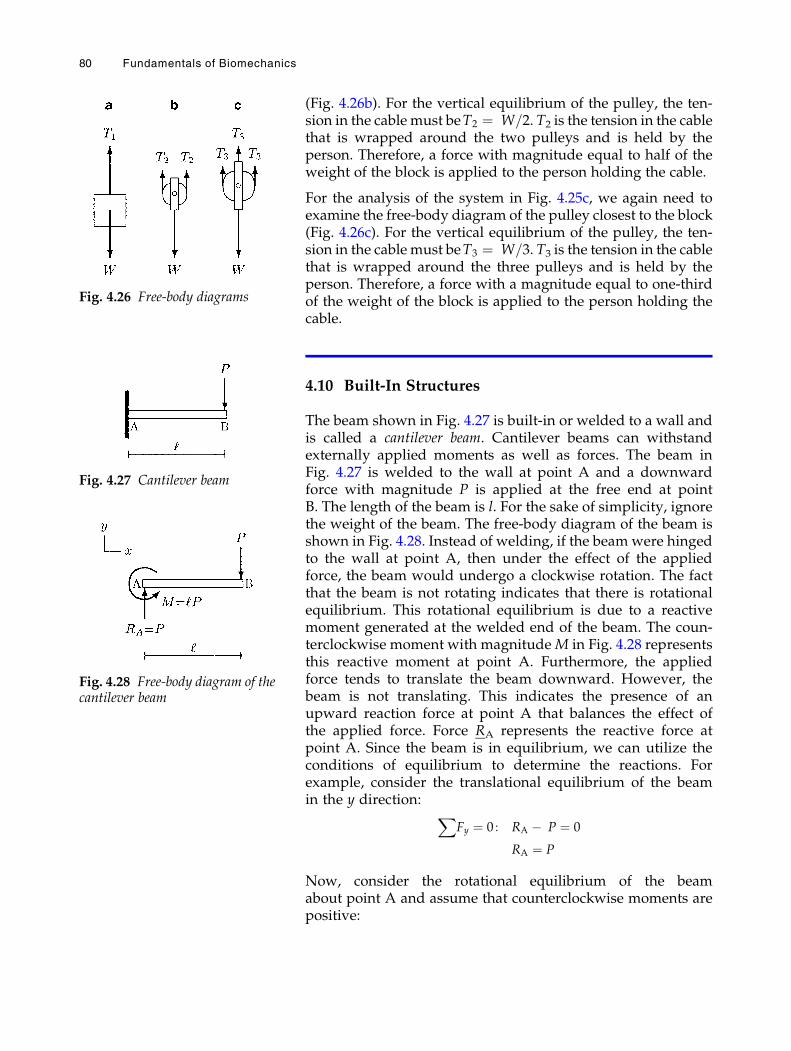
(Fig. 4.26b). For the vertical equilibrium of the pulley, the ten-sion in the cable must beT2 ¼ W=2. T2 is the tension in the cablethat is wrapped around the two pulleys and is held by theperson. Therefore, a force with magnitude equal to half of theweight of the block is applied to the person holding the cable.
For the analysis of the system in Fig. 4.25c, we again need toexamine the free-body diagram of the pulley closest to the block(Fig. 4.26c). For the vertical equilibrium of the pulley, the ten-sion in the cable must beT3 ¼ W=3. T3 is the tension in the cablethat is wrapped around the three pulleys and is held by theperson. Therefore, a force with a magnitude equal to one-thirdof the weight of the block is applied to the person holding thecable.
4.10 Built-In Structures
The beam shown in Fig. 4.27 is built-in or welded to a wall andis called a cantilever beam. Cantilever beams can withstandexternally applied moments as well as forces. The beam inFig. 4.27 is welded to the wall at point A and a downwardforce with magnitude P is applied at the free end at pointB. The length of the beam is l. For the sake of simplicity, ignorethe weight of the beam. The free-body diagram of the beam isshown in Fig. 4.28. Instead of welding, if the beamwere hingedto the wall at point A, then under the effect of the appliedforce, the beam would undergo a clockwise rotation. The factthat the beam is not rotating indicates that there is rotationalequilibrium. This rotational equilibrium is due to a reactivemoment generated at the welded end of the beam. The coun-terclockwise moment with magnitudeM in Fig. 4.28 representsthis reactive moment at point A. Furthermore, the appliedforce tends to translate the beam downward. However, thebeam is not translating. This indicates the presence of anupward reaction force at point A that balances the effect ofthe applied force. Force RA represents the reactive force atpoint A. Since the beam is in equilibrium, we can utilize theconditions of equilibrium to determine the reactions. Forexample, consider the translational equilibrium of the beamin the y direction: X
Fy ¼ 0 : RA � P ¼ 0
RA ¼ P
Now, consider the rotational equilibrium of the beamabout point A and assume that counterclockwise moments arepositive:
Fig. 4.26 Free-body diagrams
Fig. 4.27 Cantilever beam
Fig. 4.28 Free-body diagram of thecantilever beam
80 Fundamentals of Biomechanics
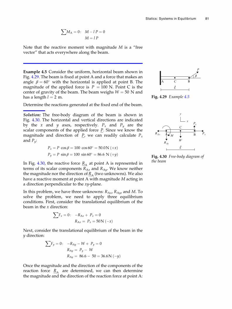
XMA ¼ 0 : M� l P ¼ 0
M ¼ l P
Note that the reactive moment with magnitude M is a “freevector” that acts everywhere along the beam.
Example 4.5 Consider the uniform, horizontal beam shown inFig. 4.29. The beam is fixed at point A and a force that makes anangle β ¼ 60� with the horizontal is applied at point B. Themagnitude of the applied force is P ¼ 100 N. Point C is thecenter of gravity of the beam. The beam weighs W ¼ 50 N andhas a length l ¼ 2 m.
Determine the reactions generated at the fixed end of the beam.
Solution: The free-body diagram of the beam is shown inFig. 4.30. The horizontal and vertical directions are indicatedby the x and y axes, respectively. Px and Py are thescalar components of the applied force P. Since we know themagnitude and direction of P, we can readily calculate Px
and Py:
Px ¼ P cos β ¼ 100 cos 60� ¼ 50:0N þxð ÞPy ¼ P sin β ¼ 100 sin 60� ¼ 86:6 N þyð Þ
In Fig. 4.30, the reactive force RA at point A is represented interms of its scalar components RAx and RAy. We know neitherthe magnitude nor the direction ofRA (two unknowns). We alsohave a reactive moment at point A with magnitude M acting ina direction perpendicular to the xy-plane.
In this problem, we have three unknowns: RAx, RAy, and M. Tosolve the problem, we need to apply three equilibriumconditions. First, consider the translational equilibrium of thebeam in the x direction:X
Fx ¼ 0 : �RAx þ Px ¼ 0
RAx ¼ Px ¼ 50N �xð Þ
Next, consider the translational equilibrium of the beam in they direction:X
Fy ¼ 0 : �RAy �W þ Py ¼ 0
RAy ¼ Py � W
RAy ¼ 86:6� 50 ¼ 36:6N �yð Þ
Once the magnitude and the direction of the components of thereaction force RA are determined, we can then determinethe magnitude and the direction of the reaction force at point A:
A C B
P
b
Fig. 4.29 Example 4.5
B
C
ARAx
RAy
Py
W
MPx
x
y
Fig. 4.30 Free-body diagram ofthe beam
Statics: Systems in Equilibrium 81

R2A ¼ R2
Ax þ R2Ay
RA ¼ffiffiffiffiffiffiffiffiffiffiffiffiffiffiffiffiffiffiffiffiffiffiffiR2Ax þ R2
Ay
q
RA ¼ffiffiffiffiffiffiffiffiffiffiffiffiffiffiffiffiffiffiffiffiffiffiffiffiffi502 þ 36:62
p¼ 62N
Finally, consider the rotational equilibrium of the beam aboutpoint A. Assuming that counterclockwise moments arepositive:
XMA ¼ 0 : MþW � l
2� Py � l ¼ 0
M ¼ Py � l�W � l2
M ¼ 86:6 � 2� 50 � 22¼ 123:2 Nm cwð Þ
As we determined the magnitude of the reaction force and themagnitude and the direction of the reactive moment atpoint A, we can also determine the direction of the reactionforce RA If α is an angle that the line of action of the reactionforce RA makes with the horizontal, then:
tan α ¼ RAy
RAx
α ¼ arc tanRAy
RAx
� �¼ 36:2�
The final free-body diagram of the beam is shown in Fig. 4.31.
Example 4.6 Consider the L-shaped beam illustrated inFig. 4.32. The beam is welded to the wall at point A, the armAB extends in the positive z direction, and the arm BCextends in the negative x direction. A force P is applied in thenegative y direction at point B. The lengths of arms AB and BCare a ¼ 20 cm and b ¼ 30 cm, respectively, and the magnitudeof the applied force is P ¼ 120 N.
Assuming that the weight of the beam is negligibly small ascompared to the magnitude of the applied force, determine thereactions at the fixed end of the beam.
This is a three-dimensional problem and we shall employ twomethods to analyze it. The first method will utilize the conceptsof couple and couple-moment introduced in the previous chap-ter, and the second method will utilize the vector properties offorces and moments.
x
y
B
C
ARA W
M
P
Fig. 4.31 Forces and moment act-ing on the beam
Fig. 4.32 Example 4.6
82 Fundamentals of Biomechanics
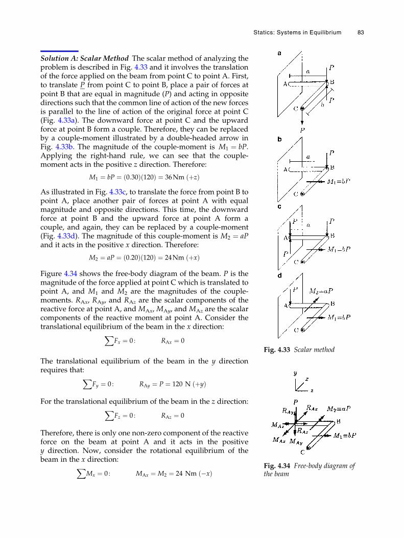
Solution A: Scalar Method The scalar method of analyzing theproblem is described in Fig. 4.33 and it involves the translationof the force applied on the beam from point C to point A. First,to translate P from point C to point B, place a pair of forces atpoint B that are equal in magnitude (P) and acting in oppositedirections such that the common line of action of the new forcesis parallel to the line of action of the original force at point C(Fig. 4.33a). The downward force at point C and the upwardforce at point B form a couple. Therefore, they can be replacedby a couple-moment illustrated by a double-headed arrow inFig. 4.33b. The magnitude of the couple-moment is M1 ¼ bP.Applying the right-hand rule, we can see that the couple-moment acts in the positive z direction. Therefore:
M1 ¼ bP ¼ 0:30ð Þ 120ð Þ ¼ 36Nm þzð Þ
As illustrated in Fig. 4.33c, to translate the force from point B topoint A, place another pair of forces at point A with equalmagnitude and opposite directions. This time, the downwardforce at point B and the upward force at point A form acouple, and again, they can be replaced by a couple-moment(Fig. 4.33d). The magnitude of this couple-moment is M2 ¼ aPand it acts in the positive x direction. Therefore:
M2 ¼ aP ¼ 0:20ð Þ 120ð Þ ¼ 24Nm þxð Þ
Figure 4.34 shows the free-body diagram of the beam. P is themagnitude of the force applied at point C which is translated topoint A, and M1 and M2 are the magnitudes of the couple-moments. RAx, RAy, and RAz are the scalar components of thereactive force at point A, and MAx, MAy, and MAz are the scalarcomponents of the reactive moment at point A. Consider thetranslational equilibrium of the beam in the x direction:X
Fx ¼ 0 : RAx ¼ 0
The translational equilibrium of the beam in the y directionrequires that:X
Fy ¼ 0 : RAy ¼ P ¼ 120 N þyð Þ
For the translational equilibrium of the beam in the z direction:XFz ¼ 0 : RAz ¼ 0
Therefore, there is only one non-zero component of the reactiveforce on the beam at point A and it acts in the positivey direction. Now, consider the rotational equilibrium of thebeam in the x direction:X
Mx ¼ 0 : MAx ¼M2 ¼ 24 Nm �xð Þ
Fig. 4.33 Scalar method
Fig. 4.34 Free-body diagram ofthe beam
Statics: Systems in Equilibrium 83
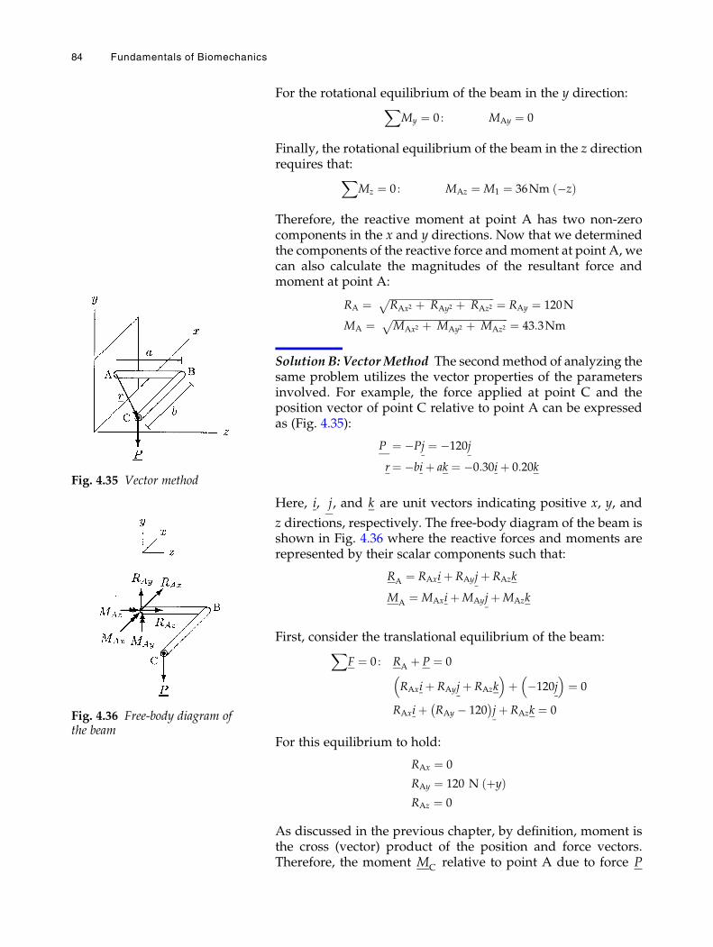
For the rotational equilibrium of the beam in the y direction:XMy ¼ 0 : MAy ¼ 0
Finally, the rotational equilibrium of the beam in the z directionrequires that:X
Mz ¼ 0 : MAz ¼M1 ¼ 36Nm �zð Þ
Therefore, the reactive moment at point A has two non-zerocomponents in the x and y directions. Now that we determinedthe components of the reactive force andmoment at point A, wecan also calculate the magnitudes of the resultant force andmoment at point A:
RA ¼ffiffiffiffiffiffiffiffiffiffiffiffiffiffiffiffiffiffiffiffiffiffiffiffiffiffiffiffiffiffiffiffiffiffiffiffiffiffiffiffiffiffiRAx2 þ RAy2 þ RAz2
p ¼ RAy ¼ 120N
MA ¼ffiffiffiffiffiffiffiffiffiffiffiffiffiffiffiffiffiffiffiffiffiffiffiffiffiffiffiffiffiffiffiffiffiffiffiffiffiffiffiffiffiffiffiffiffiffiMAx2 þ MAy2 þ MAz2
p ¼ 43:3Nm
Solution B: VectorMethod The secondmethod of analyzing thesame problem utilizes the vector properties of the parametersinvolved. For example, the force applied at point C and theposition vector of point C relative to point A can be expressedas (Fig. 4.35):
P ¼ �Pj ¼ �120jr¼ �biþ ak ¼ �0:30iþ 0:20k
Here, i, j, and k are unit vectors indicating positive x, y, and
z directions, respectively. The free-body diagram of the beam isshown in Fig. 4.36 where the reactive forces and moments arerepresented by their scalar components such that:
RA ¼ RAxiþ RAyjþ RAzk
MA ¼MAxiþMAyjþMAzk
First, consider the translational equilibrium of the beam:XF ¼ 0 : RA þ P ¼ 0
RAxiþ RAyjþ RAzk� �
þ �120j� �
¼ 0
RAxiþ RAy � 120� �
jþ RAzk ¼ 0
For this equilibrium to hold:
RAx ¼ 0
RAy ¼ 120 N þyð ÞRAz ¼ 0
As discussed in the previous chapter, by definition, moment isthe cross (vector) product of the position and force vectors.Therefore, the moment MC relative to point A due to force P
Fig. 4.35 Vector method
Fig. 4.36 Free-body diagram ofthe beam
84 Fundamentals of Biomechanics
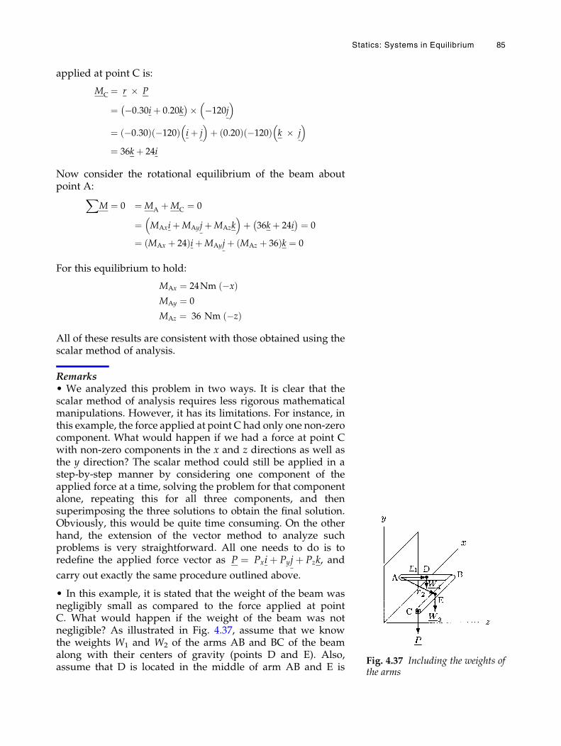
applied at point C is:
MC ¼ r � P
¼ �0:30iþ 0:20k� �� �120j
� �
¼ �0:30ð Þ �120ð Þ iþ j� �
þ 0:20ð Þ �120ð Þ k � j� �
¼ 36kþ 24i
Now consider the rotational equilibrium of the beam aboutpoint A:X
M ¼ 0 ¼MA þMC ¼ 0
¼ MAxiþMAyjþMAzk� �
þ 36kþ 24i� � ¼ 0
¼ MAx þ 24ð ÞiþMAyjþ MAz þ 36ð Þk ¼ 0
For this equilibrium to hold:
MAx ¼ 24Nm �xð ÞMAy ¼ 0
MAz ¼ 36 Nm �zð Þ
All of these results are consistent with those obtained using thescalar method of analysis.
Remarks• We analyzed this problem in two ways. It is clear that thescalar method of analysis requires less rigorous mathematicalmanipulations. However, it has its limitations. For instance, inthis example, the force applied at point C had only one non-zerocomponent. What would happen if we had a force at point Cwith non-zero components in the x and z directions as well asthe y direction? The scalar method could still be applied in astep-by-step manner by considering one component of theapplied force at a time, solving the problem for that componentalone, repeating this for all three components, and thensuperimposing the three solutions to obtain the final solution.Obviously, this would be quite time consuming. On the otherhand, the extension of the vector method to analyze suchproblems is very straightforward. All one needs to do is toredefine the applied force vector as P ¼ Pxiþ Pyjþ Pzk, and
carry out exactly the same procedure outlined above.
• In this example, it is stated that the weight of the beam wasnegligibly small as compared to the force applied at pointC. What would happen if the weight of the beam was notnegligible? As illustrated in Fig. 4.37, assume that we knowthe weights W1 and W2 of the arms AB and BC of the beamalong with their centers of gravity (points D and E). Also,assume that D is located in the middle of arm AB and E is
Fig. 4.37 Including the weights ofthe arms
Statics: Systems in Equilibrium 85
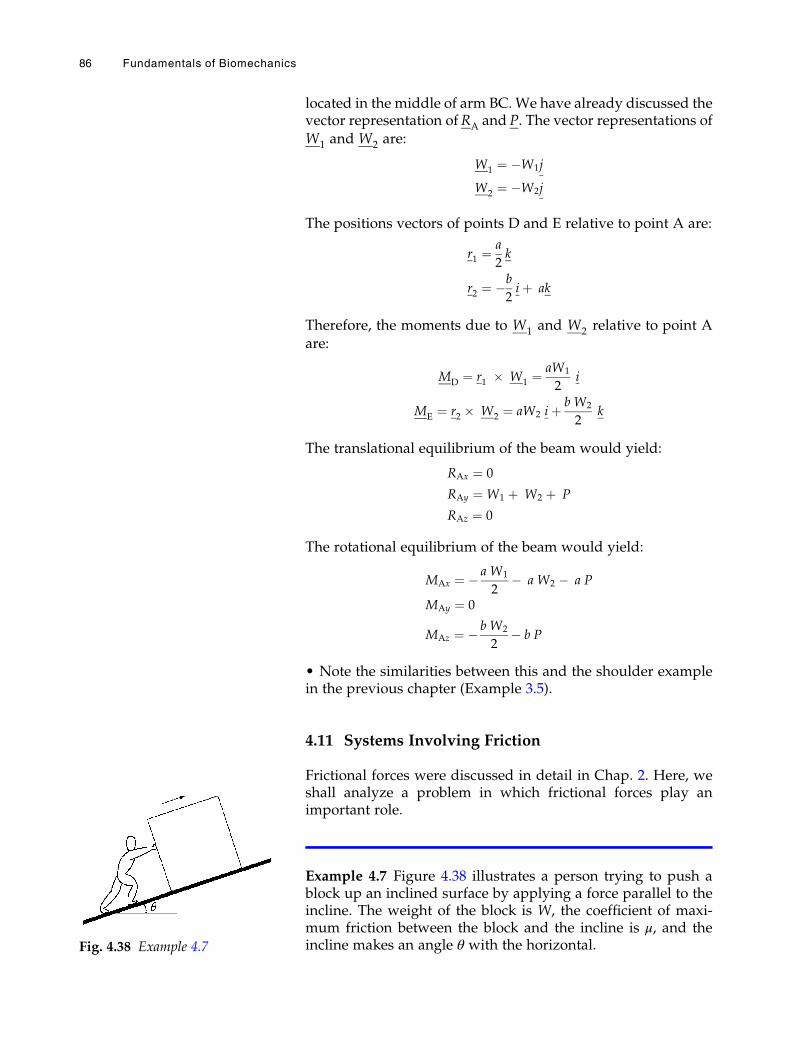
located in the middle of arm BC. We have already discussed thevector representation ofRA and P. The vector representations ofW1 and W2 are:
W1 ¼ �W1j
W2 ¼ �W2j
The positions vectors of points D and E relative to point A are:
r1 ¼a
2k
r2 ¼ �b
2iþ ak
Therefore, the moments due to W1 and W2 relative to point Aare:
MD ¼ r1 � W1 ¼aW1
2i
ME ¼ r2 � W2 ¼ aW2 iþ b W2
2k
The translational equilibrium of the beam would yield:
RAx ¼ 0
RAy ¼W1 þ W2 þ P
RAz ¼ 0
The rotational equilibrium of the beam would yield:
MAx ¼ � a W1
2� a W2 � a P
MAy ¼ 0
MAz ¼ � b W2
2� b P
• Note the similarities between this and the shoulder examplein the previous chapter (Example 3.5).
4.11 Systems Involving Friction
Frictional forces were discussed in detail in Chap. 2. Here, weshall analyze a problem in which frictional forces play animportant role.
Example 4.7 Figure 4.38 illustrates a person trying to push ablock up an inclined surface by applying a force parallel to theincline. The weight of the block is W, the coefficient of maxi-mum friction between the block and the incline is μ, and theincline makes an angle θ with the horizontal.Fig. 4.38 Example 4.7
86 Fundamentals of Biomechanics
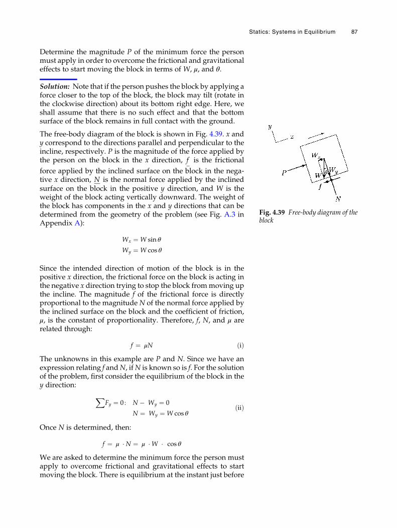
Determine the magnitude P of the minimum force the personmust apply in order to overcome the frictional and gravitationaleffects to start moving the block in terms of W, μ, and θ.
Solution: Note that if the person pushes the block by applying aforce closer to the top of the block, the block may tilt (rotate inthe clockwise direction) about its bottom right edge. Here, weshall assume that there is no such effect and that the bottomsurface of the block remains in full contact with the ground.
The free-body diagram of the block is shown in Fig. 4.39. x andy correspond to the directions parallel and perpendicular to theincline, respectively. P is the magnitude of the force applied bythe person on the block in the x direction, f is the frictional
force applied by the inclined surface on the block in the nega-tive x direction, N is the normal force applied by the inclinedsurface on the block in the positive y direction, and W is theweight of the block acting vertically downward. The weight ofthe block has components in the x and y directions that can bedetermined from the geometry of the problem (see Fig. A.3 inAppendix A):
Wx ¼W sin θ
Wy ¼W cos θ
Since the intended direction of motion of the block is in thepositive x direction, the frictional force on the block is acting inthe negative x direction trying to stop the block frommoving upthe incline. The magnitude f of the frictional force is directlyproportional to the magnitude N of the normal force applied bythe inclined surface on the block and the coefficient of friction,μ, is the constant of proportionality. Therefore, f, N, and μ arerelated through:
f ¼ μN ðiÞThe unknowns in this example are P and N. Since we have anexpression relating f andN, ifN is known so is f. For the solutionof the problem, first consider the equilibrium of the block in they direction:
XFy ¼ 0 : N � Wy ¼ 0
N ¼ Wy ¼W cos θðiiÞ
Once N is determined, then:
f ¼ μ �N ¼ μ �W � cos θ
We are asked to determine the minimum force the person mustapply to overcome frictional and gravitational effects to startmoving the block. There is equilibrium at the instant just before
Fig. 4.39 Free-body diagram of theblock
Statics: Systems in Equilibrium 87
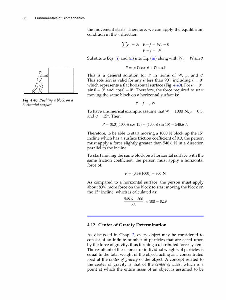
the movement starts. Therefore, we can apply the equilibriumcondition in the x direction:
XFx ¼ 0 : P� f � Wx ¼ 0
P ¼ f þ Wx
Substitute Eqs. (i) and (ii) into Eq. (iii) along withWx ¼W sin θ:
P ¼ μ W cos θ þW sin θ
This is a general solution for P in terms of W, μ, and θ.This solution is valid for any θ less than 90�, including θ ¼ 0�
which represents a flat horizontal surface (Fig. 4.40). For θ ¼ 0�,sin 0 ¼ 0� and cos 0 ¼ 0�. Therefore, the force required to startmoving the same block on a horizontal surface is:
P ¼ f ¼ μW
To have a numerical example, assume thatW ¼ 1000 N,μ ¼ 0:3,and θ ¼ 15�. Then:
P ¼ 0:3ð Þ 1000ð Þ cos 15ð Þ þ 1000ð Þ sin 15ð Þ ¼ 548:6 N
Therefore, to be able to start moving a 1000 N block up the 15�
incline which has a surface friction coefficient of 0.3, the personmust apply a force slightly greater than 548.6 N in a directionparallel to the incline.
To start moving the same block on a horizontal surface with thesame friction coefficient, the person must apply a horizontalforce of:
P ¼ 0:3ð Þ 1000ð Þ ¼ 300 N
As compared to a horizontal surface, the person must applyabout 83% more force on the block to start moving the block onthe 15� incline, which is calculated as:
548:6� 300
300� 100 ¼ 82:9
4.12 Center of Gravity Determination
As discussed in Chap. 2, every object may be considered toconsist of an infinite number of particles that are acted uponby the force of gravity, thus forming a distributed force system.The resultant of these forces or individual weights of particles isequal to the total weight of the object, acting as a concentratedload at the center of gravity of the object. A concept related tothe center of gravity is that of the center of mass, which is apoint at which the entire mass of an object is assumed to be
Fig. 4.40 Pushing a block on ahorizontal surface
88 Fundamentals of Biomechanics
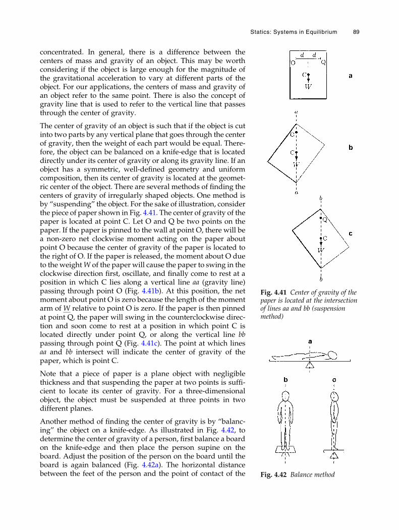
concentrated. In general, there is a difference between thecenters of mass and gravity of an object. This may be worthconsidering if the object is large enough for the magnitude ofthe gravitational acceleration to vary at different parts of theobject. For our applications, the centers of mass and gravity ofan object refer to the same point. There is also the concept ofgravity line that is used to refer to the vertical line that passesthrough the center of gravity.
The center of gravity of an object is such that if the object is cutinto two parts by any vertical plane that goes through the centerof gravity, then the weight of each part would be equal. There-fore, the object can be balanced on a knife-edge that is locateddirectly under its center of gravity or along its gravity line. If anobject has a symmetric, well-defined geometry and uniformcomposition, then its center of gravity is located at the geomet-ric center of the object. There are several methods of finding thecenters of gravity of irregularly shaped objects. One method isby “suspending” the object. For the sake of illustration, considerthe piece of paper shown in Fig. 4.41. The center of gravity of thepaper is located at point C. Let O and Q be two points on thepaper. If the paper is pinned to the wall at point O, there will bea non-zero net clockwise moment acting on the paper aboutpoint O because the center of gravity of the paper is located tothe right of O. If the paper is released, the moment about O dueto the weightW of the paper will cause the paper to swing in theclockwise direction first, oscillate, and finally come to rest at aposition in which C lies along a vertical line aa (gravity line)passing through point O (Fig. 4.41b). At this position, the netmoment about point O is zero because the length of the momentarm ofW relative to point O is zero. If the paper is then pinnedat point Q, the paper will swing in the counterclockwise direc-tion and soon come to rest at a position in which point C islocated directly under point Q, or along the vertical line bbpassing through point Q (Fig. 4.41c). The point at which linesaa and bb intersect will indicate the center of gravity of thepaper, which is point C.
Note that a piece of paper is a plane object with negligiblethickness and that suspending the paper at two points is suffi-cient to locate its center of gravity. For a three-dimensionalobject, the object must be suspended at three points in twodifferent planes.
Another method of finding the center of gravity is by “balanc-ing” the object on a knife-edge. As illustrated in Fig. 4.42, todetermine the center of gravity of a person, first balance a boardon the knife-edge and then place the person supine on theboard. Adjust the position of the person on the board until theboard is again balanced (Fig. 4.42a). The horizontal distancebetween the feet of the person and the point of contact of the
Fig. 4.41 Center of gravity of thepaper is located at the intersectionof lines aa and bb (suspensionmethod)
Fig. 4.42 Balance method
Statics: Systems in Equilibrium 89
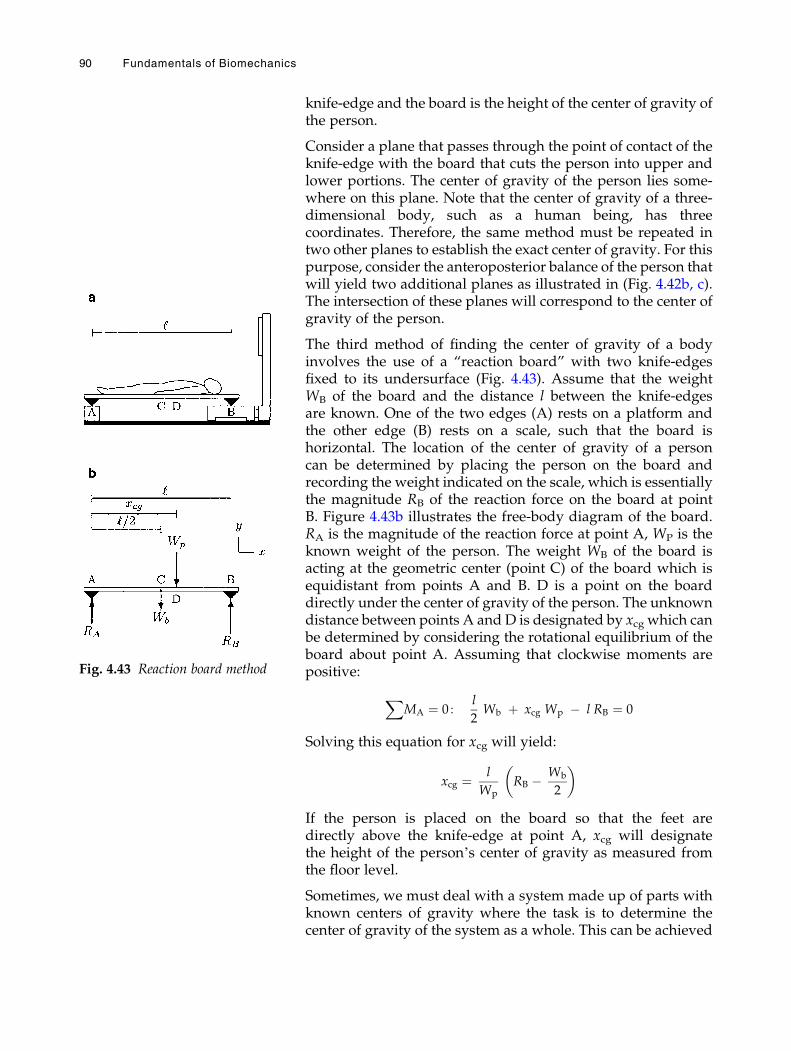
knife-edge and the board is the height of the center of gravity ofthe person.
Consider a plane that passes through the point of contact of theknife-edge with the board that cuts the person into upper andlower portions. The center of gravity of the person lies some-where on this plane. Note that the center of gravity of a three-dimensional body, such as a human being, has threecoordinates. Therefore, the same method must be repeated intwo other planes to establish the exact center of gravity. For thispurpose, consider the anteroposterior balance of the person thatwill yield two additional planes as illustrated in (Fig. 4.42b, c).The intersection of these planes will correspond to the center ofgravity of the person.
The third method of finding the center of gravity of a bodyinvolves the use of a “reaction board” with two knife-edgesfixed to its undersurface (Fig. 4.43). Assume that the weightWB of the board and the distance l between the knife-edgesare known. One of the two edges (A) rests on a platform andthe other edge (B) rests on a scale, such that the board ishorizontal. The location of the center of gravity of a personcan be determined by placing the person on the board andrecording the weight indicated on the scale, which is essentiallythe magnitude RB of the reaction force on the board at pointB. Figure 4.43b illustrates the free-body diagram of the board.RA is the magnitude of the reaction force at point A, WP is theknown weight of the person. The weight WB of the board isacting at the geometric center (point C) of the board which isequidistant from points A and B. D is a point on the boarddirectly under the center of gravity of the person. The unknowndistance between points A and D is designated by xcg which canbe determined by considering the rotational equilibrium of theboard about point A. Assuming that clockwise moments arepositive:
XMA ¼ 0 :
l
2Wb þ xcg Wp � l RB ¼ 0
Solving this equation for xcg will yield:
xcg ¼ l
WpRB � Wb
2
� �
If the person is placed on the board so that the feet aredirectly above the knife-edge at point A, xcg will designatethe height of the person’s center of gravity as measured fromthe floor level.
Sometimes, we must deal with a system made up of parts withknown centers of gravity where the task is to determine thecenter of gravity of the system as a whole. This can be achieved
Fig. 4.43 Reaction board method
90 Fundamentals of Biomechanics
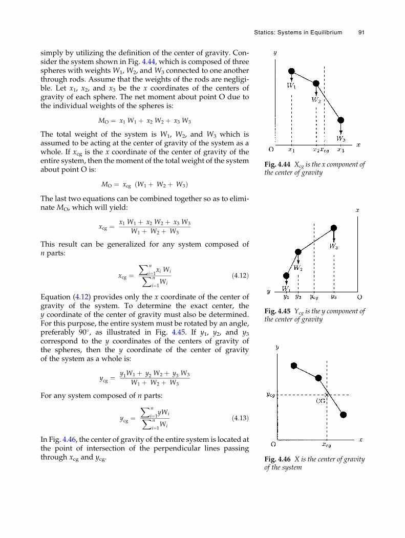
simply by utilizing the definition of the center of gravity. Con-sider the system shown in Fig. 4.44, which is composed of threespheres with weightsW1, W2, and W3 connected to one anotherthrough rods. Assume that the weights of the rods are negligi-ble. Let x1, x2, and x3 be the x coordinates of the centers ofgravity of each sphere. The net moment about point O due tothe individual weights of the spheres is:
MO ¼ x1 W1 þ x2 W2 þ x3 W3
The total weight of the system is W1, W2, and W3 which isassumed to be acting at the center of gravity of the system as awhole. If xcg is the x coordinate of the center of gravity of theentire system, then the moment of the total weight of the systemabout point O is:
MO ¼ xcg W1 þ W2 þ W3ð ÞThe last two equations can be combined together so as to elimi-nate MO, which will yield:
xcg ¼ x1 W1 þ x2 W2 þ x3 W3
W1 þ W2 þ W3
This result can be generalized for any system composed ofn parts:
xcg ¼Xn
i¼1xi WiXn
i¼1Wi
ð4:12Þ
Equation (4.12) provides only the x coordinate of the center ofgravity of the system. To determine the exact center, they coordinate of the center of gravity must also be determined.For this purpose, the entire system must be rotated by an angle,preferably 90�, as illustrated in Fig. 4.45. If y1, y2, and y3correspond to the y coordinates of the centers of gravity ofthe spheres, then the y coordinate of the center of gravityof the system as a whole is:
ycg ¼y1W1 þ y2 W2 þ y3 W3
W1 þ W2 þ W3
For any system composed of n parts:
ycg ¼Xn
i¼1yWiXn
i¼1Wi
ð4:13Þ
In Fig. 4.46, the center of gravity of the entire system is located atthe point of intersection of the perpendicular lines passingthrough xcg and ycg.
Fig. 4.44 Xcg is the x component ofthe center of gravity
Fig. 4.45 Ycg is the y component ofthe center of gravity
Fig. 4.46 X is the center of gravityof the system
Statics: Systems in Equilibrium 91
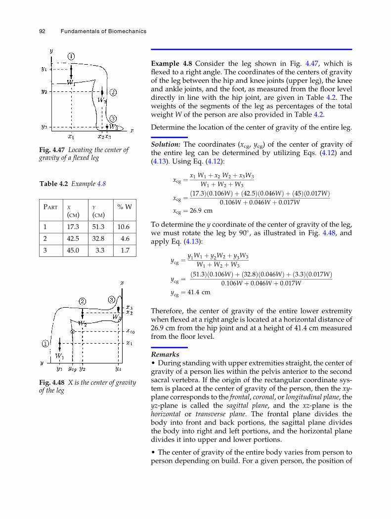
Example 4.8 Consider the leg shown in Fig. 4.47, which isflexed to a right angle. The coordinates of the centers of gravityof the leg between the hip and knee joints (upper leg), the kneeand ankle joints, and the foot, as measured from the floor leveldirectly in line with the hip joint, are given in Table 4.2. Theweights of the segments of the leg as percentages of the totalweight W of the person are also provided in Table 4.2.
Determine the location of the center of gravity of the entire leg.
Solution: The coordinates (xcg, ycg) of the center of gravity ofthe entire leg can be determined by utilizing Eqs. (4.12) and(4.13). Using Eq. (4.12):
xcg ¼ x1 W1 þ x2 W2 þ x3W3
W1 þW2 þW3
xcg ¼ 17:3ð Þ 0:106Wð Þ þ 42:5ð Þ 0:046Wð Þ þ 45ð Þ 0:017Wð Þ0:106W þ 0:046W þ 0:017W
xcg ¼ 26:9 cm
To determine the y coordinate of the center of gravity of the leg,we must rotate the leg by 90�, as illustrated in Fig. 4.48, andapply Eq. (4.13):
ycg ¼y1W1 þ y2W2 þ y3W3
W1 þW2 þW3
ycg ¼51:3ð Þ 0:106Wð Þ þ 32:8ð Þ 0:046Wð Þ þ 3:3ð Þ 0:017Wð Þ
0:106W þ 0:046W þ 0:017W
ycg ¼ 41:4 cm
Therefore, the center of gravity of the entire lower extremitywhen flexed at a right angle is located at a horizontal distance of26.9 cm from the hip joint and at a height of 41.4 cm measuredfrom the floor level.
Remarks• During standing with upper extremities straight, the center ofgravity of a person lies within the pelvis anterior to the secondsacral vertebra. If the origin of the rectangular coordinate sys-tem is placed at the center of gravity of the person, then the xy-plane corresponds to the frontal, coronal, or longitudinal plane, theyz-plane is called the sagittal plane, and the xz-plane is thehorizontal or transverse plane. The frontal plane divides thebody into front and back portions, the sagittal plane dividesthe body into right and left portions, and the horizontal planedivides it into upper and lower portions.
• The center of gravity of the entire body varies from person toperson depending on build. For a given person, the position of
Fig. 4.47 Locating the center ofgravity of a flexed leg
Table 4.2 Example 4.8
PART X
(CM)Y
(CM)% W
1 17.3 51.3 10.6
2 42.5 32.8 4.6
3 45.0 3.3 1.7
Fig. 4.48 X is the center of gravityof the leg
92 Fundamentals of Biomechanics
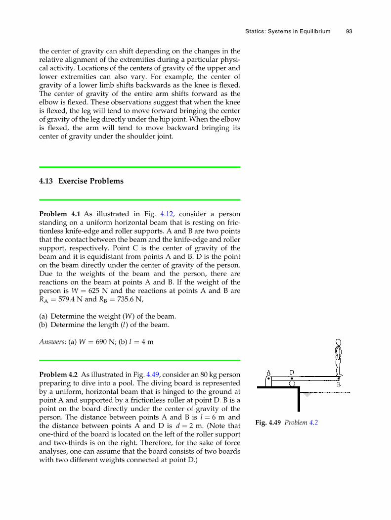
the center of gravity can shift depending on the changes in therelative alignment of the extremities during a particular physi-cal activity. Locations of the centers of gravity of the upper andlower extremities can also vary. For example, the center ofgravity of a lower limb shifts backwards as the knee is flexed.The center of gravity of the entire arm shifts forward as theelbow is flexed. These observations suggest that when the kneeis flexed, the leg will tend to move forward bringing the centerof gravity of the leg directly under the hip joint. When the elbowis flexed, the arm will tend to move backward bringing itscenter of gravity under the shoulder joint.
4.13 Exercise Problems
Problem 4.1 As illustrated in Fig. 4.12, consider a personstanding on a uniform horizontal beam that is resting on fric-tionless knife-edge and roller supports. A and B are two pointsthat the contact between the beam and the knife-edge and rollersupport, respectively. Point C is the center of gravity of thebeam and it is equidistant from points A and B. D is the pointon the beam directly under the center of gravity of the person.Due to the weights of the beam and the person, there arereactions on the beam at points A and B. If the weight of theperson is W ¼ 625 N and the reactions at points A and B areRA ¼ 579.4 N and RB ¼ 735.6 N,
(a) Determine the weight (W) of the beam.(b) Determine the length (l) of the beam.
Answers: (a) W ¼ 690 N; (b) l ¼ 4 m
Problem 4.2 As illustrated in Fig. 4.49, consider an 80 kg personpreparing to dive into a pool. The diving board is representedby a uniform, horizontal beam that is hinged to the ground atpoint A and supported by a frictionless roller at point D. B is apoint on the board directly under the center of gravity of theperson. The distance between points A and B is l ¼ 6 m andthe distance between points A and D is d ¼ 2 m. (Note thatone-third of the board is located on the left of the roller supportand two-thirds is on the right. Therefore, for the sake of forceanalyses, one can assume that the board consists of two boardswith two different weights connected at point D.)
Fig. 4.49 Problem 4.2
Statics: Systems in Equilibrium 93
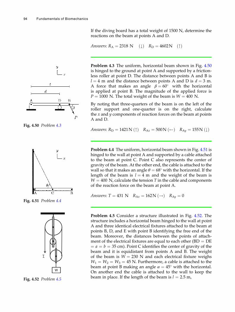
If the diving board has a total weight of 1500 N, determine thereactions on the beam at points A and D.
Answers: RA ¼ 2318 N #ð Þ RD ¼ 4602N "ð Þ
Problem 4.3 The uniform, horizontal beam shown in Fig. 4.50is hinged to the ground at point A and supported by a friction-less roller at point D. The distance between points A and B isl ¼ 4 m and the distance between points A and D is d ¼ 3 m.A force that makes an angle β ¼ 60� with the horizontalis applied at point B. The magnitude of the applied force isP ¼ 1000 N. The total weight of the beam is W ¼ 400 N.
By noting that three-quarters of the beam is on the left of theroller support and one-quarter is on the right, calculatethe x and y components of reaction forces on the beam at pointsA and D.
Answers: RD ¼ 1421N "ð Þ RAx ¼ 500N ð Þ RAy ¼ 155N #ð Þ
Problem 4.4 The uniform, horizontal beam shown in Fig. 4.51 ishinged to the wall at point A and supported by a cable attachedto the beam at point C. Point C also represents the center ofgravity of the beam. At the other end, the cable is attached to thewall so that it makes an angle θ ¼ 68� with the horizontal. If thelength of the beam is l ¼ 4 m and the weight of the beam isW ¼ 400 N, calculate the tension T in the cable and componentsof the reaction force on the beam at point A.
Answers: T ¼ 431 N RAx ¼ 162N !ð Þ RAy ¼ 0
Problem 4.5 Consider a structure illustrated in Fig. 4.52. Thestructure includes a horizontal beam hinged to the wall at pointA and three identical electrical fixtures attached to the beam atpoints B, D, and E with point B identifying the free end of thebeam. Moreover, the distances between the points of attach-ment of the electrical fixtures are equal to each other (BD ¼ DE¼ a ¼ b ¼ 35 cm). Point C identifies the center of gravity of thebeam and it is equidistant from points A and B. The weightof the beam is W ¼ 230 N and each electrical fixture weighsW1 ¼ W2 ¼ W3 ¼ 45 N. Furthermore, a cable is attached to thebeam at point B making an angle α ¼ 45� with the horizontal.On another end the cable is attached to the wall to keep thebeam in place. If the length of the beam is l ¼ 2.5 m,
Fig. 4.50 Problem 4.3
Fig. 4.51 Problem 4.4
W
T
Fig. 4.52 Problem 4.5
94 Fundamentals of Biomechanics
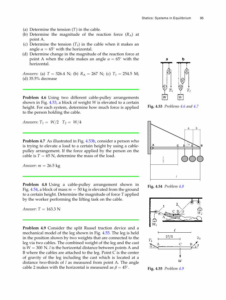
(a) Determine the tension (T) in the cable.(b) Determine the magnitude of the reaction force (RA) at
point A.(c) Determine the tension (T1) in the cable when it makes an
angle α ¼ 65� with the horizontal.(d) Determine change in the magnitude of the reaction force at
point A when the cable makes an angle α ¼ 65� with thehorizontal.
Answers: (a) T ¼ 326.4 N; (b) RA ¼ 267 N; (c) T1 ¼ 254.5 M;(d) 35.5% decrease
Problem 4.6 Using two different cable-pulley arrangementsshown in Fig. 4.53, a block of weight W is elevated to a certainheight. For each system, determine how much force is appliedto the person holding the cable.
Answers: T1 ¼ W=2 T2 ¼ W=4
Problem 4.7 As illustrated in Fig. 4.53b, consider a person whois trying to elevate a load to a certain height by using a cable-pulley arrangement. If the force applied by the person on thecable is T ¼ 65 N, determine the mass of the load.
Answer: m ¼ 26.5 kg
Problem 4.8 Using a cable-pulley arrangement shown inFig. 4.54, a block of massm ¼ 50 kg is elevated from the groundto a certain height. Determine the magnitude of force T appliedby the worker performing the lifting task on the cable.
Answer: T ¼ 163.3 N
Problem 4.9 Consider the split Russel traction device and amechanical model of the leg shown in Fig. 4.55. The leg is heldin the position shown by two weights that are connected to theleg via two cables. The combined weight of the leg and the castisW ¼ 300 N. l is the horizontal distance between points A andB where the cables are attached to the leg. Point C is the centerof gravity of the leg including the cast which is located at adistance two-thirds of l as measured from point A. The anglecable 2 makes with the horizontal is measured as β ¼ 45�.
Fig. 4.53 Problems 4.6 and 4.7
A C D E B
· · · ·
a b
α
2
Fig. 4.54 Problem 4.8
Fig. 4.55 Problem 4.9
Statics: Systems in Equilibrium 95
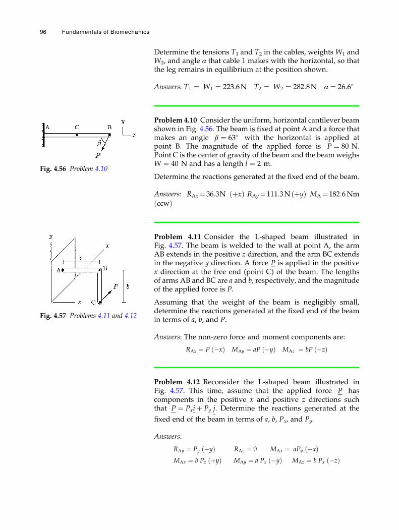
Determine the tensions T1 and T2 in the cables, weights W1 andW2, and angle α that cable 1 makes with the horizontal, so thatthe leg remains in equilibrium at the position shown.
Answers: T1 ¼ W1 ¼ 223:6N T2 ¼ W2 ¼ 282:8N α ¼ 26:6�
Problem 4.10 Consider the uniform, horizontal cantilever beamshown in Fig. 4.56. The beam is fixed at point A and a force thatmakes an angle β ¼ 63� with the horizontal is applied atpoint B. The magnitude of the applied force is P ¼ 80 N.Point C is the center of gravity of the beam and the beamweighsW ¼ 40 N and has a length l ¼ 2 m.
Determine the reactions generated at the fixed end of the beam.
Answers: RAx¼36:3N þxð Þ RAy¼111:3N þyð Þ MA¼182:6Nm
ccwð Þ
Problem 4.11 Consider the L-shaped beam illustrated inFig. 4.57. The beam is welded to the wall at point A, the armAB extends in the positive z direction, and the arm BC extendsin the negative y direction. A force P is applied in the positivex direction at the free end (point C) of the beam. The lengthsof arms AB and BC are a and b, respectively, and the magnitudeof the applied force is P.
Assuming that the weight of the beam is negligibly small,determine the reactions generated at the fixed end of the beamin terms of a, b, and P.
Answers: The non-zero force and moment components are:
RAx ¼ P �xð Þ MAy ¼ aP �yð Þ MAz ¼ bP �zð Þ
Problem 4.12 Reconsider the L-shaped beam illustrated inFig. 4.57. This time, assume that the applied force P hascomponents in the positive x and positive z directions suchthat P ¼ Pxiþ Py j. Determine the reactions generated at the
fixed end of the beam in terms of a, b, Px, and Py.
Answers:
RAy ¼ Py �yð Þ RAz ¼ 0 MAx ¼ aPy þxð ÞMAx ¼ b Pz þyð Þ MAy ¼ a Px �yð Þ MAz ¼ b Px �zð Þ
Fig. 4.56 Problem 4.10
Fig. 4.57 Problems 4.11 and 4.12
96 Fundamentals of Biomechanics
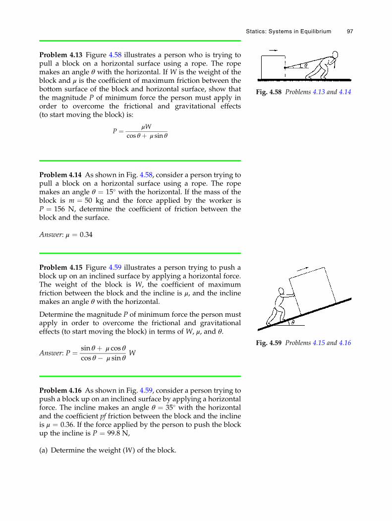
Problem 4.13 Figure 4.58 illustrates a person who is trying topull a block on a horizontal surface using a rope. The ropemakes an angle θ with the horizontal. If W is the weight of theblock and μ is the coefficient of maximum friction between thebottom surface of the block and horizontal surface, show thatthe magnitude P of minimum force the person must apply inorder to overcome the frictional and gravitational effects(to start moving the block) is:
P ¼ μW
cos θ þ μ sin θ
Problem 4.14 As shown in Fig. 4.58, consider a person trying topull a block on a horizontal surface using a rope. The ropemakes an angle θ ¼ 15� with the horizontal. If the mass of theblock is m ¼ 50 kg and the force applied by the worker isP ¼ 156 N, determine the coefficient of friction between theblock and the surface.
Answer: μ ¼ 0.34
Problem 4.15 Figure 4.59 illustrates a person trying to push ablock up on an inclined surface by applying a horizontal force.The weight of the block is W, the coefficient of maximumfriction between the block and the incline is μ, and the inclinemakes an angle θ with the horizontal.
Determine the magnitude P of minimum force the person mustapply in order to overcome the frictional and gravitationaleffects (to start moving the block) in terms of W, μ, and θ.
Answer: P ¼ sin θ þ μ cos θ
cos θ � μ sin θW
Problem 4.16 As shown in Fig. 4.59, consider a person trying topush a block up on an inclined surface by applying a horizontalforce. The incline makes an angle θ ¼ 35� with the horizontaland the coefficient pf friction between the block and the inclineis μ ¼ 0.36. If the force applied by the person to push the blockup the incline is P ¼ 99.8 N,
(a) Determine the weight (W) of the block.
Fig. 4.59 Problems 4.15 and 4.16
Fig. 4.58 Problems 4.13 and 4.14
Statics: Systems in Equilibrium 97
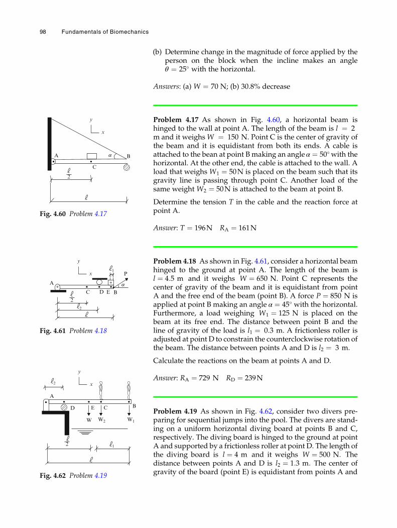
(b) Determine change in the magnitude of force applied by theperson on the block when the incline makes an angleθ ¼ 25� with the horizontal.
Answers: (a) W ¼ 70 N; (b) 30.8% decrease
Problem 4.17 As shown in Fig. 4.60, a horizontal beam ishinged to the wall at point A. The length of the beam is l ¼ 2m and it weighsW ¼ 150 N. Point C is the center of gravity ofthe beam and it is equidistant from both its ends. A cable isattached to the bean at point B making an angleα ¼ 50�with thehorizontal. At the other end, the cable is attached to the wall. Aload that weighs W1 ¼ 50N is placed on the beam such that itsgravity line is passing through point C. Another load of thesame weight W2 ¼ 50N is attached to the beam at point B.
Determine the tension T in the cable and the reaction force atpoint A.
Answer: T ¼ 196N RA ¼ 161N
Problem 4.18 As shown in Fig. 4.61, consider a horizontal beamhinged to the ground at point A. The length of the beam isl ¼ 4:5 m and it weighs W ¼ 650 N. Point C represents thecenter of gravity of the beam and it is equidistant from pointA and the free end of the beam (point B). A force P ¼ 850 N isapplied at point B making an angle α ¼ 45� with the horizontal.Furthermore, a load weighing W1 ¼ 125 N is placed on thebeam at its free end. The distance between point B and theline of gravity of the load is l1 ¼ 0:3 m. A frictionless roller isadjusted at point D to constrain the counterclockwise rotation ofthe beam. The distance between points A and D is l2 ¼ 3 m.
Calculate the reactions on the beam at points A and D.
Answer: RA ¼ 729 N RD ¼ 239N
Problem 4.19 As shown in Fig. 4.62, consider two divers pre-paring for sequential jumps into the pool. The divers are stand-ing on a uniform horizontal diving board at points B and C,respectively. The diving board is hinged to the ground at pointA and supported by a frictionless roller at point D. The length ofthe diving board is l ¼ 4 m and it weighs W ¼ 500 N: Thedistance between points A and D is l2 ¼ 1:3 m: The center ofgravity of the board (point E) is equidistant from points A and
x
y
A
C
2
Ba
Fig. 4.60 Problem 4.17
x
y
2
1
2
A
C D E B
P
a
Fig. 4.61 Problem 4.18
2 x
y
2 1
A
CD E
W
B
W1W2
Fig. 4.62 Problem 4.19
98 Fundamentals of Biomechanics
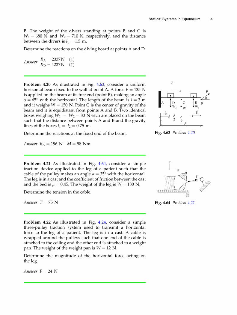
B. The weight of the divers standing at points B and C isW1 ¼ 680 N and W2 ¼ 710 N, respectively, and the distancebetween the divers is l1 ¼ 1:5 m:
Determine the reactions on the diving board at points A and D.
Answer:RA ¼ 2337N #ð ÞRD ¼ 4227N "ð Þ
Problem 4.20 As illustrated in Fig. 4.63, consider a uniformhorizontal beam fixed to the wall at point A. A force F ¼ 135 Nis applied on the beam at its free end (point B), making an angleα ¼ 65� with the horizontal. The length of the beam is l ¼ 3 mand it weighs W ¼ 150 N. Point C is the center of gravity of thebeam and it is equidistant from points A and B. Two identicalboxes weighing W1 ¼ W2 ¼ 80 N each are placed on the beamsuch that the distance between points A and B and the gravitylines of the boxes l1 ¼ l2 ¼ 0:75 m:
Determine the reactions at the fixed end of the beam.
Answer: RA ¼ 196 N M ¼ 98 Nm
Problem 4.21 As illustrated in Fig. 4.64, consider a simpletraction device applied to the leg of a patient such that thecable of the pulley makes an angle α ¼ 35� with the horizontal.The leg is in a cast and the coefficient of friction between the castand the bed is μ ¼ 0:45. The weight of the leg is W ¼ 180 N:
Determine the tension in the cable.
Answer: T ¼ 75 N
Problem 4.22 As illustrated in Fig. 4.24, consider a simplethree-pulley traction system used to transmit a horizontalforce to the leg of a patient. The leg is in a cast. A cable iswrapped around the pulleys such that one end of the cable isattached to the ceiling and the other end is attached to a weightpan. The weight of the weight pan is W ¼ 12 N.
Determine the magnitude of the horizontal force acting onthe leg.
Answer: F ¼ 24 N
2
2
1
a
A D C E
W W1W2
B
x
y
F
Fig. 4.63 Problem 4.20
x
y
aT
Fig. 4.64 Problem 4.21
Statics: Systems in Equilibrium 99
Chapter 5
Applications of Staticsto Biomechanics
5.1 Skeletal Joints / 103
5.2 Skeletal Muscles / 104
5.3 Basic Considerations / 105
5.4 Basic Assumptions and Limitations / 106
5.5 Mechanics of the Elbow / 107
5.6 Mechanics of the Shoulder / 112
5.7 Mechanics of the Spinal Column / 116
5.8 Mechanics of the Hip / 121
5.9 Mechanics of the Knee / 128
5.10 Mechanics of the Ankle / 133
5.11 Exercise Problems / 135
References / 139
The original version of this chapter was revised. An erratum to this chapter can befound at https://doi.org/10.1007/978-3-319-44738-4_16
# Springer International Publishing Switzerland 2017N. Ozkaya et al., Fundamentals of Biomechanics, DOI 10.1007/978-3-319-44738-4_5
101

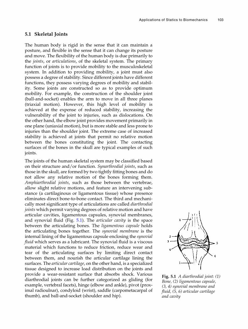
5.1 Skeletal Joints
The human body is rigid in the sense that it can maintain aposture, and flexible in the sense that it can change its postureand move. The flexibility of the human body is due primarily tothe joints, or articulations, of the skeletal system. The primaryfunction of joints is to provide mobility to the musculoskeletalsystem. In addition to providing mobility, a joint must alsopossess a degree of stability. Since different joints have differentfunctions, they possess varying degrees of mobility and stabil-ity. Some joints are constructed so as to provide optimummobility. For example, the construction of the shoulder joint(ball-and-socket) enables the arm to move in all three planes(triaxial motion). However, this high level of mobility isachieved at the expense of reduced stability, increasing thevulnerability of the joint to injuries, such as dislocations. Onthe other hand, the elbow joint provides movement primarily inone plane (uniaxial motion), but is more stable and less prone toinjuries than the shoulder joint. The extreme case of increasedstability is achieved at joints that permit no relative motionbetween the bones constituting the joint. The contactingsurfaces of the bones in the skull are typical examples of suchjoints.
The joints of the human skeletal system may be classified basedon their structure and/or function. Synarthrodial joints, such asthose in the skull, are formed by two tightly fitting bones and donot allow any relative motion of the bones forming them.Amphiarthrodial joints, such as those between the vertebrae,allow slight relative motions, and feature an intervening sub-stance (a cartilaginous or ligamentous tissue) whose presenceeliminates direct bone-to-bone contact. The third and mechani-cally most significant type of articulations are called diarthrodialjointswhich permit varying degrees of relative motion and havearticular cavities, ligamentous capsules, synovial membranes,and synovial fluid (Fig. 5.1). The articular cavity is the spacebetween the articulating bones. The ligamentous capsule holdsthe articulating bones together. The synovial membrane is theinternal lining of the ligamentous capsule enclosing the synovialfluid which serves as a lubricant. The synovial fluid is a viscousmaterial which functions to reduce friction, reduce wear andtear of the articulating surfaces by limiting direct contactbetween them, and nourish the articular cartilage lining thesurfaces. The articular cartilage, on the other hand, is a specializedtissue designed to increase load distribution on the joints andprovide a wear-resistant surface that absorbs shock. Variousdiarthrodial joints can be further categorized as gliding (forexample, vertebral facets), hinge (elbow and ankle), pivot (prox-imal radioulnar), condyloid (wrist), saddle (carpometacarpal ofthumb), and ball-and-socket (shoulder and hip).
Fig. 5.1 A diarthrodial joint: (1)Bone, (2) ligamentous capsule,(3, 4) synovial membrane andfluid, (5, 6) articular cartilageand cavity
Applications of Statics to Biomechanics 103
The nature of motion about a diarthrodial joint and the stabilityof the joint are dependent upon many factors, including themanner in which the articulating surfaces fit together, theproperties of the joint capsule, the structure and length of theligaments around the joint, and the number and orientation ofthe muscles crossing the joint.
5.2 Skeletal Muscles
In general, there are over 600 muscles in the human body,accounting for about 45� of the total body weight.
There are three types of muscles: cardiac, smooth, and skeletal.Cardiac muscle is the contractive tissue found in the heart thatpumps the blood for circulation. Smooth muscle is found in thestomach, intestinal tracts, and the walls of blood vessels. Skeletalmuscle is connected to the bones of the body and whencontracted, causes body segments to move.
Movement of human body segments is achieved as a result offorces generated by skeletal muscles that convert chemicalenergy into mechanical work. The structural unit of skeletalmuscle is the muscle fiber, which is composed of myofibrils.Myofibrils are made up of actin and myosin filaments. Musclesexhibit viscoelastic material behavior. That is, they have bothsolid and fluid-like material properties. Muscles are elastic inthe sense that when a muscle is stretched and released it willresume its original (unstretched) size and shape. Muscles areviscous in the sense that there is an internal resistance to motion.
A skeletal muscle is attached, via soft tissues such asaponeuroses and/or tendons, to at least two different bonescontrolling the relative motion of one segment with respect tothe other. When its fibers contract under the stimulation of anerve, the muscle exerts a pulling effect on the bones to whichit is attached. Contraction is a unique property of the muscletissue. In engineering mechanics, contraction impliesshortening under compressive forces. In muscle mechanics,contraction can occur as a result of muscle shortening or musclelengthening, or it can occur without any change in the musclelength. Furthermore, the result of amuscle contraction is alwaystension: a muscle can only exert a pull. Muscles cannot exerta push.
There are various types of muscle contractions: a concentriccontraction occurs simultaneously as the length of the muscledecreases (for example, the biceps during flexion of the fore-arm); a static contraction occurs while muscle length remainsconstant (the biceps when the forearm is flexed and held with-out any movement); and an eccentric contraction occurs as thelength of the muscle increases (the biceps during the extension
104 Fundamentals of Biomechanics
of the forearm). A muscle can cause movement only while itslength is shortening (concentric contraction). If the length of amuscle increases during a particular activity, then the tensiongenerated by the muscle contraction is aimed at controlling themovement of the body segments associated with that muscle(eccentric contraction). If a muscle contracts but there is nosegmental motion, then the tension in the muscle balances theeffects of applied forces such as those due to gravity (isometriccontraction).
The skeletal muscles can also be named according to thefunctions they serve during a particular activity. For example,a muscle is called agonist if it causes movement through theprocess of its own contraction. Agonist muscles are the primarymuscles responsible for generating a specific movement. Anantagonistmuscle opposes the action of anothermuscle. Synergicmuscle is that which assists the agonist muscle in performingthe same joint motion.
5.3 Basic Considerations
In this chapter, we want to apply the principles of statics toinvestigate the forces involved in various muscle groups andjoints for various postural positions of the human body and itssegments. Our immediate purpose is to provide answers toquestions such as: what tension must the neck extensor musclesexert on the head to support the head in a specified position?When a person bends, what would be the force exerted by theerector spinae on the fifth lumbar vertebra? How does thecompression at the elbow, knee, and ankle joints vary withexternally applied forces and with different segmentalarrangements? How does the force on the femoral head varywith loads carried in the hand? What are the forces involved invarious muscle groups and joints during different exerciseconditions?
The forces involved in the human body can be grouped asinternal and external. Internal forces are those associated withmuscles, ligaments, and tendons, and at the joints. Externallyapplied forces include the effect of gravitational acceleration onthe body or on its segments, manually and/or mechanicallyapplied forces on the body during exercise and stretching, andforces applied to the body by prostheses and implements. Ingeneral, the unknowns in static problems involving the muscu-loskeletal system are the joint reaction forces and muscletensions. Mechanical analysis of a joint requires that we knowthe vector characteristics of tension in the muscle including theproper locations of muscle attachments, the weights or massesof body segments, the centers of gravity of the body segments,and the anatomical axis of rotation of the joint.
Applications of Statics to Biomechanics 105
5.4 Basic Assumptions and Limitations
The complete analysis of muscle forces required to sustainvarious postural positions is difficult because of the complexarrangement of muscles within the human body and because oflimited information. In general, the relative motion of bodysegments about a given joint is controlled by more than onemuscle group. To be able to reduce a specific problem of biome-chanics to one that is statically determinate and apply theequations of equilibrium, only the muscle group that is theprimary source of control over the joint can be taken into con-sideration. Possible contributions of other muscle groups to theload-bearing mechanism of the joint must be ignored. Notehowever that approximations of the effect of other musclesmay be made by considering their cross-sectional areas andtheir relative positions in relation to the joint. Also, if the phasicactivity of muscles is known via some experiments such as theelectromyography (EMG) measurements of muscle signals,then the tension in different muscle groups may be estimated.
To apply the principles of statics to analyze the mechanics ofhuman joints, we shall adopt the following assumptions andlimitations:
• The anatomical axes of rotation of joints are known.
• The locations of muscle attachments are known.
• The line of action of muscle tension is known.
• Segmental weights and their centers of gravity are known.
• Frictional factors at the joints are negligible.
• Dynamic aspects of the problems will be ignored.
• Only two-dimensional problems will be considered.
These analyses require that the anthropometric data about thesegment to be analyzed must be available. For this purpose,there are tables listing anthropometric information includingaverage weights, lengths, and centers of gravity of bodysegments. See Chaffin, Andersson, and Martin (1999), andWinter (2004) for a review of the anthropometric data available.
It is clear from this discussion that we shall analyze certainidealized problems of biomechanics. Based on the resultsobtained and experience gained, these models may beexpanded by taking additional factors into consideration. How-ever, a given problem will become more complex as morefactors are considered.
106 Fundamentals of Biomechanics
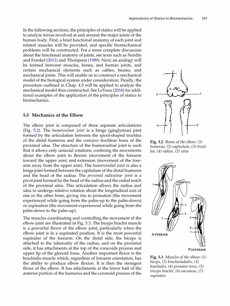
In the following sections, the principles of statics will be appliedto analyze forces involved at and around the major joints of thehuman body. First, a brief functional anatomy of each joint andrelated muscles will be provided, and specific biomechanicalproblems will be constructed. For a more complete discussionabout the functional anatomy of joints, see texts such as Nordinand Frankel (2011) and Thompson (1989). Next, an analogy willbe formed between muscles, bones, and human joints, andcertain mechanical elements such as cables, beams, andmechanical joints. This will enable us to construct a mechanicalmodel of the biological system under consideration. Finally, theprocedure outlined in Chap. 4.5 will be applied to analyze themechanical model thus constructed. See LeVeau (2010) for addi-tional examples of the application of the principles of statics tobiomechanics.
5.5 Mechanics of the Elbow
The elbow joint is composed of three separate articulations(Fig. 5.2). The humeroulnar joint is a hinge (ginglymus) jointformed by the articulation between the spool-shaped trochleaof the distal humerus and the concave trochlear fossa of theproximal ulna. The structure of the humeroulnar joint is suchthat it allows only uniaxial rotations, confining the movementsabout the elbow joint to flexion (movement of the forearmtoward the upper arm) and extension (movement of the fore-arm away from the upper arm). The humeroradial joint is also ahinge joint formed between the capitulum of the distal humerusand the head of the radius. The proximal radioulnar joint is apivot joint formed by the head of the radius and the radial notchof the proximal ulna. This articulation allows the radius andulna to undergo relative rotation about the longitudinal axis ofone or the other bone, giving rise to pronation (the movementexperienced while going from the palm-up to the palm-down)or supination (the movement experienced while going from thepalm-down to the palm-up).
The muscles coordinating and controlling the movement of theelbow joint are illustrated in Fig. 5.3. The biceps brachii muscleis a powerful flexor of the elbow joint, particularly when theelbow joint is in a supinated position. It is the most powerfulsupinator of the forearm. On the distal side, the biceps isattached to the tuberosity of the radius, and on the proximalside, it has attachments at the top of the coracoids process andupper lip of the glenoid fossa. Another important flexor is thebrachialis muscle which, regardless of forearm orientation, hasthe ability to produce elbow flexion. It is then the strongestflexor of the elbow. It has attachments at the lower half of theanterior portion of the humerus and the coronoid process of the
Fig. 5.2 Bones of the elbow: (1)humerus, (2) capitulum, (3) troch-lea, (4) radius, (5) ulna
Fig. 5.3 Muscles of the elbow: (1)biceps, (2) brachioradialis, (3)brachialis, (4) pronator teres, (5)triceps brachii, (6) anconeus, (7)supinator
Applications of Statics to Biomechanics 107
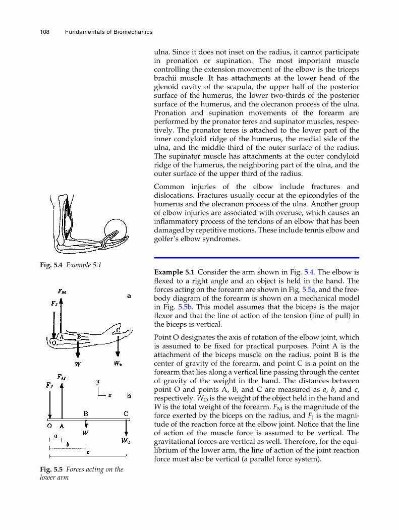
ulna. Since it does not inset on the radius, it cannot participatein pronation or supination. The most important musclecontrolling the extension movement of the elbow is the tricepsbrachii muscle. It has attachments at the lower head of theglenoid cavity of the scapula, the upper half of the posteriorsurface of the humerus, the lower two-thirds of the posteriorsurface of the humerus, and the olecranon process of the ulna.Pronation and supination movements of the forearm areperformed by the pronator teres and supinator muscles, respec-tively. The pronator teres is attached to the lower part of theinner condyloid ridge of the humerus, the medial side of theulna, and the middle third of the outer surface of the radius.The supinator muscle has attachments at the outer condyloidridge of the humerus, the neighboring part of the ulna, and theouter surface of the upper third of the radius.
Common injuries of the elbow include fractures anddislocations. Fractures usually occur at the epicondyles of thehumerus and the olecranon process of the ulna. Another groupof elbow injuries are associated with overuse, which causes aninflammatory process of the tendons of an elbow that has beendamaged by repetitive motions. These include tennis elbow andgolfer’s elbow syndromes.
Example 5.1 Consider the arm shown in Fig. 5.4. The elbow isflexed to a right angle and an object is held in the hand. Theforces acting on the forearm are shown in Fig. 5.5a, and the free-body diagram of the forearm is shown on a mechanical modelin Fig. 5.5b. This model assumes that the biceps is the majorflexor and that the line of action of the tension (line of pull) inthe biceps is vertical.
Point O designates the axis of rotation of the elbow joint, whichis assumed to be fixed for practical purposes. Point A is theattachment of the biceps muscle on the radius, point B is thecenter of gravity of the forearm, and point C is a point on theforearm that lies along a vertical line passing through the centerof gravity of the weight in the hand. The distances betweenpoint O and points A, B, and C are measured as a, b, and c,respectively.WO is the weight of the object held in the hand andW is the total weight of the forearm. FM is the magnitude of theforce exerted by the biceps on the radius, and FJ is the magni-tude of the reaction force at the elbow joint. Notice that the lineof action of the muscle force is assumed to be vertical. Thegravitational forces are vertical as well. Therefore, for the equi-librium of the lower arm, the line of action of the joint reactionforce must also be vertical (a parallel force system).
Fig. 5.4 Example 5.1
Fig. 5.5 Forces acting on thelower arm
108 Fundamentals of Biomechanics
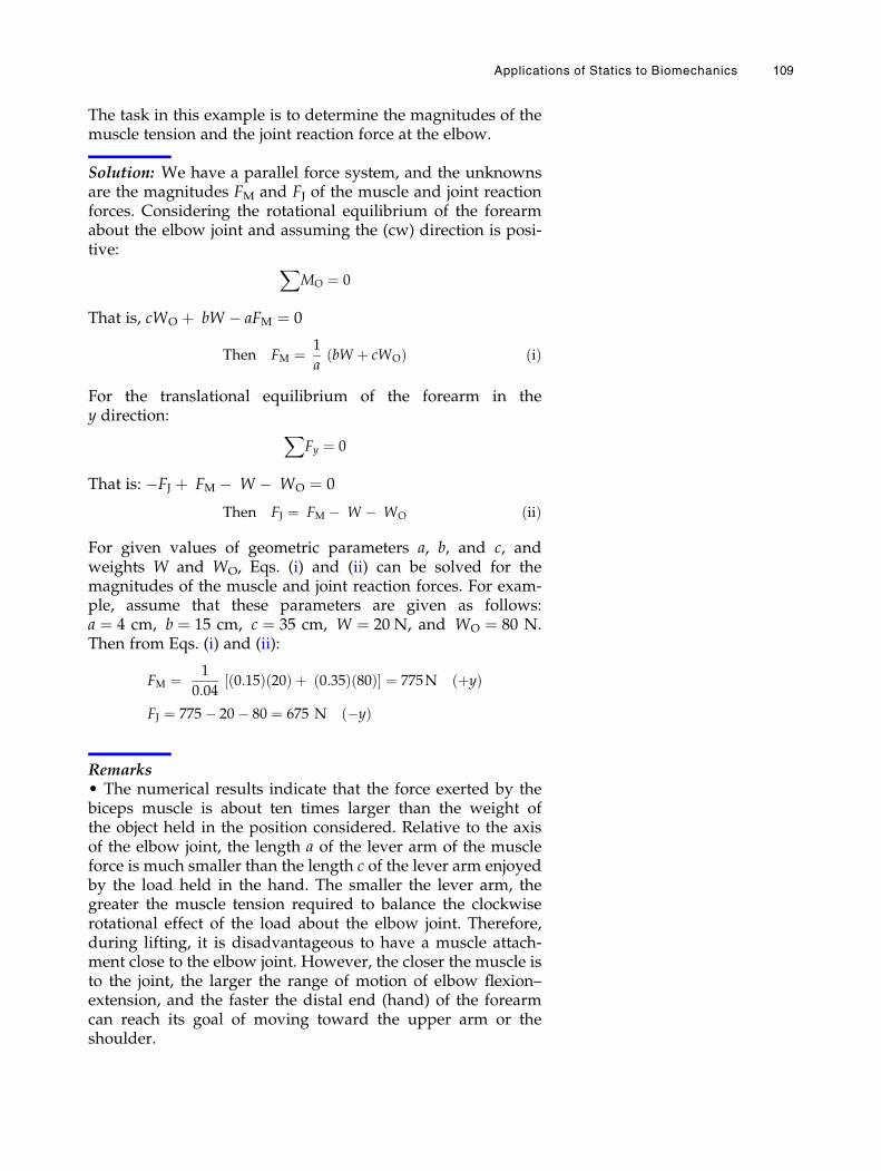
The task in this example is to determine the magnitudes of themuscle tension and the joint reaction force at the elbow.
Solution: We have a parallel force system, and the unknownsare the magnitudes FM and FJ of the muscle and joint reactionforces. Considering the rotational equilibrium of the forearmabout the elbow joint and assuming the (cw) direction is posi-tive: X
MO ¼ 0
That is, cWO þ bW � aFM ¼ 0
Then FM ¼ 1
abW þ cWOð Þ ðiÞ
For the translational equilibrium of the forearm in they direction: X
Fy ¼ 0
That is: �FJ þ FM � W � WO ¼ 0
Then FJ ¼ FM � W � WO ðiiÞ
For given values of geometric parameters a, b, and c, andweights W and WO, Eqs. (i) and (ii) can be solved for themagnitudes of the muscle and joint reaction forces. For exam-ple, assume that these parameters are given as follows:a ¼ 4 cm, b ¼ 15 cm, c ¼ 35 cm, W ¼ 20 N, and WO ¼ 80 N.Then from Eqs. (i) and (ii):
FM ¼ 1
0:040:15ð Þ 20ð Þ þ 0:35ð Þ 80ð Þ½ � ¼ 775N þyð Þ
FJ ¼ 775� 20� 80 ¼ 675 N �yð Þ
Remarks• The numerical results indicate that the force exerted by thebiceps muscle is about ten times larger than the weight ofthe object held in the position considered. Relative to the axisof the elbow joint, the length a of the lever arm of the muscleforce is much smaller than the length c of the lever arm enjoyedby the load held in the hand. The smaller the lever arm, thegreater the muscle tension required to balance the clockwiserotational effect of the load about the elbow joint. Therefore,during lifting, it is disadvantageous to have a muscle attach-ment close to the elbow joint. However, the closer the muscle isto the joint, the larger the range of motion of elbow flexion–extension, and the faster the distal end (hand) of the forearmcan reach its goal of moving toward the upper arm or theshoulder.
Applications of Statics to Biomechanics 109
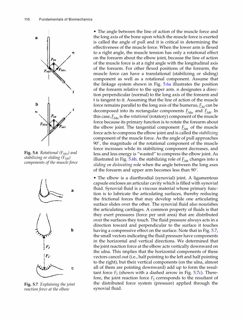
• The angle between the line of action of the muscle force andthe long axis of the bone upon which the muscle force is exertedis called the angle of pull and it is critical in determining theeffectiveness of the muscle force. When the lower arm is flexedto a right angle, the muscle tension has only a rotational effecton the forearm about the elbow joint, because the line of actionof the muscle force is at a right angle with the longitudinal axisof the forearm. For other flexed positions of the forearm, themuscle force can have a translational (stabilizing or sliding)component as well as a rotational component. Assume thatthe linkage system shown in Fig. 5.6a illustrates the positionof the forearm relative to the upper arm. n designates a direc-tion perpendicular (normal) to the long axis of the forearm andt is tangent to it. Assuming that the line of action of the muscleforce remains parallel to the long axis of the humerus,FM can bedecomposed into its rectangular components FMn and FMt. Inthis case,FMn is the rotational (rotatory) component of themuscleforce because its primary function is to rotate the forearm aboutthe elbow joint. The tangential component FMt of the muscleforce acts to compress the elbow joint and is called the stabilizingcomponent of the muscle force. As the angle of pull approaches90�, the magnitude of the rotational component of the muscleforce increases while its stabilizing component decreases, andless and less energy is “wasted” to compress the elbow joint. Asillustrated in Fig. 5.6b, the stabilizing role of FMt changes into asliding or dislocating role when the angle between the long axesof the forearm and upper arm becomes less than 90�.
• The elbow is a diarthrodial (synovial) joint. A ligamentouscapsule encloses an articular cavity which is filled with synovialfluid. Synovial fluid is a viscous material whose primary func-tion is to lubricate the articulating surfaces, thereby reducingthe frictional forces that may develop while one articulatingsurface slides over the other. The synovial fluid also nourishesthe articulating cartilages. A common property of fluids is thatthey exert pressures (force per unit area) that are distributedover the surfaces they touch. The fluid pressure always acts in adirection toward and perpendicular to the surface it toucheshaving a compressive effect on the surface. Note that in Fig. 5.7,the small vectors indicating the fluid pressure have componentsin the horizontal and vertical directions. We determined thatthe joint reaction force at the elbow acts vertically downward onthe ulna. This implies that the horizontal components of thesevectors cancel out (i.e., half pointing to the left and half pointingto the right), but their vertical components (on the ulna, almostall of them are pointing downward) add up to form the resul-tant force FJ (shown with a dashed arrow in Fig. 5.7c). There-fore, the joint reaction force FJ corresponds to the resultant ofthe distributed force system (pressure) applied through thesynovial fluid.
Fig. 5.6 Rotational (FMn) andstabilizing or sliding (FMt)components of the muscle force
Fig. 5.7 Explaining the jointreaction force at the elbow
110 Fundamentals of Biomechanics
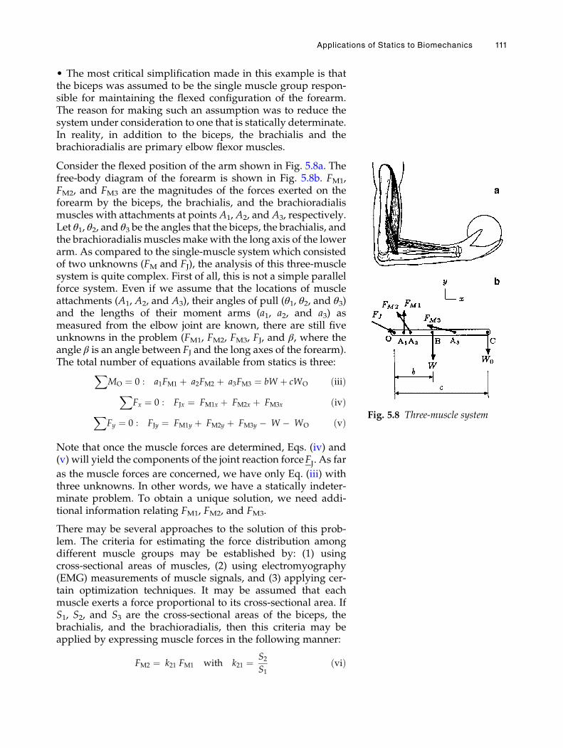
• The most critical simplification made in this example is thatthe biceps was assumed to be the single muscle group respon-sible for maintaining the flexed configuration of the forearm.The reason for making such an assumption was to reduce thesystem under consideration to one that is statically determinate.In reality, in addition to the biceps, the brachialis and thebrachioradialis are primary elbow flexor muscles.
Consider the flexed position of the arm shown in Fig. 5.8a. Thefree-body diagram of the forearm is shown in Fig. 5.8b. FM1,FM2, and FM3 are the magnitudes of the forces exerted on theforearm by the biceps, the brachialis, and the brachioradialismuscles with attachments at points A1, A2, and A3, respectively.Let θ1, θ2, and θ3 be the angles that the biceps, the brachialis, andthe brachioradialis muscles makewith the long axis of the lowerarm. As compared to the single-muscle system which consistedof two unknowns (FM and FJ), the analysis of this three-musclesystem is quite complex. First of all, this is not a simple parallelforce system. Even if we assume that the locations of muscleattachments (A1, A2, and A3), their angles of pull (θ1, θ2, and θ3)and the lengths of their moment arms (a1, a2, and a3) asmeasured from the elbow joint are known, there are still fiveunknowns in the problem (FM1, FM2, FM3, FJ, and β, where theangle β is an angle between FJ and the long axes of the forearm).The total number of equations available from statics is three:X
MO ¼ 0 : a1FM1 þ a2FM2 þ a3FM3 ¼ bW þ cWO ðiiiÞX
Fx ¼ 0 : FJx ¼ FM1x þ FM2x þ FM3x ðivÞX
Fy ¼ 0 : FJy ¼ FM1y þ FM2y þ FM3y � W � WO ðvÞ
Note that once the muscle forces are determined, Eqs. (iv) and(v) will yield the components of the joint reaction forceFJ. As far
as the muscle forces are concerned, we have only Eq. (iii) withthree unknowns. In other words, we have a statically indeter-minate problem. To obtain a unique solution, we need addi-tional information relating FM1, FM2, and FM3.
There may be several approaches to the solution of this prob-lem. The criteria for estimating the force distribution amongdifferent muscle groups may be established by: (1) usingcross-sectional areas of muscles, (2) using electromyography(EMG) measurements of muscle signals, and (3) applying cer-tain optimization techniques. It may be assumed that eachmuscle exerts a force proportional to its cross-sectional area. IfS1, S2, and S3 are the cross-sectional areas of the biceps, thebrachialis, and the brachioradialis, then this criteria may beapplied by expressing muscle forces in the following manner:
FM2 ¼ k21 FM1 with k21 ¼ S2S1
ðviÞ
Fig. 5.8 Three-muscle system
Applications of Statics to Biomechanics 111
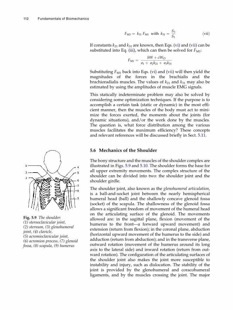
FM3 ¼ k31 FM1 with k31 ¼ S3S1
ðviiÞ
If constants k21 and k31 are known, then Eqs. (vi) and (vii) can besubstituted into Eq. (iii), which can then be solved for FM1:
FM1 ¼ bW þ cWO
a1 þ a2k21 þ a3k31
Substituting FM1 back into Eqs. (vi) and (vii) will then yield themagnitudes of the forces in the brachialis and thebrachioradialis muscles. The values of k21 and k31 may also beestimated by using the amplitudes of muscle EMG signals.
This statically indeterminate problem may also be solved byconsidering some optimization techniques. If the purpose is toaccomplish a certain task (static or dynamic) in the most effi-cient manner, then the muscles of the body must act to mini-mize the forces exerted, the moments about the joints (fordynamic situations), and/or the work done by the muscles.The question is, what force distribution among the variousmuscles facilitates the maximum efficiency? These conceptsand relevant references will be discussed briefly in Sect. 5.11.
5.6 Mechanics of the Shoulder
The bony structure and the muscles of the shoulder complex areillustrated in Figs. 5.9 and 5.10. The shoulder forms the base forall upper extremity movements. The complex structure of theshoulder can be divided into two: the shoulder joint and theshoulder girdle.
The shoulder joint, also known as the glenohumeral articulation,is a ball-and-socket joint between the nearly hemisphericalhumeral head (ball) and the shallowly concave glenoid fossa(socket) of the scapula. The shallowness of the glenoid fossaallows a significant freedom of movement of the humeral headon the articulating surface of the glenoid. The movementsallowed are: in the sagittal plane, flexion (movement of thehumerus to the front—a forward upward movement) andextension (return from flexion); in the coronal plane, abduction(horizontal upward movement of the humerus to the side) andadduction (return from abduction); and in the transverse plane,outward rotation (movement of the humerus around its longaxis to the lateral side) and inward rotation (return from out-ward rotation). The configuration of the articulating surfaces ofthe shoulder joint also makes the joint more susceptible toinstability and injury, such as dislocation. The stability of thejoint is provided by the glenohumeral and coracohumeralligaments, and by the muscles crossing the joint. The major
Fig. 5.9 The shoulder:(1) sternoclavicular joint,(2) sternum, (3) glenohumeraljoint, (4) clavicle,(5) acromioclavicular joint,(6) acromion process, (7) glenoidfossa, (8) scapula, (9) humerus
112 Fundamentals of Biomechanics
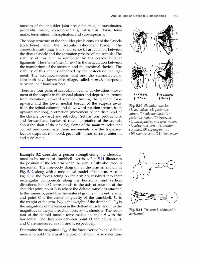
muscles of the shoulder joint are: deltoideus, supraspinatus,pectoralis major, coracobrachialis, latissimus dorsi, teresmajor, teres minor, infraspinatus, and subscapularis.
The bony structure of the shoulder girdle consists of the clavicle(collarbone) and the scapula (shoulder blade). Theacromioclavicular joint is a small synovial articulation betweenthe distal clavicle and the acromion process of the scapula. Thestability of this joint is reinforced by the coracoclavicularligaments. The sternoclavicular joint is the articulation betweenthe manubrium of the sternum and the proximal clavicle. Thestability of this joint is enhanced by the costoclavicular liga-ment. The acromioclavicular joint and the sternoclavicularjoint both have layers of cartilage, called menisci, interposedbetween their bony surfaces.
There are four pairs of scapular movements: elevation (move-ment of the scapula in the frontal plane) and depression (returnfrom elevation), upward rotation (turning the glenoid fossaupward and the lower medial border of the scapula awayfrom the spinal column) and downward rotation (return fromupward rotation), protraction (movement of the distal end ofthe clavicle forward) and retraction (return from protraction),and forward and backward rotation (rotation of the scapulaabout the shaft of the clavicle). Some of the main muscles thatcontrol and coordinate these movements are the trapezius,levator scapulae, rhomboid, pectoralis minor, serratus anterior,and subclavius.
Example 5.2 Consider a person strengthening the shouldermuscles by means of dumbbell exercises. Fig. 5.11 illustratesthe position of the left arm when the arm is fully abducted tohorizontal. The free-body diagram of the arm is shown inFig. 5.12 along with a mechanical model of the arm. Also inFig. 5.12, the forces acting on the arm are resolved into theirrectangular components along the horizontal and verticaldirections. Point O corresponds to the axis of rotation of theshoulder joint, point A is where the deltoid muscle is attachedto the humerus, point B is the center of gravity of the entire arm,and point C is the center of gravity of the dumbbell. W isthe weight of the arm, WO is the weight of the dumbbell, FM isthe magnitude of the tension in the deltoid muscle, and FJ is themagnitude of the joint reaction force at the shoulder. The resul-tant of the deltoid muscle force makes an angle θ with thehorizontal. The distances between point O and points A, B,and C are measured as a, b, and c, respectively.
Determine the magnitude FM of the force exerted by the deltoidmuscle to hold the arm at the position shown. Also determine
Fig. 5.10 Shoulder muscles:(1) deltoideus, (2) pectoralisminor, (3) subscapularis, (4)pectoralis major, (5) trapezius,(6) infraspinatus and teres minor,(7) latissimus dorsi, (8) levatorscapulae, (9) supraspinatus,(10) rhomboideus, (11) teres major
Fig. 5.11 The arm is abducted tohorizontal
Applications of Statics to Biomechanics 113
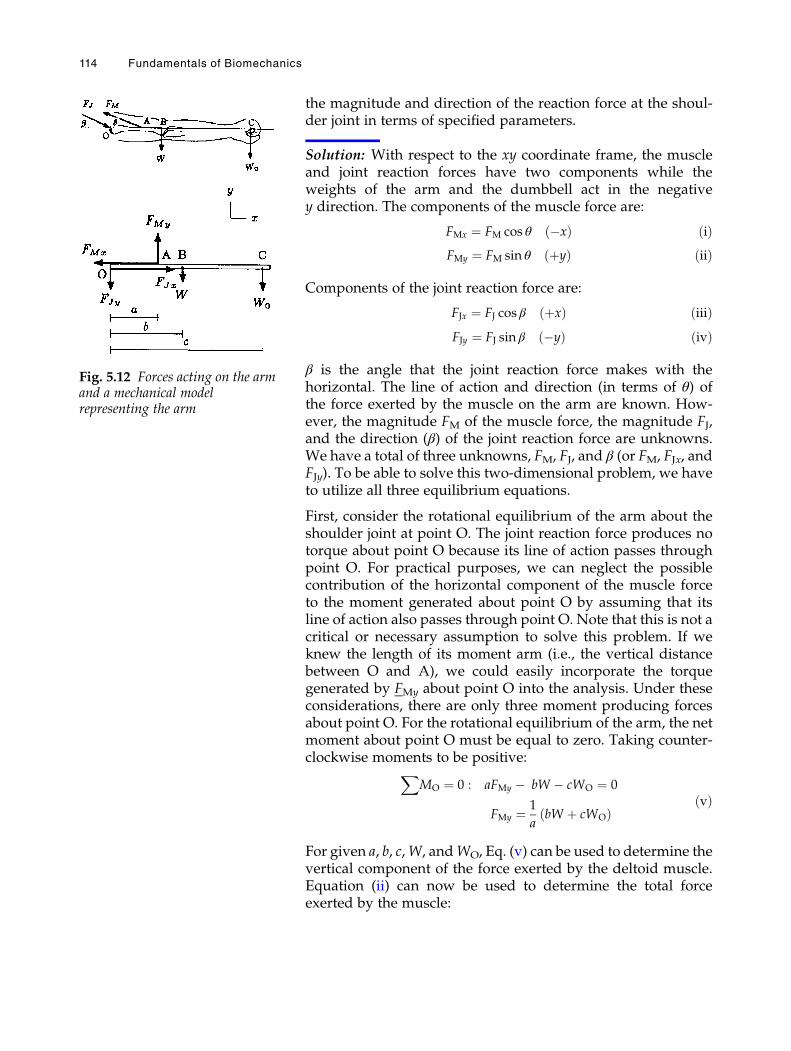
the magnitude and direction of the reaction force at the shoul-der joint in terms of specified parameters.
Solution: With respect to the xy coordinate frame, the muscleand joint reaction forces have two components while theweights of the arm and the dumbbell act in the negativey direction. The components of the muscle force are:
FMx ¼ FM cos θ �xð Þ ðiÞFMy ¼ FM sin θ þyð Þ ðiiÞ
Components of the joint reaction force are:
FJx ¼ FJ cos β þxð Þ ðiiiÞFJy ¼ FJ sin β �yð Þ ðivÞ
β is the angle that the joint reaction force makes with thehorizontal. The line of action and direction (in terms of θ) ofthe force exerted by the muscle on the arm are known. How-ever, the magnitude FM of the muscle force, the magnitude FJ,and the direction (β) of the joint reaction force are unknowns.We have a total of three unknowns, FM, FJ, and β (or FM, FJx, andFJy). To be able to solve this two-dimensional problem, we haveto utilize all three equilibrium equations.
First, consider the rotational equilibrium of the arm about theshoulder joint at point O. The joint reaction force produces notorque about point O because its line of action passes throughpoint O. For practical purposes, we can neglect the possiblecontribution of the horizontal component of the muscle forceto the moment generated about point O by assuming that itsline of action also passes through point O. Note that this is not acritical or necessary assumption to solve this problem. If weknew the length of its moment arm (i.e., the vertical distancebetween O and A), we could easily incorporate the torquegenerated by FMy about point O into the analysis. Under theseconsiderations, there are only three moment producing forcesabout point O. For the rotational equilibrium of the arm, the netmoment about point O must be equal to zero. Taking counter-clockwise moments to be positive:X
MO ¼ 0 : aFMy � bW � cWO ¼ 0
FMy ¼ 1
abW þ cWOð Þ
ðvÞ
For given a, b, c,W, andWO, Eq. (v) can be used to determine thevertical component of the force exerted by the deltoid muscle.Equation (ii) can now be used to determine the total forceexerted by the muscle:
Fig. 5.12 Forces acting on the armand a mechanical modelrepresenting the arm
114 Fundamentals of Biomechanics
FM ¼ FMy
sin θðviÞ
Knowing FM, Eq. (i) will yield the horizontal component of thetension in the muscle:
FMx ¼ FM cos θ ðviiÞ
The components of the joint reaction force can be determined byconsidering the translational equilibrium of the arm in thehorizontal and vertical directions:X
Fx ¼ 0 that is : FJx � FMx ¼ 0, then FJx ¼ FMx ðviiiÞX
Fy ¼ 0 that is : � FJy þ FMy �W �WO ¼ 0
then FJy ¼ FMy �W �WO
ðixÞ
Knowing the rectangular components of the joint reaction forceenables us to compute the magnitude of the force itself and theangle its line of action makes with the horizontal:
FJ ¼ffiffiffiffiffiffiffiffiffiffiffiffiffiffiffiffiffiffiffiffiffiffiffiffiffiffiffiffiffiffiffiFJx� �2 þ FJy
� �2qðxÞ
β ¼ tan �1 FJy
FJx
� �ðxiÞ
Now consider that a ¼ 15cm, b ¼ 30 cm, c ¼ 60cm, θ ¼ 15�,W ¼ 40N, and WO ¼ 60 N. Then:
FMy ¼ 1
0:150:30ð Þ 40ð Þ þ 0:60ð Þ 60ð Þ½ �
¼ 320N þyð Þ
FM ¼ 320
sin 15�¼ 1236N
FMx ¼ 1236ð Þ cos 15�ð Þ ¼ 1194N �xð ÞFJx ¼ 1194N þxð Þ
FJy ¼ 320� 40� 60 ¼ 220 N �yð Þ
FJ ¼ffiffiffiffiffiffiffiffiffiffiffiffiffiffiffiffiffiffiffiffiffiffiffiffiffiffiffiffiffiffiffiffiffiffiffiffi1194ð Þ2 þ 220ð Þ2
q¼ 1214N
β ¼ tan �1 220
1194
� �¼ 10�
Remarks• FMx is the stabilizing component and FMy is the rotationalcomponent of the deltoid muscle. FMx is approximately fourtimes larger than FMy. A large stabilizing component suggeststhat the horizontal position of the arm is not stable, and that themuscle needs to exert a high horizontal force to stabilize it.
Applications of Statics to Biomechanics 115
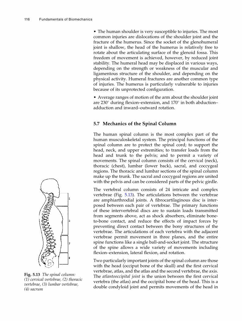
• The human shoulder is very susceptible to injuries. The mostcommon injuries are dislocations of the shoulder joint and thefracture of the humerus. Since the socket of the glenohumeraljoint is shallow, the head of the humerus is relatively free torotate about the articulating surface of the glenoid fossa. Thisfreedom of movement is achieved, however, by reduced jointstability. The humeral head may be displaced in various ways,depending on the strength or weakness of the muscular andligamentous structure of the shoulder, and depending on thephysical activity. Humeral fractures are another common typeof injuries. The humerus is particularly vulnerable to injuriesbecause of its unprotected configuration.
• Average ranges of motion of the arm about the shoulder jointare 230� during flexion–extension, and 170� in both abduction–adduction and inward–outward rotation.
5.7 Mechanics of the Spinal Column
The human spinal column is the most complex part of thehuman musculoskeletal system. The principal functions of thespinal column are to protect the spinal cord; to support thehead, neck, and upper extremities; to transfer loads from thehead and trunk to the pelvis; and to permit a variety ofmovements. The spinal column consists of the cervical (neck),thoracic (chest), lumbar (lower back), sacral, and coccygealregions. The thoracic and lumbar sections of the spinal columnmake up the trunk. The sacral and coccygeal regions are unitedwith the pelvis and can be considered parts of the pelvic girdle.
The vertebral column consists of 24 intricate and complexvertebrae (Fig. 5.13). The articulations between the vertebraeare amphiarthrodial joints. A fibrocartilaginous disc is inter-posed between each pair of vertebrae. The primary functionsof these intervertebral discs are to sustain loads transmittedfrom segments above, act as shock absorbers, eliminate bone-to-bone contact, and reduce the effects of impact forces bypreventing direct contact between the bony structures of thevertebrae. The articulations of each vertebra with the adjacentvertebrae permit movement in three planes, and the entirespine functions like a single ball-and-socket joint. The structureof the spine allows a wide variety of movements includingflexion–extension, lateral flexion, and rotation.
Two particularly important joints of the spinal column are thosewith the head (occiput bone of the skull) and the first cervicalvertebrae, atlas, and the atlas and the second vertebrae, the axis.The atlantooccipital joint is the union between the first cervicalvertebra (the atlas) and the occipital bone of the head. This is adouble condyloid joint and permits movements of the head in
Fig. 5.13 The spinal column:(1) cervical vertebrae, (2) thoracicvertebrae, (3) lumbar vertebrae,(4) sacrum
116 Fundamentals of Biomechanics
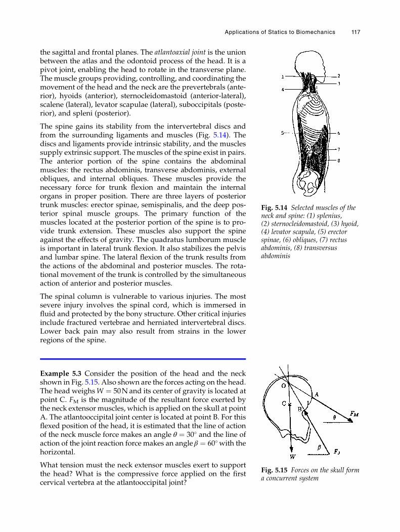
the sagittal and frontal planes. The atlantoaxial joint is the unionbetween the atlas and the odontoid process of the head. It is apivot joint, enabling the head to rotate in the transverse plane.The muscle groups providing, controlling, and coordinating themovement of the head and the neck are the prevertebrals (ante-rior), hyoids (anterior), sternocleidomastoid (anterior-lateral),scalene (lateral), levator scapulae (lateral), suboccipitals (poste-rior), and spleni (posterior).
The spine gains its stability from the intervertebral discs andfrom the surrounding ligaments and muscles (Fig. 5.14). Thediscs and ligaments provide intrinsic stability, and the musclessupply extrinsic support. The muscles of the spine exist in pairs.The anterior portion of the spine contains the abdominalmuscles: the rectus abdominis, transverse abdominis, externalobliques, and internal obliques. These muscles provide thenecessary force for trunk flexion and maintain the internalorgans in proper position. There are three layers of posteriortrunk muscles: erector spinae, semispinalis, and the deep pos-terior spinal muscle groups. The primary function of themuscles located at the posterior portion of the spine is to pro-vide trunk extension. These muscles also support the spineagainst the effects of gravity. The quadratus lumborum muscleis important in lateral trunk flexion. It also stabilizes the pelvisand lumbar spine. The lateral flexion of the trunk results fromthe actions of the abdominal and posterior muscles. The rota-tional movement of the trunk is controlled by the simultaneousaction of anterior and posterior muscles.
The spinal column is vulnerable to various injuries. The mostsevere injury involves the spinal cord, which is immersed influid and protected by the bony structure. Other critical injuriesinclude fractured vertebrae and herniated intervertebral discs.Lower back pain may also result from strains in the lowerregions of the spine.
Example 5.3 Consider the position of the head and the neckshown in Fig. 5.15. Also shown are the forces acting on the head.The head weighsW ¼ 50N and its center of gravity is located atpoint C. FM is the magnitude of the resultant force exerted bythe neck extensor muscles, which is applied on the skull at pointA. The atlantooccipital joint center is located at point B. For thisflexed position of the head, it is estimated that the line of actionof the neck muscle force makes an angle θ ¼ 30� and the line ofaction of the joint reaction force makes an angle β ¼ 60�with thehorizontal.
What tension must the neck extensor muscles exert to supportthe head? What is the compressive force applied on the firstcervical vertebra at the atlantooccipital joint?
Fig. 5.14 Selected muscles of theneck and spine: (1) splenius,(2) sternocleidomastoid, (3) hyoid,(4) levator scapula, (5) erectorspinae, (6) obliques, (7) rectusabdominis, (8) transversusabdominis
Fig. 5.15 Forces on the skull forma concurrent system
Applications of Statics to Biomechanics 117
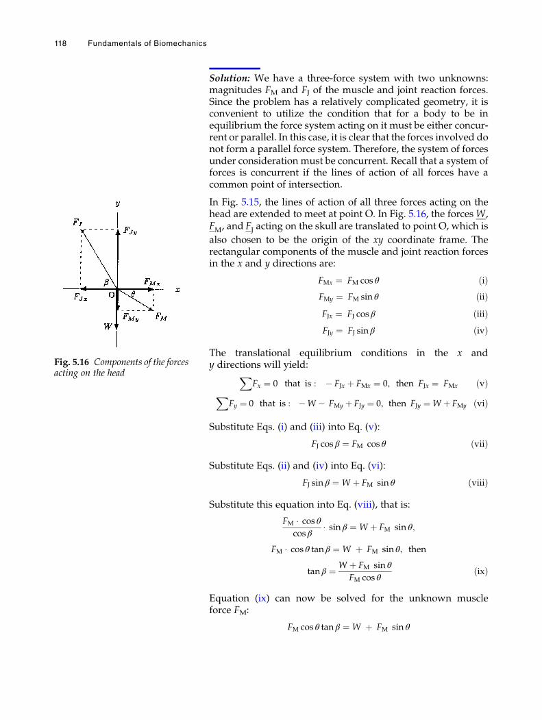
Solution: We have a three-force system with two unknowns:magnitudes FM and FJ of the muscle and joint reaction forces.Since the problem has a relatively complicated geometry, it isconvenient to utilize the condition that for a body to be inequilibrium the force system acting on it must be either concur-rent or parallel. In this case, it is clear that the forces involved donot form a parallel force system. Therefore, the system of forcesunder consideration must be concurrent. Recall that a system offorces is concurrent if the lines of action of all forces have acommon point of intersection.
In Fig. 5.15, the lines of action of all three forces acting on thehead are extended to meet at point O. In Fig. 5.16, the forcesW,FM, and FJ acting on the skull are translated to point O, which is
also chosen to be the origin of the xy coordinate frame. Therectangular components of the muscle and joint reaction forcesin the x and y directions are:
FMx ¼ FM cos θ ðiÞFMy ¼ FM sin θ ðiiÞFJx ¼ FJ cos β ðiiiÞFJy ¼ FJ sin β ðivÞ
The translational equilibrium conditions in the x andy directions will yield:X
Fx ¼ 0 that is : � FJx þ FMx ¼ 0, then FJx ¼ FMx ðvÞX
Fy ¼ 0 that is : �W � FMy þ FJy ¼ 0, then FJy ¼W þ FMy ðviÞ
Substitute Eqs. (i) and (iii) into Eq. (v):
FJ cos β ¼ FM cos θ ðviiÞ
Substitute Eqs. (ii) and (iv) into Eq. (vi):
FJ sin β ¼ W þ FM sin θ ðviiiÞ
Substitute this equation into Eq. (viii), that is:
FM � cos θcos β
� sin β ¼ W þ FM sin θ;
FM � cos θ tan β ¼ W þ FM sin θ, then
tan β ¼ W þ FM sin θ
FM cos θðixÞ
Equation (ix) can now be solved for the unknown muscleforce FM:
FM cos θ tan β ¼ W þ FM sin θ
Fig. 5.16 Components of the forcesacting on the head
118 Fundamentals of Biomechanics
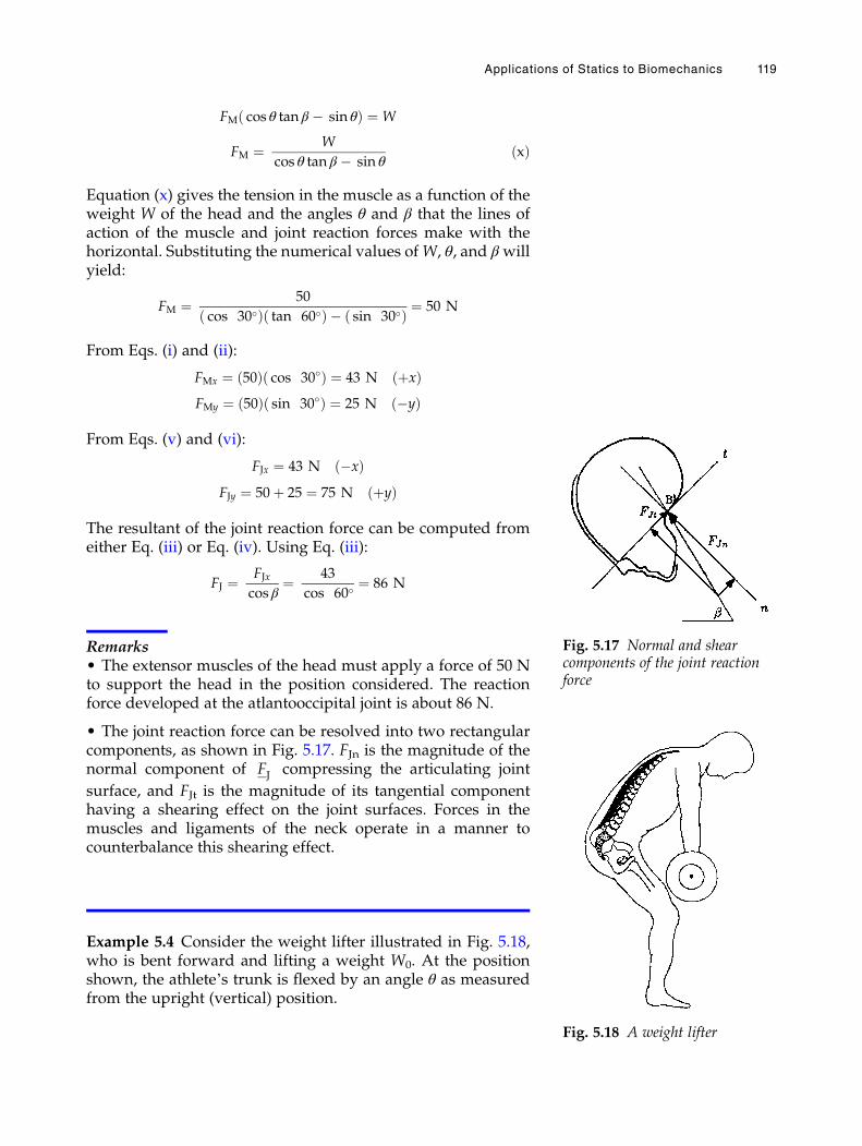
FM cos θ tan β � sin θð Þ ¼ W
FM ¼ W
cos θ tan β � sin θðxÞ
Equation (x) gives the tension in the muscle as a function of theweight W of the head and the angles θ and β that the lines ofaction of the muscle and joint reaction forces make with thehorizontal. Substituting the numerical values ofW, θ, and β willyield:
FM ¼ 50
cos 30�ð Þ tan 60�ð Þ � sin 30�ð Þ ¼ 50 N
From Eqs. (i) and (ii):
FMx ¼ 50ð Þ cos 30�ð Þ ¼ 43 N þxð ÞFMy ¼ 50ð Þ sin 30�ð Þ ¼ 25 N �yð Þ
From Eqs. (v) and (vi):
FJx ¼ 43 N �xð ÞFJy ¼ 50þ 25 ¼ 75 N þyð Þ
The resultant of the joint reaction force can be computed fromeither Eq. (iii) or Eq. (iv). Using Eq. (iii):
FJ ¼ FJxcos β
¼ 43
cos 60�¼ 86 N
Remarks• The extensor muscles of the head must apply a force of 50 Nto support the head in the position considered. The reactionforce developed at the atlantooccipital joint is about 86 N.
• The joint reaction force can be resolved into two rectangularcomponents, as shown in Fig. 5.17. FJn is the magnitude of thenormal component of FJ compressing the articulating joint
surface, and FJt is the magnitude of its tangential componenthaving a shearing effect on the joint surfaces. Forces in themuscles and ligaments of the neck operate in a manner tocounterbalance this shearing effect.
Example 5.4 Consider the weight lifter illustrated in Fig. 5.18,who is bent forward and lifting a weight W0. At the positionshown, the athlete’s trunk is flexed by an angle θ as measuredfrom the upright (vertical) position.
Fig. 5.17 Normal and shearcomponents of the joint reactionforce
Fig. 5.18 A weight lifter
Applications of Statics to Biomechanics 119
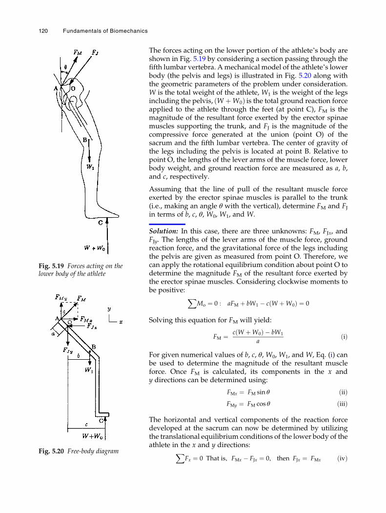
The forces acting on the lower portion of the athlete’s body areshown in Fig. 5.19 by considering a section passing through thefifth lumbar vertebra. Amechanical model of the athlete’s lowerbody (the pelvis and legs) is illustrated in Fig. 5.20 along withthe geometric parameters of the problem under consideration.W is the total weight of the athlete, W1 is the weight of the legsincluding the pelvis, W þW0ð Þ is the total ground reaction forceapplied to the athlete through the feet (at point C), FM is themagnitude of the resultant force exerted by the erector spinaemuscles supporting the trunk, and FJ is the magnitude of thecompressive force generated at the union (point O) of thesacrum and the fifth lumbar vertebra. The center of gravity ofthe legs including the pelvis is located at point B. Relative topoint O, the lengths of the lever arms of the muscle force, lowerbody weight, and ground reaction force are measured as a, b,and c, respectively.
Assuming that the line of pull of the resultant muscle forceexerted by the erector spinae muscles is parallel to the trunk(i.e., making an angle θ with the vertical), determine FM and FJin terms of b, c, θ, W0, W1, and W.
Solution: In this case, there are three unknowns: FM, FJx, andFJy. The lengths of the lever arms of the muscle force, groundreaction force, and the gravitational force of the legs includingthe pelvis are given as measured from point O. Therefore, wecan apply the rotational equilibrium condition about point O todetermine the magnitude FM of the resultant force exerted bythe erector spinae muscles. Considering clockwise moments tobe positive: X
Mo ¼ 0 : aFM þ bW1 � c W þW0ð Þ ¼ 0
Solving this equation for FM will yield:
FM ¼ c W þW0ð Þ � bW1
aðiÞ
For given numerical values of b, c, θ, W0, W1, and W, Eq. (i) canbe used to determine the magnitude of the resultant muscleforce. Once FM is calculated, its components in the x andy directions can be determined using:
FMx ¼ FM sin θ ðiiÞFMy ¼ FM cos θ ðiiiÞ
The horizontal and vertical components of the reaction forcedeveloped at the sacrum can now be determined by utilizingthe translational equilibrium conditions of the lower body of theathlete in the x and y directions:X
Fx ¼ 0 That is, FMx � FJx ¼ 0, then FJx ¼ FMx ðivÞ
Fig. 5.19 Forces acting on thelower body of the athlete
Fig. 5.20 Free-body diagram
120 Fundamentals of Biomechanics
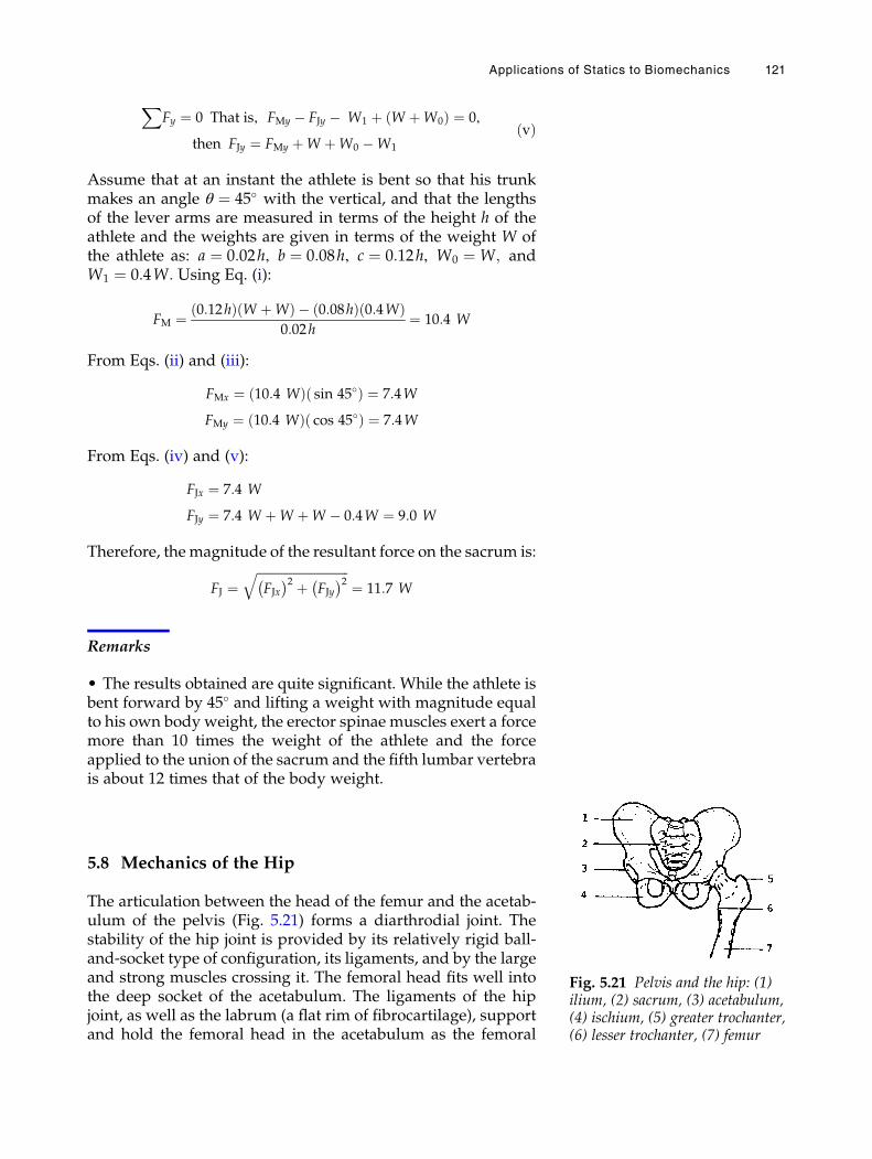
XFy ¼ 0 That is, FMy � FJy � W1 þ W þW0ð Þ ¼ 0,
then FJy ¼ FMy þW þW0 �W1
ðvÞ
Assume that at an instant the athlete is bent so that his trunkmakes an angle θ ¼ 45� with the vertical, and that the lengthsof the lever arms are measured in terms of the height h of theathlete and the weights are given in terms of the weight W ofthe athlete as: a ¼ 0:02h, b ¼ 0:08h, c ¼ 0:12h, W0 ¼ W; andW1 ¼ 0:4W: Using Eq. (i):
FM ¼ 0:12hð Þ W þWð Þ � 0:08hð Þ 0:4Wð Þ0:02h
¼ 10:4 W
From Eqs. (ii) and (iii):
FMx ¼ 10:4 Wð Þ sin 45�ð Þ ¼ 7:4W
FMy ¼ 10:4 Wð Þ cos 45�ð Þ ¼ 7:4W
From Eqs. (iv) and (v):
FJx ¼ 7:4 W
FJy ¼ 7:4 W þW þW � 0:4W ¼ 9:0 W
Therefore, the magnitude of the resultant force on the sacrum is:
FJ ¼ffiffiffiffiffiffiffiffiffiffiffiffiffiffiffiffiffiffiffiffiffiffiffiffiffiffiffiffiffiffiFJx� �2 þ FJy
� �2q¼ 11:7 W
Remarks
• The results obtained are quite significant. While the athlete isbent forward by 45� and lifting a weight with magnitude equalto his own body weight, the erector spinae muscles exert a forcemore than 10 times the weight of the athlete and the forceapplied to the union of the sacrum and the fifth lumbar vertebrais about 12 times that of the body weight.
5.8 Mechanics of the Hip
The articulation between the head of the femur and the acetab-ulum of the pelvis (Fig. 5.21) forms a diarthrodial joint. Thestability of the hip joint is provided by its relatively rigid ball-and-socket type of configuration, its ligaments, and by the largeand strong muscles crossing it. The femoral head fits well intothe deep socket of the acetabulum. The ligaments of the hipjoint, as well as the labrum (a flat rim of fibrocartilage), supportand hold the femoral head in the acetabulum as the femoral
Fig. 5.21 Pelvis and the hip: (1)ilium, (2) sacrum, (3) acetabulum,(4) ischium, (5) greater trochanter,(6) lesser trochanter, (7) femur
Applications of Statics to Biomechanics 121
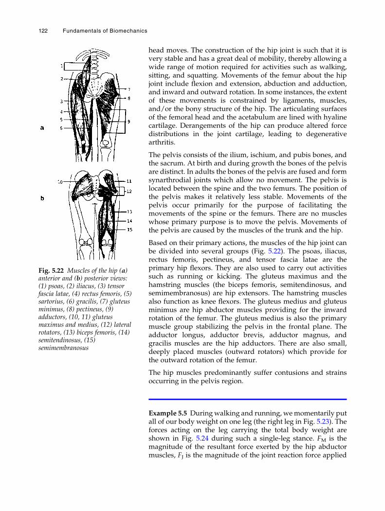
head moves. The construction of the hip joint is such that it isvery stable and has a great deal of mobility, thereby allowing awide range of motion required for activities such as walking,sitting, and squatting. Movements of the femur about the hipjoint include flexion and extension, abduction and adduction,and inward and outward rotation. In some instances, the extentof these movements is constrained by ligaments, muscles,and/or the bony structure of the hip. The articulating surfacesof the femoral head and the acetabulum are lined with hyalinecartilage. Derangements of the hip can produce altered forcedistributions in the joint cartilage, leading to degenerativearthritis.
The pelvis consists of the ilium, ischium, and pubis bones, andthe sacrum. At birth and during growth the bones of the pelvisare distinct. In adults the bones of the pelvis are fused and formsynarthrodial joints which allow no movement. The pelvis islocated between the spine and the two femurs. The position ofthe pelvis makes it relatively less stable. Movements of thepelvis occur primarily for the purpose of facilitating themovements of the spine or the femurs. There are no muscleswhose primary purpose is to move the pelvis. Movements ofthe pelvis are caused by the muscles of the trunk and the hip.
Based on their primary actions, the muscles of the hip joint canbe divided into several groups (Fig. 5.22). The psoas, iliacus,rectus femoris, pectineus, and tensor fascia latae are theprimary hip flexors. They are also used to carry out activitiessuch as running or kicking. The gluteus maximus and thehamstring muscles (the biceps femoris, semitendinosus, andsemimembranosus) are hip extensors. The hamstring musclesalso function as knee flexors. The gluteus medius and gluteusminimus are hip abductor muscles providing for the inwardrotation of the femur. The gluteus medius is also the primarymuscle group stabilizing the pelvis in the frontal plane. Theadductor longus, adductor brevis, adductor magnus, andgracilis muscles are the hip adductors. There are also small,deeply placed muscles (outward rotators) which provide forthe outward rotation of the femur.
The hip muscles predominantly suffer contusions and strainsoccurring in the pelvis region.
Example 5.5 Duringwalking and running, wemomentarily putall of our body weight on one leg (the right leg in Fig. 5.23). Theforces acting on the leg carrying the total body weight areshown in Fig. 5.24 during such a single-leg stance. FM is themagnitude of the resultant force exerted by the hip abductormuscles, FJ is the magnitude of the joint reaction force applied
Fig. 5.22 Muscles of the hip (a)anterior and (b) posterior views:(1) psoas, (2) iliacus, (3) tensorfascia latae, (4) rectus femoris, (5)sartorius, (6) gracilis, (7) gluteusminimus, (8) pectineus, (9)adductors, (10, 11) gluteusmaximus and medius, (12) lateralrotators, (13) biceps femoris, (14)semitendinosus, (15)semimembranosus
122 Fundamentals of Biomechanics
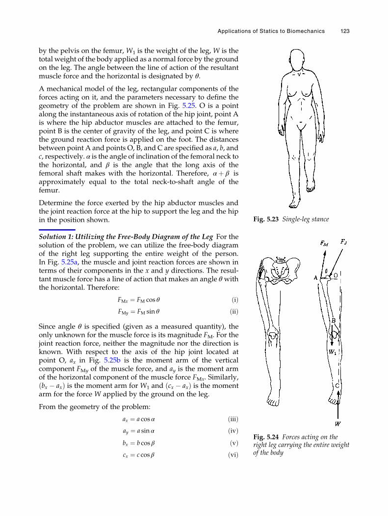
by the pelvis on the femur, W1 is the weight of the leg, W is thetotal weight of the body applied as a normal force by the groundon the leg. The angle between the line of action of the resultantmuscle force and the horizontal is designated by θ.
A mechanical model of the leg, rectangular components of theforces acting on it, and the parameters necessary to define thegeometry of the problem are shown in Fig. 5.25. O is a pointalong the instantaneous axis of rotation of the hip joint, point Ais where the hip abductor muscles are attached to the femur,point B is the center of gravity of the leg, and point C is wherethe ground reaction force is applied on the foot. The distancesbetween point A and points O, B, and C are specified as a, b, andc, respectively. α is the angle of inclination of the femoral neck tothe horizontal, and β is the angle that the long axis of thefemoral shaft makes with the horizontal. Therefore, αþ β isapproximately equal to the total neck-to-shaft angle of thefemur.
Determine the force exerted by the hip abductor muscles andthe joint reaction force at the hip to support the leg and the hipin the position shown.
Solution 1: Utilizing the Free-Body Diagram of the Leg For thesolution of the problem, we can utilize the free-body diagramof the right leg supporting the entire weight of the person.In Fig. 5.25a, the muscle and joint reaction forces are shown interms of their components in the x and y directions. The resul-tant muscle force has a line of action that makes an angle θ withthe horizontal. Therefore:
FMx ¼ FM cos θ ðiÞFMy ¼ FM sin θ ðiiÞ
Since angle θ is specified (given as a measured quantity), theonly unknown for the muscle force is its magnitude FM. For thejoint reaction force, neither the magnitude nor the direction isknown. With respect to the axis of the hip joint located atpoint O, ax in Fig. 5.25b is the moment arm of the verticalcomponent FMy of the muscle force, and ay is the moment armof the horizontal component of the muscle force FMx. Similarly,bx � axð Þ is the moment arm for W1 and cx � axð Þ is the momentarm for the force W applied by the ground on the leg.
From the geometry of the problem:
ax ¼ a cos α ðiiiÞay ¼ a sin α ðivÞbx ¼ b cos β ðvÞcx ¼ c cos β ðviÞ
Fig. 5.23 Single-leg stance
Fig. 5.24 Forces acting on theright leg carrying the entire weightof the body
Applications of Statics to Biomechanics 123
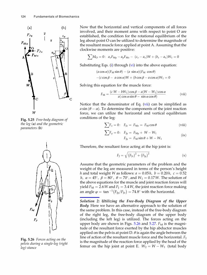
Now that the horizontal and vertical components of all forcesinvolved, and their moment arms with respect to point O areestablished, the condition for the rotational equilibrium of theleg about point O can be utilized to determine the magnitude ofthe resultant muscle force applied at point A. Assuming that theclockwise moments are positive:X
MO ¼ 0 : axFMy � ayFMx � cx � axð ÞW þ bx � axð ÞW1 ¼ 0
Substituting Eqs. (i) through (vi) into the above equation:
a cos αð Þ FM sin θð Þ � a sin αð Þ FM cos θð Þ� c cos β � a cos αð ÞW þ b cos β � a cos αð ÞW1 ¼ 0
Solving this equation for the muscle force:
FM ¼ c W � bW1ð Þ cos β � a W �W1ð Þ cos αa cos α sin θ � sin α cos θð Þ ðviiÞ
Notice that the denominator of Eq. (vii) can be simplified asa sin θ � αð Þ. To determine the components of the joint reactionforce, we can utilize the horizontal and vertical equilibriumconditions of the leg:X
Fx ¼ 0 : FJx ¼ FMx ¼ FM cos θ ðviiiÞX
Fy ¼ 0 : FJy ¼ FMy þ W �W1
FJy ¼ FM sin θ þW �W1
ðixÞ
Therefore, the resultant force acting at the hip joint is:
FJ ¼ffiffiffiffiffiffiffiffiffiffiffiffiffiffiffiffiffiffiffiffiffiffiffiffiffiffiffiffiffiffiFJx� �2 þ FJy
� �2qðxÞ
Assume that the geometric parameters of the problem and theweight of the leg are measured in terms of the person’s heighth and total weight W as follows: a ¼ 0:05h, b ¼ 0:20h, c ¼ 0:52h, α ¼ 45�, β ¼ 80�, θ ¼ 70�; andW1 ¼ 0:17W: The solution ofthe above equations for the muscle and joint reaction forces willyield FM ¼ 2:6W and FJ ¼ 3:4W, the joint reaction force making
an angle φ ¼ tan �1 FJy=FJx� � ¼ 74:8� with the horizontal.
Solution 2: Utilizing the Free-Body Diagram of the UpperBody Here we have an alternative approach to the solution ofthe same problem. In this case, instead of the free-body diagramof the right leg, the free-body diagram of the upper body(including the left leg) is utilized. The forces acting on theupper body are shown in Figs. 5.26 and 5.27. FM is the magni-tude of the resultant force exerted by the hip abductor musclesapplied on the pelvis at point D. θ is again the angle between theline of action of the resultant muscle force and the horizontal. FJis the magnitude of the reaction force applied by the head of thefemur on the hip joint at point E. W2 ¼ W �W1 (total body
Fig. 5.25 Free-body diagram ofthe leg (a) and the geometricparameters (b)
Fig. 5.26 Forces acting on thepelvis during a single-leg (rightleg) stance
124 Fundamentals of Biomechanics
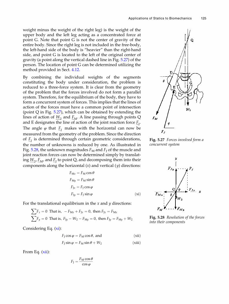
weight minus the weight of the right leg) is the weight of theupper body and the left leg acting as a concentrated force atpoint G. Note that point G is not the center of gravity of theentire body. Since the right leg is not included in the free-body,the left-hand side of the body is “heavier” than the right-handside, and point G is located to the left of the original center ofgravity (a point along the vertical dashed line in Fig. 5.27) of theperson. The location of point G can be determined utilizing themethod provided in Sect. 4.12.
By combining the individual weights of the segmentsconstituting the body under consideration, the problem isreduced to a three-force system. It is clear from the geometryof the problem that the forces involved do not form a parallelsystem. Therefore, for the equilibrium of the body, they have toform a concurrent system of forces. This implies that the lines ofaction of the forces must have a common point of intersection(point Q in Fig. 5.27), which can be obtained by extending thelines of action of W2 and FM. A line passing through points Qand E designates the line of action of the joint reaction force FJ.
The angle φ that FJ makes with the horizontal can now be
measured from the geometry of the problem. Since the directionof FJ is determined through certain geometric considerations,
the number of unknowns is reduced by one. As illustrated inFig. 5.28, the unknownmagnitudes FM and FJ of the muscle andjoint reaction forces can now be determined simply by translat-ingW2, FM, and FJ to point Q, and decomposing them into their
components along the horizontal (x) and vertical (y) directions:
FMx ¼ FM cos θ
FMy ¼ FM sin θ
FJx ¼ FJ cosφ
FJy ¼ FJ sinφ ðxiÞ
For the translational equilibrium in the x and y directions:XFx ¼ 0 That is, � FMx þ FJx ¼ 0, then FJx ¼ FMxXFy ¼ 0 That is, FJy �W2 � FMy ¼ 0, then FJy ¼ FMy þW2
Considering Eq. (xi):
FJ cosφ ¼ FM cos θ, and ðxiiÞFJ sinφ ¼ FM sin θ þW2 ðxiiiÞ
From Eq. (xii):
FJ ¼ FM cos θ
cosφ
Fig. 5.27 Forces involved form aconcurrent system
Fig. 5.28 Resolution of the forcesinto their components
Applications of Statics to Biomechanics 125
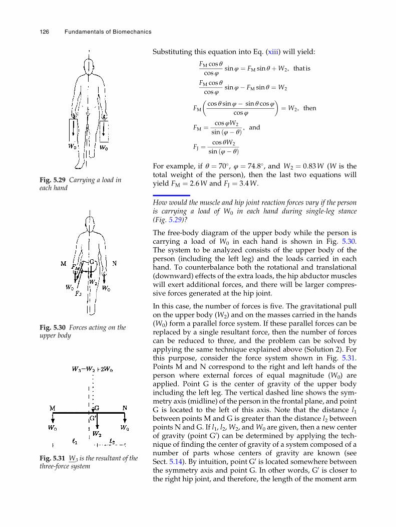
Substituting this equation into Eq. (xiii) will yield:
FM cos θ
cosφsinφ ¼ FM sin θ þW2, that is
FM cos θ
cosφsinφ� FM sin θ ¼ W2
FMcos θ sinφ� sin θ cosφ
cosφ
� �¼ W2, then
FM ¼ cosφW2
sin φ� θð Þ , and
FJ ¼ cos θW2
sin φ� θð Þ
For example, if θ ¼ 70�, φ ¼ 74:8�, and W2 ¼ 0:83W (W is thetotal weight of the person), then the last two equations willyield FM ¼ 2:6W and FJ ¼ 3:4W.
How would the muscle and hip joint reaction forces vary if the personis carrying a load of W0 in each hand during single-leg stance(Fig. 5.29)?
The free-body diagram of the upper body while the person iscarrying a load of W0 in each hand is shown in Fig. 5.30.The system to be analyzed consists of the upper body of theperson (including the left leg) and the loads carried in eachhand. To counterbalance both the rotational and translational(downward) effects of the extra loads, the hip abductor muscleswill exert additional forces, and there will be larger compres-sive forces generated at the hip joint.
In this case, the number of forces is five. The gravitational pullon the upper body (W2) and on the masses carried in the hands(W0) form a parallel force system. If these parallel forces can bereplaced by a single resultant force, then the number of forcescan be reduced to three, and the problem can be solved byapplying the same technique explained above (Solution 2). Forthis purpose, consider the force system shown in Fig. 5.31.Points M and N correspond to the right and left hands of theperson where external forces of equal magnitude (W0) areapplied. Point G is the center of gravity of the upper bodyincluding the left leg. The vertical dashed line shows the sym-metry axis (midline) of the person in the frontal plane, and pointG is located to the left of this axis. Note that the distance l1between points M and G is greater than the distance l2 betweenpoints N and G. If l1, l2,W2, andW0 are given, then a new centerof gravity (point G0) can be determined by applying the tech-nique of finding the center of gravity of a system composed of anumber of parts whose centers of gravity are known (seeSect. 5.14). By intuition, point G0 is located somewhere betweenthe symmetry axis and point G. In other words, G0 is closer tothe right hip joint, and therefore, the length of the moment arm
Fig. 5.29 Carrying a load ineach hand
Fig. 5.30 Forces acting on theupper body
Fig. 5.31 W3 is the resultant of thethree-force system
126 Fundamentals of Biomechanics
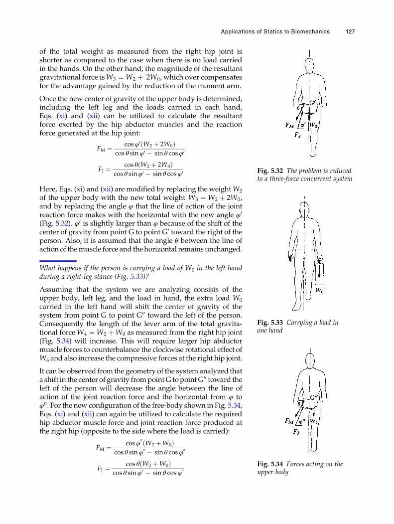
of the total weight as measured from the right hip joint isshorter as compared to the case when there is no load carriedin the hands. On the other hand, the magnitude of the resultantgravitational force isW3 ¼ W2 þ 2W0, which over compensatesfor the advantage gained by the reduction of the moment arm.
Once the new center of gravity of the upper body is determined,including the left leg and the loads carried in each hand,Eqs. (xi) and (xii) can be utilized to calculate the resultantforce exerted by the hip abductor muscles and the reactionforce generated at the hip joint:
FM ¼ cosφ0 W2 þ 2W0ð Þcos θ sinφ0 � sin θ cosφ0
FJ ¼ cos θ W2 þ 2W0ð Þcos θ sinφ0 � sin θ cosφ0
Here, Eqs. (xi) and (xii) are modified by replacing the weightW2
of the upper body with the new total weight W3 ¼ W2 þ 2W0,and by replacing the angle φ that the line of action of the jointreaction force makes with the horizontal with the new angle φ0
(Fig. 5.32). φ0 is slightly larger than φ because of the shift of thecenter of gravity from point G to point G0 toward the right of theperson. Also, it is assumed that the angle θ between the line ofaction of themuscle force and the horizontal remains unchanged.
What happens if the person is carrying a load of W0 in the left handduring a right-leg stance (Fig. 5.33)?
Assuming that the system we are analyzing consists of theupper body, left leg, and the load in hand, the extra load W0
carried in the left hand will shift the center of gravity of thesystem from point G to point G00 toward the left of the person.Consequently the length of the lever arm of the total gravita-tional forceW4 ¼ W2 þW0 as measured from the right hip joint(Fig. 5.34) will increase. This will require larger hip abductormuscle forces to counterbalance the clockwise rotational effect ofW4 and also increase the compressive forces at the right hip joint.
It can be observed from the geometry of the system analyzed thata shift in the center of gravity frompointG to pointG00 toward theleft of the person will decrease the angle between the line ofaction of the joint reaction force and the horizontal from φ toφ00. For the new configuration of the free-body shown in Fig. 5.34,Eqs. (xi) and (xii) can again be utilized to calculate the requiredhip abductor muscle force and joint reaction force produced atthe right hip (opposite to the side where the load is carried):
FM ¼ cosφ00W2 þW0ð Þ
cos θ sinφ00 � sin θ cosφ00
FJ ¼ cos θ W2 þW0ð Þcos θ sinφ00 � sin θ cosφ00
Fig. 5.32 The problem is reducedto a three-force concurrent system
Fig. 5.33 Carrying a load inone hand
Fig. 5.34 Forces acting on theupper body
Applications of Statics to Biomechanics 127
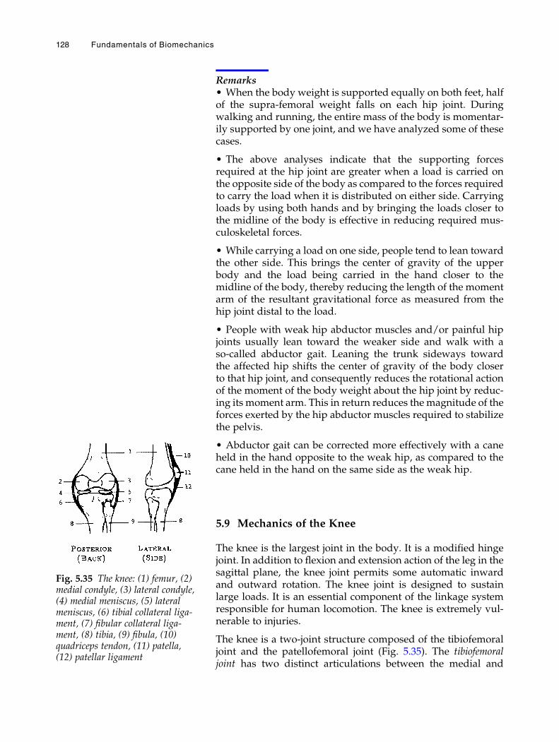
Remarks• When the body weight is supported equally on both feet, halfof the supra-femoral weight falls on each hip joint. Duringwalking and running, the entire mass of the body is momentar-ily supported by one joint, and we have analyzed some of thesecases.
• The above analyses indicate that the supporting forcesrequired at the hip joint are greater when a load is carried onthe opposite side of the body as compared to the forces requiredto carry the load when it is distributed on either side. Carryingloads by using both hands and by bringing the loads closer tothe midline of the body is effective in reducing required mus-culoskeletal forces.
• While carrying a load on one side, people tend to lean towardthe other side. This brings the center of gravity of the upperbody and the load being carried in the hand closer to themidline of the body, thereby reducing the length of the momentarm of the resultant gravitational force as measured from thehip joint distal to the load.
• People with weak hip abductor muscles and/or painful hipjoints usually lean toward the weaker side and walk with aso-called abductor gait. Leaning the trunk sideways towardthe affected hip shifts the center of gravity of the body closerto that hip joint, and consequently reduces the rotational actionof the moment of the body weight about the hip joint by reduc-ing its moment arm. This in return reduces the magnitude of theforces exerted by the hip abductor muscles required to stabilizethe pelvis.
• Abductor gait can be corrected more effectively with a caneheld in the hand opposite to the weak hip, as compared to thecane held in the hand on the same side as the weak hip.
5.9 Mechanics of the Knee
The knee is the largest joint in the body. It is a modified hingejoint. In addition to flexion and extension action of the leg in thesagittal plane, the knee joint permits some automatic inwardand outward rotation. The knee joint is designed to sustainlarge loads. It is an essential component of the linkage systemresponsible for human locomotion. The knee is extremely vul-nerable to injuries.
The knee is a two-joint structure composed of the tibiofemoraljoint and the patellofemoral joint (Fig. 5.35). The tibiofemoraljoint has two distinct articulations between the medial and
Fig. 5.35 The knee: (1) femur, (2)medial condyle, (3) lateral condyle,(4) medial meniscus, (5) lateralmeniscus, (6) tibial collateral liga-ment, (7) fibular collateral liga-ment, (8) tibia, (9) fibula, (10)quadriceps tendon, (11) patella,(12) patellar ligament
128 Fundamentals of Biomechanics
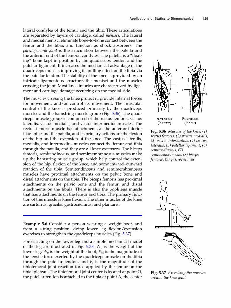
lateral condyles of the femur and the tibia. These articulationsare separated by layers of cartilage, called menisci. The lateraland medial menisci eliminate bone-to-bone contact between thefemur and the tibia, and function as shock absorbers. Thepatellofemoral joint is the articulation between the patella andthe anterior end of the femoral condyles. The patella is a “float-ing” bone kept in position by the quadriceps tendon and thepatellar ligament. It increases the mechanical advantage of thequadriceps muscle, improving its pulling effect on the tibia viathe patellar tendon. The stability of the knee is provided by anintricate ligamentous structure, the menisci and the musclescrossing the joint. Most knee injuries are characterized by liga-ment and cartilage damage occurring on the medial side.
The muscles crossing the knee protect it, provide internal forcesfor movement, and/or control its movement. The muscularcontrol of the knee is produced primarily by the quadricepsmuscles and the hamstring muscle group (Fig. 5.36). The quad-riceps muscle group is composed of the rectus femoris, vastuslateralis, vastus medialis, and vastus intermedius muscles. Therectus femoris muscle has attachments at the anterior-inferioriliac spine and the patella, and its primary actions are the flexionof the hip and the extension of the knee. The vastus lateralis,medialis, and intermedius muscles connect the femur and tibiathrough the patella, and they are all knee extensors. The bicepsfemoris, semitendinosus, and semimembranosus muscles makeup the hamstring muscle group, which help control the exten-sion of the hip, flexion of the knee, and some inward–outwardrotation of the tibia. Semitendinosus and semimembranosusmuscles have proximal attachments on the pelvic bone anddistal attachments on the tibia. The biceps femoris has proximalattachments on the pelvic bone and the femur, and distalattachments on the fibula. There is also the popliteus musclethat has attachments on the femur and tibia. The primary func-tion of this muscle is knee flexion. The other muscles of the kneeare sartorius, gracilis, gastrocnemius, and plantaris.
Example 5.6 Consider a person wearing a weight boot, andfrom a sitting position, doing lower leg flexion/extensionexercises to strengthen the quadriceps muscles (Fig. 5.37).
Forces acting on the lower leg and a simple mechanical modelof the leg are illustrated in Fig. 5.38. W1 is the weight of thelower leg, W0 is the weight of the boot, FM is the magnitude ofthe tensile force exerted by the quadriceps muscle on the tibiathrough the patellar tendon, and FJ is the magnitude of thetibiofemoral joint reaction force applied by the femur on thetibial plateau. The tibiofemoral joint center is located at point O,the patellar tendon is attached to the tibia at point A, the center
Fig. 5.36 Muscles of the knee: (1)rectus femoris, (2) vastus medialis,(3) vastus intermedius, (4) vastuslateralis, (5) patellar ligament, (6)semitendinosus, (7)semimembranosus, (8) bicepsfemoris, (9) gastrocnemius
Fig. 5.37 Exercising the musclesaround the knee joint
Applications of Statics to Biomechanics 129
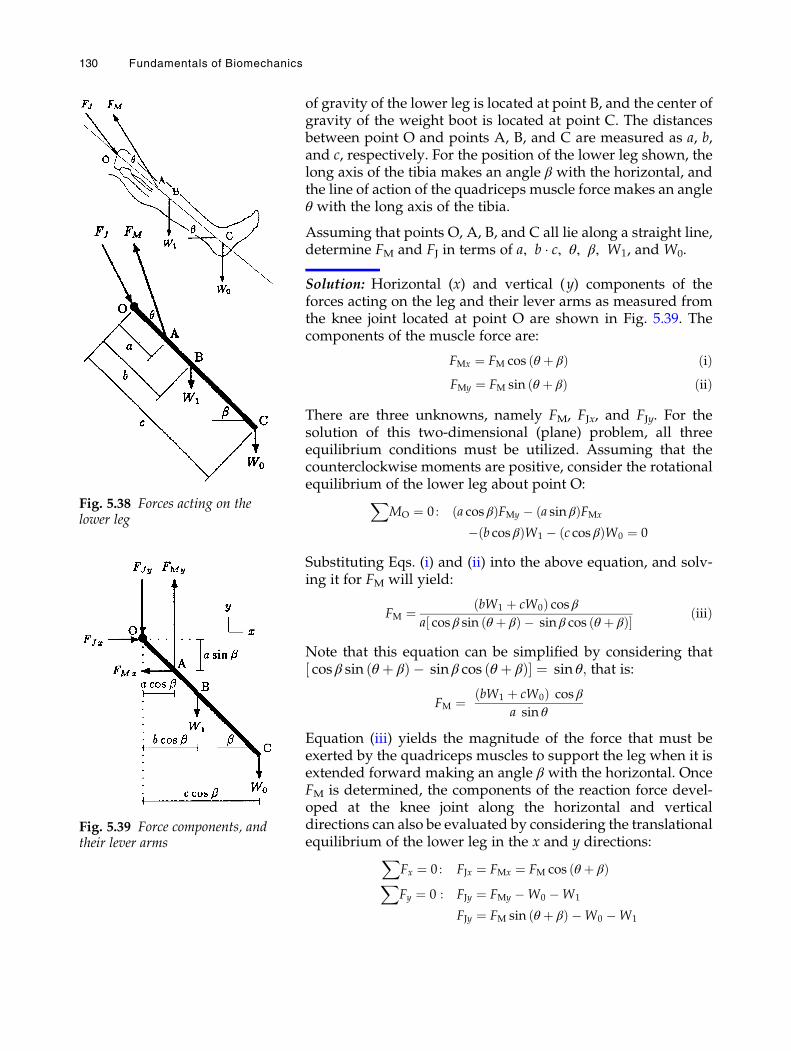
of gravity of the lower leg is located at point B, and the center ofgravity of the weight boot is located at point C. The distancesbetween point O and points A, B, and C are measured as a, b,and c, respectively. For the position of the lower leg shown, thelong axis of the tibia makes an angle β with the horizontal, andthe line of action of the quadriceps muscle force makes an angleθ with the long axis of the tibia.
Assuming that points O, A, B, and C all lie along a straight line,determine FM and FJ in terms of a, b � c, θ, β, W1, and W0.
Solution: Horizontal (x) and vertical (y) components of theforces acting on the leg and their lever arms as measured fromthe knee joint located at point O are shown in Fig. 5.39. Thecomponents of the muscle force are:
FMx ¼ FM cos θ þ βð Þ ðiÞFMy ¼ FM sin θ þ βð Þ ðiiÞ
There are three unknowns, namely FM, FJx, and FJy. For thesolution of this two-dimensional (plane) problem, all threeequilibrium conditions must be utilized. Assuming that thecounterclockwise moments are positive, consider the rotationalequilibrium of the lower leg about point O:X
MO ¼ 0 : a cos βð ÞFMy � a sin βð ÞFMx
� b cos βð ÞW1 � c cos βð ÞW0 ¼ 0
Substituting Eqs. (i) and (ii) into the above equation, and solv-ing it for FM will yield:
FM ¼ bW1 þ cW0ð Þ cos βa cos β sin θ þ βð Þ � sin β cos θ þ βð Þ½ � ðiiiÞ
Note that this equation can be simplified by considering thatcos β sin θ þ βð Þ � sin β cos θ þ βð Þ½ � ¼ sin θ; that is:
FM ¼ bW1 þ cW0ð Þ cos β
a sin θ
Equation (iii) yields the magnitude of the force that must beexerted by the quadriceps muscles to support the leg when it isextended forward making an angle β with the horizontal. OnceFM is determined, the components of the reaction force devel-oped at the knee joint along the horizontal and verticaldirections can also be evaluated by considering the translationalequilibrium of the lower leg in the x and y directions:X
Fx ¼ 0 : FJx ¼ FMx ¼ FM cos θ þ βð ÞXFy ¼ 0 : FJy ¼ FMy �W0 �W1
FJy ¼ FM sin θ þ βð Þ �W0 �W1
Fig. 5.38 Forces acting on thelower leg
Fig. 5.39 Force components, andtheir lever arms
130 Fundamentals of Biomechanics
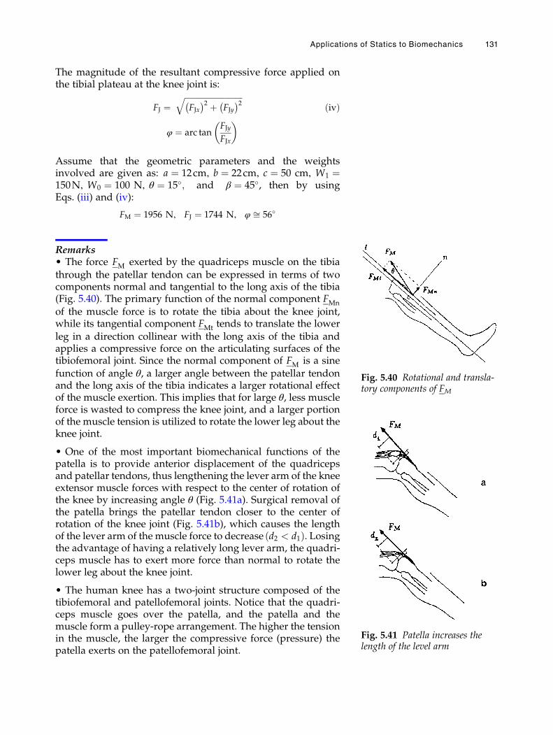
The magnitude of the resultant compressive force applied onthe tibial plateau at the knee joint is:
FJ ¼ffiffiffiffiffiffiffiffiffiffiffiffiffiffiffiffiffiffiffiffiffiffiffiffiffiffiffiffiffiffiFJx� �2 þ FJy
� �2qðivÞ
φ ¼ arc tanFJy
FJx
� �
Assume that the geometric parameters and the weightsinvolved are given as: a ¼ 12cm, b ¼ 22cm, c ¼ 50 cm, W1 ¼150N, W0 ¼ 100 N, θ ¼ 15�; and β ¼ 45�, then by usingEqs. (iii) and (iv):
FM ¼ 1956 N, FJ ¼ 1744 N, φ ffi 56�
Remarks• The force FM exerted by the quadriceps muscle on the tibiathrough the patellar tendon can be expressed in terms of twocomponents normal and tangential to the long axis of the tibia(Fig. 5.40). The primary function of the normal component FMn
of the muscle force is to rotate the tibia about the knee joint,while its tangential component FMt tends to translate the lowerleg in a direction collinear with the long axis of the tibia andapplies a compressive force on the articulating surfaces of thetibiofemoral joint. Since the normal component of FM is a sinefunction of angle θ, a larger angle between the patellar tendonand the long axis of the tibia indicates a larger rotational effectof the muscle exertion. This implies that for large θ, less muscleforce is wasted to compress the knee joint, and a larger portionof the muscle tension is utilized to rotate the lower leg about theknee joint.
• One of the most important biomechanical functions of thepatella is to provide anterior displacement of the quadricepsand patellar tendons, thus lengthening the lever arm of the kneeextensor muscle forces with respect to the center of rotation ofthe knee by increasing angle θ (Fig. 5.41a). Surgical removal ofthe patella brings the patellar tendon closer to the center ofrotation of the knee joint (Fig. 5.41b), which causes the lengthof the lever arm of the muscle force to decrease d2 < d1ð Þ. Losingthe advantage of having a relatively long lever arm, the quadri-ceps muscle has to exert more force than normal to rotate thelower leg about the knee joint.
• The human knee has a two-joint structure composed of thetibiofemoral and patellofemoral joints. Notice that the quadri-ceps muscle goes over the patella, and the patella and themuscle form a pulley-rope arrangement. The higher the tensionin the muscle, the larger the compressive force (pressure) thepatella exerts on the patellofemoral joint.
Fig. 5.40 Rotational and transla-tory components of FM
Fig. 5.41 Patella increases thelength of the level arm
Applications of Statics to Biomechanics 131
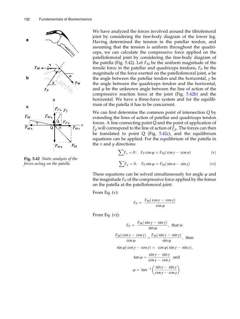
We have analyzed the forces involved around the tibiofemoraljoint by considering the free-body diagram of the lower leg.Having determined the tension in the patellar tendon, andassuming that the tension is uniform throughout the quadri-ceps, we can calculate the compressive force applied on thepatellofemoral joint by considering the free-body diagram ofthe patella (Fig. 5.42). Let FM be the uniform magnitude of thetensile force in the patellar and quadriceps tendons, FP be themagnitude of the force exerted on the patellofemoral joint, α bethe angle between the patellar tendon and the horizontal, γ bethe angle between the quadriceps tendon and the horizontal,and φ be the unknown angle between the line of action of thecompressive reaction force at the joint (Fig. 5.42b) and thehorizontal. We have a three-force system and for the equilib-rium of the patella it has to be concurrent.
We can first determine the common point of intersection Q byextending the lines of action of patellar and quadriceps tendonforces. A line connecting point Q and the point of application ofFP will correspond to the line of action of FP. The forces can thenbe translated to point Q (Fig. 5.42c), and the equilibriumequations can be applied. For the equilibrium of the patella inthe x and y directions:X
Fx ¼ 0 : FP cosφ ¼ FM cos γ � cos αð Þ ðvÞX
Fy ¼ 0 : FP sinφ ¼ FM sin α� sin γð Þ ðviÞ
These equations can be solved simultaneously for angle φ andthe magnitude FP of the compressive force applied by the femuron the patella at the patellofemoral joint:
From Eq. (v):
FP ¼ FM cos γ � cos γð Þcosφ
From Eq. (vi):
FP ¼ FM sin γ � sin γð Þsinφ
, that is
FM cos γ � cos γð Þcosφ
¼ FM sin γ � sin γð Þsinφ
, then
sinφ cos γ � cos γð Þ ¼ cosφ sin γ � sin γð Þ;
tanφ ¼ sin γ � sin γ
cos γ � cos γand
φ ¼ tan �1 sin γ � sin γ
cos γ � cos γ
� �
Fig. 5.42 Static analysis of theforces acting on the patella
132 Fundamentals of Biomechanics
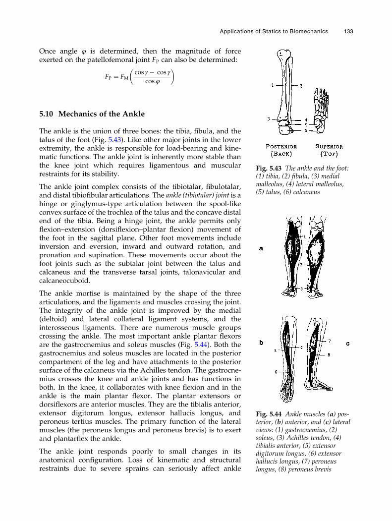
Once angle φ is determined, then the magnitude of forceexerted on the patellofemoral joint FP can also be determined:
FP ¼ FMcos γ � cos γ
cosφ
� �
5.10 Mechanics of the Ankle
The ankle is the union of three bones: the tibia, fibula, and thetalus of the foot (Fig. 5.43). Like other major joints in the lowerextremity, the ankle is responsible for load-bearing and kine-matic functions. The ankle joint is inherently more stable thanthe knee joint which requires ligamentous and muscularrestraints for its stability.
The ankle joint complex consists of the tibiotalar, fibulotalar,and distal tibiofibular articulations. The ankle (tibiotalar) joint is ahinge or ginglymus-type articulation between the spool-likeconvex surface of the trochlea of the talus and the concave distalend of the tibia. Being a hinge joint, the ankle permits onlyflexion–extension (dorsiflexion–plantar flexion) movement ofthe foot in the sagittal plane. Other foot movements includeinversion and eversion, inward and outward rotation, andpronation and supination. These movements occur about thefoot joints such as the subtalar joint between the talus andcalcaneus and the transverse tarsal joints, talonavicular andcalcaneocuboid.
The ankle mortise is maintained by the shape of the threearticulations, and the ligaments and muscles crossing the joint.The integrity of the ankle joint is improved by the medial(deltoid) and lateral collateral ligament systems, and theinterosseous ligaments. There are numerous muscle groupscrossing the ankle. The most important ankle plantar flexorsare the gastrocnemius and soleus muscles (Fig. 5.44). Both thegastrocnemius and soleus muscles are located in the posteriorcompartment of the leg and have attachments to the posteriorsurface of the calcaneus via the Achilles tendon. The gastrocne-mius crosses the knee and ankle joints and has functions inboth. In the knee, it collaborates with knee flexion and in theankle is the main plantar flexor. The plantar extensors ordorsiflexors are anterior muscles. They are the tibialis anterior,extensor digitorum longus, extensor hallucis longus, andperoneus tertius muscles. The primary function of the lateralmuscles (the peroneus longus and peroneus brevis) is to exertand plantarflex the ankle.
The ankle joint responds poorly to small changes in itsanatomical configuration. Loss of kinematic and structuralrestraints due to severe sprains can seriously affect ankle
Fig. 5.43 The ankle and the foot:(1) tibia, (2) fibula, (3) medialmalleolus, (4) lateral malleolus,(5) talus, (6) calcaneus
Fig. 5.44 Ankle muscles (a) pos-terior, (b) anterior, and (c) lateralviews: (1) gastrocnemius, (2)soleus, (3) Achilles tendon, (4)tibialis anterior, (5) extensordigitorum longus, (6) extensorhallucis longus, (7) peroneuslongus, (8) peroneus brevis
Applications of Statics to Biomechanics 133
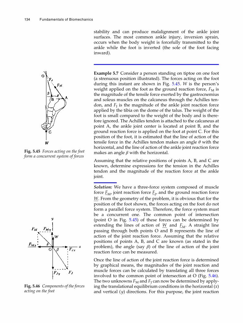
stability and can produce malalignment of the ankle jointsurfaces. The most common ankle injury, inversion sprain,occurs when the body weight is forcefully transmitted to theankle while the foot is inverted (the sole of the foot facinginward).
Example 5.7 Consider a person standing on tiptoe on one foot(a strenuous position illustrated). The forces acting on the footduring this instant are shown in Fig. 5.45. W is the person’sweight applied on the foot as the ground reaction force, FM isthe magnitude of the tensile force exerted by the gastrocnemiusand soleus muscles on the calcaneus through the Achilles ten-don, and FJ is the magnitude of the ankle joint reaction forceapplied by the tibia on the dome of the talus. The weight of thefoot is small compared to the weight of the body and is there-fore ignored. The Achilles tendon is attached to the calcaneus atpoint A, the ankle joint center is located at point B, and theground reaction force is applied on the foot at point C. For thisposition of the foot, it is estimated that the line of action of thetensile force in the Achilles tendon makes an angle θ with thehorizontal, and the line of action of the ankle joint reaction forcemakes an angle β with the horizontal.
Assuming that the relative positions of points A, B, and C areknown, determine expressions for the tension in the Achillestendon and the magnitude of the reaction force at the anklejoint.
Solution: We have a three-force system composed of muscleforce FM, joint reaction force FJ, and the ground reaction force
W. From the geometry of the problem, it is obvious that for theposition of the foot shown, the forces acting on the foot do notform a parallel force system. Therefore, the force system mustbe a concurrent one. The common point of intersection(point O in Fig. 5.45) of these forces can be determined byextending the lines of action of W and FM. A straight linepassing through both points O and B represents the line ofaction of the joint reaction force. Assuming that the relativepositions of points A, B, and C are known (as stated in theproblem), the angle (say β) of the line of action of the jointreaction force can be measured.
Once the line of action of the joint reaction force is determinedby graphical means, the magnitudes of the joint reaction andmuscle forces can be calculated by translating all three forcesinvolved to the common point of intersection at O (Fig. 5.46).The two unknowns FM and FJ can now be determined by apply-ing the translational equilibrium conditions in the horizontal (x)and vertical (y) directions. For this purpose, the joint reaction
Fig. 5.45 Forces acting on the footform a concurrent system of forces
Fig. 5.46 Components of the forcesacting on the foot
134 Fundamentals of Biomechanics
and muscle forces must be decomposed into their rectangularcomponents first:
FMx ¼ FM cos θ
FMy ¼ FM sin θ
FJx ¼ FJ cos β
FJy ¼ FJ sin β
For the translational equilibrium of the foot in the horizontaland vertical directions:X
Fx ¼ 0 : FJx ¼ FMx, that is FJ cos β ¼ FM cos θXFy ¼ 0 : FJy ¼ FMy þ W, that is FJ sin β ¼ FM sin θ þW
Simultaneous solutions of these equations will yield:
FM ¼ W cos β
cos θ sin β � sin θ cos β, that is : FM ¼ W cos β
sin β � θð ÞFJ ¼ W cos θ
cos θ sin β � sin θ cos β, that is : FJ ¼ W cos θ
sin β � θð Þ
For example, assume that θ ¼ 45� and β ¼ 60�. Then:
FM ¼ 1:93 W FJ ¼ 2:73 W
5.11 Exercise Problems
Problem 5.1 Consider a person holding an object in his handwith his elbow flexed at the right angle with respect to theupper arm (Fig. 5.4). The forces acting on the forearm and themechanics model of the system are shown in Fig. 5.5a, b. As forthis system assume that the biceps is the major flexor and theline of action of the muscle makes the right angle with the longaxis of the forearm. Point O designates the axis of rotation at theelbow joint, A is the point of attachment of the biceps muscle tothe radius, point B is the center of gravity of the forearm, andpoint C is the center of gravity of the object held in the hand.Furthermore, the distances between the axis of rotation of theelbow joint (point O) and points A, B, and C are a ¼ 4.5 cm,b ¼ 16.5 cm, and c ¼ 37 cm. If the total weight of the forearm isW ¼ 83 N, and the magnitude of the muscle force isFM ¼ 780 N:
(a) Determine the weight (W0) of the object held in the hand.(b) Determine the magnitude of the reaction force (FJ) at the
elbow joint.
Applications of Statics to Biomechanics 135
(c) Determine the magnitude of the muscle (FM1) and jointreaction (FJ1) forces when the weight of the object held inthe hand is increased by 5 N.
Answers: (a) W0 ¼ 57.8 N; (b) FJ ¼ 639.2 N; (c) FM1 ¼ 820 N,FJ1 ¼ 674.2 N
Problem 5.2 Consider a person performing shoulder exercisesby using a dumbbell (Fig. 5.11). The forces acting on the armand the mechanical model of the system are shown in Fig. 5.12.For this system assume that the arm of the person is fullyextended to the horizontal. Point O designates the axis of rota-tion of the shoulder joint, A is the point of attachment of thedeltoid muscle to the humerus, point B is the center of gravityof the entire arm, and point C is the center of gravity ofthe dumbbell. The distances between the axis of rotation of theshoulder joint (point O) and points A, B, and C are a ¼ 17 cm,b ¼ 33 cm, and c ¼ 63 cm. The dumbbell weighs W0 ¼ 64 Nand for this position of the arm it is estimated that the magni-tude of the muscle force is FM ¼ 1051 N. If the lines of action ofthe muscle (FM) and the joint reaction forces (FJ) make anangle θ ¼ 18� and β ¼ 12� with the horizontal, respectively:
(a) Determine the magnitude of reaction force (FJ) at the shoul-der joint.
(b) Determine the total weight (W) of the arm.(c) Determine the magnitude of the muscle (FM1) and joint
reaction (FJ1) forces when the weight of the dumbbell isincreased by 5 N.
Answers: (a) FJ ¼ 1021.9 N; (b) W ¼ 47.3 N; (c) FM1 ¼ 1136.5 N,FJ1 ¼ 1105 N
Problem 5.3 Consider the position of the head and neck as wellas forces acting on the head shown in Fig. 5.15. For this equilib-rium condition assume that the forces involved form a concur-rent force system. Point C is the center of gravity of the head,A isthe point of application of force (FM) exerted by the neck exten-sor muscles on the head, and point B is the center of rotation ofthe atlantooccipital joint. For this position of the head, it isestimated that the magnitude of the resultant force exerted bythe neck extensormuscles is FM ¼ 57N, and the lines of action ofthe muscles and the joint reaction forces make an angle θ ¼ 36�
and β ¼ 63� with the horizontal, respectively. Determine themagnitude of the gravitational force acting on the head.
Answer: W ¼ 47 N
136 Fundamentals of Biomechanics
Problem 5.4 Consider a weight lifter who is trying to lift abarbell. The forces acting on the lower part of the athlete’sbody and the mechanical model of the system are shown inFigs. 5.19 and 5.20, respectively. Point O designates the center ofrotation at the joint formed by the sacrum and the fifth lumbarvertebra. A is the point of application of force exerted by theback muscles, point B is the center of gravity of the lower body,and C is the point of application of the ground reaction force.With respect to point O, a ¼ 3.6 cm, b ¼ 14.6 cm, and c ¼ 22 cm,are the shortest distances between the lines of action of the backmuscles’ force, the lower body’s gravitational force, and theground reaction force with the center of rotation of the joint.For a weight lifter in this position, it is estimated that the forceexerted by the back muscles is FM ¼ 6856 N and the line ofaction of this force makes an angle θ ¼ 43� with the vertical. Ifthe barbell weighsW0 ¼ 637 N and the magnitude of the gravi-tational force acting on the lower body is W1 ¼ 333 N:
(a) Determine the weight (W) of the athlete.(b) Determine the magnitude of the reaction force (FJ) acting at
the joint.(c) Determine an angle α that the line of action of the joint
reaction force makes with the horizontal.
Answers: (a) W ¼ 705.9 N; (b) FJ ¼ 7625.8 N; (c) α ¼ 52�
Problem 5.5 Consider a person that momentarily put the entireweight of his body on one leg when walking or running.The forces acting on the leg and the mechanical model of thesystem are shown in Figs. 5.24 and 5.25, respectively. Point Odesignates the center of rotation of the hip joint. A is the point ofattachment of the hip abductor muscles to the femur, point B isthe center of gravity of the leg, and C is the point of applicationof the ground reaction force. The distances between point A andpoints O, B, and C are specified as a ¼ 8.6 cm, b ¼ 34.3 cm, andc ¼ 89.4 cm. The angles that the femoral neck and the long axisof the femoral shaft make with the horizontal are specified asα ¼ 43� and β ¼ 79�, respectively. Furthermore, for this single-leg stance, it is estimated that the magnitude of force exerted bythe hip abductor muscles is FM ¼ 2062.6 N and its line of actionmakes an angle θ ¼ 69� with the horizontal. If the magnitude ofgravitational force acting on the leg is W1 ¼ 125 N:
(a) Determine the total weight (W) of the person.(b) Determine the magnitude of the reaction force (FJ) acting at
the hip joint.
Applications of Statics to Biomechanics 137

(c) Determine an angle γ that the line of action of the jointreaction force makes with the horizontal.
Answers: (a) W ¼ 729.7 N; (b) FJ ¼ 2636.1 N; (c) γ ¼ 73.7�
Problem 5.6 Consider a person performing lower leg flexion–extension exercises from a sitting position while wearing aweight boot. Forces acting on the leg and the mechanicalmodel of the system are shown in Fig. 5.38. Point O designatesthe center of rotation of the tibiofemoral joint. A is the point ofattachment of the patellar tendon to the tibia, point B is thecenter of gravity of the lower leg, and point C is the center ofgravity of the weight boot. For this system assume that thepoints O, A, B, and C all lie along a straight line. The distancesbetween point O and points A, B, and C are measured as a ¼ 13cm, b ¼ 23.5 cm, and c ¼ 53 cm, respectively. For this positionof the leg, the long axis of the tibia makes an angle β ¼ 47� withthe horizontal, and the line of action of the quadriceps muscleforce makes an angle θ ¼ 17� with the long axis of the tibia.Furthermore, for this position of the leg, it is estimated that theforce exerted by the quadriceps muscle is FM ¼ 1.940 N.
If the weight of the lower leg is W1 ¼ 163 N:
(a) Determine the weight (W0) of the weight boot.(b) Determine the magnitude of the reaction force (FJ) of the
tibiofemoral joint.(c) Determine an angle φ that the line of action the joint reaction
force makes with the horizontal.
Answers: (a) W0 ¼ 98.4 N; (b) FJ ¼ 1707.5 N; (c) φ ¼ 60.2�
Problem 5.7 Consider a person standing on tiptoe on one foot.For this position, the forces acting on the foot are shown inFig. 5.45. Point A is the point of attachment of the Achillestendon through which a force is exerted by the gastrocnemiusand soleus muscles on the calcaneus. Point B designates thecenter of the ankle joint and C is the point of application of theground reaction force. For this system assume that the weight ofthe foot can be ignored as it is relatively small when comparedto the weight of the entire body of the person. For this positionof the foot, it is estimated that the lines of action of the tensileforce in the Achilles tendon and the reaction force (FJ) of theankle joint make an angle θ ¼ 49� and β ¼ 65� with the hori-zontal, respectively. Furthermore, for this position of the foot,it is also estimated that the magnitude of force exerted by
138 Fundamentals of Biomechanics
the gastrocnemius and soleus muscles on the calcaneus isFM ¼ 1275.4 N.
(a) Determine the entire weight (W) of the person.(b) Determine the magnitude of the reaction force (FJ) of the
ankle joint.
Answers: (a) W ¼ 831.8 N; (b) FJ ¼ 1980.3 N
References
Chaffin, D.B., Andersson, G.B.J., & Martin, B.J. 1999. Occupational Biomechanics(3rd ed.). New York: John Wiley & Sons.
LeVeau, B.F., 2010. Biomechanics of Human Motion: Basics and Beyond for theHealth Professions. Thorofare, NJ. SLACK Incorporated.
Nordin, M., & Frankel, V.H (Eds.). 2011. Basic Biomechanics of the Musculoskele-tal System (4th ed.). Philadelphia, PA: Lippincott Williams & Wilkins.
Thompson, CW, 1989, Manual of Structural Kinesiology, 11th Ed. St. Louis,MO: Times-Mirror/Mosby.
Winter, D.A. 2004. Biomechanics and Motor Control of Human Movement (3rded.). New York: John Wiley & Sons.
Applications of Statics to Biomechanics 139
Chapter 6
Introduction to Dynamics
6.1 Dynamics / 143
6.2 Kinematics and Kinetics / 143
6.3 Linear, Angular, and General Motions / 144
6.4 Distance and Displacement / 145
6.5 Speed and Velocity / 145
6.6 Acceleration / 145
6.7 Inertia and Momentum / 146
6.8 Degree of Freedom / 146
6.9 Particle Concept / 146
6.10 Reference Frames and Coordinate Systems / 147
6.11 Prerequisites for Dynamic Analysis / 147
6.12 Topics to Be Covered / 147
# Springer International Publishing Switzerland 2017N. Ozkaya et al., Fundamentals of Biomechanics, DOI 10.1007/978-3-319-44738-4_6
141

6.1 Dynamics
Dynamics is the study of bodies in motion. Dynamics isconcerned with describing motion and explaining its causes.The general field of dynamics consists of two major areas:kinematics and kinetics. Each of these areas can be furtherdivided to describe and explain linear, angular, or generalmotion of bodies. The fundamental concepts in dynamics arespace (relative position or displacement), time, mass, and force.Other important concepts include velocity, acceleration, torque,moment, work, energy, power, impulse, and momentum.
The broad definitions of basic terms and concepts in dynamicswill be introduced in this chapter. The details of kinematic andkinetic characteristics of moving bodies will be covered in thefollowing chapters.
6.2 Kinematics and Kinetics
The field of kinematics is concerned with the description ofgeometric and time-dependent aspects of motion without deal-ing with the forces causing the motion. Kinematic analyses arebased on the relationships between displacement, velocity, andacceleration vectors. These relationships appear in the form ofdifferential and integral equations.
The field of kinetics is based on kinematics, and it incorporatesinto the analyses the effects of forces and torques that cause themotion. Kinetic analyses utilize Newton’s second law of motionthat can take various mathematical forms. There are a numberof different approaches to the solutions of problems in kinetics.These approaches are based on the equations of motion, workand energy methods, and impulse and momentum methods.Different methods may be applied to different situations, ordepending on what is required to be determined. For example,the equations of motion are used for problems requiring theanalysis of acceleration. Energy methods are suitable when aproblem requires the analysis of forces related to changes invelocity. Momentummethods are applied if the forces involvedare impulsive, which is the case during impact and collision.
There is also the field of kinesiology that is related to the study ofhuman motion characteristics, joint and muscle forces, andneurological and other factors that may be important in study-ing human motion. The term “kinesiology” is not a mechanicalbut a medical term. It is commonly used to refer to the biome-chanics of human motion.
Introduction to Dynamics 143
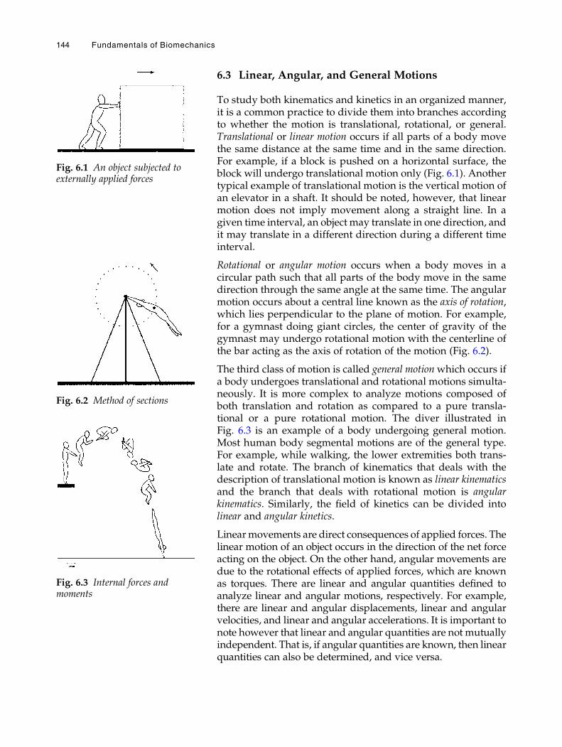
6.3 Linear, Angular, and General Motions
To study both kinematics and kinetics in an organized manner,it is a common practice to divide them into branches accordingto whether the motion is translational, rotational, or general.Translational or linear motion occurs if all parts of a body movethe same distance at the same time and in the same direction.For example, if a block is pushed on a horizontal surface, theblock will undergo translational motion only (Fig. 6.1). Anothertypical example of translational motion is the vertical motion ofan elevator in a shaft. It should be noted, however, that linearmotion does not imply movement along a straight line. In agiven time interval, an object may translate in one direction, andit may translate in a different direction during a different timeinterval.
Rotational or angular motion occurs when a body moves in acircular path such that all parts of the body move in the samedirection through the same angle at the same time. The angularmotion occurs about a central line known as the axis of rotation,which lies perpendicular to the plane of motion. For example,for a gymnast doing giant circles, the center of gravity of thegymnast may undergo rotational motion with the centerline ofthe bar acting as the axis of rotation of the motion (Fig. 6.2).
The third class of motion is called general motionwhich occurs ifa body undergoes translational and rotational motions simulta-neously. It is more complex to analyze motions composed ofboth translation and rotation as compared to a pure transla-tional or a pure rotational motion. The diver illustrated inFig. 6.3 is an example of a body undergoing general motion.Most human body segmental motions are of the general type.For example, while walking, the lower extremities both trans-late and rotate. The branch of kinematics that deals with thedescription of translational motion is known as linear kinematicsand the branch that deals with rotational motion is angularkinematics. Similarly, the field of kinetics can be divided intolinear and angular kinetics.
Linearmovements are direct consequences of applied forces. Thelinear motion of an object occurs in the direction of the net forceacting on the object. On the other hand, angular movements aredue to the rotational effects of applied forces, which are knownas torques. There are linear and angular quantities defined toanalyze linear and angular motions, respectively. For example,there are linear and angular displacements, linear and angularvelocities, and linear and angular accelerations. It is important tonote however that linear and angular quantities are not mutuallyindependent. That is, if angular quantities are known, then linearquantities can also be determined, and vice versa.
Fig. 6.1 An object subjected toexternally applied forces
Fig. 6.2 Method of sections
Fig. 6.3 Internal forces andmoments
144 Fundamentals of Biomechanics
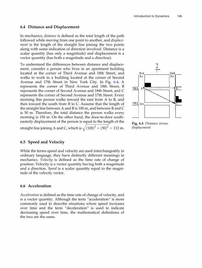
6.4 Distance and Displacement
In mechanics, distance is defined as the total length of the pathfollowed while moving from one point to another, and displace-ment is the length of the straight line joining the two pointsalong with some indication of direction involved. Distance is ascalar quantity (has only a magnitude) and displacement is avector quantity (has both a magnitude and a direction).
To understand the differences between distance and displace-ment, consider a person who lives in an apartment buildinglocated at the corner of Third Avenue and 18th Street, andwalks to work in a building located at the corner of SecondAvenue and 17th Street in New York City. In Fig. 6.4, Arepresents the corner of Third Avenue and 18th Street, Brepresents the corner of Second Avenue and 18th Street, and Crepresents the corner of Second Avenue and 17th Street. Everymorning this person walks toward the east from A to B, andthen toward the south from B to C. Assume that the length ofthe straight line between A and B is 100 m, and between B and Cis 50 m. Therefore, the total distance the person walks everymorning is 150 m. On the other hand, the door-to-door south-easterly displacement of the person is equal to the length of the
straight line joining A and C, which isffiffiffiffiffiffiffiffiffiffiffiffiffiffiffiffiffiffiffiffiffiffiffiffiffiffiffiffiffiffi
100ð Þ2 þ 50ð Þ2q
¼ 112 m.
6.5 Speed and Velocity
While the terms speed and velocity are used interchangeably inordinary language, they have distinctly different meanings inmechanics. Velocity is defined as the time rate of change ofposition. Velocity is a vector quantity having both a magnitudeand a direction. Speed is a scalar quantity equal to the magni-tude of the velocity vector.
6.6 Acceleration
Acceleration is defined as the time rate of change of velocity, andis a vector quantity. Although the term “acceleration” is morecommonly used to describe situations where speed increasesover time and the term “deceleration” is used to indicatedecreasing speed over time, the mathematical definitions ofthe two are the same.
Fig. 6.4 Distance versusdisplacement
Introduction to Dynamics 145
6.7 Inertia and Momentum
Inertia is the tendency of an object to maintain its state of rest oruniform motion. Inertia can also be defined as the resistance tothe change in motion of an object. The more inertia an objecthas, the more difficult it is to start moving it from rest or tochange its state of motion. The greater the mass of the object, thegreater its inertia. For example, a truck has a greater inertia thana passenger car because of the difference in their mass. If both ofthem are traveling at the same speed, it is always more difficultto stop the truck as compared to the car.
Like inertia, momentum is a tendency to resist changes in theexisting state of motion and is defined as the product of massand velocity. Only moving objects have momentum, whereasevery object—stationary or moving—has an inertia. If twomoving objects having the same mass are considered, then theone with higher speed has the greater momentum. If twomoving objects having the same speed are considered, thenthe one with higher mass has the greater momentum.
6.8 Degree of Freedom
Degree of freedom is an expression that describes the ability of anobject to move in space. A completely unrestrained object, suchas a ball, has six degrees of freedom (three related to transla-tional motion along three mutually perpendicular axes andthree related to rotational motion about the same axes). Thehuman hip joint has three degrees of freedom because it enablesthe lower extremity to rotate about one axis and undergo angu-lar movements in two planes. On the other hand, the elbow andforearm system has two degrees of freedom because it allowsthe lower arm to rotate about one axis and undergo angularmovement in one plane.
6.9 Particle Concept
The “particle” concept in mechanics is rather a hypotheticalone. It undermines the size and shape of the object underconsideration, and assumes that the object is a particle with amass equal to the total mass of the object and located at thecenter of gravity of the object. In some problems, the shape ofthe object under investigation may not be pertinent to the dis-cussion of certain aspects of its motion. This is particularly trueif the object is undergoing a translational motion only. Forexample, what is significant for a person pushing a wheelchairis the total mass of the wheelchair, not its size or shape. There-fore, the wheelchair may be treated as a particle with a mass
146 Fundamentals of Biomechanics
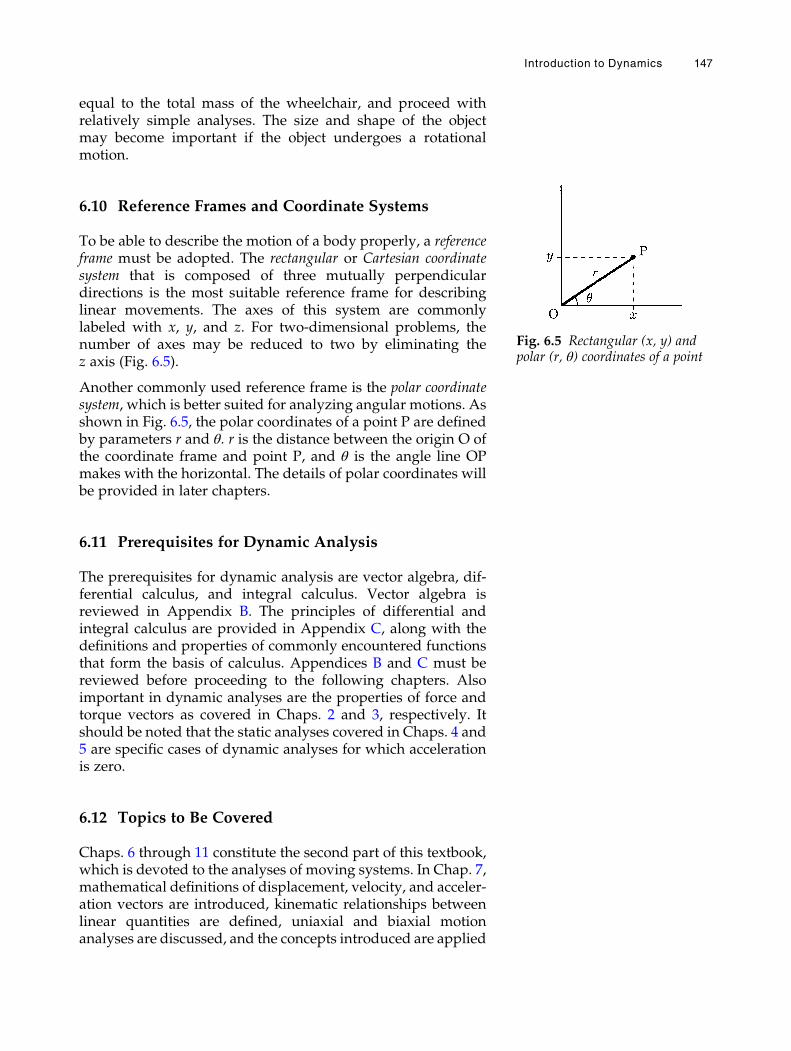
equal to the total mass of the wheelchair, and proceed withrelatively simple analyses. The size and shape of the objectmay become important if the object undergoes a rotationalmotion.
6.10 Reference Frames and Coordinate Systems
To be able to describe the motion of a body properly, a referenceframe must be adopted. The rectangular or Cartesian coordinatesystem that is composed of three mutually perpendiculardirections is the most suitable reference frame for describinglinear movements. The axes of this system are commonlylabeled with x, y, and z. For two-dimensional problems, thenumber of axes may be reduced to two by eliminating thez axis (Fig. 6.5).
Another commonly used reference frame is the polar coordinatesystem, which is better suited for analyzing angular motions. Asshown in Fig. 6.5, the polar coordinates of a point P are definedby parameters r and θ. r is the distance between the origin O ofthe coordinate frame and point P, and θ is the angle line OPmakes with the horizontal. The details of polar coordinates willbe provided in later chapters.
6.11 Prerequisites for Dynamic Analysis
The prerequisites for dynamic analysis are vector algebra, dif-ferential calculus, and integral calculus. Vector algebra isreviewed in Appendix B. The principles of differential andintegral calculus are provided in Appendix C, along with thedefinitions and properties of commonly encountered functionsthat form the basis of calculus. Appendices B and C must bereviewed before proceeding to the following chapters. Alsoimportant in dynamic analyses are the properties of force andtorque vectors as covered in Chaps. 2 and 3, respectively. Itshould be noted that the static analyses covered in Chaps. 4 and5 are specific cases of dynamic analyses for which accelerationis zero.
6.12 Topics to Be Covered
Chaps. 6 through 11 constitute the second part of this textbook,which is devoted to the analyses of moving systems. In Chap. 7,mathematical definitions of displacement, velocity, and acceler-ation vectors are introduced, kinematic relationships betweenlinear quantities are defined, uniaxial and biaxial motionanalyses are discussed, and the concepts introduced are applied
Fig. 6.5 Rectangular (x, y) andpolar (r, θ) coordinates of a point
Introduction to Dynamics 147
to problems of sports biomechanics. Linear kinetics is studied inChap. 8. Solving problems in kinetics using the equations ofmotion and work and energy methods are discussed in Chap. 8.Angular kinematics and kinetics are covered in Chaps. 9 and 10,respectively, and the concepts and procedures introduced areapplied to investigate some of the problems of biomechanics.Topics such as impulse, momentum, impact, and collision arecovered in Chap. 11.
148 Fundamentals of Biomechanics
Chapter 7
Linear Kinematics
7.1 Uniaxial Motion / 151
7.2 Position, Displacement, Velocity, and Acceleration /151
7.3 Dimensions and Units / 153
7.4 Measured and Derived Quantities / 154
7.5 Uniaxial Motion with Constant Acceleration / 155
7.6 Examples of Uniaxial Motion / 157
7.7 Biaxial Motion / 163
7.8 Position, Velocity, and Acceleration Vectors / 163
7.9 Biaxial Motion with Constant Acceleration / 166
7.10 Projectile Motion / 167
7.11 Applications to Athletics / 170
7.12 Exercise Problems / 175
# Springer International Publishing Switzerland 2017N. Ozkaya et al., Fundamentals of Biomechanics, DOI 10.1007/978-3-319-44738-4_7
149

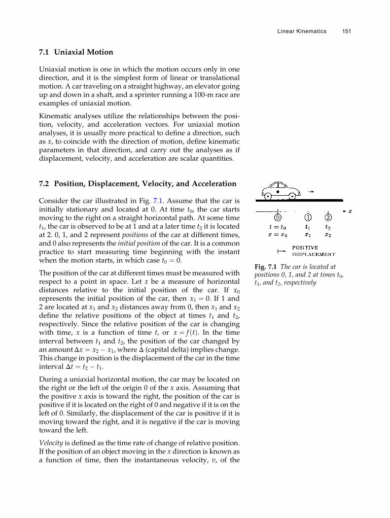
7.1 Uniaxial Motion
Uniaxial motion is one in which the motion occurs only in onedirection, and it is the simplest form of linear or translationalmotion. A car traveling on a straight highway, an elevator goingup and down in a shaft, and a sprinter running a 100-m race areexamples of uniaxial motion.
Kinematic analyses utilize the relationships between the posi-tion, velocity, and acceleration vectors. For uniaxial motionanalyses, it is usually more practical to define a direction, suchas x, to coincide with the direction of motion, define kinematicparameters in that direction, and carry out the analyses as ifdisplacement, velocity, and acceleration are scalar quantities.
7.2 Position, Displacement, Velocity, and Acceleration
Consider the car illustrated in Fig. 7.1. Assume that the car isinitially stationary and located at 0. At time t0, the car startsmoving to the right on a straight horizontal path. At some timet1, the car is observed to be at 1 and at a later time t2 it is locatedat 2. 0, 1, and 2 represent positions of the car at different times,and 0 also represents the initial position of the car. It is a commonpractice to start measuring time beginning with the instantwhen the motion starts, in which case t0 ¼ 0.
The position of the car at different times must be measured withrespect to a point in space. Let x be a measure of horizontaldistances relative to the initial position of the car. If x0represents the initial position of the car, then x1 ¼ 0. If 1 and2 are located at x1 and x2 distances away from 0, then x1 and x2define the relative positions of the object at times t1 and t2,respectively. Since the relative position of the car is changingwith time, x is a function of time t, or x ¼ f tð Þ. In the timeinterval between t1 and t2, the position of the car changed byan amountΔx ¼ x2 � x1, where Δ (capital delta) implies change.This change in position is the displacement of the car in the timeinterval Δt ¼ t2 � t1.
During a uniaxial horizontal motion, the car may be located onthe right or the left of the origin 0 of the x axis. Assuming thatthe positive x axis is toward the right, the position of the car ispositive if it is located on the right of 0 and negative if it is on theleft of 0. Similarly, the displacement of the car is positive if it ismoving toward the right, and it is negative if the car is movingtoward the left.
Velocity is defined as the time rate of change of relative position.If the position of an object moving in the x direction is known asa function of time, then the instantaneous velocity, v, of the
Fig. 7.1 The car is located atpositions 0, 1, and 2 at times t0,t1, and t2, respectively
Linear Kinematics 151
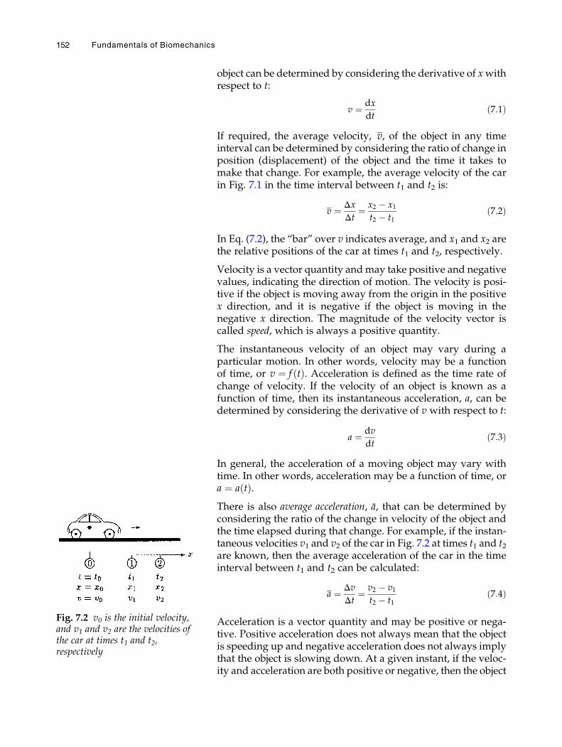
object can be determined by considering the derivative of xwithrespect to t:
v ¼ dx
dtð7:1Þ
If required, the average velocity, v, of the object in any timeinterval can be determined by considering the ratio of change inposition (displacement) of the object and the time it takes tomake that change. For example, the average velocity of the carin Fig. 7.1 in the time interval between t1 and t2 is:
v ¼ ΔxΔt
¼ x2 � x1t2 � t1
ð7:2Þ
In Eq. (7.2), the “bar” over v indicates average, and x1 and x2 arethe relative positions of the car at times t1 and t2, respectively.
Velocity is a vector quantity andmay take positive and negativevalues, indicating the direction of motion. The velocity is posi-tive if the object is moving away from the origin in the positivex direction, and it is negative if the object is moving in thenegative x direction. The magnitude of the velocity vector iscalled speed, which is always a positive quantity.
The instantaneous velocity of an object may vary during aparticular motion. In other words, velocity may be a functionof time, or v ¼ f tð Þ. Acceleration is defined as the time rate ofchange of velocity. If the velocity of an object is known as afunction of time, then its instantaneous acceleration, a, can bedetermined by considering the derivative of v with respect to t:
a ¼ dv
dtð7:3Þ
In general, the acceleration of a moving object may vary withtime. In other words, acceleration may be a function of time, ora ¼ a tð Þ.There is also average acceleration, a, that can be determined byconsidering the ratio of the change in velocity of the object andthe time elapsed during that change. For example, if the instan-taneous velocities v1 and v2 of the car in Fig. 7.2 at times t1 and t2are known, then the average acceleration of the car in the timeinterval between t1 and t2 can be calculated:
a ¼ ΔvΔt
¼ v2 � v1t2 � t1
ð7:4Þ
Acceleration is a vector quantity and may be positive or nega-tive. Positive acceleration does not always mean that the objectis speeding up and negative acceleration does not always implythat the object is slowing down. At a given instant, if the veloc-ity and acceleration are both positive or negative, then the object
Fig. 7.2 v0 is the initial velocity,and v1 and v2 are the velocities ofthe car at times t1 and t2,respectively
152 Fundamentals of Biomechanics
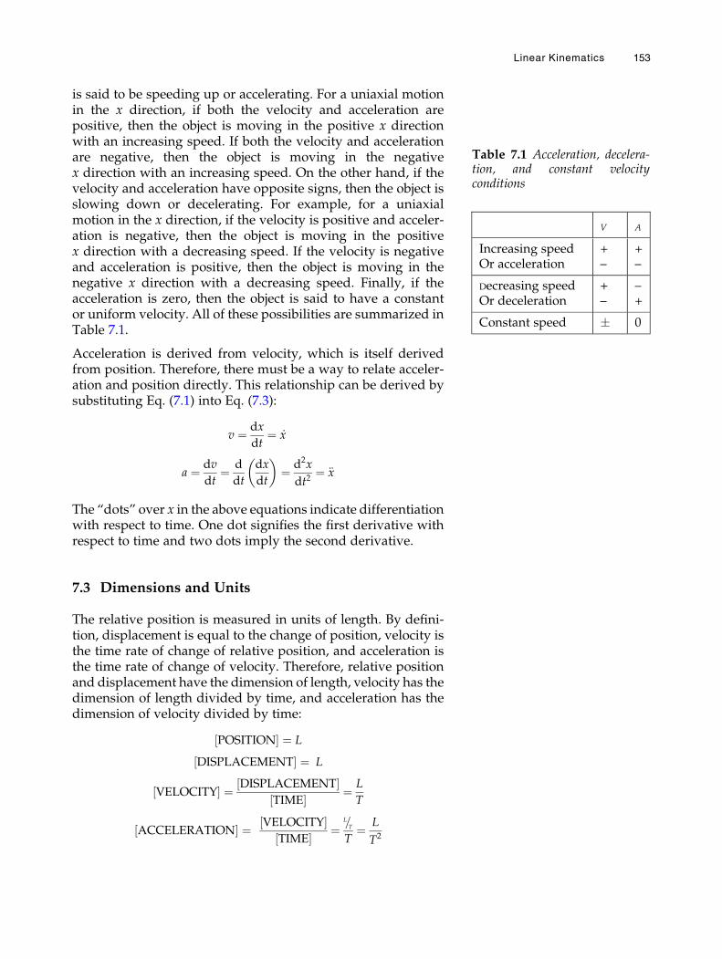
is said to be speeding up or accelerating. For a uniaxial motionin the x direction, if both the velocity and acceleration arepositive, then the object is moving in the positive x directionwith an increasing speed. If both the velocity and accelerationare negative, then the object is moving in the negativex direction with an increasing speed. On the other hand, if thevelocity and acceleration have opposite signs, then the object isslowing down or decelerating. For example, for a uniaxialmotion in the x direction, if the velocity is positive and acceler-ation is negative, then the object is moving in the positivex direction with a decreasing speed. If the velocity is negativeand acceleration is positive, then the object is moving in thenegative x direction with a decreasing speed. Finally, if theacceleration is zero, then the object is said to have a constantor uniform velocity. All of these possibilities are summarized inTable 7.1.
Acceleration is derived from velocity, which is itself derivedfrom position. Therefore, there must be a way to relate acceler-ation and position directly. This relationship can be derived bysubstituting Eq. (7.1) into Eq. (7.3):
v ¼ dx
dt¼ _x
a ¼ dv
dt¼ d
dt
dx
dt
� �¼ d2x
dt2¼ €x
The “dots” over x in the above equations indicate differentiationwith respect to time. One dot signifies the first derivative withrespect to time and two dots imply the second derivative.
7.3 Dimensions and Units
The relative position is measured in units of length. By defini-tion, displacement is equal to the change of position, velocity isthe time rate of change of relative position, and acceleration isthe time rate of change of velocity. Therefore, relative positionand displacement have the dimension of length, velocity has thedimension of length divided by time, and acceleration has thedimension of velocity divided by time:
POSITION½ � ¼ L
DISPLACEMENT½ � ¼ L
VELOCITY½ � ¼ DISPLACEMENT½ �TIME½ � ¼ L
T
ACCELERATION½ � ¼ VELOCITY½ �TIME½ � ¼
L=T
T¼ L
T2
Table 7.1 Acceleration, decelera-tion, and constant velocityconditions
V A
Increasing speedOr acceleration
+–
+–
Decreasing speedOr deceleration
+–
–+
Constant speed � 0
Linear Kinematics 153
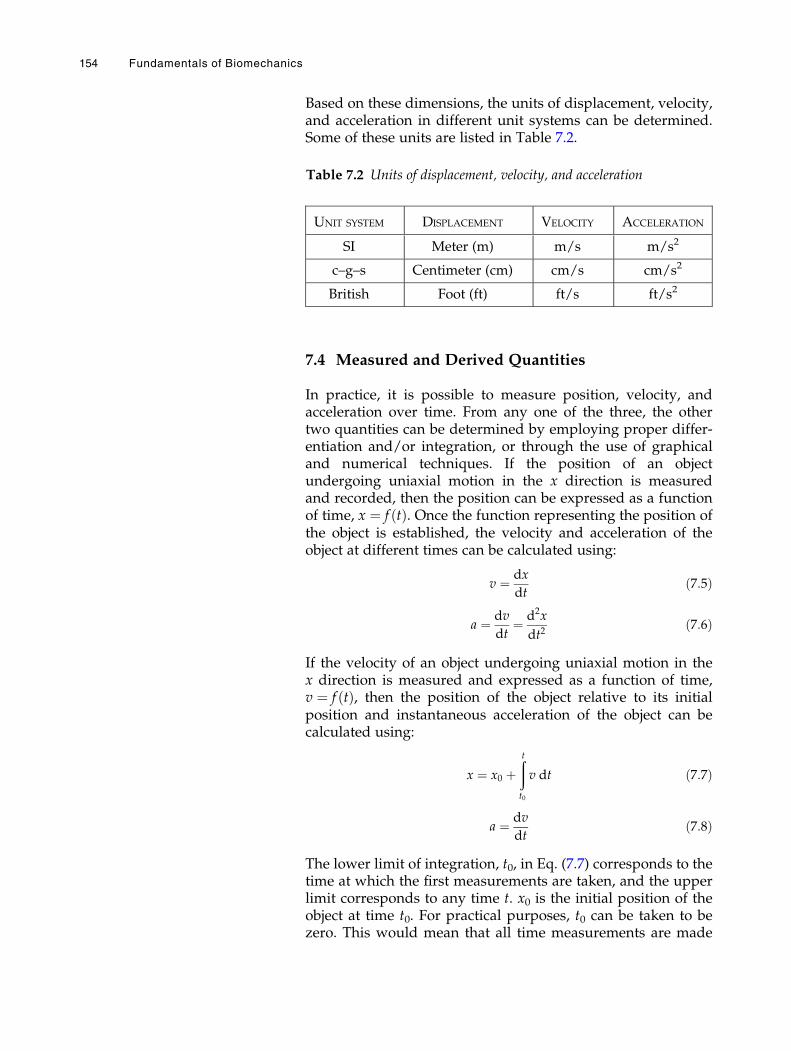
Based on these dimensions, the units of displacement, velocity,and acceleration in different unit systems can be determined.Some of these units are listed in Table 7.2.
7.4 Measured and Derived Quantities
In practice, it is possible to measure position, velocity, andacceleration over time. From any one of the three, the othertwo quantities can be determined by employing proper differ-entiation and/or integration, or through the use of graphicaland numerical techniques. If the position of an objectundergoing uniaxial motion in the x direction is measuredand recorded, then the position can be expressed as a functionof time, x ¼ f tð Þ. Once the function representing the position ofthe object is established, the velocity and acceleration of theobject at different times can be calculated using:
v ¼ dx
dtð7:5Þ
a ¼ dv
dt¼ d2x
dt2ð7:6Þ
If the velocity of an object undergoing uniaxial motion in thex direction is measured and expressed as a function of time,v ¼ f tð Þ, then the position of the object relative to its initialposition and instantaneous acceleration of the object can becalculated using:
x ¼ x0 þðtt0
v dt ð7:7Þ
a ¼ dv
dtð7:8Þ
The lower limit of integration, t0, in Eq. (7.7) corresponds to thetime at which the first measurements are taken, and the upperlimit corresponds to any time t. x0 is the initial position of theobject at time t0. For practical purposes, t0 can be taken to bezero. This would mean that all time measurements are made
Table 7.2 Units of displacement, velocity, and acceleration
UNIT SYSTEM DISPLACEMENT VELOCITY ACCELERATION
SI Meter (m) m/s m/s2
c–g–s Centimeter (cm) cm/s cm/s2
British Foot (ft) ft/s ft/s2
154 Fundamentals of Biomechanics
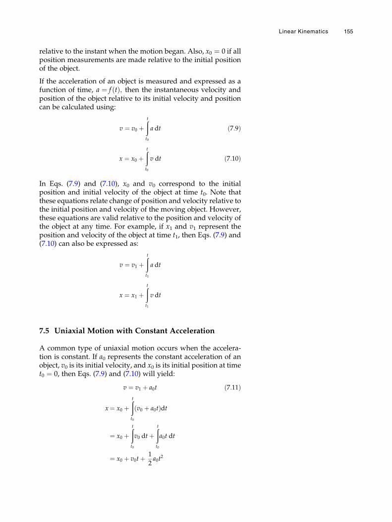
relative to the instant when the motion began. Also, x0 ¼ 0 if allposition measurements are made relative to the initial positionof the object.
If the acceleration of an object is measured and expressed as afunction of time, a ¼ f tð Þ; then the instantaneous velocity andposition of the object relative to its initial velocity and positioncan be calculated using:
v ¼ v0 þðtt0
a dt ð7:9Þ
x ¼ x0 þðtt0
v dt ð7:10Þ
In Eqs. (7.9) and (7.10), x0 and v0 correspond to the initialposition and initial velocity of the object at time t0. Note thatthese equations relate change of position and velocity relative tothe initial position and velocity of the moving object. However,these equations are valid relative to the position and velocity ofthe object at any time. For example, if x1 and v1 represent theposition and velocity of the object at time t1, then Eqs. (7.9) and(7.10) can also be expressed as:
v ¼ v1 þðtt1
a dt
x ¼ x1 þðtt1
v dt
7.5 Uniaxial Motion with Constant Acceleration
A common type of uniaxial motion occurs when the accelera-tion is constant. If a0 represents the constant acceleration of anobject, v0 is its initial velocity, and x0 is its initial position at timet0 ¼ 0, then Eqs. (7.9) and (7.10) will yield:
v ¼ v1 þ a0t ð7:11Þ
x¼ x0 þðtt0
v0 þ a0tð Þdt
¼ x0 þðtt0
v0 dtþðtt0
a0t dt
¼ x0 þ v0tþ 1
2a0t
2
Linear Kinematics 155
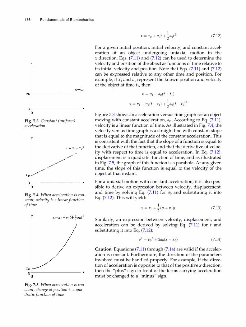
x ¼ x0 þ v0tþ 1
2a0t
2 ð7:12Þ
For a given initial position, initial velocity, and constant accel-eration of an object undergoing uniaxial motion in thex direction, Eqs. (7.11) and (7.12) can be used to determine thevelocity and position of the object as functions of time relative toits initial velocity and position. Note that Eqs. (7.11) and (7.12)can be expressed relative to any other time and position. Forexample, if x1 and v1 represent the known position and velocityof the object at time t1, then:
v ¼ v1 þ a0 t� t1ð Þ
x ¼ x1 þ v1 t� t1ð Þ þ 1
2a0 t� t1ð Þ2
Figure 7.3 shows an acceleration versus time graph for an objectmoving with constant acceleration, a0. According to Eq. (7.11),velocity is a linear function of time. As illustrated in Fig. 7.4, thevelocity versus time graph is a straight line with constant slopethat is equal to the magnitude of the constant acceleration. Thisis consistent with the fact that the slope of a function is equal tothe derivative of that function, and that the derivative of veloc-ity with respect to time is equal to acceleration. In Eq. (7.12),displacement is a quadratic function of time, and as illustratedin Fig. 7.5, the graph of this function is a parabola. At any giventime, the slope of this function is equal to the velocity of theobject at that instant.
For a uniaxial motion with constant acceleration, it is also pos-sible to derive an expression between velocity, displacement,and time by solving Eq. (7.11) for a0 and substituting it intoEq. (7.12). This will yield:
x ¼ x0 þ 1
2vþ v0ð Þt ð7:13Þ
Similarly, an expression between velocity, displacement, andacceleration can be derived by solving Eq. (7.11) for t andsubstituting it into Eq. (7.12):
v2 ¼ v02 þ 2a0 x� x0ð Þ ð7:14Þ
Caution. Equations (7.11) through (7.14) are valid if the acceler-ation is constant. Furthermore, the direction of the parametersinvolved must be handled properly. For example, if the direc-tion of acceleration is opposite to that of the positive x direction,then the “plus” sign in front of the terms carrying accelerationmust be changed to a “minus” sign.
Fig. 7.3 Constant (uniform)acceleration
Fig. 7.4 When acceleration is con-stant, velocity is a linear functionof time
Fig. 7.5 When acceleration is con-stant, change of position is a qua-dratic function of time
156 Fundamentals of Biomechanics
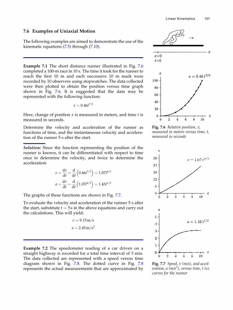
7.6 Examples of Uniaxial Motion
The following examples are aimed to demonstrate the use of thekinematic equations (7.5) through (7.10).
Example 7.1 The short distance runner illustrated in Fig. 7.6completed a 100-m race in 10 s. The time it took for the runner toreach the first 10 m and each successive 10 m mark wererecorded by 10 observers using stopwatches. The data collectedwere then plotted to obtain the position versus time graphshown in Fig. 7.6. It is suggested that the data may berepresented with the following function:
x ¼ 0:46t7=3
Here, change of position x is measured in meters, and time t ismeasured in seconds.
Determine the velocity and acceleration of the runner asfunctions of time, and the instantaneous velocity and accelera-tion of the runner 5 s after the start.
Solution: Since the function representing the position of therunner is known, it can be differentiated with respect to timeonce to determine the velocity, and twice to determine theacceleration:
v ¼ dx
dt¼ d
dt0:46t7=3
� �¼ 1:07t4=3
a ¼ dv
dt¼ d
dt1:07t4=3
� �¼ 1:43t1=3
The graphs of these functions are shown in Fig. 7.7.
To evaluate the velocity and acceleration of the runner 5 s afterthe start, substitute t ¼ 5s in the above equations and carry outthe calculations. This will yield:
v ¼ 9:15m=s
a ¼ 2:45m=s2
Example 7.2 The speedometer reading of a car driven on astraight highway is recorded for a total time interval of 3 min.The data collected are represented with a speed versus timediagram shown in Fig. 7.8. The dotted curve in Fig. 7.8represents the actual measurements that are approximated by
Fig. 7.6 Relative position, x,measured in meters versus time, t,measured in seconds
Fig. 7.7 Speed, v (m/s), and accel-eration, a (m/s2), versus time, t (s),curves for the runner
Linear Kinematics 157
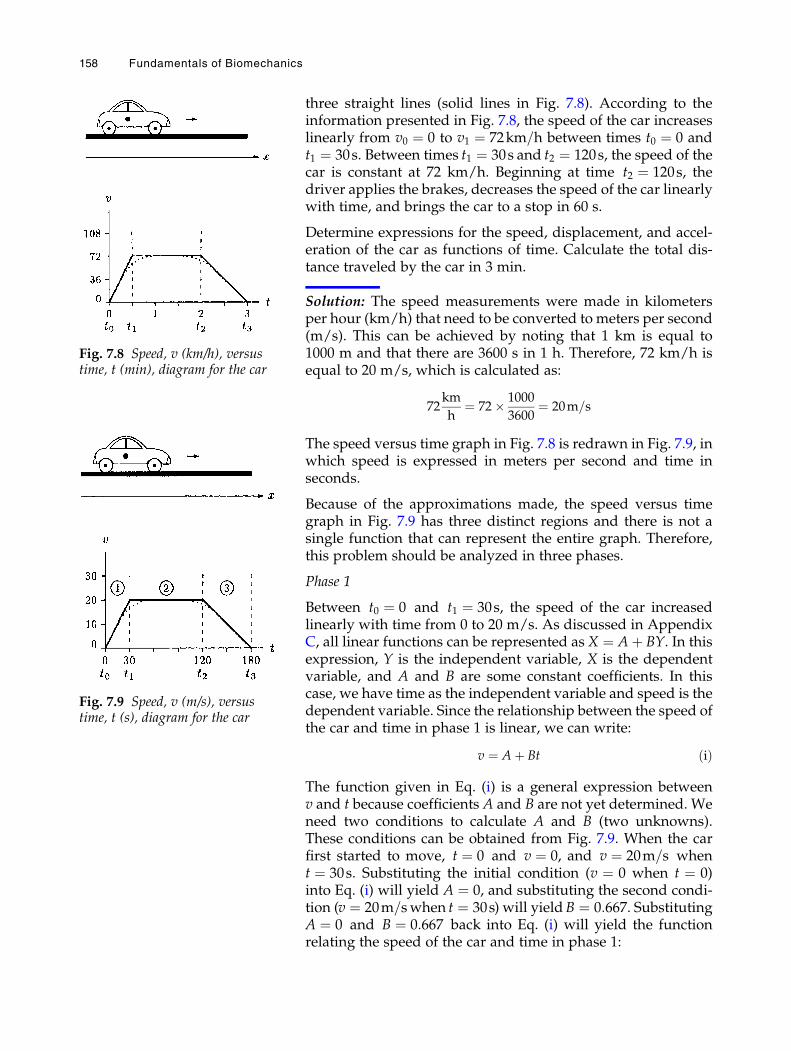
three straight lines (solid lines in Fig. 7.8). According to theinformation presented in Fig. 7.8, the speed of the car increaseslinearly from v0 ¼ 0 to v1 ¼ 72km=h between times t0 ¼ 0 andt1 ¼ 30s. Between times t1 ¼ 30s and t2 ¼ 120s, the speed of thecar is constant at 72 km/h. Beginning at time t2 ¼ 120s, thedriver applies the brakes, decreases the speed of the car linearlywith time, and brings the car to a stop in 60 s.
Determine expressions for the speed, displacement, and accel-eration of the car as functions of time. Calculate the total dis-tance traveled by the car in 3 min.
Solution: The speed measurements were made in kilometersper hour (km/h) that need to be converted to meters per second(m/s). This can be achieved by noting that 1 km is equal to1000 m and that there are 3600 s in 1 h. Therefore, 72 km/h isequal to 20 m/s, which is calculated as:
72km
h¼ 72� 1000
3600¼ 20m=s
The speed versus time graph in Fig. 7.8 is redrawn in Fig. 7.9, inwhich speed is expressed in meters per second and time inseconds.
Because of the approximations made, the speed versus timegraph in Fig. 7.9 has three distinct regions and there is not asingle function that can represent the entire graph. Therefore,this problem should be analyzed in three phases.
Phase 1
Between t0 ¼ 0 and t1 ¼ 30s, the speed of the car increasedlinearly with time from 0 to 20 m/s. As discussed in AppendixC, all linear functions can be represented asX ¼ Aþ BY. In thisexpression, Y is the independent variable, X is the dependentvariable, and A and B are some constant coefficients. In thiscase, we have time as the independent variable and speed is thedependent variable. Since the relationship between the speed ofthe car and time in phase 1 is linear, we can write:
v ¼ Aþ Bt ðiÞ
The function given in Eq. (i) is a general expression betweenv and t because coefficients A and B are not yet determined. Weneed two conditions to calculate A and B (two unknowns).These conditions can be obtained from Fig. 7.9. When the carfirst started to move, t ¼ 0 and v ¼ 0, and v ¼ 20m=s whent ¼ 30s. Substituting the initial condition (v ¼ 0 when t ¼ 0)into Eq. (i) will yield A ¼ 0, and substituting the second condi-tion (v ¼ 20m=swhen t ¼ 30s) will yieldB ¼ 0:667. SubstitutingA ¼ 0 and B ¼ 0:667 back into Eq. (i) will yield the functionrelating the speed of the car and time in phase 1:
Fig. 7.8 Speed, v (km/h), versustime, t (min), diagram for the car
Fig. 7.9 Speed, v (m/s), versustime, t (s), diagram for the car
158 Fundamentals of Biomechanics
v ¼ 0:667t ðiiÞ
Note that since we already converted speed measurements intometer per second and time into seconds, the speed in Eq. (ii) isin meters per second and time is in seconds.
Now, Eqs. (7.7) and (7.8) can be utilized to determine the dis-placement and acceleration of the car in phase 1. If we measuredisplacements relative to the starting point, then the initialposition of the car was x0 ¼ 0. Therefore:
x ¼ x0 þðt0
v dt ¼ðt0
0:667tð Þdt ¼ 0:667t2
2
� � t
0
¼ 0:333t2 ðiiiÞ
a ¼ dv
dt¼ d
dt0:667tð Þ ¼ 0:667 ðivÞ
From Eq. (iv), the acceleration of the car in phase 1 was constantat 0.667 m/s2. The total distance traveled by the car at the end ofphase 1 can be determined by substituting t ¼ 30s into Eq. (iii).This will yield:
x1 ¼ 0:333t2 ¼ 0:333 30ð Þ2 ¼ 300m
Phase 2
Phase 2 starts when time is t1 ¼ 30s and ends when it ist2 ¼ 120s. In phase 2, the speed of the car was constant at20 m/s. Therefore, the function representing the speed inphase 2 is:
v ¼ 20 ðvÞ
The total distance traveled by the car in phase 1 was computedas x1 ¼ 300m. x1 ¼ 300m also represents the initial position ofthe car in phase 2. Phase 1 ended when time was t1 ¼ 30s.Therefore, phase 2 began when time t1 ¼ 30s. We can nowwrite Eq. (7.7) relative to t1 and x1:
x ¼ x1 þðt2t1
v dt ¼ 300þðt230
20 dt ¼ 300þ 20 t½ �t2t1
x ¼ 300þ 20 t2 � t1ð Þ ðviÞ
The acceleration of the car in phase 2 can be determined usingEq. (7.8):
a ¼ dv
dt¼ 0 ðviiÞ
From Eq. (vii), the acceleration of the car in phase 2 is zero. Thetotal distance traveled by the car at the end of phase 2 can bedetermined by substituting t ¼ 120s into Eq. (vi). This will yield:
x2 ¼ 300þ 20 120� 30ð Þ ¼ 300þ 1800 ¼ 2100m
Linear Kinematics 159
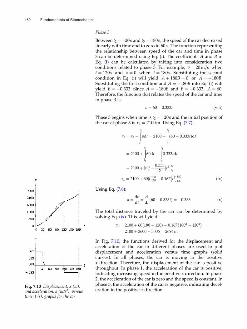
Phase 3
Between t2 ¼ 120s and t3 ¼ 180s, the speed of the car decreasedlinearly with time and to zero in 60 s. The function representingthe relationship between speed of the car and time in phase3 can be determined using Eq. (i). The coefficients A and B inEq. (i) can be calculated by taking into consideration twoconditions related to phase 3. For example, v ¼ 20m=s whent ¼ 120s and v ¼ 0 when t ¼ 180s. Substituting the secondcondition in Eq. (i) will yield Aþ 180B ¼ 0 or A ¼ �180B.Substituting the first condition and A ¼ �180B into Eq. (i) willyield B ¼ �0:333. Since A ¼ �180B and B ¼ �0:333, A ¼ 60.Therefore, the function that relates the speed of the car and timein phase 3 is:
v ¼ 60� 0:333t ðviiiÞ
Phase 3 begins when time is t2 ¼ 120s and the initial position ofthe car at phase 3 is x2 ¼ 2100m. Using Eq. (7.7):
x3 ¼ x2 þðt3t2
vdt ¼ 2100þðt3t2
60� 0:333tð Þdt
¼ 2100þðt3t2
60dt�ðt3t2
0:333tdt
¼ 2100þ t½ �t3t2 �0:333
2t2� t3
t2
x3 ¼ 2100þ 60 t½ �180120 � 0:167 t2� 180
120ðixÞ
Using Eq. (7.8):
a ¼ dv
dt¼ d
dt60� 0:333tð Þ ¼ �0:333 ðxÞ
The total distance traveled by the car can be determined bysolving Eq. (ix). This will yield:
x3 ¼ 2100þ 60 180� 120ð Þ � 0:167 1802 � 1202 �
¼ 2100þ 3600� 3006 ¼ 2694m
In Fig. 7.10, the functions derived for the displacement andacceleration of the car in different phases are used to plotdisplacement and acceleration versus time graphs (solidcurves). In all phases, the car is moving in the positivex direction. Therefore, the displacement of the car is positivethroughout. In phase 1, the acceleration of the car is positive,indicating increasing speed in the positive x direction. In phase2, the acceleration of the car is zero and the speed is constant. Inphase 3, the acceleration of the car is negative, indicating decel-eration in the positive x direction.
Fig. 7.10 Displacement, x (m),and acceleration, a (m/s2), versustime, t (s), graphs for the car
160 Fundamentals of Biomechanics
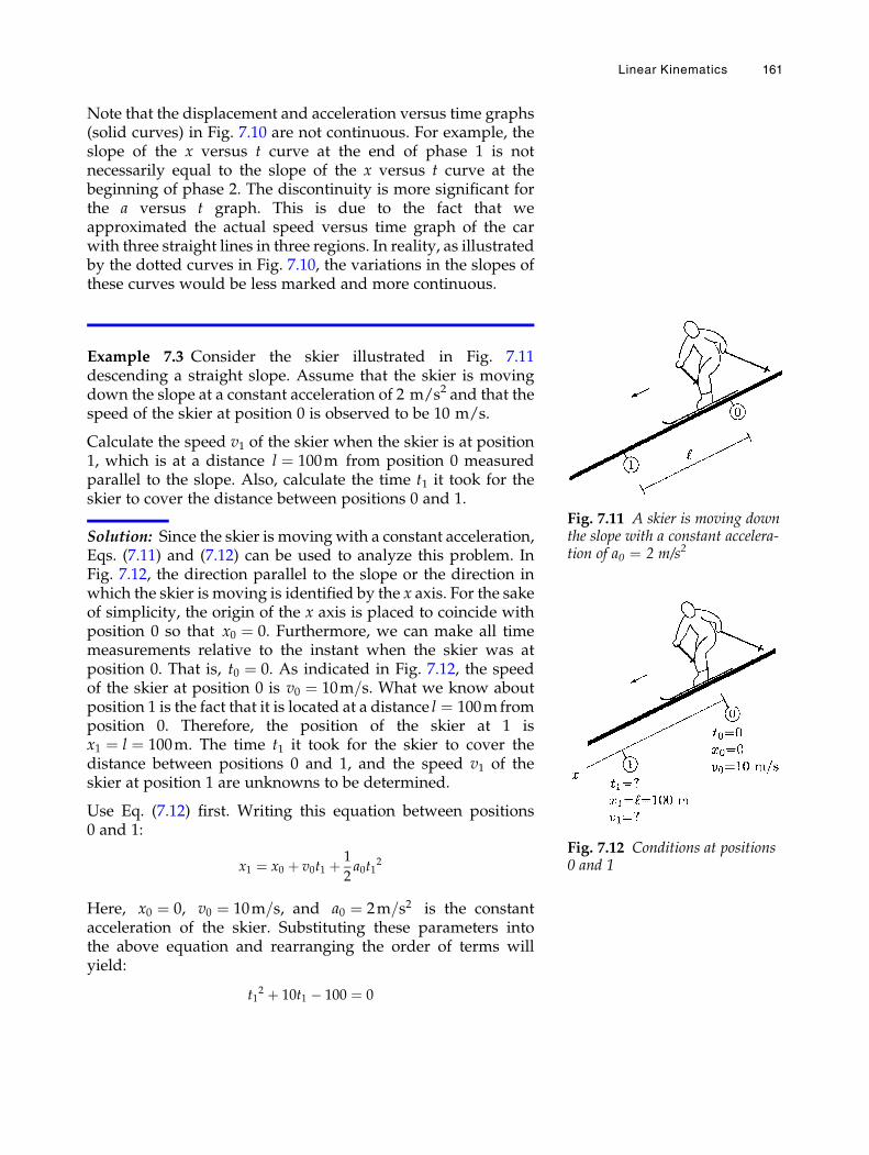
Note that the displacement and acceleration versus time graphs(solid curves) in Fig. 7.10 are not continuous. For example, theslope of the x versus t curve at the end of phase 1 is notnecessarily equal to the slope of the x versus t curve at thebeginning of phase 2. The discontinuity is more significant forthe a versus t graph. This is due to the fact that weapproximated the actual speed versus time graph of the carwith three straight lines in three regions. In reality, as illustratedby the dotted curves in Fig. 7.10, the variations in the slopes ofthese curves would be less marked and more continuous.
Example 7.3 Consider the skier illustrated in Fig. 7.11descending a straight slope. Assume that the skier is movingdown the slope at a constant acceleration of 2 m/s2 and that thespeed of the skier at position 0 is observed to be 10 m/s.
Calculate the speed v1 of the skier when the skier is at position1, which is at a distance l ¼ 100m from position 0 measuredparallel to the slope. Also, calculate the time t1 it took for theskier to cover the distance between positions 0 and 1.
Solution: Since the skier is moving with a constant acceleration,Eqs. (7.11) and (7.12) can be used to analyze this problem. InFig. 7.12, the direction parallel to the slope or the direction inwhich the skier is moving is identified by the x axis. For the sakeof simplicity, the origin of the x axis is placed to coincide withposition 0 so that x0 ¼ 0. Furthermore, we can make all timemeasurements relative to the instant when the skier was atposition 0. That is, t0 ¼ 0. As indicated in Fig. 7.12, the speedof the skier at position 0 is v0 ¼ 10m=s. What we know aboutposition 1 is the fact that it is located at a distance l ¼ 100mfromposition 0. Therefore, the position of the skier at 1 isx1 ¼ l ¼ 100m. The time t1 it took for the skier to cover thedistance between positions 0 and 1, and the speed v1 of theskier at position 1 are unknowns to be determined.
Use Eq. (7.12) first. Writing this equation between positions0 and 1:
x1 ¼ x0 þ v0t1 þ 1
2a0t1
2
Here, x0 ¼ 0, v0 ¼ 10m=s, and a0 ¼ 2m=s2 is the constantacceleration of the skier. Substituting these parameters intothe above equation and rearranging the order of terms willyield:
t12 þ 10t1 � 100 ¼ 0
Fig. 7.11 A skier is moving downthe slope with a constant accelera-tion of a0 ¼ 2 m/s2
Fig. 7.12 Conditions at positions0 and 1
Linear Kinematics 161
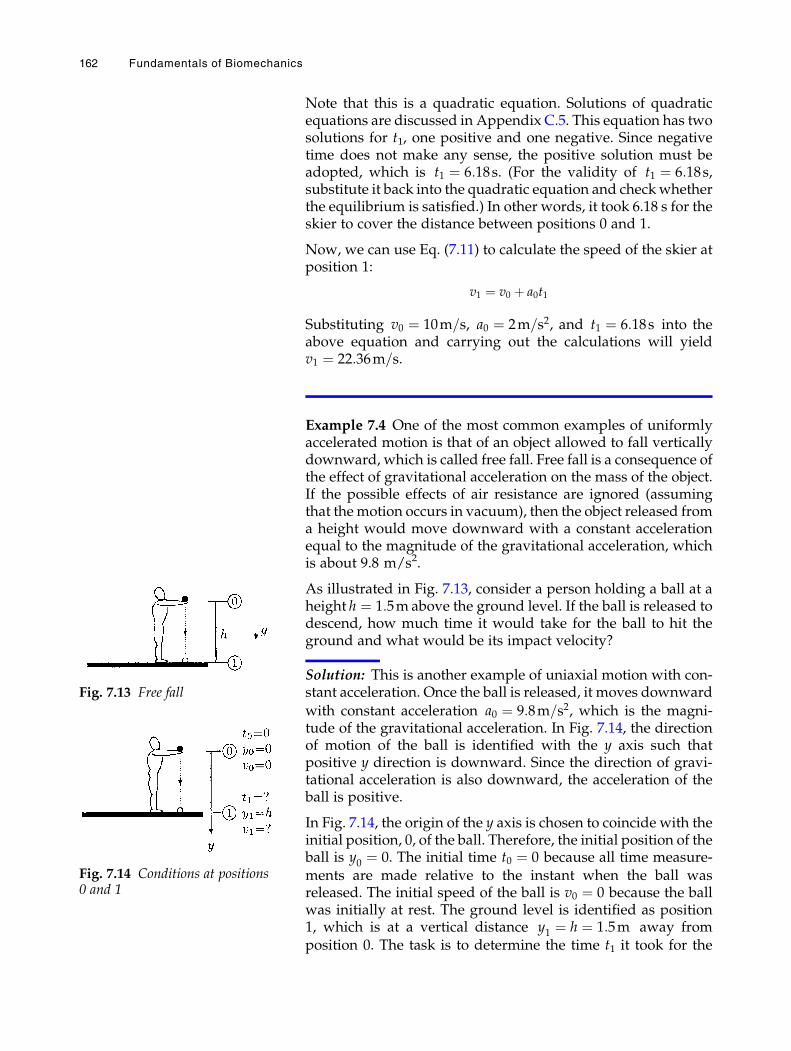
Note that this is a quadratic equation. Solutions of quadraticequations are discussed in Appendix C.5. This equation has twosolutions for t1, one positive and one negative. Since negativetime does not make any sense, the positive solution must beadopted, which is t1 ¼ 6:18s. (For the validity of t1 ¼ 6:18s,substitute it back into the quadratic equation and checkwhetherthe equilibrium is satisfied.) In other words, it took 6.18 s for theskier to cover the distance between positions 0 and 1.
Now, we can use Eq. (7.11) to calculate the speed of the skier atposition 1:
v1 ¼ v0 þ a0t1
Substituting v0 ¼ 10m=s, a0 ¼ 2m=s2, and t1 ¼ 6:18s into theabove equation and carrying out the calculations will yieldv1 ¼ 22:36m=s.
Example 7.4 One of the most common examples of uniformlyaccelerated motion is that of an object allowed to fall verticallydownward, which is called free fall. Free fall is a consequence ofthe effect of gravitational acceleration on the mass of the object.If the possible effects of air resistance are ignored (assumingthat themotion occurs in vacuum), then the object released froma height would move downward with a constant accelerationequal to the magnitude of the gravitational acceleration, whichis about 9.8 m/s2.
As illustrated in Fig. 7.13, consider a person holding a ball at aheight h ¼ 1:5m above the ground level. If the ball is released todescend, how much time it would take for the ball to hit theground and what would be its impact velocity?
Solution: This is another example of uniaxial motion with con-stant acceleration. Once the ball is released, it moves downward
with constant acceleration a0 ¼ 9:8m=s2, which is the magni-tude of the gravitational acceleration. In Fig. 7.14, the directionof motion of the ball is identified with the y axis such thatpositive y direction is downward. Since the direction of gravi-tational acceleration is also downward, the acceleration of theball is positive.
In Fig. 7.14, the origin of the y axis is chosen to coincide with theinitial position, 0, of the ball. Therefore, the initial position of theball is y0 ¼ 0. The initial time t0 ¼ 0 because all time measure-ments are made relative to the instant when the ball wasreleased. The initial speed of the ball is v0 ¼ 0 because the ballwas initially at rest. The ground level is identified as position1, which is at a vertical distance y1 ¼ h ¼ 1:5m away fromposition 0. The task is to determine the time t1 it took for the
Fig. 7.13 Free fall
Fig. 7.14 Conditions at positions0 and 1
162 Fundamentals of Biomechanics
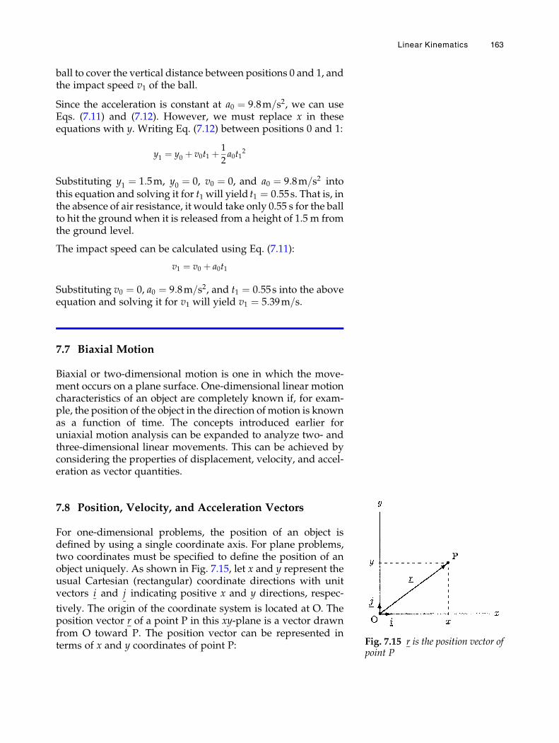
ball to cover the vertical distance between positions 0 and 1, andthe impact speed v1 of the ball.
Since the acceleration is constant at a0 ¼ 9:8m=s2, we can useEqs. (7.11) and (7.12). However, we must replace x in theseequations with y. Writing Eq. (7.12) between positions 0 and 1:
y1 ¼ y0 þ v0t1 þ 1
2a0t1
2
Substituting y1 ¼ 1:5m, y0 ¼ 0, v0 ¼ 0, and a0 ¼ 9:8m=s2 intothis equation and solving it for t1 will yield t1 ¼ 0:55s. That is, inthe absence of air resistance, it would take only 0.55 s for the ballto hit the ground when it is released from a height of 1.5 m fromthe ground level.
The impact speed can be calculated using Eq. (7.11):
v1 ¼ v0 þ a0t1
Substituting v0 ¼ 0, a0 ¼ 9:8m=s2, and t1 ¼ 0:55s into the aboveequation and solving it for v1 will yield v1 ¼ 5:39m=s.
7.7 Biaxial Motion
Biaxial or two-dimensional motion is one in which the move-ment occurs on a plane surface. One-dimensional linear motioncharacteristics of an object are completely known if, for exam-ple, the position of the object in the direction of motion is knownas a function of time. The concepts introduced earlier foruniaxial motion analysis can be expanded to analyze two- andthree-dimensional linear movements. This can be achieved byconsidering the properties of displacement, velocity, and accel-eration as vector quantities.
7.8 Position, Velocity, and Acceleration Vectors
For one-dimensional problems, the position of an object isdefined by using a single coordinate axis. For plane problems,two coordinates must be specified to define the position of anobject uniquely. As shown in Fig. 7.15, let x and y represent theusual Cartesian (rectangular) coordinate directions with unitvectors i and j indicating positive x and y directions, respec-
tively. The origin of the coordinate system is located at O. Theposition vector r of a point P in this xy-plane is a vector drawnfrom O toward P. The position vector can be represented interms of x and y coordinates of point P: Fig. 7.15 r is the position vector of
point P
Linear Kinematics 163
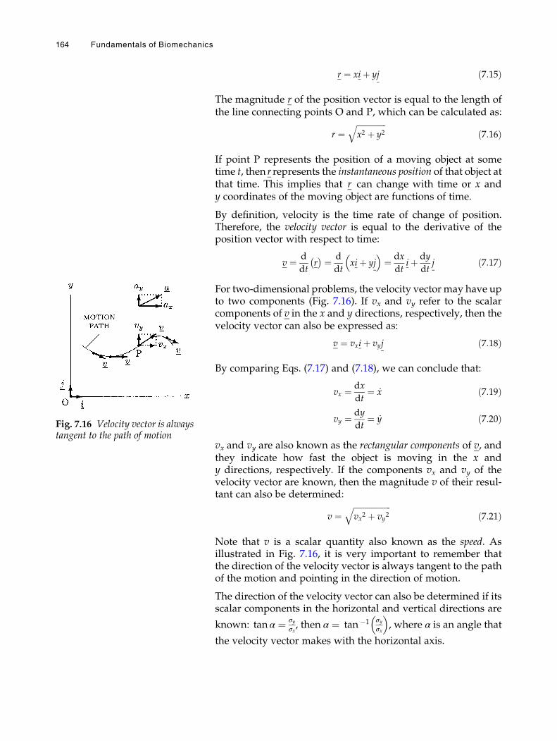
r ¼ xiþ yj ð7:15Þ
The magnitude r of the position vector is equal to the length ofthe line connecting points O and P, which can be calculated as:
r ¼ffiffiffiffiffiffiffiffiffiffiffiffiffiffiffix2 þ y2
qð7:16Þ
If point P represents the position of a moving object at sometime t, then r represents the instantaneous position of that object atthat time. This implies that r can change with time or x andy coordinates of the moving object are functions of time.
By definition, velocity is the time rate of change of position.Therefore, the velocity vector is equal to the derivative of theposition vector with respect to time:
v ¼ d
dtr � ¼ d
dtxiþ yj
� �¼ dx
dtiþ dy
dtj ð7:17Þ
For two-dimensional problems, the velocity vector may have upto two components (Fig. 7.16). If vx and vy refer to the scalarcomponents of v in the x and y directions, respectively, then thevelocity vector can also be expressed as:
v ¼ vxiþ vyj ð7:18Þ
By comparing Eqs. (7.17) and (7.18), we can conclude that:
vx ¼ dx
dt¼ _x ð7:19Þ
vy ¼ dy
dt¼ _y ð7:20Þ
vx and vy are also known as the rectangular components of v, andthey indicate how fast the object is moving in the x andy directions, respectively. If the components vx and vy of thevelocity vector are known, then the magnitude v of their resul-tant can also be determined:
v ¼ffiffiffiffiffiffiffiffiffiffiffiffiffiffiffiffiffiffiffivx2 þ vy2
qð7:21Þ
Note that v is a scalar quantity also known as the speed. Asillustrated in Fig. 7.16, it is very important to remember thatthe direction of the velocity vector is always tangent to the pathof the motion and pointing in the direction of motion.
The direction of the velocity vector can also be determined if itsscalar components in the horizontal and vertical directions are
known: tan α ¼ σyσx, then α ¼ tan �1 σy
σx
� �, where α is an angle that
the velocity vector makes with the horizontal axis.
Fig. 7.16 Velocity vector is alwaystangent to the path of motion
164 Fundamentals of Biomechanics
By definition, acceleration is the time rate of change of velocity.Therefore, if the velocity vector of an object is known as afunction of time, then its acceleration vector a can also bedetermined by considering the derivative of v with respect totime:
a ¼ d
dtv � ¼ d
dtvxiþ vyj
� �¼ dvx
dtiþ dvy
dtj ð7:22Þ
The acceleration vector can also be expressed in terms of itscomponents in the x and y directions (Fig. 7.16):
a ¼ axiþ ayj ð7:23Þ
By comparing Eqs. (7.22) and (7.23), the rectangularcomponents of the acceleration vector can alternatively be writ-ten as:
ax ¼ dvxdt
¼ d2x
dt2¼ €x ð7:24Þ
ay ¼dvy
dt¼ d2y
dt2¼ €y ð7:25Þ
If needed, the magnitude a of the acceleration vector can becalculated as:
a ¼ffiffiffiffiffiffiffiffiffiffiffiffiffiffiffiffiffiffiax2 þ ay2
qð7:26Þ
The extension of these concepts to analyze three-dimensionalmovements is straightforward. For three-dimensional motionanalyses, there is a need for a third dimension, namely z. Forexample, the position vector of a point in space can beexpressed as:
r ¼ xiþ yjþ zk
Here, k is the unit vector indicating the positive z direction.Similarly, the velocity and acceleration vectors in space can beexpressed as:
v ¼ vxiþ vyjþ vzk
a ¼ axiþ ayjþ azk
For example, vz is the speed of the object in the z direction and isequal to the time rate of change of position in the z direction,and az is the scalar component of the acceleration vector in thez direction and is equal to the time rate of change of the speed ofthe object in the z direction.
Linear Kinematics 165
7.9 Biaxial Motion with Constant Acceleration
Two-dimensional linear motion of an object in the xy-plane canbe analyzed in two stages by first considering its motion in thex and y directions separately and then combining the resultsusing the vectorial properties of the parameters involved. Theparameters defining the motion in the x direction are x, its firsttime derivative vx, and its second time derivative ax. Similarly,y, vy, and ay are the parameters that define the motion of theobject in the y direction. If the acceleration of an objectundergoing two-dimensional linear motion is constant, then axand ay must be constants. The details of uniaxial motion withconstant acceleration were analyzed in the previous sections.The results of these analyses can readily be adopted to analyzetwo-dimensional motions with constant acceleration.
In the x direction, Eqs. (7.11) and (7.12) can be rewritten in thefollowing more specific forms:
vx ¼ vx0 þ ax0t ð7:27Þ
x ¼ x0 þ vx0 tþ1
2ax0 t
2 ð7:28Þ
Similarly, in the y direction:
vy ¼ vy0 þ ay0t ð7:29Þ
y ¼ y0 þ vy0 tþ1
2ay0 t
2 ð7:30Þ
Here, x0 and y0 are the initial coordinates of the object,vx0 andvy0are the initial velocity components in the x and y directions, andax0 anday0 are the constant components of the acceleration vector
in the x and y directions, respectively. For given x0, y0, vx0 , vy0 ,
ax0 , anday0 , Eqs. (7.27) through (7.30) can be used to calculate the
relative position of the moving object and its velocitycomponents at any time t.
Furthermore, these equations are valid if acceleration is con-stant and its direction coincides with the direction of motion. Ifthe direction of acceleration is opposite the direction of motion,then the sign in front of the terms carrying the acceleration mustbe changed into minus (�). In the x direction, Eqs. (7.11) and(7.12) can be rewritten in the following forms:
vx ¼ vx0 � ax0t
x ¼ x0 þ vx0 t�1
2ax0 t
2
Similarly, in the y direction:
vy ¼ vy0 � ay0t
166 Fundamentals of Biomechanics
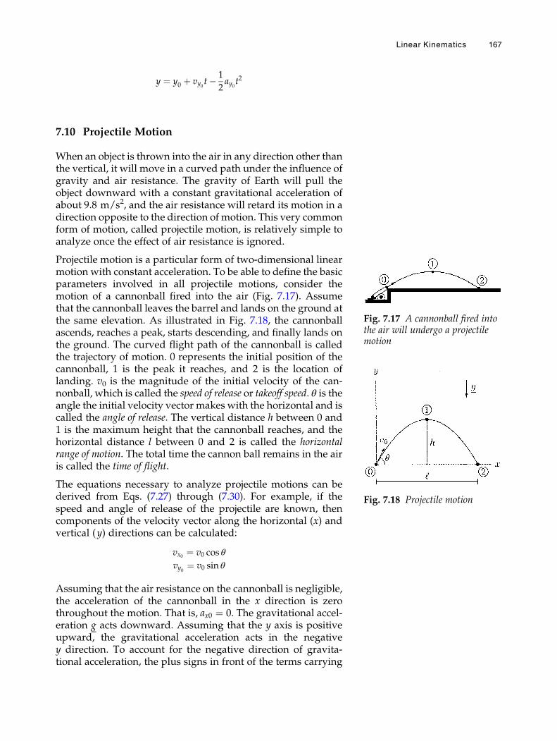
y ¼ y0 þ vy0 t�1
2ay0 t
2
7.10 Projectile Motion
When an object is thrown into the air in any direction other thanthe vertical, it will move in a curved path under the influence ofgravity and air resistance. The gravity of Earth will pull theobject downward with a constant gravitational acceleration ofabout 9.8 m/s2, and the air resistance will retard its motion in adirection opposite to the direction of motion. This very commonform of motion, called projectile motion, is relatively simple toanalyze once the effect of air resistance is ignored.
Projectile motion is a particular form of two-dimensional linearmotion with constant acceleration. To be able to define the basicparameters involved in all projectile motions, consider themotion of a cannonball fired into the air (Fig. 7.17). Assumethat the cannonball leaves the barrel and lands on the ground atthe same elevation. As illustrated in Fig. 7.18, the cannonballascends, reaches a peak, starts descending, and finally lands onthe ground. The curved flight path of the cannonball is calledthe trajectory of motion. 0 represents the initial position of thecannonball, 1 is the peak it reaches, and 2 is the location oflanding. v0 is the magnitude of the initial velocity of the can-nonball, which is called the speed of release or takeoff speed. θ is theangle the initial velocity vector makes with the horizontal and iscalled the angle of release. The vertical distance h between 0 and1 is the maximum height that the cannonball reaches, and thehorizontal distance l between 0 and 2 is called the horizontalrange of motion. The total time the cannon ball remains in the airis called the time of flight.
The equations necessary to analyze projectile motions can bederived from Eqs. (7.27) through (7.30). For example, if thespeed and angle of release of the projectile are known, thencomponents of the velocity vector along the horizontal (x) andvertical (y) directions can be calculated:
vx0 ¼ v0 cos θ
vy0 ¼ v0 sin θ
Assuming that the air resistance on the cannonball is negligible,the acceleration of the cannonball in the x direction is zerothroughout the motion. That is, ax0 ¼ 0. The gravitational accel-eration g acts downward. Assuming that the y axis is positiveupward, the gravitational acceleration acts in the negativey direction. To account for the negative direction of gravita-tional acceleration, the plus signs in front of the terms carrying
Fig. 7.17 A cannonball fired intothe air will undergo a projectilemotion
Fig. 7.18 Projectile motion
Linear Kinematics 167
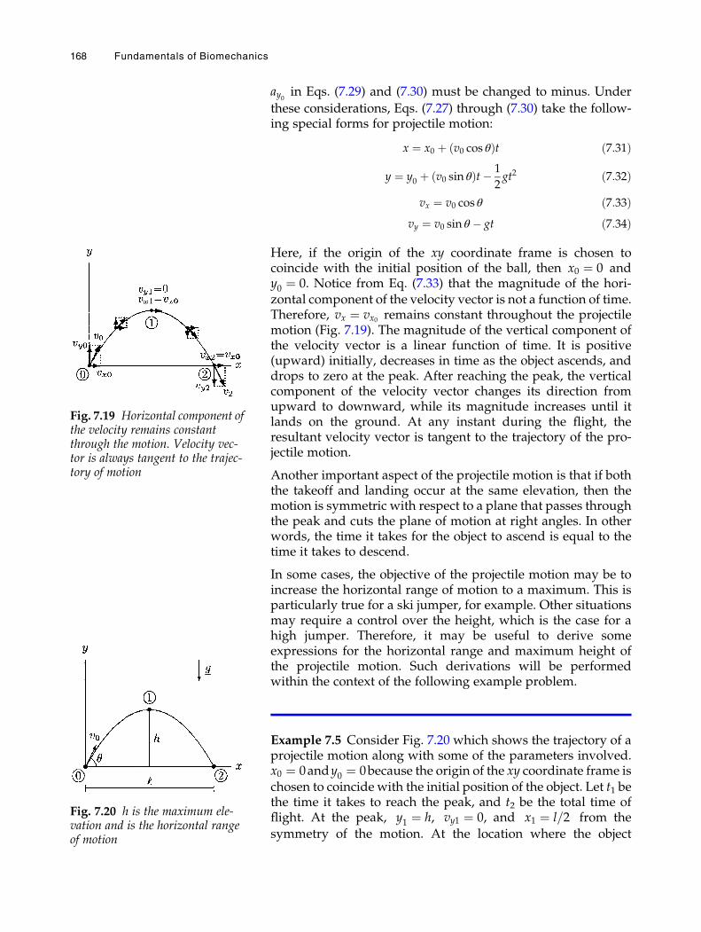
ay0 in Eqs. (7.29) and (7.30) must be changed to minus. Under
these considerations, Eqs. (7.27) through (7.30) take the follow-ing special forms for projectile motion:
x ¼ x0 þ v0 cos θð Þt ð7:31Þ
y ¼ y0 þ v0 sin θð Þt� 1
2gt2 ð7:32Þ
vx ¼ v0 cos θ ð7:33Þvy ¼ v0 sin θ � gt ð7:34Þ
Here, if the origin of the xy coordinate frame is chosen tocoincide with the initial position of the ball, then x0 ¼ 0 andy0 ¼ 0. Notice from Eq. (7.33) that the magnitude of the hori-zontal component of the velocity vector is not a function of time.Therefore, vx ¼ vx0 remains constant throughout the projectilemotion (Fig. 7.19). The magnitude of the vertical component ofthe velocity vector is a linear function of time. It is positive(upward) initially, decreases in time as the object ascends, anddrops to zero at the peak. After reaching the peak, the verticalcomponent of the velocity vector changes its direction fromupward to downward, while its magnitude increases until itlands on the ground. At any instant during the flight, theresultant velocity vector is tangent to the trajectory of the pro-jectile motion.
Another important aspect of the projectile motion is that if boththe takeoff and landing occur at the same elevation, then themotion is symmetric with respect to a plane that passes throughthe peak and cuts the plane of motion at right angles. In otherwords, the time it takes for the object to ascend is equal to thetime it takes to descend.
In some cases, the objective of the projectile motion may be toincrease the horizontal range of motion to a maximum. This isparticularly true for a ski jumper, for example. Other situationsmay require a control over the height, which is the case for ahigh jumper. Therefore, it may be useful to derive someexpressions for the horizontal range and maximum height ofthe projectile motion. Such derivations will be performedwithin the context of the following example problem.
Example 7.5 Consider Fig. 7.20 which shows the trajectory of aprojectile motion along with some of the parameters involved.x0 ¼ 0andy0 ¼ 0because the origin of the xy coordinate frame ischosen to coincide with the initial position of the object. Let t1 bethe time it takes to reach the peak, and t2 be the total time offlight. At the peak, y1 ¼ h, vy1 ¼ 0, and x1 ¼ l=2 from the
symmetry of the motion. At the location where the object
Fig. 7.19 Horizontal component ofthe velocity remains constantthrough the motion. Velocity vec-tor is always tangent to the trajec-tory of motion
Fig. 7.20 h is the maximum ele-vation and is the horizontal rangeof motion
168 Fundamentals of Biomechanics
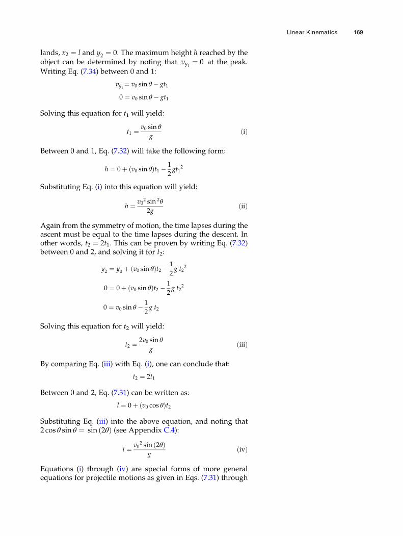
lands, x2 ¼ l and y2 ¼ 0. The maximum height h reached by theobject can be determined by noting that vy1 ¼ 0 at the peak.
Writing Eq. (7.34) between 0 and 1:
vy1¼ v0 sin θ � gt1
0 ¼ v0 sin θ � gt1
Solving this equation for t1 will yield:
t1 ¼ v0 sin θ
gðiÞ
Between 0 and 1, Eq. (7.32) will take the following form:
h ¼ 0þ v0 sin θð Þt1 � 1
2gt1
2
Substituting Eq. (i) into this equation will yield:
h ¼ v02 sin 2θ
2gðiiÞ
Again from the symmetry of motion, the time lapses during theascent must be equal to the time lapses during the descent. Inother words, t2 ¼ 2t1. This can be proven by writing Eq. (7.32)between 0 and 2, and solving it for t2:
y2 ¼ y0 þ v0 sin θð Þt2 � 1
2g t2
2
0 ¼ 0þ v0 sin θð Þt2 � 1
2g t2
2
0 ¼ v0 sin θ � 1
2g t2
Solving this equation for t2 will yield:
t2 ¼ 2v0 sin θ
gðiiiÞ
By comparing Eq. (iii) with Eq. (i), one can conclude that:
t2 ¼ 2t1
Between 0 and 2, Eq. (7.31) can be written as:
l ¼ 0þ v0 cos θð Þt2
Substituting Eq. (iii) into the above equation, and noting that2 cos θ sin θ ¼ sin 2θð Þ (see Appendix C.4):
l ¼ v02 sin 2θð Þ
gðivÞ
Equations (i) through (iv) are special forms of more generalequations for projectile motions as given in Eqs. (7.31) through
Linear Kinematics 169
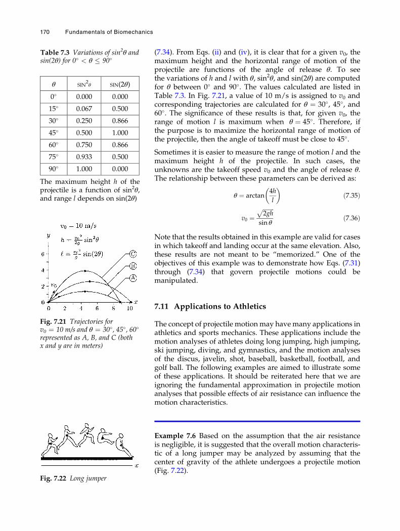
(7.34). From Eqs. (ii) and (iv), it is clear that for a given v0, themaximum height and the horizontal range of motion of theprojectile are functions of the angle of release θ. To seethe variations of h and l with θ, sin2θ, and sin(2θ) are computedfor θ between 0� and 90�. The values calculated are listed inTable 7.3. In Fig. 7.21, a value of 10 m/s is assigned to v0 andcorresponding trajectories are calculated for θ ¼ 30�, 45�, and60�. The significance of these results is that, for given v0, therange of motion l is maximum when θ ¼ 45�. Therefore, ifthe purpose is to maximize the horizontal range of motion ofthe projectile, then the angle of takeoff must be close to 45�.
Sometimes it is easier to measure the range of motion l and themaximum height h of the projectile. In such cases, theunknowns are the takeoff speed v0 and the angle of release θ.The relationship between these parameters can be derived as:
θ ¼ arctan4h
l
� �ð7:35Þ
v0 ¼ffiffiffiffiffiffiffiffi2gh
psin θ
ð7:36Þ
Note that the results obtained in this example are valid for casesin which takeoff and landing occur at the same elevation. Also,these results are not meant to be “memorized.” One of theobjectives of this example was to demonstrate how Eqs. (7.31)through (7.34) that govern projectile motions could bemanipulated.
7.11 Applications to Athletics
The concept of projectile motionmay havemany applications inathletics and sports mechanics. These applications include themotion analyses of athletes doing long jumping, high jumping,ski jumping, diving, and gymnastics, and the motion analysesof the discus, javelin, shot, baseball, basketball, football, andgolf ball. The following examples are aimed to illustrate someof these applications. It should be reiterated here that we areignoring the fundamental approximation in projectile motionanalyses that possible effects of air resistance can influence themotion characteristics.
Example 7.6 Based on the assumption that the air resistanceis negligible, it is suggested that the overall motion characteris-tic of a long jumper may be analyzed by assuming that thecenter of gravity of the athlete undergoes a projectile motion(Fig. 7.22).
Fig. 7.21 Trajectories forv0 ¼ 10 m/s and θ ¼ 30�, 45�, 60�represented as A, B, and C (bothx and y are in meters)
Table 7.3 Variations of sin2θ andsin(2θ) for 0� < θ � 90�
θ SIN2θ SIN(2θ)
0� 0.000 0.000
15� 0.067 0.500
30� 0.250 0.866
45� 0.500 1.000
60� 0.750 0.866
75� 0.933 0.500
90� 1.000 0.000
The maximum height h of theprojectile is a function of sin2θ,and range l depends on sin(2θ)
Fig. 7.22 Long jumper
170 Fundamentals of Biomechanics
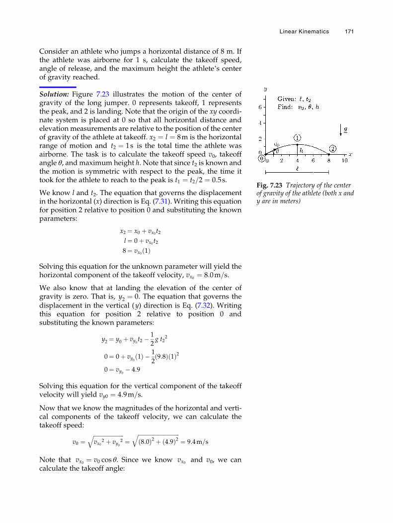
Consider an athlete who jumps a horizontal distance of 8 m. Ifthe athlete was airborne for 1 s, calculate the takeoff speed,angle of release, and the maximum height the athlete’s centerof gravity reached.
Solution: Figure 7.23 illustrates the motion of the center ofgravity of the long jumper. 0 represents takeoff, 1 representsthe peak, and 2 is landing. Note that the origin of the xy coordi-nate system is placed at 0 so that all horizontal distance andelevation measurements are relative to the position of the centerof gravity of the athlete at takeoff. x2 ¼ l ¼ 8m is the horizontalrange of motion and t2 ¼ 1s is the total time the athlete wasairborne. The task is to calculate the takeoff speed v0, takeoffangle θ, and maximum height h. Note that since t2 is known andthe motion is symmetric with respect to the peak, the time ittook for the athlete to reach to the peak is t1 ¼ t2=2 ¼ 0:5s.
We know l and t2. The equation that governs the displacementin the horizontal (x) direction is Eq. (7.31). Writing this equationfor position 2 relative to position 0 and substituting the knownparameters:
x2 ¼ x0 þ vx0t2
l¼ 0þ vx0 t2
8¼ vx0 1ð Þ
Solving this equation for the unknown parameter will yield thehorizontal component of the takeoff velocity, vx0 ¼ 8:0m=s.
We also know that at landing the elevation of the center ofgravity is zero. That is, y2 ¼ 0. The equation that governs thedisplacement in the vertical (y) direction is Eq. (7.32). Writingthis equation for position 2 relative to position 0 andsubstituting the known parameters:
y2 ¼ y0 þ vy0t2 �1
2g t2
2
0¼ 0þ vy0 1ð Þ � 1
29:8ð Þ 1ð Þ2
0¼ vy0 � 4:9
Solving this equation for the vertical component of the takeoffvelocity will yield vy0 ¼ 4:9m=s.
Now that we know the magnitudes of the horizontal and verti-cal components of the takeoff velocity, we can calculate thetakeoff speed:
v0 ¼ffiffiffiffiffiffiffiffiffiffiffiffiffiffiffiffiffiffiffiffiffiffivx0
2 þ vy02
q¼
ffiffiffiffiffiffiffiffiffiffiffiffiffiffiffiffiffiffiffiffiffiffiffiffiffiffiffiffiffiffi8:0ð Þ2 þ 4:9ð Þ2
q¼ 9:4m=s
Note that vx0 ¼ v0 cos θ. Since we know vx0 and v0, we cancalculate the takeoff angle:
Fig. 7.23 Trajectory of the centerof gravity of the athlete (both x andy are in meters)
Linear Kinematics 171
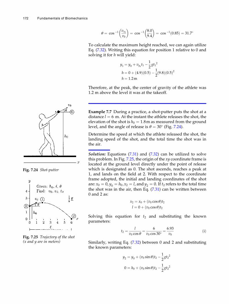
θ ¼ cos �1 vx0v0
� �¼ cos �1 8:0
9:4
� �¼ cos �1 0:85ð Þ ¼ 31:7�
To calculate the maximum height reached, we can again utilizeEq. (7.32). Writing this equation for position 1 relative to 0 andsolving it for h will yield:
y1 ¼ y0 þ vy0 t1 �1
2gt1
2
h¼ 0þ 4:9ð Þ 0:5ð Þ � 1
29:8ð Þ 0:5ð Þ2
h¼ 1:2m
Therefore, at the peak, the center of gravity of the athlete was1.2 m above the level it was at the takeoff.
Example 7.7 During a practice, a shot-putter puts the shot at adistance l ¼ 6 m. At the instant the athlete releases the shot, theelevation of the shot is h0 ¼ 1:8m as measured from the groundlevel, and the angle of release is θ ¼ 30� (Fig. 7.24).
Determine the speed at which the athlete released the shot, thelanding speed of the shot, and the total time the shot was inthe air.
Solution: Equations (7.31) and (7.32) can be utilized to solvethis problem. In Fig. 7.25, the origin of the xy coordinate frame islocated at the ground level directly under the point of releasewhich is designated as 0. The shot ascends, reaches a peak at1, and lands on the field at 2. With respect to the coordinateframe adopted, the initial and landing coordinates of the shotare: x0 ¼ 0, y0 ¼ h0;x2 ¼ l, and y2 ¼ 0. If t2 refers to the total timethe shot was in the air, then Eq. (7.31) can be written between0 and 2 as:
x2 ¼ x0 þ v0 cos θð Þt2l ¼ 0þ v0 cos θð Þt2
Solving this equation for t2 and substituting the knownparameters:
t2 ¼ l
v0 cos θ¼ 6
v0 cos 30�¼ 6:93
v0ðiÞ
Similarly, writing Eq. (7.32) between 0 and 2 and substitutingthe known parameters:
y2 ¼ y0 þ v0 sin θð Þt2 � 1
2gt2
2
0 ¼ h0 þ v0 sin θð Þt2 � 1
2gt2
2
Fig. 7.24 Shot-putter
Fig. 7.25 Trajectory of the shot(x and y are in meters)
172 Fundamentals of Biomechanics
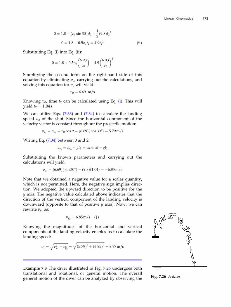
0 ¼ 1:8þ v0 sin 30�ð Þt2 � 1
29:8ð Þt22
0 ¼ 1:8þ 0:5v0t2 ¼ 4:9t22 ðiiÞ
Substituting Eq. (i) into Eq. (ii):
0 ¼ 1:8þ 0:5v06:93
v0
� �� 4:9
6:93
v0
� �2
Simplifying the second term on the right-hand side of thisequation by eliminating v0, carrying out the calculations, andsolving this equation for v0 will yield:
v0 ¼ 6:69 m=s
Knowing v0, time t2 can be calculated using Eq. (i). This willyield t2 ¼ 1:04s.
We can utilize Eqs. (7.33) and (7.34) to calculate the landingspeed v2 of the shot. Since the horizontal component of thevelocity vector is constant throughout the projectile motion:
vx2 ¼ vx0 ¼ v0 cos θ ¼ 6:69ð Þ cos 30�ð Þ ¼ 5:79m=s
Writing Eq. (7.34) between 0 and 2:
vy2 ¼ vy0 � gt2 ¼ v0 sin θ � gt2
Substituting the known parameters and carrying out thecalculations will yield:
vy2 ¼ 6:69ð Þ sin 30�ð Þ � 9:8ð Þ 1:04ð Þ ¼ �6:85m=s
Note that we obtained a negative value for a scalar quantity,which is not permitted. Here, the negative sign implies direc-tion. We adopted the upward direction to be positive for they axis. The negative value calculated above indicates that thedirection of the vertical component of the landing velocity isdownward (opposite to that of positive y axis). Now, we canrewrite vy2 as:
vy2 ¼ 6:85m=s #ð Þ
Knowing the magnitudes of the horizontal and verticalcomponents of the landing velocity enables us to calculate thelanding speed:
v2 ¼ffiffiffiffiffiffiffiffiffiffiffiffiffiffiffiffiffiffiv2x2 þ v2y2
q¼
ffiffiffiffiffiffiffiffiffiffiffiffiffiffiffiffiffiffiffiffiffiffiffiffiffiffiffiffiffiffiffiffiffiffiffi5:79ð Þ2 þ 6:85ð Þ2
q¼ 8:97m=s
Example 7.8 The diver illustrated in Fig. 7.26 undergoes bothtranslational and rotational, or general motion. The overallgeneral motion of the diver can be analyzed by observing the Fig. 7.26 A diver
Linear Kinematics 173
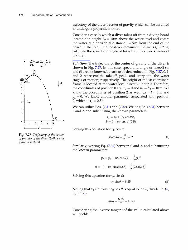
trajectory of the diver’s center of gravity which can be assumedto undergo a projectile motion.
Consider a case in which a diver takes off from a diving boardlocated at a height h0 ¼ 10m above the water level and entersthe water at a horizontal distance l ¼ 5m from the end of theboard. If the total time the diver remains in the air is t2 ¼ 2:5s,calculate the speed and angle of takeoff of the diver’s center ofgravity.
Solution: The trajectory of the center of gravity of the diver isshown in Fig. 7.27. In this case, speed and angle of takeoff (v0and θ) are not known, but are to be determined. In Fig. 7.27, 0, 1,and 2 represent the takeoff, peak, and entry into the waterstages of motion, respectively. The origin of the xy coordinateframe is located at the water level directly under 0. Therefore,the coordinates of position 0 are: x0 ¼ 0 and y0 ¼ h0 ¼ 10m. Weknow the coordinates of position 2 as well: x2 ¼ l ¼ 5m andy2 ¼ 0. We know another parameter associated with position2, which is t2 ¼ 2:5s.
We can utilize Eqs. (7.31) and (7.32). Writing Eq. (7.31) between0 and 2, and substituting the known parameters:
x2 ¼ x0 þ v0 cos θð Þt25 ¼ 0þ v0 cos θð Þ 2:5ð Þ
Solving this equation for v0 cos θ:
v0 cos θ ¼ 5
2:5¼ 2 ðiÞ
Similarly, writing Eq. (7.32) between 0 and 2, and substitutingthe known parameters:
y2 ¼ y0 þ v0 cos θð Þt2 � 1
2gt2
2
0 ¼ 10þ v0 sin θð Þ 2:5ð Þ � 1
29:8ð Þ 2:5ð Þ2
Solving this equation for v0 sin θ:
v0 sin θ ¼ 8:25 ðiiÞ
Noting that v0 sin θ over v0 cos θ is equal to tan θ, divide Eq. (ii)by Eq. (i):
tan θ ¼ 8:25
2¼ 4:125
Considering the inverse tangent of the value calculated abovewill yield:
Fig. 7.27 Trajectory of the centerof gravity of the diver (both x andy are in meters)
174 Fundamentals of Biomechanics
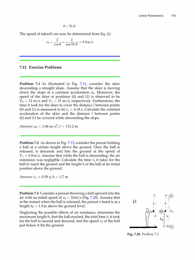
θ ¼ 76:4�
The speed of takeoff can now be determined from Eq. (i):
v0 ¼ 2
cos θ¼ 2
cos 76:4�¼ 8:5m=s
7.12 Exercise Problems
Problem 7.1 As illustrated in Fig. 7.11, consider the skierdescending a straight slope. Assume that the skier is movingdown the slope at a constant acceleration a0. Moreover, thespeed of the skier at positions (0) and (1) is observed to beV0 ¼ 12 m/s and V1 ¼ 21 m/s, respectively. Furthermore, thetime it took for the skier to cover the distance l between points(0) and (1) is measured to be t1 ¼ 6.18 s. Calculate the constantacceleration of the skier and the distance l between points(0) and (1) he covered while descending the slope.
Answers: a0 ¼ 1.94 m/s2; l ¼ 111.2 m
Problem 7.2 As shown in Fig. 7.13, consider the person holdinga ball at a certain height above the ground. Once the ball isreleased, it descends and hits the ground at the speed ofV1 ¼ 5:8m=s. Assume that while the ball is descending, the airresistance was negligible. Calculate the time t1 it takes for theball to reach the ground and the height h of the ball at its initialposition above the ground.
Answers: t1 ¼ 0.59 s; h ¼ 1.7 m
Problem 7.3 Consider a person throwing a ball upward into theair with an initial speed of v0 ¼ 10m=s (Fig. 7.28). Assume thatat the instant when the ball is released, the person’s hand is at aheight h0 ¼ 1:5m above the ground level.
Neglecting the possible effects of air resistance, determine themaximum height h1 that the ball reached, the total time t2 it tookfor the ball to ascend and descend, and the speed v2 of the balljust before it hit the ground.
Fig. 7.28 Problem 7.3
Linear Kinematics 175
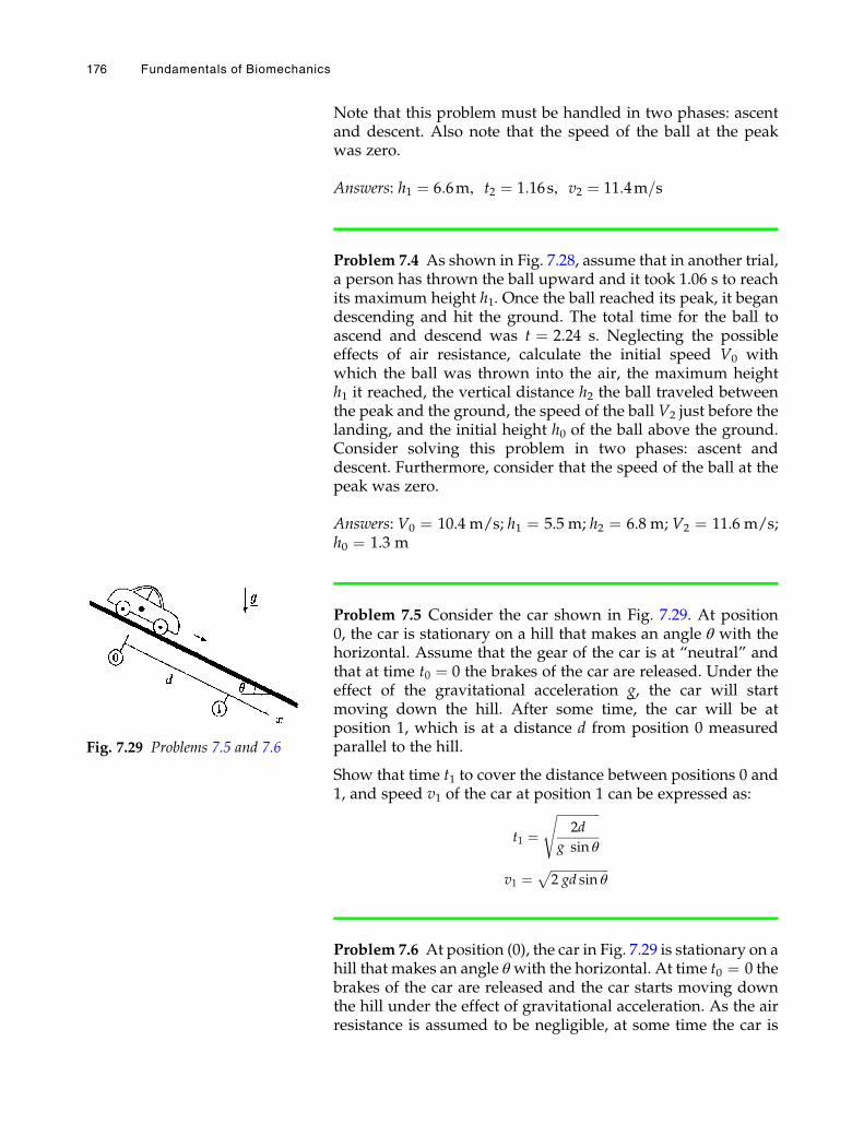
Note that this problem must be handled in two phases: ascentand descent. Also note that the speed of the ball at the peakwas zero.
Answers: h1 ¼ 6:6m, t2 ¼ 1:16s, v2 ¼ 11:4m=s
Problem 7.4 As shown in Fig. 7.28, assume that in another trial,a person has thrown the ball upward and it took 1.06 s to reachits maximum height h1. Once the ball reached its peak, it begandescending and hit the ground. The total time for the ball toascend and descend was t ¼ 2.24 s. Neglecting the possibleeffects of air resistance, calculate the initial speed V0 withwhich the ball was thrown into the air, the maximum heighth1 it reached, the vertical distance h2 the ball traveled betweenthe peak and the ground, the speed of the ball V2 just before thelanding, and the initial height h0 of the ball above the ground.Consider solving this problem in two phases: ascent anddescent. Furthermore, consider that the speed of the ball at thepeak was zero.
Answers: V0 ¼ 10.4 m/s; h1 ¼ 5.5 m; h2 ¼ 6.8 m; V2 ¼ 11.6 m/s;h0 ¼ 1.3 m
Problem 7.5 Consider the car shown in Fig. 7.29. At position0, the car is stationary on a hill that makes an angle θ with thehorizontal. Assume that the gear of the car is at “neutral” andthat at time t0 ¼ 0 the brakes of the car are released. Under theeffect of the gravitational acceleration g, the car will startmoving down the hill. After some time, the car will be atposition 1, which is at a distance d from position 0 measuredparallel to the hill.
Show that time t1 to cover the distance between positions 0 and1, and speed v1 of the car at position 1 can be expressed as:
t1 ¼ffiffiffiffiffiffiffiffiffiffiffiffiffiffi2d
g sin θ
s
v1 ¼ffiffiffiffiffiffiffiffiffiffiffiffiffiffiffiffiffiffiffi2 gd sin θ
p
Problem 7.6 At position (0), the car in Fig. 7.29 is stationary on ahill that makes an angle θwith the horizontal. At time t0 ¼ 0 thebrakes of the car are released and the car starts moving downthe hill under the effect of gravitational acceleration. As the airresistance is assumed to be negligible, at some time the car is
Fig. 7.29 Problems 7.5 and 7.6
176 Fundamentals of Biomechanics
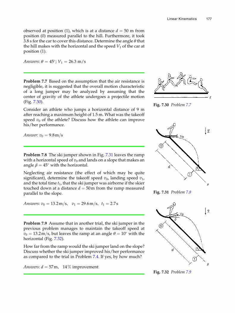
observed at position (1), which is at a distance d ¼ 50 m fromposition (0) measured parallel to the hill. Furthermore, it took3.8 s for the car to cover this distance. Determine the angle θ thatthe hill makes with the horizontal and the speed V1 of the car atposition (1).
Answers: θ ¼ 45�; V1 ¼ 26.3 m/s
Problem 7.7 Based on the assumption that the air resistance isnegligible, it is suggested that the overall motion characteristicof a long jumper may be analyzed by assuming that thecenter of gravity of the athlete undergoes a projectile motion(Fig. 7.30).
Consider an athlete who jumps a horizontal distance of 9 mafter reaching amaximum height of 1.5 m.What was the takeoffspeed v0 of the athlete? Discuss how the athlete can improvehis/her performance.
Answer: v0 ¼ 9:8m=s
Problem 7.8 The ski jumper shown in Fig. 7.31 leaves the rampwith a horizontal speed of v0 and lands on a slope that makes anangle β ¼ 45� with the horizontal.
Neglecting air resistance (the effect of which may be quitesignificant), determine the takeoff speed v0, landing speed v1,and the total time t1, that the ski jumper was airborne if the skiertouched down at a distance d ¼ 50m from the ramp measuredparallel to the slope.
Answers: v0 ¼ 13:2m=s, v1 ¼ 29:6m=s, t1 ¼ 2:7s
Problem 7.9 Assume that in another trial, the ski jumper in theprevious problem manages to maintain the takeoff speed atv0 ¼ 13:2m=s, but leaves the ramp at an angle θ ¼ 10� with thehorizontal (Fig. 7.32).
How far from the rampwould the ski jumper land on the slope?Discuss whether the ski jumper improved his/her performanceas compared to the trial in Problem 7.4. If yes, by how much?
Answers: d ¼ 57m, 14% improvement
Fig. 7.30 Problem 7.7
Fig. 7.31 Problem 7.8
Fig. 7.32 Problem 7.9
Linear Kinematics 177
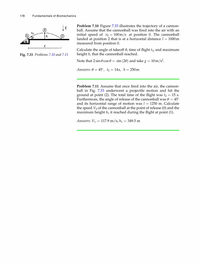
Problem 7.10 Figure 7.33 illustrates the trajectory of a cannon-ball. Assume that the cannonball was fired into the air with aninitial speed of v0 ¼ 100m=s at position 0. The cannonballlanded at position 2 that is at a horizontal distance l ¼ 1000mmeasured from position 0.
Calculate the angle of takeoff θ, time of flight t2, and maximumheight h, that the cannonball reached.
Note that 2 sin θ cos θ ¼ sin 2θð Þ and take g ¼ 10m=s2.
Answers: θ ¼ 45�, t2 ¼ 14s, h ¼ 250m
Problem 7.11 Assume that once fired into the air, the cannon-ball in Fig. 7.33 underwent a projectile motion and hit theground at point (2). The total time of the flight was t2 ¼ 15 s.Furthermore, the angle of release of the cannonball was θ ¼ 45�
and its horizontal range of motion was l ¼ 1250 m. Calculatethe speed V0 of the cannonball at the point of release (0) and themaximum height h1 it reached during the flight at point (1).
Answers: V1 ¼ 117.9 m/s; h1 ¼ 349.5 m
Fig. 7.33 Problems 7.10 and 7.11
178 Fundamentals of Biomechanics
Chapter 8
Linear Kinetics
8.1 Overview / 181
8.2 Equations of Motion / 181
8.3 Special Cases of Translational Motion / 183
8.3.1 Force Is Constant / 183
8.3.2 Force Is a Function of Time / 184
8.3.3 Force Is a Function of Displacement / 184
8.4 Procedure for Problem Solving in Kinetics / 185
8.5 Work and Energy Methods / 187
8.6 Mechanical Work / 188
8.6.1 Work Done by a Constant Force / 188
8.6.2 Work Done by a Varying Force / 189
8.6.3 Work as a Scalar Product / 189
8.7 Mechanical Energy / 190
8.7.1 Potential Energy / 190
8.7.2 Kinetic Energy / 191
8.8 Work–Energy Theorem / 191
8.9 Conservation of Energy Principle / 191
8.10 Dimension and Units of Work and Energy / 192
8.11 Power / 192
8.12 Applications of Energy Methods / 193
8.13 Exercise Problems / 198
The original version of this chapter was revised. An erratum to this chapter can befound at https://doi.org/10.1007/978-3-319-44738-4_16
# Springer International Publishing Switzerland 2017N. Ozkaya et al., Fundamentals of Biomechanics, DOI 10.1007/978-3-319-44738-4_8
179

8.1 Overview
As studied in the previous chapter, kinematic analyses areconcerned with the description of the geometric and time-dependent aspects of motion in terms of displacement, velocity,and acceleration without dealing with the factors causing themotion. The field of kinetics, on the other hand, is based onkinematics and incorporates into the analysis the effects offorces that cause the motion.
Based on the type of motion involved, the field of kinetics can bedivided into linear (translational) and angular (rotational)kinetics. Translation is caused by the net force applied on anobject, whereas rotation is the consequence of the net torque. Anobject will translate and rotate simultaneously (undergo a gen-eral motion) if there is both a net force and a net moment actingon it. In addition to classifying a motion as translational, rota-tional, or general, the field of kinetics can be further distin-guished as the kinetics of particles and the kinetics of rigid bodies.Particle kinetics is easier to implement than rigid body kineticsthat introduces the size and shape of the bodies into theanalyses. The distinction between a particle and a rigid bodyis particularly important if the object is undergoing a rotationalmotion. If the object is sufficiently small or it is undergoingtranslational motion only, then the geometric characteristics ofthe object may be ignored and the object can be treated as aparticle located at its center of gravity with a mass equal to thetotal mass of the object. For example, what is significant for aperson pushing a block on a flat surface is the total mass of theblock, not its size or shape.
Kinetic analyses utilize Newton’s second law of motion whichcan be formulated in various ways. One way of representingNewton’s second law of motion is in terms of the equations ofmotion, which are particularly suitable for solving problemsrequiring the analysis of acceleration. The use of the equationsof motion for linear kinetics will be discussed next. Anotherway of formulating Newton’s second law is through work andenergy methods that will also be discussed in this chapterwithin the context of linear kinetics. There are also methodsbased on impulse and momentum that will be presented inChap. 11.
8.2 Equations of Motion
A body accelerates if there is a non-zero net force acting onit. Newton’s second law of motion states that the magnitude ofthe acceleration of a body is directly proportional to the magni-tude of the resultant force and inversely proportional to its
Linear Kinetics 181
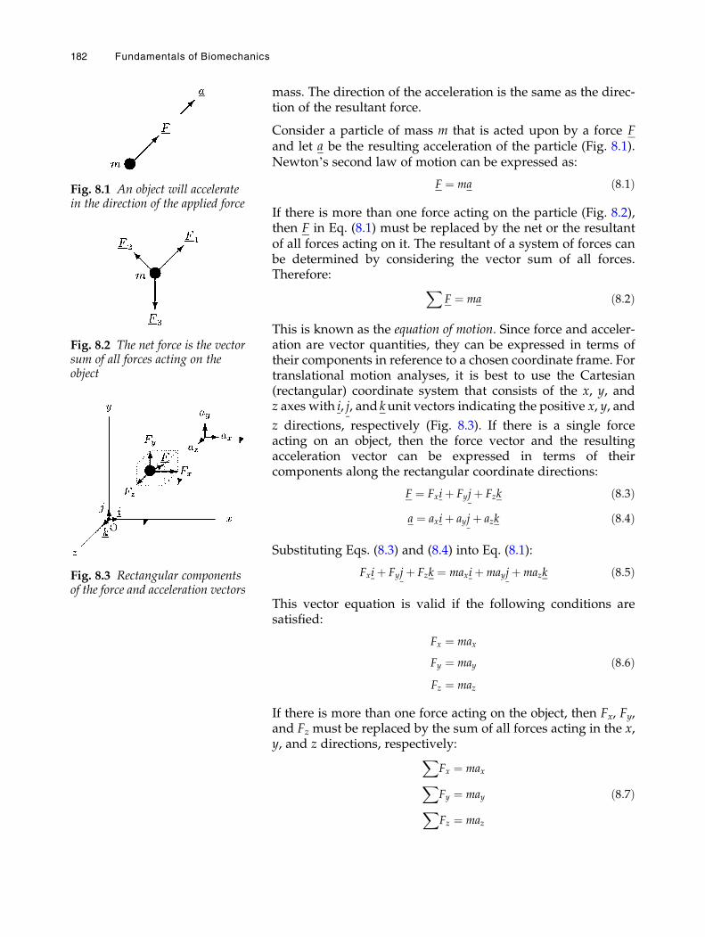
mass. The direction of the acceleration is the same as the direc-tion of the resultant force.
Consider a particle of mass m that is acted upon by a force Fand let a be the resulting acceleration of the particle (Fig. 8.1).Newton’s second law of motion can be expressed as:
F ¼ ma ð8:1Þ
If there is more than one force acting on the particle (Fig. 8.2),then F in Eq. (8.1) must be replaced by the net or the resultantof all forces acting on it. The resultant of a system of forces canbe determined by considering the vector sum of all forces.Therefore: X
F ¼ ma ð8:2Þ
This is known as the equation of motion. Since force and acceler-ation are vector quantities, they can be expressed in terms oftheir components in reference to a chosen coordinate frame. Fortranslational motion analyses, it is best to use the Cartesian(rectangular) coordinate system that consists of the x, y, andz axes with i, j, and kunit vectors indicating the positive x, y, and
z directions, respectively (Fig. 8.3). If there is a single forceacting on an object, then the force vector and the resultingacceleration vector can be expressed in terms of theircomponents along the rectangular coordinate directions:
F ¼ Fxiþ Fyjþ Fzk ð8:3Þa ¼ axiþ ayjþ azk ð8:4Þ
Substituting Eqs. (8.3) and (8.4) into Eq. (8.1):
Fxiþ Fyjþ Fzk ¼ maxiþmayjþmazk ð8:5Þ
This vector equation is valid if the following conditions aresatisfied:
Fx ¼ max
Fy ¼ may ð8:6ÞFz ¼ maz
If there is more than one force acting on the object, then Fx, Fy,and Fz must be replaced by the sum of all forces acting in the x,y, and z directions, respectively:X
Fx ¼ maxXFy ¼ may ð8:7Þ
XFz ¼ maz
Fig. 8.1 An object will acceleratein the direction of the applied force
Fig. 8.2 The net force is the vectorsum of all forces acting on theobject
Fig. 8.3 Rectangular componentsof the force and acceleration vectors
182 Fundamentals of Biomechanics
Equations (8.7) state that the sum of all forces acting in onedirection is equal to the mass times the acceleration of thebody in that direction. Note that for one-dimensional motionanalysis, only one of these equations need to be considered. Fora two-dimensional case, two of the above equations are suffi-cient to analyze the problem.
8.3 Special Cases of Translational Motion
A force can be applied in various ways. For example, an appliedforce may be constant or it may vary over time. Applied forcescan be measured in various ways as well. The magnitude of aforce vector can be measured as a function of time, as a functionof the relative position of the object upon which it is applied, oras a function of velocity. Some of these cases will be discussednext. To illustrate the methods of handling these cases in aconcise manner, it will be assumed that the motion is along astraight line in the x direction and under the effect of only oneapplied force. Using the vectorial properties of the parametersinvolved, these methods can be easily expanded to analyze two-and three-dimensional translational motions under the action ofmore than one force.
Note that the derivations provided in this section are aimed todemonstrate that different cases can be handled through propermathematical manipulations. The mathematics involved for thecases in which the applied force is a function of displacementmay be beyond the scope of this text, and can be omittedwithout losing the continuity of the topics to be covered in thefollowing sections.
8.3.1 Force Is Constant
If a force applied on an object has a constant magnitude anddirection, the object will move with a constant acceleration inthe direction of the applied force. Assume that a force withmagnitude Fx is applied on an object with mass m. The magni-tude ax of the constant acceleration of the object in thex direction can be calculated using the equation of motion inthe x direction:
ax ¼ Fxm¼ constant
Once the acceleration of the object is determined, the kinematicequations can be utilized to calculate the velocity and displace-ment of the object as well:
Linear Kinetics 183
vx ¼ vx0 þðt
t0
axdt ¼ vx0 þFxm
t ð8:8Þ
x ¼ x0 þðt
t0
vxdt ¼ x0 þ vx0tþ1
2
Fxm
t2 ð8:9Þ
Here, vx0 and x0 are the initial speed and displacement of theobject in the x direction at time t ¼ 0. Note that these results canbe used for a situation in which there is a second force withconstant magnitude Fy acting on the object in the y directionsimply by replacing x with y throughout the equations.
8.3.2 Force Is a Function of Time
If the magnitude of a force applied on an object is a function oftime, then Fx ¼ Fxt. The resulting acceleration of the object isalso a function of time:
ax tð Þ ¼ Fx tð Þm
The velocity and displacement of the object can now be deter-mined using the kinematic relationships:
vx ¼ vx0 þðt
t0
ax tð Þdt ð8:10Þ
x ¼ x0 þðt
t0
vx tð Þdt ð8:11Þ
The function Fx(t) must be provided so that the integral inEq. (8.10) can be evaluated.
8.3.3 Force Is a Function of Displacement
Sometimes it is more convenient to express force as a function ofdisplacement, in which case Fx ¼ Fx xð Þ. By definition, accelera-tion is equal to the time rate of change of velocity. Therefore, theequation of motion in the x direction can be expressed as:
dvxdt¼ Fx xð Þ
m
Employing the chain rule of differentiation (see Appendix C.2.6),the time derivative of velocity can be expressed as:
184 Fundamentals of Biomechanics
dvxdt¼ dvx
dx
dx
dt¼ dvx
dxvx
Therefore, the equation of motion in the x direction is:
vxdvxdx¼ Fx xð Þ
m
Multiplying both sides by dx:
vxdvx ¼ Fx xð Þm
dx
The left-hand side of this equation is a function of vx only andcan be integrated with respect to vx, and the right-hand side is afunction of x only and can be integrated with respect to x:
ðvx
vx0
vxdvx ¼ðx
x0
Fx xð Þm
dx
Evaluating the integral on the left-hand side:
1
2vx
2 � vx02
� � ¼ 1
m
ðx
x0
Fx xð Þdx
Rearranging the order of terms:
vx2 ¼ vx0
2 þ 2
m
ðx
x0
Fx xð Þdx ð8:12Þ
Fx must be provided as a function of x, so that the integral inEq. (8.12) can be evaluated. For given Fx(x), Eq. (8.12) will yieldvx as a function of x. Once Fx is known, the acceleration of theobject can be determined using:
ax ¼ vxdvxdx
ð8:13Þ
8.4 Procedure for Problem Solving in Kinetics
The procedure for analyzing the kinetic characteristics ofobjects undergoing translational motion using the equations ofmotion can be outlined as follows:
• Draw a simple, neat diagram of the system to be analyzed.
• Isolate the bodies of interest from their surroundings anddraw their free-body diagrams by showing all external forcesacting on them. Indicate the correct directions for the knownforces. If the direction of a force vector is not known, assume a
Linear Kinetics 185
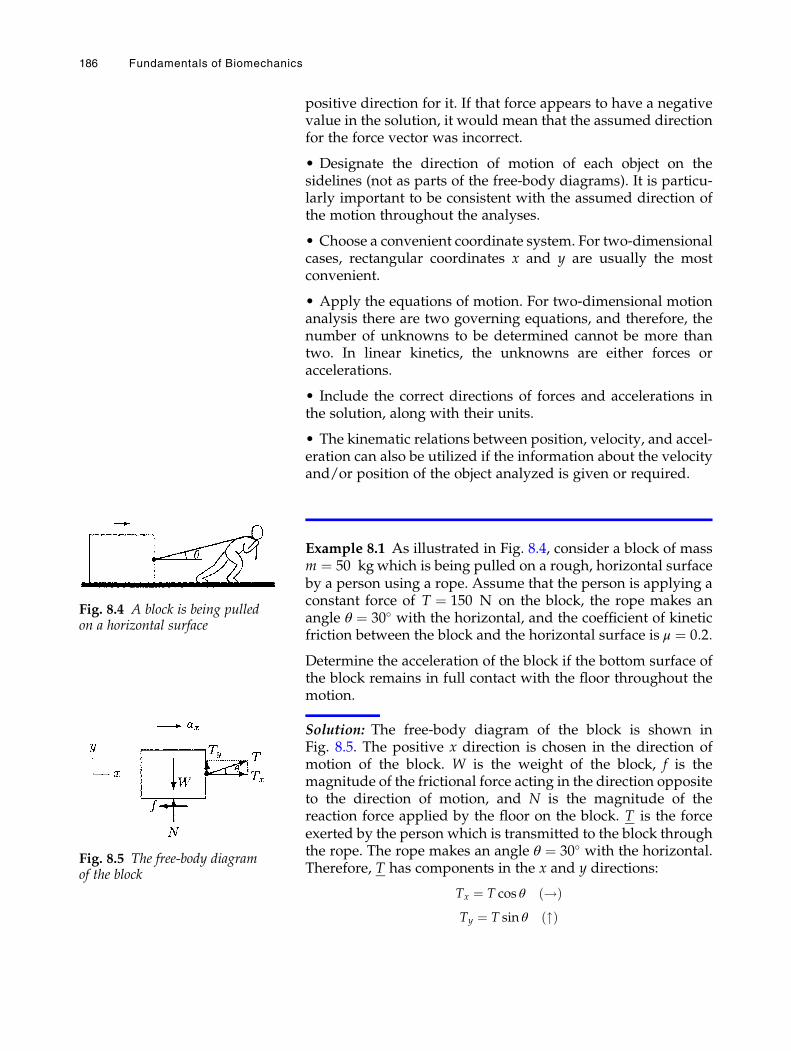
positive direction for it. If that force appears to have a negativevalue in the solution, it would mean that the assumed directionfor the force vector was incorrect.
• Designate the direction of motion of each object on thesidelines (not as parts of the free-body diagrams). It is particu-larly important to be consistent with the assumed direction ofthe motion throughout the analyses.
• Choose a convenient coordinate system. For two-dimensionalcases, rectangular coordinates x and y are usually the mostconvenient.
• Apply the equations of motion. For two-dimensional motionanalysis there are two governing equations, and therefore, thenumber of unknowns to be determined cannot be more thantwo. In linear kinetics, the unknowns are either forces oraccelerations.
• Include the correct directions of forces and accelerations inthe solution, along with their units.
• The kinematic relations between position, velocity, and accel-eration can also be utilized if the information about the velocityand/or position of the object analyzed is given or required.
Example 8.1 As illustrated in Fig. 8.4, consider a block of massm ¼ 50 kgwhich is being pulled on a rough, horizontal surfaceby a person using a rope. Assume that the person is applying aconstant force of T ¼ 150 N on the block, the rope makes anangle θ ¼ 30� with the horizontal, and the coefficient of kineticfriction between the block and the horizontal surface is μ ¼ 0:2:
Determine the acceleration of the block if the bottom surface ofthe block remains in full contact with the floor throughout themotion.
Solution: The free-body diagram of the block is shown inFig. 8.5. The positive x direction is chosen in the direction ofmotion of the block. W is the weight of the block, f is themagnitude of the frictional force acting in the direction oppositeto the direction of motion, and N is the magnitude of thereaction force applied by the floor on the block. T is the forceexerted by the person which is transmitted to the block throughthe rope. The rope makes an angle θ ¼ 30� with the horizontal.Therefore, T has components in the x and y directions:
Tx ¼ T cos θ !ð ÞTy ¼ T sin θ "ð Þ
Fig. 8.4 A block is being pulledon a horizontal surface
Fig. 8.5 The free-body diagramof the block
186 Fundamentals of Biomechanics

The weight of the block is due to the gravitational effect of Earthon the mass of the block, and can be expressed as:
W ¼ mg #ð Þ
The magnitude of the frictional force is proportional to themagnitude of the normal force, and they are related throughthe coefficient of friction between the surfaces in contact:
f ¼ μN ð Þ ðiÞ
Equations of motion in the x and y directions can now beapplied to determine an expression for the acceleration of theblock. The block has no motion in the y direction, and therefore,the acceleration of the block in the y direction is zero (ay ¼ 0).
The equation of motion in the y direction is:XFy ¼ 0 : N þ Ty �W ¼ 0
Solving this equilibrium equation for force N will yield:
N ¼W � Ty ¼ mg� T sin θ ðiiÞ
Substituting Eq. (ii) into Eq. (i) will yield:
f ¼ μ mg� T sin θð Þ ðiiiÞ
Now, the equation of motion in the x direction can be consid-ered: X
Fx ¼ max : Tx � f ¼ max
Solving this equation for ax will yield
ax ¼ 1
mTx � fð Þ ðivÞ
Substituting Eq. (iii) and Tx ¼ T cos θ into Eq. (iv):
ax ¼ 1
mT cos θ � μ mg� T sin θð Þ½ �
Substituting the numerical values m ¼ 50 kg, T ¼ 150 N,θ ¼ 30�, μ ¼ 0:2, and g ¼ 9:8 m=s, and carrying out the
calculations will yield ax ¼ 0:94 m=s2 !ð Þ.
8.5 Work and Energy Methods
The fundamental method of analyzing the kinetic charac-teristics of bodies is based on the equations of motion whichare mathematical representations of Newton’s second law ofmotion. Using the equations of motion, one can determineaccelerations. In some cases, particularly when the forces
Linear Kinetics 187
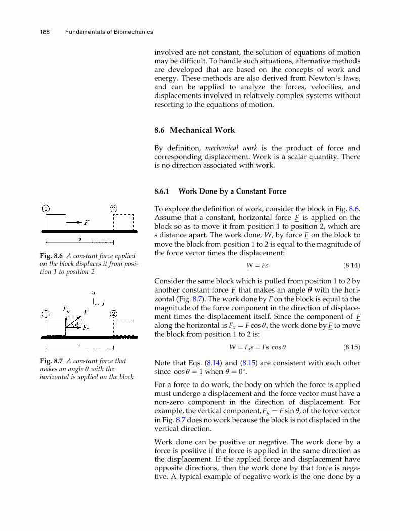
involved are not constant, the solution of equations of motionmay be difficult. To handle such situations, alternative methodsare developed that are based on the concepts of work andenergy. These methods are also derived from Newton’s laws,and can be applied to analyze the forces, velocities, anddisplacements involved in relatively complex systems withoutresorting to the equations of motion.
8.6 Mechanical Work
By definition, mechanical work is the product of force andcorresponding displacement. Work is a scalar quantity. Thereis no direction associated with work.
8.6.1 Work Done by a Constant Force
To explore the definition of work, consider the block in Fig. 8.6.Assume that a constant, horizontal force F is applied on theblock so as to move it from position 1 to position 2, which ares distance apart. The work done, W, by force F on the block tomove the block from position 1 to 2 is equal to the magnitude ofthe force vector times the displacement:
W ¼ Fs ð8:14Þ
Consider the same block which is pulled from position 1 to 2 byanother constant force F that makes an angle θ with the hori-zontal (Fig. 8.7). The work done by F on the block is equal to themagnitude of the force component in the direction of displace-ment times the displacement itself. Since the component of Falong the horizontal is Fx ¼ F cos θ; the work done by F to movethe block from position 1 to 2 is:
W ¼ Fxs ¼ Fs cos θ ð8:15Þ
Note that Eqs. (8.14) and (8.15) are consistent with each othersince cos θ ¼ 1 when θ ¼ 0�.
For a force to do work, the body on which the force is appliedmust undergo a displacement and the force vector must have anon-zero component in the direction of displacement. Forexample, the vertical component,Fy ¼ F sin θ, of the force vectorin Fig. 8.7 does no work because the block is not displaced in thevertical direction.
Work done can be positive or negative. The work done by aforce is positive if the force is applied in the same direction asthe displacement. If the applied force and displacement haveopposite directions, then the work done by that force is nega-tive. A typical example of negative work is the one done by a
Fig. 8.6 A constant force appliedon the block displaces it from posi-tion 1 to position 2
Fig. 8.7 A constant force thatmakes an angle θ with thehorizontal is applied on the block
188 Fundamentals of Biomechanics
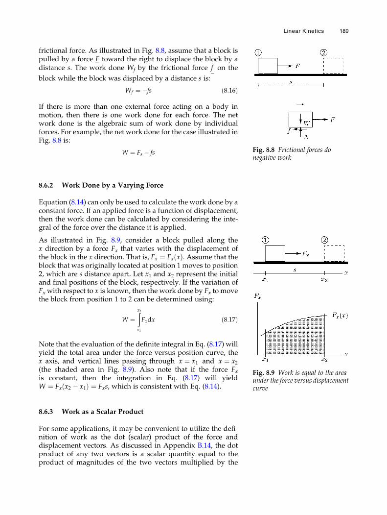
frictional force. As illustrated in Fig. 8.8, assume that a block ispulled by a force F toward the right to displace the block by adistance s. The work done Wf by the frictional force f on the
block while the block was displaced by a distance s is:
Wf ¼ �fs ð8:16Þ
If there is more than one external force acting on a body inmotion, then there is one work done for each force. The network done is the algebraic sum of work done by individualforces. For example, the net work done for the case illustrated inFig. 8.8 is:
W ¼ Fs � fs
8.6.2 Work Done by a Varying Force
Equation (8.14) can only be used to calculate the work done by aconstant force. If an applied force is a function of displacement,then the work done can be calculated by considering the inte-gral of the force over the distance it is applied.
As illustrated in Fig. 8.9, consider a block pulled along thex direction by a force Fx that varies with the displacement ofthe block in the x direction. That is, Fx ¼ Fx xð Þ. Assume that theblock that was originally located at position 1 moves to position2, which are s distance apart. Let x1 and x2 represent the initialand final positions of the block, respectively. If the variation ofFx with respect to x is known, then the work done by Fx to movethe block from position 1 to 2 can be determined using:
W ¼ðx2
x1
Fxdx ð8:17Þ
Note that the evaluation of the definite integral in Eq. (8.17) willyield the total area under the force versus position curve, thex axis, and vertical lines passing through x ¼ x1 and x ¼ x2(the shaded area in Fig. 8.9). Also note that if the force Fxis constant, then the integration in Eq. (8.17) will yieldW ¼ Fx x2 � x1ð Þ ¼ Fxs, which is consistent with Eq. (8.14).
8.6.3 Work as a Scalar Product
For some applications, it may be convenient to utilize the defi-nition of work as the dot (scalar) product of the force anddisplacement vectors. As discussed in Appendix B.14, the dotproduct of any two vectors is a scalar quantity equal to theproduct of magnitudes of the two vectors multiplied by the
Fig. 8.8 Frictional forces donegative work
Fig. 8.9 Work is equal to the areaunder the force versus displacementcurve
Linear Kinetics 189
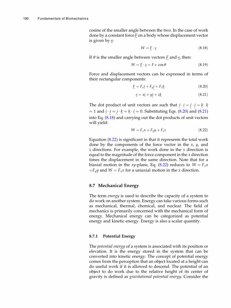
cosine of the smaller angle between the two. In the case of workdone by a constant forceFon a body whose displacement vectoris given by s:
W ¼ F � s ð8:18Þ
If θ is the smaller angle between vectors F and s, then:
W ¼ F � s ¼ F s cos θ ð8:19Þ
Force and displacement vectors can be expressed in terms oftheir rectangular components:
F ¼ Fxiþ Fyjþ Fzk ð8:20Þs ¼ xiþ yjþ zk ð8:21Þ
The dot product of unit vectors are such that i � i ¼ j � j ¼ k � k¼ 1 and i � j ¼ j � k ¼ k � i ¼ 0. Substituting Eqs. (8.20) and (8.21)
into Eq. (8.18) and carrying out the dot products of unit vectorswill yield:
W ¼ Fxxþ Fyyþ Fzz ð8:22Þ
Equation (8.22) is significant in that it represents the total workdone by the components of the force vector in the x, y, andz directions. For example, the work done in the x direction isequal to the magnitude of the force component in the x directiontimes the displacement in the same direction. Note that for abiaxial motion in the xy-plane, Eq. (8.22) reduces to W ¼ Fxx
þFyy and W ¼ Fxx for a uniaxial motion in the x direction.
8.7 Mechanical Energy
The term energy is used to describe the capacity of a system todowork on another system. Energy can take various forms suchas mechanical, thermal, chemical, and nuclear. The field ofmechanics is primarily concerned with the mechanical form ofenergy. Mechanical energy can be categorized as potentialenergy and kinetic energy. Energy is also a scalar quantity.
8.7.1 Potential Energy
The potential energy of a system is associated with its position orelevation. It is the energy stored in the system that can beconverted into kinetic energy. The concept of potential energycomes from the perception that an object located at a height cando useful work if it is allowed to descend. The potential of anobject to do work due to the relative height of its center ofgravity is defined as gravitational potential energy. Consider the
190 Fundamentals of Biomechanics
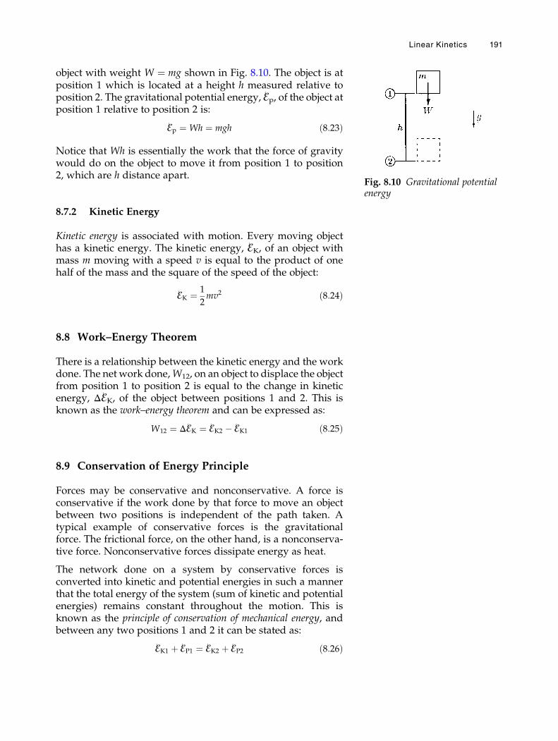
object with weight W ¼ mg shown in Fig. 8.10. The object is atposition 1 which is located at a height h measured relative toposition 2. The gravitational potential energy, ℰp, of the object atposition 1 relative to position 2 is:
ℰp ¼Wh ¼ mgh ð8:23Þ
Notice that Wh is essentially the work that the force of gravitywould do on the object to move it from position 1 to position2, which are h distance apart.
8.7.2 Kinetic Energy
Kinetic energy is associated with motion. Every moving objecthas a kinetic energy. The kinetic energy, ℰK, of an object withmass m moving with a speed v is equal to the product of onehalf of the mass and the square of the speed of the object:
ℰK ¼ 1
2mv2 ð8:24Þ
8.8 Work–Energy Theorem
There is a relationship between the kinetic energy and the workdone. The net work done,W12, on an object to displace the objectfrom position 1 to position 2 is equal to the change in kineticenergy, ΔℰK, of the object between positions 1 and 2. This isknown as the work–energy theorem and can be expressed as:
W12 ¼ ΔℰK ¼ ℰK2 � ℰK1 ð8:25Þ
8.9 Conservation of Energy Principle
Forces may be conservative and nonconservative. A force isconservative if the work done by that force to move an objectbetween two positions is independent of the path taken. Atypical example of conservative forces is the gravitationalforce. The frictional force, on the other hand, is a nonconserva-tive force. Nonconservative forces dissipate energy as heat.
The network done on a system by conservative forces isconverted into kinetic and potential energies in such a mannerthat the total energy of the system (sum of kinetic and potentialenergies) remains constant throughout the motion. This isknown as the principle of conservation of mechanical energy, andbetween any two positions 1 and 2 it can be stated as:
ℰK1 þ ℰP1 ¼ ℰK2 þ ℰP2 ð8:26Þ
Fig. 8.10 Gravitational potentialenergy
Linear Kinetics 191
8.10 Dimension and Units of Work and Energy
Mechanical work and energy have the same dimension andunits. By definition, work done is force times displacement.Therefore, work has the dimension of force times the dimensionof length.
Work½ � ¼ Force½ � Displacement½ � ¼ML2
T2
The units of work and energy in different systems of units areprovided in Table 8.1.
8.11 Power
Power, P, is defined as the time rate of work done:
P ¼ dW
dtð8:27Þ
The work done by a constant force on an object can be deter-mined by considering the dot product of the force and displace-ment vectors (W ¼ F � s):
P ¼ d
dtF � s� �
If the force vector F is constant, then:
P ¼ F � dsdt¼ F � v� � ð8:28Þ
In Eq. (8.28), v is the velocity vector of the object. If the appliedforce is collinear with the velocity, then P ¼ Fv. Power is ascalar quantity, and has the dimension of force times velocity.The units of power are given in Table 8.2.
Table 8.1 Units of work and energy
SYSTEM UNITS OF WORK AND ENERGY SPECIAL NAME
SI Newton-meter (Nm) Joule (J)
c–g–s Dyne-centimeter (dyn cm) erg
British Pound-foot (lb ft)
192 Fundamentals of Biomechanics
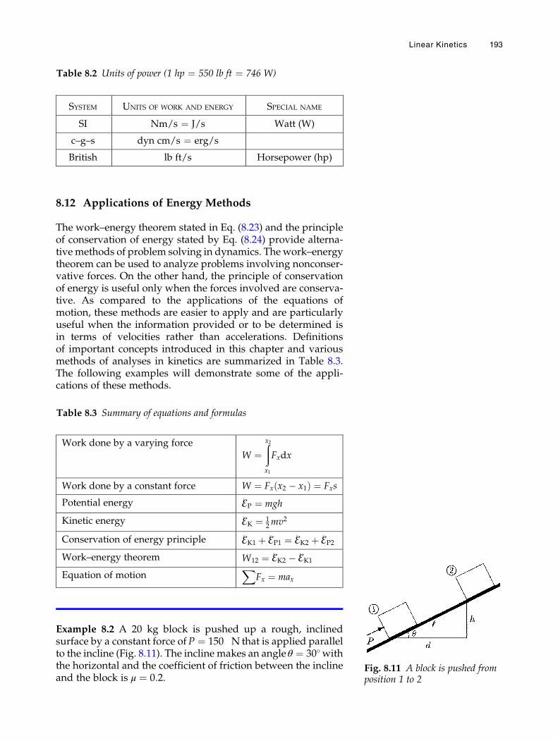
8.12 Applications of Energy Methods
The work–energy theorem stated in Eq. (8.23) and the principleof conservation of energy stated by Eq. (8.24) provide alterna-tive methods of problem solving in dynamics. The work–energytheorem can be used to analyze problems involving nonconser-vative forces. On the other hand, the principle of conservationof energy is useful only when the forces involved are conserva-tive. As compared to the applications of the equations ofmotion, these methods are easier to apply and are particularlyuseful when the information provided or to be determined isin terms of velocities rather than accelerations. Definitionsof important concepts introduced in this chapter and variousmethods of analyses in kinetics are summarized in Table 8.3.The following examples will demonstrate some of the appli-cations of these methods.
Example 8.2 A 20 kg block is pushed up a rough, inclinedsurface by a constant force ofP ¼ 150 N that is applied parallelto the incline (Fig. 8.11). The incline makes an angle θ ¼ 30�withthe horizontal and the coefficient of friction between the inclineand the block is μ ¼ 0:2.
Table 8.2 Units of power (1 hp ¼ 550 lb ft ¼ 746 W)
SYSTEM UNITS OF WORK AND ENERGY SPECIAL NAME
SI Nm/s ¼ J/s Watt (W)
c–g–s dyn cm/s ¼ erg/s
British lb ft/s Horsepower (hp)
Table 8.3 Summary of equations and formulas
Work done by a varying force
W ¼ðx2
x1
Fxdx
Work done by a constant force W ¼ Fx x2 � x1ð Þ ¼ Fxs
Potential energy ℰP ¼ mgh
Kinetic energy ℰK ¼ 12mv2
Conservation of energy principle ℰK1 þ ℰP1 ¼ ℰK2 þ ℰP2
Work–energy theorem W12 ¼ ℰK2 � ℰK1
Equation of motionX
Fx ¼ max
Fig. 8.11 A block is pushed fromposition 1 to 2
Linear Kinetics 193
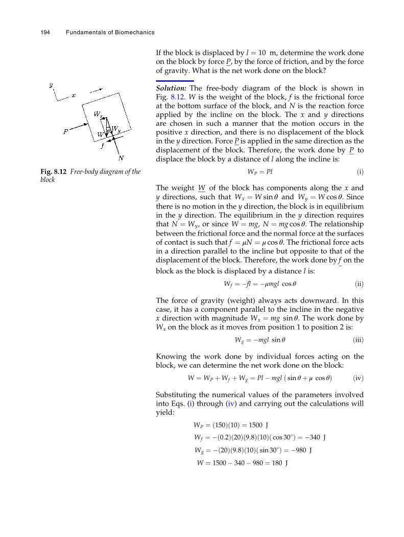
If the block is displaced by l ¼ 10 m, determine the work doneon the block by force P, by the force of friction, and by the forceof gravity. What is the net work done on the block?
Solution: The free-body diagram of the block is shown inFig. 8.12. W is the weight of the block, f is the frictional forceat the bottom surface of the block, and N is the reaction forceapplied by the incline on the block. The x and y directionsare chosen in such a manner that the motion occurs in thepositive x direction, and there is no displacement of the blockin the y direction. Force P is applied in the same direction as thedisplacement of the block. Therefore, the work done by P todisplace the block by a distance of l along the incline is:
WP ¼ Pl ðiÞ
The weight W of the block has components along the x andy directions, such that Wx ¼W sin θ and Wy ¼W cos θ. Sincethere is no motion in the y direction, the block is in equilibriumin the y direction. The equilibrium in the y direction requiresthat N ¼Wy, or since W ¼ mg, N ¼ mg cos θ. The relationship
between the frictional force and the normal force at the surfacesof contact is such that f ¼ μN ¼ μ cos θ. The frictional force actsin a direction parallel to the incline but opposite to that of thedisplacement of the block. Therefore, the work done by f on the
block as the block is displaced by a distance l is:
Wf ¼ �fl ¼ �μmgl cos θ ðiiÞ
The force of gravity (weight) always acts downward. In thiscase, it has a component parallel to the incline in the negativex direction with magnitude Wx ¼ mg sin θ. The work done byWx on the block as it moves from position 1 to position 2 is:
Wg ¼ �mgl sin θ ðiiiÞ
Knowing the work done by individual forces acting on theblock, we can determine the net work done on the block:
W ¼WP þWf þWg ¼ Pl�mgl sin θ þ μ cos θð Þ ðivÞ
Substituting the numerical values of the parameters involvedinto Eqs. (i) through (iv) and carrying out the calculations willyield:
WP ¼ 150ð Þ 10ð Þ ¼ 1500 J
Wf ¼ � 0:2ð Þ 20ð Þ 9:8ð Þ 10ð Þ cos 30�ð Þ ¼ �340 J
Wg ¼ � 20ð Þ 9:8ð Þ 10ð Þ sin 30�ð Þ ¼ �980 J
W ¼ 1500� 340� 980 ¼ 180 J
Fig. 8.12 Free-body diagram of theblock
194 Fundamentals of Biomechanics
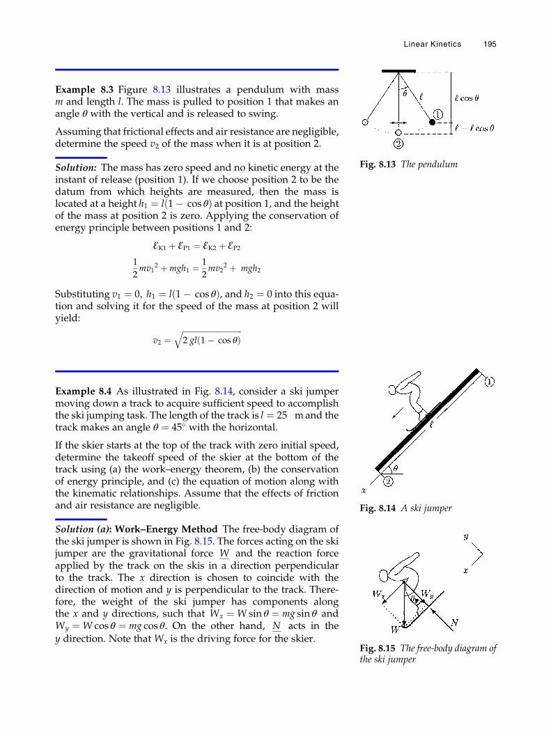
Example 8.3 Figure 8.13 illustrates a pendulum with massm and length l. The mass is pulled to position 1 that makes anangle θ with the vertical and is released to swing.
Assuming that frictional effects and air resistance are negligible,determine the speed v2 of the mass when it is at position 2.
Solution: The mass has zero speed and no kinetic energy at theinstant of release (position 1). If we choose position 2 to be thedatum from which heights are measured, then the mass islocated at a height h1 ¼ l 1� cos θð Þ at position 1, and the heightof the mass at position 2 is zero. Applying the conservation ofenergy principle between positions 1 and 2:
ℰK1 þ ℰP1 ¼ ℰK2 þ ℰP2
1
2mv1
2 þmgh1 ¼ 1
2mv2
2 þ mgh2
Substituting v1 ¼ 0, h1 ¼ l 1� cos θð Þ, and h2 ¼ 0 into this equa-tion and solving it for the speed of the mass at position 2 willyield:
v2 ¼ffiffiffiffiffiffiffiffiffiffiffiffiffiffiffiffiffiffiffiffiffiffiffiffiffiffiffiffiffiffiffi2 gl 1� cos θð Þ
q
Example 8.4 As illustrated in Fig. 8.14, consider a ski jumpermoving down a track to acquire sufficient speed to accomplishthe ski jumping task. The length of the track is l ¼ 25 mand thetrack makes an angle θ ¼ 45� with the horizontal.
If the skier starts at the top of the track with zero initial speed,determine the takeoff speed of the skier at the bottom of thetrack using (a) the work–energy theorem, (b) the conservationof energy principle, and (c) the equation of motion along withthe kinematic relationships. Assume that the effects of frictionand air resistance are negligible.
Solution (a): Work–Energy Method The free-body diagram ofthe ski jumper is shown in Fig. 8.15. The forces acting on the skijumper are the gravitational force W and the reaction forceapplied by the track on the skis in a direction perpendicularto the track. The x direction is chosen to coincide with thedirection of motion and y is perpendicular to the track. There-fore, the weight of the ski jumper has components alongthe x and y directions, such that Wx ¼W sin θ ¼ mg sin θ andWy ¼W cos θ ¼ mg cos θ. On the other hand, N acts in the
y direction. Note that Wx is the driving force for the skier.
Fig. 8.13 The pendulum
Fig. 8.14 A ski jumper
Fig. 8.15 The free-body diagram ofthe ski jumper
Linear Kinetics 195
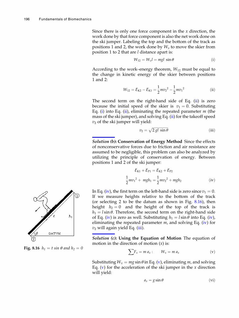
Since there is only one force component in the x direction, thework done by that force component is also the net work done onthe ski jumper. Labeling the top and the bottom of the track aspositions 1 and 2, the work done by Wx to move the skier fromposition 1 to 2 that are l distance apart is:
W12 ¼Wxl ¼ mgl sin θ ðiÞ
According to the work–energy theorem, W12 must be equal tothe change in kinetic energy of the skier between positions1 and 2:
W12 ¼ ℰK2 � ℰK1 ¼ 1
2mv2
2 � 1
2mv1
2 ðiiÞ
The second term on the right-hand side of Eq. (ii) is zerobecause the initial speed of the skier is v1 ¼ 0. SubstitutingEq. (i) into Eq. (ii), eliminating the repeated parameter m (themass of the ski jumper), and solving Eq. (ii) for the takeoff speedv2 of the ski jumper will yield:
v2 ¼ffiffiffiffiffiffiffiffiffiffiffiffiffiffiffiffiffiffiffi2 gl sin θ
pðiiiÞ
Solution (b): Conservation of Energy Method Since the effectsof nonconservative forces due to friction and air resistance areassumed to be negligible, this problem can also be analyzed byutilizing the principle of conservation of energy. Betweenpositions 1 and 2 of the ski jumper:
ℰK1 þ ℰP1 ¼ ℰK2 þ ℰP2
1
2mv1
2 þ mgh1 ¼ 1
2mv2
2 þmgh2 ðivÞ
In Eq. (iv), the first term on the left-hand side is zero since v1 ¼ 0:If we measure heights relative to the bottom of the track(or selecting 2 to be the datum as shown in Fig. 8.16), thenheight h2 ¼ 0 and the height of the top of the track ish1 ¼ l sin θ. Therefore, the second term on the right-hand sideof Eq. (iv) is zero as well. Substituting h1 ¼ l sin θ into Eq. (iv),eliminating the repeated parameter m, and solving Eq. (iv) forv2 will again yield Eq. (iii).
Solution (c): Using the Equation of Motion The equation ofmotion in the direction of motion (x) is:X
Fx ¼ m ax : Wx ¼ m ax ðvÞ
SubstitutingWx ¼ mg sin θ in Eq. (v), eliminatingm, and solvingEq. (v) for the acceleration of the ski jumper in the x directionwill yield:
ax ¼ g sin θ ðviÞ
Fig. 8.16 h1 ¼ t sin θ and h2 ¼ 0
196 Fundamentals of Biomechanics
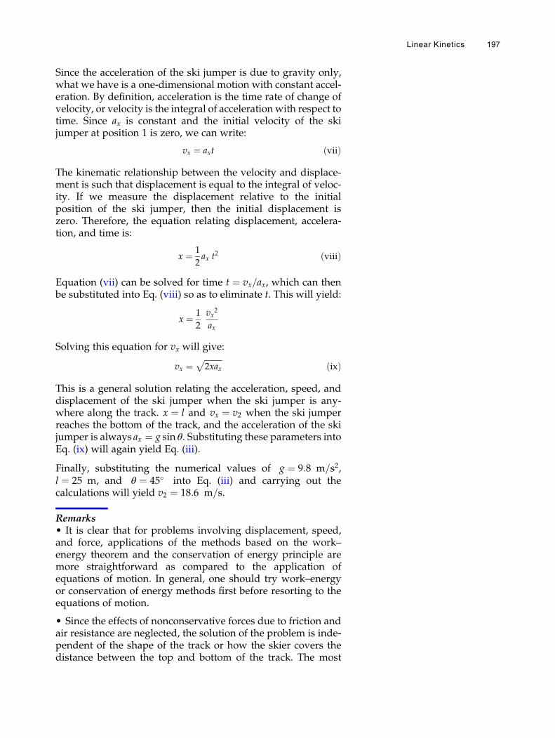
Since the acceleration of the ski jumper is due to gravity only,what we have is a one-dimensional motion with constant accel-eration. By definition, acceleration is the time rate of change ofvelocity, or velocity is the integral of acceleration with respect totime. Since ax is constant and the initial velocity of the skijumper at position 1 is zero, we can write:
vx ¼ axt ðviiÞ
The kinematic relationship between the velocity and displace-ment is such that displacement is equal to the integral of veloc-ity. If we measure the displacement relative to the initialposition of the ski jumper, then the initial displacement iszero. Therefore, the equation relating displacement, accelera-tion, and time is:
x ¼ 1
2ax t
2 ðviiiÞ
Equation (vii) can be solved for time t ¼ vx=ax, which can thenbe substituted into Eq. (viii) so as to eliminate t. This will yield:
x ¼ 1
2
vx2
ax
Solving this equation for vx will give:
vx ¼ffiffiffiffiffiffiffiffiffi2xax
pðixÞ
This is a general solution relating the acceleration, speed, anddisplacement of the ski jumper when the ski jumper is any-where along the track. x ¼ l and vx ¼ v2 when the ski jumperreaches the bottom of the track, and the acceleration of the skijumper is always ax ¼ g sin θ. Substituting these parameters intoEq. (ix) will again yield Eq. (iii).
Finally, substituting the numerical values of g ¼ 9:8 m=s2,l ¼ 25 m, and θ ¼ 45� into Eq. (iii) and carrying out thecalculations will yield v2 ¼ 18:6 m=s.
Remarks• It is clear that for problems involving displacement, speed,and force, applications of the methods based on the work–energy theorem and the conservation of energy principle aremore straightforward as compared to the application ofequations of motion. In general, one should try work–energyor conservation of energy methods first before resorting to theequations of motion.
• Since the effects of nonconservative forces due to friction andair resistance are neglected, the solution of the problem is inde-pendent of the shape of the track or how the skier covers thedistance between the top and bottom of the track. The most
Linear Kinetics 197
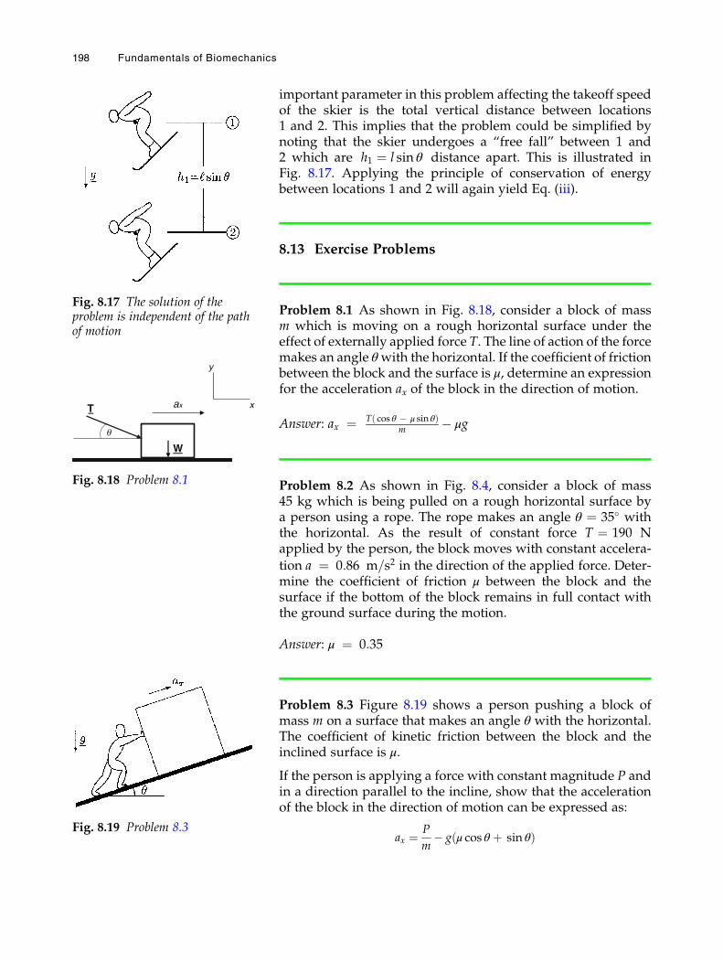
important parameter in this problem affecting the takeoff speedof the skier is the total vertical distance between locations1 and 2. This implies that the problem could be simplified bynoting that the skier undergoes a “free fall” between 1 and2 which are h1 ¼ l sin θ distance apart. This is illustrated inFig. 8.17. Applying the principle of conservation of energybetween locations 1 and 2 will again yield Eq. (iii).
8.13 Exercise Problems
Problem 8.1 As shown in Fig. 8.18, consider a block of massm which is moving on a rough horizontal surface under theeffect of externally applied force T. The line of action of the forcemakes an angle θwith the horizontal. If the coefficient of frictionbetween the block and the surface is μ, determine an expressionfor the acceleration ax of the block in the direction of motion.
Answer: ax ¼ T cos θ � μ sin θð Þm � μg
Problem 8.2 As shown in Fig. 8.4, consider a block of mass45 kg which is being pulled on a rough horizontal surface bya person using a rope. The rope makes an angle θ ¼ 35� withthe horizontal. As the result of constant force T ¼ 190 Napplied by the person, the block moves with constant accelera-
tion a ¼ 0:86 m=s2 in the direction of the applied force. Deter-mine the coefficient of friction μ between the block and thesurface if the bottom of the block remains in full contact withthe ground surface during the motion.
Answer: μ ¼ 0:35
Problem 8.3 Figure 8.19 shows a person pushing a block ofmass m on a surface that makes an angle θ with the horizontal.The coefficient of kinetic friction between the block and theinclined surface is μ.
If the person is applying a force with constant magnitude P andin a direction parallel to the incline, show that the accelerationof the block in the direction of motion can be expressed as:
ax ¼ P
m� g μ cos θ þ sin θð Þ
W
T ax
y
x
q
Fig. 8.18 Problem 8.1
Fig. 8.19 Problem 8.3
Fig. 8.17 The solution of theproblem is independent of the pathof motion
198 Fundamentals of Biomechanics
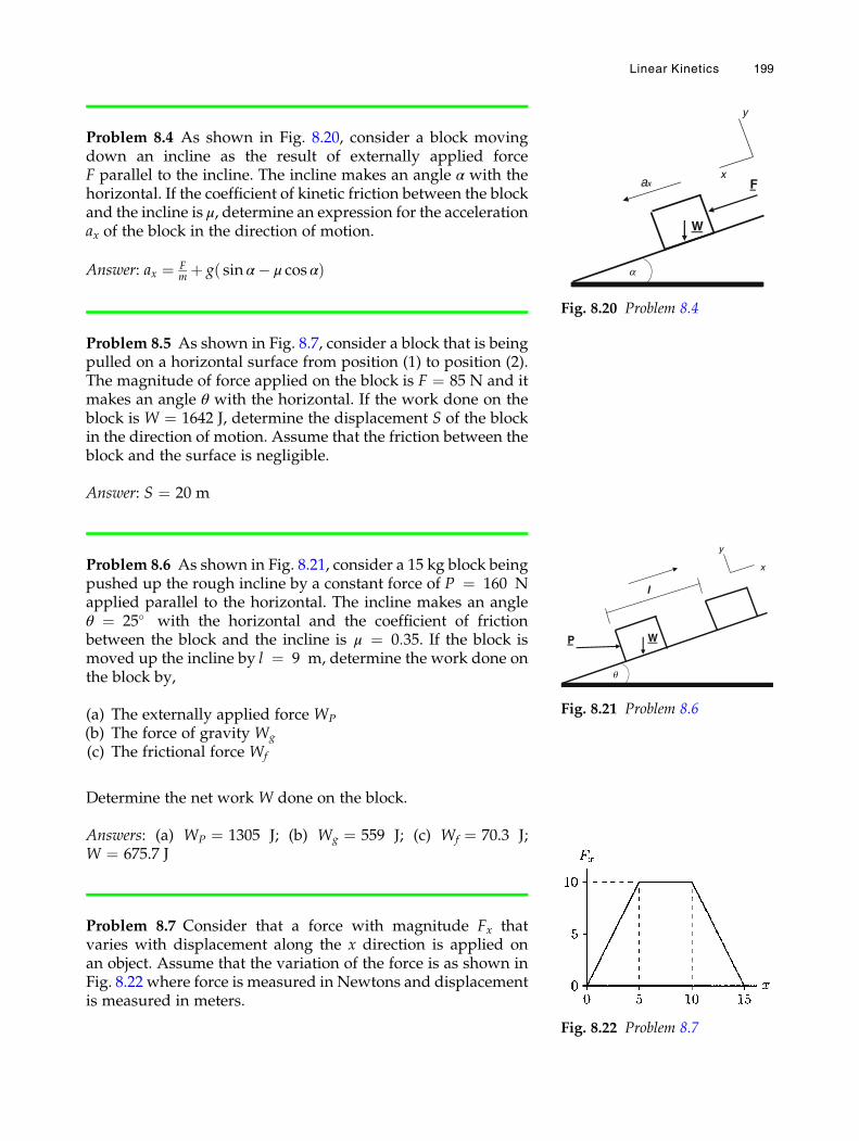
Problem 8.4 As shown in Fig. 8.20, consider a block movingdown an incline as the result of externally applied forceF parallel to the incline. The incline makes an angle α with thehorizontal. If the coefficient of kinetic friction between the blockand the incline is μ, determine an expression for the accelerationax of the block in the direction of motion.
Answer: ax ¼ Fmþ g sin α� μ cos αð Þ
Problem 8.5 As shown in Fig. 8.7, consider a block that is beingpulled on a horizontal surface from position (1) to position (2).The magnitude of force applied on the block is F ¼ 85 N and itmakes an angle θ with the horizontal. If the work done on theblock is W ¼ 1642 J, determine the displacement S of the blockin the direction of motion. Assume that the friction between theblock and the surface is negligible.
Answer: S ¼ 20 m
Problem 8.6 As shown in Fig. 8.21, consider a 15 kg block beingpushed up the rough incline by a constant force of P ¼ 160 Napplied parallel to the horizontal. The incline makes an angleθ ¼ 25� with the horizontal and the coefficient of frictionbetween the block and the incline is μ ¼ 0:35. If the block ismoved up the incline by l ¼ 9 m, determine the work done onthe block by,
(a) The externally applied force WP
(b) The force of gravity Wg
(c) The frictional force Wf
Determine the net work W done on the block.
Answers: (a) WP ¼ 1305 J; (b) Wg ¼ 559 J; (c) Wf ¼ 70.3 J;W ¼ 675.7 J
Problem 8.7 Consider that a force with magnitude Fx thatvaries with displacement along the x direction is applied onan object. Assume that the variation of the force is as shown inFig. 8.22 where force is measured in Newtons and displacementis measured in meters.
ax F
W
x
a
y
Fig. 8.20 Problem 8.4
W
x
q
y
P
l
Fig. 8.21 Problem 8.6
Fig. 8.22 Problem 8.7
Linear Kinetics 199
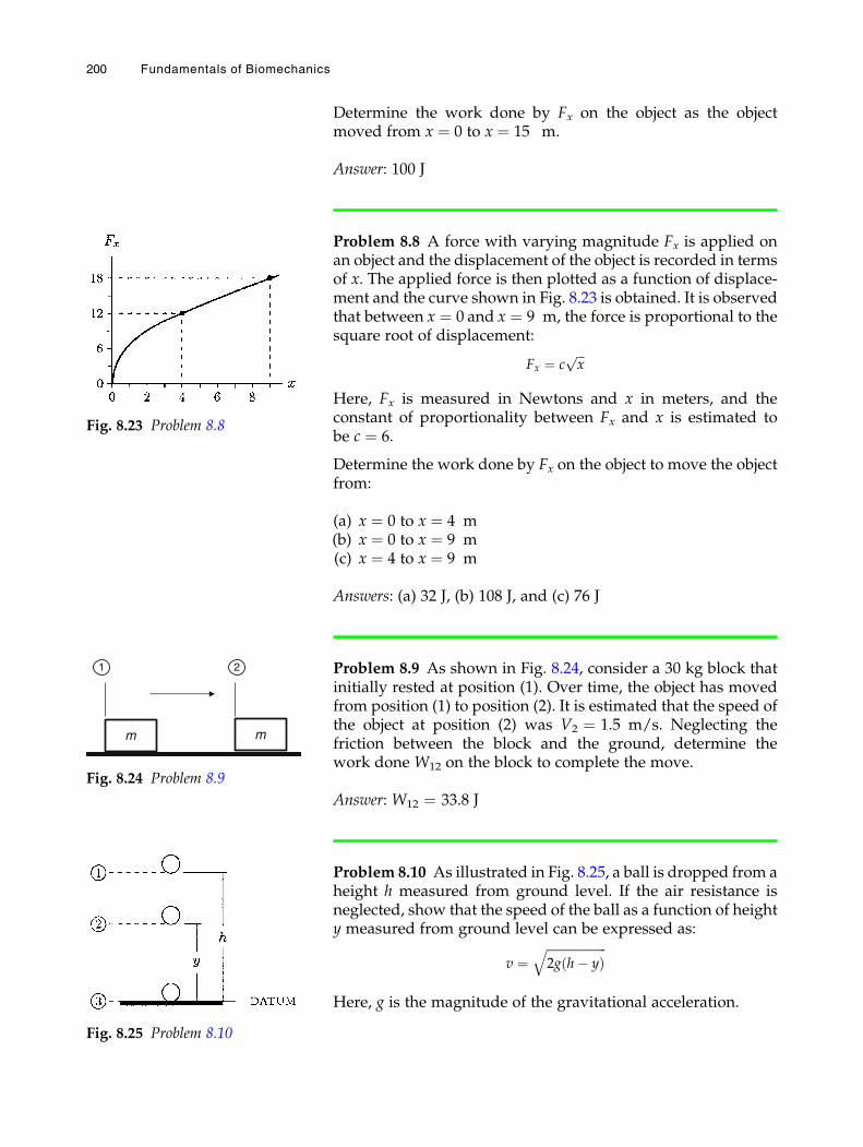
Determine the work done by Fx on the object as the objectmoved from x ¼ 0 to x ¼ 15 m.
Answer: 100 J
Problem 8.8 A force with varying magnitude Fx is applied onan object and the displacement of the object is recorded in termsof x. The applied force is then plotted as a function of displace-ment and the curve shown in Fig. 8.23 is obtained. It is observedthat between x ¼ 0 and x ¼ 9 m, the force is proportional to thesquare root of displacement:
Fx ¼ cffiffiffixp
Here, Fx is measured in Newtons and x in meters, and theconstant of proportionality between Fx and x is estimated tobe c ¼ 6.
Determine the work done by Fx on the object to move the objectfrom:
(a) x ¼ 0 to x ¼ 4 m(b) x ¼ 0 to x ¼ 9 m(c) x ¼ 4 to x ¼ 9 m
Answers: (a) 32 J, (b) 108 J, and (c) 76 J
Problem 8.9 As shown in Fig. 8.24, consider a 30 kg block thatinitially rested at position (1). Over time, the object has movedfrom position (1) to position (2). It is estimated that the speed ofthe object at position (2) was V2 ¼ 1.5 m/s. Neglecting thefriction between the block and the ground, determine thework done W12 on the block to complete the move.
Answer: W12 ¼ 33.8 J
Problem 8.10 As illustrated in Fig. 8.25, a ball is dropped from aheight h measured from ground level. If the air resistance isneglected, show that the speed of the ball as a function of heighty measured from ground level can be expressed as:
v ¼ffiffiffiffiffiffiffiffiffiffiffiffiffiffiffiffiffiffiffiffi2g h� yð Þ
q
Here, g is the magnitude of the gravitational acceleration.
Fig. 8.23 Problem 8.8
m m
1 2
Fig. 8.24 Problem 8.9
Fig. 8.25 Problem 8.10
200 Fundamentals of Biomechanics
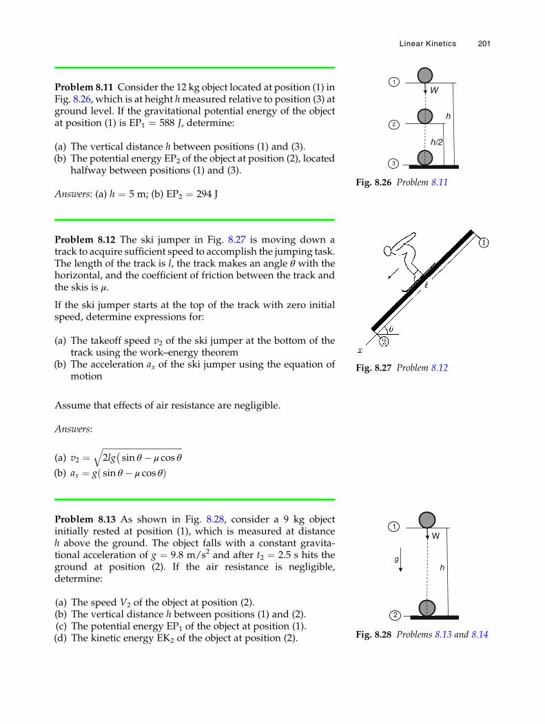
Problem 8.11 Consider the 12 kg object located at position (1) inFig. 8.26, which is at height hmeasured relative to position (3) atground level. If the gravitational potential energy of the objectat position (1) is EP1 ¼ 588 J, determine:
(a) The vertical distance h between positions (1) and (3).(b) The potential energy EP2 of the object at position (2), located
halfway between positions (1) and (3).
Answers: (a) h ¼ 5 m; (b) EP2 ¼ 294 J
Problem 8.12 The ski jumper in Fig. 8.27 is moving down atrack to acquire sufficient speed to accomplish the jumping task.The length of the track is l, the track makes an angle θ with thehorizontal, and the coefficient of friction between the track andthe skis is μ.
If the ski jumper starts at the top of the track with zero initialspeed, determine expressions for:
(a) The takeoff speed v2 of the ski jumper at the bottom of thetrack using the work–energy theorem
(b) The acceleration ax of the ski jumper using the equation ofmotion
Assume that effects of air resistance are negligible.
Answers:
(a) v2 ¼ffiffiffiffiffiffiffiffiffiffiffiffiffiffiffiffiffiffiffiffiffiffiffiffiffiffiffiffiffiffiffiffiffiffiffiffiffiffi2lg
�sin θ � μ cos θ
q(b) ax ¼ g sin θ � μ cos θð Þ
Problem 8.13 As shown in Fig. 8.28, consider a 9 kg objectinitially rested at position (1), which is measured at distanceh above the ground. The object falls with a constant gravita-tional acceleration of g ¼ 9.8 m/s2 and after t2 ¼ 2.5 s hits theground at position (2). If the air resistance is negligible,determine:
(a) The speed V2 of the object at position (2).(b) The vertical distance h between positions (1) and (2).(c) The potential energy EP1 of the object at position (1).(d) The kinetic energy EK2 of the object at position (2).
1
2
3
W
h/2
h
Fig. 8.26 Problem 8.11
Fig. 8.27 Problem 8.12
1
W
h
2
g
Fig. 8.28 Problems 8.13 and 8.14
Linear Kinetics 201
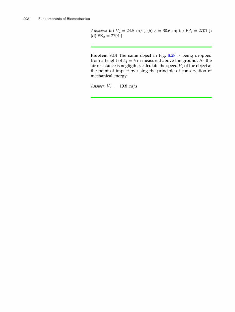
Answers: (a) V2 ¼ 24.5 m/s; (b) h ¼ 30.6 m; (c) EP1 ¼ 2701 J;(d) EK2 ¼ 2701 J
Problem 8.14 The same object in Fig. 8.28 is being droppedfrom a height of h1 ¼ 6 m measured above the ground. As theair resistance is negligible, calculate the speed V2 of the object atthe point of impact by using the principle of conservation ofmechanical energy.
Answer: V2 ¼ 10:8 m=s
202 Fundamentals of Biomechanics
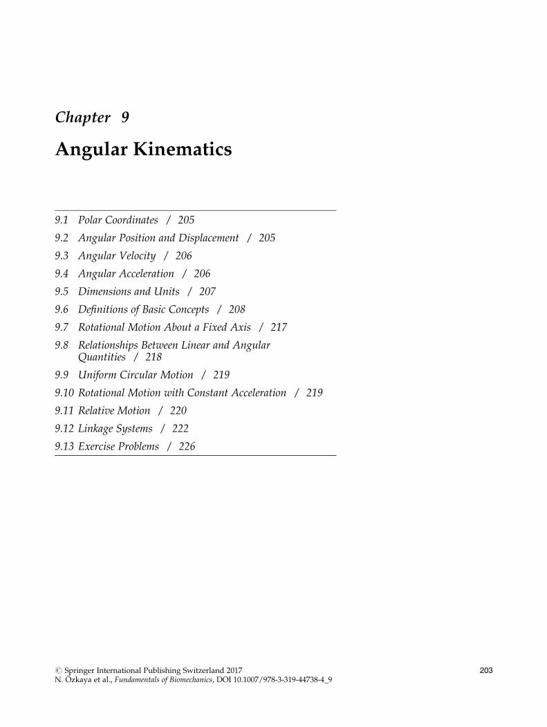
Chapter 9
Angular Kinematics
9.1 Polar Coordinates / 205
9.2 Angular Position and Displacement / 205
9.3 Angular Velocity / 206
9.4 Angular Acceleration / 206
9.5 Dimensions and Units / 207
9.6 Definitions of Basic Concepts / 208
9.7 Rotational Motion About a Fixed Axis / 217
9.8 Relationships Between Linear and AngularQuantities / 218
9.9 Uniform Circular Motion / 219
9.10 Rotational Motion with Constant Acceleration / 219
9.11 Relative Motion / 220
9.12 Linkage Systems / 222
9.13 Exercise Problems / 226
# Springer International Publishing Switzerland 2017N. Ozkaya et al., Fundamentals of Biomechanics, DOI 10.1007/978-3-319-44738-4_9
203

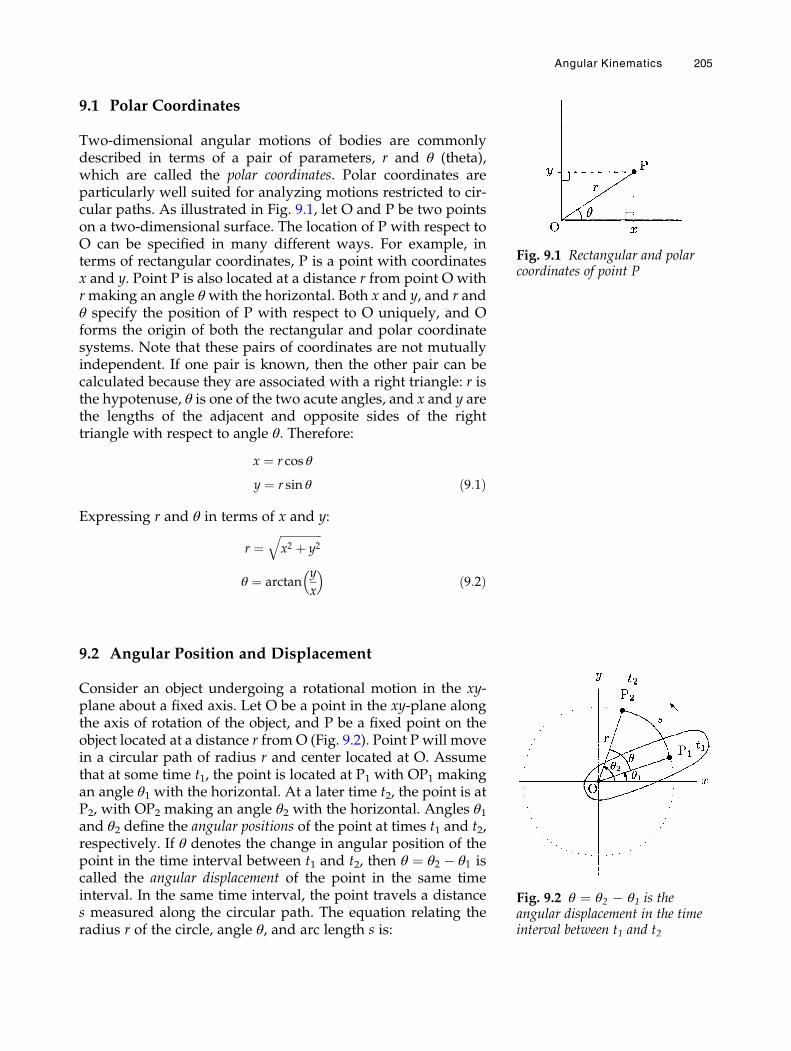
9.1 Polar Coordinates
Two-dimensional angular motions of bodies are commonlydescribed in terms of a pair of parameters, r and θ (theta),which are called the polar coordinates. Polar coordinates areparticularly well suited for analyzing motions restricted to cir-cular paths. As illustrated in Fig. 9.1, let O and P be two pointson a two-dimensional surface. The location of P with respect toO can be specified in many different ways. For example, interms of rectangular coordinates, P is a point with coordinatesx and y. Point P is also located at a distance r from point O withrmaking an angle θ with the horizontal. Both x and y, and r andθ specify the position of P with respect to O uniquely, and Oforms the origin of both the rectangular and polar coordinatesystems. Note that these pairs of coordinates are not mutuallyindependent. If one pair is known, then the other pair can becalculated because they are associated with a right triangle: r isthe hypotenuse, θ is one of the two acute angles, and x and y arethe lengths of the adjacent and opposite sides of the righttriangle with respect to angle θ. Therefore:
x ¼ r cos θ
y ¼ r sin θ ð9:1Þ
Expressing r and θ in terms of x and y:
r ¼ffiffiffiffiffiffiffiffiffiffiffiffiffiffiffix2 þ y2
q
θ ¼ arctany
x
� �ð9:2Þ
9.2 Angular Position and Displacement
Consider an object undergoing a rotational motion in the xy-plane about a fixed axis. Let O be a point in the xy-plane alongthe axis of rotation of the object, and P be a fixed point on theobject located at a distance r from O (Fig. 9.2). Point P will movein a circular path of radius r and center located at O. Assumethat at some time t1, the point is located at P1 with OP1 makingan angle θ1 with the horizontal. At a later time t2, the point is atP2, with OP2 making an angle θ2 with the horizontal. Angles θ1and θ2 define the angular positions of the point at times t1 and t2,respectively. If θ denotes the change in angular position of thepoint in the time interval between t1 and t2, then θ ¼ θ2 � θ1 iscalled the angular displacement of the point in the same timeinterval. In the same time interval, the point travels a distances measured along the circular path. The equation relating theradius r of the circle, angle θ, and arc length s is:
Fig. 9.1 Rectangular and polarcoordinates of point P
Fig. 9.2 θ ¼ θ2 � θ1 is theangular displacement in the timeinterval between t1 and t2
Angular Kinematics 205
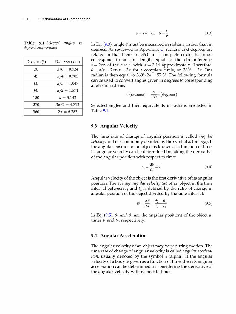
s ¼ r θ or θ ¼ s
rð9:3Þ
In Eq. (9.3), angle θ must be measured in radians, rather than indegrees. As reviewed in Appendix C, radians and degrees arerelated in that there are 360� in a complete circle that mustcorrespond to an arc length equal to the circumference,s ¼ 2πr, of the circle, with π ¼ 3:14 approximately. Therefore,θ ¼ s=r ¼ 2πr=r ¼ 2π for a complete circle, or 360� ¼ 2π. Oneradian is then equal to 360�=2π ¼ 57:3�. The following formulacan be used to convert angles given in degrees to correspondingangles in radians:
θ radiansð Þ ¼ π
180θ degrees� �
Selected angles and their equivalents in radians are listed inTable 9.1.
9.3 Angular Velocity
The time rate of change of angular position is called angularvelocity, and it is commonly denoted by the symbolω (omega). Ifthe angular position of an object is known as a function of time,its angular velocity can be determined by taking the derivativeof the angular position with respect to time:
ω ¼ dθ
dt¼ _θ ð9:4Þ
Angular velocity of the object is the first derivative of its angularposition. The average angular velocity (ω) of an object in the timeinterval between t1 and t2 is defined by the ratio of change inangular position of the object divided by the time interval:
ω ¼ ΔθΔt
¼ θ2 � θ1t2 � t1
ð9:5Þ
In Eq. (9.5), θ1 and θ2 are the angular positions of the object attimes t1 and t2, respectively.
9.4 Angular Acceleration
The angular velocity of an object may vary during motion. Thetime rate of change of angular velocity is called angular accelera-tion, usually denoted by the symbol α (alpha). If the angularvelocity of a body is given as a function of time, then its angularacceleration can be determined by considering the derivative ofthe angular velocity with respect to time:
Table 9.1 Selected angles indegrees and radians
DEGREES (�) RADIANS (RAD)
30 π=6 ¼ 0:524
45 π=4 ¼ 0:785
60 π=3 ¼ 1:047
90 π=2 ¼ 1:571
180 π ¼ 3:142
270 3π=2 ¼ 4:712
360 2π ¼ 6:283
206 Fundamentals of Biomechanics
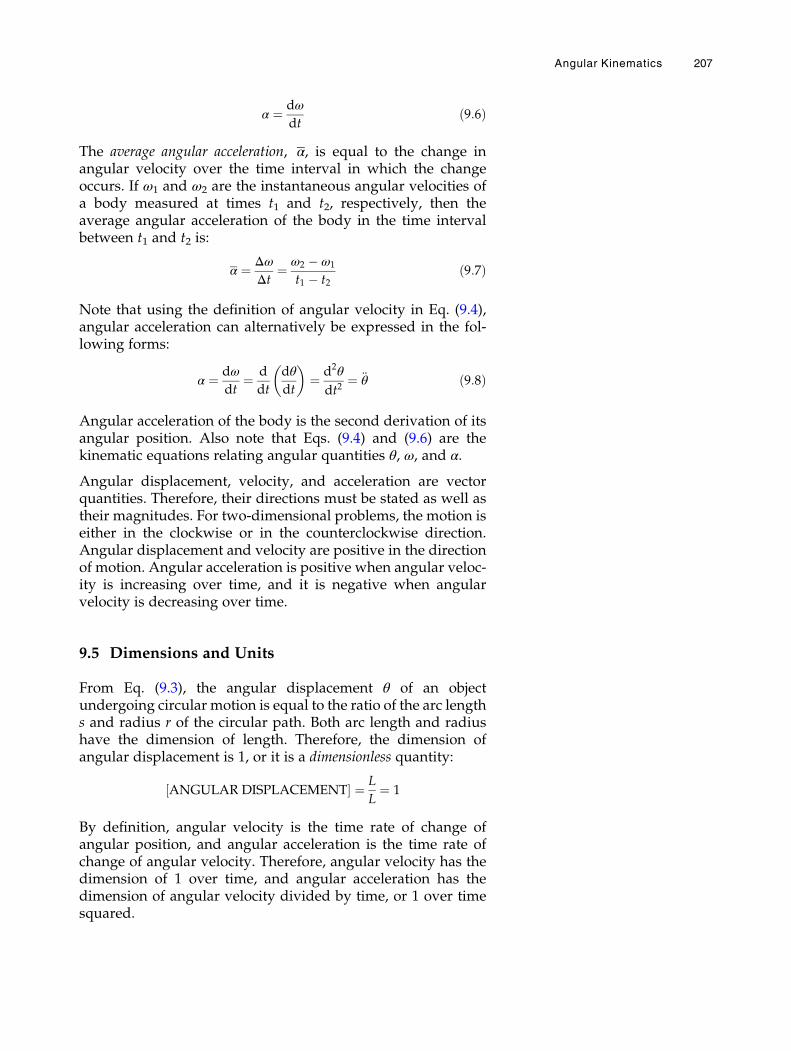
α ¼ dω
dtð9:6Þ
The average angular acceleration, α, is equal to the change inangular velocity over the time interval in which the changeoccurs. If ω1 and ω2 are the instantaneous angular velocities ofa body measured at times t1 and t2, respectively, then theaverage angular acceleration of the body in the time intervalbetween t1 and t2 is:
α ¼ ΔωΔt
¼ ω2 � ω1
t1 � t2ð9:7Þ
Note that using the definition of angular velocity in Eq. (9.4),angular acceleration can alternatively be expressed in the fol-lowing forms:
α ¼ dω
dt¼ d
dt
dθ
dt
� �¼ d2θ
dt2¼ €θ ð9:8Þ
Angular acceleration of the body is the second derivation of itsangular position. Also note that Eqs. (9.4) and (9.6) are thekinematic equations relating angular quantities θ, ω, and α.
Angular displacement, velocity, and acceleration are vectorquantities. Therefore, their directions must be stated as well astheir magnitudes. For two-dimensional problems, the motion iseither in the clockwise or in the counterclockwise direction.Angular displacement and velocity are positive in the directionof motion. Angular acceleration is positive when angular veloc-ity is increasing over time, and it is negative when angularvelocity is decreasing over time.
9.5 Dimensions and Units
From Eq. (9.3), the angular displacement θ of an objectundergoing circular motion is equal to the ratio of the arc lengths and radius r of the circular path. Both arc length and radiushave the dimension of length. Therefore, the dimension ofangular displacement is 1, or it is a dimensionless quantity:
ANGULAR DISPLACEMENT½ � ¼ L
L¼ 1
By definition, angular velocity is the time rate of change ofangular position, and angular acceleration is the time rate ofchange of angular velocity. Therefore, angular velocity has thedimension of 1 over time, and angular acceleration has thedimension of angular velocity divided by time, or 1 over timesquared.
Angular Kinematics 207
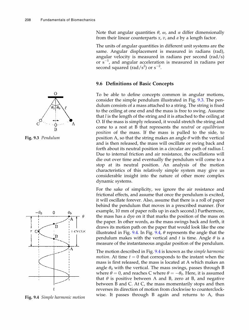
Note that angular quantities θ, ω, and α differ dimensionallyfrom their linear counterparts x, v, and a by a length factor.
The units of angular quantities in different unit systems are thesame. Angular displacement is measured in radians (rad),angular velocity is measured in radians per second (rad/s)or s�1, and angular acceleration is measured in radians persecond squared (rad/s2) or s�2.
9.6 Definitions of Basic Concepts
To be able to define concepts common in angular motions,consider the simple pendulum illustrated in Fig. 9.3. The pen-dulum consists of a mass attached to a string. The string is fixedto the ceiling at one end and the mass is free to swing. Assumethat l is the length of the string and it is attached to the ceiling atO. If the mass is simply released, it would stretch the string andcome to a rest at B that represents the neutral or equilibriumposition of the mass. If the mass is pulled to the side, toposition A, so that the string makes an angle θ with the verticaland is then released, the mass will oscillate or swing back andforth about its neutral position in a circular arc path of radius l.Due to internal friction and air resistance, the oscillations willdie out over time and eventually the pendulum will come to astop at its neutral position. An analysis of the motioncharacteristics of this relatively simple system may give usconsiderable insight into the nature of other more complexdynamic systems.
For the sake of simplicity, we ignore the air resistance andfrictional effects, and assume that once the pendulum is excited,it will oscillate forever. Also, assume that there is a roll of paperbehind the pendulum that moves in a prescribed manner. (Forexample, 10 mm of paper rolls up in each second.) Furthermore,the mass has a dye on it that marks the position of the mass onthe paper. In other words, as the mass swings back and forth, itdraws its motion path on the paper that would look like the oneillustrated in Fig. 9.4. In Fig. 9.4, θ represents the angle that thependulum makes with the vertical and t is time. Angle θ is ameasure of the instantaneous angular position of the pendulum.
The motion described in Fig. 9.4 is known as the simple harmonicmotion. At time t ¼ 0 that corresponds to the instant when themass is first released, the mass is located at A which makes anangle θ0 with the vertical. The mass swings, passes through Bwhere θ ¼ 0, and reaches C where θ ¼ �θ0. Here, it is assumedthat θ is positive between A and B, zero at B, and negativebetween B and C. At C, the mass momentarily stops and thenreverses its direction of motion from clockwise to counterclock-wise. It passes through B again and returns to A, thus
Fig. 9.4 Simple harmonic motion
Fig. 9.3 Pendulum
208 Fundamentals of Biomechanics

completing one full cycle in a time interval of τ (tau) seconds,which is called the period of harmonic motion. The total anglecovered by the pendulum between A and C is called the range ofmotion (ROM) and, in this case, it is equal to 2θ0. Also, the entiremotion of the pendulum is confined betweenþθ and�θ that setthe limits of the range of motion. Half of the range of motion iscalled the amplitude of the oscillations measured in radians andhere is equal to θ0. Note that in this case, both the amplitude andperiod of the harmonic motion are constants. Also note thatsince the effects of friction and air resistance are neglected, theseries of events between A, B, C, B, and A are repeated foreverin τ time intervals.
From Fig. 9.4, it is clear that angular position θ is a function oftime t. Furthermore, θ is a harmonic, cyclic function of t thatmust remind us of trigonometric functions. As discussed inAppendix C, the θ versus t graph in Fig. 9.4 can be comparedto the graphs of known functions to establish the functions thatrelate θ and t. It can be shown that:
θ ¼ θ0 cos φtð Þ
In this equation, the parameter θ0 multiplied with the cosinefunction is the amplitude of the harmonic motion and φ (phi) iscalled the angular frequency measured in radians per second(rad/s). The period and angular frequency are related:
φ ¼ 2π
τπ ¼ 3:1416ð Þ
For oscillatory motions, the reciprocal of the period is called thefrequency, f, measured in Hertz (Hz) that represents the totalnumber of cycles occurring per second:
f ¼ 1
τ¼ φ
2π
Note that for the simple harmonic motion discussed herein theparameters involved (range of motion, amplitude, period, andfrequency) are constants. Also note that the validity of thefunction relating angular position and time can be checked byassigning values to t and calculating corresponding θ values.For example, at A: t ¼ 0, φt ¼ 0, cos 0ð Þ ¼ 1, and θ ¼ θ0. At B:t ¼ τ=4, φt ¼ π=2 ¼ 90�, cos 90ð Þ ¼ 0, and θ ¼ 0. At C: t ¼ τ=2,φt ¼ π ¼ 180�, cos 180ð Þ ¼ �1, and θ ¼ �θ0. All of these areconsistent with the observations in Fig. 9.4.
Now that we have defined most of the important parametersinvolved, we can also determine the angular velocity and angu-lar acceleration of the pendulum. Utilizing Eqs. (9.4) and (9.6):
ω ¼ dθ
dt¼ �θ0φ sin φtð Þ
Angular Kinematics 209
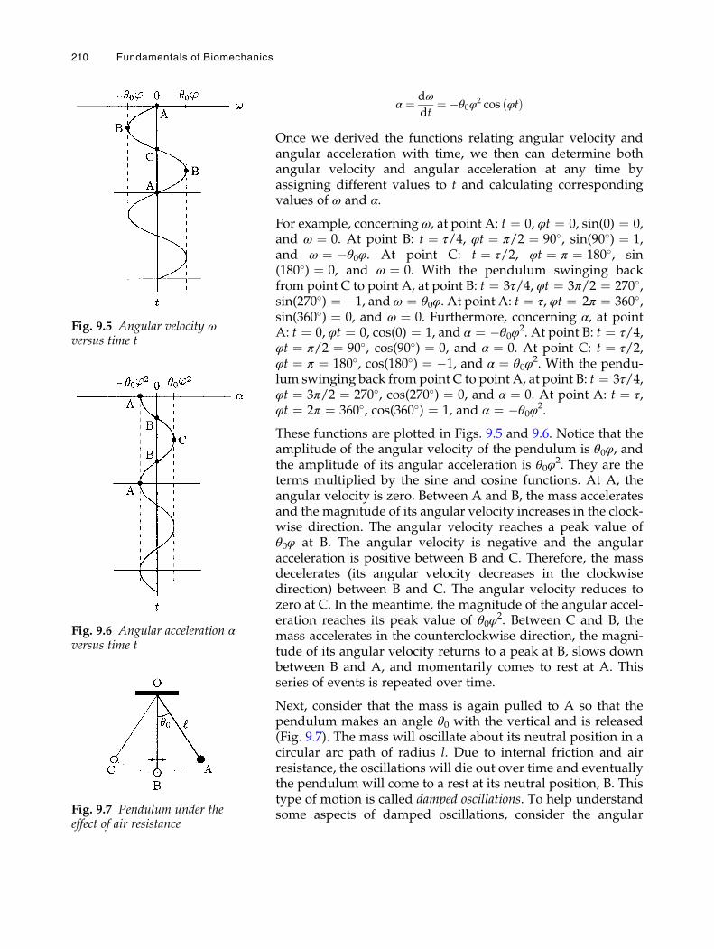
α ¼ dω
dt¼ �θ0φ
2 cos φtð Þ
Once we derived the functions relating angular velocity andangular acceleration with time, we then can determine bothangular velocity and angular acceleration at any time byassigning different values to t and calculating correspondingvalues of ω and α.
For example, concerning ω, at point A: t ¼ 0, φt ¼ 0, sin(0) ¼ 0,and ω ¼ 0. At point B: t ¼ τ/4, φt ¼ π/2 ¼ 90�, sin(90�) ¼ 1,and ω ¼ �θ0φ. At point C: t ¼ τ/2, φt ¼ π ¼ 180�, sin(180�) ¼ 0, and ω ¼ 0. With the pendulum swinging backfrom point C to point A, at point B: t ¼ 3τ/4, φt ¼ 3π/2 ¼ 270�,sin(270�) ¼ �1, and ω ¼ θ0φ. At point A: t ¼ τ, φt ¼ 2π ¼ 360�,sin(360�) ¼ 0, and ω ¼ 0. Furthermore, concerning α, at pointA: t ¼ 0, φt ¼ 0, cos(0) ¼ 1, and α ¼ �θ0φ
2. At point B: t ¼ τ/4,φt ¼ π/2 ¼ 90�, cos(90�) ¼ 0, and α ¼ 0. At point C: t ¼ τ/2,φt ¼ π ¼ 180�, cos(180�) ¼ �1, and α ¼ θ0φ
2. With the pendu-lum swinging back from point C to point A, at point B: t ¼ 3τ/4,φt ¼ 3π/2 ¼ 270�, cos(270�) ¼ 0, and α ¼ 0. At point A: t ¼ τ,φt ¼ 2π ¼ 360�, cos(360�) ¼ 1, and α ¼ �θ0φ
2.
These functions are plotted in Figs. 9.5 and 9.6. Notice that theamplitude of the angular velocity of the pendulum is θ0φ, andthe amplitude of its angular acceleration is θ0φ
2. They are theterms multiplied by the sine and cosine functions. At A, theangular velocity is zero. Between A and B, the mass acceleratesand the magnitude of its angular velocity increases in the clock-wise direction. The angular velocity reaches a peak value ofθ0φ at B. The angular velocity is negative and the angularacceleration is positive between B and C. Therefore, the massdecelerates (its angular velocity decreases in the clockwisedirection) between B and C. The angular velocity reduces tozero at C. In the meantime, the magnitude of the angular accel-eration reaches its peak value of θ0φ
2. Between C and B, themass accelerates in the counterclockwise direction, the magni-tude of its angular velocity returns to a peak at B, slows downbetween B and A, and momentarily comes to rest at A. Thisseries of events is repeated over time.
Next, consider that the mass is again pulled to A so that thependulum makes an angle θ0 with the vertical and is released(Fig. 9.7). The mass will oscillate about its neutral position in acircular arc path of radius l. Due to internal friction and airresistance, the oscillations will die out over time and eventuallythe pendulum will come to a rest at its neutral position, B. Thistype of motion is called damped oscillations. To help understandsome aspects of damped oscillations, consider the angular
Fig. 9.5 Angular velocity ωversus time t
Fig. 9.6 Angular acceleration αversus time t
Fig. 9.7 Pendulum under theeffect of air resistance
210 Fundamentals of Biomechanics
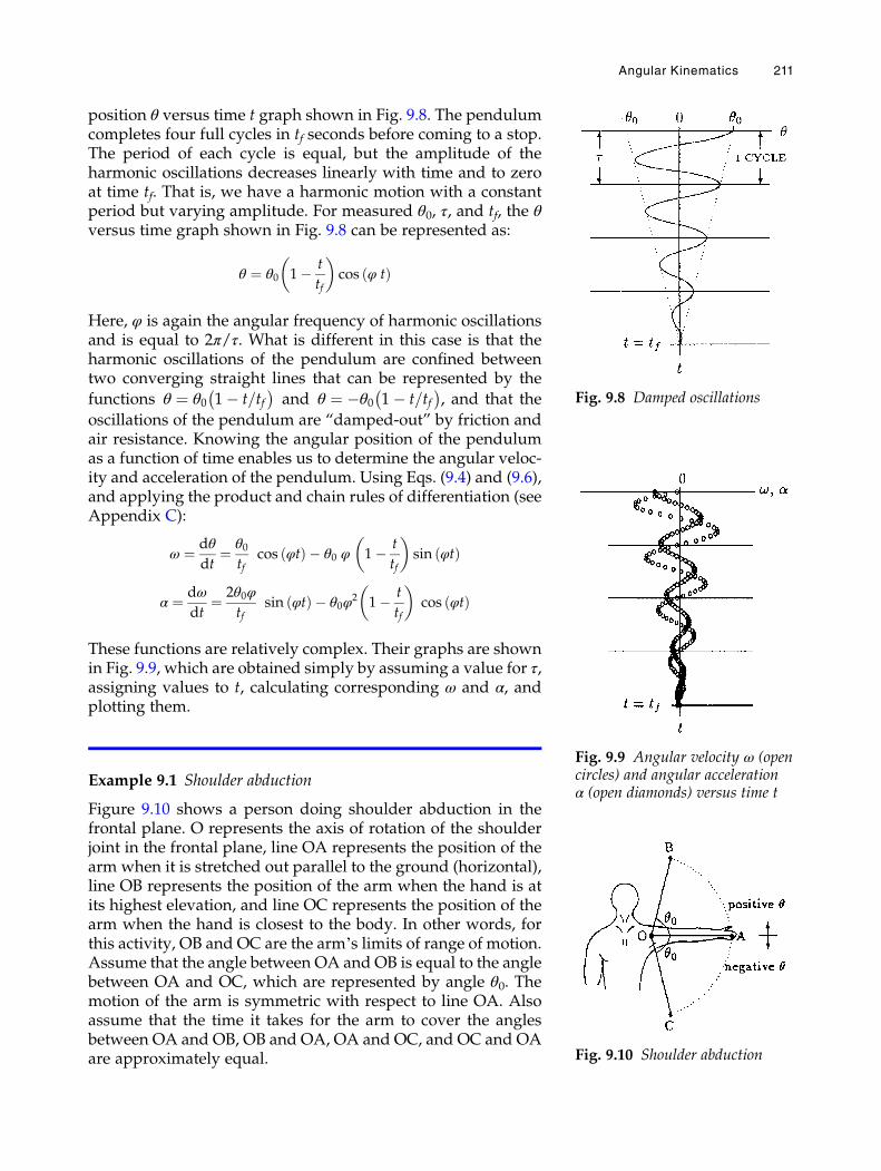
position θ versus time t graph shown in Fig. 9.8. The pendulumcompletes four full cycles in tf seconds before coming to a stop.The period of each cycle is equal, but the amplitude of theharmonic oscillations decreases linearly with time and to zeroat time tf. That is, we have a harmonic motion with a constantperiod but varying amplitude. For measured θ0, τ, and tf, the θversus time graph shown in Fig. 9.8 can be represented as:
θ ¼ θ0 1� t
tf
� �cos φ tð Þ
Here, φ is again the angular frequency of harmonic oscillationsand is equal to 2π/τ. What is different in this case is that theharmonic oscillations of the pendulum are confined betweentwo converging straight lines that can be represented by the
functions θ ¼ θ0 1� t=tf� �
and θ ¼ �θ0 1� t=tf� �
, and that the
oscillations of the pendulum are “damped-out” by friction andair resistance. Knowing the angular position of the pendulumas a function of time enables us to determine the angular veloc-ity and acceleration of the pendulum. Using Eqs. (9.4) and (9.6),and applying the product and chain rules of differentiation (seeAppendix C):
ω ¼ dθ
dt¼ θ0
tfcos φtð Þ � θ0 φ 1� t
tf
� �sin φtð Þ
α ¼ dω
dt¼ 2θ0φ
tfsin φtð Þ � θ0φ
2 1� t
tf
� �cos φtð Þ
These functions are relatively complex. Their graphs are shownin Fig. 9.9, which are obtained simply by assuming a value for τ,assigning values to t, calculating corresponding ω and α, andplotting them.
Example 9.1 Shoulder abduction
Figure 9.10 shows a person doing shoulder abduction in thefrontal plane. O represents the axis of rotation of the shoulderjoint in the frontal plane, line OA represents the position of thearm when it is stretched out parallel to the ground (horizontal),line OB represents the position of the arm when the hand is atits highest elevation, and line OC represents the position of thearm when the hand is closest to the body. In other words, forthis activity, OB and OC are the arm’s limits of range of motion.Assume that the angle between OA and OB is equal to the anglebetween OA and OC, which are represented by angle θ0. Themotion of the arm is symmetric with respect to line OA. Alsoassume that the time it takes for the arm to cover the anglesbetween OA and OB, OB and OA, OA and OC, and OC and OAare approximately equal.
Fig. 9.8 Damped oscillations
Fig. 9.9 Angular velocity ω (opencircles) and angular accelerationα (open diamonds) versus time t
Fig. 9.10 Shoulder abduction
Angular Kinematics 211
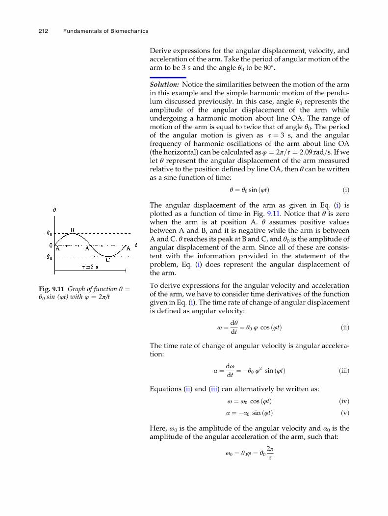
Derive expressions for the angular displacement, velocity, andacceleration of the arm. Take the period of angular motion of thearm to be 3 s and the angle θ0 to be 80�.
Solution: Notice the similarities between the motion of the armin this example and the simple harmonic motion of the pendu-lum discussed previously. In this case, angle θ0 represents theamplitude of the angular displacement of the arm whileundergoing a harmonic motion about line OA. The range ofmotion of the arm is equal to twice that of angle θ0. The periodof the angular motion is given as τ ¼ 3 s, and the angularfrequency of harmonic oscillations of the arm about line OA(the horizontal) can be calculated asφ ¼ 2π=τ ¼ 2:09rad=s. If welet θ represent the angular displacement of the arm measuredrelative to the position defined by line OA, then θ can be writtenas a sine function of time:
θ ¼ θ0 sin φtð Þ ðiÞ
The angular displacement of the arm as given in Eq. (i) isplotted as a function of time in Fig. 9.11. Notice that θ is zerowhen the arm is at position A. θ assumes positive valuesbetween A and B, and it is negative while the arm is betweenA and C. θ reaches its peak at B and C, and θ0 is the amplitude ofangular displacement of the arm. Since all of these are consis-tent with the information provided in the statement of theproblem, Eq. (i) does represent the angular displacement ofthe arm.
To derive expressions for the angular velocity and accelerationof the arm, we have to consider time derivatives of the functiongiven in Eq. (i). The time rate of change of angular displacementis defined as angular velocity:
ω ¼ dθ
dt¼ θ0 φ cos φtð Þ ðiiÞ
The time rate of change of angular velocity is angular accelera-tion:
α ¼ dω
dt¼ �θ0 φ
2 sin φtð Þ ðiiiÞ
Equations (ii) and (iii) can alternatively be written as:
ω ¼ ω0 cos φtð Þ ðivÞα ¼ �α0 sin φtð Þ ðvÞ
Here, ω0 is the amplitude of the angular velocity and α0 is theamplitude of the angular acceleration of the arm, such that:
ω0 ¼ θ0φ ¼ θ02π
τ
Fig. 9.11 Graph of function θ ¼θ0 sin (φt) with φ ¼ 2π/t
212 Fundamentals of Biomechanics
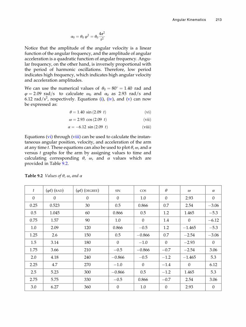
α0 ¼ θ0 φ2 ¼ θ0
4π2
τ2
Notice that the amplitude of the angular velocity is a linearfunction of the angular frequency, and the amplitude of angularacceleration is a quadratic function of angular frequency. Angu-lar frequency, on the other hand, is inversely proportional withthe period of harmonic oscillations. Therefore, low periodindicates high frequency, which indicates high angular velocityand acceleration amplitudes.
We can use the numerical values of θ0 ¼ 80� ¼ 1:40 rad andφ ¼ 2:09 rad=s to calculate ω0 and α0 as 2.93 rad/s and6.12 rad/s2, respectively. Equations (i), (iv), and (v) can nowbe expressed as:
θ ¼ 1:40 sin 2:09 tð Þ ðviÞω ¼ 2:93 cos 2:09 tð Þ ðviiÞα ¼ �6:12 sin 2:09 tð Þ ðviiiÞ
Equations (vi) through (viii) can be used to calculate the instan-taneous angular position, velocity, and acceleration of the armat any time t. These equations can also be used to plot θ, ω, and αversus t graphs for the arm by assigning values to time andcalculating corresponding θ, ω, and α values which areprovided in Table 9.2.
Table 9.2 Values of θ, ω, and α
t (φt) (RAD) (φt) (DEGREE) SIN COS θ ω α
0 0 0 0 1.0 0 2.93 0
0.25 0.523 30 0.5 0.866 0.7 2.54 �3.06
0.5 1.045 60 0.866 0.5 1.2 1.465 �5.3
0.75 1.57 90 1.0 0 1.4 0 �6.12
1.0 2.09 120 0.866 �0.5 1.2 �1.465 �5.3
1.25 2.6 150 0.5 �0.866 0.7 �2.54 �3.06
1.5 3.14 180 0 �1.0 0 �2.93 0
1.75 3.66 210 �0.5 �0.866 �0.7 �2.54 3.06
2.0 4.18 240 �0.866 �0.5 �1.2 �1.465 5.3
2.25 4.7 270 �1.0 0 �1.4 0 6.12
2.5 5.23 300 �0.866 0.5 �1.2 1.465 5.3
2.75 5.75 330 �0.5 0.866 �0.7 2.54 3.06
3.0 6.27 360 0 1.0 0 2.93 0
Angular Kinematics 213
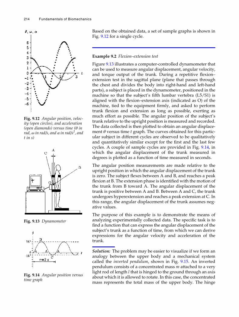
Based on the obtained data, a set of sample graphs is shown inFig. 9.12 for a single cycle.
Example 9.2 Flexion–extension test
Figure 9.13 illustrates a computer-controlled dynamometer thatcan be used to measure angular displacement, angular velocity,and torque output of the trunk. During a repetitive flexion–extension test in the sagittal plane (plane that passes throughthe chest and divides the body into right-hand and left-handparts), a subject is placed in the dynamometer, positioned in themachine so that the subject’s fifth lumbar vertebra (L5/S1) isaligned with the flexion–extension axis (indicated as O) of themachine, tied to the equipment firmly, and asked to performtrunk flexion and extension as long as possible, exerting asmuch effort as possible. The angular position of the subject’strunk relative to the upright position is measured and recorded.The data collected is then plotted to obtain an angular displace-ment θ versus time t graph. The curves obtained for this partic-ular subject in different cycles are observed to be qualitativelyand quantitatively similar except for the first and the last fewcycles. A couple of sample cycles are provided in Fig. 9.14, inwhich the angular displacement of the trunk measured indegrees is plotted as a function of time measured in seconds.
The angular position measurements are made relative to theupright position in which the angular displacement of the trunkis zero. The subject flexes between A and B, and reaches a peakflexion at B. The extension phase is identified with the motion ofthe trunk from B toward A. The angular displacement of thetrunk is positive between A and B. Between A and C, the trunkundergoes hyperextension and reaches a peak extension at C. Inthis range, the angular displacement of the trunk assumes neg-ative values.
The purpose of this example is to demonstrate the means ofanalyzing experimentally collected data. The specific task is tofind a function that can express the angular displacement of thesubject’s trunk as a function of time, from which we can deriveexpressions for the angular velocity and acceleration of thetrunk.
Solution: The problem may be easier to visualize if we form ananalogy between the upper body and a mechanical systemcalled the inverted pendulum, shown in Fig. 9.15. An invertedpendulum consists of a concentrated mass m attached to a verylight rod of length l that is hinged to the ground through an axisabout which it is allowed to rotate. In this case, the concentratedmass represents the total mass of the upper body. The hinge
Fig. 9.12 Angular position, veloc-ity (open circles), and acceleration(open diamonds) versus time (θ inrad, ω in rad/s, and α in rad/s2, andt in s)
Fig. 9.13 Dynamometer
Fig. 9.14 Angular position versustime graph
214 Fundamentals of Biomechanics
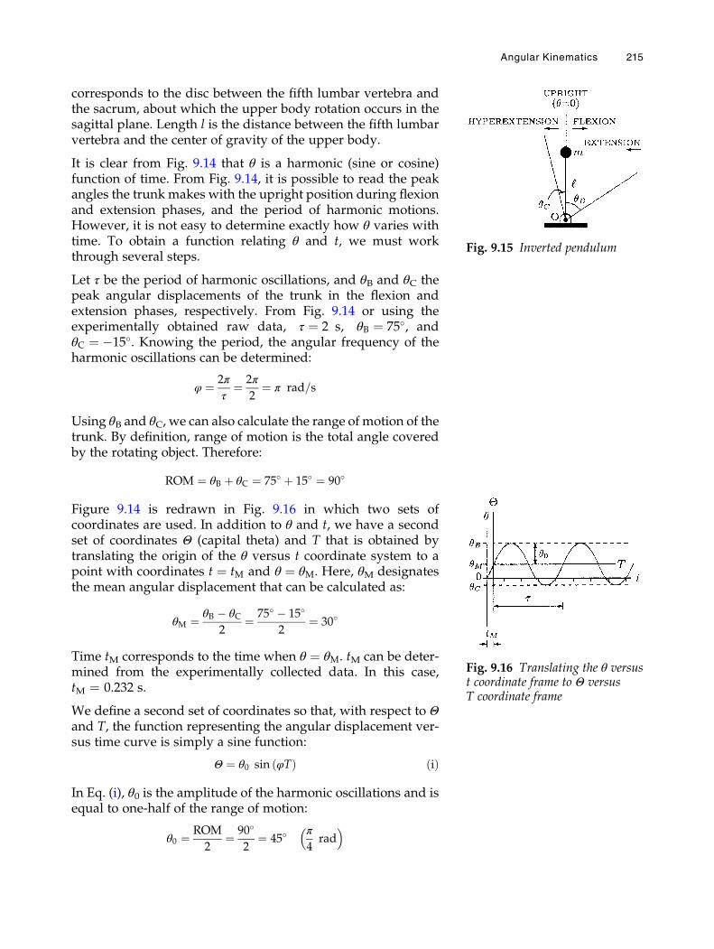
corresponds to the disc between the fifth lumbar vertebra andthe sacrum, about which the upper body rotation occurs in thesagittal plane. Length l is the distance between the fifth lumbarvertebra and the center of gravity of the upper body.
It is clear from Fig. 9.14 that θ is a harmonic (sine or cosine)function of time. From Fig. 9.14, it is possible to read the peakangles the trunk makes with the upright position during flexionand extension phases, and the period of harmonic motions.However, it is not easy to determine exactly how θ varies withtime. To obtain a function relating θ and t, we must workthrough several steps.
Let τ be the period of harmonic oscillations, and θB and θC thepeak angular displacements of the trunk in the flexion andextension phases, respectively. From Fig. 9.14 or using theexperimentally obtained raw data, τ ¼ 2 s, θB ¼ 75�, andθC ¼ �15�. Knowing the period, the angular frequency of theharmonic oscillations can be determined:
φ ¼ 2π
τ¼ 2π
2¼ π rad=s
Using θB and θC, we can also calculate the range of motion of thetrunk. By definition, range of motion is the total angle coveredby the rotating object. Therefore:
ROM ¼ θB þ θC ¼ 75� þ 15� ¼ 90�
Figure 9.14 is redrawn in Fig. 9.16 in which two sets ofcoordinates are used. In addition to θ and t, we have a secondset of coordinates Θ (capital theta) and T that is obtained bytranslating the origin of the θ versus t coordinate system to apoint with coordinates t ¼ tM and θ ¼ θM. Here, θM designatesthe mean angular displacement that can be calculated as:
θM ¼ θB � θC2
¼ 75� � 15�
2¼ 30�
Time tM corresponds to the time when θ ¼ θM. tM can be deter-mined from the experimentally collected data. In this case,tM ¼ 0.232 s.
We define a second set of coordinates so that, with respect to Θand T, the function representing the angular displacement ver-sus time curve is simply a sine function:
Θ ¼ θ0 sin φTð Þ ðiÞ
In Eq. (i), θ0 is the amplitude of the harmonic oscillations and isequal to one-half of the range of motion:
θ0 ¼ ROM
2¼ 90�
2¼ 45�
π
4rad
� �
Fig. 9.15 Inverted pendulum
Fig. 9.16 Translating the θ versust coordinate frame to Θ versusT coordinate frame
Angular Kinematics 215
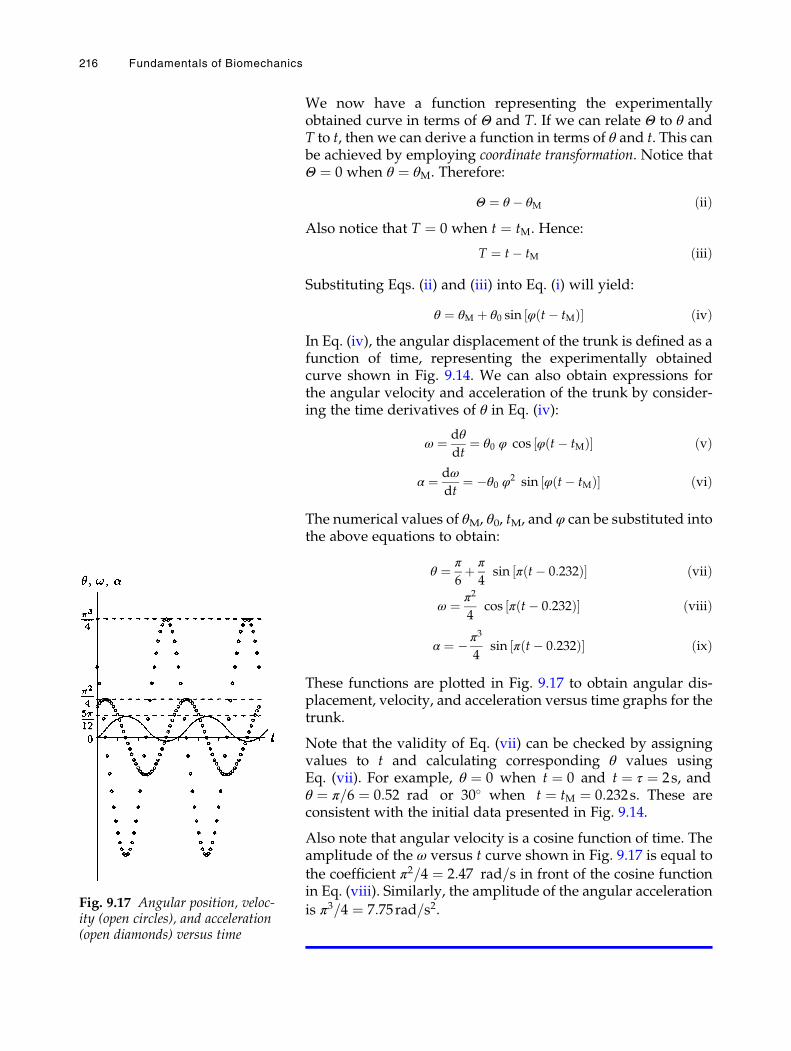
We now have a function representing the experimentallyobtained curve in terms of Θ and T. If we can relate Θ to θ andT to t, then we can derive a function in terms of θ and t. This canbe achieved by employing coordinate transformation. Notice thatΘ ¼ 0 when θ ¼ θM. Therefore:
Θ ¼ θ � θM ðiiÞAlso notice that T ¼ 0 when t ¼ tM. Hence:
T ¼ t� tM ðiiiÞ
Substituting Eqs. (ii) and (iii) into Eq. (i) will yield:
θ ¼ θM þ θ0 sin φ t� tMð Þ½ � ðivÞIn Eq. (iv), the angular displacement of the trunk is defined as afunction of time, representing the experimentally obtainedcurve shown in Fig. 9.14. We can also obtain expressions forthe angular velocity and acceleration of the trunk by consider-ing the time derivatives of θ in Eq. (iv):
ω ¼ dθ
dt¼ θ0 φ cos φ t� tMð Þ½ � ðvÞ
α ¼ dω
dt¼ �θ0 φ
2 sin φ t� tMð Þ½ � ðviÞ
The numerical values of θM, θ0, tM, and φ can be substituted intothe above equations to obtain:
θ ¼ π
6þ π
4sin π t� 0:232ð Þ½ � ðviiÞ
ω ¼ π2
4cos π t� 0:232ð Þ½ � ðviiiÞ
α ¼ � π3
4sin π t� 0:232ð Þ½ � ðixÞ
These functions are plotted in Fig. 9.17 to obtain angular dis-placement, velocity, and acceleration versus time graphs for thetrunk.
Note that the validity of Eq. (vii) can be checked by assigningvalues to t and calculating corresponding θ values usingEq. (vii). For example, θ ¼ 0 when t ¼ 0 and t ¼ τ ¼ 2s, andθ ¼ π=6 ¼ 0:52 rad or 30� when t ¼ tM ¼ 0:232s. These areconsistent with the initial data presented in Fig. 9.14.
Also note that angular velocity is a cosine function of time. Theamplitude of the ω versus t curve shown in Fig. 9.17 is equal to
the coefficient π2=4 ¼ 2:47 rad=s in front of the cosine functionin Eq. (viii). Similarly, the amplitude of the angular acceleration
is π3=4 ¼ 7:75rad=s2.Fig. 9.17 Angular position, veloc-ity (open circles), and acceleration(open diamonds) versus time
216 Fundamentals of Biomechanics
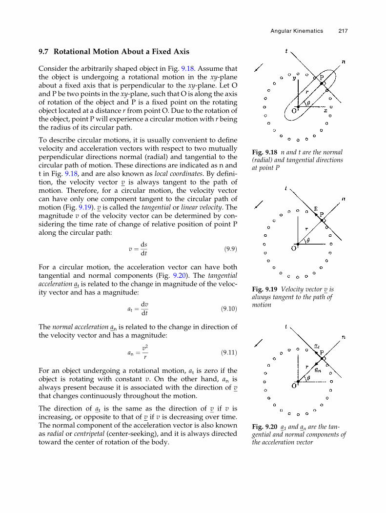
9.7 Rotational Motion About a Fixed Axis
Consider the arbitrarily shaped object in Fig. 9.18. Assume thatthe object is undergoing a rotational motion in the xy-planeabout a fixed axis that is perpendicular to the xy-plane. Let Oand P be two points in the xy-plane, such that O is along the axisof rotation of the object and P is a fixed point on the rotatingobject located at a distance r from point O. Due to the rotation ofthe object, point P will experience a circular motion with r beingthe radius of its circular path.
To describe circular motions, it is usually convenient to definevelocity and acceleration vectors with respect to two mutuallyperpendicular directions normal (radial) and tangential to thecircular path of motion. These directions are indicated as n andt in Fig. 9.18, and are also known as local coordinates. By defini-tion, the velocity vector v is always tangent to the path ofmotion. Therefore, for a circular motion, the velocity vectorcan have only one component tangent to the circular path ofmotion (Fig. 9.19). v is called the tangential or linear velocity. Themagnitude v of the velocity vector can be determined by con-sidering the time rate of change of relative position of point Palong the circular path:
v ¼ ds
dtð9:9Þ
For a circular motion, the acceleration vector can have bothtangential and normal components (Fig. 9.20). The tangentialacceleration at is related to the change in magnitude of the veloc-ity vector and has a magnitude:
at ¼ dv
dtð9:10Þ
The normal acceleration an is related to the change in direction ofthe velocity vector and has a magnitude:
an ¼ v2
rð9:11Þ
For an object undergoing a rotational motion, at is zero if theobject is rotating with constant v. On the other hand, an isalways present because it is associated with the direction of vthat changes continuously throughout the motion.
The direction of at is the same as the direction of v if v isincreasing, or opposite to that of v if v is decreasing over time.The normal component of the acceleration vector is also knownas radial or centripetal (center-seeking), and it is always directedtoward the center of rotation of the body.
Fig. 9.18 n and t are the normal(radial) and tangential directionsat point P
Fig. 9.19 Velocity vector v isalways tangent to the path ofmotion
Fig. 9.20 a1 and an are the tan-gential and normal components ofthe acceleration vector
Angular Kinematics 217
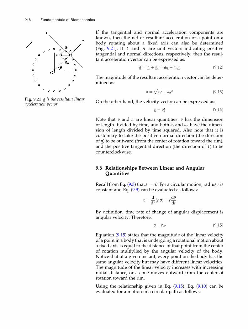
If the tangential and normal acceleration components areknown, then the net or resultant acceleration of a point on abody rotating about a fixed axis can also be determined(Fig. 9.21). If t and n are unit vectors indicating positivetangential and normal directions, respectively, then the resul-tant acceleration vector can be expressed as:
a ¼ at þ an ¼ attþ ann ð9:12Þ
The magnitude of the resultant acceleration vector can be deter-mined as:
a ¼ffiffiffiffiffiffiffiffiffiffiffiffiffiffiffiffiffiffiat2 þ an2
pð9:13Þ
On the other hand, the velocity vector can be expressed as:
v ¼ vt ð9:14Þ
Note that v and a are linear quantities. v has the dimensionof length divided by time, and both at and an have the dimen-sion of length divided by time squared. Also note that it iscustomary to take the positive normal direction (the directionof n) to be outward (from the center of rotation toward the rim),and the positive tangential direction (the direction of t) to becounterclockwise.
9.8 Relationships Between Linear and AngularQuantities
Recall from Eq. (9.3) that s ¼ rθ. For a circular motion, radius r isconstant and Eq. (9.9) can be evaluated as follows:
v ¼ d
dtr θð Þ ¼ r
dθ
dt
By definition, time rate of change of angular displacement isangular velocity. Therefore:
v ¼ rω ð9:15Þ
Equation (9.15) states that the magnitude of the linear velocityof a point in a body that is undergoing a rotational motion abouta fixed axis is equal to the distance of that point from the centerof rotation multiplied by the angular velocity of the body.Notice that at a given instant, every point on the body has thesame angular velocity but may have different linear velocities.The magnitude of the linear velocity increases with increasingradial distance, or as one moves outward from the center ofrotation toward the rim.
Using the relationship given in Eq. (9.15), Eq. (9.10) can beevaluated for a motion in a circular path as follows:
Fig. 9.21 a is the resultant linearacceleration vector
218 Fundamentals of Biomechanics
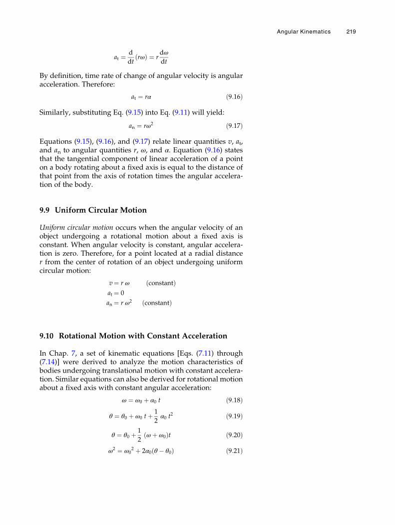
at ¼ d
dtrωð Þ ¼ r
dω
dt
By definition, time rate of change of angular velocity is angularacceleration. Therefore:
at ¼ rα ð9:16Þ
Similarly, substituting Eq. (9.15) into Eq. (9.11) will yield:
an ¼ rω2 ð9:17Þ
Equations (9.15), (9.16), and (9.17) relate linear quantities v, at,and an to angular quantities r, ω, and α. Equation (9.16) statesthat the tangential component of linear acceleration of a pointon a body rotating about a fixed axis is equal to the distance ofthat point from the axis of rotation times the angular accelera-tion of the body.
9.9 Uniform Circular Motion
Uniform circular motion occurs when the angular velocity of anobject undergoing a rotational motion about a fixed axis isconstant. When angular velocity is constant, angular accelera-tion is zero. Therefore, for a point located at a radial distancer from the center of rotation of an object undergoing uniformcircular motion:
v¼ r ω constantð Þat ¼ 0
an ¼ r ω2 constantð Þ
9.10 Rotational Motion with Constant Acceleration
In Chap. 7, a set of kinematic equations [Eqs. (7.11) through(7.14)] were derived to analyze the motion characteristics ofbodies undergoing translational motion with constant accelera-tion. Similar equations can also be derived for rotational motionabout a fixed axis with constant angular acceleration:
ω ¼ ω0 þ α0 t ð9:18Þ
θ ¼ θ0 þ ω0 tþ 1
2α0 t
2 ð9:19Þ
θ ¼ θ0 þ 1
2ωþ ω0ð Þt ð9:20Þ
ω2 ¼ ω02 þ 2α0 θ � θ0ð Þ ð9:21Þ
Angular Kinematics 219
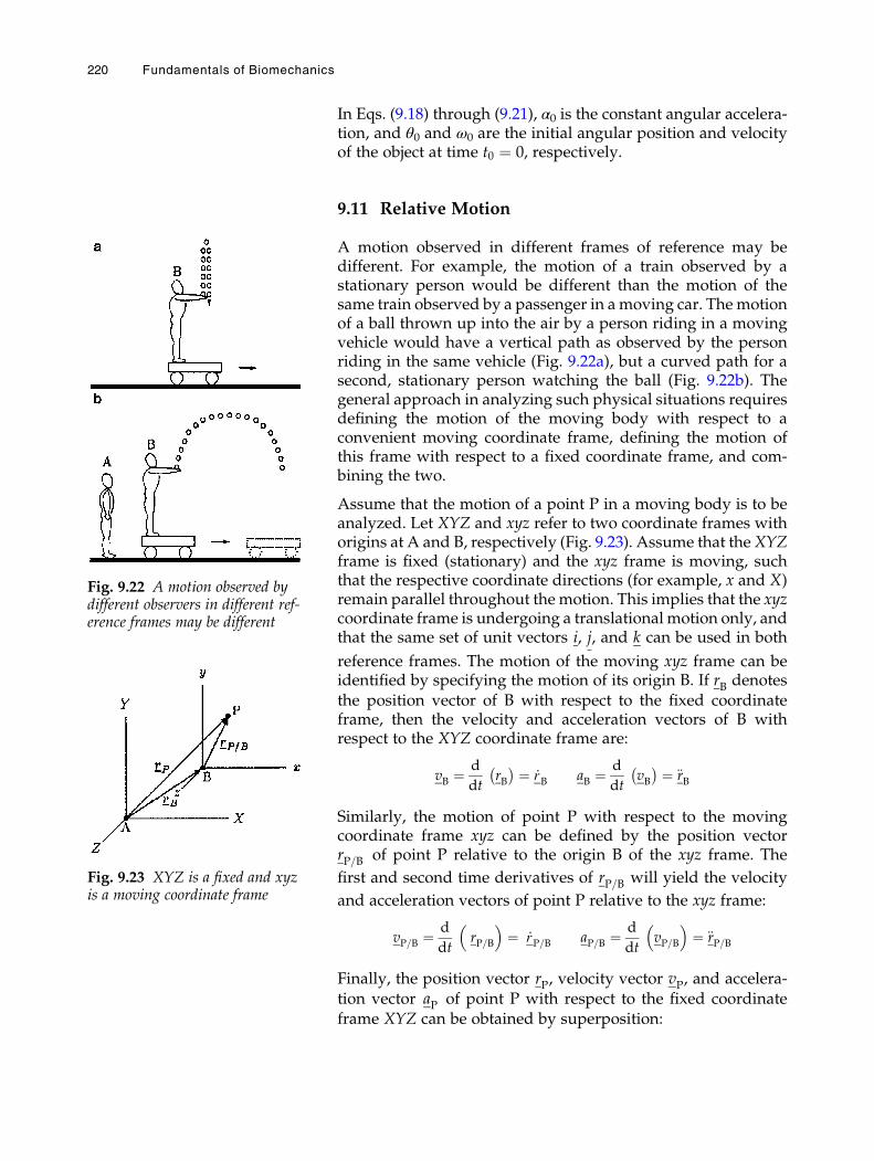
In Eqs. (9.18) through (9.21), α0 is the constant angular accelera-tion, and θ0 and ω0 are the initial angular position and velocityof the object at time t0 ¼ 0, respectively.
9.11 Relative Motion
A motion observed in different frames of reference may bedifferent. For example, the motion of a train observed by astationary person would be different than the motion of thesame train observed by a passenger in amoving car. Themotionof a ball thrown up into the air by a person riding in a movingvehicle would have a vertical path as observed by the personriding in the same vehicle (Fig. 9.22a), but a curved path for asecond, stationary person watching the ball (Fig. 9.22b). Thegeneral approach in analyzing such physical situations requiresdefining the motion of the moving body with respect to aconvenient moving coordinate frame, defining the motion ofthis frame with respect to a fixed coordinate frame, and com-bining the two.
Assume that the motion of a point P in a moving body is to beanalyzed. Let XYZ and xyz refer to two coordinate frames withorigins at A and B, respectively (Fig. 9.23). Assume that theXYZframe is fixed (stationary) and the xyz frame is moving, suchthat the respective coordinate directions (for example, x and X)remain parallel throughout the motion. This implies that the xyzcoordinate frame is undergoing a translational motion only, andthat the same set of unit vectors i, j, and k can be used in both
reference frames. The motion of the moving xyz frame can beidentified by specifying the motion of its origin B. If rB denotesthe position vector of B with respect to the fixed coordinateframe, then the velocity and acceleration vectors of B withrespect to the XYZ coordinate frame are:
vB ¼ d
dtrB� � ¼ _rB aB ¼ d
dtvB� � ¼ €rB
Similarly, the motion of point P with respect to the movingcoordinate frame xyz can be defined by the position vectorrP=B of point P relative to the origin B of the xyz frame. The
first and second time derivatives of rP=B will yield the velocity
and acceleration vectors of point P relative to the xyz frame:
vP=B ¼ d
dtrP=B
� �¼ _rP=B aP=B ¼ d
dtvP=B
� �¼ €rP=B
Finally, the position vector rP, velocity vector vP, and accelera-tion vector aP of point P with respect to the fixed coordinateframe XYZ can be obtained by superposition:
Fig. 9.22 A motion observed bydifferent observers in different ref-erence frames may be different
Fig. 9.23 XYZ is a fixed and xyzis a moving coordinate frame
220 Fundamentals of Biomechanics
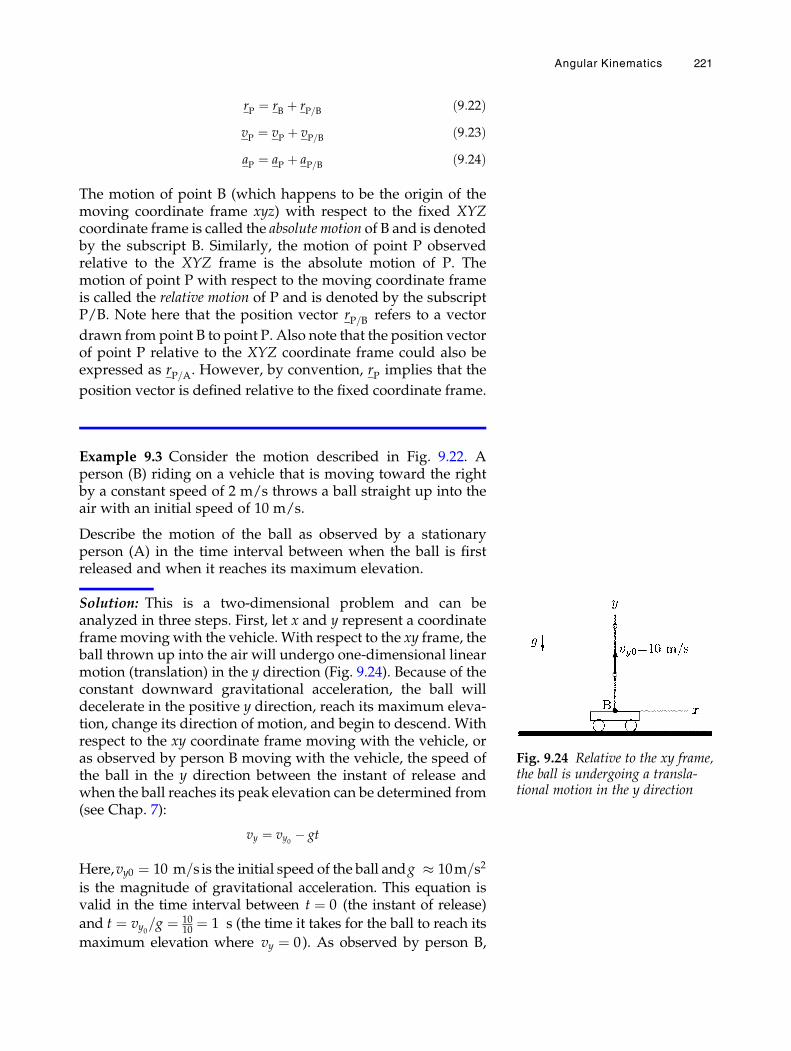
rP ¼ rB þ rP=B ð9:22ÞvP ¼ vP þ vP=B ð9:23ÞaP ¼ aP þ aP=B ð9:24Þ
The motion of point B (which happens to be the origin of themoving coordinate frame xyz) with respect to the fixed XYZcoordinate frame is called the absolute motion of B and is denotedby the subscript B. Similarly, the motion of point P observedrelative to the XYZ frame is the absolute motion of P. Themotion of point P with respect to the moving coordinate frameis called the relative motion of P and is denoted by the subscriptP/B. Note here that the position vector rP=B refers to a vector
drawn from point B to point P. Also note that the position vectorof point P relative to the XYZ coordinate frame could also beexpressed as rP=A. However, by convention, rP implies that the
position vector is defined relative to the fixed coordinate frame.
Example 9.3 Consider the motion described in Fig. 9.22. Aperson (B) riding on a vehicle that is moving toward the rightby a constant speed of 2 m/s throws a ball straight up into theair with an initial speed of 10 m/s.
Describe the motion of the ball as observed by a stationaryperson (A) in the time interval between when the ball is firstreleased and when it reaches its maximum elevation.
Solution: This is a two-dimensional problem and can beanalyzed in three steps. First, let x and y represent a coordinateframemoving with the vehicle. With respect to the xy frame, theball thrown up into the air will undergo one-dimensional linearmotion (translation) in the y direction (Fig. 9.24). Because of theconstant downward gravitational acceleration, the ball willdecelerate in the positive y direction, reach its maximum eleva-tion, change its direction of motion, and begin to descend. Withrespect to the xy coordinate frame moving with the vehicle, oras observed by person B moving with the vehicle, the speed ofthe ball in the y direction between the instant of release andwhen the ball reaches its peak elevation can be determined from(see Chap. 7):
vy ¼ vy0 � gt
Here,vy0 ¼ 10 m=s is the initial speed of the ball andg � 10m=s2
is the magnitude of gravitational acceleration. This equation isvalid in the time interval between t ¼ 0 (the instant of release)
and t ¼ vy0=g ¼ 1010 ¼ 1 s (the time it takes for the ball to reach its
maximum elevation where vy ¼ 0). As observed by person B,
Fig. 9.24 Relative to the xy frame,the ball is undergoing a transla-tional motion in the y direction
Angular Kinematics 221
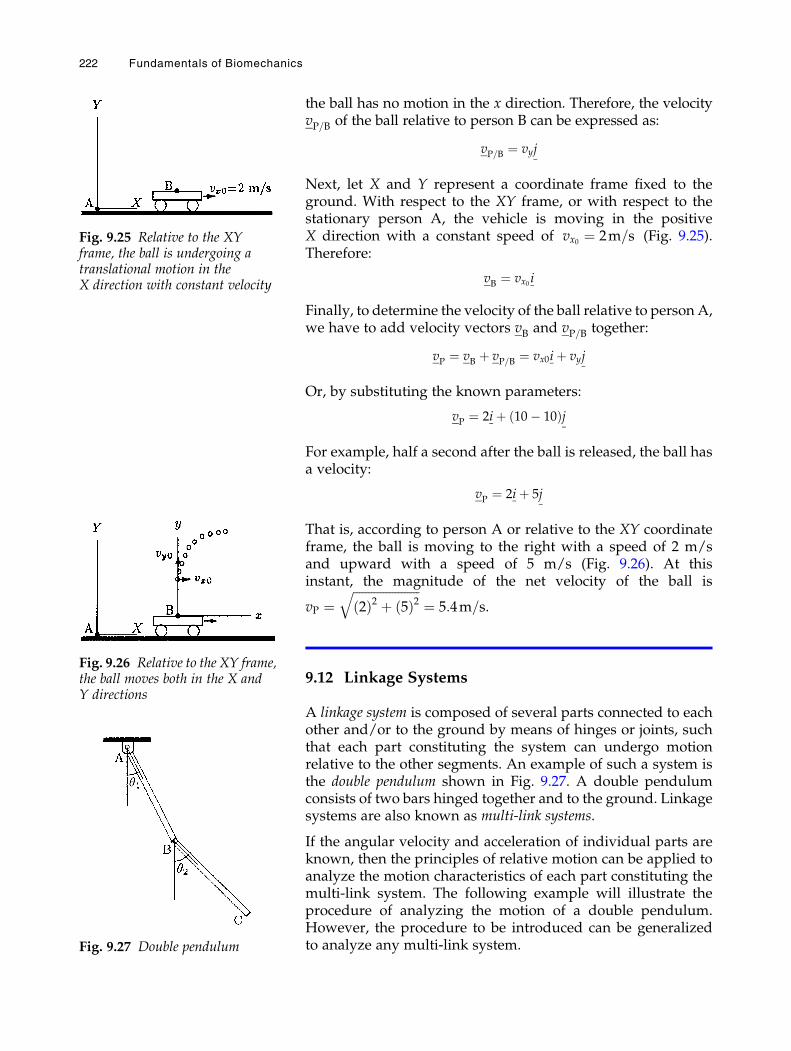
the ball has no motion in the x direction. Therefore, the velocityvP=B of the ball relative to person B can be expressed as:
vP=B ¼ vyj
Next, let X and Y represent a coordinate frame fixed to theground. With respect to the XY frame, or with respect to thestationary person A, the vehicle is moving in the positiveX direction with a constant speed of vx0 ¼ 2m=s (Fig. 9.25).Therefore:
vB ¼ vx0 i
Finally, to determine the velocity of the ball relative to person A,we have to add velocity vectors vB and vP=B together:
vP ¼ vB þ vP=B ¼ vx0iþ vyj
Or, by substituting the known parameters:
vP ¼ 2iþ 10� 10ð Þj
For example, half a second after the ball is released, the ball hasa velocity:
vP ¼ 2iþ 5j
That is, according to person A or relative to the XY coordinateframe, the ball is moving to the right with a speed of 2 m/sand upward with a speed of 5 m/s (Fig. 9.26). At thisinstant, the magnitude of the net velocity of the ball is
vP ¼ffiffiffiffiffiffiffiffiffiffiffiffiffiffiffiffiffiffiffiffiffiffi2ð Þ2 þ 5ð Þ2
q¼ 5:4m=s.
9.12 Linkage Systems
A linkage system is composed of several parts connected to eachother and/or to the ground by means of hinges or joints, suchthat each part constituting the system can undergo motionrelative to the other segments. An example of such a system isthe double pendulum shown in Fig. 9.27. A double pendulumconsists of two bars hinged together and to the ground. Linkagesystems are also known as multi-link systems.
If the angular velocity and acceleration of individual parts areknown, then the principles of relative motion can be applied toanalyze the motion characteristics of each part constituting themulti-link system. The following example will illustrate theprocedure of analyzing the motion of a double pendulum.However, the procedure to be introduced can be generalizedto analyze any multi-link system.
Fig. 9.25 Relative to the XYframe, the ball is undergoing atranslational motion in theX direction with constant velocity
Fig. 9.26 Relative to the XY frame,the ball moves both in the X andY directions
Fig. 9.27 Double pendulum
222 Fundamentals of Biomechanics
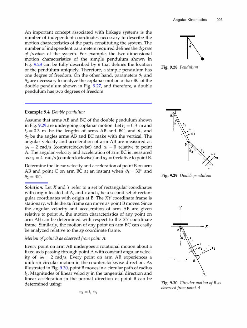
An important concept associated with linkage systems is thenumber of independent coordinates necessary to describe themotion characteristics of the parts constituting the system. Thenumber of independent parameters required defines the degreesof freedom of the system. For example, the two-dimensionalmotion characteristics of the simple pendulum shown inFig. 9.28 can be fully described by θ that defines the locationof the pendulum uniquely. Therefore, a simple pendulum hasone degree of freedom. On the other hand, parameters θ1 andθ2 are necessary to analyze the coplanar motion of bar BC of thedouble pendulum shown in Fig. 9.27, and therefore, a doublependulum has two degrees of freedom.
Example 9.4 Double pendulum
Assume that arms AB and BC of the double pendulum shownin Fig. 9.29 are undergoing coplanar motion. Let l1 ¼ 0:3 m andl2 ¼ 0:3 m be the lengths of arms AB and BC, and θ1 andθ2 be the angles arms AB and BC make with the vertical. Theangular velocity and acceleration of arm AB are measured asω1 ¼ 2 rad=s (counterclockwise) and α1 ¼ 0 relative to pointA. The angular velocity and acceleration of arm BC is measuredasω2 ¼ 4 rad=s (counterclockwise) andα2 ¼ 0 relative to point B.
Determine the linear velocity and acceleration of point B on armAB and point C on arm BC at an instant when θ1 ¼ 30� andθ2 ¼ 45�.
Solution: Let X and Y refer to a set of rectangular coordinateswith origin located at A, and x and y be a second set of rectan-gular coordinates with origin at B. The XY coordinate frame isstationary, while the xy frame can move as point B moves. Sincethe angular velocity and acceleration of arm AB are givenrelative to point A, the motion characteristics of any point onarm AB can be determined with respect to the XY coordinateframe. Similarly, the motion of any point on arm BC can easilybe analyzed relative to the xy coordinate frame.
Motion of point B as observed from point A:
Every point on arm AB undergoes a rotational motion about afixed axis passing through point A with constant angular veloc-ity of ω1 ¼ 2 rad=s. Every point on arm AB experiences auniform circular motion in the counterclockwise direction. Asillustrated in Fig. 9.30, point B moves in a circular path of radiusl1. Magnitudes of linear velocity in the tangential direction andlinear acceleration in the normal direction of point B can bedetermined using:
vB ¼ l1 ω1
Fig. 9.28 Pendulum
Fig. 9.29 Double pendulum
Fig. 9.30 Circular motion of B asobserved from point A
Angular Kinematics 223
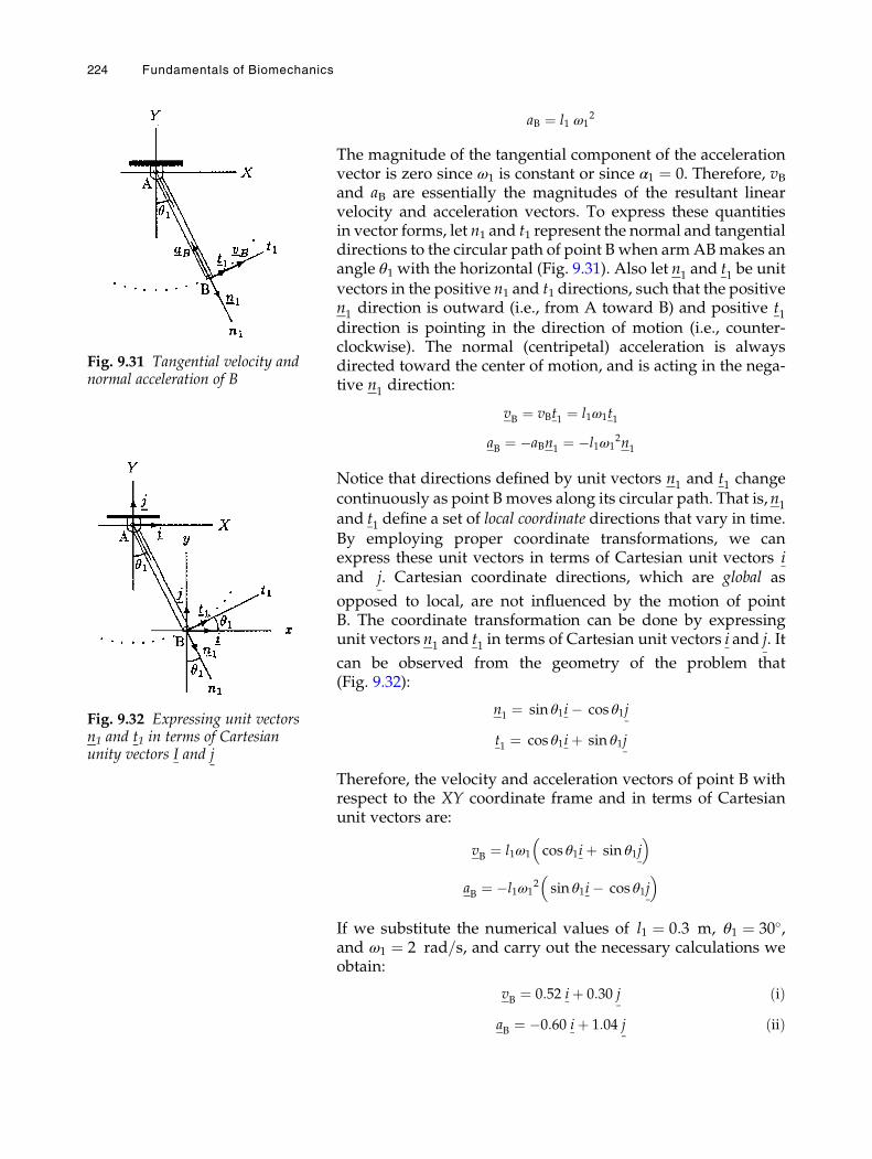
aB ¼ l1 ω12
The magnitude of the tangential component of the accelerationvector is zero since ω1 is constant or since α1 ¼ 0. Therefore, vBand aB are essentially the magnitudes of the resultant linearvelocity and acceleration vectors. To express these quantitiesin vector forms, let n1 and t1 represent the normal and tangentialdirections to the circular path of point B when armABmakes anangle θ1 with the horizontal (Fig. 9.31). Also let n1 and t1 be unitvectors in the positive n1 and t1 directions, such that the positiven1 direction is outward (i.e., from A toward B) and positive t1direction is pointing in the direction of motion (i.e., counter-clockwise). The normal (centripetal) acceleration is alwaysdirected toward the center of motion, and is acting in the nega-tive n1 direction:
vB ¼ vBt1 ¼ l1ω1t1
aB ¼ �aBn1 ¼ �l1ω12n1
Notice that directions defined by unit vectors n1 and t1 changecontinuously as point B moves along its circular path. That is,n1and t1 define a set of local coordinate directions that vary in time.By employing proper coordinate transformations, we canexpress these unit vectors in terms of Cartesian unit vectors iand j. Cartesian coordinate directions, which are global as
opposed to local, are not influenced by the motion of pointB. The coordinate transformation can be done by expressingunit vectors n1 and t1 in terms of Cartesian unit vectors i and j. It
can be observed from the geometry of the problem that(Fig. 9.32):
n1 ¼ sin θ1i� cos θ1j
t1 ¼ cos θ1iþ sin θ1j
Therefore, the velocity and acceleration vectors of point B withrespect to the XY coordinate frame and in terms of Cartesianunit vectors are:
vB ¼ l1ω1 cos θ1iþ sin θ1j� �
aB ¼ �l1ω12 sin θ1i� cos θ1j� �
If we substitute the numerical values of l1 ¼ 0:3 m, θ1 ¼ 30�,and ω1 ¼ 2 rad=s, and carry out the necessary calculations weobtain:
vB ¼ 0:52 iþ 0:30 j ðiÞaB ¼ �0:60 iþ 1:04 j ðiiÞ
Fig. 9.31 Tangential velocity andnormal acceleration of B
Fig. 9.32 Expressing unit vectorsn1 and t1 in terms of Cartesianunity vectors I and j
224 Fundamentals of Biomechanics
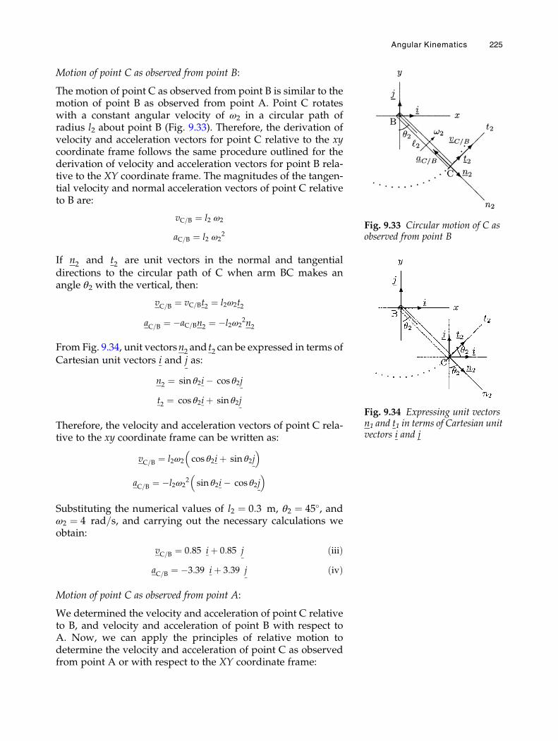
Motion of point C as observed from point B:
The motion of point C as observed from point B is similar to themotion of point B as observed from point A. Point C rotateswith a constant angular velocity of ω2 in a circular path ofradius l2 about point B (Fig. 9.33). Therefore, the derivation ofvelocity and acceleration vectors for point C relative to the xycoordinate frame follows the same procedure outlined for thederivation of velocity and acceleration vectors for point B rela-tive to the XY coordinate frame. The magnitudes of the tangen-tial velocity and normal acceleration vectors of point C relativeto B are:
vC=B ¼ l2 ω2
aC=B ¼ l2 ω22
If n2 and t2 are unit vectors in the normal and tangentialdirections to the circular path of C when arm BC makes anangle θ2 with the vertical, then:
vC=B ¼ vC=Bt2 ¼ l2ω2t2
aC=B ¼ �aC=Bn2 ¼ �l2ω22n2
From Fig. 9.34, unit vectorsn2 and t2 can be expressed in terms ofCartesian unit vectors i and j as:
n2 ¼ sin θ2i� cos θ2j
t2 ¼ cos θ2iþ sin θ2j
Therefore, the velocity and acceleration vectors of point C rela-tive to the xy coordinate frame can be written as:
vC=B ¼ l2ω2 cos θ2iþ sin θ2j� �
aC=B ¼ �l2ω22 sin θ2i� cos θ2j� �
Substituting the numerical values of l2 ¼ 0:3 m, θ2 ¼ 45�, andω2 ¼ 4 rad=s, and carrying out the necessary calculations weobtain:
vC=B ¼ 0:85 iþ 0:85 j ðiiiÞaC=B ¼ �3:39 iþ 3:39 j ðivÞ
Motion of point C as observed from point A:
We determined the velocity and acceleration of point C relativeto B, and velocity and acceleration of point B with respect toA. Now, we can apply the principles of relative motion todetermine the velocity and acceleration of point C as observedfrom point A or with respect to the XY coordinate frame:
Fig. 9.33 Circular motion of C asobserved from point B
Fig. 9.34 Expressing unit vectorsn1 and t1 in terms of Cartesian unitvectors i and j
Angular Kinematics 225
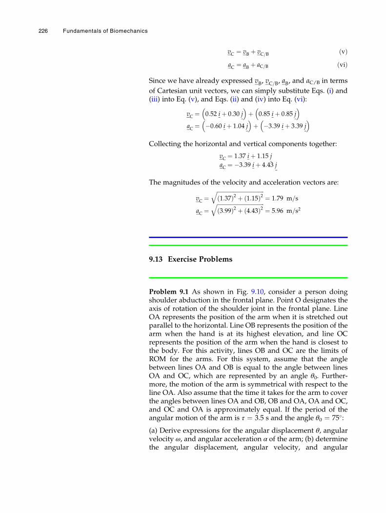
vC ¼ vB þ vC=B ðvÞaC ¼ aB þ aC=B ðviÞ
Since we have already expressed vB, vC=B, aB, and aC/B in terms
of Cartesian unit vectors, we can simply substitute Eqs. (i) and(iii) into Eq. (v), and Eqs. (ii) and (iv) into Eq. (vi):
vC ¼ 0:52 iþ 0:30 j� �
þ 0:85 iþ 0:85 j� �
aC ¼ �0:60 iþ 1:04 j� �
þ �3:39 iþ 3:39 j� �
Collecting the horizontal and vertical components together:
vC ¼ 1:37 iþ 1:15 j
aC ¼ �3:39 iþ 4:43 j
The magnitudes of the velocity and acceleration vectors are:
vC ¼ffiffiffiffiffiffiffiffiffiffiffiffiffiffiffiffiffiffiffiffiffiffiffiffiffiffiffiffiffiffiffiffiffiffiffi1:37ð Þ2 þ 1:15ð Þ2
q¼ 1:79 m=s
aC ¼ffiffiffiffiffiffiffiffiffiffiffiffiffiffiffiffiffiffiffiffiffiffiffiffiffiffiffiffiffiffiffiffiffiffiffi3:99ð Þ2 þ 4:43ð Þ2
q¼ 5:96 m=s2
9.13 Exercise Problems
Problem 9.1 As shown in Fig. 9.10, consider a person doingshoulder abduction in the frontal plane. Point O designates theaxis of rotation of the shoulder joint in the frontal plane. LineOA represents the position of the arm when it is stretched outparallel to the horizontal. Line OB represents the position of thearm when the hand is at its highest elevation, and line OCrepresents the position of the arm when the hand is closest tothe body. For this activity, lines OB and OC are the limits ofROM for the arms. For this system, assume that the anglebetween lines OA and OB is equal to the angle between linesOA and OC, which are represented by an angle θ0. Further-more, the motion of the arm is symmetrical with respect to theline OA. Also assume that the time it takes for the arm to coverthe angles between lines OA and OB, OB and OA, OA and OC,and OC and OA is approximately equal. If the period of theangular motion of the arm is τ ¼ 3.5 s and the angle θ0 ¼ 75�:
(a) Derive expressions for the angular displacement θ, angularvelocity ω, and angular acceleration α of the arm; (b) determinethe angular displacement, angular velocity, and angular
226 Fundamentals of Biomechanics
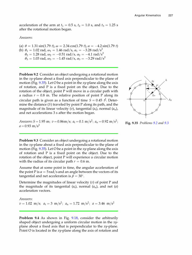
acceleration of the arm at t1 ¼ 0.5 s, t2 ¼ 1.0 s, and t3 ¼ 1.25 safter the rotational motion began.
Answers:
(a) θ ¼ 1.31 sin(1.79 t), ω ¼ 2.34 cos(1.79 t), α ¼ �4.2 sin(1.79 t)(b) θ1 ¼ 1.02 rad, ω1 ¼ 1.46 rad/s, α1 ¼ �3.28 rad/s2
θ2 ¼ 1.28 rad, ω2 ¼ �0.51 rad/s, α2 ¼ �4.1 rad/s2
θ3 ¼ 1.03 rad, ω3 ¼ �1.45 rad/s, α3 ¼ �3.29 rad/s2
Problem 9.2 Consider an object undergoing a rotational motionin the xy-plane about a fixed axis perpendicular to the plane ofmotion (Fig. 9.35). Let O be a point in the xy-plane along the axisof rotation, and P is a fixed point on the object. Due to therotation of the object, point P will move in a circular path witha radius r ¼ 0.8 m. The relative position of point P along its
circular path is given as a function of time S ¼ 0:45 t43. Deter-
mine the distance (S) traveled by point P along its path, and themagnitude of its linear velocity (v), tangential (at), normal (an),and net accelerations 3 s after the motion began.
Answers:S¼ 1:95 m; v¼ 0:86m=s; at ¼ 0:1 m=s2; an ¼ 0:92 m=s2;
a¼ 0:93 m=s2
Problem 9.3 Consider an object undergoing a rotational motionin the xy-plane about a fixed axis perpendicular to the plane ofmotion (Fig. 9.35). Let O be a point in the xy-plane along the axisof rotation and P is a fixed point on the object. Due to therotation of the object, point P will experience a circular motionwith the radius of its circular path r ¼ 0.6 m.
Assume that at some point in time, the angular acceleration ofthe point P is α ¼ 5rad=s and an angle between the vectors of itstangential and net acceleration is β ¼ 30�.
Determine the magnitudes of linear velocity (v) of point P andthe magnitude of its tangential (at), normal (an), and net (a)acceleration vectors.
Answers:
v ¼ 1:02 m=s; at ¼ 3 m=s2; an ¼ 1:72 m=s2; a ¼ 3:46 m=s2
Problem 9.4 As shown in Fig. 9.18, consider the arbitrarilyshaped object undergoing a uniform circular motion in the xy-plane about a fixed axis that is perpendicular to the xy-plane.Point O is located in the xy-plane along the axis of rotation and
Ay
h
P
0
an
at
a
Fig. 9.35 Problems 9.2 and 9.3
Angular Kinematics 227
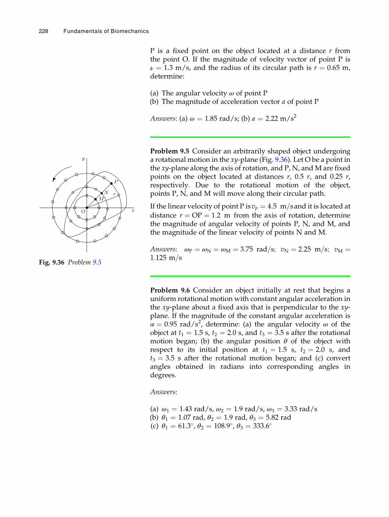
P is a fixed point on the object located at a distance r fromthe point O. If the magnitude of velocity vector of point P isν ¼ 1.3 m/s, and the radius of its circular path is r ¼ 0.65 m,determine:
(a) The angular velocity ω of point P(b) The magnitude of acceleration vector a of point P
Answers: (a) ω ¼ 1.85 rad/s; (b) a ¼ 2.22 m/s2
Problem 9.5 Consider an arbitrarily shaped object undergoinga rotational motion in the xy-plane (Fig. 9.36). Let O be a point inthe xy-plane along the axis of rotation, and P, N, andM are fixedpoints on the object located at distances r, 0.5 r, and 0.25 r,respectively. Due to the rotational motion of the object,points P, N, and M will move along their circular path.
If the linear velocity of point P isvp ¼ 4:5 m=sand it is located at
distance r ¼ OP ¼ 1:2 m from the axis of rotation, determinethe magnitude of angular velocity of points P, N, and M, andthe magnitude of the linear velocity of points N and M.
Answers: ωP ¼ ωN ¼ ωM ¼ 3:75 rad=s; vN ¼ 2:25 m=s; vM ¼1:125 m=s
Problem 9.6 Consider an object initially at rest that begins auniform rotational motion with constant angular acceleration inthe xy-plane about a fixed axis that is perpendicular to the xy-plane. If the magnitude of the constant angular acceleration isα ¼ 0.95 rad/s2, determine: (a) the angular velocity ω of theobject at t1 ¼ 1.5 s, t2 ¼ 2.0 s, and t3 ¼ 3.5 s after the rotationalmotion began; (b) the angular position θ of the object withrespect to its initial position at t1 ¼ 1.5 s, t2 ¼ 2.0 s, andt3 ¼ 3.5 s after the rotational motion began; and (c) convertangles obtained in radians into corresponding angles indegrees.
Answers:
(a) ω1 ¼ 1.43 rad/s, ω2 ¼ 1.9 rad/s, ω3 ¼ 3.33 rad/s(b) θ1 ¼ 1.07 rad, θ2 ¼ 1.9 rad, θ3 ¼ 5.82 rad(c) θ1 ¼ 61.3�, θ2 ¼ 108.9�, θ3 ¼ 333.6�
y
x
rM
N
P
O
Fig. 9.36 Problem 9.5
228 Fundamentals of Biomechanics
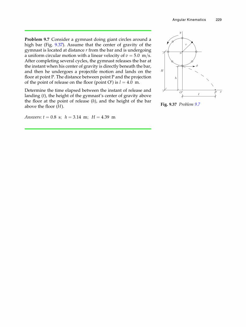
Problem 9.7 Consider a gymnast doing giant circles around ahigh bar (Fig. 9.37). Assume that the center of gravity of thegymnast is located at distance r from the bar and is undergoinga uniform circular motion with a linear velocity of v ¼ 5:0 m=s.After completing several cycles, the gymnast releases the bar atthe instant when his center of gravity is directly beneath the bar,and then he undergoes a projectile motion and lands on thefloor at point P. The distance between point P and the projectionof the point of release on the floor (point O0) is l ¼ 4:0 m.
Determine the time elapsed between the instant of release andlanding (t), the height of the gymnast’s center of gravity abovethe floor at the point of release (h), and the height of the barabove the floor (H).
Answers: t ¼ 0:8 s; h ¼ 3:14 m; H ¼ 4:39 m
P
ϑ
r
h
H
y
x
0
Fig. 9.37 Problem 9.7
Angular Kinematics 229
Chapter 10
Angular Kinetics
10.1 Kinetics of Angular Motion / 233
10.2 Torque and Angular Acceleration / 239
10.3 Mass Moment of Inertia / 240
10.4 Parallel-Axis Theorem / 242
10.5 Radius of Gyration / 242
10.6 Segmental Motion Analysis / 243
10.7 Rotational Kinetic Energy / 247
10.8 Angular Work and Power / 248
10.9 Exercise Problems / 250
# Springer International Publishing Switzerland 2017N. Ozkaya et al., Fundamentals of Biomechanics, DOI 10.1007/978-3-319-44738-4_10
231

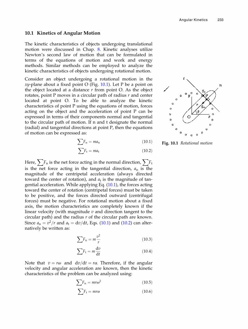
10.1 Kinetics of Angular Motion
The kinetic characteristics of objects undergoing translationalmotion were discussed in Chap. 8. Kinetic analyses utilizeNewton’s second law of motion that can be formulated interms of the equations of motion and work and energymethods. Similar methods can be employed to analyze thekinetic characteristics of objects undergoing rotational motion.
Consider an object undergoing a rotational motion in thexy-plane about a fixed point O (Fig. 10.1). Let P be a point onthe object located at a distance r from point O. As the objectrotates, point P moves in a circular path of radius r and centerlocated at point O. To be able to analyze the kineticcharacteristics of point P using the equations of motion, forcesacting on the object and the acceleration of point P can beexpressed in terms of their components normal and tangentialto the circular path of motion. If n and t designate the normal(radial) and tangential directions at point P, then the equationsof motion can be expressed as:X
Fn ¼ man ð10:1ÞXFt ¼ mat ð10:2Þ
Here,X
Fn is the net force acting in the normal direction,X
Ftis the net force acting in the tangential direction, an is themagnitude of the centripetal acceleration (always directedtoward the center of rotation), and at is the magnitude of tan-gential acceleration. While applying Eq. (10.1), the forces actingtoward the center of rotation (centripetal forces) must be takento be positive, and the forces directed outward (centrifugalforces) must be negative. For rotational motion about a fixedaxis, the motion characteristics are completely known if thelinear velocity (with magnitude v and direction tangent to thecircular path) and the radius r of the circular path are known.
Since an ¼ v2=r and at ¼ dv=dt, Eqs. (10.1) and (10.2) can alter-natively be written as:
XFn ¼ m
v2
rð10:3Þ
XFt ¼ m
dv
dtð10:4Þ
Note that v ¼ rω and dv=dt ¼ rα. Therefore, if the angularvelocity and angular acceleration are known, then the kineticcharacteristics of the problem can be analyzed using:X
Fn ¼ mrω2 ð10:5ÞXFt ¼ mrα ð10:6Þ
Fig. 10.1 Rotational motion
Angular Kinetics 233
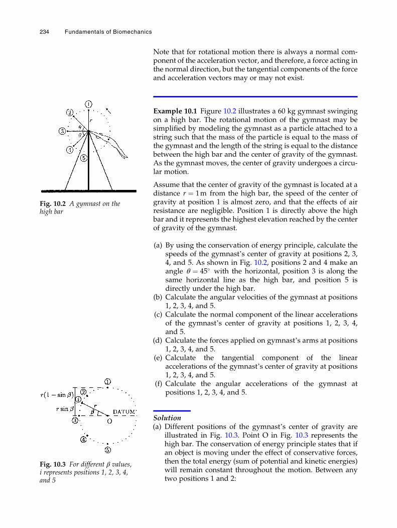
Note that for rotational motion there is always a normal com-ponent of the acceleration vector, and therefore, a force acting inthe normal direction, but the tangential components of the forceand acceleration vectors may or may not exist.
Example 10.1 Figure 10.2 illustrates a 60 kg gymnast swingingon a high bar. The rotational motion of the gymnast may besimplified by modeling the gymnast as a particle attached to astring such that the mass of the particle is equal to the mass ofthe gymnast and the length of the string is equal to the distancebetween the high bar and the center of gravity of the gymnast.As the gymnast moves, the center of gravity undergoes a circu-lar motion.
Assume that the center of gravity of the gymnast is located at adistance r ¼ 1m from the high bar, the speed of the center ofgravity at position 1 is almost zero, and that the effects of airresistance are negligible. Position 1 is directly above the highbar and it represents the highest elevation reached by the centerof gravity of the gymnast.
(a) By using the conservation of energy principle, calculate thespeeds of the gymnast’s center of gravity at positions 2, 3,4, and 5. As shown in Fig. 10.2, positions 2 and 4 make anangle θ ¼ 45� with the horizontal, position 3 is along thesame horizontal line as the high bar, and position 5 isdirectly under the high bar.
(b) Calculate the angular velocities of the gymnast at positions1, 2, 3, 4, and 5.
(c) Calculate the normal component of the linear accelerationsof the gymnast’s center of gravity at positions 1, 2, 3, 4,and 5.
(d) Calculate the forces applied on gymnast’s arms at positions1, 2, 3, 4, and 5.
(e) Calculate the tangential component of the linearaccelerations of the gymnast’s center of gravity at positions1, 2, 3, 4, and 5.
(f) Calculate the angular accelerations of the gymnast atpositions 1, 2, 3, 4, and 5.
Solution(a) Different positions of the gymnast’s center of gravity are
illustrated in Fig. 10.3. Point O in Fig. 10.3 represents thehigh bar. The conservation of energy principle states that ifan object is moving under the effect of conservative forces,then the total energy (sum of potential and kinetic energies)will remain constant throughout the motion. Between anytwo positions 1 and 2:
Fig. 10.3 For different β values,i represents positions 1, 2, 3, 4,and 5
Fig. 10.2 A gymnast on thehigh bar
234 Fundamentals of Biomechanics
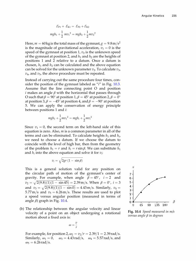
EP1 þ EK1 ¼ EP2 þ EK2
mgh1 þ 1
2mv1
2 ¼ mgh2 þ 1
2mv2
2
Here,m ¼ 60kgis the total mass of the gymnast,g ¼ 9:8m=s2
is the magnitude of gravitational acceleration, v1 ¼ 0 is thespeed of the gymnast at position 1, v2 is the unknown speedof the gymnast at position 2, and h1 and h2 are the heights ofpositions 1 and 2 relative to a datum. Once a datum ischosen, h1 and h2 can be calculated and the above equationcan be solved for the unknown parameter v2. To calculate v3,v4, and v5, the above procedure must be repeated.
Instead of carrying out the same procedure four times, con-sider the position of the gymnast labeled as “i” in Fig. 10.3.Assume that the line connecting point O and positioni makes an angle β with the horizontal that passes throughO such that β ¼ 90� at position 1, β ¼ 45� at position 2, β ¼ 0�
at position 3, β ¼ �45� at position 4, andβ ¼ �90� at position5. We can apply the conservation of energy principlebetween positions 1 and i:
mgh1 þ 1
2mv1
2 ¼ mghi þ 1
2mvi
2
Since v1 ¼ 0, the second term on the left-hand side of thisequation is zero. Also,m is a common parameter in all of theterms and can be eliminated. To calculate heights h1 and hi,we need to choose a datum. If we choose the datum tocoincide with the level of high bar, then from the geometryof the problem h1 ¼ r and hi ¼ r sin β. We can substitute h1and hi into the above equation and solve it for vi:
vi ¼ffiffiffiffiffiffiffiffiffiffiffiffiffiffiffiffiffiffiffiffiffiffiffiffiffiffiffiffiffiffiffi2gr 1� sin βð Þ
q
This is a general solution valid for any position onthe circular path of motion of the gymnast’s center ofgravity. For example, when angle β ¼ 45�, i ¼ 2 and
v2 ¼ffiffiffiffiffiffiffiffiffiffiffiffiffiffiffiffiffiffiffiffiffiffiffiffiffiffiffiffiffiffiffiffiffiffiffiffiffiffiffiffiffiffiffi2 9:8ð Þ 1ð Þ 1� sin 45ð Þp ¼ 2:39m=s. When β ¼ 0�, i ¼ 3
and v3 ¼ffiffiffiffiffiffiffiffiffiffiffiffiffiffiffiffiffiffiffiffiffiffiffiffiffiffiffiffiffiffiffiffiffiffiffiffiffiffiffiffiffi2 9:8ð Þ 1ð Þ 1� sin 0ð Þp ¼ 4:43m=s. Similarly, v4 ¼
5:77m=s and v5 ¼ 6:26m=s. These results are used to plota speed versus angular position (measured in terms ofangle β) graph in Fig. 10.4.
(b) The relationship between the angular velocity and linearvelocity of a point on an object undergoing a rotationalmotion about a fixed axis is:
ω ¼ v
r
For example, for position 2,ω2 ¼ v2=r ¼ 2:39=1 ¼ 2:39rad=s.Similarly, ω1 ¼ 0, ω3 ¼ 4:43rad=s, ω4 ¼ 5:57rad=s, andω5 ¼ 6:26rad=s.
Fig. 10.4 Speed measured in m/sversus angle β in degrees
Angular Kinetics 235
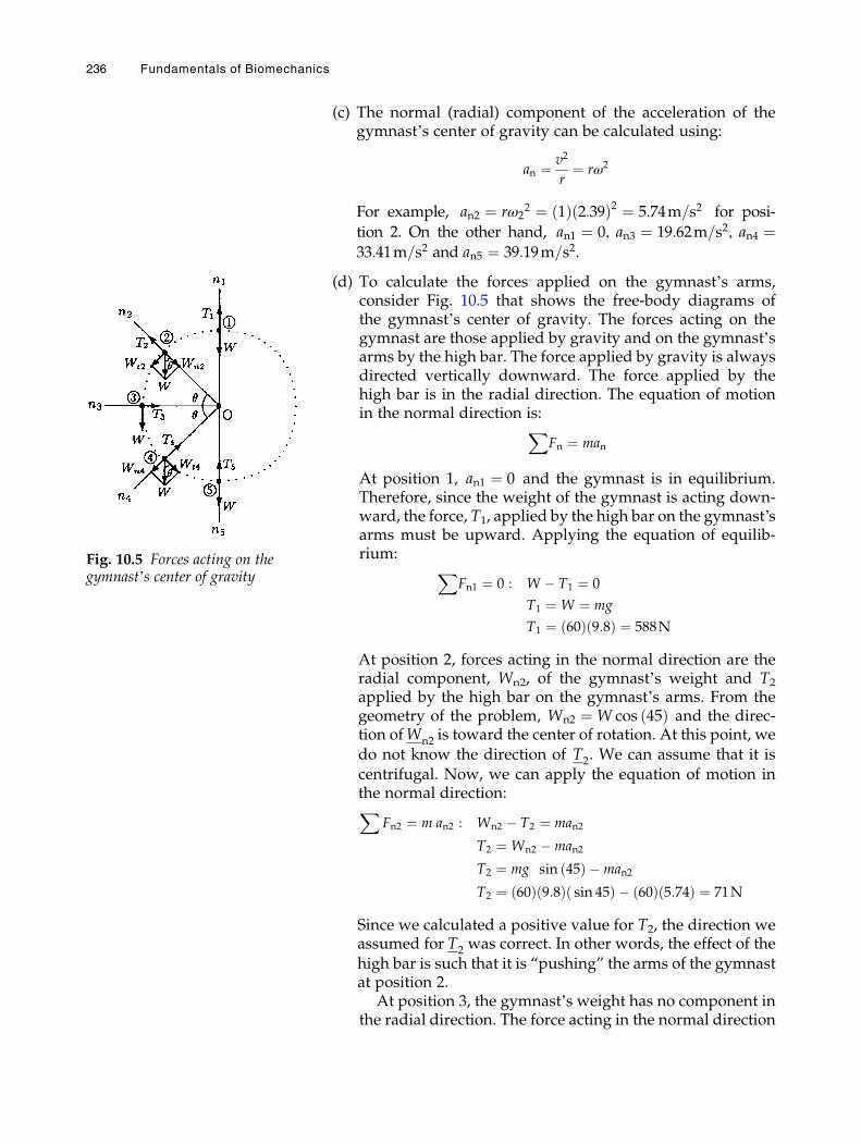
(c) The normal (radial) component of the acceleration of thegymnast’s center of gravity can be calculated using:
an ¼ v2
r¼ rω2
For example, an2 ¼ rω22 ¼ 1ð Þ 2:39ð Þ2 ¼ 5:74m=s2 for posi-
tion 2. On the other hand, an1 ¼ 0, an3 ¼ 19:62m=s2, an4 ¼33:41m=s2 and an5 ¼ 39:19m=s2.
(d) To calculate the forces applied on the gymnast’s arms,consider Fig. 10.5 that shows the free-body diagrams ofthe gymnast’s center of gravity. The forces acting on thegymnast are those applied by gravity and on the gymnast’sarms by the high bar. The force applied by gravity is alwaysdirected vertically downward. The force applied by thehigh bar is in the radial direction. The equation of motionin the normal direction is:X
Fn ¼ man
At position 1, an1 ¼ 0 and the gymnast is in equilibrium.Therefore, since the weight of the gymnast is acting down-ward, the force, T1, applied by the high bar on the gymnast’sarms must be upward. Applying the equation of equilib-rium: X
Fn1 ¼ 0 : W � T1 ¼ 0
T1 ¼ W ¼ mg
T1 ¼ 60ð Þ 9:8ð Þ ¼ 588N
At position 2, forces acting in the normal direction are theradial component, Wn2, of the gymnast’s weight and T2
applied by the high bar on the gymnast’s arms. From thegeometry of the problem, Wn2 ¼ W cos 45ð Þ and the direc-tion ofWn2 is toward the center of rotation. At this point, wedo not know the direction of T2. We can assume that it iscentrifugal. Now, we can apply the equation of motion inthe normal direction:X
Fn2 ¼ m an2 : Wn2 � T2 ¼ man2
T2 ¼ Wn2 �man2
T2 ¼ mg sin 45ð Þ �man2
T2 ¼ 60ð Þ 9:8ð Þ sin 45ð Þ � 60ð Þ 5:74ð Þ ¼ 71N
Since we calculated a positive value for T2, the direction weassumed for T2 was correct. In other words, the effect of thehigh bar is such that it is “pushing” the arms of the gymnastat position 2.
At position 3, the gymnast’s weight has no component inthe radial direction. The force acting in the normal direction
Fig. 10.5 Forces acting on thegymnast’s center of gravity
236 Fundamentals of Biomechanics
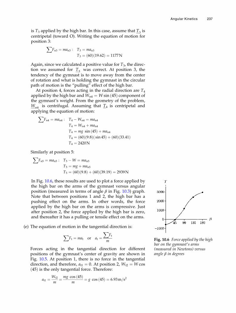
is T3 applied by the high bar. In this case, assume that T3 iscentripetal (toward O). Writing the equation of motion forposition 3:X
Fn3 ¼ man3 : T3 ¼ man3
T3 ¼ 60ð Þ 19:62ð Þ ¼ 1177N
Again, since we calculated a positive value for T3, the direc-tion we assumed for T3 was correct. At position 3, thetendency of the gymnast is to move away from the centerof rotation and what is holding the gymnast in the circularpath of motion is the “pulling” effect of the high bar.
At position 4, forces acting in the radial direction are T4
applied by the high bar andWn4 ¼ W sin 45ð Þ component ofthe gymnast’s weight. From the geometry of the problem,Wn4 is centrifugal. Assuming that T4 is centripetal andapplying the equation of motion:X
Fn4 ¼ man4 : T4 �Wn4 ¼ man4
T4 ¼ Wn4 þman4
T4 ¼ mg sin 45ð Þ þman4
T4 ¼ 60ð Þ 9:8ð Þ sin 45ð Þ þ 60ð Þ 33:41ð ÞT4 ¼ 2420N
Similarly at position 5:XFn5 ¼ man5 : T5 �W ¼ man5
T5 ¼ mgþman5
T5 ¼ 60ð Þ 9:8ð Þ þ 60ð Þ 39:19ð Þ ¼ 2939N
In Fig. 10.6, these results are used to plot a force applied bythe high bar on the arms of the gymnast versus angularposition (measured in terms of angle β in Fig. 10.3) graph.Note that between positions 1 and 2, the high bar has apushing effect on the arms. In other words, the forceapplied by the high bar on the arms is compressive. Justafter position 2, the force applied by the high bar is zero,and thereafter it has a pulling or tensile effect on the arms.
(e) The equation of motion in the tangential direction is:
XFt ¼ mat or at ¼
XFt
m
Forces acting in the tangential direction for differentpositions of the gymnast’s center of gravity are shown inFig. 10.5. At position 1, there is no force in the tangentialdirection, and therefore, at1 ¼ 0. At position 2, Wt2 ¼ W cos45ð Þ is the only tangential force. Therefore:
at1 ¼ Wt2
m¼ mg cos 45ð Þ
m¼ g cos 45ð Þ ¼ 6:93m=s2
Fig. 10.6 Force applied by the highbar on the gymnast’s arms(measured in Newtons) versusangle β in degrees
Angular Kinetics 237
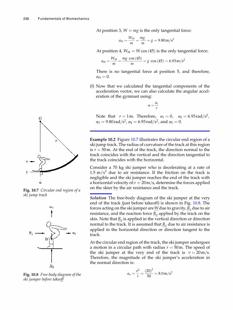
At position 3, W ¼ mg is the only tangential force:
at3 ¼ Wt3
m¼ mg
m¼ g ¼ 9:80m=s2
At position 4, Wt4 ¼ W cos 45ð Þ is the only tangential force:
at4 ¼ Wt4
m¼ mg cos 45ð Þ
m¼ g cos 45ð Þ ¼ 6:93m=s2
There is no tangential force at position 5, and therefore,at5 ¼ 0.
(f) Now that we calculated the tangential components of theacceleration vector, we can also calculate the angular accel-eration of the gymnast using:
α ¼ atr
Note that r ¼ 1m. Therefore, α1 ¼ 0, α2 ¼ 6:93rad=s2,
α3 ¼ 9:80rad=s2, α4 ¼ 6:93rad=s2, and α5 ¼ 0.
Example 10.2 Figure 10.7 illustrates the circular end region of aski jump track. The radius of curvature of the track at this regionis r ¼ 50m. At the end of the track, the direction normal to thetrack coincides with the vertical and the direction tangential tothe track coincides with the horizontal.
Consider a 70 kg ski jumper who is decelerating at a rate of1.5 m/s2 due to air resistance. If the friction on the track isnegligible and the ski jumper reaches the end of the track witha horizontal velocity ofv ¼ 20m=s, determine the forces appliedon the skier by the air resistance and the track.
Solution The free-body diagram of the ski jumper at the veryend of the track (just before takeoff) is shown in Fig. 10.8. Theforces acting on the ski jumper areWdue to gravity,R1 due to airresistance, and the reaction force R2 applied by the track on theskis. Note thatR2 is applied in the vertical direction or directionnormal to the track. It is assumed that R1 due to air resistance isapplied in the horizontal direction or direction tangent to thetrack.
At the circular end region of the track, the ski jumper undergoesa motion in a circular path with radius r ¼ 50m. The speed ofthe ski jumper at the very end of the track is v ¼ 20m=s.Therefore, the magnitude of the ski jumper’s acceleration inthe normal direction is:
an ¼ v2
r¼ 20ð Þ2
50¼ 8:0m=s2
Fig. 10.7 Circular end region of aski jump track
Fig. 10.8 Free-body diagram of theski jumper before takeoff
238 Fundamentals of Biomechanics
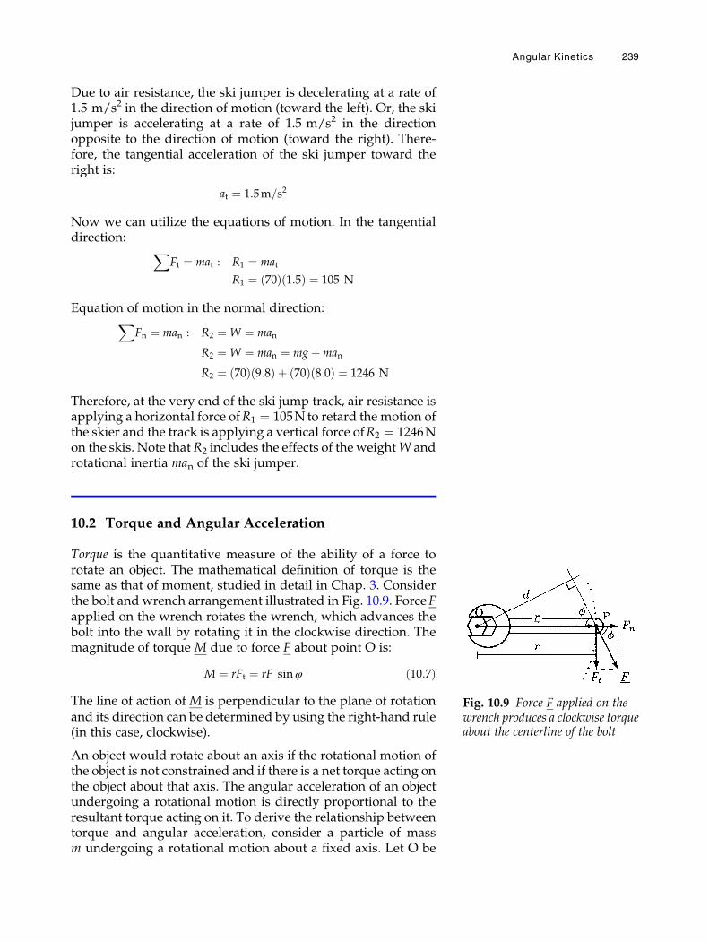
Due to air resistance, the ski jumper is decelerating at a rate of1.5 m/s2 in the direction of motion (toward the left). Or, the skijumper is accelerating at a rate of 1.5 m/s2 in the directionopposite to the direction of motion (toward the right). There-fore, the tangential acceleration of the ski jumper toward theright is:
at ¼ 1:5m=s2
Now we can utilize the equations of motion. In the tangentialdirection: X
Ft ¼ mat : R1 ¼ mat
R1 ¼ 70ð Þ 1:5ð Þ ¼ 105 N
Equation of motion in the normal direction:XFn ¼ man : R2 ¼ W ¼ man
R2 ¼ W ¼ man ¼ mgþman
R2 ¼ 70ð Þ 9:8ð Þ þ 70ð Þ 8:0ð Þ ¼ 1246 N
Therefore, at the very end of the ski jump track, air resistance isapplying a horizontal force ofR1 ¼ 105N to retard the motion ofthe skier and the track is applying a vertical force ofR2 ¼ 1246Non the skis. Note that R2 includes the effects of the weightW androtational inertia man of the ski jumper.
10.2 Torque and Angular Acceleration
Torque is the quantitative measure of the ability of a force torotate an object. The mathematical definition of torque is thesame as that of moment, studied in detail in Chap. 3. Considerthe bolt and wrench arrangement illustrated in Fig. 10.9. ForceFapplied on the wrench rotates the wrench, which advances thebolt into the wall by rotating it in the clockwise direction. Themagnitude of torque M due to force F about point O is:
M ¼ rFt ¼ rF sinφ ð10:7Þ
The line of action of M is perpendicular to the plane of rotationand its direction can be determined by using the right-hand rule(in this case, clockwise).
An object would rotate about an axis if the rotational motion ofthe object is not constrained and if there is a net torque acting onthe object about that axis. The angular acceleration of an objectundergoing a rotational motion is directly proportional to theresultant torque acting on it. To derive the relationship betweentorque and angular acceleration, consider a particle of massm undergoing a rotational motion about a fixed axis. Let O be
Fig. 10.9 Force F applied on thewrench produces a clockwise torqueabout the centerline of the bolt
Angular Kinetics 239
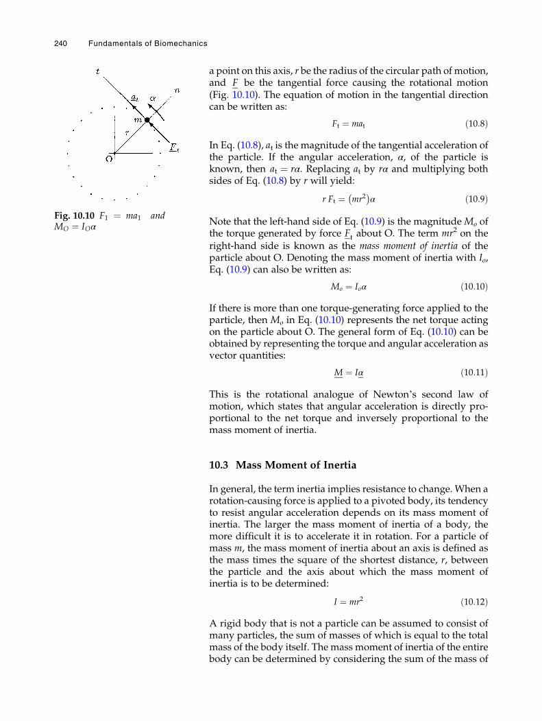
a point on this axis, r be the radius of the circular path of motion,and F be the tangential force causing the rotational motion(Fig. 10.10). The equation of motion in the tangential directioncan be written as:
Ft ¼ mat ð10:8Þ
In Eq. (10.8), at is the magnitude of the tangential acceleration ofthe particle. If the angular acceleration, α, of the particle isknown, then at ¼ rα. Replacing at by rα and multiplying bothsides of Eq. (10.8) by r will yield:
r Ft ¼ mr2� �
α ð10:9Þ
Note that the left-hand side of Eq. (10.9) is the magnitudeMo ofthe torque generated by force Ft about O. The term mr2 on theright-hand side is known as the mass moment of inertia of theparticle about O. Denoting the mass moment of inertia with Io,Eq. (10.9) can also be written as:
Mo ¼ Ioα ð10:10Þ
If there is more than one torque-generating force applied to theparticle, then Mo in Eq. (10.10) represents the net torque actingon the particle about O. The general form of Eq. (10.10) can beobtained by representing the torque and angular acceleration asvector quantities:
M ¼ Iα ð10:11Þ
This is the rotational analogue of Newton’s second law ofmotion, which states that angular acceleration is directly pro-portional to the net torque and inversely proportional to themass moment of inertia.
10.3 Mass Moment of Inertia
In general, the term inertia implies resistance to change. When arotation-causing force is applied to a pivoted body, its tendencyto resist angular acceleration depends on its mass moment ofinertia. The larger the mass moment of inertia of a body, themore difficult it is to accelerate it in rotation. For a particle ofmass m, the mass moment of inertia about an axis is defined asthe mass times the square of the shortest distance, r, betweenthe particle and the axis about which the mass moment ofinertia is to be determined:
I ¼ mr2 ð10:12Þ
A rigid body that is not a particle can be assumed to consist ofmany particles, the sum of masses of which is equal to the totalmass of the body itself. The mass moment of inertia of the entirebody can be determined by considering the sum of the mass of
Fig. 10.10 F1 ¼ ma1 andMO ¼ IOα
240 Fundamentals of Biomechanics
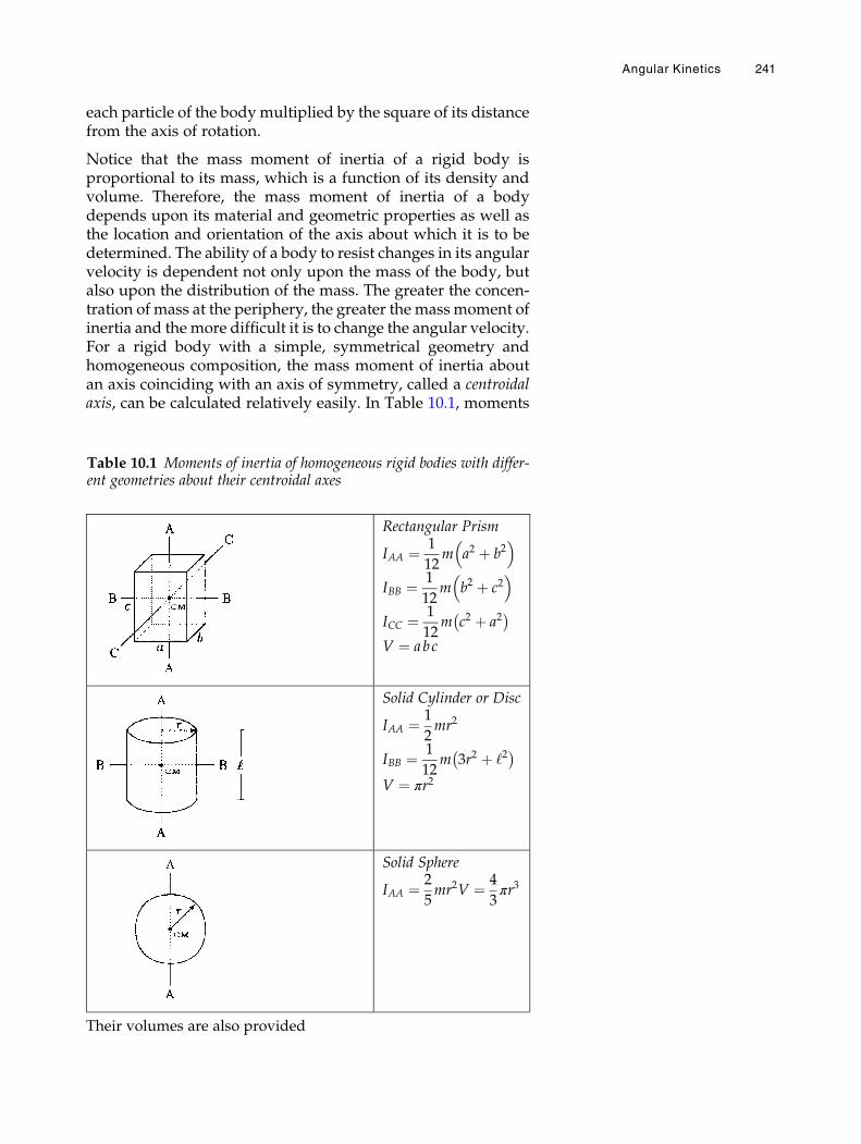
each particle of the bodymultiplied by the square of its distancefrom the axis of rotation.
Notice that the mass moment of inertia of a rigid body isproportional to its mass, which is a function of its density andvolume. Therefore, the mass moment of inertia of a bodydepends upon its material and geometric properties as well asthe location and orientation of the axis about which it is to bedetermined. The ability of a body to resist changes in its angularvelocity is dependent not only upon the mass of the body, butalso upon the distribution of the mass. The greater the concen-tration of mass at the periphery, the greater the mass moment ofinertia and the more difficult it is to change the angular velocity.For a rigid body with a simple, symmetrical geometry andhomogeneous composition, the mass moment of inertia aboutan axis coinciding with an axis of symmetry, called a centroidalaxis, can be calculated relatively easily. In Table 10.1, moments
Table 10.1 Moments of inertia of homogeneous rigid bodies with differ-ent geometries about their centroidal axes
Rectangular Prism
IAA ¼ 1
12m a2 þ b2� �
IBB ¼ 1
12m b2 þ c2� �
ICC ¼ 1
12m c2 þ a2� �
V ¼ abc
Solid Cylinder or Disc
IAA ¼ 1
2mr2
IBB ¼ 1
12m 3r2 þ ‘2� �
V ¼ πr2
Solid Sphere
IAA ¼ 2
5mr2V ¼ 4
3πr3
Their volumes are also provided
Angular Kinetics 241
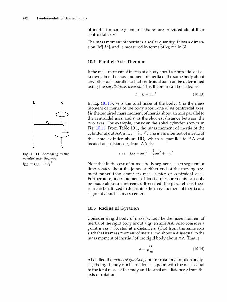
of inertia for some geometric shapes are provided about theircentroidal axes.
The mass moment of inertia is a scalar quantity. It has a dimen-sion [M][L2], and is measured in terms of kg m2 in SI.
10.4 Parallel-Axis Theorem
If the massmoment of inertia of a body about a centroidal axis isknown, then themassmoment of inertia of the same body aboutany other axis parallel to that centroidal axis can be determinedusing the parallel-axis theorem. This theorem can be stated as:
I ¼ Ic þmrc2 ð10:13Þ
In Eq. (10.13), m is the total mass of the body, Ic is the massmoment of inertia of the body about one of its centroidal axes,I is the requiredmassmoment of inertia about an axis parallel tothe centroidal axis, and rc is the shortest distance between thetwo axes. For example, consider the solid cylinder shown inFig. 10.11. From Table 10.1, the mass moment of inertia of the
cylinder about AA is IAA ¼ 12mr2. The mass moment of inertia of
the same cylinder about DD, which is parallel to AA andlocated at a distance rc from AA, is:
IDD ¼ IAA þmrc2 ¼ 1
2mr2 þmrc
2
Note that in the case of human body segments, each segment orlimb rotates about the joints at either end of the moving seg-ment rather than about its mass center or centroidal axes.Furthermore, mass moment of inertia measurements can onlybe made about a joint center. If needed, the parallel-axis theo-rem can be utilized to determine themassmoment of inertia of asegment about its mass center.
10.5 Radius of Gyration
Consider a rigid body of mass m. Let I be the mass moment ofinertia of the rigid body about a given axis AA. Also consider apoint mass m located at a distance ρ (rho) from the same axissuch that itsmassmoment of inertiamρ2 aboutAA is equal to themass moment of inertia I of the rigid body about AA. That is:
ρ ¼ffiffiffiffiI
m
rð10:14Þ
ρ is called the radius of gyration, and for rotational motion analy-sis, the rigid body can be treated as a point with the mass equalto the total mass of the body and located at a distance ρ from theaxis of rotation.
Fig. 10.11 According to theparallel-axis theorem,IDD ¼ IAA þmrc
2
242 Fundamentals of Biomechanics

10.6 Segmental Motion Analysis
The information provided in the previous sections can beutilized to develop mathematical models for analyzing themotion characteristics of human body segments. Here, the gen-eral procedure for developing a dynamic model of a bodysegment will be outlined, and then applied to analyze therotational motion of the lower leg about the knee joint.
The first step of a dynamic model analysis involves defining theforces acting on the body segment. These may include thegravitational (weight), external, inertial, muscle, and joint reac-tion forces. The weight of the body segment can be assumed toact at its center of gravity, and therefore, the center of gravity ofthe segment must be known. The magnitude, point of applica-tion, and direction of any external force present must bespecified. Inertial forces are those present due to the dynamicsof the problem under consideration. One way of incorporatinginertial effects into the model is through the use of the radius ofgyration. Muscle and joint reaction forces are the unknowns tobe determined as a result of these analyses. It is important todraw the free-body diagram of the segment to be analyzed, andto identify all the known and unknown forces acting on it.
The next step of dynamic analysis is the identification of mea-surable quantities. In general, both the angular displacement ofthe moving body segment and the net torque generated aboutits axis of rotation can be measured as functions of time over therange of segmental motion. The angular displacement measure-ment techniques include goniometric, dynamometric, and pho-togrammetric methods. Through the use of kinematicrelationships, the angular displacement data can be used tocalculate the angular velocity and angular acceleration of themoving segment. If the angular displacement θ is known as afunction of time t, then the angular velocity ω and angularacceleration α can be determined by considering the first andsecond derivatives of θ with respect to t:
ω ¼ dθ
dtα ¼ dω
dt¼ d2θ
dt2
If it is not possible to find a function representing the relation-ship between the angular displacement and time, then numeri-cal differentiation techniques can be employed. Once theangular acceleration is determined, the relationship betweentorque, mass moment of inertia, and angular acceleration canbe used to calculate the net torque produced about the jointcenter, provided that the mass moment of inertia (or the radiusof gyration) of the segment about the joint center is known.
For a two-dimensional (planar) motion analysis of a segmentabout its joint center, if the net torque M produced about the
Angular Kinetics 243
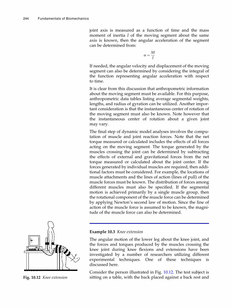
joint axis is measured as a function of time and the massmoment of inertia I of the moving segment about the sameaxis is known, then the angular acceleration of the segmentcan be determined from:
α ¼ M
I
If needed, the angular velocity and displacement of the movingsegment can also be determined by considering the integral ofthe function representing angular acceleration with respectto time.
It is clear from this discussion that anthropometric informationabout the moving segment must be available. For this purpose,anthropometric data tables listing average segmental weights,lengths, and radius of gyration can be utilized. Another impor-tant consideration is that the instantaneous center of rotation ofthe moving segment must also be known. Note however thatthe instantaneous center of rotation about a given jointmay vary.
The final step of dynamic model analyses involves the compu-tation of muscle and joint reaction forces. Note that the nettorque measured or calculated includes the effects of all forcesacting on the moving segment. The torque generated by themuscles crossing the joint can be determined by subtractingthe effects of external and gravitational forces from the nettorque measured or calculated about the joint center. If theforces generated by individual muscles are required, then addi-tional factors must be considered. For example, the locations ofmuscle attachments and the lines of action (lines of pull) of themuscle forces must be known. The distribution of forces amongdifferent muscles must also be specified. If the segmentalmotion is achieved primarily by a single muscle group, thenthe rotational component of the muscle force can be determinedby applying Newton’s second law of motion. Since the line ofaction of the muscle force is assumed to be known, the magni-tude of the muscle force can also be determined.
Example 10.3 Knee extension
The angular motion of the lower leg about the knee joint, andthe forces and torques produced by the muscles crossing theknee joint during knee flexions and extensions have beeninvestigated by a number of researchers utilizing differentexperimental techniques. One of these techniques isdiscussed here.
Consider the person illustrated in Fig. 10.12. The test subject issitting on a table, with the back placed against a back rest andFig. 10.12 Knee extension
244 Fundamentals of Biomechanics
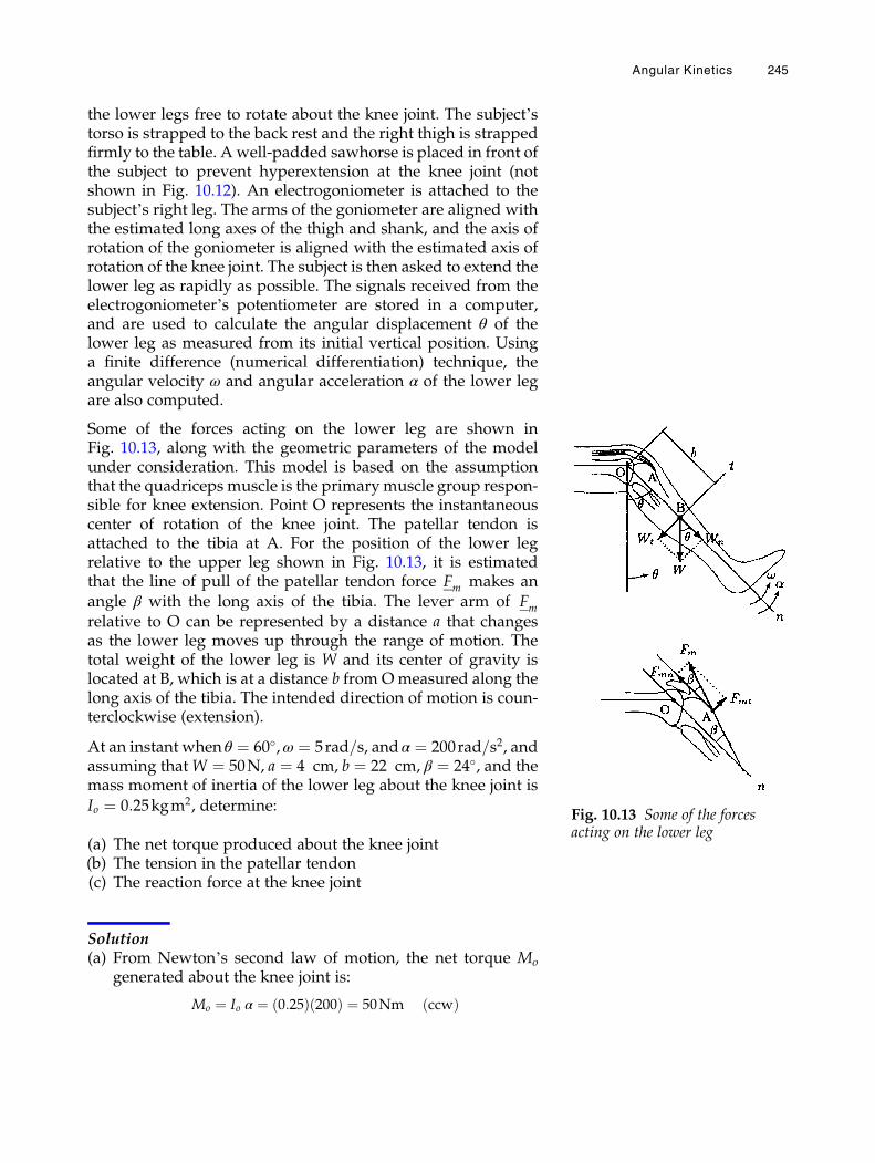
the lower legs free to rotate about the knee joint. The subject’storso is strapped to the back rest and the right thigh is strappedfirmly to the table. A well-padded sawhorse is placed in front ofthe subject to prevent hyperextension at the knee joint (notshown in Fig. 10.12). An electrogoniometer is attached to thesubject’s right leg. The arms of the goniometer are aligned withthe estimated long axes of the thigh and shank, and the axis ofrotation of the goniometer is aligned with the estimated axis ofrotation of the knee joint. The subject is then asked to extend thelower leg as rapidly as possible. The signals received from theelectrogoniometer’s potentiometer are stored in a computer,and are used to calculate the angular displacement θ of thelower leg as measured from its initial vertical position. Usinga finite difference (numerical differentiation) technique, theangular velocity ω and angular acceleration α of the lower legare also computed.
Some of the forces acting on the lower leg are shown inFig. 10.13, along with the geometric parameters of the modelunder consideration. This model is based on the assumptionthat the quadriceps muscle is the primarymuscle group respon-sible for knee extension. Point O represents the instantaneouscenter of rotation of the knee joint. The patellar tendon isattached to the tibia at A. For the position of the lower legrelative to the upper leg shown in Fig. 10.13, it is estimatedthat the line of pull of the patellar tendon force Fm makes anangle β with the long axis of the tibia. The lever arm of Fmrelative to O can be represented by a distance a that changesas the lower leg moves up through the range of motion. Thetotal weight of the lower leg is W and its center of gravity islocated at B, which is at a distance b from Omeasured along thelong axis of the tibia. The intended direction of motion is coun-terclockwise (extension).
At an instant when θ ¼ 60�,ω ¼ 5rad=s, andα ¼ 200rad=s2, andassuming thatW ¼ 50N, a ¼ 4 cm, b ¼ 22 cm, β ¼ 24�, and themass moment of inertia of the lower leg about the knee joint is
Io ¼ 0:25kgm2, determine:
(a) The net torque produced about the knee joint(b) The tension in the patellar tendon(c) The reaction force at the knee joint
Solution(a) From Newton’s second law of motion, the net torque Mo
generated about the knee joint is:
Mo ¼ Io α ¼ 0:25ð Þ 200ð Þ ¼ 50Nm ccwð Þ
Fig. 10.13 Some of the forcesacting on the lower leg
Angular Kinetics 245
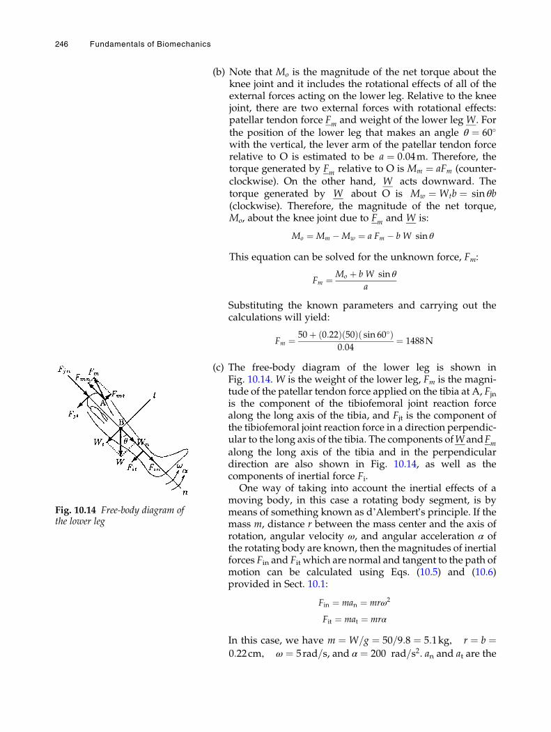
(b) Note that Mo is the magnitude of the net torque about theknee joint and it includes the rotational effects of all of theexternal forces acting on the lower leg. Relative to the kneejoint, there are two external forces with rotational effects:patellar tendon force Fm and weight of the lower leg W. Forthe position of the lower leg that makes an angle θ ¼ 60�
with the vertical, the lever arm of the patellar tendon forcerelative to O is estimated to be a ¼ 0:04m. Therefore, thetorque generated by Fm relative to O is Mm ¼ aFm (counter-clockwise). On the other hand, W acts downward. Thetorque generated by W about O is Mw ¼ Wtb ¼ sin θb(clockwise). Therefore, the magnitude of the net torque,Mo, about the knee joint due to Fm and W is:
Mo ¼ Mm �Mw ¼ a Fm � b W sin θ
This equation can be solved for the unknown force, Fm:
Fm ¼ Mo þ b W sin θ
a
Substituting the known parameters and carrying out thecalculations will yield:
Fm ¼ 50þ 0:22ð Þ 50ð Þ sin 60�ð Þ0:04
¼ 1488N
(c) The free-body diagram of the lower leg is shown inFig. 10.14. W is the weight of the lower leg, Fm is the magni-tude of the patellar tendon force applied on the tibia at A, Fjnis the component of the tibiofemoral joint reaction forcealong the long axis of the tibia, and Fjt is the component ofthe tibiofemoral joint reaction force in a direction perpendic-ular to the long axis of the tibia. The components ofW andFmalong the long axis of the tibia and in the perpendiculardirection are also shown in Fig. 10.14, as well as thecomponents of inertial force Fi.
One way of taking into account the inertial effects of amoving body, in this case a rotating body segment, is bymeans of something known as d’Alembert’s principle. If themass m, distance r between the mass center and the axis ofrotation, angular velocity ω, and angular acceleration α ofthe rotating body are known, then the magnitudes of inertialforces Fin and Fit which are normal and tangent to the path ofmotion can be calculated using Eqs. (10.5) and (10.6)provided in Sect. 10.1:
Fin ¼ man ¼ mrω2
Fit ¼ mat ¼ mrα
In this case, we have m ¼ W=g ¼ 50=9:8 ¼ 5:1kg, r ¼ b ¼0:22cm, ω ¼ 5rad=s, and α ¼ 200 rad=s2. an and at are the
Fig. 10.14 Free-body diagram ofthe lower leg
246 Fundamentals of Biomechanics
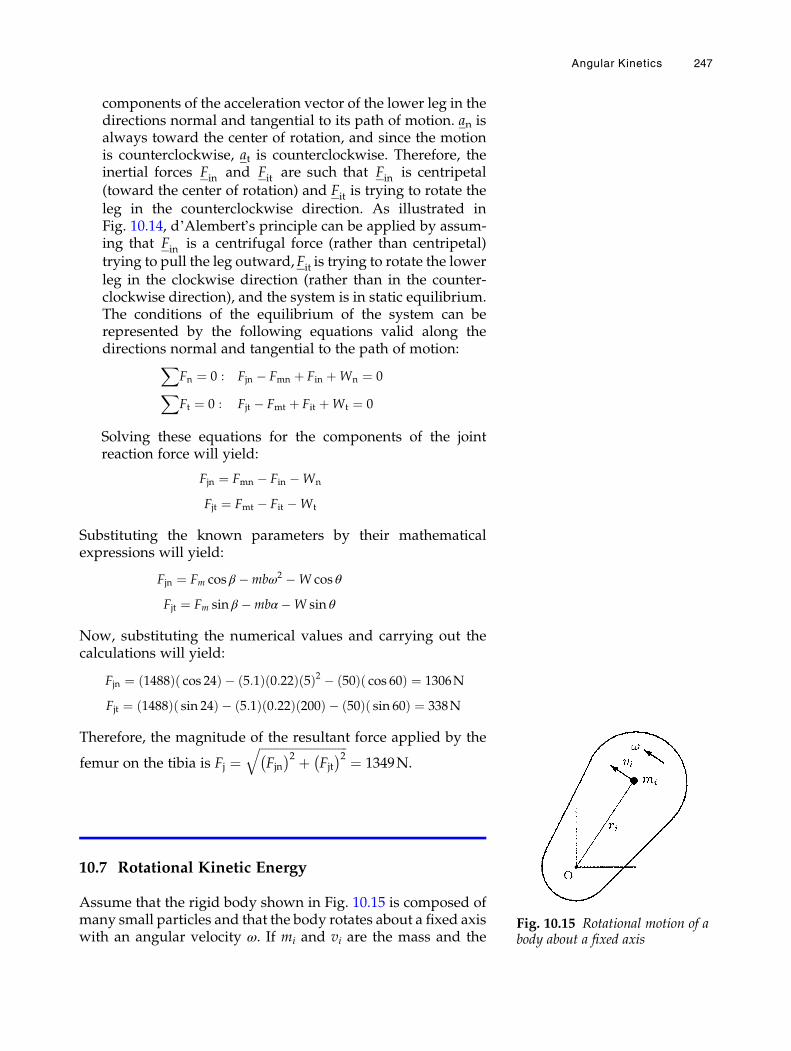
components of the acceleration vector of the lower leg in thedirections normal and tangential to its path of motion. an isalways toward the center of rotation, and since the motionis counterclockwise, at is counterclockwise. Therefore, theinertial forces Fin and Fit are such that Fin is centripetal(toward the center of rotation) and Fit is trying to rotate theleg in the counterclockwise direction. As illustrated inFig. 10.14, d’Alembert’s principle can be applied by assum-ing that Fin is a centrifugal force (rather than centripetal)trying to pull the leg outward,Fit is trying to rotate the lowerleg in the clockwise direction (rather than in the counter-clockwise direction), and the system is in static equilibrium.The conditions of the equilibrium of the system can berepresented by the following equations valid along thedirections normal and tangential to the path of motion:X
Fn ¼ 0 : Fjn � Fmn þ Fin þWn ¼ 0XFt ¼ 0 : Fjt � Fmt þ Fit þWt ¼ 0
Solving these equations for the components of the jointreaction force will yield:
Fjn ¼ Fmn � Fin �Wn
Fjt ¼ Fmt � Fit �Wt
Substituting the known parameters by their mathematicalexpressions will yield:
Fjn ¼ Fm cos β �mbω2 �W cos θ
Fjt ¼ Fm sin β �mbα�W sin θ
Now, substituting the numerical values and carrying out thecalculations will yield:
Fjn ¼ 1488ð Þ cos 24ð Þ � 5:1ð Þ 0:22ð Þ 5ð Þ2 � 50ð Þ cos 60ð Þ ¼ 1306N
Fjt ¼ 1488ð Þ sin 24ð Þ � 5:1ð Þ 0:22ð Þ 200ð Þ � 50ð Þ sin 60ð Þ ¼ 338N
Therefore, the magnitude of the resultant force applied by the
femur on the tibia is Fj ¼ffiffiffiffiffiffiffiffiffiffiffiffiffiffiffiffiffiffiffiffiffiffiffiffiffiffiffiffiffiFjn� �2 þ Fjt
� �2q¼ 1349N.
10.7 Rotational Kinetic Energy
Assume that the rigid body shown in Fig. 10.15 is composed ofmany small particles and that the body rotates about a fixed axiswith an angular velocity ω. If mi and vi are the mass and the
Fig. 10.15 Rotational motion of abody about a fixed axis
Angular Kinetics 247
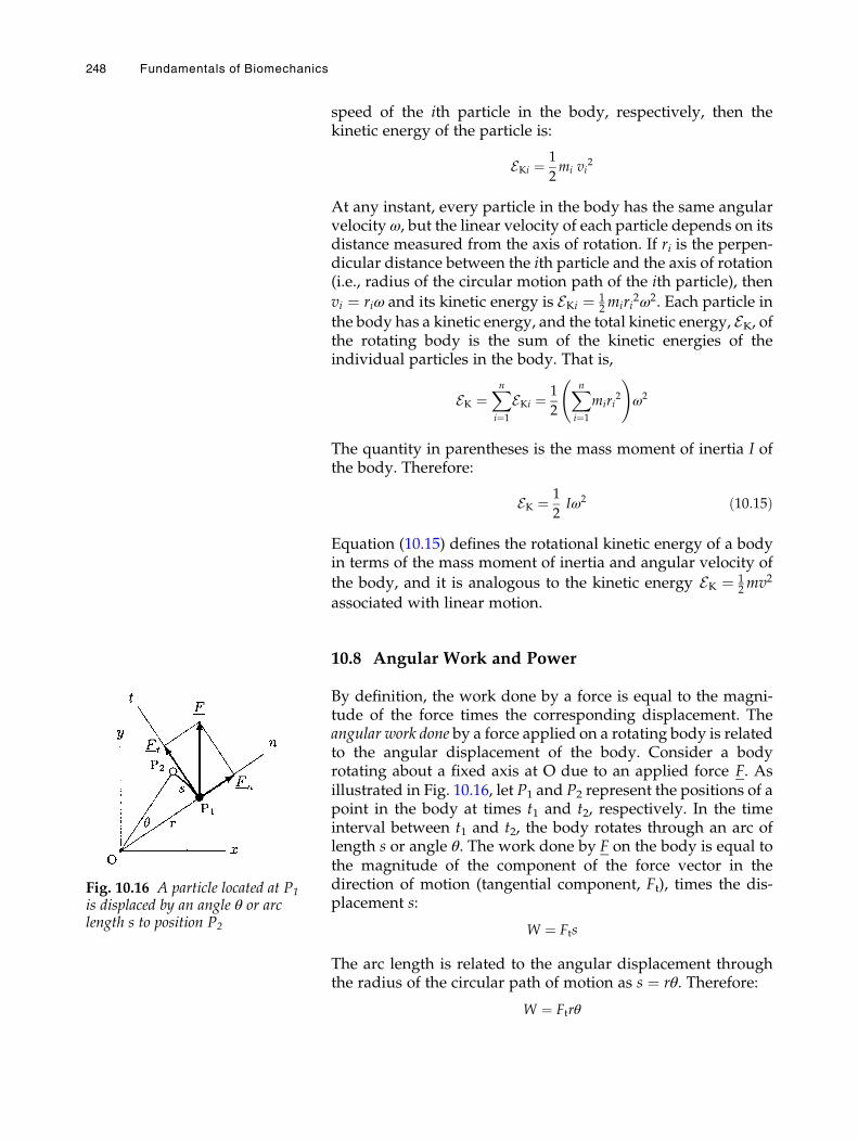
speed of the ith particle in the body, respectively, then thekinetic energy of the particle is:
EKi ¼ 1
2mi vi
2
At any instant, every particle in the body has the same angularvelocity ω, but the linear velocity of each particle depends on itsdistance measured from the axis of rotation. If ri is the perpen-dicular distance between the ith particle and the axis of rotation(i.e., radius of the circular motion path of the ith particle), then
vi ¼ riω and its kinetic energy is EKi ¼ 12miri
2ω2. Each particle in
the body has a kinetic energy, and the total kinetic energy, EK, ofthe rotating body is the sum of the kinetic energies of theindividual particles in the body. That is,
EK ¼Xni¼1
EKi ¼ 1
2
Xni¼1
miri2
!ω2
The quantity in parentheses is the mass moment of inertia I ofthe body. Therefore:
EK ¼ 1
2Iω2 ð10:15Þ
Equation (10.15) defines the rotational kinetic energy of a bodyin terms of the mass moment of inertia and angular velocity of
the body, and it is analogous to the kinetic energy EK ¼ 12mv2
associated with linear motion.
10.8 Angular Work and Power
By definition, the work done by a force is equal to the magni-tude of the force times the corresponding displacement. Theangular work done by a force applied on a rotating body is relatedto the angular displacement of the body. Consider a bodyrotating about a fixed axis at O due to an applied force F. Asillustrated in Fig. 10.16, let P1 and P2 represent the positions of apoint in the body at times t1 and t2, respectively. In the timeinterval between t1 and t2, the body rotates through an arc oflength s or angle θ. The work done by F on the body is equal tothe magnitude of the component of the force vector in thedirection of motion (tangential component, Ft), times the dis-placement s:
W ¼ Fts
The arc length is related to the angular displacement throughthe radius of the circular path of motion as s ¼ rθ. Therefore:
W ¼ Ftrθ
Fig. 10.16 A particle located at P1
is displaced by an angle θ or arclength s to position P2
248 Fundamentals of Biomechanics
By definition, Ftr is the magnitudeM of the torque generated byforce F about O. Hence:
W ¼ Mθ ð10:16Þ
In other words, the work done by a rotation-producing force isequal to the torque generated by the force times the angulardisplacement of the body. Notice that the normal (radial) com-ponent of the force vector does not work on a body undergoingrotational motion because there is no motion in the normaldirection.
It must be pointed out here that the relationship between angu-lar work done, torque, and angular displacement given inEq. (10.16) is valid when the torque is constant. The workdone by a torque, which is a function of angular displacement,on a body to rotate the body from position 1 to 2 is:
W ¼ðθ2θ1
M dθ ð10:17Þ
Here, θ1 and θ2 are the angular displacements of the body atpositions 1 and 2, respectively. Equation (10.17) can also bewritten in terms of the change in angular velocity by notingthat M ¼ Iα and α ¼ dω=dt. Using the chain rule of differentia-tion:
M ¼ Iα ¼ Idω
dt¼ I
dω
dθ
dθ
dt¼ Iω
dω
dθ
Substituting this into Eq. (10.17):
W ¼ðω2
ω1
Iω dω ¼ 1
2Iω2
2 � 1
2Iω1
2 ð10:18Þ
In Eq. (10.18), ω1 and ω2 are the angular velocities of the body atpositions 1 and 2, respectively. Equation (10.18), known as thework-energy theorem in rotational motion, states that the net angu-lar work done on a rigid body in rotating the body about a fixedaxis is equal to the change in the body’s rotational kineticenergy.
The rate at which work is done is known as power. The angularpower describes the rate at which angular work is done. For aconstant torque:
P ¼ dW
dt¼ M
dθ
dt¼ Mω ð10:19Þ
That is, the angular power is equal to the product of the appliedtorque and the angular velocity of the body.
Angular Kinetics 249
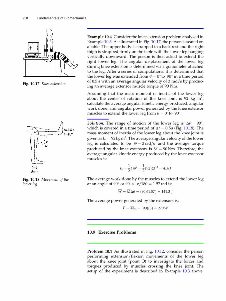
Example 10.4 Consider the knee extension problem analyzed inExample 10.3. As illustrated in Fig. 10.17, the person is seated ona table. The upper body is strapped to a back rest and the rightthigh is strapped firmly on the table with the lower leg hangingvertically downward. The person is then asked to extend theright lower leg. The angular displacement of the lower legduring knee extension is determined via a goniometer attachedto the leg. After a series of computations, it is determined thatthe lower leg was extended from θ ¼ 0� to 90� in a time periodof 0.5 s with an average angular velocity of 3 rad/s by produc-ing an average extensor muscle torque of 90 Nm.
Assuming that the mass moment of inertia of the lower legabout the center of rotation of the knee joint is 92 kg m2,calculate the average angular kinetic energy produced, angularwork done, and angular power generated by the knee extensormuscles to extend the lower leg from θ ¼ 0� to 90�.
Solution: The range of motion of the lower leg is Δθ ¼ 90�,which is covered in a time period of Δt ¼ 0:5s (Fig. 10.18). Themass moment of inertia of the lower leg about the knee joint is
given as Io ¼ 92kgm2. The average angular velocity of the lowerleg is calculated to be ω ¼ 3rad=s and the average torque
produced by the knee extensors is M ¼ 90Nm. Therefore, theaverage angular kinetic energy produced by the knee extensormuscles is:
εk ¼ 1
2Ioω
2 ¼ 1
292ð Þ 3ð Þ2 ¼ 414 J
The average work done by the muscles to extend the lower legat an angle of 90� or 90 � π=180 ¼ 1:57rad is:
W ¼ MΔθ ¼ 90ð Þ 1:57ð Þ ¼ 141:3 J
The average power generated by the extensors is:
P ¼ Mω ¼ 90ð Þ 3ð Þ ¼ 270W
10.9 Exercise Problems
Problem 10.1 As illustrated in Fig. 10.12, consider the personperforming extension/flexion movements of the lower legabout the knee joint (point O) to investigate the forces andtorques produced by muscles crossing the knee joint. Thesetup of the experiment is described in Example 10.3 above.
Fig. 10.17 Knee extension
Fig. 10.18 Movement of thelower leg
250 Fundamentals of Biomechanics
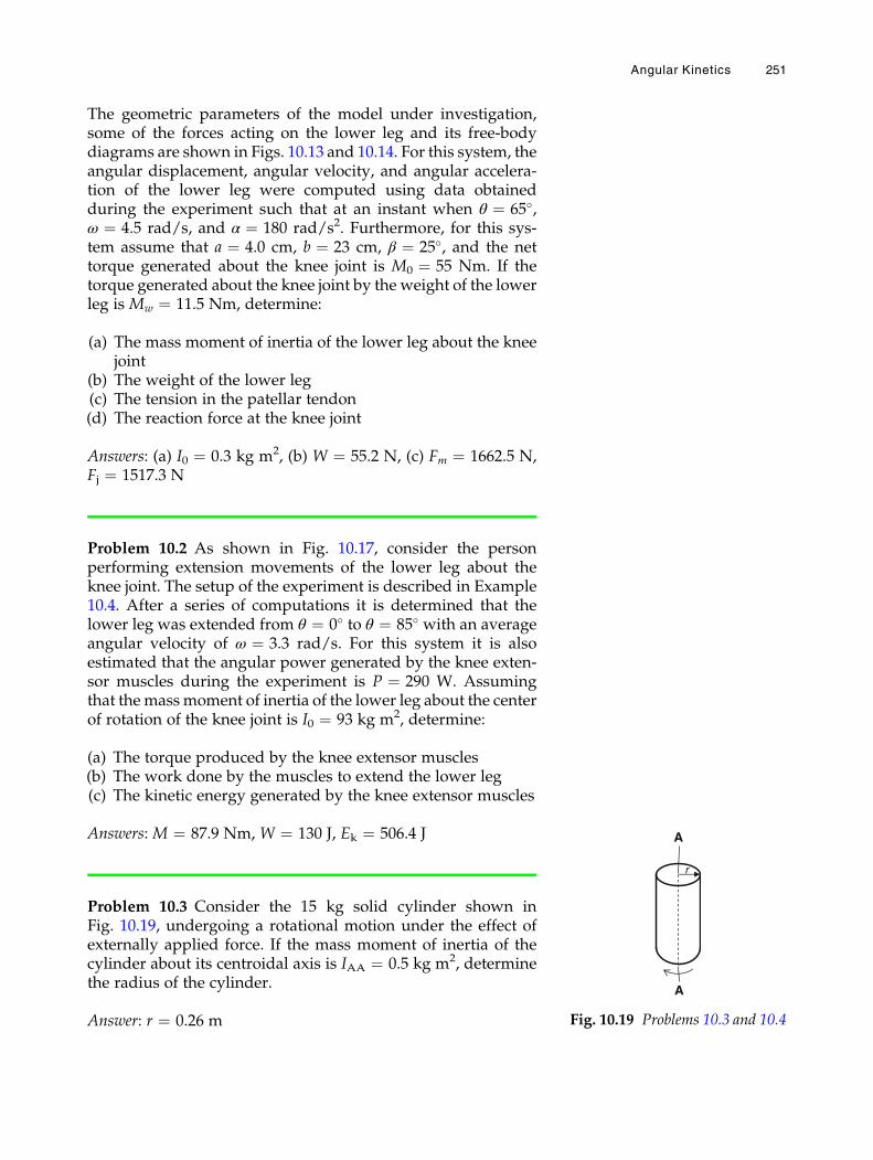
The geometric parameters of the model under investigation,some of the forces acting on the lower leg and its free-bodydiagrams are shown in Figs. 10.13 and 10.14. For this system, theangular displacement, angular velocity, and angular accelera-tion of the lower leg were computed using data obtainedduring the experiment such that at an instant when θ ¼ 65�,ω ¼ 4.5 rad/s, and α ¼ 180 rad/s2. Furthermore, for this sys-tem assume that a ¼ 4.0 cm, b ¼ 23 cm, β ¼ 25�, and the nettorque generated about the knee joint is M0 ¼ 55 Nm. If thetorque generated about the knee joint by the weight of the lowerleg is Mw ¼ 11.5 Nm, determine:
(a) The mass moment of inertia of the lower leg about the kneejoint
(b) The weight of the lower leg(c) The tension in the patellar tendon(d) The reaction force at the knee joint
Answers: (a) I0 ¼ 0.3 kg m2, (b) W ¼ 55.2 N, (c) Fm ¼ 1662.5 N,Fj ¼ 1517.3 N
Problem 10.2 As shown in Fig. 10.17, consider the personperforming extension movements of the lower leg about theknee joint. The setup of the experiment is described in Example10.4. After a series of computations it is determined that thelower leg was extended from θ ¼ 0� to θ ¼ 85� with an averageangular velocity of ω ¼ 3.3 rad/s. For this system it is alsoestimated that the angular power generated by the knee exten-sor muscles during the experiment is P ¼ 290 W. Assumingthat themassmoment of inertia of the lower leg about the centerof rotation of the knee joint is I0 ¼ 93 kg m2, determine:
(a) The torque produced by the knee extensor muscles(b) The work done by the muscles to extend the lower leg(c) The kinetic energy generated by the knee extensor muscles
Answers: M ¼ 87.9 Nm, W ¼ 130 J, Ek ¼ 506.4 J
Problem 10.3 Consider the 15 kg solid cylinder shown inFig. 10.19, undergoing a rotational motion under the effect ofexternally applied force. If the mass moment of inertia of thecylinder about its centroidal axis is IAA ¼ 0.5 kg m2, determinethe radius of the cylinder.
Answer: r ¼ 0.26 m
A
A
r
Fig. 10.19 Problems 10.3 and 10.4
Angular Kinetics 251

Problem 10.4 As shown in Fig. 10.19, consider a solid cylinderundergoing a rotational motion about its centroidal axis AAwith angular velocity of ω ¼ 3.5 rad/s. For this system it isestimated that the rotational kinetic energy of the cylinderis Ek ¼ 30 J. If the radius of the cylinder is r ¼ 0.5 m, determine:
(a) The mass moment of inertia of the cylinder about itscentroidal axis
(b) The mass of the cylinder
Answers: (a) IAA ¼ 4.9 kg m2, (b) m ¼ 19.6 kg
Problem 10.5 In Fig. 10.20, a solid cylinder is undergoing arotational motion about its centroidal axis AA. If the mass ofthe cylinder ism ¼ 12 kg and its radius is r ¼ 0.3 m, determine:
(a) The mass moment of inertia of the cylinder about thecentroidal axis
(b) Themassmoment of inertia of the cylinder about an axis DDwhich is located at a distance rc ¼ 0.2 m parallel to thecentroidal axis
Answers: (a) IAA ¼ 0.54 kg m2, (b) IDD ¼ 1.02 kg m2
A
rc
A
r
D
D
C 90°
Fig. 10.20 Problem 10.5
252 Fundamentals of Biomechanics
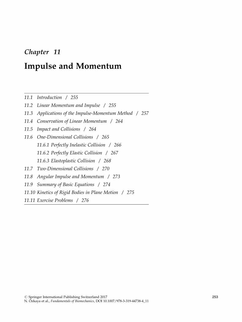
Chapter 11
Impulse and Momentum
11.1 Introduction / 255
11.2 Linear Momentum and Impulse / 255
11.3 Applications of the Impulse-Momentum Method / 257
11.4 Conservation of Linear Momentum / 264
11.5 Impact and Collisions / 264
11.6 One-Dimensional Collisions / 265
11.6.1 Perfectly Inelastic Collision / 266
11.6.2 Perfectly Elastic Collision / 267
11.6.3 Elastoplastic Collision / 268
11.7 Two-Dimensional Collisions / 270
11.8 Angular Impulse and Momentum / 273
11.9 Summary of Basic Equations / 274
11.10 Kinetics of Rigid Bodies in Plane Motion / 275
11.11 Exercise Problems / 276
# Springer International Publishing Switzerland 2017N. Ozkaya et al., Fundamentals of Biomechanics, DOI 10.1007/978-3-319-44738-4_11
253

11.1 Introduction
In Chap. 8, Newton’s second law of motion is presented in theform of “equations of motion.” In Chap. 10, the concepts ofwork and energy are introduced. Based on the same law,“work-energy” and “conservation of energy” methods aredevised to facilitate the solutions of specific problems in kinetics.In this chapter, the concepts of linear momentum and impulsewill be defined. Newton’s second law of motion will bereformulated to introduce other methods for kinetic analysesbased on the “impulse-momentum theorem” and the principleof “conservation of linear momentum.” These methods willthen be applied to analyze the impact and collision of bodies.
11.2 Linear Momentum and Impulse
Consider an object with massm acted upon by an external forceF. Let a be the acceleration of the object under the action of theapplied force. The relationship between F, m, and a is describedby the equation of motion in the following vector form:
F ¼ ma ð11:1Þ
By definition, acceleration is the time rate of change of velocity.If the mass of the object is constant, then Eq. (11.1) can bewritten as:
F ¼ d
dtmv� � ð11:2Þ
The vector mv is called the linear momentum (or simply themomentum) of the object, and is denoted by p:
p ¼ mv ð11:3Þ
Momentum is a vector quantity. The line of action and directionof the momentum vector is the same as the velocity vector of theobject. The magnitude of the momentum is equal to the productof the mass and the speed of the object.
The equation of motion can now be expressed in terms ofmomentum by substituting Eq. (11.3) into Eq. (11.2):
F ¼dp
dtð11:4Þ
If there is more than one force acting on the object, then F inEq. (11.4) must be replaced by the vector sum of all forces (theresultant force) acting on the object. Equation (11.4) states thatthe time rate of change of momentum of an object is equal to theresultant force acting on the object.
Impulse and Momentum 255
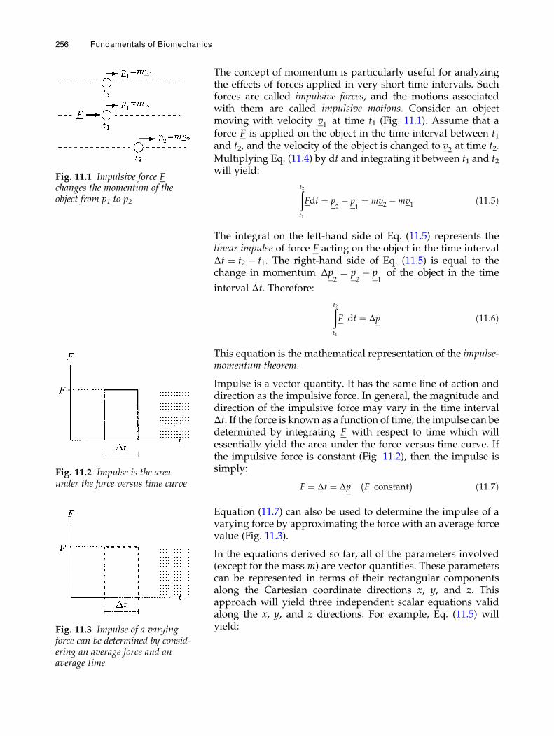
The concept of momentum is particularly useful for analyzingthe effects of forces applied in very short time intervals. Suchforces are called impulsive forces, and the motions associatedwith them are called impulsive motions. Consider an objectmoving with velocity v1 at time t1 (Fig. 11.1). Assume that aforce F is applied on the object in the time interval between t1and t2, and the velocity of the object is changed to v2 at time t2.Multiplying Eq. (11.4) by dt and integrating it between t1 and t2will yield:
ðt2t1
Fdt ¼ p2� p
1¼ mv2 �mv1 ð11:5Þ
The integral on the left-hand side of Eq. (11.5) represents thelinear impulse of force F acting on the object in the time intervalΔt ¼ t2 � t1. The right-hand side of Eq. (11.5) is equal to thechange in momentum Δp
2¼ p
2� p
1of the object in the time
interval Δt. Therefore:
ðt2t1
F dt ¼ Δp ð11:6Þ
This equation is the mathematical representation of the impulse-momentum theorem.
Impulse is a vector quantity. It has the same line of action anddirection as the impulsive force. In general, the magnitude anddirection of the impulsive force may vary in the time intervalΔt. If the force is known as a function of time, the impulse can bedetermined by integrating F with respect to time which willessentially yield the area under the force versus time curve. Ifthe impulsive force is constant (Fig. 11.2), then the impulse issimply:
F ¼ Δt ¼ Δp F constant� � ð11:7Þ
Equation (11.7) can also be used to determine the impulse of avarying force by approximating the force with an average forcevalue (Fig. 11.3).
In the equations derived so far, all of the parameters involved(except for the mass m) are vector quantities. These parameterscan be represented in terms of their rectangular componentsalong the Cartesian coordinate directions x, y, and z. Thisapproach will yield three independent scalar equations validalong the x, y, and z directions. For example, Eq. (11.5) willyield:
Fig. 11.2 Impulse is the areaunder the force versus time curve
Fig. 11.1 Impulsive force Fchanges the momentum of theobject from p1 to p2
Fig. 11.3 Impulse of a varyingforce can be determined by consid-ering an average force and anaverage time
256 Fundamentals of Biomechanics
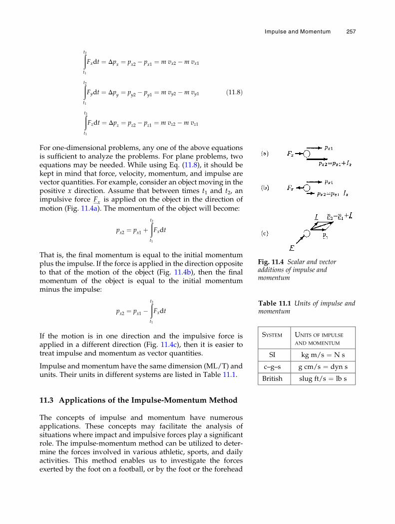
ðt2t1
Fxdt ¼ Δpx ¼ px2 � px1 ¼ m vx2 �m vx1
ðt2t1
Fydt ¼ Δpy ¼ py2 � py1 ¼ m vy2 �m vy1 ð11:8Þ
ðt2t1
Fzdt ¼ Δpz ¼ pz2 � pz1 ¼ m vz2 �m vz1
For one-dimensional problems, any one of the above equationsis sufficient to analyze the problems. For plane problems, twoequations may be needed. While using Eq. (11.8), it should bekept in mind that force, velocity, momentum, and impulse arevector quantities. For example, consider an object moving in thepositive x direction. Assume that between times t1 and t2, animpulsive force Fx is applied on the object in the direction ofmotion (Fig. 11.4a). The momentum of the object will become:
px2 ¼ px1 þðt2t1
Fxdt
That is, the final momentum is equal to the initial momentumplus the impulse. If the force is applied in the direction oppositeto that of the motion of the object (Fig. 11.4b), then the finalmomentum of the object is equal to the initial momentumminus the impulse:
px2 ¼ px1 �ðt2t1
Fxdt
If the motion is in one direction and the impulsive force isapplied in a different direction (Fig. 11.4c), then it is easier totreat impulse and momentum as vector quantities.
Impulse and momentum have the same dimension (ML/T) andunits. Their units in different systems are listed in Table 11.1.
11.3 Applications of the Impulse-Momentum Method
The concepts of impulse and momentum have numerousapplications. These concepts may facilitate the analysis ofsituations where impact and impulsive forces play a significantrole. The impulse-momentum method can be utilized to deter-mine the forces involved in various athletic, sports, and dailyactivities. This method enables us to investigate the forcesexerted by the foot on a football, or by the foot or the forehead
Table 11.1 Units of impulse andmomentum
SYSTEM UNITS OF IMPULSE
AND MOMENTUM
SI kg m/s ¼ N s
c–g–s g cm/s ¼ dyn s
British slug ft/s ¼ lb s
Fig. 11.4 Scalar and vectoradditions of impulse andmomentum
Impulse and Momentum 257
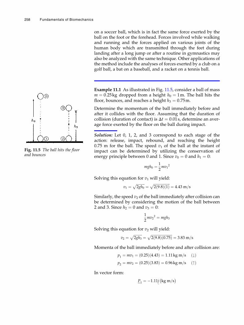
on a soccer ball, which is in fact the same force exerted by theball on the foot or the forehead. Forces involved while walkingand running and the forces applied on various joints of thehuman body which are transmitted through the feet duringlanding after a long jump or after a routine in gymnastics mayalso be analyzed with the same technique. Other applications ofthe method include the analyses of forces exerted by a club on agolf ball, a bat on a baseball, and a racket on a tennis ball.
Example 11.1 As illustrated in Fig. 11.5, consider a ball of massm ¼ 0:25kg dropped from a height h0 ¼ 1m. The ball hits thefloor, bounces, and reaches a height h3 ¼ 0:75m.
Determine the momentum of the ball immediately before andafter it collides with the floor. Assuming that the duration ofcollision (duration of contact) is Δt ¼ 0:01s, determine an aver-age force exerted by the floor on the ball during impact.
Solution: Let 0, 1, 2, and 3 correspond to each stage of theaction: release, impact, rebound, and reaching the height0.75 m for the ball. The speed v1 of the ball at the instant ofimpact can be determined by utilizing the conservation ofenergy principle between 0 and 1. Since v0 ¼ 0 and h1 ¼ 0:
mgh0 ¼ 1
2mv1
2
Solving this equation for v1 will yield:
v1 ¼ffiffiffiffiffiffiffiffiffiffi2gh0
p¼
ffiffiffiffiffiffiffiffiffiffiffiffiffiffiffiffiffiffiffi2 9:8ð Þ 1ð Þ
p¼ 4:43 m=s
Similarly, the speed v2 of the ball immediately after collision canbe determined by considering the motion of the ball between2 and 3. Since h2 ¼ 0 and v3 ¼ 0:
1
2mv2
2 ¼ mgh3
Solving this equation for v2 will yield:
v2 ¼ffiffiffiffiffiffiffiffiffiffi2gh3
p¼
ffiffiffiffiffiffiffiffiffiffiffiffiffiffiffiffiffiffiffiffiffiffiffiffiffi2 9:8ð Þ 0:75ð Þ
p¼ 3:83 m=s
Momenta of the ball immediately before and after collision are:
p1 ¼ mv1 ¼ 0:25ð Þ 4:43ð Þ ¼ 1:11kg m=s #ð Þp2 ¼ mv2 ¼ 0:25ð Þ 3:83ð Þ ¼ 0:96kg m=s "ð Þ
In vector form:
P1 ¼ �1:11j kg m=s� �
Fig. 11.5 The ball hits the floorand bounces
258 Fundamentals of Biomechanics
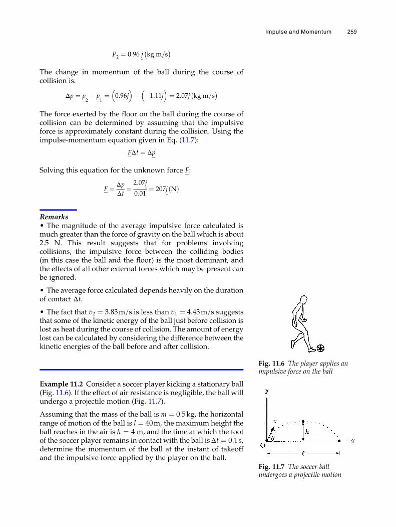
P2 ¼ 0:96 j kg m=s� �
The change in momentum of the ball during the course ofcollision is:
Δp ¼ p2� p
1¼ 0:96j
� �� �1:11j� �
¼ 2:07j kg m=s� �
The force exerted by the floor on the ball during the course ofcollision can be determined by assuming that the impulsiveforce is approximately constant during the collision. Using theimpulse-momentum equation given in Eq. (11.7):
FΔt ¼ Δp
Solving this equation for the unknown force F:
F ¼ ΔpΔt
¼2:07j
0:01¼ 207j Nð Þ
Remarks• The magnitude of the average impulsive force calculated ismuch greater than the force of gravity on the ball which is about2.5 N. This result suggests that for problems involvingcollisions, the impulsive force between the colliding bodies(in this case the ball and the floor) is the most dominant, andthe effects of all other external forces which may be present canbe ignored.
• The average force calculated depends heavily on the durationof contact Δt.
• The fact that v2 ¼ 3:83m=s is less than v1 ¼ 4:43m=s suggeststhat some of the kinetic energy of the ball just before collision islost as heat during the course of collision. The amount of energylost can be calculated by considering the difference between thekinetic energies of the ball before and after collision.
Example 11.2 Consider a soccer player kicking a stationary ball(Fig. 11.6). If the effect of air resistance is negligible, the ball willundergo a projectile motion (Fig. 11.7).
Assuming that the mass of the ball is m ¼ 0:5kg, the horizontalrange of motion of the ball is l ¼ 40m, the maximum height theball reaches in the air is h ¼ 4 m, and the time at which the footof the soccer player remains in contact with the ball isΔt ¼ 0:1s,determine the momentum of the ball at the instant of takeoffand the impulsive force applied by the player on the ball.
Fig. 11.6 The player applies animpulsive force on the ball
Fig. 11.7 The soccer ballundergoes a projectile motion
Impulse and Momentum 259
Solution: To determine the momentum of the ball at the instantof takeoff, we need to calculate the takeoff speed of the ball andits angle of takeoff first. For this purpose, we can utilize theformulas given in Sect. 7.10. The angle of takeoff is provided inEq. (7.35) in terms of the maximum height and horizontal rangeof motion of the projectile motion in the following form:
θ ¼ arc tan4h
l
� �
Substituting the numerical values of h ¼ 4m and l ¼ 40m intothe above equation, and carrying out the calculations will yield:
θ ¼ arc tan4 4ð Þ40
¼ 21:8�
Using Eq. (8.40), the speed of takeoff can also be determined:
v ¼ffiffiffiffiffiffiffiffi2gh
psin θ
¼ffiffiffiffiffiffiffiffiffiffiffiffiffiffiffiffiffiffiffi2 9:8ð Þ 4ð Þpsin 21:8�
¼ 23:8m=s
The velocity of takeoff v has components both in the x andy directions with magnitudes:
vx ¼ v cos θ ¼ 23:8ð Þ cos 21:8�ð Þ ¼ 22:1m=s !ð Þvy ¼ v sin θ ¼ 23:8ð Þ sin 21:8�ð Þ ¼ 8:8m=s "ð Þ
Therefore, the takeoff velocity of the ball in vector form is:
v ¼ 22:1iþ 8:8j m=sð Þ
The momentum of the soccer ball at the instant of takeoff(immediately after impact) can be determined as:
p ¼ mv ¼ 0:5 22:1iþ 8:8j� �
¼ 11:1iþ 4:4j kg �m=s� �
The ball is stationary and its momentum is zero immediatelybefore the soccer player kicks the ball. Therefore, the change inmomentum of the ball during the course of contact with theplayer’s foot is equal to its takeoff momentum. The impulse-momentum equation [Eq. (11.7)] can now be utilized to deter-mine an average impulsive force exerted by the soccer player onthe ball:
F ¼ ΔpΔt
¼11:1iþ 4:4j
0:1¼ 111iþ 44j Nð Þ
Therefore, the net or the resultant force applied on the ball bythe player is:
F ¼ffiffiffiffiffiffiffiffiffiffiffiffiffiffiffiffiffiffiffiffiffiffiffiffiffiffiffiffiffiffi111ð Þ2 þ 44ð Þ2
q¼ 119:4N
260 Fundamentals of Biomechanics
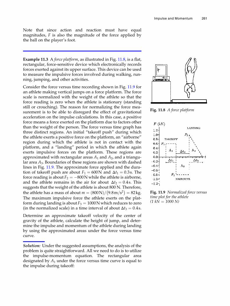
Note that since action and reaction must have equalmagnitudes, F is also the magnitude of the force applied bythe ball on the player’s foot.
Example 11.3 A force platform, as illustrated in Fig. 11.8, is a flat,rectangular, force-sensitive device which electronically recordsforces exerted against its upper surface. This device can be usedto measure the impulsive forces involved during walking, run-ning, jumping, and other activities.
Consider the force versus time recording shown in Fig. 11.9 foran athlete making vertical jumps on a force platform. The forcescale is normalized with the weight of the athlete so that theforce reading is zero when the athlete is stationary (standingstill or crouching). The reason for normalizing the force mea-surement is to be able to disregard the effect of gravitationalacceleration on the impulse calculations. In this case, a positiveforce means a force exerted on the platform due to factors otherthan the weight of the person. The force versus time graph hasthree distinct regions. An initial “takeoff push” during whichthe athlete exerts a positive force on the platform, an “airborne”region during which the athlete is not in contact with theplatform, and a “landing” period in which the athlete againexerts impulsive forces on the platform. These regions areapproximated with rectangular areas A1 and A2, and a triangu-lar area A3. Boundaries of these regions are shown with dashedlines in Fig. 11.9. The approximate force applied and the dura-tion of takeoff push are about F1 ¼ 600N and Δt1 ¼ 0:3s. Theforce reading is about F2 ¼ �800Nwhile the athlete is airborne,and the athlete remains in the air for about Δt2 ¼ 0:4s. Thissuggests that the weight of the athlete is about 800 N. Therefore,
the athlete has a mass of about m ¼ 800Nð Þ= 9:8m=s2� � ¼ 82kg.
The maximum impulsive force the athlete exerts on the plat-form during landing is about F3 ¼ 1000Nwhich reduces to zero(in the normalized scale) in a time interval of about Δt3 ¼ 0:4s.
Determine an approximate takeoff velocity of the center ofgravity of the athlete, calculate the height of jump, and deter-mine the impulse and momentum of the athlete during landingby using the approximated areas under the force versus timecurve.
Solution: Under the suggested assumptions, the analysis of theproblem is quite straightforward. All we need to do is to utilizethe impulse-momentum equation. The rectangular areadesignated by A1 under the force versus time curve is equal tothe impulse during takeoff:
Fig. 11.8 A force platform
Fig. 11.9 Normalized force versustime plot for the athlete(1 kN ¼ 1000 N)
Impulse and Momentum 261
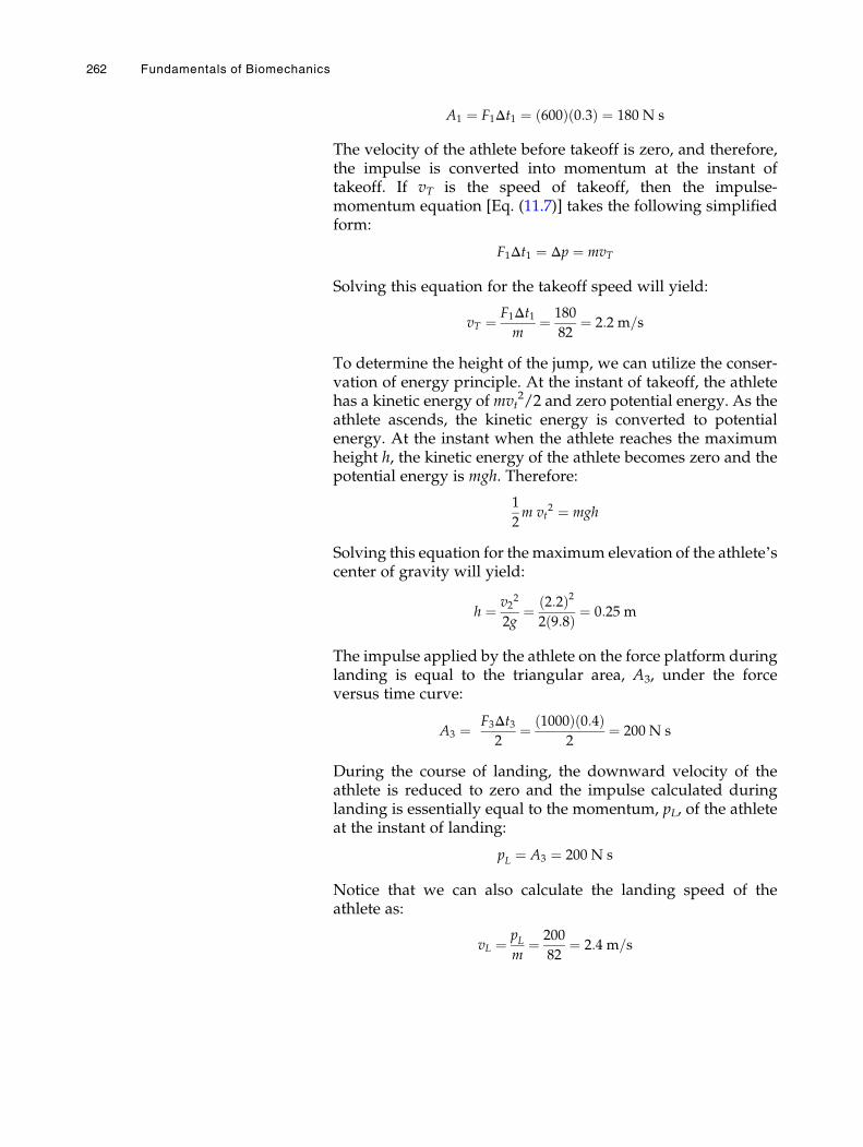
A1 ¼ F1Δt1 ¼ 600ð Þ 0:3ð Þ ¼ 180 N s
The velocity of the athlete before takeoff is zero, and therefore,the impulse is converted into momentum at the instant oftakeoff. If vT is the speed of takeoff, then the impulse-momentum equation [Eq. (11.7)] takes the following simplifiedform:
F1Δt1 ¼ Δp ¼ mvT
Solving this equation for the takeoff speed will yield:
vT ¼ F1Δt1m
¼ 180
82¼ 2:2 m=s
To determine the height of the jump, we can utilize the conser-vation of energy principle. At the instant of takeoff, the athletehas a kinetic energy of mvt
2/2 and zero potential energy. As theathlete ascends, the kinetic energy is converted to potentialenergy. At the instant when the athlete reaches the maximumheight h, the kinetic energy of the athlete becomes zero and thepotential energy is mgh. Therefore:
1
2m vt
2 ¼ mgh
Solving this equation for themaximum elevation of the athlete’scenter of gravity will yield:
h ¼ v22
2g¼ 2:2ð Þ2
2 9:8ð Þ ¼ 0:25 m
The impulse applied by the athlete on the force platform duringlanding is equal to the triangular area, A3, under the forceversus time curve:
A3 ¼ F3Δt32
¼ 1000ð Þ 0:4ð Þ2
¼ 200 N s
During the course of landing, the downward velocity of theathlete is reduced to zero and the impulse calculated duringlanding is essentially equal to the momentum, pL, of the athleteat the instant of landing:
pL ¼ A3 ¼ 200 N s
Notice that we can also calculate the landing speed of theathlete as:
vL ¼ pLm
¼ 200
82¼ 2:4 m=s
262 Fundamentals of Biomechanics
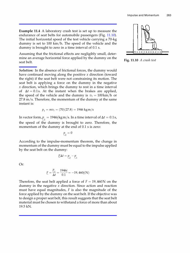
Example 11.4 A laboratory crash test is set up to measure theendurance of seat belts for automobile passengers (Fig. 11.10).The initial horizontal speed of the test vehicle carrying a 70-kgdummy is set to 100 km/h. The speed of the vehicle and thedummy is brought to zero in a time interval of 0.1 s.
Assuming that the frictional effects are negligibly small, deter-mine an average horizontal force applied by the dummy on theseat belt.
Solution: In the absence of frictional forces, the dummy wouldhave continued moving along the positive x direction (towardthe right) if the seat belt were not constraining its motion. Theseat belt is applying a force on the dummy in the negativex direction, which brings the dummy to rest in a time intervalof Δt ¼ 0:1s. At the instant when the brakes are applied,the speed of the vehicle and the dummy is v1 ¼ 100km=h or27.8 m/s. Therefore, the momentum of the dummy at the sameinstant is:
p1 ¼ mv1 ¼ 70ð Þ 27:8ð Þ ¼ 1946 kgm=s
In vector form, p1¼ 1946ikgm=s. In a time interval ofΔt ¼ 0:1s,
the speed of the dummy is brought to zero. Therefore, themomentum of the dummy at the end of 0.1 s is zero:
p2¼ 0
According to the impulse-momentum theorem, the change inmomentum of the dummymust be equal to the impulse appliedby the seat belt on the dummy:
FΔt ¼ p2� p
1
Or:
F ¼p1
Δt¼ 1946i
0:1¼ �19, 460i Nð Þ
Therefore, the seat belt applied a force of F ¼ 19, 460N on thedummy in the negative x direction. Since action and reactionmust have equal magnitudes, F is also the magnitude of theforce applied by the dummy on the seat belt. If the objective wasto design a proper seat belt, this result suggests that the seat beltmaterial must be chosen to withstand a force of more than about19.5 kN.
Fig. 11.10 A crash test
Impulse and Momentum 263
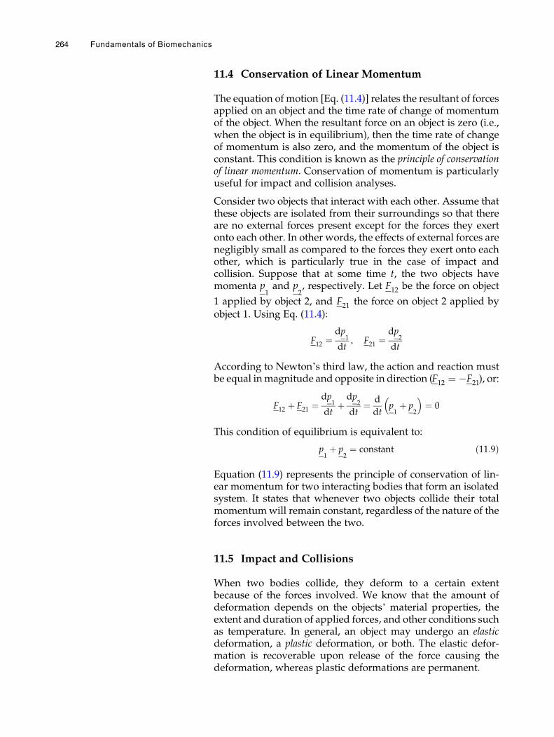
11.4 Conservation of Linear Momentum
The equation of motion [Eq. (11.4)] relates the resultant of forcesapplied on an object and the time rate of change of momentumof the object. When the resultant force on an object is zero (i.e.,when the object is in equilibrium), then the time rate of changeof momentum is also zero, and the momentum of the object isconstant. This condition is known as the principle of conservationof linear momentum. Conservation of momentum is particularlyuseful for impact and collision analyses.
Consider two objects that interact with each other. Assume thatthese objects are isolated from their surroundings so that thereare no external forces present except for the forces they exertonto each other. In other words, the effects of external forces arenegligibly small as compared to the forces they exert onto eachother, which is particularly true in the case of impact andcollision. Suppose that at some time t, the two objects havemomenta p
1and p
2, respectively. Let F12 be the force on object
1 applied by object 2, and F21 the force on object 2 applied byobject 1. Using Eq. (11.4):
F12 ¼dp
1
dt, F21 ¼
dp2
dt
According to Newton’s third law, the action and reaction mustbe equal inmagnitude and opposite in direction (F12 ¼ �F21), or:
F12 þ F21 ¼dp
1
dtþdp
2
dt¼ d
dtp1þ p
2
� �¼ 0
This condition of equilibrium is equivalent to:
p1þ p
2¼ constant ð11:9Þ
Equation (11.9) represents the principle of conservation of lin-ear momentum for two interacting bodies that form an isolatedsystem. It states that whenever two objects collide their totalmomentumwill remain constant, regardless of the nature of theforces involved between the two.
11.5 Impact and Collisions
When two bodies collide, they deform to a certain extentbecause of the forces involved. We know that the amount ofdeformation depends on the objects’ material properties, theextent and duration of applied forces, and other conditions suchas temperature. In general, an object may undergo an elasticdeformation, a plastic deformation, or both. The elastic defor-mation is recoverable upon release of the force causing thedeformation, whereas plastic deformations are permanent.
264 Fundamentals of Biomechanics
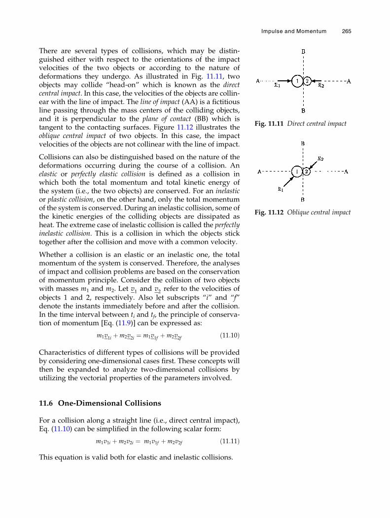
There are several types of collisions, which may be distin-guished either with respect to the orientations of the impactvelocities of the two objects or according to the nature ofdeformations they undergo. As illustrated in Fig. 11.11, twoobjects may collide “head-on” which is known as the directcentral impact. In this case, the velocities of the objects are collin-ear with the line of impact. The line of impact (AA) is a fictitiousline passing through the mass centers of the colliding objects,and it is perpendicular to the plane of contact (BB) which istangent to the contacting surfaces. Figure 11.12 illustrates theoblique central impact of two objects. In this case, the impactvelocities of the objects are not collinear with the line of impact.
Collisions can also be distinguished based on the nature of thedeformations occurring during the course of a collision. Anelastic or perfectly elastic collision is defined as a collision inwhich both the total momentum and total kinetic energy ofthe system (i.e., the two objects) are conserved. For an inelasticor plastic collision, on the other hand, only the total momentumof the system is conserved. During an inelastic collision, some ofthe kinetic energies of the colliding objects are dissipated asheat. The extreme case of inelastic collision is called the perfectlyinelastic collision. This is a collision in which the objects sticktogether after the collision and move with a common velocity.
Whether a collision is an elastic or an inelastic one, the totalmomentum of the system is conserved. Therefore, the analysesof impact and collision problems are based on the conservationof momentum principle. Consider the collision of two objectswith masses m1 and m2. Let v1 and v2 refer to the velocities ofobjects 1 and 2, respectively. Also let subscripts “i” and “f”denote the instants immediately before and after the collision.In the time interval between ti and tf, the principle of conserva-tion of momentum [Eq. (11.9)] can be expressed as:
m1v1i þm2v2i ¼ m1v1f þm2v2f ð11:10Þ
Characteristics of different types of collisions will be providedby considering one-dimensional cases first. These concepts willthen be expanded to analyze two-dimensional collisions byutilizing the vectorial properties of the parameters involved.
11.6 One-Dimensional Collisions
For a collision along a straight line (i.e., direct central impact),Eq. (11.10) can be simplified in the following scalar form:
m1v1i þm2v2i ¼ m1v1f þm2v2f ð11:11Þ
This equation is valid both for elastic and inelastic collisions.
Fig. 11.11 Direct central impact
Fig. 11.12 Oblique central impact
Impulse and Momentum 265
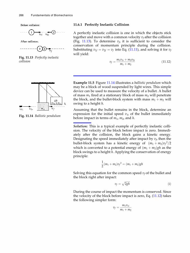
11.6.1 Perfectly Inelastic Collision
A perfectly inelastic collision is one in which the objects sticktogether and move with a common velocity vf after the collision(Fig. 11.13). To determine vf, it is sufficient to consider theconservation of momentum principle during the collision.Substituting v1f ¼ v2f ¼ vf into Eq. (11.11), and solving it for vfwill yield:
vf ¼ m1v1i þm2v2im1 þm2
ð11:12Þ
Example 11.5 Figure 11.14 illustrates a ballistic pendulum whichmay be a block of wood suspended by light wires. This simpledevice can be used to measure the velocity of a bullet. A bulletof mass m1 fired at a stationary block of mass m2 will penetratethe block, and the bullet-block system with mass m1 þm2 willswing to a height h.
Assuming that the bullet remains in the block, determine anexpression for the initial speed v1i of the bullet immediatelybefore impact in terms of m1, m2, and h.
Solution: This is a typical example of perfectly inelastic colli-sion. The velocity of the block before impact is zero. Immedi-ately after the collision, the block gains a kinetic energy.Designating the speed immediately after impact by vf, then the
bullet-block system has a kinetic energy of m1 þm2ð Þvf 2=2which is converted to a potential energy of m1 þm2ð Þgh as theblock swings to a height h. Applying the conservation of energyprinciple:
1
2m1 þm2ð Þvf 2 ¼ m1 þm2ð Þgh
Solving this equation for the common speed vf of the bullet andthe block right after impact:
vf ¼ffiffiffiffiffiffiffiffi2gh
pðiÞ
During the course of impact the momentum is conserved. Sincethe velocity of the block before impact is zero, Eq. (11.12) takesthe following simpler form:
vf ¼ m1v1im1 þm2
Fig. 11.13 Perfectly inelasticcollision
Fig. 11.14 Ballistic pendulum
266 Fundamentals of Biomechanics
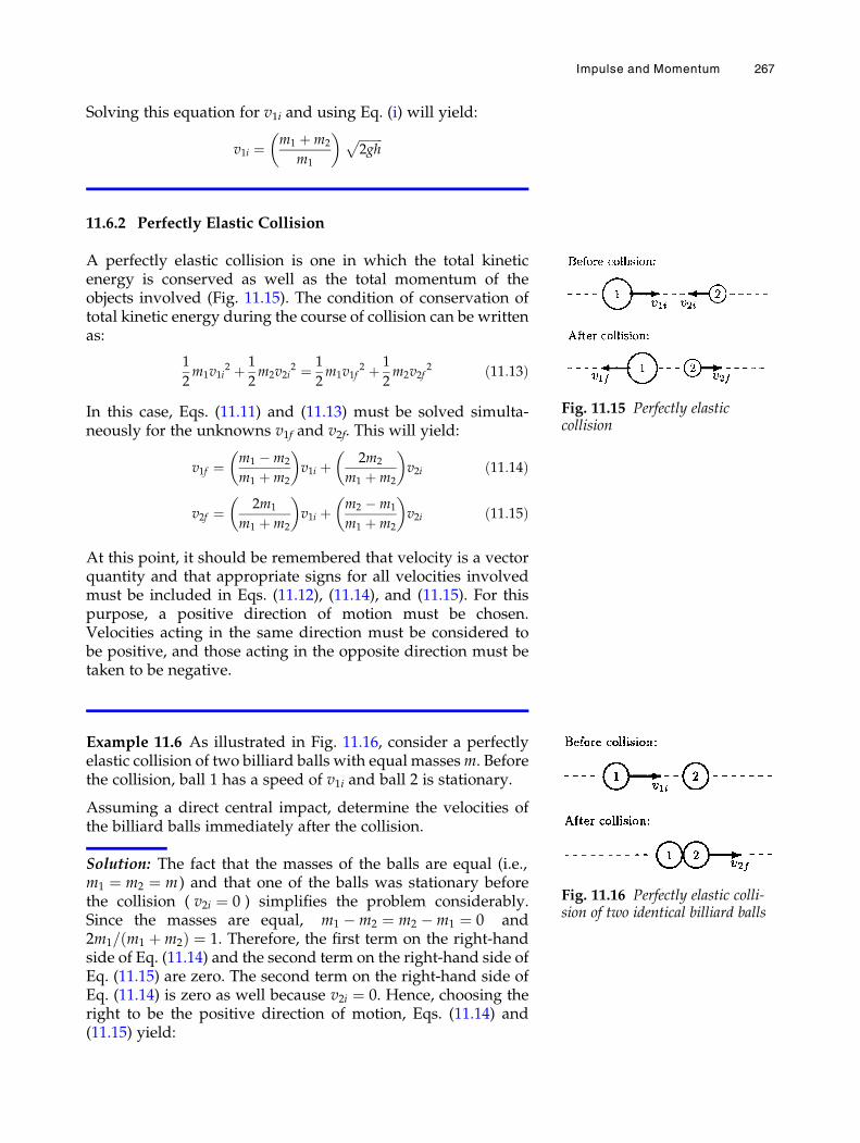
Solving this equation for v1i and using Eq. (i) will yield:
v1i ¼ m1 þm2
m1
� � ffiffiffiffiffiffiffiffi2gh
p
11.6.2 Perfectly Elastic Collision
A perfectly elastic collision is one in which the total kineticenergy is conserved as well as the total momentum of theobjects involved (Fig. 11.15). The condition of conservation oftotal kinetic energy during the course of collision can be writtenas:
1
2m1v1i
2 þ 1
2m2v2i
2 ¼ 1
2m1v1f
2 þ 1
2m2v2f
2 ð11:13Þ
In this case, Eqs. (11.11) and (11.13) must be solved simulta-neously for the unknowns v1f and v2f. This will yield:
v1f ¼ m1 �m2
m1 þm2
� �v1i þ 2m2
m1 þm2
� �v2i ð11:14Þ
v2f ¼ 2m1
m1 þm2
� �v1i þ m2 �m1
m1 þm2
� �v2i ð11:15Þ
At this point, it should be remembered that velocity is a vectorquantity and that appropriate signs for all velocities involvedmust be included in Eqs. (11.12), (11.14), and (11.15). For thispurpose, a positive direction of motion must be chosen.Velocities acting in the same direction must be considered tobe positive, and those acting in the opposite direction must betaken to be negative.
Example 11.6 As illustrated in Fig. 11.16, consider a perfectlyelastic collision of two billiard balls with equal massesm. Beforethe collision, ball 1 has a speed of v1i and ball 2 is stationary.
Assuming a direct central impact, determine the velocities ofthe billiard balls immediately after the collision.
Solution: The fact that the masses of the balls are equal (i.e.,m1 ¼ m2 ¼ m) and that one of the balls was stationary beforethe collision ( v2i ¼ 0 ) simplifies the problem considerably.Since the masses are equal, m1 �m2 ¼ m2 �m1 ¼ 0 and2m1= m1 þm2ð Þ ¼ 1. Therefore, the first term on the right-handside of Eq. (11.14) and the second term on the right-hand side ofEq. (11.15) are zero. The second term on the right-hand side ofEq. (11.14) is zero as well because v2i ¼ 0. Hence, choosing theright to be the positive direction of motion, Eqs. (11.14) and(11.15) yield:
Fig. 11.15 Perfectly elasticcollision
Fig. 11.16 Perfectly elastic colli-sion of two identical billiard balls
Impulse and Momentum 267
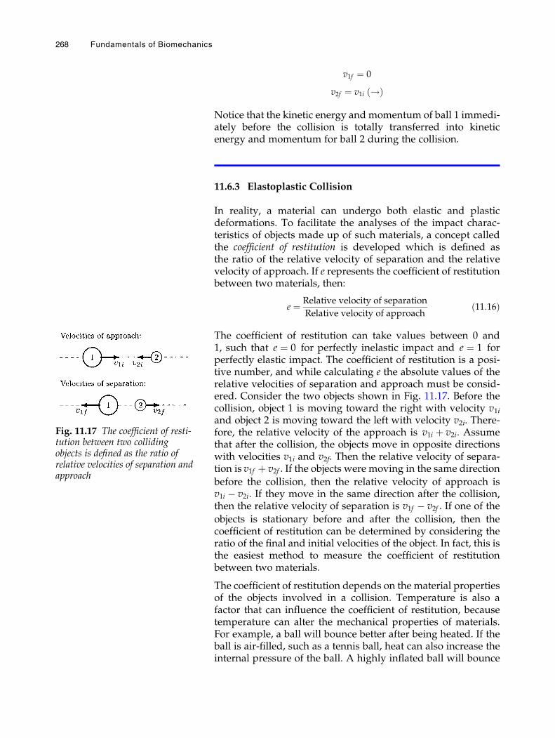
v1f ¼ 0
v2f ¼ v1i !ð Þ
Notice that the kinetic energy and momentum of ball 1 immedi-ately before the collision is totally transferred into kineticenergy and momentum for ball 2 during the collision.
11.6.3 Elastoplastic Collision
In reality, a material can undergo both elastic and plasticdeformations. To facilitate the analyses of the impact charac-teristics of objects made up of such materials, a concept calledthe coefficient of restitution is developed which is defined asthe ratio of the relative velocity of separation and the relativevelocity of approach. If e represents the coefficient of restitutionbetween two materials, then:
e ¼ Relative velocity of separation
Relative velocity of approachð11:16Þ
The coefficient of restitution can take values between 0 and1, such that e ¼ 0 for perfectly inelastic impact and e ¼ 1 forperfectly elastic impact. The coefficient of restitution is a posi-tive number, and while calculating e the absolute values of therelative velocities of separation and approach must be consid-ered. Consider the two objects shown in Fig. 11.17. Before thecollision, object 1 is moving toward the right with velocity v1iand object 2 is moving toward the left with velocity v2i. There-fore, the relative velocity of the approach is v1i þ v2i. Assumethat after the collision, the objects move in opposite directionswith velocities v1i and v2f. Then the relative velocity of separa-tion is v1f þ v2f . If the objects were moving in the same direction
before the collision, then the relative velocity of approach isv1i � v2i. If they move in the same direction after the collision,then the relative velocity of separation is v1f � v2f . If one of the
objects is stationary before and after the collision, then thecoefficient of restitution can be determined by considering theratio of the final and initial velocities of the object. In fact, this isthe easiest method to measure the coefficient of restitutionbetween two materials.
The coefficient of restitution depends on the material propertiesof the objects involved in a collision. Temperature is also afactor that can influence the coefficient of restitution, becausetemperature can alter the mechanical properties of materials.For example, a ball will bounce better after being heated. If theball is air-filled, such as a tennis ball, heat can also increase theinternal pressure of the ball. A highly inflated ball will bounce
Fig. 11.17 The coefficient of resti-tution between two collidingobjects is defined as the ratio ofrelative velocities of separation andapproach
268 Fundamentals of Biomechanics
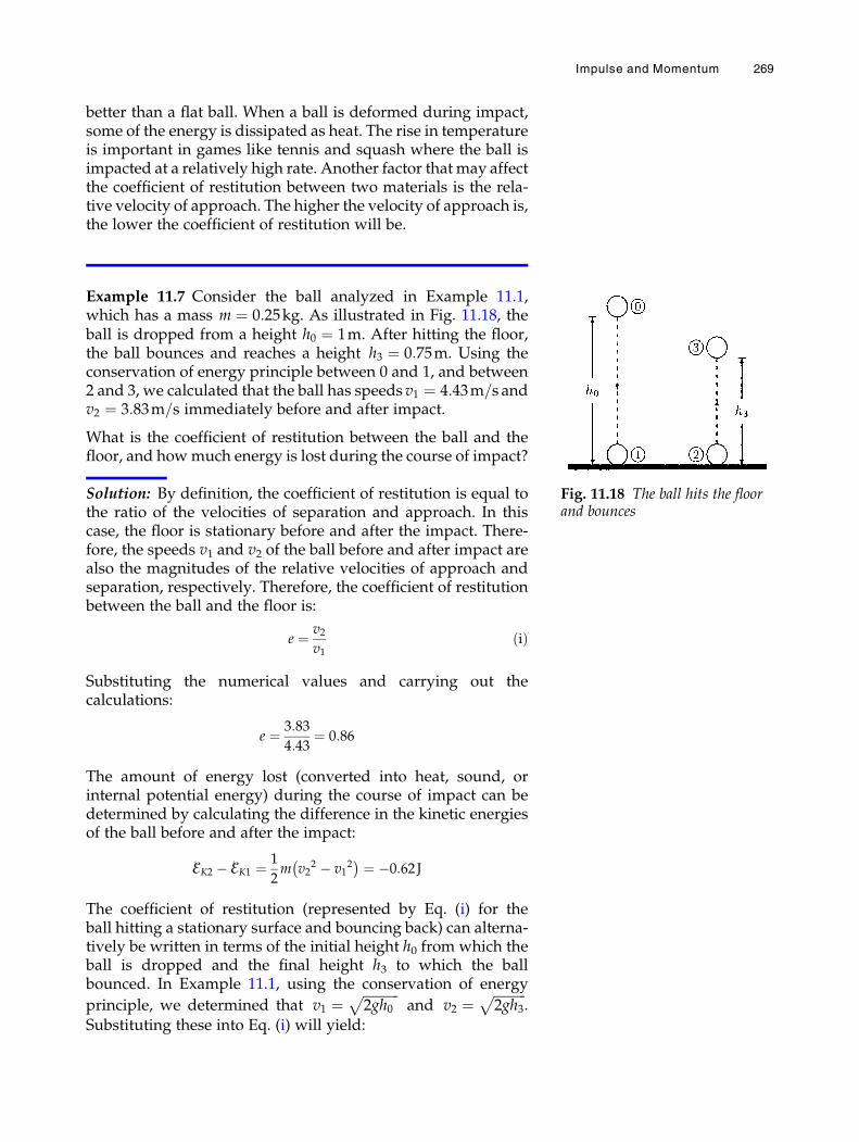
better than a flat ball. When a ball is deformed during impact,some of the energy is dissipated as heat. The rise in temperatureis important in games like tennis and squash where the ball isimpacted at a relatively high rate. Another factor that may affectthe coefficient of restitution between two materials is the rela-tive velocity of approach. The higher the velocity of approach is,the lower the coefficient of restitution will be.
Example 11.7 Consider the ball analyzed in Example 11.1,which has a mass m ¼ 0:25kg. As illustrated in Fig. 11.18, theball is dropped from a height h0 ¼ 1m. After hitting the floor,the ball bounces and reaches a height h3 ¼ 0:75m. Using theconservation of energy principle between 0 and 1, and between2 and 3, we calculated that the ball has speeds v1 ¼ 4:43m=s andv2 ¼ 3:83m=s immediately before and after impact.
What is the coefficient of restitution between the ball and thefloor, and howmuch energy is lost during the course of impact?
Solution: By definition, the coefficient of restitution is equal tothe ratio of the velocities of separation and approach. In thiscase, the floor is stationary before and after the impact. There-fore, the speeds v1 and v2 of the ball before and after impact arealso the magnitudes of the relative velocities of approach andseparation, respectively. Therefore, the coefficient of restitutionbetween the ball and the floor is:
e ¼ v2v1
ðiÞ
Substituting the numerical values and carrying out thecalculations:
e ¼ 3:83
4:43¼ 0:86
The amount of energy lost (converted into heat, sound, orinternal potential energy) during the course of impact can bedetermined by calculating the difference in the kinetic energiesof the ball before and after the impact:
ℰK2 � ℰK1 ¼ 1
2m v2
2 � v12
� � ¼ �0:62J
The coefficient of restitution (represented by Eq. (i) for theball hitting a stationary surface and bouncing back) can alterna-tively be written in terms of the initial height h0 from which theball is dropped and the final height h3 to which the ballbounced. In Example 11.1, using the conservation of energy
principle, we determined that v1 ¼ffiffiffiffiffiffiffiffiffiffiffi2gh0
pand v2 ¼
ffiffiffiffiffiffiffiffiffiffi2gh3
p.
Substituting these into Eq. (i) will yield:
Fig. 11.18 The ball hits the floorand bounces
Impulse and Momentum 269
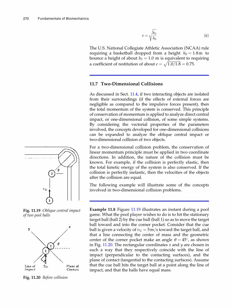
e ¼ffiffiffiffiffih3h0
sðiiÞ
The U.S. National Collegiate Athletic Association (NCAA) rulerequiring a basketball dropped from a height h0 ¼ 1:8m tobounce a height of about h3 ¼ 1:0 m is equivalent to requiring
a coefficient of restitution of about e ¼ ffiffiffiffiffiffiffiffiffiffiffiffiffiffiffi1:0=1:8
p ¼ 0:75.
11.7 Two-Dimensional Collisions
As discussed in Sect. 11.4, if two interacting objects are isolatedfrom their surroundings (if the effects of external forces arenegligible as compared to the impulsive forces present), thenthe total momentum of the system is conserved. This principleof conservation of momentum is applied to analyze direct centralimpact, or one-dimensional collision, of some simple systems.By considering the vectorial properties of the parametersinvolved, the concepts developed for one-dimensional collisionscan be expanded to analyze the oblique central impact ortwo-dimensional collision of two objects.
For a two-dimensional collision problem, the conservation oflinear momentum principle must be applied in two coordinatedirections. In addition, the nature of the collision must beknown. For example, if the collision is perfectly elastic, thenthe total kinetic energy of the system is also conserved. If thecollision is perfectly inelastic, then the velocities of the objectsafter the collision are equal.
The following example will illustrate some of the conceptsinvolved in two-dimensional collision problems.
Example 11.8 Figure 11.19 illustrates an instant during a poolgame. What the pool player wishes to do is to hit the stationarytarget ball (ball 2) by the cue ball (ball 1) so as to move the targetball toward and into the corner pocket. Consider that the cueball is given a velocity of v1i ¼ 5m=s toward the target ball, andthat a line connecting the center of mass and the geometriccenter of the corner pocket make an angle θ ¼ 45�, as shownin Fig. 11.20. The rectangular coordinates x and y are chosen insuch a way that they respectively coincide with the line ofimpact (perpendicular to the contacting surfaces), and theplane of contact (tangential to the contacting surfaces). Assumethat the cue ball hits the target ball at a point along the line ofimpact, and that the balls have equal mass.
Fig. 11.19 Oblique central impactof two pool balls
Fig. 11.20 Before collision
270 Fundamentals of Biomechanics
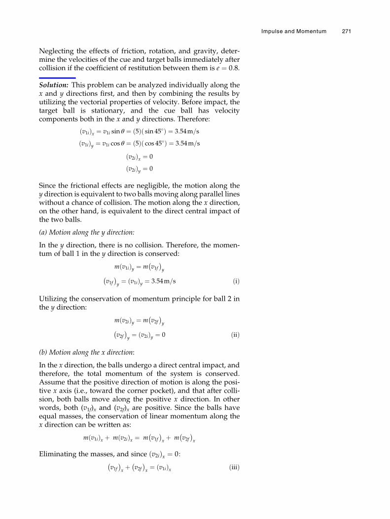
Neglecting the effects of friction, rotation, and gravity, deter-mine the velocities of the cue and target balls immediately aftercollision if the coefficient of restitution between them is e ¼ 0:8.
Solution: This problem can be analyzed individually along thex and y directions first, and then by combining the results byutilizing the vectorial properties of velocity. Before impact, thetarget ball is stationary, and the cue ball has velocitycomponents both in the x and y directions. Therefore:
v1ið Þx ¼ v1i sin θ ¼ 5ð Þ sin 45�ð Þ ¼ 3:54m=s
v1ið Þy ¼ v1i cos θ ¼ 5ð Þ cos 45�ð Þ ¼ 3:54m=s
v2ið Þx ¼ 0
v2ið Þy ¼ 0
Since the frictional effects are negligible, the motion along they direction is equivalent to two balls moving along parallel lineswithout a chance of collision. The motion along the x direction,on the other hand, is equivalent to the direct central impact ofthe two balls.
(a) Motion along the y direction:
In the y direction, there is no collision. Therefore, the momen-tum of ball 1 in the y direction is conserved:
m v1ið Þy ¼ m v1f� �
y
v1f� �
y¼ v1ið Þy ¼ 3:54m=s ðiÞ
Utilizing the conservation of momentum principle for ball 2 inthe y direction:
m v2ið Þy ¼ m v2f� �
y
v2f� �
y¼ v2ið Þy ¼ 0 ðiiÞ
(b) Motion along the x direction:
In the x direction, the balls undergo a direct central impact, andtherefore, the total momentum of the system is conserved.Assume that the positive direction of motion is along the posi-tive x axis (i.e., toward the corner pocket), and that after colli-sion, both balls move along the positive x direction. In otherwords, both (v1f)x and (v2f)x are positive. Since the balls haveequal masses, the conservation of linear momentum along thex direction can be written as:
m v1ið Þx þ m v2ið Þx ¼ m v1f� �
xþ m v2f
� �x
Eliminating the masses, and since v2ið Þx ¼ 0:
v1f� �
xþ v2f� �
x¼ v1ið Þx ðiiiÞ
Impulse and Momentum 271

The coefficient of restitution for the collision is given as e ¼ 0:8.By definition, e is equal to the ratio of the relative velocities ofseparation and approach. Before impact, ball 2 is stationary.Hence the relative velocity of approach in the x direction isequal to the initial speed of ball 1 in the x direction. Because ofthe assumed directions of motion after the collision, the relativevelocity of separation in the x direction is equal to the differenceof the velocity components of the balls along the x direction.Assuming that (v2f)x is larger than (v1f)x:
e ¼ v2f� �
x� v1f� �
x
v1ið ÞxThis equation can also be written as:
v2f� �
x� v1f� �
x¼ e v1ið Þx ðivÞ
We have two equations, Eqs. (iii) and (iv), for two unknowns,(v2f)x and (v1f)x. Solving these equations simultaneously willyield:
v1f� �
x¼ e� 1ð Þ
2v1ið Þx ðvÞ
v2f� �
x¼ eþ 1ð Þ
2v1ið Þx ðviÞ
Substituting v1f� �
x¼ 3:54m=s and e ¼ 0:8 into these equations
will yield:
v1f� �
x¼ �0:35
v2f� �
x¼ 3:19
Hence, the velocities of the balls after the collision are:
v1f ¼ �0:35iþ 3:54j m=sð Þv2f ¼ 3:19i m=sð Þ
Immediately after the collision, the target ball will move with aspeed of 3.19 m/s toward the corner pocket (i.e., along thepositive x direction). As illustrated in Fig. 11.21, the cue ball
will move with a speed of v1f ¼ffiffiffiffiffiffiffiffiffiffiffiffiffiffiffiffiffiffiffiffiffiffiffiffiffiffiffiffiffiffiffiffiffiffiffi0:35ð Þ2 þ 3:54ð Þ2
q¼ 3:56m=s
along a direction which makes an angle arctan 3:54=0:35ð Þ ¼ 84�
with the negative x direction, or at an angle β ¼ 84� � 45� ¼ 39�
with the horizontal.
While utilizing the equations for the coefficient of restitutionand conservation of momentum, we assumed that the velocitycomponents of both balls would be in the positive x direction.As a result of our computations, we determined a negativevalue for (v1f)x which means that it is acting along the negativex direction.
Fig. 11.21 After the collision
272 Fundamentals of Biomechanics
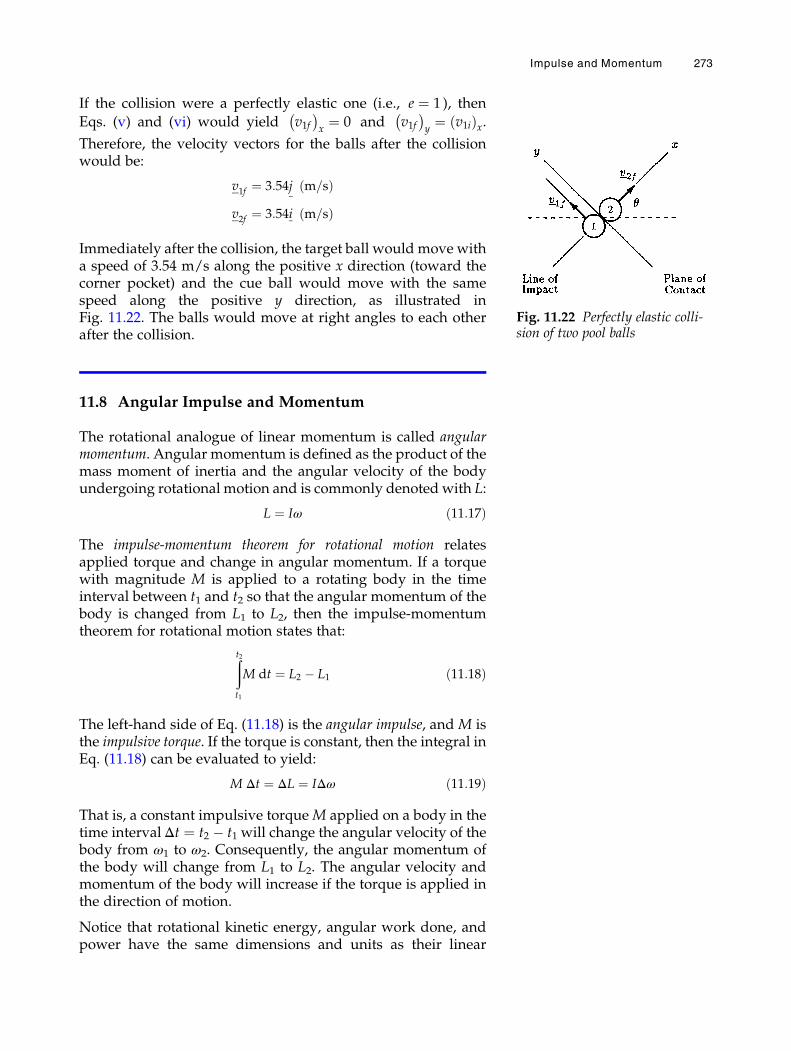
If the collision were a perfectly elastic one (i.e., e ¼ 1 ), then
Eqs. (v) and (vi) would yield v1f� �
x¼ 0 and v1f
� �y¼ v1ið Þx.
Therefore, the velocity vectors for the balls after the collisionwould be:
v1f ¼ 3:54j m=sð Þv2f ¼ 3:54i m=sð Þ
Immediately after the collision, the target ball would move witha speed of 3.54 m/s along the positive x direction (toward thecorner pocket) and the cue ball would move with the samespeed along the positive y direction, as illustrated inFig. 11.22. The balls would move at right angles to each otherafter the collision.
11.8 Angular Impulse and Momentum
The rotational analogue of linear momentum is called angularmomentum. Angular momentum is defined as the product of themass moment of inertia and the angular velocity of the bodyundergoing rotational motion and is commonly denoted with L:
L ¼ Iω ð11:17Þ
The impulse-momentum theorem for rotational motion relatesapplied torque and change in angular momentum. If a torquewith magnitude M is applied to a rotating body in the timeinterval between t1 and t2 so that the angular momentum of thebody is changed from L1 to L2, then the impulse-momentumtheorem for rotational motion states that:
ðt2t1
M dt ¼ L2 � L1 ð11:18Þ
The left-hand side of Eq. (11.18) is the angular impulse, and M isthe impulsive torque. If the torque is constant, then the integral inEq. (11.18) can be evaluated to yield:
M Δt ¼ ΔL ¼ IΔω ð11:19Þ
That is, a constant impulsive torqueM applied on a body in thetime intervalΔt ¼ t2 � t1 will change the angular velocity of thebody from ω1 to ω2. Consequently, the angular momentum ofthe body will change from L1 to L2. The angular velocity andmomentum of the body will increase if the torque is applied inthe direction of motion.
Notice that rotational kinetic energy, angular work done, andpower have the same dimensions and units as their linear
Fig. 11.22 Perfectly elastic colli-sion of two pool balls
Impulse and Momentum 273
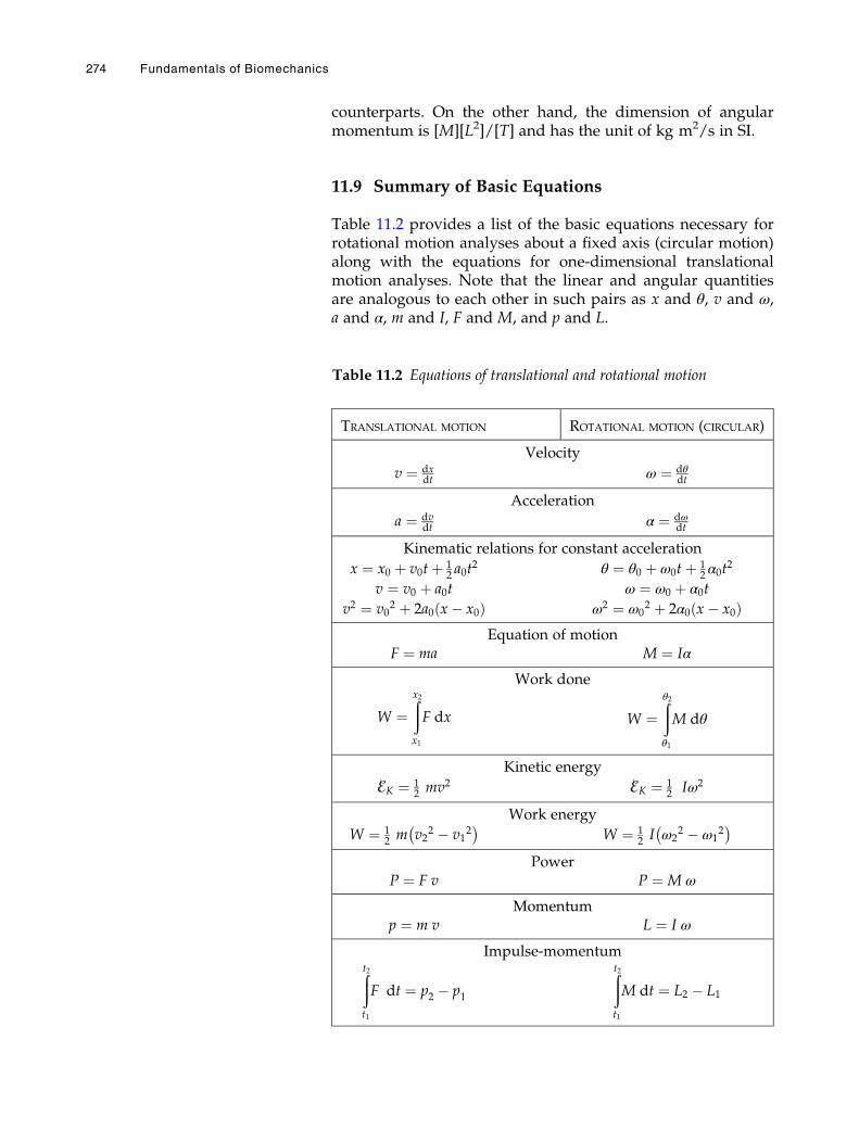
counterparts. On the other hand, the dimension of angularmomentum is [M][L2]/[T] and has the unit of kg m2/s in SI.
11.9 Summary of Basic Equations
Table 11.2 provides a list of the basic equations necessary forrotational motion analyses about a fixed axis (circular motion)along with the equations for one-dimensional translationalmotion analyses. Note that the linear and angular quantitiesare analogous to each other in such pairs as x and θ, v and ω,a and α, m and I, F and M, and p and L.
Table 11.2 Equations of translational and rotational motion
TRANSLATIONAL MOTION ROTATIONAL MOTION (CIRCULAR)
Velocity
v ¼ dxdt ω ¼ dθ
dt
Acceleration
a ¼ dvdt α ¼ dω
dt
Kinematic relations for constant acceleration
x ¼ x0 þ v0tþ 12 a0t
2 θ ¼ θ0 þ ω0tþ 12 α0t
2
v ¼ v0 þ a0t ω ¼ ω0 þ α0t
v2 ¼ v02 þ 2a0 x� x0ð Þ ω2 ¼ ω0
2 þ 2α0 x� x0ð ÞEquation of motion
F ¼ ma M ¼ Iα
Work done
W ¼ðx2x1
F dx W ¼ðθ2θ1
M dθ
Kinetic energy
ℰK ¼ 12 mv2 ℰK ¼ 1
2 Iω2
Work energy
W ¼ 12 m v2
2 � v12
� �W ¼ 1
2 I ω22 � ω1
2� �
PowerP ¼ F v P ¼ M ω
Momentump ¼ m v L ¼ I ω
Impulse-momentumðt2t1
F dt ¼ p2 � p1
ðt2t1
M dt ¼ L2 � L1
274 Fundamentals of Biomechanics
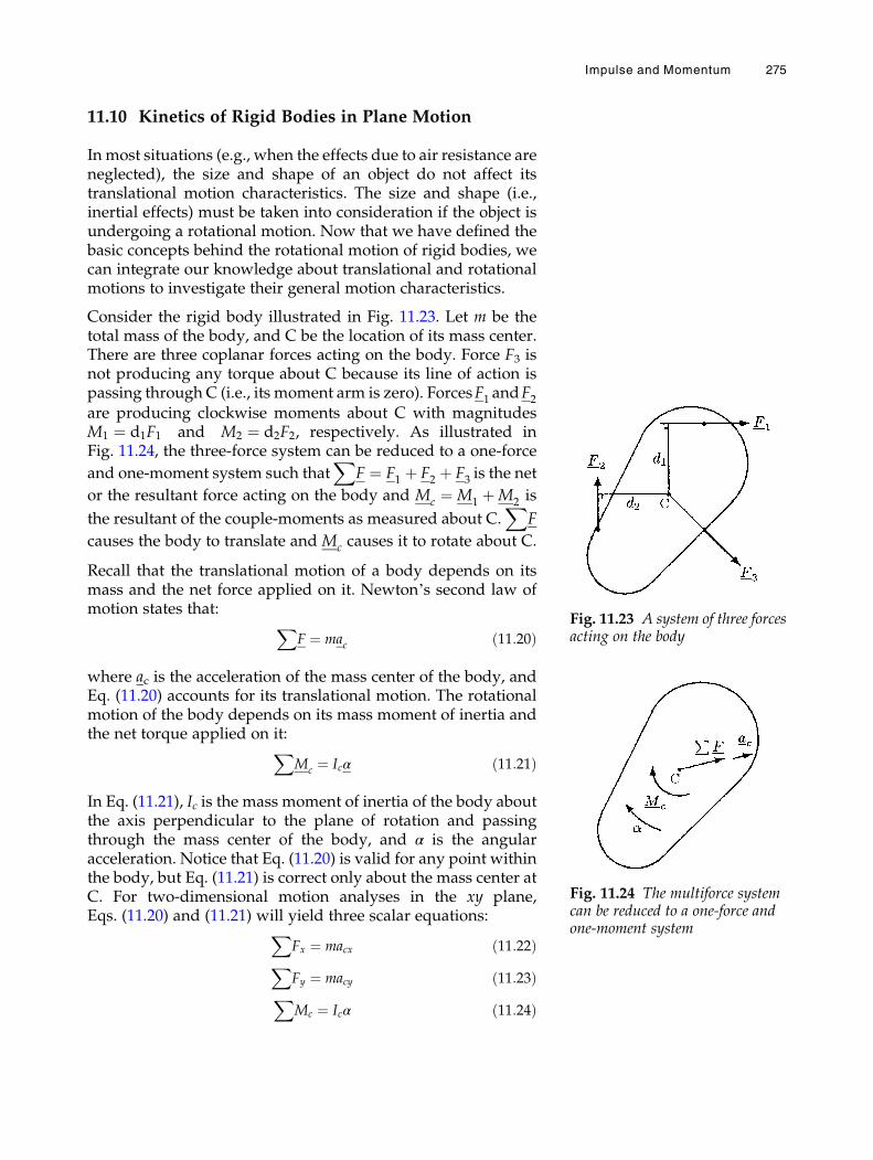
11.10 Kinetics of Rigid Bodies in Plane Motion
In most situations (e.g., when the effects due to air resistance areneglected), the size and shape of an object do not affect itstranslational motion characteristics. The size and shape (i.e.,inertial effects) must be taken into consideration if the object isundergoing a rotational motion. Now that we have defined thebasic concepts behind the rotational motion of rigid bodies, wecan integrate our knowledge about translational and rotationalmotions to investigate their general motion characteristics.
Consider the rigid body illustrated in Fig. 11.23. Let m be thetotal mass of the body, and C be the location of its mass center.There are three coplanar forces acting on the body. Force F3 isnot producing any torque about C because its line of action ispassing through C (i.e., its moment arm is zero). ForcesF1 andF2are producing clockwise moments about C with magnitudesM1 ¼ d1F1 and M2 ¼ d2F2, respectively. As illustrated inFig. 11.24, the three-force system can be reduced to a one-force
and one-moment system such thatX
F ¼ F1 þ F2 þ F3 is the net
or the resultant force acting on the body and Mc ¼ M1 þM2 is
the resultant of the couple-moments as measured about C.X
F
causes the body to translate and Mc causes it to rotate about C.
Recall that the translational motion of a body depends on itsmass and the net force applied on it. Newton’s second law ofmotion states that: X
F ¼ mac ð11:20Þ
where ac is the acceleration of the mass center of the body, andEq. (11.20) accounts for its translational motion. The rotationalmotion of the body depends on its mass moment of inertia andthe net torque applied on it:X
Mc ¼ Icα ð11:21Þ
In Eq. (11.21), Ic is the mass moment of inertia of the body aboutthe axis perpendicular to the plane of rotation and passingthrough the mass center of the body, and α is the angularacceleration. Notice that Eq. (11.20) is valid for any point withinthe body, but Eq. (11.21) is correct only about the mass center atC. For two-dimensional motion analyses in the xy plane,Eqs. (11.20) and (11.21) will yield three scalar equations:X
Fx ¼ macx ð11:22ÞXFy ¼ macy ð11:23ÞXMc ¼ Icα ð11:24Þ
Fig. 11.23 A system of three forcesacting on the body
Fig. 11.24 The multiforce systemcan be reduced to a one-force andone-moment system
Impulse and Momentum 275
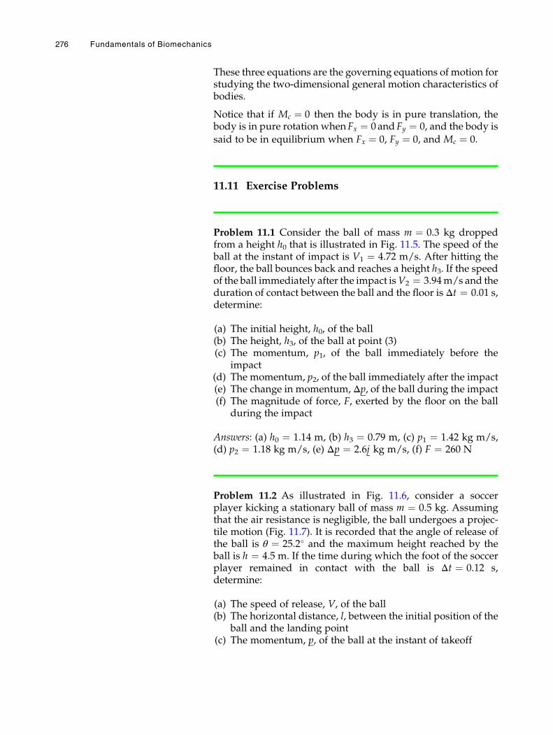
These three equations are the governing equations of motion forstudying the two-dimensional general motion characteristics ofbodies.
Notice that if Mc ¼ 0 then the body is in pure translation, thebody is in pure rotation whenFx ¼ 0 andFy ¼ 0, and the body is
said to be in equilibrium when Fx ¼ 0, Fy ¼ 0, and Mc ¼ 0.
11.11 Exercise Problems
Problem 11.1 Consider the ball of mass m ¼ 0.3 kg droppedfrom a height h0 that is illustrated in Fig. 11.5. The speed of theball at the instant of impact is V1 ¼ 4.72 m/s. After hitting thefloor, the ball bounces back and reaches a height h3. If the speedof the ball immediately after the impact isV2 ¼ 3.94m/s and theduration of contact between the ball and the floor is Δt ¼ 0.01 s,determine:
(a) The initial height, h0, of the ball(b) The height, h3, of the ball at point (3)(c) The momentum, p1, of the ball immediately before the
impact(d) The momentum, p2, of the ball immediately after the impact(e) The change in momentum, Δp, of the ball during the impact(f) The magnitude of force, F, exerted by the floor on the ball
during the impact
Answers: (a) h0 ¼ 1.14 m, (b) h3 ¼ 0.79 m, (c) p1 ¼ 1.42 kg m/s,(d) p2 ¼ 1.18 kg m/s, (e) Δp ¼ 2.6j kg m/s, (f) F ¼ 260 N
Problem 11.2 As illustrated in Fig. 11.6, consider a soccerplayer kicking a stationary ball of mass m ¼ 0.5 kg. Assumingthat the air resistance is negligible, the ball undergoes a projec-tile motion (Fig. 11.7). It is recorded that the angle of release ofthe ball is θ ¼ 25.2� and the maximum height reached by theball is h ¼ 4.5 m. If the time during which the foot of the soccerplayer remained in contact with the ball is Δt ¼ 0.12 s,determine:
(a) The speed of release, V, of the ball(b) The horizontal distance, l, between the initial position of the
ball and the landing point(c) The momentum, p, of the ball at the instant of takeoff
276 Fundamentals of Biomechanics
(d) The magnitude of force, F, applied on the ball by the soccerplayer
Answers: (a) V ¼ 22.06 m/s, (b) l ¼ 38.3 m, (c) p ¼ 9.98i + 4.7j(kg m/s), (d) F ¼ 110.3 N
Problem 11.3 A laboratory test was conducted to analyze theendurance of seat belts used by automobile passengers.According to the test protocol, an 85 kg dummy was insidethe test vehicle which had its initial horizontal speed set to110 km/h. At a certain instant the brakes were applied, bringingthe vehicle to rest. It was recorded that while in motion, the seatbelt applied a force of F ¼ 20,008 N on the dummy (Fig. 11.10).Assuming that the effects of friction are negligibly small, deter-mine the time interval,Δt, duringwhich the speed of the vehiclewith the dummy was brought to zero.
Answer: Δt ¼ 0.13 s
Problem 11.4 A test was conducted to measure the velocity of abullet by using a ballistic pendulummade from a wooden blocksuspended by light wires. As illustrated in Fig. 11.14, assumethe weight of the block is m2 ¼ 3.5 kg. A bullet of massm1 ¼ 30 g fired at the stationary block and penetrated theblock causing it to swing to a height h ¼ 5.5 cm. Assumingthat the bullet remained in the block, determine the speed ofthe bullet, Vb, immediately before impact.
Answer: Vb ¼ 122.2 m/s
Problem 11.5 As illustrated in Fig. 11.16, consider a perfectlyelastic collision of two billiard balls with equal massesm. Beforethe collision, the ball (1) had a speed of V1i ¼ 1.3 m/s and ball(2) was stationary (V2i ¼ 0). Assuming a direct central impact,determine the speed of the billiard balls, V1f and V2f, immedi-ately after the collision.
Answer: V1f ¼ 0, V2f ¼ 1.3 m/s
Problem 11.6 A ball of a mass m ¼ 0.3 kg is dropped from aheight h0 ¼ 1.5 m, as shown in Fig. 11.18. After hitting the floor,the ball bounces and reaches a height h3. The speed of the ballimmediately before the impact was V1 ¼ 5.4 m/s. If the
Impulse and Momentum 277
coefficient of restitution between the ball and the floor ise ¼ 0.79, determine:
(a) The speed of the ball, V2, immediately after the impact(b) The height, h3, reached by the ball after bouncing up from
the floor(c) The amount of energy, ɛ, lost during the course of impact
Answers: (a) V2 ¼ 4.27 m/s, (b) h3 ¼ 0.93 m, (c) ɛ ¼ 1.64 J
278 Fundamentals of Biomechanics
Chapter 12
Introduction to DeformableBody Mechanics
12.1 Overview / 281
12.2 Applied Forces and Deformations / 282
12.3 Internal Forces and Moments / 282
12.4 Stress and Strain / 283
12.5 General Procedure / 284
12.6 Mathematics Involved / 285
12.7 Topics to Be Covered / 285
Suggested Reading / 286
# Springer International Publishing Switzerland 2017N. Ozkaya et al., Fundamentals of Biomechanics, DOI 10.1007/978-3-319-44738-4_12
279

12.1 Overview
Basic concepts of statics were introduced in Chaps. 4 and 5along with some of their applications. The field of statics isbased on Newton’s laws (Newtonian mechanics). It constitutesone of the two main branches of the more general field of rigidbody mechanics, dynamics being the other branch. The basicassumption in rigid body mechanics is that the bodies involveddo not deform under applied loads. This idealization is neces-sary to simplify the problem under investigation for the sake ofanalyzing external forces andmoments. The field of deformablebody mechanics, on the other hand, does not treat the body asrigid, but incorporates the deformability (ability to undergoshape change) and the material properties of the body into theanalyses. This field of applied mechanics utilizes the experi-mentally determined and/or verified relationships betweenapplied forces and corresponding deformations.
Rigid body mechanics has its limitations. One of theselimitations was discussed in Sect. 4.6 where the concept ofstatically indeterminant systems was introduced. A system forwhich the equations of equilibrium are not sufficient to deter-mine the unknown forces is called statically indeterminate. Forthe analyses of such systems, there is a need for equations inaddition to those provided by the conditions of static equilib-rium. These additional equations can be derived by consideringthe material properties of the parts constituting a system and byrelating forces to deformations, which is the focus of deform-able body mechanics.
The desire to analyze statically determinate systems is only oneof the reasons why deformable body mechanics is important.The applications of this field extend to almost all branches ofengineering by providing essential design and analysis tools.The task of an engineer—mechanical, civil, electrical, or bio-medical—is to determine the safest andmost efficient operatingcondition for a machine, a structure, a piece of equipment, or aprosthetic device. A design engineer can accomplish this taskby first assessing the proper operational environment throughforce analyses, making the correct structural design, andchoosing the material that can sustain the forces involved inthat environment. The primary concern of a design engineer isto make sure that when loaded, a machine part, a structure, apiece of equipment, or a device will not break or deformexcessively.
Introduction to Deformable Body Mechanics 281
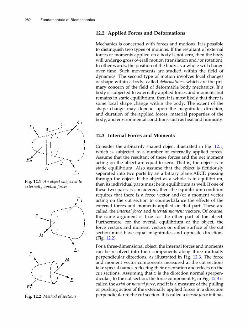
12.2 Applied Forces and Deformations
Mechanics is concerned with forces and motions. It is possibleto distinguish two types of motions. If the resultant of externalforces or moments applied on a body is not zero, then the bodywill undergo gross overall motion (translation and/or rotation).In other words, the position of the body as a whole will changeover time. Such movements are studied within the field ofdynamics. The second type of motion involves local changesof shape within a body, called deformations, which are the pri-mary concern of the field of deformable body mechanics. If abody is subjected to externally applied forces and moments butremains in static equilibrium, then it is most likely that there issome local shape change within the body. The extent of theshape change may depend upon the magnitude, direction,and duration of the applied forces, material properties of thebody, and environmental conditions such as heat and humidity.
12.3 Internal Forces and Moments
Consider the arbitrarily shaped object illustrated in Fig. 12.1,which is subjected to a number of externally applied forces.Assume that the resultant of these forces and the net momentacting on the object are equal to zero. That is, the object is instatic equilibrium. Also assume that the object is fictitiouslyseparated into two parts by an arbitrary plane ABCD passingthrough the object. If the object as a whole is in equilibrium,then its individual parts must be in equilibrium aswell. If one ofthese two parts is considered, then the equilibrium conditionrequires that there is a force vector and/or a moment vectoracting on the cut section to counterbalance the effects of theexternal forces and moments applied on that part. These arecalled the internal force and internal moment vectors. Of course,the same argument is true for the other part of the object.Furthermore, for the overall equilibrium of the object, theforce vectors and moment vectors on either surface of the cutsection must have equal magnitudes and opposite directions(Fig. 12.2).
For a three-dimensional object, the internal forces and momentscan be resolved into their components along three mutuallyperpendicular directions, as illustrated in Fig. 12.3. The forceand moment vector components measured at the cut sectionstake special names reflecting their orientation and effects on thecut sections. Assuming that x is the direction normal (perpen-dicular) to the cut section, the force component Px in Fig. 12.3 iscalled the axial or normal force, and it is a measure of the pullingor pushing action of the externally applied forces in a directionperpendicular to the cut section. It is called a tensile force if it has
Fig. 12.1 An object subjected toexternally applied forces
Fig. 12.2 Method of sections
282 Fundamentals of Biomechanics
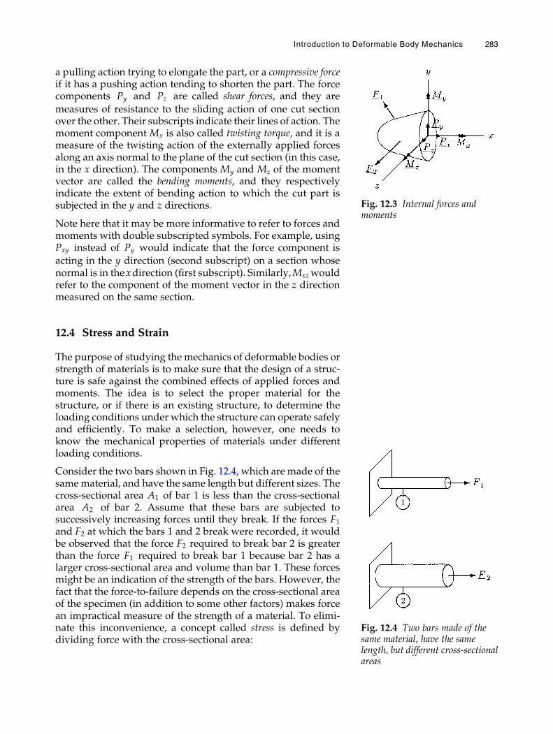
a pulling action trying to elongate the part, or a compressive forceif it has a pushing action tending to shorten the part. The forcecomponents Py and Pz are called shear forces, and they are
measures of resistance to the sliding action of one cut sectionover the other. Their subscripts indicate their lines of action. Themoment component Mx is also called twisting torque, and it is ameasure of the twisting action of the externally applied forcesalong an axis normal to the plane of the cut section (in this case,in the x direction). The components My and Mz of the momentvector are called the bending moments, and they respectivelyindicate the extent of bending action to which the cut part issubjected in the y and z directions.
Note here that it may be more informative to refer to forces andmoments with double subscripted symbols. For example, usingPxy instead of Py would indicate that the force component is
acting in the y direction (second subscript) on a section whosenormal is in thexdirection (first subscript). Similarly,Mxzwouldrefer to the component of the moment vector in the z directionmeasured on the same section.
12.4 Stress and Strain
The purpose of studying the mechanics of deformable bodies orstrength of materials is to make sure that the design of a struc-ture is safe against the combined effects of applied forces andmoments. The idea is to select the proper material for thestructure, or if there is an existing structure, to determine theloading conditions under which the structure can operate safelyand efficiently. To make a selection, however, one needs toknow the mechanical properties of materials under differentloading conditions.
Consider the two bars shown in Fig. 12.4, which are made of thesamematerial, and have the same length but different sizes. Thecross-sectional area A1 of bar 1 is less than the cross-sectionalarea A2 of bar 2. Assume that these bars are subjected tosuccessively increasing forces until they break. If the forces F1and F2 at which the bars 1 and 2 break were recorded, it wouldbe observed that the force F2 required to break bar 2 is greaterthan the force F1 required to break bar 1 because bar 2 has alarger cross-sectional area and volume than bar 1. These forcesmight be an indication of the strength of the bars. However, thefact that the force-to-failure depends on the cross-sectional areaof the specimen (in addition to some other factors) makes forcean impractical measure of the strength of a material. To elimi-nate this inconvenience, a concept called stress is defined bydividing force with the cross-sectional area:
Fig. 12.3 Internal forces andmoments
Fig. 12.4 Two bars made of thesame material, have the samelength, but different cross-sectionalareas
Introduction to Deformable Body Mechanics 283
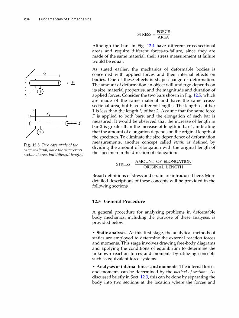
STRESS ¼ FORCE
AREA
Although the bars in Fig. 12.4 have different cross-sectionalareas and require different forces-to-failure, since they aremade of the same material, their stress measurement at failurewould be equal.
As stated earlier, the mechanics of deformable bodies isconcerned with applied forces and their internal effects onbodies. One of these effects is shape change or deformation.The amount of deformation an object will undergo depends onits size, material properties, and the magnitude and duration ofapplied forces. Consider the two bars shown in Fig. 12.5, whichare made of the same material and have the same cross-sectional area, but have different lengths. The length l1 of bar1 is less than the length l2 of bar 2. Assume that the same forceF is applied to both bars, and the elongation of each bar ismeasured. It would be observed that the increase of length inbar 2 is greater than the increase of length in bar 1, indicatingthat the amount of elongation depends on the original length ofthe specimen. To eliminate the size dependence of deformationmeasurements, another concept called strain is defined bydividing the amount of elongation with the original length ofthe specimen in the direction of elongation:
STRESS ¼ AMOUNT OF ELONGATION
ORIGINAL LENGTH
Broad definitions of stress and strain are introduced here. Moredetailed descriptions of these concepts will be provided in thefollowing sections.
12.5 General Procedure
A general procedure for analyzing problems in deformablebody mechanics, including the purpose of these analyses, isprovided below.
• Static analyses. At this first stage, the analytical methods ofstatics are employed to determine the external reaction forcesand moments. This stage involves drawing free-body diagramsand applying the conditions of equilibrium to determine theunknown reaction forces and moments by utilizing conceptssuch as equivalent force systems.
• Analyses of internal forces andmoments. The internal forcesand moments can be determined by the method of sections. Asdiscussed briefly in Sect. 12.3, this can be done by separating thebody into two sections at the location where the forces and
Fig. 12.5 Two bars made of thesame material, have the same cross-sectional area, but different lengths
284 Fundamentals of Biomechanics
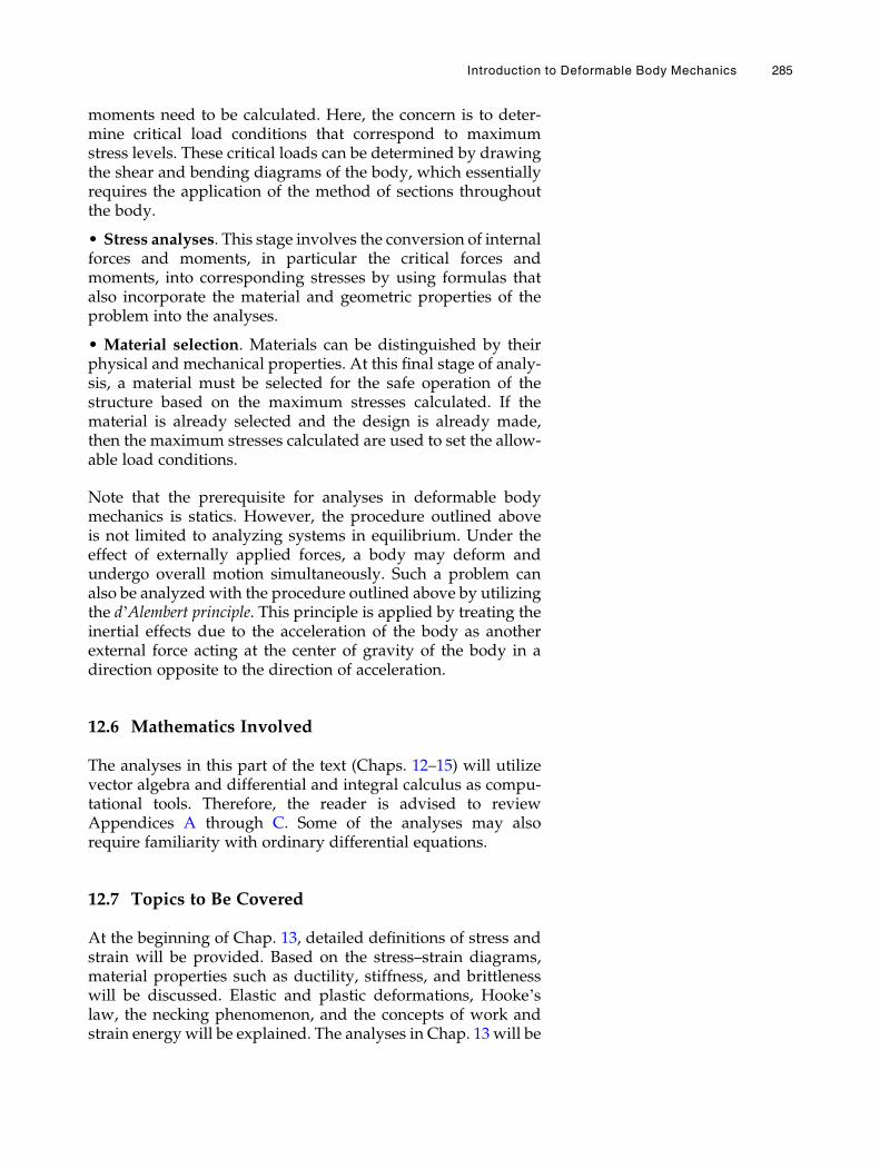
moments need to be calculated. Here, the concern is to deter-mine critical load conditions that correspond to maximumstress levels. These critical loads can be determined by drawingthe shear and bending diagrams of the body, which essentiallyrequires the application of the method of sections throughoutthe body.
• Stress analyses. This stage involves the conversion of internalforces and moments, in particular the critical forces andmoments, into corresponding stresses by using formulas thatalso incorporate the material and geometric properties of theproblem into the analyses.
• Material selection. Materials can be distinguished by theirphysical and mechanical properties. At this final stage of analy-sis, a material must be selected for the safe operation of thestructure based on the maximum stresses calculated. If thematerial is already selected and the design is already made,then the maximum stresses calculated are used to set the allow-able load conditions.
Note that the prerequisite for analyses in deformable bodymechanics is statics. However, the procedure outlined aboveis not limited to analyzing systems in equilibrium. Under theeffect of externally applied forces, a body may deform andundergo overall motion simultaneously. Such a problem canalso be analyzed with the procedure outlined above by utilizingthe d’Alembert principle. This principle is applied by treating theinertial effects due to the acceleration of the body as anotherexternal force acting at the center of gravity of the body in adirection opposite to the direction of acceleration.
12.6 Mathematics Involved
The analyses in this part of the text (Chaps. 12–15) will utilizevector algebra and differential and integral calculus as compu-tational tools. Therefore, the reader is advised to reviewAppendices A through C. Some of the analyses may alsorequire familiarity with ordinary differential equations.
12.7 Topics to Be Covered
At the beginning of Chap. 13, detailed definitions of stress andstrain will be provided. Based on the stress–strain diagrams,material properties such as ductility, stiffness, and brittlenesswill be discussed. Elastic and plastic deformations, Hooke’slaw, the necking phenomenon, and the concepts of work andstrain energy will be explained. The analyses in Chap. 13 will be
Introduction to Deformable Body Mechanics 285
limited to uniaxial deformations. The concepts introduced willbe applied to analyze relatively simple systems.
In Chap. 14, more advanced topics in stress–strain analyses willbe introduced. Two- and three-dimensional stress analyses,techniques of transforming stresses from one plane to another,methods for finding critical stresses, reasons why stressanalyses are important in the design of structures, failuretheories, concepts such as fatigue, endurance, and stress con-centration will also be discussed in Chap. 14. Also in Chap. 14,analyses of bodies subjected to torsion, bending, and combinedloading will be explained.
In Chap. 15, the viscoelastic behavior of materials and empiricalmodels of viscoelasticity will be reviewed, and elasticity andviscoelasticity will be compared. Also in Chap. 15, the mechan-ical properties of biological tissues including bone, tendons,ligaments, muscles, and articular cartilage will be discussedand the relevance of mechanical concepts introduced earlier toorthopaedics will be demonstrated.
Suggested Reading1
Beer, F.P., Johnston, R.E., DeWolf, J.T. and Mazurek, D.F., 2015. Mechanics ofMaterials, 7th Edition. New York: McGraw-Hill Education.
Boresi, A.P. and Schmidt, R.J., 2002. Advanced Mechanics of Materials, 6th Edi-tion. New York: Wiley.
deSilva, C.W., 2013. Mechanics of Materials. Boca Raton: CRC Press.Gere, J.M. and Goodno, B.J., 2012. Mechanics of Materials. Stamford: CENGAGE
Learning.Hibbeler, R.C., 2013. Mechanics of Materials, 9th Edition. Upper Saddle River:
Prentice Hall.Phipot, T.A., 2012. Mechanics of Materials: An Integrated Learning System, 3rd
Edition. Somerset: Wiley.Popov, E.P. 1999. Engineering Mechanics of Solids. Upper Saddle River, NJ:
Prentice-Hall.Shames, I.H. 1989. Introduction to Solid Mechanics. Englewood Cliffs, NJ:
Prentice-Hall.Timoshekno, S.P., 1969. Strength of Materials: Elementary Theory and Problems.
New York: Van Nostrand Reinhold, Inc.
1 The field of deformable body mechanics has been studied under various titlessuch as solid mechanics, mechanics of materials, and strength of materials. Thesubjects covered within deformable body mechanics form the basis for the studyof more advanced topics in elasticity, inelasticity, and continuum mechanics.The following books can be reviewed to gain more detailed informationon the principles of deformable body mechanics.
286 Fundamentals of Biomechanics
Chapter 13
Stress and Strain
13.1 Basic Loading Configurations / 289
13.2 Uniaxial Tension Test / 289
13.3 Load-Elongation Diagrams / 290
13.4 Simple Stress / 291
13.5 Simple Strain / 292
13.6 Stress–Strain Diagrams / 294
13.7 Elastic Deformations / 295
13.8 Hooke’s Law / 297
13.9 Plastic Deformations / 297
13.10 Necking / 298
13.11 Work and Strain Energy / 299
13.12 Strain Hardening / 299
13.13 Hysteresis Loop / 299
13.14 Properties Based on Stress–Strain Diagrams / 300
13.15 Idealized Models of Material Behavior / 300
13.16 Mechanical Properties of Materials / 301
13.17 Example Problems / 302
13.18 Exercise Problems / 309
The original version of this chapter was revised. An erratum to this chapter can befound at https://doi.org/10.1007/978-3-319-44738-4_16
# Springer International Publishing Switzerland 2017N. Ozkaya et al., Fundamentals of Biomechanics, DOI 10.1007/978-3-319-44738-4_13
287

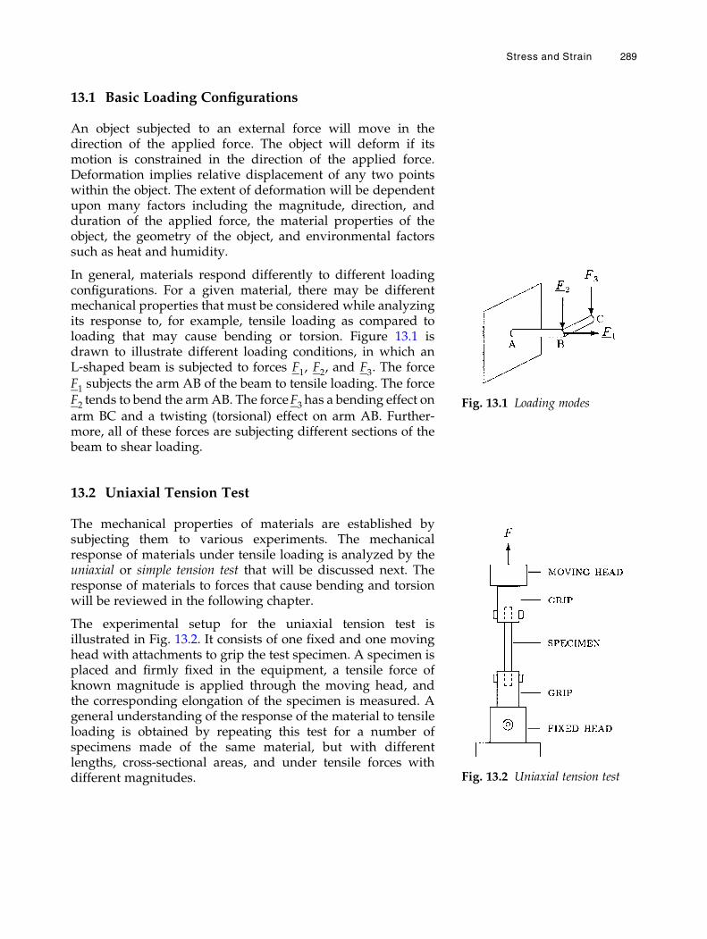
13.1 Basic Loading Configurations
An object subjected to an external force will move in thedirection of the applied force. The object will deform if itsmotion is constrained in the direction of the applied force.Deformation implies relative displacement of any two pointswithin the object. The extent of deformation will be dependentupon many factors including the magnitude, direction, andduration of the applied force, the material properties of theobject, the geometry of the object, and environmental factorssuch as heat and humidity.
In general, materials respond differently to different loadingconfigurations. For a given material, there may be differentmechanical properties that must be considered while analyzingits response to, for example, tensile loading as compared toloading that may cause bending or torsion. Figure 13.1 isdrawn to illustrate different loading conditions, in which anL-shaped beam is subjected to forces F1, F2, and F3. The forceF1 subjects the arm AB of the beam to tensile loading. The forceF2 tends to bend the armAB. The forceF3 has a bending effect onarm BC and a twisting (torsional) effect on arm AB. Further-more, all of these forces are subjecting different sections of thebeam to shear loading.
13.2 Uniaxial Tension Test
The mechanical properties of materials are established bysubjecting them to various experiments. The mechanicalresponse of materials under tensile loading is analyzed by theuniaxial or simple tension test that will be discussed next. Theresponse of materials to forces that cause bending and torsionwill be reviewed in the following chapter.
The experimental setup for the uniaxial tension test isillustrated in Fig. 13.2. It consists of one fixed and one movinghead with attachments to grip the test specimen. A specimen isplaced and firmly fixed in the equipment, a tensile force ofknown magnitude is applied through the moving head, andthe corresponding elongation of the specimen is measured. Ageneral understanding of the response of the material to tensileloading is obtained by repeating this test for a number ofspecimens made of the same material, but with differentlengths, cross-sectional areas, and under tensile forces withdifferent magnitudes.
Fig. 13.1 Loading modes
Fig. 13.2 Uniaxial tension test
Stress and Strain 289
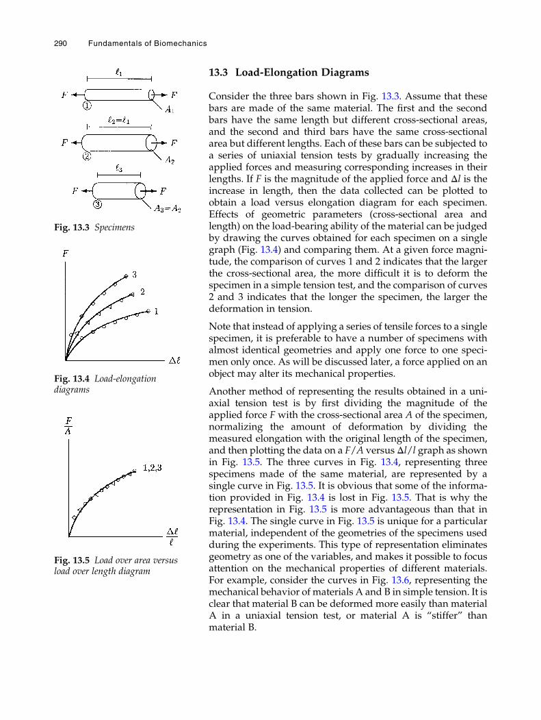
13.3 Load-Elongation Diagrams
Consider the three bars shown in Fig. 13.3. Assume that thesebars are made of the same material. The first and the secondbars have the same length but different cross-sectional areas,and the second and third bars have the same cross-sectionalarea but different lengths. Each of these bars can be subjected toa series of uniaxial tension tests by gradually increasing theapplied forces and measuring corresponding increases in theirlengths. If F is the magnitude of the applied force and Δl is theincrease in length, then the data collected can be plotted toobtain a load versus elongation diagram for each specimen.Effects of geometric parameters (cross-sectional area andlength) on the load-bearing ability of the material can be judgedby drawing the curves obtained for each specimen on a singlegraph (Fig. 13.4) and comparing them. At a given force magni-tude, the comparison of curves 1 and 2 indicates that the largerthe cross-sectional area, the more difficult it is to deform thespecimen in a simple tension test, and the comparison of curves2 and 3 indicates that the longer the specimen, the larger thedeformation in tension.
Note that instead of applying a series of tensile forces to a singlespecimen, it is preferable to have a number of specimens withalmost identical geometries and apply one force to one speci-men only once. As will be discussed later, a force applied on anobject may alter its mechanical properties.
Another method of representing the results obtained in a uni-axial tension test is by first dividing the magnitude of theapplied force F with the cross-sectional area A of the specimen,normalizing the amount of deformation by dividing themeasured elongation with the original length of the specimen,and then plotting the data on a F/A versus Δl/l graph as shownin Fig. 13.5. The three curves in Fig. 13.4, representing threespecimens made of the same material, are represented by asingle curve in Fig. 13.5. It is obvious that some of the informa-tion provided in Fig. 13.4 is lost in Fig. 13.5. That is why therepresentation in Fig. 13.5 is more advantageous than that inFig. 13.4. The single curve in Fig. 13.5 is unique for a particularmaterial, independent of the geometries of the specimens usedduring the experiments. This type of representation eliminatesgeometry as one of the variables, and makes it possible to focusattention on the mechanical properties of different materials.For example, consider the curves in Fig. 13.6, representing themechanical behavior of materials A and B in simple tension. It isclear that material B can be deformed more easily than materialA in a uniaxial tension test, or material A is “stiffer” thanmaterial B.
Fig. 13.5 Load over area versusload over length diagram
Fig. 13.3 Specimens
Fig. 13.4 Load-elongationdiagrams
290 Fundamentals of Biomechanics
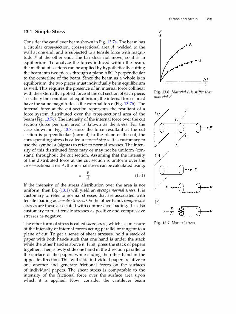
13.4 Simple Stress
Consider the cantilever beam shown in Fig. 13.7a. The beam hasa circular cross-section, cross-sectional area A, welded to thewall at one end, and is subjected to a tensile force with magni-tude F at the other end. The bar does not move, so it is inequilibrium. To analyze the forces induced within the beam,the method of sections can be applied by hypothetically cuttingthe beam into two pieces through a plane ABCD perpendicularto the centerline of the beam. Since the beam as a whole is inequilibrium, the two pieces must individually be in equilibriumas well. This requires the presence of an internal force collinearwith the externally applied force at the cut section of each piece.To satisfy the condition of equilibrium, the internal forces musthave the same magnitude as the external force (Fig. 13.7b). Theinternal force at the cut section represents the resultant of aforce system distributed over the cross-sectional area of thebeam (Fig. 13.7c). The intensity of the internal force over the cutsection (force per unit area) is known as the stress. For thecase shown in Fig. 13.7, since the force resultant at the cutsection is perpendicular (normal) to the plane of the cut, thecorresponding stress is called a normal stress. It is customary touse the symbol σ (sigma) to refer to normal stresses. The inten-sity of this distributed force may or may not be uniform (con-stant) throughout the cut section. Assuming that the intensityof the distributed force at the cut section is uniform over thecross-sectional areaA, the normal stress can be calculated using:
σ ¼ F
Að13:1Þ
If the intensity of the stress distribution over the area is notuniform, then Eq. (13.1) will yield an average normal stress. It iscustomary to refer to normal stresses that are associated withtensile loading as tensile stresses. On the other hand, compressivestresses are those associated with compressive loading. It is alsocustomary to treat tensile stresses as positive and compressivestresses as negative.
The other form of stress is called shear stress, which is a measureof the intensity of internal forces acting parallel or tangent to aplane of cut. To get a sense of shear stresses, hold a stack ofpaper with both hands such that one hand is under the stackwhile the other hand is above it. First, press the stack of paperstogether. Then, slowly slide one hand in the direction parallel tothe surface of the papers while sliding the other hand in theopposite direction. This will slide individual papers relative toone another and generate frictional forces on the surfacesof individual papers. The shear stress is comparable to theintensity of the frictional force over the surface area uponwhich it is applied. Now, consider the cantilever beam
Fig. 13.6 Material A is stiffer thanmaterial B
Fig. 13.7 Normal stress
Stress and Strain 291
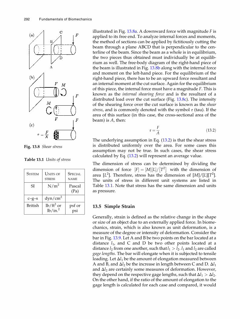
illustrated in Fig. 13.8a. A downward force with magnitude F isapplied to its free end. To analyze internal forces and moments,the method of sections can be applied by fictitiously cutting thebeam through a plane ABCD that is perpendicular to the cen-terline of the beam. Since the beam as a whole is in equilibrium,the two pieces thus obtained must individually be at equilib-rium as well. The free-body diagram of the right-hand piece ofthe beam is illustrated in Fig. 13.8b along with the internal forceand moment on the left-hand piece. For the equilibrium of theright-hand piece, there has to be an upward force resultant andan internal moment at the cut surface. Again for the equilibriumof this piece, the internal force must have a magnitude F. This isknown as the internal shearing force and is the resultant of adistributed load over the cut surface (Fig. 13.8c). The intensityof the shearing force over the cut surface is known as the shearstress, and is commonly denoted with the symbol τ (tau). If thearea of this surface (in this case, the cross-sectional area of thebeam) is A, then:
τ ¼ F
Að13:2Þ
The underlying assumption in Eq. (13.2) is that the shear stressis distributed uniformly over the area. For some cases thisassumption may not be true. In such cases, the shear stresscalculated by Eq. (13.2) will represent an average value.
The dimension of stress can be determined by dividing the
dimension of force F½ � ¼ M½ � L½ �= T2� �
with the dimension of
area [L2]. Therefore, stress has the dimension of [M]/[L][T2].The units of stress in different unit systems are listed inTable 13.1. Note that stress has the same dimension and unitsas pressure.
13.5 Simple Strain
Generally, strain is defined as the relative change in the shapeor size of an object due to an externally applied force. In biome-chanics, strain, which is also known as unit deformation, is ameasure of the degree or intensity of deformation. Consider thebar in Fig. 13.9. Let A and B be two points on the bar located at adistance l1, and C and D be two other points located at adistance l2 from one another, such that l1 > l2. l1 and l2 are calledgage lengths. The bar will elongate when it is subjected to tensileloading. Let Δl1 be the amount of elongation measured betweenA and B, and Δl2 be the increase in length between C and D. Δl1and Δl2 are certainly some measures of deformation. However,they depend on the respective gage lengths, such thatΔl1 > Δl2.On the other hand, if the ratio of the amount of elongation to thegage length is calculated for each case and compared, it would
Fig. 13.8 Shear stress
Table 13.1 Units of stress
SYSTEM UNITS OF
STRESS
SPECIAL
NAME
SI N/m2 Pascal(Pa)
c–g–s dyn/cm2
British lb/ft2 orlb/in.2
psf orpsi
292 Fundamentals of Biomechanics
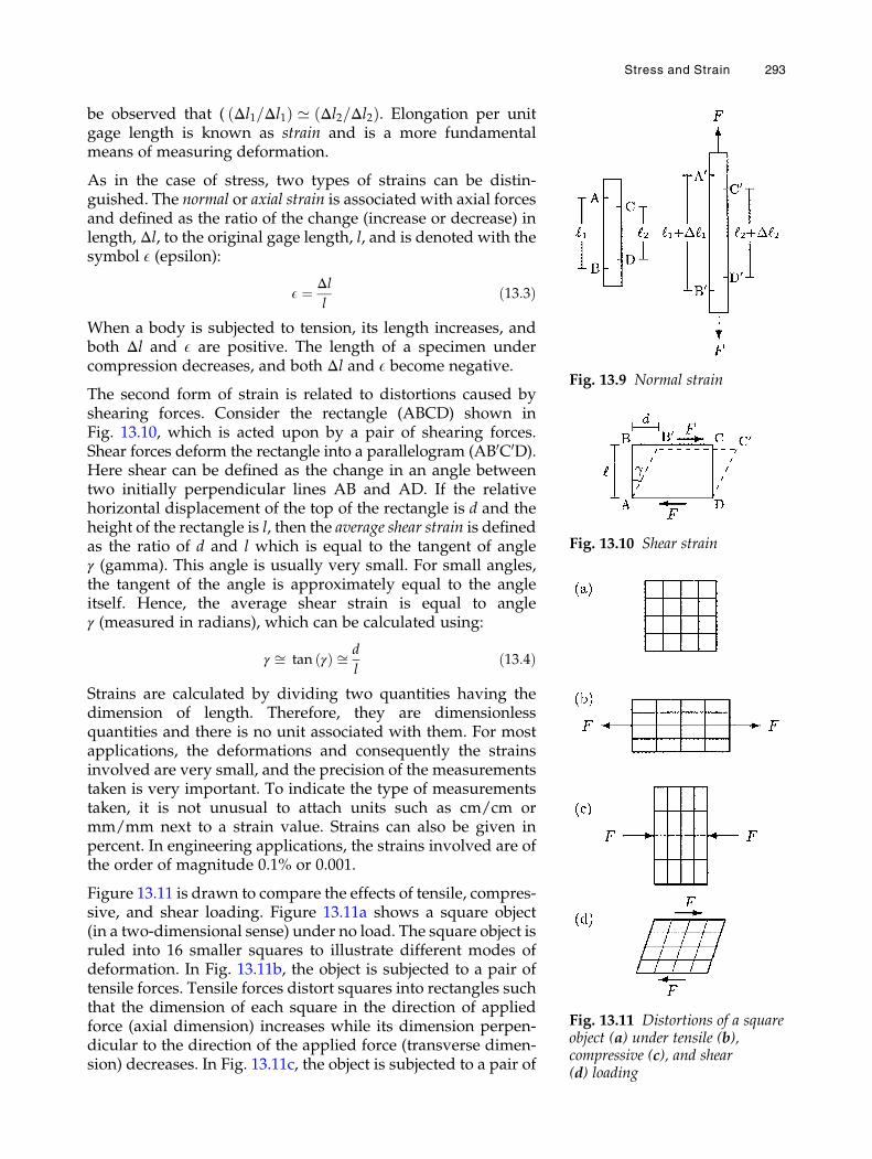
be observed that ( Δl1=Δl1ð Þ ’ Δl2=Δl2ð Þ. Elongation per unitgage length is known as strain and is a more fundamentalmeans of measuring deformation.
As in the case of stress, two types of strains can be distin-guished. The normal or axial strain is associated with axial forcesand defined as the ratio of the change (increase or decrease) inlength, Δl, to the original gage length, l, and is denoted with thesymbol E (epsilon):
E ¼ Δll
ð13:3Þ
When a body is subjected to tension, its length increases, andboth Δl and E are positive. The length of a specimen undercompression decreases, and both Δl and E become negative.
The second form of strain is related to distortions caused byshearing forces. Consider the rectangle (ABCD) shown inFig. 13.10, which is acted upon by a pair of shearing forces.Shear forces deform the rectangle into a parallelogram (AB0C0D).Here shear can be defined as the change in an angle betweentwo initially perpendicular lines AB and AD. If the relativehorizontal displacement of the top of the rectangle is d and theheight of the rectangle is l, then the average shear strain is definedas the ratio of d and l which is equal to the tangent of angleγ (gamma). This angle is usually very small. For small angles,the tangent of the angle is approximately equal to the angleitself. Hence, the average shear strain is equal to angleγ (measured in radians), which can be calculated using:
γ ffi tan γð Þ ffi d
lð13:4Þ
Strains are calculated by dividing two quantities having thedimension of length. Therefore, they are dimensionlessquantities and there is no unit associated with them. For mostapplications, the deformations and consequently the strainsinvolved are very small, and the precision of the measurementstaken is very important. To indicate the type of measurementstaken, it is not unusual to attach units such as cm/cm ormm/mm next to a strain value. Strains can also be given inpercent. In engineering applications, the strains involved are ofthe order of magnitude 0.1% or 0.001.
Figure 13.11 is drawn to compare the effects of tensile, compres-sive, and shear loading. Figure 13.11a shows a square object(in a two-dimensional sense) under no load. The square object isruled into 16 smaller squares to illustrate different modes ofdeformation. In Fig. 13.11b, the object is subjected to a pair oftensile forces. Tensile forces distort squares into rectangles suchthat the dimension of each square in the direction of appliedforce (axial dimension) increases while its dimension perpen-dicular to the direction of the applied force (transverse dimen-sion) decreases. In Fig. 13.11c, the object is subjected to a pair of
Fig. 13.9 Normal strain
Fig. 13.10 Shear strain
Fig. 13.11 Distortions of a squareobject (a) under tensile (b),compressive (c), and shear(d) loading
Stress and Strain 293
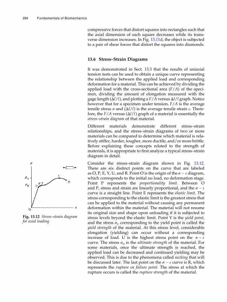
compressive forces that distort squares into rectangles such thatthe axial dimension of each square decreases while its trans-verse dimension increases. In Fig. 13.11d, the object is subjectedto a pair of shear forces that distort the squares into diamonds.
13.6 Stress–Strain Diagrams
It was demonstrated in Sect. 13.3 that the results of uniaxialtension tests can be used to obtain a unique curve representingthe relationship between the applied load and correspondingdeformation for a material. This can be achieved by dividing theapplied load with the cross-sectional area (F/A) of the speci-men, dividing the amount of elongation measured with thegage length (Δl/l), and plotting a F/A versusΔl/l graph. Noticehowever that for a specimen under tension, F/A is the averagetensile stress σ and (Δl/l) is the average tensile strain E. There-fore, the F/A versus (Δl/l) graph of a material is essentially thestress–strain diagram of that material.
Different materials demonstrate different stress–strainrelationships, and the stress–strain diagrams of two or morematerials can be compared to determine which material is rela-tively stiffer, harder, tougher, more ductile, and/ormore brittle.Before explaining these concepts related to the strength ofmaterials, it is appropriate to first analyze a typical stress–straindiagram in detail.
Consider the stress–strain diagram shown in Fig. 13.12.There are six distinct points on the curve that are labeledas O, P, E, Y, U, and R. Point O is the origin of the σ � Ediagram,which corresponds to the initial no load, no deformation stage.Point P represents the proportionality limit. Between Oand P, stress and strain are linearly proportional, and the σ � Ecurve is a straight line. Point E represents the elastic limit. Thestress corresponding to the elastic limit is the greatest stress thatcan be applied to the material without causing any permanentdeformation within the material. The material will not resumeits original size and shape upon unloading if it is subjected tostress levels beyond the elastic limit. Point Y is the yield point,and the stress σy corresponding to the yield point is called theyield strength of the material. At this stress level, considerableelongation (yielding) can occur without a correspondingincrease of load. U is the highest stress point on the σ � Ecurve. The stress σu is the ultimate strength of the material. Forsome materials, once the ultimate strength is reached, theapplied load can be decreased and continued yielding may beobserved. This is due to the phenomena called necking that willbe discussed later. The last point on the σ � E curve is R, whichrepresents the rupture or failure point. The stress at which therupture occurs is called the rupture strength of the material.
Fig. 13.12 Stress–strain diagramfor axial loading
294 Fundamentals of Biomechanics
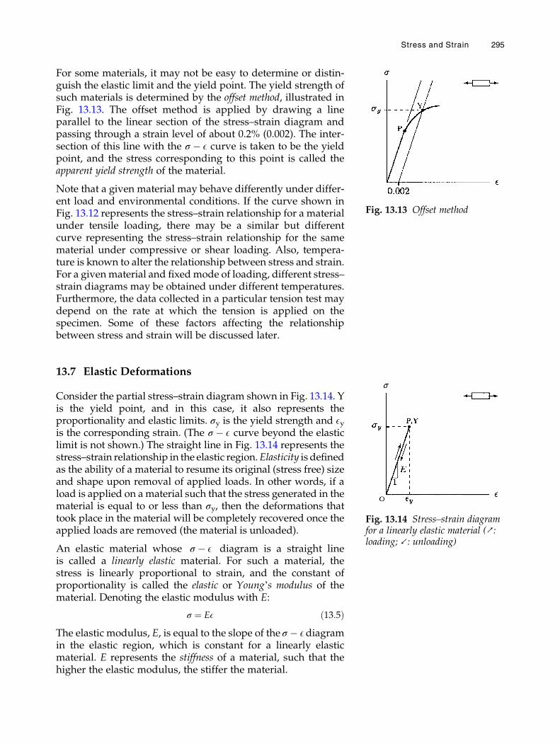
For some materials, it may not be easy to determine or distin-guish the elastic limit and the yield point. The yield strength ofsuch materials is determined by the offset method, illustrated inFig. 13.13. The offset method is applied by drawing a lineparallel to the linear section of the stress–strain diagram andpassing through a strain level of about 0.2% (0.002). The inter-section of this line with the σ � E curve is taken to be the yieldpoint, and the stress corresponding to this point is called theapparent yield strength of the material.
Note that a given material may behave differently under differ-ent load and environmental conditions. If the curve shown inFig. 13.12 represents the stress–strain relationship for a materialunder tensile loading, there may be a similar but differentcurve representing the stress–strain relationship for the samematerial under compressive or shear loading. Also, tempera-ture is known to alter the relationship between stress and strain.For a givenmaterial and fixedmode of loading, different stress–strain diagrams may be obtained under different temperatures.Furthermore, the data collected in a particular tension test maydepend on the rate at which the tension is applied on thespecimen. Some of these factors affecting the relationshipbetween stress and strain will be discussed later.
13.7 Elastic Deformations
Consider the partial stress–strain diagram shown in Fig. 13.14. Yis the yield point, and in this case, it also represents theproportionality and elastic limits. σy is the yield strength and Eyis the corresponding strain. (The σ � E curve beyond the elasticlimit is not shown.) The straight line in Fig. 13.14 represents thestress–strain relationship in the elastic region.Elasticity is definedas the ability of a material to resume its original (stress free) sizeand shape upon removal of applied loads. In other words, if aload is applied on amaterial such that the stress generated in thematerial is equal to or less than σy, then the deformations thattook place in the material will be completely recovered once theapplied loads are removed (the material is unloaded).
An elastic material whose σ � E diagram is a straight lineis called a linearly elastic material. For such a material, thestress is linearly proportional to strain, and the constant ofproportionality is called the elastic or Young’s modulus of thematerial. Denoting the elastic modulus with E:
σ ¼ EE ð13:5ÞThe elastic modulus, E, is equal to the slope of the σ � Ediagramin the elastic region, which is constant for a linearly elasticmaterial. E represents the stiffness of a material, such that thehigher the elastic modulus, the stiffer the material.
Fig. 13.13 Offset method
Fig. 13.14 Stress–strain diagramfor a linearly elastic material (↗:loading; ↙: unloading)
Stress and Strain 295
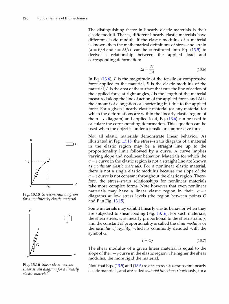
The distinguishing factor in linearly elastic materials is theirelastic moduli. That is, different linearly elastic materials havedifferent elastic moduli. If the elastic modulus of a materialis known, then the mathematical definitions of stress and strainσ ¼ F=A and E ¼ Δl=lð Þ can be substituted into Eq. (13.5) toderive a relationship between the applied load andcorresponding deformation:
Δl ¼ Fl
EAð13:6Þ
In Eq. (13.6), F is the magnitude of the tensile or compressiveforce applied to the material, E is the elastic modulus of thematerial,A is the area of the surface that cuts the line of action ofthe applied force at right angles, l is the length of the materialmeasured along the line of action of the applied force, and Δl isthe amount of elongation or shortening in l due to the appliedforce. For a given linearly elastic material (or any material forwhich the deformations are within the linearly elastic region ofthe σ � E diagram) and applied load, Eq. (13.6) can be used tocalculate the corresponding deformation. This equation can beused when the object is under a tensile or compressive force.
Not all elastic materials demonstrate linear behavior. Asillustrated in Fig. 13.15, the stress–strain diagram of a materialin the elastic region may be a straight line up to theproportionality limit followed by a curve. A curve impliesvarying slope and nonlinear behavior. Materials for which theσ � E curve in the elastic region is not a straight line are knownas nonlinear elastic materials. For a nonlinear elastic material,there is not a single elastic modulus because the slope of theσ � E curve is not constant throughout the elastic region. There-fore, the stress–strain relationships for nonlinear materialstake more complex forms. Note however that even nonlinearmaterials may have a linear elastic region in their σ � Ediagrams at low stress levels (the region between points Oand P in Fig. 13.15).
Some materials may exhibit linearly elastic behavior when theyare subjected to shear loading (Fig. 13.16). For such materials,the shear stress, τ, is linearly proportional to the shear strain, γ,and the constant of proportionality is called the shear modulus orthe modulus of rigidity, which is commonly denoted with thesymbol G:
τ ¼ Gγ ð13:7ÞThe shear modulus of a given linear material is equal to theslope of the τ � γ curve in the elastic region. The higher the shearmodulus, the more rigid the material.
Note that Eqs. (13.5) and (13.6) relate stresses to strains for linearlyelasticmaterials, and are calledmaterial functions. Obviously, for a
Fig. 13.15 Stress–strain diagramfor a nonlinearly elastic material
Fig. 13.16 Shear stress versusshear strain diagram for a linearlyelastic material
296 Fundamentals of Biomechanics
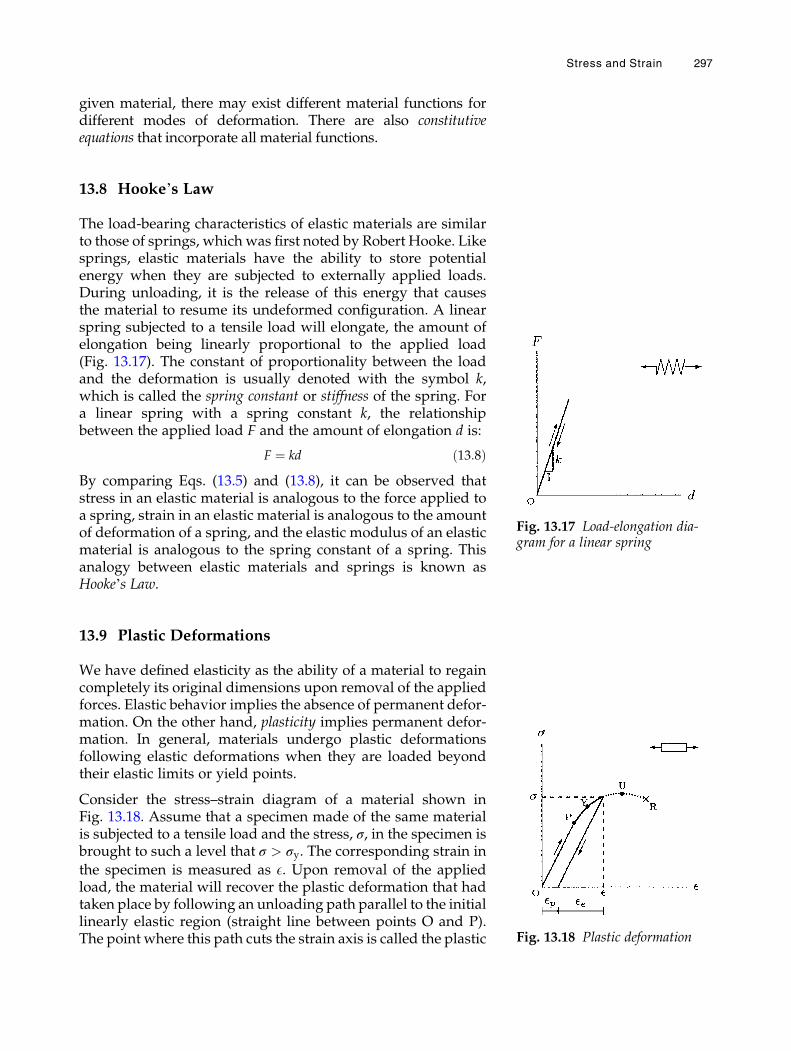
given material, there may exist different material functions fordifferent modes of deformation. There are also constitutiveequations that incorporate all material functions.
13.8 Hooke’s Law
The load-bearing characteristics of elastic materials are similarto those of springs, which was first noted by Robert Hooke. Likesprings, elastic materials have the ability to store potentialenergy when they are subjected to externally applied loads.During unloading, it is the release of this energy that causesthe material to resume its undeformed configuration. A linearspring subjected to a tensile load will elongate, the amount ofelongation being linearly proportional to the applied load(Fig. 13.17). The constant of proportionality between the loadand the deformation is usually denoted with the symbol k,which is called the spring constant or stiffness of the spring. Fora linear spring with a spring constant k, the relationshipbetween the applied load F and the amount of elongation d is:
F ¼ kd ð13:8ÞBy comparing Eqs. (13.5) and (13.8), it can be observed thatstress in an elastic material is analogous to the force applied toa spring, strain in an elastic material is analogous to the amountof deformation of a spring, and the elastic modulus of an elasticmaterial is analogous to the spring constant of a spring. Thisanalogy between elastic materials and springs is known asHooke’s Law.
13.9 Plastic Deformations
We have defined elasticity as the ability of a material to regaincompletely its original dimensions upon removal of the appliedforces. Elastic behavior implies the absence of permanent defor-mation. On the other hand, plasticity implies permanent defor-mation. In general, materials undergo plastic deformationsfollowing elastic deformations when they are loaded beyondtheir elastic limits or yield points.
Consider the stress–strain diagram of a material shown inFig. 13.18. Assume that a specimen made of the same materialis subjected to a tensile load and the stress, σ, in the specimen isbrought to such a level that σ > σy. The corresponding strain in
the specimen is measured as E. Upon removal of the appliedload, the material will recover the plastic deformation that hadtaken place by following an unloading path parallel to the initiallinearly elastic region (straight line between points O and P).The point where this path cuts the strain axis is called the plastic
Fig. 13.17 Load-elongation dia-gram for a linear spring
Fig. 13.18 Plastic deformation
Stress and Strain 297
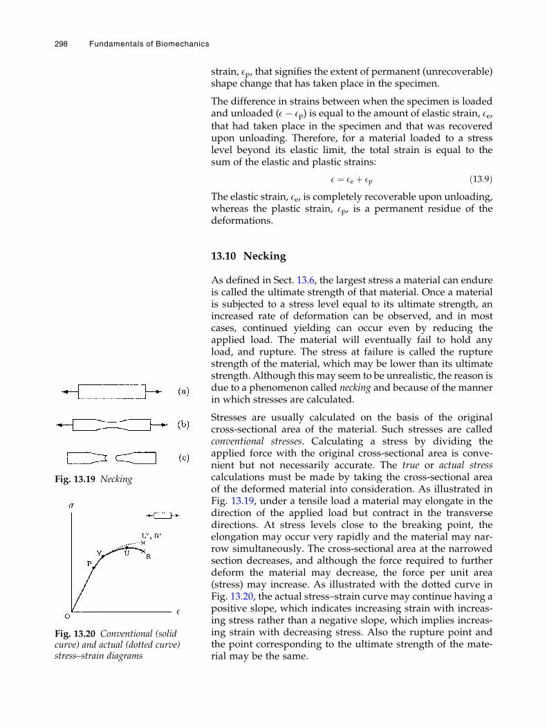
strain, Ep, that signifies the extent of permanent (unrecoverable)shape change that has taken place in the specimen.
The difference in strains between when the specimen is loadedand unloaded (E� Ep) is equal to the amount of elastic strain, Ee,that had taken place in the specimen and that was recoveredupon unloading. Therefore, for a material loaded to a stresslevel beyond its elastic limit, the total strain is equal to thesum of the elastic and plastic strains:
E ¼ Ee þ Ep ð13:9ÞThe elastic strain, Ee, is completely recoverable upon unloading,whereas the plastic strain, Ep, is a permanent residue of thedeformations.
13.10 Necking
As defined in Sect. 13.6, the largest stress a material can endureis called the ultimate strength of that material. Once a materialis subjected to a stress level equal to its ultimate strength, anincreased rate of deformation can be observed, and in mostcases, continued yielding can occur even by reducing theapplied load. The material will eventually fail to hold anyload, and rupture. The stress at failure is called the rupturestrength of the material, which may be lower than its ultimatestrength. Although this may seem to be unrealistic, the reason isdue to a phenomenon called necking and because of the mannerin which stresses are calculated.
Stresses are usually calculated on the basis of the originalcross-sectional area of the material. Such stresses are calledconventional stresses. Calculating a stress by dividing theapplied force with the original cross-sectional area is conve-nient but not necessarily accurate. The true or actual stresscalculations must be made by taking the cross-sectional areaof the deformed material into consideration. As illustrated inFig. 13.19, under a tensile load a material may elongate in thedirection of the applied load but contract in the transversedirections. At stress levels close to the breaking point, theelongation may occur very rapidly and the material may nar-row simultaneously. The cross-sectional area at the narrowedsection decreases, and although the force required to furtherdeform the material may decrease, the force per unit area(stress) may increase. As illustrated with the dotted curve inFig. 13.20, the actual stress–strain curve may continue having apositive slope, which indicates increasing strain with increas-ing stress rather than a negative slope, which implies increas-ing strain with decreasing stress. Also the rupture point andthe point corresponding to the ultimate strength of the mate-rial may be the same.
Fig. 13.19 Necking
Fig. 13.20 Conventional (solidcurve) and actual (dotted curve)stress–strain diagrams
298 Fundamentals of Biomechanics
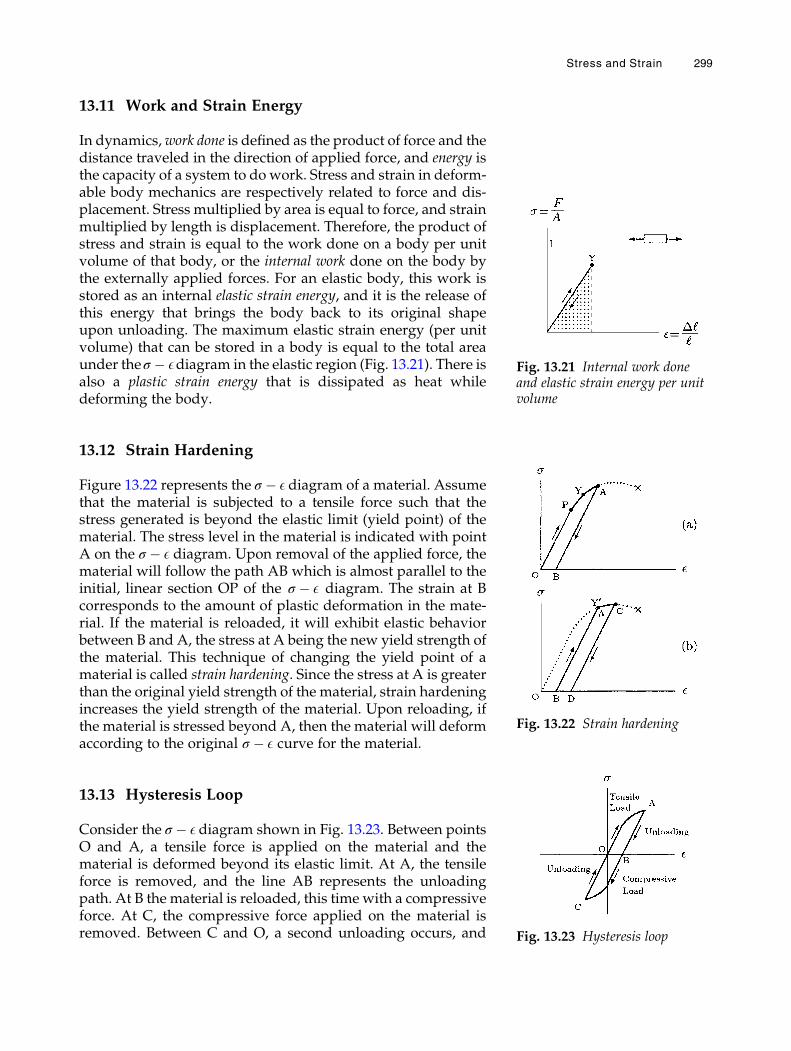
13.11 Work and Strain Energy
In dynamics,work done is defined as the product of force and thedistance traveled in the direction of applied force, and energy isthe capacity of a system to do work. Stress and strain in deform-able body mechanics are respectively related to force and dis-placement. Stress multiplied by area is equal to force, and strainmultiplied by length is displacement. Therefore, the product ofstress and strain is equal to the work done on a body per unitvolume of that body, or the internal work done on the body bythe externally applied forces. For an elastic body, this work isstored as an internal elastic strain energy, and it is the release ofthis energy that brings the body back to its original shapeupon unloading. The maximum elastic strain energy (per unitvolume) that can be stored in a body is equal to the total areaunder theσ � Ediagram in the elastic region (Fig. 13.21). There isalso a plastic strain energy that is dissipated as heat whiledeforming the body.
13.12 Strain Hardening
Figure 13.22 represents the σ � E diagram of a material. Assumethat the material is subjected to a tensile force such that thestress generated is beyond the elastic limit (yield point) of thematerial. The stress level in the material is indicated with pointA on the σ � E diagram. Upon removal of the applied force, thematerial will follow the path AB which is almost parallel to theinitial, linear section OP of the σ � E diagram. The strain at Bcorresponds to the amount of plastic deformation in the mate-rial. If the material is reloaded, it will exhibit elastic behaviorbetween B and A, the stress at A being the new yield strength ofthe material. This technique of changing the yield point of amaterial is called strain hardening. Since the stress at A is greaterthan the original yield strength of the material, strain hardeningincreases the yield strength of the material. Upon reloading, ifthe material is stressed beyond A, then the material will deformaccording to the original σ � E curve for the material.
13.13 Hysteresis Loop
Consider the σ � E diagram shown in Fig. 13.23. Between pointsO and A, a tensile force is applied on the material and thematerial is deformed beyond its elastic limit. At A, the tensileforce is removed, and the line AB represents the unloadingpath. At B the material is reloaded, this time with a compressiveforce. At C, the compressive force applied on the material isremoved. Between C and O, a second unloading occurs, and
Fig. 13.21 Internal work doneand elastic strain energy per unitvolume
Fig. 13.22 Strain hardening
Fig. 13.23 Hysteresis loop
Stress and Strain 299
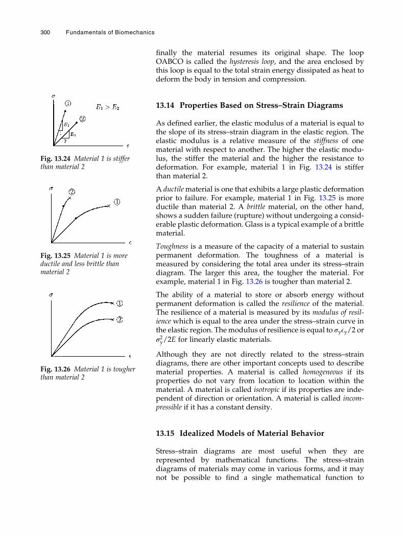
finally the material resumes its original shape. The loopOABCO is called the hysteresis loop, and the area enclosed bythis loop is equal to the total strain energy dissipated as heat todeform the body in tension and compression.
13.14 Properties Based on Stress–Strain Diagrams
As defined earlier, the elastic modulus of a material is equal tothe slope of its stress–strain diagram in the elastic region. Theelastic modulus is a relative measure of the stiffness of onematerial with respect to another. The higher the elastic modu-lus, the stiffer the material and the higher the resistance todeformation. For example, material 1 in Fig. 13.24 is stifferthan material 2.
A ductilematerial is one that exhibits a large plastic deformationprior to failure. For example, material 1 in Fig. 13.25 is moreductile than material 2. A brittle material, on the other hand,shows a sudden failure (rupture) without undergoing a consid-erable plastic deformation. Glass is a typical example of a brittlematerial.
Toughness is a measure of the capacity of a material to sustainpermanent deformation. The toughness of a material ismeasured by considering the total area under its stress–straindiagram. The larger this area, the tougher the material. Forexample, material 1 in Fig. 13.26 is tougher than material 2.
The ability of a material to store or absorb energy withoutpermanent deformation is called the resilience of the material.The resilience of a material is measured by its modulus of resil-ience which is equal to the area under the stress–strain curve inthe elastic region. Themodulus of resilience is equal to σyEy/2 orσ2y/2E for linearly elastic materials.
Although they are not directly related to the stress–straindiagrams, there are other important concepts used to describematerial properties. A material is called homogeneous if itsproperties do not vary from location to location within thematerial. A material is called isotropic if its properties are inde-pendent of direction or orientation. A material is called incom-pressible if it has a constant density.
13.15 Idealized Models of Material Behavior
Stress–strain diagrams are most useful when they arerepresented by mathematical functions. The stress–straindiagrams of materials may come in various forms, and it maynot be possible to find a single mathematical function to
Fig. 13.24 Material 1 is stifferthan material 2
Fig. 13.25 Material 1 is moreductile and less brittle thanmaterial 2
Fig. 13.26 Material 1 is tougherthan material 2
300 Fundamentals of Biomechanics
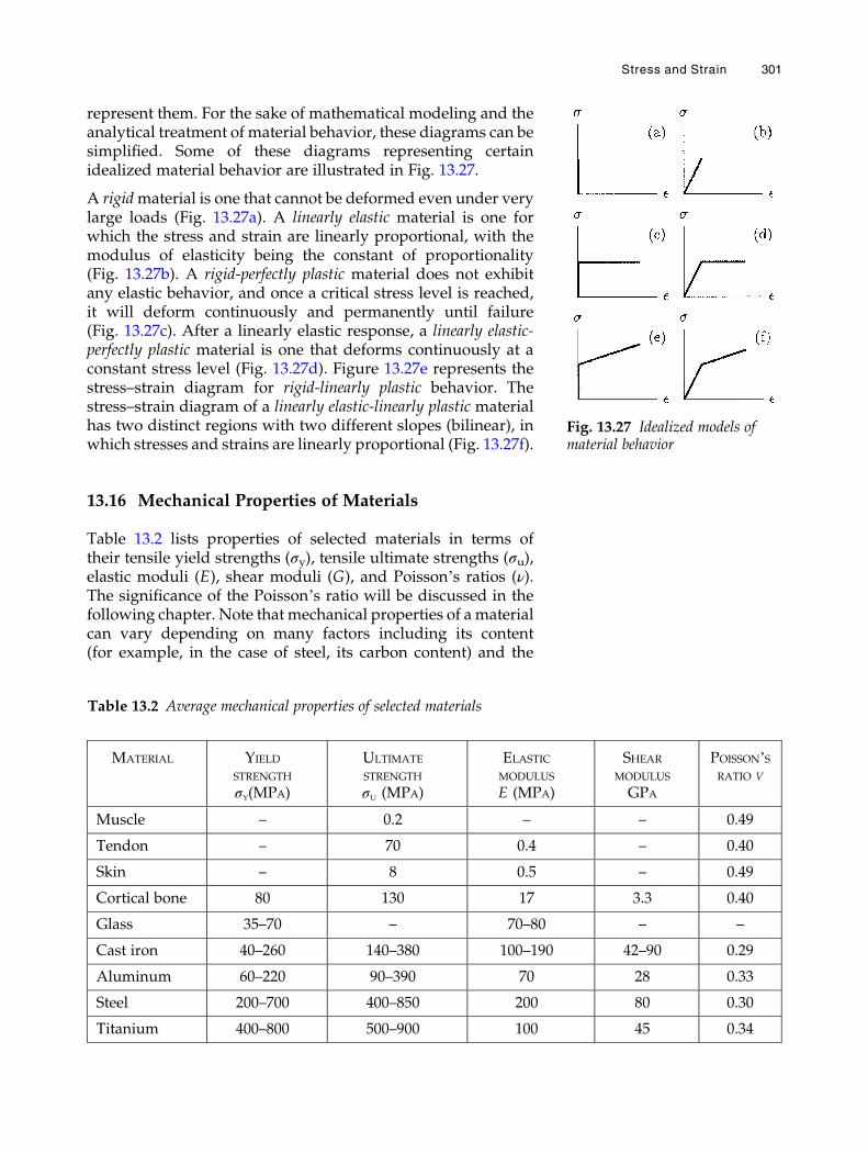
represent them. For the sake of mathematical modeling and theanalytical treatment of material behavior, these diagrams can besimplified. Some of these diagrams representing certainidealized material behavior are illustrated in Fig. 13.27.
A rigidmaterial is one that cannot be deformed even under verylarge loads (Fig. 13.27a). A linearly elastic material is one forwhich the stress and strain are linearly proportional, with themodulus of elasticity being the constant of proportionality(Fig. 13.27b). A rigid-perfectly plastic material does not exhibitany elastic behavior, and once a critical stress level is reached,it will deform continuously and permanently until failure(Fig. 13.27c). After a linearly elastic response, a linearly elastic-perfectly plastic material is one that deforms continuously at aconstant stress level (Fig. 13.27d). Figure 13.27e represents thestress–strain diagram for rigid-linearly plastic behavior. Thestress–strain diagram of a linearly elastic-linearly plastic materialhas two distinct regions with two different slopes (bilinear), inwhich stresses and strains are linearly proportional (Fig. 13.27f).
13.16 Mechanical Properties of Materials
Table 13.2 lists properties of selected materials in terms oftheir tensile yield strengths (σy), tensile ultimate strengths (σu),elastic moduli (E), shear moduli (G), and Poisson’s ratios (ν).The significance of the Poisson’s ratio will be discussed in thefollowing chapter. Note that mechanical properties of a materialcan vary depending on many factors including its content(for example, in the case of steel, its carbon content) and the
Fig. 13.27 Idealized models ofmaterial behavior
Table 13.2 Average mechanical properties of selected materials
MATERIAL YIELD
STRENGTH
σY(MPA)
ULTIMATE
STRENGTH
σU (MPA)
ELASTIC
MODULUS
E (MPA)
SHEAR
MODULUS
GPA
POISSON’SRATIO V
Muscle – 0.2 – – 0.49
Tendon – 70 0.4 – 0.40
Skin – 8 0.5 – 0.49
Cortical bone 80 130 17 3.3 0.40
Glass 35–70 – 70–80 – –
Cast iron 40–260 140–380 100–190 42–90 0.29
Aluminum 60–220 90–390 70 28 0.33
Steel 200–700 400–850 200 80 0.30
Titanium 400–800 500–900 100 45 0.34
Stress and Strain 301
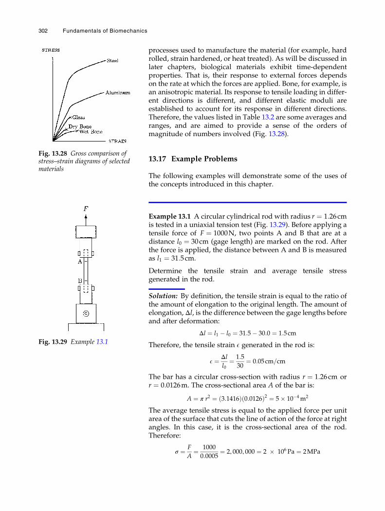
processes used to manufacture the material (for example, hardrolled, strain hardened, or heat treated). As will be discussed inlater chapters, biological materials exhibit time-dependentproperties. That is, their response to external forces dependson the rate at which the forces are applied. Bone, for example, isan anisotropic material. Its response to tensile loading in differ-ent directions is different, and different elastic moduli areestablished to account for its response in different directions.Therefore, the values listed in Table 13.2 are some averages andranges, and are aimed to provide a sense of the orders ofmagnitude of numbers involved (Fig. 13.28).
13.17 Example Problems
The following examples will demonstrate some of the uses ofthe concepts introduced in this chapter.
Example 13.1 A circular cylindrical rod with radius r ¼ 1:26cmis tested in a uniaxial tension test (Fig. 13.29). Before applying atensile force of F ¼ 1000N, two points A and B that are at adistance l0 ¼ 30cm (gage length) are marked on the rod. Afterthe force is applied, the distance between A and B is measuredas l1 ¼ 31:5cm.
Determine the tensile strain and average tensile stressgenerated in the rod.
Solution: By definition, the tensile strain is equal to the ratio ofthe amount of elongation to the original length. The amount ofelongation, Δl, is the difference between the gage lengths beforeand after deformation:
Δl ¼ l1 � l0 ¼ 31:5� 30:0 ¼ 1:5cm
Therefore, the tensile strain E generated in the rod is:
E ¼ Δll0
¼ 1:5
30¼ 0:05cm=cm
The bar has a circular cross-section with radius r ¼ 1:26cm orr ¼ 0:0126m. The cross-sectional area A of the bar is:
A ¼ π r2 ¼ 3:1416ð Þ 0:0126ð Þ2 ¼ 5� 10�4m2
The average tensile stress is equal to the applied force per unitarea of the surface that cuts the line of action of the force at rightangles. In this case, it is the cross-sectional area of the rod.Therefore:
σ ¼ F
A¼ 1000
0:0005¼ 2, 000, 000 ¼ 2 � 106 Pa ¼ 2MPa
Fig. 13.28 Gross comparison ofstress–strain diagrams of selectedmaterials
Fig. 13.29 Example 13.1
302 Fundamentals of Biomechanics
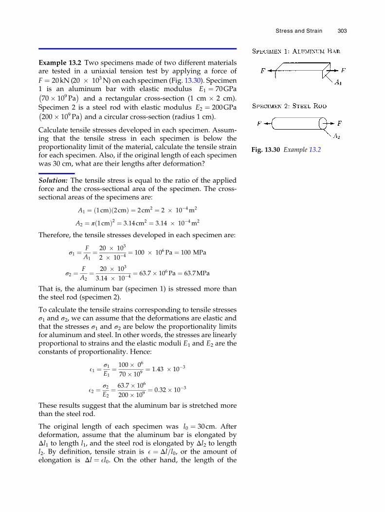
Example 13.2 Two specimens made of two different materialsare tested in a uniaxial tension test by applying a force of
F ¼ 20kN (20 � 103N) on each specimen (Fig. 13.30). Specimen1 is an aluminum bar with elastic modulus E1 ¼ 70GPa
70� 109 Pa� �
and a rectangular cross-section (1 cm � 2 cm).
Specimen 2 is a steel rod with elastic modulus E2 ¼ 200GPa
200� 109 Pa� �
and a circular cross-section (radius 1 cm).
Calculate tensile stresses developed in each specimen. Assum-ing that the tensile stress in each specimen is below theproportionality limit of the material, calculate the tensile strainfor each specimen. Also, if the original length of each specimenwas 30 cm, what are their lengths after deformation?
Solution: The tensile stress is equal to the ratio of the appliedforce and the cross-sectional area of the specimen. The cross-sectional areas of the specimens are:
A1 ¼ 1cmð Þ 2cmð Þ ¼ 2cm2 ¼ 2 � 10�4m2
A2 ¼ π 1cmð Þ2 ¼ 3:14cm2 ¼ 3:14 � 10�4m2
Therefore, the tensile stresses developed in each specimen are:
σ1 ¼ F
A1¼ 20 � 103
2 � 10�4¼ 100 � 106 Pa ¼ 100 MPa
σ2 ¼ F
A2¼ 20 � 103
3:14 � 10�4¼ 63:7� 106 Pa ¼ 63:7MPa
That is, the aluminum bar (specimen 1) is stressed more thanthe steel rod (specimen 2).
To calculate the tensile strains corresponding to tensile stressesσ1 and σ2, we can assume that the deformations are elastic andthat the stresses σ1 and σ2 are below the proportionality limitsfor aluminum and steel. In other words, the stresses are linearlyproportional to strains and the elastic moduli E1 and E2 are theconstants of proportionality. Hence:
E1 ¼ σ1E1
¼ 100� 06
70� 109¼ 1:43 � 10�3
E2 ¼ σ2E2
¼ 63:7� 106
200� 109¼ 0:32� 10�3
These results suggest that the aluminum bar is stretched morethan the steel rod.
The original length of each specimen was l0 ¼ 30cm. Afterdeformation, assume that the aluminum bar is elongated byΔl1 to length l1, and the steel rod is elongated by Δl2 to lengthl2. By definition, tensile strain is E ¼ Δl=l0, or the amount ofelongation is Δl ¼ El0. On the other hand, the length of the
Fig. 13.30 Example 13.2
Stress and Strain 303
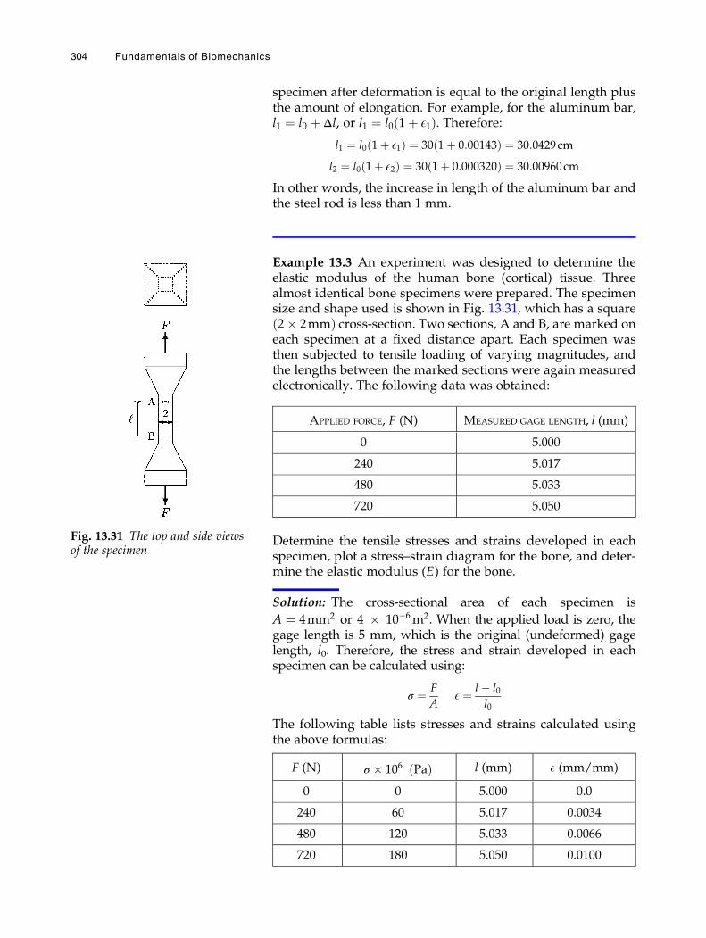
specimen after deformation is equal to the original length plusthe amount of elongation. For example, for the aluminum bar,l1 ¼ l0 þ Δl, or l1 ¼ l0 1þ E1ð Þ. Therefore:
l1 ¼ l0 1þ E1ð Þ ¼ 30 1þ 0:00143ð Þ ¼ 30:0429cm
l2 ¼ l0 1þ E2ð Þ ¼ 30 1þ 0:000320ð Þ ¼ 30:00960cm
In other words, the increase in length of the aluminum bar andthe steel rod is less than 1 mm.
Example 13.3 An experiment was designed to determine theelastic modulus of the human bone (cortical) tissue. Threealmost identical bone specimens were prepared. The specimensize and shape used is shown in Fig. 13.31, which has a square2� 2mmð Þ cross-section. Two sections, A and B, are marked oneach specimen at a fixed distance apart. Each specimen wasthen subjected to tensile loading of varying magnitudes, andthe lengths between the marked sections were again measuredelectronically. The following data was obtained:
APPLIED FORCE, F (N) MEASURED GAGE LENGTH, l (mm)
0 5.000
240 5.017
480 5.033
720 5.050
Determine the tensile stresses and strains developed in eachspecimen, plot a stress–strain diagram for the bone, and deter-mine the elastic modulus (E) for the bone.
Solution: The cross-sectional area of each specimen is
A ¼ 4mm2 or 4 � 10�6m2. When the applied load is zero, thegage length is 5 mm, which is the original (undeformed) gagelength, l0. Therefore, the stress and strain developed in eachspecimen can be calculated using:
σ ¼ F
AE ¼ l� l0
l0
The following table lists stresses and strains calculated usingthe above formulas:
F (N) σ � 106 Pað Þ l (mm) E (mm/mm)
0 0 5.000 0.0
240 60 5.017 0.0034
480 120 5.033 0.0066
720 180 5.050 0.0100
Fig. 13.31 The top and side viewsof the specimen
304 Fundamentals of Biomechanics
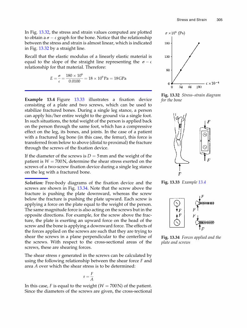
In Fig. 13.32, the stress and strain values computed are plottedto obtain a σ � E graph for the bone. Notice that the relationshipbetween the stress and strain is almost linear, which is indicatedin Fig. 13.32 by a straight line.
Recall that the elastic modulus of a linearly elastic material isequal to the slope of the straight line representing the σ � Erelationship for that material. Therefore:
E ¼ σ
E¼ 180� 106
0:0100¼ 18� 109 Pa ¼ 18GPa
Example 13.4 Figure 13.33 illustrates a fixation deviceconsisting of a plate and two screws, which can be used tostabilize fractured bones. During a single leg stance, a personcan apply his/her entire weight to the ground via a single foot.In such situations, the total weight of the person is applied backon the person through the same foot, which has a compressiveeffect on the leg, its bones, and joints. In the case of a patientwith a fractured leg bone (in this case, the femur), this force istransferred from below to above (distal to proximal) the fracturethrough the screws of the fixation device.
If the diameter of the screws isD ¼ 5mm and the weight of thepatient is W ¼ 700N, determine the shear stress exerted on thescrews of a two-screw fixation device during a single leg stanceon the leg with a fractured bone.
Solution: Free-body diagrams of the fixation device and thescrews are shown in Fig. 13.34. Note that the screw above thefracture is pushing the plate downward, whereas the screwbelow the fracture is pushing the plate upward. Each screw isapplying a force on the plate equal to the weight of the person.The samemagnitude force is also acting on the screws but in theopposite directions. For example, for the screw above the frac-ture, the plate is exerting an upward force on the head of thescrew and the bone is applying a downward force. The effects ofthe forces applied on the screws are such that they are trying toshear the screws in a plane perpendicular to the centerline ofthe screws. With respect to the cross-sectional areas of thescrews, these are shearing forces.
The shear stress τ generated in the screws can be calculated byusing the following relationship between the shear force F andarea A over which the shear stress is to be determined:
τ ¼ F
A
In this case, F is equal to the weight (W ¼ 700N) of the patient.Since the diameters of the screws are given, the cross-sectional
Fig. 13.32 Stress–strain diagramfor the bone
Fig. 13.33 Example 13.4
Fig. 13.34 Forces applied and theplate and screws
Stress and Strain 305
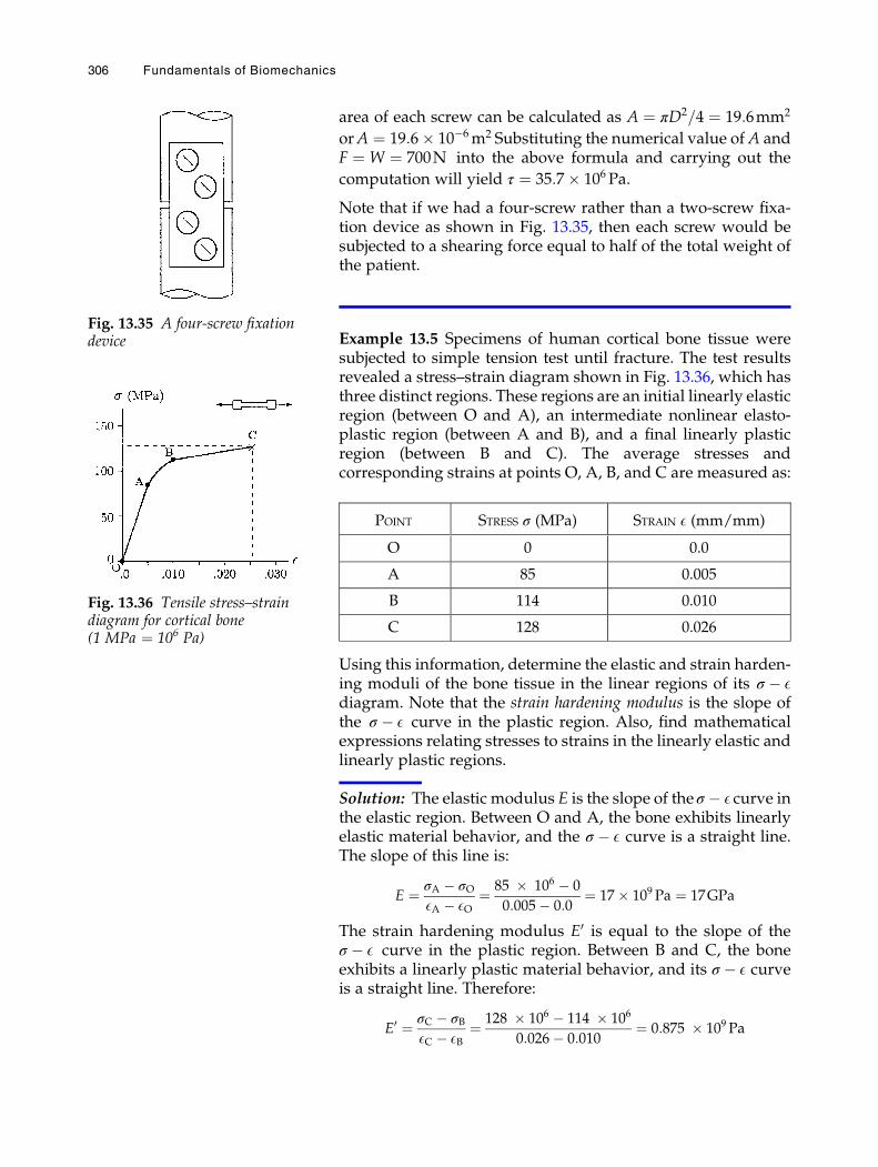
area of each screw can be calculated as A ¼ πD2=4 ¼ 19:6mm2
orA ¼ 19:6� 10�6m2 Substituting the numerical value of A andF ¼ W ¼ 700N into the above formula and carrying out the
computation will yield τ ¼ 35:7� 106 Pa.
Note that if we had a four-screw rather than a two-screw fixa-tion device as shown in Fig. 13.35, then each screw would besubjected to a shearing force equal to half of the total weight ofthe patient.
Example 13.5 Specimens of human cortical bone tissue weresubjected to simple tension test until fracture. The test resultsrevealed a stress–strain diagram shown in Fig. 13.36, which hasthree distinct regions. These regions are an initial linearly elasticregion (between O and A), an intermediate nonlinear elasto-plastic region (between A and B), and a final linearly plasticregion (between B and C). The average stresses andcorresponding strains at points O, A, B, and C are measured as:
POINT STRESS σ (MPa) STRAIN E (mm/mm)
O 0 0.0
A 85 0.005
B 114 0.010
C 128 0.026
Using this information, determine the elastic and strain harden-ing moduli of the bone tissue in the linear regions of its σ � Ediagram. Note that the strain hardening modulus is the slope ofthe σ � E curve in the plastic region. Also, find mathematicalexpressions relating stresses to strains in the linearly elastic andlinearly plastic regions.
Solution: The elastic modulus E is the slope of the σ � E curve inthe elastic region. Between O and A, the bone exhibits linearlyelastic material behavior, and the σ � E curve is a straight line.The slope of this line is:
E ¼ σA � σOEA � EO
¼ 85 � 106 � 0
0:005� 0:0¼ 17� 109 Pa ¼ 17GPa
The strain hardening modulus E0 is equal to the slope of theσ � E curve in the plastic region. Between B and C, the boneexhibits a linearly plastic material behavior, and its σ � E curveis a straight line. Therefore:
E0 ¼ σC � σBEC � EB
¼ 128 � 106 � 114 � 106
0:026� 0:010¼ 0:875 � 109 Pa
Fig. 13.35 A four-screw fixationdevice
Fig. 13.36 Tensile stress–straindiagram for cortical bone(1 MPa ¼ 106 Pa)
306 Fundamentals of Biomechanics
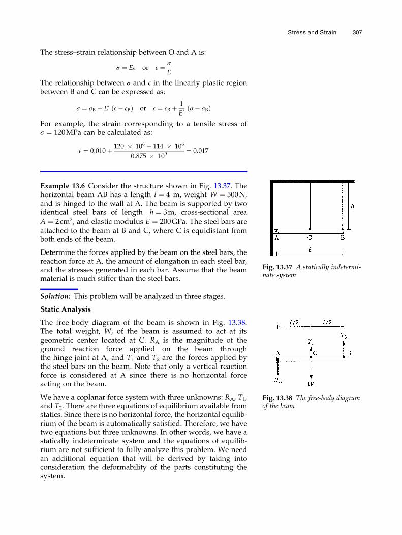
The stress–strain relationship between O and A is:
σ ¼ EE or E ¼ σ
E
The relationship between σ and E in the linearly plastic regionbetween B and C can be expressed as:
σ ¼ σB þ E0 E� EBð Þ or E ¼ EB þ 1
E0 σ � σBð Þ
For example, the strain corresponding to a tensile stress ofσ ¼ 120MPa can be calculated as:
E ¼ 0:010þ 120 � 106 � 114 � 106
0:875 � 109¼ 0:017
Example 13.6 Consider the structure shown in Fig. 13.37. Thehorizontal beam AB has a length l ¼ 4 m, weight W ¼ 500N,and is hinged to the wall at A. The beam is supported by twoidentical steel bars of length h ¼ 3m, cross-sectional area
A ¼ 2cm2, and elastic modulus E ¼ 200GPa. The steel bars areattached to the beam at B and C, where C is equidistant fromboth ends of the beam.
Determine the forces applied by the beam on the steel bars, thereaction force at A, the amount of elongation in each steel bar,and the stresses generated in each bar. Assume that the beammaterial is much stiffer than the steel bars.
Solution: This problem will be analyzed in three stages.
Static Analysis
The free-body diagram of the beam is shown in Fig. 13.38.The total weight, W, of the beam is assumed to act at itsgeometric center located at C. RA is the magnitude of theground reaction force applied on the beam throughthe hinge joint at A, and T1 and T2 are the forces applied bythe steel bars on the beam. Note that only a vertical reactionforce is considered at A since there is no horizontal forceacting on the beam.
We have a coplanar force system with three unknowns: RA, T1,and T2. There are three equations of equilibrium available fromstatics. Since there is no horizontal force, the horizontal equilib-rium of the beam is automatically satisfied. Therefore, we havetwo equations but three unknowns. In other words, we have astatically indeterminate system and the equations of equilib-rium are not sufficient to fully analyze this problem. We needan additional equation that will be derived by taking intoconsideration the deformability of the parts constituting thesystem.
Fig. 13.37 A statically indetermi-nate system
Fig. 13.38 The free-body diagramof the beam
Stress and Strain 307
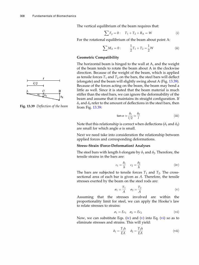
The vertical equilibrium of the beam requires that:X
Fy ¼ 0 : T1 þ T2 þ RA ¼ W ðiÞFor the rotational equilibrium of the beam about point A:
XMA ¼ 0 :
1
2T1 þ T2 ¼ 1
2W ðiiÞ
Geometric Compatibility
The horizontal beam is hinged to the wall at A, and the weightof the beam tends to rotate the beam about A in the clockwisedirection. Because of the weight of the beam, which is appliedas tensile forces T1 and T2 on the bars, the steel bars will deflect(elongate) and the beamwill slightly swing about A (Fig. 13.39).Because of the forces acting on the beam, the beam may bend alittle as well. Since it is stated that the beam material is muchstiffer than the steel bars, we can ignore the deformability of thebeam and assume that it maintains its straight configuration. Ifδ1 and δ2 refer to the amount of deflections in the steel bars, thenfrom Fig. 13.39:
tan α ’ δ1l=2
’ δ2l
ðiiiÞ
Note that this relationship is correct when deflections (δ1 and δ2)are small for which angle α is small.
Next we need take into consideration the relationship betweenapplied forces and corresponding deformations.
Stress–Strain (Force-Deformation) Analyses
The steel bars with length h elongate by δ1 and δ2. Therefore, thetensile strains in the bars are:
E1 ¼ δ1h
E2 ¼ δ2h
ðivÞ
The bars are subjected to tensile forces T1 and T2. The cross-sectional area of each bar is given as A. Therefore, the tensilestresses exerted by the beam on the steel rods are:
σ1 ¼ T1
Aσ2 ¼ T2
AðvÞ
Assuming that the stresses involved are within theproportionality limit for steel, we can apply the Hooke’s lawto relate stresses to strains:
σ1 ¼ EE1 σ2 ¼ EE2 ðviÞNow, we can substitute Eqs. (iv) and (v) into Eq. (vi) so as toeliminate stresses and strains. This will yield:
δ1 ¼ T1h
EAδ2 ¼ T2h
EAðviiÞ
Fig. 13.39 Deflection of the beam
308 Fundamentals of Biomechanics
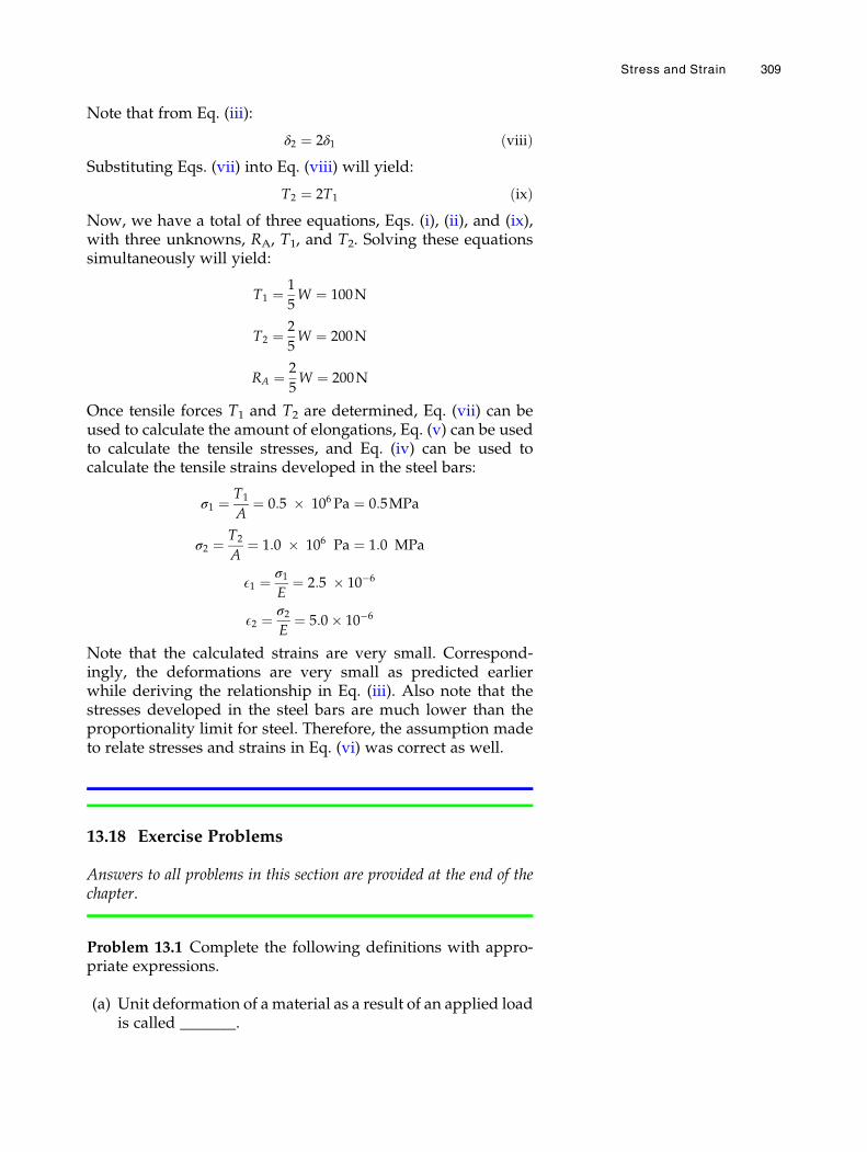
Note that from Eq. (iii):
δ2 ¼ 2δ1 ðviiiÞSubstituting Eqs. (vii) into Eq. (viii) will yield:
T2 ¼ 2T1 ðixÞNow, we have a total of three equations, Eqs. (i), (ii), and (ix),with three unknowns, RA, T1, and T2. Solving these equationssimultaneously will yield:
T1 ¼ 1
5W ¼ 100N
T2 ¼ 2
5W ¼ 200N
RA ¼ 2
5W ¼ 200N
Once tensile forces T1 and T2 are determined, Eq. (vii) can beused to calculate the amount of elongations, Eq. (v) can be usedto calculate the tensile stresses, and Eq. (iv) can be used tocalculate the tensile strains developed in the steel bars:
σ1 ¼ T1
A¼ 0:5 � 106 Pa ¼ 0:5MPa
σ2 ¼ T2
A¼ 1:0 � 106 Pa ¼ 1:0 MPa
E1 ¼ σ1E
¼ 2:5 � 10�6
E2 ¼ σ2E
¼ 5:0� 10�6
Note that the calculated strains are very small. Correspond-ingly, the deformations are very small as predicted earlierwhile deriving the relationship in Eq. (iii). Also note that thestresses developed in the steel bars are much lower than theproportionality limit for steel. Therefore, the assumption madeto relate stresses and strains in Eq. (vi) was correct as well.
13.18 Exercise Problems
Answers to all problems in this section are provided at the end of thechapter.
Problem 13.1 Complete the following definitions with appro-priate expressions.
(a) Unit deformation of a material as a result of an applied loadis called _______.
Stress and Strain 309
(b) The internal resistance of a material to deformation due toexternally applied forces is called _______.
(c) _______ is a measure of the intensity of internal forcesacting parallel or tangent to a plane of cut, while _______are associated with the intensity of internal forces that areperpendicular to the plane of cut.
(d) On the stress–strain diagram, the stress corresponding tothe _______ is the highest stress that can be applied to thematerial without causing permanent deformation.
(e) On the stress–strain diagram, the highest stress levelcorresponds to the _______ of the material.
(f) For some materials, it may not be easy to distinguish theyield point. The yield strength of such materials may bedetermined by the _______.
(g) _______ is defined as the ability of a material to resume itsoriginal (stress-free) size and shape upon removal ofapplied loads.
(h) For linearly elastic materials, stress is linearly proportionalto strain and the constant of proportionality is called the_______ of the material.
(i) The distinguishing factor in linearly elastic materials istheir _______.
(j) Materials for which the stress–strain curve in the elasticregion is not a straight line are known as _______ materials.
(k) _______ is the constant of proportionality between shearstress and shear strain for linearly elastic materials.
(l) A mathematical equation that relates stresses to strains iscalled a _______.
(m) The analogy between elastic materials and springs isknown as _______.
(n) _______ implies permanent (unrecoverable) deformations.(o) The area under the stress–strain diagram in the elastic
region corresponds to the _______ energy stored in thematerial while deforming the material.
(p) _______ energy is dissipated as heat while deforming thematerial.
(q) The area enclosed by the _______ signifies the total strainenergy dissipated as heat while loading and unloading amaterial.
(r) The technique of changing the yield point of a material byloading the material beyond its yield point is called_______.
(s) The elastic modulus of a material is a relative measure ofthe _______ of one material with respect to another.
(t) A _______ material is one that exhibits a large plastic defor-mation prior to failure.
(u) A _______ material is one that shows a sudden failure(rupture) without undergoing a considerable plasticdeformation.
310 Fundamentals of Biomechanics
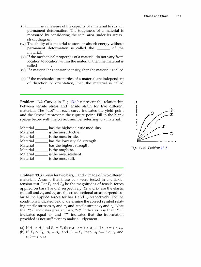
(v) _______ is a measure of the capacity of a material to sustainpermanent deformation. The toughness of a material ismeasured by considering the total area under its stress–strain diagram.
(w) The ability of a material to store or absorb energy withoutpermanent deformation is called the _______ of thematerial.
(x) If the mechanical properties of a material do not vary fromlocation to location within the material, then the material iscalled _______.
(y) If a material has constant density, then thematerial is called_______.
(z) If the mechanical properties of a material are independentof direction or orientation, then the material is called_______.
Problem 13.2 Curves in Fig. 13.40 represent the relationshipbetween tensile stress and tensile strain for five differentmaterials. The “dot” on each curve indicates the yield pointand the “cross” represents the rupture point. Fill in the blankspaces below with the correct number referring to a material.
Material _______ has the highest elastic modulus.Material _______ is the most ductile.Material _______ is the most brittle.Material _______ has the lowest yield strength.Material _______ has the highest strength.Material _______ is the toughest.Material _______ is the most resilient.Material _______ is the most stiff.
Problem 13.3 Consider two bars, 1 and 2, made of two differentmaterials. Assume that these bars were tested in a uniaxialtension test. Let F1 and F2 be the magnitudes of tensile forcesapplied on bars 1 and 2, respectively. E1 and E2 are the elasticmoduli and A1 and A2 are the cross-sectional areas perpendicu-lar to the applied forces for bar 1 and 2, respectively. For theconditions indicated below, determine the correct symbol relat-ing tensile stresses σ1 and σ2 and tensile strains E1 and E2. Notethat “>” indicates greater than, “<” indicates less than, “¼”indicates equal to, and “?” indicates that the informationprovided is not sufficient to make a judgement.
(a) If A1 > A2 and F1 ¼ F2 then σ1 >¼ ? < σ2 and E1 >¼ ? < E2.(b) If E1 > E2, A1 ¼ A2 and F1 ¼ F2 then σ1 >¼ ? < σ2 and
E1 >¼ ? < E2
Fig. 13.40 Problem 13.2
Stress and Strain 311
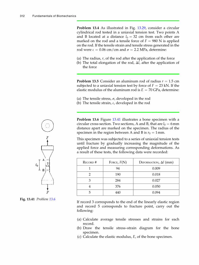
Problem 13.4 As illustrated in Fig. 13.29, consider a circularcylindrical rod tested in a uniaxial tension test. Two points Aand B located at a distance l0 ¼ 32 cm from each other aremarked on the rod and a tensile force of F ¼ 980 N is appliedon the rod. If the tensile strain and tensile stress generated in therod were E ¼ 0.06 cm/cm and σ ¼ 2.2 MPa, determine:
(a) The radius, r, of the rod after the application of the force(b) The total elongation of the rod, Δl, after the application of
the force
Problem 13.5 Consider an aluminum rod of radius r ¼ 1.5 cmsubjected to a uniaxial tension test by force of F ¼ 23 kN. If theelastic modulus of the aluminum rod is E ¼ 70 GPa, determine:
(a) The tensile stress, σ, developed in the rod(b) The tensile strain, E, developed in the rod
Problem 13.6 Figure 13.41 illustrates a bone specimen with acircular cross-section. Two sections, A and B, that are l0 ¼ 6mmdistance apart are marked on the specimen. The radius of thespecimen in the region between A and B is r0 ¼ 1mm.
This specimen was subjected to a series of uniaxial tension testsuntil fracture by gradually increasing the magnitude of theapplied force and measuring corresponding deformations. Asa result of these tests, the following data were recorded:
RECORD # FORCE, F(N) DEFORMATION, Δl (mm)
1 94 0.009
2 190 0.018
3 284 0.027
4 376 0.050
5 440 0.094
If record 3 corresponds to the end of the linearly elastic regionand record 5 corresponds to fracture point, carry out thefollowing:
(a) Calculate average tensile stresses and strains for eachrecord.
(b) Draw the tensile stress–strain diagram for the bonespecimen.
(c) Calculate the elastic modulus, E, of the bone specimen.
Fig. 13.41 Problem 13.6
312 Fundamentals of Biomechanics
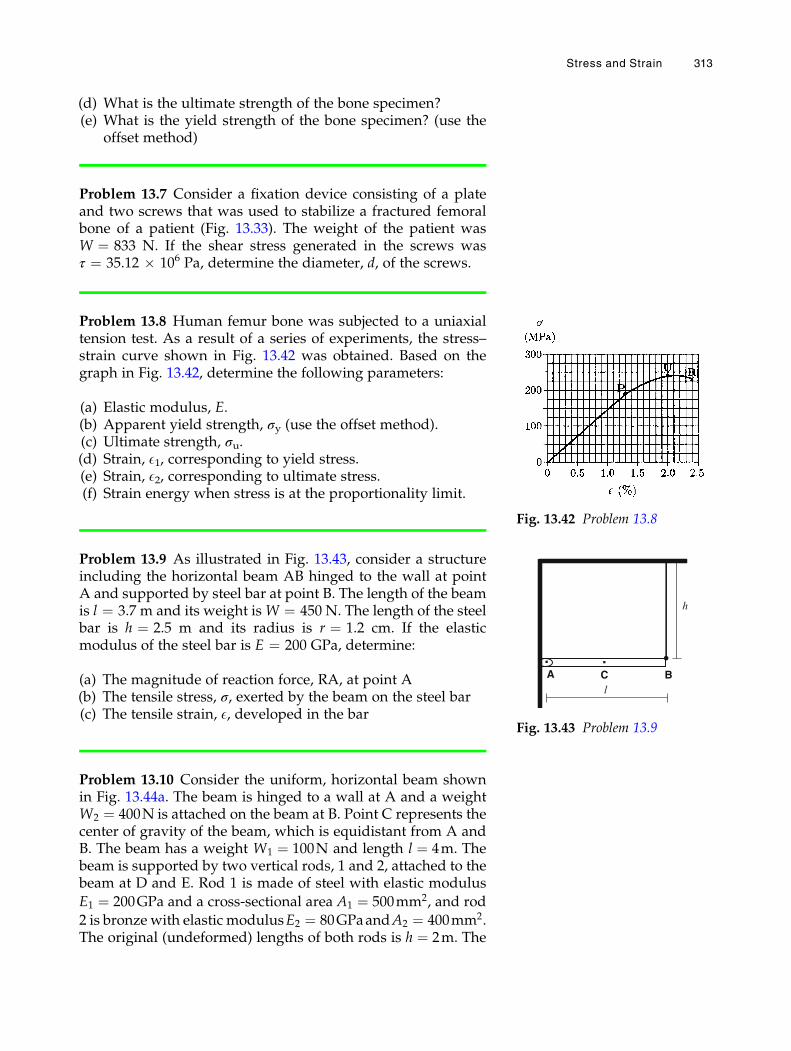
(d) What is the ultimate strength of the bone specimen?(e) What is the yield strength of the bone specimen? (use the
offset method)
Problem 13.7 Consider a fixation device consisting of a plateand two screws that was used to stabilize a fractured femoralbone of a patient (Fig. 13.33). The weight of the patient wasW ¼ 833 N. If the shear stress generated in the screws wasτ ¼ 35.12 � 106 Pa, determine the diameter, d, of the screws.
Problem 13.8 Human femur bone was subjected to a uniaxialtension test. As a result of a series of experiments, the stress–strain curve shown in Fig. 13.42 was obtained. Based on thegraph in Fig. 13.42, determine the following parameters:
(a) Elastic modulus, E.(b) Apparent yield strength, σy (use the offset method).(c) Ultimate strength, σu.(d) Strain, E1, corresponding to yield stress.(e) Strain, E2, corresponding to ultimate stress.(f) Strain energy when stress is at the proportionality limit.
Problem 13.9 As illustrated in Fig. 13.43, consider a structureincluding the horizontal beam AB hinged to the wall at pointA and supported by steel bar at point B. The length of the beamis l ¼ 3.7 m and its weight isW ¼ 450 N. The length of the steelbar is h ¼ 2.5 m and its radius is r ¼ 1.2 cm. If the elasticmodulus of the steel bar is E ¼ 200 GPa, determine:
(a) The magnitude of reaction force, RA, at point A(b) The tensile stress, σ, exerted by the beam on the steel bar(c) The tensile strain, E, developed in the bar
Problem 13.10 Consider the uniform, horizontal beam shownin Fig. 13.44a. The beam is hinged to a wall at A and a weightW2 ¼ 400N is attached on the beam at B. Point C represents thecenter of gravity of the beam, which is equidistant from A andB. The beam has a weight W1 ¼ 100N and length l ¼ 4m. Thebeam is supported by two vertical rods, 1 and 2, attached to thebeam at D and E. Rod 1 is made of steel with elastic modulus
E1 ¼ 200GPa and a cross-sectional area A1 ¼ 500mm2, and rod
2 is bronze with elastic modulusE2 ¼ 80GPaandA2 ¼ 400mm2.The original (undeformed) lengths of both rods is h ¼ 2m. The
Fig. 13.42 Problem 13.8
A B . .
C l
h
Fig. 13.43 Problem 13.9
Stress and Strain 313
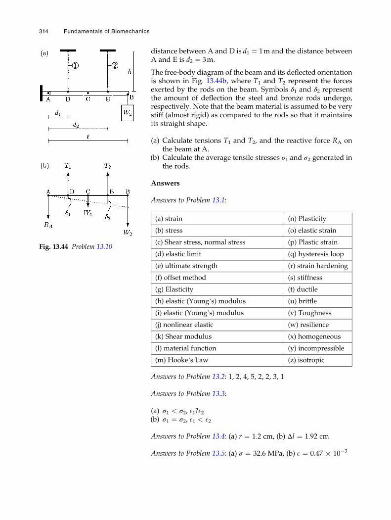
distance between A and D is d1 ¼ 1m and the distance betweenA and E is d2 ¼ 3m.
The free-body diagram of the beam and its deflected orientationis shown in Fig. 13.44b, where T1 and T2 represent the forcesexerted by the rods on the beam. Symbols δ1 and δ2 representthe amount of deflection the steel and bronze rods undergo,respectively. Note that the beam material is assumed to be verystiff (almost rigid) as compared to the rods so that it maintainsits straight shape.
(a) Calculate tensions T1 and T2, and the reactive force RA onthe beam at A.
(b) Calculate the average tensile stresses σ1 and σ2 generated inthe rods.
Answers
Answers to Problem 13.1:
(a) strain (n) Plasticity
(b) stress (o) elastic strain
(c) Shear stress, normal stress (p) Plastic strain
(d) elastic limit (q) hysteresis loop
(e) ultimate strength (r) strain hardening
(f) offset method (s) stiffness
(g) Elasticity (t) ductile
(h) elastic (Young’s) modulus (u) brittle
(i) elastic (Young’s) modulus (v) Toughness
(j) nonlinear elastic (w) resilience
(k) Shear modulus (x) homogeneous
(l) material function (y) incompressible
(m) Hooke’s Law (z) isotropic
Answers to Problem 13.2: 1, 2, 4, 5, 2, 2, 3, 1
Answers to Problem 13.3:
(a) σ1 < σ2, E1?E2(b) σ1 ¼ σ2, E1 < E2
Answers to Problem 13.4: (a) r ¼ 1.2 cm, (b) Δl ¼ 1.92 cm
Answers to Problem 13.5: (a) σ ¼ 32.6 MPa, (b) E ¼ 0.47 � 10�3
Fig. 13.44 Problem 13.10
314 Fundamentals of Biomechanics
Answers to Problem 13.6:
(c) E ¼ 20 GPa(d) σu ¼ 140 MPa(e) σy ¼ 118 MPa
Answer to Problem 13.7: d ¼ 5.5 mm
Answers to Problem 13.8:
(a) E ¼ 14.6 GPa(b) σy ¼ 235 MPa(c) σu ¼ 240 MPa(d) ε2 ¼ 0.018(e) ε2 ¼ 0.02(f) 1.235 MPa
Answers to Problem 13.9: (a) RA ¼ 225 N, (b) σ ¼ 0.5 MPa,(c) E ¼ 2.5 � 10�6
Answers to Problem 13.10:
(a) T1 ¼ 464N, T2 ¼ 445N, RA ¼ 409N(b) σ1 ¼ 0:928MPa, σ2 ¼ 1:113MPa
Stress and Strain 315
Chapter 14
Multiaxial Deformationsand Stress Analyses
14.1 Poisson’s Ratio / 319
14.2 Biaxial and Triaxial Stresses / 320
14.3 Stress Transformation / 325
14.4 Principal Stresses / 326
14.5 Mohr’s Circle / 327
14.6 Failure Theories / 330
14.7 Allowable Stress and Factor of Safety / 332
14.8 Factors Affecting the Strength of Materials / 333
14.9 Fatigue and Endurance / 334
14.10 Stress Concentration / 335
14.11 Torsion / 337
14.12 Bending / 344
14.13 Combined Loading / 354
14.14 Exercise Problems / 356
# Springer International Publishing Switzerland 2017N. Ozkaya et al., Fundamentals of Biomechanics, DOI 10.1007/978-3-319-44738-4_14
317

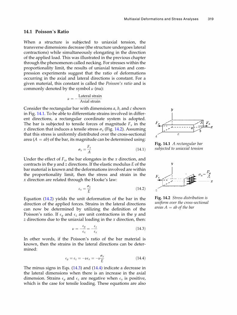
14.1 Poisson’s Ratio
When a structure is subjected to uniaxial tension, thetransverse dimensions decrease (the structure undergoes lateralcontractions) while simultaneously elongating in the directionof the applied load. This was illustrated in the previous chapterthrough the phenomenon called necking. For stresses within theproportionality limit, the results of uniaxial tension and com-pression experiments suggest that the ratio of deformationsoccurring in the axial and lateral directions is constant. For agiven material, this constant is called the Poisson’s ratio and iscommonly denoted by the symbol ν (nu):
ν ¼ �Lateral strain
Axial strain
Consider the rectangular bar with dimensions a, b, and c shownin Fig. 14.1. To be able to differentiate strains involved in differ-ent directions, a rectangular coordinate system is adopted.The bar is subjected to tensile forces of magnitude Fx in thex direction that induces a tensile stress σx (Fig. 14.2). Assumingthat this stress is uniformly distributed over the cross-sectionalarea (A ¼ ab) of the bar, its magnitude can be determined using:
σx ¼ FxA
ð14:1Þ
Under the effect of Fx, the bar elongates in the x direction, andcontracts in the y and z directions. If the elastic modulus E of thebar material is known and the deformations involved are withinthe proportionality limit, then the stress and strain in thex direction are related through the Hooke’s law:
Ex ¼ σxE
ð14:2Þ
Equation (14.2) yields the unit deformation of the bar in thedirection of the applied forces. Strains in the lateral directionscan now be determined by utilizing the definition of thePoisson’s ratio. If Ey and Ez are unit contractions in the y andz directions due to the uniaxial loading in the x direction, then:
ν ¼ �EyEx
¼ �EzEx
ð14:3Þ
In other words, if the Poisson’s ratio of the bar material isknown, then the strains in the lateral directions can be deter-mined:
Ey ¼ Ez ¼ �νEx ¼ �νσxE
ð14:4Þ
The minus signs in Eqs. (14.3) and (14.4) indicate a decrease inthe lateral dimensions when there is an increase in the axialdimension. Strains Ey and Ez are negative when Ex is positive,which is the case for tensile loading. These equations are also
Fig. 14.1 A rectangular barsubjected to uniaxial tension
Fig. 14.2 Stress distribution isuniform over the cross-sectionalareas A ¼ ab of the bar
Multiaxial Deformations and Stress Analyses 319
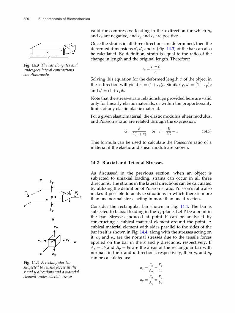
valid for compressive loading in the x direction for which σxand Ex are negative, and Ey and Ez are positive.
Once the strains in all three directions are determined, then thedeformed dimensions a0, b0, and c0 (Fig. 14.3) of the bar can alsobe calculated. By definition, strain is equal to the ratio of thechange in length and the original length. Therefore:
Ex ¼ c0 � c
c
Solving this equation for the deformed length c0 of the object in
the x direction will yield c0 ¼ 1þ Exð Þc. Similarly, a0 ¼ 1þ Ey� �
a
and b0 ¼ 1þ Ezð Þb.Note that the stress–strain relationships provided here are validonly for linearly elastic materials, or within the proportionalitylimits of any elastic-plastic material.
For a given elastic material, the elastic modulus, shear modulus,and Poisson’s ratio are related through the expression:
G ¼ E
2 1þ νð Þ or ν ¼ E
2G� 1 ð14:5Þ
This formula can be used to calculate the Poisson’s ratio of amaterial if the elastic and shear moduli are known.
14.2 Biaxial and Triaxial Stresses
As discussed in the previous section, when an object issubjected to uniaxial loading, strains can occur in all threedirections. The strains in the lateral directions can be calculatedby utilizing the definition of Poisson’s ratio. Poisson’s ratio alsomakes it possible to analyze situations in which there is morethan one normal stress acting in more than one direction.
Consider the rectangular bar shown in Fig. 14.4. The bar issubjected to biaxial loading in the xy-plane. Let P be a point inthe bar. Stresses induced at point P can be analyzed byconstructing a cubical material element around the point. Acubical material element with sides parallel to the sides of thebar itself is shown in Fig. 14.4, along with the stresses acting onit. σx and σy are the normal stresses due to the tensile forcesapplied on the bar in the x and y directions, respectively. IfAx ¼ ab and Ay ¼ bc are the areas of the rectangular bar withnormals in the x and y directions, respectively, then σx and σycan be calculated as:
σx ¼ FxAx
¼ Fxab
σy ¼Fy
Ay¼ Fy
bc
Fig. 14.3 The bar elongates andundergoes lateral contractionssimultaneously
Fig. 14.4 A rectangular barsubjected to tensile forces in thex and y directions and a materialelement under biaxial stresses
320 Fundamentals of Biomechanics
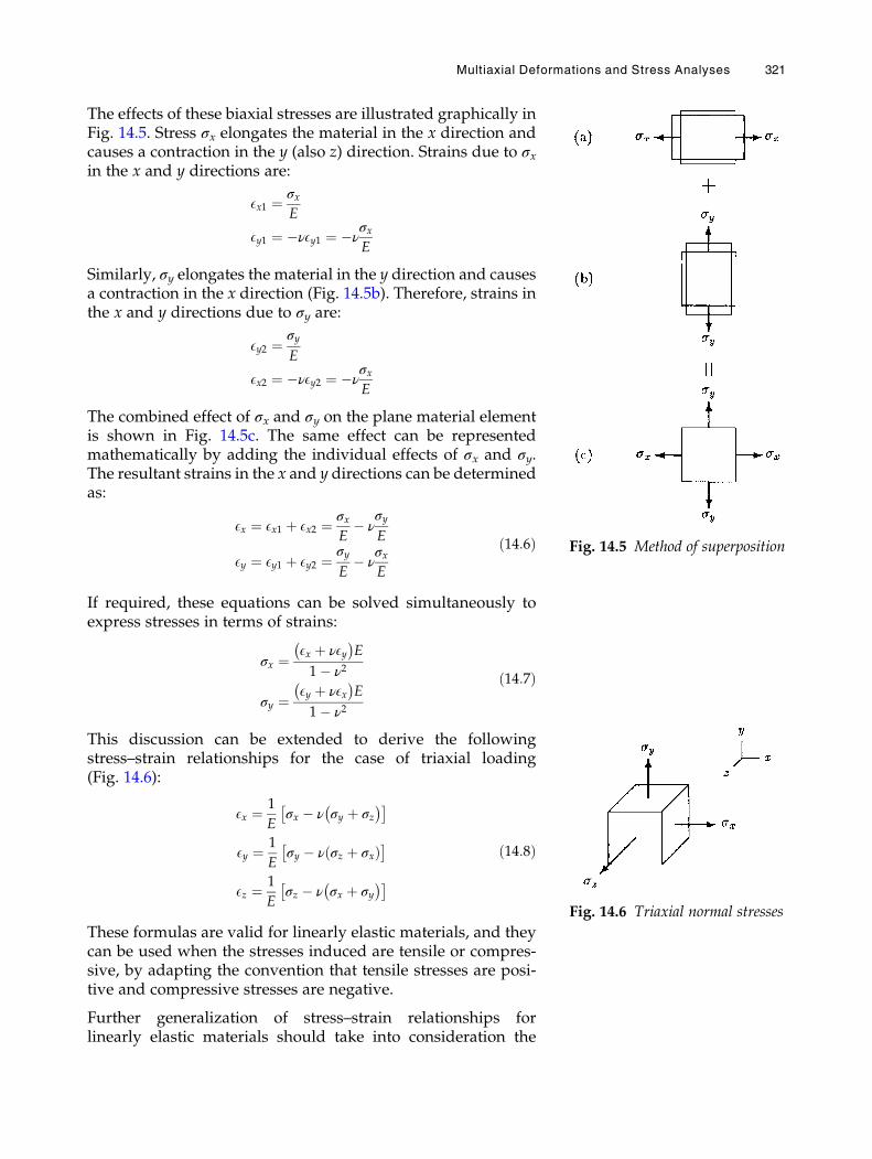
The effects of these biaxial stresses are illustrated graphically inFig. 14.5. Stress σx elongates the material in the x direction andcauses a contraction in the y (also z) direction. Strains due to σxin the x and y directions are:
Ex1 ¼ σxE
Ey1 ¼ �νEy1 ¼ �νσxE
Similarly, σy elongates the material in the y direction and causesa contraction in the x direction (Fig. 14.5b). Therefore, strains inthe x and y directions due to σy are:
Ey2 ¼σyE
Ex2 ¼ �νEy2 ¼ �νσxE
The combined effect of σx and σy on the plane material elementis shown in Fig. 14.5c. The same effect can be representedmathematically by adding the individual effects of σx and σy.The resultant strains in the x and y directions can be determinedas:
Ex ¼ Ex1 þ Ex2 ¼ σxE� ν
σyE
Ey ¼ Ey1 þ Ey2 ¼σyE� ν
σxE
ð14:6Þ
If required, these equations can be solved simultaneously toexpress stresses in terms of strains:
σx ¼Ex þ νEy� �
E
1� ν2
σy ¼Ey þ νEx� �
E
1� ν2
ð14:7Þ
This discussion can be extended to derive the followingstress–strain relationships for the case of triaxial loading(Fig. 14.6):
Ex ¼ 1
Eσx � ν σy þ σz
� �� �
Ey ¼ 1
Eσy � ν σz þ σxð Þ� �
Ez ¼ 1
Eσz � ν σx þ σy
� �� �ð14:8Þ
These formulas are valid for linearly elastic materials, and theycan be used when the stresses induced are tensile or compres-sive, by adapting the convention that tensile stresses are posi-tive and compressive stresses are negative.
Further generalization of stress–strain relationships forlinearly elastic materials should take into consideration the
Fig. 14.5 Method of superposition
Fig. 14.6 Triaxial normal stresses
Multiaxial Deformations and Stress Analyses 321
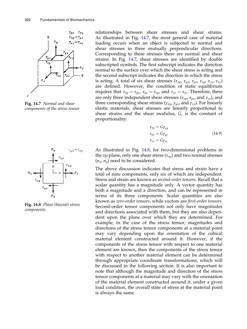
relationships between shear stresses and shear strains.As illustrated in Fig. 14.7, the most general case of materialloading occurs when an object is subjected to normal andshear stresses in three mutually perpendicular directions.Corresponding to these stresses there are normal and shearstrains. In Fig. 14.7, shear stresses are identified by doublesubscripted symbols. The first subscript indicates the directionnormal to the surface over which the shear stress is acting andthe second subscript indicates the direction in which the stressis acting. A total of six shear stresses (τxy, τyx, τyz, τzy, τzx, τxz)are defined. However, the condition of static equilibriumrequires that τxy ¼ τyx, τyz ¼ τzy, and τzx ¼ τxz. Therefore, thereare only three independent shear stresses (τxy, τyz, and τzx), andthree corresponding shear strains (γxy, γyz, and γzx). For linearlyelastic materials, shear stresses are linearly proportional toshear strains and the shear modulus, G, is the constant ofproportionality:
τxy ¼ Gγxy
τyz ¼ Gγyz
τzx ¼ Gγzx
ð14:9Þ
As illustrated in Fig. 14.8, for two-dimensional problems inthe xy-plane, only one shear stress (τxy) and two normal stresses(σx, σy) need to be considered.
The above discussion indicates that stress and strain have atotal of nine components, only six of which are independent.Stress and strain are known as second-order tensors. Recall that ascalar quantity has a magnitude only. A vector quantity hasboth a magnitude and a direction, and can be represented interms of its three components. Scalar quantities are alsoknown as zero-order tensors, while vectors are first-order tensors.Second-order tensor components not only have magnitudesand directions associated with them, but they are also depen-dent upon the plane over which they are determined. Forexample, in the case of the stress tensor, magnitudes anddirections of the stress tensor components at a material pointmay vary depending upon the orientation of the cubicalmaterial element constructed around it. However, if thecomponents of the stress tensor with respect to one materialelement are known, then the components of the stress tensorwith respect to another material element can be determinedthrough appropriate coordinate transformations, which willbe discussed in the following section. It is also important tonote that although the magnitude and direction of the stresstensor components at a material may vary with the orientationof the material element constructed around it, under a givenload condition, the overall state of stress at the material pointis always the same.
Fig. 14.7 Normal and shearcomponents of the stress tensor
Fig. 14.8 Plane (biaxial) stresscomponents
322 Fundamentals of Biomechanics
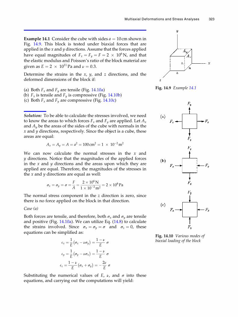
Example 14.1 Consider the cube with sides a ¼ 10cm shown inFig. 14.9. This block is tested under biaxial forces that areapplied in the x and y directions. Assume that the forces applied
have equal magnitudes of Fx ¼ Fy ¼ F ¼ 2 � 106N, and that
the elastic modulus and Poisson’s ratio of the block material are
given as E ¼ 2 � 1011 Pa and ν ¼ 0:3.
Determine the strains in the x, y, and z directions, and thedeformed dimensions of the block if:
(a) Both Fx and Fy are tensile (Fig. 14.10a)(b) Fx is tensile and Fy is compressive (Fig. 14.10b)(c) Both Fx and Fy are compressive (Fig. 14.10c)
Solution: To be able to calculate the stresses involved, we needto know the areas to which forces Fx and Fy are applied. Let Ax
and Ay be the areas of the sides of the cube with normals in thex and y directions, respectively. Since the object is a cube, theseareas are equal:
Ax ¼ Ay ¼ A ¼ a2 ¼ 100cm2 ¼ 1 � 10�2m2
We can now calculate the normal stresses in the x andy directions. Notice that the magnitudes of the applied forcesin the x and y directions and the areas upon which they areapplied are equal. Therefore, the magnitudes of the stresses inthe x and y directions are equal as well:
σx ¼ σy ¼ σ ¼ F
A¼ 2� 106N
1� 10�2m2¼ 2� 108 Pa
The normal stress component in the z direction is zero, sincethere is no force applied on the block in that direction.
Case (a)
Both forces are tensile, and therefore, both σx and σy are tensileand positive (Fig. 14.10a). We can utilize Eq. (14.8) to calculatethe strains involved. Since σx ¼ σy ¼ σ and σz ¼ 0, these
equations can be simplified as:
Ex ¼ 1
Eσx � νσy� � ¼ 1� ν
Eσ
Ey ¼ 1
Eσy � νσx� � ¼ 1� ν
Eσ
Ez ¼ 1� ν
Eσx þ σy� � ¼ � 2ν
Eσ
Substituting the numerical values of E, ν, and σ into theseequations, and carrying out the computations will yield:
Fig. 14.9 Example 14.1
Fig. 14.10 Various modes ofbiaxial loading of the block
Multiaxial Deformations and Stress Analyses 323
Ex ¼ 0:7� 10�3
Ey ¼ 0:7� 10�3
Ez ¼ �0:6� 10�3
Note that both Ex and Ey are positive, while Ez is negative. Asa result of the applied forces, the dimensions of the block inthe x and y directions increase, while its dimension in thez direction decreases. If ax, ay, and az are the new (deformed)dimensions of the block, then:
ax ¼ 1þ Exð Þa ¼ 1þ 0:0007ð Þ 10cmð Þ ¼ 10:007cm
ay ¼ 1þ Ey� �
a ¼ 1þ 0:0007ð Þ 10cmð Þ ¼ 10:007cm
az ¼ 1þ Ezð Þa ¼ 1� 0:0006ð Þ 10cmð Þ ¼ 9:994cm
Case (b)
In this case, σx is tensile and positive while σy is compressiveand negative (Fig. 14.10b). Therefore, the stress–strainrelationships take the following forms:
Ex ¼ 1
Eσx þ νσy� � ¼ 1þ ν
Eσ
Ey ¼ 1
E�σy � νσx� � ¼ � 1þ ν
Eσ
Ez ¼ �ν
Eσx þ σy� � ¼ 0
Substituting the numerical values of the parameters involved intothese equations, and carrying out the computations will yield:
Ex ¼ 1:3� 10�3
Ey ¼ �1:3� 10�3
Ez ¼ 0
The tensile force applied in the x direction and the compressiveforce applied in the y direction elongates the block in the x direc-tion and reduces its dimension in theydirection. In the zdirection,the contraction caused by the tensile stress σx is counterbalancedby the expansion caused by the compressive stress σy.
Case (c)
In this case, both forces are compressive. Therefore, both σxand σy are compressive and negative (Fig. 14.10c). Thesimplified equations relating normal strains to normal stressesfor this case are:
Ex ¼ 1
E�σx þ νσy� � ¼ 1� ν
Eσ
Ey ¼ 1
E�σy � νσx� � ¼ � 1� ν
Eσ
Ez ¼ �ν
E�σx � σy� � ¼ 2ν
Eσ
324 Fundamentals of Biomechanics
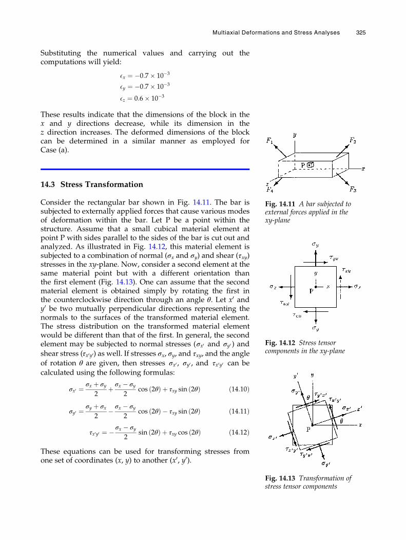
Substituting the numerical values and carrying out thecomputations will yield:
Ex ¼ �0:7� 10�3
Ey ¼ �0:7� 10�3
Ez ¼ 0:6� 10�3
These results indicate that the dimensions of the block in thex and y directions decrease, while its dimension in thez direction increases. The deformed dimensions of the blockcan be determined in a similar manner as employed forCase (a).
14.3 Stress Transformation
Consider the rectangular bar shown in Fig. 14.11. The bar issubjected to externally applied forces that cause various modesof deformation within the bar. Let P be a point within thestructure. Assume that a small cubical material element atpoint P with sides parallel to the sides of the bar is cut out andanalyzed. As illustrated in Fig. 14.12, this material element issubjected to a combination of normal (σx and σy) and shear (τxy)stresses in the xy-plane. Now, consider a second element at thesame material point but with a different orientation thanthe first element (Fig. 14.13). One can assume that the secondmaterial element is obtained simply by rotating the first inthe counterclockwise direction through an angle θ. Let x0 andy0 be two mutually perpendicular directions representing thenormals to the surfaces of the transformed material element.The stress distribution on the transformed material elementwould be different than that of the first. In general, the secondelement may be subjected to normal stresses (σx0 and σy0 ) andshear stress (τx0y0) as well. If stresses σx, σy, and τxy, and the angle
of rotation θ are given, then stresses σx0 , σy0 , and τx0y0 can be
calculated using the following formulas:
σx0 ¼σx þ σy
2þ σx � σy
2cos 2θð Þ þ τxy sin 2θð Þ ð14:10Þ
σy0 ¼σy þ σx
2� σx � σy
2cos 2θð Þ � τxy sin 2θð Þ ð14:11Þ
τx0y0 ¼ � σx � σy2
sin 2θð Þ þ τxy cos 2θð Þ ð14:12Þ
These equations can be used for transforming stresses fromone set of coordinates (x, y) to another (x0, y0).
Fig. 14.11 A bar subjected toexternal forces applied in thexy-plane
Fig. 14.12 Stress tensorcomponents in the xy-plane
Fig. 14.13 Transformation ofstress tensor components
Multiaxial Deformations and Stress Analyses 325
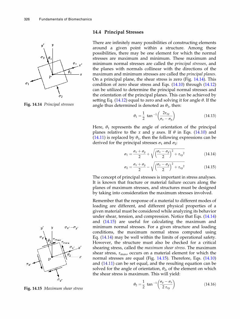
14.4 Principal Stresses
There are infinitely many possibilities of constructing elementsaround a given point within a structure. Among thesepossibilities, there may be one element for which the normalstresses are maximum and minimum. These maximum andminimum normal stresses are called the principal stresses, andthe planes with normals collinear with the directions of themaximum and minimum stresses are called the principal planes.On a principal plane, the shear stress is zero (Fig. 14.14). Thiscondition of zero shear stress and Eqs. (14.10) through (14.12)can be utilized to determine the principal normal stresses andthe orientation of the principal planes. This can be achieved bysetting Eq. (14.12) equal to zero and solving it for angle θ. If theangle thus determined is denoted as θ1, then:
θ1 ¼ 1
2tan �1 2τxy
σx � σy
� �ð14:13Þ
Here, θ1 represents the angle of orientation of the principalplanes relative to the x and y axes. If θ in Eqs. (14.10) and(14.11) is replaced by θ1, then the following expressions can bederived for the principal stresses σ1 and σ2:
σ1 ¼σx þ σy
2þ
ffiffiffiffiffiffiffiffiffiffiffiffiffiffiffiffiffiffiffiffiffiffiffiffiffiffiffiffiffiffiffiffiffiffiffiffiσx � σy
2
2
þ τxy2r
ð14:14Þ
σ2 ¼σx þ σy
2�
ffiffiffiffiffiffiffiffiffiffiffiffiffiffiffiffiffiffiffiffiffiffiffiffiffiffiffiffiffiffiffiffiffiffiffiffiσx � σy
2
2
þ τxy2r
ð14:15Þ
The concept of principal stresses is important in stress analyses.It is known that fracture or material failure occurs along theplanes of maximum stresses, and structures must be designedby taking into consideration the maximum stresses involved.
Remember that the response of a material to different modes ofloading are different, and different physical properties of agiven material must be considered while analyzing its behaviorunder shear, tension, and compression. Notice that Eqs. (14.14)and (14.15) are useful for calculating the maximum andminimum normal stresses. For a given structure and loadingconditions, the maximum normal stress computed usingEq. (14.14) may be well within the limits of operational safety.However, the structure must also be checked for a criticalshearing stress, called the maximum shear stress. The maximumshear stress, τmax, occurs on a material element for which thenormal stresses are equal (Fig. 14.15). Therefore, Eqs. (14.10)and (14.11) can be set equal, and the resulting equation can besolved for the angle of orientation, θ2, of the element on whichthe shear stress is maximum. This will yield:
θ2 ¼ 1
2tan �1 σy � σx
2 τxy
� �ð14:16Þ
Fig. 14.15 Maximum shear stress
Fig. 14.14 Principal stresses
326 Fundamentals of Biomechanics
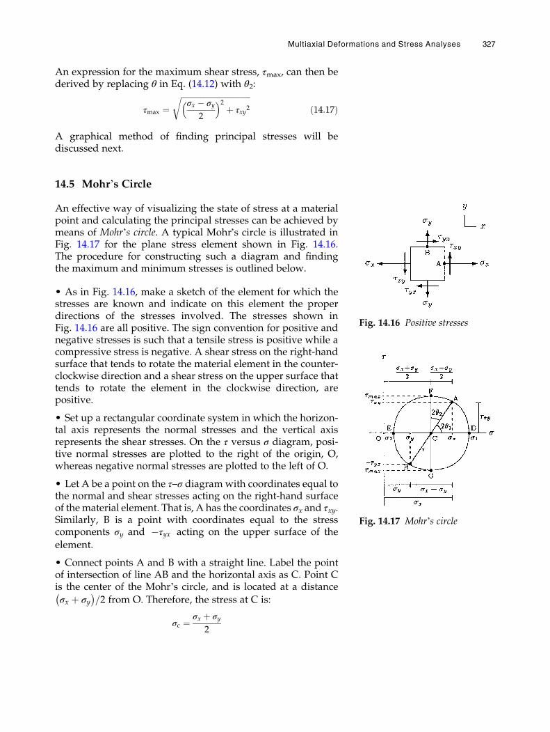
An expression for the maximum shear stress, τmax, can then bederived by replacing θ in Eq. (14.12) with θ2:
τmax ¼ffiffiffiffiffiffiffiffiffiffiffiffiffiffiffiffiffiffiffiffiffiffiffiffiffiffiffiffiffiffiffiffiffiffiffiffiσx � σy
2
2
þ τxy2r
ð14:17Þ
A graphical method of finding principal stresses will bediscussed next.
14.5 Mohr’s Circle
An effective way of visualizing the state of stress at a materialpoint and calculating the principal stresses can be achieved bymeans of Mohr’s circle. A typical Mohr’s circle is illustrated inFig. 14.17 for the plane stress element shown in Fig. 14.16.The procedure for constructing such a diagram and findingthe maximum and minimum stresses is outlined below.
• As in Fig. 14.16, make a sketch of the element for which thestresses are known and indicate on this element the properdirections of the stresses involved. The stresses shown inFig. 14.16 are all positive. The sign convention for positive andnegative stresses is such that a tensile stress is positive while acompressive stress is negative. A shear stress on the right-handsurface that tends to rotate the material element in the counter-clockwise direction and a shear stress on the upper surface thattends to rotate the element in the clockwise direction, arepositive.
• Set up a rectangular coordinate system in which the horizon-tal axis represents the normal stresses and the vertical axisrepresents the shear stresses. On the τ versus σ diagram, posi-tive normal stresses are plotted to the right of the origin, O,whereas negative normal stresses are plotted to the left of O.
• Let A be a point on the τ–σ diagramwith coordinates equal tothe normal and shear stresses acting on the right-hand surfaceof thematerial element. That is, A has the coordinates σx and τxy.Similarly, B is a point with coordinates equal to the stresscomponents σy and �τyx acting on the upper surface of the
element.
• Connect points A and B with a straight line. Label the pointof intersection of line AB and the horizontal axis as C. Point Cis the center of the Mohr’s circle, and is located at a distance
σx þ σy� �
=2 from O. Therefore, the stress at C is:
σc ¼σx þ σy
2
Fig. 14.16 Positive stresses
Fig. 14.17 Mohr’s circle
Multiaxial Deformations and Stress Analyses 327
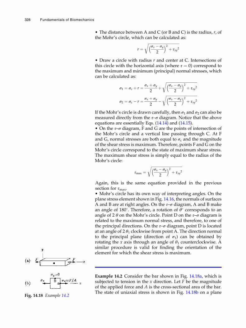
• The distance between A and C (or B and C) is the radius, r, ofthe Mohr’s circle, which can be calculated as:
r ¼ffiffiffiffiffiffiffiffiffiffiffiffiffiffiffiffiffiffiffiffiffiffiffiffiffiffiffiffiffiffiffiffiffiffiffiffiσx � σy
2
2
þ τxy2r
• Draw a circle with radius r and center at C. Intersections ofthis circle with the horizontal axis (where τ ¼ 0) correspond tothe maximum and minimum (principal) normal stresses, whichcan be calculated as:
σ1 ¼ σc þ r ¼ σx þ σy2
þffiffiffiffiffiffiffiffiffiffiffiffiffiffiffiffiffiffiffiffiffiffiffiffiffiffiffiffiffiffiffiffiffiffiffiffiσx � σy
2
2
þ τxy2r
σ2 ¼ σc � r ¼ σx þ σy2
�ffiffiffiffiffiffiffiffiffiffiffiffiffiffiffiffiffiffiffiffiffiffiffiffiffiffiffiffiffiffiffiffiffiffiffiffiσx � σy
2
2
þ τxy2r
If theMohr’s circle is drawn carefully, then σ1 and σ2 can also bemeasured directly from the τ–σ diagram. Notice that the aboveequations are essentially Eqs. (14.14) and (14.15).• On the τ–σ diagram, F and G are the points of intersection ofthe Mohr’s circle and a vertical line passing through C. At Fand G, normal stresses are both equal to σc and the magnitudeof the shear stress is maximum. Therefore, points F and G on theMohr’s circle correspond to the state of maximum shear stress.The maximum shear stress is simply equal to the radius of theMohr’s circle:
τmax ¼ffiffiffiffiffiffiffiffiffiffiffiffiffiffiffiffiffiffiffiffiffiffiffiffiffiffiffiffiffiffiffiffiffiffiffiffiσx � σy
2
2þ τxy2
r
Again, this is the same equation provided in the previoussection for τmax.• Mohr’s circle has its own way of interpreting angles. On theplane stress element shown in Fig. 14.16, the normals of surfacesA and B are at right angles. On the τ–σ diagram, A and B makean angle of 180�. Therefore, a rotation of θ� corresponds to anangle of 2 θ on the Mohr’s circle. Point D on the τ–σ diagram isrelated to the maximum normal stress, and therefore, to one ofthe principal directions. On the τ–σ diagram, point D is locatedat an angle of 2 θ1 clockwise from point A. The direction normalto the principal plane (direction of σ1) can be obtained byrotating the x axis through an angle of θ1 counterclockwise. Asimilar procedure is valid for finding the orientation of theelement for which the shear stress is maximum.
Example 14.2 Consider the bar shown in Fig. 14.18a, which issubjected to tension in the x direction. Let F be the magnitudeof the applied force and A is the cross-sectional area of the bar.The state of uniaxial stress is shown in Fig. 14.18b on a plane
Fig. 14.18 Example 14.2
328 Fundamentals of Biomechanics
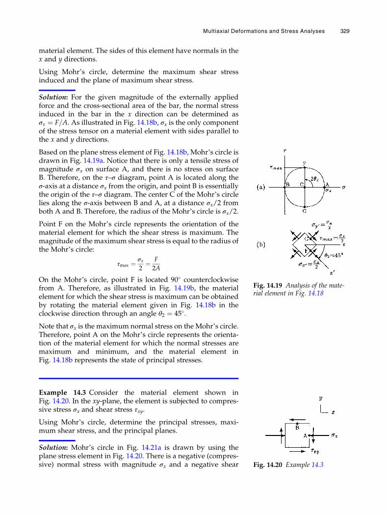
material element. The sides of this element have normals in thex and y directions.
Using Mohr’s circle, determine the maximum shear stressinduced and the plane of maximum shear stress.
Solution: For the given magnitude of the externally appliedforce and the cross-sectional area of the bar, the normal stressinduced in the bar in the x direction can be determined asσx ¼ F=A. As illustrated in Fig. 14.18b, σx is the only componentof the stress tensor on a material element with sides parallel tothe x and y directions.
Based on the plane stress element of Fig. 14.18b, Mohr’s circle isdrawn in Fig. 14.19a. Notice that there is only a tensile stress ofmagnitude σx on surface A, and there is no stress on surfaceB. Therefore, on the τ–σ diagram, point A is located along theσ-axis at a distance σx from the origin, and point B is essentiallythe origin of the τ–σ diagram. The center C of the Mohr’s circlelies along the σ-axis between B and A, at a distance σx/2 fromboth A and B. Therefore, the radius of the Mohr’s circle is σx/2.
Point F on the Mohr’s circle represents the orientation of thematerial element for which the shear stress is maximum. Themagnitude of the maximum shear stress is equal to the radius ofthe Mohr’s circle:
τmax ¼ σx2¼ F
2A
On the Mohr’s circle, point F is located 90� counterclockwisefrom A. Therefore, as illustrated in Fig. 14.19b, the materialelement for which the shear stress is maximum can be obtainedby rotating the material element given in Fig. 14.18b in theclockwise direction through an angle θ2 ¼ 45�.
Note that σx is the maximum normal stress on the Mohr’s circle.Therefore, point A on the Mohr’s circle represents the orienta-tion of the material element for which the normal stresses aremaximum and minimum, and the material element inFig. 14.18b represents the state of principal stresses.
Example 14.3 Consider the material element shown inFig. 14.20. In the xy-plane, the element is subjected to compres-sive stress σx and shear stress τxy.
Using Mohr’s circle, determine the principal stresses, maxi-mum shear stress, and the principal planes.
Solution: Mohr’s circle in Fig. 14.21a is drawn by using theplane stress element in Fig. 14.20. There is a negative (compres-sive) normal stress with magnitude σx and a negative shear
Fig. 14.19 Analysis of the mate-rial element in Fig. 14.18
Fig. 14.20 Example 14.3
Multiaxial Deformations and Stress Analyses 329
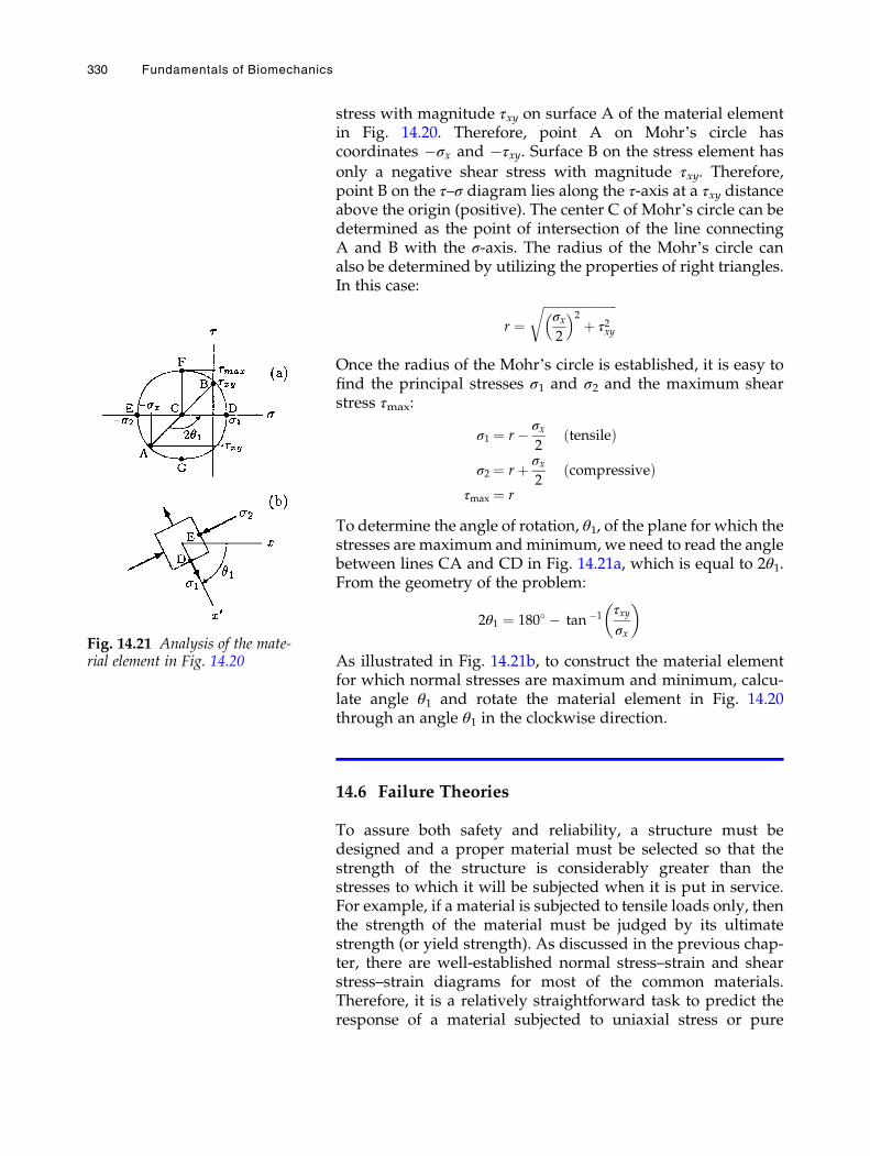
stress with magnitude τxy on surface A of the material elementin Fig. 14.20. Therefore, point A on Mohr’s circle hascoordinates �σx and �τxy. Surface B on the stress element has
only a negative shear stress with magnitude τxy. Therefore,point B on the τ–σ diagram lies along the τ-axis at a τxy distanceabove the origin (positive). The center C of Mohr’s circle can bedetermined as the point of intersection of the line connectingA and B with the σ-axis. The radius of the Mohr’s circle canalso be determined by utilizing the properties of right triangles.In this case:
r ¼ffiffiffiffiffiffiffiffiffiffiffiffiffiffiffiffiffiffiffiffiffiffiffiffiσx2
2þ τ2xy
r
Once the radius of the Mohr’s circle is established, it is easy tofind the principal stresses σ1 and σ2 and the maximum shearstress τmax:
σ1 ¼ r� σx2
tensileð Þ
σ2 ¼ rþ σx2
compressiveð Þτmax ¼ r
To determine the angle of rotation, θ1, of the plane for which thestresses are maximum andminimum, we need to read the anglebetween lines CA and CD in Fig. 14.21a, which is equal to 2θ1.From the geometry of the problem:
2θ1 ¼ 180� � tan �1 τxyσx
� �
As illustrated in Fig. 14.21b, to construct the material elementfor which normal stresses are maximum and minimum, calcu-late angle θ1 and rotate the material element in Fig. 14.20through an angle θ1 in the clockwise direction.
14.6 Failure Theories
To assure both safety and reliability, a structure must bedesigned and a proper material must be selected so that thestrength of the structure is considerably greater than thestresses to which it will be subjected when it is put in service.For example, if a material is subjected to tensile loads only, thenthe strength of the material must be judged by its ultimatestrength (or yield strength). As discussed in the previous chap-ter, there are well-established normal stress–strain and shearstress–strain diagrams for most of the common materials.Therefore, it is a relatively straightforward task to predict theresponse of a material subjected to uniaxial stress or pure
Fig. 14.21 Analysis of the mate-rial element in Fig. 14.20
330 Fundamentals of Biomechanics
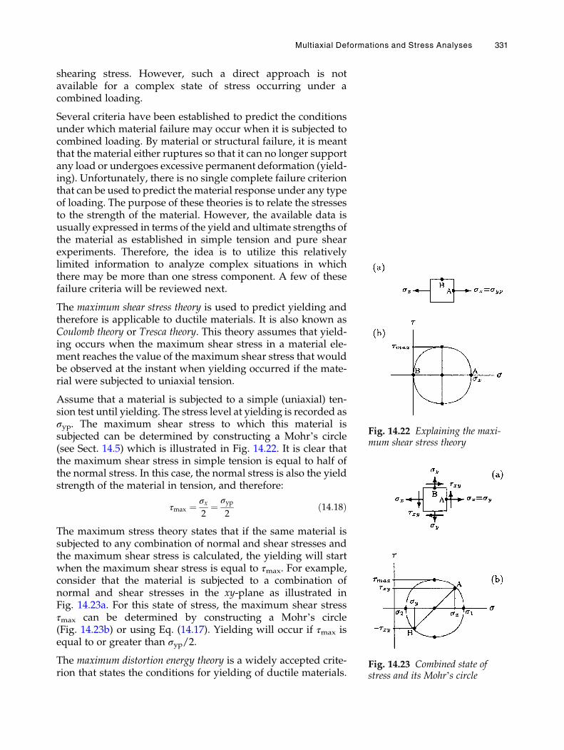
shearing stress. However, such a direct approach is notavailable for a complex state of stress occurring under acombined loading.
Several criteria have been established to predict the conditionsunder which material failure may occur when it is subjected tocombined loading. By material or structural failure, it is meantthat the material either ruptures so that it can no longer supportany load or undergoes excessive permanent deformation (yield-ing). Unfortunately, there is no single complete failure criterionthat can be used to predict the material response under any typeof loading. The purpose of these theories is to relate the stressesto the strength of the material. However, the available data isusually expressed in terms of the yield and ultimate strengths ofthe material as established in simple tension and pure shearexperiments. Therefore, the idea is to utilize this relativelylimited information to analyze complex situations in whichthere may be more than one stress component. A few of thesefailure criteria will be reviewed next.
The maximum shear stress theory is used to predict yielding andtherefore is applicable to ductile materials. It is also known asCoulomb theory or Tresca theory. This theory assumes that yield-ing occurs when the maximum shear stress in a material ele-ment reaches the value of the maximum shear stress that wouldbe observed at the instant when yielding occurred if the mate-rial were subjected to uniaxial tension.
Assume that a material is subjected to a simple (uniaxial) ten-sion test until yielding. The stress level at yielding is recorded asσyp. The maximum shear stress to which this material issubjected can be determined by constructing a Mohr’s circle(see Sect. 14.5) which is illustrated in Fig. 14.22. It is clear thatthe maximum shear stress in simple tension is equal to half ofthe normal stress. In this case, the normal stress is also the yieldstrength of the material in tension, and therefore:
τmax ¼ σx2¼ σyp
2ð14:18Þ
The maximum stress theory states that if the same material issubjected to any combination of normal and shear stresses andthe maximum shear stress is calculated, the yielding will startwhen the maximum shear stress is equal to τmax. For example,consider that the material is subjected to a combination ofnormal and shear stresses in the xy-plane as illustrated inFig. 14.23a. For this state of stress, the maximum shear stressτmax can be determined by constructing a Mohr’s circle(Fig. 14.23b) or using Eq. (14.17). Yielding will occur if τmax isequal to or greater than σyp/2.
The maximum distortion energy theory is a widely accepted crite-rion that states the conditions for yielding of ductile materials.
Fig. 14.22 Explaining the maxi-mum shear stress theory
Fig. 14.23 Combined state ofstress and its Mohr’s circle
Multiaxial Deformations and Stress Analyses 331
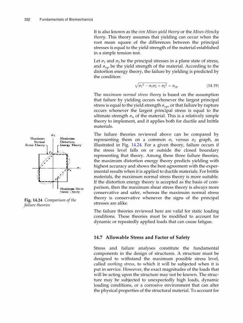
It is also known as the von Mises yield theory or theMises-Henckytheory. This theory assumes that yielding can occur when theroot mean square of the differences between the principalstresses is equal to the yield strength of the material establishedin a simple tension test.
Let σ1 and σ2 be the principal stresses in a plane state of stress,and σyp be the yield strength of the material. According to thedistortion energy theory, the failure by yielding is predicted bythe condition: ffiffiffiffiffiffiffiffiffiffiffiffiffiffiffiffiffiffiffiffiffiffiffiffiffiffiffiffiffiffiffiffiffiffi
σ12 � σ1σ2 þ σ22p
¼ σyp ð14:19Þ
The maximum normal stress theory is based on the assumptionthat failure by yielding occurs whenever the largest principalstress is equal to the yield strength σyp, or that failure by ruptureoccurs whenever the largest principal stress is equal to theultimate strength σu of the material. This is a relatively simpletheory to implement, and it applies both for ductile and brittlematerials.
The failure theories reviewed above can be compared byrepresenting them on a common σ1 versus σ2 graph, asillustrated in Fig. 14.24. For a given theory, failure occurs ifthe stress level falls on or outside the closed boundaryrepresenting that theory. Among these three failure theories,the maximum distortion energy theory predicts yielding withhighest accuracy and shows the best agreement with the exper-imental results when it is applied to ductile materials. For brittlematerials, the maximum normal stress theory is more suitable.If the distortion energy theory is accepted as the basis of com-parison, then the maximum shear stress theory is always moreconservative and safer, whereas the maximum normal stresstheory is conservative whenever the signs of the principalstresses are alike.
The failure theories reviewed here are valid for static loadingconditions. These theories must be modified to account fordynamic or repeatedly applied loads that can cause fatigue.
14.7 Allowable Stress and Factor of Safety
Stress and failure analyses constitute the fundamentalcomponents in the design of structures. A structure must bedesigned to withstand the maximum possible stress level,called working stress, to which it will be subjected when it isput in service. However, the exact magnitudes of the loads thatwill be acting upon the structure may not be known. The struc-ture may be subjected to unexpectedly high loads, dynamicloading conditions, or a corrosive environment that can alterthe physical properties of the structural material. To account for
Fig. 14.24 Comparison of thefailure theories
332 Fundamentals of Biomechanics
the effects of uncertainties, a stress level called the allowablestress must be set considerably lower than the ultimate strengthof the material. The allowable stress must be low enough toprovide a margin of safety. It must also allow for an efficient useof the material.
Safety against unpredictable conditions can be achieved byconsidering a factor of safety. The factor of safety n is usuallydetermined as the ratio of the ultimate strength of the materialto the allowable stress. The factor of safety is a number greaterthan one, and may vary depending on whether the material isloaded under tension, compression, or shear. Instead of theultimate strength, the factor of safety can also be based on theyield strength of the material. This is particularly important foroperational conditions in which excessive yielding or plasticdeformations cannot be tolerated. In the case of fatigue loading,endurance limit or the fatigue strength of the material must beused. Once the factor of safety is established, the allowablestress σall can be determined. For example, based on the ulti-mate strength σu criteria:
σall ¼ σun
ð14:20Þ
14.8 Factors Affecting the Strength of Materials
As discussed in the previous chapter, elastic and shear moduli,yield strength, ultimate strength, stress at failure, and the areaunder the stress–strain diagram for a material are indications ofthe strength of the material. There are many physical and envi-ronmental factors that may influence the properties of a mate-rial. For example, temperature can alter the strength of amaterial by altering its physical properties. Common materialsexpand when heated and contract when cooled. An increase intemperature will lower the ultimate strength of a material. Thestresses in structures caused by temperature changes can bequite considerable.
Friction occurs when two surfaces roll or slide over one another.Friction dissipates energy primarily as heat. Another conse-quence of the sliding action of two surfaces is the removal ofmaterial from the surfaces, which is called wear. Wear can alterthe surface quality of structures, expose them to corrosiveenvironments, and consequently reduce their mechanicalstrength. Corrosion is one of the primary causes of mechanicalfailure. Failure by corrosion can be accelerated by the presenceof stresses. Corrosion can cause the development of minutecracks in the material, which can propagate in a stressed envi-ronment. In general, friction, wear, corrosion, and the presenceof discontinuities in a material can lower its strength.
Multiaxial Deformations and Stress Analyses 333
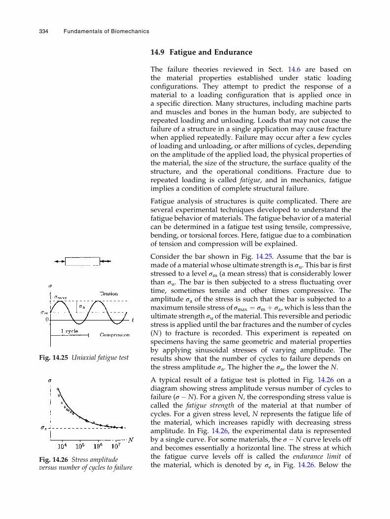
14.9 Fatigue and Endurance
The failure theories reviewed in Sect. 14.6 are based onthe material properties established under static loadingconfigurations. They attempt to predict the response of amaterial to a loading configuration that is applied once ina specific direction. Many structures, including machine partsand muscles and bones in the human body, are subjected torepeated loading and unloading. Loads that may not cause thefailure of a structure in a single application may cause fracturewhen applied repeatedly. Failure may occur after a few cyclesof loading and unloading, or after millions of cycles, dependingon the amplitude of the applied load, the physical properties ofthe material, the size of the structure, the surface quality of thestructure, and the operational conditions. Fracture due torepeated loading is called fatigue, and in mechanics, fatigueimplies a condition of complete structural failure.
Fatigue analysis of structures is quite complicated. There areseveral experimental techniques developed to understand thefatigue behavior of materials. The fatigue behavior of a materialcan be determined in a fatigue test using tensile, compressive,bending, or torsional forces. Here, fatigue due to a combinationof tension and compression will be explained.
Consider the bar shown in Fig. 14.25. Assume that the bar ismade of a material whose ultimate strength is σu. This bar is firststressed to a level σm (a mean stress) that is considerably lowerthan σu. The bar is then subjected to a stress fluctuating overtime, sometimes tensile and other times compressive. Theamplitude σa of the stress is such that the bar is subjected to amaximum tensile stress of σmax ¼ σm þ σa, which is less than theultimate strength σu of thematerial. This reversible and periodicstress is applied until the bar fractures and the number of cycles(N) to fracture is recorded. This experiment is repeated onspecimens having the same geometric and material propertiesby applying sinusoidal stresses of varying amplitude. Theresults show that the number of cycles to failure depends onthe stress amplitude σa. The higher the σa, the lower the N.
A typical result of a fatigue test is plotted in Fig. 14.26 on adiagram showing stress amplitude versus number of cycles tofailure (σ �N). For a given N, the corresponding stress value iscalled the fatigue strength of the material at that number ofcycles. For a given stress level, N represents the fatigue life ofthe material, which increases rapidly with decreasing stressamplitude. In Fig. 14.26, the experimental data is representedby a single curve. For some materials, the σ �N curve levels offand becomes essentially a horizontal line. The stress at whichthe fatigue curve levels off is called the endurance limit ofthe material, which is denoted by σe in Fig. 14.26. Below the
Fig. 14.25 Uniaxial fatigue test
Fig. 14.26 Stress amplitudeversus number of cycles to failure
334 Fundamentals of Biomechanics
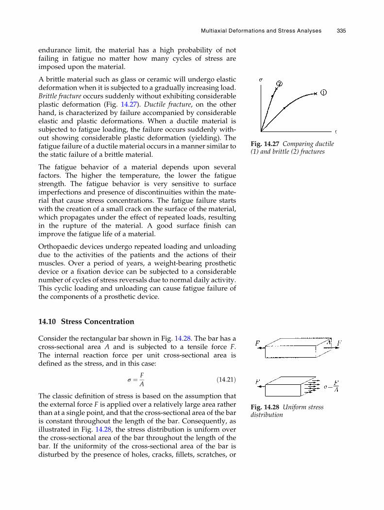
endurance limit, the material has a high probability of notfailing in fatigue no matter how many cycles of stress areimposed upon the material.
A brittle material such as glass or ceramic will undergo elasticdeformation when it is subjected to a gradually increasing load.Brittle fracture occurs suddenly without exhibiting considerableplastic deformation (Fig. 14.27). Ductile fracture, on the otherhand, is characterized by failure accompanied by considerableelastic and plastic deformations. When a ductile material issubjected to fatigue loading, the failure occurs suddenly with-out showing considerable plastic deformation (yielding). Thefatigue failure of a ductile material occurs in a manner similar tothe static failure of a brittle material.
The fatigue behavior of a material depends upon severalfactors. The higher the temperature, the lower the fatiguestrength. The fatigue behavior is very sensitive to surfaceimperfections and presence of discontinuities within the mate-rial that cause stress concentrations. The fatigue failure startswith the creation of a small crack on the surface of the material,which propagates under the effect of repeated loads, resultingin the rupture of the material. A good surface finish canimprove the fatigue life of a material.
Orthopaedic devices undergo repeated loading and unloadingdue to the activities of the patients and the actions of theirmuscles. Over a period of years, a weight-bearing prostheticdevice or a fixation device can be subjected to a considerablenumber of cycles of stress reversals due to normal daily activity.This cyclic loading and unloading can cause fatigue failure ofthe components of a prosthetic device.
14.10 Stress Concentration
Consider the rectangular bar shown in Fig. 14.28. The bar has across-sectional area A and is subjected to a tensile force F.The internal reaction force per unit cross-sectional area isdefined as the stress, and in this case:
σ ¼ F
Að14:21Þ
The classic definition of stress is based on the assumption thatthe external force F is applied over a relatively large area ratherthan at a single point, and that the cross-sectional area of the baris constant throughout the length of the bar. Consequently, asillustrated in Fig. 14.28, the stress distribution is uniform overthe cross-sectional area of the bar throughout the length of thebar. If the uniformity of the cross-sectional area of the bar isdisturbed by the presence of holes, cracks, fillets, scratches, or
Fig. 14.27 Comparing ductile(1) and brittle (2) fractures
Fig. 14.28 Uniform stressdistribution
Multiaxial Deformations and Stress Analyses 335
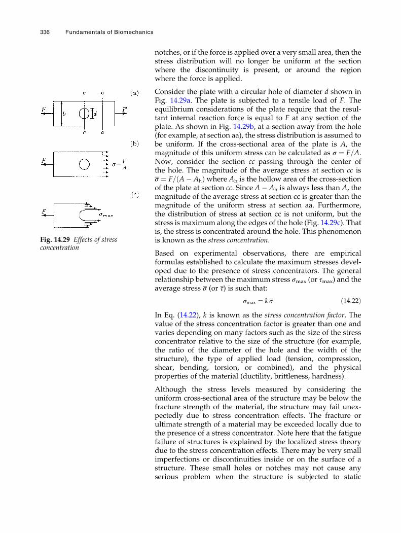
notches, or if the force is applied over a very small area, then thestress distribution will no longer be uniform at the sectionwhere the discontinuity is present, or around the regionwhere the force is applied.
Consider the plate with a circular hole of diameter d shown inFig. 14.29a. The plate is subjected to a tensile load of F. Theequilibrium considerations of the plate require that the resul-tant internal reaction force is equal to F at any section of theplate. As shown in Fig. 14.29b, at a section away from the hole(for example, at section aa), the stress distribution is assumed tobe uniform. If the cross-sectional area of the plate is A, themagnitude of this uniform stress can be calculated as σ ¼ F=A.Now, consider the section cc passing through the center ofthe hole. The magnitude of the average stress at section cc isσ ¼ F= A� Ahð Þwhere Ah is the hollow area of the cross-sectionof the plate at section cc. Since A� Ah is always less than A, themagnitude of the average stress at section cc is greater than themagnitude of the uniform stress at section aa. Furthermore,the distribution of stress at section cc is not uniform, but thestress is maximum along the edges of the hole (Fig. 14.29c). Thatis, the stress is concentrated around the hole. This phenomenonis known as the stress concentration.
Based on experimental observations, there are empiricalformulas established to calculate the maximum stresses devel-oped due to the presence of stress concentrators. The generalrelationship between the maximum stress σmax (or τmax) and theaverage stress σ (or τ) is such that:
σmax ¼ k σ ð14:22ÞIn Eq. (14.22), k is known as the stress concentration factor. Thevalue of the stress concentration factor is greater than one andvaries depending on many factors such as the size of the stressconcentrator relative to the size of the structure (for example,the ratio of the diameter of the hole and the width of thestructure), the type of applied load (tension, compression,shear, bending, torsion, or combined), and the physicalproperties of the material (ductility, brittleness, hardness).
Although the stress levels measured by considering theuniform cross-sectional area of the structure may be below thefracture strength of the material, the structure may fail unex-pectedly due to stress concentration effects. The fracture orultimate strength of a material may be exceeded locally due tothe presence of a stress concentrator. Note here that the fatiguefailure of structures is explained by the localized stress theorydue to the stress concentration effects. There may be very smallimperfections or discontinuities inside or on the surface of astructure. These small holes or notches may not cause anyserious problem when the structure is subjected to static
Fig. 14.29 Effects of stressconcentration
336 Fundamentals of Biomechanics
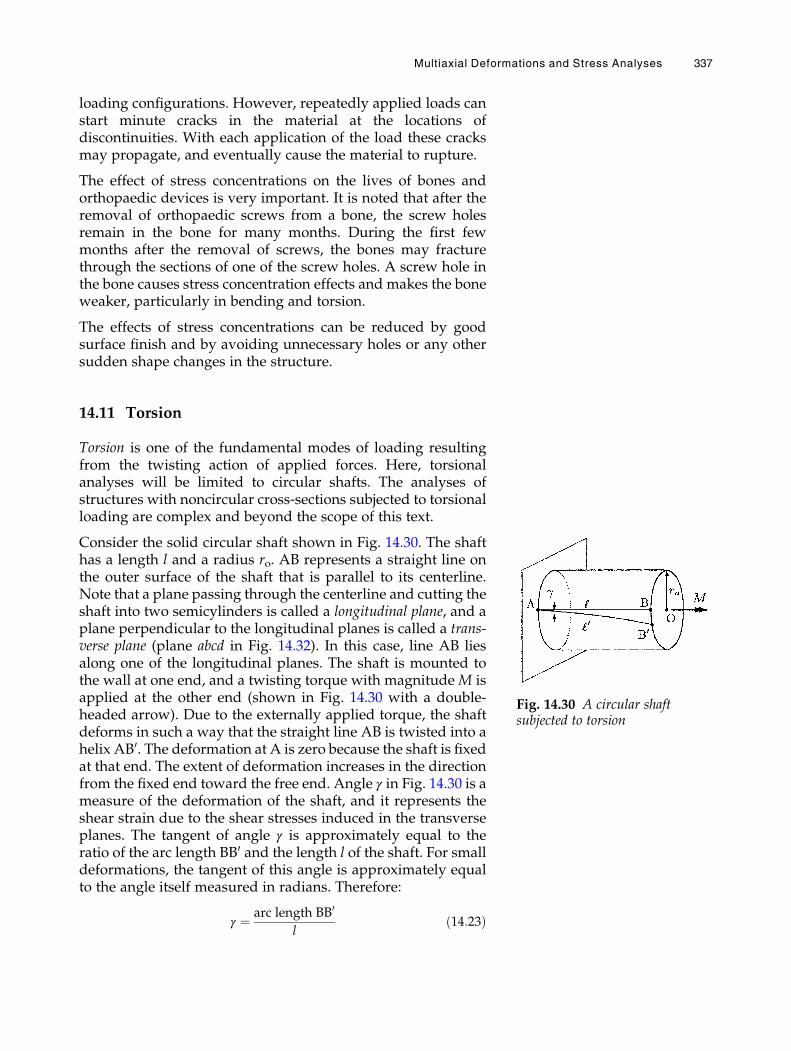
loading configurations. However, repeatedly applied loads canstart minute cracks in the material at the locations ofdiscontinuities. With each application of the load these cracksmay propagate, and eventually cause the material to rupture.
The effect of stress concentrations on the lives of bones andorthopaedic devices is very important. It is noted that after theremoval of orthopaedic screws from a bone, the screw holesremain in the bone for many months. During the first fewmonths after the removal of screws, the bones may fracturethrough the sections of one of the screw holes. A screw hole inthe bone causes stress concentration effects and makes the boneweaker, particularly in bending and torsion.
The effects of stress concentrations can be reduced by goodsurface finish and by avoiding unnecessary holes or any othersudden shape changes in the structure.
14.11 Torsion
Torsion is one of the fundamental modes of loading resultingfrom the twisting action of applied forces. Here, torsionalanalyses will be limited to circular shafts. The analyses ofstructures with noncircular cross-sections subjected to torsionalloading are complex and beyond the scope of this text.
Consider the solid circular shaft shown in Fig. 14.30. The shafthas a length l and a radius ro. AB represents a straight line onthe outer surface of the shaft that is parallel to its centerline.Note that a plane passing through the centerline and cutting theshaft into two semicylinders is called a longitudinal plane, and aplane perpendicular to the longitudinal planes is called a trans-verse plane (plane abcd in Fig. 14.32). In this case, line AB liesalong one of the longitudinal planes. The shaft is mounted tothe wall at one end, and a twisting torque with magnitude M isapplied at the other end (shown in Fig. 14.30 with a double-headed arrow). Due to the externally applied torque, the shaftdeforms in such a way that the straight line AB is twisted into ahelix AB0. The deformation at A is zero because the shaft is fixedat that end. The extent of deformation increases in the directionfrom the fixed end toward the free end. Angle γ in Fig. 14.30 is ameasure of the deformation of the shaft, and it represents theshear strain due to the shear stresses induced in the transverseplanes. The tangent of angle γ is approximately equal to theratio of the arc length BB0 and the length l of the shaft. For smalldeformations, the tangent of this angle is approximately equalto the angle itself measured in radians. Therefore:
γ ¼ arc length BB0
lð14:23Þ
Fig. 14.30 A circular shaftsubjected to torsion
Multiaxial Deformations and Stress Analyses 337
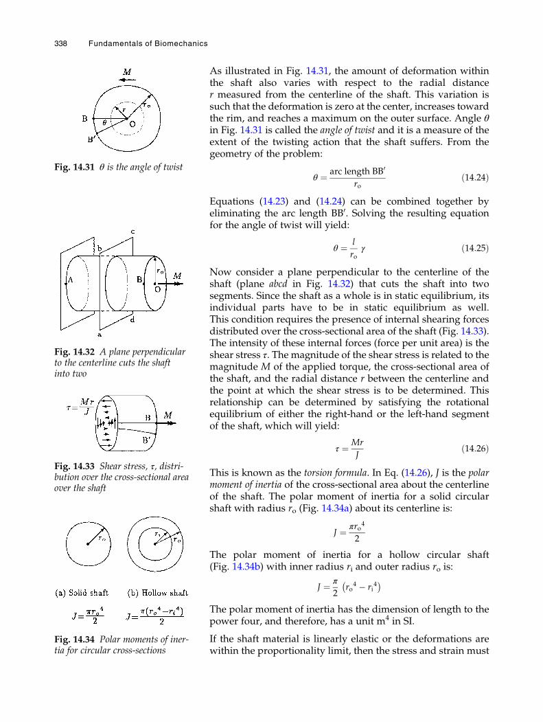
As illustrated in Fig. 14.31, the amount of deformation withinthe shaft also varies with respect to the radial distancer measured from the centerline of the shaft. This variation issuch that the deformation is zero at the center, increases towardthe rim, and reaches a maximum on the outer surface. Angle θin Fig. 14.31 is called the angle of twist and it is a measure of theextent of the twisting action that the shaft suffers. From thegeometry of the problem:
θ ¼ arc length BB0
roð14:24Þ
Equations (14.23) and (14.24) can be combined together byeliminating the arc length BB0. Solving the resulting equationfor the angle of twist will yield:
θ ¼ l
roγ ð14:25Þ
Now consider a plane perpendicular to the centerline of theshaft (plane abcd in Fig. 14.32) that cuts the shaft into twosegments. Since the shaft as a whole is in static equilibrium, itsindividual parts have to be in static equilibrium as well.This condition requires the presence of internal shearing forcesdistributed over the cross-sectional area of the shaft (Fig. 14.33).The intensity of these internal forces (force per unit area) is theshear stress τ. The magnitude of the shear stress is related to themagnitude M of the applied torque, the cross-sectional area ofthe shaft, and the radial distance r between the centerline andthe point at which the shear stress is to be determined. Thisrelationship can be determined by satisfying the rotationalequilibrium of either the right-hand or the left-hand segmentof the shaft, which will yield:
τ ¼ Mr
Jð14:26Þ
This is known as the torsion formula. In Eq. (14.26), J is the polarmoment of inertia of the cross-sectional area about the centerlineof the shaft. The polar moment of inertia for a solid circularshaft with radius ro (Fig. 14.34a) about its centerline is:
J ¼ πro4
2
The polar moment of inertia for a hollow circular shaft(Fig. 14.34b) with inner radius ri and outer radius ro is:
J ¼ π
2ro
4 � ri4
� �
The polar moment of inertia has the dimension of length to thepower four, and therefore, has a unit m4 in SI.
If the shaft material is linearly elastic or the deformations arewithin the proportionality limit, then the stress and strain must
Fig. 14.32 A plane perpendicularto the centerline cuts the shaftinto two
Fig. 14.31 θ is the angle of twist
Fig. 14.33 Shear stress, τ, distri-bution over the cross-sectional areaover the shaft
Fig. 14.34 Polar moments of iner-tia for circular cross-sections
338 Fundamentals of Biomechanics
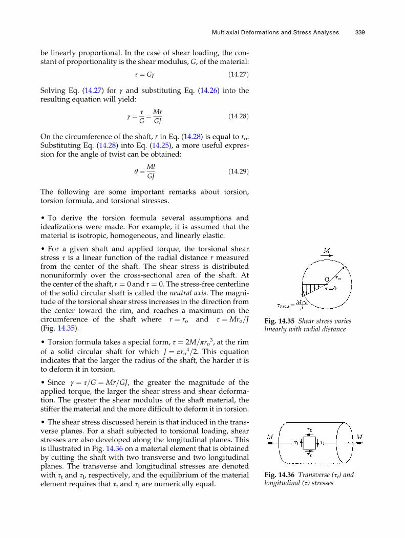
be linearly proportional. In the case of shear loading, the con-stant of proportionality is the shear modulus, G, of the material:
τ ¼ Gγ ð14:27Þ
Solving Eq. (14.27) for γ and substituting Eq. (14.26) into theresulting equation will yield:
γ ¼ τ
G¼ Mr
GJð14:28Þ
On the circumference of the shaft, r in Eq. (14.28) is equal to ro.Substituting Eq. (14.28) into Eq. (14.25), a more useful expres-sion for the angle of twist can be obtained:
θ ¼ Ml
GJð14:29Þ
The following are some important remarks about torsion,torsion formula, and torsional stresses.
• To derive the torsion formula several assumptions andidealizations were made. For example, it is assumed that thematerial is isotropic, homogeneous, and linearly elastic.
• For a given shaft and applied torque, the torsional shearstress τ is a linear function of the radial distance r measuredfrom the center of the shaft. The shear stress is distributednonuniformly over the cross-sectional area of the shaft. Atthe center of the shaft, r ¼ 0 and τ ¼ 0. The stress-free centerlineof the solid circular shaft is called the neutral axis. The magni-tude of the torsional shear stress increases in the direction fromthe center toward the rim, and reaches a maximum on thecircumference of the shaft where r ¼ ro and τ ¼ Mro=J(Fig. 14.35).
• Torsion formula takes a special form, τ ¼ 2M=πro3, at the rimof a solid circular shaft for which J ¼ πro4=2. This equationindicates that the larger the radius of the shaft, the harder it isto deform it in torsion.
• Since γ ¼ τ=G ¼ Mr=GJ, the greater the magnitude of theapplied torque, the larger the shear stress and shear deforma-tion. The greater the shear modulus of the shaft material, thestiffer the material and the more difficult to deform it in torsion.
• The shear stress discussed herein is that induced in the trans-verse planes. For a shaft subjected to torsional loading, shearstresses are also developed along the longitudinal planes. Thisis illustrated in Fig. 14.36 on a material element that is obtainedby cutting the shaft with two transverse and two longitudinalplanes. The transverse and longitudinal stresses are denotedwith τt and τl, respectively, and the equilibrium of the materialelement requires that τt and τl are numerically equal.
Fig. 14.35 Shear stress varieslinearly with radial distance
Fig. 14.36 Transverse (τt) andlongitudinal (τ) stresses
Multiaxial Deformations and Stress Analyses 339
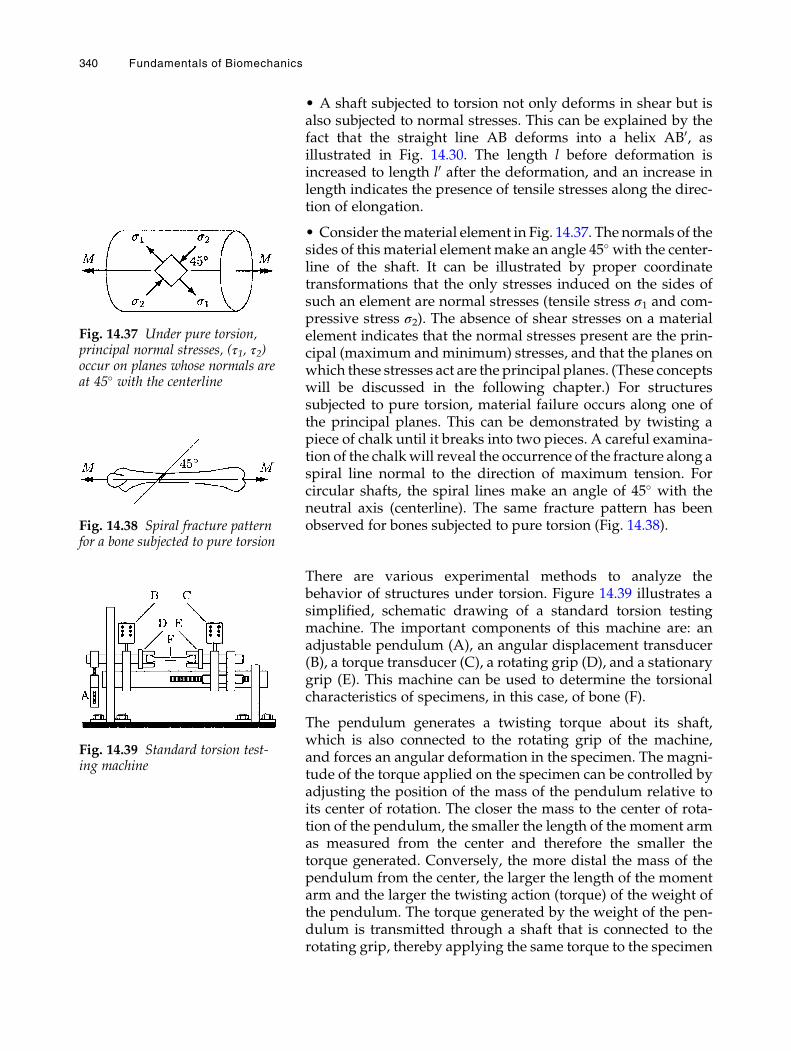
• A shaft subjected to torsion not only deforms in shear but isalso subjected to normal stresses. This can be explained by thefact that the straight line AB deforms into a helix AB0, asillustrated in Fig. 14.30. The length l before deformation isincreased to length l0 after the deformation, and an increase inlength indicates the presence of tensile stresses along the direc-tion of elongation.
• Consider thematerial element in Fig. 14.37. The normals of thesides of this material element make an angle 45� with the center-line of the shaft. It can be illustrated by proper coordinatetransformations that the only stresses induced on the sides ofsuch an element are normal stresses (tensile stress σ1 and com-pressive stress σ2). The absence of shear stresses on a materialelement indicates that the normal stresses present are the prin-cipal (maximum andminimum) stresses, and that the planes onwhich these stresses act are the principal planes. (These conceptswill be discussed in the following chapter.) For structuressubjected to pure torsion, material failure occurs along one ofthe principal planes. This can be demonstrated by twisting apiece of chalk until it breaks into two pieces. A careful examina-tion of the chalkwill reveal the occurrence of the fracture along aspiral line normal to the direction of maximum tension. Forcircular shafts, the spiral lines make an angle of 45� with theneutral axis (centerline). The same fracture pattern has beenobserved for bones subjected to pure torsion (Fig. 14.38).
There are various experimental methods to analyze thebehavior of structures under torsion. Figure 14.39 illustrates asimplified, schematic drawing of a standard torsion testingmachine. The important components of this machine are: anadjustable pendulum (A), an angular displacement transducer(B), a torque transducer (C), a rotating grip (D), and a stationarygrip (E). This machine can be used to determine the torsionalcharacteristics of specimens, in this case, of bone (F).
The pendulum generates a twisting torque about its shaft,which is also connected to the rotating grip of the machine,and forces an angular deformation in the specimen. The magni-tude of the torque applied on the specimen can be controlled byadjusting the position of the mass of the pendulum relative toits center of rotation. The closer the mass to the center of rota-tion of the pendulum, the smaller the length of the moment armas measured from the center and therefore the smaller thetorque generated. Conversely, the more distal the mass of thependulum from the center, the larger the length of the momentarm and the larger the twisting action (torque) of the weight ofthe pendulum. The torque generated by the weight of the pen-dulum is transmitted through a shaft that is connected to therotating grip, thereby applying the same torque to the specimen
Fig. 14.37 Under pure torsion,principal normal stresses, (τ1, τ2)occur on planes whose normals areat 45� with the centerline
Fig. 14.38 Spiral fracture patternfor a bone subjected to pure torsion
Fig. 14.39 Standard torsion test-ing machine
340 Fundamentals of Biomechanics
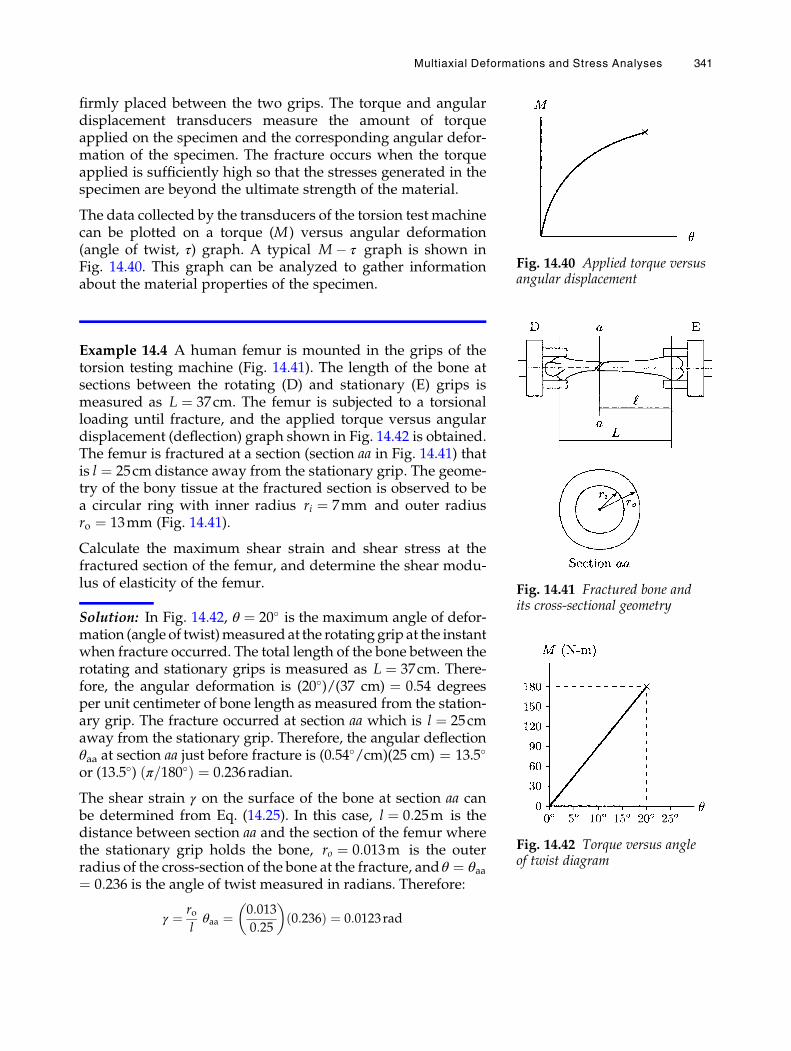
firmly placed between the two grips. The torque and angulardisplacement transducers measure the amount of torqueapplied on the specimen and the corresponding angular defor-mation of the specimen. The fracture occurs when the torqueapplied is sufficiently high so that the stresses generated in thespecimen are beyond the ultimate strength of the material.
The data collected by the transducers of the torsion test machinecan be plotted on a torque (M) versus angular deformation(angle of twist, τ) graph. A typical M� τ graph is shown inFig. 14.40. This graph can be analyzed to gather informationabout the material properties of the specimen.
Example 14.4 A human femur is mounted in the grips of thetorsion testing machine (Fig. 14.41). The length of the bone atsections between the rotating (D) and stationary (E) grips ismeasured as L ¼ 37cm. The femur is subjected to a torsionalloading until fracture, and the applied torque versus angulardisplacement (deflection) graph shown in Fig. 14.42 is obtained.The femur is fractured at a section (section aa in Fig. 14.41) thatis l ¼ 25cm distance away from the stationary grip. The geome-try of the bony tissue at the fractured section is observed to bea circular ring with inner radius ri ¼ 7mm and outer radiusro ¼ 13mm (Fig. 14.41).
Calculate the maximum shear strain and shear stress at thefractured section of the femur, and determine the shear modu-lus of elasticity of the femur.
Solution: In Fig. 14.42, θ ¼ 20� is the maximum angle of defor-mation (angle of twist)measured at the rotatinggrip at the instantwhen fracture occurred. The total length of the bone between therotating and stationary grips is measured as L ¼ 37cm. There-fore, the angular deformation is (20�)/(37 cm) ¼ 0.54 degreesper unit centimeter of bone length as measured from the station-ary grip. The fracture occurred at section aa which is l ¼ 25cmaway from the stationary grip. Therefore, the angular deflectionθaa at section aa just before fracture is (0.54�/cm)(25 cm) ¼ 13.5�
or (13.5�) π=180�ð Þ ¼ 0:236radian.
The shear strain γ on the surface of the bone at section aa canbe determined from Eq. (14.25). In this case, l ¼ 0:25m is thedistance between section aa and the section of the femur wherethe stationary grip holds the bone, ro ¼ 0:013m is the outerradius of the cross-section of the bone at the fracture, andθ ¼ θaa¼ 0:236 is the angle of twist measured in radians. Therefore:
γ ¼ rolθaa ¼ 0:013
0:25
� �0:236ð Þ ¼ 0:0123rad
Fig. 14.40 Applied torque versusangular displacement
Fig. 14.41 Fractured bone andits cross-sectional geometry
Fig. 14.42 Torque versus angleof twist diagram
Multiaxial Deformations and Stress Analyses 341
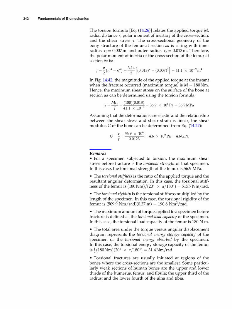
The torsion formula [Eq. (14.26)] relates the applied torque M,radial distance r, polar moment of inertia J of the cross-section,and the shear stress τ. The cross-sectional geometry of thebony structure of the femur at section aa is a ring with innerradius ri ¼ 0:007m and outer radius ro ¼ 0:013m. Therefore,the polar moment of inertia of the cross-section of the femur atsection aa is:
J ¼ π
2ro
4 � ri4
� � ¼ 3:14
20:013ð Þ2 � 0:007ð Þ4
h i¼ 41:1 � 10�9m4
In Fig. 14.42, the magnitude of the applied torque at the instantwhen the fracture occurred (maximum torque) is M ¼ 180Nm.Hence, the maximum shear stress on the surface of the bone atsection aa can be determined using the torsion formula:
τ ¼ MroJ
¼ 180ð Þ 0:013ð Þ41:1 � 10�9
¼ 56:9 � 106 Pa ¼ 56:9MPa
Assuming that the deformations are elastic and the relationshipbetween the shear stress and shear strain is linear, the shearmodulus G of the bone can be determined from Eq. (14.27):
G ¼ τ
γ¼ 56:9 � 106
0:0123¼ 4:6 � 109 Pa ¼ 4:6GPa
Remarks• For a specimen subjected to torsion, the maximum shearstress before fracture is the torsional strength of that specimen.In this case, the torsional strength of the femur is 56.9 MPa.
• The torsional stiffness is the ratio of the applied torque and theresultant angular deformation. In this case, the torsional stiff-ness of the femur is 180Nmð Þ= 20� � π=180�ð Þ ¼ 515:7Nm=rad.
• The torsional rigidity is the torsional stiffness multiplied by thelength of the specimen. In this case, the torsional rigidity of thefemur is (509.9 Nm/rad)(0.37 m) ¼ 190.8 Nm2/rad.
• Themaximum amount of torque applied to a specimen beforefracture is defined as the torsional load capacity of the specimen.In this case, the torsional load capacity of the femur is 180 N m.
• The total area under the torque versus angular displacementdiagram represents the torsional energy storage capacity of thespecimen or the torsional energy absorbed by the specimen.In this case, the torsional energy storage capacity of the femur
is 12 180Nmð Þ 20� � π=180�ð Þ ¼ 31:4Nm=rad.
• Torsional fractures are usually initiated at regions of thebones where the cross-sections are the smallest. Some particu-larly weak sections of human bones are the upper and lowerthirds of the humerus, femur, and fibula; the upper third of theradius; and the lower fourth of the ulna and tibia.
342 Fundamentals of Biomechanics
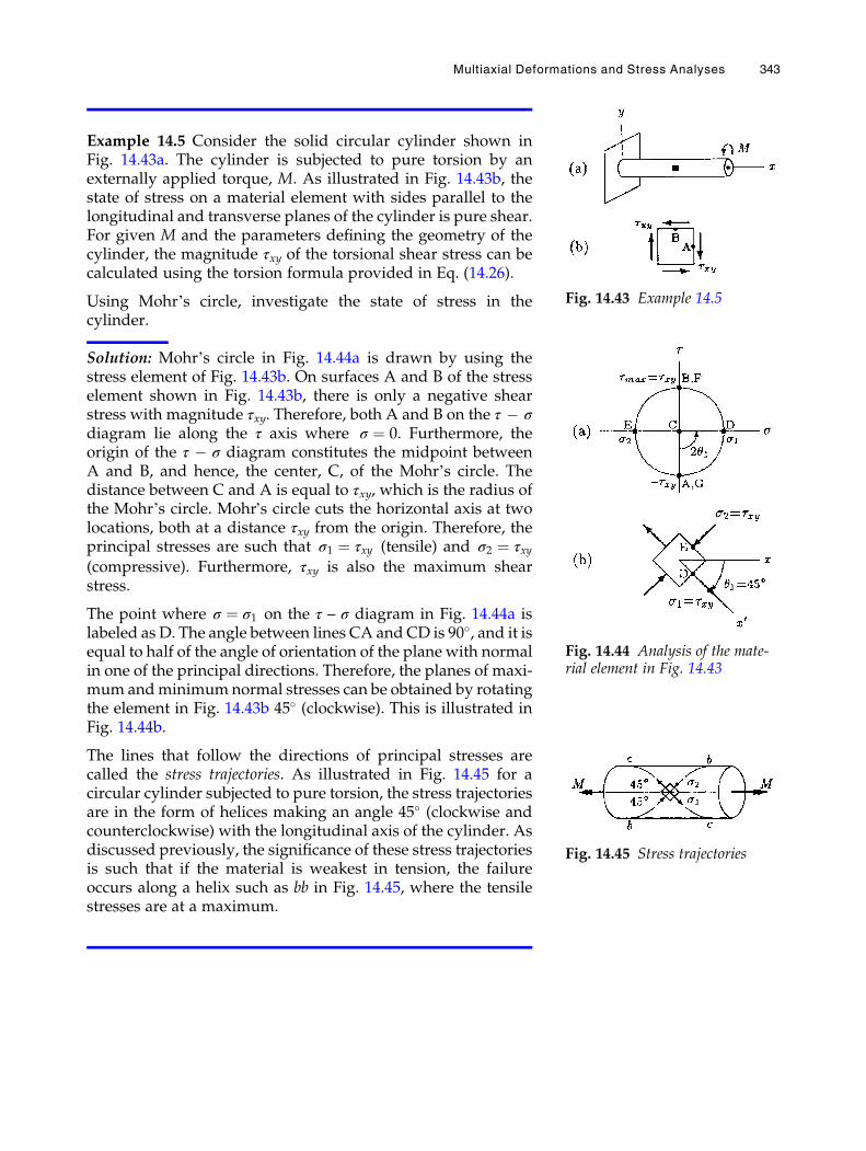
Example 14.5 Consider the solid circular cylinder shown inFig. 14.43a. The cylinder is subjected to pure torsion by anexternally applied torque, M. As illustrated in Fig. 14.43b, thestate of stress on a material element with sides parallel to thelongitudinal and transverse planes of the cylinder is pure shear.For given M and the parameters defining the geometry of thecylinder, the magnitude τxy of the torsional shear stress can becalculated using the torsion formula provided in Eq. (14.26).
Using Mohr’s circle, investigate the state of stress in thecylinder.
Solution: Mohr’s circle in Fig. 14.44a is drawn by using thestress element of Fig. 14.43b. On surfaces A and B of the stresselement shown in Fig. 14.43b, there is only a negative shearstress with magnitude τxy. Therefore, both A and B on the τ � σdiagram lie along the τ axis where σ ¼ 0. Furthermore, theorigin of the τ � σ diagram constitutes the midpoint betweenA and B, and hence, the center, C, of the Mohr’s circle. Thedistance between C and A is equal to τxy, which is the radius ofthe Mohr’s circle. Mohr’s circle cuts the horizontal axis at twolocations, both at a distance τxy from the origin. Therefore, theprincipal stresses are such that σ1 ¼ τxy (tensile) and σ2 ¼ τxy(compressive). Furthermore, τxy is also the maximum shearstress.
The point where σ ¼ σ1 on the τ – σ diagram in Fig. 14.44a islabeled as D. The angle between lines CA and CD is 90�, and it isequal to half of the angle of orientation of the plane with normalin one of the principal directions. Therefore, the planes of maxi-mum andminimumnormal stresses can be obtained by rotatingthe element in Fig. 14.43b 45� (clockwise). This is illustrated inFig. 14.44b.
The lines that follow the directions of principal stresses arecalled the stress trajectories. As illustrated in Fig. 14.45 for acircular cylinder subjected to pure torsion, the stress trajectoriesare in the form of helices making an angle 45� (clockwise andcounterclockwise) with the longitudinal axis of the cylinder. Asdiscussed previously, the significance of these stress trajectoriesis such that if the material is weakest in tension, the failureoccurs along a helix such as bb in Fig. 14.45, where the tensilestresses are at a maximum.
Fig. 14.43 Example 14.5
Fig. 14.44 Analysis of the mate-rial element in Fig. 14.43
Fig. 14.45 Stress trajectories
Multiaxial Deformations and Stress Analyses 343
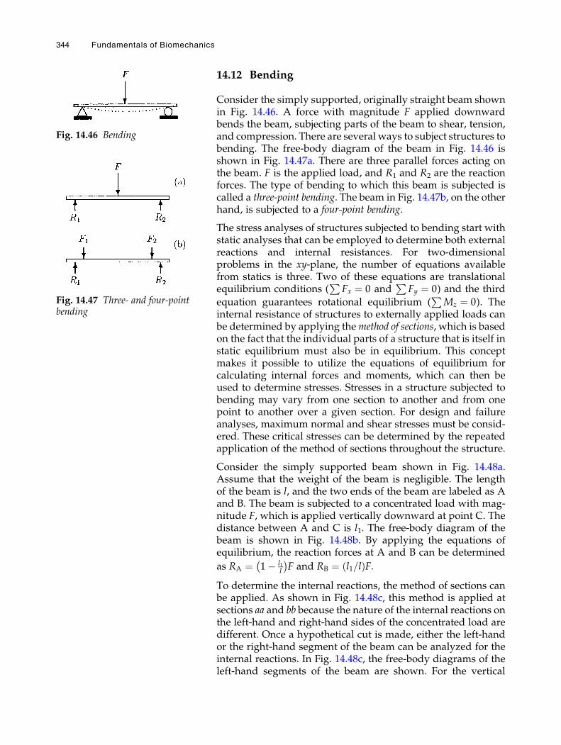
14.12 Bending
Consider the simply supported, originally straight beam shownin Fig. 14.46. A force with magnitude F applied downwardbends the beam, subjecting parts of the beam to shear, tension,and compression. There are several ways to subject structures tobending. The free-body diagram of the beam in Fig. 14.46 isshown in Fig. 14.47a. There are three parallel forces acting onthe beam. F is the applied load, and R1 and R2 are the reactionforces. The type of bending to which this beam is subjected iscalled a three-point bending. The beam in Fig. 14.47b, on the otherhand, is subjected to a four-point bending.
The stress analyses of structures subjected to bending start withstatic analyses that can be employed to determine both externalreactions and internal resistances. For two-dimensionalproblems in the xy-plane, the number of equations availablefrom statics is three. Two of these equations are translationalequilibrium conditions (
PFx ¼ 0 and
PFy ¼ 0) and the third
equation guarantees rotational equilibrium (P
Mz ¼ 0). Theinternal resistance of structures to externally applied loads canbe determined by applying themethod of sections, which is basedon the fact that the individual parts of a structure that is itself instatic equilibrium must also be in equilibrium. This conceptmakes it possible to utilize the equations of equilibrium forcalculating internal forces and moments, which can then beused to determine stresses. Stresses in a structure subjected tobending may vary from one section to another and from onepoint to another over a given section. For design and failureanalyses, maximum normal and shear stresses must be consid-ered. These critical stresses can be determined by the repeatedapplication of the method of sections throughout the structure.
Consider the simply supported beam shown in Fig. 14.48a.Assume that the weight of the beam is negligible. The lengthof the beam is l, and the two ends of the beam are labeled as Aand B. The beam is subjected to a concentrated load with mag-nitude F, which is applied vertically downward at point C. Thedistance between A and C is l1. The free-body diagram of thebeam is shown in Fig. 14.48b. By applying the equations ofequilibrium, the reaction forces at A and B can be determined
as RA ¼ 1� l1l
� �F and RB ¼ l1=lð ÞF.
To determine the internal reactions, the method of sections canbe applied. As shown in Fig. 14.48c, this method is applied atsections aa and bb because the nature of the internal reactions onthe left-hand and right-hand sides of the concentrated load aredifferent. Once a hypothetical cut is made, either the left-handor the right-hand segment of the beam can be analyzed for theinternal reactions. In Fig. 14.48c, the free-body diagrams of theleft-hand segments of the beam are shown. For the vertical
Fig. 14.46 Bending
Fig. 14.47 Three- and four-pointbending
344 Fundamentals of Biomechanics
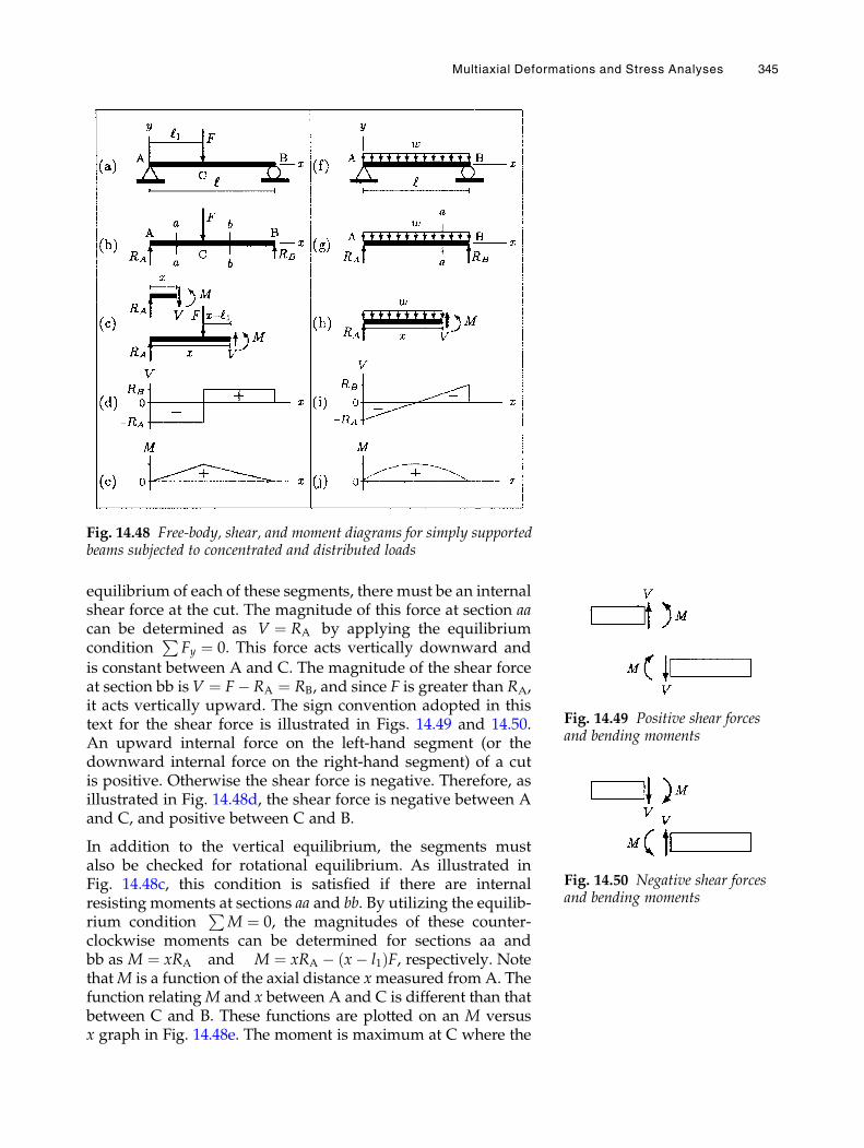
equilibrium of each of these segments, there must be an internalshear force at the cut. The magnitude of this force at section aacan be determined as V ¼ RA by applying the equilibriumcondition
PFy ¼ 0. This force acts vertically downward and
is constant between A and C. The magnitude of the shear forceat section bb isV ¼ F� RA ¼ RB, and since F is greater than RA,it acts vertically upward. The sign convention adopted in thistext for the shear force is illustrated in Figs. 14.49 and 14.50.An upward internal force on the left-hand segment (or thedownward internal force on the right-hand segment) of a cutis positive. Otherwise the shear force is negative. Therefore, asillustrated in Fig. 14.48d, the shear force is negative between Aand C, and positive between C and B.
In addition to the vertical equilibrium, the segments mustalso be checked for rotational equilibrium. As illustrated inFig. 14.48c, this condition is satisfied if there are internalresisting moments at sections aa and bb. By utilizing the equilib-rium condition
PM ¼ 0, the magnitudes of these counter-
clockwise moments can be determined for sections aa andbb as M ¼ xRA and M ¼ xRA � x� l1ð ÞF, respectively. NotethatM is a function of the axial distance xmeasured fromA. Thefunction relatingM and x between A and C is different than thatbetween C and B. These functions are plotted on an M versusx graph in Fig. 14.48e. The moment is maximum at C where the
Fig. 14.48 Free-body, shear, and moment diagrams for simply supportedbeams subjected to concentrated and distributed loads
Fig. 14.49 Positive shear forcesand bending moments
Fig. 14.50 Negative shear forcesand bending moments
Multiaxial Deformations and Stress Analyses 345
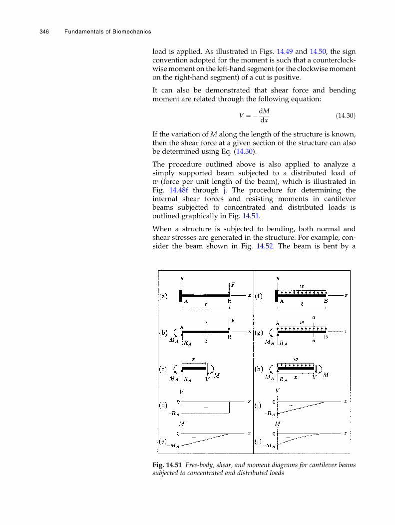
load is applied. As illustrated in Figs. 14.49 and 14.50, the signconvention adopted for the moment is such that a counterclock-wisemoment on the left-hand segment (or the clockwisemomenton the right-hand segment) of a cut is positive.
It can also be demonstrated that shear force and bendingmoment are related through the following equation:
V ¼ �dM
dxð14:30Þ
If the variation of M along the length of the structure is known,then the shear force at a given section of the structure can alsobe determined using Eq. (14.30).
The procedure outlined above is also applied to analyze asimply supported beam subjected to a distributed load ofw (force per unit length of the beam), which is illustrated inFig. 14.48f through j. The procedure for determining theinternal shear forces and resisting moments in cantileverbeams subjected to concentrated and distributed loads isoutlined graphically in Fig. 14.51.
When a structure is subjected to bending, both normal andshear stresses are generated in the structure. For example, con-sider the beam shown in Fig. 14.52. The beam is bent by a
Fig. 14.51 Free-body, shear, and moment diagrams for cantilever beamssubjected to concentrated and distributed loads
346 Fundamentals of Biomechanics
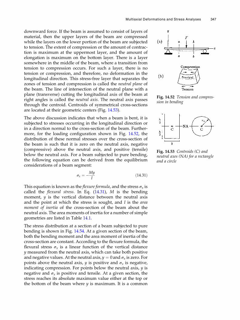
downward force. If the beam is assumed to consist of layers ofmaterial, then the upper layers of the beam are compressedwhile the layers on the lower portion of the beam are subjectedto tension. The extent of compression or the amount of contrac-tion is maximum at the uppermost layer, and the amount ofelongation is maximum on the bottom layer. There is a layersomewhere in the middle of the beam, where a transition fromtension to compression occurs. For such a layer, there is notension or compression, and therefore, no deformation in thelongitudinal direction. This stress-free layer that separates thezones of tension and compression is called the neutral plane ofthe beam. The line of intersection of the neutral plane with aplane (transverse) cutting the longitudinal axis of the beam atright angles is called the neutral axis. The neutral axis passesthrough the centroid. Centroids of symmetrical cross-sectionsare located at their geometric centers (Fig. 14.53).
The above discussion indicates that when a beam is bent, it issubjected to stresses occurring in the longitudinal direction orin a direction normal to the cross-section of the beam. Further-more, for the loading configuration shown in Fig. 14.52, thedistribution of these normal stresses over the cross-section ofthe beam is such that it is zero on the neutral axis, negative(compressive) above the neutral axis, and positive (tensile)below the neutral axis. For a beam subjected to pure bending,the following equation can be derived from the equilibriumconsiderations of a beam segment:
σx ¼ �My
Ið14:31Þ
This equation is known as the flexure formula, and the stress σx iscalled the flexural stress. In Eq. (14.31), M is the bendingmoment, y is the vertical distance between the neutral axisand the point at which the stress is sought, and I is the areamoment of inertia of the cross-section of the beam about theneutral axis. The area moments of inertia for a number of simplegeometries are listed in Table 14.1.
The stress distribution at a section of a beam subjected to purebending is shown in Fig. 14.54. At a given section of the beam,both the bending moment and the area moment of inertia of thecross-section are constant. According to the flexure formula, theflexural stress σx is a linear function of the vertical distancey measured from the neutral axis, which can take both positiveand negative values. At the neutral axis,y ¼ 0and σx is zero. Forpoints above the neutral axis, y is positive and σx is negative,indicating compression. For points below the neutral axis, y isnegative and σx is positive and tensile. At a given section, thestress reaches its absolute maximum value either at the top orthe bottom of the beam where y is maximum. It is a common
Fig. 14.53 Centroids (C) andneutral axes (NA) for a rectangleand a circle
Fig. 14.52 Tension and compres-sion in bending
Multiaxial Deformations and Stress Analyses 347
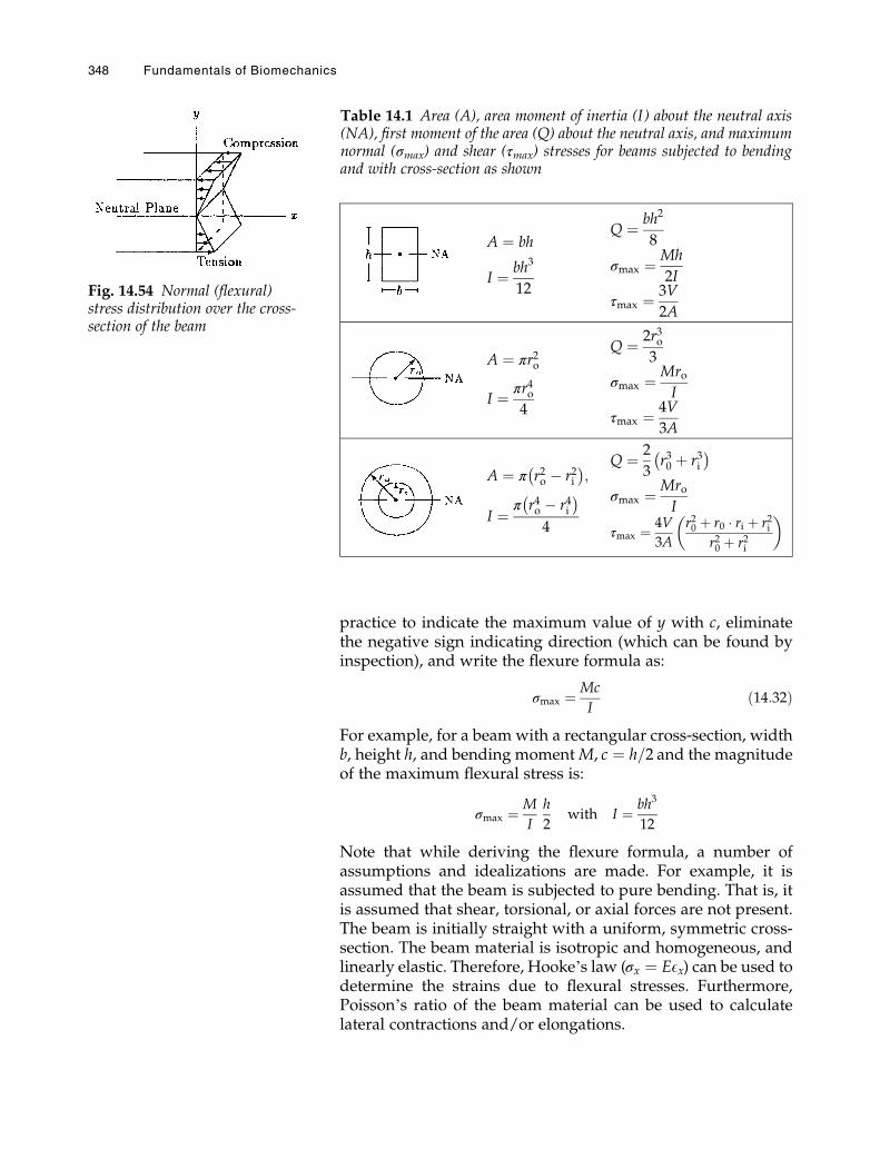
practice to indicate the maximum value of y with c, eliminatethe negative sign indicating direction (which can be found byinspection), and write the flexure formula as:
σmax ¼ Mc
Ið14:32Þ
For example, for a beam with a rectangular cross-section, widthb, height h, and bending momentM, c ¼ h=2 and the magnitudeof the maximum flexural stress is:
σmax ¼ M
I
h
2with I ¼ bh3
12
Note that while deriving the flexure formula, a number ofassumptions and idealizations are made. For example, it isassumed that the beam is subjected to pure bending. That is, itis assumed that shear, torsional, or axial forces are not present.The beam is initially straight with a uniform, symmetric cross-section. The beam material is isotropic and homogeneous, andlinearly elastic. Therefore, Hooke’s law (σx ¼ EEx) can be used todetermine the strains due to flexural stresses. Furthermore,Poisson’s ratio of the beam material can be used to calculatelateral contractions and/or elongations.
Table 14.1 Area (A), area moment of inertia (I) about the neutral axis(NA), first moment of the area (Q) about the neutral axis, and maximumnormal (σmax) and shear (τmax) stresses for beams subjected to bendingand with cross-section as shown
A ¼ bh
I ¼ bh3
12
Q ¼ bh2
8
σmax ¼ Mh
2I
τmax ¼ 3V
2A
A ¼ πr2o
I ¼ πr4o4
Q ¼ 2r3o3
σmax ¼ MroI
τmax ¼ 4V
3A
A ¼ π r2o � r2i� �
;
I ¼ π r4o � r4i� �
4
Q ¼ 2
3r30 þ r3i� �
σmax ¼ MroI
τmax ¼ 4V
3A
r20 þ r0 � ri þ r2ir20 þ r2i
� �
Fig. 14.54 Normal (flexural)stress distribution over the cross-section of the beam
348 Fundamentals of Biomechanics
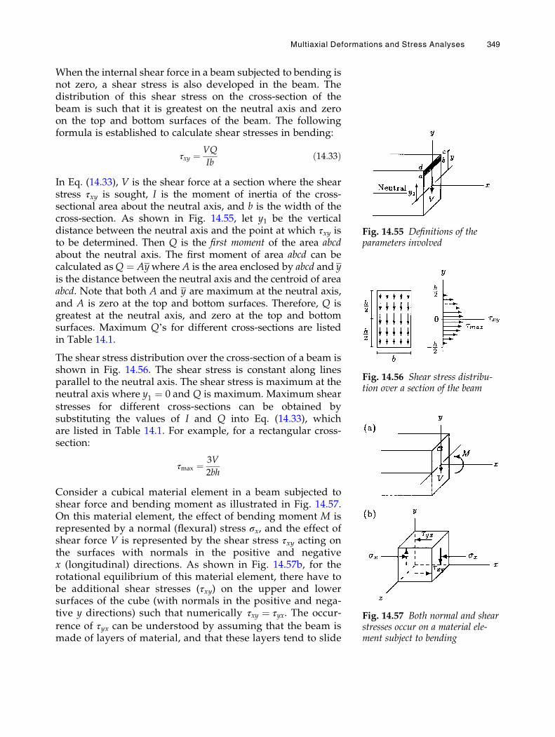
When the internal shear force in a beam subjected to bending isnot zero, a shear stress is also developed in the beam. Thedistribution of this shear stress on the cross-section of thebeam is such that it is greatest on the neutral axis and zeroon the top and bottom surfaces of the beam. The followingformula is established to calculate shear stresses in bending:
τxy ¼ VQ
Ibð14:33Þ
In Eq. (14.33), V is the shear force at a section where the shearstress τxy is sought, I is the moment of inertia of the cross-sectional area about the neutral axis, and b is the width of thecross-section. As shown in Fig. 14.55, let y1 be the verticaldistance between the neutral axis and the point at which τxy isto be determined. Then Q is the first moment of the area abcdabout the neutral axis. The first moment of area abcd can becalculated asQ ¼ Aywhere A is the area enclosed by abcd and yis the distance between the neutral axis and the centroid of areaabcd. Note that both A and y are maximum at the neutral axis,and A is zero at the top and bottom surfaces. Therefore, Q isgreatest at the neutral axis, and zero at the top and bottomsurfaces. Maximum Q’s for different cross-sections are listedin Table 14.1.
The shear stress distribution over the cross-section of a beam isshown in Fig. 14.56. The shear stress is constant along linesparallel to the neutral axis. The shear stress is maximum at theneutral axis where y1 ¼ 0 and Q is maximum. Maximum shearstresses for different cross-sections can be obtained bysubstituting the values of I and Q into Eq. (14.33), whichare listed in Table 14.1. For example, for a rectangular cross-section:
τmax ¼ 3V
2bh
Consider a cubical material element in a beam subjected toshear force and bending moment as illustrated in Fig. 14.57.On this material element, the effect of bending moment M isrepresented by a normal (flexural) stress σx, and the effect ofshear force V is represented by the shear stress τxy acting onthe surfaces with normals in the positive and negativex (longitudinal) directions. As shown in Fig. 14.57b, for therotational equilibrium of this material element, there have tobe additional shear stresses (τxy) on the upper and lowersurfaces of the cube (with normals in the positive and nega-tive y directions) such that numerically τxy ¼ τyx. The occur-
rence of τyx can be understood by assuming that the beam ismade of layers of material, and that these layers tend to slide
Fig. 14.55 Definitions of theparameters involved
Fig. 14.56 Shear stress distribu-tion over a section of the beam
Fig. 14.57 Both normal and shearstresses occur on a material ele-ment subject to bending
Multiaxial Deformations and Stress Analyses 349
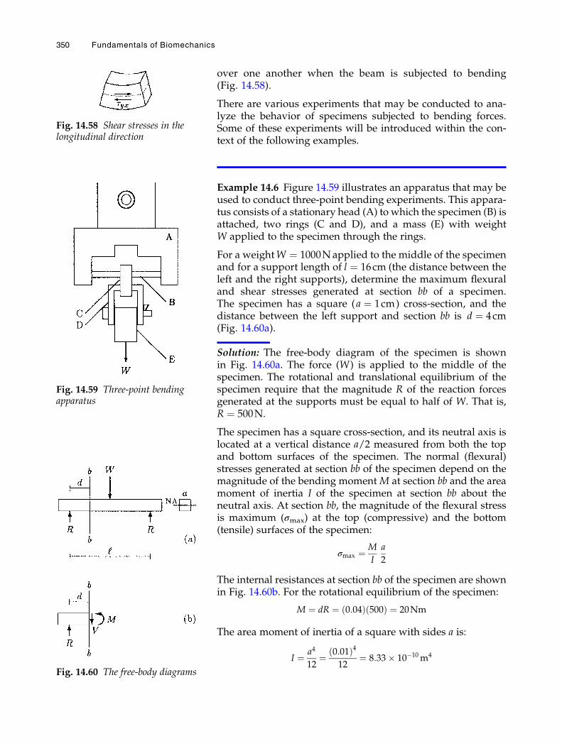
over one another when the beam is subjected to bending(Fig. 14.58).
There are various experiments that may be conducted to ana-lyze the behavior of specimens subjected to bending forces.Some of these experiments will be introduced within the con-text of the following examples.
Example 14.6 Figure 14.59 illustrates an apparatus that may beused to conduct three-point bending experiments. This appara-tus consists of a stationary head (A) to which the specimen (B) isattached, two rings (C and D), and a mass (E) with weightW applied to the specimen through the rings.
For a weightW ¼ 1000Napplied to the middle of the specimenand for a support length of l ¼ 16cm (the distance between theleft and the right supports), determine the maximum flexuraland shear stresses generated at section bb of a specimen.The specimen has a square (a ¼ 1cm) cross-section, and thedistance between the left support and section bb is d ¼ 4cm(Fig. 14.60a).
Solution: The free-body diagram of the specimen is shownin Fig. 14.60a. The force (W) is applied to the middle of thespecimen. The rotational and translational equilibrium of thespecimen require that the magnitude R of the reaction forcesgenerated at the supports must be equal to half of W. That is,R ¼ 500N.
The specimen has a square cross-section, and its neutral axis islocated at a vertical distance a/2 measured from both the topand bottom surfaces of the specimen. The normal (flexural)stresses generated at section bb of the specimen depend on themagnitude of the bending moment M at section bb and the areamoment of inertia I of the specimen at section bb about theneutral axis. At section bb, the magnitude of the flexural stressis maximum (σmax) at the top (compressive) and the bottom(tensile) surfaces of the specimen:
σmax ¼ M
I
a
2
The internal resistances at section bb of the specimen are shownin Fig. 14.60b. For the rotational equilibrium of the specimen:
M ¼ dR ¼ 0:04ð Þ 500ð Þ ¼ 20Nm
The area moment of inertia of a square with sides a is:
I ¼ a4
12¼ 0:01ð Þ4
12¼ 8:33� 10�10m4
Fig. 14.59 Three-point bendingapparatus
Fig. 14.60 The free-body diagrams
Fig. 14.58 Shear stresses in thelongitudinal direction
350 Fundamentals of Biomechanics
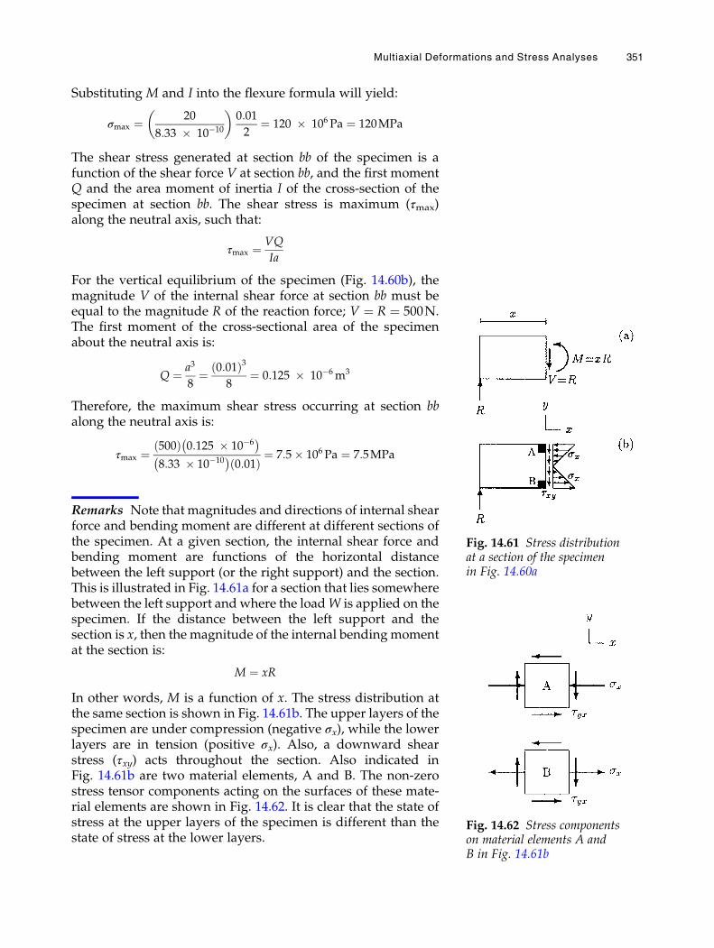
Substituting M and I into the flexure formula will yield:
σmax ¼ 20
8:33 � 10�10
� �0:01
2¼ 120 � 106 Pa ¼ 120MPa
The shear stress generated at section bb of the specimen is afunction of the shear force V at section bb, and the first momentQ and the area moment of inertia I of the cross-section of thespecimen at section bb. The shear stress is maximum (τmax)along the neutral axis, such that:
τmax ¼ VQ
Ia
For the vertical equilibrium of the specimen (Fig. 14.60b), themagnitude V of the internal shear force at section bb must beequal to the magnitude R of the reaction force; V ¼ R ¼ 500N.The first moment of the cross-sectional area of the specimenabout the neutral axis is:
Q ¼ a3
8¼ 0:01ð Þ3
8¼ 0:125 � 10�6m3
Therefore, the maximum shear stress occurring at section bbalong the neutral axis is:
τmax ¼500ð Þ 0:125 � 10�6
� �8:33 � 10�10� �
0:01ð Þ ¼ 7:5� 106 Pa ¼ 7:5MPa
Remarks Note that magnitudes and directions of internal shearforce and bending moment are different at different sections ofthe specimen. At a given section, the internal shear force andbending moment are functions of the horizontal distancebetween the left support (or the right support) and the section.This is illustrated in Fig. 14.61a for a section that lies somewherebetween the left support and where the loadW is applied on thespecimen. If the distance between the left support and thesection is x, then the magnitude of the internal bendingmomentat the section is:
M ¼ xR
In other words, M is a function of x. The stress distribution atthe same section is shown in Fig. 14.61b. The upper layers of thespecimen are under compression (negative σx), while the lowerlayers are in tension (positive σx). Also, a downward shearstress (τxy) acts throughout the section. Also indicated inFig. 14.61b are two material elements, A and B. The non-zerostress tensor components acting on the surfaces of these mate-rial elements are shown in Fig. 14.62. It is clear that the state ofstress at the upper layers of the specimen is different than thestate of stress at the lower layers.
Fig. 14.61 Stress distributionat a section of the specimenin Fig. 14.60a
Fig. 14.62 Stress componentson material elements A andB in Fig. 14.61b
Multiaxial Deformations and Stress Analyses 351
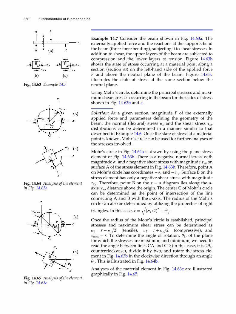
Example 14.7 Consider the beam shown in Fig. 14.63a. Theexternally applied force and the reactions at the supports bendthe beam (three-force bending), subjecting it to shear stresses. Inaddition to shear, the upper layers of the beam are subjected tocompression and the lower layers to tension. Figure 14.63bshows the state of stress occurring at a material point along asection (section aa) on the left-hand side of the applied forceF and above the neutral plane of the beam. Figure 14.63cillustrates the state of stress at the same section below theneutral plane.
Using Mohr’s circle, determine the principal stresses and maxi-mum shear stresses occurring in the beam for the states of stressshown in Fig. 14.63b and c.
Solution: At a given section, magnitude F of the externallyapplied force and parameters defining the geometry of thebeam, the normal (flexural) stress σx and the shear stress τxydistributions can be determined in a manner similar to thatdescribed in Example 14.6. Once the state of stress at a materialpoint is known,Mohr’s circle can be used for further analyses ofthe stresses involved.
Mohr’s circle in Fig. 14.64a is drawn by using the plane stresselement of Fig. 14.63b. There is a negative normal stress withmagnitude σx and a negative shear stress with magnitude τxy onsurface A of the stress element in Fig. 14.63b. Therefore, point Aon Mohr’s circle has coordinates�σx and�τxy. Surface B on the
stress element has only a negative shear stress with magnitudeτxy. Therefore, point B on the τ � σ diagram lies along the σ-axis, τxy distance above the origin. The center C of Mohr’s circlecan be determined as the point of intersection of the lineconnecting A and B with the σ-axis. The radius of the Mohr’scircle can also be determined by utilizing the properties of right
triangles. In this case, r ¼ffiffiffiffiffiffiffiffiffiffiffiffiffiffiffiffiffiffiffiffiffiffiffiffiffiffiffiσx=2ð Þ2 þ r2xy
q.
Once the radius of the Mohr’s circle is established, principalstresses and maximum shear stress can be determined asσ1 ¼ r� σx=2 (tensile), σ2 ¼ rþ σx=2 (compressive), andτmax ¼ r. To determine the angle of rotation, θ1, of the planefor which the stresses are maximum and minimum, we need toread the angle between lines CA and CD (in this case, it is 2θ1,counterclockwise), divide it by two, and rotate the stress ele-ment in Fig. 14.63b in the clockwise direction through an angleθ1. This is illustrated in Fig. 14.64b.
Analyses of the material element in Fig. 14.63c are illustratedgraphically in Fig. 14.65.
Fig. 14.63 Example 14.7
Fig. 14.64 Analysis of the elementin Fig. 14.63b
Fig. 14.65 Analysis of the elementin Fig. 14.63c
352 Fundamentals of Biomechanics
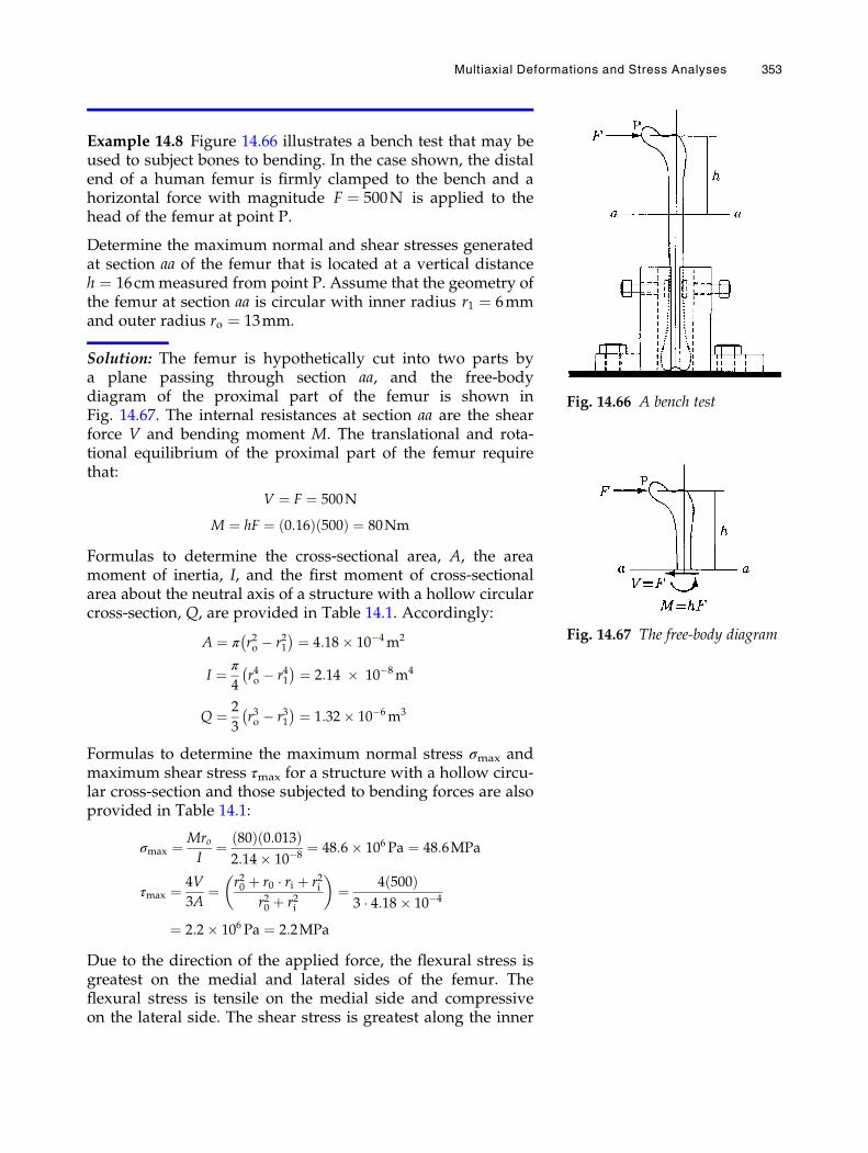
Example 14.8 Figure 14.66 illustrates a bench test that may beused to subject bones to bending. In the case shown, the distalend of a human femur is firmly clamped to the bench and ahorizontal force with magnitude F ¼ 500N is applied to thehead of the femur at point P.
Determine the maximum normal and shear stresses generatedat section aa of the femur that is located at a vertical distanceh ¼ 16cmmeasured from point P. Assume that the geometry ofthe femur at section aa is circular with inner radius r1 ¼ 6mmand outer radius ro ¼ 13mm.
Solution: The femur is hypothetically cut into two parts bya plane passing through section aa, and the free-bodydiagram of the proximal part of the femur is shown inFig. 14.67. The internal resistances at section aa are the shearforce V and bending moment M. The translational and rota-tional equilibrium of the proximal part of the femur requirethat:
V ¼ F ¼ 500N
M ¼ hF ¼ 0:16ð Þ 500ð Þ ¼ 80Nm
Formulas to determine the cross-sectional area, A, the areamoment of inertia, I, and the first moment of cross-sectionalarea about the neutral axis of a structure with a hollow circularcross-section, Q, are provided in Table 14.1. Accordingly:
A ¼ π r2o � r21� � ¼ 4:18� 10�4m2
I ¼ π
4r4o � r41� � ¼ 2:14 � 10�8m4
Q ¼ 2
3r3o � r31� � ¼ 1:32� 10�6m3
Formulas to determine the maximum normal stress σmax andmaximum shear stress τmax for a structure with a hollow circu-lar cross-section and those subjected to bending forces are alsoprovided in Table 14.1:
σmax ¼ MroI
¼ 80ð Þ 0:013ð Þ2:14� 10�8
¼ 48:6� 106 Pa ¼ 48:6MPa
τmax ¼ 4V
3A¼ r20 þ r0 � ri þ r2i
r20 þ r2i
� �¼ 4 500ð Þ
3 � 4:18� 10�4
¼ 2:2� 106 Pa ¼ 2:2MPa
Due to the direction of the applied force, the flexural stress isgreatest on the medial and lateral sides of the femur. Theflexural stress is tensile on the medial side and compressiveon the lateral side. The shear stress is greatest along the inner
Fig. 14.66 A bench test
Fig. 14.67 The free-body diagram
Multiaxial Deformations and Stress Analyses 353
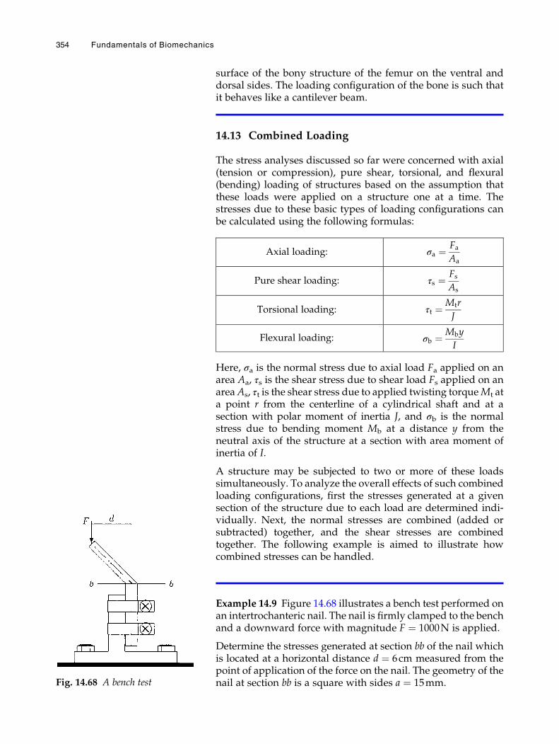
surface of the bony structure of the femur on the ventral anddorsal sides. The loading configuration of the bone is such thatit behaves like a cantilever beam.
14.13 Combined Loading
The stress analyses discussed so far were concerned with axial(tension or compression), pure shear, torsional, and flexural(bending) loading of structures based on the assumption thatthese loads were applied on a structure one at a time. Thestresses due to these basic types of loading configurations canbe calculated using the following formulas:
Axial loading: σa ¼ FaAa
Pure shear loading: τs ¼ FsAs
Torsional loading: τt ¼ Mtr
J
Flexural loading: σb ¼ Mby
I
Here, σa is the normal stress due to axial load Fa applied on anarea Aa, τs is the shear stress due to shear load Fs applied on anareaAs, τt is the shear stress due to applied twisting torqueMt ata point r from the centerline of a cylindrical shaft and at asection with polar moment of inertia J, and σb is the normalstress due to bending moment Mb at a distance y from theneutral axis of the structure at a section with area moment ofinertia of I.
A structure may be subjected to two or more of these loadssimultaneously. To analyze the overall effects of such combinedloading configurations, first the stresses generated at a givensection of the structure due to each load are determined indi-vidually. Next, the normal stresses are combined (added orsubtracted) together, and the shear stresses are combinedtogether. The following example is aimed to illustrate howcombined stresses can be handled.
Example 14.9 Figure 14.68 illustrates a bench test performed onan intertrochanteric nail. The nail is firmly clamped to the benchand a downward force with magnitude F ¼ 1000N is applied.
Determine the stresses generated at section bb of the nail whichis located at a horizontal distance d ¼ 6cm measured from thepoint of application of the force on the nail. The geometry of thenail at section bb is a square with sides a ¼ 15mm.Fig. 14.68 A bench test
354 Fundamentals of Biomechanics
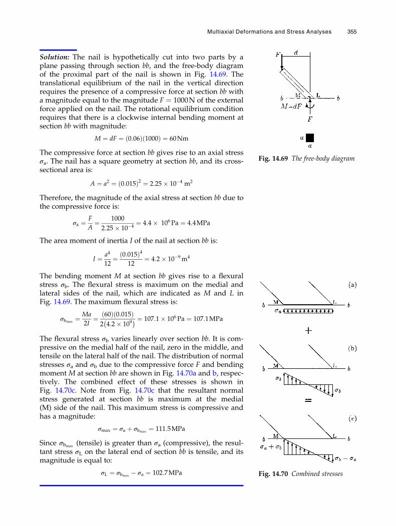
Solution: The nail is hypothetically cut into two parts by aplane passing through section bb, and the free-body diagramof the proximal part of the nail is shown in Fig. 14.69. Thetranslational equilibrium of the nail in the vertical directionrequires the presence of a compressive force at section bb witha magnitude equal to the magnitude F ¼ 1000N of the externalforce applied on the nail. The rotational equilibrium conditionrequires that there is a clockwise internal bending moment atsection bb with magnitude:
M ¼ dF ¼ ð0:06Þ 1000ð Þ ¼ 60Nm
The compressive force at section bb gives rise to an axial stressσa. The nail has a square geometry at section bb, and its cross-sectional area is:
A ¼ a2 ¼ 0:015ð Þ2 ¼ 2:25� 10�4 m2
Therefore, the magnitude of the axial stress at section bb due tothe compressive force is:
σa ¼ F
A¼ 1000
2:25� 10�4¼ 4:4� 106 Pa ¼ 4:4MPa
The area moment of inertia I of the nail at section bb is:
I ¼ a4
12¼ 0:015ð Þ4
12¼ 4:2� 10�9m4
The bending moment M at section bb gives rise to a flexuralstress σb. The flexural stress is maximum on the medial andlateral sides of the nail, which are indicated as M and L inFig. 14.69. The maximum flexural stress is:
σbmax¼ Ma
2I¼ 60ð Þ 0:015ð Þ
2 4:2� 109� � ¼ 107:1� 106 Pa ¼ 107:1MPa
The flexural stress σb varies linearly over section bb. It is com-pressive on the medial half of the nail, zero in the middle, andtensile on the lateral half of the nail. The distribution of normalstresses σa and σb due to the compressive force F and bendingmoment M at section bb are shown in Fig. 14.70a and b, respec-tively. The combined effect of these stresses is shown inFig. 14.70c. Note from Fig. 14.70c that the resultant normalstress generated at section bb is maximum at the medial(M) side of the nail. This maximum stress is compressive andhas a magnitude:
σmax ¼ σa þ σbmax¼ 111:5MPa
Since σbmax(tensile) is greater than σa (compressive), the resul-
tant stress σL on the lateral end of section bb is tensile, and itsmagnitude is equal to:
σL ¼ σbmax� σa ¼ 102:7MPa
Fig. 14.69 The free-body diagram
Fig. 14.70 Combined stresses
Multiaxial Deformations and Stress Analyses 355
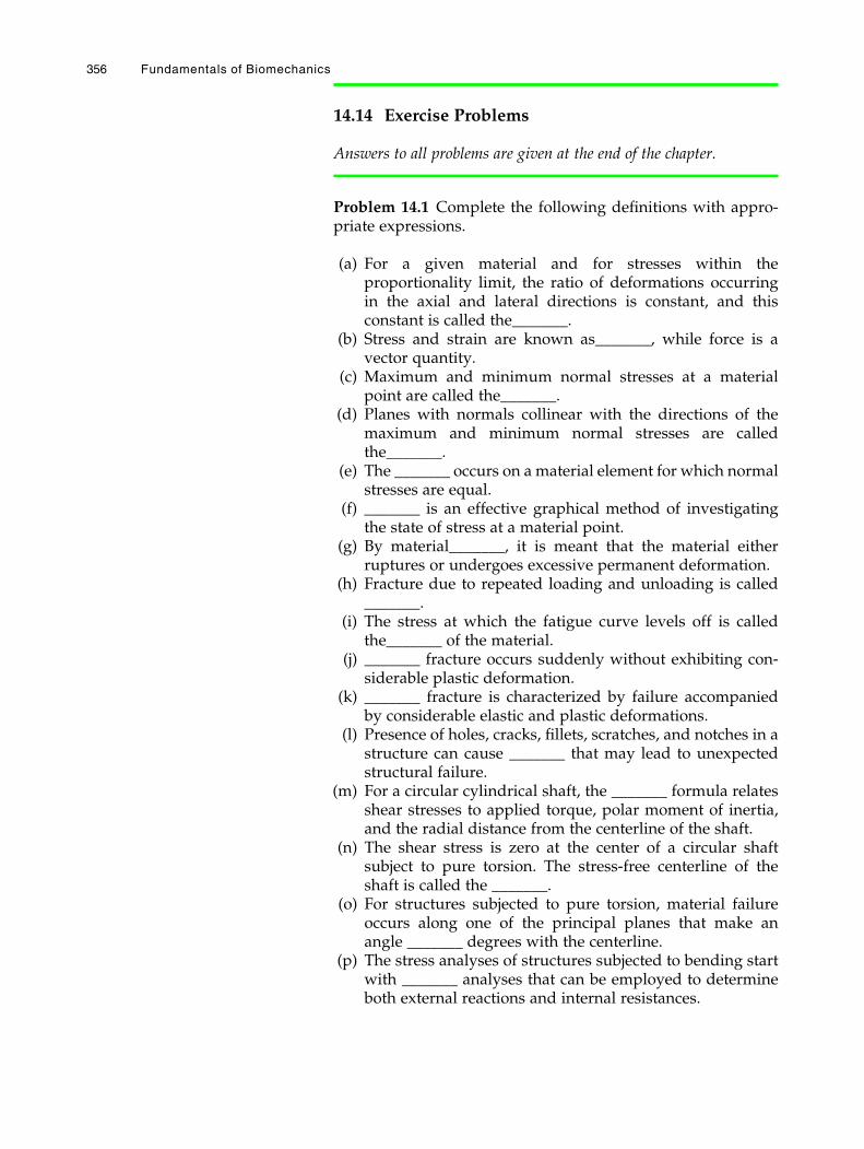
14.14 Exercise Problems
Answers to all problems are given at the end of the chapter.
Problem 14.1 Complete the following definitions with appro-priate expressions.
(a) For a given material and for stresses within theproportionality limit, the ratio of deformations occurringin the axial and lateral directions is constant, and thisconstant is called the_______.
(b) Stress and strain are known as_______, while force is avector quantity.
(c) Maximum and minimum normal stresses at a materialpoint are called the_______.
(d) Planes with normals collinear with the directions of themaximum and minimum normal stresses are calledthe_______.
(e) The _______ occurs on a material element for which normalstresses are equal.
(f) _______ is an effective graphical method of investigatingthe state of stress at a material point.
(g) By material_______, it is meant that the material eitherruptures or undergoes excessive permanent deformation.
(h) Fracture due to repeated loading and unloading is called_______.
(i) The stress at which the fatigue curve levels off is calledthe_______ of the material.
(j) _______ fracture occurs suddenly without exhibiting con-siderable plastic deformation.
(k) _______ fracture is characterized by failure accompaniedby considerable elastic and plastic deformations.
(l) Presence of holes, cracks, fillets, scratches, and notches in astructure can cause _______ that may lead to unexpectedstructural failure.
(m) For a circular cylindrical shaft, the _______ formula relatesshear stresses to applied torque, polar moment of inertia,and the radial distance from the centerline of the shaft.
(n) The shear stress is zero at the center of a circular shaftsubject to pure torsion. The stress-free centerline of theshaft is called the _______.
(o) For structures subjected to pure torsion, material failureoccurs along one of the principal planes that make anangle _______ degrees with the centerline.
(p) The stress analyses of structures subjected to bending startwith _______ analyses that can be employed to determineboth external reactions and internal resistances.
356 Fundamentals of Biomechanics
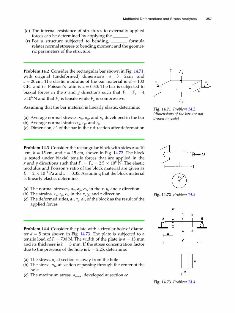
(q) The internal resistance of structures to externally appliedforces can be determined by applying the _______.
(r) For a structure subjected to bending, _______ formularelates normal stresses to bendingmoment and the geomet-ric parameters of the structure.
Problem 14.2 Consider the rectangular bar shown in Fig. 14.71,with original (undeformed) dimensions a ¼ b ¼ 2cm andc ¼ 20cm. The elastic modulus of the bar material is E ¼ 100GPa and its Poisson’s ratio is ν ¼ 0:30. The bar is subjected to
biaxial forces in the x and y directions such that Fx ¼ Fy ¼ 4
�106N and that Fx is tensile while Fy is compressive.
Assuming that the bar material is linearly elastic, determine:
(a) Average normal stresses σx, σy, and σz developed in the bar(b) Average normal strains Ex, Ey, and Ez(c) Dimension, c´, of the bar in the x direction after deformation
Problem 14.3 Consider the rectangular block with sides a ¼ 10cm, b ¼ 15 cm, and c ¼ 15 cm, shown in Fig. 14.72. The blockis tested under biaxial tensile forces that are applied in thex and y directions such that Fx ¼ Fy ¼ 2.5 � 106 N. The elasticmodulus and Poisson’s ratio of the block material are given asE ¼ 2 � 1011 Pa and ν ¼ 0.35. Assuming that the block materialis linearly elastic, determine:
(a) The normal stresses, σx, σy, σz, in the x, y, and z direction(b) The strains, Ex, Ey, Ez, in the x, y, and z direction(c) The deformed sides, ax, ay, az, of the block as the result of the
applied forces
Problem 14.4 Consider the plate with a circular hole of diame-ter d ¼ 5 mm shown in Fig. 14.73. The plate is subjected to atensile load of F ¼ 700 N. The width of the plate is a ¼ 13 mmand its thickness is b ¼ 3 mm. If the stress concentration factordue to the presence of the hole is k ¼ 2.25, determine:
(a) The stress, σ, at section cc away from the hole(b) The stress, σh, at section ee passing through the center of the
hole(c) The maximum stress, σmax, developed at section ee
Fig. 14.71 Problem 14.2(dimensions of the bar are notdrawn to scale)
Fig. 14.72 Problem 14.3
Fig. 14.73 Problem 14.4
Multiaxial Deformations and Stress Analyses 357
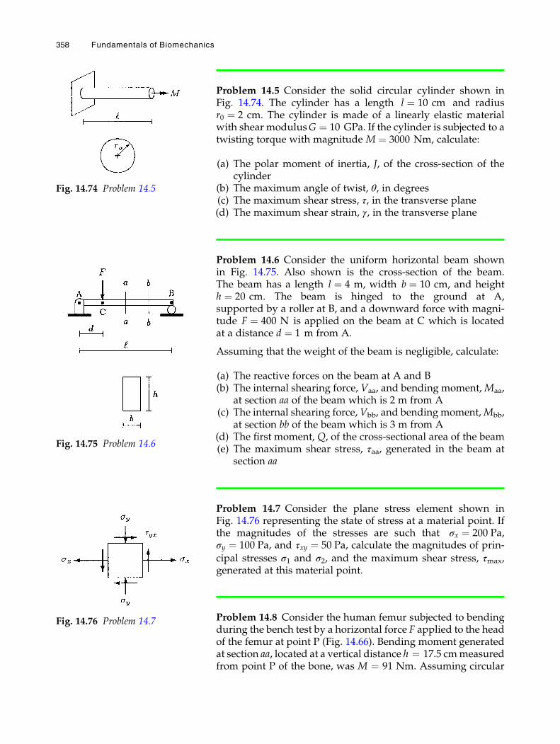
Problem 14.5 Consider the solid circular cylinder shown inFig. 14.74. The cylinder has a length l ¼ 10 cm and radiusr0 ¼ 2 cm. The cylinder is made of a linearly elastic materialwith shear modulusG ¼ 10 GPa. If the cylinder is subjected to atwisting torque with magnitude M ¼ 3000 Nm, calculate:
(a) The polar moment of inertia, J, of the cross-section of thecylinder
(b) The maximum angle of twist, θ, in degrees(c) The maximum shear stress, τ, in the transverse plane(d) The maximum shear strain, γ, in the transverse plane
Problem 14.6 Consider the uniform horizontal beam shownin Fig. 14.75. Also shown is the cross-section of the beam.The beam has a length l ¼ 4 m, width b ¼ 10 cm, and heighth ¼ 20 cm. The beam is hinged to the ground at A,supported by a roller at B, and a downward force with magni-tude F ¼ 400 N is applied on the beam at C which is locatedat a distance d ¼ 1 m from A.
Assuming that the weight of the beam is negligible, calculate:
(a) The reactive forces on the beam at A and B(b) The internal shearing force, Vaa, and bending moment,Maa,
at section aa of the beam which is 2 m from A(c) The internal shearing force, Vbb, and bending moment,Mbb,
at section bb of the beam which is 3 m from A(d) The first moment, Q, of the cross-sectional area of the beam(e) The maximum shear stress, τaa, generated in the beam at
section aa
Problem 14.7 Consider the plane stress element shown inFig. 14.76 representing the state of stress at a material point. Ifthe magnitudes of the stresses are such that σx ¼ 200 Pa,σy ¼ 100 Pa, and τxy ¼ 50 Pa, calculate the magnitudes of prin-
cipal stresses σ1 and σ2, and the maximum shear stress, τmax,generated at this material point.
Problem 14.8 Consider the human femur subjected to bendingduring the bench test by a horizontal force F applied to the headof the femur at point P (Fig. 14.66). Bending moment generatedat section aa, located at a vertical distance h ¼ 17.5 cmmeasuredfrom point P of the bone, was M ¼ 91 Nm. Assuming circular
Fig. 14.74 Problem 14.5
Fig. 14.75 Problem 14.6
Fig. 14.76 Problem 14.7
358 Fundamentals of Biomechanics
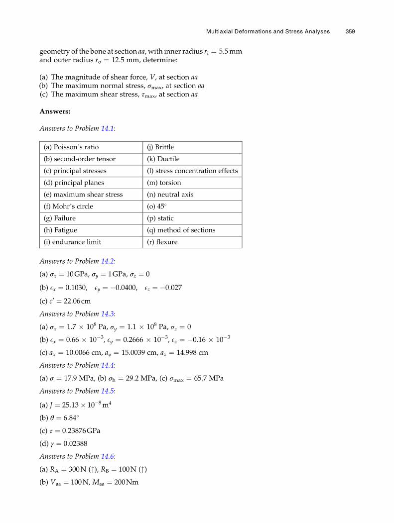
geometry of the bone at section aa, with inner radius ri ¼ 5.5mmand outer radius ro ¼ 12.5 mm, determine:
(a) The magnitude of shear force, V, at section aa(b) The maximum normal stress, σmax, at section aa(c) The maximum shear stress, τmax, at section aa
Answers:
Answers to Problem 14.1:
(a) Poisson’s ratio (j) Brittle
(b) second-order tensor (k) Ductile
(c) principal stresses (l) stress concentration effects
(d) principal planes (m) torsion
(e) maximum shear stress (n) neutral axis
(f) Mohr’s circle (o) 45�
(g) Failure (p) static
(h) Fatigue (q) method of sections
(i) endurance limit (r) flexure
Answers to Problem 14.2:
(a) σx ¼ 10GPa, σy ¼ 1GPa, σz ¼ 0
(b) Ex ¼ 0:1030, Ey ¼ �0:0400, Ez ¼ �0:027
(c) c0 ¼ 22:06cm
Answers to Problem 14.3:
(a) σx ¼ 1.7 � 108 Pa, σy ¼ 1.1 � 108 Pa, σz ¼ 0
(b) Ex ¼ 0.66 � 10�3, Ey ¼ 0.2666 � 10�3, Ez ¼ �0.16 � 10�3
(c) ax ¼ 10.0066 cm, ay ¼ 15.0039 cm, az ¼ 14.998 cm
Answers to Problem 14.4:
(a) σ ¼ 17.9 MPa, (b) σh ¼ 29.2 MPa, (c) σmax ¼ 65.7 MPa
Answers to Problem 14.5:
(a) J ¼ 25:13� 10�8m4
(b) θ ¼ 6:84�
(c) τ ¼ 0:23876GPa
(d) γ ¼ 0:02388
Answers to Problem 14.6:
(a) RA ¼ 300N ("), RB ¼ 100N (")(b) Vaa ¼ 100N, Maa ¼ 200Nm
Multiaxial Deformations and Stress Analyses 359
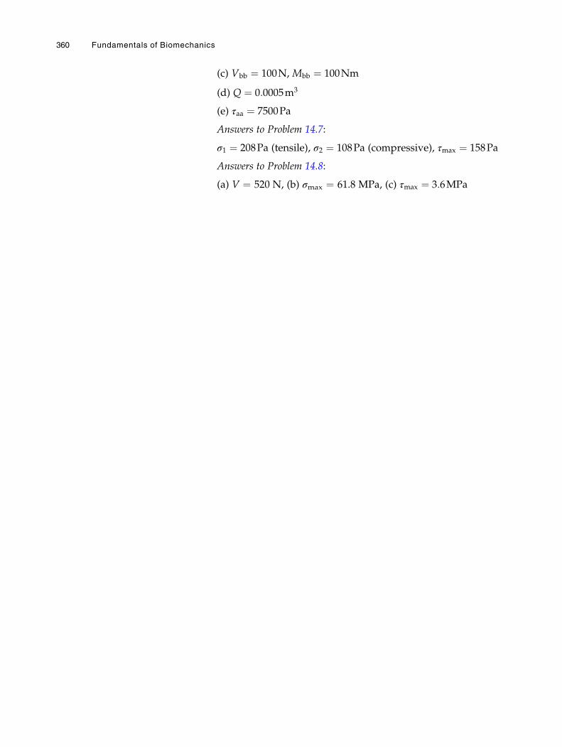
(c) Vbb ¼ 100N, Mbb ¼ 100Nm
(d) Q ¼ 0:0005m3
(e) τaa ¼ 7500Pa
Answers to Problem 14.7:
σ1 ¼ 208Pa (tensile), σ2 ¼ 108Pa (compressive), τmax ¼ 158Pa
Answers to Problem 14.8:
(a) V ¼ 520 N, (b) σmax ¼ 61.8 MPa, (c) τmax ¼ 3:6MPa
360 Fundamentals of Biomechanics
Chapter 15
Mechanical Propertiesof Biological Tissues
15.1 Viscoelasticity / 363
15.2 Analogies Based on Springs and Dashpots / 364
15.3 Empirical Models of Viscoelasticity / 365
15.3.1 Kelvin-Voight Model / 365
15.3.2 Maxwell Model / 366
15.3.3 Standard Solid Model / 367
15.4 Time-Dependent Material Response / 368
15.5 Comparison of Elasticity and Viscoelasticity / 369
15.6 Common Characteristics of Biological Tissues / 371
15.7 Biomechanics of Bone / 373
15.7.1 Composition of Bone / 373
15.7.2 Mechanical Properties of Bone / 374
15.7.3 Structural Integrity of Bone / 376
15.7.4 Bone Fractures / 377
15.8 Tendons and Ligaments / 378
15.9 Skeletal Muscles / 379
15.10 Articular Cartilage / 381
15.11 Discussion / 382
15.12 Exercise Problems / 383
# Springer International Publishing Switzerland 2017N. Ozkaya et al., Fundamentals of Biomechanics, DOI 10.1007/978-3-319-44738-4_15
361

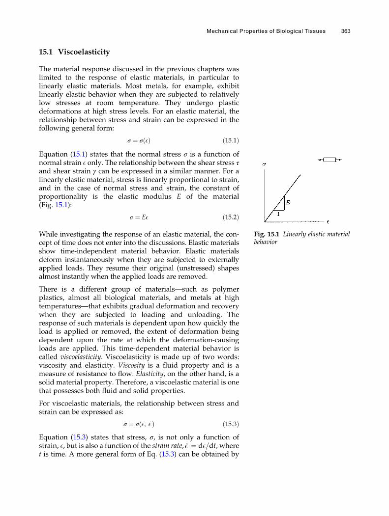
15.1 Viscoelasticity
The material response discussed in the previous chapters waslimited to the response of elastic materials, in particular tolinearly elastic materials. Most metals, for example, exhibitlinearly elastic behavior when they are subjected to relativelylow stresses at room temperature. They undergo plasticdeformations at high stress levels. For an elastic material, therelationship between stress and strain can be expressed in thefollowing general form:
σ ¼ σ Eð Þ ð15:1ÞEquation (15.1) states that the normal stress σ is a function ofnormal strain E only. The relationship between the shear stress τand shear strain γ can be expressed in a similar manner. For alinearly elastic material, stress is linearly proportional to strain,and in the case of normal stress and strain, the constant ofproportionality is the elastic modulus E of the material(Fig. 15.1):
σ ¼ EE ð15:2Þ
While investigating the response of an elastic material, the con-cept of time does not enter into the discussions. Elastic materialsshow time-independent material behavior. Elastic materialsdeform instantaneously when they are subjected to externallyapplied loads. They resume their original (unstressed) shapesalmost instantly when the applied loads are removed.
There is a different group of materials—such as polymerplastics, almost all biological materials, and metals at hightemperatures—that exhibits gradual deformation and recoverywhen they are subjected to loading and unloading. Theresponse of such materials is dependent upon how quickly theload is applied or removed, the extent of deformation beingdependent upon the rate at which the deformation-causingloads are applied. This time-dependent material behavior iscalled viscoelasticity. Viscoelasticity is made up of two words:viscosity and elasticity. Viscosity is a fluid property and is ameasure of resistance to flow. Elasticity, on the other hand, is asolid material property. Therefore, a viscoelastic material is onethat possesses both fluid and solid properties.
For viscoelastic materials, the relationship between stress andstrain can be expressed as:
σ ¼ σ E, _Eð Þ ð15:3ÞEquation (15.3) states that stress, σ, is not only a function ofstrain, E, but is also a function of the strain rate, _E ¼ dE=dt, wheret is time. A more general form of Eq. (15.3) can be obtained by
Fig. 15.1 Linearly elastic materialbehavior
Mechanical Properties of Biological Tissues 363
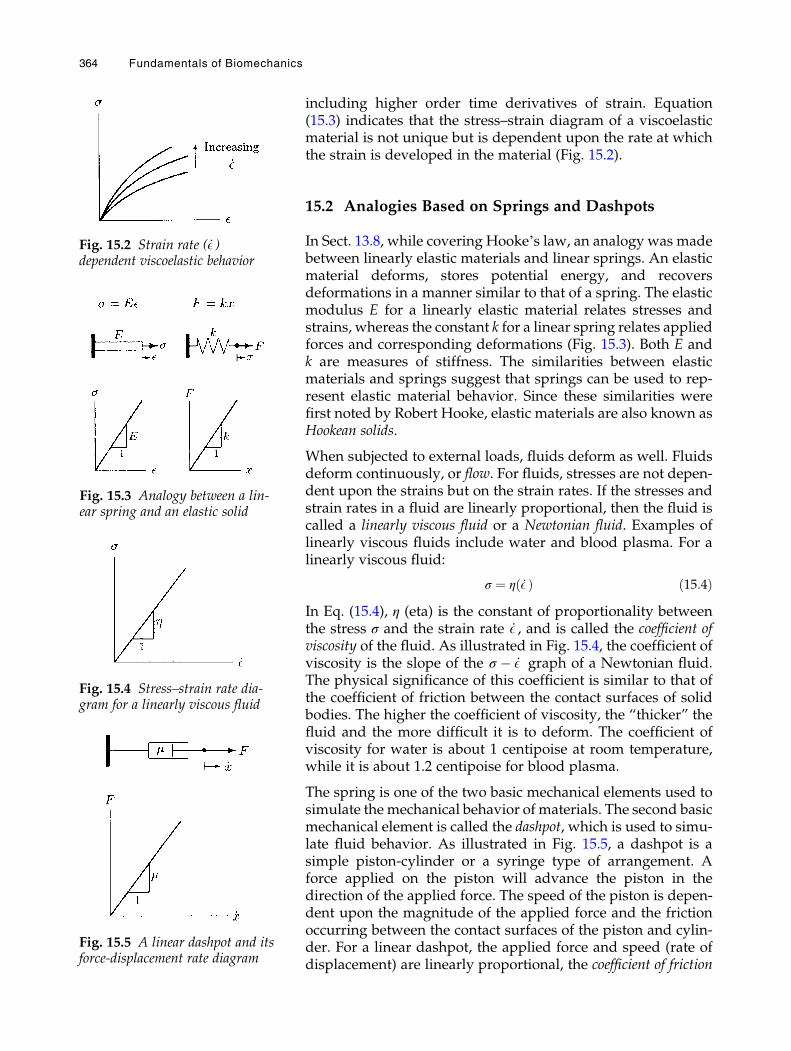
including higher order time derivatives of strain. Equation(15.3) indicates that the stress–strain diagram of a viscoelasticmaterial is not unique but is dependent upon the rate at whichthe strain is developed in the material (Fig. 15.2).
15.2 Analogies Based on Springs and Dashpots
In Sect. 13.8, while covering Hooke’s law, an analogy was madebetween linearly elastic materials and linear springs. An elasticmaterial deforms, stores potential energy, and recoversdeformations in a manner similar to that of a spring. The elasticmodulus E for a linearly elastic material relates stresses andstrains, whereas the constant k for a linear spring relates appliedforces and corresponding deformations (Fig. 15.3). Both E andk are measures of stiffness. The similarities between elasticmaterials and springs suggest that springs can be used to rep-resent elastic material behavior. Since these similarities werefirst noted by Robert Hooke, elastic materials are also known asHookean solids.
When subjected to external loads, fluids deform as well. Fluidsdeform continuously, or flow. For fluids, stresses are not depen-dent upon the strains but on the strain rates. If the stresses andstrain rates in a fluid are linearly proportional, then the fluid iscalled a linearly viscous fluid or a Newtonian fluid. Examples oflinearly viscous fluids include water and blood plasma. For alinearly viscous fluid:
σ ¼ η _Eð Þ ð15:4ÞIn Eq. (15.4), η (eta) is the constant of proportionality betweenthe stress σ and the strain rate _E , and is called the coefficient ofviscosity of the fluid. As illustrated in Fig. 15.4, the coefficient ofviscosity is the slope of the σ � _E graph of a Newtonian fluid.The physical significance of this coefficient is similar to that ofthe coefficient of friction between the contact surfaces of solidbodies. The higher the coefficient of viscosity, the “thicker” thefluid and the more difficult it is to deform. The coefficient ofviscosity for water is about 1 centipoise at room temperature,while it is about 1.2 centipoise for blood plasma.
The spring is one of the two basic mechanical elements used tosimulate the mechanical behavior of materials. The second basicmechanical element is called the dashpot, which is used to simu-late fluid behavior. As illustrated in Fig. 15.5, a dashpot is asimple piston-cylinder or a syringe type of arrangement. Aforce applied on the piston will advance the piston in thedirection of the applied force. The speed of the piston is depen-dent upon the magnitude of the applied force and the frictionoccurring between the contact surfaces of the piston and cylin-der. For a linear dashpot, the applied force and speed (rate ofdisplacement) are linearly proportional, the coefficient of friction
Fig. 15.2 Strain rate ( _E )dependent viscoelastic behavior
Fig. 15.3 Analogy between a lin-ear spring and an elastic solid
Fig. 15.4 Stress–strain rate dia-gram for a linearly viscous fluid
Fig. 15.5 A linear dashpot and itsforce-displacement rate diagram
364 Fundamentals of Biomechanics
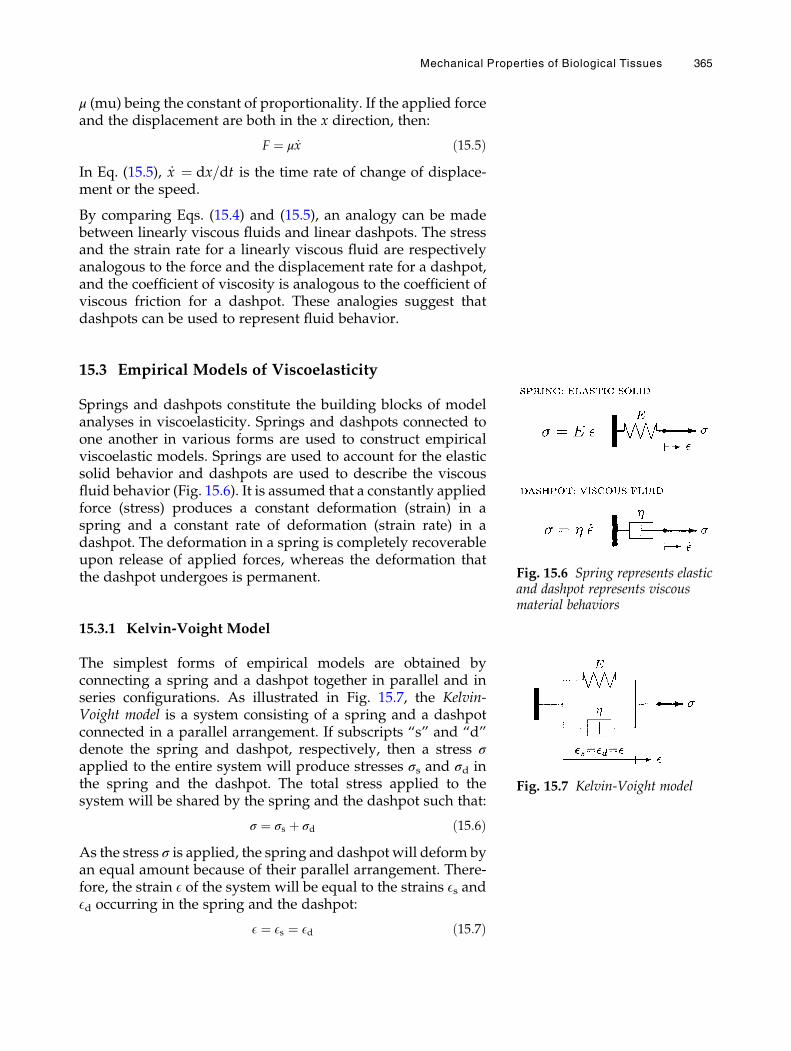
μ (mu) being the constant of proportionality. If the applied forceand the displacement are both in the x direction, then:
F ¼ μ _x ð15:5ÞIn Eq. (15.5), _x ¼ dx=dt is the time rate of change of displace-ment or the speed.
By comparing Eqs. (15.4) and (15.5), an analogy can be madebetween linearly viscous fluids and linear dashpots. The stressand the strain rate for a linearly viscous fluid are respectivelyanalogous to the force and the displacement rate for a dashpot,and the coefficient of viscosity is analogous to the coefficient ofviscous friction for a dashpot. These analogies suggest thatdashpots can be used to represent fluid behavior.
15.3 Empirical Models of Viscoelasticity
Springs and dashpots constitute the building blocks of modelanalyses in viscoelasticity. Springs and dashpots connected toone another in various forms are used to construct empiricalviscoelastic models. Springs are used to account for the elasticsolid behavior and dashpots are used to describe the viscousfluid behavior (Fig. 15.6). It is assumed that a constantly appliedforce (stress) produces a constant deformation (strain) in aspring and a constant rate of deformation (strain rate) in adashpot. The deformation in a spring is completely recoverableupon release of applied forces, whereas the deformation thatthe dashpot undergoes is permanent.
15.3.1 Kelvin-Voight Model
The simplest forms of empirical models are obtained byconnecting a spring and a dashpot together in parallel and inseries configurations. As illustrated in Fig. 15.7, the Kelvin-Voight model is a system consisting of a spring and a dashpotconnected in a parallel arrangement. If subscripts “s” and “d”denote the spring and dashpot, respectively, then a stress σapplied to the entire system will produce stresses σs and σd inthe spring and the dashpot. The total stress applied to thesystem will be shared by the spring and the dashpot such that:
σ ¼ σs þ σd ð15:6ÞAs the stress σ is applied, the spring and dashpot will deform byan equal amount because of their parallel arrangement. There-fore, the strain E of the system will be equal to the strains Es andEd occurring in the spring and the dashpot:
E ¼ Es ¼ Ed ð15:7Þ
Fig. 15.6 Spring represents elasticand dashpot represents viscousmaterial behaviors
Fig. 15.7 Kelvin-Voight model
Mechanical Properties of Biological Tissues 365
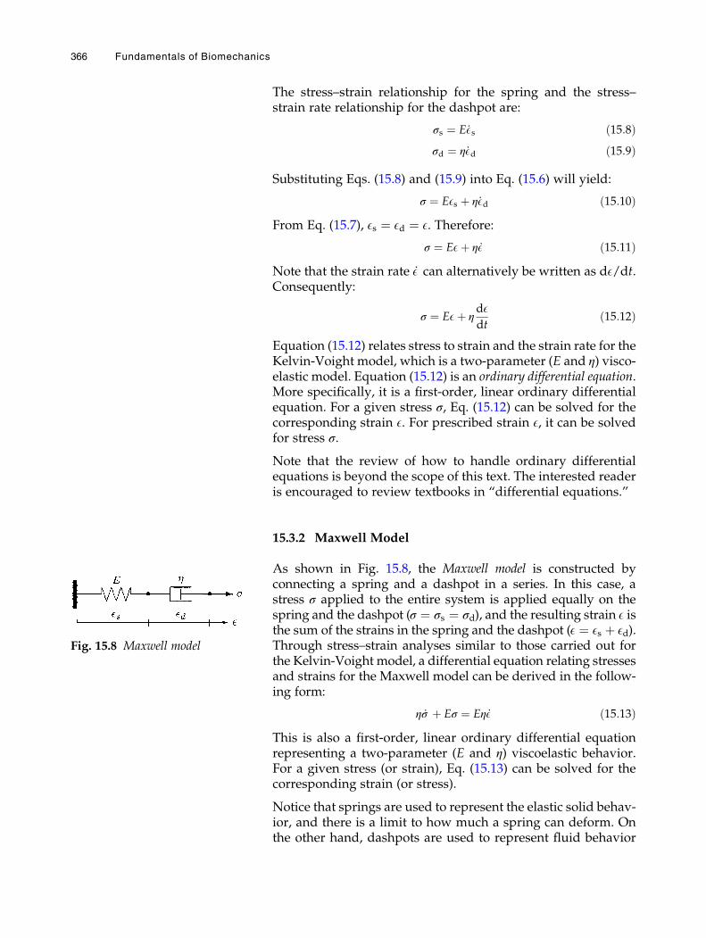
The stress–strain relationship for the spring and the stress–strain rate relationship for the dashpot are:
σs ¼ E _Es ð15:8Þσd ¼ η _Ed ð15:9Þ
Substituting Eqs. (15.8) and (15.9) into Eq. (15.6) will yield:
σ ¼ EEs þ η _Ed ð15:10ÞFrom Eq. (15.7), Es ¼ Ed ¼ E. Therefore:
σ ¼ EEþ η _E ð15:11ÞNote that the strain rate _E can alternatively be written as dE/dt.Consequently:
σ ¼ EEþ ηdEdt
ð15:12Þ
Equation (15.12) relates stress to strain and the strain rate for theKelvin-Voight model, which is a two-parameter (E and η) visco-elastic model. Equation (15.12) is an ordinary differential equation.More specifically, it is a first-order, linear ordinary differentialequation. For a given stress σ, Eq. (15.12) can be solved for thecorresponding strain E. For prescribed strain E, it can be solvedfor stress σ.
Note that the review of how to handle ordinary differentialequations is beyond the scope of this text. The interested readeris encouraged to review textbooks in “differential equations.”
15.3.2 Maxwell Model
As shown in Fig. 15.8, the Maxwell model is constructed byconnecting a spring and a dashpot in a series. In this case, astress σ applied to the entire system is applied equally on thespring and the dashpot (σ ¼ σs ¼ σd), and the resulting strain E isthe sum of the strains in the spring and the dashpot (E ¼ Es þ Ed).Through stress–strain analyses similar to those carried out forthe Kelvin-Voight model, a differential equation relating stressesand strains for the Maxwell model can be derived in the follow-ing form:
η _σ þ Eσ ¼ Eη _E ð15:13ÞThis is also a first-order, linear ordinary differential equationrepresenting a two-parameter (E and η) viscoelastic behavior.For a given stress (or strain), Eq. (15.13) can be solved for thecorresponding strain (or stress).
Notice that springs are used to represent the elastic solid behav-ior, and there is a limit to how much a spring can deform. Onthe other hand, dashpots are used to represent fluid behavior
Fig. 15.8 Maxwell model
366 Fundamentals of Biomechanics
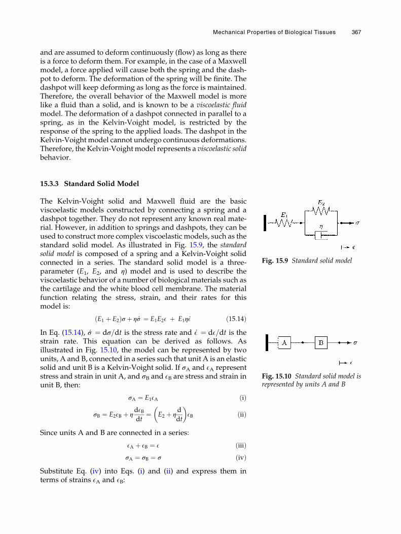
and are assumed to deform continuously (flow) as long as thereis a force to deform them. For example, in the case of a Maxwellmodel, a force applied will cause both the spring and the dash-pot to deform. The deformation of the spring will be finite. Thedashpot will keep deforming as long as the force is maintained.Therefore, the overall behavior of the Maxwell model is morelike a fluid than a solid, and is known to be a viscoelastic fluidmodel. The deformation of a dashpot connected in parallel to aspring, as in the Kelvin-Voight model, is restricted by theresponse of the spring to the applied loads. The dashpot in theKelvin-Voight model cannot undergo continuous deformations.Therefore, the Kelvin-Voightmodel represents a viscoelastic solidbehavior.
15.3.3 Standard Solid Model
The Kelvin-Voight solid and Maxwell fluid are the basicviscoelastic models constructed by connecting a spring and adashpot together. They do not represent any known real mate-rial. However, in addition to springs and dashpots, they can beused to construct more complex viscoelastic models, such as thestandard solid model. As illustrated in Fig. 15.9, the standardsolid model is composed of a spring and a Kelvin-Voight solidconnected in a series. The standard solid model is a three-parameter (E1, E2, and η) model and is used to describe theviscoelastic behavior of a number of biological materials such asthe cartilage and the white blood cell membrane. The materialfunction relating the stress, strain, and their rates for thismodel is:
E1 þ E2ð Þσ þ η _σ ¼ E1E2E þ E1η _E ð15:14ÞIn Eq. (15.14), _σ ¼ dσ=dt is the stress rate and _E ¼ dE=dt is thestrain rate. This equation can be derived as follows. Asillustrated in Fig. 15.10, the model can be represented by twounits, A and B, connected in a series such that unit A is an elasticsolid and unit B is a Kelvin-Voight solid. If σA and EA representstress and strain in unit A, and σB and EB are stress and strain inunit B, then:
σA ¼ E1EA ðiÞ
σB ¼ E2EB þ ηdEBdt
¼ E2 þ ηd
dt
� �EB ðiiÞ
Since units A and B are connected in a series:
EA þ EB ¼ E ðiiiÞσA ¼ σB ¼ σ ðivÞ
Substitute Eq. (iv) into Eqs. (i) and (ii) and express them interms of strains EA and EB:
Fig. 15.9 Standard solid model
Fig. 15.10 Standard solid model isrepresented by units A and B
Mechanical Properties of Biological Tissues 367
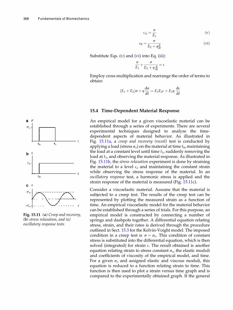
EA ¼ σ
E1ðvÞ
EB ¼ σ
E2 þ ηddt
ðviÞ
Substitute Eqs. (v) and (vi) into Eq. (iii):
σ
E1þ σ
E2 þ η ddt
¼ E
Employ cross multiplication and rearrange the order of terms toobtain:
E1 þ E2ð Þσ þ ηdσ
dt¼ E1E2Eþ E1η
dEdt
15.4 Time-Dependent Material Response
An empirical model for a given viscoelastic material can beestablished through a series of experiments. There are severalexperimental techniques designed to analyze the time-dependent aspects of material behavior. As illustrated inFig. 15.11a, a creep and recovery (recoil) test is conducted byapplying a load (stress σo) on thematerial at time t0, maintainingthe load at a constant level until time t1, suddenly removing theload at t1, and observing the material response. As illustrated inFig. 15.11b, the stress relaxation experiment is done by strainingthe material to a level Eo and maintaining the constant strainwhile observing the stress response of the material. In anoscillatory response test, a harmonic stress is applied and thestrain response of the material is measured (Fig. 15.11c).
Consider a viscoelastic material. Assume that the material issubjected to a creep test. The results of the creep test can berepresented by plotting the measured strain as a function oftime. An empirical viscoelastic model for the material behaviorcan be established through a series of trials. For this purpose, anempirical model is constructed by connecting a number ofsprings and dashpots together. A differential equation relatingstress, strain, and their rates is derived through the procedureoutlined in Sect. 15.3 for the Kelvin-Voight model. The imposedcondition in a creep test is σ ¼ σo. This condition of constantstress is substituted into the differential equation, which is thensolved (integrated) for strain E. The result obtained is anotherequation relating strain to stress constant σo, the elastic moduliand coefficients of viscosity of the empirical model, and time.For a given σo and assigned elastic and viscous moduli, thisequation is reduced to a function relating strain to time. Thisfunction is then used to plot a strain versus time graph and iscompared to the experimentally obtained graph. If the general
Fig. 15.11 (a) Creep and recovery,(b) stress relaxation, and (c)oscillatory response tests
368 Fundamentals of Biomechanics
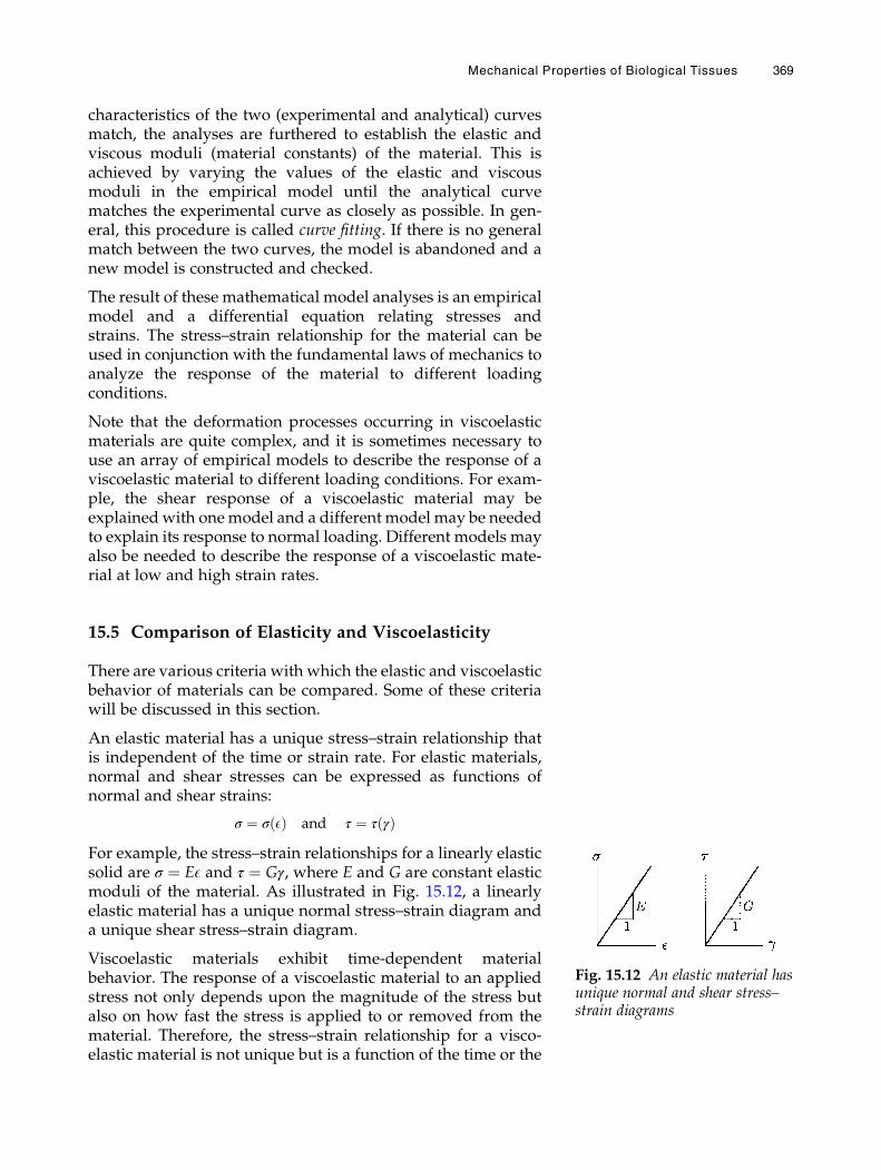
characteristics of the two (experimental and analytical) curvesmatch, the analyses are furthered to establish the elastic andviscous moduli (material constants) of the material. This isachieved by varying the values of the elastic and viscousmoduli in the empirical model until the analytical curvematches the experimental curve as closely as possible. In gen-eral, this procedure is called curve fitting. If there is no generalmatch between the two curves, the model is abandoned and anew model is constructed and checked.
The result of these mathematical model analyses is an empiricalmodel and a differential equation relating stresses andstrains. The stress–strain relationship for the material can beused in conjunction with the fundamental laws of mechanics toanalyze the response of the material to different loadingconditions.
Note that the deformation processes occurring in viscoelasticmaterials are quite complex, and it is sometimes necessary touse an array of empirical models to describe the response of aviscoelastic material to different loading conditions. For exam-ple, the shear response of a viscoelastic material may beexplained with onemodel and a different model may be neededto explain its response to normal loading. Different models mayalso be needed to describe the response of a viscoelastic mate-rial at low and high strain rates.
15.5 Comparison of Elasticity and Viscoelasticity
There are various criteria with which the elastic and viscoelasticbehavior of materials can be compared. Some of these criteriawill be discussed in this section.
An elastic material has a unique stress–strain relationship thatis independent of the time or strain rate. For elastic materials,normal and shear stresses can be expressed as functions ofnormal and shear strains:
σ ¼ σ Eð Þ and τ ¼ τ γð ÞFor example, the stress–strain relationships for a linearly elasticsolid are σ ¼ EE and τ ¼ Gγ, where E and G are constant elasticmoduli of the material. As illustrated in Fig. 15.12, a linearlyelastic material has a unique normal stress–strain diagram anda unique shear stress–strain diagram.
Viscoelastic materials exhibit time-dependent materialbehavior. The response of a viscoelastic material to an appliedstress not only depends upon the magnitude of the stress butalso on how fast the stress is applied to or removed from thematerial. Therefore, the stress–strain relationship for a visco-elastic material is not unique but is a function of the time or the
Fig. 15.12 An elastic material hasunique normal and shear stress–strain diagrams
Mechanical Properties of Biological Tissues 369
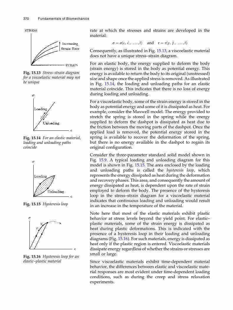
rate at which the stresses and strains are developed in thematerial:
σ ¼ σ E, _E , . . . , tð Þ and τ ¼ τ γ, _γ , . . . , tð ÞConsequently, as illustrated in Fig. 15.13, a viscoelastic materialdoes not have a unique stress–strain diagram.
For an elastic body, the energy supplied to deform the body(strain energy) is stored in the body as potential energy. Thisenergy is available to return the body to its original (unstressed)size and shape once the applied stress is removed. As illustratedin Fig. 15.14, the loading and unloading paths for an elasticmaterial coincide. This indicates that there is no loss of energyduring loading and unloading.
For a viscoelastic body, some of the strain energy is stored in thebody as potential energy and some of it is dissipated as heat. Forexample, consider the Maxwell model. The energy provided tostretch the spring is stored in the spring while the energysupplied to deform the dashpot is dissipated as heat due tothe friction between the moving parts of the dashpot. Once theapplied load is removed, the potential energy stored in thespring is available to recover the deformation of the spring,but there is no energy available in the dashpot to regain itsoriginal configuration.
Consider the three-parameter standard solid model shown inFig. 15.9. A typical loading and unloading diagram for thismodel is shown in Fig. 15.15. The area enclosed by the loadingand unloading paths is called the hysteresis loop, whichrepresents the energy dissipated as heat during the deformationand recovery phases. This area, and consequently the amount ofenergy dissipated as heat, is dependent upon the rate of strainemployed to deform the body. The presence of the hysteresisloop in the stress–strain diagram for a viscoelastic materialindicates that continuous loading and unloading would resultin an increase in the temperature of the material.
Note here that most of the elastic materials exhibit plasticbehavior at stress levels beyond the yield point. For elastic–plastic materials, some of the strain energy is dissipated asheat during plastic deformations. This is indicated with thepresence of a hysteresis loop in their loading and unloadingdiagrams (Fig. 15.16). For suchmaterials, energy is dissipated asheat only if the plastic region is entered. Viscoelastic materialsdissipate energy regardless of whether the strains or stresses aresmall or large.
Since viscoelastic materials exhibit time-dependent materialbehavior, the differences between elastic and viscoelastic mate-rial responses are most evident under time-dependent loadingconditions, such as during the creep and stress relaxationexperiments.
Fig. 15.16 Hysteresis loop for anelastic–plastic material
Fig. 15.13 Stress–strain diagramfor a viscoelastic material may notbe unique
Fig. 15.14 For an elastic material,loading and unloading pathscoincide
Fig. 15.15 Hysteresis loop
370 Fundamentals of Biomechanics
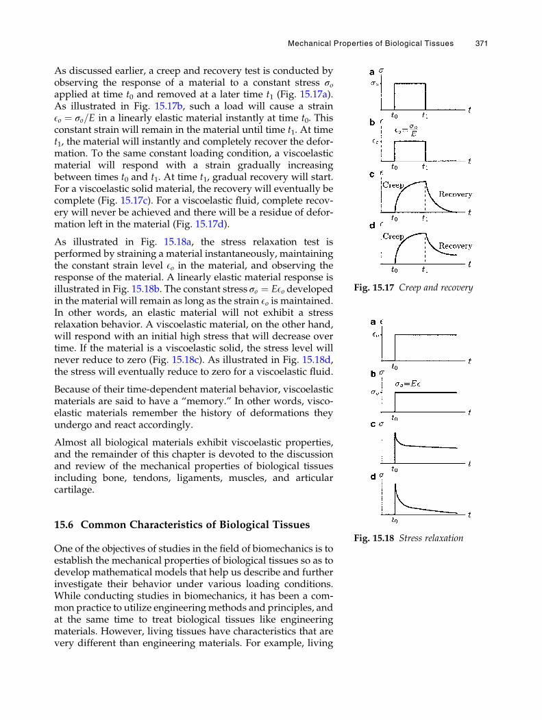
As discussed earlier, a creep and recovery test is conducted byobserving the response of a material to a constant stress σoapplied at time t0 and removed at a later time t1 (Fig. 15.17a).As illustrated in Fig. 15.17b, such a load will cause a strainEo ¼ σo=E in a linearly elastic material instantly at time t0. Thisconstant strain will remain in the material until time t1. At timet1, the material will instantly and completely recover the defor-mation. To the same constant loading condition, a viscoelasticmaterial will respond with a strain gradually increasingbetween times t0 and t1. At time t1, gradual recovery will start.For a viscoelastic solid material, the recovery will eventually becomplete (Fig. 15.17c). For a viscoelastic fluid, complete recov-ery will never be achieved and there will be a residue of defor-mation left in the material (Fig. 15.17d).
As illustrated in Fig. 15.18a, the stress relaxation test isperformed by straining a material instantaneously, maintainingthe constant strain level Eo in the material, and observing theresponse of the material. A linearly elastic material response isillustrated in Fig. 15.18b. The constant stress σo ¼ EEo developedin the material will remain as long as the strain Eo is maintained.In other words, an elastic material will not exhibit a stressrelaxation behavior. A viscoelastic material, on the other hand,will respond with an initial high stress that will decrease overtime. If the material is a viscoelastic solid, the stress level willnever reduce to zero (Fig. 15.18c). As illustrated in Fig. 15.18d,the stress will eventually reduce to zero for a viscoelastic fluid.
Because of their time-dependent material behavior, viscoelasticmaterials are said to have a “memory.” In other words, visco-elastic materials remember the history of deformations theyundergo and react accordingly.
Almost all biological materials exhibit viscoelastic properties,and the remainder of this chapter is devoted to the discussionand review of the mechanical properties of biological tissuesincluding bone, tendons, ligaments, muscles, and articularcartilage.
15.6 Common Characteristics of Biological Tissues
One of the objectives of studies in the field of biomechanics is toestablish the mechanical properties of biological tissues so as todevelop mathematical models that help us describe and furtherinvestigate their behavior under various loading conditions.While conducting studies in biomechanics, it has been a com-mon practice to utilize engineeringmethods and principles, andat the same time to treat biological tissues like engineeringmaterials. However, living tissues have characteristics that arevery different than engineering materials. For example, living
Fig. 15.17 Creep and recovery
Fig. 15.18 Stress relaxation
Mechanical Properties of Biological Tissues 371
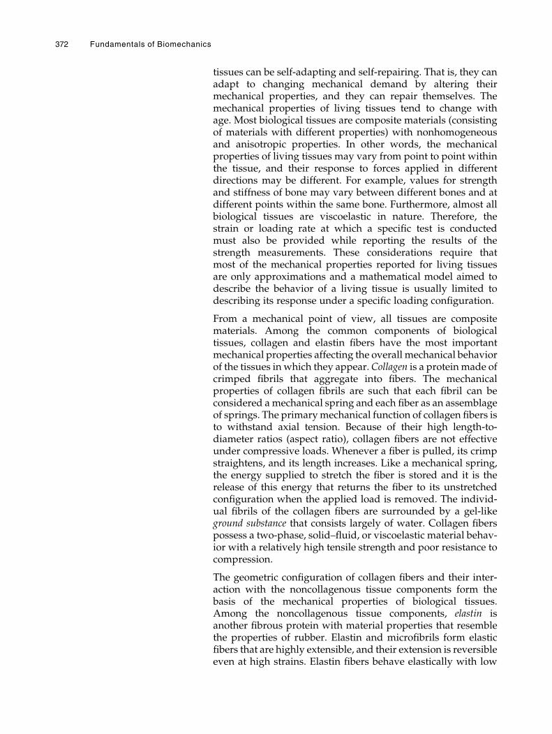
tissues can be self-adapting and self-repairing. That is, they canadapt to changing mechanical demand by altering theirmechanical properties, and they can repair themselves. Themechanical properties of living tissues tend to change withage. Most biological tissues are composite materials (consistingof materials with different properties) with nonhomogeneousand anisotropic properties. In other words, the mechanicalproperties of living tissues may vary from point to point withinthe tissue, and their response to forces applied in differentdirections may be different. For example, values for strengthand stiffness of bone may vary between different bones and atdifferent points within the same bone. Furthermore, almost allbiological tissues are viscoelastic in nature. Therefore, thestrain or loading rate at which a specific test is conductedmust also be provided while reporting the results of thestrength measurements. These considerations require thatmost of the mechanical properties reported for living tissuesare only approximations and a mathematical model aimed todescribe the behavior of a living tissue is usually limited todescribing its response under a specific loading configuration.
From a mechanical point of view, all tissues are compositematerials. Among the common components of biologicaltissues, collagen and elastin fibers have the most importantmechanical properties affecting the overall mechanical behaviorof the tissues in which they appear. Collagen is a protein made ofcrimped fibrils that aggregate into fibers. The mechanicalproperties of collagen fibrils are such that each fibril can beconsidered amechanical spring and each fiber as an assemblageof springs. The primarymechanical function of collagen fibers isto withstand axial tension. Because of their high length-to-diameter ratios (aspect ratio), collagen fibers are not effectiveunder compressive loads. Whenever a fiber is pulled, its crimpstraightens, and its length increases. Like a mechanical spring,the energy supplied to stretch the fiber is stored and it is therelease of this energy that returns the fiber to its unstretchedconfiguration when the applied load is removed. The individ-ual fibrils of the collagen fibers are surrounded by a gel-likeground substance that consists largely of water. Collagen fiberspossess a two-phase, solid–fluid, or viscoelastic material behav-ior with a relatively high tensile strength and poor resistance tocompression.
The geometric configuration of collagen fibers and their inter-action with the noncollagenous tissue components form thebasis of the mechanical properties of biological tissues.Among the noncollagenous tissue components, elastin isanother fibrous protein with material properties that resemblethe properties of rubber. Elastin and microfibrils form elasticfibers that are highly extensible, and their extension is reversibleeven at high strains. Elastin fibers behave elastically with low
372 Fundamentals of Biomechanics
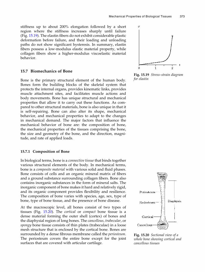
stiffness up to about 200% elongation followed by a shortregion where the stiffness increases sharply until failure(Fig. 15.19). The elastin fibers do not exhibit considerable plasticdeformation before failure, and their loading and unloadingpaths do not show significant hysteresis. In summary, elastinfibers possess a low-modulus elastic material property, whilecollagen fibers show a higher-modulus viscoelastic materialbehavior.
15.7 Biomechanics of Bone
Bone is the primary structural element of the human body.Bones form the building blocks of the skeletal system thatprotects the internal organs, provides kinematic links, providesmuscle attachment sites, and facilitates muscle actions andbody movements. Bone has unique structural and mechanicalproperties that allow it to carry out these functions. As com-pared to other structural materials, bone is also unique in that itis self-repairing. Bone can also alter its shape, mechanicalbehavior, and mechanical properties to adapt to the changesin mechanical demand. The major factors that influence themechanical behavior of bone are: the composition of bone,the mechanical properties of the tissues comprising the bone,the size and geometry of the bone, and the direction, magni-tude, and rate of applied loads.
15.7.1 Composition of Bone
In biological terms, bone is a connective tissue that binds togethervarious structural elements of the body. In mechanical terms,bone is a composite material with various solid and fluid phases.Bone consists of cells and an organic mineral matrix of fibersand a ground substance surrounding collagen fibers. Bone alsocontains inorganic substances in the form of mineral salts. Theinorganic component of bone makes it hard and relatively rigid,and its organic component provides flexibility and resilience.The composition of bone varies with species, age, sex, type ofbone, type of bone tissue, and the presence of bone disease.
At the macroscopic level, all bones consist of two types oftissues (Fig. 15.20). The cortical or compact bone tissue is adense material forming the outer shell (cortex) of bones andthe diaphysial region of long bones. The cancellous, trabecular, orspongy bone tissue consists of thin plates (trabeculae) in a loosemesh structure that is enclosed by the cortical bone. Bones aresurrounded by a dense fibrous membrane called the periosteum.The periosteum covers the entire bone except for the jointsurfaces that are covered with articular cartilage.
Fig. 15.19 Stress–strain diagramfor elastin
Fig. 15.20 Sectional view of awhole bone showing cortical andcancellous tissues
Mechanical Properties of Biological Tissues 373
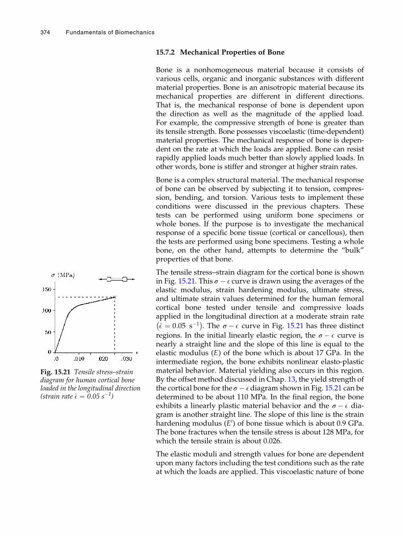
15.7.2 Mechanical Properties of Bone
Bone is a nonhomogeneous material because it consists ofvarious cells, organic and inorganic substances with differentmaterial properties. Bone is an anisotropic material because itsmechanical properties are different in different directions.That is, the mechanical response of bone is dependent uponthe direction as well as the magnitude of the applied load.For example, the compressive strength of bone is greater thanits tensile strength. Bone possesses viscoelastic (time-dependent)material properties. The mechanical response of bone is depen-dent on the rate at which the loads are applied. Bone can resistrapidly applied loads much better than slowly applied loads. Inother words, bone is stiffer and stronger at higher strain rates.
Bone is a complex structural material. The mechanical responseof bone can be observed by subjecting it to tension, compres-sion, bending, and torsion. Various tests to implement theseconditions were discussed in the previous chapters. Thesetests can be performed using uniform bone specimens orwhole bones. If the purpose is to investigate the mechanicalresponse of a specific bone tissue (cortical or cancellous), thenthe tests are performed using bone specimens. Testing a wholebone, on the other hand, attempts to determine the “bulk”properties of that bone.
The tensile stress–strain diagram for the cortical bone is shownin Fig. 15.21. This σ � E curve is drawn using the averages of theelastic modulus, strain hardening modulus, ultimate stress,and ultimate strain values determined for the human femoralcortical bone tested under tensile and compressive loadsapplied in the longitudinal direction at a moderate strain rate_E ¼ 0:05 s�1
� �. The σ � E curve in Fig. 15.21 has three distinct
regions. In the initial linearly elastic region, the σ � E curve isnearly a straight line and the slope of this line is equal to theelastic modulus (E) of the bone which is about 17 GPa. In theintermediate region, the bone exhibits nonlinear elasto-plasticmaterial behavior. Material yielding also occurs in this region.By the offset method discussed in Chap. 13, the yield strength ofthe cortical bone for theσ � Ediagram shown in Fig. 15.21 can bedetermined to be about 110 MPa. In the final region, the boneexhibits a linearly plastic material behavior and the σ � E dia-gram is another straight line. The slope of this line is the strainhardening modulus (E0) of bone tissue which is about 0.9 GPa.The bone fractures when the tensile stress is about 128 MPa, forwhich the tensile strain is about 0.026.
The elastic moduli and strength values for bone are dependentupon many factors including the test conditions such as the rateat which the loads are applied. This viscoelastic nature of bone
Fig. 15.21 Tensile stress–straindiagram for human cortical boneloaded in the longitudinal direction(strain rate _E ¼ 0.05 s�1)
374 Fundamentals of Biomechanics
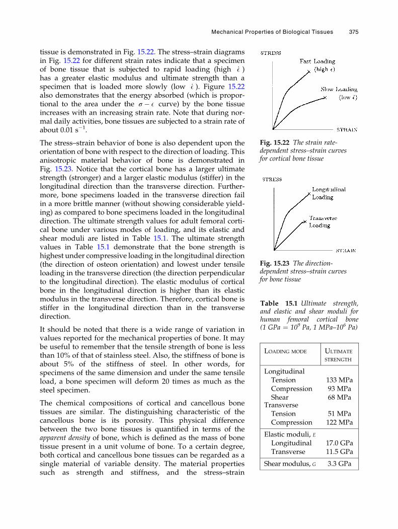
tissue is demonstrated in Fig. 15.22. The stress–strain diagramsin Fig. 15.22 for different strain rates indicate that a specimenof bone tissue that is subjected to rapid loading (high _E )has a greater elastic modulus and ultimate strength than aspecimen that is loaded more slowly (low _E ). Figure 15.22also demonstrates that the energy absorbed (which is propor-tional to the area under the σ � E curve) by the bone tissueincreases with an increasing strain rate. Note that during nor-mal daily activities, bone tissues are subjected to a strain rate ofabout 0.01 s�1.
The stress–strain behavior of bone is also dependent upon theorientation of bone with respect to the direction of loading. Thisanisotropic material behavior of bone is demonstrated inFig. 15.23. Notice that the cortical bone has a larger ultimatestrength (stronger) and a larger elastic modulus (stiffer) in thelongitudinal direction than the transverse direction. Further-more, bone specimens loaded in the transverse direction failin a more brittle manner (without showing considerable yield-ing) as compared to bone specimens loaded in the longitudinaldirection. The ultimate strength values for adult femoral corti-cal bone under various modes of loading, and its elastic andshear moduli are listed in Table 15.1. The ultimate strengthvalues in Table 15.1 demonstrate that the bone strength ishighest under compressive loading in the longitudinal direction(the direction of osteon orientation) and lowest under tensileloading in the transverse direction (the direction perpendicularto the longitudinal direction). The elastic modulus of corticalbone in the longitudinal direction is higher than its elasticmodulus in the transverse direction. Therefore, cortical bone isstiffer in the longitudinal direction than in the transversedirection.
It should be noted that there is a wide range of variation invalues reported for the mechanical properties of bone. It maybe useful to remember that the tensile strength of bone is lessthan 10% of that of stainless steel. Also, the stiffness of bone isabout 5% of the stiffness of steel. In other words, forspecimens of the same dimension and under the same tensileload, a bone specimen will deform 20 times as much as thesteel specimen.
The chemical compositions of cortical and cancellous bonetissues are similar. The distinguishing characteristic of thecancellous bone is its porosity. This physical differencebetween the two bone tissues is quantified in terms of theapparent density of bone, which is defined as the mass of bonetissue present in a unit volume of bone. To a certain degree,both cortical and cancellous bone tissues can be regarded as asingle material of variable density. The material propertiessuch as strength and stiffness, and the stress–strain
Fig. 15.22 The strain rate-dependent stress–strain curvesfor cortical bone tissue
Fig. 15.23 The direction-dependent stress–strain curvesfor bone tissue
Table 15.1 Ultimate strength,and elastic and shear moduli forhuman femoral cortical bone(1 GPa ¼ 109 Pa, 1 MPa–106 Pa)
LOADING MODE ULTIMATE
STRENGTH
LongitudinalTension 133 MPaCompression 93 MPaShear 68 MPa
TransverseTension 51 MPaCompression 122 MPa
Elastic moduli, ELongitudinal 17.0 GPaTransverse 11.5 GPa
Shear modulus, G 3.3 GPa
Mechanical Properties of Biological Tissues 375
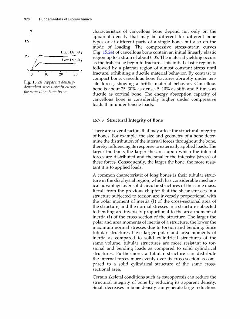
characteristics of cancellous bone depend not only on theapparent density that may be different for different bonetypes or at different parts of a single bone, but also on themode of loading. The compressive stress–strain curves(Fig. 15.24) of cancellous bone contain an initial linearly elasticregion up to a strain of about 0.05. The material yielding occursas the trabeculae begin to fracture. This initial elastic region isfollowed by a plateau region of almost constant stress untilfracture, exhibiting a ductile material behavior. By contrast tocompact bone, cancellous bone fractures abruptly under ten-sile forces, showing a brittle material behavior. Cancellousbone is about 25–30% as dense, 5–10% as stiff, and 5 times asductile as cortical bone. The energy absorption capacity ofcancellous bone is considerably higher under compressiveloads than under tensile loads.
15.7.3 Structural Integrity of Bone
There are several factors that may affect the structural integrityof bones. For example, the size and geometry of a bone deter-mine the distribution of the internal forces throughout the bone,thereby influencing its response to externally applied loads. Thelarger the bone, the larger the area upon which the internalforces are distributed and the smaller the intensity (stress) ofthese forces. Consequently, the larger the bone, the more resis-tant it is to applied loads.
A common characteristic of long bones is their tubular struc-ture in the diaphysial region, which has considerable mechan-ical advantage over solid circular structures of the same mass.Recall from the previous chapter that the shear stresses in astructure subjected to torsion are inversely proportional withthe polar moment of inertia (J ) of the cross-sectional area ofthe structure, and the normal stresses in a structure subjectedto bending are inversely proportional to the area moment ofinertia (I ) of the cross-section of the structure. The larger thepolar and area moments of inertia of a structure, the lower themaximum normal stresses due to torsion and bending. Sincetubular structures have larger polar and area moments ofinertia as compared to solid cylindrical structures of thesame volume, tubular structures are more resistant to tor-sional and bending loads as compared to solid cylindricalstructures. Furthermore, a tubular structure can distributethe internal forces more evenly over its cross-section as com-pared to a solid cylindrical structure of the same cross-sectional area.
Certain skeletal conditions such as osteoporosis can reduce thestructural integrity of bone by reducing its apparent density.Small decreases in bone density can generate large reductions
Fig. 15.24 Apparent density-dependent stress–strain curvesfor cancellous bone tissue
376 Fundamentals of Biomechanics
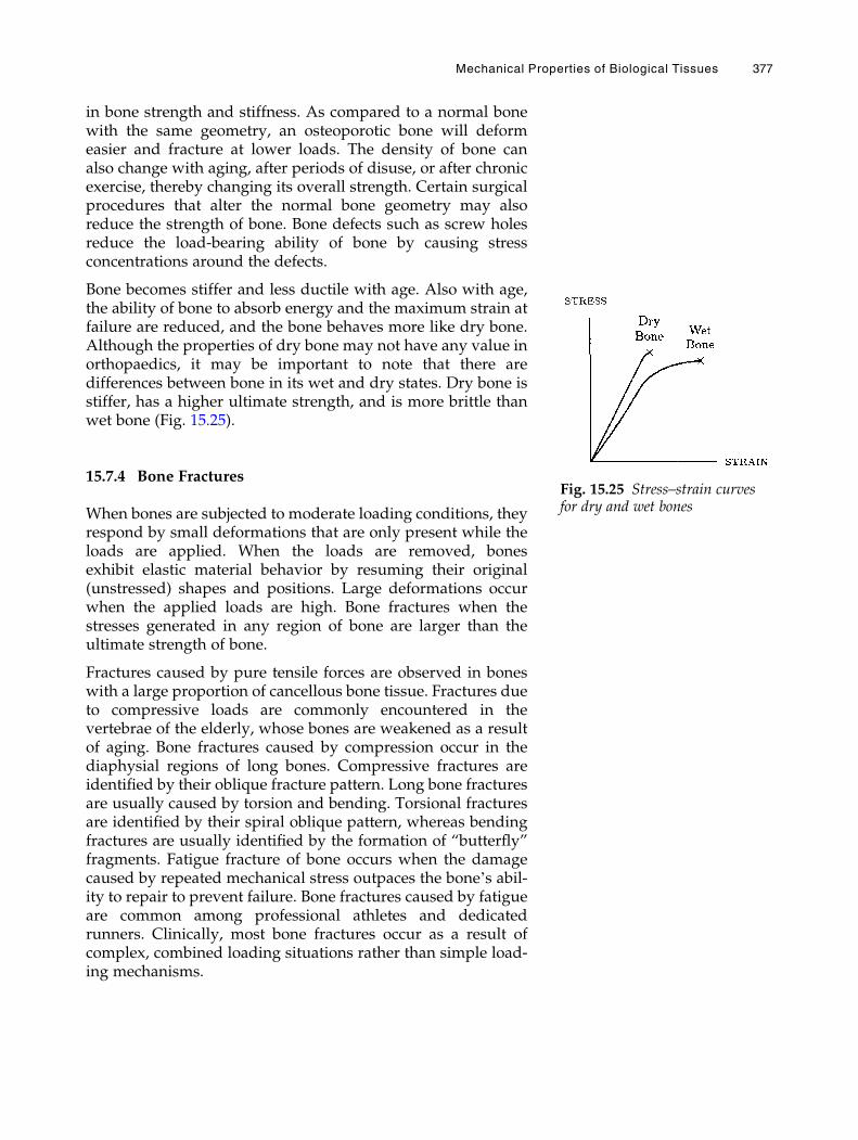
in bone strength and stiffness. As compared to a normal bonewith the same geometry, an osteoporotic bone will deformeasier and fracture at lower loads. The density of bone canalso change with aging, after periods of disuse, or after chronicexercise, thereby changing its overall strength. Certain surgicalprocedures that alter the normal bone geometry may alsoreduce the strength of bone. Bone defects such as screw holesreduce the load-bearing ability of bone by causing stressconcentrations around the defects.
Bone becomes stiffer and less ductile with age. Also with age,the ability of bone to absorb energy and the maximum strain atfailure are reduced, and the bone behaves more like dry bone.Although the properties of dry bone may not have any value inorthopaedics, it may be important to note that there aredifferences between bone in its wet and dry states. Dry bone isstiffer, has a higher ultimate strength, and is more brittle thanwet bone (Fig. 15.25).
15.7.4 Bone Fractures
When bones are subjected to moderate loading conditions, theyrespond by small deformations that are only present while theloads are applied. When the loads are removed, bonesexhibit elastic material behavior by resuming their original(unstressed) shapes and positions. Large deformations occurwhen the applied loads are high. Bone fractures when thestresses generated in any region of bone are larger than theultimate strength of bone.
Fractures caused by pure tensile forces are observed in boneswith a large proportion of cancellous bone tissue. Fractures dueto compressive loads are commonly encountered in thevertebrae of the elderly, whose bones are weakened as a resultof aging. Bone fractures caused by compression occur in thediaphysial regions of long bones. Compressive fractures areidentified by their oblique fracture pattern. Long bone fracturesare usually caused by torsion and bending. Torsional fracturesare identified by their spiral oblique pattern, whereas bendingfractures are usually identified by the formation of “butterfly”fragments. Fatigue fracture of bone occurs when the damagecaused by repeated mechanical stress outpaces the bone’s abil-ity to repair to prevent failure. Bone fractures caused by fatigueare common among professional athletes and dedicatedrunners. Clinically, most bone fractures occur as a result ofcomplex, combined loading situations rather than simple load-ing mechanisms.
Fig. 15.25 Stress–strain curvesfor dry and wet bones
Mechanical Properties of Biological Tissues 377
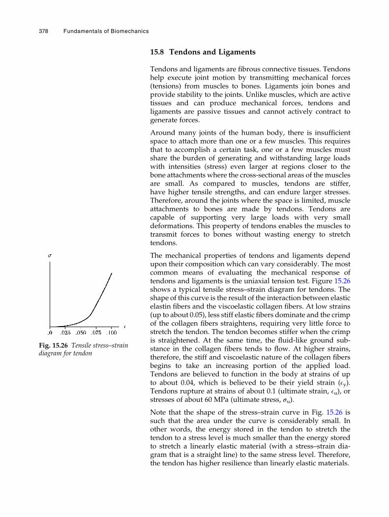
15.8 Tendons and Ligaments
Tendons and ligaments are fibrous connective tissues. Tendonshelp execute joint motion by transmitting mechanical forces(tensions) from muscles to bones. Ligaments join bones andprovide stability to the joints. Unlike muscles, which are activetissues and can produce mechanical forces, tendons andligaments are passive tissues and cannot actively contract togenerate forces.
Around many joints of the human body, there is insufficientspace to attach more than one or a few muscles. This requiresthat to accomplish a certain task, one or a few muscles mustshare the burden of generating and withstanding large loadswith intensities (stress) even larger at regions closer to thebone attachments where the cross-sectional areas of the musclesare small. As compared to muscles, tendons are stiffer,have higher tensile strengths, and can endure larger stresses.Therefore, around the joints where the space is limited, muscleattachments to bones are made by tendons. Tendons arecapable of supporting very large loads with very smalldeformations. This property of tendons enables the muscles totransmit forces to bones without wasting energy to stretchtendons.
The mechanical properties of tendons and ligaments dependupon their composition which can vary considerably. The mostcommon means of evaluating the mechanical response oftendons and ligaments is the uniaxial tension test. Figure 15.26shows a typical tensile stress–strain diagram for tendons. Theshape of this curve is the result of the interaction between elasticelastin fibers and the viscoelastic collagen fibers. At low strains(up to about 0.05), less stiff elastic fibers dominate and the crimpof the collagen fibers straightens, requiring very little force tostretch the tendon. The tendon becomes stiffer when the crimpis straightened. At the same time, the fluid-like ground sub-stance in the collagen fibers tends to flow. At higher strains,therefore, the stiff and viscoelastic nature of the collagen fibersbegins to take an increasing portion of the applied load.Tendons are believed to function in the body at strains of upto about 0.04, which is believed to be their yield strain (Ey).Tendons rupture at strains of about 0.1 (ultimate strain, Eu), orstresses of about 60 MPa (ultimate stress, σu).
Note that the shape of the stress–strain curve in Fig. 15.26 issuch that the area under the curve is considerably small. Inother words, the energy stored in the tendon to stretch thetendon to a stress level is much smaller than the energy storedto stretch a linearly elastic material (with a stress–strain dia-gram that is a straight line) to the same stress level. Therefore,the tendon has higher resilience than linearly elastic materials.
Fig. 15.26 Tensile stress–straindiagram for tendon
378 Fundamentals of Biomechanics
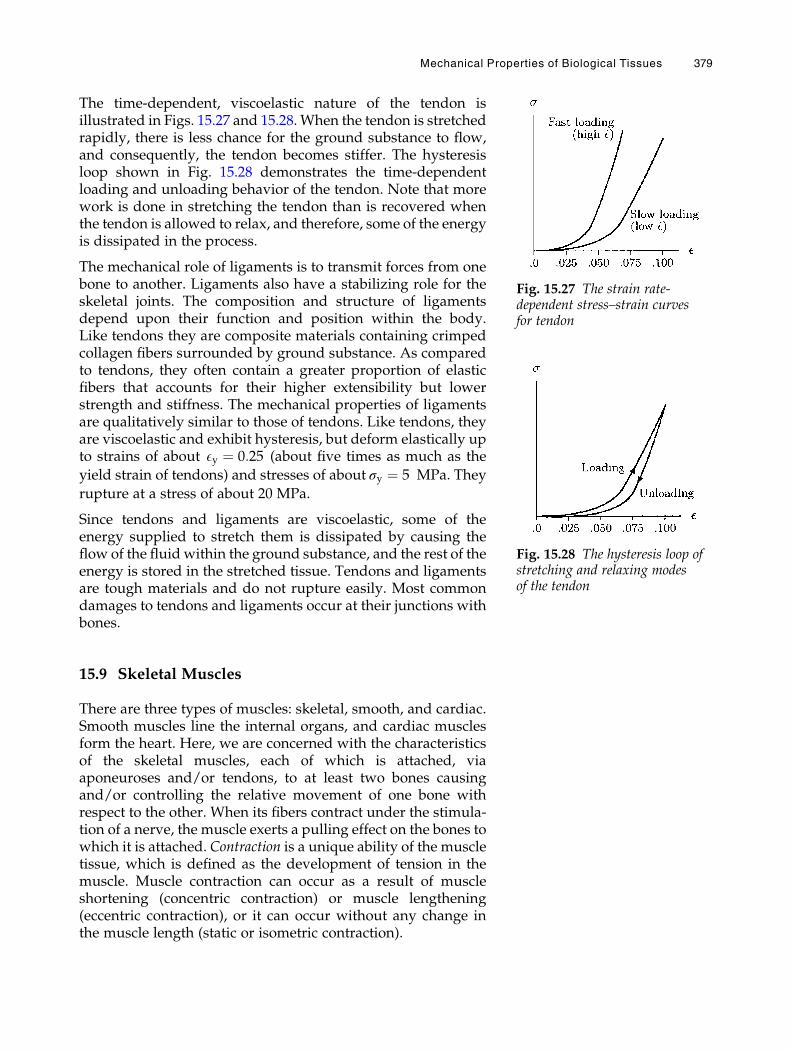
The time-dependent, viscoelastic nature of the tendon isillustrated in Figs. 15.27 and 15.28. When the tendon is stretchedrapidly, there is less chance for the ground substance to flow,and consequently, the tendon becomes stiffer. The hysteresisloop shown in Fig. 15.28 demonstrates the time-dependentloading and unloading behavior of the tendon. Note that morework is done in stretching the tendon than is recovered whenthe tendon is allowed to relax, and therefore, some of the energyis dissipated in the process.
The mechanical role of ligaments is to transmit forces from onebone to another. Ligaments also have a stabilizing role for theskeletal joints. The composition and structure of ligamentsdepend upon their function and position within the body.Like tendons they are composite materials containing crimpedcollagen fibers surrounded by ground substance. As comparedto tendons, they often contain a greater proportion of elasticfibers that accounts for their higher extensibility but lowerstrength and stiffness. The mechanical properties of ligamentsare qualitatively similar to those of tendons. Like tendons, theyare viscoelastic and exhibit hysteresis, but deform elastically upto strains of about Ey ¼ 0:25 (about five times as much as the
yield strain of tendons) and stresses of about σy ¼ 5 MPa. They
rupture at a stress of about 20 MPa.
Since tendons and ligaments are viscoelastic, some of theenergy supplied to stretch them is dissipated by causing theflow of the fluid within the ground substance, and the rest of theenergy is stored in the stretched tissue. Tendons and ligamentsare tough materials and do not rupture easily. Most commondamages to tendons and ligaments occur at their junctions withbones.
15.9 Skeletal Muscles
There are three types of muscles: skeletal, smooth, and cardiac.Smooth muscles line the internal organs, and cardiac musclesform the heart. Here, we are concerned with the characteristicsof the skeletal muscles, each of which is attached, viaaponeuroses and/or tendons, to at least two bones causingand/or controlling the relative movement of one bone withrespect to the other. When its fibers contract under the stimula-tion of a nerve, the muscle exerts a pulling effect on the bones towhich it is attached. Contraction is a unique ability of the muscletissue, which is defined as the development of tension in themuscle. Muscle contraction can occur as a result of muscleshortening (concentric contraction) or muscle lengthening(eccentric contraction), or it can occur without any change inthe muscle length (static or isometric contraction).
Fig. 15.27 The strain rate-dependent stress–strain curvesfor tendon
Fig. 15.28 The hysteresis loop ofstretching and relaxing modesof the tendon
Mechanical Properties of Biological Tissues 379
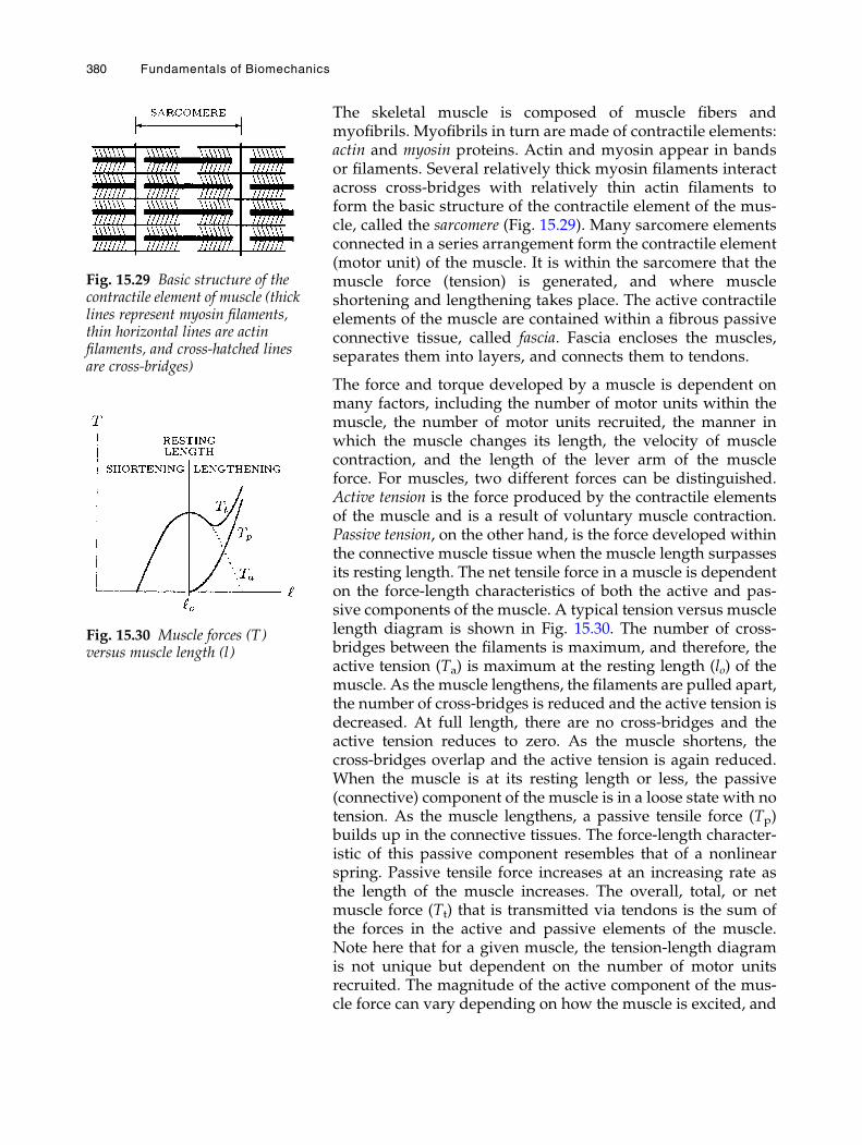
The skeletal muscle is composed of muscle fibers andmyofibrils. Myofibrils in turn are made of contractile elements:actin and myosin proteins. Actin and myosin appear in bandsor filaments. Several relatively thick myosin filaments interactacross cross-bridges with relatively thin actin filaments toform the basic structure of the contractile element of the mus-cle, called the sarcomere (Fig. 15.29). Many sarcomere elementsconnected in a series arrangement form the contractile element(motor unit) of the muscle. It is within the sarcomere that themuscle force (tension) is generated, and where muscleshortening and lengthening takes place. The active contractileelements of the muscle are contained within a fibrous passiveconnective tissue, called fascia. Fascia encloses the muscles,separates them into layers, and connects them to tendons.
The force and torque developed by a muscle is dependent onmany factors, including the number of motor units within themuscle, the number of motor units recruited, the manner inwhich the muscle changes its length, the velocity of musclecontraction, and the length of the lever arm of the muscleforce. For muscles, two different forces can be distinguished.Active tension is the force produced by the contractile elementsof the muscle and is a result of voluntary muscle contraction.Passive tension, on the other hand, is the force developed withinthe connective muscle tissue when the muscle length surpassesits resting length. The net tensile force in a muscle is dependenton the force-length characteristics of both the active and pas-sive components of the muscle. A typical tension versus musclelength diagram is shown in Fig. 15.30. The number of cross-bridges between the filaments is maximum, and therefore, theactive tension (Ta) is maximum at the resting length (lo) of themuscle. As the muscle lengthens, the filaments are pulled apart,the number of cross-bridges is reduced and the active tension isdecreased. At full length, there are no cross-bridges and theactive tension reduces to zero. As the muscle shortens, thecross-bridges overlap and the active tension is again reduced.When the muscle is at its resting length or less, the passive(connective) component of the muscle is in a loose state with notension. As the muscle lengthens, a passive tensile force (Tp)builds up in the connective tissues. The force-length character-istic of this passive component resembles that of a nonlinearspring. Passive tensile force increases at an increasing rate asthe length of the muscle increases. The overall, total, or netmuscle force (Tt) that is transmitted via tendons is the sum ofthe forces in the active and passive elements of the muscle.Note here that for a given muscle, the tension-length diagramis not unique but dependent on the number of motor unitsrecruited. The magnitude of the active component of the mus-cle force can vary depending on how the muscle is excited, and
Fig. 15.29 Basic structure of thecontractile element of muscle (thicklines represent myosin filaments,thin horizontal lines are actinfilaments, and cross-hatched linesare cross-bridges)
Fig. 15.30 Muscle forces (T)versus muscle length (l)
380 Fundamentals of Biomechanics
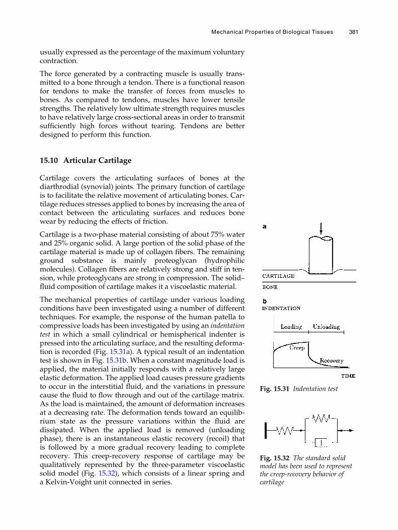
usually expressed as the percentage of the maximum voluntarycontraction.
The force generated by a contracting muscle is usually trans-mitted to a bone through a tendon. There is a functional reasonfor tendons to make the transfer of forces from muscles tobones. As compared to tendons, muscles have lower tensilestrengths. The relatively low ultimate strength requires musclesto have relatively large cross-sectional areas in order to transmitsufficiently high forces without tearing. Tendons are betterdesigned to perform this function.
15.10 Articular Cartilage
Cartilage covers the articulating surfaces of bones at thediarthrodial (synovial) joints. The primary function of cartilageis to facilitate the relative movement of articulating bones. Car-tilage reduces stresses applied to bones by increasing the area ofcontact between the articulating surfaces and reduces bonewear by reducing the effects of friction.
Cartilage is a two-phase material consisting of about 75% waterand 25% organic solid. A large portion of the solid phase of thecartilage material is made up of collagen fibers. The remainingground substance is mainly proteoglycan (hydrophilicmolecules). Collagen fibers are relatively strong and stiff in ten-sion, while proteoglycans are strong in compression. The solid–fluid composition of cartilage makes it a viscoelastic material.
The mechanical properties of cartilage under various loadingconditions have been investigated using a number of differenttechniques. For example, the response of the human patella tocompressive loads has been investigated by using an indentationtest in which a small cylindrical or hemispherical indenter ispressed into the articulating surface, and the resulting deforma-tion is recorded (Fig. 15.31a). A typical result of an indentationtest is shown in Fig. 15.31b. When a constant magnitude load isapplied, the material initially responds with a relatively largeelastic deformation. The applied load causes pressure gradientsto occur in the interstitial fluid, and the variations in pressurecause the fluid to flow through and out of the cartilage matrix.As the load is maintained, the amount of deformation increasesat a decreasing rate. The deformation tends toward an equilib-rium state as the pressure variations within the fluid aredissipated. When the applied load is removed (unloadingphase), there is an instantaneous elastic recovery (recoil) thatis followed by a more gradual recovery leading to completerecovery. This creep-recovery response of cartilage may bequalitatively represented by the three-parameter viscoelasticsolid model (Fig. 15.32), which consists of a linear spring anda Kelvin-Voight unit connected in series.
Fig. 15.31 Indentation test
Fig. 15.32 The standard solidmodel has been used to representthe creep-recovery behavior ofcartilage
Mechanical Properties of Biological Tissues 381
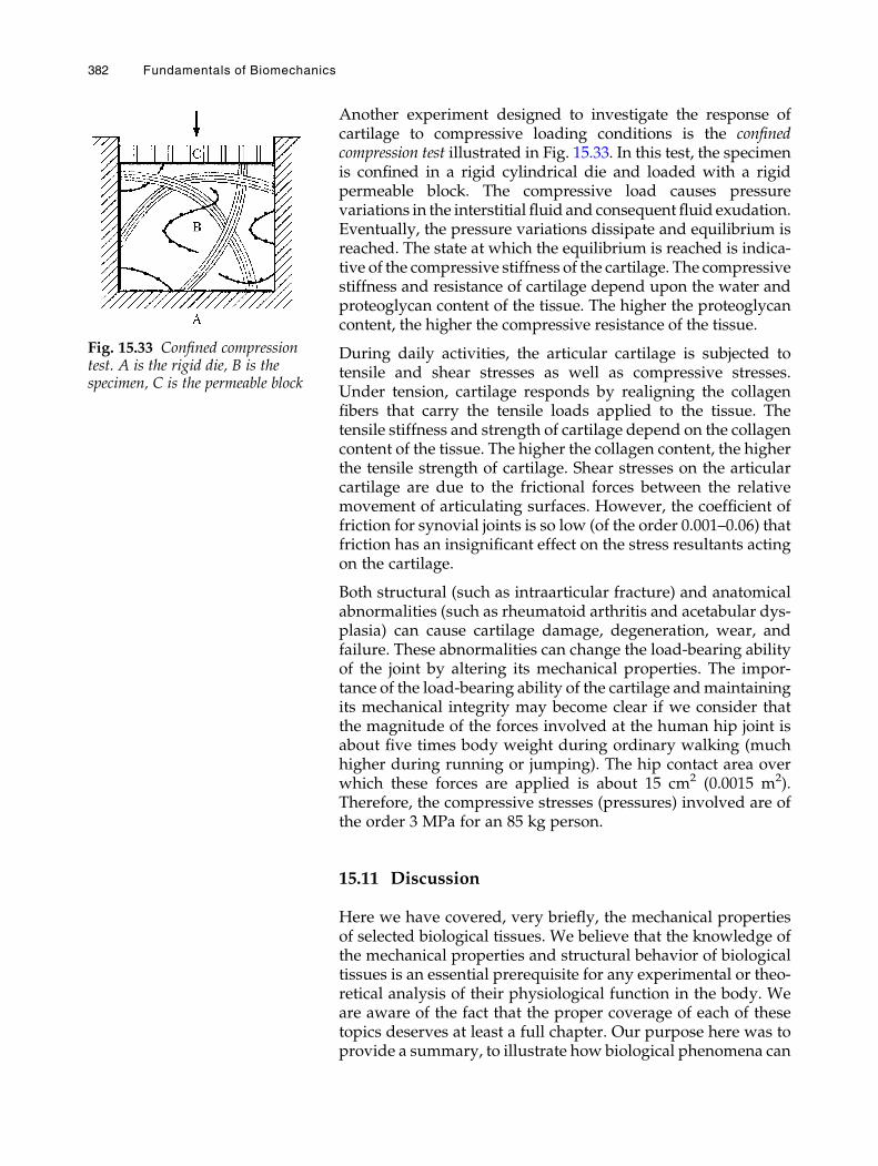
Another experiment designed to investigate the response ofcartilage to compressive loading conditions is the confinedcompression test illustrated in Fig. 15.33. In this test, the specimenis confined in a rigid cylindrical die and loaded with a rigidpermeable block. The compressive load causes pressurevariations in the interstitial fluid and consequent fluid exudation.Eventually, the pressure variations dissipate and equilibrium isreached. The state at which the equilibrium is reached is indica-tive of the compressive stiffness of the cartilage. The compressivestiffness and resistance of cartilage depend upon the water andproteoglycan content of the tissue. The higher the proteoglycancontent, the higher the compressive resistance of the tissue.
During daily activities, the articular cartilage is subjected totensile and shear stresses as well as compressive stresses.Under tension, cartilage responds by realigning the collagenfibers that carry the tensile loads applied to the tissue. Thetensile stiffness and strength of cartilage depend on the collagencontent of the tissue. The higher the collagen content, the higherthe tensile strength of cartilage. Shear stresses on the articularcartilage are due to the frictional forces between the relativemovement of articulating surfaces. However, the coefficient offriction for synovial joints is so low (of the order 0.001–0.06) thatfriction has an insignificant effect on the stress resultants actingon the cartilage.
Both structural (such as intraarticular fracture) and anatomicalabnormalities (such as rheumatoid arthritis and acetabular dys-plasia) can cause cartilage damage, degeneration, wear, andfailure. These abnormalities can change the load-bearing abilityof the joint by altering its mechanical properties. The impor-tance of the load-bearing ability of the cartilage andmaintainingits mechanical integrity may become clear if we consider thatthe magnitude of the forces involved at the human hip joint isabout five times body weight during ordinary walking (muchhigher during running or jumping). The hip contact area overwhich these forces are applied is about 15 cm2 (0.0015 m2).Therefore, the compressive stresses (pressures) involved are ofthe order 3 MPa for an 85 kg person.
15.11 Discussion
Here we have covered, very briefly, the mechanical propertiesof selected biological tissues. We believe that the knowledge ofthe mechanical properties and structural behavior of biologicaltissues is an essential prerequisite for any experimental or theo-retical analysis of their physiological function in the body. Weare aware of the fact that the proper coverage of each of thesetopics deserves at least a full chapter. Our purpose here was toprovide a summary, to illustrate how biological phenomena can
Fig. 15.33 Confined compressiontest. A is the rigid die, B is thespecimen, C is the permeable block
382 Fundamentals of Biomechanics
be described in terms of the mechanical concepts introducedearlier, and hope that the interested reader would refer to morecomplete sources of information to improve his or her knowl-edge of the subject matter.
15.12 Exercise Problems
Answers are provided at the end of the chapter.
Problem 15.1 Complete the following definitions with appro-priate expressions.
(a) Elastic materials show time-independent material behav-ior. Elastic materials deform ____ when they are subjectedto externally applied loads.
(b) Time dependent material behavior is known as ____ .(c) Elasticity is a solid material behavior, whereas ____ is a
fluid property and is a measure of resistance to flow.(d) For a viscoelastic material, stress is not only a function of
strain, but also a function of ____ .(e) ____ and ____ are basic mechanical elements that are used
to simulate elastic solid and viscous fluid behaviors,respectively.
(f) The ____ is a viscoelastic model consisting of a spring and adashpot connected in a parallel arrangement.
(g) The ____ is a viscoelastic model consisting of a spring and adashpot connected in a series arrangement.
(h) The ____ is a viscoelastic model consisting of a spring and aKelvin-Voight solid connected in a series.
(i) A ____ test is conducted by applying a load on the material,maintaining the load at a constant level for some time,suddenly removing the load, and observing the materialresponse.
(j) A ____ test is conducted by straining the material at a leveland maintaining the strain at a constant level while observ-ing the stress response of the material.
(k) In a ____ test, a harmonic stress is applied on the materialand the strain response of the material is observed.
(l) The area enclosed by the loading and unloading paths iscalled the ____, which represents the energy dissipatedas heat.
(m) Because of their time-dependent behavior, viscoelasticmaterials are said to have a ____ .
(n) Living tissues have characteristics that are very differentthan engineering materials. For example, they are ____ and____ .
(o) Among the common components of biological tissues, ____and ____ fibers have the most important mechanical
Mechanical Properties of Biological Tissues 383
properties affecting the overall mechanical behavior of thetissues in which they appear.
(p) ____ is a protein made of crimped fibrils that aggregate intofibers.
(q) ____ is a fibrous protein with material properties thatresemble the properties of rubber.
(r) In biological terms, bone is a ____ tissue that binds togethervarious structural elements of the body. In mechanicalterms, bone is a ____ material with various solid and fluidphases.
(s) The ____ bone tissue is a dense material forming the outershell (cortex) of bones and the diaphysial region of longbones.
(t) The ____ bone tissue consists of thin plates (trabeculae) in aloose mesh structure that is enclosed by the cortical bone.
(u) Bone is stiffer and stronger at ____ strain rates.(v) Cortical bone strength is highest under compressive load-
ing in the ____ direction (direction of osteon orientation)and lowest under tensile loading in the ____ direction(direction perpendicular to the longitudinal direction).
(w) The tensile strength of bone is less than ____ percent ofstainless steel, and the stiffness of bone is about ____ per-cent of the stiffness of steel.
(x) The chemical compositions of cortical and cancellous bonetissues are similar. The distinguishing characteristic of thecancellous bone is its ____ .
(y) ____ is a unique ability of the muscle tissue, which isdefined as the development of tension in the muscle.
(z) ____ tension is the force produced by the contractileelements of the muscle and is a result of voluntary musclecontraction, and tension is the force developed within theconnective muscle tissue when the muscle length surpassesits resting length.
Problem 15.2 Complete the following definitions with appro-priate expressions.
(a) For an elastic material, the stress–strain relationship is______________ of the time or strain rate.
(b) For a viscoelastic material, the stress–strain relationship__________ on the rate at which the stress and strain aredeveloped in the material.
(c) For an elastic body, the energy supplied to deform the bodyis stored in the body as ___________. This energy is avail-able to ____________ the body to its original size and shapeonce the applied stress is removed.
(d) There is no loss of _________ during loading andunloading.
384 Fundamentals of Biomechanics
(e) For a viscoelastic body, some of the energy supplied todeform the body is stored in the body as________________ and some of it is dissipated as ______.There is no _______ of energy.
(f) Almost all biological materials exhibit _________________properties.
(g) Factors that influence the mechanical behavior of bone arethe composition of the bone, the mechanical properties ofthe tissues comprising the bone, the size and geometry ofthe bone, and the_________, _________, and ______ofapplied force.
(h) Cortical bone is stronger and stiffer in the ______________direction than in the ____________ direction.
(i) Density of bone is defined as the _________ of its tissuepresent in a unit volume of the bone.
(j) Certain skeletal conditions such as ________________ canreduce the skeletal integrity of bone by reducing its appar-ent density.
(k) A small decrease in bone density can generate large reduc-tion in bone __________ and _____.
(l) Bone fractures when the stress generated in any region ofthe bone is larger than the _____________ _________ ofthe bone.
(m) Fractures caused by pure tensile forces are observed inbones with ________ proportion of ______________ bonetissue.
(n) Bone becomes stiffer and less ductile with ________.(o) Dry bone is stiffer, stronger, and more brittle than the
___________ bone.(p) The larger the bone, the ______ resistant it is to applied
loads.(q) Fractures of long bones are usually caused by
______________ and ___________.(r) Tendons help execute joint motion by ______________
mechanical forces from muscles to bones.(s) Ligaments join bones and provide _______________ to the
joints.(t) Tendons and ligaments are ____________ tissues and can-
not actively contract to generate forces.(u) Tendons are stiffer, have larger tensile strength, and can
endure large stresses as compared to _____________.(v) Tendons are capable of supporting very large loads with
very small _____________.(w) The mechanical role of ligaments is to ________________
forces from one bone to another.(x) Ligaments have a ________________role for the skeletal
joints.(y) Most common damage to tendons and ligaments occurs at
their _____________with bones.(z) There are three types of muscles:_____________,
____________, and____________.
Mechanical Properties of Biological Tissues 385
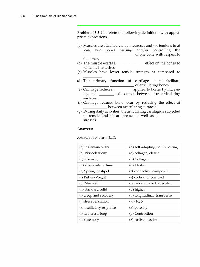
Problem 15.3 Complete the following definitions with appro-priate expressions.
(a) Muscles are attached via aponeuroses and/or tendons to atleast two bones causing and/or controlling the____________ _______________ of one bone with respect tothe other.
(b) The muscle exerts a _______________ effect on the bones towhich it is attached.
(c) Muscles have lower tensile strength as compared to__________.
(d) The primary function of cartilage is to facilitate______________ _____________ of articulating bones.
(e) Cartilage reduces __________ applied to bones by increas-ing the ________ of contact between the articulatingsurfaces.
(f) Cartilage reduces bone wear by reducing the effect of_____________ between articulating surfaces.
(g) During daily activities, the articulating cartilage is subjectedto tensile and shear stresses a well as _____________stresses.
Answers:
Answers to Problem 15.1:
(a) Instantaneously (n) self-adapting, self-repairing
(b) Viscoelasticity (o) collagen, elastin
(c) Viscosity (p) Collagen
(d) strain rate or time (q) Elastin
(e) Spring, dashpot (r) connective, composite
(f) Kelvin-Voight (s) cortical or compact
(g) Maxwell (t) cancellous or trabecular
(h) standard solid (u) higher
(i) creep and recovery (v) longitudinal, transverse
(j) stress relaxation (w) 10, 5
(k) oscillatory response (x) porosity
(l) hysteresis loop (y) Contraction
(m) memory (z) Active, passive
386 Fundamentals of Biomechanics

Answers to Problem 15.2:
(a) independent (n) age
(b) depends (o) wet
(c) potential energy, return (p) more
(d) energy (q) torsion, bending
(e) potential energy, heat, loss (r) transmitting
(f) viscoelastic (s) stability
(g) direction, magnitude, rate (t) passive
(h) longitudinal, transverse (u) muscles
(i) mass (v) deformation
(j) osteoporosis (w) translate
(k) strength, stiffness (x) stabilizing
(l) ultimate strength (y) junctions
(m) large, cancellous (z) skeletal, smooth, cardiac
Answers to Problem 15.3:
(a) relative movement(b) pulling(c) tendons(d) relative movement(e) stress, area(f) friction(g) compressive
Mechanical Properties of Biological Tissues 387
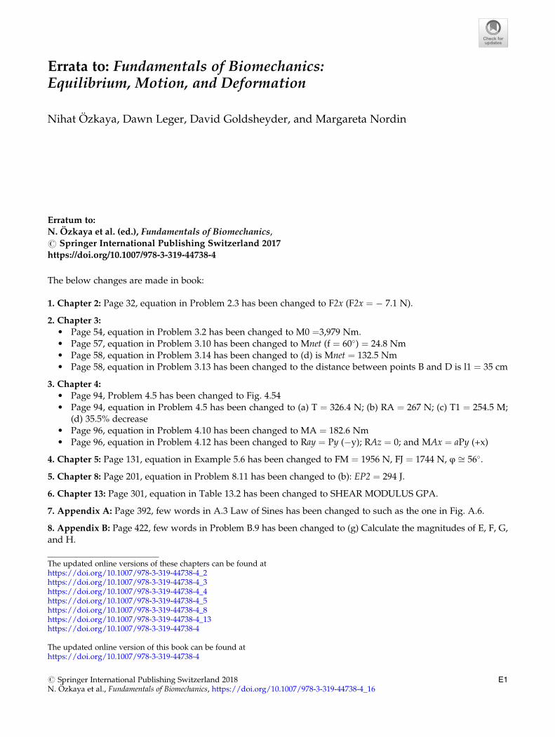
Errata to: Fundamentals of Biomechanics:Equilibrium, Motion, and Deformation
Nihat Ozkaya, Dawn Leger, David Goldsheyder, and Margareta Nordin
Erratum to:
N. Ozkaya et al. (ed.), Fundamentals of Biomechanics,# Springer International Publishing Switzerland 2017
https://doi.org/10.1007/978-3-319-44738-4
The below changes are made in book:
1. Chapter 2: Page 32, equation in Problem 2.3 has been changed to F2x (F2x ¼ � 7.1 N).
2. Chapter 3:
• Page 54, equation in Problem 3.2 has been changed to M0 ¼3,979 Nm.• Page 57, equation in Problem 3.10 has been changed to Mnet (f ¼ 60�) ¼ 24.8 Nm• Page 58, equation in Problem 3.14 has been changed to (d) is Mnet ¼ 132.5 Nm• Page 58, equation in Problem 3.13 has been changed to the distance between points B and D is l1 ¼ 35 cm
3. Chapter 4:
• Page 94, Problem 4.5 has been changed to Fig. 4.54• Page 94, equation in Problem 4.5 has been changed to (a) T ¼ 326.4 N; (b) RA ¼ 267 N; (c) T1 ¼ 254.5 M;
(d) 35.5% decrease• Page 96, equation in Problem 4.10 has been changed to MA ¼ 182.6 Nm• Page 96, equation in Problem 4.12 has been changed to Ray ¼ Py (�y); RAz ¼ 0; and MAx ¼ aPy (+x)
4. Chapter 5: Page 131, equation in Example 5.6 has been changed to FM ¼ 1956 N, FJ ¼ 1744 N, φ ffi 56�.
5. Chapter 8: Page 201, equation in Problem 8.11 has been changed to (b): EP2 ¼ 294 J.
6. Chapter 13: Page 301, equation in Table 13.2 has been changed to SHEAR MODULUS GPA.
7. Appendix A: Page 392, few words in A.3 Law of Sines has been changed to such as the one in Fig. A.6.
8. Appendix B: Page 422, few words in Problem B.9 has been changed to (g) Calculate the magnitudes of E, F, G,and H.
The updated online versions of these chapters can be found athttps://doi.org/10.1007/978-3-319-44738-4_2https://doi.org/10.1007/978-3-319-44738-4_3https://doi.org/10.1007/978-3-319-44738-4_4https://doi.org/10.1007/978-3-319-44738-4_5https://doi.org/10.1007/978-3-319-44738-4_8https://doi.org/10.1007/978-3-319-44738-4_13https://doi.org/10.1007/978-3-319-44738-4
The updated online version of this book can be found athttps://doi.org/10.1007/978-3-319-44738-4
# Springer International Publishing Switzerland 2018N. Ozkaya et al., Fundamentals of Biomechanics, https://doi.org/10.1007/978-3-319-44738-4_16
E1
Appendix A:
Plane Geometry
A.1 Angles / 391
A.2 Triangles / 391
A.3 Law of Sines / 392
A.4 Law of Cosine / 392
A.5 The Right Triangle / 392
A.6 Pythagorean Theorem / 392
A.7 Sine, Cosine, and Tangent / 393
A.8 Inverse Sine, Cosine, and Tangent / 394
A.9 Exercise Problems / 397
The original version of this chapter was revised. An erratum to this chapter can befound at https://doi.org/10.1007/978-3-319-44738-4_16
# Springer International Publishing Switzerland 2017N. Ozkaya et al., Fundamentals of Biomechanics, DOI 10.1007/978-3-319-44738-4
389
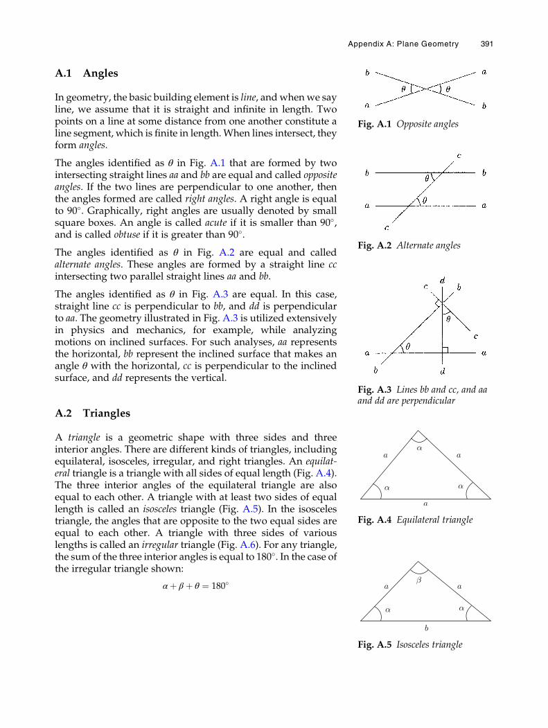
A.1 Angles
In geometry, the basic building element is line, andwhenwe sayline, we assume that it is straight and infinite in length. Twopoints on a line at some distance from one another constitute aline segment, which is finite in length.When lines intersect, theyform angles.
The angles identified as θ in Fig. A.1 that are formed by twointersecting straight lines aa and bb are equal and called oppositeangles. If the two lines are perpendicular to one another, thenthe angles formed are called right angles. A right angle is equalto 90�. Graphically, right angles are usually denoted by smallsquare boxes. An angle is called acute if it is smaller than 90�,and is called obtuse if it is greater than 90�.
The angles identified as θ in Fig. A.2 are equal and calledalternate angles. These angles are formed by a straight line ccintersecting two parallel straight lines aa and bb.
The angles identified as θ in Fig. A.3 are equal. In this case,straight line cc is perpendicular to bb, and dd is perpendicularto aa. The geometry illustrated in Fig. A.3 is utilized extensivelyin physics and mechanics, for example, while analyzingmotions on inclined surfaces. For such analyses, aa representsthe horizontal, bb represent the inclined surface that makes anangle θ with the horizontal, cc is perpendicular to the inclinedsurface, and dd represents the vertical.
A.2 Triangles
A triangle is a geometric shape with three sides and threeinterior angles. There are different kinds of triangles, includingequilateral, isosceles, irregular, and right triangles. An equilat-eral triangle is a triangle with all sides of equal length (Fig. A.4).The three interior angles of the equilateral triangle are alsoequal to each other. A triangle with at least two sides of equallength is called an isosceles triangle (Fig. A.5). In the isoscelestriangle, the angles that are opposite to the two equal sides areequal to each other. A triangle with three sides of variouslengths is called an irregular triangle (Fig. A.6). For any triangle,the sum of the three interior angles is equal to 180�. In the case ofthe irregular triangle shown:
αþ β þ θ ¼ 180�
Fig. A.1 Opposite angles
Fig. A.2 Alternate angles
Fig. A.3 Lines bb and cc, and aaand dd are perpendicular
Fig. A.4 Equilateral triangle
Fig. A.5 Isosceles triangle
Appendix A: Plane Geometry 391
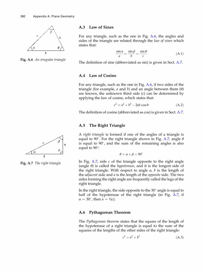
A.3 Law of Sines
For any triangle, such as the one in Fig. A.6, the angles andsides of the triangle are related through the law of sines whichstates that:
sin α
a¼ sin β
b¼ sin θ
cðA:1Þ
The definition of sine (abbreviated as sin) is given in Sect. A.7.
A.4 Law of Cosine
For any triangle, such as the one in Fig. A.6, if two sides of thetriangle (for example, a and b) and an angle between them (θ)are known, the unknown third side (c) can be determined byapplying the law of cosine, which states that:
c2 ¼ a2 þ b2 � 2ab cos θ ðA:2ÞThe definition of cosine (abbreviated as cos) is given in Sect. A.7.
A.5 The Right Triangle
A right triangle is formed if one of the angles of a triangle isequal to 90�. For the right triangle shown in Fig. A.7, angle θis equal to 90�, and the sum of the remaining angles is alsoequal to 90�:
θ ¼ αþ β ¼ 90�
In Fig. A.7, side c of the triangle opposite to the right angle(angle θ) is called the hypotenuse, and it is the longest side ofthe right triangle. With respect to angle α, b is the length ofthe adjacent side and a is the length of the opposite side. The twosides forming the right angle are frequently called the legs of theright triangle.
In the right triangle, the side opposite to the 30� angle is equal tohalf of the hypotenuse of the right triangle (in Fig. A.7, ifα ¼ 30�, then a ¼ ½c).
A.6 Pythagorean Theorem
The Pythagorean theorem states that the square of the length ofthe hypotenuse of a right triangle is equal to the sum of thesquares of the lengths of the other sides of the right triangle:
c2 ¼ a2 þ b2 ðA:3Þ
Fig. A.6 An irregular triangle
Fig. A.7 The right triangle
392 Appendix A: Plane Geometry
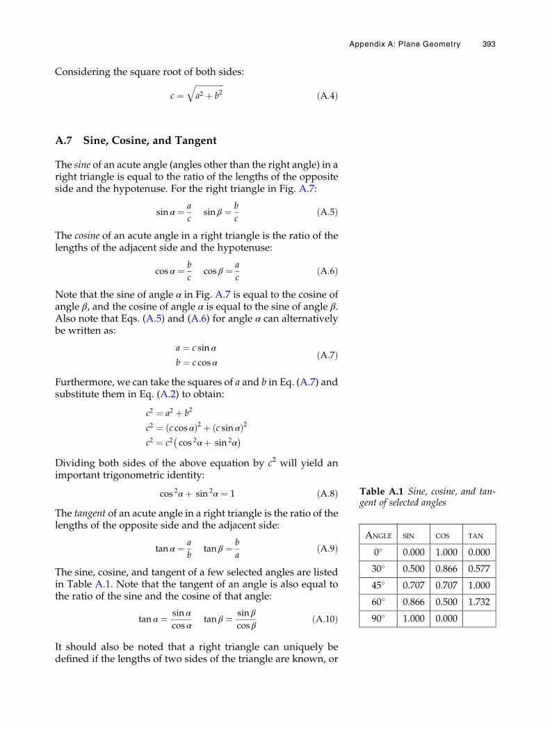
Considering the square root of both sides:
c ¼ffiffiffiffiffiffiffiffiffiffiffiffiffiffiffia2 þ b2
qðA:4Þ
A.7 Sine, Cosine, and Tangent
The sine of an acute angle (angles other than the right angle) in aright triangle is equal to the ratio of the lengths of the oppositeside and the hypotenuse. For the right triangle in Fig. A.7:
sin α ¼ a
csin β ¼ b
cðA:5Þ
The cosine of an acute angle in a right triangle is the ratio of thelengths of the adjacent side and the hypotenuse:
cos α ¼ b
ccos β ¼ a
cðA:6Þ
Note that the sine of angle α in Fig. A.7 is equal to the cosine ofangle β, and the cosine of angle α is equal to the sine of angle β.Also note that Eqs. (A.5) and (A.6) for angle α can alternativelybe written as:
a ¼ c sin α
b ¼ c cos αðA:7Þ
Furthermore, we can take the squares of a and b in Eq. (A.7) andsubstitute them in Eq. (A.2) to obtain:
c2 ¼ a2 þ b2
c2 ¼ c cos αð Þ2 þ c sin αð Þ2c2 ¼ c2 cos 2αþ sin 2α
� �Dividing both sides of the above equation by c2 will yield animportant trigonometric identity:
cos 2αþ sin 2α ¼ 1 ðA:8ÞThe tangent of an acute angle in a right triangle is the ratio of thelengths of the opposite side and the adjacent side:
tan α ¼ a
btan β ¼ b
aðA:9Þ
The sine, cosine, and tangent of a few selected angles are listedin Table A.1. Note that the tangent of an angle is also equal tothe ratio of the sine and the cosine of that angle:
tan α ¼ sin α
cos αtan β ¼ sin β
cos βðA:10Þ
It should also be noted that a right triangle can uniquely bedefined if the lengths of two sides of the triangle are known, or
Table A.1 Sine, cosine, and tan-gent of selected angles
ANGLE SIN COS TAN
0� 0.000 1.000 0.000
30� 0.500 0.866 0.577
45� 0.707 0.707 1.000
60� 0.866 0.500 1.732
90� 1.000 0.000
Appendix A: Plane Geometry 393
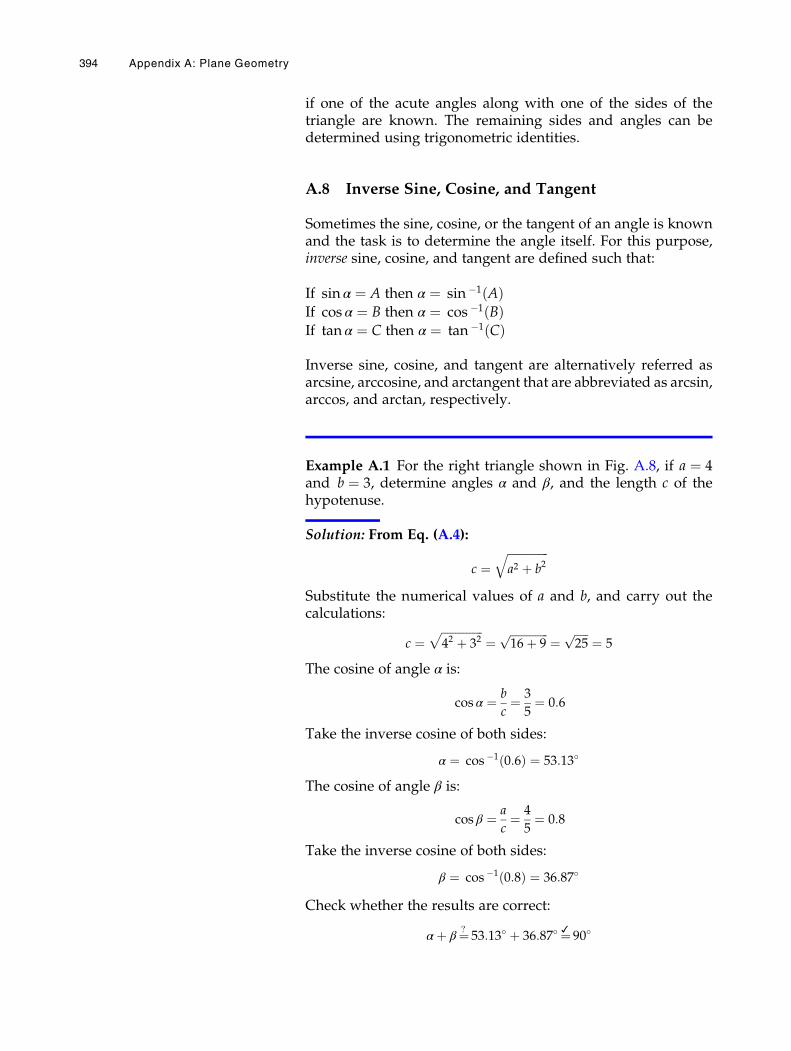
if one of the acute angles along with one of the sides of thetriangle are known. The remaining sides and angles can bedetermined using trigonometric identities.
A.8 Inverse Sine, Cosine, and Tangent
Sometimes the sine, cosine, or the tangent of an angle is knownand the task is to determine the angle itself. For this purpose,inverse sine, cosine, and tangent are defined such that:
If sin α ¼ A then α ¼ sin �1 Að ÞIf cos α ¼ B then α ¼ cos �1 Bð ÞIf tan α ¼ C then α ¼ tan �1 Cð Þ
Inverse sine, cosine, and tangent are alternatively referred asarcsine, arccosine, and arctangent that are abbreviated as arcsin,arccos, and arctan, respectively.
Example A.1 For the right triangle shown in Fig. A.8, if a ¼ 4and b ¼ 3, determine angles α and β, and the length c of thehypotenuse.
Solution: From Eq. (A.4):
c ¼ffiffiffiffiffiffiffiffiffiffiffiffiffiffiffia2 þ b2
qSubstitute the numerical values of a and b, and carry out thecalculations:
c ¼ffiffiffiffiffiffiffiffiffiffiffiffiffiffiffi42 þ 32
p¼ ffiffiffiffiffiffiffiffiffiffiffiffiffiffi
16þ 9p ¼
ffiffiffiffiffi25
p¼ 5
The cosine of angle α is:
cos α ¼ b
c¼ 3
5¼ 0:6
Take the inverse cosine of both sides:
α ¼ cos �1 0:6ð Þ ¼ 53:13�
The cosine of angle β is:
cos β ¼ a
c¼ 4
5¼ 0:8
Take the inverse cosine of both sides:
β ¼ cos �1 0:8ð Þ ¼ 36:87�
Check whether the results are correct:
αþ β¼? 53:13� þ 36:87� ¼✓ 90�
394 Appendix A: Plane Geometry
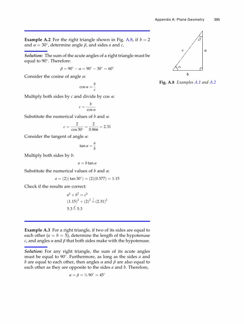
Example A.2 For the right triangle shown in Fig. A.8, if b ¼ 2and α ¼ 30�, determine angle β, and sides a and c.
Solution: The sum of the acute angles of a right trianglemust beequal to 90�. Therefore:
β ¼ 90� � α ¼ 90� � 30� ¼ 60�
Consider the cosine of angle α:
cos α ¼ b
c
Multiply both sides by c and divide by cos α:
c ¼ b
cos α
Substitute the numerical values of b and α:
c ¼ 2
cos 30�¼ 2
0:866¼ 2:31
Consider the tangent of angle α:
tan α ¼ a
b
Multiply both sides by b:
a ¼ b tan α
Substitute the numerical values of b and α:
a ¼ 2ð Þ tan 30�ð Þ ¼ 2ð Þ 0:577ð Þ ¼ 1:15
Check if the results are correct:
a2 þ b2 ¼ c2
1:15ð Þ2 þ 2ð Þ2 ¼? 2:31ð Þ2
5:3¼✓ 5:3
Example A.3 For a right triangle, if two of its sides are equal toeach other (a ¼ b ¼ 5), determine the length of the hypotenusec, and angles α and β that both sides make with the hypotenuse.
Solution: For any right triangle, the sum of its acute anglesmust be equal to 90�. Furthermore, as long as the sides a andb are equal to each other, then angles α and β are also equal toeach other as they are opposite to the sides a and b. Therefore,
α ¼ β ¼ ½ 90� ¼ 45�
Fig. A.8 Examples A.1 and A.2
Appendix A: Plane Geometry 395
From Eq. (A.4),
c ¼ffiffiffiffiffiffiffiffiffiffiffiffiffiffiffiffiffiffiffiffia2 þ b2
� �r
Substitute the numerical values of a and b:
c ¼ffiffiffiffiffiffiffiffiffiffiffiffiffiffiffiffiffiffiffiffiffiffiffiffiffiffiffiffiffiffiffiffiffiffiffiffiffiffiffiffiffiffiffiffiffiffiffiffiffi52 þ 52� � ¼ ffiffiffiffiffi
50p
¼ 7:07
q
Example A.4 For the irregular triangle shown in Fig. A.6, ifa ¼ 3.5, b ¼ 5.0, and α ¼ 43�, determine angles β and θ andthe side c.
Solution: From Eq. (A.1),
sin α
a¼ sin β
b
Therefore,
b sin α ¼ a sin β
and
sin β ¼ b sin α
a
Substitute the numerical values of a, b, and angle α:
sin β ¼ 5:0 sin 43�
3:5¼ 0:97
Then,
β ¼ 〖 sin 〗 �1ð Þ 0:97ð Þ ¼ 75:9�
Furthermore, as the sum of interior angles of the triangle mustbe equal to 180�, then
θ ¼ 180� � α þ βð Þ ¼ 180� � 43� þ 75:9�ð Þ ¼ 180� � 118:9� ¼ 61:1�
From Eq. (A.1),
sin α
a¼ sin θ
c
Therefore,
c sin α ¼ a sin θ
and
c ¼ a sin θ
sin α
Substitute the numerical values of a and angles α and θ:
c ¼ 3:5 sin 61:1�
sin 43�ð Þ ¼ 4:5
396 Appendix A: Plane Geometry
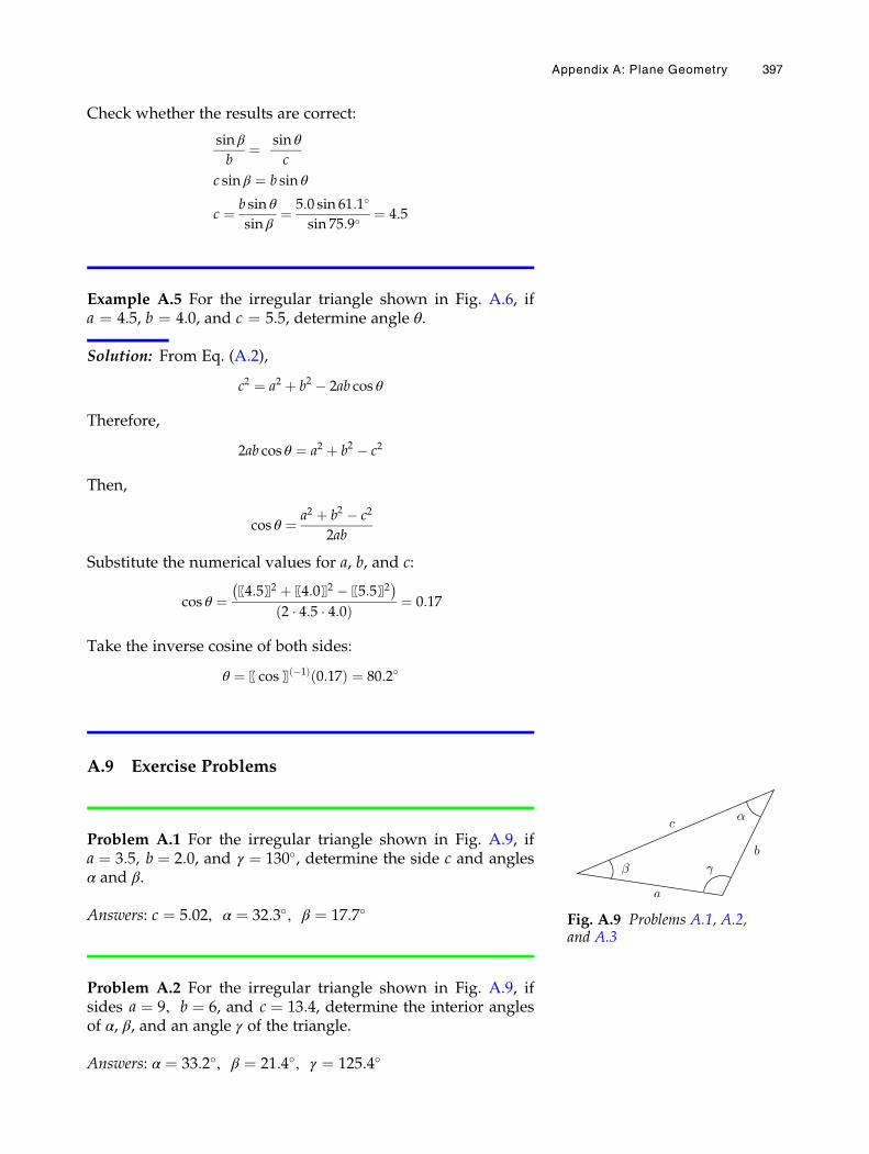
Check whether the results are correct:
sin β
b¼ sin θ
c
c sin β ¼ b sin θ
c ¼ b sin θ
sin β¼ 5:0 sin 61:1�
sin 75:9�¼ 4:5
Example A.5 For the irregular triangle shown in Fig. A.6, ifa ¼ 4.5, b ¼ 4.0, and c ¼ 5.5, determine angle θ.
Solution: From Eq. (A.2),
c2 ¼ a2 þ b2 � 2ab cos θ
Therefore,
2ab cos θ ¼ a2 þ b2 � c2
Then,
cos θ ¼ a2 þ b2 � c2
2ab
Substitute the numerical values for a, b, and c:
cos θ ¼ 〖4:5〗2 þ 〖4:0〗2 � 〖5:5〗2� �
2 � 4:5 � 4:0ð Þ ¼ 0:17
Take the inverse cosine of both sides:
θ ¼ 〖 cos 〗 �1ð Þ 0:17ð Þ ¼ 80:2�
A.9 Exercise Problems
Problem A.1 For the irregular triangle shown in Fig. A.9, ifa ¼ 3:5, b ¼ 2:0, and γ ¼ 130�, determine the side c and anglesα and β.
Answers: c ¼ 5:02, α ¼ 32:3�, β ¼ 17:7�
Problem A.2 For the irregular triangle shown in Fig. A.9, ifsides a ¼ 9, b ¼ 6, and c ¼ 13:4, determine the interior anglesof α, β, and an angle γ of the triangle.
Answers: α ¼ 33:2�, β ¼ 21:4�, γ ¼ 125:4�
Fig. A.9 Problems A.1, A.2,and A.3
Appendix A: Plane Geometry 397
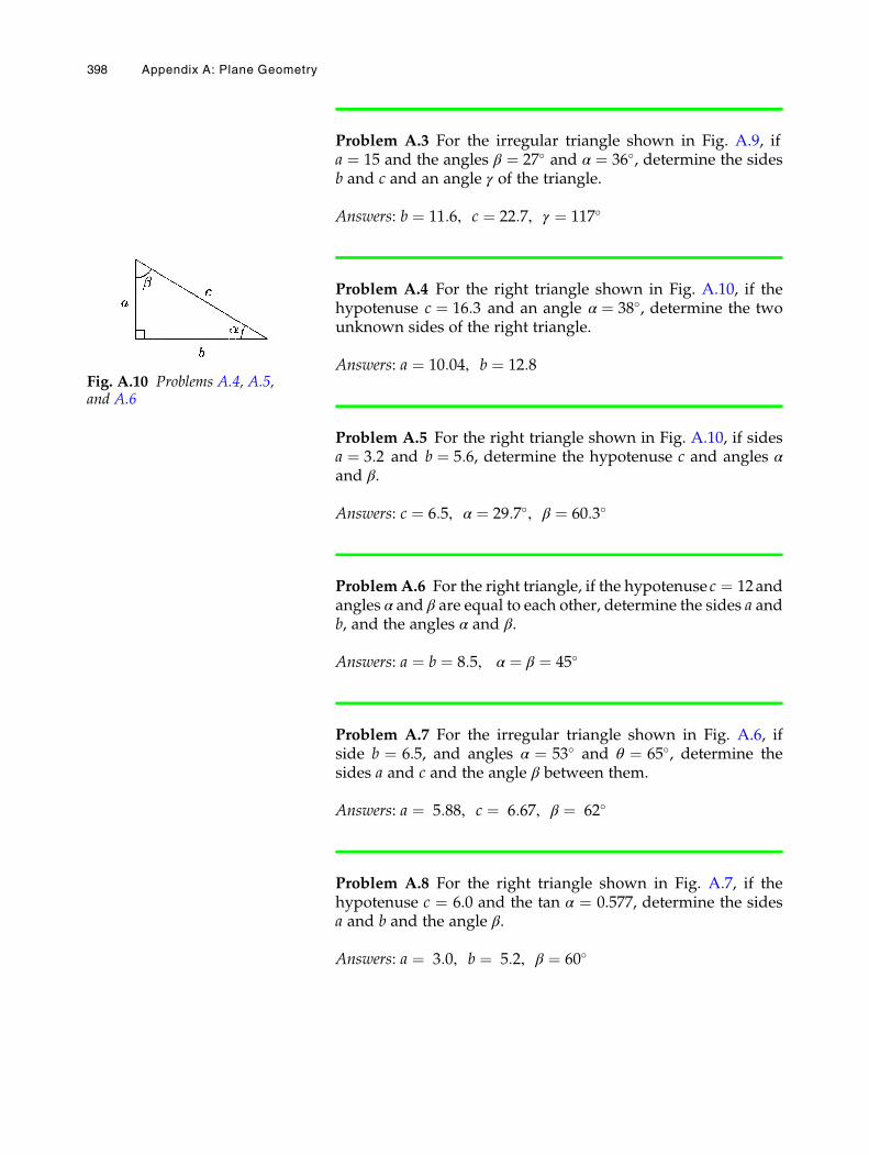
Problem A.3 For the irregular triangle shown in Fig. A.9, ifa ¼ 15 and the angles β ¼ 27� and α ¼ 36�, determine the sidesb and c and an angle γ of the triangle.
Answers: b ¼ 11:6, c ¼ 22:7, γ ¼ 117�
Problem A.4 For the right triangle shown in Fig. A.10, if thehypotenuse c ¼ 16:3 and an angle α ¼ 38�, determine the twounknown sides of the right triangle.
Answers: a ¼ 10:04, b ¼ 12:8
Problem A.5 For the right triangle shown in Fig. A.10, if sidesa ¼ 3:2 and b ¼ 5:6, determine the hypotenuse c and angles αand β.
Answers: c ¼ 6:5, α ¼ 29:7�, β ¼ 60:3�
ProblemA.6 For the right triangle, if the hypotenuse c ¼ 12andangles α and β are equal to each other, determine the sides a andb, and the angles α and β.
Answers: a ¼ b ¼ 8:5, α ¼ β ¼ 45�
Problem A.7 For the irregular triangle shown in Fig. A.6, ifside b ¼ 6.5, and angles α ¼ 53� and θ ¼ 65�, determine thesides a and c and the angle β between them.
Answers: a ¼ 5:88, c ¼ 6:67, β ¼ 62�
Problem A.8 For the right triangle shown in Fig. A.7, if thehypotenuse c ¼ 6.0 and the tan α ¼ 0.577, determine the sidesa and b and the angle β.
Answers: a ¼ 3:0, b ¼ 5:2, β ¼ 60�
Fig. A.10 Problems A.4, A.5,and A.6
398 Appendix A: Plane Geometry
Problem A.9 For the isosceles triangle shown in Fig. A.5, ifside b ¼ 12.0 and the opposite angle β ¼ 120�, determine twoother sides and interior angles of the triangle.
Answers: a ¼ 6:93, α ¼ 30�
Problem A.10 For the isosceles triangle shown in Fig. A.5, ifside a ¼ 4.5 and the angle β ¼ 55�, determine the side b and theangle α.
Answers: b ¼ 3:9, α ¼ 70
Problem A.11 For the irregular triangle shown in Fig. A.6, ifside b ¼ 4.6, and the angles α ¼ 36� and θ ¼ 78�, determinesides a and c and the angle β.
Answers: a ¼ 2:96, c ¼ 3:17, β ¼ 66�
Appendix A: Plane Geometry 399
Appendix B:
Vector Algebra
B.1 Definitions / 403
B.2 Notation / 403
B.3 Multiplication of a Vector by a Scalar / 404
B.4 Negative Vector / 404
B.5 Addition of Vectors: Graphical Methods / 404
B.6 Subtraction of Vectors / 405
B.7 Addition of More Than Two Vectors / 405
B.8 Projection of Vectors / 406
B.9 Resolution of Vectors / 406
B.10 Unit Vectors / 407
B.11 Rectangular Coordinates / 407
B.12 Addition of Vectors: Trigonometric Method / 409
B.13 Three-Dimensional Components of Vectors / 414
B.14 Dot (Scalar) Product of Vectors / 415
B.15 Cross (Vector) Product of Vectors / 416
B.16 Exercise Problems / 419
# Springer International Publishing Switzerland 2017N. Ozkaya et al., Fundamentals of Biomechanics, DOI 10.1007/978-3-319-44738-4
401
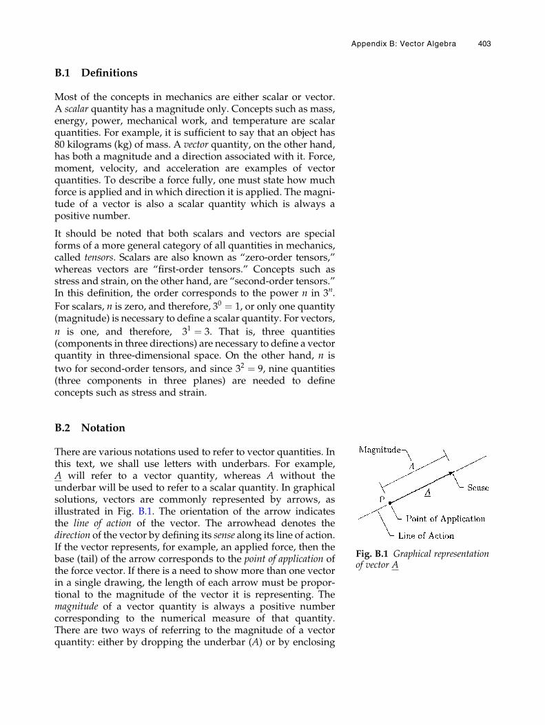
B.1 Definitions
Most of the concepts in mechanics are either scalar or vector.A scalar quantity has a magnitude only. Concepts such as mass,energy, power, mechanical work, and temperature are scalarquantities. For example, it is sufficient to say that an object has80 kilograms (kg) of mass. A vector quantity, on the other hand,has both a magnitude and a direction associated with it. Force,moment, velocity, and acceleration are examples of vectorquantities. To describe a force fully, one must state how muchforce is applied and in which direction it is applied. The magni-tude of a vector is also a scalar quantity which is always apositive number.
It should be noted that both scalars and vectors are specialforms of a more general category of all quantities in mechanics,called tensors. Scalars are also known as “zero-order tensors,”whereas vectors are “first-order tensors.” Concepts such asstress and strain, on the other hand, are “second-order tensors.”In this definition, the order corresponds to the power n in 3n.
For scalars, n is zero, and therefore, 30 ¼ 1, or only one quantity(magnitude) is necessary to define a scalar quantity. For vectors,
n is one, and therefore, 31 ¼ 3. That is, three quantities(components in three directions) are necessary to define a vectorquantity in three-dimensional space. On the other hand, n is
two for second-order tensors, and since 32 ¼ 9, nine quantities(three components in three planes) are needed to defineconcepts such as stress and strain.
B.2 Notation
There are various notations used to refer to vector quantities. Inthis text, we shall use letters with underbars. For example,A will refer to a vector quantity, whereas A without theunderbar will be used to refer to a scalar quantity. In graphicalsolutions, vectors are commonly represented by arrows, asillustrated in Fig. B.1. The orientation of the arrow indicatesthe line of action of the vector. The arrowhead denotes thedirection of the vector by defining its sense along its line of action.If the vector represents, for example, an applied force, then thebase (tail) of the arrow corresponds to the point of application ofthe force vector. If there is a need to show more than one vectorin a single drawing, the length of each arrow must be propor-tional to the magnitude of the vector it is representing. Themagnitude of a vector quantity is always a positive numbercorresponding to the numerical measure of that quantity.There are two ways of referring to the magnitude of a vectorquantity: either by dropping the underbar (A) or by enclosing
Fig. B.1 Graphical representationof vector A
Appendix B: Vector Algebra 403
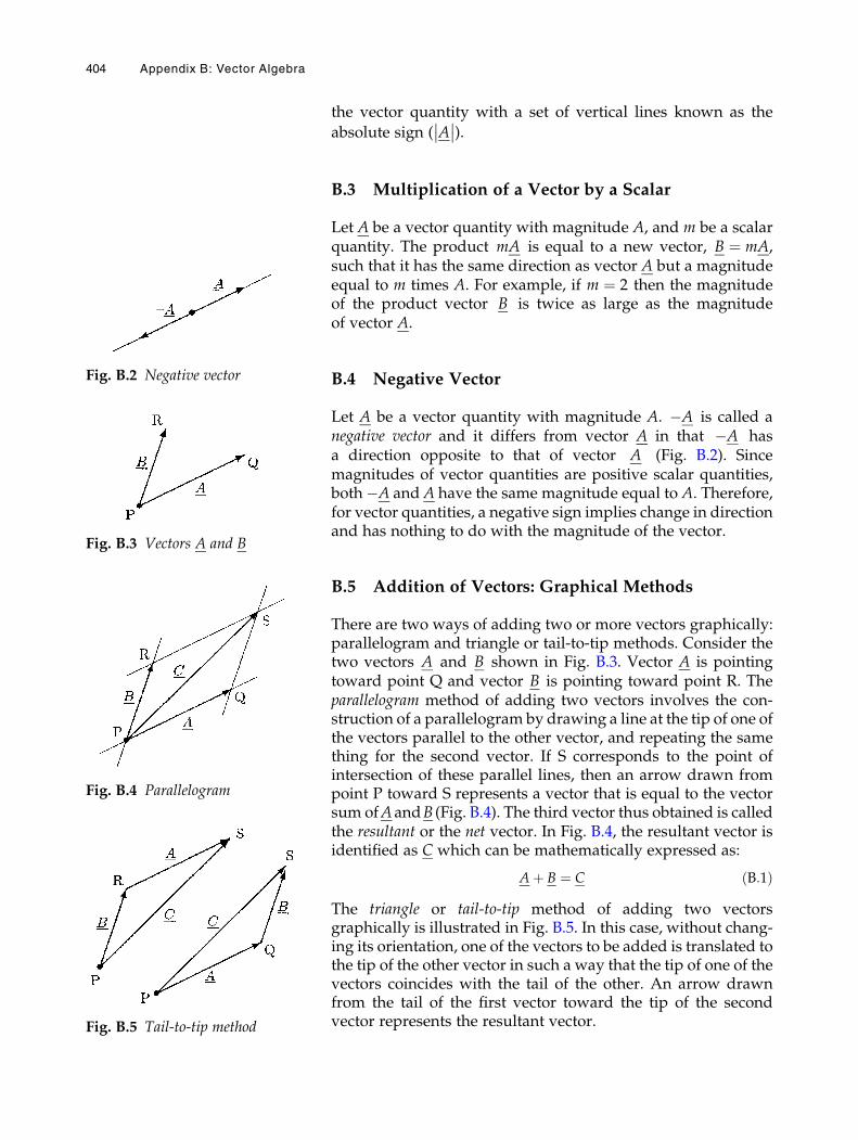
the vector quantity with a set of vertical lines known as the
absolute sign ( A�� ��).
B.3 Multiplication of a Vector by a Scalar
Let A be a vector quantity with magnitude A, and m be a scalarquantity. The product mA is equal to a new vector, B ¼ mA,such that it has the same direction as vector A but a magnitudeequal to m times A. For example, if m ¼ 2 then the magnitudeof the product vector B is twice as large as the magnitudeof vector A.
B.4 Negative Vector
Let A be a vector quantity with magnitude A. �A is called anegative vector and it differs from vector A in that �A hasa direction opposite to that of vector A (Fig. B.2). Sincemagnitudes of vector quantities are positive scalar quantities,both�A and A have the same magnitude equal to A. Therefore,for vector quantities, a negative sign implies change in directionand has nothing to do with the magnitude of the vector.
B.5 Addition of Vectors: Graphical Methods
There are two ways of adding two or more vectors graphically:parallelogram and triangle or tail-to-tip methods. Consider thetwo vectors A and B shown in Fig. B.3. Vector A is pointingtoward point Q and vector B is pointing toward point R. Theparallelogram method of adding two vectors involves the con-struction of a parallelogram by drawing a line at the tip of one ofthe vectors parallel to the other vector, and repeating the samething for the second vector. If S corresponds to the point ofintersection of these parallel lines, then an arrow drawn frompoint P toward S represents a vector that is equal to the vectorsum ofAandB (Fig. B.4). The third vector thus obtained is calledthe resultant or the net vector. In Fig. B.4, the resultant vector isidentified as C which can be mathematically expressed as:
Aþ B ¼ C ðB:1Þ
The triangle or tail-to-tip method of adding two vectorsgraphically is illustrated in Fig. B.5. In this case, without chang-ing its orientation, one of the vectors to be added is translated tothe tip of the other vector in such a way that the tip of one of thevectors coincides with the tail of the other. An arrow drawnfrom the tail of the first vector toward the tip of the secondvector represents the resultant vector.
Fig. B.2 Negative vector
Fig. B.3 Vectors A and B
Fig. B.4 Parallelogram
Fig. B.5 Tail-to-tip method
404 Appendix B: Vector Algebra
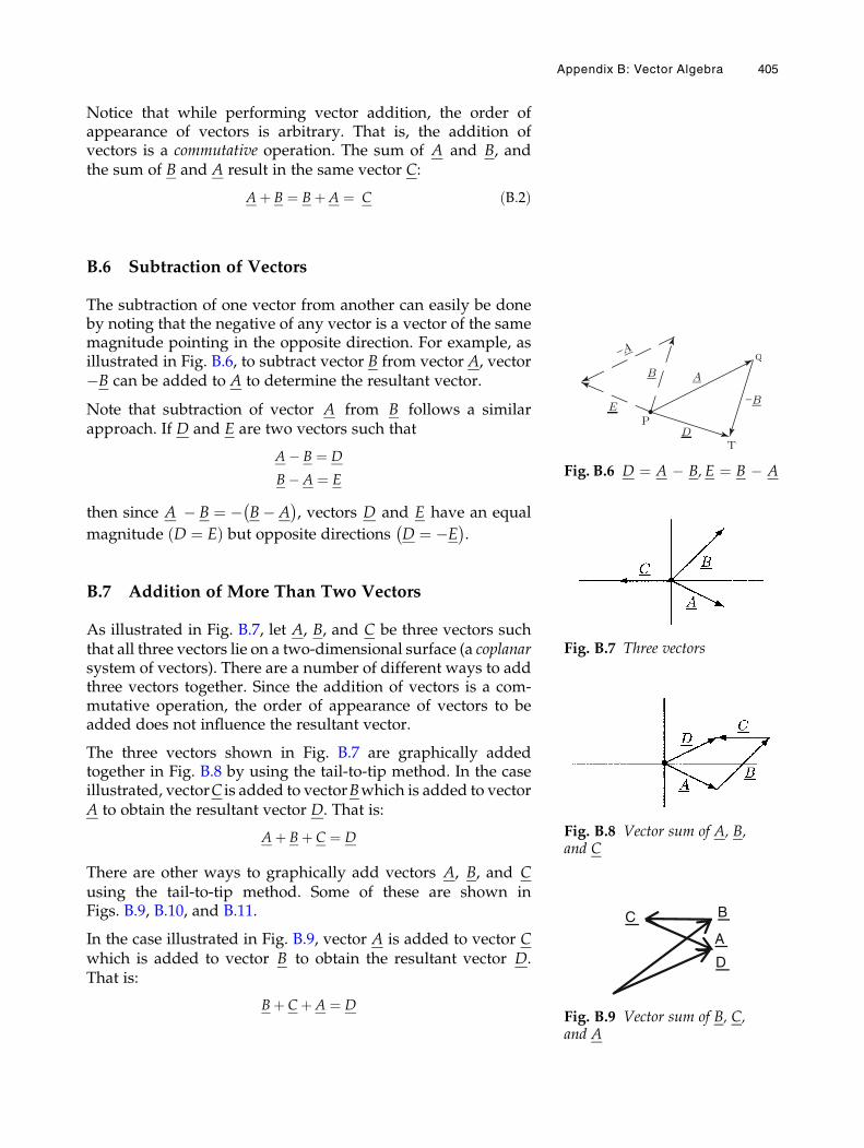
Notice that while performing vector addition, the order ofappearance of vectors is arbitrary. That is, the addition ofvectors is a commutative operation. The sum of A and B, andthe sum of B and A result in the same vector C:
Aþ B ¼ Bþ A ¼ C ðB:2Þ
B.6 Subtraction of Vectors
The subtraction of one vector from another can easily be doneby noting that the negative of any vector is a vector of the samemagnitude pointing in the opposite direction. For example, asillustrated in Fig. B.6, to subtract vector B from vector A, vector�B can be added to A to determine the resultant vector.
Note that subtraction of vector A from B follows a similarapproach. If D and E are two vectors such that
A� B ¼ D
B� A ¼ E
then since A � B ¼ � B� A� �
, vectors D and E have an equal
magnitude D ¼ Eð Þ but opposite directions D ¼ �E� �
.
B.7 Addition of More Than Two Vectors
As illustrated in Fig. B.7, let A, B, and C be three vectors suchthat all three vectors lie on a two-dimensional surface (a coplanarsystem of vectors). There are a number of different ways to addthree vectors together. Since the addition of vectors is a com-mutative operation, the order of appearance of vectors to beadded does not influence the resultant vector.
The three vectors shown in Fig. B.7 are graphically addedtogether in Fig. B.8 by using the tail-to-tip method. In the caseillustrated, vectorC is added to vectorBwhich is added to vectorA to obtain the resultant vector D. That is:
Aþ Bþ C ¼ D
There are other ways to graphically add vectors A, B, and Cusing the tail-to-tip method. Some of these are shown inFigs. B.9, B.10, and B.11.
In the case illustrated in Fig. B.9, vector A is added to vector Cwhich is added to vector B to obtain the resultant vector D.That is:
Bþ Cþ A ¼ D
Fig. B.6 D ¼ A � B, E ¼ B � A
Fig. B.7 Three vectors
Fig. B.8 Vector sum of A, B,and C
BC
A
D
Fig. B.9 Vector sum of B, C,and A
Appendix B: Vector Algebra 405
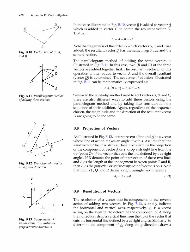
In the case illustrated in Fig. B.10, vector B is added to vector Awhich is added to vector C to obtain the resultant vector D.That is:
Cþ Aþ B ¼ D
Note that regardless of the order in which vectorsA,B, andCareadded, the resultant vector D has the same magnitude and thesame direction.
The parallelogram method of adding the same vectors isillustrated in Fig. B.11. In this case, two (B and C) of the threevectors are added together first. The resultant (vector E) of thisoperation is then added to vector A and the overall resultant(vector D) is determined. The sequence of additions illustratedin Fig. B.11 can be mathematically expressed as:
Aþ Bþ C� � ¼ Aþ E ¼ D
Similar to the tail-to-tip method used to add vectorsA,B, andC,there are also different ways to add these vectors using theparallelogram method and by taking into consideration thesequence of their addition. Again, regardless of the sequencechosen, the magnitude and the direction of the resultant vectorD are going to be the same.
B.8 Projection of Vectors
As illustrated in Fig. B.12, let s represent a line andA be a vectorwhose line of action makes an angle θ with s. Assume that lines and vectorA lie on a plane surface. To determine the projectionor the component of vector A on s, drop a straight line from thetip (point Q) of the vector that cuts the line defined by s at rightangles. If R denotes the point of intersection of these two linesand As is the length of the line segment between points P and R,then As is the projection or scalar component of vectorA on s. Notethat points P, Q, and R define a right triangle, and therefore:
As ¼ A cos θ ðB:3Þ
B.9 Resolution of Vectors
The resolution of a vector into its components is the reverseaction of adding two vectors. In Fig. B.13, x and y indicatethe horizontal and vertical axes, respectively. A is a vectoracting on the x-plane. To determine the component of A alongthe x direction, drop a vertical line from the tip of the vector thatcuts the horizontal line defined by x at right angles. Similarly, todetermine the component of A along the y direction, draw a
Fig. B.10 Vector sum of C, A,and B
Fig. B.11 Parallelogram methodof adding three vectors
Fig. B.12 Projection of a vectoron a given direction
Fig. B.13 Components of avector along two mutuallyperpendicular directions
406 Appendix B: Vector Algebra
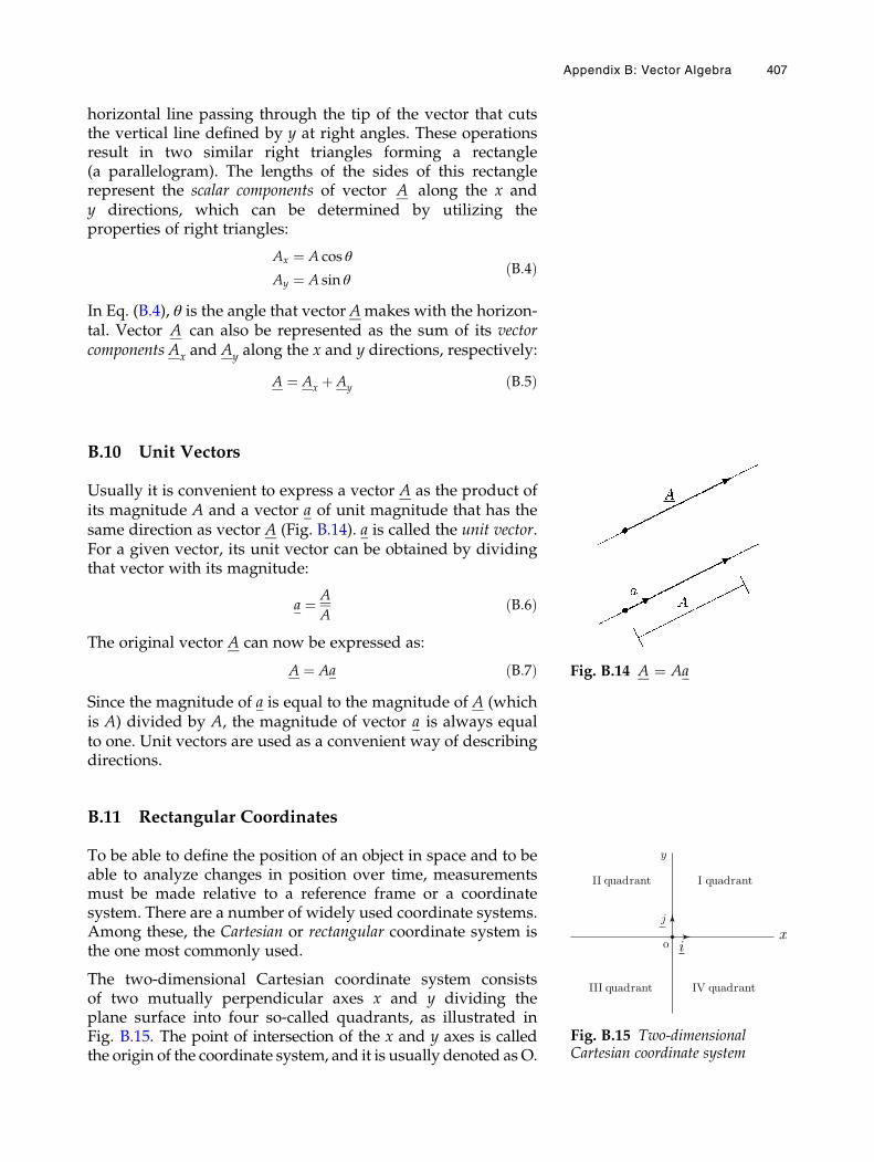
horizontal line passing through the tip of the vector that cutsthe vertical line defined by y at right angles. These operationsresult in two similar right triangles forming a rectangle(a parallelogram). The lengths of the sides of this rectanglerepresent the scalar components of vector A along the x andy directions, which can be determined by utilizing theproperties of right triangles:
Ax ¼ A cos θ
Ay ¼ A sin θðB:4Þ
In Eq. (B.4), θ is the angle that vectorAmakes with the horizon-tal. Vector A can also be represented as the sum of its vectorcomponents Ax and Ay along the x and y directions, respectively:
A ¼ Ax þ Ay ðB:5Þ
B.10 Unit Vectors
Usually it is convenient to express a vector A as the product ofits magnitude A and a vector a of unit magnitude that has thesame direction as vector A (Fig. B.14). a is called the unit vector.For a given vector, its unit vector can be obtained by dividingthat vector with its magnitude:
a ¼ A
AðB:6Þ
The original vector A can now be expressed as:
A ¼ Aa ðB:7Þ
Since the magnitude of a is equal to the magnitude of A (whichis A) divided by A, the magnitude of vector a is always equalto one. Unit vectors are used as a convenient way of describingdirections.
B.11 Rectangular Coordinates
To be able to define the position of an object in space and to beable to analyze changes in position over time, measurementsmust be made relative to a reference frame or a coordinatesystem. There are a number of widely used coordinate systems.Among these, the Cartesian or rectangular coordinate system isthe one most commonly used.
The two-dimensional Cartesian coordinate system consistsof two mutually perpendicular axes x and y dividing theplane surface into four so-called quadrants, as illustrated inFig. B.15. The point of intersection of the x and y axes is calledthe origin of the coordinate system, and it is usually denoted asO.
Fig. B.14 A ¼ Aa
Fig. B.15 Two-dimensionalCartesian coordinate system
Appendix B: Vector Algebra 407
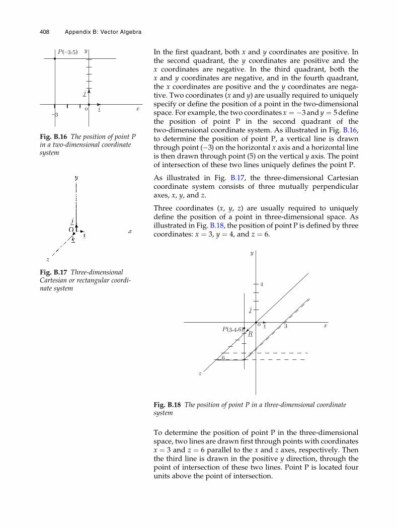
In the first quadrant, both x and y coordinates are positive. Inthe second quadrant, the y coordinates are positive and thex coordinates are negative. In the third quadrant, both thex and y coordinates are negative, and in the fourth quadrant,the x coordinates are positive and the y coordinates are nega-tive. Two coordinates (x and y) are usually required to uniquelyspecify or define the position of a point in the two-dimensionalspace. For example, the two coordinatesx ¼ �3andy ¼ 5definethe position of point P in the second quadrant of thetwo-dimensional coordinate system. As illustrated in Fig. B.16,to determine the position of point P, a vertical line is drawnthrough point (�3) on the horizontal x axis and a horizontal lineis then drawn through point (5) on the vertical y axis. The pointof intersection of these two lines uniquely defines the point P.
As illustrated in Fig. B.17, the three-dimensional Cartesiancoordinate system consists of three mutually perpendicularaxes, x, y, and z.
Three coordinates (x, y, z) are usually required to uniquelydefine the position of a point in three-dimensional space. Asillustrated in Fig. B.18, the position of point P is defined by threecoordinates: x ¼ 3, y ¼ 4, and z ¼ 6.
To determine the position of point P in the three-dimensionalspace, two lines are drawn first through points with coordinatesx ¼ 3 and z ¼ 6 parallel to the x and z axes, respectively. Thenthe third line is drawn in the positive y direction, through thepoint of intersection of these two lines. Point P is located fourunits above the point of intersection.
Fig. B.16 The position of point Pin a two-dimensional coordinatesystem
Fig. B.17 Three-dimensionalCartesian or rectangular coordi-nate system
Fig. B.18 The position of point P in a three-dimensional coordinatesystem
408 Appendix B: Vector Algebra
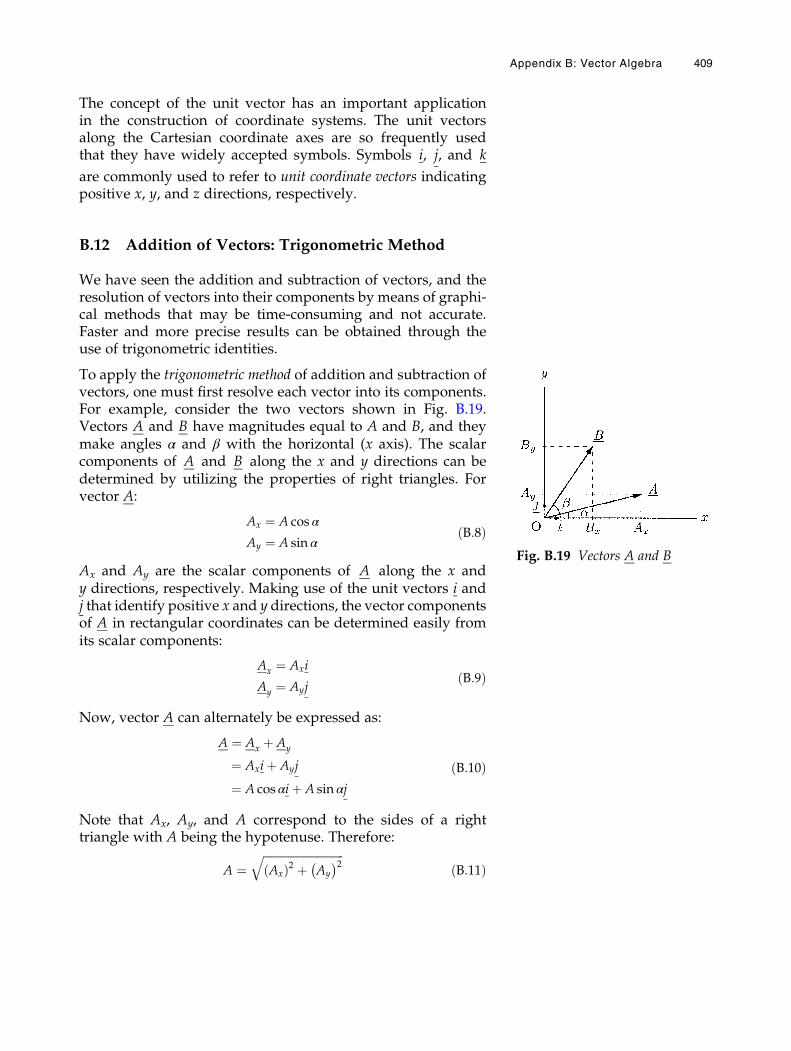
The concept of the unit vector has an important applicationin the construction of coordinate systems. The unit vectorsalong the Cartesian coordinate axes are so frequently usedthat they have widely accepted symbols. Symbols i, j, and k
are commonly used to refer to unit coordinate vectors indicatingpositive x, y, and z directions, respectively.
B.12 Addition of Vectors: Trigonometric Method
We have seen the addition and subtraction of vectors, and theresolution of vectors into their components by means of graphi-cal methods that may be time-consuming and not accurate.Faster and more precise results can be obtained through theuse of trigonometric identities.
To apply the trigonometric method of addition and subtraction ofvectors, one must first resolve each vector into its components.For example, consider the two vectors shown in Fig. B.19.Vectors A and B have magnitudes equal to A and B, and theymake angles α and β with the horizontal (x axis). The scalarcomponents of A and B along the x and y directions can bedetermined by utilizing the properties of right triangles. Forvector A:
Ax ¼ A cos α
Ay ¼ A sin αðB:8Þ
Ax and Ay are the scalar components of A along the x andy directions, respectively. Making use of the unit vectors i andj that identify positive x and y directions, the vector componentsof A in rectangular coordinates can be determined easily fromits scalar components:
Ax ¼ Axi
Ay ¼ AyjðB:9Þ
Now, vector A can alternately be expressed as:
A ¼ Ax þ Ay
¼ Axiþ Ayj
¼ A cos αiþ A sin αj
ðB:10Þ
Note that Ax, Ay, and A correspond to the sides of a righttriangle with A being the hypotenuse. Therefore:
A ¼ffiffiffiffiffiffiffiffiffiffiffiffiffiffiffiffiffiffiffiffiffiffiffiffiffiffiffiffiffiAxð Þ2 þ Ay
� �2qðB:11Þ
Fig. B.19 Vectors A and B
Appendix B: Vector Algebra 409
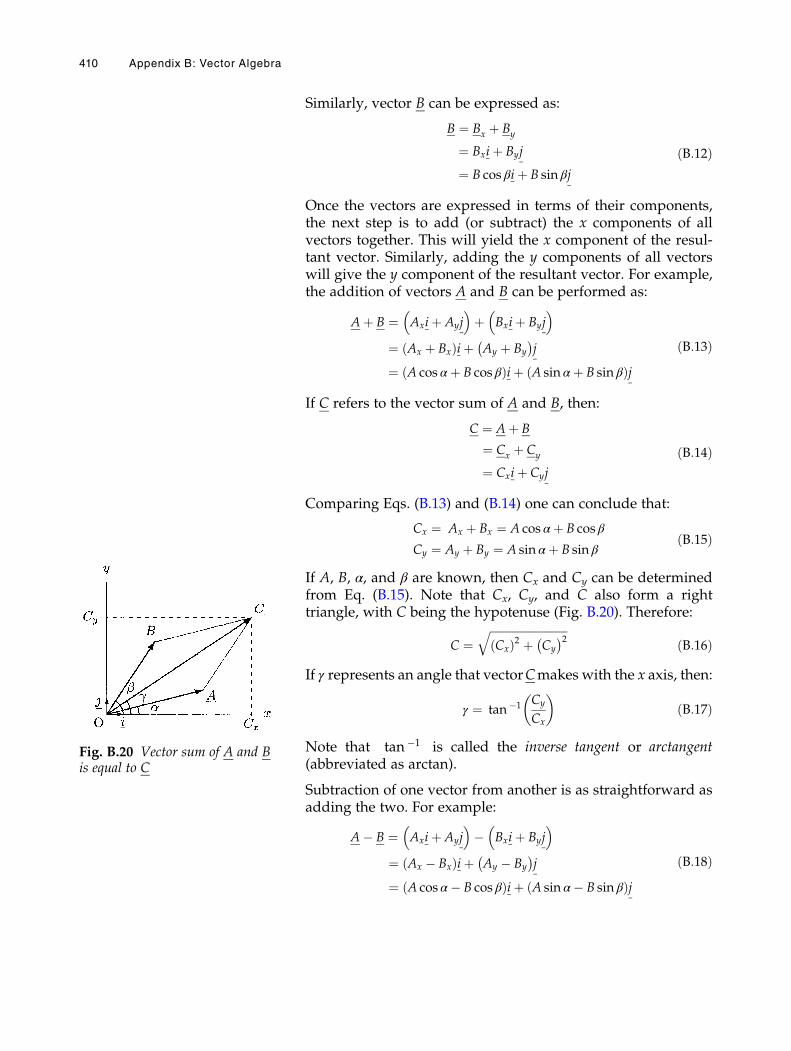
Similarly, vector B can be expressed as:
B ¼ Bx þ By
¼ Bxiþ Byj
¼ B cos βiþ B sin βj
ðB:12Þ
Once the vectors are expressed in terms of their components,the next step is to add (or subtract) the x components of allvectors together. This will yield the x component of the resul-tant vector. Similarly, adding the y components of all vectorswill give the y component of the resultant vector. For example,the addition of vectors A and B can be performed as:
Aþ B ¼ Axiþ Ayj� �
þ Bxiþ Byj� �
¼ Ax þ Bxð Þiþ Ay þ By
� �j
¼ A cos αþ B cos βð Þiþ A sin αþ B sin βð ÞjðB:13Þ
If C refers to the vector sum of A and B, then:
C ¼ Aþ B
¼ Cx þ Cy
¼ Cxiþ Cyj
ðB:14Þ
Comparing Eqs. (B.13) and (B.14) one can conclude that:
Cx ¼ Ax þ Bx ¼ A cos αþ B cos β
Cy ¼ Ay þ By ¼ A sin αþ B sin βðB:15Þ
If A, B, α, and β are known, then Cx and Cy can be determinedfrom Eq. (B.15). Note that Cx, Cy, and C also form a righttriangle, with C being the hypotenuse (Fig. B.20). Therefore:
C ¼ffiffiffiffiffiffiffiffiffiffiffiffiffiffiffiffiffiffiffiffiffiffiffiffiffiffiffiffiCxð Þ2 þ Cy
� �2qðB:16Þ
If γ represents an angle that vectorCmakes with the x axis, then:
γ ¼ tan �1 Cy
Cx
� ðB:17Þ
Note that tan �1 is called the inverse tangent or arctangent(abbreviated as arctan).
Subtraction of one vector from another is as straightforward asadding the two. For example:
A� B ¼ Axiþ Ayj� �
� Bxiþ Byj� �
¼ Ax � Bxð Þiþ Ay � By
� �j
¼ A cos α� B cos βð Þiþ A sin α� B sin βð ÞjðB:18Þ
Fig. B.20 Vector sum of A and Bis equal to C
410 Appendix B: Vector Algebra
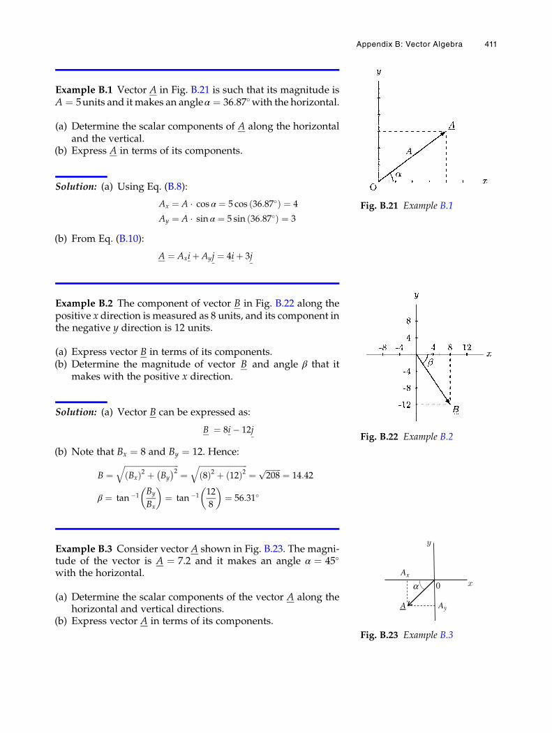
Example B.1 Vector A in Fig. B.21 is such that its magnitude isA ¼ 5units and it makes an angleα ¼ 36:87�with the horizontal.
(a) Determine the scalar components of A along the horizontaland the vertical.
(b) Express A in terms of its components.
Solution: (a) Using Eq. (B.8):
Ax ¼ A � cos α ¼ 5 cos 36:87�ð Þ ¼ 4
Ay ¼ A � sin α ¼ 5 sin 36:87�ð Þ ¼ 3
(b) From Eq. (B.10):
A ¼ Axiþ Ayj ¼ 4iþ 3j
Example B.2 The component of vector B in Fig. B.22 along thepositive x direction is measured as 8 units, and its component inthe negative y direction is 12 units.
(a) Express vector B in terms of its components.(b) Determine the magnitude of vector B and angle β that it
makes with the positive x direction.
Solution: (a) Vector B can be expressed as:
B ¼ 8i� 12j
(b) Note that Bx ¼ 8 and By ¼ 12. Hence:
B ¼ffiffiffiffiffiffiffiffiffiffiffiffiffiffiffiffiffiffiffiffiffiffiffiffiffiffiffiffiBxð Þ2 þ By
� �2q¼
ffiffiffiffiffiffiffiffiffiffiffiffiffiffiffiffiffiffiffiffiffiffiffiffiffi8ð Þ2 þ 12ð Þ2
q¼ ffiffiffiffiffiffiffiffi
208p ¼ 14:42
β ¼ tan �1By
Bx
� ¼ tan �1 12
8
� ¼ 56:31�
Example B.3 Consider vector A shown in Fig. B.23. The magni-tude of the vector is A ¼ 7.2 and it makes an angle α ¼ 45�
with the horizontal.
(a) Determine the scalar components of the vector A along thehorizontal and vertical directions.
(b) Express vector A in terms of its components.
Fig. B.22 Example B.2
Fig. B.21 Example B.1
A
x
y
0a
Ax
Ay
Fig. B.23 Example B.3
Appendix B: Vector Algebra 411
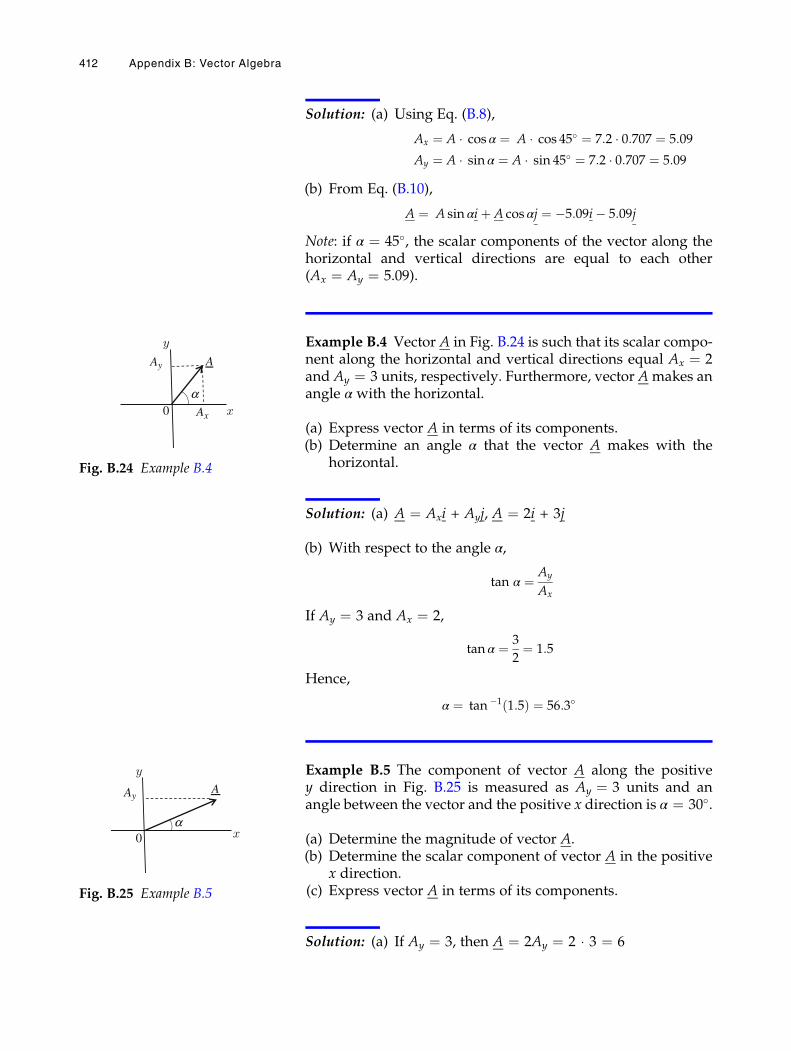
Solution: (a) Using Eq. (B.8),
Ax ¼ A � cos α ¼ A � cos 45� ¼ 7:2 � 0:707 ¼ 5:09
Ay ¼ A � sin α ¼ A � sin 45� ¼ 7:2 � 0:707 ¼ 5:09
(b) From Eq. (B.10),
A ¼ A sin αiþ A cos αj ¼ �5:09i� 5:09j
Note: if α ¼ 45�, the scalar components of the vector along thehorizontal and vertical directions are equal to each other(Ax ¼ Ay ¼ 5.09).
Example B.4 Vector A in Fig. B.24 is such that its scalar compo-nent along the horizontal and vertical directions equal Ax ¼ 2and Ay ¼ 3 units, respectively. Furthermore, vector Amakes anangle α with the horizontal.
(a) Express vector A in terms of its components.(b) Determine an angle α that the vector A makes with the
horizontal.
Solution: (a) A ¼ Axi + Ayj, A ¼ 2i + 3j
(b) With respect to the angle α,
tan α ¼ Ay
Ax
If Ay ¼ 3 and Ax ¼ 2,
tan α ¼ 3
2¼ 1:5
Hence,
α ¼ tan �1 1:5ð Þ ¼ 56:3�
Example B.5 The component of vector A along the positivey direction in Fig. B.25 is measured as Ay ¼ 3 units and anangle between the vector and the positive x direction is α ¼ 30�.
(a) Determine the magnitude of vector A.(b) Determine the scalar component of vector A in the positive
x direction.(c) Express vector A in terms of its components.
Solution: (a) If Ay ¼ 3, then A ¼ 2Ay ¼ 2 � 3 ¼ 6
x
y
0a
Ay
Ax
A
Fig. B.24 Example B.4
A
x
y
0a
Ay
Fig. B.25 Example B.5
412 Appendix B: Vector Algebra
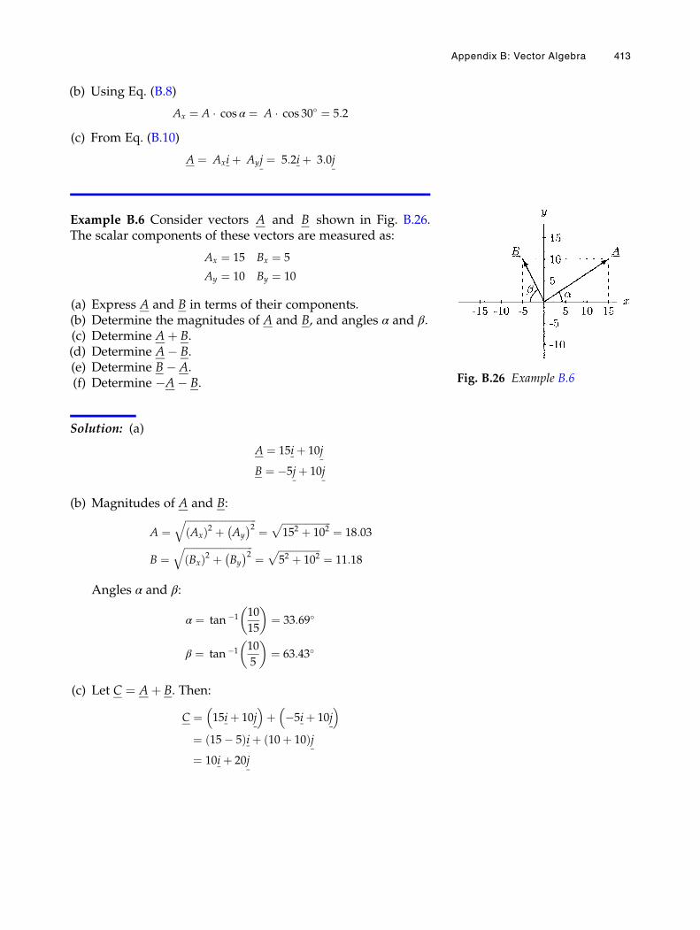
(b) Using Eq. (B.8)
Ax ¼ A � cos α ¼ A � cos 30� ¼ 5:2
(c) From Eq. (B.10)
A ¼ Axiþ Ayj ¼ 5:2iþ 3:0j
Example B.6 Consider vectors A and B shown in Fig. B.26.The scalar components of these vectors are measured as:
Ax ¼ 15 Bx ¼ 5
Ay ¼ 10 By ¼ 10
(a) Express A and B in terms of their components.(b) Determine the magnitudes of A and B, and angles α and β.(c) Determine Aþ B.(d) Determine A� B.(e) Determine B� A.(f) Determine �A� B.
Solution: (a)
A ¼ 15iþ 10j
B ¼ �5jþ 10j
(b) Magnitudes of A and B:
A ¼ffiffiffiffiffiffiffiffiffiffiffiffiffiffiffiffiffiffiffiffiffiffiffiffiffiffiffiffiffiAxð Þ2 þ Ay
� �2q¼
ffiffiffiffiffiffiffiffiffiffiffiffiffiffiffiffiffiffiffiffi152 þ 102
p¼ 18:03
B ¼ffiffiffiffiffiffiffiffiffiffiffiffiffiffiffiffiffiffiffiffiffiffiffiffiffiffiffiffiBxð Þ2 þ By
� �2q¼
ffiffiffiffiffiffiffiffiffiffiffiffiffiffiffiffiffi52 þ 102
p¼ 11:18
Angles α and β:
α ¼ tan �1 10
15
� ¼ 33:69�
β ¼ tan �1 10
5
� ¼ 63:43�
(c) Let C ¼ Aþ B. Then:
C ¼ 15iþ 10j� �
þ �5iþ 10j� �
¼ 15� 5ð Þiþ 10þ 10ð Þj¼ 10iþ 20j
Fig. B.26 Example B.6
Appendix B: Vector Algebra 413
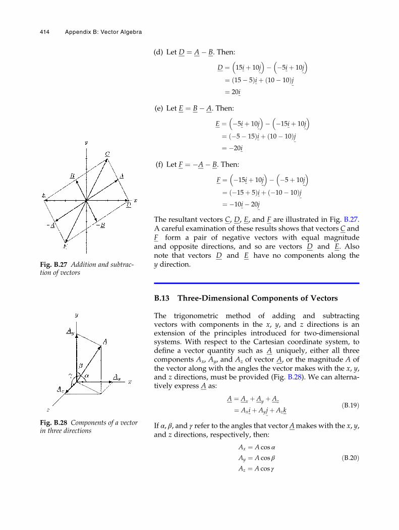
(d) Let D ¼ A� B. Then:
D ¼ 15iþ 10j� �
� �5iþ 10j� �
¼ 15� 5ð Þiþ 10� 10ð Þj¼ 20i
(e) Let E ¼ B� A. Then:
E ¼ �5iþ 10j� �
� �15iþ 10j� �
¼ �5� 15ð Þiþ 10� 10ð Þj¼ �20i
(f) Let F ¼ �A� B. Then:
F ¼ �15iþ 10j� �
� �5þ 10j� �
¼ �15þ 5ð Þiþ �10� 10ð Þj¼ �10i� 20j
The resultant vectors C, D, E, and F are illustrated in Fig. B.27.A careful examination of these results shows that vectors C andF form a pair of negative vectors with equal magnitudeand opposite directions, and so are vectors D and E. Alsonote that vectors D and E have no components along they direction.
B.13 Three-Dimensional Components of Vectors
The trigonometric method of adding and subtractingvectors with components in the x, y, and z directions is anextension of the principles introduced for two-dimensionalsystems. With respect to the Cartesian coordinate system, todefine a vector quantity such as A uniquely, either all threecomponents Ax, Ay, and Az of vector A, or the magnitude A ofthe vector along with the angles the vector makes with the x, y,and z directions, must be provided (Fig. B.28). We can alterna-tively express A as:
A ¼ Ax þ Ay þ Az
¼ Axiþ Ayjþ AzkðB:19Þ
If α, β, and γ refer to the angles that vectorAmakes with the x, y,and z directions, respectively, then:
Ax ¼ A cos α
Ay ¼ A cos β
Az ¼ A cos γ
ðB:20Þ
Fig. B.27 Addition and subtrac-tion of vectors
Fig. B.28 Components of a vectorin three directions
414 Appendix B: Vector Algebra
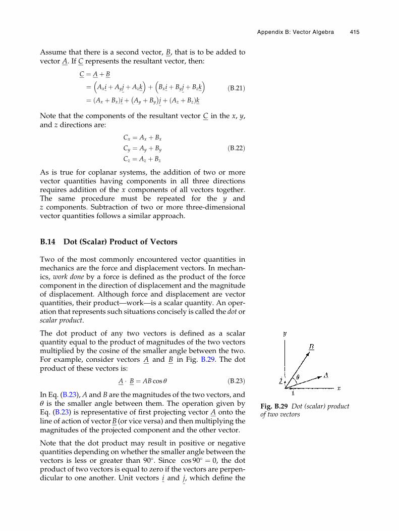
Assume that there is a second vector, B, that is to be added tovector A. If C represents the resultant vector, then:
C ¼ Aþ B
¼ Axiþ Ayjþ Azk� �
þ Bxiþ Byjþ Bzk� �
¼ Ax þ Bxð Þiþ Ay þ By
� �jþ Az þ Bzð Þk
ðB:21Þ
Note that the components of the resultant vector C in the x, y,and z directions are:
Cx ¼ Ax þ Bx
Cy ¼ Ay þ By
Cz ¼ Az þ Bz
ðB:22Þ
As is true for coplanar systems, the addition of two or morevector quantities having components in all three directionsrequires addition of the x components of all vectors together.The same procedure must be repeated for the y andz components. Subtraction of two or more three-dimensionalvector quantities follows a similar approach.
B.14 Dot (Scalar) Product of Vectors
Two of the most commonly encountered vector quantities inmechanics are the force and displacement vectors. In mechan-ics, work done by a force is defined as the product of the forcecomponent in the direction of displacement and the magnitudeof displacement. Although force and displacement are vectorquantities, their product—work—is a scalar quantity. An oper-ation that represents such situations concisely is called the dot orscalar product.
The dot product of any two vectors is defined as a scalarquantity equal to the product of magnitudes of the two vectorsmultiplied by the cosine of the smaller angle between the two.For example, consider vectors A and B in Fig. B.29. The dotproduct of these vectors is:
A � B ¼ AB cos θ ðB:23ÞIn Eq. (B.23),A and B are the magnitudes of the two vectors, andθ is the smaller angle between them. The operation given byEq. (B.23) is representative of first projecting vector A onto theline of action of vectorB (or vice versa) and then multiplying themagnitudes of the projected component and the other vector.
Note that the dot product may result in positive or negativequantities depending on whether the smaller angle between thevectors is less or greater than 90�. Since cos 90� ¼ 0, the dotproduct of two vectors is equal to zero if the vectors are perpen-dicular to one another. Unit vectors i and j, which define the
Fig. B.29 Dot (scalar) productof two vectors
Appendix B: Vector Algebra 415
positive x and y directions, respectively, are also vectorquantities with magnitudes equal to unity. The concept of thedot product is applicable to unit vectors as well:
i � i ¼ j � j ¼ k � k ¼ 1 � 1 � cos 0� ¼ 1
i � j ¼ j � k ¼ k � i ¼ 1 � 1 � cos 90� ¼ 0ðB:24Þ
To take the dot product of the vectors shown in Fig. B.29, we canfirst represent each vector in terms of its components along thex and y directions, and then apply the dot product to the unitvectors:
A � B ¼ Axiþ Ayj� �
� Bxiþ Byj� �
¼ AxBx i � i� �þ AyBy i � j� �
þ AyBx j � i� �
þ AyBy j � j� �
¼ AxBx þ AyBy
ðB:25Þ
The following are some of the properties of the dot product.
• The dot product of two vectors is a commutative operation:
A � B ¼ B � A• The dot product is a distributive operation:
A � Bþ C� � ¼ A � Bþ A � C
• A vector multiplied by itself as a dot product is equal to thesquare of the magnitude of the vector:
A � A ¼ A2
• The dot product of two three-dimensional vector quantitiesAand B expressed in terms of their Cartesian components is:
A � B ¼ AxBx þ AyBy þ AzBz
• The scalar component of a vector along a given directionis equal to the dot product of the vector times the unit vectoralong that direction. For example, the x and y components of avector A are:
Ax ¼ A � i Ay ¼ A � j
B.15 Cross (Vector) Product of Vectors
There are other interactions between vector quantities thatresult in other vector quantities. An example of suchinteractions is the moment or torque generated by an appliedforce. The mathematical tool developed to define suchinteractions is called the cross or vector product.
416 Appendix B: Vector Algebra
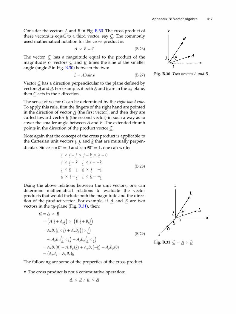
Consider the vectors A and B in Fig. B.30. The cross product ofthese vectors is equal to a third vector, say C. The commonlyused mathematical notation for the cross product is:
A � B ¼ C ðB:26ÞThe vector C has a magnitude equal to the product of themagnitudes of vectors C and B times the sine of the smallerangle (angle θ in Fig. B.30) between the two:
C ¼ AB sin θ ðB:27ÞVector C has a direction perpendicular to the plane defined byvectorsA andB. For example, if bothA andB are in the xy plane,then C acts in the z direction.
The sense of vector C can be determined by the right-hand rule.To apply this rule, first the fingers of the right hand are pointedin the direction of vector A (the first vector), and then they arecurled toward vector B (the second vector) in such a way as tocover the smaller angle between A and B. The extended thumbpoints in the direction of the product vector C.
Note again that the concept of the cross product is applicable tothe Cartesian unit vectors i, j, and k that are mutually perpen-
dicular. Since sin 0� ¼ 0 and sin 90� ¼ 1, one can write:
i � i ¼ j � j ¼ k � k ¼ 0
i � j ¼ k j � i ¼ �k
j � k ¼ i k � j ¼ �i
k � i ¼ j i � k ¼ �j
ðB:28Þ
Using the above relations between the unit vectors, one candetermine mathematical relations to evaluate the vectorproducts that would include both the magnitude and the direc-tion of the product vector. For example, if A and B are twovectors in the xy-plane (Fig. B.31), then:
C ¼ A � B
¼ Axiþ Ayj� �
� Bxiþ Byj� �
¼ AxBx i� i� �þ AxBy i� j
� �þ AyBx j� i
� �þ AyBy j� j
� �¼ AxBx 0ð Þ þ AxBy k
� �þ AyBx �k� �þ AyBy 0ð Þ
¼ AxBy � AyBx
� �k
ðB:29Þ
The following are some of the properties of the cross product.
• The cross product is not a commutative operation:
A � B 6¼ B � A
Fig. B.30 Two vectors A and B
Fig. B.31 C ¼ A � B
Appendix B: Vector Algebra 417
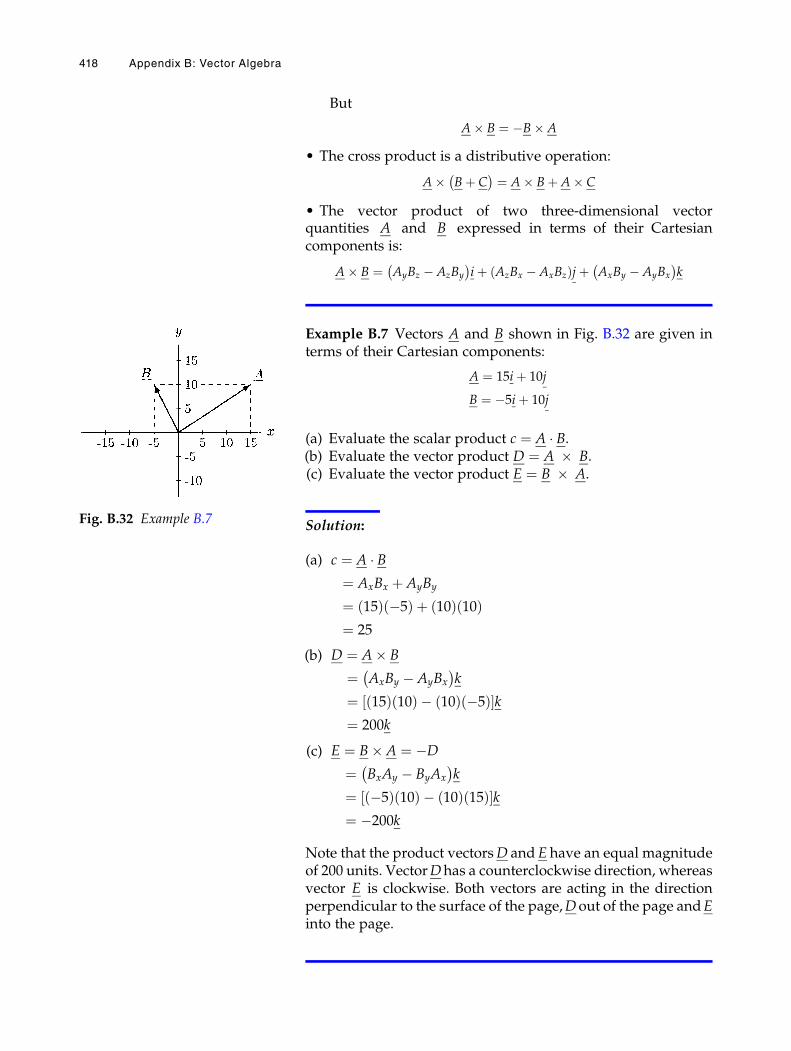
But
A� B ¼ �B� A
• The cross product is a distributive operation:
A� Bþ C� � ¼ A� Bþ A� C
• The vector product of two three-dimensional vectorquantities A and B expressed in terms of their Cartesiancomponents is:
A� B ¼ AyBz � AzBy
� �iþ AzBx � AxBzð Þjþ AxBy � AyBx
� �k
Example B.7 Vectors A and B shown in Fig. B.32 are given interms of their Cartesian components:
A ¼ 15iþ 10j
B ¼ �5iþ 10j
(a) Evaluate the scalar product c ¼ A � B.(b) Evaluate the vector product D ¼ A � B.(c) Evaluate the vector product E ¼ B � A.
Solution:
(a) c ¼ A � B¼ AxBx þ AyBy
¼ 15ð Þ �5ð Þ þ 10ð Þ 10ð Þ¼ 25
(b) D ¼ A� B
¼ AxBy � AyBx
� �k
¼ 15ð Þ 10ð Þ � 10ð Þ �5ð Þ½ �k¼ 200k
(c) E ¼ B� A ¼ �D
¼ BxAy � ByAx
� �k
¼ �5ð Þ 10ð Þ � 10ð Þ 15ð Þ½ �k¼ �200k
Note that the product vectorsD and E have an equal magnitudeof 200 units. VectorDhas a counterclockwise direction, whereasvector E is clockwise. Both vectors are acting in the directionperpendicular to the surface of the page,Dout of the page andEinto the page.
Fig. B.32 Example B.7
418 Appendix B: Vector Algebra
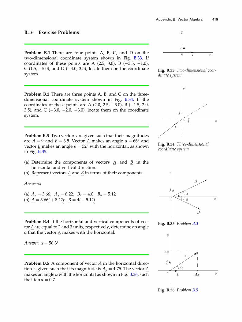
B.16 Exercise Problems
Problem B.1 There are four points A, B, C, and D on thetwo-dimensional coordinate system shown in Fig. B.33. Ifcoordinates of these points are A (2.5, 3.0), B (�3.5, �1.0),C (1.5, �5.0), and D (�4.0, 3.5), locate them on the coordinatesystem.
Problem B.2 There are three points A, B, and C on the three-dimensional coordinate system shown in Fig. B.34. If thecoordinates of these points are A (2.0, 2.5, �3.0), B (�1.5, 2.0,3.5), and C (�3.0, �2.0, �3.0), locate them on the coordinatesystem.
Problem B.3 Two vectors are given such that their magnitudesare A ¼ 9 and B ¼ 6:5. Vector A makes an angle α ¼ 66� andvector B makes an angle β ¼ 52� with the horizontal, as shownin Fig. B.35.
(a) Determine the components of vectors A and B in thehorizontal and vertical direction.
(b) Represent vectors A and B in terms of their components.
Answers:
(a) Ax ¼ 3:66; Ay ¼ 8:22; Bx ¼ 4:0; By ¼ 5:12
(b) A ¼ 3:66iþ 8:22j; B ¼ 4i� 5:12j
Problem B.4 If the horizontal and vertical components of vec-torA are equal to 2 and 3 units, respectively, determine an angleα that the vector A makes with the horizontal.
Answer: α ¼ 56:3�
Problem B.5 A component of vector A in the horizontal direc-tion is given such that its magnitude is Ay ¼ 4:75. The vector A
makes an angle αwith the horizontal as shown in Fig. B.36, suchthat tan α ¼ 0:7:
Fig. B.33 Two-dimensional coor-dinate system
k
Fig. B.34 Three-dimensionalcoordinate system
Fig. B.35 Problem B.3
Fig. B.36 Problem B.5
Appendix B: Vector Algebra 419
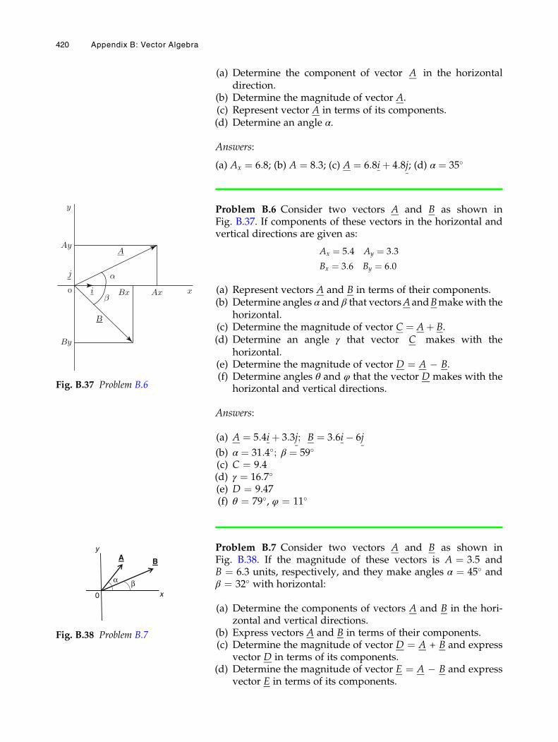
(a) Determine the component of vector A in the horizontaldirection.
(b) Determine the magnitude of vector A.(c) Represent vector A in terms of its components.(d) Determine an angle α.
Answers:
(a) Ax ¼ 6:8; (b) A ¼ 8:3; (c) A ¼ 6:8iþ 4:8j; (d) α ¼ 35�
Problem B.6 Consider two vectors A and B as shown inFig. B.37. If components of these vectors in the horizontal andvertical directions are given as:
Ax ¼ 5:4 Ay ¼ 3:3
Bx ¼ 3:6 By ¼ 6:0
(a) Represent vectors A and B in terms of their components.(b) Determine angles α and β that vectorsAandBmake with the
horizontal.(c) Determine the magnitude of vector C ¼ Aþ B.(d) Determine an angle γ that vector C makes with the
horizontal.(e) Determine the magnitude of vector D ¼ A � B.(f) Determine angles θ and φ that the vector D makes with the
horizontal and vertical directions.
Answers:
(a) A ¼ 5:4iþ 3:3j; B ¼ 3:6i� 6j
(b) α ¼ 31:4�; β ¼ 59�
(c) C ¼ 9.4(d) γ ¼ 16:7�
(e) D ¼ 9.47(f) θ ¼ 79�, φ ¼ 11�
Problem B.7 Consider two vectors A and B as shown inFig. B.38. If the magnitude of these vectors is A ¼ 3.5 andB ¼ 6.3 units, respectively, and they make angles α ¼ 45� andβ ¼ 32� with horizontal:
(a) Determine the components of vectors A and B in the hori-zontal and vertical directions.
(b) Express vectors A and B in terms of their components.(c) Determine the magnitude of vector D ¼ A + B and express
vector D in terms of its components.(d) Determine the magnitude of vector E ¼ A � B and express
vector E in terms of its components.
B
Fig. B.37 Problem B.6
A
x
y
0
α β
B
Fig. B.38 Problem B.7
420 Appendix B: Vector Algebra

(e) Determine the magnitude of vector F ¼ B � A and expressvector F in terms of its components.
(f) Determine the magnitude of vector G ¼ �A � B andexpress vector G in terms of its components.
Answers:
(a) Ax ¼ 2.47, Ay ¼ 2.47; Bx ¼ 5.34, By ¼ 3.34(b) A ¼ 2.47i + 2.47j(c) D ¼ 9.73, D ¼ 7.81i + 5.81j(d) E ¼ 2.99, E ¼ �2.87i � 0.87j(e) F ¼ 2.99, F ¼ 2.87i + 0.87j(f) G ¼ 9.73, G ¼ �7.81i � 5.81j
Problem B.8 Consider three vectors A, B, and C as shown inFig. B.39. If the magnitude of these vectorsA ¼ 4.5, B ¼ 7.0, andC ¼ 5 units, respectively, and they make angles α ¼ 35�,β ¼ 65�, and γ ¼ 27� with the horizontal:
(a) Determine the components of vectors A, B, and C in thehorizontal and vertical directions.
(b) Express vectors A, B, and C in terms of their components.(c) Determine vector D ¼ A + B + C.(d) Determine the magnitude of vector D and an angle θ it
makes with the horizontal.(e) Determine vector E ¼ A + B � C.(f) Determine the magnitude of vector E and an angle λ it
makes with the horizontal.(g) Determine vector F ¼ A � B � C.(h) Determine the magnitude of vector F and an angle φ it
makes with the vertical.(i) Determine vector G ¼ �A � B � C.(j) Determine the magnitude of vector G and an angle ϕ it
makes with the vertical.
Answers:
(a) Ax ¼ 3.69, Ay ¼ 2.57; Bx ¼ 2.96, By ¼ 6.34; Cx ¼ 4.46,Cy ¼ 2.27
(b) A ¼ 3.69i + 2.57j; B ¼ 2.96i + 6.34j; C ¼ �4.46i + 2.27j(c) D ¼ 2.19i + 1.18j(d) D ¼ 11.4; θ ¼ 78.9�
(e) E ¼ 11.11i + 6.64j(f) E ¼ 12.9; λ ¼ 30.9�
(g) F ¼ 5.19i � 6.04j(h) F ¼ 7.96; φ ¼ 40.7�
(i) G ¼ �2.19i � 11.18j(j) G ¼ 11.4; ϕ ¼ 11.1�
A
x
y
0α
β
B
Cγ
Fig. B.39 Problem B.8
Appendix B: Vector Algebra 421
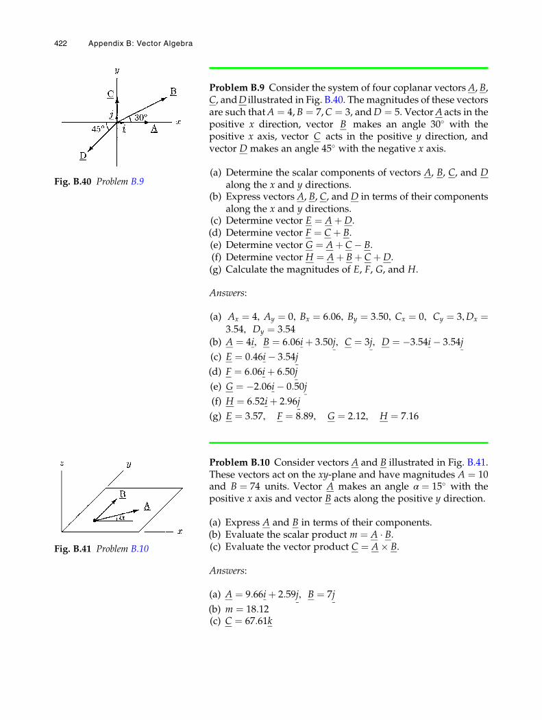
Problem B.9 Consider the system of four coplanar vectorsA, B,C, andD illustrated in Fig. B.40. Themagnitudes of these vectorsare such thatA ¼ 4,B ¼ 7,C ¼ 3, andD ¼ 5. VectorA acts in thepositive x direction, vector B makes an angle 30� with thepositive x axis, vector C acts in the positive y direction, andvector D makes an angle 45� with the negative x axis.
(a) Determine the scalar components of vectors A, B, C, and Dalong the x and y directions.
(b) Express vectors A, B, C, andD in terms of their componentsalong the x and y directions.
(c) Determine vector E ¼ AþD.(d) Determine vector F ¼ Cþ B.(e) Determine vector G ¼ Aþ C� B.(f) Determine vector H ¼ Aþ Bþ CþD.(g) Calculate the magnitudes of E, F, G, and H.
Answers:
(a) Ax ¼ 4, Ay ¼ 0, Bx ¼ 6:06, By ¼ 3:50, Cx ¼ 0, Cy ¼ 3,Dx ¼3:54, Dy ¼ 3:54
(b) A ¼ 4i, B ¼ 6:06iþ 3:50j, C ¼ 3j, D ¼ �3:54i� 3:54j
(c) E ¼ 0:46i� 3:54j
(d) F ¼ 6:06iþ 6:50j
(e) G ¼ �2:06i� 0:50j
(f) H ¼ 6:52iþ 2:96j
(g) E ¼ 3:57, F ¼ 8:89, G ¼ 2:12, H ¼ 7:16
Problem B.10 Consider vectors A and B illustrated in Fig. B.41.These vectors act on the xy-plane and have magnitudes A ¼ 10and B ¼ 74 units. Vector A makes an angle α ¼ 15� with thepositive x axis and vector B acts along the positive y direction.
(a) Express A and B in terms of their components.(b) Evaluate the scalar product m ¼ A � B.(c) Evaluate the vector product C ¼ A� B.
Answers:
(a) A ¼ 9:66iþ 2:59j, B ¼ 7j
(b) m ¼ 18:12(c) C ¼ 67:61k
Fig. B.40 Problem B.9
Fig. B.41 Problem B.10
422 Appendix B: Vector Algebra
Appendix C:
Calculus
C.1 Functions / 425
C.2 The Derivative / 432
C.3 The Integral / 439
C.4 Trigonometric Identities / 445
C.5 The Quadratic Formula / 446
C.6 Exercise Problems / 447
# Springer International Publishing Switzerland 2017N. Ozkaya et al., Fundamentals of Biomechanics, DOI 10.1007/978-3-319-44738-4
423
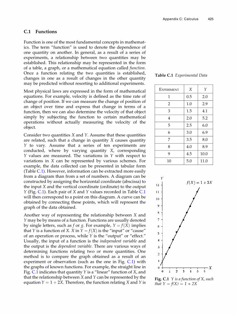
C.1 Functions
Function is one of the most fundamental concepts in mathemat-ics. The term “function” is used to denote the dependence ofone quantity on another. In general, as a result of a series ofexperiments, a relationship between two quantities may beestablished. This relationship may be represented in the formof a table, a graph, or a mathematical equation called function.Once a function relating the two quantities is established,changes in one as a result of changes in the other quantitymay be predicted without resorting to additional experiments.
Most physical laws are expressed in the form of mathematicalequations. For example, velocity is defined as the time rate ofchange of position. If we can measure the change of position ofan object over time and express that change in terms of afunction, then we can also determine the velocity of that objectsimply by subjecting the function to certain mathematicaloperations without actually measuring the velocity of theobject.
Consider two quantities X and Y. Assume that these quantitiesare related, such that a change in quantity X causes quantityY to vary. Assume that a series of ten experiments areconducted, where by varying quantity X, correspondingY values are measured. The variations in Y with respect tovariations in X can be represented by various schemes. Forexample, the data collected can be presented in tabular form(Table C.1). However, information can be extracted more easilyfrom a diagram than from a set of numbers. A diagram can beconstructed by assigning the horizontal coordinate (abscissa) tothe input X and the vertical coordinate (ordinate) to the outputY (Fig. C.1). Each pair of X and Y values recorded in Table C.1will then correspond to a point on this diagram. A curve can beobtained by connecting these points, which will represent thegraph of the data obtained.
Another way of representing the relationship between X andYmay be by means of a function. Functions are usually denotedby single letters, such as f or g. For example, Y ¼ f Xð Þ impliesthat Y is a function of X. X in Y ¼ f Xð Þ is the “input” or “cause”of an operation or process, while Y is the “output” or “effect.”Usually, the input of a function is the independent variable andthe output is the dependent variable. There are various ways ofdetermining functions relating two or more quantities. Onemethod is to compare the graph obtained as a result of anexperiment or observation (such as the one in Fig. C.1) withthe graphs of known functions. For example, the straight line inFig. C.1 indicates that quantity Y is a “linear” function of X, andthat the relationship between X and Y can be represented by theequationY ¼ 1þ 2X. Therefore, the function relating X and Y is
Table C.1 Experimental Data
EXPERIMENT X Y
1 0.5 2.0
2 1.0 2.9
3 1.5 4.1
4 2.0 5.2
5 2.5 6.0
6 3.0 6.9
7 3.5 8.0
8 4.0 8.9
9 4.5 10.0
10 5.0 11.0
Fig. C.1 Y is a function of X, suchthat Y ¼ f(X) ¼ 1 + 2X
Appendix C: Calculus 425
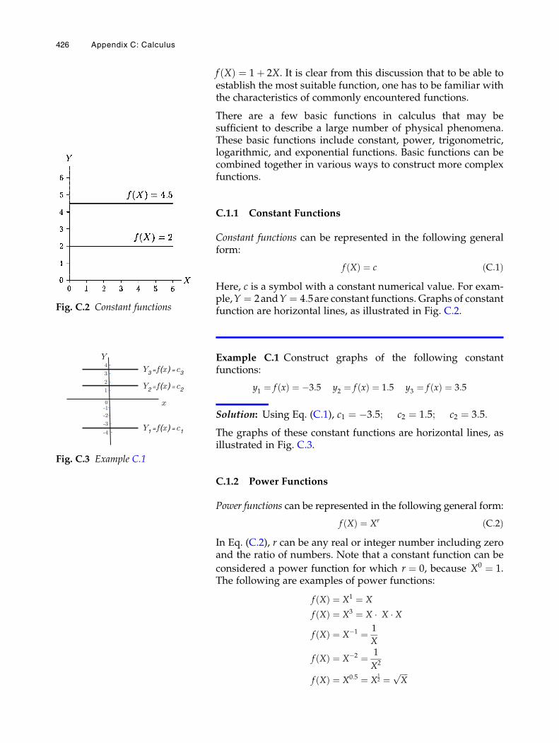
f Xð Þ ¼ 1þ 2X. It is clear from this discussion that to be able toestablish the most suitable function, one has to be familiar withthe characteristics of commonly encountered functions.
There are a few basic functions in calculus that may besufficient to describe a large number of physical phenomena.These basic functions include constant, power, trigonometric,logarithmic, and exponential functions. Basic functions can becombined together in various ways to construct more complexfunctions.
C.1.1 Constant Functions
Constant functions can be represented in the following generalform:
f Xð Þ ¼ c ðC:1ÞHere, c is a symbol with a constant numerical value. For exam-ple,Y ¼ 2andY ¼ 4:5are constant functions. Graphs of constantfunction are horizontal lines, as illustrated in Fig. C.2.
Example C.1 Construct graphs of the following constantfunctions:
y1 ¼ f xð Þ ¼ �3:5 y2 ¼ f xð Þ ¼ 1:5 y3 ¼ f xð Þ ¼ 3:5
Solution: Using Eq. (C.1), c1 ¼ �3:5; c2 ¼ 1:5; c2 ¼ 3:5:
The graphs of these constant functions are horizontal lines, asillustrated in Fig. C.3.
C.1.2 Power Functions
Power functions can be represented in the following general form:
f Xð Þ ¼ Xr ðC:2ÞIn Eq. (C.2), r can be any real or integer number including zeroand the ratio of numbers. Note that a constant function can be
considered a power function for which r ¼ 0, because X0 ¼ 1.The following are examples of power functions:
f Xð Þ ¼ X1 ¼ X
f Xð Þ ¼ X3 ¼ X � X � Xf Xð Þ ¼ X�1 ¼ 1
X
f Xð Þ ¼ X�2 ¼ 1
X2
f Xð Þ ¼ X0:5 ¼ X12 ¼ ffiffiffiffi
Xp
Fig. C.2 Constant functions
Fig. C.3 Example C.1
426 Appendix C: Calculus
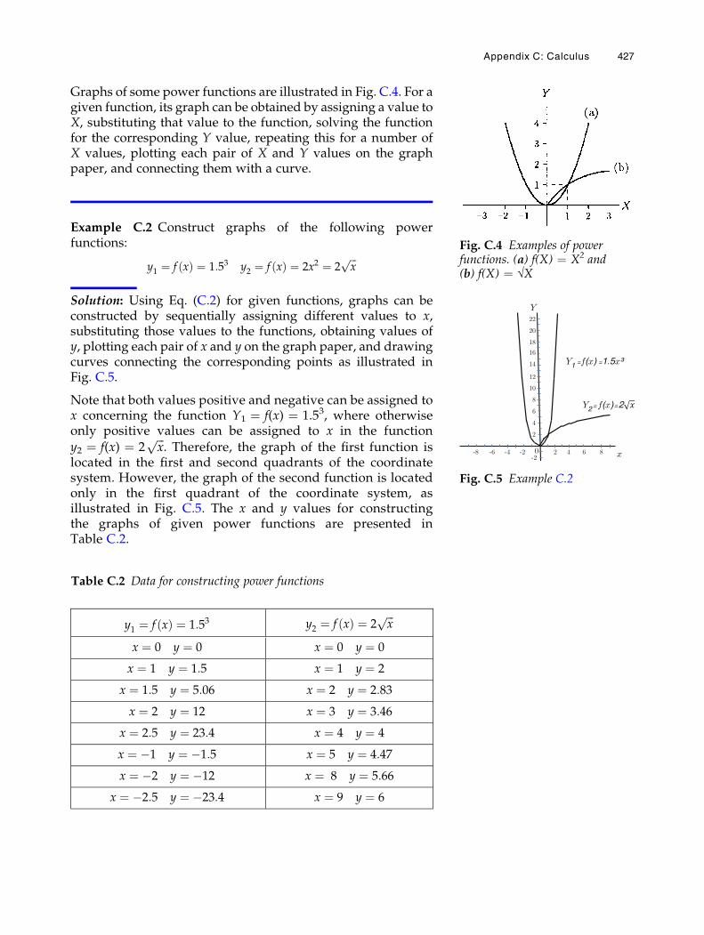
Graphs of some power functions are illustrated in Fig. C.4. For agiven function, its graph can be obtained by assigning a value toX, substituting that value to the function, solving the functionfor the corresponding Y value, repeating this for a number ofX values, plotting each pair of X and Y values on the graphpaper, and connecting them with a curve.
Example C.2 Construct graphs of the following powerfunctions:
y1 ¼ f xð Þ ¼ 1:53 y2 ¼ f xð Þ ¼ 2x2 ¼ 2ffiffiffix
p
Solution: Using Eq. (C.2) for given functions, graphs can beconstructed by sequentially assigning different values to x,substituting those values to the functions, obtaining values ofy, plotting each pair of x and y on the graph paper, and drawingcurves connecting the corresponding points as illustrated inFig. C.5.
Note that both values positive and negative can be assigned tox concerning the function Y1 ¼ f(x) ¼ 1.53, where otherwiseonly positive values can be assigned to x in the functiony2 ¼ f(x) ¼ 2
ffiffiffix
p. Therefore, the graph of the first function is
located in the first and second quadrants of the coordinatesystem. However, the graph of the second function is locatedonly in the first quadrant of the coordinate system, asillustrated in Fig. C.5. The x and y values for constructingthe graphs of given power functions are presented inTable C.2.
Fig. C.4 Examples of powerfunctions. (a) f(X) ¼ X2 and(b) f(X) ¼ √X
Fig. C.5 Example C.2
Table C.2 Data for constructing power functions
y1 ¼ f xð Þ ¼ 1:53 y2 ¼ f xð Þ ¼ 2ffiffiffix
p
x ¼ 0 y ¼ 0 x ¼ 0 y ¼ 0
x ¼ 1 y ¼ 1:5 x ¼ 1 y ¼ 2
x ¼ 1:5 y ¼ 5:06 x ¼ 2 y ¼ 2:83
x ¼ 2 y ¼ 12 x ¼ 3 y ¼ 3:46
x ¼ 2:5 y ¼ 23:4 x ¼ 4 y ¼ 4
x ¼ �1 y ¼ �1:5 x ¼ 5 y ¼ 4:47
x ¼ �2 y ¼ �12 x ¼ 8 y ¼ 5:66
x ¼ �2:5 y ¼ �23:4 x ¼ 9 y ¼ 6
Appendix C: Calculus 427
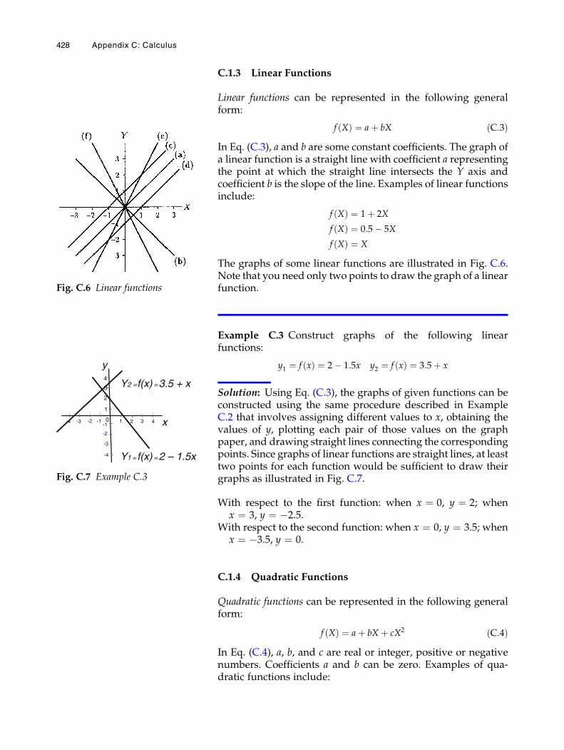
C.1.3 Linear Functions
Linear functions can be represented in the following generalform:
f Xð Þ ¼ aþ bX ðC:3ÞIn Eq. (C.3), a and b are some constant coefficients. The graph ofa linear function is a straight line with coefficient a representingthe point at which the straight line intersects the Y axis andcoefficient b is the slope of the line. Examples of linear functionsinclude:
f Xð Þ ¼ 1þ 2X
f Xð Þ ¼ 0:5� 5X
f Xð Þ ¼ X
The graphs of some linear functions are illustrated in Fig. C.6.Note that you need only two points to draw the graph of a linearfunction.
Example C.3 Construct graphs of the following linearfunctions:
y1 ¼ f xð Þ ¼ 2� 1:5x y2 ¼ f xð Þ ¼ 3:5þ x
Solution: Using Eq. (C.3), the graphs of given functions can beconstructed using the same procedure described in ExampleC.2 that involves assigning different values to x, obtaining thevalues of y, plotting each pair of those values on the graphpaper, and drawing straight lines connecting the correspondingpoints. Since graphs of linear functions are straight lines, at leasttwo points for each function would be sufficient to draw theirgraphs as illustrated in Fig. C.7.
With respect to the first function: when x ¼ 0, y ¼ 2; whenx ¼ 3, y ¼ �2.5.
With respect to the second function: when x ¼ 0, y ¼ 3.5; whenx ¼ �3.5, y ¼ 0.
C.1.4 Quadratic Functions
Quadratic functions can be represented in the following generalform:
f Xð Þ ¼ aþ bX þ cX2 ðC:4ÞIn Eq. (C.4), a, b, and c are real or integer, positive or negativenumbers. Coefficients a and b can be zero. Examples of qua-dratic functions include:
Fig. C.6 Linear functions
x
y
0
1
-1
-2
-3
-4
2
3
4
-1 -2 -4 -3 1 3 2 4
Y1 = f(x) = 2 – 1.5x
Y2 = f(x) = 3.5 + x
Fig. C.7 Example C.3
428 Appendix C: Calculus
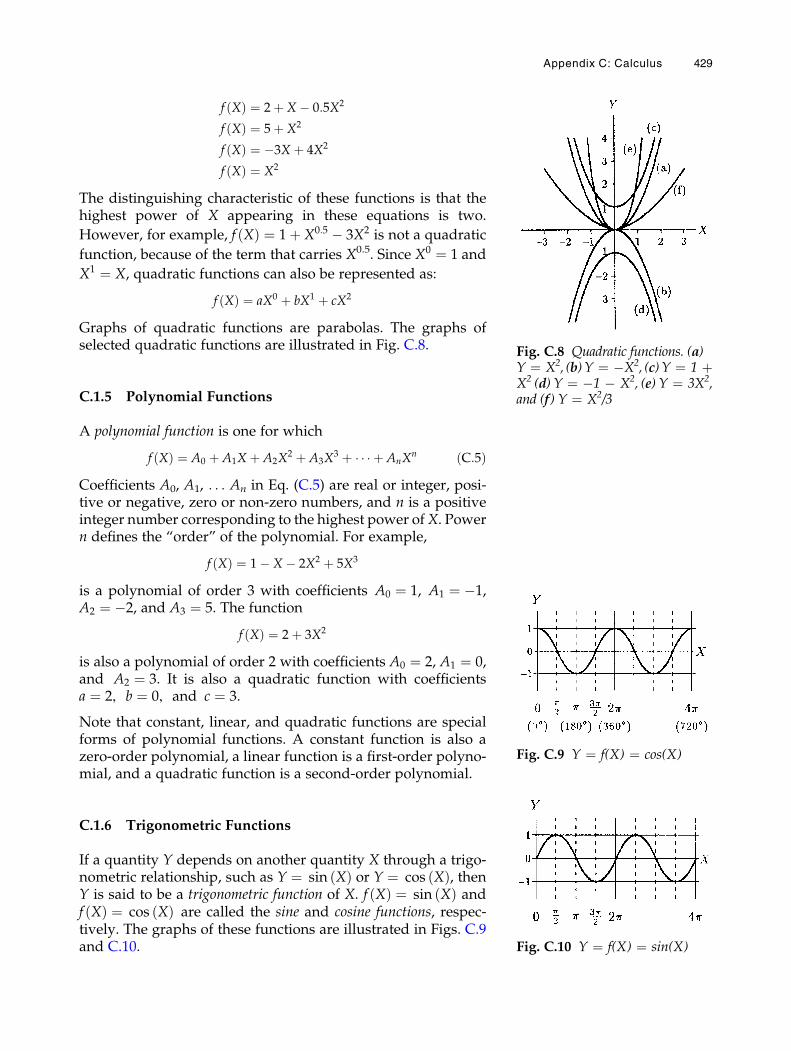
f Xð Þ ¼ 2þ X � 0:5X2
f Xð Þ ¼ 5þ X2
f Xð Þ ¼ �3X þ 4X2
f Xð Þ ¼ X2
The distinguishing characteristic of these functions is that thehighest power of X appearing in these equations is two.
However, for example, f Xð Þ ¼ 1þ X0:5 � 3X2 is not a quadratic
function, because of the term that carries X0.5. Since X0 ¼ 1 and
X1 ¼ X, quadratic functions can also be represented as:
f Xð Þ ¼ aX0 þ bX1 þ cX2
Graphs of quadratic functions are parabolas. The graphs ofselected quadratic functions are illustrated in Fig. C.8.
C.1.5 Polynomial Functions
A polynomial function is one for which
f Xð Þ ¼ A0 þ A1X þ A2X2 þ A3X
3 þ � � � þ AnXn ðC:5Þ
Coefficients A0, A1, . . . An in Eq. (C.5) are real or integer, posi-tive or negative, zero or non-zero numbers, and n is a positiveinteger number corresponding to the highest power ofX. Powern defines the “order” of the polynomial. For example,
f Xð Þ ¼ 1� X � 2X2 þ 5X3
is a polynomial of order 3 with coefficients A0 ¼ 1, A1 ¼ �1,A2 ¼ �2, and A3 ¼ 5. The function
f Xð Þ ¼ 2þ 3X2
is also a polynomial of order 2 with coefficients A0 ¼ 2, A1 ¼ 0,and A2 ¼ 3. It is also a quadratic function with coefficientsa ¼ 2, b ¼ 0, and c ¼ 3.
Note that constant, linear, and quadratic functions are specialforms of polynomial functions. A constant function is also azero-order polynomial, a linear function is a first-order polyno-mial, and a quadratic function is a second-order polynomial.
C.1.6 Trigonometric Functions
If a quantity Y depends on another quantity X through a trigo-nometric relationship, such as Y ¼ sin Xð Þ or Y ¼ cos Xð Þ, thenY is said to be a trigonometric function of X. f Xð Þ ¼ sin Xð Þ andf Xð Þ ¼ cos Xð Þ are called the sine and cosine functions, respec-tively. The graphs of these functions are illustrated in Figs. C.9and C.10.
Fig. C.8 Quadratic functions. (a)Y ¼ X2, (b) Y ¼ �X2, (c) Y ¼ 1 þX2 (d) Y ¼ �1 � X2, (e) Y ¼ 3X2,and (f) Y ¼ X2/3
Fig. C.9 Y ¼ f(X) ¼ cos(X)
Fig. C.10 Y ¼ f(X) ¼ sin(X)
Appendix C: Calculus 429
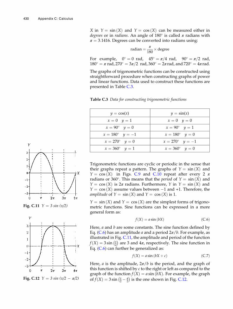
X in Y ¼ sin Xð Þ and Y ¼ cos Xð Þ can be measured either indegrees or in radians. An angle of 180� is called π radians withπ ¼ 3:1416. Degrees can be converted into radians using:
radian ¼ π
180� degree
For example, 0� ¼ 0 rad, 45� ¼ π=4 rad, 90� ¼ π=2 rad,180� ¼ π rad, 270� ¼ 3π=2 rad, 360� ¼ 2π rad, and720� ¼ 4π rad.
The graphs of trigonometric functions can be constructed usingstraightforward procedure when constructing graphs of powerand linear functions. Data used to construct these functions arepresented in Table C.3.
Trigonometric functions are cyclic or periodic in the sense thattheir graphs repeat a pattern. The graphs of Y ¼ sin Xð Þ andY ¼ cos Xð Þ in Figs. C.9 and C.10 repeat after every 2 πradians or 360�. This means that the period of Y ¼ sin Xð Þ andY ¼ cos Xð Þ is 2π radians. Furthermore, Y in Y ¼ sin Xð Þ andY ¼ cos Xð Þ assume values between �1 and +1. Therefore, theamplitude of Y ¼ sin Xð Þ and Y ¼ cos Xð Þ is 1.Y ¼ sin Xð Þ and Y ¼ cos Xð Þ are the simplest forms of trigono-metric functions. Sine functions can be expressed in a moregeneral form as:
f Xð Þ ¼ a sin bXð Þ ðC:6ÞHere, a and b are some constants. The sine function defined byEq. (C.6) has an amplitude a and a period 2π/b. For example, asillustrated in Fig. C.11, the amplitude and period of the function
f Xð Þ ¼ 3 sin x2
� �are 3 and 4π, respectively. The sine function in
Eq. (C.6) can further be generalized as:
f Xð Þ ¼ a sin bX þ cð Þ ðC:7ÞHere, a is the amplitude, 2π/b is the period, and the graph ofthis function is shifted by c to the right or left as compared to thegraph of the function f Xð Þ ¼ a sin bXð Þ. For example, the graph
of f Xð Þ ¼ 3 sin x2 � π
2
� �is the one shown in Fig. C.12.
Table C.3 Data for constructing trigonometric functions
y ¼ cos(x) y ¼ sin(x)
x ¼ 0 y ¼ 1 x ¼ 0 y ¼ 0
x ¼ 90� y ¼ 0 x ¼ 90� y ¼ 1
x ¼ 180� y ¼ �1 x ¼ 180� y ¼ 0
x ¼ 270� y ¼ 0 x ¼ 270� y ¼ �1
x ¼ 360� y ¼ 1 x ¼ 360� y ¼ 0
Fig. C.11 Y ¼ 3 sin (x/2)
Fig. C.12 Y ¼ 3 sin (x/2 � π/2)
430 Appendix C: Calculus
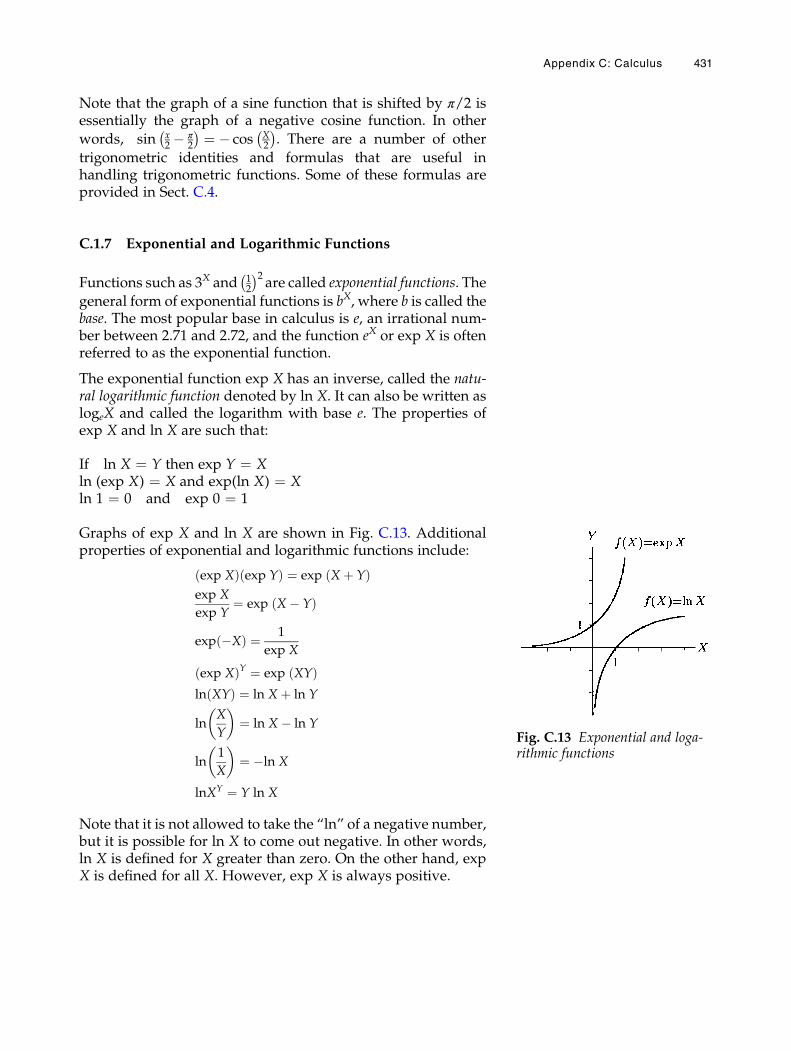
Note that the graph of a sine function that is shifted by π/2 isessentially the graph of a negative cosine function. In other
words, sin x2 � π
2
� � ¼ � cos X2
� �. There are a number of other
trigonometric identities and formulas that are useful inhandling trigonometric functions. Some of these formulas areprovided in Sect. C.4.
C.1.7 Exponential and Logarithmic Functions
Functions such as 3X and 12
� �2are called exponential functions. The
general form of exponential functions is bX, where b is called thebase. The most popular base in calculus is e, an irrational num-ber between 2.71 and 2.72, and the function eX or exp X is oftenreferred to as the exponential function.
The exponential function exp X has an inverse, called the natu-ral logarithmic function denoted by ln X. It can also be written aslogeX and called the logarithm with base e. The properties ofexp X and ln X are such that:
If ln X ¼ Y then exp Y ¼ Xln (exp X) ¼ X and exp(ln X) ¼ Xln 1 ¼ 0 and exp 0 ¼ 1
Graphs of exp X and ln X are shown in Fig. C.13. Additionalproperties of exponential and logarithmic functions include:
exp Xð Þ exp Yð Þ ¼ exp X þ Yð Þexp X
exp Y¼ exp X � Yð Þ
exp �Xð Þ ¼ 1
exp X
exp Xð ÞY ¼ exp XYð Þln XYð Þ ¼ ln X þ ln Y
lnX
Y
� ¼ ln X � ln Y
ln1
X
� ¼ �ln X
lnXY ¼ Y ln X
Note that it is not allowed to take the “ln” of a negative number,but it is possible for ln X to come out negative. In other words,ln X is defined for X greater than zero. On the other hand, expX is defined for all X. However, exp X is always positive.
Fig. C.13 Exponential and loga-rithmic functions
Appendix C: Calculus 431
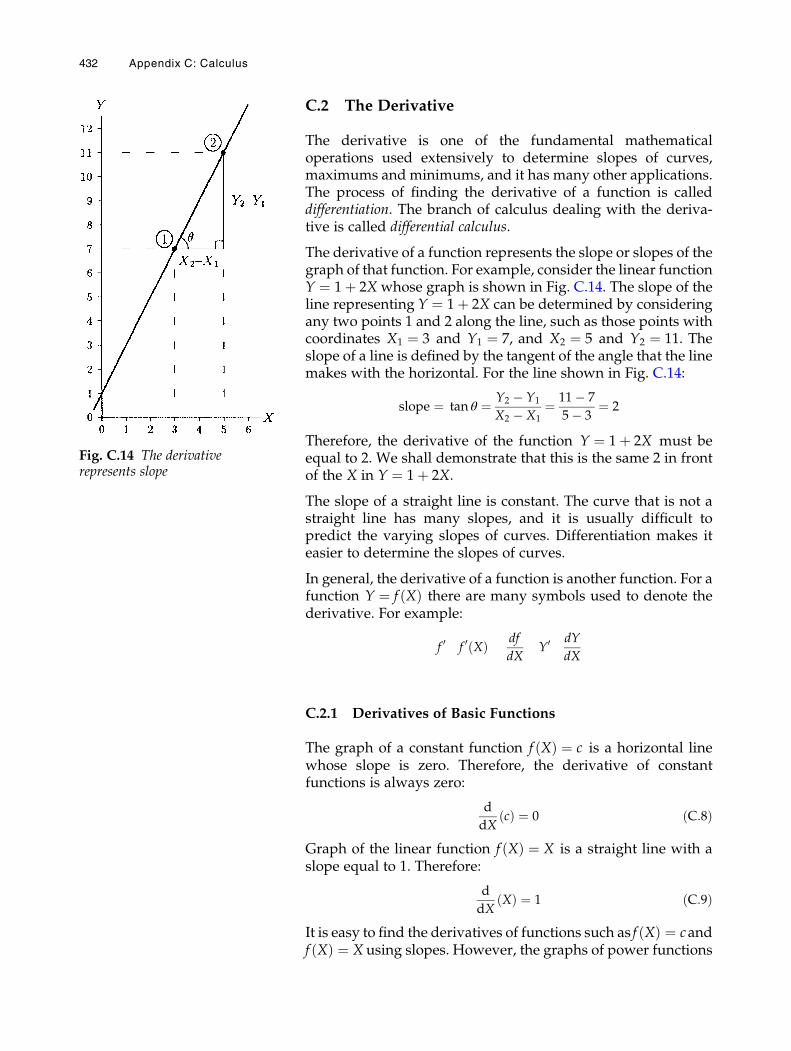
C.2 The Derivative
The derivative is one of the fundamental mathematicaloperations used extensively to determine slopes of curves,maximums and minimums, and it has many other applications.The process of finding the derivative of a function is calleddifferentiation. The branch of calculus dealing with the deriva-tive is called differential calculus.
The derivative of a function represents the slope or slopes of thegraph of that function. For example, consider the linear functionY ¼ 1þ 2X whose graph is shown in Fig. C.14. The slope of theline representing Y ¼ 1þ 2X can be determined by consideringany two points 1 and 2 along the line, such as those points withcoordinates X1 ¼ 3 and Y1 ¼ 7, and X2 ¼ 5 and Y2 ¼ 11. Theslope of a line is defined by the tangent of the angle that the linemakes with the horizontal. For the line shown in Fig. C.14:
slope ¼ tan θ ¼ Y2 � Y1
X2 � X1¼ 11� 7
5� 3¼ 2
Therefore, the derivative of the function Y ¼ 1þ 2X must beequal to 2. We shall demonstrate that this is the same 2 in frontof the X in Y ¼ 1þ 2X.
The slope of a straight line is constant. The curve that is not astraight line has many slopes, and it is usually difficult topredict the varying slopes of curves. Differentiation makes iteasier to determine the slopes of curves.
In general, the derivative of a function is another function. For afunction Y ¼ f Xð Þ there are many symbols used to denote thederivative. For example:
f 0 f 0 Xð Þ df
dXY0 dY
dX
C.2.1 Derivatives of Basic Functions
The graph of a constant function f Xð Þ ¼ c is a horizontal linewhose slope is zero. Therefore, the derivative of constantfunctions is always zero:
d
dXcð Þ ¼ 0 ðC:8Þ
Graph of the linear function f Xð Þ ¼ X is a straight line with aslope equal to 1. Therefore:
d
dXXð Þ ¼ 1 ðC:9Þ
It is easy to find the derivatives of functions such as f Xð Þ ¼ candf Xð Þ ¼ X using slopes. However, the graphs of power functions
Fig. C.14 The derivativerepresents slope
432 Appendix C: Calculus
such asX3,ffiffiffiffiX
p, andX�2 have varying slopes, and it is not easy to
predict their derivatives. To differentiate a power function Xr,multiply the function by its power and reduce the power by 1:
d
dXXrð Þ ¼ rXr�1 ðC:10Þ
Equation (C.10) is known as the Power Rule. The followingexamples illustrate the use of the Power Rule.
FUNCTION, f(X) DERIVATIVE, f 0
X4 4X3
X�2 �2X�3
X2.3 2.3X1.3
ffiffiffiffiX
p ¼ X12 1
2X�1
2 ¼ 1
2ffiffiffiffiX
p
If the power r is zero, then X0 ¼ 1 regardless of what X is.Therefore, 1 is X0 or a power function with r ¼ 0, andthe Power Rule as given in Eq. (C.10) can be applied to differ-entiate it:
d
dX1ð Þ ¼ d
dXX0� � ¼ 0X�1 ¼ 0
Note that anything multiplied by zero is equal to zero. Thefunction f Xð Þ ¼ X is also a power function with r ¼ 1. Therefore:
d
dXXð Þ ¼ d
dXX1� � ¼ 1X0 ¼ 1
The definition of the derivative can be utilized for the differen-tiation of other basic functions. We shall adopt the followingdefinitions without presenting any proofs:
d
dXsinXð Þ ¼ cosX ðC:11Þ
d
dXcosXð Þ ¼ � sinX ðC:12Þ
d
dXexpXð Þ ¼ expX ðC:13Þ
d
dXlnXð Þ ¼ 1
XðC:14Þ
C.2.2 The Constant Multiple Rule
To differentiate a function in the form of a product of a constantc and another function f(X), take the derivative of the functionand then multiply it with the constant:
Appendix C: Calculus 433
d
dXcf Xð Þ½ � ¼ c
df
dX¼ cf 0 ðC:15Þ
The following examples illustrate the use of Eq. (C.15).
FUNCTION, f(X) DERIVATIVE, f 0
2X2 4X
�1:25X�3 3:75 X�4
0.5 cos X �0:5 sinX
�3 expX �3 expX
C.2.3 The Sum Rule
The derivative of a function in the form of the sum of twofunctions is equal to the sum of the derivatives of the functions.If f1(X) and f2(X) represent two functions, then the derivative ofthe function f Xð Þ ¼ f 1 Xð Þ þ f 2 Xð Þ is:
d
dXf 1 Xð Þ þ f 2 Xð Þ � ¼ f 01 þ f 02 ðC:16Þ
For example:
d
dX3X � 2 sinXð Þ ¼ d
dX3Xð Þ þ d
dX�2 sinXð Þ ¼ 3� 2 cosX
The sum rule can also be applied to take the derivative of linearand quadratic functions. If a, b, and c are constants, then:
d
dXaþ bXð Þ ¼ b ðC:17Þ
d
dXaþ bX þ cX2� � ¼ bþ 2cX ðC:18Þ
Recall that linear and quadratic functions are special forms ofpolynomial functions. If A0, A1, A2, . . ., and An are someconstants, then the derivative of a polynomial is:
d
dXA0 þ A1X þ A2X
2 þ � � � þ AnXn
� �¼ A1 þ 2A2X þ � � � þ nAnX
n�1ðC:19Þ
Note that differentiation reduces the order of the polynomial byone. For example, the derivative of a quadratic function(second-order polynomial) is a linear function (first-order poly-nomial). Similarly, the derivative of a third-order polynomial isa quadratic function. For example:
d
dX3� 2X þ 5X2 � X3� � ¼ �2þ 10X � 3X2
434 Appendix C: Calculus
C.2.4 The Product Rule
The derivative of a function in the form of a product oftwo functions is equal to the first function multiplied by thederivative of the second function plus the second functionmultiplied by the derivative of the first function. If f1(X)and f2(X) are two functions, then the derivative of the functionf Xð Þ ¼ f 1 Xð Þf 2 Xð Þ is:
d
dXf 1 Xð Þf 2 Xð Þ � ¼ f 1f
02 þ f 01f 2 ðC:20Þ
For example:
d
dXX2 cosX� � ¼ X2
� � d
dXcosXð Þ þ cosXð Þ d
dXX2� �
¼ X2� � � sinXð Þ þ cosXð Þ 2Xð Þ
¼ 2X cosX � X2 sinX
Note that the application of the product rule can be expanded toinclude functions in the form of the product of more than twofunctions. For example:
d
dXf 1 Xð Þf 2 Xð Þf 3 Xð Þ � ¼ f 1 f 2 f
03 þ f 1 f
02 f 3 þ f 01 f 2 f 3
C.2.5 The Quotient Rule
The derivative of a function in the form of a ratio of twofunctions is equal to the derivative of the function in the numer-ator times the function in the denominator, minus the functionin the numerator times the derivative of the function in thedenominator, all divided by the square of the function in thedenominator. If f1(X) and f2(X) represent two functions, thenthe derivative of the function f Xð Þ ¼ f 1 Xð Þ=f 2 Xð Þ is:
d
dX
f 1 Xð Þf 2 Xð Þ
� ¼ f 01 f 2 � f 1 f
02
f 22ðC:21Þ
For example:
d
dX
2þ 3X2
X2
� ¼
X2� � d
dX2þ 3X2� �� 2þ 3X2
� � d
dXX2� �
X2� �2
¼ X2� �
6Xð Þ � 2þ 3X2� �
2Xð ÞX4
¼ 6X3 � 4X � 6X3
X4
¼ � 4
X3
Appendix C: Calculus 435
Alternatively:
d
dX
2þ 3X2
X2
� ¼ d
dX
2
X2þ 3
�
¼X2� � d
dX2ð Þ � 2ð Þ d
dXX2� �
X2� �2 þ d
dX3ð Þ
¼ X2� �
0ð Þ � 2ð Þ 2Xð ÞX4
þ 0
¼ � 4
X3
Note that trigonometric functions tan X, cot X, sec X, andcsc X are various quotients of sin X and cos X. Therefore, thequotient rule can be applied to determine their derivatives.For example:
d
dXtanXð Þ ¼ d
dX
sinX
cosX
�
¼cosXð Þ d
dXsinXð Þ � sinXð Þ d
dXcosXð Þ
cosXð Þ2
¼ cosXð Þ cosXð Þ � sinXð Þ � sinXð Þcos 2X
¼ cos 2X þ sin 2X
cos 2X
Since cos 2X þ sin 2X ¼ 1 :
d
dXtanXð Þ ¼ 1
cos 2X¼ sec 2X ðC:22Þ
Similarly:
d
dXcotXð Þ ¼ � 1
sin 2X¼ �csc2X ðC:23Þ
d
dXsecXð Þ ¼ sinX
cos 2X¼ secX tanX ðC:24Þ
d
dXcscXð Þ ¼ � cosX
sin 2X¼ �cscX cotX ðC:25Þ
C.2.6 The Chain Rule
Sometimes functions appear in forms other than those analyzedin previous sections. None of the above rules can be applied todifferentiate functions such as cos(X3), exp 2� 5Xð Þ, and ln(4X).For example, consider the function f Xð Þ ¼ exp 2� 5Xð Þ: Wehave already seen the derivatives of exp X and 2� 5X, butthe derivative of exp 2� 5Xð Þ follows a different rule. To takethe derivative of f Xð Þ ¼ exp 2� 5Xð Þ, define the terms in the
436 Appendix C: Calculus
parentheses as Z ¼ 2� 5X, so that the original function can bereduced to a form f Xð Þ ¼ expZ. The chain rule states that:
df
dX¼ df
dZ
dZ
dXðC:26Þ
Now, we can take the derivative of f Xð Þ ¼ exp 2� 5Xð Þ.d
dXexp 2� 5Xð Þ½ � ¼ d
dXexpZð Þ d
dXZð Þ ¼ d
dXexpZð Þ d
dX2� 5Xð Þ
¼ expZð Þ �5ð Þ¼ �5exp 2� 5Xð Þ
The chain rule has a vast number of applications. For example,
to take the derivative of Y ¼ sin X2� �
, let Z ¼ X2 and Y ¼ sinZ.
The derivative of Ywith respect to Z is cos X, and the derivativeof Z with respect to X is 2X. Therefore:
d
dXsin X2
� � �¼ d
dZsinZð Þ d
dXZð Þ
¼ cosZð Þ 2Xð Þ¼ 2X cos X2
� �Consider the functionY ¼ 3þ X2
� �2. There are twoways to take
the derivative of this function. One way is by expanding the
parentheses, writing the function asY ¼ 9þ 6X2 þ X4, and thentaking the derivative:
d
dX3þ X2� �2h i
¼ d
dX9þ 6X2 þ X4� �
¼ 0þ 12X þ 4X3
¼ 12X þ 4X3
The second way is to let Z ¼ 3þ X2 so that Y ¼ Z2, takingindividual derivatives, and then applying the chain rule:
d
dX3þ X2� �2h i
¼ d
dZZ2� � d
dX3þ X2� �
¼ 2Zð Þ 2Xð Þ ¼ 2 3þ X2� �
2Xð Þ¼ 12X þ 4X3
For any Z that is a function of X, applications of the chain rulecan be summarized in the following form:
d
dXZnð Þ ¼ nZn�1 dZ
dXðC:27Þ
d
dXsinZð Þ ¼ cosZ
dZ
dXðC:28Þ
d
dXcosZð Þ ¼ � sinZ
dZ
dXðC:29Þ
Appendix C: Calculus 437
d
dXexpZð Þ ¼ expZ
dZ
dXðC:30Þ
d
dXlnZð Þ ¼ 1
Z
dZ
dXðC:31Þ
C.2.7 Implicit Differentiation
Sometimes a quantity may be an implicit function of anotherquantity. For example, in
Y2 � X2 ¼ 4
Y is an implicit function of X. The same equation can berewritten in an explicit form as:
Y ¼ 4þ X2� �1
2
The derivative of Ywith respect to X can now be determined byapplying the chain rule:
dY
dX¼ 1
24þ X2� ��1
2 2Xð Þ ¼ X
4þ X2� �1
2
Note that the derivative of Y with respect to X could also bedetermined directly from the implicit expression, by taking thederivative of both sides of the equation with respect to X:
2YdY
dX� 2X ¼ 0
dY
dX¼ X
Y¼ X
4þ X2� �1
2
C.2.8 Higher Derivatives
The derivative f 0(X) of a function f(X) is also a function. Thederivative of f 0(X) is yet another function, called the secondderivative of f(X) and denoted by f 00(X). Some of the notationsused for the second derivative are:
f00
f00Xð Þ d2f
dX2Y
00 d2Y
dX2
Similarly, f 000(X) refers to the first derivative of f 00(X), the secondderivative of f 0(X), and the third derivative of f(X).
Consider the following examples:
Y ¼ 1þ 3X � X2 þ 2X3
Y0 ¼ 3� 2X þ 6X2
Y00 ¼ �2þ 12X
Y000 ¼ 12
438 Appendix C: Calculus
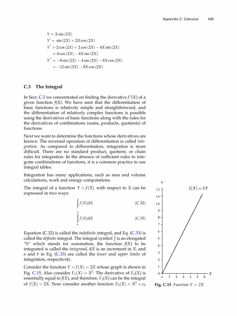
Y ¼ X sin 2Xð ÞY0 ¼ sin 2Xð Þ þ 2X cos 2Xð ÞY
00 ¼ 2 cos 2Xð Þ þ 2 cos 2Xð Þ � 4X sin 2Xð Þ¼ 4 cos 2Xð Þ � 4X sin 2Xð Þ
Y000 ¼ �8 sin 2Xð Þ � 4 sin 2Xð Þ � 8X cos 2Xð Þ¼ �12 sin 2Xð Þ � 8X cos 2Xð Þ
C.3 The Integral
In Sect. C.2 we concentrated on finding the derivative f 0(X) of agiven function f(X). We have seen that the differentiation ofbasic functions is relatively simple and straightforward, andthe differentiation of relatively complex functions is possibleusing the derivatives of basic functions along with the rules forthe derivatives of combinations (sums, products, quotients) offunctions.
Next we want to determine the functions whose derivatives areknown. The reversed operation of differentiation is called inte-gration. As compared to differentiation, integration is moredifficult. There are no standard product, quotient, or chainrules for integration. In the absence of sufficient rules to inte-grate combinations of functions, it is a common practice to useintegral tables.
Integration has many applications, such as area and volumecalculations, work and energy computations.
The integral of a function Y ¼ f Xð Þ with respect to X can beexpressed in two ways: ð
f Xð ÞdX ðC:32Þ
ðba
f Xð ÞdX ðC:33Þ
Equation (C.32) is called the indefinite integral, and Eq. (C.33) iscalled the definite integral. The integral symbol
Ðis an elongated
“S” which stands for summation, the function f(X) to beintegrated is called the integrand, dX is an increment in X, anda and b in Eq. (C.33) are called the lower and upper limits ofintegration, respectively.
Consider the function Y ¼ f Xð Þ ¼ 2X whose graph is shown in
Fig. C.15. Also consider F1 Xð Þ ¼ X2. The derivative of F1(X) isessentially equal to f(X), and therefore, F1(X) can be the integral
of f Xð Þ ¼ 2X. Now consider another function F2 Xð Þ ¼ X2 þ c0 Fig. C.15 Function Y ¼ 2X
Appendix C: Calculus 439
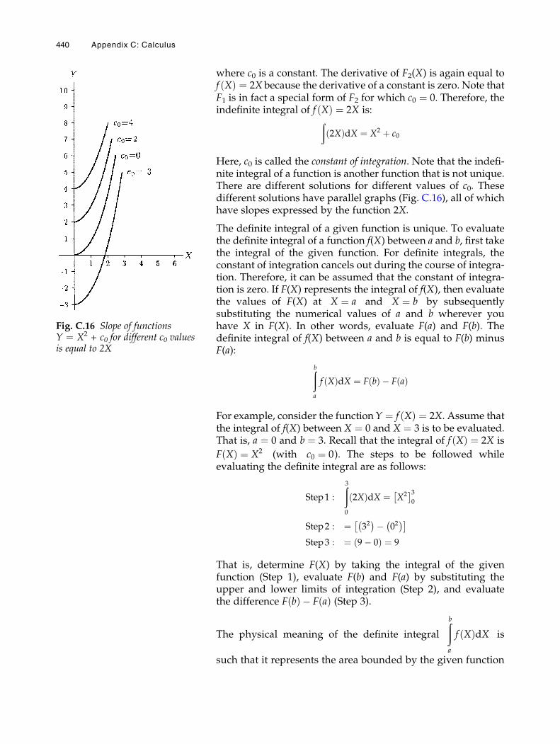
where c0 is a constant. The derivative of F2(X) is again equal tof Xð Þ ¼ 2X because the derivative of a constant is zero. Note thatF1 is in fact a special form of F2 for which c0 ¼ 0. Therefore, theindefinite integral of f Xð Þ ¼ 2X is:ð
2Xð ÞdX ¼ X2 þ c0
Here, c0 is called the constant of integration. Note that the indefi-nite integral of a function is another function that is not unique.There are different solutions for different values of c0. Thesedifferent solutions have parallel graphs (Fig. C.16), all of whichhave slopes expressed by the function 2X.
The definite integral of a given function is unique. To evaluatethe definite integral of a function f(X) between a and b, first takethe integral of the given function. For definite integrals, theconstant of integration cancels out during the course of integra-tion. Therefore, it can be assumed that the constant of integra-tion is zero. If F(X) represents the integral of f(X), then evaluatethe values of F(X) at X ¼ a and X ¼ b by subsequentlysubstituting the numerical values of a and b wherever youhave X in F(X). In other words, evaluate F(a) and F(b). Thedefinite integral of f(X) between a and b is equal to F(b) minusF(a):
ðba
f Xð ÞdX ¼ F bð Þ � F að Þ
For example, consider the functionY ¼ f Xð Þ ¼ 2X. Assume thatthe integral of f(X) between X ¼ 0 and X ¼ 3 is to be evaluated.That is, a ¼ 0 and b ¼ 3. Recall that the integral of f Xð Þ ¼ 2X is
F Xð Þ ¼ X2 (with c0 ¼ 0). The steps to be followed whileevaluating the definite integral are as follows:
Step1 :
ð30
2Xð ÞdX ¼ X2 �3
0
Step2 : ¼ 32� �� 02
� � �Step3 : ¼ 9� 0ð Þ ¼ 9
That is, determine F(X) by taking the integral of the givenfunction (Step 1), evaluate F(b) and F(a) by substituting theupper and lower limits of integration (Step 2), and evaluatethe difference F bð Þ � F að Þ (Step 3).
The physical meaning of the definite integral
ðba
f Xð ÞdX is
such that it represents the area bounded by the given function
Fig. C.16 Slope of functionsY ¼ X2 + c0 for different c0 valuesis equal to 2X
440 Appendix C: Calculus
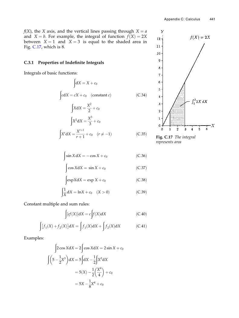
f(X), the X axis, and the vertical lines passing through X ¼ aand X ¼ b. For example, the integral of function f Xð Þ ¼ 2Xbetween X ¼ 1 and X ¼ 3 is equal to the shaded area inFig. C.17, which is 8.
C.3.1 Properties of Indefinite Integrals
Integrals of basic functions:ðdX ¼ X þ c0
ðcdX ¼ cX þ c0 constant cð Þ ðC:34Þ
ðXdX ¼ X2
2þ c0
ðX2dX ¼ X3
3þ c0
ðXrdX ¼ Xrþ1
rþ 1þ c0 r 6¼ �1ð Þ ðC:35Þ
ðsinXdX ¼ � cosX þ c0 ðC:36ÞðcosXdX ¼ sinX þ c0 ðC:37Þ
ðexpXdX ¼ exp X þ c0 ðC:38Þ
ð1
XdX ¼ lnX þ c0 X > 0ð Þ ðC:39Þ
Constant multiple and sum rules:ðcf Xð Þ½ �dX ¼ c
ðf Xð ÞdX ðC:40Þ
ðf 1 Xð Þ þ f 2 Xð Þ �
dX ¼ðf 1 Xð ÞdX þ
ðf 2 Xð ÞdX ðC:41Þ
Examples: ð2 cosXdX¼ 2
ðcosXdX ¼ 2 sinX þ c0ð
5� 1
2X3
� dX¼ 5
ðdX � 1
2
ðX3dX
¼ 5 Xð Þ � 1
2
X4
4
� þ c0
¼ 5X � 1
8X4 þ c0
Fig. C.17 The integralrepresents area
Appendix C: Calculus 441
ð1
X2þ sinX
� dX¼
ðX�2dX þ
ðsinXdX
¼ X�1
�1
� þ � cosXð Þ þ c0
¼ �1
X� cosX þ c0
C.3.2 Properties of Definite Integrals
Let F(X) represent the integral of a function f(X) with respect toX. That is:
F Xð Þ ¼ðf Xð ÞdX
Also let f1(X) and f2(X) be two other functions. Then:
ðba
f Xð ÞdX ¼ F bð Þ � F að Þ ðC:42Þ
ðba
cf Xð Þ½ �dX ¼ c
ðba
f Xð ÞdX ¼ c F bð Þ � F að Þ½ � ðC:43Þ
ðba
f 1 Xð Þ þ f 2 Xð Þ �dX ¼
ðba
f 1 Xð ÞdX þðba
f 2 Xð ÞdX ðC:44Þ
ðba
f Xð ÞdX þðcb
f Xð ÞdX ¼ðca
f Xð ÞdX ðC:45Þ
ðba
f Xð ÞdX ¼ �ðab
f Xð ÞdX ðC:46Þ
Definite integrals of basic functions:
ðba
dX ¼ X½ � ba ¼ b� a
ðba
XdX ¼ X2
2
� b
a
¼ b2
2� a2
2
" #¼ 1
2b2 � a2
� �
ðba
X2dX ¼ X3
3
� b
a
¼ b3
3� a3
3
" #¼ 1
3b3 � a3
� �
442 Appendix C: Calculus
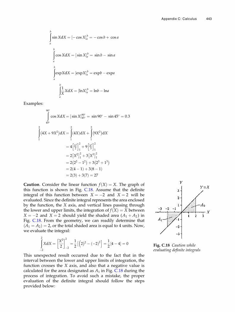
ðba
sinXdX ¼ � cosX½ � ba ¼ � cos bþ cos a
ðba
cosXdX ¼ sinX½ � ba ¼ sin b� sin a
ðba
expXdX ¼ expX½ � ba ¼ expb� expa
ðba
1
XXdX ¼ lnX½ � ba ¼ lnb� lna
Examples:
ð90�45�
cosXdX¼ sinX½ �90�45� ¼ sin 90� � sin 45� ¼ 0:3
ð21
4X þ 9X2� �
dX¼ð21
4Xð ÞdX þð21
9X2� �
dX
¼ 4 X2
2
h i21þ 9 X3
3
h i21
¼ 2 X2 �2
1þ 3 X3
�21
¼ 2 22 � 12� �þ 3 23 þ 13
� �¼ 2 4� 1ð Þ þ 3 8� 1ð Þ¼ 2 3ð Þ þ 3 7ð Þ ¼ 27
Caution. Consider the linear function f Xð Þ ¼ X. The graph ofthis function is shown in Fig. C.18. Assume that the definiteintegral of this function between X ¼ �2 and X ¼ 2 will beevaluated. Since the definite integral represents the area enclosedby the function, the X axis, and vertical lines passing throughthe lower and upper limits, the integration of f Xð Þ ¼ X betweenX ¼ �2 and X ¼ 2 should yield the shaded area (A1 þ A2 ) inFig. C.18. From the geometry, we can readily determine thatA1 ¼ A2ð Þ ¼ 2, or the total shaded area is equal to 4 units. Now,we evaluate the integral:
ð2�2
XdX ¼ X2
2
� 2�2
¼ 1
2
2�2 � �2ð Þ2
� i¼ 1
24� 4½ � ¼ 0
This unexpected result occurred due to the fact that in theinterval between the lower and upper limits of integration, thefunction crosses the X axis, and also that a negative value iscalculated for the area designated as A1 in Fig. C.18 during theprocess of integration. To avoid such a mistake, the properevaluation of the definite integral should follow the stepsprovided below:
Fig. C.18 Caution whileevaluating definite integrals
Appendix C: Calculus 443
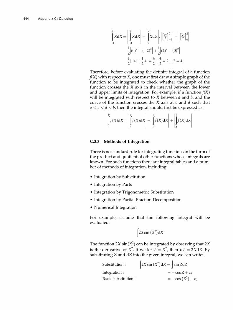
ð2�2
XdX¼ð0�2
XdX
������������þ
ð20
XdX
������������, X2
2
h i0�2
��������þ X2
2
h i20
��������
1
20ð Þ2 � �2ð Þ2
��� ���þ 1
22ð Þ2 � 0ð Þ2
��� ���1
2�4j j þ 1
24j j ¼ 4
2þ 4
2¼ 2þ 2 ¼ 4
Therefore, before evaluating the definite integral of a functionf(X) with respect to X, one must first draw a simple graph of thefunction to be integrated to check whether the graph of thefunction crosses the X axis in the interval between the lowerand upper limits of integration. For example, if a function f(X)will be integrated with respect to X between a and b, and thecurve of the function crosses the X axis at c and d such thata < c < d < b, then the integral should first be expressed as:
ðba
f Xð ÞdX ¼ðca
f Xð ÞdX������
������þðdc
f Xð ÞdX������
������þðbd
f Xð ÞdX������
������
C.3.3 Methods of Integration
There is no standard rule for integrating functions in the form ofthe product and quotient of other functions whose integrals areknown. For such functions there are integral tables and a num-ber of methods of integration, including:
• Integration by Substitution
• Integration by Parts
• Integration by Trigonometric Substitution
• Integration by Partial Fraction Decomposition
• Numerical Integration
For example, assume that the following integral will beevaluated: ð
2X sin X2� �
dX
The function 2X sin(X2) can be integrated by observing that 2X
is the derivative of X2. If we let Z ¼ X2, then dZ ¼ 2XdX. Bysubstituting Z and dZ into the given integral, we can write:
Substitution :
ð2X sin X2
� �dX ¼
ðsinZdZ
Integration : ¼ � cosZþ c0
Back substitution : ¼ � cos X2� �þ c0
444 Appendix C: Calculus
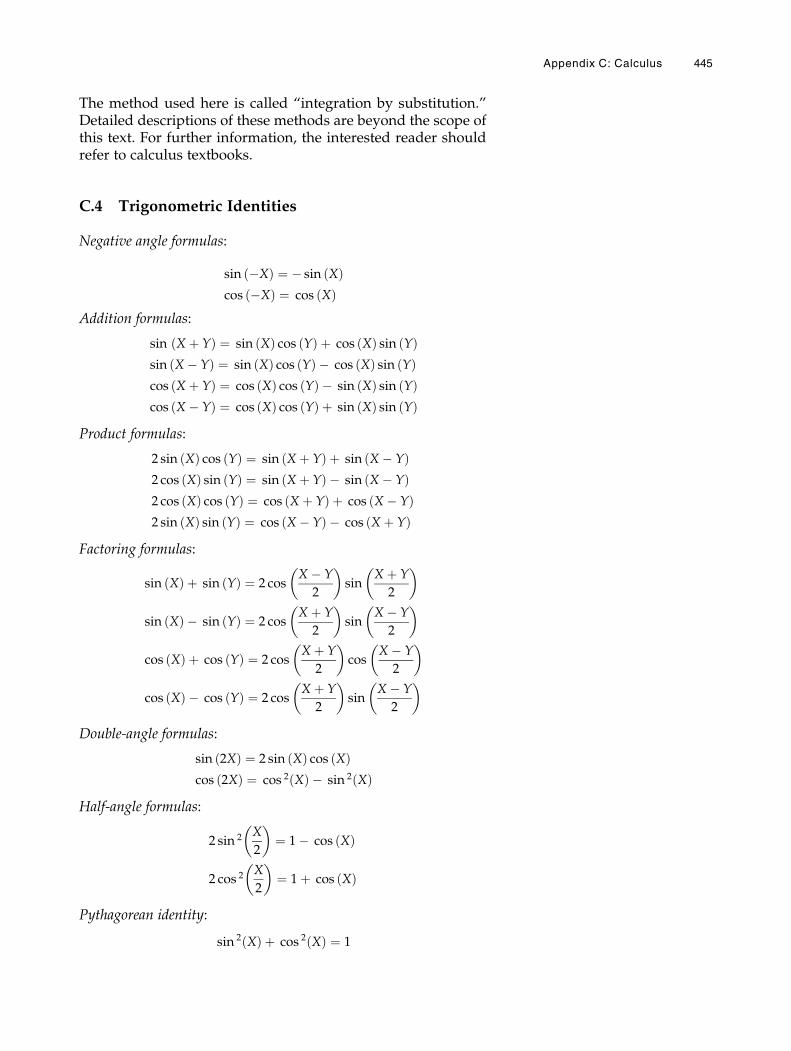
The method used here is called “integration by substitution.”Detailed descriptions of these methods are beyond the scope ofthis text. For further information, the interested reader shouldrefer to calculus textbooks.
C.4 Trigonometric Identities
Negative angle formulas:
sin �Xð Þ ¼ � sin Xð Þcos �Xð Þ ¼ cos Xð Þ
Addition formulas:
sin X þ Yð Þ ¼ sin Xð Þ cos Yð Þ þ cos Xð Þ sin Yð Þsin X � Yð Þ ¼ sin Xð Þ cos Yð Þ � cos Xð Þ sin Yð Þcos X þ Yð Þ ¼ cos Xð Þ cos Yð Þ � sin Xð Þ sin Yð Þcos X � Yð Þ ¼ cos Xð Þ cos Yð Þ þ sin Xð Þ sin Yð Þ
Product formulas:
2 sin Xð Þ cos Yð Þ ¼ sin X þ Yð Þ þ sin X � Yð Þ2 cos Xð Þ sin Yð Þ ¼ sin X þ Yð Þ � sin X � Yð Þ2 cos Xð Þ cos Yð Þ ¼ cos X þ Yð Þ þ cos X � Yð Þ2 sin Xð Þ sin Yð Þ ¼ cos X � Yð Þ � cos X þ Yð Þ
Factoring formulas:
sin Xð Þ þ sin Yð Þ ¼ 2 cosX � Y
2
� sin
X þ Y
2
�
sin Xð Þ � sin Yð Þ ¼ 2 cosX þ Y
2
� sin
X � Y
2
�
cos Xð Þ þ cos Yð Þ ¼ 2 cosX þ Y
2
� cos
X � Y
2
�
cos Xð Þ � cos Yð Þ ¼ 2 cosX þ Y
2
� sin
X � Y
2
�
Double-angle formulas:
sin 2Xð Þ ¼ 2 sin Xð Þ cos Xð Þcos 2Xð Þ ¼ cos 2 Xð Þ � sin 2 Xð Þ
Half-angle formulas:
2 sin 2 X
2
� ¼ 1� cos Xð Þ
2 cos 2 X
2
� ¼ 1þ cos Xð Þ
Pythagorean identity:
sin 2 Xð Þ þ cos 2 Xð Þ ¼ 1
Appendix C: Calculus 445
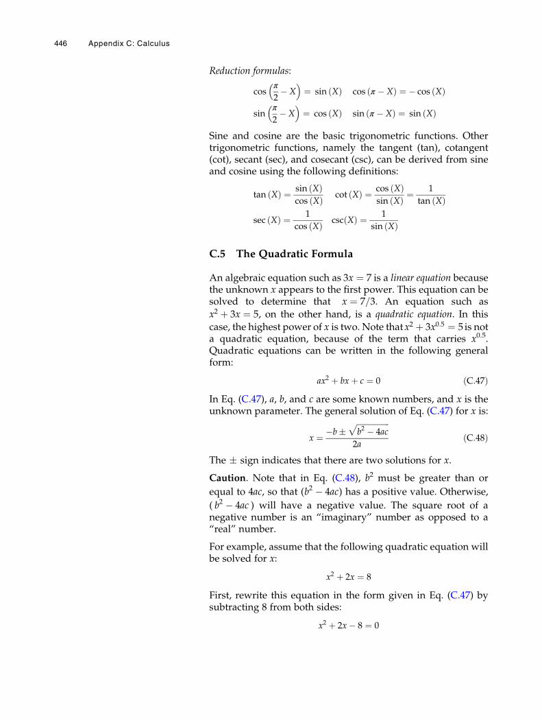
Reduction formulas:
cosπ
2� X
� �¼ sin Xð Þ cos π � Xð Þ ¼ � cos Xð Þ
sinπ
2� X
� �¼ cos Xð Þ sin π � Xð Þ ¼ sin Xð Þ
Sine and cosine are the basic trigonometric functions. Othertrigonometric functions, namely the tangent (tan), cotangent(cot), secant (sec), and cosecant (csc), can be derived from sineand cosine using the following definitions:
tan Xð Þ ¼ sin Xð Þcos Xð Þ cot Xð Þ ¼ cos Xð Þ
sin Xð Þ ¼1
tan Xð Þsec Xð Þ ¼ 1
cos Xð Þ csc Xð Þ ¼ 1
sin Xð Þ
C.5 The Quadratic Formula
An algebraic equation such as 3x ¼ 7 is a linear equation becausethe unknown x appears to the first power. This equation can besolved to determine that x ¼ 7=3. An equation such as
x2 þ 3x ¼ 5, on the other hand, is a quadratic equation. In this
case, the highest power of x is two. Note thatx2 þ 3x0:5 ¼ 5 is nota quadratic equation, because of the term that carries x0.5.Quadratic equations can be written in the following generalform:
ax2 þ bxþ c ¼ 0 ðC:47ÞIn Eq. (C.47), a, b, and c are some known numbers, and x is theunknown parameter. The general solution of Eq. (C.47) for x is:
x ¼ �b�ffiffiffiffiffiffiffiffiffiffiffiffiffiffiffiffiffib2 � 4ac
p2a
ðC:48Þ
The � sign indicates that there are two solutions for x.
Caution. Note that in Eq. (C.48), b2 must be greater than or
equal to 4ac, so that (b2 � 4ac) has a positive value. Otherwise,
( b2 � 4ac ) will have a negative value. The square root of anegative number is an “imaginary” number as opposed to a“real” number.
For example, assume that the following quadratic equation willbe solved for x:
x2 þ 2x ¼ 8
First, rewrite this equation in the form given in Eq. (C.47) bysubtracting 8 from both sides:
x2 þ 2x� 8 ¼ 0
446 Appendix C: Calculus
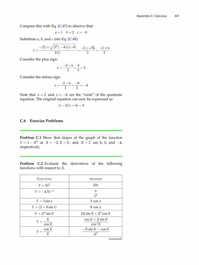
Compare this with Eq. (C.47) to observe that:
a ¼ 1 b ¼ 2 c ¼ �8
Substitute a, b, and c into Eq. (C.48):
x ¼� 2ð Þ �
ffiffiffiffiffiffiffiffiffiffiffiffiffiffiffiffiffiffiffiffiffiffiffiffiffiffiffiffiffiffiffiffiffi22� �� 4 1ð Þ �8ð Þ
q2 1ð Þ ¼ �2� ffiffiffiffiffi
36p
2¼ �2� 6
2
Consider the plus sign:
x ¼ �2þ 6
2¼ 4
2¼ 2
Consider the minus sign:
x ¼ �2� 6
2¼ �8
2¼ �4
Note that x ¼ 2 and x ¼ �4 are the “roots” of the quadraticequation. The original equation can now be expressed as:
x� 2ð Þ xþ 4ð Þ ¼ 0
C.6 Exercise Problems
Problem C.1 Show that slopes of the graph of the function
Y ¼ 1� X2 at X ¼ �2,X ¼ 0; and X ¼ 2 are 4, 0, and �4,respectively.
Problem C.2 Evaluate the derivatives of the followingfunctions with respect to X.
FUNCTIONS ANSWERS
Y ¼ 5x2 10x
Y ¼ �4:5x�2 9
x3
Y ¼ 3 sin x 3 cos x
Y ¼ 2þ 8 sin xð Þ 8 cos x
Y ¼ X2 sinX 2X sinX þ X2 cosX
Y ¼ X
cosX
cosX þ X sinX
cos 2X
Y ¼ cosX
X
�X sinX � cosX
X2
(continued)
Appendix C: Calculus 447
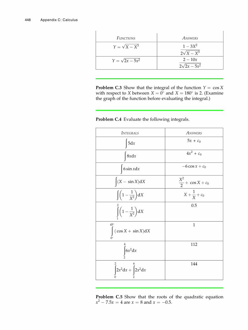
FUNCTIONS ANSWERS
Y ¼ffiffiffiffiffiffiffiffiffiffiffiffiffiffiffiX � X3
p1� 3X2
2ffiffiffiffiffiffiffiffiffiffiffiffiffiffiffiX � X3
p
Y ¼ffiffiffiffiffiffiffiffiffiffiffiffiffiffiffiffiffiffi2x� 5x2
p2� 10x
2ffiffiffiffiffiffiffiffiffiffiffiffiffiffiffiffiffiffi2x� 5x2
p
Problem C.3 Show that the integral of the function Y ¼ cosXwith respect to X between X ¼ 0� and X ¼ 180� is 2. (Examinethe graph of the function before evaluating the integral.)
Problem C.4 Evaluate the following integrals.
INTEGRALS ANSWERSð5dx
5x + c0
ð8xdx
4x2 + c0
ð6 sin xdx
�6 cos xþ c0
ðX � sinXð ÞdX X2
2þ cosX þ c0ð
1� 1
X2
� dX X þ 1
Xþ c0
ð21
1� 1
X2
� dX
0.5
ð45�0�
cosX þ sinXð ÞdX1
ð42
6x2dx
112
ð20
2x2dxþð62
2x2dx
144
Problem C.5 Show that the roots of the quadratic equationx2 � 7.5x ¼ 4 are x ¼ 8 and x ¼ �0.5.
448 Appendix C: Calculus
Index1
AAbductor gait, 128Acceleration
angular, 64, 206–207, 239–240,239f, 240f
average, 152constant, 155–156, 156fdefinition, 6, 145normal, 217tangential, 217vector
radial/centripetal, 217tangential and normalcomponent, 217, 217f
Acromioclavicular joint, 113Actin and myosin, 104, 380Angular acceleration, 10t, 64Angular kinematics
acceleration, 206–207air resistance, 208, 210famplitude, 209coordinate transformation, 216damped oscillation1, 210, 211fdimensions and units, 207–208displacement, velocity, and
acceleration vs. time, 214f, 216flexion-extension test, 214, 214ffrequency, 209inverted pendulum, 214linear and angular quantities,
218–219linkage systems
circular motion, 223, 225fdouble pendulum, 223, 223fsingle pendulum, 222, 223ftangential velocity and normalacceleration, 224f, 225
uniform circular motion,219, 223f
unit vectors, 224–226, 225fneutral/equilibrium position, 208
pendulum, 208, 208fpolar coordinates, 205, 205fposition and displacement,
205–206, 205f, 206tposition vs. time, 213, 214, 214frange of motion, 209relative motion, 220–222, 220frotational motion
about fixed axis, 217–218,217f, 218f
constant acceleration, 219–220shoulder abduction, 211–212, 211fsimple harmonic motion, 208f,
209–210uniform circular motion, 219velocity, 206, 210, 210f, 211, 211f
Angular kineticsmass moment of inertia, 240–242of motion
arms, gymnast vs. angularposition, 237, 237f
circular end region, ski jump,238, 238f
free-body diagrams, 194, 194fgymnast, on high bar, 234, 234fnet force, 233rotational motion, 233f, 234speed vs. angular position,235, 235f
parallel-axis theorem, 242, 242fradius of gyration, 242rotational kinetic energy,
247–248, 247fsegmental motion analysis
angular displacementand time, 243
dynamic model, 243knee extension, 244–247, 244ftwo-dimensional (planar) motionanalysis, 243–244
velocity and displacement, 244
torque and angular acceleration,239–240, 239f, 240f
work and powerangular displacements, 248–249definition, 248knee extension, 250, 250fwork–energy theorem, 249
Angular motion, 64Ankle, 133–134Antagonist muscle, 105Apparent yield strength, 295Area, 10tArea moment of inertia, 347Articular cartilage, 103, 381–382,
381f, 382fAtlantoaxial joint, 117Atlantooccipital joint, 116Axis
centroidal, 241neutral, 339, 347rotational motion about, 217–218,
217f, 218f
BBalance method, 89fBallistic pendulum, 266, 267fBeam(s)
cantilever, 57, 80, 80fhinged to ground, with roller
on top, 94, 358hinged to wall, with cable support,
76, 76fL-shaped
scalar analysis of, 83–84, 83fvector analysis of, 84–85, 84f
on wedge and roller support, 72–73Bending
bench test, 353, 353fcantilever beams, 346, 346fcentroids and neutral axes, 347, 347f
1Note: Page numbers followed by f indicate figures; those followed by t indicate table.
# Springer International Publishing Switzerland 2017N. Ozkaya et al., Fundamentals of Biomechanics, DOI 10.1007/978-3-319-44738-4
449
Bending (cont.)element analyses, 352, 352ffemur, 353flexural stress distribution, 347, 348fflexure formula, 347free-body diagram, 350–351, 350fmaterial elements, stress
components, 351, 351fmethod of section, 344negative shear forces, 345f, 346normal and shear force, 349, 349fparameters involved definitions,
349, 349fpositive shear forces, 345, 345fshear, and moment diagram,
344, 345fshear stress distribution, 349, 349fstraight beam, 344, 344fstress distribution, 351, 351ftension and compression, 347, 347fthree and four-point bending,
344, 344fthree-point bending apparatus,
350, 350fBending effects, 39, 39fBiaxial and triaxial stresses
block loading, 323, 323fcubical material element, 320, 320ffirst order tensors, 322normal and shear components,
322, 322fplane stress components, 322, 322fsecond order tensors, 322stress–strain relationships, 321, 321fsuperposition method, 321, 321ftensile/compressive, 321
Biological tissuesarticular cartilage, 381–382,
381f, 382fbone
composition, 373, 373ffractures, 377mechanical properties, 374–376,374f–376f
structural integrity, 376–377, 377fcharacteristics of, 371–373, 373felasticity vs. viscoelasticity,
369–371, 369f–371fskeletal muscles, 379–381, 380fsprings and dashpots, 364–365, 364ftendons and ligaments, 378–379,
378f, 379ftime-dependent material response,
368–369, 368fviscoelasticity, 363–364, 363f–364f
definition, 363empirical models, 365
Kelvin-Voight model,365–366, 365f
linearly elastic material,363, 363f
Maxwell model, 366–367, 366fstandard solid model,367–368, 367f
stress and strain, 363Biomechanics, 5–6Bone
composition, 373, 373ffractures, 377mechanical properties, 374–376,
374f–376fstructural integrity, 376–377, 377f
Built-in member, 72tBuilt-in structures
cantilever beam, 80, 80fL-shaped beam, 82–84, 82f, 83f
CCable-pulley systems, 78–80Cannonball, 167Cantilever beams, 80Center of gravity
determinations of, 88–99of system, 91
Center of mass, 27, 88Centroidal axis, 241Collinear forces, 26Compressive force, 25Concentrated load, 27Concurrent forces, 26, 26fConstitutive equations, 297Coplanar force system, 25
moments due to, 66fnet moment, 42–43, 42fscalar method, 48
Coulomb theory, 331Couple, 47, 47fCouple moment, 47Crash test, 263, 263fCross (vector) product, 48
DD’Alembert principle, 285Damped oscillations, 210Deformable body mechanics
applied forcesand deformations, 282
internal forces and moments,282–283
mathematics, 285procedure, 284–285rigid body mechanics, 281
statically determinate andindeterminate systems, 281
stress and strain, 283–284, 283f, 284fDegrees of freedom, 223Diarthrodial joints, 31, 103, 103f, 110,
121, 381Dimensional analysis, 7–9Dynamics, 4
acceleration, 145definitions, 143differential and integral
calculus, 147distance and displacement,
145, 145ffriction, 29inertia and momentum, 146kinematics and kinetics, 143linear, angular, and general
motions, 144, 144fparticle concept, 146–147reference frames and coordinate
systems, 147, 147fspeed and velocity, 145vector algebra, 147
Dynamometer, 214, 214f
EElastic deformations, 295–297, 295f,
296fElasto-plastic collision, 268–270,
268f, 269fElbow
arm, 108, 108fbones, 107, 107fbrachialis and brachioradialis
muscles, 111diarthrodial joint, 110forearm, 108, 108fhumeroradial and humeroulnar
joints, 107injuries of, 108joint reaction force, 108–109, 110f, 134muscles, 107, 107fparallel force system, 109pronation and supination
movements, 108proximal radioulnar joint, 107rotational and stabilizing/sliding
components, 110, 110fthree-muscle system, 111, 111f
Endurance limit, 334–335Energy, 12tEngineering mechanics, 6Equation(s)
equilibrium, 70–71of motion, 63
450 Index

Equilibrium, 7conditions for, 65–67definition of, 65rotational, 65static, 65translational, 65
Equilibrium equations, 70–71Equilibrium systems
analysis of, 68–69built-in structures
cantilever beam, 80, 80fL-shaped beam, 82–84, 82f, 83f
cable-pulley systems, 78–80center of gravity determinations in,
88–99conditions for, 65–67constraints and reactions in, 71, 72tdefinition, 63equations on, 69–71free-body diagrams, 67–68, 68ffriction in, 86–88, 86f–88fsimply supported structures, 71–78,
73f, 74f, 76f–78ftraction devices, 78–80, 79f
Equivalent force, 27External forces, 24–25
FFirst law, Newton’s, 7, 63Flexion–extension test, 214–216, 214fForce(s), 10t, 15Force vector
collinear, 26, 26fcompressive, 25, 25fconcurrent, 26, 26fcoplanar, 25definition, 23dimension and units of, 23–24distributed force systems and
pressure, 27–28, 27f, 28f, 28tequivalent, 27external, 24–25frictional, 29–31, 29f, 30f, 30tgravitational/weight, 26–27,
26t, 27finternal, 24–25normal, 25, 25fparallel, 26, 26fproperties of, 23, 23freactive, 71resultant, 23, 23ftangential, 25, 25ftensile, 25, 25ftranslation, 47–48, 48f
Free body diagrams, 67–68, 67f, 68fFriction
coefficient of, 30, 30tkinetic and static, 29–30systems with, 86–88, 86f, 87f, 88f
Frictional forces, 29–31, 29f, 30f, 30tFrontal plane, 92
GGlenohumeral articulation, 112Golfer’s elbow syndrome, 108Gravitational acceleration, 26tGravitational force, 26–27, 26tGravity, center of
determinations of, 88–93, 89f, 90f,91f, 92f, 92t
leg, 92, 92fGravity line, 89Greek alphabet, 13t
HHammering, 64fHamstring muscle, 122Hip
bony structure, 122femoral head, 121, 122forces, 122, 124ffree-body diagram
abductor gait, 128carrying load, hand, 126, 126f,127, 127f
center of gravity, 126–127, 126fconcurrent system, 125, 125fgravitational force, 127leg, 123–124, 124fmuscle and joint reaction forces,125, 125f
pelvis, 124, 124fthree-force system, 125, 126ftranslational equilibrium,125–126
pelvis, 121, 121fsingle-leg stance, 122, 123f
Hooke’s law, 297, 297fHumeroradial joint, 107Humeroulnar joint, 107, 107fHysteresis loop, 299–300, 299f
IImpulse and momentum
angular, 273–274applications
ball hits, floor and bounces,258–259, 258f
crash test, 263, 263fforce platform, 261, 261fforce vs. time, athlete,261–262, 261f
soccer player, 259, 259fbasic equations, 274, 274t, 275conservation of linear
momentum, 264
impact and collisions, 264–265, 265flinear
average force and an averagetime, 256, 256f
definition, 255force vs. time curve, 256, 256fimpulse-momentumtheorem, 255
impulsive forces and impulsivemotions, 256
scalar and vector additions,257, 257f
units, 257, 257tvector quantity, 255
one-dimensional collisionselastoplastic collision,268–269, 268f
perfectly elastic collision, 265,267, 267f
perfectly inelastic collision,266, 266f
rigid bodies in plane motion,275–276, 275f
two-dimensional collisionsconservation of momentum, 270elastic collision, 273, 273foblique central impact, poolballs, 270, 270f
target and cue ball, 270–273Impulse-momentum theorem, 255Inertia
area moment, 347, 350, 353mass moment of, 64
Internal forces, 24–25International System of Units (SI), 10t
conversion of, 11t–12t
KKelvin-Voight model, 365–366, 365fKinematics, 4Kinetic friction, 29Kinetics
angular (see Angular kinetics)definition, 4linear, 181–202 (see also Linear
kinetics)rigid bodies, plane motion,
275–276, 275fKnee
exercises, 129, 129fforces acting, lower leg, 129, 130flever arms, 130, 130fmuscles, 129, 129fpatella, 131–132, 131f, 132fpatellofemoral joint, 128, 128f, 131rotational and translatory
components, 131, 131ftibial plateau, 131tibiofemoral joint, 128, 131f
Index 451
LLe Systeme International d’Unites
(SI), 9Ligamentous capsule, 103, 103fLinear kinematics
athletics applicationscenter of gravity, 170, 170f, 171,171f, 174–175, 174f
diver, 174–175, 173flong jumper, 170, 170fshot-putter, 172, 172ftrajectory, 171, 172f
biaxial motionwith constant acceleration,166–167
two-and three-dimensionallinear movements, 163
dimensions and units, 153–154, 154tdisplacement, velocity, and
acceleration, 151–153, 151f,152f, 153t
measured and derived quantities,154–155
position, velocity, and accelerationvectors, 163–165, 163f, 164f
projectile motioncannonball fired, 167, 167fgravity and air resistance, 167motion trajectory, 167speed of release, 167time lapses, 169trajectory, 168, 168fvelocity vector, 168, 168f
uniaxial motion, 151car speed, 157–161constant acceleration,161–162, 161f
with constant acceleration,155–156
displacement and acceleration vs.time, 160, 160f
free fall, 162, 162fimpact speed, 163relative position vs. time,157, 157f
skier speed, 161, 161fspeed vs. time, 157, 158, 158funiformly acceleratedmotion, 162
Linear kineticsconservation of energy principle
in, 191dimension and units, 192, 192tenergy methods in, applications of
acceleration, 196–197block, 193–194, 193fconservation, 196equations and formulas, 193, 193t
free-body diagram, 194–196,194f, 195f
pendulum, 195, 195fski jumper, 195, 195fvelocity and displacement, 197
equations of motion, 181–183, 182fmechanical work
constant force, 188–189, 188f, 189fscalar product, 189–190varying force, 189, 189f
Newton’s second lawof motion, 143
potential energy, 190–191, 191fpower, 192, 193tprocedure, 185–187translational motion, 183–185work and energy methods,
187–188work–energy theorem, 191
Linear motion, 64Load intensity, 28Longitudinal plane, 92L-shaped beams
scalar analysis of, 82–84, 83fvector analysis of, 84–85, 84f
Lubricants, 31
MMathematics, 12–13Maximum distortion energy theory,
331–332Maxwell model, 366–367, 366fMechanical work
constant force, 188–189, 188f, 189fdefinition, 188scalar product, 189–190varying force, 189, 189f
Mechanics, 3–5Mises-Hencky theory, 332Mohr’s circle
material element, 329–330,329f, 330f
maximum shear stress, 326plane stress element, 327, 327fpositive and negative stresses, 327principal stresses, 327
Moment(s), 10tcouple, 47definitions, 39dimension and, 40direction of, 39–40fine points on, 41–42, 41fmagnitude of, 39net/resultant, 42–47opposite, 41, 41fresolution of forces and, 41, 41funder sliding force, 41, 41f
vector product, 48–53, 48f, 49fin wrench and bolt, 40, 40f
Moment arm, 39Motion(s)
angular, 64from coplanar force, 66fequations of, 63linear, 64
Multiaxial deformations and stressanalyses
allowable stress and safety factor,332–333
bendingbench test, 353f, 353fcantilever beams, 346, 346fcentroids and neutral axes,347, 347f
element analyses, 352, 352ffemur, 353flexural stress distribution,347, 348f
flexure formula, 347free-body diagram, 350–351, 350fmethod of section, 344negative shear forces, 345f, 346normal and shear force, 349, 349fparameters involved definitions,349, 349f
positive shear forces, 345, 345fshear, and moment diagram,344, 345f
shear stress distribution,349, 349f
straight beam, 344, 344fstress distribution, 351, 351ftension and compression,347, 347f
three-point bending apparatus,350, 350f
biaxial and triaxial stressesblock loading, 323, 323fcubical material element,320, 320f
first order tensors, 322normal and shear components,322, 322f
plane stress components,322, 322f
second order tensors, 322stress–strain relationships,321, 321f
superposition method, 321, 321ftensile/compressive, 321
combined loading, 354–355Coulomb/Tresca theory, 331fatigue and endurance, 334–335,
334f, 335fmaterials strength, 333
452 Index
maximum distortion energy theory,331–332
maximum normal stress theory, 332maximum shear stress theory,
331, 331fMohr’s circle
material element, 329–330,329f, 330f
maximum shear stress, 326plane stress element, 327, 327fpositive and negativestresses, 327
principal stresses, 327normal and shear stresses,
331, 331fPoisson’s ratio, 319–320, 319fprincipal stresses, 326–327, 326fsafety and reliability, 330stress concentration, 335–337,
335f, 336fstress transformation, 325, 325ftorsion
angle of twist, 338, 338fcircular shaft, 338, 338fdefinition, 337formula and stresses,338–339, 338f
fractured bone, 341, 341flongitudinal and transverseplanes, 339
material element, 343, 343fpendulum, 340–341plane perpendicular, centerlinecuts, 338, 338f
polar moment of inertia, 338shear stress, 338, 338fsolid circular cylinder, 343, 343fspiral fracture pattern, 340, 340fstandard torsion testing machine,340, 340f
stress trajectories, 343, 343ftorque vs. angle of twist,341–342, 341f
torque vs. angular displacement,341, 341f
von Mises yield/Mises-Henckytheory, 332
NNecking, 298, 298fNet moment, 42–47Neutral axis, 339, 340, 347Newton’s first law, 7Newton’s laws of mechanics, 63–65Newton’s second law, 7Newton’s second law of motion, 181
Newton’s third law, 7Normal force, 25Notation, 15
OOffset method, 295, 295fOne-dimensional collisions
elasto-plastic collision, 268–270,268f, 269f
perfectly elastic collision,267–268, 267f
perfectly inelastic collision,266–267, 266f
Osteoporosis, 376
PParallel-axis theorem, 242, 242fParallel force, 26, 26fPatellofemoral joint, 128–129, 128fPerfectly elastic collision,
267–268, 267fPerfectly inelastic collision,
266–267, 266fPlastic deformations, 297–298Poisson’s ratio, 319–320, 320fPower, 10tPressure, 10tPulley traction, 79f
RRadioulnar joint, proximal, 107Radius of gyration, 242Reaction board method, 90, 90fReactions, 71, 72tRectangular/Cartesian coordinate
system, 147Resultant moment, 42–47Right-hand rule, 40, 40f
in Cartesian coordinate directions,49, 49f
couple-moment, 47, 82Rotational effect, 39, 39fRotational equilibrium, 43, 65
SSagittal plane, 92Scalars, 13Secondary dimensions, 8Second law, Newton’s, 63Segmental motion analysis
angular displacementand time, 243
dynamic model, 243
knee extension, 244–245, 244ftwo-dimensional (planar) motion
analysis, 243–244velocity and displacement, 244
Shoulderacromioclavicular joint, 113arm, 113, 113fbony structure, 113glenohumeral articulation, 112injuries, 116joint reaction force, 114–115mechanical model, 113, 114fmuscles, 113, 113fscapular movements, 113sternoclavicular joint, 113
Simply supported structures, 71–78,73f–78f
SI units, 10tSkeletal muscles, 379–381, 380fSpinal column
athlete’s body, 120, 120fatlantoaxial joint, 117atlantooccipital joint, 116–117free-body diagram, 120, 120fhead and the neck, 117, 117finjuries, 117joint reaction force, 119, 119fligaments and muscles, 117, 117fsacrum, 120–121three-force system, 117–118,
117f–118fvertebral column, 116, 116fweight lifter, 119, 119f
Standard solid model, 367–368, 367fStatically determinate systems, 70–71Statically indeterminate systems, 71Static equilibrium, 65Static friction, 29Statics, 4
assumptions and limitations,106–107
basic considerations, 105mechanics
ankle, 133–134elbow (see Elbow)hip (see Hip)knee (see Knee)shoulder (see Shoulder)spinal column (see Spinalcolumn)
skeletal joints, 103–104skeletal muscles, 104–105
Sternoclavicular joint, 113Strain, 292. See also Stress and strain
average shearaxial, 293, 293fdefinitions, 295
Index 453
Strain (cont.)elastic, 299, 299fnormal, 293, 293fplastic, 297–298, 297fshear, 293, 293fsimple, 292–294, 293ftensile, 302, 302f
Stress(es), 10taverage normal stress, 291conventional stresses, 298, 298fdefinitions, 296normal stress, 291, 291fshear, 291, 292, 292fsimple, 291–292, 291f, 292ttensile, 302–304, 303f, 304ftrue/actual, 298
Stress and strain average shearbone specimens, 304, 304fdeflections, 308, 308felastic deformations, 295–297,
295f–296ffixation device, 305, 305ffree-body diagram, 307, 307fHooke’s law, 297, 297fhuman cortical bone tissue,
304, 306fhysteresis loop in, 299–300, 299fload-elongation diagrams, 290, 290floading configurations, 289material behavior, in idealized,
300–301, 301fmechanical properties of materials,
301–302, 301t, 302fnecking, 176–177, 176f–177fplastic deformations, 297–298, 297fstatically indeterminate system,
307, 307fstrain hardening, 299, 299fstress–strain diagrams, 294–295,
294f–295f, 300, 300ftensile strain and average tensile
stress, 302, 302funiaxial tension test, 303–304, 303fwork done, 299, 299f
Supplementary units, 10Synovial fluid, 31, 103Synovial membrane, 103Systems of units, 9–10
TTangential force, 25Tensile force, 25Third law, Newton’s, 64–65Three-force systems, 70Tibiofemoral joint, 128–129, 128fTorque, 10t
definition of, 39dimension and units of, 40, 41t
Torsionangle of twist, 338, 338fcircular shaft, 338, 338fdefinition, 337formula and stresses,
338–339, 338ffractured bone, 341, 341flongitudinal and transverse
planes, 339material element, 343, 343fpendulum, 340–341plane perpendicular, centerline
cuts, 338, 338fpolar moment of inertia, 338shear stress, 338, 338fsolid circular cylinder, 343, 343fspiral fracture pattern, 340, 340fstandard torsion testing machine,
340, 340fstress trajectories, 343, 343ftorque vs. angle of twist,
341–342, 341ftorque vs. angular displacement,
341, 341fTraction devices, 78–79Translational equilibrium, 65Transverse plane, 92Tresca theory, 331Two-force systems, 70
UUniaxial motion, 151
car speed, 158–159constant acceleration, 161, 161fwith constant acceleration,
155–156displacement and acceleration vs.
time, 161, 160ffree fall, 162, 162fimpact speed, 163relative position vs. time, 157, 157fskier speed, 161, 161fspeed vs. time, 157, 158, 157funiformly accelerated motion, 162
Unit(s)conversion of, 11–12of force, 23–24systems of, 9–10
VVectors, 13Velocity, 10tViscoelasticity
definition, 363empirical models, 365Kelvin-Voight model,
365–366, 365flinearly elastic material, 363, 363fMaxwell model, 366–367, 366fstandard solid model, 367–368, 367fstress and strain, 363
Volume, 10t
WWeight, 26–27Work, 10tWork–energy theorem, 191, 249
YYoung’s modulus, 295
454 Index


