MASARYK UNIVERSITY

FACULTY OF INFORMATICS

}w���������� ������������� !"#$%&'()+,-./012345<yA|Neighbour-based intrusion detection

in wireless sensor networks

MASTER THESIS

Bc. Lukáš Folkman

Brno, 2010

Declaration

Hereby I declare, that this paper is my original authorial work, which I have worked out bymy own. All sources, references and literature used or excerpted during elaboration of thiswork are properly cited and listed in complete reference to the due source.

Advisor: RNDr. Andriy Stetsko

ii

Acknowledgement

I would like to thank RNDr. Andriy Stetsko, the advisor of my master thesis, for his valu-able comments, suggestions and time he spent helping me with this work. I would like tothank Bc. Veronika Neužilová for her language concerned advice and moral support andmy parents for supporting my university studies.

iii

Abstract

Sensor nodes situated spatially close to each other tend to have similar behaviour. Theneighbour-based detection technique is based on this principle and should provide meansfor anomaly intrusion detection in wireless sensor networks without prior training. Recently,this technique has been successfully applied to detect the fabricated information attack inwireless sensor networks.

This work provides a description of selective forwarding, jamming, hello flood, sinkhole,sybil, packet alteration and fabricated information attacks together with their symptoms.Furthermore, a neighbour-based intrusion detection system capable of revealing selectiveforwarding, jamming and hello flood attacks is designed and implemented for the operatingsystem TinyOS. The intrusion detection system comes in two modifications – one with localknowledge of immediate neighbours only and one involving information exchanged amongone-hop or two-hops neighbours. Results of the simulations, namely the number of falsenegatives and the number of false positives, are described in the thesis also.

iv

Keywords

hello flood attack, intrusion detection system, jamming, neighbour-based intrusion detec-tion, selective forwarding, watchdog monitoring technique, wireless sensor network

v

Contents

1 Wireless sensor networks . . . . . . . . . . . . . . . . . . . . . . . . . . . . . . . . . 21.1 Sensor nodes and gateways . . . . . . . . . . . . . . . . . . . . . . . . . . . . . 31.2 Software . . . . . . . . . . . . . . . . . . . . . . . . . . . . . . . . . . . . . . . . 41.3 Security . . . . . . . . . . . . . . . . . . . . . . . . . . . . . . . . . . . . . . . . . 4

2 Intrusion detection systems . . . . . . . . . . . . . . . . . . . . . . . . . . . . . . . . 62.1 IDS classification . . . . . . . . . . . . . . . . . . . . . . . . . . . . . . . . . . . 72.2 Blueprint of an intrusion detection system architecture . . . . . . . . . . . . . 82.3 Neighbour-based intrusion detection techniques . . . . . . . . . . . . . . . . . 9

2.3.1 Insider attacker detection scheme . . . . . . . . . . . . . . . . . . . . . 92.3.2 Group-based intrusion detection scheme . . . . . . . . . . . . . . . . . 10

3 Attacks . . . . . . . . . . . . . . . . . . . . . . . . . . . . . . . . . . . . . . . . . . . . 133.1 Jamming . . . . . . . . . . . . . . . . . . . . . . . . . . . . . . . . . . . . . . . . 133.2 Hello flood attack . . . . . . . . . . . . . . . . . . . . . . . . . . . . . . . . . . . 153.3 Selective forwarding . . . . . . . . . . . . . . . . . . . . . . . . . . . . . . . . . 163.4 Sinkhole attack . . . . . . . . . . . . . . . . . . . . . . . . . . . . . . . . . . . . 173.5 Sybil attack . . . . . . . . . . . . . . . . . . . . . . . . . . . . . . . . . . . . . . . 183.6 Packet alteration . . . . . . . . . . . . . . . . . . . . . . . . . . . . . . . . . . . . 193.7 Fabricated information attack . . . . . . . . . . . . . . . . . . . . . . . . . . . . 203.8 Neighbour-based detection of the attacks . . . . . . . . . . . . . . . . . . . . . 20

4 IDS design and implementation . . . . . . . . . . . . . . . . . . . . . . . . . . . . . 214.1 IDS component model . . . . . . . . . . . . . . . . . . . . . . . . . . . . . . . . 214.2 Ambiguous collisions and low gain mode monitoring . . . . . . . . . . . . . . 234.3 Detections . . . . . . . . . . . . . . . . . . . . . . . . . . . . . . . . . . . . . . . 24

4.3.1 Detections in networks with an aggregation protocol . . . . . . . . . . 254.3.2 Detections in networks with the Collection tree protocol . . . . . . . . 26

4.4 Clustering . . . . . . . . . . . . . . . . . . . . . . . . . . . . . . . . . . . . . . . 274.4.1 Selective forwarding . . . . . . . . . . . . . . . . . . . . . . . . . . . . . 274.4.2 Jamming . . . . . . . . . . . . . . . . . . . . . . . . . . . . . . . . . . . . 30

4.5 Collaboration . . . . . . . . . . . . . . . . . . . . . . . . . . . . . . . . . . . . . 325 Simulations and results . . . . . . . . . . . . . . . . . . . . . . . . . . . . . . . . . . 35

5.1 Deployment of the IDS . . . . . . . . . . . . . . . . . . . . . . . . . . . . . . . . 355.2 Simulating intrusion detection in networks with attackers . . . . . . . . . . . 36

5.2.1 Networks with an aggregation protocol . . . . . . . . . . . . . . . . . . 365.2.1.1 Hello flood attack . . . . . . . . . . . . . . . . . . . . . . . . . 365.2.1.2 Jamming . . . . . . . . . . . . . . . . . . . . . . . . . . . . . . 375.2.1.3 Selective forwarding . . . . . . . . . . . . . . . . . . . . . . . . 375.2.1.4 Black hole attack . . . . . . . . . . . . . . . . . . . . . . . . . . 37

5.2.2 Networks with the Collection tree protocol . . . . . . . . . . . . . . . . 375.2.2.1 Hello flood attack . . . . . . . . . . . . . . . . . . . . . . . . . 385.2.2.2 Deceptive jamming . . . . . . . . . . . . . . . . . . . . . . . . 39

vi

5.2.2.3 Random jamming . . . . . . . . . . . . . . . . . . . . . . . . . 395.2.2.4 Selective forwarding . . . . . . . . . . . . . . . . . . . . . . . . 40

5.3 Configuration options of the IDS . . . . . . . . . . . . . . . . . . . . . . . . . . 425.3.1 Sparse networks . . . . . . . . . . . . . . . . . . . . . . . . . . . . . . . 425.3.2 Two-hop collaboration . . . . . . . . . . . . . . . . . . . . . . . . . . . . 435.3.3 Detection interval length influence . . . . . . . . . . . . . . . . . . . . . 44

6 Conclusions . . . . . . . . . . . . . . . . . . . . . . . . . . . . . . . . . . . . . . . . . 46Bibliography . . . . . . . . . . . . . . . . . . . . . . . . . . . . . . . . . . . . . . . . . . . 51A Energy consumption estimation using PowerTOSSIM . . . . . . . . . . . . . . . . 52

A.1 Deployment in PowerTOSSIM . . . . . . . . . . . . . . . . . . . . . . . . . . . 52A.2 Energy consumption simulations . . . . . . . . . . . . . . . . . . . . . . . . . . 52

vii

Introduction

Wireless sensor networks are composed of tiny nodes that are supposed to provide somephysical measurements about their surroundings. They are left unattended in their hostileenvironment and are not equipped with any tamper proof mechanisms. A malicious ad-versary might be capable of compromising some of the nodes and even retrieve the cryp-tographic material from them. Intrusion detection systems are deployed in wireless sensornetworks in order to secure them.

The neighbour-based intrusion detection technique is based on the principle that nodessituated spatially close to each other tend to have similar behaviour. If a node does not tendto behave similarly to its neighbouring nodes, it is considered an attacker. A neighbour-based intrusion detection system is designed and implemented in this thesis. It is capable ofrevealing selective forwarding, jamming and hello flood attacks. An effectiveness evaluationof the proposed intrusion detection system, namely the number of false negatives and thenumber of false positives, using the simulator TOSSIM is provided in this work as well.

The basic introduction to the topic of wireless sensor networks and their security issuesis provided in the first chapter.

A description of intrusion detection systems together with their classification can befound in chapter 2. It also discusses known implementations of the neighbour-based de-tection technique.

The description of jamming, hello flood, selective forwarding, sinkhole, sybil, packet al-teration and fabricated information attacks is summarized in the third chapter. It describessymptoms and statistics which can be used by intrusion detection systems in order to re-veal these attacks. Discussion on applicability of these statistics for implementation of aneighbour-based intrusion detection system is included.

In the fourth chapter, design and implementation issues of our system are depicted. Itprovides motivation for introducing the clustering method used in detections in the Collec-tion tree protocol operating networks as well as for usage of collaboration with neighbourswhich can refine statistics used for detections of the attacks.

The fifth chapter describes performed simulations in the TOSSIM simulator for TinyOSnetworks. An effectiveness evaluation of the proposed intrusion detection system can befound there. Deployment of our system and its configuration options are described in chap-ter 5 too.

We conclude the thesis in the last chapter and mention the possible future work.The PowerTOSSIM plug-in for TOSSIM is used to simulate energy consumption of soft-

ware running on sensor nodes. The installation and usage instructions of PowerTOSSIM aswell as energy consumption estimation of our intrusion detection system are enclosed in theappendix.

1

Chapter 1

Wireless sensor networks

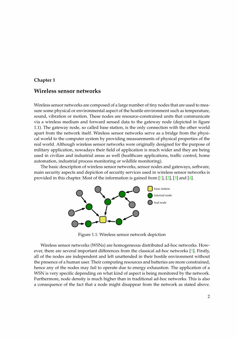
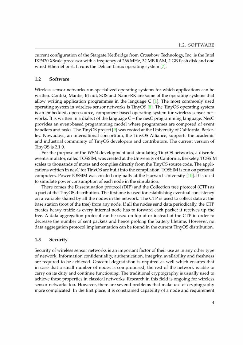
Wireless sensor networks are composed of a large number of tiny nodes that are used to mea-sure some physical or environmental aspect of the hostile environment such as temperature,sound, vibration or motion. These nodes are resource-constrained units that communicatevia a wireless medium and forward sensed data to the gateway node (depicted in figure1.1). The gateway node, so called base station, is the only connection with the other worldapart from the network itself. Wireless sensor networks serve as a bridge from the physi-cal world to the computer system by providing measurements of physical properties of thereal world. Although wireless sensor networks were originally designed for the purpose ofmilitary application, nowadays their field of application is much wider and they are beingused in civilian and industrial areas as well (healthcare applications, traffic control, homeautomation, industrial process monitoring or wildlife monitoring).

The basic description of wireless sensor networks, sensor nodes and gateways, software,main security aspects and depiction of security services used in wireless sensor networks isprovided in this chapter. Most of the information is gained from [1], [2], [3] and [4].

leaf node

base station

internal node

Figure 1.1: Wireless sensor network depiction

Wireless sensor networks (WSNs) are homogeneous distributed ad-hoc networks. How-ever, there are several important differences from the classical ad-hoc networks [5]. Firstly,all of the nodes are independent and left unattended in their hostile environment withoutthe presence of a human user. Their computing resources and batteries are more constrained,hence any of the nodes may fail to operate due to energy exhaustion. The application of aWSN is very specific depending on what kind of aspect is being monitored by the network.Furthermore, node density is much higher than in traditional ad-hoc networks. This is alsoa consequence of the fact that a node might disappear from the network as stated above.

2

1.1. SENSOR NODES AND GATEWAYS

Another important issue is security vulnerability of nodes deployed with no constraint ofphysical access to them and hence they might be captured by an attacker or might fail to op-erate. A WSN is highly distributed and its nodes are independent, self-configurable, capableof establishing the routing subsystem without any priorly given infrastructure and able tocooperate with each other.

A sensor network topology may be flat or hierarchical. In case of a hierarchical topology,the network is divided into clusters. Each cluster has a cluster head node which is usually amore powerful node. Cluster heads usually take some responsibilities for network mainte-nance as for example intrusion detection systems can be installed on these nodes. However,they become a single point of failure. In order to prevent this problem, flat sensor networksare deployed.

1.1 Sensor nodes and gateways

Sensor nodes, often referred to as motes, are basic units of WSNs and are capable of pro-cessing, collecting sensed data and communicating with their neighbours in the network.A node consists of a sensor, micro-controller, memory unit, transceiver and power source.A variety of sensor types is used depending on the application of the network. They mightmonitor radiation, temperature, light, movement, sound, humidity, pressure, etc. An ana-logue signal received by a sensor is digitalized and sent to the processing unit. There areseveral choices for wireless transmission. Optical communication is rarely used due to therequirement of line-of-sight among communicating nodes and inconvenient broadcasting.Sensor nodes usually make use of the ISM band for the radio wave transmission and op-erate with communication frequencies between 433 MHz and 2.4 GHz. For this purpose, atransceiver, which is a unit capable of both transmitting and receiving a radio signal, forms apart of every node. Different types of batteries and capacitors are used as power sources forsensor nodes. They might be classified by the type of the electrode, their size, whether theyare re-chargeable or not. Some motes are able to renew their batteries using solar energy orthermo-generators.

There is a wide variety of manufactures of both sensor and gateway nodes as for exampleMoteiv. The intrusion detection system implemented in this work can be compiled for theMoteiv’s Tmote Sky node. Tmote Sky comes with 8 MHz Texas Instruments MSP430 F1611micro-controller, 10 kB of RAM and another 48 kB of flash memory. The micro-controller isa 16-bit RISC ultra low power processor which runs with extremely low active and sleepenergy consumption. IEEE 802.15.4 compliant Chipcon Wireless Transceiver operates at theISM 2.4 GHz frequency band with a data rate of 250 kbit/s. The mote has integrated humid-ity, temperature and light sensors [6].

A gateway node, usually referred to as a base station, provides a connection to the outerworld, most commonly to the Internet. It is a much more powerful device than a sensor nodeand its energy resources are more long-lasting too. It serves as a collector of the measuredvalues and security alerts from the motes in the network it is governing. Since the basestation is connected to the Internet, it is maintained by a human user. As an example, the

3

1.2. SOFTWARE

current configuration of the Stargate NetBridge from Crossbow Technology, Inc. is the IntelIXP420 XScale processor with a frequency of 266 MHz, 32 MB RAM, 2 GB flash disk and onewired Ethernet port. It runs the Debian Linux operating system [7].

1.2 Software

Wireless sensor networks run specialized operating systems for which applications can bewritten. Contiki, Mantis, BTnut, SOS and Nano-RK are some of the operating systems thatallow writing application programmes in the language C [1]. The most commonly usedoperating system in wireless sensor networks is TinyOS [8]. The TinyOS operating systemis an embedded, open-source, component-based operating system for wireless sensor net-works. It is written in a dialect of the language C – the nesC programming language. NesCprovides an event-based programming model where programmes are composed of eventhandlers and tasks. The TinyOS project [9] was rooted at the University of California, Berke-ley. Nowadays, an international consortium, the TinyOS Alliance, supports the academicand industrial community of TinyOS developers and contributors. The current version ofTinyOS is 2.1.0.

For the purpose of the WSN development and simulating TinyOS networks, a discreteevent simulator, called TOSSIM, was created at the University of California, Berkeley. TOSSIMscales to thousands of motes and compiles directly from the TinyOS source code. The appli-cations written in nesC for TinyOS are built into the compilation. TOSSIM is run on personalcomputers. PowerTOSSIM was created originally at the Harvard University [10]. It is usedto simulate power consumption of each node in the simulation.

There comes the Dissemination protocol (DIP) and the Collection tree protocol (CTP) asa part of the TinyOS distribution. The first one is used for establishing eventual consistencyon a variable shared by all the nodes in the network. The CTP is used to collect data at thebase station (root of the tree) from any node. If all the nodes send data periodically, the CTPcreates heavy traffic as every internal node has to forward each packet it receives up thetree. A data aggregation protocol can be used on top of or instead of the CTP in order todecrease the number of sent packets and hence prolong the battery lifetime. However, nodata aggregation protocol implementation can be found in the current TinyOS distribution.

1.3 Security

Security of wireless sensor networks is an important factor of their use as in any other typeof network. Information confidentiality, authentication, integrity, availability and freshnessare required to be achieved. Graceful degradation is required as well which ensures thatin case that a small number of nodes is compromised, the rest of the network is able tocarry on its duty and continue functioning. The traditional cryptography is usually used toachieve these properties in classical networks. Research in this field is ongoing for wirelesssensor networks too. However, there are several problems that make use of cryptographymore complicated. In the first place, it is constrained capability of a node and requirement

4

1.3. SECURITY

for its price to be as low as possible (networks consist of thousands of nodes). The ad-hocinfrastructure-less nature of sensor networks makes the problem more challenging as wellbecause there is no trusted central authority there. Furthermore, nodes are left unattendedand because of their desired low price, they cannot have any tamper resistant or reactionmechanisms built in them. An adversary is then able to capture a node, retrieve its crypto-graphic material and be aware of its internal state and control its communication with therest of the network [4].

As described in [4], there are several attacker types considered in wireless sensor net-works. A passive attacker is only able to read ongoing communication, gather it, analyseand possibly extract cryptographic keys using cryptography analysis. Defence against a pas-sive attacker is usually the encryption of data traffic. On the other hand, there is an activeattacker which can also alter or inject new messages into the network communication. Theyare able to destroy some messages as well. An active attacker can perform external or inter-nal attacks (we talk of a malicious outsider or insider respectively). External attacks are runby an attacker that does not compose a part of the network. Employing encryption mecha-nisms is not enough here and security is enhanced by authentication and synchronizationmechanisms. An internal attacker is a legitimate mote in the network and has access to allof the mote’s key material. That is why cryptographic techniques cannot help defendingagainst internal attacks. An intrusion detection system (IDS) has to be used in the network.An IDS monitors behaviour of the nodes in the network and alerts the gateway node in casethere is a suspect of an internal attacker. Finally, attackers may be divided based on the typeof the device they use. Mote-class attackers misuse motes to run their attacks. Laptop-classattackers use more powerful devices with higher radio transceiver power and longer batterylife-time.

5

Chapter 2

Intrusion detection systems

A wireless sensor network is deployed without a predefined infrastructure and left unat-tended. It is required for a WSN to be inherently autonomous. This involves to be able toreact on certain unusual events and reconfigure the network without human assistance or aslittle assistance as possible. To achieve the self-reconfigurability property, a situation aware-ness mechanism needs to be installed in the network so it is aware of the unusual eventswhich the WSN should react on. A situation awareness mechanism has to be lightweightbecause of limited computational and battery resources of tiny nodes [11].

Intrusion detection systems are installed in order to detect internal attackers in networks.As stated in [11], “the major task of an IDS is to monitor computer networks and systemsto detect these eventual intrusions in the network, alert users after specific intrusions havebeen detected, and finally, if possible, reconfigure the network and mark the root of theproblem as malicious”. A classification of different types of intrusion detection systems anddescription of components of an IDS for WSNs is given in this chapter. At its end, twoapproaches how to implement a neighbour-based intrusion detection system that is able tomonitor several network properties at a time are presented.

In classical networks, intrusion detection systems are mainly situated on powerful main-frames of network segments and are able to process efficiently all data coming from the seg-ment on which they operate. Unfortunately, there are no such devices in the case of WSNs. Itmust be decided how to take the advantage of redundancy in means of the number of nodesand how to deal with low-performance processing. It is essential to find optimal distribu-tion of performance, battery saving and robustness. Moreover, an access to the mainframesin classical networks can be physically limited which makes them a reliable source of in-formation. As opposed to this advantage, information gained from IDSs running on sensornodes needs to be filtered because of possible presence of malicious adversaries.

Authors of [11] use a metaphor that a WSN should be able to heal itself by which theymean that a WSN should be self-reconfigurable. They liken a wireless sensor network to aliving body where nodes are cells of the body and a base station is the brain. In such reason-ing, network’s malicious intruders, the nodes captured by an attacker, represent diseasesand viruses. This metaphor is good because the way by which diseases are discovered inliving bodies is the same as in intrusion detection systems for wireless sensor networks. AnIDS monitors network’s behaviour and looks for symptoms of diseases, possible attacks.

6

2.1. IDS CLASSIFICATION

2.1 IDS classification

The description of different kinds of IDS classification based on [4] are summarized in thissection.

There are generally two types of an intrusion detection – anomaly detection and sig-nature (sometimes denoted as misuse) detection. A difference can be seen in the way theydiscover malicious nodes. Any unusual behavioural deviations in the network opposed toits normal behaviour is announced as an anomaly in case of the anomaly detection. An IDSof such a type has to be able to learn about the normal behaviour of the network. There isusually a start-up phase, often denoted as a training phase, of an IDS for this purpose andthe IDS only gathers information about normal flow for some period of time. It has to beensured that no intruders exist in the network during this phase which might be hard toachieve. “Signature based detection techniques match the known attack profiles with suspi-cious behaviours” as stated in [12]. For this purpose, attack footprints have to be defined foreach type of the attack that should be recognized by the IDS.

Both anomaly and signature based IDSs have their pros and cons. A signature baseddetection is very effective in revealing known attacks whose patterns are defined in theIDS. However, it fails completely to uncover unknown attacks. They can be recognized byan anomaly detection though. Unfortunately, such an IDS requires training to learn whata normal traffic flow looks like and if network’s dynamics have changed, the IDS has tobe re-trained. Employing both detection techniques should provide an effective detectionmechanism for a sensor network. Additionally, a specification detection is sometimes intro-duced as the third type of IDSs. It is very similar to an anomaly detection, however, the setof rules is defined a priori and so no training phase is involved. This work deals with theneighbour-based intrusion detection which is a specific type of the anomaly detection. Theneighbour-based detection technique is well-described later in this chapter.

From another point of view, intrusion detection systems might be classified dependingon their collaboration abilities into collaborative and non-collaborative (also referred to asdistributed and stand-alone respectively). In case of a distributed IDS, a false informationfiltering system should be implemented as the IDS may collaborate with IDSs running onnodes captured by an adversary. Reputation schemes are often employed for this purpose.Stand-alone detection systems do not suffer with these problems. On the other hand, theremight not be enough information gathered locally to decide some types of attacks. We de-signed and implemented both collaborative and non-collaborative modifications of an IDSfor flat wireless sensor networks. More information is available in chapter 4.

Collaborative IDSs are categorized as peer-to-peer and hierarchical. Peer-to-peer IDSscreate high communication overhead. Hence, information should be distributed just in asmall neighbourhood around a node. Hierarchical IDSs assume existence of nodes whichtake responsibilities of cluster heads which brings the problem of a single point of failure.An attacker who captures just a few nodes which are actually the cluster heads paralysesfunctioning of an IDS for the whole network. The IDS proposed in this thesis belongs to thepeer-to-peer category of IDSs.

7

2.2. BLUEPRINT OF AN INTRUSION DETECTION SYSTEM ARCHITECTURE

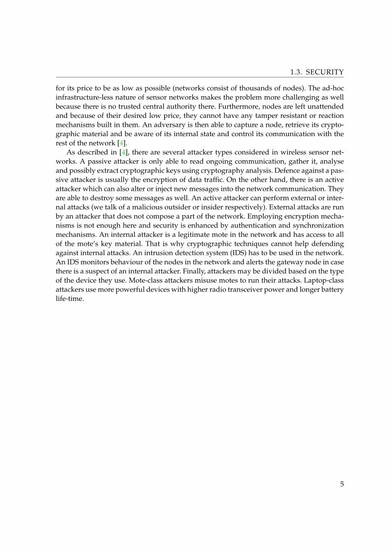
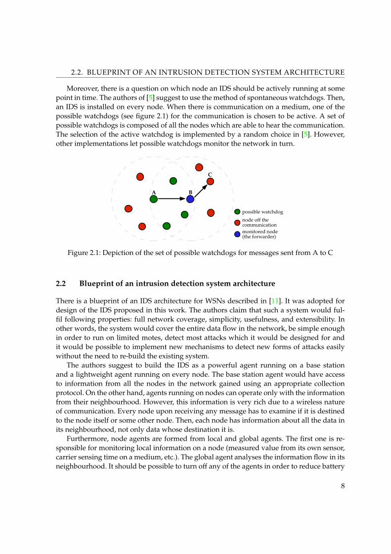
Moreover, there is a question on which node an IDS should be actively running at somepoint in time. The authors of [5] suggest to use the method of spontaneous watchdogs. Then,an IDS is installed on every node. When there is communication on a medium, one of thepossible watchdogs (see figure 2.1) for the communication is chosen to be active. A set ofpossible watchdogs is composed of all the nodes which are able to hear the communication.The selection of the active watchdog is implemented by a random choice in [5]. However,other implementations let possible watchdogs monitor the network in turn.

A B

C

node off the communicationmonitored node (the forwarder)

possible watchdog

Figure 2.1: Depiction of the set of possible watchdogs for messages sent from A to C

2.2 Blueprint of an intrusion detection system architecture

There is a blueprint of an IDS architecture for WSNs described in [11]. It was adopted fordesign of the IDS proposed in this work. The authors claim that such a system would ful-fil following properties: full network coverage, simplicity, usefulness, and extensibility. Inother words, the system would cover the entire data flow in the network, be simple enoughin order to run on limited motes, detect most attacks which it would be designed for andit would be possible to implement new mechanisms to detect new forms of attacks easilywithout the need to re-build the existing system.

The authors suggest to build the IDS as a powerful agent running on a base stationand a lightweight agent running on every node. The base station agent would have accessto information from all the nodes in the network gained using an appropriate collectionprotocol. On the other hand, agents running on nodes can operate only with the informationfrom their neighbourhood. However, this information is very rich due to a wireless natureof communication. Every node upon receiving any message has to examine if it is destinedto the node itself or some other node. Then, each node has information about all the data inits neighbourhood, not only data whose destination it is.

Furthermore, node agents are formed from local and global agents. The first one is re-sponsible for monitoring local information on a node (measured value from its own sensor,carrier sensing time on a medium, etc.). The global agent analyses the information flow in itsneighbourhood. It should be possible to turn off any of the agents in order to reduce battery

8

2.3. NEIGHBOUR-BASED INTRUSION DETECTION TECHNIQUES

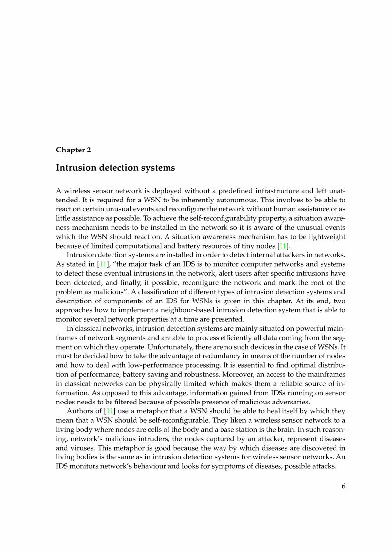
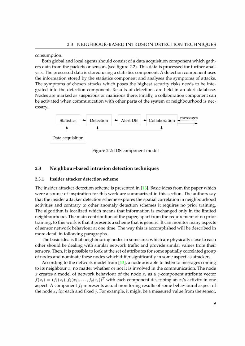
consumption.Both global and local agents should consist of a data acquisition component which gath-

ers data from the packets or sensors (see figure 2.2). This data is processed for further anal-ysis. The processed data is stored using a statistics component. A detection component usesthe information stored by the statistics component and analyses the symptoms of attacks.The symptoms of chosen attacks which poses the highest security risks needs to be inte-grated into the detection component. Results of detections are held in an alert database.Nodes are marked as suspicious or malicious there. Finally, a collaboration component canbe activated when communication with other parts of the system or neighbourhood is nec-essary.

messagesDetectionStatistics Alert DB Collaboration

Data acquisition

Figure 2.2: IDS component model

2.3 Neighbour-based intrusion detection techniques

2.3.1 Insider attacker detection scheme

The insider attacker detection scheme is presented in [13]. Basic ideas from the paper whichwere a source of inspiration for this work are summarized in this section. The authors saythat the insider attacker detection scheme explores the spatial correlation in neighbourhoodactivities and contrary to other anomaly detection schemes it requires no prior training.The algorithm is localized which means that information is exchanged only in the limitedneighbourhood. The main contribution of the paper, apart from the requirement of no priortraining, to this work is that it presents a scheme that is generic. It can monitor many aspectsof sensor network behaviour at one time. The way this is accomplished will be described inmore detail in following paragraphs.

The basic idea is that neighbouring nodes in some area which are physically close to eachother should be dealing with similar network traffic and provide similar values from theirsensors. Then, it is possible to look at the set of attributes for some spatially correlated groupof nodes and nominate these nodes which differ significantly in some aspect as attackers.

According to the network model from [13], a node x is able to listen to messages comingto its neighbour xi no matter whether or not it is involved in the communication. The nodex creates a model of network behaviour of the node xi as a q-component attribute vectorf(xi) = (f1(xi), f2(xi), . . . , fq(xi))T with each component describing an xi’s activity in oneaspect. A component fj represents actual monitoring results of some behavioural aspect ofthe node xi for each and fixed j. For example, it might be a measured value from the sensor,

9

2.3. NEIGHBOUR-BASED INTRUSION DETECTION TECHNIQUES

a number of dropped packets per burst period, packet delivery ratio per some period oftime, etc. Behavioural aspects are chosen as appropriate and quantifiable properties whichrepresent statistics that are used to evaluate symptoms of attacks which should be detectedby the IDS. The authors assume that for any local area of normal sensor nodes xi, all f(xi)follow the same multivariate normal distribution.

The data acquisition component of the node x gathers information from its neighbour-hood and creates the set F (x) = {(f(xi) = (f1(xi), f2(xi), . . . , fq(xi))T |xi ∈ N(x)} of at-tribute vectors, where N(x) is the set of neighbours of the node x. This set of attributes isbroadcast within the neighbourhood N(x) and is taken as a source of statistics for the de-tection component. This approach eliminates the need of the training phase and storing itsresults permanently in the database of the detection component of the IDS. In each period,the normal behaviour of a node is defined as the “centre” of the set F (x).

According to [13], the detection component of the insider attacker detection schememarks malicious intruders after studying the data set F (x). Actually, each node possessesthe data set of sets {F (xi)|xi ∈ N(x)}. This fact is not taken into account in [13] and it is notclear what happens with the data sets F (xi) which were broadcast. The paper follows withassuming only the data set F (x).

Malicious attackers are considered nodes which are further from the “centre” of the setF (x) than a threshold t0. Details on a computation of the Mahalanobis distance using Or-thogonalized Gnanadesikan-Kettenring estimators can be found in [13] as well as the deter-mination of the threshold t0. The paper continues with a description of a voting protocolfor the final decision about malicious nodes. Different nodes mark the attacker based oninformation from different neighbourhoods. A node has to be considered an intruder by amajority of its neighbours in order to be excluded from routing tables, reported in the alertdatabase and announced to the base station.

The authors assume that the network on which the insider attacker detection system canbe installed is operating a data aggregation protocol. This assumption is important becauseit ensures that traffic loads in some neighbourhood are correlated. We will try to extendour solution onto networks operating the Collection tree protocol. This will be achieved byemploying clustering (see section 4.4). Furthermore, the implemented IDS that was testedin the discussed paper is programmed to reveal a single attack – fabricated informationattack (a malicious node alters the information gained from its sensor). We would like tofind out what other attacks can be revealed by the proposed scheme (see chapter 3) andimplement an IDS which can detect most of them. As mentioned in the text above, there isan open question what happens with the data set of sets {F (xi)|xi ∈ N(x)} gathered by thecollaboration component. Hence, we provide results for several collaborating options andcompare them (see section 4.5).

2.3.2 Group-based intrusion detection scheme

The full description of the group-based intrusion detection can be found in [12]. The de-tection component of this scheme is very similar to the insider attacker detection scheme.

10

2.3. NEIGHBOUR-BASED INTRUSION DETECTION TECHNIQUES

There is even a comparison of simulation results with the insider attacker detection at theend of the paper. The group-based intrusion detection scheme is said to be more precisein marking malicious nodes as attackers and its false alarm rate is lower at the same time.Additionally, it consumes less energy. These satisfying results come from the way nodes aregrouped. When the IDS agents are started, preferably after the network start-up, a groupingalgorithm is initiated. It is an initial phase after which agents are ready to detect intruders.

The grouping algorithm starts with some nodes sending grouping requests after waitinga random period of time. If a node receives such a grouping request, it joins the group onlyif it is spatially close enough and its sensed values of the physical environment are similar tothe root node of the grouping request. Nodes that are not grouped wait a random amount oftime to initiate another grouping request (hence, they become the roots of these new groups).The thresholds limiting the maximal distance between nodes in some group and the group’sroot node and the maximal deviation of their sensed values have to be defined accordinglyto the nature of the network and its application.

Each group is divided into several subgroups which monitor the entire group in turn inorder to reduce battery consumption. The data acquisition components of nodes of activesubgroups work the same as in the case of the previously mentioned IDS. However, a set ofattribute vectors F (x) is not broadcast among the group neither the subgroup. The detectionmechanism processes F (x) locally and makes its decision about outliers (malicious nodes)in the group (again, the same principle and mathematics functions are used as in the case ofthe IDS mentioned in the previous section). No majority voting follows. If an IDS agent findsan attacker, it alerts the entire group with a warning message about the attacker. If there aremore such messages, the entire group wakes up and all of the nodes monitor the agitatorand the proposed malicious node. If abnormal behaviour is detected in any of these two, thebase station is alerted and the actual malicious node is excluded from routing tables.

The authors of the paper include the list of attacks (together with information that needsto be collected for their detection) which are suitable for their scheme. The list can be seen intable 2.1. However, they implemented their IDS only for the fabricated information attack.We will point out that there is no need to use the neighbour-based detection technique toreveal packet alteration in section 3.6. Furthermore, detection of a sinkhole attack based on ahigh packet receiving rate would provide inaccurate detection results as there may be sink-holes which are not malicious in a network too (see section 3.4). As mentioned before, theauthors implemented their IDS to reveal the fabricated information attack. Hence, they pro-grammed the grouping algorithm to group according to the correlation of values measuredby nodes’ sensors. If a generic IDS capable of revealing several attacks at a time should beimplemented, it is not clear how to group nodes effectively.

11

2.3. NEIGHBOUR-BASED INTRUSION DETECTION TECHNIQUES

Collected information Attacksensor sensed data fabricated information attackpacket sending rate jamming

packet dropping rate selective forwardingpacket mismatch rate packet alterationpacket receiving rate sinkhole attack

packet sending power hello flood attack

Table 2.1: Attacks whose detection is possible with the neighbour-based detection techniqueand statistics needed to reveal them

12

Chapter 3

Attacks

There are different types of attackers and many types of attacks they are able to perform.We focus on active external and internal attackers (insiders) as they are able to run moreconvenient attacks and the intrusion detection system is deployed to defend against theseattacks. An IDS is used to differentiate among trusted nodes and attackers as they mightform a legitimate part of the network. In this chapter, the basic description and symptomsof chosen attacks are introduced.

Symptoms of attacks are very important for the study of intrusion detection systems forWSNs. An IDS may determine an internal attacker in the network based on the pre-definedsymptoms of known attacks. This work deals with jamming, hello flood, selective forward-ing, sinkhole, sybil, packet alteration and fabricated information attacks. The description ofthese attacks is outlined here based on [14], [15] and [16]. This chapter also discusses whethersome of the symptoms mentioned for each attack are appropriate to be used for implemen-tation of a neighbour-based IDS as described in the previous chapter (section 2.3.1).

3.1 Jamming

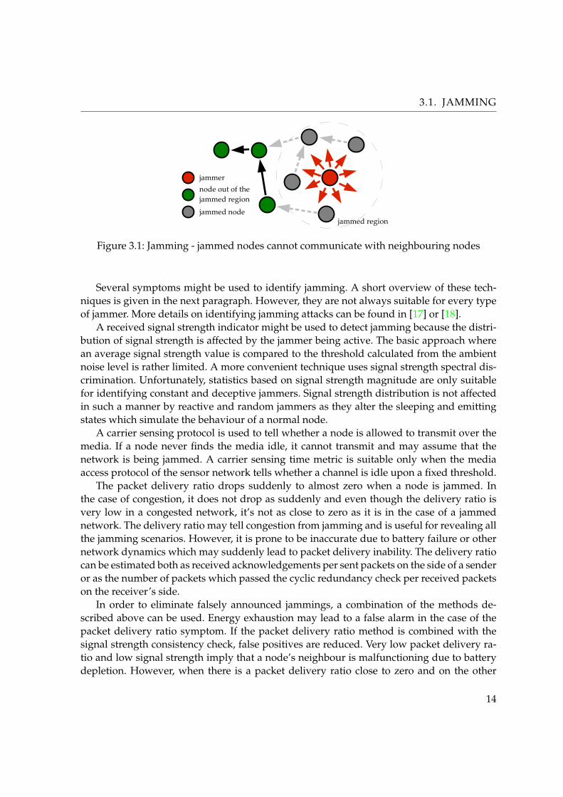
Jamming is interfering with the radio frequency used by nodes for their communication. Itis performed by deliberate transmission of radio signals. It is used to conduct a denial ofservice attack as nodes cannot communicate at all while a jamming attack is ongoing (figure3.1). Nodes consider their communication media to be in use, or they believe some node istransmitting and so they remain in a receiving mode the whole time. A jamming attack iscaused by a device which is usually referred to as a jammer. It might be a sensor node orsome other device able to interfere with the radio frequency of the wireless sensor network.We may distinguish among various types of jamming attacks and jammers. Among the onesthat may be the most effective are constant, deceptive, random and reactive jammers [17].

A constant jammer continually emits a radio signal without respecting any medium ac-cess protocol. In this case, other nodes never find the medium idle. A deceptive jammeruniformly injects regular packets without any gap so other nodes stay in the receiving modemost of the time. A random jammer emits or is asleep to reduce battery consumption. Itswitches these two states in a random manner. Random jamming may be implemented byboth constant and deceptive jammers. A reactive jammer emits only when there is commu-nication on the medium. It is harder to detect than the previous techniques and again it maybe implemented by both constant and deceptive jammers.

13

3.1. JAMMING

jammed regionjammed node

jammernode out of the jammed region

Figure 3.1: Jamming - jammed nodes cannot communicate with neighbouring nodes

Several symptoms might be used to identify jamming. A short overview of these tech-niques is given in the next paragraph. However, they are not always suitable for every typeof jammer. More details on identifying jamming attacks can be found in [17] or [18].

A received signal strength indicator might be used to detect jamming because the distri-bution of signal strength is affected by the jammer being active. The basic approach wherean average signal strength value is compared to the threshold calculated from the ambientnoise level is rather limited. A more convenient technique uses signal strength spectral dis-crimination. Unfortunately, statistics based on signal strength magnitude are only suitablefor identifying constant and deceptive jammers. Signal strength distribution is not affectedin such a manner by reactive and random jammers as they alter the sleeping and emittingstates which simulate the behaviour of a normal node.

A carrier sensing protocol is used to tell whether a node is allowed to transmit over themedia. If a node never finds the media idle, it cannot transmit and may assume that thenetwork is being jammed. A carrier sensing time metric is suitable only when the mediaaccess protocol of the sensor network tells whether a channel is idle upon a fixed threshold.

The packet delivery ratio drops suddenly to almost zero when a node is jammed. Inthe case of congestion, it does not drop as suddenly and even though the delivery ratio isvery low in a congested network, it’s not as close to zero as it is in the case of a jammednetwork. The delivery ratio may tell congestion from jamming and is useful for revealing allthe jamming scenarios. However, it is prone to be inaccurate due to battery failure or othernetwork dynamics which may suddenly lead to packet delivery inability. The delivery ratiocan be estimated both as received acknowledgements per sent packets on the side of a senderor as the number of packets which passed the cyclic redundancy check per received packetson the receiver’s side.

In order to eliminate falsely announced jammings, a combination of the methods de-scribed above can be used. Energy exhaustion may lead to a false alarm in the case of thepacket delivery ratio symptom. If the packet delivery ratio method is combined with thesignal strength consistency check, false positives are reduced. Very low packet delivery ra-tio and low signal strength imply that a node’s neighbour is malfunctioning due to batterydepletion. However, when there is a packet delivery ratio close to zero and on the other

14

3.2. HELLO FLOOD ATTACK

hand signal strength is high, a jamming attack is ongoing in the wireless sensor networkwith highest probability.

The last method, actually the combination of two of them, should provide the most re-liable way to reveal jamming. It is even suitable for all of the jamming scenarios definedin this section. Unfortunately, the delivery ratio is meant to be compared with a predefinedthreshold (a number close to zero). From this point of view, the neighbour-based techniquewould not be convenient to use (it compares the delivery ratio values among the nodesin the neighbourhood and that is not intended by the packet delivery ratio method). Theneighbour-based detection scheme described in the previous chapter is determined to serveas a global agent (see section 2.2) – it monitors the behaviour of its neighbourhood (notthe node running the IDS agent itself). That is why detection based on carrier sensing timecannot also be implemented. Carrier sensing time is a statistic appropriate for monitoringby local agents. We exclude monitoring of the distribution of signal strength because of thesame reason.

A packet sending rate (PSR) is easy to monitor and simple assumption would suggestthat a node which sends an abnormal amount of packets is one that produces jamming [12].We can definitely detect deceptive jammers by monitoring the PSRs of the neighbouringnodes. However, it depends on the jammer’s implementation and the network protocol usedwhether detection of random and reactive jammers is possible. Eventually, we use a verynaive and limited approach to reveal constant jamming. If there is a node producing anextraordinarily strong signal when communicating with other nodes, it is suspected of beinga possible jammer which would be able to jam a reasonably large part of the network.

3.2 Hello flood attack

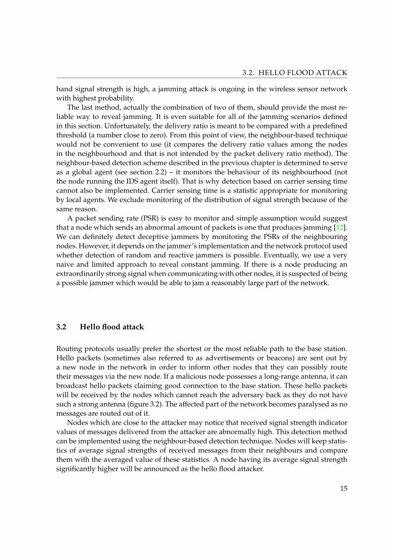
Routing protocols usually prefer the shortest or the most reliable path to the base station.Hello packets (sometimes also referred to as advertisements or beacons) are sent out bya new node in the network in order to inform other nodes that they can possibly routetheir messages via the new node. If a malicious node possesses a long-range antenna, it canbroadcast hello packets claiming good connection to the base station. These hello packetswill be received by the nodes which cannot reach the adversary back as they do not havesuch a strong antenna (figure 3.2). The affected part of the network becomes paralysed as nomessages are routed out of it.

Nodes which are close to the attacker may notice that received signal strength indicatorvalues of messages delivered from the attacker are abnormally high. This detection methodcan be implemented using the neighbour-based detection technique. Nodes will keep statis-tics of average signal strengths of received messages from their neighbours and comparethem with the averaged value of these statistics. A node having its average signal strengthsignificantly higher will be announced as the hello flood attacker.

15

3.3. SELECTIVE FORWARDING

radio range of the attacker

node unable to reach the attacker

attacker

node close to the attacker

Figure 3.2: Hello flood - nodes which cannot reach the attacker will choose it for their parentmost probably, hence paralysing themselves

3.3 Selective forwarding

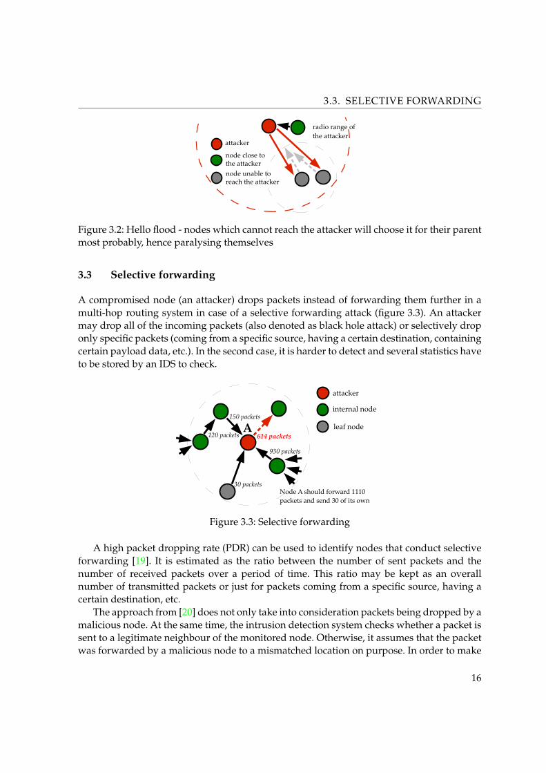
A compromised node (an attacker) drops packets instead of forwarding them further in amulti-hop routing system in case of a selective forwarding attack (figure 3.3). An attackermay drop all of the incoming packets (also denoted as black hole attack) or selectively droponly specific packets (coming from a specific source, having a certain destination, containingcertain payload data, etc.). In the second case, it is harder to detect and several statistics haveto be stored by an IDS to check.

614 packets

150 packets

120 packets

30 packets

930 packets

leaf node

attacker

internal node

A

Node A should forward 1110 packets and send 30 of its own

Figure 3.3: Selective forwarding

A high packet dropping rate (PDR) can be used to identify nodes that conduct selectiveforwarding [19]. It is estimated as the ratio between the number of sent packets and thenumber of received packets over a period of time. This ratio may be kept as an overallnumber of transmitted packets or just for packets coming from a specific source, having acertain destination, etc.

The approach from [20] does not only take into consideration packets being dropped by amalicious node. At the same time, the intrusion detection system checks whether a packet issent to a legitimate neighbour of the monitored node. Otherwise, it assumes that the packetwas forwarded by a malicious node to a mismatched location on purpose. In order to make

16

3.4. SINKHOLE ATTACK

this technique work, the form of a hello packet (used to establish routing tables when a newnode is added to the network) has to be changed so each node is able to derive its two-hopneighbours from it. This requirement makes this mechanism harder to implement than inthe case of packet dropping rate monitoring. The protocol for finding out node’s two-hopneighbours would mean another communicational and computational overhead for tinynodes. The described neighbour-based intrusion detection is supposed to be a lightweightagent and is not considered to provide such a functionality.

On the other hand, the packet dropping rate is an appropriate metric that can be usedto monitor the network behaviour of a node’s neighbourhood in the neighbour-based IDS.Nodes that are in spatial correlation (according to the insider attacker detection described inthe previous chapter) should be dealing with a similar traffic load and network dynamics.The PDR should be similar as well and if a node drops packets in extreme numbers, it isprobably malicious.

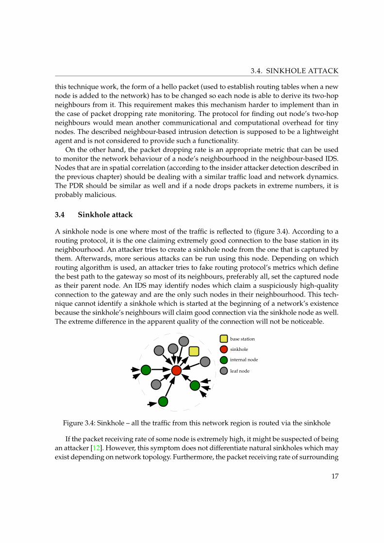
3.4 Sinkhole attack

A sinkhole node is one where most of the traffic is reflected to (figure 3.4). According to arouting protocol, it is the one claiming extremely good connection to the base station in itsneighbourhood. An attacker tries to create a sinkhole node from the one that is captured bythem. Afterwards, more serious attacks can be run using this node. Depending on whichrouting algorithm is used, an attacker tries to fake routing protocol’s metrics which definethe best path to the gateway so most of its neighbours, preferably all, set the captured nodeas their parent node. An IDS may identify nodes which claim a suspiciously high-qualityconnection to the gateway and are the only such nodes in their neighbourhood. This tech-nique cannot identify a sinkhole which is started at the beginning of a network’s existencebecause the sinkhole’s neighbours will claim good connection via the sinkhole node as well.The extreme difference in the apparent quality of the connection will not be noticeable.

sinkhole

base station

internal node

leaf node

Figure 3.4: Sinkhole – all the traffic from this network region is routed via the sinkhole

If the packet receiving rate of some node is extremely high, it might be suspected of beingan attacker [12]. However, this symptom does not differentiate natural sinkholes which mayexist depending on network topology. Furthermore, the packet receiving rate of surrounding

17

3.5. SYBIL ATTACK

nodes will become high as well because they will gain very good connection to the basestation via the sinkhole node. This approach is considered very limited and not suitable forintrusion detection techniques.

Although a malicious node may claim that its connection to the gateway is better thanit actually is, nodes in its neighbourhood do not have to change their parents straight away(this depends on a routing protocol, e.g. the CTP in TinyOS is designed this way). An at-tacker has to downgrade the quality of other nodes’ connections in this case. A maliciousnode may spoof fake root update packets impersonating its neighbours. The authors of [21]suggest that this form of sinkhole attack may be revealed by an IDS which observes whethersenders of root update packets are in the neighbourhood of the node running the IDS. If notor if they are even sent by the node running the IDS itself (possible when the packet’s headeris altered), some node is running the sinkhole attack in the network.

This technique effectively reveals attackers that try to downgrade the quality of othernodes’ connections. If some node finds out that another node spoofs packets, it should alertother nodes about this immediately. It does not matter what the common behaviour of theneighbourhood is. From this point of view, this technique is not suitable for the neighbour-based intrusion detection. Unfortunately, no other technique that could be used is known.

3.5 Sybil attack

A sybil node is one that is claiming multiple identities. An attacker that owns these identi-ties may take advantage in voting protocols or create routing paths for their own benefits.Communication with sybil nodes may be direct or indirect. In direct communication, thecompromised node communicates with the other nodes in charge of all of its identities. Inindirect communication, the sybil node claims that it communicates with nodes that actuallydo not exist. Sybil identities might be fabricated or stolen. A sybil attack can be performedsimultaneously or non-simultaneously depending on whether the sybil node uses its iden-tities at once or over time.

A sybil node may be revealed by location testing which is based on the principle thatsome number of cooperating nodes are able to estimate another node’s location based onsome measurements. If they find out that two nodes are located at the same position, a sybilattack is most likely being conducted by an attacker.

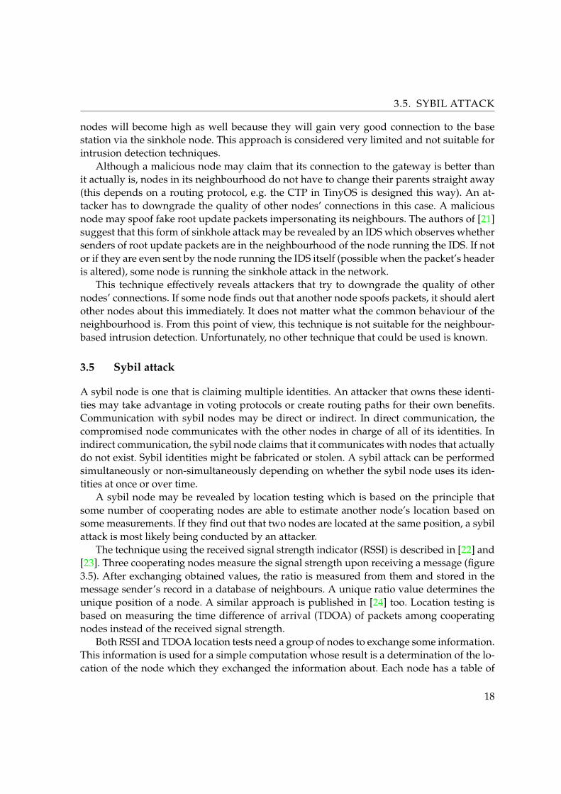
The technique using the received signal strength indicator (RSSI) is described in [22] and[23]. Three cooperating nodes measure the signal strength upon receiving a message (figure3.5). After exchanging obtained values, the ratio is measured from them and stored in themessage sender’s record in a database of neighbours. A unique ratio value determines theunique position of a node. A similar approach is published in [24] too. Location testing isbased on measuring the time difference of arrival (TDOA) of packets among cooperatingnodes instead of the received signal strength.

Both RSSI and TDOA location tests need a group of nodes to exchange some information.This information is used for a simple computation whose result is a determination of the lo-cation of the node which they exchanged the information about. Each node has a table of

18

3.6. PACKET ALTERATION

-70 dB

AB

if green nodes exchange the RSSI information with each other, they will find out that A and B broadcast from the same location

-70 dB

-73 dB

-73 dB

-74 dB

-74 dBsybil node

node performing RSSI-location testing

Figure 3.5: RSSI location testing of sybil attack

such locations of the nodes in its neighbourhood. Both techniques do not look for a propertyof network behaviour which should not vary noticeably for a node in some group of neigh-bouring nodes. This is the reason why it cannot be used for the studied neighbour-basedIDS. Unfortunately, we do not know any other technique that could be implemented.

3.6 Packet alteration

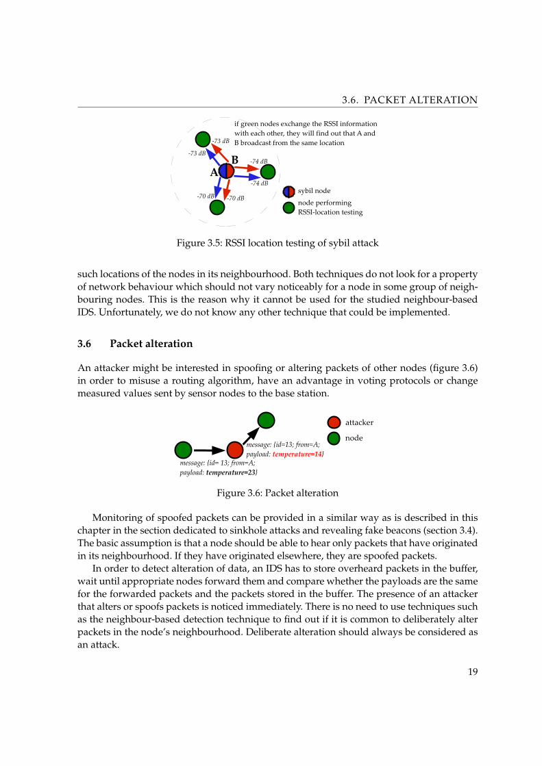
An attacker might be interested in spoofing or altering packets of other nodes (figure 3.6)in order to misuse a routing algorithm, have an advantage in voting protocols or changemeasured values sent by sensor nodes to the base station.

message: {id= 13; from=A; payload: temperature=23}

message: {id=13; from=A; payload: temperature=14}

attacker

node

Figure 3.6: Packet alteration

Monitoring of spoofed packets can be provided in a similar way as is described in thischapter in the section dedicated to sinkhole attacks and revealing fake beacons (section 3.4).The basic assumption is that a node should be able to hear only packets that have originatedin its neighbourhood. If they have originated elsewhere, they are spoofed packets.

In order to detect alteration of data, an IDS has to store overheard packets in the buffer,wait until appropriate nodes forward them and compare whether the payloads are the samefor the forwarded packets and the packets stored in the buffer. The presence of an attackerthat alters or spoofs packets is noticed immediately. There is no need to use techniques suchas the neighbour-based detection technique to find out if it is common to deliberately alterpackets in the node’s neighbourhood. Deliberate alteration should always be considered asan attack.

19

3.7. FABRICATED INFORMATION ATTACK

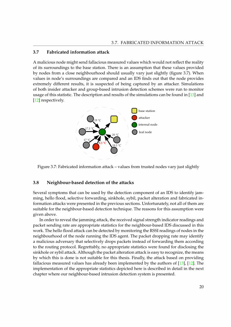
3.7 Fabricated information attack

A malicious node might send fallacious measured values which would not reflect the realityof its surroundings to the base station. There is an assumption that these values providedby nodes from a close neighbourhood should usually vary just slightly (figure 3.7). Whenvalues in node’s surroundings are compared and an IDS finds out that the node providesextremely different results, it is suspected of being captured by an attacker. Simulationsof both insider attacker and group-based intrusion detection schemes were run to monitorusage of this statistic. The description and results of the simulations can be found in [13] and[12] respectively.

19 °C

17.5 °C

17 °C

20 °Cleaf node

base station

internal node

19.5 °C8.5 °C

attacker

Figure 3.7: Fabricated information attack – values from trusted nodes vary just slightly

3.8 Neighbour-based detection of the attacks

Several symptoms that can be used by the detection component of an IDS to identify jam-ming, hello flood, selective forwarding, sinkhole, sybil, packet alteration and fabricated in-formation attacks were presented in the previous sections. Unfortunately, not all of them aresuitable for the neighbour-based detection technique. The reasons for this assumption weregiven above.

In order to reveal the jamming attack, the received signal strength indicator readings andpacket sending rate are appropriate statistics for the neighbour-based IDS discussed in thiswork. The hello flood attack can be detected by monitoring the RSSI readings of nodes in theneighbourhood of the node running the IDS agent. The packet dropping rate may identifya malicious adversary that selectively drops packets instead of forwarding them accordingto the routing protocol. Regrettably, no appropriate statistics were found for disclosing thesinkhole or sybil attack. Although the packet alteration attack is easy to recognize, the meansby which this is done is not suitable for this thesis. Finally, the attack based on providingfallacious measured values has already been implemented by the authors of [13], [12]. Theimplementation of the appropriate statistics depicted here is described in detail in the nextchapter where our neighbour-based intrusion detection system is presented.

20

Chapter 4

IDS design and implementation

This chapter describes the design of the intrusion detection system that has been imple-mented for the purpose of this research. The IDS uses the neighbour-based intrusion de-tection technique (as described in chapter 2) and it serves as a global agent which meansthat it monitors its neighbouring nodes and does not monitor the behaviour of the noderunning the IDS agent itself. The neighbour-based detection technique as described in pre-vious chapters is an anomaly detection technique and the normal behaviour (contrary toanomaly) is defined as actual common behaviour of the neighbourhood. It is assumed thatnon-malicious (referred to as trusted or fair) nodes always prevail in a neighbourhood overthe malicious ones. The decomposition and design of the IDS is mostly based on [11] (seechapter 2). The IDS comes in two modifications. The first one is built to operate over the Col-lection tree protocol [25], [26] and the other one to be run on networks with an aggregationprotocol.

This chapter starts with the depiction of the IDS component model and the description ofthe technique used to process promiscuously overheard communication of the neighbour-ing nodes. It describes how each of the statistics is measured and what other mechanismsare needed to do so. A clustering technique is introduced as the consequence of unsatisfy-ing detection results of selective forwarding and jamming in the CTP operating networks.Finally, implementation of the collaboration component is described.

4.1 IDS component model

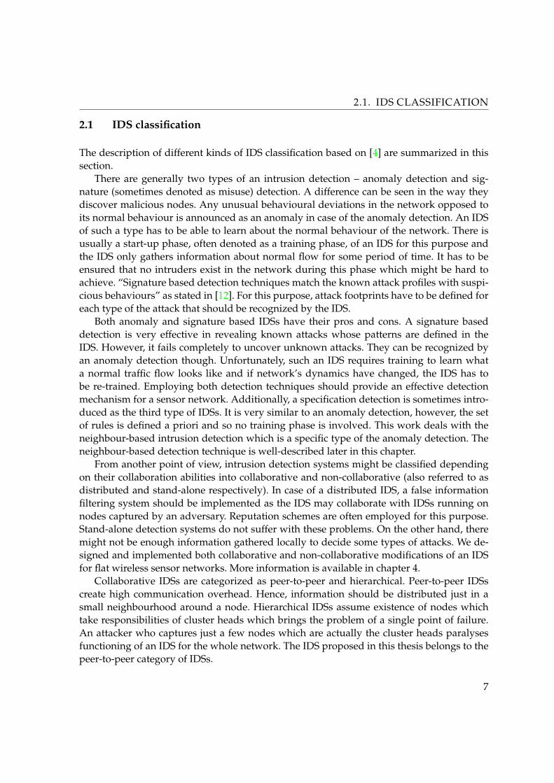
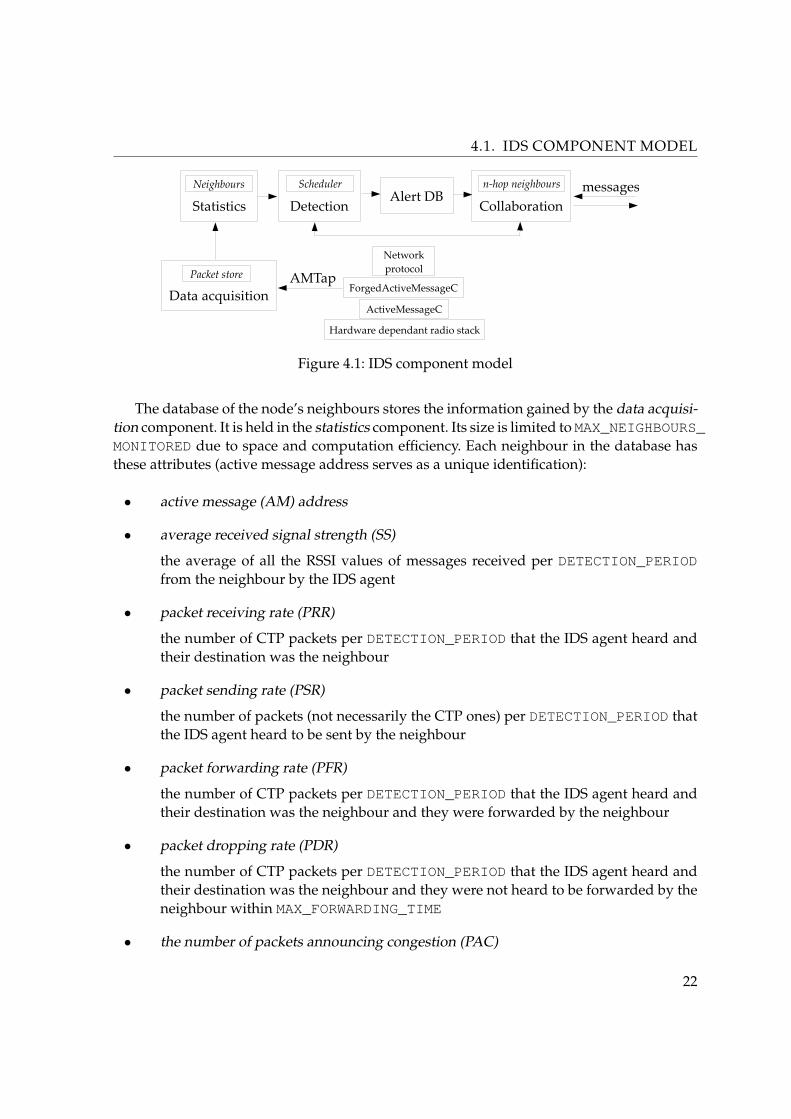
The component model is adopted from [11] and its depiction is summarized in section2.2. The IDS is composed of data acquisition, statistics, detection, collaboration and alertdatabase components (figure 4.1).

The data acquisition component is adopted from [27] and its detailed description canbe found there. It introduces AMTap interface which provides three events: onReceive(message_t* msg, ...), onSnoop(message_t* msg, ...), onSend(message_t*msg, ...). The events are signalled on receiving a message (in case its destination is thisnode), on snooping a message (this occurs if the node can hear the message, however, themessage is not destined to the node itself) and on sending a message by the node. It is pos-sible to gain information about communication involving the node itself or communicationof its neighbours by writing handlers for these events.

21

4.1. IDS COMPONENT MODEL

messagesDetectionStatistics

Alert DBCollaboration

AMTap

Neighbours

ActiveMessageC

ForgedActiveMessageC

Hardware dependant radio stack

Networkprotocol

Data acquisitionPacket store

Scheduler n-hop neighbours

Figure 4.1: IDS component model

The database of the node’s neighbours stores the information gained by the data acquisi-tion component. It is held in the statistics component. Its size is limited to MAX_NEIGHBOURS_MONITORED due to space and computation efficiency. Each neighbour in the database hasthese attributes (active message address serves as a unique identification):

• active message (AM) address

• average received signal strength (SS)

the average of all the RSSI values of messages received per DETECTION_PERIODfrom the neighbour by the IDS agent

• packet receiving rate (PRR)

the number of CTP packets per DETECTION_PERIOD that the IDS agent heard andtheir destination was the neighbour

• packet sending rate (PSR)

the number of packets (not necessarily the CTP ones) per DETECTION_PERIOD thatthe IDS agent heard to be sent by the neighbour

• packet forwarding rate (PFR)

the number of CTP packets per DETECTION_PERIOD that the IDS agent heard andtheir destination was the neighbour and they were forwarded by the neighbour

• packet dropping rate (PDR)

the number of CTP packets per DETECTION_PERIOD that the IDS agent heard andtheir destination was the neighbour and they were not heard to be forwarded by theneighbour within MAX_FORWARDING_TIME

• the number of packets announcing congestion (PAC)

22

4.2. AMBIGUOUS COLLISIONS AND LOW GAIN MODE MONITORING

the number of packets per DETECTION_PERIOD that the IDS agent heard to be sentby the neighbour and the congestion notification bit was set to 1 in these packets’headers

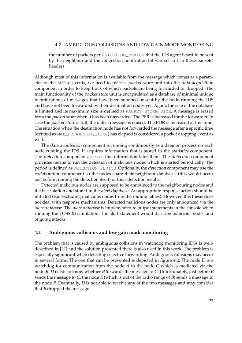
Although most of this information is available from the message which comes as a param-eter of the AMTap events, we need to place a packet store unit into the data acquisitioncomponent in order to keep track of which packets are being forwarded or dropped. Themain functionality of the packet store unit is encapsulated as a database of minimal uniqueidentifications of messages that have been snooped or sent by the node running the IDSand have not been forwarded by their destination nodes yet. Again, the size of the databaseis limited and its maximum size is defined as PACKET_STORE_SIZE. A message is erasedfrom the packet store when it has been forwarded. The PFR is increased for the forwarder. Incase the packet store is full, the oldest message is erased. The PDR is increased at this time.The situation when the destination node has not forwarded the message after a specific time(defined as MAX_FORWARDING_TIME) has elapsed is considered a packet dropping event aswell.

The data acquisition component is running continuously as a daemon process on eachnode running the IDS. It acquires information that is stored in the statistics component.The detection component accesses this information later there. The detection componentprovides means to run the detection of malicious nodes which is started periodically. Theperiod is defined as DETECTION_PERIOD. Optionally, the detection component may use thecollaboration component so the nodes share their neighbour databases (this would occurjust before running the detection itself) or their detection results.

Detected malicious nodes are supposed to be announced to the neighbouring nodes andthe base station and stored in the alert database. An appropriate response action should beinitiated (e.g. excluding malicious nodes from the routing tables). However, this thesis doesnot deal with response mechanisms. Detected malicious nodes are only announced via thealert database. The alert database is implemented to output statements in the console whenrunning the TOSSIM simulation. The alert statement would describe malicious nodes andongoing attacks.

4.2 Ambiguous collisions and low gain mode monitoring

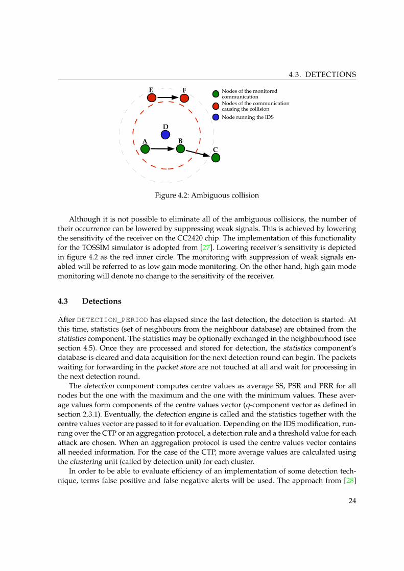
The problem that is caused by ambiguous collisions in watchdog monitoring IDSs is well-described in [27] and the solution presented there is also used in this work. The problem isespecially significant when detecting selective forwarding. Ambiguous collisions may occurin several forms. The one that can be prevented is depicted in figure 4.2. The node D is awatchdog for communication from the node A to the node C which is mediated via thenode B. D needs to know whether B forwards the message to C. Unfortunately, just before Bsends the message to C, the node E (which is out of the radio range of B) sends a message tothe node F. Eventually, D is not able to receive any of the two messages and may considerthat B dropped the message.

23

4.3. DETECTIONS

A BC

Nodes of the monitored communication

D

E F

Nodes of the communication causing the collisionNode running the IDS

Figure 4.2: Ambiguous collision

Although it is not possible to eliminate all of the ambiguous collisions, the number oftheir occurrence can be lowered by suppressing weak signals. This is achieved by loweringthe sensitivity of the receiver on the CC2420 chip. The implementation of this functionalityfor the TOSSIM simulator is adopted from [27]. Lowering receiver’s sensitivity is depictedin figure 4.2 as the red inner circle. The monitoring with suppression of weak signals en-abled will be referred to as low gain mode monitoring. On the other hand, high gain modemonitoring will denote no change to the sensitivity of the receiver.

4.3 Detections

After DETECTION_PERIOD has elapsed since the last detection, the detection is started. Atthis time, statistics (set of neighbours from the neighbour database) are obtained from thestatistics component. The statistics may be optionally exchanged in the neighbourhood (seesection 4.5). Once they are processed and stored for detection, the statistics component’sdatabase is cleared and data acquisition for the next detection round can begin. The packetswaiting for forwarding in the packet store are not touched at all and wait for processing inthe next detection round.

The detection component computes centre values as average SS, PSR and PRR for allnodes but the one with the maximum and the one with the minimum values. These aver-age values form components of the centre values vector (q-component vector as defined insection 2.3.1). Eventually, the detection engine is called and the statistics together with thecentre values vector are passed to it for evaluation. Depending on the IDS modification, run-ning over the CTP or an aggregation protocol, a detection rule and a threshold value for eachattack are chosen. When an aggregation protocol is used the centre values vector containsall needed information. For the case of the CTP, more average values are calculated usingthe clustering unit (called by detection unit) for each cluster.

In order to be able to evaluate efficiency of an implementation of some detection tech-nique, terms false positive and false negative alerts will be used. The approach from [28]

24

4.3. DETECTIONS

is adopted and detailed definitions of these terms can be found there. The term false pos-itive will refer to any alert warning of a node which is not malicious, hence it is accusedfalsely. The number of false positives will be the number of all such alert warnings for adetection period (note that there can be several alert warnings announcing the same node).On the other hand, if a malicious node is not announced by the IDS agent monitoring it,the situation is considered false negative because the presence of the attacker was evaluatedfalsely negative. Again, several false negatives may refer to the same node. Furthermore,the number of nodes falsely accused as malicious is always lower or equal to the number offalse positives and expresses how many different nodes were announced by false positivealert warnings. When the IDS is tested, the number of attackers involved in the network isknown, hence the number of attackers that were not revealed by at least one IDS agent canbe calculated. It is equal to the difference of the number of attackers in the network and thenumber of attackers revealed at least by one IDS agent.

Different detection rules and thresholds are used when running the IDS in networks withan aggregation protocol and the CTP. First of all, network dynamics as PSR or PRR are verycorrelated in case of an aggregation protocol, however, they differ significantly for nodessituated at different levels of the CTP tree or for nodes whose number of children vary to aconsiderable degree. Secondly, PDR and PFR can be monitored only in the case of the CTP.In order to be able to monitor these properties in networks with an aggregation protocol,the IDS would have to know the way messages are aggregated. That is not intended in thiswork.

4.3.1 Detections in networks with an aggregation protocol

In case of the IDS for the aggregation protocol operating networks, a rule is evaluated foreach neighbour in the set of statistics. If a node satisfies the rule, an alert is signalled usingthe alert database. The rules are:

Rule 4.1: Hello flood and constant jamming attacks

node(SS) - centreValues(SS) > SS_THRESHOLD

Rule 4.2: Jamming attack

node(PSR) - centreValues(PSR) > PSR_THRESHOLD

Rule 4.3: Selective forwarding attack (data aggregation protocol networks only)

centreValues(PSR) - node(PSR) > PDR_THRESHOLD OR node(PSR) = 0

We are able to detect a jammer (deceptive, random or reactive) if it emits more messagesthan it is common in its neighbourhood. In the case of the selective forwarding attack, a

25

4.3. DETECTIONS

node which leaves out some of the burst periods is believed to be a dropper. This can benoticed when the PSR of some node is lower than its neighbours’ PSRs. A node which emitsno packets is a black hole and can be identified by the second part of the detection rule 4.3even when the averaged value of PSRs in its neighbourhood is lower than PDR_THRESHOLD.

The thresholds values are identified empirically by the network administrator so thenumbers of false positives and false negatives are bearable (see the chapter Simulations andresults for more information).

4.3.2 Detections in networks with the Collection tree protocol

In case of having the IDS installed on nodes of a network using the CTP, the detection ofhello and constant jamming attacks is done exactly the same way as in networks with anaggregation protocol (rule 4.1).

We are able to detect deceptive, random and reactive jamming. The rules for the detectionof random and reactive jamming attacks will be defined later in the text (section 4.4.2), thedeceptive jamming rule is defined in the previous section (rule 4.2)

The rule for the detection of selective forwarding can be based on comparing the per-centage of the dropped packets. The percentage of the dropped packets will be denoted aspacket dropping ratio. It is defined as the ratio of PDR and receiving rate of packets thatwere supposed to forwarded. This receiving rate can be computed as the sum of PDR andPFR.

Rule 4.4: Selective forwarding attack (CTP networks only)

100 * node(PDR) / (node(PFR) + node(PDR)) -100 * centreValues(PDR) / (centreValues(PFR) + centreValues(PDR)) >PDR_THRESHOLD

However, there are several problems to face. Even though the rules’ definitions are reason-able and express the nature of the attacks, finding threshold values so the trade-off of falsepositives and negatives is bearable might be difficult. Several reasons can be provided toexplain this and a change of the way the rules are applied may make results better.

First of all, for the case of selective forwarding, there are ambiguous collisions whichfalsely increase PDRs for internal nodes of the CTP tree. Even though we decrease the num-ber of their occurrence by low gain mode monitoring, they cannot be omitted totally. Itshould be noted that ambiguous collisions are not an issue for networks with an aggrega-tion protocol because the data traffic is much lower there.

Secondly, and this applies to both jamming and selective forwarding, neighbour-baseddetection is based on the principle that neighbouring nodes deal with similar sensor read-ings, network dynamics, etc. However, this is not true for several metrics describing networkflow which a node deals with in the CTP. Packet receiving rates differ significantly for nodesspatially close to each other if they lie at different levels of the CTP tree or have a different

26

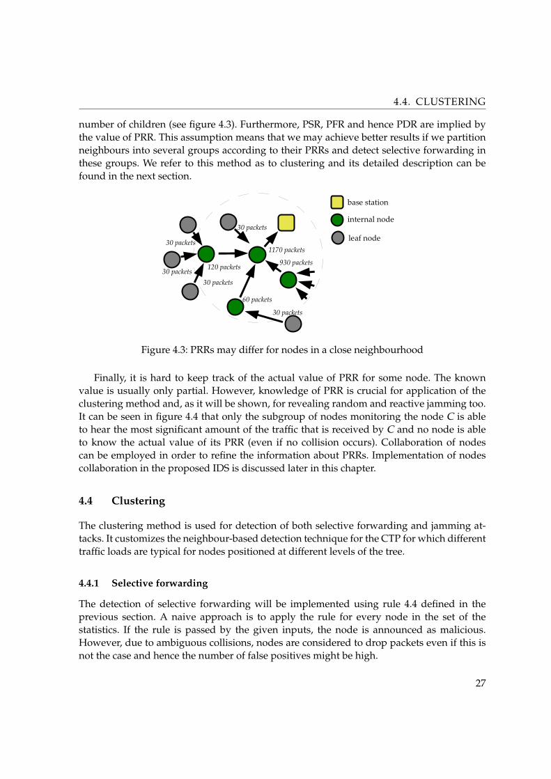
4.4. CLUSTERING

number of children (see figure 4.3). Furthermore, PSR, PFR and hence PDR are implied bythe value of PRR. This assumption means that we may achieve better results if we partitionneighbours into several groups according to their PRRs and detect selective forwarding inthese groups. We refer to this method as to clustering and its detailed description can befound in the next section.

1170 packets

30 packets

120 packets

60 packets

30 packets

30 packets

30 packets30 packets

930 packets

leaf node

base station

internal node

Figure 4.3: PRRs may differ for nodes in a close neighbourhood

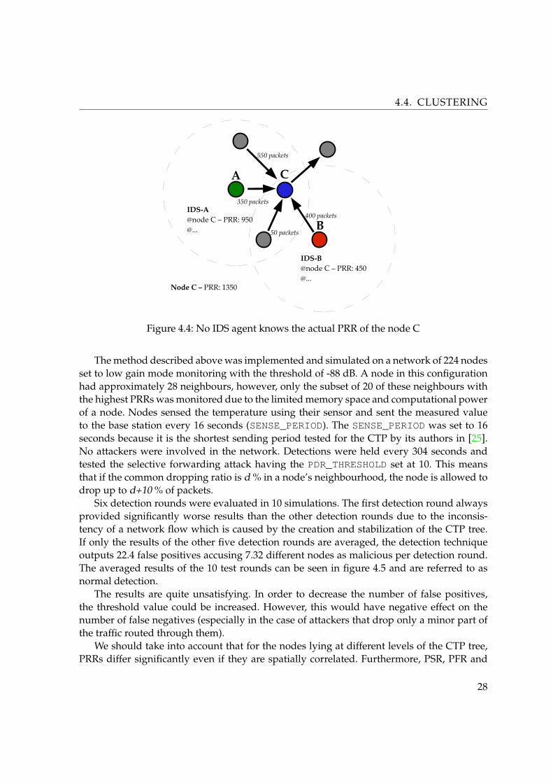
Finally, it is hard to keep track of the actual value of PRR for some node. The knownvalue is usually only partial. However, knowledge of PRR is crucial for application of theclustering method and, as it will be shown, for revealing random and reactive jamming too.It can be seen in figure 4.4 that only the subgroup of nodes monitoring the node C is ableto hear the most significant amount of the traffic that is received by C and no node is ableto know the actual value of its PRR (even if no collision occurs). Collaboration of nodescan be employed in order to refine the information about PRRs. Implementation of nodescollaboration in the proposed IDS is discussed later in this chapter.

4.4 Clustering

The clustering method is used for detection of both selective forwarding and jamming at-tacks. It customizes the neighbour-based detection technique for the CTP for which differenttraffic loads are typical for nodes positioned at different levels of the tree.

4.4.1 Selective forwarding

The detection of selective forwarding will be implemented using rule 4.4 defined in theprevious section. A naive approach is to apply the rule for every node in the set of thestatistics. If the rule is passed by the given inputs, the node is announced as malicious.However, due to ambiguous collisions, nodes are considered to drop packets even if this isnot the case and hence the number of false positives might be high.

27

4.4. CLUSTERING

400 packets

C

550 packets

350 packets

A

B

IDS-B@node C – PRR: 450@...

IDS-A@node C – PRR: 950@... 50 packets

Node C – PRR: 1350

Figure 4.4: No IDS agent knows the actual PRR of the node C

The method described above was implemented and simulated on a network of 224 nodesset to low gain mode monitoring with the threshold of -88 dB. A node in this configurationhad approximately 28 neighbours, however, only the subset of 20 of these neighbours withthe highest PRRs was monitored due to the limited memory space and computational powerof a node. Nodes sensed the temperature using their sensor and sent the measured valueto the base station every 16 seconds (SENSE_PERIOD). The SENSE_PERIOD was set to 16seconds because it is the shortest sending period tested for the CTP by its authors in [25].No attackers were involved in the network. Detections were held every 304 seconds andtested the selective forwarding attack having the PDR_THRESHOLD set at 10. This meansthat if the common dropping ratio is d % in a node’s neighbourhood, the node is allowed todrop up to d+10 % of packets.

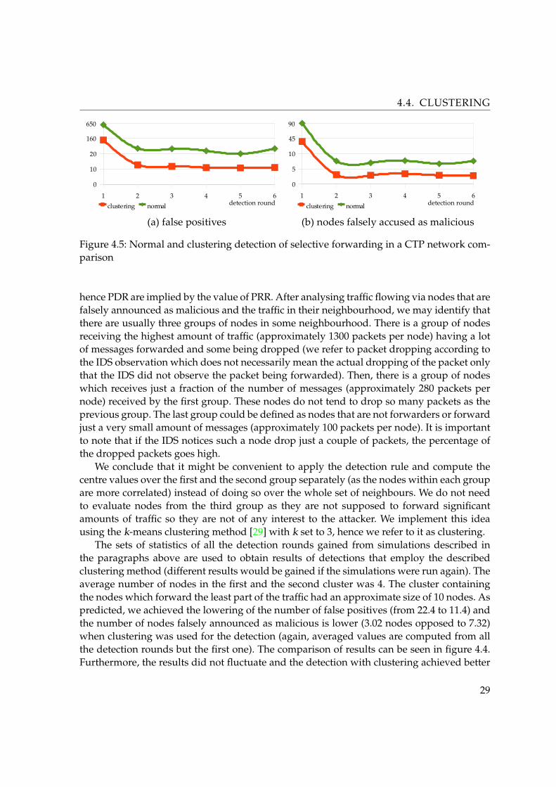
Six detection rounds were evaluated in 10 simulations. The first detection round alwaysprovided significantly worse results than the other detection rounds due to the inconsis-tency of a network flow which is caused by the creation and stabilization of the CTP tree.If only the results of the other five detection rounds are averaged, the detection techniqueoutputs 22.4 false positives accusing 7.32 different nodes as malicious per detection round.The averaged results of the 10 test rounds can be seen in figure 4.5 and are referred to asnormal detection.

The results are quite unsatisfying. In order to decrease the number of false positives,the threshold value could be increased. However, this would have negative effect on thenumber of false negatives (especially in the case of attackers that drop only a minor part ofthe traffic routed through them).

We should take into account that for the nodes lying at different levels of the CTP tree,PRRs differ significantly even if they are spatially correlated. Furthermore, PSR, PFR and

28

4.4. CLUSTERING

1 2 3 4 5 6

0

10

20

30

40

50

clustering normal detection round1 2 3 4 5 6

0

5

10

15

20

25

clustering normal

160

650

45

90

detection round

(b) nodes falsely accused as malicious(a) false positives

Figure 4.5: Normal and clustering detection of selective forwarding in a CTP network com-parison

hence PDR are implied by the value of PRR. After analysing traffic flowing via nodes that arefalsely announced as malicious and the traffic in their neighbourhood, we may identify thatthere are usually three groups of nodes in some neighbourhood. There is a group of nodesreceiving the highest amount of traffic (approximately 1300 packets per node) having a lotof messages forwarded and some being dropped (we refer to packet dropping according tothe IDS observation which does not necessarily mean the actual dropping of the packet onlythat the IDS did not observe the packet being forwarded). Then, there is a group of nodeswhich receives just a fraction of the number of messages (approximately 280 packets pernode) received by the first group. These nodes do not tend to drop so many packets as theprevious group. The last group could be defined as nodes that are not forwarders or forwardjust a very small amount of messages (approximately 100 packets per node). It is importantto note that if the IDS notices such a node drop just a couple of packets, the percentage ofthe dropped packets goes high.

We conclude that it might be convenient to apply the detection rule and compute thecentre values over the first and the second group separately (as the nodes within each groupare more correlated) instead of doing so over the whole set of neighbours. We do not needto evaluate nodes from the third group as they are not supposed to forward significantamounts of traffic so they are not of any interest to the attacker. We implement this ideausing the k-means clustering method [29] with k set to 3, hence we refer to it as clustering.

The sets of statistics of all the detection rounds gained from simulations described inthe paragraphs above are used to obtain results of detections that employ the describedclustering method (different results would be gained if the simulations were run again). Theaverage number of nodes in the first and the second cluster was 4. The cluster containingthe nodes which forward the least part of the traffic had an approximate size of 10 nodes. Aspredicted, we achieved the lowering of the number of false positives (from 22.4 to 11.4) andthe number of nodes falsely announced as malicious is lower (3.02 nodes opposed to 7.32)when clustering was used for the detection (again, averaged values are computed from allthe detection rounds but the first one). The comparison of results can be seen in figure 4.4.Furthermore, the results did not fluctuate and the detection with clustering achieved better

29

4.4. CLUSTERING

result in every single detection round of every simulation.Detection using clustering becomes a part of a default configuration of the proposed IDS

when installed on networks operating the CTP. It is possible to turn off this feature whenneeded. There is no need to use clustering for the detection in networks with an aggregationprotocol because the nodes in these networks should receive and send approximately thesame amount of traffic.

4.4.2 Jamming

The motivation for searching for more advanced techniques for revealing jamming is thesame as in the previous section for the case of selective forwarding. Nodes at different levelsof the CTP tree send different amounts of traffic even though they lie close to each other. Ifwe consider the network from the simulations described in the previous section, it is com-mon that the PSRs of the 20 neighbouring nodes vary from 1,000 to 20 and for some nodesit even goes up to 3,000 or 4,000 (still having leaf nodes with 20 packets sent per detectioninterval in the neighbourhood).

Firstly, we consider deceptive jamming where the jammer is sending packets one afteranother without considering the medium access (MAC) protocol. In this scenario, nodesthat are jammed are the ones within the radio range of the jammer. However, their effort toreach the idle medium grows exponentially and hence they may paralyse their neighboursas well. Furthermore, they are not able to hear any other messages from other nodes becauseof the jamming. If the average value of all the PSRs in the set of the statistics gathered bythe IDS were computed, the number of false positives would be high in the case there wereno jammers in the network (nodes which forward 4,000 packets per detection period wouldbe announced as the jammers). Clustering will be used to differentiate the group of nodeswhich detection will be held on. This will be the union of the two clusters of the nodeshaving the highest PSRs. The clusters are joined together because their average sizes arequite small (2.5 and 2.7 nodes). The other cluster of the nodes whose PSRs are low will notgo through the detection (approximately 13 nodes in this cluster). The detection rule for thedeceptive jamming (rule 4.2) is the one stated in section 4.3.2.

10 simulation tests were run to identify the number of false positives for the case ofrevealing deceptive jamming using clustering disabled and clustering enabled detections.The configuration of the network and the IDS was the same as in the previous section. Thethreshold of how much more a node was allowed to send than the common value in itscluster was set to 2,000. It should be noted that a deceptive jammer in used simulation con-figuration produces up to 60,000 messages per detection round.

The achieved results (the average of all detection rounds but the first one) were 5.78 falsepositives in contrast to 23.56 (when clustering was not used). Approximately less than onenode (0.78) per test round was announced as malicious when clustering was used (it was1.14 in the other case). The results per detection round can be seen in figure 4.6.

We would like to be able to detect another type of jammer as well. It is said to be moreconvenient as it injects packets into the traffic only at the time when other nodes are trans-

30

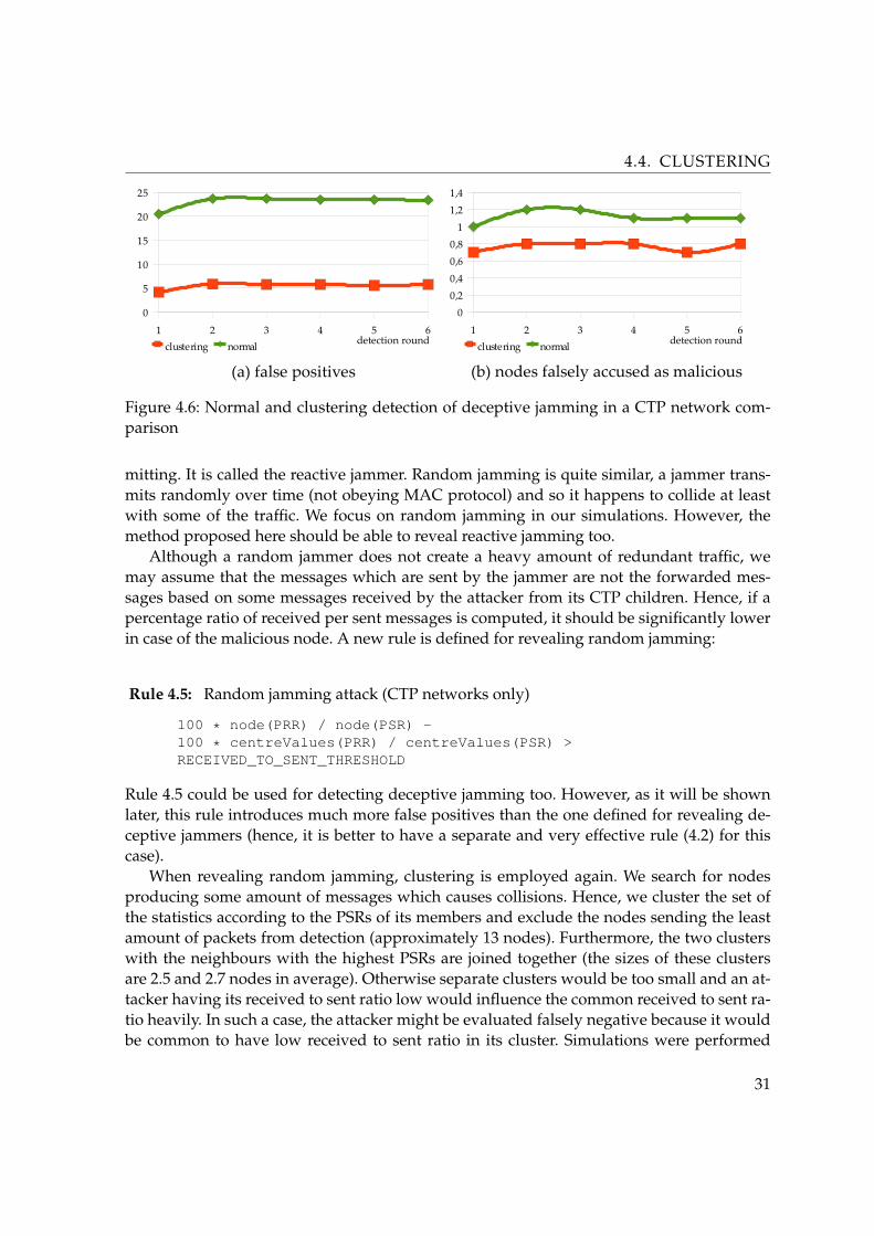
4.4. CLUSTERING

1 2 3 4 5 6

0

5

10

15

20

25

clustering normal detection round1 2 3 4 5 6

00,20,40,60,8

11,21,4

clustering normal detection round

(b) nodes falsely accused as malicious(a) false positives

Figure 4.6: Normal and clustering detection of deceptive jamming in a CTP network com-parison

mitting. It is called the reactive jammer. Random jamming is quite similar, a jammer trans-mits randomly over time (not obeying MAC protocol) and so it happens to collide at leastwith some of the traffic. We focus on random jamming in our simulations. However, themethod proposed here should be able to reveal reactive jamming too.

Although a random jammer does not create a heavy amount of redundant traffic, wemay assume that the messages which are sent by the jammer are not the forwarded mes-sages based on some messages received by the attacker from its CTP children. Hence, if apercentage ratio of received per sent messages is computed, it should be significantly lowerin case of the malicious node. A new rule is defined for revealing random jamming:

Rule 4.5: Random jamming attack (CTP networks only)

100 * node(PRR) / node(PSR) -100 * centreValues(PRR) / centreValues(PSR) >RECEIVED_TO_SENT_THRESHOLD

Rule 4.5 could be used for detecting deceptive jamming too. However, as it will be shownlater, this rule introduces much more false positives than the one defined for revealing de-ceptive jammers (hence, it is better to have a separate and very effective rule (4.2) for thiscase).

When revealing random jamming, clustering is employed again. We search for nodesproducing some amount of messages which causes collisions. Hence, we cluster the set ofthe statistics according to the PSRs of its members and exclude the nodes sending the leastamount of packets from detection (approximately 13 nodes). Furthermore, the two clusterswith the neighbours with the highest PSRs are joined together (the sizes of these clustersare 2.5 and 2.7 nodes in average). Otherwise separate clusters would be too small and an at-tacker having its received to sent ratio low would influence the common received to sent ra-tio heavily. In such a case, the attacker might be evaluated falsely negative because it wouldbe common to have low received to sent ratio in its cluster. Simulations were performed

31

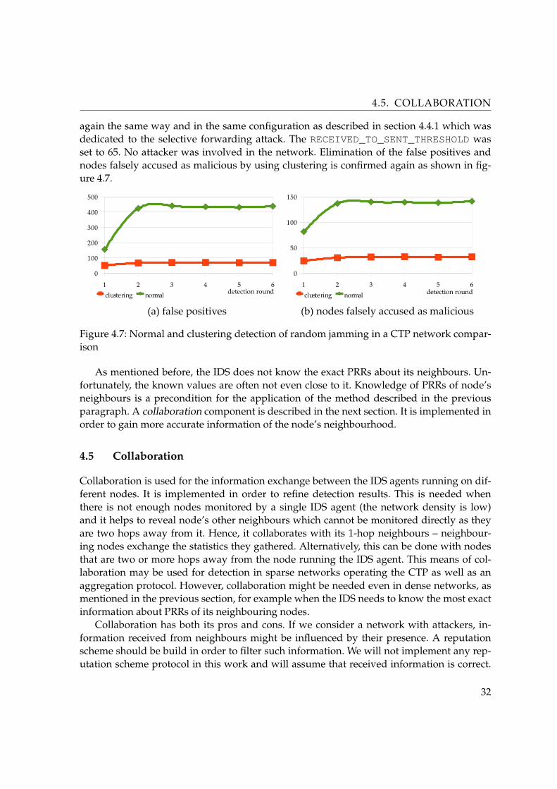
4.5. COLLABORATION

again the same way and in the same configuration as described in section 4.4.1 which wasdedicated to the selective forwarding attack. The RECEIVED_TO_SENT_THRESHOLD wasset to 65. No attacker was involved in the network. Elimination of the false positives andnodes falsely accused as malicious by using clustering is confirmed again as shown in fig-ure 4.7.

1 2 3 4 5 6

0

100

200

300

400

500

clustering normal detection round1 2 3 4 5 6

0

50

100

150

clustering normal detection round

(b) nodes falsely accused as malicious(a) false positives

Figure 4.7: Normal and clustering detection of random jamming in a CTP network compar-ison

As mentioned before, the IDS does not know the exact PRRs about its neighbours. Un-fortunately, the known values are often not even close to it. Knowledge of PRRs of node’sneighbours is a precondition for the application of the method described in the previousparagraph. A collaboration component is described in the next section. It is implemented inorder to gain more accurate information of the node’s neighbourhood.

4.5 Collaboration

Collaboration is used for the information exchange between the IDS agents running on dif-ferent nodes. It is implemented in order to refine detection results. This is needed whenthere is not enough nodes monitored by a single IDS agent (the network density is low)and it helps to reveal node’s other neighbours which cannot be monitored directly as theyare two hops away from it. Hence, it collaborates with its 1-hop neighbours – neighbour-ing nodes exchange the statistics they gathered. Alternatively, this can be done with nodesthat are two or more hops away from the node running the IDS agent. This means of col-laboration may be used for detection in sparse networks operating the CTP as well as anaggregation protocol. However, collaboration might be needed even in dense networks, asmentioned in the previous section, for example when the IDS needs to know the most exactinformation about PRRs of its neighbouring nodes.

Collaboration has both its pros and cons. If we consider a network with attackers, in-formation received from neighbours might be influenced by their presence. A reputationscheme should be build in order to filter such information. We will not implement any rep-utation scheme protocol in this work and will assume that received information is correct.

32

4.5. COLLABORATION

Unfortunately, even then, collaboration may have negative effects. Presence of inaccuratestatistics is increased after exchanging such statistics. On the other hand, statistics might berefined based on the knowledge of node’s neighbours. According to our aim, we need to de-cide if the IDS should prefer information coming from its neighbouring nodes (which mightbe richer in some context) or its own knowledge. Furthermore, received statistics can bejoined together with node’s own statistics or can be used only to refine them. In the secondcase, the number of neighbours would not grow.

The collaboration component, as designed in this work, starts exchanging messages atthe moment when detection is supposed to occur (detection is rescheduled after collabo-ration has finished). Local statistics are stored in the collaboration component and so thestatistics component can be restarted to gather new statistics. Messages are broadcast to 1-hop neighbours. The fields of these messages are DETECTION_NUMBER, IS_FIRST_ROUND,NEIGHBOUR_1, NEIGHBOUR_2. The first field indicates to which detection (numbered fromthe network start-up) this messages belongs to. The following field indicates whether it is thefirst or the second collaboration round and is used only in case of the 2-hop neighbours ex-change (see below). Records of two of the neighbours from the statistics component follow.When a node receives such a message, it checks if the detection number is the number of theactual detection round. If so, it accepts the message and stores its content into the collabora-tion database. The exchange message period ends after MAX_BOOT_TIME + SEND_DELAY.MAX_BOOT_TIME refers to the period when nodes are being booted at the network start-up and SEND_DELAY is defined as time needed for the last node to send out its statistics.After this time, nodes discard any collaboration messages until the actual detection roundfinishes. All the received statistics are joined together and with the IDS agent’s own ones. Itis common that several IDS agents running on neighbouring nodes monitor the same node.When the collaboration component is used in such case, the IDS agent has several recordsabout the same node after joining all of the statistics together. The one with the highest PRRis kept in our IDS. It is presumed that a node usually knows only about part of the messagesreceived by its neighbour (see figure 4.4). However, it cannot know about messages thatwere not sent to a node. Hence, the node which heard the highest amount of the packets isthe one possessing the most accurate information about neighbour’s PRR. The resulting setis passed to the detection engine for the detection.

There is 2-hop neighbours collaboration implemented too. It is done in two rounds. Thefirst one is the same as described in the previous paragraph. When having all the statisticsjoined together, they are said to be the statistics gathered by the actual IDS agent and sent outagain the same way. In order to be able to address to which collaboration round a receivedmessage belongs, the IS_FIRST_ROUND field is defined. The proposed IDS comes in threemodifications – the one without collaboration and two with it – namely the 1-hop and 2-hopneighbours collaborations.

We would like to know if the collaboration component eliminates occurrence of falsepositives when revealing random jamming. Assumption is that it may do so due to moreprecise information about PRRs of the monitored nodes. However, the number of false pos-itives may be multiplied by accepting falsely alert positive statistics from other nodes at the

33

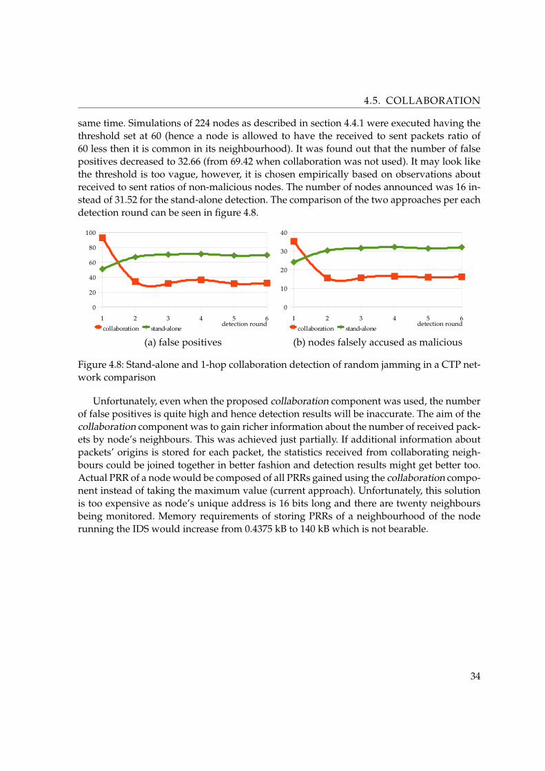
4.5. COLLABORATION

same time. Simulations of 224 nodes as described in section 4.4.1 were executed having thethreshold set at 60 (hence a node is allowed to have the received to sent packets ratio of60 less then it is common in its neighbourhood). It was found out that the number of falsepositives decreased to 32.66 (from 69.42 when collaboration was not used). It may look likethe threshold is too vague, however, it is chosen empirically based on observations aboutreceived to sent ratios of non-malicious nodes. The number of nodes announced was 16 in-stead of 31.52 for the stand-alone detection. The comparison of the two approaches per eachdetection round can be seen in figure 4.8.

1 2 3 4 5 6

0

20

40

60

80

100

collaboration stand-alonedetection round

1 2 3 4 5 6

0

10

20

30

40

collaboration stand-alonedetection round

(b) nodes falsely accused as malicious(a) false positives

Figure 4.8: Stand-alone and 1-hop collaboration detection of random jamming in a CTP net-work comparison

Unfortunately, even when the proposed collaboration component was used, the numberof false positives is quite high and hence detection results will be inaccurate. The aim of thecollaboration component was to gain richer information about the number of received pack-ets by node’s neighbours. This was achieved just partially. If additional information aboutpackets’ origins is stored for each packet, the statistics received from collaborating neigh-bours could be joined together in better fashion and detection results might get better too.Actual PRR of a node would be composed of all PRRs gained using the collaboration compo-nent instead of taking the maximum value (current approach). Unfortunately, this solutionis too expensive as node’s unique address is 16 bits long and there are twenty neighboursbeing monitored. Memory requirements of storing PRRs of a neighbourhood of the noderunning the IDS would increase from 0.4375 kB to 140 kB which is not bearable.

34

Chapter 5

Simulations and results

This chapter starts with brief instructions how to deploy our intrusion detection system onTmote Sky hardware or TOSSIM simulator. Description of performed simulations in net-works involving malicious nodes and the results from these simulations follow. Depictionof several optional IDS’ settings and their influence on performance of the IDS can be foundin this chapter as well.

5.1 Deployment of the IDS

The proposed IDS can be incorporated into any wireless sensor network application. How-ever, its performance depends on the configuration of the IDS and the actual network. TheIDS can be configured before compiling by defining macros in the application’s Makefile.Description of these configuration options can be found in the Makefile.template (dis-abling and enabling of clustering, collaboration or low gain monitoring). Furthermore, thedetection period, low gain monitoring threshold, maximum number of monitored neigh-bours and thresholds used in detections can be set in Ids.h.

We only mention here that disabling hardware address recognition is necessary for theIDS to function. Otherwise the transceiver would reject packets that are not destined toit, hence the IDS agent would not be able to monitor its neighbourhood. Disabling hard-ware address recognition can be done by adding the following rule to the application’sMakefile.

CFLAGS += -DCC2420_NO_ADDRESS_RECOGNITION

The path to the IDS source code has to be added there too:

CFLAGS += -I$(IDS_DIR)

Finally, the application can be compiled for Tmote Sky mote or for simulating usingTOSSIM. After a node is booted, the IDS starts up – the data acquisition component pro-cesses network traffic and the first detection is scheduled. Detection and AlertDb chan-nels can be added in order to see detection outputs and alerts while simulation is runningin TOSSIM. This is done by calling addChannel(channel, output) on the Tossim ob-ject in C++ or Python source code which manages the simulation. File pointer or standardoutput can be provided as the output parameter.

35

5.2. SIMULATING INTRUSION DETECTION IN NETWORKS WITH ATTACKERS

C++ Tossim* t = new Tossim(NULL);t->addChannel("Detection", stdout);

Python >>> t = Tossim([])>>> t.addChannel("Detection", sys.stdout)

5.2 Simulating intrusion detection in networks with attackers

Results from simulations of networks including malicious nodes are summarized in thissection. Firstly, simulations of a networks with an aggregation protocol are described. CTPoperating network simulations follow.

5.2.1 Networks with an aggregation protocol

The way data is aggregated is no matter to the functionality of our IDS. Hence, it was suffi-cient to alter the CTP for the purpose of simulating an aggregation protocol. The forwardingengine was disabled and so each node sent only its own values up the network tree. As thenumber of packets sent in the network was lowered, less retransmissions were needed andless collisions occurred while monitoring.

A network of 224 nodes set to low gain mode monitoring with the threshold of -88 dBwas used for simulations. A node in this configuration had approximately 28 neighbours,however, only the subset of 20 of these neighbours with the highest PRRs was monitored.Nodes sent the measured values from their sensors to the gateway every 8 seconds. Thedetection period was set to 304 seconds. The collaboration component was not used.

Six detection rounds were evaluated in 5 simulations for each attack. We wanted to knowthe number of false positives, nodes falsely accused as malicious, false negatives and num-ber of alerts about malicious nodes. Five attackers were involved in each simulation. Wetested hello flood, jamming, selective forwarding and black hole attacks. The threshold val-ues differentiating malicious and trusted nodes were defined empirically.

The terms false positives, nodes falsely accused as malicious and false negatives have al-ready been explained in section 4.3. The number of alerts about malicious nodes will denoteonly to correct alert warnings when the IDS marks a malicious node as malicious. Hence,false positives and false negatives are not counted in this number.

5.2.1.1 Hello flood attack

A hello flood attacker was implemented as a node whose signal strength is 40 dB strongerthan it would be if a normal node was used situated at the same place in the network. SS_TRESHOLD was set to 30 dB which means that a node having its average signal strengthhigher by more than 30 dB than the average value for its neighbourhood will be announcedas an attacker.

36

5.2. SIMULATING INTRUSION DETECTION IN NETWORKS WITH ATTACKERS

The IDS was able to recognize all of the attackers and produced 92 to 98.2 alerts in aver-age per detection round having 0 false positives. 824.6 to 966.2 false negatives were recordedin average per detection round. This is understandable. Messages from an attacker are re-ceived by its neighbourhood with an extremely strong signal and nodes in this neighbour-hood are able to reveal the attacker. However, there are a lot of nodes which are spatiallyfar away from the attacker still receiving its messages with the RSSI value not so high anymore. These nodes cannot point out the malicious node as the attacker. Furthermore, theradio range of the attacker is big and so there are plenty of such nodes.

5.2.1.2 Jamming

Five jammers were sending messages randomly at least every 1.5 seconds but not more oftenthan every second. All of them were successfully revealed by their neighbours when PSR_THRESHOLD was set to 100 messages. This means that the PSR of a node cannot be higherby more than 100 messages from the average PSR of node’s neighbourhood. The attackerswere announced in 71 to 78 alerts in average in every detection round. No false positivesand no false negatives occurred.

5.2.1.3 Selective forwarding

In our scenario, a selective forwarder is a node which omits its every other burst period.The IDS revealed all of the five selective forwarders having produced no false positives andfalse negatives. Malicious nodes were announced using 80 to 83 messages in average perdetection round. PDR_THRESHOLD was set to 10 packets.

5.2.1.4 Black hole attack

A black hole node does not generate any traffic except for beaconing. The IDS produced 66.4to 81.8 messages warning about five such nodes. Again, no false positives or false negativesoccurred and PDR_THRESHOLD was set to 10.

5.2.2 Networks with the Collection tree protocol

The simulation environment for the CTP operating network is very similar to the one de-scribed in the section dedicated to networks with an aggregation protocol. The only differ-ences are that nodes send messages containing values from their sensors every 16 secondsand, of course, the CTP is used to deliver these messages to the gateway. Clustering as itwas described in the previous chapter is used for detection of deceptive and random jam-ming and selective forwarding attacks. Ten tests will be provided for each attack this timeas the results tend to fluctuate more. Results from simulations of networks with hello floodattackers, deceptive and random jammers and selective forwarders will be shown in thissection.

37

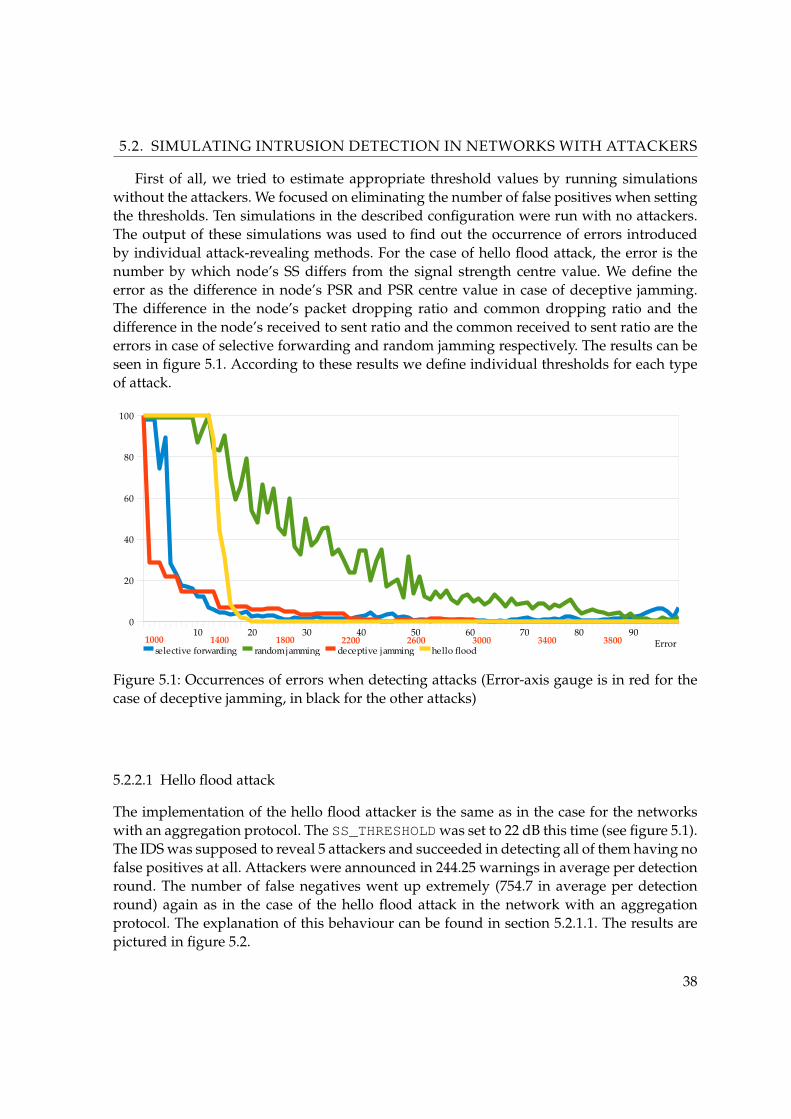
5.2. SIMULATING INTRUSION DETECTION IN NETWORKS WITH ATTACKERS

First of all, we tried to estimate appropriate threshold values by running simulationswithout the attackers. We focused on eliminating the number of false positives when settingthe thresholds. Ten simulations in the described configuration were run with no attackers.The output of these simulations was used to find out the occurrence of errors introducedby individual attack-revealing methods. For the case of hello flood attack, the error is thenumber by which node’s SS differs from the signal strength centre value. We define theerror as the difference in node’s PSR and PSR centre value in case of deceptive jamming.The difference in the node’s packet dropping ratio and common dropping ratio and thedifference in the node’s received to sent ratio and the common received to sent ratio are theerrors in case of selective forwarding and random jamming respectively. The results can beseen in figure 5.1. According to these results we define individual thresholds for each typeof attack.

0

20

40

60

80

100

120

selective forwarding random jamming deceptive jamming hello flood

10 20 30 40 50 60 70 80 901000 1400 1800 2200 30002600 3400 3800 Error

Figure 5.1: Occurrences of errors when detecting attacks (Error-axis gauge is in red for thecase of deceptive jamming, in black for the other attacks)

5.2.2.1 Hello flood attack

The implementation of the hello flood attacker is the same as in the case for the networkswith an aggregation protocol. The SS_THRESHOLD was set to 22 dB this time (see figure 5.1).The IDS was supposed to reveal 5 attackers and succeeded in detecting all of them having nofalse positives at all. Attackers were announced in 244.25 warnings in average per detectionround. The number of false negatives went up extremely (754.7 in average per detectionround) again as in the case of the hello flood attack in the network with an aggregationprotocol. The explanation of this behaviour can be found in section 5.2.1.1. The results arepictured in figure 5.2.

38

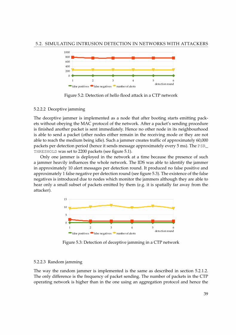
5.2. SIMULATING INTRUSION DETECTION IN NETWORKS WITH ATTACKERS

1 2 3 4 5 6

0

200

400

600

800

1000

false positives false negatives number of alertsdetection round

Figure 5.2: Detection of hello flood attack in a CTP network

5.2.2.2 Deceptive jamming

The deceptive jammer is implemented as a node that after booting starts emitting pack-ets without obeying the MAC protocol of the network. After a packet’s sending procedureis finished another packet is sent immediately. Hence no other node in its neighbourhoodis able to send a packet (other nodes either remain in the receiving mode or they are notable to reach the medium being idle). Such a jammer creates traffic of approximately 60,000packets per detection period (hence it sends message approximately every 5 ms). The PSR_THRESHOLD was set to 2200 packets (see figure 5.1).

Only one jammer is deployed in the network at a time because the presence of sucha jammer heavily influences the whole network. The IDS was able to identify the jammerin approximately 10 alert messages per detection round. It produced no false positive andapproximately 1 false negative per detection round (see figure 5.3). The existence of the falsenegatives is introduced due to nodes which monitor the jammers although they are able tohear only a small subset of packets emitted by them (e.g. it is spatially far away from theattacker).

1 2 3 4 5 6

0

5

10

15

false positives false negatives number of alertsdetection round

Figure 5.3: Detection of deceptive jamming in a CTP network

5.2.2.3 Random jamming

The way the random jammer is implemented is the same as described in section 5.2.1.2.The only difference is the frequency of packet sending. The number of packets in the CTPoperating network is higher than in the one using an aggregation protocol and hence the

39

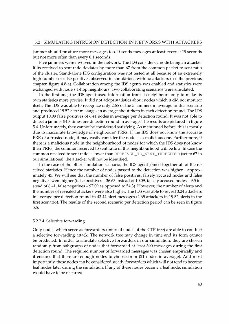
5.2. SIMULATING INTRUSION DETECTION IN NETWORKS WITH ATTACKERS

jammer should produce more messages too. It sends messages at least every 0.25 secondsbut not more often than every 0.1 seconds.

Five jammers were involved in the network. The IDS considers a node being an attackerif its received to sent ratio deviates by more than 67 from the common packet to sent ratioof the cluster. Stand-alone IDS configuration was not tested at all because of an extremelyhigh number of false positives observed in simulations with no attackers (see the previouschapter, figure 4.8-a). Collaboration among the IDS agents was enabled and statistics wereexchanged with node’s 1-hop neighbours. Two collaborating scenarios were simulated.

In the first one, the IDS agent used information from its neighbours only to make itsown statistics more precise. It did not adopt statistics about nodes which it did not monitoritself. The IDS was able to recognize only 2.65 of the 5 jammers in average in this scenarioand produced 19.52 alert messages in average about them in each detection round. The IDSoutput 10.09 false positives of 6.41 nodes in average per detection round. It was not able todetect a jammer 54.3 times per detection round in average. The results are pictured in figure5.4. Unfortunately, they cannot be considered satisfying. As mentioned before, this is mostlydue to inaccurate knowledge of neighbours’ PRRs. If the IDS does not know the accuratePRR of a trusted node, it may easily consider the node as a malicious one. Furthermore, ifthere is a malicious node in the neighbourhood of nodes for which the IDS does not knowtheir PRRs, the common received to sent ratio of this neighbourhood will be low. In case thecommon received to sent ratio is lower than RECEIVED_TO_SENT_THRESHOLD (set to 67 inour simulations), the attacker will not be identified.

In the case of the other simulation scenario, the IDS agent joined together all of the re-ceived statistics. Hence the number of nodes passed to the detection was higher – approx-imately 45. We will see that the number of false positives, falsely accused nodes and falsenegatives went higher (false positives – 36.63 instead of 10.09, falsely accused nodes – 9.5 in-stead of 6.41, false negatives – 97.09 as opposed to 54.3). However, the number of alerts andthe number of revealed attackers were also higher. The IDS was able to reveal 3.24 attackersin average per detection round in 43.44 alert messages (2.65 attackers in 19.52 alerts in thefirst scenario). The results of the second scenario per detection period can be seen in figure5.5.

5.2.2.4 Selective forwarding

Only nodes which serve as forwarders (internal nodes of the CTP tree) are able to conducta selective forwarding attack. The network tree may change in time and its form cannotbe predicted. In order to simulate selective forwarders in our simulation, they are chosenrandomly from subgroups of nodes that forwarded at least 300 messages during the firstdetection round. The required number of forwarded messages was chosen empirically andit ensures that there are enough nodes to choose from (21 nodes in average). And mostimportantly, these nodes can be considered steady forwarders which will not tend to becomeleaf nodes later during the simulation. If any of these nodes became a leaf node, simulationwould have to be restarted.

40

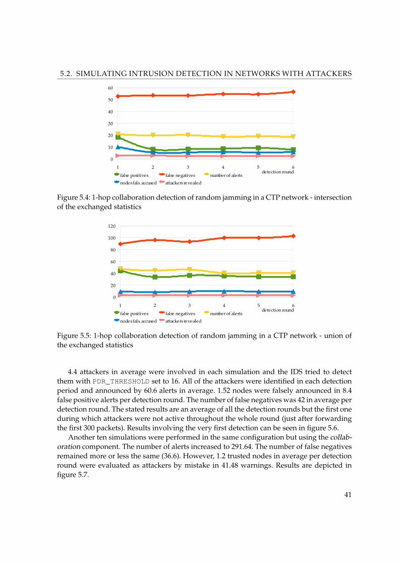
5.2. SIMULATING INTRUSION DETECTION IN NETWORKS WITH ATTACKERS

1 2 3 4 5 6

0

10

20

30

40

50

60

false positives false negatives number of alertsnodes fals. accused attackers revealed

detection round

Figure 5.4: 1-hop collaboration detection of random jamming in a CTP network - intersectionof the exchanged statistics

1 2 3 4 5 6

0

20

40

60

80

100

120

false positives false negatives number of alertsnodes fals. accused attackers revealed

detection round

Figure 5.5: 1-hop collaboration detection of random jamming in a CTP network - union ofthe exchanged statistics

4.4 attackers in average were involved in each simulation and the IDS tried to detectthem with PDR_THRESHOLD set to 16. All of the attackers were identified in each detectionperiod and announced by 60.6 alerts in average. 1.52 nodes were falsely announced in 8.4false positive alerts per detection round. The number of false negatives was 42 in average perdetection round. The stated results are an average of all the detection rounds but the first oneduring which attackers were not active throughout the whole round (just after forwardingthe first 300 packets). Results involving the very first detection can be seen in figure 5.6.

Another ten simulations were performed in the same configuration but using the collab-oration component. The number of alerts increased to 291.64. The number of false negativesremained more or less the same (36.6). However, 1.2 trusted nodes in average per detectionround were evaluated as attackers by mistake in 41.48 warnings. Results are depicted infigure 5.7.

41

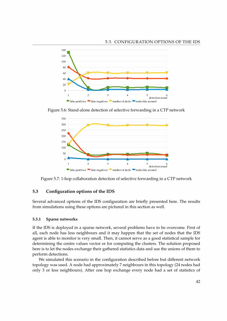
5.3. CONFIGURATION OPTIONS OF THE IDS

1 2 3 4 5 6

0

20

40

60

80

100

120

140

false positives false negatives number of alerts nodes fals. accuseddetection round

Figure 5.6: Stand-alone detection of selective forwarding in a CTP network

1 2 3 4 5 6

0

50

100

150

200

250

300

350

false positives false negatives number of alerts nodes fals. accuseddetection round

Figure 5.7: 1-hop collaboration detection of selective forwarding in a CTP network

5.3 Configuration options of the IDS

Several advanced options of the IDS configuration are briefly presented here. The resultsfrom simulations using these options are pictured in this section as well.

5.3.1 Sparse networks

If the IDS is deployed in a sparse network, several problems have to be overcome. First ofall, each node has less neighbours and it may happen that the set of nodes that the IDSagent is able to monitor is very small. Then, it cannot serve as a good statistical sample fordetermining the centre values vector or for computing the clusters. The solution proposedhere is to let the nodes exchange their gathered statistics data and use the unions of them toperform detections.

We simulated this scenario in the configuration described before but different networktopology was used. A node had approximately 7 neighbours in this topology (24 nodes hadonly 3 or less neighbours). After one hop exchange every node had a set of statistics of

42

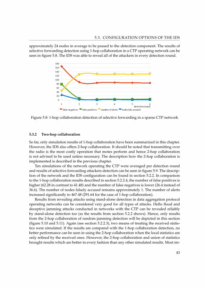
5.3. CONFIGURATION OPTIONS OF THE IDS

approximately 24 nodes in average to be passed to the detection component. The results ofselective forwarding detection using 1-hop collaboration in a CTP operating network can beseen in figure 5.8. The IDS was able to reveal all of the attackers in every detection round.

1 2 3 4 5 6

0

20

40

60

80100

120

140

160

180

false negatives false positives number of alerts nodes fals. accuseddetection round

Figure 5.8: 1-hop collaboration detection of selective forwarding in a sparse CTP network

5.3.2 Two-hop collaboration

So far, only simulation results of 1-hop collaboration have been summarized in this chapter.However, the IDS also offers 2-hop collaboration. It should be noted that transmitting overthe radio is the most costly operation that motes perform and hence 2-hop collaborationis not advised to be used unless necessary. The description how the 2-hop collaboration isimplemented is described in the previous chapter.

Ten simulations of the network operating the CTP were averaged per detection roundand results of selective forwarding attackers detection can be seen in figure 5.9. The descrip-tion of the network and the IDS configuration can be found in section 5.2.2. In comparisonto the 1-hop collaboration results described in section 5.2.2.4, the number of false positives ishigher (62.28 in contrast to 41.48) and the number of false negatives is lower (26.4 instead of36.6). The number of nodes falsely accused remains approximately 1. The number of alertsincreased significantly to 467.48 (291.64 for the case of 1-hop collaboration).

Results from revealing attacks using stand-alone detection in data aggregation protocoloperating networks can be considered very good for all types of attacks. Hello flood anddeceptive jamming attacks conducted in networks with the CTP can be revealed reliablyby stand-alone detection too (as the results from section 5.2.2 shows). Hence, only resultsfrom the 2-hop collaboration of random jamming detection will be depicted in this section(figure 5.10 and 5.11). Again (see section 5.2.2.3), two means of treating the received statis-tics were simulated. If the results are compared with the 1-hop collaboration detection, nobetter performance can be seen in using the 2-hop collaboration when the local statistics areonly refined by the received ones. However, the 2-hop collaboration and union of statisticsbrought results which are better in every fashion than any other simulated results. Most im-

43

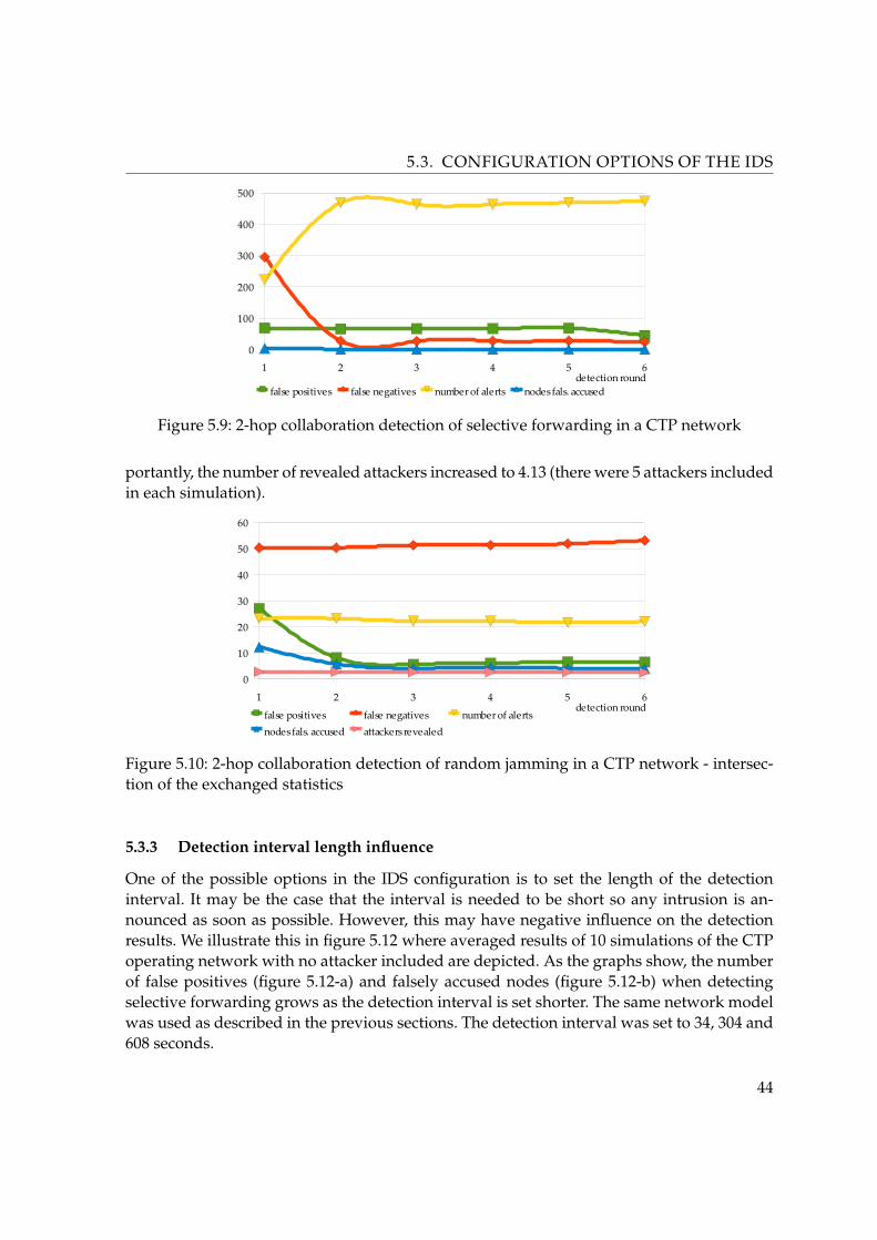
5.3. CONFIGURATION OPTIONS OF THE IDS

1 2 3 4 5 6

0

100

200

300

400

500

false positives false negatives number of alerts nodes fals. accuseddetection round

Figure 5.9: 2-hop collaboration detection of selective forwarding in a CTP network

portantly, the number of revealed attackers increased to 4.13 (there were 5 attackers includedin each simulation).

1 2 3 4 5 6

0

10

20

30

40

50

60

false positives false negatives number of alertsnodes fals. accused attackers revealed

detection round

Figure 5.10: 2-hop collaboration detection of random jamming in a CTP network - intersec-tion of the exchanged statistics

5.3.3 Detection interval length influence

One of the possible options in the IDS configuration is to set the length of the detectioninterval. It may be the case that the interval is needed to be short so any intrusion is an-nounced as soon as possible. However, this may have negative influence on the detectionresults. We illustrate this in figure 5.12 where averaged results of 10 simulations of the CTPoperating network with no attacker included are depicted. As the graphs show, the numberof false positives (figure 5.12-a) and falsely accused nodes (figure 5.12-b) when detectingselective forwarding grows as the detection interval is set shorter. The same network modelwas used as described in the previous sections. The detection interval was set to 34, 304 and608 seconds.

44

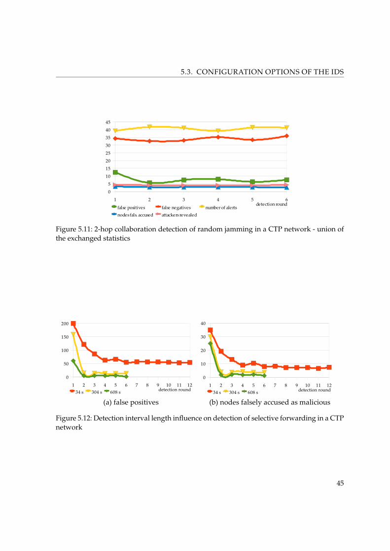
5.3. CONFIGURATION OPTIONS OF THE IDS

1 2 3 4 5 6

0

5

10

15

2025

30

35

40

45

false positives false negatives number of alertsnodes fals. accused attackers revealed

detection round

Figure 5.11: 2-hop collaboration detection of random jamming in a CTP network - union ofthe exchanged statistics

1 2 3 4 5 6 7 8 9 10 11 12

0

50

100

150

200

250

34 s 304 s 608 s detection round1 2 3 4 5 6 7 8 9 10 11 12

0

10

20

30

40

34 s 304 s 608 s detection round

(b) nodes falsely accused as malicious(a) false positives

Figure 5.12: Detection interval length influence on detection of selective forwarding in a CTPnetwork

45

Chapter 6

Conclusions

We have dealt with the neighbour-based intrusion detection technique in this thesis. In orderto design a generic IDS capable of revealing several types of attacks at a time, symptoms andstatistics have to be defined for these attacks. This work provides a study of several attackswhich can be conducted in WSNs and describes possible statistics which can be used toreveal them. It is pointed out that only some of them are appropriate for the neighbour-based detection technique as the technique was defined in [13], [12].

A neighbour-based IDS was designed, implemented and evaluated in the thesis. It wasprogrammed to detect different types of jammers, hello flood and selective forwarding at-tackers. It was shown that detection in aggregation protocol operating networks providesvery good and stable detection results. The IDS was able to reveal all of the attackers in ev-ery single simulation producing no false positives or false negatives except for the case ofthe hello flood attack. Approximately 900 false negative alerts were produced when therewere 5 hello flood attackers deployed in the network. However, this behaviour of the IDSwas explained.

Furthermore, we were able to enhance the IDS to be able to detect mentioned attackersin networks with the CTP as well. We described how the clustering method can be usedin order to achieve this. By employing it, we decreased the number of false positives andfalse negatives almost to 0 in case of the detection of a deceptive jammer. The IDS was neverable to reveal all of the random jammers deployed in the network. The best detection resultswhen the number of false positives was below 10 and at the same time approximately 4random jammers out of 5 deployed were revealed was achieved only by enabling 2-hopcollaboration. Detection of selective forwarding in CTP networks provided approximately60 accurate alerts about 5 malicious nodes revealing all of them and accused falsely onlyless than 2 nodes in average. Even though the number of false negatives was quite high(approximately 42), it was below the number of the accurate alerts.

The IDS comes in several modifications - stand-alone, 1-hop and 2-hop collaboration.Collaboration can be used in order to refine the statistics gathered by the IDS agent. It canalso be used when the IDS is deployed in a sparse network where the number of monitorednodes by a single IDS agent is too low. IDS agents share their knowledge of their neighbour-hoods and gain information about their 2-hop or 3-hop neighbours.

It should be noted that an important advantage of the neighbour-based detection tech-nique is that it requires no prior training. However, the IDS has to be configured before itis deployed in a specific network. The automation of these configuration settings could im-

46

6. CONCLUSIONS

prove the usability of such IDS in the future. Study of advanced clustering techniques couldenhance the current solution and provide better detection results in networks without an ag-gregation protocol. However, this is left for future work in this field.

47

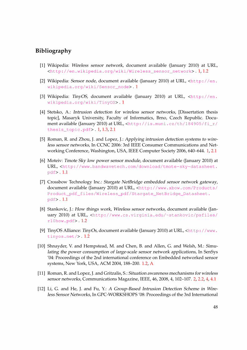
Bibliography

[1] Wikipedia: Wireless sensor network, document available (January 2010) at URL,<http://en.wikipedia.org/wiki/Wireless_sensor_network> . 1, 1.2

[2] Wikipedia: Sensor node, document available (January 2010) at URL, <http://en.wikipedia.org/wiki/Sensor_node> . 1

[3] Wikipedia: TinyOS, document available (January 2010) at URL, <http://en.wikipedia.org/wiki/TinyOS> . 1

[4] Stetsko, A.: Intrusion detection for wireless sensor networks, [Dissertation thesistopic], Masaryk University, Faculty of Informatics, Brno, Czech Republic. Docu-ment available (January 2010) at URL, <http://is.muni.cz/th/184905/fi_r/thesis_topic.pdf> . 1, 1.3, 2.1

[5] Roman, R. and Zhou, J. and Lopez, J.: Applying intrusion detection systems to wire-less sensor networks, In CCNC 2006: 3rd IEEE Consumer Communications and Net-working Conference, Washington, USA, IEEE Computer Society 2006, 640–644. 1, 2.1

[6] Moteiv: Tmote Sky low power sensor module, document available (January 2010) atURL, <http://www.bandwavetech.com/download/tmote-sky-datasheet.pdf> . 1.1

[7] Crossbow Technology Inc.: Stargate NetBridge embedded sensor network gateway,document available (January 2010) at URL, <http://www.xbow.com/Products/Product_pdf_files/Wireless_pdf/Stargate_NetBridge_Datasheet.pdf> . 1.1

[8] Stankovic, J.: How things work, Wireless sensor networks, document available (Jan-uary 2010) at URL, <http://www.cs.virginia.edu/~stankovic/psfiles/r10how.pdf> . 1.2

[9] TinyOS Alliance: TinyOs, document available (January 2010) at URL, <http://www.tinyos.net/> . 1.2

[10] Shnayder, V. and Hempstead, M. and Chen, B. and Allen, G. and Welsh, M.: Simu-lating the power consumption of large-scale sensor network applications, In SenSys’04: Proceedings of the 2nd international conference on Embedded networked sensorsystems, New York, USA, ACM 2004, 188–200. 1.2, A

[11] Roman, R. and Lopez, J. and Gritzalis, S.: Situation awareness mechanisms for wirelesssensor networks, Communications Magazine, IEEE, 46, 2008, 4, 102–107. 2, 2.2, 4, 4.1

[12] Li, G. and He, J. and Fu, Y.: A Group-Based Intrusion Detection Scheme in Wire-less Sensor Networks, In GPC-WORKSHOPS ’08: Proceedings of the 3rd International

48

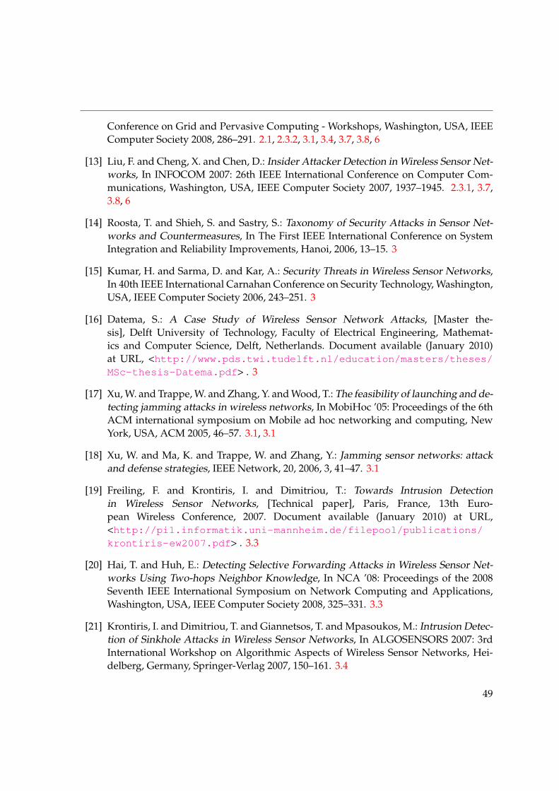
Conference on Grid and Pervasive Computing - Workshops, Washington, USA, IEEEComputer Society 2008, 286–291. 2.1, 2.3.2, 3.1, 3.4, 3.7, 3.8, 6

[13] Liu, F. and Cheng, X. and Chen, D.: Insider Attacker Detection in Wireless Sensor Net-works, In INFOCOM 2007: 26th IEEE International Conference on Computer Com-munications, Washington, USA, IEEE Computer Society 2007, 1937–1945. 2.3.1, 3.7,3.8, 6

[14] Roosta, T. and Shieh, S. and Sastry, S.: Taxonomy of Security Attacks in Sensor Net-works and Countermeasures, In The First IEEE International Conference on SystemIntegration and Reliability Improvements, Hanoi, 2006, 13–15. 3

[15] Kumar, H. and Sarma, D. and Kar, A.: Security Threats in Wireless Sensor Networks,In 40th IEEE International Carnahan Conference on Security Technology, Washington,USA, IEEE Computer Society 2006, 243–251. 3

[16] Datema, S.: A Case Study of Wireless Sensor Network Attacks, [Master the-sis], Delft University of Technology, Faculty of Electrical Engineering, Mathemat-ics and Computer Science, Delft, Netherlands. Document available (January 2010)at URL, <http://www.pds.twi.tudelft.nl/education/masters/theses/MSc-thesis-Datema.pdf> . 3

[17] Xu, W. and Trappe, W. and Zhang, Y. and Wood, T.: The feasibility of launching and de-tecting jamming attacks in wireless networks, In MobiHoc ’05: Proceedings of the 6thACM international symposium on Mobile ad hoc networking and computing, NewYork, USA, ACM 2005, 46–57. 3.1, 3.1

[18] Xu, W. and Ma, K. and Trappe, W. and Zhang, Y.: Jamming sensor networks: attackand defense strategies, IEEE Network, 20, 2006, 3, 41–47. 3.1

[19] Freiling, F. and Krontiris, I. and Dimitriou, T.: Towards Intrusion Detectionin Wireless Sensor Networks, [Technical paper], Paris, France, 13th Euro-pean Wireless Conference, 2007. Document available (January 2010) at URL,<http://pi1.informatik.uni-mannheim.de/filepool/publications/krontiris-ew2007.pdf> . 3.3

[20] Hai, T. and Huh, E.: Detecting Selective Forwarding Attacks in Wireless Sensor Net-works Using Two-hops Neighbor Knowledge, In NCA ’08: Proceedings of the 2008Seventh IEEE International Symposium on Network Computing and Applications,Washington, USA, IEEE Computer Society 2008, 325–331. 3.3

[21] Krontiris, I. and Dimitriou, T. and Giannetsos, T. and Mpasoukos, M.: Intrusion Detec-tion of Sinkhole Attacks in Wireless Sensor Networks, In ALGOSENSORS 2007: 3rdInternational Workshop on Algorithmic Aspects of Wireless Sensor Networks, Hei-delberg, Germany, Springer-Verlag 2007, 150–161. 3.4

49

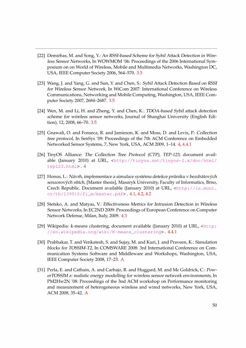
[22] Demirbas, M. and Song, Y.: An RSSI-based Scheme for Sybil Attack Detection in Wire-less Sensor Networks, In WOWMOM ’06: Proceedings of the 2006 International Sym-posium on on World of Wireless, Mobile and Multimedia Networks, Washington DC,USA, IEEE Computer Society 2006, 564–570. 3.5

[23] Wang, J. and Yang, G. and Sun, Y. and Chen, S.: Sybil Attack Detection Based on RSSIfor Wireless Sensor Network, In WiCom 2007: International Conference on WirelessCommunications, Networking and Mobile Computing, Washington, USA, IEEE Com-puter Society 2007, 2684–2687. 3.5

[24] Wen, M. and Li, H. and Zheng, Y. and Chen, K.: TDOA-based Sybil attack detectionscheme for wireless sensor networks, Journal of Shanghai University (English Edi-tion), 12, 2008, 66–70. 3.5

[25] Gnawali, O. and Fonseca, R. and Jamieson, K. and Moss, D. and Levis, P.: Collectiontree protocol, In SenSys ’09: Proceedings of the 7th ACM Conference on EmbeddedNetworked Sensor Systems, 7, New York, USA, ACM 2009, 1–14. 4, 4.4.1

[26] TinyOS Alliance: The Collection Tree Protocol (CTP), TEP-123, document avail-able (January 2010) at URL, <http://tinyos.net/tinyos-2.x/doc/html/tep123.html> . 4

[27] Honus, L.: Návrh, implementace a simulace systému detekce pruniku v bezdrátovýchsenzorových sítích, [Master thesis], Masaryk University, Faculty of Informatics, Brno,Czech Republic. Document available (January 2010) at URL, <http://is.muni.cz/th/139910/fi_m/master.pdf> . 4.1, 4.2, 4.2

[28] Stetsko, A. and Matyas, V.: Effectiveness Metrics for Intrusion Detection in WirelessSensor Networks, In EC2ND 2009: Proceedings of European Conference on ComputerNetwork Defense, Milan, Italy, 2009. 4.3

[29] Wikipedia: k-means clustering, document available (January 2010) at URL, <http://en.wikipedia.org/wiki/K-means_clustering> . 4.4.1

[30] Prabhakar, T. and Venkatesh, S. and Sujay, M. and Kuri, J. and Praveen, K.: Simulationblocks for TOSSIM-T2, In COMSWARE 2008: 3rd International Conference on Com-munication Systems Software and Middleware and Workshops, Washington, USA,IEEE Computer Society 2008, 17–23. A

[31] Perla, E. and Cathain, A. and Carbajo, R. and Huggard, M. and Mc Goldrick, C.: Pow-erTOSSIM z: realistic energy modelling for wireless sensor network environments, InPM2Hw2N ’08: Proceedings of the 3nd ACM workshop on Performance monitoringand measurement of heterogeneous wireless and wired networks, New York, USA,ACM 2008, 35–42. A

50

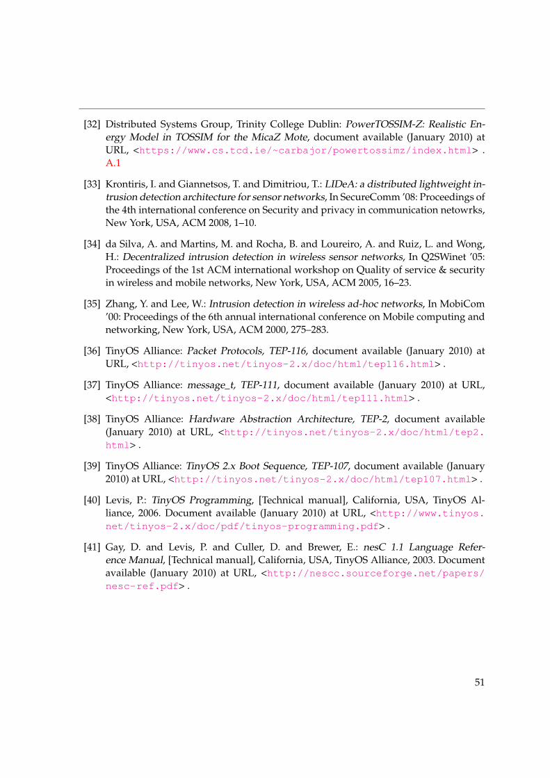
[32] Distributed Systems Group, Trinity College Dublin: PowerTOSSIM-Z: Realistic En-ergy Model in TOSSIM for the MicaZ Mote, document available (January 2010) atURL, <https://www.cs.tcd.ie/~carbajor/powertossimz/index.html> .A.1

[33] Krontiris, I. and Giannetsos, T. and Dimitriou, T.: LIDeA: a distributed lightweight in-trusion detection architecture for sensor networks, In SecureComm ’08: Proceedings ofthe 4th international conference on Security and privacy in communication netowrks,New York, USA, ACM 2008, 1–10.

[34] da Silva, A. and Martins, M. and Rocha, B. and Loureiro, A. and Ruiz, L. and Wong,H.: Decentralized intrusion detection in wireless sensor networks, In Q2SWinet ’05:Proceedings of the 1st ACM international workshop on Quality of service & securityin wireless and mobile networks, New York, USA, ACM 2005, 16–23.

[35] Zhang, Y. and Lee, W.: Intrusion detection in wireless ad-hoc networks, In MobiCom’00: Proceedings of the 6th annual international conference on Mobile computing andnetworking, New York, USA, ACM 2000, 275–283.

[36] TinyOS Alliance: Packet Protocols, TEP-116, document available (January 2010) atURL, <http://tinyos.net/tinyos-2.x/doc/html/tep116.html> .

[37] TinyOS Alliance: message_t, TEP-111, document available (January 2010) at URL,<http://tinyos.net/tinyos-2.x/doc/html/tep111.html> .

[38] TinyOS Alliance: Hardware Abstraction Architecture, TEP-2, document available(January 2010) at URL, <http://tinyos.net/tinyos-2.x/doc/html/tep2.html> .

[39] TinyOS Alliance: TinyOS 2.x Boot Sequence, TEP-107, document available (January2010) at URL, <http://tinyos.net/tinyos-2.x/doc/html/tep107.html> .

[40] Levis, P.: TinyOS Programming, [Technical manual], California, USA, TinyOS Al-liance, 2006. Document available (January 2010) at URL, <http://www.tinyos.net/tinyos-2.x/doc/pdf/tinyos-programming.pdf> .

[41] Gay, D. and Levis, P. and Culler, D. and Brewer, E.: nesC 1.1 Language Refer-ence Manual, [Technical manual], California, USA, TinyOS Alliance, 2003. Documentavailable (January 2010) at URL, <http://nescc.sourceforge.net/papers/nesc-ref.pdf> .

51

Appendix A

Energy consumption estimation using PowerTOSSIM

Sensor nodes run on batteries and so the evaluation of software’s energy consumption isimportant. PowerTOSSIM was originally developed at Harvard University [10] and wasdedicated for TinyOS 1.x networks. It was based on the energy model of mica2 mote whichuses the CC1000 radio chip. Later, it was redesigned for TinyOS 2.x [30]. There is a version ofPowerTOSSIM for TinyOS 2.x available from Trinity College Dublin researches which usedthe micaZ mote with the CC2420 radio chip [31]. We used this version of PowerTOSSIMto estimate power consumption of our intrusion detection system (the Tmote Sky node forwhich our IDS can be compiled uses the CC2420 radio chip).

A.1 Deployment in PowerTOSSIM

PowerTOSSIM downloaded from [32] is dedicated for TinyOS 2.x simulations. Our IDS iswritten for TinyOS 2.1.0. Even though these versions are compatible, some of the featuresmay not be available.

After uncompressing the downloaded archive of PowerTOSSIM, there are three direc-tories obtained – tos, postprocessZ and powercurses. The first one is a replica of thedirectories and files that were modified inside the TinyOS 2.x tree. They can be hard-copiedinto TinyOS’ installation or included at the compile time by defining appropriate rules inthe application’s Makefile. After accomplishing this part, PowerTOSSIM can be consid-ered as installed. In order to record power consumption of a simulation, ENERGY_HANDLERchannel needs to be added to the simulation source code. Once the output of this channelis obtained in a file, a post-processor can be used to summarize the energy consumptionresults. It is located in postprocessZ directory. In order to see all of its available options,the python postprocessZ.py command can be run in the shell. PowerCurses is a soft-ware for graphical representation of nodes’ energy consumption and can be found in thelast directory.

A.2 Energy consumption simulations

We would like to know the energy consumption introduced by running our intrusion detec-tion system on every node of a network. The most expensive operation that nodes performis communication using the radio. Therefore, we will be interested in comparing energyconsumption of the IDS with and without the collaboration.

52

A.2. ENERGY CONSUMPTION SIMULATIONS

We ran simulations of stand-alone modification of the IDS, 1-hop collaborating modifi-cation of the IDS and a simulation of a network without the IDS installed. The simulatednetworks were composed of 224 nodes that sensed the temperature every 16 seconds andsent the measured values using the CTP to the gateway. Nodes were set to the low gainmonitoring mode with the threshold of -88 dB. It should be noted that this should positivelyinfluence the energy consumption even in the case when the IDS agent is not running on anode. The detections (when the IDS was installed) were held every 304 seconds and 6 suchdetections were simulated during 2001 seconds. We only mention that running the post-processor on the output of such a simulation takes several hours (Intel Core Duo 1.7 GHz, 1GB RAM). The energy consumptions results can be seen in table A.1.

CPU (mJ) Radio chip (mJ) Messages sentno IDS installed 117.43 117776.26 670stand-alone IDS 117.43 117774.23 769

collaborative IDS 117.43 117774.75 731

Table A.1: Average sensor node energy consumption

The simulated energy consumption of a node in average seems to be the same for allthe tested scenarios. This was not expected. The IDS is believed to consume a lot of energybecause of its requirement to disable early dropping of packets which are not destined tothe node running the IDS agent (this is done by disabling address recognition in the appli-cation’s Makefile). Unfortunately, the TOSSIM network model used for the simulations ofour IDS cannot be set to early packet dropping mode. Hence, we programmed this featurefor TOSSIM. It may be the case that PowerTOSSIM is not compatible with this change andhence the power consumption of the radio chips remains the same even when the IDS isturned off.

Almost no difference in energy consumption was found when comparing the stand-alone and 1-hop collaborating modifications of the IDS. This might be due to a huge numberof messages sent when the CTP is used to deliver packets to the base station. Furthermore,the number of messages differs for every simulation. From another point of view, we mayestimate power consumption of the collaboration component in means of what part of thetotal radio chip’s consumption it represents. Five simulations of the IDS having its collabo-ration component enabled were performed. Until the beginning of the sixth detection, therewere approximately 170,000 packets sent in total. Only 6,700 messages (less than 4 %) wereproduced by the collaboration component. Hence, the power consumption of the collabora-tion component is 4 % (the CPU energy consumption is not taken into account because thetotal CPU consumption in the simulations performed with PowerTOSSIM was only 0.01 %of the total node’s energy consumption).

53