arX

iv:c

ond-

mat

/040

3339

v2 [

cond

-mat

.oth

er]

16

Mar

200

4

Neighborhood models of minority opinion spreading

C.J. Tessone1, R. Toral 1,2, P. Amengual1, H.S. Wio1,2 and M. San Miguel1,2

1Instituto Mediterraneo de Estudios Avanzados IMEDEA (CSIC-UIB),Campus UIB, E-07122 Palma de Mallorca, Spain

2Departamento de Fısica, Universitat de les Illes Balears, E-07122 Palma de Mallorca, Spain(Dated: February 2, 2008)

We study the effect of finite size population in Galam’s model [Eur. Phys. J. B 25 (2002) 403]of minority opinion spreading and introduce neighborhood models that account for local spatialeffects. For systems of different sizes N , the time to reach consensus is shown to scale as ln N in theoriginal version, while the evolution is much slower in the new neighborhood models. The thresholdvalue of the initial concentration of minority supporters for the defeat of the initial majority, whichis independent of N in Galam’s model, goes to zero with growing system size in the neighborhoodmodels. This is a consequence of the existence of a critical size for the growth of a local domain ofminority supporters.

I. INTRODUCTION

There is a growing interest among theoretical physi-cists in complex phenomena in fields departing from thetraditional realm of physics research. In particular, theapplication of statistical physics methods to social phe-nomena is discussed in several reviews [1, 2, 3, 4]. Oneof the sociological problems that attracts much attentionis the building or the lack of consensus out of some ini-tial condition. There are several different models thatsimulate and analyze the dynamics of such processes inopinion formation, cultural dynamics, etc. [5, 6, 7, 8,9, 10, 11, 12, 13, 14, 15, 16, 17, 18, 19, 20, 21, 22].Among all those models, the one introduced by Galam[7, 8] to describe the spreading of a minority opinion, in-corporates basic mechanisms of social inertia, resultingin democratic rejection of social reforms initially favoredby a majority. In this model, individuals gather duringtheir social life in meeting cells of different sizes wherethey discuss about a topic until a final decision, in favoror against, is taken by the entire group. The decision isbased on the majority rule such that everybody in themeeting cell adopts the opinion of the majority. Galamintroduced the idea of “social inertia” in the form of abias corresponding to a resistance to changes or reforms,that is: in case of tie, one of the decisions (in the orig-inal version, the one against) is systematically adopted.We will describe in detail the model and its main con-clusions in the next sections. This simple model is ableto explain why an initially minority opinion can becomea majority in the long run. An interesting example wasits application to the spread of rumors concerning someSeptember 11-th opinions in France [8]. One of the ma-jor conclusions of the mean-field-like analysis in Ref.[7], isthe existence of a threshold value pc < 1/2 for the initialconcentration of individuals with the minority opinion(against the social reform). For p > pc every individualeventually adopts the opinion of the initial minority, sothat the social reform is rejected and the status quo ismaintained. A related message of this result is that a ru-mor spreads, although initially supported by a minority,if the society has some bias towards accepting it.

Galam traces back his results to dynamical effects pro-duced by the existence of asymmetric unstable pointspreviously considered by Granovetter [23] and Schelling[24]. These are fixed points of recursion relations describ-ing the dynamics of the fraction of a population adoptingone of two possible choices. In threshold models these re-lations are obtained considering a mean field type of in-teraction in which individual thresholds to change choice(tolerance) are compared with the fraction of the popula-tion that has already adopted the new choice. Granovet-ter himself [23] discusses that the stability of the fixedpoints can be changed by spatial effects, noting that theassumption that each individual is responsive to the be-havior of all the others is often inappropriate. In [7] suchcomplete connectedness of the population seems to be cir-cumvented by the introduction of the meeting cells. Onlyindividuals in each meeting cell interact among them-selves. In this sense each meeting cell plays the role ofa bounded neighborhood [24] and it is still possible toobtain analytically recursion relations for the dynamics.However, contrary to the bounded neighborhood modelof Schelling, individuals enter and leave these neighbor-hoods randomly, and the neighborhoods do not have anycharacteristic identity other than their sizes. Even if themeeting cells are thought of as sites where local discus-sions take place, Galam’s model [7] does not incorporatelocal interactions since the individuals are randomly re-distributed in the meeting cells at each time step of thedynamics.

The alternative considered by Schelling to the bounded

neighborhood model is a spatial proximity model inwhich everybody defines his neighborhood by referenceto his own spatial location. The spatial arrangementor configuration within the neighborhood mediates theinteractions. We propose here a different neighbor-hood model which shares some characteristics with thebounded neighborhood and spatial proximity models:The meeting cells are neighborhoods defined by spatiallocation, therefore introducing important local effects,but the interaction within the neighborhood is indepen-dent of the spatial configuration within the cell. Con-trary to the model in [7] the individuals are here located

2

at fixed sites of a lattice. The local neighborhood ormeeting cell in which a given individual interacts changeswith time, reflecting neighborhoods of changing shapeand size. Such neighborhood model could be appropri-ate for a relatively primitive society in which interactionsare predominantly among neighbors, but the size of theneighborhood or interaction range is not fixed.

A different version of Galam’s model was introduced byStauffer [14]. At variance with our neighborhood modelsin which individuals are fixed in the sites of a lattice andthe meeting cells have a maximum size, Stauffer consid-ers the situation in which individuals freely diffuse in alattice with only a fraction of sites being occupied. Thisdiffusion process leads to the formation of “natural” clus-ters which play the role of our meeting cells: It is withineach one of these clusters in which the rule of major-ity opinion and bias towards minority in case of a tie aretaken. Stauffer finds in his model that the time to reach aconsensus opinion grows logarithmically with system sizeN . We also find this dependence in the original model ofGalam, while in our neighborhood models the consensustime takes much larger values and is compatible with apower law dependence. A related model, including thefigure of the “contrarians” (that is, people that alwaysoppose to the majority position), was later introducedby Galam [25] and also analyzed by Stauffer [26].

A main consequence of introducing the spatial ef-fects considered in our neighborhood models is that thethreshold found in [7] disappears with system size, i.e.limN→∞ pc = 0, so that in large systems the minorityopinion always spreads and overcomes the initial major-ity for whatever initial proportion of the minority opin-ion. This is a consequence of the existence of a criticalsize for a local domain of minority supporters. Domainsof size larger than the critical one will expand and oc-cupy the whole system. For large systems there is al-ways a finite probability to have a domain of over-criticalsize in the initial condition. While in traditional Statisti-cal Physics we are mostly concerned with the thermody-namic limit of large systems, these findings emphasize theimportant role of system size in the sociological contextof models of interacting individual entities.

The outline of the paper is as follows. Section 2 re-views the original definition of Galam’s model [7, 8] andintroduces our new local neighborhood models. In Sect.3 we go beyond the mean field limit of Refs.[7, 8] by dis-cussing the system size dependence of the predictions ofthe original model. Steady-state and dynamical proper-ties of our neighborhood models are presented in Sects.4 and 5. General conclusions are summarized in Sect. 6.

II. DEFINITION OF THE MODEL

A. Galam’s original non-local model

The model considers a population of N individuals whorandomly gather in “meeting cells”. A meeting cell is just

defined by the number of individuals k that can meetin the cell. Let us define ak as the probability that aparticular person is found in a cell of size k. Obviously,it is

∑

k ak = 1.The dynamics of the model is as follows: first the meet-

ing cells are defined by giving each one a size accordingto the probability distribution {ak}, such that the sumof all the cell sizes equals the number of individuals N ,but otherwise their location or shape are not specified.These cells are not modified during the whole dynamicalprocess. The persons have an initial binary (against, +,or in favor, −) opinion about a certain topic. The prob-ability that a person shares the + opinion at time t isP+(t) and an equivalent definition for P−(t) = 1−P+(t).Initially one sets P+(t = 0) = p. Alternatively, P+(t)can be thought of as the proportion of people supportingopinion + at time t.

The N individuals are then distributed randomlyamong the different cells. The basic premise of the modelis that all the people within a cell adopt the opinion ofthe majority of the cell. Furthermore, in the case of atie (which can only occur if the cell size k is an evennumber), one of the opinions, that we arbitrarily identifywith the + opinion, is adopted. Once an opinion withinthe different cells has been taken, time increases by one,t → t + 1 and the individuals rearrange by distributingthemselves again randomly among the different cells.

The main finding of this model is that an initially mi-nority opinion, corresponding to p < 1/2 can win in thelong term. This is an effect of the tie rule that selectsthe + opinion in case of a tie.

It is possible to write down a recursion relation for thedensity of people that at time t have the + opinion as [7]

P+(t + 1) =

M∑

k=1

ak

M∑

j=[ M

2+1]

(

k

j

)

P+(t)j [1 − P+(t)]k−j

,

(1)Simultaneously[28]

P−(t + 1) =

M∑

k=1

ak

M∑

j=[ M+1

2 ]

(

k

j

)

P−(t)j [1 − P−(t)]k−j

,

(2)the notation [x] indicates the integer part of x. This is amean-field equation that neglects possible fluctuations.

For a wide range of distributions {ak} this map hasthree fixed points: two stable ones at P+ = 1 and P+ = 0and an unstable one, the faith point, at P+ = pc. Hence,the dynamics is such that

limt→∞

P+(t) =

{

1 if P+(0) > pc

0 if P+(0) < pc(3)

B. Neighborhood models

We now introduce our Neighborhood Models that in-corporate local spatial effects in the interacting dynamics

3

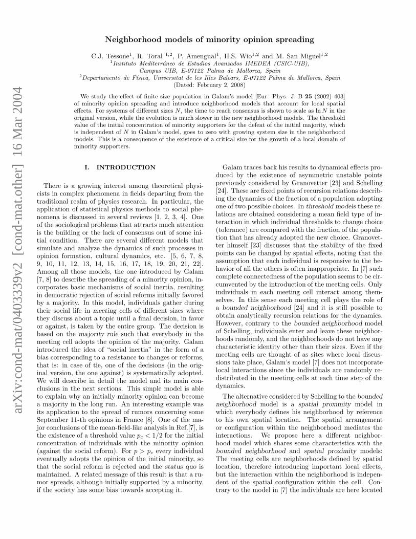
FIG. 1: (a) Regular 2D tessellation: All the cells are simul-taneously created, being mx and my uniformly distributedbetween 1 and M . (b) Locally grown tessellation: A site(i, j) is chosen, and from it a cell of size mx, my, excludingthose already belonging to other cell.

proposed by Galam. In these local models, individualsare fixed at the sites of a regular lattice and they interactwith other individuals in their spatial neighborhood. Wehave considered several cases:

1. One-dimensional neighborhood model: synchronousupdate

The N individuals are distributed at the sites of a lin-ear lattice i = 1, 2, . . . , N . Once distributed, they nevermove again. Initially they are assigned a probability p ofadopting the + opinion, and (1 − p) the − opinion. Thedynamics starts by defining the meeting cells k = 1, 2, . . .as the segments [ik, ik+1 − 1] of length mk = ik+1 − ik.The cell sizes mk are distributed according to a uniformdistribution in the interval [1, M ]. The average cell size

is hence 〈mk〉 = (M+1)2 and the average number of cells

is N/〈mk〉. Once the cells are defined, the dynamicalrules of Galam’s model are applied synchronously to allthe cells, time increases by one t → t + 1. In the next

time step, new cells, uncorrelated to the previous onesare defined and the dynamical rules applied again. Theprocess continues until there is a single common opinionin the whole system.

2. Two-dimensional neighborhood model: synchronousupdate

The two-dimensional case is very similar to the 1D ver-sion explained above. The only difference is the way themeeting cells are defined in the two-dimensional lattice.An individual is now characterized by two indexes (i, j)with 1 ≤ i, j ≤ L, such that the total number of indi-viduals is N = L2. We have considered two differentdefinitions of the cells originated in two tessellations ofthe plane: (a) the regular tessellation and (b) the locally-

grown tessellation. In the regular tessellation, we de-fine segments in the i and j axis independently, suchthat the sizes are in both cases uniformly distributed be-tween 1 and M in the same way that we did in the one-dimensional case. Figure 1a plots a typical example. Inthe locally-grown tessellation we first choose a site of thelattice and then define a rectangle around it whose sidesare both uniformly distributed between 1 and M . Thecell is defined then as the sites in the resulting rectangleexcluding those sites that already were part of a previ-ously defined cell. Figure 1b shows a typical example.

Once the cells are defined, the dynamical rules are ap-plied synchronously to all the cells and a common opinionis formed within each cell. Time then increases by onet → t+1. In the next time step, new cells are defined andthe process continues until a consensus opinion is reachedin the whole population.

3. Asynchronous update

The 1D and 2D models have been also considered inthe asynchronous update version. In this case, a lat-tice site is randomly chosen and a cell defined around itas a segment (1D) of size m or a rectangle (2D) of size(mx, my). It is only within this cell that the biased ma-jority rule is applied. Time increases by t → t + m/Nin 1D and by t → t + (mx my)/N in 2D. Then a newsite is selected randomly and the process iterates until aconsensus opinion is obtained.

III. RESULTS FOR GALAM’S ORIGINAL

NON-LOCAL MODEL.

We present in this section an analysis of Galam’s orig-inal non-local model. Our aim is to go beyond the mean-field approach of references [7, 8, 25] by studying thesystem size dependence of the different magnitudes ofinterest. Some of the results are based on numerical sim-ulations of the model.

4

0.1 0.2 0.3 0.4 0.5 0.6p

c

0

20

40

60

80M

+

consensus to-

consensus to

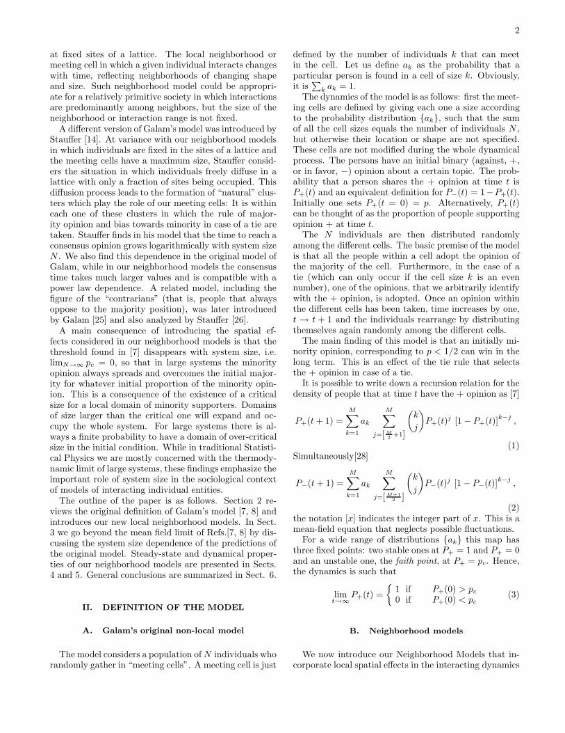
FIG. 2: Phase diagram of the original Galam’s model in theplane (pc, M).

We consider N individuals that distribute themselvesrandomly in meeting cells whose size is uniformly dis-

tributed between 1 and M . In the notation of Eq. (1),this means that ak = 2k/(M(M + 1)), k ∈ [1, M ], as itfollows from the fact that ak measures the probabilityfor an individual of being in any of the k sites of a cellof size k. Initially we assign to each of the persons anyof the two possible opinions, such that the probability ofhaving the favored opinion is p. Again, in the languageof Eq. (1), we are setting P+(0) = p. We then applythe dynamical rules of Galam’s model until a consensusopinion is formed. By iteration of this procedure, wemeasure the probability ρ that the consensus opinion co-incides with the favored one, +. This is precisely definedas the fraction of realizations that end up in the favored+ opinion.

The analysis of Eq. (1) predicts a first order phasetransition in the sense that the “order parameter” ρ = 0if p < pc and ρ = 1 if p > pc. In Fig. 2 we show, inthe parameter space (pc, M), the regions where the twosolutions, as obtained by finding numerically the non-trivial fixed point of the recurrence Eq. (1), exists. Notethat, as expected, the larger the decision cells, the closerthe faith point to 1/2. Notice also in this figure thatsome pairs of consecutive values of M give almost thesame value for pc. The reason is that, for odd values ofM , the rule that applies in case of a tie is used only upto the value M − 1 (which is even), so odd numbers givesimilar values of pc than the precedent even number.

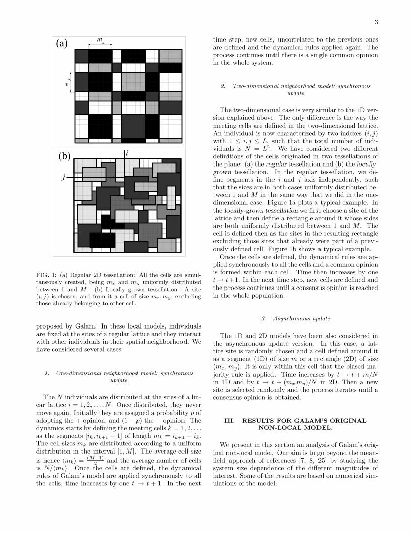
Since Eq. (1) neglects possible system size fluctuations,Eq. (3) this result is only valid in the limit N → ∞. Weplot in Fig. 3a the raw results of our simulations fordifferent system sizes. The analysis carried out in Fig.3b shows that the asymptotic results of N → ∞ are

0.1 0.2 0.3 0.4 0.5p

0.0

0.2

0.4

0.6

0.8

1.0

ρ

(a)

-4 -2 0 2 4

(p - pc ) N

1/2

0.0

0.2

0.4

0.6

0.8

1.0

ρ

(b)

FIG. 3: (a) Order parameter in Galam’s non-local model.The white symbols correspond to the case M = 4 (pc =0.2133077908 . . .), while the black ones to M = 5 (pc =0.3467871056 . . .). The values of N range between N = 103

and N = 106. (b) The order parameter for both values of M

for rescaled values of p according to (p − pc)N1/2. Also, it is

shown a fit with the function ρ(p,N) = (1 + erf(x/1.17))/2

with the scaling variable x = (p − pc)/N1/2.

achieved by means of the following scaling relation

ρ(p, N) = f(

(p − pc)N−1/2)

. (4)

Therefore, there is a region of size N−1/2 where there isa significant probability that the results differ from theinfinite size limit.

We now analyze the time T it takes to reach the consen-sus opinion. Strictly speaking, in the mean field approachthe number of iterations needed for Eq. (1) to convergeto the fixed point is infinity. In Ref. [7] it was adoptedthe criterion that the fixed point had been reached at the

5

0.1 0.2 0.3 0.4 0.5p

0

10

20

30

40T

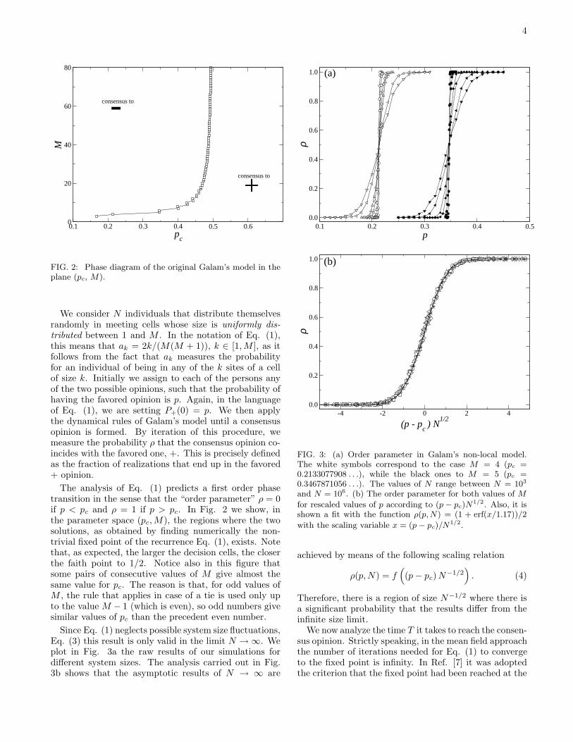
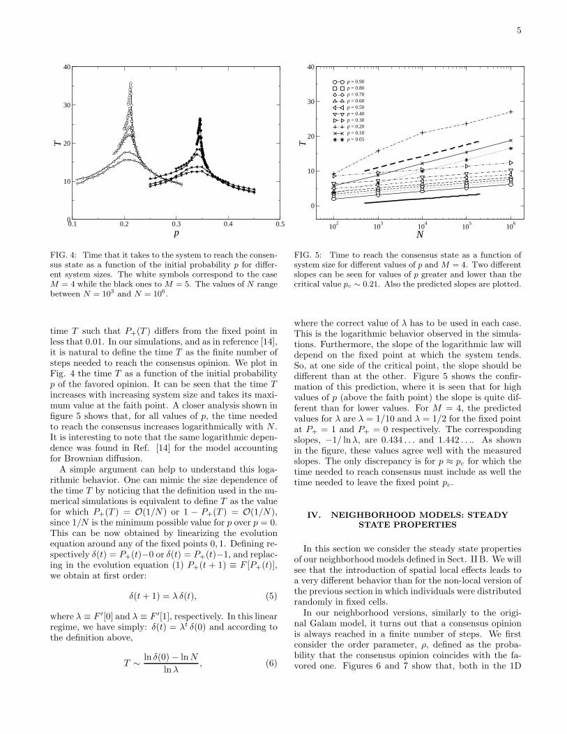
FIG. 4: Time that it takes to the system to reach the consen-sus state as a function of the initial probability p for differ-ent system sizes. The white symbols correspond to the caseM = 4 while the black ones to M = 5. The values of N rangebetween N = 103 and N = 106.

time T such that P+(T ) differs from the fixed point inless that 0.01. In our simulations, and as in reference [14],it is natural to define the time T as the finite number ofsteps needed to reach the consensus opinion. We plot inFig. 4 the time T as a function of the initial probabilityp of the favored opinion. It can be seen that the time Tincreases with increasing system size and takes its maxi-mum value at the faith point. A closer analysis shown infigure 5 shows that, for all values of p, the time neededto reach the consensus increases logarithmically with N .It is interesting to note that the same logarithmic depen-dence was found in Ref. [14] for the model accountingfor Brownian diffusion.

A simple argument can help to understand this loga-rithmic behavior. One can mimic the size dependence ofthe time T by noticing that the definition used in the nu-merical simulations is equivalent to define T as the valuefor which P+(T ) = O(1/N) or 1 − P+(T ) = O(1/N),since 1/N is the minimum possible value for p over p = 0.This can be now obtained by linearizing the evolutionequation around any of the fixed points 0, 1. Defining re-spectively δ(t) = P+(t)−0 or δ(t) = P+(t)−1, and replac-ing in the evolution equation (1) P+(t + 1) ≡ F [P+(t)],we obtain at first order:

δ(t + 1) = λ δ(t), (5)

where λ ≡ F ′[0] and λ ≡ F ′[1], respectively. In this linearregime, we have simply: δ(t) = λt δ(0) and according tothe definition above,

T ∼ln δ(0) − lnN

lnλ, (6)

102

103

104

105

106

N

0

10

20

30

40

T

p = 0.90 p = 0.80 p = 0.70 p = 0.60 p = 0.50 p = 0.40 p = 0.30 p = 0.20 p = 0.10 p = 0.05

FIG. 5: Time to reach the consensus state as a function ofsystem size for different values of p and M = 4. Two differentslopes can be seen for values of p greater and lower than thecritical value pc ∼ 0.21. Also the predicted slopes are plotted.

where the correct value of λ has to be used in each case.This is the logarithmic behavior observed in the simula-tions. Furthermore, the slope of the logarithmic law willdepend on the fixed point at which the system tends.So, at one side of the critical point, the slope should bedifferent than at the other. Figure 5 shows the confir-mation of this prediction, where it is seen that for highvalues of p (above the faith point) the slope is quite dif-ferent than for lower values. For M = 4, the predictedvalues for λ are λ = 1/10 and λ = 1/2 for the fixed pointat P+ = 1 and P+ = 0 respectively. The correspondingslopes, −1/ lnλ, are 0.434 . . . and 1.442 . . .. As shownin the figure, these values agree well with the measuredslopes. The only discrepancy is for p ≈ pc for which thetime needed to reach consensus must include as well thetime needed to leave the fixed point pc.

IV. NEIGHBORHOOD MODELS: STEADY

STATE PROPERTIES

In this section we consider the steady state propertiesof our neighborhood models defined in Sect. II B. We willsee that the introduction of spatial local effects leads toa very different behavior than for the non-local version ofthe previous section in which individuals were distributedrandomly in fixed cells.

In our neighborhood versions, similarly to the origi-nal Galam model, it turns out that a consensus opinionis always reached in a finite number of steps. We firstconsider the order parameter, ρ, defined as the proba-bility that the consensus opinion coincides with the fa-vored one. Figures 6 and 7 show that, both in the 1D

6

0 0.2 0.4 0.6 0.8 1p

0

0.2

0.4

0.6

0.8

1

ρ

10-1

100

101

102

p N0.70

0

0.2

0.4

0.6

0.8

1

ρ

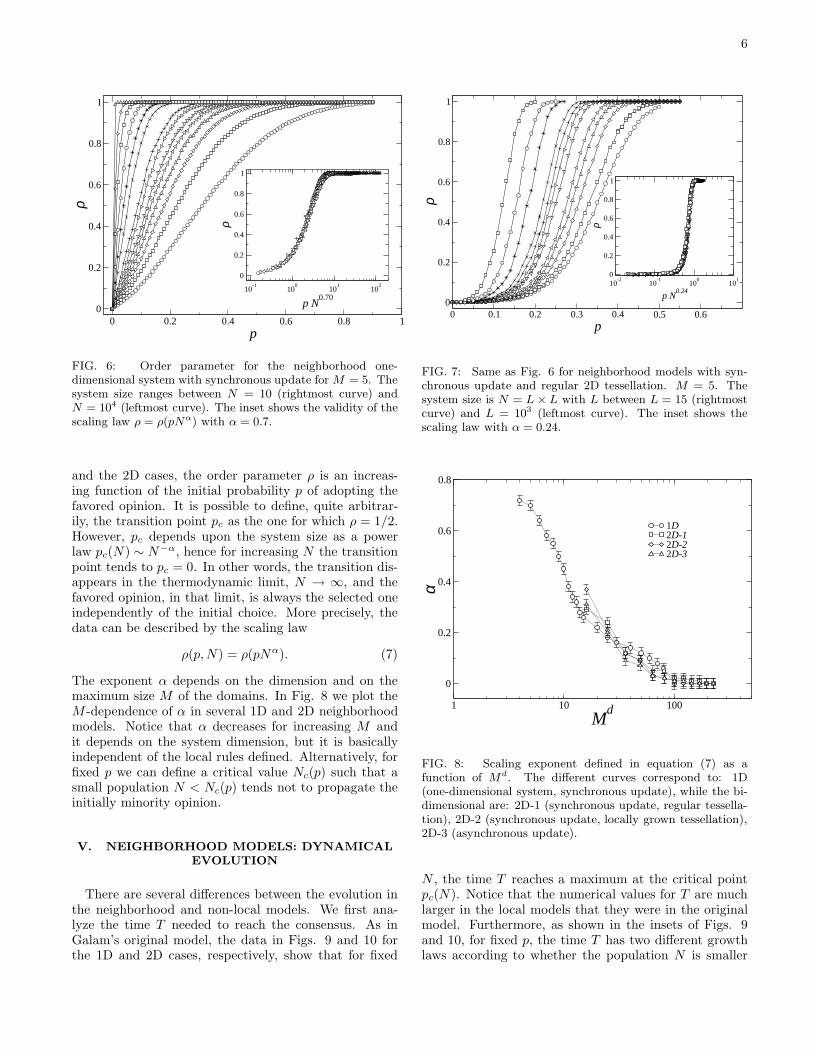
FIG. 6: Order parameter for the neighborhood one-dimensional system with synchronous update for M = 5. Thesystem size ranges between N = 10 (rightmost curve) andN = 104 (leftmost curve). The inset shows the validity of thescaling law ρ = ρ(pNα) with α = 0.7.

and the 2D cases, the order parameter ρ is an increas-ing function of the initial probability p of adopting thefavored opinion. It is possible to define, quite arbitrar-ily, the transition point pc as the one for which ρ = 1/2.However, pc depends upon the system size as a powerlaw pc(N) ∼ N−α, hence for increasing N the transitionpoint tends to pc = 0. In other words, the transition dis-appears in the thermodynamic limit, N → ∞, and thefavored opinion, in that limit, is always the selected oneindependently of the initial choice. More precisely, thedata can be described by the scaling law

ρ(p, N) = ρ(pNα). (7)

The exponent α depends on the dimension and on themaximum size M of the domains. In Fig. 8 we plot theM -dependence of α in several 1D and 2D neighborhoodmodels. Notice that α decreases for increasing M andit depends on the system dimension, but it is basicallyindependent of the local rules defined. Alternatively, forfixed p we can define a critical value Nc(p) such that asmall population N < Nc(p) tends not to propagate theinitially minority opinion.

V. NEIGHBORHOOD MODELS: DYNAMICAL

EVOLUTION

There are several differences between the evolution inthe neighborhood and non-local models. We first ana-lyze the time T needed to reach the consensus. As inGalam’s original model, the data in Figs. 9 and 10 forthe 1D and 2D cases, respectively, show that for fixed

0 0.1 0.2 0.3 0.4 0.5 0.6p

0

0.2

0.4

0.6

0.8

1

ρ

10-2

10-1

100

101

p N0.24

0

0.2

0.4

0.6

0.8

1

ρ

FIG. 7: Same as Fig. 6 for neighborhood models with syn-chronous update and regular 2D tessellation. M = 5. Thesystem size is N = L × L with L between L = 15 (rightmostcurve) and L = 103 (leftmost curve). The inset shows thescaling law with α = 0.24.

1 10 100

Md

0

0.2

0.4

0.6

0.8

α

1D2D-12D-22D-3

FIG. 8: Scaling exponent defined in equation (7) as afunction of Md. The different curves correspond to: 1D(one-dimensional system, synchronous update), while the bi-dimensional are: 2D-1 (synchronous update, regular tessella-tion), 2D-2 (synchronous update, locally grown tessellation),2D-3 (asynchronous update).

N , the time T reaches a maximum at the critical pointpc(N). Notice that the numerical values for T are muchlarger in the local models that they were in the originalmodel. Furthermore, as shown in the insets of Figs. 9and 10, for fixed p, the time T has two different growthlaws according to whether the population N is smaller

7

0 0.2 0.4 0.6 0.8 1p

100

101

102

103

104

105

T 101

102

103

104

105

N

100

102

104

T

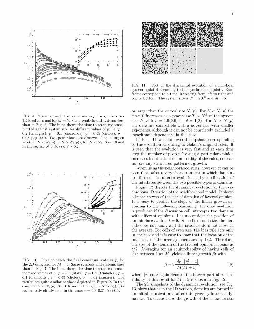
FIG. 9: Time to reach the consensus vs p, for synchronous1D local cells and for M = 5. Same symbols and systems sizesthan in Fig. 6. The inset shows the time to reach consensusplotted against system size, for different values of p, i.e. p =0.2 (triangles), p = 0.1 (diamonds), p = 0.05 (circles), p =0.02 (squares). Two power-laws are observed (depending onwhether N < Nc(p) or N > Nc(p)); for N < Nc, β ≈ 1.6 andin the regime N > Nc(p), β ≈ 0.2.

0 0.1 0.2 0.3 0.4 0.5 0.6p

100

101

102

103

104

105

T

102

104

106

N

100

101

102

103

104

T

FIG. 10: Time to reach the final consensus state vs p, forthe 2D cells, and for M = 5. Same symbols and systems sizesthan in Fig. 7. The inset shows the time to reach consensusfor fixed values of p: p = 0.3 (stars), p = 0.2 (triangles), p =0.1 (diamonds), p = 0.05 (circles), p = 0.02 (squares). Theresults are quite similar to those depicted in Figure 9. In thiscase, for N < Nc(p), β ≈ 0.6 and in the regime N > Nc(p) (aregime only clearly seen in the cases p = 0.3, 0.2), β ≈ 0.1.

FIG. 11: Plot of the dynamical evolution of a non-localsystem updated according to the synchronous update. Eachframe correspond to a time, increasing from left to right andtop to bottom. The system size is N = 2562 and M = 5.

or larger than the critical size Nc(p). For N < Nc(p) thetime T increases as a power-law T ∼ Nβ of the systemsize N with β = 1.6(0.6) for d = 1(2). For N > Nc(p)the data are compatible with a power law with smallerexponents, although it can not be completely excluded alogarithmic dependence in this case.

In Fig. 11 we plot several snapshots correspondingto the evolution according to Galam’s original rules. Itis seen that the evolution is very fast and at each timestep the number of people favoring a particular opinionincreases but due to the non-locality of the rules, one cannot see any structured pattern of growth.

When using the neighborhood rules, however, it can beseen that, after a very short transient in which domainsare formed, the ulterior evolution is by modification ofthe interfaces between the two possible types of domains.

Figure 12 depicts the dynamical evolution of the syn-chronous 1D version of the neighborhood model. It showsa linear growth of the size of domains of favored opinion.It is easy to predict the slope of the linear growth ac-cording to the following reasoning: the only evolutionis produced if the discussion cell intercepts two domainswith different opinions. Let us consider the position ofan interface at time t = 0. For cells of odd size, the biasrule does not apply and the interface does not move inthe average. For cells of even size, the bias rule acts onlyin one case and it is easy to show that the location of theinterface, on the average, increases by 1/2. Therefore,the size of the domain of the favored opinion increase ast/2. Averaging for an equiprobability of having cells ofsize between 1 an M , yields a linear growth βt with

β = 2

[

M2

] [

M2 + 1

]

M(M + 1), (8)

where [x] once again denotes the integer part of x. Thevalidity of this result for M = 5 is shown in Fig. 12.

The 2D snapshots of the dynamical evolution, see Fig.13, show that as in the 1D version, domains are formed inan initial transient, and after this, grow by interface dy-namics. To characterize the growth of the characteristic

8

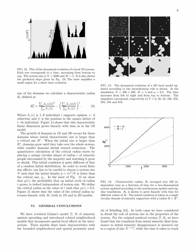
FIG. 12: Plot of the dynamical evolution of a local 1D system.Each row corresponds to a time, increasing from bottom totop. The system size is N = 5000 and M = 5. It is also shownthe predicted slope given by Eq. (8) The inset amplifies asmall region for a short time evolution.

size of the domains we calculate a characteristic radiusRc defined as

R2c =

∑

i δ+(i)~ri2

∑

i δ+(i)−

(∑

i δ+(i)~ri∑

i δ+(i)

)2

. (9)

Where δ+(i) is 1 if individual i supports opinion +, 0otherwise and ~ri is the position in the square lattice ofi−th individual. Figure 14 shows that this characteristiclinear dimension grows linearly with time as in the 1Dmodel.

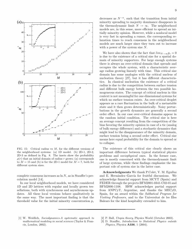
The growth of domains in 1D and 2D occurs for thosedomains whose initial characteristic size is larger thana critical one R∗. When the initial size is larger thanR∗, domains grow until they take over the whole system,while smaller domains shrink toward extinction. Thequantitative calculation of the critical radius starts byplacing a unique circular island of radius r of minoritypeople surrounded by the majority and watching it growor shrink. This initial condition is quite different of thatof a random initial distribution. In order to avoid finitesize effects, one has to be careful to choose a system sizeN such that the initial density p = πr2/N is lower thanthe critical one, pc. In the inset of Fig. 15 we showthat ρ(r), the probability that an initial circle of radiusr grows, is indeed independent of system size. We definethe critical radius as the value of r such that ρ(r) = 0.5.Figure 15 shows that the value of the critical radius in-creases linearly with M , both in 1D and in 2D models.

VI. GENERAL CONCLUSIONS

We have revisited Galam’s model [7, 8] of minorityopinion spreading and introduced related neighborhoodmodels that incorporate spatial local effects in the inter-actions. These models share basic characteristics withthe bounded neighborhood and spatial proximity mod-

FIG. 13: The dynamical evolution of a 2D local model up-dated according to the asynchronous rule is shown. In thesimulation N = 400 × 400, M = 5 and p = 0.2. The timeincreases from left to right and from top to bottom. Thesnapshots correspond, respectively to T = 0, 20, 52, 106, 276,394, 594 and 818.

0 1000 2000 3000t0

2000

4000

Rc

M = 10M = 5

FIG. 14: Characteristic radius, Rc averaged over 100 in-dependent runs as a function of time for a two-dimensionalsystem updated according to the synchronous update and reg-ular tessellation. Rc is shown to grow linearly with time fordifferent values of M . The initial condition is taken as a singlecircular domain of minority supporters with a radius R > R∗.

els of Schelling [24]. In both cases we have consideredin detail the role of system size in the properties of thesystem. For the original nonlocal version [7, 8], we havefound that the transition from initial minority final dom-inance to initial minority disappearance is smeared outin a region of size N−1/2, while the time it takes to reach

9

0 10 20 30r

0.0

0.5

1.0ρ

0 10 20 30 40

M

0

10

20

30

40

50R

*

(a)

0 10 20 30r

0.0

0.5

1.0

ρ

0 5 10 15 20

M

0

50

100

R*

2D-12D-22D-3

(b)

FIG. 15: Critical radius vs M , for the different versions ofthe neighborhood systems: (a) 1D model. (b) 2D-1, 2D-2,2D-3 as defined in Fig. 8. The insets show the probabilityρ(r) that an initial domain of radius r grows; (a) correspondsto M = 15 and (b) is for the 2D-1 model for M = 7, both fordifferent system sizes.

complete consensus increases as ln N , as in Stauffer’s per-colation model [14].

In our local neighborhood models, we have considered1D and 2D lattices with regular and locally grown tes-sellations, both with synchronous and asynchronous up-dates. All these local versions behave qualitatively inthe same way. The most important finding is that thethreshold value for the initial minority concentration pc

decreases as N−α, such that the transition from initialminority spreading to majority dominance disappears inthe thermodynamic limit N → ∞. The neighborhoodmodels are, in this sense, more efficient to spread an ini-tially minority opinion. However, while a nonlocal modelis very fast in spreading a rumor, the corresponding re-laxation times to reach consensus in the neighborhoodmodels are much larger since they turn out to increasewith a power of the system size N .

We have also shown that the fact that limN→∞pc = 0is due to the existence of a critical size for a spatial do-main of minority supporters. For large enough systemsthere is always an over-critical domain that spreads andoccupies the whole system, with a characteristic aver-age radius growing linearly with time. This critical sizedomain has some analogies with the critical nucleus ofnucleation theory [27], but it has different characteris-tics. In classical nucleation the existence of a criticalradius is due to the competition between surface tensionand different bulk energy between the two possible ho-mogeneous states. The concept of critical nucleus in thiscontext is not meaningful for one-dimensional systems forwhich no surface tension exists. An over-critical dropletappears as a rare fluctuation in the bulk of a metastablestate and it then grows deterministically. Noisy pertur-bations in the growth dynamics are generally a secondorder effect. In our case over-critical domains appear inthe random initial condition. The critical size is herean average concept resulting from the competition of thebias favoring the minority opinion in case of a tie (analogof bulk energy difference) and a stochastic dynamics thatmight lead to the disappearance of the minority domain,surface tension being a second order effect. Critical sizemeans here equal probability for the domain to spread orto collapse.

The existence of this critical size clearly shows animportant difference between typical statistical physicsproblems and sociophysical ones. In the former case,one is mostly concerned with the thermodynamic limitof large systems, while these findings emphasize the im-portant role of system size in the latter case.

Acknowledgments We thank P.Colet, V. M. Eguıluzand E. Hernandez–Garcıa for fruitful discussions. Weacknowledge financial support from MCYT (Spain) andFEDER through the projects BFM2001-0341-C02-01 andBFM2000-1108. HSW acknowledges partial supportfrom ANPCyT, Argentine, and thanks the MECyD,Spain, for an award within the Sabbatical Program for

Visiting Professors, and to the Universitat de les IllesBalears for the kind hospitality extended to him.

[1] W. Weidlich, Sociodynamics-A systematic approach tomathematical modeling in social sciences (Taylor & Fran-cis, London, 2002).

[2] P. Ball, Utopia theory, Physics World (October 2003).[3] D. Stauffer, Introduction to Statistical Physics outside

Physics, Physica A336, 1 (2004).

10

[4] S. Galam, Sociophysics: a personal testimony, PhysicaA336, 49 (2004).

[5] S. Galam, B. Chopard, A. Masselot and M. Droz, Eur.Phys. J. B 4 (1998) 529-531.

[6] S. Galam and J. D. Zucker, Physica A 287 (2000) 644-659.

[7] S. Galam, Eur. Phys. J. B 25 (2002) 403.[8] S. Galam, Physica A 320 (2003) 571-580.[9] G. Deffuant, D. Neau, F. Amblard and G. Weisbuch,

Adv. Complex Syst. (2000) 3, 87; G. Weisbuch, G. Def-fuant, F. Amblard and J.-P. Nadal, Complexity (2002)7, 55.

[10] R. Hegselmann and U. Krausse, J. of Ar-tif. Soc. and Social Sim. 5 (2002) 3,http://www.soc.surrey.ac.uk/JASS/5/3/2.html

[11] K. Sznajd-Weron and J. Sznajd, Int. J. Mod. Phys. C11

(2000) 1157; K. Sznajd-Weron, Phys. Rev. E 66 (2002)046131; K. Sznajd-Weron and J. Sznajd, Int. J. Mod.Phys. C13 (2000) 115.

[12] F. Slanina and H. Lavicka, Eur. Phys. J. B 35 (2003)279.

[13] D. Stauffer, A.O. Souza and S. Moss de Oliveira, Int. J.Mod. Phys. C11 (2000) 1239; D. Stauffer, Int. J. Mod.Phys. C13 (2002) 315; D. Stauffer and P. C. M. Oliveira,Eur. Phys. J. B 30 (2002) 587.

[14] D.Stauffer, Int. J. Mod. Phys. C13 (2002) 975.[15] D. Stauffer, J. of Artificial Societies

and Social Simulation 5 (2001) 1,http://www.soc.surrey.ac.uk/JASS/5/1/4.html; D.Stauffer, How to convince others?: Monte Carlo simula-tions of the Sznajd model, in Proc. Conf. on the MonteCarlo Method in the Physical Sciences, J.E. Gubernatis,

Ed., (AIP, in press), cond-mat/0307133; D. Stauffer,Computing in Science and Engineering 5 (2003) 71.

[16] C. Castellano, M. Marsili, and A. Vespignani, Phys. Rev.Lett. 85 (2000) 3536; D. Vilone, A. Vespignani and C.Castellano, Eur. Phys. J. B 30 (2002) 399.

[17] K. Klemm, V. M. Eguiluz, R. Toral and M. San Miguel,Phys. Rev. E 67 (2003) 026120.

[18] K. Klemm, V. M. Eguiluz, R. Toral and M. San Miguel,Phys. Rev. E 67 (2003) 045101R.

[19] K. Klemm, V. M. Eguiluz, R. Toral and M. San Miguel,Globalization, polarization and cultural drift J. EconomicDynamics and Control (in press).

[20] P.L. Krapivsky and S. Redner, Phys. Rev. Lett. 90 (2003)238701.

[21] M. Mobilia, Phys. Rev. Lett. 91 (2003) 028701.[22] M. Mobilia and S. Redner, cond-mat/0306061 (2003).[23] M. Granovetter, American J. Sociology 83 (1978) 1420.[24] T.C. Schelling, J. Math. Sociology 1 (1971) 143-186; T.

C. Schelling, Micromotives and Macrobehavior (Nortonand Co., New York, 1978)

[25] S. Galam, Contrarian deterministic effect: the “hungelections scenario”, Physica A333, 453 (2004).

[26] D. Stauffer and S.A. Sa Martins, Simulation of Galam’scontrarian opinions in percolative lattices, Physica A334,558 (2004).

[27] J. D. Gunton, M. San Miguel and P. S. Sahni in PhaseTransitions and Critical Phenomena, vol. 8, pp.269-466edited by C. Domb and J. Lebowitz (Academic Press,London,1983).

[28] These expressions correct a misprint in Eqs. (4,5) of ref-erence [7].