Natural and non-natural spacecraft formations near the L1 and L2 libration points in the Sun–Earth/Moon ephemeris system

Dynamical Systems: An International Journal, Vol. 20, No. 1, March 2005, 149–173

Natural and non-natural spacecraft formations near the

L1 and L2 libration points in the Sun–Earth/Moon

ephemeris system

K. C. HOWELL* and B. G. MARCHAND

School of Aeronautics and Astronautics, Purdue University,

315 N. Grant Street, West Lafayette, IN 47907-2023, USA

(Received 23 April 2004; in final form 14 September 2004)

Space-based observatory and interferometry missions, such as Terrestrial PlanetFinder (TPF), Stellar Imager, and MAXIM, have sparked great interest inmulti-spacecraft formation flight in the vicinity of the Sun–Earth/Moon (SEM)libration points. The initial phase of this research considered the formationkeeping problem from the perspective of continuous control as applied tonon-natural formations. In the present study, closer inspection of the flowcorresponding to the stable and centre manifolds near the reference orbit, revealssome interesting natural relative motions as well as some discrete controlstrategies for deployment. In addition, some implementation issues associatedwith discrete formation keeping of natural versus non-natural configurationsare addressed in the present study.

1. Introduction

Some new concepts for space-based observatories and interferometry missionsnow incorporate formation flight to meet their objectives [1–4]. Much of theavailable research on formation flight focuses on Earth orbiting configurations[5–20] where the influence of other gravitational perturbations can be safely ignored.However, renewed interest in formations that evolve near the vicinity of theSun–Earth libration points has inspired new studies regarding formation keepingin the three-body problem [21–36]. Some of these investigations focus on thesimplified circular restricted three-body problem (CR3BP) [28, 30, 32–34]. Previousstudies [34] consider linear optimal control, as applied to nonlinear time varyingsystems, as well as nonlinear control techniques, including input and output feed-back linearization. That analysis is initially performed in the CR3BP, but is

*Corresponding author. Email: [email protected]

Dynamical Systems: An International Journal

ISSN 1468–9367 print/ISSN 1468–9375 online # 2005 Taylor & Francis Ltd

http://www.tandf.co.uk/journals

DOI: 10.1080/1468936042000298224

later transitioned into the more complete ephemeris (EPHEM) model [35, 36]. These

control strategies are applied to a two spacecraft formation where the chief space-

craft evolves along a three-dimensional periodic halo orbit near the L2 libration

point. The deputy vehicle, through continuous thrusting, is then commanded to

follow a non-natural arc relative to the chief.

This particular effort does not constitute the only application of continuous con-

trol techniques in the CR3BP. Scheeres and Vinh [28] develop a non-traditional yet

innovative continuous controller, based on the local eigenstructure of the linear

system, to achieve bounded motion near the vicinity of a halo orbit. Other research

efforts have also focused on the effectiveness of continuous control techniques in the

general CR3BP, though ‘not’ in the vicinity of the libration points. Gurfil and

Kasdin, for instance, consider both linear quadratic regulator (LQR) techniques

[30] and adaptive neural control [33] for formation keeping in the CR3BP. The

second approach, described in Gurfil et al. [33], incorporates uncertainties intro-

duced by modelling errors, inaccurate measurements, and external disturbances.

Luquette and Sanner [32] apply adaptive nonlinear control to address the same

sources of uncertainties in the nonlinear CR3BP.

Formations modelled in the CR3BP do represent a good starting point. However,

ultimately, any definitive formation keeping studies must be performed in the n-body

EPHEM model, where the time invariance properties of the CR3BP are lost and,

consequently, precisely periodic orbits do not exist near the libration points. Folta

et al. [27] and Hamilton [31] consider linear optimal control for formation flight

relative to Lissajous trajectories, as determined in the EPHEM model. In their

studies, the evolution of the controlled formation is approximated from a linear

dynamical model relative to the integrated reference orbit. Finally, Howell and

Barden [23–25] also investigate formation flying near the vicinity of the libration

points in the perturbed Sun–Earth/Moon (SEM) system. Their results are deter-

mined in the full nonlinear EPHEM model. Initially, their focus is the determination

of the natural behaviour on the centre manifold near the libration points and the first

step of their study captures a naturally occurring six-satellite formation near L1 or L2

[24]. Further analysis considers strategies to maintain a planar formation of the

six vehicles in an orbit about the Sun–Earth L1 point [23, 25, 26], that is, controlling

the deviations of each spacecraft relative to the initial formation plane. A

discrete station keeping/control approach is devised to force the orientation of

the formation plane to remain fixed inertially. An alternate approach is also

implemented by Gomez et al. [29] in a study of the deployment and station keeping

requirements for the TPF nominal configuration. Their analysis is initially per-

formed in a simpler model but the simulation results are transitioned into the

EPHEM model.

In the present study, two types of impulsive control are considered. The first is

a basic targeter approach that is, in concept, similar to that implemented by

Howell and Barden [23, 25, 26] in the EPHEM model. This particular controller

is applied here to an inertially fixed non-natural formation. Also, the station

keeping techniques previously implemented by Simo et al. [21] and Howell and

Keeter [22], based on a Floquet controller, are adapted here to the formation

keeping problem. In particular, the Floquet controller is applied to study naturally

existing formations near the libration points and the potential deployment into

such configurations.

150 K. C. Howell and B. G. Marchand

2. Dynamical model

In this investigation, the dynamical model that is employed is based on the standardrelative equations of motion for the n-body problem, as formulated in the inertialframe ðXX�YY�ZZÞ. The equations are, however, modified to include the effects ofsolar radiation pressure (SRP). Hence, the dynamical evolution of each vehicle in theformation, relative to the Earth, �rrP2Ps , is governed by

I €�rr�rrP2Ps ¼ ��P2

ðrP2Ps Þ3þ

XNj¼ 1, j 6¼2, s

�Pj

�rrPsPj

rPsPj� �3 � �rrP2Pj

rP2Pj� �3

!þ �ff ðPsÞ

srp : ð1Þ

For notational purposes, let P2 denote the central body of integration, in this casethe Earth. Then, Ps represents the spacecraft, and the sum over j symbolizes thepresence of other gravitational perturbations. Note that �P2

and �Pjrepresent the

gravitational parameters of the central body, P2, and the jth perturbing body, Pj,respectively. The SRP force vector, as discussed by McInnes [37], is modelled as

�ff ðPsÞsrp ¼

kS0A

msc

D20

d2

!cos2� nn, ð2Þ

where k denotes the absorptivity of the spacecraft surface (k ¼ 2 for a perfectlyreflective surface), S0 is the energy flux measured at the Earth’s distance from theSun [W �m�2], D0 is the mean Sun–Earth distance [km], A represents the constantspacecraft ‘effective’ cross-sectional area [km2], c is the speed of light [km � s�1], ms isthe spacecraft mass [kg], � is the angle of incidence of the incoming photons, nndenotes the unit surface normal, and d [km] represents the Sun–spacecraft distance.

3. Discrete formation keeping

Based on results from previous investigations [30, 32–36], it appears that it is poss-ible, at least computationally, to achieve precise formations in the CR3BP and in theEPHEM model. That is, ‘if ’ continuous control is both available and feasible.Past studies [34–36] demonstrate that, depending on the constraints imposed onthe formation configuration, a continuous control approach may nominally requirethrust levels ranging from 10�3 to 10�9N. In contrast, the present state of propulsiontechnology allows for operational thrust levels on the order of 90–1000 mN viapulsed plasma thrusters, such as those available for attitude control onboardEO-1 (http://space-power.grc.nasa-gov/ppo/projects/eo1/eo1-ppt.html). Of course,increased interest in micro- and nano-satellites continues to motivate theoreticaland experimental studies to further lower these thrust levels, as discussed byMueller [38], Gonzalez and Baker [39] and Phipps and Luke [40]. Gonzalez andBaker [39] estimate that a lower bound of 0.3 nN is possible via laser inducedablation of aluminium. Aside from their immediate application to micro- andnano-satellite missions, these concepts are also potentially promising for formationflight near the libration points.

Ultimately, the level of accuracy achievable in tracking the nominal motion, fora given configuration, depends strongly on the ability to deliver the required thrustlevels accurately. Although continuous control approaches are mathematically

151Natural and non-natural spacecraft formations

sound, the science goals of deep space missions may impose a series of constraintsthat eliminate continuous control as a feasible option. Some also suggest that main-taining a precise formation is, perhaps, ultimately not as critical as generating preciseknowledge of the relative position of each spacecraft in the formation. In these cases,a discrete formation keeping strategy may represent an important capability.

3.1 Investigation of various discrete control strategies

In this study, two discrete control strategies are considered for formation keeping.Both of these rely on knowledge of the linearized dynamics associated with thereference orbit, but incorporate the nonlinear response of the vehicle. In this case,the reference orbit is the path of the chief spacecraft, assumed to evolve along a2� 105 km halo orbit, as determined in the SEM ephemeris system. The deputydynamics, then, are modelled as a perturbation relative to the reference orbit. Thesuccess of a particular control strategy depends, in part, on the nominal motion thatis required of the deputy.

In the first method, a simple linear targeter is applied to enforce a non-naturalformation. In particular, the nominal path of the deputy spacecraft is characterizedas an inertially fixed distance and orientation, relative to the chief spacecraft. Sincethis type of motion does not exist naturally near the libration points, continuouscontrol is necessary to ‘precisely’ enforce the formation for the duration of themission. It is assumed that the goals of the mission require formation keepingaccuracies below 10�3m. Here, instead of applying continuous control, the pathof the deputy is divided into segments. At the beginning of each segment, an impul-sive manoeuvre is implemented that targets the nominal state at the end of thesegment. If the nominal separation between the chief and deputy spacecraft issmall, this approach proves to be effective if the required tolerances are on theorder of 10�2m. Whether this represents an acceptable tolerance level depends onthe goals of the mission. For instance, as presently envisioned, missions like StellarImager require that the nominal vehicle configuration be maintained to within10�6m. The results from earlier studies [34–36] clearly indicate, then, the need forcontinuous formation control if non-natural relative motions are of interest.

Alternatively, a controller derived from Floquet analysis, based on the referenceorbit, is designed to remove the unstable component of the relative state, as well astwo of the four centre subspace modes that are associated with the reference orbit.The path of the deputy, then, is representative of a synthesis between the stable andcentre flows. In contrast with the first method, this type of control does ‘not’ targeta non-natural reference motion. Instead, the control scheme nominally places thedeputy spacecraft on a naturally existing path that exhibits nearly periodic behav-iour, bounded motion, or quasi-periodic motion relative to the chief spacecraft. Thecontrol essentially seeks to return the deputy to this natural path.

4. Discrete control of non-natural formations in the ephemeris model

Driven by control and/or implementation requirements, some new consideration iswarranted concerning the degree of accuracy to which the formation can be main-tained via discrete impulses. A discrete LQR controller yields the optimal magnitudefor each differential control impulse at specified time intervals. This approach is


suitable for station keeping of natural solutions, such as Lissajous trajectories orhalo orbits, which nominally require no control. However, non-natural solutions dorequire a nominal control input. The value of the nominal control input that must beadded is still assumed to be continuously available. Hence, the LQR method, in thiscase, does not yield a truly discrete formation keeping strategy.

4.1 Targeting a nominal relative state

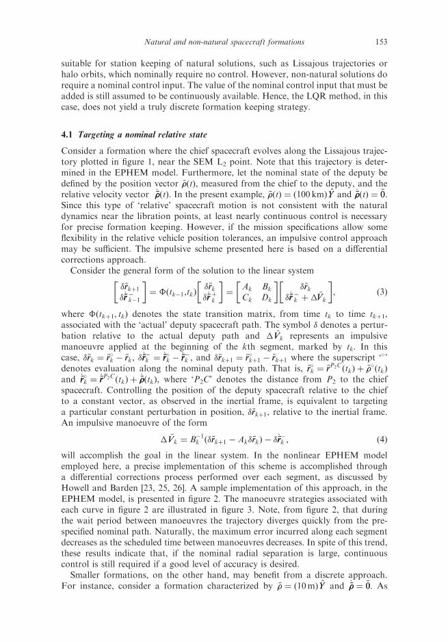
Consider a formation where the chief spacecraft evolves along the Lissajous trajec-tory plotted in figure 1, near the SEM L2 point. Note that this trajectory is deter-mined in the EPHEM model. Furthermore, let the nominal state of the deputy bedefined by the position vector ��ðtÞ, measured from the chief to the deputy, and therelative velocity vector _��ðtÞ. In the present example, ��ðtÞ ¼ ð100 kmÞYY and _��ðtÞ ¼ �00.Since this type of ‘relative’ spacecraft motion is not consistent with the naturaldynamics near the libration points, at least nearly continuous control is necessaryfor precise formation keeping. However, if the mission specifications allow someflexibility in the relative vehicle position tolerances, an impulsive control approachmay be sufficient. The impulsive scheme presented here is based on a differentialcorrections approach.

Consider the general form of the solution to the linear system

��rrkþ1

�_�rr�rr �k�1

� �¼ �ðtk�1,tkÞ

��rrk�_�rr�rr þk

� �¼

Ak Bk

Ck Dk

� ��rrk

�_�rr�rr �k þ� �VVk

� �, ð3Þ

where �(tkþ1, tk) denotes the state transition matrix, from time tk to time tkþ1,associated with the ‘actual’ deputy spacecraft path. The symbol � denotes a pertur-bation relative to the actual deputy path and � �VVk represents an impulsivemanoeuvre applied at the beginning of the kth segment, marked by tk. In thiscase, ��rrk ¼ �rr�k � �rrk, �_�rr�rr

�k ¼ _�rr�rr�k � _�rr�rr�k , and ��rrkþ1 ¼ �rr�kþ1 � �rrkþ1 where the superscript ‘�’

denotes evaluation along the nominal deputy path. That is, �rr�k ¼ �rrP2CðtkÞ þ ��ðtkÞand _�rr�rr�k ¼ _�rr�rrP2CðtkÞ þ _��ðtkÞ, where ‘P2C’ denotes the distance from P2 to the chiefspacecraft. Controlling the position of the deputy spacecraft relative to the chiefto a constant vector, as observed in the inertial frame, is equivalent to targetinga particular constant perturbation in position, ��rrkþ1, relative to the inertial frame.An impulsive manoeuvre of the form

� �VVk ¼ B�1k ð��rrkþ1 � Ak��rrkÞ � �_�rr�rr�k , ð4Þ

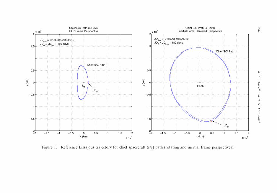
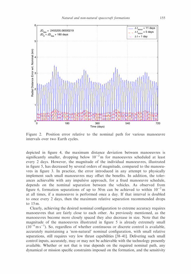
will accomplish the goal in the linear system. In the nonlinear EPHEM modelemployed here, a precise implementation of this scheme is accomplished througha differential corrections process performed over each segment, as discussed byHowell and Barden [23, 25, 26]. A sample implementation of this approach, in theEPHEM model, is presented in figure 2. The manoeuvre strategies associated witheach curve in figure 2 are illustrated in figure 3. Note, from figure 2, that duringthe wait period between manoeuvres the trajectory diverges quickly from the pre-specified nominal path. Naturally, the maximum error incurred along each segmentdecreases as the scheduled time between manoeuvres decreases. In spite of this trend,these results indicate that, if the nominal radial separation is large, continuouscontrol is still required if a good level of accuracy is desired.

Smaller formations, on the other hand, may benefit from a discrete approach.For instance, consider a formation characterized by �� ¼ ð10mÞYY and _�� ¼ �00. As


−2 −1.5 −1 −0.5 0 0.5 1 1.5 2

x 106

−2

−1.5

−1

−0.5

0

0.5

1

1.5

2x 10

6

x (km)

Chief S/C Path (4 Revs)RLP Frame Perspective

y (k

m)

L2

Chief S/C Path

JDliss

= 2455205.06500219JD

0 = JD

liss + 180 days

JD0

−2 −1.5 −1 −0.5 0 0.5 1 1.5 2

x 106

−2

−1.5

−1

−0.5

0

0.5

1

1.5

2x 10

6

x (km)

Chief S/C Path (4 Revs)Inertial Earth Centered Perspective

y (k

m)

Earth

Chief S/C Path

JDliss

= 2455205.06500219JD

0 = JD

liss + 180 days

JD0

Figure 1. Reference Lissajous trajectory for chief spacecraft (s/c) path (rotating and inertial frame perspectives).

154

K.C.Howell

andB.G.March

and

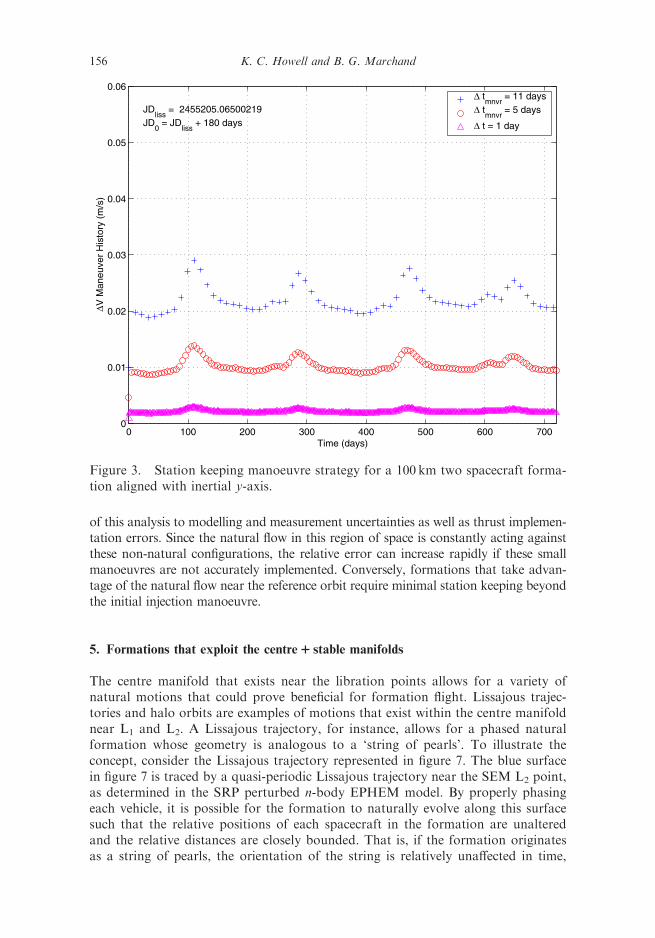
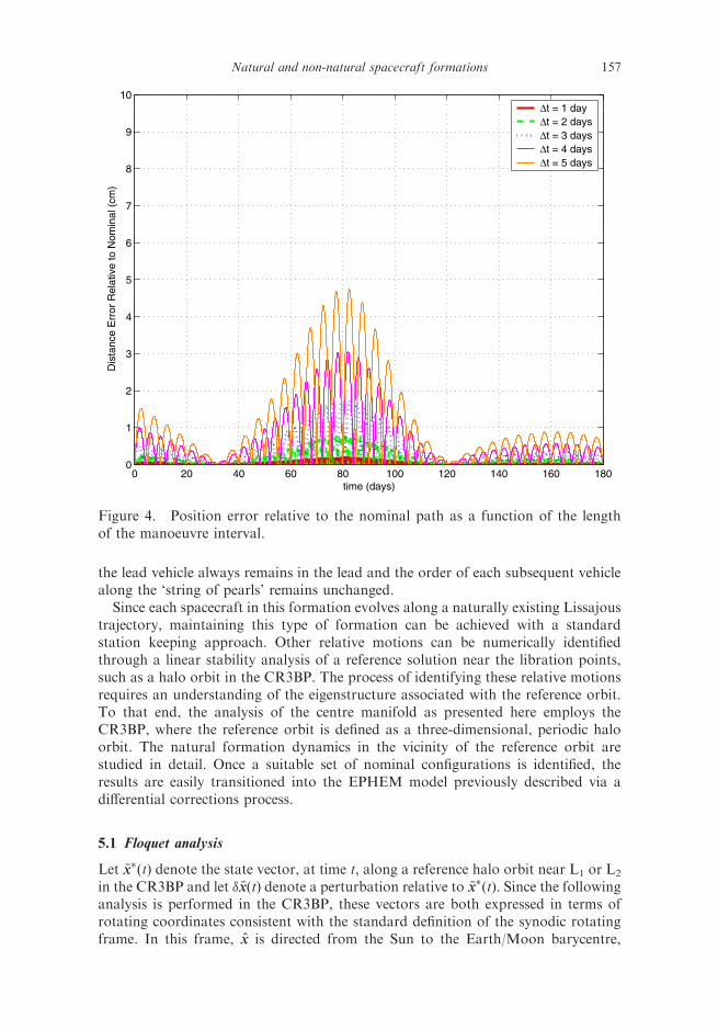
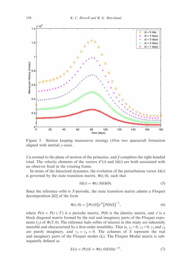
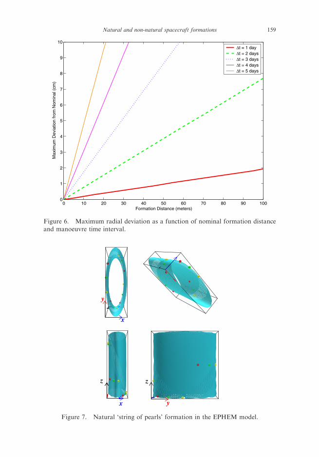
depicted in figure 4, the maximum distance deviation between manoeuvres issignificantly smaller, dropping below 10�2m for manoeuvres scheduled at leastevery 2 days. However, the magnitude of the individual manoeuvres, illustratedin figure 5, has decreased by several orders of magnitude, compared to the manoeu-vres in figure 3. In practice, the error introduced in any attempt to physicallyimplement such small manoeuvres may offset the benefits. In addition, the toler-ances achievable with any impulsive approach, for a fixed manoeuvre schedule,depends on the nominal separation between the vehicles. As observed fromfigure 6, formation separations of up to 50m can be achieved to within 10�2mat all times, if a manoeuvre is performed once a day. If that interval is doubledto once every 2 days, then the maximum relative separation recommended dropsto 15m.

Clearly, achieving the desired nominal configuration to extreme accuracy requiresmanoeuvres that are fairly close to each other. As previously mentioned, as themanoeuvres become more closely spaced they also decrease in size. Note that themagnitude of the manoeuvres illustrated in figure 5 is already extremely small(10�6m s�1). So, regardless of whether continuous or discrete control is available,accurately maintaining a ‘non-natural’ nominal configuration, with small relativeseparations, still requires very low thrust capabilities [38–41]. Delivering such smallcontrol inputs, accurately, may or may not be achievable with the technology presentlyavailable. Whether or not that is true depends on the required nominal path, anydynamical or mission specific constraints imposed on the formation, and the sensitivity

0 180 360 540 7200

1

2

3

4

5

6

Time (days)

Rad

ial D

ista

nce

Err

or w

rt. N

omin

al (

km)

∆ tmnvr

= 11 days∆ t

mnvr = 5 days

∆ t = 1 day

JDliss

= 2455205.06500219JD

0 = JD

liss + 180 days

Figure 2. Position error relative to the nominal path for various manoeuvreintervals over two Earth cycles.


of this analysis to modelling and measurement uncertainties as well as thrust implemen-tation errors. Since the natural flow in this region of space is constantly acting againstthese non-natural configurations, the relative error can increase rapidly if these smallmanoeuvres are not accurately implemented. Conversely, formations that take advan-tage of the natural flow near the reference orbit require minimal station keeping beyondthe initial injection manoeuvre.

5. Formations that exploit the centre1 stable manifolds

The centre manifold that exists near the libration points allows for a variety ofnatural motions that could prove beneficial for formation flight. Lissajous trajec-tories and halo orbits are examples of motions that exist within the centre manifoldnear L1 and L2. A Lissajous trajectory, for instance, allows for a phased naturalformation whose geometry is analogous to a ‘string of pearls’. To illustrate theconcept, consider the Lissajous trajectory represented in figure 7. The blue surfacein figure 7 is traced by a quasi-periodic Lissajous trajectory near the SEM L2 point,as determined in the SRP perturbed n-body EPHEM model. By properly phasingeach vehicle, it is possible for the formation to naturally evolve along this surfacesuch that the relative positions of each spacecraft in the formation are unalteredand the relative distances are closely bounded. That is, if the formation originatesas a string of pearls, the orientation of the string is relatively unaffected in time,

0 100 200 300 400 500 600 7000

0.01

0.02

0.03

0.04

0.05

0.06

Time (days)

∆V M

aneu

ver

His

tory

(m

/s)

∆ tmnvr

= 11 days∆ t

mnvr = 5 days

∆ t = 1 day

JDliss

= 2455205.06500219JD

0 = JD

liss + 180 days

Figure 3. Station keeping manoeuvre strategy for a 100 km two spacecraft forma-tion aligned with inertial y-axis.


the lead vehicle always remains in the lead and the order of each subsequent vehiclealong the ‘string of pearls’ remains unchanged.

Since each spacecraft in this formation evolves along a naturally existing Lissajoustrajectory, maintaining this type of formation can be achieved with a standardstation keeping approach. Other relative motions can be numerically identifiedthrough a linear stability analysis of a reference solution near the libration points,such as a halo orbit in the CR3BP. The process of identifying these relative motionsrequires an understanding of the eigenstructure associated with the reference orbit.To that end, the analysis of the centre manifold as presented here employs theCR3BP, where the reference orbit is defined as a three-dimensional, periodic haloorbit. The natural formation dynamics in the vicinity of the reference orbit arestudied in detail. Once a suitable set of nominal configurations is identified, theresults are easily transitioned into the EPHEM model previously described via adifferential corrections process.

5.1 Floquet analysis

Let �xx�ðtÞ denote the state vector, at time t, along a reference halo orbit near L1 or L2

in the CR3BP and let � �xxðtÞ denote a perturbation relative to �xx�ðtÞ. Since the followinganalysis is performed in the CR3BP, these vectors are both expressed in terms ofrotating coordinates consistent with the standard definition of the synodic rotatingframe. In this frame, xx is directed from the Sun to the Earth/Moon barycentre,

0 20 40 60 80 100 120 140 160 1800

1

2

3

4

5

6

7

8

9

10

time (days)

Dis

tanc

e E

rror

Rel

ativ

e to

Nom

inal

(cm

)∆t = 1 day∆t = 2 days∆t = 3 days∆t = 4 days∆t = 5 days

Figure 4. Position error relative to the nominal path as a function of the lengthof the manoeuvre interval.


zz is normal to the plane of motion of the primaries, and yy completes the right-handedtriad. The velocity elements of the vectors �xx�ðtÞ and � �xxðtÞ are both associated withan observer fixed in the rotating frame.

In terms of the linearized dynamics, the evolution of the perturbation vector � �xxðtÞis governed by the state transition matrix, �(t, 0), such that

� �xxðtÞ ¼ �ðt, 0Þ� �xxð0Þ: ð5Þ

Since the reference orbit is T-periodic, the state transition matrix admits a Floquetdecomposition [42] of the form

�ðt, 0Þ ¼ PðtÞS� �

eJt Pð0ÞS� ��1

, ð6Þ

where P(t) ¼ P(tþT ) is a periodic matrix, P(0) is the identity matrix, and J is ablock diagonal matrix formed by the real and imaginary parts of the Floquet expo-nents (gj) of �(T, 0). The reference halo orbits of interest in this study are inherentlyunstable and characterized by a first-order instability. That is, g1>0, g2<0, g3 and g4are purely imaginary, and g5 ¼ g6 ¼ 0. The columns of S represent the realand imaginary parts of the Floquet modes ð�ssjÞ. The Floquet Modal matrix is sub-sequently defined as

EðtÞ ¼ PðtÞS ¼ �ðt, 0ÞEð0Þe�Jt: ð7Þ

0 20 40 60 80 100 120 140 160 1800

0.2

0.4

0.6

0.8

1

1.2

1.4x 10

6

time (days)

Man

euve

r H

isto

ry (

m/s

ec)

∆t = 5 day∆t = 4 days∆t = 3 days∆t = 2 days∆t = 1 days

Figure 5. Station keeping manoeuvre strategy (10m two spacecraft formationaligned with inertial y-axis).


0 10 20 30 40 50 60 70 80 90 1000

1

2

3

4

5

6

7

8

9

10

Formation Distance (meters)

Max

imum

Dev

iatio

n fr

om N

omin

al (

cm)

∆t = 1 day∆t = 2 days∆t = 3 days∆t = 4 days∆t = 5 days

Figure 6. Maximum radial deviation as a function of nominal formation distanceand manoeuvre time interval.

x

z z

y

y

x

Figure 7. Natural ‘string of pearls’ formation in the EPHEM model.


Note that, since P(t) is periodic, and S is a constant matrix, E(t) ¼ E(tþT ) andE(0) ¼ S. The Floquet modes at each point along the reference orbit can be com-puted from equation (7). Now, at a point in time, the perturbation � �xxðtÞ can beexpressed in terms of any six-dimensional basis. The Floquet modes ð �eejÞ, defined bythe columns of E(t), form a non-orthogonal six-dimensional basis. Hence, � �xxðtÞ canbe expressed as

� �xxðtÞ ¼X6j¼1

� �xxjðtÞ ¼X6j¼1

cjðtÞ �eejðtÞ, ð8Þ

where � �xxjðtÞ denotes the component of � �xxðtÞ along the jth mode, �eejðtÞ, and thecoefficients cj(t) are easily determined as the elements of the vector �ccðtÞ defined by

�ccðtÞ ¼ EðtÞ�1� �xxðtÞ: ð9Þ

The Floquet analysis presented above is implemented by Howell and Keeter [22],based on work originally performed by Simo et al. [21], as the basis of a stationkeeping strategy for a single spacecraft evolving along a halo orbit. In their study,Howell and Keeter (following [21]) determine the impulsive manoeuvre scheme thatis required to periodically remove the unstable component, � �xx1, of the perturbation,� �xxðtÞ. In the present analysis, a similar approach is employed to remove thecomponent of � �xx that is associated with the unstable mode as well as two of thefour centre modes. Thus, the control will eliminate three components. To illustratethis, let

� �xxðtÞ� ¼X

j¼2, 3, 4 orj¼2, 5, 6

ð1þ �jðtÞÞ� �xxj, ð10Þ

denote the ‘desired’ perturbation relative to the reference orbit, where the �j(t)denote some yet to be determined coefficients. The control problem, then, reducesto finding the impulsive manoeuvre, � �VVðtÞ, such that

Xj¼2, 3, 4 orj¼2, 5, 6

ð1þ �jðtÞÞ� �xxjðtÞ ¼X6j¼1

� �xxj þ03

� �VV

� �: ð11Þ

Let � �xxjr denote the first three elements of the vector � �xxj, � �xxjv the last three elements of� �xxj, and �� represent a 5� 1 vector formed by the �j coefficients in equation (11).Then, the � �VV required to remove modes �ee1, �ee3, and �ee4 is computed as

�� VV

� �¼

� �xx2�rr � �xx5�rr � �xx6�rr 03� �xx2 �vv � �xx5 �vv � �xx6 �vv �I3

� ��1

ð� �xx1 þ � �xx3 þ � �xx4Þ: ð12Þ

Similarly, the � �VV required to remove modes �ee1, �ee5, and �ee6 is exactly determined from

�� VV

� �¼

� �xx2�rr � �xx3�rr � �xx4�rr 03� �xx2 �vv � �xx3 �vv � �xx4 �vv �I3z

� ��1

ð� �xx1 þ � �xx5 þ � �xx6Þ: ð13Þ

Either one of these controllers leads to motion that exhibits not only the overallfeatures of the associated centre subspaces, but also some of the features morecommonly associated with motion along a stable manifold. As a direct result, thecontrollers described by equations (12) and (13) not only define other potential


nominal configurations, but also deployment into these configurations, as is demon-strated below.

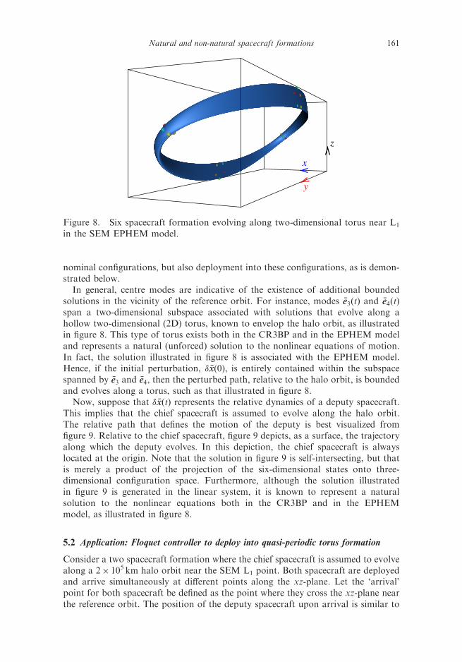
In general, centre modes are indicative of the existence of additional boundedsolutions in the vicinity of the reference orbit. For instance, modes �ee3ðtÞ and �ee4ðtÞspan a two-dimensional subspace associated with solutions that evolve along ahollow two-dimensional (2D) torus, known to envelop the halo orbit, as illustratedin figure 8. This type of torus exists both in the CR3BP and in the EPHEM modeland represents a natural (unforced) solution to the nonlinear equations of motion.In fact, the solution illustrated in figure 8 is associated with the EPHEM model.Hence, if the initial perturbation, � �xxð0Þ, is entirely contained within the subspacespanned by �ee3 and �ee4, then the perturbed path, relative to the halo orbit, is boundedand evolves along a torus, such as that illustrated in figure 8.

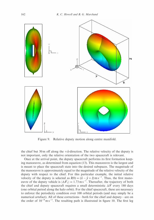
Now, suppose that � �xxðtÞ represents the relative dynamics of a deputy spacecraft.This implies that the chief spacecraft is assumed to evolve along the halo orbit.The relative path that defines the motion of the deputy is best visualized fromfigure 9. Relative to the chief spacecraft, figure 9 depicts, as a surface, the trajectoryalong which the deputy evolves. In this depiction, the chief spacecraft is alwayslocated at the origin. Note that the solution in figure 9 is self-intersecting, but thatis merely a product of the projection of the six-dimensional states onto three-dimensional configuration space. Furthermore, although the solution illustratedin figure 9 is generated in the linear system, it is known to represent a naturalsolution to the nonlinear equations both in the CR3BP and in the EPHEMmodel, as illustrated in figure 8.

5.2 Application: Floquet controller to deploy into quasi-periodic torus formation

Consider a two spacecraft formation where the chief spacecraft is assumed to evolvealong a 2� 105 km halo orbit near the SEM L1 point. Both spacecraft are deployedand arrive simultaneously at different points along the xz-plane. Let the ‘arrival’point for both spacecraft be defined as the point where they cross the xz-plane nearthe reference orbit. The position of the deputy spacecraft upon arrival is similar to

y

z

x

Figure 8. Six spacecraft formation evolving along two-dimensional torus near L1

in the SEM EPHEM model.


the chief but 50m off along the þxx-direction. The relative velocity of the deputy is

not important, only the relative orientation of the two spacecraft is relevant.

Once at the arrival point, the deputy spacecraft performs its first formation keep-

ing manoeuvre, as determined from equation (13). This manoeuvre is the largest and

is meant to place the spacecraft state into the desired subspaces. The magnitude of

the manoeuvre is approximately equal to the magnitude of the relative velocity of the

deputy with respect to the chief. For this particular example, the initial relative

velocity of the deputy is selected as _�rr�rrð0Þ ¼ ðxx� yyþ zzÞms�1. Thus, the first mano-

euvre of the deputy vehicle is j� �VV1j ¼ 1:73m s�1. Thereafter, the trajectory of both

the chief and deputy spacecraft requires a small deterministic � �VV every 180 days

(one orbital period along the halo orbit). For the chief spacecraft, these are necessary

to enforce the periodicity condition over 100 orbital periods (and may simply be a

numerical artefact). All of these corrections—both for the chief and deputy—are on

the order of 10�8m s�1. The resulting path is illustrated in figure 10. The first leg

Figure 9. Relative deputy motion along centre manifold.


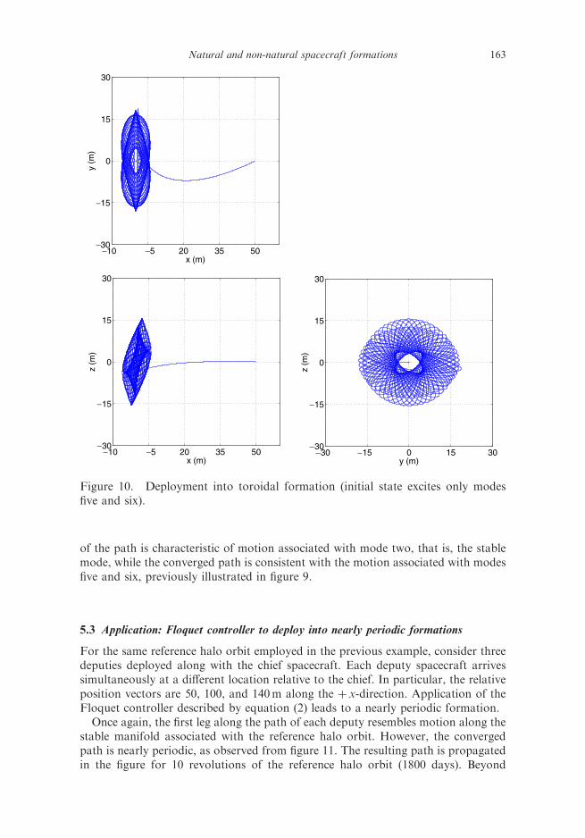
of the path is characteristic of motion associated with mode two, that is, the stablemode, while the converged path is consistent with the motion associated with modesfive and six, previously illustrated in figure 9.

5.3 Application: Floquet controller to deploy into nearly periodic formations

For the same reference halo orbit employed in the previous example, consider threedeputies deployed along with the chief spacecraft. Each deputy spacecraft arrivessimultaneously at a different location relative to the chief. In particular, the relativeposition vectors are 50, 100, and 140m along the þ x-direction. Application of theFloquet controller described by equation (2) leads to a nearly periodic formation.

Once again, the first leg along the path of each deputy resembles motion along thestable manifold associated with the reference halo orbit. However, the convergedpath is nearly periodic, as observed from figure 11. The resulting path is propagatedin the figure for 10 revolutions of the reference halo orbit (1800 days). Beyond

−10 −5 20 35 50−30

−15

0

15

30

x (m)

y (m

)

−10 −5 20 35 50−30

−15

0

15

30

x (m)

z (m

)

−30 −15 0 15 30−30

−15

0

15

30

y (m)

z (m

)

Figure 10. Deployment into toroidal formation (initial state excites only modesfive and six).


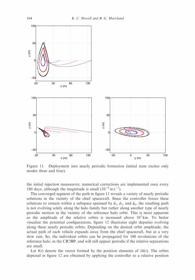
the initial injection manoeuvre, numerical corrections are implemented once every180 days, although the magnitude is small (10�8m s�1).

The converged segment of the path in figure 11 reveals a variety of nearly periodicsolutions in the vicinity of the chief spacecraft. Since the controller forces thesesolutions to remain within a subspace spanned by �ee2, �ee5, and �ee6, the resulting pathis not evolving solely along the halo family but rather along another type of nearlyperiodic motion in the vicinity of the reference halo orbit. This is most apparentas the amplitude of the relative orbits is increased above 103 km. To bettervisualize the potential configurations, figure 12 illustrates eight deputies evolvingalong these nearly periodic orbits. Depending on the desired orbit amplitude, theactual path of each vehicle expands away from the chief spacecraft, but at a veryslow rate. So, the individual orbits can be propagated for 100 revolutions of thereference halo, in the CR3BP, and will still appear periodic if the relative separationsare small.

Let �rrðtÞ denote the vector formed by the position elements of � �xxðtÞ. The orbitsdepicted in figure 12 are obtained by applying the controller to a relative position

−50 0 50 100

−50

0

50

100

y (m)

z (m

)

20 30 80 130

−50

0

50

100

x (m)

y (m

)

20 30 80 130

−50

0

50

100

x (m)

z (m

)

Figure 11. Deployment into nearly periodic formation (initial state excites onlymodes three and four).


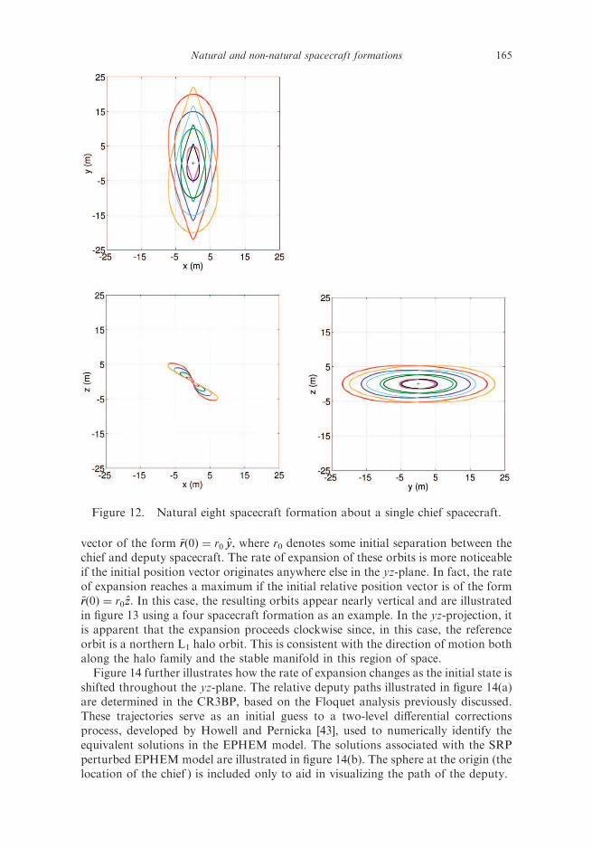
vector of the form �rrð0Þ ¼ r0 yy, where r0 denotes some initial separation between thechief and deputy spacecraft. The rate of expansion of these orbits is more noticeableif the initial position vector originates anywhere else in the yz-plane. In fact, the rateof expansion reaches a maximum if the initial relative position vector is of the form�rrð0Þ ¼ r0zz. In this case, the resulting orbits appear nearly vertical and are illustratedin figure 13 using a four spacecraft formation as an example. In the yz-projection, itis apparent that the expansion proceeds clockwise since, in this case, the referenceorbit is a northern L1 halo orbit. This is consistent with the direction of motion bothalong the halo family and the stable manifold in this region of space.

Figure 14 further illustrates how the rate of expansion changes as the initial state isshifted throughout the yz-plane. The relative deputy paths illustrated in figure 14(a)are determined in the CR3BP, based on the Floquet analysis previously discussed.These trajectories serve as an initial guess to a two-level differential correctionsprocess, developed by Howell and Pernicka [43], used to numerically identify theequivalent solutions in the EPHEM model. The solutions associated with the SRPperturbed EPHEM model are illustrated in figure 14(b). The sphere at the origin (thelocation of the chief ) is included only to aid in visualizing the path of the deputy.

Figure 12. Natural eight spacecraft formation about a single chief spacecraft.


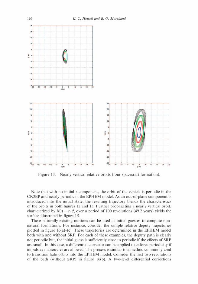
Note that with no initial z-component, the orbit of the vehicle is periodic in theCR3BP and nearly periodic in the EPHEM model. As an out-of-plane component isintroduced into the initial state, the resulting trajectory blends the characteristicsof the orbits in both figures 12 and 13. Further propagating a nearly vertical orbit,characterized by �rrð0Þ ¼ r0 zz, over a period of 100 revolutions (49.2 years) yields thesurface illustrated in figure 15.

These naturally existing motions can be used as initial guesses to compute non-natural formations. For instance, consider the sample relative deputy trajectoriesplotted in figure 16(a)–(c). These trajectories are determined in the EPHEM modelboth with and without SRP. For each of these examples, the deputy path is clearlynot periodic but, the initial guess is sufficiently close to periodic if the effects of SRPare small. In this case, a differential corrector can be applied to enforce periodicity ifimpulsive manouvres are allowed. The process is similar to a method commonly usedto transition halo orbits into the EPHEM model. Consider the first two revolutionsof the path (without SRP) in figure 16(b). A two-level differential corrections

Figure 13. Nearly vertical relative orbits (four spacecraft formation).


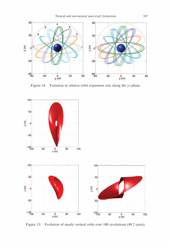
Figure 14. Variation in relative orbit expansion rate along the yz-plane.

Figure 15. Evolution of nearly vertical orbit over 100 revolutions (49.2 years).


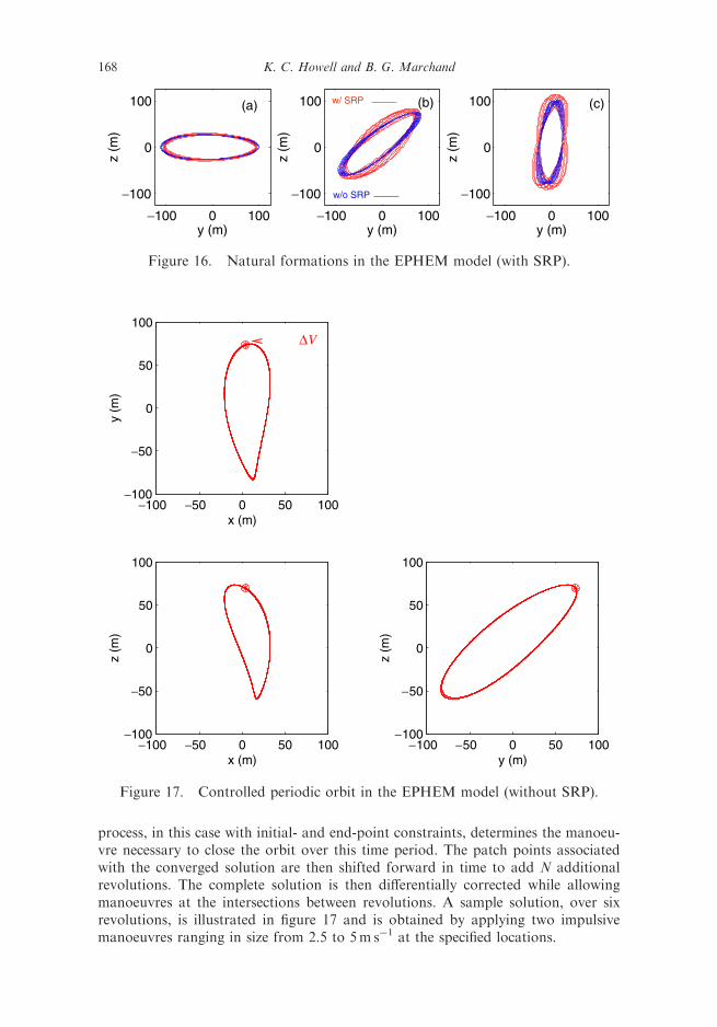
process, in this case with initial- and end-point constraints, determines the manoeu-vre necessary to close the orbit over this time period. The patch points associatedwith the converged solution are then shifted forward in time to add N additionalrevolutions. The complete solution is then differentially corrected while allowingmanoeuvres at the intersections between revolutions. A sample solution, over sixrevolutions, is illustrated in figure 17 and is obtained by applying two impulsivemanoeuvres ranging in size from 2.5 to 5m s�1 at the specified locations.

−100 0 100

−100

0

100

y (m)

z (m

)

−100 0 100

−100

0

100

y (m)

z (m

)

−100 0 100

−100

0

100

y (m)

z (m

)

w/ SRP

w/o SRP

(a) (b) (c)

Figure 16. Natural formations in the EPHEM model (with SRP).

−100 −50 0 50 100−100

−50

0

50

100

x (m)

y (m

)

−100 −50 0 50 100−100

−50

0

50

100

x (m)

z (m

)

−100 −50 0 50 100−100

−50

0

50

100

y (m)

z (m

)

∆V

Figure 17. Controlled periodic orbit in the EPHEM model (without SRP).


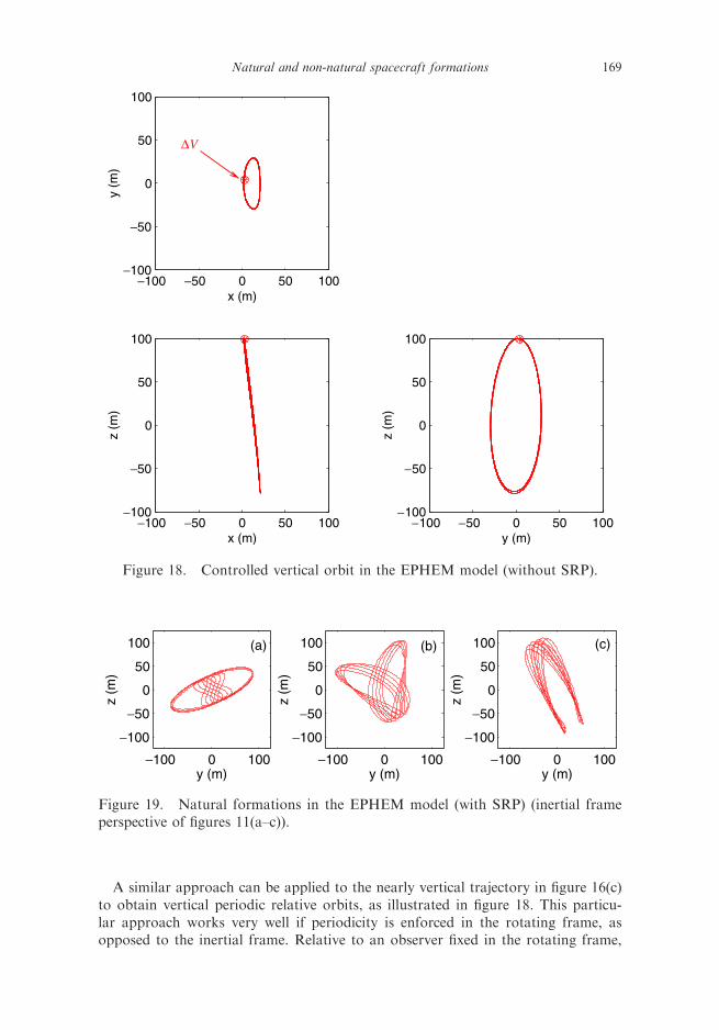
A similar approach can be applied to the nearly vertical trajectory in figure 16(c)to obtain vertical periodic relative orbits, as illustrated in figure 18. This particu-lar approach works very well if periodicity is enforced in the rotating frame, asopposed to the inertial frame. Relative to an observer fixed in the rotating frame,

−100 −50 0 50 100−100

−50

0

50

100

x (m)

y (m

)

−100 −50 0 50 100−100

−50

0

50

100

x (m)

z (m

)

−100 −50 0 50 100−100

−50

0

50

100

y (m)

z (m

)

∆V

Figure 18. Controlled vertical orbit in the EPHEM model (without SRP).

−100 0 100

−100

−50

0

50

100

y (m)

z (m

)

−100 0 100

−100

−50

0

50

100

y (m)

z (m

)

−100 0 100

−100

−50

0

50

100

y (m)

z (m

)

(a) (b) (c)

Figure 19. Natural formations in the EPHEM model (with SRP) (inertial frameperspective of figures 11(a–c)).


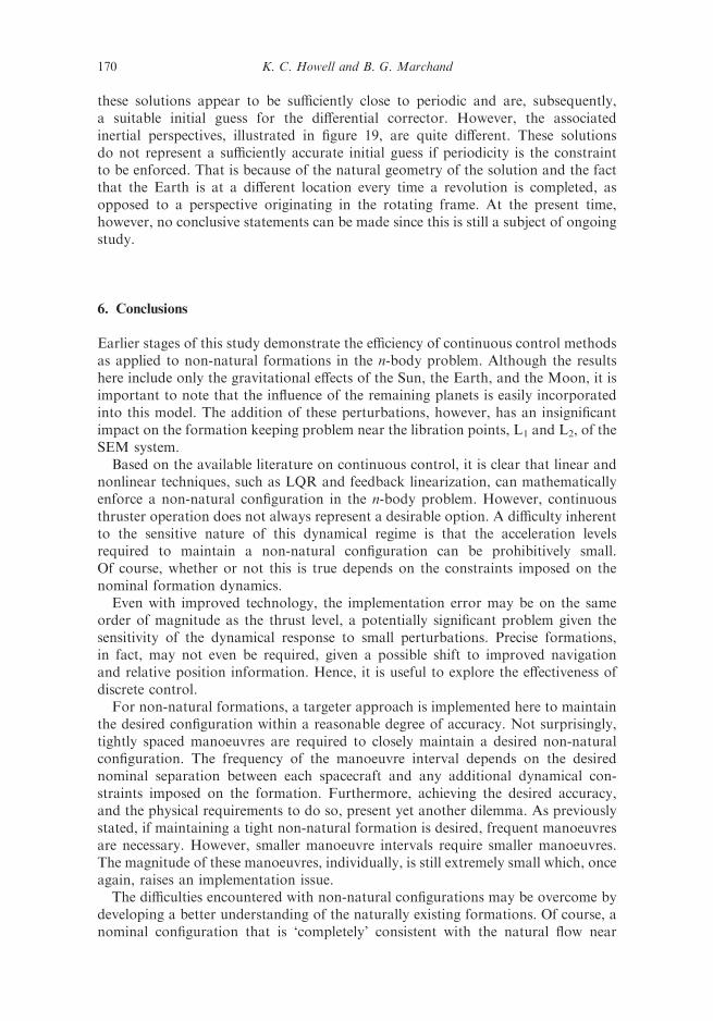
these solutions appear to be sufficiently close to periodic and are, subsequently,a suitable initial guess for the differential corrector. However, the associatedinertial perspectives, illustrated in figure 19, are quite different. These solutionsdo not represent a sufficiently accurate initial guess if periodicity is the constraintto be enforced. That is because of the natural geometry of the solution and the factthat the Earth is at a different location every time a revolution is completed, asopposed to a perspective originating in the rotating frame. At the present time,however, no conclusive statements can be made since this is still a subject of ongoingstudy.

6. Conclusions

Earlier stages of this study demonstrate the efficiency of continuous control methodsas applied to non-natural formations in the n-body problem. Although the resultshere include only the gravitational effects of the Sun, the Earth, and the Moon, it isimportant to note that the influence of the remaining planets is easily incorporatedinto this model. The addition of these perturbations, however, has an insignificantimpact on the formation keeping problem near the libration points, L1 and L2, of theSEM system.

Based on the available literature on continuous control, it is clear that linear andnonlinear techniques, such as LQR and feedback linearization, can mathematicallyenforce a non-natural configuration in the n-body problem. However, continuousthruster operation does not always represent a desirable option. A difficulty inherentto the sensitive nature of this dynamical regime is that the acceleration levelsrequired to maintain a non-natural configuration can be prohibitively small.Of course, whether or not this is true depends on the constraints imposed on thenominal formation dynamics.

Even with improved technology, the implementation error may be on the sameorder of magnitude as the thrust level, a potentially significant problem given thesensitivity of the dynamical response to small perturbations. Precise formations,in fact, may not even be required, given a possible shift to improved navigationand relative position information. Hence, it is useful to explore the effectiveness ofdiscrete control.

For non-natural formations, a targeter approach is implemented here to maintainthe desired configuration within a reasonable degree of accuracy. Not surprisingly,tightly spaced manoeuvres are required to closely maintain a desired non-naturalconfiguration. The frequency of the manoeuvre interval depends on the desirednominal separation between each spacecraft and any additional dynamical con-straints imposed on the formation. Furthermore, achieving the desired accuracy,and the physical requirements to do so, present yet another dilemma. As previouslystated, if maintaining a tight non-natural formation is desired, frequent manoeuvresare necessary. However, smaller manoeuvre intervals require smaller manoeuvres.The magnitude of these manoeuvres, individually, is still extremely small which, onceagain, raises an implementation issue.

The difficulties encountered with non-natural configurations may be overcome bydeveloping a better understanding of the naturally existing formations. Of course, anominal configuration that is ‘completely’ consistent with the natural flow near


the reference orbit may not satisfy all the dynamical requirements imposed by aparticular mission. However, understanding these naturally existing behaviourscan lead to the development of techniques to aid the construction of nominal for-mations that do meet the proposed mission objectives, while exploiting the naturalstructure. To that end, a modified Floquet-based controller is successfully appliedhere that reveals some interesting natural formations as well as deployment intothese configurations.

Acknowledgements

Any opinions, findings, and conclusions or recommendations expressed in this paperare those of the authors and do not necessarily reflect the views of the NationalAeronautics and Space Administration. This research was carried out at PurdueUniversity with support from the Clare Boothe Luce Foundation. It was alsofunded under Cooperative Agreement NCC5-727 through the NASA GSFCFormation Flying NASA Research Announcement.

References

[1] Micro Arcsecond X-Ray Imaging Mission (MAXIM) [Online]. Available at http://maxim.gsfc.nasa.gov

[2] Stellar Imager Homepage [Online]. Available at http://bires.gsfc.nasa.gov/�si/[3] Terrestrial Planet Finder (TPF) [Online]. Available at http://planetquest.ipl.nasa.gov/TPF/

tpf_index.html[4] Terrestrial Planet Finder (TPF) Book [Online]. (May 1999) Available at http://planetquest.jpl.nasa.-

gov/TPF/tpf_book/index.html.[5] Vassar, R.H. and Sherwood, R.B., 1985, Eormationkeeping for a pair of satellites in a circular orbit.

Journal of Guidance, Control and Dynamics, 8, 235–242.[6] Ulybyshev, Y., 1998, Long-term formation keeping of satellite constellation using linear quadratic

controller. Journal of Guidance, Control, and Dynamics, 21(1), 109–115.[7] Chao, C.C., Pollard, J.E. and Janson, S.W., 1999, Dynamics and control of cluster orbits for dis-

tributed space missions. AAS/AIAA Space Flight Mechanics Meeting, 7–10 February 1999(Breckenridge, CO: AAS), AAS Paper 99-126.

[8] de Queiroz, M.S., Kapila, V. and Yan, Q., 2000, Adaptive nonlinear control of multiple s/c formationflying. Journal of Guidance, Control, and Dynamics, 23(3), 385–390.

[9] Kapila, V., Sparks, A.G., Buffington, J.M. and Yan, Q., 2000, Spacecraft formation flying: dynamicsand control. Journal of Guidance, Control, and Dynamics, 23(3), 561–563.

[10] Sparks, A., 2000, Satellite formationkeeping control in the presence of gravity perturbations.American Control Conference, 28–30 June 2000 (Chicago, IL: ACC).

[11] Stansbery, D.T. and Cloutier, J.R., 2000, Nonlinear control of satellite formation flight. AIAAGuidance, Navigation, and Control Conference and Exhibit, 14–17 August 2000 (Denver, CO:AIAA), AIAA Paper 2000-4436.

[12] Tan, Z., Bainum, P.M. and Strong, A., 2000, The implementation of maintaining constant distancebetween satellites in elliptic orbits. AAS/AIAA Space Flight Mechanics Meeting, 23–26 January 2000(Clearwater, FL: AAS), pp. 667–683.

[13] Wang, Z., Khorrami, F. and Grossman, W., 2000, Robust adaptive control of satelliteformationkeeping for a pair of satellites. American Control Conference, 28–30 June 2000(Chicago, IL: ACC).

[14] Yan, Q., Yang, G., Kapila, V. and de Queiroz, M.S., 2000, Nonlinear dynamics nad output feedbackcontrol of multiple spacecraft in elliptic orbits. American Control Conference, 28–30 June 2000(Chicago, IL: ACC).

[15] Yedevalli, R.K. and Sparks, A.G., 2000, Satellite formation flying control design based onhybrid control system stability analysis. American Control Conference, 28–30 June 2000 (Chicago,IL: ACC).


[16] Irvin, D.J. Jr. and Jacques, D.R., 2001, Linear vs. nonlinear control techniques for the reconfigura-tion of satellite formations. AIAA Guidance, Navigation, and Control Conference and Exhibit,6–9 August 2001 (Montreal, Canada: AIAA), AIAA Paper 2001-4089.

[17] Sabol, C., Burns, R. and McLaughlin, C., 2001, Satellite formation flying design and evolution.Journal of Spacecraft and Rockets, 38(2), 270–278.

[18] Schaub, H. and Alfriend, K.T., 2001, Impulsive spacecraft formation flying control to establishspecific mean orbit elements. Journal of Guidance, Control, and Dynamics, 24(4), 739–745.

[19] Starin, S.R., Yedavalli, R.K. and Sparks, A.G., 2001, Spacecraft formation flying manoeuversusing linear quadratic regulation with no radial axis inputs. AIAA Guidance, Navigation, andControl Conference and Exhibit, 6–9 August 2001 (Montreal, Canada: AIAA), AIAA Paper2001-4029.

[20] Vadali, S.R., Vaddi, S.S., Naik, K. and Alfriend, K.T., 2001, Control of satellite formations. AIAAGuidance, Navigation, and Control Conference and Exhibit, 6–9 August 2001 (Montreal, Canada:AIAA), AIAA Paper 2001-4028.

[21] Simo, C., Gomez, G., Llibre, J., Martinez, R. and Rodriguez, J., 1987, On the station keeping controlof halo orbits. Acta Astronautica, 15(6/7), 391–397.

[22] Howell, K.C. and Keeter, T., 1995, Station-keeping strategies for libration point orbits—target pointand Floquet mode approaches. Advances in the Astronautical Sciences, 89(2), 1377–1396.

[23] Barden, B.T. and Howell, K.C., 1998a, Formation flying in the vicinity of libration point orbits.Advances in Astronautical Sciences, 99(2), 969–988.

[24] Barden, B.T. and Howell, K.C., 1998b, Fundamental motions near collinear libration points and theirtransitions. The Journal of the Astronautical Sciences, 46(4), 361–378.

[25] Barden, B.T. and Howell, K.C., 1999, Dynamical issues associated with relative configurations ofmultiple spacecraft near the Sun–Earth/Moon L1 point. AAS/AIAA Astrodynamics SpecialistsConference, 16–19 August 1999 (Girdwood, AK: AAS), AAS Paper 99-450.

[26] Howell, K.C. and Barden, B.T., 1999, Trajectory design and stationkeeping for multiple spacecraft information near the Sun–Earth L1 point. IAF 50th International Astronautical Congress, 4–8 October1999 (Amsterdam, the Netherlands: IAF/IAA), IAF/IAA Paper 99-A707.

[27] Folta, D., Carpenter, J.R. and Wagner, C., 2000, Formation flying with decentralized controlin libration point orbits. International Symposium: Spaceflight Dynamics, June 2000 (Biarritz,France).

[28] Scheeres, D.J. and Vinh, N.X., 2000, Dynamics and control of relative motion in an unstable orbit.AIAA/AAS Astrodynamics Specialist Conference, 14–17 August 2000 (Denver, CO: AIAA), AIAAPaper 2000-4135.

[29] Gomez, G., Lo, M., Masdemont, J. and Museth, K., 2001, Simulation of formation flight nearLagrange points for the TPF mission. AAS/AIAA Astrodynamics Conference, 30 July–2 August2001 (Quebec, Canada: AAS), AAS Paper 01-305.

[30] Gurfil, P. and Kasdin, N.J., 2001, Dynamics and control of spacecraft formation flying in three-bodytrajectories. AIAA Guidance, Navigation, and Control Conference and Exhibit, 6–9 August 2001(Montreal, Canada: AIAA), AIAA Paper 2001-4026.

[31] Hamilton, N.H., 2001, Formation flying satellite control around the L2 Sun–Earth libration point.MS thesis, George Washington University, Washington, DC.

[32] Luquette, R.J. and Sanner, R.M., 2001, A non-linear approach to spacecraft formation control in thevicinity of a collinear libration point. AAS/AIAA Astrodynamics Conference, 30 July–2 August 2001(Quebec, Canada: AAS), AAS Paper 01-330.

[33] Gurfil, P., Idan, M. and Kasdin, N.J., 2002, Adaptive neural control of deep-space formation flying.American Control Conference, 8–10 May 2002 (Anchorage, AK: ACC), pp. 2842–2847.

[34] Howell, K.C. and Marchand, B.G., 2003, Control strategies for formation flight in the vicinity of thelibration points. AAS/AIAA Space Flight Mechanics Conference, 9–13 February 2003 (Ponce, PuertoRico: AAS), AAS Paper 03-113.

[35] Marchand, B.G. and Howell, K.C., 2003, Formation flight near L1 and L2 in the Sun–Earth/Moonephemeris system including solar radiation pressure. AAS/AIAA Astrodynamics SpecialistsConference, 3–8 August 2003 (Big Sky, MT: AAS), AAS Paper 03-596.

[36] Marchand, B.G. and Howell, K.C., 2004, Aspherical formations near the libration points of theSun–Earth/Moon system. AAS/AIAA Space Flight Mechanics Meeting, 7–12 February 2004(Maui, HI: AAS), AAS Paper 04-157.

[37] McInnes, C.R., 1999, Solar Sailing: Technology, Dynamics and Mission Applications, Springer–PraxisSeries in Space Sciences and Technology (UK: Praxis Publishing Ltd.).

[38] Mueller, J., 1997, Thruster options for microspacecraft: a review and evaluation of existing hardwareand emerging technologies. 33rd AIAA/ASME/SAE/ASEE Joint Propulsion Conference andExhibit, 6–9 July 1997 (Seattle, WA: AIAA), AIAA Paper 97-3058.

[39] Gonzales, A.D. and Baker, R.P., 2001, Microchip laser propulsion for small satellites. 37th AIAA/ASME/SAE/ASEE Joint Propulsion Conference and Exhibit, 8–11 July 2001 (Salt Lake City,UT: AIAA), AIAA Paper 2001-3789.


[40] Phipps, C. and Luke, J., 2002, Diode laser-driven microthrusters—a new departure for micropropul-sion. AIAA Journal, 40(2), 310–318.

[41] http://space-power.grc.nasa.gov/ppo/projects/eo1/eo1-ppt.html[42] Nayfeh, A.H. and Mook, D.T., 1979, Nonlinear Oscillators (New York: John Wiley).[43] Howell, K.C. and Pernicka, H.J., 1988, Numerical determination of Lissajous trajectories in the

restricted three-body problem. Celestial Mechanics, 41, 107–124.


Documents

Natural and non-natural spacecraft formations near the L1 and L2 libration points in the Sun–Earth/Moon ephemeris system