SANDIA REPORT SAND2007-1423 Unlimited Release Printed March 2007

A Multi-Scale Q1/P0 Approach to Lagrangian Shock Hydrodynamics Guglielmo Scovazzi, Edward Love, and Mikhail Shashkov Prepared by Sandia National Laboratories Albuquerque, New Mexico 87185 and Livermore, California 94550 Sandia is a multiprogram laboratory operated by Sandia Corporation, a Lockheed Martin Company, for the United States Department of Energy’s National Nuclear Security Administration under Contract DE-AC04-94AL85000. Approved for public release; further dissemination unlimited.

2

Issued by Sandia National Laboratories, operated for the United States Department of Energy by Sandia Corporation. NOTICE: This report was prepared as an account of work sponsored by an agency of the United States Government. Neither the United States Government, nor any agency thereof, nor any of their employees, nor any of their contractors, subcontractors, or their employees, make any warranty, express or implied, or assume any legal liability or responsibility for the accuracy, completeness, or usefulness of any information, apparatus, product, or process disclosed, or represent that its use would not infringe privately owned rights. Reference herein to any specific commercial product, process, or service by trade name, trademark, manufacturer, or otherwise, does not necessarily constitute or imply its endorsement, recommendation, or favoring by the United States Government, any agency thereof, or any of their contractors or subcontractors. The views and opinions expressed herein do not necessarily state or reflect those of the United States Government, any agency thereof, or any of their contractors. Printed in the United States of America. This report has been reproduced directly from the best available copy. Available to DOE and DOE contractors from U.S. Department of Energy Office of Scientific and Technical Information P.O. Box 62 Oak Ridge, TN 37831 Telephone: (865) 576-8401 Facsimile: (865) 576-5728 E-Mail: reports@adonis.osti.gov Online ordering: http://www.osti.gov/bridge Available to the public from U.S. Department of Commerce National Technical Information Service 5285 Port Royal Rd. Springfield, VA 22161 Telephone: (800) 553-6847 Facsimile: (703) 605-6900 E-Mail: orders@ntis.fedworld.gov Online order: http://www.ntis.gov/help/ordermethods.asp?loc=7-4-0#online

DEP

ARTMENT OF ENERGY

• •UN

ITED

STATES OF AM

ERIC

A

SAND2007-1423Unlimited Release

Printed March 2007

A Multi-Scale Q1/P0 Approach to Lagrangian Shock

Hydrodynamics

Guglielmo Scovazzi

1431 Computational Shock- and Multi-physics Department

Sandia National Laboratories

P.O. Box 5800, MS 1319

Albuquerque, NM 87185-1319, USA

gscovaz@sandia.gov

Edward Love

1431 Computational Shock- and Multi-physics Department

Sandia National Laboratories

P.O. Box 5800, MS 1319

Albuquerque, NM 87185-1319, USA

elove@sandia.gov

Mikhail J. Shashkov

Theoretical Division, Group T-7, MS B284

Los Alamos National Laboratory

Los Alamos, NM 87545, USA

shashkov@lanl.gov

Abstract

A new multi-scale, stabilized method for Q1/P0 finite element computations of Lagrangian shockhydrodynamics is presented. Instabilities (of hourglass type) are controlled by a stabilizing operatorderived using the variational multi-scale analysis paradigm. The resulting stabilizing term takes the formof a pressure correction. With respect to currently implemented hourglass control approaches, the noveltyof the method resides in its residual-based character. The stabilizing residual has a definite physicalmeaning, since it embeds a discrete form of the Clausius-Duhem inequality. Effectively, the proposedstabilization samples and acts to counter the production of entropy due to numerical instabilities. Theproposed technique is applicable to materials with no shear strength, for which there exists a caloricequation of state. The stabilization operator is incorporated into a mid-point, predictor/multi-correctortime integration algorithm, which conserves mass, momentum and total energy. Encouraging numericalresults in the context of compressible gas dynamics confirm the potential of the method.

3

Acknowledgments

This research was partially funded by the DOE NNSA Advanced Scientific Computing Program and theComputer Science Research Institute (CSRI) at Sandia National Laboratories.

The partial support through LDRD “A Mathematical Framework for Multiscale Science and Engi-neering: The Variational Multiscale Method and Interscale Transfer Operators” is also acknowledged.LDRD funding was essential in the early stage of development, when the outcome of this research was stilluncertain.

We would like to thank Professor Thomas J.R. Hughes, and Dr. Pavel Bochev, Dr. Allen Robinson,and Dr. John Shadid for very insightful discussions. Many thanks also to Dr. Greg Weirs for providing uswith very insightful test cases. The first two authors would like to thank Dr. Randy Summers, Dr. JohnShadid, Dr. Allen Robinson, and Dr. Scott Collis for their genuine support.

4

Contents

1 Introduction . . . . . . . . . . . . . . . . . . . . . . . . . . . . . . . . . . . . . . . . . . . . . . . . . . . . . . . . . . . . . . . . . . . . . . 7

2 Equations of Lagrangian shock hydrodynamics . . . . . . . . . . . . . . . . . . . . . . . . . . . . . . . . . . . . 8

2.1 Constitutive laws . . . . . . . . . . . . . . . . . . . . . . . . . . . . . . . . . . . . . . . . . . . . . . . . . . . . . . . . . . . . . 10

3 Variational formulation of Lagrangian hydrodynamics . . . . . . . . . . . . . . . . . . . . . . . . . . . . . 11

4 Time integration and discrete weak forms . . . . . . . . . . . . . . . . . . . . . . . . . . . . . . . . . . . . . . . . . 11

4.1 Test and trial spaces . . . . . . . . . . . . . . . . . . . . . . . . . . . . . . . . . . . . . . . . . . . . . . . . . . . . . . . . . . . 114.2 Variational equations . . . . . . . . . . . . . . . . . . . . . . . . . . . . . . . . . . . . . . . . . . . . . . . . . . . . . . . . . . . 124.3 Global conservation properties . . . . . . . . . . . . . . . . . . . . . . . . . . . . . . . . . . . . . . . . . . . . . . . . . . 154.4 A predictor/multi-corrector approach . . . . . . . . . . . . . . . . . . . . . . . . . . . . . . . . . . . . . . . . . . . . . 16

5 A multi-scale, residual-based hourglass control . . . . . . . . . . . . . . . . . . . . . . . . . . . . . . . . . . . . 17

5.1 Variational multi-scale analysis . . . . . . . . . . . . . . . . . . . . . . . . . . . . . . . . . . . . . . . . . . . . . . . . . . . 175.2 The case of materials with no shear strength . . . . . . . . . . . . . . . . . . . . . . . . . . . . . . . . . . . . . . . 20

6 Artificial viscosity and discontinuity capturing operator . . . . . . . . . . . . . . . . . . . . . . . . . . . 28

7 General considerations on implementation . . . . . . . . . . . . . . . . . . . . . . . . . . . . . . . . . . . . . . . . 30

7.1 Numerical quadratures . . . . . . . . . . . . . . . . . . . . . . . . . . . . . . . . . . . . . . . . . . . . . . . . . . . . . . . . . 307.2 Hourglass stabilization and artificial viscosity parameters . . . . . . . . . . . . . . . . . . . . . . . . . . . . . 317.3 CFL condition . . . . . . . . . . . . . . . . . . . . . . . . . . . . . . . . . . . . . . . . . . . . . . . . . . . . . . . . . . . . . . . . 31

8 Numerical computations . . . . . . . . . . . . . . . . . . . . . . . . . . . . . . . . . . . . . . . . . . . . . . . . . . . . . . . . . . 31

8.1 Acoustic pulse computations and hourglass control . . . . . . . . . . . . . . . . . . . . . . . . . . . . . . . . . . 318.2 Saltzmann test . . . . . . . . . . . . . . . . . . . . . . . . . . . . . . . . . . . . . . . . . . . . . . . . . . . . . . . . . . . . . . . . 338.3 Sedov test in two dimensions . . . . . . . . . . . . . . . . . . . . . . . . . . . . . . . . . . . . . . . . . . . . . . . . . . . . 348.4 Noh test in two dimensions . . . . . . . . . . . . . . . . . . . . . . . . . . . . . . . . . . . . . . . . . . . . . . . . . . . . . . 418.5 Sedov test in three dimensions . . . . . . . . . . . . . . . . . . . . . . . . . . . . . . . . . . . . . . . . . . . . . . . . . . . 468.6 Noh test in three dimensions . . . . . . . . . . . . . . . . . . . . . . . . . . . . . . . . . . . . . . . . . . . . . . . . . . . . . 49

9 Summary . . . . . . . . . . . . . . . . . . . . . . . . . . . . . . . . . . . . . . . . . . . . . . . . . . . . . . . . . . . . . . . . . . . . . . . . . 50

References . . . . . . . . . . . . . . . . . . . . . . . . . . . . . . . . . . . . . . . . . . . . . . . . . . . . . . . . . . . . . . . . . . . . . . . . . . . 53

5

6

A Multi-Scale Q1/P0 Approach to Lagrangian Shock

Hydrodynamics

1 Introduction

In [31, 30], a multi-scale approach was applied in finite element computations of Lagrangian shock hydro-dynamics. In that case, a piece-wise linear, continuous approximation in space was adopted for all thesolution variables.

Given the encouraging results of the approach in [31], extensions to the case of Q1/P0 finite elementare investigated in the present work. Q1/P0 refers to the piece-wise linear, continuous approximationof the kinematic variables (position/displacement, velocity, acceleration), and the piece-wise constant,discontinuous approximation of the thermodynamic variables (density, pressure, internal energy).

Among the requirements in developing a consistent formulation, conservation of mass, momentumand total energy are considered essential. In addition, a straightforward definition of the total energyof the system is also considered very important. In fact, most of the finite element implementations forshock hydrodynamics leverage a central difference time integrator in which displacements, velocities andaccelerations are collocated in time according to a staggered approach (see, e.g., [5] for a review of thestate of the practice). Although very efficient in terms of storage and computational cost, such centraldifference implementations suffer from a cumbersome definition of the kinetic energy, which involves theproduct of algorithmic velocities at two different time instants. This is seen as a problem by the authors,since, by definition, the algorithmic kinetic energy is not ensured to be positive [5].

The present paper proposes an alternative approach, in which a mid-point type integrator is im-plemented by means of a conservative predictor/multi-corrector procedure. Thanks to this approach,a straightforward definition of the total energy is obtained. To the authors’ best knowledge, the proposedalgorithm is new in finite element hydrocode implementations, although a similar approach was origi-nally proposed by Caramana, Shashkov and Whalen [6], in the context of mimetic finite differences. Theproposed approach also shares significant similarities with the space-time integrators discussed in [31].

At the core of the algorithm is a novel, multi-scale operator which controls hourglass-type instabilities.Applying the multi-scale analysis [18, 19] to the base Galerkin formulation shows how instabilities can becontrolled. For materials with no shear strength (e.g., fluids) the stabilization takes the form of a pressureenrichment, ultimately dependent on the residual of a rate equation for the pressure. The residual charac-ter of the stabilization preserves the consistency of the method, and, at the same time, reveals importantconnections between numerical instabilities and physical aspects of the problem simulated. In fact, thepressure equation residual can be interpreted as a statement of the Clausius-Duhem entropy inequality.Effectively, the pressure residual samples and counters the production of entropy due to numerical insta-bilities. Previous work has gone in the direction of physical hourglass control design [2, 3, 29]: The presentwork takes an even closer look at the interplay between physical consistency and numerical instabilities ofalgorithms.

One very important point is that the multi-scale stabilization operator, when applied to a three-dimensional, compressible, inviscid flow, acts only on the hourglass modes which are not divergence-free.This should not be surprising, since, per se, the material has no shear strength, and, therefore, therecannot be any residual equation providing shear resistance. However, divergence-free modes associated

7

with non-homogeneous deviatoric motion (shear) are an integral part of the hourglass eigenspace.

The multi-scale approach enables a clear delineation of the true dilemma faced by the analyst whenusing Q1/P0 finite elements formulations for fluid flow computations. On the one hand, any attempt toinclude artificial shear strength in the fluid may negatively affect the quality of the simulation. On the otherhand, three-dimensional computations may be unstable if non-homogeneous shear modes are undamped.This fact is considered by the authors not as a shortcoming of the multi-scale approach, but rather as afundamental flaw of Q1/P0 formulations for inviscid fluids.

In order to stabilize the non-homogeneous shear modes, an artificial viscosity acting on the fluctuationof the deviatoric part of the symmetric velocity gradient is introduced. This correction term does notperturb the convergence rates of the method, since it acts to damp the difference between the deviatorof the symmetric gradient of the velocity and its element-average. Contrary to all other examples ofhourglass control techniques for fluids, the multi-scale analysis shows that the stabilization operators fornon-homogeneous shear modes can be designed in a completely autonomous way with respect to thecontrol of hourglass modes which are not divergence-free. The multi-scale approach provides therefore anew perspective on an old problem, posing a clear boundary between what can be stabilized on physicalgrounds, and what has to be stabilized with purely artificial mechanisms. It is also of interest that in thevast literature of SUPG methods (see, e.g., [25, 22, 21, 20, 14, 15, 16, 27, 33, 37, 36, 41, 42, 38, 39, 40] andreferences therein) no hourglass instabilities of shear type were ever observed. Further investigation onthis subject is in our opinion required, to fully evaluate whether or not standard SUPG methods on piece-wise linear approximations necessitate “deviatoric” stabilization when applied to Lagrangian or Euleriancomputations of inviscid flows.

An integral part of the proposed approach is the shock-capturing operator, in the form of an artificialstress tensor, based on the symmetric part of the velocity gradient. This choice, , already explored in[31], yields an objective stress tensor, which proves superior to standard artificial viscosity operators,constructed with the velocity divergence. Whenever spurious homogeneous shear modes are generatedacross the shock layer, the tensor viscosity delivers much improved results, from both the accuracy androbustness standpoints. In particular, improvements with respect to [31] on the selection of the lengthscale in the artificial viscosity are discussed.

The rest of the exposition is organized as follows: The basic equations of Lagrangian hydrodynamics areintroduced in Section 2. The variational formulation is established in Section 3, and the time-integrationalgorithm is described in Section 4. Section 5 is devoted to the multi-scale analysis and design of themulti-scale hourglass stabilization. The shock-capturing operator is described in Section 6. Section 7contains additional comments on the implementation of the algorithm, the integration quadratures used,and the time step CFL constraints for the method. Results of the numerical tests are analyzed in Section8. Conclusions and future research perspectives are summarized in Section 9.

2 Equations of Lagrangian shock hydrodynamics

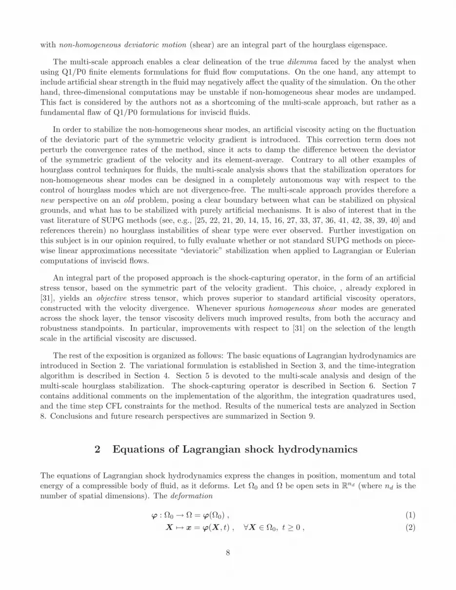
The equations of Lagrangian shock hydrodynamics express the changes in position, momentum and totalenergy of a compressible body of fluid, as it deforms. Let Ω0 and Ω be open sets in Rnd (where nd is thenumber of spatial dimensions). The deformation

ϕ : Ω0 → Ω = ϕ(Ω0) , (1)

X 7→ x = ϕ(X , t) , ∀X ∈ Ω0, t ≥ 0 , (2)

8

Ω0

Ω

ϕ

X

x

Figure 1. Sketch of the Lagrangian map ϕ.

is the mapping from the original to the current configuration of the material. Here X is the materialcoordinate, representing the initial position of an infinitesimal material particle of the body, and x is theposition of that particle in the current configuration (see Fig. 1). Ω0 is the domain occupied by the bodyin its initial configuration, with boundary Γ0. ϕ maps Ω0 to Ω, the domain occupied by the body inits current configuration, with boundary Γ. It is also useful to define the deformation gradient, and thedeformation Jacobian determinant :

F = ∇Xϕ =∂ϕi

∂Xj=

∂xi

∂Xj, (3)

J = det(F ) . (4)

On a domain Ω in the current configuration, the conservative form of the equations of Lagrangian hydro-dynamics, consisting of mass, momentum and energy, can be formulated as follows:

ρ J = ρ0 , (5)

ρ v = ρ g + ∇x· σ , (6)

ρ E = ρ g · v + ρ r + ∇x· (σTv + q) , (7)

u = v . (8)

Here, ∇x and ∇x · are the current configuration gradient and divergence operators, and ˙(·) indicates thematerial, or Lagrangian time derivative. u = x−X is the displacement vector, ρ0 is the reference (initial)density, ρ is the (current) density, v is the velocity, g is the body force, σ is the Cauchy stress (a symmetrictensor), E = ǫ+ v · v/2 is the total energy, the sum of the internal energy e and the kinetic energy v · v/2,r is the energy source term, and q is the heat flux. E, ǫ, g, r are measured per unit mass.

Remarks

1. Equations (6) and (7) are in Lagrangian conservative (or divergence) form. In fact, the Lagrangian

9

rate of change of an intensive, scalar variable φ is given by

d

dt

∫

Ωρφ dΩ =

d

dt

∫

Ωρ0φ dΩ0 =

∫

Ωρ0φ dΩ0 =

∫

Ωρφ dΩ , (9)

where (5) has been used, together with the identity

ρ0 dΩ0 = ρJ dΩ0 = ρ dΩ . (10)

2. The kinetic energy equation, the inner product of (6) and the velocity vector field, can be subtractedfrom equation (7), yielding

ρǫ = ρ r + ∇xv : σ + ∇x· q , (11)

where, in index notation, σT : ∇xv = σji ∂xivj, and ∇xv : σ = σ : ∇xv = σT : ∇xv, since σ issymmetric. Clearly (11) is not in conservative form. However, it will be possible to use this equationin appropriate variational formulations maintaining global conservation properties (see Section 4).

The system of equations (5)–(8) has to be complemented with appropriate boundary conditions. As-

suming that the boundary Γ = ∂Ω is partitioned as Γ = Γg ∪ Γh, Γg ∩ Γh = ∅, displacement boundaryconditions are applied on Γg, the Dirichlet boundary, and traction boundary conditions are applied on Γh,the Neumann boundary. Namely,

u|Γg = ubc(x, t) , (12)

σn|Γh = t(x, t) . (13)

Equations (5)–(8) and boundary conditions (12)-(13) completely defines the evolution of the system, onceinitial conditions are specified.

2.1 Constitutive laws

The analysis presented in what follows is specific to materials with no deformation strength. In this case,the Cauchy stress σ reduces to an isotropic tensor, dependent only on the thermodynamic pressure:

σ = −pInd×nd, (14)

or, in index notation,σij = −p δij , (15)

with δij the Kronecker tensor. An equation of state of the type

p = p(ρ, ǫ) , (16)

is assumed. Equations of state of Mie-Gruneisen type are compatible with (16), namely

p(ρ, ǫ) = f1(ρ) + f2(ρ)ǫ , (17)

and apply to materials such as compressible ideal gases, co-volume gases, high explosives, and elastic-plastic solids with no strength (a situation that can be achieved when bulk stresses in the material arelarger than shear stresses by orders of magnitude). For example, ideal gases satisfy (17), with f1 = 0 andf2 = (γ − 1)ρ, to yield

p(ρ, ǫ) = (γ − 1)ρǫ . (18)

10

3 Variational formulation of Lagrangian hydrodynamics

Finite element approximations leverage a variational statement of the equations of motion. The first stepin the development of a variational form for (5), (6), (7) (or, (11)), and (8), is to define the (variational)trial spaces for the kinematic and thermodynamic variables, which characterize the state of the system.In particular, Sκ denotes the space of admissible displacements, or more generally, the space of admissiblevalues for the kinematic variables (displacements, velocities, accelerations). Analogously, Sγ is the space ofadmissible thermodynamic states. Specific discrete definitions of Sκ and Sγ are given in the next section,where the discrete form of the variational equations is presented. For now, it is important to observe thatthe space Sκ incorporates the set of essential boundary conditions (12), that is, boundary conditions ofkinematic (Dirichlet) type are imposed strongly. In addition, test spaces can be defined: Vκ is the space ofvariations – compatible with (12) – for the kinematic variables, and Vγ is the space of variations for thethermodynamic variables. Using (9) and (10), the variational problem associated with (5), (6), (11) reads:

Find ρ ∈ Sγ, v ∈ Sκ, and ǫ ∈ Sγ , such that, ∀ψγ ∈ Vγ, and ∀ψκ ∈ Vκ,

0 =

∫

Ω0

ψγ (ρ0 − ρJ) dΩ0 , (19)

0 =

∫

Ω0

ψκ · (ρ0v) dΩ0 +

∫

Ω∇s

xψκ : σ dΩ −

∫

Γh

ψκ · t dΓ −∫

Ωψκ · (ρg) dΩ , (20)

0 =

∫

Ω0

ψγ (ρ0ǫ) dΩ0 −∫

Ωψγ (∇s

xv : σ + ∇x · q + ρr) dΩ , (21)

where ∇sx

= 1/2(∇x

T +∇x ) is the symmetric part of the gradient operator, and ∇xv : σ = ∇sxv : σ, since σ

is symmetric. Notice that the traction (or, natural) boundary conditions are imposed in (20) through theweak form.

4 Time integration and discrete weak forms

The variational form of the Lagrangian hydrodynamics equations and its conservation properties are strictlyrelated to the choice of time-integration algorithm. In the present work, a mid-point type integration schemeis adopted, which, in combination with an appropriate predictor/corrector solution strategy, yields an ex-plicit iterative algorithm. The proposed formulation conserves mass, momentum and total energy, withoutresorting to any staggered approach in time, with striking analogies to the space-time integration presentedin [31]. A similar approach is usually adopted in the context of mimetic or compatible discretizations [6].

4.1 Test and trial spaces

In terms of the spatial discretization, the proposed approach is no different from standard Lagrangianhydrodynamic finite element methods [5, 13]. Kinematic variables are approximated by piecewise-linear,continuous functions (node-centered degrees-of-freedom), and all thermodynamic variables are approxi-mated by piecewise-constant, discontinuous functions (cell-centered degrees-of-freedom). Consequently,the test-space for the momentum equation consists of piecewise-linear, continuous functions, while the testspace for the mass and energy equations is given by the piecewise-constant, discontinuous functions. The

11

trial function spaces Sh and test function spaces Vh are then given by:

Shκ =

ψκ ∈ (C0(Ω))nd : ψhκ

∣

∣

∣

Ωe

∈ (P1(Ωe))nd ,ψh

κ = gbc(t) on Γg

, (22)

Vhκ =

ψκ ∈ (C0(Ω))nd : ψhκ

∣

∣

∣

Ωe

∈ (P1(Ωe))nd ,ψh

κ = 0 on Γg

, (23)

Shγ =

ψhγ ∈ L2(Ω) : ψh

γ

∣

∣

∣

Ωe

∈ P0(Ωe),

, (24)

Vhγ = Sh

γ , (25)

where gbc(t) indicates the essential (Dirichlet) boundary conditions, possibly dependent on time.

4.2 Variational equations

The momentum and energy balances are considered first. For the sake of simplicity, it is assumed thatbody forces, heat fluxes and heat sources are absent. The time step is indicated by ∆t, and the mid-pointvalue of a quantity f is defined as:

fn+1/2 =fn + fn+1

2. (26)

4.2.1 Momentum balance

Find v ∈ Shκ , such that, ∀ψh

κ ∈ Vh,

∫

Ω0

ψhκ · ρ0 (vn+1 − vn) dΩ0

+∆t

∫

Ωn+1/2

(∇xψhκ)n+1/2 : σn+1/2 dΩ − ∆t

∫

Γhn+1/2

ψhκ · tn+1/2 dΓ = 0 , (27)

where ∇x is the current configuration gradient operator. Notice the slight abuse of notation, since the su-perscript “h”, indicating spatial discretization, should be applied to all solution variables, discrete gradientoperators, and the domain geometry. This is avoided whenever possible, to favor a simpler presentationof algebraic expressions. Notice that the physical traction t acts only on the Neumann boundary (i.e.,t|Γg = 0), and the notation σ indicates an algorithmic stress, whose general expression is

σ = σ + σvms + σart , (28)

where σvms is the multi-scale, residual-based stress tensor, designed to control hourglass instabilities, andσart is the artificial viscosity stress tensor, designed to capture shock layers.

It is usual practice in hydrodynamic computations to lump the mass matrix in the momentum equation,to avoid any matrix inversions in the solution procedure. The velocity field at time t• is interpolated as

v• =

nnp∑

B=1

NB(X)v•;B . (29)

12

Here v•;B and NB(X) are the nd-dimensional vector of velocity degrees-of-freedom and the shape function,both associated with nodeB, and nnp is the number of nodes in the computational mesh. The mass lumpingis achieved applying the following approximation (no index sum is implied unless expressly stated):

∫

Ω•

NA(X) (ρvi)• dΩ =

∫

Ω0

NA(X)ρ0(vi)• dΩ0

=

nnp∑

B=1

(∫

Ω0

NA(X)NB(X)ρ0 dΩ0

)

(vi)•;B

≈nnp∑

B=1

(∫

Ω0

NA(X) δAB ρ0 dΩ0

)

(vi)•;B

= MAL (vi)•;A , (30)

where vi and vi are the ith components of v and v, respectively, A = 1, 2, . . . , nnp, δAB is the Kronecker

symbol, and

MAL =

∫

Ω0

NA(X)ρ0 dΩ0 (31)

is the the mass associated to node A in the global numbering. Defining

[ML] = [diagMAL ,MA

L ,MALT ] , (32)

Fn+1/2 = Fn+1/2;A , (33)

Fn+1/2;A =

∫

Ωn+1/2

σn+1/2(∇xNA)n+1/2 dΩ −

∫

Γn+1/2

NAtn+1/2 dΓ , (34)

where [ML] is a diagonal [(nd × nnp)× (nd × nnp)]-matrix and Fn+1/2 is a (nd × nnp)-vector, equation (27)reduces to

[ML] (vn+1 − vn) + ∆t Fn+1/2 = 0 . (35)

4.2.2 Energy balance

Integrating in time (21), yields:

Find ǫ ∈ Shγ , such that, ∀ψh

γ ∈ Vh,∫

Ω0

ψhγρ0 (ǫn+1 − ǫn) dΩ0 − ∆t

∫

Ωn+1/2

ψhγ (∇xv)n+1/2 : σn+1/2 dΩ = 0 . (36)

Recalling that ψγ , ǫ, and ρ are constant over each element, one can introduce the following definitions:

[Mel] = [diagMel] , (37)

Mel = Me , (38)

Me =

∫

Ω•;e

ρ• dΩ =

∫

Ω0;e

ρ0 dΩ0 . (39)

Wn+1/2 = Wn+1/2;e , (40)

Wn+1/2;e =

−∫

Ωn+1/2;e

(∇xv)n+1/2 : σn+1/2 dΩ

, (41)

(42)

13

where Ω•;e is the element domain at time t•, Mel and Wn+1/2 are nel-dimensional vectors, and nel is thenumber of elements in the computational list. Then, equation (36) reduces to

[Mel] (ǫn+1 − ǫn) + ∆t Wn+1/2 = 0 . (43)

where ǫ• is the vector of cell-centered degrees-of-freedom for the internal energy ǫ at time t•.

4.2.3 Mass balance

The mass conservation equation (19) can be slightly rearranged to yield:

Find ρ ∈ Shγ , such that, ∀ψh

γ ∈ Vh,∫

Ω0

ψhγρ0 dΩ0 =

∫

Ω0

ψhγρJ dΩ0 =

∫

Ωψh

γρdΩ . (44)

Integrating the previous equation element-by-element results in

Mel = [V•]ρ• , (45)

where

ρ• = ρ•;e , (46)

[V•] = [diagV•] , (47)

V• = V•;e , (48)

V•;e =

∫

Ω0;e

J• dΩ0 = meas(Ω•;e) . (49)

4.2.4 Displacement equations

The time-discretization of the rate equations for the position field

xn+1 − xn − ∆t vn+1/2 = 0 (50)

yields a set of ordinary differential equations for the nodal positions, namely

xn+1 − xn − ∆t vn+1/2 = 0 . (51)

4.2.5 Equation of state

The equation of state can be applied at each time step to obtain the pressure (or, in general, the stressfield),

σn+1 = −pn+1I = −p(ρn+1, ǫn+1)I . (52)

Expressing (52) in terms of the cell-centered degrees-of-freedom, one obtains

pn+1 = p(ρn+1, ǫn+1) , (53)

(54)

where

p• = p•;e , (55)

p(ρ•, ǫ•) = p(ρ•;e, ǫ•;e) . (56)

14

4.3 Global conservation properties

It is immediate to realize that equations (44) and (45) are statements of global and local conservation ofmass, respectively. It is also evident from equation (27) or (35) that the proposed algorithm conserves thetotal momentum of the system. Proving conservation of total energy is somewhat less obvious, and, forthis purpose, equations (27) and (36) are used. Conservation statements are usually proven in the case ofhomogenous Neumann boundary conditions, for which the test and trial function spaces for the velocitiescoincide (i.e., Sh

κ = Vhκ ). Evaluating the sum over all the nodes of (27), with ψh

κ = vn+1/2, the kineticenergy balance for the system is obtained:

1

2

∫

Ωn+1

ρn+1(v · v)n+1 dΩ − 1

2

∫

Ωn

ρn(v · v)n dΩ = −∆t

∫

Ωn+1/2

(∇xv)n+1/2 : σn+1/2 dΩ , (57)

The previous equation is derived using the following identity:∫

Ω0

ρ0vn+1/2 · (vn+1 − vn) dΩ0 =1

2

∫

Ω0

ρ0 ((v · v)n+1 − (v · v)n) dΩ0

=1

2

∫

Ωn+1

ρn+1(v · v)n+1 dΩ − 1

2

∫

Ωn

ρn(v · v)n dΩ . (58)

Testing (36) with a unit constant shape function over the entire domain (i.e., ψhγ = 1) yields

∫

Ωn+1

(ρǫ)n+1 dΩ −∫

Ωn

(ρǫ)n dΩ =

∫

Ω0

ρ0 (ǫn+1 − ǫn) dΩ0

= ∆t

∫

Ωn+1/2

(∇xv)n+1/2 : σn+1/2 dΩ . (59)

By summing (57) and (59), and noticing that their right hand sides are equal and opposite, one can derivethe following conservation statement for the total energy between time steps n and n+ 1:

∫

Ωn+1

ρn+1

(

1

2(v · v)n+1 + ǫn+1

)

dΩ =

∫

Ωn

ρn

(

1

2(v · v)n + ǫn

)

dΩ . (60)

The previous derivations can be repeated in the case when mass lumping is applied. Using (35), an analogueof (57) can be derived, namely,

1

2vT

n+1[ML]vn+1 −1

2vT

n [ML]vn = −vTn+1/2Fn+1/2 . (61)

Using the vector notation, (59) can be recast as (43) multiplied by 1, a nel-dimensional vector whose entriesare all unity, that is,

MTel (ǫn+1 − ǫn) = −∆t 1T Wn+1/2 . (62)

Finally, realizing that, by definition,

vTn+1/2Fn+1/2 = −1T Wn+1/2 , (63)

a statement of conservation of total energy analogous to (60) can be expressed as

1

2vT

n+1[ML]vn+1 + MTelǫn+1 =

1

2vT

n [ML]vn + MTelǫn . (64)

15

Retrieve loop parameters: nstep, imax

Initialize all variables with initial conditionsForm [ML] and Mel

For n = 0, . . . , nstep (Time-step loop begins)Set ∆t (respecting the CFL condition)

Predictor: Y(0)n+1 = Yn

For i = 0, . . . , imax − 1 (Multi-corrector loop begins)

Assembly: F(i)n+1/2

Velocity update: v(i+1)n+1 = vn − ∆t[ML]−1F

(i)n+1/2

Assembly: W(i,i+1)n+1/2

Internal energy update: ǫ(i+1)n+1 = ǫn − ∆t [Mel]

−1W(i,i+1)n+1/2

Position update: x(i+1)n+1 = xn + ∆t v

(i+1)n+1/2

Volume update: V(i+1)n+1 = V(x

(i+1)n+1 )

Density update: ρ(i+1)n+1 = [V

(i+1)n+1 ]−1Mel

Equation of state update: p(i+1)n+1 = p

(

ρ(i+1)n+1 , ǫ

(i+1)n+1

)

End (Multi-corrector loop ends)

Time update: Yn+1 = Y(imax)n+1

End (Time-step loop ends)Exit

Table 1. Outline of the predictor-multicorrector algorithm. Notice that all matrices are diagonal,so that all inverse operations are just vector divisions. Three iterations of the predictor/multi-corrector were used in the computations.

Remarks

1. Under appropriate boundary conditions, total angular momentum is also conserved. This is a directconsequence of the symmetry of the stress tensor and the use of a mid-point time integrator [35].

2. The total energy conservation statement (60) is a direct consequence of the cancellation of the righthand sides of (57) and (59), which are equal and opposite. This fact is used to derive artificial viscosityand variational multi-scale stabilization operators which preserve total energy in the system. In fact,to ensure conservation, it is sufficient that the discrete expression for the overall σ term remains thesame in the momentum and energy equations.

4.4 A predictor/multi-corrector approach

The algorithm developed so far requires the inversion of a matrix, since the force and work terms arecomputed at the mid-point in time, and necessitate knowledge of the solution at time tn+1. However, afully explicit algorithm can be recovered by resorting to a predictor/multi-corrector approach. This sectionis devoted to this purpose.

16

A number of preliminary definitions are needed. The state of system at time t = t• is defined by means

of the vector Y• = [xT• , v

T• ,ρ

T• , ǫ

T• ,p

T• ]T . F

(i)n+1/2 indicates the evaluation of Fn+1/2 using the state Y at

iterate (i). The definition of the iterate of the work vector Wn+1/2 is somewhat different:

W(i,j)n+1/2 = W(i,j)

n+1/2;e , (65)

W(i,j)n+1/2;e =

∫

Ω(i)n+1/2;e

((∇x )(i)n+1/2v

(j)n+1/2) : σ

(i)n+1/2 dΩ

. (66)

Here ∇x

(i)n+1/2 and v

(j)n+1/2 indicate the (current configuration) gradient operator and the velocity field at

t = tn+1/2 and iterate i and j, respectively. This notation is needed to understand how conservation isenforced at each iteration of the predictor/multi-corrector procedure.

As it can be appreciated in Table 1, the proposed approach consists of a velocity update, followed, inthe order, by internal energy, position, volume, density and pressure (or, more generally, stress) updates.

Remark (conservation of total energy)The proposed predictor/multi-corrector approach maintains all the conservation properties of the base mid-point algorithm it is derived from. The crucial step in the design of the algorithm is to recognize that the

work vector W(i,i+1)n+1/2 in Table 1 has to be computed holding the geometry and all the terms in the integral

(66) at iterate (i), with the exception of the velocity vn+1/2, which is evaluated using the new iterate (i+1),available after the momentum equation is integrated in time. Using arguments virtually identical to theones presented in Section 4.3, it is easy to realize that, indeed, each iterate of the predictor/multi-correctorconserves total energy, namely

1

2(v

(i+1)n+1 )T [ML]v

(i+1)n+1 + MT

elǫ(i+1)n+1 =

1

2vT

n [ML]vn + MTelǫn , (67)

since the following cancellation takes place:

(v(i+1)n+1/2)

T Fin+1/2 = −1T W

(i;i+1)n+1/2 . (68)

The numerical tests in Section 8.5, in the context of blast-type flows, show that the proposed methodindeed conserves total energy within machine precision.

5 A multi-scale, residual-based hourglass control

The present section develops an analysis of the Lagrangian shock hydrodynamics equations, using anapproach similar to [18, 19, 24]. The final goal is to stabilize hourglass instabilities while retaining theglobal conservation properties of the underlying discretization. A minimal approach is pursued, in thesense that the simplest and most efficient expression for the hourglass control term is sought. In the caseof materials with no shear strength, the proposed strategy leads to a stabilization term in the form of apressure enrichment, very easy to incorporate in state-of-the-practice hydrocodes.

5.1 Variational multi-scale analysis

Assume that the exact solution for the state Y = [xT ,vT , ρ, ǫ, p]T ∈ S of the system can be decomposed asY = Y h + Y ′. Y h ∈ Sh is the mesh- or coarse-scale solution, represented by the discrete approximation

17

space Sh used to characterize the solution on the computational grid. Y ′ ∈ S ′ is the subgrid- or fine-scalesolution, the component of the solution which cannot represented on the computational mesh. Obviously,S = Sh

⊕S ′.

In (27)-(36), the explicit notations ψhκ and ψh

γ were used to indicate that the equations for the exact state

of the system are tested on the discrete test function space Vh. The superscript “h” for the componentsof the solution Y h was omitted in most of the derivations in Section 4, since in that case there was no riskof confusion. In the discussion that follows, however, it is important to precisely account for the fine- andcoarse-scale spaces. Hence:

v = vh + v′ , (69)

ρ0 = ρh0 + ρ′0 , (70)

ρ = ρh + ρ′ , (71)

σ = σh + σ′ , (72)

ǫ = ǫh + ǫ′ . (73)

(74)

Using the previous decomposition, (20) and (21) reduce to

∫

Ω0

ψhκ · (ρh

0 + ρ′0)(vh + v′) dΩ0 +

∫

Ω(∇s

xψh

κ) : (σh + σ′) dΩ = 0 , (75)

∫

Ω0

ψhγ (ρh

0 + ρ′0)(ǫh + ǫ′) dΩ0 −

∫

Ωψh

γ (∇sx(vh + v′)) : (σh + σ′) dΩ = 0 , (76)

where, in order to simplify the analysis, homogenous Dirichlet boundary conditions are imposed for thevelocity. No approximation has been made so far, and the initial geometry of the computational grid,as well as the displacement field are assumed to be known exactly. At this point, it becomes useful todecompose the stress σ as follows:

σ = −pI + devσ , (77)

p = −trσ

3= −1

3

nd∑

k=1

σkk , (78)

devσ = σ − trσ

3I = σ + pI . (79)

An analogous decomposition holds for σh and σ′, and the generic symmetric gradient of a vector w:

∇sxw = (∇s

x·w)I + dev(∇s

xw) . (80)

Therefore, the stress integrals in (75) and (76) can be recast in terms of the following expressions:

∫

Ω(∇s

xψh

κ) : σ• dΩ = −∫

Ω(∇x ·ψh

κ) : p• dΩ +

∫

Ωdev(∇s

x· ψh

κ) : devσ• dΩ , (81)

∫

Ωψh

γ ∇sx(v⋄) : σ• dΩ = −

∫

Ωψh

γ (∇x · v⋄) : p• dΩ +

∫

Ωψh

γ dev(∇sxv⋄) : devσ• dΩ , (82)

where σ• = σh or σ′, p• = ph or p′, and v⋄ = vh or v′. Some additional assumptions are now needed toderive a simple stabilization operator.

18

Assumptions I (coarse-scale equations)

(i) Fine-scale terms are considered small with respect to coarse-scale terms. Therefore, products offine-scale terms are neglected, being higher-order corrections.

(ii) Fine-scale components of the node positions and mesh geometry are considered negligible.

(iii) ρ′0 is considered negligible, since ρ0 is a datum of the problem.

(iv) Time derivatives of the fine-scales are neglected. This quasi-static approximation is equivalent toassuming that the fine scales adjust instantaneously to complement the coarse scales. Some authors[9] have been arguing in favor of tracking in time the subgrid-scale component in the solution.However, this would involve the additional computational cost of storing and integrating in time thefine-scale component of the state variables. In the current work, this additional cost is avoided.

(v) The following integral is neglected:

∫

Ωψh

γ ph ∇x · v′ dΩ =

nel∑

e=1

(

ψhγ;e p

he

∫

Ωe

∇x · v′ dΩ

)

, (83)

where the subscript e indicates the element values of the piece-wise constant, discontinuous interpo-lation for ψh

γ and ph. There are two important reasons to neglect this term. First of all, the typicalvelocity instabilities arising in the base Galerkin formulation are hourglass modes, whose divergenceintegrate to zero over each element. If an hourglass mode has to be counterbalanced, the correctivefield v′ must lie in the space of hourglass modes, and its divergence must integrate to zero over eachelement. Therefore, assuming that (83) is negligible or vanishes is equivalent to pose the correctconstraint on the fine-scale velocity space. Another important reason not to include (83) is that itsdiscretization would yield a non-conservative formulation. Because a number of non-linear, higher-order terms have been removed from the original equations, global conservation of total energy is notensured a priori, but has to be checked and enforced a posteriori.

(vi) In order to obtain a conservative method, the term

∫

Ωψh

γ dev(∇sxv′) : devσh dΩ (84)

is also neglected. In the case of a fluid, this assumption is not needed, since devσh vanishes exactly.

With the previous assumptions, (75)–(76) reduce to:

0 =

∫

Ω0

ψhκ · ρh

0 vh dΩ0 −

∫

Ω(∇x ·ψκ)h ph dΩ +

∫

Ωdev(∇s

xψκ)h : devσh dΩ

−∫

Ω(∇x ·ψκ)h p′ dΩ +

∫

Ωdev(∇s

xψκ)h : devσ′ dΩ , (85)

0 =

∫

Ω0

ψhγρ

h0 ǫ

h dΩ0 +

∫

Ωψh

γ (∇x · v)h ph dΩ −∫

Ωψh

γ dev(∇sxv)h : devσh dΩ

+

∫

Ωψh

γ (∇x · v)h p′ dΩ −∫

Ωψh

γ dev(∇sxv)h : devσ′ dΩ . (86)

19

Assumptions II (fine-scale representation)

(vii) The constitutive law of the material is assumed to have the form [12]

σ = ˆσ(σ,∇xv) , (87)

where the structure of ˆσ is such that objectivity of the stress update procedure is ensured. Then,testing the variational formulation on the fine-scale space V ′, and applying a typical multi-scaleapproximation to the subgrid-scale Green’s function operator [31, 30], the subgrid-scale stress σ canbe expressed with the ansatz :

σ′ = −τReshσ, (88)

Reshσ

= (LIN(Resσ))h , (89)

Resσ = σ − ˆσ(σ,∇xv) . (90)

where LIN is a linearization operator and τ is an appropriate scaling term to be defined subsequently.As in many error estimation techniques, it is assumed that the error σ′ is dependent on the numericalresidual of constitutive equation, Res

hσ.

The multi-scale approach pursued so far is very general, and may be exploited to derive stabilizationtechniques in the case of materials with very general constitutive laws, including solids. In the nextsection, materials with no shear strength is considered.

5.2 The case of materials with no shear strength

In the case of materials which do not possess shear strength, the terms devσ, devσh, and devσ′ vanishexactly, and (85)–(86) simplify to

∫

Ω0

ψhκ · ρh

0 vh dΩ0 −

∫

Ω(∇x ·ψκ)h (ph + p′) dΩ = 0 , (91)

∫

Ω0

ψhγρ

h0 ǫ

h dΩ0 +

∫

Ωψh

γ (∇x · v)h (ph + p′) dΩ = 0 . (92)

Remarks

1. The additional stabilization term is a pressure correction term.

2. The proposed approach maintains the original conservation properties of the proposed algorithm. Infact, all the conservation statements (60), (64), and (67) hold with the substitution σ = −(ph + p′)I.

It now remains to find an expression for the the subgrid-scale pressure p′. Using the assumption of smallnessof the fine-scales, a Taylor expansion can be applied to the equation of state (16), namely

p′ = p− ph ≈ LIN(p − ph) = (∂ρp)hρ′ + (∂ǫp)

hǫ′ . (93)

The linearization in (93) and the structure of the residuals for the mass conservation and internal energyequations can be exploited to yield

p′ = −τ(

(∂ρp)hRes

hρ + (∂ǫp)

hRes

hǫ

)

, (94)

20

where

Reshρ = (Resρ)

h , (95)

Resρ = ρ+ ρ ∇x · v , (96)

Reshǫ = (Resǫ)

h , (97)

Resǫ = ρǫ+ p ∇x · v . (98)

The residual Resρ is actually the mass balance, written in the current configuration, namely

0 = J−1ρ0 = J−1(ρJ)· = ρ+ ρ(J−1J) = ρ+ ρ∇x · v , (99)

and τ is an appropriate scaling term to be defined subsequently. As previously pointed out, it is consistentwith many error estimation techniques to assume the error ρ′ = ρ− ρh in the density is a function of themass conservation residual Res

hρ . Thus, the subgrid-scale pressure can be expressed as:

p′ = −τ (∂ρp Resρ + ∂ǫp Resǫ)h

= −τ(

∂ρp (ρ+ ρ ∇x · v) + ∂ǫp

(

ǫ+p

ρ∇x · v

))h

= −τ(

p+ ρ

(

∂ρp+p

ρ2∂ǫp

)

∇x · v)h

. (100)

To further simplify the previous expression, some thermodynamic identities are needed. The first andsecond law of thermodynamics combined yield the Gibbs identity [10],

Θdη = dǫ− p/ρ2dρ , (101)

with η the entropy per unit mass, and Θ the absolute temperature. Hence,

p

ρ2=

∂ǫ

∂ρ

∣

∣

∣

∣

η

. (102)

It is easy then to derive

p′ = −τ(

p+ ρ

(

∂ρp+ ∂ǫp∂ǫ

∂ρ

∣

∣

∣

∣

η

)

∇x · v)h

= −τ(

p+ ρ∂p

∂ρ

∣

∣

∣

∣

η

∇x · v)h

= −τ(

p+ ρc2s∇x · v)h

= −τ Reshp , (103)

where

Resp = p+ ρc2s∇x · v , (104)

and cs is the (isentropic) speed of sound in the medium. Denoting with he the element characteristic lengthscale, the value of τ is defined as

τ = cτ∆t

2 CFL=cτ2

∆t

max1≤e≤nel

(

cs∆the

) =cτ2

min1≤e≤nel

(

he

cs

)

, (105)

21

where cτ = 7.0 (values in the range [5.0, 15.0] were found appropriate). Definition (105) is analogous tothe one in [31, 30], and prevents the dramatic reduction of τ when the time step is small. The expressionfor the multi-scale stabilization tensor is then

σvms = −p′I = τ ReshpI . (106)

In the case of the proposed mid-point algorithm for time integration, (106) can be recast as:

σvms =τ

∆t

(

phn+1 − ph

n + ∆t(

ρc2s)h

n+1/2

(

∇x

h · vh)

n+1/2

)

I . (107)

Remarks

1. For a general material, the final expression for σvms is more complicated than (106), since it involvesalso the deviator of the tensor σ′. Specific expressions depend on the structure of the constitutivelaws.

2. In order to have a non-vanishing multi-scale stabilization term, expression (107) cannot be integratedwith a single-point quadrature at the centroid of quadrilateral or hexahedral elements, where thedivergence of the velocity vanishes even if spurious hourglass modes are present. In fact, (107) mustbe evaluated with multi-point quadratures or equivalent difference formulas. The result summarizedin (106)–(107) applies to a very general class of materials, since the only assumption made is theexistence of the equation of state (16).

5.2.1 A rational thermodynamic interpretation

The structure of the pressure residual Resp is related to the Clausius-Duhem inequality for an adiabaticprocess of a non-dissipative material. To prove this point, the approach of rational thermodynamics [1, 43,44] is adopted. The energy balance equation can be arranged as:

ρΘη = −∇x · q + ρr + Dint , (108)

whereDint

def= ρΘη − ρǫ− p∇x · v . (109)

The Clausius-Duhem inequality [44] requires that Dint ≥ 0. Using mass conservation, ∇x · v = −ρ/ρ and

ρDint = pρ+ ρ2Θη − ρ2ǫ ≥ 0 . (110)

Assume there exists a caloric equation of state [10], that is, a function ǫ(ρ, η) (convex with respect to ρ−1

and η) such that ǫ = ǫ(ρ, η). Substituting this into (110) yields

ρDint = (p − ρ2∂ρǫ)ρ + ρ2(Θ − ∂η ǫ)η ≥ 0 , (111)

which is required to hold for all admissible thermodynamic processes. By the Coleman-Noll energy prin-ciple [1], this implies that

p = ρ2∂ρǫ(ρ, η) and Θ = ∂η ǫ(ρ, η) . (112)

Thus Dint = 0, and (108) reduces toρΘη = −∇x · q + ρr . (113)

22

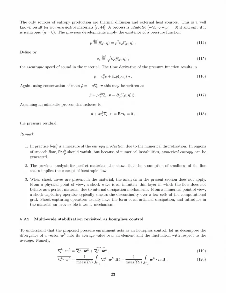
The only sources of entropy production are thermal diffusion and external heat sources. This is a wellknown result for non-dissipative materials [7, 44]: A process is adiabatic (−∇x · q+ ρr = 0) if and only if itis isentropic (η = 0). The previous developments imply the existence of a pressure function

pdef= p(ρ, η) = ρ2∂ρǫ(ρ, η) . (114)

Define by

csdef=√

∂ρ p(ρ, η) , (115)

the isentropic speed of sound in the material. The time derivative of the pressure function results in

p = c2s ρ+ ∂ηp(ρ, η) η . (116)

Again, using conservation of mass ρ = −ρ∇x · v this may be written as

p+ ρc2s∇x · v = ∂ηp(ρ, η) η . (117)

Assuming an adiabatic process this reduces to

p+ ρc2s∇x · v = Resp = 0 , (118)

the pressure residual.

Remark

1. In practice Reshp is a measure of the entropy production due to the numerical discretization. In regions

of smooth flow, Reshp should vanish, but because of numerical instabilities, numerical entropy can be

generated.

2. The previous analysis for perfect materials also shows that the assumption of smallness of the finescales implies the concept of isentropic flow.

3. When shock waves are present in the material, the analysis in the present section does not apply.From a physical point of view, a shock wave is an infinitely thin layer in which the flow does notbehave as a perfect material, due to internal dissipation mechanisms. From a numerical point of view,a shock-capturing operator typically smears the discontinuity over a few cells of the computationalgrid. Shock-capturing operators usually have the form of an artificial dissipation, and introduce inthe material an irreversible internal mechanism.

5.2.2 Multi-scale stabilization revisited as hourglass control

To understand that the proposed pressure enrichment acts as an hourglass control, let us decompose thedivergence of a vector wh into its average value over an element and the fluctuation with respect to theaverage. Namely,

∇x

h ·wh = ∇xh ·wh + ∇x

h ·wh , (119)

∇xh ·wh =

1

meas(Ωe)

∫

Ωe

∇x

h ·wh dΩ =1

meas(Ωe)

∫

Γe

wh · n dΓ . (120)

23

By definition, ∇xh ·wh and ∇x

h ·wh are orthogonal in the L2 sense. Consider the structure of the stabilizationterm developed in the previous section. The expressions (91) and (92) can be rearranged as:

∫

Ωe

(∇x

h · ψhκ) p′ dΩ = −

∫

Ωe

(∇x

h ·ψhκ)τ

(

ph +(

ρc2s)h ∇x

h · vh)

dΩ

= −∫

Ωe

(∇x

h ·ψhκ)τ

(

ph +(

ρc2s)h ∇x

h · vh + ∇xh · vh

)

dΩ

= −∫

Ωe

(∇x

h ·ψhκ)τ

(

ph +(

ρc2s)h ∇x

h · vh)

dΩ

− τ(

ρc2s)h∫

Ωe

(

∇x

h ·ψhκ

)(

∇xh · vh

)

dΩ

= − τ(

ph + ρc2s ∇xh · vh

)

e

∫

Ωe

(

∇x

h ·ψhκ

)

dΩ + HG1;e , (121)

∫

Ωe

(∇x

h · vh) p′ dΩ = − τ(

ph +(

ρc2s)h ∇x

h · vh)

e∇x

h · vh meas(Ωe) + HG2;e , (122)

with

HG1;e = −τ∫

Ωe

(

ρc2s)h(

˜∇xh ·ψh

κ

)

(

∇xh · vh

)

dΩ , (123)

HG2;e = −τ∫

Ωe

(

ρc2s)h(

∇xh · vh

)2

dΩ . (124)

To provide an interpretation of (121)–(122), it is important to realize that, for the proposed second-orderin time algorithm,

(

ph +(

ρc2s)h ∇x

h · vh)

e=(

ph −(

c2s)hρh)

e

≈ ∆t(

phn+1 − ph

n −(

c2s)h

n+1/2

(

ρhn+1 − ρh

n

))

e

= O(∆t2) . (125)

When hourglass modes arise, the expression in (125) tends to be much smaller than the terms HG1;e

and HG2;e, which represent the discretization of a (∇x ·)-(∇x ·) dissipative operator acting on the hourglassmodes.

Remarks

1. In regions where a shock is present and the artificial viscosity operator is active, (125) may not hold.

2. Notice that HG1;e and HG2;e scale with the square of the speed of sound and the density of thematerial, similarly to many hourglass control viscosities [4].

3. In order for the hourglass control to work, the HG1;e and HG2;e terms must be evaluated at locationswhere the discrete divergence operator is non-vanishing. Therefore, full integration (or equivalentdifference formulas) are required. However, the integration involves only kinematic terms, and notthe thermodynamic variables, which need only one evaluation per element.

The previous observations can also be used to define an alternative class of hourglass operators. Thebasic idea is to define a time interpolation for (ρc2s)

h, so that, element-by-element, (ph + ρhc2s ∇xh · vh)e

24

vanishes exactly. This can be done with a secant approximation of ρc2s, enforcing explicitly

(

ρc2s)h

n+1/2

def=

phn+1 − ph

n

∆t∇xh · vh

. (126)

If this is the case, the stabilization term reduces to:

∫

Ωe

(∇x

h · ψhκ) p′ dΩ = HG1;e , (127)

∫

Ωe

(∇x

h · vh) p′ dΩ = HG2;e . (128)

This alternative class of stabilization operators is clearly augmenting the original variational formulationby means of a purely dissipative operator. A different choice of the scaling for τ is also possible in thiscase, namely,

τe = τ |Ωe= τ

he

cs ∆t, (129)

where this time cτ = 3.0 (values in the range [1.0, 7.0] were found appropriate), and he is a characteristic

mesh length, for which many possible definitions can be used. One of them is he (meas(Ωe))1/nd . If this is

the case, then the stabilization term introduced would scale like the viscous part of the Flanagan-Belytschkohourglass control [11, 45, 12, 4].

5.2.3 Multi-scale stabilization in three dimensions

By design, the proposed hourglass control detects only those unstable modes whose divergence is non-zero.This is not unexpected, since the residual stabilization is tied to the physics of the system to be simulated.Specifically, any material satisfying a constitutive law like (15) does not possess shear strength, but canonly react to changes in volume (or, equivalently, a non-zero velocity divergence). This poses interestingimplications. In two dimensions, none of the hourglass modes are divergence-free, and the stabilizationmechanisms are straightforward to understand. In three dimensions, however, the situation is different.In fact, for a hexahedral element, the space H of the modes of hourglass deformations is spanned by 12hourglass eigenmodes [29]. The space H can be further divided into two subspaces (see Fig. 2):

1. The space Hdiv of modes which are divergence-free only at the centroid of the element, but are notdivergence-free elsewhere in the element. Specifically,

Hdiv = span

ξ1ξ2ξ300

,

0ξ1ξ2ξ3

0

,

00

ξ1ξ2ξ3

,

ξ1ξ200

,

0ξ2ξ30

,

00ξ3ξ1

, (130)

where ξi is the ith coordinate in the parent domain. These modes are dissipated by the multi-scalehourglass control.

2. The set Hshear of point-wise divergence-free modes, associated with purely deviatoric motion. Namely,

Hshear = span

ξ2ξ300

,

0ξ1ξ30

,

00ξ1ξ2

,

ξ3ξ1−ξ3ξ2

0

,

0ξ1ξ2

−ξ1ξ3

,

−ξ2ξ10

ξ2ξ3

. (131)

25

Figure 2. Sketch of the typical hourglass modes in three dimensions. The two modes on the leftcolumn are associated with the space Hdiv, and their divergence is zero only at the centroid of theelement. The two modes on the right column are associated with the space Hshear of divergence-freeshear modes. The four hourglass modes shown are associated with the ξ1 coordinate in the parentdomain. The other eight modes are obtained by rotation, and they are aligned along the ξ2 and ξ3axes, respectively.

Given the structure of (103), it is clear that these modes are not dissipated by the multi-scale stabilization.On the contrary, for a solid, the constitutive law yields a Cauchy stress which is more complex than a simplepressure. As a consequence, the fine scale stress also possesses a deviatoric component, which providesstabilization for the modes in Hshear.

It becomes clear at this point what was referred in the Introduction as the Q1/P0-element dilemma influids: On the one hand, modes in Hshear require control; on the other hand, any shear damping would beunphysical, and may destroy important features of the flow.

The multi-scale approach highlights this paradox with great precision, since physical stabilization isonly provided to the modes in Hdiv. An important discussion on some implications in the case of unstableshear modes and SUPG stabilization is provided in the next two remarks.

Remarks

1. It can also be shown that SUPG stabilized methods for piecewise-linear, continuous discretizationsdo not damp divegence-free hourglass modes in Hshear. As a simple example, consider a frictionless,Euler flow problem on a Cartesian mesh in which the velocity vector v is seeded with a point-wisedivergence-free mode in Hshear. It is unimportant whether the mesh is fixed (Eulerian) or tied tothe material (Lagrangian). For the sake of simplicity, all thermodynamic variables are assumedinitially constant. SUPG operators are introduced to stabilize numerical computations by means ofa combination of the residuals Res

hρ , Res

hǫ , and Resh

v, where

Resv = ρv + ∇xp . (132)

26

Since the pressure is constant, and the velocity mode is divergence-free, it is easy to realize thatρ = ǫ = p = 0 and v = 0. As a result, Res

hρ = Res

hǫ = 0, and Resh

v= 0. Therefore, the entire SUPG

operator vanishes, and any velocity field in Hshear is undamped. This is a manifestation of the residualapproach: The constitutive law of the material is unable to produce shear forces. Notice, however,that no instabilities related to modes in Hshear are mentioned in the vast literature of SUPG methodsfor the compressible Euler equations [25, 22, 21, 20, 14, 15, 16, 27, 33, 37, 36, 41, 42, 38, 39, 40].This seems to indicate that the underlying finite element space is playing a crucial role in preventingshear modes, an aspect which may be the object of future investigation.

2. The previous remark can also be considered from a reverse perspective. In very complex flows, suchas the ones generated by multiple interactions of curved shocks, modes in Hshear may be generatedas physical features.

In order to develop a stable formulation in three dimensions, an additional hourglass-control operatoris added, in the form of an artificial stress:

σhg = νhg dev∇sxv , (133)

νhg =(

chg;1 h2e ‖dev∇s

xv‖l2 + chg;2 he cs

)

echg;3

Ve;n+1Ve;n , (134)

˜dev∇sxψκ = dev∇s

xw − dev∇s

xw , (135)

where ‖T ‖l2 represent the Frobenius norm of the tensor T , that is ‖T ‖2l2 = T : T , and Ve;• is the element

volume at time t•. The constants are chosen to be chg;1 = 3.0, chg;2 = 0.06, and chg;3 = 2.0.

Remarks

1. The form of (133) is such that the fluctuation of the deviator of the symmetric gradient of the velocity

field is damped. In terms of kinematics, dev∇sxv is associated with the modes in Hshear, which are

therefore the target of the proposed damping operator.

2. The proposed approach does not affect the consistency of the method, and, consequently, the con-vergence rates, since it applies to gradient fluctuations.

3. The constant chg;1 is considerably larger than the constant chg;2, implying that the acoustic scalingis considered of minor importance. This is an acceptable choice since the tensor σhg does not carryany physical meaning.

4. The exponential (non-dimensional) term

echg;3

Ve;n+1Ve;n (136)

increases the viscosity in expansion regions, where the hourglass modes are more likely to grow, andreduces it in compression regions, where the modes are more likely to reduce their intensity. The latteris a very important feature in implosion computations, since an overly strong hourglass viscosity mayresult in computational failure, as documented in the numerical computations of Section 8. Usuallyvalues in the range [1.0, 3.0] were found appropriate, for the constant chg;3.

5. There is a substantial amount of freedom in the design of the hourglass viscosity operator and this isa direct consequence of the multi-scale perspective. One can take advantage of this fact to developa more flexible approach to hourglass stabilization.

27

6. Finally, it is important to realize that the multi-scale operator and the hourglass viscosity may beactive at the same time on some of the elements of the discretization. Since the hourglass operator is asecond-order correction, and acts on divergence-free fluctuations of the velocity field, it is reasonableto assume it does not produce a large perturbation to the Clausius-Duhem residual (104).

7. In the case of a solid, the proposed hourglass viscosity would be unnecessary, since the residual of thestress update equation can provide shear-stabilization terms. This is due to the fact that contraryto a fluid, a typical solid does possess shear strength.

6 Artificial viscosity and discontinuity capturing operator

The discontinuity capturing operator is implemented as follows:

σart =

ρ νart∇sxv , if ∇x · v < 0 ,

0nd×nd, otherwise .

(137)

Remarks

1. The use of the symmetric gradient in the definition of σart ensures, at the continuum level, objectivityof the artificial viscosity operator.

2. The definition (137) is more effective in damping artificial pure shear motion, with respect to themore common definition [5]

σart = − (ρ νart∇x · v) I . (138)

Artificially produced homogeneous shear motion can have disruptive consequences on shock hydro-dynamics computations of fluids, since it is not resisted by hourglass controls (of any type), nor thediscretized physical stress.

Several choices of the artificial viscosity parameter νart are possible. Among the most commonly used,

νKur =

cKur2

γ − 1

4|∇x · v|hart +

√

(

cKur2

γ − 1

4|∇x · v|hart

)2

+ c2Kur1c2s

hart , (139)

νdyna = c1cshart + c2|∇x · v|h2art , (140)

where, the values c1 = 1.2 and c2 = 0.5 have been used in the computations of Section 8. Also, cKur1 =cKur2 = 1, and γ is the isentropic constant in the gas. The expression for the so-called Kuropatenkoviscosity νKur [26] holds only for an ideal gas, while νdyna is general enough to include all materialssatisfying (15)–(16). The length-scale hart needs to be defined according to one main requirement: Itshould stably sample a mesh length along the normal to the shock front. This means that, for a givenmesh, hart should not vary abruptly for small changes in the direction of the shock normal. An effectivedefinition was found to be

hart =2

√

nTsh

(

F2FT2

)−1nsh

, (141)

F2 =∂x

∂ξ, (142)

28

Figure 3. Sketch of the length-scale hart as a function of the direction of nsh. The plots show theenvelope of hart as the angle that nsh forms with the x1-axis varies from 0 to 360 degrees. Noticethe smooth transition of the length-scale near the corners of the elements.

where nsh is a unit vector in the direction normal to the shock front, and F2 the gradient of the mappingfrom the parent domain to the element in the current configuration. In practice,

(

F2FT2

)

measures thestretch in the direction given by nsh. A plot of the envelope of hart as the shock normal angle spansthe interval [0, 360]-degrees is presented in Figure 3, for various quadrilateral elements. This definition isanalogous to the one adopted in [23]. An effective approximation to nsh is given by:

nsh =∇xfb

||∇xfb||, (143)

fb =||v||l2

max1≤e≤nel(||v||l2)

+ 10−3 ρ

max1≤e≤nel(ρ)

, (144)

where ||v||l2 =√v · v is the velocity magnitude, and ρ is the nodal projection of the density, namely

ρ =

nnp∑

A=1

ρANA(X) , (145)

ρA =

nel

Ae=1

∫

Ωe

NA ρ dΩ

nel

Ae=1

∫

Ωe

NA dΩ

=

nel

Ae=1

(

ρe

∫

Ωe

NA dΩ

)

nel

Ae=1

∫

Ωe

NA dΩ

, (146)

with A the assembly operator [17, 4].

Remarks

1. The definitions (143)–(144) are meant to use primarily the gradient of the velocity magnitude asa measure of the shock normal. There are a number of cases – such as implosions with radial or

29

spherical symmetry – in which the simple use of the gradient of the velocity norm may result toonoisy in the region preceding the shock location. This is why fb rather then ||v||l2 is introduced. Theuse of the gradient of the projected nodal density is reminiscent of [42].

2. The tensor σart just defined is evaluated at the midpoint in time, together with the other termscontributing to the nodal forces. Collocation at the mid-point in time ensures incremental objectivityof the tensor σart [34].

7 General considerations on implementation

7.1 Numerical quadratures

First and foremost, as already noted, the divergence of the velocity in the pressure residual Reshp vanishes at

the centroid of quadrilateral or hexahedral elements. Therefore, four/eight-point quadratures must be usedto compute the stabilization term. Notice that all other terms in the pressure residual are constant overeach of the elements, and do not need multi-point evaluation. The hourglass control for divergence-freeshear modes in three dimensions also require multi-point quadratures.

Second, when the shock capturing operator is active, non-linear coupling effects may take place betweenthe artificial viscosity and the multi-scale stabilization operator, as already mentioned. The optimal choiceis to integrate both the artificial viscosity and the multi-scale operator with the same quadrature rule. Withthis approach, incidentally, the computational cost for the multi-scale operator is negligible with respectto the cost of the artificial viscosity, since the divergence of the velocity is needed by both. Some examplesof the effects of single-point and multi-point integration for the viscosity are presented in Section 8.3.

To understand why superior results are obtained when the multi-scale and artificial viscosity operatorsshare the same quadrature rule, one needs to recall that where the artificial dissipation is active, the multi-scale approach is not strictly applicable. A single-point evaluation of the artificial viscosity is equivalentto enforcing that the value of the artificial viscosity is constant over the entire element. Especially in thecase of rapid transients, this may be a very coarse approximation. Indeed, on a particular element ofthe mesh, the artificial viscosity may be active only in just a few of the quadrature points. Single-pointintegration redistributes the effect of the artificial viscosity over the entire element, generating a spuriouspressure residual at the quadrature points where there should be no artificial dissipation. In the end, themulti-scale approach, which leverages a local evaluation of the residual, may be affected by the incorrectevaluation of the artificial dissipation.

In terms of quadrature rules, the details of the implementation can be then summarized as follows:

1. The integral of the physical stress term σ is evaluated with a single-point quadrate at the centroidof the element.

2. The multi-scale residual-based stabilization operator is computed with multi-point quadratures.

3. Unless otherwise specified, it should be implicitly assumed that the artificial viscosity operator isintegrated with full quadrature.

30

7.2 Hourglass stabilization and artificial viscosity parameters

Most of the numerical results are obtained using the multi-scale operator as defined in (107). This methodis denoted by VMS-I, and the choice cτ = 7 is made to evaluate expression (105) (a range of recommendedvalues could be [5.0, 15.0]). In addition, some computations using the approach of (123)–(124) are per-formed. This method is denoted by VMS-II, and the the choice cτ = 3 is made to evaluate expression(129) (a range of recommended values could be [1.0, 5.0]). In three dimensions, VMS-I and VMS-II arecomplemented with the deviatoric fine-scale artificial viscosity detailed in (133)–(135).

In order to compare the proposed multi-scale approach with existing approaches, a viscous-type hour-glass control a la Flanagan-Belytschko [4, 11, 12, 45] is also used: This method is referred to as FB. Unlessotherwise specified, the constant parameter is chosen to be cFB = 0.15. Typical recommended values [12]span the interval [0.05, 0.15]. The choice of making the hourglass control as dissipative as possible withinthe recommended range has the purpose of maximizing robustness.

An artificial viscosity of type (140) is used in all computations, with c1 = 0.5 and c2 = 1.2.

7.3 CFL condition

The following constraint on the time step has been adopted:

∆t = CFLh2

min

νtot +√

ν2tot + (cshmin)2

, (147)

νtot = νart + max(cshe, νhg) , (148)

νhg =

τ∆tc2s , for VMS-I ,τ∆tc2s , for VMS-II ,cFBhecs , for FB ,

(149)

hmin = min1≤A≤nnp

hA . (150)

Here, hmin is the minimum of the node distances. This definition of the time-step constraint is similar tothe one adopted in the LS-DYNA algorithm [13].

8 Numerical computations

8.1 Acoustic pulse computations and hourglass control

A very interesting test to check the the effect of the hourglass control is to propagate an acoustic pulse ona mesh in which the nodes are initially located according to an hourglass pattern (see Fig. 4(a)). For this

31

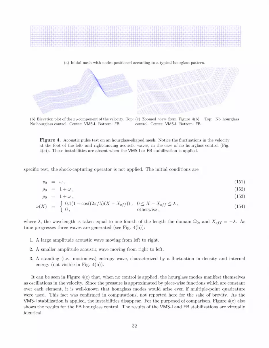
(a) Initial mesh with nodes positioned according to a typical hourglass pattern.

(b) Elevation plot of the x1-component of the velocity. Top:No hourglass control. Center: VMS-I. Bottom: FB.

(c) Zoomed view from Figure 4(b). Top: No hourglasscontrol. Center: VMS-I. Bottom: FB.

Figure 4. Acoustic pulse test on an hourglass-shaped mesh. Notice the fluctuations in the velocityat the foot of the left- and right-moving acoustic waves, in the case of no hourglass control (Fig.4(c)). These instabilities are absent when the VMS-I or FB stabilization is applied.

specific test, the shock-capturing operator is not applied. The initial conditions are

v0 = ω , (151)

ρ0 = 1 + ω , (152)

p0 = 1 + ω , (153)

ω(X) =

0.1(1 − cos((2π/λ)(X −Xoff )) , 0 ≤ X −Xoff ≤ λ ,0 , otherwise ,

(154)

where λ, the wavelength is taken equal to one fourth of the length the domain Ω0, and Xoff = −λ. Astime progresses three waves are generated (see Fig. 4(b)):

1. A large amplitude acoustic wave moving from left to right.

2. A smaller amplitude acoustic wave moving from right to left.

3. A standing (i.e., motionless) entropy wave, characterized by a fluctuation in density and internalenergy (not visible in Fig. 4(b)).

It can be seen in Figure 4(c) that, when no control is applied, the hourglass modes manifest themselvesas oscillations in the velocity. Since the pressure is approximated by piece-wise functions which are constantover each element, it is well-known that hourglass modes would arise even if multiple-point quadraturewere used. This fact was confirmed in computations, not reported here for the sake of brevity. As theVMS-I stabilization is applied, the instabilities disappear. For the purposed of comparison, Figure 4(c) alsoshows the results for the FB hourglass control. The results of the VMS-I and FB stabilizations are virtuallyidentical.

32

(a) Initial mesh.

(b) Density color plot at T = 0.7: VMS-I stabilization.

(c) Density color plot at T = 0.7: FB stabilization.

Figure 5. Saltzmann test: Comparison between VMS-I and FB.

8.2 Saltzmann test

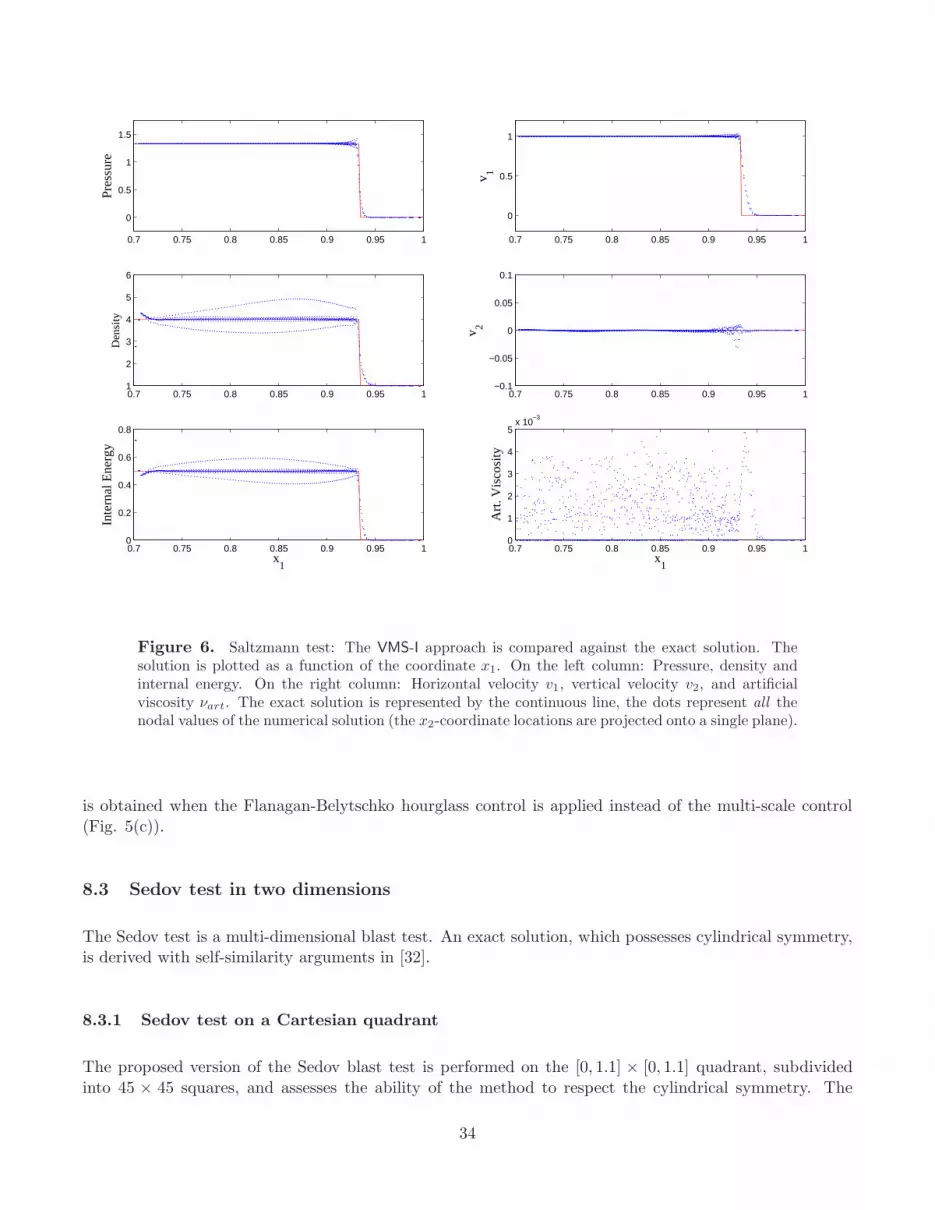
The Saltzmann test evaluates the ability of a distorted mesh to capture the features of a planar shock. Arectangular domain of gas (γ = 5/3) is initially at rest. The left boundary moves with unit velocity andgenerates a compression shock propagating from left to right through the domain. All other boundaryconditions are of “roller” type, that is, zero normal velocity (and, consequently, zero normal displacement).The Saltzmann test is both a robustness and an accuracy test. The initial mesh, an integral part of thetest case, is presented in Figure 5(a). Computations are performed at CFL = 0.8.

As it can be seen from the results in Figures 5(b), 5(c), and 6), aside from some over-/under-shootnear the boundaries, the numerical and exact solution show fair agreement. A reason for the over-/under-shoot near the boundaries may be the inaccurate representation of homogeneous gradients on generalunstructured meshes for the piece-wise constant approximation of the pressure [8]. An analogous result

33

0.7 0.75 0.8 0.85 0.9 0.95 1

0

0.5

1

1.5

Pres

sure

0.7 0.75 0.8 0.85 0.9 0.95 11

2

3

4

5

6

Den

sity

0.7 0.75 0.8 0.85 0.9 0.95 10

0.2

0.4

0.6

0.8

Inte

rnal

Ene

rgy

x1

0.7 0.75 0.8 0.85 0.9 0.95 1

0

0.5

1

v 1

0.7 0.75 0.8 0.85 0.9 0.95 1−0.1

−0.05

0

0.05

0.1

v 2

0.7 0.75 0.8 0.85 0.9 0.95 10

1

2

3

4

5x 10

−3

Art

. Vis

cosi

ty

x1

Figure 6. Saltzmann test: The VMS-I approach is compared against the exact solution. Thesolution is plotted as a function of the coordinate x1. On the left column: Pressure, density andinternal energy. On the right column: Horizontal velocity v1, vertical velocity v2, and artificialviscosity νart. The exact solution is represented by the continuous line, the dots represent all thenodal values of the numerical solution (the x2-coordinate locations are projected onto a single plane).

is obtained when the Flanagan-Belytschko hourglass control is applied instead of the multi-scale control(Fig. 5(c)).

8.3 Sedov test in two dimensions

The Sedov test is a multi-dimensional blast test. An exact solution, which possesses cylindrical symmetry,is derived with self-similarity arguments in [32].

8.3.1 Sedov test on a Cartesian quadrant

The proposed version of the Sedov blast test is performed on the [0, 1.1] × [0, 1.1] quadrant, subdividedinto 45 × 45 squares, and assesses the ability of the method to respect the cylindrical symmetry. The

34

(a) Mesh deformation, no stabilization. (b) Mesh deformation, VMS-I.

(c) Density color plot, no stabilization. (d) Density color plot, VMS-I.

Figure 7. Two-dimensional Sedov test. Left Column: No hourglass stabilization. Right column:VMS-I with full-integration of the shock-capturing term. When no stabilization is applied, it is clearlyvisible a pronounced hourglass pattern, which forces the computation to stop before completion.

initial mesh configuration, for the sake of brevity, is not shown. The initial density has a uniform unitdistribution, γ = 1.4, and the energy is “zero” (actually, 10−14) everywhere, except the first square zoneon the bottom left corner of the quadrant, near the origin, where it takes the value 409.7. Figure 7 shows acomparison of the results when no stabilization and VMS-I stabilization are applied. When no stabilizationis applied, the computation cannot be run to completion, since an hourglass pattern forms in the mesh(see Fig. 7(a)). As a consequence, the distance between some of the nodes decreases progressively duringthe simulation, forcing the same behavior in the time step, due to the CFL constraint. On the contrary,the VMS-I approach runs to completion and with a very smooth mesh and density profiles (Figs. 7(b) and7(d)).

35

(a) FB, single-point quadrature for σart. (b) FB, four-point quadrature for σart.

(c) VMS-I, single-point quadrature for σart. (d) VMS-I, four-point quadrature for σart.

(e) VMS-II, single-point quadrature for σart. (f) VMS-II, four-point quadrature for σart.

Figure 8. Two-dimensional Sedov test, comparison of the FB, VMS-I, and VMS-II stabilizationapproaches. Left column: Single-point integration for σart. Right column: four-point integrationfor σart.

36

(a) FB, cF B = 0.05, cτ = 7. (b) FB, cF B = 0.08, cτ = 7.

(c) FB, cF B = 0.12, cτ = 7. (d) FB, cF B = 0.15, cτ = 7.

Figure 9. Two-dimensional Sedov test, zoomed view near the origin. Comparison of the VMS-I

and FB stabilization approaches, for different value of the constant parameter in the FB hourglassviscosity. For all four pictures, FB in red, VMS-I in blue.

The six pictures composing Figure 8 show an interesting comparison between the effect of the VMS-I,VMS-II, and FB approaches in combination with different quadrature rules for the artificial viscosity. Inparticular, the effects of non-linear coupling between the artificial viscosity and the VMS-I stabilizationterm appear clear in Figure 8(c). The best result in terms of smoothness of the final grid configurationand absence of note-to-node oscillations is given by the VMS-I method with full integration of the shock-capturing term (Fig. 8(d)).

However, when the VMS-I method is combined with single-point quadrature, the mesh distortion in-creases considerably near the origin (Fig. 8(c)). For single-point quadrature, the VMS-II method offerssuperior results (Fig. 8(e)). However, when VMS-II is combined with full-quadrature, probably because ofthe incomplete definition of the pressure residual, the results are less accurate than for the VMS-I method.

37

0 0.2 0.4 0.6 0.8 1

0

0.05

0.1

0.15

0.2

Pres

sure

0 0.2 0.4 0.6 0.8 10

1

2

3

4

5

6

7

Den

sity

0 0.2 0.4 0.6 0.8 10

0.5

1

1.5

2

2.5

3

Inte

rnal

Ene

rgy

r

0 0.2 0.4 0.6 0.8 10

0.1

0.2

0.3

0.4

0.5

v r

0 0.2 0.4 0.6 0.8 1−0.05

0

0.05

v t

0 0.2 0.4 0.6 0.8 10

1

2

3

4

5x 10

−3

Art

ific

ial V

isco

sity

r

Figure 10. Two-dimensional Sedov test: Comparison with the exact solution. VMS-I with fully-integrated artificial viscosity. On the left column, from the top down: Pressure, density and internalenergy. On the right column, from top down: Radial velocity vr, tangential velocity vt, and artificialviscosity νart. Each variable is plotted as a function of the radius r =

√

x2

1+ x2

2. All solution points

are rotated around the origin to align on a single radial plane. Results in the case of single-pointintegration for the artificial viscosity only, and single-point integration for the entire stress tensor σwith Flanagan-Belytschko hourglass control are virtually identical.

Figures 8(a) and 8(b) show the results for the FB hourglass control and a constant cFB = 0.15. The FB

yields the best results with single-point quadrature integration, but it is somewhat inferior to the VMS-I

method when full integration is performed. To see more clearly this last point, Figure 9 shows a comparisonof the VMS-I and the FB approaches, as the constant in the FB viscosity spans the interval [0.05, 0.15].For low values of cFB, an hourglass pattern, originating in the large element in the lower left corner of thedomain, is clearly visible in Figure 9(a). As the the constant cFB is increased (see Figs. 9(b), 9(c), and9(d)), the hourglass pattern, although increasingly more damped, persists.

38

(a) Mesh deformation.

(b) Density color plot.

Figure 11. Two-dimensional Noh test on a Cartesian mesh, VMS-I with fully-integrated artificialviscosity.

39

0 0.05 0.1 0.15 0.2 0.25 0.3 0.35 0.4

0

1

2

3

4

5

6

Pres

sure

0 0.05 0.1 0.15 0.2 0.25 0.3 0.35 0.40

5

10

15

Den

sity

r

0 0.05 0.1 0.15 0.2 0.25 0.3 0.35 0.4

0

0.2

0.4

0.6

0.8

1

Inte

rnal

Ene

rgy

r

0 0.05 0.1 0.15 0.2 0.25 0.3 0.35 0.4

−1

−0.8

−0.6

−0.4

−0.2

0

v r

0 0.05 0.1 0.15 0.2 0.25 0.3 0.35 0.4−0.05

0

0.05

v t

0 0.05 0.1 0.15 0.2 0.25 0.3 0.35 0.40

0.005

0.01

0.015

Art

. Vis

cosi

ty

r

Figure 12. Two dimensional Noh test: Comparison with the exact solution. VMS-I with fully-integrated artificial viscosity. On the left column, from the top down: Pressure, density and internalenergy. On the right column, from top down: Radial velocity vr, tangential velocity vt, and artificialviscosity νart. Each variable is plotted as a function of the radius r =

√

x2

1+ x2

2. All solution points

are rotated around the origin to align on a single radial plane.

Quantitative comparison between the VMS-I approach and the exact solution to the Sedov problemare shown in Figure 10: When full integration is applied, the VMS-II and FB yield very similar results.It is worthwhile to notice the peak of the density value at approximately 5.5, against the exact value of6.0. This is a very accurate result, considering the coarseness of the initial mesh. In the proposed testperfect cylindrical symmetry is not expected, since, due to the geometry of the mesh and initial/boundaryconditions, the geometrical axis of symmetry is the bi-secant of the quadrant. Notice then the perfectlymirrored pattern in the solution for the tangential component of the velocity.

40

(a) Trisector mesh. (b) Radial mesh.

Figure 13. Two-dimensional Noh test on a radial trisector mesh. The initial mesh is given byan hexagonal pattern at the center, with a transition to a radially symmetric pattern towards theoutside boundary, as shown in Figure 13(a). The mesh is composed of three identical sectors, rotatedby 120 and 240 degrees with respect to one another. Figure 13(b) presents a radially symmetricmesh, composed of 36 elements along the circumference, and 24 along the radius, which is used togenerate a reference solution.

8.4 Noh test in two dimensions

The Noh [28] test is an implosion test. The velocity has an initial uniform radial distribution (the velocityfield points to the origin, and has unit magnitude, except at the origin, where it is forced to zero).

The initial energy should be zero, but for practical purposes the value 10−14 is used. The constantγ = 5/3 is applied to all computations. The exact solution for the density behind the shock is 16.0 anddecays as 1 + t/r in front of the shock, where t is time and r =

√

x21 + x2

2 is the radius. The pressure pastthe shock takes the value 16/3. The shock speed is 1/3, so that at the final time of 0.6 in the computation,the discontinuity is found at r = 0.2.

8.4.1 Noh test on a Cartesian quadrant

Similarly to the case of the Sedov test, a Cartesian quadrant [0, 1]× [0, 1] is initially subdivided into 50×50squares. Mesh deformation and density color plots are presented in Figure 11: The smoothness of theshocked grid is appreciable. Comparison with the exact solution are presented in Figure 12. The resultsshow smoothness in all variables, and values of the plateaus for the density and pressure are in goodagreement with the exact solution, considering the coarseness of the mesh (for extensive studies on thisproblem, see, e.g., [28]).

41

(a) Mesh deformation.

(b) Density color plot.

Figure 14. Two-dimensional Noh test on the trisector mesh. FB with the artificial stress tensorσart defined as in (138).

42

(a) Mesh deformation.

(b) Density color plot.

Figure 15. Two-dimensional Noh test on the trisector mesh. VMS-I with the artificial stresstensor σart is defined as in (137). Very similar results are obtained with FB.

43

0 0.05 0.1 0.15 0.2 0.25 0.3 0.35 0.4

0

1

2

3

4

5

6

Pres

sure

0 0.05 0.1 0.15 0.2 0.25 0.3 0.35 0.40

5

10

15

Den

sity

r

0 0.05 0.1 0.15 0.2 0.25 0.3 0.35 0.4

0

0.2

0.4

0.6

0.8

1

Inte

rnal

Ene

rgy

r

0 0.05 0.1 0.15 0.2 0.25 0.3 0.35 0.4

−1

−0.8

−0.6

−0.4

−0.2

0

v r

0 0.05 0.1 0.15 0.2 0.25 0.3 0.35 0.4−0.05

0

0.05

v t

0 0.05 0.1 0.15 0.2 0.25 0.3 0.35 0.40

0.005

0.01

0.015

0.02

0.025

0.03

Art

. Vis

cosi

ty

r

Figure 16. Two-dimensional Noh test: Comparison with the exact solution (continuous red curve)of the results of Figure 14 (red dots) and Figure 15 (blue dots). The continuous black line representsthe solution on the radially symmetric mesh of Figure 13(b), using the tensor artificial viscosity(137). The components of the solution are presented as in Figure 12.

8.4.2 Noh test on a mesh with trisector symmetry

From this variant of the two-dimensional Noh test, very important conclusions can be drawn on someaspects of the artificial viscosity implementation. In particular, this is an interesting test for comparingthe performance of σart as defined in (137) with respect to more classical definition (138). Due to the initialnode configuration (see Fig. 13(a)), the shocked mesh tends to produce homogenous shear modes alongthe secant lines at 0, 120, and 240 degrees. Shear-induced, “jet-like” patterns can be clearly seen in Figure14. The hourglass control is no help in this case, since pure shear motion is point-wise divergence-free,and two-dimensional hourglass modes are not divergence-free. The situation is much improved in the casewhen the artificial stress σart is defined according to (137). As can be seen in Figure 15, shear motion isappropriately damped in the shock layer, and does not propagate to the rest of the flow. Consequently,mesh smoothness, and the accuracy of the solution are much improved (see Fig. 15).

44

(a) Perspective view.

(b) Side view from the x1-axis.

Figure 17. Three-dimensional Sedov test, VMS-I approach, density contour plots.

45

0 0.2 0.4 0.6 0.8 1

0

0.05

0.1

0.15

0.2

Pres

sure

0 0.2 0.4 0.6 0.8 10

1

2

3

4

5

6

7

Den

sity

0 0.2 0.4 0.6 0.8 10

0.5

1

1.5

2

2.5

3

Inte

rnal

Ene

rgy

r

0 0.2 0.4 0.6 0.8 10

0.1

0.2

0.3

0.4

0.5

v r

0 0.2 0.4 0.6 0.8 1

0

0.02

0.04

0.06

0.08

0.1

|vt|

0 0.2 0.4 0.6 0.8 10

0.002

0.004

0.006

0.008

0.01

Art

ific

ial V

isco

sity

r

Figure 18. Three-dimensional Sedov test: Comparison between the VMS-I approach and theexact solution. On the left, from the top down: Pressure, density and internal energy. On the right,from top down: Radial velocity vr, tangential velocity vt, and artificial viscosity νart. Each variableis plotted as a function of the radius r =

√

x2

1+ x2

2+ x2

3.

Notice in Figure 16 the large errors in the solution plateaus and arrival time of the shock wave whenthe pressure-like artificial viscosity operator (138) is used. By contrast, the solution for the tensor artificialviscosity (137) is much improved, and significantly closer to the reference numerical solution on the radialmesh of Figure 13(b).

8.5 Sedov test in three dimensions

The Sedov test in three dimensions is much more challenging than its two-dimensional counterpart, dueto the increased distortion undergone by the elements. The proposed version of the Sedov blast test isperformed on the [0, 1.1] × [0, 1.1] × [0, 1.1] octant, subdivided into 20× 20× 20 cubes. The initial densityhas a uniform unit distribution. The value γ = 1.4 was used. The simulations are performed at CFL = 0.5.For FB, VMS-I, and VMS-II, it was not possible to successfully run to completion computations in whichthe initial condition for the energy involved concentrating all the initial internal energy in one cell ofthe mesh. Therefore, a “mitigated” initial condition for the internal energy is adopted, in which nodalprojection followed by cell averaging redistributed the initial energy over eight corner cells rather than one.Indicating with the triplet (i, j, k) = (0, 0, 0) the corner cell where the internal energy e0 = 639.4 had to

46

0 0.1 0.2 0.3 0.4 0.5 0.60

0.2

0.4

0.6

0.8

1

t

Nor

mal

ized

kin

etic

/inte

rnal

ene

rgy

(a) Normalized kinetic/internal energies.

0 0.1 0.2 0.3 0.4 0.5 0.6

0

1

2

3

4

5x 10

−14

t

Tot

al e

nerg

y re

lativ

e er

ror

(b) Total energy relative error.

Figure 19. Energy history for the three-dimensional Sedov test. Figure 19(a) shows the timehistory of the kinetic (red) and internal (blue) energies, normalized with respect to the initial totalenergy, Etot

0. Figure 19(b) shows the time history of the relative error on the total energy (Etot(t)−

Etot0 )/Etot

0 . Notice that the scale of the vertical axis is multiplied by 10−14.

be originally concentrated, the following initial energy distribution was adopted:

e(0,0,0) =27

64e0 , (155)

e(1,0,0) = e(0,1,0) = e(0,0,1) =9

64e0 , (156)

e(1,1,0) = e(0,1,1) = e(1,0,1) =3

64e0 , (157)

e(1,1,1) =1

64e0 , (158)

where, for example, the subscript (1, 0, 0) indicates the cell next to the corner cell along the x1 direction.The internal energy is set to “zero” (actually 10−14) everywhere else in the initial domain. Results areshown in Figure 17 and Figure 18 for the VMS-II case. Similar results have been obtained with the FB

approach, but with a constant cFB = 0.25, considerably higher than the suggested range of values. It is alsoimportant to notice that this choice of the constant is not appropriate for the three-dimensional Noh testdocumented below, for which the constant cFB had to be reduced to values in the interval [0.05, 0.075]. Thissuggests that, the practice of not separating the physical from the artificial components of the hourglasscontrol – as is usually done in the extensions of the FB approach to fluids – may endanger robustness. Tobe more specific, the Flanagan-Belytschko hourglass control was originally intended for solids, and only ata later stage was applied to fluid computations. In the case of a solid, applying an hourglass viscosity toboth the Hdiv and Hshear modes is a very sensible choice, since the material possesses shear strength. Butfor a fluid, the modes in Hdiv have a physical significance, while the modes in Hshear are pure artifactsof the element technology. Therefore, the variational multi-scale approach seems to offer a pathway forincreased robustness in hourglass control.

47

(a) Perspective view.

(b) Side view from the x1-axis.

Figure 20. Three-dimensional Noh test on the 603 mesh, VMS-I approach, density contour plots.

48

Figure 21. Three-dimensional Noh test: Comparison with the exact solution for the 203 (red), 303

(blue), and 603 (black) meshes. VMS-I with fully-integrated artificial viscosity. On the left column,from the top down: Pressure, density and internal energy. On the right column, from top down:Radial velocity vr, tangential velocity vt, and artificial viscosity νart. Each variable is plotted as afunction of the radius r =

√

x2

1+ x2

2+ x2

3.

Figure 18 shows somewhat less accurate results than Figure 10. This may be due to the coarseness of themesh, also in conjunction to the modifications applied to the initial conditions, and the three-dimensionalnature of the solution. Figure 19(a) shows the time-history of the total kinetic energy and the total internalenergy, normalized with respect to the initial total energy, E tot

0 = E tot(t0). Given the imposed boundaryconditions, the total energy must be conserved throughout the computation. Figure 19(b) shows that therelative error in the total energy is on the order of 10−14, well within the machine precision.

8.6 Noh test in three dimensions

The initial conditions for the Noh test in three dimensions are analogous to the two-dimensional case: Inthree dimension, the initial velocity vector field is of unit magnitude and points to the origin of the referenceframe, while the thermodynamic variables have the same initial conditions as in the two-dimensional case.The domain [0, 1.1] × [0, 1.1] × [0, 1.1] is uniformly meshed with three meshes of resolution 20 × 20 × 20,30×30×30, and 60×60×60 cubes. The exact solution for the density behind the shock is 64.0 and decaysas (1 + t/r)2 in front of the shock, where t is time and r =

√

x21 + x2

2 + x23 is the radius. The pressure past

the shock takes the value 62/3. The shock speed is 1/3, so that at the final time of 0.6 in the computation,the discontinuity is found at r = 0.2.

49

Only results for VMS-I are presented, in Figures 20 and 21. Similar results can be obtained with FB,but, as already mentioned, to avoid volume inversions near the origin, the constant cFB has to be reducedto values in the range [0.05, 0.075]. Because the plateaus of the density and pressure at at much highervalues than in the two-dimensional case, even a resolution of 603 elements is still coarse to fully capture thesolution. In Figure 21, it can be appreciated the convergence of the numerical to the exact solution, as themesh is refined. These results are in very good agreement with the one-dimensional, spherically-symmetricsolution, computed in [28] using 50 − 70 radial zones. As mentioned in [28], an acceptable resolution forthis problem would be 100 radial zones, roughly equivalent to 100 × 100 × 100 cartesian cells. This wouldrequire a numerical computation of one million elements, a task beyond the scope of the present work.

9 Summary

A novel multi-scale method for Lagrangian shock hydrodynamics has been presented. The formulationof the proposed method in the context of Q1/P0 finite elements makes it widely applicable to state-ofthe-practice hydrodynamic algorithms.

The proposed method builds on a mid-point time integrator implemented as a conservative predic-tor/multicorrector scheme. The stabilization augments the original Galerkin formulation without perturb-ing its global conservation properties.

The multi-scale approach leads to a consistent method, in which instabilities (typically, of hourglasstype) are controlled by the stabilizing effect of an appropriate pressure residual.

By rational thermodynamic arguments, it has been shown that the pressure residual is tied to theClausius-Duhem inequality, and, effectively, measures the creation of entropy due to instabilities in thenumerical discretization. These arguments imply the physical consistency of the multi-scale stabilization.Connections with previous work on physical hourglass stabilization have been drawn. However, the pro-posed approach takes the discussion to a new level, since, in past developments, many aspects of theinterplay between physics and numerics have been overlooked.

In the case of three-dimensional flows, the addition of a hourglass viscosity aimed at damping divergence-free, non-homogeneous shear is necessary. This pinpointed a major disadvantage in fluid computations ofthe Q1/P0 element technology, which requires stabilization of fine-scale shear modes, although inviscidfluids have no shear-strength or shear-damping mechanisms. In this context, the multi-scale analysis pro-vides a new perspective, and allows for a more flexible design of hourglass viscosities aimed at dampingsuch hourglass instabilities.

Numerical results in two and three dimensions in the case of compressible gas dynamics show thatthe method has comparable and in some cases superior performance to state-of-the-practice techniques forhourglass control.

More work is needed to fully investigate the robustness and accuracy properties of the proposed method,and extend it to more complex computations, involving multiple materials, or multiple-physics. Of greatimportance is also the extension of the proposed multi-scale approach to solids. In this case, the multi-scale approach should provide the full stabilization mechanism for Q1/P0 formulations, since the materialpossess shear strength, and additional fine-scale shear control mechanisms should not be required.

50

References

[1] S. S. Antman. Nonlinear problems of elasticity, volume 107 of Applied mathematical sciences. Springer,New York, 2nd edition, 2005.

[2] T. Belytschko and L. P. Bindeman. Assumed strain stabilization of the 4-node quadrilateral with 1-point quadrature for nonlinear problems. Computer Methods in Applied Mechanics and Engineering,88(3):311–340, 1991.

[3] T. Belytschko and L. P. Bindeman. Assumed strain stabilization of the eight node hexahedral element.Computer Methods in Applied Mechanics and Engineering, 105(2):225–260, 1993.

[4] T. Belytschko, W. K. Liu, and B. Moran. Nonlinear Finite Elements for Continua and Structures. J.Wiley & Sons, New York, 2000.

[5] D. J. Benson. Computational methods in Lagrangian and Eulerian hydrocodes. Computer Methodsin Applied Mechanics and Engineering, 99:235–394, 1992.

[6] E. J. Caramana, M. J. Shashkov, and P. P. Whalen. Formulations of artificial viscosity for multi-dimensional shock wave computations. Journal of Computational Physics, 144:70–97, 1998.

[7] D. E. Carlson. Linear thermoelasticity. In C. A. Truesdell, editor, Mechanics of Solids, volume II,chapter 2, pages 297–345. Springer-Verlag, New York, 1984.

[8] M. A. Christon. Pressure gradient approximations for staggered-grid finite element hydrodynamics.International Journal for Numerical Methods in Fluids, 2005. In preparation.

[9] R. Codina, J. Principe, O. Guash, and S. Badia. Time dependent subscales in the stabilized finiteelement approximation of incompressible flow problems, 2006. Submitted.

[10] B. D. Coleman and V. J. Mizel. Existence of caloric equations of state in thermodynamics. TheJournal of Chemical Physics, 40(4):1116–1125, 1964.

[11] D. P. Flanagan and T. Belytschko. A uniform strain hexahedron and quadrilateral with orthogonalhourglass control. International Journal for Numerical Methods in Engineering, 17(5):679–706, 1981.

[12] G. L. Goudreau and J. O. Hallquist. Recent developments in large-scale finite element Lagrangianhydrocode technology. Computer Methods in Applied Mechanics and Engineering, 33(1-3):725–757,September 1982.

[13] J. O. Hallquist. LS-DYNA theory manual. Technical report, Livermore Software Technology Corpo-ration, Livermore, CA, March 2006. Available at: http://www.lstc.com.

[14] G. Hauke. Simple stabilizing matrices for the computation of compressible flows in primitive variables.Computer Methods in Applied Mechanics and Engineering, 190:6881–6893, 2001.

[15] G. Hauke and T. J. R. Hughes. A unified approach to compressible and incompressible flows. ComputerMethods in Applied Mechanics and Engineering, 113:389–396, 1994.

[16] G. Hauke and T. J. R. Hughes. A comparative study of different sets of variables for solving compress-ible and incompressible flows. Computer Methods in Applied Mechanics and Engineering, 153:1–44,1998.

[17] T. J. R. Hughes. The Finite Element Method: Linear Static and Dynamic Finite Element Analysis.Prentice-Hall, Englewood Cliffs, New Jersey, 1987. (Dover reprint, 2000).

51

[18] T. J. R. Hughes. Multiscale phenomena: Green’s functions, the Dirichlet-to-Neumann formulation,subgrid-scale models, bubbles and the origin of stabilized methods. Computer Methods in AppliedMechanics and Engineering, 127:387–401, 1995.

[19] T. J. R. Hughes, G.R. Feijoo, L. Mazzei, and J.-B. Quincy. The Variational Multiscale Method —a paradigm for computational mechanics. Computer Methods in Applied Mechanics and Engineering,166:3–24, 1998.

[20] T. J. R. Hughes, L. P. Franca, and G. M. Hulbert. A new finite element formulation for computationalfluid dynamics: VIII. The Galerkin/least-squares method for advective-diffusive equations. ComputerMethods in Applied Mechanics and Engineering, 73:173–189, 1989.

[21] T. J. R. Hughes, L. P. Franca, and M. Mallet. A new finite element formulation for computational fluiddynamics: VI. Convergence analysis of the generalized SUPG formulation for linear time-dependentmultidimensional advective-diffusive systems. Computer Methods in Applied Mechanics and Engineer-ing, 63:97–112, 1987.

[22] T. J. R. Hughes and M. Mallet. A new finite element formulation for computational fluid dynamics:III. The generalized streamline operator for multidimensional advective-diffusive systems. ComputerMethods in Applied Mechanics and Engineering, 58:305–328, 1986.

[23] T. J. R. Hughes, M. Mallet, and A. Mizukami. A new finite element formulation for computational fluiddynamics: II. Beyond SUPG. Computer Methods in Applied Mechanics and Engineering, 54:341–355,1986.

[24] T. J. R. Hughes, G. Scovazzi, and Franca L.P. Multiscale and stabilized methods. In E. Stein,R. de Borst, and T. J. R. Hughes, editors, Encyclopedia of Computational Mechanics. John Wiley &Sons, 2004.

[25] T. J. R. Hughes and T. E. Tezduyar. Finite element methods for first-order hyperbolic systems withparticular emphasis on the compressible Euler equations. Computer Methods in Applied Mechanicsand Engineering, 45:217–284, 1984.

[26] V. F. Kuropatenko. On difference methods for the equations of hydrodynamics. In N. N. Janenko, ed-itor, Difference methods for solutions of problems of mathematical physics, I. American MathematicalSociety, Providence, RI, 1967.

[27] A. Masud. Effects of mesh motion on the stability and convergence of ALE based formulations formoving boundary flows. Computational Mechanics, DOI:10.1007/s00466–006–0062–9 (to appear),2006.

[28] W. F. Noh. Errors for calculations of strong shocks using an artificial viscosity and an artificial heatflux. Journal of Computational Physics, 72:78–120, 1987.

[29] M. A. Puso. A highly efficient enhanced assumed strain physically stabilized hexahedral element.International Journal for Numerical Methods in Engineering, 49(8):1029–1064, November 2000.

[30] G. Scovazzi. Stabilized shock hydrodynamics: II. Design and physical interpretation of the SUPGoperator for Lagrangian computations. Computer Methods in Applied Mechanics and Engineering,196(4–6):966–978, 2007.

[31] G. Scovazzi, M. A. Christon, T. J. R. Hughes, and J. N. Shadid. Stabilized shock hydrodynamics: I.A Lagrangian method. Computer Methods in Applied Mechanics and Engineering, 196(4–6):923–966,2007.

52

[32] L. I. Sedov. Similarity and Dimensional Methods in Mechanics. Academic Press, New York, 1959.

[33] F. Shakib, T. J. R. Hughes, and Z. Johan. A new finite element formulation for computational fluiddynamics: X. The compressible Euler and Navier-Stokes equations. Computer Methods in AppliedMechanics and Engineering, 89:141–219, 1991.

[34] J. C. Simo and T. J. R. Hughes. Computational Inelasticity. Springer, New York, 1998.

[35] J. C. Simo and N. Tarnow. The discrete energy-momentum method. Conserving algorithms for non-linear elastodynamics. Zeitschrift fur Angewandte Mathematik und Physik (ZAMP), 43(5):757–792,September 1992.

[36] T. E. Tezduyar. Stabilized finite element formulations for incompressible flow computations. Advancesin Applied Mechanics, 28:1–44, 1992.

[37] T. E. Tezduyar. Computation of moving boundaries and interfaces and stabilization parameters.International Journal for Numerical Methods in Fluids, 43:555–575, 2003.

[38] T. E. Tezduyar. Finite element methods for fluid dynamics with moving boundaries and iterfaces. InE. Stein, R. de Borst, and T. J. R. Hughes, editors, Encyclopedia of Computational Mechanics. JohnWiley & Sons, 2004.

[39] T. E. Tezduyar, M. Behr, and J. Liou. A new strategy for finite element computations involving movingboundaries and interfaces – The deforming-spatial-domain/space-time procedure: I. The concept andthe preliminary numerical tests. Computer Methods in Applied Mechanics and Engineering, 94:339–351, 1992.

[40] T. E. Tezduyar, M. Behr, S. Mittal, and J. Liou. A new strategy for finite element computationsinvolving moving boundaries and interfaces – The deforming-spatial-domain/space-time procedure:II. Computation of free-surface flows, two-liquid flows, and flows with drifting cylinders. ComputerMethods in Applied Mechanics and Engineering, 94:353–371, 1992.

[41] T. E. Tezduyar, S. Mittal, S. E. Ray, and R. Shih. Incompressible flow computations with stabilizedbilinear and linear equal-order-interpolation velocity-pressure element. Computer Methods in AppliedMechanics and Engineering, 95:221–242, 1992.

[42] T. E. Tezduyar and M. Senga. Stabilization and shock-capturing parameters in SUPG formulation ofcompressible flows. Computer Methods in Applied Mechanics and Engineering, 195:1621–1632, 2006.

[43] C. A. Truesdell. Rational thermodynamics. Springer-Verlag, New York, 2nd edition, 1984.

[44] C. A. Truesdell and W. Noll. The non-linear field theories of mechanics. Springer-Verlag, New York,2nd edition, 1992.

[45] F. Van der Ween and T. Belytschko. Correction of article by D. P. Flanagan and T. Belytschko.International Journal for Numerical Methods in Engineering, 19(3):467–468, 1983.

53

DISTRIBUTION:

1 Thomas J. R. HughesICES, U. Texas at Austin1 University Station C0200Austin, TX 78712-0027

1 Mikhail ShashkovTheoretical Division, Group T7LANL, MS-B284Los Alamos, New Mexico 87545

1 MS 1319Pavel Bochev, 1414

1 MS 1319S. Scott Collis, 1414

1 MS 0380Martin Heinstein, 1542

1 MS 1319Edward Love, 1431

1 MS 1319Richard Lehoucq, 1414

1 MS 0378William Rider, 1431

1 MS 0378Allen Robinson, 1431

1 MS 1319Guglielmo Scovazzi, 1431

1 MS 0316John Shadid, 1437

1 MS 0382James Stewart, 1543

1 MS 0378Randall Summers, 1431

1 MS 0378Michael Wong, 1431

2 MS 9018Central Technical Files, 8944

2 MS 0899Technical Library, 4536

54