Multitasking associative networks

Elena Agliari ∗, Adriano Barra †, Andrea Galluzzi ‡,Francesco Guerra §, Francesco Moauro ¶

12 Nov 2011

Abstract

We introduce a bipartite, diluted and frustrated, network as a sparse restricted Boltzman machineand we show its thermodynamical equivalence to an associative working memory able to retrieve mul-tiple patterns in parallel without falling into spurious states typical of classical neural networks. Wefocus on systems processing in parallel a finite (up to logarithmic growth in the volume) amountof patterns, mirroring the low-level storage of standard Amit-Gutfreund-Sompolinsky theory. Re-sults obtained trough statistical mechanics, signal-to-noise technique and Monte Carlo simulationsare overall in perfect agreement and carry interesting biological insights. Indeed, these associativenetworks pave new perspectives in the understanding of multitasking features expressed by complexsystems, e.g. neural and immune networks.

1 Sparse restricted Boltzman machines as associative networks

Neural networks rapidly became the ”harmonic oscillators” of parallel processing: Neurons (spins),thought of as ”binary nodes” of a network, perform simultaneously to retrieve information, the latterbeing spread over the synapses, thought of as the (weighted) interconnections among nodes. However,common intuition of parallel processing is not only the ”underlying” parallel work performed by theneurons to retrieve say an image -a book cover-, but instead, for instance, reading the manuscript, whilekeeping it securely in hand and noticing beyond its edges the room where we are reading in. A stepforward standard parallel processing could be managing the main figure (the book) and a recognizedbackground, and still maintaining available the capacity of further retrieve as a safety mechanism.

Standard Hopfield networks are not able to accomplish this kind of parallel process (apart from thenetwork studied by Cugliandolo and Tsodsky [10], where multiple, not-spurious, patterns were contem-porary recalled thanks to the correlations among them, the network studied by Coolen and Noest [8, 9],where partial inhibition of a single pattern recovery were allowed by chemical modulation or the ap-proaches with integrate and fire neurons of Amit Bernacchia and Yakovlev [3], which are far away fromthe Hopfield framework). Indeed, spurious states cannot be looked at as the contemporary retrieval ofseveral patterns, being rather unwanted outcomes, yielding to a glassy blackout [2]. Such a limit ofHopfield networks can be understood by focusing on the deep connection (in both direct [4] and inverse[14] approach) with restricted Boltzmann machines (RBM) [7]. Given a machine with its set of visible(neurons) and hidden (training data) units, one gets, under marginalization, that the thermodynamicevolution of the visible layer is equivalent to that of an Hopfield network. It follows that an underlyingfully-connected bipartite restricted machine necessarily leads to bit strings of length equal to the systemsize and whose retrieval requires an orchestrated arrangement of the whole set of spins. This impliesthat no resources are left for further tasks, which is, from a biological point of view, too strong anoversimplification.

∗Universita di Parma, Dipartimento di Fisica, Viale Usberti 7, 00198, Parma, Italy and INFN Gruppo collegato diParma†Sapienza Universita di Roma, Dipartimento di Fisica, Piazzale Aldo Moro 2, 00185 Roma, Italy‡Sapienza Universita di Roma, Dipartimento di Fisica, Piazzale Aldo Moro 2, 00185 Roma, Italy and INFN Sezione di

Roma§Sapienza Universita di Roma, Dipartimento di Fisica, Piazzale Aldo Moro 2, 00185 Roma, Italy¶Sapienza Universita di Roma, Dipartimento di Fisica, Piazzale Aldo Moro 2, 00185 Roma, Italy

1

arX

iv:1

111.

5191

v1 [

cond

-mat

.dis

-nn]

22

Nov

201

1

σ5

σ4

σ3

σ2

σ1

τ1

τ3

τ2 σ2

σ3

σ1

+2σ5

−1

−2

−1

−1

+1

+1

+1

σ4

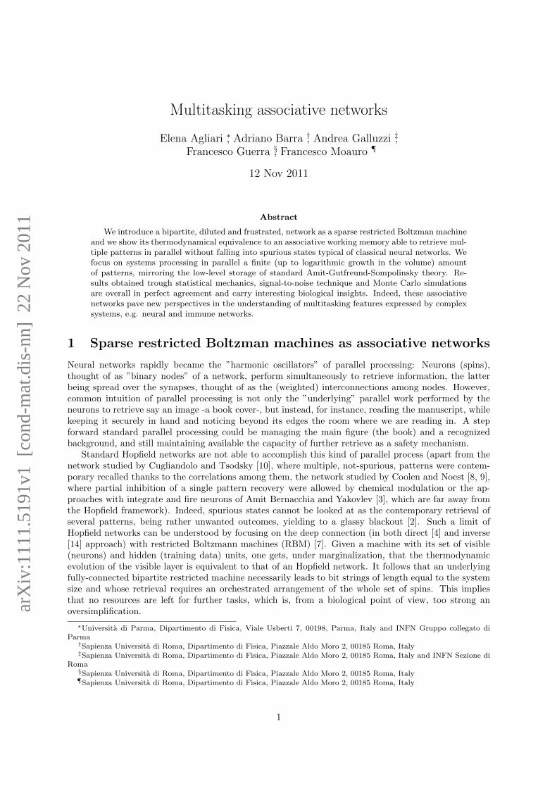
Figure 1: Schematic representation of a diluted restricted Bolzmann machine made up of N = 5 elementsand P = 3 (left) and its corresponding weakened associative network (right). On the latter, the threepatterns appear as ξ1 = [−1,−1, 0, 0, 0], ξ2 = [+1,+1, 0,−1, 0], ξ3 = [0,−1,+1,+1,+1] and the weightassociated to each link (i, j) is

∑µ ξ

µi ξ

µj .

Here we introduce a possible way to relax this feature: Starting from a RBM we perform dilutionon its links in such a way that nodes in the external layer are connected to only a fraction of nodes inthe inner layer (see fig.1, left). As we show, this leads to a ”weakened” associative network which, fornon-extreme dilutions, is still embedded in a fully connected topology, but the bit-strings encoding forinformation are sparse (i.e. their entries are +1,−1 as well as 0) (fig.1, right).

More precisely, let us denote the P dichotomic spins making up the external layer as τµ = ±1, µ ∈[1, ..., P ] and the N dichotomic spins making up the internal layer as σi, i ∈ [1, ..., N ]. RBMs admit anHamiltonian description such that we can write

H(σ, τ ; ξ) =1√N

N,P∑i,µ

ξµi σiτµ,

where we called ξµi the (quenched) interaction strength between the ith spin of the inner layer with theµth spin of the external layer (possibly to be extracted from a proper probability distribution P (ξµi )).Usually one defines α = limN→∞ P/N as the storage value; in this first work we deal with the ”lowstorage” regime, i.e. P ∼ logN , corresponding to α = 0.

2 Statistical mechanics and signal to noise analysis

The thermodynamics of the system is then obtained by explicit calculation of the (quenched) free energyvia the partition function, which read off respectively as

f(α = 0, β) = limN→∞

1

NE logZN,P (β), (1)

ZN,P (β) =∑σ,τ

exp(− βH(σ, τ ; ξ)

). (2)

A key point here is that the interaction is already one-body in each layer, such that marginalizing overone spin variable is straightforward and gives (expanding up to second order the hyperbolic sine)

ZN,P (β) =∑σ

P∏µ=1

[cosh

( β√N

N∑i

ξµi σi

)](3)

=∑σ

eβ2

2N

∑N,Ni,j

∑Pµ=1 ξ

µi ξµj σiσj =

∑σ

e−N∑Pµ=1m

2µ ,

where we introduced the P Mattis magnetization mµ = N−1∑Ni ξ

µi σi. When P (ξµi = +1) = P (ξµi =

−1) = 1/2 the Hamiltonian implicitly defined in eq. 3 recovers exactly the Hopfield model (at a rescaled

2

noise level β2) and the ansatz of pure state, i.e. m = (1, 0, ..., 0) (under permutational invariance),correctly yields the proper minimization of the free-energy in the low-noise limit. This means that, onceequilibrium is reached, the state of the system σ will be parallel (under gauge invariance) to the patternξ1, phenomenon which is understood as recovery of a pattern of information.

As anticipated, here we remove the hypothesis of fully-connection for the bipartite network, dilutingrandomly its links in such a way that the coupling distribution gets

P (ξµi ) = (D/2)δξµi −1 + (D/2)δξµi +1 + (1−D)δξµi ,

where D ∈ [0, 1] is a proper dilution parameter. It is easy to see that with this distribution, aftermarginalizing over one party as usual, we get an associative network, where the P patterns ξµ (µ =1, ..., P ) now contain zeros, on average for a fraction (1 − D) of their length. As a result, the purestate ansatz can no longer work. In fact, now, the retrieval of a pattern does not employ all availablespins and those corresponding to null entries can be used to recall other patterns: This is because theenergy is a quadratic form in the Mattis magnetizations; its minimization requires that further patterns(up to the exhaustion of all available spins) are recalled in a hierarchical fashion. More precisely, the(thermodynamical and quenched) average of the Mattis magnetization of the kth pattern retrieved isDk(1 − D), that is the overlap with the spins still available is maximized. The overall number of

retrieved patterns K therefore corresponds to∑Kk=0D(1 − D)k = 1, with the cut-off at finite N as

D(1−D)K ≥ N−1 due to discreteness. For non pathological D (i.e. D 6= 1, 0 and not a function of N),this implies K . logN , which can be thought of as a “parallel low-storage” regime of neural networks 1.

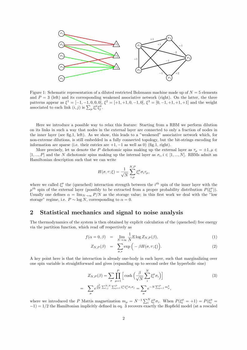
Before proceeding with the thermodynamic analysis, it is important to stress that the dilution intro-duced here is deeply different from the one introduced early by Sompolinsky [13] and more recently byCoolen [15], who showed how to solve the Hopfield model embedded in random networks, ranging fromErdos-Renyi graphs to small-worlds. In those systems, obtained by diluting directly the Hopfield net-work, the exciting results were the robustness of the retrieval under dilution: In particular, the Hopfieldmodel was shown to be able to retrieve up to 80% of link removal, but still retaining a single patternretrieval.Figure 2 allows to appreciate how the behavior of the system is affected by the level where dilution isperformed (either on the underlying bi-layer as we do or on the associative network directly): It repre-sents, respectively, the distributions Ppattern(ϕi) and Plink(ϕi) of the signal insisting on spin i, namely

ϕi =∑Ni 6=j=1 Jijσj , as a function of the related degree of dilution and calculated at zero noise level. Of

course, when dilution is zero both distributions recovers the Hopfield model.If we introduce a dilution a la Sompolinsky, since dilution affects directly links, only a fraction D of theN available spins participates to the field insisting on i so that the average value as well as the span ofϕi gets smaller as dilution is increased (Fig. 2, left). A very different scenario emerges when dilutionis performed on patterns: As D 6= 1, Ppattern(ϕi) gets broader and peaked at smaller values of fields.While the latter effect is trivial as the couplings are, on average, of smaller magnitude, the former effectdeserves more attention. At β, N and P fixed, when dilution is introduced in bit-strings, couplings aremade uniformly weaker (this effect is analogous to a rise in the fast noise) so that the distribution ofspin configurations and, consequently also P (ϕ;β,D,N, P ), gets broader. At small values of dilution thiseffects dominates, while at larger values the overall reduction of coupling strengths prevails and fields getnot only smaller but also more peaked (see Fig. 2, right). These different field distributions are expectedto produce different physics; in particular our field is expected to allow parallel retrieval of patterns: Tocheck robustness of these multiple basins of attractions, we perform a signal-to-noise analysis (at zerofast noise); for further simplicity we focus here only on P = 2 and, calling ki a random variable uniformlydistributed on [−1,+1], we ask for stable states of the form σi = ξ1i + δ(ξ1i )[ξ2i + δ(ξ2i )ki], by which wecan distinguish different possible configurations:

• ∀i : ξ1i 6= 0, ξ2i = 0 we get 〈signal〉ξ = D, 〈noise〉ξ = 0, 〈(noise)2〉ξ = αD2,

• ∀i : ξ1i 6= 0, ξ2i 6= 0 we get 〈signal〉ξ = (2D −D2 ∨D2), 〈noise〉ξ = 0, 〈(noise)2〉ξ = αD2,

• ∀i : ξ1i = 0, ξ2i 6= 0 we get 〈signal〉ξ = D(D − 1), 〈noise〉ξ = 0, 〈(noise)2〉ξ = αD2.

1By taking D vanishing as a proper power of N , a “parallel high-storage” regime would also be possible, despitemathematically very challenging.

3

0

0.2

0.4

0.6

0.8

1

1.2

1.4

1.6

1.8

2

-2 -1.5 -1 -0.5 0 0.5 1 1.5 2

P(h)

h

D=0.0D=0.1D=0.2D=0.3D=0.4D=0.5D=0.6D=0.7D=0.8

0

0.2

0.4

0.6

0.8

1

1.2

1.4

1.6

1.8

-2 -1.5 -1 -0.5 0 0.5 1 1.5 2

P(h)

h

D=0.0D=0.1D=0.2D=0.3D=0.4D=0.5D=0.6D=0.7D=0.8

Figure 2: Distributions of the fields acting on the spins in the case of dilution a’ la Sompolinsky (left)and of dilution directly in the bipartite network (right), shown for various percentages of dilution. Inthe former case D represents the average fraction of cut links, in the latter case D represents the averagefraction of null pattern entries. Notice that as D is increased, at left, P (h) behaves monotonicallycorresponding to an Hopfield model embedded on an Erdos-Renyi more and more sparse, while -at right-P (h) does not behaves monotonically and the model is still defined on a fully connected topology.

0.2 0.4 0.6 0.8 1.0D

0.2

0.4

0.6

0.8

1.0

m

m2

m1

0.2 0.4 0.6 0.8 1.0D

0.2

0.4

0.6

0.8

1.0

m

m2

m1

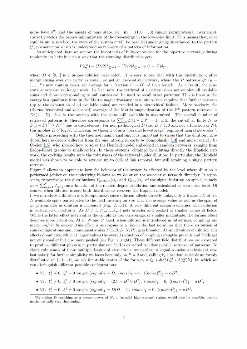
Figure 3: Two patterns analysis: (up) Analytical solution at β = 104. (down) Analytical solution atβ = 6.66. All these curve have been checked versus Monte Carlo simulations (not shown) on Cudaprocessors with N up to 100000 spins with overall perfect agreement.

Hence, in the low-storage regime α = 0 (and in the limit β → ∞), we expect stable retrieved states ofamplitude m1 = D and m2 = D(1−D), in agreement with the scaling previously outlined.To confirm this scenario we solve the statistical mechanics of the model. We stress that as no slownoise due to an extensive amount of patterns is at work (α = 0), replica trick or techniques stemmedfrom disordered system theory [12, 6], are not necessary. We introduce a generic vector for Mattismagnetizations as m = (m1, ...,mP ), a density of the states D(m) = 2−N

∑σ δ(m−m(σ)) and we write

the free-energy density as

f(β) =ln 2

β+

1

βNlog

∫dmD(m) exp

(1

2βNm2

). (4)

After some algebra this equation becomes

f(m,x) = − 1

N

∫dmdx exp

(−Nβf(m,x)

), (5)

f(m,x) = −1

2m2 − ix ·m− 1

β〈log 2 cos[βξ · x]〉ξ, (6)

which gives standard saddle point equations m = 〈ξ tanh(βξ ·m)〉ξ, whose numerical solution for thecase P = 2 is shown in Fig.3.

4

0.0 0.1 0.2 0.3 0.4t0.0

0.1

0.2

0.3

0.4m

m2

m1

0.0 0.1 0.2 0.3 0.4t0.0

0.1

0.2

0.3

0.4m

m2

m1

0.0 0.1 0.2 0.3 0.4t0.0

0.1

0.2

0.3

0.4m

m2

m1

0.0 0.1 0.2 0.3 0.4t0.0

0.1

0.2

0.3

0.4m

m2

m1

0.0 0.1 0.2 0.3 0.4t0.0

0.1

0.2

0.3

0.4m

m2

m1

0.0 0.1 0.2 0.3 0.4t0.0

0.1

0.2

0.3

0.4m

m2

m1

0.0 0.1 0.2 0.3 0.4t0.0

0.1

0.2

0.3

0.4m

m2

m1

0.0 0.1 0.2 0.3 0.4t0.0

0.1

0.2

0.3

0.4m

m2

m1

0.0 0.1 0.2 0.3 0.4t0.0

0.1

0.2

0.3

0.4m

m2

m1

0.0 0.1 0.2 0.3 0.4t0.0

0.1

0.2

0.3

0.4m

m2

m1

0.0 0.1 0.2 0.3 0.4t0.0

0.1

0.2

0.3

0.4m

m2

m1

0.0 0.1 0.2 0.3 0.4t0.0

0.1

0.2

0.3

0.4m

m2

m1

0.0 0.1 0.2 0.3 0.4t0.0

0.1

0.2

0.3

0.4m

m2

m1

0.0 0.1 0.2 0.3 0.4t0.0

0.1

0.2

0.3

0.4m

m2

m1

0.0 0.1 0.2 0.3 0.4t0.0

0.1

0.2

0.3

0.4m

m2

m1

0.0 0.1 0.2 0.3 0.4t0.0

0.1

0.2

0.3

0.4m

m2

m1

0.0 0.1 0.2 0.3 0.4t0.0

0.1

0.2

0.3

0.4m

m2

m1

0.0 0.1 0.2 0.3 0.4t0.0

0.1

0.2

0.3

0.4m

m2

m1

0.0 0.1 0.2 0.3 0.4t0.0

0.1

0.2

0.3

0.4m

m2

m1

0.0 0.1 0.2 0.3 0.4t0.0

0.1

0.2

0.3

0.4m

m2

m1

0.0 0.1 0.2 0.3 0.4t0.0

0.1

0.2

0.3

0.4m

m2

m1

0.0 0.1 0.2 0.3 0.4t0.0

0.1

0.2

0.3

0.4m

m2

m1

0.0 0.1 0.2 0.3 0.4t0.0

0.1

0.2

0.3

0.4m

m2

m1

0.0 0.1 0.2 0.3 0.4t0.0

0.1

0.2

0.3

0.4m

m2

m1

0.0 0.1 0.2 0.3 0.4t0.0

0.1

0.2

0.3

0.4m

m2

m1

0.0 0.1 0.2 0.3 0.4t0.0

0.1

0.2

0.3

0.4m

m2

m1

0.0 0.1 0.2 0.3 0.4t0.0

0.1

0.2

0.3

0.4m

m2

m1

0.0 0.1 0.2 0.3 0.4t0.0

0.1

0.2

0.3

0.4m

m2

m1

0.0 0.1 0.2 0.3 0.4t0.0

0.1

0.2

0.3

0.4m

m2

m1

0.0 0.1 0.2 0.3 0.4t0.0

0.1

0.2

0.3

0.4m

m2

m1

0.0 0.1 0.2 0.3 0.4t0.0

0.1

0.2

0.3

0.4m

m2

m1

0.0 0.1 0.2 0.3 0.4t0.0

0.1

0.2

0.3

0.4m

m2

m1

0.0 0.1 0.2 0.3 0.4t0.0

0.1

0.2

0.3

0.4m

m2

m1

0.0 0.1 0.2 0.3 0.4t0.0

0.1

0.2

0.3

0.4m

m2

m1

0.0 0.1 0.2 0.3 0.4t0.0

0.1

0.2

0.3

0.4m

m2

m1

0.0 0.1 0.2 0.3 0.4t0.0

0.1

0.2

0.3

0.4m

m2

m1

0.0 0.1 0.2 0.3 0.4t0.0

0.1

0.2

0.3

0.4m

m2

m1

0.0 0.1 0.2 0.3 0.4t0.0

0.1

0.2

0.3

0.4m

m2

m1

0.0 0.1 0.2 0.3 0.4t0.0

0.1

0.2

0.3

0.4m

m2

m1

0.0 0.1 0.2 0.3 0.4t0.0

0.1

0.2

0.3

0.4m

m2

m1

0.0 0.1 0.2 0.3 0.4t0.0

0.1

0.2

0.3

0.4m

m2

m1

0.0 0.1 0.2 0.3 0.4t0.0

0.1

0.2

0.3

0.4m

m2

m1

0.0 0.1 0.2 0.3 0.4t0.0

0.1

0.2

0.3

0.4m

m2

m1

0.0 0.1 0.2 0.3 0.4t0.0

0.1

0.2

0.3

0.4m

m2

m1

0.0 0.1 0.2 0.3 0.4t0.0

0.1

0.2

0.3

0.4m

m2

m1

0.0 0.1 0.2 0.3 0.4t0.0

0.1

0.2

0.3

0.4m

m2

m1

0.0 0.1 0.2 0.3 0.4t0.0

0.1

0.2

0.3

0.4m

m2

m1

0.0 0.1 0.2 0.3 0.4t0.0

0.1

0.2

0.3

0.4m

m2

m1

0.0 0.1 0.2 0.3 0.4t0.0

0.1

0.2

0.3

0.4m

m2

m1

0.0 0.1 0.2 0.3 0.4t0.0

0.1

0.2

0.3

0.4m

m2

m1

0.0 0.1 0.2 0.3 0.4t0.0

0.1

0.2

0.3

0.4m

m2

m1

0.0 0.1 0.2 0.3 0.4t0.0

0.1

0.2

0.3

0.4m

m2

m1

0.0 0.1 0.2 0.3 0.4t0.0

0.1

0.2

0.3

0.4m

m2

m1

0.0 0.1 0.2 0.3 0.4t0.0

0.1

0.2

0.3

0.4m

m2

m1

0.0 0.1 0.2 0.3 0.4t0.0

0.1

0.2

0.3

0.4m

m2

m1

0.0 0.1 0.2 0.3 0.4t0.0

0.1

0.2

0.3

0.4m

m2

m1

0.0 0.1 0.2 0.3 0.4t0.0

0.1

0.2

0.3

0.4m

m2

m1

0.0 0.1 0.2 0.3 0.4t0.0

0.1

0.2

0.3

0.4m

m2

m1

0.0 0.1 0.2 0.3 0.4t0.0

0.1

0.2

0.3

0.4m

m2

m1

0.0 0.1 0.2 0.3 0.4t0.0

0.1

0.2

0.3

0.4m

m2

m1

0.0 0.1 0.2 0.3 0.4t0.0

0.1

0.2

0.3

0.4m

m2

m1

0.0 0.1 0.2 0.3 0.4t0.0

0.1

0.2

0.3

0.4m

m2

m1

0.0 0.1 0.2 0.3 0.4t0.0

0.1

0.2

0.3

0.4m

m2

m1

0.0 0.1 0.2 0.3 0.4t0.0

0.1

0.2

0.3

0.4m

m2

m1

0.0 0.1 0.2 0.3 0.4t0.0

0.1

0.2

0.3

0.4m

m2

m1

0.0 0.1 0.2 0.3 0.4t0.0

0.1

0.2

0.3

0.4m

m2

m1

0.0 0.1 0.2 0.3 0.4t0.0

0.1

0.2

0.3

0.4m

m2

m1

0.0 0.1 0.2 0.3 0.4t0.0

0.1

0.2

0.3

0.4m

m2

m1

0.0 0.1 0.2 0.3 0.4t0.0

0.1

0.2

0.3

0.4m

m2

m1

0.0 0.1 0.2 0.3 0.4t0.0

0.1

0.2

0.3

0.4m

m2

m1

0.0 0.1 0.2 0.3 0.4t0.0

0.1

0.2

0.3

0.4m

m2

m1

0.0 0.1 0.2 0.3 0.4t0.0

0.1

0.2

0.3

0.4m

m2

m1

0.0 0.1 0.2 0.3 0.4t0.0

0.1

0.2

0.3

0.4m

m2

m1

0.0 0.1 0.2 0.3 0.4t0.0

0.1

0.2

0.3

0.4m

m2

m1

0.0 0.1 0.2 0.3 0.4t0.0

0.1

0.2

0.3

0.4m

m2

m1

0.0 0.1 0.2 0.3 0.4t0.0

0.1

0.2

0.3

0.4m

m2

m1

0.0 0.1 0.2 0.3 0.4t0.0

0.1

0.2

0.3

0.4m

m2

m1

0.0 0.1 0.2 0.3 0.4t0.0

0.1

0.2

0.3

0.4m

m2

m1

0.0 0.1 0.2 0.3 0.4t0.0

0.1

0.2

0.3

0.4m

m2

m1

0.0 0.1 0.2 0.3 0.4t0.0

0.1

0.2

0.3

0.4m

m2

m1

0.0 0.1 0.2 0.3 0.4t0.0

0.2

0.4

0.6

0.8

1.0m

m2

m1

0.0 0.1 0.2 0.3 0.4t0.0

0.2

0.4

0.6

0.8

1.0m

m2

m1

0.0 0.1 0.2 0.3 0.4t0.0

0.2

0.4

0.6

0.8

1.0m

m2

m1

0.0 0.1 0.2 0.3 0.4t0.0

0.2

0.4

0.6

0.8

1.0m

m2

m1

0.0 0.1 0.2 0.3 0.4t0.0

0.2

0.4

0.6

0.8

1.0m

m2

m1

0.0 0.1 0.2 0.3 0.4t0.0

0.2

0.4

0.6

0.8

1.0m

m2

m1

0.0 0.1 0.2 0.3 0.4t0.0

0.2

0.4

0.6

0.8

1.0m

m2

m1

0.0 0.1 0.2 0.3 0.4t0.0

0.2

0.4

0.6

0.8

1.0m

m2

m1

0.0 0.1 0.2 0.3 0.4t0.0

0.2

0.4

0.6

0.8

1.0m

m2

m1

0.0 0.1 0.2 0.3 0.4t0.0

0.2

0.4

0.6

0.8

1.0m

m2

m1

0.0 0.1 0.2 0.3 0.4t0.0

0.2

0.4

0.6

0.8

1.0m

m2

m1

0.0 0.1 0.2 0.3 0.4t0.0

0.2

0.4

0.6

0.8

1.0m

m2

m1

0.0 0.1 0.2 0.3 0.4t0.0

0.2

0.4

0.6

0.8

1.0m

m2

m1

0.0 0.1 0.2 0.3 0.4t0.0

0.2

0.4

0.6

0.8

1.0m

m2

m1

0.0 0.1 0.2 0.3 0.4t0.0

0.2

0.4

0.6

0.8

1.0m

m2

m1

0.0 0.1 0.2 0.3 0.4t0.0

0.2

0.4

0.6

0.8

1.0m

m2

m1

0.0 0.1 0.2 0.3 0.4t0.0

0.2

0.4

0.6

0.8

1.0m

m2

m1

0.0 0.1 0.2 0.3 0.4t0.0

0.2

0.4

0.6

0.8

1.0m

m2

m1

0.0 0.1 0.2 0.3 0.4t0.0

0.2

0.4

0.6

0.8

1.0m

m2

m1

0.0 0.1 0.2 0.3 0.4t0.0

0.2

0.4

0.6

0.8

1.0m

m2

m1

0.0 0.1 0.2 0.3 0.4t0.0

0.2

0.4

0.6

0.8

1.0m

m2

m1

0.0 0.1 0.2 0.3 0.4t0.0

0.2

0.4

0.6

0.8

1.0m

m2

m1

0.0 0.1 0.2 0.3 0.4t0.0

0.2

0.4

0.6

0.8

1.0m

m2

m1

0.0 0.1 0.2 0.3 0.4t0.0

0.2

0.4

0.6

0.8

1.0m

m2

m1

0.0 0.1 0.2 0.3 0.4t0.0

0.2

0.4

0.6

0.8

1.0m

m2

m1

0.0 0.1 0.2 0.3 0.4t0.0

0.2

0.4

0.6

0.8

1.0m

m2

m1

0.0 0.1 0.2 0.3 0.4t0.0

0.2

0.4

0.6

0.8

1.0m

m2

m1

0.0 0.1 0.2 0.3 0.4t0.0

0.2

0.4

0.6

0.8

1.0m

m2

m1

0.0 0.1 0.2 0.3 0.4t0.0

0.2

0.4

0.6

0.8

1.0m

m2

m1

0.0 0.1 0.2 0.3 0.4t0.0

0.2

0.4

0.6

0.8

1.0m

m2

m1

0.0 0.1 0.2 0.3 0.4t0.0

0.2

0.4

0.6

0.8

1.0m

m2

m1

0.0 0.1 0.2 0.3 0.4t0.0

0.2

0.4

0.6

0.8

1.0m

m2

m1

0.0 0.1 0.2 0.3 0.4t0.0

0.2

0.4

0.6

0.8

1.0m

m2

m1

0.0 0.1 0.2 0.3 0.4t0.0

0.2

0.4

0.6

0.8

1.0m

m2

m1

0.0 0.1 0.2 0.3 0.4t0.0

0.2

0.4

0.6

0.8

1.0m

m2

m1

0.0 0.1 0.2 0.3 0.4t0.0

0.2

0.4

0.6

0.8

1.0m

m2

m1

0.0 0.1 0.2 0.3 0.4t0.0

0.2

0.4

0.6

0.8

1.0m

m2

m1

0.0 0.1 0.2 0.3 0.4t0.0

0.2

0.4

0.6

0.8

1.0m

m2

m1

0.0 0.1 0.2 0.3 0.4t0.0

0.2

0.4

0.6

0.8

1.0m

m2

m1

0.0 0.1 0.2 0.3 0.4t0.0

0.2

0.4

0.6

0.8

1.0m

m2

m1

0.0 0.1 0.2 0.3 0.4t0.0

0.2

0.4

0.6

0.8

1.0m

m2

m1

0.0 0.1 0.2 0.3 0.4t0.0

0.2

0.4

0.6

0.8

1.0m

m2

m1

0.0 0.1 0.2 0.3 0.4t0.0

0.2

0.4

0.6

0.8

1.0m

m2

m1

0.0 0.1 0.2 0.3 0.4t0.0

0.2

0.4

0.6

0.8

1.0m

m2

m1

0.0 0.1 0.2 0.3 0.4t0.0

0.2

0.4

0.6

0.8

1.0m

m2

m1

0.0 0.1 0.2 0.3 0.4t0.0

0.2

0.4

0.6

0.8

1.0m

m2

m1

0.0 0.1 0.2 0.3 0.4t0.0

0.2

0.4

0.6

0.8

1.0m

m2

m1

0.0 0.1 0.2 0.3 0.4t0.0

0.2

0.4

0.6

0.8

1.0m

m2

m1

0.0 0.1 0.2 0.3 0.4t0.0

0.2

0.4

0.6

0.8

1.0m

m2

m1

0.0 0.1 0.2 0.3 0.4t0.0

0.2

0.4

0.6

0.8

1.0m

m2

m1

0.0 0.1 0.2 0.3 0.4t0.0

0.2

0.4

0.6

0.8

1.0m

m2

m1

0.0 0.1 0.2 0.3 0.4t0.0

0.2

0.4

0.6

0.8

1.0m

m2

m1

0.0 0.1 0.2 0.3 0.4t0.0

0.2

0.4

0.6

0.8

1.0m

m2

m1

0.0 0.1 0.2 0.3 0.4t0.0

0.2

0.4

0.6

0.8

1.0m

m2

m1

0.0 0.1 0.2 0.3 0.4t0.0

0.2

0.4

0.6

0.8

1.0m

m2

m1

0.0 0.1 0.2 0.3 0.4t0.0

0.2

0.4

0.6

0.8

1.0m

m2

m1

0.0 0.1 0.2 0.3 0.4t0.0

0.2

0.4

0.6

0.8

1.0m

m2

m1

0.0 0.1 0.2 0.3 0.4t0.0

0.2

0.4

0.6

0.8

1.0m

m2

m1

0.0 0.1 0.2 0.3 0.4t0.0

0.2

0.4

0.6

0.8

1.0m

m2

m1

0.0 0.1 0.2 0.3 0.4t0.0

0.2

0.4

0.6

0.8

1.0m

m2

m1

0.0 0.1 0.2 0.3 0.4t0.0

0.2

0.4

0.6

0.8

1.0m

m2

m1

0.0 0.1 0.2 0.3 0.4t0.0

0.2

0.4

0.6

0.8

1.0m

m2

m1

0.0 0.1 0.2 0.3 0.4t0.0

0.2

0.4

0.6

0.8

1.0m

m2

m1

0.0 0.1 0.2 0.3 0.4t0.0

0.2

0.4

0.6

0.8

1.0m

m2

m1

0.0 0.1 0.2 0.3 0.4t0.0

0.2

0.4

0.6

0.8

1.0m

m2

m1

0.0 0.1 0.2 0.3 0.4t0.0

0.2

0.4

0.6

0.8

1.0m

m2

m1

0.0 0.1 0.2 0.3 0.4t0.0

0.2

0.4

0.6

0.8

1.0m

m2

m1

0.0 0.1 0.2 0.3 0.4t0.0

0.2

0.4

0.6

0.8

1.0m

m2

m1

0.0 0.1 0.2 0.3 0.4t0.0

0.2

0.4

0.6

0.8

1.0m

m2

m1

0.0 0.1 0.2 0.3 0.4t0.0

0.2

0.4

0.6

0.8

1.0m

m2

m1

0.0 0.1 0.2 0.3 0.4t0.0

0.2

0.4

0.6

0.8

1.0m

m2

m1

0.0 0.1 0.2 0.3 0.4t0.0

0.2

0.4

0.6

0.8

1.0m

m2

m1

0.0 0.1 0.2 0.3 0.4t0.0

0.2

0.4

0.6

0.8

1.0m

m2

m1

0.0 0.1 0.2 0.3 0.4t0.0

0.2

0.4

0.6

0.8

1.0m

m2

m1

0.0 0.1 0.2 0.3 0.4t0.0

0.2

0.4

0.6

0.8

1.0m

m2

m1

0.0 0.1 0.2 0.3 0.4t0.0

0.2

0.4

0.6

0.8

1.0m

m2

m1

0.0 0.1 0.2 0.3 0.4t0.0

0.2

0.4

0.6

0.8

1.0m

m2

m1

0.0 0.1 0.2 0.3 0.4t0.0

0.2

0.4

0.6

0.8

1.0m

m2

m1

0.0 0.1 0.2 0.3 0.4t0.0

0.2

0.4

0.6

0.8

1.0m

m2

m1

0.0 0.1 0.2 0.3 0.4t0.0

0.2

0.4

0.6

0.8

1.0m

m2

m1

0.0 0.1 0.2 0.3 0.4t0.0

0.2

0.4

0.6

0.8

1.0m

m2

m1

0.0 0.1 0.2 0.3 0.4t0.0

0.2

0.4

0.6

0.8

1.0m

m2

m1

0.0 0.1 0.2 0.3 0.4t0.0

0.2

0.4

0.6

0.8

1.0m

m2

m1

0.0 0.1 0.2 0.3 0.4t0.0

0.2

0.4

0.6

0.8

1.0m

m2

m1

0.0 0.1 0.2 0.3 0.4t0.0

0.2

0.4

0.6

0.8

1.0m

m2

m1

0.0 0.1 0.2 0.3 0.4t0.0

0.2

0.4

0.6

0.8

1.0m

m2

m1

0.0 0.1 0.2 0.3 0.4t0.0

0.2

0.4

0.6

0.8

1.0m

m2

m1

0.0 0.1 0.2 0.3 0.4t0.0

0.2

0.4

0.6

0.8

1.0m

m2

m1

0.0 0.1 0.2 0.3 0.4t0.0

0.2

0.4

0.6

0.8

1.0m

m2

m1

0.0 0.1 0.2 0.3 0.4t0.0

0.2

0.4

0.6

0.8

1.0m

m2

m1

0.0 0.1 0.2 0.3 0.4t0.0

0.2

0.4

0.6

0.8

1.0m

m2

m1

0.0 0.1 0.2 0.3 0.4t0.0

0.2

0.4

0.6

0.8

1.0m

m2

m1

0.0 0.1 0.2 0.3 0.4t0.0

0.2

0.4

0.6

0.8

1.0m

m2

m1

0.0 0.1 0.2 0.3 0.4t0.0

0.2

0.4

0.6

0.8

1.0m

m2

m1

0.0 0.1 0.2 0.3 0.4t0.0

0.2

0.4

0.6

0.8

1.0m

m2

m1

0.0 0.1 0.2 0.3 0.4t0.0

0.2

0.4

0.6

0.8

1.0m

m2

m1

0.0 0.1 0.2 0.3 0.4t0.0

0.2

0.4

0.6

0.8

1.0m

m2

m1

0.0 0.1 0.2 0.3 0.4t0.0

0.2

0.4

0.6

0.8

1.0m

m2

m1

0.0 0.1 0.2 0.3 0.4t0.0

0.2

0.4

0.6

0.8

1.0m

m2

m1

0.0 0.1 0.2 0.3 0.4t0.0

0.2

0.4

0.6

0.8

1.0m

m2

m1

0.0 0.1 0.2 0.3 0.4t0.0

0.2

0.4

0.6

0.8

1.0m

m2

m1

0.0 0.1 0.2 0.3 0.4t0.0

0.2

0.4

0.6

0.8

1.0m

m2

m1

0.0 0.1 0.2 0.3 0.4t0.0

0.2

0.4

0.6

0.8

1.0m

m2

m1

0.0 0.1 0.2 0.3 0.4t0.0

0.2

0.4

0.6

0.8

1.0m

m2

m1

0.0 0.1 0.2 0.3 0.4t0.0

0.2

0.4

0.6

0.8

1.0m

m2

m1

0.0 0.1 0.2 0.3 0.4t0.0

0.2

0.4

0.6

0.8

1.0m

m2

m1

0.0 0.1 0.2 0.3 0.4t0.0

0.2

0.4

0.6

0.8

1.0m

m2

m1

0.0 0.1 0.2 0.3 0.4t0.0

0.2

0.4

0.6

0.8

1.0m

m2

m1

0.0 0.1 0.2 0.3 0.4t0.0

0.2

0.4

0.6

0.8

1.0m

m2

m1

0.0 0.1 0.2 0.3 0.4t0.0

0.2

0.4

0.6

0.8

1.0m

m2

m1

0.0 0.1 0.2 0.3 0.4t0.0

0.2

0.4

0.6

0.8

1.0m

m2

m1

0.0 0.1 0.2 0.3 0.4t0.0

0.2

0.4

0.6

0.8

1.0m

m2

m1

0.0 0.1 0.2 0.3 0.4t0.0

0.2

0.4

0.6

0.8

1.0m

m2

m1

0.0 0.1 0.2 0.3 0.4t0.0

0.2

0.4

0.6

0.8

1.0m

m2

m1

0.0 0.1 0.2 0.3 0.4t0.0

0.2

0.4

0.6

0.8

1.0m

m2

m1

0.0 0.1 0.2 0.3 0.4t0.0

0.2

0.4

0.6

0.8

1.0m

m2

m1

0.0 0.1 0.2 0.3 0.4t0.0

0.2

0.4

0.6

0.8

1.0m

m2

m1

0.0 0.1 0.2 0.3 0.4t0.0

0.2

0.4

0.6

0.8

1.0m

m2

m1

0.0 0.1 0.2 0.3 0.4t0.0

0.2

0.4

0.6

0.8

1.0m

m2

m1

0.0 0.1 0.2 0.3 0.4t0.0

0.2

0.4

0.6

0.8

1.0m

m2

m1

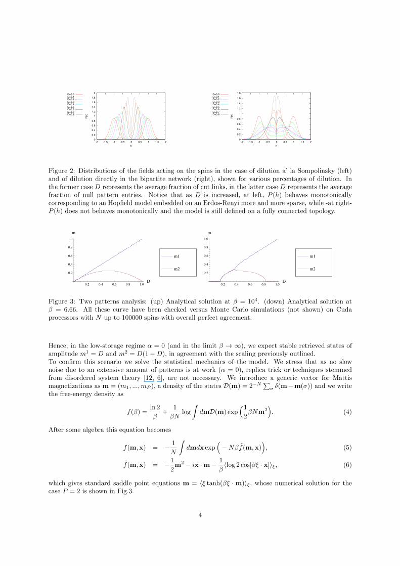
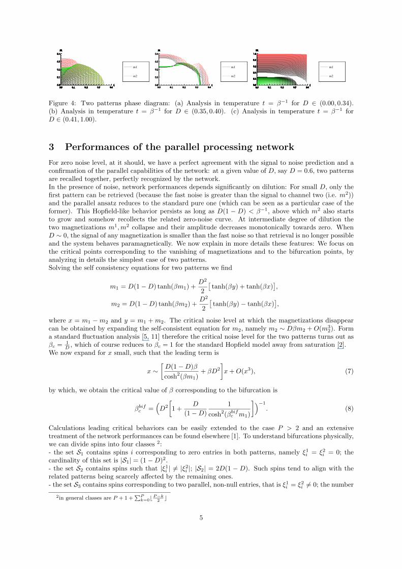
Figure 4: Two patterns phase diagram: (a) Analysis in temperature t = β−1 for D ∈ (0.00, 0.34).(b) Analysis in temperature t = β−1 for D ∈ (0.35, 0.40). (c) Analysis in temperature t = β−1 forD ∈ (0.41, 1.00).

3 Performances of the parallel processing network

For zero noise level, at it should, we have a perfect agreement with the signal to noise prediction and aconfirmation of the parallel capabilities of the network: at a given value of D, say D = 0.6, two patternsare recalled together, perfectly recognized by the network.In the presence of noise, network performances depends significantly on dilution: For small D, only thefirst pattern can be retrieved (because the fast noise is greater than the signal to channel two (i.e. m2))and the parallel ansatz reduces to the standard pure one (which can be seen as a particular case of theformer). This Hopfield-like behavior persists as long as D(1 − D) < β−1, above which m2 also startsto grow and somehow recollects the related zero-noise curve. At intermediate degree of dilution thetwo magnetizations m1,m2 collapse and their amplitude decreases monotonically towards zero. WhenD ∼ 0, the signal of any magnetization is smaller than the fast noise so that retrieval is no longer possibleand the system behaves paramagnetically. We now explain in more details these features: We focus onthe critical points corresponding to the vanishing of magnetizations and to the bifurcation points, byanalyzing in details the simplest case of two patterns.Solving the self consistency equations for two patterns we find

m1 = D(1−D) tanh(βm1) +D2

2

[tanh(βy) + tanh(βx)

],

m2 = D(1−D) tanh(βm2) +D2

2

[tanh(βy)− tanh(βx)

],

where x = m1 −m2 and y = m1 + m2. The critical noise level at which the magnetizations disappearcan be obtained by expanding the self-consistent equation for m2, namely m2 ∼ Dβm2 +O(m3

2). Forma standard fluctuation analysis [5, 11] therefore the critical noise level for the two patterns turns out asβc = 1

D , which of course reduces to βc = 1 for the standard Hopfield model away from saturation [2].We now expand for x small, such that the leading term is

x ∼[D(1−D)β

cosh2(βm1)+ βD2

]x+O(x3), (7)

by which, we obtain the critical value of β corresponding to the bifurcation is

βbifc =(D2

[1 +

D

(1−D)

1

cosh2(βbifc m1)

])−1. (8)

Calculations leading critical behaviors can be easily extended to the case P > 2 and an extensivetreatment of the network performances can be found elsewhere [1]. To understand bifurcations physically,we can divide spins into four classes 2:- the set S1 contains spins i corresponding to zero entries in both patterns, namely ξ1i = ξ2i = 0; thecardinality of this set is |S1| = (1−D)2.- the set S2 contains spins such that |ξ1i | 6= |ξ2i |; |S2| = 2D(1 − D). Such spins tend to align with therelated patterns being scarcely affected by the remaining ones.- the set S3 contains spins corresponding to two parallel, non-null entries, that is ξ1i = ξ2i 6= 0; the number

2in general classes are P + 1 +∑P

k=0bP−k2c

5

0.2 0.4 0.6 0.8 1.0D

0.2

0.4

0.6

0.8

1.0

m

m3

m2

m1

0.00 0.02 0.04 0.06 0.08 0.10 0.12 0.14D0.00

0.02

0.04

0.06

0.08

0.10

0.12

0.14

m

m6m5m4m3m2m1

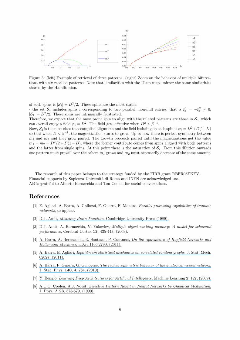
Figure 5: (left) Example of retrieval of three patterns. (right) Zoom on the behavior of multiple bifurca-tions with six recalled patterns. Note that similarities with the Ulam maps mirror the same similaritiesshared by the Hamiltonian.

of such spins is |S3| = D2/2. These spins are the most stable.- the set S4 includes spins i corresponding to two parallel, non-null entries, that is ξ1i = −ξ2i 6= 0,|S4| = D2/2. These spins are intrinsically frustrated.Therefore, we expect that the most prone spin to align with the related patterns are those in S3, whichcan overall enjoy a field ϕi = D2. The field gets effective when D2 > β−1.Now, S2 is the next class to accomplish alignment and the field insisting on each spin is ϕi = D2+D(1−D)so that when D < β−1, the magnetization starts to grow. Up to now there is perfect symmetry betweenm1 and m2 and they grow paired. The growth proceeds paired until the magnetizations get the valuem1 = m2 = D2/2 +D(1−D), where the former contribute comes from spins aligned with both patternsand the latter from single spins. At this point there is the saturation of S2. From this dilution onwardsone pattern must prevail over the other: m1 grows and m2 must necessarily decrease of the same amount.

The research of this paper belongs to the strategy funded by the FIRB grant RBFR08EKEV.Financial supports by Sapienza Universita di Roma and INFN are acknowledged too.AB is grateful to Alberto Bernacchia and Ton Coolen for useful conversations.

References

[1] E. Agliari, A. Barra, A. Galluzzi, F. Guerra, F. Moauro, Parallel processing capabilities of immunenetworks, to appear.

[2] D.J. Amit, Modeling Brain Function, Cambridge University Press (1989).

[3] D.J. Amit, A. Bernacchia, V. Yakovlev, Multiple object working memory: A model for behavoralperformance, Cerebral Cortex 13, 435-443, (2003).

[4] A. Barra, A. Bernacchia, E. Santucci, P. Contucci, On the equivalence of Hopfield Networks andBoltzmann Machines, arXiv:1105.2790, (2011).

[5] A. Barra, E. Agliari, Equilibrium statistical mechanics on correlated random graphs, J. Stat. Mech.02027, (2011).

[6] A. Barra, F. Guerra, G. Genovese, The replica symmetric behavior of the analogical neural network,J. Stat. Phys. 140, 4, 784, (2010).

[7] Y. Bengio, Learning Deep Architectures for Artificial Intelligence, Machine Learning 2, 127, (2009).

[8] A.C.C. Coolen, A.J. Noest, Selective Pattern Recall in Neural Networks by Chemical Modulation,J. Phys. A 23, 575-579, (1990).

6

[9] A.C.C. Coolen, A.J. Noest, G.B. de Vries, Modelling Chemical Modulation of Neural Processes,Network 4, 101-116, (1993).

[10] L.F. Cugliandolo, M.V. Tsodyks, Capacity of networks with correlated attractors, J. Phys. A 27,741, (1994).

[11] F. Guerra, Sum rules for the free energy in the mean field spin glass model, Math. Phys. in Math.and Phys., F.I.C. 30, 161-170, (2001).

[12] M. Mezard, G. Parisi and M. A. Virasoro, Spin glass theory and beyond, World Scientific, Singapore(1987).

[13] H. Sompolinsky, Neural networks with non-linear synapses and a static noise, Phys. Rev. A 34,2571-2584, (1986).

[14] G. Tkacik, E. Schneidman, M. J. Berry II, W. Bialek, Spin glass models for a network of realneurons, arXiv.org, q-bio, arXiv:0912.5409, (2009).

[15] B. Wemmenhove, A.C.C. Coolen, Finite Connectivity Attractor Neural Networks, J. Phys. A 36,9617-9633, (2003).

7