Embed Size (px)
Citation preview
arX
iv:h
ep-t
h/06
0319
0v2
7 A
pr 2
006
hep-th/0603190
DAMTP-2006-21
Multiply wound Polyakov loops at strong coupling
Sean A. Hartnoll1 and S. Prem Kumar2
1DAMTP, Centre for Mathematical Sciences, Cambridge University
Wilberforce Road, Cambridge CB3 OWA, UK
2Department of Physics, University of Wales Swansea
Swansea, SA2 8PP, UK
[email protected], [email protected]
Abstract
We study the expectation value of a Polyakov-Maldacena loop that wraps the
thermal circle k times in strongly coupled N = 4 super Yang-Mills theory. This
is achieved by considering probe D3 and D5 brane embeddings in the dual black
hole geometry. In contrast to multiply wound spatial Wilson loops, nontrivial
dependence on k is captured through D5 branes. We find N−2/3 corrections,
reminiscent of the scaling behaviour near a Gross-Witten transition.
1 Motivation and Introduction
1.1 Phase structure of N = 4 SYM theory
The phase structure of N = 4 super Yang-Mills (SYM) theory at large N on S3 × S1
is of interest from both gravitational and field theoretic perspectives. The AdS/CFT
correspondence [1] places both the weak and strong coupling regimes of the theory
within computational reach, suggesting the possibility of fully mapping out the phase
structure as a function of temperature and coupling.
At strong coupling it was observed [2, 3] that the Hawking-Page transition in ther-
mal AdS [4], which occurs at a critical temperature, should be interpreted as a first
order deconfinement transition in field theory.
At weak coupling there are also known to be phase transitions as a function of
temperature [5, 6, 7]. In the free theory there is again a first order transition at a critical
temperature whilst at finite small coupling there are two possibilities distinguished by
the sign of a currently unknown coefficient in the effective Lagrangian. Either there
is a single first order transition or, as one increases the temperature, a second order
transition followed by a third order transition.
The remaining question is the interpolation between weak and strong coupling
physics. A minimal interpolation suggests that the low and high temperature regimes
are separated by at least one phase transition at all couplings [6]. Nonrenormalisation
theorems in the low temperature phase [8] may suggest that the physics there depends
smoothly on the coupling. The high temperature behaviour is less clear. In a recent
work [9] we emphasised the tension between perturbative plasma physics correlators
which generically contain many threshold branch cuts and gravitational computations
of the same correlators at strong coupling which generically contain poles in frequency
space.
The order parameter used to discuss these transitions is the eigenvalue distribution
of the Polyakov loop, the SU(N) holonomy around the Euclidean time circle
U = P ei∮
A0 dτ . (1)
The eigenvalue distribution may be obtained from the expectation values of the trace
of powers of the Polyakov loop 〈TrUk〉. In the low temperature phase the distribution
is uniform while at high temperatures it is not. The possible third order transition we
mentioned is similar to the Gross-Witten transition [6, 10, 11], in which the nonuniform
eigenvalue distribution develops a gap.
The eigenvalue distribution of the Polyakov loop at strong coupling is not known and
it is the purpose of this work to begin to approach the problem. An important question
1
one would like to address is whether the non-uniform high temperature eigenvalue
distribution at strong coupling is gapped or not. An ungapped distribution would
signal a third order phase transition as a function of coupling in the high temperature
phase [12].
1.2 Multiply wound Polyakov-Maldacena loops
The AdS/CFT correspondence does not grant us access to the Polyakov loop (1) at
strong coupling but instead allows us to compute the Polyakov-Maldacena loop [13, 14]
U = P ei∮
[A0−iΦIθI(τ)]dτ , (2)
where ΦI are the six adjoint scalar fields of the N = 4 theory and θI(τ) is a trajectory
on the unit S5. This operator is no longer unitary and so we cannot speak of an
eigenvalue distribution on a circle. Instead, the expectation values 〈TrUk〉 determine
an eigenvalue distribution on the complex plane which one can hope to use as an order
parameter. For instance, it is this Polyakov-Maldacena loop which detects the strong
coupling deconfinement transition.
At large N and ’t Hooft coupling λ the AdS/CFT dictionary gives [13, 14, 15]
1
N〈TrUk〉 = e−S|k−winding , (3)
where S|k−winding is the action of a classical string configuration in the dual bulk geom-
etry that winds the thermal circle k times at the conformal boundary. Most previous
work, both for temporal and spacelike Wilson loops, has focused on the single winding
case k = 1. There are serious technical issues to overcome for multiply wound strings.
A discussion of computing 〈TrUk〉 at strong coupling for spatial Wilson loops was
given in [15]. The approach is largely qualitative and is essentially an extrapolation
to four dimensions of intuition that was developed in understanding two dimensional
QCD as a simple string theory [16, 17, 18]. The classical string configuration is a disc
worldsheet instanton embedded in the dual geometry as a k fold cover of a minimal
surface. The k winding requires the insertion of k − 1 Z2 branch cuts running from
interior points in the worldsheet to the boundary. This suggests the following expression
to leading order in α′ and string loop corrections [15]
1
N〈TrUk〉 ∼ (−1)k−1Ak−1e−kS|k=1 , (4)
where the factor of (−1)k−1 is due to the boundary conditions of fermions around the
loop and Ak−1 is a degeneracy factor due to the different possible locations of the k−1
branch points.
2
Despite the intuitive appeal of (4) it is not clear what A actually is. It could be
the renormalised area of the infinite worldsheet or for instance, as suggested in [15], it
could be the area of the worldsheet at the minimum of the background gravitational
potential. Doing the calculation rigorously requires computing the measure on the
moduli space of appropriate string instantons in the dual background. This does not
appear to be technically feasible at the moment. Furthermore one might worry about
the fact that the worldsheets have conical singularities at the branch cuts.
In a beautiful paper, Drukker and Fiol have shown how to sidestep these issues by
using a single probe D3 brane carrying electric worldvolume flux rather than fundamen-
tal strings [19]. In this approach there is no moduli space and worldvolume curvatures
are small everywhere. They computed the value of k winding supersymmetric circular
Wilson loops and gave a nontrivial match with a dual matrix model computation [20].
Even as N → ∞, λ → ∞ their result is significantly different from (4) if κ = k√
λ/4N
is kept fixed in this limit. In the following sections we will adapt their method to
compute k winding Polyakov-Maldacena loops in the high temperature phase of the
theory. We will find however that for the Polyakov loop case, nontrivial corrections
come from D5 rather than D3 branes and are expressed in terms of κ′ = k/N .
Finally, we note that there is a perhaps underdeveloped parallel between this critical
string theory story and two dimensional string theory on a circle. In that context the
‘Hawking-Page’ transition is seen as a Kosterlitz-Thouless transition in which vortices
condense on the string worldsheet [21]. This condensation precisely corresponds to the
insertion of branch cuts running to the boundary that we described above. Some of
the vortex condensates have been computed explicitly using the dual large N matrix
quantum mechanics on a circle [22].
In section 2 we consider potentially dual D3 branes in the black hole geometry.
We discuss possible boundary conditions and evaluation of the action on the solutions.
We find that the only solution to the D3 brane equations of motion is a solution in
which the D3 brane is collapsed on the cigar submanifold of the black hole. These
configurations do not lead to the expected nontrivial k dependence. In section 3 we
move on to consider D5 branes. Here we will find noncollapsed solutions that capture
the k dependence of the dual Polyakov loop. The two main results of this section are
firstly the compution of the actions with κ′ held fixed as N → ∞ and secondly the
observation that there are interesting N−2/3 corrections to the large N limit with k
fixed. Section 4 is a summary and a discussion of possible future directions.
3
2 (No) D3 brane solutions
In this section we search for probe D3 brane duals to the multiply wound Polyakov
loop. We will show that there are none, leading us on to a study of D5 branes in the
following section.
2.1 Equations of motion
The dual geometry for N = 4 SYM theory on S3 × S1 in the deconfined phase is the
Euclidean Schwarzschild black hole in AdS5 × S5:
ds2 = R2
[
f(r)dt2 +dr2
f(r)+ r2
(
dα2 + sin2 αdΩ22
)
+ dΩ25
]
, (5)
where
f(r) = 1 − r2+(1 + r2
+)
r2+ r2 . (6)
Following [19] we are looking for a probe D3 brane configuration in the dual back-
ground with the appropriate symmetries and worldvolume flux to describe a multiply
wound Polyakov loop in field theory. The action for the probe D3 brane is a sum of
the Dirac-Born-Infeld and Wess-Zumino terms
S = TD3
∫
dτd3σe−Φ√
det (⋆g + 2πα′F ) − igsTD3
∫
⋆C4 , (7)
where the tension TD3 = N/2π2R4. As usual F is the worldvolume gauge field and ⋆C4
is the pull back of the bulk Ramond-Ramond four form potential. We can take the
relevant part of the potential to be
C4 = −iR4
gsr4 sin2 αdt ∧ dα ∧ volS2 , (8)
whilst the dilaton is contant: e−Φ = 1.
The probe brane configuration must have the same symmetries as the dual Polyakov
loop: SO(3) × SO(2) ⊂ SO(4) × SO(2), the isotropy group of a point times S1 in
S3 × S1. If α, θ, φ are coordinates on the S3, then the required configuration lies
in the directions t, α, θ, φ, r, with a nontrivial dependence on only one worldvolume
coordinate
α = α(σ) , r = r(σ) . (9)
The geometry of this embedding is the cigar of the Euclidean black hole times an
S2 ⊂ S3. Thus α(σ) ∈ [0, π] determines the size of the noncollapsed S2 inside the
4
S3. We can think of the D3 brane as k fundamental strings blown up via the dielec-
tric Emparan-Myers effect [23, 24]. The string charge is induced from the worldvol-
ume gauge field which must have electric field strength with nonvanishing component
Fτσ(σ). The coefficient of the induced B field coupling to the string worldsheet will be
the momentum δS/δFτσ. This must be set equal to ik to be reinterpreted as the charge
of k fundamental strings. The presence of i will translate into the field strength being
imaginary as was found in [19]. Therefore we introduce the notation Fτσ(σ) ≡ iF (σ).
Evaluated on the ansatz we have just described, the action becomes
S =2N
π
∫
dτdσr2 sin2 α
√
(
dr
dσ
)2
+ r2f(r)
(
dα
dσ
)2
− 4π2F (σ)2
λ− r2 dα
dσ
, (10)
where we used R4 = λα′2.
The equation of motion for the gauge field gives the total string charge k ∈ Z
k = − δS
δF=
4N
λ
2πr2 sin2 αF√
(
drdσ
)2+ r2f
(
dαdσ
)2 − 4π2F 2
λ
. (11)
The equation of motion for α can be written
r2 sin2 α
[
r2 sin 2α2πF
κλ1/2+ 4r
dr
dσ
]
=d
dσ
(
r2fκλ1/2
2πF
dα
dσ
)
, (12)
where we introduced
κ =k√
λ
4N. (13)
The equation of motion for r is
2r3 sin2 α
[
sin2 α2πF
κλ1/2− 2
dα
dσ
]
+1
2
κλ1/2
2πF
d(r2f)
dr
(
dα
dσ
)2
=d
dσ
(
κλ1/2
2πF
dr
dσ
)
. (14)
One can use (11) written as
r2f
(
dα
dσ
)2
+
(
dr
dσ
)2
=(2πF )2
κ2λ
(
κ2 + r4 sin4 α)
, (15)
to eliminate F from (12) or (14). The equations depend on F only through the com-
bination
G =2πF
κλ1/2, (16)
so we will work in terms of this quantity in what follows.
Reparametrisation invariance of the action suggests that we should be able to con-
sistently set
r = σ or α = σ , (17)
and then solve for α(r) or r(α), respectively. Using the three equations of motion above
it is straightforward to show that indeed we may do this.
5
2.2 Boundary terms and boundary conditions
Once we have solved the equations of motion, we need to evaluate the action on the
solution to obtain the expectation value of the k winding Polyakov-Maldacena loop
〈TrUk〉 = e−S|k−soln. (18)
As is discussed very clearly in [19], in evaluating the action on the solution it is im-
portant to add the boundary terms. These terms implement Legendre transformations
that permit the solution to have the correct boundary conditions: fixed winding number
k and fixed momentum in the r direction.
For our configurations we need to add
S|bdy. = −∫
dτ rδS
δ∂σr
∣
∣
∣
∣
r→∞
−∫
dτ AtδS
δ∂σAt
∣
∣
∣
∣
r→∞
r=r+
. (19)
Using the action (7) this term becomes
S|bdy. = −2N
π
∫
dτr
G
dr
dσ
∣
∣
∣
∣
r→∞
+2N
π
∫ ∞
r+
dτdσκ2G . (20)
In the above expressions, and in this section in general, we have assumed for simplicity
that the configuration reaches the horizon r+. However it is possible for the solution
to close off at a finite value rmin > r+ by having α(rmin) = 0. We will consider this
possibility in later sections.
There is a further ambiguity in the boundary term following from the fact that
large gauge transformations of the background four form potential can change the
Wess-Zumino part of the action. However, it was found in [19] that using a minimal
expression for the potential compatible with the symmetries of the problem, as we have
done, together with no extra boundary term gives the correct answer for cases that can
be matched.
In order for a D3 brane configuration to contribute semiclassically to a dual Polyakov
loop it must have finite action, including the bulk and boundary terms. Let us look at
the large r behaviour of solutions. We have found two asymptotic behaviours for the
fields α(r) and G(r) at large r that lead to a finite total action
κG(r) = 1 +1
2
κ2
r2− 4B
3
κ3
r3+ · · · ,
α(r) = π − κ
r+ B
κ2
r2− 1 + 6B2
6
κ3
r3+ · · · , (21)
6
where B is an undetermined constant, and
κG(r) = 1 +9A2
2
κ4
r4− 3A2(4Aκ + 3)
2κ2
κ6
r6+ · · · ,
α(r) = π − A
κ
κ3
r3+
A(2Aκ + 3)
5κ3
κ5
r5+ · · · , (22)
where A is a free constant. A dependence on the horizon size r+ enters at higher
orders in these expansions. We have written the expansions where α → π as r → ∞.
There are very similar expansions for α → 0. The α → π case is more relevant as
configurations with increasing α have a lower action because of the Wess-Zumino term
in (10). In fact this term causes the action to behave very differently in the cases
α → π from below and α → 0 from above. Whilst both (21) and (22) lead to finite
action as α → π, only the faster falloff (22) is admissible as α → 0.
The falloffs (21) and (22) are special one parameter subfamilies of the general
behaviour of solutions near infinity, which depends on two constants of integration.
The generic behaviour at large r is
G(r) =m(r) − rm′(r)
m(r)2+ · · · ,
α(r) = π − m(r)
r+ · · · , (23)
where m(r) → ∞ as r → ∞ but m(r)/r → 0. The explicit leading order behaviour
of m(r) appears to be somewhat complicated. Numerically we find that m(r) ∼ log r
often gives a good description, but is not exact. However, without solving the equations
for m(r) it is possible to show that the action of these solutions behaves for large r as
S|soln. =−2Nβ
π
∫ ∞ dr
2
m(r)2
m(r) − rm′(r)+ · · · → −∞ . (24)
This divergence may be very precisely checked numerically. Therefore configurations
with the generic behaviour (23) have infinite action and do not contribute to the
Polyakov loop computation. It is not that the action is becoming unbounded below
but rather that these boundary conditions do not give rise to any normalisable states.
The bulk action is in fact finite with the asymptotic behaviours (21) and (22) with
another finite contribution to the action coming from the combined boundary terms.
The action evaluated on a solution with all boundary terms included may be written
S|soln. =2Nβ
π
(
− r+
√
κ2 + r4+ sin4 α+
+
∫ ∞
r+
[
r2f(r)
G
(
dα
dr
)2
− r4 sin2 αdα
dr+
r
G2
dG
dr
]
dr
)
(25)
7
where
β =2πr+
1 + 2r2+
, (26)
is the period of the time circle. The simplest solution is the collapsed solution which
has α = 0 or α = π. In this case the action is given immediately as
S|collapsed = −2Nκβr+
π= −
√λkβr+
2π. (27)
This is k times the action for a fundamental string instanton wrapping the cigar. This
connection between collapsed D branes carrying electric flux and fundamental strings
has been consistently verified in a range of examples since [23].
At this point we should note that for a general solution the dependence of the
Polyakov loop on k, N and λ is significantly restricted to be of the form
S|soln. = Nβs(κ, r+) , (28)
for some function s(κ, r+). As was emphasised in [19], although the expression (28)
is leading order in 1/N and λ, it is exact in κ = k√
λ/4N . This represents a partial
resumation of bulk higher genus string corrections. Such κ dependence could not
have been seen in the heuristic arguments of [15] leading to (4) that we reviewed in
the introduction. The result of [19] for the k winding circular spatial Wilson loop,
Sk = −2N[
κ√
1 + κ2 + sinh−1 κ]
, reduces to the naive expectation of Sk = kS1 only
in the limit κ → 0.
The important lesson from [19] is therefore that the possibility of a D3 brane blowing
up due to an Emparan-Myers effect corresponds to and captures the nontrivial λ and
N corrections which one expects from the singular nature of the fundamental string
picture. These corrections are contained in the potentially nontrivial dependence of
(28) on κ = k√
λ/4N . We will now see that in contrast to the spatial Wilson loop case,
this potential is not realised for the Polyakov loop. Instead, we will need to consider D5
branes in the following section and find that these do give corrections to the collapsed
result in terms of κ′ = k/N . At large λ these are subleading compared with the κ
corrections which appear to vanish.
2.3 Solving the equations
After extensive numerical investigation of the equations of motion (12), (14) and (15),
it has become clear that the only solutions which run from infinity to the horizon are
the collapsed solutions α = 0 and α = π, with action (27). In this section we will
combine analytic and numerical arguments to understand this fact.
8
We begin with some analytic results that are possible at large values of κ. We will
see in this regime that noncollapsed solutions do not reach the horizon but rather turn
around at some minimum radius r∗ and then go back out to infinity. We will then review
continuity theorems for the solutions as a function of κ and the boundary conditions to
show that this behaviour persists for a range of solutions away from the large κ limit.
Finally, we present numerical data indicating that none of the noncollapsed solutions
reach the horizon or close off in the interior.
We will jump between considering r(α) and α(r) depending on what is most con-
venient. G(α) or G(r) can be completely eliminated from the problem so we will not
discuss its behaviour explicitly.
2.3.1 The solutions at large κ
The equations of motion simplify when κ is taken to be large. One may find the general
solutions that have asymptotic boundary conditions (21) and (22). With the former
boundary condition the solution is
r(α) = κ1 + B(α − π)
sin α, (29)
which can of course be viewed as a transcendental equation for α(r). In the latter case
we have
α(r) = π − 3A
κ
∫ ∞
r/κ
dy
y2√
y4 − 9A2. (30)
The large κ expansion is valid for both of these solutions provided the constants B and
A are of order one and for the coordinate range r+ ≪ r ≪ κ3. Both the expressions
(29) and (30) agree excellently with numerics.
If we think of these solutions as r(α), then we see that as the solution comes in
towards the horizon from r → ∞ it turns around at some minimal radius r∗ ∼ κ ≫ r+.
The behaviour near the turnaround point is
r(α) = r∗ + C2 (α − α∗)2 + · · · . (31)
The values of the constants r∗, α∗ and C may be determined as functions of B or A
from the solutions (29) and (30), respectively. If A and B are order one, then the
turnaround occurs within the regime of validity of the solution. We note however that
(30) will only be valid for the branch of the solution going from α = π to α = α∗.
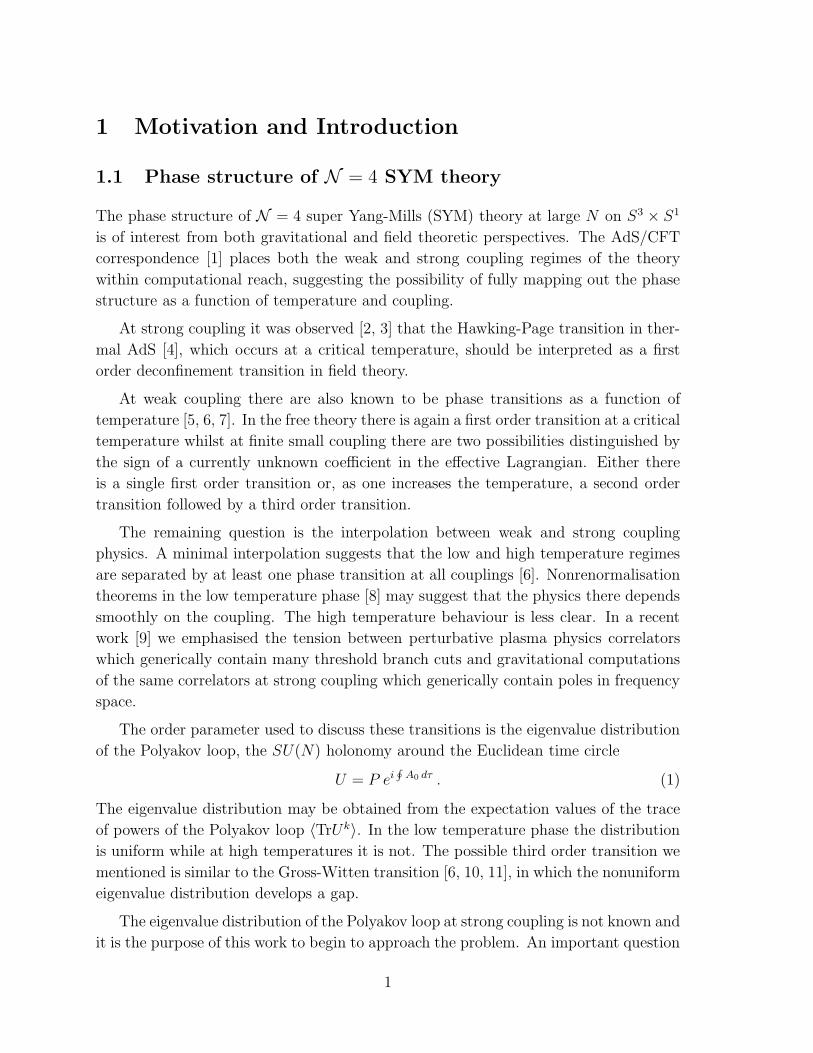
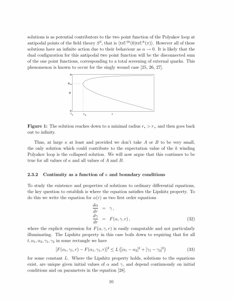
None of these noncollapsed solutions reach the horizon and close off. Instead they
come in from infinity at α = π and turn around and go back out to infinity at α = 0.
The solutions are illustrated schematically in Figure 1. The interpretation of these
9
solutions is as potential contributors to the two point function of the Polyakov loop at
antipodal points of the field theory S3, that is 〈trU †k(0)trUk(π)〉. However all of these
solutions have an infinite action due to their behaviour as α → 0. It is likely that the
dual configuration for this antipodal two point function will be the disconnected sum
of the one point functions, corresponding to a total screening of external quarks. This
phenomenon is known to occur for the singly wound case [25, 26, 27].
rrr*+
0
π
α
α *
Figure 1: The solution reaches down to a minimal radius r∗ > r+ and then goes back
out to infinity.
Thus, at large κ at least and provided we don’t take A or B to be very small,
the only solution which could contribute to the expectation value of the k winding
Polyakov loop is the collapsed solution. We will now argue that this continues to be
true for all values of κ and all values of A and B.
2.3.2 Continuity as a function of κ and boundary conditions
To study the existence and properties of solutions to ordinary differential equations,
the key question to establish is where the equation satisfies the Lipshitz property. To
do this we write the equation for α(r) as two first order equations
dα
dr= γ ,
dγ
dr= F (α, γ, r) , (32)
where the explicit expression for F (α, γ, r) is easily computable and not particularly
illuminating. The Lipshitz property in this case boils down to requiring that for all
t, α1, α2, γ1, γ2 in some rectangle we have
[F (α1, γ1, r) − F (α1, γ1, r)]2 ≤ L
(
[α1 − α2]2 + [γ1 − γ2]
2)
(33)
for some constant L. Where the Lipshitz property holds, solutions to the equations
exist, are unique given initial values of α and γ, and depend continuously on initial
conditions and on parameters in the equation [28].
10
For our equation (32) the Lipshitz property may be seen to hold everywhere except
when r → r+, r → ∞ or γ → ∞. Therefore, away from infinity and the horizon, the
only way the solution can terminate at some finite r∗ is if the derivative α′(r) diverges
at that point. We have seen that indeed this occurs in the large κ solutions, as (31)
implies α ∼ (r − r∗)1/2. One may show that such square root behaviour is the only
allowed behaviour as α′(r) → ∞.
Continuity then implies that as we vary κ and the constants A, B in the finite
action boundary conditions (21) and (22), all the solutions coming in from infinity will
turn around at some finite r∗, so long as r∗ does not approach the horizon r+. As we
approach r+ the continuity argument no longer holds. Another possible termination is
that α(rmin) = 0 for some rmin > r+ which would allow us to truncate the solution at
that point as the S2 closes off there.
Although continuity therefore gives us a window around the large κ solutions in
which the behaviour is qualitatively similar, it is not enough to cover all possible κ and
initial data. To this end we now present some numerical results.
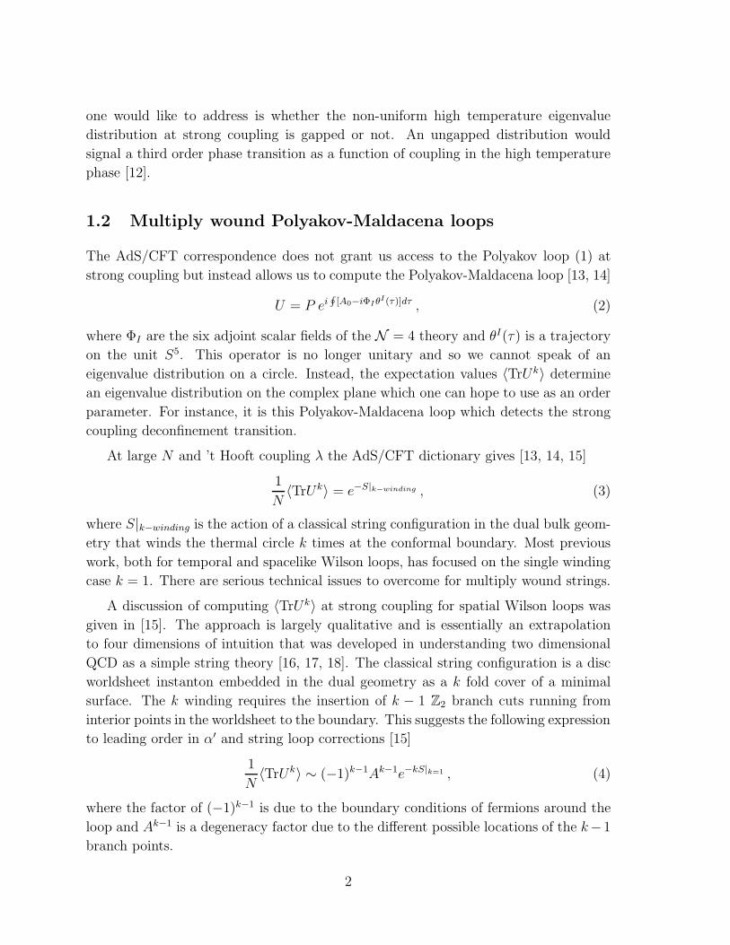
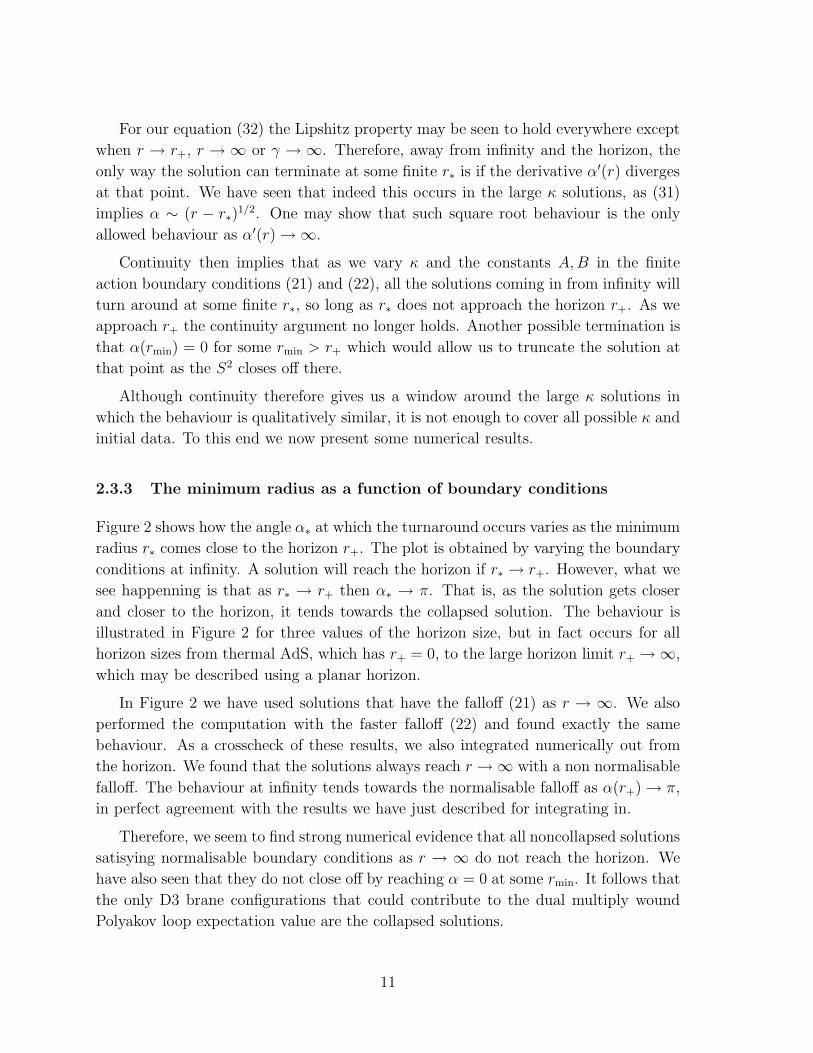
2.3.3 The minimum radius as a function of boundary conditions
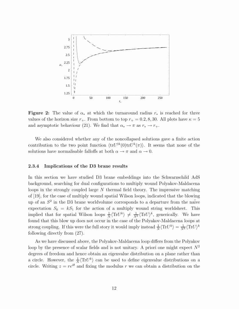
Figure 2 shows how the angle α∗ at which the turnaround occurs varies as the minimum
radius r∗ comes close to the horizon r+. The plot is obtained by varying the boundary
conditions at infinity. A solution will reach the horizon if r∗ → r+. However, what we
see happenning is that as r∗ → r+ then α∗ → π. That is, as the solution gets closer
and closer to the horizon, it tends towards the collapsed solution. The behaviour is
illustrated in Figure 2 for three values of the horizon size, but in fact occurs for all
horizon sizes from thermal AdS, which has r+ = 0, to the large horizon limit r+ → ∞,
which may be described using a planar horizon.
In Figure 2 we have used solutions that have the falloff (21) as r → ∞. We also
performed the computation with the faster falloff (22) and found exactly the same
behaviour. As a crosscheck of these results, we also integrated numerically out from
the horizon. We found that the solutions always reach r → ∞ with a non normalisable
falloff. The behaviour at infinity tends towards the normalisable falloff as α(r+) → π,
in perfect agreement with the results we have just described for integrating in.
Therefore, we seem to find strong numerical evidence that all noncollapsed solutions
satisying normalisable boundary conditions as r → ∞ do not reach the horizon. We
have also seen that they do not close off by reaching α = 0 at some rmin. It follows that
the only D3 brane configurations that could contribute to the dual multiply wound
Polyakov loop expectation value are the collapsed solutions.
11
0 50 100 150 200 250r*
1.25
1.5
1.75
2
2.25
2.5
2.75
3
Α*
Figure 2: The value of α∗ at which the turnaround radius r∗ is reached for three
values of the horizon size r+. From bottom to top r+ = 0.2, 8, 30. All plots have κ = 5
and asymptotic behaviour (21). We find that α∗ → π as r∗ → r+.
We also considered whether any of the noncollapsed solutions gave a finite action
contribution to the two point function 〈trU †k(0)trUk(π)〉. It seems that none of the
solutions have normalisable falloffs at both α → π and α → 0.
2.3.4 Implications of the D3 brane results
In this section we have studied D3 brane embeddings into the Schwarzschild AdS
background, searching for dual configurations to multiply wound Polyakov-Maldacena
loops in the strongly coupled large N thermal field theory. The impressive matching
of [19], for the case of multiply wound spatial Wilson loops, indicated that the blowing
up of an S2 in the D3 brane worldvolume corresponds to a departure from the naive
expectation Sk = kS1 for the action of a multiply wound string worldsheet. This
implied that for spatial Wilson loops 1N〈TrUk〉 6= 1
Nk 〈TrU〉k, generically. We have
found that this blow up does not occur in the case of the Polyakov-Maldacena loops at
strong coupling. If this were the full story it would imply instead 1N〈TrUk〉 = 1
Nk 〈TrU〉kfollowing directly from (27).
As we have discussed above, the Polyakov-Maldacena loop differs from the Polyakov
loop by the presence of scalar fields and is not unitary. A priori one might expect N2
degrees of freedom and hence obtain an eigenvalue distribution on a plane rather than
a circle. However, the 1N〈TrUk〉 can be used to define eigenvalue distributions on a
circle. Writing z = reiθ and fixing the modulus r we can obtain a distribution on the
12
θ circle
ρr(θ) = 1 + 2∞
∑
k=1
rk cos kθ1
N〈TrUk〉 . (34)
When 1N〈TrUk〉 = 1
Nk 〈TrU〉k there are three possibilities, depending on the value of
a = r 1N〈TrU〉. If a = 1 then the distribution is a delta function. If a < 1 then the
distribution becomes
ρr(θ) =1 − a2
1 + a2 − 2a cos θ. (35)
This is a smooth ungapped distribution on the θ circle. If a > 1 then the sum does not
converge. Analytic continuation in a leads to the result (35), but now the distribution
has a singularity that is not integrable.
It remains to be seen what the precise relation of these distributions is to the eigen-
value distribution of U , and whether they can be used as order parameters. Further-
more, the result 1N〈TrUk〉 = 1
Nk 〈TrU〉k is clearly not reliable. The initial motivation
for studying D3 branes was precisely to avoid issues that arise in the multiply wound
string picture. However, the fact that the D3 brane configurations are collapsed seems
to bring us back to that picture. Although the collapsed D3 brane retains a finite
tension which is exactly k times the fundamental string tension, it remains true that
induced curvatures on the collapsed S2 are large and not controlled within the validity
of the Dirac-Born-Infeld action.
If the corrections to the multiply wound string picture are necessarily captured
by a dependence on κ = k√
λ/4N then the fact that we do not find these corrections
would be sufficient to imply that the eigenvalue distributions discussed above are indeed
possible at leading order in N and λ. However, we will see in the following section that
by considering D5 brane probes instead of D3 branes one finds corrections in terms of
κ′ = k/N . Note that in the large λ limit κ′ ≪ κ and so these corrections are subleading
with respect to potential D3 brane corrections.
3 D5 brane solutions
In this section we search for probe D5 brane configurations in the Euclidean AdS
Schwarzschild background that have the correct charge and symmetries to contribute
to multiply wound Polyakov loops. The logic will be close to that of the previous
section so we shall be briefer in our presentation.
13
3.1 Equations of motion
The action for the probe D5 brane is again a sum of Dirac-Born-Infeld and Wess-
Zumino terms
S = TD5
∫
dτd5σe−Φ√
det (⋆g + 2πα′F ) − igsTD5
∫
2πα′F ∧ ⋆C4 , (36)
where TD5 = N√
λ/8π4R6. As we will be considering solutions that are blown up in
the S5 direction, the relevant part of the four form potential is now
C4 =R4
gs
[
3(γ − π)
2− sin3 γ cos γ − 3
2cos γ sin γ
]
volS4 , (37)
where γ ∈ [0, π] is a polar coordinate on the S5.
We need a configuration that has the symmetries of the dual Polyakov loop: the
isotropy group SO(3) × SO(2) of a point times S1 in S3 × S1, as well as an SO(5) ⊂SO(6) of the R symmetry group. This is obtained by having the D6 brane wrap an
S4 in the S5 and wrapping the time circle, while remaining at a point in the horizon
S3. Thus again the only nontrivial dependence is in γ(σ) and r(σ). The electric
worldvolume gauge field will again be imaginary, so as before we let Fτσ(σ) ≡ iF (σ).
Evaluated on this ansatz, the action becomes
S =N√
λ
3π2
∫
dτdσ
sin4 γ
√
(
dr
dσ
)2
+ f(r)
(
dγ
dσ
)2
− 4π2F (σ)2
λ− D(γ)
2πF (σ)
λ1/2
,
(38)
where we used R4 = λα′2 and introduced
D(γ) = sin3 γ cos γ +3
2cos γ sin γ − 3(γ − π)
2. (39)
We will set r = σ and look for solutions for γ(r). The equation of motion for F is
k = − δS
δF=
2N
3π
2πF
λ1/2
sin4 γ√
1 + f(r)(
dγdr
)2 − 4π2F 2
λ
+ D(γ)
, (40)
where as before k ∈ Z is the induced fundamental string charge. The equation of
motion for γ is
4 sin4 γ
[
sin3 γ cos γ3πκ′
2− D(γ)
+ 1
]
2πF
λ1/2=
d
dr
(
λ1/2
2πF
[
3πκ′
2− D(γ)
]
f(r)dγ
dr
)
, (41)
14
where we introduced
κ′ =k
N. (42)
It will also be convenient to introduce
G =2πF
λ1/2. (43)
Note that the equations of motion are invariant under k → N − k and γ → π − γ,
reflecting the fact that the Polyakov loop is sensitive to the N-ality of the source.
These equations are closely related to the D5 brane configuration that is dual to the
baryon vertex [29, 30, 31]. In fact, the solutions we will present clarify the uncertainty in
these papers concerning the interpretation of solutions with k < N units of worldvolume
flux. The simplest solutions we find will be at a constant angle γ0 on the S5, similar
in some regards to the confining string solutions described in [32]. The connection
between the baryon vertex and confining strings was realised particularly explicitly in
[33].
3.2 Boundary terms and action
The boundary terms to be added to the action are similar to the D3 brane case. The
action now depends on the derivative of one of the coordinates on the S5, γ. Therefore
we need to include an extra boundary term to impose Neumann boundary conditions
in this direction. A clear discussion of these issues can be found in [19]. The full
boundary term we need to add can be written as
S|bdy. = −N√
λ
3π2
∫
dτ1
G
[
3πκ′
2− D(γ)
] [
r + (γ − π)f(r)dγ
dr
]∣
∣
∣
∣
r→∞
+N√
λ
3π2
∫ ∞
r+
dτdr3πκ′
2G . (44)
As with the D3 branes, there are collapsed solutions with γ = π. As in the D3
brane case, these solutions take us back to the multiply wound string picture and are
not reliable. These are again seen to have action
S|collapsed = −√
λkβr+
2π, (45)
which is k times the action for a fundamental string instanton wrapping the cigar. For
a general solution we will have
S|soln. = N√
λβs(κ′, r+) , (46)
15
for some function s(κ′, r+). The D5 brane probes are sensitive to different corrections
to the dual Polyakov loop than the D3 branes, depending on κ′ rather than κ. Note
that κ′ ≪ κ in the large λ limit.
As r → ∞, the following falloff is allowed by the equations of motion and leads to
a finite action configuration:
γ(r) = π − A
r+
A(2 − A2)
6
1
r3+
2A4
9π
1
κ′
1
r4+ · · · , (47)
with A an arbitrary constant. This is the falloff considered by [29, 30] and, if the time
circle were not thermal, would give an asymptotically supersymmetric configuration.
There is another type of finite action solution which has qualitatively different
behaviour. These are solutions in which the angle γ tends to a constant γ0, determined
by κ′, as r → ∞. In particular, these include configurations in which γ = γ0 is constant
everywhere.
In contrast to the D3 brane case, numerical investigation of the equations reveals
that integrating inwards with these boundary conditions leads to solutions that reach
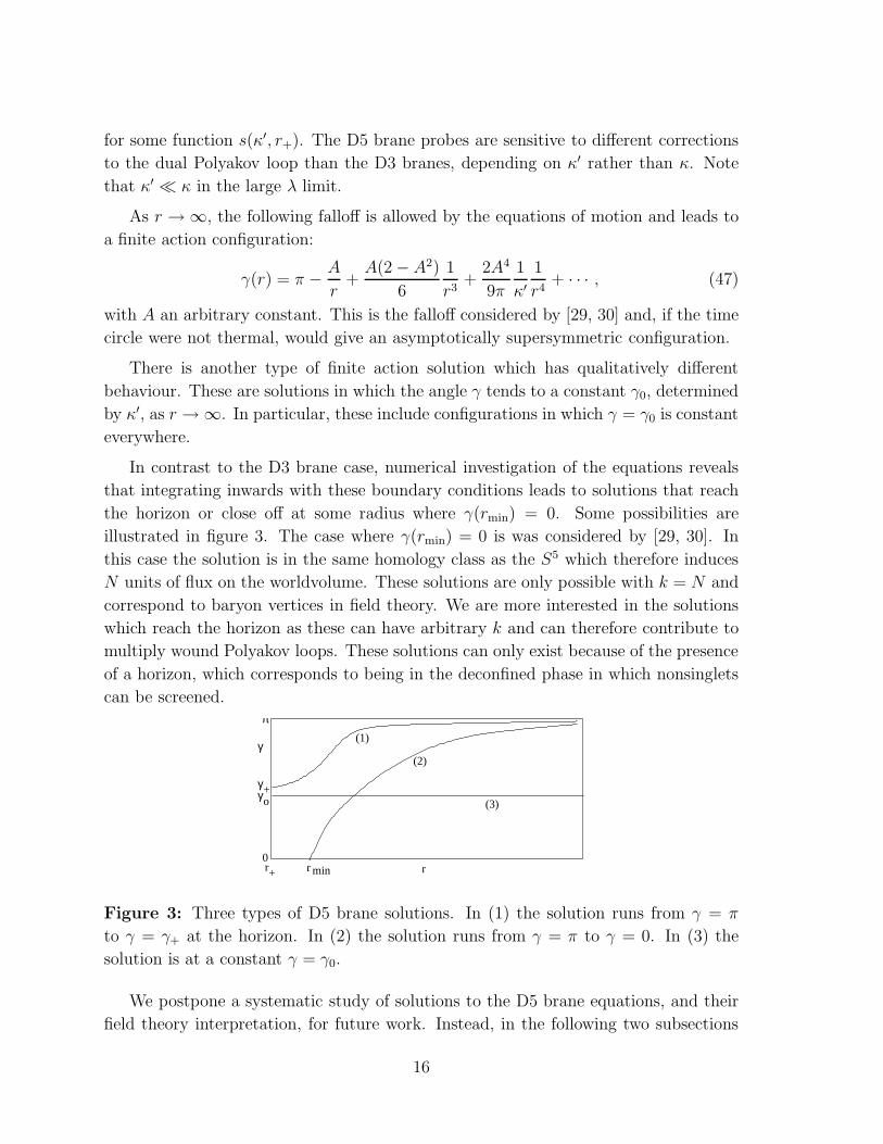
the horizon or close off at some radius where γ(rmin) = 0. Some possibilities are
illustrated in figure 3. The case where γ(rmin) = 0 is was considered by [29, 30]. In
this case the solution is in the same homology class as the S5 which therefore induces
N units of flux on the worldvolume. These solutions are only possible with k = N and
correspond to baryon vertices in field theory. We are more interested in the solutions
which reach the horizon as these can have arbitrary k and can therefore contribute to
multiply wound Polyakov loops. These solutions can only exist because of the presence
of a horizon, which corresponds to being in the deconfined phase in which nonsinglets
can be screened.
rr+0
π(1)
(2)
(3)+
γ
γγo
r min
Figure 3: Three types of D5 brane solutions. In (1) the solution runs from γ = π
to γ = γ+ at the horizon. In (2) the solution runs from γ = π to γ = 0. In (3) the
solution is at a constant γ = γ0.
We postpone a systematic study of solutions to the D5 brane equations, and their
field theory interpretation, for future work. Instead, in the following two subsections
16
we study firstly the simplest solutions, which are constant γ = γ0, and secondly we
look at the κ′ → 0 limit which is the most relevant for making direct contact with dual
field theory computations.
3.3 Constant solutions
The configuration γ = γ0 is a solution to the equations of motion if γ0 satisfies
π(κ′ − 1) = sin γ0 cos γ0 − γ0 . (48)
This remarkable solution is possible because the metric function f(r) only appears in
the equations of motion multiplied by dγ/dr, and so drops out when γ is constant.
There is a unique value of γ0 ∈ [0, π] for each value of κ′ ∈ [0, 1].
The action, with boundary terms included, evaluated on these solutions is finite
and may be written
S|γ0= −N
√λβr+
3π2sin3 γ0 . (49)
The action (49) is exact if κ′ is held fixed in the N → ∞ limit. This is not usually what
one does in field theory, where the large N limit is taken prior to computing Wilson
loop observables, with the notable exception of the supersymmetric circular Wilson
loop in N = 4 SYM theory which allows subleading N corrections to be computed
using a matrix model [20, 19]. We will consider the more usual N → ∞ limit in
the following subsection. It is also not clear that these constant solutions are the
correct duals for 1N〈trUk〉, or any other higher loop in a representation of N-ality k, as
opposed to the non constant solutions discussed around figure 3. However, given that
the constant solutions may be characterised so explicitly, let us consider the eigenvalue
distribution that would follow from using (49) to compute 1N〈trUk〉. As we note below,
recent developments disfavour this interpretation. However, given the unexpectedly
interesting result shown in figure 4, it seems possible that this computation will play a
role in a more fully developed understanding.
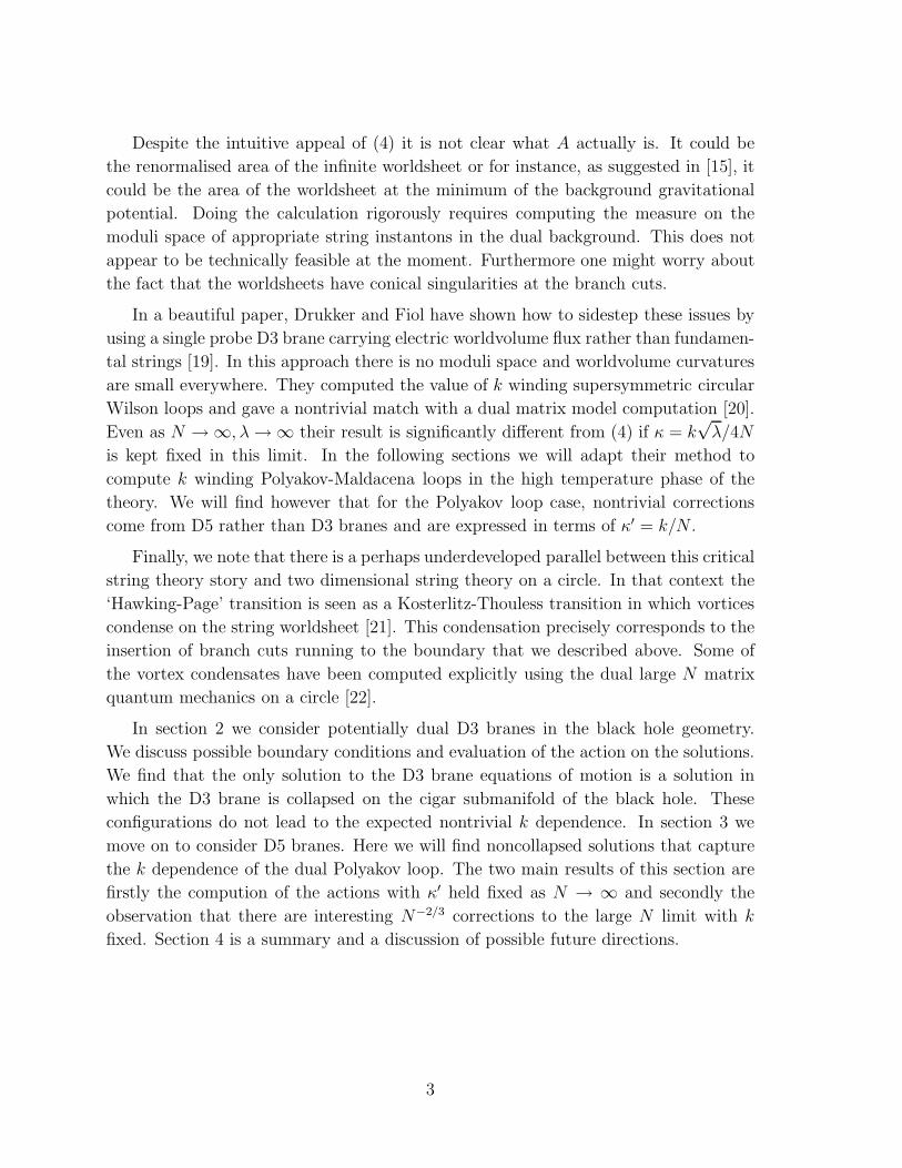
We will compute the eigenvalues numerically for a fixed, relatively large value of
N . If we were to assume that the result (49) gave us the traces
1
N〈TrUk〉 = eN 2
3πη sin3 γ0(k) , (50)
then we may determine the eigenvalues by solving a system of equations. Here we
introduced
η =
√λβr+
2π, (51)
17
which is closely related to the action for a single fundamental string. We should take
η ≫ 1 corresponding to large ’t Hooft coupling. At high temperatures βr+ ∼ O(1).
Unfortunately, this makes the system of equations which determine the eigenvalues
numerically rather intractible because the presence of Nη in the exponent means that
some equations have extremely large entries and others have entries of order one.
We will not solve this problem here. Instead, let us take η ∼ 1/N ≪ 1. This of
course takes us completely outside the regime of validity of the derivation of (49) and
leads to the important question of how strongly the eigenvalue distribution depends
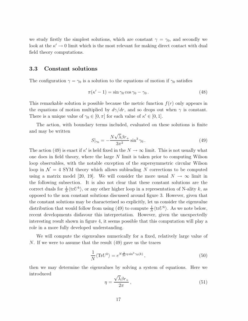
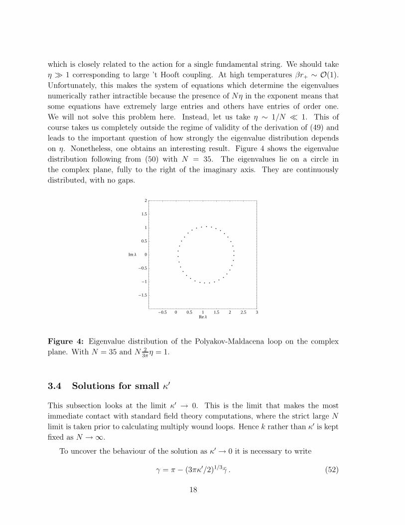
on η. Nonetheless, one obtains an interesting result. Figure 4 shows the eigenvalue
distribution following from (50) with N = 35. The eigenvalues lie on a circle in
the complex plane, fully to the right of the imaginary axis. They are continuously
distributed, with no gaps.
-0.5 0 0.5 1 1.5 2 2.5 3Re Λ
-1.5
-1
-0.5
0
0.5
1
1.5
2
Im Λ
Figure 4: Eigenvalue distribution of the Polyakov-Maldacena loop on the complex
plane. With N = 35 and N 23π
η = 1.
3.4 Solutions for small κ′
This subsection looks at the limit κ′ → 0. This is the limit that makes the most
immediate contact with standard field theory computations, where the strict large N
limit is taken prior to calculating multiply wound loops. Hence k rather than κ′ is kept
fixed as N → ∞.
To uncover the behaviour of the solution as κ′ → 0 it is necessary to write
γ = π − (3πκ′/2)1/3γ . (52)
18
Then to leading order as κ′ → 0 we have that γ must satisfy the equation
d
dr
[
f(r)dγ
dr
]
= 4γ4(
γ3 − 1)
. (53)
This is a polynomial nonlinear equation, in contrast to the general equations of motion
we have been considering. The change of variables γ = z1/3 and dr = f(r)dx takes the
equation to a form that narrowly misses having the Painleve property. A very inter-
esting result comes from computing the action on these configurations. The resulting
action may be written
S = −√
λβr+k
2π+
1
N2/3
√λβk5/3
30π2
∫ ∞
r+
dr
[
15γ8 − 8γ5 − 5f(r)
(
dγ
dr
)2]
+ · · · . (54)
The remaining higher order terms are not reliable in the strict large N limit without
including 1/N corrections to the background and the D5 brane action and so on. The
first correction to the collapsed result appears to be reliable because N−2/3 ≫ N−1.
Numerical integration of (53) shows that there are solutions with finite action which
run from infinity to the horizon. One further has the constant solution γ = 1. If
any of these provide the dual for multiply wound Polyakov loops or loops in higher
representations, then within the validity of our computation we may write
e−Sk = eηk
[
1 + Bk5/3
N2/3+ · · ·
]
, (55)
where η is defined in (51) and B is the integral given in (54). In (55) we have assumed
a 1/r falloff which implies that boundary terms don’t contribute. In the case of the
constant solution γ = 1 one has to add the boundary terms which result in a finite
total action, as in the previous subsection (49).
The appearance of the non analyticity N−2/3 suggests that the simple large N
expansion is breaking down. In fact, (55) is incredibly tantalising because in the
vicinity of a Gross-Witten transition [10], the large N expansion does break down [34]
and corrections need to be computed using a double scaling limit [35, 36, 37]. Near
the transition point, corrections are given precisely in terms of N−2/3! Note that the
nontrivial −2/3 scaling does not arise in the κ → 0 limit of the spatial Wilson loop
[19].
We should comment on the validity of the solutions. There are two constraints:
the requirement of negligible backreaction on the geometry and the requirement that
worldvolume fields vary slowly [38]. Adapted to the present situation, the former of
these requires that κ′ ≪ N and the latter requires κ′1/3 ≫ 1/λ1/4. The first is trivially
satisfied while the second is certainly satisfied for the blown up solutions with finite κ′
and can be satisfied as κ′ → 0 by taking λ sufficiently large.
19
Note Added: Soon after this paper appeared on the arXiv two closely related
preprints, [41] and [42], were posted. In the zero temperature supersymmetric spa-
tial Wilson loop context, these papers have clarified the interpretation of D5 brane
solutions. It has been argued that these solutions compute traces of Wilson loops in
the k-th antisymmetric representations of SU(N). Various interesting questions have
been thrown up and we hope to address these in the near future.
4 Summary and discussion
In this paper we have studied the expectation value of Polyakov loops winding the
thermal circle k times in N = 4 SYM theory at strong coupling. Inspired by the success
of [19] in computing multiply wound spatial Wilson loops, we began by searching for
dual probe D3 brane configurations. We have shown that there are no appropriate
solutions. Instead it appears that the correct dual description of higher Polyakov loops
are probe D5 branes. The required configurations are, unsuprisingly, similar to those
dual to the baryon vertex [29]. The blowing up of spheres in the brane worldvolume
modifies the naıve result 1N〈TrUk〉 = 1
Nk 〈TrU〉k. In the D3 brane case the blowup is
mediated by κ = k√
λ/4N while D5 brane blowups are determined by κ′ = k/N . Only
the latter corrections seem to be present for the Polyakov loop.
There are various different probe D5 brane solutions of interest. We concentrated on
two classes of solutions. Firstly, we studied solutions in which an S4 in the D5 brane
worldvolume is blown up at a constant size. The explicit nature of these solutions
allowed us to present a numerical eigenvalue distribution. This distribution however
had κ′ rather than k held fixed in the large N limit and may not be directly comparable
to the eigenvalue distributions computed in field theory.
Secondly, we looked at solutions in the limit of small κ′, or equivalently, N → ∞with k held fixed. We found that the leading correction to the naıve multiply wound
string result is of order N−2/3. This is a very curious result as N−2/3 is the scaling one
finds in the vicinity of a Gross-Witten phase transition.
Thus while we are not yet in a position to make hard statements about the behaviour
of the Polyakov loop eigenvalue distribution at strong coupling, and hence the phase
structure of the finite temperature N = 4 theory, we have identified the required degrees
of freedom on the bulk side of the duality and uncovered various hints of interesting
behaviour.
We are left with many further questions. One immediate open question is to sys-
tematically understand the different possible D5 brane configurations and their field
theory interpretations. In particular, one would like to know exactly which of the
20
configurations, if any, is dual to the multiply wound loop.
The tantalising appearance of N−2/3 corrections suggested a connection with the
double scaling limit near a Gross-Witten phase transition. A computation that could
firm up this statement would be the calculation of 〈TrUk〉, and other higher represen-
tation loops, in the double scaling limit. One would be looking for corrections of the
form k5/3/N2/3.
It is worth bearing in mind that the Polyakov loop being a composite operator, its
expectation value suffers ultraviolet divergences. The divergences in Wilson loops have
been well understood ([39] and references therein) and result in an overall multiplicative
constant whose origin is the infinite additive mass renormalisation of a static test quark
in the theory.
Finally, another possibly interesting direction for further investigation would be to
compute the traces of the Maldacena-Polyakov loop in a partially resummed field theory
model. Although this is not a controlled approximation for non supersymmetric loops,
it has recently been seen to capture important physics away from the perturbative
regime in the ’t Hooft coupling [40].
Acknowledgements
We thank Ofer Aharony, Bartomeu Fiol and Shiraz Minwalla for their criticisms and
comments on earlier versions of this work. We would also like to thank Gert Aarts,
Maciej Dunajski, Roberto Emparan, Gary Gibbons, Rob Myers, Asad Naqvi, Carlos
Nunez, Nemani Suryanarayana, Rob Pisarski and Toby Wiseman for helpful comments
during the course of our work. SAH is supported by a research fellowship from Clare
college, Cambridge. SPK is supported by a PPARC advanced fellowship. SAH would
like to thank the KITP for hospitality during an intermediate stage of this project.
This research was supported in part by the National Science Foundation under Grant
No. PHY99-07949.
References
[1] J. M. Maldacena, “The large N limit of superconformal field theories and super-
gravity,” Adv. Theor. Math. Phys. 2, 231 (1998) [Int. J. Theor. Phys. 38, 1113
(1999)] [arXiv:hep-th/9711200].
[2] E. Witten, “Anti-de Sitter space and holography,” Adv. Theor. Math. Phys. 2
(1998) 253 [arXiv:hep-th/9802150].
21
[3] E. Witten, “Anti-de Sitter space, thermal phase transition, and confinement in
gauge theories,” Adv. Theor. Math. Phys. 2 (1998) 505 [arXiv:hep-th/9803131].
[4] S. W. Hawking and D. N. Page, “Thermodynamics Of Black Holes In Anti-De
Sitter Space,” Commun. Math. Phys. 87 (1983) 577.
[5] B. Sundborg, “The Hagedorn transition, deconfinement and N = 4 SYM theory,”
Nucl. Phys. B 573 (2000) 349 [arXiv:hep-th/9908001].
[6] O. Aharony, J. Marsano, S. Minwalla, K. Papadodimas and M. Van Raamsdonk,
“The Hagedorn / deconfinement phase transition in weakly coupled large N gauge
theories,” Adv. Theor. Math. Phys. 8 (2004) 603 [arXiv:hep-th/0310285].
[7] O. Aharony, J. Marsano, S. Minwalla, K. Papadodimas and M. Van Raamsdonk,
“A first order deconfinement transition in large N Yang-Mills theory on a small
S**3,” Phys. Rev. D 71 (2005) 125018 [arXiv:hep-th/0502149].
[8] M. Brigante, G. Festuccia and H. Liu, “Inheritance principle and non-
renormalization theorems at finite temperature,” arXiv:hep-th/0509117.
[9] S. A. Hartnoll and S. Prem Kumar, “AdS black holes and thermal Yang-Mills
correlators,” JHEP 0512 (2005) 036 [arXiv:hep-th/0508092].
[10] D. J. Gross and E. Witten, “Possible Third Order Phase Transition In The Large
N Lattice Gauge Theory,” Phys. Rev. D 21 (1980) 446.
[11] L. Alvarez-Gaume, C. Gomez, H. Liu and S. Wadia, “Finite temperature effective
action, AdS(5) black holes, and 1/N expansion,” Phys. Rev. D 71 (2005) 124023
[arXiv:hep-th/0502227].
[12] S. Shenker, “http://strings04.lpthe.jussieu.fr/talks/Shenker.pdf”, talk at Strings
2004, Paris.
[13] J. M. Maldacena, “Wilson loops in large N field theories,” Phys. Rev. Lett. 80
(1998) 4859 [arXiv:hep-th/9803002].
[14] S. J. Rey and J. T. Yee, “Macroscopic strings as heavy quarks in large N
gauge theory and anti-de Sitter supergravity,” Eur. Phys. J. C 22 (2001) 379
[arXiv:hep-th/9803001].
[15] D. J. Gross and H. Ooguri, “Aspects of large N gauge theory dynamics as seen by
string theory,” Phys. Rev. D 58 (1998) 106002 [arXiv:hep-th/9805129].
[16] D. J. Gross, “Two-dimensional QCD as a string theory,” Nucl. Phys. B 400 (1993)
161 [arXiv:hep-th/9212149].
[17] D. J. Gross and W. I. Taylor, “Two-dimensional QCD is a string theory,” Nucl.
Phys. B 400 (1993) 181 [arXiv:hep-th/9301068].
22
[18] D. J. Gross and W. I. Taylor, “Twists and Wilson loops in the string theory of
two-dimensional QCD,” Nucl. Phys. B 403 (1993) 395 [arXiv:hep-th/9303046].
[19] N. Drukker and B. Fiol, “All-genus calculation of Wilson loops using D-branes,”
JHEP 0502 (2005) 010 [arXiv:hep-th/0501109].
[20] N. Drukker and D. J. Gross, “An exact prediction of N = 4 SUSYM theory for
string theory,” J. Math. Phys. 42 (2001) 2896 [arXiv:hep-th/0010274].
[21] D. J. Gross and I. R. Klebanov, “Vortices And The Nonsinglet Sector Of The C
= 1 Matrix Model,” Nucl. Phys. B 354 (1991) 459.
[22] S. Alexandrov and V. Kazakov, “Correlators in 2D string theory with vortex
condensation,” Nucl. Phys. B 610 (2001) 77 [arXiv:hep-th/0104094].
[23] R. Emparan, “Born-Infeld strings tunneling to D-branes,” Phys. Lett. B 423
(1998) 71 [arXiv:hep-th/9711106].
[24] R. C. Myers, “Dielectric-branes,” JHEP 9912 (1999) 022 [arXiv:hep-th/9910053].
[25] A. Brandhuber, N. Itzhaki, J. Sonnenschein and S. Yankielowicz, “Wilson loops
in the large N limit at finite temperature,” Phys. Lett. B 434 (1998) 36
[arXiv:hep-th/9803137].
[26] S. J. Rey, S. Theisen and J. T. Yee, “Wilson-Polyakov loop at finite temperature
in large N gauge theory and anti-de Sitter supergravity,” Nucl. Phys. B 527 (1998)
171 [arXiv:hep-th/9803135].
[27] K. Landsteiner and E. Lopez, “Probing the strong coupling limit of large N SYM
on curved backgrounds,” JHEP 9909 (1999) 006 [arXiv:hep-th/9908010].
[28] G. Birkhoff and G-C. Rota, Ordinary differential equations, Wiley, 1989.
[29] C. G. . Callan, A. Guijosa and K. G. Savvidy, “Baryons and string cre-
ation from the fivebrane worldvolume action,” Nucl. Phys. B 547 (1999) 127
[arXiv:hep-th/9810092].
[30] C. G. . Callan, A. Guijosa, K. G. Savvidy and O. Tafjord, “Baryons and flux
tubes in confining gauge theories from brane actions,” Nucl. Phys. B 555 (1999)
183 [arXiv:hep-th/9902197].
[31] J. Gomis, P. K. Townsend and M. N. R. Wohlfarth, “The ’s-rule’ exclusion princi-
ple and vacuum interpolation in worldvolume dynamics,” JHEP 0212 (2002) 027
[arXiv:hep-th/0211020].
[32] C. P. Herzog and I. R. Klebanov, “On string tensions in supersymmetric SU(M)
gauge theory,” Phys. Lett. B 526 (2002) 388 [arXiv:hep-th/0111078].
[33] S. A. Hartnoll and R. Portugues, “Deforming baryons into confining strings,”
Phys. Rev. D 70 (2004) 066007 [arXiv:hep-th/0405214].
23
[34] Y. Y. Goldschmidt, “1/N Expansion In Two-Dimensional Lattice Gauge Theory,”
J. Math. Phys. 21 (1980) 1842.
[35] V. Periwal and D. Shevitz, “Unitary Matrix Models As Exactly Solvable String
Theories,” Phys. Rev. Lett. 64 (1990) 1326.
[36] V. Periwal and D. Shevitz, “Exactly Solvable Unitary Matrix Models: Multicritical
Potentials And Correlations,” Nucl. Phys. B 344 (1990) 731.
[37] H. Liu, “Fine structure of Hagedorn transitions,” arXiv:hep-th/0408001.
[38] C. G. . Callan and J. M. Maldacena, “Brane dynamics from the Born-Infeld ac-
tion,” Nucl. Phys. B 513 (1998) 198 [arXiv:hep-th/9708147].
[39] A. Dumitru, Y. Hatta, J. Lenaghan, K. Orginos and R. D. Pisarski, “Deconfining
phase transition as a matrix model of renormalized Polyakov loops,” Phys. Rev.
D 70, 034511 (2004) [arXiv:hep-th/0311223].
[40] I. R. Klebanov, J. Maldacena and C. B. Thorn, “Dynamics of Flux Tubes in Large
N Gauge Theories,” arXiv:hep-th/0602255.
[41] S. Yamaguchi, “Wilson loops of anti-symmetric representation and D5-branes,”
arXiv:hep-th/0603208.
[42] J. Gomis and F. Passerini, “Holographic Wilson Loops,” arXiv:hep-th/0604007.
24


