Embed Size (px)
Citation preview

Multiple Entity Reconciliation
LAVINIA ANDREEA SAMOILA
Master’s Degree ProjectStockholm, Sweden September 2015

Master Thesis
Multiple entity reconciliation
Lavinia Andreea Samoila
KTH Royal Institute of Technology
VionLabs, Stockholm
Supervisors at VionLabs:Alden CootsChang Gao
Examiner, KTH:Prof. Mihhail MatskinSupervisor, KTH:
Prof. Anne Hakansson
Stockholm, September, 2015
Abstract
Living in the age of ”Big Data” is both a blessing and a curse. Onthe one hand, the raw data can be analysed and then used for weatherpredictions, user recommendations, targeted advertising and more. Onthe other hand, when data is aggregated from multiple sources, there isno guarantee that each source has stored the data in a standardized oreven compatible format to what is required by the application. So thereis a need to parse the available data and convert it to the desired form.Here is where the problems start to arise: often the correspondences arenot quite so straightforward between data instances that belong to thesame domain, but come from different sources. For example, in the filmindustry, information about movies (cast, characters, ratings etc.) can befound on numerous websites such as IMDb or Rotten Tomatoes. Findingand matching all the data referring to the same movie is a challenge. Theaim of this project is to select the most efficient algorithm to correlatemovie related information gathered from various websites automatically.We have implemented a flexible application that allows us to make theperformance comparison of multiple algorithms based on machine learningtechniques. According to our experimental results, a well chosen set ofrules is on par with the results from a neural network, these two provingto be the most effective classifiers for records with movie information ascontent.
Keywords – entity matching, data linkage, data quality, machine learning,text processing
i

Acknowledgements
I would like to express my deepest gratitude to the VionLabs team, who havesupported and advised me throughout the entire work for this thesis, and alsofor providing the invaluable datasets. I am particularly grateful to professorMihhail Matskin for his feedback and suggestions. Last but not least, I wouldlike to thank my family and my friends for being there for me, regardless of timeand place.
ii
Contents
List of figures vi
List of tables vi
1 Introduction 11.1 Background . . . . . . . . . . . . . . . . . . . . . . . . . . . . . . 11.2 Problem . . . . . . . . . . . . . . . . . . . . . . . . . . . . . . . . 11.3 Purpose . . . . . . . . . . . . . . . . . . . . . . . . . . . . . . . . 21.4 Goal . . . . . . . . . . . . . . . . . . . . . . . . . . . . . . . . . . 21.5 Method . . . . . . . . . . . . . . . . . . . . . . . . . . . . . . . . 31.6 Ethics . . . . . . . . . . . . . . . . . . . . . . . . . . . . . . . . . 31.7 Delimitations . . . . . . . . . . . . . . . . . . . . . . . . . . . . . 41.8 Outline . . . . . . . . . . . . . . . . . . . . . . . . . . . . . . . . 4
2 Theoretical Background 52.1 Reconciliation . . . . . . . . . . . . . . . . . . . . . . . . . . . . . 52.2 Feature extraction . . . . . . . . . . . . . . . . . . . . . . . . . . 6
2.2.1 Edit distance . . . . . . . . . . . . . . . . . . . . . . . . . 72.2.2 Language identification . . . . . . . . . . . . . . . . . . . 72.2.3 Proper nouns extraction . . . . . . . . . . . . . . . . . . . 82.2.4 Feature selection . . . . . . . . . . . . . . . . . . . . . . . 10
2.3 Blocking techniques . . . . . . . . . . . . . . . . . . . . . . . . . 112.4 Reconciliation approaches . . . . . . . . . . . . . . . . . . . . . . 12
2.4.1 Rule-based approaches . . . . . . . . . . . . . . . . . . . . 122.4.2 Graph-oriented approaches . . . . . . . . . . . . . . . . . 142.4.3 Machine learning oriented approaches . . . . . . . . . . . 15
2.5 Movie-context related work . . . . . . . . . . . . . . . . . . . . . 23
3 Practical Application in Movies Domain 243.1 Application requirements . . . . . . . . . . . . . . . . . . . . . . 243.2 Tools used . . . . . . . . . . . . . . . . . . . . . . . . . . . . . . . 243.3 Datasets . . . . . . . . . . . . . . . . . . . . . . . . . . . . . . . . 26
3.3.1 Data formats . . . . . . . . . . . . . . . . . . . . . . . . . 263.3.2 Extracted features . . . . . . . . . . . . . . . . . . . . . . 27
3.4 Movie reconciliation system architecture . . . . . . . . . . . . . . 293.4.1 General description . . . . . . . . . . . . . . . . . . . . . . 293.4.2 Filter component . . . . . . . . . . . . . . . . . . . . . . . 303.4.3 Similarities component . . . . . . . . . . . . . . . . . . . . 323.4.4 Reconciliation component . . . . . . . . . . . . . . . . . . 33
3.5 Reconciliation techniques . . . . . . . . . . . . . . . . . . . . . . 333.5.1 Rule-based approach . . . . . . . . . . . . . . . . . . . . . 343.5.2 Naive Bayes . . . . . . . . . . . . . . . . . . . . . . . . . . 343.5.3 Decision Tree . . . . . . . . . . . . . . . . . . . . . . . . . 353.5.4 SVM . . . . . . . . . . . . . . . . . . . . . . . . . . . . . . 353.5.5 Neural network approach . . . . . . . . . . . . . . . . . . 36
iii

4 Evaluation 384.1 Experimental methodology . . . . . . . . . . . . . . . . . . . . . 38
4.1.1 Hardware . . . . . . . . . . . . . . . . . . . . . . . . . . . 384.1.2 Datasets . . . . . . . . . . . . . . . . . . . . . . . . . . . . 384.1.3 Evaluation metrics . . . . . . . . . . . . . . . . . . . . . . 38
4.2 Experimental results . . . . . . . . . . . . . . . . . . . . . . . . . 404.2.1 Rule-based approach . . . . . . . . . . . . . . . . . . . . . 404.2.2 Naive Bayes . . . . . . . . . . . . . . . . . . . . . . . . . . 414.2.3 Decision Tree . . . . . . . . . . . . . . . . . . . . . . . . . 414.2.4 SVM . . . . . . . . . . . . . . . . . . . . . . . . . . . . . . 424.2.5 Neural network approach . . . . . . . . . . . . . . . . . . 444.2.6 Discussion . . . . . . . . . . . . . . . . . . . . . . . . . . . 45
5 Conclusion 48
6 Further work 50
7 References 52
iv

Acronyms
ACE Automatic Content Extraction. 28
ANN Artificial Neural Network. 20, 25
CoNLL Conference on Natural Language Learning. 28
CRF Conditional Random Field. 9
ECI European Corpus Initiative. 8
ERP Enterprise Resource Planning. 22
HMM Hidden Markov Model. 23
MUC Message Understanding Conferences. 9, 28
NER Named Entity Recognition. vi, 8–10, 28
NLP Natural Language Processing. 10
PCA Principal Component Analysis. 10
RBF Radial Basis Function. 20, 43, 44
RDF Resource Description Framework. 23
RP Random Projection. 10
SVM Support Vector Machine. 8, 9, 19, 20, 25, 32, 33, 35, 41, 44, 46
TF/IDF Term Frequency/ Inverse Document Frequency. 11, 12
v

List of figures
1 NER learning techniques . . . . . . . . . . . . . . . . . . . . . . . 92 Linking thresholds. . . . . . . . . . . . . . . . . . . . . . . . . . . 133 Maximal margin hyperplane . . . . . . . . . . . . . . . . . . . . . 194 Basic neural network model . . . . . . . . . . . . . . . . . . . . . 215 Neural network with one hidden layer . . . . . . . . . . . . . . . 226 Reconciliation process overview . . . . . . . . . . . . . . . . . . . 307 Reconciliation process detailed stages . . . . . . . . . . . . . . . . 318 Rules estimation results . . . . . . . . . . . . . . . . . . . . . . . 409 Naive Bayes - comparison by the features used . . . . . . . . . . 4110 Decision trees - comparison by maximum depth . . . . . . . . . . 4311 Decision tree with max depth 2 . . . . . . . . . . . . . . . . . . . 4312 Overall reconciliation comparison . . . . . . . . . . . . . . . . . . 46
List of tables
1 User profiles reconciliation example . . . . . . . . . . . . . . . . . 62 Record 1 on Police Academy 4. . . . . . . . . . . . . . . . . . . . 253 Record 2 on Police Academy 4. . . . . . . . . . . . . . . . . . . . 264 SVM results . . . . . . . . . . . . . . . . . . . . . . . . . . . . . . 425 Neural network results . . . . . . . . . . . . . . . . . . . . . . . . 44
vi
1 Introduction
”The purpose of computing isinsight, not numbers.”
Richard Hamming
1.1 Background
Entity reconciliation is the process of taking multiple pieces of data, analysingthem and identifying those that refer to the same real-world object. An entitycan be viewed as a collection of key-value pairs describing an object. In re-lated literature, entity reconciliation is also referred to as data matching, objectmatching, record linkage, entity resolution, or identity uncertainty. Reconcili-ation is used for example when we want to match profiles from different socialwebsites to a person, or when multiple databases are merged together and thereare inconsistencies in how the data was originally stored. Practical applicationsand research related to data matching can be found in various domains suchas health, crime and fraud detection, online libraries, geocode matching1 andmore.
This thesis is oriented towards the more practical aspects of reconciliation:how to employ reconciliation techniques on domain-specific data. We are goingto look at different data matching algorithms and see which ones have thehighest accuracy when applied on movie related information.
IMDb2, the most popular online movie database, contains information aboutmore than 6 million people (actors, producers, directors, etc) and more than 3million titles, including tv episodes [1]. Information is constantly being added,the number of titles having doubled in the last 4 years. Besides IMDb, there arenumerous other sources for movie information online. It is obvious that not allof them have the same content. Their focus can be on basic information suchas cast and release year, on user reviews, on financial aspects such as budgetand gross revenues, on audio and video analysis results of a movie, or on acombination of the items listed previously.
Among the advantages of reconciliation are the improvement of data qual-ity, the removal of duplicates in a dataset, and the assembly of heterogeneousdatasets, thus obtaining information which would otherwise not be available.
1.2 Problem
If we try to gather and organize in one place all the available movie-relatedinformation, we will face several distinct difficulties. Besides crawling, parsingand storing issues, one important problem we need to solve is uniquely identi-fying the movie a piece of data is referring to. Although it may seem trivial at
1Matching an address to geographic coordinates.2The Internet Movie Database, http://www.imdb.com
1

first, when we examine the problem deeper, we see that there are many cases inwhich the solution is not so obvious.
The main reasons why matching movie information can be hard are the fol-lowing:
• incomplete information - not all data sources have information on all thefields describing a movie or the access is limited e.g. some may not havethe release year, or the release year is not available in the publicly releasedinformation;
• language - data sources can be written in various languages;
• ambiguity - not all data sources structure the information in the same way.For example, some may include the release year as part of the title, othersmay have a specific place-holder for the year;
• alternate names - the use of abbreviations or alternate movie titles can beproblematic;
• spelling and grammar mistakes - movie information is edited by people,which means that it is prone to linguistic errors.
To illustrate these reasons, we will use an example. Assume we have storedin a database a list of all the movies, each movie being described by: IMDb id,title, cast and people in other roles (e.g. director). We have also gathered movieinformation from SF Anytime3, which gives us title, cast, release year, genre,and a short plot description. We know that the IMDb ids are unique, but movietitles are not. So the goal is to match the information from SF Anytime to thecorresponding unique identifier (IMDb id in this case). The catch is that SFAnytime is not available in English, so the title may have been modified, andalso, the plot description is in Swedish or one of the other Nordic languages. Sowe cannot completely rely on matching the title: it might be the same, it mightnot, depends on the movie. We need to find alternative comparisons to identifythe correct IMDb id.
1.3 Purpose
This thesis aims to investigate the effectiveness of machine learning reconcil-iation techniques applied in a movie context. We will decide which algorithmperforms better when applied on movie-related data, and examine what domain-specific adjustments are necessary to improve the results.
1.4 Goal
The goal of this thesis is to match movie information gathered from variousonline sources against the known, annotated data existing in our database. Thecurrent reconciliation system at VionLabs has a precision of 60%, so we aim toimprove this number. We will implement several machine learning classificationalgorithms and compare them against a baseline of hand crafted rules. This
3Nordic video-on-demand service, http://sfanytime.com
2
will allow us to decide whether it is worth to change the existing reconciliationsystem with a more complex one.
We will be working with heterogeneous data sources, each one providing differ-ent types of information, or similar types, but in a different format. To managethese data inconsistencies, we will design a functional architecture which will beeasily extended to accept different data formats.
1.5 Method
In this thesis, we seek to answer the following research questions:
• How effective are the machine learning techniques when applied to themovie reconciliation problem described previously?
• How to design an extensible reconciliation system that allows various datasources as input?
The research process can be divided into three main phases, which also cor-respond to the structure of this report: literature study, design and implemen-tation, testing and evaluation.
Because we work with large amounts of data (movie databases, training sam-ples, crawled movie information), we have adopted the quantitative researchmethod [2]. As philosophical assumption, naturally, we have chosen the posi-tivism: we can quantify the variables we are dealing with. Experimental researchis our research strategy. Using experiments, we collect data and try to decidewhich machine learning algorithms are more suitable for movie reconciliationand what can be done to adapt them for better results. To analyse the obtaineddata, we use techniques borrowed from statistics such as mean and standarddeviation. As for quality assurance, we make sure its principles are respectedas follows:
• validity - we have developed various tests to check the accuracy of ourresults;
• reliability - when running the tests multiple times, we get similar results,confirmed by computing the standard deviation;
• replicability - if the same tests are repeated, the same results will be ob-tained;
1.6 Ethics
An important area where reconciliation has a crucial role is people profiles link-ing. Whether being in a medical or a social context, the lack of unique identifiersis there for a reason: user privacy and data confidentiality. However, we aredealing with publicly available movie information, thus in our case, there are noconcerns regarding privacy.
3
1.7 Delimitations
This work will not present details on how the data was obtained. We focuson the matching of data instances, not on how they have been acquired.
Both accuracy and fast execution are important concerns, and we try toimprove both as much as possible. However, when faced with a choice, wewill prioritize accuracy over speed. The parallelization of the application is apossible future development.
Though in the reconciliation domain, both graph-oriented and machine learn-ing oriented approaches have been employed, we will concentrate here only onmachine learning techniques since they are more suitable for raw text analysis.
1.8 Outline
The layout of this report is organized as follows: Section 2 provides anoverview of entity matching techniques and text feature comparison methods.In section 3, the application architecture and the reconciliation methods wehave chosen to compare are described. Section 4 shows the obtained results andtheir interpretation. Sections 5 and 6 present the conclusions drawn and outlinepossible future work directions.
4
2 Theoretical Background
”Can machines think?... The newform of the problem can bedescribed in terms of a gamewhich we call the imitationgame.”
Alan Turing
2.1 Reconciliation
The first mention of record linkage in a computer science research paper wasin 1959, by Newcombe et al. [3], back when punch cards were still being usedin programming. The term record linkage had previously been used to define”the bringing together of two or more separately recorded pieces of informationconcerning a particular individual or family” [3], so only information pertainingdirectly to a person. Their paper is part of a research study concerning the de-pendency between fertility issues and hereditary diseases. As such, they neededa way to automatically connect birth records to marriage records. The diffi-culties they encountered are similar to what we are facing in movie matching:misspellings, duplicates, inconsistencies in name format, incorrect or altogethermissing information. In order to achieve their goal, they are comparing birthrecords to a filtered set of marriage records, each compared characteristics pairbeing given a weight in the computed match probability. The marriage recordsare filtered by the husband’s last name and the wife’s maiden name to reducethe search space, and the characteristics being compared for each record includename, birthplace, age. They report that using this procedure enabled them todiscover 98.3% of all potential 〈 birth record, marriage record 〉 pairs.
Later, the record linkage problem has been expressed in mathematical termsby Fellegi and Sunter [4]. They extend the record linkage definition from per-sons, to objects and events as well. Afterwards, the reconciliation problem hasbeen researched in various contexts: administration - records matching, medicaland genetic research, databases, artificial intelligence.
Definition 1. Given 2 sets of records, S1 and S2, by reconciliation we seekto find all correspondences (A, B), with A ∈ S1, B ∈ S2, referring to the samereal-world object.
Definition 2. Each set of records, S1 and S2, has a number of characteristics,
λ1 =[α11α12 . . . α1n
], λ2 =
[α21α22 . . . α2m
], and for each characteristic, each record has a value, which may be null or not:
λ1A =[a11Aa12A . . . a1nA
], λ2B =
[a21Ba22B . . . a2mB
], A ∈ S1, B ∈ S2.
Note that the characteristics of the two sets do not have to be identical.
5

Definition 3. To compare two records, we define a similarities array, alsoreferred to as weight vector in other papers,
φAB =[θAB1
θAB2. . . θABp
], A ∈ S1, B ∈ S2.
We will call an element of the similarities array a feature. Thus, a featureis the result of a function f(λ), which takes 2 or more characteristics as inputparameters and returns a numerical value representing the degree of closenessbetween the given characteristics.
Example. Table 1 contains two possible records representing two user profilesfrom two different websites. The results of reconciliation would tell us theprobability that the two profiles belong to the same person.
Characteristic Value
Username john23Birthdate 10.10.1990City StockholmGender MaleHobbies Movies, music
Characteristic Value
Nickname johnBirth day 10Birth month OctoberBirth year 1990Gender MaleLikes Tennis, movies
Table 1: User profiles reconciliation example.
The similarities array can contain the following features:
• Levenshtein distance [5] between Username and Nickname;• Birthday match - the function will have as parameters the Birthdate, Birth
day, Birth month, Birth year and it will have to manage the two differentdate formats;
• Gender match;• Degree of similarity between Hobbies and Likes.
The City characteristic will have to be ignored, since the second record doesnot contain any information related to location.
Based on the similarities array, and previous knowledge, we apply an al-gorithm and obtain the probability that the two records represent the samereal-world object. In the user profiles case we presented, we should obtain amoderately high probability that the two records are indeed referring to thesame person. We will see in the following sections possible models we can useto decide if there is a match or not. Given the computed probability, and theselected threshold, we can decide whether a pair of records represents a match(DY ES) or not (DNO).
2.2 Feature extraction
No matter the algorithm we choose to use, we will need methods of quantifyinghow likely it is that two records, two pieces of structured text, refer to the
6
same movie instance. This means that we need to find metrics that expresshow similar certain characteristics are. We will present here the more complextechniques used when processing text information, and in the following sectionswe will describe exactly how we apply these techniques on our data.
2.2.1 Edit distance
To compare two strings, the most widely used edit distance metric is the Lev-enshtein distance [5]. It computes the minimum number of modifications neededto transform two strings from one to the other. The allowed modifications areinsertions, deletions and substitutions, each of them having a unit cost. If thetwo strings are completely different, the value of the edit distance will be thelength of the longest string. Otherwise, if the strings are identical, the distancewill be 0. Using a dynamic programming implementation, the complexity of thisalgorithm is O(length of string1 × length of string2). Thus, the algorithm iscomputationally intensive and its use is feasible only on rather short strings.
It is important to know the language of a text in order to know whether theresults from certain comparison methods are relevant or not. For example, it isnot useful to know the edit distance between two titles, one written in English,the other in Swedish. Whether they represent the same movie or not, they willbe different anyway, so this score should not have a large weight in the finaldecision.
2.2.2 Language identification
A simple way of identifying the language a text is written in is using stopwords. In each language, there are common words like prepositions and con-junctions which can have no meaning by themselves, but are used in all phrasesas connectors. If no list of stop words is available, there are automatic methodsto generate it from documents written in the required language. For instance,one such method would be to take the available documents, tokenize them intowords and count each individual word. To get the stop words, the completeword list is filtered by word length and frequency. However, this solution doesnot take into account spelling mistakes.
Language identification can be considered a subclass of a larger problem: textcategorization. Cavnar and Trenkle [6] tackle this text categorization problemand propose an N-gram-based approach. They compute the N-gram frequencyprofile for each language and then compare this profile to that of the targettext - the text for which we want to recognize the language. N-grams arecontiguous word substrings of N characters or start/end of word markers, andthese character associations are language-specific. They tested the system onmore than 3400 articles extracted from Usenet4. The results varied with howmany N-grams are available in the profile of each language, and stabilized afteraround 400, with 99.8% accuracy. Anomalies occurred when the target textcontained words from more than one language. The advantage of this techniquelies in its speed and robustness.
4Usenet is a communications network, functional since before the World Wide Web.http://www.usenet.org/
7
Grefenstette [7] has used the ECI corpus data5 to compare the stop wordstechnique against the tri-gram method. According to the results, the longer thetarget text, the better the accuracy is in both cases. This makes sense becauselonger text increases the chances of recognizing both tri-grams and stop words,thus leading to a higher confidence when deciding the language. For one tothree word sentences, the tri-gram method outperforms the stop words method,since it is less likely that shorter sentences contain stop words. For sentenceswith more than six words, the accuracy in recognizing the correct language isover 95% in both cases.
Computing and comparing the N-gram profiles for large texts takes time andconsiderable processing power. To minimize the feature space, Teytaud andJalam [8] have suggested the use of SVMs with a radial kernel for the languageidentification problem.
The previous methods consider that the language uses space-separated words.However, that is not always true, like in the case of Chinese and Thai. To ac-commodate this type of languages, Baldwin and Lui [9] use byte N-grams andcodepoint N-grams, thus ignoring any spacing. In their experiments, they com-pare three techniques: nearest neighbour - with cosine similarity, skew diver-gence and term frequency as distance measures, naive Bayes and SVMs withlinear kernels. The conclusion is that SVMs and nearest-neighbour with co-sine similarity perform best. However, when there is a mix of languages in adocument, the results deteriorate.
2.2.3 Proper nouns extraction
Nouns that are used to identify a particular location or person are calledproper nouns, like John and Nevada. In scientific papers, distinguishing propernouns from other words is referred to as named entity recognition (NER). Atfirst, researchers oriented towards rule-based approaches, like Rau [10] who usedprepositions, conjunctions and letter cases to identify the company names in aseries of financial news articles. However, rule-based systems have the disad-vantage of not being portable across domains, and also, maintaining the rulesup-to-date can be expensive.
Nadeau and Sekine [11] divide the possible features into three categories:
• word-level features - word case, punctuation, length, character types, suf-fixes and prefixes;
• list lookup features - general dictionary, common words in organisationnames (e.g. Inc), abbreviations and so on;
• document and corpus features - repeated occurrences, tags and labels,page headers, position in sentence.
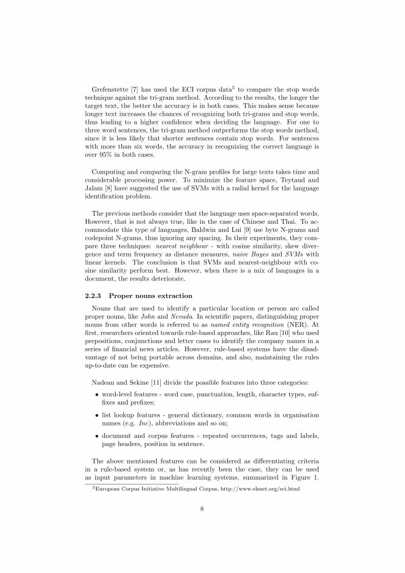
The above mentioned features can be considered as differentiating criteriain a rule-based system or, as has recently been the case, they can be usedas input parameters in machine learning systems, summarized in Figure 1.
5European Corpus Initiative Multilingual Corpus, http://www.elsnet.org/eci.html
8
Figure 1: NER learning techniques.
Bikel et al. [12] apply a vari-ant of the hidden Markov models onthe MUC-66 dataset and obtain over90% precision for English and Span-ish. Sekine [13] labels named entitiesfrom Japanese texts using C4.5 de-cision trees, dictionaries and a part-of-speech tagger. More recently, butfor the same problem, Asahara andMatsumoto [14] have chosen to use aSVM-based classifier, with character-level features as input (position ofcharacter within the word, charactertype, part-of-speech obtained froma morphological analyser), thus cor-rectly identifying more than threequarters of the named entities presentin the test documents. Conditionalrandom fields (CRF) are a generalizedform of hidden Markov models, allowing powerful feature functions which canrefer not only to previously observed words, but to any input word combination.Combining CRFs with a vast lexicon obtained by scouring the Web, McCallumand Li [15] have obtained decent results on documents written in English andGerman.
Even though supervised learning dominates the research done in this field,the disadvantage is that it requires a labelled training set which is often notavailable, or not large enough. In such cases, semi-supervised and unsupervisedapproaches have been investigated, where extrapolation and clustering are themain techniques.
At Google, Pasca et al. [16] attempt to generalize the extraction of factualknowledge using patterns. The tests are executed on 300 million Web pageswritten in English, which have been stripped from HTML tags and then splitinto sentences. In their experiments, they start from 10 seed items in the form(Bob Dylan, 1941), representing the year a person is born in. From the sen-tences which contain one of the input facts, basic patterns are extracted in theform (Prefix, Infix, Postfix). Using pre-computed word classes (e.g. names ofmonths, jobs, nationalities), the patterns are modified into more general onesand duplicates are removed. Using the obtained patterns, more candidate seedsare extracted and the top results are added to the initial seed set for a newiteration. With this method, more than 90% of the 1 million extracted factshave the full name and the accurate year.
A problem is establishing the boundaries of named entities, especially difficultin the case of book and movie titles which do not contain proper names, like
6The 6th Message Understanding Conference, http://cs.nyu.edu/faculty/grishman/muc6.html
9
The Good, The Bad and The Ugly. Downey et al. [17] employ an unsupervisedlearning method: they assume that all contiguous sequences of capitalized wordsare named entities if they appear in the same formation often enough in thedocument. The method requires a large corpus for the results to be relevant,but the data does not have to be annotated, so this condition can be easilyfulfilled.
Instead of using only one classifier, Saha and Ekbal [18] leverage between thedecisions from multiple NER systems mentioned above, so as to achieve a betterprecision. The classifier ensemble was tested on documents in Bengali, Hindiand Telugu and according to the results, associating weights to each classifier ismore effective than a voting scheme.
2.2.4 Feature selection
There are many text comparison techniques encountered in the research donein various NLP sub-fields. It is important to note that, the more features thedecision algorithm has to consider, the more computation power is needed. Also,it may be the case that the algorithm requires independent features, like thenaive Bayes classifier, and with a high number of features, it is unlikely thatthere are no dependencies among them. So, having a large number of similar-ity metrics means that we need to consider dimensionality reduction either byselecting the most relevant, or finding a way to combine several features intoone without information loss. We define Fk×N as the input dataset, wherek is the number of features, and N is the number of samples. The purpose offeature reduction is to reduce k, even N if possible.
Usually in text classification tasks, the features are the words composing thedocuments, thus the feature space can reach a high dimensionality, a high k. Insuch cases, there are several techniques that can be used, as described by Tascıand Gungor [19]. These techniques are based on statistics such as informationgain, document frequency, chi-square7. Dasgupta et al. [20] propose a differentalgorithm which assigns weights to features, depending on the results obtainedwhen the classification algorithm is run with various smaller sets of features.
Principal component analysis (PCA) [21, chap. 1, 4] is another way to reducedimensionality while preserving as much as possible of the original information,with focus on the variance. The process involves computing the covariance ma-trix of the data, identifying the eigenvalues and the corresponding eigenvectors,which are then orthogonalized and normalized. The vectors obtained are theso-called principal components of the dataset, they can be considered a sum-mary of the input dataset. A method less computationally expensive is randomprojection (RP) [22], which involves generating a random matrix Rd×k, d � kand multiplying it with Fk×N , thus lowering the number of features while main-taining the distance between the samples.
7Independence test between two random variables.
10
Choosing the right features has a significant influence on how a learning al-gorithm works. Having too many features, or irrelevant ones, can lead not onlyto an increased complexity, but also to a tendency to overfit. Overfitting occurswhen the learning algorithm attempts to match the training data as close aspossible, which results in a poor generalisation of the data and so, to a poorperformance on the test data. It is also important that the training data hasa balanced number of samples for each feature in order to minimize the risk ofoverfitting.
2.3 Blocking techniques
Given 2 sets of records, S1 and S2, there are |S1| ∗ |S2| possible record pairsto evaluate. Or if the task is to remove the duplicates from S1, then there are|S1|2 ∗ (|S1| − 1) possible pairs. For each of these pairs, the similarities array
has to be computed. Regardless of the decision model used, this computationis the most time and resource consuming from the entire reconciliation process,especially problematic when dealing with large record sets. That is why usuallya filter method is used to reduce the number of pairs that need to be evaluated.
Standard blocking is an intuitive method where the filtering is done by certainkey fields. For instance, in personal profile records, key fields could be consideredthe first and last name. The records that have exactly the same value, or avalue within an accepted error boundary, are selected. These key fields shouldbe chosen so that the resulting selection is not too small that is does not containthe matches, nor too large that the evaluation of candidate pairs still takes toolong. Sorted neighbourhood is a variant of standard blocking, except that therecords are first sorted by the key fields, and then from among w consecutiverecords, candidate pairs are generated. This window is then moved to the nextrecords in the list and the process is repeated. However, true matches may beskipped if more than w records match a key field value, so this parameter shouldbe chosen carefully.
Bi-gram indexing, or more general, k-gram indexing, is another blocking tech-nique more suitable for phrases, especially when the phrases contain commonwords, and for incomplete or incorrectly-spelled queries. The query terms aresplit into a list of k-grams8. A number of permutations are generated fromthese k-grams, and then inserted into an inverted index. A record containingthe initial query term will be added to all the keys of the inverted index. Takingthe records in this index two by two, we obtain our list of candidate pairs. Withthis method, more candidate pairs will be evaluated than in standard block-ing. Canopy clustering with TF/IDF splits the entire dataset by taking randomseed records and grouping them with their nearest neighbours in terms of theirTF/IDF9 distance metric. Once a record has been included into a group, it willno longer participate in the selection process.
8K-gram - a series of k consecutive characters in a word or phrase.9TF/IDF - a numerical measure indicating the relevance of a word in a document relative
to the collection of documents to which it belongs. A high word frequency in a documentis balanced out by the overall collection frequency, thus giving an informed estimate of theword’s significance.
11
Baxter et al. [23] have studied the effects in results quality of the blockingtechniques we have presented previously. They compare the classical methods(standard blocking and sorted neighbourhood), to the newer ones: bi-gram in-dexing and TF/IDF clustering. They have used as dataset a mailing list createdautomatically using specialized software, ensuring that each email instance hasat least one duplicate. This allows them to accurately measure the performanceof each algorithm in terms of precision and computation reduction. Accordingto their experiments, with certain parameter adjustments, bi-gram indexing andTF/IDF indexing perform better than the classical methods. It remains to beseen whether the same improvements occur with a real-world dataset as well.
McCallum et al. [24] study the clustering of large data sets with the practi-cal application tested on a set bibliographic references from computer sciencepapers. Their goal is to identify the citations referring to the same paper. Theapproach they have chosen has points in common with the TF/IDF clustering,but it is slightly more complex, requiring two steps:
• first, the dataset is divided into overlapping groups, also called canopies,according to a computationally cheap distance measure. Note that herethe groups can have elements in common, and the distance measure is com-puted between all possible data point pairs, unlike in the Baxter canopymethod;
• secondly, a traditional clustering approach (e.g. k-means), with a moreexpensive distance metric (e.g. string edit distance) is used to identifythe duplicates within a canopy. The computational effort is reduced be-cause no comparisons are made between elements belonging to completelydifferent canopies.
To create the canopies, two distance thresholds are used, T1, T2 with T1 > T2. Apoint X from the dataset is selected, the distance to all the others is computed,and the first canopy contains the points within T1 radius from X. The closestpoints to X, those within T2 radius, are removed from the dataset. The process isrepeated until the dataset is empty. This model can be adapted to be employedas a hierarchical filter, if we adjust the second step and just use it as a modalityto further split and decrease the search space.
2.4 Reconciliation approaches
2.4.1 Rule-based approaches
If all the data was clearly and uniquely labelled, reconciliation would only bea matter of matching equivalent identifiers and merging the information. Forinstance, the Jinni10 movie descriptions can be easily matched to the corre-sponding IMDb page since they contain the IMDb id. However, this is just ahappy coincidence. Often there is missing or incorrect information and morecomplex techniques are required to find the right correspondences.
Deterministic linking is a straightforward method, also referred to as rule-based linking. It performs best when the sets to be reconciled have characteris-tics in common that can be used to compare two records. A pair is considered
10Jinni - a movie recommendations engine, http://www.jinni.com
12
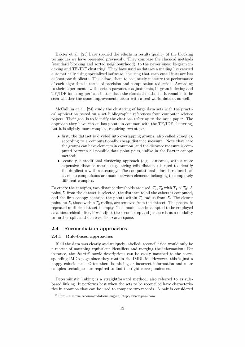
Figure 2: Example of linking thresholds. Assuming a number of P com-parison methods which return a value in the [0, 1] interval and a unitary weightvector, pair records with a similarities array sum lower than P
4 are classified as
a non-match. If the sum is higher than 3P4 , then the pair is considered a match.
Otherwise, it cannot be said whether the record pair is a match or not. Imageadapted from [25].
a match if all or a certain subset of characteristics correspond. With this typeof algorithm, the result is dichotomous: either there is a match or not.
In the case of probabilistic linking, weights are associated to the elements ofthe similarities array. Each element will have a different degree of influence onthe final output. The values in the similarities array are proportioned to the as-signed weight, summed and then, according to a threshold, the pair is classifiedas a match or as a mismatch. If two thresholds are used, then another classi-fication is possible: possible match, as we can see in the example in Figure 2.With probabilistic linking, we obtain not just a classification, but the likelihoodof that classification, which allows adjusting the thresholds according to what isthe main interest of the user: increasing the amount of true matches identifiedor decreasing the amount of false links.
The weights in probabilistic linking are computed as a function of the ac-tual data, using either a simple three-step iterative process: apply the rules,evaluate the results, refine the weights and/or thresholds, or more complexmethods based on statistic models like maximum likelihood estimation. As op-posed to that, in deterministic linking, the discriminative criteria have beenpre-determined, based on domain knowledge, not on the available data.
The Link King11 is a public domain software used for linking and removingduplicates from administrative datasets. It provides the users with the optionto choose which algorithm fits them best. With deterministic linking, the usersdefine which combination of fields must match, and whether partial matchesare acceptable or not. The probabilistic algorithm relies on research done byWhalen et al. [26] for the Substance Abuse and Mental Health Services Admin-istration’s (SAMHSA) Integrated Database Project. In their study, the priorprobabilities needed to compute the weights are calculated on a dataset obtainedusing deterministic rules. Also, to each field value, a scale factor is associatedto express the impact of agreement on a certain variable e.g. name agreementon ’Smith’ is not as important as name agreement on ’Henderson’.
These two linking approaches, deterministic and probabilistic, have been com-pared on a dataset containing patient information, so fields such as date of birth,postcode, gender and hospital code [27]. Using the number of false matches and
11The Link King, http://www.the-link-king.com/
13
false mismatches as an evaluation criteria, the authors show that in datasetswith noticeable error rates (amount of typing errors), the probabilistic approachclearly outperforms the deterministic one. With very small error rates in thedataset, both techniques have similar results. The deterministic method sim-ply does not have enough discriminating power, while using the probabilis-tic method, the weights of each variable are fitted according to the availabledataset. The probabilistic strategy works better, but there is a price to pay:higher complexity, thus longer computation times.
In account reconciliation, Chew and Robinson [28] use a more complex ap-proach, which combines deterministic and probabilistic techniques, in order tomatch receipts to disbursements. These records consist of date, description andamount, so the key information in the description must be identified in orderto find the correct pairs. First, the terms from each description are ranked ac-cording to their distinctiveness using the PMI measure12. Then, the Pearsonproduct-moment correlation coefficient13 is computed on the term PMI vectorsfor each transaction pair and if the value is high enough, the pair is declared amatch. For their particular set of data containing tens of thousands of transac-tions, they obtain near perfect precision and recall. However, it should be notedthat one-to-many and many-to-many matches have not been dealt with in thispaper.
As we have seen, the rules-based approach is relatively simple and easy tounderstand. Moreover, there is no need for labelled data, since no training isrequired. However, it has several disadvantages: the rules can become exceed-ingly complex and thus difficult to maintain. Also, the rules are specific to onedataset and cannot be migrated to another application.
2.4.2 Graph-oriented approaches
Movies are connected to each other through cast, crew, sometimes even char-acters in the case of prequels/sequels. We could organize the available infor-mation in the form of a graph and apply graph-related algorithms in order toidentify which nodes we can join together, thus making use of the connectionsbetween the entities, rather than just characteristic similarities.
This type of approach has been used to identify aliases belonging to thesame person by analysing the content posted by those aliases. Modelling socialnetworks and trying to map the nodes to each other across multiple networks issimilar to the graph isomorphism problem. Unfortunately, no efficient algorithmhas been found yet for this problem for all types of graphs [29]. However, insocial graphs, we do not expect an exact mapping and some of the work hasalready been done by the users who link their accounts.
Graph algorithms are based on the topology of the network, like the oneproposed by Narayanan and Shmatikov [30]: the algorithm starts from seed
12Pointwise Mutual Information - indicates how likely is a term to occur in a document.13Pearson product-moment correlation coefficient - index used in statistics as a measure of
the linear dependence between two variables.
14
nodes, which are known in both the anonymous target graph and in the graphcontaining the auxiliary information, and maps them accordingly. The next stepis the propagation phase, in which the mapping obtained previously is extendedby relying on the topology of the network. The propagation is an incrementalprocess which takes place until the entire graph has been explored.
Yartseva and Grossglauser [31] suggest a different approach based on perco-lation theory, the study of clusters in random graphs. It works by matchingtwo nodes if those nodes already have a certain number of neighbours alreadymatched (controlled by a parameter r). Besides the algorithm itself, they alsoshow how to compute the optimal size for the initial set based on the networkparameters and r. The algorithm works like this: for each vertex, a count iskept. Each round a pair we know is correctly matched is chosen, and the countfor each of the neighbours is increased. Then a vertex whose count is bigger thanr is chosen and added to the list of matched pairs. This process is continueduntil there are no more changes.
Korula and Lattanzi’s algorithm [32] combines both techniques. Initially, ac-cording to the available information, nodes are linked with certain probabilities.Like in percolation graph matching, for each vertex, a count of the matchedneighbours is kept. Each round, the two nodes with the highest count in eachof the graphs are matched. To improve the error rate, nodes with higher degreeare preferred. More specifically, each round, only nodes with degree > D
2i canbe matched, where D is highest degree in the graph, and i the round number.So the degrees of the nodes allowed to be matched decrease as the algorithmprogresses.
2.4.3 Machine learning oriented approaches
Machine learning oriented approaches require training data. However, it ispossible that training data is not available or is in insufficient quantity and dif-ficult to produce. Christen [33][25] proposes a way to automatically generatetraining data, without human supervision. The algorithm relies on the assump-tion that two records that have only high similarity values refer to the sameentity, and the opposite in the case of low similarity values. So these two typesof records are selected, then used as training set for a supervised algorithm sothat the most likely matches computed can be appended to the training set.The selection can be made using thresholds, but better results were obtainedwith a nearest-based criterion: only the weight vectors closest in terms of Man-hattan distance14 to the ideal match, respectively mismatch vector are chosen.In their experiments, this approach outperforms using an unsupervised k-meansalgorithm.
In machine learning, the first and simplest algorithms taught are variationson Nearest Neighbour, like k-NN. This is what researchers call a lazy learner : itstores in memory the entire training dataset, and every time a query to classifyan instance is run, it iterates through the entire dataset to reach a decision.
14Manhattan distance - also known as taxicab metric, it is the sum of absolute differencesbetween two vectors.
15
On the other hand, eager learner algorithms try to fit the dataset to a model,thus not being necessary to retain in memory the initial dataset. Also, theclassification process is much faster since it is not required to evaluate eachentry in the training set for every query. Examples of eager learner approachesinclude naive Bayes, neural networks and decision trees.
Naive Bayes
A model widely used in text classification is naive Bayes [44, Ch. 4]. In allBayes-derived methods, the following theorem is crucial:
P (A|B) =P (B|A)P (A)
P (B)
, which shows how to compute the posterior probability of an event A, knowingthat event B took place, in terms of the likelihood of event B given event A, theprior probability of event A and the evidence of event B.
The theorem can be generalized, since the evidence can refer to several fea-tures, not just one:
P (A|B1, B2, ..., Bn) =P (B1, B2, ..., Bn|A)P (A)
P (B1, B2, ..., Bn)
Naive Bayes is a probabilistic model that makes the assumption that thesefeatures are independent. This assumption is made in order to simplify thecomputation of the denominator, bringing it to the form:
P (A|B1, B2, ..., Bn) =P (A)
∏ni=1 P (Bi|A)
P (B1, B2, ..., Bn)
The event priors and the likelihoods for each feature are computed based onthe training set, generally assuming a Gaussian distribution of the samples.
P (Bi|A = a) =1√
2πσ2a
exp
(− (Bi − µa)2
2σ2a
), where µa - the mean of the samples belonging to event a, and σa - the standarddeviation.
To find which event A has occurred, given the feature vector B, maximumlikelihood estimates are used. The probabilities for every possible event A arecomputed, and the largest one is chosen:
arg maxa
P (A = a)
n∏i=1
P (Bi|A = a)
The advantages of naive Bayes lie in its simplicity and its scalability to largenumber of features. The algorithm is known for being a decent classifier, espe-cially in spam filtering, but the computed probabilities do not necessarily reflectthe reality [34]. Also, the independence assumption is often not quite accurate.Moreover, a Gaussian distribution may not reflect how the data looks like, whichin turn may lead to errors in parameter estimation.
16
In the legal domain, Dozier et al. [35] have applied the Bayes theory in orderto create a database of expert witnesses profiles by gathering data from severalsources. To merge the duplicates, 6 pieces of evidence are used to asses thematch probability between two profiles. These pieces of evidence are the resultsof the comparison between the various profile fields, such as name, location,area of expertise. In this scenario, the variables obtained are considered, andare indeed, independent. The comparison yields only five possible results: ex-act, strong fuzzy, weak fuzzy, mismatch, unknown - for missing information.The probability that two profiles are a match given the evidence is computedaccording to the Bayes equation. The prior probabilities are given values basedon estimates from experience and observation. To obtain the conditional prob-abilities, a manually created subset of profiles and the corresponding pairs hasbeen created.
Decision Trees
In a decision tree [44, Ch. 6], each internal node represents a decision point,and each leaf represents a class or an event or a final decision. Given the input,the tree is traversed starting from the root. At each internal node, a methodevaluates the input and decides which branch will be followed next. The methodcan be a simple comparison of an input field with a fixed value, or it can bea more complex function, not necessarily linear, taking several parameters intoaccount. If a leaf node has been reached, then the input sample that reachedthe node is associated its label.
The trees can be created manually, method very close to the rule estimation,since a path from root to leaf represents a rule. Or they can be created au-tomatically, based on a training set. To be noted that not all attributes mustnecessarily take part in the decision process, some may be considered irrelevantby the tree creation algorithm. To create a tree, the training set is evaluated andthe feature considered to have the most discriminative power is chosen for thedecision at root level. Then the set is split, and the process is repeated for eachof the new nodes until there are no more splits possible, meaning all samples ina subset belong to the same class. This is known as the ID3 algorithm [36], butit has some limitations which are addressed by the C4.5 algorithm [37]:
• ID3 deals only with discrete attributes. C4.5 can process continuous at-tributes using thresholds to create value intervals;
• C4.5 accepts data with missing attribute values - if the sample set has novalues for the attribute checked by an internal node, that node becomes aleaf with the label of the most frequent class;
• ID3 does not guarantee the creation of the smallest possible tree. Thus,after the tree has been created, C4.5 prunes it by removing redundantbranches and turns them into leafs.
If the created tree does not classify the data well enough, a subset of the sampleswhich have been misclassified can be added to the training set and the processis repeated until we obtain a satisfactory tree.
17
To determine which attribute to use as set division criterion, we need to sortthe attributes by their power to distinguish samples. In order to do that, firstwe quantify the impurity or the entropy of the data. The entropy of a datasetS is a numerical indicator of the diversity of S and is defined mathematically:
Entropy(S) = −∑i
pi log2 pi
, where pi is the proportion of samples belonging to class i. In a binary clas-sification problem, an entropy of 1 means that the samples are equally dividedbetween the two classes. When the set is partitioned by the attribute, we expecta reduction in the impurity of the subsets. Logically, we choose the attribute Awith the highest such reduction, also referred to as information gain:
Gain(S,A) = Entropy(S)−∑
k∈values(A)
|Sk||S|
Entropy(Sk)
, where Sk is the subset of samples with value k for attribute A. Another setdiversity indicator that can be used is the Gini impurity [38]:
Gini(S) =∑i
pi(1− pi)
With Gini splits, the goal is to have nodes with samples belonging to the sameclass, while entropy attempts to divide the sample set equally between the childnodes.
The worst case scenario is when each sample reaches a different leaf, meaningthat there as many leaves as there are samples. This is a clear example of over-fitting. If it is not controlled, the tree can become extremely large, leading to adeterioration of the results. Possible solutions are tree pruning and limiting howmuch the tree can grow. For pruning, each internal node in turn is considered aleaf (with the dominant class as label) and if the new tree is just as reliable asthe initial one on a validation set, then the node remains a leaf. However, thisis a costly operation since it requires the evaluation of multiple trees.
Decision trees have proven to be effective as part of a system designed toidentify record duplicates in a dataset containing student and university staffinformation [39]. The records hold information such as first and last name,home address and telephone number. The authors of the paper have used anerror and duplicate generating software to render the dataset unreliable. Toidentify the duplicates, a 4-step process is proposed:
• clean the data and convert it to a standard format;• sort the records according to a pre-determined attribute. Domain specific
information is required here. Using a sliding window, generate pairs ofmatch candidate record pairs;
• apply on the candidate pairs a clustering algorithm to split the pairs intomatches and mismatches;
• use the previously obtained labelled data as training set to create a deci-sion tree, then prune it if necessary.
By combining clustering and classification procedures, they have identified 98%of the duplicates.
18
SVMs
A Support Vector Machine (SVM) [40] is a supervised binary classificationtechnique. Its origins lie with the maximal margin classifier, which improved,became the support vector classifier, which was further extended to the supportvector machine.
A hyperplane is a p dimensional subspace splitting a space one dimensionhigher. The hyperplane is defined as:
β0 + β1X1 + ...+ βpXp = 0
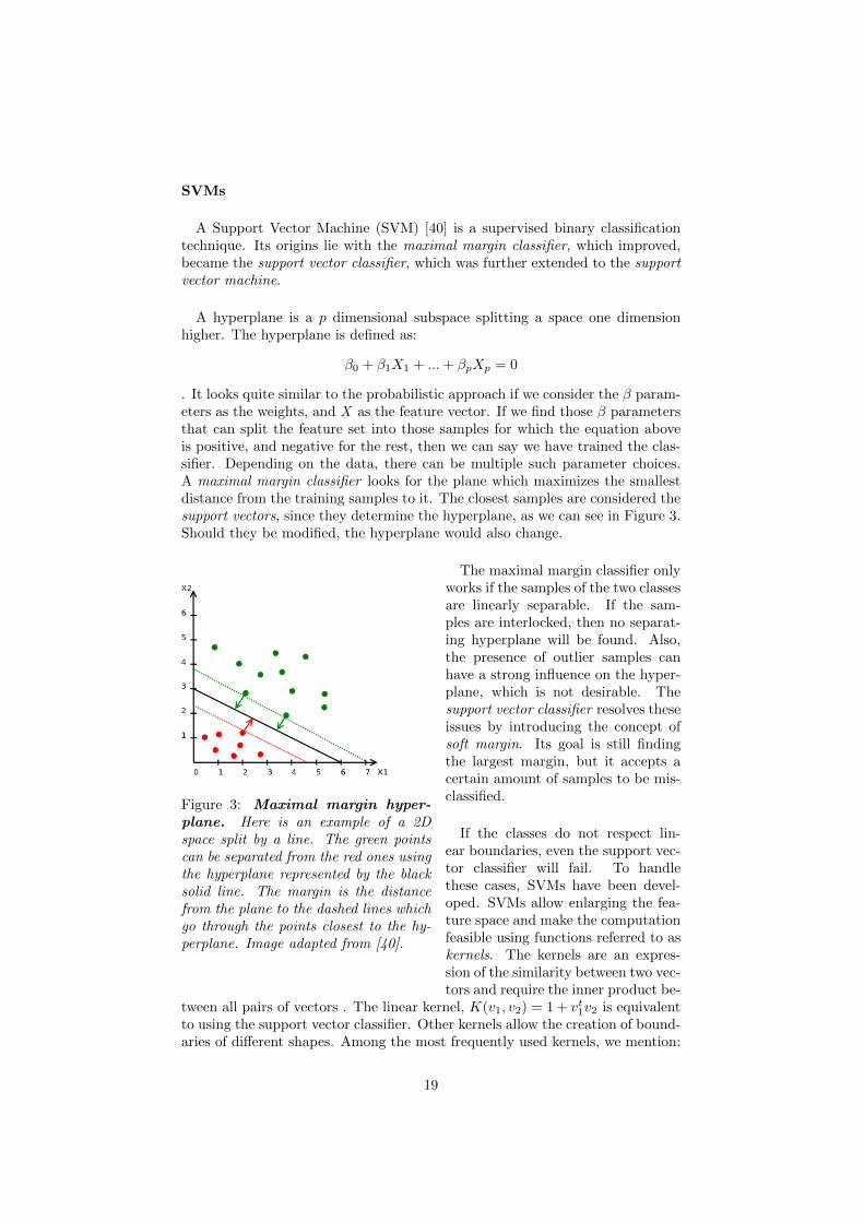
. It looks quite similar to the probabilistic approach if we consider the β param-eters as the weights, and X as the feature vector. If we find those β parametersthat can split the feature set into those samples for which the equation aboveis positive, and negative for the rest, then we can say we have trained the clas-sifier. Depending on the data, there can be multiple such parameter choices.A maximal margin classifier looks for the plane which maximizes the smallestdistance from the training samples to it. The closest samples are considered thesupport vectors, since they determine the hyperplane, as we can see in Figure 3.Should they be modified, the hyperplane would also change.
Figure 3: Maximal margin hyper-plane. Here is an example of a 2Dspace split by a line. The green pointscan be separated from the red ones usingthe hyperplane represented by the blacksolid line. The margin is the distancefrom the plane to the dashed lines whichgo through the points closest to the hy-perplane. Image adapted from [40].
The maximal margin classifier onlyworks if the samples of the two classesare linearly separable. If the sam-ples are interlocked, then no separat-ing hyperplane will be found. Also,the presence of outlier samples canhave a strong influence on the hyper-plane, which is not desirable. Thesupport vector classifier resolves theseissues by introducing the concept ofsoft margin. Its goal is still findingthe largest margin, but it accepts acertain amount of samples to be mis-classified.
If the classes do not respect lin-ear boundaries, even the support vec-tor classifier will fail. To handlethese cases, SVMs have been devel-oped. SVMs allow enlarging the fea-ture space and make the computationfeasible using functions referred to askernels. The kernels are an expres-sion of the similarity between two vec-tors and require the inner product be-
tween all pairs of vectors . The linear kernel, K(v1, v2) = 1 + vt1v2 is equivalentto using the support vector classifier. Other kernels allow the creation of bound-aries of different shapes. Among the most frequently used kernels, we mention:
19
• the polynomial kernel: K(v1, v2) = (vt1v2 + 1)d, where d - the degree ofthe polynomial;
• the radial basis function kernel (RBF): K(v1, v2) = exp(− 〈v1,v2〉
2
2σ2
), where
σ - tuning parameter, 〈v1, v2〉 - the Euclidean distance between two vec-tors;
• the sigmoid kernel: K(v1, v2) = tanh(γ〈v1, v2〉+r), where γ and r - tuningparameters.
SVMs have been employed in a wide range of applications, including duplicatedetection. Su et al. [41] tackle the problem of removing duplicate records fromquery results over multiple Web databases. Since the records from one sourcetypically have the same format, first duplicates from one set are removed. Then,this set is used for the training of two classifiers, a SVM with a linear kernel anda probabilistic linker. The results obtained when applying the trained classifierson the data are added to the training set and the process is repeated untilno more duplicates are found. They have chosen the SVM because it workswell with a limited amount of training samples and it is not sensitive to thepositive/negative samples ratio. The advantage of the proposed technique isthat it does not require manually verified labelled data. The authors report aperformance similar to the one of other supervised techniques when applied ondatasets with information about paper citations, books, hotels and movies.
Another example of SVM usage is the work of Bilenko and Mooney [42], whogo beyond the standard string edit distance and cosine similarity. Depending onthe domain, the relevancy of the string similarities can be improved by takinginto account sensible domain characteristics. For example, the noun ”street”is not as important when comparing addresses as it is when comparing peoplenames. So, to escape the deficiencies of the standard comparison methods,they train two classifiers, one using expectation-maximization for shorter stringsbased on character-level features, and an SVM for longer strings with the vector-space model of the text as input.
Neural Networks
Even though it is still not entirely clear how the human brain works, whatwe do know is that the electrical signals travel along paths formed betweenneurons, and depending on the experiences of each person, some paths are moretravelled than others, some things are more familiar to us than others. Attemptsto emulate this process have lead to the emergence of artificial neural networks,ANNs [43]. They are considered simplified versions of the brain, partly due to alack of understanding of the brain, partly due to a lack of computation power.
A neural network consists of simple processing elements called neurons, con-nected to each other through links characterized by weights. The neurons workin a parallel and distributed fashion. They learn by automatically adjusting theweights. An ANN is characterized by:
• learning method - supervised, unsupervised, reinforcement ;
20
• direction of information flow:
– feed-forward networks - information flows one way only;
– feedback networks - information flows both ways.
• weight update methods - usually a form of gradient descent with errorbackpropagation;
• activation function - most common being the step and sigmoid functions;
• number of layers and neurons per layer.
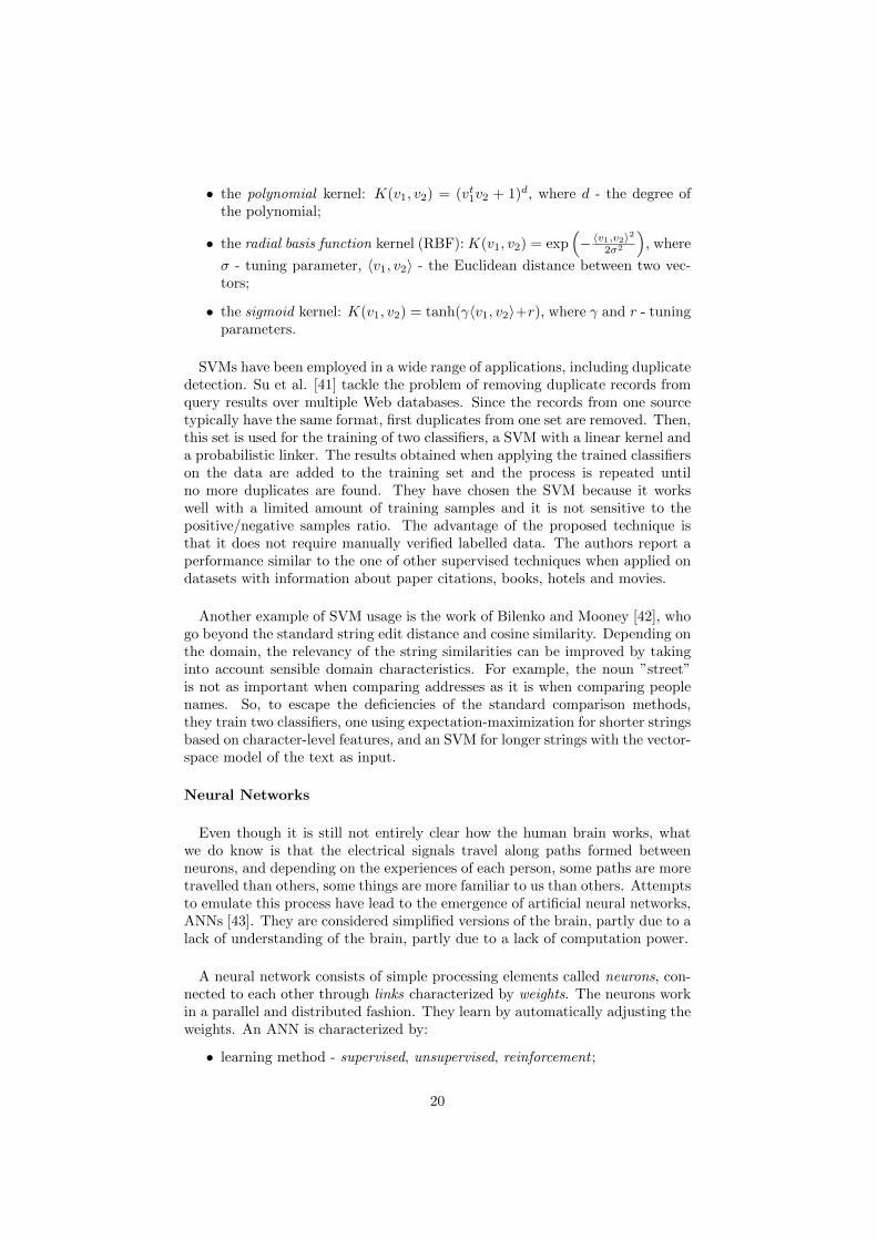
Figure 4: Basic neural networkmodel. The neuron shown here hasa bias value of t and P incoming con-nections, associated to the wPy weights.Image adapted from [44, Ch. 7.3].
In Figure 4 we have represented thebasic form of the neural network, alsoknown as a perceptron, which takes Pinputs and returns one value as out-put, y. The output is computed ac-cording to the following equation:
y(θ) = f
(P∑i=1
wPyiθi + t
), where t is the bias value, and f isthe activation function. Usually, fora more concise expression, the bias isincluded in the sum by adding an ex-tra input, θ0 = 1 and prepending thebias to the weight vector:
y(θ) = f
(P∑i=0
wPyiθi
).
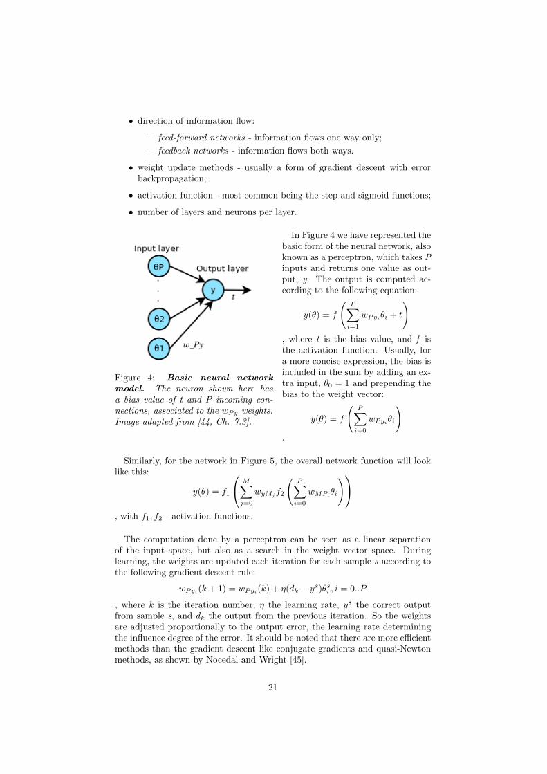
Similarly, for the network in Figure 5, the overall network function will looklike this:
y(θ) = f1
M∑j=0
wyMjf2
(P∑i=0
wMPiθi
), with f1, f2 - activation functions.
The computation done by a perceptron can be seen as a linear separationof the input space, but also as a search in the weight vector space. Duringlearning, the weights are updated each iteration for each sample s according tothe following gradient descent rule:
wPyi(k + 1) = wPyi(k) + η(dk − ys)θsi , i = 0..P
, where k is the iteration number, η the learning rate, ys the correct outputfrom sample s, and dk the output from the previous iteration. So the weightsare adjusted proportionally to the output error, the learning rate determiningthe influence degree of the error. It should be noted that there are more efficientmethods than the gradient descent like conjugate gradients and quasi-Newtonmethods, as shown by Nocedal and Wright [45].
21
Figure 5: Neural network with one hidden layer. The feed-forward networkin this example consists of P input features, 1 hidden layer with M neurons and1 output value. The θ0 and h0 neurons are used as threshold equivalents. wMP
and wyM represent the vectors of computed weights. Image adapted from [43].
Neural networks have been applied to the problem of identifying the fieldswhich represent the same information across several different databases (at-tribute correspondences) [46]. As input, schema information (column names,data types, constraints) and statistics obtained from the database content areused. All this information needs to be converted to a numerical format. Thereare transformations depending on the type of fields. For example, binary valuesare converted to 0/1, numerical values are normalized to the [0..1] range usinga sigmoid function (not a linear transformation in order to avoid false matchesand false drops), and for string fields, statistics such as field length are used.The reconciliation algorithm proposed follows these steps:
• parse information obtained from database;• apply classifier to decide which fields in a database represent the same
information, so that when the neural network is applied, a field in databaseX is not mapped to two fields in database Y. Moreover, it leads to lowerrunning time and reduced complexity for the neural network;
• use a neural network to learn which fields across multiple databases rep-resent the same information.
Another example of neural networks in reconciliation problems is their ap-plication in enterprise resource planning (ERP) to find duplicate records [47],occurrences due to the lack of unique identifiers. Instead of relying on stringcomparisons to determine record similarities, the authors use a semantic ap-proach instead. Vectors containing discriminating keywords are deduced fromthe records, and then a neural network establishes the similarity degree. Theyshow superior results to other methods based on computing string edit distancesdifferences.
22
2.5 Movie-context related work
For ontologies reconciliation, Huang et al. [48] propose an algorithm whichleverages techniques from the rule-based and learning-based approaches. Boththese approaches have their own disadvantages: rule-based algorithms are fast,but the rules are set in stone. They do not adapt to changes in data, and morethan that, the rules do not always take into consideration all the relevant dis-criminative factors. Learning-based algorithms are slower and may need largequantities of learning data. An ontology is considered to have the followingcomponents: name, properties and relationships. These aspects will form thediscriminant criteria for the proposed algorithm, Superconcept Formation Sys-tem (SFS). SFS uses a three neuron network, one neuron for each of the threecomponent of an ontology concept. Initial weights are assigned to each neuronand then gradient descent is used to update the rules, based on the trainingsamples. The input data for the neurons represents the results from similarityfunctions for each ontology concept aspect. To evaluate their algorithm, theytake two real world ontologies and compare their result with that of humanexperts and report to have identified 85% correct predictions.
LinkedMDB15 is a project aiming to connect several databases with infor-mation pertaining to the film universe. It uses several web pages like Freebaseand IMDb, as sources for movie information, information which is enriched bylinking it to other pages such as DBpedia/YAGO for persons, MusicBrainz forsoundtracks, Flickr for movie posters. The links are automatically generatedusing string matching algorithms: Jaccard, Levenshtein, HMM and not only.The tuples obtained are stored using the RDF model for clarity and ease ofcomprehension. Hassanzadeh and Consens [49] report the weighted Jaccardsimilarity16 as the edit distance to provide the highest number of correct links.Choosing a threshold to determine when the similarity score is high enough andthe link is deemed as valid, is a compromise between the amount of discoveredlinks and the how many of them are correct. However, it must be noted thatbecause of data copyright issues and crawling limitations, only 40k movie en-tities are processed and 10k links to DBpedia/YAGO are discovered with 95%confidence.
15Linked Movie Database, http://linkedmdb.org16Weighted Jaccard similarity - a measure of the amount of common N-grams between two
documents, taking into account the frequency of the N-grams.
23
3 Practical Application in Movies Domain
”Simplicity is prerequisite forreliability.”
Edsger Dijkstra
3.1 Application requirements
Given a set of records containing movie-related information, we want to grouptogether those records that refer to the same movie instance. We are going toachieve this in a pairwise fashion, comparing the records two by two and checkingif they describe two different movies or not.
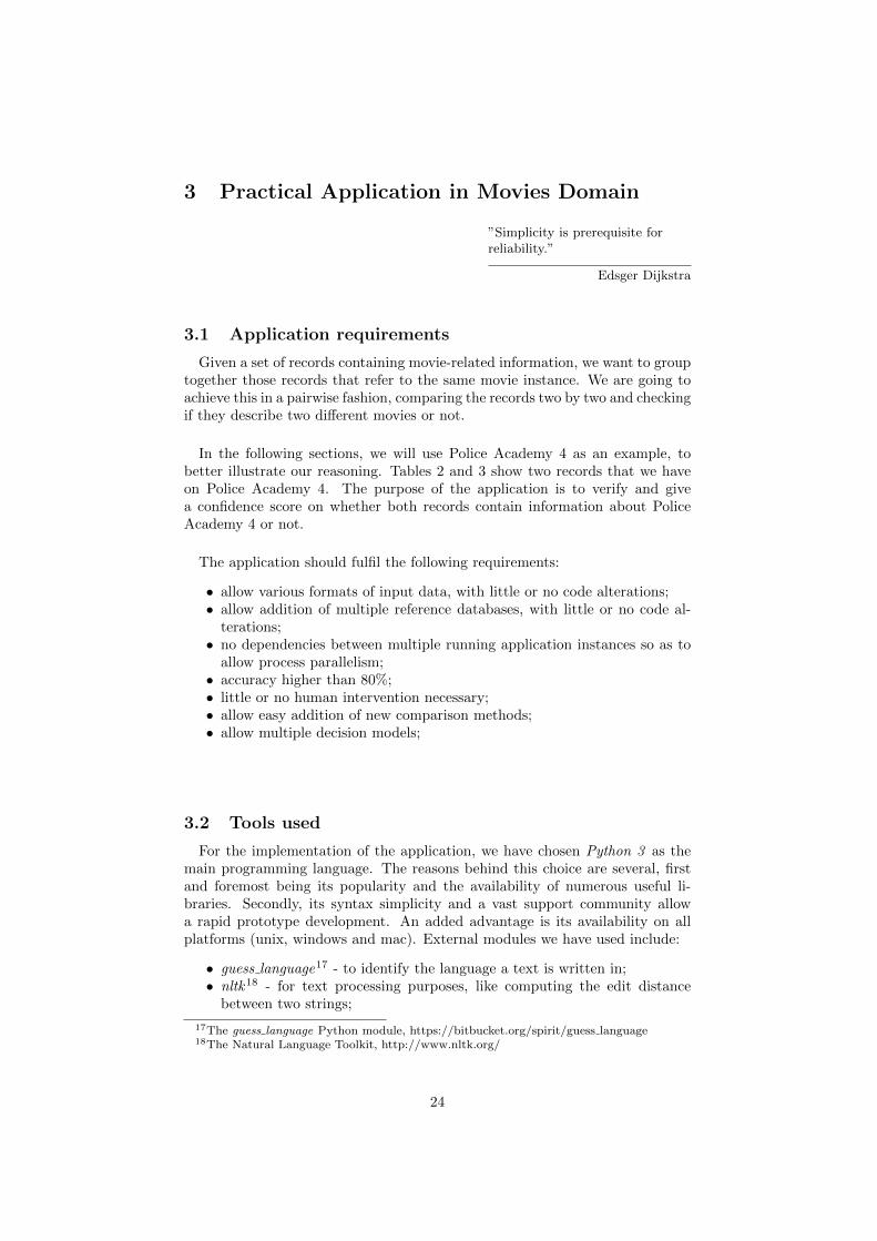
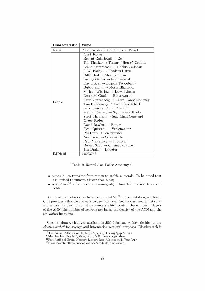
In the following sections, we will use Police Academy 4 as an example, tobetter illustrate our reasoning. Tables 2 and 3 show two records that we haveon Police Academy 4. The purpose of the application is to verify and givea confidence score on whether both records contain information about PoliceAcademy 4 or not.
The application should fulfil the following requirements:
• allow various formats of input data, with little or no code alterations;• allow addition of multiple reference databases, with little or no code al-
terations;• no dependencies between multiple running application instances so as to
allow process parallelism;• accuracy higher than 80%;• little or no human intervention necessary;• allow easy addition of new comparison methods;• allow multiple decision models;
3.2 Tools used
For the implementation of the application, we have chosen Python 3 as themain programming language. The reasons behind this choice are several, firstand foremost being its popularity and the availability of numerous useful li-braries. Secondly, its syntax simplicity and a vast support community allowa rapid prototype development. An added advantage is its availability on allplatforms (unix, windows and mac). External modules we have used include:
• guess language17 - to identify the language a text is written in;• nltk18 - for text processing purposes, like computing the edit distance
between two strings;
17The guess language Python module, https://bitbucket.org/spirit/guess language18The Natural Language Toolkit, http://www.nltk.org/
24
Characteristic Value
Name Police Academy 4: Citizens on Patrol
People
Cast RolesBobcat Goldthwait → ZedTab Thacker → Tommy ”House” ConklinLeslie Easterbrook → Debbie CallahanG.W. Bailey → Thadeus HarrisBillie Bird → Mrs. FeldmanGeorge Gaines → Eric LassardDavid Graf → Eugene TackleberryBubba Smith → Moses HightowerMichael Winslow → Larvell JonesDerek McGrath → ButterworthSteve Guttenberg → Cadet Carey MahoneyTim Kazurinsky → Cadet SweetchuckLance Kinsey → Lt. ProctorMarion Ramsey → Sgt. Lavern HooksScott Thomson → Sgt. Chad CopelandCrew RolesDavid Rawlins → EditorGene Quintano → ScreenwriterPat Proft → ScreenwriterNeal Israel → ScreenwriterPaul Maslansky → ProducerRobert Saad → CinematographerJim Drake → Director
IMDb id tt0093756
Table 2: Record 1 on Police Academy 4.
• roman19 - to translate from roman to arabic numerals. To be noted thatit is limited to numerals lower than 5000;
• scikit-learn20 - for machine learning algorithms like decision trees andSVMs;
For the neural network, we have used the FANN21 implementation, written inC. It provides a flexible and easy to use multilayer feed-forward neural network,and allows the user to adjust parameters which control the number of layersof the ANN, the number of neurons per layer, the density of the ANN and theactivation functions.
Since the data we had was available in JSON format, we have decided to useelasticsearch22 for storage and information retrieval purposes. Elasticsearch is
19The roman Python module, https://pypi.python.org/pypi/roman20Machine Learning in Python, http://scikit-learn.org/stable/21Fast Artificial Neural Network Library, http://leenissen.dk/fann/wp/22Elasticsearch, https://www.elastic.co/products/elasticsearch
25
Characteristic Value
Name Polisskolan 4: KvarterspatrullenYear 1987Length 5280Genres KomediDirectors Jim Drake
Actors
David GrafSteve GuttenbergMichael WinslowBubba Smith
Description Rektor Lassard pa Polisskolan har ett nytt projekt.Han vill trana ett antal civila frivilliga till att ingai sitt nya projekt for att halla ordning och reda isamhallet – kvarterspatrullen. Han tar in sina gamlaelever for att utfora uppgiften. Trots att projektethar starkt stod fran myndigheterna sa har den ri-valiserande kapten Harris hellre lust att se projektetmisslyckas. . .
Table 3: Record 2 on Police Academy 4.
a full-text search engine built on Apache Lucene23 for applications dealing withcomplex search queries and large amounts of data.
We will present more details on how all these tools have been used in thefollowing sections.
3.3 Datasets
3.3.1 Data formats
The datasets used in the experiments have been provided by the VionLabsteam. Like we mentioned before, rather than keeping them in text files in aJSON format, we have preferred to store them using elasticsearch.
We have worked with three datasets, each containing a different amount ofrecords:
• Dataset 1 - 324518 records with title, cast and crew information;• Dataset 2 - 86443 records with title, release year, and occasionally cast;• Dataset 3 - 178870 records with title, cast, description and other informa-
tion.
All the datasets contain unique identifiers, which has facilitated the evaluationphase of our work. We have used the first two datasets for reference information,and the third as the one to be reconciled. Note that not all records contain allthe information advertised, cast information or description or other fields may
23Apache Lucene - Java-based information retrieval library, https://lucene.apache.org/
26
be missing. Also, even though all the datasets respect the JSON format, theydo not use a consistent key name scheme from one set to another.
3.3.2 Extracted features
In our work context, features are ways of comparing the available movie in-formation. Depending on for which characteristics we have values, we may havemore or less comparison options. In our experiments, we have used the followingmethods:
• titles comparison;
• language recognition;
• proper nouns extraction from the plot description;
• actors and other people lists match;
• title numerals match;
• release year match.
To compare the titles, we have employed the Levenshtein distance. First weconvert both title strings to lowercase and remove any trailing blank characters.Then we compute the edit distance and divide it by the length of the longeststring, to get a value in the [0, 1] interval. By division, we make sure thecomparison with other pairs will be fair, regardless of absolute value of the editdistance. We want a high value to indicate a good match, so we return 1 minusthe previously obtained value. Thus, a value of 1 will indicate a perfect match,while 0 will indicate completely different strings.Example.
Title 1: ”Police Academy 4: Citizens on Patrol”Title 2: ”Polisskolan 4: Kvarterspatrullen”Levenshtein distance: 23Title comparison value: 0.361
According to this result, we have a low degree of similarity between the twotitles, even though we know that the titles refer to the same movie. Movie titlesare usually given alternatives, depending on the country they are playing in.This is the case here: since we have crawled the information from a Swedishwebsite, we get the Swedish version of the title. So, a movie may have differentnames, which is why the title match criteria alone is not enough to positivelyidentify whether two records represent the same movie.
For the language recognition, we have used the guess language Python pack-age. We have applied the language recognition methods on the title and plotdescription characteristics of the available records. If the strings given as param-eters are too short, we lengthen them by duplication. If one of the two stringsis empty or missing, we assume identical language and return 1. The packageworks by relying on tri-grams to identify a language. Knowing the language ofeach record is useful because it allows us to assign lower importance to the titlescomparison when we have records in different languages. If we have the samelanguage, we know to expect a high title similarity.
27
Example. We consider the movie titles in the previous example.Title 1 language: enTitle 2 language: svLanguage comparison value: 0
As we can see, we identify English for the first title, and Swedish for the secondone. This language difference explains the low title comparison value obtainedearlier.
One other feature is proper nouns match. We have extracted the proper nounsfrom the movie description and we have compared the obtained nouns with thepeople names listed as cast or crew. To accomplish this, we have used theNER system available in the nltk package. To identify named entities, the NERsystem uses a classifier trained on data from CoNLL24, MUC-6 and ACE25.Example. To compute the proper nouns match, we check how many of theidentified proper nouns can be found in the Crew Roles and Cast Roles lists.
Extracted proper nouns: Rektor, Lassard, Polisskolan, Harris.Proper nouns match: 0.5
The nouns Lassard and Harris can be found in the Cast Roles list, so we havea 50% match.
Another comparison we make is between the lists of people existing in the tworecords. We take each person listed in the unreconciled record, and check if thename is also listed in the other record. The more matches we find, the betterthe score. If in one of the records there are no people listed, then a score of 0is returned as an indicator that this feature should be ignored for this pair ofrecords. If a name from the unreconciled record is not found, the overall scoreis decreased.Example. In the case of Record 1 and Record 2, we have a 100% people match,since all the names listed in Record 1 can be found in Record 2.
A problem we encountered was that often we were matching a movie to oneof its sequels or prequels. In this case, the titles are similar, the cast and crewlists almost identical, so it is difficult to differentiate between the two. In orderto avoid this problem, we have added a comparison function which takes anynumerals it finds in the titles and checks if they are the same or not. Manymovies, like Rocky IV, use roman numerals to indicate the continuation of theseries. So, first we translate all numerals we find to arabic numbers, and thenwe compare them. If the titles are similar and there is a numeral mismatch,then we return a negative score. A positive score is returned otherwise, and 0if the titles do not contain any numeric values.Example. For Police Academy 4: Citizens on Patrol and Polisskolan 4: Kvarterspa-trullen, a score of 1 will be returned since both titles contain number 4.
The release year is an important piece of movie meta-data since it helpsdiscriminate between a remake and the original movie. The year comparisonmethod returns the absolute value of the difference between the release years ofthe two records. A value of 0 or 1 indicates a match possibility, larger values
24The NER task of the CoNLL 2003 conference, http://www.cnts.ua.ac.be/conll2003/ner/25Source: https://catalog.ldc.upenn.edu/LDC2011T02
28
mean that the two movies are most likely different.Example.
Release year for Record 1: N/ARelease year for Record 1: 1987Release year comparison: -1
The value -1 is returned to indicate missing information.
3.4 Movie reconciliation system architecture
3.4.1 General description
The best solutions are those tailored to fit as well as possible the problem athand. The approach we have chosen for the movie reconciliation uses generaltechniques, but with carefully customized input. It is a compromise betweenusing ad-hoc heuristics and a generic, off-the-shelf reconciliation software.
The general architecture of the application is split into components, whichcommunicate with one another to generate the end results. Also, each compo-nent can be easily altered, thus allowing the users to adapt the application totheir requirements.
In order to be able to find the unique identifiers of the unreconciled records, weneed a set of labelled records with enough information to help us determine thecorrect matches. The application allows several labelled datasets, with differentformats. The access to the information from these datasets about a movieinstance is unified through the TaggedMovie class. It must be noted that whenadding a new dataset, which can have a different format, this class has to beupdated to reflect the new data source.
An unreconciled record is represented by an UnreconciledRecord class in-stance. The reason for using this class and not accessing directly the infor-mation from the record itself is to allow an increased modularity. Thus, if atsome point we want to change the format of the unreconciled dataset, we justneed to modify the UnreconciledRecord class, and not references to that recordscattered throughout the entire application.
In Figure 6, the main steps of the entire reconciliation process are listed. Theapplication receives as input a record to be reconciled, and multiple labelleddatasets, used for reference information. First, from all the pairs possible, themost likely ones are selected by the filter component. Next, for each of thecandidate pairs, the similarity measures are computed. Based on these similarityvectors, a classification algorithm is applied which will return the most likelymatch.
In the detailed description of each component, when we list the parameters,we refer to parts of the application that can be adjusted in order to fit otherdata environments. We have also highlighted these parameters using the blueelements in Figure 7 . Our application can manage data in other formats thanthose used during our experiments just by extending the two classes that control
29
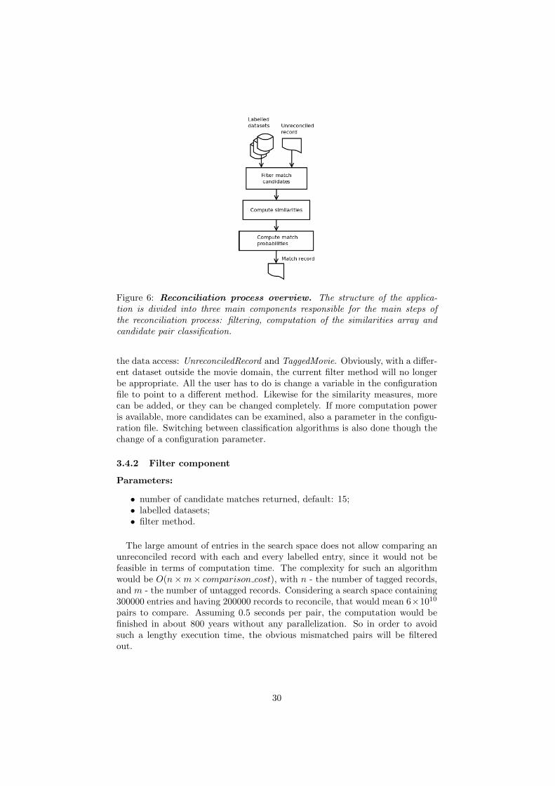
Figure 6: Reconciliation process overview. The structure of the applica-tion is divided into three main components responsible for the main steps ofthe reconciliation process: filtering, computation of the similarities array andcandidate pair classification.
the data access: UnreconciledRecord and TaggedMovie. Obviously, with a differ-ent dataset outside the movie domain, the current filter method will no longerbe appropriate. All the user has to do is change a variable in the configurationfile to point to a different method. Likewise for the similarity measures, morecan be added, or they can be changed completely. If more computation poweris available, more candidates can be examined, also a parameter in the configu-ration file. Switching between classification algorithms is also done though thechange of a configuration parameter.
3.4.2 Filter component
Parameters:
• number of candidate matches returned, default: 15;• labelled datasets;• filter method.
The large amount of entries in the search space does not allow comparing anunreconciled record with each and every labelled entry, since it would not befeasible in terms of computation time. The complexity for such an algorithmwould be O(n×m× comparison cost), with n - the number of tagged records,and m - the number of untagged records. Considering a search space containing300000 entries and having 200000 records to reconcile, that would mean 6×10¹⁰
pairs to compare. Assuming 0.5 seconds per pair, the computation would befinished in about 800 years without any parallelization. So in order to avoidsuch a lengthy execution time, the obvious mismatched pairs will be filteredout.
30
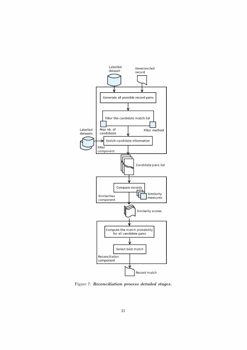
Figure 7: Reconciliation process detailed stages.
31
The filter component takes as input the record to be matched and one or mul-tiple datasets with already tagged information. The number of tagged datasetsdepends on the number of distinct movie-related information resources. It ismore convenient to keep them separate for usability reasons, in case they areneeded for other applications as well.
First, the dataset with the largest number of entries is chosen and from it,a limited amount of entries is selected based on title and actor similarity. Thefiltering is done using an elasticsearch match query. In our implementation,we have set the limit to 15 results in order to have a reasonably fast executionof the algorithm over the entire dataset. It is important to note that we haveused an or query, and we have assigned to the actor similarity a higher weightthan to the title similarity. The reason for this is that the filter operation canintroduce bias in the way it selects the results, and leveraging between actors andtitle should increase the odds of capturing the correct match among the filteredentries, especially when we are searching for non-English titles. Should the userconsider this filter method inadequate, then it can be changed by altering thevalue of config.FILTER METHOD in the configuration file.
We refer to the second operation that the filter component performs as dataenrichment. Based on the unique identifiers of the movies returned by the filteroperation, we add the corresponding information from the other tagged datasets.This data is exposed to the other components of the application through theTaggedMovie class instance. The user can decide which datasets will be con-sidered by modifying the constants.LABELED INDEXES in the configurationfile.
3.4.3 Similarities component
Parameters:
• similarity measures.
The similarities component is responsible for computing the correlation be-tween an unreconciled record and a tagged one. It takes as input a list of Tagged-Movie objects and an UnreconciledRecord object. Then, for each 〈UnreconciledRecord,TaggedMovie〉 pair, it applies a number of methods designed to compare certainfeatures of the two entities. For each pair, it outputs a list of float values, rep-resenting the return values for each of the similarity methods applied. We willrefer to this list as sample.
As we have shown earlier, on the Police Academy example, the similaritymeasures that we have used include the edit distance between titles, languagecomparison, people match, a comparison of the numerals in the title, the differ-ence between the release years and the proper nouns match. In the Evaluationsection, we will see which of these measures have the most impact on the matchdecision.
32
3.4.4 Reconciliation component
Parameters:
• decision model.
The reconciliation component is responsible for the actual decision on whetherthe two records are a match or not. This is done in two steps. First, we apply thereconciliation technique on each sample, obtaining a confidence value. Then, inthe selection phase, the most likely match for the unreconciled record is chosenand the result is returned.
Each sample represents the similarity measures between two movies. Foreach sample, the output will be a real number in the [0, 1] interval, repre-senting the confidence that the two samples are about the same movie. Wehave implemented and compared the following reconciliation techniques: rule-based, naive Bayes, decision trees, SVMs and neural networks, and we canselect which one to use through the configuration file by adjusting the con-stants.RECONCILIATION TYPE parameter.
The selection process means choosing the sample with the highest confidencevalue. However, if that value is under a certain threshold, it indicates twopossibilities: either the correct match is not in the tagged dataset, or the correctmatch has not been selected by the filter component. Depending on the correctmatch, the pair will be counted either as a true negative or as a false negative.
3.5 Reconciliation techniques
We have chosen to implement the heuristic and machine learning orientedapproaches, disregarding graph-based techniques. The reason for this choice isthat in the movie context, the resulting graph would be extremely large, andall of the graph algorithms mentioned in the Graph-oriented approaches sectionhave a high computational complexity, and would not be scalable. Unlike socialgraphs, where an exact match is not always needed, in the movie context we donot want to publish erroneous information. This strict restriction makes thesetypes of algorithm not viable for our application.
Since we do not want to build everything from square one and the focus ofour work is on the evaluation of various algorithms that can be used in themovie reconciliation context, we have used external libraries, like the scikit-learn Python module for naive Bayes, SVMs and decision trees. In this section,we will provide detailed information on how we have employed these libraries,what parameters we have chosen and the reasoning behind these choices.
For the algorithms that require training, the training data is representedby the matrix φ, containing the comparison results between the characteristicsfrom a number of movie information samples, accompanied by the correct matchdecision Di, i ∈ {Y ES,NO}.
33
3.5.1 Rule-based approach
We have implemented 4 intuitive methods, each taking into account a differentsubset of features. This allows us to comment on the relevance of each featurein particular, and also lets us see how much seemingly similar rules can differin performance.
When taking into account all the similarities, first we look at the languagematch. If the two records are written in different languages, then there is ahigh chance that the titles will not match, and then the title match shouldnot count as much as in the normal case. The same reasoning is applied forthe proper nouns match, because often there are multiple names for the samelocation, depending on the nationality of person referring to it. However, thenames of the cast and crew do not change from a language to another, so thisis not influenced by the language similarity. So, depending on the languagethe records are written in, the other parameters mentioned here are assigneddifferent weights.
The similarities relying on numerical features are language-independent, sothey have a fixed maximum weight. Regarding release years, equality would bepreferred, a difference of one year is also acceptable since it could mean that amovie was published towards the end of the year and online sources have storedit as having been published the following year. A difference larger than two is astrong indicator that the records are about two distinct movies, or a movie andits sequel/prequel. Another sign of distinct movies belonging to the same sagaare the numerals present in the title, which accounts for up to one fifth of thefinal match confidence. On the other hand, a discrepancy in numerals decreasesthis confidence by up to 30%.
For the other subsets of similarities, we have applied the same reasoningas above, but we have adjusted the weights to reflect the lack of additionalattributes. For example, when considering only title and people similarities, eachhas a 50% stake in the final decision. The rules are simple, easy to understandand fast to execute. The downside is that they are specific to the current datasetand the similarities defined on it, and if new information is added, the rules donot automatically adapt to it. Also, they do not incorporate previous matchresults, so they do not get better in time.
3.5.2 Naive Bayes
When applying Bayesian learning to our reconciliation problem, we are look-ing to determine the most probable decision D for a similarities array φAB ,given the available training data. In other words, classifying the pair that thesimilarities array represents into a match or a non-match. The Bayes modelrelies on the Bayes theorem, which given our problem context, looks like this:
P (D|φ) =P (φ|D)P (D)
P (φ)
, where
34
• P (D) - prior probability of match/non-match decisions;• P (φ) - prior probability that the similarities array φ will be observed;• P (φ|D) - probability of observing the similarities array φ given the decisionD, also known as the likelihood of the data;
• P (D|φ) - what we want to know is the posterior probability, which is theprobability of decision D, given φ.
The naive assumption of feature independence allows us to compute the matchprobability according to the following formula:
decision(φ) = arg maxd
P (D = d)
p∏i=1
P (θi|D = d)
For the implementation, we have used the GaussianNB class from the scikit-learn library. Thus, the likelihoods of the similarities are computed assuminga normal distribution. The class has methods both for directly predicting theclass, and for returning the probabilities for each possible class, thus allowingthe user to select an appropriate threshold.
3.5.3 Decision Tree
Using decision trees is similar to the rule estimation method, except that therules are determined automatically, based on the training set. Having a balancedtraining set ensures that resulted tree will not be biased towards a certain cat-egory. An advantage of the decision trees is that they can be visualized, whichmakes it easy to understand why a certain decision has been made.
The set from which the decision tree is created consists of the similarity arrayscomputed by the similarities component. For the implementation of the decisiontrees, we have also used the scikit-learn library. The DecisionTreeClassifier classallows customizing settings such as the set diversity metric (entropy or Giniimpurity), the maximum depth of the tree or the minimum number of samplesrequired to split a node. We have chosen the entropy as the split quality criterionand compared the performance obtained by trees of various sizes.
3.5.4 SVM
Due to the use of kernels, SVMs perform well even in high dimensional spaces.That means that we can add as many similarity methods as we deem necessaryand SVMs will still be effective as long as we provide enough training samples.Their versatility is also owed to the fact that we have the freedom to designcustom kernel methods, should we require more than the standard ones.
Applied to the movie reconciliation context, the kernel definitions will usethe similarities arrays as the input vectors. In our reconciliation application, weoffer the possibility to choose which kernel to use by setting the kernel parameterto linear, poly, rbf or sigmoid.
35
Because training and testing SVMs with a large degree polynomial kernelson large datasets is an expensive process time-wise, we have chosen to use onlydegree 2 polynomials in our experiments. Moreover, low degree polynomialshave been shown to be more effective when dealing with text classification tasks[50] [51]. Higher degree polynomials tend to over-fit the training data, thusyielding poorer results.
For the SVMs implementation we have elected to use the SVC class fromthe scikit-learn library. It is a flexible class, granting the user the power tocustomize to the smallest detail the class instances, by setting parameters suchas the number of permitted instances to classify erroneously, the various kerneltuning variables, the tolerance for the stopping criterion and more. By default,an SVM classifier will only return the class predicted for each sample instance.However, the library also provides the option to return the probability that asample instance belongs to a certain class. Because this is done through five-foldcross validation, it considerably lengthens the execution time of the classifier.
3.5.5 Neural network approach
Given the capacity of neural networks to model extremely complex functions,this approach was the next logical step in our search for the most suitabledecision mechanism in the movie-information reconciliation domain. Of course,just to name the neural networks as the best solution to our problem is notenough: we also need to determine the most appropriate values, or at leastbounds for the main parameters of the neural network. In order to do that,first we have restricted the design of the network - no backward connectionsbetween the neurons, and secondly we have empirically tested multiple networksizes and shapes on our dataset.
Restricting the network design to only feed-forward networks does not affectthe results of the experiment, because we are not dealing with a time-dependentproblem. According to Hassoun [52], a recurrent architecture is most suitablefor time-dependent inputs, like modelling the process of an unknown plant. Inthe case of a recurrent network, the dependencies between the neurons vary notonly according to the input signals, but also according to the output producedby those inputs at a given time instance. However, in our case, there are notime dependencies and thus, a feed-forward network will suffice.
With regards to implementation, we have chosen the FANN library for theneural network part of our application. The library allows the user to create afeed-forward neural network, train and execute it through simple function calls.Several different parameters can be adjusted before and during the trainingphase, the most important being the learning rate and the size and shape of thenetwork. During the experiments, we have decided on 0.7 as the learning rate,with a symmetric sigmoid activation function .
The shape and size of the network matters and greatly affects the resultsobtained. Should we choose too many layers and neurons, the learning processwill be slow and we risk over-fitting the input data, not being able to generalize.
36

Should we choose too few layers and neurons, the network will not be able tolearn the rules and the error rate will most likely oscillate, without reachinglow enough levels. Therefore, during the experiments, we have tested severalnetwork configurations.
37
4 Evaluation
”A program that has not beentested does not work.”
Bjarne Stroustrup
4.1 Experimental methodology
4.1.1 Hardware
The experiments have been run on a Dell Inspiron N5110, equipped with anIntel R© CoreTM i7-2630QM CPU with 8 cores at a 2.00GHz frequency, 8 MB L3cache and 8 GB RAM. The system is running Ubuntu 14.04.2 LTS.
4.1.2 Datasets
The training set includes 1000 samples: 500 positive, 500 negative, so therewill be no bias in either direction. In the similarities arrays, duplicates canbe found: it is possible for 2 different pairs made of 4 distinct movies to haveidentical similarities arrays.
The test data is comprised of 178870 records for which we know the correctunique identifier. After the filtering phase, the list of candidates contains thecorrect match in 173278 of cases, so 96.87%. The classification algorithms havethe task of finding the correct match from the list of candidates.
Depending on whether a pair is an actual match or not and on the algorithmdecision, there are 4 possible type of results:
• true positive (TP) - the pair is an actual match and has been identified assuch;
• true negative (TN) - the algorithm could not find a match for an un-reconciled record, so the pair is not a match and has been identified assuch;
• false positive (FP) - the pair has been falsely classified as a match;• false negative (FN) - the pair is an actual match, but it has not been
recognized by the algorithm.
4.1.3 Evaluation metrics
If this application is to be used as part of a public user service like Vionel,then it is important to know how much we can trust the results, how confidentwe are that the computed matches are correct and can be published online.In order to evaluate performance of the application, we have considered thefollowing metrics:
• accuracy - expresses the percent of correct results, regardless of whetherthey represent a positive match or not;
TP + TN
TP + FP + TN + FN
38
• precision - also known as positive predictive value, it shows how muchconfidence we can have in a positive match, the probability of two recordsbeing identified as one movie when, in fact, this is not the case;
TP
TP + FP
• recall - it indicates what percent of positive matches has been identifiedfrom all the positive matches evaluated by the learning algorithm;
TP
TP + FN
• false positive rate - it expresses how many mismatches have been classifiedas matches out of all the negative pairs;
FP
TN + FP
, which have been expressed in percentages in the Experimental results section.
A low recall is not what we are looking for, but it would be better thanhaving a low precision. A low precision means that we cannot rely on thematches provided by application and that we would need to manually verifyeach and every one of them and it is precisely this effort that we wish to avoid.To better illustrate the meaning of these metrics, consider the following fictiveexample: out of a set of 100 pairs, 80 are true matches. Applying a reconciliationalgorithm on this set, 60 pairs of the true matches are discovered as such, butso are 10 other pairs from the non-matches. Therefore, we would obtain thesemetrics:
• accuracy = 60+1060+10+10+20 = 0.7;
• precision = 6060+10 ≈ 0.85;
• recall = 6060+20 = 0.75;
• false positive rate = 1010+10 = 0.5.
In order to see how the algorithms behave when using different features, wehave selected 4 sets of features on which we have run tests:
• set 1 - S1: title match, language comparison, people match, numeralsmatch, release year difference, proper nouns match (all features);
• set 2 - S2: title match, numerals match, people match, release year differ-ence;
• set 3 - S3: title and people match;• set 4 - S4: title match and release year difference.
39
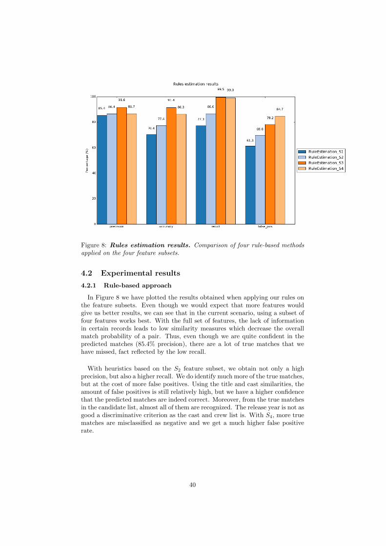
Figure 8: Rules estimation results. Comparison of four rule-based methodsapplied on the four feature subsets.
4.2 Experimental results
4.2.1 Rule-based approach
In Figure 8 we have plotted the results obtained when applying our rules onthe feature subsets. Even though we would expect that more features wouldgive us better results, we can see that in the current scenario, using a subset offour features works best. With the full set of features, the lack of informationin certain records leads to low similarity measures which decrease the overallmatch probability of a pair. Thus, even though we are quite confident in thepredicted matches (85.4% precision), there are a lot of true matches that wehave missed, fact reflected by the low recall.
With heuristics based on the S2 feature subset, we obtain not only a highprecision, but also a higher recall. We do identify much more of the true matches,but at the cost of more false positives. Using the title and cast similarities, theamount of false positives is still relatively high, but we have a higher confidencethat the predicted matches are indeed correct. Moreover, from the true matchesin the candidate list, almost all of them are recognized. The release year is not asgood a discriminative criterion as the cast and crew list is. With S4, more truematches are misclassified as negative and we get a much higher false positiverate.
40
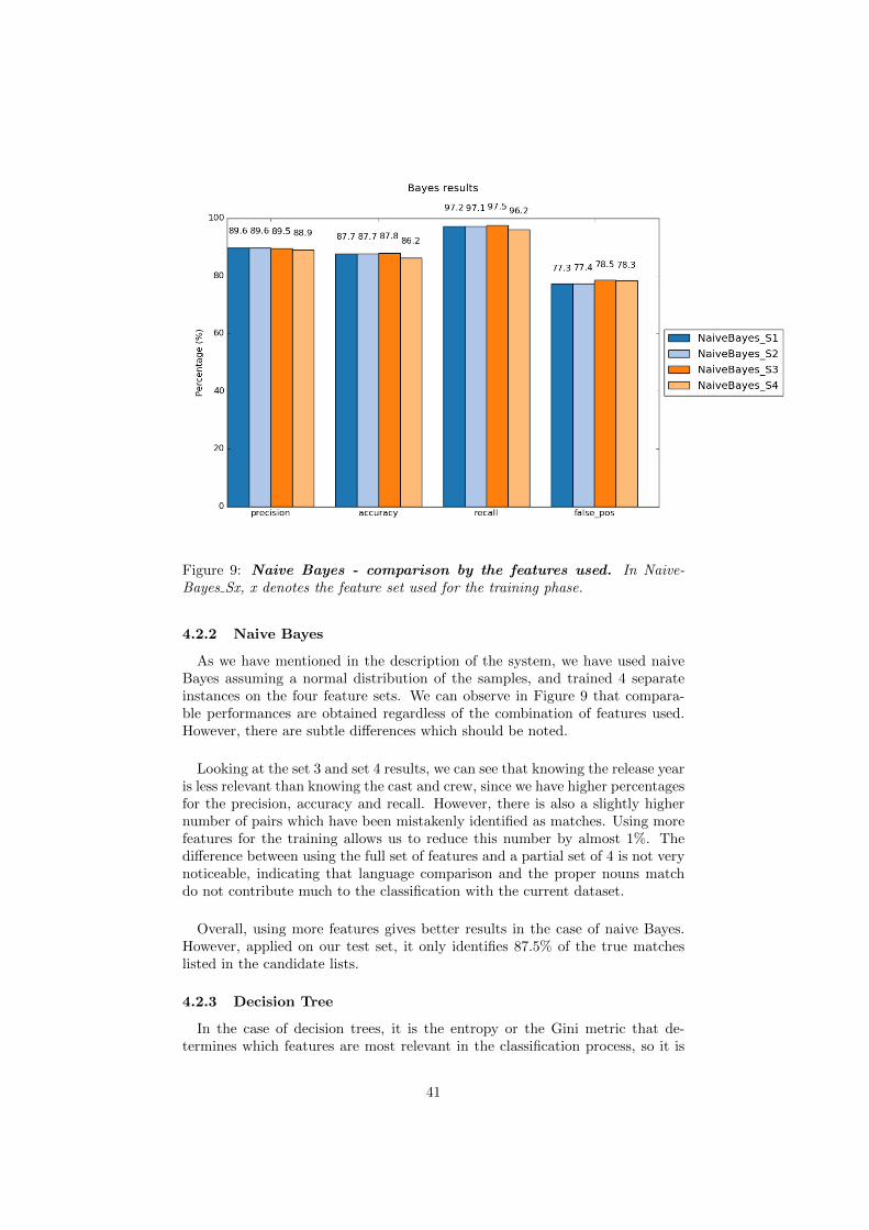
Figure 9: Naive Bayes - comparison by the features used. In Naive-Bayes Sx, x denotes the feature set used for the training phase.
4.2.2 Naive Bayes
As we have mentioned in the description of the system, we have used naiveBayes assuming a normal distribution of the samples, and trained 4 separateinstances on the four feature sets. We can observe in Figure 9 that compara-ble performances are obtained regardless of the combination of features used.However, there are subtle differences which should be noted.
Looking at the set 3 and set 4 results, we can see that knowing the release yearis less relevant than knowing the cast and crew, since we have higher percentagesfor the precision, accuracy and recall. However, there is also a slightly highernumber of pairs which have been mistakenly identified as matches. Using morefeatures for the training allows us to reduce this number by almost 1%. Thedifference between using the full set of features and a partial set of 4 is not verynoticeable, indicating that language comparison and the proper nouns matchdo not contribute much to the classification with the current dataset.
Overall, using more features gives better results in the case of naive Bayes.However, applied on our test set, it only identifies 87.5% of the true matcheslisted in the candidate lists.
4.2.3 Decision Tree
In the case of decision trees, it is the entropy or the Gini metric that de-termines which features are most relevant in the classification process, so it is
41

not necessary to train the decision trees on the feature subsets defined earlier.Instead, we are comparing the metrics obtained by training trees up to severallevels of depth. The higher the depth, the higher the risk of over-fitting thetraining data and not generalising enough.
The over-fitting problem is obvious when we look at the results. In the train-ing phase, the accuracy grows from 98.1% to 98.7%. In contrast, in the testingphase, the accuracy drops drastically to 89.6%, almost 10% smaller than thetraining one. And as the depth increases, the accuracy keeps decreasing, whilethe false positives rate is going up. The effect is rather visible for trees withmaximum depth 4 and higher.
In Figure 10 we have the output from applying the decision tree classifier onour test set, with entropy as the split criterion. Again, we see very high valuesin precision, accuracy and especially recall. Confirming the Bayes results, herethe title is the first feature to split the set by, followed by the cast and crewmatch, as we can see in the tree with a maximum depth of 2 in Figure 11.
With a 3 layer tree, we obtain the best precision, 90.7%. The 3 layer treemanages to find a balance between the amount of true positive and false positivepairs, also having the lowest false positive rate. While with the 2 layer tree weobtain the best generalisation (best accuracy - 89.6%) and a higher number oftrue positive pairs, we also get a higher number of false positives, which wewould prefer to avoid.
4.2.4 SVM
Kernel TP FP TN FN precision accuracy recall false+ rateLinear 153327 17267 4914 3362 89.8 88.4 97.8 77.8Polynomial, d=2 152095 17592 4946 4237 89.6 87.7 97.2 78.0RBF, γ=0.5 146802 17885 4856 9327 89.1 84.7 94.0 78.6RBF, γ=1 145262 18748 4786 10074 88.5 83.8 93.5 79.6RBF, γ=2 140003 18531 5577 14759 88.3 81.3 90.4 76.8Sigmoid, r=0.3 90174 72216 3849 12631 55.5 52.5 87.7 94.9Sigmoid, r=0.5 89852 71671 4037 13310 55.6 52.5 87.0 94.6Sigmoid, r=1 89104 69751 4511 15504 56.0 52.3 85.1 98.9Sigmoid, r=2 86553 67326 5462 19529 56.2 51.4 81.5 92.4
Table 4: SVM results. The precision, accuracy, recall and the false positiverate are all expressed in percentages.
In Table 4, we have presented the best results obtained when running exper-iments with SVMs as the classification algorithm, and varying the kernels andtheir parameters.
42
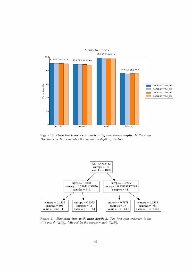
Figure 10: Decision trees - comparison by maximum depth. In the nameDecisionTree Dx, x denotes the maximum depth of the tree.
Figure 11: Decision tree with max depth 2. The first split criterion is thetitle match (X[0]), followed by the people match (X[2]).
43
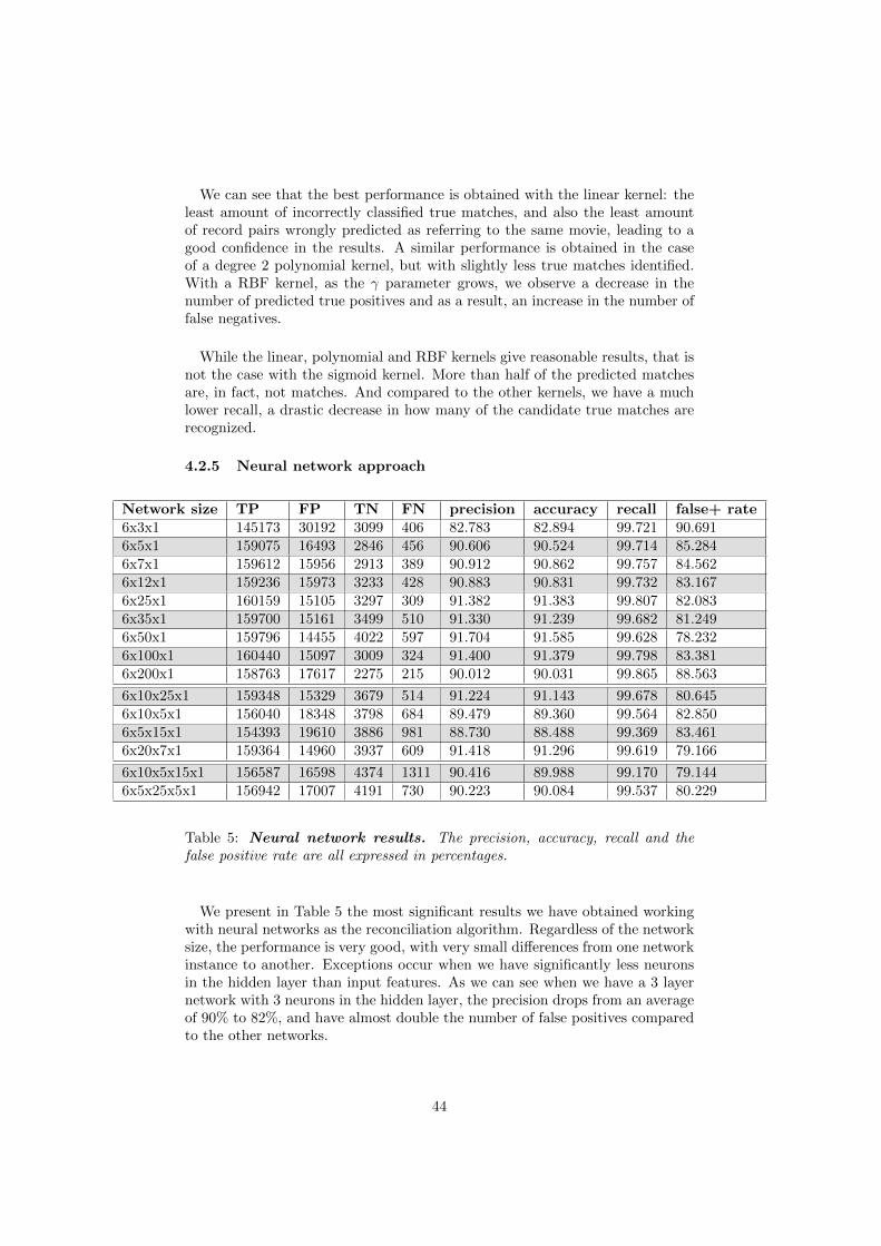
We can see that the best performance is obtained with the linear kernel: theleast amount of incorrectly classified true matches, and also the least amountof record pairs wrongly predicted as referring to the same movie, leading to agood confidence in the results. A similar performance is obtained in the caseof a degree 2 polynomial kernel, but with slightly less true matches identified.With a RBF kernel, as the γ parameter grows, we observe a decrease in thenumber of predicted true positives and as a result, an increase in the number offalse negatives.
While the linear, polynomial and RBF kernels give reasonable results, that isnot the case with the sigmoid kernel. More than half of the predicted matchesare, in fact, not matches. And compared to the other kernels, we have a muchlower recall, a drastic decrease in how many of the candidate true matches arerecognized.
4.2.5 Neural network approach
Network size TP FP TN FN precision accuracy recall false+ rate6x3x1 145173 30192 3099 406 82.783 82.894 99.721 90.6916x5x1 159075 16493 2846 456 90.606 90.524 99.714 85.2846x7x1 159612 15956 2913 389 90.912 90.862 99.757 84.5626x12x1 159236 15973 3233 428 90.883 90.831 99.732 83.1676x25x1 160159 15105 3297 309 91.382 91.383 99.807 82.0836x35x1 159700 15161 3499 510 91.330 91.239 99.682 81.2496x50x1 159796 14455 4022 597 91.704 91.585 99.628 78.2326x100x1 160440 15097 3009 324 91.400 91.379 99.798 83.3816x200x1 158763 17617 2275 215 90.012 90.031 99.865 88.563
6x10x25x1 159348 15329 3679 514 91.224 91.143 99.678 80.6456x10x5x1 156040 18348 3798 684 89.479 89.360 99.564 82.8506x5x15x1 154393 19610 3886 981 88.730 88.488 99.369 83.4616x20x7x1 159364 14960 3937 609 91.418 91.296 99.619 79.166
6x10x5x15x1 156587 16598 4374 1311 90.416 89.988 99.170 79.1446x5x25x5x1 156942 17007 4191 730 90.223 90.084 99.537 80.229
Table 5: Neural network results. The precision, accuracy, recall and thefalse positive rate are all expressed in percentages.
We present in Table 5 the most significant results we have obtained workingwith neural networks as the reconciliation algorithm. Regardless of the networksize, the performance is very good, with very small differences from one networkinstance to another. Exceptions occur when we have significantly less neuronsin the hidden layer than input features. As we can see when we have a 3 layernetwork with 3 neurons in the hidden layer, the precision drops from an averageof 90% to 82%, and have almost double the number of false positives comparedto the other networks.
44
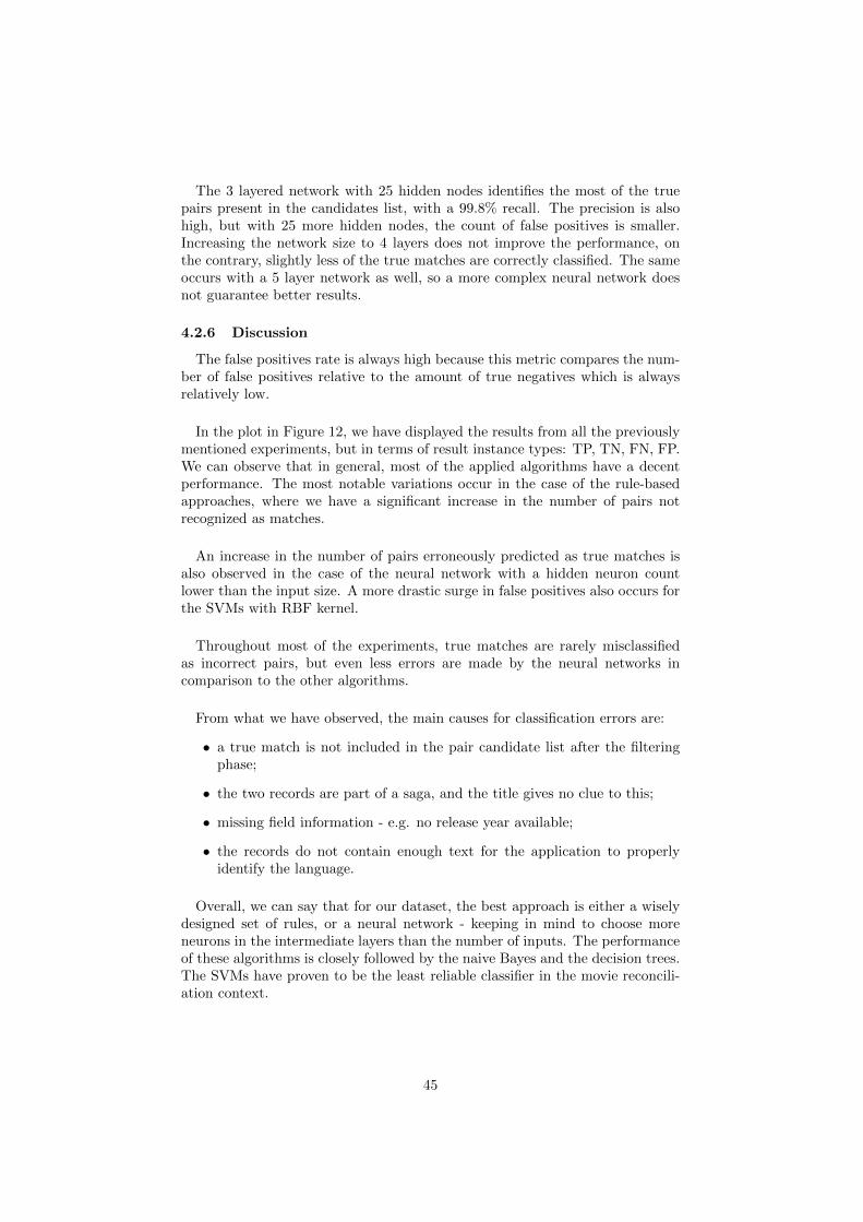
The 3 layered network with 25 hidden nodes identifies the most of the truepairs present in the candidates list, with a 99.8% recall. The precision is alsohigh, but with 25 more hidden nodes, the count of false positives is smaller.Increasing the network size to 4 layers does not improve the performance, onthe contrary, slightly less of the true matches are correctly classified. The sameoccurs with a 5 layer network as well, so a more complex neural network doesnot guarantee better results.
4.2.6 Discussion
The false positives rate is always high because this metric compares the num-ber of false positives relative to the amount of true negatives which is alwaysrelatively low.
In the plot in Figure 12, we have displayed the results from all the previouslymentioned experiments, but in terms of result instance types: TP, TN, FN, FP.We can observe that in general, most of the applied algorithms have a decentperformance. The most notable variations occur in the case of the rule-basedapproaches, where we have a significant increase in the number of pairs notrecognized as matches.
An increase in the number of pairs erroneously predicted as true matches isalso observed in the case of the neural network with a hidden neuron countlower than the input size. A more drastic surge in false positives also occurs forthe SVMs with RBF kernel.
Throughout most of the experiments, true matches are rarely misclassifiedas incorrect pairs, but even less errors are made by the neural networks incomparison to the other algorithms.
From what we have observed, the main causes for classification errors are:
• a true match is not included in the pair candidate list after the filteringphase;
• the two records are part of a saga, and the title gives no clue to this;
• missing field information - e.g. no release year available;
• the records do not contain enough text for the application to properlyidentify the language.
Overall, we can say that for our dataset, the best approach is either a wiselydesigned set of rules, or a neural network - keeping in mind to choose moreneurons in the intermediate layers than the number of inputs. The performanceof these algorithms is closely followed by the naive Bayes and the decision trees.The SVMs have proven to be the least reliable classifier in the movie reconcili-ation context.
45
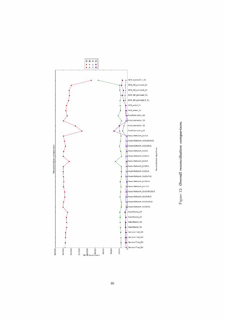
Fig
ure
12:
Overa
llre
con
cil
iati
on
com
pari
son
.
46
5 Conclusion
”Do what you think is interesting,do something that you think isfun and worthwhile, becauseotherwise you won’t do it wellanyway.”
Brian Kernighan
Reconciliation has become an important research topic due to the existenceof numerous heterogeneous information resources. When attempting to collectrelevant data in a certain domain, identification and disambiguation problemsarise: dealing with similar records corresponding to the same unique entityand differentiating between seemingly identical records which actually refer todifferent entities. Further complications include missing values, inconsistentformatting, different languages, large number of records. Performing this pro-cess manually is definitely not feasible when handling hundreds of thousands ofrecords.
In this thesis, we have addressed the problem of reconciling movie informationgathered from various web resources. We believe we have achieved our goal ofcreating an application that is suited to the movie context, while at the sametime allowing for rapid extension to fit other problem variants.
The application we are proposing works in stages. First, we limit the numberof candidate pairs to the most likely ones. Then, considering the data we havehad available, both labelled and unlabelled, we have implemented six compar-ison methods which express the similarity degree for a pair of movie records.Based on these measures, we have compared multiple classification algorithmswith various parameters to determine whether the pair in question is a matchor not.
Our application can be extended to datasets from other domains easily forthe following reasons:
• it can handle input data with other formats, the user just having to extendtwo classes which define the data accessors;
• should a new labelled dataset become available, its addition to the com-putation is done simply by adjusting one configuration parameter;
• if it is used in a different context, the similarity component can be in-structed to employ a different set of similarity methods;
• the classification algorithm can be selected from the a wide range (naiveBayes, decision tree, SVM, neural network), or a new one can be added.
We have tested our application on a practical problem, the identification ofmovie record matches. The supervised algorithms have been trained on a set of1000 samples, the positive samples having an equal share to the negative ones.The test set contains almost 180000 records, uniquely labelled so there was no
47

need for statistic result estimation, we have shown the actual numbers obtainedin the Evaluation section. According to our results, we can conclude that thebest choice for the classification algorithm would be either a neural network,or a carefully selected set of rules. If we would know that the data availabledoes not change, then a set of rules would be the less computationally intensiveand less time consuming. However, if the data is expected to go often throughchanges, a neural network would be easier to adapt to these changes rather thanhaving to manually modify the classification rules. Should the neural networkbe considered too complex, naive Bayes and decision trees have also shown asatisfactory performance.
Especially looking at the results using a set of rules and those using neuralnetworks, we have clearly fulfilled our goal of improving the precision from 60%to 90%. However, it should be noted that the initial precision has been computedon different datasets. After discussing the results with the VionLabs team, ithas been decided that they will not choose to implement a complex machinelearning reconciliation approach, but that they will improve the existing set ofrules.
It is our view that there is no unique solution to reconciliation. Data match-ing is domain and data dependent: it requires extensive domain knowledge,knowledge about data matching techniques, occasionally manual interventiontoo. And even having all that, the results will still strongly depend on the dataavailable to match against.
48
6 Further work
”Thus we may have knowledge ofthe past but cannot control it; wemay control the future but haveno knowledge of it.”
Claude Elwood Shannon
During this research, we have implemented an application to facilitate theintegration of movie records from multiple sources to one database, by deter-mining the proper unique identifier for the movies the records refer to. Theapplication we have developed so far can be improved further by exploring sev-eral areas: execution time, results quality, performance evaluation, and userfriendliness.
As we have mentioned, the experiments have been run on a single machine.However, the nature of application and the architecture itself allow for paral-lelization in order to reduce the execution time. One possibility is to split intogroups the records that need to be reconciled and run the groups in parallel,as there are no dependencies from a record computation to another. Also, ifmultiple machine learning algorithms have been selected to be applied on theinput data, each one can be run separately and concurrently with the other.
In our application, we have used a standard blocking technique based onthe movie titles and actors. Employing other filtering techniques, like thosementioned in [23], [24] might improve the accuracy of the results, by includingmore true matches in the candidate pairs. Also, to avoid the case when thesorted neighbourhood block technique does not function properly (more recordsthan the window size correspond to a value of the key fields), an idea would benot to use a window size at all, but to take the entire block of records respectiveto a key field value, plus a number of previous and successive records in theordered list, and generate candidate pairs among these records. How manyextra records are chosen can be a fixed value, or it can be a function of thenumber of the initial records that matched the key field value.
Since we are using supervised techniques, the training data is of crucial im-portance. In order to better evaluate the performance of the algorithms and alsoasses the influence of the training set, more work can be done in the training setcreation. More tests can be done on a training set containing various ratios ofpositive to negative samples, thus allowing us to determine which ratio wouldgive the best results. Moreover, we can be more particular about the sampleswe want included in the training set.
There are cases in which the characteristics we have compared are not enoughto confidently classify a movie record pair, especially if one or more fields aremissing. However, other fields may be available, which would permit reachingthe correct decision. In order to do that, we would need to add more comparisonmethods, more elements in the characteristics array, according to the data we
49

have available. For example, we could compare poster images. Another possi-bility is text comparison using the Soundex algorithm [53], especially useful inthe case of data known to contain spelling mistakes. Keep in mind that this willincrease the execution time, so it is best to customize the comparison methodsto the data available.
To make our application more user friendly, a graphical interface would facili-tate operations such as adding unreconciled records and labelled data, selectingor adding comparison methods, or choosing classification algorithms. Installa-tion and configuration of the application would be easier and more intuitive,requiring less documentation research for the basic uses.
50
7 References
[1] IMDb.com Inc. Database statistics, 2015.
[2] Anne Hakansson. Portal of Research Methods and Methodologies for Re-search Projects and Degree Projects. Proceedings of the International Con-ference on Frontiers in Education: Computer Science and Computer Engi-neering FECS’13, pages 67–73, 2013.
[3] H.B. Newcombe, J.M. Kennedy, S.J. Axford, and A.P. James. Automaticlinkage of vital records. Science, 130(3381):954–959, 1959.
[4] Ivan P Fellegi and Alan B Sunter. A theory for record linkage. Journal ofthe American Statistical Association, 64(328):1183–1210, 1969.
[5] Vladimir I. Levenshtein. Binary codes capable of correcting deletions, in-sertions, and reversals. Soviet physics doklady, 10(8):707–710, 1966.
[6] William B. Cavnar and John M. Trenkle. N-Gram-Based Text Categoriza-tion. Ann Arbor MI, 48113(2):161–175, 1994.
[7] Gregory Grefenstette. Comparing two language identification schemes. Pro-ceedings of the Third International Conference on the Statistical Analysisof Textual Data (JADT’95), pages 263–268, 1995.
[8] Olivier Teytaud and Radwan Jalam. Kernel-based text categorization.Proceedings of the International Joint Conference on Neural Networks(IJCNN’2001), 2001.
[9] Timothy Baldwin and Marco Lui. Language identification: The long andthe short of the matter. In Human Language Technologies: The 2010 An-nual Conference of the North American Chapter of the Association forComputational Linguistics, pages 229–237. Association for ComputationalLinguistics, 2010.
[10] Lisa F Rau. Extracting company names from text. In Artificial IntelligenceApplications, 1991. Proceedings., Seventh IEEE Conference on, volume 1,pages 29–32. IEEE, 1991.
[11] David Nadeau and Satoshi Sekine. A survey of named entity recognitionand classification. Lingvisticae Investigationes, 30(1):3–26, 2007.
[12] Daniel M Bikel, Scott Miller, Richard Schwartz, and Ralph Weischedel.Nymble: a high-performance learning name-finder. In Proceedings of thefifth conference on Applied natural language processing, pages 194–201. As-sociation for Computational Linguistics, 1997.
[13] Satoshi Sekine. NYU: Description of the Japanese NE system used forMET-2. In Proc. Message Understanding Conference, 1998.
[14] Masayuki Asahara and Yuji Matsumoto. Japanese named entity extrac-tion with redundant morphological analysis. In Proceedings of the 2003Conference of the North American Chapter of the Association for Compu-tational Linguistics on Human Language Technology-Volume 1, pages 8–15.Association for Computational Linguistics, 2003.
51
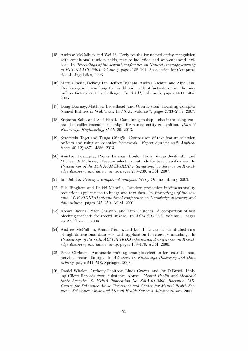
[15] Andrew McCallum and Wei Li. Early results for named entity recognitionwith conditional random fields, feature induction and web-enhanced lexi-cons. In Proceedings of the seventh conference on Natural language learningat HLT-NAACL 2003-Volume 4, pages 188–191. Association for Computa-tional Linguistics, 2003.
[16] Marius Pasca, Dekang Lin, Jeffrey Bigham, Andrei Lifchits, and Alpa Jain.Organizing and searching the world wide web of facts-step one: the one-million fact extraction challenge. In AAAI, volume 6, pages 1400–1405,2006.
[17] Doug Downey, Matthew Broadhead, and Oren Etzioni. Locating ComplexNamed Entities in Web Text. In IJCAI, volume 7, pages 2733–2739, 2007.
[18] Sriparna Saha and Asif Ekbal. Combining multiple classifiers using votebased classifier ensemble technique for named entity recognition. Data &Knowledge Engineering, 85:15–39, 2013.
[19] Serafettin Tascı and Tunga Gungor. Comparison of text feature selectionpolicies and using an adaptive framework. Expert Systems with Applica-tions, 40(12):4871–4886, 2013.
[20] Anirban Dasgupta, Petros Drineas, Boulos Harb, Vanja Josifovski, andMichael W Mahoney. Feature selection methods for text classification. InProceedings of the 13th ACM SIGKDD international conference on Knowl-edge discovery and data mining, pages 230–239. ACM, 2007.
[21] Ian Jolliffe. Principal component analysis. Wiley Online Library, 2002.
[22] Ella Bingham and Heikki Mannila. Random projection in dimensionalityreduction: applications to image and text data. In Proceedings of the sev-enth ACM SIGKDD international conference on Knowledge discovery anddata mining, pages 245–250. ACM, 2001.
[23] Rohan Baxter, Peter Christen, and Tim Churches. A comparison of fastblocking methods for record linkage. In ACM SIGKDD, volume 3, pages25–27. Citeseer, 2003.
[24] Andrew McCallum, Kamal Nigam, and Lyle H Ungar. Efficient clusteringof high-dimensional data sets with application to reference matching. InProceedings of the sixth ACM SIGKDD international conference on Knowl-edge discovery and data mining, pages 169–178. ACM, 2000.
[25] Peter Christen. Automatic training example selection for scalable unsu-pervised record linkage. In Advances in Knowledge Discovery and DataMining, pages 511–518. Springer, 2008.
[26] Daniel Whalen, Anthony Pepitone, Linda Graver, and Jon D Busch. Link-ing Client Records from Substance Abuse. Mental Health and MedicaidState Agencies. SAMHSA Publication No. SMA-01-3500. Rockville, MD:Center for Substance Abuse Treatment and Center for Mental Health Ser-vices, Substance Abuse and Mental Health Services Administration, 2001.
52
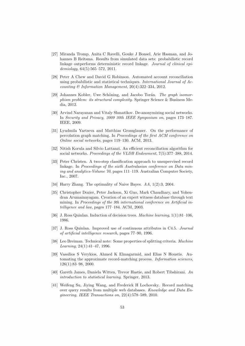
[27] Miranda Tromp, Anita C Ravelli, Gouke J Bonsel, Arie Hasman, and Jo-hannes B Reitsma. Results from simulated data sets: probabilistic recordlinkage outperforms deterministic record linkage. Journal of clinical epi-demiology, 64(5):565–572, 2011.
[28] Peter A Chew and David G Robinson. Automated account reconciliationusing probabilistic and statistical techniques. International Journal of Ac-counting & Information Management, 20(4):322–334, 2012.
[29] Johannes Kobler, Uwe Schoning, and Jacobo Toran. The graph isomor-phism problem: its structural complexity. Springer Science & Business Me-dia, 2012.
[30] Arvind Narayanan and Vitaly Shmatikov. De-anonymizing social networks.In Security and Privacy, 2009 30th IEEE Symposium on, pages 173–187.IEEE, 2009.
[31] Lyudmila Yartseva and Matthias Grossglauser. On the performance ofpercolation graph matching. In Proceedings of the first ACM conference onOnline social networks, pages 119–130. ACM, 2013.
[32] Nitish Korula and Silvio Lattanzi. An efficient reconciliation algorithm forsocial networks. Proceedings of the VLDB Endowment, 7(5):377–388, 2014.
[33] Peter Christen. A two-step classification approach to unsupervised recordlinkage. In Proceedings of the sixth Australasian conference on Data min-ing and analytics-Volume 70, pages 111–119. Australian Computer Society,Inc., 2007.
[34] Harry Zhang. The optimality of Naive Bayes. AA, 1(2):3, 2004.
[35] Christopher Dozier, Peter Jackson, Xi Guo, Mark Chaudhary, and Yohen-dran Arumainayagam. Creation of an expert witness database through textmining. In Proceedings of the 9th international conference on Artificial in-telligence and law, pages 177–184. ACM, 2003.
[36] J. Ross Quinlan. Induction of decision trees. Machine learning, 1(1):81–106,1986.
[37] J. Ross Quinlan. Improved use of continuous attributes in C4.5. Journalof artificial intelligence research, pages 77–90, 1996.
[38] Leo Breiman. Technical note: Some properties of splitting criteria. MachineLearning, 24(1):41–47, 1996.
[39] Vassilios S Verykios, Ahmed K Elmagarmid, and Elias N Houstis. Au-tomating the approximate record-matching process. Information sciences,126(1):83–98, 2000.
[40] Gareth James, Daniela Witten, Trevor Hastie, and Robert Tibshirani. Anintroduction to statistical learning. Springer, 2013.
[41] Weifeng Su, Jiying Wang, and Frederick H Lochovsky. Record matchingover query results from multiple web databases. Knowledge and Data En-gineering, IEEE Transactions on, 22(4):578–589, 2010.
53
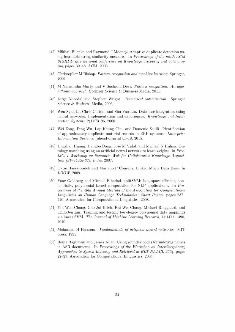
[42] Mikhail Bilenko and Raymond J Mooney. Adaptive duplicate detection us-ing learnable string similarity measures. In Proceedings of the ninth ACMSIGKDD international conference on Knowledge discovery and data min-ing, pages 39–48. ACM, 2003.
[43] Christopher M Bishop. Pattern recognition and machine learning. Springer,2006.
[44] M Narasimha Murty and V Susheela Devi. Pattern recognition: An algo-rithmic approach. Springer Science & Business Media, 2011.
[45] Jorge Nocedal and Stephen Wright. Numerical optimization. SpringerScience & Business Media, 2006.
[46] Wen-Syan Li, Chris Clifton, and Shu-Yao Liu. Database integration usingneural networks: Implementation and experiences. Knowledge and Infor-mation Systems, 2(1):73–96, 2000.
[47] Wei Zong, Feng Wu, Lap-Keung Chu, and Domenic Sculli. Identificationof approximately duplicate material records in ERP systems. EnterpriseInformation Systems, (ahead-of-print):1–18, 2015.
[48] Jingshan Huang, Jiangbo Dang, Jose M Vidal, and Michael N Huhns. On-tology matching using an artificial neural network to learn weights. In Proc.IJCAI Workshop on Semantic Web for Collaborative Knowledge Acquisi-tion (SWeCKa-07), India, 2007.
[49] Oktie Hassanzadeh and Mariano P Consens. Linked Movie Data Base. InLDOW, 2009.
[50] Yoav Goldberg and Michael Elhadad. splitSVM: fast, space-efficient, non-heuristic, polynomial kernel computation for NLP applications. In Pro-ceedings of the 46th Annual Meeting of the Association for ComputationalLinguistics on Human Language Technologies: Short Papers, pages 237–240. Association for Computational Linguistics, 2008.
[51] Yin-Wen Chang, Cho-Jui Hsieh, Kai-Wei Chang, Michael Ringgaard, andChih-Jen Lin. Training and testing low-degree polynomial data mappingsvia linear SVM. The Journal of Machine Learning Research, 11:1471–1490,2010.
[52] Mohamad H Hassoun. Fundamentals of artificial neural networks. MITpress, 1995.
[53] Hema Raghavan and James Allan. Using soundex codes for indexing namesin ASR documents. In Proceedings of the Workshop on InterdisciplinaryApproaches to Speech Indexing and Retrieval at HLT-NAACL 2004, pages22–27. Association for Computational Linguistics, 2004.
54