Moving archetypes

ELSEVIER Physica D 107 (1997) 1-16

I

Moving archetypes Adele Cut le r *, E m i l y S tone

Department of Mathematics and Statistics, Utah State University, Logan, UT 84322-3900, USA

Received 18 July 1996; revised 13 March 1997; accepted 18 March 1997 Communicated by J.D. Meiss

Abstract

We introduce a variation of the statistical method archetypal analysis (Cutler and Breiman, 1994) that tracks moving structures, such as traveling waves or solitons, in a data set. By using this method the traveling part of the motion is separated from the stationary (or semi-stationary) pattern.

Keywords: Archetypal analysis; Archetypes; Dynamical systems; Principal components; Coherent structures

1. Introduction

The application of principal component analysis

(PCA) to data sets obtained from dynamical systems has received much attention in the past 10 years.

The idea of using PCA to elucidate structure and dy-

namics in fluid mechanical data was first presented by John Lumley in a 1967 paper [16], in which

he called the method the proper orthogonal decomposition (POD). Implementation of the procedure, however, was delayed until computing capabilities

had advanced enough to make it practical. In a 1987 paper Sirovich [17] identified the eigenvectors of PCA applied to fluid data as "coherent structures",

a term used to describe large scale organized motion in turbulent fluid systems. Sirovich referred to the analysis as the Karhunen-Lo6ve decomposition (KL). Concurrently a group at Cornell, headed by Lumley, was working on the application of PCA

* Corresponding author.

to data from a turbulent pipe flow experiment, and the results of that study appeared in a 1988 Jour-

nal of Fluid Mechanics paper [4]. The goal of the

Comell work, and of later studies (see for example [5,18]) was to construct a low-dimensional model

of the experimental system. Other applications, on

data sets as diverse as animations of speaking mouths for lip-reading purposes [12], and simulations of

partial differential equations, Ref. [l l] have followed. Papers on the theory of application of PCA

to dynamic data sets can also be found [3]. Inter- est in the method also prompted the creation of a

computer software package that automates the procedure and provides convenient graphics capabilities

[2]. Data sets possessing spatial structures that translate

in time present a special problem to those hoping to reduce them using the KL decomposition. The decomposition produces a Fourier basis from data that has a circulant covariance matrix, i,e., data that is translationally invariant. Thus, if the translating structure is sufficiently regular, the eigenfunctions

0167-2789/97/$17.00 Copyright © 1997 Elsevier Science B.V. All rights reserved PH S0 167-2789(97)0052-3

A. Cutler, E. Stone/Physica D 107 (1997) 1-16

will be sines and cosines [17]. This is important in analyzing fluid mechanical systems, where spatially homogeneous data will have Fourier modes for KL eigenfunctions [16]. Therefore, in situations where

the translating structure itself is the feature to be extracted, a direct application of the KL decomposition will not suffice. One possible approach is to preprocess the data, subtracting out the translating part in some way. This has been done and results of such analysis are presented in [1,11]. Another approach is a variation of KL suggested by Broomhead et al. [6] called an "adaptive basis method". They apply the KL decomposition to subsets of the data, forming separate local bases for the dynamics. These bases are then linked by transition matrices that describe the time evolution of the data set. This method creates a time dependent basis for the data, comprised of the locally chosen bases and transition matrices between bases.

We propose a method that builds on archetypal analysis, a new statistical method for extracting rel- evant features from experimental data sets developed by Cutler and Breiman [7]. Archetypes character- ize extreme data values (on the convex hull of the data set) and an approximation to the data can be constructed in terms of these values. For results of the application of archetypal analysis to dynamical systems see [20,21]. The variation on archetypal analysis presented here finds archetypes that actually move with the traveling structure, in an objective manner. The shape of the structure itself is extracted (or possibly shapes, if the structure itself is varying as well as translating) as well as information on how the structure is moving across the spatial domain. The algorithm requires no preprocessing of the data.

Section 2 gives a brief overview of the Karhunen- Lobve decomposition, archetypal analysis, and the moving archetype algorithm. In Section 3 we present the results of applying moving archetypes to spatio- temporal data sets from a numerical experiment (sim- ulating the Kuramoto-Sivashinsky equation) and a physical experiment (data from D. Luss' lab at the University of Houston). We summarize our findings in Section 4.

2. The mathematical formulation

We describe here briefly the Karhunen-Lotve decomposition, archetypal analysis and the moving archetype algorithm. The Karhunen-Lo~ve decomposition (KL) applied to dynamical systems has been described in great detail in many recent publications [5,17]. We also refer the reader to [7,20,21] for more details on the archetype algorithm and archetypes applied to dynamical systems data sets.

In all our examples we consider a data set

{xi, i = 1 . . . . . n},

where each xi is an m-vector

X i = (Xli . . . . . Xmi) T.

Each vector could be a discrete time sampled real- ization of a pattern which is further discretized in a single spatial direction. Hence the time interval over which the measurements were taken is broken up into n points and the spatial domain into m points.

The problem is to find a set of vectors that forms an "optimal" basis, by which we mean that given a basis for the data vectors

m

x, = a,j j, j = l

the approximation

P

YCi = E a i j~ j ' p < m, j = l

has minimum error, defined

ep = ( l lx i - . r i l l2) ,

where ( ) denotes an ensemble average. Minimiz- ing ep subject to the constraint (~i, ~ j ) = ~ij via Lagrange multipliers becomes an eigenvalue problem for the ~i's that is called principal component analysis or the Karhunen-Lo~ve decomposition. The eigenfunctions • form a complete set with real, non- negative eigenvalues: ~-I > "'" > Z m . The statistical variance of the data set in the direction of the j th eigenvector ~ j is proportional to the j th eigenvalue. In fact, it is easily shown that ep = Y~=p+l ~-J. The


~/i's, which appear in many contexts, are called the empirical eigenfunctions [16], coherent structures [17], etc., by the dynamical systems community.

Archetypes were developed by Cutler and Breiman

[7] as a variant of principal component analysis. Archetypal analysis represents each "individual" in a data set as a mixture of "individuals of pure type",

or "archetypes". The archetypes themselves are re-

stricted to be mixtures of the individuals in the data set. Archetypes are selected to minimize the squared

error in representing each individual as a mixture of archetypes. That is, to minimize ep where now:

P

ffi : Z ~ikZk, Otik > 0 ,

k : l

zk = ~ &jxj , &j >_ O, j = l

Z O t i k : 1 ,

Z ~ k j = 1 .

J

- T h e archetypes are not "nested" - each set of

archetypes (p = 1, 2 . . . . ) must be calculated separately.

- The archetype algorithm is not guaranteed to find a global minimum. All our results use the best of 10

random starts. The archetype algorithm is implemented in Fortran

and interfaced with Splus, a statistical software

package which facilitates graphical presentation and other statistical analysis. Fortran code and the

Splus interface are available from the first author

(adele @ sunfs.math.usu.edu).

Moving archetypes are calculated by incorporating another optimization step into the algorithm, one that

shifts the data vectors in the spatial domain, mimicking a spatial translation. For each data vector we specify

a cyclic permutation of the indices to represent a shift

of the function across the spatial domain:

The Zl . . . . . Zp solving this optimization problem are called "archetypes".

It can be shown that for p large enough, the

archetypes approximate the vertices of the convex hull of the data set, i.e., they represent extreme data values such that all of the data can be well-represented as

convex mixtures of the archetypes [7]. The system is

then interpreted as moving between these "extremes" (the archetypes) as time progresses. At a given time,

the extent to which the system resembles an archetype Zk is measured by the mixture coefficient ctik.

Computing the archetypes is a nonlinear least

squares problem which is solved using an alternating

minimization algorithm. Details of the archetype al-

gorithm and convergence properties are given in [7]. Some important ways in which archetype analysis dif- fers from KL are discussed in [7,20] and summarized below:

- Archetype analysis does not produce an orthogonal basis.

- Archetype analysis is not designed to detect direc- tions of change.

- The archetypes approximate the convex hull of the data.

- The archetypes will usually be very sensitive to out- liers in the data.

x i ( t ) = (xti, Xt+l,i . . . . . Xrni, Xli . . . . . X t - l . i ) T,

for any integer t = 1 . . . . . m. This assumes periodic

boundary conditions, which is most often the case in

systems that possess traveling structures as solutions.

A set of p initial archetypes zl . . . . . Zp is chosen by randomly sampling p members of the data set {xi, i = 1 . . . . . n} and letting the initial archetypes be the sam-

pled points. The objective function, ep, is minimized alternately, first with respect to both the shifts ti and

the coefficients aik, and second with respect to the archetypes. More specifically, given the current set of

z's, for each i ---- 1 . . . . . n and for each ti E { I . . . . . m }, we minimize

Xi (ti) P 2 Ep,i(ti) =- -- Z O t i k Z k k = l

with respect to ctil . . . . . Otip, subject to the constraints:

Otik >__ O, E k Otik : 1. These problems are least squares problems with convexity constraints on the parameters, and are solved using the non-negative least squares algorithm given in [14], using a penalty term to ensure that the equality constraints are satisfied. Now, for each i, pick the ti (and the accompanying

optimal Otil . . . . . Olip ) with the smallest Ep,i(ti). This generates a set o f n t i 's and n x p aik'S, which are held


fixed for the entire calculation of the new archetypes

zl . . . . . Zp. The new archetypes are calculated by cy- cling through the set, updating one archetype while

holding the others fixed. The updating requires solv-

ing another least squares problem with convexity constraints on the parameters. Details of this last step

can be found in [7], with the current optimally shifted

data, xi(t i) , replacing xi. The alternating procedure is repeated until convergence [7], and yields not only

archetypes Zl . . . . . zp and coefficients ctik, but also optimal shifts tl . . . . . t,,.

A simple example that illustrates how moving archetypes can track translating spatial structures is a

single soliton-type pulse moving with constant veloc-

ity on a ring. It was noted in [6] that the KL decomposition of this data set results in the expected sines

and cosines, which we also confirmed. In contrast,

the shape of the soliton is captured with one moving

archetype, the velocity information being contained

in the time shift vector as the slope of a linear ramp function. Higher numbers of moving archetypes du-

plicate the first set. This is, of course, a contrived example, designed

to show moving archetypes to their best advantage.

A natural question to ask is whether the moving archetypes capture more information than simply

"lining up" the data and applying stationary archetype analysis. To answer this question, we shifted each data vector (except the first) until the Euclidean distance to

the first data vector was minimized. Mathematically,

for each i ----- 2, 3 . . . . . n we chose si ~ {1 . . . . . m} to minimize

6i (Si) : ]]xi (Si) - - X1112.

The stationary archetype algorithm was then applied

to the shifted data X i ( S i ) , i ----- 1,2 . . . . . n, with sl : 1. This preprocessing, followed by stationary archetypal analysis, is referred to as "shifted archetypes". For the translating soliton example moving and shifted archetypes give identical results. In the rest of the paper we show the analysis of other experimental data sets, both numerical and physical, where the data preprocessing technique does not give such good results. We discuss some of the advantages and disadvantages of the moving archetype approach.

3. Experimental results

3.1. The Kuramoto-Sivashinsky equation

To illustrate the moving archetype technique we

first present data from a numerical simulation of the Kuramoto-Sivashinsky equation [ 19]:

ut +4Uxxxx + y(Uxx + ½(ux) 2) = O,

with periodic boundary conditions:

u(O, t) = u(h, t), ux(O, t) = ux(h, t) . . . . .

Uxxxx (0, t) = Uxxxx (h, t).

The periodic length h is subsequently normalized to 1

and y is used as a bifurcation parameter. For a thor-

ough numerical investigation of its varied behavior we refer the reader to [9,10]. The PDE governs the con-

tinuous time evolution of a continuous function u(x),

while in our simulation and subsequent data reduction we will be dealing with the doubly discretized data set,

as described in Section 2. The vectors are ui, where the i 's range over the time interval sampled. Hence

the time scale appearing in the figures will be over the

integers, with "real" time obtainable by multiplying i by the time interval between realizations.

We examined in an earlier paper [21] a modulated

traveling wave regime that occurs at 2/ = 18.0. To summarize our results: without any sort of prior data

processing the moving archetype algorithm extracts

the extreme shapes of the moving structure. The traveling wave nature of the data is captured by the tj vector, which approximates a ramp that indicates a constant time shift of the structure across the spatial domain. The slope of the ramp gives the wave speed, in units of (spatial unit)/frame.

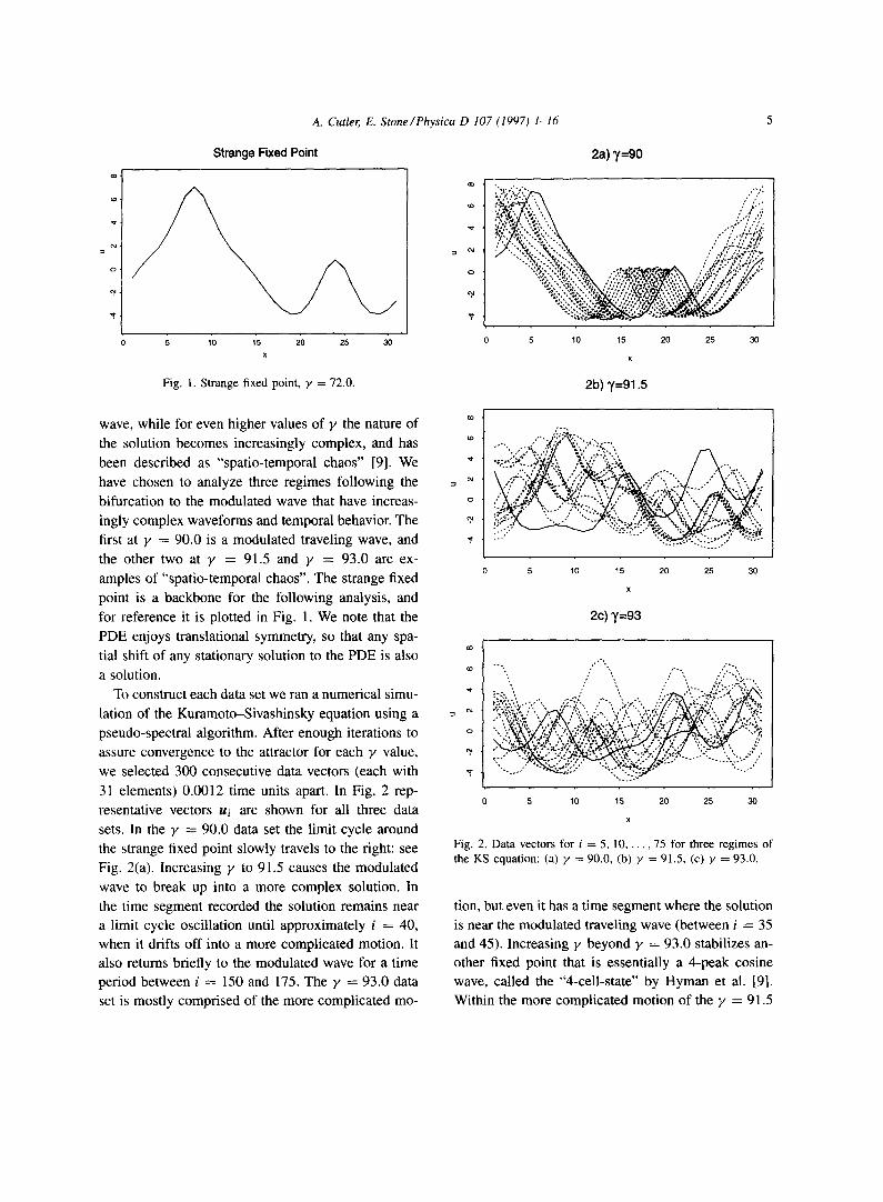
In this paper we study three higher 2/regimes to ex- plore the performance of moving archetypes on more temporally complicated data sets. The existence of a "strange fixed point'! solution to the PDE at y = 72.0 was discovered by Hyman et al. [9], the term coined by the authors to indicate the function's broad Fourier spectrum. They also discovered a Hopf bifurcation of the fixed point to a limit cycle for y = 83.25. At ~, = 86.0 this limit cycle bifurcates to a modulated

A. Cutler, E. Stone/Physica D 107 (1997) 1-16 5

Strange Fixed Point

a~

~t

o

0 5 10 15 20 25 30 x

2a) 7=90

-A':."." ' " . ~ . ' ~ - ' ." .'

", ' .~" J'?;: ' .".A "../..::' * r ; , , ; , . " - - , ' , ' : , .

= y ...~ .. / .".-<,'....%... • % ¢~r, j . ,

. % . . ; ; . pj. ,' . , ; . . o . L , ,' , .o % ..;:;~,,,:.XL'...~ . . . " . . / / ' . . . , "

. ~ • ~ " • " * , * " °~ ,-°.t " "

0 5 10 15 20 25 30

x

Fig. 1. Strange fixed point, y = 72.0. 2 b ) T = 9 1 . 5

wave, while for even higher values of y the nature of

the solution becomes increasingly complex, and has

been described as "spatio-temporal chaos" [9]. We

have chosen to analyze three regimes following the

bifurcation to the modulated wave that have increas-

ingly complex waveforms and temporal behavior. The

first at y -- 90.0 is a modulated traveling wave, and

the other two at y = 91.5 and y = 93.0 are ex-

amples of "spatio-temporal chaos". The strange fixed

point is a backbone for the following analysis, and

for reference it is plotted in Fig. 1. We note that the

PDE enjoys translational symmetry, so that any spa-

tial shift of any stationary solution to the PDE is also

a solution.

To construct each data set we ran a numerical simu-

lation of the Kuramoto-Sivashinsky equation using a

pseudo-spectral algorithm. After enough iterations to

assure convergence to the attractor for each ~, value,

we selected 300 consecutive data vectors (each with

31 elements) 0.0012 time units apart. In Fig. 2 rep-

resentative vectors ui are shown for all three data

sets. In the y = 90.0 data set the limit cycle around

the strange fixed point slowly travels to the right: see

Fig. 2(a). Increasing y to 91.5 causes the modulated

wave to break up into a more complex solution. In

the time segment recorded the solution remains near

a limit cycle oscillation until approximately i = 40,

when it drifts off into a more complicated motion. It

also returns briefly to the modulated wave for a t ime

period between i = 150 and 175. The y = 93.0 data

set is mostly comprised of the more complicated mo-

,-. . ',,,;-,,~,~,,, ,, .... ,..,,--.,L ,.?!~ "::,."-'~,.": r " , %-.. : " - . , ' , ' , ":, - ' .x ' .~."¢, , ,-,,:,,

.~. : . : ~'... "....;~.~'..-~...~. .:,% -.. ..

5 10 15 20 25 30

x

2 c ) ' y = 9 3

= ---.., /,'"'.., ./..... /::.:::::, . . . .

" * . . . ' . . . . . . ' . ~ . : . : . . . . •

, '~ ~ . ~ . . . / . j ~ ..:. ' . . " . . " . . . ¢. " . . . , . - , '< . %='. ..". "to.-'.

o ' ~ " " " " " " ':':'": "\' " ~ ' ¢ " ; ' " " "

5 25 30 10 15 20

x

Fig. 2. Data vectors for i = 5, 10 . . . . . 75 for three regimes of the KS equation: (a) y = 90.0, (b) y = 91.5, (c) y = 93.0.

tion, but even it has a time segment where the solution

is near the modulated traveling wave (between i = 35

and 45). Increasing y beyond y = 93.0 stabilizes an-

other fixed point that is essentially a 4-peak cosine

wave, called the "4-cell-state" by Hyman et al. [9].

Within the more complicated motion of the y --- 91.5


and ~/ = 93.0 sets the solution approaches this fixed point closely.

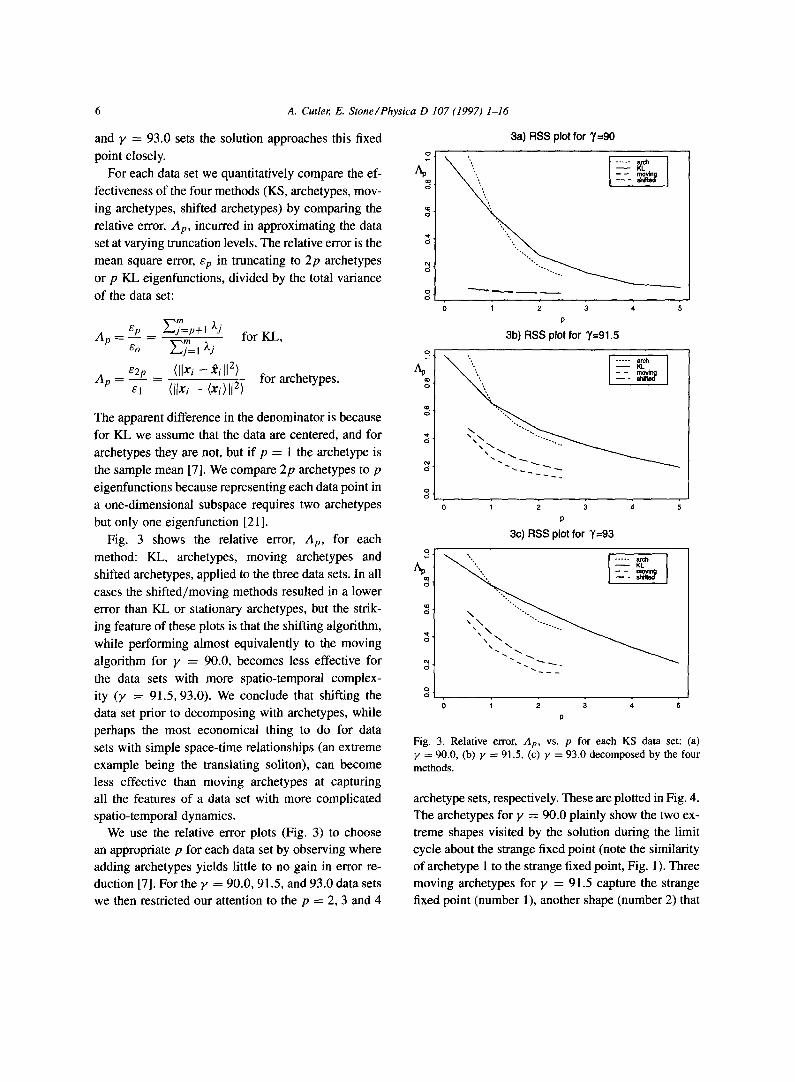
For each data set we quantitatively compare the ef-

fectiveness of the four methods (KS, archetypes, mov-

ing archetypes, shifted archetypes) by comparing the relative error, Ap , incurred in approximating the data set at varying truncation levels. The relative error is the

mean square error, ep in truncating to 2p archetypes

or p KL eigenfunctions, divided by the total variance

of the data set:

A p -- ~p ~jm__p+l Xj - for KL,

~'o E j m = l ~ . j

A p = E2._.pp _ ([Ixi - -~i [12) for archetypes. el (llXi -- (Xi)l[ 2)

m ` 5

co , 5 '

, 5 '

t~ d '

o `5"

co `5

`5

o

`5

co

~r d

ot d

The apparent difference in the denominator is because for KL we assume that the data are centered, and for

archetypes they are not, but if p = 1 the archetype is the sample mean [7]. We compare 2p archetypes to p

eigenfunctions because representing each data point in

a one-dimensional subspace requires two archetypes

but only one eigenfunction [21 ]. Fig. 3 shows the relative error, Ap , for each

method: KL, archetypes, moving archetypes and

shifted archetypes, applied to the three data sets. In all cases the shifted/moving methods resulted in a lower error than KL or stationary archetypes, but the strik- ing feature of these plots is that the shifting algorithm,

while performing almost equivalently to the moving algorithm for F = 90.0, becomes less effective for

the data sets with more spatio-temporal complexity (F = 91.5, 93.0). We conclude that shifting the data set prior to decomposing with archetypes, while perhaps the most economical thing to do for data sets with simple space-time relationships (an extreme

example being the translating soliton), can become less effective than moving archetypes at capturing all the features of a data set with more complicated spatio-temporal dynamics.

We use the relative error plots (Fig. 3) to choose an appropriate p for each data set by observing where adding archetypes yields little to no gain in error reduction [7]. For the F = 90.0, 91.5, and 93.0 data sets we then restricted our attention to the p = 2, 3 and 4

3a) RSS plot for 7=90

] ------ KL=~ - - 9 1

0 I 2 3 4 5

P

3b) RSS plot for ~'=91.5

0 1 2 3 4 5

P

3c) RSS plot for 7=93

I--- I

0 1 2 3 4 5

P

Fig. 3. Relative error, Ap, vs. p for each KS data set: (a) y = 90.0, (b) y = 91.5, (c) y = 93.0 decomposed by the four methods.

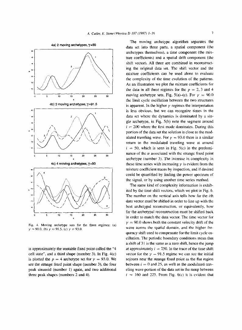
archetype sets, respectively. These are plotted in Fig. 4. The archetypes for F = 90.0 plainly show the two extreme shapes visited by the solution during the limit cycle about the strange fixed point (note the similarity of archetype 1 to the strange fixed point, Fig. 1). Three moving archetypes for y ---- 91.5 capture the strange fixed point (number 1), another shape (number 2) that

4a) 2 moving archetypes, 7=90

1

o -


5 10 15 20 25 30

x

4b) 3 moving archetypes, 'y=91.5

o.

/"\ .Y""" ''' r "~ ." /.>i.', ..X

5 10 15 20 25 30

X

4c) 4 moving archetypes, ~'=93

oo

to

e4

o

~ , 4 3

,",, , ,, f \ \ . . ,

0 5 10 15 20 25 30

x

Fig. 4. Moving archetype sets for the three regimes: (a) V = 90.0, (b) y = 91.5, (c) y = 93.0.

is approximately the unstable fixed point called the "4 cell state", and a third shape (number 3). In Fig. 4(c) is plotted the p = 4 archetype set for y = 93.0. We

see the strange fixed point shape (number 3), the four

peak sinusoid (number 1) again, and two additional three peak shapes (numbers 2 and 4).

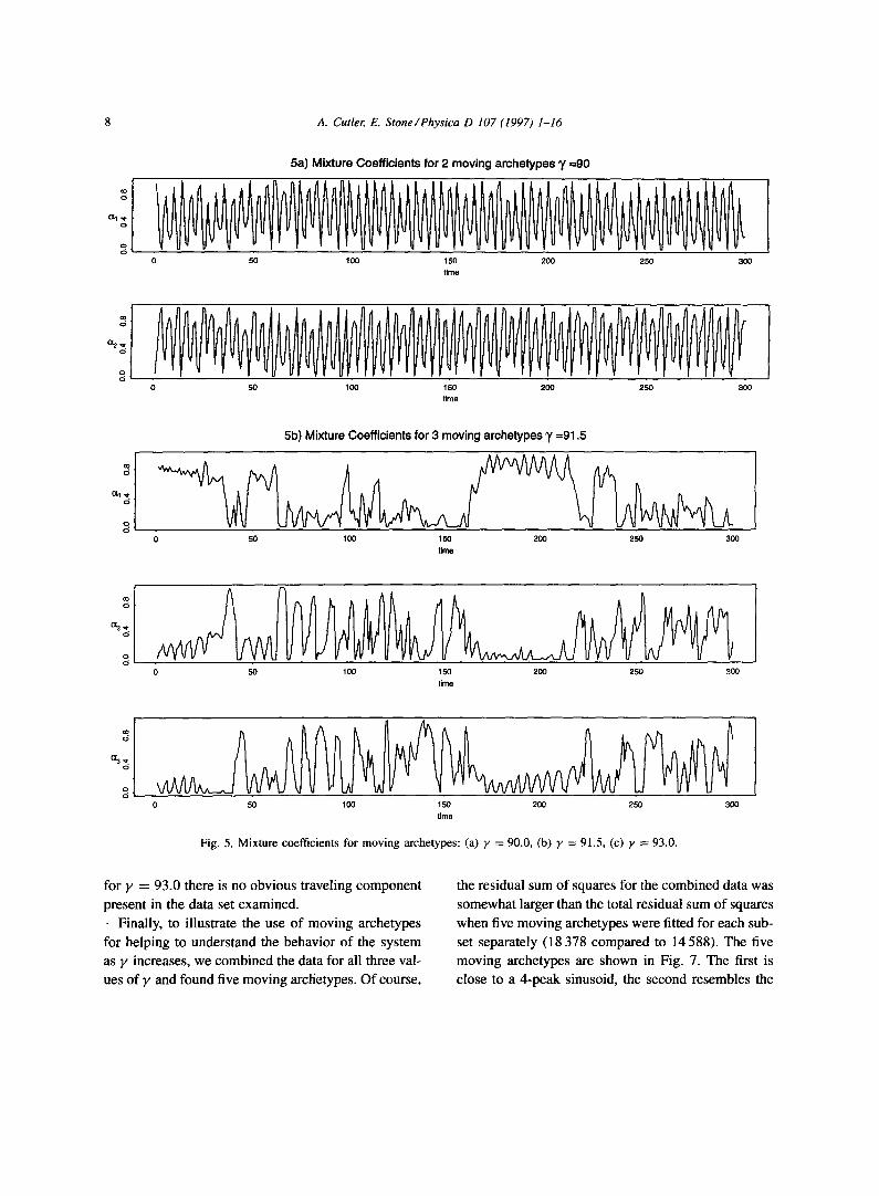
The moving archetype algorithm separates the

data set into three parts, a spatial component (the

archetypes themselves), a time component (the mix-

ture coefficients) and a spatial drift component (the

shift vector). All three are combined in reconstruct-

ing the original data set. The shift vector and the

mixture coefficients can be used alone to evaluate

the complexity of the time evolution of the patterns.

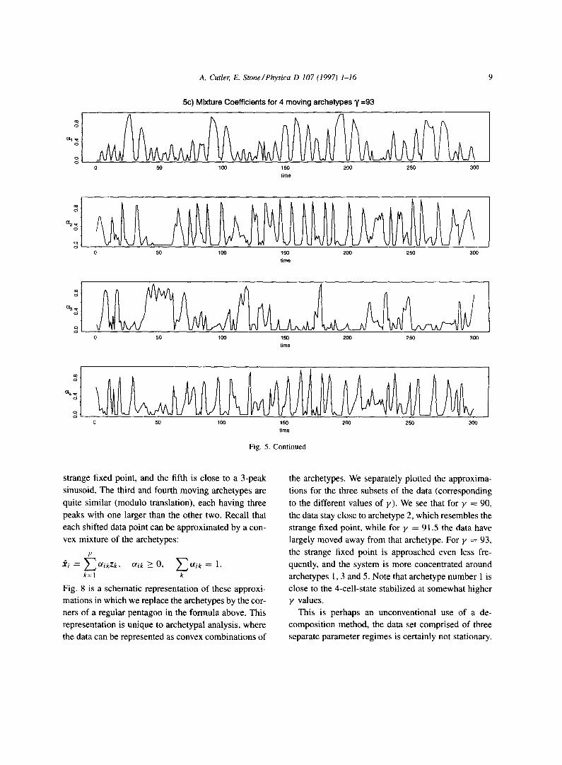
As an illustration we plot the mixture coefficients for

the data in all three regimes for the p = 2, 3 and 4

moving archetype sets, Fig. 5(a)-(c). For V -- 90.0

the limit cycle oscillation between the two structures

is apparent. In the higher y regimes the interpretation

is less obvious, but we can recognize times in the

data set where the dynamics is dominated by a sin-

gle archetype, in Fig. 5(b) note the segment around

i -- 200 where the first mode dominates. During this

portion of the data set the solution is close to the mod-

ulated traveling wave. For y = 93.0 there is a similar

return to the modulated traveling wave at around

i = 50, which is seen in Fig. 5(c) in the predomi-

nance of the u associated with the strange fixed point

archetype (number 3). The increase in complexity in

these time series with increasing y is evident from the

mixture coefficient traces by inspection, and if desired

could be quantified by finding the power spectrum of

the signal, or by using another time series method.

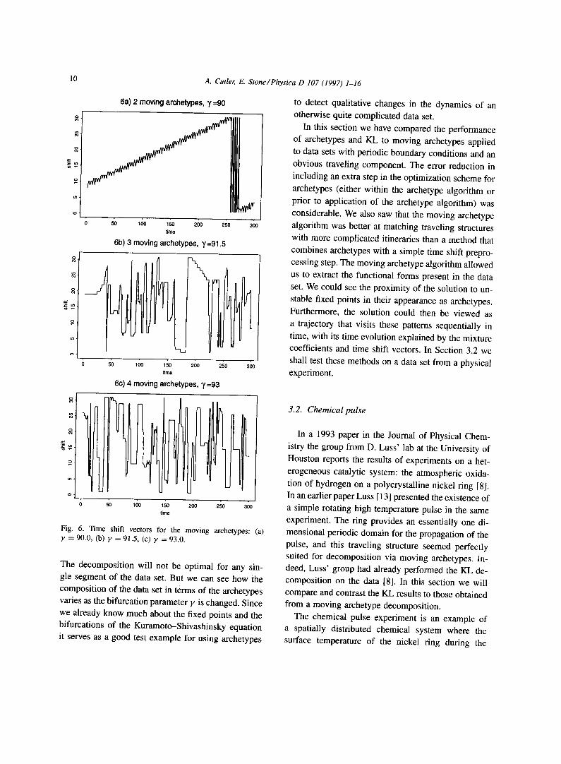
The same kind of complexity information is exhib-

ited by the time shift vectors, which we plot in Fig. 6.

The number on the vertical axis tells how far the ith

data vector m us~ be shifted in order to line up with the

best archetypal reconstruction, or equivalently, how

far the archetypal reconstruction must be shifted back

in order to match the data vector. The time vector for

Y -- 90.0 shows both the constant velocity drift of the

wave across the spatial domain, and the higher fre-

quency shift used to compensate for the limit cycle os-

cillation. The periodic boundary conditions mean that

a shift of 31 is the same as a zero shift, hence the jump

at approximately i = 250. In the trace of the time shift vector for the V = 91.5 regime we can see the initial sojourn near the strange fixed point as the fiat region between i ---- 0 and 25, as well as the modulated trav-

eling wave portion of the data set in the ramp between i = 160 and 225. From Fig. 6(c) it is evident that

8 A. Cutler, E. Stone/Physica D 107 (1997) 1-16

5a) Mixture Coefficients for 2 moving archetypes 'y =90

co d

o

50 1 O0 150 200 250 300 time

o

0 50 100 150 200 250 300 time

5b) Mixture Coefficients for 3 moving archetypes y =91.5

00 d

o

0 ~ 100 150 200 2 ~ 300

Ume

¢o d

0 50 100 150 200 250 300

time

¢o d

o d

50 100 150 200 250 300

~me

Fig. 5. Mixture coefficients for moving archetypes: (a) y = 90.0, (b) y = 91.5, (c) y = 93.0.

for Y = 93.0 there is no obvious traveling component

present in the data set examined.

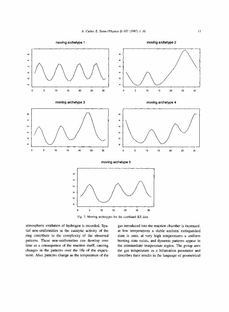
- Finally, to illustrate the use of moving archetypes

for helping to understand the behavior of the system

as y increases, we combined the data for all three val-

ues of y and found five moving archetypes. Of course,

the residual sum of squares for the combined data was

somewhat larger than the total residual sum of squares

when five moving archetypes were fitted for each sub-

set separately (18 378 compared to 14588). The five

moving archetypes are shown in Fig. 7. The first is

close to a 4-peak sinusoid, the second resembles the


5c) Mixture Coefficients for 4 moving archetypes 7 =93

oo

(7.1 ,q, <5

o ¢5

0 50 100 150 200 250 300

time

0 50 1 O0 150 200 250 300

time

0 50 100 150

time

200 250 300

to 6

Or4 -e" c5

o ci

@ 50 1 O0 150 200 250 300

time

Fig. 5. Continued

strange fixed point, and the fifth is close to a 3-peak sinusoid. The third and fourth moving archetypes are

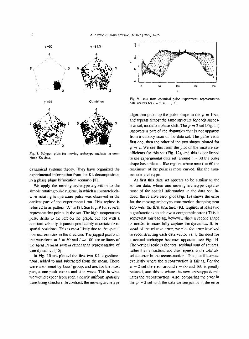
quite similar (modulo translation), each having three peaks with one larger than the other two. Recall that each shifted data point can be approximated by a convex mixture of the archetypes:

P

~_~ OlikZk, Otik >__ O, ~ Otik = 1. k=l k

Fig. 8 is a schematic representation of these approxi- mations in which we replace the archetypes by the cor- ners of a regular pentagon in the formula above. This representation is unique to archetypal analysis, where the data can be represented as convex combinations of

the archetypes. We separately plotted the approxima-

tions for the three subsets of the data (corresponding to the different values of y). We see that for y = 90,

the data stay close to archetype 2, which resembles the strange fixed point, while for y = 91.5 the data have largely moved away from that archetype. For y ----- 93, the strange fixed point is approached even less fre- quently, and the system is more concentrated around archetypes 1, 3 and 5. Note that archetype number 1 is close to the 4-cell-state stabilized at somewhat higher y values.

This is perhaps an unconventional use of a decomposition method, the data set comprised of three separate parameter regimes is certainly not stationary.


6a) 2 moving archetypes, 7 =90

to

o ,

- ~ .

o

to

o

1 ~ 1 ~ 2 ~ 2 ~ 3 ~

time

6b) 3 moving archetypes, ~'=91.5

t0o t~0 20o time

6c) 4 moving archetypes, 7 =93

2s0 3~0

o

o

0 50 100 150 200 250 300

time

Fig. 6. Time shift vectors for the moving archetypes: (a) y = 90.0, (b) y = 91.5, (c) y = 93.0.

The decomposition will not be optimal for any single segment of the data set. But we can see how the composition of the data set in terms of the archetypes varies as the bifurcation parameter y is changed. Since we already know much about the fixed points and the bifurcations of the Kuramoto-Shivashinsky equation it serves as a good test example for using archetypes

to detect qualitative changes in the dynamics of an otherwise quite complicated data set.

In this section we have compared the performance of archetypes and KL to moving archetypes applied to data sets with periodic boundary conditions and an

obvious traveling component. The error reduction in

including an extra step in the optimization scheme for

archetypes (either within the archetype algorithm or prior to application of the archetype algorithm) was considerable. We also saw that the moving archetype

algorithm was better at matching traveling structures

with more complicated itineraries than a method that combines archetypes with a simple time shift prepro-

cessing step. The moving archetype algorithm allowed us to extract the functional forms present in the data set. We could see the proximity of the solution to unstable fixed points in their appearance as archetypes.

Furthermore, the solution could then be viewed as

a trajectory that visits these patterns sequentially in

time, with its time evolution explained by the mixture coefficients and time shift vectors. In Section 3.2 we

shall test these methods on a data set from a physical experiment.

3.2. Chemical pulse

In a 1993 paper in the Journal of Physical Chem-

istry the group from D. Luss' lab at the University of Houston reports the results of experiments on a het-

erogeneous catalytic system: the atmospheric oxidation of hydrogen on a polycrystalline nickel ring [8]. In an earlier paper Luss [ 13] presented the existence of a simple rotating high temperature pulse in the same experiment. The ring provides an essentially one dimensional periodic domain for the propagation of the

pulse, and this traveling structure seemed perfectly suited for decomposition via moving archetypes. In- deed, Luss' group had already performed the KL decomposition on the data [8]. In this section we will compare and contrast the KL results to those obtained from a moving archetype decomposition.

The chemical pulse experiment is an example of a spatially distributed chemical system where the surface temperature of the nickel ring during the

A. Cutler, E. Stone/Physica D 107 (1997) 1-16 I 1

moving archetype 1

5 10 15 20 25 30

moving archetype 2

5 10 15 20 25 30

moving archetype 3 moving archetype 4

o

5 10 15 20 25 30

04

o

.~-

0 5 10 15 20 25 30

moving archetype 5

5 10 15 20 25 30

Fig. 7. Moving archetypes for the combined KS data.

atmospheric oxidation of hydrogen is recorded. Spa-

tial non-uniformities in the catalytic activity of the

ring contribute to the complexity of the observed patterns. These non-uniformities can develop over

time as a consequence of the reaction itself, causing changes in the patterns over the life of the experi-

ment. Also, patterns change as the temperature of the

gas introduced into the reaction chamber is increased:

at low temperatures a stable uniform extinguished state is seen, at very high temperatures a uniform

burning state exists, and dynamic patterns appear in the intermediate temperature region. The group uses the gas temperature as a bifurcation parameter and

describes their results in the language of geometrical


y=90

4

5 ................................................ i: 3 -\

"\., .................... . ~ ' / 1 2

~/=91.5

4

...." • •oo+,.,

.~" ++ P . iP',.. 5 ~,=*=o. • •,,.¢°.~1.'8-. 3

ir :/ -.._.,¢. ,It I ' : , L ~ + .

I . . . . . . . . - - 2

• ,,,,• .;.,;:?

x

-/=93 Combined

4 4

.7 +. "/ ' • o •

• ° o,b• .,'

1 2 1 2

Fig. 8. Polygon plots for moving archetype analysis on combined KS data.

dynamical systems theory. They have organized the

experimental information from the KL decomposition

in a phase plane bifurcation scenario [8].

We apply the moving archetype algorithm to the

simple rotating pulse regime, in which a counterclock-

wise rotating temperature pulse was observed in the

earliest part of the experimental run. This regime is

referred to as pattern "A" in [8]. See Fig. 9 for several

representative points in the set. The high temperature

pulse drifts to the left on the graph, but not with a constant velocity, it pauses predictably at certain fixed spatial positions• This is most likely due to the spatial

non-uniformities in the medium• The jagged points in

the waveform at i = 50 and i = 100 are artifacts of the measurement system rather than representative of true dynamics [ 15].

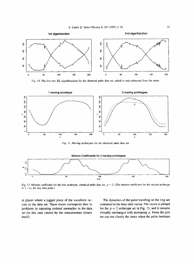
In Fig. 10 are plotted the first two KL eigenfunc-

tions, added to and subtracted from the mean. These were also found by Luss' group, and are, for the most part, a one peak cosine and sine wave. This is what

we would expect from such a nearly uniform spatially translating structure. In contrast, the moving archetype

Fig. 9. Data from chemical pulse experiment: representative data vectors for i = 2, 4 . . . . . 30.

algorithm picks up the pulse shape in the p = 1 set,

and repeats almost the same structure for each succes-

sive set, modulo a phase shift. The p = 2 set (Fig. 1 l)

uncovers a part of the dynamics that is not apparent

from a cursory scan of the data set. The pulse visits

first one, then the other of the two shapes plotted for

p = 2. We see this from the plot of the mixture co-

efficients for this set (Fig. 12), and this is confirmed

in the experimental data set: around i = 30 the pulse

shape has a plateau-like region, where near i = 60 the

maximum of the pulse is more curved, like the num-

ber one archetype.

At first this data set appears to be similar to the

soliton data, where one moving archetype captures

most of the spatial information in the data set. In-

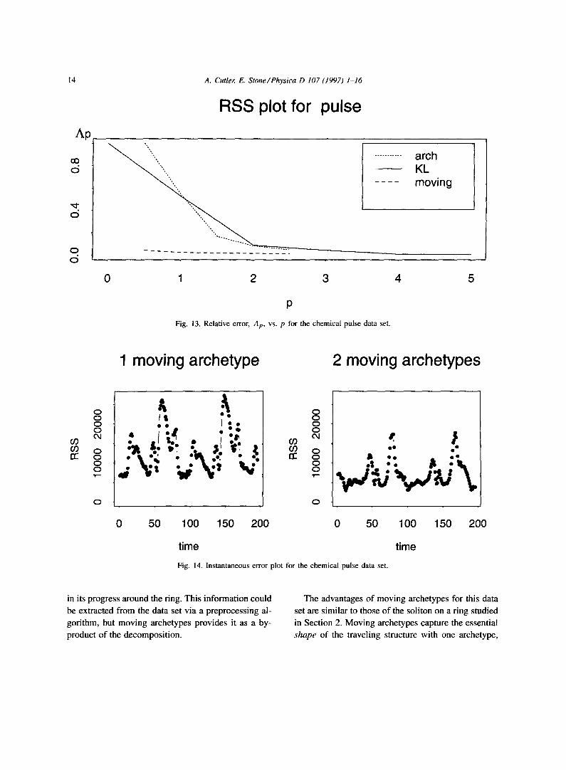
deed, the relative error plot (Fig. 13) shows the error

for the moving archetype construction dropping near

zero with the first structure. (KL requires at least two

eigenfunctions to achieve a comparable error.) This is

somewhat misleading, however, since a second shape

is needed to more fully capture the dynamics. If, in- stead of the relative error, we plot the error involved

in reconstructing each data vector vs. i, the need for

a second archetype becomes apparent, see Fig. 14.

The vertical scale is the total residual sum of squares, rather than a fraction, and thus represents the total ab- solute error in the reconstruction. This plot illustrates

explicitly where the reconstruction is failing. For the p = 2 set the error around i = 60 and 160 is greatly

reduced, and this is where the new archetype dominates the reconstruction. Also, comparing the error in the p = 2 set with the data we see jumps in the error


1st eigenfunction 2nd eigenfunction

8

0 ~ 1 ~ 1 ~ 2 ~ 0 ~ 1 ~ 1 ~ 2 ~

Fig. 10. The first two KL eigenfunctions for the chemical pulse data set, added to and subtracted from the mean.

13

8

o

o

1 moving archetype

0 50 1 ~ 1 ~ 200

x

2 moving archetypes

x

Fig. 11. Moving archetypes for the chemical pulse data set.

Mixture Coefficients for 2 moving archetypes

ao d

cq

o d

0 50 100 150

time

200

Fig. 12. Mixture coefficient for the first archetype, chemical pulse data set, p = 2. (The mixture coefficient for the second archetype is 1 - c¢1 for any data point.)

at places where a jagged piece of the waveform oc-

curs in the data set. These errors correspond then to

problems in captur ing isolated anomal ies in the data

set (in this case caused by the measu remen t system

itself).

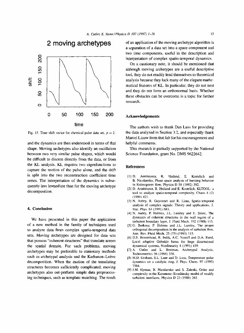
The dynamics of the pulse traveling on the ring are

conta ined in the t ime shift vector. The vector is plotted

for the p = 2 archetype set in Fig. 15, and it remains

virtually unchanged with increasing p. From the plot

we can see clearly the t imes when the pulse hesitates


Ap

RSS plot for pulse

CO (:5

O

O <:5

........... arch KL moving

0 1 2 3

P

Fig. 13. Relative error, Ap, vs. p for the chemical pulse data set.

4 5

1 moving archetype 2 moving archetypes

g

0

. ' ~ . " , ' oTA ",,• 1;' ,-I

0 5 0

8 o o

. - g o o

100 150

time

O

2 0 0

.,: • S - • II • l k

• x .

0 50 100 150 200

Fig. 14. Instantaneous error plot for the chemical pulse data set.

time

in its progress around the ring. This information could

be extracted from the data set via a preprocessing al-

gorithm, but moving archetypes provides it as a by-

product of the decomposition.

The advantages of moving archetypes for this data

set are similar to those of the soliton on a ring studied

in Section 2. Moving archetypes capture the essential

shape of the traveling structure with one archetype,

0 0

0 tO

8 cO v - -

0 tO

0


2 moving archetypes

\

15

of an application of the moving archetype algorithm is

a separation of a data set into a space component and

two time components, useful in the description and

interpretation of complex spatio-temporal dynamics.

On a cautionary note, it should be mentioned that

although moving archetypes are a useful descriptive

tool, they do not readily lend themselves to theoretical

analysis because they lack many of the elegant mathe-

matical features of KL, In particular, they do not nest

and they do not form an orthonormal basis. Whether

these obstacles can be overcome is a topic for further

research.

0 50 100 150 200

time

Fig. 15. Time shift vector for chemical pulse data set, p = 2.

and the dynamics are then understood in terms of that

shape. Moving archetypes also identify an oscillation

between two very similar pulse shapes, which would

be difficult to discern directly from the data, or from

the KL analysis. KL requires two eigenfunctions to

capture the motion of the pulse alone, and the drift

is split into the two reconstruction coefficient time

series. The interpretation of the dynamics is subse-

quently less immediate than for the moving archetype

decomposition.

4. Conclusion

We have presented in this paper the application

of a new method in the family of techniques used to analyze data from complex spatio-temporal data

sets. Moving archetypes are designed for data sets

that possess "coherent structures" that translate across

the spatial domain. For such problems, moving

archetypes may be preferable to stationary methods such as archetypal analysis and the Karhunen-Lo6ve decomposition. When the motion of the translating

structures becomes sufficiently complicated, moving archetypes also out-perform simple data preprocessing techniques, such as template matching. The result

Acknowledgements

The authors wish to thank Dan Luss for providing

the data analyzed in Section 3.2, and especially thank

Marcel Liauw from that lab for his encouragement and

helpful comments.

This research is partially supported by the National

Science Foundation, grant No. DMS 9622642.

References

[1] D. Armbruster, R. Heiland, E. Kostelich and B. Nicolaenko, Phase space analysis of bursting behavior in Kolmogorov flow, Physica D 58 (1992) 392.

[2] D. Armbruster, R. Heiland and E. Kostelich, KLTOOL: a tool to analyze spatio-temporal complexity, Chaos 4 (2) (1994) 421.

[3] N. Aubry, R. Guyonnet and R. Lima, Spatio-temporal analysis of complex signals: Theory and applications, J. Stat. Phys. 63 (1991) 683.

[4] N. Aubry, P. Holmes, J.L. Lumley and E. Stone, The dynamics of coherent structures in the wall region of a turbulent boundary layer, J. Fluid Mech. 192 (1988) 115.

[5] G. Berkooz, E Holmes and J.L. Lumley, The proper orthogonal decomposition in the analysis of turbulent flow. Ann. Rev. Fluid Mech. 25 (75) (1993) 115.

[6] D.S. Broomhead, R. Indik, A.C. Newell and D.A. Rand, Local adaptive Galerkin bases for large dimensional dynamical systems, Nonlinearity 4 (1991) 159.

[7l A. Cutler and L. Breiman, Archetypal Analysis, Technometrics 36 (1994) 338.

[8] M.D. Graham, S.L. Lane and D. Luss, Temperature pulse dynamics on a catalytic ring, J. Phys. Chem. 97 (1993) 7564.

[9] J.M. Hyman, B. Nicolaenko and S. Zaleski, Order and complexity in the Kuramoto--Sivashinsky model of weakly turbulent interfaces, Physica D 23 (1986) 265.


[10] I.G. Kevrikidis, B. Nicolaenko and C. Scovel, Back in the saddle again: A computer assisted study of the Kuramoto- Sivashinsky equation, SIAM J. Appl. Math. 50 (1990) 760.

[11] M. Kirby and D. Armbruster, Reconstructing phase-space from PDE simulations, ZAMP 43 (1992) 999.

[12] M. Kirby, F. Weisser and G. Dangelmayr, A model problem in the representation of digital image sequences, Pattern Recognition 26 (1) (1993) 63.

[13] S.L. Lane and D. Luss, Rotating temperature pulse during hydrogen oxidation of a nickel ring, Phys. Rev. Lett. 70 (1993) 830.

[14] C.L. Lawson and R.J. Hanson, Solving Least Squares Problems (Prentice-Hall, New Jersey, 1974).

[15] M. Liauw, Personal communication (1995). [16] J.L. Lumley, The structure of inhomogeneous turbulent

flows, in: Atmospheric Turbulence and Radio Wave

Propagation, eds. A.M. Yaglom and V.I. Tatarski (Nauka, Moscow, 1967)pp. 166-178.

[17] L. Sirovich, Turbulence and the dynamics of coherent structures Parts I-III, Quarterly of Applied Mathematics, Vol. XLV, 3 (1987) 561.

[18] L. Sirovich and J. Rodriguez, Coherent structures and chaos: A model problem, Phys. Lett. A 120 (1987) 211.

[19] G.I. Sivashinsky, Nonlinear analysis of hydrodynamic stability of laminar flames: Derivation of basic equations, Acta Astr. 4 (1977) 1177.

[20] E. Stone and A. Cutler, Archetypal analysis of spatio- temporal dynamics, Physica D 90 (1996) 209.

[21] E. Stone and A. Cutler, Introduction to archetypal analysis of spatio-temporal dynamics, Physica D 96 (1996) 110.

Documents

Moving archetypes