Motion of deformable bodies - JÜRGEN FUCHS

Karlstad university

Faculty for health, science and technology

FYGB08

Motion of deformable bodies

Author:Axel Hedengren.

SupervisorProfessor Jürgen Fuchs.

—————————————-January 23, 2017

Motion of deformable bodies Abstract

AbstractThis work analyses the motion of deformable bodies. The main point of departureis Lagrange’s form of d’Alembert’s principle, which says that ”The total virtualwork of the impressed forces plus the internal forces vanishes for reversible displace-ments”. The first part of the theory states which coordinate systems involved andtheir relations. In the second part the different forces that could possibly act onor in the body and its effect on the different coordinate systems are stated, firstin a general case for deformable bodies, after that in cases with constraints andat last reduced to a special case for the motion of a rigid body.

1

Motion of deformable bodies Contents

ContentsAbstract 1

Introduction 3

Background 4

Theory 4Geometric representation . . . . . . . . . . . . . . . . . . . . . . . . . . . 4Dynamical equations of motion . . . . . . . . . . . . . . . . . . . . . . . 6

General case: Elastic body . . . . . . . . . . . . . . . . . . . . . . . 6Motion of deformable body with constraints . . . . . . . . . . . . . 11Special case: Rigid body . . . . . . . . . . . . . . . . . . . . . . . . 11

Conclusion 13

2

Motion of deformable bodies Introduction

IntroductionDeformation is defined as change of size or form of an object due to appliedforces. These forces could be external forces or internal forces, for example internalforces due to temperature changes. For the calculations in this work two mainassumptions have been adopted. The first, and probably the roughest, is that anyatomic structure has been neglected and that the structure of the body is saidto be continuous, this assumption is called the continuum principle. The secondmain assumption is called solidification principle and means that the body consistsof mathematical points at infinitesimal distances, each point is said to act underrigid body conditions. This leads to Lagrange’s form of d’Alembert’s principle,which states that ”The total virtual work of the impressed forces plus the internalforces vanishes for reversible displacements”,∑

i

(Fi −miai) · δri = 0. (1)

This principle is the dynamical analogue to the principle of virtual work for appliedforces in static systems, and is in fact more general than Hamilton’s principle. Thegoal with this paper is to obtain the equations of motion for deformable bodies,not to solve them.

3

Motion of deformable bodies Theory

BackgroundConsider a cat that is dropped upside down, if the cat is assumed to be a rigidbody (for example a wood crafted cat) it will, as long as there are no externalforces acting on it, land on its back. However if the cat is alive it will with thegreatest probability land on its feet. To physically explain this phenomenon andother motions of deformable bodies we are forced to go deeper into the theorythan for motions of rigid bodies.

Theory

Geometric representation

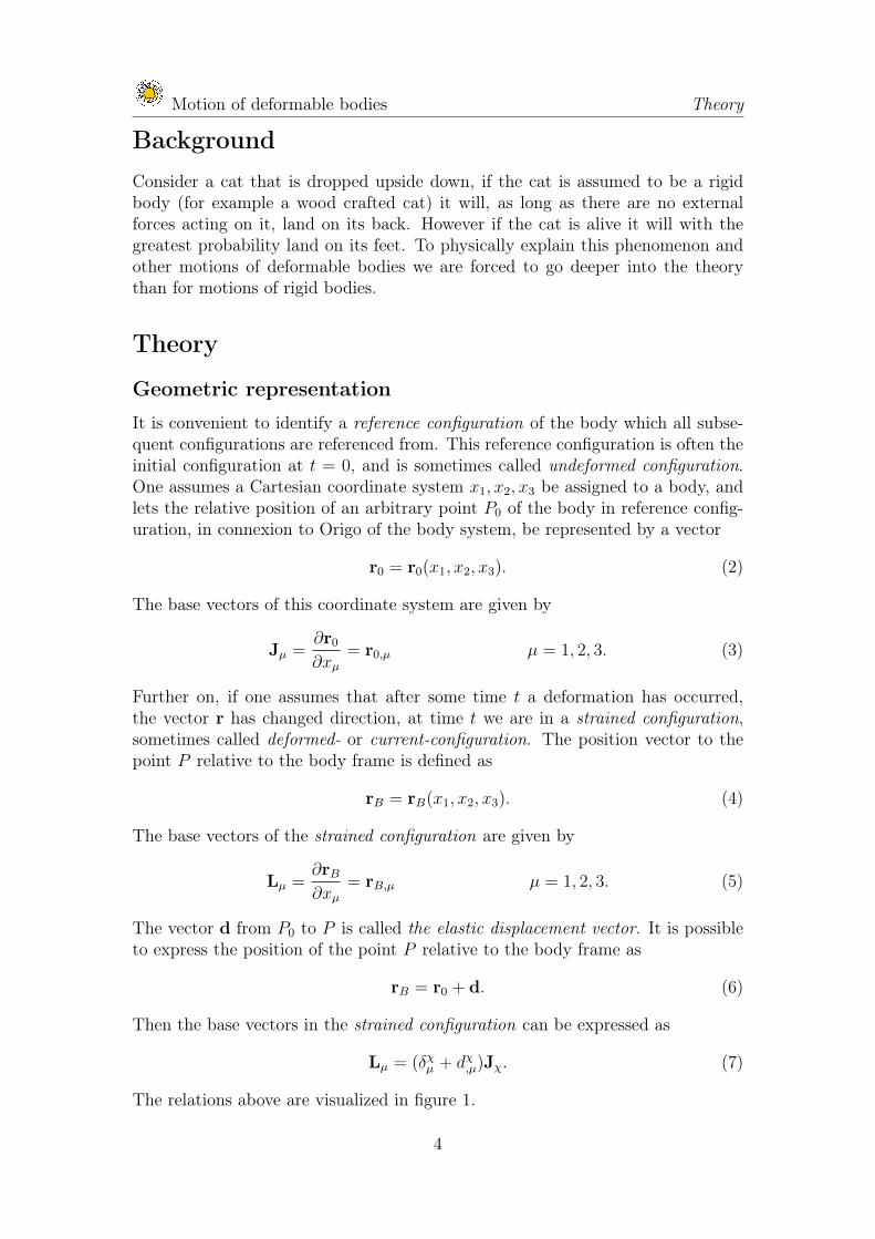
It is convenient to identify a reference configuration of the body which all subse-quent configurations are referenced from. This reference configuration is often theinitial configuration at t = 0, and is sometimes called undeformed configuration.One assumes a Cartesian coordinate system x1, x2, x3 be assigned to a body, andlets the relative position of an arbitrary point P0 of the body in reference config-uration, in connexion to Origo of the body system, be represented by a vector

r0 = r0(x1, x2, x3). (2)

The base vectors of this coordinate system are given by

Jµ =∂r0∂xµ

= r0,µ µ = 1, 2, 3. (3)

Further on, if one assumes that after some time t a deformation has occurred,the vector r has changed direction, at time t we are in a strained configuration,sometimes called deformed- or current-configuration. The position vector to thepoint P relative to the body frame is defined as

rB = rB(x1, x2, x3). (4)

The base vectors of the strained configuration are given by

Lµ =∂rB∂xµ

= rB,µ µ = 1, 2, 3. (5)

The vector d from P0 to P is called the elastic displacement vector. It is possibleto express the position of the point P relative to the body frame as

rB = r0 + d. (6)

Then the base vectors in the strained configuration can be expressed as

Lµ = (δχµ + dχ,µ)Jχ. (7)

The relations above are visualized in figure 1.

4


Figure 1: The point P0 and P relative to a body system.

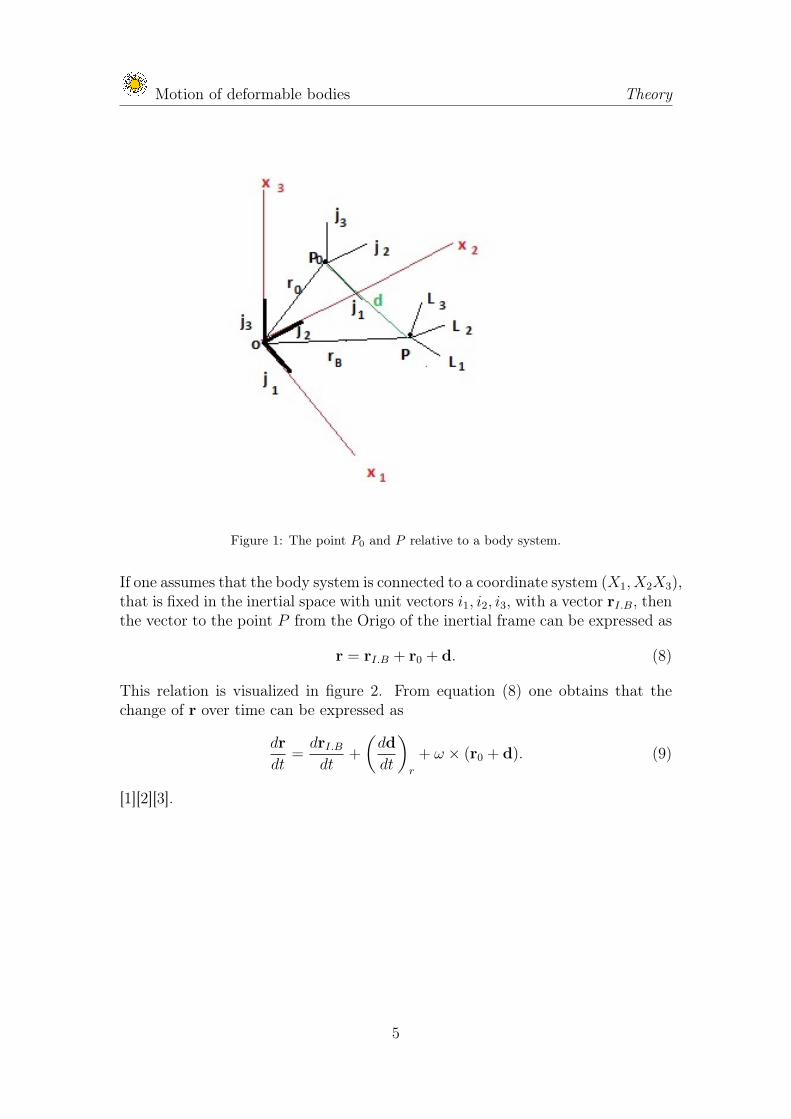
If one assumes that the body system is connected to a coordinate system (X1, X2X3),that is fixed in the inertial space with unit vectors i1, i2, i3, with a vector rI.B, thenthe vector to the point P from the Origo of the inertial frame can be expressed as

r = rI.B + r0 + d. (8)

This relation is visualized in figure 2. From equation (8) one obtains that thechange of r over time can be expressed as

dr

dt=drI.Bdt

+

(dd

dt

)r

+ ω × (r0 + d). (9)

[1][2][3].

5


Figure 2: The point P0 and P relative to a inertial system.

Dynamical equations of motion

The relation between the inertial frame and the body frame can be expressed withan orthogonal matrix A:

Jα = Aiβ. (10)

And from equation (7) one can obtain that

Lα = ZJγ = ZAiβ. (11)

General case: Elastic body

By the theory of virtual work one can obtain that the internal virtual work mustequal the external virtual work, such that

δWI = δWE. (12)

In an elastic body, the possible virtual forces are

External:

• Body surface forces (B(xi, t)).

• Body forces (F(xi, t)).

6


• Inertia ”forces” (−ρ(d2r

dt2

)),(This is actually not a force in strict meaning

but it has a force-like behaviour and are therefore treated as a force. Theterm comes from the right hand side of newtons second law F = ma).

Internal:

• Elastic energy (σσσµ · (δr),µ).

This gives the dynamical virtual work expression∫V

σσσµ · (δr),µdV =

∫V

(F(xi, t)− ρ

(d2r

dt2

))dV +

∫S

B(xi, t) · δrdS. (13)

By using that

rrr = rαiiiα FFF = F βJJJβ (14)BBB = BγJJJγ σσσµ = σµζLLLζ , (15)

one can rewrite equation (13), to see each term more explicitly, as∫V

F βJJJβ · δrαiiiαdVi +∫S

BγJJJγ · δrαiiiαdS −∫V

ρd2rα

dt2iiiα · δrαiiiαdV

−∫V

σµζLLLζ · (δrαiiiα),µdV = 0. (16)

The virtual displacement is given by

δrrr = δrrrI.B + δddd+ δθθθ × (rrr0 + ddd). (17)

It can be rewritten in the same manner as for the virtual work, so that

δrαiiiα = δrαI.Biiiα + δdαjjjα + δθαjjjα × (rβ0jjjβ + dβjjjβ). (18)

Now we have an expression for the virtual work and for the virtual displacement,but they are expressed in a mix of coordinate systems. By rewriting the equationsin matrix form and using equations (10) and (11) one could express the equationsfor the virtual work and displacement in the inertial frame. One then obtains theequation for the virtual work as∫

V

(At{F})t{δr}dV +

∫S

(At{B})t{δr}dS −∫V

ρ{d2r

dt2}t{δr}dV

−∫V

(AtZt{σµ})t{δr,µ}dV = 0, (19)

and the equation for the virtual displacement as

{δr} = {δrI.B}+ At{δd}+ Atδθ({r0}+ {d}). (20)

We can from equation (20) derive {δr,µ}, here is {rI.B} not a function of bodyaxis variables and are therefore treated as a constant,

{δr,µ} = At{δd,µ}+ Atδθ({r0,µ}+ {d,µ}). (21)

Now we want to analyse each integral in equation (19).

7


• First we take the first integral in equation (19), rewrite it in the body framesystem (J) and substitute equation 20, such that∫

V

(At{F})t{δr}dV =

∫V

{F}t(A{δrI.B}+ {δd}+ {δθ}({r0}+ {d}))dV.

(22)

Recall that this part represents the virtual work due to the resultant appliedforces, therefore we further on denote the force-term in this integral with anindex B.

To proceed one needs to determine the absolute velocity of the body frame in com-parison with the inertial system. Suppose that we have n generalized coordinates.The velocity is

{vI.B} = {rI.B} =n∑j=1

∂

∂qj{rI.B}qj +

∂

∂t{rI.B}. (23)

Defining a velocity coefficient in the inertial frame

{γI.Bj } =∂

∂qj{rI.B}, (24)

the virtual displacement of {rI.B} can be expressed as

{δrI.B} =n∑j=1

{γI.Bj }δqj. (25)

The velocity of {d} is a relative velocity. Expressed in body space we have

{d} =n∑j=1

∂

∂qj{d}qj. (26)

Define

{γdj } =∂

∂qj{d} = ∂

∂qj{d}. (27)

The virtual displacement of {d} is

{δd} =n∑j=1

{γdj }δqj. (28)

This leads to the derivative

{δd,µ} =n∑j=1

{γdj,µ}δqj. (29)

8


Now we almost have all tools to continue with the virtual work equation, we justhave to obtain the virtual work due to inertial moments. Defining the angularvelocity coefficient in body space as

{βj} =∂

∂qj{ω}. (30)

Then we can express a small virtual rotation as

{δθ} =n∑j=1

{βj}δqj. (31)

Now we can continue with the first integral. Inserting the results from equation(25), (28) and (31) into equation (22) gives∫

V

(At{F})t{δr}dV =n∑j=1

∫V

{FB}t{γj}dV δqj, (32)

where

{γj} = A{γI.Bj }+ {γdj }+ {βj}({ro}+ {d}). (33)

• The surface integral in equation (19) can be obtained by a similar procedure,where the external surface force is denoted by an index S,∫

S

(At{B})t{δr}dS =n∑j=1

∫S

{FS}t{γj}dSδqj. (34)

• In the third integral we have a second order time derivative of r. Fromequation (8) we have

{r} = {rI.B}+ At{r0}+ At{d}. (35)

Where all terms varying with time except for r0. We also have that

A = −ωA = ωtA. (36)

The second order time derivative of r therefore becomes

{r} = {rI.B}+ At ˜ω{r0}+ Atω2{r0}+ At ˜ω{d}+ Atω2{d}+ 2Atω{d}+ At{d}.(37)

By substituting this expression into the third integral of equation (19) anddefine the inertial force as

F∗ = −ρ(A{rI.B}+ ˜ω{r0}+ ω2{r0}+ ˜ω{d}+ ω2{d}+ 2ω{d}+ {d}), (38)

one obtains

−∫V

ρrt{δr}dV =n∑j=1

∫V

{F∗}t{γj}dV δqj. (39)

9


• In the last integral of equation (19) one can use the equation for the derivativeof the virtual displacement, equation (21), and also the virtual displacementof d and of virtual rotation, equations (29) and (31). This gives, in bodyframe components, that

−∫V

(AtZt{σµ})t{δrµ}dV =n∑j=1

∫V

{F µE}

t{γdj,µ}dV δqj, (40)

where the elastic force is denoted by an index E, and is defined as

{F µE} = −Z

t{σµ}. (41)

If we define:

• The generalized external applied forces

Qj =

∫V

{FB}t{γj}dV +

∫S

{FS}t{γj}dS. (42)

• The generalized inertia forces

Q∗j =

∫V

{F∗}t{γj}dV. (43)

• The generalized elastic force

QEj =

∫V

{F µE}

t{γdj,µ}dV. (44)

By use d’Alembert’s principle one obtains

n∑j=1

(Qj +Q∗J +QE

j )δqj = 0. (45)

Further, if one assumes that the various qj are linearly independent, then eachcoefficient of δqj must vanish, and we obtain

Qj +Q∗J +QE

j = 0, (j = 1, 2, .., n). (46)

And in greater detail we have

Qj =

∫V

ρ(A{rI.B}+ ˜ω{r0}+ ω2{r0}+ ˜ω{d}+ ω2{d}+ 2ω{d}+ {d})t{γj}dV

+

∫V

(Zt{σµ})t{γdj,µ}dV, (j = 1, 2, .., n). (47)

which is the matrix form of the general dynamical equations of motion.[2][3][4].

10


Motion of deformable body with constraints

Equation (47) gives the equations of motion for a dynamical body without anyholonomic or nonholonomic constraints on the generalized coordinates. It cansomehow be an advantage in the computation to introduce constraints if thereis possible to detect in the abstraction of the problem. Therefore it is prefer-able to determine the dynamical equations of motion with constraints. In generalfor a system with n degrees of freedom we need n generalized coordinates, sayq1, q2, .., qn, to describe the system. However assume that there exist m indepen-dent constraints such that

n∑i=1

aji(q, t)qi + ajt(q, t) = 0, j = 1, 2, ..,m. (48)

Introduce a set of n−m independent parameters uj, called generalized speeds:

uj =n∑i=1

ψji(q, t)qi + ψjt(q, t), j = 1, 2, .., n−m. (49)

By using the generalized speeds in the velocity- and angular velocity coefficients,such that

{γI.Bj } =∂

∂uj{rI.B}, {γdj } =

∂

∂uj{d} (50)

{γdj,µ} =∂

∂uj{ ˙d,µ} {βj} =

∂

∂uj{ω}, (51)

equation (47) does not change except for that j = 1, 2, .., n−m, and we have

Qj =

∫V

ρ(A{rI.B}+ ˜ω{r0}+ ω2{r0}+ ˜ω{d}+ ω2{d}+ 2ω{d}+ {d})t{γj}dV

+

∫V

(Zt{σµ})t{γdj,µ}dV, (j = 1, 2, .., n−m). (52)

[2][3][4].

Special case: Rigid body

From the dynamical equations of motions we can now go to the equations of motionfor a rigid body. First assume that the body frame system is fixed in the body.Further, the mass of the body is m and the distance from the origin of the bodyframe system is rrrc.m. We also have the correspondence between the total massand the density such that ∫

V

ρdV = m. (53)

And we also have ∫V

ρrrrodV = mrrrc.m. (54)

11


With these limitations one can show that equation (19), with some algebraicmanipulations, in vector form, reduces to

m(rrrI.B + rrrc.m) · γγγI.Bj + (III · ωωω +ωωω × III ·ωωω +mrrrc.m × rrrI.B) · βββj = QQQj, j = 1, 2, .., n,

(55)

where n is the number of independent coordinates and the inertia term III is takenwith respect to the origin of the body system, [5].

12

Motion of deformable bodies Conclusion

ConclusionIn this work, a general formalism for the motion of deformable bodies has beenexplained. However, the method is based on the theory of infinitesimals, whereasreal materials have atomic structure that has been neglected. So the calculations,that mathematically are exact, are invalid for real deformable bodies. However themethod gives a good approximation, and it can have the same accuracy as for finitemodels. The equations of motion for deformable bodies that have been derivedhere are, except for very simple special cases, very difficult or even impossible tosolve analytically and are often only numerically treatable. The formalism that hasbeen explained in this paper could be expanded to cover the motion of multibodysystems.

13

Motion of deformable bodies References

References[1] Terzopoulos Demetri, Witkin Andrew, Deformable Models: Physically Based

Models with Rigid and Deformable Components, IEEE computer graphics andapplications, Vol. 8 No. 6: 41-51, 1988.

[2] Escalona J.L., Valverde J., Mayo J., Dominiguez J., Reference motion in de-formable bodies under rigid body motion and vibration. Part I: theory, Journalof sound and vibration, No. 264: 1045-1056, 2003.

[3] Weng Shui-Lin, Greenwood Donald T,General Dynamical Equations of Motionfor Elastic Body Systems, Journal of guidance control and dynamics, Vol. 15No. 6: 1434-1442, 1992.

[4] Tong David, Classical dynamics, University of Cambridge, 2004,http://www.damtp.cam.ac.uk/user/tong/dynamics.html, (accessed 2017-01-07).

[5] Greenwood D.T.,Principles of dynamics, 2nd ed., Prentice-Hall, New Jersey,1988.

14

Documents

Motion of deformable bodies - JÜRGEN FUCHS