MODIFIED LLL ALGORITHM WITH SHIFTED START COLUMN FOR COMPLEXITY REDUCTION

International Journal of Wireless & Mobile Networks (IJWMN) Vol. 8, No. 3, June 2016

DOI : 10.5121/ijwmn.2016.8306 83

MODIFIED LLL ALGORITHM WITH SHIFTED START

COLUMN FOR COMPLEXITY REDUCTION

Nizar OUNI1 and Ridha BOUALLEGUE2

1National Engineering School of Tunis, SUP’COM, InnovCom laboratory, Tunisia 2SUP’COM, InnovCom laboratory, Tunisia

ABSTRACT Multiple-input multiple-output (MIMO) systems are playing an important role in the recent wireless

communication. The complexity of the different systems models challenge different researches to get a good

complexity to performance balance. Lattices Reduction Techniques and Lenstra-Lenstra-Lovàsz (LLL)

algorithm bring more resources to investigate and can contribute to the complexity reduction purposes.

In this paper, we are looking to modify the LLL algorithm to reduce the computation operations by

exploiting the structure of the upper triangular matrix without “big” performance degradation. Basically,

the first columns of the upper triangular matrix contain many zeroes, so the algorithm will perform several

operations with very limited income. We are presenting a performance and complexity study and our

proposal show that we can gain in term of complexity while the performance results remains almost the

same.

KEYWORDS MIMO systems, LR-aided, Lattice, LLL, BER, Complexity, flops.

1. INTRODUCTION MIMO communication systems are used to provide high data rate. Basically, the MIMO system

consists of transmitting multiple independent data symbols over multiple antennas. At the

receiver side, a MIMO decoder need to be used to detect, separate, and reconstruct the received

symbols. Several linear detection schemes can be used, such as the zero-forcing (ZF) or the

minimum mean square error (MMSE) criterion, Maximum likelihood (ML) is consider as the

optimal solution for the MIMO detection. But, unfortunately the ML algorithm remains complex

for hardware implementations. Therefore, linear MIMO detection techniques like ZF and MMSE

seems to be suitable in term of complexity, but suffers from bit error-rate (BER) performance

degradation.

During last years, a lattice-reduction (LR) pre-processing techniques has been proposed to be

used with linear detection in order to transform the system model into an equivalent system with

better effect channel matrix.

The populated LR algorithm is called the Lenstra-Lenstra-Lovàsz (LLL) algorithm is the most

used one. It was called according to the name of the inventors [1]. But, the LLL algorithm brings

many challenges due to higher processing complexity and the nondeterministic execution time

[2].

Multiple other varieties of the LLL are presented, such as [4] and [5] where the goal was to give a

good complexity to performance balance.


84

In this paper, we will focus on the ZF decoding technique and we propose a modification to the

original LLL algorithm to reduce the number of loops by shifting the iteration start point. This

reduces the complexity of the algorithm and keeps the BER degradation negligible.

2. SYSTEM MODEL DESCRIPTION

During this paper we will consider that (. ) and (. ) denote respectively the hermitian transpose

and the transpose of a matrix.

We consider the spatial multiplexing MIMO system with transmit and receive antennas

with a Rayleigh channel non variant in the time.

= . + (1)

Where = [ , ,… , ] ; ( ∊ ) is the information vector with being a constellation set of

square quadrature amplitude modulation(QAM) with [ ] = . and the real and

imaginary parts are {− + 1,… ,−1, 1, … , M − 1} with M being the constellation size. We

will suppose that the average transmit power of each antenna is normalized to one, so [ ] = . With I is the m ×m identity matrix.

is an × ; ( ≥ )complex channel matrix, = [ , ,… , ] is the received signal

vector, and n = [n , n , … , n ] is the complex additive white Gaussian noise (AWGN) vector

with zero mean and covariance . .

On the receiver side, = [ , ,… , ] are the symbols at receiver’s respective antennas

which will be used to estimate transmitted symbols [3]. The receiver will analyse all received

information to compute the transmitted data. So, a detection, computation, equalization and

estimation of the received data will happen.

At receiver side, the linear zero forcing (ZF) detector compute the inverse of the channel matrix

to estimate the transmitted symbols which can be expressed by,

s = ( . ) .

. x (2)

The channel matrix is QR decomposed into two parts as = .

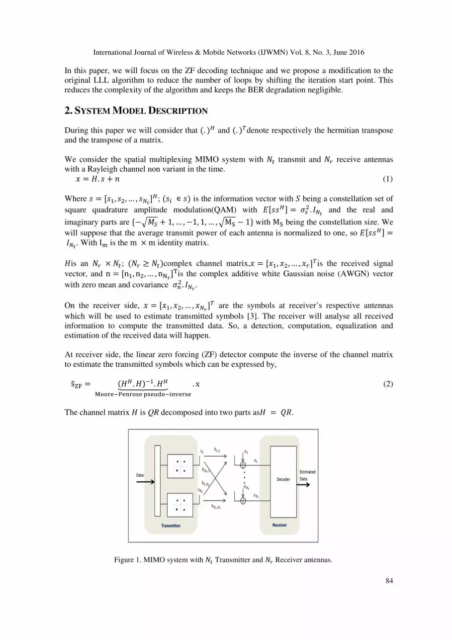
Figure 1. MIMO system with Transmitter and Receiver antennas.


85

3. LATTICE REDUCTION TECHNIQUE

We can interpret the columns ℎ of the channel matrix as the basis of a lattice and assume that

the possible transmit vectors are given by ℤ , the m dimensional infinite integer space.

Consequently, the set of all possible undisturbed received signals is given by the lattice.

( ) = (ℎ ,… , ℎ ) ∶= ∑ ℎ ℤ (3)

The LR algorithm generates a lattices reduced and near-orthogonal channel matrix = . .

With matrix = . generates the same lattice as , if and only if the m×m matrix T is

unimodular [2], i.e. contains only integer entries and ( ) = ±1:

( ) = ( ) ⇔ = (4)

Also,

. = (5)

We can find multiple bases that can be included in the space , and the goal of the LR algorithm

is to find a set of least correlated base with the shortest basis vectors [5].Initially, an efficient (but

supposed not optimal) way to determine a reduced basis was proposed by Lenstra, Lenstra and

Lovàsz [1].Where they defined (LLL-Reduced): A basis with QR decomposition = . is

called LLL-reduced with parameter δwith(1/4 < ≤ 1), if

, ≤ . , 1 ≤ < ≤ (6)

And

, ≤ , + , = 2,… , (7)

The first condition is called, size-reduced and the second one is called Lovàsz condition. The

parameter plays an important role to the quality of the reduced basis. We will assume = 3 4⁄

as proposed in [1]. After applying the QR decomposition of H and doing successive size-reduces

operations if the condition is fulfilled, the algorithm exchanges two vectors if Lovàsz condition is

not fulfilled to generate and compute and . And so, the LLL algorithm will output , and .

Looking to the LLL algorithm [1], one important element of its complexity is related to the fact

that the LLL algorithm is applied for the real integer vectors. It is mandatory to reformulate the

different matrices to their real-valued form, so we got:

= ( ) − ( )

( ) ( ) , (8)

= ( )( ) , (9)

= ( )( ) = ( )

( ) (10)


86

This kind of reformulation increases the number of operations and adds more latency for the

system.

The idea behind LR-aided linear detection is to consider the equivalent system model and perform

the nonlinear quantisation on it [8]. In fact, if we combine equations (1) and (5), we can get:

= . . + (11)

With = . the equivalent model and in this case will represent a better channel quality.

And so, the detector can be represented with an equivalent model with better performance due to

the less noise enhancement increased by . Thus, the basic idea behind approximate lattice

decoding (LD) is to use LR in conjunction with traditional low-complexity decoders. With LR,

the basis B is transformed into a new basis consisting of roughly orthogonal vectors [8].

After processing the Zero Forcing lattice reduction (ZF-LR) mechanism and by combining

equations (2) and (11), we can generate:

z = . s = . = + . (12)

The different enhancements for the original algorithm were looking for a limited iterations in term

of stopping criteria, like in [5]. But we believe that the structure of the triangular matrix generated

by the QR decomposition can be an axe of improvement and complexity reduction.

Table 1. The LLL algorithm

Input: H:thechannelmatrixconvertedtothereal-valuedformOutput: R,Q,T1 Initialization:T = I ;Keepinginmindtherealvalued;Hmatrix2 [Q, R] ∶= qr(H);3 R = R;Q = Q;4 δ = 3 4⁄ 5 k = 26 whilek ≤ N 7 forl = k − 1downeto18 μ ∶= R(l, k) R(l, k)⁄ 9 ≠ 010 (1: , ) ∶= (1: , ) − . (1: , )11 (: , ) ∶= (: , ) − . (: , )12 13 14 . ( − 1, − 1) > ( , ) + ( − 1, ) 15 − 1

16

ℎ :

= − ℎ= ( − 1, − 1)

( − 1: , − 1)= ( , − 1)

( − 1: , − 1)

17 ( − 1: , − 1: ) ∶= . ( − 1: , − 1: )


87

18 (: , − 1: ) ∶= (: , − 1: ). 19 ∶= { − 1,2}20 21 ∶= + 122 end23 end

3.1. Exploiting R matrix’s structure to improve the LLL algorithm

As shown in table 1 the outputs of the algorithm will be , , . With is an upper triangle

matrix. The relation between them will follow (5).

. . = . = (13)

Looking to the LLL algorithm, at lines 4 & 5 we can see that the loop is starting from = 2. This

choice is taken to reach the first column of . This means that we can start from any other column

> 2 and in this case we will not perform the column swap of columns1 − 2.

So, in the case that the loop starts from 3; we will not perform column swap for first column. In

this case we will gain 1 loop iteration and we will reduce the column swaps at least by 1. Looking

to the morphology of the matrix R which is a triangle matrix, so the first column contains only 1

active element (the rest are“0”). The major number of active elements is in the rest of the matrix.

3.2.R matrix’s structure

Below, is a representation of the matrix R in the case of 4 × 4 MIMO system. The number of

elements by column is increasing from left to right

=

R , R ,0 R ,

R , R ,R , R ,

0 00 0

R , R ,0 R ,

,

R , R ,R , R ,

R , R ,R , R ,

R , R ,R , R ,

R , R ,R , R ,

,

0 00 0

0 00 00 0

0 00 00 0

R , R ,0 R ,

R , R ,R , R ,

0 00 0

R , R ,0 R ,

(14)

Let’s decompose it schematically as 2 parts, , and , (Just to mention that the above choice

is arbitrary).

In , , we have 26 active elements and in R , we have only 10 active elements. So, if we

consider , we can get 72% of the matrix elements. Adding the , column we can get 30

elements and so 83% of the matrix elements. We are adding , to be conforming to lines 6 to

11, 13 and 16 to 17 in table 1; if we consider = 5.


88

If we consider a new matrix R that conisists of the elements of R from column R , to

R , , so we will get a matrix 5 × 8R . Which consist of 83% of actives elements ofR.

Thus, at the output of the LLL algorithm we will generate a matrix with 3 first elements

as and R will keep the firsts 3 elements of .

=

R , R ,0 R ,

R , R ,R , R ,

0 00 0

R , R ,0 R ,

R , R ,R , R ,

R , R ,R , R ,

R , R ,R , R ,

R , R ,R , R ,

0 00 0

0 00 0

0 00 0

0 00 0

R , R ,0 R ,

R , R ,R , R ,

0 00 0

R , R ,0 R ,

(15)

=

1 00 1

0 T ,0 T ,

0 00 0

1 T ,0 T ,

T , T ,T , T ,

T , T ,T , T ,

T , T ,T , T ,

T , T ,T , T ,

0 00 0

0 T ,0 T ,

0 00 0

0 T ,0 T ,

T , T ,T , T ,

T , T ,T , T ,

T , T ,T , T ,

T , T ,T , T ,

(16)

This means that we have generated only 40 from 64 possible matrix element and only 5 from 8

possible columns for the matrix T. Consequently, for matrix we have manipulated only 30 from

36 possible active elements. This is a considerable computation relaxation.

This approach can be generated for all column indexes which allow to gain more operations, and

so we can change the algorithm of table 1 as below.

Table 2. The LLL algorithm with modified start point.

Input: H:thechannelmatrixconvertedtothereal-valuedformOutput: , ,

1 Initialization:T = I ;2 [Q, R] ∶= qr(H);3 = ; = ;4 δ = 3 4⁄ 5 = (N 2)⁄ ;oranyvalue>26 = 7 whilek ≤ N 8 forl = k − 1downeto19 μ ∶= R(l, k) R(l, k)⁄ 10 ifμ ≠ 0


89

11 R(1: l, k) ∶= R(1: l, k) − μ. R(1: l, l)12 T(: , k) ∶= T(: , k) − μ. T(: , l)13 end14 end15 ifδ. R(k − 1, k − 1) > R(k, k) + R(k − 1, k) 16 ktok − 1columnsswapforRandT

17

ComputingtheGivensrotaionMatrix:

Θ = α β−β α with

α = R(k − 1, k − 1)R(k − 1: k, k − 1)

β = R(k, k − 1)R(k − 1: k, k − 1)

18 R(k − 1: k, k − 1:m) ∶= Θ. R(k − 1: k, k − 1:m)19 Q(: , k − 1: k) ∶= Q(: , k − 1: k). Θ 20 ∶= { − 1, }21 else22 k ∶= k + 123 end24 end

But we should note that, logically the BER performance degradation will increase. In fact, we

have some compromises to take into consideration (operations vs performance balance). Also,

this approach will be more efficient as much as we use more antennas for both sides of the

system. This means that we need to evaluate the cases where the approach will be beneficial in

terms of complexity while keeping an acceptable performance.

In the next sections we will present the simulation results and the complexity study of the

proposed approach.

4. SIMULATION RESULTS

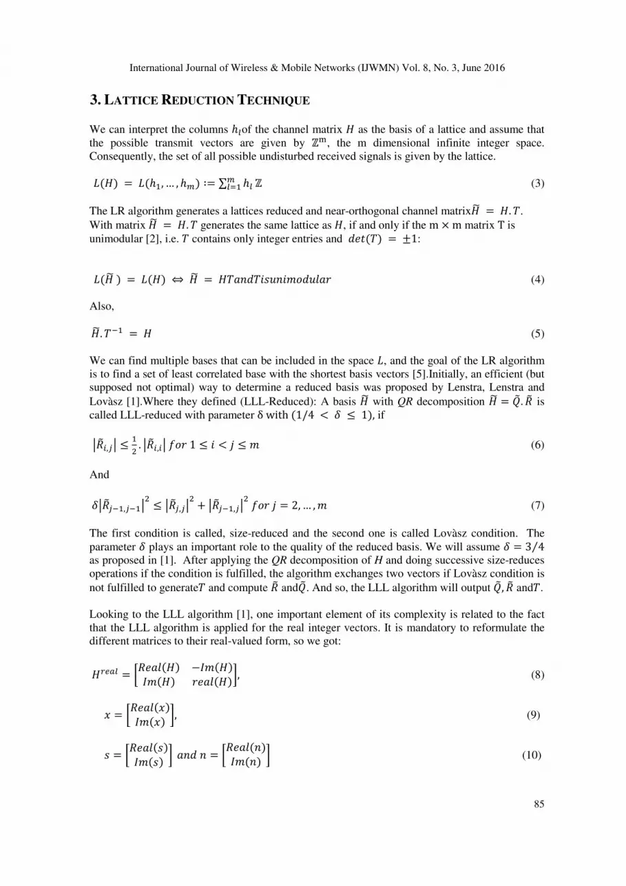
Figure 2. The BER performance comparison between the original LLL and the modified LLL algorithm

( = 3 and = 4). Simulation related to16QAM 4 × 4 MIMO system.

0 5 10 15 20 25 3010

-4

10-3

10-2

10-1

100

SNR per receiver antenna [average in dB]

BE

R

Original LLL

Modified Start Point LLL(3)


The performancedegrdadtion is around1dB


90

Figure 2, shows that if we consider the LLL algorithm starting point at column 3 or 4, the BER is

not dramatically degrading (limited). But we gain a lot in terms of computation operations. In fact

the proposed modification will avoid that the algorithm do more iterations and operations to

reduce the elements of R (simultaneously to generate T), especially for the vectors without big

effects on the results (performance). So, we will focus on the matrix column with maximum of

active elements and avoiding making operation with almost "zeros" valued columns.

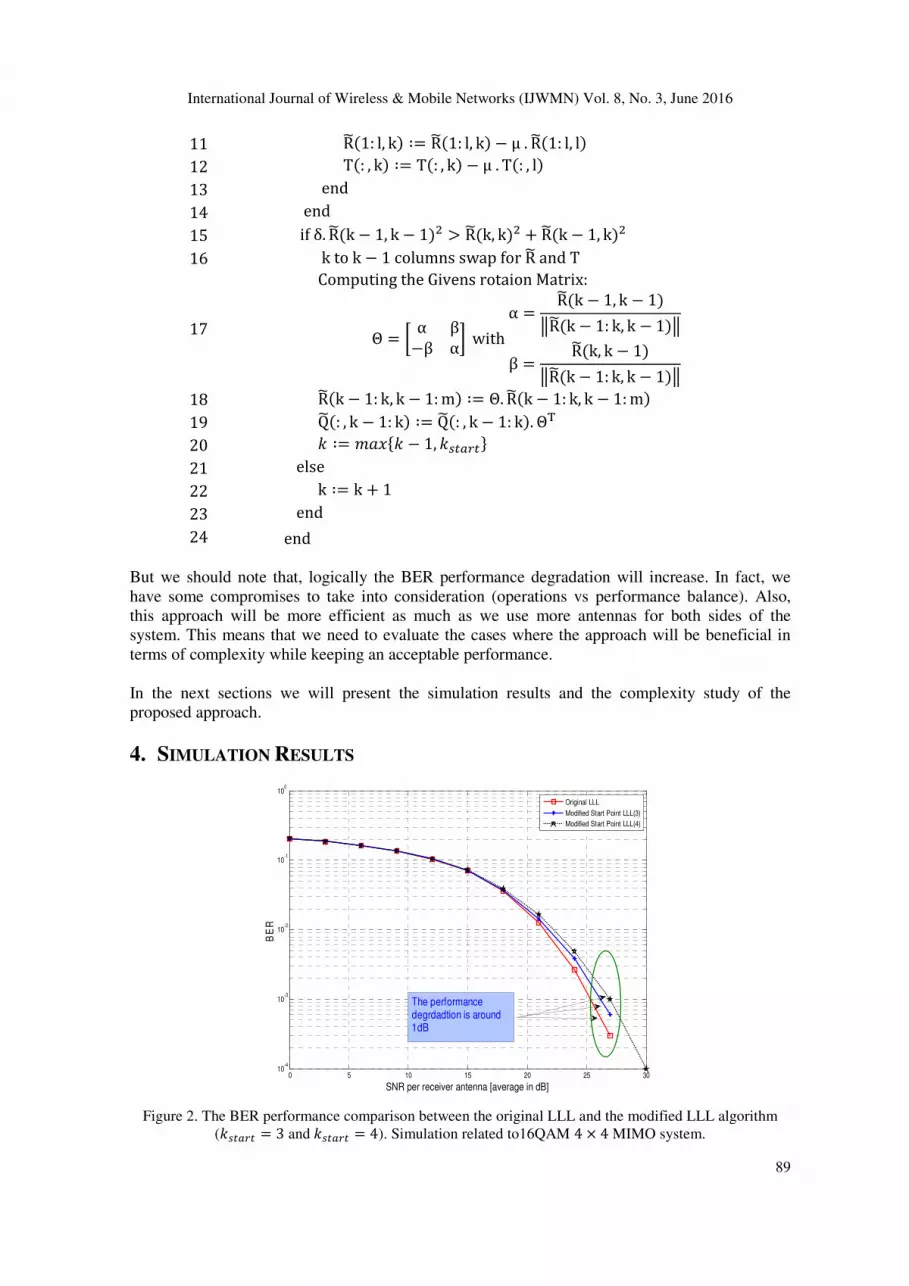
Figure 3. The BER performance comparison between the original LLL and the starting point modified LLL

algorithm (k = 5 ). Simulation related to 16QAM 4 × 4 MIMO system.

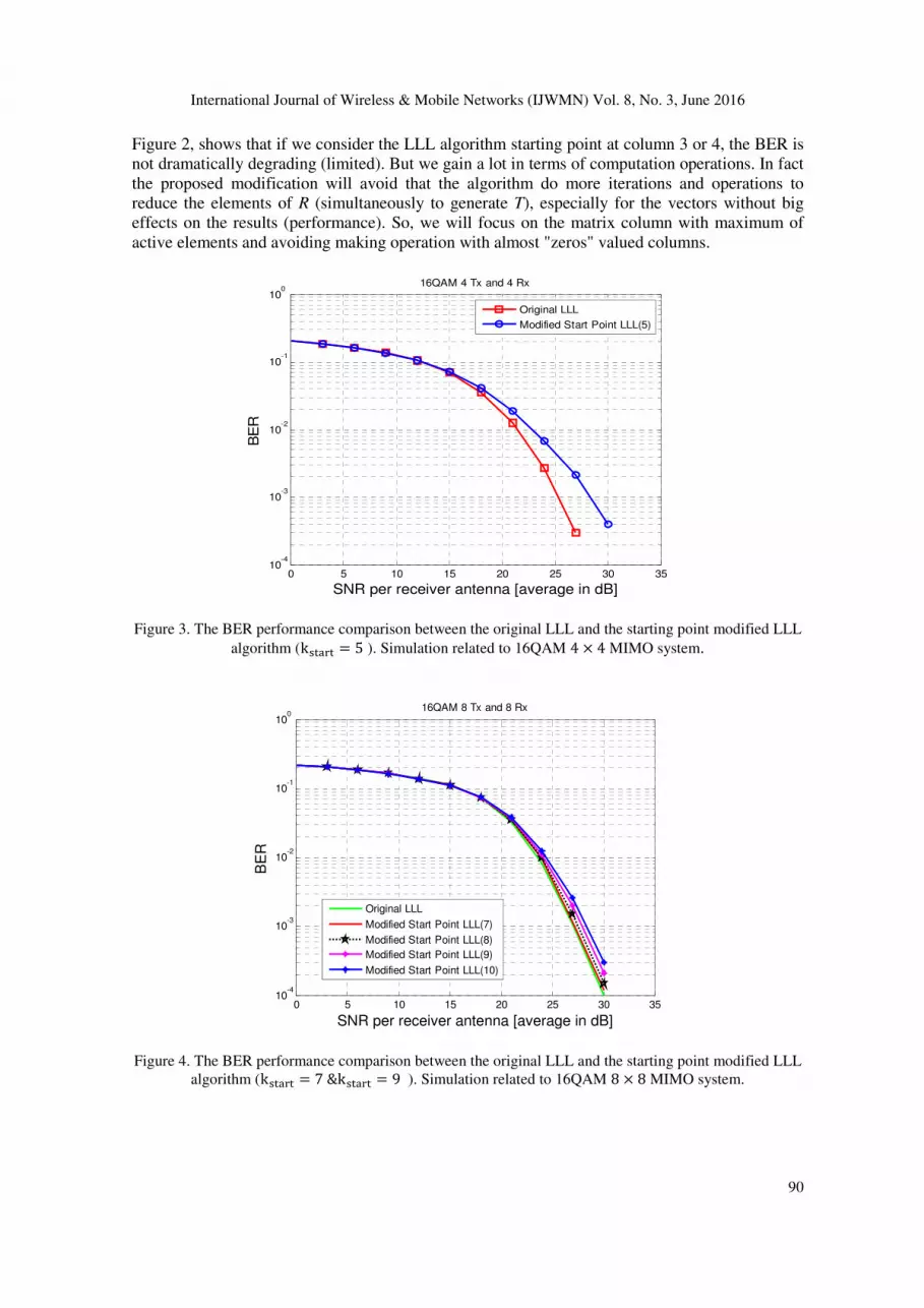
Figure 4. The BER performance comparison between the original LLL and the starting point modified LLL

algorithm (k = 7&k = 9 ). Simulation related to 16QAM 8 × 8 MIMO system.

0 5 10 15 20 25 30 3510

-4

10-3

10-2

10-1

100


BE

R

16QAM 4 Tx and 4 Rx

Original LLL


0 5 10 15 20 25 30 3510

-4

10-3

10-2

10-1

100


BE

R

16QAM 8 Tx and 8 Rx

Original LLL






91

Figure 4 shows the BER performance for the same approach applied to an 8×8 MIMO system. It

illustrates clearly that the approach can be applied for any × MIMO system. Also, we can

observe that for big sized matrixes the approach is showing better results. In fact, as much as we

increase the matrix size we have more “zeroes” in the first columns and more “non-zeroes”

elements for the right part of the matrix. So, we will get more possibilities to shift the start

column index.

5. COMPLEXITY GAIN

In this section we will present an analysis of the operations load of the algorithm while being

executed. After that, we will show the gain in term of operations and complexity that we can

make after applying our proposed approach.

5.1 Operations analysis

By looking to the algorithm in table 1, we can observe that:

• The size reduction operations (lines 7 to 13), is doing a kind of loop with − 1 iterations

for a set of operation that contains; a division, two subtractions (than can be considered as

addition [6]) and two multiplications if the line 9 is valid. So, in maximum of cases, the

size reduction can be done with operations.

= ( − 1) × {1 × ( ) + 2 × ( + )}(17)

• Line 14 representing Lovàsz’s conditions require:

à = {4 × ( ) + 2 × ( )}(18)

Considering that the superior verification can be achieved via a subtractions operation

[6].

• The columns permutation operation is being done elements by elements. Knowing that

the simple two elements permutation is equivalent to three additions. Also, the algorithm

doesn’t make difference for zero or non-zero values. So, the column permutation will be

done in:

= 2 × {3 × ( )}(19)

• The Givens rotation matrix corresponds to the computation of the and parameters and

this is being done via a “norm” calculation from one side, which corresponds to a square

root operation, two multiplications and one additions. And, two divisions from another

side.

= {2 × ( ) + 2 × ( ) + 1 × ( ) + 1 × ( )}(20)

• The unitary matrix and the rotation matrix multiplication correspond to a matrix 2 ×2 and matrix 2 × (2 − + 2) multiplications [5].

= 2 × {2 × ( ) + 1 × ( )} × (2 − + 2)(21)

• Line 18 corresponds to multiplication of two “2 × 2“ matrixes.


92

= 2 × {2 × ( ) + 1 × ( )} × 2 (22)

• Line 19 corresponds to a comparison and an assignment.

= 2 × ( )(23)

This doesn’t take in consideration the constellation, since we are using the same constellation for

all the paper and so the analysis remains the same.

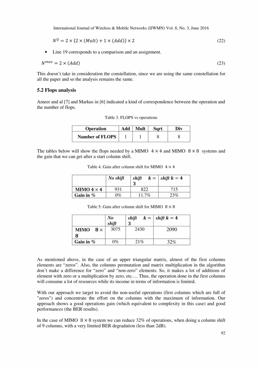
5.2 Flops analysis

Ameer and al [7] and Markus in [6] indicated a kind of correspondence between the operation and

the number of flops.

Table 3. FLOPS vs operations

Operation Add Mult Sqrt Div

Number of FLOPS 1 1 8 8

The tables below will show the flops needed by a MIMO 4 × 4 and MIMO 8 × 8 systems and

the gain that we can get after a start column shift.

Table 4. Gain after column shift for MIMO 4 × 4

No shift shift =

shift =

MIMO × 931 822 715 Gain in % 0% 11.7% 23%

Table 5: Gain after column shift for MIMO 8 × 8

No

shift shift =

shift =

MIMO ×

3075 2430 2090

Gain in % 0% 21% 32%

As mentioned above, in the case of an upper triangular matrix, almost of the first columns

elements are “zeros”. Also, the columns permutation and matrix multiplication in the algorithm

don’t make a difference for “zero” and “non-zero” elements. So, it makes a lot of additions of

element with zero or a multiplication by zero, etc.… Thus, the operation done in the first columns

will consume a lot of resources while its income in terms of information is limited.

With our approach we target to avoid the non-useful operations (first columns which are full of

"zeros") and concentrate the effort on the columns with the maximum of information. Our

approach shows a good operations gain (which equivalent to complexity in this case) and good

performances (the BER results).

In the case of MIMO 8 × 8 system we can reduce 32% of operations, when doing a column shift

of 9 columns, with a very limited BER degradation (less than 2dB).


93

We should note that in this paper, we didn’t present the case of MIMO 2 × 2 system. This was

related to the size of the matrix which is small and the new algorithm will not bring a

considerable outcome. Keeping in mind that the LLL algorithm is mainly used to simplify the

decoding with “big size” channels matrixes [2].

6. CONCLUSION

In this paper, we proposed a modified LLL algorithm that exploits a kind of shift start column.

We started from the original LLL algorithm and we modified it to escape the almost “zeros”

columns of the upper triangular matrix R. And so, we avoided doing computation for the columns

without big influence on the BER performance. The proposed approach is not one of the fashion

modification of the LLL algorithm, but its added value come from its simplicity and complexity

gain.This approach was simulated for both 4×4 and 8×8 MIMO systems and can be extended for

any other MIMO system model. We have presented that we can gain, respectively, 23% and 32%

for the MIMO 4×4 and MIMO 8×8 scheme. This is an important point, we are reducing the

computation operations and so the decoding time with very limited BER degradation. So, the

trade-off complexity vs performance is interesting and the gain in terms of complexity

counterbalance the limited performance degradation.

We considered the 16QAM modulation and ZF receiver where our approach shows good results.

It will be interesting to extend this study to the MMSE and other modulation techniques. Also, in

this paper, we discussed the case with a same antennas number on both sides. The case with a

different antennas number on both sides will be the subject of a new study. Finally, this approach

is showing better results for the “big size” MIMO systems and it we believe that extend it to the

case of massive MIMO will be interesting.

REFERENCES

[1] A. K. Lenstra, H. W. Lenstra, and L. Lovàsz, (1982), ”Factoring polynomials with rational

coefficients,” in Math. Ann, vol. 261, pp. 515 - 534.

[2] D. Wubben, D. Seethaler, J. Jalden, and G. Matz, (2011),”Lattice reduction,” in IEEE Signal

Processing Magazine, vol. 28, no. 4, pp. 70 - 91.

[3] Qingsong Wen, Qi Zhou, and Xiaoli Ma, (2014), “An Enhanced Fixed-Complexity LLL Algorithm

for MIMO Detection”, Globecom 2014 - Signal Processing for Communications Symposium.

[4] C. P. Schnorr and M. Euchner, (1994), “Lattice Basis Reduction: Improved Practical Alorithms and

Solving Subset Sum Problems”. Mathematical Programming, vol. 66, pp. 181.191.

[5] Z. Ma, B. Honary, P. Fan, and E. Larsson, (2009) “Stopping criterion for complexity reduction of

sphere decoding,” IEEE Commun. Lett., vol. 13 , no. 6, pp. 402–404.

[6] Markus Bläser, (2013), “Fast Matrix Multiplication”, Theory of Computing, Graduate Surveys ,

vol. 5 ,p. 1-60

[7] Ameer Youssef , Mahdi Shabany , P. Glenn Gulak, (2011), “Performance analysis of lattice-reduction

algorithms for a novel LR-compatible K-Best MIMO detector,” Conference: International

Symposium on Circuits and Systems, DOI: 10.1109/ISCAS.2011.5937662, Rio de Janeiro, Brazil.

[8] Md Hashem Ali Khan, Jin-Gyun Chung and Moon Ho Lee, (2015), “Lattice reduction aided with

block diagonalization for multiuser MIMO systems”, EURASIP Journal on Wireless Communications

and Networking 2015:254, DOI 10.1186/s13638-015-0476-1

Documents

MODIFIED LLL ALGORITHM WITH SHIFTED START COLUMN FOR COMPLEXITY REDUCTION