Embed Size (px)
Citation preview
980779
Models for the Prediction of Performance and Emissions in aSpark Ignition Engine - A Sequentially Structured Approach
Ivan Arsie, Cesare Pianese, Gianfranco RizzoDepartment of Mechanical Engineering, University of Salerno, Italy
Copyright © 1998 Society of Automotive Engineers, Inc.
ABSTRACT
A thermodynamic model for the simulation ofperformance and emissions in a spark ignition engine ispresented. The model is part of an integrated system ofmodels with a hierarchical structure developed for thestudy and the optimal design of engine controlstrategies. In order to reduce the uncertainty due to themutual interference during the validation phase, themodel has been developed accordingly with ahierarchical and sequential structure.
The main thermodynamic model is based on theclassical two zone approach. A multi-zone model is thenderived form the two zone calculation, for a properevaluation of temperature gradients in the burned gasregion. The emissions of HC, CO and NOx are thenpredicted by three sub-models.
In order to make the precision of emission modelssuitable for engine control design, an identificationtechnique based on decomposition approach has beendeveloped, for the definition of optimal model structurewith a minimum number of parameters.
The results of the thermodynamic cycle modelvalidation, performed over more than 300 engineoperating conditions, show a satisfactory level ofagreement between measured and predicted datacycles. Afterward, the two step identification procedurehas been applied for the emission models parametersidentification. From this analysis, it has been found thatthe model precision achieved can be comparable withthat obtained via conventional mapping proceduresusing black-box models, but with a drastic reduction ofthe experimental effort. Moreover, the proposedapproach allows substantial computational time savingwith respect to conventional identification techniques.
INTRODUCTION
Many models for the study and the design of internalcombustion engines (ICE’s) have been proposed inliterature, in order to assist the development of engineswith performance complying with future pollution controlregulations. Much effort is being spent toward the
development of comprehensive 3-D models, describingall the relevant phenomena relating to engine operationand emission formation at the maximum allowed levelof detail. Although their use can be precious in order toconsider the mutual influence of geometrical andoperating parameters on the complex fluid-dynamicsand thermo-chemical phenomena involved in engineoperation, they do not yet represent the ultimate solutionfor all applications in the ICE’s sector. The practicalutility of these models, which require very highcomputational power, may be questionable in thosecases where many repeated computations are involved,as in design applications. Moreover, their quantitativeprecision, which requires an appropriate “balancedprecision” in all their sub-models, could even beinadequate for some applications.
Therefore, notwithstanding the continuous effort towardthe development of comprehensive 3-D models, manydifferent models can still be found in literature, oftencharacterized by substantial differences in structure,goals and complexity [1], [4], [5], [9]. A significantnumber of them are devoted to design of optimal enginecontrol strategies and to the development of new enginecontrol technologies. They range from input-outputblack-box models, mostly oriented to control design, togray-box mean-value models, with a simplifieddescription of the most relevant physical processes[1],[2],[3], up to complex 3-D fluid-dynamic models[4],[5]. These classes of model substantially differ interms of computational time and experimental datarequired: for the validation of the simplest black-boxmodels, hundreds or thousands of engine data could beneeded to compensate for the lack of physicalinformation, resulting in high experimental effort andlower model flexibility; on the other hands, thecomputational cost of the detailed 3-D models is notcompatible with many control applications.
THE MODELING APPROACH
From these considerations, it emerges that in manycases a proper solution could be represented by theadoption of a suitable mixed approach, in order tocombine the advantages of various kind of models.
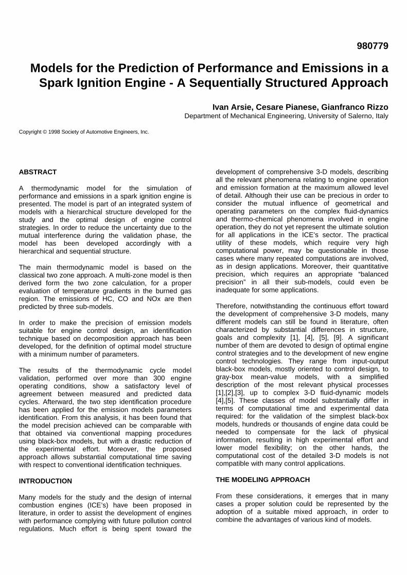
A hierarchical model structure (figure 1) has beendeveloped by the authors for the optimal design ofengine control strategies [6], where it is assumed thatthe engine geometry is assigned. At the final stage, thisset of models will be embedded in a more generalengine control strategy rapid prototyping procedure. Agray-box mean-value dynamical model [8],[9] is linkedwith the computer code ODECS for control simulationand optimization [10], which is now in use by MagnetiMarelli. At higher level, phenomenological models [11]are used in conjunction with experimental techniques tosimulate in off-line mode engine performance to buildfast black-box model, which in turn are used for optimaldesign of engine control strategies [6], [11], [24]. Theinteraction between experiments and models can besuperintended by interactive Experimental Designtechniques, which can give further substantial benefits inguiding and reducing the experimental tests needed forengine model validation [7].
Phenomenological
Engine Models
Grey-Box and Black-Box
Engine Models
Experimental Design
Techniques
over a Driving Cycle
with Dynamic & Stochastic Effects
Optimizer
Verification
of Optimal Control
Strategies
EngineControl
Strategy
Engine Performance & Emissions
ENGINE
Code ODECS
figure 1 – A hierarchical model structure for enginecontrol design
The phenomenological models have been builtaccording to a sequential structure of modules, ratherthan as a single comprehensive block. This approachoffers a substantial advantage in the validation phase,because it is possible to identify the values of the modelparameters just acting on the appropriate module, andlimiting the uncertainty due to mutual influences andcorrelation among the variables.
The adoption of a suitable sequential structure and ofidentification techniques based on decompositionapproach has allowed substantial saving ofcomputational power with respect to conventionalapproaches in determining structure and values of themodel parameters for engine emissions [12], whoseknowledge represents an important task for controlapplications. At this moment, fully predictive emissionmodels suitable for the optimal design of engine controlstrategies, which requires extensive computations, arenot yet available. Therefore, some model parameters
must be identified by comparison with experimentaldata, and their relationships with operating variablesdetermined, in order to use the model for prediction. Tothis purpose a parameter identification procedure basedon decomposition approach has been proposed in orderto reduce the number of engine experimental data andthe computational time required for model validation[12].
In the following chapters, the main features of thethermodynamic engine model used in the abovedescribed hierarchical structure are presented, and a setof results for emission prediction levels reviewed.Afterward, the results obtained by the use of thedecomposition approach for the identification ofemission model parameters are presented anddiscussed.
THE THERMODYNAMIC MODEL
The prediction of emission levels requires an accuratedescription of thermodynamic, fluid dynamic andchemical processes occurring inside the combustionchamber. Moreover, for the three main engine exhaustproducts (HC, CO, NOx), the formation processes arecharacterized by different mechanisms which must bedescribed with suitable independent sub-models. Theapproach followed in the present work is based on a twozone model [13] to predict in-chamber pressure andburned and unburned gas temperature as function ofengine geometry and operating parameters. Then,starting from the two-zone calculation, three differentsub-models are used for the simulation of each emissionproduct.
TWO ZONE THERMODYNAMIC MODEL
The classical approach described by Ferguson [13] hasbeen selected for the thermodynamic simulation of S.I.engine due to its simple formulation, for the wellstructured documentation available and for its highcomputational efficiency. The model is briefly reviewedin the following.
The combustion chamber is divided into two zones,corresponding to burned and unburned gas regions, byan infinitesimal flame front with a spherical shape. Ineach zone the thermodynamic state is defined by themean thermodynamic properties; the burned gas areassumed in chemical equilibrium during combustion andfor the main expansion stroke, while near the end of theexpansion process the mixture is assumed frozen[4],[5],[13],[14].
To account for the radial evolution of flame front aburned mass fraction function x is used to describe thespatial dynamics of combustion process. Assuming mthe total mass evolving in the cylinder, the specificinternal energy is:
uU
mxu x ub u= = + −( )1 (1.)
where subscripts u and b refer to unburned and burnedgas respectively. uu is the specific internal energy ofunburned gases at temperature Tu and ub is the specificinternal energy of burned gases at temperature Tb. Ananalogous relation is derived for the specific volume:
vV
mxv x vb u= = + −( )1 (2.)
The energy balance for an open system bounded bycombustion chamber walls holds [13]:
mdu
du
dm
d
dQ
dP
dV
d
m hl l
θ θ θ θ ω+ = − −
&(3.)
where θ is crank angle, ω angular speed, m total mass inthe cylinder, u specific internal energy (eq. 1), Q amountof heat flowing into the control volume, P gas pressureand V total volume. The last term in equation (3)represents the energy flow due to blow-by. The heat flowmodel describes heat transfer between gas and cylinderwalls:
dQd
Q Q Ql b u
θ ω ω=
−=
− −& & &(4.)
In the above equation the two heat flux terms for burnedand unburned gases are modeled as follows:
( ) &Q A T Tb b b b w= −h (5.)
( ) &Q A T Tu u u u w= −h (6.)
where Ab and Au are the combustion chamber wall areasin contact with burned and unburned gases respectivelyand Tw is the cylinder wall temperature. The surfaceareas are computed as function of cylinder bore b andinstantaneous combustion chamber volume V with thefollowing relations:
Ab V
bxb = +
π 21 2
2
4(7.)
( ) Ab V
bxu = +
−
π 21 2
2
41 (8.)
It is assumed that the burned gas contact wall surface isproportional to the square root of burned mass fractionto account for the greater volume filled by burned gaseswith respect to unburned ones. These relationships areconsistent with the whole heat exchange modeldescribed below.
The instantaneous convective heat transfer coefficient h
[W/m2/K] is computed from the well known correlationproposed by Woschni [14] as function of cylinder bore b[cm], pressure P [bar], gas temperature T [K] and meangas velocity w [m/s]:
h = ⋅ ⋅ ⋅ ⋅− −326 0 2 0 8 0 55 0 8b P T w. . . . (9.)
with the mean gas velocity w related to the mean pistonspeed U p and combustion phenomena [4],[13]:
( )w C U CVTPV
P pp m= + −
1 20
0 0(10.)
T0, P0 and V0 are temperature, pressure and volume atinlet valve closing, respectively; pm is the motoredpressure. The constants C1 and C2 are derived fromWoschni [14].
Thermodynamic gas properties routines have beenimplemented from Ferguson [13] and adapted to thepurpose of the present work. These routines give thethermodynamic gas properties as function of pressure,temperature and equivalence ratio φ for the mixture ofair, fuel and residual gas fraction f (FARG) and for themixture of burned gases at equilibrium (ECP):
( , , , , ) ( , , )u v hT p
f T pb
b∂
∂∂∂
φ= (11.)
( , , , , ) ( , , , )u v hT p
f T p fu
u∂
∂∂∂
φ= (12.)
For the heat release law the well suited Wiebe functionhas been applied [4] to compute the burned massfraction x(θ):
( )x
s
s
b
n
s=
<
− ⋅−
>
0
1 0 001
θ θθ θ
θθ θexp ln .
(13.)
where θs is the ignition crank angle and θb thecombustion angular period. In accordance with Heywood[4] the parameter n has been fixed to a constant valueof 3.
The problem described with equation (1) throughequation (10), relating the in-cylinder pressure variationrate, the amount of work and heat exchange as functionof crank angle, constitutes a set of ordinary differentialequations. For the integration of this system a 4th orderRunge-Kutta scheme with adaptive step size has beenadopted [15].
EMISSIONS MODELS
From the thermodynamic model just described, theburned mass fraction, the pressure and the mean
temperatures are computed for each crank angle,together with other useful data relating to work, heattransfer and chemical equilibrium properties of burnedand unburned gases. Starting from the two zone enginecycle simulation, the emissions levels for HC, CO andNOx are predicted through three distinct sub-models.
The NOx and CO formation is controlled by chemicalkinetic reactions [4],[5],[16],[17], therefore theirproduction rates are non-linearly dependent from burnedgas temperature. Thus, the two-zone modelapproximation is not feasible to account for differentthermo-chemical states experienced by burned gasregions throughout the combustion process until the endof expansion stroke. Therefore, a multi-zonediscretization of burned gas region has been consideredfollowing the approach described in the next section.
The mechanisms which mainly influence the HCemissions are the adsorption and desorption ofunburned hydrocarbons into the wall wetting oil layer,the inflow and outflow from the crevices and the post-flame oxidation [18],[19], while experimental evidences[20] show that the flame quenching on the walls is not apredominant formation mechanism. Moreover, thediffusion of hydrocarbons from the quenching layer intothe bulk gas takes places in few milliseconds resulting ina limited amount of unburned hydrocarbons left on thewall surfaces [4].
MULTI-ZONE THERMAL MODEL
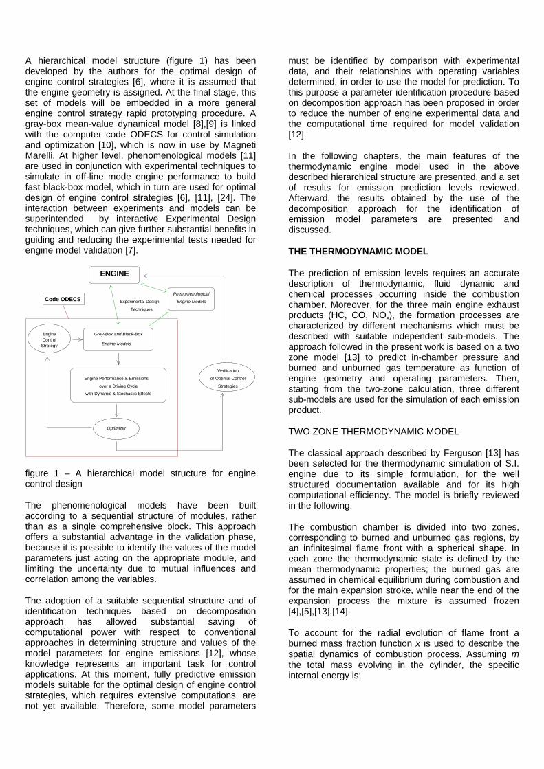
To account for different gas composition andtemperature gradients occurring in the variouscombustion chamber regions (e.g. spark plug, pistonhead), the burned gas volume is divided into N* zonesrepresenting an adiabatic core region. A further externalzone has been also considered as thermal boundaryregion of the central adiabatic core zones, primarilyresponsible for the heat transfer. It is assumed that nomixing occurs between neighboring zones and that atthe end of combustion the same mass fraction is presentin each zone (see figure 2). This schematization isconsistent with the hypothesis that burned gasesexperience a continuos adiabatic compression processas the combustion proceeds [4],[5],[21].
From the ignition event the formation of the first zonestarts, the development of this region ending when thefirst 1/N*-th mass fraction has burned. Afterward a newregion formation begins and the process goes on until afurther 1/N* amount of mass has burned. The formationof the other zones proceeds analogously until the end ofcombustion, where the total amount of burned gas isdistributed among the boundary layer and the N* zones.Since the zones are formed from the latest burnedgases and the flame front is assumed spherical, theactual forming region is the most external one and isadjacent to the flame front.
boundary zone
flame front
adiabatic core
figure 2 - Combustion chamber with multi-zoneschematization.
The mass of boundary layer is computed as a product ofits volume and density. The volume is derived fromgeometrical considerations assuming a constantthickness, while the density is derived from alogarithmic weighted average between wall and meanburned gas temperatures.
The current temperature of the already formed zones iscomputed accordingly with an adiabatic isoentropiccompression, which for the j-th zone at current crankangle θi can be written as follows [5], [21]:
( ) ( ) ( )( )T TP
Pj i j ii
iθ θ
θθ
γγ
=
−
−
−
11
1
(14.)
To derive both burning mass and the temperature of thezone adjacent to the flame front (i.e. forming zone) anenergy-mass balance equations system is written. Theenergy balance between the boundary layer, the formedzones and the burning zone compared with the meanburned gas energy, computed with the two zones modelis assumed. The mass balance is related with thedistribution of the last burned gas fraction among theboundary layer and the flame front where the adiabaticflame temperature is considered.
The resulting burned gas temperature distribution willtherefore depend on the parameters describing thethermal boundary layer and on the assumed number ofzones in burned gas, which can account for the relativerole of mixing processes and heat transfer.
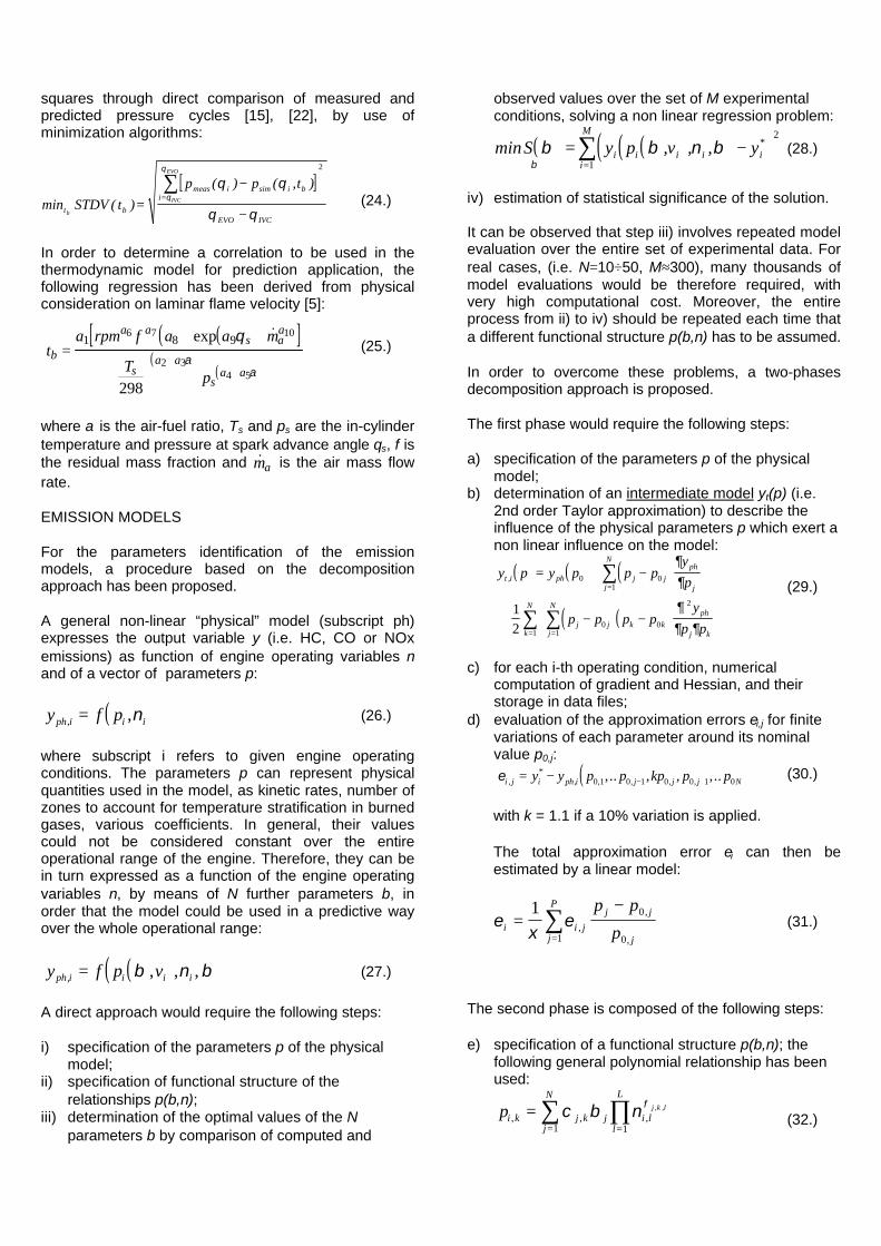
CARBON MONOXIDE FORMATION MODEL
From experimental evidence the CO levels at exhaustof internal combustion engines are mainly related withmixture equivalence ratio. Nevertheless, the exhaustedCO concentrations are lower than in-chamber measuredCO while higher concentrations are found in comparisonwith CO equilibrium concentration at exhaust referenceconditions [4]. These considerations allow theassumption of a chemical kinetically controlled COformation process [5], which in turn requires a detailed
description of burned gases thermal field being modeledwith the previous multi-zone model.
The formation and decomposition of carbon oxide ismainly controlled by the following chemical reactions:
CO OH CO H+ ↔ +2 (15.)
CO O CO O2 2+ ↔ + (16.)
though the latter influence is remarkable only for hightemperatures.
Assuming that OH, CO2 and O2 are in chemicalequilibrium state, the CO concentration rate of variationis:
( )112V
dndt
R RCOCOb
CO1
e= + ⋅ −
[ ][ ]
(17.)
where nCO is the number of moles present in the burnedgas volume Vb, while the equations equilibrium rates aregiven by:
R k CO OH kT
e e1 1 1106 76 10
1102= = ⋅ ⋅
+ +[ ] [ ] . exp
R k CO O kTe e2 2 2 2
122 5 1024055
= = ⋅ ⋅−
− −[ ] [ ] . exp
The equation (17) is solved numerically with a fourthorder Runge-Kutta scheme for each of N* zones, andthe final CO concentration is computed as the volumeweighted mean of CO concentration for each zone.
NITROGEN OXIDES FORMATION MODEL
To describe the NO formation process the extendedZeldovich mechanism is adopted [4],[5],[16],[17]:
O N NO N+ 2 ↔ +
N O NO O+ ↔ +2 (18.)
N OH NO H+ ↔ +
Some simplification can be made to the above systemof reactions. Due to the low concentration level ofatomic nitrogen, a steady state assumption is made:
d N
dt
[ ]≈ 0 (19.)
Moreover, since the energy contribution of NO reactionsto the combustion process energy balance is negligibleand due to their high energy activation levels, thedecoupling of the NO formation mechanism from themain combustion chemical kinetics reactions, which inturn exhibit higher reaction rates, is assumed. Thus, in
the reactions set (18) is useful to consider theequilibrium concentration for O, O2, OH, H and N2 in thecompletely burned gas zones.
Once these assumptions are made, the Zeldovichmechanism holds the following rate of variation for themoles of NO [21]:
[ ][ ]
[ ][ ]
1
2 1
1
1
2
1
2 3
Vdn
dt
RNONO
NONO
RR R
b
NOeq
eq
=
−
+
++
(20.)
where nNO is the number of moles present in the burnedgas volume Vb, while R1, R2 and R3 are computed asfollows:
R k O N kTe e1 1 2 1
137 6 1038000
= = ⋅ ⋅−
+ +[ ] [ ] . exp
R k NO O kTe e2 2 2
915 1019500
= = ⋅ ⋅−
− −[ ] [ ] . exp
R k NO H kTe e3 3 3
142 1023650
= = ⋅ ⋅−
− −[ ] [ ] exp
The relationships reported for the reaction rate constantsk1, k2 and k3 are the most frequently used in theliterature [4],[21]; such values present some uncertaintydue to the experimental tests they have been carried outwith. The exhausted gas NOx concentration is a volumeweighted mean of the NOx concentration computed foreach zone.
At moment in this sub-model the formation of promptNO, which is formed in the flame reaction zone, isneglected. It has been shown [4] that the NO producedin the post-flame region is the main source of S.I.engine exhausted NO; nevertheless, someimprovements in the model will be carried out toaccount for prompt NO also.
UNBURNED HYDROCARBONS
After Schramm and Sorenson [18] the HC formationmechanism can be briefly summarized in the followingpoints:
• the unburned mixture fills the piston crevices duringcompression stroke and is released duringexpansion; the mixture released ahead the flamefront is burned instantaneously, while the mixturereleased in the burned region undergoes akinetically controlled oxidation process;
• the oil film layer adsorbs the mixture fuel duringintake and compression strokes, part of this fuel is

desorbed behind the flame front and is oxidizedfollowing the same oxidation process cited in theabove point.
The mass mixture rate of change in the crevices is:
( )dmd
dPd
RT
Vcr p
crθθ
θ= (21.)
where mcr is the mixture mass in the crevices volumeVcr, P is the in-cylinder pressure and Tp the pistontemperature.
The adsorption/desorption of fuel into the oil layer ismodeled with the following one-dimensional Fourierequation expressing the fuel mass concentration rate ofchange in the oil film:
∂∂
∂∂
Yt
DY
x=
2
2(22.)
where Y is the fuel mass concentration in the oil, D(1.6⋅10-5 [cm2/sec], [19]) is the diffusion coefficient forthe fuel in the oil and x is the radial coordinate of oilfilm. This partial differential equation is solved with afinite difference explicit scheme where the spacederivative is approximated with a second order centralformula, while time integration is performed with a fourthorder Runge-Kutta method. The oil film layer domainhas been discretized in space with 20 slices, with radialsymmetry each, and 10 concentrical computationalcells. From Schramm and Sorenson [18] and Trinker etal. [19], for space boundary conditions von Neumanncondition at cylinder wall (i.e. zero gradient of fuelconcentration) is chosen. At oil film-gas interface thecurrent concentration is derived from Henry’s law whichrelates the fuel mole fraction in the oil as function of thefuel gas phase partial pressure in the mixture throughthe Henry’s constant (1.069 [atm], [19]). For a moredetailed description of Henry’s law the reader isaddressed to the references [18], [19]. As initialconditions it is assumed that no fuel is present in the oilfilm.
The fuel released into the burned gas region is oxidizedin a boundary layer near the wall with an intermediatetemperature derived from wall and mean burned gastemperatures. This post-flame oxidation is governed bythe following Arrhenius equation [18]:
d HC
dtC k HC O
RTR
[ ][ ][ ]= − −
1 2
37230exp (23.)
where the kinetic rate k1 is equal to 7.7⋅1015 , while CR isa calibration constant which is used to fit theexperimental data with the model parameteridentification described in the next section.
In the present model the HC post-flame oxidation is
supposed to end at the exhaust opening valve crankangle, while in the real engine the HC oxidationcontinues during the exhaust stroke into the exhaustmanifold. This further process will be considered in thefuture version of the whole model which will take intoaccount the intake and exhaust strokes. After theimplementation of exhaust valve flow sub-model theimplementation of post-flame oxidation in the exhaustport will be a straightforward task. As shown in theresults section, neglecting this additional oxidationprocess the final HC concentration simulated will beoverestimated with respect the measured concentration.
MODEL PARAMETER IDENTIFICATION
From the description of the thermodynamic modelpresented, it emerges that some model parametersshould be identified in order to make the model suitablefor prediction.
The main unknown parameters of the presented modelare the variables which affect the heat release law(combustion time duration tb and the Wiebe exponentcoefficient n), the heat transfer parameters and thefurther parameters which influence temperaturestratification and emission formation.
An effective identification of all unknown modelparameters could not be achieved by conventionaltechniques, due to the strong non linearities of themodel and to the correlation existing between some setof parameters (e.g. between combustion duration andWiebe exponent n, heat transfer coefficient andcombustion chamber wall temperature). The uncertaintydue to the combined effect of these mutual correlationsand of the measurement errors would not allow inpractical cases a precise parameter identification.Therefore, a sequential identification procedure hasbeen adopted.
HEAT TRANSFER
An estimation of mean cylinder wall temperature (seeeqs. 5 and 6) is made by processing measured pressuredata during compression stroke. This temperature isassumed equal to the temperature of the gas at thecrank angle where the instantaneous polytropiccompression exponent is equal to the correspondingadiabatic iso-entropic one. Heat transfer coefficients canbe then estimated by least square techniques. Thisapproach allow to overcome the quoted problems due tothe mutual correlation of wall temperature with heattransfer coefficients [23].
COMBUSTION MODEL
Combustion time values have been identified by leastsquare techniques [11], whereas for Wiebe exponent aconstant value is used. Other parameters exertingsecondary influence on cycle prediction are taken fromliterature data. For each pressure cycle the combustiontime duration tb is identified by means of non linear least
squares through direct comparison of measured andpredicted pressure cycles [15], [22], by use ofminimization algorithms:
[ ]min ( )
( ) ( , )
t b
meas i sim i bi
EVO IVCb
IVC
EVO
STDV t
p p t
=−
−=∑ θ θ
θ θθ
θ 2
(24.)
In order to determine a correlation to be used in thethermodynamic model for prediction application, thefollowing regression has been derived from physicalconsideration on laminar flame velocity [5]:
( )( )[ ]( )
( )
t
a rpm f a a m
Tp
b
a as a
a
sa a
sa a
=+
++
1 8 96 7 10
2 34 5
298
exp &θα
α
(25.)
where α is the air-fuel ratio, Ts and ps are the in-cylindertemperature and pressure at spark advance angle θs, f isthe residual mass fraction and &ma is the air mass flowrate.
EMISSION MODELS
For the parameters identification of the emissionmodels, a procedure based on the decompositionapproach has been proposed.
A general non-linear “physical” model (subscript ph)expresses the output variable y (i.e. HC, CO or NOxemissions) as function of engine operating variables νand of a vector of parameters p:
( ) y f pph i i i, ,= ν (26.)
where subscript i refers to given engine operatingconditions. The parameters p can represent physicalquantities used in the model, as kinetic rates, number ofzones to account for temperature stratification in burnedgases, various coefficients. In general, their valuescould not be considered constant over the entireoperational range of the engine. Therefore, they can bein turn expressed as a function of the engine operatingvariables ν, by means of N further parameters β, inorder that the model could be used in a predictive wayover the whole operational range:
( )( ) y f p vph i i i i, , , ,= β ν β (27.)
A direct approach would require the following steps:
i) specification of the parameters p of the physicalmodel;
ii) specification of functional structure of therelationships p(β,ν);
iii) determination of the optimal values of the Nparameters β by comparison of computed and
observed values over the set of M experimentalconditions, solving a non linear regression problem:
( ) ( )( )( )min , , , *S y p v yi i i i ii
M
β β ν ββ
= −=∑
2
1
(28.)
iv) estimation of statistical significance of the solution.
It can be observed that step iii) involves repeated modelevaluation over the entire set of experimental data. Forreal cases, (i.e. N=10÷50, M≈300), many thousands ofmodel evaluations would be therefore required, withvery high computational cost. Moreover, the entireprocess from ii) to iv) should be repeated each time thata different functional structure p(β,ν) has to be assumed.
In order to overcome these problems, a two-phasesdecomposition approach is proposed.
The first phase would require the following steps:
a) specification of the parameters p of the physicalmodel;
b) determination of an intermediate model yt(p) (i.e.2nd order Taylor approximation) to describe theinfluence of the physical parameters p which exert anon linear influence on the model:
( ) ( ) ( )
( )( )
y p y p p py
p
p p p py
p p
t i ph j jph
jj
N
k
N
j jj
N
k kph
j k
, = + − +
+ − −
=
= =
∑
∑ ∑
0 01
10
10
212
∂∂
∂∂ ∂
(29.)
c) for each i-th operating condition, numericalcomputation of gradient and Hessian, and theirstorage in data files;
d) evaluation of the approximation errors εi,j for finitevariations of each parameter around its nominalvalue p0,j:
( ) εi j i ph i j j j Ny y p p kp p p,*
, , , , ,,.. , , ,..= − − +0 1 0 1 0 0 1 0(30.)
with k = 1.1 if a 10% variation is applied.
The total approximation error εi can then beestimated by a linear model:
εξ
εi i j
j j
jj
P p p
p=
−
=∑1 0
01,
,
,
(31.)
The second phase is composed of the following steps:
e) specification of a functional structure p(β,ν); thefollowing general polynomial relationship has beenused:
pi k j k j i ll
L
j
Nj k l
, , ,, ,=
==∏∑χ β ν φ
11(32.)

where the actual functional form is determined bythe matrices φ and χ; this latter assumes 0 or 1values, and can be changed according to thestepwise procedure to include or exclude someterms in eq. (32);
f) determination of the optimal values of theparameters β by solving a non linear constrainedminimization problem (33, 34), using the Taylorapproximation; constraints (34) are introduced toavoid that unfeasible solutions could be proposed,where the estimated approximation error is largerthan a given limit εmax:
( ) ( )( )( ) min , , , *
ββ β ν βS y p v yi i i i i
i
M
= −=∑
2
1(33.)
( ) ε β εi i M≤ =max ,1 (34.)
the optimization problem has been solved byAugmented Lagrangian approach, using the Powellconjugate directions algorithm [15] [22];
g) estimation of the limits of confidence regions atlevel of probability (1-α) for parameters β, bynumerical solution of the following equation:
( ) ( ) ( ) S SN
M NF N M Nβ β α= +
−− −
* , ,1 1 (35.)
where S(β*) represents the sum of squarescorresponding to the solution of problem (33, 34),and F is the Fisher distribution with N parameters, Mobservations at (1-α) probability [25];
h) elimination of the less significant parameters β, byzeroing the corresponding χ values in eq. (32);
i) check of the termination criteria and repetition ofsteps f and g (backward stepwise regression).
This procedure offers the following advantages:
• Only the first phase requires a full model evaluationon the entire data set (step c) to compute gradientand Hessian. This information can be stored andeasily updated if further parameters would be addedto the model. Parallel or concurrent computationaltechniques can also be easily used in such phase.
• Each iteration of the regression technique (step f) ismuch more faster since it operates on polynomialapproximations rather than on the full model.
• The resulting objective function is quadratic, withlinear constraints, and very fast convergence can beachieved by classical optimization techniques.
• The entire process can be easily iterated for eachdifferent model parametrization, and a stepwiseapproach can be followed in order to determine themost significant model parameters.
• As final result, an entire class of models with adecreasing number of parameters is obtained, and atrade-off between number of parameters and fitting
precision can be achieved.
RESULTS
In the following, the result of the combustion timeduration identification together with the prediction ofemission levels are reported, in comparison withexperimental data. The purpose of this analysis is toverify the physical correctness and the precision of eachemission submodels in order to define a startingaccuracy level before the use of the two stepidentification procedure summarized at the end of theprevious section. To show the precision improvementachievable with the decomposition approach someresults are also presented.
The thermodynamic model has been validated over alarge set of experimental data; 342 engine pressurecycles have been measured on FIAT 2 liters S.I. engineon a dynamic test bench at CNR - Istituto Motori and arerepresentative of engine working operation for an ECE15 transient cycle.
In the figure 3 the rms between predicted and measuredpressure cycles distribution is reported after theidentification of combustion time duration. As it can beseen from the figure most of simulated cycles exhibit anerror less then 0.5 [bar], which expresses a satisfactorylevel of precision achievable with the thermodynamicmodel.
rms [bar]
engine cycles
0
5
10
15
20
25
30
35
40
0 0.2 0.4 0.6 0.8 1 1.2 1.4
figure 3 - Rms of computed and measured pressurecycle distribution for 342 engine cycles.
A non linear parameter identification has beenperformed to find the ten coefficients ai of equation (25).The comparison between identified combustion time andthe data simulated through the equation (25) are shownin the figure 4, where a satisfactory prediction level forequation (25) is evidenced; the correlation index for theidentification parameters analysis is R2 = 0.88.

figure 4 - Comparison between identified and simulated(eq. 25) combustion time duration.
Starting from the engine cycle simulation, performedusing the burning time identified, the emissions levelshave been predicted with the three sub-models beforedescribed. The computations refer to the 342 engineworking conditions investigated during the experimentalanalysis. Regard to the emission sub-models, thepresented results have been obtained with standardvalues of the parameters, taken from literature data(e.g. kinetic constants, film layer thickness, volumecrevices, number of zones). These results represent thestarting point for the identification of the emissionmodels [12].
In the figure 5 the results of CO predictions arecompared with the measured exhaust port CO levels; asit was expected, the maximum uncertainty in thesimulations is found in the region of low CO emissionlevels around lean operating points. To show the abilityof the sub-model in capturing the main physical featuresof CO formation process, the comparison of predictedand measured CO levels as function of air-fuel ratio fortwo engine operating condition is presented in figure 6and figure 7.
For the NOx the comparison of predicted emission levelswith experimental data is reported in the figure 8. Theanalysis of the figure evidences the scattering ofcomputed data set; nevertheless in the mean theprediction can be considered acceptable since neitherunderestimation or overestimation are found. Besides,the capability of the sub-models in describing thephysical influence of the engine operating conditions onthe NOx formation process is displayed in the figure 9and figure 10 where predicted and measured NOx levelsas function of air-fuel ratio are plotted.
figure 5 - Computed vs. measured CO - R2=0.858.
figure 6 - Comparison between computed and measuredCO as function of Air-Fuel ratio at 2000 rpm, 50 [Nm]Torque.
figure 7 - Comparison between computed and measuredCO as function of Air-Fuel ratio at 3000 rpm, 90 [Nm]Torque.
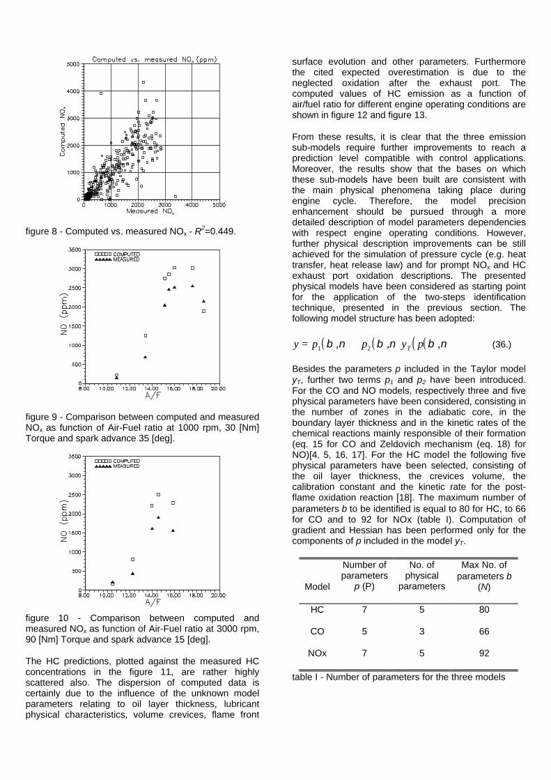
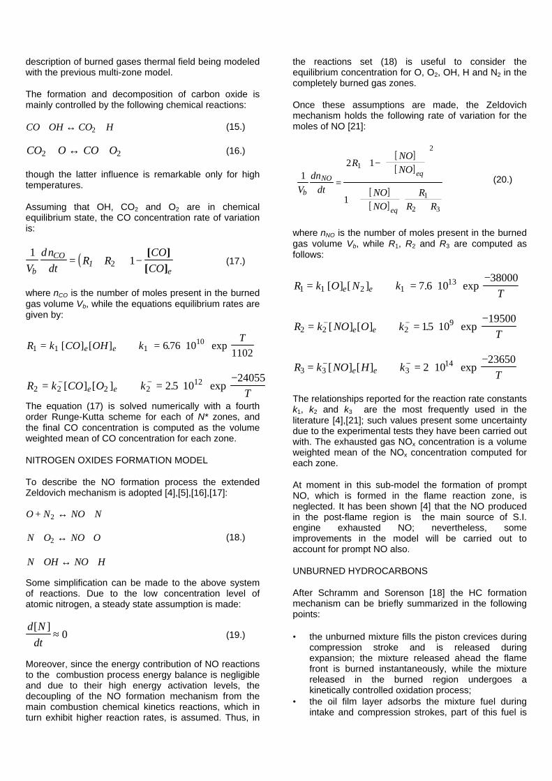
figure 8 - Computed vs. measured NOx - R2=0.449.
figure 9 - Comparison between computed and measuredNOx as function of Air-Fuel ratio at 1000 rpm, 30 [Nm]Torque and spark advance 35 [deg].
figure 10 - Comparison between computed andmeasured NOx as function of Air-Fuel ratio at 3000 rpm,90 [Nm] Torque and spark advance 15 [deg].
The HC predictions, plotted against the measured HCconcentrations in the figure 11, are rather highlyscattered also. The dispersion of computed data iscertainly due to the influence of the unknown modelparameters relating to oil layer thickness, lubricantphysical characteristics, volume crevices, flame front
surface evolution and other parameters. Furthermorethe cited expected overestimation is due to theneglected oxidation after the exhaust port. Thecomputed values of HC emission as a function ofair/fuel ratio for different engine operating conditions areshown in figure 12 and figure 13.
From these results, it is clear that the three emissionsub-models require further improvements to reach aprediction level compatible with control applications.Moreover, the results show that the bases on whichthese sub-models have been built are consistent withthe main physical phenomena taking place duringengine cycle. Therefore, the model precisionenhancement should be pursued through a moredetailed description of model parameters dependencieswith respect engine operating conditions. However,further physical description improvements can be stillachieved for the simulation of pressure cycle (e.g. heattransfer, heat release law) and for prompt NOx and HCexhaust port oxidation descriptions. The presentedphysical models have been considered as starting pointfor the application of the two-steps identificationtechnique, presented in the previous section. Thefollowing model structure has been adopted:
( ) ( ) ( )( )y p p y pT= +1 2β ν β ν β ν, , , (36.)
Besides the parameters p included in the Taylor modelyT, further two terms p1 and p2 have been introduced.For the CO and NO models, respectively three and fivephysical parameters have been considered, consisting inthe number of zones in the adiabatic core, in theboundary layer thickness and in the kinetic rates of thechemical reactions mainly responsible of their formation(eq. 15 for CO and Zeldovich mechanism (eq. 18) forNO)[4, 5, 16, 17]. For the HC model the following fivephysical parameters have been selected, consisting ofthe oil layer thickness, the crevices volume, thecalibration constant and the kinetic rate for the post-flame oxidation reaction [18]. The maximum number ofparameters β to be identified is equal to 80 for HC, to 66for CO and to 92 for NOx (table I). Computation ofgradient and Hessian has been performed only for thecomponents of p included in the model yT.
Model
Number ofparameters
p (P)
No. ofphysical
parameters
Max No. ofparameters β
(N)
HC 7 5 80
CO 5 3 66
NOx 7 5 92
table I - Number of parameters for the three models
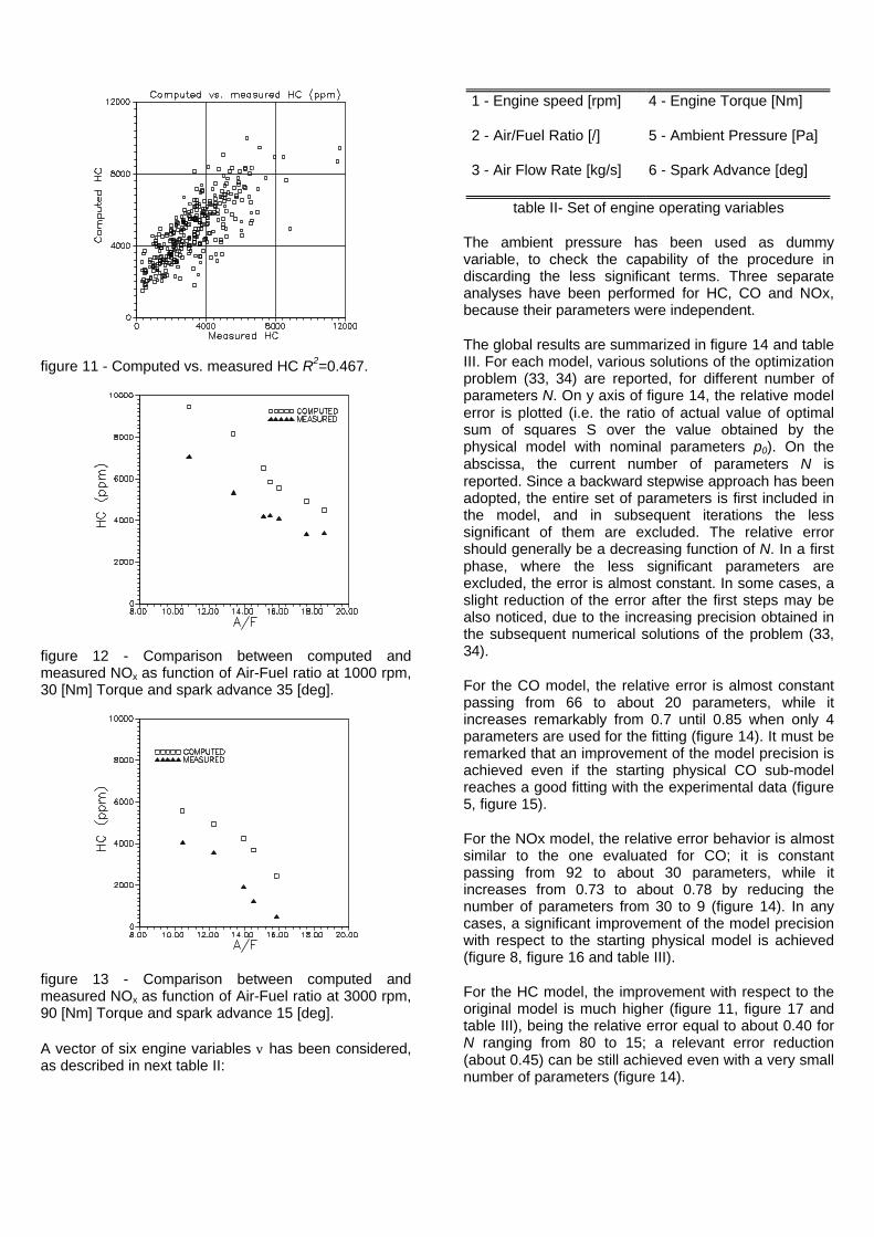
figure 11 - Computed vs. measured HC R2=0.467.
figure 12 - Comparison between computed andmeasured NOx as function of Air-Fuel ratio at 1000 rpm,30 [Nm] Torque and spark advance 35 [deg].
figure 13 - Comparison between computed andmeasured NOx as function of Air-Fuel ratio at 3000 rpm,90 [Nm] Torque and spark advance 15 [deg].
A vector of six engine variables ν has been considered,as described in next table II:
1 - Engine speed [rpm] 4 - Engine Torque [Nm]
2 - Air/Fuel Ratio [/] 5 - Ambient Pressure [Pa]
3 - Air Flow Rate [kg/s] 6 - Spark Advance [deg]
table II- Set of engine operating variables
The ambient pressure has been used as dummyvariable, to check the capability of the procedure indiscarding the less significant terms. Three separateanalyses have been performed for HC, CO and NOx,because their parameters were independent.
The global results are summarized in figure 14 and tableIII. For each model, various solutions of the optimizationproblem (33, 34) are reported, for different number ofparameters N. On y axis of figure 14, the relative modelerror is plotted (i.e. the ratio of actual value of optimalsum of squares S over the value obtained by thephysical model with nominal parameters p0). On theabscissa, the current number of parameters N isreported. Since a backward stepwise approach has beenadopted, the entire set of parameters is first included inthe model, and in subsequent iterations the lesssignificant of them are excluded. The relative errorshould generally be a decreasing function of N. In a firstphase, where the less significant parameters areexcluded, the error is almost constant. In some cases, aslight reduction of the error after the first steps may bealso noticed, due to the increasing precision obtained inthe subsequent numerical solutions of the problem (33,34).
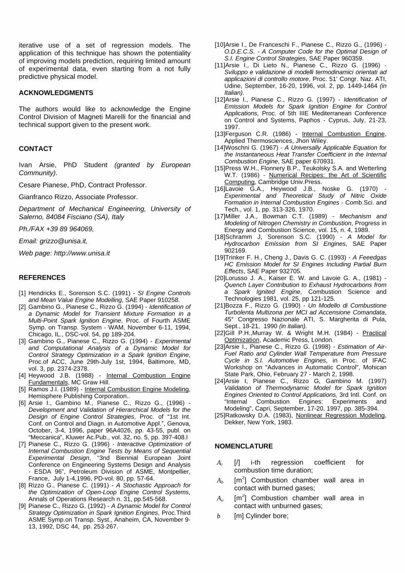
For the CO model, the relative error is almost constantpassing from 66 to about 20 parameters, while itincreases remarkably from 0.7 until 0.85 when only 4parameters are used for the fitting (figure 14). It must beremarked that an improvement of the model precision isachieved even if the starting physical CO sub-modelreaches a good fitting with the experimental data (figure5, figure 15).
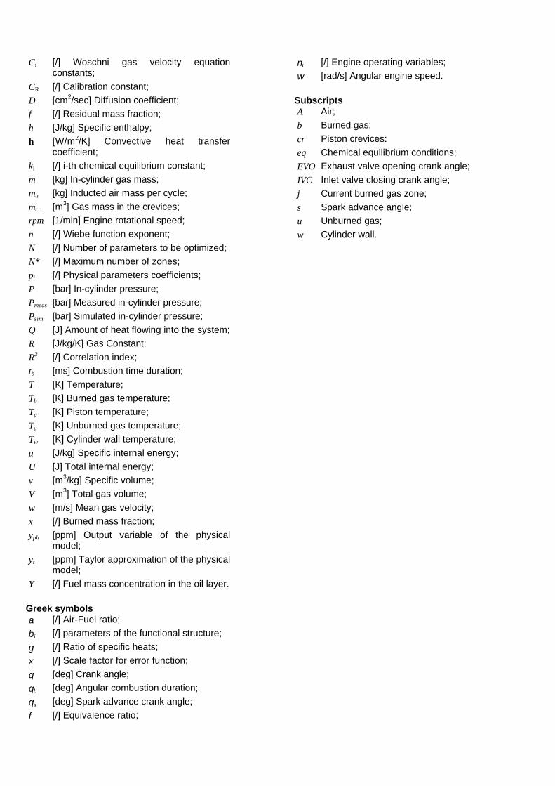
For the NOx model, the relative error behavior is almostsimilar to the one evaluated for CO; it is constantpassing from 92 to about 30 parameters, while itincreases from 0.73 to about 0.78 by reducing thenumber of parameters from 30 to 9 (figure 14). In anycases, a significant improvement of the model precisionwith respect to the starting physical model is achieved(figure 8, figure 16 and table III).
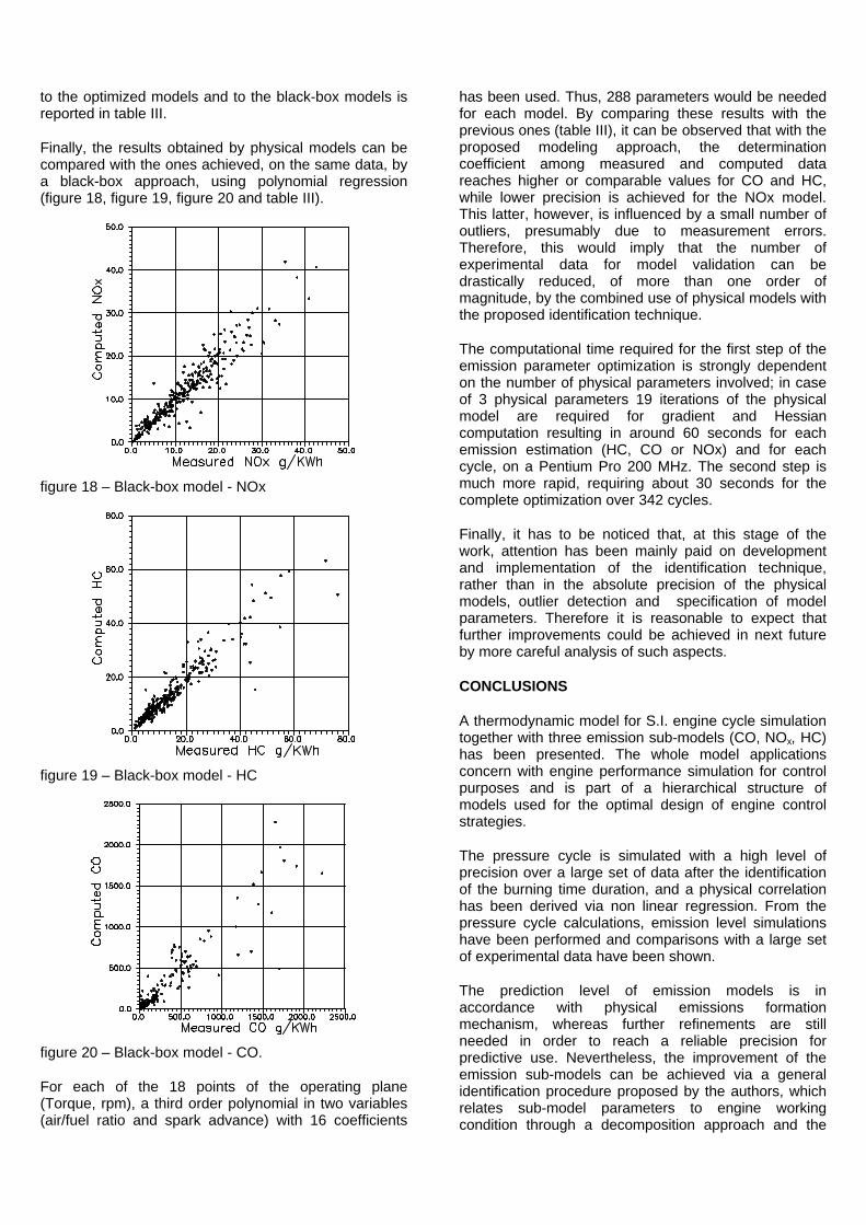
For the HC model, the improvement with respect to theoriginal model is much higher (figure 11, figure 17 andtable III), being the relative error equal to about 0.40 forN ranging from 80 to 15; a relevant error reduction(about 0.45) can be still achieved even with a very smallnumber of parameters (figure 14).
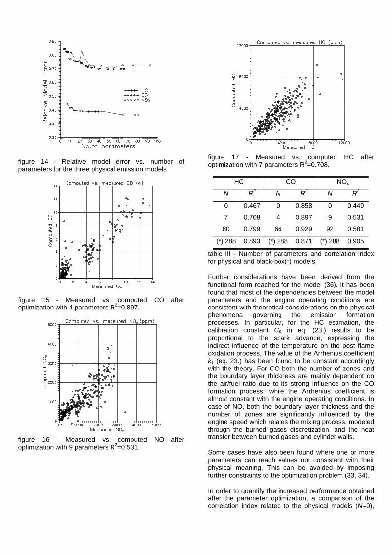
figure 14 - Relative model error vs. number ofparameters for the three physical emission models
figure 15 - Measured vs. computed CO afteroptimization with 4 parameters R2=0.897.
figure 16 - Measured vs. computed NO afteroptimization with 9 parameters R2=0.531.
figure 17 - Measured vs. computed HC afteroptimization with 7 parameters R2=0.708.
HC CO NOx
N R2 N R2 N R2
0 0.467 0 0.858 0 0.449
7 0.708 4 0.897 9 0.531
80 0.799 66 0.929 92 0.581
(*) 288 0.893 (*) 288 0.871 (*) 288 0.905
table III - Number of parameters and correlation indexfor physical and black-box(*) models.
Further considerations have been derived from thefunctional form reached for the model (36). It has beenfound that most of the dependencies between the modelparameters and the engine operating conditions areconsistent with theoretical considerations on the physicalphenomena governing the emission formationprocesses. In particular, for the HC estimation, thecalibration constant CR in eq. (23.) results to beproportional to the spark advance, expressing theindirect influence of the temperature on the post flameoxidation process. The value of the Arrhenius coefficientk1 (eq. 23.) has been found to be constant accordinglywith the theory. For CO both the number of zones andthe boundary layer thickness are mainly dependent onthe air/fuel ratio due to its strong influence on the COformation process, while the Arrhenius coefficient isalmost constant with the engine operating conditions. Incase of NO, both the boundary layer thickness and thenumber of zones are significantly influenced by theengine speed which relates the mixing process, modeledthrough the burned gases discretization, and the heattransfer between burned gases and cylinder walls.
Some cases have also been found where one or moreparameters can reach values not consistent with theirphysical meaning. This can be avoided by imposingfurther constraints to the optimization problem (33, 34).
In order to quantify the increased performance obtainedafter the parameter optimization, a comparison of thecorrelation index related to the physical models (N=0),
to the optimized models and to the black-box models isreported in table III.
Finally, the results obtained by physical models can becompared with the ones achieved, on the same data, bya black-box approach, using polynomial regression(figure 18, figure 19, figure 20 and table III).
figure 18 – Black-box model - NOx
figure 19 – Black-box model - HC
figure 20 – Black-box model - CO.
For each of the 18 points of the operating plane(Torque, rpm), a third order polynomial in two variables(air/fuel ratio and spark advance) with 16 coefficients
has been used. Thus, 288 parameters would be neededfor each model. By comparing these results with theprevious ones (table III), it can be observed that with theproposed modeling approach, the determinationcoefficient among measured and computed datareaches higher or comparable values for CO and HC,while lower precision is achieved for the NOx model.This latter, however, is influenced by a small number ofoutliers, presumably due to measurement errors.Therefore, this would imply that the number ofexperimental data for model validation can bedrastically reduced, of more than one order ofmagnitude, by the combined use of physical models withthe proposed identification technique.
The computational time required for the first step of theemission parameter optimization is strongly dependenton the number of physical parameters involved; in caseof 3 physical parameters 19 iterations of the physicalmodel are required for gradient and Hessiancomputation resulting in around 60 seconds for eachemission estimation (HC, CO or NOx) and for eachcycle, on a Pentium Pro 200 MHz. The second step ismuch more rapid, requiring about 30 seconds for thecomplete optimization over 342 cycles.
Finally, it has to be noticed that, at this stage of thework, attention has been mainly paid on developmentand implementation of the identification technique,rather than in the absolute precision of the physicalmodels, outlier detection and specification of modelparameters. Therefore it is reasonable to expect thatfurther improvements could be achieved in next futureby more careful analysis of such aspects.
CONCLUSIONS
A thermodynamic model for S.I. engine cycle simulationtogether with three emission sub-models (CO, NOx, HC)has been presented. The whole model applicationsconcern with engine performance simulation for controlpurposes and is part of a hierarchical structure ofmodels used for the optimal design of engine controlstrategies.
The pressure cycle is simulated with a high level ofprecision over a large set of data after the identificationof the burning time duration, and a physical correlationhas been derived via non linear regression. From thepressure cycle calculations, emission level simulationshave been performed and comparisons with a large setof experimental data have been shown.
The prediction level of emission models is inaccordance with physical emissions formationmechanism, whereas further refinements are stillneeded in order to reach a reliable precision forpredictive use. Nevertheless, the improvement of theemission sub-models can be achieved via a generalidentification procedure proposed by the authors, whichrelates sub-model parameters to engine workingcondition through a decomposition approach and the
iterative use of a set of regression models. Theapplication of this technique has shown the potentialityof improving models prediction, requiring limited amountof experimental data, even starting from a not fullypredictive physical model.
ACKNOWLEDGMENTS
The authors would like to acknowledge the EngineControl Division of Magneti Marelli for the financial andtechnical support given to the present work.
CONTACT
Ivan Arsie, PhD Student (granted by EuropeanCommunity).
Cesare Pianese, PhD, Contract Professor.
Gianfranco Rizzo, Associate Professor.
Department of Mechanical Engineering, University ofSalerno, 84084 Fisciano (SA), Italy
Ph./FAX +39 89 964069,
Email: [email protected],
Web page: http://www.unisa.it
REFERENCES
[1] Hendricks E., Sorenson S.C. (1991) - SI Engine Controlsand Mean Value Engine Modelling, SAE Paper 910258.
[2] Gambino G., Pianese C., Rizzo G. (1994) - Identification ofa Dynamic Model for Transient Mixture Formation in aMulti-Point Spark Ignition Engine, Proc. of Fourth ASMESymp. on Transp. System - WAM, November 6-11, 1994,Chicago, IL., DSC-vol. 54, pp 189-204.
[3] Gambino G., Pianese C., Rizzo G. (1994) - Experimentaland Computational Analysis of a Dynamic Model forControl Strategy Optimization in a Spark Ignition Engine,Proc.of ACC, June 29th-July 1st, 1994, Baltimore, MD,vol. 3, pp. 2374-2378.
[4] Heywood J.B. (1988) - Internal Combustion EngineFundamentals, MC Graw Hill.
[5] Ramos J.I. (1989) - Internal Combustion Engine Modeling,Hemisphere Publishing Corporation..
[6] Arsie I., Gambino M., Pianese C., Rizzo G., (1996) -Development and Validation of Hierarchical Models for theDesign of Engine Control Strategies, Proc. of “1st Int.Conf. on Control and Diagn. in Automotive Appl.”, Genova,October, 3-4, 1996, paper 96A4026, pp. 43-55, publ. on“Meccanica”, Kluwer Ac.Pub., vol. 32, no. 5, pp. 397-408.l
[7] Pianese C., Rizzo G. (1996) - Interactive Optimization ofInternal Combustion Engine Tests by Means of SequentialExperimental Design, “3nd Biennial European JointConference on Engineering Systems Design and Analysis- ESDA 96”, Petroleum Division of ASME, Montpellier,France, July 1-4,1996, PD-vol. 80, pp. 57-64.
[8] Rizzo G., Pianese C. (1991) - A Stochastic Approach forthe Optimization of Open-Loop Engine Control Systems,Annals of Operations Research n. 31, pp.545-568.
[9] Pianese C., Rizzo G. (1992) - A Dynamic Model for ControlStrategy Optimization in Spark Ignition Engines, Proc.ThirdASME Symp.on Transp. Syst., Anaheim, CA, November 9-13, 1992, DSC 44, pp. 253-267.
[10] Arsie I., De Franceschi F., Pianese C., Rizzo G., (1996) -O.D.E.C.S. - A Computer Code for the Optimal Design ofS.I. Engine Control Strategies, SAE Paper 960359.
[11] Arsie I., Di Lieto N., Pianese C., Rizzo G. (1996) -Sviluppo e validazione di modelli termodinamici orientati adapplicazioni di controllo motore, Proc. 51’ Congr. Naz. ATI,Udine, September, 16-20, 1996, vol. 2, pp. 1449-1464 (inItalian).
[12] Arsie I., Pianese C., Rizzo G. (1997) - Identification ofEmission Models for Spark Ignition Engine for ControlApplications, Proc. of 5th IIIE Mediterranean Conferenceon Control and Systems, Paphos - Cyprus, July, 21-23,1997.
[13] Ferguson C.R. (1986) - Internal Combustion Engine,Applied Thermosciences, Jhon Wiley.
[14] Woschni G. (1967) - A Universally Applicable Equation forthe Instantaneous Heat Transfer Coefficient in the InternalCombustion Engine, SAE paper 670931.
[15] Press W.H., Flonnery B.P., Teukolsky S.A. and WetterlingW.T. (1986) - Numerical Recipes: the Art of ScientificComputing, Cambridge Univ.Press.
[16] Lavoie G.A., Heywood J.B., Noske G. (1970) -Experimental and Theoretical Study of Nitric OxideFormation in Internal Combustion Engines - Comb.Sci. andTech., vol. 1, pp. 313-326, 1970.
[17] Miller J.A., Bowman C.T. (1989) - Mechanism andModeling of Nitrogen Chemistry in Combustion, Progress inEnergy and Combustion Science, vol. 15, n. 4, 1989.
[18] Schramm J, Sorenson S.C. (1990) - A Model forHydrocarbon Emission from SI Engines, SAE Paper902169.
[19] Trinker F. H., Cheng J., Davis G. C. (1993) - A FeeedgasHC Emission Model for SI Engines Including Partial BurnEffects, SAE Paper 932705.
[20] Lorusso J. A., Kaiser E. W. and Lavoie G. A., (1981) -Quench Layer Contribution to Exhaust Hydrocarbons froma Spark Ignited Engine, Combustion Science andTechnologies 1981, vol. 25, pp 121-125.
[21] Bozza F., Rizzo G. (1990) - Un Modello di CombustioneTurbolenta Multizona per MCI ad Accensione Comandata,45° Congresso Nazionale ATI, S. Margherita di Pula,Sept., 18-21, 1990 (in italian).
[22] Gill P.H.,Murray W. & Wright M.H. (1984) - PracticalOptimization, Academic Press, London.
[23] Arsie I., Pianese C., Rizzo G. (1998) - Estimation of Air-Fuel Ratio and Cylinder Wall Temperature from PressureCycle in S.I. Automotive Engines, in Proc. of IFACWorkshop on “Advances in Automatic Control”, MohicanState Park, Ohio, February 27 - March 2, 1998.
[24] Arsie I, Pianese C., Rizzo G, Gambino M. (1997)Validation of Thermodynamic Model for Spark IgnitionEngines Oriented to Control Applications, 3rd Intl. Conf. on“Internal Combustion Engines: Experiments andModeling”, Capri, September, 17-20, 1997, pp. 385-394.
[25] Ratkowsky D.A. (1983), Nonlinear Regression Modeling,Dekker, New York, 1983.
NOMENCLATURE
Ai [/] i-th regression coefficient forcombustion time duration;
Ab [m2] Combustion chamber wall area incontact with burned gases;
Au [m2] Combustion chamber wall area incontact with unburned gases;
b [m] Cylinder bore;
Ci [/] Woschni gas velocity equationconstants;
CR [/] Calibration constant;
D [cm2/sec] Diffusion coefficient;
f [/] Residual mass fraction;
h [J/kg] Specific enthalpy;
h [W/m2/K] Convective heat transfercoefficient;
ki [/] i-th chemical equilibrium constant;
m [kg] In-cylinder gas mass;
ma [kg] Inducted air mass per cycle;
mcr [m3] Gas mass in the crevices;
rpm [1/min] Engine rotational speed;
n [/] Wiebe function exponent;
N [/] Number of parameters to be optimized;
N* [/] Maximum number of zones;
pi [/] Physical parameters coefficients;
P [bar] In-cylinder pressure;
Pmeas [bar] Measured in-cylinder pressure;
Psim [bar] Simulated in-cylinder pressure;
Q [J] Amount of heat flowing into the system;
R [J/kg/K] Gas Constant;
R2 [/] Correlation index;
tb [ms] Combustion time duration;
T [K] Temperature;
Tb [K] Burned gas temperature;
Tp [K] Piston temperature;
Tu [K] Unburned gas temperature;
Tw [K] Cylinder wall temperature;
u [J/kg] Specific internal energy;
U [J] Total internal energy;
v [m3/kg] Specific volume;
V [m3] Total gas volume;
w [m/s] Mean gas velocity;
x [/] Burned mass fraction;
yph [ppm] Output variable of the physicalmodel;
yt [ppm] Taylor approximation of the physicalmodel;
Y [/] Fuel mass concentration in the oil layer.
Greek symbolsα [/] Air-Fuel ratio;
βi [/] parameters of the functional structure;
γ [/] Ratio of specific heats;
ξ [/] Scale factor for error function;
θ [deg] Crank angle;
θb [deg] Angular combustion duration;
θs [deg] Spark advance crank angle;
φ [/] Equivalence ratio;
νι [/] Engine operating variables;
ω [rad/s] Angular engine speed.
SubscriptsA Air;
b Burned gas;
cr Piston crevices:
eq Chemical equilibrium conditions;
EVO Exhaust valve opening crank angle;
IVC Inlet valve closing crank angle;
j Current burned gas zone;
s Spark advance angle;
u Unburned gas;
w Cylinder wall.


