1

Modelling railway ballasted track settlement in vehicle-track interaction analysis Ilaria Grossoni (1), William Powrie (2)*, Antonis Zervos (2), Yann Bezin (1), Louis Le Pen (2)

(1) Institute of Railway Research, University of Huddersfield, Huddersfield, UK

(2) University of Southampton, Southampton, UK

* corresponding author

Abstract The geometry of a ballasted railway gradually deteriorates with trafficking, mainly as a result of the

plastic settlement of the track-bed (ballast and sub-base). The rate and amount of settlement

depend on a number of factors, and for various reasons are difficult to predict or estimate

analytically. As a result, various empirical equations for estimating the rate of development of plastic

settlement of railway track with train passage have been proposed. A review of these equations

shows that they (i) do not reproduce the form of settlement vs number of load cycles relationships

usually seen in the field; (ii) do not reflect current knowledge of the behaviour of soil subgrades in

cyclic loading; and (iii) are often critically dependent on the curve fitting parameters used, which in

turn depend on the circumstances in which the calibration data were obtained. To address these

shortcomings, this paper develops a semi-analytical approach, based on the known behaviour of

granular materials under cyclic loading, for the calculation of plastic settlements of the trackbed with

train passage. The semi-analytical model is then combined with a suitable vehicle-track interaction

analysis to calculate rates of development of permanent settlement for different initial trackbed

stiffnesses, vehicle types and speeds. The model is shown to be able to reproduce recursive effects,

in which a deterioration in track geometry causes an increased variation in dynamic load, which

feeds back into a further deterioration in track geometry. The new model represents a significant

improvement on current empirical equations, in that it is able to reproduce observed aspects of

railway track settlement on the basis of the known behaviour of soils and ballast in cyclic loading.

Keywords Railway ballast, ballast permanent settlement, ballast settlement model, vehicle-track interaction,

iterative routine, trackbed stiffness

1. Introduction For nearly 200 years, most of the world’s railways have run on ballasted track. With trafficking, the

geometry of a ballasted track gradually deteriorates, mainly as a result of the plastic settlement of

the track-bed (ballast and sub-base). Intuitively, and as demonstrated by experimentation, the rate

and amount of settlement would be expected to depend on a number of factors, including [1]:

The loads imposed, including type and amount of traffic (e.g. axle load, speed, vehicle

dynamic effects, cumulative tonnage);

2

The track superstructure characteristics (e.g. rail and sleeper type, sleeper spacing, rail-

pads and any additional resilient layers such as under-sleeper pads), which influence the

distribution of loads into the underlying ballast and ground;

The ballast, sub-ballast and sub-grade layer characteristics (e.g. depth, density, stiffness or

resilient modulus, ballast specification in terms of particle size distribution and mineralogy,

ballast contamination, drainage and pore water pressure conditions), and the ability of

these supporting layers to resist cyclic loading.

When geometry defects become too severe, maintenance – usually in the form of automated

tamping or manual packing – is carried out to realign the track and enable the continued safe

running of trains. Unfortunately, tamping may also disrupt the load-bearing structure [2] and

damage individual ballast grains, resulting in a diminishing return period between maintenance

interventions until eventually the track-bed requires full renewal [3].

Four major difficulties in predicting the development of settlement are that:

1. On well-performing track, the rate of accumulation of residual (plastic or permanent)

settlement with each loading cycle is almost vanishingly small (in the order of a nanometre);

classical soil mechanics theories are not well-suited to modelling such small settlements and

their gradual accumulation over potentially millions of loading cycles.

2. Settlement may be attributable to either the ballast or the subgrade, and most likely to both

[4]. Different types of subsoil and ballast will have different tendencies to settle; even for

ballast having the same grading (particle size distribution curve) and mineralogy, the

settlement may depend on factors such as the depth of ballast, shoulder slope and the sleeper

type and sleeper / ballast interface conditions (e.g. the use or absence of under sleeper pads)

[5, 6].

3. Settlement generally arises as a result of both densification (volume change) and lateral

spreading (shear deformation) of the ballast and subgrade [5, 6].

4. It is generally differential (rather than uniform) settlements that cause the track geometry to

deteriorate to the extent that it needs maintenance [7]. The development of differential

settlement can only be replicated in an analysis if there are pre-defined initial differences, for

example in trackbed stiffness and / or in loading, that are not usually initially obvious in reality.

There is ample evidence from foundation engineering of a correlation between the maximum

settlement and the angular distortion – that is, larger settlements generally are likely to be

associated with larger differential settlements [8, 9].

These difficulties have led to the development of empirical ballast settlement equations as discussed

later, although such equations often do not take account explicitly of differences in sub-base, ballast

type and geometry, sleeper type or even loading conditions (axle load and speed).

Recent developments in modelling railway track system behaviour have focused on implementing

differentially deteriorating track support conditions in vehicle-track dynamic interaction analyses

(e.g. [10-13]), with the short-term dynamics of vehicle-track interaction (e.g. [14, 15]) linked to the

long-term degradation of the track through an iterative procedure. The approach is usually based on

a time domain simulation of vehicle-track interaction in which the force transmitted by the track

system (superstructure) to the supporting layers is calculated at each sleeper position and then used

3

as input into a settlement equation for track geometry degradation prediction [1]. However, there is

no consensus on which ballast settlement equation to use. This is unsurprising, because the

equations are empirical and their applicability depends on prevailing conditions including traffic

type, track structure type and ballast condition.

The aims of this paper are to

review current ballast settlement equations, the range of variables and parameters they can

take into account, and the conditions for which they were derived

develop an alternative semi-analytical approach to estimating track support system

settlement, based on established soil mechanics principles and referenced to field and full

scale laboratory test data

demonstrate the implementation of the proposed approach in a vehicle-track dynamic

interaction analysis model to calculate rates of differential track settlement and track

geometry deterioration, and compare it with previous methods.

2. Current ballast settlement equations A prerequisite to an improved ability to predict the development of differential settlement along a

section of track is a better understanding of the relationship between plastic settlement and loading,

based on the relevant properties of the ballast and the subgrade at a local scale. Ideally, a ballast

settlement equation would be able to account for the effects of the

1. number and magnitude of load cycles

2. train speed (allowing for dynamic load)

3. subgrade separately from the ballast

4. condition of the ballast, subgrade and the interface with the track.

Many, if not all, of these factors are acknowledged within track geometry prediction tools used by

industry to plan maintenance over route-scale lengths of track. For example, the T-SPA module

within VTISM [16] modifies the basic ballast settlement equation through two main factors. These

are the “Local Track Section Factor” (LTSF), which scales the empirical track geometry deterioration

equation to the locally measured rate; and the “Ballast Condition Factor” (BCF), which attempts to

replicate the observed reduction in the time interval between successive maintenance tamps,

generally held to be the result of fines from tamping-damaged ballast grains filling the voids. There

are also equations in the literature that attempt to link the development of track geometry

deterioration (standard deviation from the desired level) to these factors directly (e.g. [17]).

However, these are few and are outside the scope of this paper, which focuses on estimating the

rate of track settlement at the level of individual sleepers.

Most authors, including Sato [17] and Dahlberg [18], speculate that there are two major stages of

ballasted track settlement, occurring as a result of cumulative loading expressed in million gross

tonnes (MGT) or, more usually, the number of cycles of an (often assumed constant) load:

1. Stage 1: after tamping, settlement occurs initially relatively rapidly with MGT or number of

cycles as the ballast grains rearrange to establish a structure capable of carrying the applied

external loads. This is characterised by a reduction in void ratio and a densification of the

ballast [17], i.e. volumetric effects dominate

4

2. Stage 2: settlement occurs at a slower rate, increasing approximately linearly with MGT or

number of cycles. This is attributed to a variety of causes, including the lateral movement of

the ballast, penetration of the ballast into the subgrade, and ballast grain breakage and

abrasion [18]. Essentially, non-volumetric effects (including shear / lateral spreading)

dominate.

Basic equations Most of the equations that have been proposed to characterise track settlement are empirical. Many

take one of two forms:

1. Logarithmic or “ORE-type”: 𝑆𝑁 = 𝑆0. (1 + 𝐶. 𝑙𝑜𝑔10𝑁) or 𝑆 = 𝑆0. (1 + 𝐶. 𝑙𝑛𝑁)

(e.g. ORE 1970 [19], Shenton [20], Stewart [21]); or

2. Exponential or “Selig type”: 𝑆𝑁 = 𝑆0. 𝑁𝑎 (e.g. Selig [4], Indraratna [22], Cuellar [23])

where SN is the settlement after N load cycles, S0 is the settlement after one loading cycle,

and C and a are empirically-determined constants. Slightly more complex expressions are

given by, for example, Jeffs [24], Thom [25] and Indraratna [26].

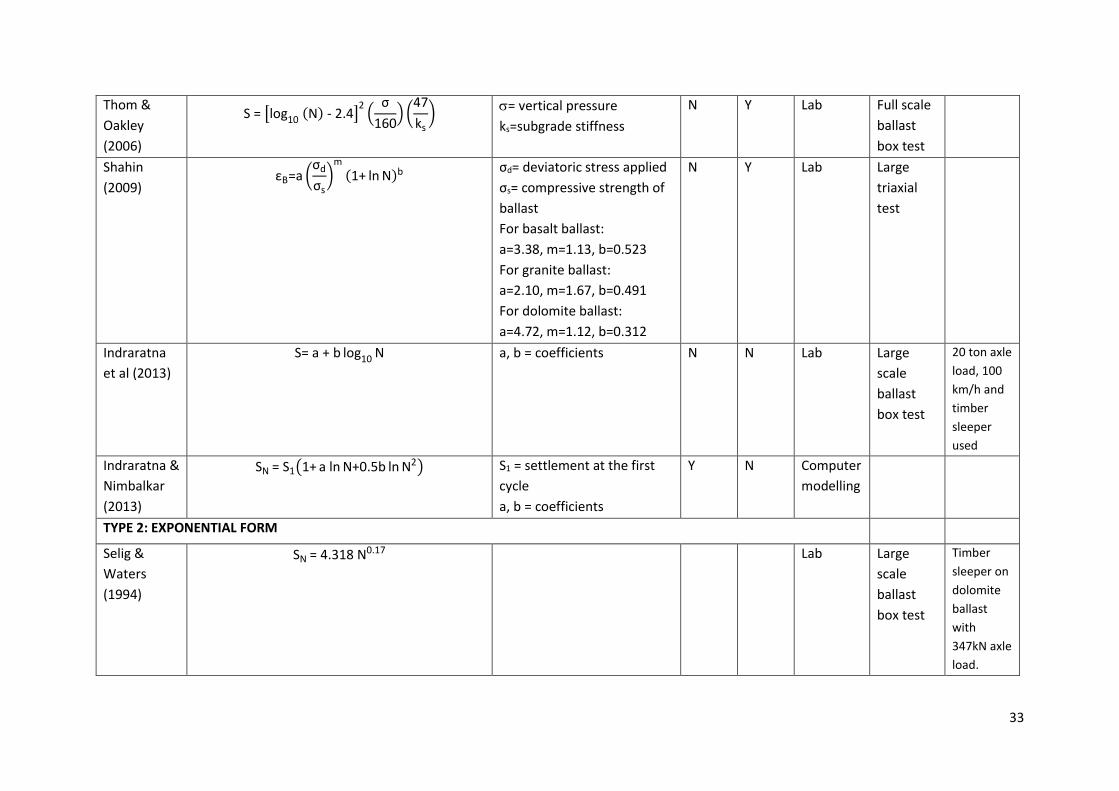
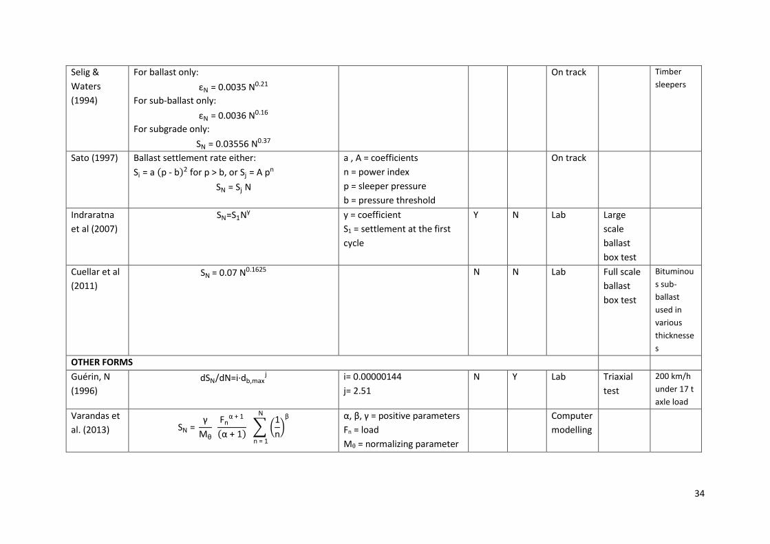
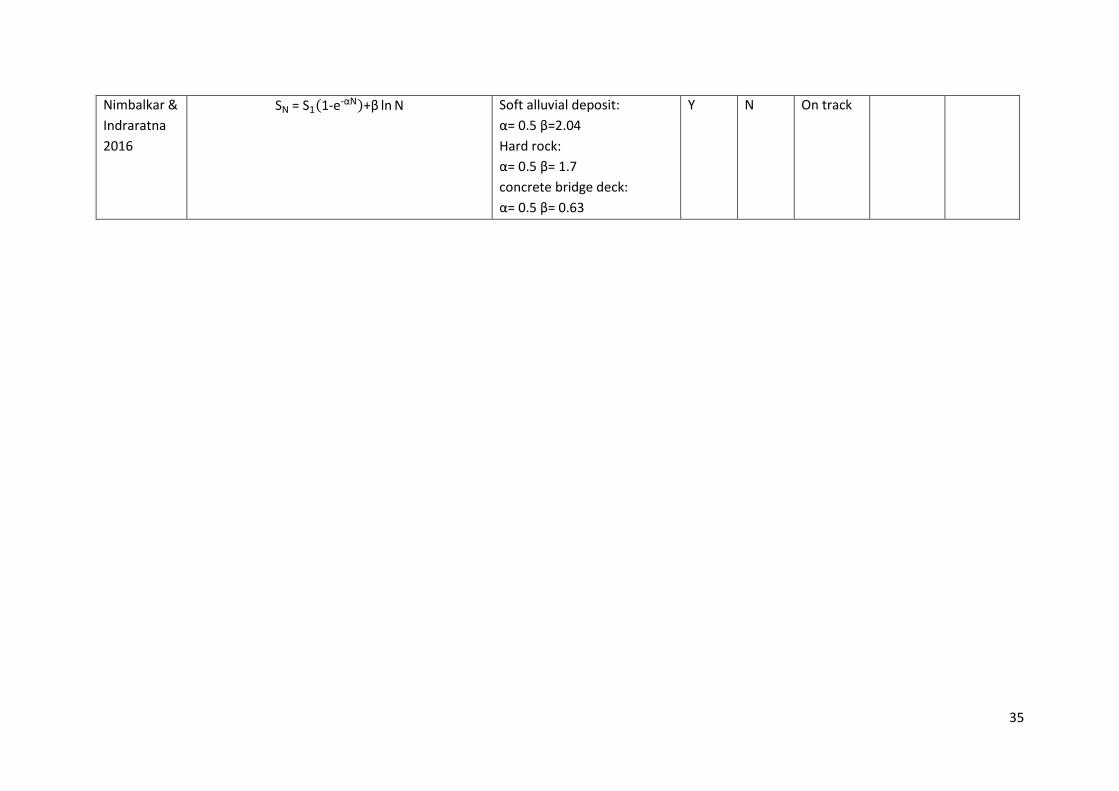
The more commonly used or cited track settlement equations are summarised in Appendix 1; some

of these were reviewed in [18]. A review of empirical permanent deformation models for soils in the

context of pavement and railway design was recently presented in [27].

Many equations relate the settlement after N load cycles to the settlement after the first cycle,

either explicitly or by inference. Arguably, this is a way of taking into account at least implicitly a

range of factors including the load per cycle, assuming that this remains constant. Other equations

take into account of a number of factors explicitly, such as the stiffness, condition or nature of the

ballast and in some cases the subgrade.

Three problems with these types of equations are that

1. they do not reproduce the form of settlement vs number of load cycles relationships usually

seen in large scale laboratory tests or in the field

2. the outcomes are critically dependent on the curve fitting parameters used, which in turn

depend on the circumstances in which the calibration data were obtained

3. those expressed in terms of the number of loading cycles do not generally account for the

effect of differing axle loads. (Equations expressed in terms of MGT may do, but assume –

probably unrealistically – that the effect of an increase in load is linear).

The second of these points is illustrated in Figure 1, which compares the settlement calculated after

100,000 cycles using the example ballast settlement equations indicated in Table 1 with the curve

fitting parameters proposed by the original authors, categorised according to the type of test on

which they are based.

5

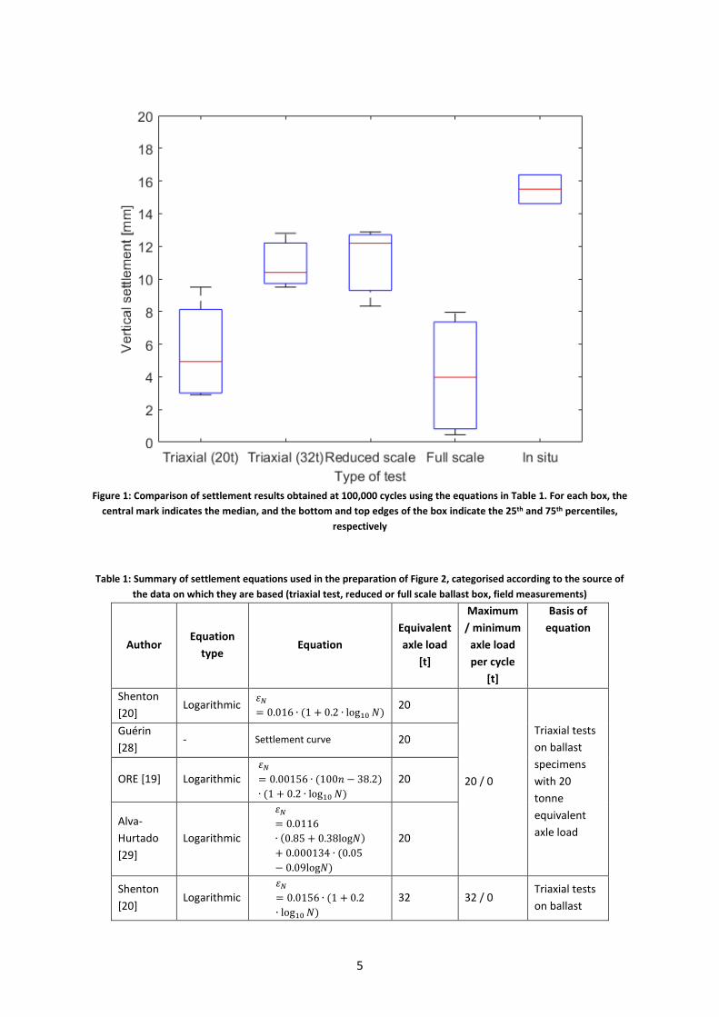
Figure 1: Comparison of settlement results obtained at 100,000 cycles using the equations in Table 1. For each box, the

central mark indicates the median, and the bottom and top edges of the box indicate the 25th and 75th percentiles,

respectively

Table 1: Summary of settlement equations used in the preparation of Figure 2, categorised according to the source of

the data on which they are based (triaxial test, reduced or full scale ballast box, field measurements)

Author Equation

type Equation

Equivalent

axle load

[t]

Maximum

/ minimum

axle load

per cycle

[t]

Basis of

equation

Shenton

[20] Logarithmic

𝜀𝑁

= 0.016 ∙ (1 + 0.2 ∙ log10 𝑁) 20

20 / 0

Triaxial tests

on ballast

specimens

with 20

tonne

equivalent

axle load

Guérin

[28] - Settlement curve 20

ORE [19] Logarithmic 𝜀𝑁

= 0.00156 ∙ (100𝑛 − 38.2)

∙ (1 + 0.2 ∙ log10 𝑁)

20

Alva-

Hurtado

[29]

Logarithmic

𝜀𝑁

= 0.0116

∙ (0.85 + 0.38log𝑁)

+ 0.000134 ∙ (0.05

− 0.09log𝑁)

20

Shenton

[20] Logarithmic

𝜀𝑁

= 0.0156 ∙ (1 + 0.2

∙ log10 𝑁)

32 32 / 0 Triaxial tests

on ballast

6

ORE [19] Logarithmic 𝜀𝑁

= 0.00345 ∙ (100𝑛 − 38.2)

∙ (1 + 0.2 ∙ log10 𝑁)

32 specimens

with 32

tonne

equivalent

axle load Alva-

Hurtado

[29]

Logarithmic

𝜀𝑁

= 0.0156

∙ (0.85 + 0.38log𝑁)

+ 0.000243 ∙ (0.05

− 0.09log𝑁)

32

Steward

[21, 30] Logarithmic

𝜀𝑁

= 0.0156 ∙ (1 + 0.29

∙ log10 𝑁)

20

23.3 / 5

Reduced

scale ballast

box test

Indraratna

[22, 31] Logarithmic

𝑆𝑁

= 2.31 ∙ (1 + 0.345

∙ log10 𝑁)

25

Indraratna

[26] Logarithmic

𝑆𝑁

= 0.5 ∙ (1 + 0.43log𝑁

+ 0.8log𝑁2)

25

Thom [25] Logarithmic 𝑆𝑁 = (log10 𝑁 − 2.4)2 20

19 / 3

Full scale

ballast box

test

Cedex

[23] Exponential 𝑆𝑁 = 0.07𝑁0.1625 17

Abadi [32] - Settlement curve 20

Partington

[33] Logarithmic 𝑆𝑁 = 0.29 log10 𝑁1.77 22

24 / 4

In situ

measure-

ments Fröhling

[34] - Settlement curve 26

Figure 1 shows large discrepancies between the calculated settlements, both within and between

each category of experimental basis. In most cases, the discrepancies between categories are

intuitively unsurprising. The in situ settlements are largest, but potentially include a contribution

from the subgrade, which none of the laboratory measurements do. The equations based on triaxial

tests simulating a 20 tonne axle load and the full-scale ballast tests are reasonably consistent; both

include only the ballast settlement and the equivalent axle loads are the same. The equations based

on parameters from triaxial tests simulating a 32 tonne axle load give greater settlements than those

based on triaxial tests simulating a 20 tonne axle load, which again seems intuitively reasonable. The

only counter-intuitive difference between categories of equation is that the calculations based on

reduced scale ballast box tests seem rather high.

Within an individual category, the variation is greatest for the equations based on triaxial tests

simulating a 20 tonne axle load and full scale ballast box tests. It is not clear why this should be, but

the potential variability of test specimens, the number of datasets involved and factors such as the

frequency of loading could all potentially have an influence. Figure 1 highlights the important

influence of the conditions under which a settlement equation and its associated parameters have

been derived. Harmonisation would require the development of either a common test procedure

that takes into account the effects of vehicle-track interaction, or a modelling approach built up by

considering the fundamental behaviour of each of the system components.

More complex equations In tests carried out to millions of cycles, data of track settlement vs number of load cycles generally

7

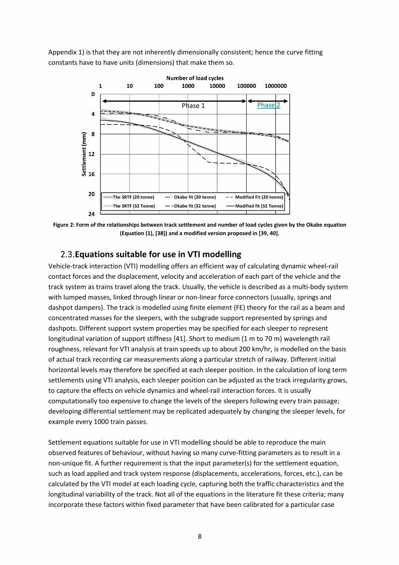
show two inflexion points [6, 35, 36] as indicated in Figure 2, which also shows approximately the

phases identified by Sato and Dahlberg. A simple logarithmic or exponential relationship is unable to

reproduce this form of curve. (Interestingly, data from a large scale test rig simulating 4 million

cycles of high speed train loading presented by Zhang et al, 2019 [37], do not show the second

inflexion point and do conform reasonably well to a simple Shenton-type logarithmic equation).

To improve the fit with experimental data exhibiting both phases of behaviour characterised by two

inflexion points on the logarithmic graph, more complex equations are needed. Figure 2 shows curve

fits from two empirically determined equations able to match a second downturn in the settlement

rate on a log scale. The first of these (referred to as the Okabe equation or fit) was originally

proposed in [38] (in the same form as that more recently presented in [17]); it combines logarithmic

and linear terms (Equation 1):

𝑆𝑁 = (𝐶1 − 𝐶2 ∙ 𝑒−𝛼𝑁) + 𝛽𝑁 (Equation 1)

where SN is the settlement at cycle N, N is the number of loading cycles (or cumulative MGT), and C1,

C2, α and β are empirically-determined coefficients.

A more complex equation was proposed in [39], based on vibration experiments on columns of

confined glass particles, and was fitted by [40] to ballast settlements measured in ballast / sleeper

tests carried out to a relatively low number of cycles (10,000), in which the ballast was confined

horizontally (Equation 2).

𝑆𝑁 = 𝑆1 + 𝑆2 [1 −1

1 + 𝛼𝑙𝑛 (1 +𝑁𝑁0

)] (Equation 2)

where S1 is the settlement measured after the first cycle and S2, , N0 are curve-fitting parameters

with arguable physical meanings.

Equation 2 was developed for settlement occurring solely as a result of densification and is not able

to reproduce the later downward phase shown in tests to millions of cycles, which is probably

attributable mainly to lateral ballast spreading at the sleeper ends / ballast shoulder. To allow for

lateral spreading at higher cycles, Equation 2 can be modified by adding the βN term from Equation

1 to create Equation 3: this is the second equation plotted in Figure 2, referred to as the modified fit.

𝑆𝑁 = 𝑆1 + 𝑆2 [1 −1

1 + 𝛼𝑙𝑛 (1 +𝑁𝑁0

)] + 𝛽𝑁 (Equation 3)

Using algorithms to determine the constants, Equation 3 can be fitted to data from laboratory

sleeper settlement tests to 3 million cycles (Figure 2). However, the large number of constants of

Equation 3 means that there is no unique best fit solution, so it is necessary to constrain the

permissible ranges of some of the constants. Different stages of settlement are apparent in both the

data and the fitted curves shown in Figure 2, with Equation 3 achieving very good fits. However,

whether the components / constants of Equations 1 and 3 individually represent different stages of

ballast settlement, and indeed the underlying mechanisms responsible, remains a matter of

conjecture. A further feature of these equations (and most if not all of the others reported in

8

Appendix 1) is that they are not inherently dimensionally consistent; hence the curve fitting

constants have to have units (dimensions) that make them so.

Figure 2: Form of the relationships between track settlement and number of load cycles given by the Okabe equation

(Equation (1), [38]) and a modified version proposed in [39, 40].

Equations suitable for use in VTI modelling Vehicle-track interaction (VTI) modelling offers an efficient way of calculating dynamic wheel-rail

contact forces and the displacement, velocity and acceleration of each part of the vehicle and the

track system as trains travel along the track. Usually, the vehicle is described as a multi-body system

with lumped masses, linked through linear or non-linear force connectors (usually, springs and

dashpot dampers). The track is modelled using finite element (FE) theory for the rail as a beam and

concentrated masses for the sleepers, with the subgrade support represented by springs and

dashpots. Different support system properties may be specified for each sleeper to represent

longitudinal variation of support stiffness [41]. Short to medium (1 m to 70 m) wavelength rail

roughness, relevant for VTI analysis at train speeds up to about 200 km/hr, is modelled on the basis

of actual track recording car measurements along a particular stretch of railway. Different initial

horizontal levels may therefore be specified at each sleeper position. In the calculation of long term

settlements using VTI analysis, each sleeper position can be adjusted as the track irregularity grows,

to capture the effects on vehicle dynamics and wheel-rail interaction forces. It is usually

computationally too expensive to change the levels of the sleepers following every train passage;

developing differential settlement may be replicated adequately by changing the sleeper levels, for

example every 1000 train passes.

Settlement equations suitable for use in VTI modelling should be able to reproduce the main

observed features of behaviour, without having so many curve-fitting parameters as to result in a

non-unique fit. A further requirement is that the input parameter(s) for the settlement equation,

such as load applied and track system response (displacements, accelerations, forces, etc.), can be

calculated by the VTI model at each loading cycle, capturing both the traffic characteristics and the

longitudinal variability of the track. Not all of the equations in the literature fit these criteria; many

incorporate these factors within fixed parameter that have been calibrated for a particular case

Phase 1 Phase 2

9

study. The equations proposed by Guérin [28], Sato [42] and Fröhling [34] have been selected for

further study as they do meet the criteria. They are described briefly below.

2.3.1. Guérin’s equation

Guérin [28] carried out an extensive series of tests at a loading frequency of 30 Hz, representing

approximately the tenth harmonic of the car passing frequency at a train speed of 215 km/h. (For a

discussion of the relationship between frequencies of loading, train speed and train geometry, see

[43] or [44]). The results suggested that the rate of accumulation of permanent settlement of the

ballast may be expressed as a function of the current maximum sleeper deflection:

𝑑𝑆𝑁

𝑑𝑁= 1.44 ∙ 10−6 ∙ 𝑑𝑏,𝑚𝑎𝑥

2.51 (Equation 4)

where N is the number of cycles and db,max the maximum elastic sleeper deflection. db,max is a function

of N, and expression of Equation 3 in non-differential form would require the ability to specify and

integrate this function.

The numerical values of the parameters in Equation 3 proposed by Guérin were for the particular

circumstances of the tests used to obtain the baseline data. More recently an extension in the

applicability of the formula to train speeds in excess of 350 km/h and “normal” or “soft” soil has

been proposed [45]. A major drawback of the Guérin formulation is that it is ill-adapted to a change

in track configuration, because the ratio of plastic deformation to maximum displacement will likely

change with varying ballast type, depth, etc. There is also a dimensional inconsistency owing to the

exponent applied to db,max.

.

2.3.2. Sato’s equation

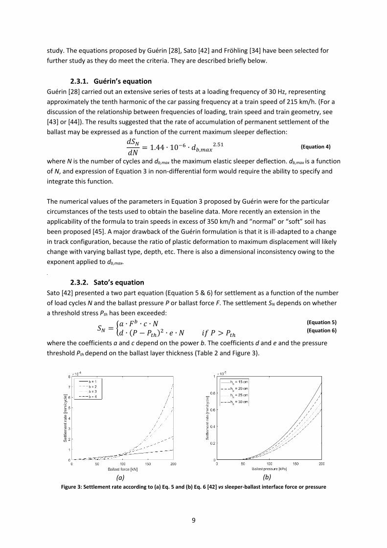
Sato [42] presented a two part equation (Equation 5 & 6) for settlement as a function of the number

of load cycles N and the ballast pressure P or ballast force F. The settlement SN depends on whether

a threshold stress Pth has been exceeded:

𝑆𝑁 = {𝑎 ∙ 𝐹𝑏 ∙ 𝑐 ∙ 𝑁 𝑑 ∙ (𝑃 − 𝑃𝑡ℎ)2 ∙ 𝑒 ∙ 𝑁 𝑖𝑓 𝑃 > 𝑃𝑡ℎ

(Equation 5)

(Equation 6)

where the coefficients a and c depend on the power b. The coefficients d and e and the pressure

threshold Pth depend on the ballast layer thickness (Table 2 and Figure 3).

(a)

(b)

Figure 3: Settlement rate according to (a) Eq. 5 and (b) Eq. 6 [42] vs sleeper-ballast interface force or pressure

10

Table 2: Parameters used in Sato’s equations [42]

Value of parameter b Value of parameter a Value of parameter c1

1 1.403 10-6 0.33

2 9.411 10-9 0.66

3 4.382 10-11 1.40

4 1.839 10-13 2.50

Value of parameter d Ballast depth hb, cm Threshold stress Pth, kPa Value of parameter e

2.70 10-10 15 37.5 1.30

20 38.6 1.14

25 39.6 1.00

30 40.6 0.88

Sato’s use of different equations above and below the threshold strain reflect the importance of

stress dependent non-linear soil behaviour. However, the equations contain dimensional

inconsistences and the settlements calculated are sensitive to the stress threshold used. The

threshold stress must be assumed to increase with stiffness, otherwise a stiffer trackbed support

leads to higher stress transfer from the track superstructure onto the ballast and consequently

higher calculated settlements, which is contrary to general experience [46]. The main input

parameter for Equation 4, the stress on the ballast, may be computed at each step in a vehicle-track

interaction analysis.

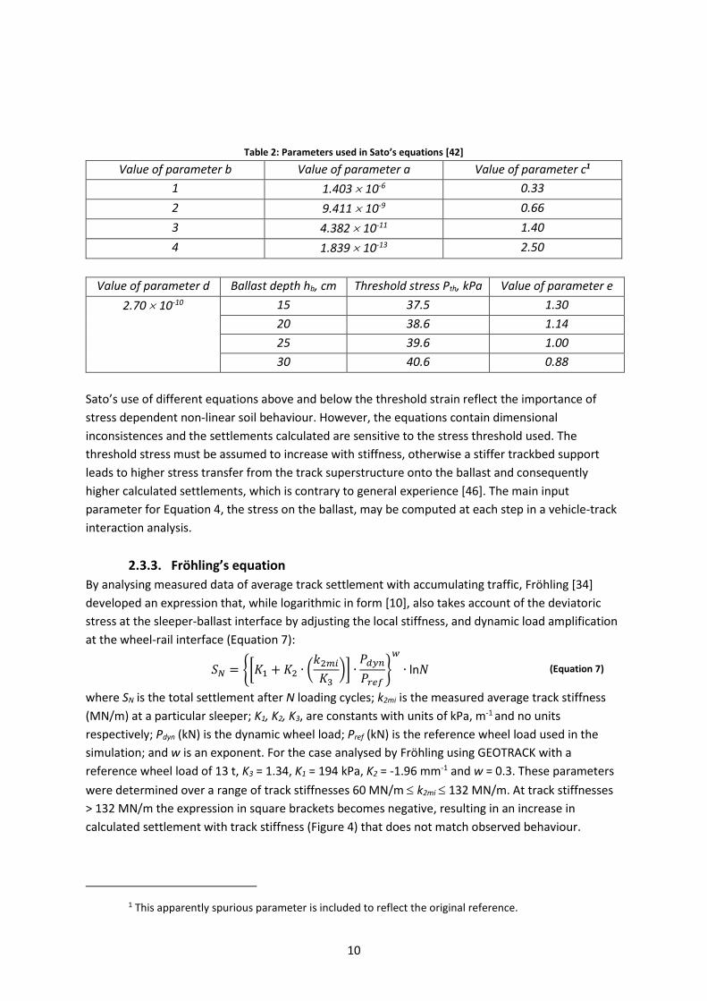
2.3.3. Fröhling’s equation

By analysing measured data of average track settlement with accumulating traffic, Fröhling [34]

developed an expression that, while logarithmic in form [10], also takes account of the deviatoric

stress at the sleeper-ballast interface by adjusting the local stiffness, and dynamic load amplification

at the wheel-rail interface (Equation 7):

𝑆𝑁 = {[𝐾1 + 𝐾2 ∙ (𝑘2𝑚𝑖

𝐾3)] ∙

𝑃𝑑𝑦𝑛

𝑃𝑟𝑒𝑓}

𝑤

∙ ln𝑁 (Equation 7)

where SN is the total settlement after N loading cycles; k2mi is the measured average track stiffness

(MN/m) at a particular sleeper; K1, K2, K3, are constants with units of kPa, m-1 and no units

respectively; Pdyn (kN) is the dynamic wheel load; Pref (kN) is the reference wheel load used in the

simulation; and w is an exponent. For the case analysed by Fröhling using GEOTRACK with a

reference wheel load of 13 t, K3 = 1.34, K1 = 194 kPa, K2 = -1.96 mm-1 and w = 0.3. These parameters

were determined over a range of track stiffnesses 60 MN/m k2mi 132 MN/m. At track stiffnesses

> 132 MN/m the expression in square brackets becomes negative, resulting in an increase in

calculated settlement with track stiffness (Figure 4) that does not match observed behaviour.

1 This apparently spurious parameter is included to reflect the original reference.

11

Figure 4: Variation of settlement predictions with trackbed stiffness using the Fröhling equation within (-)_and without

(--) the defined limits.

The input variables Pdyn and k2mi can be determined as outputs from each step of a VTI analysis, but

Equation 7 does have dimensional inconsistencies.

3. Proposed semi-analytical approach The review of equations currently used to estimate railway track settlement are mainly empirical; do

not incorporate a subgrade behaviour consistent with modern soil mechanics understanding and

principles (a point also evident in [27]); do not generally account for differences in axle load; and do

not reproduce patterns of settlement with trafficking seen in the field. In this section, a new model

for calculating ballast settlements is proposed, which is based on the observed behaviour of soils in

cyclic loading, is sensitive to axle load as well as cumulative loading, and is able to reproduce the

observed behaviour of ballast under cyclic loading.

In the following, 𝜎 is the vertical stress and the total strain 𝜀 = 𝜀𝑒 + 𝜀𝑝 comprises an elastic

(reversible) component 𝜀𝑒 and a plastic (irreversible) one 𝜀𝑝. Using a superposed dot to denote

increments of a quantity and assuming linear elasticity, elastic strain increments are calculated as

𝜀̇𝑒 =�̇�

𝐸𝑒, where 𝐸𝑒 is the elastic modulus. We define the plastic strain increment 𝜀̇𝑝 directly, using a

rate equation that fulfils the following requirements:

𝜀̇𝑝 is an increasing function of �̇�, so that larger stress increments cause larger plastic strain

increments

Failure occurs at a limiting or ultimate value of stress 𝜎𝑢; we assume 𝜀̇𝑝 → ∞ as 𝜎 → 𝜎𝑢.

Plastic strain develops only during loading, and only if the stress exceeds a threshold 𝜎𝑡 ≤ 𝜎𝑢

𝜀̇𝑝 is an increasing function of the difference (𝜎𝑢 − 𝜎𝑡), so that the greater the margin by which

the threshold stress is a exceeded, the larger the corresponding plastic strain increment.

An expression satisfying these requirements is:

𝜀̇𝑝 =1

𝐴∙ (

𝜎 − 𝜎𝑡

𝜎𝑢 − 𝜎) ∙ �̇� (Equation 8)

where 𝐴 is a material parameter with units of stress, which is interpreted as a plastic modulus. This

expression was arrived at heuristically, and is potentially the simplest one satisfying the above

requirements while introducing only one additional parameter.

12

Consecutive load cycles of equal magnitude are known to result in progressively smaller increments

of plastic strain, hence 𝜎𝑡 must also increase with loading. It is therefore assumed that 𝜎𝑡 is a

function of an internal parameter 𝑘, loosely quantifying how the properties of the material change

during the course of deformation; it is assumed that 𝑘 ≡ 𝜀𝑝 as a first approximation. However, 𝜎𝑡 ≤

𝜎𝑢 always; hence 𝜎𝑡 must increase at decreasing rate with 𝜀𝑝. In addition, other things being equal,

a higher elastic modulus 𝐸𝑒 would be expected to be associated with a higher 𝜎𝑡 and a higher 𝜎𝑢.

A general expression that satisfies the above requirements is:

𝜎𝑡 = 𝜎𝑡,𝑟𝑒𝑓(𝜀𝑝) ∙ [1 − 𝐶 (1 −𝐸𝑒

𝐸𝑟𝑒𝑓𝑒 )] (Equation 9)

where 𝜎𝑡,𝑟𝑒𝑓(𝜀𝑝) captures the dependence of 𝜎𝑡 on the plastic strain, while the square bracketed

term takes into account the (assumed linear) dependence of 𝜎𝑡 on the elastic stiffness. 𝐸𝑟𝑒𝑓𝑒 is a

reference value of the elastic stiffness and 𝐶 a constant calibration parameter. Further, the data

support the assumption that 𝜎𝑡,𝑟𝑒𝑓 is a simple hyperbolic function 𝜎𝑡,𝑟𝑒𝑓(𝜀𝑝) =

(𝛼1 ∙ 𝜀𝑝 + 𝛼2) (𝛼3 ∙ 𝜀𝑝 + 1)⁄ where 𝛼1, 𝛼2 and 𝛼3 are calibration parameters. The hyperbolic

function can be defined fully by three constraints. Assuming that, for 𝐸𝑒 = 𝐸𝑟𝑒𝑓𝑒 , 𝜎𝑡,0 and ℎ0

𝑝 are the

initial values of the threshold stress and its first derivative respectively, and 𝜎𝑢,𝑟𝑒𝑓 the value of the

ultimate stress, yields:

𝜎𝑡,𝑟𝑒𝑓(𝜀𝑝) =ℎ0

𝑝∙ 𝜎𝑢,𝑟𝑒𝑓 ∙ 𝜀𝑝 + 𝜎𝑡,0 ∙ (𝜎𝑢,𝑟𝑒𝑓 − 𝜎𝑡,0)

ℎ0𝑝

∙ 𝜀𝑝 + 𝜎𝑢,𝑟𝑒𝑓 − 𝜎𝑡,0

(Equation 10)

(Equation 9 and (Equation 10 imply that the ultimate stress varies with elastic stiffness as:

𝜎𝑢 = 𝜎𝑢,𝑟𝑒𝑓 ∙ [1 − 𝐶 (1 −𝐸𝑒

𝐸𝑟𝑒𝑓𝑒 )] (Equation 11)

This is reasonable, in that a higher peak strength and stiffness are both characteristics of dense or

overconsolidated soils. In other words, the stiffness and the strength of a soil would be expected to

be correlated, with a stiffer soil also being stronger. For any given soil, the value of the C parameter

could be determined on the basis of triaxial tests at different void ratios or preconsolidation

stresses, as appropriate for the type of soil and the relevant field conditions.

Informed by Equation 9 for 𝜎𝑡, the two equations for 𝜀̇𝑒 and 𝜀̇𝑝 can be integrated numerically using

the trapezium rule to determine the elastic, plastic and total strain response corresponding to any

given stress history. Integrating over a typical load cycle 𝜎1 → 𝜎2 → 𝜎1 using 20 increments was

found to provide good resolution and accuracy for the stress-strain response.

Although integrating each load cycle is not onerous, in the sense that results for tens of thousands of

cycles on a single sleeper can be produced within a few minutes on a desktop computer,

implementing this as part of a vehicle-track interaction analysis over a length of track with hundreds

of sleepers leads to a significant computational burden. It is desirable to carry out the integration

more efficiently, if possible within a single computational step for each load cycle, even at the

expense of a loss of accuracy. Assuming that a load cycle 𝜎1 → 𝜎2 → 𝜎1 increases the plastic strain

from 𝜀1𝑝

to 𝜀2𝑝

, for known 𝜀1𝑝

, 𝜀2𝑝

can be calculated as:

13

𝜀2𝑝

= 𝜀1𝑝

+ ∫1

𝐴∙

1

𝜎𝑢 − 𝜎∙ (𝜎 − 𝜎𝑡(𝜀𝑝, 𝐸𝑒)) ∙ 𝑑𝜎

𝜎2

𝜎1

(Equation 12)

Taking the Taylor expansion of 𝜎𝑡(𝜀𝑝, 𝐸𝑒), keeping the first (constant) term so that 𝜎𝑡(𝜀𝑝, 𝐸𝑒) ≅

𝜎𝑡(𝜀1𝑝

, 𝐸𝑒), and carrying out the algebra, eventually leads to:

𝜀2𝑝

≅ 𝜀1𝑝

+1

𝐴∙ [(𝜎𝑢 − 𝜎1) ∙ 𝑙𝑛 (

𝜎𝑢 − 𝜎1

𝜎𝑢 − 𝜎2) − (𝜎2 − 𝜎1)] (Equation 13)

Using this approximation results in a loss of accuracy in the order of 5%, which is more than

compensated for by the observed two orders of magnitude increase in the speed of calculation.

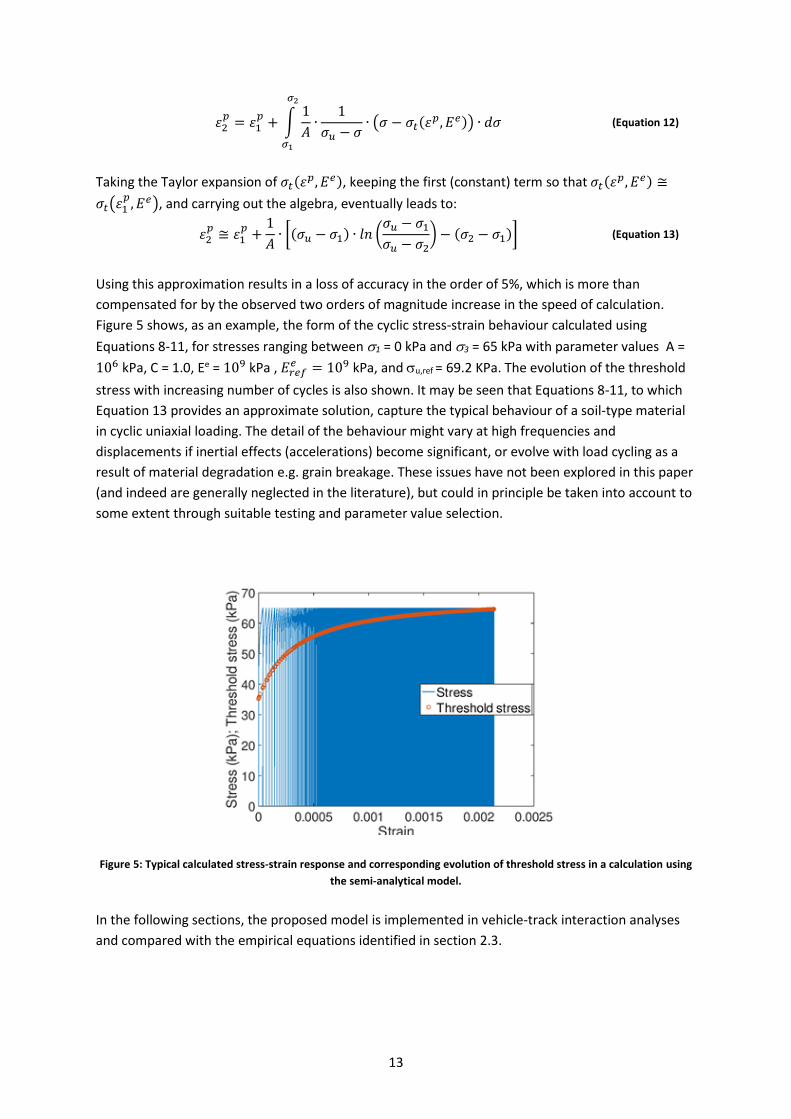
Figure 5 shows, as an example, the form of the cyclic stress-strain behaviour calculated using

Equations 8-11, for stresses ranging between 1 = 0 kPa and 3 = 65 kPa with parameter values A =

106 kPa, C = 1.0, Ee = 109 kPa , 𝐸𝑟𝑒𝑓𝑒 = 109 kPa, and u,ref = 69.2 KPa. The evolution of the threshold

stress with increasing number of cycles is also shown. It may be seen that Equations 8-11, to which

Equation 13 provides an approximate solution, capture the typical behaviour of a soil-type material

in cyclic uniaxial loading. The detail of the behaviour might vary at high frequencies and

displacements if inertial effects (accelerations) become significant, or evolve with load cycling as a

result of material degradation e.g. grain breakage. These issues have not been explored in this paper

(and indeed are generally neglected in the literature), but could in principle be taken into account to

some extent through suitable testing and parameter value selection.

Figure 5: Typical calculated stress-strain response and corresponding evolution of threshold stress in a calculation using

the semi-analytical model.

In the following sections, the proposed model is implemented in vehicle-track interaction analyses

and compared with the empirical equations identified in section 2.3.

14

4. Implementation of settlement equations in vehicle-track

interaction analyses

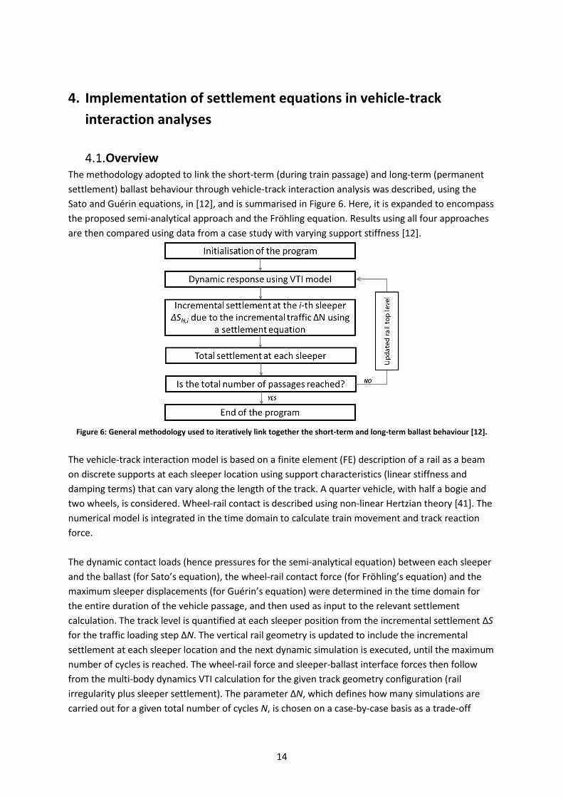
Overview The methodology adopted to link the short-term (during train passage) and long-term (permanent

settlement) ballast behaviour through vehicle-track interaction analysis was described, using the

Sato and Guérin equations, in [12], and is summarised in Figure 6. Here, it is expanded to encompass

the proposed semi-analytical approach and the Fröhling equation. Results using all four approaches

are then compared using data from a case study with varying support stiffness [12].

Figure 6: General methodology used to iteratively link together the short-term and long-term ballast behaviour [12].

The vehicle-track interaction model is based on a finite element (FE) description of a rail as a beam

on discrete supports at each sleeper location using support characteristics (linear stiffness and

damping terms) that can vary along the length of the track. A quarter vehicle, with half a bogie and

two wheels, is considered. Wheel-rail contact is described using non-linear Hertzian theory [41]. The

numerical model is integrated in the time domain to calculate train movement and track reaction

force.

The dynamic contact loads (hence pressures for the semi-analytical equation) between each sleeper

and the ballast (for Sato’s equation), the wheel-rail contact force (for Fröhling’s equation) and the

maximum sleeper displacements (for Guérin’s equation) were determined in the time domain for

the entire duration of the vehicle passage, and then used as input to the relevant settlement

calculation. The track level is quantified at each sleeper position from the incremental settlement ΔS

for the traffic loading step ΔN. The vertical rail geometry is updated to include the incremental

settlement at each sleeper location and the next dynamic simulation is executed, until the maximum

number of cycles is reached. The wheel-rail force and sleeper-ballast interface forces then follow

from the multi-body dynamics VTI calculation for the given track geometry configuration (rail

irregularity plus sleeper settlement). The parameter ΔN, which defines how many simulations are

carried out for a given total number of cycles N, is chosen on a case-by-case basis as a trade-off

15

between accuracy and computational costs. The total settlement is evaluated as the sum of the

settlement reached at the previous iteration and the incremental settlement in the current step of

N cycles.

Parameter values for the semi-analytical model were determined with reference to single sleeper

settlement tests in the Southampton Railway Testing Facility (SRTF) [6]. For the other empirical

models, the parameter values specified in the original references were adopted. For the avoidance

of doubt, the equations or methods investigated and the parameter values applied in this

comparison work are summarised in Table 3.

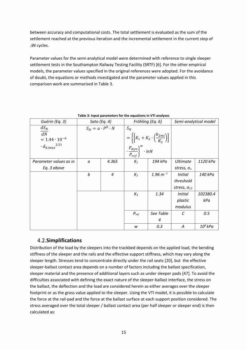
Table 3: Input parameters for the equations in VTI analyses

Guérin (Eq. 3) Sato (Eq. 4) Fröhling (Eq. 6) Semi-analytical model

𝑑𝑆𝑁

𝑑𝑁= 1.44 ∙ 10−6

∙ 𝑑𝑏,𝑚𝑎𝑥2.51

𝑆𝑁 = 𝑎 ∙ 𝑃𝑏 ∙ 𝑁 𝑆𝑁

= {[𝐾1 + 𝐾2 ∙ (𝑘2𝑚𝑖

𝐾3)]

∙𝑃𝑑𝑦𝑛

𝑃𝑟𝑒𝑓}

𝑤

∙ ln𝑁

Parameter values as in

Eq. 3 above

a 4.365 K1 194 kPa Ultimate

stress, σu

1120 kPa

b 4 K2 1.96 m -1 Initial

threshold

stress, σt,0

140 kPa

K3 1.34 Initial

plastic

modulus

102380.4

kPa

Pref See Table

4

C 0.5

w 0.3 A 106 kPa

Simplifications Distribution of the load by the sleepers into the trackbed depends on the applied load, the bending

stiffness of the sleeper and the rails and the effective support stiffness, which may vary along the

sleeper length. Stresses tend to concentrate directly under the rail seats [20], but the effective

sleeper-ballast contact area depends on a number of factors including the ballast specification,

sleeper material and the presence of additional layers such as under sleeper pads [47]. To avoid the

difficulties associated with defining the exact nature of the sleeper-ballast interface, the stress on

the ballast, the deflection and the load are considered herein as either averages over the sleeper

footprint or as the gross value applied to the sleeper. Using the VTI model, it is possible to calculate

the force at the rail-pad and the force at the ballast surface at each support position considered. The

stress averaged over the total sleeper / ballast contact area (per half sleeper or sleeper end) is then

calculated as:

16

𝜎 =𝐹𝑏

𝐴𝑠2⁄

(Equation 14)

where Fb is the force (from a single rail) at the ballast level and As is the area of the sleeper soffit.

5. Results from two case study sites

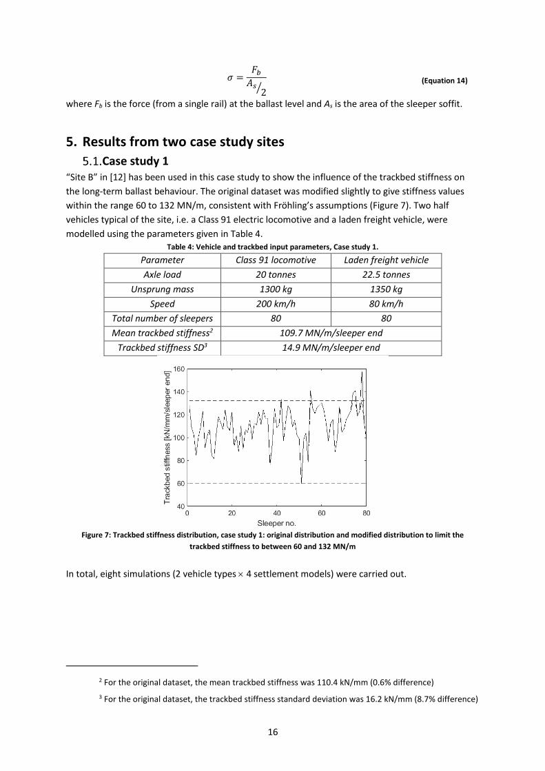
Case study 1 “Site B” in [12] has been used in this case study to show the influence of the trackbed stiffness on

the long-term ballast behaviour. The original dataset was modified slightly to give stiffness values

within the range 60 to 132 MN/m, consistent with Fröhling’s assumptions (Figure 7). Two half

vehicles typical of the site, i.e. a Class 91 electric locomotive and a laden freight vehicle, were

modelled using the parameters given in Table 4. Table 4: Vehicle and trackbed input parameters, Case study 1.

Parameter Class 91 locomotive Laden freight vehicle

Axle load 20 tonnes 22.5 tonnes

Unsprung mass 1300 kg 1350 kg

Speed 200 km/h 80 km/h

Total number of sleepers 80 80

Mean trackbed stiffness2 109.7 MN/m/sleeper end

Trackbed stiffness SD3 14.9 MN/m/sleeper end

Figure 7: Trackbed stiffness distribution, case study 1: original distribution and modified distribution to limit the

trackbed stiffness to between 60 and 132 MN/m

In total, eight simulations (2 vehicle types 4 settlement models) were carried out.

2 For the original dataset, the mean trackbed stiffness was 110.4 kN/mm (0.6% difference)

3 For the original dataset, the trackbed stiffness standard deviation was 16.2 kN/mm (8.7% difference)

17

(a)

(b)

(c)

(d)

(e)

(f)

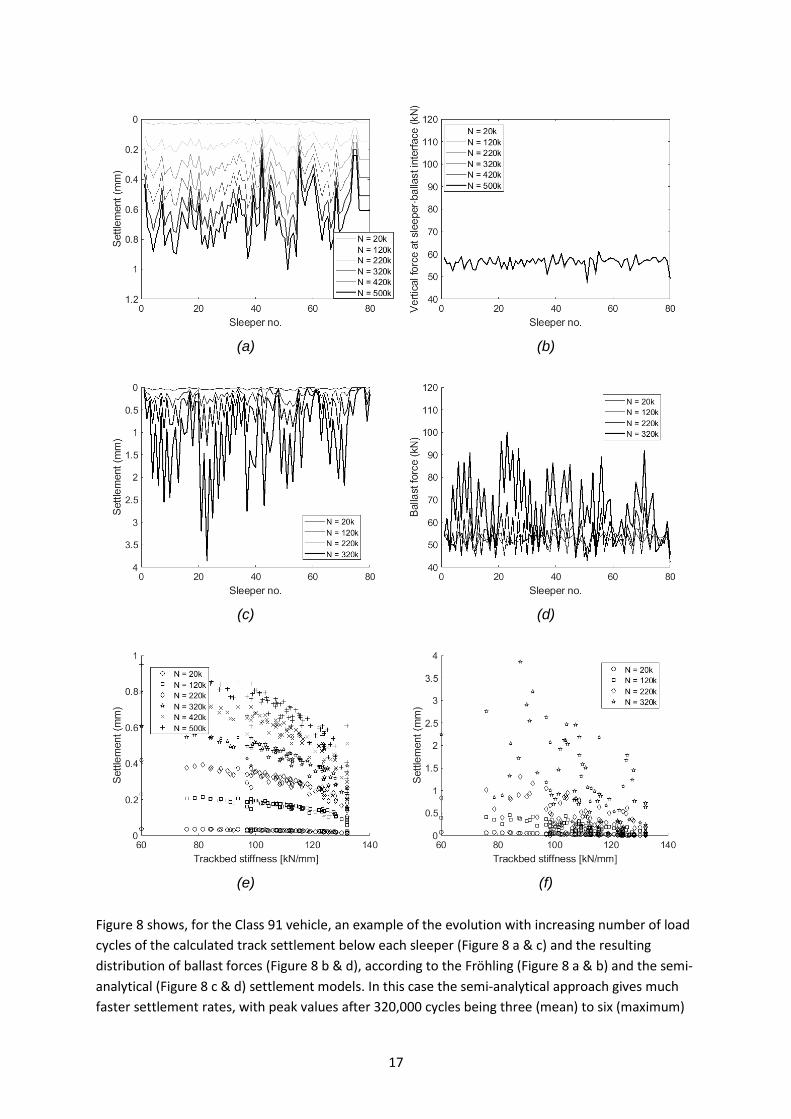
Figure 8 shows, for the Class 91 vehicle, an example of the evolution with increasing number of load

cycles of the calculated track settlement below each sleeper (Figure 8 a & c) and the resulting

distribution of ballast forces (Figure 8 b & d), according to the Fröhling (Figure 8 a & b) and the semi-

analytical (Figure 8 c & d) settlement models. In this case the semi-analytical approach gives much

faster settlement rates, with peak values after 320,000 cycles being three (mean) to six (maximum)

18

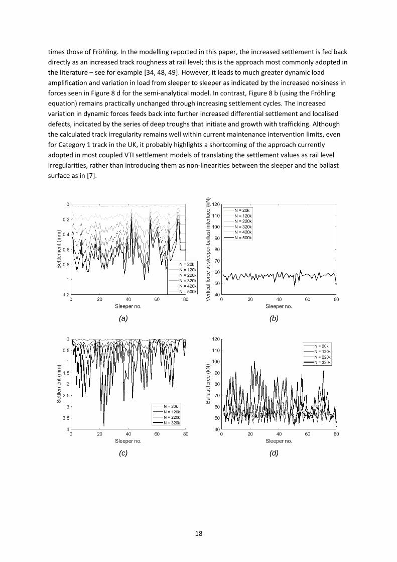
times those of Fröhling. In the modelling reported in this paper, the increased settlement is fed back

directly as an increased track roughness at rail level; this is the approach most commonly adopted in

the literature – see for example [34, 48, 49]. However, it leads to much greater dynamic load

amplification and variation in load from sleeper to sleeper as indicated by the increased noisiness in

forces seen in Figure 8 d for the semi-analytical model. In contrast, Figure 8 b (using the Fröhling

equation) remains practically unchanged through increasing settlement cycles. The increased

variation in dynamic forces feeds back into further increased differential settlement and localised

defects, indicated by the series of deep troughs that initiate and growth with trafficking. Although

the calculated track irregularity remains well within current maintenance intervention limits, even

for Category 1 track in the UK, it probably highlights a shortcoming of the approach currently

adopted in most coupled VTI settlement models of translating the settlement values as rail level

irregularities, rather than introducing them as non-linearities between the sleeper and the ballast

surface as in [7].

(a)

(b)

(c)

(d)

19

(e)

(f)

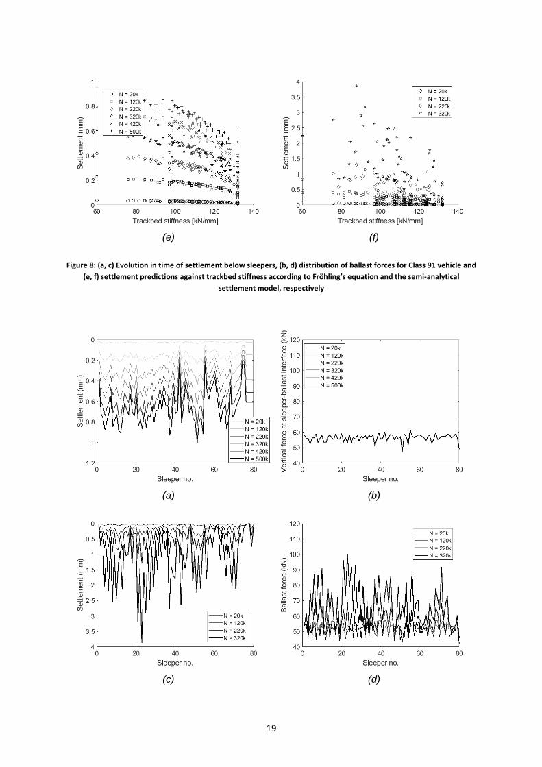
Figure 8: (a, c) Evolution in time of settlement below sleepers, (b, d) distribution of ballast forces for Class 91 vehicle and

(e, f) settlement predictions against trackbed stiffness according to Fröhling’s equation and the semi-analytical

settlement model, respectively

(a)

(b)

(c)

(d)

20

(e)

(f)

Figure 8 (e & f) shows that both approaches calculate lower settlement rates at locations with higher

trackbed stiffness and vice versa. This is in line with expectations, as the rate of settlement

calculated using Fröhling’s equation is inversely proportional to the trackbed stiffness, while in the

semi-analytical model the threshold stress is proportional to the trackbed stiffness. Settlements

calculated using the semi-analytical approach show increasing scatter between individual sleepers

with increasing number of cycles, owing to the amplification effect of such track irregularities on the

dynamic loads as discussed above.

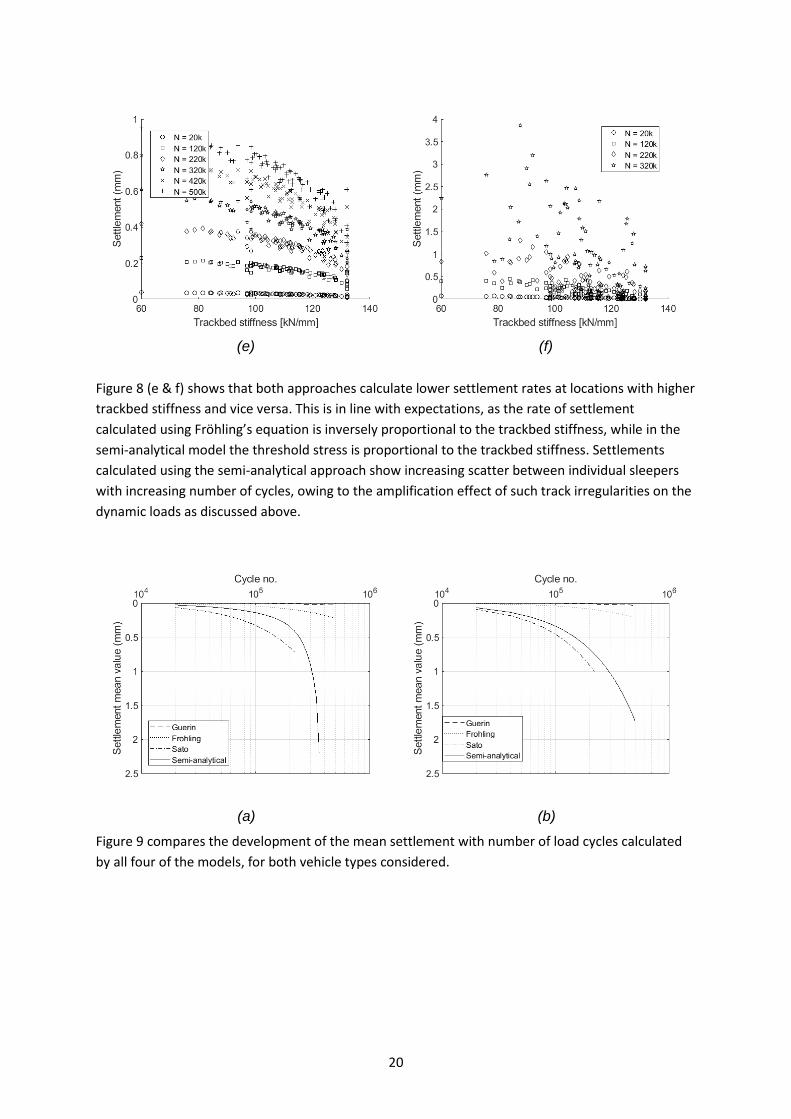
(a)

(b)

Figure 9 compares the development of the mean settlement with number of load cycles calculated

by all four of the models, for both vehicle types considered.

21

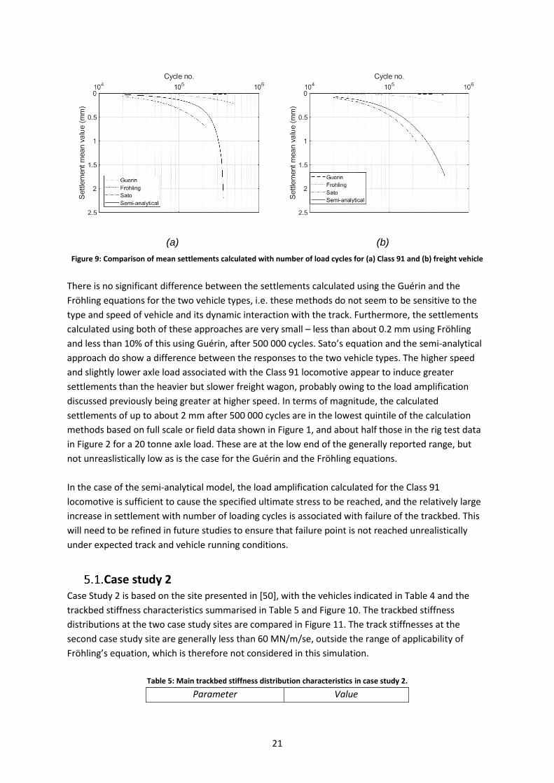
(a)

(b)

Figure 9: Comparison of mean settlements calculated with number of load cycles for (a) Class 91 and (b) freight vehicle

There is no significant difference between the settlements calculated using the Guérin and the

Fröhling equations for the two vehicle types, i.e. these methods do not seem to be sensitive to the

type and speed of vehicle and its dynamic interaction with the track. Furthermore, the settlements

calculated using both of these approaches are very small – less than about 0.2 mm using Fröhling

and less than 10% of this using Guérin, after 500 000 cycles. Sato’s equation and the semi-analytical

approach do show a difference between the responses to the two vehicle types. The higher speed

and slightly lower axle load associated with the Class 91 locomotive appear to induce greater

settlements than the heavier but slower freight wagon, probably owing to the load amplification

discussed previously being greater at higher speed. In terms of magnitude, the calculated

settlements of up to about 2 mm after 500 000 cycles are in the lowest quintile of the calculation

methods based on full scale or field data shown in Figure 1, and about half those in the rig test data

in Figure 2 for a 20 tonne axle load. These are at the low end of the generally reported range, but

not unreaslistically low as is the case for the Guérin and the Fröhling equations.

In the case of the semi-analytical model, the load amplification calculated for the Class 91

locomotive is sufficient to cause the specified ultimate stress to be reached, and the relatively large

increase in settlement with number of loading cycles is associated with failure of the trackbed. This

will need to be refined in future studies to ensure that failure point is not reached unrealistically

under expected track and vehicle running conditions.

Case study 2 Case Study 2 is based on the site presented in [50], with the vehicles indicated in Table 4 and the

trackbed stiffness characteristics summarised in Table 5 and Figure 10. The trackbed stiffness

distributions at the two case study sites are compared in Figure 11. The track stiffnesses at the

second case study site are generally less than 60 MN/m/se, outside the range of applicability of

Fröhling’s equation, which is therefore not considered in this simulation.

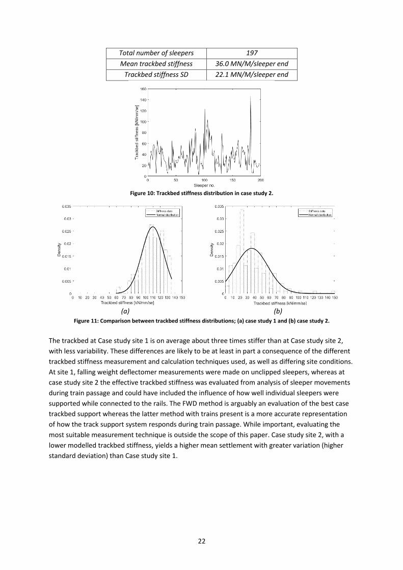
Table 5: Main trackbed stiffness distribution characteristics in case study 2.

Parameter Value

22

Total number of sleepers 197

Mean trackbed stiffness 36.0 MN/M/sleeper end

Trackbed stiffness SD 22.1 MN/M/sleeper end

Figure 10: Trackbed stiffness distribution in case study 2.

(a)

(b)

Figure 11: Comparison between trackbed stiffness distributions; (a) case study 1 and (b) case study 2.

The trackbed at Case study site 1 is on average about three times stiffer than at Case study site 2,

with less variability. These differences are likely to be at least in part a consequence of the different

trackbed stiffness measurement and calculation techniques used, as well as differing site conditions.

At site 1, falling weight deflectomer measurements were made on unclipped sleepers, whereas at

case study site 2 the effective trackbed stiffness was evaluated from analysis of sleeper movements

during train passage and could have included the influence of how well individual sleepers were

supported while connected to the rails. The FWD method is arguably an evaluation of the best case

trackbed support whereas the latter method with trains present is a more accurate representation

of how the track support system responds during train passage. While important, evaluating the

most suitable measurement technique is outside the scope of this paper. Case study site 2, with a

lower modelled trackbed stiffness, yields a higher mean settlement with greater variation (higher

standard deviation) than Case study site 1.

23

(a)

(b)

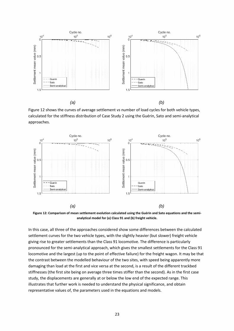
Figure 12 shows the curves of average settlement vs number of load cycles for both vehicle types,

calculated for the stiffness distribution of Case Study 2 using the Guérin, Sato and semi-analytical

approaches.

(a)

(b)

Figure 12: Comparison of mean settlement evolution calculated using the Guérin and Sato equations and the semi-

analytical model for (a) Class 91 and (b) freight vehicle.

In this case, all three of the approaches considered show some differences between the calculated

settlement curves for the two vehicle types, with the slightly heavier (but slower) freight vehicle

giving rise to greater settlements than the Class 91 locomotive. The difference is particularly

pronounced for the semi-analytical approach, which gives the smallest settlements for the Class 91

locomotive and the largest (up to the point of effective failure) for the freight wagon. It may be that

the contrast between the modelled behaviour of the two sites, with speed being apparently more

damaging than load at the first and vice versa at the second, is a result of the different trackbed

stiffnesses (the first site being on average three times stiffer than the second). As in the first case

study, the displacements are generally at or below the low end of the expected range. This

illustrates that further work is needed to understand the physical significance, and obtain

representative values of, the parameters used in the equations and models.

24

The semi-analytical model would benefit from being refined through the selection of parameters

more suitable to each case study site. Nonetheless, it does have the potential to capture a range of

different track behaviours that the more empirically-based equations do not. Realistic

representation of the track in vehicle-track interaction analysis, and the calculation of track

cumulative settlements as a result of train passage is in its infancy. The purpose of this paper has

been to demonstrate the feasibility and potential of a soil mechanics based approach. Further work

is needed, both to understand the physical meaning and quantify the parameters underlying the

new model; and to validate the approach with reference to high quality, long-term datasets of track

settlement, which at present are rare to non-existent.

6. Summary and conclusions Equations that have been proposed to represent the gradual accumulation of plastic settlement of

railway track with train passage have been reviewed. Three were selected for further study, on the

basis that they are able to reproduce the main observed features of track settlement behaviour, and

that they can take as inputs the outputs from an associated vehicle-track interaction model.

A semi-analytical expression, based on the known behaviour of granular materials under cyclic

loading, has been developed. This expression is able to reproduce the accumulation of plastic

settlement with each load cycle, with the amount of plastic settlement per cycle related to the stress

in excess of a threshold stress. The threshold stress increases with the number of load cycles (work

hardening), and with the initial stiffness of the trackbed. It also features an ultimate stress, at which

plastic deformation continues unchecked.

When combined with a suitable vehicle-track interaction analysis, the semi-analytical model has

been shown to be able to capture differences in the rate of development of permanent settlement

as a result of differences in the initial trackbed stiffness, vehicle type and speed; and the

development of rail roughness through differential settlement. It is also able to reproduce recursive

effects, in which a deterioration in track geometry causes an increased variation in dynamic load,

which feeds back into a further deterioration in track geometry.

While there remains considerable scope for refinement of the semi-analytical approach, particularly

through the selection of parameter values appropriate to different site conditions, it shows

considerable promise in being able to reproduce observed aspects of railway track settlement on the

basis of the known behaviour of geomaterials (soils and ballast) in cyclic loading.

The work has also highlighted areas in which the vehicle-track interaction modelling approach needs

improvement, in particular by applying the settlement growth at the interface between sleepers and

the ballast, rather than as an equivalent rail irregularity as adopted in much of the current literature.

Evaluation of the trackbed stiffness for input into such models also needs further research.

Acknowledgements This work was funded by the UK EPSRC project Track to the Future (grant agreement no.

EP/M025276/1). The authors are grateful to Dr Taufan Abadi, Dr Edgar Ferro and Mr Giacomo

25

Ognibene for their assistance with the review of track settlement equations, and to Dr Taufan Abadi

for his help in compiling the Appendix.

References

1. In2Rail, Deliverable D3.3: Evaluation of optimised track systems. 2017.

2. Aingaran, S., L. Le Pen, A. Zervos, and W. Powrie, Modelling the effects of trafficking and tamping on scaled railway ballast in triaxial tests. Transportation Geotechnics, 2018. 15: p. 84-90.

3. Lichtberger, B., Track Compendium - Formation, Permanent way, Maintenance, Economics. 2005, Hamburg: Eurailpress.

4. Selig, E.T. and J.M. Waters, Track geotechnology and substructure management. 1994: Thomas Telford.

5. Abadi, T., L. Le Pen, A. Zervos, and W. Powrie, Effect of Sleeper Interventions on Railway Track Performance. Journal of Geotechnical and Geoenvironmental Engineering, 2019. 145(4).

6. Abadi, T., L. Le Pen, A. Zervos, and W. Powrie, Improving the performance of railway tracks through ballast interventions. Proceedings of the Institution of Mechanical Engineers, Part F: Journal of Rail and Rapid Transit, 2016. 232(2): p. 337-355.

7. Nielsen, J.C.O. and X. Li, Railway track geometry degradation due to differential settlement of ballast/subgrade – Numerical prediction by an iterative procedure. Journal of Sound and Vibration, 2018. 412: p. 441-456.

8. Skempton, A.W. and D.H. MacDonald, The allowable settlements of buildings. Proceedings of the Institution of Civil Engineers, 1956. 5(6): p. 727-768.

9. Ricceri, G. and M. Soranzo, An analysis on allowable settlement of structures. Rivista Italiana di Geotecnica, 1985. 4: p. 177-188.

10. Frohling, R.D., Deterioration of railway track due to dynamic vehicle loading and spacially varying track stiffness, in Faculty of Engineering. 1997, University of Pretoria: Pretoria.

11. Li, X., J.C.O. Nielsen, and B.A. Palsson, Simulation of track settlement in railway turnouts. Vehicle System Dynamics, 2014. 52(Suppl.1): p. 421-439.

12. Grossoni, I., A. Andrade, Y. Bezin, and S. Neves, The role of track stiffness and its spatial variability on long-term track quality deterioration. Proceedings of the Institution of Mechanical Engineers, Part F: Journal of Rail and Rapid Transit, 2019. 233(1): p. 16-32.

13. Nguyen, K., J. Goicolea, and F. Galbadón. Dynamic effect of high speed railway traffic loads on the ballast track settlement. in Actas del Congresso de Métodos Numéricos em Engenharia (14/06/2011–17/06/2011), P. 2011.

14. Mosayebi, S.-A., J.-A. Zakeri, and M. Esmaeili, Vehicle/track dynamic interaction considering developed railway substructure models. Structural Engineering and Mechanics, 2017. 61(6): p. 775-784.

15. Zakeri, J.A. and M.R. Tajalli, Comparison of Linear and Nonlinear Behavior of Track Elements in Contact-Impact Models. Periodica Polytechnica Civil Engineering, 2018. 62(4): p. 963-970.

16. Serco, VTISM analysis to inform the allocation of variable usage costs to individual vehicles 2012.

26

17. Sato, Y., Japanese studies on deterioration of ballasted track. Vehicle System Dynamics, 1995. 24 Suppl.(1): p. 197-208.

18. Dahlberg, T., Some railroad settlement models—a critical review. Proceedings of the Institution of Mechanical Engineers, Part F: Journal of Rail and Rapid Transit, 2001. 215(4): p. 289-300.

19. ORE, Question D 71 Stresses in the Rails, the Ballast and in the Formation Resulting from Traffic Loads. 1970, Uthecht.

20. Shenton, M. Deformation of railway ballast under repeated loading conditions. in Symposium on Railroad Track Mechanics, RRIS 01 130826, Publication 7602. 1975.

21. Stewart, H. and E. Selig, Correlation of Concrete Tie Track Performance in Revenue Service and at the Facility for Accelerated Service Testing - Volume II: Prediction and Evaluation of Track Settlement. 1984, US Department of Transportation Federal Railroad Administration: Washington, DC.

22. Indraratna, B., M.A. Shahin, and W. Salim, Stabilisation of granular media and formation soil using geosynthetics with special reference to railway engineering. Journal of Ground Improvement, 2007. 11(1): p. 27-44.

23. Cuellar, V., F. Navarro, M.A. Andreau, J.L. Camara, F. Gonzalez, M. Rodriguez, A. Nunes, P. Gonzale, R. Diaz, J. Navarro, and R. Rodriguez, Short and long term behaviour of high speed lines as determined in 1:1 scale laboratory tests, in 9th World Congress on Railway Research. 2011: Lille.

24. Jeffs, T. and S. Marich, Ballast characteristics in the laboratory, in Conference on Railway Engineering. 1987, Institution of Engineers, Australia.

25. Thom, N. and J. Oakley, Predicting differential settlement in a railway trackbed, in Railway foundations conference: Railfound. 2006. p. 190-200.

26. Indraratna, B. and S. Nimbalkar, Stress-strain degradation response of railway ballast stabilized with geosynthetics. Journal of geotechnical and geoenvironmental engineering, 2013. 139(5): p. 684-700.

27. Ramos, A., A. Gomes Correia, B. Indraratna, T. Ngo, R. Calçada, and P.A. Costa, Mechanistic-empirical permanent deformation models: Laboratory testing, modelling and ranking. Transportation Geotechnics, 2020. 23: p. 100326.

28. Guerin, N., Approche experimentale et numerique du comportement du ballast des voies ferrees, in Structures et materiaux. 1996, Ecole nationale des ponts et chausses: Paris.

29. Alva-Hurtado, J.E. and E.T. Selig, Permanent strain behavior of railroad ballast, in 10th International Conference on Soil Mechanics and Foundation Engineering. 1981: Stockholm (Sweden).

30. Stewart, H.E. and E. Selif, Correlation of concrete tie track performance in revenue service and at the facility for accelerated service testing-Volume ii: Predictions and evaluations of track settlement. 1984.

31. Indraratna, B., M.A. Shahin, and W. Salim, Stabilisation of granular media and formation soil using geosynthetics with special reference to railway engineering. Ground Improvement, 2007. 11(1): p. 27-43.

32. Abadi, T., L. Le Pen, A. Zervos, and W. Powrie, A Review and Evaluation of Ballast Settlement Models using Results from the Southampton Railway Testing Facility (SRTF). Procedia Engineering, 2016. 143: p. 999-1006.

27

33. Partington, W., TM-TS-097: Track deterioration study - Results of the track laboratory experiments. 1979, British Railway Research: Derby.

34. Frohling, R.D., Low frequency dynamic vehicle-track interaction: modelling and simulation. Vehicle System Dynamics, 1998. 29 Suppl.(1): p. 30-46.

35. Abadi, T., L.L. Pen, A. Zervos, and W. Powrie, Effect of Sleeper Interventions on Railway Track Performance. Journal of Geotechnical and Geoenvironmental Engineering, 2019. 145(4).

36. Shenton, M., Ballast Deformation and Track Deterioration, in Track Technology. 1984, Thomas Telford Ltd: London.

37. Zhang, X., C. Zhao, W. Zhai, C. Shi, and Y. Feng, Investigation of track settlement and ballast degradation in the high-speed railway using a full-scale laboratory test. Proceedings of the Institution of Mechanical Engineers, Part F: Journal of Rail and Rapid Transit, 2019. 233(8): p. 869-881.

38. Okabe, Z. and N. Yasuyama, Laboratory Investigation of Railroad Sub-Ballast. 1961. p. 33-45.

39. Knight, J.B., C.G. Fandrich, C.N. Lau, H.M. Jaeger, and S.R. Nagel, Density relaxation in a vibrated granular material. Physical review E, 1995. 51(5): p. 3957-3963.

40. Saussine, G., J. Quezada, P. Breul, and F. Radjai, Railway Ballast Settlement: A New Predictive Model, in Second International Conference on Railway Technology: Research, Development and Maintenance. 2014, Civil-Comp Press: Ajaccio.

41. Grossoni, I., S. Iwnicki, Y. Bezin, and C. Gong, Dynamics of a vehicle–track coupling system at a rail joint. Proceedings of the Institution of Mechanical Engineers, Part F: Journal of Rail and Rapid Transit, 2015. 229(4): p. 364-374.

42. Sato, Y., Optimization of track maintenance work on ballasted track, in World Congress on Railway Research (WCRR’97). 1997: Florence. p. 405-411.

43. Milne, D.R.M., L.M. Le Pen, D.J. Thompson, and W. Powrie, Properties of train load frequencies and their applications. Journal of Sound and Vibration, 2017. 397: p. 123-140.

44. Powrie, W., L. Le Pen, D. Milne, and D. Thompson, Train loading effects in railway geotechnical engineering: Ground response, analysis, measurement and interpretation. Transportation Geotechnics, 2019. 21: p. 100261.

45. Al Shaer, A., D. Duhamel, K. Sab, G. Forêt, and L. Schmitt, Experimental settlement and dynamic behavior of a portion of ballasted railway track under high speed trains. Journal of Sound and Vibration, 2008. 316(1-5): p. 211-233.

46. Sussman, T., W. Ebersöhn, and E. Selig, Fundamental nonlinear track load-deflection behavior for condition evaluation. Transportation Research Record, 2001. 1742(1): p. 61-67.

47. Abadi, T., L. Le Pen, A. Zervos, and W. Powrie, Measuring the area and number of ballast particle contacts at sleeper/ballast and ballast/subgrade interfaces. The International Journal of Railway Technology, 2015. 4(2): p. 45-72.

48. Bruni, S., A. Collina, and R. Corradi, Numerical modelling of railway runnability and ballast settlement in railroad bridges. EURODYN 2002, 2002: p. 1143-1148.

49. Ferreira, P.A. and A. López-Pita, Numerical modeling of high-speed train/track system to assess track vibrations and settlement prediction. Journal of Transportation Engineering, 2012. 139(3): p. 330-337.

50. Le Pen, L., D. Milne, D. Thompson, and W. Powrie, Evaluating railway track support stiffness from trackside measurements in the absence of wheel load data. Canadian Geotechnical Journal, 2016. 53(7): p. 1156-1166.

28

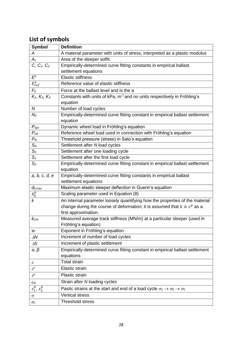
List of symbols Symbol Definition

A A material parameter with units of stress, interpreted as a plastic modulus

As Area of the sleeper soffit.

C, C1, C2 Empirically-determined curve fitting constants in empirical ballast

settlement equations

Ee Elastic stiffness

𝐸𝑟𝑒𝑓𝑒 Reference value of elastic stiffness

Fb Force at the ballast level and is the a

K1, K2, K3 Constants with units of kPa, m-1 and no units respectively in Fröhling’s

equation

N Number of load cycles

N0 Empirically-determined curve fitting constant in empirical ballast settlement

equation

Pdyn Dynamic wheel load in Fröhling’s equation

Pref Reference wheel load used in connection with Fröhling’s equation

Pth Threshold pressure (stress) in Sato’s equation

SN Settlement after N load cycles

S0 Settlement after one loading cycle

S1 Settlement after the first load cycle

S2 Empirically-determined curve fitting constant in empirical ballast settlement

equation

a, b, c, d, e Empirically-determined curve fitting constants in empirical ballast

settlement equations

db,max Maximum elastic sleeper deflection in Guerin’s equation

ℎ0𝑝 Scaling parameter used in Equation (8)

k An internal parameter loosely quantifying how the properties of the material

change during the course of deformation; it is assumed that 𝑘 ≡ 𝜀𝑝 as a

first approximation.

k2mi Measured average track stiffness (MN/m) at a particular sleeper (used in

Fröhling’s equation)

w Exponent in Fröhling’s equation

N Increment of number of load cycles

S Increment of plastic settlement

α, β Empirically-determined curve fitting constant in empirical ballast settlement

equations

Total strain

e Elastic strain

p Plastic strain

N Strain after N loading cycles

𝜀1𝑝, 𝜀2

𝑝 Pastic strains at the start and end of a load cycle 1 2 1

Vertical stress

t Threshold stress

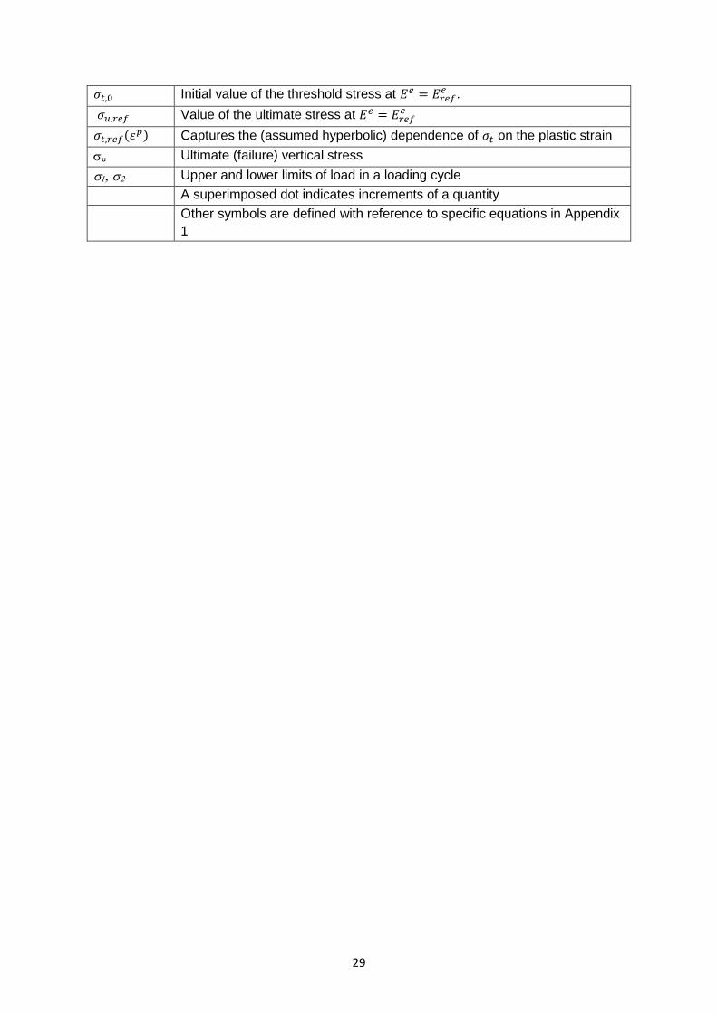
29

𝜎𝑡,0 Initial value of the threshold stress at 𝐸𝑒 = 𝐸𝑟𝑒𝑓𝑒 .

𝜎𝑢,𝑟𝑒𝑓 Value of the ultimate stress at 𝐸𝑒 = 𝐸𝑟𝑒𝑓𝑒

𝜎𝑡,𝑟𝑒𝑓(𝜀𝑝) Captures the (assumed hyperbolic) dependence of 𝜎𝑡 on the plastic strain

u Ultimate (failure) vertical stress

Upper and lower limits of load in a loading cycle

A superimposed dot indicates increments of a quantity

Other symbols are defined with reference to specific equations in Appendix

1

30

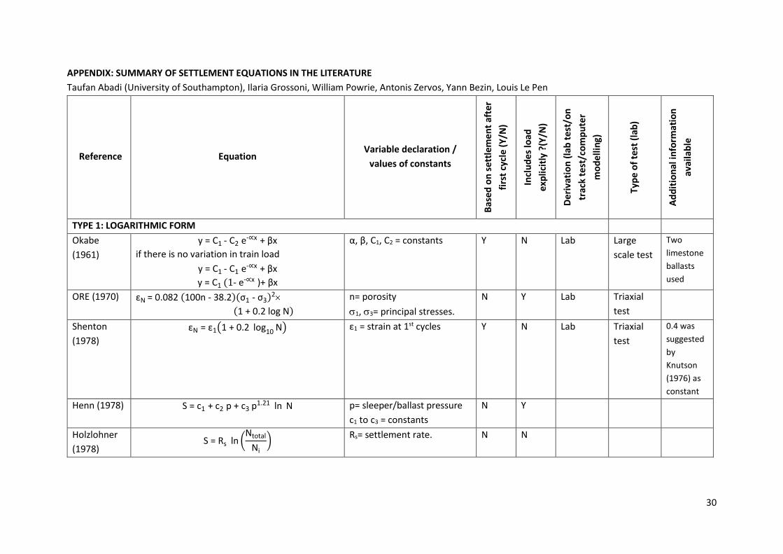
APPENDIX: SUMMARY OF SETTLEMENT EQUATIONS IN THE LITERATURE

Taufan Abadi (University of Southampton), Ilaria Grossoni, William Powrie, Antonis Zervos, Yann Bezin, Louis Le Pen

Reference Equation Variable declaration /

values of constants

Bas

ed

on

se

ttle

me

nt

afte

r

firs

t cy

cle

(Y

/N)

Incl

ud

es

load

exp

licit

ly ?

(Y/N

)

De

riva

tio

n (

lab

te

st/o

n

trac

k te

st/c

om

pu

ter

mo

de

llin

g)

Typ

e o

f te

st (

lab

)

Ad

dit

ion

al in

form

atio

n

avai

lab

le

TYPE 1: LOGARITHMIC FORM

Okabe

(1961)

y = C1 - C2 e-∝x + βx

if there is no variation in train load

y = C1 - C1 e-∝x + βx

y = C1 (1- e-∝x )+ βx

α, β, C1, C2 = constants Y N Lab Large

scale test

Two

limestone

ballasts

used

ORE (1970) εN = 0.082 (100n - 38.2)(σ1 - σ3)2

(1 + 0.2 log N)

n= porosity

1, 3= principal stresses.

N Y Lab Triaxial

test

Shenton

(1978)

εN = ε1(1 + 0.2 log10 N) ε1 = strain at 1st cycles Y N Lab Triaxial

test

0.4 was

suggested

by

Knutson

(1976) as

constant

Henn (1978) S = c1 + c2 p + c3 p1.21 ln N p= sleeper/ballast pressure

c1 to c3 = constants

N Y

Holzlohner

(1978) S = Rs ln (

Ntotal

Ni)

Rs= settlement rate. N N

31

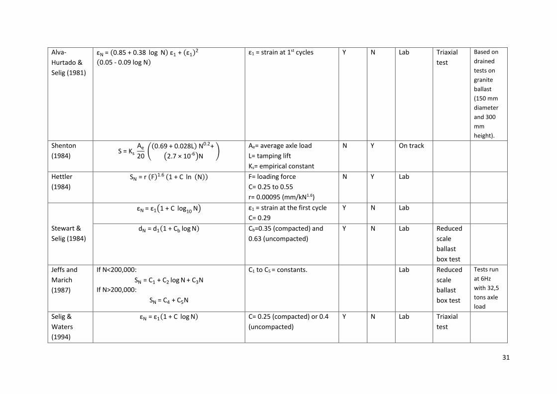
Alva-

Hurtado &

Selig (1981)

εN = (0.85 + 0.38 log N) ε1 + (ε1)2

(0.05 - 0.09 log N)

ε1 = strain at 1st cycles Y N Lab Triaxial

test

Based on

drained

tests on

granite

ballast

(150 mm

diameter

and 300

mm

height).

Shenton

(1984) S = Ks

Ae

20 (

(0.69 + 0.028L) N0.2+

(2.7 × 10-6)N)

Ae= average axle load

L= tamping lift

Ks= empirical constant

N Y On track

Hettler

(1984)

SN = r (F)1.6 (1 + C ln (N)) F= loading force

C= 0.25 to 0.55

r= 0.00095 (mm/kN1.6)

N Y Lab

Stewart &

Selig (1984)

εN = ε1(1 + C log10 N) ε1 = strain at the first cycle

C= 0.29

Y N Lab

dN = d1(1 + Cb log N) Cb=0.35 (compacted) and

0.63 (uncompacted)

Y N Lab Reduced

scale

ballast

box test

Jeffs and

Marich

(1987)

If N<200,000:

SN = C1 + C2 log N + C3N

If N>200,000:

SN = C4 + C5N

C1 to C5 = constants. Lab Reduced

scale

ballast

box test

Tests run

at 6Hz

with 32,5

tons axle

load

Selig &

Waters

(1994)

εN = ε1(1 + C log N) C= 0.25 (compacted) or 0.4

(uncompacted)

Y N Lab Triaxial

test

32

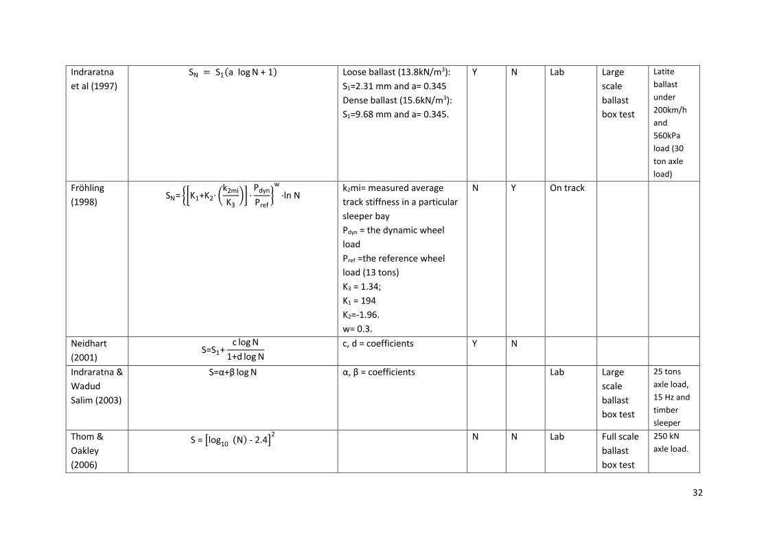
Indraratna

et al (1997)

SN = S1(a log N + 1) Loose ballast (13.8kN/m3):

S1=2.31 mm and a= 0.345

Dense ballast (15.6kN/m3):

S1=9.68 mm and a= 0.345.

Y N Lab Large

scale

ballast

box test

Latite

ballast

under

200km/h

and

560kPa

load (30

ton axle

load)

Fröhling

(1998)

SN= {[K1+K2∙ (k2mi

K3)] ∙

Pdyn

Pref}

w

∙ln N k2mi= measured average

track stiffness in a particular

sleeper bay

Pdyn = the dynamic wheel

load

Pref =the reference wheel

load (13 tons)

K3 = 1.34;

K1 = 194

K2=-1.96.

w= 0.3.

N Y On track

Neidhart

(2001) S=S1+

c log N

1+d log N

c, d = coefficients Y N

Indraratna &

Wadud

Salim (2003)

S=α+β log N α, β = coefficients Lab Large

scale

ballast

box test

25 tons

axle load,

15 Hz and

timber

sleeper

Thom &

Oakley

(2006)

S = [log10 (N) - 2.4]2 N N Lab Full scale

ballast

box test

250 kN

axle load.

33

Thom &

Oakley

(2006)

S = [log10 (N) - 2.4]2

(σ

160) (

47

ks)

= vertical pressure

ks=subgrade stiffness

N Y Lab Full scale

ballast

box test

Shahin

(2009) εB=a (

σd

σs)

m

(1+ ln N)b σd= deviatoric stress applied

σs= compressive strength of

ballast

For basalt ballast:

a=3.38, m=1.13, b=0.523

For granite ballast:

a=2.10, m=1.67, b=0.491

For dolomite ballast:

a=4.72, m=1.12, b=0.312

N Y Lab Large

triaxial

test

Indraratna

et al (2013)

S= a + b log10 N a, b = coefficients N N Lab Large

scale

ballast

box test

20 ton axle

load, 100

km/h and

timber

sleeper

used

Indraratna &

Nimbalkar

(2013)

SN = S1(1+ a ln N+0.5b ln N2) S1 = settlement at the first

cycle

a, b = coefficients

Y N Computer

modelling

TYPE 2: EXPONENTIAL FORM

Selig &

Waters

(1994)

SN = 4.318 N0.17 Lab Large

scale

ballast

box test

Timber

sleeper on

dolomite

ballast

with

347kN axle

load.

34

Selig &

Waters

(1994)

For ballast only:

εN = 0.0035 N0.21

For sub-ballast only:

εN = 0.0036 N0.16

For subgrade only:

SN = 0.03556 N0.37

On track Timber

sleepers

Sato (1997) Ballast settlement rate either:

Si = a (p - b)2 for p > b, or Sj = A pn

SN = Sj N

a , A = coefficients

n = power index

p = sleeper pressure

b = pressure threshold

On track

Indraratna

et al (2007)

SN=S1Ny y = coefficient

S1 = settlement at the first

cycle

Y N Lab Large

scale

ballast

box test

Cuellar et al

(2011)

SN = 0.07 N0.1625 N N Lab Full scale

ballast

box test

Bituminou

s sub-

ballast

used in

various

thicknesse

s

OTHER FORMS

Guérin, N

(1996)

dSN/dN=i∙db,maxj i= 0.00000144

j= 2.51

N Y Lab Triaxial

test

200 km/h

under 17 t

axle load

Varandas et

al. (2013) SN = γ

Mθ

Fnα + 1

(α + 1) ∑ (

1

n)

β N

n = 1

α, β, γ = positive parameters

Fn = load

Mθ = normalizing parameter

Computer

modelling

35

Nimbalkar &

Indraratna

2016

SN = S1(1-e-αN)+β ln N Soft alluvial deposit:

α= 0.5 β=2.04

Hard rock:

α= 0.5 β= 1.7

concrete bridge deck:

α= 0.5 β= 0.63

Y N On track