www.elsevier.com/locate/rse

Remote Sensing of Environm

Modelling local distribution of an Arctic dwarf shrub indicates an

important role for remote sensing of snow cover

Pieter S.A. Beck a,*, Ellen Kalmbach b, Daniel Joly c, Audun Stien a, Lennart Nilsen a

aInstitute of Biology, University of Tromsø, N-9037 Tromsø, NorwaybAnimal Ecology Group, University of Groningen, PO Box 14, 9750AA Haren, The Netherlands

cTheMA, Universite de Franche-Comte, rue Megevand, 25030 Besancon, France

Received 19 October 2004; received in revised form 1 July 2005; accepted 6 July 2005

Abstract

Despite the intensive research effort directed at predicting the effects of climate change on plants in the Arctic, the impact of

environmental change on species’ distributions remains difficult to quantify. Predictive habitat distribution models provide a tool to predict

the geographical distribution of a species based on the ecological gradients that determine it, and to estimate how the distribution of a species

might respond to environmental change. Here, we present a model of the distribution of the dwarf shrub Dryas octopetala L. around the fjord

Kongsfjorden, Svalbard. The model was built from field observations, an Advanced Space-borne Thermal Emission and Reflection

Radiometer (ASTER) image, a GIS database containing environmental data at a spatial resolution of 20 m, and relied on generalized linear

models (GLMs). We used a logistic GLM to predict the occurrence of the species and a Gaussian GLM to predict its abundance at the sites

where it occurred. Temperature and topographical exposure and inclination of a site appeared to promote both the occurrence and the

abundance of D. octopetala. The occurrence of the species was additionally negatively influenced by snow and water cover and

topographical exposure towards the north, whereas the abundance of the species appeared lower on calciferous substrates. Validation of the

model using independent data and the resulting distribution map showed that they successfully recover the distribution of D. octopetala in the

study area (j =0.46, AUC=0.81 for the logistic GLM [n =200], r2=0.29 for the Gaussian GLM [n =36]). The results further highlight that

models predicting the local distribution of plant species in an Arctic environment would greatly benefit from data on the distribution and

duration of snow cover. Furthermore, such data are necessary to make quantitative estimates for the impact of changes in temperature and

winter precipitation on the distribution of plants in the Arctic.

D 2005 Elsevier Inc. All rights reserved.

Keywords: Equilibrium distribution models; Tundra plants; Snow models; Digital elevation model; Realized niche model; Geographical information system

1. Introduction

Most climate models predict a pronounced climate

change in Arctic regions with summer temperatures over

land increasing between 4 and 7.5 -C and winter precip-

itation by 5–80% by the year 2080 (ACIA, 2004; McCarthy

et al., 2001). As the physical environment controls plant

establishment and growth in the Arctic, climate change will

affect plant life in the Arctic tundra (Billings, 1987; Press et

0034-4257/$ - see front matter D 2005 Elsevier Inc. All rights reserved.

doi:10.1016/j.rse.2005.07.002

* Corresponding author. Tel.: +47 77 64 44 06.

E-mail address: pieter.beck@ib.uit.no (P.S.A. Beck).

al., 1998). One observed effect of climate change on

vegetation is that the spatial distribution of species changes,

with populations either expanding, declining, or migrating

(Huntley, 1991; Sturm et al., 2001). Such alterations can

have implications for vegetation structure (Huntley, 1991),

animal life (Thompson et al., 1998), and biosphere

atmosphere interactions (Chapin et al., 2000; Wu & Lynch,

2000). In order to predict how the distribution of Arctic

plant species will respond to climate change, it is necessary

that we are capable of modelling their present distribution

with sufficient accuracy.

Predictive habitat distribution modelling provides a tool

to mimic the distribution of species given a set of environ-

ent 98 (2005) 110 – 121

P.S.A. Beck et al. / Remote Sensing of Environment 98 (2005) 110–121 111

mental conditions (Guisan & Zimmermann, 2000). It uses

data on the spatial distribution of environmental factors that

are assumed important for the species’ ecology (predictor

variables, Franklin, 1995; Lenihan, 1993). By relating the

observed occurrence of a species at sampling sites to the

prevailing environmental conditions at those sites, a model

of the realized niche of the species is produced (Westman,

1991). This model is then used to assess which sites in the

landscape satisfy the niche requirements and thus qualify as

a potential habitat for the species (Brown et al., 1995). The

accuracy of a model can be quantified, by comparing the

predicted habitat distribution with observed patterns of

occurrence and abundance.

The outlined method for creating species distribution

models assumes a state of (pseudo-)equilibrium between the

sampled populations and their environment and is hence

also referred to as equilibrium distribution modelling

(Guisan & Theurillat, 2000a). The alternative to equilibrium

modelling is mechanistic modelling of species distribution

based on physiology and demography. Mechanistic model-

ling relies on extensive knowledge about the processes

underlying a species’ response to environmental variability,

knowledge which is not yet available for most plant species.

Equilibrium models, in contrast, are based on observed

correlations between environmental gradients and a species

performance, requiring little understanding of the processes

causing these correlations.

Environmental gradients which can serve as predictor

variables in habitat distribution models can be classified

into three types, according to the way they affect an

organism’s performance (Austin, 1980). Resource gra-

dients, such as soil moisture content, represent variables

that are consumed by the organism. Direct gradients, such

as temperature and pH, are of a direct physiological

importance to the species without being consumed. Indirect

gradients, such as topography, snow cover or wind speed

have no direct physiological meaning for an organism but

can affect it through their correlation with direct and

resource gradients (Guisan et al., 1999). The mechanism

causing this correlation, and thereby the effect of the

indirect gradient on a species’ performance, is often

complex and poorly understood. Nevertheless, indirect

gradients are widely used as predictor variables in

predictive habitat distribution models, because the main

purpose of these models is predictive accuracy rather than

biological explanation. Furthermore, indirect gradients can

replace a set of resource and direct gradients in a simple

way (Guisan et al., 1999). In that case, using them rather

than the gradients, they can replace as predictor variables

generates more parsimonious models, which are preferred

from a statistical point of view. Most importantly, however,

direct and resource gradients are often difficult to measure,

especially for larger areas (Austin, 2002). Contrastingly,

several indirect ecological gradients can be modeled

spatially and accurately, thanks to the recent developments

in remote sensing and GIS software.

So far, the integration of remotely sensed data in

predictive habitat distribution modelling has been limited.

Digital elevation models have been used to derive variables

related to topography (e.g., Guisan et al., 1999; Jelaska et

al., 2003), while data from individual spectral of satellite

sensors and snow cover indices from aerial photography

have occasionally served as predictor variables in habitat

distribution models (Guisan & Theurillat, 2000b). However,

high-quality remote sensing data at different resolutions is

becoming increasingly available and make it possible to

map different ecological variables at various scales. As the

demand for distribution models for plants in environments

vulnerable to climate change, such as the Arctic, grows, so

does the need to investigate where remote sensing can

contribute most to such models. More specifically, models

should be developed and it should be assessed which

predictor variables need to be mapped more precisely to

improve the models. Accordingly, the use of new remote

sensing techniques available to map important environ-

mental gradients should be investigated and developed

further.

Here, we present the first habitat distribution for a plant

species in an Arctic environment. We modelled the

distribution of Dryas octopetala L., a well-studied Arctic

species. Advanced Space-borne Thermal Emission and

Reflection Radiometer (ASTER) imagery was used for

snow mapping, and a GIS database of environmental

variables and different types of generalized linear models

(GLMs) predict the occurrence and the abundance of the

species. We address the following questions: (1) How well

does the model describe the distribution of D. octopetala in

the study area? (2) Is the realized niche model, which was

developed to optimize predictive accuracy, consistent with

the results of observational and experimental studies on the

ecology of the species? (3) How can remote sensing data be

of most use to improve predictive habitat distribution

models for Arctic plant species?

2. Data and methods

2.1. Dryas octopetala L.

D. octopetala ssp. octopetala is a perennial dwarf shrub

found in large parts of the Arctic tundra and boreal areas, as

well as in Alpine tundra at lower latitudes (Hulten, 1959).

The species is among the most studied in the Arctic and a

large number of observational and experimental studies

provide detailed insights into its ecology (e.g., Cooper &

Wookey, 2003; McGraw, 1985; McGraw & Antonovics,

1983; Welker et al., 1993). Vegetation dominated by D.

octopetala ssp. octopetala typically develops on alkaline or

circumneutral soils, at sites with low soil moisture and little

to no snow cover during winter, in particular at wind-

exposed sites and on ridges (Elkington, 1971; Elvebakk,

1994). In warmer and less exposed areas, D. octopetala is

P.S.A. Beck et al. / Remote Sensing of Environment 98 (2005) 110–121112

outcompeted by Cassiope tetragona (L.) D. Don. (Elve-

bakk, 1994).

Experimental studies on D. octopetala have shown that

different environmental factors control its sexual reproduc-

tion and its clonal vegetative growth (Welker et al., 1997;

Wookey et al., 1995). More specifically, a rise in temperature

greatly favours all aspects of sexual reproduction in D.

octopetala, which currently is hardly ever successful in the

Arctic (Welker et al., 1997; Wookey et al., 1993). While the

effects of increased water availability remain unclear (Welker

et al., 1993), increases in nutrient availability in the short

term lead to higher leaf nitrogen concentration, biomass, and

photosynthetic rate (Baddeley et al., 1994). Overall, temper-

ature, snow cover, and soil characteristics seem to be

determining environmental factors for D. octopetala and

are expected to be significant predictor variables in a

potential habitat distribution model for the species.

2.2. Study area

The study area comprises the landmasses around the

fjord Kongsfjorden (79- N 12- E) in the north-western part

of the Svalbard archipelago (Fig. 1). The study was

conducted on the peninsula Brøggerhalvøya, the hill Ossian

Sars-fjellet and the island Blomstrandhalvøya.

Ny-Alesund (78-56V N, 11-53V E), a small permanent

settlement at Brøggerhalvøya, has a mean temperature of

4.4 -C during the summer months of July and August, and

Fig. 1. Svalbard archipelago, the area around the fjord Kongsfjorden and

the gradsect sampling design. The gradsects were placed to cover a

maximal variation in topography, and vegetation was sampled at 80 m

intervals along them (see text for further details).

�11.7 -C during the winter from October to April (Førland

et al., 1997). The mean monthly precipitation values for

these periods are 33 and 34 mm, respectively (Førland et al.,

1997). On the landmasses surrounding Kongsfjorden,

temperature generally increases from west to east (Joly et

al., 2003). Snow starts accumulating around mid-September

and is redistributed by wind, causing complex spatial

variations in snow depth (Winther et al., 2002). The snow

cover becomes thinner from the end of May and most of the

snow has disappeared by the end of June (Gerland et al.,

1999; Lloyd, 1999). The landscape mainly consists of

Alpine areas, which are partially covered by ice, marine

terraces (especially at Brøggerhalvøya), calcareous ridges

and moraines (Brossard et al., 1984). At Brøggerhalvøya,

vascular plants are mainly restricted to the coastal platforms

that contrast heavily with the steep interior mountains. At

Blomstrandhalvøya and Ossian Sars-fjellet, the vegetation

extends to more mountainous terrain as well.

2.3. Database development

A GIS database of environmental variables, stored in a

raster format at a spatial resolution of 20 m, was created

using the IDRISI software (Clark Labs, 2003). This data-

base contained topography, substrate geology, snow and

water cover, and air temperature variables.

2.3.1. Topography

A Digital Elevation Model (DEM; spatial resolution

20 m, created from aerial photography at scale 1:15000),

provided by the Norwegian Polar Institute, was used to

calculate local elevation, terrain slope, terrain aspect, flow

accumulation potential, and topographical position on

various scales. Using trigonometric functions of the aspect

values on the azimuth scale, two variables with a linear

nature were calculated: ‘‘southness,’’ representing a north–

south gradient and ‘‘eastness,’’ a west–east gradient

(Skidmore, 1989). Areas of flat terrain were assigned a

value zero for both variables. Three variables related to

topographical position were calculated by subtracting from

the elevation of a pixel in the DEM, the average elevation of

the window of surrounding pixels (Guisan et al., 1999).

Each of these variables used a window with a different

diameter, namely, 60, 100 or 300 m. From these continuous

variables, additional binary variables were created to

distinguish between sites that were exposed in the landscape

and sites that were not. To calculate the binary variables,

the continuous variables were classified using a threshold

of 0.1 m, except for the variable calculated using the 300 m

windows where a threshold of 0.5 m was used.

2.3.2. Substrate geology

A geological map in vector format, on a scale 1:100000

(Hjelle et al., 1999), was converted to a raster format using

nearest neighbour resampling. The 23 legend categories

present in the study area were reclassified to four general

P.S.A. Beck et al. / Remote Sensing of Environment 98 (2005) 110–121 113

classes [(1) moraines and alluvial deposits; (2) tertiary

substrates and chert; (3) carboniferous dolomites and

protozoic marbles; (4) protozoic mica schist) to reduce the

number of categories and group the original units according

to their significance for vegetation (Elvebakk, 1982).

2.3.3. Snow and water cover

Two binary variables representing water cover and snow

cover in the study area were calculated. This was done using

a calibrated and atmospherically corrected (Level-2)

ASTER image of surface reflectance of the study area,

taken on 26 June 2001. Geometrical rectification was

performed using georeferenced aerial photographs with a

10-m spatial resolution provided by the Norwegian Polar

Institute and a first-order polynomial fitted to 64 control

points. The image does not cover the extremity of

Brøggerhalvøya, which was therefore excluded from this

study.

To produce a map of snow cover, a normalized difference

snow index (NDSI, Hall et al., 1995) was applied to the

ASTER image. NDSI has previously been calculated as the

difference between reflectance in MODIS bands 4 (0.545–

0.565 Am) and 6 (1.628–1.652 Am), divided by the sum of

bands 4 and 6 (Bitner et al., 2002) or the equivalent bands of

the Landsat Thematic Mapper (Vogel, 2002). In the present

study, NDSI was calculated from surface reflectance values

recorded by bands 1 (0.52–0.60 Am, spatial resolution 15

m) and 4 (1.600–1.700 Am, spatial resolution 30 m) of the

ASTER sensor. Misclassification of clouds as snow was

improbable since the image had an estimated cloud cover of

less than 2% (estimated by the supplier company, Jet

Propulsion Laboratory, California Institute of Technology).

The calculated NDSI image was resampled by bilinear

interpolation to a spatial resolution of 20 m and classified to

produce a binary variable distinguishing between snow-

covered sites (NDSI�0.4) and snow-free sites (NDSI<0.4,

Dozier, 1989).

Because the ASTER image was taken late in spring when

the snow cover was already heavily reduced, an additional

binary variable related to water cover was calculated from it.

Pixels representing water-covered sites (either liquid or as

snow or ice) tend to produce higher reflectance values in

ASTER band 1 than in ASTER band 3 (Wessels et al.,

2002). Hence, an image of the ratio of reflectance in ASTER

band 1 to reflectance in ASTER band 3 (spatial resolution

15 m) was calculated and resampled by bilinear interpola-

tion to the baseline spatial resolution of 20 m. A threshold of

1.2 was then applied on this image to create a binary

variable distinguishing between water-free (<1.2) and

water-covered sites (�1.2).

2.3.4. Air temperature

Daily mean temperatures for June, July, and August were

modelled using the methods described by Joly et al. (2003)

and the DEM of the study area. Temperature data were

obtained from 83 loggers (HOBO H8 Pro Temp/external

logger, with external thermocouple sensor, Onset Compu-

ting, Bourne, MA), which were placed throughout the study

area and recorded for 3 years at 30 min intervals with an

accuracy of 0.1 -C.The variables calculated for this study are based on mean

daily temperature values for June, July, and August during

2001 and 2002 and June 2003. Some loggers showed

mechanical failure during these months, and therefore, the

number of records available to create daily temperature

maps varied with a minimum of 25. For the maps grouped

per month, the root mean square errors using cross-

validation were 0.8 -C for June, 0.5 -C for July and 0.5

-C for August and the mean of the errors or bias 0.03,

�0.005 and �0.01 -C, respectively.Monthly mean temperatures, monthly minimum tempe-

ratures, and monthly maximum temperatures for June, July,

and August were used as variables in the present study. In

addition, mean temperature was calculated for the period

spanning the 3 months. Since the temperature models did

not take into account the effect of snow, the temperature

variables for June were corrected using the ASTER image.

For pixels that were classified as snow covered, mean and

maximum June temperatures were set at 0 -C since

temperatures in the snow pack are known to be 0 -C or

slightly lower from the beginning of snow melt (Gerland et

al., 1999).

2.4. Field sampling

Field sampling was carried out during July and August

2003. To measure the cover of D. octopetala in the field, a

gradsect sampling method (Gillison & Brewer, 1985) was

applied. A gradsect is a transect that is purposely oriented so

it corresponds to the environmental gradient which is

thought to be most influential in the distribution of the

focal species in the study area. Based on what is known

about the ecology of D. octopetala, this gradient was

believed to be related to snow cover. At the time of the field

work, data on depth and duration of snow cover for the

entire study area was unavailable. Therefore, topographical

gradients, which are known to partially determine snow

cover (Benson & Sturm, 1993; Liston & Sturm, 1998), were

used instead to position the gradsects. Using a digitized map

(Norsk Polarinstitutt, 1990), 32 gradsects, varying in length

from 160 to 2720 m, were placed throughout the study area

(Fig. 1). Moraines, on which vegetation is still in a stage of

colonisation (Moreau, 2003), and areas higher than 250 m

a.s.l. were not sampled.

Along each gradsect, plots measuring 2 m�2 m were

positioned at 80 m intervals and corresponding to the

centres of 20 m�20 m pixels in the DEM. The

coordinates of the plots were located in the field using a

handheld GPS receiver. Once in place, a plot was overlaid

with a regular 20 cm�20 cm grid and the presence or

absence of D. octopetala recorded at the 121 intersection

points of the grid. Of the 284 plots, 236 were located at

P.S.A. Beck et al. / Remote Sensing of Environment 98 (2005) 110–121114

Brøggerhalvøya, 31 at Blomstrandhalvøya, and 17 at

Ossian Sars-fjellet and 79% of all plots were located at

an altitude under 100 m a.s.l.

2.5. Model development and validation

The establishment of D. octopetala at a site depends on

successful sexual reproduction, whereas the amount of

vegetative cover at sites where it is found depends on

vegetative growth. Since reproduction and growth in D.

octopetala are known to be steered by different environ-

mental factors, we expected the occurrence of the species

and its abundance to depend also on different factors

(Welker et al., 1997; Wookey et al., 1995). We therefore

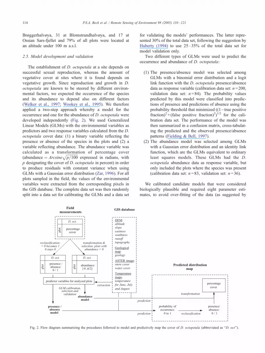
applied a two-step approach whereby a model for the

occurrence and one for the abundance of D. octopetala were

developed independently (Fig. 2). We used Generalized

Linear Models (GLMs) with the environmental variables as

predictors and two response variables calculated from the D.

octopetala cover data: (1) a binary variable reflecting the

presence or absence of the species in the plots and (2) a

variable reflecting abundance. The abundance variable was

calculated as a transformation of percentage cover

(abundance ¼ Arcsineffiffiffiffiffiffiffiffiffiffiffiffiffip=100

pexpressed in radians, with

p designating the cover of D. octopetala in percent) in order

to produce residuals with constant variance when using

GLMs with a Gaussian error distribution (Zar, 1996). For all

plots sampled in the field, the values of the environmental

variables were extracted from the corresponding pixels in

the GIS database. The complete data set was then randomly

split into a data set for calibrating the GLMs and a data set

Fig. 2. Flow diagram summarizing the procedures followed to model and p

for validating the models’ performances. The latter repre-

sented 30% of the total data set, following the suggestion by

Huberty (1994) to use 25–35% of the total data set for

model validation only.

Two different types of GLMs were used to predict the

occurrence and abundance of D. octopetala:

(1) The presence/absence model was selected among

GLMs with a binomial error distribution and a logit

link function with the D. octopetala presence/absence

data as response variable (calibration data set: n =200,

validation data set: n =84). The probability values

predicted by this model were classified into predic-

tions of presence and predictions of absence using the

probability threshold that minimized ((1�true positive

fraction)2+ (false positive fraction)2)1/2 for the cali-

bration data set. The performance of the model was

then summarized in a confusion matrix, cross-tabulat-

ing the predicted and the observed presence/absence

patterns (Fielding & Bell, 1997).

(2) The abundance model was selected among GLMs

with a Gaussian error distribution and an identity link

function, which are the GLMs equivalent to ordinary

least squares models. These GLMs had the D.

octopetala abundance data as response variable, but

only included the plots where the species was present

(calibration data set: n =83, validation set: n =36).

We calibrated candidate models that were considered

biologically plausible and required eight parameter esti-

mates, to avoid over-fitting of the data (as suggested by

redictively map the cover of D. octopetala (abbreviated as ‘‘D. oct’’).

Table 1

Parameter estimates (PE) with their respective standard errors (SE) and the

range of the observations used during model calibration (n =200) for the

predictor variables in the presence/absence model

Variable PE SE Range

Water covered �0.52 0.24 category

Mean June temperature 0.72 0.29 [0 -C; 4.5 -C]Topographically exposed (300 m) 1.0 0.2 category

Southness 0.60 0.30 [�1; 1]

Slope 0.36 0.10 [1-; 27-]

Slope2 �0.012 0.004

P.S.A. Beck et al. / Remote Sensing of Environment 98 (2005) 110–121 115

Harrell et al., 1996). Although a quantitative criterion was

not set, highly correlated predictor variables, such as the

different topographical position variables, were not included

simultaneously in the models. Some of the candidate models

included second-order polynomials and transformations

using the natural logarithm of continuous predictor varia-

bles, since non-linear responses to the environmental

variables were considered likely. Two-way interaction terms

between first-order predictor variables were present in some

models. Automated stepwise model simplification, based on

minimizing the AICC (Hurvich & Tsai, 1989), was used to

eliminate non-contributing predictor variables from the

candidate models (Venables & Ripley, 2002). The AICC is

a modified version of Akaike’s Information Criterion (AIC,

Akaike, 1973) and is preferred over the original AIC when

K, the number of parameters estimated in the model, is large

relative to the sample size n, i.e., n/K <about 40 (Burnham

& Anderson, 2000).

AICC ¼ AICþ 2K K þ 1ð Þn� K � 1

: ð1Þ

Among the resulting models of each type, the GLM with

the lowest AICC was chosen (Johnson & Omland, 2004).

These two models, the presence/absence and the abundance

model, were validated and used to predict the distribution of

D. octopetala.

Three main statistics were used to quantify the predictive

performance of the presence/absence model: adjusted d2

(Guisan et al., 1999), j (Cohen, 1960), and the area (AUC)

under the receiver operating characteristic function (ROC)

(Zweig & Campbell, 1993).

The adjusted d2 is a measure of goodness of fit for

models which are fitted using maximum-likelihood estima-

tion. The d2 quantifies the deviance reduction achieved by a

model, just as the r2 quantifies the variance reduction

achieved by a model based on least-squares estimation. The

adjusted d2 is additionally corrected for the sample size n

and for K, the number of parameters estimated by the

model.

adjusted d2 ¼ 1� n� 1ð Þ= n� Kð Þ½ � 1� d2� �

: ð2Þ

j is a measure of agreement between observed and

predicted values that compensates and corrects for the

proportion of agreement that might occur by chance. It is a

simple and standardised statistic but depends on the thresh-

old chosen to classify the predicted probability values to

presence/absence values (Manel et al., 2001). This is not the

case for the AUC, which provides an estimate for the

probability that the model correctly ranks a pair consisting

of a presence and an absence observation (Deleo, 1993).

Finally, the positive predictive power (PPP) and the negative

predictive power (NPP) were calculated from the confusion

matrix (Fielding & Bell, 1997). The overall predictive

performance of the abundance model was evaluated using

plots of observed abundance values against predicted

abundance values and r2.

All statistical analyses were performed using S-Plus 6.1

software (Insightful, 2002) with the library MASS (Ven-

ables & Ripley, 2002) enabled and the additional functions

developed by Doug Mahoney and Beth Atkinson, for the

ROC procedures.

3. Results

3.1. Presence/absence model

The predictor variables in the presence/absence model

were related to water cover, temperature, topographical

position, aspect, and slope (Table 1). The model predicted a

higher probability of D. octopetala occurrence at sites with

a higher mean temperature in June and exposed towards the

south rather than the north. Since a quadratic term was

retained for the slope variable, the model fitted a unimodal

response curve to this predictor. D. octopetala was

considered most likely to occur at sites with a topographical

slope between 5- and 25- and least likely to occur at sites

with a topographical slope steeper than 30-. The occurrenceof D. octopetala was generally estimated less likely at sites

classified as water-covered and more likely to occur at

exposed sites.

The model performed well for both the calibration and

validation data set (Table 2). The threshold used to classify

the predicted probabilities into presence/absence values was

set at 0.472, resulting in a j value of 0.62 using the

calibration data set (n=200) and 0.46 using the validation

data set (n =84). For both data sets, the predictions of

absence produced by the model were more likely to be

correct than the predictions of presence (NPP>PPP).

3.2. Abundance model

The predictor variables in the abundance model

represented mean August temperature, topographical slope

and position, and geology (Table 3). Abundance of D.

octopetala was predicted to increase with slope and mean

August temperature. The effect of topographical exposure

on D. octopetala abundance is small but clearly positive.

Using the geological class termed moraines and alluvial

deposits as a reference, an effect of substrate geology

Table 2

Statistical measures of model performance for the presence/absence model

Adjusted d2 AUC (SE) Threshold j PPP NPP

Calibration

(n =200)

0.33 0.87 (0.03) 0.472 0.62 0.76 0.82

Validation

(n =84)

0.81 (0.04) 0.46 0.69 0.77

Adjusted d2 is given, as are the area under the ROC curve (AUC) with its

standard error (SE), Cohen’s j, the positive predictive power (PPP) and the

negative predictive power (NPP) for the calibration and the validation data

set. The threshold used to classify the predicted probabilities into presence

and absence values was determined using the calibration data set.

P.S.A. Beck et al. / Remote Sensing of Environment 98 (2005) 110–121116

was only detected for the third class, termed carbon-

iferous dolomites and protozoic marbles, for which a

marginally lower abundance was predicted (PE=�0.035,

SE=0.010).

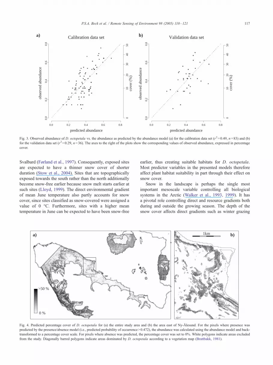
The abundance model explained about half of the

variation in the observed abundance of D. octopetala

(r2=0.49, n =83) and one third of the variation in the

validation data set (r2=0.29, n =36). For the calibration data

set, a trend was observed in the relationship of observed

abundance values to predicted abundance values: The

abundance of D. octopetala was generally overestimated

by the model for plots where it in fact was low (<10%) and

underestimated for plots where it actually was high (>20%)

(Fig. 3a). This trend was not as strong in the corresponding

plot for the validation data set (Fig. 3b).

Table 3

Parameter estimates (PE) with their respective standard errors (SE) and the

range of the observations used during model calibration (n =83) for the

predictor variables in the abundance model

Variable PE SE Range

Log (mean August temperature+1) 1.0 0.3 [5.0 -C; 6.2 -C]

Log (slope+1) 0.073 0.022 [1-; 27-]

Topographically exposed (100 m) 0.061 0.012 category

Substrate geology:

Tertiary sandstones and

permian chert

0.023 0.026 category

Carboniferous dolomites and

protozoic marbles

�0.035 0.010 category

Protozoic mica schist 0.022 0.012 category

The substrate geology variable contained four classes, and therefore, three

parameters were estimated in the model using the class termed ‘‘moraines

and alluvial deposits‘‘ as a reference.

4. Discussion

4.1. Predictive accuracy of the model

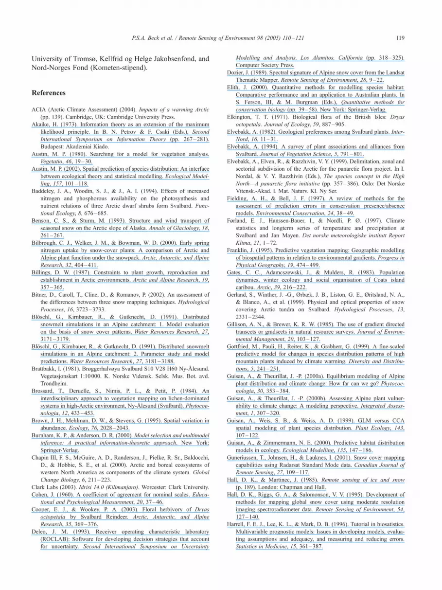
We compared the distribution map of D. octopetala

predicted by the model, with a vegetation map covering

part of the study area (Fig. 4). This showed that the model

gives a good description of the distribution of the species.

Elith (2000) considered presence/absence models with an

AUC of 0.75 or higher as potentially useful in reserve

planning. The AUC of the presented model (0.81) falls

well within this range. In a similar study aimed at

modelling the distribution of 62 vascular plant species in

an Alpine environment, Guisan and Theurillat (2000b)

found e values ranging from 0.16 to 0.84 for the

calibration data set (n =205) and from 0 to 0.62 for the

validation data set (n =92). Compared to these results too,

the presence/absence model in our study, with j values of

0.62 (calibration data set) and 0.47 (validation data set),

performs reasonably well. Guisan and Theurillat (2000b)

obtained better models for species with clear-cut ecological

requirements. In our study area, D. octopetala belongs to

this group of species and the distribution of other species

in the area might thus be more difficult to predict. In the

abundance model, a considerable portion of the observed

variation remained unaccounted for. This might be caused

by essential ecological gradients not being present in the

realized niche model.

4.2. Realized niche model

Nutrient availability, which is known to significantly

affect vegetative growth in D. octopetala, was not explicitly

included as a predictor variable in our study. As an indirect

predictor variable, the geological substrate variable, which

is based on a geological bedrock map, might not be

sufficiently correlated to the nutrient status and other

properties of the thin topsoil. This could explain why the

abundance model predicts a lower cover of D. octopetala on

substrates classified as carboniferous dolomites and proto-

zoic marbles, while D. octopetala normally thrives on

calciferous substrates (Elvebakk, 1982). In this case, the

coarse texture of the substrate and consequent lack of soil,

rather than its chemical composition and resulting nutrient

availability might cause its negative correlation with D.

octopetala abundance.

The modelled positive effects of summer temperature and

exposure towards the south on D. octopetala conform to the

results of observational and experimental studies on the

species (Wada, 1999; Wookey et al., 1995). The same is the

case for the preference of D. octopetala for exposed sites

predicted by both the presence/absence and the abundance

model (McGraw, 1985; Rønning, 1965). Only one of the

predictor variables derived from the ASTER image was

retained in the models. This was the water cover variable,

designed to distinguish between dry sites and those covered

by snow, ice or liquid water, which was selected in the

presence/absence model. The modelled response was

expected given the preference of D. octopetala for sites

with little snow cover during winter (e.g., Elvebakk et al.,

1999; Rønning, 1965).

Various indirect environmental gradients, retained as

predictor variables, such as topographical position and

topographical aspect also account for snow patterns. Strong

winds during winter make snow drift extremely common on

predicted abundance

obse

rved

abu

ndan

ce

0.0 0.2 0.4 0.6 0.8

0.0

0.2

0.4

0.6

0.8

Calibration data seta)

010

2030

4050

cove

r (%

)

predicted abundance

obse

rved

abu

ndan

ce

0.0 0.2 0.4 0.6 0.8

0.0

0.2

0.4

0.6

0.8

Validation data setb)

010

2030

4050

cove

r (%

)

Fig. 3. Observed abundance of D. octopetala vs. the abundance as predicted by the abundance model (a) for the calibration data set (r2=0.49, n =83) and (b)

for the validation data set (r2=0.29, n =36). The axes to the right of the plots show the corresponding values of observed abundance, expressed in percentage

cover.

P.S.A. Beck et al. / Remote Sensing of Environment 98 (2005) 110–121 117

Svalbard (Førland et al., 1997). Consequently, exposed sites

are expected to have a thinner snow cover of shorter

duration (Stow et al., 2004). Sites that are topographically

exposed towards the south rather than the north additionally

become snow-free earlier because snow melt starts earlier at

such sites (Lloyd, 1999). The direct environmental gradient

of mean June temperature also partly accounts for snow

cover, since sites classified as snow-covered were assigned a

value of 0 -C. Furthermore, sites with a higher mean

temperature in June can be expected to have been snow-free

>50 %

0 %

a)

Fig. 4. Predicted percentage cover of D. octopetala for (a) the entire study area

predicted by the presence/absence model (i.e., predicted probability of occurrence>

transformed to a percentage cover scale. For pixels where absence was predicted, t

from the study. Diagonally barred polygons indicate areas dominated by D. octop

earlier, thus creating suitable habitats for D. octopetala.

Most predictor variables in the presented models therefore

affect plant habitat suitability in part through their effect on

snow cover.

Snow in the landscape is perhaps the single most

important mesoscale variable controlling all biological

systems in the Arctic (Walker et al., 1993, 1999). It has

a pivotal role controlling direct and resource gradients both

during and outside the growing season. The depth of the

snow cover affects direct gradients such as winter grazing

b)1km

and (b) the area east of Ny-Alesund. For the pixels where presence was

0.472), the abundance was calculated using the abundance model and back-

he percentage cover was set to 0%. White polygons indicate areas excluded

etala according to a vegetation map (Brattbakk, 1981).

P.S.A. Beck et al. / Remote Sensing of Environment 98 (2005) 110–121118

(Gates et al., 1983), the degree to which plants are

protected from abrasion and desiccation by wind (Savile,

1972), the length of the growing season (Bilbrough et al.,

2000), and winter temperature (Taras et al., 2002). The

spring snow distribution in combination with topography

and drainage additionally plays a major role in the

availability of water as a resource for plants during the

growing season (Liston & Sturm, 1998). This is especially

the case in areas such as Svalbard, where more than 75%

of the annual precipitation falls as snow or sleet between

mid-September and the end of May (Førland et al., 1997).

Most of the ecological gradients affected by snow cover

are crucial to plant growth in the Arctic but very difficult

to map. Hence, in order to create accurate predictive

habitat distribution models for Arctic plants, we need to

expand our knowledge about the temporal and spatial

distribution of snow.

4.3. A need for snow maps

In this study, the only available snow cover data were

the variables derived from the single ASTER image taken

in late June of 2001, resulting in a useful but relatively

crude source of information on patterns of snow distribu-

tion and melt. A sequence of remote sensing images, rather

than a single picture, could provide more information on

these patterns. For modelling on local scales, aerial

photography can provide images for snow mapping at a

ground resolution of 25 m and less (Bloschl et al., 1991a,

1991b; Konig & Sturm, 1998). When working on a

regional scale, as in our study, high- and moderate-

resolution space-borne sensors become a more likely source

of data, because they cover large areas thereby reducing the

costs to the user. To their disadvantage, however, optical

satellite data are heavily affected by clouds and darkness

(Slater et al., 1999). In this study, the frequent presence of

clouds and fog on the west coast of Spitsbergen, the long

polar night, and the rapid snow melt made it impossible to

acquire a time series of snow cover images from optical

satellite sensors.

An alternative to optical remote sensing of snow is to use

Synthetic Aperture Radars (SARs) as they actively use

microwaves which penetrate clouds (Hall & Martinec,

1985). Sensors such as SAR and Advanced SAR (ASAR)

aboard RADARSAT, the Environment Satellite (ENVISAT),

allow for the estimation of snow covered area, and other

parameters such as snow water equivalent and snow wetness

which have been used to predict water supplies for

hydropower stations (e.g., Koskinen et al., 1997) and

forecasting floods (e.g., Low et al., 2002). SAR has

excellent properties for detecting wet snow (Nagler & Rott,

2000; Shi & Dozier, 1997), but detection of dry snow is

more challenging due to low contrast between bare soil and

dry snow (Guneriussen et al., 2001; Rango, 1993). Geo-

metric and radiometric distortion caused by topography may

also cause problems, but can be overcome by precise

geocoding and calibration of the data (Malnes & Guner-

iussen, 2002).

A very promising method for low- and moderate-

resolution snow cover mapping is to combine optical and

microwave imagery by multitemporal and multi-sensor

methods (Tait et al., 2000). Recently, Solberg et al. (2004)

have demonstrated the possibility of deriving daily snow

cover maps in southern Norway with the use of Moderate

Resolution Imaging Spectroradiometer and ASAR data. In

the future, the outlined novel snow mapping techniques

could be applied to map snow melt in the Arctic across a

range of spatial scales, starting grounds resolutions as low as

10 m, which is difficult with techniques solely based on

optical sensors.

4.4. Incorporating climate change scenarios

A quantitative estimate of the impact of climate

change on the distribution of D. octopetala in our study

area could not be made using the presented models.

Previously, equilibrium models for plants have been used

to predict species distribution after climate change by

manipulating temperature variables in the model prior to

predicting habitat suitability (Gottfried et al., 1999;

Guisan & Theurillat, 2000a). In the Arctic, however,

large-scale alterations in temperature, especially in spring,

are likely to affect plant species significantly through

their effect on snow cover. If climate warming scenarios

are to be incorporated in models of Arctic plant

distribution, the impact of temperature variability on the

distribution and duration of snow cover will therefore

need to be quantified. This could be achieved by

integrating physical end-of-winter snow depth models

and physical models of temperature-induced differential

snowmelt (Marks et al., 1999; Tuteja & Cunnane, 1999)

into snow maps. The results would make it possible to

simulate the effect of climate change on factors of prime

importance for plants in the Artic landscape. Furthermore,

they would allow the incorporation of the impact of

winter climate change, both regarding temperature and

precipitation, into predictive habitat distribution models.

This is essential since winter climate change is likely to

be greater than summer climate change in the Arctic

(Kallen et al., 2001).

Acknowledgements

We thank the French Polar Institute (IPEV) and Anna

Thomson for help with the field work and Wolfgang

Cramer, Carl Markon, Arve Elvebakk, Per Fauchald and

Eirik Malnes, and two anonymous referees for comments on

the manuscript. At the Norwegian Polar Institute, we thank

Max Konig and Harald Faste Aas for data support. This

study was funded through grants by the Norwegian Polar

Institute (Arktisstipend), the Amundsen Centre of the

P.S.A. Beck et al. / Remote Sensing of Environment 98 (2005) 110–121 119

University of Tromsø, Kellfrid og Helge Jakobsenfond, and

Nord-Norges Fond (Kometen-stipend).

References

ACIA (Arctic Climate Assessment) (2004). Impacts of a warming Arctic

(pp. 139). Cambridge, UK’ Cambridge University Press.

Akaike, H. (1973). Information theory as an extension of the maximum

likelihood principle. In B. N. Petrov & F. Csaki (Eds.), Second

International Symposium on Information Theory (pp. 267–281).

Budapest’ Akademiai Kiado.

Austin, M. P. (1980). Searching for a model for vegetation analysis.

Vegetatio, 46, 19–30.

Austin, M. P. (2002). Spatial prediction of species distribution: An interface

between ecological theory and statistical modelling. Ecological Model-

ling, 157, 101–118.

Baddeley, J. A., Woodin, S. J., & J., A. I. (1994). Effects of increased

nitrogen and phosphorous availability on the photosynthesis and

nutrient relations of three Arctic dwarf shrubs form Svalbard. Func-

tional Ecology, 8, 676–685.

Benson, C. S., & Sturm, M. (1993). Structure and wind transport of

seasonal snow on the Arctic slope of Alaska. Annals of Glaciology, 18,

261–267.

Bilbrough, C. J., Welker, J. M., & Bowman, W. D. (2000). Early spring

nitrogen uptake by snow-cover plants: A comparison of Arctic and

Alpine plant function under the snowpack. Arctic, Antarctic, and Alpine

Research, 32, 404–411.

Billings, D. W. (1987). Constraints to plant growth, reproduction and

establishment in Arctic environments. Arctic and Alpine Research, 19,

357–365.

Bitner, D., Caroll, T., Cline, D., & Romanov, P. (2002). An assessment of

the differences between three snow mapping techniques. Hydrological

Processes, 16, 3723–3733.

Bloschl, G., Kirnbauer, R., & Gutknecht, D. (1991). Distributed

snowmelt simulations in an Alpine catchment: 1. Model evaluation

on the basis of snow cover patterns. Water Resources Research, 27,

3171–3179.

Bloschl, G., Kirnbauer, R., & Gutknecht, D. (1991). Distributed snowmelt

simulations in an Alpine catchment: 2. Parameter study and model

predictions. Water Resources Research, 27, 3181–3188.

Brattbakk, I. (1981). Brøggerhalvøya Svalbard S10 V28 H60 Ny-Alesund.

Vegetasjonskart 1:10000. K. Norske Vidensk. Selsk. Mus. Bot. avd.

Trondheim.

Brossard, T., Deruelle, S., Nimis, P. L., & Petit, P. (1984). An

interdisciplinary approach to vegetation mapping on lichen-dominated

systems in high-Arctic environment, Ny-Alesund (Svalbard). Phytocoe-

nologia, 12, 433–453.

Brown, J. H., Mehlman, D. W., & Stevens, G. (1995). Spatial variation in

abundance. Ecology, 76, 2028–2043.

Burnham, K. P., & Anderson, D. R. (2000).Model selection and multimodel

inference: A practical information-theoretic approach. New York’

Springer-Verlag.

Chapin III, F. S., McGuire, A. D., Randerson, J., Pielke, R. Sr., Baldocchi,

D., & Hobbie, S. E., et al. (2000). Arctic and boreal ecosystems of

western North America as components of the climate system. Global

Change Biology, 6, 211–223.

Clark Labs (2003). Idrisi 14.0 (Kilimanjaro). Worcester’ Clark University.

Cohen, J. (1960). A coefficient of agreement for nominal scales. Educa-

tional and Psychological Measurement, 20, 37–46.

Cooper, E. J., & Wookey, P. A. (2003). Floral herbivory of Dryas

octopetala by Svalbard Reindeer. Arctic, Antarctic, and Alpine

Research, 35, 369–376.

Deleo, J. M. (1993). Receiver operating characteristic laboratory

(ROCLAB): Software for developing decision strategies that account

for uncertainty. Second International Symposium on Uncertainty

Modelling and Analysis, Los Alamitos, California (pp. 318–325).

Computer Society Press.

Dozier, J. (1989). Spectral signature of Alpine snow cover from the Landsat

Thematic Mapper. Remote Sensing of Environment, 28, 9–22.

Elith, J. (2000). Quantitative methods for modelling species habitat:

Comparative performance and an application to Australian plants. In

S. Ferson, III, & M. Burgman (Eds.), Quantitative methods for

conservation biology (pp. 39–58). New York’ Springer-Verlag.

Elkington, T. T. (1971). Biological flora of the British Isles: Dryas

octopetala. Journal of Ecology, 59, 887–905.

Elvebakk, A. (1982). Geological preferences among Svalbard plants. Inter-

Nord, 16, 11–31.

Elvebakk, A. (1994). A survey of plant associations and alliances from

Svalbard. Journal of Vegetation Science, 5, 791–801.

Elvebakk, A., Elven, R., & Razzhivin, V. Y. (1999). Delimitation, zonal and

sectorial subdivision of the Arctic for the panarctic flora project. In I.

Nordal, & V. Y. Razzhivin (Eds.), The species concept in the High

North—A panarctic flora initiative (pp. 357–386). Oslo’ Det NorskeVitensk.-Akad. I. Mat. Naturv. Kl. Ny Ser.

Fielding, A. H., & Bell, J. F. (1997). A review of methods for the

assessment of prediction errors in conservation presence/absence

models. Environmental Conservation, 24, 38–49.

Førland, E. J., Hanssen-Bauer, I., & Nordli, P. Ø. (1997). Climate

statistics and longterm series of temperature and precipitation at

Svalbard and Jan Mayen. Det norske meteorologiske institutt Report

Klima, 21, 1–72.

Franklin, J. (1995). Predictive vegetation mapping: Geographic modelling

of biospatial patterns in relation to environmental gradients. Progress in

Physical Geography, 19, 474–499.

Gates, C. C., Adamcszewski, J., & Mulders, R. (1983). Population

dynamics, winter ecology and social organisation of Coats island

caribou. Arctic, 39, 216–222.

Gerland, S., Winther, J. -G., Ørbæk, J. B., Liston, G. E., Øritsland, N. A.,

& Blanco, A., et al. (1999). Physical and optical properties of snow

covering Arctic tundra on Svalbard. Hydrological Processes, 13,

2331–2344.

Gillison, A. N., & Brewer, K. R. W. (1985). The use of gradient directed

transects or gradsects in natural resource surveys. Journal of Environ-

mental Management, 20, 103–127.

Gottfried, M., Pauli, H., Reiter, K., & Grabherr, G. (1999). A fine-scaled

predictive model for changes in species distribution patterns of high

mountain plants induced by climate warming. Diversity and Distribu-

tions, 5, 241–251.

Guisan, A., & Theurillat, J. -P. (2000a). Equilibrium modeling of Alpine

plant distribution and climate change: How far can we go? Phytocoe-

nologia, 30, 353–384.

Guisan, A., & Theurillat, J. -P. (2000b). Assessing Alpine plant vulner-

ability to climate change: A modeling perspective. Integrated Assess-

ment, 1, 307–320.

Guisan, A., Weis, S. B., & Weiss, A. D. (1999). GLM versus CCA

spatial modeling of plant species distribution. Plant Ecology, 143,

107–122.

Guisan, A., & Zimmermann, N. E. (2000). Predictive habitat distribution

models in ecology. Ecological Modelling, 135, 147–186.

Guneriussen, T., Johnsen, H., & Lauknes, I. (2001). Snow cover mapping

capabilities using Radarsat Standard Mode data. Canadian Journal of

Remote Sensing, 27, 109–117.

Hall, D. K., & Martinec, J. (1985). Remote sensing of ice and snow

(p. 189). London’ Chapman and Hall.

Hall, D. K., Riggs, G. A., & Salomonson, V. V. (1995). Development of

methods for mapping global snow cover using moderate resolution

imaging spectroradiometer data. Remote Sensing of Environment, 54,

127–140.

Harrell, F. E. J., Lee, K. L., & Mark, D. B. (1996). Tutorial in biosatistics.

Multivariable prognostic models: Issues in developing models, evalua-

ting assumptions and adequacy, and measuring and reducing errors.

Statistics in Medicine, 15, 361–387.

P.S.A. Beck et al. / Remote Sensing of Environment 98 (2005) 110–121120

Hjelle, A., Piepjohn, K., Saalmann, K., Ohta, Y., Thiedig, F., & Salvigsen,

O., et al. (1999). Sheet A7G Kongsfjorden, Temakart 30. Geological

map of Svalbard 1:100000. Tromsø’ Norsk Polarinstitutt.

Huberty, C. J. (1994). Applied discriminant analysis (p. 466). New York’

Wiley.

Hulten, E. (1959). Studies in the genus Dryas. Svensk Botanisk Tidskrift,

53, 507–542.

Huntley, B. (1991). How plants respond to climate change: Migration rates,

individualism and the consequences for plant communities. Annals of

Botany, 67(Supplement 1), 15–22.

Hurvich, C. M., & Tsai, C. -L. (1989). Regression and time series model

selection in small samples. Biometrika, 76, 297–300.

Insightful (2002). S-plus \ 6.1 for Windows, professional edition, Release

1. Seattle’ Insightful Corporation.

Jelaska, S. D., Antonic, O., Nikolic, T., Hrsak, V., Plazibat, M., &

Krizan, J. (2003). Estimating plant species occurrence in MTB/64

quadrants as a function of DEM-based variables—A case study

for Medvednica Nature Park, Croatia. Ecological Modelling, 170,

333–343.

Johnson, J. B., & Omland, K. S. (2004). Model selection in ecology and

evolution. Trends in Ecology and Evolution, 19, 101–108.

Joly, D., Nilsen, L., Fury, R., Elvebakk, A., & Brossard, T. (2003).

Temperature interpolation at a large scale: Test on a small area in

Svalbard. International Journal of Climatology, 23, 1637–1654.

Kallen, E., Kattsov, V., Walsh, J., & Weatherhead, E. (2001). Report from

the Arctic Climate Impact Assessment Modeling and Scenarios Work-

shop (pp. 35). Stockholm, Sweden, Fairbanks’ ACIA Secretariat.

Konig, M., & Sturm, M. (1998). Mapping snow distribution in the Alaskan

Arctic using aerial photography and topographic relationships. Water

Resources Research, 34, 3471–3483.

Koskinen, J. T., Pulliainen, J. T., & Hallikainen, M. T. (1997). The use of

ERS-1 SAR data in snow melt monitoring. IEEE Transactions on

Geoscience and Remote Sensing, 35, 601–610.

Lenihan, J. M. (1993). Ecological response surfaces for North American

Boreal tree species and their use in forest classification. Journal of

Vegetation Science, 20, 667–680.

Liston, G., & Sturm, M. (1998). A snow transport model for complex

terrain. Journal of Glaciology, 44, 498–516.

Lloyd, C. R. (1999). Final Report of the Land Arctic Physical Processes

(LAPP) Project, contract No. ENV4-CT95-0093 (p. 134). Brussels’European Commission, Climate and Environment Programme.

Low, A., Ludwig, R., & Mauser, W. (2002). Land use dependent snow

cover retrieval using multitemporal, multisensoral SAR-images to

drive operation flood forecasting models. EARSeL-LISSIG-Workshop

Observing our Cryosphere from Space, March 11–13, 2002, Bern, vol.

2 (pp. 128–139).

Malnes, E. & Guneriussen, T. (2002). Mapping snow covered area with

Radarsat in Norway. IEEE 24th IGARSS, 24–28 June 2002, Toronto,

Canada.

Manel, S., Williams, H. C., & Ormerod, S. J. (2001). Evaluating presence–

absence models in ecology: The need to account for prevalence. Journal

of Applied Ecology, 38, 921–931.

Marks, D., Domingo, J., Susong, D., Link, T., & Garen, D. (1999). A

spatially distributed energy balance snowmelt model for application in

mountain basins. Hydrological Processes, 13, 1935–1959.

McCarthy, J. J., Canziani, O. F., Leary, N. A., Dokken, D. J., & White, K. S.

(2001). Climate change 2001: Impacts, adaptation, and vulnerability.

Contribution of Working Group II to the Third Assessment Report of the

Intergovernmental Panel on Climate Change Published for the Inter-

governmental Panel on Climate Change (p. 1032). Cambridge’ Cam-

bridge University Press.

McGraw, J. B. (1985). Experimental ecology of Dryas octopetala ecotypes:

III. Environmental factors and plant growth. Arctic and Alpine

Research, 17, 229–239.

McGraw, J. B., & Antonovics, J. (1983). Experimental ecology of Dryas

octopetala ecotypes: II. A demographic model of growth branching and

fecundity. Journal of Ecology, 71, 899–912.

Moreau, M. (2003). La reconquete vegetale des marges liberees des glaces,

depuis la fin du Petit Age Glaciaire, au Spitsberg. Bulletin de

l’Association des Geographes Francais, 80, 377–385.

Nagler, T., & Rott, H. (2000). Retrieval of wet snow by means of

multitemporal SAR data. IEEE Transactions on Geoscience and Remote

Sensing, 38, 754–765.

Norsk Polarinstitutt (1990). Kartblad A7 Kongsfjorden. Topografiske kart

Svalbard 1:100000. Oslo’ Norsk Polarinstitutt.

Press, M. C., Callaghan, T. V., & Lee, J. A. (1998). How will European

Arctic ecosystems respond to projected global environmental change?

Ambio, 27, 306–311.

Rango, A. (1993). II. Snow hydrology processes and remote sensing.

Hydrological Processes, 7, 121–138.

Rønning, O. I. (1965). Studies in Dryadion of Svalbard. Norsk Polar-

institutt Skrifter, 134, 1–52.

Savile, D. B. O. (1972). Arctic adaptations in plants. Canada Department of

Agriculture Research Branch Monograph, 6, 1–181.

Shi, J., & Dozier, J. (1997). Mapping seasonal snow with SIR-C/X-

SAR in mountaineous areas. Remote Sensing of Environment, 59,

294–307.

Skidmore, A. K. (1989). A comparison of techniques for calculating

gradient and aspect from a gridded digital elevation model. Interna-

tional Journal of Geographical Information Systems, 3, 323–334.

Slater, M. T., Sloggett, D. R., Rees, W. G., & Steel, A. (1999). Potential

operational multi-satellite sensor mapping of snow cover in maritime

sub-polar regions. International Journal of Remote Sensing, 20.

Solberg, R. J., Amlien, J., Koren, H., Malnes, E., & Storvold, R. (2004).

Multi-sensor and time-series approaches for monitoring of snow

parameters. IGARSS 04, 20–24 September, 2004, Anchorage, USA.

Stow, D. A., Hope, A., McGuire, D., Verbyla, D., Gamon, J., &

Huemmrich, F., et al. (2004). Remote sensing of vegetation and land-

cover change in Arctic Tundra Ecosystems. Remote Sensing of

Environment, 89, 281–308.

Sturm, M., Racine, C., & Tape, K. (2001). Increasing shrub abundance in

the Arctic. Nature, 411, 546–547.

Tait, A. B., Hall, D. K., Foster, J. L., & Armstrong, R. L. (2000). Utilizing

multiple datasets for snow-cover mapping. Remote Sensing of Environ-

ment, 72, 111–126.

Taras, B., Sturm, M., & Liston, G. E. (2002). Snow-ground interface

temperatures in the Kuparuk River Basin, Arctic Alaska: Measurements

and model. Journal of Hydrometeorology, 377–394.

Thompson, I. D., Flannigan, M. D., Wotton, B. M., & Suffling, R.

(1998). The effects of climate change on landscape diversity: An

example in Ontario forests. Environmental Monitoring and Assessment,

49, 213–233.

Tuteja, N. K., & Cunnane, C. (1999). A quasi physical snowmelt runoff

modelling system for small catchments. Hydrological Processes, 13,

1961–1975.

Venables, W. N., & Ripley, B. D. (2002). Modern applied statistics with S.

Berlin’ Springer.

Vogel, S. W. (2002). Usage of high-resolution Landsat 7 band 8

for single-band snow-cover classification. Annals of Glaciology, 34,

53–57.

Wada, N. (1999). Factors affecting the seed-setting success of Dryas

octopetala in front of Brøggerbreen (Brøgger glacier) in the high Arctic,

Ny-Alesund, Svalbard. Polar Research, 18, 261–268.

Walker, D. A., Halfpenny, J. C., Walker, M. D., & Wessmann, C. (1993).

Long-term studies of snow-vegetation interactions. Bioscience, 43,

287–301.

Walker, M. D., Walker, D. A., Welker, J. M., Arft, A. M., Bardsley, T., &

Brooks, P. D., et al. (1999). Long-term experimental manipulation of

winter snow regime and summer temperature in Arctic and Alpine

tundra. Hydrological Processes, 13, 2315–2330.

Welker, J. M., Molau, U., Parsons, A. N., Robinson, C. H., & Wookey, P. A.

(1997). Responses of Dryas octopetala to ITEX environmental

manipulations: A synthesis with circumpolar comparisons. Global

Change Biology, 3(suppl. 1), 61–73.

P.S.A. Beck et al. / Remote Sensing of Environment 98 (2005) 110–121 121

Welker, J. M., Wookey, P. A., Parsons, A. N., Press, M. C., Callaghan,

T. V., & Lee, J. A. (1993). Leaf carbon isotope discrimination and

vegetative responses of Dryas octopetala to temperature and water

manipulations in a High Arctic polar semi-desert, Svalbard. Oecologia,

95, 463–469.

Wessels, R. L., Kargel, J. S., & Kieffer, H. H. (2002). ASTER measurement

of supraglacial lakes in the Mount Everest region of the Himalaya.

Annals of Glaciology, 34, 399–408.

Westman, W. E. (1991). Measuring realized niche spaces: Climatic response

of chaparral and coastal sage scrub. Ecology, 72, 1678–1684.

Winther, J. -G., Godtliebsen, F., Gerland, S., & Isachsen, P. E. (2002).

Surface albedo in Ny-Alesund, Svalbard: Variability and trends during

1981–97. Global and Planetary Change, 32, 127–139.

Wookey, P. A., Parsons, A. N., Welker, J. M., Potter, J. A., Callaghan, T. V.,

& Lee, J. A., et al. (1993). Comparative responses and reproductive

development to simulated environmental change in sub-Arctic and high

Arctic plants. Oikos, 67, 490–502.

Wookey, P. A., Robinson, C. H., Parsons, A. N., Welker, J. M., Press, M. C.,

& Callaghan, T. V., et al. (1995). Environmental constraints on the

growth, photosynthesis and reproductive development of Dryas

octopetala at a high Arctic polar semi-desert, Svalbard. Oecologia,

102, 478–489.

Wu, W., & Lynch, A. H. (2000). Response of the seasonal carbon cycle in

high latitudes to climate anomalies. Journal of Geographical Research,

105, 897–908.

Zar, J. H. (1996). Biostatistical analysis (p. 662). Upper Saddle River’Prentice-Hall.

Zweig, M. H., & Campbell, G. (1993). Receiver-Operating Characteristic

(ROC) plots: A fundamental evaluation tool in clinical medicine.

Clinical Chemistry, 39, 561–577.