Modelling and Correcting the Time-Dependent ACS PSF

arX

iv:a

stro

-ph/

0512

170v

3 2

Mar

200

6

2005 HST Calibration WorkshopSpace Telescope Science Institute, 2005A. Koekemoer, P. Goudfrooij, and L. Dressel, eds.

Modeling and Correcting the Time-Dependent ACS PSF

Jason Rhodes

Jet Propulsion Laboratory, 4800 Oak Grove Drive, Pasadena, CA 91109

Richard Massey, Justin Albert, James E. Taylor

California Institute of Technology, 1200 East California Blvd, Pasadena, CA 91125

Anton M. Koekemoer

Space Telescope Science Institute, 3700 San Martin Drive, Baltimore, MD, 21218

Alexie Leauthaud

Laboratoire d’Astrophysique de Marseille, BP 8, Traverse du Siphon, 13376Marseille Cedex 12, France

Abstract. The ability to accurately measure the shapes of faint objects in imagestaken with the Advanced Camera for Surveys (ACS) on the Hubble Space Telescope(HST) depends upon detailed knowledge of the Point Spread Function (PSF). Weshow that thermal fluctuations cause the PSF of the ACS Wide Field Camera (WFC)to vary over time. We describe a modified version of the TinyTim PSF modelingsoftware to create artificial grids of stars across the ACS field of view at a range oftelescope focus values. These models closely resemble the stars in real ACS images.Using ∼ 10 bright stars in a real image, we have been able to measure HST’s apparentfocus at the time of the exposure. TinyTim can then be used to model the PSF at anyposition on the ACS field of view. This obviates the need for images of dense stellarfields at different focus values, or interpolation between the few observed stars. Weshow that residual differences between our TinyTim models and real data are likelydue to the effects of Charge Transfer Efficiency (CTE) degradation. Furthermore, wediscuss stochastic noise that is added to the shape of point sources when distortion isremoved, and we present MultiDrizzle parameters that are optimal for weak lensingscience. Specifically, we find that reducing the MultiDrizzle output pixel scale andchoosing a Gaussian kernel significantly stabilizes the resulting PSF after imagecombination, while still eliminating cosmic rays/bad pixels, and correcting the largegeometric distortion in the ACS. We discuss future plans, which include more detailedstudy of the effects of CTE degradation on object shapes and releasing our TinyTimmodels to the astronomical community.

1. Introduction and motivation

Accurate shape measurements of faint, small galaxies are crucial for certain applications,most notably the measurement of weak gravitational lensing. Quantifying the slight dis-tortion of background galaxies by foreground matter relies on detecting small but coherentchanges in the shapes of many galaxies (see Refregier 2003 for a recent review). To ex-tract the lensing signal, it is crucial to remove instrumental effects from galaxies’ measuredshapes. On the Hubble Space Telescope (HST), these include:

1

http://arXiv.org/abs/astro-ph/0512170v3

2 Rhodes, Massey, Albert, Taylor, Koekemoer & Leauthaud

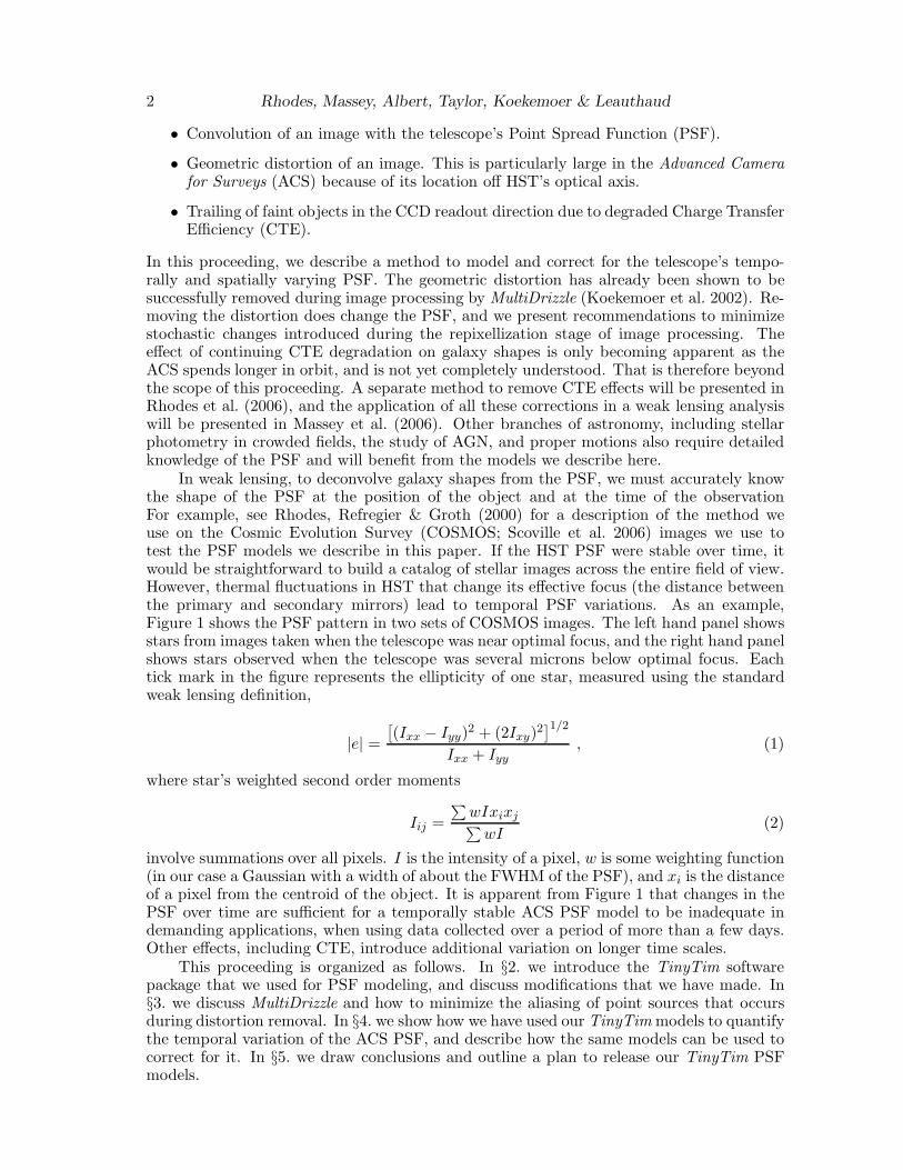
• Convolution of an image with the telescope’s Point Spread Function (PSF).

• Geometric distortion of an image. This is particularly large in the Advanced Camerafor Surveys (ACS) because of its location off HST’s optical axis.

• Trailing of faint objects in the CCD readout direction due to degraded Charge TransferEfficiency (CTE).

In this proceeding, we describe a method to model and correct for the telescope’s tempo-rally and spatially varying PSF. The geometric distortion has already been shown to besuccessfully removed during image processing by MultiDrizzle (Koekemoer et al. 2002). Re-moving the distortion does change the PSF, and we present recommendations to minimizestochastic changes introduced during the repixellization stage of image processing. Theeffect of continuing CTE degradation on galaxy shapes is only becoming apparent as theACS spends longer in orbit, and is not yet completely understood. That is therefore beyondthe scope of this proceeding. A separate method to remove CTE effects will be presented inRhodes et al. (2006), and the application of all these corrections in a weak lensing analysiswill be presented in Massey et al. (2006). Other branches of astronomy, including stellarphotometry in crowded fields, the study of AGN, and proper motions also require detailedknowledge of the PSF and will benefit from the models we describe here.

In weak lensing, to deconvolve galaxy shapes from the PSF, we must accurately knowthe shape of the PSF at the position of the object and at the time of the observationFor example, see Rhodes, Refregier & Groth (2000) for a description of the method weuse on the Cosmic Evolution Survey (COSMOS; Scoville et al. 2006) images we use totest the PSF models we describe in this paper. If the HST PSF were stable over time, itwould be straightforward to build a catalog of stellar images across the entire field of view.However, thermal fluctuations in HST that change its effective focus (the distance betweenthe primary and secondary mirrors) lead to temporal PSF variations. As an example,Figure 1 shows the PSF pattern in two sets of COSMOS images. The left hand panel showsstars from images taken when the telescope was near optimal focus, and the right hand panelshows stars observed when the telescope was several microns below optimal focus. Eachtick mark in the figure represents the ellipticity of one star, measured using the standardweak lensing definition,

|e| =

[

(Ixx − Iyy)2 + (2Ixy)

2]1/2

Ixx + Iyy, (1)

where star’s weighted second order moments

Iij =

∑

wIxixj∑

wI(2)

involve summations over all pixels. I is the intensity of a pixel, w is some weighting function(in our case a Gaussian with a width of about the FWHM of the PSF), and xi is the distanceof a pixel from the centroid of the object. It is apparent from Figure 1 that changes in thePSF over time are sufficient for a temporally stable ACS PSF model to be inadequate indemanding applications, when using data collected over a period of more than a few days.Other effects, including CTE, introduce additional variation on longer time scales.

This proceeding is organized as follows. In §2. we introduce the TinyTim softwarepackage that we used for PSF modeling, and discuss modifications that we have made. In§3. we discuss MultiDrizzle and how to minimize the aliasing of point sources that occursduring distortion removal. In §4. we show how we have used our TinyTim models to quantifythe temporal variation of the ACS PSF, and describe how the same models can be used tocorrect for it. In §5. we draw conclusions and outline a plan to release our TinyTim PSFmodels.

Modeling and Correcting the Time-Dependent ACS PSF 3

Figure 1.: The ellipticity of stars in the COSMOS survey observed with the ACS WFC whileHST happened to be at nominal (left panel) and low (right panel) focus. The orientation andsize of each tick mark represents the ellipticity of one star; both panels contain stars fromseveral different fields. The difference in the PSF patterns is apparent, and demonstratesthe need for a time dependent PSF model.

2. TinyTim PSF models

We have adapted version 6.3 of the TinyTim software package (Krist & Hook 2004) to createsimulated images of stars. TinyTim creates FITS images containing one or more stars thatinclude the effects of diffraction, geometric distortion, and charge diffusion within the CCDs.By default the images appear as they would in raw ACS data; they are highly distortedand have a pixel scale of 0.05 arcseconds per pixel. We have written an IDL wrapper toundo the distortion, resample the images, and combine adjacent PSFs to mimic the effectsof dithering. The wrapper can also run TinyTim multiple times and create a grid of PSFmodels across the whole ACS field of view. We insert our artificial stars into blank imageswith the same dimensions and FITS structure as real ACS data, thereby manufacturingarbitrarily dense starfields.

This basic pipeline calculates a diffraction pattern (spot diagram), distorts it, and addscharge diffusion; all three effects usually depend upon the position of the star in the ACSfield of view. We have made two versions of artificial starfields with important changes tothis basic pipeline. The deviations from this default are:

• In order to examine the effects of the distortion removal process, we have created aversion of our TinyTim starfields where each star has an identical diffraction patternand charge diffusion, but a geometric distortion determined by the location of the PSFwithin the ACS field of view. Once the geometric distortion is removed (for exampleby running the field through MultiDrizzle), these stars should all appear identical.

• In order to correct data, we have created a second version of our TinyTim starfieldsthat do not contain the effects of geometric distortion at all, instead modeling starsas they would appear after a perfect removal of geometric distortion. Conversionbetween distorted and non-distorted frames, which is necessary to simulate chargediffusion in the raw CCD, was performed using very highly oversampled images. Thisavoids stochastic aliasing of the PSF (see §3.), and minimizes noise in the PSF models.

We describe the application of these simulations in the following two sections.


3. Optimization of MultiDrizzle parameters for Weak Lensing Science

MultiDrizzle is used to combine dithered exposures, remove cosmic rays and bad pixels,and eliminate the large geometric distortion in ACS WFC images (Koekemoer et al. 2002).However, the transformation of pixels from the distorted input image to the undistortedoutput plane can introduce significant “aliasing” of pixels if the output pixel scale is com-parable to the input scale. When transforming a single input image to the output plane,point sources can be enlarged, and their ellipticities changed by several percent, dependingupon their sub-pixel position. This is one of the fundamental reasons why dithering is rec-ommended for observations, since the source is at a different sub-pixel position in differentexposures, hence the effects are mitigated to some extent when all the exposures are com-bined. However, the remaining effect in combined images is still quite sufficient to preventthe measurement of small, faint galaxies at the precision required for weak lensing analysis.

Of course, such pixellization effects are unavoidable during the initial exposure, whenthe detector discretely samples an image. However, it is clearly desirable to minimizerelated effects during data reduction. The effect on each individual object depends on howthe input and output pixel grids line up. Indeed, this can be mitigated by using a finergrid of output pixels (e.g. Lombardi et al. 2005). The reduction in pixel scale (which willcause a corresponding increase in computer overheads) can be performed in conjunctionwith simultaneously “shrinking” the area of the input pixels that contains the signal, bymaking use of the MultiDrizzle pixfrac parameter and convolution kernel.

We have run a series of tests on the simulated PSF grids described in §2. to determinethe optimal values of the MultiDrizzle parameters specifically for weak lensing science. Tothis end, we first produced a grid of stars that ought to look identical after the removalof geometric distortion. Figure 2 shows the “aliasing” produced when the distortion isremoved from a single image. We have also created a series of four dithered input images(with the linear dither pattern used for the COSMOS survey); the scatter in the ellipticitiesof the output stars is then approximately half as big. This confirms the idea that therepixellization adds stochastic noise to the ellipticity when the four sub-pixel positionsare uncorrelated. For weak lensing purposes, this noise is still substantial. With enoughdithered input images, the scatter of ellipticities could be reduced further, but this is notfeasible for most observations.

We then ran a series of tests using MultiDrizzle on the same input image but with arange of output pixel scales, convolution kernels, and values of pixfrac. We then measuredthe scatter in the ellipticity values in the output images. The smaller that scatter, the moreaccurately the PSF is represented. We found the results were not strongly dependent onthe choice ofpixfrac and settled on a value of 0.8 for that parameter. We show in Figure 3that PSF stability is improved dramatically by reducing the output pixel scale from 0.05arcseconds (the default) to 0.03 arcseconds. There is only a very slight gain in going tosmaller output pixel sizes and the storage requirements rapidly become problematic. Thegain in going to smaller pixel scales is more stable with a Gaussian kernel for than withthe default square kernel. Therefore, for weak lensing work, we recommend an output pixelscale of 0.03 arcseconds, pixfrac=0.8, and a Gaussian kernel in order to best preserve thePSF during this stage of image reduction. We note that, despite its clear advantages forweak lensing studies, the Gaussian kernel does have some general drawbacks, such as theintroduction of more correlated noise which may not be desirable for other types of sciencewhere minimization of correlated noise is important.

4. Quantification of the PSF and focus variability

We can measure HST’s effective focus at the time of an observation using ∼ 10 fairlybright stars in the field. We first created dense grids of artificial stars across the ACS field


Figure 2.: “Aliasing” of the PSF introduced when transforming a single distorted inputimage to the undistorted output frame. The tick marks represent the ellipticity of starsthat have undergone identical diffraction in the telescope’s optics and should therefore lookidentical. The only difference between stars is their sub-pixel position when their geometricdistortion is removed and the images are combined. The apparent difference between thetick marks shows that the PSF is changed. The problem can be ameliorated by alteringseveral of the MultiDrizzle settings, in particular reducing the output pixel scale.

of view. By changing the separation of the primary and secondary mirrors in TinyTim’sraytracing model, these models were made at successive displacements of the focus fromnominal, from −10µm to +5µm in 1µm increments. These are reasonable bounds on themaximum extent of physical variations in HST. The stars are created without geometricdistortion, to avoid the noise that would have been introduced had it been necessary tocarry out geometric transformations on the stellar fields. We then compare the ∼ 10 brightstars in each COSMOS field to the TinyTim PSF grids at each focus value. Minimizing thedifference in ellipticity between the models and the data finds the best fit value of telescopefocus for that particular field. Tests on observations of dense stellar fields that containmany suitable stars show that this procedure is repeatable with an rms error ∼ 1µm, whenusing ten different stars repeatedly selected at random.

Figure 4 shows our estimation of HST’s focus in microns away from nominal duringseveral months in Cycles 12 and 13, using a uniform set of COSMOS images. HST was notmanually refocussed during this time, but the apparent focus still oscillates. At times, theoscillations seem periodic, but there are also sharp jumps and more erratic behavior. Therandom component probably depends in a complex fashion upon the orientation of HSTwith respect to the sun and the Earth during preceding exposures, and we do not believethat it can be easily predicted in advance.

Note that the uncertainty on the focus value during any single pointing is quite large;more so than the tests on dense stellar fields would suggest. A major component of thiserror is undoubtedly the ∼ 3µm thermal fluctuations in focus that HST experiences duringeach orbit due to “breathing”. The COSMOS images are all taken with a total exposuretime of one orbit, and the apparent focus therefore represents the integral of a graduallychanging PSF. We have not been able to investigate focus changes on short time periodsand, given this behavior, it is even more curious that long term patterns are so clearlypresent in Figure 4.


Figure 3.: RMS ellipticity introduced during the process of removing geometric distortionand combining dithered images, for a range of MultiDrizzle parameters. Lower values showmore stable behavior of the PSF during this process. Based on this plot, we recommenda Gaussian kernel and an output pixel size of 0.03 arcseconds in order to minimize theeffect of undersampling on the PSF and produce images that are optimal for weak lensingscience. We note that the Gaussian kernel introduces significant additional correlated noiserelative to the square kernel, which is not important for weak lensing science but may notbe optimal for other types of science.


Figure 4.: Apparent offset of HST from nominal focus during COSMOS observations incycles 12 and 13. We describe the procedure by which we estimate the telescope’s focus in§4.

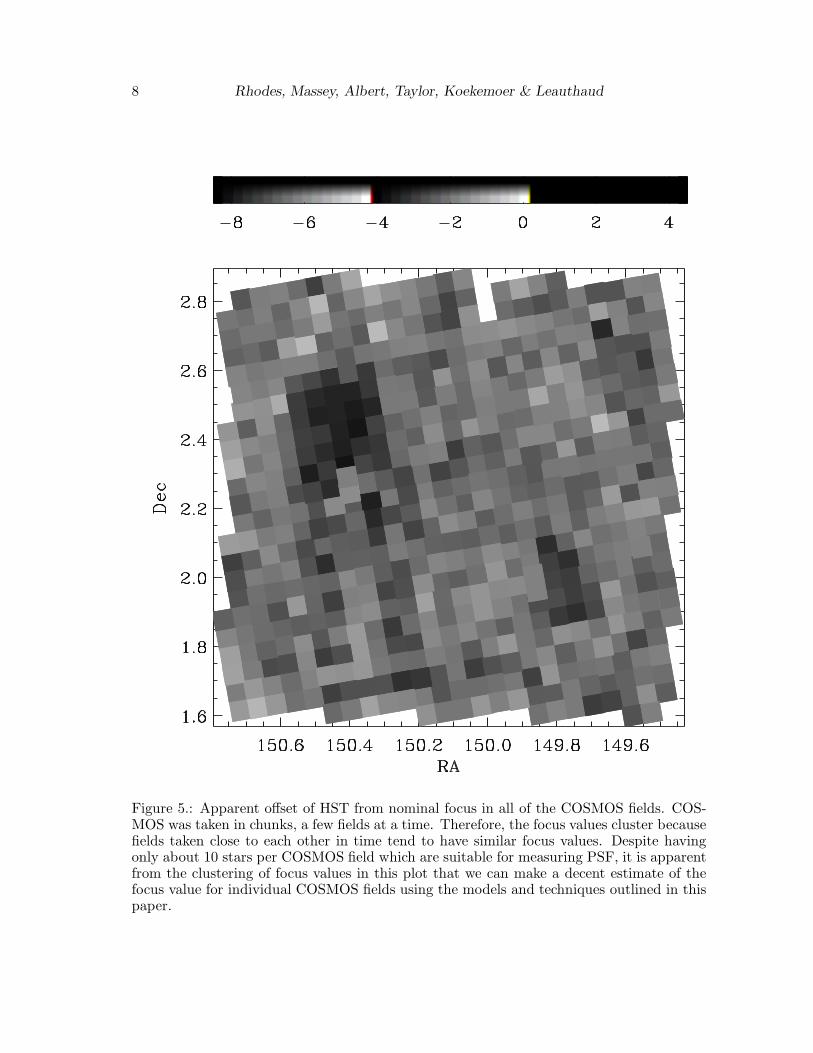
Figure 5 shows the focus values determined for all of the COSMOS fields. The obviousclustering of focus values in that plot is due to the observing strategy used for COSMOS,in which data was typically taken in chunks of a few fields at a time. Adjacent fields arelikely to have been taken at similar times, and therefore tend to have a similar focus values.

Figure 6 shows the TinyTim models at focus −3µm and all the stars from the COSMOSfields with a best-fit focus value of −3µm. The COSMOS stars have been averaged in aspatial grid of approximately 600 × 600 0.03 arcsecond pixels. There is good agreementbetween the models and the stars over most of the field. The agreement is not as goodin the boxed area near the center of the field. We believe this is due to a degradation ofthe CTE of the ACS CCDs. This degradation causes trailing of low flux objects in thereadout direction (the y direction). The effect is most pronounced the further away theobject is from the readout registers at the bottom and top of the field (Mutchler & Sirianni2005; Riess & Mack 2004). This causes the objects to be elongated vertically. Thus, fainterCOSMOS stars appear more elongated in the y direction at the center of the field than theTinyTim models, which do not include the effects of CTE. Note that this does not affectthe estimation of focus positions, because the bright stars matched to our PSF models areless affected by CTE than the faint sources. We are currently exploring ways to correct forCTE in all objects, and will publish the results in Rhodes et al. (2006).

5. Conclusions and Future Work

We have shown that TinyTim can produce model PSFs that are very close to those observedin real data (for example the COSMOS 2-Square Degree Survey). This required somemodifications to the TinyTim code, most importantly adding the ability to mimic thedistortion correction and dithering normally implemented via MultiDrizzle, and to producegrids of PSFs across the entire ACS WFC field of view. We used TinyTim model starsto find the best values for MultiDrizzle and found that using a Gaussian kernel, pixfrac= 0.8, and an output pixel scale of 0.03 arcseconds greatly reduced the “aliasing” of pointsources introduced during repixellization.


Figure 5.: Apparent offset of HST from nominal focus in all of the COSMOS fields. COS-MOS was taken in chunks, a few fields at a time. Therefore, the focus values cluster becausefields taken close to each other in time tend to have similar focus values. Despite havingonly about 10 stars per COSMOS field which are suitable for measuring PSF, it is apparentfrom the clustering of focus values in this plot that we can make a decent estimate of thefocus value for individual COSMOS fields using the models and techniques outlined in thispaper.


Figure 6.: The TinyTim PSF models (left panel) for a focus value of −3µm and observedstars (right panel) in COSMOS fields with a similar apparent focus. There is good agreementbetween the data and the models over much of the ACS field. The shaded area near thecenter of the chip does not show good agreement and this is likely due to the effects ofdegradation of the Charge Transfer Efficiency (CTE) in the ACS WFC CCDs.

Discrepancies between our models and the COSMOS data can be attributed largelyto a degradation in the ACS CTE since launch. We are currently studying this problemand will present a complete PSF solution including how to correct for CTE in Rhodes et al.(2006). We plan to correct science images for CTE on a pixel-by-pixel basis, like the Bristowcode developed for STIS (Bristow et al./ 2002), moving charge back to where it belongs,rather than including the effects of CTE in our model PSF (like Rhodes et al. 2004). Thus,the model PSFs we present here are the ones we plan to use in our weak lensing analysis.

At the time of press, we have thoroughly tested PSF models in only the F814W filter.However, our IDL routines preserve TinyTim’s ability to create PSFs in other filters, andfor sources of any colors. Our routines are therefore easily adaptable to other data sets.

The whole method is intentionally designed to be as adaptable as possible for manymethods. The desire to know the PSF at any arbitrary position on the sky is far fromunique to weak lensing. But even in lensing, advanced methods like Shapelets will, inthe near future, be able to take advantage of more detailed information about the PSFshape than it is reasonable to expect from interpolation between a few stars (Massey &Refregier 2005; Refregier & Bacon 2004). This is even more exaggerated when consideringhigher order shape parameters, with an intrinsically lower signal to noise. The creation ofnoise-free, oversampled stars at any position on an image allows such analysis in any ACSdata.

In the near future, we plan to release our PSF models to the community along withthe wrapper we have written forTinyTim which will allow users to create PSF models indifferent filters and at user-defined positions in the ACS field of view. Interested readersare advised to contact the authors for these resources.

Acknowledgments. We would like to thank Catherine Heymans for sharing her knowl-edge of the ACS PSF. We are grateful to John Krist for guiding our poor lost souls throughthe underbelly of TinyTim. Great thanks go to Andy Fruchter and Marco Lombardi foruseful discussions about MultiDrizzle. Adam Riess and Marco Sirianni provided expertknowledge about CTE effects. Richard Ellis and Alexandre Refregier have engaged us inmany useful and interesting discussions about the COSMOS field. We are also pleased toacknowledge the continuing support of Nick Scoville, Patrick Shopbell and the whole COS-


MOS team in obtaining and analyzing the COSMOS images that were used to test our PSFmodels.

References

Bristow et al. 2002, Modelling Charge Transfer on the STIS CCD, in The 2002 HSTCalibration Workshop : Hubble after the Installation of the ACS and the NICMOSCooling System, Eds Arribas, Koekemoer, & Whitmore, STScI

Koekemoer, A. M., Fruchter, A., Hook, R. & Hack, W., 2002, ‘MultiDrizzle: An IntegratedPyraf Script for Registering, Cleaning and Combining Images,’ in The 2002 HSTCalibration Workshop : Hubble after the Installation of the ACS and the NICMOSCooling System, Eds Arribas, Koekemoer, & Whitmore, STScI, p. 337

Krist, J. & Hook, R., 2004, ‘The TinyTim User’s Guide’, STScI, 339

Lombardi, M. et al., 2005, ApJ, 623, 42

Massey R. & Refregier, A. 2005, MNRAS 363, 197

Massey R. et al. 2006, in preparation

Mutchler, M. & Sirianni, M., 2005, Instrument Science Report ACS 2005-003,(Baltimore: STScI), available through http://www.stsci.edu/hst/acs

Refregier, A., 2003, ARA&A, 41, 645

Refregier, A. & Bacon, D., 2002, MNRAS, 338, 48

Rhodes, J. et al. 2006, in preparation

Rhodes et al. 2004, ApJ, 605, 29

Rhodes, J., Refregier, A. & Groth, E., 2000, ApJ, 536, 79

Riess, A. & Mack, J., 2004, ISR ACS 2004-006,STScI

Scoville, N. et al. 2006, in preparation

http://www.stsci.edu/hst/acs

Documents

Modelling and Correcting the Time-Dependent ACS PSF