Embed Size (px)
Citation preview
626
NN
T:2
020I
PPA
T041 Modelisation stochastique et physique
de la propagation 5G indoor enbandes millimetriques
These de doctorat de l’Institut Polytechnique de Parispreparee a Telecom Paris
Ecole doctorale n626 Ecole doctorale de l’Institut Polytechnique de Paris (EDIPP)Specialite de doctorat : Informatique
These presentee et soutenue a Palaiseau, le 09 Decembre 2020, par
GEORGES NASSIF
Composition du Jury :
Joe WIARTProfesseur, Telecom Paris President
Xavier LAGRANGEProfesseur, IMT Atlantique Rapporteur
Anthony BUSSONProfesseur, IUT Lyon 1 Rapporteur
Jean-Pierre ROSSIIngenieur de recherche, Orange Labs Examinateur
Lina MROUEHProfesseur, ISEP Examinatrice
Philippe MARTINSProfesseur, Telecom Paris Directeur de these
Catherine GLOAGUENIngenieur de recherche, Orange Labs Co-directrice de these

2

To my lovely family and my beloved fiancée.
3

4

Declaration
I hereby declare that this Ph.D. dissertation has been composed solely by myself, ex-cept where specific reference is made to the work of others. The contents of this manuscriptare original and have not been submitted in whole or in part for consideration for anyother degree or qualification in this, or any other university.
Georges Nassif15 September 2020
5

6

Acknowledgments
“No one who achieves success does so without acknowledging the help of others. Thewise and confident acknowledge this help with gratitude.” - Alfred North Whitehead.
Dr. Catherine Gloaguen and Prof. Philippe Martins, I consider myself the luckiestto have had you as my Ph.D. supervisors. Your mentorship, guidance, and support haveimpacted both my personal and professional life in the most positive ways, and for that,I will be forever thankful.
To my colleagues at Orange Labs and Télécom Paris, thank you for providing such anamazing working environment where you can grow and reach your potential, an environ-ment where you can learn from the best and exchange constructive thoughts. I would liketo also thank everyone who contributed in shedding light on my work and accomplish-ments, be it internally or externally.
Last but not least, my family and my fiancée who supported me in every step through-out my Ph.D. thesis, always encouraging me in my worst and best days. I am extremelythankful for every piece of advice and motivation that helped me reach my goals.
7

8
Abstract
5G millimeter wave (mmWave) is a promising solution to the spectrum scarcity prob-lem since very large bandwidths are available. However, due to their propagation proper-ties, namely their very short wavelength, this frequency band can severely impact trans-mission, leading to a new major challenge: indoor coverage. This requires new studies toanswer three major questions: What is the impact of the various environment geometries(apartment, factory, etc.) on indoor mmWave propagation? What is the impact of thevarious environment materials (concrete, plasterboard, etc.) on indoor mmWave propa-gation? and what planning methods should we use for the various indoor 5G applications(fixed wireless access, industry 4.0, etc.).
In this work, we address this challenge through a novel theoretical framework thatcombines stochastic indoor environment modeling with advanced physical propagationsimulation. This approach is particularly adapted to investigate indoor-to-indoor 5GmmWave propagation. Its system implementation, so-called iGeoStat, generates parame-terized typical environments that account for the indoor spatial variations, then simulatesradio propagation based on the physical interaction between electromagnetic waves andmaterial properties. This framework is not dedicated to a particular environment, ma-terial, frequency or use case and aims to statistically understand the influence of indoorenvironment parameters on mmWave propagation properties, especially coverage, SINR,and path loss.
iGeoStat’s system implementation raises numerous computational challenges that wesolve by formulating an adapted link budget and designing new memory optimizationalgorithms. The first simulation results for two major 5G applications (fixed wirelessaccess and industry 4.0) are validated with measurement data and show the efficiencyof iGeoStat to simulate multiple diffusion in realistic environments, within a reasonableamount of time and memory resources. Generated output maps confirm that diffusionhas a critical impact on indoor mmWave propagation and that proper physical modelingis of the utmost importance to generate relevant propagation models.
Using iGeoStat, the main propagation parameters are investigated in various scenarios,showing that the complex refractive index of the indoor material has a moderate impacton the received power, while its surface roughness parameter has a major impact and maycompletely change the power profile in the environment. Various acceleration techniquesare also presented in this work where we show through the simulation results that theperformance of iGeoStat can be further enhanced and that we can achieve at least 50%reduction in time simulation and memory usage without impacting the physical aspect ofpropagation.
9

10
Résumé
La 5G introduit des nouvelles bandes de fréquences, les ondes millimétriques, qui estune solution prometteuse au problème de l’épuisement du spectre grâce à la disponibilitéde larges bandes passantes. Cependant, en raison de leurs propriétés de propagation,notamment leur très courte longueur d’onde, cette bande de fréquences peut avoir unimpact sévère sur la transmission, conduisant à un nouveau défi majeur : la couvertureindoor. Cela nécessite de nouvelles études pour répondre à trois questions fondamentales :Quel est l’impact des diverses géométries d’environnement (appartement, usine, etc.) surla propagation des ondes millimétriques en indoor ? Quel est l’impact des divers matériauxde l’environnement (béton, bois, etc.) sur la propagation des ondes millimétriques enindoor ? et quelles méthodes de planification doit-on utiliser pour les diverses applications5G indoor (accès fixe, industrie 4.0, etc.).
Dans ce manuscrit, nous abordons ce problème à travers un nouveau cadre théoriquequi combine la modélisation stochastique de l’environnement indoor avec la simulationavancée de la propagation physique. Cette approche est particulièrement adaptée pourétudier la propagation des ondes millimétriques 5G dans le cas où l’émetteur et le ré-cepteur sont tous les deux en indoor. L’implémentation informatique de cette approche,appelée iGeoStat, génère des environnements typiques paramétrés qui tiennent compte desvariations spatiales en indoor, puis simule la propagation radio en fonction de l’interactionphysique entre les ondes électromagnétiques et les propriétés des matériaux. Ce cadre n’estpas dédié à un environnement, un matériau, une fréquence ou un cas d’usage particulier etvise à comprendre statistiquement l’influence des paramètres de l’environnement indoorsur les propriétés de propagation des ondes millimétriques, en particulier la couverture,le SINR et le path loss.
L’implémentation d’iGeoStat soulève de nombreux défis de calcul informatique quenous résolvons en formulant un bilan de liaison adapté et de nouveaux algorithmesd’optimisation de la mémoire. Les premiers résultats de simulation pour deux appli-cations 5G majeures (accès fixe et industrie 4.0) sont comparés à des données de mesureet montrent l’efficacité d’iGeoStat pour simuler la diffusion multiple dans des environ-nements réalistes, dans un temps et des ressources mémoire raisonnables. iGeostat génèredes cartes qui confirment que la diffusion a potentiellement un impact majeur sur la prop-agation des ondes millimétriques en indoor et qu’une modélisation physique appropriéeest de la plus haute importance pour générer des modèles de propagation pertinents.
En utilisant iGeoStat, les principaux paramètres de propagation sont étudiés dansdivers scénarios, montrant que l’indice de réfraction complexe du matériau indoor a unimpact modéré sur la puissance reçue, tandis que la rugosité de surface a un impact ma-jeur, pouvant modifier profondément le profil de puissance mesurée dans l’environnement.
11

12
Diverses techniques d’accélération sont également présentées dans ce travail où nous mon-trons à travers les résultats de simulations que les performances d’iGeoStat peuvent êtreaméliorées davantage et qu’il est possible d’obtenir une réduction d’au moins 50% dutemps de simulation et de l’utilisation de la mémoire sans impacter l’aspect physique dela propagation.
Nomenclature
a Unit polarization vector.
~B Magnetic field, in T = N s C−1 m−1 = kg s−2 A−1
C(r) Correlation coefficient.
c Speed of light in a vacuum; c = 299 792 458 m s−1
~D Displacement field, in C m−2 = A s m−2
dF Fraunhofer distance, in dimension [L]
~E Electric field, in N C−1 = V m−1 = kg m s−3 A−1
~F Lorentz force in N = kg m s−2
Fn Fresnel number.
f Wave frequency, in Hz
~H Magnetizing field, in A m−1
ha Antenna’s height, in dimension [L].
hc Ceiling height, in dimension [L].
hwa Average walls height, in dimension [L].
hwm Minimum walls height, in dimension [L].
I Intensity of the EM wave in W m−2 = kg s−3
~Jf Free charge current density, in A m−2
K(χ) Inclination factor. χ is the angle of diffraction.
~k Wave vector, k is the angular wavenumber in rad m−1
k Unit wave vector.
LA Mean total edge length per unit area.
13
14 NOMENCLATURE
N0 Number of antenna trajectories.
n normal unit vector to the local surface.
nb Bisecting unit vector, dimensionless.
nc Complex refractive index of the medium, dimensionless. nr is the real part, and niis the imaginary part.
P0 Antenna’s emitted power, in W.
PL Path loss, in dB.
Pth Power threshold, in W.
p p-polarization unit vector.
R Fresnel reflection coefficient, dimensionless. R2 is the Fresnel reflectivity.
R Angular distribution of the anisotropy function.
~r Position vector of the EM wave. x, y, z, r are the spatilal coordinates and distancein dimension [L]
~S Poynting vector, in W m−2 = kg s−3
s s-polarization unit vector.
T Fresnel transmission coefficient, dimensionless. T 2 is the Fresnel transmissivity.
U Energy carried by the EM wave in J = kg m2 s−2
u Energy density carried by the EM wave in J m−3
v Phase velocity of the EM wave in the medium, in m s−1
w0 Opening width, in dimension [L].
wc Corridor width, in dimension [L].
α Anisotropy coefficient.
αb Bisecting angle in rad.
∆θ,∆φ Discretization steps of the diffusion lobe, in degrees. ∆θ0,∆φ0 are the ones forthe antenna lobe.
ε Permittivity, in F m−1 = kg−1 m−3 s4 A2
ε0 Permittivity of free space, ε0 ≈ 8.854× 10⁻¹² F m−1
εr Complex relative permittivity, dimensionless

NOMENCLATURE 15
ζ Anisotropy parameter.
η Wave impedance, in Ω = kg m2 s−3 A−2
Λ Parameter of the Poisson point process.
λ Wavelength, in m
λc Intensity of the STIT process per unit area.
λe Intensity of the Poisson line process per unit area.
λp Intensity of the Poisson point process per unit area.
µ Permeability, in H m−1 = kg m−1 s−2 A−2
µ0 Permeability of free space, µ0 ≈ 4π × 10−7 H m−1
µr Complex relative permeability, dimensionless
ν(·) Lebesgue measure.
ξ(x, y) Gaussian distributed random function of the rough surface.
ρf Free volumetric charge density, in C m−3 = A s m−3
ρth BRDF threshold, in sr−1.
ρθi(θd, φd) Bidirectional reflectance distribution function (BRDF), in sr−1. ρpolθi(θd, φd) is
the BRDF for a polarized incident field and ρnpolθi(θd, φd) is for the non-polarized
one.
ρddθi (θd, φd) Directional diffuse component of the BRDF, in sr−1
ρsrθi (θd, φd) Specular reflection component of the BRDF, in sr−1
ρtrθi(θd, φd) Fraction of transmitted energy, in sr−1
ρudθi (θd, φd) Uniform diffuse component of the BRDF, in sr−1
σ Electric conductivity, in S m−1 = kg−1 m−3 s3 A2
σ0 Surface roughness paramater, in dimension [L].
σe Effective surface roughness paramater, in dimension [L].
τ autocorrelation distance, in dimension [L].
ϕ Phase angle of the wave, in rad
Ω Solid angle, in sr.
Ωa Antenna’s angular aperture, in sr, centered at (θa0 , φa0).

16 NOMENCLATURE
ω Angular frequency, in rad s−1
Conventions
v Normalized vector ~v.
‖~v‖ Norm or magnitude of vector ~v.
~v 2 Square of vector ~v. ~v 2 = ‖~v‖2.
〈x〉 Average of x.
kix x component of the vector ~ki. Same for the y component kiy and z component kiz.

Contents
I Introduction 21
1 Introduction 231.1 Background and Motivation . . . . . . . . . . . . . . . . . . . . . . . . . . 231.2 Contributions . . . . . . . . . . . . . . . . . . . . . . . . . . . . . . . . . . 241.3 Publications . . . . . . . . . . . . . . . . . . . . . . . . . . . . . . . . . . . 26
II Theoretical Study 27
2 Electromagnetic Wave Properties 292.1 Maxwell’s Equations . . . . . . . . . . . . . . . . . . . . . . . . . . . . . . 292.2 Electromagnetic Waves and their Properties . . . . . . . . . . . . . . . . . 30
2.2.1 Electromagnetic wave equation . . . . . . . . . . . . . . . . . . . . 312.2.2 Near and far fields . . . . . . . . . . . . . . . . . . . . . . . . . . . 312.2.3 Complex refractive index . . . . . . . . . . . . . . . . . . . . . . . . 332.2.4 Energy in electromagnetic waves . . . . . . . . . . . . . . . . . . . . 33
3 Electromagnetic Wave Propagation 373.1 Interface Conditions for Electromagnetic Fields . . . . . . . . . . . . . . . 373.2 Reflection and Transmission . . . . . . . . . . . . . . . . . . . . . . . . . . 39
3.2.1 Polarization . . . . . . . . . . . . . . . . . . . . . . . . . . . . . . . 393.2.2 Snell-Descartes law . . . . . . . . . . . . . . . . . . . . . . . . . . . 403.2.3 Fresnel coefficients . . . . . . . . . . . . . . . . . . . . . . . . . . . 413.2.4 Reflectance and transmittance . . . . . . . . . . . . . . . . . . . . . 43
3.3 Diffraction . . . . . . . . . . . . . . . . . . . . . . . . . . . . . . . . . . . . 433.3.1 Huygens-Fresnel principle . . . . . . . . . . . . . . . . . . . . . . . 433.3.2 Fresnel zones . . . . . . . . . . . . . . . . . . . . . . . . . . . . . . 453.3.3 Kirchhoff diffraction theory . . . . . . . . . . . . . . . . . . . . . . 463.3.4 Fresnel and Fraunhofer diffraction . . . . . . . . . . . . . . . . . . . 49
3.4 Diffusion . . . . . . . . . . . . . . . . . . . . . . . . . . . . . . . . . . . . . 503.4.1 Diffusion from rough surfaces . . . . . . . . . . . . . . . . . . . . . 503.4.2 Diffusion models . . . . . . . . . . . . . . . . . . . . . . . . . . . . 513.4.3 Kirchhoff theory . . . . . . . . . . . . . . . . . . . . . . . . . . . . 52
17

18 CONTENTS
4 He’s Diffusion Model 554.1 Kirchhoff Approximation . . . . . . . . . . . . . . . . . . . . . . . . . . . . 554.2 Random Surface Modeling . . . . . . . . . . . . . . . . . . . . . . . . . . . 564.3 Evaluating Kirchhoff’s Approximation Integral . . . . . . . . . . . . . . . . 584.4 Bidirectional Reflectance Distribution Function . . . . . . . . . . . . . . . 59
4.4.1 Shadowing and masking . . . . . . . . . . . . . . . . . . . . . . . . 604.4.2 Effective roughness . . . . . . . . . . . . . . . . . . . . . . . . . . . 614.4.3 Specular reflection component . . . . . . . . . . . . . . . . . . . . . 624.4.4 Directional diffusion component . . . . . . . . . . . . . . . . . . . . 634.4.5 Uniform diffusion component . . . . . . . . . . . . . . . . . . . . . 644.4.6 Polarization . . . . . . . . . . . . . . . . . . . . . . . . . . . . . . . 654.4.7 BRDF visualization . . . . . . . . . . . . . . . . . . . . . . . . . . . 66
4.5 Link Budget . . . . . . . . . . . . . . . . . . . . . . . . . . . . . . . . . . . 67
5 Stochastic Geometry 695.1 Poisson Point Process . . . . . . . . . . . . . . . . . . . . . . . . . . . . . . 69
5.1.1 Definition and properties . . . . . . . . . . . . . . . . . . . . . . . . 695.1.2 Homogeneous Poisson point process . . . . . . . . . . . . . . . . . . 705.1.3 Simulation . . . . . . . . . . . . . . . . . . . . . . . . . . . . . . . . 70
5.2 Random Tessellations . . . . . . . . . . . . . . . . . . . . . . . . . . . . . . 715.2.1 Poisson line tessellation . . . . . . . . . . . . . . . . . . . . . . . . . 725.2.2 STable by ITeration tessellation . . . . . . . . . . . . . . . . . . . . 73
5.3 Morphological Features and Fitting . . . . . . . . . . . . . . . . . . . . . . 74
III 5G Indoor Propagation Simulator 77
6 Sytem Implementation of iGeoStat 796.1 Generating Parameterized Indoor Environments . . . . . . . . . . . . . . . 79
6.1.1 Generating a random tessellation . . . . . . . . . . . . . . . . . . . 806.1.2 Constructing a 2D floor plan . . . . . . . . . . . . . . . . . . . . . . 826.1.3 2D plan to 3D environment transformation . . . . . . . . . . . . . . 83
6.2 Radio Propagation Simulation . . . . . . . . . . . . . . . . . . . . . . . . . 846.2.1 Implementation methodology . . . . . . . . . . . . . . . . . . . . . 856.2.2 BRDF implementation . . . . . . . . . . . . . . . . . . . . . . . . . 866.2.3 Antenna parameters . . . . . . . . . . . . . . . . . . . . . . . . . . 866.2.4 Trajectory tracking . . . . . . . . . . . . . . . . . . . . . . . . . . . 87
6.3 Measurement Plane and Simulation Output . . . . . . . . . . . . . . . . . 896.3.1 Measurement plane . . . . . . . . . . . . . . . . . . . . . . . . . . . 896.3.2 Covering the measurement plane with a grid . . . . . . . . . . . . . 906.3.3 Simulation output . . . . . . . . . . . . . . . . . . . . . . . . . . . . 91
7 Modeling and Implementation Challenges 937.1 BRDF Computation and Storage . . . . . . . . . . . . . . . . . . . . . . . 93
7.1.1 Memory management and optimization . . . . . . . . . . . . . . . . 937.1.2 Storing and retrieving BRDF values . . . . . . . . . . . . . . . . . . 94
CONTENTS 19
7.1.3 Deducing the uniform diffusion component . . . . . . . . . . . . . . 967.2 Tracking Impact Points . . . . . . . . . . . . . . . . . . . . . . . . . . . . . 96
7.2.1 Choosing the optimal data structure . . . . . . . . . . . . . . . . . 967.2.2 Traversing a tree structure . . . . . . . . . . . . . . . . . . . . . . . 97
7.3 Managing Diffusion Directions . . . . . . . . . . . . . . . . . . . . . . . . . 987.4 Miscellaneous . . . . . . . . . . . . . . . . . . . . . . . . . . . . . . . . . . 99
7.4.1 Floating Point Numbers . . . . . . . . . . . . . . . . . . . . . . . . 997.4.2 Factorials . . . . . . . . . . . . . . . . . . . . . . . . . . . . . . . . 1007.4.3 Static Variables . . . . . . . . . . . . . . . . . . . . . . . . . . . . . 100
IV Simulations and Performance Results 101
8 First Simulations Results 1038.1 Simulation Setup . . . . . . . . . . . . . . . . . . . . . . . . . . . . . . . . 103
8.1.1 Apartment configuration . . . . . . . . . . . . . . . . . . . . . . . . 1038.1.2 Factory configuration . . . . . . . . . . . . . . . . . . . . . . . . . . 1048.1.3 BRDF tables computation and storage . . . . . . . . . . . . . . . . 1058.1.4 Hardware configuration . . . . . . . . . . . . . . . . . . . . . . . . . 105
8.2 FWA at 60 GHz - Reflection vs. Single Diffusion . . . . . . . . . . . . . . . 1058.3 i4.0 at 26 GHz - Single vs. Double Diffusion . . . . . . . . . . . . . . . . . 1078.4 Results Validation . . . . . . . . . . . . . . . . . . . . . . . . . . . . . . . . 108
8.4.1 60 GHz use case . . . . . . . . . . . . . . . . . . . . . . . . . . . . . 1088.4.2 26 GHz use case . . . . . . . . . . . . . . . . . . . . . . . . . . . . . 109
8.5 Performance Results . . . . . . . . . . . . . . . . . . . . . . . . . . . . . . 110
9 Propagation Parameters Investigation 1139.1 Complex Refractive Index . . . . . . . . . . . . . . . . . . . . . . . . . . . 1139.2 Surface Roughness Profile . . . . . . . . . . . . . . . . . . . . . . . . . . . 1169.3 Power Threshold . . . . . . . . . . . . . . . . . . . . . . . . . . . . . . . . 1189.4 BRDF Threshold . . . . . . . . . . . . . . . . . . . . . . . . . . . . . . . . 1219.5 Stochastic Environment . . . . . . . . . . . . . . . . . . . . . . . . . . . . 124
V Conclusion 129
10 Conclusion and Perspectives 13110.1 Conclusion . . . . . . . . . . . . . . . . . . . . . . . . . . . . . . . . . . . . 13110.2 Perspectives . . . . . . . . . . . . . . . . . . . . . . . . . . . . . . . . . . . 132
Résumé du manuscrit en français 137

20 CONTENTS

Part I
Introduction
21

Chapter 1
Introduction
1.1 Background and Motivation
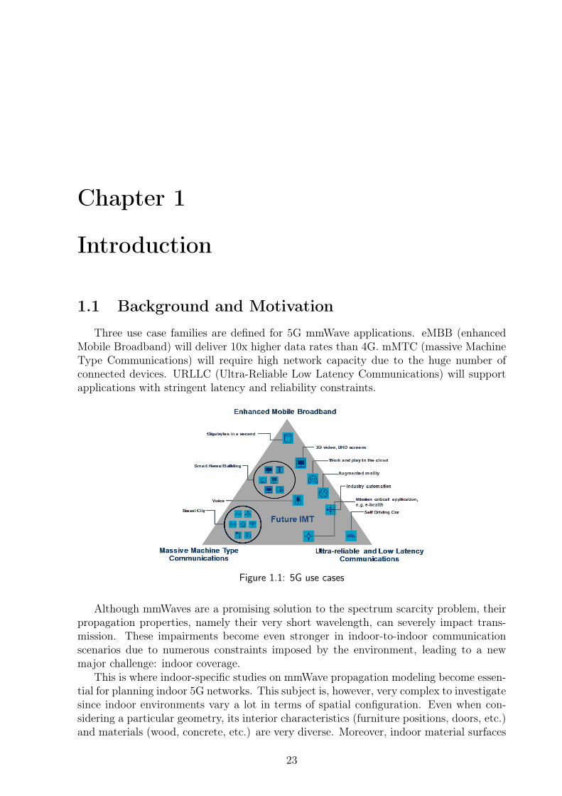
Three use case families are defined for 5G mmWave applications. eMBB (enhancedMobile Broadband) will deliver 10x higher data rates than 4G. mMTC (massive MachineType Communications) will require high network capacity due to the huge number ofconnected devices. URLLC (Ultra-Reliable Low Latency Communications) will supportapplications with stringent latency and reliability constraints.
Figure 1.1: 5G use cases
Although mmWaves are a promising solution to the spectrum scarcity problem, theirpropagation properties, namely their very short wavelength, can severely impact trans-mission. These impairments become even stronger in indoor-to-indoor communicationscenarios due to numerous constraints imposed by the environment, leading to a newmajor challenge: indoor coverage.
This is where indoor-specific studies on mmWave propagation modeling become essen-tial for planning indoor 5G networks. This subject is, however, very complex to investigatesince indoor environments vary a lot in terms of spatial configuration. Even when con-sidering a particular geometry, its interior characteristics (furniture positions, doors, etc.)and materials (wood, concrete, etc.) are very diverse. Moreover, indoor material surfaces
23
24 CHAPTER 1. INTRODUCTION
are generally rough; this roughness is comparable to the wavelength of mmWaves andthus, electromagnetic (EM) diffusion cannot be ignored and must be studied.
Existing investigations rely on measurement campaigns or system simulations. Con-ducting measurements is a heavy process and requires a lot of resources. The few studies[1, 2] based on this method carry out measurements in a specific environment type andsetting; collected data are accurate for that particular scenario only and do not accountfor the propagation diversity inherent to an environment’s topology, morphology and ma-terial properties. Since it is impractical to conduct measurements in various environmentconfigurations, generated empirical models cannot be used in other indoor mmWave appli-cations, nor can they provide information regarding the influence of indoor characteristicson propagation mechanisms, especially diffusion.
System simulations offer a flexible alternative to predict propagation behavior. Exist-ing indoor mmWave simulators allow users to study propagation in various environmentsettings. Each of these simulators uses different implementation techniques of propaga-tion mechanisms; however, most of them suffer from major drawbacks when it comesto diffusion which is the most complex mechanism but certainly the one that should bemostly investigated. In [3] for example, the diffusion lobe which physically describes theangular distribution of EM energy is oversimplified and set by the user, choosing betweena Lambert or directive model, and whether or not to include backscattering, setting alsothe back lobe. Some simulators as [4] utilize empirical models, and others as [5] do notconsider diffusion due to its implementation challenges. Hence, these simulators cannotpredict the actual indoor mmWave behavior, nor can generated models provide conclu-sions regarding the impact of indoor geometry and materials on mmWave propagation.
1.2 Contributions
In this work, we present a novel modeling framework for 5G indoor mmWave prop-agation that combines stochastic indoor environment generation with advanced physicalpropagation simulation. Its system implementation, so-called iGeoStat, utilizes the the-ory of stochastic geometry to generate parameterized typical environments that accountfor the statistical indoor variability, and employs the complex but comprehensive physicalmodel of He [6] to simulate radio propagation based on the physical interaction betweenEM waves and indoor materials. Practical implementation of this framework raises highlychallenging computational tasks that we solve by formulating an adapted link budget anddesigning new memory management and optimization algorithms. This makes iGeoStatthe first to simulate multiple diffusion in realistic environments, allowing us to study theactual indoor behavior of 5G mmWave propagation.
The proposed framework aims to statistically understand the influence of the environ-ment’s geometry and materials’ parameters on mmWave propagation properties, especiallycoverage and path loss. Therefore, generated models are not defined by the geometry ormaterial itself, but rather by the parameters that characterize them. This framework isnot dedicated to a particular environment, material, frequency or use case, making it veryefficient for indoor 5G mmWave propagation modeling.
An original stochastic approach was firstly developed and used in [7] for outdoor where

1.2. CONTRIBUTIONS 25
parameterized urban environments with typical buildings are generated based on randomprocesses that design city street networks [8]. Radio propagation (reflection) is thensimulated based on ray tracing, generating power maps as output. This approach allowsto statistically study the influence of the environment parameters (mean building blockarea (MBBA), city street model, etc.) on outdoor propagation indicators (received power,mean path loss, etc.)
iGeoStat tackles the challenges of indoor propagation modeling using a similar stochas-tic approach. However, this is far from being a simple extension: indoor adapted stochasticmodels have to be defined with all the appropriate parameters to generate typical envi-ronments, and diffusion has to be taken into account alongside reflection. Indeed, forcentimeter wave (cmWave) and mmWave bands, indoor materials (walls, furniture, bod-ies, etc.) can no longer be considered as smooth surfaces; on the contrary, their roughnesshas a major impact on diffusion lobes.
We note that physical diffusion models are mostly used in computer graphics andvideo games [9], but have never been used in such approach as in iGeoStat.
The contributions of this work are summarized as follows:
1. We introduce a new stochastic modeling approach that generates parameterized andrealistic 3D environments, taking into account the indoor spatial variability.
2. We present the first implementation of the physical model of He for radio propa-gation simulation based on the physical interaction between EM waves and indoormaterials.
3. We formulate an adapted link budget that enables multiple diffusion simulation andpower tracking at any point in the environment.
4. We design advanced algorithms for memory optimization, multiple diffusion man-agement and simulation acceleration.
5. We generate the first physical-based output maps (power, SINR, coverage, path lossand delay spread) for 5G Fixed Wireless Access at 60 GHz and industry 4.0 at 26GHz.
6. We investigate the impact of major propagation parameters on the received powermap.
7. We evaluate the effects of power and/or diffusion lobe thresholds on the propagationprofile and the simulation performance.
The rest of the manuscript is organized as follows: chapters 2 and 3 present the the-ory behind the electromagnetic wave properties and propagation phenomena. Chapter 4introduces the physical model of He and the components of the bidirectional reflectancedistribution function. Chapter 5 is a brief introduction to the theory of stochastic ge-ometry and random tessellations. Chapters 6 and 7 present our propagation simulatorand the challenges related to its modeling and implementation. In chapter 8 we evaluatethe performance of iGeoStat for two major 5G applications, and validate our simulation
26 CHAPTER 1. INTRODUCTION
results with existing measurement data. In chapter 9 we investigate how simulation re-sults can highlight the impact of major propagation parameters. We also demonstratethe effectiveness of power and BRDF threshold techniques on the simulation performance.Finally, conclusions and perspectives are drawn in chapter 10.
1.3 PublicationsThis work led to the publication of the following article:
A Combined Stochastic and Physical Framework for Modeling Indoor 5G Mil-limeter Wave Propagation - https://arxiv.org/abs/2002.05162 - ArXiv preprintversion published on 17 February 2020. This article is in the process of an ongoing sub-mission to the IEEE Transactions on Antennas and Propagation.
This work was also accepted for presentation in the 9th conference of Stochastic Ge-ometry Days 2020 (GDR GeoSto), 12 - 16 October 2020.
Part II
Theoretical Study
27


Chapter 2
Electromagnetic Wave Properties
This chapter provides a brief review of the electromagnetic (EM) waves theory, suf-ficient to understand the material in later chapters. The following discussions includeconcepts of the EM field and its main characteristics. For further information, the readermay refer to [10].
2.1 Maxwell’s Equations
The Scottish mathematician and physicist James Clerk Maxwell was the first to unifythe laws of electricity and magnetism to a super law of electromagnetism [11]. His math-ematical theory, so-called Maxwell’s equations, describe how electric ~E and magnetic ~Bfields are generated by charges and currents, and how those fields change in time, and in-teract with each other and with the medium. Maxwell’s equations were the mathematicaloutcome of experimental observations that led to the following laws:
• Gauss’s law for electricity: electric charges produce an ~E field. The total electricflux out of any closed surface is proportional to the total charge contained withinthat surface.
• Gauss’s law for magnetism: there are no sources of magnetic charges or “mag-netic monopoles”. The ~B field due to a material is generated by a configurationcalled a dipole, and the net magnetic flux across any closed surface is zero.
• Faraday’s law of induction: a time-varying ~B field induces an ~E field. It alsostates that the curl of the ~E field around a closed loop is equal to the negative ofthe rate of change of the magnetic flux through the enclosed surface.
• Ampère’s circuital law: a ~B field can be generated by a steady electric current.Maxwell added that it can also be generated by a time-varying ~E field, which hecalled displacement current.
The mathematical formulation of these laws has two major variants: “microscopic”or “in vacuum”, and “macroscopic” or “in matter”. Both versions are general and haveuniversal applicability; the microscopic one is unwieldy for common calculations since it
29
30 CHAPTER 2. ELECTROMAGNETIC WAVE PROPERTIES
expresses the ~E and ~B fields in terms of the total charge and current at a complicatedatomic-level. The macroscopic one is more commonly used for calculations since it de-scribes the large-scale behavior of the ~E and ~B fields in matter without having to consideratomic scale charges and currents, or quantum phenomena. Formulating the macroscopicMaxwell’s equations requires the introduction of the following quantities:
• Permittivity: ε = ε0 εr. ε0 ≈ 8.854 × 10⁻¹² F/m is the free space permittivity, andεr is the complex relative permittivity of the material.
• Displacement field: ~D = ε~E.
• Permeability: µ = µ0 µr. µ0 ≈ 4π × 10−7 H/m is the free space permeability, andµr is the complex relative permeability of the material.
• Magnetizing field: ~H = 1µ~B.
• Electric conductivity: σ.
• Free volumetric charge density: ρf .
• Free charge current density: ~Jf = σ ~E.
Maxwell’s macroscopic equations in the SI units convention are thus defined as:
Gauss’s law for electricity: ∇ · ~D = ρf
Gauss’s law for magnetism: ∇ · ~B = 0
Faraday’s law of induction: ∇∧ ~E = −∂~B
∂t
Ampère’s circuital law: ∇∧ ~H = ~Jf +∂ ~D
∂t
(2.1)
These partial differential equations are used to locally evaluate the fields at individualpoints in space. We note that the physical laws governing Maxwell’s equations turnedout to be compatible with the theory of special relativity which expressed the ~E and ~Bfields as a unique mathematical object, so-called the electromagnetic tensor, describingthe EM field in space and time.
2.2 Electromagnetic Waves and their PropertiesIn order to find a solution for Maxwell’s equations, we assume that the medium is
homogeneous, isotropic, and lossless, i.e. ε, µ, and σ are constants, and that there are nosources of free charges ρf = 0 or currents ~Jf = 0 in the region. Hence, eq. 2.1 yields to:(
ε µ∂2
∂t2−∇2
)~E = 0(
ε µ∂2
∂t2−∇2
)~B = 0
(2.2)
2.2. ELECTROMAGNETIC WAVES AND THEIR PROPERTIES 31
which represent the general form of the EM wave equation. These equations describe thepropagation of EM waves through a medium at a phase velocity v = 1√
ε µ. In vacuum,
EM waves propagate at the speed of light c = 1√ε0 µ0
.
2.2.1 Electromagnetic wave equation
There exists two main classes of particular solutions to Maxwell’s EM wave equation:plane waves and spherical waves. The sinusoidal plane waves are synchronized oscillationsof ~E and ~B fields. In homogeneous and isotropic media, the oscillations of the two fieldsare orthogonal to each other and to the direction of energy and wave propagation, forminga “transverse” wave. The position of a wave within the EM spectrum is characterized byits frequency of oscillation f or its wavelength λ = v/f . Noting ~r = (x, y, z) the positionvector, the sinusoidal solution to the EM wave equation is:
~E(~r, t) = ~E0 ei(~k·~r−ωt+ϕ)
v ~B = ~k ∧ ~E(2.3)
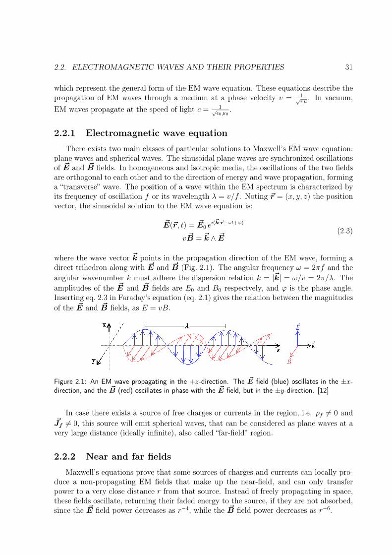
where the wave vector ~k points in the propagation direction of the EM wave, forming adirect trihedron along with ~E and ~B (Fig. 2.1). The angular frequency ω = 2πf and theangular wavenumber k must adhere the dispersion relation k = |~k| = ω/v = 2π/λ. Theamplitudes of the ~E and ~B fields are E0 and B0 respectvely, and ϕ is the phase angle.Inserting eq. 2.3 in Faraday’s equation (eq. 2.1) gives the relation between the magnitudesof the ~E and ~B fields, as E = vB.
Figure 2.1: An EM wave propagating in the +z-direction. The ~E field (blue) oscillates in the ±x-direction, and the ~B (red) oscillates in phase with the ~E field, but in the ±y-direction. [12]
In case there exists a source of free charges or currents in the region, i.e. ρf 6= 0 and~Jf 6= 0, this source will emit spherical waves, that can be considered as plane waves at avery large distance (ideally infinite), also called “far-field” region.
2.2.2 Near and far fields
Maxwell’s equations prove that some sources of charges and currents can locally pro-duce a non-propagating EM fields that make up the near-field, and can only transferpower to a very close distance r from that source. Instead of freely propagating in space,these fields oscillate, returning their faded energy to the source, if they are not absorbed,since the ~E field power decreases as r−4, while the ~B field power decreases as r−6.
32 CHAPTER 2. ELECTROMAGNETIC WAVE PROPERTIES
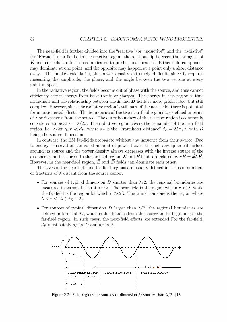
The near-field is further divided into the “reactive” (or “inductive”) and the “radiative”(or “Fresnel”) near fields. In the reactive region, the relationship between the strengths of~E and ~B fields is often too complicated to predict and measure. Either field componentmay dominate at one point, and the opposite may happen at a point only a short distanceaway. This makes calculating the power density extremely difficult, since it requiresmeasuring the amplitude, the phase, and the angle between the two vectors at everypoint in space.
In the radiative region, the fields become out of phase with the source, and thus cannotefficiently return energy from its currents or charges. The energy in this region is thusall radiant and the relationship between the ~E and ~B fields is more predictable, but stillcomplex. However, since the radiative region is still part of the near field, there is potentialfor unanticipated effects. The boundaries of the two near-field regions are defined in termsof λ or distance r from the source. The outer boundary of the reactive region is commonlyconsidered to be at r = λ/2π. The radiative region covers the remainder of the near-fieldregion, i.e. λ/2π r dF , where dF is the “Fraunhofer distance” dF = 2D2/λ, with Dbeing the source dimension.
In contrast, the EM far-fields propagate without any influence from their source. Dueto energy conservation, an equal amount of power travels through any spherical surfacearound its source and the power density always decreases with the inverse square of thedistance from the source. In the far-field region, ~E and ~B fields are related by v ~B = ~k∧ ~E.However, in the near-field region, ~E and ~B fields can dominate each other.
The sizes of the near-field and far-field regions are usually defined in terms of numbersor fractions of λ distant from the source center:
• For sources of typical dimension D shorter than λ/2, the regional boundaries aremeasured in terms of the ratio r/λ. The near-field is the region within r λ, whilethe far-field is the region for which r 2λ. The transition zone is the region whereλ ≤ r ≤ 2λ (Fig. 2.2).
• For sources of typical dimension D larger than λ/2, the regional boundaries aredefined in terms of dF , which is the distance from the source to the beginning of thefar-field region. In such cases, the near-field effects are extended For the far-field,dF must satisfy dF D and dF λ.
Figure 2.2: Field regions for sources of dimension D shorter than λ/2. [13]
2.2. ELECTROMAGNETIC WAVES AND THEIR PROPERTIES 33
2.2.3 Complex refractive index
A medium is characterized by its dimensionless complex refractive index nc that highlydepends on λ:
nc = nr + ini (2.4)
The real part nr = c/v = λ0/λ represents the factor by which the propagation speed andwavelength are reduced with respect to their vacuum values c and λ0 respectively. Thereal part nr also determines how much the path of an EM wave is bent or “refracted”, whenentering a material [14]. The imaginary part ni > 0, also called the extinction coefficient,represents the amount of EM attenuation or absorption for a propagating wave throughthe medium. This attenuation can be observed by inserting nc into the ~E field of an EMwave traveling in the z-direction by relating the complex wave number k to nc throughk = 2π nc/λ0:
~E(z, t) = <~E0ei(kz−wt) = e−2πniz/λ0 <~E0e
i(kz−wt) (2.5)
This shows that ni results in an exponential decay of the propagating EM wave. Since theintensity I of the EM wave is proportional to the square of the ~E field, it will decrease bythe factor exp(−4πniz/λ0), resulting in an attenuation coefficient equal to α = 4πni/λ0.
The complex refractive index nc can be expressed in terms of the complex relativepermittivity εr and permeability µr as the following:
nc =√εr µr (2.6)
For non-magnetic material (µr ≈ 1), nc ≈√εr. The complex refractive index nc can be
also expressed in terms of η which is equal everywhere for a transverse EM plane wavetraveling in a homogeneous medium. The wave impedance η can be also defined as:
η =
√iωµ
σ + iωε(2.7)
In case of an non-conductive medium or ideal dielectric (σ = 0), η reduces to:
η =
õ
ε= η0
√µrεr
= η0µrnc
(2.8)
And for non-magnetic material (µr ≈ 1),
nc =η0
η(2.9)
2.2.4 Energy in electromagnetic waves
In lossless media, ~E and ~B fields are in phase, allowing EM waves to carry energyas they travel. Thus, these fields exert a force ~F on a point particle of electric charge qmoving at velocity ~v according to Lorentz Force law:
~F = q ~E + q~v ∧ ~B (2.10)
34 CHAPTER 2. ELECTROMAGNETIC WAVE PROPERTIES
The energy of the wave is defined by the wave amplitude which is the maximum fieldstrength of the ~E and ~B fields. The energy density u is the sum of the energy stored inits ~E component uE (capacitance) and its ~B component uB (inductance):
uE =1
2ε~E2 , uB =
1
2µ~B2
u =1
2ε~E2 +
1
2µ~B2
(2.11)
E = vB shows that uE = uB and that half the energy in an EM wave is carried by the ~Efield, and the other half by the ~B field. Thus, the total energy density of an EM wave is:
u = ε~E2 =1
µ~B2 (2.12)
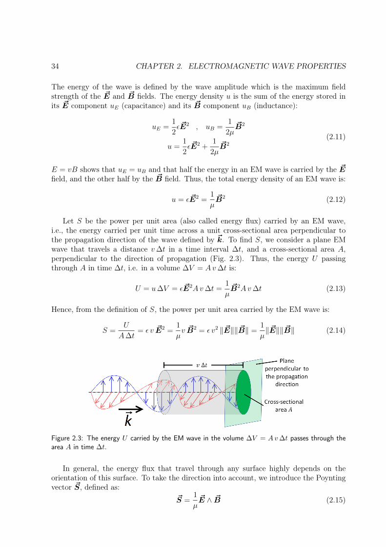
Let S be the power per unit area (also called energy flux) carried by an EM wave,i.e., the energy carried per unit time across a unit cross-sectional area perpendicular tothe propagation direction of the wave defined by ~k. To find S, we consider a plane EMwave that travels a distance v∆t in a time interval ∆t, and a cross-sectional area A,perpendicular to the direction of propagation (Fig. 2.3). Thus, the energy U passingthrough A in time ∆t, i.e. in a volume ∆V = Av∆t is:
U = u∆V = ε~E2Av∆t =1
µ~B2Av∆t (2.13)
Hence, from the definition of S, the power per unit area carried by the EM wave is:
S =U
A∆t= ε v ~E2 =
1
µv ~B2 = ε v2 ‖~E‖‖ ~B‖ =
1
µ‖~E‖‖ ~B‖ (2.14)
Figure 2.3: The energy U carried by the EM wave in the volume ∆V = Av∆t passes through thearea A in time ∆t.
In general, the energy flux that travel through any surface highly depends on theorientation of this surface. To take the direction into account, we introduce the Poyntingvector ~S, defined as:
~S =1
µ~E ∧ ~B (2.15)
2.2. ELECTROMAGNETIC WAVES AND THEIR PROPERTIES 35
The cross-product ~E∧ ~B points in the direction perpendicular to both vectors and confirmsthat ~S points in the direction of wave propagation. The energy flux at any position alsovaries in time. Using 2.3 and 2.14, S can be rewritten as:
S(~r, t) = ε v ~E2 =1
µv ~B2 (2.16)
The time average of the energy flux is the intensity I of the EM wave. Replacing theexponential expression ei(
~k·~r−ωt) by its cosine representation cos(~k · ~r − ωt), it can bededuced by averaging the cosine function in S(~r, t) over one period T :
I = 〈S(~r, t)〉 =1
T
∫ T
0
S(~r, t) dt (2.17)
I =1
2ε v ~E2
0 =1
2µv ~B2
0 =1
2µ~E0~B0 (2.18)
The intensity I can be also expressed in terms of the wave impedance η = E0/H0 by thefollowing:
I = 〈S(~r, t)〉 =1
2η|~E0|2 (2.19)
These relations show that energy in a wave is related to the amplitude squared of the~E field. Moreover, for sinusoidal EM waves, the peak intensity I0 is twice the averageintensity I, i.e. I0 = 2I. The intensity I is also referred to as the power density anddecreases as r−2 if the radiation is dispersed uniformly in all directions (isotropic source).

36 CHAPTER 2. ELECTROMAGNETIC WAVE PROPERTIES
Chapter 3
Electromagnetic Wave Propagation
This chapter presents the major physical phenomena that occur when a propagatingEM wave is intercepted by an interface separating two different media. These phenomenainclude reflection, transmission, diffraction, and diffusion. For further information, thereader may refer to [15].
3.1 Interface Conditions for Electromagnetic Fields
Interface or boundary conditions describe the behavior of electric ~E, magnetic ~B,displacement ~D, and magnetizing ~H fields at the interface of two materials.
When an EM wave propagates from a medium to another, the continuity of the solutionto Maxwell’s equations must be satisfied at the interface separating both media. Thisis imposed by the physical laws governing Maxwell’s equations which ensure mediumcontinuity at that interface. We assume that both materials are dielectrics (σ = 0) andthat there are no sources of surface charges (ρs = 0) or currents ( ~Js = 0) between bothmedia. Let us consider medium 1 (ε1, µ1) and medium 2 (ε2, µ2) separated by an interface,and normal unit vector n21 going from medium 2 to medium 1.
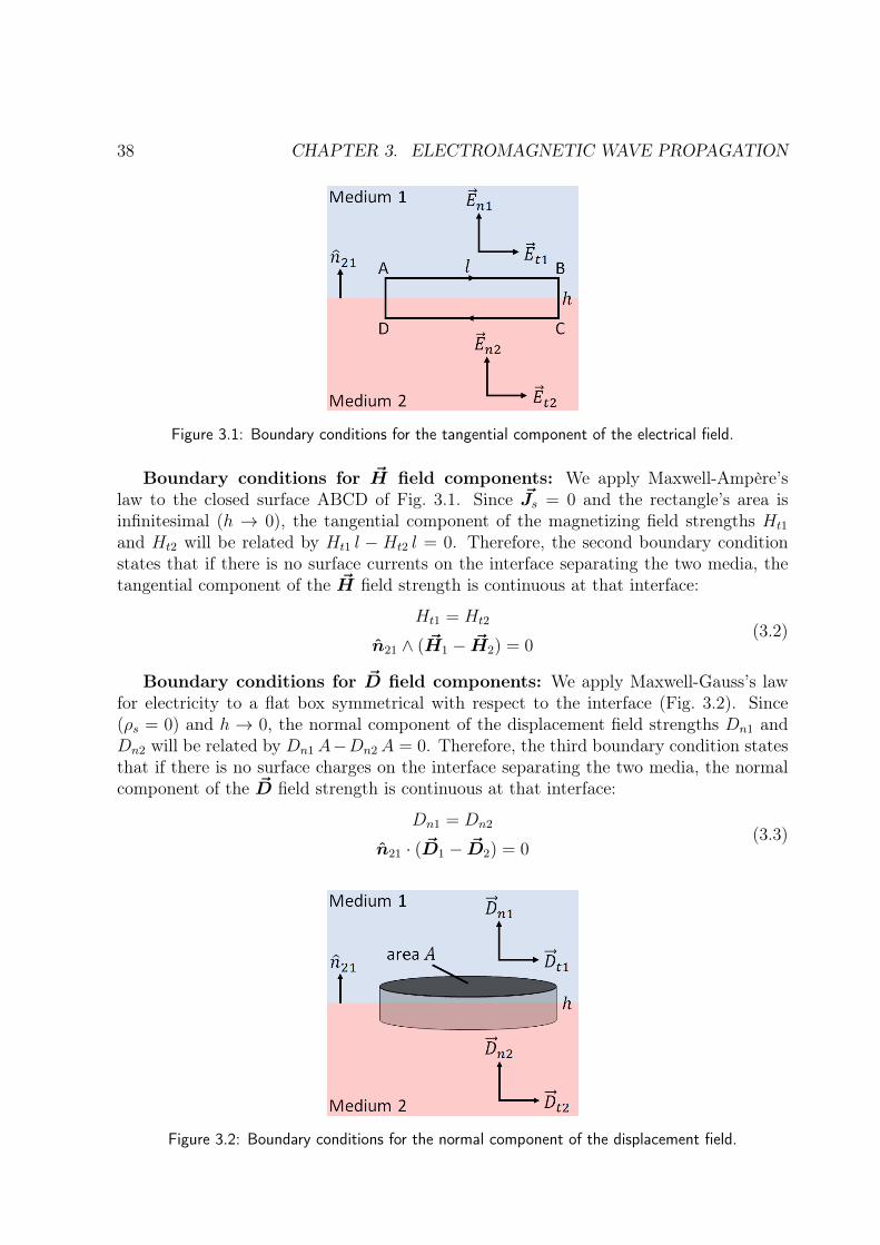
Boundary conditions for ~E field components: We project each of the electricfield strengths ~E1 and ~E2 in the two media near the interface into tangential (Et1, Et2) andnormal (En1, En2) components (Fig. 3.1), and apply Maxwell-Faraday’s law to a closedsurface ABCD: a rectangle of sides l and infinitesimal thickness h which is symmetricalwith respect to the interface. Since h→ 0, the rectangle’s area will also tend to zero, untilthe closed surface ABCD will enclose no magnetic flux, giving Et1 l−Et2 l = 0. Therefore,the first boundary condition states that the tangential component of the ~E field strengthis continuous at the interface separating the two media, i.e., it has the same value on bothsides of the interface:
Et1 = Et2
n21 ∧ (~E1 − ~E2) = 0(3.1)
37
38 CHAPTER 3. ELECTROMAGNETIC WAVE PROPAGATION
Figure 3.1: Boundary conditions for the tangential component of the electrical field.
Boundary conditions for ~H field components: We apply Maxwell-Ampère’slaw to the closed surface ABCD of Fig. 3.1. Since ~Js = 0 and the rectangle’s area isinfinitesimal (h → 0), the tangential component of the magnetizing field strengths Ht1
and Ht2 will be related by Ht1 l − Ht2 l = 0. Therefore, the second boundary conditionstates that if there is no surface currents on the interface separating the two media, thetangential component of the ~H field strength is continuous at that interface:
Ht1 = Ht2
n21 ∧ ( ~H1 − ~H2) = 0(3.2)
Boundary conditions for ~D field components: We apply Maxwell-Gauss’s lawfor electricity to a flat box symmetrical with respect to the interface (Fig. 3.2). Since(ρs = 0) and h → 0, the normal component of the displacement field strengths Dn1 andDn2 will be related by Dn1A−Dn2A = 0. Therefore, the third boundary condition statesthat if there is no surface charges on the interface separating the two media, the normalcomponent of the ~D field strength is continuous at that interface:
Dn1 = Dn2
n21 · ( ~D1 − ~D2) = 0(3.3)
Figure 3.2: Boundary conditions for the normal component of the displacement field.
3.2. REFLECTION AND TRANSMISSION 39
Boundary conditions for ~B field components: We apply Maxwell-Gauss’s lawfor magnetism to the box of Fig. 3.2. Since h→ 0, the normal component of the magneticfield strengths Bn1 and Bn2 will be related by Bn1A − Bn2A = 0. Therefore, the fourthboundary condition states that the normal component of the ~B field strength is continuousat the interface separating the two media:
Bn1 = Bn2
n21 · ( ~B1 − ~B2) = 0(3.4)
Now that we have defined the interface conditions that describe the behavior of ~E,~B, ~D, and ~H fields, we will present in the following sections the main propagationmechanisms undergone by a EM plane wave when it travels from a medium to another. Wenote that the occurring propagation mechanism depends highly on the physical interactionbetween the EM wave properties (mainly its wavelength) and the interface characteristics(mainly its roughness).
3.2 Reflection and TransmissionReflection occurs when a propagating EM wave is incident on an obstacle with surface
dimensions larger than its wavelength, also called “smooth surface”. During reflection,part of the wave may be transmitted into that obstacle, and the remainder of the wavemay be reflected back into the originally traveling medium. For further information, thereader may refer to [16].
3.2.1 Polarization
Polarization is a property applying to transverse waves, specifying the geometric orien-tation of the oscillations. We mentioned earlier that in a homogeneous isotropic medium,a plane wave’s ~E and ~B fields are in directions perpendicular to each other and to thewave propagation direction (which is parallel to ~k). By convention, the polarization of anEM wave refers to the ~E field direction.
In linear polarization, each field oscillates in a single direction. In circular or ellipticalpolarization, the fields rotate at a constant rate in a plane as the wave propagates. Thefields can rotate in a clockwise manner (right circular polarization) or counterclockwise(left circular polarization) with respect to the wave propagation direction. In the courseof this work, only linear polarization will be used.
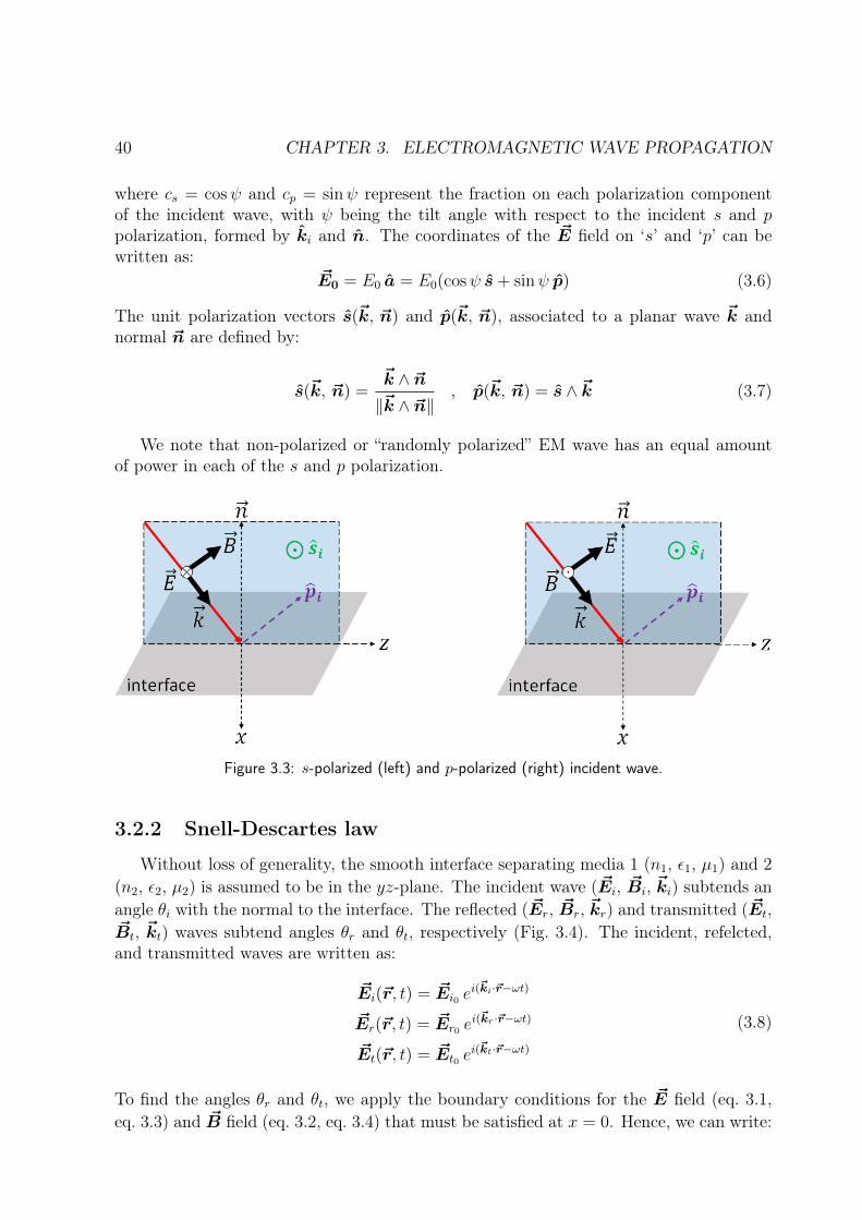
A polarization state a can be resolved into a combination of two orthogonal compo-nents: ‘s’ and ‘p’ polarization, defined for an incident EM wave and a planar interfacewhich is responsible for breaking the symmetry and introducing these two natural po-larization directions. The s-polarization (Fig. 3.3) (also called transverse-electric (TE))refers to a wave’s ~E field perpendicular to the plane of incidence; the ~B field is thus in theplane of incidence. The p-polarization (Fig. 3.3) (also called transverse-magnetic (TM))refers to a wave’s ~E field in the plane of incidence; the ~B field is thus perpendicular tothe plane of incidence. Hence, we can write:
a = cs si(ki, n) + cp pi(ki, n) (3.5)
40 CHAPTER 3. ELECTROMAGNETIC WAVE PROPAGATION
where cs = cosψ and cp = sinψ represent the fraction on each polarization componentof the incident wave, with ψ being the tilt angle with respect to the incident s and ppolarization, formed by ki and n. The coordinates of the ~E field on ‘s’ and ‘p’ can bewritten as:
~E0 = E0 a = E0(cosψ s+ sinψ p) (3.6)
The unit polarization vectors s(~k, ~n) and p(~k, ~n), associated to a planar wave ~k andnormal ~n are defined by:
s(~k, ~n) =~k ∧ ~n‖~k ∧ ~n‖
, p(~k, ~n) = s ∧~k (3.7)
We note that non-polarized or “randomly polarized” EM wave has an equal amountof power in each of the s and p polarization.
Figure 3.3: s-polarized (left) and p-polarized (right) incident wave.
3.2.2 Snell-Descartes law
Without loss of generality, the smooth interface separating media 1 (n1, ε1, µ1) and 2(n2, ε2, µ2) is assumed to be in the yz-plane. The incident wave (~Ei, ~Bi, ~ki) subtends anangle θi with the normal to the interface. The reflected (~Er, ~Br, ~kr) and transmitted (~Et,~Bt, ~kt) waves subtend angles θr and θt, respectively (Fig. 3.4). The incident, refelcted,and transmitted waves are written as:
~Ei(~r, t) = ~Ei0 ei(~ki·~r−ωt)
~Er(~r, t) = ~Er0 ei(~kr·~r−ωt)
~Et(~r, t) = ~Et0 ei(~kt·~r−ωt)
(3.8)
To find the angles θr and θt, we apply the boundary conditions for the ~E field (eq. 3.1,eq. 3.3) and ~B field (eq. 3.2, eq. 3.4) that must be satisfied at x = 0. Hence, we can write:
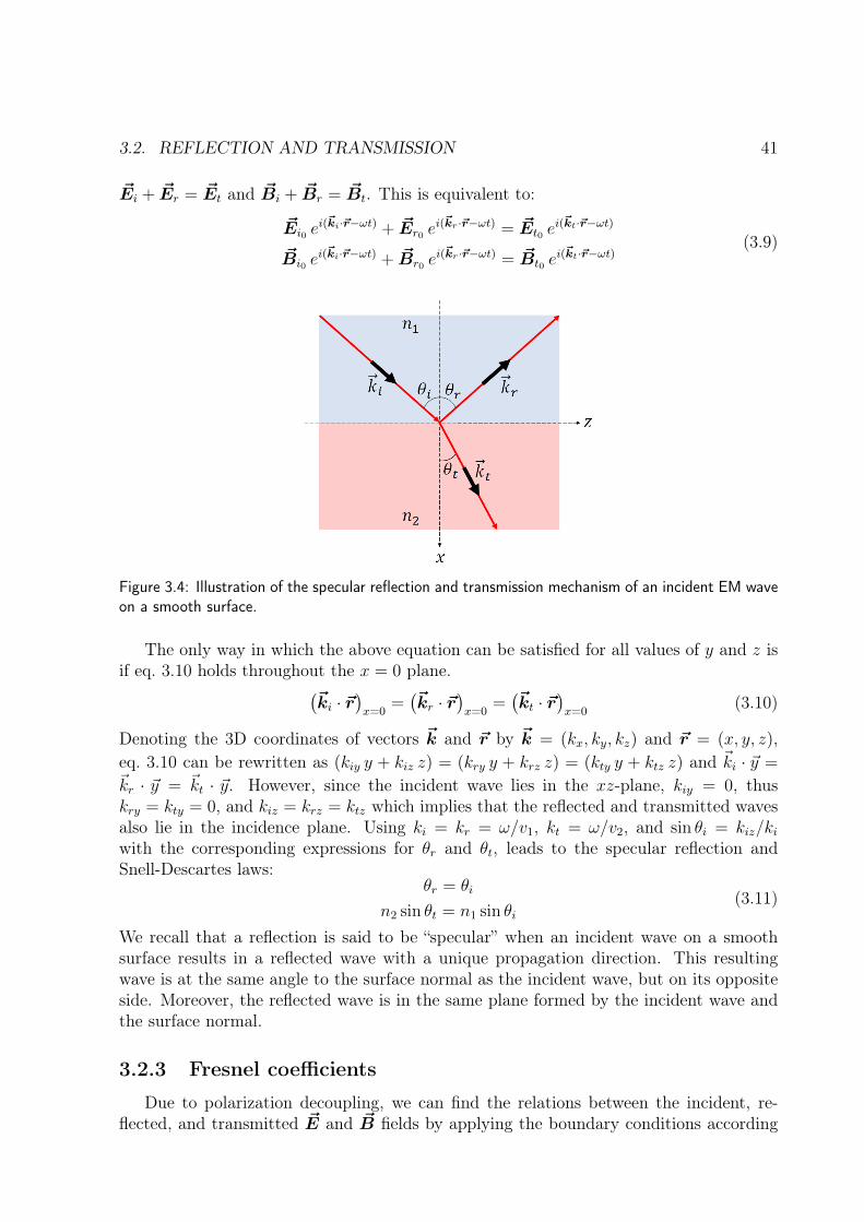
3.2. REFLECTION AND TRANSMISSION 41
~Ei + ~Er = ~Et and ~Bi + ~Br = ~Bt. This is equivalent to:
~Ei0 ei(~ki·~r−ωt) + ~Er0 e
i(~kr·~r−ωt) = ~Et0 ei(~kt·~r−ωt)
~Bi0 ei(~ki·~r−ωt) + ~Br0 e
i(~kr·~r−ωt) = ~Bt0 ei(~kt·~r−ωt)
(3.9)
Figure 3.4: Illustration of the specular reflection and transmission mechanism of an incident EM waveon a smooth surface.
The only way in which the above equation can be satisfied for all values of y and z isif eq. 3.10 holds throughout the x = 0 plane.(
~ki · ~r)x=0
=(~kr · ~r
)x=0
=(~kt · ~r
)x=0
(3.10)
Denoting the 3D coordinates of vectors ~k and ~r by ~k = (kx, ky, kz) and ~r = (x, y, z),eq. 3.10 can be rewritten as (kiy y + kiz z) = (kry y + krz z) = (kty y + ktz z) and ~ki · ~y =~kr · ~y = ~kt · ~y. However, since the incident wave lies in the xz-plane, kiy = 0, thuskry = kty = 0, and kiz = krz = ktz which implies that the reflected and transmitted wavesalso lie in the incidence plane. Using ki = kr = ω/v1, kt = ω/v2, and sin θi = kiz/kiwith the corresponding expressions for θr and θt, leads to the specular reflection andSnell-Descartes laws:
θr = θi
n2 sin θt = n1 sin θi(3.11)
We recall that a reflection is said to be “specular” when an incident wave on a smoothsurface results in a reflected wave with a unique propagation direction. This resultingwave is at the same angle to the surface normal as the incident wave, but on its oppositeside. Moreover, the reflected wave is in the same plane formed by the incident wave andthe surface normal.
3.2.3 Fresnel coefficients
Due to polarization decoupling, we can find the relations between the incident, re-flected, and transmitted ~E and ~B fields by applying the boundary conditions according
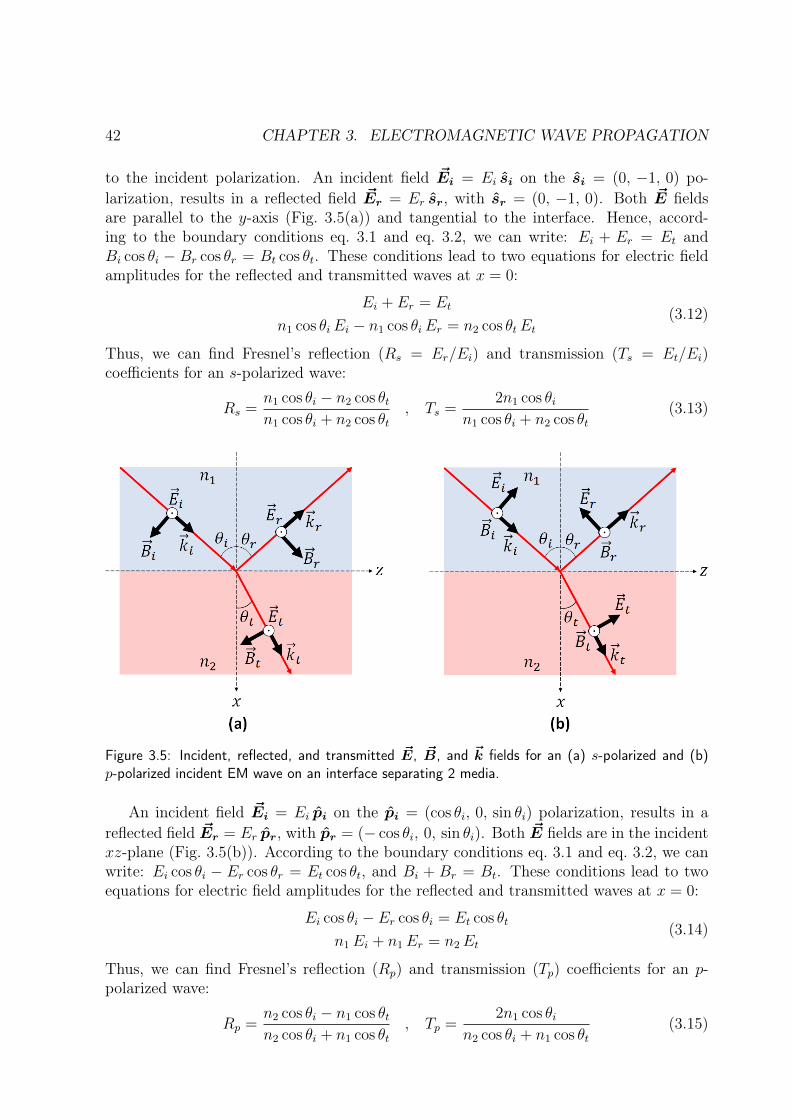
42 CHAPTER 3. ELECTROMAGNETIC WAVE PROPAGATION
to the incident polarization. An incident field ~Ei = Ei si on the si = (0, −1, 0) po-larization, results in a reflected field ~Er = Er sr, with sr = (0, −1, 0). Both ~E fieldsare parallel to the y-axis (Fig. 3.5(a)) and tangential to the interface. Hence, accord-ing to the boundary conditions eq. 3.1 and eq. 3.2, we can write: Ei + Er = Et andBi cos θi − Br cos θr = Bt cos θt. These conditions lead to two equations for electric fieldamplitudes for the reflected and transmitted waves at x = 0:
Ei + Er = Et
n1 cos θiEi − n1 cos θiEr = n2 cos θtEt(3.12)
Thus, we can find Fresnel’s reflection (Rs = Er/Ei) and transmission (Ts = Et/Ei)coefficients for an s-polarized wave:
Rs =n1 cos θi − n2 cos θtn1 cos θi + n2 cos θt
, Ts =2n1 cos θi
n1 cos θi + n2 cos θt(3.13)
Figure 3.5: Incident, reflected, and transmitted ~E, ~B, and ~k fields for an (a) s-polarized and (b)p-polarized incident EM wave on an interface separating 2 media.
An incident field ~Ei = Ei pi on the pi = (cos θi, 0, sin θi) polarization, results in areflected field ~Er = Er pr, with pr = (− cos θi, 0, sin θi). Both ~E fields are in the incidentxz-plane (Fig. 3.5(b)). According to the boundary conditions eq. 3.1 and eq. 3.2, we canwrite: Ei cos θi − Er cos θr = Et cos θt, and Bi + Br = Bt. These conditions lead to twoequations for electric field amplitudes for the reflected and transmitted waves at x = 0:
Ei cos θi − Er cos θi = Et cos θt
n1Ei + n1Er = n2Et(3.14)
Thus, we can find Fresnel’s reflection (Rp) and transmission (Tp) coefficients for an p-polarized wave:
Rp =n2 cos θi − n1 cos θtn2 cos θi + n1 cos θt
, Tp =2n1 cos θi
n2 cos θi + n1 cos θt(3.15)
3.3. DIFFRACTION 43
3.2.4 Reflectance and transmittance
The ratio of waves ~E field amplitudes are obtained; however, in practice we are oftenmore interested in the power coefficients. The wave’s power is generally proportional to thesquare of the ~E or ~B field amplitude. “Reflectance” or “Reflectivity” (R2) is the fractionof incident power that is reflected from the interface. The fraction that is transmitted intothe second medium is called “Transmittance” or “Transmissivity” (T 2). The reflectivityfor s and p polarized waves are respectively given by:
R2s =
∣∣∣∣n1 cos θi − n2 cos θtn1 cos θi + n2 cos θt
∣∣∣∣2 =
∣∣∣∣η2 cos θi − η1 cos θtη2 cos θi + η1 cos θt
∣∣∣∣2R2p =
∣∣∣∣n2 cos θi − n1 cos θtn2 cos θi + n1 cos θt
∣∣∣∣2 =
∣∣∣∣η1 cos θi − η2 cos θtη1 cos θi + η2 cos θt
∣∣∣∣2(3.16)
where the relation between the complex refractive index nc and the impedance η is givenin eq. 2.9. As a consequence of energy conservation, T 2
s = 1 − R2s and T 2
p = 1 − R2p. For
non-polarized EM wave, there is an equal amount of power in the s and p polarization.The reflectivity is thus:
R2npol =
1
2(R2
s +R2p) (3.17)
For the case of normal incidence, θi = θt = 0, the reflectivity simplifies to:
R2 =
∣∣∣∣n1 − n2
n1 + n2
∣∣∣∣2 (3.18)
3.3 Diffraction
Diffraction occurs when a propagating EM wave encounters an obstacle with sharpedges, allowing the wave to bend around it or pass through a small aperture whose sizeis comparable to the wavelength allowing the wave to spread out past the aperture.
3.3.1 Huygens-Fresnel principle
Diffraction is described by Huygens–Fresnel principle: it states that each point on awavefront reached by a propagating EM wave is a source of secondary spherical wavelets,the resulting wavelets from different points mutually interfere, and their sum forms a newwavefront. For further information, the reader may refer to [17].
44 CHAPTER 3. ELECTROMAGNETIC WAVE PROPAGATION
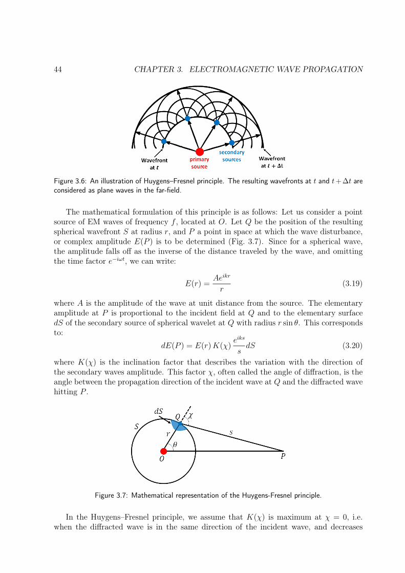
Figure 3.6: An illustration of Huygens–Fresnel principle. The resulting wavefronts at t and t+ ∆t areconsidered as plane waves in the far-field.
The mathematical formulation of this principle is as follows: Let us consider a pointsource of EM waves of frequency f , located at O. Let Q be the position of the resultingspherical wavefront S at radius r, and P a point in space at which the wave disturbance,or complex amplitude E(P ) is to be determined (Fig. 3.7). Since for a spherical wave,the amplitude falls off as the inverse of the distance traveled by the wave, and omittingthe time factor e−iωt, we can write:
E(r) =Aeikr
r(3.19)
where A is the amplitude of the wave at unit distance from the source. The elementaryamplitude at P is proportional to the incident field at Q and to the elementary surfacedS of the secondary source of spherical wavelet at Q with radius r sin θ. This correspondsto:
dE(P ) = E(r)K(χ)eiks
sdS (3.20)
where K(χ) is the inclination factor that describes the variation with the direction ofthe secondary waves amplitude. This factor χ, often called the angle of diffraction, is theangle between the propagation direction of the incident wave at Q and the diffracted wavehitting P .
Figure 3.7: Mathematical representation of the Huygens-Fresnel principle.
In the Huygens–Fresnel principle, we assume that K(χ) is maximum at χ = 0, i.e.when the diffracted wave is in the same direction of the incident wave, and decreases
3.3. DIFFRACTION 45
rapidly to 0 at χ = π/2, i.e. when the diffracted wave is tangential to the wavefront. Thetotal disturbance at P is the sum of the complex amplitudes of the vibrations producedby all the elementary secondary sources:
E(P ) = E(r)
∫∫S
K(χ)eiks
sdS (3.21)
Evaluating this integral, also known as the Huygens-Fresnel integral, is very complicated,that’s why Fresnel proposed a new method of calculation based on the division of thewavefront at r into zones, called Fresnel zone construction.
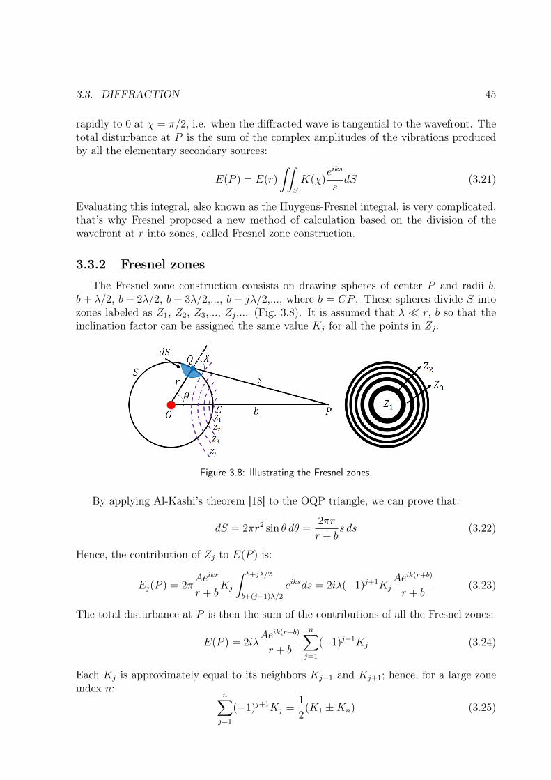
3.3.2 Fresnel zones
The Fresnel zone construction consists on drawing spheres of center P and radii b,b + λ/2, b + 2λ/2, b + 3λ/2,..., b + jλ/2,..., where b = CP . These spheres divide S intozones labeled as Z1, Z2, Z3,..., Zj,... (Fig. 3.8). It is assumed that λ r, b so that theinclination factor can be assigned the same value Kj for all the points in Zj.
Figure 3.8: Illustrating the Fresnel zones.
By applying Al-Kashi’s theorem [18] to the OQP triangle, we can prove that:
dS = 2πr2 sin θ dθ =2πr
r + bs ds (3.22)
Hence, the contribution of Zj to E(P ) is:
Ej(P ) = 2πAeikr
r + bKj
∫ b+jλ/2
b+(j−1)λ/2
eiksds = 2iλ(−1)j+1KjAeik(r+b)
r + b(3.23)
The total disturbance at P is then the sum of the contributions of all the Fresnel zones:
E(P ) = 2iλAeik(r+b)
r + b
n∑j=1
(−1)j+1Kj (3.24)
Each Kj is approximately equal to its neighbors Kj−1 and Kj+1; hence, for a large zoneindex n:
n∑j=1
(−1)j+1Kj =1
2(K1 ±Kn) (3.25)
46 CHAPTER 3. ELECTROMAGNETIC WAVE PROPAGATION
where the ± is based on whether n is odd or even respectively, and hence, using eq. 3.23,we can write:
E(P ) = iλ (K1 ±Kn)Aeik(r+b)
r + b=
1
2[E1(P )± En(P )] (3.26)
For Zn, the last Fresnel zone seen by P , we have χ = π/2, i.e. QP is tangential to thewavefront which corresponds as already mentioned to K(π/2) = Kn = 0. Hence,
E(P ) = iλK1Aeik(r+b)
r + b=
1
2[E1(P )± En(P )] =
1
2E1(P ) (3.27)
Showing that the total disturbance at P is equal to half the one due to Z1. This confirmsthat the resulting waves from two consecutive zones have opposite phases, as path differ-ence between them is λ/2, which follows that two neighboring zones cancel each other.Therefore, if we start from the first zone and sum all the contributions of the other zones,these will cancel two by two and there will remain only the contribution of the first zone.
In order for eq. 3.27 to agree with the expression of a freely propagating spherical wavefrom the source O to point P , of the form:
E(P ) =Aeik(r+b)
r + b(3.28)
we should have iλK1 = 1, i.e.:
K1 = − iλ
=e−iπ/2
λ(3.29)
The factor e−iπ/2 assumes that the secondary wavelets oscillate a quarter of a period aheadof the primary, while the factor 1/λ assumes that the amplitudes of these wavelets are inthe ratio of 1 : λ to the ones of the primary. With these assumptions regarding the phaseand amplitude of the secondary waves, the Huygens-Fresnel principle leads to the correctexpression for the propagation of a spherical wave.
3.3.3 Kirchhoff diffraction theory
Kirchhoff showed that the Huygens-Fresnel principle is an approximation to a certainintegral theorem, later called the Fresnel-Kirchhoff integral, which expresses the solutionof a homogeneous wave equation at an arbitrary point P in terms of all points on anarbitrary closed surface surrounding P .
Let us consider a point source at O that emits a homogeneous monochromatic scalarwave, defined by the Helmholtz equation:
(∇2 + k2)E = 0 (3.30)
Kirchhoff showed that the Huygens-Fresnel principle is only an approximate solution tothis wave equation. Using Green’s identities, he derived a more exact solution at anarbitrary point P in terms of the solution values of E and and its first order derivative
3.3. DIFFRACTION 47
∂E/∂n at all points on an arbitrary surface S enclosing P . This solution has the form ofthe Helmholtz-Kirchhoff integral and is expressed as:
E(P ) =1
4π
∫∫S
[E∂
∂n
(eiks
s
)−(eiks
s
)∂E
∂n
]dS (3.31)
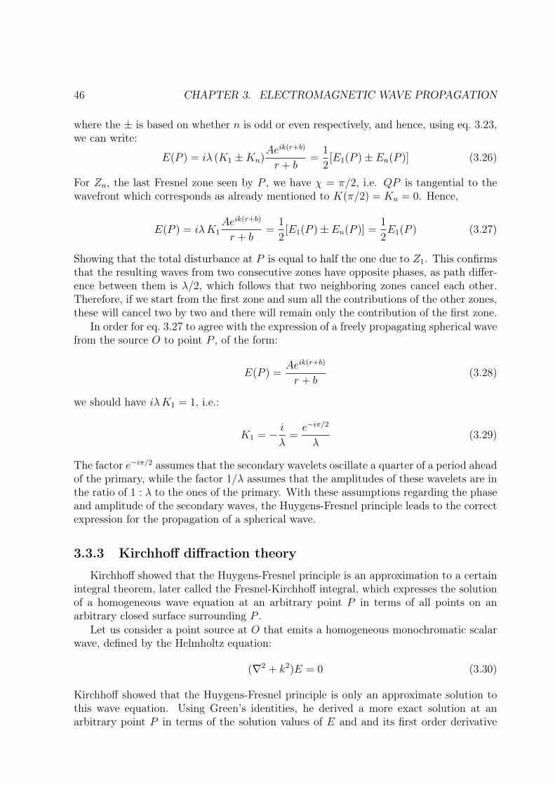
where ∂/∂n is the differentiation along the inward normal to S, and s is the distancebetween P and dS.
Now let us consider the case of this point source O illuminating an aperture in a planeopaque screen (Fig. 3.9). We assume here that the dimensions of the aperture are largerthan λ but smaller than r and s. For the boundary conditions, Kirchhoff assumed thatboth E and ∂E/∂n are continuous across the aperture as if there were no screen, anddiscontinuous on the shadowed side of the screen, i.e. E = ∂E/∂n = 0 (physically untrueunless the dimensions of the aperture are very large relative to λ). To find the totaldisturbance at P , we apply the Helmholtz-Kirchhoff integral on S formed by the apertureS1, a portion S2 of the shadowed side of the screen, and a portion S3 of a large sphere ofradius R centered at P :
E(P ) =1
4π
∫∫S1
+
∫∫S2
+
∫∫S3
[E∂
∂n
(eiks
s
)−(eiks
s
)∂E
∂n
]dS (3.32)
Figure 3.9: An illustration of the Kirchhoff diffraction theory.
From Kirchhoff’s boundary conditions we have:
ES1 =Aeikr
r,
∂ES1
∂n=Aeikr
r
[ik − 1
r
]cos(n, r)
ES2 = 0 ,∂ES2
∂n= 0
(3.33)
The contribution from S3 is also assumed to be zero, i.e. ES3 = 0 and ∂ES3∂n
= 0. Kirchhoffjustified this by making two assumptions: R → ∞ and the source starts to radiate at aparticular time such that when considering the disturbance at P , no contributions from
48 CHAPTER 3. ELECTROMAGNETIC WAVE PROPAGATION
S3 will have arrived there. This implies that the considered wave is not monochromatic,since such waves must exist at all times. Neglecting the terms 1/r and 1/s compared tok, since r and s are assumed much larger than λ = 2π/k, the total disturbance at P is:
E(P ) = −iA2λ
∫∫S1
eik(r+s)
rs[cos(n, r)− cos(n, s)] dS1 (3.34)
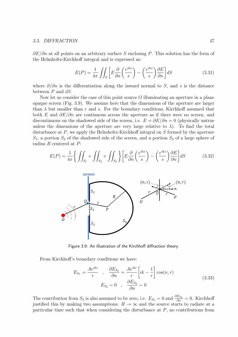
which is known as the Fresnel-Kirchhoff diffraction integral.To express Kirchhoff’s formula in a form similar to the Huygens–Fresnel principle, we
make some geometrical arrangements to the closed surface. Any other type of aperturescan be chosen for S1. In our case, let’s replace it by a portion S4 of a wavefront from O thatalmost fills the aperture, and a portion S5 of a cone with a vertex at O and generatorsthrough the rim of the aperture (Fig. 3.10). If the radius of curvature of the wave islarge enough, the contribution from S5 can be neglected. We also have cos(n, r) = 1 andχ = π − cos(r, s); hence, eq. 3.21 becomes:
E(P ) = − i
2λ
Aeikr
r
∫∫S4
Aeiks
s(1 + cosχ) dS4 (3.35)
which is known as the Kirchhoff diffraction integral. This result is in agreement with theHuygens-Fresnel principle.
Figure 3.10: An illustration of the diffraction formula.
In comparison with eq. 3.21, we can deduce the expression of the inclination factor:
K(χ) = − i
2λ(1 + cosχ) (3.36)
For the central zone Z1, χ = 0, giving K1 = K(0) = −1/λ, which is in agreement witheq. 3.29. However, it is untrue that K(π/2) = 0 as Fresnel assumed.
3.3. DIFFRACTION 49
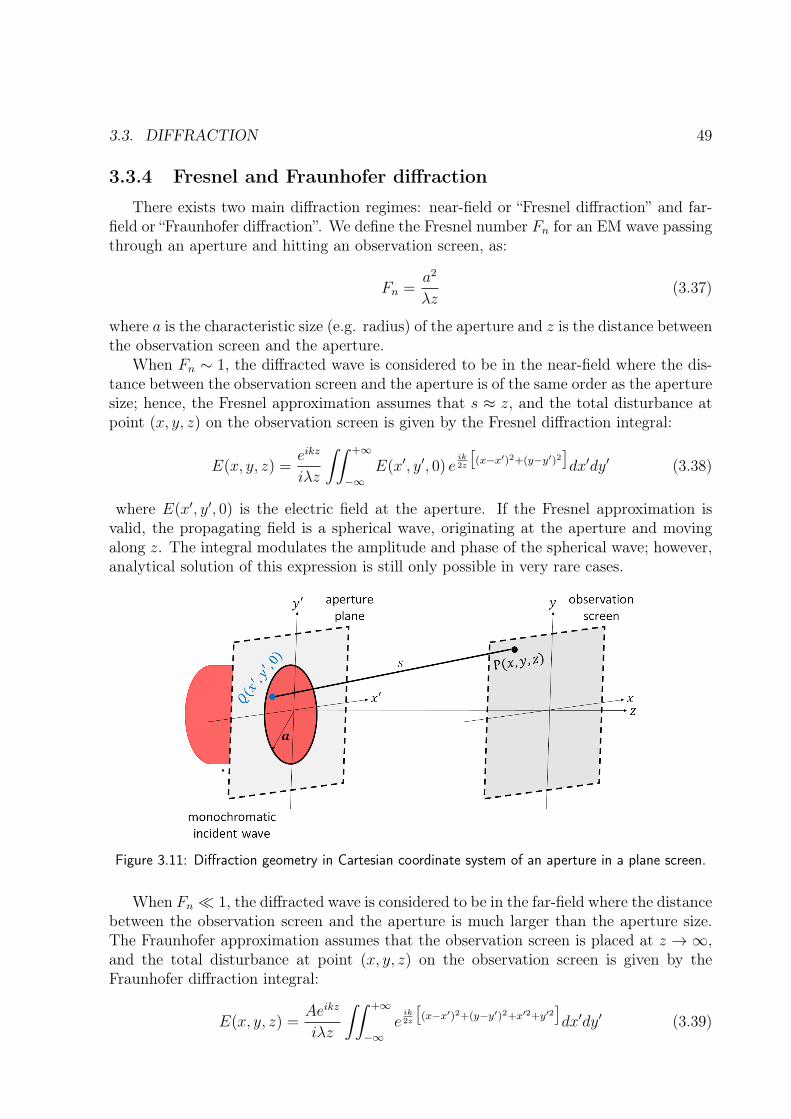
3.3.4 Fresnel and Fraunhofer diffraction
There exists two main diffraction regimes: near-field or “Fresnel diffraction” and far-field or “Fraunhofer diffraction”. We define the Fresnel number Fn for an EM wave passingthrough an aperture and hitting an observation screen, as:
Fn =a2
λz(3.37)
where a is the characteristic size (e.g. radius) of the aperture and z is the distance betweenthe observation screen and the aperture.
When Fn ∼ 1, the diffracted wave is considered to be in the near-field where the dis-tance between the observation screen and the aperture is of the same order as the aperturesize; hence, the Fresnel approximation assumes that s ≈ z, and the total disturbance atpoint (x, y, z) on the observation screen is given by the Fresnel diffraction integral:
E(x, y, z) =eikz
iλz
∫∫ +∞
−∞E(x′, y′, 0) e
ik2z
[(x−x′)2+(y−y′)2
]dx′dy′ (3.38)
where E(x′, y′, 0) is the electric field at the aperture. If the Fresnel approximation isvalid, the propagating field is a spherical wave, originating at the aperture and movingalong z. The integral modulates the amplitude and phase of the spherical wave; however,analytical solution of this expression is still only possible in very rare cases.
Figure 3.11: Diffraction geometry in Cartesian coordinate system of an aperture in a plane screen.
When Fn 1, the diffracted wave is considered to be in the far-field where the distancebetween the observation screen and the aperture is much larger than the aperture size.The Fraunhofer approximation assumes that the observation screen is placed at z →∞,and the total disturbance at point (x, y, z) on the observation screen is given by theFraunhofer diffraction integral:
E(x, y, z) =Aeikz
iλz
∫∫ +∞
−∞eik2z
[(x−x′)2+(y−y′)2+x′2+y′2
]dx′dy′ (3.39)
50 CHAPTER 3. ELECTROMAGNETIC WAVE PROPAGATION
where A is the complex amplitude of the incident plane wave at the aperture. TheFraunhofer approximation is a much simplified case; however, unlike Fresnel diffraction itdoes not account for the curvature of the wavefront to correctly calculate the relative phaseof interfering waves. We note that the Fraunhofer diffraction integral can be expressed invarious equivalent forms, notably as the Fourier transform of the aperture function.
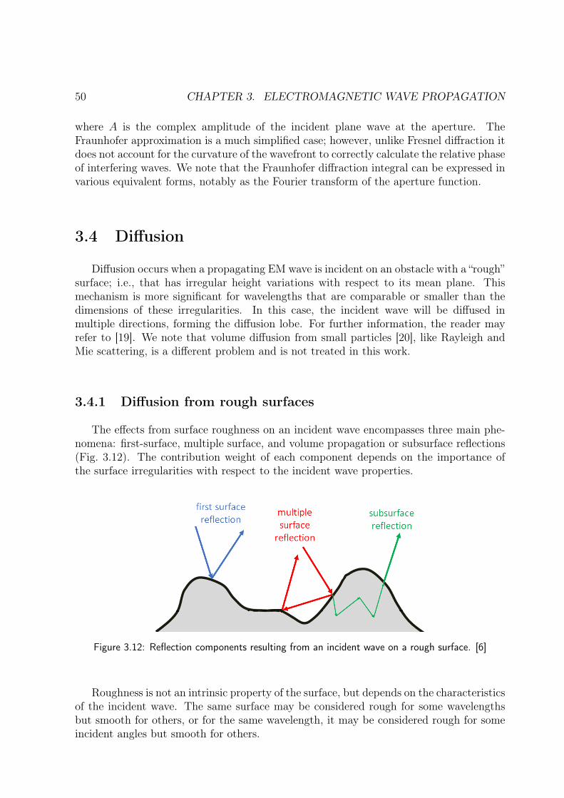
3.4 Diffusion
Diffusion occurs when a propagating EM wave is incident on an obstacle with a “rough”surface; i.e., that has irregular height variations with respect to its mean plane. Thismechanism is more significant for wavelengths that are comparable or smaller than thedimensions of these irregularities. In this case, the incident wave will be diffused inmultiple directions, forming the diffusion lobe. For further information, the reader mayrefer to [19]. We note that volume diffusion from small particles [20], like Rayleigh andMie scattering, is a different problem and is not treated in this work.
3.4.1 Diffusion from rough surfaces
The effects from surface roughness on an incident wave encompasses three main phe-nomena: first-surface, multiple surface, and volume propagation or subsurface reflections(Fig. 3.12). The contribution weight of each component depends on the importance ofthe surface irregularities with respect to the incident wave properties.
Figure 3.12: Reflection components resulting from an incident wave on a rough surface. [6]
Roughness is not an intrinsic property of the surface, but depends on the characteristicsof the incident wave. The same surface may be considered rough for some wavelengthsbut smooth for others, or for the same wavelength, it may be considered rough for someincident angles but smooth for others.
3.4. DIFFUSION 51
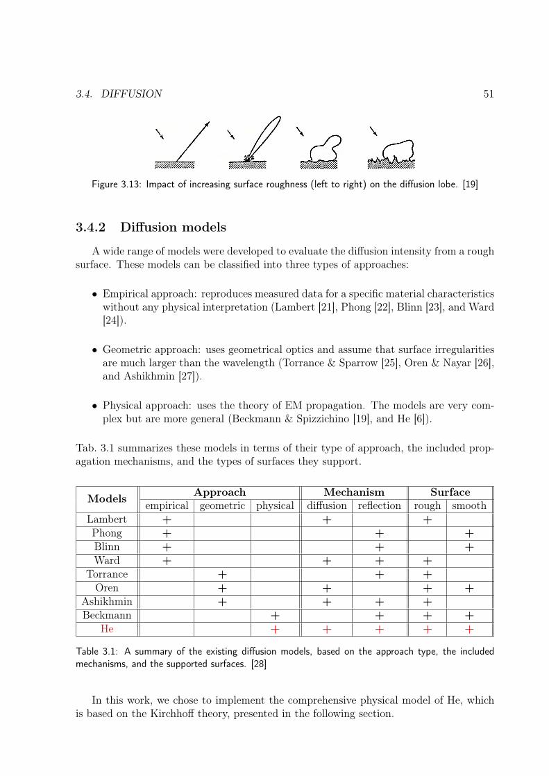
Figure 3.13: Impact of increasing surface roughness (left to right) on the diffusion lobe. [19]
3.4.2 Diffusion models
A wide range of models were developed to evaluate the diffusion intensity from a roughsurface. These models can be classified into three types of approaches:
• Empirical approach: reproduces measured data for a specific material characteristicswithout any physical interpretation (Lambert [21], Phong [22], Blinn [23], and Ward[24]).
• Geometric approach: uses geometrical optics and assume that surface irregularitiesare much larger than the wavelength (Torrance & Sparrow [25], Oren & Nayar [26],and Ashikhmin [27]).
• Physical approach: uses the theory of EM propagation. The models are very com-plex but are more general (Beckmann & Spizzichino [19], and He [6]).
Tab. 3.1 summarizes these models in terms of their type of approach, the included prop-agation mechanisms, and the types of surfaces they support.
Models Approach Mechanism Surfaceempirical geometric physical diffusion reflection rough smooth
Lambert + + +Phong + + +Blinn + + +Ward + + + +
Torrance + + +Oren + + + +
Ashikhmin + + + +Beckmann + + + +
He + + + + +
Table 3.1: A summary of the existing diffusion models, based on the approach type, the includedmechanisms, and the supported surfaces. [28]
In this work, we chose to implement the comprehensive physical model of He, whichis based on the Kirchhoff theory, presented in the following section.
52 CHAPTER 3. ELECTROMAGNETIC WAVE PROPAGATION
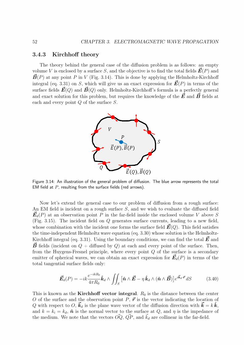
3.4.3 Kirchhoff theory
The theory behind the general case of the diffusion problem is as follows: an emptyvolume V is enclosed by a surface S, and the objective is to find the total fields ~E(P ) and~B(P ) at any point P in V (Fig. 3.14). This is done by applying the Helmholtz-Kirchhoffintegral (eq. 3.31) on S, which will give us an exact expression for ~E(P ) in terms of thesurface fields ~E(Q) and ~B(Q) only. Helmholtz-Kirchhoff’s formula is a perfectly generaland exact solution for this problem, but requires the knowledge of the ~E and ~B fields ateach and every point Q of the surface S.
Figure 3.14: An illustration of the general problem of diffusion. The blue arrow represents the totalEM field at P , resulting from the surface fields (red arrows).
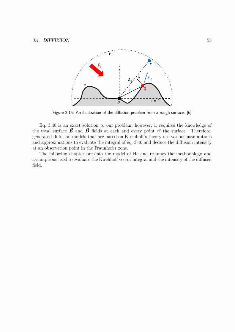
Now let’s extend the general case to our problem of diffusion from a rough surface:An EM field is incident on a rough surface S, and we wish to evaluate the diffused field~Ed(P ) at an observation point P in the far-field inside the enclosed volume V above S(Fig. 3.15). The incident field on Q generates surface currents, leading to a new field,whose combination with the incident one forms the surface field ~E(Q). This field satisfiesthe time-independent Helmholtz wave equation (eq. 3.30) whose solution is the Helmholtz-Kirchhoff integral (eq. 3.31). Using the boundary conditions, we can find the total ~E and~B fields (incident on Q + diffused by Q) at each and every point of the surface. Then,from the Huygens-Fresnel principle, where every point Q of the surface is a secondaryemitter of spherical waves, we can obtain an exact expression for ~Ed(P ) in terms of thetotal tangential surface fields only:
~Ed(P ) = −ik e−ikR0
4πR0
kd ∧∫∫
S
[n ∧ ~E − η kd ∧ (n ∧ ~B)
]ei~kd·~r dS (3.40)
This is known as the Kirchhoff vector integral. R0 is the distance between the centerO of the surface and the observation point P , ~r is the vector indicating the location ofQ with respect to O, ~kd is the plane wave vector of the diffusion direction with ~k = k k,and k = ki = kd, n is the normal vector to the surface at Q, and η is the impedance ofthe medium. We note that the vectors ~OQ, ~QP , and ~kd are collinear in the far-field.
3.4. DIFFUSION 53
Figure 3.15: An illustration of the diffusion problem from a rough surface. [6]
Eq. 3.40 is an exact solution to our problem; however, ir requires the knowledge ofthe total surface ~E and ~B fields at each and every point of the surface. Therefore,generated diffusion models that are based on Kirchhoff’s theory use various assumptionsand approximations to evaluate the integral of eq. 3.40 and deduce the diffusion intensityat an observation point in the Fraunhofer zone.
The following chapter presents the model of He and resumes the methodology andassumptions used to evaluate the Kirchhoff vector integral and the intensity of the diffusedfield.

54 CHAPTER 3. ELECTROMAGNETIC WAVE PROPAGATION
Chapter 4
He’s Diffusion Model
To our knowledge, He’s model is the latest and most comprehensive one. It encom-passes all the other models, supports different types of surface roughness and includes allmajor EM propagation mechanisms: reflection, diffusion, surface diffraction, interference,masking and shadowing. Although developed for visible light, its physical approach allowsit to be used for any frequency. Moreover, the vector nature of the EM wave is explicitand addresses polarization through diffused intensities. He’s model relies on the Kirchhoffapproximation and the height distribution model of the surface to evaluate eq. 3.40 anddeduce the diffused intensity. We note that the material in this chapter is mostly takenfrom [6].
4.1 Kirchhoff Approximation
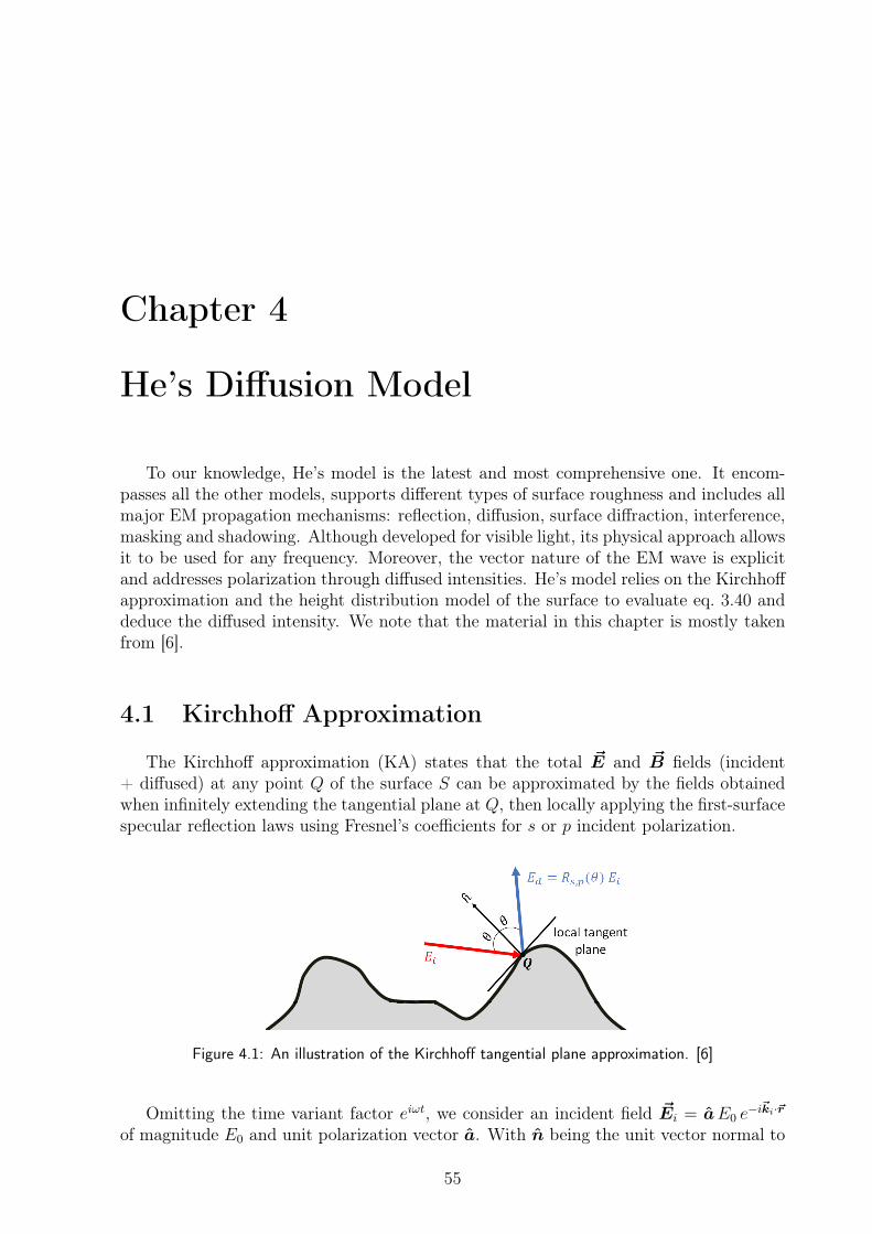
The Kirchhoff approximation (KA) states that the total ~E and ~B fields (incident+ diffused) at any point Q of the surface S can be approximated by the fields obtainedwhen infinitely extending the tangential plane at Q, then locally applying the first-surfacespecular reflection laws using Fresnel’s coefficients for s or p incident polarization.
Figure 4.1: An illustration of the Kirchhoff tangential plane approximation. [6]
Omitting the time variant factor eiωt, we consider an incident field ~Ei = aE0 e−i~ki·~r
of magnitude E0 and unit polarization vector a. With n being the unit vector normal to
55
56 CHAPTER 4. HE’S DIFFUSION MODEL
the local surface, we define t and d as:
t =ki ∧ n‖ki ∧ n‖
, d = ki ∧ t (4.1)
By decomposing the incident field to its s and p polarization, we can express the to-tal tangential fields in terms of the corresponding Fresnel coefficients Rs and Rp as thefollowing:
n ∧ ~E = [(1 +Rs)(a · t)(n ∧ t)− (1−Rp)(n · ki)(a · d) t ]E0
η(n ∧ ~B) = −[(1 +Rp)(a · d)(n ∧ t) + (1−Rs)(n · ki)(a · t) t ]E0
(4.2)
replacing eq. 4.2 in eq. 3.40, the diffused field at any observation point in the far-fieldabove the surface is expressed by the Kirchhoff approximation integral:
~Ed(P ) = −ik e−ikR0
4πR0
kd ∧∫∫
S
[n ∧ ~E − η kd ∧ (n ∧ ~B)
]ei(~kd−~ki)·~r dS (4.3)
The main difference with eq. 3.40 is the term (~kd−~ki) which appears in the integrand andrepresents the incident and diffused fields by each surface point. Moreover, ~E and ~B areno longer unknown, but are replaced by computable expressions. This solution is basedon the assumption that smooth-surface reflection occurs at each and every point on thesurface; this only holds when the local curvature radius of the surface is very large com-pared to the wavelength λ. Moreover, the Kirchhoff approximation integral as expressedabove, does not account for the shadowing effect nor does it take into account multi-ple surface and subsurface scattering, since only first-surface reflections are considered.eq. 4.3 is analytically very difficult to calculate, especially without any exact informationregarding the geometrical properties of the surface. However, an approximate value canbe obtained under various assumptions. One major assumption considered in He’s modelis the representation of the rough surface by the height distribution model.
4.2 Random Surface ModelingInformation regarding the length scales of the surface points compared to the wave-
length are crucial when using the Kirchhoff theory. We rarely have an exact geometricalrepresentation of a surface. However, since the observation point is always in the far-field,we are not interested in the microscopic variations of the EM field on the surface, as theyaverage out when viewed from a very large distance. Hence, we can rely on statisticalmodels where surface irregularities are modeled based on random processes. One of thesemodels is the height distribution model, used by He.
The random variable considered in this model is the height z of the irregularities withrespect to the mean surface plane in the (x, y) plane. z = ξ(x, y) is assumed to follow azero-mean Gaussian distribution with standard deviation σ0, and to be spatially isotropicover the surface realizations. The probability density function (PDF) of z is written as:
p(z) =1
σ0
√2π
e−z2/2σ2
0 (4.4)
4.2. RANDOM SURFACE MODELING 57
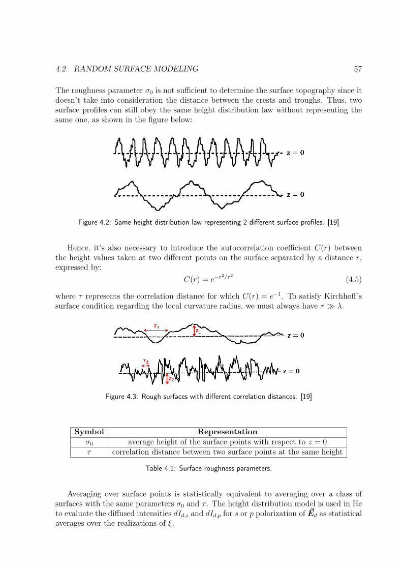
The roughness parameter σ0 is not sufficient to determine the surface topography since itdoesn’t take into consideration the distance between the crests and troughs. Thus, twosurface profiles can still obey the same height distribution law without representing thesame one, as shown in the figure below:
Figure 4.2: Same height distribution law representing 2 different surface profiles. [19]
Hence, it’s also necessary to introduce the autocorrelation coefficient C(r) betweenthe height values taken at two different points on the surface separated by a distance r,expressed by:
C(r) = e−r2/τ2 (4.5)
where τ represents the correlation distance for which C(r) = e−1. To satisfy Kirchhoff’ssurface condition regarding the local curvature radius, we must always have τ λ.
Figure 4.3: Rough surfaces with different correlation distances. [19]
Symbol Representationσ0 average height of the surface points with respect to z = 0τ correlation distance between two surface points at the same height
Table 4.1: Surface roughness parameters.
Averaging over surface points is statistically equivalent to averaging over a class ofsurfaces with the same parameters σ0 and τ . The height distribution model is used in Heto evaluate the diffused intensities dId,s and dId,p for s or p polarization of ~Ed as statisticalaverages over the realizations of ξ.
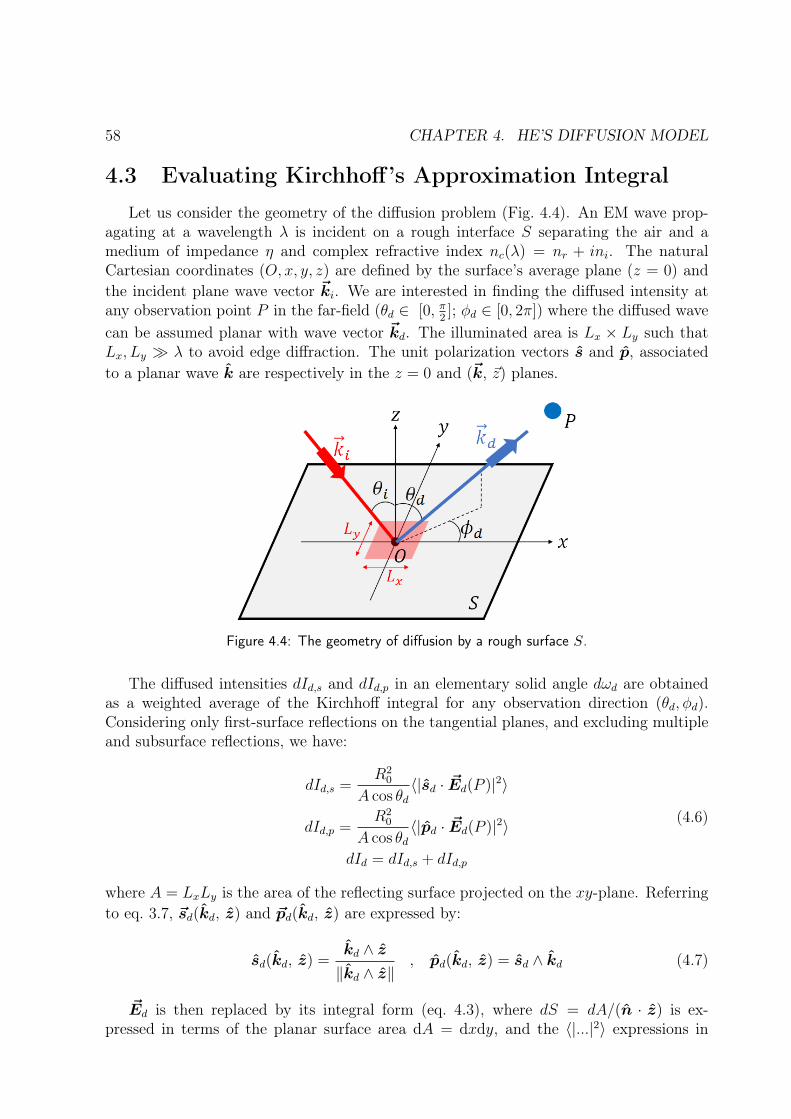
58 CHAPTER 4. HE’S DIFFUSION MODEL
4.3 Evaluating Kirchhoff’s Approximation IntegralLet us consider the geometry of the diffusion problem (Fig. 4.4). An EM wave prop-
agating at a wavelength λ is incident on a rough interface S separating the air and amedium of impedance η and complex refractive index nc(λ) = nr + ini. The naturalCartesian coordinates (O, x, y, z) are defined by the surface’s average plane (z = 0) andthe incident plane wave vector ~ki. We are interested in finding the diffused intensity atany observation point P in the far-field (θd ∈ [0, π
2]; φd ∈ [0, 2π]) where the diffused wave
can be assumed planar with wave vector ~kd. The illuminated area is Lx × Ly such thatLx, Ly λ to avoid edge diffraction. The unit polarization vectors s and p, associatedto a planar wave k are respectively in the z = 0 and (~k, ~z) planes.
Figure 4.4: The geometry of diffusion by a rough surface S.
The diffused intensities dId,s and dId,p in an elementary solid angle dωd are obtainedas a weighted average of the Kirchhoff integral for any observation direction (θd, φd).Considering only first-surface reflections on the tangential planes, and excluding multipleand subsurface reflections, we have:
dId,s =R2
0
A cos θd〈|sd · ~Ed(P )|2〉
dId,p =R2
0
A cos θd〈|pd · ~Ed(P )|2〉
dId = dId,s + dId,p
(4.6)
where A = LxLy is the area of the reflecting surface projected on the xy-plane. Referringto eq. 3.7, ~sd(kd, z) and ~pd(kd, z) are expressed by:
sd(kd, z) =kd ∧ z‖kd ∧ z‖
, pd(kd, z) = sd ∧ kd (4.7)
~Ed is then replaced by its integral form (eq. 4.3), where dS = dA/(n · z) is ex-pressed in terms of the planar surface area dA = dxdy, and the 〈|...|2〉 expressions in
4.4. BIDIRECTIONAL REFLECTANCE DISTRIBUTION FUNCTION 59
eq. 4.6 are expanded in terms of double surface integrals over two area elements from A,∫∫Adx1dy1
∫∫Adx2dy2.
Calculations are thus carried out on the irradiated parts of the surface only. Assumingthat the surface is isotropic and stationary, the integration is a function of x′ = x1 − x2
and y′ = y1 − y2. Thus, by integrating separately over x′′ = x2 and y′′ = y2, we get afactor S · A, where S is the fraction of the surface that is both illuminated and viewedand represents the shadowing function.
The remaining integrals depend only on the surface through the height distribution ξ,the tangent fields, and the normals n1 and n2 at two points of the surface. Refering toeq. 4.3, we define the function F involving the Fresnel coefficients and written accordingto the local tangential fields and the polarization vector through the following remainingdouble integral:
...
∫∫ +∞
−∞〈e−i(~kd−~ki)·z(ξ1−ξ2)F(n1, n2, a)〉dx′dy′ (4.8)
We denote σe the effective surface roughness which is a function of σ0 and representsthe illuminated and visible parts of the surface. If for (dωd, dωi) the surface is very rough,i.e. ((~kd −~ki)zσe)2 1 or if the surface has gentle slopes, i.e. σe τ , F is evaluated atnb, the unit bisector vector of ~kd and ~ki. F(n1, n2, a) ∼ F(nb, nb, a); thus, eq. 4.8 canbe rewritten as:
... F(nb, nb, a)
∫∫ +∞
−∞〈e−i(~kd−~ki)·z(ξ1−ξ2)〉dx′dy′ (4.9)
The integrand is developed in series; the first term N1 is the specular diffusion com-ponent, the rest N2 which is the directional diffusion component takes into account first-surface reflections (with diffraction and interference). The total diffused intensity in dωdcan then be rewritten in function of the Fresnel coefficient functions, the different diffusioncomponents and shadowing as follows:
dId(θd, φd) =|E0|2
(4π)2 cos θdS(N1 +N2)[F(nb, a)s + F(nb, a)p] (4.10)
where the square of the incident field amplitude |E0|2 is related to the incident intensityIi by |E0|2 = Iidωi. The subscripts s and p, denote respectively the s-polarization andp-polarization components of the F(nb, a) function.
Based on this result, He’s model expresses the statistical average of the diffused in-tensity Id(P ) over the realizations of S in terms of the incident one Ii, through theBidirectional Reflectance Distribution Function (BRDF).
4.4 Bidirectional Reflectance Distribution FunctionThe BRDF, denoted ρθi(θd, φd) in (sr−1), represents the spatial distribution of Id(P )
and is defined in He’s model as the ratio of total diffused intensity in the direction (θd, φd)to incident intensity on the surface element in the direction θi.
ρθi(θd, φd) =dId(θd, φd)
Ii(θi) cos θidωi(4.11)
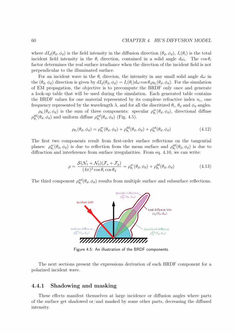
60 CHAPTER 4. HE’S DIFFUSION MODEL
where dId(θd, φd) is the field intensity in the diffusion direction (θd, φd), Ii(θi) is the totalincident field intensity in the θi direction, contained in a solid angle dωi. The cos θifactor determines the real surface irradiance when the direction of the incident field is notperpendicular to the illuminated surface.
For an incident wave in the θi direcion, the intensity in any small solid angle dω inthe (θd, φd) direction is given by dId(θd, φd) = Ii(θi)dω cos θiρθi(θd, φd). For the simulationof EM propagation, the objective is to precompute the BRDF only once and generatea look-up table that will be used during the simulation. Each generated table containsthe BRDF values for one material represented by its complexe refractive index nc, onefrequency represented by the wavelength λ, and for all the discritized θi, θd and φd angles.
ρθi(θd, φd) is the sum of three components: specular ρsrθi (θd, φd), directional diffuseρddθi (θd, φd) and uniform diffuse ρudθi (θd, φd) (Fig. 4.5).
ρθi(θd, φd) = ρsrθi (θd, φd) + ρddθi (θd, φd) + ρudθi (θd, φd) (4.12)
The first two components result from first-order surface reflections on the tangentialplanes: ρsrθi (θd, φd) is due to reflection from the mean surface and ρddθi (θd, φd) is due todiffraction and interference from surface irregularities. From eq. 4.10, we can write:
ρ =S(N1 +N2)(Fs + Fp)
(4π)2 cos θi cos θd= ρsrθi (θd, φd) + ρddθi (θd, φd) (4.13)
The third component ρudθi (θd, φd) results from multiple surface and subsurface reflections.
Figure 4.5: An illustration of the BRDF components.
The next sections present the expressions derivation of each BRDF component for apolarized incident wave.
4.4.1 Shadowing and masking
These effects manifest themselves at large incidence or diffusion angles where partsof the surface get shadowed or/and masked by some other parts, decreasing the diffusedintensity.
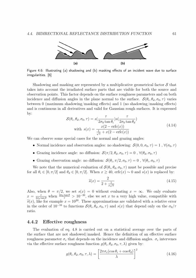
4.4. BIDIRECTIONAL REFLECTANCE DISTRIBUTION FUNCTION 61
Figure 4.6: Illustrating (a) shadowing and (b) masking effects of an incident wave due to surfaceirregularities. [6]
Shadowing and masking are represented by a multiplicative geometrical factor S thattakes into account the irradiated surface parts that are visible for both the source andobservation points. This factor depends on the surface roughness parameters and on bothincidence and diffusion angles in the plane normal to the surface. S(θi, θd, σ0, τ) variesbetween 0 (maximum shadowing/masking effects) and 1 (no shadowing/masking effects)and is continuous in all derivatives and valid for Gaussian rough surfaces. It is expressedby:
S(θi, θd, σ0, τ) = s(τ
2σ0 tan θi)s(
τ
2σ0 tan θd)
with s(x) =x(2− erfc(x))
1√π
+ x(2− erfc(x))
(4.14)
We can observe some special cases for the normal and grazing angles:
• Normal incidence and observation angles: no shadowing: S(0, 0, σ0, τ) = 1 , ∀(σ0, τ)
• Grazing incidence angle: no diffusion: S(π/2, θd, σ0, τ) = 0 , ∀(θd, σ0, τ)
• Grazing observation angle: no diffusion: S(θi, π/2, σ0, τ) = 0 , ∀(θi, σ0, τ)
We note that the numerical evaluation of S(θi, θd, σ0, τ) must be possible and precisefor all θi ∈ [0, π/2] and θd ∈ [0, π/2]. When x ≥ 40, erfc(x) ∼ 0 and s(x) is replaced by:
s(x) =2
2 + 1x√π
(4.15)
Also, when θ = π/2, we set s(x) = 0 without evaluating x = ∞. We only evaluatex = τ
2σ0 tan θwhen 2σ0 tan θ
τ> 10−20, else we set x to a very high value, compatible with
s(x), like for example x = 1020. These approximations are validated with a relative errorin the order of 10−16 to functions S(θi, θd, σ0, τ) and s(x) that depend only on the σ0/τratio.
4.4.2 Effective roughness
The evaluation of eq. 4.8 is carried out on a statistical average over the parts ofthe surface that are not shadowed/masked. Hence the definition of an effective surfaceroughness parameter σe that depends on the incidence and diffusion angles. σe intervenesvia the effective surface roughness function g(θi, θd, σ0, τ, λ) given by:
g(θi, θd, σ0, τ, λ) =
[2πσe(cos θi + cos θd)
λ
]2
(4.16)
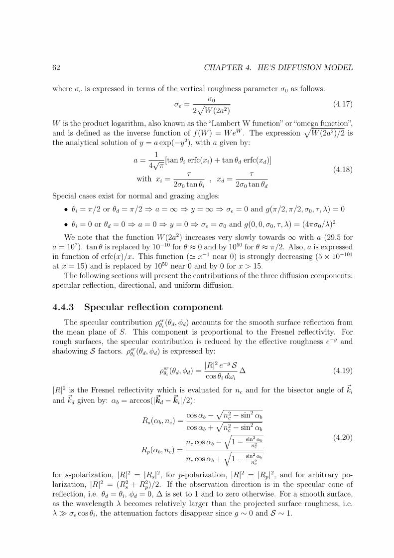
62 CHAPTER 4. HE’S DIFFUSION MODEL
where σe is expressed in terms of the vertical roughness parameter σ0 as follows:
σe =σ0
2√W (2a2)
(4.17)
W is the product logarithm, also known as the “Lambert W function” or “omega function”,and is defined as the inverse function of f(W ) = WeW . The expression
√W (2a2)/2 is
the analytical solution of y = a exp(−y2), with a given by:
a =1
4√π
[tan θi erfc(xi) + tan θd erfc(xd)]
with xi =τ
2σ0 tan θi, xd =
τ
2σ0 tan θd
(4.18)
Special cases exist for normal and grazing angles:
• θi = π/2 or θd = π/2 ⇒ a =∞ ⇒ y =∞ ⇒ σe = 0 and g(π/2, π/2, σ0, τ, λ) = 0
• θi = 0 or θd = 0 ⇒ a = 0 ⇒ y = 0 ⇒ σe = σ0 and g(0, 0, σ0, τ, λ) = (4πσ0/λ)2
We note that the function W (2a2) increases very slowly towards ∞ with a (29.5 fora = 107). tan θ is replaced by 10−10 for θ ≈ 0 and by 1050 for θ ≈ π/2. Also, a is expressedin function of erfc(x)/x. This function (' x−1 near 0) is strongly decreasing (5 × 10−101
at x = 15) and is replaced by 1050 near 0 and by 0 for x > 15.The following sections will present the contributions of the three diffusion components:
specular reflection, directional, and uniform diffusion.
4.4.3 Specular reflection component
The specular contribution ρsrθi (θd, φd) accounts for the smooth surface reflection fromthe mean plane of S. This component is proportional to the Fresnel reflectivity. Forrough surfaces, the specular contribution is reduced by the effective roughness e−g andshadowing S factors. ρsrθi (θd, φd) is expressed by:
ρsrθi (θd, φd) =|R|2 e−g Scos θi dωi
∆ (4.19)
|R|2 is the Fresnel reflectivity which is evaluated for nc and for the bisector angle of ~kiand ~kd given by: αb = arccos(|~kd −~ki|/2):
Rs(αb, nc) =cosαb −
√n2c − sin2 αb
cosαb +√n2c − sin2 αb
Rp(αb, nc) =nc cosαb −
√1− sin2 αb
n2c
nc cosαb +√
1− sin2 αbn2c
(4.20)
for s-polarization, |R|2 = |Rs|2, for p-polarization, |R|2 = |Rp|2, and for arbitrary po-larization, |R|2 = (R2
s + R2p)/2. If the observation direction is in the specular cone of
reflection, i.e. θd = θi, φd = 0, ∆ is set to 1 and to zero otherwise. For a smooth surface,as the wavelength λ becomes relatively larger than the projected surface roughness, i.e.λ σe cos θi, the attenuation factors disappear since g ∼ 0 and S ∼ 1.
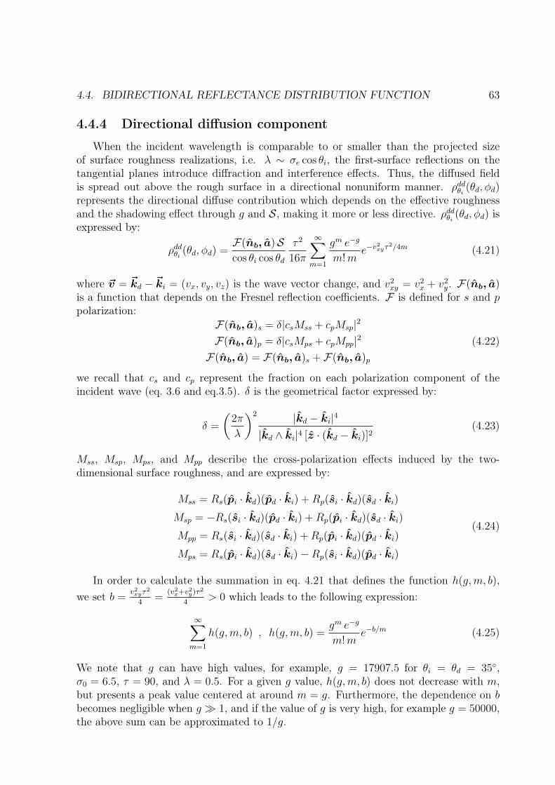
4.4. BIDIRECTIONAL REFLECTANCE DISTRIBUTION FUNCTION 63
4.4.4 Directional diffusion component
When the incident wavelength is comparable to or smaller than the projected sizeof surface roughness realizations, i.e. λ ∼ σe cos θi, the first-surface reflections on thetangential planes introduce diffraction and interference effects. Thus, the diffused fieldis spread out above the rough surface in a directional nonuniform manner. ρddθi (θd, φd)represents the directional diffuse contribution which depends on the effective roughnessand the shadowing effect through g and S, making it more or less directive. ρddθi (θd, φd) isexpressed by:
ρddθi (θd, φd) =F(nb, a)Scos θi cos θd
τ 2
16π
∞∑m=1
gm e−g
m!me−v
2xyτ
2/4m (4.21)
where ~v = ~kd − ~ki = (vx, vy, vz) is the wave vector change, and v2xy = v2
x + v2y. F(nb, a)
is a function that depends on the Fresnel reflection coefficients. F is defined for s and ppolarization:
F(nb, a)s = δ|csMss + cpMsp|2
F(nb, a)p = δ|csMps + cpMpp|2
F(nb, a) = F(nb, a)s + F(nb, a)p
(4.22)
we recall that cs and cp represent the fraction on each polarization component of theincident wave (eq. 3.6 and eq.3.5). δ is the geometrical factor expressed by:
δ =
(2π
λ
)2 |kd − ki|4
|kd ∧ ki|4 [z · (kd − ki)]2(4.23)
Mss, Msp, Mps, and Mpp describe the cross-polarization effects induced by the two-dimensional surface roughness, and are expressed by:
Mss = Rs(pi · kd)(pd · ki) +Rp(si · kd)(sd · ki)Msp = −Rs(si · kd)(pd · ki) +Rp(pi · kd)(sd · ki)Mpp = Rs(si · kd)(sd · ki) +Rp(pi · kd)(pd · ki)Mps = Rs(pi · kd)(sd · ki)−Rp(si · kd)(pd · ki)
(4.24)
In order to calculate the summation in eq. 4.21 that defines the function h(g,m, b),we set b =
v2xyτ2
4=
(v2x+v2y)τ2
4> 0 which leads to the following expression:
∞∑m=1
h(g,m, b) , h(g,m, b) =gm e−g
m!me−b/m (4.25)
We note that g can have high values, for example, g = 17907.5 for θi = θd = 35,σ0 = 6.5, τ = 90, and λ = 0.5. For a given g value, h(g,m, b) does not decrease with m,but presents a peak value centered at around m = g. Furthermore, the dependence on bbecomes negligible when g 1, and if the value of g is very high, for example g = 50000,the above sum can be approximated to 1/g.
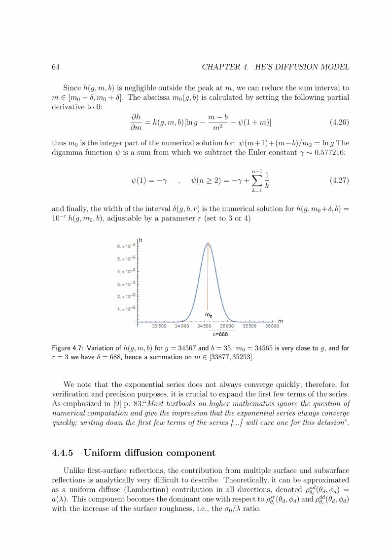
64 CHAPTER 4. HE’S DIFFUSION MODEL
Since h(g,m, b) is negligible outside the peak at m, we can reduce the sum interval tom ∈ [m0 − δ,m0 + δ]. The abscissa m0(g, b) is calculated by setting the following partialderivative to 0:
∂h
∂m= h(g,m, b)[ln g − m− b
m2− ψ(1 +m)] (4.26)
thusm0 is the integer part of the numerical solution for: ψ(m+1)+(m−b)/m2 = ln g Thedigamma function ψ is a sum from which we subtract the Euler constant γ ∼ 0.577216:
ψ(1) = −γ , ψ(n ≥ 2) = −γ +n−1∑k=1
1
k(4.27)
and finally, the width of the interval δ(g, b, r) is the numerical solution for h(g,m0 +δ, b) =10−r h(g,m0, b), adjustable by a parameter r (set to 3 or 4)
Figure 4.7: Variation of h(g,m, b) for g = 34567 and b = 35. m0 = 34565 is very close to g, and forr = 3 we have δ = 688, hence a summation on m ∈ [33877, 35253].
We note that the exponential series does not always converge quickly; therefore, forverification and precision purposes, it is crucial to expand the first few terms of the series.As emphasized in [9] p. 83:“Most textbooks on higher mathematics ignore the question ofnumerical computation and give the impression that the exponential series always convergequickly; writing down the first few terms of the series [...] will cure one for this delusion”.
4.4.5 Uniform diffusion component
Unlike first-surface reflections, the contribution from multiple surface and subsurfacereflections is analytically very difficult to describe. Theoretically, it can be approximatedas a uniform diffuse (Lambertian) contribution in all directions, denoted ρudθi (θd, φd) =a(λ). This component becomes the dominant one with respect to ρsrθi (θd, φd) and ρ
ddθi
(θd, φd)with the increase of the surface roughness, i.e., the σ0/λ ratio.
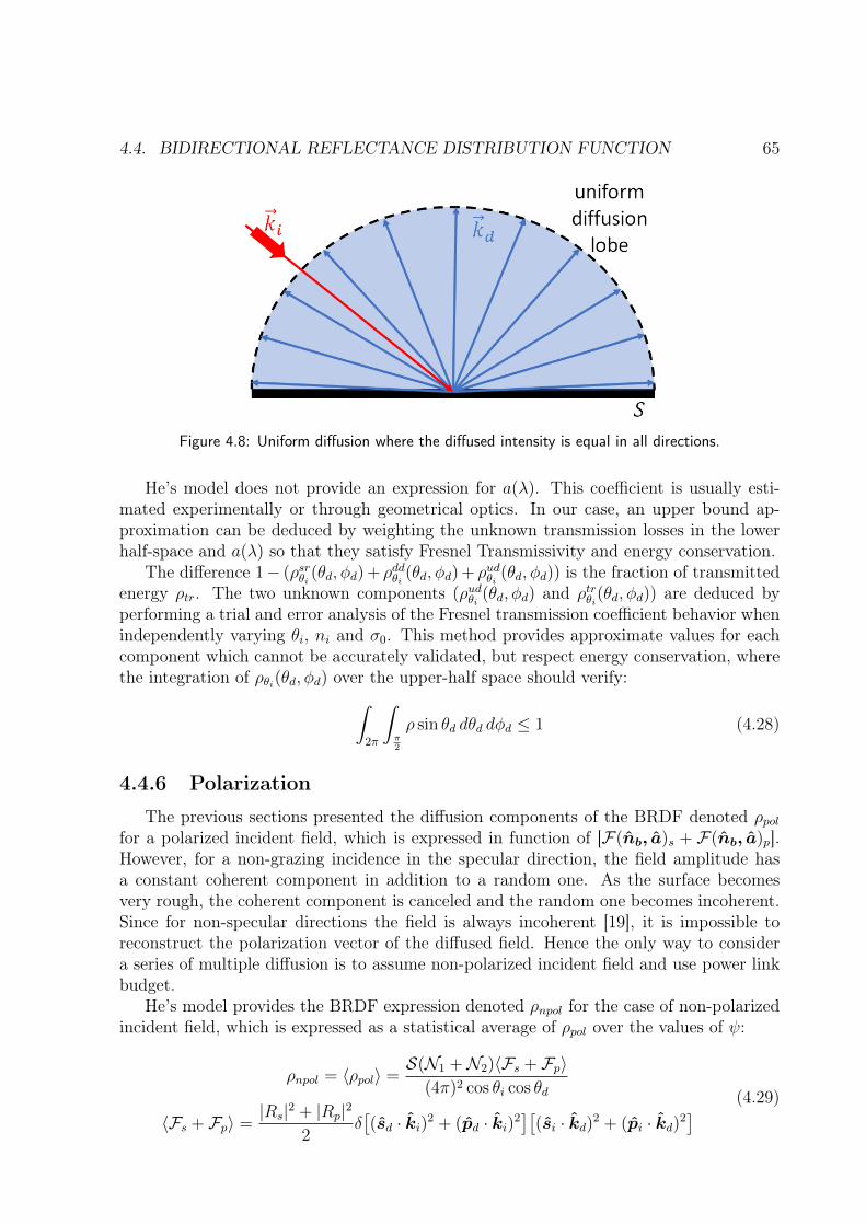
4.4. BIDIRECTIONAL REFLECTANCE DISTRIBUTION FUNCTION 65
Figure 4.8: Uniform diffusion where the diffused intensity is equal in all directions.
He’s model does not provide an expression for a(λ). This coefficient is usually esti-mated experimentally or through geometrical optics. In our case, an upper bound ap-proximation can be deduced by weighting the unknown transmission losses in the lowerhalf-space and a(λ) so that they satisfy Fresnel Transmissivity and energy conservation.
The difference 1− (ρsrθi (θd, φd) + ρddθi (θd, φd) + ρudθi (θd, φd)) is the fraction of transmittedenergy ρtr. The two unknown components (ρudθi (θd, φd) and ρtrθi(θd, φd)) are deduced byperforming a trial and error analysis of the Fresnel transmission coefficient behavior whenindependently varying θi, ni and σ0. This method provides approximate values for eachcomponent which cannot be accurately validated, but respect energy conservation, wherethe integration of ρθi(θd, φd) over the upper-half space should verify:∫
2π
∫π2
ρ sin θd dθd dφd ≤ 1 (4.28)
4.4.6 Polarization
The previous sections presented the diffusion components of the BRDF denoted ρpolfor a polarized incident field, which is expressed in function of [F(nb, a)s + F(nb, a)p].However, for a non-grazing incidence in the specular direction, the field amplitude hasa constant coherent component in addition to a random one. As the surface becomesvery rough, the coherent component is canceled and the random one becomes incoherent.Since for non-specular directions the field is always incoherent [19], it is impossible toreconstruct the polarization vector of the diffused field. Hence the only way to considera series of multiple diffusion is to assume non-polarized incident field and use power linkbudget.
He’s model provides the BRDF expression denoted ρnpol for the case of non-polarizedincident field, which is expressed as a statistical average of ρpol over the values of ψ:
ρnpol = 〈ρpol〉 =S(N1 +N2)〈Fs + Fp〉
(4π)2 cos θi cos θd
〈Fs + Fp〉 =|Rs|2 + |Rp|2
2δ[(sd · ki)2 + (pd · ki)2
][(si · kd)2 + (pi · kd)2
] (4.29)
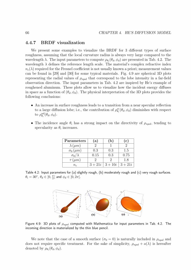
66 CHAPTER 4. HE’S DIFFUSION MODEL
4.4.7 BRDF visualization
We present some examples to visualize the BRDF for 3 different types of surfaceroughness, assuming that the local curvature radius is always very large compared to thewavelength λ. The input parameters to compute ρθi(θd, φd) are presented in Tab. 4.2. Thewavelength λ defines the reference length scale. The material’s complex refractive indexnc(λ) required for the Fresnel coefficient is not usually known a priori; measurement valuescan be found in [29] and [30] for some typical materials. Fig. 4.9 are spherical 3D plotsrepresenting the radial values of ρnpol that correspond to the lobe intensity in a far-fieldobservation direction. The input parameters in Tab. 4.2 are inspired by He’s example ofroughened aluminum. These plots allow us to visualize how the incident energy diffusesin space as a function of (θd, φd). The physical interpretation of the 3D plots provides thefollowing conclusions:
• An increase in surface roughness leads to a transition from a near specular reflectionto a large diffusion lobe; i.e., the contribution of ρsrθi (θd, φd) diminishes with respectto ρudθi (θd, φd).
• The incidence angle θi has a strong impact on the directivity of ρnpol, tending tospecularity as θi increases.
Parameters (a) (b) (c)λ (µm) 2 1 2σ0 (µm) 0.3 0.3 1.5σ0/λ 0.15 0.3 0.75τ (µm) 2 2 1.8nc 3 + 21i 3 + 10i 3 + 21i
Table 4.2: Input parameters for (a) slightly rough, (b) moderately rough and (c) very rough surfaces.θi = 30, θd ∈ [0, π2 ] and φd ∈ [0, 2π].
Figure 4.9: 3D plots of ρnpol computed with Mathematica for input parameters in Tab. 4.2. Theincoming direction is materialized by the thin blue pencil.
We note that the case of a smooth surface (σ0 = 0) is naturally included in ρnpol anddoes not require specific treatment. For the sake of simplicity, ρnpol + a(λ) is hereafterdenoted by ρθi(θd, φd).
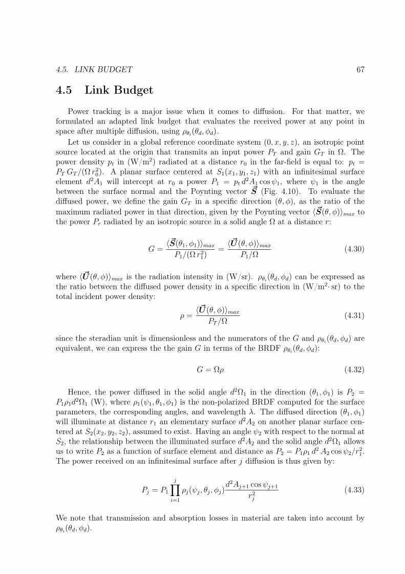
4.5. LINK BUDGET 67
4.5 Link Budget
Power tracking is a major issue when it comes to diffusion. For that matter, weformulated an adapted link budget that evaluates the received power at any point inspace after multiple diffusion, using ρθi(θd, φd).
Let us consider in a global reference coordinate system (0, x, y, z), an isotropic pointsource located at the origin that transmits an input power PT and gain GT in Ω. Thepower density pt in (W/m2) radiated at a distance r0 in the far-field is equal to: pt =PT GT/(Ω r2
0). A planar surface centered at S1(x1, y1, z1) with an infinitesimal surfaceelement d2A1 will intercept at r0 a power P1 = pt d
2A1 cosψ1, where ψ1 is the anglebetween the surface normal and the Poynting vector ~S (Fig. 4.10). To evaluate thediffused power, we define the gain GT in a specific direction (θ, φ), as the ratio of themaximum radiated power in that direction, given by the Poynting vector 〈~S(θ, φ)〉max tothe power Pr radiated by an isotropic source in a solid angle Ω at a distance r:
G =〈~S(θ1, φ1)〉maxP1/(Ω r2
1)=〈~U(θ, φ)〉max
P1/Ω(4.30)
where 〈~U(θ, φ)〉max is the radiation intensity in (W/sr). ρθi(θd, φd) can be expressed asthe ratio between the diffused power density in a specific direction in (W/m2· sr) to thetotal incident power density:
ρ =〈~U(θ, φ)〉max
PT/Ω(4.31)
since the steradian unit is dimensionless and the numerators of the G and ρθi(θd, φd) areequivalent, we can express the the gain G in terms of the BRDF ρθi(θd, φd):
G = Ωρ (4.32)
Hence, the power diffused in the solid angle d2Ω1 in the direction (θ1, φ1) is P2 =P1ρ1d
2Ω1 (W), where ρ1(ψ1, θ1, φ1) is the non-polarized BRDF computed for the surfaceparameters, the corresponding angles, and wavelength λ. The diffused direction (θ1, φ1)will illuminate at distance r1 an elementary surface d2A2 on another planar surface cen-tered at S2(x2, y2, z2), assumed to exist. Having an angle ψ2 with respect to the normal atS2, the relationship between the illuminated surface d2A2 and the solid angle d2Ω1 allowsus to write P2 as a function of surface element and distance as P2 = P1ρ1 d
2A2 cosψ2/r21.
The power received on an infinitesimal surface after j diffusion is thus given by:
Pj = P1
j∏i=1
ρj(ψj, θj, φj)d2Aj+1 cosψj+1
r2j
(4.33)
We note that transmission and absorption losses in material are taken into account byρθi(θd, φd).
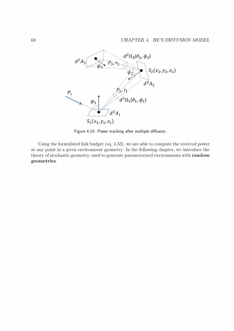
68 CHAPTER 4. HE’S DIFFUSION MODEL
Figure 4.10: Power tracking after multiple diffusion.
Using the formulated link budget (eq. 4.33), we are able to compute the received powerat any point in a given environment geometry. In the following chapter, we introduce thetheory of stochastic geometry, used to generate parameterized environments with randomgeometries.
Chapter 5
Stochastic Geometry
Stochastic geometry is a powerful tool used to generate mathematical models basedon spatial probabilities [31]. It provides statistical information about the random config-urations that we wish to analyze. This tool is used in several disciplines like computervision [32], fixed [33] and wireless networks [34], where analytic calculations and/or simu-lations can be done with a low number of input parameters. This chapter provides a briefreview of the mathematical theory of stochastic geometry, used to generate parameterizedtypical 3D indoor environments. The following sections first present the Poisson pointprocess which is the basis of many tessellation models, then the Poisson Line and STITtessellations along with their morphology features and fitting characteristics. For furtherinformation, the reader may refer to [35].
5.1 Poisson Point Process
In probability and statistics, a Poisson point process (named after the French math-ematician Siméon Denis Poisson) consists of randomly positioned points located on anunderlying mathematical space of finite size, where the number of points is a random vari-able with a Poisson distribution, and the positions of the generated points are completelyindependent of each other. In this section, we will be considering the spatial Poissonpoint process defined in the Euclidean R2 space. This process is frequently used to modelseemingly disordered spatial configurations of certain wireless communication networks,where it is assumed that the base stations are positioned according to a Poisson pointprocess.
5.1.1 Definition and properties
A point process X is a finite random subset of a given bounded region S ⊂ R2. Therealization of X is a point pattern x = x1, ..., xn of n ≥ 0 points in S. The distributionof X is specified according to the probability distribution of a random variable N suchthat N = n for all the n points in X with n ≥ 1. This is equivalent to specifying thedistribution of the count variables N(B) for subsets B ⊆ S. The specificity of the Poissonpoint process is that it has two key properties:
69
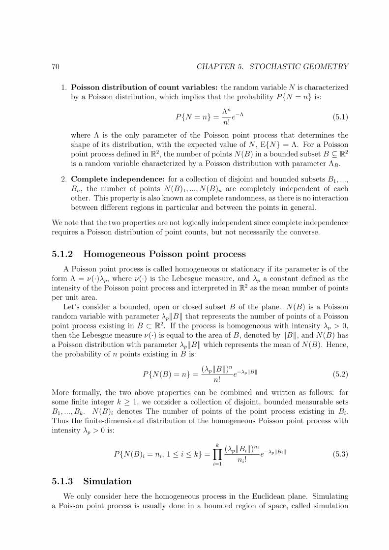
70 CHAPTER 5. STOCHASTIC GEOMETRY
1. Poisson distribution of count variables: the random variable N is characterizedby a Poisson distribution, which implies that the probability PN = n is:
PN = n =Λn
n!e−Λ (5.1)
where Λ is the only parameter of the Poisson point process that determines theshape of its distribution, with the expected value of N , EN = Λ. For a Poissonpoint process defined in R2, the number of points N(B) in a bounded subset B ⊆ R2
is a random variable characterized by a Poisson distribution with parameter ΛB.
2. Complete independence: for a collection of disjoint and bounded subsets B1, ...,Bn, the number of points N(B)1, ..., N(B)n are completely independent of eachother. This property is also known as complete randomness, as there is no interactionbetween different regions in particular and between the points in general.
We note that the two properties are not logically independent since complete independencerequires a Poisson distribution of point counts, but not necessarily the converse.
5.1.2 Homogeneous Poisson point process
A Poisson point process is called homogeneous or stationary if its parameter is of theform Λ = ν(·)λp, where ν(·) is the Lebesgue measure, and λp a constant defined as theintensity of the Poisson point process and interpreted in R2 as the mean number of pointsper unit area.
Let’s consider a bounded, open or closed subset B of the plane. N(B) is a Poissonrandom variable with parameter λp‖B‖ that represents the number of points of a Poissonpoint process existing in B ⊂ R2. If the process is homogeneous with intensity λp > 0,then the Lebesgue measure ν(·) is equal to the area of B, denoted by ‖B‖, and N(B) hasa Poisson distribution with parameter λp‖B‖ which represents the mean of N(B). Hence,the probability of n points existing in B is:
PN(B) = n =(λp‖B‖)n
n!e−λp‖B‖ (5.2)
More formally, the two above properties can be combined and written as follows: forsome finite integer k ≥ 1, we consider a collection of disjoint, bounded measurable setsB1, ..., Bk. N(B)i denotes The number of points of the point process existing in Bi.Thus the finite-dimensional distribution of the homogeneous Poisson point process withintensity λp > 0 is:
PN(B)i = ni, 1 ≤ i ≤ k =k∏i=1
(λp‖Bi‖)nini!
e−λp‖Bi‖ (5.3)
5.1.3 Simulation
We only consider here the homogeneous process in the Euclidean plane. Simulatinga Poisson point process is usually done in a bounded region of space, called simulation
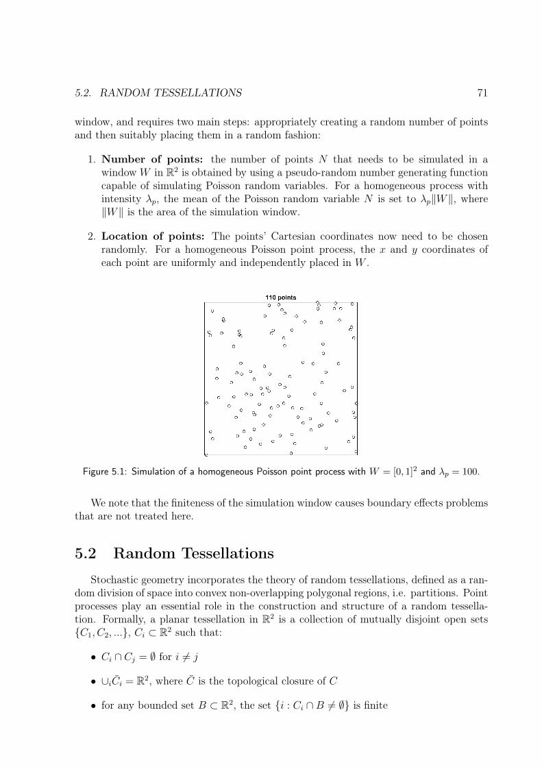
5.2. RANDOM TESSELLATIONS 71
window, and requires two main steps: appropriately creating a random number of pointsand then suitably placing them in a random fashion:
1. Number of points: the number of points N that needs to be simulated in awindow W in R2 is obtained by using a pseudo-random number generating functioncapable of simulating Poisson random variables. For a homogeneous process withintensity λp, the mean of the Poisson random variable N is set to λp‖W‖, where‖W‖ is the area of the simulation window.
2. Location of points: The points’ Cartesian coordinates now need to be chosenrandomly. For a homogeneous Poisson point process, the x and y coordinates ofeach point are uniformly and independently placed in W .
Figure 5.1: Simulation of a homogeneous Poisson point process with W = [0, 1]2 and λp = 100.
We note that the finiteness of the simulation window causes boundary effects problemsthat are not treated here.
5.2 Random Tessellations
Stochastic geometry incorporates the theory of random tessellations, defined as a ran-dom division of space into convex non-overlapping polygonal regions, i.e. partitions. Pointprocesses play an essential role in the construction and structure of a random tessella-tion. Formally, a planar tessellation in R2 is a collection of mutually disjoint open setsC1, C2, ..., Ci ⊂ R2 such that:
• Ci ∩ Cj = ∅ for i 6= j
• ∪iCi = R2, where C is the topological closure of C
• for any bounded set B ⊂ R2, the set i : Ci ∩B 6= ∅ is finite
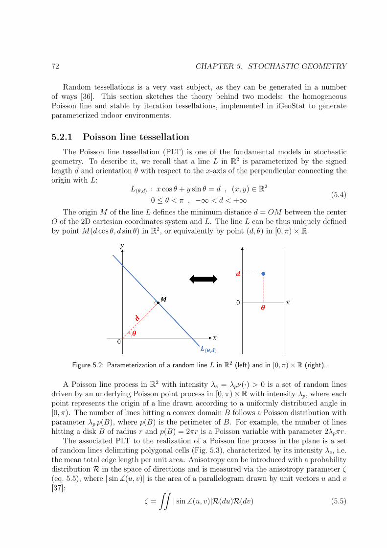
72 CHAPTER 5. STOCHASTIC GEOMETRY
Random tessellations is a very vast subject, as they can be generated in a numberof ways [36]. This section sketches the theory behind two models: the homogeneousPoisson line and stable by iteration tessellations, implemented in iGeoStat to generateparameterized indoor environments.
5.2.1 Poisson line tessellation
The Poisson line tessellation (PLT) is one of the fundamental models in stochasticgeometry. To describe it, we recall that a line L in R2 is parameterized by the signedlength d and orientation θ with respect to the x-axis of the perpendicular connecting theorigin with L:
L(θ,d) : x cos θ + y sin θ = d , (x, y) ∈ R2
0 ≤ θ < π , −∞ < d < +∞(5.4)
The origin M of the line L defines the minimum distance d = OM between the centerO of the 2D cartesian coordinates system and L. The line L can be thus uniquely definedby point M(d cos θ, d sin θ) in R2, or equivalently by point (d, θ) in [0, π)× R.
Figure 5.2: Parameterization of a random line L in R2 (left) and in [0, π)× R (right).
A Poisson line process in R2 with intensity λe = λpν(·) > 0 is a set of random linesdriven by an underlying Poisson point process in [0, π)×R with intensity λp, where eachpoint represents the origin of a line drawn according to a uniformly distributed angle in[0, π). The number of lines hitting a convex domain B follows a Poisson distribution withparameter λp p(B), where p(B) is the perimeter of B. For example, the number of lineshitting a disk B of radius r and p(B) = 2πr is a Poisson variable with parameter 2λpπr.
The associated PLT to the realization of a Poisson line process in the plane is a setof random lines delimiting polygonal cells (Fig. 5.3), characterized by its intensity λe, i.e.the mean total edge length per unit area. Anisotropy can be introduced with a probabilitydistribution R in the space of directions and is measured via the anisotropy parameter ζ(eq. 5.5), where | sin](u, v)| is the area of a parallelogram drawn by unit vectors u and v[37]:
ζ =
∫∫| sin](u, v)|R(du)R(dv) (5.5)
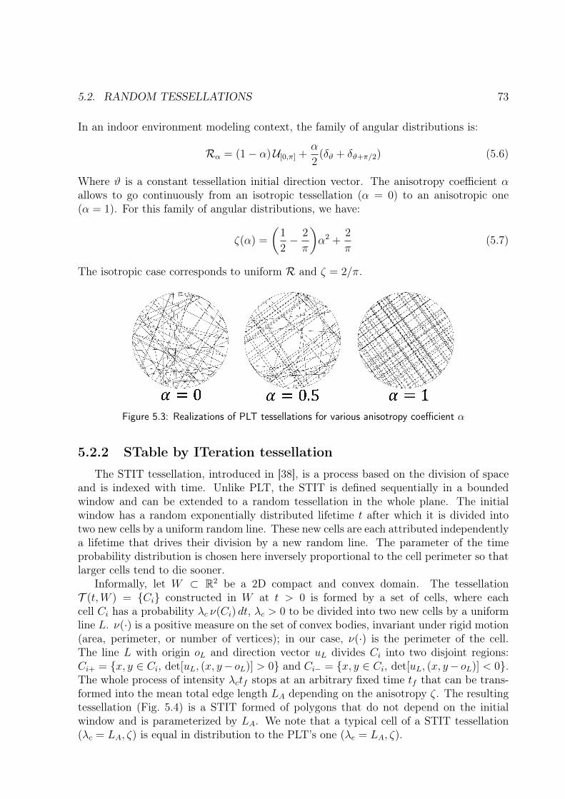
5.2. RANDOM TESSELLATIONS 73
In an indoor environment modeling context, the family of angular distributions is:
Rα = (1− α)U[0,π] +α
2(δϑ + δϑ+π/2) (5.6)
Where ϑ is a constant tessellation initial direction vector. The anisotropy coefficient αallows to go continuously from an isotropic tessellation (α = 0) to an anisotropic one(α = 1). For this family of angular distributions, we have:
ζ(α) =
(1
2− 2
π
)α2 +
2
π(5.7)
The isotropic case corresponds to uniform R and ζ = 2/π.
Figure 5.3: Realizations of PLT tessellations for various anisotropy coefficient α
5.2.2 STable by ITeration tessellation
The STIT tessellation, introduced in [38], is a process based on the division of spaceand is indexed with time. Unlike PLT, the STIT is defined sequentially in a boundedwindow and can be extended to a random tessellation in the whole plane. The initialwindow has a random exponentially distributed lifetime t after which it is divided intotwo new cells by a uniform random line. These new cells are each attributed independentlya lifetime that drives their division by a new random line. The parameter of the timeprobability distribution is chosen here inversely proportional to the cell perimeter so thatlarger cells tend to die sooner.
Informally, let W ⊂ R2 be a 2D compact and convex domain. The tessellationT (t,W ) = Ci constructed in W at t > 0 is formed by a set of cells, where eachcell Ci has a probability λc ν(Ci) dt, λc > 0 to be divided into two new cells by a uniformline L. ν(·) is a positive measure on the set of convex bodies, invariant under rigid motion(area, perimeter, or number of vertices); in our case, ν(·) is the perimeter of the cell.The line L with origin oL and direction vector uL divides Ci into two disjoint regions:Ci+ = x, y ∈ Ci, det[uL, (x, y− oL)] > 0 and Ci− = x, y ∈ Ci, det[uL, (x, y− oL)] < 0.The whole process of intensity λctf stops at an arbitrary fixed time tf that can be trans-formed into the mean total edge length LA depending on the anisotropy ζ. The resultingtessellation (Fig. 5.4) is a STIT formed of polygons that do not depend on the initialwindow and is parameterized by LA. We note that a typical cell of a STIT tessellation(λc = LA, ζ) is equal in distribution to the PLT’s one (λe = LA, ζ).
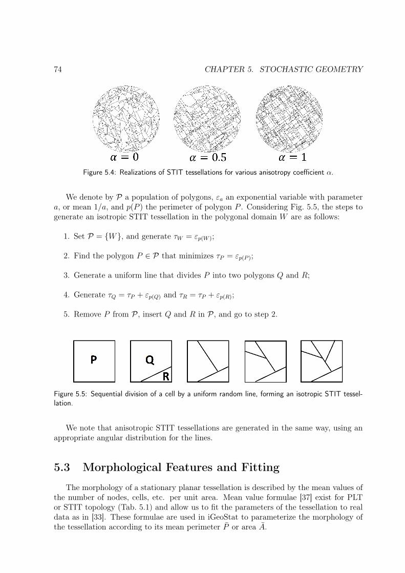
74 CHAPTER 5. STOCHASTIC GEOMETRY
Figure 5.4: Realizations of STIT tessellations for various anisotropy coefficient α.
We denote by P a population of polygons, εa an exponential variable with parametera, or mean 1/a, and p(P ) the perimeter of polygon P . Considering Fig. 5.5, the steps togenerate an isotropic STIT tessellation in the polygonal domain W are as follows:
1. Set P = W, and generate τW = εp(W );
2. Find the polygon P ∈ P that minimizes τP = εp(P );
3. Generate a uniform line that divides P into two polygons Q and R;
4. Generate τQ = τP + εp(Q) and τR = τP + εp(R);
5. Remove P from P , insert Q and R in P , and go to step 2.
Figure 5.5: Sequential division of a cell by a uniform random line, forming an isotropic STIT tessel-lation.
We note that anisotropic STIT tessellations are generated in the same way, using anappropriate angular distribution for the lines.
5.3 Morphological Features and Fitting
The morphology of a stationary planar tessellation is described by the mean values ofthe number of nodes, cells, etc. per unit area. Mean value formulae [37] exist for PLTor STIT topology (Tab. 5.1) and allow us to fit the parameters of the tessellation to realdata as in [33]. These formulae are used in iGeoStat to parameterize the morphology ofthe tessellation according to its mean perimeter P or area A.
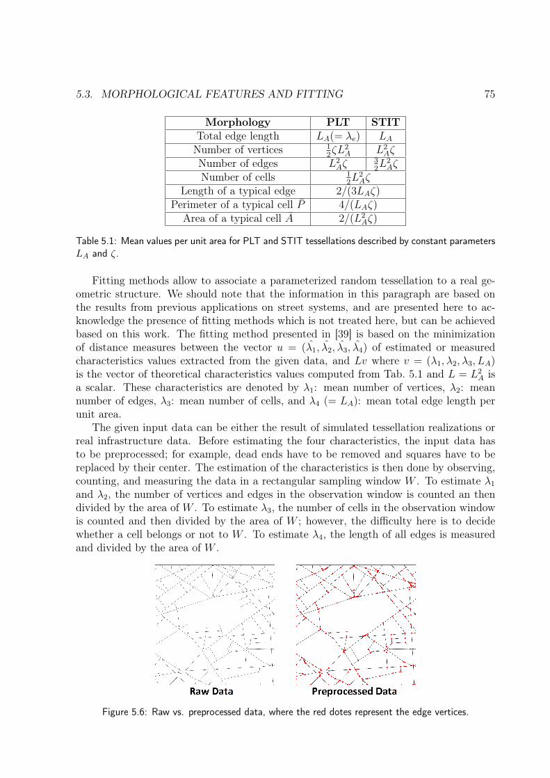
5.3. MORPHOLOGICAL FEATURES AND FITTING 75
Morphology PLT STITTotal edge length LA(= λe) LANumber of vertices 1
2ζL2
A L2Aζ
Number of edges L2Aζ
32L2Aζ
Number of cells 12L2Aζ
Length of a typical edge 2/(3LAζ)Perimeter of a typical cell P 4/(LAζ)
Area of a typical cell A 2/(L2Aζ)
Table 5.1: Mean values per unit area for PLT and STIT tessellations described by constant parametersLA and ζ.
Fitting methods allow to associate a parameterized random tessellation to a real ge-ometric structure. We should note that the information in this paragraph are based onthe results from previous applications on street systems, and are presented here to ac-knowledge the presence of fitting methods which is not treated here, but can be achievedbased on this work. The fitting method presented in [39] is based on the minimizationof distance measures between the vector u = (λ1, λ2, λ3, λ4) of estimated or measuredcharacteristics values extracted from the given data, and Lv where v = (λ1, λ2, λ3, LA)is the vector of theoretical characteristics values computed from Tab. 5.1 and L = L2
A isa scalar. These characteristics are denoted by λ1: mean number of vertices, λ2: meannumber of edges, λ3: mean number of cells, and λ4 (= LA): mean total edge length perunit area.
The given input data can be either the result of simulated tessellation realizations orreal infrastructure data. Before estimating the four characteristics, the input data hasto be preprocessed; for example, dead ends have to be removed and squares have to bereplaced by their center. The estimation of the characteristics is then done by observing,counting, and measuring the data in a rectangular sampling window W . To estimate λ1
and λ2, the number of vertices and edges in the observation window is counted an thendivided by the area of W . To estimate λ3, the number of cells in the observation windowis counted and then divided by the area of W ; however, the difficulty here is to decidewhether a cell belongs or not to W . To estimate λ4, the length of all edges is measuredand divided by the area of W .
Figure 5.6: Raw vs. preprocessed data, where the red dotes represent the edge vertices.

76 CHAPTER 5. STOCHASTIC GEOMETRY
Fitting is then done based on minimizing the distance d between u and Lv, takinginto account the Euclidean (absolute or relative) distance measures, whose solutions areknown ([8] p. 158). The optimal tessellation according to the chosen distance measurecorresponds to v = (λ1, λ2, λ3, LA) with L2
A = L. However, the distance measure choice isnot obvious at all; hence, several possibilities are usually studied.
We note that in general, only 3 characteristics measures are sufficient for the simpletessellations like the PLT for which the vertices define the boundaries of the cells; inthis case, the 4-vector characteristics is overdetermined. This is not the case for the STITwhich is not a simple tessellation (not “face to face” (seitentreu) as the PLT); a cell edge cansupport one or multiple vertices other than the pair that defines its ends, hence we shouldtake into account the number of T-crossings. The fitting process of indoor environmentsmay require different or additional characteristics vectors like identifying the presence ofcorridors and extract their width. Moreover, study and analyze the characteristics of atypical indoor cell that might have different representations like a room, an open-space,etc. This is still an open problem and depends on the objective that the user wants toachieve.
Part III
5G Indoor Propagation Simulator
77

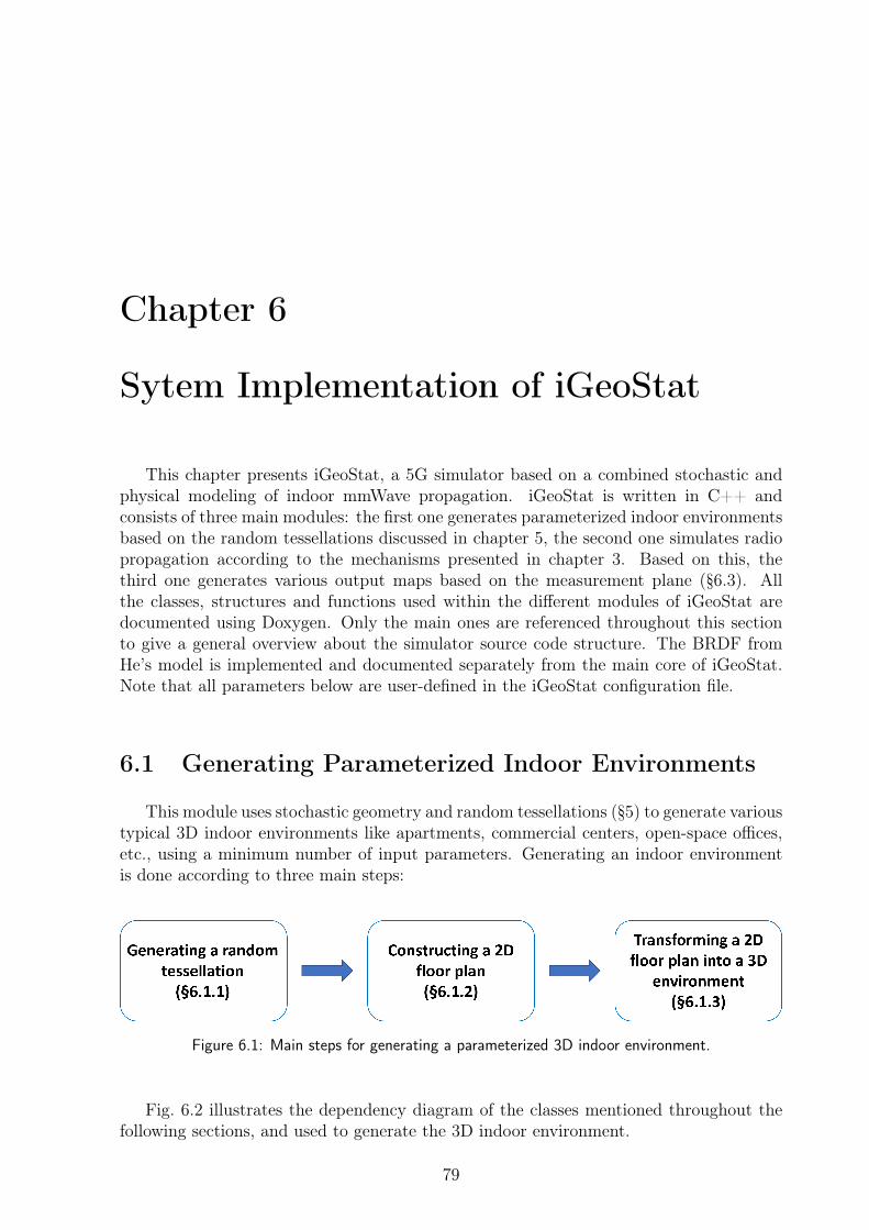
Chapter 6
Sytem Implementation of iGeoStat
This chapter presents iGeoStat, a 5G simulator based on a combined stochastic andphysical modeling of indoor mmWave propagation. iGeoStat is written in C++ andconsists of three main modules: the first one generates parameterized indoor environmentsbased on the random tessellations discussed in chapter 5, the second one simulates radiopropagation according to the mechanisms presented in chapter 3. Based on this, thethird one generates various output maps based on the measurement plane (§6.3). Allthe classes, structures and functions used within the different modules of iGeoStat aredocumented using Doxygen. Only the main ones are referenced throughout this sectionto give a general overview about the simulator source code structure. The BRDF fromHe’s model is implemented and documented separately from the main core of iGeoStat.Note that all parameters below are user-defined in the iGeoStat configuration file.
6.1 Generating Parameterized Indoor Environments
This module uses stochastic geometry and random tessellations (§5) to generate varioustypical 3D indoor environments like apartments, commercial centers, open-space offices,etc., using a minimum number of input parameters. Generating an indoor environmentis done according to three main steps:
Figure 6.1: Main steps for generating a parameterized 3D indoor environment.
Fig. 6.2 illustrates the dependency diagram of the classes mentioned throughout thefollowing sections, and used to generate the 3D indoor environment.
79
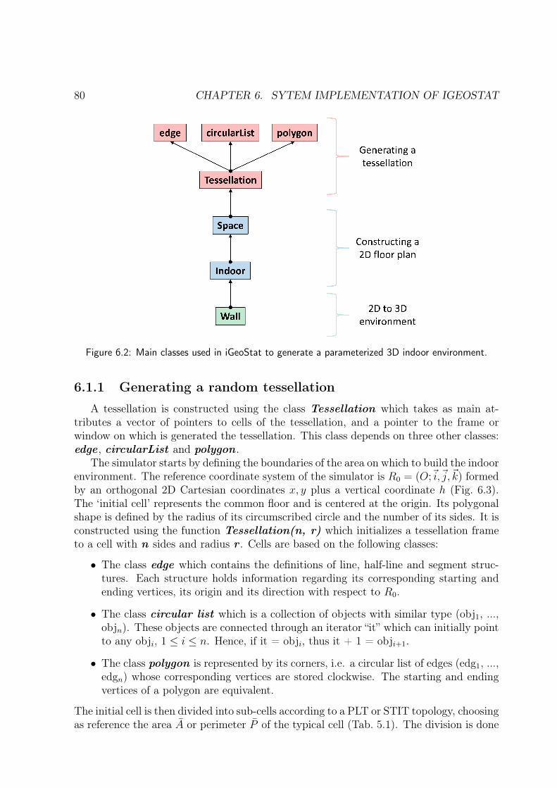
80 CHAPTER 6. SYTEM IMPLEMENTATION OF IGEOSTAT
Figure 6.2: Main classes used in iGeoStat to generate a parameterized 3D indoor environment.
6.1.1 Generating a random tessellation
A tessellation is constructed using the class Tessellation which takes as main at-tributes a vector of pointers to cells of the tessellation, and a pointer to the frame orwindow on which is generated the tessellation. This class depends on three other classes:edge , circularList and polygon .
The simulator starts by defining the boundaries of the area on which to build the indoorenvironment. The reference coordinate system of the simulator is R0 = (O;~i,~j,~k) formedby an orthogonal 2D Cartesian coordinates x, y plus a vertical coordinate h (Fig. 6.3).The ‘initial cell’ represents the common floor and is centered at the origin. Its polygonalshape is defined by the radius of its circumscribed circle and the number of its sides. It isconstructed using the function Tessellation(n, r) which initializes a tessellation frameto a cell with n sides and radius r . Cells are based on the following classes:
• The class edge which contains the definitions of line, half-line and segment struc-tures. Each structure holds information regarding its corresponding starting andending vertices, its origin and its direction with respect to R0.
• The class circular list which is a collection of objects with similar type (obj1, ...,objn). These objects are connected through an iterator “it” which can initially pointto any obji, 1 ≤ i ≤ n. Hence, if it = obji, thus it + 1 = obji+1.
• The class polygon is represented by its corners, i.e. a circular list of edges (edg1, ...,edgn) whose corresponding vertices are stored clockwise. The starting and endingvertices of a polygon are equivalent.
The initial cell is then divided into sub-cells according to a PLT or STIT topology, choosingas reference the area A or perimeter P of the typical cell (Tab. 5.1). The division is done
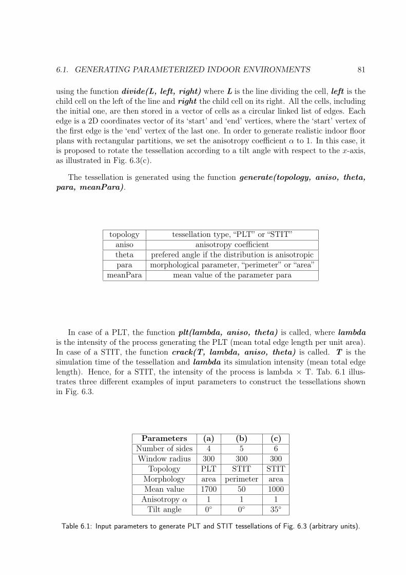
6.1. GENERATING PARAMETERIZED INDOOR ENVIRONMENTS 81
using the function divide(L, left, right) where L is the line dividing the cell, left is thechild cell on the left of the line and right the child cell on its right. All the cells, includingthe initial one, are then stored in a vector of cells as a circular linked list of edges. Eachedge is a 2D coordinates vector of its ‘start’ and ‘end’ vertices, where the ‘start’ vertex ofthe first edge is the ‘end’ vertex of the last one. In order to generate realistic indoor floorplans with rectangular partitions, we set the anisotropy coefficient α to 1. In this case, itis proposed to rotate the tessellation according to a tilt angle with respect to the x-axis,as illustrated in Fig. 6.3(c).
The tessellation is generated using the function generate(topology, aniso, theta,para, meanPara).
topology tessellation type, “PLT” or “STIT”aniso anisotropy coefficienttheta prefered angle if the distribution is anisotropicpara morphological parameter, “perimeter” or “area”
meanPara mean value of the parameter para
In case of a PLT, the function plt(lambda, aniso, theta) is called, where lambdais the intensity of the process generating the PLT (mean total edge length per unit area).In case of a STIT, the function crack(T, lambda, aniso, theta) is called. T is thesimulation time of the tessellation and lambda its simulation intensity (mean total edgelength). Hence, for a STIT, the intensity of the process is lambda × T. Tab. 6.1 illus-trates three different examples of input parameters to construct the tessellations shownin Fig. 6.3.
Parameters (a) (b) (c)Number of sides 4 5 6Window radius 300 300 300
Topology PLT STIT STITMorphology area perimeter areaMean value 1700 50 1000Anisotropy α 1 1 1Tilt angle 0 0 35
Table 6.1: Input parameters to generate PLT and STIT tessellations of Fig. 6.3 (arbitrary units).
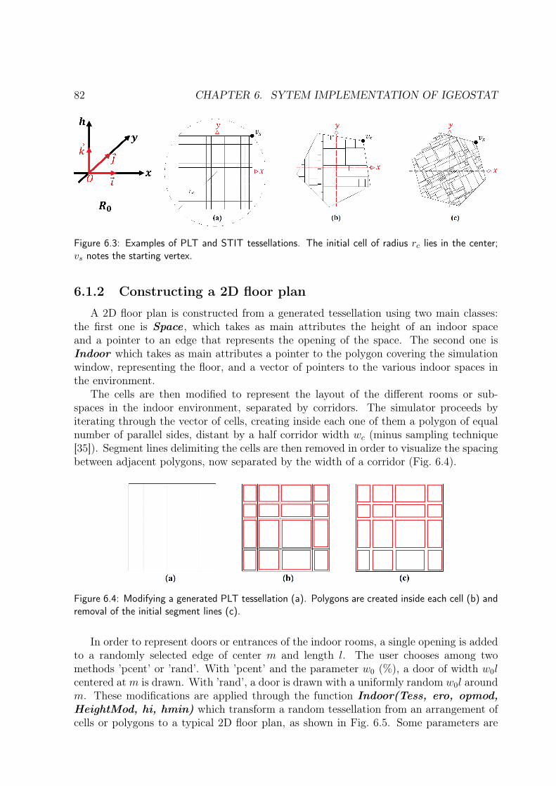
82 CHAPTER 6. SYTEM IMPLEMENTATION OF IGEOSTAT
Figure 6.3: Examples of PLT and STIT tessellations. The initial cell of radius rc lies in the center;vs notes the starting vertex.
6.1.2 Constructing a 2D floor plan
A 2D floor plan is constructed from a generated tessellation using two main classes:the first one is Space , which takes as main attributes the height of an indoor spaceand a pointer to an edge that represents the opening of the space. The second one isIndoor which takes as main attributes a pointer to the polygon covering the simulationwindow, representing the floor, and a vector of pointers to the various indoor spaces inthe environment.
The cells are then modified to represent the layout of the different rooms or sub-spaces in the indoor environment, separated by corridors. The simulator proceeds byiterating through the vector of cells, creating inside each one of them a polygon of equalnumber of parallel sides, distant by a half corridor width wc (minus sampling technique[35]). Segment lines delimiting the cells are then removed in order to visualize the spacingbetween adjacent polygons, now separated by the width of a corridor (Fig. 6.4).
Figure 6.4: Modifying a generated PLT tessellation (a). Polygons are created inside each cell (b) andremoval of the initial segment lines (c).
In order to represent doors or entrances of the indoor rooms, a single opening is addedto a randomly selected edge of center m and length l. The user chooses among twomethods ’pcent’ or ’rand’. With ’pcent’ and the parameter w0 (%), a door of width w0lcentered atm is drawn. With ’rand’, a door is drawn with a uniformly random w0l aroundm. These modifications are applied through the function Indoor(Tess, ero, opmod,HeightMod, hi, hmin) which transform a random tessellation from an arrangement ofcells or polygons to a typical 2D floor plan, as shown in Fig. 6.5. Some parameters are
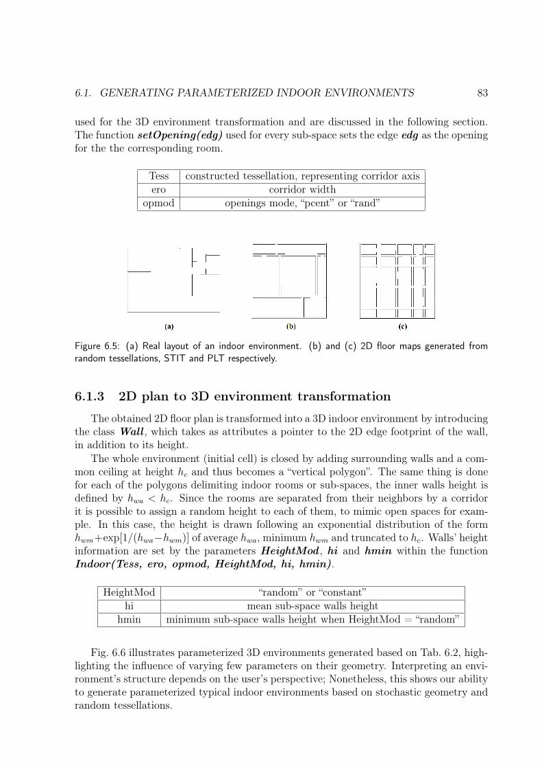
6.1. GENERATING PARAMETERIZED INDOOR ENVIRONMENTS 83
used for the 3D environment transformation and are discussed in the following section.The function setOpening(edg) used for every sub-space sets the edge edg as the openingfor the the corresponding room.
Tess constructed tessellation, representing corridor axisero corridor width
opmod openings mode, “pcent” or “rand”
Figure 6.5: (a) Real layout of an indoor environment. (b) and (c) 2D floor maps generated fromrandom tessellations, STIT and PLT respectively.
6.1.3 2D plan to 3D environment transformation
The obtained 2D floor plan is transformed into a 3D indoor environment by introducingthe class Wall , which takes as attributes a pointer to the 2D edge footprint of the wall,in addition to its height.
The whole environment (initial cell) is closed by adding surrounding walls and a com-mon ceiling at height hc and thus becomes a “vertical polygon”. The same thing is donefor each of the polygons delimiting indoor rooms or sub-spaces, the inner walls height isdefined by hwa < hc. Since the rooms are separated from their neighbors by a corridorit is possible to assign a random height to each of them, to mimic open spaces for exam-ple. In this case, the height is drawn following an exponential distribution of the formhwm+exp[1/(hwa−hwm)] of average hwa, minimum hwm and truncated to hc. Walls’ heightinformation are set by the parameters HeightMod , hi and hmin within the functionIndoor(Tess, ero, opmod, HeightMod, hi, hmin).
HeightMod “random” or “constant”hi mean sub-space walls height
hmin minimum sub-space walls height when HeightMod = “random”
Fig. 6.6 illustrates parameterized 3D environments generated based on Tab. 6.2, high-lighting the influence of varying few parameters on their geometry. Interpreting an envi-ronment’s structure depends on the user’s perspective; Nonetheless, this shows our abilityto generate parameterized typical indoor environments based on stochastic geometry andrandom tessellations.
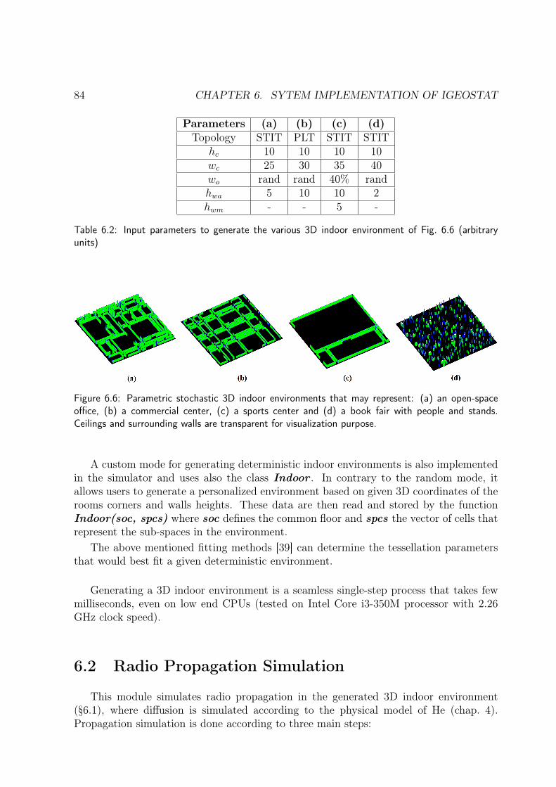
84 CHAPTER 6. SYTEM IMPLEMENTATION OF IGEOSTAT
Parameters (a) (b) (c) (d)Topology STIT PLT STIT STIT
hc 10 10 10 10wc 25 30 35 40wo rand rand 40% randhwa 5 10 10 2hwm - - 5 -
Table 6.2: Input parameters to generate the various 3D indoor environment of Fig. 6.6 (arbitraryunits)
Figure 6.6: Parametric stochastic 3D indoor environments that may represent: (a) an open-spaceoffice, (b) a commercial center, (c) a sports center and (d) a book fair with people and stands.Ceilings and surrounding walls are transparent for visualization purpose.
A custom mode for generating deterministic indoor environments is also implementedin the simulator and uses also the class Indoor . In contrary to the random mode, itallows users to generate a personalized environment based on given 3D coordinates of therooms corners and walls heights. These data are then read and stored by the functionIndoor(soc, spcs) where soc defines the common floor and spcs the vector of cells thatrepresent the sub-spaces in the environment.
The above mentioned fitting methods [39] can determine the tessellation parametersthat would best fit a given deterministic environment.
Generating a 3D indoor environment is a seamless single-step process that takes fewmilliseconds, even on low end CPUs (tested on Intel Core i3-350M processor with 2.26GHz clock speed).
6.2 Radio Propagation Simulation
This module simulates radio propagation in the generated 3D indoor environment(§6.1), where diffusion is simulated according to the physical model of He (chap. 4).Propagation simulation is done according to three main steps:
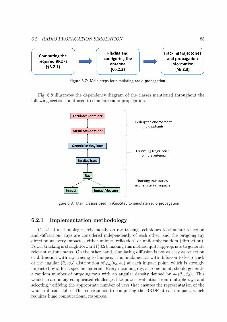
6.2. RADIO PROPAGATION SIMULATION 85
Figure 6.7: Main steps for simulating radio propagation.
Fig. 6.8 illustrates the dependency diagram of the classes mentioned throughout thefollowing sections, and used to simulate radio propagation.
Figure 6.8: Main classes used in iGeoStat to simulate radio propagation.
6.2.1 Implementation methodology
Classical methodologies rely mostly on ray tracing techniques to simulate reflectionand diffraction: rays are considered independently of each other, and the outgoing raydirection at every impact is either unique (reflection) or uniformly random (diffraction).Power tracking is straightforward (§3.2), making this method quite appropriate to generaterelevant output maps. On the other hand, simulating diffusion is not as easy as reflectionor diffraction with ray tracing techniques: it is fundamental with diffusion to keep trackof the angular (θd, φd) distribution of ρθi(θd, φd) at each impact point, which is stronglyimpacted by θi for a specific material. Every incoming ray, at some point, should generatea random number of outgoing rays with an angular density defined by ρθi(θd, φd). Thiswould create many complicated challenges like power evaluation from multiple rays andselecting/verifying the appropriate number of rays that ensures the representation of thewhole diffusion lobe. This corresponds to computing the BRDF at each impact, whichrequires huge computational resources.
86 CHAPTER 6. SYTEM IMPLEMENTATION OF IGEOSTAT
Our implementation of diffusion consists of computing the required BRDFs for all θi,θd, and φd, for each material in the environment, and storing them in databases. This isdone only once prior to the simulation and allows us to reuse the databases in other sim-ulations. Then in iGeoStat, propagation after each impact is based on the discretizationof diffusion directions, with steps ∆θd and ∆φd. Each diffusion direction (θd, φd) is at-tributed a solid angle and diffused power, computed by fetching the appropriate ρθi(θd, φd)value from the database, enabling straightforward power tracking through the adaptedlink budget (§4.5). Diffusion is thus monitored at each impact in a physical way; thisallows us to reduce the set of (θd, φd) directions by adapting discretization steps or addingthresholds on ρθi(θd, φd) and power values (§7.3)
6.2.2 BRDF implementation
As mentioned earlier, the BRDF from He’s model is implemented separately from themain core of iGeoStat using the mathematical library PARI [40]. To avoid computingρθi(θd, φd) for the same input parameters over and over again, numerical simulations ofρθi(θd, φd) are executed for a whole set of input parameters and stored in a database usingSQLite [41]. Hence, at each impact point, the incoming direction and surface normaldefine the incidence angle θi, and the corresponding ρθi(θd, φd) value of each diffusiondirection (θd, φd) is retrieved from the database.
Each BRDF database corresponds to the computation of ρθi(θd, φd) for a single mate-rial (σ0, τ , nc) and wavelength (λ), and all discretized incident angles (θi), and diffusiondirections θd ∈ (∆θd ,
π2−∆θd), φd ∈ (∆φd , 2π−∆φd). The BRDF is computed using the
function bidirectional_reflectance_nonpol (theta_i, theta_r, phi_r, sigma_0,tau, lambda, n_r, n_i) (BRDF code documentation), which corresponds to eq. 4.29.Further details concerning the challenges related to the implementation of He’s model,along with the computation, storage, and retrieval of ρθi(θd, φd) values are discussed in§7.1.
6.2.3 Antenna parameters
The antenna is placed in the environment at (xa, ya, ha), according to the reference3D Cartesian coordinate system Ra = (A;~i,~j,~k). Its position can be fixed with respectto the geometry of a deterministic environment, or randomly set in a stochastic one.This approach aims to derive statistics on various propagation indicators related to theglobal parameters of the environment (Tab. 6.1, Tab. 6.2), and not to thoroughly studydeterministic settings.
The class GenericFastRayTrace is used to place the antenna. Its main attributesare a pointer to the indoor environment under consideration, along with the antenna. Themain function is placeAntenna(posmod, pos, mat) where posmod is the positioningmode of the antenna, it can be “free”, i.e. placed according to the coordinates given bypos or “roof”, i.e. placed randomly between the highest wall in the environment and theceiling of the initial cell. mat adds an additional height to the antenna’s position.
By assumption, the antenna emits uniformly a total power P0 at wavelength λ in asolid angle Ωa centered in the spherical direction (θa0 in azimuth, φa0 in elevation). Ωa is
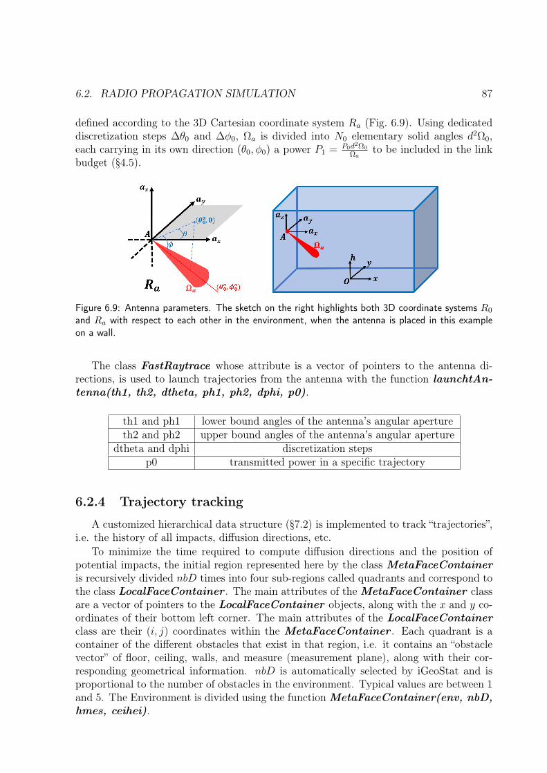
6.2. RADIO PROPAGATION SIMULATION 87
defined according to the 3D Cartesian coordinate system Ra (Fig. 6.9). Using dedicateddiscretization steps ∆θ0 and ∆φ0, Ωa is divided into N0 elementary solid angles d2Ω0,each carrying in its own direction (θ0, φ0) a power P1 = P0d2Ω0
Ωato be included in the link
budget (§4.5).
Figure 6.9: Antenna parameters. The sketch on the right highlights both 3D coordinate systems R0
and Ra with respect to each other in the environment, when the antenna is placed in this exampleon a wall.
The class FastRaytrace whose attribute is a vector of pointers to the antenna di-rections, is used to launch trajectories from the antenna with the function launchtAn-tenna(th1, th2, dtheta, ph1, ph2, dphi, p0).
th1 and ph1 lower bound angles of the antenna’s angular apertureth2 and ph2 upper bound angles of the antenna’s angular aperture
dtheta and dphi discretization stepsp0 transmitted power in a specific trajectory
6.2.4 Trajectory tracking
A customized hierarchical data structure (§7.2) is implemented to track “trajectories”,i.e. the history of all impacts, diffusion directions, etc.
To minimize the time required to compute diffusion directions and the position ofpotential impacts, the initial region represented here by the class MetaFaceContaineris recursively divided nbD times into four sub-regions called quadrants and correspond tothe class LocalFaceContainer . The main attributes of the MetaFaceContainer classare a vector of pointers to the LocalFaceContainer objects, along with the x and y co-ordinates of their bottom left corner. The main attributes of the LocalFaceContainerclass are their (i, j) coordinates within the MetaFaceContainer . Each quadrant is acontainer of the different obstacles that exist in that region, i.e. it contains an “obstaclevector” of floor, ceiling, walls, and measure (measurement plane), along with their cor-responding geometrical information. nbD is automatically selected by iGeoStat and isproportional to the number of obstacles in the environment. Typical values are between 1and 5. The Environment is divided using the function MetaFaceContainer(env, nbD,hmes, ceihei).
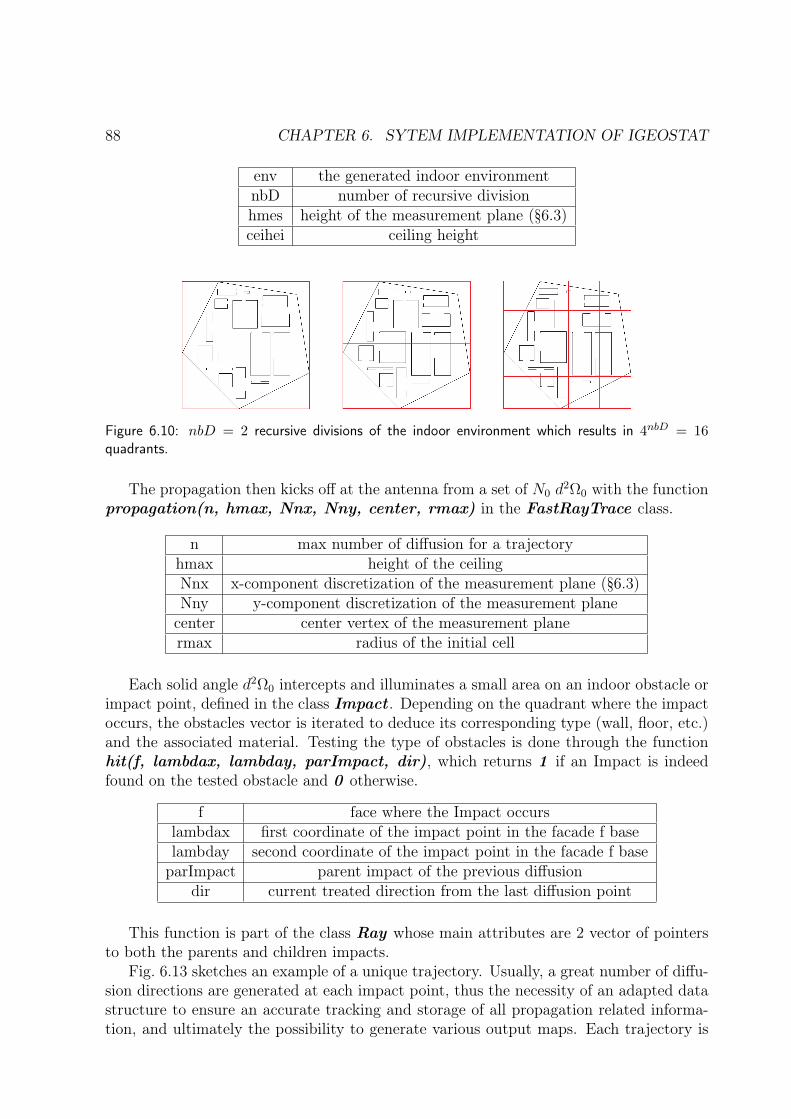
88 CHAPTER 6. SYTEM IMPLEMENTATION OF IGEOSTAT
env the generated indoor environmentnbD number of recursive divisionhmes height of the measurement plane (§6.3)ceihei ceiling height
Figure 6.10: nbD = 2 recursive divisions of the indoor environment which results in 4nbD = 16quadrants.
The propagation then kicks off at the antenna from a set of N0 d2Ω0 with the function
propagation(n, hmax, Nnx, Nny, center, rmax) in the FastRayTrace class.
n max number of diffusion for a trajectoryhmax height of the ceilingNnx x-component discretization of the measurement plane (§6.3)Nny y-component discretization of the measurement planecenter center vertex of the measurement planermax radius of the initial cell
Each solid angle d2Ω0 intercepts and illuminates a small area on an indoor obstacle orimpact point, defined in the class Impact . Depending on the quadrant where the impactoccurs, the obstacles vector is iterated to deduce its corresponding type (wall, floor, etc.)and the associated material. Testing the type of obstacles is done through the functionhit(f, lambdax, lambday, parImpact, dir), which returns 1 if an Impact is indeedfound on the tested obstacle and 0 otherwise.
f face where the Impact occurslambdax first coordinate of the impact point in the facade f baselambday second coordinate of the impact point in the facade f baseparImpact parent impact of the previous diffusion
dir current treated direction from the last diffusion point
This function is part of the class Ray whose main attributes are 2 vector of pointersto both the parents and children impacts.
Fig. 6.13 sketches an example of a unique trajectory. Usually, a great number of diffu-sion directions are generated at each impact point, thus the necessity of an adapted datastructure to ensure an accurate tracking and storage of all propagation related informa-tion, and ultimately the possibility to generate various output maps. Each trajectory is
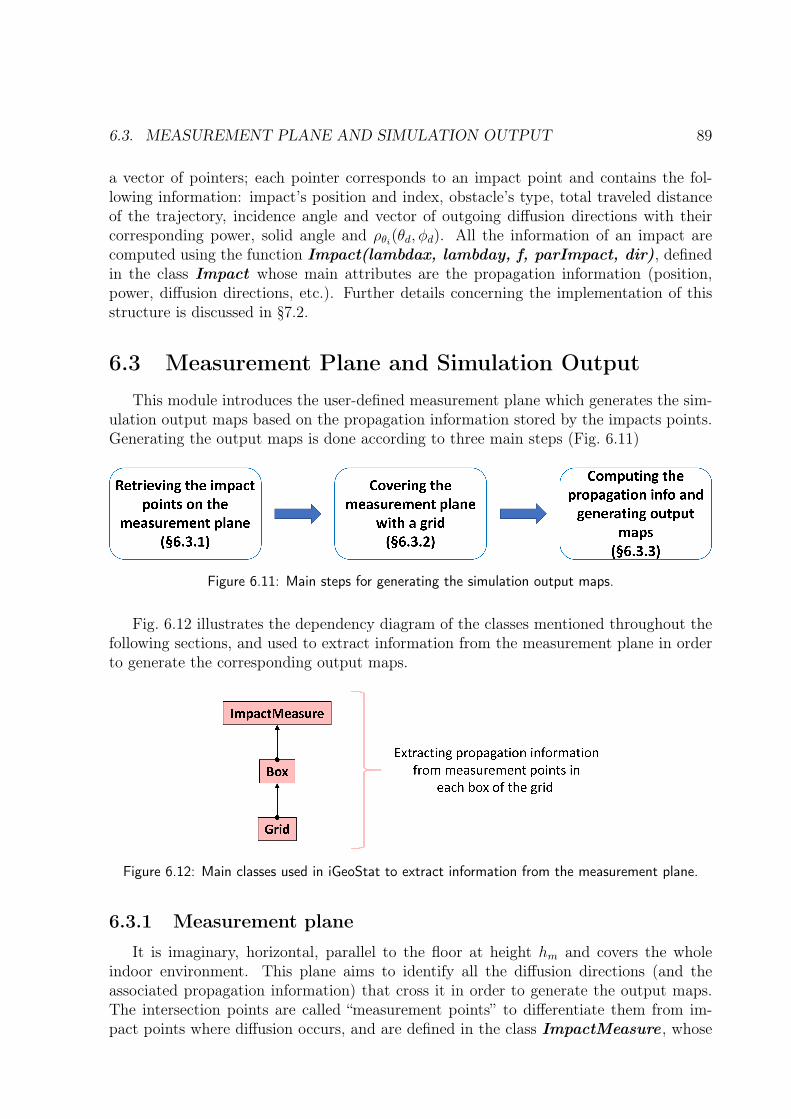
6.3. MEASUREMENT PLANE AND SIMULATION OUTPUT 89
a vector of pointers; each pointer corresponds to an impact point and contains the fol-lowing information: impact’s position and index, obstacle’s type, total traveled distanceof the trajectory, incidence angle and vector of outgoing diffusion directions with theircorresponding power, solid angle and ρθi(θd, φd). All the information of an impact arecomputed using the function Impact(lambdax, lambday, f, parImpact, dir), definedin the class Impact whose main attributes are the propagation information (position,power, diffusion directions, etc.). Further details concerning the implementation of thisstructure is discussed in §7.2.
6.3 Measurement Plane and Simulation OutputThis module introduces the user-defined measurement plane which generates the sim-
ulation output maps based on the propagation information stored by the impacts points.Generating the output maps is done according to three main steps (Fig. 6.11)
Figure 6.11: Main steps for generating the simulation output maps.
Fig. 6.12 illustrates the dependency diagram of the classes mentioned throughout thefollowing sections, and used to extract information from the measurement plane in orderto generate the corresponding output maps.
Figure 6.12: Main classes used in iGeoStat to extract information from the measurement plane.
6.3.1 Measurement plane
It is imaginary, horizontal, parallel to the floor at height hm and covers the wholeindoor environment. This plane aims to identify all the diffusion directions (and theassociated propagation information) that cross it in order to generate the output maps.The intersection points are called “measurement points” to differentiate them from im-pact points where diffusion occurs, and are defined in the class ImpactMeasure , whose
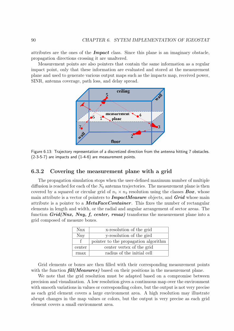
90 CHAPTER 6. SYTEM IMPLEMENTATION OF IGEOSTAT
attributes are the ones of the Impact class. Since this plane is an imaginary obstacle,propagation directions crossing it are unaltered.
Measurement points are also pointers that contain the same information as a regularimpact point, only that these information are evaluated and stored at the measurementplane and used to generate various output maps such as the impacts map, received power,SINR, antenna coverage, path loss, and delay spread.
Figure 6.13: Trajectory representation of a discretized direction from the antenna hitting 7 obstacles.(2-3-5-7) are impacts and (1-4-6) are measurement points.
6.3.2 Covering the measurement plane with a grid
The propagation simulation stops when the user-defined maximum number of multiplediffusion is reached for each of theN0 antenna trajectories. The measurement plane is thencovered by a squared or circular grid of n1 × n2 resolution using the classes Box , whosemain attribute is a vector of pointers to ImpactMeasure objects, and Grid whose mainattribute is a pointer to a MetaFaceContainer . This fixes the number of rectangularelements in length and width, or the radial and angular arrangement of sector areas. Thefunction Grid(Nnx, Nny, f, center, rmax) transforms the measurement plane into agrid composed of measure boxes.
Nnx x-resolution of the gridNny y-resolution of the girdf pointer to the propagation algorithm
center center vertex of the gridrmax radius of the initial cell
Grid elements or boxes are then filled with their corresponding measurement pointswith the function fill(Measures) based on their positions in the measurement plane.
We note that the grid resolution must be adapted based on a compromise betweenprecision and visualization. A low resolution gives a continuous map over the environmentwith smooth variations in values or corresponding colors, but the output is not very preciseas each grid element covers a large environment area. A high resolution may illustrateabrupt changes in the map values or colors, but the output is very precise as each gridelement covers a small environment area.
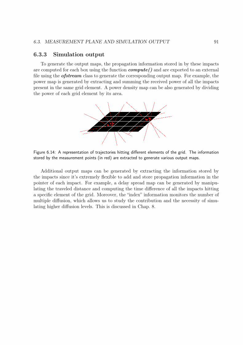
6.3. MEASUREMENT PLANE AND SIMULATION OUTPUT 91
6.3.3 Simulation output
To generate the output maps, the propagation information stored in by these impactsare computed for each box using the function compute() and are exported to an externalfile using the ofstream class to generate the corresponding output map. For example, thepower map is generated by extracting and summing the received power of all the impactspresent in the same grid element. A power density map can be also generated by dividingthe power of each grid element by its area.
Figure 6.14: A representation of trajectories hitting different elements of the grid. The informationstored by the measurement points (in red) are extracted to generate various output maps.
Additional output maps can be generated by extracting the information stored bythe impacts since it’s extremely flexible to add and store propagation information in thepointer of each impact. For example, a delay spread map can be generated by manipu-lating the traveled distance and computing the time difference of all the impacts hittinga specific element of the grid. Moreover, the “index” information monitors the number ofmultiple diffusion, which allows us to study the contribution and the necessity of simu-lating higher diffusion levels. This is discussed in Chap. 8.

92 CHAPTER 6. SYTEM IMPLEMENTATION OF IGEOSTAT

Chapter 7
Modeling and ImplementationChallenges
This chapter presents the challenges related to the computation, storage, and retrievalof BRDF values, the modeling and implementation of a data structure that managesdiffusion, and effective strategies that prevent the explosion of diffusion directions.
7.1 BRDF Computation and Storage
The main implementation challenge of the diffusion model is to efficiently compute,store, and retrieve ρθi(θd, φd) values, since they are needed at each impact point.
The mathematical functions required by He’s model (§4) to compute the BRDF arenot included in any internal C++ library (Lambert W function, Digamma, etc.). Variousexternal open-source libraries were investigated like PARI, SageMath [42], Boost [43], etc.We selected PARI since it is written in C, contains all the required functions, and supportsmulti-precision computations.
7.1.1 Memory management and optimization
PARI initializes a stack in the memory where BRDF values are computed. The ob-jective behind our implementation is to minimize memory usage and allow numericalsimulations regardless of the system’s performance. However, without any optimization,computing ρθi(θd, φd) for a single incident angle consumes a huge amount of memory andeventually crashes when simulating for all θi. This major issue was tackled by implement-ing a customized algorithm for manual memory management and optimization (Alg. 1).
Objects are created in the PARI stack as ρθi(θd, φd) is computed for each discretizeddirection of the diffusion plane. Since these directions are independent of each other,initialized objects at each iteration become useless once the corresponding ρθi(θd, φd) valueis computed. At each iteration, the “Garbage Collection” (GC) algorithm reclaims thememory occupied by these ‘garbage’ objects and overwrites each ρθi(θd, φd) computationon the same memory resources, hence, minimizing PARI stack’s requirements withoutimpacting performance.
93
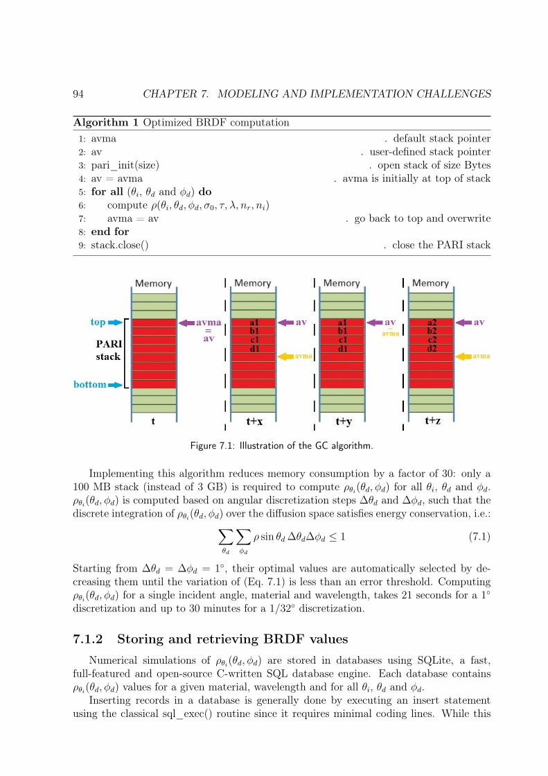
94 CHAPTER 7. MODELING AND IMPLEMENTATION CHALLENGES
Algorithm 1 Optimized BRDF computation1: avma . default stack pointer2: av . user-defined stack pointer3: pari_init(size) . open stack of size Bytes4: av = avma . avma is initially at top of stack5: for all (θi, θd and φd) do6: compute ρ(θi, θd, φd, σ0, τ, λ, nr, ni)7: avma = av . go back to top and overwrite8: end for9: stack.close() . close the PARI stack
Figure 7.1: Illustration of the GC algorithm.
Implementing this algorithm reduces memory consumption by a factor of 30: only a100 MB stack (instead of 3 GB) is required to compute ρθi(θd, φd) for all θi, θd and φd.ρθi(θd, φd) is computed based on angular discretization steps ∆θd and ∆φd, such that thediscrete integration of ρθi(θd, φd) over the diffusion space satisfies energy conservation, i.e.:∑
θd
∑φd
ρ sin θd ∆θd∆φd ≤ 1 (7.1)
Starting from ∆θd = ∆φd = 1, their optimal values are automatically selected by de-creasing them until the variation of (Eq. 7.1) is less than an error threshold. Computingρθi(θd, φd) for a single incident angle, material and wavelength, takes 21 seconds for a 1
discretization and up to 30 minutes for a 1/32 discretization.
7.1.2 Storing and retrieving BRDF values
Numerical simulations of ρθi(θd, φd) are stored in databases using SQLite, a fast,full-featured and open-source C-written SQL database engine. Each database containsρθi(θd, φd) values for a given material, wavelength and for all θi, θd and φd.
Inserting records in a database is generally done by executing an insert statementusing the classical sql_exec() routine since it requires minimal coding lines. While this
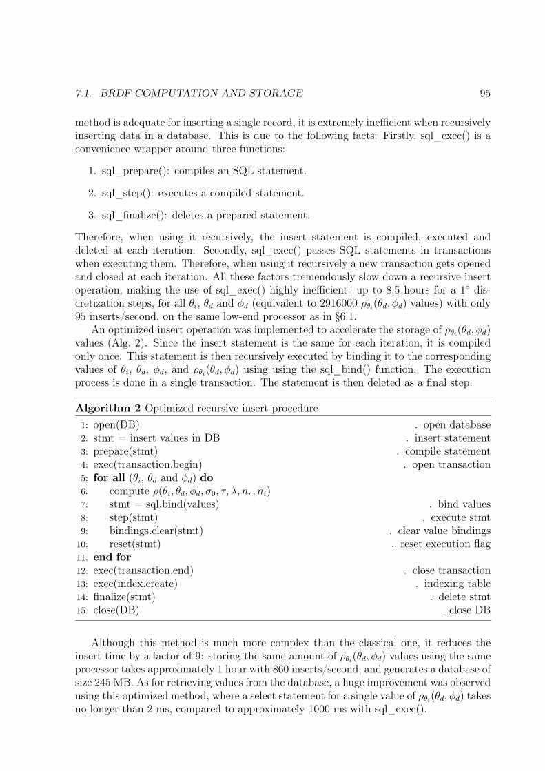
7.1. BRDF COMPUTATION AND STORAGE 95
method is adequate for inserting a single record, it is extremely inefficient when recursivelyinserting data in a database. This is due to the following facts: Firstly, sql_exec() is aconvenience wrapper around three functions:
1. sql_prepare(): compiles an SQL statement.
2. sql_step(): executes a compiled statement.
3. sql_finalize(): deletes a prepared statement.
Therefore, when using it recursively, the insert statement is compiled, executed anddeleted at each iteration. Secondly, sql_exec() passes SQL statements in transactionswhen executing them. Therefore, when using it recursively a new transaction gets openedand closed at each iteration. All these factors tremendously slow down a recursive insertoperation, making the use of sql_exec() highly inefficient: up to 8.5 hours for a 1 dis-cretization steps, for all θi, θd and φd (equivalent to 2916000 ρθi(θd, φd) values) with only95 inserts/second, on the same low-end processor as in §6.1.
An optimized insert operation was implemented to accelerate the storage of ρθi(θd, φd)values (Alg. 2). Since the insert statement is the same for each iteration, it is compiledonly once. This statement is then recursively executed by binding it to the correspondingvalues of θi, θd, φd, and ρθi(θd, φd) using using the sql_bind() function. The executionprocess is done in a single transaction. The statement is then deleted as a final step.
Algorithm 2 Optimized recursive insert procedure1: open(DB) . open database2: stmt = insert values in DB . insert statement3: prepare(stmt) . compile statement4: exec(transaction.begin) . open transaction5: for all (θi, θd and φd) do6: compute ρ(θi, θd, φd, σ0, τ, λ, nr, ni)7: stmt = sql.bind(values) . bind values8: step(stmt) . execute stmt9: bindings.clear(stmt) . clear value bindings
10: reset(stmt) . reset execution flag11: end for12: exec(transaction.end) . close transaction13: exec(index.create) . indexing table14: finalize(stmt) . delete stmt15: close(DB) . close DB
Although this method is much more complex than the classical one, it reduces theinsert time by a factor of 9: storing the same amount of ρθi(θd, φd) values using the sameprocessor takes approximately 1 hour with 860 inserts/second, and generates a database ofsize 245 MB. As for retrieving values from the database, a huge improvement was observedusing this optimized method, where a select statement for a single value of ρθi(θd, φd) takesno longer than 2 ms, compared to approximately 1000 ms with sql_exec().
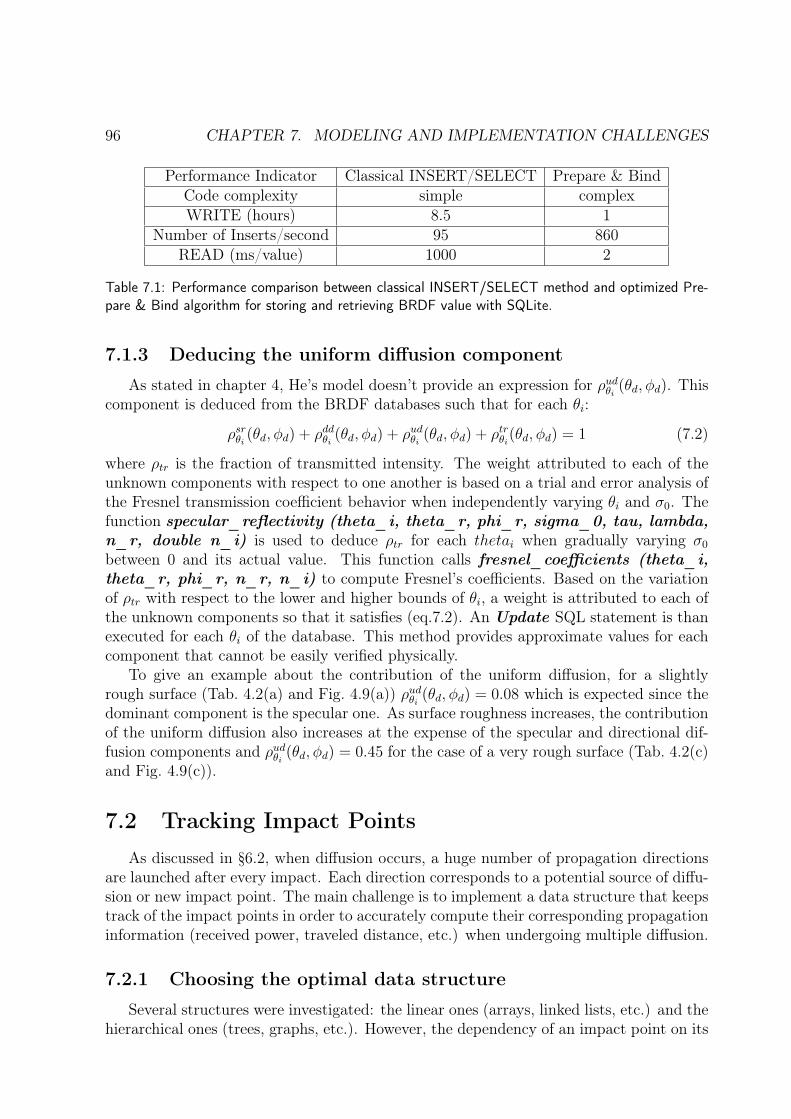
96 CHAPTER 7. MODELING AND IMPLEMENTATION CHALLENGES
Performance Indicator Classical INSERT/SELECT Prepare & BindCode complexity simple complexWRITE (hours) 8.5 1
Number of Inserts/second 95 860READ (ms/value) 1000 2
Table 7.1: Performance comparison between classical INSERT/SELECT method and optimized Pre-pare & Bind algorithm for storing and retrieving BRDF value with SQLite.
7.1.3 Deducing the uniform diffusion component
As stated in chapter 4, He’s model doesn’t provide an expression for ρudθi (θd, φd). Thiscomponent is deduced from the BRDF databases such that for each θi:
ρsrθi (θd, φd) + ρddθi (θd, φd) + ρudθi (θd, φd) + ρtrθi(θd, φd) = 1 (7.2)
where ρtr is the fraction of transmitted intensity. The weight attributed to each of theunknown components with respect to one another is based on a trial and error analysis ofthe Fresnel transmission coefficient behavior when independently varying θi and σ0. Thefunction specular_reflectivity (theta_i, theta_r, phi_r, sigma_0, tau, lambda,n_r, double n_i) is used to deduce ρtr for each thetai when gradually varying σ0
between 0 and its actual value. This function calls fresnel_coefficients (theta_i,theta_r, phi_r, n_r, n_i) to compute Fresnel’s coefficients. Based on the variationof ρtr with respect to the lower and higher bounds of θi, a weight is attributed to each ofthe unknown components so that it satisfies (eq.7.2). An Update SQL statement is thanexecuted for each θi of the database. This method provides approximate values for eachcomponent that cannot be easily verified physically.
To give an example about the contribution of the uniform diffusion, for a slightlyrough surface (Tab. 4.2(a) and Fig. 4.9(a)) ρudθi (θd, φd) = 0.08 which is expected since thedominant component is the specular one. As surface roughness increases, the contributionof the uniform diffusion also increases at the expense of the specular and directional dif-fusion components and ρudθi (θd, φd) = 0.45 for the case of a very rough surface (Tab. 4.2(c)and Fig. 4.9(c)).
7.2 Tracking Impact PointsAs discussed in §6.2, when diffusion occurs, a huge number of propagation directions
are launched after every impact. Each direction corresponds to a potential source of diffu-sion or new impact point. The main challenge is to implement a data structure that keepstrack of the impact points in order to accurately compute their corresponding propagationinformation (received power, traveled distance, etc.) when undergoing multiple diffusion.
7.2.1 Choosing the optimal data structure
Several structures were investigated: the linear ones (arrays, linked lists, etc.) and thehierarchical ones (trees, graphs, etc.). However, the dependency of an impact point on its
7.2. TRACKING IMPACT POINTS 97
previous one induces a parent −→ child relationship, which mostly correspond to a treestructure.
The analogy between the tree components (Fig. 7.2) and diffusion is as follows: theroot and its edges represent the antenna and its trajectories. A parent node and itsoutward edges correspond to an impact point and its outgoing propagation directions.Each child node represents the resulting impact point from these directions and a leafnode corresponds to the last impact point of an antenna’s trajectory. At each diffusion,a child node becomes a new parent node.
Figure 7.2: Main components of a tree data structure.
7.2.2 Traversing a tree structure
The challenge that arises when implementing a tree is the choice of its traversal, i.e. theorder in which the tree nodes are treated. In our case, treating a node means computingpower, distance, diffusion directions, etc. at that impact point. We recall that an impactpoint is a pointer containing all the propagation information. Several tree traversals wereinvestigated (Depth-first (DFS), Breadth-First (BFS), Monte Carlo (MCTS), etc.).
BFS is a corecursive level-order algorithm, i.e. it uses self-produced data bit-by-bit asthey become available to produce further bits of data. It is implemented using a queue;starting from the root, tree nodes are explored by visiting horizontally all the adjacentnodes of the current level before moving to the next one. Referring to Fig. 7.2, this isequivalent to the following visiting order: C - E - G - B - J - D - A - H - F - I. BFS hasa time complexity equal to O(|N |+ |E|), and a space complexity equal to O(|N |), whereN is the number of nodes and E the number of edges.
A customized BFS algorithm (Alg. 3) was implemented as it corresponds the most tothe logic of multiple diffusion. Starting from the antenna, all the adjacent parent impactsmust be treated before any of their child impacts. Alg. 3 integrates a Garbage Collectorthat treats antenna trajectories independently from each other, allowing each one of themto reuse the same memory resources regardless of the number of antennas and trajectoriesN0.
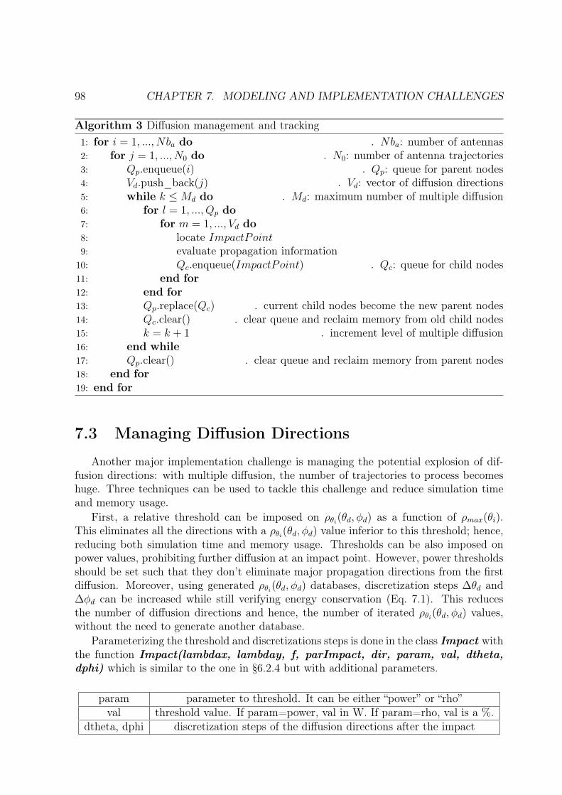
98 CHAPTER 7. MODELING AND IMPLEMENTATION CHALLENGES
Algorithm 3 Diffusion management and tracking1: for i = 1, ..., Nba do . Nba: number of antennas2: for j = 1, ..., N0 do . N0: number of antenna trajectories3: Qp.enqueue(i) . Qp: queue for parent nodes4: Vd.push_back(j) . Vd: vector of diffusion directions5: while k ≤Md do . Md: maximum number of multiple diffusion6: for l = 1, ..., Qp do7: for m = 1, ..., Vd do8: locate ImpactPoint9: evaluate propagation information
10: Qc.enqueue(ImpactPoint) . Qc: queue for child nodes11: end for12: end for13: Qp.replace(Qc) . current child nodes become the new parent nodes14: Qc.clear() . clear queue and reclaim memory from old child nodes15: k = k + 1 . increment level of multiple diffusion16: end while17: Qp.clear() . clear queue and reclaim memory from parent nodes18: end for19: end for
7.3 Managing Diffusion Directions
Another major implementation challenge is managing the potential explosion of dif-fusion directions: with multiple diffusion, the number of trajectories to process becomeshuge. Three techniques can be used to tackle this challenge and reduce simulation timeand memory usage.
First, a relative threshold can be imposed on ρθi(θd, φd) as a function of ρmax(θi).This eliminates all the directions with a ρθi(θd, φd) value inferior to this threshold; hence,reducing both simulation time and memory usage. Thresholds can be also imposed onpower values, prohibiting further diffusion at an impact point. However, power thresholdsshould be set such that they don’t eliminate major propagation directions from the firstdiffusion. Moreover, using generated ρθi(θd, φd) databases, discretization steps ∆θd and∆φd can be increased while still verifying energy conservation (Eq. 7.1). This reducesthe number of diffusion directions and hence, the number of iterated ρθi(θd, φd) values,without the need to generate another database.
Parameterizing the threshold and discretizations steps is done in the class Impact withthe function Impact(lambdax, lambday, f, parImpact, dir, param, val, dtheta,dphi) which is similar to the one in §6.2.4 but with additional parameters.
param parameter to threshold. It can be either “power” or “rho”val threshold value. If param=power, val in W. If param=rho, val is a %.
dtheta, dphi discretization steps of the diffusion directions after the impact
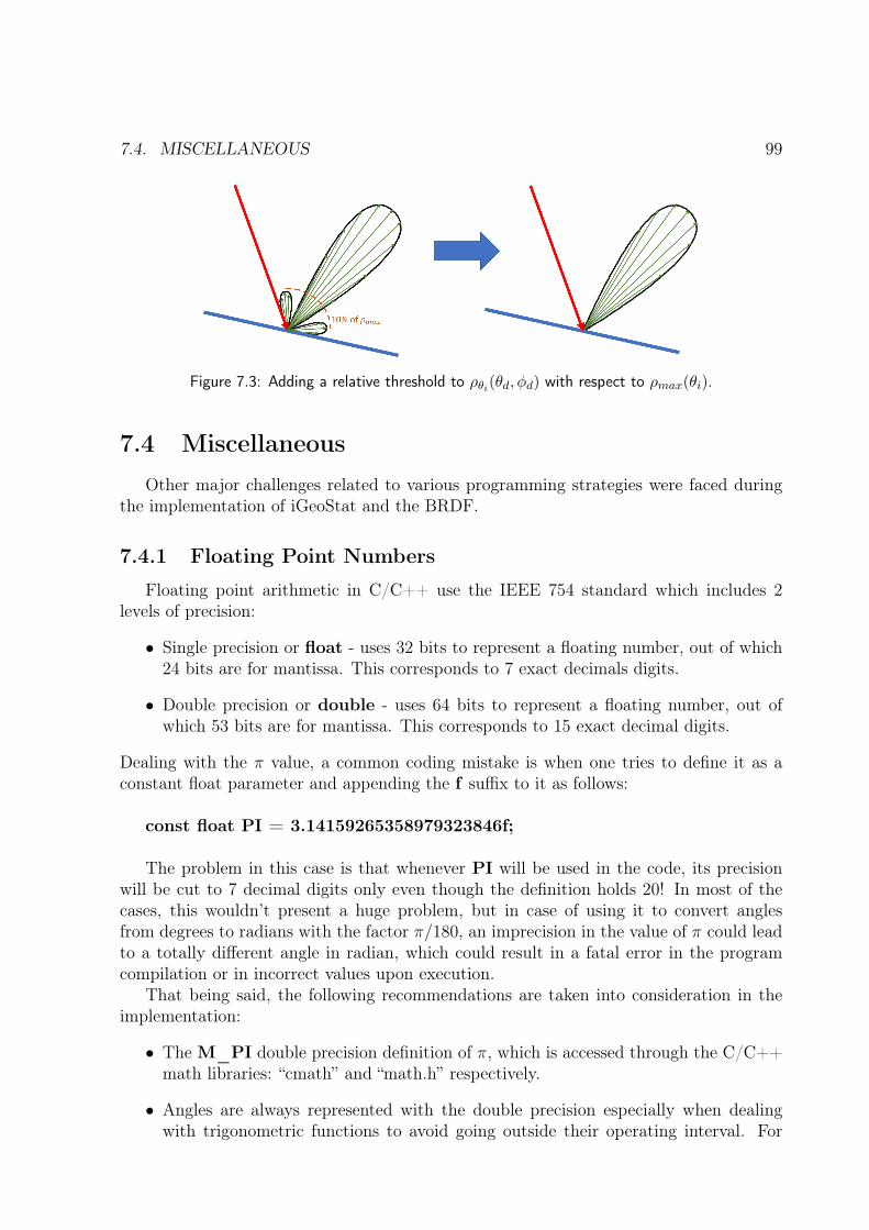
7.4. MISCELLANEOUS 99
Figure 7.3: Adding a relative threshold to ρθi(θd, φd) with respect to ρmax(θi).
7.4 MiscellaneousOther major challenges related to various programming strategies were faced during
the implementation of iGeoStat and the BRDF.
7.4.1 Floating Point Numbers
Floating point arithmetic in C/C++ use the IEEE 754 standard which includes 2levels of precision:
• Single precision or float - uses 32 bits to represent a floating number, out of which24 bits are for mantissa. This corresponds to 7 exact decimals digits.
• Double precision or double - uses 64 bits to represent a floating number, out ofwhich 53 bits are for mantissa. This corresponds to 15 exact decimal digits.
Dealing with the π value, a common coding mistake is when one tries to define it as aconstant float parameter and appending the f suffix to it as follows:
const float PI = 3.14159265358979323846f;
The problem in this case is that whenever PI will be used in the code, its precisionwill be cut to 7 decimal digits only even though the definition holds 20! In most of thecases, this wouldn’t present a huge problem, but in case of using it to convert anglesfrom degrees to radians with the factor π/180, an imprecision in the value of π could leadto a totally different angle in radian, which could result in a fatal error in the programcompilation or in incorrect values upon execution.
That being said, the following recommendations are taken into consideration in theimplementation:
• The M_PI double precision definition of π, which is accessed through the C/C++math libraries: “cmath” and “math.h” respectively.
• Angles are always represented with the double precision especially when dealingwith trigonometric functions to avoid going outside their operating interval. For
100 CHAPTER 7. MODELING AND IMPLEMENTATION CHALLENGES
example, with the function arccos, using float angles results in values outside theinterval [−1, 1], causing a fatal error on execution.
7.4.2 Factorials
PARI library contains the functionmpfact(x) that calculates the factorial of x, i.e. x!,which is used to calculate the directional diffusion component of the BRDF (function di-rectional_diffusion_nonpol (theta_i, theta_r, phi_r, sigma_0, tau, lambda,n_r, n_i) in the BRDF code documentation). Simulations have shown that even forvery large values of x the computation of mpfact(x) is still relatively fast. Unfortunately,this is not the case when performing a sum of factorials
∑x=nx=m x!. The following sum
is executed using a for loop on mpfact() which slows down terribly the execution timeespecially when m and n are very large. As a solution the for loop was rewritten in sucha way that it only executes mpfact() once. Using the simple fact that x! = (x− 1)!× x,the sum can be rewritten as the following:
Algorithm 4 Optimized recursive factorial1: fact = (m− 1)! ← integer . set initial state of fact2: sum = 0 ← integer . set initial state of sum3: for x=m:n do4: fact = fact× x5: sum = sum+ fact6: end for
Using this algorithm, mpfact() is only executed once before the for loop, thus opti-mizing execution time.
7.4.3 Static Variables
One of the limitations in C/C++ is that a function can only have a unique return. Atypical workaround is to declare a structure or a class inside this function, in which allsecondary functions with their respective returns are initialized. Local variables of theprimary function have to be initialized as static variables in order to access them, since aclass/structure is blind outside its declaration scope.
Usually, a static variable is instantly initialized with its deceleration. The problemoccurs when executing a for loop on the static variable to change its value. This resultsin a fatal error at compilation time in case of a C compiler or with wrong values afterexecution in case of a C++ compiler, since we’re asking the compiler to modify a staticvariable which has both its declaration and value static.
The only way in C++ to execute a for loop on a static variable with the intentionof changing its value is by doing the initialization and the declaration separately in twosteps. So when it goes out of scope, the static variable is reset to its initial state i.e.without any value attached to it, and hence the possibility to recursively assign a newvalue to it with the for loop. I should note that a C compiler doesn’t support changing astatic variables in all cases.

Part IV
Simulations and Performance Results
101

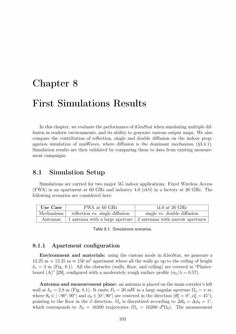
Chapter 8
First Simulations Results
In this chapter, we evaluate the performance of iGeoStat when simulating multiple dif-fusion in realistic environments, and its ability to generate various output maps. We alsocompare the contribution of reflection, single and double diffusion on the indoor prop-agation simulation of mmWaves, where diffusion is the dominant mechanism (§3.4.1).Simulation results are then validated by comparing them to data from existing measure-ment campaigns.
8.1 Simulation Setup
Simulations are carried for two major 5G indoor applications: Fixed Wireless Access(FWA) in an apartment at 60 GHz and industry 4.0 (i4.0) in a factory at 26 GHz. Thefollowing scenarios are considered here:
Use Case FWA at 60 GHz i4.0 at 26 GHzMechanisms reflection vs. single diffusion single vs. double diffusionAntennas 1 antenna with a large aperture 2 antennas with narrow apertures
Table 8.1: Simulations scenarios.
8.1.1 Apartment configuration
Environment and materials: using the custom mode in iGeoStat, we generate a12.25 m × 12.25 m ≈ 150 m2 apartment where all the walls go up to the ceiling of heighthc = 3 m (Fig. 8.1). All the obstacles (walls, floor, and ceiling) are covered in “Plaster-board (A)” [29], configured with a moderately rough surface profile (σ0/λ = 0.57).
Antenna and measurement plane: an antenna is placed on the main corridor’s leftwall at ha = 2.8 m (Fig. 8.1). It emits P0 = 20 mW in a large angular aperture Ωa = π sr,where θ0 ∈ [−90, 90] and φ0 ∈ [0, 90] are centered in the direction (θa0 = 0, φa0 = 45),pointing to the floor in the ~x direction. Ωa is discretized according to ∆θ0 = ∆φ0 = 1,which corresponds to N0 = 16200 trajectories (Ωa = 16200 d2Ω0). The measurement
103
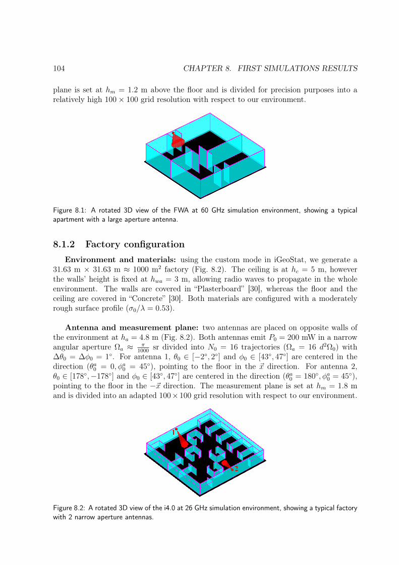
104 CHAPTER 8. FIRST SIMULATIONS RESULTS
plane is set at hm = 1.2 m above the floor and is divided for precision purposes into arelatively high 100× 100 grid resolution with respect to our environment.
Figure 8.1: A rotated 3D view of the FWA at 60 GHz simulation environment, showing a typicalapartment with a large aperture antenna.
8.1.2 Factory configuration
Environment and materials: using the custom mode in iGeoStat, we generate a31.63 m × 31.63 m ≈ 1000 m2 factory (Fig. 8.2). The ceiling is at hc = 5 m, howeverthe walls’ height is fixed at hwa = 3 m, allowing radio waves to propagate in the wholeenvironment. The walls are covered in “Plasterboard” [30], whereas the floor and theceiling are covered in “Concrete” [30]. Both materials are configured with a moderatelyrough surface profile (σ0/λ = 0.53).
Antenna and measurement plane: two antennas are placed on opposite walls ofthe environment at ha = 4.8 m (Fig. 8.2). Both antennas emit P0 = 200 mW in a narrowangular aperture Ωa ≈ π
1000sr divided into N0 = 16 trajectories (Ωa = 16 d2Ω0) with
∆θ0 = ∆φ0 = 1. For antenna 1, θ0 ∈ [−2, 2] and φ0 ∈ [43, 47] are centered in thedirection (θa0 = 0, φa0 = 45), pointing to the floor in the ~x direction. For antenna 2,θ0 ∈ [178,−178] and φ0 ∈ [43, 47] are centered in the direction (θa0 = 180, φa0 = 45),pointing to the floor in the −~x direction. The measurement plane is set at hm = 1.8 mand is divided into an adapted 100× 100 grid resolution with respect to our environment.
Figure 8.2: A rotated 3D view of the i4.0 at 26 GHz simulation environment, showing a typical factorywith 2 narrow aperture antennas.
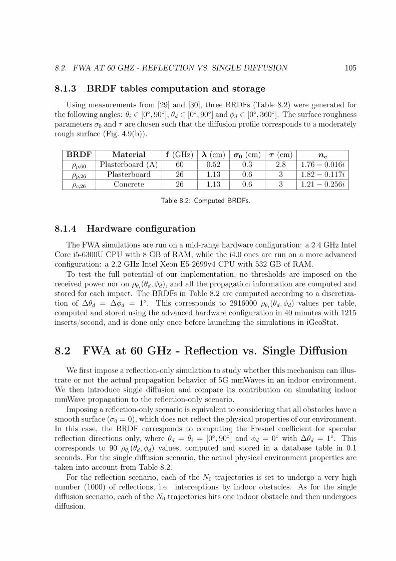
8.2. FWA AT 60 GHZ - REFLECTION VS. SINGLE DIFFUSION 105
8.1.3 BRDF tables computation and storage
Using measurements from [29] and [30], three BRDFs (Table 8.2) were generated forthe following angles: θi ∈ [0, 90], θd ∈ [0, 90] and φd ∈ [0, 360]. The surface roughnessparameters σ0 and τ are chosen such that the diffusion profile corresponds to a moderatelyrough surface (Fig. 4.9(b)).
BRDF Material f (GHz) λ (cm) σ0 (cm) τ (cm) ncρp,60 Plasterboard (A) 60 0.52 0.3 2.8 1.76− 0.016iρp,26 Plasterboard 26 1.13 0.6 3 1.82− 0.117iρc,26 Concrete 26 1.13 0.6 3 1.21− 0.256i
Table 8.2: Computed BRDFs.
8.1.4 Hardware configuration
The FWA simulations are run on a mid-range hardware configuration: a 2.4 GHz IntelCore i5-6300U CPU with 8 GB of RAM, while the i4.0 ones are run on a more advancedconfiguration: a 2.2 GHz Intel Xeon E5-2699v4 CPU with 532 GB of RAM.
To test the full potential of our implementation, no thresholds are imposed on thereceived power nor on ρθi(θd, φd), and all the propagation information are computed andstored for each impact. The BRDFs in Table 8.2 are computed according to a discretiza-tion of ∆θd = ∆φd = 1. This corresponds to 2916000 ρθi(θd, φd) values per table,computed and stored using the advanced hardware configuration in 40 minutes with 1215inserts/second, and is done only once before launching the simulations in iGeoStat.
8.2 FWA at 60 GHz - Reflection vs. Single Diffusion
We first impose a reflection-only simulation to study whether this mechanism can illus-trate or not the actual propagation behavior of 5G mmWaves in an indoor environment.We then introduce single diffusion and compare its contribution on simulating indoormmWave propagation to the reflection-only scenario.
Imposing a reflection-only scenario is equivalent to considering that all obstacles have asmooth surface (σ0 = 0), which does not reflect the physical properties of our environment.In this case, the BRDF corresponds to computing the Fresnel coefficient for specularreflection directions only, where θd = θi = [0, 90] and φd = 0 with ∆θd = 1. Thiscorresponds to 90 ρθi(θd, φd) values, computed and stored in a database table in 0.1seconds. For the single diffusion scenario, the actual physical environment properties aretaken into account from Table 8.2.
For the reflection scenario, each of the N0 trajectories is set to undergo a very highnumber (1000) of reflections, i.e. interceptions by indoor obstacles. As for the singlediffusion scenario, each of the N0 trajectories hits one indoor obstacle and then undergoesdiffusion.
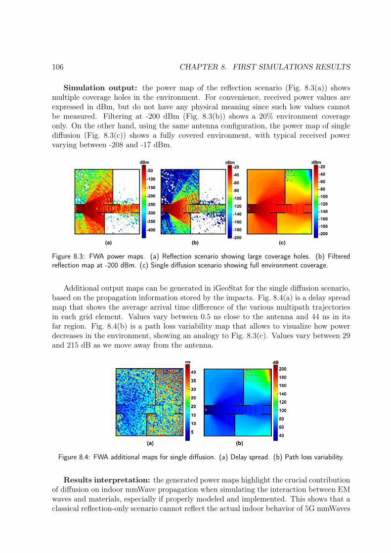
106 CHAPTER 8. FIRST SIMULATIONS RESULTS
Simulation output: the power map of the reflection scenario (Fig. 8.3(a)) showsmultiple coverage holes in the environment. For convenience, received power values areexpressed in dBm, but do not have any physical meaning since such low values cannotbe measured. Filtering at -200 dBm (Fig. 8.3(b)) shows a 20% environment coverageonly. On the other hand, using the same antenna configuration, the power map of singlediffusion (Fig. 8.3(c)) shows a fully covered environment, with typical received powervarying between -208 and -17 dBm.
Figure 8.3: FWA power maps. (a) Reflection scenario showing large coverage holes. (b) Filteredreflection map at -200 dBm. (c) Single diffusion scenario showing full environment coverage.
Additional output maps can be generated in iGeoStat for the single diffusion scenario,based on the propagation information stored by the impacts. Fig. 8.4(a) is a delay spreadmap that shows the average arrival time difference of the various multipath trajectoriesin each grid element. Values vary between 0.5 ns close to the antenna and 44 ns in itsfar region. Fig. 8.4(b) is a path loss variability map that allows to visualize how powerdecreases in the environment, showing an analogy to Fig. 8.3(c). Values vary between 29and 215 dB as we move away from the antenna.
Figure 8.4: FWA additional maps for single diffusion. (a) Delay spread. (b) Path loss variability.
Results interpretation: the generated power maps highlight the crucial contributionof diffusion on indoor mmWave propagation when simulating the interaction between EMwaves and materials, especially if properly modeled and implemented. This shows that aclassical reflection-only scenario cannot reflect the actual indoor behavior of 5G mmWaves
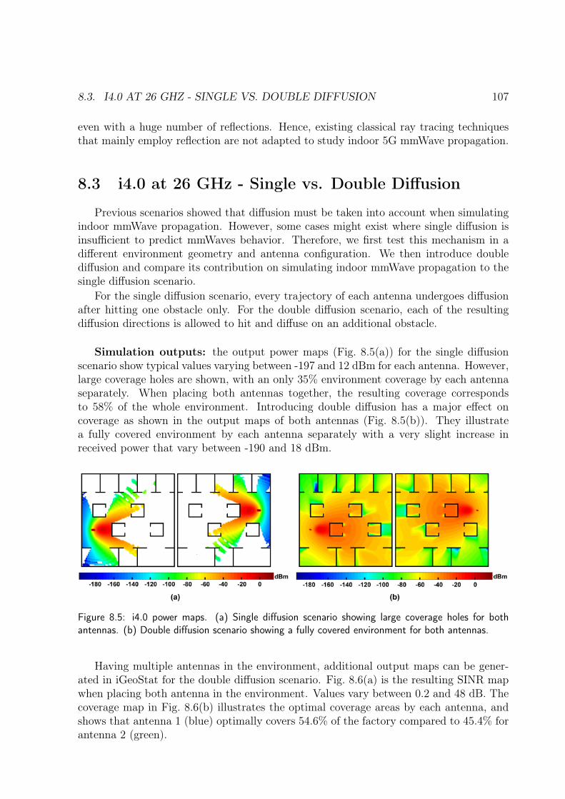
8.3. I4.0 AT 26 GHZ - SINGLE VS. DOUBLE DIFFUSION 107
even with a huge number of reflections. Hence, existing classical ray tracing techniquesthat mainly employ reflection are not adapted to study indoor 5G mmWave propagation.
8.3 i4.0 at 26 GHz - Single vs. Double Diffusion
Previous scenarios showed that diffusion must be taken into account when simulatingindoor mmWave propagation. However, some cases might exist where single diffusion isinsufficient to predict mmWaves behavior. Therefore, we first test this mechanism in adifferent environment geometry and antenna configuration. We then introduce doublediffusion and compare its contribution on simulating indoor mmWave propagation to thesingle diffusion scenario.
For the single diffusion scenario, every trajectory of each antenna undergoes diffusionafter hitting one obstacle only. For the double diffusion scenario, each of the resultingdiffusion directions is allowed to hit and diffuse on an additional obstacle.
Simulation outputs: the output power maps (Fig. 8.5(a)) for the single diffusionscenario show typical values varying between -197 and 12 dBm for each antenna. However,large coverage holes are shown, with an only 35% environment coverage by each antennaseparately. When placing both antennas together, the resulting coverage correspondsto 58% of the whole environment. Introducing double diffusion has a major effect oncoverage as shown in the output maps of both antennas (Fig. 8.5(b)). They illustratea fully covered environment by each antenna separately with a very slight increase inreceived power that vary between -190 and 18 dBm.
Figure 8.5: i4.0 power maps. (a) Single diffusion scenario showing large coverage holes for bothantennas. (b) Double diffusion scenario showing a fully covered environment for both antennas.
Having multiple antennas in the environment, additional output maps can be gener-ated in iGeoStat for the double diffusion scenario. Fig. 8.6(a) is the resulting SINR mapwhen placing both antenna in the environment. Values vary between 0.2 and 48 dB. Thecoverage map in Fig. 8.6(b) illustrates the optimal coverage areas by each antenna, andshows that antenna 1 (blue) optimally covers 54.6% of the factory compared to 45.4% forantenna 2 (green).
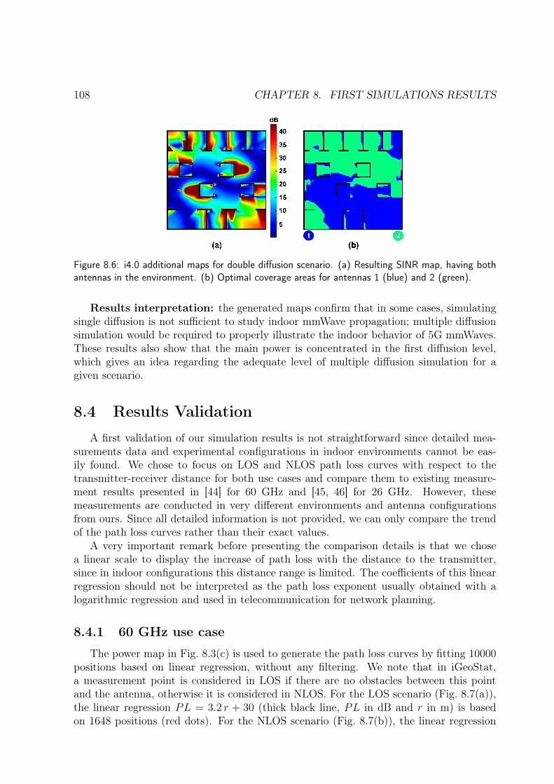
108 CHAPTER 8. FIRST SIMULATIONS RESULTS
Figure 8.6: i4.0 additional maps for double diffusion scenario. (a) Resulting SINR map, having bothantennas in the environment. (b) Optimal coverage areas for antennas 1 (blue) and 2 (green).
Results interpretation: the generated maps confirm that in some cases, simulatingsingle diffusion is not sufficient to study indoor mmWave propagation; multiple diffusionsimulation would be required to properly illustrate the indoor behavior of 5G mmWaves.These results also show that the main power is concentrated in the first diffusion level,which gives an idea regarding the adequate level of multiple diffusion simulation for agiven scenario.
8.4 Results ValidationA first validation of our simulation results is not straightforward since detailed mea-
surements data and experimental configurations in indoor environments cannot be eas-ily found. We chose to focus on LOS and NLOS path loss curves with respect to thetransmitter-receiver distance for both use cases and compare them to existing measure-ment results presented in [44] for 60 GHz and [45, 46] for 26 GHz. However, thesemeasurements are conducted in very different environments and antenna configurationsfrom ours. Since all detailed information is not provided, we can only compare the trendof the path loss curves rather than their exact values.
A very important remark before presenting the comparison details is that we chosea linear scale to display the increase of path loss with the distance to the transmitter,since in indoor configurations this distance range is limited. The coefficients of this linearregression should not be interpreted as the path loss exponent usually obtained with alogarithmic regression and used in telecommunication for network planning.
8.4.1 60 GHz use case
The power map in Fig. 8.3(c) is used to generate the path loss curves by fitting 10000positions based on linear regression, without any filtering. We note that in iGeoStat,a measurement point is considered in LOS if there are no obstacles between this pointand the antenna, otherwise it is considered in NLOS. For the LOS scenario (Fig. 8.7(a)),the linear regression PL = 3.2 r + 30 (thick black line, PL in dB and r in m) is basedon 1648 positions (red dots). For the NLOS scenario (Fig. 8.7(b)), the linear regression
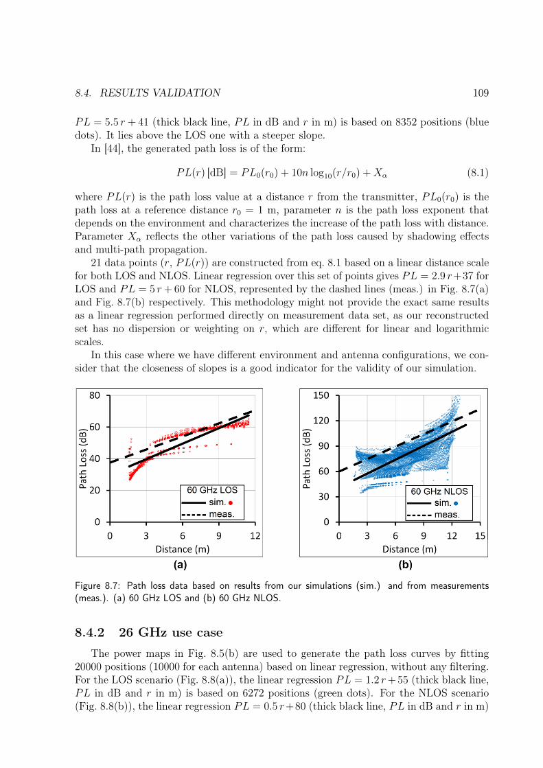
8.4. RESULTS VALIDATION 109
PL = 5.5 r + 41 (thick black line, PL in dB and r in m) is based on 8352 positions (bluedots). It lies above the LOS one with a steeper slope.
In [44], the generated path loss is of the form:
PL(r) [dB] = PL0(r0) + 10n log10(r/r0) +Xα (8.1)
where PL(r) is the path loss value at a distance r from the transmitter, PL0(r0) is thepath loss at a reference distance r0 = 1 m, parameter n is the path loss exponent thatdepends on the environment and characterizes the increase of the path loss with distance.Parameter Xα reflects the other variations of the path loss caused by shadowing effectsand multi-path propagation.
21 data points (r, PL(r)) are constructed from eq. 8.1 based on a linear distance scalefor both LOS and NLOS. Linear regression over this set of points gives PL = 2.9 r+37 forLOS and PL = 5 r+ 60 for NLOS, represented by the dashed lines (meas.) in Fig. 8.7(a)and Fig. 8.7(b) respectively. This methodology might not provide the exact same resultsas a linear regression performed directly on measurement data set, as our reconstructedset has no dispersion or weighting on r, which are different for linear and logarithmicscales.
In this case where we have different environment and antenna configurations, we con-sider that the closeness of slopes is a good indicator for the validity of our simulation.
Figure 8.7: Path loss data based on results from our simulations (sim.) and from measurements(meas.). (a) 60 GHz LOS and (b) 60 GHz NLOS.
8.4.2 26 GHz use case
The power maps in Fig. 8.5(b) are used to generate the path loss curves by fitting20000 positions (10000 for each antenna) based on linear regression, without any filtering.For the LOS scenario (Fig. 8.8(a)), the linear regression PL = 1.2 r+ 55 (thick black line,PL in dB and r in m) is based on 6272 positions (green dots). For the NLOS scenario(Fig. 8.8(b)), the linear regression PL = 0.5 r+80 (thick black line, PL in dB and r in m)
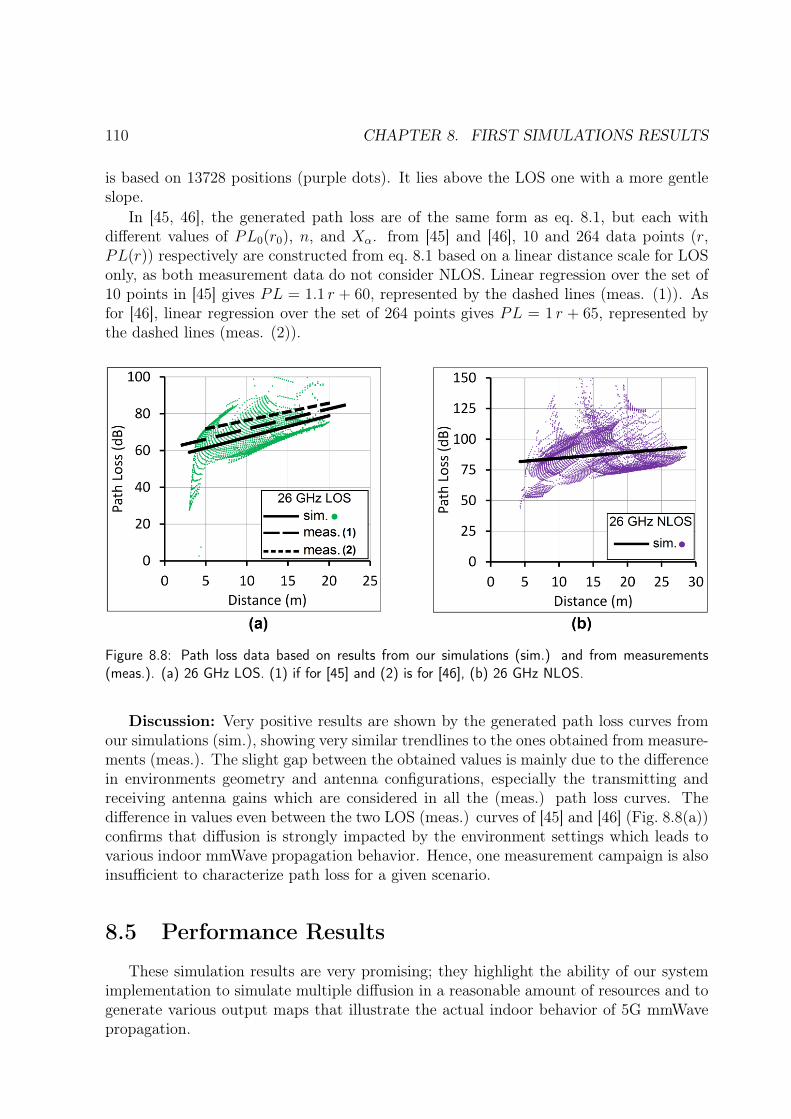
110 CHAPTER 8. FIRST SIMULATIONS RESULTS
is based on 13728 positions (purple dots). It lies above the LOS one with a more gentleslope.
In [45, 46], the generated path loss are of the same form as eq. 8.1, but each withdifferent values of PL0(r0), n, and Xα. from [45] and [46], 10 and 264 data points (r,PL(r)) respectively are constructed from eq. 8.1 based on a linear distance scale for LOSonly, as both measurement data do not consider NLOS. Linear regression over the set of10 points in [45] gives PL = 1.1 r + 60, represented by the dashed lines (meas. (1)). Asfor [46], linear regression over the set of 264 points gives PL = 1 r + 65, represented bythe dashed lines (meas. (2)).
Figure 8.8: Path loss data based on results from our simulations (sim.) and from measurements(meas.). (a) 26 GHz LOS. (1) if for [45] and (2) is for [46], (b) 26 GHz NLOS.
Discussion: Very positive results are shown by the generated path loss curves fromour simulations (sim.), showing very similar trendlines to the ones obtained from measure-ments (meas.). The slight gap between the obtained values is mainly due to the differencein environments geometry and antenna configurations, especially the transmitting andreceiving antenna gains which are considered in all the (meas.) path loss curves. Thedifference in values even between the two LOS (meas.) curves of [45] and [46] (Fig. 8.8(a))confirms that diffusion is strongly impacted by the environment settings which leads tovarious indoor mmWave propagation behavior. Hence, one measurement campaign is alsoinsufficient to characterize path loss for a given scenario.
8.5 Performance Results
These simulation results are very promising; they highlight the ability of our systemimplementation to simulate multiple diffusion in a reasonable amount of resources and togenerate various output maps that illustrate the actual indoor behavior of 5G mmWavepropagation.
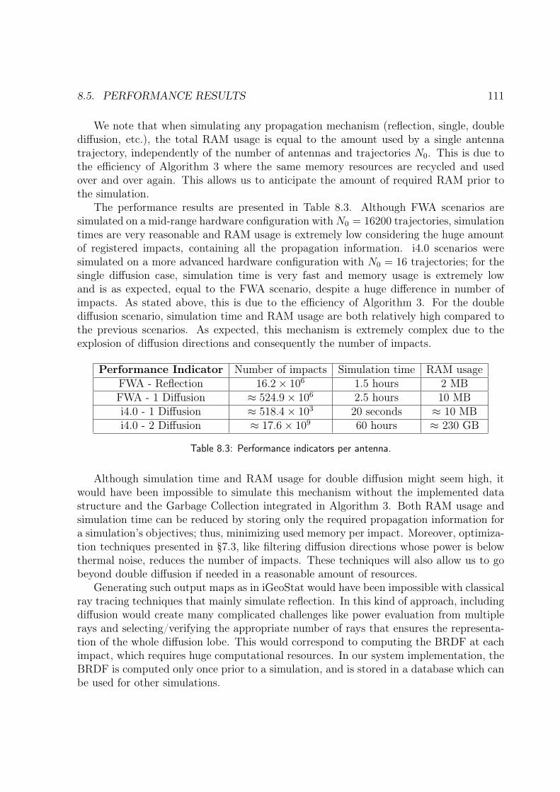
8.5. PERFORMANCE RESULTS 111
We note that when simulating any propagation mechanism (reflection, single, doublediffusion, etc.), the total RAM usage is equal to the amount used by a single antennatrajectory, independently of the number of antennas and trajectories N0. This is due tothe efficiency of Algorithm 3 where the same memory resources are recycled and usedover and over again. This allows us to anticipate the amount of required RAM prior tothe simulation.
The performance results are presented in Table 8.3. Although FWA scenarios aresimulated on a mid-range hardware configuration withN0 = 16200 trajectories, simulationtimes are very reasonable and RAM usage is extremely low considering the huge amountof registered impacts, containing all the propagation information. i4.0 scenarios weresimulated on a more advanced hardware configuration with N0 = 16 trajectories; for thesingle diffusion case, simulation time is very fast and memory usage is extremely lowand is as expected, equal to the FWA scenario, despite a huge difference in number ofimpacts. As stated above, this is due to the efficiency of Algorithm 3. For the doublediffusion scenario, simulation time and RAM usage are both relatively high compared tothe previous scenarios. As expected, this mechanism is extremely complex due to theexplosion of diffusion directions and consequently the number of impacts.
Performance Indicator Number of impacts Simulation time RAM usageFWA - Reflection 16.2× 10⁶ 1.5 hours 2 MBFWA - 1 Diffusion ≈ 524.9× 10⁶ 2.5 hours 10 MBi4.0 - 1 Diffusion ≈ 518.4× 10³ 20 seconds ≈ 10 MBi4.0 - 2 Diffusion ≈ 17.6× 10⁹ 60 hours ≈ 230 GB
Table 8.3: Performance indicators per antenna.
Although simulation time and RAM usage for double diffusion might seem high, itwould have been impossible to simulate this mechanism without the implemented datastructure and the Garbage Collection integrated in Algorithm 3. Both RAM usage andsimulation time can be reduced by storing only the required propagation information fora simulation’s objectives; thus, minimizing used memory per impact. Moreover, optimiza-tion techniques presented in §7.3, like filtering diffusion directions whose power is belowthermal noise, reduces the number of impacts. These techniques will also allow us to gobeyond double diffusion if needed in a reasonable amount of resources.
Generating such output maps as in iGeoStat would have been impossible with classicalray tracing techniques that mainly simulate reflection. In this kind of approach, includingdiffusion would create many complicated challenges like power evaluation from multiplerays and selecting/verifying the appropriate number of rays that ensures the representa-tion of the whole diffusion lobe. This would correspond to computing the BRDF at eachimpact, which requires huge computational resources. In our system implementation, theBRDF is computed only once prior to a simulation, and is stored in a database which canbe used for other simulations.

112 CHAPTER 8. FIRST SIMULATIONS RESULTS
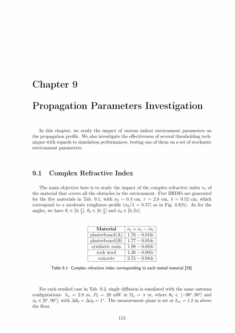
Chapter 9
Propagation Parameters Investigation
In this chapter, we study the impact of various indoor environment parameters onthe propagation profile. We also investigate the effectiveness of several thresholding tech-niques with regards to simulation performances, testing one of them on a set of stochasticenvironment parameters.
9.1 Complex Refractive Index
The main objective here is to study the impact of the complex refractive index nc ofthe material that covers all the obstacles in the environment. Five BRDFs are generatedfor the five materials in Tab. 9.1, with σ0 = 0.3 cm, τ = 2.8 cm, λ = 0.52 cm, whichcorrespond to a moderate roughness profile (σ0/λ = 0.57) as in Fig. 4.9(b). As for theangles, we have θi ∈ [0, π
2], θd ∈ [0, π
2] and φd ∈ [0, 2π].
Material nc = nr − iniplasterboard(A) 1.76− 0.016iplasterboard(B) 1.77− 0.054isynthetic resin 1.98− 0.083i
rock wool 1.26− 0.005iconcrete 2.55− 0.084i
Table 9.1: Complex refractive index corresponding to each tested material [29].
For each studied case in Tab. 9.2, single diffusion is simulated with the same antennaconfigurations: ha = 2.8 m, P0 = 20 mW in Ωa = π sr, where θ0 ∈ [−90, 90] andφ0 ∈ [0, 90], with ∆θ0 = ∆φ0 = 1. The measurement plane is set at hm = 1.2 m abovethe floor.
113
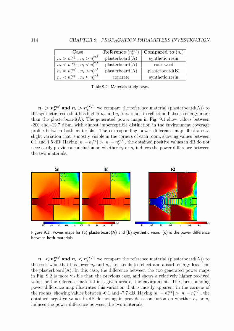
114 CHAPTER 9. PROPAGATION PARAMETERS INVESTIGATION
Case Reference (nrefc ) Compared to (nc)nr > nrefr , ni > nrefi plasterboard(A) synthetic resinnr < nrefr , ni < nrefi plasterboard(A) rock woolnr ≈ nrefr , ni > nrefi plasterboard(A) plasterboard(B)nr < nrefr , ni ≈ nrefi concrete synthetic resin
Table 9.2: Materials study cases.
nr > nrefr and ni > nrefi : we compare the reference material (plasterboard(A)) tothe synthetic resin that has higher nr and ni, i.e., tends to reflect and absorb energy morethan the plasterboard(A). The generated power maps in Fig. 9.1 show values between-200 and -12.7 dBm, with almost imperceptible distinction in the environment coverageprofile between both materials. The corresponding power difference map illustrates aslight variation that is mostly visible in the corners of each room, showing values between0.1 and 1.5 dB. Having |ni−nrefi | > |nr−nrefr |, the obtained positive values in dB do notnecessarily provide a conclusion on whether nr or ni induces the power difference betweenthe two materials.
Figure 9.1: Power maps for (a) plasterboard(A) and (b) synthetic resin. (c) is the power differencebetween both materials.
nr < nrefr and ni < nrefi : we compare the reference material (plasterboard(A)) tothe rock wool that has lower nr and ni, i.e., tends to reflect and absorb energy less thanthe plasterboard(A). In this case, the difference between the two generated power mapsin Fig. 9.2 is more visible than the previous case, and shows a relatively higher receivedvalue for the reference material in a given area of the environment. The correspondingpower difference map illustrates this variation that is mostly apparent in the corners ofthe rooms, showing values between -0.1 and -7.7 dB. Having |nr − nrefr | > |ni− n
refi |, the
obtained negative values in dB do not again provide a conclusion on whether nr or niinduces the power difference between the two materials.
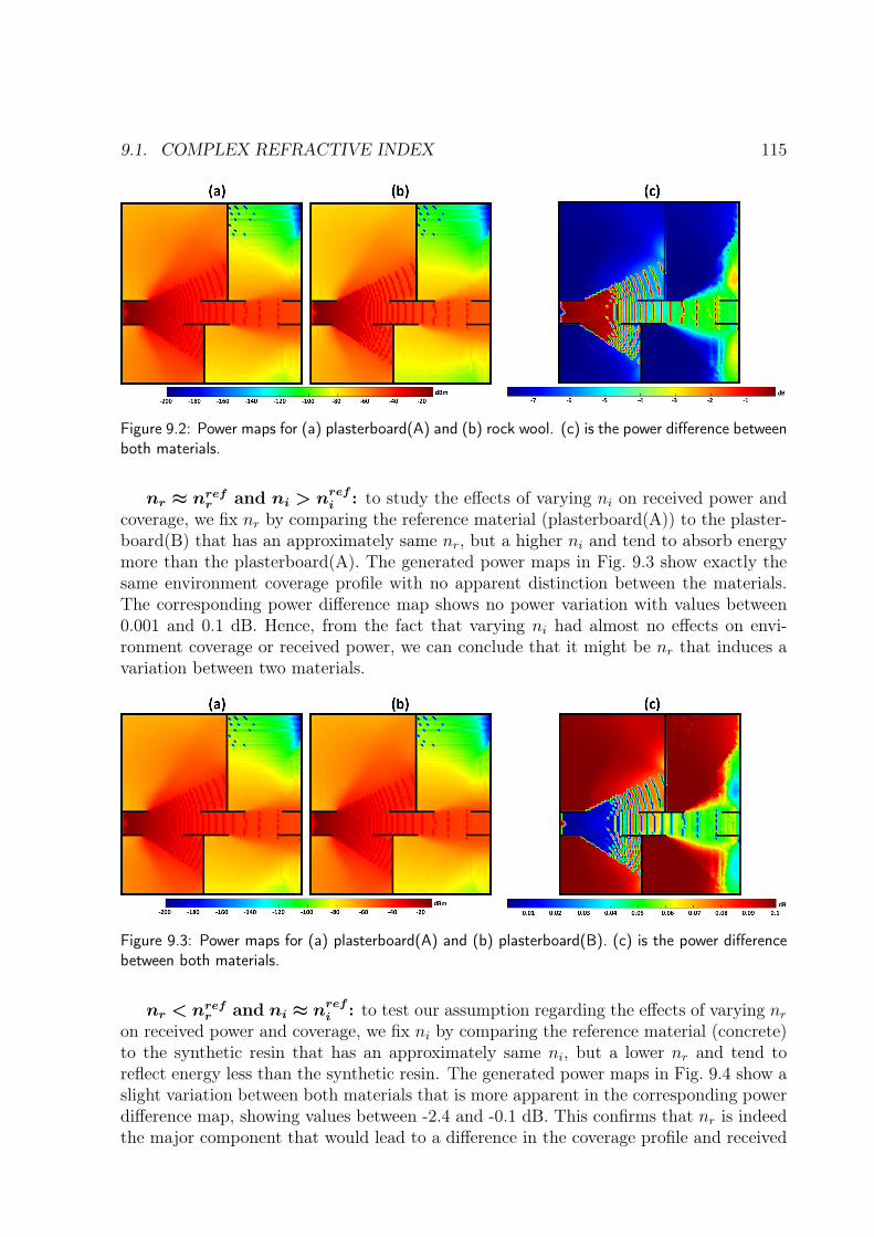
9.1. COMPLEX REFRACTIVE INDEX 115
Figure 9.2: Power maps for (a) plasterboard(A) and (b) rock wool. (c) is the power difference betweenboth materials.
nr ≈ nrefr and ni > nrefi : to study the effects of varying ni on received power andcoverage, we fix nr by comparing the reference material (plasterboard(A)) to the plaster-board(B) that has an approximately same nr, but a higher ni and tend to absorb energymore than the plasterboard(A). The generated power maps in Fig. 9.3 show exactly thesame environment coverage profile with no apparent distinction between the materials.The corresponding power difference map shows no power variation with values between0.001 and 0.1 dB. Hence, from the fact that varying ni had almost no effects on envi-ronment coverage or received power, we can conclude that it might be nr that induces avariation between two materials.
Figure 9.3: Power maps for (a) plasterboard(A) and (b) plasterboard(B). (c) is the power differencebetween both materials.
nr < nrefr and ni ≈ nrefi : to test our assumption regarding the effects of varying nron received power and coverage, we fix ni by comparing the reference material (concrete)to the synthetic resin that has an approximately same ni, but a lower nr and tend toreflect energy less than the synthetic resin. The generated power maps in Fig. 9.4 show aslight variation between both materials that is more apparent in the corresponding powerdifference map, showing values between -2.4 and -0.1 dB. This confirms that nr is indeedthe major component that would lead to a difference in the coverage profile and received
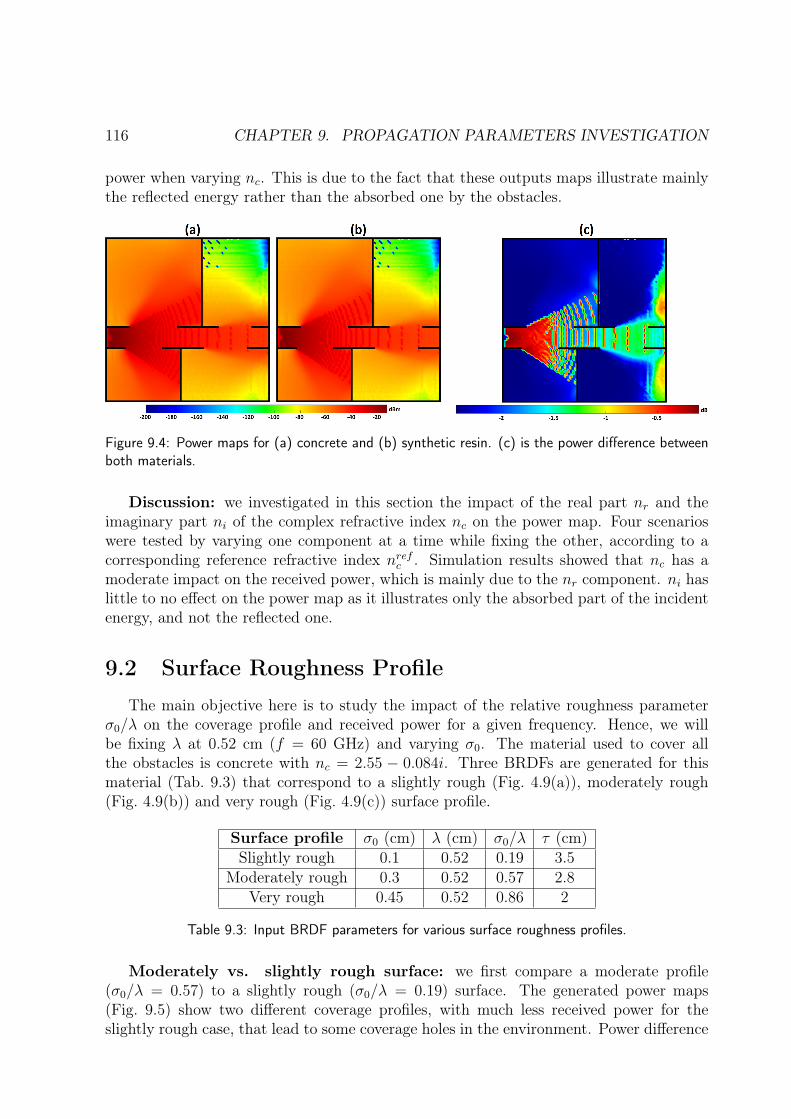
116 CHAPTER 9. PROPAGATION PARAMETERS INVESTIGATION
power when varying nc. This is due to the fact that these outputs maps illustrate mainlythe reflected energy rather than the absorbed one by the obstacles.
Figure 9.4: Power maps for (a) concrete and (b) synthetic resin. (c) is the power difference betweenboth materials.
Discussion: we investigated in this section the impact of the real part nr and theimaginary part ni of the complex refractive index nc on the power map. Four scenarioswere tested by varying one component at a time while fixing the other, according to acorresponding reference refractive index nrefc . Simulation results showed that nc has amoderate impact on the received power, which is mainly due to the nr component. ni haslittle to no effect on the power map as it illustrates only the absorbed part of the incidentenergy, and not the reflected one.
9.2 Surface Roughness ProfileThe main objective here is to study the impact of the relative roughness parameter
σ0/λ on the coverage profile and received power for a given frequency. Hence, we willbe fixing λ at 0.52 cm (f = 60 GHz) and varying σ0. The material used to cover allthe obstacles is concrete with nc = 2.55 − 0.084i. Three BRDFs are generated for thismaterial (Tab. 9.3) that correspond to a slightly rough (Fig. 4.9(a)), moderately rough(Fig. 4.9(b)) and very rough (Fig. 4.9(c)) surface profile.
Surface profile σ0 (cm) λ (cm) σ0/λ τ (cm)Slightly rough 0.1 0.52 0.19 3.5
Moderately rough 0.3 0.52 0.57 2.8Very rough 0.45 0.52 0.86 2
Table 9.3: Input BRDF parameters for various surface roughness profiles.
Moderately vs. slightly rough surface: we first compare a moderate profile(σ0/λ = 0.57) to a slightly rough (σ0/λ = 0.19) surface. The generated power maps(Fig. 9.5) show two different coverage profiles, with much less received power for theslightly rough case, that lead to some coverage holes in the environment. Power difference
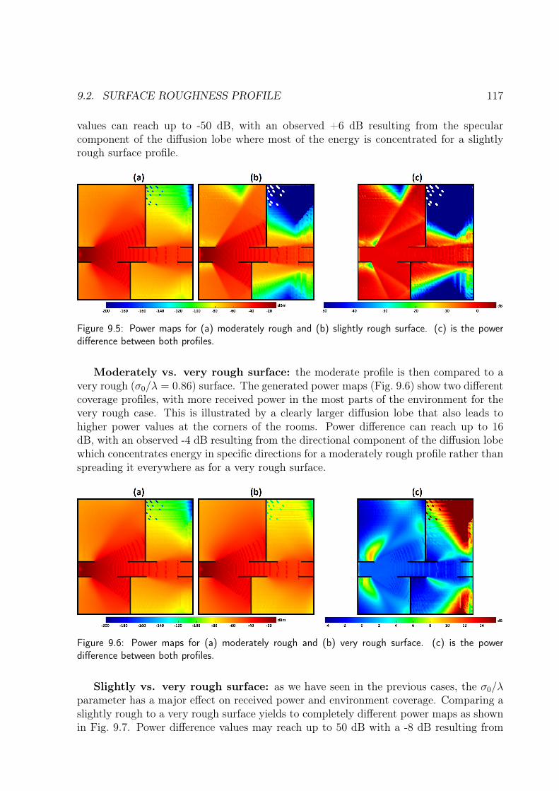
9.2. SURFACE ROUGHNESS PROFILE 117
values can reach up to -50 dB, with an observed +6 dB resulting from the specularcomponent of the diffusion lobe where most of the energy is concentrated for a slightlyrough surface profile.
Figure 9.5: Power maps for (a) moderately rough and (b) slightly rough surface. (c) is the powerdifference between both profiles.
Moderately vs. very rough surface: the moderate profile is then compared to avery rough (σ0/λ = 0.86) surface. The generated power maps (Fig. 9.6) show two differentcoverage profiles, with more received power in the most parts of the environment for thevery rough case. This is illustrated by a clearly larger diffusion lobe that also leads tohigher power values at the corners of the rooms. Power difference can reach up to 16dB, with an observed -4 dB resulting from the directional component of the diffusion lobewhich concentrates energy in specific directions for a moderately rough profile rather thanspreading it everywhere as for a very rough surface.
Figure 9.6: Power maps for (a) moderately rough and (b) very rough surface. (c) is the powerdifference between both profiles.
Slightly vs. very rough surface: as we have seen in the previous cases, the σ0/λparameter has a major effect on received power and environment coverage. Comparing aslightly rough to a very rough surface yields to completely different power maps as shownin Fig. 9.7. Power difference values may reach up to 50 dB with a -8 dB resulting from
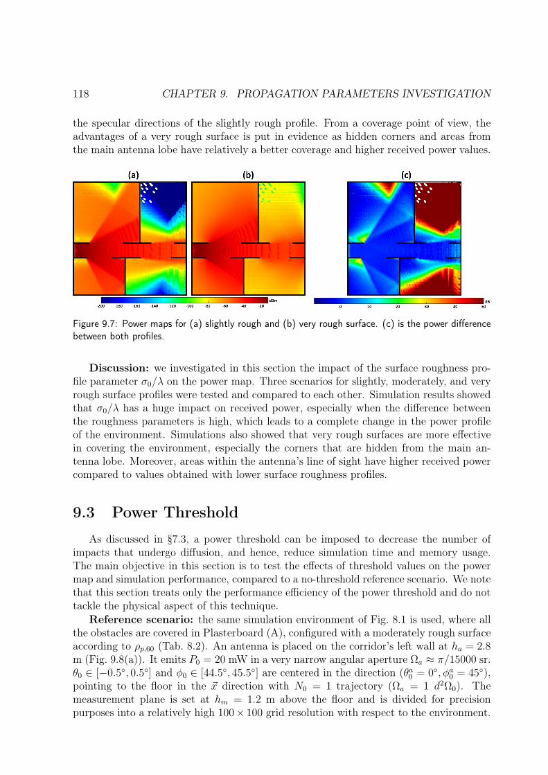
118 CHAPTER 9. PROPAGATION PARAMETERS INVESTIGATION
the specular directions of the slightly rough profile. From a coverage point of view, theadvantages of a very rough surface is put in evidence as hidden corners and areas fromthe main antenna lobe have relatively a better coverage and higher received power values.
Figure 9.7: Power maps for (a) slightly rough and (b) very rough surface. (c) is the power differencebetween both profiles.
Discussion: we investigated in this section the impact of the surface roughness pro-file parameter σ0/λ on the power map. Three scenarios for slightly, moderately, and veryrough surface profiles were tested and compared to each other. Simulation results showedthat σ0/λ has a huge impact on received power, especially when the difference betweenthe roughness parameters is high, which leads to a complete change in the power profileof the environment. Simulations also showed that very rough surfaces are more effectivein covering the environment, especially the corners that are hidden from the main an-tenna lobe. Moreover, areas within the antenna’s line of sight have higher received powercompared to values obtained with lower surface roughness profiles.
9.3 Power Threshold
As discussed in §7.3, a power threshold can be imposed to decrease the number ofimpacts that undergo diffusion, and hence, reduce simulation time and memory usage.The main objective in this section is to test the effects of threshold values on the powermap and simulation performance, compared to a no-threshold reference scenario. We notethat this section treats only the performance efficiency of the power threshold and do nottackle the physical aspect of this technique.
Reference scenario: the same simulation environment of Fig. 8.1 is used, where allthe obstacles are covered in Plasterboard (A), configured with a moderately rough surfaceaccording to ρp,60 (Tab. 8.2). An antenna is placed on the corridor’s left wall at ha = 2.8m (Fig. 9.8(a)). It emits P0 = 20 mW in a very narrow angular aperture Ωa ≈ π/15000 sr.θ0 ∈ [−0.5, 0.5] and φ0 ∈ [44.5, 45.5] are centered in the direction (θa0 = 0, φa0 = 45),pointing to the floor in the ~x direction with N0 = 1 trajectory (Ωa = 1 d2Ω0). Themeasurement plane is set at hm = 1.2 m above the floor and is divided for precisionpurposes into a relatively high 100× 100 grid resolution with respect to the environment.
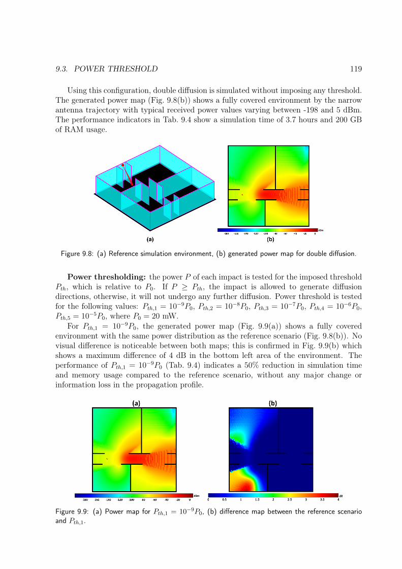
9.3. POWER THRESHOLD 119
Using this configuration, double diffusion is simulated without imposing any threshold.The generated power map (Fig. 9.8(b)) shows a fully covered environment by the narrowantenna trajectory with typical received power values varying between -198 and 5 dBm.The performance indicators in Tab. 9.4 show a simulation time of 3.7 hours and 200 GBof RAM usage.
Figure 9.8: (a) Reference simulation environment, (b) generated power map for double diffusion.
Power thresholding: the power P of each impact is tested for the imposed thresholdPth, which is relative to P0. If P ≥ Pth, the impact is allowed to generate diffusiondirections, otherwise, it will not undergo any further diffusion. Power threshold is testedfor the following values: Pth,1 = 10−9P0, Pth,2 = 10−8P0, Pth,3 = 10−7P0, Pth,4 = 10−6P0,Pth,5 = 10−5P0, where P0 = 20 mW.
For Pth,1 = 10−9P0, the generated power map (Fig. 9.9(a)) shows a fully coveredenvironment with the same power distribution as the reference scenario (Fig. 9.8(b)). Novisual difference is noticeable between both maps; this is confirmed in Fig. 9.9(b) whichshows a maximum difference of 4 dB in the bottom left area of the environment. Theperformance of Pth,1 = 10−9P0 (Tab. 9.4) indicates a 50% reduction in simulation timeand memory usage compared to the reference scenario, without any major change orinformation loss in the propagation profile.
Figure 9.9: (a) Power map for Pth,1 = 10−9P0, (b) difference map between the reference scenarioand Pth,1.
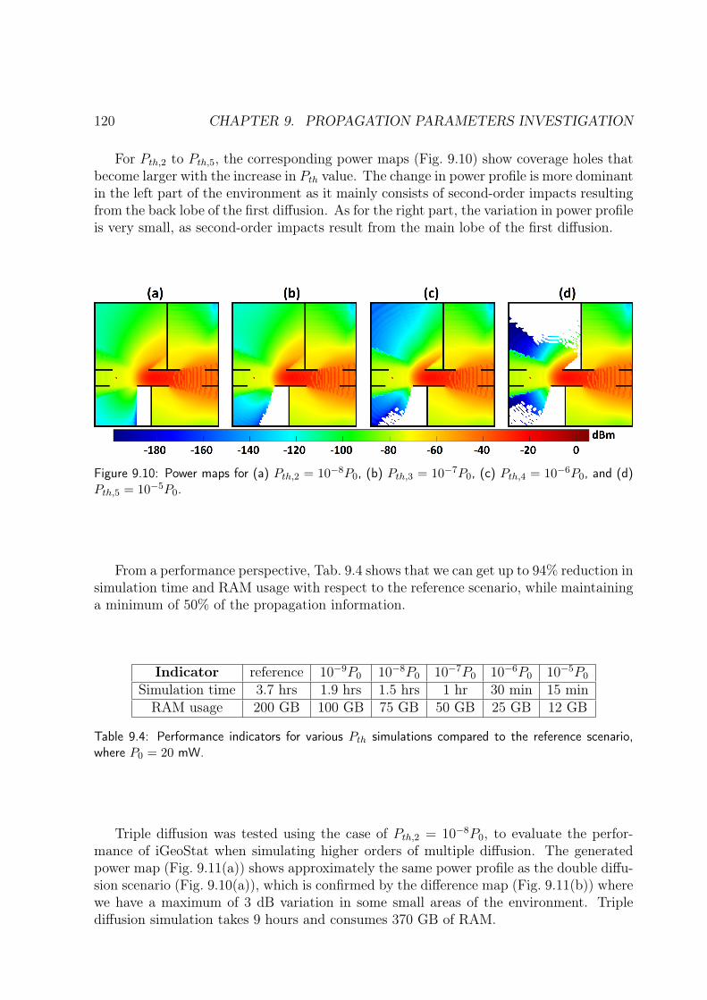
120 CHAPTER 9. PROPAGATION PARAMETERS INVESTIGATION
For Pth,2 to Pth,5, the corresponding power maps (Fig. 9.10) show coverage holes thatbecome larger with the increase in Pth value. The change in power profile is more dominantin the left part of the environment as it mainly consists of second-order impacts resultingfrom the back lobe of the first diffusion. As for the right part, the variation in power profileis very small, as second-order impacts result from the main lobe of the first diffusion.
Figure 9.10: Power maps for (a) Pth,2 = 10−8P0, (b) Pth,3 = 10−7P0, (c) Pth,4 = 10−6P0, and (d)Pth,5 = 10−5P0.
From a performance perspective, Tab. 9.4 shows that we can get up to 94% reduction insimulation time and RAM usage with respect to the reference scenario, while maintaininga minimum of 50% of the propagation information.
Indicator reference 10−9P0 10−8P0 10−7P0 10−6P0 10−5P0
Simulation time 3.7 hrs 1.9 hrs 1.5 hrs 1 hr 30 min 15 minRAM usage 200 GB 100 GB 75 GB 50 GB 25 GB 12 GB
Table 9.4: Performance indicators for various Pth simulations compared to the reference scenario,where P0 = 20 mW.
Triple diffusion was tested using the case of Pth,2 = 10−8P0, to evaluate the perfor-mance of iGeoStat when simulating higher orders of multiple diffusion. The generatedpower map (Fig. 9.11(a)) shows approximately the same power profile as the double diffu-sion scenario (Fig. 9.10(a)), which is confirmed by the difference map (Fig. 9.11(b)) wherewe have a maximum of 3 dB variation in some small areas of the environment. Triplediffusion simulation takes 9 hours and consumes 370 GB of RAM.
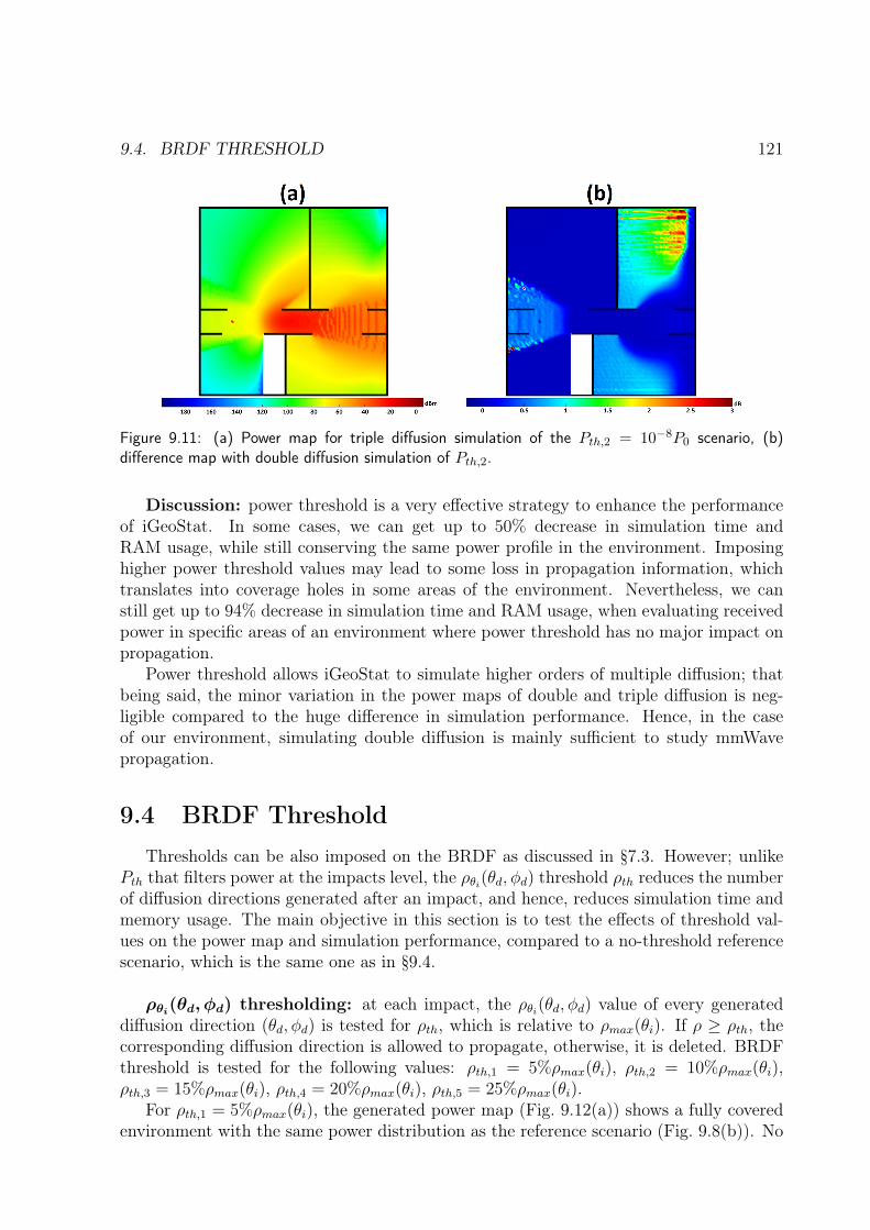
9.4. BRDF THRESHOLD 121
Figure 9.11: (a) Power map for triple diffusion simulation of the Pth,2 = 10−8P0 scenario, (b)difference map with double diffusion simulation of Pth,2.
Discussion: power threshold is a very effective strategy to enhance the performanceof iGeoStat. In some cases, we can get up to 50% decrease in simulation time andRAM usage, while still conserving the same power profile in the environment. Imposinghigher power threshold values may lead to some loss in propagation information, whichtranslates into coverage holes in some areas of the environment. Nevertheless, we canstill get up to 94% decrease in simulation time and RAM usage, when evaluating receivedpower in specific areas of an environment where power threshold has no major impact onpropagation.
Power threshold allows iGeoStat to simulate higher orders of multiple diffusion; thatbeing said, the minor variation in the power maps of double and triple diffusion is neg-ligible compared to the huge difference in simulation performance. Hence, in the caseof our environment, simulating double diffusion is mainly sufficient to study mmWavepropagation.
9.4 BRDF ThresholdThresholds can be also imposed on the BRDF as discussed in §7.3. However; unlike
Pth that filters power at the impacts level, the ρθi(θd, φd) threshold ρth reduces the numberof diffusion directions generated after an impact, and hence, reduces simulation time andmemory usage. The main objective in this section is to test the effects of threshold val-ues on the power map and simulation performance, compared to a no-threshold referencescenario, which is the same one as in §9.4.
ρθi(θd, φd) thresholding: at each impact, the ρθi(θd, φd) value of every generateddiffusion direction (θd, φd) is tested for ρth, which is relative to ρmax(θi). If ρ ≥ ρth, thecorresponding diffusion direction is allowed to propagate, otherwise, it is deleted. BRDFthreshold is tested for the following values: ρth,1 = 5%ρmax(θi), ρth,2 = 10%ρmax(θi),ρth,3 = 15%ρmax(θi), ρth,4 = 20%ρmax(θi), ρth,5 = 25%ρmax(θi).
For ρth,1 = 5%ρmax(θi), the generated power map (Fig. 9.12(a)) shows a fully coveredenvironment with the same power distribution as the reference scenario (Fig. 9.8(b)). No
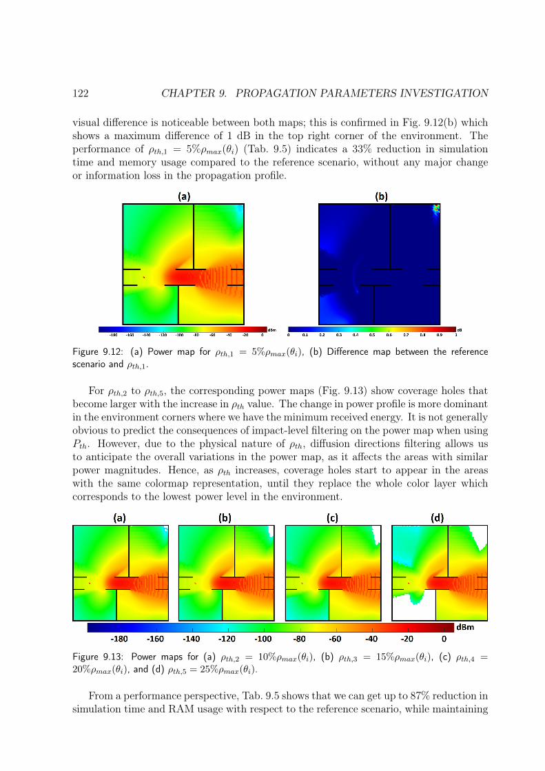
122 CHAPTER 9. PROPAGATION PARAMETERS INVESTIGATION
visual difference is noticeable between both maps; this is confirmed in Fig. 9.12(b) whichshows a maximum difference of 1 dB in the top right corner of the environment. Theperformance of ρth,1 = 5%ρmax(θi) (Tab. 9.5) indicates a 33% reduction in simulationtime and memory usage compared to the reference scenario, without any major changeor information loss in the propagation profile.
Figure 9.12: (a) Power map for ρth,1 = 5%ρmax(θi), (b) Difference map between the referencescenario and ρth,1.
For ρth,2 to ρth,5, the corresponding power maps (Fig. 9.13) show coverage holes thatbecome larger with the increase in ρth value. The change in power profile is more dominantin the environment corners where we have the minimum received energy. It is not generallyobvious to predict the consequences of impact-level filtering on the power map when usingPth. However, due to the physical nature of ρth, diffusion directions filtering allows usto anticipate the overall variations in the power map, as it affects the areas with similarpower magnitudes. Hence, as ρth increases, coverage holes start to appear in the areaswith the same colormap representation, until they replace the whole color layer whichcorresponds to the lowest power level in the environment.
Figure 9.13: Power maps for (a) ρth,2 = 10%ρmax(θi), (b) ρth,3 = 15%ρmax(θi), (c) ρth,4 =20%ρmax(θi), and (d) ρth,5 = 25%ρmax(θi).
From a performance perspective, Tab. 9.5 shows that we can get up to 87% reduction insimulation time and RAM usage with respect to the reference scenario, while maintaining
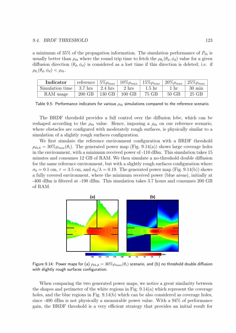
9.4. BRDF THRESHOLD 123
a minimum of 35% of the propagation information. The simulation performance of Pth isusually better than ρth where the round trip time to fetch the ρθi(θd, φd) value for a givendiffusion direction (θd, φd) is considered as a lost time if this direction is deleted; i.e. ifρθi(θd, φd) < ρth.
Indicator reference 5%ρmax 10%ρmax 15%ρmax 20%ρmax 25%ρmaxSimulation time 3.7 hrs 2.4 hrs 2 hrs 1.5 hr 1 hr 30 minRAM usage 200 GB 130 GB 100 GB 75 GB 50 GB 25 GB
Table 9.5: Performance indicators for various ρth simulations compared to the reference scenario.
The BRDF threshold provides a full control over the diffusion lobe, which can bereshaped according to the ρth value. Hence, imposing a ρth on our reference scenario,where obstacles are configured with moderately rough surfaces, is physically similar to asimulation of a slightly rough surfaces configuration.
We first simulate the reference environment configuration with a BRDF thresholdρth,6 = 30%ρmax(θi). The generated power map (Fig. 9.14(a)) shows large coverage holesin the environment, with a minimum received power of -110 dBm. This simulation takes 15minutes and consumes 12 GB of RAM. We then simulate a no-threshold double diffusionfor the same reference environment, but with a slightly rough surfaces configuration whereσ0 = 0.1 cm, τ = 3.5 cm, and σ0/λ = 0.19. The generated power map (Fig. 9.14(b)) showsa fully covered environment, where the minimum received power (blue areas), initially at-400 dBm is filtered at -198 dBm. This simulation takes 3.7 hours and consumes 200 GBof RAM.
Figure 9.14: Power maps for (a) ρth,6 = 30%ρmax(θi) scenario, and (b) no threshold double diffusionwith slightly rough surfaces configuration.
When comparing the two generated power maps, we notice a great similarity betweenthe shapes and perimeter of the white regions in Fig. 9.14(a) which represent the coverageholes, and the blue regions in Fig. 9.14(b) which can be also considered as coverage holes,since -400 dBm is not physically a measurable power value. With a 94% of performancegain, the BRDF threshold is a very efficient strategy that provides an initial result for
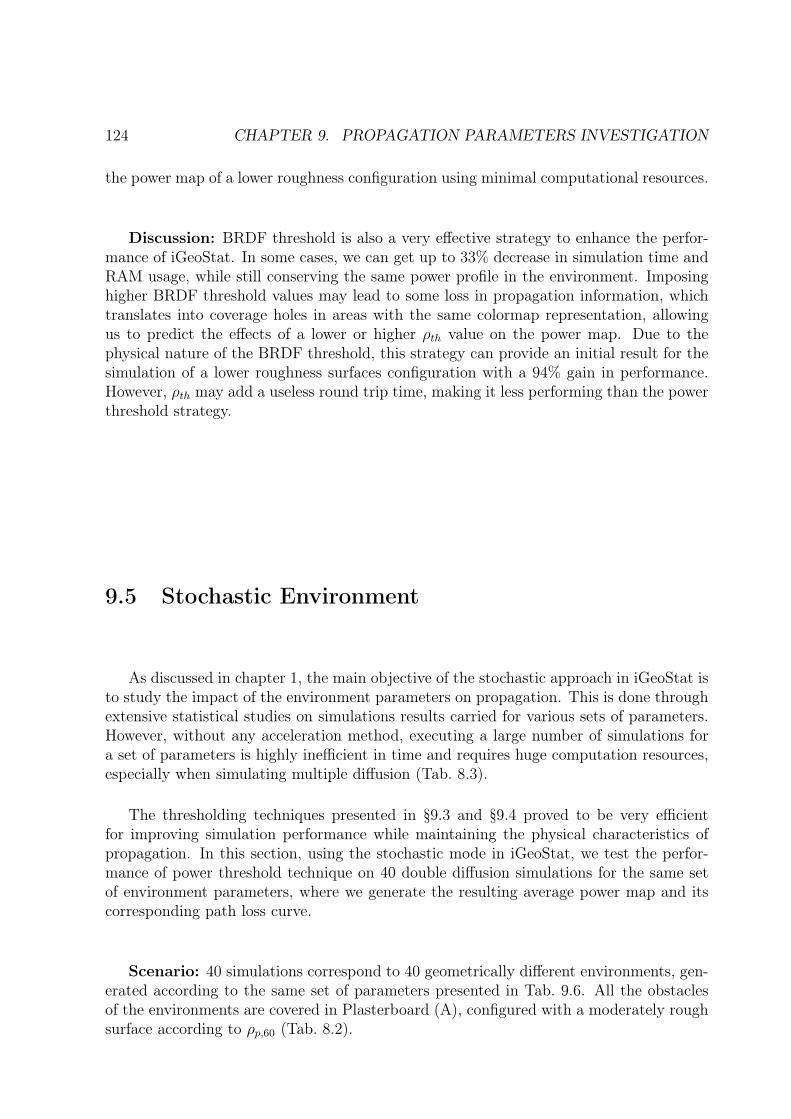
124 CHAPTER 9. PROPAGATION PARAMETERS INVESTIGATION
the power map of a lower roughness configuration using minimal computational resources.
Discussion: BRDF threshold is also a very effective strategy to enhance the perfor-mance of iGeoStat. In some cases, we can get up to 33% decrease in simulation time andRAM usage, while still conserving the same power profile in the environment. Imposinghigher BRDF threshold values may lead to some loss in propagation information, whichtranslates into coverage holes in areas with the same colormap representation, allowingus to predict the effects of a lower or higher ρth value on the power map. Due to thephysical nature of the BRDF threshold, this strategy can provide an initial result for thesimulation of a lower roughness surfaces configuration with a 94% gain in performance.However, ρth may add a useless round trip time, making it less performing than the powerthreshold strategy.
9.5 Stochastic Environment
As discussed in chapter 1, the main objective of the stochastic approach in iGeoStat isto study the impact of the environment parameters on propagation. This is done throughextensive statistical studies on simulations results carried for various sets of parameters.However, without any acceleration method, executing a large number of simulations fora set of parameters is highly inefficient in time and requires huge computation resources,especially when simulating multiple diffusion (Tab. 8.3).
The thresholding techniques presented in §9.3 and §9.4 proved to be very efficientfor improving simulation performance while maintaining the physical characteristics ofpropagation. In this section, using the stochastic mode in iGeoStat, we test the perfor-mance of power threshold technique on 40 double diffusion simulations for the same setof environment parameters, where we generate the resulting average power map and itscorresponding path loss curve.
Scenario: 40 simulations correspond to 40 geometrically different environments, gen-erated according to the same set of parameters presented in Tab. 9.6. All the obstaclesof the environments are covered in Plasterboard (A), configured with a moderately roughsurface according to ρp,60 (Tab. 8.2).
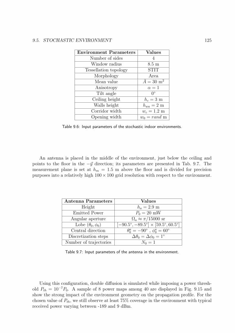
9.5. STOCHASTIC ENVIRONMENT 125
Environment Parameters ValuesNumber of sides 4Window radius 8.5 m
Tessellation topology STITMorphology AreaMean value A = 30 m2
Anisotropy α = 1Tilt angle 0
Ceiling height hc = 3 mWalls height hwa = 2 m
Corridor width wc = 1.2 mOpening width w0 = rand m
Table 9.6: Input parameters of the stochastic indoor environments.
An antenna is placed in the middle of the environment, just below the ceiling andpoints to the floor in the −~y direction; its parameters are presented in Tab. 9.7. Themeasurement plane is set at hm = 1.5 m above the floor and is divided for precisionpurposes into a relatively high 100× 100 grid resolution with respect to the environment.
Antenna Parameters ValuesHeight ha = 2.9 m
Emitted Power P0 = 20 mWAngular aperture Ωa ≈ π/15000 srLobe (θ0, φ0) [−90.5,−89.5]× [59.5, 60.5]
Central direction θa0 = −90 , φa0 = 60
Discretization steps ∆θ0 = ∆φ0 = 1
Number of trajectories N0 = 1
Table 9.7: Input parameters of the antenna in the environment.
Using this configuration, double diffusion is simulated while imposing a power thresh-old Pth = 10−7P0. A sample of 8 power maps among 40 are displayed in Fig. 9.15 andshow the strong impact of the environment geometry on the propagation profile. For thechosen value of Pth, we still observe at least 75% coverage in the environment with typicalreceived power varying between -189 and 9 dBm.
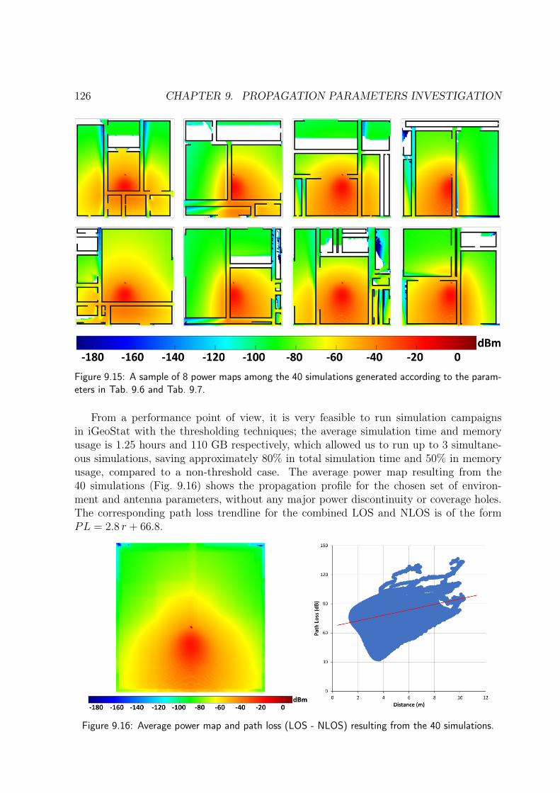
126 CHAPTER 9. PROPAGATION PARAMETERS INVESTIGATION
Figure 9.15: A sample of 8 power maps among the 40 simulations generated according to the param-eters in Tab. 9.6 and Tab. 9.7.
From a performance point of view, it is very feasible to run simulation campaignsin iGeoStat with the thresholding techniques; the average simulation time and memoryusage is 1.25 hours and 110 GB respectively, which allowed us to run up to 3 simultane-ous simulations, saving approximately 80% in total simulation time and 50% in memoryusage, compared to a non-threshold case. The average power map resulting from the40 simulations (Fig. 9.16) shows the propagation profile for the chosen set of environ-ment and antenna parameters, without any major power discontinuity or coverage holes.The corresponding path loss trendline for the combined LOS and NLOS is of the formPL = 2.8 r + 66.8.
Figure 9.16: Average power map and path loss (LOS - NLOS) resulting from the 40 simulations.

9.5. STOCHASTIC ENVIRONMENT 127
This shows the effectiveness of the thresholding techniques when a large number ofsimulations is required to study the propagation profile. We note that at this stage, wecannot draw conclusions regarding the measurement characteristic that would define therelationship between the stochastic parameters and the power profile of the environment.

128 CHAPTER 9. PROPAGATION PARAMETERS INVESTIGATION

Part V
Conclusion
129

Chapter 10
Conclusion and Perspectives
10.1 Conclusion
This work introduced a novel modeling framework for indoor 5G mmWave propaga-tion, combining stochastic environment modeling with physical propagation simulation.Its system implementation, iGeoStat, generates parameterized typical environments thataccount for the statistical indoor variability, then simulates radio propagation based onthe physical interaction between EM waves and indoor materials. Challenging computa-tional tasks were solved by formulating an adapted link budget and designing new memorymanagement and optimization algorithms, making iGeoStat the first to simulate multiplediffusion in realistic environments.
First simulations were carried for FWA at 60 GHz and i4.0 at 26 GHz to investigatethe contribution of reflection, single and double diffusion on indoor mmWave propagationsimulation, where diffusion is the most complex but certainly the most essential mech-anism. Illustrated results confirmed that a reflection-only simulation cannot describeindoor mmWaves behavior. They also showed that received power is mostly concentratedin single diffusion; however, simulating this mechanism is not always sufficient to studyindoor mmWave coverage, and may require double diffusion. Such conclusions cannot beobtained with classical ray tracing techniques.
Simulation results were successfully validated by comparing the generated LOS andNLOS path loss curves to the ones obtained from measurements at 60 and 26 GHz. Theperformance results showed the efficiency of iGeoStat to simulate multiple diffusion andgenerate various output maps (power, SINR, coverage, path loss and delay spread) in areasonable amount of time and memory. Our implementation enables us to determine theimpact of a given multiple diffusion level and to predict the required time and RAM forany propagation mechanism.
We investigated in this work the impact of the main environment parameters on thepropagation profile; simulation results showed that the complex refractive index has amoderate impact on the received power, and is mainly due to its real component. On theother hand, the surface roughness parameter has a major impact on received power andmay lead in some cases to a completely different power profile in the environment.
Several optimization and acceleration techniques were presented and tested in thiswork; for example, power or BRDF thresholding can further reduce simulation time and
131
132 CHAPTER 10. CONCLUSION AND PERSPECTIVES
memory usage by at least 50% without impacting the physical characteristics of propa-gation, allowing us to go beyond double diffusion if needed. The performance of powerthresholding was tested on 40 simulations for a set of stochastic environment parameters,showing that we can save up to 80% in total simulation time and 50% in memory usage.
10.2 Perspectives
The current implementation of iGeoStat can be used by operators and radio planningengineers as a first indicator for predicting received power, SINR, path loss, and delayspread in a given environment. The flexibility of our implementation will enable us tofurther improve iGeoStat’s main modules.
The stochastic environment module can be enhanced by adding furniture or othertypes of indoor obstacles with polygonal shapes through the implementation of iteratedtessellations. We can also study the characteristics of a typical indoor cell and analyze thepossible link between its parameters and its different representations (room, open-space,etc.). Moreover, we need to develop an adapted fitting method: what is the characteristicsvector and how to automatically identify the presence of doors and corridors with theirwidth parameters, which is a starting point for finding the structuring parameters of anindoor environment.
The radio propagation module can be also enhanced by implementing additionalmechanisms: Fresnel zones have to be taken into account in the simulator to identifyconstructive and destructive interference, which mostly occur for polarized waves. Trans-mission through obstacles can be added by allowing a trajectory to traverse the objectafter an impact. Its direction would be defined by the Snell-Descartes law and the frac-tion of carried energy ρtrθi(θd, φd) would be deduced from the BRDF where ρtrθi(θd, φd) =1 − (ρsrθi (θd, φd) + ρddθi (θd, φd) + ρudθi (θd, φd)). We note that this mechanism introduces theproblem of energy re-emission from walls and various indoor obstacles that should betaken into account in the link budget. Diffraction from edges can be also included bylaunching trajectories within a uniform lobe, where the carried fraction of energy is thesame in all directions. Periodic and other types of rough surfaces can be also integratedin iGeoStat through the BRDF approach. Moreover, since He’s model is based on thephysical theory of electromagnetism for visible light, terahertz transmission applicationslike Li-Fi and optical wireless communications can be simulated in iGeoStat. However,we must make sure that the curvature radius condition of the surface still holds for thechosen wavelength.
Additional modules can be also implemented in iGeoStat to solve the indoor challengesof 5G mmWave planning and dimensioning, like the optimization of antenna placementwhile taking into account the position and geometry of the obstacles to achieve bettercoverage and SINR. A throughput analysis module can be also implemented to studythe network and end-user capacity based on the generated power and SINR maps ofthe studied environment, and based on the antenna configuration and signal bandwidth.Moreover, a Multiple-Input and Multiple-Output (MIMO) module can be added with

10.2. PERSPECTIVES 133
various configurations (transmit diversity, spatial multiplexing, and beamforming) to en-hance the transmitter or receiver gain.
From a performance perspective, further optimization techniques are envisioned thatwould reduce both simulation time and memory usage in iGeoStat. For example, paral-lel computing allows the simultaneous simulation of multiple antenna trajectories whichreduces time drastically. The maximum number of trajectories per one simulation isbounded by the available memory. Moreover, the data structure holding the vector ofimpacts can be further optimized such that it frees more memory as we move from adiffusion level to another, which reduces RAM usage per simulation.
Using the acceleration techniques presented in this work, multiple simulation cam-paigns will be conducted in iGeoStat for various sets of parameterized stochastic environ-ments (geometry and materials). Extensive statistical studies on simulations results willbe then carried to propose the first parameterized analytical formulae of indoor propa-gation models that are not dedicated to a particular environment, frequency or use case.However, several questions still need to be answered, like what is the number of simu-lations that is required to deduce the propagation profile, or how to adapt the power ofBRDF threshold to the environment.

134 CHAPTER 10. CONCLUSION AND PERSPECTIVES

Résumé du manuscrit en français
135

Chapitre 1
Introduction
1.1 Contexte et motivation
Trois familles de cas d’usage sont définies pour les applications 5G basées sur lesondes millimétriques. eMBB (Enhanced Mobile Broadband) offrira des débits de données10 fois plus élevés que la 4G. mMTC (massive Machine Type Communications) exigeraune capacité réseau élevée en raison du grand nombre d’appareils connectés. URLLC(Ultra-Reliable Low Latency Communications) prendra en charge les applications avecdes contraintes de latence et de fiabilité strictes.
Bien que les ondes millimétriques soient une solution prometteuse au problème del’épuisement du spectre, leurs propriétés de propagation, notamment leur très courtelongueur d’onde, peuvent avoir un impact important sur la transmission. Ces dégradationsdeviennent encore plus fortes dans les scénarios de communication indoor-indoor en raisondes nombreuses contraintes imposées par l’environnement, conduisant à un nouveau défimajeur : la couverture indoor.
Cela nécessite des études spécifiques sur la propagation indoor des ondes millimé-triques afin de planifier les réseaux 5G en indoor. Ce sujet est cependant très complexeà étudier puisque les environnements indoors varient beaucoup en termes de configura-tion spatiale. Même si nous considérons une géométrie particulière, ses caractéristiquesintérieures (positions de meubles, portes, etc.) et ses matériaux (bois, béton, etc.) sonttrès variés. De plus, les surfaces des matériaux indoors sont généralement rugueuses ; cetterugosité est comparable à la longueur d’onde des ondes millimétriques et donc, la diffusionélectromagnétique (EM) ne peut pas être ignorée et doit être étudiée.
Les études existantes reposent sur des campagnes de mesure ou des simulations sys-tème. La réalisation de mesures est un processus très lourd et nécessite beaucoup deressources. Les études [1, 2] basées sur cette méthode effectuent des mesures dans un typeet un environnement spécifiques ; les données recueillies sont exactes pour ce scénario par-ticulier seulement et ne prennent pas en compte la diversité de propagation inhérente àla topologie, à la morphologie et aux propriétés matérielles d’un environnement. Étantdonné qu’il n’est pas pratique d’effectuer des mesures dans diverses configurations envi-ronnementales, les modèles empiriques générés ne peuvent pas être utilisés dans d’autresapplications indoor, ni fournir des informations concernant l’influence des caractéristiquesindoors sur les mécanismes de propagation, en particulier la diffusion.
137
138 CHAPITRE 1. INTRODUCTION
Les simulateurs offrent une alternative flexible pour étudier la propagation. Les simu-lateurs existants des ondes millimétriques en indoor permettent aux utilisateurs d’étu-dier la propagation dans divers environnements. Chacun de ces simulateurs utilise diffé-rentes techniques d’implémentation des mécanismes de propagation ; cependant, la plupartd’entre eux présentent des inconvénients majeurs quant à la diffusion qui est le mécanismele plus complexe et qui certainement mérite d’être étudié en détail. Dans [3] par exemple,le lobe de diffusion qui décrit physiquement la distribution angulaire de l’énergie EMest trop simplifié : il et est défini par l’utilisateur qui choisit entre un modèle Lambertou directif, décide d’introduire ou non la rétrodiffusion en spécifiant le cas échéant lelobe arrière. Certains simulateurs comme [4] utilisent des modèles empiriques, et d’autrescomme [5] ne considèrent pas la diffusion en raison des difficultés d’implémentation. Parconséquent, ces simulateurs ne peuvent pas prédire de manière suffisamment réaliste lecomportement des ondes millimétriques. Les modèles qui en sont déduits ne sont ainsipas en mesure de proposer des conclusions quant à l’impact de la géométrie indoor et desmatériaux sur la propagation de ces ondes.
1.2 Contributions
Dans ce manuscrit, nous présentons un nouveau cadre de modélisation de la propaga-tion des ondes millimétriques 5G en indoor qui combine la génération 3D d’environnementstochastique avec une simulation avancée de la propagation physique. Son implémentationsystème, appelée iGeoStat, utilise la théorie de la géométrie stochastique pour générer desenvironnements typiques paramétrés qui tiennent compte de la variabilité statistique enindoor, puis utilise le modèle physique complexe mais complet de He [6] pour simuler lapropagation radio basée sur l’interaction physique entre les ondes EM et les matériauxindoors. L’implémentation pratique de ce cadre soulève des tâches informatiques très dif-ficiles que nous résolvons en formulant un bilan de liaison adapté et en concevant denouveaux algorithmes de gestion et d’optimisation de la mémoire. Cela fait d’iGeoStatla première approche pratique à simuler la diffusion multiple dans des environnementsréalistes, ce qui nous permet d’étudier le comportement indoor réel de la propagation desonde millimétriques 5G et ses applications industrielles.
Le cadre proposé vise à comprendre statistiquement l’influence de la géométrie de l’en-vironnement et des paramètres des matériaux sur les propriétés de propagation des ondesmillimétriques, en particulier la couverture, le SINR et le path loss. Par conséquent, lesmodèles générés ne sont pas définis par la géométrie ou le matériau lui-même, mais plutôtpar les paramètres qui les caractérisent. Ce cadre n’est pas dédié à un environnement,matériel, fréquence ou cas d’utilisation particulier, ce qui le rend très efficace pour lamodélisation indoor de la propagation des ondes millimétriques 5G.
Une approche stochastique originale a été développée et utilisée dans [7] pour l’outdooroù des environnements urbains paramétrés avec des bâtiments typiques sont générés sur labase de processus aléatoires qui conçoivent les réseaux de rues de la ville [8]. La propaga-tion radio (réflexion) est ensuite simulée en fonction du tracé des rayons, générant en sortiedes cartes de puissance. Cette approche permet d’étudier statistiquement l’influence desparamètres de l’environnement (surface moyenne des blocs d’immeubles (MBBA), modèle
1.2. CONTRIBUTIONS 139
de rue, etc.) sur les indicateurs de propagation outdoor (puissance, path loss, etc.)iGeoStat s’attaque aux défis de la modélisation de la propagation indoor à l’aide
d’une approche stochastique similaire. Cependant, ceci est très loin d’en être une simpleextension : les modèles stochastiques adaptés à l’indoor doivent être définis avec des para-mètres appropriés pour générer des environnements typiques, et la diffusion doit être priseen compte avec la réflexion. En effet, pour les bandes centimétriques et millimétriques, lesmatériaux indoor (murs, meubles, corps, etc.) ne peuvent plus être considérés comme dessurfaces lisses ; au contraire, leur rugosité a un impact majeur sur les lobes de diffusion.
Nous notons que les modèles de diffusion physique sont principalement utilisés dansl’infographie et les jeux vidéo [9], mais n’ont jamais été utilisés dans une approche telleque dans iGeoStat.
Les contributions de ce travail sont résumées comme suit :
1. Nous introduisons une nouvelle approche de modélisation stochastique qui génèredes environnements 3D paramétrés et réalistes, en tenant compte de la variabilitéspatiale indoor.
2. Nous présentons la première implémentation du modèle physique de He pour lasimulation de propagation radio basée sur l’interaction physique entre les ondes EMet les matériaux indoors.
3. Nous formulons un bilan de liaison adapté qui permet la simulation de la diffusionmultiple et le suivi de la puissance en un point quelconque de l’environnement.
4. Nous concevons des algorithmes avancés pour l’optimisation de la mémoire, la ges-tion de la diffusion multiple et l’accélération de la simulation.
5. Nous générons les premières cartes de sortie physiques (puissance, SINR, couverture,path loss et delay spread) pour pour les cas exemples de l’accès fixe 5G à 60 GHzet l’industrie 4.0 à 26 GHz.
6. Nous étudions l’impact des paramètres de propagation majeurs sur la carte de puis-sance reçue.
7. Nous évaluons les effets des seuils de puissance et/ou du lobe de diffusion sur leprofil de propagation et sur les performances de simulation.
Le reste du manuscrit est organisé comme suit : les chapitres 2 et 3 présentent deséléments théoriques sur les propriétés des ondes électromagnétiques et les phénomènesde propagation. Le chapitre 4 présente le modèle physique de He et les composantes dela fonction de distribution de réflectivité bidirectionnelle. Le chapitre 5 est une brève in-troduction à la théorie de la géométrie stochastique et des tessellations aléatoires. Leschapitres 6 et 7 présentent notre simulateur de propagation et les difficultés liées à samodélisation et à son implémentation. Dans le chapitre 8 nous évaluons les performancesd’iGeoStat pour deux applications 5G majeures, et nous validons nos résultats de simula-tion avec des données de mesure existantes. Dans le chapitre 9 nous étudions comment lesrésultats de simulation peuvent mettre en évidence l’impact des paramètres majeurs de
140 CHAPITRE 1. INTRODUCTION
propagation. Nous démontrons également l’efficacité des techniques de seuil de puissanceet de BRDF sur les performances de simulation. Enfin, les conclusions et les perspectivessont tirées dans le chapitre 10.
1.3 PublicationsCe travail a conduit à la publication de l’article suivant :
A Combined Stochastic and Physical Framework for Modeling Indoor 5G Mil-limeter Wave Propagation - https://arxiv.org/abs/2002.05162 - ArXiv versionpréimprimation publiée le 17 février 2020. Cet article est en cours de soumission à IEEETransactions on Antennas and Propagation.
Ce travail a également été accepté pour présentation lors de la 9e conférence de «Stochastic Geometry Days 2020 » (GDR GeoSto), du 12 au 16 octobre 2020.
Chapitre 2
Propriétés des ondesélectromagnétiques
Ce chapitre résume la théorie des ondes électromagnétiques (EM) et ses principalescaractéristiques. Pour plus d’informations, le lecteur peut se référer à [10].
Nous présentons tout d’abord les équations de Maxwell qui décrivent la générationdes champs électriques ~E et magnétiques ~B par les charges et les courants, et leursinteractions les uns avec les autres et avec le milieu. En supposant que le milieu est homo-gène, isotrope, et sans perte ni sources de charges ou courants libres dans la région, noustrouvons une solution qui représente la forme générale de l’équation des ondes EM. Nousprésentons ensuite une solutions particulières à l’équation des ondes EM : les ondes planes.
Les équations de Maxwell prouvent que certaines sources de charges et de courantspeuvent produire localement un champ EM non-propageant qui compose le champ proche,et ne peut transférer la puissance qu’à une distance très courte de cette source. Ces champsoscillent, renvoyant leur énergie en diminution à la source, s’ils ne sont pas absorbés. Enrevanche, les champs lointains se propagent sans aucune influence de leur source.
Nous introduisons ensuite l’indice de réfraction complexe du milieu nc = nr + ini quidépend de la longueur d’onde λ. La partie réelle nr représente le facteur par lequel lavitesse de propagation v et λ sont réduites par rapport à leurs valeurs c et λ0 dans le vide.nr détermine également la fraction réfractée d’une onde EM lors de son passage dans unmatériau [14]. La partie imaginaire ni, également appelée coefficient d’extinction, repré-sente la quantité d’atténuation ou d’absorption de l’onde qui se propage à travers le milieu.
Les ondes EM transportent de l’énergie pendant qu’elles se propagent. Cette énergieest définie par l’amplitude de l’onde qui est l’intensité maximale des champs ~E et ~B.La densité d’énergie u est la somme des énergies stockées dans ~E et ~B, notées uE etuB où uE = uB. Le vecteur de Poynting ~S représente la puissance par unité de surfacetransportée par une onde EM. ~S est le produit vectoriel ~E∧ ~B et pointe dans la directionde propagation ~k de l’onde. Le flux d’énergie varie dans le temps ; sa moyenne, l’intensitéI, montre que l’énergie de l’onde EM est liée à l’amplitude carrée du champ ~E.
141
Chapitre 3
Propagation des ondesélectromagnétiques
Ce chapitre présente les principaux phénomènes physiques qui se produisent lorsqu’uneonde EM qui se propage est interceptée par l’interface entre deux milieux différents [15].
Nous introduisons tout d’abord les lois physiques qui décrivent le comportement deschamps EM à l’interface de deux matériaux. Les principaux mécanismes de propagationsubis par l’onde dépendent fortement de l’interaction physique entre les propriétés del’onde EM et les caractéristiques de l’interface.
La réflexion et la transmission se produisent lorsqu’une onde EM est incidente surun obstacle avec des dimensions de surface plus grandes que sa longueur d’onde [16].Une partie de l’énergie portée par l’onde est transmise dans cet obstacle, et le reste del’onde réfléchi dans le milieu de propagation d’origine. La loi de Snell-Descartes permetde trouver la direction de l’onde réfléchie et transmise par rapport à la normal de la surface.
La polarisation est une propriété s’appliquant aux ondes transversales, spécifiantl’orientation géométrique des oscillations. Par convention, la polarisation se réfère à la di-rection du champ ~E. Dans ce manuscrit, seule la polarisation linéaire est utilisée. Tout étatde polarisation peut être résolu en une combinaison de deux composantes orthogonales :les polarisations s (~E est perpendiculaire au plan d’incidence) et p ( ~B est perpendiculaireau plan d’incidence) peuvent être définies pour une onde EM incidente et une interfaceplane. Les coefficients de Fresnel fournissent les fractions de l’énergie réfléchie et transmisepour les deux polarisations.
La diffraction se produit lorsqu’une onde EM rencontre un obstacle avec des arêtespointues. Ce mécanisme est décrit par le principe de Huygens–Fresnel : elle stipule quechaque point d’un front d’onde atteint par une onde EM en propagation est une sourced’ondes sphériques [17]. La perturbation totale en un point P dans l’espace est la sommedes amplitudes complexes des vibrations produites par toutes les sources secondaires élé-mentaires. Cette somme forme l’intégrale de Huygens-Fresnel qui est très compliquée àcalculer. C’est pourquoi Fresnel a proposé une nouvelle méthode de calcul basée sur la
142
143
division du front d’onde, appelée construction de zone de Fresnel. La perturbation totaleen P est alors la somme des contributions de toutes les zones de Fresnel. Kirchhoff a mon-tré que le principe de Huygens-Fresnel est une approximation d’une intégrale qui exprimela solution d’une équation d’onde homogène en un point arbitraire P faisant intervenirtous les points sur une surface arbitraire fermée entourant P . En utilisant les identités deGreen, il a dérivé une solution plus exacte qui est l’intégrale de Helmholtz-Kirchhoff. Ilexiste deux régimes principaux de diffraction : le champ proche ou diffraction de Fresnelet le champ lointain ou la diffraction de Fraunhofer.
La diffusion se produit lorsqu’une onde EM est incidente sur un obstacle avec une sur-face rugueuse ; c’est-à-dire qui présente des variations de hauteur irrégulières par rapportà son plan moyen. Ce mécanisme est plus important pour des longueurs d’onde compa-rables ou inférieures aux dimensions de ces irrégularités. Dans ce cas, l’onde incidente seradiffusée dans plusieurs directions, formant le lobe de diffusion. Pour plus d’informations,le lecteur peut se référer à [19]. La diffusion volumique à partir de petites particules [20],comme la diffusion de Rayleigh et Mie, est un autre problème qui n’est pas traitée dansce manuscrit.
Une large gamme de modèles a été développée pour évaluer l’intensité de diffusion àpartir d’une surface rugueuse. Ces modèles peuvent être classés en trois types d’approches :
• Approche empirique : reproduit les données mesurées pour des caractéristiques spé-cifiques du matériau sans aucune interprétation physique (Lambert [21], Phong [22],Blinn [23] et Ward [24]).
• Approche géométrique : utilise l’optique géométrique et suppose que les irrégularitésde surface sont beaucoup plus grandes que la longueur d’onde (Torrance & Sparrow[25], Oren & Nayar [26] et Ashikhmin [27]).
• Approche physique : utilise la théorie de la propagation EM. Les modèles sont trèscomplexes mais plus généraux (Beckmann & Spizzichino [19], et He [6]).
Dans ce travail, nous avons choisi d’implémenter le modèle physique de He.
Chapitre 4
Modèle de He
À notre connaissance, le modèle de He est le plus récent et le plus complet. Ce modèleenglobe tous les autres modèles, prend en charge différents types de rugosité de surface etinclut tous les principaux mécanismes de propagation EM : réflexion, polarisation, diffu-sion, diffraction de surface, interférence, masquage et ombrage. Son approche physique luipermet d’être utilisé pour n’importe quelle fréquence. Ce modèle s’appuie sur l’approxi-mation de Kirchhoff et le modèle de distribution de hauteur de la surface pour évaluerl’intensité diffusée en un point P dans le champ lointain. Nous notons que le matériel dece chapitre est principalement tiré de [6].
L’approximation de Kirchhoff stipule que le champ total de ~E et ~B (incident + dif-fusé) en tout point Q de la surface S peut être approximé par les champs obtenus enétendant à l’infini le plan tangentiel à Q, puis en appliquant localement les lois de ré-flexion spéculaire en utilisant les coefficients de Fresnel pour la polarisation incidente sou p. Le champ diffusé en tout point d’observation dans le champ lointain est expriméalors par l’intégrale d’approximation de Kirchhoff. Cette solution est basée sur l’hypothèseque la réflexion sur une surface lisse se produit en chaque point de la surface ; ceci n’estvalable que lorsque le rayon de courbure local de la surface est très grand par rapport àla longueur d’onde λ. Cette intégrale est analytiquement très difficile à calculer, surtouten l’absence d’information exacte concernant les propriétés géométriques de la surface.Cependant, une valeur approximative peut être obtenue sous diverses hypothèses, dont laprise en compte dans [6] du modèle de distribution de hauteur pour représenter la surfacerugueuse.
Ce modèle s’appuie sur la représentation statistique des irrégularités de surface quisont modélisées à partir de processus aléatoires. La variable aléatoire considérée est lahauteur z des irrégularités par rapport au plan de surface moyen dans le plan (x, y).z = ξ(x, y) suit une distribution gaussienne de moyenne zéro avec un écart type σ0 quireprésente le paramètre de rugosité. Le deuxième paramètre est la distance de corrélationτ entre les hauteurs prises en deux points différents de la surface. He utilise ce modèlepour évaluer les intensités diffusées dId,s et dId,p pour les polarisation s ou p de ~Ed commemoyennes statistiques sur les réalisations de ξ.
144
4.1. FONCTION DE DISTRIBUTION DE RÉFLECTIVITÉ BIDIRECTIONNELLE (BRDF)145
4.1 Fonction de distribution de réflectivité bidirection-nelle (BRDF)
La BRDF, noté ρθi(θd, φd) et exprimée en (sr−1), représente la distribution spatialede l’intensité de diffusion Id(P ) en P . ρθi(θd, φd) est défini dans le modèle He comme lerapport de l’intensité totale diffusée dans la direction (θd, φd) à l’intensité incidente surune surface élémentaire dans la direction θi. ρθi(θd, φd) est la somme de trois composantes :spéculaire ρsrθi (θd, φd), directionnelle diffuse ρddθi (θd, φd) et uniforme diffuse ρudθi (θd, φd).
Les deux premières composantes résultent de réflexions de surface de premier ordre surles plans tangentiels : ρsrθi (θd, φd) est due à la réflexion de la surface moyenne et ρddθi (θd, φd)est due à la diffraction et aux interférences des irrégularités de surface. La troisièmecomposante ρudθi (θd, φd) résulte de multiples réflexions de surface et de sous-surface. Lemodèle de He ne fournit pas d’expression pour ρudθi (θd, φd) qui est généralement estiméexpérimentalement ou par l’optique géométrique.
Le modèle de He fournit les expressions pour la BRDF polarisée, noté ρpol. Lorsque lasurface devient très rugueuse, la composante cohérente du champ s’annule et la compo-sante aléatoire devient incohérente. Puisque pour les directions non spéculaires le champest toujours incohérent [19], il est impossible de reconstruire le vecteur de polarisation duchamp diffusé. Par conséquent, la seule façon de considérer une série de diffusions mul-tiples est de supposer un champ incident non polarisé et d’utiliser la BRDF non polariséeρnpol. Dans ce cas, le suivi de puissance est un enjeu majeur ; nous avons donc formuléun bilan de liaison adapté qui évalue la puissance reçue en tout point de l’espace aprèsplusieurs diffusions, en utilisant ρnpol.
Chapitre 5
Géométrie stochastique
Ce chapitre fournit une brève revue de la théorie mathématique de la géométrie sto-chastique [35] utilisée pour générer des environnements indoors 3D typiques paramétrés.
Nous introduisons tout d’abord le processus ponctuel de Poisson qui génère des pointspositionnés aléatoirement dans un espace mathématique de taille finie. Le nombre depoints est une variable aléatoire avec une distribution de Poisson, et les positions despoints générés sont complètement indépendantes les unes des autres. Dans ce manuscrit,nous considérons le processus ponctuel spatial de Poisson défini dans l’espace euclidien R2.
Nous présentons les tessellations aléatoires, définies comme une division aléatoire del’espace en régions polygonales convexes et non superposés (partition). Ce travail se basesur deux modèles : la tessellation de Poisson ligne (PLT) homogène et les tessellationsstables par itération (STIT), implémentés dans iGeoStat pour générer des environnementsindoors paramétrés.
Le PLT est l’un des modèles fondamentaux de la géométrie stochastique. Pour le dé-crire, nous rappelons qu’une ligne L dans R2 est paramétrée par la longueur d et l’orien-tation θ de la perpendiculaire reliant l’origine à L. Un PLT dans R2 avec une intensitéλe > 0 est un ensemble de lignes aléatoires pilotées par un processus ponctuel de Poissondans [0, π) × R et d’intensité λp, où chaque point représente l’origine d’une ligne tracéeselon un angle uniformément distribué dans [0, π). Le PLT associé dans le plan est ca-ractérisé par son intensité λe qui correspond à la longueur totale moyenne des bords parunité de surface. L’anisotropie peut être introduite par une distribution de probabilité Rdans l’espace des directions et est mesurée via le paramètre d’anisotropie ζ. Le coefficientd’anisotropie α permet de passer en continu d’une tessellation isotrope (α = 0) à unetessellation anisotrope (α = 1).
Le STIT, introduit dans [38], est un processus basé sur la division de l’espace et in-dexé dans le temps. Contrairement au PLT, le STIT est défini séquentiellement dans unefenêtre bornée et peut être étendu à une tessellation dans tout le plan. La fenêtre initialea une durée de vie aléatoire t distribuée exponentiellement avant d’être divisée en deuxnouvelles cellules par une ligne aléatoire uniforme. Ces nouvelles cellules se voient chacuneattribuer indépendamment une durée de vie qui entraîne leur division par une nouvelle
146
147
ligne aléatoire L. Le paramètre de la distribution de probabilité temporelle est choisi iciinversement proportionnel au périmètre de la cellule de sorte que les cellules plus grandesont tendance à disparaitre plus tôt. L’ensemble du processus d’intensité λctf s’arrête à uninstant fixe arbitraire tf qui peut être transformé en longueur d’arête totale moyenne LAen fonction de l’anisotropie ζ. La tessellation résultante est un STIT formé de polygonesqui ne dépendent pas de la fenêtre initiale et est paramétré par LA. Nous notons qu’unecellule typique d’un STIT est égale en distribution à celle du PLT.
La morphologie d’une tessellation planaire stationnaire est décrite par les valeursmoyennes du nombre de nœuds, de cellules, etc. par unité de surface. Des formules re-liant les valeurs moyennes aux paramètres [37] existent pour la topologie PLT ou STITet nous permettent d’ajuster les paramètres de la tessellation aux données réelles commedans [33]. Ces formules sont utilisées dans iGeoStat pour paramétrer la morphologie dela tessellation en fonction de son périmètre moyen P ou aire A.
Les méthodes de fitting permettent d’associer un modèle de tessellation aléatoire pa-ramétré à une structure géométrique réelle. La méthode de fitting présentée dans [39] estbasée sur la minimisation des mesures de distance entre le vecteur u = (λ1, λ2, λ3, λ4) desvaleurs de caractéristiques estimées ou mesurées extraites des données données, et Lv oùv = (λ1, λ2, λ3, LA) est le vecteur des valeurs de caractéristiques théoriques et L = L2
A estun scalaire. Ces caractéristiques sont notées λ1 : nombre moyen de sommets, λ2 : nombremoyen d’arêtes, λ3 : nombre moyen de cellules, et λ4 (= LA) : longueur d’arête totalemoyenne par unité de surface.
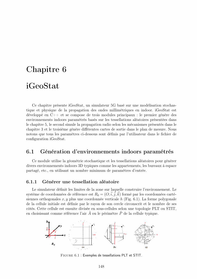
Chapitre 6
iGeoStat
Ce chapitre présente iGeoStat, un simulateur 5G basé sur une modélisation stochas-tique et physique de la propagation des ondes millimétriques en indoor. iGeoStat estdéveloppé en C++ et se compose de trois modules principaux : le premier génère desenvironnements indoors paramétrés basés sur les tessellations aléatoires présentées dansle chapitre 5, le second simule la propagation radio selon les mécanismes présentés dans lechapitre 3 et le troisième génère différentes cartes de sortie dans le plan de mesure. Nousnotons que tous les paramètres ci-dessous sont définis par l’utilisateur dans le fichier deconfiguration iGeoStat.
6.1 Génération d’environnements indoors paramétrésCe module utilise la géométrie stochastique et les tessellations aléatoires pour générer
divers environnements indoors 3D typiques comme les appartements, les bureaux à espacepartagé, etc., en utilisant un nombre minimum de paramètres d’entrée.
6.1.1 Générer une tessellation aléatoire
Le simulateur définit les limites de la zone sur laquelle construire l’environnement. Lesystème de coordonnées de référence est R0 = (O;~i,~j,~k) formé par les coordonnées carté-siennes orthogonales x, y plus une coordonnée verticale h (Fig. 6.1). La forme polygonalede la cellule initiale est définie par le rayon de son cercle circonscrit et le nombre de sescôtés. Cette cellule est ensuite divisée en sous-cellules selon une topologie PLT ou STIT,en choisissant comme référence l’air A ou le périmètre P de la cellule typique.
Figure 6.1 : Exemples de tessellations PLT et STIT.
148
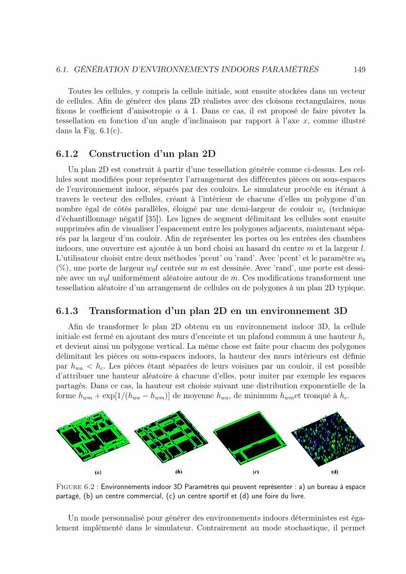
6.1. GÉNÉRATION D’ENVIRONNEMENTS INDOORS PARAMÉTRÉS 149
Toutes les cellules, y compris la cellule initiale, sont ensuite stockées dans un vecteurde cellules. Afin de générer des plans 2D réalistes avec des cloisons rectangulaires, nousfixons le coefficient d’anisotropie α à 1. Dans ce cas, il est proposé de faire pivoter latessellation en fonction d’un angle d’inclinaison par rapport à l’axe x, comme illustrédans la Fig. 6.1(c).
6.1.2 Construction d’un plan 2D
Un plan 2D est construit à partir d’une tessellation générée comme ci-dessus. Les cel-lules sont modifiées pour représenter l’arrangement des différentes pièces ou sous-espacesde l’environnement indoor, séparés par des couloirs. Le simulateur procède en itérant àtravers le vecteur des cellules, créant à l’intérieur de chacune d’elles un polygone d’unnombre égal de côtés parallèles, éloigné par une demi-largeur de couloir wc (techniqued’échantillonnage négatif [35]). Les lignes de segment délimitant les cellules sont ensuitesupprimées afin de visualiser l’espacement entre les polygones adjacents, maintenant sépa-rés par la largeur d’un couloir. Afin de représenter les portes ou les entrées des chambresindoors, une ouverture est ajoutée à un bord choisi au hasard du centre m et la largeur l.L’utilisateur choisit entre deux méthodes ’pcent’ ou ’rand’. Avec ’pcent’ et le paramètre w0
(%), une porte de largeur w0l centrée sur m est dessinée. Avec ’rand’, une porte est dessi-née avec un w0l uniformément aléatoire autour de m. Ces modifications transforment unetessellation aléatoire d’un arrangement de cellules ou de polygones à un plan 2D typique.
6.1.3 Transformation d’un plan 2D en un environnement 3D
Afin de transformer le plan 2D obtenu en un environnement indoor 3D, la celluleinitiale est fermé en ajoutant des murs d’enceinte et un plafond commun à une hauteur hcet devient ainsi un polygone vertical. La même chose est faite pour chacun des polygonesdélimitant les pièces ou sous-espaces indoors, la hauteur des murs intérieurs est définiepar hwa < hc. Les pièces étant séparées de leurs voisines par un couloir, il est possibled’attribuer une hauteur aléatoire à chacune d’elles, pour imiter par exemple les espacespartagés. Dans ce cas, la hauteur est choisie suivant une distribution exponentielle de laforme hwm + exp[1/(hwa − hwm)] de moyenne hwa, de minimum hwmet tronqué à hc.
Figure 6.2 : Environnements indoor 3D Paramétrés qui peuvent représenter : a) un bureau à espacepartagé, (b) un centre commercial, (c) un centre sportif et (d) une foire du livre.
Un mode personnalisé pour générer des environnements indoors déterministes est éga-lement implémenté dans le simulateur. Contrairement au mode stochastique, il permet
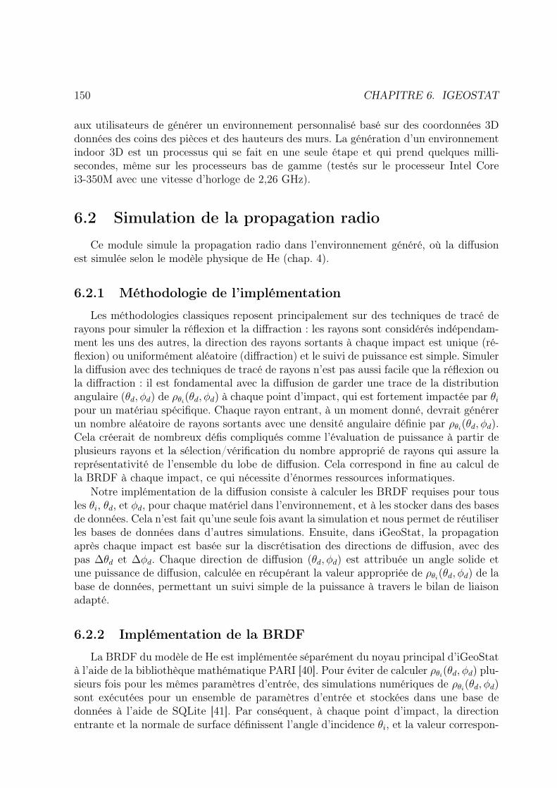
150 CHAPITRE 6. IGEOSTAT
aux utilisateurs de générer un environnement personnalisé basé sur des coordonnées 3Ddonnées des coins des pièces et des hauteurs des murs. La génération d’un environnementindoor 3D est un processus qui se fait en une seule étape et qui prend quelques milli-secondes, même sur les processeurs bas de gamme (testés sur le processeur Intel Corei3-350M avec une vitesse d’horloge de 2,26 GHz).
6.2 Simulation de la propagation radio
Ce module simule la propagation radio dans l’environnement généré, où la diffusionest simulée selon le modèle physique de He (chap. 4).
6.2.1 Méthodologie de l’implémentation
Les méthodologies classiques reposent principalement sur des techniques de tracé derayons pour simuler la réflexion et la diffraction : les rayons sont considérés indépendam-ment les uns des autres, la direction des rayons sortants à chaque impact est unique (ré-flexion) ou uniformément aléatoire (diffraction) et le suivi de puissance est simple. Simulerla diffusion avec des techniques de tracé de rayons n’est pas aussi facile que la réflexion oula diffraction : il est fondamental avec la diffusion de garder une trace de la distributionangulaire (θd, φd) de ρθi(θd, φd) à chaque point d’impact, qui est fortement impactée par θipour un matériau spécifique. Chaque rayon entrant, à un moment donné, devrait générerun nombre aléatoire de rayons sortants avec une densité angulaire définie par ρθi(θd, φd).Cela créerait de nombreux défis compliqués comme l’évaluation de puissance à partir deplusieurs rayons et la sélection/vérification du nombre approprié de rayons qui assure lareprésentativité de l’ensemble du lobe de diffusion. Cela correspond in fine au calcul dela BRDF à chaque impact, ce qui nécessite d’énormes ressources informatiques.
Notre implémentation de la diffusion consiste à calculer les BRDF requises pour tousles θi, θd, et φd, pour chaque matériel dans l’environnement, et à les stocker dans des basesde données. Cela n’est fait qu’une seule fois avant la simulation et nous permet de réutiliserles bases de données dans d’autres simulations. Ensuite, dans iGeoStat, la propagationaprès chaque impact est basée sur la discrétisation des directions de diffusion, avec despas ∆θd et ∆φd. Chaque direction de diffusion (θd, φd) est attribuée un angle solide etune puissance de diffusion, calculée en récupérant la valeur appropriée de ρθi(θd, φd) de labase de données, permettant un suivi simple de la puissance à travers le bilan de liaisonadapté.
6.2.2 Implémentation de la BRDF
La BRDF du modèle de He est implémentée séparément du noyau principal d’iGeoStatà l’aide de la bibliothèque mathématique PARI [40]. Pour éviter de calculer ρθi(θd, φd) plu-sieurs fois pour les mêmes paramètres d’entrée, des simulations numériques de ρθi(θd, φd)sont exécutées pour un ensemble de paramètres d’entrée et stockées dans une base dedonnées à l’aide de SQLite [41]. Par conséquent, à chaque point d’impact, la directionentrante et la normale de surface définissent l’angle d’incidence θi, et la valeur correspon-
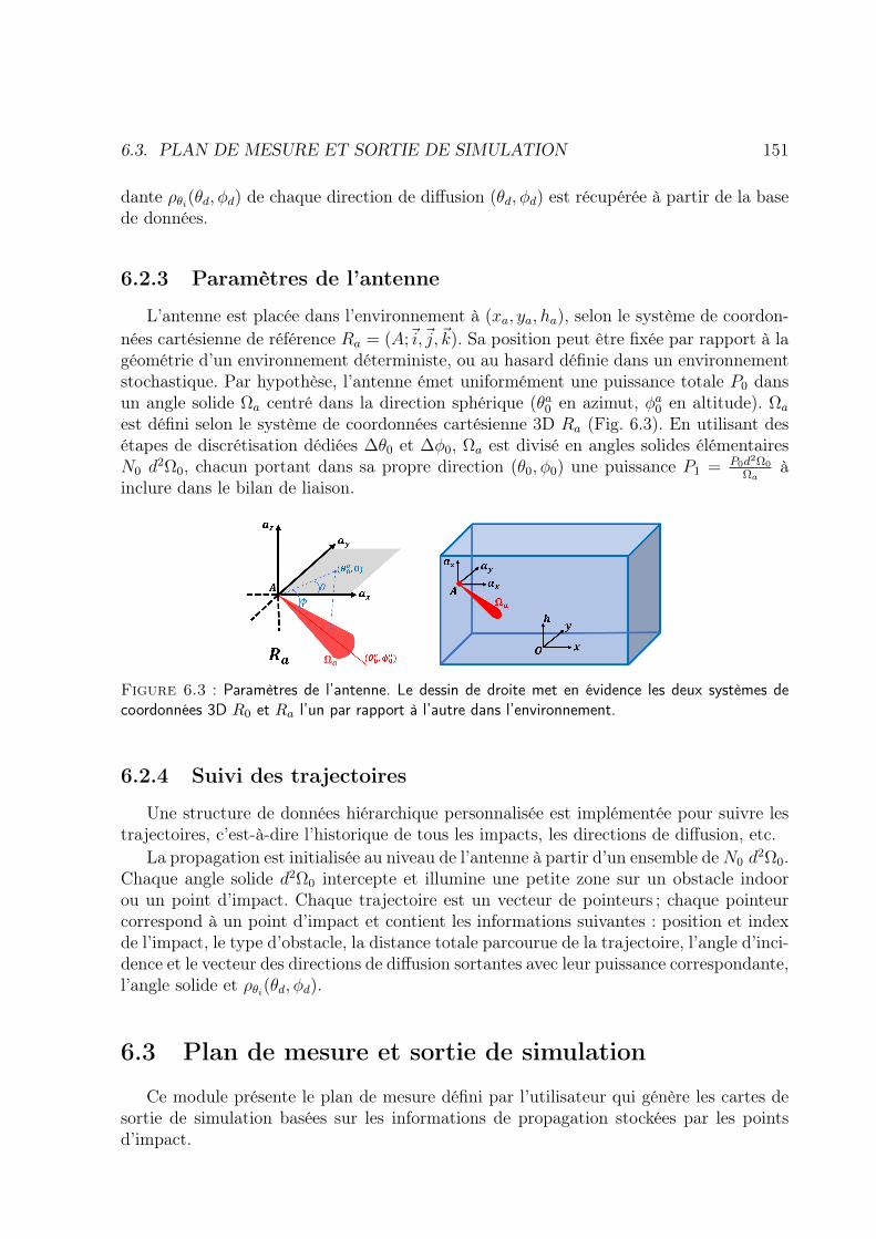
6.3. PLAN DE MESURE ET SORTIE DE SIMULATION 151
dante ρθi(θd, φd) de chaque direction de diffusion (θd, φd) est récupérée à partir de la basede données.
6.2.3 Paramètres de l’antenne
L’antenne est placée dans l’environnement à (xa, ya, ha), selon le système de coordon-nées cartésienne de référence Ra = (A;~i,~j,~k). Sa position peut être fixée par rapport à lagéométrie d’un environnement déterministe, ou au hasard définie dans un environnementstochastique. Par hypothèse, l’antenne émet uniformément une puissance totale P0 dansun angle solide Ωa centré dans la direction sphérique (θa0 en azimut, φa0 en altitude). Ωa
est défini selon le système de coordonnées cartésienne 3D Ra (Fig. 6.3). En utilisant desétapes de discrétisation dédiées ∆θ0 et ∆φ0, Ωa est divisé en angles solides élémentairesN0 d
2Ω0, chacun portant dans sa propre direction (θ0, φ0) une puissance P1 = P0d2Ω0
Ωaà
inclure dans le bilan de liaison.
Figure 6.3 : Paramètres de l’antenne. Le dessin de droite met en évidence les deux systèmes decoordonnées 3D R0 et Ra l’un par rapport à l’autre dans l’environnement.
6.2.4 Suivi des trajectoires
Une structure de données hiérarchique personnalisée est implémentée pour suivre lestrajectoires, c’est-à-dire l’historique de tous les impacts, les directions de diffusion, etc.
La propagation est initialisée au niveau de l’antenne à partir d’un ensemble deN0 d2Ω0.
Chaque angle solide d2Ω0 intercepte et illumine une petite zone sur un obstacle indoorou un point d’impact. Chaque trajectoire est un vecteur de pointeurs ; chaque pointeurcorrespond à un point d’impact et contient les informations suivantes : position et indexde l’impact, le type d’obstacle, la distance totale parcourue de la trajectoire, l’angle d’inci-dence et le vecteur des directions de diffusion sortantes avec leur puissance correspondante,l’angle solide et ρθi(θd, φd).
6.3 Plan de mesure et sortie de simulation
Ce module présente le plan de mesure défini par l’utilisateur qui génère les cartes desortie de simulation basées sur les informations de propagation stockées par les pointsd’impact.
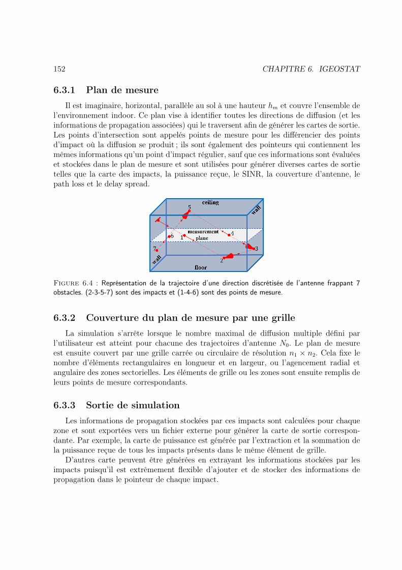
152 CHAPITRE 6. IGEOSTAT
6.3.1 Plan de mesure
Il est imaginaire, horizontal, parallèle au sol à une hauteur hm et couvre l’ensemble del’environnement indoor. Ce plan vise à identifier toutes les directions de diffusion (et lesinformations de propagation associées) qui le traversent afin de générer les cartes de sortie.Les points d’intersection sont appelés points de mesure pour les différencier des pointsd’impact où la diffusion se produit ; ils sont également des pointeurs qui contiennent lesmêmes informations qu’un point d’impact régulier, sauf que ces informations sont évaluéeset stockées dans le plan de mesure et sont utilisées pour générer diverses cartes de sortietelles que la carte des impacts, la puissance reçue, le SINR, la couverture d’antenne, lepath loss et le delay spread.
Figure 6.4 : Représentation de la trajectoire d’une direction discrétisée de l’antenne frappant 7obstacles. (2-3-5-7) sont des impacts et (1-4-6) sont des points de mesure.
6.3.2 Couverture du plan de mesure par une grille
La simulation s’arrête lorsque le nombre maximal de diffusion multiple défini parl’utilisateur est atteint pour chacune des trajectoires d’antenne N0. Le plan de mesureest ensuite couvert par une grille carrée ou circulaire de résolution n1 × n2. Cela fixe lenombre d’éléments rectangulaires en longueur et en largeur, ou l’agencement radial etangulaire des zones sectorielles. Les éléments de grille ou les zones sont ensuite remplis deleurs points de mesure correspondants.
6.3.3 Sortie de simulation
Les informations de propagation stockées par ces impacts sont calculées pour chaquezone et sont exportées vers un fichier externe pour générer la carte de sortie correspon-dante. Par exemple, la carte de puissance est générée par l’extraction et la sommation dela puissance reçue de tous les impacts présents dans le même élément de grille.
D’autres carte peuvent être générées en extrayant les informations stockées par lesimpacts puisqu’il est extrêmement flexible d’ajouter et de stocker des informations depropagation dans le pointeur de chaque impact.
Chapitre 7
Défis de modélisation etd’implémentation
Ce chapitre présente les défis liés au calcul, au stockage et à la récupération des valeursde la BRDF, à la modélisation et à l’implémentation d’une structure de données qui gèrela diffusion et à des stratégies efficaces pour éviter l’explosion du nombre de directions dediffusion.
7.1 Calcul et stockage de la BRDF
Le principal défi d’implémentation du modèle de He est de calculer, stocker et récupérerefficacement les valeurs de ρθi(θd, φd). Les fonctions mathématiques requises pour calculerla BRDF ne sont incluses dans aucune bibliothèque interne de C++ (fonction Lambert W,Digamma, etc.). Parmi les diverses bibliothèques disponibles, nous avons choisi PARI quiest écrite en C, contient toutes les fonctions, et prend en compte le calcule multi-précision.
7.1.1 Gestion et optimisation de la mémoire
Sans aucune optimisation, calculer ρθi(θd, φd) pour un seul θi consomme énormémentde mémoire. Ce problème majeur a été résolu en implémentant un algorithme personnalisépour la gestion et l’optimisation manuelle de la mémoire : les objets sont créés dans la pilePARI lorsque ρθi(θd, φd) est calculé pour chaque direction discrétisée du plan de diffusion.les objets initialisés à chaque itération deviennent inutiles une fois que la valeur ρθi(θd, φd)correspondante est calculée. À chaque itération, la mémoire occupée par ces objets estrécupérée afin que le calcul de ρθi(θd, φd) est fait sur les mêmes ressources mémoire. Celaréduit la consommation de mémoire d’un facteur de 30 : seule une pile de 100 Mo (aulieu de 3 Go) est nécessaire pour calculer ρθi(θd, φd) pour tout θi, θd et φd. Le calcul deρθi(θd, φd) pour un seul θi, matériau et λ prend 21 secondes pour une discrétisation de 1
et jusqu’à 30 minutes pour 1/32.
153
154 CHAPITRE 7. DÉFIS DE MODÉLISATION ET D’IMPLÉMENTATION
7.1.2 Stockage et récupération de la BRDF
Les simulations numériques de ρθi(θd, φd) sont stockées dans des bases de données àl’aide de SQLite. Chaque base de données contient des valeurs de ρθi(θd, φd) pour unmatériau donné, une longueur d’onde et pour tout θi, θd et φd.
En général, l’insertion dans la base de données se fait en exécutant la routine sql_exec()qui nécessite un minimum lignes de code. Cette méthode soit adéquate pour insérer uneseule ligne, mais inefficace pour l’insertion récursive de données : jusqu’à 8,5 heures pourune discrétisation de 1, pour tout θi, θd et φd avec seulement 95 insertions/seconde.
Une opération d’insertion optimisée a été implémentée pour accélérer le stockage desvaleurs de ρθi(θd, φd). Puisque l’instruction d’insertion est la même pour chaque itération,elle n’est compilée qu’une seule fois. Cette instruction est ensuite exécutée de manièrerécursive en la liant aux valeurs correspondantes de θi, θd, φd et ρθi(θd, φd) en utilisantla fonction sql_bind(). L’exécution se fait dans une seule transaction et l’instruction estensuite supprimée comme étape finale. Cette méthode est plus complexe que la méthodeclassique mais elle réduit le temps d’insertion d’un facteur de 9 : le stockage du mêmenombre de valeurs de ρθi(θd, φd) prend 1 heure avec 860 insertions/seconde et génère unebase de données de 245 Mo. En utilisant cette méthode optimisée, une énorme améliorationa été observée pour la récupération d’une valeur de ρθi(θd, φd) qui ne prend pas plus de 2ms, contre environ 1000 ms avec sql_exec().
7.1.3 Déduction de la composante de diffusion uniforme
Comme indiqué dans le chapitre 4, le modèle de He ne fournit pas d’expression pourρudθi (θd, φd). Cette composante est déduite des bases de données de la BRDF telles quepour chaque θi : ρsrθi (θd, φd) + ρddθi (θd, φd) + ρudθi (θd, φd) + ρtrθi(θd, φd) = 1 où ρtrθi(θd, φd) estla fraction d’intensité transmise. Le poids attribué à chacune des composantes inconnuesles unes par rapport aux autres est basé sur une analyse du comportement du coefficientde transmission de Fresnel en faisant varier indépendamment θi et σ0. En se basant surla variation de ρtrθi(θd, φd) par rapport aux bornes inférieure et supérieure de θi, un poidsest attribué à chacune des composantes inconnues afin qu’elle satisfasse la conservationd’énergie. Cette méthode fournit des valeurs approximatives pour chaque composant quine peuvent pas être facilement vérifiées.
7.2 Suivi des points d’impact
En présence de diffusion, un grand nombre de directions de propagation sont lancéesaprès chaque impact. Chaque direction correspond à une source potentielle de diffusion(point d’impact). Le principal défi est d’implémenter une structure de données qui garde latrace des points d’impact afin de calculer avec précision leurs informations de propagation(puissance reçue, distance parcourue, etc.) lors d’une diffusion multiple.
7.3. GESTION DES DIRECTIONS DE DIFFUSION 155
7.2.1 Choix de la structure de données optimale
Plusieurs structures linéaires et hiérarchiques ont été étudiées. Cependant, la dépen-dance d’un point d’impact sur son précédent induit une relation parent −→ enfant, quicorrespond principalement à une structure d’arbre.
7.2.2 Traverser une structure d’arbre
Le défi qui se pose lors de l’implémentation d’une structure d’arbre est le choix deson parcours, c’est-à-dire l’ordre dans lequel les nœuds de l’arbre sont traités. Dans notrecas, ceci correspond à calculer la puissance, la distance, les directions de diffusion, etc.en ce point d’impact. Plusieurs traversées d’arbres ont été étudiées (Depth-first (DFS),Breadth-First (BFS), Monte Carlo (MCTS), etc.).
Un algorithme BFS personnalisé a été implémenté car il correspond le plus à la lo-gique de diffusion multiple. En partant de l’antenne, tous les impacts des parents adjacentsdoivent être traités avant tout impact de leurs enfants. Notre algorithme intègre un Gar-bage Collector qui traite les trajectoires d’antennes indépendamment les unes des autres,permettant à chacune d’elles de réutiliser les mêmes ressources mémoire quel que soit lenombre d’antennes et de trajectoires N0.
7.3 Gestion des directions de diffusionUn autre défi majeur d’implémentation est la gestion de l’explosion potentielle des
directions de diffusion : avec la diffusion multiple, le nombre de trajectoires à traiterdevient énorme. Trois techniques peuvent être utilisées pour relever ce défi et réduire letemps de simulation et l’utilisation de la mémoire.
Premièrement, un seuil relatif peut être imposé à ρθi(θd, φd) en fonction de ρmax(θi).Ceci élimine toutes les directions avec une valeur ρθi(θd, φd) inférieure à ce seuil, réduisantà la fois le temps de simulation et l’utilisation de la mémoire. Des seuils peuvent égalementêtre imposés aux valeurs de puissance, interdisant toute diffusion ultérieure à un pointd’impact. De plus, en utilisant les bases de données de ρθi(θd, φd) générées, les pas dediscrétisation ∆θd et ∆φd peuvent être augmentées tout en vérifiant la conservation del’énergie. Cela réduit le nombre de directions de diffusion et donc le nombre de valeurs deρθi(θd, φd) itérées, sans qu’il soit nécessaire de générer une autre base de données.
Chapitre 8
Résultats des premières simulations
Dans ce chapitre, nous évaluons les performances d’iGeoStat pour la simulation dela diffusion multiple dans des environnements réalistes, et sa capacité de générer diversescartes de sortie. Nous comparons également la contribution de la réflexion, diffusion simpleet double sur la propagation des ondes millimétriques en indoor. Les résultats sont ensuitevalidés en les comparant aux données des campagnes de mesures existantes.
8.1 Configuration des simulations
Les simulations sont réalisées pour deux applications 5G : l’accès fixe (FWA) dans unappartement à 60 GHz et l’industrie 4.0 (i4.0) dans une usine à 26 GHz. Pour le FWA nouscomparons la réfléxion à la diffusion simple avec une antenne d’ouverture angulaire large(Ωa = π sr et N0 = 16200). Pour l’i4.0, nous comparons la diffusion simple à la diffusiondouble avec deux antennes d’une ouverture angulaire étroite (Ωa = π
1000sr et N0 = 16).
Les simulations FWA sont exécutées sur une configuration moyenne, tandis que cellesde l’i4.0 sont exécutés sur une configuration plus avancée. Les BRDFs correspondantesaux matériaux des environnements sont générées en utilisant les mesures de [29] et [30].Les paramètres de rugosité de surface σ0 et τ sont choisis de telle sorte que le profil dediffusion correspond à une surface moyennement rugueuse.
8.2 FWA - réflexion vs. diffusion simple
La réflexion est imposée pour étudier si ce mécanisme est capable d’illustrer le compor-tement réel des ondes millimétriques en indoor. La diffusion simple est ensuite introduiteet sa contribution sur la propagation de ces ondes est comparée au scénario de la réflexion.
Pour la réflexion, la carte de puissance montre plusieurs trous de couverture dans l’en-vironnement. Le filtrage à -200 dBm montre que seulement 20% de l’environnement estcouvert. D’autre part, pour la diffusion simple, la carte de puissance montre un environ-nement entièrement couvert, avec des valeurs de puissance typiques variant entre -208 et-17 dBm. Des cartes de sortie supplémentaires sont générées avec la diffusion simple : lacarte de delay spread avec des valeurs entre 0,5 ns et 44 ns, et la carte de variabilité dupath loss dans l’environnement avec des valeurs entre 29 et 215 dB.
156
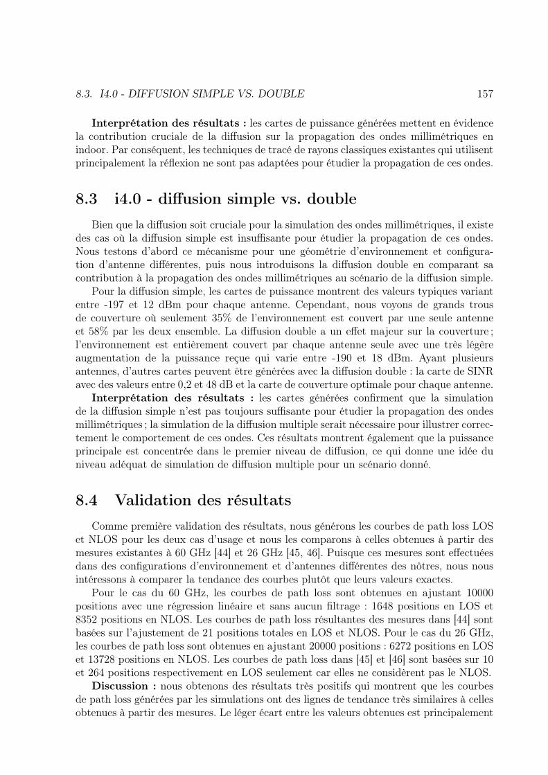
8.3. I4.0 - DIFFUSION SIMPLE VS. DOUBLE 157
Interprétation des résultats : les cartes de puissance générées mettent en évidencela contribution cruciale de la diffusion sur la propagation des ondes millimétriques enindoor. Par conséquent, les techniques de tracé de rayons classiques existantes qui utilisentprincipalement la réflexion ne sont pas adaptées pour étudier la propagation de ces ondes.
8.3 i4.0 - diffusion simple vs. doubleBien que la diffusion soit cruciale pour la simulation des ondes millimétriques, il existe
des cas où la diffusion simple est insuffisante pour étudier la propagation de ces ondes.Nous testons d’abord ce mécanisme pour une géométrie d’environnement et configura-tion d’antenne différentes, puis nous introduisons la diffusion double en comparant sacontribution à la propagation des ondes millimétriques au scénario de la diffusion simple.
Pour la diffusion simple, les cartes de puissance montrent des valeurs typiques variantentre -197 et 12 dBm pour chaque antenne. Cependant, nous voyons de grands trousde couverture où seulement 35% de l’environnement est couvert par une seule antenneet 58% par les deux ensemble. La diffusion double a un effet majeur sur la couverture ;l’environnement est entièrement couvert par chaque antenne seule avec une très légèreaugmentation de la puissance reçue qui varie entre -190 et 18 dBm. Ayant plusieursantennes, d’autres cartes peuvent être générées avec la diffusion double : la carte de SINRavec des valeurs entre 0,2 et 48 dB et la carte de couverture optimale pour chaque antenne.
Interprétation des résultats : les cartes générées confirment que la simulationde la diffusion simple n’est pas toujours suffisante pour étudier la propagation des ondesmillimétriques ; la simulation de la diffusion multiple serait nécessaire pour illustrer correc-tement le comportement de ces ondes. Ces résultats montrent également que la puissanceprincipale est concentrée dans le premier niveau de diffusion, ce qui donne une idée duniveau adéquat de simulation de diffusion multiple pour un scénario donné.
8.4 Validation des résultatsComme première validation des résultats, nous générons les courbes de path loss LOS
et NLOS pour les deux cas d’usage et nous les comparons à celles obtenues à partir desmesures existantes à 60 GHz [44] et 26 GHz [45, 46]. Puisque ces mesures sont effectuéesdans des configurations d’environnement et d’antennes différentes des nôtres, nous nousintéressons à comparer la tendance des courbes plutôt que leurs valeurs exactes.
Pour le cas du 60 GHz, les courbes de path loss sont obtenues en ajustant 10000positions avec une régression linéaire et sans aucun filtrage : 1648 positions en LOS et8352 positions en NLOS. Les courbes de path loss résultantes des mesures dans [44] sontbasées sur l’ajustement de 21 positions totales en LOS et NLOS. Pour le cas du 26 GHz,les courbes de path loss sont obtenues en ajustant 20000 positions : 6272 positions en LOSet 13728 positions en NLOS. Les courbes de path loss dans [45] et [46] sont basées sur 10et 264 positions respectivement en LOS seulement car elles ne considèrent pas le NLOS.
Discussion : nous obtenons des résultats très positifs qui montrent que les courbesde path loss générées par les simulations ont des lignes de tendance très similaires à cellesobtenues à partir des mesures. Le léger écart entre les valeurs obtenues est principalement
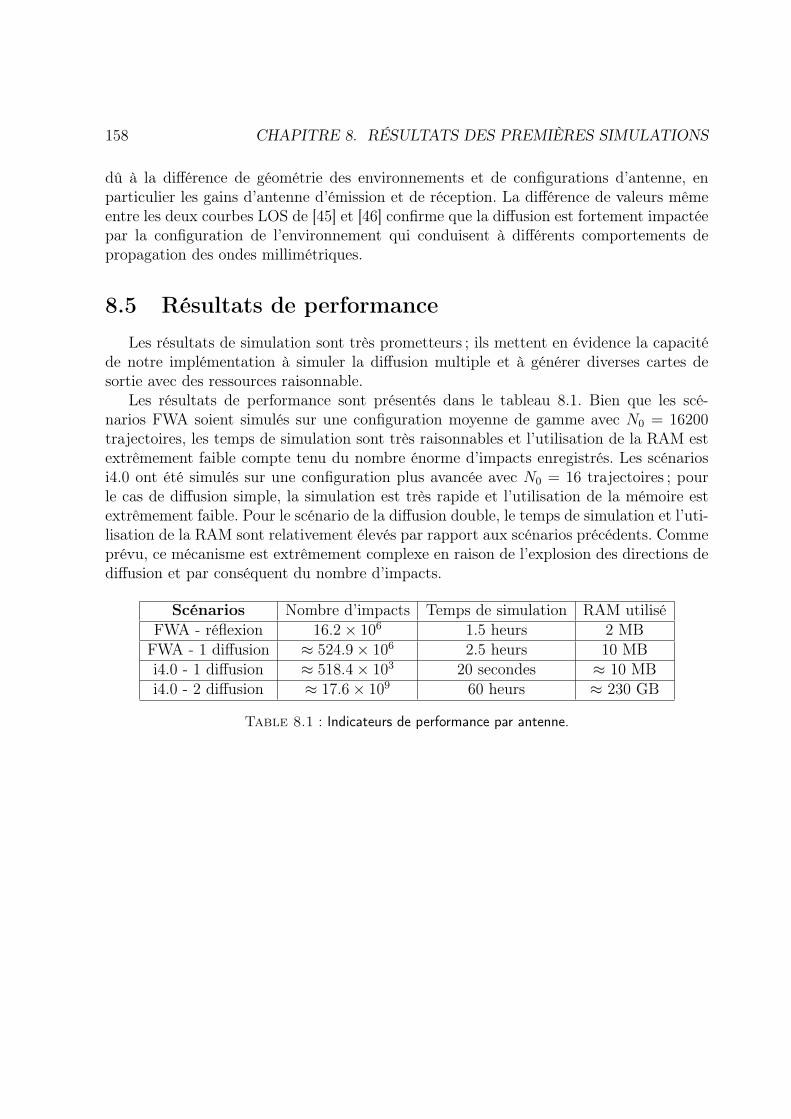
158 CHAPITRE 8. RÉSULTATS DES PREMIÈRES SIMULATIONS
dû à la différence de géométrie des environnements et de configurations d’antenne, enparticulier les gains d’antenne d’émission et de réception. La différence de valeurs mêmeentre les deux courbes LOS de [45] et [46] confirme que la diffusion est fortement impactéepar la configuration de l’environnement qui conduisent à différents comportements depropagation des ondes millimétriques.
8.5 Résultats de performanceLes résultats de simulation sont très prometteurs ; ils mettent en évidence la capacité
de notre implémentation à simuler la diffusion multiple et à générer diverses cartes desortie avec des ressources raisonnable.
Les résultats de performance sont présentés dans le tableau 8.1. Bien que les scé-narios FWA soient simulés sur une configuration moyenne de gamme avec N0 = 16200trajectoires, les temps de simulation sont très raisonnables et l’utilisation de la RAM estextrêmement faible compte tenu du nombre énorme d’impacts enregistrés. Les scénariosi4.0 ont été simulés sur une configuration plus avancée avec N0 = 16 trajectoires ; pourle cas de diffusion simple, la simulation est très rapide et l’utilisation de la mémoire estextrêmement faible. Pour le scénario de la diffusion double, le temps de simulation et l’uti-lisation de la RAM sont relativement élevés par rapport aux scénarios précédents. Commeprévu, ce mécanisme est extrêmement complexe en raison de l’explosion des directions dediffusion et par conséquent du nombre d’impacts.
Scénarios Nombre d’impacts Temps de simulation RAM utiliséFWA - réflexion 16.2× 10⁶ 1.5 heurs 2 MBFWA - 1 diffusion ≈ 524.9× 10⁶ 2.5 heurs 10 MBi4.0 - 1 diffusion ≈ 518.4× 10³ 20 secondes ≈ 10 MBi4.0 - 2 diffusion ≈ 17.6× 10⁹ 60 heurs ≈ 230 GB
Table 8.1 : Indicateurs de performance par antenne.
Chapitre 9
Investigation des paramètres depropagation
Nous étudions dans ce chapitre l’impact de divers paramètres de l’environnement in-door sur le profil de propagation. Nous étudions également l’efficacité de plusieurs tech-niques de seuillage sur les performances de simulation, en testant l’une d’entre elles surun ensemble de paramètres d’environnement stochastique.
9.1 Indice de réfraction complexe
L’objectif principal ici est d’étudier l’impact de l’indice de réfraction complexe nc dumatériau qui recouvre tous les obstacles de l’environnement. Cinq BRDFs sont généréespour cinq différents matériaux et sont configurés avec le même profil de rugosité modérée.Pour chaque cas, nous étudions l’effet de varier nr ou ni sur la carte de puissance. Quatrescénarios ont été testés en faisant varier une composante à la fois tout en fixant l’autre,par rapport à un nc de référence. Les résultats des simulations ont montré que nc a unimpact modéré sur la puissance reçue, principalement dû à la composante nr. ni n’a peuou pas d’effet sur la carte de puissance car cette composante illustre uniquement la partieabsorbée de l’énergie incidente, et non celle qui est réfléchie.
9.2 Rugosité de surface
L’objectif principal ici est d’étudier l’impact du paramètre de rugosité σ0 pour la mêmelongueur d’onde λ, et l’effet de varier le rapport σ0/λ sur les cartes de couverture et depuissance. Le matériau utilisé pour couvrir tous les obstacles est le béton. Trois BRDFssont générées pour ce matériau et correspondent à trois profils de rugosité différents :légèrement rugueux, moyennement rugueux et très rugueux. En comparant les profils derugosité entre eux, les résultats des simulations ont montrées que σ0/λ a un impact majeursur la puissance reçue, en particulier lorsque la différence entre les σ0 est grande, ce quientraine un changement complet du profil de puissance. Les simulations ont égalementmontré que les surfaces très rugueuses sont plus efficaces pour couvrir l’environnement,en particulier les coins inaccessibles par le lobe principal de l’antenne.
159
160 CHAPITRE 9. INVESTIGATION DES PARAMÈTRES DE PROPAGATION
9.3 Seuils de puissance
Un seuil de puissance Pth peut être imposé pour diminuer le nombre d’impacts quisubissent la diffusion, et par conséquent, réduire le temps de simulation et l’utilisation dela mémoire. L’objectif ici est de tester les effets de 5 valeurs de seuil différents sur la cartede puissance et les performances de simulation, par rapport à un scénario de référencesans seuil. Les résultats de simulation ont montré que cette technique est très efficacepour améliorer les performances d’iGeoStat. Dans certains cas, nous pouvons obtenirjusqu’à 50% de réduction du temps de simulation et de l’utilisation de la RAM, tout enconservant le même profil de puissance. L’imposition de valeurs plus élevées de seuil peutentraîner une certaine perte d’informations de propagation, ce qui se traduit par des trousde couverture dans certaines zones de l’environnement.
Le seuil de puissance permet à iGeoStat de simuler des ordres supérieurs de diffusionmultiple ; cela étant dit, la variation mineure entre les cartes de puissance de la double etla triple diffusion est négligeable par rapport à l’énorme différence de performances.
9.4 Seuils de BRDF
Des seuils ρth peuvent également être imposés sur la BRDF. Toutefois ; contrairementà Pth qui filtre la puissance au niveau des impacts, ρth réduit le nombre de directions dediffusion générées après un impact, minimisant aussi le temps de simulation et l’utilisationde la RAM. L’objectif ici est de tester les effets de 5 valeurs de seuil différents sur la cartede puissance et les performances de simulation, par rapport à un scénario de référencesans seuil. Les résultats de simulations ont également montré c’est aussi une méthodetrès efficace pour améliorer les performances d’iGeoStat. Dans certains cas, nous pouvonsobtenir jusqu’à 33% de réduction du temps de simulation et de l’utilisation de la RAM,tout en conservant le même profil dde puissance. L’imposition de valeurs plus élevées deρth peut entraîner une certaine perte d’informations de propagation. Cela se traduit pardes trous de couverture dans des zones avec la même représentation de palette de couleurs,ce qui nous permet de prédire les effets d’une valeur ρth inférieure ou supérieure sur lacarte de puissance. En raison de la nature physique du seuil BRDF, cette stratégie peutfournir un premier résultat pour la simulation d’une configuration de surfaces de rugositéinférieure avec un gain de performance de 94%. Cependant, ρth peut ajouter un tempsd’aller-retour inutile, le rendant moins performant que la stratégie de seuil de puissance.
9.5 Environnement stochastique
L’objectif principal de l’approche stochastique dans iGeoStat est d’étudier l’impact desparamètres d’environnement sur la propagation. Cela se fait grâce à des études statistiquessur les résultats de simulations réalisées pour divers ensembles de paramètres. Cependant,sans aucune méthode d’accélération, exécuter un grand nombre de simulations pour unensemble de paramètres est très inefficace en temps et nécessite d’énormes ressources decalcul, surtout pour la simulation de la diffusion multiple. Les techniques de seuillage sesont avérées très efficaces pour améliorer les performances de simulation tout en conservant

9.5. ENVIRONNEMENT STOCHASTIQUE 161
les caractéristiques physiques de propagation. En utilisant le mode stochastique, noustestons les performances de la stratégie du seuil de puissance sur 40 simulations de doublediffusion pour le même ensemble de paramètres d’environnement, où nous générons lacarte de puissance moyennée sur les 40 simulations et sa courbe de path loss.
Pour la valeur choisie de Pth = 10−7P0 avec P0 = 20 mW, nous observons toujours unecouverture d’au moins 75% de l’environnement avec une puissance reçue typique qui varieentre -189 et 9 dBm. D’un point de vue performance, il est tout à fait faisable de lancerdes campagnes de simulation dans iGeoStat avec les techniques de seuillage ; le tempsde simulation moyen et l’utilisation de la mémoire sont respectivement de 1,25 heure et110 Go, ce qui nous a permis d’exécuter jusqu’à 3 simulations simultanées, économisantenviron 80% en temps de simulation total et 50% en utilisation de la mémoire, par rapportà un cas sans seuil.
Chapitre 10
Conclusion et Perspectives
10.1 Conclusion
Nous avons introduit dans ce travail un nouveau cadre de modélisation pour la pro-pagation indoor des ondes millimétriques 5G, combinant la génération d’environnementstochastique avec la simulation de la propagation physique. Son implémentation système,iGeoStat, génère des environnements typiques paramétrés qui tiennet compte de la varia-bilité statistique en indoor, puis simule la propagation radio en fonction de l’interactionphysique entre les ondes EM et les matériaux. Les défis informatiques ont été résolues enformulant un bilan de liaison adapté et en concevant de nouveaux algorithmes de gestionet d’optimisationde de la mémoire, faisant d’iGeoStat le premier à simuler la diffusionmultiple dans des environnements réalistes.
Les premières simulations ont été réalisées pour l’accès fixe à 60 GHz et l’industrie 4.0à 26 GHz afin d’étudier la contribution de la réflexion et la diffusion simple et double surla simulation de la propagation des onde millimétriques en indoor, où la diffusion est lemécanisme le plus complexe mais certainement le plus essentiel. Les résultats ont confirméqu’une simulation avec uniquement de la réflexion ne peut pas décrire le comportementindoor des ces ondes. Ils ont également montré que la puissance reçue est principalementconcentré dans la diffusion simple ; cependant, simuler ce mécanisme n’est pas toujourssuffisant pour étudier la couverture des ondes millimétriques en indoor et peut nécessiterla diffusion double. De telles conclusions ne peuvent être obtenues avec des techniquesclassiques de tracé des rayons.
Les résultats de simulation ont été validés avec succès en comparant les courbes depath loss (LOS et NLOS) générées à celles obtenues à partir de mesures à 60 et 26 GHz.Les résultats de performance ont montré l’efficacité d’iGeoStat pour simuler la diffusionmultiple et générer diverses cartes de sortie (puissance, SINR, couverture, path loss etdelay spread) dans un laps de temps et de mémoire raisonnables. Notre implémentationnous permet de déterminer l’impact d’un niveau de diffusion multiple donné et de prédirele temps et la mémoire requis pour tout mécanisme de propagation.
Nous avons étudié dans ce travail l’impact des principaux paramètres de l’environne-ment sur le profil de propagation ; les résultats de la simulation ont montré que l’indice deréfraction complexe a un impact modéré sur la puissance reçue, et est principalement dueà sa composante réelle. D’autre part, le paramètre de rugosité de la surface a un impact
162
10.2. PERSPECTIVES 163
majeur sur la puissance reçue et peut conduire dans certains cas à un profil de puissancecomplètement différent dans l’environnement.
Plusieurs techniques d’optimisation et d’accélération ont été présentées et testées dansce travail ; par exemple, les seuils de puissance et de BRDF peuvent réduire davantage letemps de simulation et l’utilisation de la mémoire d’au moins 50% sans avoir d’impactsur les caractéristiques physiques de la propagation, ce qui nous permet d’aller au-delàde la diffusion double si nécessaire. La performance du seuil de puissance a été testée sur40 simulations pour un ensemble de paramètres d’environnement stochastique, montrantque nous pouvons économiser jusqu’à 80% en temps de simulation total et 50% dansl’utilisation de la mémoire.
10.2 Perspectives
L’implémentation actuelle d’iGeoStat peut être utilisée par les opérateurs et les ingé-nieurs de planification radio comme premier indicateur pour prédire la puissance reçue, leSINR, le path loss et le delay spread dans un environnement donné. La flexibilité de notreimplémentation nous permettra d’améliorer davantage les principaux modules d’iGeoStat.
Le module d’environnement stochastique reste à améliorer en ajoutant des meubles oud’autres types d’obstacles indoors avec des formes polygonales grâce à l’implémentationde tessellations itérées. Nous pouvons également étudier les caractéristiques d’une celluleindoor typique et analyser le lien possible entre ses paramètres et ses différentes repré-sentations (chambre, espace partagé, etc.). En outre, il faut développer une méthode defitting adaptée : quel vecteur de caractéristiques et comment identifier automatiquementla présence de portes et couloirs et leurs paramètres des ouvertures. Cela constitue unpoint de départ pour trouver les paramètres structurants d’un environnement indoor.
Le module de propagation radio peut également être amélioré par l’implémentation demécanismes supplémentaires : les zones de Fresnel doivent être prises en compte dans lesimulateur pour identifier les interférences constructives et destructrices, qui se produisentprincipalement pour les ondes polarisées. Il est aussi possible d’ajouter la transmission àtravers les obstacles en permettant à une trajectoire de traverser l’objet après un impact.Sa direction serait définie par la loi de Snell-Descartes et la fraction de l’énergie transpor-tée ρtrθi(θd, φd) serait déduite de la BRDF où ρtrθi(θd, φd) = 1 − (ρsrθi (θd, φd) + ρddθi (θd, φd) +ρudθi (θd, φd)). Nous notons que ce mécanisme introduit le problème de la réémission del’énergie des murs et des divers obstacles indoors qui devraient être pris en compte dansle bilan de liaison. La diffraction par les bords peut également être incluse en lançantdes trajectoires dans un lobe uniforme, où la fraction d’énergie transportée est la mêmedans toutes les directions. Les surfaces périodiques et d’autres type de surfaces rugueusespeuvent également être intégrés dans iGeoStat grâce à l’approche de la BRDF. En outre,puisque le modèle de He est basé sur la théorie physique de l’électromagnétisme pour lalumière visible, les applications de transmission de térahertz comme le Li-Fi et les com-munications optiques sans fil peuvent être simulées dans iGeoStat. Toutefois, nous devonsnous assurer que la condition du rayon de courbure de la surface tient toujours pour lalongueur d’onde choisie.
164 CHAPITRE 10. CONCLUSION ET PERSPECTIVES
Des modules supplémentaires peuvent également être implémentés dans iGeoStat pourrésoudre les défis indoors reliés à la planification et le dimensionnement des ondes millimé-triques 5G, comme l’optimisation du positionnement de l’antenne tout en tenant comptede la position et de la géométrie des obstacles pour obtenir une meilleure couverture etSINR. Un module d’analyse des débits peut également être implémenté pour étudier lacapacité du réseau et de l’utilisateur en fonction de la puissance générée et des cartes SINRde l’environnement étudié, et en fonction de la configuration de l’antenne et de la bandepassante du signal. De plus, un module MIMO (Multiple-Input and Multiple-Output)peut être ajouté avec différentes configurations (diversité de transmission, multiplexagespatial et beamforming) pour améliorer le gain de l’émetteur ou du récepteur.
D’un point de vue performance, d’autres techniques d’optimisation sont envisageablepour réduire davantage le temps de simulation et l’utilisation de la mémoire dans iGeo-Stat. Par exemple, la programmation parallèle permet la simulation simultanée de multipletrajectoires d’antenne ce qui réduit considérablement le temps. Le nombre maximal detrajectoires par simulation est limité par la mémoire disponible. En outre, il est possibled’optimiser la structure de données qui maintient le vecteur d’impacts de telle sorte qu’ellelibère plus de mémoire au fur et à mesure que nous passons d’un niveau de diffusion à unautre, ce qui réduit l’utilisation de la RAM par simulation.
En utilisant les techniques d’accélération présentées dans ce travail, des campagnesde simulation seront menées dans iGeoStat pour divers ensembles d’environnements sto-chastiques paramétrés (géométrie et matériaux). Des études statistiques approfondies surles résultats des simulations seront ensuite réalisées pour proposer les premières formulesanalytiques paramétrées de modèles de propagation en indoor qui ne sont pas dédiés àun environnement, une fréquence ou un cas d’usage particulier. Cependant, cela pose desquestions non traitées dans ce manuscrit, comme le nombre de simulations nécessairespour déduire le profil de propagation, ou comment adapter la puissance du seuil BRDF àl’environnement.
Bibliography
[1] K. Haneda et al., “Indoor 5G 3GPP-like channel models for office and shopping mallenvironments,” in 2016 IEEE International Conference on Communications Work-shops (ICC), May 2016, pp. 694–699.
[2] G. R. Maccartney et al., “Indoor Office Wideband Millimeter-Wave PropagationMeasurements and Channel Models at 28 and 73 GHz for Ultra-Dense 5G WirelessNetworks,” IEEE Access, vol. 3, pp. 2388–2424, 2015.
[3] Remcom, “Wireless InSite,” https://www.remcom.com/wireless-insite-em-propagation-software/.
[4] Altair, “Winprop,” https://altairhyperworks.com/product/feko/winprop-propagation-modeling/.
[5] D. Steinmetzer, J. Classen, and M. Hollick, “mmTrace: Modeling millimeter-wave in-door propagation with image-based ray-tracing,” in 2016 IEEE Conference on Com-puter Communications Workshops, April 2016, pp. 429–434.
[6] X. D. He et al., “A comprehensive physical model for light reflection,” ACM SIG-GRAPH computer graphics, vol. 25, no. 4, pp. 175–186, 1991.
[7] T. Courtat, L. Decreusefond, and P. Martins, “Stochastic simulation of urban envi-ronments. application to path-loss in wireless systems,” arXiv e-prints, 2016.
[8] T. Courtat, “Walk on city maps - mathematical and physical phenomenology of thecity, a geometrical approach,” Theses, Université Paris-Diderot - Paris VII, Jan.2012. [Online]. Available: https://tel.archives-ouvertes.fr/tel-00714310
[9] M. d. Berg et al., Computational Geometry: Algorithms and Applications, 3rd ed.Santa Clara, CA, USA: Springer-Verlag TELOS, 2008.
[10] E. M. Purcell and D. J. Morin, Electricity and magnetism. Cambridge UniversityPress, 2013.
[11] J. C. Maxwell, A treatise on electricity and magnetism. Clarendon Press, 1873.
[12] E. Boutet, “Electromagnetic wave,” https://upload.wikimedia.org/wikipedia/commons/3/35/Onde_electromagnetique.svg.
165
166 BIBLIOGRAPHY
[13] U. S. D. of Labor, “Electromagnetic radiation: Field memo,” https://www.osha.gov/SLTC/radiofrequencyradiation/electromagnetic_fieldmemo/electromagnetic.html.
[14] R. Siegel and J. Howell, Thermal Radiation Heat Transfer, Fourth Edition. Taylor& Francis, 2001.
[15] G. S. Smith, An introduction to classical electromagnetic radiation. CambridgeUniversity Press, 1997.
[16] E. Hecht, Optics. Addison-Wesley, 2002.
[17] M. Born, E. Wolf, and A. Bhatia, Principles of Optics: Electromagnetic Theory ofPropagation, Interference and Diffraction of Light. Cambridge University Press,2000.
[18] Wikipedia, “Law of cosines,” https://en.wikipedia.org/wiki/Law_of_cosines.
[19] P. Beckmann and A. Spizzichino, The scattering of electromagnetic waves from roughsurfaces. Artech House, 1987.
[20] D. W. Hahn, “Light scattering theory,” http://plaza.ufl.edu/dwhahn/Rayleigh%20and%20Mie%20Light%20Scattering.pdf, 2009.
[21] J.-H. Lambert, Photometria, sive de Mensura et gradibus luminis, colorum et umbrae.sumptibus viduae E. Klett, 1760.
[22] B. T. Phong, “Illumination for computer generated pictures,” Communications of theACM, vol. 18, no. 6, pp. 311–317, 1975.
[23] J. F. Blinn, “Models of light reflection for computer synthesized pictures,” in Proceed-ings of the 4th annual conference on Computer graphics and interactive techniques,1977, pp. 192–198.
[24] G. J. Ward, “Measuring and modeling anisotropic reflection,” in Proceedings of the19th annual conference on Computer graphics and interactive techniques, 1992, pp.265–272.
[25] K. E. Torrance and E. M. Sparrow, “Theory for off-specular reflection from roughenedsurfaces,” Josa, vol. 57, no. 9, pp. 1105–1114, 1967.
[26] M. Oren and S. K. Nayar, “Generalization of lambert’s reflectance model,” in Proceed-ings of the 21st annual conference on Computer graphics and interactive techniques,1994, pp. 239–246.
[27] M. Ashikhmin, S. Premože, and P. Shirley, “A microfacet-based brdf generator,”in Proceedings of the 27th annual conference on Computer graphics and interactivetechniques, 2000, pp. 65–74.
[28] V. Domurado, “Étude et modélisation de la réflectance de la surface d’objets réels,”https://domurado.pagesperso-orange.fr/Memoire/.
BIBLIOGRAPHY 167
[29] K. Sato et al., “Measurements of reflection characteristics and refractive indices of in-terior construction materials in millimeter-wave bands,” in 1995 IEEE 45th VehicularTechnology Conference, vol. 1, 1995, pp. 449–453.
[30] L. Li, Y. Wang, and K. Gong, “Measurements of building construction materials atKa-band,” International journal of infrared and millimeter waves, vol. 19, no. 9, pp.1293–1298, 1998.
[31] W. Kendall and I. Molchanov, New Perspectives in Stochastic Geometry. Oxford,01 2010.
[32] N. G. Pedotov and M. E. Larin, “Computer vision and stochastic geometry,” inArtificial Intelligence IV. Amsterdam: North-Holland, 1990, pp. 415 – 421.
[33] C. Gloaguen and E. Cali, “Cost estimation of a fixed network deployment over anurban territory,” Annals of Telecommunications, vol. 73, no. 5-6, pp. 367–380, 2017.
[34] M. Haenggi, Stochastic Geometry for Wireless Networks. Cambridge: CambridgeUniversity Press, 2012.
[35] S. N. Chiu et al., Stochastic geometry and its applications; 3rd ed., ser. Wiley Seriesin Probability and Statistics. Hoboken, NJ: Wiley, 2013.
[36] F. Fleischer, Analysis and Fitting of Random Tessellation Models: Applications inTelecommunication and Cell Biology. VDM Verlag, 2008.
[37] W. Nagel and W. Viola, “Mean values for homogeneous stit tessellations in 3d,” ImageAnalysis and Stereology, vol. 27, p. 29–37, 2008.
[38] W. Nagel and V. Weiss, “Crack stit tessellations: characterization of stationary ran-dom tessellations stable with respect to iteration,” Advances in Applied Probability,vol. 37, no. 4, p. 859–883, 2005.
[39] C. Gloaguen et al., “Fitting of stochastic telecommunication network models via dis-tance measures and Monte–Carlo tests,” Telecommunication Systems, vol. 31, no. 4,pp. 353–377, 2006.
[40] H. Cohen and K. Belabas, “PARI/GP - Computer algebra system for fast computa-tions,” https://pari.math.u-bordeaux.fr/.
[41] D. Richard Hipp, “SQLite - Relational database management system,” https://www.sqlite.org/.
[42] W. Stein, “SageMath - Open-Source Mathematical Software System,” https://www.sagemath.org/.
[43] B. Dawes and D. Abrahams, “Boost - Portable C++ source libraries,” https://www.boost.org/.

168 BIBLIOGRAPHY
[44] M. Kacou et al., “Coverage and Throughput Analysis at 60 GHz for Indoor WLANwith Indirect Paths,” in 2018 IEEE 29th Annual International Symposium on Per-sonal, Indoor and Mobile Radio Communications (PIMRC), 2018, pp. 1–5.
[45] L. Rubio et al., “Wideband Propagation Channel Measurements in an Indoor OfficeEnvironment at 26 GHz,” in 2019 IEEE International Symposium on Antennas andPropagation and USNC-URSI Radio Science Meeting, 2019, pp. 2075–2076.
[46] D. Pimienta-del Valle et al., “Indoor Path Loss Measurements at the 5G Millimeter-Wave Bands of 26 and 39 GHz,” in 2019 13th European Conference on Antennas andPropagation (EuCAP), 2019, pp. 1–5.
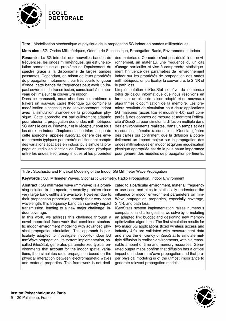
Titre : Modelisation stochastique et physique de la propagation 5G indoor en bandes millimetriques
Mots cles : 5G, Ondes Millimetriques, Geometrie Stochastique, Propagation Radio, Environnement Indoor
Resume : La 5G introduit des nouvelles bandes defrequences, les ondes millimetriques, qui est une so-lution prometteuse au probleme de l’epuisement duspectre grace a la disponibilite de larges bandespassantes. Cependant, en raison de leurs proprietesde propagation, notamment leur tres courte longueurd’onde, cette bande de frequences peut avoir un im-pact severe sur la transmission, conduisant a un nou-veau defi majeur : la couverture indoor.Dans ce manuscrit, nous abordons ce probleme atravers un nouveau cadre theorique qui combine lamodelisation stochastique de l’environnement indooravec la simulation avancee de la propagation phy-sique. Cette approche est particulierement adapteepour etudier la propagation des ondes millimetriques5G dans le cas ou l’emetteur et le recepteur sont tousles deux en indoor. L’implementation informatique decette approche, appelee iGeoStat, genere des envi-ronnements typiques parametres qui tiennent comptedes variations spatiales en indoor, puis simule la pro-pagation radio en fonction de l’interaction physiqueentre les ondes electromagnetiques et les proprietes
des materiaux. Ce cadre n’est pas dedie a un envi-ronnement, un materiau, une frequence ou un casd’usage particulier et vise a comprendre statistique-ment l’influence des parametres de l’environnementindoor sur les proprietes de propagation des ondesmillimetriques, en particulier la couverture, le SINR etle path loss.L’implementation d’iGeoStat souleve de nombreuxdefis de calcul informatique que nous resolvons enformulant un bilan de liaison adapte et de nouveauxalgorithmes d’optimisation de la memoire. Les pre-miers resultats de simulation pour deux applications5G majeures (acces fixe et industrie 4.0) sont com-pares a des donnees de mesure et montrent l’effica-cite d’iGeoStat pour simuler la diffusion multiple dansdes environnements realistes, dans un temps et desressources memoire raisonnables. iGeostat generedes cartes qui confirment que la diffusion a poten-tiellement un impact majeur sur la propagation desondes millimetriques en indoor et qu’une modelisationphysique appropriee est de la plus haute importancepour generer des modeles de propagation pertinents.
Title : Stochastic and Physical Modeling of the Indoor 5G Millimeter Wave Propagation
Keywords : 5G, Millimeter Waves, Stochastic Geometry, Radio Propagation, Indoor Environment
Abstract : 5G millimeter wave (mmWave) is a promi-sing solution to the spectrum scarcity problem sincevery large bandwidths are available. However, due totheir propagation properties, namely their very shortwavelength, this frequency band can severely impacttransmission, leading to a new major challenge: in-door coverage.In this work, we address this challenge through anovel theoretical framework that combines stochas-tic indoor environment modeling with advanced phy-sical propagation simulation. This approach is par-ticularly adapted to investigate indoor-to-indoor 5GmmWave propagation. Its system implementation, so-called iGeoStat, generates parameterized typical en-vironments that account for the indoor spatial varia-tions, then simulates radio propagation based on thephysical interaction between electromagnetic wavesand material properties. This framework is not dedi-
cated to a particular environment, material, frequencyor use case and aims to statistically understand theinfluence of indoor environment parameters on mm-Wave propagation properties, especially coverage,SINR, and path loss.iGeoStat’s system implementation raises numerouscomputational challenges that we solve by formulatingan adapted link budget and designing new memoryoptimization algorithms. The first simulation results fortwo major 5G applications (fixed wireless access andindustry 4.0) are validated with measurement dataand show the efficiency of iGeoStat to simulate mul-tiple diffusion in realistic environments, within a reaso-nable amount of time and memory resources. Gene-rated output maps confirm that diffusion has a criticalimpact on indoor mmWave propagation and that pro-per physical modeling is of the utmost importance togenerate relevant propagation models.
Institut Polytechnique de Paris91120 Palaiseau, France