Embed Size (px)
Citation preview

Lecture Notes in Computer Science 4244Commenced Publication in 1973Founding and Former Series Editors:Gerhard Goos, Juris Hartmanis, and Jan van Leeuwen
Editorial Board
David HutchisonLancaster University, UK
Takeo KanadeCarnegie Mellon University, Pittsburgh, PA, USA
Josef KittlerUniversity of Surrey, Guildford, UK
Jon M. KleinbergCornell University, Ithaca, NY, USA
Friedemann MatternETH Zurich, Switzerland
John C. MitchellStanford University, CA, USA
Moni NaorWeizmann Institute of Science, Rehovot, Israel
Oscar NierstraszUniversity of Bern, Switzerland
C. Pandu RanganIndian Institute of Technology, Madras, India
Bernhard SteffenUniversity of Dortmund, Germany
Madhu SudanMassachusetts Institute of Technology, MA, USA
Demetri TerzopoulosUniversity of California, Los Angeles, CA, USA
Doug TygarUniversity of California, Berkeley, CA, USA
Moshe Y. VardiRice University, Houston, TX, USA
Gerhard WeikumMax-Planck Institute of Computer Science, Saarbruecken, Germany

Stefano Spaccapietra (Ed.)
Journal onDataSemantics VII
13

Volume Editor
Stefano SpaccapietraDatabase Laboratory, EPFL1015 Lausanne, SwitzerlandE-mail: [email protected]
Library of Congress Control Number: 2006935770
CR Subject Classification (1998): H.2, H.3, I.2, H.4, C.2
LNCS Sublibrary: SL 3 – Information Systems and Application, incl. Internet/Weband HCI
ISSN 1861-2032ISBN-10 3-540-46329-1 Springer Berlin Heidelberg New YorkISBN-13 978-3-540-46329-0 Springer Berlin Heidelberg New York
This work is subject to copyright. All rights are reserved, whether the whole or part of the material isconcerned, specifically the rights of translation, reprinting, re-use of illustrations, recitation, broadcasting,reproduction on microfilms or in any other way, and storage in data banks. Duplication of this publicationor parts thereof is permitted only under the provisions of the German Copyright Law of September 9, 1965,in its current version, and permission for use must always be obtained from Springer. Violations are liableto prosecution under the German Copyright Law.
Springer is a part of Springer Science+Business Media
springer.com
© Springer-Verlag Berlin Heidelberg 2006Printed in Germany
Typesetting: Camera-ready by author, data conversion by Scientific Publishing Services, Chennai, IndiaPrinted on acid-free paper SPIN: 11890591 06/3142 5 4 3 2 1 0

The LNCS Journal on Data Semantics
Computerized information handling has changed its focus from centralized data man-agement systems to decentralized data exchange facilities. Modern distribution channels, such as high-speed Internet networks and wireless communication infrastructure, pro-vide reliable technical support for data distribution and data access, materializing the new, popular idea that data may be available to anybody, anywhere, anytime. However, providing huge amounts of data on request often turns into a counterproductive service, making the data useless because of poor relevance or inappropriate level of detail. Se-mantic knowledge is the essential missing piece that allows the delivery of information that matches user requirements. Semantic agreement, in particular, is essential to mean-ingful data exchange.
Semantic issues have long been open issues in data and knowledge management. However, the boom in semantically poor technologies, such as the Web and XML, has boosted renewed interest in semantics. Conferences on the Semantic Web, for instance, attract crowds of participants, while ontologies on their own have become a hot and popular topic in the database and artificial intelligence communities.
Springer's LNCS Journal on Data Semantics aims at providing a highly visible dissemination channel for most remarkable work that in one way or another addresses research and development on issues related to the semantics of data. The target do-main ranges from theories supporting the formal definition of semantic content to innovative domain-specific application of semantic knowledge. This publication channel should be of the highest interest to researchers and advanced practitioners working on the Semantic Web, interoperability, mobile information services, data warehousing, knowledge representation and reasoning, conceptual database model-ing, ontologies, and artificial intelligence.
Topics of relevance to this journal include:
• Semantic interoperability, semantic mediators • Ontologies • Ontology, schema and data integration, reconciliation and alignment • Multiple representations, alternative representations • Knowledge representation and reasoning • Conceptualization and representation • Multi-model and multi-paradigm approaches • Mappings, transformations, reverse engineering • Metadata • Conceptual data modeling • Integrity description and handling • Evolution and change • Web semantics and semi-structured data • Semantic caching

Preface VI
• Data warehousing and semantic data mining • Spatial, temporal, multimedia and multimodal semantics • Semantics in data visualization • Semantic services for mobile users • Supporting tools • Applications of semantic-driven approaches
These topics are to be understood as specifically related to semantic issues. Contri-butions submitted to the journal and dealing with semantics of data will be considered even if they are not within the topics in the list.
While the physical appearance of the journal issues looks like the books from the well-known Springer LNCS series, the mode of operation is that of a journal. Contribu-tions can be freely submitted by authors and are reviewed by the Editorial Board. Con-tributions may also be invited, and nevertheless carefully reviewed, as in the case for issues that contain extended versions of best papers from major conferences addressing data semantics issues. Special issues, focusing on a specific topic, are coordinated by guest editors once the proposal for a special issue is accepted by the Editorial Board. Finally, it is also possible that a journal issue be devoted to a single text.
The journal published its first volume in 2003 (LNCS 2800). That initial volume, as well as volumes II (LNCS 3360), III (LNCS 3534), V (LNCS 3870), and coming volume VIII represent the annual occurrence of a special issue devoted to publication of selected extended versions of best conference papers from previous year confer-ences. Volumes III and VI are annual special issues on a dedicated topic. Volume III, coordinated by guest editor Esteban Zimányi, addressed Semantic-based Geographi-cal Information Systems, while volume VI, coordinated by guest editors Karl Aberer and Philippe Cudre-Mauroux, addressed Emergent Semantics. The fourth volume was the first "normal" volume, built from spontaneous submissions on any of the topics of interest to the Journal. This volume VII is the second of this type.
The Editorial Board comprises one Editor-in-Chief (with overall responsibility), a co-editor-in-chief, and several members. The Editor-in-Chief has a four-year man-date. Members of the board have a three-year mandate. Mandates are renewable. New members may be elected anytime.
We are happy to welcome you to our readership and authorship, and hope we will share this privileged contact for a long time.
Stefano Spaccapietra Editor-in-Chief http://lbdwww.epfl.ch/e/Springer/

JoDS Volume VII – Preface
This JoDS volume results from a rigorous selection among 35 abstract/paper submis-sions received in response to a call for contributions issued July 2005.
After two rounds of reviews, nine papers, spanning a wide variety of topics, were eventually accepted for publication. They are listed in the table of contents herein.
We would like to thank authors of all submitted papers as well as all reviewers who contributed to improving the papers through their detailed comments.
Forthcoming volume VIII will contain extended versions of best papers from 2005 conferences covering semantics aspects. Its publication is expected towards the end of 2006.
We hope you'll enjoy reading this volume. Stefano Spaccapietra Editor-in-Chief

Reviewers
We are very grateful to the external reviewers listed below who helped the editorial board in the reviewing task:
Daniele Barone, Università Milano Bicocca, Italy
Stefano Borgo, Laboratory for Applied Ontology (ISTC-CNR), Italy
Federico Cabitza, Università Milano Bicocca, Italy
Flavio De Paoli, Università Milano Bicocca, Italy
Denise de Vries, Flinders University, Australia
Ying Ding, University of Innsbruck, Austria
Gillian Dobbie, University of Auckland, New Zealand
Fabrice Estiévenart, University of Namur, Belgium
Silvia Gabrielli, Università di Roma 1 “La Sapienza,” Italy
Birte Glimm, The University of Manchester, UK
Giancarlo Guizzardi, Laboratory for Applied Ontology (ISTC-CNR), Italy
Benjamin Habegger, Università di Roma 1 “La Sapienza,” Italy
Markus Kirchberg, Massey University, New Zealand
Jacek Kopecký, DERI Innsbruck, Austria
Changqing Li, National University of Singapore, Singapore
Sebastian Link, Massey University, New Zealand
Andrea Maurino, Università Milano Bicocca, Italy
Jean-Roch Meurisse, University of Namur, Belgium
Diego Milano, Università di Roma 1 “La Sapienza,” Italy
Wei Nei, National University of Singapore, Singapore
Fabio Porto, EPFL, Switzerland
Saurav Sahay, Georgia Institute of Technology, USA
Christelle Vangenot, EPFL, Switzerland
Evgeny Zolin, The University of Manchester, UK

JoDS Editorial Board
Editor-in-chief Stefano Spaccapietra, EPFL, Switzerland Co-editor-in-chief Lois Delcambre, Portland State University, USA
Members of the Board Carlo Batini, Università di Milano Bicocca, Italy Alex Borgida, Rutgers University, USA Shawn Bowers, University of California Davis, USA Tiziana Catarci, Università di Roma “La Sapienza,” Italy David W. Embley, Brigham Young University, USA Jerome Euzenat, INRIA Alpes, France Dieter Fensel, University of Innsbruck, Austria Nicola Guarino, National Research Council, Italy Jean-Luc Hainaut, FUNDP Namur, Belgium Ian Horrocks, University of Manchester, UK Arantza Illarramendi, Universidad del País Vasco, Spain Larry Kerschberg, George Mason University, USA Michael Kifer, State University of New York at Stony Brook, USA Tok Wang Ling, National University of Singapore, Singapore Shamkant B. Navathe, Georgia Institute of Technology, USA Antoni Olivé, Universitat Politècnica de Catalunya, Spain José Palazzo M. de Oliveira, Universidade Federal do Rio Grande do Sul, Brazil Christine Parent, Université de Lausanne, Switzerland John Roddick, Flinders University, Australia Klaus-Dieter Schewe, Massey University, New Zealand Heiner Stuckenschmidt, University Manheim, Germany Katsumi Tanaka, University of Kyoto, Japan Yair Wand, University of British Columbia, Canada Eric Yu, University of Toronto, Canada Esteban Zimányi, Université Libre de Bruxelles (ULB), Belgium
Previous EB members who contributed reviews for this JoDS volume VII:
Maurizio Lenzerini, Università di Roma “La Sapienza,” Italy Salvatore T. March, Vanderbilt University, USA John Mylopoulos, University of Toronto, Canada

Table of Contents
Discovering the Semantics of Relational Tables Through Mappings . . . . . 1Yuan An, Alex Borgida, John Mylopoulos
Specifying the Semantics of Operation Contracts in ConceptualModeling . . . . . . . . . . . . . . . . . . . . . . . . . . . . . . . . . . . . . . . . . . . . . . . . . . . . . . . . 33
Anna Queralt, Ernest Teniente
Model-Driven Ontology Engineering . . . . . . . . . . . . . . . . . . . . . . . . . . . . . . . . . 57Yue Pan, Guotong Xie, Li Ma, Yang Yang, ZhaoMing Qiu,Juhnyoung Lee
Inheritance in Rule-Based Frame Systems: Semantics and Inference . . . . 79Guizhen Yang, Michael Kifer
Unsupervised Duplicate Detection Using Sample Non-duplicates . . . . . . . . 136Patrick Lehti, Peter Fankhauser
Towards Algebraic Query Optimisation for XQuery . . . . . . . . . . . . . . . . . . . . 165Markus Kirchberg, Faizal Riaz-ud-Din, Klaus-Dieter Schewe,Alexei Tretiakov
Automatic Image Description Based on Textual Data . . . . . . . . . . . . . . . . . . 196Youakim Badr, Richard Chbeir
Reasoning About ORA-SS Data Models Using the Semantic Web . . . . . . . 219Yuan Fang Li, Jing Sun, Gillian Dobbie, Hai H. Wang, Jun Sun
A Pragmatic Approach to Model and Exploit the Semanticsof Product Information . . . . . . . . . . . . . . . . . . . . . . . . . . . . . . . . . . . . . . . . . . . . 242
Taehee Lee, Junho Shim, Hyunja Lee, Sang-goo Lee
Author Index . . . . . . . . . . . . . . . . . . . . . . . . . . . . . . . . . . . . . . . . . . . . . . . . . . . 267

Discovering the Semantics of Relational TablesThrough Mappings �
Yuan An1, Alex Borgida2, and John Mylopoulos1
1 Department of Computer Science, University of Toronto, Canada{yuana, jm}@cs.toronto.edu
2 Department of Computer Science, Rutgers University, [email protected]
Abstract. Many problems in Information and Data Management require a se-mantic account of a database schema. At its best, such an account consists offormulas expressing the relationship (“mapping”) between the schema and a for-mal conceptual model or ontology (CM) of the domain. In this paper we describethe underlying principles, algorithms, and a prototype tool that finds such se-mantic mappings from relational tables to ontologies, when given as input simplecorrespondences from columns of the tables to datatype properties of classes inan ontology. Although the algorithm presented is necessarily heuristic, we offerformal results showing that the answers returned by the tool are “correct” for re-lational schemas designed according to standard Entity-Relationship techniques.To evaluate its usefulness and effectiveness, we have applied the tool to a numberof public domain schemas and ontologies. Our experience shows that significanteffort is saved when using it to build semantic mappings from relational tables toontologies.
Keywords: Semantics, ontologies, mappings, semantic interoperability.
1 Introduction and Motivation
A number of important database problems have been shown to have improved solutionsby using a conceptual model or an ontology (CM) to provide precise semantics for adatabase schema. These1 include federated databases, data warehousing [2], and infor-mation integration through mediated schemas [13,8]. Since much information on theweb is generated from databases (the “deep web”), the recent call for a Semantic Web,which requires a connection between web content and ontologies, provides additionalmotivation for the problem of associating semantics with database-resident data (e.g.,[10]). In almost all of these cases, semantics of the data is captured by some kind ofsemantic mapping between the database schema and the CM. Although sometimes themapping is just a simple association from terms to terms, in other cases what is requiredis a complex formula, often expressed in logic or a query language [14].
For example, in both the Information Manifold data integration system presented in[13] and the DWQ data warehousing system [2], formulas of the form T (X) :- Φ(X, Y )
� This is an expanded and refined version of a research paper presented at ODBASE’05 [1].1 For a survey, see [23].
S. Spaccapietra (Ed.): Journal on Data Semantics VII, LNCS 4244, pp. 1–32, 2006.c© Springer-Verlag Berlin Heidelberg 2006

2 Y. An, A. Borgida, and J. Mylopoulos
are used to connect a relational data source to a CM expressed in terms of a Descrip-tion Logic, where T (X) is a single predicate representing a table in the relational datasource, and Φ(X, Y ) is a conjunctive formula over the predicates representing the con-cepts and relationships in the CM. In the literature, such a formalism is called local-as-view (LAV), in contrast to global-as-view (GAV), where atomic ontology concepts andproperties are specified by queries over the database [14].
In all previous work it has been assumed that humans specify the mapping formulas– a difficult, time-consuming and error-prone task, especially since the specifier mustbe familiar with both the semantics of the database schema and the contents of the on-tology. As the size and complexity of ontologies increase, it becomes desirable to havesome kind of computer tool to assist people in the task. Note that the problem of seman-tic mapping discovery is superficially similar to that of database schema mapping, how-ever the goal of the later is finding queries/rules for integrating/translating/exchangingthe underlying data. Mapping schemas to ontologies, on the other hand, is aimed at un-derstanding the semantics of a schema expressed in terms of a given semantic model.This requires paying special attentions to various semantic constructs in both schemaand ontology languages.
We have proposed in [1] a tool that assists users in discovering mapping formulasbetween relational database schemas and ontologies, and presented the algorithms andthe formal results. In this paper, we provide, in addition to what appears in [1], more de-tailed examples for explaining the algorithms, and we also present proofs to the formalresults. Moreover, we show how to handle GAV formulas that are often useful for manypractical data integration systems. The heuristics that underlie the discovery processare based on a careful study of standard design process relating the constructs of therelational model with those of conceptual modeling languages. In order to improve theeffectiveness of our tool, we assume some user input in addition to the database schemaand the ontology. Specifically, inspired by the Clio project [17], we expect the tooluser to provide simple correspondences between atomic elements used in the databaseschema (e.g., column names of tables) and those in the ontology (e.g., attribute/”datatype property” names of concepts). Given the set of correspondences, the tool is ex-pected to reason about the database schema and the ontology, and to generate a listof candidate formulas for each table in the relational database. Ideally, one of the for-mulas is the correct one — capturing user intention underlying given correspondences.The claim is that, compared to composing logical formulas representing semantic map-pings, it is much easier for users to (i) draw simple correspondences/arrows from col-umn names of tables in the database to datatype properties of classes in the ontology2
and then (ii) evaluate proposed formulas returned by the tool. The following exampleillustrates the input/output behavior of the tool proposed.
Example 1.1. An ontology contains concepts (classes), attributes of concepts (datatypeproperties of classes), relationships between concepts (associations), and cardinalityconstraints on occurrences of the participating concepts in a relationship. Graphically,we use the UML notations to represent the above information. Figure 1 is an enter-prise ontology containing some basic concepts and relationships. (Recall that cardinality
2 In fact, there exist already tools used in schema matching which help perform such tasks usinglinguistic, structural, and statistical information (e.g., [4,21]).

Discovering the Semantics of Relational Tables Through Mappings 3
-hasSsn
-hasName-hasAddress-hasAge
Employee
-hasDeptNumber
-hasName-.-.
Department
works_for
controlssup
erv
isio
n
4..* 1..1
1..10..1
1..1 0..*
1..*
0..1
0..*
0..1
-hasNumber
-hasName-.-.
Worksite
manages
works_on 0..1
Employee(ssn, name, dept, proj)
Fig. 1. Relational table, Ontology, and Correspondences
constraints in UML are written at the opposite end of the association: a Departmenthas at least 4 Employees working for it, and an Employee works in one Department.)Suppose we wish to discover the semantics of a relational table Employee(ssn,name,dept, proj) with key ssn in terms of the enterprise ontology. Suppose that by looking atcolumn names of the table and the ontology graph, the user draws the simple correspon-dences shown as dashed arrows in Figure 1. This indicates, for example, that the ssncolumn corresponds to the hasSsn property of the Employee concept. Using prefixesT and O to distinguish tables in the relational schema and concepts in the ontology(both of which will eventually be thought of as predicates), we represent the correspon-dences as follows:T : Employee.ssn�O : Employee.hasSsn
T : Employee.name�O : Employee.hasName
T : Employee.dept�O : Department.hasDeptNumber
T : Employee.proj�O : Worksite.hasNumber
Given the above inputs, the tool is expected to produce a list of plausible mappingformulas, which would hopefully include the following formula, expressing a possiblesemantics for the table:T :Employee(ssn, name, dept, proj) :-
O:Employee(x1), O:hasSsn(x1,ssn), O:hasName(x1,name), O:Department(x2),O:works for(x1,x2), O:hasDeptNumber(x2,dept), O:Worksite(x3), O:works on(x1,x3),O:hasNumber(x3,proj).
Note that, as explained in [14], the above, admittedly confusing notation in the litera-ture, should really be interpreted as the First Order Logic formula
(∀ssn, name, dept, proj) T :Employee(ssn, name, dept, proj) ⇒(∃x1, x2, x3) O:Employee(x1) ∧...
because the ontology explains what is in the table (i.e., every tuple corresponds to anemployee), rather than guaranteeing that the table satisfies the closed world assumption(i.e., for every employee there is a tuple in the table). �
An intuitive (but somewhat naive) solution, inspired by early work of Quillian [20], isbased on finding the shortest connections between concepts. Technically, this involves

4 Y. An, A. Borgida, and J. Mylopoulos
(i) finding the minimum spanning tree(s) (actually Steiner trees3) connecting the “corre-sponded concepts” — those that have datatype properties corresponding to tablecolumns, and then (ii) encoding the tree(s) into formulas. However, in some cases thespanning/Steiner tree may not provide the desired semantics for a table because of knownrelational schema design rules. For example, consider the relational table Project(name, supervisor), where the column name is the key and corresponds to the at-tribute O:Worksite.hasName, and column supervisor corresponds to the attributeO:Employee.hasSsn in Figure 1. The minimum spanning tree consisting of Worksite,Employee, and the edge works on probably does not match the semantics of tableProject because there are multiple Employees working on a Worksite according tothe ontology cardinality, yet the table allows only one to be recorded, since supervisoris functionally dependent on name, the key. Therefore we must seek a functional con-nection from Worksite to Employee, and the connection will be the manager of thedepartment controlling the worksite. In this paper, we use ideas of standard relationalschema design from ER diagrams in order to craft heuristics that systematically uncoverthe connections between the constructs of relational schemas and those of ontologies.We propose a tool to generate “reasonable” trees connecting the set of corresponded con-cepts in an ontology. In contrast to the graph theoretic results which show that there maybe too many minimum spanning/Steiner trees among the ontology nodes (for example,there are already 5 minimum spanning trees connecting Employee, Department, andWorksite in the very simple graph in Figure 1), we expect the tool to generate only asmall number of “reasonable” trees. These expectations are born out by our experimentalresults, in Section 6.
As mentioned earlier, our approach is directly inspired by the Clio project [17,18],which developed a successful tool that infers mappings from one set of relational tablesand/or XML schemas to another, given just a set of correspondences between theirrespective attributes. Without going into further details at this point, we summarize thecontributions of this work:
– We identify a new version of the data mapping problem: that of inferring complexformulas expressing the semantic mapping between relational database schemasand ontologies from simple correspondences.
– We propose an algorithm to find “reasonable” tree connection(s) in the ontologygraph. The algorithm is enhanced to take into account information about the schema(key and foreign key structure), the ontology (cardinality restrictions), and standarddatabase schema design guidelines.
– To gain theoretical confidence, we give formal results for a limited class of schemas.We show that if the schema was designed from a CM using techniques well-knownin the Entity Relationship literature (which provide a natural semantic mapping andcorrespondences for each table), then the tool will recover essentially all and onlythe appropriate semantics. This shows that our heuristics are not just shots in thedark: in the case when the ontology has no extraneous material, and when a table’sscheme has not been denormalized, the algorithm will produce good results.
3 A Steiner tree for a set M of nodes in graph G is a minimum spanning tree of M that maycontain nodes of G which are not in M .
Discovering the Semantics of Relational Tables Through Mappings 5
– To test the effectiveness and usefulness of the algorithm in practice, we imple-mented the algorithm in a prototype tool and applied it to a variety of databaseschemas and ontologies drawn from a number of domains. We ensured that theschemas and the ontologies were developed independently; and the schemas mightor might not be derived from a CM using the standard techniques. Our experiencehas shown that the user effort in specifying complex mappings by using the tool issignificantly less than that by manually writing formulas from scratch.
The rest of the paper is structured as follows. We contrast our approach with relatedwork in Section 2, and in Section 3 we present the technical background and notation.Section 4 describes an intuitive progression of ideas underlying our approach, whileSection 5 provides the mapping inference algorithm. In Section 6 we report on theprototype implementation of these ideas and experiments with the prototype. Section 7shows how to filter out unsatisfied mapping formulas by ontology reasoning. Section 8discusses the issues of generating GAV mapping formulas. Finally, Section 9 concludesand discusses future work.
2 Related Work
The Clio tool [17,18] discovers formal queries describing how target schemas canbe populated with data from source schemas. To compare with it, we could view thepresent work as extending Clio to the case when the source schema is a relational data-base while the target is an ontology. For example, in Example 1.1, if one viewed theontology as a relational schema made of unary tables (such as Employee(x1)), binarytables (such as hasSsn(x1, ssn)) and the obvious foreign key constraints from binaryto unary tables, then one could in fact try to apply directly the Clio algorithm to the prob-lem. The desired mapping formula from Example 1.1 would not be produced for severalreasons: (i) Clio [18] works by taking each table and using a chase-like algorithm to re-peatedly extend it with columns that appear as foreign keys referencing other tables.Such “logical relations” in the source and target are then connected by queries. In thisparticular case, this would lead to logical relations such as works for �� Employee�� Department, but none that join, through some intermediary, hasSsn(x1, ssn) andhasDeptNumber(x2, dept), which is part of the desired formula in this case. (ii) Thefact that ssn is a key in the table T :Employee, leads us to prefer (see Section 4)a many-to-one relationship, such as works for, over some many-to-many relation-ship which could have been part of the ontology (e.g., O:previouslyWorkedFor);Clio does not differentiate the two. So the work to be presented here analyzes the keystructure of the tables and the semantics of relationships (cardinality, IsA) to elimi-nate/downgrade unreasonable options that arise in mappings to ontologies.
Other potentially relevant work includes data reverse engineering, which aims toextract a CM, such as an ER diagram, from a database schema. Sophisticated algorithmsand approaches to this have appeared in the literature over the years (e.g., [15,9]). Themajor difference between data reverse engineering and our work is that we are givenan existing ontology, and want to interpret a legacy relational schema in terms of it,whereas data reverse engineering aims to construct a new ontology.

6 Y. An, A. Borgida, and J. Mylopoulos
Schema matching (e.g., [4,21]) identifies semantic relations between schema ele-ments based on their names, data types, constraints, and schema structures. The primarygoal is to find the one-to-one simple correspondences which are part of the input for ourmapping inference algorithms.
3 Formal Preliminaries
We do not restrict ourselves to any particular language for describing ontologies in thispaper. Instead, we use a generic conceptual modeling language (CML), which containscommon aspects of most semantic data models, UML, ontology languages such as OWL,and description logics. In the sequel, we use CM to denote an ontology prescribed by thegeneric CML. Specifically, the language allows the representation of classes/concepts(unary predicates over individuals), object properties/relationships (binary predicatesrelating individuals), and datatype properties/attributes (binary predicates relating in-dividuals with values such as integers and strings); attributes are single valued in thispaper. Concepts are organized in the familiar is-a hierarchy. Object properties, and theirinverses (which are always present), are subject to constraints such as specification ofdomain and range, plus cardinality constraints, which here allow 1 as lower bounds(called total relationships), and 1 as upper bounds (called functional relationships).
We shall represent a given CM using a labeled directed graph, called an ontologygraph. We construct the ontology graph from a CM as follows: We create a conceptnode labeled with C for each concept C, and an edge labeled with p from the conceptnode C1 to the concept node C2 for each object property p with domain C1 and rangeC2; for each such p, there is also an edge in the opposite direction for its inverse, referredto as p−. For each attribute f of concept C, we create a separate attribute node denotedas Nf,C , whose label is f , and add an edge labeled f from node C to Nf,C .4 Foreach is-a edge from a subconcept C1 to a superconcept C2, we create an edge labeledwith is-a from concept node C1 to concept node C2. For the sake of succinctness, wesometimes use UML notations, as in Figure 1, to represent the ontology graph. Note thatin such a diagram, instead of drawing separate attribute nodes, we place the attributesinside the rectangle nodes; and relationships and their inverses are represented by asingle undirected edge. The presence of such an undirected edge, labeled p, betweenconcepts C and D will be written in text as C ---p--- D . If the relationship p isfunctional from C to D, we write C ---p->-- D . For expressive CMLs such asOWL, we may also connect C to D by p if we find an existential restriction stating thateach instance of C is related to some instance or only instances of D by p.
For relational databases, we assume the reader is familiar with standard notions aspresented in [22], for example. We will use the notation T (K, Y ) to represent a rela-tional table T with columns KY , and key K . If necessary, we will refer to the indi-vidual columns in Y using Y [1], Y [2], . . ., and use XY as concatenation of columns.Our notational convention is that single column names are either indexed or appear inlower-case. Given a table such as T above, we use the notation key(T), nonkey(T) andcolumns(T) to refer to K , Y and KY respectively. (Note that we use the terms “table”and “column” when talking about relational schemas, reserving “relation(ship)” and
4 Unless ambiguity arises, we say “node C”, when we mean “concept node labeled C”.

Discovering the Semantics of Relational Tables Through Mappings 7
“attribute” for aspects of the CM.) A foreign key (abbreviated as f.k. henceforth) in Tis a set of columns F that references the key of table T ′, and imposes a constraint thatthe projection of T on F is a subset of the projection of T ′ on key(T ′).
In this paper, a correspondence T.c �D.f relates column c of table T to attributef of concept D. Since our algorithms deal with ontology graphs, formally a corre-spondence L will be a mathematical relation L(T, c, D, f, Nf,D), where the first twoarguments determine unique values for the last three. This means that we only treatthe case when a table column corresponds to single attribute of a concept, and leaveto future work dealing with complex correspondences, which may represent unions,concatenations, etc.
Finally, for LAV-like mapping, we use Horn-clauses in the form T (X) :- Φ(X, Y ),as described in Section 1, to represent semantic mappings, where T is a table withcolumns X (which become arguments to its predicate), and Φ is a conjunctive formulaover predicates representing the CM, with Y existentially quantified, as usual.
4 Principles of Mapping Inference
Given a table T , and correspondencesL to an ontology provided by a person or a tool, letthe set CT consist of those concept nodes which have at least one attribute correspondingto some column of T (i.e., D such that there is at least one tuple L( , , D, , )). Ourtask is to find semantic connections between concepts in CT , because attributes can thenbe connected to the result using the correspondence relation: for any node D, one canimagine having edges f to M , for every entry L( , , D, f, M). The primary principle ofour mapping inference algorithm is to look for smallest “reasonable” trees connectingnodes in CT . We will call such a tree a semantic tree.
As mentioned before, the naive solution of finding minimum spanning trees or Steinertrees does not give good results, because it must also be “reasonable”. We aim to describemore precisely this notion of “reasonableness”.
Consider the case when T (c, b) is a table with key c, corresponding to an attributef on concept C, and b is a foreign key corresponding to an attribute e on concept B.Then for each value of c (and hence instance of C), T associates at most one value ofb (instance of B). Hence the semantic mapping for T should be some formula that actsas a function from its first to its second argument. The semantic trees for such formulaslook like functional edges in the ontology, and hence are more reasonable. For example,given table Dep(dept, ssn, . . .), and correspondencesT :Dep.dept �O:Department.hasDeptNumberT :Dep.ssn �O:Employee.hasSsnfrom the table columns to attributes of the ontology in Figure 1, the proper semantic treeusesmanages− (i.e.,hasManager) rather thanworks_for− (i.e.,hasWorkers).
Conversely, for table T ′(c, b), where c and b are as above, an edge that is functionalfrom C to B, or from B to C, is likely not to reflect a proper semantics since it wouldmean that the key chosen for T ′ is actually a super-key – an unlikely error. (In ourexample, consider a table T (ssn, dept), where both columns are foreign keys.)
To deal with such problems, our algorithm works in two stages: first connects theconcepts corresponding to key columns into a skeleton tree, then connects the rest ofthe corresponded nodes to the skeleton by functional edges (whenever possible).

8 Y. An, A. Borgida, and J. Mylopoulos
We must however also deal with the assumption that the relational schema andthe CM were developed independently, which implies that not all parts of the CMare reflected in the database schema. This complicates things, since in building thesemantic tree we may need to go through additional nodes, which end up not cor-responding to columns of the relational table. For example, consider again the tableProject(name, supervisor) and its correspondences mentioned in Section 1. Be-cause of the key structure of this table, based on the above arguments we will preferthe functional path5 controls−.manages− (i.e., controlledBy followed byhasManager), passing through node Department, over the shorter path consistingof edge works_on, which is not functional. Similar situations arise when the CMcontains detailed aggregation hierarchies (e.g., city part-of township part-of countypart-of state), which are abstracted in the database (e.g., a table with columns for cityand state only).
We have chosen to flesh out the above principles in a systematic manner by con-sidering the behavior of our proposed algorithm on relational schemas designed fromEntity Relationship diagrams — a technique widely covered in undergraduate databasecourses [22]. (We refer to this er2rel schema design.) One benefit of this approach isthat it allows us to prove that our algorithm, though heuristic in general, is in somesense “correct” for a certain class of schemas. Of course, in practice such schemas maybe “denormalized” in order to improve efficiency, and, as we mentioned, only parts ofthe CM may be realized in the database. Our algorithm uses the general principles enun-ciated above even in such cases, with relatively good results in practice. Also note thatthe assumption that a given relational schema was designed from some ER conceptualmodel does not mean that given ontology is this ER model, or is even expressed in theER notation. In fact, our heuristics have to cope with the fact that it is missing essentialinformation, such as keys for weak entities.
To reduce the complexity of the algorithms, which essentially enumerate all trees,and to reduce the size of the answer set, we modify an ontology graph by collapsingmultiple edges between nodes E and F , labeled p1, p2, . . . say, into at most three edges,each labeled by a string of the form ′pj1 ; pj2 ; . . .′: one of the edges has the names of allfunctions from E to F ; the other all functions from F to E; and the remaining labels onthe third edge. (Edges with empty labels are dropped.) Note that there is no way that ouralgorithm can distinguish between semantics of the labels on one kind of edge, so thetool offers all of them. It is up to the user to choose between alternative labels, thoughthe system may offer suggestions, based on additional information such as heuristicsconcerning the identifiers labeling tables and columns, and their relationship to propertynames.
5 Semantic Mapping Inference Algorithms
As mentioned, our algorithm is based in part on the relational database schema designmethodology from ER models. We introduce the details of the algorithm iteratively, byincrementally adding features of an ER model that appear as part of the CM. We assume
5 One consisting of a sequence of edges, each of which represents a function from its source toits target.

Discovering the Semantics of Relational Tables Through Mappings 9
that the reader is familiar with basics of ER modeling and database design [22], thoughwe summarize the ideas.
5.1 ER0: An Initial Subset of ER Notions
We start with a subset, ER0, of ER that supports entity sets E (called just “entity”here), with attributes (referred to by attribs(E)), and binary relationship sets. In orderto facilitate the statement of correspondences and theorems, we assume in this sectionthat attributes in the CM have globally unique names. (Our implemented tool does notmake this assumption.) An entity is represented as a concept/class in our CM. A bi-nary relationship set corresponds to two properties in our CM, one for each direction.Such a relationship is called many-many if neither it nor its inverse is functional. Astrong entity S has some attributes that act as identifier. We shall refer to these usingunique(S) when describing the rules of schema design. A weak entity W has insteadlocalUnique(W ) attributes, plus a functional total binary relationship p (denoted asidRel(W )) to an identifying owner entity (denoted as idOwn(W )).
Example 5.1. An ER0 diagram is shown in Figure 2, which has a weak entity Dependentand three strong entities: Employee, Department, and Project. The owner entity ofDependent is Employee and the identifying relationship is dependents of . Using thenotation we introduced, this means thatlocalUnique(Dependent) =deName, idRel(Dependent)= dependents of ,idOwn(Dependent)= Employee. For the owner entity Employee,unique(Employee)= hasSsn. �
-hasSsn-hasName-hasAddress-hasAge
Employee-hasDeptNumber-hasName-.-.
Department-deName-birthDate-gender-relationship
Dependent
works_for participatesdependents_of4..* 1..1 1..* 0..*1..10..*
-hasNumber-hasName-.-.
Project
Fig. 2. An ER0 Example
Note that information about multi-attribute keys cannot be represented formally in evenhighly expressive ontology languages such as OWL. So functions like unique are onlyused while describing the er2rel mapping, and are not assumed to be available duringsemantic inference. The er2rel design methodology (we follow mostly [15,22]) is de-fined by two components. To begin with, Table 1 specifies a mapping τ(O) returning arelational table scheme for every CM component O, where O is either a concept/entityor a binary relationship. (For each relationship exactly one of the directions will bestored in a table.)
In addition to the schema (columns, key, f.k.’s), Table 1 also associates with a rela-tional table T (V ) a number of additional notions:
– an anchor, which is the central object in the CM from which T is derived, andwhich is useful in explaining our algorithm (it will be the root of the semantic tree);

10 Y. An, A. Borgida, and J. Mylopoulos
Table 1. er2rel Design Mapping
ER Model object O Relational Table τ (O)
Strong Entity S columns: X
primary key: K
Let X=attribs(S) f.k.’s: none
Let K=unique(S) anchor: S
semantics: T (X) :- S(y),hasAttribs(y, X).
identifier: identifyS(y, K) :- S(y),hasAttribs(y, K).
Weak Entity W columns: ZX
let primary key: UX
E = idOwn(W ) f.k.’s: X
P = idrel(W ) anchor: W
Z=attribs(W ) semantics: T (X, U, V ) :- W (y), hasAttribs(y, Z), E(w),P (y, w),
X = key(τ(E)) identifyE(w, X).
U =localUnique(W ) identifier: identifyW (y, UX) :- W (y),E(w), P (y, w), hasAttribs(y, U),
V = Z − U identifyE(w, X).
Functional columns: X1X2
Relationship F primary key: X1
E1 --F->- E2 f.k.’s: Xi references τ(Ei),
let Xi = key(τ(Ei)) anchor: E1
for i = 1, 2 semantics: T (X1, X2) :- E1(y1),identifyE1(y1, X1), F (y1, y2), E2(y2),
identifyE2(y2, X2).
Many-many columns: X1X2
Relationship M primary key: X1X2
E1 --M-- E2 f.k.’s: Xi references τ(Ei),
let Xi = key(τ(Ei)) semantics: T (X1, X2) :- E1(y1),identifyE1(y1, X1), M(y1, y2),E2(y2),
for i = 1, 2 identifyE2(y2, X2).
– a formula for the semantic mapping for the table, expressed as a formula with headT (V ) (this is what our algorithm should be recovering); in the body of the formula,the function hasAttribs(x, Y ) returns conjuncts attrj(x, Y [j]) for the individualcolumns Y [1], Y [2], . . . in Y , where attrj is the attribute name corresponded bycolumn Y [j].
– the formula for a predicate identifyC(x, Y ), showing how object x in (strong orweak) entity C can be identified by values in Y 6.
Note that τ is defined recursively, and will only terminate if there are no “cycles” in theCM (see [15] for definition of cycles in ER).
Example 5.2. When τ is applied to concept Employee in Figure 2, we get thetable T :Employee(hasSsn, hasName, hasAddress, hasAge), with the anchorEmployee, and the semantics expressed by the mapping:T :Employee(hasSsn, hasName, hasAddress,hasAge) :-
O:Employee(y), O:hasSsn(y, hasSsn), O:hasName(y, hasName),O:hasAddress(y, hasAddress), O:hasAge(y, hasAge).
6 This is needed in addition to hasAttribs, because weak entities have identifying values spreadover several concepts.

Discovering the Semantics of Relational Tables Through Mappings 11
Its identifier is represented byidentifyEmployee(y, hasSsn) :- O:Employee(y), O:hasSsn(y, hasSsn).
In turn, τ(Dependent) produces the table T :Dependent(deName, hasSsn,birthDate,...), whose anchor is Dependent. Note that the hasSsn column is a foreignkey referencing the hasSsn column in the T :Employee table. Accordingly, its seman-tics is represented as:T :Dependent(deName, hasSsn, birthDate, ...) :-
O:Dependent(y), O:Employee(w), O:dependents of(y, w),identifyEmployee(w, hasSsn), O:deName(y, deName),O:birthDate(y, birthDate) ...
and its identifier is represented as:identifyDependent(y, deName,hasSsn) :-
O:Dependent(y), O:Employee(w), O:dependents of(y, w),identifyEmployee(w, hasSsn), O:deName(y, deName).
τ can be applied similarly to the other objects in Figure 2. τ(works for) producesthe table works for(hasSsn, hasDeptNumber). τ(participates) generates the tableparticipates(hasNumber, hasDeptNumber). Please note that the anchor of the tablegenerated by τ(works for) is Employee, while no single anchor is assigned to thetable generated by τ(participates). �The second step of the er2rel schema design methodology suggests that the schemagenerated using τ can be modified by (repeatedly) merging into the table T0 of an en-tity E the table T1 of some functional relationship involving the same entity E (whichhas a foreign key reference to T0). If the semantics of T0 is T0(K, V ) :- φ(K, V ),and of T1 is T1(K, W ) :- ψ(K, W ), then the semantics of table T=merge(T0,T1)is, to a first approximation, T (K, V, W ) :- φ(K, V ), ψ(K, W ). And the anchor of Tis the entity E. (We defer the description of the treatment of null values which canarise in the non-key columns of T1 appearing in T .) For example, we could merge thetable τ(Employee) with the table τ(works for) in Example 5.2 to form a new ta-ble T :Employee2 (hasSsn, hasName, hasAddress, hasAge, hasDeptNumber),where the column hasDeptNumber is an f.k. referencing τ(Department). The se-mantics of the table is:T :Employee2(hasSsn, hasName, hasAddress,hasAge,hasDeptNumber):-
O:Employee(y), O:hasSsn(y, hasSsn), O:hasName(y, hasName),O:hasAddress(y, hasAddress), O:hasAge(y, hasAge),O:Department(w), O:works for(y, w), O:hasDeptNumber(w, hasDeptNumber).
Please note that one conceptual model may result in several different relational schemas,since there are choices in which direction a one-to-one relationship is encoded (whichentity acts as a key), and how tables are merged. Note also that the resulting schema isin Boyce-Codd Normal Form, if we assume that the only functional dependencies arethose that can be deduced from the ER schema (as expressed in FOL).
In this subsection, we assume that the CM has no so-called “recursive” relationshipsrelating an entity to itself, and no attribute of an entity corresponds to multiple columnsof any table generated from the CM. (We deal with these in Section 5.3.) Note that bythe latter assumption, we rule out for now the case when there are several relationships

12 Y. An, A. Borgida, and J. Mylopoulos
between a weak entity and its owner entity, such as hasMet connecting Dependentand Employee, because in this case τ(hasMet) will need columns deName, ssn1,ssn2, with ssn1 helping to identify the dependent, and ssn2 identifying the (other)employee they met.
Now we turn to the algorithm for finding the semantics of a table in terms of a givenCM. It amounts to finding the semantic trees between nodes in the set CT singled out bythe correspondences from columns of the table T to attributes in the CM. As mentionedpreviously, the algorithm works in several steps:
1. Determine a skeleton tree connecting the concepts corresponding to key columns;also determine, if possible, a unique anchor for this tree.
2. Link the concepts corresponding to non-key columns using shortest functionalpaths to the skeleton/anchor tree.
3. Link any unaccounted-for concepts corresponding to other columns by arbitraryshortest paths to the tree.
To flesh out the above steps, we begin with the tables created by the standard de-sign process. If a table is derived by the er2rel methodology from an ER0 diagram,then Table 1 provides substantial knowledge about how to determine the skeleton tree.However, care must be taken when weak entities are involved. The following exampledescribes the right process to discover the skeleton and the anchor of a weak entity table.
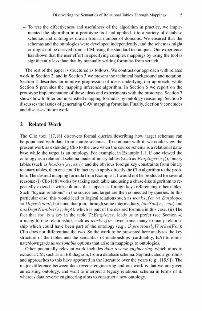
Example 5.3. Consider table T :Dept(number, univ, dean), with foreign key (f.k.)univ referencing table T :Univ(name, address) and correspondences shown in Fig-ure 3. We can tell that T :Dept represents a weak entity since its key has one f.k. as asubset (referring to the strong entity on which Department depends). To find the skele-ton and anchor of the table T :Dept, we first need to find the skeleton and anchor of thetable referenced by the f.k. univ. The answer is University. Next, we should lookfor a total functional edge (path) from the correspondent of number, which is con-cept Department, to the anchor, University. As a result, the link Department
---belongsTo-->- University is returned as the skeleton, and Departmentis returned as the anchor. Finally, we can correctly identify the dean relationship as theremainder of the connection, rather than the president relationship, which would haveseemed a superficially plausible alternative to begin with.
Furthermore, suppose we need to interpret the table T :Portal(dept, univ, address)with the following correspondences:T : Portal.dept�O : Department.hasDeptNumber
T : Portal.univ�O : University.hasUnivName
T : Portal.address�O : Host.hostName,where not only is {dept, univ} the key but also an f.k. referencing the key of tableT :Dept. To find the anchor and skeleton of table T :Portal, the algorithm first recur-sively works on the referenced table. This is also needed when the owner entity of aweak entity is itself a weak entity. �The following is the function getSkeleton which returns a set of (skeleton, anchor)-pairs, when given a table T and a set of correspondences L from key(T ). The functionis essentially a recursive algorithm attempting to reverse the function τ in Table 1.

Discovering the Semantics of Relational Tables Through Mappings 13
-hasUnivName-hasAddres
University
-hasDeptNumber-.
Department
-hasName
-hasBoD
Employee
belongsTo
0..* 0..1 0..*1..1 1..* -hostName-.
Host
hasServerAt
president dean
1..11..1
0..10..1
Dept( number,univ , dean), univ and dean are f.k.s.
Fig. 3. Finding Correct Skeleton Trees and Anchors
In order to accommodate tables not designed according to er2rel, the algorithm hasbranches for finding minimum spanning/Steiner trees as skeletons.
Function getSkeleton(T,L)input: table T , correspondences L for key(T )output: a set of (skeleton tree, anchor) pairssteps:Suppose key(T ) contains f.k.s F1,. . . ,Fn referencing tables T1(K1),..,Tn(Kn);
1. If n ≤ 1 and onc(key(T ))7 is just a singleton set {C}, then return (C, {C}).8/*T is likelyabout a strong entity: base case.*/
2. Else, let Li={Ti.Ki�L(T, Fi)}/*translate corresp’s thru f.k. reference.*/;compute (Ssi, Anci) = getSkeleton(Ti, Li), for i = 1, .., n.
(a) If key(T ) = F1, then return (Ss1, Anc1). /*T looks like the table for the functionalrelationship of a weak entity, other than its identifying relationship.*/
(b) If key(T )=F1A, where columns A are not part of an f.k. then /*T is possibly a weakentity*/
if Anc1 = {N1} and onc(A) = {N} such that there is a (shortest) total functionalpath π from N to N1, then return (combine9(π, Ss1), {N}). /*N is a weak entity.cf. Example 5.3.*/
(c) Else suppose key(T ) has non-f.k. columns A[1], . . . A[m], (m≥0); let Ns={Anci, i =1, .., n} ∪ {onc(A[j]), j = 1, .., m}; find skeleton tree S′ connecting the nodes in Ns
where any pair of nodes in Ns is connected by a (shortest) non-functional path; return(combine(S′, {Ssj}), Ns). /*Deal with many-to-many binary relationships; also thedefault action for non-standard cases, such as when not finding identifying relationshipfrom a weak entity to the supposed owner entity. In this case no unique anchor exists.*/
7 onc(X) is the function which gets the set M of concepts corresponded by the columns X.8 Both here and elsewhere, when a concept C is added to a tree, so are edges and nodes for C’s
attributes that appear in L.9 Function combine merges edges of trees into a larger tree.

14 Y. An, A. Borgida, and J. Mylopoulos
In order for getSkeleton to terminate, it is necessary that there be no cycles inf.k. references in the schema. Such cycles (which may have been added to representadditional integrity constraints, such as the fact that a property is total) can be elim-inated from a schema by replacing the tables involved with their outer join over thekey. getSkeleton deals with strong entities and their functional relationships in step(1), with weak entities in step (2.b), and so far, with functional relationships of weakentities in (2.a). In addition to being a catch-all, step (2.c) deals with tables represent-ing many-many relationships (which in this section have key K = F1F2), by findinganchors for the ends of the relationship, and then connecting them with paths that arenot functional, even when every edge is reversed.
To find the entire semantic tree of a table T , we must connect the concepts corre-sponded by the rest of the columns, i.e., nonkey(T ), to the anchor(s). The connectionsshould be (shortest) functional edges (paths), since the key determines at most one valuefor them; however, if such a path cannot be found, we use an arbitrary shortest path. Thefollowing function, getTree, achieves the goal.
Function getTree(T,L)input: table T , correspondences L for columns(T )output: set of semantic trees 10
steps:
1. Let Lk be the subset of L containing correspondences from key(T );compute (S′, Anc′)=getSkeleton(T ,Lk).
2. If onc(nonkey(T )) − onc(key(T )) is empty, then return (S′, Anc′). /*if all columns cor-respond to the same set of concepts as the key does, then return the skeleton tree.*/
3. For each f.k. Fi in nonkey(T ) referencing Ti(Ki):let Li
k = {Ti.Ki�L(T, Fi)}, and compute (Ss′′i , Anc′′
i )= getSkeleton(Ti,Lik). /*recall
that the function L(T, Fi) is derived from a correspondence L(T, Fi, D, f, Nf,D) such thatit gives a concept D and its attribute f (Nf,D is the attribute node in the ontology graph.)*/find πi=shortest functional path from Anc′ to Anc′′
i ; let S = combine(S′, πi, {Ss′′i }).
4. For each column c in nonkey(T) that is not part of an f.k., let N = onc(c); find π=shortestfunctional path from Anc′ to N ; update S := combine(S, π). /*cf. Example 5.4.*/
5. In all cases above asking for functional paths, use a shortest path if a functional one does notexist.
6. Return S.
The following example illustrates the use of getTree when seeking to interpret a ta-ble using a different CM than the one from which it was originally derived.
Example 5.4. In Figure 4, the table T :Assignment(emp, proj, site) was originally de-rived from a CM with the entity Assignment shown on the right-hand side of the verticaldashed line. To interpret it by the CM on the left-hand side, the function getSkeleton, inStep 2.c, returns Employee ---assignedTo--- Project as the skeleton, andno single anchor exists. The set {Employee, Project} accompanying the skeleton is
10 To make the description simpler, at times we will not explicitly account for the possibility ofmultiple answers. Every function is extended to set arguments by element-wise application ofthe function to set members.

Discovering the Semantics of Relational Tables Through Mappings 15
returned. Subsequently, the function getTree seeks for the shortest functional link fromelements in {Employee, Project} to Worksite at Step 4. Consequently, it connectsWorksite to Employee via works on to build the final semantic tree. �
-employee
-project
-site
Assignment
-projNumber
Project
-empNumber
Employee
works_on
1..* 0..*
1..*
-siteName
Worksite
assignedTo
1..1
Assignment( emp ,proj ,site)
derived from
Fig. 4. Independently Developed Table and CM
To get the logic formula from a tree based on correspondence L, we provide the proce-dure encodeTree(S, L) below, which basically assigns variables to nodes, and connectsthem using edge labels as predicates.
Function encodeTree(S,L)input: subtree S of ontology graph, correspondences L from table columns to attributesof concept nodes in S.output: variable name generated for root of S, and conjunctive formula for the tree.steps: Suppose N is the root of S. Let Ψ = true.1. if N is an attribute node with label f
find d such that L( , d, , f, N) = true;return(d, true). /*for leaves of the tree, which are attribute nodes, return the corresponding
column name as the variable and the formula true.*/2. if N is a concept node with label C, then introduce new variable x; add conjunctC(x) to Ψ ;
for each edge pi from N to Ni /*recursively get the subformulas.*/let Si be the subtree rooted at Ni,let (vi, φi(Zi))=encodeTree(Si, L),add conjuncts pi(x, vi) ∧ φi(Zi) to Ψ ;
3. return (x, Ψ).
Example 5.5. Figure 5 is the fully specified semantic tree returned by the algorithm forthe T :Dept(number, univ, dean) table in Example 5.3. Taking Department as theroot of the tree, function encodeTree generates the following formula:
Department(x), hasDeptNumber(x, number), belongsTo(x, v1), University(v1),hasUnivName(v1, univ), dean(x, v2), Employee(v2), hasName(v2, dean).
As expected, the formula is the semantics the table T :Dept as assigned by the er2reldesign τ . �
16 Y. An, A. Borgida, and J. Mylopoulos
University Department Employee
belongsTo dean
hasUnivName hasDeptNumber hasName
hasUnivName hasNamehasDeptNumber
Fig. 5. Semantic Tree For Dept Table
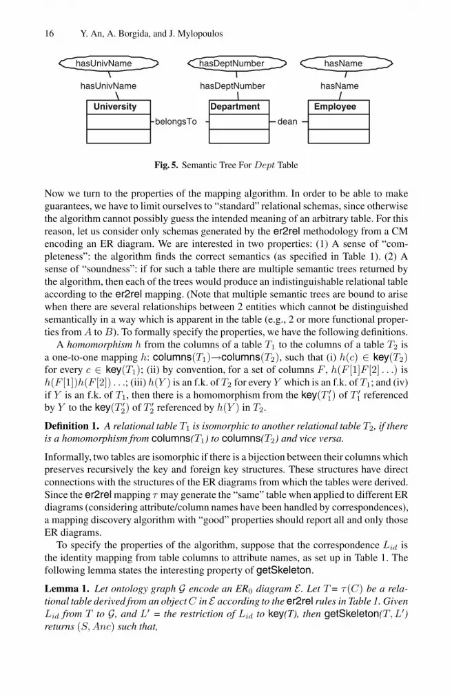
Now we turn to the properties of the mapping algorithm. In order to be able to makeguarantees, we have to limit ourselves to “standard” relational schemas, since otherwisethe algorithm cannot possibly guess the intended meaning of an arbitrary table. For thisreason, let us consider only schemas generated by the er2rel methodology from a CMencoding an ER diagram. We are interested in two properties: (1) A sense of “com-pleteness”: the algorithm finds the correct semantics (as specified in Table 1). (2) Asense of “soundness”: if for such a table there are multiple semantic trees returned bythe algorithm, then each of the trees would produce an indistinguishable relational tableaccording to the er2rel mapping. (Note that multiple semantic trees are bound to arisewhen there are several relationships between 2 entities which cannot be distinguishedsemantically in a way which is apparent in the table (e.g., 2 or more functional proper-ties from A to B). To formally specify the properties, we have the following definitions.
A homomorphism h from the columns of a table T1 to the columns of a table T2 isa one-to-one mapping h: columns(T1)→columns(T2), such that (i) h(c) ∈ key(T2)for every c ∈ key(T1); (ii) by convention, for a set of columns F , h(F [1]F [2] . . .) ish(F [1])h(F [2]) . . .; (iii) h(Y ) is an f.k. of T2 for every Y which is an f.k. of T1; and (iv)if Y is an f.k. of T1, then there is a homomorphism from the key(T ′
1) of T ′1 referenced
by Y to the key(T ′2) of T ′
2 referenced by h(Y ) in T2.
Definition 1. A relational table T1 is isomorphic to another relational table T2, if thereis a homomorphism from columns(T1) to columns(T2) and vice versa.
Informally, two tables are isomorphic if there is a bijection between their columns whichpreserves recursively the key and foreign key structures. These structures have directconnections with the structures of the ER diagrams from which the tables were derived.Since the er2rel mapping τ may generate the “same” table when applied to different ERdiagrams (considering attribute/column names have been handled by correspondences),a mapping discovery algorithm with “good” properties should report all and only thoseER diagrams.
To specify the properties of the algorithm, suppose that the correspondence Lid isthe identity mapping from table columns to attribute names, as set up in Table 1. Thefollowing lemma states the interesting property of getSkeleton.
Lemma 1. Let ontology graph G encode an ER0 diagram E . Let T = τ(C) be a rela-tional table derived from an object C in E according to the er2rel rules in Table 1. GivenLid from T to G, and L′ = the restriction of Lid to key(T), then getSkeleton(T, L′)returns (S, Anc) such that,

Discovering the Semantics of Relational Tables Through Mappings 17
– Anc is the anchor of T (anchor(T )).– If C corresponds to a (strong or weak) entity, then encodeTree(S, L′) is logically
equivalent to identifyC .
Proof The lemma is proven by using induction on the number of applications of thefunction getSkeleton resulting from a single call on the table T .
At the base case, step 1 of getSkeleton indicates that key(T ) links to a single con-cept in G. According to the er2rel design, table T is derived either from a strong en-tity or a functional relationship from a strong entity. For either case, anchor(T ) is thestrong entity, and encodeTree(S, L′) is logically equivalent to identifyE , where E isthe strong entity.
For the induction hypothesis, we assume that the lemma holds for each table that isreferenced by a foreign key in T .
On the induction steps, step 2.(a) identifies that table T is derived from a functionalrelationship from a weak entity. By the induction hypothesis, the lemma holds for theweak entity. So does it for the relationship.
Step 2.(b) identifies that T is a table representing a weak entity W with an ownerentity E. Since there is only one total functional relationship from a weak entity toits owner entity, getSkeleton correctly returns the identifying relationship. By the in-duction hypothesis, we prove that encodeTree(S, L′) is logically equivalent toidentifyW . �We now state the desirable properties of the mapping discovery algorithm. First, getTreefinds the desired semantic mapping, in the sense that
Theorem 1. Let ontology graph G encode an ER0 diagram E . Let table T be part of arelational schema obtained by er2rel derivation from E . Given Lid from T to G, thensome tree S returned by getTree(T, Lid) has the property that the formula generatedby encodeTree(S, Lid) is logically equivalent to the semantics assigned to T by theer2rel design.
Proof. Suppose T is obtained by merging the table for a entity E with tables represent-ing functional relationships f1, . . . , fn, n ≥ 0, involving the same entity.
When n = 0, all columns will come from E, if it is a strong entity, or from Eand its owner entiti(es), whose attributes appear in key(T). In either case, step 2 ofgetTree will apply, returning the skeleton S. encodeTree then uses the full originalcorrespondence to generate a formula where the attributes of E corresponding to non-key columns generate conjuncts that are added to formula identifyE . Following Lemma1, it is easy to show by induction on the number of such attributes that the result iscorrect.
When n > 0, step 1 of getTree constructs a skeleton tree, which represents E byLemma 1. Step 3 adds edges f1, . . . , fn from E to other entity nodes E1, . . . , En re-turned respectively as roots of skeletons for the other foreign keys of T . Lemma 1 alsoshows that these translate correctly. Steps 4 and 5 cannot apply to tables generatedaccording to er2rel design. So it only remains to note that encodeTree creates theformula for the final tree, by generating conjuncts for f1, . . . , fn and for the non-keyattributes of E, and adding these to the formulas generated for the skeleton subtrees atE1, . . . , En.

18 Y. An, A. Borgida, and J. Mylopoulos
This leaves tables generated from relationships in ER0 — the cases covered in thelast two rows of Table 1 — and these can be dealt with using Lemma 1. �Note that this result is non-trivial, since, as explained earlier, it would not be satisfiedby the current Clio algorithm [18], if applied blindly to E viewed as a relational schemawith unary and binary tables. Since getTree may return multiple answers, the followingconverse “soundness” result is significant.
Theorem 2. If S′ is any tree returned by getTree(T, Lid), with T , Lid, and E as abovein Theorem 1, then the formula returned by encodeTree(S′, Lid) represents the seman-tics of some table T ′ derivable by er2rel design from E , where T ′ is isomorphic to T .
Proof. The theorem is proven by showing that each tree returned by getTree will resultin table T ′ isomorphic to T .
For the four cases in Table 1, getTree will return a single semantic tree for a tablederived from an entity (strong or weak), and possibly multiple semantic trees for a (func-tional) relationship table. Each of the semantic trees returned for a relationship table isidentical to the original ER diagram in terms of the shape and the cardinality constraints.As a result, applying τ to the semantic tree generates a table isomorphic to T .
Now suppose T is a table obtained by merging the table for entity E with n tablesrepresenting functional relationships f1, . . . , fn from E to some n other entities. Therecursive calls getTree in step 3 will return semantic trees, each of which representfunctional relationships from E. As above, these would result in tables that are isomor-phic to the tables derived from the original functional relationships fi, i = 1...n. By thedefinition of the merge operation, the result of merging these will also result in a tableT ′ which is isomorphic to T . �We wish to emphasize that the above algorithms has been designed to deal even withschemas not derived using er2rel from some ER diagram. An application of this wasillustrated already in Example 5.4. Another application of this is the use of functionalpaths instead of just functional edges. The following example illustrates an interestingscenario in which we obtained the right result.
Example 5.6. Consider the following relational tableT (personName, cityName, countryName),
where the columns correspond to, respectively, attributes pname, cname, and ctrnameof concepts Person, City and Country in a CM. If the CM contains a path suchthat Person -- bornIn ->- City -- locatedIn ->- Country , then theabove table, which is not in 3NF and was not obtained using er2rel design (whichwould have required a table for City), would still get the proper semantics:T(personName, cityName, countryName) :-
Person(x1), City(x2),Country(x3), bornIn(x1,x2), locatedIn(x2,x3),pname(x1,personName), cname(x2,cityName),ctrname(x3,countryName).
If, on the other hand, there was a shorter functional path from Person to Country, sayan edge labeled citizenOf, then the mapping suggested would have been:T(personName, cityName, countryName) :-
Person(x1), City(x2), Country(x3), bornIn (x1,x2 ),citizenOf(x1,x3), ...

Discovering the Semantics of Relational Tables Through Mappings 19
which corresponds to the er2rel design. Moreover, had citizenOf not been func-tional, then once again the semantics produced by the algorithm would correspond to thenon-3NF interpretation, which is reasonable since the table, having only personNameas key, could not store multiple country names for a person. �
5.2 ER1: Reified Relationships
It is desirable to also have n-ary relationship sets connecting entities, and to allow re-lationship sets to have attributes in an ER model; we label the language allowing us tomodel such aspects by ER1. Unfortunately, these features are not directly supported inmost CMLs, such as OWL, which only have binary relationships. Such notions mustinstead be represented by “reified relationships” [3] (we use an annotation * to indicatethe reified relationships in a diagram): concepts whose instances represent tuples, con-nected by so-called “roles” to the tuple elements. So, if Buys relates Person, Shopand Product, through roles buyer, source and object, then these are explicitly repre-sented as (functional) binary associations, as in Figure 6. And a relationship attribute,such as when the buying occurred, becomes an attribute of the Buys concept, such aswhenBought.
Person
-whenBought
Buys* Shop
product
buyer source
object1..1
0..*
1..11..1 0..* 0..*
Fig. 6. N-ary Relationship Reified
Unfortunately, reified relationships cannot be distinguished reliably from ordinaryentities in normal CMLs based on purely formal, syntactic grounds, yet they need to betreated in special ways during semantic recovery. For this reason we assume that theycan be distinguished on ontological grounds. For example, in Dolce [7], they are sub-classes of top-level concepts Quality and Perdurant/Event. For a reified relation-ship R, we use functions roles(R) and attribs(R) to retrieve the appropriate (binary)properties.
The er2rel design τ of relational tables for reified relationships is an extension of thetreatment of binary relationships, and is shown in Table 2. As with entity keys, we areunable to capture in CM situations where some subset of more than one roles uniquelyidentifies the relationship. The er2rel design τ on ER1 also admits the merge operationon tables generated by τ . Merging applies to an entity table with other tables of somefunctional relationships involving the same entity. In this case, the merged semantics is

20 Y. An, A. Borgida, and J. Mylopoulos
Table 2. er2rel Design for Reified Relationship
ER model object O Relational Table τ (O)
Reified Relationship R columns: ZX1 . . . Xn
if there is a functional primary key: X1
role r1 for R f.k.’s: X1, . . . , Xn
E1 --<- r1 ->-- R anchor: R
--- rj ->-- Ej semantics: T (ZX1 . . . Xn) :- R(y),Ei(wi), hasAttribs(y, Z), ri(y, wi),
let Z=attribs(R) identifyEi(wi, Xi), . . .
Xi=key(τ(Ei)) identifier: identifyR(y, X1) :- R(y), E1(w), r1(y, w),
where Ei fills role ri identifyE1(w, X1).
Reified Relationship R columns: ZX1 . . . Xn
if r1, . . . , rn are roles of R primary key: X1 . . . Xn
let Z=attribs(R) f.k.’s: X1, . . . , Xn
Xi=key(τ(Ei)) anchor: R
where Ei fills role ri semantics: T (ZX1 . . . Xn) :- R(y),Ei(wi), hasAttribs(y, Z), ri(y, wi),
identifyEi(wi, Xi), . . .
identifier: identifyR(y, . . . Xi . . .) :- R(y), . . . Ei(wi), ri(y, wi),
identifyEi(wi, Xi),...
the same as that of merging tables obtained by applying τ to ER0, with the exceptionthat some functional relationships may be reified.
To discover the correct anchor for reified relationships and get the proper tree, weneed to modify getSkeleton, by adding the following case between steps 2(b) and 2(c):
– If key(T )=F1F2 . . . Fn and there exist reified relationship R with n roles r1, . . . , rn
pointing at the singleton nodes in Anc1, . . . , Ancn respectively,then let S = combine({rj}, {Ssj}), and return (S, {R}).
getTree should compensate for the fact that if getSkeleton finds a reified version of amany-many binary relationship, it will no longer look for an unreified one in step 2c.So after step 1. we add
– if key(T ) is the concatenation of two foreign keys F1F2, and nonkey(T) is empty,compute (Ss1,Anc1) and (Ss2, Anc2) as in step 2. of getSkeleton; then findρ=shortest many-many path connecting Anc1 to Anc2;return (S′) ∪ (combine(ρ, Ss1, Ss2))
In addition, when traversing the ontology graph for finding shortest paths in both func-tions, we need to recalculate the lengths of paths when reified relationship nodes arepresent. Specifically, a path of length 2 passing through a reified relationship nodeshould be counted as a path of length 1, because a reified binary relationship couldhave been eliminated, leaving a single edge.11 Note that a semantic tree that includes areified relationship node is valid only if all roles of the reified relationship have been in-cluded in the tree. Moreover, if the reified relation had attributes of its own, they wouldshow up as columns in the table that are not part of any foreign key. Therefore, a filteris required at the last stage of the algorithm:11 A different way of “normalizing” things would have been to reify even binary associations.

Discovering the Semantics of Relational Tables Through Mappings 21
– If a reified relationship R appears in the final semantic tree, then so must all itsrole edges. And if one such R has as attributes the columns of the table which donot appear in foreign keys or the key, then all other candidate semantics need to beeliminated.
The previous version of getTree was set up so that with these modifications, roles andattributes to reified relationships will be found properly.
If we continue to assume that no more than one column corresponds to the sameentity attribute, the previous theorems hold for ER1 as well. To see this, consider thefollowing two points. First, the tree identified for any table generated from a reified re-lationship is isomorphic to the one from which it was generated, since the foreign keysof the table identify exactly the participants in the relationship, so the only ambiguitypossible is the reified relationship (root) itself. Second, if an entity E has a set of (bi-nary) functional relationships connecting to a set of entities E1,. . .,En, then mergingthe corresponding tables with τ(E) results in a table that is isomorphic to a reified re-lationship table, where the reified relationship has a single functional role with filler Eand all other role fillers are the set of entities E1,. . .,En.
5.3 Replication
We next deal with the equivalent of the full ER1 model, by allowing recursive relation-ships, where a single entity plays multiple roles, and the merging of tables for differentfunctional relationships connecting the same pair of entity sets (e.g., works_for andmanages). In such cases, the mapping described in Table 1 is not quite correct becausecolumn names would be repeated in the multiple occurrences of the foreign key. In ourpresentation, we will distinguish these (again, for ease of presentation) by adding su-perscripts as needed. For example, if entity set Person, with key ssn, is connected toitself by the likes property, then the table for likes will have schema T [ssn1, ssn2].
During mapping discovery, such situations are signaled by the presence of multi-ple columns c and d of table T corresponding to the same attribute f of concept C.In such situations, we modify the algorithm to first make a copy Ccopy of node C,as well as its attributes, in the ontology graph. Furthermore, Ccopy participates in allthe object relations C did, so edges for this must also be added. After replication, wecan set onc(c) = C and onc(d) = Ccopy , or onc(d) = C and onc(c) = Ccopy
(recall that onc(c) retrieves the concept corresponded to by column c in the algo-rithm). This ambiguity is actually required: given a CM with Person and likes asabove, a table T [ssn1, ssn2] could have two possible semantics: likes(ssn1, ssn2) andlikes(ssn2, ssn1), the second one representing the inverse relationship, likedBy. Theproblem arises not just with recursive relationships, as illustrated by the case of a ta-ble T [ssn, addr1, addr2], where Person is connected by two relationships, home andoffice, to concept Building, which has an address attribute.
The main modification needed to the getSkeleton and getTree algorithms is thatno tree should contain two or more functional edges of the form D --- p ->-- C
and its replicate D --- p ->-- Ccopy , because a function p has a single value, and
hence the different columns of a tuple corresponding to it will end up having identicalvalues: a clearly poor schema.

22 Y. An, A. Borgida, and J. Mylopoulos
As far as our previous theorems, one can prove that by making copies of an entity E(say E and Ecopy), and also replicating its attributes and participating relationships, oneobtains an ER diagram from which one can generate isomorphic tables with identicalsemantics, according to the er2rel mapping. This will hold true as long as the predicateused for both E and Ecopy is E( ); similarly, we need to use the same predicate for thecopies of the attributes and associations in which E and Ecopy participate.
Even in this case, the second theorem may be in jeopardy if there are multiple possi-ble “identifying relationships” for a weak entity, as illustrated by the following example.
Example 5.7. An educational department in a provincial government records the trans-fers of students between universities in its databases. A student is a weak entity de-pending for identification on the university in which the student is currently registered.A transfered student must have registered in another university before transferring. Thetable T :Transferred(sno, univ, sname) records who are the transferred students,and their name. The table T :previous(sno, univ, pUniv) stores the information aboutthe previousUniv relationship. A CM is depicted in Figure 7. To discover the seman-
-sno
-sname
TransferredStudent
-name
-address
UniversityregisterIn
previousUniv
1..11..*
0..* 1..1
TransferredStudent( sno,univ ,sname )
Fig. 7. A Weak Entity and Its Owner Entity
tics of table T :Transferred, we link the columns to the attributes in the CM as shownin Figure 7. One of the skeletons returned by the algorithm for the T :Transferred
will be TransferredStudent --- previousUniv ->-- University .But the design resulting from this according to the er2rel mapping is not isomorphicto key(Transferred), since previousUniv is not the identifying relationship of theweak entity TransferredStudent. �From above example, we can see that the problem is the inability of CMLs such asUML and OWL to fully capture notions like “weak entity” (specifically the notion ofidentifying relationship), which play a crucial role in ER-based design. We expect suchcases to be quite rare though – we certainly have not encountered any in our exampledatabases.
5.4 Extended ER: Adding Class Specialization
The ability to represent subclass hierarchies, such as the one in Figure 8 is a hallmarkof CMLs and modern so-called Extended ER (EER) modeling.
Almost all textbooks (e.g., [22]) describe several techniques for designing relationalschemas in the presence of class hierarchies

Discovering the Semantics of Relational Tables Through Mappings 23
1. Map each concept/entity into a separate table following the standard er2rel rules.This approach requires two adjustments: First, subclasses must inherit identifyingattributes from a single super-class, in order to be able to generate keys for theirtables. Second, in the table created for an immediate subclass C′ of class C, itskey key(τ(C′)) should also be set to reference as a foreign key τ(C), as a way ofmaintaining inclusion constraints dictated by the is-a relationship.
2. Expand inheritance, so that all attributes and relations involving a class C appear onall its subclasses C′. Then generate tables as usual for the subclasses C′, though notfor C itself. This approach is used only when the subclasses cover the superclass.
3. Some researchers also suggest a third possibility: “Collapse up” the informationabout subclasses into the table for the superclass. This can be viewed as the resultof merge(TC , TC′), where TC(K, A) and TC′(K, B) are the tables generated forC and its subclass C′ according to technique (1.) above. In order for this design tobe “correct”, [15] requires that TC′ not be the target of any foreign key references(hence not have any relationships mapped to tables), and that B be non-null (so thatinstances of C′ can be distinguished from those of C).
-ss#
Person
-college
Faculty
-csrId
Course
Assist. ProfessorProfessor Lecturer
teach
coord
1..* 0..1
0..1
1..*
Fig. 8. Specialization Hierarchy
The use of the key for the root class, together with inheritance and the use of foreignkeys to also check inclusion constraints, make many tables highly ambiguous. For ex-ample, according to the above, table T (ss#, crsId), with ss# as the key and a foreignkey referencing T ′, could represent at least(a) Faculty teach Course(b) Lecturer teach Course(c) Lecturer coord Course.This is made combinatorially worse by the presence of multiple and deep hierarchies(e.g., imagine a parallel Course hierarchy), and the fact that not all ontology concepts

24 Y. An, A. Borgida, and J. Mylopoulos
are realized in the database schema, according to our scenario. For this reason, we havechosen to deal with some of the ambiguity by relying on users, during the establishmentof correspondences. Specifically, the user is supposed to provide a correspondence fromcolumn c to attribute f on the lowest class whose instances provide data appearing inthe column. Therefore, in the above example of table T (ss#, crsId), ss# should beset to correspond to ssn on Faculty in case (a), while in cases (b) and (c) it shouldcorrespond to ss# on Lecturer. This decision was also prompted by the CM manip-ulation tool that we are using, which automatically expands inheritance, so that ss#appears on all subclasses.
Under these circumstances, in order to deal appropriately with designs (1.) and (2.)above, we do not need to modify our earlier algorithm in any way, as long as we first ex-pand inheritance in the graph. So the graph would show Lecturer -- teaches;
coord ->- Course in the above example, and Lecturer would have all the at-tributes of Faculty.
To handle design (3.), we add to the graph an actual edge for the inverse of theis-a relation: a functional edge labeled alsoA, with lower-bound 0; e.g., Faculty
--- alsoA ->-- Lecturer . It is then sufficient to allow in getTree for func-tional paths between concepts to include alsoA edges; e.g., Faculty can now beconnected to Course through path alsoA followed by coord. The alsoA edge istranslated into the identity predicate, and it is assigned cost zero in evaluating a func-tional path mixed with alsoA edge and other ordinary functional edges.12
In terms of the properties of the algorithm we have been considering so far, the abovethree paragraphs have explained that among the answers returned by the algorithm willbe the correct one. On the other hand, if there are multiple results returned by the al-gorithm, as shown in Example 5.7, some semantic trees may not result in isomorphictables to the original table, if there are more than one total functional relationships froma weak entity to its owner entity.
5.5 Outer Joins
The observant reader has probably noticed that the definition of the semantic mappingfor T = merge(TE , Tp), where TE(K, V ) :- φ(K, V ) and Tp(K, W ) :- ψ(K, W ), wasnot quite correct: T (K, V, W ):-φ(K, V ),ψ (K, W ) describes a join on K , rather thana left-outer join, which is what is required if p is a non-total relationship. In order tospecify the equivalent of outer joins in a perspicuous manner, we will use conjunctsof the form �μ(X, Y )�Y , which will stand for the formula μ(X, Y ) ∨ (Y = null ∧¬∃Z.μ(X, Z)), indicating that null should be used if there are no satisfying values forthe variables Y . With this notation, the proper semantics for merge is T (K, V, W ) :−φ(K, V ), �ψ(K, W )�W .
In order to obtain the correct formulas from trees, encodeTree needs to be modifiedso that when traversing a non-total edge pi that is not part of the skeleton, in the second-to-last line of the algorithm we must allow for the possibility of vi not existing.
12 It seems evident that if B is-a C, and B is associated with A via p, then this is a strongersemantic connection between C and A than if C is associated to D via a q1, and D is associatedto A via q2.

Discovering the Semantics of Relational Tables Through Mappings 25
6 Implementation and Experimentation
So far, we have developed the mapping inference algorithm by investigating the con-nections between the semantic constraints in relational models and that in ontologies.The theoretical results show that our algorithm will report the “right” semantics formost schemas designed following the widely accepted design methodology. Nonethe-less, it is crucial to test the algorithm in real-world schemas and ontologies to see itsoverall performance. To do this, we have implemented the mapping inference algorithmin our prototype system MAPONTO, and have applied it on a set of real-world schemasand ontologies. In this section, we describe the implementation and provide some evi-dence for the effectiveness and usefulness of the prototype tool by discussing the set ofexperiments and our experience.
Implementation. We have implemented the MAPONTO tool as a third-party plugin ofthe well-known KBMS Protege13 which is an open platform for ontology modeling andknowledge acquisition. As OWL becomes the official ontology language of the W3C,intended for use with Semantic Web initiatives, we use OWL as the CML in the tool.This is also facilitated by the Protege’s OWL plugin [12], which can be used to editOWL ontologies, to access reasoners for them, and to acquire instances for semanticmarkup. The MAPONTO plugin is implemented as a full-size user interface tab thattakes advantage of the views of Protege user interface. As shown in Figure 9, userscan choose database schemas and ontologies, create and manipulate correspondences,generate and edit candidate mapping formulas and graphical connections, and produceand save the final mappings into designated files. In addition, there is a library of otherProtege plugins that visualize ontologies graphically and manage ontology versions.Those plugins sustain our goal of providing an interactively intelligent tool to data-base administrators so that they may establish semantic mappings from the database toontologies more effectively.
Schemas and Ontologies. Our test data were obtained from various sources, and wehave ensured that the databases and ontologies were developed independently. The testdata are listed in Table 3. They include the following databases: the Department ofComputer Science database in the University of Toronto; the VLDB conference data-base; the DBLP computer science bibliography database; the COUNTRY database ap-pearing in one of reverse engineering papers [11] (Although the country schema is nota real-world database, it appears as a complex experimental example in [11], and hassome reified relationship tables, so we chose it to test this aspect of our algorithm); andthe test schemas in OBSERVER [16] project. For the ontologies, our test data include:the academic department ontology in the DAML library; the academic conference on-tology from the SchemaWeb ontology repository; the bibliography ontology in the li-brary of the Stanford’s Ontolingua server; and the CIA factbook ontology. Ontologiesare described in OWL. For each ontology, the number of links indicates the numberof edges in the multi-graph resulted from object properties. We have made all theseschemas and ontologies available on our web page: www.cs.toronto.edu/ ˜yuana/research/maponto/relational/testData.html.
13 http://protege.stanford.edu

26 Y. An, A. Borgida, and J. Mylopoulos
Fig. 9. MAPONTO Plugin of Protege
Table 3. Characteristics of Schemas and Ontologies for the Experiments
Database Schema Number of Number of Ontology Number of Number of
Tables Columns Nodes Links
UTCS Department 8 32 Academic Department 62 1913
VLDB Conference 9 38 Academic Conference 27 143
DBLP Bibliography 5 27 Bibliographic Data 75 1178
OBSERVER Project 8 115 Bibliographic Data 75 1178
Country 6 18 CIA factbook 52 125
Results and Experience. To evaluate our tool, we sought to understand whether thetool could produce the intended mapping formula if the simple correspondences weregiven. We were especially concerned with the number of formulas presented by the toolfor users to sift through. Further, we wanted to know whether the tool was still useful ifthe correct formula was not generated. In this case, we expected that a user could moreeasily debug a generated formula to reach the correct one instead of creating it fromscratch. A summary of the experimental results are listed in Table 4 which shows theaverage size of each relational table schema in each database, the average number ofcandidates generated, and the average time for generating the candidates. Notice thatthe number of candidates is the number of semantic trees obtained by the algorithm.Also, a single edge of an semantic tree may represent the multiple edges between twonodes, collapsed using our p; q abbreviation. If there are m edges in a semantic tree andeach edge has ni (i = 1, .., m) original edges collapsed, then there are
∏mi ni original
semantic trees. We show below a formula generated from such a collapsed semantictree:TaAssignment(courseName, studentName) :-

Discovering the Semantics of Relational Tables Through Mappings 27
Course(x1), GraduateStudent(x2), [hasTAs;takenBy](x1,x2),workTitle(x1,courseName), personName(x2,studentName).
where, in the semantic tree, the node Course and the node GraduateStudent areconnected by a single edge with label hasTAs;takenBy, which represents two separateedges, hasTAs and takenBy.
Table 4. Performance Summary for Generating Mappings from Relational Tables to Ontologies
Database Schema Avg. Number of Avg. Number of Avg. Execution
Cols/per table Candidates generated time(ms)
UTCS Department 4 4 279
VLDB Conference 5 1 54
DBLP Bibliography 6 3 113
OBSERVER Project 15 2 183
Country 3 1 36
Table 4 indicates that MAPONTO only presents a few mapping formulas for users toexamine. This is due in part to our compact representation of parallel edges betweentwo nodes shown above. To measure the overall performance, we manually created themapping formulas for all the 36 tables and compared them to the formulas generated bythe tool. We observed that the tool produced correct formulas for 31 tables. This demon-strates that the tool is able to infer the semantics of many relational tables occurring inpractice in terms of an independently developed ontology.
We were also interested in the usefulness of the tool in those cases where the formu-las generated were not the intended ones. For each such formula, we compared it to themanually generated correct one, and we used a very coarse measurement to record howmuch effort it would take to “debug” the generated formula: the number of changes ofpredicate names in a formula. For example, the tool generated the following formulafor the table Student(name, office, position, email, phone, supervisor):
Student(x1), emailAddress(x1,email), personName(x1,name), Professor(x2),Department(x3), head(x3,x2), affiliatedOf(x3,x1),personName(x2, supervisor)... (1)
If the intended semantics for the above table columns is:
Student(x1), emailAddress(x1,email), personName(x1,name), Professor(x2),ResearchGroup(x3), head(x3,x2), affiliatedOf(x3,x1),personName(x2, supervisor)... (2)
then one can change the predicate Department(x3) to ResearchGroup(x3) in formula (1)instead of writing the entire formula (2) from scratch. Our experience working with thedata sets shows that at average only about 30% predicates in a single incorrect formula

28 Y. An, A. Borgida, and J. Mylopoulos
returned by the MAPONTO tool needed to be modified to reach the correct formula. Thisis a significant saving in terms of human labors.
Tables 4 indicate that execution times were not significant, since, as predicted, thesearch for subtrees and paths took place in a relatively small neighborhood.
We believe it is instructive to consider the various categories of problematic schemasand mappings, and the kind of future work they suggest.
(i) Absence of tables which should be present according to er2rel. For example, weexpect the connection Person -- researchInterest --- Research to bereturned for the table AreaOfInterest(name, area). However, MAPONTO returnedPerson -<- headOf --- ResearchGroup -<- researchProject ---
Research , because there was no table for the concept Research in the schema,and so MAPONTO treated it as a weak entity table. Such problems are caused, amongothers, by the elimination of tables that represent finite enumerations, or ones that canbe recovered by projection from tables representing total many-to-many relationships.These pose an important open problem for now.
(ii) Mapping formula requiring selection. The table European(country, gnp) meanscountries which are located in Europe. From the database point of view, this selectstuples representing European countries. Currently, MAPONTO is incapable of generat-ing formulas involving the equivalent to relational selection. This particular case is aninstance of the need to express “higher-order” correspondences, such as between ta-ble/column names and ontology values. A similar example appears in [17].
(iii) Non-standard design. One of the bibliography tables had columns for authorand otherAuthors for each document. MAPONTO found a formula that was close to thedesired one, with conjuncts hasAuthor(d, author), hasAuthor(d, otherAuthors),but not surprisingly, could not add the requirement that otherAuthors is really theconcatenation of all but the first author.
7 Filtering Mappings Through Ontology Reasoning
Rich ontologies provide a new opportunity for eliminating “unreasonable” mappings.For example, suppose the ontology specifies that in a library, once a book is reserved foran event, it cannot be borrowed by a person. In this case, a candidate semantic formulasuch as
Book(x), borrow(x, y), Person(y), reservedFor(x, z), Event(z)
can be eliminated, since no objects x can satisfy it14.When ontologies, which include constraints such as the one about borrowing and
reservedFor, are expressed in OWL, one can use OWL reasoning to detect these prob-lems. To do so, one first translates the semantic tree into an OWL concept, and thenchecks it for (un)satisfiability in the context of the ontology axioms, using the standardreasoning algorithms for Description Logics.
14 Maybe a relationship like contactAuthor(x, y), different from borrow(x, y), needs to beused.

Discovering the Semantics of Relational Tables Through Mappings 29
For example, the above formula is equivalent to the OWL concept:
<owl:intersectionOf><owl:Class rdf:about="#Book"/><owl:Restriction>
<owl:onProperty rdf:resource=#borrow/><owl:someValuesFrom rdf:resource="#Person"/>
</owl:Restriction><owl:Restriction>
<owl:onProperty rdf:resource=#reservedFor/><owl:someValuesFrom rdf:resource="#Event"/>
</owl:Restriction></owl:intersectionOf>
The algorithm for performing this translation in general, encodeTreeAsConcept(S),is almost identical to encodeTree, except that the recursive calls return OWL conceptsCi, which lead to conjuncts of the form restriction(pi, someValuesFrom(Ci)):
Function encodeTreeAsConcept(S)input: subtree S of ontology graphoutput: abstract syntax of OWL concept logically equivalent to the FOL formulaencodeTree(S, L)steps: Suppose N is the root of S.1. if N is an attribute node with label f
return restriction(f ,minCardinality(1)). /*for leaves of the tree, which are attributenodes, just ensure that the attribute is present.*/2. if N is a concept node with label C, then initialize Ψ to be intersectionOf(C);
for each edge pi from N to Ni /*recursively get the restrictions */let Si be the subtree rooted at Ni;let φi=encodeTreeAsConcept(Si);add to Ψ a someValuesFrom(φi) restriction on pi.
3. return Ψ .
The ontologies we have found so far are unfortunately not sufficiently rich to demon-strate the usefulness of this idea.
8 Finding GAV Mappings
Arguments have been made that the proper way to connect ontologies and databases forthe purpose of information integration is to show how concepts and properties in theontology can be expressed as queries over the database – the so-called GAV approach.
To illustrate the idea, consider Example 1.1, from Section 1, where the semanticmapping we proposed wasT :Employee(ssn, name, dept, proj) :-
O:Employee(x1), O:hasSsn(x1,ssn), O:hasName(x1,name), O:Department(x2),O:works for(x1,x2), O:hasDeptNumber(x2,dept), O:Worksite(x3), O:works on(x1,x3),O:hasNumber(x3,proj).

30 Y. An, A. Borgida, and J. Mylopoulos
In this case, we are looking for formulas which express O:Department, O:works on,etc. in terms of T :Employee, etc., as illustrated below.
We note that a strong motivation for mappings between ontologies and databasesexpressed in this way is that they can be used to populate the ontology with instancesfrom the database – a task that is expected to be important for the Semantic Web.
An essential initial step is dealing with the fact that in the ontology (as in objectoriented databases), objects have intrinsic identity, which is lost in the relational datamodel, where this notion is replaced by external identifiers/keys. For this purpose, thestandard approach is to introduce special Skolem functions that generate these identi-fiers from the appropriate keys, as in:
O:Employee(ff(ssn)) :- T :Employee(ssn, , , ).One then needs to express the external identifiers using axioms that relate these Skolemfunctions with the appropriate ontology attributes:
O:hasSsn(ff(ssn),ssn) :- T :Employee(ssn, , , ).Finally, one can express the associations by using the above identifiers:
O:works on(ff(ssn),gg(dept)) :- T :Employee(ssn, ,dept, ).The following less ad-hoc approach leads to almost identical results, but relies on the
logical translation of the original mapping, found by the algorithms presented earlier inthis paper. For example, the actual semantics of table T :Employee is expressed by theformula
(∀ssn, name, dept, proj) T :Employee(ssn, name, dept, proj) ⇒(∃x, y, z) O:Employee(x)∧ O:hasSsn(x,ssn) ∧ O:hasName(x,name) ∧O:Department(y) ∧ O:hasDeptNumber(y,dept) ∧ O:works for(x,y) ∧O:Worksite(z) ∧ O:works on(x,z) ∧ O:hasNumber(z,proj).
The above formula can be Skolemized to eliminate the existential quantifiers to yield15:(∀ssn, name, dept) T :Employee(ssn, name, dept) ⇒
O:Employee(f(ssn, name, dept)) ∧ O:hasSsn(f(ssn, name, dept),ssn) ∧O:hasName(f(ssn, name, dept),name) ∧ O:Department(g(ssn, name, dept)) ∧O:hasDeptNumber(g(ssn, name, dept),dept)∧O:works for(f(ssn, name, dept),g(ssn, name, dept)).
This implies logically a collection of formulas, including(∀ssn, name, dept) O:Employee(f(ssn, name, dept)) ⇐ T :Employee(ssn, name, dept).(∀ssn, name, dept) O:hasSsn(f(ssn, name, dept),ssn) ⇐ T :Employee(ssn, name, dept).(∀ssn, name, dept) O:works for(f(ssn, name, dept),g(ssn, name, dept)) ⇐
T :Employee(ssn, name, dept).Note however that different tables, such as T :manages(ssn, dept) say, introduce dif-ferent Skolem functions, as in :
O:Employee(h(ssn, dept)) ⇐ T :manages(ssn, dept).O:hasSsn(h(ssn, dept),ssn) ⇐ T :manages(ssn, dept).
Unfortunately, this appears to leave open the problem of connecting the ontology indi-viduals obtained from T :manages and T :Employee. The answer is provided by thefact that O:hasSsn is inverse functional (ssn is a key), which means that there shouldbe an ontology axiom
(∀u, v, ssn) O:hasSsn(u, ssn) ∧ O:hasSsn(v, ssn) ⇒ u = v
15 For simplicity, we eliminate henceforth the part dealing with projects.

Discovering the Semantics of Relational Tables Through Mappings 31
This implies, among others, that(∀ssn, name, dept) f(ssn, name, dept) = h(ssn, dept).
So we need to answer queries over the ontology using all such axioms.
A final, important connection to make in this case is with the research on answeringqueries using views [6]: The semantic mappings found by the earlier algorithms in thispaper can be regarded as view definitions for each relational tables, using conjunctivequeries over ontology predicates (“tables”). What we are seeking in this section is an-swers to queries phrased in terms of the ontology predicates, but rephrased in terms ofrelational tables, where the data instances reside — which is exactly the problem ofquery answering using views. The kind of rules we proposed earlier in this section areknown as “inverse rules” [19], and in fact Duschka and Levy [5] even deal (implicitly)with the alias problem we mentioned above by their solution to the query answeringproblem in the presence of functional dependencies: keys functionally determine therest of the columns in the table.
The one difference in our case worth noting is that we are willing to countenanceanswers which contain Skolem functions (since this is how we generate object id’s inthe ontology).
9 Conclusion and Future Work
We have proposed a heuristic algorithm for inferring semantic mapping formulas be-tween relational tables and ontologies starting from simple correspondences. Our algo-rithm relies on information from the database schema (key and foreign key structure)and the ontology (cardinality restrictions, is-a hierarchies). Theoretically, our algorithminfers all and only the relevant semantics if a relational schema was generated usingstandard database design principles. In practice, our experience working with indepen-dently developed schemas and ontologies has shown that significant effort can be savedin specifying the LAV mapping formulas.
Numerous additional sources of knowledge, including richer ontologies, actual datastored in the tables, linguistic and semantic relationships between identifiers in tablesand the ontology, can be used to refine the suggestions of MAPONTO, including provid-ing a rank ordering for them. As in the original Clio system, more complex correspon-dences (e.g., from columns to sets of attribute names or class names), should also beinvestigated in order to generate the full range of mappings encountered in practice.
Acknowledgments. We are most grateful to Renee Miller and Yannis Velegrakis fortheir clarifications concerning Clio, comments on our results, and encouragement. Re-maining errors are, of course, our own. We also deeply appreciate the reviewers’ carefulreadings and constructive comments.
References
1. Y. An, A. Borgida, and J. Mylopoulos Inferring Complex Semantic Mappings between Re-lational Tables and Ontologies from Simple Correspondences. In ODBASE’05, pages 1152-1169, 2005.

32 Y. An, A. Borgida, and J. Mylopoulos
2. D. Calvanese, G. D. Giacomo, M. Lenzerini, D. Nardi, and R. Rosati. Data Integration inData Warehousing. J. of Coop. Info. Sys., 10(3):237–271, 2001.
3. M. Dahchour and A. Pirotte. The Semantics of Reifying n-ary Relationships as Classes. InICEIS’02, pages 580–586, 2002.
4. R. Dhamankar, Y. Lee, A. Doan, A. Halevy, and P. Domingos. iMAP: Discovering ComplexSemantic Matches between Database Schemas. In SIGMOD’04, pages 383–394, 2004.
5. O. M. Duschka and A. Y. Levy. Recursive Plans for Information Gathering. In IJCAI’97,pages 778-784, 1997.
6. A. Y. Halevy. Answering queries using views: A survey. VLDB Journal, 10(4):270-294,2001.
7. A. Gangemi, N. Guarino, C. Masolo, A. Oltramari, and L. Schneider. Sweetening Ontologieswith DOLCE. In EKAW’02, pages 166–181, 2002.
8. F. Goasdoue et al. Answering queries using views: A KRDB perspective for the semanticweb. ACM TOIT, 4(3), 2004.
9. J.-L. Hainaut. Database Reverse Engineering. http:// citeseer.ist.psu.edu/ article/ hain-aut98database.html, 1998.
10. S. Handschuh, S. Staab, and R. Volz. On Deep Annotation. In Proc. WWW’03, 2003.11. P. Johannesson. A method for transforming relational schemas into conceptual schemas. In
ICDE, pages 190–201, 1994.12. H. Knublauch, R. W. Fergerson, N. F. Noy, and M. A. Musen. The Protege OWL Plugin: An
Open Development Environment for Semantic Web Applications. In ISWC2004, Nov. 2004.13. A. Y. Levy, D. Srivastava, and T. Kirk. Data Model and Query Evaluation in Global Infor-
mation Systems. J. of Intelligent Info. Sys., 5(2):121–143, Dec 1996.14. A. Y. Levy. Logic-Based Techniques in Data Integration. In Jack Minker (ed), Logic Based
Artificial Intelligence., Kluwer Publishers, 200015. V. M. Markowitz and J. A. Makowsky. Identifying Extended Entity-Relationship Object
Structures in Relational Schemas. IEEE TSE, 16(8):777–790, August 1990.16. E. Mena, V. Kashyap, A. Sheth, and A. Illarramendi. OBSERVER: An Approach for Query
Processing in Global Information Systems Based on Interoperation Across Preexisting On-tologies. In CoopIS’96, pages 14–25, 1996.
17. R. Miller, L. M. Haas, and M. A. Hernandez. Schema Mapping as Query Discovery. InVLDB’00, pages 77–88, 2000.
18. L. Popa, Y. Velegrakis, R. J. Miller, M. Hernandes, and R. Fagin. Translating Web Data. InVLDB’02, pages 598–609, 2002.
19. Xiaolei Qian. Query Folding. In Proc. ICDE, 48-55, 1996.20. M. R. Quillian. Semantic Memory. In Semantic Information Processing. Marvin Minsky
(editor). 227-270. The MIT Press. 1968.21. E. Rahm and P. A. Bernstein. A Survey of Approaches to Automatic Schema Matching.
VLDB Journal, 10:334–350, 2001.22. R. Ramakrishnan and M. Gehrke. Database Management Systems (3rd ed.). McGraw Hill,
2002.23. H. Wache, T. Vogele, U. Visser, H. Stuckenschmidt, G. Schuster, H. Neumann, and S. Hub-
ner. Ontology-Based Integration of Information - A Survey of Existing Approaches. InIJCAI’01 Workshop. on Ontologies and Information Sharing, 2001.

Specifying the Semantics of Operation Contracts in
Conceptual Modeling
Anna Queralt and Ernest Teniente
Universitat Politècnica de Catalunya Dept. de Llenguatges i Sistemes Informàtics
c/ Jordi Girona 1-3, 08034 Barcelona (Catalonia, Spain)
Abstract. This paper describes two different ways of understanding operation contracts in conceptual modeling: the strict and extended interpretations. The main difference between them lies in the way operation postconditions and integrity constraints are guaranteed, which has an impact on the desirable properties of operation contracts according to recommended good practice for requirements specification. Both interpretations are formalized and compared in terms of these properties. We find that the strict interpretation provides several advantages over the extended one. This conclusion is supported by evidence from a case study. The results of the case study also indicate that the strict interpretation significantly facilitates the specification task.
1 Introduction
An information system maintains a representation of the state of a domain in its information base. The state of the information base is the set of instances of the entity and relationship types defined in the conceptual schema. In addition, a conceptual schema contains a set of integrity constraints that define conditions that each state of the information base must satisfy.
The content of the information base is changed by the execution of operations. The effect of an operation on the information base is usually defined using preconditions and postconditions. A precondition expresses a condition that the information base must satisfy when the call to the operation is made. A postcondition expresses a condition that the information base must satisfy following application of the operation.
Several books on conceptual modeling deal with both the structural and the behavioral components of a conceptual schema and give precise definitions for integrity constraints, as well as for preconditions and postconditions [4, 10, 11, 13, 17, 20, 22]. However, they usually pay little attention to the precise semantics of operation contracts, since they do not generally establish an explicit relationship between operation postconditions and the integrity constraints defined in the conceptual schema. This is an important open issue in conceptual modeling, since the semantics of an operation should precisely define both the conditions under which the operation can be applied and the new state of the information base obtained as a result
S. Spaccapietra (Ed.): Journal on Data Semantics VII, LNCS 4244, pp. 33 – , 2006. © Springer-Verlag Berlin Heidelberg 2006
5 6
-
{aqueralt, teniente}@lsi.upc.edu

of its execution. The latter cannot be defined if we do not establish the precise way in which satisfaction of integrity constraints is guaranteed once the postcondition of the operation is satisfied.
This paper describes two different ways in which operation contracts can be understood in conceptual modeling: the strict and the extended interpretations. The main difference between them lies in the way in which operation postconditions and integrity constraints are guaranteed, which has an impact on the desirable properties of operation contracts. A strict interpretation assumes passive behavior of operations, since it prevents an operation from being applied if an integrity constraint is violated (although both its preconditions and postconditions are satisfied). In contrast, an extended interpretation entails reactive behavior of operations, since it must ensure that integrity constraints are satisfied whenever they are violated, so that the operation will always be applied if its precondition is satisfied.
Previous proposals that consider the relationship between operation contracts and integrity constraints have assumed an extended interpretation [4, 13, 15]. As we will see, however, this interpretation involves several drawbacks regarding recommended good practice for requirements specification [1]. To overcome these limitations, we propose the strict interpretation as an alternative means of defining the semantics of operation contracts in conceptual modeling.
Both interpretations are formalized and then illustrated and compared using several examples. Our results indicate that the strict interpretation provides several advantages over the extended one. This is confirmed through the use of a case study, which also reveals that the strict interpretation significantly facilitates the specification task.
There are three main contributions made by this study. Firstly, we clearly state the relationship between integrity constraints and operation postconditions, an issue that has not been fully elucidated in conceptual modeling. Secondly, we highlight the main drawbacks of the classical, extended interpretation used to date with operation contracts. Finally, we propose the strict interpretation as an alternative to define the semantics of operation contracts and we show that it provides several advantages over the extended interpretation in the case of conceptual modeling.
Since the work presented here is independent of any specific conceptual modeling language, the results can be applied to any such language, provided that it allows the definition of operations and integrity constraints. In addition, the results can be applied to almost all current conceptual modeling approaches [4, 10, 11, 13, 15, 17].
The ideas developed in this paper were initially outlined in [18], where we sketched the two possible semantics of operation contracts. However, the work presented here extends our previous work in several directions. Firstly, we give the formal definitions for each of the interpretations. Secondly, we provide illustrative examples that focus on their main relevant features. Thirdly, we compare both interpretations regarding the relevant characteristics of good software specification. Finally, we provide experimental results in support of our conclusions.
The next section reviews related work. Section 3 presents basic concepts and an example used throughout the paper. Section 4 defines the strict and extended interpretations, while Section 5 compares them. In Section 6 we provide some experimental results, and finally, we present our conclusions and consider future work in Section 7.
34 A. Queralt and E. Teniente

2 Related Work
Previous work on conceptual modeling has provided precise definitions for integrity constraints and definitions for preconditions and postconditions, but sometimes without explicitly establishing a clear relationship between them. Thus, little attention has generally been paid to the precise semantics of operation contracts, in terms of how the satisfaction of integrity constraints is guaranteed after each operation is executed.
In many proposals, integrity constraints are kept separated from the discussion of operation contracts when, in fact, they determine the way contracts are specified. In some studies, definitions are given for integrity constraints and for preconditions and postconditions, but the implications that constraints have on the way operation contracts are specified is not really discussed [11, 17, 20, 22]. In one chapter, it is even stated explicitly that integrity constraints are not included in the discussion of preconditions and postconditions for the sake of simplicity [10]. All of these approaches make clear that integrity constraints must hold before and after every operation execution. However, they do not define whether the operation must guarantee consistency by repairing the information base or by rejecting the operation when a violation occurs.
In contrast, the relationship between operation contracts and integrity constraints is clearly established by some authors [4, 13, 15]. According to them, the state of the information base generated by the execution of an operation must satisfy both the postcondition and the integrity constraints every time the precondition is satisfied. This means that each operation is responsible for recovering the consistency of the information base when this is lost during execution of the operation. As we will see, this semantics corresponds to our extended interpretation of operation contracts, and as we will discuss, involves several drawbacks from the point of view of the characteristics of good software specification.
Finally, this relationship has been disputed when it deals with the specification of business rules [6]. In that analysis, the authors concluded that preconditions, postconditions and invariants should not be offered as concepts in object-oriented analysis and, thus, two new special kinds of constraints (class and event constraints) must be introduced to model business rules. In this paper, we show that a strict interpretation of operation contracts allows successful use of preconditions, postconditions and invariants in conceptual modeling, without the need for consideration of new concepts.
Since we study how integrity constraints affect operation contracts, the previous discussion does not concern proposals that do not allow the explicit definition of integrity constraints in the conceptual schema, like Taxis [14].
3 Basic Concepts
The conceptual schema of an information system must include all relevant static and dynamic aspects of its domain [9]. The part of a conceptual schema that deals with static aspects is called the structural schema and the part that deals with dynamic aspects is called the behavioral schema.
Specifying the Semantics of Operation Contracts 35

The structural schema consists of a taxonomy of entity types together with their attributes, a taxonomy of relationship types among entity types, and a set of integrity constraints. An information system maintains a representation of the state of a domain in its information base. The state of the information base is the set of instances of the entity types and relationship types defined in the structural schema. The integrity constraints define conditions that each state of the information base must satisfy. Those constraints can have a graphical representation or can be defined through a particular language.
The behavioral schema contains a set of operations. The effect of each operation on the information base is specified by an operation contract. An operation contract is defined by a precondition, which expresses a condition that must be satisfied when the call to the operation is made, and a postcondition, which expresses a condition that the new state of the information base must satisfy. The content of the information base changes as a result of the execution of the operations specified in the behavioral schema. Changes in the state of the information base are defined by a set of one or more structural events to be applied that are drawn from the preconditions and postconditions of the operation contracts.
A structural event is an elementary change in the population of an entity type or a relationship type, i.e. the creation, deletion or modification of instances of a given type. The precise number and meaning of structural events depend on the conceptual modeling language used. In this paper, we assume the following kinds of structural events1:
- Entity insertion: creates a new instance of an entity type insert(EntityType(attribute1,...,attributen))
- Entity deletion: deletes an instance of an entity type delete(EntityType(instance))
- Entity generalization: an instance is moved from an entity type to its supertypes
generalize(instance, EntityType) - Entity specialization: an instance is moved from an entity type to one of its
subtypes specialize(instance, EntityType(attribute1,...,attributen))
- Relationship insertion: links a set of instances of entity types. When the relationship type is an association class, values for its attributes must be indicated
newLink(RelationshipType(participant1,...,participantn, [attr1,...,attrn])). - Relationship deletion: deletes a link between a set of instances
deleteLink(RelationshipType (participant1,...,participantn)
- Attribute update: changes the value of an attribute update(EntityType(attribute, value))
The application of a set of structural events to a state IB of the information base results in a new state IB’. Given a state of the information base IB, there are several
1 More complex events can be expressed in terms of these ones. For instance, an entity migration can be specified as an entity generalization and an entity specialization.
sets of structural events that lead to new states satisfying an operation postcondition. Of these, we are only interested in the minimal ones. A set S of structural events is
36 A. Queralt and E. Teniente

minimal if no proper subset of S is also a set of structural events that satisfies the postcondition. This is the way in which we deal with the frame problem [2].
As we will see, the particular semantics given to an operation contract determines the set of structural events to be applied to the information base when the operation is executed.
Throughout this paper we will consider an example based on the internet auctions domain. In an auction site, items are owned by users and may be auctioned for a certain period of time during which the auction is open. Users registered on the site can place several bids for an auctioned item as long as the auction is not closed. The amount of a new bid must be greater than any other bid placed so far. Moreover, several operations can be performed in such a domain. The following are examples of such operations: newUser, to register new users; unregisterUser, to unregister users; and bid, which allows users to place a bid for a certain item at a certain time.
Textual integrity constraints
- Users are identified by e-mail context User inv emailIsUnique: User.allInstances()->isUnique(e-mail)
- Items are identified by code context Item inv codeIsUnique: Item.allInstances()->isUnique(code)
- An item may not have more than one auction open simultaneously context Item inv oneOpenAuction: self.auction->select(a.oclIsTypeOf(OpenAuction))-> size()<=1
- The amount of a bid must be greater than any previous bid in the same auction context Bid inv amountAbovePreviousBids: self.auction.bid->select(time.instant < self.time.instant)->
forall(amount < self.amount)
Fig. 1. Structural schema for internet auctions
Specifying the Semantics of Operation Contracts 37

We will provide a textual description and an OCL formalization of some relevant operation contracts in the next section when discussing the different semantics considered in this paper.
4 Semantics of Operation Contracts
Each operation contract in the behavioral schema is defined by a precondition and a postcondition. An operation precondition expresses the requirements that any call to the operation must satisfy in order to be correct, while its postcondition expresses properties that are ensured in return by the execution of the call [12].
In addition to preconditions and postconditions, integrity constraints play an important role in the definition of the semantics of operation contracts. Every operation can assume that the integrity constraints are true when it is entered and must in return ensure that they are true on its completion [8]. The semantics of operation contracts in conceptual modeling identified in this paper mainly differ in terms of the way in which integrity constraints are considered.
Given an information base IB and an operation Op2, the semantics of Op defines the conditions under which Op can be applied and the new IB’ obtained as a result of applying Op to IB.
In this section we analyze the traditional semantics of operation contracts, which we call extended interpretation, and demonstrate that it has important drawbacks in terms of the desirable properties of software specifications. To solve these problems we propose a different way of specifying contracts, called strict interpretation.
4.1 Extended Interpretation of Operation Contracts
An operation contract states that if the conditions specified in the precondition are satisfied, then the state described in the postcondition is guaranteed, together with the integrity constraints specified in the schema [12]. In other words, satisfaction of the precondition always implies satisfaction of the postcondition and the integrity constraints. We will call this extended interpretation, since integrity constraints are considered as clauses implicitly added to the postcondition, i.e. it is the responsibility of the operation to ensure satisfaction not only of the postcondition but also of the integrity constraints of the schema.
Let IB and IB’ be states of the information base. Let Op(IB, IB’) denote that IB’ is the result of applying an operation Op on IB. Let Pre and Post be the precondition and postcondition of Op respectively. Let IB’ = S(IB) denote that IB’ is obtained as a result of applying all the structural events in S to IB. Let S, S2 and S3 be sets of
2 Since there is a one to one correspondence between each operation and the operation contract specifying its behavior, we will use the two terms interchangeably.
38 A. Queralt and E. Teniente
The behavioral schema of the previous example is not shown here because the formalization of its operation contracts depends on the particular semantics assumed.
necessary textual integrity constraints are first defined and then formalized in OCL [16, 21].
The structural UML schema of our working example is shown in Figure 1. The

a) IB ⊨ Pre ∧ IC b) IB’ = S2(IB) and S ⊆ S2 c) IB’ ⊨ Post ∧ IC d) ¬∃ S3, S ⊆ S3 ⊂ S2 such that S3(IB) ⊨ Post ∧ IC
Intuitively, the first condition states that the transition is only possible if IB satisfies Pre and it is consistent. The second condition asserts that to obtain IB’ at least the structural events in S must be applied. However, it does not rule out the application of additional structural events to IB. The third condition requires IB’ to satisfy Post and to be consistent. Finally, the fourth condition states a minimality condition on S2 in the sense that there is no proper subset of S2 that satisfies Post and IC.
An extended interpretation allows for several different sets of structural events Si to be applied to IB, provided that all of them include at least the events in S and satisfy the minimality condition. The additional structural events in Si must be such that they guarantee that no constraint is violated in the resulting state, even though some of them were violated by the events in S. Clearly, if S itself does not violate any constraint there is no need to consider additional structural events.
We will use the operation newUser, aimed at registering new users in our internet auctions domain, to illustrate that the previous definition formalizes the traditional meaning of a contract. The contract shown in Figure 2 specifies this operation.
Operation: newUser(email: String, creditCard: String) Pre: --there is no user with e-mail=email
not User.allInstances() → exists(uu.e-mail=email) Post: --a new instance u of Registered, identified by
--email and with credit card=creditCard is created
u.oclIsNew() and u.oclIsTypeOf(Registered) and u.e-mail = email and u.credit-card = creditCard
Fig. 2. Contract for the operation newUser
Here, S={insert(Registered(email,creditCard))} is sufficient to satisfy the postcondition of newUser(email,creditCard), since it is the only structural event that causes IB' to satisfy the postcondition.
We will now show the conditions under which newUser can be applied to IB and the new IB’ arising from the application of newUser according to the extended semantics. Two different situations must be distinguished, depending on the contents of IB:
3 Exceptionally, several minimal sets S can exist but only in those cases in which some kind of
random behavior is desired. In that case, any of them can be arbitrarily chosen.
Specifying the Semantics of Operation Contracts 39
structural events and S be the minimal set that satisfies Post when applied to IB3. Let IC be the set of integrity constraints defined in the conceptual schema.
Definition 1: Extended Interpretation of an Operation Op
∀ IB, IB’ such that Op(IB, IB’), the following four conditions hold:

that a user with the same email does not already exist, no integrity constraint can be violated by the application of S, so S = S2 in this case.
− Condition d) is also satisfied, since there is no subset of S2 = {insert(Registered(email,creditCard))} satisfying Post.
2. IB contains a user identified by email. In this case, the operation will not be executed, since its precondition is not satisfied and condition a) of Definition 1 does not hold.
In summary, according to an extended interpretation the semantics of the operation newUser is such that if IB does not contain any user identified by email then the operation leads to the insertion of a new registered user, with the specified e-mail and credit card. Otherwise, the operation will not be applied and IB will remain unchanged.
However, we see an important drawback in the previous operation contract. The problem is that its precondition is redundant, since the same aspect of the specified system (two users with the same e-mail cannot exist) is already guaranteed by the emailIsUnique constraint. Non-redundant conceptual schemas provide several advantages regarding desirable properties of software specifications and ease of design and implementation, such as conciseness, modifiability and consistency [3].
To avoid redundancy in the specification of the operation newUser we should define an operation contract like the one shown in Figure 2 but with an empty precondition, as shown in Figure 3.
Operation: newUser(email: String, creditCard: String) Pre: Post: --a new instance u of Registered, identified by
--email and with credit card=creditCard is created
u.oclIsNew() and u.oclIsTypeOf(Registered) and u.e-mail = email and u.credit card = creditCard
Fig. 3. Non-redundant contract for operation newUser
Assuming an extended interpretation of the previous operation contract, we obtain the following behavior. Since the postcondition has not changed, the set S will be the same as before, S={insert(Registered(email,creditCard))}. We distinguish the same two relevant situations depending on the contents of IB.
1. IB does not contain any user identified by email. In this case the behavior is the same as in the contract shown in Figure 2. Hence, IB’ is obtained by inserting a registered user with email and creditCard into IB.
40 A. Queralt and E. Teniente
1. IB does not contain any user identified by email. In this case:
− Condition a) is guaranteed, since Pre is satisfied and IB is consistent.
− b) states that IB’ = S2(IB) and S ⊆ S2, i.e. any information base resulting from applying a set S2 of structural events that contains S={insert(Registered(email,creditCard))} will satisfy this condition.
− c) states that IB’ must imply both the postcondition (this is always true since it is satisfied by S) and all integrity constraints. Under the assumption

In summary, according to the semantics of the non-redundant operation contract for newUser based on an extended interpretation, if IB does not contain a user identified by email the operation results in the application of the structural event insert(Registered(email,creditCard)). Otherwise, if IB contains a user user identified by email, it results in the application of S2 = S ∪ {delete(User(user))}, in order to satisfy the postcondition and repair the violation. Clearly, this is not the intended behavior of this operation. If a user with the same e-mail already exists the operation should not be applied and the only way to specify this according to the extended semantics of contracts is by repeating this information in the precondition.
Avoiding redundancy in an extended interpretation may also lead to other inconveniences. These are illustrated using the following contract for the operation bid, aimed at allowing users to place bids in our internet auctions domain:
Operation: bid(u:Registered, a:OpenAuction, amt:Money) Pre: Post: --a new instance b of Bid, with amount amt and
--defined by the user u, the auction a and the --current time is created
b.oclIsNew() and b.oclIsTypeOf(Bid) and b.bidder = u and b.auction=a and b.amount=amt and b.time=now()
Fig. 4. Contract for the operation bid
We distinguish two relevant situations:
1. amt is greater than the amount of all the previous bids of a. In this case, the operation results in the application of S={newLink(Bid(u,a,now,amt))}, the minimal set of structural events that satisfies Post, since it does not violate any constraint.
2. amt is not greater than all previous bids. Now, the application of S alone would result in the violation of the constraint amountAbovePreviousBids. To avoid this violation, additional structural events should be taken into account. In particular, they should repair the violation by either decreasing or eliminating previous bids.
According to this, the previous operation contract admits two different sets of structural events to be applied to IB. In addition to the events in S, one of them contains structural events to decrease the amount of previous bids, while the other contains the deletion of previous bids (note that both of them satisfy both Post and IC). Clearly, both alternatives correspond to completely different business rules and random behavior of this operation is not acceptable.
Specifying the Semantics of Operation Contracts 41
2. IB contains a user user identified by email: − a) is guaranteed. − b) states that any IB’ resulting from applying a set S2 , S ⊆ S2, of structural
events that contains S will satisfy this condition. − c) states that IB’ must imply both the postcondition and all integrity
constraints. Since S itself violates the first integrity constraint, S2 must be a superset of S.
− d) states that S2 must be minimal. Adding delete(User(user)) to S is sufficient both to satisfy this condition and repair the previous violation.
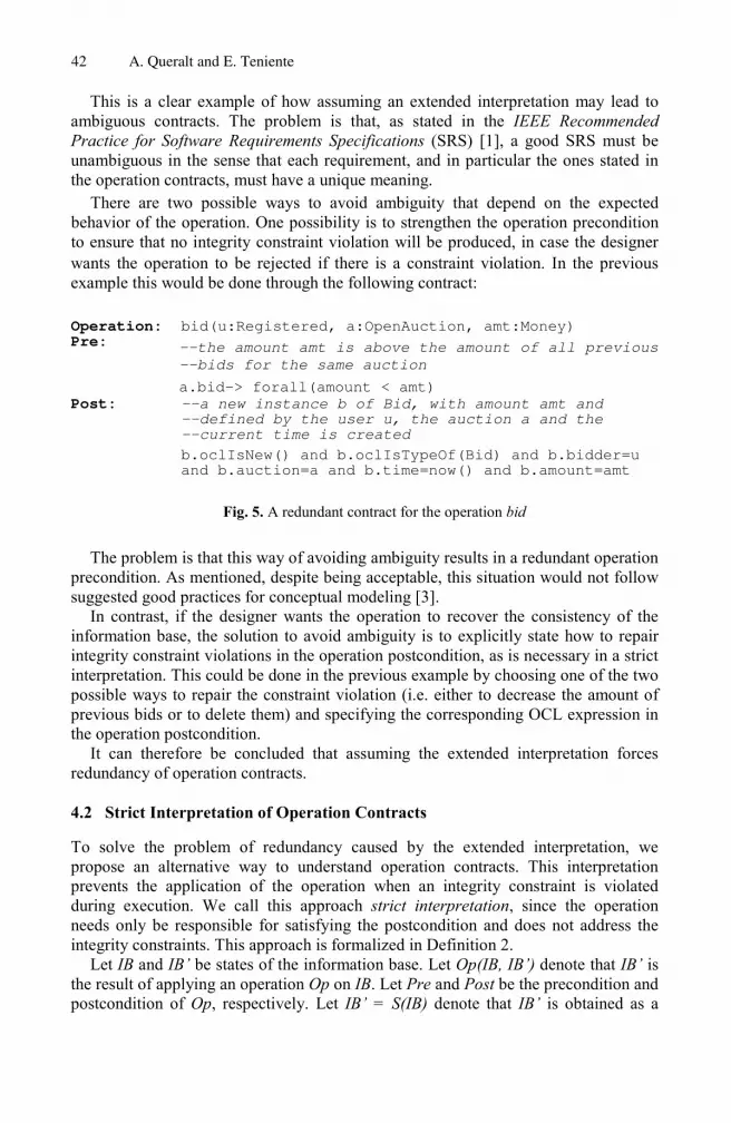
Operation: bid(u:Registered, a:OpenAuction, amt:Money) Pre: --the amount amt is above the amount of all previous
--bids for the same auction
a.bid-> forall(amount < amt)
Post: --a new instance b of Bid, with amount amt and --defined by the user u, the auction a and the --current time is created
b.oclIsNew() and b.oclIsTypeOf(Bid) and b.bidder=u and b.auction=a and b.time=now() and b.amount=amt
Fig. 5. A redundant contract for the operation bid
The problem is that this way of avoiding ambiguity results in a redundant operation precondition. As mentioned, despite being acceptable, this situation would not follow suggested good practices for conceptual modeling [3].
In contrast, if the designer wants the operation to recover the consistency of the information base, the solution to avoid ambiguity is to explicitly state how to repair integrity constraint violations in the operation postcondition, as is necessary in a strict interpretation. This could be done in the previous example by choosing one of the two possible ways to repair the constraint violation (i.e. either to decrease the amount of previous bids or to delete them) and specifying the corresponding OCL expression in the operation postcondition.
It can therefore be concluded that assuming the extended interpretation forces redundancy of operation contracts.
4.2 Strict Interpretation of Operation Contracts
To solve the problem of redundancy caused by the extended interpretation, we propose an alternative way to understand operation contracts. This interpretation prevents the application of the operation when an integrity constraint is violated during execution. We call this approach strict interpretation, since the operation needs only be responsible for satisfying the postcondition and does not address the integrity constraints. This approach is formalized in Definition 2.
Let IB and IB’ be states of the information base. Let Op(IB, IB’) denote that IB’ is the result of applying an operation Op on IB. Let Pre and Post be the precondition and postcondition of Op, respectively. Let IB’ = S(IB) denote that IB’ is obtained as a
42 A. Queralt and E. Teniente
This is a clear example of how assuming an extended interpretation may lead to ambiguous contracts. The problem is that, as stated in the IEEE Recommended Practice for Software Requirements Specifications (SRS) [1], a good SRS must be unambiguous in the sense that each requirement, and in particular the ones stated in the operation contracts, must have a unique meaning.
There are two possible ways to avoid ambiguity that depend on the expected behavior of the operation. One possibility is to strengthen the operation precondition to ensure that no integrity constraint violation will be produced, in case the designer wants the operation to be rejected if there is a constraint violation. In the previous example this would be done through the following contract:

Moreover, according to the second condition, IB’ is obtained exactly as a result of applying the minimal set S of structural events that satisfies Post to IB. Finally, the third condition requires IB’ to satisfy Post (always true according to b)) and to be consistent. If any of the conditions do not hold, Op is not applied to IB.
Notice that the resulting state will always be consistent, since integrity constraints were satisfied before the operation and they will always be satisfied at the end. If the execution of the operation does not violate any of the integrity constraints, then they are already guaranteed. On the other hand, if the execution violates any of them, the operation is rejected and the state remains unchanged.
An example is provided by the conditions under which the non-redundant contract of newUser¸ as specified in Figure 3, can be applied to IB and the new IB’ resulting from its execution according to the strict interpretation. Recall that S={insert(Registered(email,creditCard))} is the minimal set of structural events that satisfies the postcondition. We distinguish the same two situations as before depending on the contents of IB:
1. IB does not contain any user identified by email: − a) is guaranteed. − b) states that IB’ = S(IB). − IB’, as obtained according to b), satisfies c) since S necessarily satisfies the
postcondition and applying S to IB never violates any integrity constraint.
2. IB contains a user identified by email: − a) is guaranteed. − b) states that IB’ = S(IB), i.e. IB’ is obtained by inserting a registered user
with email and creditCard into IB − c) is not satisfied since IB’ will always violate the first integrity constraint.
Thus, newUser may not be applied in such an IB since it is impossible to satisfy all conditions required by a strict interpretation.
In summary, according to a strict interpretation the semantics of the operation newUser is such that if IB does not contain any user identified by email then the operation results in the application of the structural event insert(Registered(email,creditCard)). Otherwise, the operation may not be applied since it leads to the violation of an integrity constraint. Clearly, this is the intended
Specifying the Semantics of Operation Contracts 43
result of applying all the structural events in S to IB. Let S be the minimal set of structural events that satisfies Post when applied to IB. Let IC be the set of integrity constraints defined in the conceptual schema.
Definition 2: Strict Interpretation of an Operation Op
∀ IB, IB’ such that Op(IB, IB’), the following three conditions hold:
a) IB ⊨ Pre ∧ IC b) IB’ = S(IB)
c) IB’ ⊨ Post ∧ IC
As in Definition 1, the first condition states that there is a transition from an information base IB to an information base IB’ as a result of applying an operation Op only if IB satisfies Pre and it is consistent (i.e. it satisfies all integrity constraints ).

4.3 More on the Strict and Extended Interpretations
As we have just seen, the strict interpretation solves the problem of redundancy in contracts in those cases in which the intended behavior of an operation is to avoid execution if it is about to violate an integrity constraint. However, in some specific situations, the designer's intention is not to reject the operation but to apply it while still maintaining the consistency of the information base. In those cases, an extended interpretation may be better. The next example is useful to illustrate this situation.
If we want to define an operation unregisterUser aimed at unregistering users, we can specify the following operation contract:
Operation: unregisterUser(u:Registered) Pre: Post: --user u becomes an instance of Unregistered in the
--current time and ceases to be an instance of --Registered
u.oclIsTypeOf(Unregistered) and u.oclAsType(Unregistered).date = now() and not u.oclIsTypeOf(Registered)
Fig. 6. Contract for the operation unregisterUser
According to a strict interpretation, the minimal set of structural events that satisfies Post is S={specialize(u, Unregistered(now)), generalize(u, Registered)}. Then, according to Definition 2, IB' is obtained from IB by inserting u as an instance of Unregistered and removing it from Registered. Note that this operation always results in a state IB' that satisfies both the postcondition and the integrity constraints.
Clearly, the previous semantics is the one expected for the operation unregisterUser. However, the postcondition of the contract explicitly states that u must no longer be a registered user. Moreover, the class diagram already includes the condition that if u is Unregistered (as also enforced by the contract postcondition) it may not be Registered (because of the disjointness constraint). Thus, we could argue that the same behavior would be achieved by removing “not
u.oclIsTypeOf(Registered)” from Post, as shown in Figure 7.
44 A. Queralt and E. Teniente
behavior of this operation and it has been obtained without the need to specify a redundant precondition.
The desired effect of the non-redundant contract for the operation bid (see Figure 4) is also obtained when we assume a strict interpretation. The minimal set of structural events that satisfies Post is S={newLink (Bid(u,a,currentTime,amt))}. So, according to a strict interpretation, the semantics of bid is such that if amt is greater than the amount of all the previous bids of a, then the operation results in the application of the structural event newLink(Bid(u,a,currentTime,amt)). Otherwise, the operation cannot be applied since it would violate the constraint amountAbovePreviousBids. This interpretation corresponds to the expected semantics of an operation bid.

constraint is violated will be sufficient to detect that this change is also required without the need to state it explicitly.
Thus, according to Definition 1, the semantics of the contract in Figure 7 when an extended interpretation is assumed is as follows:
− a) is guaranteed. − b) states that IB’ = S2(IB) and S ⊆ S2, S={specialize(u, Unregistered(now))}. − Note that the application of S alone would violate the disjointness constraint of
the User specialization. Then, according to c), S2 must be a superset of S. − The minimal superset of S that satisfies both Post and IC is S2 = S ∪
{generalize(u, Registered)}.
Thus, the previous contract always requires the application of two structural events: {specialize(u, Unregistered(now)), generalize(u, Registered)}. However, only one of them is explicitly stated in the postcondition.
The previous example shows that there are some specific situations in which an extended interpretation is not ambiguous without the need to specify additional information in the operation contracts. In this example, a disjointness constraint is violated, and since the only possible way to repair it is by deleting u as a registered user, no ambiguity exists at all. In general, the extended interpretation of an operation contract will not be ambiguous when all integrity constraints that are violated by execution of the operation only allow for a single repair.
4.4 Summarizing Strict and Extended Interpretations
The main differences between strict and extended interpretations lie in the way integrity constraints are enforced. When there is no violation of integrity constraints, the semantics of a given operation contract is equivalent in both interpretations. In this case, the new state of the information base is always obtained by applying the minimal set S of structural events that satisfy the operation postcondition. However, if
Specifying the Semantics of Operation Contracts 45
The problem is that if we do that a strict interpretation of the contract would never allow the operation unregisterUser to be applied, since the information base resulting from inserting u as an unregistered user (the minimal set of structural events that would now satisfy the postcondition) would always violate the disjointness constraint. Hence, a strict interpretation requires “not u.oclIsTypeOf(Registered)” to be stated in the operation postcondition.
An extended interpretation does not involve the same drawback since we do not need to specify in the postcondition of unregisterUser that u is no longer registered. The reason is that the reactive behavior of an extended interpretation when a
Operation: unregisterUser(u:Registered) Pre: Post: --user u now becomes an instance of Unregistered
u.oclIsTypeOf(Unregistered) and u.oclAsType(Unregistered).date = now()
Fig. 7. Contract for the operation unregisterUser

does not violate the constraints. An example of this situation can be found in the contract for the operation bid specified in Figure 5.
We summarize in Table 1 how (in addition to the intended behavior of the operation) the treatment of integrity constraints should be specified in a contract, depending on both the interpretation chosen and whether we want the operation to be rejected or applied when the events in S violate an integrity constraint.
Table 1. Avoiding violation of integrity constraints
Reject the operation Apply the operation
Strict Nothing else needs to be done Specify how to satisfy the constraints in Post
Extended Add redundant checks to Pre Specify how to satisfy the constraints in Post (if the contract is ambiguous)
5 Discussion
We have compared strict and extended interpretations from the point of view of the relevant characteristics of a good software requirements specification (SRS) [1, 5]. As recommended there, we assumed an unambiguous operation contract specification. In general, this is always true in a strict interpretation, since deterministic behavior is usually desired. Regarding the extended interpretation, in this section we will concentrate on those situations in which non-ambiguity is achieved by strengthening either the operation pre- or postcondition, since this is the most frequent case in practice.
46 A. Queralt and E. Teniente
On the other hand, under an extended interpretation, the operation may be applied even though some constraint is violated by S, and the new state of the information base is obtained by applying a set of structural events S’, a superset of S, that guarantees that no constraint is violated. Note that S’ is unique as long as there is a single way to guarantee the constraints, as shown in Section 4.3 with a disjointness constraint violation. If S’ is not unique the operation contract is ambiguous. To avoid ambiguities, we must specify the way to preserve consistency in the postcondition (as must be made in a strict interpretation).
Alternatively, if we want to maintain consistency by rejecting the operation, its precondition must include redundant checks to ensure that execution of the operation
the violation of a constraint occurs when the structural events in S are applied, the semantics of the contract depends on the chosen interpretation.
On the one hand, under a strict interpretation the violation of a constraint means that the operation is not applied and, thus, the information base remains unchanged. Consequently, no redundant checks are needed in the precondition. A strict interpretation of the contract of bid in Figure 4 serves as an example of this situation. Alternatively, if we do not want the operation to be rejected, its postcondi tion must explicitly state how to satisfy the constraints after execution of the operation. This can be seen in the contract for unregisterUser in Figure 6.

5.2 Consistency
An SRS is consistent if, and only if, no conflict occurs between subsets of individual requirements described within it.
Although neither of the approaches leads directly to an inconsistent specification, a strict interpretation facilitates having a consistent one while an extended interpretation is more prone to the specification of conflicting requirements. The reason is that, since integrity constraints are sometimes specified both in the structural schema and as preconditions of operations in the behavioral schema, they can be in contradiction and, therefore, lead to an inconsistent specification.
For instance, it will be more difficult to keep the specification of bid consistent with the operation contract specified in Figure 5 than with the one specified in Figure 4. The reason is that we could easily have specified in the precondition of the first contract that the amount of a bid must be greater than or equal to the amount of the previous bids for the same auction. This would be clearly inconsistent with the integrity constraint amountAbovePreviousBids, which forces a bid to be higher than the previous ones.
5.3 Verifiability
An SRS is verifiable if, and only if, every requirement stated therein is verifiable. A requirement is verifiable if, and only if, there exists some finite cost-effective process with which a person or machine can check that the software product meets the requirement.
Unlike the previous criterion, verifiability is more easily achieved with an extended interpretation. Although both approaches allow the verification of the software
Specifying the Semantics of Operation Contracts 47
For instance, understanding the operation bid (see Figure 5) from the point of view of an extended interpretation, we always obtain a defined result when the precondition is satisfied, which is exactly the one specified in the postcondition (a new bid is created and linked to the user and auction specified as parameters and the current time) plus the additional changes, if any, required to satisfy all integrity constraints.
Understanding bid from the point of view of a strict interpretation (see Figure 4), we have two kinds of results when the precondition holds. In those cases in which no integrity constraint is violated, the resulting state of the information base is the one specified in the postcondition, as occurs with an extended interpretation. On the other hand, when an integrity constraint is violated, bid is rejected and the information base remains unchanged.
5.1 Completeness
An SRS is complete if it includes the definition of the responses of the software to all possible classes of input data in all possible classes of situations. From this point of view, both approaches can be considered complete. An extended interpretation avoids erroneous execution of an operation by means of its precondition, while a strict one assumes that the response to undesired situations is the rejection of the changes made by the operation. Moreover, when the precondition is not satisfied, both approaches act in the same way, by rejecting the operation.

condition in order to be consistent, and ensure that the same is done in every contract affected by the change. However, with a strict interpretation, we do not need to make any additional changes, since requirements stated by integrity constraints are only stated in the structural schema.
Much less frequently, we find a similar drawback when the postcondition already specifies how to maintain a certain integrity constraint. This drawback is shared by both approaches. On the one hand, a strict interpretation always needs to specify this reactive behavior in the postcondition, while on the other, an extended interpretation requires doing the same to guarantee that there is only one possible reaction to the violation of each integrity constraint.
5.5 Conciseness
Given two SRS for the same system, each exhibiting identical levels of all the qualities mentioned previously, the SRS that is shorter is also better.
Taking conciseness into account, it is clear that the strict interpretation approach helps to obtain shorter specifications, since each integrity constraint is specified in exactly one place. This can easily be seen by comparing the contracts in Figures 4 and 5. It is clear that both of them have the same meaning, while the one in Figure 4, in addition to being correct under a strict interpretation, is shorter.
5.6 Summary
The following table summarizes the discussion in this section. Rows correspond to desirable properties of a good software requirements specification, while columns refer to the interpretations we have defined in this paper. The symbol � in a cell
to modify the precondition of the operation bid (see Figure 5) stating again the same
48 A. Queralt and E. Teniente
5.4 Modifiability
An SRS is modifiable if, and only if, its structure and style are such that any changes to the requirements can be made easily, completely, and consistently. Modifiability generally requires that an SRS is not redundant.
In the case of modifiability, an extended interpretation is again more prone to errors due to the necessary duplication of integrity constraints in the preconditions. When changing a requirement, it is easy to forget to change it in every precondition in which it appears, and this can lead both to inconsistencies and to wasting more time.
Suppose that a requirement changes and we want to enforce that a bid may only be placed if it is 5 % higher than the highest previous bid for the same auction. In this case, the integrity constraint amountAbovePreviousBids must be changed in order to express this requirement. Moreover, with an extended interpretation we will also have
product, this process can become more complicated when a strict interpretation is assumed due to the dispersion of the requirements that affect an operation.
For example, to verify the correct behavior of the operation bid as defined in Figure 4, we must also take into account the integrity constraint amountAbovePreviousBids. However, taking the contract in Figure 5, no additional information is needed in order to verify it.

6 Case Studies
We have applied the ideas discussed in this paper to the specification of two real-life applications, far beyond the simple examples used so far. In particular, we have developed a conceptual schema for the EU-Rent Car Rentals system [7], a widely known case study promoted as a basis for demonstration of product capabilities, and we have also specified a generic conceptual schema for the e-marketplace domain [19]
EU-Rent is a company with branches in several countries that provides typical car rental services. The conceptual schema we have developed assumes a strict interpretation of operation contracts and consists of 59 entity types, 50 relationship types, 38 integrity constraints and 81 non-query operations. An analysis of the EU-Rent conceptual schema highlights the advantages of assuming a strict interpretation of operation contracts. The results of the analysis are summarized in this section.
Almost all of the integrity constraints in this case study (36 out of 38) require that the related operations must be rejected when they are violated. Assuming a strict interpretation, these constraints need not be taken into account when specifying operation preconditions, since this interpretation already provides the desired behavior. In contrast, with an extended interpretation, redundant addi tional preconditions should be included in 79 of the 81 operations of the conceptual schema to ensure that they are successfully executed.
Only two integrity constraints require that the related operations perform some kind of maintenance instead of rejecting the changes. Assuming a strict interpretation, only 2 of the 81 operations require doing the maintenance of those constraints explicitly in the postcondition, while an extended interpretation does not entail any change in the operation contracts.
The previous results show that 97.5% of the operations benefited from the strict interpretation, while only 2.5% did not. If we had assumed an extended interpretation,
Specifying the Semantics of Operation Contracts 49
Table 2. Comparison of the approaches
Extended interpretation Strict interpretation
Completeness � � Consistency � Verifiability � Modifiability � Conciseness �
denotes the appropriateness of the corresponding interpretation to achieve the property.
As we can see, completeness is achieved in both interpretations, while consistency, modifiability and conciseness are easier to achieve in a strict interpretation, and verifiability in an extended one. For this reason, we can conclude that in general terms a strict interpretation of operation contracts provides several advantages over an extended one in conceptual modeling.

Below, we show a small part of the EU-Rent conceptual schema (14 entity types and 18 constraints) to further illustrate the conclusions regarding the semantics of operation contracts that we have drawn from the development of this case study.
Fig. 8. EU-Rent class diagram
50 A. Queralt and E. Teniente
include several additional preconditions to verify the corresponding integrity constraints. In our case study, the number of additional preconditions lies between 1 and 10.
As a result of this analysis, we can conclude that assuming a strict interpretation leads in practice to a significant reduction of the time and complexity required to specify the conceptual schema of EU-Rent. The resulting schema is also much more concise, consistent and modifiable than if specified assuming an extended interpretation. The main reason is that a strict interpretation allows redundancy between integrity constraints and operation contracts to be avoided, thereby resulting in a simpler EU-Rent conceptual schema.
the result would have been exactly the opposite: only the 2.5% of the operations would have benefited from the choice.
Additionally, in a strict interpretation there is a direct one-to-one correspondence between the two operation contracts that require additional postconditions and the two integrity constraints that motivate them. In contrast, with an extended interpretation, each integrity constraint generally involves the modification of several operation contracts. In fact, 53% of the constraints require several operation contracts to be modified, while the maximum number of contracts that must be modified because of a single integrity constraint is 8. Moreover, each modified operation contract can

assuming a strict interpretation. The user indicates the identification of the renter (renterId), the desired beginning and end dates of the rental (beginning and ending),
Operation: MakeReservation(renterId: String, beginning: DateTime, end:
DateTime, pickUp: String, dropOff: String, countries:
Set(String), carGroup: String, carModel: String)
Pre: --1. there are cars available
let pickUpBranch: Branch = Branch.allInstances()-> select(b
| b.name = pickUp) in
pickUpBranch.car -> select(c| c.carGroup = carGroup) ->
reject(c | c.rentalAgreement.oclAsType(Reservation)->
exists(r | r.agreedEnd > beginning and r.agreedEnd < end and
not r.oclIsTypeOf(CanceledReservation))->
union(Car.allInstances()-> select(c | c.carGroup = carGroup
and c.rentalAgreement->exists(r | r.agreedEnd < beginning
and r.dropOffBranch = pickUpBranch) ->notEmpty()
Post: --a new reservation is created with the information provided
res.oclIsNew() and res.oclIsTypeOf(Reservation) and
res.renter.id = renterId and
res.beginning.date = beginning and
res.initEnd = end and
res.pickUpBranch.name = pickUp and
res.dropOffBranch.name = dropOff and
res.country.name = countries and
not carGroup.oclIsUndefined() implies
res.requestedGroup.name = carGroup and
not carModel.oclIsUndefined() implies
res.requestedModel.name = carModel and
res.reservationDate = currentTime()
Fig. 9. Contract for MakeReservation, specified assuming a strict interpretation
Specifying the Semantics of Operation Contracts 51
- The countries visited within a rental include the pick-up and drop-off countries - Drivers and renters must be older than 25 - Blacklisted individual cannot participate in a rental - A customer cannot have overlapping rentals - There are no cycles in the relationship better-worse between car groups - The cancellation date of a reservation is after the reservation date and before the
beginning of the rental - The rentals assigned to a car cannot overlap
Figure 9 shows the contract for the operation MakeReservation, which involves registering a reservation for a car of the specified group for a certain period of time,
The integrity constraints corresponding to the fragment in Figure 8 are the following:
- Persons are identified by id, countries by name, branches by name, cars by registration number, car models by name, car groups by name and dates by date.
- The interval of a rental agreement is correct - The pick-up time of a rental is after the indicated beginning
- The return time of a rental is later than its pick-up time - The reservation date of a rental is prior to its beginning
the pick-up and drop-off branches (pickUp and dropOff), the countries that will be

Had we assumed an extended interpretation, the same operation should have beenspecified as shown in Figure 10. Although they specify exactly the same behavior,this contract is much longer than the one in Figure 9 (11 preconditions compared with1). The reason is that 10 additional preconditions are required to enforce integrityconstraint violations of the conceptual schema such as checking that the personmaking the reservation already exists and that he or she is not blacklisted.
To specify the contract in Figure 10 we had to detect which constraints of the whole set (both textual and graphical) are related to this operation, and then include them as preconditions. In addition, the implicit constraints (for example, the creation of a relationship requires the existence of the two participants) had to be taken into account. This redundancy, besides complicating the specification task itself, clearly interferes with conciseness, consistency and modifiability of the whole conceptual schema.
Operation: MakeReservation(renterId: String, beginning: DateTime,
end: DateTime, pickUp: String, dropOff: String,
countries: Set(String), carGroup: String, carModel: String)
Pre: --1. renter exists
EU_RentPerson.allInstances()->exists(p | p.id = renterId)
and
--2. renter not blacklisted
not Blacklisted.allInstances()->exists(p | p.id = renterId)
and
--3. renter does not have overlapping rentals
let renter:Person = Person.allInstances()-> select(p|p.id =
renterId)
in renter.rentalAgreement-> reject(rA |
rA.oclIsTypeOf(CanceledReservation))->select(rA |
renter.rentalAgreement->select(rAOther |
rAOther.beginning.date >= rA.beginning.date and
rAOther.beginning.date <= rA.agreedEnd))
52 A. Queralt and E. Teniente
Taking into account that the conceptual schema includes 38 textual integrity constraints that potentially affect the operation, in addition to those constraints that can be expressed graphically in the class diagram, the result is that the contract becomes much easier and faster to specify when a strict interpretation is assumed, since none of the constraints need to be considered when the operation is specified. The only precondition of this contract corresponds to a dynamic condition that cannot be specified in the form of an integrity constraint. Notice then that as a consequence of the interpretation chosen we can forget about all static conditions when specifying operations, since we can assume that they are guaranteed somewhere else in the conceptual schema, and only worry about the dynamic behavior that is specific to the operation.
Note that in the previous contract it is not necessary to specify explicitly in the precondition the conditions that are already guaranteed by integrity constraints because of the strict interpretation assumed.
With this information, the system registers a new reservation if there are cars available for the requested period.
visited (countries) and the desired car group (carGroup) or car model (carModel).
Fig. 10. Contract for MakeReservation, specified assuming an extended interpretation
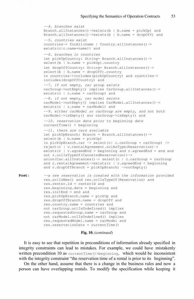
--11. there are cars available
let pickUpBranch: Branch = Branch.allInstances()->
select(b | b.name = pickUp)
in pickUpBranch.car -> select(c| c.carGroup = carGroup) ->
reject(c | c.rentalAgreement.oclAsType(Reservation)->
exists(r | r.agreedEnd > beginning and r.agreedEnd < end and
not r.oclIsTypeOf(CanceledReservation))->
union(Car.allInstances()-> select(c | c.carGroup = carGroup
and c.rentalAgreement->exists(r | r.agreedEnd < beginning
and r.dropOffBranch = pickUpBranch) ->notEmpty()
Post: --a new reservation is created with the information provided
res.oclIsNew() and res.oclIsTypeOf(Reservation) and
res.renter.id = renterId and
res.beginning.date = beginning and
res.initEnd = end and
res.pickUpBranch.name = pickUp and
res.dropOffBranch.name = dropOff and
res.country.name = countries and
not carGroup.oclIsUndefined() implies
res.requestedGroup.name = carGroup and
not carModel.oclIsUndefined() implies
res.requestedModel.name = carModel and
res.reservationDate = currentTime()
It is easy to see that repetition in preconditions of information already specified in integrity constraints can lead to mistakes. For example, we could have mistakenly written precondition 10 as currentTime()>beginning, which would be inconsistent with the integrity constraint “the reservation time of a rental is prior to its beginning”.
On the other hand, assume that there is a change in the business rules and now a person can have overlapping rentals. To modify the specification while keeping it
Specifying the Semantics of Operation Contracts 53
--6. branches in countries
let pickUpCountry: String= Branch.allInstances()->
select(b | b.name = pickUp).country
let dropOffCountry: String= Branch.allInstances()->
select(b | b.name = dropOff).country
in countries->includes(pickUpCountry) and countries->
includes(dropOffCountry) and
--7. if not empty, car group exists
carGroup->notEmpty() implies CarGroup.allInstances()->
exists(c | c.name = carGroup) and
--8. if not empty, car model exists
carModel->notEmpty() implies CarModel.allInstances()->
exists(c | c.name = carModel) and
--9. either carModel or carGroup are empty, and not both
carModel->isEmpty() xor carGroup->isEmpty() and
--10. reservation date prior to beginning date
currentTime() < beginning
--4. branches exist
Branch.allInstances()->exists(b | b.name = pickUp) and
Branch.allInstances()->exists(b | b.name = dropOff) and
--5. countries exist
countries-> forAll(name | Country.allInstances()->
exists(c|c.name=name)) and
Fig. 10. (continued)
7 Conclusions and Further Work
In this paper we have dealt with the semantics of operation contracts in conceptual modeling. We have described two different interpretations of operation contracts, a strict and an extended one, which differ in the way that the relationship between operation postconditions and integrity constraints is understood. Roughly speaking, a strict interpretation prevents an operation from being applied if an integrity constraint is violated. In contrast, an extended interpretation assumes its semantics must take care of maintaining integrity constraints when they are violated as a consequence of applying the events that satisfy the postcondition.
We have provided formal definitions for the strict and the extended interpretations and compared them in a number of issues from the perspective of the characteristics of a good software specification. We conclude that a strict interpretation performs better than an extended one in terms of consistency, modifiability and conciseness of the conceptual schema, while an extended interpretation is better in terms of verifiability, and they both offer similar contributions in relation to completeness. Moreover, our case studies indicate that a strict interpretation considerably simplifies the task of developing a specification. Thus, we have shown that a strict interpretation of operation contracts provides several advantages over an extended one.
This study was independent of any specific conceptual modeling language and our results can therefore be applied to any of such language, provided that it allows the definition of integrity constraints in the structural schema and operations in the behavioral one.
54 A. Queralt and E. Teniente
We have also applied our ideas to the specification of a generic conceptual schema for the e-marketplace domain [19]. This conceptual schema is specified in UML, incombination with OCL, to formalize the structural and behavioral properties of thisinformation system.
Our generic e-marketplace conceptual schema has been drawn from an external study of some well-known e-marketplaces and auction sites like eBay, OnSale and Amazon, as well as the job search site Monster, and it covers the main functions of an e-marketplace: determining product offerings, searching for products and price discovery. The whole specification includes 54 entity types, 26 relationship types, 94 constraints and 51 operations that can modify the state of the information base.
We used a strict interpretation of operation contracts in the specification of this conceptual schema. The results of this case study are very similar to the ones for EU-Rent, but even more revealing, since this time all the operations benefited from the choice of a strict interpretation.
consistent, not only will we have to modify the constraint “a customer cannot have overlapping rentals”, but also review each of the 81 operations in order to update their preconditions in case this requirement appears in them. This, as well as making the modification tedious, can lead to inconsistencies if it is overlooked in a given contract.

[5] Davis, A. M.: Software Requirements: Objects, Functions and States. Prentice Hall, Englewood Cliffs (1993)
[6] Devos, F., Steegmans, E.: Specifying Business Rules in Object-Oriented Analysis. Software and Systems Modeling 4 (2005) 297-309
[7] Frias, L., Queralt, A., Olivé, A.: EU-Rent Car Rentals Specification. Departament de LSI, UPC, Technical Report LSI-03-59-R (2003)
[8] Hoare, C. A. R.: Proof of Correctness of Data Representations. Acta Informatica 1 (1972) 271-281
[9] ISO/TC97/SC5/WG3: Concepts and Terminology for the Conceptual Schema and the Information Base. In: J. J. van Griethuysen, (ed.) (1982)
[10] Larman, C.: Applying UML and Patterns: An Introduction to Object-Oriented Analysis and Design and Iterative Development. 3rd edn. Prentice Hall PTR, Upper Saddle River,NJ (2004)
[11] Martin, J., Odell, J. J.: Object-Oriented Methods. A Foundation. P T R Prentice Hall, Englewood Cliffs, New Jersey (1999)
[12] Meyer, B.: Applying 'Design by Contract'. Computer 25 (1992) 40-51 [13]
Meyer, B.: Object-Oriented Software Construction. 2nd edn. Prentice Hall, New York (1997)
[14] Mylopoulos, J., Bernstein, P. A., Wong, H. K. T.: A Language Facility for Designing Database-Intensive Applications. ACM Transactions on Database Systems 5 (1980) 185-207
[15] Olivé, A.: Definition of Events and their Effects in Object-Oriented Conceptual Modeling Languages. In: Conceptual Modeling - ER 2004. LNCS 3288 (2004)
[16] OMG: UML 2.0 OCL Specification. (2003) [17] Pressman, R. S.: Software Engineering: A Practitioner's Approach. 6th edn . McGraw-
Hill (2004) [18] Queralt, A., Teniente, E.: On the Semantics of Operation Contracts in Conceptual
Modeling. In: Proc. CAiSE Forum - 17th Conference on Advanced Information Systems Engineering (CAiSE'05) (2005)
Specifying the Semantics of Operation Contracts 55
-
-
-
References
[1] IEEE Recommended Practice for Software Requirements Specifications (IEEE Std 830
-1998). (1998)
[2] Borgida, A., Mylopoulos, J., Reiter, R.: On the frame problem in procedure specifications. IEEE Transactions on Software Engineering 21 (1995) 785-798
[3] Costal, D., Sancho, M. R., Teniente, E.: Understanding Redundancy in UML Models for Object-Oriented Analysis. In: Advanced Information Systems Engineering: 14th International Conference, CAiSE 2002 Proceedings. LNCS 2348 (2002) 659-674
[4] D'Souza, D. F., Wills, A. C.: Objects, Components and Frameworks with UML: TheCatalysis Approach. Addison-Wesley (1998)
-
Acknowledgements. We would like to thank Jordi Cabot, Jordi Conesa, Dolors Costal, Cristina Gómez, Antoni Olivé, Xavier de Palol, Ruth Raventós, Maria Ribera Sancho and Òscar Hernández for helpful discussions and comments on previous drafts of the manuscript. This work was partially supported by funds from the Ministerio de Educación y Ciencia under project TIN 2005-06253.
Further work may be devoted to addressing whether state diagrams have an impact on the interpretations we have proposed, since there is a close relationship between the events that cause state transitions, operation postconditions and constraints.

[19] Queralt, A., Teniente, E . : A Platform Independent Model for the Electronic Marketplace Domain. Departament de LSI, UPC, Technical Report LSI-05-9-R (2005)
[20] Rumbaugh, J., Jacobson, I., Booch, G.: The Unified Modeling Language Reference Manual. Addison Wesley Professional (2004)
[21] Warmer, J., Kleppe, A.: The Object Constraint Language: Getting Your Models Ready for MDA. 2nd edn. Addison-Wesley Professional (2003)
[22] Wieringa, R. : A Survey of Structured and Object -Oriented Software Specification Methods and Techniques. ACM Comput. Surv. 30 (1998) 459-527
5 A. Queralt and E. Teniente 6

S. Spaccapietra (Ed.): Journal on Data Semantics VII, LNCS 4244, pp. 57 – 78, 2006. © Springer-Verlag Berlin Heidelberg 2006
Model-Driven Ontology Engineering
1Yue Pan, 1Guotong Xie, 1Li Ma, 1Yang Yang, 1ZhaoMing Qiu, and 2Juhnyoung Lee
1 IBM China Research Lab Beijing, China
{panyue, xieguot, malli, yangyy, qiuzhaom}@cn.ibm.com 2 IBM Watson Research Center
Hawthorne, New York [email protected]
Abstract. W3C’s Semantic Web provides a common framework that allows data to be shared and reused across application and enterprise. As the Semantic Web shapes the future of the Web, it becomes more and more important in software engineering and enterprise application development. While existing ontology engineering tools provide a stack of ontology management support and are used successfully in certain domains, there still remains a gap between the ontology engineering tools and the traditional software engineering. For several decades, software engineering has been established on different model-ing languages and methodologies such as Unified Modeling Language (UML). The differences in modeling languages and methodologies cause difficulties in enterprise application development involving the Semantic Web technologies. The existing ontology engineering tools provide only an ad hoc approach to bridging this gap with limited functionality and performance. The primary objective of our work is to bridge this gap between two different, but comple-mentary engineering disciplines with a systematic approach. Our approach lev-erages Model-Driven Architecture (MDA) and Ontology Definition Metamodel (ODM), which enable model transformation. This approach allows seamlessly supporting existing models in UML and other languages in Semantic Web-based software development. In addition, it allows exploiting the availability and features of UML tools for creation of vocabularies and ontologies. Furthermore, MDA enables code generation and facilitates software tool devel-opment. This paper presents an MDA-based system for ontology engineering. In addition, it presents the entire stack of individual components of the devel-oped ontology engineering tool.
Keywords: Semantic Web, ontology engineering, model-driven architecture.
1 Introduction
W3C’s Semantic Web [1] provides a common framework that allows data to be shared and reused across application and enterprise. It is based on the Resource De-scription Framework (RDF), which describes various resources using XML for syntax and URIs for naming [10], and Web Ontology Language (OWL), which provides

58 Y. Pan et al.
modeling constructs for specifying and inferring about knowledge [16]. As the Se-mantic Web shapes the future of the Web, it becomes more and more important in software engineering and enterprise application development. To meet the needs, a number of tools and systems for ontology development and management such as Pro-tégé [28], Jena [4], Sesame [29], Pellet [26], KAON [15], RStar [14], and SnoBase [12], have been developed.
While these ontology engineering tools provide a relatively complete stack of ontol-ogy management support and are used successfully in certain domains, there still remains a gap between the ontology engineering tools and the traditional software engineering. For more than a decade, software engineering has been established on different modeling languages and methodologies such as OMG’s Unified Modeling Language (UML). This difference in modeling languages and methodologies causes difficulties in large-scale en-terprise application development involving the Semantic Web technologies. The existing ontology engineering tools provide only an ad hoc approach to bridging this gap with limited functionality and performance. The creation of ontologies and their use in soft-ware engineering projects is currently cumbersome and not seamless. The transformation of UML models to OWL ontologies and vice versa is conducted only in an ad hoc and incomplete way. Therefore, it is difficult to utilize the vast investment of enterprises in software engineering models, which are often accumulated over a decade, in ontology engineering. For the Semantic Web to have impact on enterprises and their business, and also to be widely accepted as a value-adding technology, bridging this gap in software and ontology engineering is critical.
The primary objective of our work is to bridge this gap between two different, but complementary engineering disciplines with a systematic approach. We leverage OMG’s Model-Driven Architecture (MDA) [3] and Ontology Definition Metamodel (ODM) [25] to provide model transformation. This approach allows seamlessly sup-porting existing models in UML and other languages in Semantic Web-based soft-ware development. In addition, it allows exploiting the availability and features of UML tools for creation of vocabularies and ontologies. Furthermore, MDA enables code generation and facilitates tool development. This paper presents a model-driven approach to ontology engineering. It describes the architecture of the ontology engi-neering system, and mappings between UML and OWL for model transformation. In addition, it presents the entire stack of individual components of the developed ontol-ogy engineering tool.
The rest of this paper is structured as follows: In Section 2, we describe a number of existing software tools for ontology development and management. It discusses a gap between these ontology engineering tools and the traditional software engineering tools. Sections 3 and 4 summarize technical background information on the Model-Driven Architecture and Ontology Definition Metamodel, respectively. In Section 5, we explain how EMF-based technologies for MDA and ODM are used to realize the proposed system for ontology engineering. Section 6 presents an implementation of the proposed system with the entire stack of components. Section 7 presents use sce-narios illustrating how the features of the developed ontology engineering tool can be utilized in real-world applications. In Section 8, conclusions are drawn and future work is outlined.

Model-Driven Ontology Engineering 59
2 Traditional Ontology Management Systems
In recent years, there has been a surge of interest in using ontological information for communicating knowledge among software systems. As a result, an increasing range of software systems engage in a variety of ontology management tasks, including the creation, storage, search, query, reuse, maintenance, and integration of ontologies. Recently, there have been efforts to externalize such ontology management burden from individual software systems and put them together in middleware known as an ontology management system. An ontology management system provides a mecha-nism to deal with ontological information at an appropriate level of abstraction. By using programming interfaces and query languages the ontology management system provides, application programs can manipulate and query ontologies without the need to know their details or to re-implement the semantics of standard ontology lan-guages. Examples of such ontology management systems include Protégé [28], Jena [4], Sesame [29], Pellet [26], KAON [15], Jastor [23], D2RQ [19], RStar [14], and SnoBase [12].
Table 1 summarizes a few ontology management systems. It is important to note that these systems mainly focus on the manipulation of ontologies. The interoperability with other modeling languages and development tools comes as a secondary feature for these systems. That is, they assume separate workspaces for ontology management and software development, and fail to provide a tightly integrated environment for software and ontology engineering.
Table 1. Traditional Ontology Management Systems
Name Functionalities Standards InteroperabilityJena A program development frame-
work for ontology manipulation and query
RDF, RDFS, OWL, SPARQL
N/A
Sesame An RDF database allowing ontol-ogy manipulation and query
RDF, RDFS, OWL N/A
Protégé A graphical ontology editor and knowledge base framework for on-tology manipulation and query
RDF, RDFS, OWL
Through plugins (with limited capability); UML OWL ontol-ogy
KOAN A suite of ontology management tools including ontology creation, ontology manipulation, and infer-ence and query
RDF, RDFS, OWL RDB schema RDFS
ontology
Jastor A java code generator for creating Java beans from OWL ontologies
RDF, RDFS, OWL
OWL ontology Java Beans
D2RQ A language and a tool for specify-ing mappings between relational database schema and OWL on-tologies
RDF, RDFS, OWL RDB schema OWL
ontology

60 Y. Pan et al.
While these ontology engineering tools provide a stack of ontology management support, they also show certain limitations in supporting large-scale software engi-neering projects. Participating in a number of enterprise application development pro-jects by using the SnoBase and RStar Ontology Management System, we learned firsthand that it is critical to provide a comprehensive development environment in-cluding supporting tools and facilities for the application developers. A pick-and-choose approach to the best of the breed tools from different environments does not always work well for the majority of the developers and often results in a longer learning curve for the developers. A comprehensive ontology development environ-ment often means a tight integration of tools for software and ontology engineering, and model import and transformation, among others.
Semantic markup languages such as W3C’s RDF and OWL are based on the work in the logic and Artificial Intelligence communities, such as Description Logic and Knowledge Representation. The syntax of these languages is less intuitive to those trained for object-oriented programming and simple XML-based languages. The lack of a tightly integrated development environment for software and ontology engineer-ing makes the job of subject matter experts and software engineers difficult, and often affects negatively to the adoption of the semantic technology in industry. An effective ontology application development environment should bridge this gap between soft-ware engineering and ontology engineering by providing a seamlessly integrated environment.
Another consideration for industry adoption of the semantic Web technology is the interoperability of the semantic markup languages with the well-established and widely-accepted industry standard modeling languages and methodologies such as Entity-Relation (ER) diagrams and Unified Modeling Language (UML). Enterprises developed software models in these languages for more than a decade and invested significantly in building systems around them. Despite all the theoretical advantages the semantic technology brings in, in practice, it is highly unlikely that the enterprises abandon the legacy systems and develop new systems around the semantic Web tech-nology. Instead, users in industry would be interested in the interoperability of the modeling languages, and the reuse of the existing models and data with the semantic Web technology. The traditional ontology management systems currently provide only ad hoc and incomplete methods for the model interoperability. To address the practical requirements of industry, this paper introduces a novel approach to ontology engineering based on the Model Driven Architecture (MDA), which enables software engineers and users to design, build, integrate and manage ontologies and software applications in an integrated development environment.
3 Model-Driven Architecture
Before presenting the model-driven approach to ontology engineering, we summarize the Object Management Group’s Model Driven Architecture, which is one of the two pillars of the system’s architecture, along with Ontology Definition Metamodel.
In the history of software engineering, there has been a notable increase of the use of models and the level of abstraction in the models. Modeling has become separated from underlying development and deployment platforms, making them more reusable

Model-Driven Ontology Engineering 61
and easier to create and modify by domain experts, and requiring less knowledge of specific deployment systems. This trend places software modeling closer to knowl-edge engineering. The current stage in this evolution is the Model Driven Architec-ture, which grew out of the standards work conducted in the 1990s for the Unified Modeling Language.
The basic idea of MDA is that the system functionality is defined as a platform-independent model, using an appropriate specification language and then translated to one or more platform-specific models for the actual implementation. To accomplish this goal, the MDA defines an architecture that provides a set of guidelines for structur-ing specifications expressed as models. The translation between platform-independent model and platform-specific models is normally performed using automated tools. Specifically, MDA defines three levels of abstraction: Computation Independent Model (CIM), Platform Independent Model (PIM) and Platform Specific Model (PSM). CIM is a view of a system that does not show the details of a system structure. In soft-ware engineering, it is also known as a domain model, which is concerned by domain experts. It is similar to the concept of ontology. PIM is a model that is computation de-pendent, but it is not aware of specific computer platform details. In other words, it is targeted for a technology-neutral virtual machine. Specification of complete system is completed with PSM. The goal is to move human work from PSM to CIM and PIM, and let the detail implementation for a specific platform be generated as much as pos-sible by automated tools which perform the transformation from PIM to PSM.
MDA comprises of a four-layer metamodel architecture: meta-metamodel (M3) layer, metamodel (M2) layer, model (M1) layer, and instance (M0) layer. Also, it util-izes several complementary standards from OMG including Meta-Object Facility (MOF), Unified Modeling Language (UML) and XML Metadata Interchange (XMI). On the top of the MDA architecture is the meta-metamodel, i.e., MOF. It defines an abstract language and framework for specifying, constructing and managing technol-ogy neutral metamodels. It is the foundation for defining any modeling language such as UML or even MOF itself. MOF also defines a framework for implementing reposi-tories that hold metadata (e.g., models) described by metamodels [24]. The main ob-jective of having the four layers with a common meta-metamodel is to support multi-ple metamodels and models and to enable their extensibility, integration and generic model and metamodel management.
All metamodels, standard or custom, defined by MOF are positioned on the M2 layer. One of these is UML, a graphical modeling language for specifying, visualizing and documenting software systems. With UML profiles, basic UML concepts (e.g., class, association, etc.) can be extended with new concepts (stereotypes) and adapted to specific modeling needs. The models of the real world, represented by concepts de-fined in the corresponding metamodel at M2 layer (e.g., UML metamodel) are on M1 layer. Finally, at M0 layer, are things from the real world. Another related standard is XMI. It defines mapping from MOF-defined metamodels to XML documents and schemas. Because of versatile software tool availability for XML, XMI representa-tions of models, metamodels and meta-metamodel facilitate their sharing in software application development.

62 Y. Pan et al.
MOF tools use metamodels to generate code for managing models and metadata. The generated code includes access mechanisms, or application programming interfaces, to read and manipulate, serialize and transform, and abstract the details of various interfaces based on access patterns. Eclipse Modeling Framework (EMF) [21] provides a Java im-plementation of a core subset of the MOF API. EMF started out as an implementation of the MOF specification, and evolved into a generic modeling framework and code genera-tion facility for building tools and other applications based on a structured data model. The MOF-like core metamodel in EMF is called Ecore. From a model specification writ-ten in XMI, EMF generates tools and runtime support to produce a set of Java classes for the model, a set of adapter classes that enable viewing and command-based editing of the model, and a basic editor. Models can be specified using annotated Java, XML docu-ments, or modeling tools like Rational Rose, then imported into EMF. It is important to note that EMF provides the foundation for interoperability with other EMF-based tools and applications. The proposed MDA-based system leverages EMF for implementing ontology management tools which run on the Eclipse environment, and utilizes its support for model interoperability.
4 Ontology Definition Metamodel
MDA and its four-layer architecture provide a solid basis for defining metamodels of any modeling language, and so provide a foundation for bringing together software engineering and methodologies such as UML with the semantic technology based on W3C’s RDF and OWL. Once a semantic markup language such as OWL is defined in MOF, its users can utilize MOF’s capabilities for modeling creation, model manage-ment, code generation, and interoperability with other MOF-defined metamodels.
Another OMG standard, Ontology Definition Metamodel (ODM) [25] took this approach. To comprehend common ontology concepts, ODM used as a starting point OWL, which is the result of the evolution of existing ontology representation lan-guages. ODM defined individual constructs of OWL in MOF, creating an ODM metamodel. To leverage graphical modeling capabilities of UML in dealing with OWL constructs, ODM also defined an ontology UML profile to support UML nota-tion for ontology definition. This profile enables graphical editing of ontologies in OWL using UML diagrams as well as other benefits of using mature UML CASE tools. Finally, the following bi-directional mappings between metamodels complete the picture:
1. mappings between OWL and ODM, 2. mappings between ODM and the ontology UML profile, and 3. mappings from the ontology UML profile to other UML profiles.
Figure 1 shows a simple example of the bi-directional mappings between metamod-els. In practice, both UML and ODM models are serialized in XMI, and OWL model in XML, the two-way mappings can be implemented by XSLT-based transformations [5]. Gasevic et al. summarized existing approaches and tools for transformation

Model-Driven Ontology Engineering 63
Fig. 1. Bi-directional mapping among metamodels
based transformations, instead of XSLT, to leverage EMF’s generic modeling frame between UML models (or UML profiles) and OWL models in [5, 7], and pointed out that the XSLT-based transformation is widely used in them. Our work utilized EMF-work and code generation facility for building tools and other applications. We implemented EODM (EMF-based ODM), which is the underlying object model generated from ODM by using EMF, for model transformations among OWL, UML and other modeling languages. More details will be given in the next section.
Before moving to the main body of this paper, it is useful to briefly mention yet another related effort from W3C, namely, Ontology Driven Architecture (ODA) [17]. It combines MDA with the semantic technology differently from the ODM approach. It attempts to augment the MDA standards and methodology stack with the semantic technology to improve the discipline. It aims to enable unambiguous representation of domain terminology, distinct from the rules, enable automated consistency checking and validation of invariant rules, preconditions, and post-conditions, and support knowledge-based terminology mediation and transformation for increased scalability and composition of components. This effort still is in its infancy and at a draft stage.
5 EMF-Based Ontology Engineering System
For realizing the model-driven ontology engineering, we utilized the Eclipse Model-ing Framework, which is open source MDA infrastructure for integration of modeling tools [21]. A model specification described in various modeling languages including UML, XML Schema, and annotated Java source can be imported into EMF. Then EMF produces a set of Java classes for the model, a set of adapter classes that enable viewing and editing of the model, and a basic editor. In its current implementation, EMF does not provide formal semantics definitions, inference and the related model specifications. Our work adds this capability to EMF for providing a comprehensive ontology engineering environment and dynamic application integration.
For adding the semantic model transformation capability to EMF, we leverage the specification of Ontology Definition Metamodel. By using EMF and ODM, we gen-erated a foundational memory model, i.e., Java classes, for the constructs of OWL. This foundational memory model is referred to as EODM (EMF-based Ontology Definition Metamodel). By adding several necessary helper classes and methods to EODM, we can use it to create, edit, and navigate any models in OWL.

64 Y. Pan et al.
Also, we added an OWL parser to EODM, which can load OWL files into EMF and generate OWL files from EMF, i.e., serialize EMF models to standard OWL files in XML. The parser utilizes an XMI adaptor which enables the transformation between the OWL models and EODM Ecore models. The transformation is made possible by the bi-directional mapping between OWL and the Ecore metamodel. The transformation opens a way to interoperability between OWL models and other EMF supported models, which currently include ones defined in UML, XML Schema, and annotated Java classes. The support of other models such as Entity Relationship mod-els in EMF will be provided in the near future. By leveraging the OWL parser and the bi-directional transformation between the OWL models and the Ecore models, ontol-ogy application developers can develop ontologies using their favorite model building tools, import them into EMF, transform their models into OWL ontologies, enrich them with semantics, leverage their inference capability, and utilize the comprehen-sive development facility of Eclipse and EMF.
To be more specific, the EODM Ecore model is the MOF core model that repre-sents ontologies in memory. It is an intermediate model for imported and transformed legacy models, as well as the generated ontology, Java code, Java editor and Java edit. The development environment allows its users to manipulate EODM Ecore models, enrich it with semantic specification, and generate Java code. A default set of bi-directional mappings between metamodels of legacy models and OWL are developed in EMF. Eclipse plug-in developers can extend the mappings to handle other types of legacy models, or other elements in legacy models specifying semantics. The gener-ated Java editor and Java edit provide ready-to-use visual tools to populate or manipu-lated instances of OWL models. The visual tools are actually copies of the standard methods of supporting application development in EMF. Figure 2 illustrates the op-eration of the EMF-based ontology engineering system.
XML Schema
ER Model
IMPORT
EODMEcoreModel
Model transformationand semantics enrichment
Java code
G E N E R A TE
RDF/OWL Ontology
UMLModel
Java Edit
Java Editor
Fig. 2. EMF-based ontology engineering system
6 Components of the EMF-Based Ontology Engineering System
This section presents the entire stack of components of the developed, EMF-based on-tology engineering system. We had two primary design objectives for this system: first, support for the entire lifecycle of ontology engineering, and, second, avoiding

Model-Driven Ontology Engineering 65
reinvention of tools and facilities that are already proven to work in software engi-neering. To achieve these objectives, we designed a software stack which consists of six interdependent layers.
At the core of this EMF-based ontology engineering system is the EODM model, which is derived from the Ontology Definition Metamodel and implemented in Eclipse Modeling Framework. The bottom layer, EODM core model, provides the basic Java programming model for OWL ontologies with all the necessary getter and setter functions. It is automatically generated by EMF from the UML models for OWL. To this generated core model implementation, certain utility classes and methods are added, to benefit Java programmers. On top of the EODM core model comes the OWL Parser which parses OWL ontologies, translates them into EODM models, and serializes EODM models to standard RDF/XML files. EODM core and OWL Parser form the foundation for the entire software stack. The top layer is composed of three relatively independent components that are build on top of this foundation. The first component is the OWL Inference Engine. It takes an EODM model as input, and executes user queries, reasoning about instances and relationships among instances and classes. The second component is the Model Transformation. It imports existing conceptual models represented in various modeling languages such as UML, ER diagrams, and Java interfaces. Then, it transforms the models into one or more EODM models. Finally, the OWL Editor provides a graphical ontology author-ing environment where OWL ontologies in graphic notations are serialized to OWL files in a standard XML format. Figure 3 shows the components of the EMF-based ontology engineering system. In the rest of this section, we describe each component in detail.
Fig. 3. EMF-based ontology engineering system architecture
6.1 EODM Core Model
The EMF-based ontology engineering system provides tightly integrated environment for software and ontology engineering, providing a stack of useful components. EODM provides the run-time library that allows applications to input and output OWL ontologies, manipulate them by using Java objects, invoke the inference engine and access result sets, and transform among ontologies and other legacy models.
The EODM core model provides useful classes and methods to access OWL on-tologies and their instances. Its metamodel is defined in the Ontology Definition Metamodel (ODM) specification [25]. It is an MOF2 compliant metamodel that
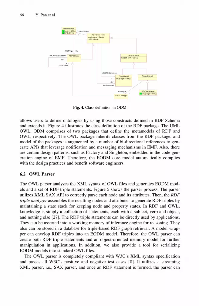
66 Y. Pan et al.
RDFXMLLiteral
language : String
RDFSLiteral
lexicalForm : StringRDFSClass
0..*
0..*
+RDFSSubClassOf
0..*
+subClass0..*
PlainLiteral
language : String
Namespace
name : Strin...URI : String
RDFSResource
localName : String/ URI : String
0..*+RDFType 0..*
0..*
+RDFSComment
0..*
0..*
+RDFSLabel
0..*
1
+namespace
1
RDFSDatatype
TypedLiteral
1+datatype
1
Fig. 4. Class definition in ODM
allows users to define ontologies by using those constructs defined in RDF Schema and extends it. Figure 4 illustrates the class definition of the RDF package. The UML OWL. ODM comprises of two packages that define the metamodels of RDF and OWL, respectively. The OWL package inherits classes from the RDF package, and model of the packages is augmented by a number of bi-directional references to gen-erate APIs that leverage notification and messaging mechanisms in EMF. Also, there are certain design patterns, such as Factory and Singleton, embedded in the code gen-eration engine of EMF. Therefore, the EODM core model automatically complies with the design practices and benefit software engineers.
6.2 OWL Parser
The OWL parser analyzes the XML syntax of OWL files and generates EODM mod-els and a set of RDF triple statements. Figure 5 shows the parser process. The parser utilizes XML SAX API to correctly parse each node and its attributes. Then, the RDF triple analyzer assembles the resulting nodes and attributes to generate RDF triples by maintaining a state stack for keeping node and property states. In RDF and OWL, knowledge is simply a collection of statements, each with a subject, verb and object, and nothing else [27]. The RDF triple statements can be directly used by applications. They can be asserted into a working memory of inference engine for reasoning. They also can be stored in a database for triple-based RDF graph retrieval. A model wrap-per can envelop RDF triples into an EODM model. Therefore, the OWL parser can create both RDF triple statements and an object-oriented memory model for further manipulation in applications. In addition, we also provide a tool for serializing EODM models into standard OWL files. The OWL parser is completely compliant with W3C’s XML syntax specification and passes all W3C’s positive and negative test cases [8]. It utilizes a streaming XML parser, i.e., SAX parser, and once an RDF statement is formed, the parser can

Model-Driven Ontology Engineering 67
Fig. 5. OWL parser process
immediately export the statement. This property allows the parser to require minimal amount of memory and thus to be scalable in handing large-scale models. Also, it is important to note that the OWL parser can be used independently of other compo-nents of the system.
6.3 Inference Engine
The inference engine of the EMF-based ontology engineering system approaches the core inference problem of OWL by a structural subsumption algorithm. The present Description Logic classification algorithm is based on the tableau algorithm [9], which can provide sound and complete reasoning on a very expressive language by satisfaction test. However, this approach focuses on the tractability of a single sub-sumption test and the worst case computational complexity is NEXP-time [13]. In practical cases, however, an algorithm with high efficiency but less expressiveness would be more useful in supporting large-scale taxonomic classification problems. To achieve a balance between efficiency and expressive power, we leveraged the struc-tural subsumption algorithm, which is known to be an efficient technique but also known to be limited due to its inability to provide complete reasoning for expressive languages. The concepts and axioms supported by this approach is defined as follows:
Concepts: (Cyclic concept definitions are not supported) C, D t A (atomic concept), º (universal concept), Ω (bottom concept),
C6D (intersection), C7D (union), ≥R.C (some value from restriction)≤R.C (all value from restriction), ≥R.{x}| (hasValue)
Axioms: Axioms t CbD (concept inclusion), RbS (role inclusion)
In ontologies without an acyclic definition, every defined concept is treated as a re-striction on some properties, and an atom concept is treated as a “special” restriction. For example, C h A 6 B 6 ≤R.(≤S.C) is treated as a concept with restriction on RA, RB, R, where RA, RB is special restriction brought by atom concept A and B. To de-cide whether two concepts are subsumed by each other, we can recursively compare those restrictions by applying basic comparison rules captured in Table 2. Figure 6 il-lustrates a simple example of a structural subsumption test by using the comparison rules.
OWL ontology
files
SAX parser
RDF tripleanalyzer
Modelwrapper EODM model
RDF triple statements

68 Y. Pan et al.
Table 2. Comparison rules for structural subsumption tests
Concept A
Concept B
A b B Condition
≥R.C ≥S.D Iff R ] S and CbD ≤R.C ≤S.D Iff S ] R and CbD únR.C úmS.D Iff R ] S and CbD and nñm ñnR.C ñmS.D Iff S ] R and DbC and núm
EbG
b
b
b
Given Ah≥R1.C6≥R2.(≤R4.D)6≤R3.E, Bh≥R2.(≤R4.F) 6≤R3.G, DbF, EbG, it can be concluded that AbB.
≥R2.(≤R4.D)
≤R3.E
≥R2.(≤R4.F)
≤R3.G
≤R4.F
≤R4.D
≥R1.C
A B
DbF
b
Fig. 6. A simple structural subsumption test example
The main idea of the extended structural subsumption algorithm is to leverage the information of concept definitions by maintaining a classification tree to perform taxonomic classification. The algorithm starts with building the classification tree. Given an axiom CbD, the algorithm first recursively classifies C, D and all the sub constitutes until all of them have been correctly linked into the classification tree. Then, it adds the subsumption link between C and D, which will automatically remove all the outdated links. More details of the inference algorithm is a subject of another paper we are preparing. Figure 7 shows an example of classifying a TBox which contains the following definitions:
C h ≥R3.(A6B) 6 ≥R4.D F h ≥R1.A 6 ≥R2.B D b E, ≥R3.A b ≥R2.B ≥R4.E b ≥R1.A
6.4 Model Transformation
This layer in the EMF-based ontology engineering system addresses the ontology ac-quisition and model interoperability issues, as we discussed earlier. Enterprises devel-oped IT models in various modeling languages such as UML and ER diagrams for

Model-Driven Ontology Engineering 69
1. Initial classification tree, D b E,≥R3.A b ≥R2.B, ≥R4.E b ≥R1.A
º
≥R2.BA E B ≥R1.A
D ≥R3.A ≥R4.E
z
º
≥R2.BA E B ≥R1.A
D ≥R3.A ≥R4.E
2. Recursively classify C: Adding A6B
z
A6B
º
≥R2.BA E B ≥R1.A
D ≥R3.A ≥R4.E
3. Recursively classify C: Adding ≥R3.(A6B), ≥R4.D and C
z
A6B
≥R3.(A6B) ≥R4.D
C
º
≥R2.BA E B ≥R1.A
D ≥R3.A ≥R4.E
z
A6B
≥R3.(A6B) ≥R4.D
C
F
4. Classify F
Fig. 7. An example of classifying a TBox
several decades and invested heavily in building systems around them. It is important for the enterprises to protect their investment in the legacy systems. Also, it is impor-tant to leverage domain knowledge captured in the existing IT models. Thus, users in industry are interested in the interoperability of the modeling languages and the reuse of the existing models with the semantic Web technology. The interoperability allows exploiting the availability and features of UML tools for creation of vocabularies and ontologies. In addition, it allows augmenting the legacy models with formal seman-tics, and enabling an inference capability with the models, which can return sound and complete query results.
Figure 8 shows the Ecore metamodel and its role in MDA. Ecore is a java imple-mentation of the MOF model. Therefore, we can utilize Ecore as an intermediate model to support model transformation between OWL and other modeling languages. For example, a UML class diagram can be, first, transformed into an Ecore model by using the mapping between the UML metamodel and the Ecore metamodel, and, then, the resulting Ecore model can be transformed into an EODM model by using the mapping between the ODM metamodel and the Ecore metamodel. This way, it is pos-sible to construct an ontology from legacy models. On the other hand, an OWL ontol-ogy can be transformed into a UML diagram. There already exist transformations defined between the Ecore model and other modeling languages such as UML, XSD and Java interfaces. In EODM, a mapping between the Ecore metamodel and the ODM OWL metamodel is defined. Then, we can implement model transformation by leveraging well-developed facilities of EMF as much as possible. XSLT-based ap-proaches are more or less affected by the syntax of OWL and XMI, because the files written in these languages can be represented in different forms, but with the same semantics [5, 7]. Our approach is based on a memory model mapping approach, and,
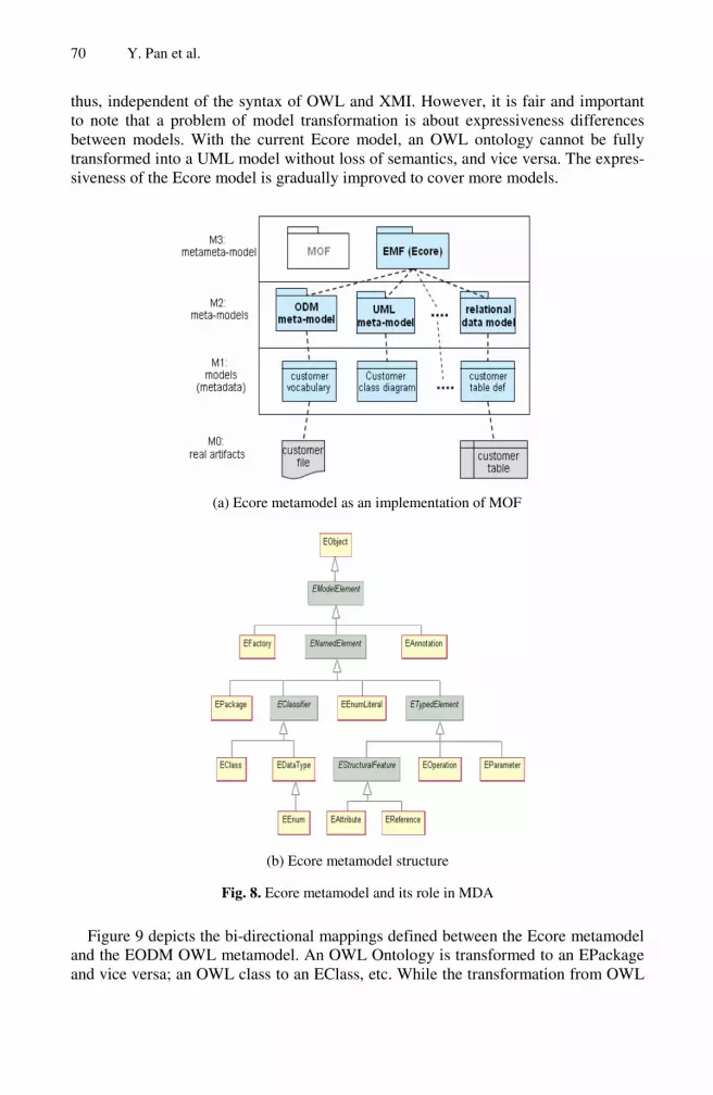
70 Y. Pan et al.
thus, independent of the syntax of OWL and XMI. However, it is fair and important to note that a problem of model transformation is about expressiveness differences between models. With the current Ecore model, an OWL ontology cannot be fully transformed into a UML model without loss of semantics, and vice versa. The expres-siveness of the Ecore model is gradually improved to cover more models.
(a) Ecore metamodel as an implementation of MOF
(b) Ecore metamodel structure
Fig. 8. Ecore metamodel and its role in MDA
Figure 9 depicts the bi-directional mappings defined between the Ecore metamodel and the EODM OWL metamodel. An OWL Ontology is transformed to an EPackage and vice versa; an OWL class to an EClass, etc. While the transformation from OWL

Model-Driven Ontology Engineering 71
to Ecore model looks straightforward, there are a few gaps. As in UML, Eclass is a first-class entity in the Ecore model. All other entities such as properties are subordi-nates to Eclass. In OWL, however, all entities in OWL are equal. Thus, different enti-ties must have different names in OWL. For example, if two properties belonging to two different Eclasses have an identical name, a straightforward transformation will cause a name conflict problem. The EODM Transformation engine renames proper-ties with an identical name to ensure a unique name for every entity. Another gap comes from the difference in expressiveness from different modeling languages. OWL is a formal language which is based on Description Logic. OWL is more ex-pressive than the Ecore model. There are several OWL constructs that the Ecore model does support, e.g., OWL property restrictions used for precise definition of concepts. Therefore, some semantics are lost inevitably when conducting transforma-tion from OWL to Ecore. Also, The Ecore model does not support inference of OWL. Particularly, anonymous classes created by using OWL restrictions make the situation with inference even more difficult. To address these gaps, the EODM Model Trans-formation engine currently employs the following tactics:
• It appends all unsupported OWL constructs as comments; • It utilizes the inference engine during transformation to capture all implicit
subsumption relationships; • It only transforms named OWL classes, and discards all anonymous classes;
and • It renames properties with an identical name to ensure a unique name for
every entity.
OWLClass
Ontology
SubClassOf
OWLObjectProperty
RDFSRange
Cardinality
inverseOf
RDFSRange
OWLDatatypeProperty
RDFSDataType
OneOf
RDFComment
Individual
EClass
EPackage
eSuperType
eReference
eReferenceType
Multiplicity
eOppsite
eAttriuteType
eAttribute
EDataType
EEnum
EAnnotation
eLiteral
ECore Model EODM OWL Model
Fig. 9. Transformation between OWL and Ecore

72 Y. Pan et al.
The well-built model mapping realizes model-driven ontology engineering. How-ever, it should be pointed out that the differences between model-driven software engineering and model-driven ontology engineering. The MDA-based approach to software engineering is mostly used to build IT models, automatically transform them into deployable code, and effectively maintain the models and the code. On the other hand, ontology engineering described in this paper aims at creating, representing and maintaining business domain models, which provide rich semantics and are founded on well-formed description logic for knowledge representation. The purpose of the MDA-based ontology engineering is twofold. First, ontology engineering leverages mature technologies and tools developed in software engineering. Second, it is an ap-proach to linking ontologies (business models) and IT models and thus imposing rich semantics to IT models.
6.5 OWL Editor
Finally, the OWL editor provides ontology authors with a GUI which enables them to visually create an ontology file, enrich OWL ontology files transformed from legacy models, and update ontology files. We utilized EMF to automatically generate a tree-based editor in Eclipse, and replaced the default XMI parser in the generated editor with the OWL parser of EODM. The editor framework in EMF follows the Model-Control-View pattern [6] and uses the adaptor pattern [6] to provide a generic content management capability. In addition to the EMF-generated OWL editor, we utilized the Graphic Editing Framework (GEF) [20] to develop a graphic editor referred to as the EODM workbench, to provide the foundation for graphic views of OWL ontolo-gies. GEF also supports drag and drop operations and drawing functions. The EODM
Fig. 10. Screenshot of EODM workbench

Model-Driven Ontology Engineering 73
workbench provides two hierarchical views; one for OWL classes and restrictions, and the other for OWL objects and datatype properties. Furthermore, it provides mul-tiple views of OWL ontologies and supports different development perspectives. Op-erations in different views are automatically synchronized in the Eclipse platform. Figure 10 gives a screenshot of the EODM workbench.
In the left hand side of the screen, there are two views of class and property hierar-chy, which are constructed based on rdfs:subClassOf and rdfs:subPropertyOf. Users can also add classes and properties such as subClassOf and subPropertyOf in the two trees. In the right hand side, there are a palette, a graphical editor and a property view. Users can drag and drop elements in the palette to the editor. Detailed information about the ontology and its elements that are not showed in the limited space of the editor is viewed and edited in the property view.
7 Use Scenarios
This section presents use scenarios illustrating how the features of the proposed EMF-based ontology engineering tool can be utilized in real-world applications. Our exam-ple is the model-driven business transformation [11]. Business transformation employs business models such as component business models [18] to identify opportunities for reducing costs or improve business processes. The model-driven approach to business transformation requires a model representation of a variety of business entities such as business processes, components, competencies, activities, resources, metrics, KPIs (Key Performance Indicators), etc. and their relations. Semantic models or ontologies provide useful representation of business models because they can effectively represent different types of relations among business entities. Also, the automatic reasoning capability of semantic models provides an effective method for analyzing business models for identifying cost-saving or process improvement opportunities.
For example, business performance metrics are associated with business activities. By using the relations between business activities and metrics, and also the relations between business components and business activities represented in a semantic model, a business analyst can infer relations between business components and met-rics. This type of analysis provides business insights into how the corporate can im-prove its performance metrics by addressing issues with the business components as-sociated with the selected set of metrics. Then, by identifying, again in the semantic model, IT systems associated with the business components, the analyst may be able to suggest recommendations about IT system management to improve performance metrics. The first step in realizing this model-driven business analysis scenario is the con-struction of semantic models of various business entities including business processes, components, competencies, activities, resources, operational metrics, KPIs. In many cases in most enterprises, the classes and relations of these business entities are al-ready captured in certain legacy modeling languages such as UML class diagrams, ER diagrams, relational data models, Java interfaces, spreadsheets, or text documents. Therefore, the task of semantic model construction simplifies to transforming the leg-acy models and merging them into OWL ontologies. The merged OWL ontologies

74 Y. Pan et al.
can be enriched with certain semantics such as generalization and specification, and cardinality constraints to enhance the effects of business analysis queries.
To summarize the model transformation process using the EMF-based ontology engineering system, it starts by capturing formal and informal semantics of legacy models. The model transformation engine transforms formal semantics of input leg-acy models into OWL models, by utilizing pre-defined mappings between OWL and the metamodels of the input models. The ontology engineering system allows an ex-pert to look into annotations and code of legacy models, and represent the semantics in OWL models. Informal semantics are captured as additional axioms and added to the OWL models by using the OWL editor. Optional functions of the system, such as the source code analysis or natural language processing, facilitate automatically cap-turing of certain informal semantics and improve the productivity of human experts. The overall process of capturing of formal and informal semantics of legacy models and representing them in OWL models is referred to as semantics enrichment.
We have implemented a non-trivial model transformation by using the EODM transformation engine. The source model is the Financial Business Object Model (FS-BOM) from IBM’s Information FrameWork (IFW). IFW permits many types of in-formation models required by complex enterprise systems for storing and correlating classes in a consistent manner. FS-BOM is a component of the overall suite of IFW for Financial Services. It was written in UML and provides an enterprise-wide, ge-neric and flexible model for financial services business. It is usually used as a starting point for analysis and design of business systems. Its rich content can be viewed from the fact that it has 582 classes and 5878 attributes and associations. This complicated structure indicates that more knowledge may be buried deep in the FS-BOM. There-fore, an inference-enabled representation, for example, by using OWL, is desirable. This transformation was conducted by using the EODM transformation engine.
For another use scenario, we have practiced model-driven ontology engineering in customer data integration (CDI) by using the Integrated Ontology Development Tool-kit (IODT) [22] which includes EODM, the EODM workbench and a persistent ontol-ogy repository. IODT is publicly available at IBM’s alphaWorks. In the CDI project, we used OWL ontologies to model concepts and properties describing customers, and populated customer data as instance in the OWL ontologies. More precisely, ontologies are adopted to describe and automatically classify customer data, and eventually support semantic queries on the customer data. Figure 11 shows a skeleton model transformation process in CDI. First, there are legacy UML class diagrams represent-ing customer classification hierarchies, for example, (bank subCategoryOf FinancialIn-stitute). By using the EODM transformation engine, the UML diagrams are trans-formed into an Ecore model as shown. Next, the Ecore model is transformed into an OWL ontology. In the EODM workbench, the generated ontology is further custom-ized by adding, modifying or deleting classes and properties, as necessary. For instance, an OWL class named “BDWCustomer” is additionally defined as a someVal-uesFrom restriction on Property “buy” with “BDW” as the range class (BDW means Banking Data Warehouse.). Then, as shown in Figure 12, we deployed the semanti-cally enriched ontologies into IODT’s persistent repository and populated customer data as ontology instances. In the ontology repository, customer data is represented and stored as RDF triples. The customer data is classified based on OWL ontology reason-ing. For example, the customer “SD Bank” is automatically classified as an

Model-Driven Ontology Engineering 75
Fig. 11. A model transformation example
Original Customer DataID Name BuyProduct …10243 SD Bank MD:BDW001 …10244 Hydri Co.Ltd VoIP …10245 Laser Co.Ltd ThinkPad …
Ontology Data<uri_10243, rdf: type, Customer><uri_10243, customerName, “SD Bank”><uri_10243, buy, MD:BDW001><MD:BDW001, rdf:type, MD:BDW><uri_10244, rdf:type, Customer><uri_10244, customerName, “Hydri Co.Ltd”><uri_10244, buy, VoIP><uri_10245, rdf:type, Customer><uri_10245, customerName, “Laser Co.Ltd”><uri_10245, buy, Thinkpad>
Ontology Data after Reasoning<uri_10243, rdf:type, BDWCustomer><uri_10243, customerName, “SD Bank”><uri_10244, rdf:type, TelecomCompany><uri_10244, customerName,”Hydri Co.Ltd”><uri_10245, rdf:type, Others><uri_10245, customerName, “Laser Co.Ltd”>
Populate
Inference
SPARQL Query Example:PREFIX md:<http://ibm.com/CDI> SELECT?name, ?productsWHERE ( ? customer rdf:type md:Bank ) ( ? customer md:buy ?products )( ?customer md:customerName ?name )
Results:name products
SD Bank MD:BDW001 Fig. 12. Queries in ontology-driven customer data integration

76 Y. Pan et al.
instance of class “BDWCustomer.” Finally, users can issue SPARQL queries on the customer data and obtain query results accordingly. Figure 12 illustrates queries in the ontology-driven customer data integration system. In summary, we started from legacy customer models in UML. By using the EODM transformation engine and the EODM workbench, an OWL ontology for customer data is generated and enriched. After customer data is populated into a persistent ontology repository, inference is conducted for instance classification. The EODM reasoning engine is used for OWL ontology TBox inference. Also, SPARQL queries are sup-ported for semantic search on customer data. The CDI system provides a use scenario that validates the importance and efficiency of model-driven ontology engineering.
8 Concluding Remarks
As the Semantic Web shapes the future of the Web, it becomes more and more impor-tant in software engineering and enterprise application development. However, the adoption of Semantic Web by industry has been slowed by a gap between ontology engineering tools and the traditional software engineering. Ontology engineering and software engineering have been established on different modeling languages and methodologies, which has caused difficulties in large-scale enterprise application de-velopment involving the Semantic Web technologies. Currently, transformation of UML models to OWL ontologies and vice versa is conducted only in an ad hoc and incomplete way.
This paper presented a novel approach to bridging this gap between two different, but complementary engineering disciplines with a systematic approach. We leveraged OMG’s Model-Driven Architecture and Ontology Definition Metamodel to provide model transformation, utilizing underlying standards including MOF-based metamod-els, XMI representation, UML extension with profiling, and EMF implementation of MOF. This approach allows seamlessly supporting legacy models in UML and other languages in Semantic Web-based software development. In addition, it allows ex-ploiting the availability and features of UML tools for creation of vocabularies and ontologies. Furthermore, it supports code generation and facilitates tool development. This paper presented the methodology and architecture of the EMF-based ontology engineering system, and mappings between UML and OWL for model transforma-tion. In addition, it presented the entire stack of the developed ontology engineering system. Finally, it presented use scenarios illustrating how the features of this system can be utilized in real-world applications.
This model-driven ontology engineering is still in its infancy. For this approach to meet its promises and scale for industry applications, a number of technical chal-lenges need to be addressed. Some directions for further investigation include:
• Study of the theoretical limitations of the model transformation under the EMF context and a complete definition of bi-directional mappings between the Ecore metamodel and semantic metamodels to support model transformation;
• Support for more legacy modeling languages and methodologies in addition to UML, XSD and Java interfaces which we have addressed in the current sys-tem, e.g., relational data models and spreadsheets traditionally popular in the business environment;

Model-Driven Ontology Engineering 77
• Validation of the proposed advantage of utilizing features of visual UML tools for creating and editing ontologies in real-world applications;
• Evaluation of EMF’s capability of code generation for facilitating tool devel-opment;
• Augmenting the proposed model transformation method with capabilities for source code analysis and text mining to facilitate acquisition of certain infor-mal semantics of legacy models; and
• Maturation of the holistic EMF-based ontology engineering framework by applying and validating it in real-world business applications.
References
1. T. Berners-Lee, J. Hendler, O. Lassila, “The Semantic WEB,” Scientific American, 2001. 2. D. Brickley and R. Guha, “RDF Vocabulary Description Language 1.0: RDF Schema,”
W3C Recommendation, http://www.w3.org/TR/rdf-schema/, 2004. 3. Brown, “An introduction to Model Driven Architecture – Part I: MDA and today’s sys-
tems”, http://www-106.ibm.com/developerworks/rational/library/3100.html, 2004. 4. J. J. Carroll, I. Dickinson, C. Dollin, D. Reynolds, A. Seaborne, K. Wilkinson, “Jena: Im-
plementing the Semantic Web Recommendations”, Proc. of WWW 2004. 5. Djuric, D. Gaševic, and V. Devedžic, “Ontology Modeling and MDA,” Journal of Object
technology, Vol. 4, No. 1, 2005. 6. Gamma, R. Helm, R. Johnson, J. Vlissides, “Design Patterns: Elements of Reusable Ob-
ject-Oriented Software,” Addison-Wesley Professional; 1st edition, January 15, 1995. 7. D. Gasevic, D. Djuric, V. Devedzic, "Bridging MDA and OWL ontologies," Journal of
Web Engineering, Vol.4, No.2, 2005, pp. 119-134. 8. J. Grant and D. Beckett, “RDF Test Cases,” http://www.w3.org/TR/rdf-testcases/, 10 Feb.
2004. 9. Hladik, “Implementation and Optimisation of a Tableau Algorithm for the Guarded Frag-
ment,” Lecture Notes In Computer Science; Vol. 2381 archive, Proceedings of the Interna-tional Conference on Automated Reasoning with Analytic Tableaux and Related Methods, Pages: 145 - 159, 2002.
10. G. Klyne and J. Carroll, “Resource Description Framework (RDF): Concepts and Abstract Syntax,” W3C Recommendation, http://www.w3.org/TR/rdf-concepts/, 2004.
11. Lee, “Model-Driven Business Transformation and Semantic Web,” The Communications of the ACM, Special Issue on Semantic eBusiness Vision, December 2005.
12. J. Lee and R. Goodwin, “Ontology Management for Large-Scale E-Commerce Applica-tions,” International Workshop on Data Engineering Issues in E-Commerce, Tokyo, Japan, April 9, 2005.
13. Lutz, “NEXP TIME-Complete Description Logics with Concrete Domains,” ACM Trans-actions on Computational Logic (TOCL) archive, Volume 5, Issue 4, October 2004.
14. L. Ma, Z. Su, Y. Pan, L. Zhang, T. Liu, “RStar: An RDF Storage and Query System for Enterprise Resource Management”, Proc. of ACM CIKM, pp. 484-491, 2004.
15. Oberle, R. Volz, B. Motik, S. Staab, “An Extensible Ontology Software Environment,” In Steffen Staab and Rudi Studer, Handbook on Ontologies, chapter III, pp. 311-333. Springer, 2004.
16. M. K. Smith, C. Welty, and D. L. McGuinness, “OWL Web Ontology language Guide,” http://www.w3.org/TR/owl-guide/, 2004.

78 Y. Pan et al.
17. Tetlow, et al., “Ontology Driven Architectures and Potential Uses of the Semantic Web in Systems and Software Engineering,” http://www.w3.org/2001/sw/BestPractices/SE/ODA/, 2005.
18. CBM: Component Business Modeling, http://www-306.ibm.com/e-business/ondemand/us/ innovation/ cbm/ cbm_b.shtml.
19. D2RQ V0.4: Treating Non-RDF Databases as Virtual RDF Graphs, http://www.wiwiss.fu-berlin.de/suhl/bizer/d2rq/.
20. GEF (Graphical Editing Framework), http://www.eclipse.org/gef, 2004. 21. EMF (Eclipse Modeling Framework), http://www.eclipse.org/emf, 2004. 22. IBM Integrated Ontology Toolkit, http://www.alphaworks.ibm.com/tech/semanticstk,
2005. 23. Jastor, http://jastor.sourceforge.net/. 24. MOF: Meta-Object Facility, Version 1.4, http://www.omg.org/technology/documents/
formal/mof.htm. 25. ODM: Ontology Definition Metamodel, http://www.omg.org/docs/ontology/04-08-01.pdf,
2004. 26. Pellet: an Open-Source Java Based OWL DL Reasoner, http://www.mindswap.org/2003/
pellet/index.shtml. 27. Primer: Getting into RDF & Semantic Web using N3, http://www.w3.org/2000/10/swap
Primer.html. 28. Protégé, http://protege.stanford.edu/index.html, 2004. 29. Sesame, an Open Source RDF Database with Support for RDF Schema Inferencing and
Querying,” http://www.openrdf.org/, 2002.

Inheritance in Rule-Based Frame Systems:Semantics and Inference
Guizhen Yang1 and Michael Kifer2
1 Artificial Intelligence CenterSRI International, Menlo Park, CA 94025, USA
[email protected] Department of Computer Science
State University of New York at Stony BrookStony Brook, NY 11794, [email protected]
Abstract. Knowledge representation languages that combine rules withobject-oriented features akin to frame systems have recently attracted alot of research interest, and F-logic is widely seen as a basis to achieve thisintegration. In this paper we extend the original F-logic formalism withan array of salient features that are essential for representing and reason-ing with commonsense knowledge. In particular, we extend the syntaxand semantics of F-logic to incorporate nonmonotonic multiple inheri-tance of class and instance methods in the presentence of class hierarchiesdefined via rules. The new semantics is completely model-theoretic and isfree of the defects that caused the original F-logic to produce unintuitiveresults due to the unusual interaction between default inheritance andinference via rules. Moreover, we provide a computational frameworkfor the new F-logic semantics which can be implemented by inferenceengines using either forward or backward chaining mechanisms.
1 Introduction
With computer systems getting more powerful and once esoteric informationmanagement problems becoming commonplace, attention is again shifting toknowledge representation languages that combine rules with object-oriented fea-tures akin to frame systems. Recently, W3C created a new working group, whichis chartered with producing a recommendation for a standardized rule languagethat could serve as an interchange format for various rule-based systems [38].According to the charter, the future language will support features inspired byobject-oriented and frame-based languages.
As a prominent formalism in applications where both rules and frame-basedrepresentation are highly desired, F-logic has found its success in many areas, in-cluding Semantic Web [9,10,3,8], intelligent networking [24], software engineering[17,13], and industrial knowledge management [2,39]. F-logic based systems areavailable both commercially [33] and from the academia [14,46,40,30]. These sys-tems were built for different purposes and offer different degrees of completenesswith respect to the original specification.
S. Spaccapietra (Ed.): Journal on Data Semantics VII, LNCS 4244, pp. 79–135, 2006.c© Springer-Verlag Berlin Heidelberg 2006

80 G. Yang and M. Kifer
One major technical difficulty in this field is inheritance semantics, especiallythe issues related to overriding and conflict resolution [22,45]. A recent study [29]shows that inheritance — especially multiple inheritance — permeates RDFschemas developed by various communities over the past few years. Multipleinheritance is therefore likely to arise in Semantic Web applications as theygrow in complexity and as rule engines start playing a more prominent role insuch applications. However, current Semantic Web standards do not supportmultiple inheritance. Some of the F-logic based systems mentioned earlier donot support it either. Support provided by other systems is either incomplete orproblematic in various ways.
The difficulty in defining a semantics for inheritance is due to the intricateinteraction between inference by default inheritance and inference via rules. Weillustrate this problem in Section 3. Although this problem was known at thetime of the original publication on F-logic [22], no satisfactory solution wasfound then. Subsequent works either tried to rationalize the original solution orto impose unreasonable restrictions on the language [32,19,31]. We discuss theselimitations of the related work in Section 11.
Our earlier work [45] proposed a solution to the above problem by develop-ing a semantics that is both theoretically sound and computationally feasible.However, this semantics (like the one in [22] and most other related works) isrestricted to the so called class methods [36] (or static methods in Java terminol-ogy) and to a particular type of inheritance, known as value inheritance, whichis more common in Artificial Intelligence. The notion of instance methods — amuch more important object-oriented modeling tool — was not supported in thelanguage or its semantics. In this paper we extend F-logic to include instancemethods and a new kind of inheritance, called code inheritance, which is analo-gous to inheritance used in programming languages like C++ and Java (and isdifferent from inheritance typically found in AI systems).
Of course, neither instance method nor code inheritance is new by itself.Our contribution is in porting these notions to a logic-based language and thedevelopment of a complete model theory and inference procedure for this newclass of methods and inheritance. Furthermore, these concepts are defined forvastly more general frameworks than what is found in programming languagesor in the literature on logic-based inheritance. This includes systems with classhierarchies defined via rules (intensional class hierarchies), multiple inheritancewith overriding, deductive systems with inheritance, both instance and classmethods, and both value and code inheritance.
This paper is organized as follows. Section 2 introduces the basic F-logic syn-tax that is used throughout the paper. Section 3 motivates the research problemsconcerning inheritance and rules by presenting several motivating examples. Thenew three-valued semantics for F-logic is introduced in Section 4. Section 5 de-fines inheritance postulates, which bridge the formal semantics and its “realworld” interpretation, and Section 6 formalizes the associated notion of ob-ject models. The computational framework is presented in Section 7. Section 8introduces the notion of stable object models. Section 9 further develops the

Inheritance in Rule-Based Frame Systems: Semantics and Inference 81
cautious object model semantics and discusses its properties. It is shown thatevery F-logic knowledge base has a unique cautious object model. Implementa-tion of the cautious object model semantics and its computational complexity isdescribed in Section 10. This implementation can be realized using any deductiveengine that supports the well-founded semantics for negation [15] and thereforecan be done using either forward or backward chaining mechanisms. Relatedwork is discussed in Section 11 and Section 12 concludes the paper. Since someof the proofs are rather subtle and lengthy, we relegate them to the Appendixin the hope that this will help the reader focus on the main story line. Shorterproofs appear directly in the main text.
2 Preliminaries
F-logic provides frame-based syntax and semantics. It treats instances, classes,properties, and methods as objects in a uniform way. For instance, in one context,the object ostrich can be viewed as a class by itself (with members such as tweetyand fred); in a different context, this object can be a member of another class(e.g., species). Whether an object functions as an instance or a class depends onits syntactic position in a logical statement. F-logic does not require instancesand classes to be disjoint.1
To focus the discussion, we will use a subset of the F-logic syntax and includeonly three kinds of atomic formulas. A formula of the form o : c says that objecto is a member of class c; s :: c says that class s is a (not necessarily immediate)subclass of class c; and e[m → v] says that object e has an inheritable method,m, whose result is a set that contains object v.2 The symbols o, c, s, e, m, andv here are the usual first-order terms.3
Traditional object-oriented languages distinguish between two different kindsof methods: instance methods and class methods (also known as “static” meth-ods in Java). The former apply to all instances of a class while the latter toclasses themselves. In object-oriented data modeling, especially in the case ofsemistructured objects, it is useful to be able to define object methods, whichare explicitly attached to individual objects. These explicitly attached methodsoverride the methods inherited from superclasses. Object methods are similar toclass methods except that they are not intended to be inherited. In F-logic bothinstance and class/object methods are specified using rules.
Let A be an atom. A literal of the form A is called a positive literal and¬A is called a negative literal. An F-logic knowledge base (abbr. KB) is a finite
1 The same idea is adopted in RDF and OWL-Full.2 The syntax for inheritable methods in [22] and in systems like Flora-2 is e[m �→ v],
while atoms of the form e[m → v] are used for noninheritable methods. However,noninheritable methods are of no interest here, so we opted for a simpler notation.
3 Recall that a first-order term is a constant, a variable, or a structure of theform f(t1, . . . , tn), where f is an n-ary function symbol and t1, . . . , tn are first-orderterms.

82 G. Yang and M. Kifer
set of rules where all variables are universally quantified at the front of a rule.There are two kinds of rules: regular rules and template rules . Regular ruleswere introduced in the original F-logic [22] while the concept of template rules isone of the new contributions of this paper. Generally, regular rules define classmembership, subclass relationship, and class/object methods. Template rulesrepresent pieces of code that define instance methods.
A regular rule has the form H :− L1, . . . , Ln, where n ≥ 0, H is a positiveliteral, called the rule head, and each Li is either a positive or a negative literal.The conjunction of Li’s is called the rule body. A template rule for class c has theform code(c) @this[m → v] :− L1, . . . , Ln. It is similar to a regular rule exceptthat: (i) it is prefixed with the special notation code(c); (ii) its head mustspecify a method (i.e., it cannot be o : c or s :: c); and (iii) the object-position inthe head literal is occupied by the template term @this (which can also appear inother parts of the rule). We will also assume that c is ground (i.e., variable-free)and will say that such a template rule defines instance method m for class c.
In the rest of this paper, we will use uppercase names to denote variablesand lowercase names to denote constants. A rule with an empty body is calleda fact. When a regular rule or a template rule has an empty body, we will call ita regular fact or a template fact , respectively. For facts, the symbol “ :− ” willbe omitted.
3 Motivating Examples
We will now illustrate some of the problems that arise from unusual interactionamong inference via rules, default inheritance, and intensional class hierarchies(i.e., class hierarchies that are defined using rules). In the following examples, asolid arrow from a node x to another node y indicates that x is either an instanceor a subclass of y. All examples in this section are discussed informally. Theformal treatment is given in Sections 4, 5, 7, and 9.
3.1 Interaction Between Default Inheritance and Rules
Inheritance Triggering Further Inheritance. Consider the KB in Figure 1. With-out inheritance, this KB has a unique model, which consists of the first twofacts. With inheritance, however, the common intuition tells us that o ought toinherit m → a from c. But if we only add o[m → a], the new set of facts wouldnot be a model, since the last rule is no longer satisfied: with the inherited fact
c[m−>a]
o
o : c.c[m → a].c[m → b] :− o[m → a].
Fig. 1. Inheritance Leading to More Inheritance

Inheritance in Rule-Based Frame Systems: Semantics and Inference 83
included, the least model must also contain c[m → b]. However, this begs thequestion as to whether o should inherit m → b from c as well. The intuitionsuggests that the intended model should be “stable” with respect to not onlyinference via rules but default inheritance as well. Therefore o[m → b] shouldalso be in that model. This problem was recognized in [22], but the proposedsolution was not stable in the above sense — it was based on plausible, ad hocfixpoint computations rather than semantic principles.
c[m−>a]
o
o : c.c[m → a].o[m → b] :− o[m → a].
Fig. 2. Interaction between Derived and Inherited Facts
Derived vs. Inherited Information. Now consider Figure 2, which has the sameKB as in Figure 1 except for the head of the last rule. Again, the intuition sug-gests that o[m → a] ought to be inherited, and o[m → b] be derived to makethe resulting set of facts into a model in the conventional sense. This, however,leads to the following observation. The method m of o now has one value, a,which is inherited, and another, b, which is derived via a rule. Although the tra-ditional frameworks for inheritance were developed without deduction in mind,it is clear that derived facts like o[m → b] in this example are akin to “explicit”method definitions and should be treated differently. Typically, explicit defini-tions should override inheritance. Thus our conclusion is that although deriva-tion is done “after” inheritance, this derivation undermines the original reasonfor inheritance. Again, the framework presented in this paper, which is basedon semantic principles, differs from the ad hoc computation in [22] (which keepsboth derived and inherited facts).
o
c1[m−>a]
c2[m−>b]
o : c1.c2 :: c1.c1[m → a].c2[m → b].o : c2 :− o[m → a].
Fig. 3. Inheritance and Intensional Class Hierarchy
Intensionally Defined Class Hierarchy. Figure 3 is an example of an intensionalclass hierarchy. Initially, o is not known to be an instance of c1. So, it seemsthat o can inherit m → a from c1. However, this makes the fact o[m → a] true,which in turn causes o : c2 to be derived by the last rule of the KB. Since thismakes c2 a more specific superclass of o than c1 is, it appears that o ought

84 G. Yang and M. Kifer
to inherit m → b from c2 rather than m → a from c1. However, this wouldmake the fact o : c2 unsupported. Either way, the deductive inference enabledby the original inheritance undermines the support for the inheritance itself.Unlike [22], a logically correct solution in this case would be to leave both o : c2
and o[m → a] underdefined. The dashed arrow from o to c2 in Figure 3 representsthe underdefinedness of o : c2.
c2[m−>b]
o
c1[m−>a]c1[m → a].c2[m → b].o : c1.o : c2 :− o[m → a].
Fig. 4. Derivation Causing Multiple Inheritance Conflicts
Derivation and Multiple Inheritance Conflicts. The example in Figure 4 illus-trates a similar problem, but this time it occurs in the context of nonmonotonicmultiple inheritance. Initially c2 is not known to be a superclass of o. So thereis no multiple inheritance conflict and the intuition suggests that o should in-herit m → a from c1. But then o : c2 has to be added to the model in order tosatisfy the last rule. This makes c2 a superclass of o and introduces a multipleinheritance conflict. As in the previous example, although this conflict becameapparent only after inheritance took place, it undermines the original reasonfor inheritance (which was based on the assumption that c1[m → a] is the onlysource of inheritance for o). Therefore, both o[m → a] and o : c2 should be leftunderdefined. Again, this conclusion differs from [22].
3.2 Inheritance of Code
The inheritance shown in the previous examples is called value inheritance. Itis called so because what gets inherited are the individual values that methodshave in particular classes rather than the definitions of those methods.
We should note that value inheritance is data-dependent. Consider the exam-ple in Figure 5. At first glance, it appears that there is a multiple inheritanceconflict for object o2 with respect to method m from class c1 and c2. Indeed,in a traditional programming language like C++, the first two rules in Figure 5would be considered as part of the code that defines method m in class c1 andc2, respectively. Since o2 is an instance of both classes, we have a multiple inheri-tance conflict. In contrast, value inheritance takes into account what holds in themodel of the KB. Clearly, in the example of Figure 5, the premise of the first ruleis true whereas the second is false. This means that the model makes c1[m → a]true but c2[m → b] false.4 Therefore, if we only look at the values of method mthat actually hold in the model of the KB, then no conflict exists and m → acan be readily inherited from c1 by o2 (and o1) through value inheritance.4 Our claims here rely on the closed world assumption.

Inheritance in Rule-Based Frame Systems: Semantics and Inference 85
o1
c1
o2
c2 c1[m → a] :− p[f → d].c2[m → b] :− p[f → e].o1 : c1.o2 : c1.o2 : c2.p[f → d].
Fig. 5. Value Inheritance vs. Code Inheritance
Code inheritance, in contrast, behaves like in traditional programming lan-guages and the above example would require conflict resolution. In this paper,we resolve multiple inheritance conflicts cautiously — whenever a conflict arises,nothing is inherited. To appreciate the difference between value and code in-heritance, let us revisit the example of Figure 5 using code inheritance. Nowsuppose the first two regular rules in Figure 5 are replaced by the following twotemplate rules (introduced in Section 2):
code(c1) @this[m → a] :− p[f → d].code(c2) @this[m → b] :− p[f → e].
Note that template rules are prefixed with the notation code(c), for some classc, to indicate that they make up the code that defines the instance methods fora particular class.
We call the above rules template rules because they are not the actual rulesthat we require to hold true in the model of the KB. Instead, once inherited,they will be “instantiated” to the actual regular rules that are required to holdtrue. In the case of o2, no code is inherited due to multiple inheritance conflict,as we just explained above. However, o1 can inherit the first template rule fromc1, since there is no conflict. Inheritance of such a template rule is achievedby substituting the template term @this with o1 in the rule. This results in aregular rule of the form o1[m → a] :− p[f → d]. This rule and the fact p[f → d]together enable the derivation of a new fact, o1[m → a].
The above example illustrates the intended use of template rules. The tem-plate term in a template rule acts as a placeholder for instances of that class.When the rule is inherited by an instance, the template term is replaced by thatinstance and the result is a regular rule. This is akin to late binding in traditionalobject-oriented languages.
The treatment of template rules should make it clear that the method m inour example above behaves like an instance method in a language like Java:the template rule does not define anything for class c1 as an object; instead, itdefines the method m for all instances of c1. This is because template rules arenot meant to be true in the model of the KB — but those regular rules resultingfrom code inheritance are.
The above example also alludes to the fact that value inheritance is a more“model-theoretic” notion than code inheritance, and that developing a model

86 G. Yang and M. Kifer
theory for code inheritance is not straightforward. We develop a suitable modeltheory in Section 6.
c2[m−>b]c1
o[f−>b]
code(c1) @this[m → a] :− @this[f → b].o : c1.o[f → b].o : c2 :− o[m → a].c2[m → b].
Fig. 6. Interaction between Template Rules and Regular Rules
Subtle interaction may arise between template rules and regular rules. To il-lustrate the issue, Figure 6 shows a template rule that defines instance methodm for class c1. On the surface, it seems that o should inherit this piece of codefrom c1 and thus acquire the regular rule o[m → a] :− o[f → b]. (Recall thatthe template term in the rule is replaced with the inheriting instance). This in-heritance seems to be possible because o is a member of c1 and at this momentwe cannot conclude that o also belongs to c2.
A more careful look indicates, however, that there is a multiple inheritanceconflict. If o inherits the above rule, then we can derive o[m → a]. But thenwe can also derive o : c2 using the fourth rule in Figure 6 (which is a regularrule). Now, since c2[m → b] is also true, we have a multiple inheritance conflictanalogous to the example of Figure 4. As in the example of Figure 4, the logicallycorrect solution here is to leave both o[m → a] and o : c2 underdefined.
We thus see that template rules can interact with regular rules in subtle waysand cause inheritance to be canceled out. In other cases, such interaction mightenable more inheritance. For instance, if instead of c2[m → b] we had c2[n → b],then inheritance of the template rule by o would not be blocked. Furthermore,o would inherit n → b from c2 by value inheritance.
3.3 Observations
Nonmonotonic Inheritance. Overriding of inheritance leads to nonmonotonicreasoning, since more specific definitions take precedence over more general ones.However, overriding is not the only source of nonmonotonicity here. When anobject belongs to multiple incomparable classes, inheritance conflicts can ariseand their “canceling” effects can also lead to nonmonotonic inheritance.
Intensional Class Hierarchies. A class hierarchy becomes intensional when classmembership and/or subclass relationship is defined using rules. In such cases, theinheritance hierarchy can be decided only at runtime, as complex interactionsmay come into play between inference via default inheritance and inference viarules. In this interaction, an earlier inference by inheritance may trigger a chainof deductions via rules which can result in violation of the assumptions that ledto the original inheritance.

Inheritance in Rule-Based Frame Systems: Semantics and Inference 87
Value Inheritance vs. Code Inheritance. Inheritance of values is fundamentallydifferent from inheritance of code. Value inheritance is data-dependent — itdepends on the set of assertions in the current KB. Code inheritance is notdependent on data. Recall that in the example of Figure 5 we derived the facto2[m → a] via value inheritance because the premise of the second rule was falseand therefore inheritance was conflict-free from the perspective of value inheri-tance. If we add the fact p[f → e], then the second rule will derive c2[m → b]and create a multiple inheritance conflict. In this case, o2 may inherit nothing.
In contrast, if we turn the rules in Figure 5 into template rules, then a multipleinheritance conflict would always exist regardless of whether the premise of eitherrule can be satisfied. As a result, o2 would inherit nothing — whether p[f → d]and p[f → e] hold true or not.
4 Three-Valued Semantics
The examples in Section 3 illustrate the complex interactions between inferencevia default inheritance and inference via rules. These interactions cause infer-ence to behave nonmonotonically and in many ways like default negation. Thissuggests that stable models [16] or well-founded models [15] could be adoptedas a basis for our semantics. Since default negation is part of our language any-way, adoption of one of these two approaches is fairly natural. In this paperwe base the semantics on well-founded models. Since well-founded models arethree-valued and the original F-logic models were two-valued [22], we first needto define a suitable three-valued semantics for F-logic KBs. We also need to ex-tend this semantics to accommodate template rules and to make it possible todistinguish facts derived by default inheritance from facts derived via rules.
Let P be an F-logic KB. The Herbrand universe of P, denoted HUP, con-sists of all the ground (i.e., variable-free) terms constructed using the functionsymbols and constants found in the KB. The Herbrand instantiation of P, de-noted ground(P), is the set of rules obtained by consistently substituting allthe terms in HUP for all variables in every rule of P. The Herbrand base of P,denoted HBP, consists of the following sorts of atoms: o : c, s :: c, s[m → v]ex,o[m → v] c
val, and o[m → v] ccode, where o, c, s, m, and v are terms from HUP.
An atom of the form o : c is intended to represent the fact that o is an instanceof class c; s :: c states that s is a subclass of c. An atom of the form s[m → v]exstates that m → v is explicitly defined at s via a regular rule. Atoms of theforms o[m → v] c
val and o[m → v] ccode, where o �= c, imply that object o inherits
m → v from class c by value and code inheritance, respectively.A three-valued interpretation I of an F-logic KB P is a pair 〈T; U 〉, where
T and U are disjoint subsets of HBP. The set T contains all atoms that aretrue whereas U contains all atoms that are underdefined. Underdefined atomsare called this way because there is insufficient evidence to establish their truthor falsehood. The set F of the false atoms in I is defined as F = HBP − (T ∪ U).It is easy to see that the usual two-valued interpretations are a special case ofthree-valued interpretations of the form 〈T; ∅ 〉.

88 G. Yang and M. Kifer
Following [34], we will define the truth valuation functions for atoms, literals,and regular rules. The atoms in HBP can have one of the following three truthvalues: t, f , and u. Intuitively, u (underdefined) means possibly true or possiblefalse. Underdefined atoms are viewed as being “more true” than false atoms,but “less true” than true atoms. This is captured by the following truth orderingamong the truth values: f < u < t. Given an interpretation I = 〈T; U 〉 of anF-logic KB P, for any atom A from HBP we can define the corresponding truthvaluation function I as follows:
I(A) =
⎧⎨
⎩
t, if A ∈ T;u, if A ∈ U;f , otherwise.
Truth valuations are extended to conjunctions of atoms in HBP as follows:
I(A1 ∧ . . . ∧ An) = min{I(Ai)|1 ≤ i ≤ n}
The intuitive reading of a regular rule is as follows: its rule head acts as anexplicit definition while its rule body as a query. In particular, if s[m → v] is inthe head of a regular rule and the body of this rule is satisfied, then m → v isexplicitly defined for s. In the body of a regular rule, the literal s[m → v] is trueif s has either an explicit definition of m → v, or s inherits m → v from one ofits superclasses by value or code inheritance. Therefore, the truth valuation of aground F-logic literal depends on whether it appears in a rule head or in a rulebody. This is formally defined as follows.
Definition 1 (Truth Valuation of Literals). Let I be an interpretation ofan F-logic KB P. The truth valuation functions, Vh
I and VbI (h and b stand for
head and body, respectively), on ground F-logic literals are defined as follows:
VhI (o : c) = Vb
I (o : c) = I(o : c) VhI (s :: c) = Vb
I (s :: c) = I(s :: c)
VhI (s[m → v]) = I(s[m → v]ex)
VbI (o[m → v])=maxc∈HUP{I(o[m → v]ex), I(o[m → v] c
val), I(o[m → v] ccode)}
Let L and Li (1 ≤ i ≤ n) be ground literals. Then:
VbI (¬ L) = ¬Vb
I (L) VbI (L1 ∧ . . . ∧ Ln) = min{Vb
I (Li) | 1 ≤ i ≤ n}
For completeness, we define the negation of a truth value as follows: ¬ f = t,¬ t = f , and ¬u = u.
The following two lemmas follow directly from the above definitions.
Lemma 1. Let I = 〈T; U 〉 be an interpretation of an F-logic KB P, L a groundliteral in ground(P), J = 〈T; ∅ 〉, and K = 〈T ∪ U; ∅ 〉. Then:
(1) If L is a positive literal, then VbI (L) = t iff Vb
J (L) = t.(2) If L is a negative literal, then Vb
I (L) = t iff VbK(L) = t.

Inheritance in Rule-Based Frame Systems: Semantics and Inference 89
(3) If L is a positive literal, then VbI (L) ≥ u iff Vb
K(L) = t.(4) If L is a negative literal, then Vb
I (L) ≥ u iff VbJ (L) = t.
Lemma 2. Let I = 〈A; ∅ 〉 and J = 〈B; ∅ 〉 be two-valued interpretations ofan F-logic KB P such that A ⊆ B, and let L be a ground literal in ground(P).Then:
(1) If L is a positive literal and VbI (L) = t, then Vb
J (L) = t.(2) If L is a negative literal and Vb
J (L) = t, then VbI (L) = t.
Having defined the truth valuation functions VhI and Vb
I for ground literals, wenow extend the truth valuation function I to ground regular rules. Intuitively,a ground regular rule is true if and only if the truth value of its head is at leastas high as truth value of the rule body (according to the truth ordering). Notethat the truth valuation of either the head or the body is three-valued, but thetruth valuation of a rule is always two-valued.
Definition 2 (Truth Valuation of Regular Rules). Given an interpretationI of an F-logic KB P, the truth valuation function I on a ground regular rule,H :− B ∈ ground(P), is defined as follows:
I(H :− B) ={
t, if VhI (H) ≥ Vb
I (B);f , otherwise.
Given a ground regular fact, H ∈ ground(P):
I(H) ={
t, if VhI (H) = t;
f , otherwise.
Satisfaction of nonground regular rules in an interpretation is defined via instan-tiation, as usual.
Definition 3 (Regular Rule Satisfaction). A three-valued interpretation Isatisfies the regular rules of an F-logic KB P if I(R) = t for every regular ruleR in ground(P).
5 Inheritance Postulates
Even if an interpretation I satisfies all the regular rules of an F-logic KB P,it does not necessarily mean that I is an intended model of P. An intendedmodel must also include facts that are derived via inheritance and must notinclude unsupported facts. As we saw in Section 3, defining what should beinherited exactly is a subtle issue. The main purpose of this section is to formalizethe common intuition behind default inheritance using what we call inheritancepostulates.

90 G. Yang and M. Kifer
5.1 Basic Concepts
Intuitively, c[m] is an inheritance context for object o, if o is an instance ofclass c, and either c[m → v] is defined as a regular fact or is derived via aregular rule (in this case we say that m → v is explicitly defined at c); or ifthere is a template rule which specifies the instance method m for class c. Inher-itance context is necessary for inheritance to take place, but it is not sufficient:inheritance of m from c might be overridden by a more specific inheritance con-text that sits below c along the inheritance path. If an inheritance context isnot overridden by any other inheritance context, then we call it an inheritancecandidate . Inheritance candidates represent potential sources for inheritance.But there must be exactly one inheritance candidate for inheritance to takeplace — having more than one leads to a multiple inheritance conflict, whichblocks inheritance.
The concepts to be defined in this section come in two flavors: strong or weak.The “strong” flavor of a concept requires that all relevant facts be positivelyestablished while the “weak” flavor allows some or all facts to be underdefined.
Definition 4 (Explicit Definition). Let P be an F-logic KB and I an in-terpretation of P. We say that s[m] has a strong explicit definition in I, ifmax{I(s[m → v]ex)|v ∈ HUP} = t. We say that s[m] has a weak explicit de-finition in I if max{I(s[m → v]ex)|v ∈ HUP} = u.
Definition 5 (Value Inheritance Context). Given an interpretation I of anF-logic KB P, c[m] is a strong value inheritance context for o in I, if c �= o (i.e.,c and o are distinct terms) and min{I(o : c), max{c[m → v]ex|v ∈ HUP}} = t.We say that c[m] is a weak value inheritance context for o in I, if c �= o andmin{I(o : c), max{c[m → v]ex|v ∈ HUP}} = u.
Definition 6 (Code Inheritance Context). Given an interpretation I of anF-logic KB P, c[m] is a strong (respectively, weak) code inheritance context for oin I, if c �= o, I(o : c) = t (respectively, I(o : c) = u), and there is a template rulein P of the form code(c) @this[m → . . .] :− . . ., i.e., there is a template rulethat defines instance method m for class c.
When the specific type of an inheritance context is immaterial as, for example,in the following definitions, we will use the term inheritance context withoutindicating whether a value or a code inheritance context is meant.
Definition 7 (Overriding). Let I be an interpretation of an F-logic KB P.We will say that class s strongly overrides inheritance context c[m] for o, if s �= c,I(s :: c) = t, and s[m] is a strong (value or code) inheritance context for o.
We will say class s weakly overrides c[m] for o, if either(1) I(s :: c) = t and s[m] is a weak inheritance context for o; or(2) I(s :: c) = u and s[m] is a weak or a strong inheritance context for o.
Definition 8 (Value Inheritance Candidate). Given an interpretation I ofan F-logic KB P, c[m] is a strong value inheritance candidate for o, denoted

Inheritance in Rule-Based Frame Systems: Semantics and Inference 91
c[m] s.val�I o, if c[m] is a strong value inheritance context for o and there is no
class s that strongly or weakly overrides c[m] for o.c[m] is a weak value inheritance candidate for o, denoted c[m] w.val
� I o, if theabove conditions are relaxed by allowing c[m] to be a weak value inheritancecontext and/or allowing weak overriding. Formally, this means that there is noclass s that strongly overrides c[m] for o and either
(1) c[m] is a weak value inheritance context for o; or(2) c[m] is a strong value inheritance context for o and there is some class
s that weakly overrides c[m] for o.
Definition 9 (Code Inheritance Candidate). Let I be an interpretation foran F-logic KB P. c[m] is called a strong code inheritance candidate for o, denotedc[m] s.code
� I o, if c[m] is a strong code inheritance context for o and there is no sthat strongly or weakly overrides c[m] for o.
c[m] is a weak code inheritance candidate for o, denoted c[m] w.code� I o, if the
above conditions are relaxed by allowing c[m] to be a weak code inheritance con-text and/or allowing weak overriding. Formally, this means that there is no classs that strongly overrides c[m] for o and either
(1) c[m] is a weak code inheritance context for o; or(2) c[m] is a strong code inheritance context for o and there is some class
s that weakly overrides c[m] for o.
c1
c5c4[m−>c]
c2[m−>a]c3[m−>b]
c1 : c2. c1 : c5.
c2 :: c4. c3 :: c5.
c2[m → a]. c3[m → b]. c4[m → c].
code(c5) @this[m → v] :− @this[f → x].
Fig. 7. Inheritance Context, Overriding, and Inheritance Candidate
Example 1. Consider an interpretation I = 〈T; U 〉 of an F-logic KB P, where
T = {c1 : c2, c1 : c4, c1 : c5, c2 :: c4, c3 :: c5} ∪{c2[m → a]ex, c3[m → b]ex, c4[m → c]ex}
U = {c1 : c3}
I and P are shown in Figure 7, where solid and dashed arrows represent trueand underdefined values, respectively.
In the interpretation I, c2[m] and c4[m] are strong value inheritance contextsfor c1. c5[m] is a strong code inheritance context for c1. c3[m] is a weak valueinheritance context for c1. The class c2 strongly overrides c4[m] for c1, whilec3 weakly overrides c5[m] for c1. c2[m] is a strong value inheritance candidatefor c1. c3[m] is a weak value inheritance candidate for c1. c5[m] is a weak codeinheritance candidate for c1. Finally, c4[m] is neither a strong nor a weak valueinheritance candidate for c1.

92 G. Yang and M. Kifer
For convenience, we will simply write c[m] �I o when it does not matterwhether c[m] is a strong or a weak value/code inheritance candidate. Now weare ready to introduce the postulates for nonmonotonic multiple value and codeinheritance. The inheritance postulates consist of two parts: core inheritancepostulates and cautious inheritance postulates. We formalize the core inheritancepostulates first.
5.2 Core Inheritance Postulates
The following definition says that class membership and subclass relationshipmust satisfy the usual transitive closure property.
Definition 10 (Positive ISA Transitivity). An interpretation I of anF-logic KB P satisfies the positive ISA transitivity constraint if the set of trueclass membership and subclass relationship atoms is transitively closed. Formallythis means that the following two conditions hold:
(1) for all s and c: if there is x such that I(s :: x) = t and I(x :: c) = t,then I(s :: c) = t;
(2) for all o and c: if there is x such that I(o : x) = t and I(x :: c) = t,then I(o : c) = t.
The context consistency constraint below captures the idea that only explicitdefinitions are inherited and that explicit definitions override inheritance.
Definition 11 (Context Consistency). An interpretation I of an F-logicKB P satisfies the context consistency constraint, if the following conditionshold:
(1) for all o, m, v: I(o[m → v] oval) = f and I(o[m → v] o
code) = f ;(2) for all c, m, v: if I(c[m → v]ex) = f , then I(o[m → v] c
val) = f for all o;(3) for all c, m: if ground(P) has no template rule that defines instance
method m for class c, then I(o[m → v] ccode) = f for all o, v;
(4) for all o, m: if o[m] has a strong explicit definition, then for all v, c,I(o[m → v] c
val) = f and I(o[m → v] ccode) = f .
The first condition in the above definition rules out self inheritance. The secondcondition states that if m → v is not explicitly defined at c, then no one caninherit m → v from c by value inheritance. The third condition says that if aclass c does not explicitly specify an instance method m, then no object shouldinherit m → v from c by code inheritance, for any v. The fourth condition statesthat if o has an explicit definition for method m, then this definition shouldprevent o from inheriting m → v from any other class for any v (either by valueor by code inheritance).
Intuitively, we want our semantics to have the property that if inheritance isallowed, then it should take place from a unique source. This is captured by thefollowing definition.
Definition 12 (Unique Source Inheritance). An interpretation I of anF-logic KB P satisfies the unique source inheritance constraint, if the follow-ing three conditions hold:
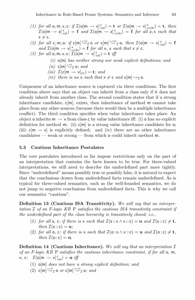
Inheritance in Rule-Based Frame Systems: Semantics and Inference 93
(1) for all o, m, v, c: if I(o[m → v] cval) = t or I(o[m → v] c
code) = t, thenI(o[m → z] x
val) = f and I(o[m → z] xcode) = f for all z, x such that
x �= c.(2) for all c, m, o: if c[m] s.val
�I o or c[m] s.code� I o, then I(o[m → v] x
val) = fand I(o[m → v] x
code) = f for all v, x such that x �= c.(3) for all o, m, v, c: I(o[m → v] c
val) = t iff(i) o[m] has neither strong nor weak explicit definitions; and(ii) c[m] s.val
�I o; and(iii) I(c[m → v]ex) = t; and(iv) there is no x such that x �= c and x[m] �I o.
Uniqueness of an inheritance source is captured via three conditions. The firstcondition above says that an object can inherit from a class only if it does notalready inherit from another class. The second condition states that if a stronginheritance candidate, c[m], exists, then inheritance of method m cannot takeplace from any other sources (because there would then be a multiple inheritanceconflict). The third condition specifies when value inheritance takes place. Anobject o inherits m → v from class c by value inheritance iff: (i) o has no explicitdefinition for method m; (ii) c[m] is a strong value inheritance candidate for o;(iii) c[m → v] is explicitly defined; and (iv) there are no other inheritancecandidates — weak or strong — from which o could inherit method m.
5.3 Cautious Inheritance Postulates
The core postulates introduced so far impose restrictions only on the part ofan interpretation that contains the facts known to be true. For three-valuedinterpretations, we still need to describe the underdefined part more tightly.Since “underdefined” means possibly true or possibly false, it is natural to expectthat the conclusions drawn from underdefined facts remain underdefined. As istypical for three-valued semantics, such as the well-founded semantics, we donot jump to negative conclusions from underdefined facts. This is why we callour semantics “cautious”.
Definition 13 (Cautious ISA Transitivity). We will say that an interpre-tation I of an F-logic KB P satisfies the cautious ISA transitivity constraint ifthe underdefined part of the class hierarchy is transitively closed; i.e.,
(1) for all s, c: if there is x such that I(s :: x ∧ x :: c) = u and I(s :: c) �= t,then I(s :: c) = u;
(2) for all o, c: if there is x such that I(o : x ∧ x :: c) = u and I(o : c) �= t,then I(o : c) = u.
Definition 14 (Cautious Inheritance). We will say that an interpretation Iof an F-logic KB P satisfies the cautious inheritance constraint, if for all o, m,v, c: I(o[m → v] c
val) = u iff(1) o[m] does not have a strong explicit definition; and(2) c[m] s.val
�I o or c[m] w.val� I o; and

94 G. Yang and M. Kifer
(3) I(c[m → v]ex) ≥ u; and(4) there is no x �= c such that x[m] s.val
�I o or x[m] s.code� I o; and
(5) I(o[m → v] cval) �= t.
The cautious inheritance constraint captures the intuition behind multiple in-heritance based on underdefined knowledge. The conditions above state whencautious value inheritance takes place. An object o cautiously inherits m → vfrom class c by value inheritance if and only if: (i) there is no strong evidencethat method m has an explicitly defined value at o; (ii) c[m] is either a strongor a weak value inheritance candidate for o; (iii) m → v is explicitly definedat c; (iv) there are no other strong inheritance candidates that can block valueinheritance from c (by the unique source inheritance constraint); and (v) o doesnot already inherit m → v from c by value inheritance.
6 Object Models
A model of an F-logic KB should satisfy all the rules in it. In Section 4 weformalized the notion of regular rule satisfaction. Here we will extend this notionto template rules. Recall that when an object inherits a template rule, the ruleis evaluated in the context of that object.
Definition 15 (Binding). Let R be the following template rule which definesinstance method m for class c: code(c) @this[m → v] :− B. The binding of Rwith respect to object o, denoted R‖o, is obtained from R by substituting o forevery occurrence of @this in R. In general, we will use X‖o to represent the termthat is obtained from X by substituting o for every occurrence of @this in X.
We call the above process “binding” because it is akin to late binding in tra-ditional programming languages like C++. Recall from Section 3 that templaterules are just templates for the regular rules that are obtained via binding whentemplate rules are inherited. Therefore, satisfaction of template rules in a modelwill have to be defined via satisfaction of their bindings. When an object inheritstemplate rules from a class, the bindings of these template rules with respect tothis object should be satisfied similarly to regular rules. However, because onlythose template rules that are actually inherited need to be satisfied, satisfactionof template rules depends on how they are inherited: strongly or weakly.
Definition 16 (Strong Code Inheritance). Let I be an interpretation of anF-logic KB P and R≡code(c) @this[m → v] :− B a template rule in ground(P).An object o strongly inherits R, if the following conditions hold:
(1) c[m] s.code� I o;
(2) o[m] has neither strong nor weak explicit definitions;(3) there is no x �= c such that x[m] �I o.
In other words, strong code inheritance happens when there is a strong codeinheritance candidate, which is not overwritten and which does not have a rivalinheritance candidate of any kind.

Inheritance in Rule-Based Frame Systems: Semantics and Inference 95
Definition 17 (Weak Code Inheritance). Let I be an interpretation of anF-logic KB P and R≡code(c) @this[m → v] :− B a template rule in ground(P).An object o weakly inherits R, if all of the following holds:
(1) c[m] s.code� I o or c[m] w.code
� I o;(2) o[m] has no strong explicit definitions;(3) there is no x �= c such that x[m] s.val
�I o or x[m] s.code� I o;
(4) o does not strongly inherit R.
In other words, o weakly inherits R, if: c[m] is a code inheritance candidate foro (strong or weak); o[m] has no strong explicit definitions; there are no otherstrong conflicting inheritance candidates; and, of course, o does not stronglyinherit R.
For convenience, we define a function, imodeI , on the bindings of groundtemplate rules, which returns the “inheritance mode” of a binding:
imodeI(R‖o) =
⎧⎨
⎩
t, if o strongly inherits R;u, if o weakly inherits R;f , otherwise.
When imodeI(R‖o) = t, we will say that R‖o is in strong code inheritance mode.Similarly, we will say R‖o is in weak code inheritance mode if imodeI(R‖o) = u.Now we can extend the truth valuation function to template rules as follows.
Definition 18 (Truth Valuation of Template Rules). Let I be an inter-pretation and R ≡ code(c) @this[m → v] :− B a ground template rule. The truthvaluation function I on R‖o is defined as follows:
I(R‖o) =
⎧⎪⎪⎨
⎪⎪⎩
t, if imodeI(R‖o) ≥ u andI(o[m → v] c
code) ≥ min{VbI (B‖o), imodeI(R‖o)};
t, if imodeI(R‖o) = f and I(o[m → v] ccode) = f ;
f , otherwise.
For ground template facts of the form F ≡ code(c) @this[m → v], their truth val-uation is defined similarly:
I(F‖o) =
⎧⎨
⎩
t, if imodeI(F‖o) ≥ u and I(o[m → v] ccode) ≥ imodeI(F‖o);
t, if imodeI(F‖o) = f and I(o[m → v] ccode) = f ;
f , otherwise.
Recall that atoms of the form o[m → v] ccode represent those facts that are derived
via code inheritance. Note that when imodeI(R‖o) = f , i.e., o does not inheritR, it is required that I(o[m → v] c
code) = f in order for R‖o to be satisfied. Thismeans that if an object, o, does not inherit a template rule, then the binding ofthat rule with respect to o should not be used to make inference.
Now the idea of template rule satisfaction and the notion of an object modelcan be formalized as follows.

96 G. Yang and M. Kifer
Definition 19 (Template Rule Satisfaction). An interpretation I satisfiesthe template rules of an F-logic KB P, if I(R‖o) = t for all template ruleR ∈ ground(P) and all o ∈ HUP.
Observe that in the event of strong code inheritance, imodeI(R‖o) = t and sothe truth valuation function on template rules reduces to that on regular rules.Indeed, for template rules, we have from Definition 18 that I(R‖o) = t iffI(o[m → v] c
code) ≥ min{VbI (B‖o), imodeI(R‖o)} = Vb
I (B‖o). A similar conclu-sion can be drawn for template facts.
Definition 20 (Object Model). An interpretation I is called an object modelof an F-logic KB P if I satisfies:
– all the regular rules in P,– all the template rules in P, and– all the core inheritance postulates (including the positive ISA transitivity con-
straint, the context consistency constraint, and the unique source inheritanceconstraint).
7 Computation
In this section we will define a series of operators, which will form the basis fora bottom-up procedure for computing object models of F-logic KBs.
First we need to extend the definition of an interpretation in Section 4 toinclude book-keeping information used by the computation. This book-keepinginformation is cast out at the last stage when the final object model is produced.The extended Herbrand base of an F-logic KB P, denoted HBP, consists of atomsfrom HBP and auxiliary atoms of the forms c[m] val
� o and c[m] code� o, where c, m,
and o are terms from HUP. During the computation, these auxiliary atomswill be used to approximate value and code inheritance candidates (with whichthey should not be confused). An extended atom set is a subset of HBP. In thesequel, we will use symbols with a hat (e.g., I ) to denote extended atom sets.The projection of an extended atom set I , denoted π( I ), is I with the auxiliaryatoms removed.
We will often need to compare a normal atom set with the projection of anextended atom set. In such cases, when confusion does not arise, we will omitthe projection operator π.
It is easy to generalize the definitions of the truth valuation functions inSection 4 to extended atom sets, since the auxiliary atoms do not occur inF-logic KBs. Formally, given an extended atom set I , let I = 〈π( I ); ∅ 〉. Wedefine: (i) valh
�I (H) def= VhI (H), for a ground rule head H; (ii) valb
�I (B) def= VbI (B),
for a ground rule body B; (iii) val�I (R) def= I(R), for a ground regular rule R;
and (iv) val�I (R‖o)
def= I(R‖o), for a binding of a ground template rule R.The computation model for F-logic KBs with regular and template rules was
inspired by the alternating fixpoint operator [42] and extends it. The new element
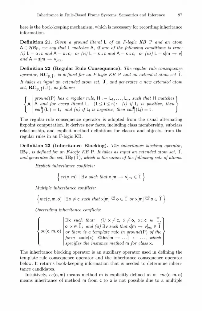
Inheritance in Rule-Based Frame Systems: Semantics and Inference 97
here is the book-keeping mechanism, which is necessary for recording inheritanceinformation.
Definition 21. Given a ground literal L of an F-logic KB P and an atomA ∈ HBP, we say that L matches A, if one of the following conditions is true:(i) L = o : c and A = o : c; or (ii) L = s :: c and A = s :: c; or (iii) L = s[m → v]and A = s[m → v]ex.
Definition 22 (Regular Rule Consequence). The regular rule consequenceoperator, RCP,�I , is defined for an F-logic KB P and an extended atom set I .
It takes as input an extended atom set, J , and generates a new extended atomset, RCP,�I ( J ), as follows:
⎧⎨
⎩A
∣∣∣∣∣∣
ground(P) has a regular rule, H :− L1, . . . , Ln, such that H matchesA and for every literal Li (1 ≤ i ≤ n): (i) if Li is positive, thenvalb
�J (Li) = t; and (ii) if Li is negative, then valb�I (Li) = t.
⎫⎬
⎭
The regular rule consequence operator is adopted from the usual alternatingfixpoint computation. It derives new facts, including class membership, subclassrelationship, and explicit method definitions for classes and objects, from theregular rules in an F-logic KB.
Definition 23 (Inheritance Blocking). The inheritance blocking operator,IBP, is defined for an F-logic KB P. It takes as input an extended atom set, I ,and generates the set, IBP( I ), which is the union of the following sets of atoms.
Explicit inheritance conflicts:{
ec(o, m) | ∃ v such that o[m → v]ex ∈ I}
Multiple inheritance conflicts:{mc(c, m, o)
∣∣∣∃ x �= c such that x[m] val
� o ∈ I or x[m] code� o ∈ I
}
Overriding inheritance conflicts:⎧⎪⎪⎪⎪⎨
⎪⎪⎪⎪⎩
ov(c, m, o)
∣∣∣∣∣∣∣∣∣∣
∃ x such that: (i) x �= c, x �= o, x :: c ∈ I ,o : x ∈ I ; and (ii) ∃ v such that x[m → v]ex ∈ Ior there is a template rule in ground(P) of theform code(x) @this[m → . . .] :− . . . , whichspecifies the instance method m for class x.
⎫⎪⎪⎪⎪⎬
⎪⎪⎪⎪⎭
The inheritance blocking operator is an auxiliary operator used in defining thetemplate rule consequence operator and the inheritance consequence operatorbelow. It returns book-keeping information that is needed to determine inheri-tance candidates.
Intuitively, ec(o, m) means method m is explicitly defined at o; mc(c, m, o)means inheritance of method m from c to o is not possible due to a multiple

98 G. Yang and M. Kifer
inheritance conflict (because there is a value or a code inheritance candidateother than c); ov(c, m, o) means inheritance of method m from c by o would beoverridden by another class that stands between o and c in the class hierarchy.From Definition 23 we can see that a class must have a explicitly defined valuefor a method or have an instance method definition to be able to override in-heritance from its superclasses. The following lemmas follow directly from theabove definitions.
Lemma 3. Given an interpretation I = 〈T; U 〉 of an F-logic KB P:(1) for all c, m, o: there is x such that x strongly overrides c[m] for o iff
ov(c, m, o) ∈ IBP(T).(2) for all c, m, o: there is x such that x strongly or weakly overrides c[m]
for o iff ov(c, m, o) ∈ IBP(T ∪ U).
Lemma 4. Given an interpretation I = 〈T; U 〉 of an F-logic KB P:
(1) for all c, m, o: c[m] s.val�I o iff (i) c �= o, o : c ∈ T; (ii) c[m → v]ex ∈ T
for some v; and (iii) ov(c, m, o) /∈ IBP(T ∪ U).(2) for all c, m, o: c[m] s.code
� I o iff (i) c �= o, o : c ∈ T; (ii) there is atemplate rule in ground(P) which specifies the instance method m forclass c; and (iii) ov(c, m, o) /∈ IBP(T ∪ U).
(3) for all c, m, o: c[m] s.val�I o or c[m] w.val
� I o iff (i) c �= o, o : c ∈ T ∪ U;(ii) c[m → v]ex ∈ T ∪ U for some v; and (iii) ov(c, m, o) /∈ IBP(T).
(4) for all c, m, o: c[m] s.code� I o or c[m] w.code
� I o iff (i) c �= o, o : c ∈ T ∪ U;(ii) there is a template rule in ground(P) which specifies the instancemethod m for class c; and (iii) ov(c, m, o) /∈ IBP(T).
(5) for all c, m, o: c[m]�I o iff (i) c �= o, o : c ∈ T ∪ U; (ii) there is atemplate rule in ground(P) which specifies the instance method m forclass c or c[m → v]ex ∈ T∪U for some v; and (iii) ov(c, m, o) /∈IBP(T).
Definition 24 (Template Rule Consequence). The template rule conse-quence operator, TCP,�I , is defined for an F-logic KB P and an extended atom
set I . It takes as input an extended atom set, J , and generates a new extendedatom set, TCP,�I ( J ), as follows:
⎧⎪⎪⎪⎪⎪⎨
⎪⎪⎪⎪⎪⎩
o[m → v] ccode
∣∣∣∣∣∣∣∣∣∣∣
c[m] code� o ∈ J , ec(o, m) /∈ IBP( I ), mc(c, m, o) /∈ IBP( I );
ground(P) has a template rule code(c) @this[m → v] :− Band for every literal L ∈ B‖o:
(i) if L is positive, then valb�J (L) = t, and
(ii) if L is negative, then valb�I (L) = t.
⎫⎪⎪⎪⎪⎪⎬
⎪⎪⎪⎪⎪⎭
The template rule consequence operator is used to derive new facts as a re-sult of code inheritance. It is similar to the regular rule consequence operatorexcept that the regular rule consequence operator is applied to all regular ruleswhereas the template rule consequence operator is applied only to those selectedtemplate rules that could be inherited according to our inheritance semantics.

Inheritance in Rule-Based Frame Systems: Semantics and Inference 99
Given an object o and a template rule, code(c) @this[m → v] :− B, whichdefines instance method m for class c, we first need to decide whether o caninherit this instance method definition from c. If so, then we will bind thisinstance method definition for o and evaluate it (note that B‖o is obtained fromB by substituting o for every occurrence of @this in B). If the rule body issatisfied in the context of o, we will derive o[m → v] c
code to represent the factthat m → v is established for o by inheritance of an instance method definitionfrom c.
We can decide whether object o can inherit the definitions of instance methodm from class c by looking up the two sets J and IBP( I ). In particular, such codeinheritance can happen only if the following conditions are true: (i) c[m] is acode inheritance candidate for o (c[m] code
� o ∈ J ); (ii) method m is not explicitlydefined at o (ec(o, m) /∈ IBP( I )); and (iii) there is no multiple inheritanceconflict (mc(c, m, o) /∈ IBP( I )).
Definition 25 (Inheritance Consequence). The inheritance consequenceoperator, ICP,�I , where P is an F-logic KB and I is an extended atom set,
takes as input an extended atom set, J , and generates a new extended atom setas follows:
ICP,�I ( J ) def= ICt ( J ) ∪ ICcP,�I ( J ) ∪ ICi
P,�I ( J ), where
ICt( J ) ={
o : c∣∣∣∃ x such that o : x ∈ J , x :: c ∈ J
}∪
{s :: c
∣∣∣ ∃ x such that s :: x ∈ J , x :: c ∈ J
}
ICcP,�I ( J ) =
{
c[m] val� o
∣∣∣∣o : c ∈ J , c �= o, c[m → v]ex ∈ J , andov(c, m, o) /∈ IBP( I )
}
∪⎧⎨
⎩c[m] code
� o
∣∣∣∣∣∣
o : c ∈ J , c �= o, there is a template rule inground(P) which specifies the instance method mfor class c, and ov(c, m, o) /∈ IBP( I )
⎫⎬
⎭
ICiP,�I ( J ) =
{
o[m → v] cval
∣∣∣∣c[m] val
� o ∈ J , c[m → v]ex ∈ J ,ec(o, m) /∈ IBP( I ), and mc(c, m, o) /∈ IBP( I )
}
The inheritance consequence operator, ICP,�I , is the union of three operators:ICt , ICc
P,�I , and ICiP,�I . The operator ICt is used to perform transitive closure of
the class hierarchy, including class membership and subclass relationship. Valueand code inheritance candidates are computed by the operator ICc
P,�I , which
relies on the overriding information provided by IBP( I ). Finally, the operatorICi
P,�I derives new facts by value inheritance. This operator also relies on the
information provided by IBP( I ).

100 G. Yang and M. Kifer
Definition 26 (KB Completion). The KB completion operator, TP,�I , where
P is an F-logic KB and I an extended atom set, takes as input an extended atomset, J , and generates a new extended atom set as follows:
TP,�I ( J ) def= RCP,�I ( J ) ∪ TCP,�I ( J ) ∪ ICP,�I ( J )
The KB completion operator is the union of the regular rule consequence oper-ator, the template rule consequence operator, and the inheritance consequenceoperator. It derives new “explicit” method definitions (via regular rules in theKB), new inherited facts (by value and code inheritance), plus inheritance can-didacy information that is used to decide which facts to inherit in the future.
We have the following lemma regarding the monotonicity property of theoperators that we have defined so far.
Lemma 5. Suppose P and I are fixed. Then the following operators are mono-tonic: RCP,�I , IBP, TCP,�I , ICt , ICc
P,�I , ICiP,�I , ICP,�I , TP,�I .
Given an F-logic KB P, the set of all subsets of the extended Herbrand baseHBP constitutes a complete lattice where the partial ordering is defined by setinclusion. Therefore, any monotonic operator, Φ, defined on this lattice has aunique least fixpoint lfp(Φ) [28].
Definition 27 (Alternating Fixpoint). The alternating fixpoint operator, ΨP,for an F-logic KB P takes as input an extended atom set, I , and generates a newextended atom set as follows: ΨP( I ) def= lfp(TP,�I ).
Definition 28 (F-logic Fixpoint). The F-logic fixpoint operator, FP, whereP is an F-logic KB, takes as input an extended atom set, I , and generates a newextended atom set as follows: FP( I ) def= ΨP(ΨP( I )).
Lemma 6. Let I be an extended atom set of an F-logic KB P, J = ΨP( I ).Then:
(1) for all c, m, o: if c[m] val� o ∈ J then c �= o.
(2) for all c, m, o: if c[m] code� o ∈ J then c �= o.
(3) for all o, m, v, c: o[m → v] cval ∈ J iff o[m → v] c
val ∈ ICiP,�I ( J ).
(4) for all o, m, v, c: o[m → v] ccode ∈ J iff o[m → v] c
code ∈ TCP,�I ( J ).
(5) for all o, m, v, c: if o[m → v] cval ∈ J then c �= o.
(6) for all o, m, v, c: if o[m → v] ccode ∈ J then c �= o.
Lemma 7. ΨP is antimonotonic when P is fixed.
Lemma 8. FP is monotonic when P is fixed.
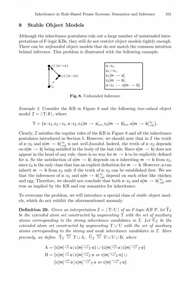
Inheritance in Rule-Based Frame Systems: Semantics and Inference 101
8 Stable Object Models
Although the inheritance postulates rule out a large number of unintended inter-pretations of F-logic KBs, they still do not restrict object models tightly enough.There can be unfounded object models that do not match the common intuitionbehind inference. This problem is illustrated with the following example.
o
c1[m−>a]
c2[m−>b]
o : c1.c2 :: c1.c1[m → a].c2[m → b].o : c2 :− o[m → b].
Fig. 8. Unfounded Inference
Example 2. Consider the KB in Figure 8 and the following two-valued objectmodel I = 〈T; ∅ 〉, where
T = {o : c1, c2 :: c1, o : c2, c1[m → a]ex, c2[m → b]ex, o[m → b] c2val}.
Clearly, I satisfies the regular rules of the KB in Figure 8 and all the inheritancepostulates introduced in Section 5. However, we should note that in I the truthof o : c2 and o[m → b] c2
val is not well-founded. Indeed, the truth of o : c2 dependson o[m → b] being satisfied in the body of the last rule. Since o[m → b] does notappear in the head of any rule, there is no way for m → b to be explicitly definedfor o. So the satisfaction of o[m → b] depends on o inheriting m → b from c2,since c2 is the only class that has an explicit definition for m → b. However, o caninherit m → b from c2 only if the truth of o : c2 can be established first. We seethat the inferences of o : c2 and o[m → b] c2
val depend on each other like chickenand egg. Therefore, we should not conclude that both o : c2 and o[m → b] c2
val aretrue as implied by the KB and our semantics for inheritance.
To overcome the problem, we will introduce a special class of stable object mod-els, which do not exhibit the aforementioned anomaly.
Definition 29. Given an interpretation I = 〈T; U 〉 of an F-logic KB P, let TIbe the extended atom set constructed by augmenting T with the set of auxiliaryatoms corresponding to the strong inheritance candidates in I. Let UI be theextended atom set constructed by augmenting T ∪ U with the set of auxiliaryatoms corresponding to the strong and weak inheritance candidates in I. Moreprecisely, we define TI
def= T ∪ A, UIdef= T ∪ U ∪ B, where
A = {c[m] val� o | c[m] s.val
�I o} ∪ {c[m] code� o | c[m] s.code
� I o}B = {c[m] val
� o | c[m] s.val�I o or c[m] w.val
� I o} ∪{c[m] code
� o | c[m] s.code� I o or c[m] w.code
� I o}

102 G. Yang and M. Kifer
Definition 30 (Stable Interpretation). Let I = 〈T; U 〉 be an interpretationof an F-logic KB P. I is called a stable interpretation of P, if TI = ΨP(UI) andUI = ΨP(TI).
Our definition of stable interpretations is closely related to that of stable modelsintroduced in [16,35]. The idea is that given an interpretation I of an F-logic KBP, we first resolve all negative premises using the information in I. The result isa residual positive KB without negation. Then I is said to be stable if and onlyif I can reproduce itself via the least fixpoint computation over the residual KB.This is how stable interpretations can prevent the kind of unfounded inferenceillustrated in Example 2.
We should note that Definition 30 only requires that a stable interpretationI = 〈T; U 〉 satisfy a certain computational property with respect to ΨP, i.e.,TI = ΨP(UI) and UI = ΨP(TI). In fact, it turns out that a stable interpretationof an F-logic KB P satisfies all the regular rules and template rules in P as wellas all the core and cautious inheritance postulates.
Theorem 1. Let I = 〈T; U 〉 be a stable interpretation of an F-logic KB P.Then I is an object model of P. Moreover, I satisfies the cautious ISA transitivityconstraint and the cautious inheritance constraint.
Proof. By Definition 20, and by Propositions 1, 2, 3, 4, 5, 6, and 7.
Since, by Theorem 1, stable interpretations satisfy all the requirements for objectmodels, we will start referring to stable interpretations as stable object models.
There is an interesting correspondence between stable object models and fix-points of FP. On one hand, it can be easily seen that stable object models areessentially fixpoints of FP. Let I = 〈T; U 〉 be a stable object model of an F-logicKB P. Then TI = ΨP(UI) and UI = ΨP(TI), by Definition 30. It follows thatTI = ΨP(UI) = ΨP(ΨP(TI)) = FP(TI) and so TI is a fixpoint of FP. Similarly,UI is also a fixpoint of FP. Moreover, TI ⊆ UI by Definition 29.
The following theorem shows that stable object models can be constructedusing certain fixpoints of FP.
Theorem 2. Let P be an F-logic KB, J a fixpoint of FP, K = ΨP( J ), andJ ⊆ K . Then I = 〈π( J ); π( K ) − π( J ) 〉, where π is the projection functiondefined in Section 7, is a stable object model of P.
Proof. Let T = π( J ) and U = π( K ) − π( J ). Thus I = 〈T; U 〉. Since J ⊆ K ,it follows that π( J ) ⊆ π( K ), and so T ∪ U = π( K ). To show that I is a stableobject model of P, we need to establish that TI = ΨP(UI) and UI = ΨP(TI).Since J is a fixpoint of FP and K = ΨP( J ), it follows that J=ΨP( K ), byDefinition 28. Therefore, if we can show that TI = J and UI = K , then itfollows that I is a stable object model of P.
Since J = ΨP( K ) = lfp(TP, �K ) and K = ΨP( J ) = lfp(TP,�J ), we can derivethe following equations, by Definitions 26 and 25:
J = RCP, �K ( J ) ∪ TCP, �K ( J ) ∪ ICt( J ) ∪ ICcP, �K ( J ) ∪ ICi
P, �K ( J )

Inheritance in Rule-Based Frame Systems: Semantics and Inference 103
K = RCP,�J ( K ) ∪ TCP,�J ( K ) ∪ ICt( K ) ∪ ICcP,�J ( K ) ∪ ICi
P,�J ( K )
First we will show that for all c, m, o: c[m] val� o ∈ J iff c[m] s.val
�I o. Indeed,c[m] val
� o ∈ J , iff c[m] val� o ∈ ICc
P, �K ( J ), iff c �= o, o : c ∈ J , c[m → v]ex ∈ J
for some v, and ov(c, m, o) /∈ IBP( K ), by Definition 25, iff c �= o, o : c ∈ π( J ),c[m → v]ex ∈ π( J ) for some v, and ov(c, m, o) /∈ IBP(π( K )), iff c �= o, o : c ∈ T,c[m → v]ex ∈ T for some v, and ov(c, m, o) /∈ IBP(T ∪ U), iff c[m] s.val
�I o, byLemma 4. Similarly, we can also show that (i) for all c, m, o: c[m] code
� o ∈ J iffc[m] s.code
� I o; and (ii) for all c, m, o: c[m] val� o ∈ K or c[m] code
� o ∈ K iff c[m] �I o.Therefore, it follows that TI = J and UI = K by Definition 29. This completesthe proof.
It is worth pointing out that the condition J ⊆ K in Theorem 2 is not necessaryfor constructing a stable object model out of the extended sets J and K . Infact, the following example shows that there is an F-logic KB P such that J isa fixpoint of FP, K = ΨP( J ), and J � K , but I = 〈π( J ); π( K ) − π( J ) 〉 is astable object model of P.
o
c1[m−>a]
c2[m−>b] o : c1.c1[m → a].c1 :: c2 :− c2[m → b].c2[m → b] :− ¬ c1 :: c2.c1 :: c2 :− o[m → a].c2[m → b] :− o[m → a].
Fig. 9. Constructive Fixpoints
Example 3. Consider the F-logic KB P in Figure 9 and the following two ex-tended sets J and K :
J = {o : c1, c1[m → a]ex, o[m → a] c1val, c1 :: c2, c2[m → b]ex} ∪
{c1[m] val� o, c2[m] val
� o}K = {o : c1, c1[m → a]ex} ∪ {c1[m] val
� o}
One can verify that J = ΨP( K ), K = ΨP( J ), and so J is a fixpoint ofΨP. Moreover, π( J ) = {o : c1, c1[m → a]ex, o[m → a] c1
val, c1 :: c2, c2[m → b]ex},π( K )−π( J ) = ∅. We can also verify that I = 〈π( J ); π( K )−π( J ) 〉 is a stableobject model of P. But clearly J − K �= ∅. Thus J � K .
Another interesting question is whether we can always construct stable objectmodels of an F-logic KB P from fixpoints of ΨP. The answer turns out to be no.The following example shows that some F-logic KBs may have fixpoints fromwhich we cannot even construct an object model for that KB.
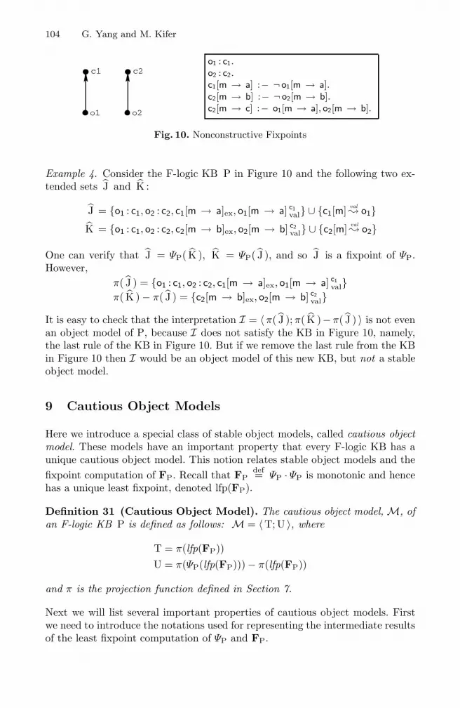
104 G. Yang and M. Kifer
o2o1
c2c1o1 : c1.o2 : c2.c1[m → a] :− ¬ o1[m → a].c2[m → b] :− ¬ o2[m → b].c2[m → c] :− o1[m → a], o2[m → b].
Fig. 10. Nonconstructive Fixpoints
Example 4. Consider the F-logic KB P in Figure 10 and the following two ex-tended sets J and K :
J = {o1 : c1, o2 : c2, c1[m → a]ex, o1[m → a] c1val} ∪ {c1[m] val
� o1}K = {o1 : c1, o2 : c2, c2[m → b]ex, o2[m → b] c2
val} ∪ {c2[m] val� o2}
One can verify that J = ΨP( K ), K = ΨP( J ), and so J is a fixpoint of ΨP.However,
π( J ) = {o1 : c1, o2 : c2, c1[m → a]ex, o1[m → a] c1val}
π( K ) − π( J ) = {c2[m → b]ex, o2[m → b] c2val}
It is easy to check that the interpretation I = 〈π( J ); π( K )−π( J ) 〉 is not evenan object model of P, because I does not satisfy the KB in Figure 10, namely,the last rule of the KB in Figure 10. But if we remove the last rule from the KBin Figure 10 then I would be an object model of this new KB, but not a stableobject model.
9 Cautious Object Models
Here we introduce a special class of stable object models, called cautious objectmodel. These models have an important property that every F-logic KB has aunique cautious object model. This notion relates stable object models and thefixpoint computation of FP. Recall that FP
def= ΨP · ΨP is monotonic and hencehas a unique least fixpoint, denoted lfp(FP).
Definition 31 (Cautious Object Model). The cautious object model, M, ofan F-logic KB P is defined as follows: M = 〈T; U 〉, where
T = π(lfp(FP))U = π(ΨP(lfp(FP))) − π(lfp(FP))
and π is the projection function defined in Section 7.
Next we will list several important properties of cautious object models. Firstwe need to introduce the notations used for representing the intermediate resultsof the least fixpoint computation of ΨP and FP.
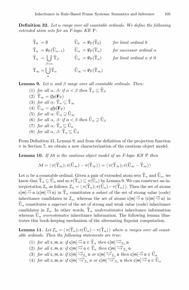
Inheritance in Rule-Based Frame Systems: Semantics and Inference 105
Definition 32. Let α range over all countable ordinals. We define the followingextended atom sets for an F-logic KB P:
T0 = ∅ U0 = ΨP(T0) for limit ordinal 0
Tα = ΨP(Uα−1) Uα = ΨP(Tα) for successor ordinal α
Tα =⋃
β<α
Tβ Uα = ΨP(Tα) for limit ordinal α �= 0
T∞ =⋃
α
Tα U∞ = ΨP(T∞)
Lemma 9. Let α and β range over all countable ordinals. Then:(1) for all α, β: if α < β then Tα ⊆ Tβ
(2) T∞ = lfp(FP)(3) for all α: Tα ⊆ T∞(4) U∞ = gfp(FP)(5) for all α: Uα ⊇ U∞(6) for all α, β: if α < β then Uα ⊇ Uβ
(7) for all α: Tα ⊆ Uα
(8) for all α, β: Tα ⊆ Uβ
From Definition 31, Lemma 9, and from the definition of the projection functionπ in Section 7, we obtain a new characterization of the cautious object model.
Lemma 10. If M is the cautious object model of an F-logic KB P then
M = 〈π(T∞); π(U∞) − π(T∞) 〉 = 〈π(T∞); π(U∞ − T∞) 〉
Let α be a countable ordinal. Given a pair of extended atom sets Tα and Uα, weknow that Tα ⊆ Uα and so π(Tα) ⊆ π(Uα) by Lemma 9. We can construct an in-terpretation Iα as follows: Iα = 〈π(Tα); π(Uα)−π(Tα) 〉. Then the set of atomsc[m] val
� o (c[m] code� o) in Tα constitutes a subset of the set of strong value (code)
inheritance candidates in Iα, whereas the set of atoms c[m] val� o (c[m] code
� o) inUα constitutes a superset of the set of strong and weak value (code) inheritancecandidates in Iα. In other words, Tα underestimates inheritance informationwhereas Uα overestimates inheritance information. The following lemma illus-trates this book-keeping mechanism of the alternating fixpoint computation.
Lemma 11. Let Iα = 〈π(Tα); π(Uα) − π(Tα) 〉 where α ranges over all count-able ordinals. Then the following statements are true:
(1) for all c, m, o: if c[m] val� o ∈ Tα then c[m] s.val
�Iα o(2) for all c, m, o: if c[m] code
� o ∈ Tα then c[m] s.code� Iα o
(3) for all c, m, o: if c[m] s.val�Iα o or c[m] w.val
� Iα o then c[m] val� o ∈ Uα
(4) for all c, m, o: if c[m] s.code� Iα o or c[m] w.code
� Iα o then c[m] code� o ∈ Uα

106 G. Yang and M. Kifer
Lemma 12. Let M be the cautious object model of an F-logic KB P. Then thefollowing statements are true:
(1) for all c, m, o: c[m] s.val�M o iff c[m] val
� o ∈ T∞(2) for all c, m, o: c[m] s.code
� M o iff c[m] code� o ∈ T∞
(3) for all c, m, o: c[m] s.val�M o or c[m] w.val
�M o iff c[m] val� o ∈ U∞
(4) for all c, m, o: c[m] s.code� M o or c[m] w.code
� M o iff c[m] code� o ∈ U∞
The lemma above says that T∞ includes exactly all the strong inheritance candi-dates while U∞ includes exactly all the strong and weak inheritance candidatesin M. This essentially implies that the cautious object model is indeed a stableobject model.
Theorem 3. The cautious object model M of an F-logic KB P is a stable objectmodel of P.
Proof. Let M = 〈T; U 〉 be the cautious object model of P. Then T = π(T∞)and U = π(U∞) − π(T∞). So by Definition 29 and Lemma 12, TM = T∞ andUM = U∞. Moreover, U∞ = ΨP(T∞) and T∞ = ΨP(U∞) by Definition 32 andLemma 9. It follows that TM = ΨP(UM) and UM = ΨP(TM). Therefore, M isa stable interpretation and thus a stable object model of P.
c2
o[f−>x]
c1[m−>a]o : c1.c2 :: c1.o : c2 :− o[m → a].o[f → x].c1[m → a].
code(c2) @this[m → b] :− @this[f → x].
Fig. 11. Computation of Cautious Object Models
Example 5. We illustrate the computation of cautious object models using theF-logic KB P in Figure 11. First let T and U denote the following sets of atoms:
T = {o : c1, c2 :: c1, o[f → x]ex, c1[m → a]ex}U = {o : c2, o[m → a] c1
val, o[m → b] c2code}
Then the computation process of ΨP is as follows:
T0 = ∅T1 = ΨP(T0) = T ∪ U ∪ {c1[m] val
� o, c2[m] code� o}
T2 = ΨP(T1) = TT3 = ΨP(T2) = T1
T4 = ΨP(T3) = T2
Therefore, lfp(FP) = T2 and ΨP(lfp(FP)) = T1, and so the cautious objectmodel of the KB in Figure 11 is 〈T; U 〉.

Inheritance in Rule-Based Frame Systems: Semantics and Inference 107
Theorem 3 gives a procedural characterization of the cautious object model,i.e., it is essentially defined as the least fixpoint of the extended alternatingfixpoint computation. Next we will present two additional characterizations ofthe cautious object model semantics.
First, by comparing the amount of “definite” information, i.e., truth and false-hood, that is contained in different stable object models of an F-logic KB P,we can define a partial order, called information ordering, among stable objectmodels.
Definition 33 (Information Ordering). Let I1 = 〈P1; Q1 〉, I2 = 〈P2; Q2 〉be two stable object models of an F-logic KB P, R1 = HBP − (P1 ∪ Q1),R2 = HBP − (P2 ∪ Q2). The information ordering on object models is definedas follows: I1 � I2 iff P1 ⊆ P2 and R1 ⊆ R2.
Intuitively, a stable object model is “smaller” in the information ordering, if itcontains fewer true facts and fewer false facts. Therefore, the least stable objectmodel contains the smallest set of true atoms and the smallest set of false atomsamong all stable object models.
Definition 34 (Least Stable Object Model). Let I be a stable object modelof an F-logic KB P. I is the least stable object model of P, if I � J for anystable object model J of P.
Theorem 4. The cautious object model M of an F-logic KB P is the leaststable object model of P.
Proof. Let I = 〈T; U 〉 be any stable object model of P. We need to show thatM � I. Recall that M = 〈π(T∞); π(U∞) − π(T∞) 〉. Therefore, to show thatM � I, it suffices to show that π(T∞) ⊆ T and π(U∞) ⊇ T ∪ U. Since Iis a stable object model of P, it follows that TI = ΨP(UI) and UI = ΨP(TI).Therefore, TI = ΨP(UI) = ΨP(ΨP(TI)) = FP(TI) and so TI is a fixpoint of FP.Similarly, UI is also a fixpoint of FP. But T∞ = lfp(FP) and U∞ = gfp(FP), byLemma 9. It follows that T∞ ⊆ TI and U∞ ⊇ UI . Thus π(T∞) ⊆ π(TI) andπ(U∞) ⊇ π(UI). Moreover, π(TI) = T and π(UI) = T ∪ U, by Definition 29.So π(T∞) ⊆ T and π(U∞) ⊇ T ∪ U.
Besides comparing different models of a KB with respect to information ordering,it is also common to compare different models based on the amount of “truth”contained in the models. Typically, the true component of a model is minimizedand the false component maximized. However, in F-logic we also need to dealwith inheritance, which complicates the matters a bit, because some facts maybe derived via inheritance. As a consequence, there are object models that looksimilar but are actually incomparable. This leads to the following definitionof truth ordering among object models, which minimizes not only the set oftrue atoms of an object model, but also the amount of positive inheritanceinformation implied by the object model.
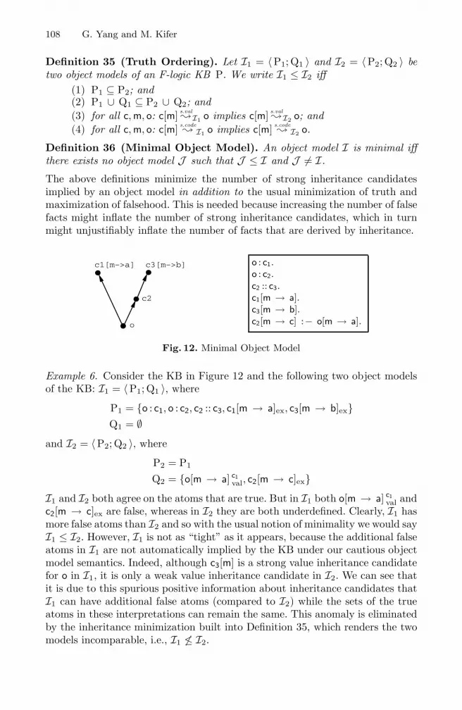
108 G. Yang and M. Kifer
Definition 35 (Truth Ordering). Let I1 = 〈P1; Q1 〉 and I2 = 〈P2; Q2 〉 betwo object models of an F-logic KB P. We write I1 ≤ I2 iff
(1) P1 ⊆ P2; and(2) P1 ∪ Q1 ⊆ P2 ∪ Q2; and(3) for all c, m, o: c[m] s.val
�I1 o implies c[m] s.val�I2 o; and
(4) for all c, m, o: c[m] s.code� I1 o implies c[m] s.code
� I2 o.
Definition 36 (Minimal Object Model). An object model I is minimal iffthere exists no object model J such that J ≤ I and J �= I.
The above definitions minimize the number of strong inheritance candidatesimplied by an object model in addition to the usual minimization of truth andmaximization of falsehood. This is needed because increasing the number of falsefacts might inflate the number of strong inheritance candidates, which in turnmight unjustifiably inflate the number of facts that are derived by inheritance.
c3[m−>b]
o
c1[m−>a]
c2
o : c1.o : c2.c2 :: c3.c1[m → a].c3[m → b].c2[m → c] :− o[m → a].
Fig. 12. Minimal Object Model
Example 6. Consider the KB in Figure 12 and the following two object modelsof the KB: I1 = 〈P1; Q1 〉, where
P1 = {o : c1, o : c2, c2 :: c3, c1[m → a]ex, c3[m → b]ex}Q1 = ∅
and I2 = 〈P2; Q2 〉, where
P2 = P1
Q2 = {o[m → a] c1val, c2[m → c]ex}
I1 and I2 both agree on the atoms that are true. But in I1 both o[m → a] c1val and
c2[m → c]ex are false, whereas in I2 they are both underdefined. Clearly, I1 hasmore false atoms than I2 and so with the usual notion of minimality we would sayI1 ≤ I2. However, I1 is not as “tight” as it appears, because the additional falseatoms in I1 are not automatically implied by the KB under our cautious objectmodel semantics. Indeed, although c3[m] is a strong value inheritance candidatefor o in I1, it is only a weak value inheritance candidate in I2. We can see thatit is due to this spurious positive information about inheritance candidates thatI1 can have additional false atoms (compared to I2) while the sets of the trueatoms in these interpretations can remain the same. This anomaly is eliminatedby the inheritance minimization built into Definition 35, which renders the twomodels incomparable, i.e., I1 �≤ I2.

Inheritance in Rule-Based Frame Systems: Semantics and Inference 109
Theorem 5. The cautious object model M of an F-logic KB P is minimalamong those object models of P that satisfy the cautious ISA transitivity con-straint and the cautious inheritance constraint.
Proof. This proof is long and is relegated to Section A.2 of the Appendix.
10 Implementation
It turns out that the (unique) cautious object model of an F-logic KB P canbe computed as the well-founded model of a certain general logic program withnegation, which is obtained from P via rewriting. Before describing the rewritingprocedure we first define a rewriting function that applies to all regular rules andtemplate rules.
Definition 37. Given an F-logic KB P and a literal L in P, the functions ρh
and ρb that rewrite head and body literals in P are defined as follows:
ρh(L) =
���
isa(o, c), if L = o : csub(s, c), if L = s :: cexmv(s,m, v), if L = s[m → v]
ρb(L) =
�������
isa(o, c), if L = o : csub(s, c), if L = s :: cmv(o, m, v), if L = o[m → v]¬ (ρb(G)), if L = ¬ G
The rewriting function ρ on regular rules and template rules in P is defined asfollows:
ρ(H :− L1, . . . , Ln) = ρh(H) :− ρb(L1), . . . , ρb(Ln)
ρ(code(c) @this[m → v] :− L1, . . . , Ln) = ins(O, m, v, c) :− ρb(B1), . . . , ρb(Bn)
where O is a new variable that does not appear in P and, each Bi = (Li)‖O, i.e.,Bi is obtained from Li by substituting O for all occurrences of the template term@this. The predicates, isa, sub, exmv, mv, and ins, are auxiliary predicatesintroduced by the rewriting.
Note that since literals in rule heads and bodies have different meanings, theyare rewritten differently. Moreover, literals in the heads of regular rules andtemplate rules are also rewritten differently. The rewriting procedure that trans-forms F-logic KBs into general logic programs is defined next.
Definition 38 (Well-Founded Rewriting). The well-founded rewriting of anF-logic KB P, denoted Pwf , is a general logic program constructed by the fol-lowing steps:
(1) For every regular rule R in P, add its rewriting ρ(R) into Pwf ;(2) For every template rule R in P, which specifies an instance method m
for a class c, add its rewriting ρ(R) into Pwf . Moreover, add a factcodedef(c, m) into Pwf ;
(3) Include the trailer rules shown in Figure 13 to Pwf (note that uppercaseletters denote variables in these trailer rules).

110 G. Yang and M. Kifer
mv(O,M, V) :− exmv(O,M, V).mv(O,M, V) :− vamv(O,M, V, C).mv(O,M, V) :− comv(O,M, V, C).
sub(S, C) :− sub(S,X), sub(X, C).isa(O, C) :− isa(O,S), sub(S,C).
vamv(O,M, V, C) :− vacan(C, M, O), exmv(C,M, V), ¬ ex(O,M), ¬ multi(C, M, O).comv(O, M, V, C) :− cocan(C, M, O), ins(O, M, V, C), ¬ ex(O,M), ¬ multi(C, M, O).
vacan(C, M, O) :− isa(O,C), exmv(C,M, V), C �= O, ¬ override(C, M, O).cocan(C, M, O) :− isa(O,C), codedef(C, M), C �= O, ¬ override(C,M, O).
ex(O,M) :− exmv(O,M, V).multi(C, M, O) :− vacan(X, M, O), X �= C.multi(C, M, O) :− cocan(X, M, O), X �= C.
override(C,M, O) :− sub(X, C), isa(O,X), exmv(X,M, V), X �= C, X �= O.override(C,M, O) :− sub(X, C), isa(O,X), codedef(X, M), X �= C, X �= O.
Fig. 13. Trailer Rules for Well-Founded Rewriting
Note that while rewriting an F-logic KB into a general logic program, weneed to output facts of the form codedef(c, m) to remember that there is atemplate rule specifying instance method m for class c. Such facts are used toderive overriding and code inheritance candidacy information.
There is a unique well-founded model for any general logic program [15].Next we will present a characterization of well-founded models based on thealternating fixpoint computation introduced in [42]. Given any general logicprogram P, we will use HBP to denote the Herbrand base of P, which consists ofall possible atoms constructed using the predicate symbols and function symbolsin P.
Definition 39. Let P be a general logic program and I a subset of HBP. Theoperator CP,I takes as input a set of atoms, J, and generates another set ofatoms, CP,I(J) ⊆ HBP, as follows:
⎧⎨
⎩H
∣∣∣∣∣∣
There is H :− A1, . . . , Am, ¬B1, . . . , ¬Bn ∈ ground(P), m ≥ 0,n ≥ 0, Ai (1 ≤ i ≤ m) and Bj (1 ≤ j ≤ n) are positive literals, andAi ∈ J for all 1 ≤ i ≤ m, Bj /∈ I for all 1 ≤ j ≤ n.
⎫⎬
⎭
Lemma 13. CP,I is monotonic when P and I are fixed.
It follows that CP,I has a unique least fixpoint. Having defined CP,I we canintroduce two more operators, SP and AP, as follows.
Definition 40. Let P be a general logic program and I be a subset of HBP.Then: SP(I) def= lfp(CP,I), AP(I) def= SP(SP(I)).
Lemma 14. SP is antimonotonic and AP is monotonic when P is fixed.
It follows that AP has a unique least fixpoint, denoted lfp(AP). The followinglemma from [42] explains how well-founded models can be defined in terms ofalternating fixpoints.

Inheritance in Rule-Based Frame Systems: Semantics and Inference 111
Lemma 15. The well-founded model, 〈T; U 〉, of a general logic program P,where T is the set of atoms that are true and U is the set of atoms that are under-defined, can be computed as follows: T = lfp(AP), U = SP(lfp(AP)) − lfp(AP).
Given the well-founded rewriting, Pwf , of an F-logic KB P, the Herbrand baseof Pwf , denoted HBPwf , consists of atoms of the following forms: isa/2, sub/2,exmv/3, vamv/4, ins/4, codedef/2, comv/4, mv/3, vacan/3, cocan/3, ex/2,multi/3, and override/3. We can establish an isomorphism between interpreta-tions of Pwf and P as follows.
Definition 41 (Isomorphism). Let Pwf be the well-founded rewriting of anF-logic KB P, HBPwf the Herbrand base of Pwf , HBP the extended Herbrandbase of P, Iwf a subset of HBPwf , and I a subset of HBP. We will say that Iwf
is isomorphic to I , if all of the following conditions hold:(1) for all o, c: isa(o, c) ∈ Iwf iff o : c ∈ I(2) for all s, c: sub(s, c) ∈ Iwf iff s :: c ∈ I(3) for all s, m, v: exmv(s, m, v) ∈ Iwf iff s[m → v]ex ∈ I(4) for all o, m, v, c: vamv(o, m, v, c) ∈ Iwf iff o[m → v] c
val ∈ I(5) for all o, m, v, c: comv(o, m, v, c) ∈ Iwf iff o[m → v] c
code ∈ I(6) for all c, m, o: vacan(c, m, o) ∈ Iwf iff c[m] val
� o ∈ I(7) for all c, m, o: cocan(c, m, o) ∈ Iwf iff c[m] code
� o ∈ I(8) for all o, m: ex(o, m) ∈ Iwf iff ec(o, m) ∈ IBP( I )(9) for all c, m, o: multi(c, m, o) ∈ Iwf iff mc(c, m, o) ∈ IBP( I )
(10) for all c, m, o: override(c, m, o) ∈ Iwf iff ov(c, m, o) ∈ IBP( I )Let Mwf be the well-founded model of Pwf and M the cautious object model ofP, Mwf = 〈Twf ; Uwf 〉, M = 〈π(T∞); π(U∞ − T∞) 〉. We will say that Mwf
is isomorphic to M, if Twf and Uwf are isomorphic to T∞ and U∞ − T∞,respectively.
Note that the definition above includes atoms which are not in any interpreta-tion of an F-logic KB P. However, if we can show that the well-founded modelof Pwf is isomorphic (according to the above definition) to the cautious ob-ject model M of P, we can then establish a one-to-one correspondence betweenisa(o, c) ∈ Mwf and o : c ∈ M, between sub(s, c) ∈ Mwf and s :: c ∈ M, betweenexmv(s, m, v) ∈ Mwf and s[m → v]ex ∈ M, between comv(o, m, v, c) ∈ Mwf
and o[m → v] ccode ∈ M, and between vamv(o, m, v, c) ∈ Mwf and o[m → v] c
val∈ M, taking into account the truth values of atoms. Thus the cautious objectmodel of P can be effectively computed by the well-founded model of Pwf .
Definition 42. Let Pwf be the well-founded rewriting of an F-logic KB P andIwf a subset of HBPwf . We will say that Iwf is in normal form, if for all o, m, v:mv(o, m, v) ∈ Iwf iff exmv(o, m, v) ∈ Iwf , or there is some class c such thatvamv(o, m, v, c) ∈ Iwf or comv(o, m, v, c) ∈ Iwf .
In the following we introduce notations to represent the intermediate resultsduring the computation of the well-founded model of a general logic program.These notations are used in the proof of the main theorem of this section.

112 G. Yang and M. Kifer
Definition 43. Let Pwf be the well-founded rewriting of an F-logic KB P. De-fine:
Twf0 = ∅ Uwf
0 = SPwf (Twf0 ) for limit ordinal 0
Twfα = SPwf (Uwf
α−1) Uwfα = SPwf (Twf
α ) for successor ordinal α
Twfα =
⋃
β<α
Twfβ Uwf
α = SPwf (Twfα ) for limit ordinal α �= 0
Twf∞ =
⋃
α
Twfα Uwf
∞ = SPwf (Twf∞ )
Now we are ready to present the main theorem of this section. This theoremrelies on a number of lemmas and propositions whose proofs are quite long; theycan be found in Section A.3 of the Appendix.
Theorem 6. Given the well-founded rewriting Pwf of an F-logic KB P, thewell-founded model of Pwf is isomorphic to the cautious object model of P.
Proof. Let Mwf = 〈Twf ; Uwf 〉 be the well-founded model of Pwf . Then byLemma 15, Twf = Twf
∞ and Uwf = Uwf∞ − Twf
∞ . Let M = 〈T; U 〉 be the cautiousobject model of P. Then by Lemma 10, T = π(T∞) and U = π(U∞ − T∞).Therefore, by Definition 41, to show that Mwf is isomorphic to M, it sufficesto show that Twf
∞ is isomorphic to T∞ and Uwf∞ is isomorphic to U∞.
First note that Twfα and Uwf
α are in normal form for any ordinal α, byProposition 9. Now we will prove by transfinite induction that Twf
α is isomorphicto Tα and Uwf
α is isomorphic to Uα, for any ordinal α. There are three cases toconsider:
(1) α = 0.The claim is vacuously true for Twf
0 and T0. Uwf0 = SPwf (Twf
0 ) = lfp(CPwf ,Twf0
),
by Definitions 43 and 40, and U0 = ΨP(T0) = lfp(TP,�T0), by Definitions 32
and 27. It follows that Uwf0 is isomorphic to U0, by Proposition 8.
(2) α is a successor ordinal.Then Twf
α = SPwf (Uwfα−1) = lfp(CPwf ,Uwf
α−1), by Definitions 43 and 40, and
Tα = ΨP(Uα−1) = lfp(TP,�Uα−1), by Definitions 32 and 27. Moreover, Uwf
α−1 is
isomorphic to Uα−1 by the induction hypothesis. It follows that Uwfα is isomor-
phic to Uα, by Proposition 8. Similarly to (1), we can also show that Uwfα is
isomorphic to Uα.
(3) α �= 0 is a limit ordinal.Then Twf
α =⋃
β<α Twfβ and Tα =
⋃β<α Tβ. Clearly, Twf
α is isomorphic to Tα,because Twf
β is isomorphic to Tβ for all β < α, by the induction hypothesis.Similarly to (1), we can also show that Uwf
α is isomorphic to Uα.

Inheritance in Rule-Based Frame Systems: Semantics and Inference 113
Note that Twf∞ =
⋃α Twf
α and T∞ =⋃
α Tα. Therefore, it follows that Twf∞
is isomorphic to T∞, because Twfα is isomorphic to Tα, for any ordinal α.
Moreover, Uwf∞ = SPwf (Twf
∞ ) = lfp(CPwf ,Twf∞
), by Definitions 43 and 40, and
U∞ = ΨP(T∞) = lfp(TP,�T∞), by Definitions 32 and 27. Thus Uwf
∞ is isomorphic
to U∞, by Proposition 8.
It is easy to see that Pwf can be computed in time linear in the size of theoriginal F-logic KB P. Also, the trailer rules in Figure 13 are fixed and do notdepend on P. Therefore, the size of Pwf is also linear relative to the size of theoriginal F-logic KB P. This observation, combined with Theorem 6, leads to thefollowing claim about the data complexity [43] of our inheritance semantics.
Theorem 7. The data complexity of the cautious object model semantics forfunction-free F-logic KBs is polynomial-time.
11 Related Work
Inheritance is one of the key aspects in frame-based knowledge representation.This problem has been studied quite extensively in the AI and database lit-erature. To make our comparison with the related work concrete, we first listthe main features of inheritance that we view should be supported by a generalframe-based knowledge system:
– Inference by default inheritance and inference via rules.– Intentional class hierarchies, i.e., the ability to define both class membership
and subclass relationship via rules.– Data-dependent and data-independent inheritance. As we have shown, value
inheritance is data-dependent, and this is the type of inheritance generallyconsidered in AI. Code inheritance is data-independent and is of the kindthat is common in imperative programming languages like C++ and Java.
– Overriding of inheritance from more general classes by more specific classes.Note that this also needs to take into account the interactions betweendata-dependent and data-independent inheritance.
– Nonmonotonic inheritance from multiple superclasses. Some proposals avoidthis problem by imposing syntactic restrictions on rules. To this end, theseproposals do not support nonmonotonic multiple inheritance.
– Introspection, by which variables can range over both class and methodnames.
– Late binding. This feature is common in imperative object-oriented lan-guages such as C++ and Java. Supporting late binding requires resolvingmethod names at runtime, when the class from which the instance methoddefinitions are inherited is decided.
There is a large body of work based on Touretzky’s framework of InheritanceNets [41]. On one hand, the overriding mechanism in this framework is more
114 G. Yang and M. Kifer
sophisticated than what is typically considered in the knowledge base context.On the other hand, this framework supports neither deductive inference via rulesnor intensional class hierarchies, which makes it too weak for many applicationsof knowledge bases. A survey on several different approaches to computing in-heritance semantics based on Inheritance Nets can be found in [26].
There is also vast literature on extending traditional relational database sys-tems with object-oriented features. However, these proposals do not supportdeduction via inference rules, which makes them mostly orthogonal to the prob-lems addressed in this paper. For a comprehensive survey on this subject werefer the readers to [23].
The original F-logic [21,22] resolved many semantic and proof-theoretic issuesin rule-based frame systems. However, the original semantics for inheritance inF-logic was problematic. It was defined through a nondeterministic inflationaryfixpoint and was not backed by a corresponding model theory. This semanticswas known to produce questionable results (cf. Section 3) when default inher-itance and inference via rules interact. In addition, only value inheritance wasconsidered in the original F-logic.
Ordered Logic [25] incorporates some aspects of the object-oriented paradigm.In this framework, both positive and negative literals are allowed in rule heads,and inference rules are grouped into a set of modules that collectively form astatic class hierarchy. Although Ordered Logic supports overriding and prop-agation of rules among different modules, the idea of late binding is not builtinto the logic. Since it is primarily committed to resolving inconsistency betweenpositive and negative literals, its semantics has a strong value-based value in-heritance flavor. Furthermore, this approach permits only fixed class hierarchiesand it does not support introspection.
Abiteboul et al. proposed a framework for implementing inheritance that isbased on program rewriting using Datalog with negation [1]. Our implementa-tion of the new F-logic semantics is close in spirit to their approach. However,their proposal is not backed by an independent model-theoretic formalization.Their framework further excludes nonmonotonic multiple inheritance and makesa very strong assumption that the rewritten knowledge base must have a total(two-valued) well-founded model. This latter assumption does not generally holdwithout strong syntactic restrictions that force stratification of the knowledgebase. The framework is also limited to value inheritance.
In [12], Dobbie and Topor developed a model theory for monotonic code in-heritance in their object-oriented deductive language Gulog. A special feature oftheir language is that all the variables in a rule must be explicitly typed accordingto a separate signature declaration. However, this language does not support anykind of nonmonotonic, data-dependent, or multiple inheritance. In [11], Dobbiefurther extends this approach to allow nonmonotonic inheritance. However, eventhis extension disallows interaction between inheritance and deduction and doesnot support multiple inheritance (the user must disambiguate inheritance con-flicts manually).

Inheritance in Rule-Based Frame Systems: Semantics and Inference 115
Liu et. al. [27] modified the original F-logic to support code inheritance. How-ever, to achieve that they had to throw out data-dependent inheritance, muchof introspection, and intensional class hierarchies.
Bugliesi and Jamil proposed a model-theoretic semantics for value and codeinheritance with overriding [5], which bears close resemblance to two-valued sta-ble models [16]. However, their semantics applies only to negation-free knowledgebases (a severe limitation) and does not handle multiple inheritance conflicts.Instead, it makes multiple inheritance behave additively. (Such behavior canbe easily simulated via rules.) In addition, their framework does not supportdata-dependent value inheritance, intensional class hierarchies, and more impor-tantly, it does not provide an algorithm to compute a canonical model undertheir semantics.
May et al. [32] applied the ideas behind the well-founded semantics to F-logic.However, inheritance is still dealt with in the same way as in the original F-logic.Deduction and inheritance are computed in two separate stages and so the com-putation process has an inflationary fixpoint flavor. As mentioned in Section 3,this semantics is known to produce counter-intuitive results when intensionalclass hierarchies interact with overriding and multiple inheritance. Code inheri-tance is also not handled by this semantics.
In [19,20], Jamil introduced a series of techniques to tackle the inheritanceproblem. Among these, the ideas of locality and context, which were proposedto resolve code inheritance and encapsulation in the language Datalog++, haveinfluenced our approach the most. However, this work does not come with amodel-theoretic inheritance semantics and supports neither intensional class hi-erarchies nor introspection. The inheritance semantics in [19] is defined by pro-gram rewriting while in [20] the approach is proof-theoretic.
Finally, May and Kandzia [31] showed that the original F-logic semantics canbe described using the inflationary extension of Reiter’s Default Logic [37]. Intheir framework, inheritance semantics is encoded using defaults. However, theirinheritance strategy is inflationary — once a fact is derived through inheritance,it is never undone. Therefore, a later inference might invalidate the originalconditions (encoded as justifications of defaults) for inheritance (cf. Section 3).Moreover, nonmonotonic multiple inheritance is handled in such a way thatwhen multiple incomparable inheritance sources exist, one of them is randomlyselected for inheritance instead of none (as in our framework). Code inheritanceis not considered in [31].
12 Conclusion and Future Work
We have developed a novel model theory and a computational framework fornonmonotonic multiple inheritance of value and code in rule-based frame sys-tems. We have shown that this semantics is implementable using a deductiveengine, such as XSB [7], that supports well-founded semantics [15]. The valueinheritance part of this semantics has been implemented in Flora-2 [44,46], aknowledge representation system, which is built around F-logic, HiLog [6], and

116 G. Yang and M. Kifer
Transaction Logic [4].5 Adding code inheritance to Flora-2 is planned for thenear future.
The semantics proposed in this paper can be extended — without adding tothe syntax — to allow a new kind of inheritable methods in addition to thetraditional instance methods. The idea is to allow the template term @this in atemplate rule to be instantiated not only with instances of the class for whichthe template rule is defined, but also with that class itself and its subclassesas well. Effectively this turns template rules into pieces of code that also defineclass methods and that are inheritable by subclasses. For instance, with such amodification, the template rule
code(employee) @this[avgSalary → A] :− A = avg{S|E :@this, E[salary → S]}.
where avg{...} is the averaging aggregate function, could be instantiated withclass employee itself to
employee[avgSalary → A] :− A = avg{S|E : employee, E[salary → S]}.
and instantiated with one of employee’s subclasses, secretary, to
secretary[avgSalary → A] :− A = avg{S|E : secretary, E[salary → S]}.
Similar rules could be obtained for other subclasses of employee, such as engineerand faculty. The last two rules above define the class method, avgSalary, forclasses employee and secretary. It returns the average salary of an employee anda secretary, respectively. This kind of methods is not possible using the earliermachinery of class and instance methods.
Our model-theoretic approach points to several future research directions.First, the proposed semantics for inheritance here can be viewed as source-based .This means that in determining whether a multiple inheritance conflict existsthe semantics takes into account only whether the same method is defined atdifferent inheritance sources. A conflict is declared even if they all return exactlythe same set of values. A content-based inheritance policy would not view thisas a conflict. Such content-based inheritance seems harder computationally, butis worth further investigation. Second, it has been observed that inheritance-likephenomena arise in many domains, such as discretionary access control and trustmanagement [18], but they cannot be formalized using a single semantics. Weare considering extensions to our framework to allow users to specify their ownad hoc inheritance policies in a programmable, yet declarative, way.
Acknowledgment
This work was supported in part by NSF grants IIS-0072927 and CCR-0311512.The authors would like to thank the anonymous referees for their helpful com-ments and suggestions.5 Flora-2 is freely available from http://flora.sourceforge.net

Inheritance in Rule-Based Frame Systems: Semantics and Inference 117
References
1. S. Abiteboul, G. Lausen, H. Uphoff, and E. Waller. Methods and rules. In ACMInternational Conference on Management of Data (SIGMOD), 1993.
2. J. Angele, E. Monch, H. Oppermann, S. Staab, and D. Wenke. Ontology-basedquery and answering in chemistry: OntoNova @ Project Halo. In InternationalSemantic Web Conference (ISWC), pages 913–928, 2003.
3. D. Berardi, H. Boley, B. Grosof, M. Gruninger, R. Hull, M. Kifer, D. Mar-tin, S. McIlraith, J. Su, and S. Tabet. SWSL: Semantic Web ServicesLanguage. Technical report, Semantic Web Services Initiative, April 2005.http://www.w3.org/Submission/SWSF-SWSL/.
4. A. J. Bonner and M. Kifer. An overview of transaction logic. Theoretical ComputerScience, 133(2):205–265, 1994.
5. M. Bugliesi and H. M. Jamil. A stable model semantics for behavioral inheritancein deductive object oriented languages. In International Conference on DatabaseTheory (ICDT), pages 222–237, 1995.
6. W. Chen, M. Kifer, and D. S. Warren. HiLog: A foundation for higher-order logicprogramming. Journal of Logic Programming (JLP), 15(3):187–230, 1993.
7. W. Chen and D. S. Warren. Tabled evaluation with delaying for general logicprograms. Journal of the ACM (JACM), 43(1):20–74, 1996.
8. J. de Bruijn, H. Lausen, R. Krummenacher, A. Polleres, L. Predoiu, and D. Fensel.The WSML family of representation languages. Technical report, DERI, March2005. http://www.w3.org/Submission/WSML/.
9. S. Decker, D. Brickley, J. Saarela, and J. Angele. A query and inference service forRDF. In QL’98 - The Query Languages Workshop, December 1998.
10. S. Decker, M. Erdmann, D. Fensel, and R. Studer. Ontobroker: Ontology based ac-cess to distributed and semi-structured information. In R. Meersman, editor, Data-base Semantics, Semantic Issues in Multimedia Systems, pages 351–369. KluwerAcademic Publisher, Boston, 1999.
11. G. Dobbie. Foundations of deductive object-oriented database systems. TechnicalReport CS-TR-96/13, Department of Computer Science, Victoria University, 1996.http://citeseer.ist.psu.edu/dobbie96foundations.html.
12. G. Dobbie and R. Topor. Resolving ambiguities caused by multiple inheritance. InInternational Conference on Deductive and Object-Oriented Databases (DOOD),pages 265–280, 1995.
13. DSTC, IBM, and CBOP. MOF Query/Views/Transformations. Technicalreport, Object Management Group (OMG), 2003. http://www.dstc.edu.au/Research/Projects/Pegamento/publications/ad-03-08-03.pdf.
14. J. Frohn, R. Himmeroder, G. Lausen, W. May, and C. Schlepphorst. Managingsemistructured data with FLORID: A deductive object-oriented perspective. In-formation Systems, 23(8):589–613, 1998.
15. A. V. Gelder, K. Ross, and J. S. Schlipf. The well-founded semantics for generallogic programs. Journal of the ACM (JACM), 38(3):620–650, 1991.
16. M. Gelfond and V. Lifschitz. The stable model semantics for logic programming.In International Conference on Logic Programming (ICLP), 1988.
17. A. Gerber, M. Lawley, K. Raymond, J. Steel, and A. Wood. Transformation:The missing link of MDA. In Graph Transformation: First International Confer-ence (ICGT), volume 2505 of Lecture Notes in Computer Science, pages 90–105.Springer Verlag, October 2002.

118 G. Yang and M. Kifer
18. S. Jajodia, P. Samarati, M. L. Sapino, and V. S. Subrahmanian. Flexible sup-port for multiple access control policies. ACM Transactions on Database Systems(TODS), 26(2):214–260, June 2001.
19. H. M. Jamil. Implementing abstract objects with inheritance in Datalogneg. InInternational Conference on Very Large Data Bases (VLDB), pages 46–65. MorganKaufmann, 1997.
20. H. M. Jamil. A logic-based language for parametric inheritance. In InternationalConference on Principles of Knowledge Representation and Reasoning (KR), 2000.
21. M. Kifer and G. Lausen. F-Logic: A higher-order language for reasoning about ob-jects, inheritance and schema. In ACM International Conference on Managementof Data (SIGMOD), pages 134–146, New York, 1989. ACM.
22. M. Kifer, G. Lausen, and J. Wu. Logical foundations of object-oriented and frame-based languages. Journal of the ACM (JACM), 42(4):741–843, 1995.
23. W. Kim and F. H. Lochovsky, editors. Object-Oriented Concepts, Databases, andApplications. ACM Press and Addison-Wesley, 1989.
24. R. Krishnan. Disruption tolerant networking: SPINDLE project. Technical report,The Internet Engineering Task Force, 2006.
25. E. Laenens and D. Vermeir. A fixpoint semantics for Ordered Logic. Journal ofLogic and Computation, 1(2):159–185, 1990.
26. L. V. S. Lakshmanan and K. Thirunarayan. Declarative frameworks for inheri-tance. In J. Chomicki and G. Saake, editors, Logics for Databases and InformationSystems, pages 357–388. Kluwer Academic Publishers, 1998.
27. M. Liu, G. Dobbie, and T. Ling. A logical foundation for deductive object-orienteddatabases. ACM Transactions on Database Systems (TODS), 27(1):117–151, 2002.
28. J. W. Lloyd. Foundations of Logic Programming. Springer Verlag, 1984.29. A. Magkanaraki, S. Alexaki, V. Christophides, and D. Plexousakis. Benchmarking
RDF Schemas for the Semantic Web. In International Semantic Web Conference(ISWC), pages 132–146, London, UK, 2002. Springer Verlag.
30. W. May. A rule-based querying and updating language for XML. In Interna-tional Workshop on Database Programming Languages (DBPL), Lecture Notes inComputer Science, pages 165–181. Springer Verlag, 2001.
31. W. May and P.-T. Kandzia. Nonmonotonic inheritance in object-oriented deductivedatabase languages. Journal of Logic and Computation, 11(4):499–525, 2001.
32. W. May, B. Ludascher, and G. Lausen. Well-founded semantics for deductiveobject-oriented database languages. In International Conference on Deductive andObject-Oriented Databases (DOOD), Lecture Notes in Computer Science, pages320–336. Springer Verlag, 1997.
33. Ontoprise, GmbH. Ontobroker. http://www.ontoprise.com/.34. T. C. Przymusinski. Every logic program has a natural stratification and an iter-
ated least fixed point model. In ACM International Symposium on Principles ofDatabase Systems (PODS), pages 11–21, New York, 1989. ACM.
35. T. C. Przymusinski. The well-founded semantics coincides with the three-valuedstable semantics. Fundamenta Informaticae, 13(4):445–464, 1990.
36. F. Rabitti, E. Bertino, W. Kim, and D. Woelk. A model of authorization for next-generation database systems. ACM Transactions on Database Systems (TODS),16(1):88–131, 1991.
37. R. Reiter. A logic for default reasoning. Artificial Intelligence, 13(1–2):81–132,1980.
38. Rule Interchange Format. W3C Working Group, 2005. http://www.w3.org/2005/rules/wg.html.

Inheritance in Rule-Based Frame Systems: Semantics and Inference 119
39. H.-P. Schnurr and J. Angele. Do not use this gear with a switching lever! Auto-motive industry experience with Semantic Guides. In International Semantic WebConference (ISWC), pages 1029–1040, 2005.
40. M. Sintek and S. Decker. TRIPLE – A query, inference, and transformation lan-guage for the semantic Web. In International Semantic Web Conference (ISWC),pages 364–378. Springer Verlag, 2002.
41. D. S. Touretzky. The Mathematics of Inheritance. Morgan-Kaufmann, 1986.42. A. Van Gelder. The alternating fixpoint of logic programs with negation. Journal
of Computer and System Sciences, 47(1):185–221, 1993.43. M. Vardi. The complexity of relational query languages. In ACM Symposium on
Theory of Computing (STOC), pages 137–146, New York, 1982. ACM.44. G. Yang and M. Kifer. Implementing an efficient DOOD system using a
tabling logic engine. In First International Conference on Computational Logic,DOOD’2000 Stream, volume 1861 of Lecture Notes in Artificial Intelligence, pages1078–1083. Springer Verlag, 2000.
45. G. Yang and M. Kifer. Well-founded optimism: Inheritance in frame-based knowl-edge bases. In International Conference on Ontologies, Databases, and Applicationsof Semantics (ODBASE), pages 1013–1032. Springer Verlag, 2002.
46. G. Yang, M. Kifer, and C. Zhao. Flora-2: User’s Manual. http://flora.sourceforge.net/, June 2005.
A Appendix: Proofs
This appendix includes the proofs of all the main theorems, their supportinglemmas, and propositions found in the main body of the paper.
A.1 Lemmas and Propositions Supporting Theorem 1 in Section 8
Lemma 16. Let P be an F-logic KB and I = 〈T; U 〉 a stable interpretation ofP, then:
TI = RCP,�UI(TI) ∪ TCP,�UI
(TI) ∪ ICt (TI) ∪ ICcP,�UI
(TI) ∪ ICiP,�UI
(TI)
UI = RCP,�TI(UI) ∪ TCP,�TI
(UI) ∪ ICt(UI) ∪ ICcP,�TI
(UI) ∪ ICiP,�TI
(UI)
Proposition 1. Let I = 〈T; U 〉 be a stable interpretation of an F-logic KB P.Then I satisfies the regular rules of P.
Proof. By contradiction.Suppose, to the contrary, that I does not satisfy the regular rules of P.
Then by Definitions 3 and 2, there is a ground regular rule, H :− L1, . . . , Ln,in ground(P), such that Vh
I (H) < VbI (L1 ∧ . . . ∧ Ln). Thus it must be the case
that VbI (L1 ∧ . . . ∧ Ln) = t and Vh
I (H) �= t, or VbI (L1 ∧ . . . ∧ Ln) = u and
VhI (H) = f .
(1) VbI (L1 ∧ . . . ∧ Ln) = t and Vh
I (H) �= tIt follows that Vb
I (Li) = t for all Li, 1 ≤ i ≤ n, by Definition 1. So by Lemma 1:(i) if Li is a positive literal then valb
�TI(Li) = t; and (ii) if Li is a negative literal

120 G. Yang and M. Kifer
then valb�UI
(Li) = t. Therefore, for the atom A ∈ HBP such that H matches A,
it follows that A ∈ RCP,�UI(TI) ⊆ TI , by Definition 22 and Lemma 16. Thus
I(A) = t, and so VhI (H) = I(A) = t by Definitions 21 and 1, a contradiction.
(2) VbI (L1 ∧ . . . ∧ Ln) = u and Vh
I (H) = fIt follows that Vb
I (Li) ≥ u for all Li, 1 ≤ i ≤ n, by Definition 1. So by Lemma 1:(i) if Li is a positive literal then valb
�UI(Li) = t; and (2) if Li is a negative literal
then valb�TI
(Li) = t. Therefore, for the atom A ∈ HBP such that H matches A,
it follows that A ∈ RCP,�TI(UI) ⊆ UI , by Definition 22 and Lemma 16. Thus
I(A) ≥ u, and so VhI (H) = I(A) ≥ u by Definitions 21 and 1, a contradiction.
Proposition 2. Let I = 〈T; U 〉 be a stable interpretation of an F-logic KB P.Then I satisfies the positive ISA transitivity constraint.
Proof. By Definition 10, we need to show that the following conditions hold:
(1) for all s, c: if there is x such that I(s :: x) = t and I(x :: c) = t, thenI(s :: c) = t;
(2) for all o, c: if there is x such that I(o : x) = t and I(x :: c) = t, thenI(o : c) = t.
Note that for all s, c: I(s :: c) = t iff s :: c ∈ T ⊆ TI and, for all o, c: I(o : c) = tiff o : c ∈ T ⊆ TI . Let s :: x ∈ T ⊆ TI and x :: c ∈ T ⊆ TI . Then s :: c ∈ ICt (TI)by Definition 25. It follows that s :: c ∈ ICt (TI) ⊆ TI , by Lemma 16. Similarly,if o : x ∈ TI and x :: c ∈ TI , then o : c ∈ ICt (TI) ⊆ TI .
Proposition 3. Let I = 〈T; U 〉 be a stable interpretation of an F-logic KB P.Then I satisfies the context consistency constraint.
Proof. By Definition 11, we need to show that the following conditions hold:
(1) for all o, m, v: I(o[m → v] oval) = f and I(o[m → v] o
code) = f .Note that I(o[m → v] o
val) = f iff o[m → v] oval /∈ T ∪ U iff o[m → v] o
val /∈ UI byDefinition 29. Similarly, I(o[m → v] o
code) = f iff o[m → v] ocode /∈ UI . Since I
is a stable interpretation of P, we have UI = ΨP(TI), by Definition 30. It thenfollows from Lemma 6 that o[m → v] o
val /∈ UI and o[m → v] ocode /∈ UI , for all
o, m, v.
(2) for all c, m, v: if I(c[m → v]ex) = f , then I(o[m → v] cval) = f for all o.
Let I(c[m → v]ex) = f . It follows that c[m → v]ex /∈ UI . We need to show thato[m → v] c
val /∈ UI for all o. Suppose, to the contrary, that there exists o suchthat o[m → v] c
val ∈ UI . Because I is a stable interpretation of P, UI = ΨP(TI).It follows that o[m → v] c
val ∈ ICiP,�TI
(UI) by Lemma 6. So c[m] val� o ∈ UI ,
by Definition 25. Thus c[m] val� o ∈ ICc
P,�TI(UI) by Lemma 16. It follows that
c[m → v]ex ∈ UI by Definition 25, which contradicts the premise.

Inheritance in Rule-Based Frame Systems: Semantics and Inference 121
(3) for all c, m: if there is no template rule in ground(P) which specifies theinstance method m for class c, then I(o[m → v] c
code) = f for all o, v.Suppose, to the contrary, that there exist o, v such that I(o[m → v] c
code) �= f .Then o[m → v] c
code ∈ T ∪ U ⊆ UI . It follows that o[m → v] ccode ∈ ICi
P,�TI(UI)
by Lemma 6. Thus c[m] code� o ∈ UI by Definition 25 and so c[m] code
� o∈ICcP,�TI
(UI)by Lemma 16. Hence, by Definition 25, there must exist a template rule inground(P) which specifies the instance method m for the class c, a contradiction.
(4) for all o, m: if o[m] is a strong explicit definition, then I(o[m → v] cval) = f
and I(o[m → v] ccode) = f for all v, c.
Let o[m] be a strong explicit definition. Then there must exist v such thato[m → v]ex ∈ T ⊆ TI by Definition 4. So ec(o, m) ∈ IBP(TI) by Definition 23.Suppose, to the contrary, that there exist v, c such that I(o[m → v] c
val) �= f .Then o[m → v] c
val ∈ T ∪ U ⊆ UI . It follows that o[m → v] cval ∈ ICi
P,�TI(UI) by
Lemma 6. Thus ec(o, m) /∈ IBP(TI) by Definition 25, a contradiction. Similarly,we can show that I(o[m → v] c
code) = f for all v, c.
Proposition 4. Let I = 〈T; U 〉 be a stable interpretation of an F-logic KB P.Then I satisfies the unique source inheritance constraint.
Proof. By Definition 12, we need to show that the following conditions hold:
(1) for all o, m, v, c: if I(o[m → v] cval) = t or I(o[m → v] c
code) = t, then for allz, x such that x �= c, I(o[m → z] x
val) = f and I(o[m → z] xcode) = f .
Because I is a stable interpretation of P, TI = ΨP(UI) and UI = ΨP(TI),by Definition 30. If I(o[m → v] c
val) = t, then o[m → v] cval ∈ T ⊆ TI by
Definition 29. So o[m → v] cval ∈ ICi
P,�UI(TI) by Lemma 6. It follows that
c[m] val� o ∈ TI by Definition 25. On the other hand, if I(o[m → v] c
code) = t,then o[m → v] c
code ∈ T ⊆ TI by Definition 29. So o[m → v] ccode ∈ TCP,�UI
(TI)
by Lemma 6. Thus c[m] code� o ∈ TI by Definition 25. Therefore, c[m] val
� o ∈ TI orc[m] code
� o ∈ TI .Suppose, to the contrary, that there are z, x such that x �=c, I(o[m → z] x
val)≥u.Then o[m → z] x
val ∈ T∪U ⊆ UI by Definition 29. So o[m → v] xval ∈ ICi
P,�TI(UI)
by Lemma 6. Therefore, mc(x, m, o) /∈ IBP(TI) by Definition 25. Since x �= c, itfollows that c[m] val
� o /∈ TI by Definition 23, which is a contradiction. Therefore,I(o[m → z] x
val) = f for all z, x such that x �= c. Similarly, we can also show thatI(o[m → z] x
code) = f for all z, x such that x �= c.
(2) for all c, m, o: if c[m] s.val�I o or c[m] s.code
� I o, then I(o[m → v] xval) = f and
I(o[m → v] xcode) = f , for all v, x such that x �= c.
Let c[m] s.val�I o or c[m] s.code
� I o. Suppose, to the contrary, that there exist v, x suchthat x �= c, o[m → v] x
val �= f . Then o[m → v] xval ∈ T ∪ U ⊆ UI by Definition 29.
Because I is a stable interpretation of P, therefore UI = ΨP(TI) by Definition 30.Thus o[m → v] x
val ∈ ICiP,�TI
(UI) by Lemma 6 and so mc(x, m, o) /∈ IBP(TI)

122 G. Yang and M. Kifer
by Definition 25. However, by Definition 29, c[m] val� o ∈ TI or c[m] code
� o ∈ TI .Note that x �= c. It follows that mc(x, m, o) ∈ IBP(TI) by Definition 23, whichis a contradiction. Therefore, I(o[m → v] x
val) = f for all v, x such that x �= c.Similarly, we can also show that I(o[m → v] x
code) = f for all v, x such thatx �= c.
(3) for all o, m, v, c: I(o[m → v] cval) = t iff
(i) o[m] is neither a strong nor a weak explicit definition; and(ii) c[m] s.val
�I o; and(iii) I(c[m → v]ex) = t; and(iv) there is no x such that x �= c and x[m] �I o.
“ ⇒ ”. Since I is a stable interpretation of P, TI = ΨP(UI) by Definition 30.Because I(o[m → v] c
val) = t, o[m → v] cval ∈ T ⊆ TI by Definition 29. Thus
o[m → v] cval ∈ ICi
P,�UI(TI) by Lemma 6, and c[m] val
� o ∈ TI , c[m → v]ex ∈ TI ,
ec(o, m) /∈ IBP(UI), and mc(c, m, o) /∈ IBP(UI), by Definition 25. Note thatec(o, m) /∈ IBP(UI). It follows that o[m → x]ex /∈ UI for all x, by Definition 23.Thus I(o[m → x]ex) = f for all x and so o[m] is neither a strong nor a weakexplicit definition, by Definition 4. Note that c[m] val
� o ∈ TI . It follows thatc[m] s.val
�I o by Definition 29. c[m → v]ex ∈ TI implies I(c[m → v]ex) = t. Be-cause mc(c, m, o) /∈ IBP(UI), therefore there is no x �= c such that x[m] val
� o ∈ UIor x[m] code
� o ∈ UI , by Definition 23. So there is no x such that x �= c andx[m] �I o, by Definition 29.“ ⇐ ”. Since o[m] is neither a strong nor a weak explicit definition, it followsthat I(o[m → x]ex) = f for all x, by Definition 4. So o[m → x]ex /∈ T ∪ U forall x, and ec(o, m) /∈ IBP(UI), by Definitions 29 and 23. Because c[m] s.val
�I o,therefore c[m] val
� o ∈ TI by Definition 29. Since I(c[m → v]ex) = t, it followsthat c[m → v]ex ∈ T ⊆ TI . Because I is a stable interpretation of P, thereforeTI = ΨP(UI), by Definition 30. So if we can show that mc(c, m, o) /∈ IBP(UI),then it follows that o[m → v] c
val ∈ ICiP,�UI
(TI) ⊆ TI , by Definition 25 and
Lemma 16. Suppose, to the contrary, that mc(c, m, o) ∈ IBP(UI). Then, byDefinition 23, there is x �= c such that x[m] val
� o ∈ UI or x[m] code� o ∈ UI . It
follows that x[m] �I o by Definition 29, which contradicts the premise. Therefore,mc(c, m, o) /∈ IBP(UI), and so o[m → v] c
val ∈ TI , I(o[m → v] cval) = t.
Proposition 5. Let I = 〈T; U 〉 be a stable interpretation of an F-logic KB P.Then I satisfies the template rules of P.
Proof. By contradiction. Because I is a stable interpretation of P, TI = ΨP(UI)and UI = ΨP(TI) by Definition 30. Suppose, to the contrary, that I does notsatisfy the template rules of P. Then, by Definition 19, ground(P) has an objecto ∈ HUP and a template rule R either of the form code(c) @this[m → v] :− Bor of the form code(c) @this[m → v], such that I(R‖o) = f . Let us assume thatR ≡ code(c) @this[m → v] :− B (the case in which R ≡ code(c) @this[m → v] issimilar). By Definition 18, there are three possible cases to consider:

Inheritance in Rule-Based Frame Systems: Semantics and Inference 123
(1) imodeI(R‖o) = t and I(o[m → v] ccode) < Vb
I (B‖o)Because imodeI(R‖o) = t, therefore by Definition 16: (i) c[m] s.code
� I o and soc[m] code
� o ∈ TI by Definition 29; (ii) ec(o, m) is neither a strong nor a weak ex-plicit definition. So ec(o, m) /∈ IBP(UI) by Definitions 23 and 4; and (iii) thereis no x �= c such that x[m] �I o. It follows that there is no x �= c such thatx[m] val
� o ∈ UI or x[m] code� o ∈ UI by Definition 29. Thus mc(c, m, o) /∈ IBP(UI).
Since TI ⊆ UI , it also follows that c[m] code� o ∈ UI , ec(o, m) /∈ IBP(TI), and
mc(c, m, o) /∈ IBP(TI), by the monotonicity of IBP.First let us assume Vb
I (B‖o) = t. It follows that I(o[m → v] ccode) �= t. Since
VbI (B‖o) = t, it follows that Vb
I (L) = t for all L ∈ B‖o, by Definition 1. So byLemma 1: (i) if L is a positive literal then valb
�TI(L) = t; and (ii) if L is a negative
literal then valb�UI
(L) = t. Therefore, o[m → v] ccode ∈ TCP,�UI
(TI) ⊆ TI , byDefinition 24 and Lemma 16. Thus I(o[m → v] c
code) = t, a contradiction. Onthe other hand, if Vb
I (B‖o) = u, then I(o[m → v] ccode) = f . Since Vb
I (B‖o) = u,it follows that Vb
I (L) ≥ u for all L ∈ B‖o, by Definition 1. So by Lemma 1: (i) ifL is a positive literal then valb
�UI(L) = t; and (2) if L is a negative literal then
valb�TI
(L) = t. Therefore, o[m → v] ccode ∈ TCP,�TI
(UI) ⊆ UI , by Definition 22and Lemma 16. Thus I(o[m → v] c
code) ≥ u, a contradiction.
(2) imodeI(R‖o) = u, I(o[m → v] ccode) = f , and Vb
I (B‖o) ≥ uBecause imodeI(R‖o) = u, by Definition 17: (i) c[m] s.code
� I o or c[m] w.code� I o, and
so c[m] code� o ∈ UI by Definition 29; (ii) ec(o, m) is not a strong explicit definition
and so ec(o, m) /∈ IBP(TI) by Definitions 23 and 4; and (iii) there is no x �= csuch that x[m] s.val
�I o or x[m] s.code� I o. It follows that there is no x �= c such that
x[m] val� o ∈ TI or x[m] code
� o ∈ TI by Definition 29. Thus mc(c, m, o) /∈ IBP(TI).Since Vb
I (B‖o) ≥ u, it follows that VbI (L) ≥ u for all L ∈ B‖o, by Definition 1. So
by Lemma 1: (i) if L is a positive literal then valb�UI
(L) = t; and (2) if L is a
negative literal then valb�TI
(L) = t. Thus o[m → v] ccode ∈ TCP,�TI
(UI) ⊆ UI , byDefinition 22 and Lemma 16. So, I(o[m → v] c
code) ≥ u, a contradiction.
(3) imodeI(R‖o) = f and I(o[m → v] ccode) ≥ u
Because I(o[m → v] ccode) ≥ u, so o[m → v] c
code ∈ U ⊆ UI . It follows thato[m → v] c
code ∈ TCP,�TI(UI) by Lemma 6. So by Definition 24, c[m] code
� o ∈ UI ,
ec(o, m) /∈ IBP(TI), and mc(c, m, o) /∈ IBP(TI). Because c[m] code� o ∈ UI , so
c[m] s.code� I o or c[m] w.code
� I o, by Definition 29. Since ec(o, m) /∈ IBP(TI), there-fore ec(o, m) is not a strong explicit definition, by Definitions 23 and 4. Be-cause mc(c, m, o) /∈ IBP(TI), so there is no x �= c such that x[m] val
� o ∈ TIor x[m] val
� o ∈ TI . It follows that there is no x �= c such that x[m] s.val�I o or
x[m] s.code� I o, by Definition 29. Thus o must either weakly or strongly inherit
R, by Definitions 17 and 16. Therefore, imodeI(R‖o) ≥ u, a contradiction.
Proposition 6. Let I = 〈T; U 〉 be a stable interpretation of an F-logic KB P.Then I satisfies the cautious ISA transitivity constraint.

124 G. Yang and M. Kifer
Proof. By Definition 13, we need to show that the following conditions hold:
(1) for all s, c: if there is x such that I(s :: x ∧ x :: c) = u and I(s :: c) �= t,then I(s :: c) = u;
(2) for all o, c: if there is x such that I(o : x ∧ x :: c) = u and I(o : c) �= t,then I(o : c) = u.
Suppose I(s :: x∧ x :: c) = u. Then s :: x ∈ T∪U and x :: c ∈ T∪U. It follows thats :: x ∈ UI and x :: c ∈ UI , by Definition 29. So s :: c ∈ ICt (UI) by Definition 25.Since UI = ΨP(TI) by Definition 30, it follows that s :: c ∈ ICt(UI) ⊆ UI , byLemma 16. Thus I(s :: c) ≥ u. But I(s :: c) �= t. It follows that I(s :: c) = u.Similarly, if I(o : x ∧ x :: c) = u and I(o : c) �= t, then I(o : c) = u.
Proposition 7. Let I = 〈T; U 〉 be a stable interpretation of an F-logic KB P.Then I satisfies the cautious inheritance constraint.
Proof. By Definition 14, we need to show for all o, m, v, c: I(o[m → v] cval) = u
iff the following conditions hold:
(i) o[m] is not a strong explicit definition;(ii) c[m] s.val
�I o or c[m] w.val� I o;
(iii) I(c[m → v]ex) ≥ u;(iv) there is no x �= such that x[m] s.val
�I o or x[m] s.code� I o;
(v) I(o[m → v] cval) �= t.
“ ⇒ ”. Because I is a stable interpretation of P, therefore UI = ΨP(TI) byDefinition 30. Because o[m → v] c
val = u, therefore o[m → v] cval ∈ T∪U ⊆ UI by
Definition 29. Thus o[m → v] cval ∈ ICi
P,�TI(UI), by Lemma 6. So c[m] val
� o ∈ UI ,
c[m → v]ex ∈ UI , ec(o, m) /∈ IBP(TI), and mc(c, m, o) /∈ IBP(TI), accordingto Definition 25. Because ec(o, m) /∈ IBP(TI), it follows that o[m → x]ex /∈ TIfor all x, by Definition 23. So I(o[m → x]ex) �= t for all x. Thus o[m] is nota strong explicit definition by Definition 4. Because c[m] val
� o ∈ UI , it fol-lows that c[m] s.val
�I o or c[m] w.val� I o, by Definition 29. c[m → v]ex ∈ UI implies
I(c[m → v]ex) ≥ u. Because mc(c, m, o) /∈ IBP(TI), it follows that there is nox �= c such that c[m] val
� o ∈ TI or c[m] code� o ∈ TI . So there is no x �= c such that
c[m] s.val�I o or c[m] s.code
� I o, by Definition 29.“ ⇐ ”. Because o[m] is not a strong explicit definition, I(o[m → x]ex) �= t for
all x, by Definition 4. It follows that o[m → x]ex /∈ T for all x, and so ec(o, m) /∈IBP(TI), by Definitions 29 and 23. Because c[m] s.val
�I o or c[m] w.val� I o, therefore
c[m] val� o ∈ UI by Definition 29. Since I(c[m → v]ex) ≥ u, it follows that
c[m → v]ex ∈ T ∪ U ⊆ UI . Because I is a stable interpretation of P, thereforeUI = ΨP(TI), by Definition 30. So if we can show mc(c, m, o) /∈ IBP(TI), then itfollows that o[m → v] cval ∈ ICi
P,�TI(UI) ⊆ UI , by Definition 25 and Lemma 16.
Suppose, to the contrary, that mc(c, m, o) ∈ IBP(TI). Then there is x �= c suchthat x[m] val
� o ∈ TI or x[m] code� o ∈ TI by Definition 23. It follows that x[m] s.val
�I oor x[m] s.code
� I o, by Definition 29, which contradicts the premise. Therefore,

Inheritance in Rule-Based Frame Systems: Semantics and Inference 125
mc(c, m, o) /∈ IBP(TI), and so o[m → v] cval ∈ UI , I(o[m → v] cval) ≥ u. ButI(o[m → v] cval) �= t. So I(o[m → v] cval) = u.
A.2 Proof of Theorem 5 in Section 9
Theorem 5. The cautious object model M of an F-logic KB P is minimalamong those object models of P that satisfy the cautious ISA transitivity con-straint and the cautious inheritance constraint.
Proof. Recall that M =〈π(T∞); π(U∞)−π(T∞) 〉. Let I = 〈T; U 〉 be an objectmodel of P that satisfies the cautious ISA transitivity constraint and the cautiousinheritance constraint. Moreover, I ≤ M. To show that M is minimal, it sufficesto show that T = T∞ and T ∪ U = U∞. By Definition 35: (i) T ⊆ T∞;(ii) T ∪ U ⊆ U∞; (iii) for all c, m, o: c[m] s.val
�I o implies c[m] s.val�M o; and (iv) for
all c, m, o: c[m] s.code� I o implies c[m] s.code
� M o. Let J = 〈T; ∅ 〉 and K = 〈T ∪ U; ∅ 〉.Suppose, to the contrary, that T ⊂ T∞. Since T∞ =
⋃γ Tγ by Definition 32
and {Tγ} is an increasing sequence by Lemma 9, let α be the first ordinal suchthat T ⊂ Tα and T ⊇ Tγ for all γ < α. Clearly, α must be a successor ordinal.Thus Tα = lfp(TP,�Uα−1
), by Definitions 32 and 27. Since TP,�Uα−1is monotonic
by Lemma 5, it follows that the ordinal powers of TP,�Uα−1is an increasing
sequence. Denote J γ = Tγ
P,�Uα−1for all ordinal γ. Let β be the first ordinal such
that T ⊂ J β and T ⊇ J γ for all γ < β. Clearly, β must be a successor ordinal.Let A be any atom in HBP such that A /∈ T and A ∈ J β . By Definitions 26and 25, we have:
Jβ = RCP,�Uα−1( Jβ−1 ) ∪ TCP,�Uα−1
( Jβ−1 ) ∪
ICt ( Jβ−1 ) ∪ ICcP,�Uα−1
( Jβ−1 ) ∪ ICiP,�Uα−1
( Jβ−1 )
There are four cases to consider:
(1) A ∈ RCP,�Uα−1( Jβ−1 )
By Definition 22, there must exist a regular rule, H :− L1, . . . , Ln, in ground(P),such that H matches A, and for all Li, 1 ≤ i ≤ n: (i) if Li is a positive literal,then valb
�Jβ−1(Li) = t; and (ii) if Li is a negative literal, then valb
�Uα−1(Li) = t.
Next we show that for all Li, 1 ≤ i ≤ n, VbI (Li) = t. If Li is a positive literal,
since Jβ−1 ⊆ T and valb�Jβ−1
(Li) = t, then it follows that VbJ (Li) = t, by
Lemma 2. Thus VbI (Li) = t by Lemma 1. Note that U∞ ⊆ Uα−1 by Lemma 9.
It follows that T ∪ U ⊆ U∞ ⊆ Uα−1. Therefore, if Li is a negative literal, sincevalb
�Uα−1(Li) = t, then it follows that Vb
K(Li) = t, by Lemma 2. Thus VbI (Li) = t
by Lemma 1. Because I satisfies P, it follows that I(A) = VhI (H) = t. Thus
A ∈ T, a contradiction.
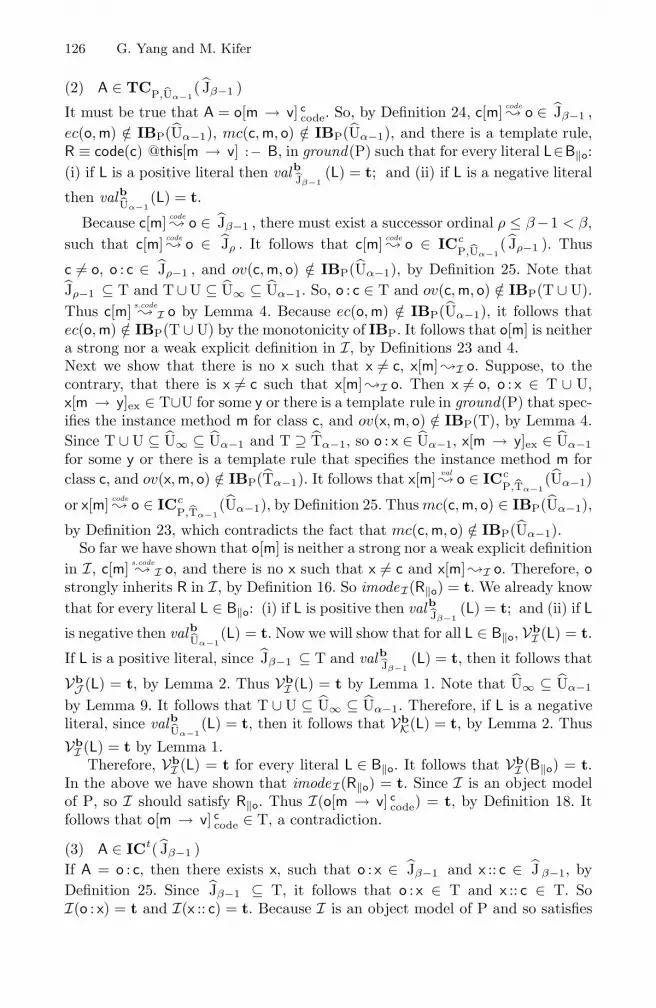
126 G. Yang and M. Kifer
(2) A ∈ TCP,�Uα−1( Jβ−1 )
It must be true that A = o[m → v] ccode. So, by Definition 24, c[m] code
� o ∈ Jβ−1 ,ec(o, m) /∈ IBP(Uα−1), mc(c, m, o) /∈ IBP(Uα−1), and there is a template rule,R ≡ code(c) @this[m → v] :− B, in ground(P) such that for every literal L∈B‖o:(i) if L is a positive literal then valb
�Jβ−1(L) = t; and (ii) if L is a negative literal
then valb�Uα−1
(L) = t.
Because c[m] code� o ∈ Jβ−1 , there must exist a successor ordinal ρ ≤ β −1 < β,
such that c[m] code� o ∈ Jρ . It follows that c[m] code
� o ∈ ICcP,�Uα−1
( Jρ−1 ). Thus
c �= o, o : c ∈ Jρ−1 , and ov(c, m, o) /∈ IBP(Uα−1), by Definition 25. Note thatJρ−1 ⊆ T and T ∪ U ⊆ U∞ ⊆ Uα−1. So, o : c ∈ T and ov(c, m, o) /∈ IBP(T ∪ U).Thus c[m] s.code
� I o by Lemma 4. Because ec(o, m) /∈ IBP(Uα−1), it follows thatec(o, m) /∈ IBP(T ∪ U) by the monotonicity of IBP. It follows that o[m] is neithera strong nor a weak explicit definition in I, by Definitions 23 and 4.Next we show that there is no x such that x �= c, x[m] �I o. Suppose, to thecontrary, that there is x �= c such that x[m] �I o. Then x �= o, o : x ∈ T ∪ U,x[m → y]ex ∈ T∪U for some y or there is a template rule in ground(P) that spec-ifies the instance method m for class c, and ov(x, m, o) /∈ IBP(T), by Lemma 4.Since T ∪ U ⊆ U∞ ⊆ Uα−1 and T ⊇ Tα−1, so o : x ∈ Uα−1, x[m → y]ex ∈ Uα−1for some y or there is a template rule that specifies the instance method m forclass c, and ov(x, m, o) /∈ IBP(Tα−1). It follows that x[m] val
� o ∈ ICcP,�Tα−1
(Uα−1)
or x[m] code� o ∈ ICc
P,�Tα−1(Uα−1), by Definition 25. Thus mc(c, m, o) ∈ IBP(Uα−1),
by Definition 23, which contradicts the fact that mc(c, m, o) /∈ IBP(Uα−1).So far we have shown that o[m] is neither a strong nor a weak explicit definition
in I, c[m] s.code� I o, and there is no x such that x �= c and x[m] �I o. Therefore, o
strongly inherits R in I, by Definition 16. So imodeI(R‖o) = t. We already knowthat for every literal L ∈ B‖o: (i) if L is positive then valb
�Jβ−1(L) = t; and (ii) if L
is negative then valb�Uα−1
(L) = t. Now we will show that for all L ∈ B‖o, VbI (L) = t.
If L is a positive literal, since Jβ−1 ⊆ T and valb�Jβ−1
(L) = t, then it follows that
VbJ (L) = t, by Lemma 2. Thus Vb
I (L) = t by Lemma 1. Note that U∞ ⊆ Uα−1
by Lemma 9. It follows that T ∪ U ⊆ U∞ ⊆ Uα−1. Therefore, if L is a negativeliteral, since valb
�Uα−1(L) = t, then it follows that Vb
K(L) = t, by Lemma 2. Thus
VbI (L) = t by Lemma 1.
Therefore, VbI (L) = t for every literal L ∈ B‖o. It follows that Vb
I (B‖o) = t.In the above we have shown that imodeI(R‖o) = t. Since I is an object modelof P, so I should satisfy R‖o. Thus I(o[m → v] c
code) = t, by Definition 18. Itfollows that o[m → v] c
code ∈ T, a contradiction.
(3) A ∈ ICt ( Jβ−1 )If A = o : c, then there exists x, such that o : x ∈ Jβ−1 and x :: c ∈ J β−1, byDefinition 25. Since Jβ−1 ⊆ T, it follows that o : x ∈ T and x :: c ∈ T. SoI(o : x) = t and I(x :: c) = t. Because I is an object model of P and so satisfies

Inheritance in Rule-Based Frame Systems: Semantics and Inference 127
the positive ISA transitivity constraint, therefore I(o : c) = t by Definition 10.It follows that o : c ∈ T, a contradiction. Similarly, if A = s :: c, then we can alsoshow that s :: c ∈ T, which is a contradiction.
(4) A ∈ ICiP,�Uα−1
( Jβ−1 )
It must be the case A = o[m → v] cval. Thus, by Definition 25, c[m] val
� o ∈ Jβ−1 ,c[m → v]ex ∈ Jβ−1 , ec(o, m) /∈ IBP(Uα−1), and mc(c, m, o) /∈ IBP(Uα−1).Because c[m] val
� o ∈ Jβ−1 , there must exist a successor ordinal ρ ≤ β − 1 < β,such that c[m] val
� o ∈ Jρ . It follows that c[m] val� o ∈ ICc
P,�Uα−1( Jρ−1 ). So, c �= o,
o : c ∈ Jρ−1 , c[m → z]ex ∈ Jρ−1 for some z, and ov(c, m, o) /∈ IBP(Uα−1), byDefinition 25. Since Jρ−1 ⊆ Jβ−1 ⊆ T and T ∪ U ⊆ U∞ ⊆ Uα−1, it followsthat o : c ∈ T, c[m → v]ex ∈ T, and ov(c, m, o) /∈ IBP(T ∪ U). Thus c[m] s.val
�I oby Lemma 4. Because ec(o, m) /∈ IBP(Uα−1), so ec(o, m) /∈ IBP(T ∪ U) by themonotonicity of IBP. It follows that o[m] is neither a strong nor a weak explicitdefinition in I, by Definitions 23 and 4.
Next we show that there is no x such that x �= c, x[m] �I o. Suppose, to thecontrary, that there is x �= c such that x[m] �I o. Then x �= o, o : x ∈ T ∪ U,x[m → y]ex ∈ T ∪ U for some y or there is a template rule in ground(P) whichspecifies the instance method m for class c, and ov(x, m, o) /∈ IBP(T), byLemma 4. Since T∪U ⊆ U∞ ⊆ Uα−1 and T ⊇ Tα−1, it follows that o : x ∈ Uα−1,x[m → y]ex ∈ Uα−1 for some y or there is a template rule that specifies theinstance method m for class c, and ov(x, m, o) /∈ IBP(Tα−1). It follows thatx[m] val
� o ∈ ICcP,�Tα−1
(Uα−1) or x[m] code� o ∈ ICc
P,�Tα−1(Uα−1), by Definition 25.
Therefore, mc(c, m, o) ∈ IBP(Uα−1), by Definition 23, which contradicts the factthat mc(c, m, o) /∈ IBP(Uα−1).
So far we have shown that o[m] is neither a strong nor a weak explicit definition inI, c[m] s.val
�I o, I(c[m → v]ex) = t, and there is no x such that x �= c and x[m] �I o.Because I is an object model of P and so satisfies the unique source inheritanceconstraint, therefore o[m → v] c
val ∈ T by Definition 12, a contradiction.
Therefore, if T ⊂ T∞, then we can derive a contradiction in all four possiblecases. So it must be true that T = T∞. It remains to show that T ∪ U = U∞.We know that T ∪ U ⊆ U∞, because I ≤ M. Therefore, if we can show thatT ∪ U ⊇ U∞, then T ∪ U = U∞. By Definitions 32 and 27, U∞ = lfp(TP,�T∞
).Since TP,�T∞
is monotonic, the ordinal powers of TP,�T∞is an increasing sequence.
Denote Kγ = Tγ
P,�T∞for all ordinal γ. We will prove by transfinite induction
that T ∪ U ⊇ Kα for all ordinal α, thus complete the proof.The case for a limit ordinal α is trivial. If α = 0, then K0 = ∅ ⊆ T ∪ U.
If α �= 0, then Kα =⋃
β<α Kβ . By the induction hypothesis we know thatT ∪ U ⊇ Kβ for all β < α. So T ∪ U ⊇ Kα .

128 G. Yang and M. Kifer
Let α be a successor ordinal and A any atom in HBP such that A ∈ Kα . Wewill show A ∈ T ∪ U. By Definitions 26 and 25, we have:
Kα = RCP,�T∞( Kα−1 ) ∪ TCP,�T∞
( Kα−1 ) ∪
ICt( Kα−1 ) ∪ ICcP,�T∞
( Kα−1 ) ∪ ICiP,�T∞
( Kα−1 )
There are four cases to consider:
(1) A ∈ RCP,�T∞( Kα−1 )
By Definition 22, there must exist a regular rule, H :− L1, . . . , Ln, in ground(P),such that H matches A, and for all Li, 1 ≤ i ≤ n: (i) if Li is a positive literal,then valb
�Kα−1(Li) = t; and (ii) if Li is a negative literal, then valb
�T∞(Li) = t.
Next we show that for all Li, 1 ≤ i ≤ n, VbI (Li) ≥ u. If Li is a positive literal, since
Kα−1 ⊆ T ∪U by the induction hypothesis and valb�Kα−1
(Li) = t, then it follows
that VbK(Li) = t, by Lemma 2. Thus Vb
I (Li) ≥ u by Lemma 1. We have provedthat T = T∞. Therefore, if Li is a negative literal, then Vb
J (Li) = Vb�T∞
(Li) = t.
Thus VbI (Li) ≥ u by Lemma 1. Because I satisfies P, so I(A) = Vh
I (H) ≥ u.Thus A ∈ T ∪ U.
(2) A ∈ TCP,�T∞( Kα−1 )
It must be true that A = o[m → v] ccode. So, by Definition 24, c[m] code
� o ∈ Kα−1 ,ec(o, m) /∈ IBP(T∞), mc(c, m, o) /∈ IBP(T∞), and ground(P) has a templaterule, R ≡ code(c) @this[m → v] :− B, such that for every literal L ∈ B‖o: (i) ifL is a positive literal then valb
�Kα−1(L) = t; and (ii) if L is a negative literal then
valb�T∞
(L) = t.
Because c[m] val� o ∈ Kα−1 , there must exist a successor ordinal ρ ≤ α−1 < α,
such that c[m] val� o ∈ Kρ . It follows that c[m] val
� o ∈ ICcP,�T∞
( Kρ−1 ). Therefore,
c �= o, o : c ∈ Kρ−1 , and ov(c, m, o) /∈ IBP(T∞), by Definition 25. Note thatKρ−1 ⊆ T ∪ U, by the induction hypothesis. We have proved that T = T∞.It follows that o : c ∈ T ∪ U and ov(c, m, o) /∈ IBP(T). Therefore c[m] s.code
� I o orc[m] w.code
� I o, by Lemma 4. Because ec(o, m) /∈ IBP(T∞), so ec(o, m) /∈ IBP(T).Thus o[m] is not a strong explicit definition, by Definitions 23 and 4. Becausec[m → v]ex ∈ Kα−1 ⊆ T ∪ U, it follows that I(c[m → v]ex) ≥ u.
Next we show that there is no x �= c such that x[m] s.val�I o or x[m] s.code
� I o. Sup-pose, to the contrary, that there exists x �= c such that x[m] s.val
�I o or x[m] s.code� I o.
Then x[m] s.val�M o or x[m] s.code
� M o, because I ≤ M. Thus x[m] val� o ∈ T∞ or
x[m] code� o ∈ T∞, by Lemma 12. Thus mc(c, m, o) ∈ IBP(T∞) by Definition 23,
which contradicts the fact that mc(c, m, o) /∈ IBP(T∞).So far we have shown that c[m] s.code
� I o or c[m] w.code� I o, o[m] is not a strong
explicit definition, and there is no x �= c such that x[m] s.val�I o or x[m] s.code
� I o.Therefore, o must either strongly or weakly inherit R in I, by Definitions 16and 16. So imodeI(R‖o) ≥ u. We already know that for every literal L ∈ B‖o:

Inheritance in Rule-Based Frame Systems: Semantics and Inference 129
(i) if L is a positive literal then valb�Kα−1
(L) = t; and (ii) if L is a negative
literal then valb�T∞
(L) = t. Now we show that for all Li, 1 ≤ i ≤ n, VbI (Li) ≥ u.
If Li is a positive literal, since Kα−1 ⊆ T ∪ U by the induction hypothesis andvalb
�Kα−1(Li) = t, then it follows that Vb
K(Li) = t, by Lemma 2. Thus VbI (Li) ≥ u
by Lemma 1. Note that T = T∞. Therefore, if Li is a negative literal, thenVbJ (Li) = Vb
�T∞(Li) = t. Thus Vb
I (Li) ≥ u by Lemma 1. Therefore, VbI (L) ≥ u for
every literal L ∈ B‖o. It follows that VbI (B‖o) ≥ u. Moreover, imodeI(R‖o) ≥ u.
Because I is an object model of P, so I should satisfy R‖o. It follows thatI(o[m → v] c
code) ≥ u, by Definition 18. Thus o[m → v] ccode ∈ T ∪ U.
(3) A ∈ ICt ( Kα−1 )If A = o : c, then there exists x such that o : x ∈ Kα−1 and x :: c ∈ Kα−1 , byDefinition 25. Since Kα−1 ⊆ T ∪ U by the induction hypothesis, it follows thato : x ∈ T∪U and x :: c ∈ T∪U. So I(o : x) ≥ u and I(x :: c) ≥ u. Because I satisfiesthe cautious ISA transitivity constraint, therefore I(o : c) ≥ u by Definitions 13and 10. It follows that o : c ∈ T∪U. Similarly, if A = s :: c, then we can also showthat s :: c ∈ T ∪ U.
(4) A ∈ ICiP,�T∞
( Kα−1 )
It must be the case that A = o[m → v] cval. It follows that c[m] val
� o ∈ Kα−1 ,c[m → v]ex ∈ Kα−1 , ec(o, m) /∈ IBP(T∞), and mc(c, m, o) /∈ IBP(T∞), byDefinition 25. Because c[m] val
� o ∈ Kα−1 , so there must exist a successor ordinalρ ≤ α − 1 < α, such that c[m] val
� o ∈ Kρ . Thus c[m] val� o ∈ ICc
P,�T∞( Kρ−1 ).
Therefore, by Definition 25, c �= o, o : c ∈ Kρ−1 , c[m → z]ex ∈ Kρ−1 for somez, and ov(c, m, o) /∈ IBP(T∞). Since Kρ−1 ⊆ Kα−1 ⊆ T ∪ U by the inductionhypothesis and T = T∞, it follows that o : c ∈ T ∪ U, c[m → v]ex ∈ T ∪ U,and ov(c, m, o) /∈ IBP(T). Thus c[m] s.val
�I o or c[m] w.val� I o by Lemma 4. Because
ec(o, m) /∈ IBP(T∞), it follows that ec(o, m) /∈ IBP(T), and so o[m] is not astrong explicit definition, by Definitions 23 and 4. Because c[m → v]ex ∈ T ∪U,it follows that I(c[m → v]ex) ≥ u.
Now we show that there is no x �= c such that x[m] s.val�I o or x[m] s.code
� I o. Suppose,to the contrary, that there exists x �= c such that x[m] s.val
�I o or x[m] s.code� I o. Then
x[m] s.val�M o or x[m] s.code
� M o, because I ≤ M. It follows that x[m] val� o ∈ T∞ or
x[m] code� o ∈ T∞, by Lemma 12. Thus mc(c, m, o) ∈ IBP(T∞) by Definition 23,
which contradicts the fact that mc(c, m, o) /∈ IBP(T∞).
So far we have shown that o[m] is not a strong explicit definition, c[m] s.val�I o
or c[m] w.val� I o, I(c[m → v]ex) ≥ u, and there is no x �= c such that x[m] s.val
�I oor x[m] s.code
� I o. Because I satisfies the cautious inheritance constraint, thereforeI(o[m → v] c
val) ≥ u, by Definition 14. So o[m → v] cval ∈ T ∪ U.
We have shown that in all four possible cases, if A ∈ Kα , then A ∈ T ∪ U. Itfollows that T ∪ U ⊇ Kα . This completes the induction step.

130 G. Yang and M. Kifer
A.3 Lemmas and Propositions Supporting Theorem 6 in Section 10
Lemma 17. Let Pwf be the well-founded rewriting of an F-logic KB P and Iwf
be a subset of HBPwf . Then lfp(CPwf ,Iwf ) is in normal form.
Lemma 18. Let Pwf be the well-founded rewriting of an F-logic KB P, I asubset of HBP, Iwf a subset of HBPwf which is isomorphic to I and is in normalform, and G a ground positive literal. Then valb
�I (¬G) = t iff ρb(G) /∈ Iwf .
Proposition 8. Let Pwf be the well-founded rewriting of an F-logic KB P, Iwf
a subset of HBPwf which is in normal form, and I a subset of HBP. If Iwf isisomorphic to I , then lfp(CPwf ,Iwf ) is isomorphic to lfp(TP,�I ).
Proof. Let Jwf = lfp(CPwf ,Iwf ) and J = lfp(TP,�I ). First we will show that all ofthe following conditions are true:
(1) for all o, c: isa(o, c) ∈ Jwf iff o : c ∈ J(2) for all s, c: sub(s, c) ∈ Jwf iff s :: c ∈ J(3) for all s, m, v: exmv(s, m, v) ∈ Jwf iff s[m → v]ex ∈ J(4) for all o, m, v, c: vamv(o, m, v, c) ∈ Jwf iff o[m → v] c
val ∈ J(5) for all o, m, v, c: comv(o, m, v, c) ∈ Jwf iff o[m → v] c
code ∈ J(6) for all c, m, o: vacan(c, m, o) ∈ Jwf iff c[m] val
� o ∈ J(7) for all c, m, o: cocan(c, m, o) ∈ Jwf iff c[m] code
� o ∈ JI. ⇒
Let us define:
Swf0 = ∅ S0 = ∅ for limit ordinal 0
Swfα = CPwf ,Iwf (Swf
α−1) Sα = TP,�I ( Sα−1 ) for successor ordinal α
Swfα =
⋃
β<α
Swfβ Sα =
⋃
β<α
Sβ for limit ordinal α �= 0
Swf∞ =⋃
α
Swfα S∞ =
⋃
α
Sα
Then Swf∞ = lfp(CPwf ,Iwf ) and S∞ = lfp(TP,�I ). We will prove by transfinite
induction that for any ordinal α and for all o, s, c, m, v, the following conditionsare true:
(1) if isa(o, c) ∈ Swfα then o : c ∈ Sα
(2) if sub(s, c) ∈ Swfα then s :: c ∈ Sα
(3) if exmv(s, m, v) ∈ Swfα then s[m → v]ex ∈ Sα
(4) if vamv(o, m, v, c) ∈ Swfα then o[m → v] c
val ∈ Sα
(5) if comv(o, m, v, c) ∈ Swfα then o[m → v] c
code ∈ Sα
(6) if vacan(c, m, o) ∈ Swfα then c[m] val
� o ∈ Sα
(7) if cocan(c, m, o) ∈ Swfα then c[m] code
� o ∈ Sα

Inheritance in Rule-Based Frame Systems: Semantics and Inference 131
The case for a limit ordinal α is trivial. Now let α be a successor ordinal. SoSwf
α = CPwf ,Iwf (Swfα−1). First we show that for any ground positive literal L, if
ρb(L) ∈ Swfα−1, then valb
�Sα−1(L) = t: (i) If L = o : c, then ρb(L) = isa(o, c). It
follows that o : c ∈ Sα−1 by the induction hypothesis. Thus valb�Sα−1
(o : c) = t;
(ii) Similarly, we can show if ρb(L) = sub(s, c) ∈ Swfα−1, then valb
�Sα−1(s :: c) = t;
(iii) If L = o[m → v], then ρb(L) = mv(o, m, v). Note that Swfγ ⊆ Swf
α−1 for allγ ≤ α − 1. Therefore, there must exist a successor ordinal ρ ≤ α − 1 such thatmv(s, m, v) ∈ Swf
ρ = CPwf ,Iwf (Swfρ−1). It follows that exmv(o, m, v) ∈ Swf
ρ−1, orthere is c such that vamv(o, m, v, c) ∈ Swf
ρ−1 or comv(o, m, v, c) ∈ Swfρ−1, according
to the trailer rules in Definition 38. Thus o[m → v]ex ∈ Sρ−1 , or there is c suchthat o[m → v] c
val ∈ Sρ−1 or o[m → v] ccode ∈ Sρ−1 , by the induction hypothesis.
Clearly, Sρ−1 ⊆ Sα−1 . Thus valb�Sα−1
(o[m → v]) = t.Now consider the following cases:
(1) isa(o, c) ∈ Swfα and isa(o, c) is derived via a rule Rwf ∈ ground(Pwf ) which
is rewritten from a regular rule R ∈ ground(P).Then Rwf ≡ isa(o, c) :− ρb(C1), . . . , ρb(Cm), ¬ ρb(G1), . . . , ¬ ρb(Gn) must be therewriting of R ≡ o : c :− C1, . . . , Cm, ¬G1, . . . , ¬Gn, where Ci, 1 ≤ i ≤ m, and Gj,1 ≤ j ≤ n, are positive literals. By Definition 39, each ρb(Ci) ∈ Swf
α−1 and eachρb(Gj) /∈ Iwf . Following the above claim, valb
�Sα−1(Ci) = t for all 1 ≤ i ≤ m.
Moreover, Iwf is isomorphic to I and is in normal form, therefore valb�I (¬Gj) = t
for all 1 ≤ j ≤ n, by Lemma 18. So o : c ∈ RCP,�I ( Sα−1 ) ⊆ TP,�I ( Sα−1 ) = Sα ,by Definitions 22 and 26.
(2) isa(o, c) ∈ Swfα and isa(o, c) is derived via a trailer rule Rwf in ground(Pwf ).
Then there exists s such that Rwf = isa(o, c) :− isa(o, s), sub(s, c). It followsthat isa(o, s) ∈ Swf
α−1 and sub(s, c) ∈ Swfα−1. Thus o : s ∈ Sα−1 and s :: c ∈ Sα−1
by the induction hypothesis. So o : c ∈ ICt( Sα−1 ) ⊆ TP,�I ( Sα−1 ) = Sα , byDefinitions 25 and 26.
(3) sub(s, c) ∈ Swfα and sub(s, c) is derived via a rule Rwf ∈ ground(Pwf ) which
is rewritten from a regular rule R ∈ ground(P).Similarly to (1), we can show that s :: c ∈ Sα .
(4) sub(s, c) ∈ Swfα and sub(s, c) is derived via a trailer rule Rwf in ground(Pwf ).
Similarly to (2), we can show that s :: c ∈ Sα .
(5) exmv(s, m, v) ∈ Swfα
Then exmv(s, m, v) must be derived via a rule Rwf ∈ ground(Pwf ) which isrewritten from a regular rule R ∈ ground(P). Similarly to (1), we can also showthat s[m → v]ex ∈ Sα .
(6) vamv(o, m, v, c) ∈ Swfα
By Definition 38, vamv(o, m, v, c) should be derived via a trailer rule fromground(Pwf ). So vacan(c, m, o) ∈ Swf
α−1, exmv(c, m, v) ∈ Swfα−1, ex(o, m) /∈ Iwf ,

132 G. Yang and M. Kifer
and multi(c, m, o) /∈ Iwf . Thus c[m] val� o ∈ Sα−1 and c[m → v]ex ∈ Sα−1 , by
the induction hypothesis. Since Iwf is isomorphic to I , ec(o, m) /∈ IBP( I ) andmc(c, m, o) /∈ IBP( I ). Thus o[m → v] c
val ∈ ICiP,�I ( Sα−1 ) ⊆ TP,�I ( Sα−1 ) = Sα ,
by Definitions 25 and 26.
(7) comv(o, m, v, c) ∈ Swfα
Then comv(o, m, v, c) must be derived via a trailer rule. So cocan(c, m, o) ∈ Swfα−1,
ins(o, m, v, c) ∈ Swfα−1, ex(o, m) /∈ Iwf , and multi(c, m, o) /∈ Iwf . By the induc-
tion hypothesis, c[m] code� o ∈ Sα−1 . Since Iwf is isomorphic to I , it follows that
ec(o, m) /∈ IBP( I ), mc(c, m, o) /∈ IBP( I ). Clearly, ins(o, m, v, c) must be derivedvia a rule Rwf ≡ ins(o, m, v, c) :− ρb(C1), . . . , ρb(Cm), ¬ ρb(G1), . . . , ¬ ρb(Gn), inground(Pwf ), which is rewritten from the following template rule in ground(P),R ≡ code(c) @this[m → v] :− B1, . . . , Bm, ¬F1, . . . , ¬Fn, where Bi and Fj arepositive literals, Ci = (Bi)‖o and Gj = (Fj)‖o, for all 1 ≤ i ≤ m and 1 ≤ j ≤ n.
Similarly to (1), we can show that valb�Sα−1
((Bi)‖o) = t for all 1 ≤ i ≤ m and
valb�I (¬ (Fj)‖o) = t for all 1 ≤ j ≤ n. It follows that by Definitions 24 and 26,
o[m → v] cval ∈ TCP,�I ( Sα−1 ) ⊆ TP,�I ( Sα−1 ) = Sα .
(8) vacan(c, m, o) ∈ Swfα
Then vacan(c, m, o) must be derived via a trailer rule in ground(Pwf ). It followsthat isa(o, c) ∈ Swf
α−1, exmv(c, m, v) ∈ Swfα−1, c �= o, and override(c, m, o) /∈ Iwf ,
by Definition 38. So o : c ∈ S α−1 and c[m → v]ex ∈ Sα−1 , by the inductionhypothesis. Moreover, ov(c, m, o) /∈ IBP( I ), since Iwf is isomorphic to I . Thusc[m] val
� o ∈ ICcP,�I ( Sα−1 ) ⊆ TP,�I ( Sα−1 ) = Sα , by Definitions 25 and 26.
(9) cocan(c, m, o) ∈ Swfα
Then cocan(c, m, o) must be derived via a trailer rule in ground(Pwf ). It followsthat isa(o, c) ∈ Swf
α−1, codedef(c, m) ∈ Swfα−1, c �= o, and override(c, m, o) /∈ Iwf ,
by Definition 38. Note that o : c ∈ S α−1, by the induction hypothesis, andov(c, m, o) /∈ IBP( I ), because Iwf is isomorphic to I . Since codedef(c, m)∈Swf
α−1,there is a template rule in P which specifies the instance method m for class c,by Definition 38. It follows that c[m] code
� o ∈ ICcP,�I ( Sα−1 ) ⊆ TP,�I ( Sα−1 ) = Sα ,
by Definitions 25 and 26.
II. ⇐Let us construct an extended atom set K from Jwf as follows: generate one
o : c in K for every isa(o, c) in Jwf , one s :: c in K for every sub(s, c) in Jwf ,one s[m → v]ex in K for every exmv(s, m, v) in Jwf , one o[m → v] c
val in K forevery vamv(o, m, v, c) in Jwf , one o[m → v] c
code in K for every comv(o, m, v, c)in Jwf , one c[m] val
� o in K for every vacan(c, m, o) in Jwf , and one c[m] code� o in
K for every cocan(c, m, o) in Jwf . Clearly, to prove that the conditions are true,it suffices to show that K ⊇ J .
Because J = lfp(TP,�I ), therefore, to show that K ⊇ J , it suffices to show
that TP,�I ( K ) ⊆ K according to the conventional fixpoint theory [28]. Recall

Inheritance in Rule-Based Frame Systems: Semantics and Inference 133
that by Definitions 26 and 25,
TP,�I ( K ) = RCP,�I ( K ) ∪ TCP,�I ( K ) ∪ ICt( K ) ∪ ICcP,�I ( K ) ∪ ICi
P,�I ( K )
Let A be any atom in TP,�I ( K ). There are five possible cases to consider:
(1) A ∈ RCP,�I ( K )Then there is a regular rule R ≡ H :− C1, . . . , Cm, ¬G1, . . . , ¬Gn in ground(P),such that H matches A, Ci (1 ≤ i ≤ m) and Gj (1 ≤ j ≤ n) are positive literals,valb
�K (Ci) = t for all 1 ≤ i ≤ m and valb�I (¬Gj) = t for all 1 ≤ j ≤ n. Consider the
rewriting Rwf of R, ρh(H) :− ρb(C1), . . . , ρb(Cm), ¬ ρb(G1), . . . , ¬ ρb(Gn). Firstwe show ρb(Ci) ∈ Jwf for all 1 ≤ i ≤ m: (i) If Ci = o : c, then ρb(Ci) = isa(o, c).Since valb
�K (o : c) = t, it follows that o : c ∈ K by Definition 1. Therefore,isa(o, c) ∈ Jwf , by the construction of K ; (ii) Similarly, we can show if Ci = s :: c,then ρb(Ci) = sub(s, c) ∈ Jwf ; (iii) If Ci = s[m → v], then ρb(Ci) = mv(s, m, v).Since valb
�K (s[m → v]) = t, so s[m → v]ex ∈ K , or there exists c such thats[m → v] c
val ∈ K or s[m → v] ccode ∈ K . So exmv(s, m, v) ∈ Jwf , or there exists
c such that vamv(s, m, v, c) ∈ Jwf or comv(s, m, v, c) ∈ Jwf , by the constructionof K . Because Jwf = CPwf ,Iwf (Jwf ), therefore mv(s, m, v) ∈ Jwf , according to thetrailer rules in Definition 38. By Lemma 18, ρb(Gj) /∈ Iwf for all 1 ≤ j ≤ n. Soρh(H) ∈ CPwf ,Iwf (Jwf ) = Jwf , by Definition 39. It follows that: (i) If A = o : c,then H = o : c. So ρh(H) = isa(o, c) ∈ Jwf , thus o : c ∈ K ; (ii) Similarly, ifA = s :: c, then s :: c ∈ K ; (iii) If A = s[m → v]ex, then H = s[m → v]. Soρh(H) = exmv(s, m, v) ∈ Jwf , thus s[m → v]ex ∈ K .
(2) A ∈ TCP,�I ( K )It must be the case that A = o[m → v] c
code. It follows that mc(c, m, o) /∈ IBP( I ),ec(o, c) /∈ IBP( I ), c[m] code
� o ∈ K , and ground(P) has a template rule, R, of theform code(c) @this[m → v] :− C1, . . . , Cm, ¬G1, . . . , ¬Gn, where Ci (1 ≤ i ≤ m)and Gj (1 ≤ j ≤ n) are positive literals, valb
�K ((Ci)‖o) = t for all 1 ≤ i ≤ m andvalb
�I (¬ (Gj)‖o) = t for all 1 ≤ j ≤ n. Consider the rewriting Rwf of R, suchthat Rwf ≡ ins(o, m, v, c) :− ρb(B1), . . . , ρb(Bm), ¬ ρb(F1), . . . , ¬ ρb(Fn), whereBi = (Ci)‖o for all 1 ≤ i ≤ m and Fj = (Gj)‖o for all 1 ≤ j ≤ n. Similarly to (1),we can also show that ρb(Bi) ∈ Jwf for all 1 ≤ i ≤ m. By Lemma 18, ρb(Fj) /∈ Iwf
for all 1 ≤ j ≤ n. So ins(o, m, v, c) ∈ CPwf ,Iwf (Jwf ) = Jwf , by Definition 39.Because c[m] code
� o ∈ K , therefore cocan(c, m, o) ∈ Jwf , by the constructionof K . Note that ec(o, c) /∈ IBP( I ) and mc(c, m, o) /∈ IBP( I ). Since Iwf isisomorphic to I , it follows that ex(o, c) /∈ Iwf and multi(c, m, o) /∈ Iwf . Socomv(o, m, v, c) ∈ CPwf ,Iwf (Jwf ) = Jwf , according to the trailer rules of Pwf andDefinition 39. It follows that o[m → v] c
code ∈ K .
(3) A ∈ ICt ( K )If A = o : c, then there is x such that o : x ∈ K , x :: c ∈ K . So isa(o, x) ∈ Jwf andsub(x, c) ∈ Jwf , by the construction of K . Thus isa(o, c) ∈ CPwf ,Iwf (Jwf ) = Jwf ,

134 G. Yang and M. Kifer
by Definition 39 and the trailer rules of Pwf . Thus o : c ∈ K . Similarly, we canshow that if A = s :: c, then s :: c ∈ K .
(4) A ∈ ICcP,�I ( K )
If A = c[m] val� o, then o : c ∈ K , c �= o, c[m → v]ex ∈ K , and ov(c, m, o) /∈ I , by
Definition 25. Because K is constructed from Jwf and Iwf is isomorphic to I ,it follows that isa(o, c) ∈ Jwf , exmv(c, m, v) ∈ Jwf , and override(c, m, o) /∈ Iwf .So vacan(c, m, o) ∈ CPwf ,Iwf (Jwf ) = Jwf , by Definition 39 and the trailer rulesof Pwf . Thus c[m] val
� o ∈ K . Similarly, if A = c[m] code� o, we can also show that
c[m] code� o ∈ K .
(5) A ∈ ICiP,�I ( K )
Then A = o[m → v] cval, and c[m] val
� o ∈ K , c[m → v]ex ∈ K , ec(o, m) /∈ I ,mc(c, m, o) /∈ I , by Definition 25. Because K is constructed from Jwf , and Iwf
is isomorphic to I , it follows that vacan(c, m, o) ∈ Jwf , exmv(c, m, v) ∈ Jwf ,ex(o, m) /∈ Iwf , multi(c, m, o) /∈ Iwf . So by Definition 39 and the trailer rules ofPwf , vamv(o, m, v, c) ∈ CPwf ,Iwf (Jwf ) = Jwf . Thus o[m → v] c
val ∈ K .
Finally, to finish the proof for the claim that Jwf is isomorphic to J , we stillneed to show that the following conditions are true:
(1) for all o, m: ex(o, m) ∈ Jwf iff ec(o, m) ∈ IBP( J )(2) for all c, m, o: multi(c, m, o) ∈ Jwf iff mc(c, m, o) ∈ IBP( J )(3) for all c, m, o: override(c, m, o) ∈ Jwf iff ov(c, m, o) ∈ IBP( J )
Note that ex/2, multi/3, and override/3 can only be derived via the trailer rulesas defined in Definition 38. Moreover, Jwf = CPwf ,Iwf (Jwf ). It follows that:
(1) ex(o, m) ∈ Jwf , iff there exists v such that exmv(o, m, v) ∈ Jwf , iff thereexits v such that o[m → v]ex ∈ J , iff ec(o, m) ∈ IBP( J ).
(2) multi(c, m, o) ∈ Jwf , iff there exists x �= c such that vacan(x, m, o) ∈ Jwf orcocan(x, m, o) ∈ Jwf , iff there is x �= c such that x[m] val
� o ∈ J or x[m] code� o ∈ J ,
iff mc(c, m, o) ∈ IBP( J ).
(3) override(c, m, o) ∈ Jwf , iff there exists some x, such that x �= c, x �= o,sub(x, c) ∈ Jwf , isa(o, x) ∈ Jwf , and there is v such that exmv(x, m, v) ∈ Jwf orcodedef(x, m) ∈ Jwf , iff there is x such that x �= c, x �= o, x :: c ∈ J , o : x ∈ J ,and there is v such that x[m → v]ex ∈ J or there is a template rule in P whichspecifies the instance method m for class c, iff ov(c, m, o) ∈ IBP( J ).
Proposition 9. Let α range over all ordinals, then Twfα , Twf
∞ , Uwfα , and Uwf
∞are all in normal form. (The notations used here are from Definition 43.)
Proof. First we show by transfinite induction that Twfα is in normal form for
any ordinal α. The case is trivial for limit ordinal 0. If α is a successor ordinal,then Twf
α = SPwf (Uwfα−1) = lfp(CPwf ,Uwf
α−1). It follows that Twf
α is in normal form,
by Lemma 17. Now suppose α �= 0 is a limit ordinal, Twfα =
⋃β<α Twf
β . Ac-cording to Definition 42, we need to show for all o, m, v: mv(o, m, v) ∈ Twf
α

Inheritance in Rule-Based Frame Systems: Semantics and Inference 135
iff exmv(o, m, v) ∈ Twfα , or there is c such that vamv(o, m, v, c) ∈ Twf
α orcomv(o, m, v, c) ∈ Twf
α .
(1) ⇒If mv(o, m, v) ∈ Twf
α , then there is β < α such that mv(o, m, v) ∈ Twfβ . By the
induction hypothesis, Twfβ ⊆ Twf
α is in normal form. Thus exmv(o, m, v) ∈ Twfβ ,
or there is c such that vamv(o, m, v, c) ∈ Twfβ or comv(o, m, v, c) ∈ Twf
β .
(2) ⇐If exmv(o, m, v) ∈ Twf
α , then there is β < α such that exmv(o, m, v) ∈ Twfβ . It fol-
lows that mv(o, m, v) ∈ Twfβ ⊆ Twf
α , since Twfβ is in normal form by the induction
hypothesis. On the other hand, if there exists c such that vamv(o, m, v, c) ∈ Twfα
or vamv(o, m, v, c) ∈ Twfα , then there is γ < α such that vamv(o, m, v, c) ∈ Twf
γ
or comv(o, m, v, c) ∈ Twfγ . It follows that mv(o, m, v, c) ∈ Twf
γ ⊆ Twfα , since Twf
γ
is in normal form by the induction hypothesis.
Similarly, we can also prove that Twf∞ is in normal form. Moreover, for anyordinal α, Uwf
α = SPwf (Twfα ) = lfp(CPwf ,Twf
α). It follows that Uwf
α is in normalform, by Lemma 17. Similarly, we can show that Uwf∞ is in the normal form.

Unsupervised Duplicate DetectionUsing Sample Non-duplicates
Patrick Lehti and Peter Fankhauser
Fraunhofer IPSIDolivostr. 15DarmstadtGermany
{Patrick.Lehti, Peter.Fankhauser}@ipsi.fraunhofer.de
Abstract. The problem of identifying objects in databases that refer tothe same real world entity, is known, among others, as duplicate detec-tion or record linkage. Objects may be duplicates, even though they arenot identical due to errors and missing data. Typical current methodsrequire deep understanding of the application domain or a good repre-sentative training set, which entails significant costs. In this paper wepresent an unsupervised, domain independent approach to duplicate de-tection that starts with a broad alignment of potential duplicates, andanalyses the distribution of observed similarity values among these po-tential duplicates and among representative sample non-duplicates toimprove the initial alignment. Additionally, the presented approach isnot only able to align flat records, but makes also use of related ob-jects, which may significantly increase the alignment accuracy. Evalua-tions show that our approach supersedes other unsupervised approachesand reaches almost the same accuracy as even fully supervised, domaindependent approaches.
1 Introduction
The goal of data integration is to provide uniform, non-redundant access to aset of typically heterogeneous data sources. If the sources contain overlappingdata, not only their schemas need to be integrated, but also their instances,i.e., duplicate instances that refer to the same real world object need to be todetected and merged.
Traditional scenarios for duplicate detection are data warehouses, which arepopulated by several data sources. Analyses on the data warehouse influencesbusiness decisions, therefore a high data quality resulting from the populating isof high importance. This is in general done by what is known as data cleansingprocess, which also detects and removes duplicates. Reaching a high data qualitywith a data cleansing process is currently very costly.
More recently duplicate detection is also arising in ad-hoc integration over theinternet, e.g., in P2P, web service or grid settings, where datasets and servicesare virtually integrated for temporary applications. In such scenarios no long
S. Spaccapietra (Ed.): Journal on Data Semantics VII, LNCS 4244, pp. 136–164, 2006.c© Springer-Verlag Berlin Heidelberg 2006

Unsupervised Duplicate Detection Using Sample Non-duplicates 137
and expensive data cleansing process can be carried out, but good duplicateestimations must be available directly.
This paper describes a method for unsupervised duplicate detection by us-ing a representative set of sample non-duplicates. These sample non-duplicatescan be obtained under the assumption that individual data sources are duplicatefree. The approach starts with a set of potential duplicates and a set of represen-tative sample non-duplicates identified in a preprocessing phase and iterativelydetermines the matching probability of the potential duplicates by analyzing thedistribution of observed similarities among the potential duplicates and amongthe non-duplicates. The approach can be alternatively used with either a re-finement of the Fellegi-Sunter model for record linkage [1], which is able to usecontinuous similarity measures and takes attribute dependencies into account, orit can be used with machine learning techniques like Support Vector Machines(SVM) [2]. Further the method can be simply extended to be used with notonly flat records, but on graph data models consisting of interrelated objects.It is shown that such an extension also increases the accuracy of the duplicatedetection process.
In more detail, the contributions of this paper are the following:
– a method for unsupervised detection of duplicates between two data sources– a way to automatically infer a representative sample of non-duplicates that
can be used by a duplicate decision model to increase the decision accuracy– the usage of the Fellegi-Sunter model for record linkage [1] with such sample
non-duplicates– the usage of Support Vector Machines with such sample non-duplicates– extensions to the classic Fellegi-Sunter model for determining the parameters
without the independence assumption and using continuous similarity values;a probabilistic model that simplifies finding a good threshold on the result;the handling of null values and multi-valued attributes
– an extension to detect duplicates not only on flat records, but on interrelatedobjects
The remainder of this paper is organized as follows. Section 1.1 gives a moreformal definition of the problem of duplicate detection. Section 2 summarizesrelated work and and briefly introduces into the Fellegi-Sunter model. Section 3gives an overview of the architecture and explains how the representative samplenon-duplicates can be obtained. Section 4 presents the extensions to the Fellegi-Sunter model and shows how it can make use of the sample non-duplicates.Section 5 presents the results of the evaluation of our approach compared toother approaches. Finally Section 6 concludes and shows potentials for futurework.
1.1 Problem Definition
The problem of detecting duplicates can be defined as follows: Given two setsof objects A and B divide the set of all object-pairs (a, b) ∈ A × B into a set

138 P. Lehti and P. Fankhauser
of matching object-pairs M and unmatching object-pairs U . Sets are denotedby upper-case letters, individual instances by lower-case letters. An object isbasically a vector of attributes (also called fields, properties or features), thus,an object-pair is a vector of attribute-pairs.
Fig. 1. General architecture of a duplicate detection system
In general the overall duplicate detection process consists of several phasesas illustrated in Figure 1. The first phase, often called blocking, tries to effi-ciently find a candidate set of duplicates, then a second phase, sometimes calledmatching, performs the actual duplicate decision. The matching phase in generalinvolves an in-depth comparison of the candidate duplicate pairs, i.e., compar-ing the individual attribute-pairs, which results in what is called a comparisonvector γ[a, b] for every candidate pair. The individual components of the com-parison vector (γi[a, b]) represent the comparison results between the individualattribute-pairs. These individual comparison results can be boolean (attributematches or does not match), discrete (e.g., matches, possibly matches or doesnot match) or continuous (e.g., attribute values have a similarity of 0.2).
The task for the matching algorithm is then to classify such a given compari-son vector γ[a, b] into the sets M or U by some kind of decision model. Thereforethe components of the comparison vector must be combined to an overall result.It can be easily seen that the individual attributes do not have the same rele-vance for this overall result. E.g., a matching ”person name” is a much strongerindication for a duplicate record than a matching ”year of birth”, because of thehigher uniqueness of ”person name” in contrast to ”year of birth”. However,a non-matching ”year of birth” is a strong indication for a non-duplicate, maybe even higher as a slightly different ”person name”, under the assumption of ahigh reliability for ”year of birth”.
2 Related Work
Methods from the Database Community In the database community a few know-ledge-intensive approaches have been developed. Hernandez and Stolfo [3]

Unsupervised Duplicate Detection Using Sample Non-duplicates 139
present a two phase data cleansing approach based on key expressions for block-ing and logic rules for the matching phase. The selection of appropriate keys aswell as the logic rules are both very knowledge-intensive tasks. Galhardas et al.[4] present a framework for data cleansing based on a set of rules. This frame-work is very flexible, but requires intensive human interaction and knowledge inorder to provide good rules. Monge and Elkan [5] compare instances based on aconcatenation of all attributes with the help of distance functions and present ablocking algorithm. A concatenation of all attributes only produces reasonableresults if all data sources are complete, i.e., have no null values for attributesand all attributes show the same relevance for duplicate detection. In our eval-uation one baseline experiment also concatenates all attribute values and usesthe string distance between these concatenated strings as overall result.
The Fellegi-Sunter Model for Record Linkage Based on the initial ideas andproblem description of Newcombe [6], Fellegi and Sunter [1] defined a theory forrecord linkage including relevance for individual attributes. To this end, theydefine the following probabilities on the comparison vector γ[a, b] for an objectpair (a, b):
m(γ[a, b]) = P (γ[a, b] | (a, b) ∈ M) (1)
u(γ[a, b]) = P (γ[a, b] | (a, b) ∈ U) (2)
Here m(γ[a, b]) is the conditional probability of γ[a, b], given that (a, b) is an ele-ment of M and u(γ[a, b]) is the conditional probability of γ[a, b], given that (a, b) isan element of U . They have shown that the ratio w(γ[a, b]) = m(γ[a, b])/u(γ[a, b])can then be used to decide for a duplicate, non-duplicate or potential duplicate.To this end they define how to set the appropriate thresholds on w(γ[a, b]) givenacceptable error rates for false misses and false matches.
In order to determine the parameters u(γ[a, b]) and m(γ[a, b]) often a con-ditional independence assumption between the individual components of thecomparison vector is made. Under this assumption the parameters u(γ[a, b]) andm(γ[a, b]) can be computed using mi and ui for the individual probabilities forthe comparison vector component γi[a, b]:
m(γ[a, b]) = m1(γ1[a, b]) ∗ m2(γ2[a, b])...mk(γk[a, b]) (3)
u(γ[a, b]) = u1(γ1[a, b]) ∗ u2(γ2[a, b])...uk(γk[a, b]) (4)
This simplification only produces good results if the conditional independenceassumption really holds, which is often not the case for real data. E.g. in theaddress domain the attributes street and city are not independent, as a particularstreet is only present in one or a few cities.
Fellegi and Sunter propose two methods for determining the individual valuesmi(γi[a, b]), one relies on additional knowledge of error rates in the values, thesecond is limited on comparison vectors of size 3. Winkler [7] showed that the EMalgorithm (Expectation-Maximization) [8] can be used for unsupervised learningof the m(γ[a, b]) and u(γ[a, b]) parameters under the independence assumption.

140 P. Lehti and P. Fankhauser
Using the independence assumption is the second baseline experiment for ourapproach.
Several approaches, e.g., from Winkler [9] and Larsen and Rubin [10] tried todetermine the m(γ[a, b]) and u(γ[a, b]) values in cases where conditional inde-pendence does not hold. All these approaches try to explicitly model the depen-dencies and only works for boolean variables.
Ravikumar and Cohen [11] present an unsupervised learning approach basedon the Fellegi-Sunter model that takes attribute dependencies into account anduses continuous similarity measures. They use a hierarchical latent variablegraphical model to model dependencies between the individual attributes withcontinuous values. They showed that their approach helps reducing overfittingof dependency models. Their model is used as third baseline in our experiments.
Machine Learning Methods. Elfeky et al. [12] claim that probabilistic recordlinkage models always have the disadvantage to handle only boolean or categor-ical values and require a training set.1 Therefore they propose to use continuousvalues with machine learning techniques either based on supervised training ofa classifier (e.g. some kind of decision model) or using unsupervised clusteringmethods like k-means. However, building an appropriate training set is a man-ual and knowledge-intensive task and simple clustering methods like k-meansare only able to identify clusters that are linear separable, which is in generalnot the case for real world data.
The AI community has proposed various other approaches using supervisedlearning. Cohen and Richman [13] learn to combine multiple similarity metrics toidentify duplicates. Bilenko and Mooney [14] learn in a first step distance metricsfor individual fields, and in a second step they learn a combining metric forsimilarity between records using Support Vector Machines (SVM). Their resultsare compared to ours in section 5. Tejada et al. [15] use a supervised learningmethod that generates rules that describe which combination of thresholds onthe individual attributes are necessary to declare a pair as duplicate. Sarawagiand Bhamidipaty [16] present an approach of active learning that reduces theuser-overhead for selecting an appropriate learning set.
A few more recent approaches try to take similarities between related ob-jects in a graph data model into account, which is orthogonal to our approach.Ananthakrishna et al. [17] use a co-occurrence similarity in addition to a simpleconcatenation based string similarity. This co-occurrence similarity checks forco-occurrences in the sets of related entities. Their approach is restricted to hi-erarchical relationships. Domingos [18] take similarities between related objectsinto account by setting up a network with a node for each record pair. This allowsto propagate duplicate detection results to related objects. Similarly Dong et al.[19] build up a graph and propagate duplicate information to related objects.Such naive propagation may also lead to significantly reduced precision, if anerrorneous duplicate detection is propagated through the graph. Bhattacharyaand Getoor [20] introduce new distance measures that take entity relationships
1 Our approach shows otherwise.

Unsupervised Duplicate Detection Using Sample Non-duplicates 141
into account. They have shown that this can be used for the duplicate detectiontask. Pasula et al. [21] introduce a generative probability model for the relatedproblem of ”identity uncertainty” based on probabilistic relational networks.
3 Extending the Fellegi-Sunter Model
The Fellegi-Sunter model uses the ratio w(γ[a, b]) = m(γ[a, b])/u(γ[a, b]) as de-cision function. The problems using this function are in general the following:1. how to find a threshold on w(γ[a, b]); 2. how to determine the parametersm(γ[a, b]) and u(γ[a, b]), when using continous similarity measures and takingdependencies into account.
3.1 A Probability Interpretation for the Fellegi-Sunter Model
In order to intuitivly define an appropriate threshold that is independent ofthe concrete application and data, a probability interpretation for the Fellegi-Sunter model is defined as the conditional probability of a and b being duplicates(element of M), given the comparison vector γ[a, b]. This conditional probabilitycan be calculated as follows:
P ((a, b) ∈ M | γ[a, b]) =m(γ[a, b]) ∗ P (M)
m(γ[a, b]) ∗ P (M) + u(γ[a, b]) ∗ P (U)(5)
This formula follows directly from the Bayes rule [2] and the total probabilitytheorem:
P ((a, b) ∈ M | γ[a, b]) =m(γ[a, b]) ∗ P (M)
P (γ[a, b])(6)
P (γ[a, b]) = m(γ[a, b]) ∗ P (M) + u(γ[a, b]) ∗ P (U) (7)
The probability P (M) is the general probability that two records are dupli-cates and is defined as the ratio between the set of duplicates and the set of allpairs:
P (M) =|M |
|M | + |U | (8)
P (U) is simply the complement of P (M); P (U) = 1 − P (M). It can be easilyseen that P (M) is always very small and P (U) always nearly 1. In particular forduplicate free individual data sets (A and B), P(M) is between 0 (no overlap)and min(|A|,|B|)
|M|+|U| (one data set is a subset of the other).The main difference to the original Fellegi-Sunter ratio is that now the value
range is {0,1}, whereas in Fellegi-Sunter it is {0,infinite}. This allows to use afixed threshold for duplicate decision, instead of the problem to find an appro-priate threshold for every duplicate detection application, e.g., if the probabilityis greater than 50% (> 0.5) than they are declared as duplicates. Additionallyour ratio introduces the term P (M). If there are only few duplicates expected,

142 P. Lehti and P. Fankhauser
P (M) will be very small and accordingly the matching probability for potentialduplicates will be small as well.
However, the order based on the original Fellegi-Sunter ratio and the orderbased on the Bayes formula 5, is always identical. This can be easily shown,because the inequation based on Bayes (9) telling that the probability for thecomparison vector γ[a, b] belonging to a duplicate is less than the probabilityfor the comparison vector γ[x, y] can be transformed by simple inequality trans-formations into the equal inequation based on the original Fellegi-Sunter ratio(10):
m(γ[a, b]) ∗ P (M)m(γ[a, b]) ∗ P (M) + u(γ[a, b]) ∗ P (U)
<m(γ[x, y]) ∗ P (M)
m(γ[x, y]) ∗ P (M) + u(γ[x, y]) ∗ P (U)(9)
m(γ[a, b])u(γ[a, b])
<m(γ[x, y])m(γ[x, y])
(10)
3.2 Definition of the m(γ[a, b]) Parameter
In the most easiest case assuming independence between the attributes andmapping the continuous similarity values of the comparison vector to booleanvalues using some threshold, the probability mi(γi[a, b]) is the ratio between thenumber of all pairs in M that match with this γi[a, b] to the size of M . Withoutthe independence assumption between the attributes, the probability m(γ) canbe defined as the ratio between the number of all pairs in M , where all individualcomponents of γ match, to the size of M .
mi(γi[a, b]) =|{(x, y) ∈ M | γi[x, y] = γi[a, b]}|
|M | (11)
m(γ[a, b]) =|{(x, y) ∈ M | ∀γi[x, y] = γi[a, b]}|
|M | (12)
In the case when the continuous similarity values should not be mapped toboolean values the definition for m(γ[a, b]) is not so obvious. But using contin-uous values is definitely preferrable, because value-pairs are not always clearlycategorizable as definite match or not match, but there is a whole range of sim-ilarity, which makes it hard to define a good threshold.
In order to define the probability m(γ[a, b]) for the continuous case, the fol-lowing assumption is made:
Assumption 1. The probability m(γ[a, b]) is monotonically increasing with theincrease of the similarity between value-pairs, i.e., if the similarity measures ina γ[a, b] are greater than the similarity measures in γ[x, y], m(γ[a, b]) is greaterthan m(γ[x, y]).
Using this assumption the independent probability mi(γi[a, b]) can be definedto be the ratio between the number of all pairs in M whose γi[a, b] is less than

Unsupervised Duplicate Detection Using Sample Non-duplicates 143
or equal to γi[a, b], to the number of all pairs in M . Without the independenceassumption this corresponds to the number of all pairs in M whose comparisonvector is absolutely less than γ[a, b] to the number of all pairs in M .
mi(γi[a, b]) =|{(x, y) ∈ M | γi[x, y] <= γi[a, b]}|
|M | (13)
m(γ[a, b]) =|{(x, y) ∈ M | ∀γi[x, y] <= γi[a, b]}|
|M | (14)
3.3 Definition of the u(γ[a, b]) Parameter
u(γ[a, b]) is analogous to the definition for m(γ[a, b]). Equation (15) definesui(γi[a, b]) when assuming independence and using boolean values. Equation(16) defines u(γ[a, b]) without the independence assumption.
ui(γi[a, b]) =|{(x, y) ∈ U | γi[x, y] = γi[a, b]}|
|U | (15)
u(γ[a, b]) =|{(x, y) ∈ U | ∀γi[x, y] = γi[a, b]}|
|U | (16)
In order to define the probability u(γ[a, b]) for the continuous case, the fol-lowing assumption is made:
Assumption 2. The probability u(γ[a, b]) is monotonically increasing with thedecrease of the similarity between value-pairs, i.e., if the similarity measures ina γ[a, b] are less than the similarity measures in γ[x, y], u(γ[a, b]) is greater thanu(γ[x, y]).
Using this assumption Equation (17) defines ui(γi[a, b]) for continuous values andassuming independence. Equation (18) defines u(γ[a, b]) for continuous valueswithout the independence assumption.
ui(γi[a, b]) =|{(x, y) ∈ U | γi[x, y] >= γi[a, b]}|
|U | (17)
u(γ[a, b]) =|{(x, y) ∈ U | ∀γi[x, y] >= γi[a, b]}|
|U | (18)
4 Unsupervised Matching
This section presents the developed approach for the matching phase. The firstsection explains the basic architecture, the following sections then present themethods and algorithms of the individual modules in detail.

144 P. Lehti and P. Fankhauser
4.1 Overview
The architecture consists of the usual two phases that are blocking, which gen-erates a set of potential duplicates, and matching, which compares the potentialduplicates in detail and finally decides for being an actual duplicate or not.However, the matching phase in the approach takes not only a set of potentialduplicates (M ′) as input, but additionally a set of non-duplicates (U ′). Thisadditional input should enable the matching algorithm to work completely un-supervised.
The idea is that the matching algorithm is able to remove the non-duplicatesfrom M ′ given the set of sample true non-duplicates of U ′. Therefore these samplenon-duplicates must be representative for the non-duplicates in M ′, which aresome kind of similar object-pairs, as otherwise they would not have been declaredas potential duplicates.
For a large family of applications this set of representative non-duplicates canbe generated in an unsupervised way. These applications are characterized bythe following properties:
– only duplicates between different data sources need to be detected– these individual data sources themselves are more or less duplicate free
These high quality data sources typically occur in commercial settings likewebshops or product catalogs or other manually maintained data sources, e.g.,the publication data bases DBLP [22] and CompuScience [23].
When these properties hold for the given application and data sources, thefollowing sets can be defined; Ω defines the set of all pairs within and betweenthe individual data sources:
Ω = A × A ∪ B × B ∪ A × B (19)
The set of duplicates M is a subset of the pairs only between the data sources:
M ⊂ A × B (20)
The set of non-duplicates U is the union of all pairs within the data sourcesand the pairs between the data sources without M .
U = Ω \ M (21)
The set of potential duplicates M ′ is generated as usual by a blocking methodon the set of object-pairs between the data sources (A × B). It is therefore asubset of all object-pairs between the data sources and also a superset of thetrue M :
M ′ ⊂ A × B (22)
M ′ ⊇ M (23)
A representative set U ′ can now be generated by applying the same block-ing algorithm to the sets of object-pairs within the individual data sources

Unsupervised Duplicate Detection Using Sample Non-duplicates 145
(A×A∪B×B). This set is a subset of U and shows the same kind of simi-larity as the non-duplicates in M ′, because they were generated using the samealgorithm.
U ′ ⊂ A × A ∪ B × B (24)
U ′ ⊂ U (25)
This architecture is shown in Figure 2.
Fig. 2. Architecture of the duplicate detection system
If the properties do not hold for the given application, because duplicateswithin a single data source should be detected or the individual data sourcescontain too many duplicates, the set of non-duplicates U ′ must be generateddifferently, e.g., by manually selecting such pairs. In the following, it is assumedthat these properties hold.
After the sets M ′ and U ′ are generated by the blocking module, a compari-son module compares the given object-pairs in detail and produces comparisonvectors for all pairs in M ′ and U ′. Given these comparison vectors as input,the decision module tries to identify actual non-duplicates in M ′ based on thesamples from U ′ and finally generates a set of duplicate pairs. This remainingset of duplicates should be ranked by some kind of confidence into this decision.
The decision module is herein faced with the problem to find a way to seperatethe data points represented by their comparison vectors into the two classesduplicates and non-duplicates.
4.2 The Comparison Module
The comparison module compares object-pairs in detail and creates a comparisonvector γ for every such object-pair. An individual component of this comparisonvector is a similarity measure for an individual attribute-pair. Such a similarity

146 P. Lehti and P. Fankhauser
measure is defined to be greater if more similarity is detected, the range forsuch a similarity value can be {-infinite,infinite}. Although one typical kind ofsimilarity measures are distance functions, which are dissimilarity measures witha range of {0,1}, where 0 means identical and 1 stands for maximal distance.These distances values are translated to a similarity measure by simply takingthe complement of it.
The influence on the overall matching performance of such similarity measurescan be enormous, i.e., a decision module has only a chance if the distributionof the similarity values between the duplicates and the non-duplicates are sig-nificantly different. But the selection of an appropriate similarity measure isdifficult, as the cause for differences between actually equivalent values can bemanifold:
– Typos: The easiest case are typos, where the same string contains wrong,missing, additional or interchanged characters or tokens. Similarity measuresfor this kind of errors are numerous and well studied [24]. They are in generalcalled distance functions, which are dissimilarity measures - the complementof a similarity measure.
– Datatype Dependency: If a value is not a simple string, but some kind of prim-itive datatype, simple string-based similarity measures often work poorly.E.g. a year value of ”2000” and ”1999” do not have a single character incommon and would therefore be judged as very different by a string-basedsimilarity measure, in this case a simple arithmetic difference based similaritymeasure would be much more effective. However, for the same datatype yearthe values ”2001” and ”2010” would be better judged by the string-basedsimilarity, as a simple typo is possible.
– Domain Dependency: The most difficult case is, where an equivalence be-tween values can only be recognized if additional domain knowledge is avail-able. E.g. in the publication domain the two values for the conference event”VLDB-95” and ”Int. Conference on Very Large Data Bases, 1995” lookvery different and can only be recognized as equivalent, when knowing that”VLDB” is a common abbreviation for ”Int. Conference on Very Large DataBases”.
Therefore the comparison module allows to use several similarity measures forthe same attribute-pair, like a string-edit-distance and an arithmetic differencefor a ”year” attribute, and stores the individual similarity values in individualcomparison vector components. That means the length of a comparison vectormay not be identical with the number of attribute-pairs.
Null Values. Datasets often contain optional attributes, i.e., attributes may con-tain null values. E.g., in the person domain, the middle name of a person oftendoes either not exist or is not available. In general such null values cannot beused by similarity functions.
Therefore the comparison module allows a comparison vector component tobe either a continuous similarity value, or ”null”, indicating that this similarity

Unsupervised Duplicate Detection Using Sample Non-duplicates 147
function was not able to calculate a similarity score for this attribute-pair. How anull value is treated for the duplicate decision is the task of the decision module.
Multi-valued Attributes. So far only flat records are handled with the approach.In order to extend it to multi-valued attributes, i.e., attributes that contain anarbitrary number of individual values, e.g., the list of authors of a publication,the approach must be slightly modified.
Comparing multi-valued attributes requires comparing all corresponding in-dividual values and results in a sequence of similarity values, i.e., a comparisonvector itself. If one multi-valued attribute contains less individual values than theother, this is seen as missing values, i.e., containing null values. The way of find-ing the corresponding value depends on whether the values are ordered or not. Ifthe multi-valued attributes are ordered, e.g., the author names of a publication,simply the values at the same position are compared. Unordered multi-valuedattributes require some form of set comparison, selecting the comparison vectorwith the shortest length.
Using a comparison vector with arbitrary length ni directly as value withinthe comparison vector (γ) of the object-pair to be examined, would result in in-dependent distributions for every occuring length of this multi-valued attribute.Therefore it is preferable to collapse the comparison vector of the multi-valuedattribute to a single similarity measure.
In order to collapse such a comparison vector, the following assumptions aremade:
– the relevance of every individual value is the same, i.e., the similarity of everyindividual value contributes the same amount to the overall similarity of theset.
– the similarities between the individual values are independent, i.e., there isno dependency between the individual values.
Under these assumptions the individual similarity values γik can be collapsedto a single similarity value by simply using the arithmetic mean of the individualsimilarity values. If several similarity functions were used for the comparison ofthe attribute-pairs, the mean of every such similarity function must be calcu-lated.
γi =∑ni
k γik
ni(26)
Relationships. Beside multi-valued attributes in many data models also relation-ships to other objects are possible. An example of such a relationship is the con-ference paper to its conference. When supporting relationships in the approach,it is necessary to compare the related objects. This is done in an independent du-plicate detection process, which needs its own sets of potential duplicates (M1′)and representative non-duplicates (U1′). In order to obtain these input sets, ablocking phase is not necessary, but these sets can be obtained from the initialpotential duplicates M ′ and non-duplicates U ′. To this end, all distinct pairs

148 P. Lehti and P. Fankhauser
of related objects from M ′ form M1′ and all distinct pairs of related objectsfrom U ′ form U1′. This initial set U1′ may still contain duplicates, because al-though U ′ only contains clear non-duplicates, the related objects may even so beduplicates, e.g., non-duplicates conference papers may still be published at thesame conference. However, because U ′ contains only pairs from the same source,duplicate related objects must be identical and therefore directly identifiable assuch. That means U1′ can be easily filtered to contain only non-duplicates.
Using these sets M1′ and U1′ as input for a separate duplicate decision, allrelated object-pairs get some kind of duplicate estimation score, which can thenbe used as similarity value in the comparison vector for the initial duplicatedetection process.
However, relationships offer additional information that can be used for theirduplicate estimation. This is the number how often two related objects occurtogether within potential duplicates. If this number is significantly higher thanthey should be randomly, this strongly indicates duplicate related objects evenif their similarity score calculated by convential methods is low. Therefore anadditional kind of similarity measures is suggested in the case of relationshipsusing this information. Such similarity measures are known as association mea-sures [25]. The most commonly used association measures in information theoryare the mutual information score [26] and the t-score [27].
It should be noted that not only explictly modeled relationships with objectseach consisting of several attributes can profit from such measures, but alsosingle attributes in flat record lists, which occur regurlarly and therefore can beseen as unnormalized relations.
If relationships are cyclic then following such a relationship recursivly wouldresult in an infinite loop. Therefore relationships that refer to objects that arecurrently estimated are ignored.
4.3 The Extended Fellegi-Sunter Model as Decision Model
The extended Fellegi-Sunter model as described in Section 3 can be used asdecision model given only the input sets M ′ and U ′. In this case only an approx-imation for P ((a, b) ∈ M | γ[a, b]) can be calculated that is called P ′ based onapproximations of m′(γ[a, b]) and u′(γ[a, b]), which are introduced below:
P ′((a, b) ∈ M | γ[a, b]) =m′(γ[a, b]) ∗ P ′(M)
m′(γ[a, b]) ∗ P ′(M) + u′(γ[a, b]) ∗ P ′(U)(27)
This P ′ is used to identify actual non-duplicates in M ′ and new revised setsM ′
1 and U ′1 are constructed. To this end all object-pairs in M ′, whose probability
P ′ is below some threshold Θ, are moved to U ′1. This threshold can be naturally
set to 50%, which corresponds to an equal probability for being a duplicate or anon-duplicate. This is iteratively done until no more non-duplicates are identifiedin M ′
t.M ′
t+1 = {(a, b) ∈ M ′t | P ′
t ((a, b) ∈ M | γ[a, b]) >= Θ} (28)
U ′t+1 = U ′
t ∪ {(a, b) ∈ M ′t | P ′
t ((a, b) ∈ M | γ[a, b]) < Θ} (29)

Unsupervised Duplicate Detection Using Sample Non-duplicates 149
This iteration always converges, because U ′t+1 ⊇ U ′
t and M ′t+1 ⊆ M ′
t. However,in order that no true duplicates are moved into U ′
t, it is important that thefollowing condition holds:
Condition 1. The estimated probability P ′t ((a, b) ∈ M | γ[a, b]) is never less
than the true probability for being a duplicate P ((a, b) ∈ M | γ[a, b]).
Pt((a, b) ∈ M | γ[a, b]) >= P ((a, b) ∈ M | γ[a, b]) (30)
The difference between P ′t ((a, b) ∈ M | γ[a, b]) and the true P ((a, b) ∈ M |
γ[a, b]) result from the fact that the parameters m′t(γ[a, b]), u′
t(γ)[a, b] and P ′t (M)
can only be calculated from the given input sets M ′t and U ′
t, which are not iden-tical with M and U . Condition 1 can be broken down to the following sufficientconditions:
Condition 2. m′t(γ[a, b]) must always be greater or equal to the true m(γ[a, b]).
m′t(γ[a, b]) >= m(γ[a, b]) (31)
Condition 3. u′t(γ[a, b]) must always be less or equal to the true u(γ[a, b]).
u′t(γ[a, b]) <= u(γ[a, b]) (32)
Condition 4. P ′t (M) must always be greater or equal to the true P (M).
P ′t (M) >= P (M) (33)
Determination of P ′t . P ′
t (M) is defined as the ratio between the size of M ′t to
the number of all possible pairs, which is definitely greater than the true P (M)as M ′
t being a superset of M , therefore this definition meets Condition 4:
P ′t (M) =
|M ′t|
|Ω| (34)
Determination of m′t(γ[a, b]). The parameter m′
t(γ[a, b]) for continuous valuesin γ[a, b] and taking dependencies into account, is defined as the ratio of thenumber of all pairs in M ′
t whose comparison vector is absolutely less than γ[a, b]to the number of all pairs in M ′
t.
m′t(γ[a, b]) =
|{(x, y) ∈ M ′t | ∀γi[x, y] <= γi[a, b]}|
|M ′t|
(35)
Although the nominator of this definition will always be greater than the truevalue, it does not guarantee Condition 2, because the denominator will also begreater as it is calculated on a superset of M . In order to fulfil the condition,an upper bound for m′
t(γ[a, b]) is required that is guaranteed to be greater thanm(γ[a, b]). Therefore statistic confidence intervals are used that allow to specifyupper and lower bounds for the occurence of an event given the number ofobservations of such an event within a sample.
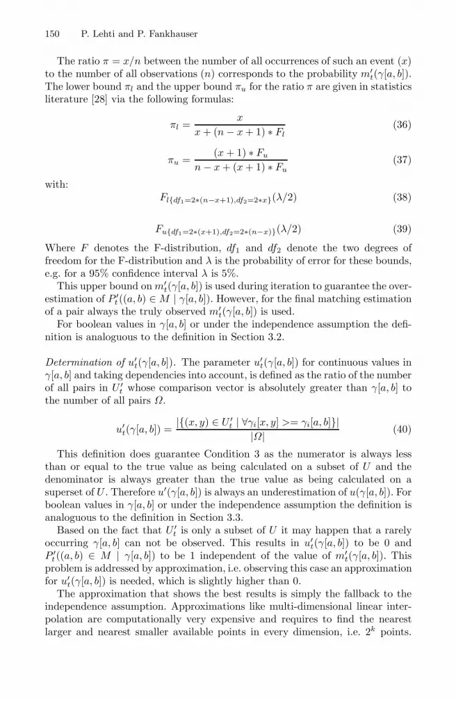
150 P. Lehti and P. Fankhauser
The ratio π = x/n between the number of all occurrences of such an event (x)to the number of all observations (n) corresponds to the probability m′
t(γ[a, b]).The lower bound πl and the upper bound πu for the ratio π are given in statisticsliterature [28] via the following formulas:
πl =x
x + (n − x + 1) ∗ Fl(36)
πu =(x + 1) ∗ Fu
n − x + (x + 1) ∗ Fu(37)
with:Fl{df1=2∗(n−x+1),df2=2∗x}(λ/2) (38)
Fu{df1=2∗(x+1),df2=2∗(n−x)}(λ/2) (39)
Where F denotes the F-distribution, df1 and df2 denote the two degrees offreedom for the F-distribution and λ is the probability of error for these bounds,e.g. for a 95% confidence interval λ is 5%.
This upper bound on m′t(γ[a, b]) is used during iteration to guarantee the over-
estimation of P ′t ((a, b) ∈ M | γ[a, b]). However, for the final matching estimation
of a pair always the truly observed m′t(γ[a, b]) is used.
For boolean values in γ[a, b] or under the independence assumption the defi-nition is analoguous to the definition in Section 3.2.
Determination of u′t(γ[a, b]). The parameter u′
t(γ[a, b]) for continuous values inγ[a, b] and taking dependencies into account, is defined as the ratio of the numberof all pairs in U ′
t whose comparison vector is absolutely greater than γ[a, b] tothe number of all pairs Ω.
u′t(γ[a, b]) =
|{(x, y) ∈ U ′t | ∀γi[x, y] >= γi[a, b]}|
|Ω| (40)
This definition does guarantee Condition 3 as the numerator is always lessthan or equal to the true value as being calculated on a subset of U and thedenominator is always greater than the true value as being calculated on asuperset of U . Therefore u′(γ[a, b]) is always an underestimation of u(γ[a, b]). Forboolean values in γ[a, b] or under the independence assumption the definition isanaloguous to the definition in Section 3.3.
Based on the fact that U ′t is only a subset of U it may happen that a rarely
occurring γ[a, b] can not be observed. This results in u′t(γ[a, b]) to be 0 and
P ′t ((a, b) ∈ M | γ[a, b]) to be 1 independent of the value of m′
t(γ[a, b]). Thisproblem is addressed by approximation, i.e. observing this case an approximationfor u′
t(γ[a, b]) is needed, which is slightly higher than 0.The approximation that shows the best results is simply the fallback to the
independence assumption. Approximations like multi-dimensional linear inter-polation are computationally very expensive and requires to find the nearestlarger and nearest smaller available points in every dimension, i.e. 2k points.

Unsupervised Duplicate Detection Using Sample Non-duplicates 151
Using the mean between a statistic upper bound for this γ occurence and 0performed poorer as it is independent of the concrete values of the comparisonvector components, i.e. the 0 vector would get the same probability as a vector,where only one component is very untypically.
However, this approximation is only used for the final estimation of the du-plicate probability. For constructing the revised sets M ′
t and U ′t the observed
probability of 0 for u′t(γ[a, b]) is used, as otherwise Condition 3 could not be
guaranteed anymore.
4.4 Handling Null Values
The problem of handling null values occurs for the determination of u′t(γ[a, b])
and m′t(γ[a, b]), when one γi[a, b] component is a null value and the other is a
continuous similarity value. There are several ways to decide, if such componentsmatch or not:
– A null value never matches a distance value. This basically means that com-parison vectors with null values can only be compared with other comparisonvectors that also contain null values for exactly the same component, i.e.,the sets U ′ and M ′ are split into subsets, one for each null value combina-tion. These subsets might be very small depending on the input sets and thiswould result in poor accuracy/confidence for the probabilities.
– A null value matches every distance value. This basically means that thiscomparison vector component is ignored and has no further influence on theresulting probabilities.
– The null value is replaced with a similarity value. This similariy value canbe the most probable value for this comparison vector component, which ise.g. the mean value of all non-null similarity values for this component.
4.5 Machine Learning Methods as Decision Model
For machine learning methods the problem can be seen as classification problem,where the unlabeled data points in M ′ should be classified into the two distinctclasses of duplicates M and non-duplicates U . In general, machine learning meth-ods can be distinguished in supervised and unsupervised methods. Supervisedmethods use a set of labeled examples to train a classification function, which isthen used to classify the unlabeled data points. State of the art for supervisedclassification are Support Vector Machines (SVM) [2]. Unsupervised methodsare in general clustering algorithms, which try to separate the unlabeled datapoints into two clusters of data points that seem to belong together based onsome distance between the data points. Examples for such clustering algorithmsare KMeans [29] and spectral clustering [30].
However, the problem at hand does have additional labeled data points foronly one class, which are the data points in U ′. Therefore these methods can notbe used in their usual way. Two state of the art machine learning methods are

152 P. Lehti and P. Fankhauser
tried as decision models in the approach; the simple KMeans clustering and theSVM classification algorithm.
Null values are handled by replacing them with the most probable similarityvalue for this component, which is the mean of all non-null similarity values.
Simple KMeans. The KMeans algorithm tries to find two cluster centroids, suchthat all data points in this cluster are nearer to their centroid than to the other.To this end KMeans starts with initial centroids, assigns all data points to thecentroid that is nearest to them and afterwards calculates new centroids for theidentified clusters. This is done iteratively until the centroids stay fixed. As thedistances to the centroid are in general calculated by a simple euclidean distance,the assumed cluster shape is spherical.
This is the main disadvantage of KMeans: it fails, if the cluster shape stronglydiffers from a spherical shape. The features of the comparison vector in duplicatedetection usally show very different distributions (based on the uniqueness andreliability of the attribute) and they may also depend on each other, which mayresult in non-spherical cluster shapes.
In order to use KMeans, one has to specify the initial cluster centroids. Inthe given scenario this can be achieved by calculating the centroid for the non-duplicates out of U ′ and setting the centroid of the duplicates to 0.
Experiments using KMeans did either perform very poor (lower accuracy thana baseline) or did fail completely (identifying random clusters). All this can beexplained with the distribution of the clusters is neither spherically shaped norlinearly separable and therefore KMeans is not well suited for this scenario.
Iterative Support Vector Machines. Support Vector Machines try to find a hy-perplane between the two classes, such that the margin between the hyperplaneand the data points of both classes is maximized. SVMs use kernel functionsthat are able to separate many kinds of cluster shapes. SVMs need to be trainedwith data points of both classes. Here the same trick as for the Fellegi-Suntermodel can be used, the set M ′ is assumed to contain only duplicates and is usedto train the SVM together with the clear non-duplicate data points from U ′.This SVM is then used to classify M ′ and altough these data points were allused as duplicate examples, the SVM will classify some as non-duplicates. Inanother iteration these detected non-duplicates can then be used as additionalnon-duplicate examples and a cleaner M ′
1 is used as better examples for the du-plicates. This is done iteratively as no further non-duplicates are detected in M ′
t.SVMs are parameterized and these parameters must in general be learned
from the training set. However, as no clean training sets exist, default parametersettings are used in this approach and still show very good results.
5 Evaluation
This section shows the results of the evaluation of the matching method. Indetail the following objectives are met by the evaluation:

Unsupervised Duplicate Detection Using Sample Non-duplicates 153
– All presented decision models outperform a simple baseline method thatsimply decides on the basis of an unweighted arithmetic mean of the distancevalues.
– The presented extensions for the Fellegi-Sunter model for continuous dis-tance values and taking dependencies into account outperform the classicapproaches.
– The SVM and Fellegi-Sunter based decision models outperform other state ofthe art unsupervised models and are even nearly as good as fully supervisedmethods.
– The used distance measure has an enormous impact on the results of thedecision module.
5.1 Datasets
For an evaluation a Restaurant and a Census data set are chosen, which werepreviously used as benchmarks for duplicate detection, e.g. in [14,11]. The restau-rant dataset contains 864 restaurant names and addresses with 112 duplicates,composed of 533 and 331 restaurants assembled from Fodor’s and Zagat’s restau-rant guides. These individual datasets are duplicate free. The attributes beingrestaurant name, street address, city and cuisine. Table 1 shows a sample dupli-cate record from this dataset.
Table 1. Sample duplicate records from the Restaurant data set
name address city cuisineuncle nick’s 747 ninth ave. new york city greekuncle nick’s 747 9th ave. between 50th and 51st sts. new york mediterranean
The census data set is a synthetic dataset containing 824 census-like recordswith 327 duplicates, composed of two duplicate free sets with 449 and 375records. The attributes being last name, first name, house number and street.Table 2 shows a sample duplicate record from this data set.
Table 2. Sample duplicate records from the Census data set
last name first name house number streetJIMENCZ WILLPAMINA S 214 BANKJIMENEZ WILHEMENIA 214 BANKS
5.2 Experimental Methodology
For the blocking phase the multi-pass algorithm as described in [31] is used witha window distance size of 0.25. On the restaurant dataset the blocking was doneon the name and address attribute resulting in 251 potential duplicate pairs

154 P. Lehti and P. Fankhauser
for the set M ′, which corresponds to 100% recall and 45% precision, and 188non-duplicate pairs for the set U ′. On the census dataset the blocking was doneon the last name and first name attribute resulting in 1524 potential duplicatepairs for the set M ′, which corresponds to 90% recall and 19% precision, and1607 non-duplicate pairs for the set U ′.
For comparison of the experimental results precision, recall and F-measures.are calculated. These are defined as usual in information retrieval [32]:
Precision =|CorrectlyIdentifiedDuplicates|
|IdentifiedDuplicates|
Recall =|CorrectlyIdentifiedDuplicates|
|TrueDuplicates|
F -measure =2 ∗ Precision ∗ Recall
Precision + Recall
The precision-recall curves in the figures use interpolated precision valuesat 20 standard recall levels following the traditional procedure in informationretrieval [32]. However, the figures show only the interesting area between therecall levels 0.6 and 1.
5.3 The Fellegi-Sunter Model as Decision Model
For the evaluation of the approach using the Fellegi-Sunter model as decisionmodel, a threshold of 50% is used, i.e. all pairs that have a matching probabilityof less than 50% are removed from M ′
t.
Dependencies. A first experiment compares the precision and recall of the Fellegi-Sunter model under and without the independence assumption. This is doneusing continuous values and in the described unsupervised way as well as asupervised way, which calculates the m(γ[a, b]) and u(γ[a, b]) values on the truesets M and U . Furthermore the results are also compared against a simplebaseline, which simply concatenates the string values of the individual attributesand takes the string similarity between these concatenated strings as overallresult - ignoring attribute relevance.
The maximum F-measures of these methods on both data sets are shown inTable 3. Figure 3 shows the precision and recall curves for the restaurant dataset,Figure 4 the curves for the census dataset.
These results show that the Fellegi-Sunter model taking dependencies intoaccount always reaches one of the highest accuracies. Even under the indepen-dence assumption it performs significantly better than the baseline. However,the effect of taking dependencies into account depends on the dataset, whichcan be explained that in the restaurant dataset, there exist less dependenciesbetween the attributes.

Unsupervised Duplicate Detection Using Sample Non-duplicates 155
Fig. 3. Precision-Recall for the restaurant dataset
Table 3. Maximum F-measures using the Fellegi-Sunter model as decision model
Method Restaurant CensusBaseline 0.916 0.725unsupervisedF&S independent 0.943 0.855F&S dependent 0.940 0.875supervisedF&S independent 0.953 0.834F&S dependent 0.973 0.909
Continuous Values. The previous experiment has already used the extension forcontinuous distances measures. In order to show the impact of these continuousvalues in contrast to thresholded boolean ”match” - ”not match” values is shownin the following experiments. The results of the Fellegi-Sunter model with con-tinuous values and taking dependency into account is compared to the resultsusing thresholded boolean values, with thresholds of 0.1, 0.2, 0.3 and 0.4. Themaximum F-measures of these methods on both data sets are shown in table 4.Figure 5 shows the precision and recall curves for the restaurant dataset, Figure6 the curves for the census dataset.
These results show that boolean values can reach results nearly as good ascontinuous values under the condition that they are well calibrated. Poorly cal-ibrated thresholds for the boolean values can result in very poor results, likethe results for the thresholds 0.1 or 0.4. Therefore the use of continuous distance

156 P. Lehti and P. Fankhauser
Fig. 4. Precision-Recall for the census dataset
Table 4. Maximum F-measures for boolean variables
Method Restaurant CensusF&S continuous 0.940 0.875boolean - 0.1 0.845 0.649boolean - 0.2 0.915 0.834boolean - 0.3 0.930 0.874boolean - 0.4 0.902 0.803
measures for the comparison vector is not only highly accurate, but also requiresmuch less user-interaction than using boolean values and is therefore preferable.
5.4 Support Vector Machines as Decision Model
The next experiment uses the support vector machines in the way as describedin Section 4.5, i.e., the svm is trained with U ′ as negative examples and withM ′ as positive examples. To this end the libsvm library was used as providedby [33], taking c-svcs, with a radial basis kernel and setting the gamma and costparameter to 1. This results in maximum f-measures for the restaurant data setof 0.949 and for the census data set of 0.908. The precision and recall curves areshown in comparison to other approaches in the following section.
These results are very convincing, but it is interesting to note that whenchanging the parameters gamma and cost the results may vary dramaticallyand particularly different for the two data sets, i.e., the best parameter settingsdepend on the data and the default settings that worked for both data sets maynot work for others!

Unsupervised Duplicate Detection Using Sample Non-duplicates 157
Fig. 5. Precision-Recall for boolean variables on the restaurant dataset
Fig. 6. Precision-Recall for boolean variables on the census dataset
5.5 Comparison of the Approaches
This section compares the Fellgi-Sunter based and SVM based approaches withother state of the art methods. This is done for the unsupervised and the

158 P. Lehti and P. Fankhauser
supervised setting. For the unsupervised setting the following approaches arecompared on the restaurant and the census data set:
– Base: this baseline simply concatenates the individual string values of theattributes and takes the string similarity between these concatenated stringsas overall result - ignoring attribute relevance.
– HGM (Hierarchical Graphical Model): this is the unsupervised approachpresented in [11] that uses the same datasets for their evaluation. Theirresults are simply copied for comparison, although they used a differentblocking algorithm.
– Fellegi-Sunter: The Fellegi-Sunter based approach using continuous distancevalues and taking dependencies into account.
– SVM: The SVM based approach.
It must be noted that the Jaro distance is used as distance function for theexperiments as provided by [34], whereas [11] was using the SoftTFIDF distanceand [14] was using the Jaccard distance. A comparison of these distance functionsis presented in [24]. The impact of different distance functions is evaluated inSection 5.6.
The maximum F-measures of these methods on both data sets are shown intable 5. Figure 7 shows the precision and recall curves for the restaurant dataset,Figure 8 the curves for the census dataset in the unsupervised setting.
These results clearly show that the proposed unsupervised methods signifi-cantly outperform other exisiting unsupervised methods and they are even notfar away from the results of fully supervised methods.
Fig. 7. Precision-Recall for the restaurant dataset
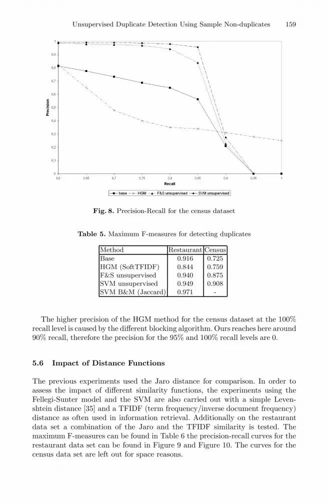
Unsupervised Duplicate Detection Using Sample Non-duplicates 159
Fig. 8. Precision-Recall for the census dataset
Table 5. Maximum F-measures for detecting duplicates
Method Restaurant CensusBase 0.916 0.725HGM (SoftTFIDF) 0.844 0.759F&S unsupervised 0.940 0.875SVM unsupervised 0.949 0.908SVM B&M (Jaccard) 0.971 -
The higher precision of the HGM method for the census dataset at the 100%recall level is caused by the different blocking algorithm. Ours reaches here around90% recall, therefore the precision for the 95% and 100% recall levels are 0.
5.6 Impact of Distance Functions
The previous experiments used the Jaro distance for comparison. In order toassess the impact of different similarity functions, the experiments using theFellegi-Sunter model and the SVM are also carried out with a simple Leven-shtein distance [35] and a TFIDF (term frequency/inverse document frequency)distance as often used in information retrieval. Additionally on the restaurantdata set a combination of the Jaro and the TFIDF similarity is tested. Themaximum F-measures can be found in Table 6 the precision-recall curves for therestaurant data set can be found in Figure 9 and Figure 10. The curves for thecensus data set are left out for space reasons.

160 P. Lehti and P. Fankhauser
Table 6. Maximum F-measures using different distance measures
Method Restaurant CensusF&S levenshtein 0.914 0.851F&S jaro 0.940 0.875F&S tfidf 0.964 0.546F&S tfidf+jaro 0.965SVM levenshtein 0.735 0.489SVM jaro 0.949 0.908SVM tfidf 0.898 0.600SVM tfidf+jaro 0.974
Fig. 9. Precision-Recall for the restaurant dataset using the Fellegi&Sunter model withdifferent similarity measures
The experiment shows that the selection of a good similarity function is ofgreat importance. It shows that the effectiveness of a similarity function dependson the data, in particular the TFIDF similarity function performs much betteron the restaurant data set than on the census data. The results further showthat the SVM approach is much more sensible to a good similarity function, bothalternative similarity functions result in a much worse accuracy. The combinationof several similarity measures significantly outperforms those with just one, thiscan be explained by that a single similarity function in general only detects onekind of error, if several kinds of error might occur, like in the restaurant dataset, several similarity measures should be used together for maximum accuracy.These results demand for further work in unsupervised finding ideal similarityfunctions.

Unsupervised Duplicate Detection Using Sample Non-duplicates 161
Fig. 10. Precision-Recall for the restaurant dataset using the SVM model with differentsimilarity measures
Relationships. In order to evaluate the approach for taking relationships intoaccount, the ”cuisine” attribute of the restaurant data set can be seen as relatedobject, because it realizes a n : 1 relationship. The similarity of these attributevalues were also difficult to measure with string similarity measures as can beeasily seen for examples like ”greek-mediterranean” or ”asian-chinese”. There-fore the jaro measure was replaced with the mutual information score, which isbasically the ratio between the true number of cooccurences of a value-pair tothe expected statistical random number of cooccurences.
Using this measure for the ”cuisine” attribute and the jaro measure for allothers, yields a maximum F-measure of 0.955 (vs. 0.940) for the Fellegi-Sunterbased model and 0.973 (vs. 0.949) for the SVM based model. This clearly showsthe potential of this method, although further experiments with other data setsare required. We expect a much more significant gain in accuracy for more rele-vant attributes/relationships in other domains.
6 Conclusion and Future Work
This paper has presented an unsupervised approach for duplicate detection, whichincorporates sample non-duplicates into the duplicate decision process. This isused either with a refinement of the classic Fellegi-Sunter model for record linkage,which allows determining appropriate parameter values using continuous simi-larity measures and taking attribute dependencies into account or by using Sup-port Vector Machines. The proposed approach is based on unsupervised learningand domain independence, which makes it completely free from user interaction,i.e., removing the main reason, why classical approaches are very expensive. The

162 P. Lehti and P. Fankhauser
evaluations on two test datasets showed that the approach reaches very high ac-curacy, outperforms existing unsupervised approaches and is nearly competitivewith fully supervised and domain dependent approaches.
It has been shown that the importance of the used similarity function is high,therefore we want to further investigate in unsupervised finding ideal (combi-nations of) similarity functions. Also the usage of association measures like themutual information score has been shown to be a simple but effective method toincorporate interrelated objects into the duplicate detection process. However,other data sets that are expected to profit more of this method need to be foundand evaluated.
Ongoing scalability experiments on large real world data sets, have shownthat the naive training of Fellegi-Sunter distributions and SVMs with the fullM ′ and U ′ sets result in quadratic behavior. The simple optimization, restrictingthe size of these training sets with a fixed threshold has shown very promisingresults and allows linear complexity and for this reason good scalability. Findingan ideal threshold is still an open issue.
References
1. Fellegi, I.P., Sunter, A.B.: A theory for record linkage. Journal of the AmericanStatistical Association 64 (1969) 1183–1210
2. Russell, S., Norvig, P.: Artificial Intelligence: A Modern Approach. Prentice Hall(2002)
3. Hernandez, M.A., Stolfo, S.J.: Real-world data is dirty: Data cleansing and themerge/purge problem. Data Mining and Knowledge Discovery 2 (1998) 9–37
4. Galhardas, H., Florescu, D., Shasha, D., Simon, E.: An extensible frameworkfor data cleaning. In: Proceddings of the 16th International Conference on DataEngineering (ICDE ’00). (2000) 312
5. Monge, A., Elkan, C.: An efficient domain independent algorithm for detectingapproximately duplicate database records. In: In Proceedings of the SIGMODWorkshop on Data Mining and Knowledge Discovery. (1997)
6. Newcombe, H.B., Kennedy, J.M., Axford, S.J., James, A.P.: Automatic linkage ofvital records. Science 130 (1959) 954–959
7. Winkler, W.E.: Using the em algorithm for weight computation in the fellegi-sunter model of record linkage. In: Proceedings of the Section on Survey ResearchMethods, American Statistical Association. (1988) 667–671
8. Dempster, A.P., Laird, N.M., Rubin, D.B.: Maximum likelihood from incompletedata via the em algorithm. Journal of the Royal Statistical Society, Series B 34(1977) 1–38
9. Winkler, W.E.: Improved decision rules in the fellegi-sunter model of record linkage.In: Proceedings of the Section on Survey Research Methods, American StatisticalAssociation. (1993) 274–279
10. Larsen, M.D., Rubin, D.B.: Alternative automated record linkage using mixturemodels. Journal of the American Statistical Association 79 (2001) 32–41
11. Ravikumar, P., Cohen, W.W.: A hierarchical graphical model for record linkage.In: AUAI ’04: Proceedings of the 20th conference on Uncertainty in artificial intel-ligence, AUAI Press (2004) 454–461

Unsupervised Duplicate Detection Using Sample Non-duplicates 163
12. Elfeky, M.G., Verykios, V.S., Elmargarid, A.K.: Tailor: A record linkage tool-box. In: Proceedings of the 18th International Conference on Data Engineering(ICDE’02), Washington, DC, USA, IEEE Computer Society (2002) 17
13. Cohen, W.W., Richman, J.: Learning to match and cluster large high-dimensionaldata sets for data integration. In: Proceedings of the Eighth ACM SIGKDD In-ternational Conference on Knowledge Discovery and Data Mining (KDD-2002),Edmonton, Alberta (2002)
14. Bilenko, M., Mooney, R.J.: Learning to combine trained distance metrics for du-plicate detection in databases. Technical Report AI 02-296, Artificial IntelligenceLaboratory, University of Texas at Austin, Austin, TX (2002)
15. Tejada, S., Knoblock, C.A., Minton, S.: Learning object identification rules forinformation integration. Information Systems Journal 26 (2001) 635–656
16. Sarawagi, S., Bhamidipaty, A.: Interactive deduplication using active learning. In:Proceedings of the Eighth ACM SIGKDD International Conference on KnowledgeDiscovery and Data Mining (KDD-2002), Edmonton, Alberta (2002)
17. Ananthakrishna, R., Chaudhuri, S., Ganti, V.: Eliminating fuzzy duplicates indata warehouses. In: Proceedings of the 28th International Conference on VeryLarge Data Bases(VLDB ’02). (2002)
18. Parag, Domingos, P.: Multi-relational record linkage. In: Proceedings of the KDD-2004 Workshop on Multi-Relational Data Mining. (2004) 31–48
19. Dong, X., Halevy, A.Y., Madhavan, J.: Reference reconciliation in complex infor-mation spaces. In: SIGMOD Conference. (2005) 85–96
20. Bhattacharya, I., Getoor, L.: Deduplication and group detection using links. In:Proceedings of the KDD-2004 Workshop on Link Analysis and Group Detection.(2004)
21. Pasula, H., Marthi, B., Milch, B., Russell, S., Shpitser, I.: Identity uncertaintyand citation matching. In: Advances in Neural Information Processing Systems15, MIT Press (2003)
22. Ley, M.: DBLP computer science bibliography. (http://dblp.uni-trier.de/)23. Fachinformationszentrum-Karlsruhe: CompuScience. (http://www.zblmath.fiz-
karlsruhe.de/cs/)24. Cohen, W.W., Ravikumar, P., Fienberg, S.E.: A comparison of string metrics for
matching names and records. In: Proceedings of the KDD-2003 Workshop on DataCleaning, Record Linkage, and Object Consolidation, Washington, DC (2003) 13–18
25. Evert, S.: Computational approaches to collocations. (http://www.collocations.de/)
26. Church, K.W., Hanks, P.: Word association norms, mutual information and lexi-cography. Computational Linguistics 16 (1990) 22–29
27. Church, K.W., Gale, W., Hanks, P., Hindle, D.: Using statistics in lexical analysis.Lexical Acquisition: Using On-line Recources to Build a Lexicon (1991) 115–164
28. Sachs, L. In: Angewandte Statistik. Springer, Berlin (2004) 434–43529. MacQueen, J.: Some methods for classification and analysis of multivariate ob-
servations. In: Proceedings of the Fifth Berkeley Symposium on Math., Stat. andProb. (1967) 281–296
30. Shi, J., Malik, J.: Normalized cuts and image segmentation. IEEE Trans. CAD-Integrated Circuits and Systems 13 (2000) 888–905
31. Lehti, P., Fankhauser, P.: A precise blocking method for record linkage. In: Pro-ceedings of the 7th International Conference on Data Warehousing and KnowledgeDiscovery (DaWaK’05). (2005)

164 P. Lehti and P. Fankhauser
32. Baeza-Yates, R., Ribiero-Neto, B. In: Modern Information Retrieval. AddisonWesley (1999) 74–79
33. Chang, C.C., Lin, C.J.: Libsvm - a library for support vector machines. (http://www.csie.ntu.edu.tw/ cjlin/libsvm/)
34. Cohen, W.W., Ravikumar, P., Fienberg, S.: Secondstring - an open-sourcejava-based package of approximate string-matching techniques. (http:// second-string.sourceforge.net/)
35. Levenshtein, V.I.: Binary codes capable of correcting insertions and reversals.Soviet Physics Doklady 10 (1966) 707–710

Towards Algebraic Query Optimisationfor XQuery�
Markus Kirchberg, Faizal Riaz-ud-Din,Klaus-Dieter Schewe, and Alexei Tretiakov
Massey University, Department of Information Systems andInformation Science Research Centre
Private Bag 11 222, Palmerston North, New Zealand{m.kirchberg, f.din, k.d.schewe, a.tretiakov}@massey.ac.nz
Abstract. XML-based databases have become a major area of interestin database research. Abstractly speaking they can be considered as aresurrection of complex-value databases using constructors for records,lists, unions plus optionality and references. XQuery has become thestandard query language for XML. As XQuery is a declarative querylanguage, the problem of query optimisation arises. In this paper an al-gebraic approach to query optimisation is introduced. This is based on atranslation of XQuery into a query algebra for rational tree types. Thealgebra uses simple operations on types and structural recursion for lists.The translation exploits linguistic reflection for the type-safe expansionof path expressions. The availability of an algebraic representation ofqueries permits query rewriting, which in combination with cost heuris-tics permits queries to be rewritten and thus optimised.
1 Introduction
Though XML is more than a database language [26], it has become a major areaof interest in database research. XML can be considered as a complex-value datamodel using constructors for records, lists, unions plus optionality and references[1,36].
Using XML for databases requires schema definition, query and update lan-guages. By now, XML Schema [46] has become the W3C standard for definingschemata, while XQuery [16,47] is the recommended standard for querying XMLdocuments. For updates only little work has been done so far, e.g. [42,22].
In fact, XML Schema supports almost directly the definition of tree typesusing the mentioned constructors. XQuery combines ideas from various prede-cessor proposals for XML query languages [4,6,12]. Most importantly, queries arecomposed of a matching part that binds variables to values according to a givenXML document, and a construction part that creates new XML documents fromthese variables.� The work reported in this paper was supported by FRST/NERF grant MAUX0025
“DIMO – Distributed Multi-Level Object Bases”.
S. Spaccapietra (Ed.): Journal on Data Semantics VII, LNCS 4244, pp. 165–195, 2006.c© Springer-Verlag Berlin Heidelberg 2006
166 M. Kirchberg et al.
As XQuery is a declarative query language with XPath [14] as its core, theproblem of query optimisation arises. This problem is directly related to theimplementation of XQuery, for which there are two major lines of research.The first one, e.g. [11], attempts a translation to SQL based on a reification ofXML via relational database technology. The drawback of this approach is thatsemantics may be lost in the translation from trees to relations. The alternativeis to approach a direct implementation of XQuery, e.g. [28].
In this paper we take a different approach, which is closer to the correspond-ing relational theory. Considering XML as a complex value data model, eachXML document can be represented by a rational tree, i.e. a (possibly infinite)tree with only finitely many different subtrees. In fact, rational trees representpossibly infinite data structures that still can be finitely represented. The semi-nal work in [10] contains the mathematical theory of rational trees. In [3,32] itwas shown that rational trees capture indeed the gist of the structural notionof “object” in object oriented databases. In [30] this was extended to show thatin fact each reasonable data model can be represented using rational trees. Infact, the finite representation of a rational tree results from breaking cycles andintroducing identifiers. Conversely, a collection of objects with identifiers andreferences based on these identifiers can be expanded into rational trees, pro-vided a condition known as “value representability” is satisfied [31,32]. Valuerepresentability and thus the representation by rational trees is also known asa necessary and sufficient condition for the unique identification of objects andthe existence of schema-defined generic update operations [32].
Our idea is to exploit a query algebra for rational trees and to use algebraicquery rewriting in combination with query costs heuristics for query optimi-sation. This idea requires a translation of XQuery into a rational tree queryalgebra. In [30] it has been shown how the gist of query algebras can be ex-pressed in a generic rational tree algebra. In fact, only operations defined forthe constructors of a type system plus a single generalised join-operation areneeded. In [19] this has been extended by showing that indeed all query algebrasthat were developed together with object oriented databases, e.g. RELOOP [8],ENCORE [33], AQUA [24], QAL [29], HERM-algebra [43] and GOMext [9,17],can be expressed in a generic rational tree algebra. Though that is has not yetbeen formally proven, the same presumably holds for algebras proposed for XMLsuch as XAlgebra [13] and TAX [15].
For short let RTA denote the query algebra for rational trees from [30]. RTAuses operators for the type system, i.e. for the abstract system of types as de-fined in [16]. In particular, it exploits structural recursion [25,41,44] for lists.More generally, structural recursion was developed for all kinds of bulk typessuch as lists, sets, multisets (aka bags), binary trees, etc. [5,41,44], but the pri-mary interest was on finite sets [40,41,45]. Structural recursion was thoroughlyinvestigated throughout the nineties. The fundamental idea of structural recur-sion on such bulk types is simple and powerful at the same time exploiting thesimple fact that non-empty lists can be constructed by using singleton lists andlist concatenation, so three constructors – the third one producing the empty

Towards Algebraic Query Optimisation for XQuery 167
list – are sufficient for the representation of lists. Consequently, operations onlists are sufficiently determined by their effects on the empty list, singleton lists,which can be defined by an operation on the list element, and lists that are theconcatenation of two sublists. Similarly, constructors for the empty set, singletonsets and set union will give us all finite sets with elements of a particular type.Koch in [23] has used a similar approach based on list comprehensions. However,his work is placed in a complexity-theoretic setting.
As shown in [20] the translation of XQuery to RTA works best, if schemainformation is available, in particular for the path expressions. This reflects thefact that the major difficulty in implementing XQuery results from path expres-sions [14,27], i.e. from the fragment of the language that subsumes XPath [7].Then it is a natural idea to exploit type-safe linguistic reflection [38,37] to dealwith this problem. The basic idea of linguistic reflection consists of providingmacros in a language that will be expanded during compilation or execution. Inthe case of XQuery these macros will be parts of FLWOR- and in particular pathexpressions. The macro expansion requires some complex computation, duringwhich the information about the schema will be needed. In order to do this, theexpression at hand will be treated as a value of some type, such that a predefinedprocess can take this value as its input and produce another value representingthe expanded macro as its output. This output value has to be treated again aspart of the code to be compiled or executed. Linguistic reflection is as old as theroots of functional programming, but due to the work of mainly Stemple andSheard [39,35,34] it has been shifted from a run-time to a compile-time approachand in addition has been extended to guarantee type-safety. The work in [18]contains an implementation of linguistic reflection in the context of persistentprogramming languages.
Using this idea of linguistic reflection is what we do in our approach, i.e.we present a translation from essential parts of XQuery to RTA and show howthis translation benefits from linguistic reflection. In case there is no schemainformation, it must be derived from a given document, but we will not explorethis direction in this paper.
Besides algebraic query optimisation, the expected benefits of the translationto a query algebra are the easy implementation of the operations and the inte-gration with programming languages, e.g. using the physical architecture from[21], and the easy extension to other constructors such as sets and multisets incase the order that comes with the list constructor is considered unnecessary oreven undesired.
We first introduce an abstract model of XML, XQuery and RTA in Sections2 and 3, respectively. In Section 4 we then outline the translation from XQueryto RTA. We focus on structural recursion and show that some of the functionsused as parameters are complicated, as they refer to path finding. We show howlinguistic reflection can be used to expand these functions. In particular, thecomplexity arising from the paths will be taken up by the translation. Section 5 isthen devoted to algebraic query optimisation. For this we explore cost heuristics

168 M. Kirchberg et al.
for the various operators of RTA, which directly lead to query rewriting rules.We conclude with a brief summary.
2 Abstract Model of XML and XQuery
In this section we describe some basics of XML and XQuery. Of course, as bothof these are complex languages, we cannot describe all details and therefore takea more abstract view focusing more on the semantics than on the syntax.
2.1 XML Documents as Trees
Start with a type system that supports records, lists and unions. Using abstractsyntax this type system can be described by
t = b | (t1, . . . , tn) | [t] | t1 ⊕ · · · ⊕ tn.
Here b represents a (not further specified) collection of base types, e.g. the basetypes supported by XML such as String , Integer , Double, ID , etc. For reasonsthat will become clear, when we add references, we only use a single type ID foridentifiers. Furthermore, assume that one of the base types is Empty with onlyone possible value. This type can be used to support optionality.
We use (t1, . . . , tn) to denote an ordered record type with component typesti, the type [t] is used for finite lists, and t1 ⊕ · · · ⊕ tn is used for a (disjoint)union type with components ti.
Each type t denotes a set of values called its domain dom(t). Formally, weobtain these domains as follows:
– dom(bi) = Vi, i.e. for each base type bi we assume some set Vi of values ofthat type, e.g. dom(EMPTY ) = {⊥}.
– dom((t1, . . . , tn)) = dom(t1) × · · · × dom(tn).– dom([t]) = {[v1, . . . , vk] | k ∈ N, vi ∈ dom(t)}.– dom(t1 ⊕ · · · ⊕ tn) = {(i, vi) | 1 ≤ i ≤ n, vi ∈ dom(ti)}.
Then an XML document can be represented by a value of some type t, whichin turn is representable as a tree, provided the document does not contain ref-erences. In particular, we can treat attributes in the same way as subelements– which is no loss of generality for databases, whereas for text markup it maymake a significant difference.
In order to also capture references, we extend the type system to
t = b | � | (t1, . . . , tn) | [t] | t1 ⊕ · · · ⊕ tn | � : t,
where � represents reference labels. The domains are simply dom(�)=dom(ID)and dom(� : t) = {(i, v) | i ∈ dom(�), v ∈ dom(t)}. Following [1] each occurrenceof a value i of type ID in some complex value v that corresponds to a labelledtype � : t defines a reference, whereas each occurrence of a value i of type ID in

Towards Algebraic Query Optimisation for XQuery 169
v that corresponds to a label � uses the reference. In XML Schema the usage ofreferences corresponds to the type IDREF , whereas the definition of referencescorresponds to the type ID . Furthermore, IDREFS corresponds to a list type[�] – in fact, here we would prefer to use a set type, but for simplicity andorthogonality of the constructors let us use only one bulk type constructor.
Example 2.1. Let us look at the following schema definition in XML Schema:
<xs:schema xmlns:xs="http://www.w3.org/2001/XMLSchema"><xs:element name="coffee-shop">
<xs:complexType><xs:sequence>
<xs:element ref="coffees"/><xs:element ref="growers"/><xs:element ref="regions"/>
</xs:sequence></xs:complexType>
</xs:element><xs:element name="coffees">
<xs:complexType><xs:sequence>
<xs:element ref="coffee" minOccurs="0" maxOccurs="unbounded"/></xs:sequence>
</xs:complexType></xs:element><xs:element name="growers">
<xs:complexType><xs:sequence>
<xs:element ref="grower" minOccurs="0" maxOccurs="unbounded"/></xs:sequence>
</xs:complexType></xs:element><xs:element name="regions">
<xs:complexType><xs:sequence>
<xs:element ref="region" minOccurs="0" maxOccurs="unbounded"/></xs:sequence>
</xs:complexType></xs:element><xs:element name="coffee">
<xs:complexType><xs:sequence>
<xs:element name="name" type="xs:string"/><xs:element name="body" type="xs:string" minOccurs="0"/><xs:element ref="blend" maxOccurs="unbounded"/><xs:element name="price" type="xs:decimal"/>
</xs:sequence><xs:attribute name="c-id" type="xs:ID" use="required"/><xs:attribute name="producer" type="xs:IDREF" use="required"/>
</xs:complexType>

170 M. Kirchberg et al.
</xs:element><xs:element name="blend">
<xs:complexType><xs:sequence>
<xs:element name="bean" type="xs:string"/><xs:element name="percentage" type="xs:integer"/>
</xs:sequence></xs:complexType>
</xs:element><xs:element name="grower">
<xs:complexType><xs:sequence>
<xs:element name="name" type="xs:string"/><xs:element name="owner" type="xs:string" maxOccurs="unbounded"/><xs:element name="area" type="xs:string" minOccurs="0"/><xs:element name="established" type="xs:date" minOccurs="0"/>
</xs:sequence><xs:attribute name="g-id" type="xs:ID" use="required"/><xs:attribute name="in-region" type="xs:IDREF" use="required"/>
</xs:complexType></xs:element><xs:element name="region">
<xs:complexType><xs:sequence>
<xs:element name="name" type="xs:string"/></xs:sequence><xs:attribute name="r-id" type="xs:ID" use="required"/><xs:attribute name="famous-coffees" type="xs:IDREFS"use="required"/>
</xs:complexType></xs:element>
</xs:schema>
That is, a coffee-shop contains a list of coffees, growers and regions. A coffeeis described by a name, a body (optional) and a blend, which is a sequence ofbeans together with their percentages. A grower is described by a name, a list ofowners, an area (optional) and an establishment date (optional). A region justhas a name. Furthermore, there are references from a coffee to the grower thatproduces it, from a grower to the region it is located in, and from a region to allits famous coffees.
Using our type system, we obtain the following complex type definitions forrepresenting this schema:
coffee-shop = (coffees, growers, regions)coffees = [c-id : coffee]growers = [g-id : grower]regions = [r-id : region]coffee = (c-name, body ⊕ Empty, [blend], price, producer)c-name = String

Towards Algebraic Query Optimisation for XQuery 171
body = Stringprice = Decimalproducer = g-idblend = (bean, percentage)bean = Stringpercentage = Integergrower = (g-name, [owner], area ⊕ Empty, established ⊕ Empty, in-region)g-name = Stringowner = Stringarea = Stringestablished = Datein-region = r-idregion = (r-name, famous-coffees)r-name = Stringfamous-coffees = [c-id]
Here c-id, g-id and r-id are labels.
Example 2.2. Consider the following XML document that is in accordance withthe schema defined in Example 2.1:
<coffee-shopxmlns:xsi="http://www.w3.org/2001/XMLSchema-instance"xsi:noNamespaceSchemaLocation="coffee.xsd"><coffees>
<coffee c-id="o11" producer="o1"><name>Java</name><body>full</body><blend>
<bean>Arabica</bean><percentage>100</percentage>
</blend><price>31.95</price>
</coffee><coffee c-id="o12" producer="o1"><name>Sumatra</name><body>very full</body><blend>
<bean>Robusta</bean><percentage>100</percentage>
</blend><price>34.95</price>
</coffee><coffee c-id="o13" producer="o1"><name>New Guinea</name><blend>
<bean>Arabica Old</bean><percentage>65</percentage>

172 M. Kirchberg et al.
</blend><blend>
<bean>Robusta Old</bean><percentage>35</percentage>
</blend><price>29.95</price>
</coffee></coffees><growers>
<grower g-id="o1" in-region="o2"><name>Fine Blend</name><owner>Mr Bean</owner><owner>Mrs Bean</owner><area>231 ha</area><established>1987-01-01</established>
</grower></growers><regions>
<region r-id="o2" famous-coffees="o11 o12"><name>Asia</name>
</region></regions>
</coffee-shop>
This XML document can be represented by the following complex value:
( [ (&o11, (Java, (1, full), [(Arabica, 100)], 31.95, &o1)),(&o12, (Sumatra, (1, very full), [(Robusta, 100)], 34.95, &o1)),(&o13, (New Guinea, (2, ⊥),
[(Arabica Old, 65), (Robusta Old, 35)], 29.95, &o1))],[ (&o1, (Fine Blend, [Mr Bean, Mrs Bean],
(1, 231 ha), (1, 1987-01-01), &o2))],[ (&o2, (Asia, [&o11, &o12]))])
2.2 XQuery in a Nutshell
XQuery is a query language allowing to extract sequences of subtrees and basetype values from any number of XML document trees, and to combine them toconstruct a sequence of trees and basic values (the so-called items) forming theresult of the query. In practice, most often the result of the query is a sequenceconsisting of a single tree.
In XQuery, the XML documents serving as input are identified by using theso-called input functions, of which the most commonly used one is doc, which ac-cepts a URL corresponding to the location of an XML document as a parameter.For example, doc("coffee-shop.xml") would retrieve the coffee-shop.xmldocument from the current directory.

Towards Algebraic Query Optimisation for XQuery 173
Sequences of subtrees are retrieved by using the so-called path expressions,consisting of one or more steps separated by a slash, /, or double slash, //. Eachstep acts on the sequence of items created by the previous step to form a furthersequence, which either forms the output of the path expression (if the step isthe last one), or serves as input for further steps. The following query, formedby combining an input function with a path expression, will result in a sequenceof name elements representing coffee names (assuming coffee-shop.xml is theXML document introduced in the previous section): doc("coffee-shop.xml")/coffee-shop/coffees/coffee/name.
doc("coffee-shop.xml")/coffee-shop results in a sequence consisting of asingle coffee-shop element, doc("coffee-shop.xml")/coffee-shop/coffeesresults in a sequence consisting of a single coffees element (a sub-element of thecoffee-shop element obtained in the previous step), doc("coffee-shop.xml")/coffee-shop/coffees/coffee will result in a sequence of all coffee elementsfrom coffees and so on. Filtering can be applied to restrict which of the items areto be included in a given step. While / retrieves child items (branches immediatelyconnected to the root), // forms a sequence consisting of all matching subtrees,at all depths. / and // are illustrated in examples 2.3 and 2.4, respectively.
As XQuery is a functional language, an XQuery program can be regarded as anexpression formed by subexpressions which, at execution time, are evaluated inthe order of precedence. The most commonly used type of expressions in XQueryare the so-called FLWOR (for, let, where, order by, return) expressions. Ina FLWOR expression, a for clause binds each item of a sequence to a variable,and evaluates the rest of the expression with that binding, resulting in as manyevaluations as there are items in the sequence. The for clause is illustrated inExample 2.4 below.
A let clause binds the whole sequence to a variable, and evaluates the restof the expression just once, with that binding. The let clause is illustrated inExamples 2.5, 2.6, and 2.7.
The where clause serves as a filter: the rest of the FLWOR expression is exe-cuted only if the boolean expression associated with the where clause evaluatesto true. This is illustrated in Example 2.5, 2.6, and 2.7.
The order by clause is used for sorting (we do not discuss it here any further).Finally, the return clause is a constructor, instantiating an item that is to
be included as the result of the query. By using return, items retrieved fromdifferent parts of the same document, or from different documents, can be com-bined together, resulting in sophisticated joins. As shown in Example 2.7, theconstructor formed by using the return clause can include subqueries, whoseoutput is incorporated into the sequence created by the constructor.
XML Query can make use of type information from XML Schema documentsassociated with XML documents inputted by the query by explicitly specifyingthe type of items to be included in sequences or to be constructed. In addition,parsers are able to analyse and to reject a query based on schema informationonly, if the query is found to construct items that do not match the declaredtypes for constructor output.

174 M. Kirchberg et al.
Example 2.3. Assume the document in Example 2.2 is stored in coffee-shop.xml.Then
<coffees>{
doc("coffee-shop.xml")/coffee-shop/coffees/coffee/name}
</coffees>
is a simple query that will select the names of coffees. For our example documentthe result would be
<coffees><name>Java</name><name>Sumatra</name><name>New Guinea</name>
</coffees>
Example 2.4. The query
<coffee-makers>{
for $N in doc("coffee-shop.xml")//ownerreturn <name>{ $N/text() }</name>
}</coffee-makers>
returns the names of coffee owners.
Example 2.5. The following is a query with a more interesting where-clause,which returns the names of Arabica coffees:
<Arabicas>{
for $W in doc("coffee-shop.xml")/coffee-shop/coffees/coffeelet $N := $W/name, $B := $W/blendwhere $B/bean/text() = "Arabica" and $B/percentage/text() = 100return <name>{ $N/text() }</name>
}</Arabicas>
Example 2.6. The following query, which contains selection conditions on thepaths, will produce a list of coffees with their producers:
<coffees>{
let $db := doc("coffee-shop.xml")for $W in $db//coffee, $V in $db//growerlet $P := $W/@producer, $N := $W/name, $M := $V/name,
$I := $V/@g-idwhere $I = $P

Towards Algebraic Query Optimisation for XQuery 175
return<coffee>
<product>{ $N/text() }</product><producer>{ $M/text() }</producer>
</coffee>}
</coffees>
Example 2.7. The following is an example of a nested query:
<coffees>{
let $db := doc("coffee-shop.xml")for $N in $db//coffee/namereturn<coffee>
{ $N }{for $W in $db//coffeewhere $W/name = $Nreturn $W/body
}</coffee>
}</coffees>
The query lists the names of all coffees, adding to each name the correspondingbody, when such information is available.
3 RTA: A Rational Tree Query Algebra
Following a basic idea in [30] we use a query algebra with operations “induced”from the type system plus a join-operation. For our purposes here it is moreconvenient to consider products instead of joins.
In doing so, let 1l denote a trivial type with only one value in its domain. Weuse a unique “forget”-operation triv : t → 1l for each type t. Assume further aboolean type BOOL with constant values T and F. Thus, we may consider theoperations ∧ : BOOL × BOOL → BOOL (conjunction), ¬ : BOOL → BOOL(negation) and ⇒: BOOL × BOOL → BOOL (implication).
We also use a polymorphic equality function eq : t × t → BOOL for any typet. Obviously, eq(x, y) = T iff x = y holds.
For record types we consider projection πi : (t1, . . . , tn) → ti and producto1 × · · · × on : t → (t1, . . . , tn) for given operations oi : t → ti. Obviously, wehave πi(x1, . . . , xn) = xi and (o1 × · · · × on)(x) = (o1(x), . . . , on(x)). As usual,we write πi1,...,ik
as a shortcut for πi1 × · · · × πik.
For union types we use the canonical embeddings ιi : ti → t1 ⊕ · · · ⊕ tnwith ιi(x) = (i, x). Other operations on union types take the form o1 + · · ·+ on :

176 M. Kirchberg et al.
t1 ⊕· · ·⊕ tn → t for given operations oi : ti → t, so we have (o1 + · · ·+on)(i, x) =oi(x).
For list types we may consider � (concatenation), the constant empty : 1l → [t]and the singleton operation single : t → [t] with well known semantics.
It should be noted here that document order is preserved through the use oflists. The ordering of the elements in the lists conforms to the ordering of theelements in the queried XML document (or conforms to specific re-ordering inthe query itself) throughout the execution process.
3.1 Structural Recursion
In addition, we consider structural recursion src[e, g, ] : [t] → t′ with a valuee of type t′, an operation g : t → t′ and an operation : (t′, t′) → t′, which isdefined as follows:
src[e, g, ]([]) = e
src[e, g, ]([x]) = g(x)src[e, g, ](X�Y ) = src[e, g, ](X) src[e, g, ](Y )
In order to be well-defined must be associative with e as neutral element,i.e. (x y) z = x (y z) and x e = e x = x hold for all x, y, z ∈ dom(t′).
Let us illustrate structural recursion by some more or less standard examples.First assume that t is a “number type”, on which addition + : t × t → t isdefined. Then src[0, id, +] with the identity function id on t defines the sum ofthe elements in a set. In this way all the known aggregate functions of SQL andmore can be defined by structural recursion.
Now consider an operation f : t → t′. We want to raise f to an operationmap(f) : [t] → [t′] by applying f to each element of a list. Obviously, we havemap(f) = src[[], single ◦ f, �].
Next consider an operation ϕ : t → BOOL, i.e. a predicate. We want to definean operation filter(ϕ) : [t] → [t], which maps a given list to the sublist of allelements satisfying the predicate ϕ. For this we may write filter(ϕ) =
src[[], if else ◦ (ϕ × single× (empty ◦ triv)), �]
with the operation if else : (BOOL, t, t) → t with (T, x, y) �→ x and(F, x, y) �→ y.
As a third example assume that t is a type, on which addition + : (t, t) → tis defined. Then src[0, id, +] with the identity id on t defines the sum of theelements in a list.
3.2 Querying XML with RTA
Let us simply illustrate now how RTA can be applied to query XML. We willuse the queries from the previous section and write equivalent queries in RTA.
Towards Algebraic Query Optimisation for XQuery 177
Example 3.1. Let us consider first the query in Example 2.3. In this case webasically have to analyse a path expression. For this assume that vin is the com-plex value in Example 2.2, i.e. it represents the corresponding XML documentcoffee-shop.xml.
The construct doc(coffee-shop.xml)/coffee-shop creates a list with the wholedocument as its only entry, which corresponds to applying the RTA-operationsingle to vin. Then /coffees selects the first successor of the root. As vin is atriple, this corresponds to applying map(π1) to [vin]. This gives
map(π1)([vin]) = src[[], single ◦ π1,�]([vin])
= single ◦ π1(vin)= [π1(vin)]
The effect of /coffee in the XQuery path expression is to produce only the listof coffees, i.e. π1(vin). This can be achieved by another application of structuralrecursion, in this case src[[], id, �]. This gives
src[[], id, �]([π1(vin)]) = π1(vin)
as desired. Finally, the effect of /name in the XQuery path expression is firstto throw away the identifiers for coffees, which can be achieved by applyingπ2, then taking the first component, i.e. to apply π1. Thus, the last step is theapplication of map(π1 ◦ π2).
In summary, the query in Example 2.3 corresponds to the query
map(π1 ◦ π2) ◦ src[[], id, �] ◦ map(π1) ◦ single.
Applied to vin we obtain the list value [Java, Sumatra, New Guinea] as desired.
Example 3.1 already gives valuable hints, how a translation of XQuery into RTAmight work. Basically, we follow the execution model for XQuery, which workson lists and applies operations to the elements of the list. So, basically each stepcorresponds to some structural recursion operation.
Example 3.1 also indicates the expected advantage from the translation intoRTA, as we were able to simplify the algebraic query. This is a first step towardsquery “optimisation”.
However, in Example 3.1 we used only explicit path expressions. The nextexample handles a query, in which we have to search for the path. We will see thatthis constitutes a much more complicated application of structural recursion.
Example 3.2. Let us now consider the query in Example 2.4. As in the pre-vious example we first have to apply single to vin to achieve the same effectas doc(coffee-shop.xml) in the XQuery path expression. However, the follow-onRTA-operation has to capture the effect of //owner, which can be done by struc-tural recursion. That is, we apply src[[], h, �] to [vin] with an operation h thatsearches for successors with the name owner.
The application of this operation h to some x can be defined recursively asfollows:

178 M. Kirchberg et al.
if type(x) = ownerthen [x]elseif type(x) = (t1, . . . , tn)then h(π1(x))� . . . �h(πn(x))elseif type(x) = [t]then src[[], h, �](x)elseif type(x) = t1 ⊕ · · · ⊕ tnthen h(π2(x))else []endif
endifendif
endif
Finally, we can neglect the return-clause, as it is just a renaming of tags, whichdo not appear in our anonymised complex values.
In summary, the corresponding RTA-query is src[[], h, �] ◦ single with
h = if then ◦ (ϕ1 × single× h1)h1 = if then ◦ (ϕ2 × (� ◦ (h ◦ π1 × � ◦ (. . . (h ◦ πn−1 × h ◦ πn) . . . ))) × h2)h2 = if then ◦ (ϕ3 × src[[], h, �] × h3)h3 = if then ◦ (ϕ4 × h ◦ π2 × empty)
and the obvious Boolean operations
ϕ1(x) ≡ type(x) = ownerϕ2(x) ≡ type(x) = (t1, . . . , tn)ϕ3(x) ≡ type(x) = [t]ϕ4(x) ≡ type(x) = t1 ⊕ · · · ⊕ tn
Example 3.2 shows that some of the operations used within RTA-queries requirecomplex definitions. It is not difficult to see that the other examples of queriesfrom the previous section require analogous techniques. We will present a generalsolution for the translation in Section 4.
3.3 Multi-dimensional Extension
Let us finally mention a “multi-dimensional” extension of structural recursion,but let us restrict for simplicity to the binary case. That is, we define an operationsrc2[f, g, h] : ([t1], [t2]) → t with parameters f : [t2] → t, g : (t1, [t2]) → t, andh : (t, t) → t. Similarly to the “one-dimensional” case we define

Towards Algebraic Query Optimisation for XQuery 179
src2[f, g, h]([], L2) = f(L2)src2[f, g, h]([x], L2) = g(x, L2)
src2[f, g, h](X�Y, L2) = h(src2[f, g, h](X, L2), src2[f, g, h](Y, L2))
This can be used to define the product of lists (both of type [t]) as
L1 × L2 = src2[[], g, �](L1, L2),
where [] is treated as a constant function, and g is defined by
g(x, L2) = src[[], single ◦ (x × id), �](L2).
4 Linguistic Reflection in Translating XQuery to RTA
Our goal is to translate XQuery into RTA. For this recall that XQuery is basicallya functional language, so each query corresponds to a sequence of function calls.For instance, for the simple query in Example 2.3 we would first evaluate 〈coffees〉by simply printing it, then evaluate the expression { doc(coffee-shop.xml)/. . . },finally evaluate 〈/coffees〉, which again amounts only to a simple print. Therefore,we concentrate on expressions of the form { . . . } with the dots standing for aFLWOR-expression.
4.1 The Basic Translation Model
XQuery works on lists, and each part of a query corresponds to some functionthat is executed on all elements of the list. As we assume to be given a FLWOR-expression, we first look at the for-construct. In its simple form it has the form
for $X in 〈path-expression〉,so we have to evaluate the path expression first:
– If doc(xxx.xml) appears in the path expression, then xxx.xml is some in-put document, which is represented by some complex value, say vin. As wehave already seen in Examples 3.1 and 3.2, the input-function doc simplycorresponds to the RTA-operation single.
– If p/name appears in the path expression, we first translate p, say the resultis trans(p). Then /name gives rise to an application of structural recursion,say src[[], g/name,
�]. Thus, the translation of p/name is
trans(p/name) = src[[], g/name,�](trans(p)).
The difficult part is then to determine the operation g/name. Note that allapplications of structural recursion in Example 3.1 refer to this step.
– If p//name appears in the path expression, we proceed analogously. That is,//name gives rise to an application of structural recursion src[[], g//name,
�],and the translation of p//name is
trans(p//name) = src[[], g//name,�](trans(p)).

180 M. Kirchberg et al.
Note that the structural recursion in Example 3.2 refers to this step. It alsoindicates how to define g = g//name in general:
g = if then ◦ (ϕ1 × single× h1)h1 = if then ◦ (ϕ2 × (� ◦ (g ◦ π1 × � ◦ (. . .
(g ◦ πn−1 × g ◦ πn) . . . ))) × h2)h2 = if then ◦ (ϕ3 × src[[], g, �] × h3)h3 = if then ◦ (ϕ4 × g ◦ π2 × empty)
with the Boolean operations
ϕ1(x) ≡ type(x) = nameϕ2(x) ≡ type(x) = (t1, . . . , tn)ϕ3(x) ≡ type(x) = [t]ϕ4(x) ≡ type(x) = t1 ⊕ · · · ⊕ tn
The crucial remaining part is to take care of the Boolean operations, as theserequire type-checks.
– If p[test] appears in the path expression, we first translate p. Furthermore,test will be translated into a Boolean condition ψ, and we can combine bothusing structural recursion, in this case a filter-operation, i.e.
trans(p[test]) = filter(ψ)(trans(p)).
If there is more than one condition in the for-clause, say
for $X1 in 〈path-expression1〉 ,. . . , $Xn in 〈path-expressionn〉,each path expression will be translated separately resulting in RTA-operationso1, . . . , on, each producing some list, say Li. Then we have to combine these listsinto one list containing all tuple combinations, i.e. we obtain L1 × · · · × Ln.
The following let-clause simply binds further variables depending on the listresulting from evaluating the for-clause. As this may again require evaluatinga path expression, we proceed analogously to translating the for-clause.
Example 4.1. Look at the query in Example 2.5. Analogous to Example 3.1 thefor-clause will be translated to the operation
src[[], id, �] ◦ map(π1) ◦ single,
which will be applied to vin. Now the first part of the let-clause corresponds tomap(π1 ◦ π2) as already seen in Example 3.1. Similarly, the second part of thelet-clause corresponds to map(first ◦ π3 ◦ π2) with an operation first thatselects the first element of a list.
However, we do not want to replace the $W -values by the $N -values or the$B-values, but keep all three, so the let-clause defines the operation
map(id × (π1 ◦ π2) × (first ◦ π3 ◦ π2)).

Towards Algebraic Query Optimisation for XQuery 181
The remaining clauses in FLWOR expressions are easy to handle. A where-clause defines a filter-operation. The greatest difficulty is to determine theBoolean operation, which may again involve the translation of a path expres-sion. An order-clause corresponds to applying a sorting-operation, which canbe expressed by structural recursion. Finally, the return-clause only constructsa value, so the only difficulty that may occur is that this construction involvesevaluating another query.
Example 4.2. Let us continue our previous example, as Example 2.5 contains awhere-clause. The list resulting from the application of the operation in Exam-ple 4.1, which represents the combination of the for- and let-clause, containstriples, where the first component corresponds to a coffee, the second one to itsname and the third one to the first-listed component of its blend. Thus, apply-ing π1 ◦ π3 to such a triple gives the requested name of the first bean, while theapplication of π2 ◦ π3 results in the corresponding percentage.
Thus, the first condition in the where-clause corresponds to the Boolean oper-ation eq◦((π1◦π3)×Arabica), in which Arabica is treated as a constant operation.Similarly, the second condition gives the Boolean operation eq◦((π2 ◦π3)×100),and thus, the whole where-clause corresponds to the RTA-operation filter(ϕ),where ϕ is defined by the Boolean operation
∧ ◦ ((eq ◦ ((π1 ◦ π3) × Arabica)) × (eq ◦ ((π2 ◦ π3) × 100))).
Finally, let us complete the translation of the query in Example 2.5. Takingall the parts together, we obtain the RTA-operation
map(π2) ◦ filter(ϕ) ◦ map((id × π1 × (first ◦ π3)) ◦ π2)◦src[[], id, �] ◦ map(π1) ◦ single
4.2 Type-Safe Linguistic Reflection
In the previous subsection we have seen that the translation of XQuery can bedone by parsing through FLWOR expressions and translating them step-by-stepinto RTA-operations, most of which happen to be special cases of structuralrecursion. More than this, all applications of structural recursion have the formsrc[[], g, �] and the real difficulty is to determine the functions g. For this weidentify two cases:
– We obtain a highly recursive operation g that searches through the wholedocument. Example 3.2 is a prototype for this case.
– We obtain an operation that is determined by the schema. Example 3.1 is aprototype for this case.
As the chances for query optimisation are much higher in the second case– as already seen in Example 3.1 – it will be advantageous to apply this case,wherever it is possible. However, this means to explore the schema. As shown in[37] a type-safe way of doing this is to apply linguistic reflection.

182 M. Kirchberg et al.
Linguistic reflection is the ability of a system to observe and manipulate itsown components. This is done by extending the system with extra modules whichare created, compiled and linked in by the system itself, either during executionor at compile-time. The language in which the system has been written would,of course, need to provide the ability for the system to behave in this manner.
The general idea is to consider constructs in a query that are used for definingan operation, such as /name for g/name in the previous subsection, as macrosthat have to be expanded. In the case of XQuery these macros will be parts ofFLWOR- and in particular path expressions. The macro expansion requires somecomplex computation, during which the information about the schema will beneeded. This can be done by ignoring that they represent query code, thus dropthis meaning, and treat them as values of some type. The expansion functionwill then take this value plus the schema, which is represented as a value of someother type, and create a new value. This new value will finally be raised back toan executable operation. This is illustrated by Figure 1.
value ofreflection type
value ofreflection type
XQuerycode
RTAcode
�
�
�
�
drop raise
trans
expand
Fig. 1. Linguistic Reflection
Therefore, we will define reflection types in the next subsection, and finallyillustrate, how the expansion procedure for paths works.
4.3 Reflection Types
In order to represent XSchema schemata we need at least reflection types fortypes, elements, attributes, and schemata. So we get the reflection type typerep= Xtyperep ⊕ RTtyperep indicating that we are using types within XSchema andthe rational tree types. For the types that are used to describe XSchema typeswe then get the following definitions:
Xtyperep = xs complex typerep ⊕ xs simple typerepxs simple typerep = Stringxs complex typerep = xs sequencerep ⊕ xs choicerepxs sequencerep = [(namerep ⊕ xs elementrep, min, max ⊕ Empty)]xs choicerep = [(namerep ⊕ xs elementrep, min, max ⊕ Empty)]min = Integermax = Integernamerep = String

Towards Algebraic Query Optimisation for XQuery 183
xs elementrep = (namerep, Xtyperep, [xs attributerep])xs attributerep = (namerep, xs simple typerep, userep)userep = StringXSchemarep = (namespacerep, namerep, [xs elementrep])namespacerep = String
Example 4.3. The value (1, (1, (1, [((1, “coffees”), 1, (1, 1)), ((1, “growers”), 1,(1, 1)), ((1, “regions”), 1, (1, 1))]))) of type typerep represents the complex typeused for the element “coffee-shop” in Example 2.1. As typerep is a union type,the leading 1 indicates that we deal with a value of type Xtyperep. Similarly, thenext one indicates a complex type, i.e. a value of type xs complex typerep, etc.Thus, the leading 1s indicate that it is a value of an XSchema type, a complextype, and a sequence type, respectively. For the sequence type representationwe obtain a list of the representations for the elements. The first of these is((1, “coffees”), 1, (1, 1)), in which the first component states that we have justa name, i.e. “coffees”. The following 1 is the default min-value, and the thirdcomponent contains the default max-value 1.
Analogously, the value (1, (1, (1, [((1, “region”), 0, (2, ⊥))]))) represents thecomplex type for the element “regions” in Example 2.1. The schema in Example2.1 is represented by the value
(“http://www.w3.org/2001/XMLSchema”, “coffee-shop”, [(“coffee-shop”,(1, (1, (1, [((1, “coffees”), 1, (1, 1)), ((1, “growers”), 1, (1, 1)),((1, “regions”), 1, (1, 1))]))), []), . . . ])
of type XSchemarep. Here the dots stand for representations of all the elementsused in the schema.
The value (“coffee”, (1, (1, [ ((2, (“name”, (2, “String”), [])), 1, (1, 1)), ((2,(“body”, (2, “String”), [])), 0, (1, 1)), ((1, “blend”), 1, (2, ⊥)), ((2, (“price”,(2, “Decimal”), [])), 1, (1, 1)) ])), [ (“c-id”, “ID”, “required”), (“producer”,“IDREF”, “required”) ]) of type xs elementrep represents the element speci-fication for “coffee” in Example 2.1. It would of course be part of the valuerepresenting the schema.
Analogously, for the types used with RTA we obtain the following reflectiontypes:
RTtyperep = (namerep, type exprep)type exprep = base typerep ⊕ labelrep ⊕ record typerep ⊕ list typerep
⊕ union typerep ⊕ labelled typerep ⊕ namerepbase typerep = Stringlabelrep = Stringrecord typerep = [type exprep]list typerep = type exprepunion typerep = [type exprep]labelled typerep = (labelrep, type exprep)

184 M. Kirchberg et al.
Example 4.4. The type grower from Example 2.1 will be represented by thevalue
(“grower”, (3, [(7, “g-name”), (4, (7, “owner”)), (5, [(7, “area”), (1, “Empty”)]),(5, [(7, “established”), (1, “Empty”)]), (7, “in-region”)]))
of type RTtyperep. Analogous to Example 4.3 it indicates that the name ofthe type is “grower”, and that it has the structure of a record type, whichis indicated by the number 3, as record typerep is the third component of theunion type type exprep. Then the following list represents the components ofthis record type. The first of these is represented by the value (7, “g-name”), sothe 7 indicates that we simply use the name of a type. The second component isrepresented by (4, (7, “owner”)), so due to the 4 we know that it is a list type,the component type of which is again simply given by a name “owner”.
Similarly, the type in-region is represented by (“in-region”, (2, “r-id”)), andthe type growers is represented by the value (“growers”, (4, (6, (“c-id”, (7, “cof-fee”))))).
Finally, we also need representation types for the RTA-operations. For this, thefollowing is sufficient:
Operationrep = base oprep ⊕ projectionrep ⊕ productrep⊕ embeddingrep ⊕ sumrep ⊕ srcrep ⊕ compositionrep
base oprep = Stringprojectionrep = Integerproductrep = [Operationrep]embeddingrep = Integersumrep = [Operationrep]srcrep = Operationrep × Operationrep × Operationrepcompositionrep = [Operationrep]
Example 4.5. The values (1, “single”) and (1, “concat”) represent the operationssingle and concatenation � on lists, respectively. The value (6, ((1, “empty”),(2, 3), (1, “concat”))) represents the operation src[[], π3,
�]. The value (7, [(2,2), (2, 1), (1, “single”)]) represents the operation π2 ◦ π1 ◦ single.
4.4 The Expansion Procedure for Paths
Let us now look at the problem of expanding paths, as this turned out to bethe core of the translation problem. We have seen above that /name gives riseto a structural recursion operation src[[], g/name,
�], so we have to determine arepresentation of g/name. In order to do so, we first determine the RT type thatcorresponds to an element in the schema using an operation
expand elt type : (String , XSchemarep) → RTtyperep,
i.e. we associate with an element name and a representation of a schema a ratio-nal tree type. This can be achieved by parsing through the schema representation

Towards Algebraic Query Optimisation for XQuery 185
and then applying the rules for type transformation that we used in Section 2.In particular, we blur the differences between subelements and attributes, andwe replace references by occurrences of the base type ID :
expand elt type(n, S) = expand elt type′(n, search(n, π3(S)), S)
search(n, S) =if π1(first(S)) = nthen (π2 × π3)(first(S))else search(n, rest(S))endif
expand elt type′(n, (e, L), S) =case π1(π2(e)) = 2then (n, (1, π2(π2(e))))
case π1(π2(π2(e))) = 1then (n, (3, check ID(parse seq(π2(π2(π2(e)))�L, S))))
case π1(π2(π2(e))) = 2then (n, (5, check ID(parse seq(π2(π2(π2(e)))�L, S))))
endcase
parse seq(L, S) =if L = []then []elsif first(L) = ((1, n′), m, M)then if m = 1 ∧ M = (1, 1)
then [π2(expand elt type(n′, S))]�parse seq(rest(L), S)elsif m = 0 ∧ M = (1, 1)then [(5, [π2(expand elt type(n′, S)), (1, “Empty”)])]�
parse seq(rest(L), S)else [(4, π2(expand elt type(n′, S)))]�parse seq(rest(L), S)endif
elsif first(L) = ((2, e), m, M)then if m = 1 ∧ M = (1, 1)
then [π2(expand elt type′(π1(e), (π2(e), π3(e)), S))]�
parse seq(rest(L), S)elsif m = 0 ∧ M = (1, 1)then [(5, [π2(expand elt type′(π1(e), (π2(e), π3(e)), S)),
(1, “Empty”)])]�parse seq(rest(L), S)else [(4, π2(expand elt type′(π1(e), (π2(e), π3(e)), S)))]�
parse seq(rest(L), S)endif
elsif first(L) = (n′, t, u)then if t �= “IDREFS”
then [(1, t)]�parse seq(rest(L), S)else [(4, (1, “ID”))]�parse seq(rest(L), S)endif
endif

186 M. Kirchberg et al.
check ID(L) =if L = []then []elsif π1(first(L)) = 1 ∧ π2(first(L)) = “ID”then (3, [first(L), (3, rest(L))])elsif first(check ID(rest(L))) = (1, “ID”)then (3, [(1, “ID”), (3, [first(L)]�π2(first(rest(check ID(rest(L))))))])else Lendif
Example 4.6. If S represents the schema from Example 2.1, we obtain
expand elt type(“coffee”, S) =(“coffee”, (3, [(1, “ID”), (3, [(1, “String”),
(5, [(1, “String”), (1, “Empty”)]),(4, (3, [(1, “String”), (1, “Integer”)])),(1, “Decimal”), (1, “ID”)])]))
and expand elt type(“name”, S) = (“c-name”, (1, “String”)) assuming in thelatter case that we add some renaming to avoid name-conflicts.
Now that we got the transformation of types, we can define the expansion ofpaths, i.e. we get an operation
expand elt : (String , XSchemarep) → Operationrep
such that expand elt(n, S) will be a representation of the operation g/n. Inorder to define the expansion we need both the types for the element n and itsparent, and the position at which the type of n appears inside the type of itsparent. We then parse through the parent type and determine the operation g/n
according to the given position:
expand elt(n, s) =parse type(π2(expand elt type(n, S)), π2(first(parents(n, π3(S)))),
π2(expand elt type(π1(first(parents(n, π3(S)))), S)))
parents(n, L) =if L = []then []else list match(n, π1(first(L)), π2(π2(π2(first(L)))), 1)�
parents(n, rest(L))endif
list match(n, n′, L, i) =if L = []then []else match(n, n′, π1(first(L)), i)�list match(n, n′, rest(L), i + 1)endif
Towards Algebraic Query Optimisation for XQuery 187
match(n, n′, e, i) =if π1(e) = 1 ∧ π2(e) = nthen [(n′, i)]elsif π1(e) = 2 ∧ π1(π2(e)) = nthen [(n′, i)]else []endif
parse type(t, i, t′) =if π1(t′) = 3 ∧ first(π2(t′)) = (1, “ID”)then (7, [parse type(t, i, first(rest(π2(t′)))), (2, 2)])else case t = t′
then (1, “id”)case π1(t′) = 3then (2, i)
case π1(t′) = 4then (1, “id”)
case π1(t′) = 5then (7, [(1, “if else”), (3, [(7, [(1, “eq”), (3, [(2, 1), (1, i)])]),
(1, “single”), (7, [(1, “empty”), (1, “triv”)])])])endcase
endif
Example 4.7. For the S in Example 2.1 we obtain expand elt(“coffee”, S) = (1,“id”), and expand elt(“name”, S) = (7, [(2, 1), (2, 2)]).
Similarly, we get an operation expand att such that expand att(n, S) will be arepresentation of the operation g/@n. We omit the details.
Finally, let us look at the expansion of paths containing some //name. In thiscase we get an operation
expand elt∗ : (String , XSchemarep) → Operationrep
such that expand elt∗(n, S) will be a representation of the operation g//n. Wealready saw the general structure of this operation, when we discussed the basicmodel of the translation into RTA, so let us now concentrate on the Booleanoperations only. The only condition that involves the element name n is ϕ1. So,let
expand bool1 : (String , XSchemarep) → Operationrep
be such that expand bool1(n, S) will be a representation of the operation ϕ1associated with n. Thus, we get:
expand bool1(n, S) = (7, [(1, “eq”), (3, [(1, “type”),(7, [(1, expand elt type(n, S)), (1, “triv”)])])])
The other operations can be obtained analogously.

188 M. Kirchberg et al.
5 Algebraic Query Optimisation
While the translation to a query algebra that we described in the previous sec-tion has its merits in its own right with respect to type-safe implementation asdiscussed in [20], let us now address the presumably largest advantage of thisapproach exploiting it for (heuristic) algebraic query optimisation. For this weconsider again the basic translation model for FLWOR-expressions, which resultin a sequence of structural recursion operations.
5.1 The For-Clauses
Let us start looking at a single for-clause, which gives rise to a sequence
fn ◦ · · · ◦ f1 ◦ single(vin),
in which each fi has the form src[[], gi,�]. Furthermore, each gi has a signa-
ture gi : ti → [ti+1], i.e. the application of gi results in a list.We investigate fi+1 ◦ fi looking first at the possible cases for gi. As the appli-
cation of gi results in a list, we must have one of the following three cases:
1. In case gi = single ◦ hi holds, i.e. fi = map(hi), we obtain fi+1 ◦ fi =src[[], gi+1 ◦hi,
�]. As it is presumably more efficient both in terms of queryprocessing time and storage needed for the intermediate result to execute justone structural recursion operation instead of two, we can use this equationas an optimisation rule:
Rule 1. Replace src[[], g, �] ◦ map(h) by src[[], g ◦ h, �].
2. In case gi = empty ◦ triv holds, fi+1 ◦ fi degenerates to a trivial functionempty ◦ triv, i.e. the result is always the empty list. This gives rise to asecond optimisation rule:
Rule 2. Replace src[[], g, �] ◦ src[[], empty ◦ triv, �] by empty ◦ triv.
3. In case gi is itself defined by structural recursion, say gi = src[e, ki, ] ◦ hi,nothing can be derived in particular, unless ki is a trivial constant e ◦ triv,in which case we obtain gi = e◦triv, which gives another optimisation rule:
Rule 3. Replace src[[], src[e, e ◦ triv, ] ◦ h, �] by src[[], e ◦ triv, �].
Example 5.1. Let us look at the sequence of structural recursion from Example3.1 which results from the translation of the for-clause in Example 2.3. Applyingrule 1 we can rewrite the query as follows:
src[[], single ◦ π1 ◦ π2,�] ◦ src[[], id, �] ◦ src[[], single ◦ π1,
�] ◦ single= src[[], single ◦ π1 ◦ π2,
�] ◦ src[[], π1,�] ◦ single
= src[[], single ◦ π1 ◦ π2,�] ◦ π1
This is exactly what we already observed in Example 3.1.
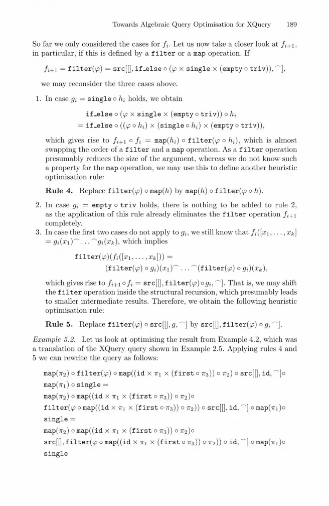
Towards Algebraic Query Optimisation for XQuery 189
So far we only considered the cases for fi. Let us now take a closer look at fi+1,in particular, if this is defined by a filter or a map operation. If
fi+1 = filter(ϕ) = src[[], if else ◦ (ϕ × single× (empty ◦ triv)), �],
we may reconsider the three cases above.
1. In case gi = single ◦ hi holds, we obtain
if else ◦ (ϕ × single× (empty ◦ triv)) ◦ hi
= if else ◦ ((ϕ ◦ hi) × (single ◦ hi) × (empty ◦ triv)),
which gives rise to fi+1 ◦ fi = map(hi) ◦ filter(ϕ ◦ hi), which is almostswapping the order of a filter and a map operation. As a filter operationpresumably reduces the size of the argument, whereas we do not know sucha property for the map operation, we may use this to define another heuristicoptimisation rule:
Rule 4. Replace filter(ϕ) ◦ map(h) by map(h) ◦ filter(ϕ ◦ h).
2. In case gi = empty ◦ triv holds, there is nothing to be added to rule 2,as the application of this rule already eliminates the filter operation fi+1completely.
3. In case the first two cases do not apply to gi, we still know that fi([x1, . . . , xk]= gi(x1)� . . . �gi(xk), which implies
filter(ϕ)(fi([x1, . . . , xk])) =(filter(ϕ) ◦ gi)(x1)� . . . �(filter(ϕ) ◦ gi)(xk),
which gives rise to fi+1◦fi = src[[], filter(ϕ)◦gi,�]. That is, we may shift
the filter operation inside the structural recursion, which presumably leadsto smaller intermediate results. Therefore, we obtain the following heuristicoptimisation rule:
Rule 5. Replace filter(ϕ) ◦ src[[], g, �] by src[[], filter(ϕ) ◦ g, �].
Example 5.2. Let us look at optimising the result from Example 4.2, which wasa translation of the XQuery query shown in Example 2.5. Applying rules 4 and5 we can rewrite the query as follows:
map(π2) ◦ filter(ϕ) ◦ map((id × π1 × (first ◦ π3)) ◦ π2) ◦ src[[], id, �]◦map(π1) ◦ single =map(π2) ◦ map((id × π1 × (first ◦ π3)) ◦ π2)◦filter(ϕ ◦ map((id × π1 × (first ◦ π3)) ◦ π2)) ◦ src[[], id, �] ◦ map(π1)◦single =map(π2) ◦ map((id × π1 × (first ◦ π3)) ◦ π2)◦src[[], filter(ϕ ◦ map((id × π1 × (first ◦ π3)) ◦ π2)) ◦ id, �] ◦ map(π1)◦single

190 M. Kirchberg et al.
Next consider the case fi+1 = map(hi+1). As before, we do not have to reconsiderthe second case above, as we cannot obtain more than rule 2, but we may lookat the other two cases again.
1. In case gi = single ◦ hi holds, we obtain
fi+1 ◦ fi = src[[], single ◦ hi+1 ◦ hi,�] = map(hi+1 ◦ hi).
So we may combine two consecutive map operations into one using the fol-lowing rule:Rule 6. Replace map(h) ◦ map(g) by map(h ◦ g).
2. In the general case we have fi([x1, . . . , xk]) = gi(x1)� . . . �gi(xk), whichimplies
map(hi+1)(fi([x1, . . . , xk])) = (map(hi+1)◦gi)(x1)� . . . �(map(hi+1)◦gi)(xk),
which further leads to fi+1 ◦ fi = src[[], fi+1 ◦ gi,�]. That is, we may shift
the map operation inside the structural recursion, which defines the followingheuristic optimisation rule:Rule 7. Replace map(h) ◦ src[[], g, �] by src[[], map(h) ◦ g, �].
Example 5.3. Carrying on from Example 5.2 above, we can now apply rules 6and 7 to perform further optimisations as follows:
map(π2) ◦ map((id × π1 × (first ◦ π3)) ◦ π2)◦src[[], filter(ϕ ◦ map((id × π1 × (first ◦ π3)) ◦ π2)) ◦ id, �] ◦ map(π1)◦single =map(π2 ◦ (id × π1 × (first ◦ π3)) ◦ π2)◦src[[], filter(ϕ ◦ map((id × π1 × (first ◦ π3)) ◦ π2)) ◦ id, �] ◦ map(π1)◦single =src[[], map(π2 ◦ (id × π1 × (first ◦ π3)) ◦ π2) ◦ filter(ϕ◦map((id × π1 × (first ◦ π3)) ◦ π2)) ◦ id, �] ◦ map(π1) ◦ single
Finally, consider several for-clauses producing lists L1, . . . , Ln, which are thencombined into
L1 × · · · × Ln = src2[[], g, �](L1, L2 × · · · × Ln)= src2[[], g, �](L1,
src2[[], g, �](L2,
. . .
src2[[], g, �](Ln−1, Ln) . . . ))
with g(x, L) = src[[], single ◦ (x × id), �](L). So basically we have to considersrc2[[], g, �](L1, L2) with L1 = src[[], g1,
�](L′1). However, even, if we consider
the case g1 = single ◦ h1, this does not give rise to meaningful equations thatcould be used to define further optimisation rules. It may, however, be the casethat structural recursion applied to the result of this product can lead to furtheroptimisation rules. We will explore this in the remaining subsection.

Towards Algebraic Query Optimisation for XQuery 191
5.2 The LWOR Clauses
As shown in the previous section, each let-clause gives rise to a map operation.However, as there may be more than one for-clause, we have to take into accountthat the result of processing the for-clauses leads to a list of tuples. Let � bethe number of for-clauses, and let m be the number of let-clauses. Then weobtain
map(π1 × · · · × π� × k1 × · · · × km)(L1 × · · · × L�)
as the subquery resulting from the for- and the let-clauses. As for the prod-uct we cannot derive anything meaningful in addition to the already discoveredoptimisation rules.
So let us address the where-clause, which gives rise to another filter oper-ation, say filter(ϕ). As this operation is applied to a list of (� + m)-tuples, wemay rewrite ϕ as a conjunction ϕ0 ∧ ϕ1 ∧ · · · ∧ ϕ�+m such that ϕi for i > 0 onlydepends on the i’th component. Then we obtain
filter(ϕ)(map(π1 × · · · × π� × k1 × · · · × km)(L1 × · · · × L�)) =filter(ϕ0)(src[[], (single ◦ π1) × · · · × (single ◦ π�)×(if else ◦ ((ϕ�+1 ◦ k1) × (single ◦ k1)) × (empty ◦ triv))× · · · ×(if else ◦ ((ϕ�+m ◦ km) × (single ◦ km) × (empty ◦ triv))), �](filter(ϕ1)(L1) × · · · × filter(ϕ�)(L�))
As we can assume that an early application of a filter operation will be ad-vantageous in terms of obtaining a smaller intermediate result, we can formulatethe following two heuristic optimisation rules, which would produce the resultabove:
Rule 8. Replace filter(ϕ ∧ ψ) by filter(ϕ) ◦ filter(ψ).
Rule 9. Replace filter(ϕ) by filter(ϕ◦πi), if the operation is to be appliedto a list of k-tuples, and ϕ only depends on the i’th component.
Example 5.4. Continuing from Example 5.3 above, we can now apply rule 9 tooptimise the filter operation as follows:
src[[], map(π2 ◦ (id × π1 × (first ◦ π3)) ◦ π2) ◦ filter(ϕ◦map((id × π1 × (first ◦ π3)) ◦ π2)) ◦ id, �] ◦ map(π1) ◦ single =src[[], map(π2 ◦ (id × π1 × (first ◦ π3)) ◦ π2) ◦ filter(ϕ ◦ π3◦map((id × π1 × (first ◦ π3)) ◦ π2)) ◦ id, �] ◦ map(π1) ◦ single
Additionally, the corresponding Boolean operation ϕ in filter would be rewrit-ten from
∧ ◦ ((eq ◦ ((π1 ◦ π3) × Arabica)) × (eq ◦ ((π2 ◦ π3) × 100)))
to∧ ◦ ((eq ◦ (π1 × Arabica)) × (eq ◦ (π2 × 100))).

192 M. Kirchberg et al.
6 Conclusion
In this paper we addressed the algebraic optimisation of XQuery based on atranslation to a rational tree query algebra. The model underlying this algebrais based on a type system that supports constructors for records, lists and unionsas well as optionality and references. The query algebra uses operations definedon this type system, in particular structural recursion for lists.
We demonstrated that the basic execution model of XQuery easily gives riseto nested structural recursion. However, the function parameters involved inthese operations require complex definitions resulting from information aboutthe schema. These functions can be generated using compile-time linguistic re-flection.
An obvious advantage of this approach is that it shifts part of the intrinsiccomplexity of XQuery to the query compilation avoiding unnecessary path searchduring query execution. Of course, this benefit cannot be claimed for ad-hocqueries, in which case the overhead resulting from the translation may bite offthe performance gain resulting from the optimised query. A careful investigationof what might still be gained for ad-hoc queries was so far beyond the scope ofour research, but will be addressed in future work.
The representation of XQuery by a query algebra gives rise to equivalencesthat are the basis for query rewriting, which is performed in a way that willalways result in queries with presumably lower costs. It may further be usedfor the generalisation of other query optimisation techniques such as join re-ordering, tableau optimisation, and selection-projection optimisation [2, chapter6]. These extensions to query optimisation will be addressed in future work. Wealso plan to support the algebraic approach to query optimisation by rigorouscase-based comparison with other approaches to XQuery implementation andoptimisation.
An obvious further advantage of the use of a query algebra is type safetyas emphasised in [20]. Furthermore, a translation to a simple query algebraenables the easy implementation of the operations and thus the integration withprogramming languages, and the easy extension to other constructors such as setsand multisets in case the order that comes with the list constructor is consideredunnecessary or even undesired. These two expected benefits, however, still haveto be explored in more detail in our future work. In particular, much of thecomplexity resulting from path expressions is captured in the translation process.
References
1. Abiteboul, S., Buneman, P., and Suciu, D. Data on the Web: From Relations toSemistructured Data and XML. Morgan Kaufmann Publishers, 2000.
2. Abiteboul, S., Hull, R., and Vianu, V. Foundations of Databases. Addison-Wesley,1995.
3. Abiteboul, S., and Kanellakis, P. C. Object identity as a query language primitive.In Building an Object-Oriented Database System, The Story of O2, F. Bancilhon,C. Delobel, and P. C. Kanellakis, Eds. Morgan Kaufmann, 1992, pp. 97–127.

Towards Algebraic Query Optimisation for XQuery 193
4. Abiteboul, S., Quass, D., McHugh, J., Widom, J., and Wiener, J. The LORELquery language for semi-structured data. International Journal on Digital Libraries1, 1 (1997), 68–88.
5. Beeri, C., and Ta-Shma, P. Bulk data types, a theoretical approach. In DatabaseProgramming Languages (DBPL-4) (1993), Workshops in Computing, Springer-Verlag, pp. 80–96.
6. Buneman, P., Davidson, S., Hillebrand, G., and Suciu, D. A query language andoptimization techniques for unstructured data. In Proceedings of the InternationalConference on Management of Data (1996), ACM, pp. 505–516.
7. Chen, Y., Davidson, S. B., and Zheng, Y. BLAS: An efficient XPath processingsystem. In Proceedings of the Symposium on Principles of Database Systems (2004),G. Weikum, A. C. Konig, and S. Deßloch, Eds., ACM, pp. 47–58.
8. Cluet, S., Delobel, C., Lecluse, C., and Richard, P. RELOOP: An algebra-basedquery language for O2. In Building an Object-Oriented Database System – TheStory of O2, F. Bancilhon, C. Delobel, and P. Kanellakis, Eds. Morgan Kaufmann,1992.
9. Cluet, S., and Moerkotte, G. Nested queries in object bases. In Database Pro-gramming Languages (DBPL-4) (1993), C. Beeri, A. Ohori, and D. Shasha, Eds.,Workshops in Computing, Springer-Verlag, pp. 226–242.
10. Courcelle, B. Fundamental properties of infinite trees. Theoretical Computer Sci-ence 25 (1983), 95–169.
11. DeHaan, D., Toman, D., Consens, M. P., and Ozsu, M. T. A comprehensive XQueryto SQL translation using dynamic interval encoding. In Proceedings of the Sym-posium on Principles of Database Systems (2003), A. Y. Halevy, Z. G. Ives, andA. Doan, Eds., ACM, pp. 623–634.
12. Deutsch, A., Fernandez, M., Florescu, D., Levy, A., and Suciu, D. A query languagefor XML. Computer Networks 31, 11–16 (1999), 1155–1169.
13. Fernandez, M. F., Simeon, J., and Wadler, P. An algebra for XML query. InProceedings of the 20th Conference on Foundations of Software Technology andTheoretical Computer Science (2000), Springer-Verlag, pp. 11–45.
14. Gottlob, G., Koch, C., and Pichler, R. The complexity XPath query evaluation.In Proceedings of the 22nd Symposium on Principles of Database Systems (2003),ACM, pp. 179–190.
15. Jagadish, H. V., Lakshmanan, L. V. S., Srivastava, D., and Thompson, K. TAX:A tree algebra for XML. In Revised Papers from the 8th International Workshopon Database Programming Languages (2002), Springer-Verlag, pp. 149–164.
16. Katz, H., Ed. XQuery from the Experts – A Guide to the W3C XML QueryLanguage. Addison-Wesley, 2003.
17. Kemper, A., and Moerkotte, G. Query optimization in object bases: Exploitingrelational techniques. In Proceedings of the Dagstuhl Workshop on Query Optimiza-tion (1993), J.-C. Freytag, D. Maier, and G. Vossen, Eds., Morgan Kaufmann.
18. Kirby, G. N. C., Connor, R. C. H., and Morrison, R. START: A linguistic reflectiontool using hyper-program technology. In Proceedings of the Sixth InternationalWorkshop on Persistent Object Systems (1994), M. P. Atkinson, D. Maier, andV. Benzaken, Eds., Workshops in Computing, Springer-Verlag, pp. 355–373.
19. Kirchberg, M., Ma, H., ud Din, F. R., and Schewe, K.-D. A unified approach toobject algebras. unpublished, available from the authors, 2003.
20. Kirchberg, M., Riaz-ud-Din, F., Schewe, K.-D., and Tretiakov, A. Using reflectionfor querying XML documents. In Database Technologies 2006. Proceedings of the17th Australasian Database Conference (ADC), J. Bailey and G. Dobbie, Eds.,vol. 49 of CRPIT. Australian Computer Society, 2006, pp. 119–128.

194 M. Kirchberg et al.
21. Kirchberg, M., Schewe, K.-D., and Tretiakov, A. A multi-level architecture fordistributed object bases. In Proceedings of the 5th International Conference onEnterprise Information Systems (ICEIS) (2003), O. Camp, J. Filipe, S. Hammoudi,and M. Piattini, Eds., vol. 1, ICEIS Press, pp. 63–70.
22. Kirchberg, M., Schewe, K.-D., and Tretiakov, A. Using XML to support mediatypes. In Information Systems Technology and its Applications, 4th InternationalConference, R. Kaschek, H. C. Mayr, and S. W. Liddle, Eds., vol. 63 of LNI. GI,2005, pp. 101–113.
23. Koch, C. On the complexity of nonrecursive XQuery and functional query lan-guages on complex values. In Principles of Database Systems (2005), ACM.
24. Leung, T. W., Mitchell, G., Subramanian, B., Vance, B., Vandenberg, S. L., andZdonik, S. B. The AQUA data model and algebra. In Database ProgrammingLanguages (DBPL-4) (1993), C. Beeri, A. Ohori, and D. Shasha, Eds., Workshopsin Computing, Springer-Verlag, pp. 157–175.
25. Libkin, L., and Wong, L. New techniques for studying set languages, bag languagesand aggregate functions. In Principles of Database Systems (PODS) (1994), ACM,pp. 155–166.
26. Lobin, H. Informationsmodellierung in XML und SGML. Springer-Verlag, 2001.27. Marx, M. Conditional XPath, the first order complete XPath dialect. In Proceed-
ings of the 23rd Symposium on Principles of Database Systems (PoDS) (2004),ACM, pp. 13–22.
28. Paparizos, S., Wu, Y., Lakshmanan, L. V. S., and Jagadish, H. V. Tree logicalclasses for efficient evaluation of XQuery. In Proceedings of the Symposium onPrinciples of Database Systems (SIGMOD) (2004), G. Weikum, A. C. Konig, andS. Deßloch, Eds., ACM, pp. 71–82.
29. Savnik, I., Tari, Z., and Mohoric, T. QAL: A query algebra of complex objects.Data and Knowledge Engineering 30, 1 (1999), 57–94.
30. Schewe, K.-D. On the unification of query algebras and their extension to rationaltree structures. In Database Technologies – Proceedings of the 12th AustralasianDatabase Conference (ADC) (2001), M. E. Orlowska and J. F. Roddick, Eds., IEEEComputer Society, pp. 52–59.
31. Schewe, K.-D., Schmidt, J. W., and Wetzel, I. Identification, genericity and con-sistency in object-oriented databases. In Proceedings of the 4th International Con-ference on Database Theory (ICDT) (1992), J. Biskup and R. Hull, Eds., vol. 646of Lecture Notes in Computer Science, Springer-Verlag, pp. 341–356.
32. Schewe, K.-D., and Thalheim, B. Fundamental concepts of object oriented data-bases. Acta Cybernetica 11, 4 (1993), 49–84.
33. Shaw, G. M., and Zdonik, S. B. An object-oriented query algebra. In Proceedings ofthe Second International Workshop on Database Programming Languages (1989),R. Hull, R. Morrison, and D. W. Stemple, Eds., Morgan Kaufmann, pp. 103–112.
34. Sheard, T., and Fegaras, L. A fold for all seasons. In Conference on FunctionalProgramming Languages and Computer Architecture (1993), ACM, pp. 233–242.
35. Sheard, T., and Stemple, D. W. Automatic verification of database transactionsafety. ACM Transactions on Database Systems 14, 3 (1989), 322–368.
36. Simeon, J., and Wadler, P. The essence of XML. In Proceedings of the 30thSymposium on Principles of Programming Languages (POPL). ACM, 2003.
37. Stemple, D. W., Fegaras, L., Sheard, T., and Socorro, A. Exceeding the limitsof polymorphism in database programming languages. In Advances in DatabaseTechnology (EDBT) (1990), F. Bancilhon, C. Thanos, and D. Tsichritzis, Eds.,vol. 416 of LNCS, Springer-Verlag, pp. 269–285.

Towards Algebraic Query Optimisation for XQuery 195
38. Stemple, D. W., Morrison, R., and Atkinson, M. P. Type-safe linguistic reflection.In Database Programming Languages: Bulk Types and Persistent Data (1991), P. C.Kanellakis and J. W. Schmidt, Eds., Morgan Kaufmann, pp. 357–360.
39. Stemple, D. W., and Sheard, T. A recursive base for database programming prim-itives. In Next Generation Information System Technology – East/West DatabaseWorkshop (1990), J. W. Schmidt and A. A. Stogny, Eds., vol. 504 of Lecture Notesin Computer Science, Springer-Verlag, pp. 311–332.
40. Suciu, D., and Wong, L. On two forms of structural recursion. In Proceedings of theInternational Conference on Database Theory (ICDT) (1995), vol. 893 of LectureNotes in Computer Science, Springer-Verlag, pp. 111–124.
41. Tannen, V., Buneman, P., and Wong, L. Naturally embedded query languages. InProceedings of the International Conference on Database Theory (ICDT), J. Biskupand R. Hull, Eds., vol. 646 of LNCS. Springer-Verlag, 1992, pp. 140–154.
42. Tatarinov, I., Ives, Z., Halevy, A., and Weld, D. Updating XML. In Proceedings ofthe International Conference on Management of Data (2001), ACM, pp. 413–424.
43. Thalheim, B. Entity-Relationship Modeling: Foundations of Database Technology.Springer-Verlag, 2000.
44. Wadler, P. Comprehending monads. Mathematical Structures in Computer Science2, 4 (1992), 461–493.
45. Wong, L. Normal forms and conservative properties for query languages overcollection types. In Principles of Database Systems (PODS) (1993), ACM, pp.26–36.
46. World Wide Web Consortium (W3C). XML Schema.http://www.w3c.org/TR/xmlschema-0, http://www.w3c.org/TR/xmlschema-1,http://www.w3c.org/TR/xmlschema-2, 2001.
47. World Wide Web Consortium (W3C). XQuery. http://www.w3c.org/TR/xquery,2004.
S. Spaccapietra (Ed.): Journal on Data Semantics VII, LNCS 4244, pp. 196 – 218, 2006. © Springer-Verlag Berlin Heidelberg 2006
Automatic Image Description Based on Textual Data
Youakim Badr1 and Richard Chbeir2
1 PRISMa – INSA de Lyon, 20 Av. Einstein F-69621 VILLEURBANNE - France Phone: (+33) 4 72 43 63 52, Fax: (+33) 4 72 43 85 18
[email protected] 2 LE2I – Bourgogne University
BP 47870 21078 DIJON CEDEX - France Phone: (+33) 3 80 39 36 55, Fax: (+33) 3 80 39 68 69
Abstract. In the last two decades, images are quite produced in increasing amounts in several application domains. In medicine, for instance, a large num-ber of images of various imaging modalities (e.g. computer tomography, mag-netic resonance, nuclear imaging, etc.) are produced daily to support clinical decision-making. Thereby, a fully functional Image Management System be-comes a requirement to the end-users. In spite of current researches, the practice has proved that the problem of image management is highly related to image representation. This paper contribution is twofold in facilitating the representa-tion of images and the extraction of its content and context descriptors. In fact, we introduce an expressiveness and extendable XML-based meta-model able to capture the metadata and content-based of images. We also propose an informa-tion extraction approach to provide automatic description of image content us-ing related metadata. It automatically generates XML instances, which mark up metadata and salient objects matched by extraction patterns. In this paper, we il-lustrate our proposal by using the medical domain of lungs x-rays and we show our first experimental results.
Keywords: Image Representation, Indexing Method, Information Extraction, Electronic Dictionaries, Specification Language.
1 Introduction
The problem of image management is a subject of extensive research in pattern rec-ognition, information retrieval, and databases communities [1, 2]. The need of effi-cient image management systems has several reasons to rapidly grow further and to play a very important role in the society. In medicine, for example, a large number of images of various imaging modalities (e.g. computer tomography, magnetic reso-nance, nuclear imaging, etc.) are produced daily to support clinical decision-making. A lot of work has been done in order to integrate image data in the standard data processing environments of different applications [3, 6, 10, 13].
In essence, the problem of image management is highly related to image represen-tation. In the literature, two complimentary approaches are used for image representa-tion:

Automatic Image Description Based on Textual Data 197
• The content-based approach: Issued from computer vision and pattern recognition community, the content-based approach uses the low-level features of images such as colors, textures, and shapes obtained through automatic extraction algorithms [1, 2, 16]. Thus, image retrieval is done automatically by similarity matching methods. However good the content-based approach is, practice has shown that the use of complementary metadata description is essential.
• The metadata-based approach: Issued from information retrieval and databases communities, the metadata-based approach consists of using alphanumeric attrib-utes to describe the context and/or the content of an image. Thus, metadata-based image retrieval follows the traditional techniques (keywords, phrases, etc.) [14, 19]. However in several application domains, it is mostly difficult or not possible to fully or adequately describe an image using metadata representation [6, 12, 16, 25]. Due to problems of subjectivity and high-expressive representations. Further-more, image description is usually done with human assistance, which is time-consuming when having huge amount of data.
The current trend is then towards a system that uses both metadata and content-based image description [4, 23, 24]. A mixed use of both approaches, results to means of image management that can satisfy many application areas. However, the proposals so far lack to address issues of:
• Extensible and high expressive image and salient objects description using both
metadata and content-based representations, • Automatic extraction methods of both (low-level and metadata) features,
In this paper, we present a novel image representation meta-model based on XML
format. The key feature of the meta-model is that it captures in a single modeling meta-concept the low-level features, the structural and semantic properties, as well as the relationship descriptions of both multimedia object and meta-object. The image description meta-model proposed here considers the main features of a still image suggested in MPEG-7 standard [41]. On the other hand, we propose an information extraction approach to provide automatic description of images using related meta-data. The main idea is to process some image related data, which are usually paragraphs of free natural text, in order to extract metadata and semantic features automatically. The extraction approach relies on extraction patterns that describe the context of relevant data and on a light parsing to recognize these data and to match them against extraction patterns. Once the matching holds successfully, the relevant metadata and features are tagged into a new XML document, which conforms to our XML-based meta-model. Hence, a repository of XML documents is built on the fly. Further documentary or database management systems can easily manipulate the im-age data model and formulate XQL or SQL queries. We complete the scheme of our work with a study case in medical x-rays imaging domain.
The paper is organized as follows. Section 2 presents a motivation example to be used throughout the paper. Related works are summarized in section 3. In section 4, we present our XML-based image data meta-model and illustrate it through a study

198 Y. Badr and R. Chbeir
case in the medical domain. In section 5, we present a high-level specification lan-guage to design extraction patterns; as well necessary dictionaries for lung x-ray are built and applied to extract relevant metadata and salient objects. Conclusions and fu-ture directions are given in section 6.
2 Motivation Example
The aim of this work is to facilitate the image retrieval by providing multi-dimensional representation. In this paper, we use the domain of lungs x-rays to illus-trate our approach where each medical image (or a set of) is associated to a diagnosis written by the physician in a natural way as free text paragraphs. Through the paper, we use the following study case to illustrate how to present the entire required image information of both metadata and content-based using the meta-model, and how to de-fine extraction patterns to extract relevant image information from diagnosis in order to fill in the meta-model. Fig. 1 shows both the image and the associated diagnosis, and the required extraction result which identifies salient objects, corresponding states and inter-relations, as well as other important metadata.
“Mrs Danielle Lee, is a 44 years old patient, manifests low back pains, worsening shortness of
breath, haemoptysis, and a weight loss of 10 lbs over the last three weeks. She has a smoking his-tory of 2 packets of cigarettes per day for 27 years. Recently, she has decreased to 1 packet per day of "light" cigarettes. She claims that she only consumes alcohol on weekends”. Her medical record contains the following lungs X-ray with the attached diagnosis:
Diagnosis : Lungs X-ray, taken at 19/02/99, a Teratoma below the right-shifted trachea inside the right lung
Required Extraction Result
- Salient objects: Teratoma, trachea, right lung
- State: right-shifted - Relation: below, inside - Image Type: x-ray - Acquisition Date: 19/02/99
Teratoma
Information Extraction
Fig. 1. The study case: An example of a diagnosis and the required extraction result
3 Related Work
In the literature, image representation and retrieval follow two directions: the meta-data oriented and the content-based oriented. For more than two decades, the work on content-based image analysis, representation and retrieval have known a big success

Automatic Image Description Based on Textual Data 199
among researchers. As a result, several applications based on automatic low-level fea-tures of color, texture, shape, etc. have been implemented [6, 10, 12]. Photobook, Ne-tra, QBIC, Surfimage, VisualSeek, CAFIIR, etc. are some of the many content-based image retrieval systems [1, 3, 6, 12, 16]. However, these systems mainly focus on re-trieval by low-level features and give emphasis (only keywords) or no emphasis to the role of metadata-based image retrieval.
The image management by metadata approach has been practiced in different fields of applications such as medicine, GIS, the Web, etc. Keywords are an example of meta-data widely used in image description. It goes without saying that there is a great waste of data when replacing an image by a set of metadata descriptors. Since subjectivity, ambiguity and imprecision are usually associated to the context and the semantic content of images, metadata descriptions are mostly incomplete [14]. This is why, some meta-data approaches suggested image description on the basis of salient objects position and relationships [42, 43, 44, 45, 46]. However, they are found to be imperfect at retrieval process in several application domains where translation, scal-ing, perfect and multiple rotations, or any arbitrary combination of transformations is applied. For instance, the spatial content in terms of relationships in surgical or radia-tion therapy of brain tumors is decisive because the location of a tumor has profound implications on a therapeutic decision [22].
In the literature, several hybrid image data models have been proposed [11, 22, 24] attempting to mix low-level feature with meta-data in order to provide multi-criteria queries. However, these models lack an appropriate representation of all necessary image related data for different applications. In [11] for example, the authors do not consider content and semantic representations of salient object related data and the re-lationship between salient objects. The approaches provided in [22, 24] do not allow the integration of several types of low-level features. This is why, a new standard has emerged called MPEG-7 for providing description of multimedia data content [41]. It offers a set of Descriptors and Description Schemes aiming to enable common access (search, filtering and browsing) to multimedia content. However, MPEG-7 suffers from its inability to taxonomically hierarchize the descriptors and thus its inability to express their semantics. This is due to the XML Schema in MPEG-7 DDL (Definition Description Language). Other drawbacks are MPEG-7 non-modularity and non-extensibility — or rather MPEG-7 inability to validate extensions of its description schemes.
As mentioned earlier, several automatic low-level features extraction algorithms are provided in the literature [6, 10, 12]. However, only rare approaches conceive an automatic extraction of metadata values. Primitive meta-data extraction approaches provided writing customized programs in programming languages such as Perl [30]. This is impractical because the programs are too hard to maintain. Some other ap-proaches defined specialized languages to create kind of Information Extraction Sys-tems and Wrappers [31, 32, 33]. These languages are expressiveness, but mastering them still requires computer expertise and skillful programmers. Most of the extrac-tion approaches [33, 34, 35], however, fail to extract properly relevant data, although the text appears to be structured in a highly regular fashion. The main reason, that makes an extraction fails to find metadata values, is the nature of the relevant data

200 Y. Badr and R. Chbeir
structure, which is irregular e.g. missing or multiple metadata values in a text or even a permutation of their order.
The growth in the amount of textual data that are available in electronic documents makes humans incapable of reading and synthesizing such a wealth of data. Informa-tion Extraction (IE) is concerned with the extraction of relevant data from a collection of documents. In the literature [59], there are two main approaches for designing IE systems: the knowledge engineering approach and the empirical or corpus-based ap-proach [60, 61]. In the first approach, the IE system is built manually by users and by using knowledge of the application domain. In the second approach, there is no simi-lar need for expertise when customizing the system for a new domain. Instead, it re-quires the annotation of the training corpus of documents to mark relevant data. A training algorithm ‘learns’ from the corpus how to extract relevant data from novel texts [62]. This approach is faster than the knowledge engineering approach, but re-quires sufficient volume of training documents.
Most of the techniques used for the empirical Natural Language Processing employ (and exclusively) statistical techniques (i.e., as n-gram models and Hidden Markov Models [63]), neural network [64], symbolic learning (i.e., transformation rules [65], decision trees [66] and symbolic methods [67]), relational learning and/or Inductive Logic Programming [68]. An intensive research has been found in the literature [20, 69] to apply learning methods to the construction of IE systems.
To our knowledge, the survey of the literature points out the beginning of the aca-demic prototypes, which deal with the information extraction. These approaches have evolved over the last decades but in some ways their behavior is not intuitive for non expert users and at times they do not behave the way the novice users may expect them to. However, the development process can be very laborious and requires exper-tise in natural language processing and information extraction approaches.
An approach of information extraction for users, who they are professional in a domain of interest (i.e. medical domain) and not expert in linguistic or programming languages, becomes interesting to match relevant data. An appropriate approach may stress on what a user wants to extract based on his/her knowledge of the domain rather than how to extract. The information extraction approach may also propose ex-pressiveness and easy extraction patterns to deal with irregular structure of data that describes, for examples, images.
4 Modeling Images
We propose here an original image meta-model able to integrate the metadata and the content features related to the whole image and/or to its salient objects. Fig. 2 shows our model in the standard DTD format. We intentionally decided to use this format to provide generic description and domain independent approach. We note that DTD format can be easily converted into other semantic formats (such as XML schema, RDF, etc.) using current XML tools (XML spy, Stylus Studio, etc.). Our meta-model associates an abstraction level to both the metadata and the salient objects. The ab-straction level notion is very important in our model and allows easy identifying of:
1. The impact of the metadata on the image description. 2. The granularity of content features.

Automatic Image Description Based on Textual Data 201
Furthermore, our meta-model takes into consideration several types of relations (temporal, spatial, semantic, etc.) between image and its salient objects, and between salient objects. In the following, we detail each component and we illustrate this in our case study.
<!ELEMENT ImageModel (MetaDataBased*, ContentBased*)> <!ELEMENT MetaDataBased (AbstractionLevel, MetaData*)> <!ELEMENT ContentBased (AbstractionLevel, SalientObject*)> <!ELEMENT AbstractionLevel (LevelName?, LevelDesription?)> <!ELEMENT MetaData (MetaName, MetaType, MetaValue)> <!ELEMENT SalientObject (Feature*, Relation*)> <!ATTLIST SalientObject SOI CDATA #REQUIRED > <!ELEMENT Relation (RelationType, RelationValue, Relationmember)> <!ELEMENT Relationmember EMPTY> <!ATTLIST Relationmember soi CDATA #REQUIRED > <!ELEMENT Feature (FeatureName?, Descriptor*)> <!ELEMENT Descriptor (DescriptorName, DescriptorValue, RepresentationFormatName)> <!ELEMENT DescriptorName (#PCDATA)> <!ELEMENT DescriptorValue (#PCDATA)> <!ELEMENT RepresentationFormatName (#PCDATA)> <!ELEMENT LevelDesription (#PCDATA)> <!ELEMENT LevelName (#PCDATA)> <!ELEMENT FeatureName (#PCDATA)> <!ELEMENT MetaName (#PCDATA)> <!ELEMENT MetaType (#PCDATA)> <!ELEMENT MetaValue (#PCDATA)> <!ELEMENT RelationType (#PCDATA)> <!ELEMENT RelationValue (#PCDATA)>
Fig. 2. Our image meta-model in DTD format
4.1 The MetaData-Based Level
The metadata-based level captures the general data, which are external to the image content. In [22], three metadata sublevels are distinguished in the medical domain. This distinction is related to the data impact on image description:
• The context-oriented sublevel: contains application-oriented data that are completely
independent of the image content and have no impact on the image description. For example, it contains data such as the hospital name, the physician identity, the patient name, gender, etc.
• The domain-oriented sublevel: includes data that are indirectly related to the image but strictly related to the application domain. For instance in the medical applica-tion, it includes the medical doctor's general observations, previous associated dis-eases, etc. This sublevel is very important because it allows one to highlight several associated issues (particularly when identifying associated medical anomalies).
• The image-oriented sublevel: corresponds to the data that are directly associated to the image. For example, the image compression type, the format of image creation (X-ray, scanner, MRI, etc.), the incidence (sagittal, coronal, axial, etc.), the scene, the study (thoracic traumatism due to a cyclist accident), the series, image acquisi-tion date, etc. These data can significantly help the image content description.
Fig. 3 shows an example of the metadata-based content level.

202 Y. Badr and R. Chbeir
<MetaDataBased>
<AbstractionLevel>
<LevelName> Domain_Oriented </LevelName>
<LevelDesription> consists of the data that are directly or indirectly related to the image </LevelDesription>
</AbstractionLevel>
<MetaData>
<MetaName>Patient Gender</MetaName>
<MetaType>String</MetaType>
<MetaValue>Woman</MetaValue>
</MetaData>
<MetaData>
<MetaName>Patient Age</MetaName>
<MetaType>Integer</MetaType>
<MetaValue>44</MetaValue>
</MetaData>
<MetaData>
<MetaName>Disease History</MetaName>
<MetaType>Long</MetaType>
<MetaValue>low back pains, worsening shortness of breath, haemoptysis, and a weight loss of 10 lbs over the last three weeks. She has a smoking history of 2 packets of cigarettes per day for 27 years. Recently, she has decreased to 1 packet per day of "light" ciga-rettes. She claims that she only consumes alcohol on week-ends”</MetaValue>
</MetaData>
</MetaDataBased>
<MetaDataBased>
<AbstractionLevel>
<LevelName>Image_Oriented</LevelName>
<LevelDesription> corresponds to the information that is directly asso-ciated to the image creation, storage, and type </LevelDesription>
</AbstractionLevel>
<MetaData>
<MetaName>Imaging Technique</MetaName>
<MetaType>String</MetaType>
<MetaValue>X-rays</MetaValue>
</MetaData>
<MetaData>
<MetaName>Compression</MetaName>
<MetaType>String</MetaType>
<MetaValue>None</MetaValue>
</MetaData>
<MetaData>
<MetaName>Acquisition Date</MetaName>
<MetaType>Date</MetaType>
<MetaValue>19/02/99</MetaValue>
</MetaData> </MetaDataBased>
Fig. 3. Example of MetaData-Based content
4.2 The Content-Based Level
The content-based level describes the content of the image using several features de-tected throughout an abstraction level. The image description meta-model proposed

Automatic Image Description Based on Textual Data 203
here is designed in a manner that considers the common features of a still image sug-gested in MPEG-7 standard. In our meta-model, content features can be assigned to the whole image and/or to its salient objects. Furthermore, the content-based level maintains relations of different types between either the salient objects, or the salient objects and the image. In the literature, physical, spatial and semantic features are commonly used and briefly described here below:
The Physical Feature: describes the image (or the salient object) using its low-level features such as color, texture, etc. The color feature, for instance, can be described by our meta-model via several descriptors (such as color distribution, histograms, domi-nant color, etc.) where each descriptor is obtained by assembling a set of values in re-spect to a color space model. Fig. 4 shows an example of several physical features represented within our meta-model. The use of physical features allows answering non-traditional queries such as: “Find lung x-rays where they contain objects that are similar (using colors) to a given salient object SO2”.
<ContentBased> <AbstractionLevel> <LevelName>Physical Level</LevelName> <LevelDesription>
describes the image (or the salient object) using its low-level features </LevelDesription> </AbstractionLevel> <SalientObject SOI="Image"> <Feature> <FeatureName>Color</FeatureName> <Descriptor> <DescriptorName>Dominant Color </DescriptorName> <DescriptorValue>(162, 158, 168) </DescriptorValue> <RepresentationFormatName> RGB Format </RepresentationFormatName> </Descriptor> </Feature> </SalientObject> <SalientObject SOI="SO_2"> <Feature> <FeatureName>Texture</FeatureName> <Descriptor> <DescriptorName> Histogram </DescriptorName> <DescriptorValue> (53, 54, 68, 14, 165, 152, 165) </DescriptorValue> <RepresentationFormatName> CMY Format </RepresentationFormatName> </Descriptor> </Feature> </SalientObject>
……..
Fig. 4. Example of content-based data applied on physical features description using our meta-model
The Spatial Feature: is an intermediate (middle-level) feature that concerns geometric aspects of either images or salient objects such as shape and position. Each spatial feature can have several descriptors such as: MBR (Minimum Bounding Rectangle), bounding circle, surface, volume, etc. Using our meta-model, each descriptor may have a set of values (Fig. 5). The use of spatial features allows replying to queries in medical systems such as: “Find lung x-rays where left lung surface is bigger than a given object SO1”.

204 Y. Badr and R. Chbeir
<ContentBased> <AbstractionLevel> <LevelName> Spatial Level </LevelName> <LevelDesription>is an intermediate (middlelevel) feature that concerns geometric aspects of images (or salient objects) </LevelDesription> </AbstractionLevel> <SalientObject SOI="SO_1"> <Feature> <FeatureName>Position</FeatureName> <Descriptor> <DescriptorName> Barycenter </DescriptorName> <DescriptorValue>(120, 154) </DescriptorValue> <RepresentationFormatName>2D Format </RepresentationFormatName> </Descriptor> </Feature> <Relation> <RelationType>Directional</RelationType> <RelationValue>Aboveright</RelationValue> <Relationmember soi="SO_2" /> </Relation> <Relation> <RelationType>Directional</RelationType> <RelationValue>Left</RelationValue> <Relationmember soi="SO_3" /> </Relation> <Relation> <RelationType>Topological</RelationType> <RelationValue>Disjoint</RelationValue> <Relationmember soi="SO_2" /> </Relation> <Relation> <RelationType>Topological</RelationType> <RelationValue>Touch</RelationValue> <Relationmember soi="SO_3" /> </Relation> </SalientObject> …
Fig. 5. Example of content-based data applied on spatial features description using our meta-model
The Semantic Feature: integrates high-level descriptions of image and salient-objects using application domain keywords. In the medical domain, for example, terms such as name (lungs, trachea, tumor, etc.), states (inflated, exhausted, dangerous, etc.) are commonly used to describe medical image content (Fig. 6). The aim of the semantic feature is to increase the expression power of users in a manner that usual domain terms can be used to describe and retrieve the image. The use of semantic features is important to answer for traditional queries in medical systems such as: “Find lung x-rays where hypervascularized tumor is invading the left lung”.
4.3 The Relation
Our meta-model allows also representing several useful types of relations between sa-lient objects (spatial, semantic, temporal, etc.).
Spatial relations may exist either between two salient objects or a salient object and the image. Three types of spatial relations are considered in the literature [48]:
• Metric relations: measure the distance between salient objects [47]. For in-
stance, the metric relation “far” between two objects A and B indicates that each pair of points Ai and Bj has a distance grater than a threshold δ.

Automatic Image Description Based on Textual Data 205
• Directional relations: describe the order between two salient objects according to a direction, or the localization of salient object inside the image [46]. In the literature, fourteen directional relations are considered:
- Strict: north, south, east, and west. - Mixed: north-east, north-west, south-east, and south-west. - Positional: left, right, up, down, front and behind.
<ContentBased>
<AbstractionLevel>
<LevelName> Semantic Level </LevelName>
<LevelDesription> integrates high-level descriptions of image (or sa-lient-objects) with the use of an application domain oriented key-words </LevelDesription>
</AbstractionLevel>
<SalientObject SOI="Image">
<Feature>
<FeatureName />
<Descriptor>
<DescriptorName> Diagnosis </DescriptorName>
<DescriptorValue> taken at 19/02/99, a tumor below the right-shifted trachea (in the inferior part of the right lung) </DescriptorValue>
<RepresentationFormatName />
</Descriptor>
<Descriptor>
<DescriptorName> Keywords </DescriptorName>
<DescriptorValue> Lungs, Trachea, Tumor </DescriptorValue>
<RepresentationFormatName />
</Descriptor>
</Feature>
</SalientObject>
<SalientObject SOI="SO_1">
<Feature>
<FeatureName />
<Descriptor>
<DescriptoName> Identification </DescriptorName>
<DescriptorValue> Trachea </DescriptorValue>
<RepresentationFormatName />
</Descriptor>
<Descriptor>
<DescriptorName> State </DescriptorName>
<DescriptorValue> Right-shifted </DescriptorValue>
<RepresentationFormatName />
</Descriptor>
</Feature>
</SalientObject>
Fig. 6. Description of the semantic features using our meta-model
Furthermore, directional relations do not exist in several configurations.
• Topological relations: describe the intersection and the incidence between ob-jects [45]. Egenhofer [45, 48] has identified six basic relations: Disjoint, Meet,

206 Y. Badr and R. Chbeir
Overlap, Cover, Contain, and Equal. Topological relations present several char-acteristics:
- they are exclusive to two objects: there is one and only one topo-
logical relation between two objects, - they have absolute value because of their constant existence be-
tween objects, - they are transformation, translation, scaling, and zooming invariant.
With our model, temporal or spatio-temporal relations can also be captured [21]. This type of relations is very useful to describe the evolution of image objects between two periods. In the medical domain, this kind of relation can be very helpful for users to study the impact of treatments (the evolution of tumor, the displacement of a fibri-nocruorique clot through a deep vein of the lower limb, etc.).
Furthermore, semantic relations are of high importance and can be considered in our meta-model as well. In several domains such as medicine, users need to search images using familiar terms like invading, attacking, shifting, etc.
In this manner, the user will have access to a comprehensive and intelligent de-scription of image and its related data. Relevant descriptions of an image can then be used to provide multi-criteria retrieval.
5 Information Extraction
We restrict our work in Information Extraction (IE) to the knowledge engineering approach. We have studied the potential of regular expressions in extracting informa-tion. We have tracked several works similar to information extraction based on regu-lar expressions and used in medical domains. These works are most commonly used as a means to identify biological terms [52], protein names [53] or as a way to extract relevant data based on ontology [54, 55].
In our context, applying information extraction to medical diagnosis aims to facili-tate image description and retrieval processes. It allows extracting two types of data: metadata related to the image-oriented level, and semantic data related to the whole image and its salient objects such as the identification of objects, their states and rela-tions. In the following paragraphs, we present the high-level specification language for information extraction applied to medical diagnosis and introduce the overall data extraction process.
5.1 High-Level Specification Language
Regular expressions are concise and expressiveness notation [28]. They are good rival for manual pattern recognition. Many people routinely use regular expressions to spec-ify searches in text editors and with standalone tools such as the Unix grep utility [29]. Relevant data can be well located by describing their context and their characteristics. Informally, characteristics such as multiple values, missing value and permutations can be easily simulated by using basic operators in regular expressions like Kleene (*),

Automatic Image Description Based on Textual Data 207
optional (?), union ( | ) and concatenation (white-space). Complex regular expressions can be built up from simpler ones by means of regular expressions operators and parenthesis. Because regular languages are closed under concatenation and union, the basic operators can be combined with any kind of regular expressions.
Using regular expressions in information extraction from natural language corpus stipulates long expressions with increasing complexity to deal with most of possible cases. Clearly, long regular expressions with multiple nesting levels and operators be-come unreadable and hard to maintain. Another drawback is encountered with regular expression engines [39, 40], which are defined on a finite set of letters. In such a way, each single word is composed of the underlying letters.
To overcome major drawbacks and restraints of regular expressions, we extended the syntax of regular expressions by words and meta-words over the alphabet of any natural language such as the English's. Meta-words denote semantic categories of re-lated words usually defined in dictionaries. Yet, another simple but powerful solution to resolve the visibility of long expressions is to provide layer-oriented approach to build regular expressions. Three layers can be introduced to decompose a long regular expression into modular pattern (called extraction pattern): term layer, expression layer and slot layer. Slot layer is made of expression layers including term layers. Such convenient extensions and hierarchy allow a concise and expressiveness abstrac-tion for casual users to compose extraction patterns by a means of words, meta-words and layers. In this manner, one builds its dictionary of extraction patterns and assigns a set of extraction patterns to image description.
The term layer consists of a finite set of terms. A term represents an abstraction of linguistic information in the text. A term t is either:
• A word: denotes a sequence of letters delimited by simple quotes such as ‘tumor’, ‘artery’, ‘near’, ‘in contact with’, ‘on the left’, and so on.
• A meta-word denoting − Generic entities delimited by open and close angles such as numbers (e.g.
<NB>), any word (e.g. <W>), empty word (e.g. <E>), − Classes of words such as general classes (e.g. <body>), specialized classes (e.g.
<bodybones>), − Classes of expressions e.g. <metric> to denote metric expressions (ml, mol/mm,
m2, etc.), <spatial> to denote directional or topological expressions (right, left, under, overlap, converge, join etc.), or <temporal> to denote time dimension (second, minute, hour, etc.).
The expression layer contains a finite set of expressions. We denote by an expres-
sion a concatenation of terms by a means of separate operator (white-space, tabula-tion, new-line). We say that an expression holds if a sequence of words in the text matches the expression. For example, the expression <body> ‘x-ray’ <show> <symp-tom> ‘on’ ‘the’ <body> recognizes all sequences of any body part followed by the term ‘x-ray’, followed by the verb ‘show’, followed by any symptom, followed by the term ‘on’, and the term ‘the’, and finally by any body part.
A slot layer is a set of alternates of expressions. We denote the alternate operator as | (pipe symbol), and we say that a slot holds if one of its expressions holds. For ex-ample, the following slot of four date expressions:
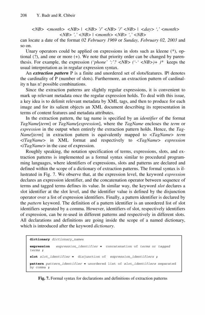
208 Y. Badr and R. Chbeir
<NB> <month> <NB> | <NB> ’/’ <NB> ’/’ <NB> | <day> ‘,’ <month> <NB> ’,’ <NB> | <month> <NB> ‘,’ <NB>
can locate a date of the format 02 February 1969 or Sunday, February 02, 2003 and so on.
Unary operators could be applied on expressions in slots such as kleene (*), op-tional (?), and one or more (+). We note that priority order can be changed by paren-thesis. For example, the expression (‘phone’ ‘:’? <NB> (‘-‘ <NB>)+ )* keeps the usual interpretation as in regular expression syntax.
An extraction pattern P is a finite and unordered set of slots/features. |P| denotes the cardinality of P (number of slots). Furthermore, an extraction pattern of cardinal-ity n has n! possible combinations.
Since the extraction patterns are slightly regular expressions, it is convenient to mark up relevant metadata once the regular expression holds. To deal with this issue, a key idea is to delimit relevant metadata by XML tags, and then to produce for each image and for its salient objects an XML document describing its representation in terms of content features and metadata attributes.
In the extraction pattern, the tag name is specified by an identifier of the format TagName[term] or TagName[expression], where the TagName encloses the term or expression in the output when entirely the extraction pattern holds. Hence, the Tag-Name[term] in extraction pattern is equivalently mapped to <TagName> term </TagName> in XML format and respectively to <TagName> expression </TagName> in the case of expression.
Roughly speaking, the notation specification of terms, expressions, slots, and ex-traction patterns is implemented as a formal syntax similar to procedural program-ming languages, where identifiers of expressions, slots and patterns are declared and defined within the scope of a dictionary of extraction patterns. The formal syntax is il-lustrated in Fig. 7. We observe that, at the expression level, the keyword expression declares an expression identifier, and the concatenation operator between sequence of terms and tagged terms defines its value. In similar way, the keyword slot declares a slot identifier at the slot level, and the identifier value is defined by the disjunction operator over a list of expression identifiers. Finally, a pattern identifier is declared by the pattern keyword. The definition of a pattern identifier is an unordered list of slot identifiers separated by a comma. However, identifiers of slot, respectively identifiers of expression, can be re-used in different patterns and respectively in different slots. All declarations and definitions are going inside the scope of a named dictionary, which is introduced after the keyword dictionary.
Fig. 7. Formal syntax for declarations and definitions of extraction patterns
dictionary dictionary_name:
expression expression_identifier = concatenation of terms or tagged terms ;
slot slot_identifier = disjunction of expression_identifiers ;
pattern pattern_identifier = unordered list of slot_identifiers separated by comma ;
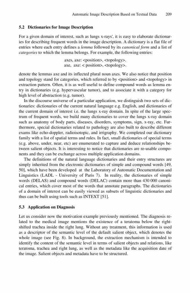
Automatic Image Description Based on Textual Data 209
5.2 Dictionaries for Image Description
For a given domain of interest, such as lungs x-rays', it is easy to elaborate dictionar-ies for describing frequent words in the image description. A dictionary is a flat file of entries where each entry defines a lemma followed by its canonical form and a list of categories to which the lemma belongs. For example, the following entries:
axes, axe: <position>, <topology>. axe, axe: < position>, <topology>.
denote the lemmas axe and its inflected plural noun axes. We also notice that position and topology stand for categories, which referred to by <position> and <topology> in extraction pattern. Often, it is as well useful to define compound words as lemma en-try in dictionaries (e.g. hypervascular tumor), and to associate it with a category for high level of abstraction (e.g. tumor).
In the discourse universe of a particular application, we distinguish two sets of dic-tionaries: dictionaries of the current natural language e.g. English, and dictionaries of the current domain of interest i.e. the lungs x-ray domain. In spite of the large spec-trum of frequent words, we build many dictionaries to cover the lungs x-ray domain such as anatomy of body parts, diseases, disorders, symptoms, sign, x-ray, etc. Fur-thermore, special dictionaries related to pathology are also built to describe different exams like echo-doppler, radioisotopic, and irrigraphy. We completed our dictionary family with a list of spatial terms and rules. In fact, small dictionaries of special terms (e.g. above, under, near, etc) are enumerated to capture and deduce relationships be-tween salient objects. It is interesting to notice that dictionaries are re-usable compo-nents and they can be exchange across multiple application domains.
The definitions of the natural language dictionaries and their entry structures are simply inherited from the electronic dictionaries of simple and compound words [49, 50], which have been developed at the Laboratory of Automatic Documentation and Linguistics (LADL - University of Paris 7). In reality, the dictionaries of simple words (DELAS) and compound words (DELAC) contain more than 430 000 canoni-cal entries, which cover most of the words that annotate paragraphs. The dictionaries of a domain of interest can be easily viewed as subsets of linguistic dictionaries and thus can be built using tools such as INTEXT [51].
5.3 Application on Diagnosis
Let us consider now the motivation example previously mentioned. The diagnosis re-lated to the medical image mentions the existence of a teratoma below the right-shifted trachea inside the right lung. Without any treatment, this information is used as a descriptor of the semantic level of the default salient object, which denotes the whole image (see Fig. 8). In background, the extraction mechanism is intended to identify the content of the semantic level in terms of salient objects and relations, like teratoma, trachea and right lung, as well as the metadata like the acquisition date of the image. Salient objects and metadata have to be structured.

210 Y. Badr and R. Chbeir
<SalientObject SO_Id="Image"> ……… <Descriptor> <DescriptorName> Diagnosis<DescriptorName/> <Value> Lungs X-ray, taken at 19/02/99, a teratoma below the
right-shifted trachea inside the right lung </Value> <RepresentationFormatName/> </Descriptor> ………
</SalientObject>
Fig. 8. A salient object and its diagnosis descriptor of an x-ray image
By XML format conforming to the DTD of the meta-model, we emphasize the metadata-based level by looking for metadata features in the image-oriented sublevel. We consider the acquisition date, for example, with four possible expressions to rec-ognize variant date formats. Then, a slot of date is defined as alternation of these ex-pressions as follows:
expression AcquisitionDate1 = DATE[ <NB> <month> <NB> ];
expression AcquisitionDate2 = DATE[ <NB> ’/’ <NB> ’/’ <NB> ];
expression AcquisitionDate3 = DATE[ <day> ‘,’ <month> <NB> ’,’ <NB> ];
expression AcquisitionDate4 = DATE[ <month> <NB> ‘,’ <NB> ];
slot Acquisition_date = AcquisitionDate1 | AcquisitionDate2 | AcquisitionDate3 | Acquisi-tionDate4 ;
When applying the date slot to the diagnosis, the second expression will recognize
the date ‘19/02/99’ and produce a date in the metadata image-oriented sublevel as il-lustrated in Fig. 9.
As we mentioned previously in semantic sublevel, we are interested in capturing salient objects features and different types of relations between salient objects. For that, several dictionaries, such as lung anatomy and pathology types are necessarily to refer to their contents by means of categories in extraction patterns.
<AbstractionLevel> <LevelName>Image_Oriented</LevelName> </LevelDesription/> </AbstractionLevel> <MetaData> <MetaName>Acquisition_Date</MetaName> <MetaType>Date</MetaType> <MetaValue>19/02/99</MetaValue> </MetaData>
Fig. 9. Output of the slot Acquisition date
In our context, body parts and diseases identify convenient salient objects. In simi-lar way, directional, metric and topological relations can be described by spatial rela-tion dictionary.
Fig. 10 snapshots a subset of our dictionaries used in metadata and semantic ex-traction process. Each entry in the lung anatomy is classified under multi-axial taxon-omy, which means that a term can be referred to by several categories or meta-words (e.g. the term posterior basal is referred by bronchial and lung categories). In

Automatic Image Description Based on Textual Data 211
…… adenocarcinoma: <lungPathology > bronchioloalveolar: <lungPathology bronchogenic cyst: <lungPathology carcinoid: <lungPathology chondrosarcoma: <lungPathology histoplasmosis granuloma: <lungPathology> lymphoma: <lungPathology mesothelioma : <lungPathology> mucoepidermoid carcinoma: <lungPathology> pericardial cyst: <lungPathology> squamous cell : <lungPathology> synchronous tumors: <lungPathology > teratoma: <lungPathology > thymic cyst: <lungPathology > thymoma: <lungPathology > thyroid: <lungPathology > ……
Pathologic Types
…… right lung: <lung> right trachea: <lung> right upper lobe bronchi: <rightMiddleLobe>,<bronchial>,<lung> right upper apical posterior: <rightUpperLobe>,<bronchial>,<lung> right upper apical anterior: <rightUpperLobe>,<bronchial>,<lung> right middle lobe bronchi: <rightMiddleLobe>, <bronchial>,<lung> right middle lateral: <rightMiddleLobe>,<bronchial>,<lung> right middle medial: <rightMiddleLobe>,<bronchial> right lower lobe bronchi: <rightLowerLobe>,<bronchial>,<lung> superior medial basal: < rightLowerLobe >,<bronchial>,<lung> superior anterior basal: < rightLowerLobe >,<bronchial>,<lung> superior lateral basal: < rightLowerLobe >,<bronchial>,<lung> posterior basal: <bronchial>, <lung> ……
Right Lung Anatomy
……near:<metric> far :<metric> right:<directional> left: <directional> up: <directional> down: <directional> west: <directional> east: <directional> front: <directional> below: <directional> disjoint:<topological> meet: <topological> overlap: <topological> cover: <topological> contain: <topological> inside: <topological> cover<topological> ……
Spatial Relations
Fig. 10. Snapshots of lung pathology, anatomy of the right lung bronchial and relations
contrast, entries in pathology and spatial relation dictionaries are classified under sin-gle category.
Based on dictionary categories, we propose some of possible expressions allowing capturing salient objects, their states, and relations in diagnosis text. Of course, other expressions can be figured out to cover large number of possible cases. Finally, a di-agnosis slot as an alternation of all possible expressions is built.
expression diagnosis1 = SO_x[<lung>] <W>* REL1[<relation>] <W>* SO_y[<lungPathology>] ;
expression diagnosis2 = SO_x[<lung>] <W>* REL1[<relation>] <W>* SO_y[<lungPathology>] <W>* REL2[<relation>] <W>* SO_z[<lung>];
expression diagnosis3 = SO_x[<lung>] <W>* REL1[<relation>] STATE1[<W> ’-‘ <W> ’ed’] <W>* SO_y[<lungPathology>] <W>* REL2[<relation>] <W>* SO_z[<lung>] ;
slot diagnosis = diagnosis1 | diagnosis2 | diagnosis3 ;
Clearly, the first diagnosis is looking for a lung body part by using the <lung>
category as a salient object SO_x, and lung disease by referring to <lungPathology> category as salient object SO_y. A relation REL1 separates SO_x and SO_y preceded and followed by many words as indicating by <W>*. The comprehension of the re-maining diagnosis expressions are defined similarly.

212 Y. Badr and R. Chbeir
The resulting of applying diagnosis slot identifies teratoma, trachea and right lung as salient objects, below and inside as directional and topological relations respec-tively, and at last right-shifted as a state. Fig. 11 shows the extraction result on the sa-lient object SO_1.
<SalientObject SOI="SO_1"> <Feature> <FeatureName/> <Descriptor> <DescriptorName>Identification </DescriptorName> <DescriptorValue>Trachea</DescriptorValue> <RepresentationFormatName/> </Descriptor> <Descriptor> <DescriptorName>State</DescriptorName> <DescriptorValue>Right-shifted</DescriptorValue> <RepresentationFormatName/> </Descriptor> </Feature> </SalientObject> <Relation> <RelationType>Directional</RelationType> <RelationValue>below</RelationValue> <Relationmember soi="SO_2"/> </Relation>
Fig. 11. Trachea salient object and its directional relation
By using previous expression identifiers, date and diagnosis, we construct an ex-traction pattern and we associate it to the original diagnosis descriptor. The resulting is an extraction of the following format:
Pattern LungDiagnosis = date, diagnosis+ ;
In order to validate our approach of information extraction, we have developed a
wrapper, called Xtractor [15], to implement the specification language of extraction patterns. The Xtractor relies on linguistic parsing of paragraphs. It applies natural lan-guage dictionaries as well as dictionaries related to a specific domain such as the lung diagnosis. More details about Xtractor are provided in [15].
6 Experimental Results
To validate our approach, we have selected a corpus of 105 patient records provided by the Rouen Hospital throughout the TIPHAD project [56]. We have focused on ex-tracting relevant data such as salient objects, relations between salient objects, acqui-sition date, image-type, states and symptoms from patient records paragraphs of lung diagnosis to in order to annotate the images. The first experimental results aimed at validating the precision of our approach but time-based performance was out of scope of tests. For our experiments, we have chosen 45 records for the tuning set and 60 re-cords for the test set. We used the tuning set to write the extraction patterns. More-over, we generalize the extraction patterns through a process of successive

Automatic Image Description Based on Textual Data 213
refinement. Beside the linguistic dictionaries of the French language provided by the INTEX [57] community, we built medical dictionaries describing the lung x-rays do-main. In order to run the experimental tests, we built the following dictionaries:
• medicament.dic: containing 3693 medical entries, • lungPathologie.dic: with 728 entries to describe the lung anatomy and the re-
lated organisms, • maladie.dic: including 69 diseases, • symptomes.dic: involving 33 symptoms, • relation.dic: containing 53 spatial and directional relations, • glossaire.dic: having 2638 medical terms.
A dictionary of 60 extraction patterns has been used to extract relevant data from x-lungs diagnosis records. The compilation of these extractions generated 463 elemen-tary regular expressions for all the expressions and the slots.
According to the information retrieval, we define a fact as a particular attribute-value pair such a salient object (Salient_Object, trachea), a relation (Relation, inside) or a metadata (Acquisition_date, 2/2/2006). If N is the number of facts in the corpus, C is the number of facts declared correctly, and I is the number declared incorrectly,
the recall ratio is NC , and the precision ratio is IC
C+ .
In experiments we conducted, the Xtractor applies extraction patterns against the pre-processed paragraphs in order to locate relevant data. As illustrated in Table 1, we were able to achieve recall and precision ratios of 0.91% and 0.97%. The measure-ment of precision and recall shows precisely the correctness of the system based on the small corpus. These high numbers are typical of the traditional information extrac-tion for small corpus and well hand written patterns.
Table 1. Recall and precision results
N C I recall precision
Salient Object1 60 57 2 0.95 0.96
Special Relation 60 60 1 1.00 0.98
Salient Object2 60 56 2 0.93 0.96
State 49 44 1 0.89 0.97
Acquisition date 60 58 0 0.96 1.00
Image type 51 51 0 1.00 1.00
Symptoms 83 62 5 0.74 0.92
All attributes 423 388 11 0.91 0.97
7 Conclusion
In this paper, we presented an original image XML-based meta-model able to de-scribe the image content and all related metadata. Built on several abstraction levels,

214 Y. Badr and R. Chbeir
our meta-model provides the possibility to be adaptable to the domain and the user needs (in respect to all current standards). We are convinced that our multi-spaced image meta-model brings new trends and provides all requirements for main efficient image operations (in particular indexing and retrieval operations.
On the other hand, we observed that image diagnosis could be used to extract some meaningful data. The relevant data exhibits some regularity that can be processed ef-ficiently by regular expressions. We extended the notation of regular expressions by providing meta-words and a mutli-layer approach to define a high specification lan-guage for extraction patterns. The notations of the specification language render long and complex regular expressions to be concise, expressiveness and easy to maintain by casual users. The extraction patterns are mainly based on different metadata per-mutations, expression disjunction and on the context to identify salient objects. Along the paper, we showed how applying extraction patterns over image descriptions pro-duce XML instances conforming to the DTD of our meta-model. We validate the fea-sibility of our information extraction approach to annotate images with the Xtractor prototype. In fact, the high specification language and the extraction wrapper (Xtrac-tor) are implemented; a lexical and syntax analyzer is developed by JavaCC [37] to recognize extraction patterns and to generate regular expressions. The resulting regu-lar expressions [38] are then used by the Xtractor wrapper to match relevant meta-data. The initial experiment results show satisfactory performance near 0.91% recall and 0.97% precision on test data.
We are currently building and updating the electronic dictionaries for a large cover of x-lung images. Furthermore, a large corpus of image descriptions and domain-specific dictionaries are compulsory to improve the precision and recall ratio and to test the complexity and the performance of our application. Future work will also ad-dress the integration of low-level features algorithms to provide fully-automated de-scription process and multi-criteria queries possibilities.
References
1. J.K.Wu and A.D. Narasimhalu and B.M. Mehtre and C.P. Lam and Y.J. Gao, CORE: A Content-Based Retrieval Engine for Multimedia Information Systems, Multimedia Sys-tems, 1995, Vol. 3, pp. 25-41.
2. S. Berchtold, C. Boehm, B. Braunmueller, et.al.: Fast Parallel Similarity Search in Multi-media Databases, SIGMOD Conference, AZ, USA, 1997, pp. 1-12.
3. A. Yoshitaka and T. Ichikawa: A Survey on Content-Based Retrieval for Multimedia Da-tabases, IEEE Transactions on Knowledge and Data Engineering, Vol. 11, No. 1, 1999, pp.81-93.
4. V.Oria, M.T. Özsu, L. Liu, et.al.: Modeling Images for Content-Based Queries: The DISMA Approach, VIS'97, San Diago, 1997, pp.339-346.
5. J.K. Wu: Content-Based Indexing of Multimedia Databases, IEEE TKDE, 1997, Vol. 9, No. 6, pp.978-989.
6. Y. Rui, T.S. Huang, S.F. Chang: Image Retrieval: Past, Present, and Future, Journal of Visual Communication and Image Representation, 1999, Vol. 10, pp.1-23.
7. M. Stonebraker, and P. Brown: Object-Relational DBMSs, Mogan Kaufmann Pub. Inc, 1999, San. Francisco, ISBN 1-55860-452-9.

Automatic Image Description Based on Textual Data 215
8. Excalibur Image Datablade Module User's Guide, Informix Press, March, 1999, Ver. 1.2, P. No. 000-5356.
9. Oracle8i, Visual Information Retrieval Users Guide & Reference, Oracle Press, 1999, Re-lease 8.1.5, A67293-01.
10. W.I. Grosky: Managing Multimedia Information in Database Systems, Communications of the ACM, 1997, Vol. 40, No. 12, pp. 72-80.
11. W.I. Grosky, and P.L. Stanchev: An Image Data Model, Advances in Visual Information Systems, Visual-2000, 4th International Conference, LNCS 1929, Springer Verlag Lyon, France, 2000, pp. 14-25.
12. J.P. Eakins, and M.E. Graham: Content-Based Image Retrieval: A Report to the JISC Technology Applications Programme, January, 1999, Inst. for Image Data Research, Univ. of Northumbria at Newcastle.
13. A.W.M. Smeulders, T. Gevers, and M.L. Kersten: Crossing the Divide Between Computer Vision and Databases in Search of Image Databases, Visual Database Systems Conf., It-aly, 1998, pp. 223-239.
14. A. Sheth, and W. Klas: Multimedia Data Management: Using Metadata to Integrate and Apply Digital Media, McGraw-Hill, 1998, San Francisco.
15. Badr Y. “Xtractor: A Light Wrapper For XML Paragraph-Centric Documents”, in Pro-ceedings of the 2005 International Conference on Signal-Image Technology & Internet - Based Systems (IEEE - SITIS’05), Yaoundé Cameroon, 2005, p. 150-155.
16. R.C. Veltkamp, and M. Tanase: Content-Based Image Retrieval Systems: A Survey, Octo-ber, 2000, Technical Report UU-cs-2000-34, Department of Computer Science, Utrecht University.
17. V. Oria, M.T. Özsu, P. Iglinski, et.al.: DISMA: An Object Oriented Approach to Develop-ing an Image Database System, ICDE 2000, February, 2000, 16th Int. Conf. on Data Engi-neering, San Diego, California.
18. V. Oria, M.T. Özsu, P. Iglinski, et.al.: DISMA: A Distributed and Interoperable Image Database System, SIGMOD 2000, May, 2000, In Proc. of ACM SIGMOD Int. Conf. on Management of Data, Dallas, Texas.
19. J.S. Duncan, and N. Ayache: Medical Image Analysis: Progress over Two Decades and the Challenges Ahead; IEEE Transactions on Pattern Analysis and Machine Intelligence, Vol. 22, No. 1, January 2000.
20. Soderland S., Fisher D., Aseltine J., and al. “Issues in inductive learning of domain-specic text extraction rules”. In Learning for Natural Language Processing. Berlin: Springer, 1996, p. 290-301.
21. Allen, J.E., Maintaining Knowledge about Temporal Intervals, Communications of ACM, Volume 26, November 1983, pp. 832-843.
22. R. Chbeir, F. Favetta: A Global Description of Medical Image with a High Precision; in IEEE International Symposium on Bio-Informatics and Biomedical Engineering IEEE-BIBE'2000, IEEE Computer Society, Washington D.C., USA, (2000) November 8th-10th, pp. 289-296.
23. W.W. Chu, ,C.C. Hsu, A.F. Cárdenas, et al.: Knowledge-Based Image Retrieval with Spa-tial and Temporal Constraints, IEEE Transactions on Knowledge and Data Engineering, Vol. 10, No. 6, November/December 1998, pp. 872-888.
24. M. Mechkour: EMIR2. An Extended Model for Image Representation and Retrieval, Da-tabase and EXpert system Applications (DEXA), Sep. 1995, pp. 395-404.
25. G. Trayser: Interactive System for Image Selection, Digital Imaging Unit Center of Medi-cal Informatics University Hospital of Geneva, http://www.expasy.ch/UIN/html1/ pro-jects/isis/isis.html

216 Y. Badr and R. Chbeir
26. A.D. Narasimhalu: Multimedia Databases, Multimedia Systems, Springer-Verlag, 1996, vol. 4, pp.226-249.
27. G. Lu: Multimedia Database Management Systems, 1999, Artech House Computing li-brary, ISBN 0-089006-342-7
28. J.E. Hopcroft, and J.D. Ullman: Introduction to automata theory languages, and computa-tion. Addison-Wesley Publishing Co., Reading, M.A., 1979.
29. A. Hume: A tale of two greps. Software Practice and Experience, volume 18, number 11, November 1988, pp. 1063-1072.
30. L. Wall, T. Christensen, and R.L. Schwartz: Programming Perl. O’Reilly & Associates, Inc., second edition, September 1996.
31. D.J. Smith, and M Lopez: Information extraction for semi-structured documents, Proc. Workshop on Management of Semi-structured Data, May 1997
32. J. Hammer, H. Garcia-Molina, J. Cho, et al.: Extracting Semi structured Information from the Web. In Proceedings of the Workshop on Management of Semistructured Data. Tuc-son, Arizona, May 1997
33. C.N. Hsu, and M.T. Dung: Generating finite-state transducers for semistructured data ex-traction from the web. Information Systems, 23(8):521-538, Special Issue on Semistruc-tured Data, 1998.
34. N. Ashish, and C. Knoblock: Wrapper Generation for Semi-structured Internet Sources. ACM SIGMOD Workshop on Management of Semi-structured Data, 1997, Tucson , Ari-zona
35. S. Kuhlins, R. Tredwell: Toolkits for Generating Wrappers: A survey, In Net.ObjectDays, Erfurt, Germany, September, 2002.
36. S. Sankar, S. Viswanadha, and R. Duncan: Java Compiler Compiler (JavaCC) 37. The Java Parser Generator. Located at \http://www.suntest.com/JavaCC/". 38. D.F. Savarese: OROmatcher - Regular Expressions for Java, http://www.savarese.org/ 39. L. Karttunen, J-P. Chanod, G. Grefenstette, A. Schiller: Regular expressions for language
engineering, Journal of national language engineering 2(4): 305-328, 1996. 40. G.V. Noord, and D. Gerdemann: An extendible regular expression compiler for finite ap-
proaches in natural language processing. In O. Boldt, H Juergensen, and L. Robbonss, edi-tors, Workshop on Implementing Automata; WIA99 Pre-Proceedings, Ptsdam Germany 1999.
41. MPEG-7 Overview, http://www.chiariglione.org/MPEG/standards/mpeg-7/mpeg-7.htm, (visited at 26/02/2006).
42. Chang S.K., Shi Q.Y., Yan C.W., “Iconic Indexing by 2-D Strings”, IEEE-Transactions-on-Pattern-Analysis-and-Machine-Intelligence, 1987, Vol. PAMI-9, N° 3, P. 413-428.
43. Chang S.K., Jungert E., “Human- and System-Directed Fusion of Multimedia and Multi-modal Information using the Sigma-Tree Data Model”, Proceedings of the 2nd Interna-tional Conference on Visual Information Systems, 1997, San Diego, P. 21-28.
44. Huang P.W. and Jean Y.R., “Using 2D C+-Strings as spatial knowledge representation for image database management systems”, Pattern Recognition, 1994, Vol. 27, N° 9, P. 1249-1257.
45. Egenhofer M., “Query Processing in Spatial Query By Sketch”, Journal of Visual Lan-guage and Computing, Vol 8 (4), 1997, P. 403-424.
46. El-kwae M.A. and Kabuka M.R., “A robust framework for Content-Based Retrieval by Spatial Similarity in Image Databases”, ACM Transactions on Information Systems, vol. 17, N° 2, avril 1999, P. 174-198.
47. Peuquet D. J., “The use of spatial relationships to aid spatial database retrieval”, Proc. Second Int. Symp. on Spatial Data Handling, Seattle, 1986, P. 459 – 471.

Automatic Image Description Based on Textual Data 217
48. Egenhofer M., Frank A., and Jackson J., “A Topological Data Model for Spatial Data-bases”, Symposium on the Design and Implementation of Large Spatial Databases, Santa Barbara, CA, Lecture Notes in Computer Science, Vol. 409, P. 271-286. , July 1989
49. Gross M. “The Use of Finite Automata in the Lexical Representation of Natural Lan-guage”. In Electronic Dictionaries and Automata in Computational Linguistics. Berlin: Springer-Verlag, 1989, vol 377, p.34-50.
50. Courtois B. “Le dictionnaire electronique des mots simples”. In Les dctionnaires electro-niques. Langue francaise no 87. Larousse, Paris.1990.
51. Max Silberztein “INTEX: a Finite State Transducer toolbox”, in Theoretical Computer Science #231:1, Elsevier Science, 1999.
52. Information Extraction from Biomedical Literature: Methodology, Evaluation and an Ap-plication. L. Venkata Subramaniam, Sougata Mukherjea, Pankaj Kankar, Biplav Srivastava, Vishal S. Batra, Pasumarti V. Kamesam, Ravi Kothari IBM India Research Lab, New Delhi, India
53. K. Fukuda, T. Tsunoda, A. Tamura, and T. Takagi, “Toward Information Extraction: Iden-tifying Protein Names from Biological Papers,” Proceedings of the Pacific Symposium on Biocomputing, Hawaii, 1998, pp. 707–718.
54. Daniel Q. and Hesham A. Ontology Specific Data Mining Based on Dynamic Grammars, Bioinformatics conference, Stanford, CA. August 16-19, 2004.
55. Embley D.W., Campbell D.M., and Smith R.D., Ontology-Based Extraction and Structur-ing of Information from Data-Rich Unstructured Documents, CIKM'98 Proceedings, Be-thesda, Maryland, 1998.
56. Bricon-Souf N., Beuscart-Zéphir M.C., Watbled L., Laforest F., Karadimas H., Anceaux F., Flory A., Lepage E., Beuscart R. Technologies de l’Information Pour l’Hospitalisation A Domicile : le projet TIPHAD, Télémédecine et e-Santé, Springer- Verlag, Collection In-formatique et Santé N° 13, Paris, 2002.
57. Unitex Home page [online]. Available at: http://www-igm.univ-mlv.fr/~unitex/ (last vis-ited march 12th 2006)
58. W.B. Frakes and R. Baeza-Yates. Information Retrieval: Data Structures & Algorithms. Prentice Hall, Englewood Cliffs, New Jersey, 1992.
59. Appelt D. E., Israel D. J. “Introduction to Information Extraction Technology”. Tutorial for IJCAI-99, 1999, Stockholm.
60. Charniak E. “Statistical Language Learning”. MIT Press, 1994, 192 p. ISBN 0262032163. 61. Brill E., Church K. “Proceedings of the Conference on Empirical Methods in Natural Lan-
guage Processing”. University of Pennsylvania. Philadelphia, PA, 1996. 62. Marcus M., Santorini B. Marcinkiewicz M. “Building a large annotated corpus of Eng-
lish”. Computational Linguistics. 1993, vol 19, n°2, p.313-330. 63. Freitag D., McCallum A. “Information extraction with HMMs and shrinkage”. Proceed-
ings of the AAAI-99 Workshopon Machine Learning for Information Extraction. 1999, p.31-36.
64. Miikkulainen R. “Subsymbolic Natural Language Processing: An Integrated Model of Scripts, Lexicon, and Memory”. MIT Press. Cambridge, MA, 1993.
65. Brill E. “Transformation-based error-driven learning and natural language processing: A case study in part-of-speech tagging”. Computational Linguistics. 1995, vol 21, n°4, p.543-565.
66. Magerman D.M. “Statistical decision-tree models for parsing”. Proceedings of the 33rd Annual Meeting of the Association for Computational Lenguistics, 1995, Cambridge, p.276-283.

218 Y. Badr and R. Chbeir
67. Wermter S., Rilo E., Scheler G. “Connectionist, Statistical, and Symbolic Approaches to Learning for Natural Language Processing”. Berlin: Springer Verlag, 1996, p. 315-328
68. Lavrac, N., & Dzeroski, S. Inductive Logic Programming: Techniques and Applications. Ellis Horwood, 1994.
69. Huffman S. “Learning information extraction patterns from examples”. In Learning for Natural Language Processing. Canada: IJCAI-95 Workshop on, 1995, p. 246-260.

Reasoning About ORA-SS Data Models Using theSemantic Web
Yuan Fang Li1, Jing Sun2, Gillian Dobbie2, Hai H. Wang3, and Jun Sun1
1 School of Computing, National University of Singapore, Republic of Singapore{liyf, sunj}@comp.nus.edu.sg
2 Department of Computer Science, The University of Auckland, New Zealand{j.sun, gill}@cs.auckland.ac.nz
3 Department of Computer Science, The University of Manchester, United [email protected]
Abstract. There has been a rapid growth in the use of semistructured data inboth web applications and database systems. Consequently, the design of a goodsemistructured data model is essential. In the relational database community, al-gorithms have been defined to transform a relational schema from one normalform to a more suitable normal form. These algorithms have been shown to pre-serve certain semantics during the transformation. The work presented in thispaper is the first step towards representing such algorithms for semistructureddata, namely formally defining the semantics necessary for achieving this goal.Formal semantics and automated reasoning tools enable us to reveal the inconsis-tencies in a semistructured data model and its instances. The Object RelationshipAttribute model for Semistructured data (ORA-SS) is a graphical notation fordesigning and representing semistructured data. This paper presents a methodol-ogy of encoding the semantics of the ORA-SS notation into the Web OntologyLanguage (OWL) and automatically verifying the semistructured data design us-ing the OWL reasoning tools. Our methodology provides automated consistencychecking of an ORA-SS data model at both the schema and instance levels.
Keywords: Semistructured Data, Semantic Web, Ontology Web Language, ORA-SS, Formal Verification.
1 Introduction
Semistructured data has become prevalent in both web applications and database sys-tems. With the growth in its usage, questions have arisen about the effective storage andmanagement of semistructured data. In the relational database community, algorithmshave been defined to transform a relational schema from one norm form to a moresuitable normal form. These algorithms have been shown to preserve certain semanticsduring the transformation. In order to verify the correctness of the similar transforma-tions for semistructured data, we need to have a standard representation of schemas andthe transformation operators that are used to transform schemas. This process can beachieved by describing a formal model for semistructured data schemas and verifyingthat instances of schemas conform to the schema model. Then the basic transformationoperators can be formally defined on this schema model. In this paper we undertake thefirst step of the process defined above.
S. Spaccapietra (Ed.): Journal on Data Semantics VII, LNCS 4244, pp. 219–241, 2006.c© Springer-Verlag Berlin Heidelberg 2006

220 Y.F. Li et al.
Many data modeling languages [1–4] for semistructured data have been introduced tocapture more detailed semantic information. The Object Relationship Attribute modelfor Semistructured data (ORA-SS) [5, 6] is a semantically enriched graphical notationfor designing and representing semistructured data [6–9]. The ORA-SS data model notonly reflects the nested structure of semistructured data, but also distinguishes betweenobject classes, relationship types and attributes. The main advantages of ORA-SS overother data models are its ability to express the semantics that are necessary for designingeffective storage and management algorithms, such as the degree of an n-ary relation-ship type, and distinguish between the attributes of relationship types and the attributesof object classes. This semantic information is essential, even crucial for semistructureddata representation and management, but it is lacking in other existing semistructureddata modeling notations.
Semistructured data also acts as a hinge technology between the data exchanged onthe web and the data represented in a database system. Recent research on the WorldWide Web has extended to the semantics of web content. More meaningful informa-tion is embedded into the web content, which makes it possible for intelligent agentprograms to retrieve relevant semantic as well as structural information based on theirrequirements. The Semantic Web [10] approach proposed by the World Wide Web Con-sortium (W3C) attracts the most attention. It is regarded as the next generation of theweb. The Web Ontology Language (OWL) [11] is an ontology language for the Se-mantic Web. It consists of three increasingly expressive sub-languages: OWL Lite, DLand Full. OWL can provide not only the structural information of the web content butalso meaningful semantics for the information presented. The aim of this paper is to en-code the semantics of the ORA-SS notation into the Web Ontology Language (OWL)and automatically verify the semistructured data design using the OWL reasoning toolRACER [12].
The reason that we chose the OWL ontology language is because of the strong re-lationship between semistructured data and web technologies. Semistructured data istypically represented using eXtensible Markup Language (XML). XML is a commonlyused exchange format in many web and database applications. The introduction of theSemantic Web is to overcome the structure-only information of XML, and to providedeeper semantic meaning to the data on the web. The ORA-SS language is a semanticallyenriched data modeling notation for describing semistructured data. From the point ofcapturing more semantic information in content representation, OWL and ORA-SS aretwo approaches that fulfil the same goal, where the former is rooted in the web commu-nity and the latter has its basis in the database community. Thus it is natural to explorethe synergy of the two approaches. We believe that semantic web and its reasoning toolscan contribute greatly to the design and verification phases of ORA-SS data models.
In this paper, we propose a methodology to verify ORA-SS data design using OWLand its reasoner RACER. Fig. 1 shows the overall process of our approach. Firstly, wedefine an ontology model of the ORA-SS data modeling language in OWL. It providesa rigorous semantic basis for the ORA-SS graphical notation and enables us to repre-sent customized ORA-SS data models and their instances in OWL. Secondly, ORA-SSschema and instance models are translated into their corresponding OWL ontologies. Fi-nally, RACER is used to perform the automated verification of the ORA-SS ontologies.

Reasoning About ORA-SS Data Models Using the Semantic Web 221
verify
input
input
model
transfer
transfer OWL ontology of the
ORA-SS language
OWL Reasoner
- RACER
Consistency checking
results
OWL ontology of the
schema and instances
The ORA-SS data
modeling notation
ORA-SS schema and
instance models
Fig. 1. The overall approach to verify ORA-SS data models using OWL
Our approach is able to provide automatic consistency checking on large ORA-SS datamodels and their instances. Examples are given through out the paper to illustrate thereasoning process.
A major concern in designing a good semistructured data model using ORA-SS for aparticular application is to reveal any possible inconsistencies at both the schema and in-stance levels. Inconsistencies at the schema level arise if a customized ORA-SS schemamodel does not conform to the ORA-SS semantics. Inconsistencies at the instance levelarise if an ORA-SS instance model is not consistent with its ORA-SS schema definition.For example, an inconsistency that might arise at the schema level is the specificationof a ternary relationship between only two object classes. An inconsistency that mightarise at the instance level is a many to many relationship between objects when a one tomany relationship is specified in the schema. These two aspects of validation are essen-tial in the semistructured data design process. Thus, the provision of formal semanticsand automated reasoning support for verifying ORA-SS semistructured data modelingis very beneficial.
There has been other research that provides a formal semantics for semistructureddata. For example, the formalization of DTD (Document Type Definition) and XMLdeclarative description documents using expressive description logic has been presentedby Calvanese et al. [13]. Anutariya et al. presented the same formalization using a the-oretical framework developed using declarative description theory [14]. Also spatialtree logics has been used to formalize semistructured data by Conforti and Ghelli [15].More recently, hybrid multimodal logic was used to formalize semistructured data byBidoit et al. [16]. We also applied a similar approach to formalize ORA-SS data modelsusing Z/EVES [17]. While this work has helped us develop a better understanding ofthe semantics of semistructured data, it does not provide automated verification. In an-other research we presented a formalization of the ORA-SS notation in the Alloy [18]language. Although the automated verification was available using the Alloy Analyzer,it had a scalability problem, making the verification of large sets of semistructured dataimpossible. In addition, there were also research for providing better validation supportof semistructured data, such as algorithms on incremental validation of XML docu-ments [19, 20]. However, these approaches still focused on the syntax-only checking ofsemistructured data instances.

222 Y.F. Li et al.
The remainder of the paper is organized as follows. Section 2 briefly introducesthe background knowledge for the semistructured data modeling language ORA-SS,Semantic Web ontology language OWL and its reasoning tool - RACER. Section 3presents OWL semantics of the ORA-SS notation and its data models. Section 4 demon-strates the ontology reasoning process through a Course-Student ORA-SS data modelexample. Examples of both class-level reasoning and instance-level reasoning are pre-sented. Section 5 concludes the paper and outlines the future work.
2 Background
2.1 The ORA-SS Data Modeling Language
The Object-Relationship-Attribute model for Semistructured data (ORA-SS) is a se-mantically enriched data modeling language for semistrctured data design [5, 6]. It hasbeen used in many XML related database applications [8, 9]. The ORA-SS notationconsists of four basic concepts: object class, relationship type, attribute and reference.A full description of the ORA-SS data modeling language can be found in [5, 6].
cs, 2, 4:n, 3:8
cp, 2, 0:5, 1:n
code
course
title
laboratory
grade
lecturetheatre
csvenueexam
prerequisite
*
name feedbackstaff
cst
preferredarea
tutor
number
namenumberstudent
home
number street name
hostel
name
sport club
join date
sportname
sm, 2, 1:n, 1:n
sm
member
sh, 2, 1:1, 1:n
cst, 3, 1:1, 1:n
student
student
Fig. 2. The ORA-SS schema diagram of a Course-Student data model
– An object class is like an entity type in an ER diagram, a class in an object-orienteddiagram or an element in an XML document. The object classes are represented aslabeled rectangles in an ORA-SS diagram.
– A relationship type represents a nesting relationship among object classes. It is de-scribed as a labeled edge by a tuple (name, n, p, c), where the name denotes thename of relationship type, integer n indicates degree of relationship type, p repre-sents participation constraint of parent object class in relationship type and c repre-sents participation constraint of child object class in relationship type.

Reasoning About ORA-SS Data Models Using the Semantic Web 223
– Attributes represent properties and are denoted by labeled circle. An attribute can bea key attribute which has a unique value and is represented as a filled circle. Othertypes of attributes include single valued attribute, multi-valued attribute, requiredattribute, composite attribute, etc. An attribute can be a property of an object class ora property of a relationship type.
– An object class can reference another object class to model recursive and symmetricrelationships, or to reduce redundancy especially for many-to-many relationships. Itis represented by a labeled dashed edge.
For the design of semistructured data, an ORA-SS schema diagram represents theconstraints on relationships, participations and cardinalities among the instances ofthe object classes in a semistructured data model. For example, Fig. 2 represents anORA-SS schema diagram of a Course-Student data model. In the diagram, eachcourse has code, title, and exam venue as its attributes. A relationship typecs, which indicates the relationship between a course object class and a studentobject class is binary, and each course consists of 4 to many students and each stu-dent can select 3 to 8 courses. The student object class in the cs relationship typehas a reference pointing to its complete definition. The grade attribute is an attributebelonging to the cs relationship type. Based on the above schema definition, two lev-els of validation can be carried out. Firstly, consistency checking can be performed todetermine whether the defined schema model is correct with respect to the ORA-SSlanguage. Secondly, consistency checking can be performed to determine whether aparticular instance of semistructured data satisfies the defined ORA-SS schema model.This checking could be done manually only if it is a relatively small sized model. How-ever, examining complicated and large ORA-SS data models for semistructured datais almost manually impossible. Furthermore, manual diagrammatic checking does notguarantee the consistency of the schema since it is likely that inconsistencies are notrevealed when the schema is large and complicated. Therefore, automated verificationsupport based on the formal specification of ORA-SS semantics is highly desirable.
2.2 Semantic Web – OWL and RACER
Description logics [21] are logical formalisms for representing information about knowl-edge in a particular domain. It is a subset of first-order predicate logic and is well-knownfor the trade-off between expressivity and decidability. Based on RDF Schema [22] andDAML+OIL [23], the Web Ontology Language (OWL) [11] is the de facto ontology lan-guage for the Semantic Web. It consists of three increasingly expressive sub-languages:OWL Lite, DL and Full. OWL DL is very expressive yet decidable. As a result, coreinference problems, namely concept subsumption, consistency and instantiation, can beperformed automatically.
In OWL, conceptual entities are organized as classes in hierarchies. Individual en-tities are grouped under classes and are called instances of the classes. Classes andindividuals can be related by properties. Table 1 summarizes the ‘DL syntax’ used inthe following sections. Interested readers may refer to [11] for full details.
RACER, the Renamed ABox and Concept Expression Reasoner [12], is a reasoningengine for ontology languages DAML+OIL and OWL. It implements a TBox and ABox

224 Y.F. Li et al.
Table 1. Summary of OWL syntax used in the paper
Notation Explanation�/⊥ Super class/sub class of every classN1 � N2 N1 is a sub class/property of N2
C1 = C2 Class equivalenceC1 � / � C2 Class intersection/union≥ 1 P � C Domain of property P is class C� � ∀ P.C Range of P is C� �≤ 1 P Property P is functionalP2 = (−P1) Property P2 is inverse of P1
∀ / ∃ P.C allValuesFrom/someValuesFrom restriction, giving the class thatfor every instance of this class that has instances of property P,the values of the property are all/some members of the class C
= / ≤ / ≥ n P Cardinality restriction, the class each of whose instances mappedby property P forms a set whose cardinality must be exactly/lessthan/greater than n
reasoner for the description logic ALCQHIR+(D)− [12]. It is automated for reasoningover OWL Lite and DL ontologies.
3 Modeling the ORA-SS Data Model in OWL
In this section, we present the modeling of ORA-SS schema and instance diagram asOWL ontologies in three steps. Firstly, we define the ORA-SS ontology, which containsthe OWL definitions of essential ORA-SS concepts, such as object class, relationshiptype, etc. Secondly, we show how individual ORA-SS schema diagram ontologies canbe constructed based on the ORA-SS ontology together with a case tool for achievingthis. Finally, in Section 3.6, we show how ORA-SS instance diagrams can be repre-sented in OWL. To effectively illustrate the modeling approach, the schema diagram inFig. 2 is used as a running example.
3.1 The ORA-SS Ontology
The ORA-SS ontology 1 contains the OWL definitions for ORA-SS concepts suchas object class, relationship type, attribute, etc. We model these definitions as OWLclasses. The basic assumption here is that all named OWL classes are by default mu-tually disjoint, which is implied in the ORA-SS diagrams. Essential properties are alsodefined in the ontology. This ontology, with a namespace of ora-ss, can be used laterto define ontologies for ORA-SS schema diagrams.
Entities – As each object class and relationship type can be associated with attributesand other object classes or relationship types, we define an OWL class ENTITY to
1 Due to the space limit, only part of the ORA-SS OWL semantics are presented in the paper. Acomplete ORA-SS ontology can be found at http://www.comp.nus.edu.sg/˜liyf/ora-ss/ora-ss.owl.

Reasoning About ORA-SS Data Models Using the Semantic Web 225
represent the super class of both object class and relationship type. The OWL classstructure is shown as follows.
ENTITY � �OBJECT � ENTITYRELATIONSHIP � ENTITY
ATTRIBUTE � �ENTITY � ATTRIBUTE = ⊥OBJECT � RELATIONSHIP = ⊥
It may not seem very intuitive to define relationship types as OWL classes. In ORA-SS, relationship types are used to relate various object classes and relationship types,it might seem more natural to model relationship types as OWL properties. However,there are two reasons that we decide to model relationship types as OWL classes. Firstly,the domain of ORA-SS relationship types can be relationship types themselves, whendescribing the relationships of ternary and more. Secondly, classes and properties inOWL DL are disjoint. In our model, an OWL relationship type consists of instanceswhich are actually pointers to the pairs of object classes or relationship types that thisrelationship relates.
As ORA-SS is a modeling notation for semistructured data, we need to cater forunstructured data. We define a subclass of ATTRIBUTE called ANY as a place holderto denote any unstructured data appearing in a model. In ORA-SS, a composite at-tribute is an attribute composed of other attributes. We also define it as a subclass ofATTRIBUTE.
ANY � ATTRIBUTEANY � CompositeAttribute = ⊥
CompositeAttribute � ATTRIBUTE
Properties – A number of essential properties are defined in the ora-ss ontology.
1. Properties among entitiesIn ORA-SS, object classes and relationship types are inter-related to form new re-lationship types. As mentioned above, since we model relationship types as OWLclasses, we need additional properties to connect various object classes and rela-tionship types.Firstly, this is accomplished by introducing two object-properties, parent and child,which map a RELATIONSHIP to its domain and range ENTITYs. The followingstatements define the domain and range of parent and child. As in ORA-SS, the do-main of a relationship (parent) can be either an object class or another relationshiptype, i.e., an ENTITY. The range (child) must be an OBJECT. These two proper-ties are functional as one relationship type has exactly one domain and one rangenode. Moreover, we assert that only relationship types can have parents and childbut object classes cannot.
≥ 1 parent � RELATIONSHIP� � ∀ parent.ENTITY� �≤ 1 parent
≥ 1 child � RELATIONSHIP� � ∀ child.OBJECT� �≤ 1 child
OBJECT � ¬ ∃ parent.�OBJECT � ¬ ∃ child.�
RELATIONSHIP � ∀ parent.ENTITYRELATIONSHIP � ∀ child.OBJECT
Secondly, we define two more object-properties: p-ENTITY-OBJECT and p-OBJECT-ENTITY. These two properties are the inverse of each other and they serve

226 Y.F. Li et al.
as the super properties of the properties that are to be defined in later ontologies ofORA-SS schema diagrams. Those properties will model the restrictions imposedon the relationship types.The domain and range of p-ENTITY-OBJECT are ENTITY and OBJECT, respec-tively. Since the two properties are inverses, the domain and range of p-OBJECT-ENTITY can be deduced.p-OBJECT-ENTITY = (−p-ENTITY-OBJECT)≥ 1 p-ENTITY-OBJECT � ENTITY� � ∀ p-ENTITY-OBJECT.OBJECT
ENTITY � ∀ p-ENTITY-OBJECT.OBJECT
≥ 1 p-OBJECT-ENTITY � OBJECT� � ∀ p-OBJECT-ENTITY.ENTITY
OBJECT � ∀ p-OBJECT-ENTITY.ENTITY
2. Properties between entities and attributesFirst of all, we define an object-property has-ATTRIBUTE, whose domain is EN-TITY and range is ATTRIBUTE. Every ENTITY must have ATTRIBUTE as the rangeof has-ATTRIBUTE.
≥ 1 has-ATTRIBUTE � ENTITY� � ∀ .has-ATTRIBUTE.ATTRIBUTE
ENTITY � ∀ has-ATTRIBUTE.ATTRIBUTE
For modeling the ORA-SS candidate and primary keys, we define two new objectproperties that are sub-properties of has-ATTRIBUTE. We also make the propertyhas-primary-key inverse functional and state that each ENTITY must have at mostone primary key. Moreover, we restrict the range of has-candidate-key to be AT-TRIBUTE.
has-candidate-key � has-ATTRIBUTE� � ∀ has-candidate-key.ATTRIBUTE
ENTITY �≤ 1 has-primary-key
has-primary-key � has-candidate-key� �≤ 1 has-primary-key−
3.2 Object Classes
In this subsection, we present how ORA-SS object classes in a schema diagram are rep-resented in OWL. Moreover, we will discuss how object class referencing is modeled.
Example 1. The schema diagram in Fig. 2 contains a number of object classes 2.
course � OBJECTstudent � OBJECThostel � OBJECT· · ·
tutor � OBJECTsport club � OBJECThome � OBJECT· · ·
Referencing – In ORA-SS, an object class can reference another object class to referto its definition. We say that a reference object class references a referenced objectclass. In our model, we model the reference object class as a sub-class of the referencedobject class. If the two object classes have the same name, the reference object classis renamed. By doing so, we ensure that all the attributes and relationship types of thereferenced object classes are reachable (meaningful). Note that there are no disjointnessaxioms among the reference and referenced object classes.
2 For brevity reasons, the class disjointness statements are not shown from here onwards.

Reasoning About ORA-SS Data Models Using the Semantic Web 227
Example 2. In Fig. 2, the object class student is referenced by object classes student andmember. Hence, we rename the reference student to student 1 and add the followingaxioms in to the model.
student � OBJECT student 1 � student member � student
3.3 Relationship Types
In this subsection, we present the details of how ORA-SS relationship types are modeledin OWL. Various kinds of relationship types, such as disjunctive relationship types andrecursive relationship types are also modeled. We begin with an example to show thebasic modeling of relationship types.
Example 3. Fig. 2 contains 5 relationship types.
cs � RELATIONSHIPsh � RELATIONSHIP
sm � RELATIONSHIPcp � RELATIONSHIP
cst � RELATIONSHIP
The relationship type cs is bound by the parent/child properties as follows. We use bothallValuesFrom and someValuesFrom restriction to make sure that only the intended classcan be the parent/child class of cs.
cs � ∀ parent.coursecs � ∃ parent.course
cs � ∀ child.student 1cs � ∃ child.student 1
Auxiliary Properties – As discussed in Section 3.1, for each ORA-SS relationshiptype we define two object-properties that are the inverse of each other.
Example 4. Take cs as an example, we construct two object-properties: p-course-student and p-student-course. Their domain and range are also defined.
p-student-course = (−p-course-student)p-student-course � p-ENTITY-OBJECTp-student-course � p-OBJECT-ENTITY
≥ 1 p-course-student � course� � ∀ p-course-student.student 1
≥ 1 p-student-course � student 1� � ∀ p-student-course.course
Participation Constraints – One of the important advantages that ORA-SS has overXML Schema language is the ability to express participation constraints for parent/childnodes of a relationship type. This ability expresses the cardinality restrictions that mustbe satisfied by ORA-SS instances.
Using the terminology defined previously, ORA-SS parent participation constraintsare expressed using cardinality restrictions in OWL on a sub-property of p-ENTITY-OBJECT to restrict the parent class Prt. Child participation constraints can be similarlymodeled, using a sub property of p-OBJECT-ENTITY.
Example 5. In Fig. 2, the constraints captured by the relationship type cs state that acourse must have at least 4 students; and a studentmust take at least 3 and at most

228 Y.F. Li et al.
8 courses. The following axioms are added to the ontology. The two object-propertiesdefined above capture the relationship type between course and student.
course �∀ p-course-student.student 1
course �≥ 4 p-course-student
student 1 � ∀ p-student-course.coursestudent 1 �≥ 3 p-student-coursestudent 1 �≤ 8 p-student-course
Disjunctive Relationship Types – In ORA-SS, a disjunctive relationship type is usedto represent relationship consists of disjunctive object classes, where only one objectcan be selected to the relationship instance from the set of disjunctive object classes. Tomodel this in OWL, we will create a dummy class as the union of the disjoint classesand use it as the range of the object-property representing the relationship type. Togetherwith the cardinality constraint that exactly one individual of the range can be selected,the disjunctive relationship type can be precisely modeled.
Example 6. In Fig. 2, sh is a disjunctive relationship type where a student must live inexactly one hostel or one home, but not both. We use the following OWL statements tomodel this situation. Note that p-student-sh is an object-property that maps student toits range class home hostel, which is the union of hostel and home.
hostel � OBJECThome hostel � OBJECT≥ 1 p-student-sh � student
home � OBJECThome hostel = hostel � home� � ∀ p-student-sh.hostel home
hostel � home = ⊥
Given the above definitions, the disjunctive relationship type sh in the schema diagramcan be modeled as follows.
student � ∀ p-student-sh.hostel home student �= 1 p-student-sh
Recursive Relationship Types – Recursive relationship types in ORA-SS are modeledusing referencing. In our model, by defining the reference object class as a sub class ofthe referenced object class, recursive relationship types can be modeled as a regularrelationship type.
Example 7. Fig. 2 depicts such a recursive relationship type where a course object classhas at most 5 prerequisite objects, whereas a prerequisite must have at least one course.This can be modeled as follows.
course � �≥ 1 p-course-prerequisite � coursep-prerequisite-course = (−p-course-prerequisite)
course �∀ p-course-prerequisite.prerequisite
course �≤ 5 p-course-prerequisite
prerequisite � course� � ∀ p-course-prerequisite.prerequisite
prerequisite �∀ p-prerequisite-course.course
prerequisite �≥ 1 p-prerequisite-course
3.4 Attributes
The semantically rich ORA-SS model notation defines many kinds of attributes for ob-ject classes and relationship types. These include candidate and primary keys, single-valued and multi-valued attributes, required and optional attributes, etc. In this subsec-tion, we will discuss how these attributes can be modeled.

Reasoning About ORA-SS Data Models Using the Semantic Web 229
Example 8. The schema diagram in Fig. 2 generates the following OWL classes forattributes.
code � ATTRIBUTEtitle � ATTRIBUTEexam venue � ATTRIBUTE· · ·
grade � ATTRIBUTEstudent number � ATTRIBUTEsport � ATTRIBUTE
Modeling Various Definitions – As OWL adopts the Open World Assumption [11]and an ORA-SS model is closed, we need to find ways to make the OWL model cap-ture the intended meaning of the original diagram. The following are some modelingconventions.
– For each ENTITY, we use an allValuesFrom restriction on has-ATTRIBUTE over theunion of all its ATTRIBUTE classes. This denotes the complete set of attributes thatthe ENTITY holds.
Example 9. In the running example, the object class student has student number andname as its attributes.
student � ∀ has-ATTRIBUTE.(student number � name)
– Each entity (object class or relationship type) can have a number of attributes. Foreach of the entity-attribute pairs in an ORA-SS schema diagram, we define an object-property, whose domain is the entity and range is the attribute. For an entity Ent andits attribute Att, we have the following definitions.
has-Ent-Att � has-ATTRIBUTE≥ 1 has-Ent-Att � Ent
� � ∀ has-Ent-Att.Att
Example 10. In Fig. 2, the object class sport club has an attribute name. It can bemodeled as follows.
≥ 1 has-sport club-name � sport club� � ∀ has-sport club-name.name
has-sport club-name � has-ATTRIBUTEsport club � ∀ has-sport club-name.name
Required and Optional Attributes – We use cardinality restrictions of respectiveobject-properties on the owning ENTITY to model the attribute cardinality constraintsin the ORA-SS model. The default is (0:1). We use a cardinality ≥ 1 restriction to statea required attribute.
Example 11. Take sport club as an example again, it can have 0 or 1 sport.
sport club �≤ 1 has-sport club-sport
Single-Valued vs. Multi-valued Attributes – Single-valued attributes can be modeledby specifying the respective object-property as functional. Multi-valued attributes, onthe contrary, are not functional. An attribute is by default single valued.
Example 12. In Fig. 2, object tutor has a single-valued attribute name. This can bemodeled as follow.
≥ 1 has-tutor-name � tutor� � ∀ has-tutor-name.name
has-tutor-name.name � has-ATTRIBUTE� �≤ 1 has-tutor-name

230 Y.F. Li et al.
Primary Key Attributes – For an entity with a primary key attribute, we use an all-ValuesFrom restriction on the property has-primary-key to constrain it. Since we havespecified that has-primary-key is inverse functional, this suffices to show that two dif-ferent objects will have different primary keys. Moreover, for every attribute that is theprimary key attribute, we assert that the corresponding object property is a sub propertyof has-primary-key.
Example 13. In Fig. 2, object class course has an attribute code as its primary keyand this is modeled as follows. The hasValuesFrom restriction enforces that eachindividual must have some code value as its primary key.
course � ∀ has-primary-key.code course � ∃ has-primary-key.code
Disjunctive Attributes – Similar to the treatment of disjunctive relationship types, wecreate a class as the union of a set of disjunctive attribute classes. Together with thecardinality ≤ 1 restriction, disjunctive attributes can be represented in OWL.
Example 14. In Fig. 2, course has a disjunctive attribute exam venue, which is eitherlecture theater or laboratory. It can be modeled as follows.
lecture theatre � ATTRIBUTElaboratory � ATTRIBUTEexam venue � ATTRIBUTE
course � ∀ has-course-exam venue.exam venuecourse �≤ 1 has-course-exam venue
lecture theatre � laboratory = ⊥exam venue = lecture theatre � laboratory
Fixed-Value Attributes – A fixed-value attribute is one whose value is the same forevery instance and cannot be changed. To model this, we define the attribute to be anOWL class that has only one instance. Suppose that the object obj has a fixed-value at-tribute attr, whose value is attr val. The OWL ontology will then contain the followingstatements.
obj � OBJECTattr � ATTRIBUTEattr val ∈ attrattr = {attr val}
has-obj-attr � has-ATTRIBUTE≥ 1 has-obj-attr � obj� � ∀ has-obj-attr.attr
3.5 Presenting and Transforming ORA-SS Diagrams in OWL
In the previous subsections, we presented some of the formal definitions of the ORA-SS language constructs in OWL. Part of the ontology (in OWL XML syntax) of theORA-SS schema diagram in Fig. 2 is shown below.
<owl:Class rdf:about="#student"><rdfs:subClassOf><owl:Restriction>
<owl:onProperty rdf:resource="http://www.comp.nus.edu.sg/˜liyf/ora-ss/ora-ss.owl#has-primary-key"/>

Reasoning About ORA-SS Data Models Using the Semantic Web 231
<owl:someValuesFrom rdf:resource="#student_number"/></owl:Restriction>
</rdfs:subClassOf><rdfs:subClassOf><owl:Restriction>
<owl:maxCardinality rdf:datatype="http://www.w3.org/2001/XMLSchema#int">1
</owl:maxCardinality><owl:onProperty>
<owl:FunctionalProperty rdf:ID="has-student-student_number"/>
</owl:onProperty></owl:Restriction>
</rdfs:subClassOf>
Note that because OWL has XML syntax as its presentation form, further automatedtransformation tools can be easily developed to assist the translation from ORA-SS datamodels into their corresponding OWL representations. We are in the process of devel-oping a visual case tool which provides a high-level and intuitive environment for con-structing ORA-SS data models in OWL. Our ORA-SS modeling tool was built basedon the meta-tool Pounamu [24]. Pounamu is a meta-case tool for developing multi-viewvisual environments. Fig. 3 shows the Course-Student schema example in section 2.1defined by the tool. From the diagram, we can see that the customized schema model
Fig. 3. A case tool for ORA-SS data modeling
can be defined easily by creating instances of the pre-defined model entities and asso-ciations. By triggering the defined event handler menu item in the tool, it transforms allthe default XML format of each entity in the diagram into a single OWL representationof the ORA-SS schmea model and saves it for later reasoning purpose. One ongoingdevelopment is to develop our tool as a plugin within the overall Protege plug-and-playframework.

232 Y.F. Li et al.
In the next section, we show how to model ORA-SS instance diagrams using OWLindividuals based on the classes, properties defined in the OWL schema ontology.
3.6 Instance Diagrams in OWL
The representation of ORA-SS instance diagrams 3 in OWL is a straightforward task. Asthe name suggests, instance diagrams are semistructured data instances of a particularORA-SS schema diagram. The translation of an instance diagram to an OWL ontologyis described by the following 3 steps:
1. Defining individuals and stating the membership of these individuals, by declaringthem as instances of the respective OWL classes of object classes, relationship typesand attributes defined in the schema diagram ontology.
2. For each OWL class, we state that all its instances are different from each other.3. By making use of the object-properties defined in the schema diagram ontology, we
state the relationships among the individuals.
This is best illustrated with an example. We create an instance ontology for theschema ontology defined in Fig. 2. In this paper, we use a table form to illustrate theORA-SS OWL instances. This is just for the sake of easy representation. Actual ORA-SS instances are defined in the ORA-SS instance diagrams and transformed into theircorresponding OWL representations in XML.
– In Table 2 below, we give a brief overview of the individuals under respective objectclasses 4.
Table 2. Instances of various objects of Fig. 2
Object classes Instancescourse course1, course2, course3, course4student student1, student 2, ..., student8prerequisite course1, course2, course3, course4home home1, home2hostel hostel1, hostel2, hostel3tutor tutor1, tutor2, tutor3sport club club1, club2, club3member student1, ..., student6
– Next, we define the instances of various attributes of Fig. 2 in Table 3 listed in theappendix.
– Having defined all the instances of objects and attributes, the next step is to relatethem. We proceed by populating various memberships. In Table 4 listed in the ap-pendix, we show the pairs of instances related by each relationship type in Fig. 2.It is worthwhile pointing out that ternary or higher-degree relationships are viewed
3 In this paper, we present the schema instances in a table format rather than in a proper ORA-SSinstance diagram. This is just for the sack of presentation purpose only.
4 Due to the space limit, not all the OWL individuals of the schema diagram in Fig. 2 are shown.

Reasoning About ORA-SS Data Models Using the Semantic Web 233
as pairs of pairs. Also note that for brevity reasons, we will refer to the membersof relationships such as cs, cst and sm as cs1,.., cs24, cst1,.. cst24 and sm1, .. sm6respectively.
– The last task in modeling this instance diagram in OWL is to associate objectclasses and relationship types to the attributes. We show the instances of objectclasses and relationship types of Fig. 2 in Table 5 listed in the appendix. Note thatattributes whose names are in italic and bold fonts are primary key attributes.
By following the above steps, we can easily represent an ORA-SS instance diagramin OWL 5. Similarly, an OWL instance diagram generation functionality is under de-velopment in the ORA-SS case tool presented earlier. In addition, direct transformationfrom an XML document into its ORA-SS OWL instance can also be implemented. Withthe constraints defined in the OWL schema ontology, we are able to perform automatedreasoning over these instances (OWL individuals), as detailed in the next section.
4 Reasoning About ORA-SS Data Models
In this section, we demonstrate the validation of ORA-SS schema and instance diagramsusing OWL and RACER. We will again use Fig. 2 as the running example.
4.1 Verification of Schema Diagram Ontologies
In order to ensure the correctness of an ORA-SS schema diagram, a number of proper-ties have to be checked, such as:
– The parent of a relationship type should be either a relationship type or an objectclass, where the child should only be an object class.
– The parent of a higher-degree relationship type (higher than 2) must be a relationshiptype.
– The child participants of a disjunctive relationship type or attribute must be a set ofdisjunctive object classes or attributes.
– A composite attribute or disjunctive attribute has an attribute that is related to two ormore sub-attributes.
– A candidate (primary) key attribute of an object class must be selected from the setof attributes of the object class.
– A composite key is selected from 2 or more attributes of an object class.– An object class or relationship type can have at most one primary key, which must be
part of the candidate keys.– Relationship attributes have to relate to an existing relationship type.– An object class can reference one object class only, but an object class can be refer-
enced by multiple object classes.
5 The complete OWL representation of the Course-Student instance example can be foundathttp://www.comp.nus.edu.sg/˜liyf/ora-ss/case_instance.owl.

234 Y.F. Li et al.
The above are some of the criteria for validating a schema diagram against the ORA-SS notation. To manually check the validity of a given schema diagram against theseconstraints is a highly laborious and error-prone task. By following the methodologypresented in this section systematically, potential violations of the above constraints canbe avoided. This is because the formal semantics of the OWL language allows precisespecifications to be expressed.
Fig. 4. Schema inconsistency detected by RACER
Moreover, highly efficient OWL reasoners such as RACER can check the consis-tency of ORA-SS schema diagrams in OWL automatically. For example, suppose thatin Fig. 2, the child of relationship type cs is mistakenly associated with a relationshiptype cst instead of the reference object class student 1. This error can be picked up byRACER automatically, as shown in Fig. 4. Three classes, cs, cst and tutor are high-lighted as inconsistent. It is inconsistent because both cst and tutor are related to csusing existential or cardinality restrictions. Other types of checking can be similarlyperformed.
4.2 Verification of Instance Diagram Ontologies
The ORA-SS instance validation is defined to check whether there are any possibleinconsistencies in a semistructured data instance, where an ORA-SS instance should beconsistent with regard to the designated ORA-SS schema diagram. Possible guidelinesfor validating an ORA-SS instance are as follow.

Reasoning About ORA-SS Data Models Using the Semantic Web 235
– Relationship instances must conform to the parent participation constraints, e.g.,the number of child objects related to a single parent object or relationship instanceshould be consistent with the parent participation constraints; and the number ofparent objects or relationship instances that a single child object relates to shouldbe consistent with the child participation constraints.
– In a disjunctive relationship, only one object class can be selected from the disjunc-tive object class set and associated to a particular parent instance.
– For a candidate key (single or composite), its value should uniquely identify theobject that this key attribute belongs to.
– Each object can have one and only one primary key.– All attributes have their own cardinality and the number of attributes that belong
to an object should be limited by the minimum and maximum cardinality values ofthe attribute.
– For a set of disjunctive attributes, only one of the attribute choices can be selectedand associated to an object instance.
These are some of the criteria of instance level validation. Given an ORA-SS instance,we first transform it into its corresponding OWL instance representation, then verifythe consistency of the instance ontology automatically by invoking ontology reasonerscapable of ABox reasoning. We will use RACER to demonstrate the checking of theabove ontology through a few examples.
– Entity/attribute cardinality constraintsIn the schema ontology, each instance of relationship type cst has exactly one tutor.Suppose that in the instance ontology, (course1, student) has both tutor1 and tutor2as the child for the relationship type cst.
〈cs1, tutor1〉∈ p-cs-tutor 〈cs1, tutor2〉∈ p-cs-tutor
By using RACER, the instance ontology is detected to be inconsistent.– Primary key related properties
Suppose that by accident, two students, student4 and student5, are both assigned tothe same student number.
〈student4, student number 4〉∈ student number
〈student5, student number 4〉∈ student number
Similarly, RACER instantly detects the inconsistency.
4.3 Debugging ORA-SS OWL Models
The OWL reasoners, such as RACER, can perform efficient reasoning on large ontolo-gies automatically. They can detect whether an OWL ontology is consistent or not asa whole. However, it is not capable of locating which individual caused the inconsis-tency. When checking satisfiability (consistency), the OWL reasoners can only providea list of unsatisfiable classes and offer no further explanation for their unsatisfiability.It means that the reasoner can only conclude if an ORA-SS data model is consistentand flag the invalid class or individuals. The process of ‘debugging’ an ORA-SS data

236 Y.F. Li et al.
model is left for the user. When faced with several unsatisfiable individuals in a mod-erately large ORA-SS data model, even expert ontology engineers can find it difficultto work out the underlying error. Debugging an ontology has been well recognized asa non-trivial task. To provide some debugging assistance for the inconsistent ORA-SSmodels, we have built an OWL debugging tool 6 based on the heuristics [25]. Our OWLdebugger has been designed to adopt the general OWL DL ontology and it can also beused to explain the errors in the ORA-SS data models as well.
Determin the mostgeneral conflict
Generate the debuggingsuper−conditions
analyse the most general
explanationconflict and generate
of OWL classesconsistency checking Identify the
unsatisfiable core
OWL Reasoner
Debugger
Fig. 5. The debugging process
Fig. 6. Debugging the ORA-SS schema model
Figure 5 illustrates the main steps of the debugging process. The user selects anOWL class for debugging, which is checked to ensure it is indeed inconsistent, andthat the user is making a valid request to the debugger. The debugger then attempts toidentify the unsatisfiable core for the input class in order to minimize the search space.The unsatisfiable core is the smallest set of local conditions (direct super classes) that
6 The work is supported in part by the CO-ODE project funded by the UK Joint InformationServices Committee and the HyOntUse Project (GR/S44686) funded by the UK Engineeringand Physical Science Research Council.

Reasoning About ORA-SS Data Models Using the Semantic Web 237
leads to the class in question being inconsistent. Having determined the unsatisfiablecore, the debugger attempts to generate the debugging super conditions, which are theconditions that are implied by the conditions in the unsatisfiable core. The debuggerthen examines the debugging super conditions in order to identify the most generalconflicting class set, which is analyzed to produce an explanation as to why the class inquestion is inconsistent.
For example, Figure 6 shows the result of the debugging for the inconsistent examplein Section 4.1, where the child of relationship type cs is mistakenly associated withanother relationship type cst instead of the reference object class student 1. Previously,three classes, cs, cst and tutor were highlighted as inconsistent by the RACER. Withthe help of our debugger, it was pinpointed that the cs should have an OBJECT in itschild relationship and not an individual from the cst relationship type. This is exactlythe reason for the inconsistency as found using manual inspection earlier.
5 Conclusion
In this paper, we explored the synergy between the Semantic Web and the database mod-eling approaches in the context of validating semistructured data design. We demon-strate the approach of using OWL and its reasoning tool for consistency checking ofthe ORA-SS data models and their instances. The advantages of our approach lie in thefollowing aspects. Firstly, we defined a Semantic Web ontology model for the ORA-SSdata modeling language. It not only provides a formal semantic for the ORA-SS graph-ical notation, but also demonstrates that Semantic Web languages such as OWL can beused to capture deeper semantic information of semistructured data. Furthermore, suchsemantics can be adopted by many Semantic Web applications that use the ORA-SSsemistructured data model. Secondly, an ontology reasoning tool was adopted to per-form automated verification of ORA-SS data models. The RACER reasoner was used tocheck the consistency of an ORA-SS schema model and its instances. We illustrated thevarious checking tasks through a Course-Student example model. In our previouswork, we used the Alloy Analyzer for the validation of the ORA-SS data model [18].The main advantage of our OWL approach over this is that consistency checking onlarge ORA-SS data models are made feasible. The current OWL reasoner can classifyan ontology with 30,000 concepts within 4 seconds [26], which well satisfies the needsfor any real-sized ORA-SS schemas and their instances.
In the future, we will further develop the visual case tool for editing and auto-generation of ORA-SS data models into their corresponding OWL representations formachine verification. Furthermore, we plan to extend and concentrate our work ondefining the basic transformation operators that are used to transform ORA-SS schemasand providing verification for transformed schemas of semistructured data. By doing so,verifying the results of applications or databases that transforms the schema of semi-structured data can be possible. In addition, we plan to extend the semantics of ORA-SSin OWL to investigate normalization issues in semistructured data design. The normalform of the ORA-SS data model for designing semistructured databases has been pro-posed in [9]. We would like to verify whether the semantics of a normalized schema isthe same as its original form, showing whether a normalization algorithm changes thesemantics of the schema during the transformation process.

238 Y.F. Li et al.
References
1. Apparao, V., Byrne, S., Champion, M., Isaacs, S., Jacobs, I., Hors, A.L., Nicol, G., Robie,J., Sutor, R., Wilson, C., Wood, L.: Document Object Model (DOM) Level 1 Specification(1998) http://www.w3.org/TR/1998/REC-DOM-Level-1-19981001/.
2. Buneman, P., Davidson, S.B., Fernandez, M.F., Suciu, D.: Adding Structure to UnstructuredData. In: ICDT ’97: Proceedings of the 6th International Conference on Database Theory,Springer-Verlag (1997) 336–350
3. Goldman, R., Widom, J.: DataGuides: Enabling Query Formulation and Optimization inSemistructured Databases. In Jarke, M., Carey, M.J., Dittrich, K.R., Lochovsky, F.H.,Loucopoulos, P., Jeusfeld, M.A., eds.: VLDB’97: Proceedings of 23rd International Con-ference on Very Large Data Bases, Morgan Kaufmann (1997) 436–445
4. McHugh, J., Abiteboul, S., Goldman, R., Quass, D., Widom, J.: Lore: A Database Manage-ment System for Semistructured Data. SIGMOD Record 26(3) (1997) 54–66
5. Dobbie, G., Wu, X., Ling, T., Lee, M.: ORA-SS: Object-Relationship-Attribute Model forSemistructured Data. Technical Report TR 21/00, School of Computing, National Universityof Singapore, Singapore (2001)
6. Ling, T.W., Lee, M.L., Dobbie, G.: Semistructured Database Design. Springer (2005)7. Chen, Y., Ling, T.W., Lee, M.L.: A Case Tool for Designing XML Views. In: DIWeb’02:
Proceedings of the 2nd International Workshop on Data Integratino over the Web, Toronto,Canada (2002) 47–57
8. Ling, T., Lee, M., Dobbie, G.: Applications of ORA-SS: An Object-Relationship-Attributedata model for Semistructured data. In: IIWAS ’01: Proceedings of 3rd International Con-ference on Information Integration and Web-based Applications and Serives. (2001)
9. Wu, X., Ling, T.W., Lee, M.L., Dobbie, G.: Designing Semistructured Databases Usingthe ORA-SS Model. In: WISE ’01: Proceedings of 2nd International Conference on WebInformation Systems Engineering, Kyoto, Japan, IEEE Computer Society (2001)
10. Berners-Lee, T., Hendler, J., Lassila, O.: The Semantic Web. Scientific American 284(5)(2001) 35–43
11. Horrocks, I., Patel-Schneider, P.F., van Harmelen, F.: From SHIQ and RDF to OWL: Themaking of a web ontology language. J. of Web Semantics 1(1) (2003) 7–26
12. Haarslev, V., Moller, R.: Practical Reasoning in Racer with a Concrete Domain for LinearInequations. In Horrocks, I., Tessaris, S., eds.: Proceedings of the International Workshop onDescription Logics (DL-2002), Toulouse, France, CEUR-WS (2002)
13. Calvanese, D., Giacomo, G.D., Lenzerini, M.: Representing and Reasoning on XML Doc-uments: A Description Logic Approach. Journal of Logic and Computation 9(3) (1999)295–318
14. Anutariya, C., Wuwongse, V., Nantajeewarawat, E., Akama, K.: Towards a Foundation forXML Document Databases. In: EC-Web. (2000) 324–333
15. Conforti, G., Ghelli, G.: Spatial Tree Logics to reason about Semistructured Data. In: SEBD.(2003) 37–48
16. Bidoit, N., Cerrito, S., Thion, V.: A First Step towards Modeling Semistructured Data inHybrid Multimodal Logic. Journal of Applied Non-Classical Logics 14(4) (2004) 447–475
17. Lee, S.U., Sun, J., Dobbie, G., Li, Y.F.: A Z Approach in Validating ORA-SS Data Models.In: 3rd International Workshop on Software Verification and Validation, Electronic Notes inTheoretical Computer Science, Volume 157, Issue 1, Manchester, United Kingdom (2005)95-109
18. Wang, L., Dobbie, G., Sun, J., Groves, L.: Validating ORA-SS Data Models using Alloy. In:The Australian Software Engineering Conference (ASWEC 2006), Sydney, Australia (2006)231–240
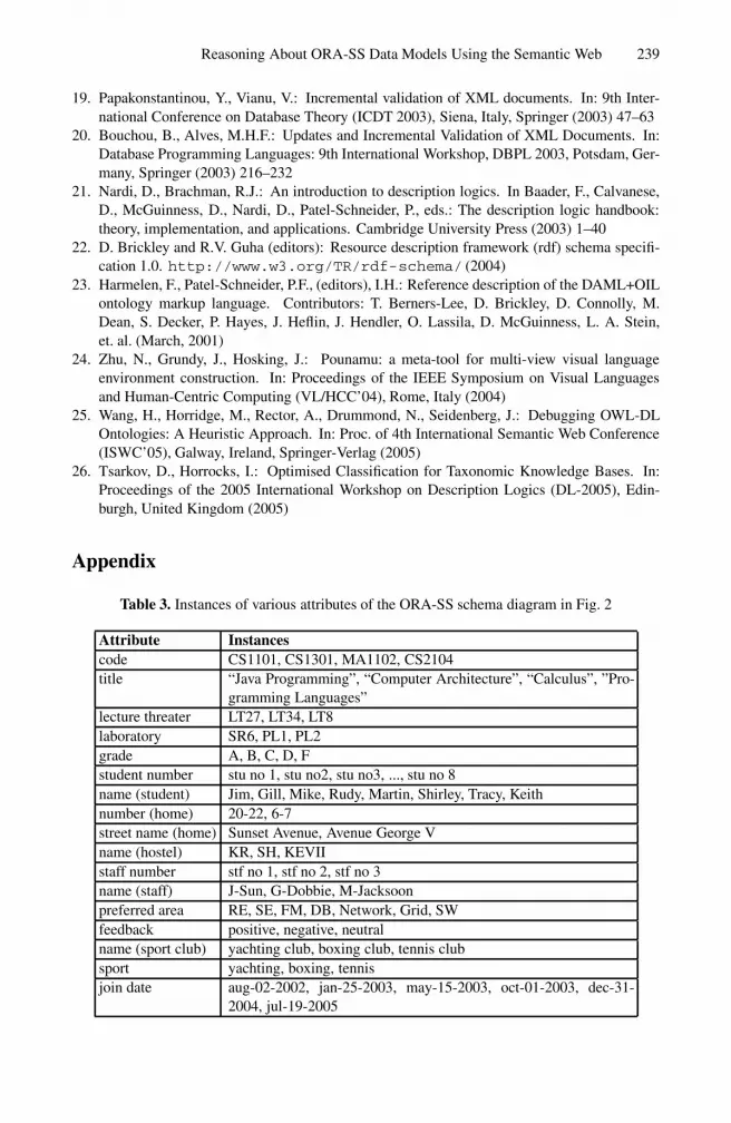
Reasoning About ORA-SS Data Models Using the Semantic Web 239
19. Papakonstantinou, Y., Vianu, V.: Incremental validation of XML documents. In: 9th Inter-national Conference on Database Theory (ICDT 2003), Siena, Italy, Springer (2003) 47–63
20. Bouchou, B., Alves, M.H.F.: Updates and Incremental Validation of XML Documents. In:Database Programming Languages: 9th International Workshop, DBPL 2003, Potsdam, Ger-many, Springer (2003) 216–232
21. Nardi, D., Brachman, R.J.: An introduction to description logics. In Baader, F., Calvanese,D., McGuinness, D., Nardi, D., Patel-Schneider, P., eds.: The description logic handbook:theory, implementation, and applications. Cambridge University Press (2003) 1–40
22. D. Brickley and R.V. Guha (editors): Resource description framework (rdf) schema specifi-cation 1.0. http://www.w3.org/TR/rdf-schema/ (2004)
23. Harmelen, F., Patel-Schneider, P.F., (editors), I.H.: Reference description of the DAML+OILontology markup language. Contributors: T. Berners-Lee, D. Brickley, D. Connolly, M.Dean, S. Decker, P. Hayes, J. Heflin, J. Hendler, O. Lassila, D. McGuinness, L. A. Stein,et. al. (March, 2001)
24. Zhu, N., Grundy, J., Hosking, J.: Pounamu: a meta-tool for multi-view visual languageenvironment construction. In: Proceedings of the IEEE Symposium on Visual Languagesand Human-Centric Computing (VL/HCC’04), Rome, Italy (2004)
25. Wang, H., Horridge, M., Rector, A., Drummond, N., Seidenberg, J.: Debugging OWL-DLOntologies: A Heuristic Approach. In: Proc. of 4th International Semantic Web Conference(ISWC’05), Galway, Ireland, Springer-Verlag (2005)
26. Tsarkov, D., Horrocks, I.: Optimised Classification for Taxonomic Knowledge Bases. In:Proceedings of the 2005 International Workshop on Description Logics (DL-2005), Edin-burgh, United Kingdom (2005)
Appendix
Table 3. Instances of various attributes of the ORA-SS schema diagram in Fig. 2
Attribute Instancescode CS1101, CS1301, MA1102, CS2104title “Java Programming”, “Computer Architecture”, “Calculus”, ”Pro-
gramming Languages”lecture threater LT27, LT34, LT8laboratory SR6, PL1, PL2grade A, B, C, D, Fstudent number stu no 1, stu no2, stu no3, ..., stu no 8name (student) Jim, Gill, Mike, Rudy, Martin, Shirley, Tracy, Keithnumber (home) 20-22, 6-7street name (home) Sunset Avenue, Avenue George Vname (hostel) KR, SH, KEVIIstaff number stf no 1, stf no 2, stf no 3name (staff) J-Sun, G-Dobbie, M-Jacksoonpreferred area RE, SE, FM, DB, Network, Grid, SWfeedback positive, negative, neutralname (sport club) yachting club, boxing club, tennis clubsport yachting, boxing, tennisjoin date aug-02-2002, jan-25-2003, may-15-2003, oct-01-2003, dec-31-
2004, jul-19-2005
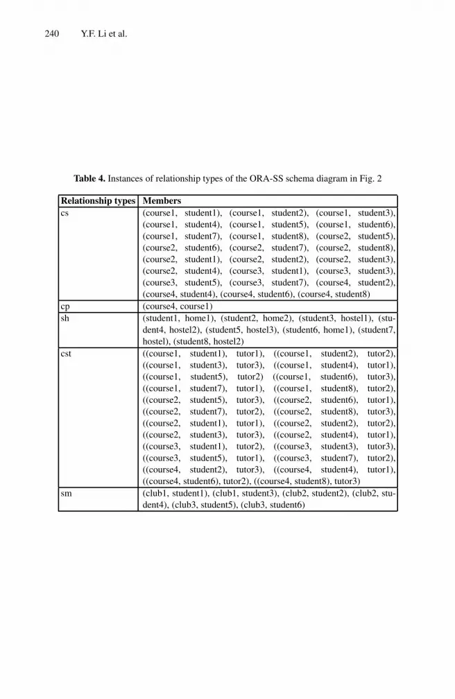
240 Y.F. Li et al.
Table 4. Instances of relationship types of the ORA-SS schema diagram in Fig. 2
Relationship types Memberscs (course1, student1), (course1, student2), (course1, student3),
(course1, student4), (course1, student5), (course1, student6),(course1, student7), (course1, student8), (course2, student5),(course2, student6), (course2, student7), (course2, student8),(course2, student1), (course2, student2), (course2, student3),(course2, student4), (course3, student1), (course3, student3),(course3, student5), (course3, student7), (course4, student2),(course4, student4), (course4, student6), (course4, student8)
cp (course4, course1)sh (student1, home1), (student2, home2), (student3, hostel1), (stu-
dent4, hostel2), (student5, hostel3), (student6, home1), (student7,hostel), (student8, hostel2)
cst ((course1, student1), tutor1), ((course1, student2), tutor2),((course1, student3), tutor3), ((course1, student4), tutor1),((course1, student5), tutor2) ((course1, student6), tutor3),((course1, student7), tutor1), ((course1, student8), tutor2),((course2, student5), tutor3), ((course2, student6), tutor1),((course2, student7), tutor2), ((course2, student8), tutor3),((course2, student1), tutor1), ((course2, student2), tutor2),((course2, student3), tutor3), ((course2, student4), tutor1),((course3, student1), tutor2), ((course3, student3), tutor3),((course3, student5), tutor1), ((course3, student7), tutor2),((course4, student2), tutor3), ((course4, student4), tutor1),((course4, student6), tutor2), ((course4, student8), tutor3)
sm (club1, student1), (club1, student3), (club2, student2), (club2, stu-dent4), (club3, student5), (club3, student6)

Reasoning About ORA-SS Data Models Using the Semantic Web 241
Table 5. Attribute values associated with the objects and relationships in Fig. 2
Entity Attribute association
course
instances code title exam venuecourse1 CS1101 “Java Programming” LT27course2 CS1301 “Computer Architecture” LT34course3 MA1102 “Calculus” LT8course4 CS2104 “Programming Languages” SR6
student
instances name student numberstudent1 Jim stu no1student2 Gill stu no2student3 Mike stu no3student4 Rudy stu no4student5 Martin stu no 5student6 Shirley stu no 6student7 Tracy stu no 7student8 Keith stu no 8
cs
instances grade instances grade instances gradecs1 A cs2 B cs3 Bcs4 C cs5 C cs6 Bcs7 A cs8 F cs9 Bcs10 D cs11 C cs12 Bcs13 B cs14 B cs15 Fcs16 A cs17 C cs18 Dcs19 C cs20 D cs21 Acs22 B cs23 B cs24 A
homeinstances number street namehome1 20-22 Sunset Avenuehome2 6-7 Avenue George V
hostel
instances namehostel1 KRhostel2 SHhostel3 KEVII
tutor
instances staff number name preferred areatutor1 stf no 1 J-Sun SE, RE, FM, SWtutor2 stf no2 G-Dobbie SE, DB, Networktutor3 stf no 3 M-Jackson RE, SE, Grid
cst
instances feedback instances feedback instances feedbackcst1 positive cst2 neutral cst3 neutralcst4 neutral cst5 neutral cst6 neutralcst7 positive cst8 negative cst9 neutral
cst10 negative cst11 neutral cst12 neutralcst13 neutral cst14 neutral cst15 negativecst16 positive cst17 neutral cst18 negativecst19 neutral cst20 negative cst21 positivecst22 neutral cst23 neutral cst24 positive
sport club
instances name sportclub1 yachting club yachtingclub2 boxing club boxingclub3 tennis club tennis
sm
instances join date instances join datesm1 aug-02-2002 sm2 may-15-2003sm3 jan-25-2003 sm4 oct-01-2003sm5 jul-19-2005 sm6 dec-31-2004

S. Spaccapietra (Ed.): Journal on Data Semantics VII, LNCS 4244, pp. 242 – 266, 2006. © Springer-Verlag Berlin Heidelberg 2006
A Pragmatic Approach to Model and Exploit the Semantics of Product Information
Taehee Lee1, Junho Shim2,*, Hyunja Lee2, and Sang-goo Lee1
1 School of Computer Science & Engineering, Seoul National University, Korea {thlee, sglee}@europa.snu.ac.kr
2 Department of Computer Science, Sookmyung Women’s University, Korea {jshim, hyunjalee}@sookmyung.ac.kr
Abstract. Recently researchers have tried to apply ontology to the product information domain. From a practical point of view, a key problem to streamline this trend is how to make a product ontology database operational. Technical solutions should consider the characteristics that a pragmatic product ontology database contains; first, the database size is quite huge, and second, ontological manipulation and utilization should be realistically feasible. We recently engaged in a project to build an operational product ontology system. The system is designed to serve as a product ontology knowledge base, not only for the design and construction of product databases but also for the search and discovery of products. From the insights gained through this project, we believe that ontological modeling and its implementation on an operational database, as well as the building applications which exploit ontological benefits, are the most important facets towards the successful deployment of a practical product ontology system. As such, searching techniques should take into account the features of an underlying ontological model especially with product searching being one of the most popular applications within product information systems. In this paper, we present these two issues; product ontology modeling and searching techniques. Although our work presented herein may not be the only way to build an operational product ontology database, it may serve as an important reference model for similar projects in future.
1 Introduction
Product information is an essential component in e-commerce. It contains information such as pricing, features, and terms about the goods and services offered or requested by the trade partners. A base of precisely and clearly defined product information is a necessary foundation for collaborative business processes. In addition, semantically enriched product information may enhance the quality and effectiveness of business transactions and can be used to support production planning and management. These features can be offered by ontology, and the potential benefits of ontology on product information have been introduced by researchers in recent years [8,23,37,17,18].
* Corresponding author.

A Pragmatic Approach to Model and Exploit the Semantics of Product Information 243
Product ontology requires specifying a conceptualization of product information in terms of classes, properties, relationships, and constraints. Although there has been a vast amount of research in ontology, there are still gaps to be filled in actual deployment of the technology/concept in a real-life commercial environment. These gaps are especially prevalent in certain domains such as product information management where mission critical applications need to be ‘operational’. We recently participated in a project to build an operational product ontology system for a government procurement service [19]. Herein, by ‘operational’ we mean that product ontology should run in a large scale database with gigabytes or terabytes size and that applications built on the product ontology database should benefit a proper degree of inference functionalities. This means that we may compensate some degree of ontological beauties such as full-fledged reasoning with the availability, robustness, and performance that operational product ontology should provide.
Two major issues for building an operational ontology not only limited to product but in other domains may include 1) how to model and implement operational ontology and 2) to build an application that runs in large scale and benefits the underlying ontology model. One of the most important and popular applications related to product information system is product searching. Product searching that exploits the ontological benefits may provide users with more a precise and relevant set of products than is possible with conventional IR-based searching. Obviously, searching techniques over product ontology should be different from the techniques of processing queries over conventional document or relational databases, and should take into account of the features of the underlying ontological model.
In this paper, we present these two issues; product ontology modeling and searching techniques. The rest of this paper is structured as follows: Section 2 describes related work and offers a brief introduction of how to build an operational product ontology system. In Sections 3 and 4, we present our modeling methodology for building an operational product ontology database and explain how our model corresponds to OWL representation. In Section 5 we discuss how to design and develop a searching technique over a product ontology model. Conclusions are drawn in Section 6.
2 Related Work
The Web has been extended in a way that information is incorporated into well-defined semantics, better enabling computers and people to work in cooperation. Ontology plays an essential role in realizing the Semantic Web. It is concerned with the taxonomic hierarchies of classes and class definitions, relationships between classes, and knowledge about beings and their world. XML based markup languages such as DAML+OIL [11] and OWL [31] have been developed to represent ontology in the Web, and also have given influence to the Web applications such as e-commerce systems.
Product information has the taxonomic hierarchies and consists of multiple attributes. In addition, exchanging product information among business partners requires it to have well-defined semantics. That makes product information an adequate domain within e-commerce where ontology can play a vital role. In [8] the

244 T. Lee et al.
authors list the difficulties of building, maintaining, and integrating product information, and propose that an ontological approach may be the answer. In [25] the authors propose to use cross industry standard classifications such as UNSPSC1 and eCl@ss2 as the upper ontology and industry specific classifications as lower ontology. An upper ontology is about concepts that are generic, abstract and, therefore, are general enough to address (at a high level) a broad range of domain areas, while lower ontology contains domain-specific knowledge [35]. An effort to introduce the ISO standard for product library is presented in [22]. All of these authors’ work, however, focuses mainly on classification standards as the shape of ontology for product information. Classification hierarchies are an essential part of product information semantics but make up only one piece of the picture.
The importance of attributes in product information management is well-introduced in [12,17]. In [12], the quality of product classification standards is evaluated by a number of factors including the quality of their attribute lists. In [17], the authors point out that a classification hierarchy is a representation of just one of many views over the set of products, and that a product’s identity and property are not decided only by how the product is classified. Product database design issues and guidelines are presented, where the focus is on properties (attributes) rather than on classification hierarchies.
For any semantic modeling to be suitable for its application domain, it is crucial to investigate what semantic concepts and relationships are desirable for the domain and to capture them in a model. More specifically, as mentioned in [8], ontological modeling of e-Catalog requires specifying a conceptualization of e-Catalog in terms of classes, properties, relationships and constraints. Concepts presented in this paper are gleaned through a real project that we participated in [19], and their formal representations are presented using description logics [21]. In this paper, we summarized the types of semantic relationships that need to be identified during product ontology modeling. Furthermore, we showed how to use OWL to formalize the semantics of product data stored in a relational database [20].
[18] is a recent work that points out that building an OWL knowledgebase is not pragmatically adequate for a large-scale ontology. Instead the authors promote a relational database approach in which reasoning is supported by storing facts in tables and representing rules in SQL triggers. However, their work is different from ours in that they focus on providing a programmatic framework rather than on modeling related issues. E-procurement is one of the most suitable domains that can benefit from well-defined product information. The process of registering or searching for a product, adding a new supplier, or placing a purchase order requires accurate product information. We have built an ontology system3 for the Public Procurement Services of Korea, which is responsible for procurement for government and public agencies. The purpose of the system is to provide a universal ontology repository with browsing and searching capabilities in order to facilitate e-catalog sharing and interoperability [19].
1 http://www.unspsc.org 2 http://www.eclass-online.com 3 The system is called KOCIS (Korea Ontology-based e-Catalog Information System), and
accessible online at http://www.g2b.go.kr:8100/index.jsp
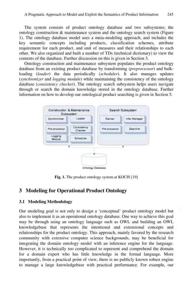
A Pragmatic Approach to Model and Exploit the Semantics of Product Information 245
The system consists of product ontology database and two subsystems; the ontology construction & maintenance system and the ontology search system (Figure 1). The ontology database model uses a meta-modeling approach, and includes the key semantic concepts including products, classification schemes, attribute requirement for each product, and unit of measures and their relationships to each other. We also organized and built a number of TDs (technical dictionary) to view the contents of the database. Further discussion on this is given in Section 3.
Ontology construction and maintenance subsystem populates the product ontology database from an existing product database by transforming (preprocessor) and bulk-loading (loader) the data periodically (scheduler). It also manages updates (synchronizer and logging module) while maintaining the consistency of the ontology database (consistency checker). The ontology search subsystem helps users navigate through or search the domain knowledge stored in the ontology database. Further information on how to develop our ontological product searching is given in Section 5.
Fig. 1. The product ontology system at KOCIS [19]
3 Modeling for Operational Product Ontology
3.1 Modeling Methodology
Our modeling goal is not only to design a ‘conceptual’ product ontology model but also to implement it as an operational ontology database. One way to achieve this goal may be through using an ontology language such as OWL and building an OWL knowledgebase that represents the intentional and extensional concepts and relationships for the product ontology. This approach, mainly favored by the research community with extensive computer science backgrounds, may be beneficial for integrating the domain ontology model with an inference engine for the language. However, it is technically too complicated to represent and comprehend the domain for a domain expert who has little knowledge in the formal language. More importantly, from a practical point of view, there is no publicly known robust engine to manage a large knowledgebase with practical performance. For example, our

246 T. Lee et al.
product ontology database contains over five hundred thousands products and more than nine hundred thousands concepts including product classes, attributes and UOMs. Concepts are linked by the semantic relationships, and the total number of the semantic links is more than twenty-one million [19], not to mention that the size of the database keeps growing. In addition, we only needed a rather limited-set of reasoning capabilities such as transitivity and inverse. Naturally, the general purpose reasoning capability of an OWL engine was considered as over-kill. Consequently, we may regard this approach to be of little pragmatic value if used for an operational product ontology.
From a purely pragmatic point of view, an alternative way is to build a product ontology database on commercially operational database systems, i.e., more specifically object-relational DBMSs. It takes advantage of existing standards for data management and the DBMS features that have been optimized over the years in terms of robustness, scalability, or performance. Although it can support a limited set of reasoning by the object-relational model itself and a featured set of reasoning should be implemented within database applications, it is a sure way to make an ontology database operational. Table 1 shows the key differences between these two comparative methodologies.
Table 1. Model implementation methodology
OWL-based knowledgebase approach Relational database approach
Theoretical background
OWL, DAML+OIL, Topic Maps, Description Logics, FOL, …
EER, Table, SQL, Relational Algebra & Calculus, …
Pragmatism Theoretical yet ideal Operational and practical
Ontology representation
Rich for various semantic constraints
Rather limited for complicated semantic constraints
Ontological Reasoning orinference
Supported by the OWL-reasoning engine. Yet reasoning complexity may be high.
Limited. And featured reasoning capabilities should be coded within applications.
Commercial level
Publicly no engine is available to support a large knowledgebase.
Many DBMSs are commercially available.
In order to moderate between those two extreme methodologies, we need an adaptive approach which is practical in scalability and yet open for future technology. We claim that one way to achieve this is through building a product ontology database on top of an operational database system and yet providing an exporting mechanism from the database to an OWL knowledgebase. In other words, each modeling construct in an object-relational database can be translated into the corresponding OWL representation. Then a set of translated representation may form an OWL knowledgebase, and the ontological reasoning could be exploited by a ‘robust’ OWL engine should the engine indeed exist.

A Pragmatic Approach to Model and Exploit the Semantics of Product Information 247
In fact, within our project we developed a mechanism to translate relational tables representing concepts such as products, classification schemes, attributes and UOMs (unit of measure), and their relationships into OWL representations. In the following subsections we discuss in more detail how we developed an ontological product model and implement it on an object-relational database. In Section 4 we overview the correspondence between our model and the OWL representation.
3.2 Meta Modeling for Product Ontology
Ontological modeling is an inherent process for building an ontology application regardless of the application domain. After the domain analysis, one needs to first conceive the key concepts and their relationships which may best portray the domain. In our product ontology, we regard products, classification scheme, attributes and UOMs as the key concepts. The products, the most important concept, are for the goods or services. The classification scheme and the attributes are used for the classifications and descriptions of products respectively. The UOM is associated with the attributes.
Fig. 2. a) Concepts and relationships in meta-level b) Taxonomy of semantic relationships
Figure 2-a) illustrates our view for product ontology using the meta-model approach. The meta-modeling approach enables a product ontology model to be more extensible and flexible. Our product model follows the basic meta-model which employs three modeling-levels: M0 meta-class level, M1 class level and M2 instance level. Within M0 level, which describes high level conceptual product ontology, we have the aforementioned key concepts as meta-classes. Key concepts are products, classification schemes, attributes and UOMs in our model, and they are represented by M_Products, M_ClassificationSchemes, M_Attributes and M_UOMs, respectively. As illustrated in Figure 2, meta-classes may have relationships (meta-relationships) with each other.
Various types of semantic relationships have been researched for a long time in multidiscipline areas such as cognitive science, logics and databases. A classification scheme by [36] presents one of the various viewpoints of classifying the semantic relationships. Based on both their work and our field experience [19], we created a taxonomy of semantic relationships for product information domain as in Figure 2-b),

248 T. Lee et al.
in which top-level relationships include the general domain relationships, e-Catalog domain specific relationships and user-defined relationships. The relationships for general domain include inclusion, attribution, and synonym. As in [34, 36], they are semantically generic to various domains and should be considered as meaningful semantic relationships for the e-Catalog domain as well.
The inclusion relationship describes cases in which an entity type contains other entity types, and it can be classified into the class inclusion or meronymic inclusion. The class inclusion represents the standard subtype/supertype relationship. The meronymic inclusion between C and D represents a part-whole relationship, i.e., C is a part of D (D is the whole of C), or simply C has D. For example, HDD and CPU are the parts of computer just as a beef-stew has beef, garlic, and onion as its ingredients. There are different semantic interpretations of this part-whole relationship. Similar to [36] we found the part-whole relationships to include component-of, substance-of, member-of, portion-of, and feature-of relationships. The attribution describes situation where an entity type describes properties or characteristics of other entity types. Finally, the synonym relationship describes an entity type that contains similar semantics to other entity types. For example, price and weight are attributes of Laptop; and Laptop is a synonym of Notebook.
The next set of semantic relationships is particularly conceivable for the e-Catalog domain. It includes substitute, complement, purchase-set, and mapped-to relationships. For examples, a pencil is a substitute of a ballpoint pen, and a LCD monitor is a substitute of a CRT monitor in that each may act as a replacement of the other. The complement relationship means that one may be added to another in order to complete a thing or extend the whole. For example, an antiglare filter is complement to a monitor. Similar but not identical to these, we may also see that such products as a monitor, an OS, and a mouse are also purchased with a personal computer. This is represented as a purchase-set, i.e., a personal computer has a purchase-set relationship with a monitor, an OS, and a mouse.
While substitute, complement, or purchase-set are relationships among product classes, the mapped-to relationship assigns a product into a specific class code within a classification scheme, or maps a class code of a classification scheme into the codes of different classification schemes. For example, a LCD panel product is mapped to (belongs to) 43172410 commodity class under a certain standard classification scheme. A product class can then be defined or classified differently depending on classification schemes. For example, the product personal computer is mapped to 43171803 in UNSPSC classification system, and 8471-10 or 8471-41 in HS code system.
Note that in Figure 2, meta-class and meta-relationships are identified by the prefix ‘M_’ to indicate that they are meta-concepts. M1 class level contains a snapshot or instance of the product ontology model in M0. That is, it illustrates a class schema of a product ontology database. The conceptual class schema may be then translated into its logical schema managed by an operational DBMS. The logical schema in our case is a set of object-relational tables and views. Figure 3 illustrates a part of the class schema of our product ontology database whereas M2 instance level refers to the physical ontology data managed by the system. For example, notebook and LCD panel products in M1 level are instances of products meta-class in M0 level, and there is a component relationship between them, i.e., a notebook contains a LCD panel and
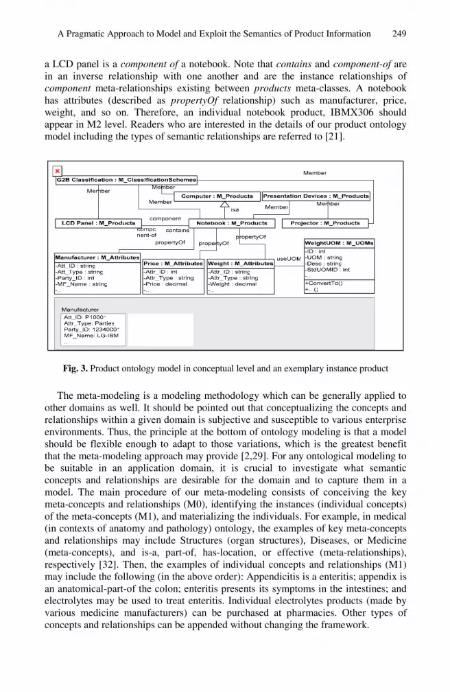
A Pragmatic Approach to Model and Exploit the Semantics of Product Information 249
a LCD panel is a component of a notebook. Note that contains and component-of are in an inverse relationship with one another and are the instance relationships of component meta-relationships existing between products meta-classes. A notebook has attributes (described as propertyOf relationship) such as manufacturer, price, weight, and so on. Therefore, an individual notebook product, IBMX306 should appear in M2 level. Readers who are interested in the details of our product ontology model including the types of semantic relationships are referred to [21].
Fig. 3. Product ontology model in conceptual level and an exemplary instance product
The meta-modeling is a modeling methodology which can be generally applied to other domains as well. It should be pointed out that conceptualizing the concepts and relationships within a given domain is subjective and susceptible to various enterprise environments. Thus, the principle at the bottom of ontology modeling is that a model should be flexible enough to adapt to those variations, which is the greatest benefit that the meta-modeling approach may provide [2,29]. For any ontological modeling to be suitable in an application domain, it is crucial to investigate what semantic concepts and relationships are desirable for the domain and to capture them in a model. The main procedure of our meta-modeling consists of conceiving the key meta-concepts and relationships (M0), identifying the instances (individual concepts) of the meta-concepts (M1), and materializing the individuals. For example, in medical (in contexts of anatomy and pathology) ontology, the examples of key meta-concepts and relationships may include Structures (organ structures), Diseases, or Medicine (meta-concepts), and is-a, part-of, has-location, or effective (meta-relationships), respectively [32]. Then, the examples of individual concepts and relationships (M1) may include the following (in the above order): Appendicitis is a enteritis; appendix is an anatomical-part-of the colon; enteritis presents its symptoms in the intestines; and electrolytes may be used to treat enteritis. Individual electrolytes products (made by various medicine manufacturers) can be purchased at pharmacies. Other types of concepts and relationships can be appended without changing the framework.

250 T. Lee et al.
3.3 Model Implementation and Technical Dictionary
We create an object-relational product ontology database consisting of more than forty base tables to reflect the aforementioned conceptual and class schemas. One novel feature that our ontology database provides is that it organizes and displays the product information in the form of technical dictionaries. Technical dictionaries, (TDs), are used frequently in the e-Catalog domain to describe the products and their properties. Well-known TDs include eOTD, GDD, and RNTD of ECCMA, EAN/UCC, and RosettaNet, respectively [7,9,28]. Compared to these TDs, our TD holds a far richer set of information that is required for machines to operate on products intelligently; such as the product’s attributes and its relationship to other products.
We have constructed a number of technical dictionaries, in a way along which we can reflect the core concepts and relationships explained in the conceptual product ontology model. The contents of each TD are extracted and organized from the different sets of underlying ontology base tables. As an example of a TD, Table 2 shows a part of the classification technical dictionary. Within the dictionary, we have a product classification for personal computers. Under this specific classification scheme (g2b), it has a class code of 43171825, and it is also called as PC, desktop computer, or workstation (synonym field). In general, a product class may be defined or classified differently depending on classification schemes. We can find such information in the code mappings. For example, personal computers are mapped to 43171803 in UNSPSC classification system, and 8471-10 or 8471-41 in HS code system. It has component (contains) relationships with CPU, HDD, and RAM, and substitute relationships with notebook computers. We may also see that such products as a monitor, an OS, and a mouse are also purchased with a personal computer.
Note that each item within the same TD might have different columns to the ones that other items have, in that they can have different classification code mappings and relationships in actual contexts. For example, while the item personal computer has
Table 2. An example of a technical dictionary: g2b classification TD
class name
G2B code
description synonyms code mappings relationships etc
UNSPSC
HS GUNGB
component
substitute purchas
e-set personal computers
43171825
A computer built for use by an individual …
PC,desktop computers, workstations 43171
803 8471-10, 8471-
7010300
CPU, HDD, RAM,
notebook computers
monitors, OS, mouse,
…
UNSPSC GUNGBcomplement
substitute purchas
e-set LCD monitors
43172410
A low-power flat-panel display used for …
LCD, liquid crystal displays, flat panel displays
43172402,4317240, 431724
7025366, 7025302
arm stand, antiGlare filter
CRT monitors
personal computers
…
… … … … … … …

A Pragmatic Approach to Model and Exploit the Semantics of Product Information 251
three columns of code mappings for UNSPSC, HS, and GUNGB, another item such as a LCD monitor has just two columns of code mappings for UNSPSC and GUNGB. This means that in the actual product ontology database the item LCD monitor does not have any mapping relationship to HS. Similarly, the types of relationships that personal computers and LCD monitors have are different; personal computers have component but no complements while LCD monitors have complement but no component products.
4 Product Ontology Model: OWL Perspectives
4.1 Comprehensive Correspondence
A feature of our modeling approach is that we may represent the product ontology model in a standard ontology language. In this section, we illustrate how the model can be represented in OWL [31,20,10]. An OWL knowledge representation for specific domain may be the best means to utilize the techniques from so-called ontology-engineering [14,32]. For instances, it is beneficial for making a knowledgebase loosely-coupled from the application codes, enabling it to develop knowledge bases independent and interoperable from each other, and automating reasoning facility by OWL inference engines [26]. Recently, in the product ontology domain, there have been efforts by researchers to transform or publish the domain representation into OWL versions as well. Two most important related works are [13,21].
In [13], the authors focus on OWL derivation for industry standard taxonomy, such as UNSPSC and eCl@ss. They classify concepts into three parts; generic concept, annotation concept, and taxonomy concept for capturing the original semantics of existing standards taxonomy. In our preliminary work [21], we introduced a modeling framework which formally represents product ontology in DL(description logics). OWL and DL share a theoretical background. Furthermore, a model in DL may be translated into OWL representation. This requires consideration of the employed OWL language in terms of expressiveness and complexity along with its practical usage in the product information domain.
Figure 4 illustrates a basic mapping from our product meta-model (Figure 2-a) to the OWL representation. Note that we rename Attribution(‘PropertyOf’) relationship between Products and Attributes with ‘hasAttribute’ to avoid confusion with the property expression in OWL.
Basically, concepts can be represented by owl:Class, and relationships by owl:ObjectProperty or owl:DatatypeProperty, in general. The class inclusion (isa) can be represented by ‘rdfs:SubClassOf’. Datatype property is used for relationships which exist between a class instance and a data value, while object property is used for relationships between class instances. An in and outgoing edge of arcs illustrates the property domain and the range of a property respectively. Note that in OWL, the domain and the range of a property limit the individuals to which the property can be applied and the property it may have as its values respectively. Relationships may have additional property restrictions (owl:Restrictions) or property characteristics

252 T. Lee et al.
Fig. 4. Basic OWL correspondence in meta-level
Fig. 5. An exemplary OWL representation for computer-related products

A Pragmatic Approach to Model and Exploit the Semantics of Product Information 253
(owl:TransitiveProperty, owl:SymmetricProperty, owl:inverseOf, or owl:FunctionalProp-erty) to convey the proper semantics of the relationship. This can be seen in Figure 5 which is essentially a more detailed illustration of Figure 4.
In Figure 5, desktop computers are members of 8471-10 and of 43171803 commodities in HS and UNSPSC classification systems respectively. The member relationship may be represented by the owl:ObjectProperty::member object property with rdfs:domain::ClassificationScheme and rdfs:range::Product restrictions. The object properties are also used in other places such as purchaseSET between LCD Monitor and Desktop Computer, and has_Size between LCD Monitor products and Displaysize attributes. ClassID is an attribute of LCD Monitors and has a string data type value of ‘25231036’. This can be represented by owl:DatatypeProperty with a restriction of rdfs:range::STRING.
Consider that desktop computers and LCD Monitors may be purchased together. This can be represented using owl:ObjectProperty::purchaseSET with an additional restriction with owl:SymmetricProperty to denote the symmetric property of the purchaseSET property. Additionally, if the domain of purchaseSET is limited to Desktop computers, then the range should be limited by adding the owl:someValuesFrom restriction.
The individual products are represented by using rdf:type, that ties an individual to a class to which it belongs. For example, LCDx1751QD and SAMSUNG MagicStation are the individuals of LCD Monitors and Desktop computers, respectively, and can be represented by <LCDMonitors rdf:ID=”LCDx1751QD”> and <DesktopComputer rdf:ID =”SAMSUNGMgicStation”>.
LCD Monitors products have DisplaySize as an attribute. This is represented by owl:ObjectPropertyOf::hasDisplaySize of which domain and range are restricted to LCD Monitors and DisplaySize. In attribute classes, DisplaySize is a sub type of Size and also synonym for MonitorSize. This may be represented using rdfs:SubClassOf and owl:EquivalentClass respectively.
Finally, DisplaySize attribute associated with the Length UOM and the instances of Length UOMS include ‘inch’ and ‘cm’. Similar to the previous examples, these may be represented using owl:ObjectPropertyOf::useUOM and rdf:type. Note that ‘inch’ and ‘cm’ UOMs may be converted, i.e., 1inch = 2.54cm. In our project, each equation is represented as a convertedTo relationship and maintained in a relational table.
4.2 OWL Property Restrictions for Semantic Relationships
As mentioned in the previous section, although relationships may be corresponded to owl:ObjectProperty, more restrictions should be selectively added to each object property to convey precise semantics. Those restrictions include owl:Transitive-Property, owl:SymmetricProperty, owl:inverseOf, and owl:FunctionalProperty, and owl:someValuesFrom and owl:allValuesFrom to further constrain the range of a property in specific contexts.
As an example, let us consider that a DC spindle motor is a component (or part) of HDD(hard disk) product which is also a component of computer products (Figure 6). The component relationship, in general, is not always transitive in that it usually contains both aggregational and functional semantics; being a functional part of its whole does not necessarily mean that the part is functional for another object which is

254 T. Lee et al.
composed of the whole [34]. However in practice, people often do not clarify the precise semantics of the component relationship that they use. For example, a query to find all hardware classes which contain DC Spindle as its “component” is not clear whether it is meant to search for any hardware having DC Spindle as its direct part or as its both direct and indirect parts (being contained within another product). In order to handle an indirect part-whole relationship, we need the transitive property, i.e., x·y & y·z⇒ x·z. This can be represented in OWL using owl:TransitiveProperty . If HDD is a component(part) of Computer, then Computer is the composed(whole) of HDD. This may be represented using owl:inverseOf. In addition, the value restriction owl:someValuesFrom should be applied to the component property since Computers have not only HDD but also other parts such as CPU, a graphic card, RAM and etc..
Fig. 6. Restrictions on component relationships
Fig. 7. Restrictions on supplement relationships

A Pragmatic Approach to Model and Exploit the Semantics of Product Information 255
Table 3. OWL correspondence to semantic relationships
General domain relationships Semantic
relationships Examples in OWL Semantic relationships Examples in OWL
ClassInclusion
Meronymic Inclusion
Restriction for Semantics
Restriction for Semantics
SubClass Of
<owl:Classrdf:ID=”DeskTopComputers”> <rdfs:subClassOf rdf:resource=”#Computers”/> <owl:disjointWithrdf:resource=”#NotebookComputers” /> </owl:Class>
Synonym
equivalentClass
<owl:Classrdf:ID=”PersonalComputer”> <equivalentClassrdf:resource=”# PC “/></owl:Class>
Attribution Restriction for Semantics DatatypeP roperty Domain Range
<owl:DatatypeProperty rdf:ID=”ClassID”><rdfs:range rdf:resource=”XMLSchema#string”/><rdfs:domain><owl:Class rdf:about=”#Product” /> </rdfs:domain> </owl:DatatypeProperty>
ObjectProperty InversePropertyTransitiveProperty(optional)
SomeValuesFrom
<owl:Class rdf:ID=”HDD”> <rdfs:subClassOf>
<owl:Restriction> <owl:someValuesFrom
rdf:resource=”#Computers”/> <owl:onProperty>
<owl:ObjectProperty rdf:ID=”component”/>
</owl:onProperty> </owl:Restriction></rdfs:subClassOf> </owl:Class> <owl:ObjectProperty rdf:about=”# component”><rdf:type rdf:resource="&owl;TransitiveProperty”/> <owl:inverseOf><owl:ObjectProperty rdf:ID=”compose”/> </owl:inverseOf>
</owl:ObjectProperty>
e-Catalog specific relationships Supplement Substitute
Restriction For Semantics
Restriction for Semantics
SymmetricPropertyTransitiveProperty
AllValuesFrom
<owl:Classrdf:ID=”LCDmonitors”> <rdfs:subClassOf> <owl:Restriction> <owl:allValuesFrom
rdf:resource=”#CRTmonitors”/> <owl:onProperty> <owl:SymmetricProperty
rdf:ID=”substitute”/> </owl:onProperty>
</owl:Restriction> </rdfs:subClassOf></owl:Class><owl:ObjectProperty rdf:about=”#substitute”>
<rdf:type rdf:resource="&owl;TransitiveProperty”/></owl:ObjectProperty>
FunctionalProperty (optional)
AllValuesFrom
<owl:Class rdf:ID=”Toner”> <rdfs:subClassOf><owl:Restri
ction><owl:onProperty> <owl:FunctionalProperty
rdf:ID=”supplement”/> </owl:onProperty>
<owl:allValuesFrom> <owl:Class
rdf:ID=”LaserPrinter”/> </owl:allValuesFrom>
</owl:Restriction> </rdfs:subClassOf> </owl:Class><owl:FunctionalProperty
rdf:about=”#supplement”/>
PurchaseSet MappedToRestriction for Semantics
Restriction for Semantics
SymmetricProperty
SomeValuesFrom
<owl:Class rdf:ID="Computer"> <rdfs:subClassOf>
<owl:Restriction> <owl:onProperty>
<owl:SymmetricProperty rdf:ID="purchaseSet"> </owl:onProperty> <owl:someValuesFrom> <owl:Class
rdf:ID="Monitors"/> </owl:someValuesFrom> </owl:Restriction> </rdfs:subClassOf>
</owl:Class>
SymmetricProperty
allValuesFrom
<owl:Class rdf:ID=” HS 8471-10”>
<rdfs:subClassOf> <owl:Restriction> <owl:allValuesFrom>
<owl:Classrdf:ID=”UNSPSC43172402”/></owl:allValuesFrom> <owl:onProperty> <owl:SymmetricProperty
rdf:ID=”MappedTO”/> </owl:onProperty> </owl:Restriction> </rdfs:subClassOf>
</owl:Class>
Let us consider that any individual antiglare filter product may serve as a supplement to any monitor product while only a specific type of toner product may serve as a laser printer. For example, TonerHP-2420 works with Laserjet2420, but

256 T. Lee et al.
other toners may work with it as well (Figure 7). In this case, owl:Objectproperty: supplement with owl:allValuesFrom may be enough to represent the supplement relationship between Antiglare filter and Monitor product classes. Whereas, we should add the owl:FuctionalProperty restriction to the supplement relationship between TonerHP-2420 and Laserjet2420.
A substitute relationship means that one may act as a replacement for the other. For example, a pencil is a substitute for a ballpoint pen. A substitute relationship might contain symmetric property, i.e., x substitute y ⇒ y substitute, which is represented in OWL as owl:ObjectProperty::substitute with the restriction of owl:SymmerticProperty.
Due to space limitations, we do not provide more details in translation scheme and associated property restrictions for each semantic relationship. Rather, we summarize them in Table 3. Readers who are interested in more details are referred to [20].
5 Building Applications on Product Ontology
5.1 Ontology-Based Searching
A product ontology may contain a large number of concepts and relationships. For naive users to search and navigate the ontology efficiently, good search and visualization functionalities should be provided. In practice, we may not expect ordinary users to have sufficient knowledge of the underlying schema to be able to compose their queries precisely in query languages such as OWL-QL or SQL. We contemplate the problem of ranking keyword search results over product ontology databases. First, we summarize some of the related works.
Traditionally ranking keyword search results have been extensively studied in the context of text. Ever since the big bang of the Internet, it has received more attention in other contexts such as web and xml documents. In the IR (information retrieval) research community, text ranking is typically done using keywords and its occurrence frequencies such as tf and idf values [30]. In the web environment, PageRank [5] and HITS [16] are the most well-known ranking algorithms. Both algorithms compute the authority of a document by considering hyperlinks. Documents with higher authority are positioned in higher ranks as they are regarded as globally important ones. The database research community has also paid attention to the keyword search problem. For example, [4] presents ObjectRank, which may be regarded as a modification of PageRank for relational databases. All the above works do not exploit ontology in their searching algorithms, which is what distinguishes our work. In [33] the authors propose a context-sensitive searching algorithm to exploit the ontology concept. However, they use ontology only for refining the meaning of search terms while the underlying data is not ontologically modeled but stored in plain HTML or XML format. An abundance of semantic relationships and their characteristics in the context of the Semantic Web are well documented in [1]. In that paper, the authors blended semantics and information-theoretic techniques for their general search model, in which users can vary their search modes to affect the ordering of results depending on whether they need conventional search or investigative search. Other researchers [27, 24] use a similar approach that combines the weight of relationships into their ranking functions. Their algorithms do not consider cases in which a search

A Pragmatic Approach to Model and Exploit the Semantics of Product Information 257
term may occur in a relationship name but only deal with the occurrence frequencies of relationships associated with each concept.
Processing keyword search queries over product ontology databases are different from processing queries over documents, web, or relational databases. First, searching product ontology should consider relationships between concepts while IR-based searching considers only the term occurrences in product data. Obviously, the ranking function should be altered to properly reflect the product ontology while utilizing IR-style information such as keyword proximity [30] as well. Considering relationships in a ranking function helps to understand the meaning of concepts and improve the recall by retrieving more related concepts. Furthermore, users in the product ontology domain tend to have more definite intention on issuing queries. They are more likely to search for products or product classes, which are represented by nodes in our product ontology graph (see the following subsection). In the semantic web or relational databases, instead, the target of the keyword search is usually a subgraph, rather than nodes. Note that a subgraph represents a relationship (or edge) between concepts or records in the semantic web or relational database respectively.
5.2 Product Searching and Product Ontology Graph
Our searching algorithm employs a graph structure, called a product ontology graph, to represent a snapshot of the underlying product ontology. An example of a product ontology graph appears in Figure 8. There are two types of nodes in a product ontology graph. The first type is a schematic node. The schematic node, represented by a rectangle in the graph, denotes a concept in M1 class-level, such as product class, classification scheme, UOM, and attribute. The second type of node is an instance node. The instance node, represented by an ellipse in the graph, denotes an instance in M2 instance level. Accordingly, every instance node has an associated schematic node. For example, an instance node “IBM S40”and “WD 2120” denote individual products which are associated with “Desktop computers” and “HDD” product class respectively. Note the schematic nodes are annotated by the corresponding concepts in M0 meta-level: e.g. Computers are annotated by <<Products>>. Example 1. Given a query to find a UNSPSC code for products “IBM P4 3.0GHz”, the system should return 48171803 (desktop computers) or 48171801 (notebook computers), or both. Conventional cumulative ranking functions such as PageRank[5] would rank desktop computers higher than notebook computers simply because they would determine that the global importance of desktop computers is greater than that of notebook computers, i.e., the number of incoming edges for desktop computers is greater. However, from a probabilistic point of view, the keywords “IBM P4 3.0GHz” are likely more relevant for notebook computers since every product in notebook computers is “IBM P4 3.0GHz” whereas only half of the products in desktop computers are “IBM P4 3.0GHz”. Note that most of the probabilistic classification algorithm such as Naïve Bayesian Classifier would return notebook computers as a result. (See Appendix for an explanation.)
Example 2. Keywords used in a query may be values, attribute names, category names, and even relationship names etc., whereas in a typical keyword search they are confined to attribute values only. As an example, in a query “IBM computer with

258 T. Lee et al.
components of P4 CPU”, the keywords “computer”, “component”, and “CPU” are names of product class, relationship, and attribute class respectively. For this query, both IBM S40 and IBM G41 may be retrieved as results, since desktop computers and notebook computers are sub-classes of the computer class, and both are made by IBM and contain P4 CPUs.
Example 3. Given a query to find an “IBM desktop computer with SG HDD”, there is no individual product satisfying the keywords in the desktop computers’ class. Since a substitute relationship between desktop and notebook computers was found in the product ontology graph, an IBM G41 notebook would be returned as a result, more precisely as a substituting product.
Fig. 8. An example of product ontology graph
As we have shown in the previous examples, there are particular features to notice in product ontology searching. First, the ranking function should consider not only the concepts that contain the keywords but also other context information such as the number of products in the same class and the number of edges (in Example 1). We use a well-known probabilistic model to accurately measure the relevance of query results, while others either use a simple additive function to compute the ranks or never even tried to apply the probabilistic model to product ontology.
Second, the ranking function should consider various kinds of relationships. There exist a large number of relationships which include member, instance, attribute and other relationships between products. As we saw in Example 2, keywords in the query can be attribute or relationship names. If a name of a relationship existing between products is matched with the given keyword, then it would make the incident products relevant with the query. We allow the ranking function to use a different score propagation method for each relationship in order to consider the types and names of relationships.
Third, a relationship, such as substitute in Example 3, could be used to offer relevant products to users. Even though the name of the relationship is not mentioned in the query, scores of the relevant nodes are propagated to adjacent nodes in the graph. In our algorithm, the propagated score decreases as the degree of propagation

A Pragmatic Approach to Model and Exploit the Semantics of Product Information 259
increases. In the following subsection we overview our ranking algorithm which considers the features mentioned above.
Our ranking model is based on the Bayesian Belief Network (BBN) [3]. In our model, every concept and relationship in ontology represents a variable and a conditional dependence on the BBN. As we have seen in previous examples, we assume that the scores of concepts are determined not only by the concepts but also by their associated relationships. Specifically, the scores of concepts are propagated to other concepts through the relationships as PageRank [5] does. But our propagation method is different from PageRank in that the scores of nodes are not equally distributed. In our model, scores are propagated to adjacent nodes by multiplying a propagation ratio which is defined distinctly on each relationship type.
As for an instance edge, we have the propagation ratio defined probabilistically. For example, the propagation ratio of an edge between an instance and a class can be defined as the probability of selecting the instance from the whole instances of the class. Then the propagation ratio of a relationship may be defined as the degree of belief on the relationship type and its value may be given by the administrator. Let us say that the substitute and synonym relationships have 1 while the part-whole relationship has 0.1 as their propagation ratios. That may rank products associated with the substitute or synonyms relationship higher compared to products associated with the part-whole relationships. In the meantime, if a relationship name contains the keywords used in query as in Example 2, the propagation ratio may be determined on the fly while processing the given query. See the Appendix for more details.
Fig. 9. A product ontology subgraph from Fig 8
Example 4. Consider a product ontology graph as in Figure 9 and a query for “IBM P4 3.0 computers.” We can otherwise assume that the scores of nodes containing given keywords are 1 and 0. Arranged according to the subscription above each node, the scores of nodes are <1, 1, 0, 1, 0, 1, 1, 0, 1>. Since the propagation ratio of the instance relationship between node 1 and node 4 (i.e. the probability of selecting node 4 among instances of node 1) is 0.5, the score of node 4 is increased by 0.5 after the score propagation. The score of node 2 is increased by 1 after the score propagation from node 6 since the score propagation ratio of the relationship between node 2 and node 6 is 1. The idea of the score propagation may be found in previous works such as PageRank and spreading activation [6]. Our contribution is that we developed a framework in

260 T. Lee et al.
which various types of relationships existing in product ontology are exploited for the score propagation. Furthermore, we are able to find not only instances (M2 level) but also classes (M1 level) in the product ontology graph. This is useful especially in product domain where users are interested in finding out not only individual products (instance) but also product classification (class), as shown in Example 1. Score propagation may be computationally expensive since the score of each node is propagated to every connected node in the ontology graph. In the KOCIS system, we limit the number of score propagations to 4 levels in depth, i.e., each node affects the nodes only reachable by equal to or less than 4 links (relationships).
6 Conclusions
Although there has been a vast amount of research in ontology, there are still gaps to be filled in the actual deployment of the technology in a commercial environment. There are numerous problems to overcome especially in those applications that require well-defined semantics in mission critical operations. Our work is based on the observation that the main challenges in building those applications is to maintain a balance between built-in functionality and domain/scenario-specific customization [17,15].
The main purpose of our paper was to present a modeling approach of a product ontology database which can be operational in practice. To achieve this; we identified the fundamental product semantics to describe product ontology. It included the definitions, properties, and relationships of the concepts and types of the semantic relationships that have to be identified in a product domain. Then we presented how the product ontology database can be modeled and implemented in a relational database so that it may be operational and also run applications on top. In addition, since exporting the database in OWL representation may be of benefit for several reasons, we showed how to formalize our model in OWL language. Our approach to make product ontology operational, as a whole rather than in the individual steps contained in the approach, has not been proposed or done before as far as we are aware.
Ontological product searching techniques should be designed in order to benefit the features that the underlying ontological model provides. Our approach enables users to reference product ontology directly through simple keyword search interface, thus opening up the door for people with little knowledge of product ontology systems. Ranking is important in practice in that searching may result in numerous outputs. We have been developing a ranking algorithm based on our product ontology search model and the Bayesian belief network. Our ranking algorithm is intended to be intuitive and also feasible to run on reasonably large ontology databases. However, neither formal description nor the practical performance competency of the algorithm is yet provided but are in progress.
The correctness verification of our product ontology database is another important subject that we continue to work on. It has been conducted in part either by providing various types of pre-processing modules and human experts to complement the quality of raw product data or by checking the consistency of OWL representation for

A Pragmatic Approach to Model and Exploit the Semantics of Product Information 261
each modeling unit basis. In addition, we are seeking alternative ways to effectively improve the correctness of the entire database.
References
1. B. Aleman-Meza, C. Halaschek, I. B. Arpinar, C. Ramakrishnan, and A. Sheth, “A Flexible approach for analyzing and ranking complex relationships on the semantic web”, IEEE Internet Computing, Special Issue on Information Discovery: Needles and Haystacks, 2005.
2. C. Atkinson and T. Kühne, "The Essence of Multilevel Metamodeling", 4th International Conference on the Unified Modeling Language, Modeling Languages, Concepts, and Tools, Springer-Verlag, 2001.
3. R. Baeza-Yates and B. Ribeiro-Neto, Modern Information Retrieval, Addison-Wesley, 1999.
4. A. Balmin, V. Hristidis, and Y. Papakonstantinou, “ObjectRank : Authority-based keyword search in databases”, VLDB, 2004.
5. S. Brin and L. Page, “The anatomy of a large-scale hyper-textual web search engine”, 7th WWW Conference, 1998.
6. F. Crestani, “Application of Spreading Activation Techniques in Information Retrieval”, Artificial Intelligence Review, Vol. 11, No. 6, Kluwer Academic Publishers, 1997.
7. eOTD, ECCMA Open Technical Dictionary, http://www.eccma.org/eotd/index.html, accessed on Sep, 2005.
8. D. Fensel, Y. Ding, B. Omelayenko, E. Schulten, G. Botquin, M. Brown, and A. Flet, “Product Data Integration in B2B E-Commerce”, IEEE Intelligent Systems, Vol. 16, No. 4, IEEE Society, 2001.
9. GDD, Global Data Dictionary, http://www.ean-ucc.org/global_smp/global_data_ dictionary. htm, accessed on Sep, 2005.
10. V. Haarslev and R. Möller, “Description Logic Systems with Concrete Domains: Applications for the Semantic Web”, 10th International Workshop on Knowledge Representation meets Databases (KRDB 2003), CEUR Workshop Proceedings, 2003.
11. F. van Harmelen, P.F. Patel-Schneider, and I. Horrocks (Eds.), Reference description of the DAML+OIL ontology markup language, http://www.daml.org/2001/03/reference, 2001.
12. M. Hepp, “Measuring the Quality of Descriptive Languages for Products and Services”, in E-Business – Standardisierung und Integration, F.-D. Dorloff, et al(Editors), Tagungsband zur Multikonferenz Wirtschaftsinformatik, 2004.
13. M. Hepp, “A Methodology for Deriving OWL Ontologies from Products and Services Categorization Standards”, 13th European Conference on Information Systems (ECIS), 2005.
14. V. Kashyap and A. Borgida, “Representing the UMLS Semantic Network Using OWL”, International Semantic Web Conference, 2003.
15. D. Kim, S. Lee, J. Shim, J. Chun, Z. Lee, and H. Park, “Practical Ontology Systems for Enterprise Application”, 10th Asian Computing Science Conference Data management on the Web (ASIAN2005), Springer-Verlag, 2005.
16. J. M. Kleinberg, “Authoritative sources in hyperlinked environment”, Journal of the ACM, Vol. 46, No. 5, ACM Press, 1999.

262 T. Lee et al.
17. S. Lee, “Design & Implementation of an e-Catalog Management System”, Tutorial at 9th International Conference on Database Systems for Advances Applications (DASFAA 2004), 2004.
18. J. Lee and R. Goodwin, “SNOBASE, for Semantic Network Ontology Base”, http:// www.alphaworks.ibm.com/aw.nsf/bios/snobase.
19. I. Lee, S. Lee, T. Lee, S. Lee, D. Kim, J. Chun, H. Lee, and J. Shim, “Practical Issues for Building a Product Ontology System”, International Workshop on Data Engineering Issues in E-Commerce (DEEC2005), IEEE Society, 2005.
20. H. Lee and J. Shim, “Product Ontology and OWL Correspondence”, IEEE Pacific Rim International Workshop on Electronic Commerce (IEEE-PRIWEC2006), 2006.
21. H. Lee, J. Shim, and D. Kim, “Ontological Modeling of e-Catalogs using EER and Description Logic”, International Workshop on Data Engineering Issues in E-Commerce (DEEC2005), IEEE Society, 2005.
22. J. Leukel, “Standardization of Product Ontologies in B2B Relationships – On the Role of ISO 13584”, 10th Americas Conference on Information Systems, 2004.
23. J. Leukel, V. Schmitz, and F. Dorloff, “A Modeling Approach for Product Classification Systems”, 13th International Conference on Database and Expert Systems Applications (DEXA 2002), Springer-Verlag, 2002.
24. S. Mukherjea and B. Bamba, “BioPatentmINER : An information retrieval system for biomedical patents”, VLDB, 2004.
25. L. Obrst, R.E. Wray, and H. Liu, “Ontological Engineering for B2B E-Commerce”, International Conference on Formal Ontology in Information Systems (FOIS’01), ACM Press, 2001.
26. J. Pollock, “Using the W3C Standard OWL in Adaptive Business Solutions”, WWW2004 Conference, http://www.w3.org/2001/sw/EO/talks, 2004.
27. C. Rocha, D. Schwabe, and M. Aragao, “A hybrid approach for searching in the semantic web”, WWW 2004 Conference, 2004.
28. RosettaNet, The RosettaNet Technical Dictionary, http://www.rosettanet.org, accessed on Sep, 2005.
29. J. Shim, S. Lee, and C. Wu, “A Unified Approach for Software Policy Modeling: Incorporating Implementation into a Modeling Methodology”, 22nd International Conference on Conceptual Modeling, Springer-Verlag, 2003.
30. A. Singhal, “Modern information retrieval : a brief overview”, IEEE Data Engineering Bulletin, Special Issue on Text and Databases, Vol. 24, No. 4, IEEE Society, 2001.
31. M.K. Smith, C. Welty, and D.L. McGuinness, “OWL Web Ontology Language Guide – W3C Recommendation”, http://www.w3c.org/TR/owl-guide/, 2004.
32. S. Staab and R. Studer (Eds.), Handbook on Ontologies. International Handbooks on Information Systems, Springer-Verlag, 2004.
33. N. Stojanovic, “On the Query Refinement in the Ontology-Based Searching for Information”, 15th International Conference on Advanced Information Systems Engineering, Lecture Notes in Computer Science 2681, Springer-Verlag, 2003.
34. V. C. Storey, “Understanding Semantic Relationships”, VLDB Journal, Vol. 2, VLDB Endowment, 1993.
35. SUO, IEEE Standard Upper Ontology Working group, http://suo.ieee.org/, accessed on Mar, 2006.
36. M.E. Winston, R. Chaffin, and D. Herrmann, “A Taxonomy of Part-whole Relations”, Cognitive Science, Vol. 11, Cognitive Science Society, 1987.
37. G. Yan, W. K. Ng, and E. Lim, “Product Schema integration for Electronic Commerce - A Synonym Comparison Approach”, IEEE Transaction on Knowledge and Data Engineering, Vol. 14, No. 3, IEEE Society, 2002.

A Pragmatic Approach to Model and Exploit the Semantics of Product Information 263
Appendix: Ranking by Probabilistic Similarity
k1
k2
k3
k4
q
d1
d2
r1
Fig. 10. An example of Bayesian Belief Network
For illustrating our searching and scoring methods, we require the fundamentals of Bayesian belief network. Figure 10 illustrates a simple Bayesian belief network model. In this model, there are nodes ki (1≤i≤4), each of which denote the ith index term. The user query q is modeled as a node and linked to the keywords node ki if the user query contains the ith index term. Nodes in product ontology graph are also modeled as nodes r1, d1, d2, which are pointed to by the keywords nodes if they contain the keywords. In the belief network model, nodes represent random variables, the arcs portray causal relationships between these variables, and the strengths of these causal influences are expressed by conditional probabilities. According to [3], P(dj|q) is adopted as the similarity of the concept dj with respect to q, which is computed as
∑∈∀
≅Kk
iiijj
i
kPkqPkdPqdP )()|()|()|( , where K is a set of all keywords (1)
The problem of equation (1) is that it does not consider a related concept, r1 in Figure 10, in ranking concept d1. Now we extend equation (1) to incorporate the related concepts in calculating the scores. Let R denotes a set of nodes related to node dj and containing the given keywords. Considering the score propagation from r to dj, we can compute )|( qdP j
as the following:
∑ ∑∈∀ ∈∀
×⎟⎠
⎞⎜⎝
⎛ ×+×≅Kk
iRr
jiijij
i
kPrdPkrPkdPkqPqdP )()|()|()|()|()|( (2)
In equation (2), the score of dj given query q is determined by not only P(dj|ki) – as is in equation (1) - but also P(dj|r) and P(r|ki). By P(dj|r) and P(r|ki), we denote the causal relationships from r to dj given keyword ki. Specifically, the score of r, P(r|ki), is propagated to dj by multiplying a propagation ratio P(dj|r) and added to its original score P(dj|ki).
To complete the belief network we need to specify the conditional probabilities, P(dj|ki), P(r|ki), P(q|ki) and P(dj|r). Distinct specifications of these probabilities allow the modeling of different ranking strategies. For example, P(dj|ki) can be estimated by

264 T. Lee et al.
i
ij
n
n, where nij and ni denote the number of occurrences of each keyword ki in dj and
the number of occurrences of ki in the entire ontology graph, respectively. Alternatively, if we normalize the value by the size of data, |dj|, P(dj|ki) can be
estimated as
∑∈Dd l
il
j
ij
ld
n
d
n
||
|| , where D is the set of concepts in the ontology. P(r|ki) can be
estimated as the same way as P(dj|ki) since both r and dj denote the concepts in the ontology graph. P(q|ki), on the other hand, can be estimated as idf value[3] of term ki since it denotes the importance of the term in the query.
P(dj|r) in equation (2) represents the degree of belief on dj given r. Even though the exact value is not known at the time of ontology construction, it can be estimated by link analysis or can be determined by an administrator. For example, din, r/rout, where din,r is the number of incoming edges of d from r and rout is the number of outgoing edges from r, can be used as such an estimation. This is similar to the PageRank computation in that the amount of score propagation is proportional to the probability of selecting node d from rout related nodes. Note that we can also simulate Naïve Bayesian Classifier if we use din, r/din instead of din, r/rout, where din is the total number of incoming edges to d. In some cases, P(dj|r) can be predefined by the administrator depending on the relationship types. For example, we can set the value to 1 for instance relationship from the instance product to the product class and 0 for reverse direction in order to make the relevance of instance products not affected by the keywords of other instances.
NaïveAlgorithm(G, k, l, n)
G : ontology of n instances; k : a set of keywords l: maximal level of inferences n : the number of returned results For each node dj in G, compute P(dj|k); Let S denote the vector : <P(d1|k), P(d2|k), …, P(dn|k)>; Let E denote the n * n vector where each element ei,j is P(di|dj); D=S;
For i = 1, 2, …, l D= E�D; S = S +D; End Return top-n elements from S
Fig. 11. Probabilistic ranking algorithm : NaïveAlgorithm
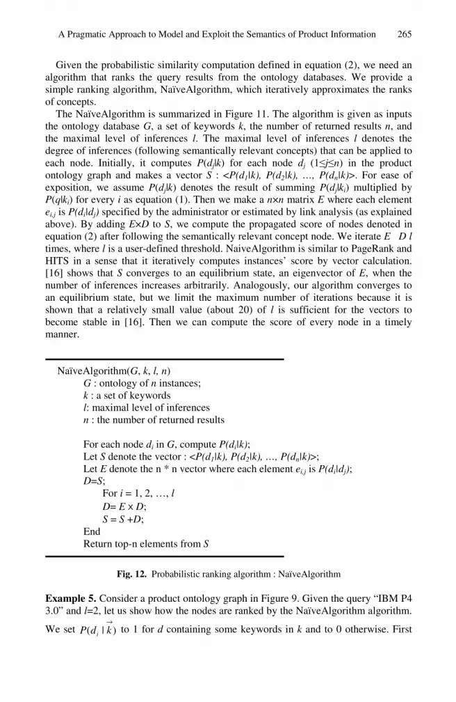
A Pragmatic Approach to Model and Exploit the Semantics of Product Information 265
Given the probabilistic similarity computation defined in equation (2), we need an algorithm that ranks the query results from the ontology databases. We provide a simple ranking algorithm, NaïveAlgorithm, which iteratively approximates the ranks of concepts.
The NaïveAlgorithm is summarized in Figure 11. The algorithm is given as inputs the ontology database G, a set of keywords k, the number of returned results n, and the maximal level of inferences l. The maximal level of inferences l denotes the degree of inferences (following semantically relevant concepts) that can be applied to each node. Initially, it computes P(dj|k) for each node dj (1≤j≤n) in the product ontology graph and makes a vector S : <P(d1|k), P(d2|k), …, P(dn|k)>. For ease of exposition, we assume P(dj|k) denotes the result of summing P(dj|ki) multiplied by P(q|ki) for every i as equation (1). Then we make a n×n matrix E where each element ei,j is P(di|dj) specified by the administrator or estimated by link analysis (as explained above). By adding E×D to S, we compute the propagated score of nodes denoted in equation (2) after following the semantically relevant concept node. We iterate E�D l times, where l is a user-defined threshold. NaiveAlgorithm is similar to PageRank and HITS in a sense that it iteratively computes instances’ score by vector calculation. [16] shows that S converges to an equilibrium state, an eigenvector of E, when the number of inferences increases arbitrarily. Analogously, our algorithm converges to an equilibrium state, but we limit the maximum number of iterations because it is shown that a relatively small value (about 20) of l is sufficient for the vectors to become stable in [16]. Then we can compute the score of every node in a timely manner.
NaïveAlgorithm(G, k, l, n)
G : ontology of n instances; k : a set of keywords l: maximal level of inferences n : the number of returned results For each node di in G, compute P(di|k);
Let S denote the vector : <P(d1|k), P(d2|k), …, P(dn|k)>; Let E denote the n * n vector where each element ei,j is P(di|dj); D=S;
For i = 1, 2, …, l D= EⅹD; S = S +D; End Return top-n elements from S
Fig. 12. Probabilistic ranking algorithm : NaïveAlgorithm
Example 5. Consider a product ontology graph in Figure 9. Given the query “IBM P4 3.0” and l=2, let us show how the nodes are ranked by the NaïveAlgorithm algorithm.
We set )|(→kdP i
to 1 for d containing some keywords in k and to 0 otherwise. First

266 T. Lee et al.
we sort the nodes according to the subscription above each node and make the score
vector S. After calculating )|(→kdP i
for each node we get <0, 0, 0, 1, 0, 1, 1, 0, 1>.
We assume that ),|( ij krdP→
is din, r/din for instance relationships and 1 for the other
relationships. Then we make the matrix E.
⎥⎥⎥⎥⎥⎥⎥⎥⎥⎥⎥⎥
⎦
⎤
⎢⎢⎢⎢⎢⎢⎢⎢⎢⎢⎢⎢
⎣
⎡
=
000100100
000010100
000001100
100000010
010000001
001000001
313131000000
000100000
00002121000
E
By EⅹS, we get D,
⎥⎥⎥⎥⎥⎥⎥⎥⎥⎥⎥⎥
⎦
⎤
⎢⎢⎢⎢⎢⎢⎢⎢⎢⎢⎢⎢
⎣
⎡
=
⎥⎥⎥⎥⎥⎥⎥⎥⎥⎥⎥⎥
⎦
⎤
⎢⎢⎢⎢⎢⎢⎢⎢⎢⎢⎢⎢
⎣
⎡
×
⎥⎥⎥⎥⎥⎥⎥⎥⎥⎥⎥⎥
⎦
⎤
⎢⎢⎢⎢⎢⎢⎢⎢⎢⎢⎢⎢
⎣
⎡
=
1
0
1
1
0
1
32
1
21
1
0
1
1
0
1
0
0
0
000100100
000010100
000001100
100000010
010000001
001000001
313131000000
000100000
00002121000
D
, and S=
⎥⎥⎥⎥⎥⎥⎥⎥⎥⎥⎥⎥
⎦
⎤
⎢⎢⎢⎢⎢⎢⎢⎢⎢⎢⎢⎢
⎣
⎡
2
0
2
2
0
2
32
1
21
.
By EⅹD again we get D=[1/2 1 2/3 3/2 1/2 2 5/3 2/3 5/3]T and S=[1 2 4/3 7/2 1/2 4
11/3 2/3 11/3] T. Overall ranking should be <6, 7, 9, 4, 2, 3, 1, 8, 5> represented by node numbers. The most relevant product is “IBM G41” represented by node 6. If our intention was to find product classes, the algorithm would return Notebook Computers as illustrated in Example 1.

Author Index
An, Yuan 1
Badr, Youakim 196Borgida, Alex 1
Chbeir, Richard 196
Dobbie, Gillian 219
Fankhauser, Peter 136
Kifer, Michael 79Kirchberg, Markus 165
Lee, Hyunja 242Lee, Juhnyoung 57Lee, Sang-goo 242Lee, Taehee 242Lehti, Patrick 136Li, Yuan Fang 219
Ma, Li 57Mylopoulos, John 1
Pan, Yue 57
Qiu, ZhaoMing 57Queralt, Anna 33
Riaz-ud-Din, Faizal 165
Schewe, Klaus-Dieter 165Shim, Junho 242Sun, Jing 219Sun, Jun 219
Teniente, Ernest 33Tretiakov, Alexei 165
Wang, Hai H. 219
Xie, Guotong 57
Yang, Guizhen 79Yang, Yang 57


