Model checking with bounded context switching

Accepted for publication July 2010 in Formal Aspects of Computing

Model Checking with BoundedContext SwitchingGerard J. Holzmann1 and Mihai Florian2

1Jet Propulsion Laboratory,

California Institute of Technology, Pasadena, CA, USA2Computer Science Department,

California Institute of Technology, Pasadena, CA, USA

Abstract. We discuss the implementation of a bounded context switching algorithm in the Spin modelchecker. The algorithm allows us to find counter-examples that are often simpler to understand, and thatmay be more likely to occur in practice. We discuss extensions of the algorithm that allow us to use thisnew algorithm in combination with most other search modes supported in Spin, including partial orderreduction and bitstate hashing. We show that, other than often assumed, the enforcement of a boundedcontext switching discipline does not decrease but increases the complexity of the model checking procedure.We discuss the performance of the algorithm on a range of applications.

Keywords: Logic model checking, depth-first search, bounded context-switching, partial order reduction,bitstate hashing, software verification.

1. Introduction

It takes only one counter-example to a correctness property to disprove its validity for a given system. Modelcheckers can excel in finding such counter-examples in large search spaces, but the first counter-examplethey locate is not necessarily also the simplest. When depth-first search is used, counter-examples are oftenlonger than necessary, and they can correspond to system executions that are more complex than necessary.Short error sequences can be found with a breadth-first discipline, but even the shortest possible counter-example is not necessarily also the simplest to understand, e.g., if it contains more context switches thanstrictly necessary to reproduce the error. A breadth-first search, furthermore, tends to increase the memoryrequirements for a search and cannot easily be used for the verification of anything other than basic safetyproperties.

In [QW04] a different type of search method was proposed, based on bounding the number of contextswitches (process preemptions) that can appear in an execution. The idea was first applied to static sourcecode analysis, but later extended also for use in software testing, and in model checking, e.g., [MQ07b].

Correspondence and offprint requests to: Gerard J. Holzmann, Jet Propulsion Laboratory, 4800 Oak Grove Drive M/S 301-230,Pasadena, CA 91109, USA. e-mail: [email protected]

2 G.J. Holzmann and M. Florian

1 Search(s)2 if s violates P3 report_error4 S = S ∪ s // add s to statespace S5 for all successors s’ of s6 if s’ not in S7 Search(s’)

Fig. 1. Standard depth-first search.

1 Search(s)2 if s violates P3 report_error4 S = S ∪ s // add s to statespace S5 for all successors s’ of s6 if s’ not in S /\ CS(s’) <= N7 Search(s’)

Fig. 2. Bounded context switching, cf. [MQ07b].

As noted in [MQ07b], even relatively low bounds on the number of context switches suffice for a modelchecker to visit all the reachable states of a model at least once. But as we will show in this paper, withcontext bounding for the verification of even simple safety properties it no longer suffices to visit eachreachable state just once. In the worst case, the number of required visits to each state can be as high asN*P, where P is the number of threads or processes in the system being analyzed and N is the bound thatis imposed on the number of context switches. This is caused by the fact that a context-bounded searchevaluates execution paths, and not just states. In a context-bounded search it can make a difference how astate is reached.

In this paper we report on the implementation of a bounded context switching algorithm in the Spinmodel checker [H04]. The algorithm can be invoked by compiling the model checking source (pan.c) with anew directive called -DBCS. The user can define a context switching bound with a new runtime parameter-Ln, where n is the bound. The default bound, when no explicit bound is defined with this parameter, iszero.

In Section 2 we discuss the basic implementation of this algorithm without the use of partial orderreduction. In Section 3 we discuss several extensions of the basic algorithm. Section 3.1 discusses an extensionto deal with cyclic executions; Section 3.2 describes an adaptation to support Spin’s bitstate hashing method,and Section 3.3 discusses the integration of the new algorithm with Spin’s partial order reduction method.Section 4 includes performance measurements. Section 5 discusses related work, and Section 6 concludes thepaper.

2. The basic algorithm

The standard depth-first search, illustrated in Figure 1, explores all successor states of a given state s,and checks whether they were visited before. Every successor state that was not visited before is then alsoexplored. This procedure repeats, recursively, until all reachable states are found. In Figure 1 we use Sto denote the statespace: the set of all visited states, which is initially empty. The search starts with thecall Search(s0), where s0 is the initial system state. If the set of reachable states is finite, the search willterminate. The algorithm in Figure 1 suffices for the verification of safety properties for finite state systems.The extension for the verification of liveness properties is well understood and not elaborated here [HPY96].

In bounded context switching, every context switch is counted towards a user-defined maximum. A high-level description of this algorithm is given in Figure 2. In this version of the depth-first search, successor states’ of state s must satisfy one additional condition, other than not having been visited before: the number ofcontext switches CS(s’) at s’ is at most equal to bound N.

Although Figure 2 shows the essence of the algorithm, it leaves out important details. One such detailis that forced context switches (so-called non-preemptive context switches) are not counted towards the

Bounded Context Switching 3

bound [MQ07b]. A context switch is considered forced if the currently executing process blocks and executionwould come to a halt if no context switch was performed.

The algorithm in Figure 2 also has a more important flaw: it cannot guarantee a critical property:

• P1 : If the algorithm in Figure 2 terminates with bound N without reporting an error, then no violationsexist for any execution with N or fewer context switches.

The property fails for a simple reason. When a state is revisited with a number of context switches that islower than the number seen on the earlier visits, then execution does not continue. It is of course possiblethat a counter-example can be constructed within bound N if the search were continued in this case.

The situation is similar to that of a depth-bounded search, as implemented in Spin with the -DREACHsearch option [H04]. Unless we store the depth at which a state is reached in the statespace S, and continuethe search whenever a state is revisited via a shorter path than before, the search risks being incomplete.Only the lowest depth at which a state is reached is stored in the statespace jointly with each state. Clearly,this means that states can be revisited many times (up to the search bound imposed).

For a context-bounded search we must similarly record the lowest number of context switches seen whenreaching each state, and again we will have to continue the search if a state is reached with a lower numberthan recorded before. Also here, then, both the space and especially the time requirements for the searchcan increase. Even with this increase, though, the complexity of the statefull search remains significantlybetter than a stateless search, with or without context bounding. In a stateless search, as for instance used instandard testing or random walks, the number of times that states can be revisited could become quadraticin the number of reachable states. (Because no states are recorded outside the search stack, the search couldin the worst case end up revisiting all reachable states for each state visited.)

The bounded context switching algorithm that we implemented has the following properties.

1. At the initial system state, all successor states are explored the same as in a standard depth-first search.2. At all other states, the model checker first tries to continue the same process that executed in the previous

execution step, thus avoiding a context switch. We distinguish two main cases.

(a) The selected process is not executable and blocks. The model checker will now expand its searchby accepting successor states from all processes. The resulting context switch is considered forced(non-preemptive) and is not counted towards the bound.

(b) The selected process does not block and the sub-tree of the successor state is explored. A preemptivecontext switch can be performed if the user-defined bound on the number of unforced context switcheshas not yet been reached. If other processes can contribute successor states, the number of contextswitches performed is now incremented for each such successor state generated in this way. We nowdistinguish four separate cases.

i The successor state that is reached was not visited before (i.e., it does not appear in S ). In thiscase, the successors of the new state are explored. We store the state jointly with the number ofcontext switches that was needed to reach it.

ii The successor state was reached before, with a number of context switches N that is smaller thanthe number M used in the current execution path, i.e. with N < M . In this case, the new path isnot better than at least one previous path, and therefore we need not explore it again.

iii The successor state was reached before, but with N > M . The current path is better, so we mustexplore it again. We store the new lower number M with the state, replacing the previous valueN.

iv The successor state was reached before with N = M . We distinguish two cases.

A We reached the successor state via a transition that belongs to the same process as the transi-tion that was executed on the earlier visit with the lowest number of context switches recordedso far. In this case we cannot discover any new paths and we need not explore the state again.

B We reached the successor state via a transition that belongs to a different process than for theearlier visit. In this case we may discover new paths. Note that it would take one extra contextswitch for the earlier path to switch to the current process, which means that we have reachedthis point with one fewer required context switches.


1 Search (s,n,p)23 Let A be the set of transitions enabled in s4 Let A’ be the subset of A of transitions with pid p5 Let A’’ be A - A’6 Let a(s) be the successor state of s after executing transition a7 Let pid(a) be the pid associated with transition a89 for the initial state, let A’ be empty1011 if s violates P12 report_error1314 S = S ∪ {(s,n,p)} // add extended state s to statespace S1516 for all a in A’ do17 { if CONSTRAINT(a(s),n,pid(a))18 { Search(a(s),n,pid(a))19 } }2021 if A’ ≡ ∅22 { u = 0 // do not count context switch23 } else24 { u = 1 // count context switch25 }2627 for all a in A’’ do28 { if CONSTRAINT(a(s),n+u,pid(a))29 { Search (a(s),n+u,pid(a))30 } }

Fig. 3. Spin implementation of bounded context switching.

We can now more clearly see the reason why a bounded context switching algorithm can require us tovisit the same state multiple times, if we reach the state via an execution path with a smaller number ofcontext switches than on all previous visits. In the worst case, if our context bound is N and the number ofexecuting processes is P , we may visit a state up to N ∗ P times. Note that with a BCS algorithm it is notonly important which states we reach but also how we reach them. It is, of course, not necessary to store anystate more than once, but a small amount of additional information is required. Minimally this additionalinformation includes not only the lowest number of context switches that was needed to reach the state butalso the id’s of all processes that contributed the last step leading to the state (see iv.A and iv.B above).

The new algorithm for a model checking procedure based on bounded context switching, as implementedin Spin is illustrated in Figure 3. The definition of CONSTRAINT(s,b,id), used on lines 16 and 26 in Figure 3,is as follows:

(b ≤ BOUND) ∧ (∀x∀y(s, x, y) ∈ S ⇒ (x > b ∨ (x = b ∧ y 6= id)))

In the actual implementation we can reduce the memory requirements by not storing each triple of a state, acontext bound, and a vector of pid numbers separately, but instead storing the state (the largest part of thedata) just once in combination with the minimum context bound seen so far and the corresponding vectorof pid numbers.

To see why the algorithm in Figure 3 satisfies property P1, consider an execution with N unforced contextswitches that leads to an error. The first step of the error sequence is necessarily explored by Figure 3, becauseit considers all process actions in this step. The algorithm in Figure 3 can only fail to explore the full errorpath if its search truncates on a previously visited state. For the successor state to be ignored, one of thetwo following cases must apply:


2b-ii : the number of context switches on the previous visit was smaller than the number on the currentpath, or

2b-iv-1 : the number of context switches is the same in the earlier execution as in the new one, and thesame process currently executing has produced at least one of the earlier visits.In both cases, if the error path was not found on the earlier visit, it cannot be found on the new path either,since the new path either has a tighter or an identical constraint. A proof for a property equivalent to P1 isgiven in Appendix A.

3. Extensions

In this section we discuss some extensions of the basic algorithm that we have made in the version that wasimplemented in the Spin model checker (version 5.2.3 and later). For simplicity, these extensions are notshown in the basic version of the algorithm discussed so far.

3.1. Dealing with cycles

Consider the case where A′ (line 4 in Figure 3) is non-empty, but all successor states explored (line 16)match previously visited states that are on the depth-first search stack. i.e., the recursive call to Search online 18 is never made. In the algorithm as shown in Figure 3, a context switch to a different process wouldcount towards the bound (line 24).

In this case, though, the execution scenario explored, with the process selected under the rules for boundedcontext switching caught in an infinite loop, would be at odds with a basic fairness assumption that can bemade about process scheduling.

In our implementation of bounded context switching we therefore do not count a context switch in thisstate (not shown in Figure 3). The same change is also needed for the integration with partial order reductionrules, to avoid cyclic deferral (known as the ignoring problem in partial order reduction theory), as discussedin Section 3.3.

3.2. Integration with bitstate hashing

Bitstate hashing was introduced in 1987 as a method to handle the large state space sizes that are oftenencountered in applications of logic model checking, using very high compression ratios on state storage [H87,H98]. The method trades a small probability of incompleteness of the search for a significant increase inproblem coverage for large problem sizes. The method is used as a search option in most of the currentlyused logic model checking tools.

In brief, the bitstate hashing algorithm, comparable to a Bloom filter [B70], uses the fact that we canachieve high compression rates by treating the hash key as a bit-address in a large memory arena. If astate is reached, the bit at the address pointed to by the hash-key (taken modulo the bit-address range ofthe memory arena) is set to one. By checking for the state of the bit, the algorithm checks for previouslyvisited states. If the number of bits is large compared to the number of states reached, the probability of ahash-collision will be small. In cases where hash-collisions do occur, the search risks becoming incomplete.The model checker retains its ability, though, to find counter-examples in the part of the state space thatis searched. The probability of incompleteness depends on the ratio of the number of available bit-positionsand the number of reachable states, and can be computed [H98]. The Spin model checker uses multipleindependent hash-functions (and multiple bit-positions per state) to reduce the effect of hash collisions.

In bitstate mode, the smallest number of context switches seen so far along an execution path and thevector of pid numbers cannot be stored separately from the state, since only a minimal hash fingerprint isstored in the bitstate hash-array. To support the new search mode in bitstate explorations, it therefore needsto be modified.

In bitstate mode, when a new state is added to the statespace S, we store separate copies for both thecurrent and all higher numbers of context switches, up to the bound. We will refer to this as the replicatedstorage method. Using this method, we can avoid unnecessary revisits of the state with a higher numberof context switches than before: they will produce matches of the bitstate hashes. The vector of process id


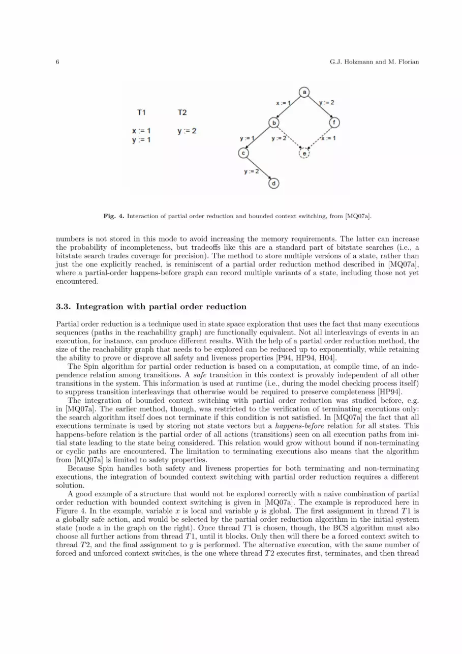
Fig. 4. Interaction of partial order reduction and bounded context switching, from [MQ07a].

numbers is not stored in this mode to avoid increasing the memory requirements. The latter can increasethe probability of incompleteness, but tradeoffs like this are a standard part of bitstate searches (i.e., abitstate search trades coverage for precision). The method to store multiple versions of a state, rather thanjust the one explicitly reached, is reminiscent of a partial order reduction method described in [MQ07a],where a partial-order happens-before graph can record multiple variants of a state, including those not yetencountered.

3.3. Integration with partial order reduction

Partial order reduction is a technique used in state space exploration that uses the fact that many executionssequences (paths in the reachability graph) are functionally equivalent. Not all interleavings of events in anexecution, for instance, can produce different results. With the help of a partial order reduction method, thesize of the reachability graph that needs to be explored can be reduced up to exponentially, while retainingthe ability to prove or disprove all safety and liveness properties [P94, HP94, H04].

The Spin algorithm for partial order reduction is based on a computation, at compile time, of an inde-pendence relation among transitions. A safe transition in this context is provably independent of all othertransitions in the system. This information is used at runtime (i.e., during the model checking process itself)to suppress transition interleavings that otherwise would be required to preserve completeness [HP94].

The integration of bounded context switching with partial order reduction was studied before, e.g.in [MQ07a]. The earlier method, though, was restricted to the verification of terminating executions only:the search algorithm itself does not terminate if this condition is not satisfied. In [MQ07a] the fact that allexecutions terminate is used by storing not state vectors but a happens-before relation for all states. Thishappens-before relation is the partial order of all actions (transitions) seen on all execution paths from ini-tial state leading to the state being considered. This relation would grow without bound if non-terminatingor cyclic paths are encountered. The limitation to terminating executions also means that the algorithmfrom [MQ07a] is limited to safety properties.

Because Spin handles both safety and liveness properties for both terminating and non-terminatingexecutions, the integration of bounded context switching with partial order reduction requires a differentsolution.

A good example of a structure that would not be explored correctly with a naive combination of partialorder reduction with bounded context switching is given in [MQ07a]. The example is reproduced here inFigure 4. In the example, variable x is local and variable y is global. The first assignment in thread T1 isa globally safe action, and would be selected by the partial order reduction algorithm in the initial systemstate (node a in the graph on the right). Once thread T1 is chosen, though, the BCS algorithm must alsochoose all further actions from thread T1, until it blocks. Only then will there be a forced context switch tothread T2, and the final assignment to y is performed. The alternative execution, with the same number offorced and unforced context switches, is the one where thread T2 executes first, terminates, and then thread


T1 executes both its statements. The complete sequence of transitions from node a to f to e and ending ina new node g is not shown in Figure 4.

The end-state (i.e., the final value of variable y) is different in these two executions, and therefore thisversion of the algorithm fails to explore all distinct sequences with the same context switching bound andwould remain incomplete.

If we directly combine the BCS algorithm with Spin’s partial order reduction rules, the same scenariowould be possible. We therefore extend the algorithm as follows.

• First, consider a point in the execution where a partial order transition is available. Ignoring it wouldcontinue the BCS search unmodified and preserve all its properties, but it would not take advantage ofpartial order reduction.

• Next, consider the case where a partial order transition from a given process P is selected, and all tran-sitions from other processes are ignored. If the execution of this transition does not require a contextswitch (i.e., process P was selected also in the previous step), then the extended algorithm is indistin-guishable from the original and it will have the same properties. If, however, a context switch is requiredto make the partial order selection, we should count it as such. This means that the selection shouldnot be allowed if the maximum number of context switches was already reached in the current executionpath. This alone, though, does not suffice.

• The context switch that is performed in this case is a restricted one, since not all executable processescan contribute transitions. By partial order reduction theory we know that executing the partial ordertransition itself is safe and as far as the correctness properties of the system are concerned is invisible toall other processes. If after the partial order transition we switch back to the process that was executingunder BCS rules before, the completeness of the search would again be preserved. We can allow for thatadditional context switch by giving a ”credit” to the number of context switches that may be made inthe remainder of the execution. The credit to be issued must be for two additional context switches. Afirst credit is needed to switch the current execution back to the originally executing process, after the(sequence of) partial order reduction transition(s) completes, and a second credit is needed to correct forthe fact that the disappearance of the safe transition from a later point in the execution (where the BCSalgorithm would normally have executed it) to the earlier point may also require an additional unforcedcontext switch.

– Consider the case where the execution that would be explored by the regular BCS algorithm consistsof the transition sequence pn,qs,qn, where pn is a non-partial order transition from process p, qs isa partial order transition and qn a non-partial order transition from a different process q. Assumefurther that the last transition executed was a transition from process p.

– The partial order reduction rules will select qs to be executed before pn at this point, where the BCSalgorithm would have selected pn. That is, using partial order reduction rules will change the transitionsequence to: qs,pn,qn. The original sequence pn,qs,qn requires just one context switch (from p to qin the second step). The partial order sequence, however, requires two additional context switches,for a total of three: one from process p to q in the first step, another from q back to p after the firststep, and a third from p to q after the second step, before the original execution context is restored.It is easy to see that the cost of the out-of-sequence execution of a partial order transition cannot belarger than two additional context switches.

Issuing the two credits for a partial order transition is conservative since it allows the search engine notonly to switch back to the original BCS processes that would have been selected without the out of orderexecution of the partial order transition, but it also allows other processes to be selected.

• The credit mechanism can be implemented by not counting context switches for partial order transitionsbefore or after they are selected. The restriction that must be maintained, though, is that a partial ordertransition can only be considered in states where the context bound has not yet been reached (i.e., itmust be possible to do a context switch, even if it is not counted).

• We also have to consider the issue of cyclic deferral (briefly also discussion in Section 3.1). If a partialorder transition is selected and it leads to a successor state on the depth-first search stack, this can createan infinite deferral of non-partial order transitions that are enabled throughout the cycle. In partial orderreduction theory this is a well-known issue called the ignoring problem. A search performed with partialorder reduction but without bounded context switching takes this into account by forcing a full expansion


1 Search (s,n,p,safe)23 Let A be the set of transitions enabled in s4 Let A’ be the subset of A of transitions with pid p5 Let A’’ be A - A’6 Let A* be a safe subset of A (the ample set), or A if no safe subset exists7 Let a(s) be the successor state of s after executing transition a8 Let pid(a) be the pid associated with transition a910 for the initial state, let A’ be empty and A* be A1112 if s violates P13 report_error1415 S = S ∪ {(s,n,p,safe)} // add extended state s to statespace S16 push(Q,s) // push s onto stack Q1718 if A* 6= A ∧ ∃a, a∈A*: a(s) ∈ Q19 { cycle = true20 A* = ∅21 } else22 { cycle = false23 }24 if A* 6= A ∧ n < BOUND25 { for all a in A* do26 { if CONSTRAINT(a(s),n,pid(a),true)27 { Search(a(s),n,pid(a),true)28 } }29 } else30 { for all a in A’ do31 { if CONSTRAINT(a(s),n,pid(a),false)32 { Search(a(s),n,pid(a),false)33 } }3435 if A’ ≡ ∅ ∨ safe ≡ true ∨ cycle ≡ true36 { u = 0 // do not count context switch37 } else38 { u = 1 // count context switch39 }4041 for all a in A’’ do42 { if CONSTRAINT(a(s),n+u,pid(a),false)43 { Search (a(s),n+u,pid(a),false)44 } } }45 pop(Q) // pop s from stack Q

Fig. 5. Combination of bounded context switching with partial order reduction.

of all successor states when a state is encountered that has no successors outside the depth-first searchstack. We use the same rule in our implementation of the bounded context switching algorithm, and wetreat it as a forced context switch, similar to the case where an executing thread blocks (i.e., the switchis not counted against the context bound).

The extended version of the algorithm is shown in Figure 5. This version of the algorithm can be shown topreserve all the properties of the simpler context bounded search algorithm, shown in Figure 3. A proof forthis property can be found in Appendix B.


0

1

2

3

4

5

t2

t1

t1

t1

t1

t1

t1

t1

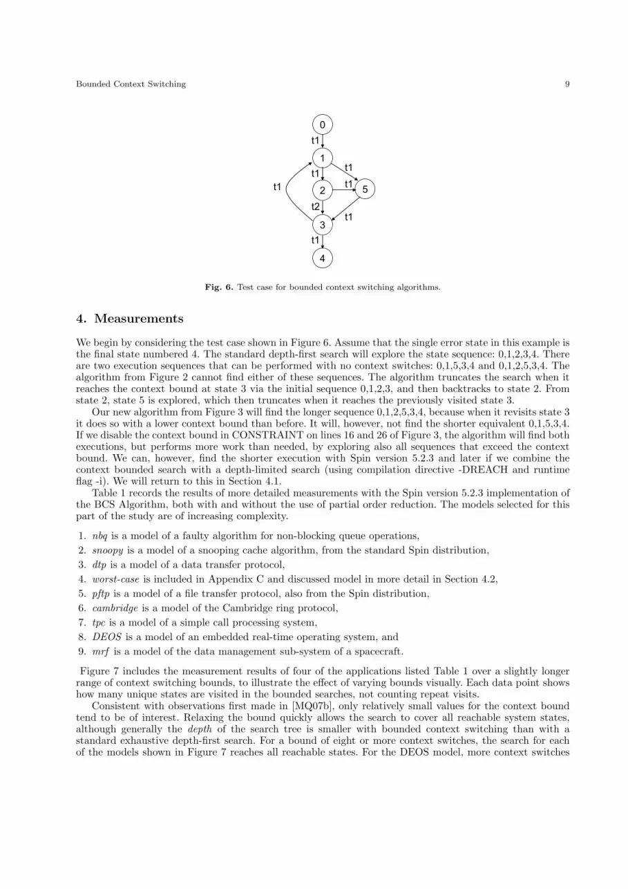
Fig. 6. Test case for bounded context switching algorithms.

4. Measurements

We begin by considering the test case shown in Figure 6. Assume that the single error state in this example isthe final state numbered 4. The standard depth-first search will explore the state sequence: 0,1,2,3,4. Thereare two execution sequences that can be performed with no context switches: 0,1,5,3,4 and 0,1,2,5,3,4. Thealgorithm from Figure 2 cannot find either of these sequences. The algorithm truncates the search when itreaches the context bound at state 3 via the initial sequence 0,1,2,3, and then backtracks to state 2. Fromstate 2, state 5 is explored, which then truncates when it reaches the previously visited state 3.

Our new algorithm from Figure 3 will find the longer sequence 0,1,2,5,3,4, because when it revisits state 3it does so with a lower context bound than before. It will, however, not find the shorter equivalent 0,1,5,3,4.If we disable the context bound in CONSTRAINT on lines 16 and 26 of Figure 3, the algorithm will find bothexecutions, but performs more work than needed, by exploring also all sequences that exceed the contextbound. We can, however, find the shorter execution with Spin version 5.2.3 and later if we combine thecontext bounded search with a depth-limited search (using compilation directive -DREACH and runtimeflag -i). We will return to this in Section 4.1.

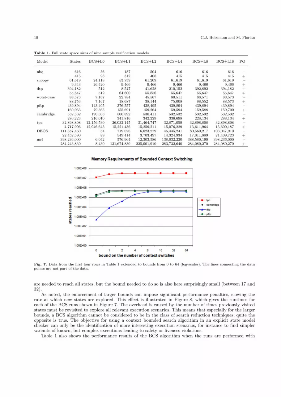
Table 1 records the results of more detailed measurements with the Spin version 5.2.3 implementation ofthe BCS Algorithm, both with and without the use of partial order reduction. The models selected for thispart of the study are of increasing complexity.

1. nbq is a model of a faulty algorithm for non-blocking queue operations,2. snoopy is a model of a snooping cache algorithm, from the standard Spin distribution,3. dtp is a model of a data transfer protocol,4. worst-case is included in Appendix C and discussed model in more detail in Section 4.2,5. pftp is a model of a file transfer protocol, also from the Spin distribution,6. cambridge is a model of the Cambridge ring protocol,7. tpc is a model of a simple call processing system,8. DEOS is a model of an embedded real-time operating system, and9. mrf is a model of the data management sub-system of a spacecraft.

Figure 7 includes the measurement results of four of the applications listed Table 1 over a slightly longerrange of context switching bounds, to illustrate the effect of varying bounds visually. Each data point showshow many unique states are visited in the bounded searches, not counting repeat visits.

Consistent with observations first made in [MQ07b], only relatively small values for the context boundtend to be of interest. Relaxing the bound quickly allows the search to cover all reachable system states,although generally the depth of the search tree is smaller with bounded context switching than with astandard exhaustive depth-first search. For a bound of eight or more context switches, the search for eachof the models shown in Figure 7 reaches all reachable states. For the DEOS model, more context switches


Table 1. Full state space sizes of nine sample verification models.

Model States BCS+L0 BCS+L1 BCS+L2 BCS+L4 BCS+L8 BCS+L16 PO

nbq 616 56 187 504 616 616 616 –415 98 312 408 415 415 415 +

snoopy 61,619 24,118 53,739 61,209 61,619 61,619 61,619 –9,343 26,420 9,466 9,466 9,466 9,466 9,466 +

dtp 394,182 512 8,547 41,628 210,152 392,892 394,182 –55,647 512 64,600 55,856 55,647 55,647 55,647 +

worst-case 88,573 7,167 22,784 45,567 80,511 88,571 88,573 –88,753 7,167 18,687 38,144 75,008 88,552 88,573 +

pftp 439,894 143,405 376,557 438,495 439,894 439,894 439,894 –160,033 79,365 155,691 159,264 159,594 159,588 159,700 +

cambridge 532,532 190,503 506,892 530,411 532,532 532,532 532,532 –286,223 216,010 341,816 342,229 336,698 228,134 288,134 +

tpc 32,898,808 12,156,530 26,032,145 31,464,747 32,871,059 32,898,808 32,898,808 –4,717,906 12,946,643 15,221,436 15,259,211 15,076,229 13,611,964 13,600,187 +

DEOS 111,587,460 54 719,626 6,023,279 45,445,241 80,560,217 103,047,910 –22,452,390 89 549,414 3,703,497 14,324,934 17,011,889 21,409,723 +

mrf 398,236,000 6,042 576,964 12,303,586 138,032,220 388,580,190 398,236,000 –284,243,830 8,430 131,674,830 225,001,910 283,732,640 284,080,270 284,080,270 +

Fig. 7. Data from the first four rows in Table 1 extended to bounds from 0 to 64 (log-scales). The lines connecting the datapoints are not part of the data.

are needed to reach all states, but the bound needed to do so is also here surprisingly small (between 17 and32).

As noted, the enforcement of larger bounds can impose significant performance penalties, slowing therate at which new states are explored. This effect is illustrated in Figure 8, which gives the runtimes foreach of the BCS runs shown in Figure 7. The overhead is caused by the number of times previously visitedstates must be revisited to explore all relevant execution scenarios. This means that especially for the largerbounds, a BCS algorithm cannot be considered to be in the class of search reduction techniques; quite theopposite is true. The objective for using a context bounded search algorithm in an explicit state modelchecker can only be the identification of more interesting execution scenarios, for instance to find simplervariants of known, but complex executions leading to safety or liveness violations.

Table 1 also shows the performance results of the BCS algorithm when the runs are performed with


Fig. 8. Runtime requirements of BCS for bounds from 0 to 64 (log-scales).

Fig. 9. Effect of partial order reduction on bounded context switching.

partial order reduction enabled. Figure 9 illustrates the difference between the two sets of runs for the largeDEOS model.

The number of distinct states reached with a bound of zero is small both with and without partial orderreduction enabled. The numbers gradually increase to match the size of a full search, which is again reachedsurprisingly quickly. Note that partial order reduction rules in combination with BCS can lead to differentstate space sizes than when the search is performed without BCS, even at larger bounds. The number ofunique states reached with a bound of 32 and partial order reduction enabled, therefore, is not necessarilysmaller than or equal to that of a full search without BCS.

The length of an execution is generally smaller when BCS rules are enforced than without those rules.It is not necessarily reduced further when partial order reduction is used as well. The maximum depth ofthe search tree for a standard search for the DEOS model, for instance, is 522,724 steps without partialorder reduction and 177,911 steps with partial order reduction. With BCS enabled and a bound of 32, the


maximum search depth drops to 68,420 steps without partial order reduction and to 69,760 with partialorder reduction.

The time required to explore the DEOS model without partial order reduction and without contextbounding is 376 seconds, corresponding to an effective exploration rate of 296,672 new states per second.The time required for the same run performed with bounded context switching enabled and a bound of32 preemptions is 8,090 seconds, which corresponds to a much lower effective exploration rate of 13,797new states per second. Both searches visit the same number of unique states, but the context boundedsearch revisits each state on average twenty times in this example, to explore all relevant paths, significantlyaffecting overall performance.

The time penalties are smaller in bitstate mode. Again without partial order reduction enabled, a ver-ification of the DEOS model with a context bound of 32 takes 691 seconds in bitstate mode, and explores82,149,957 unique states. The same bitstate run without context bounding takes only 346 seconds and visitsa larger number of 111,587,020 unique states. We used a bitstate array of 2 GB for both these runs. Notethat in bitstate mode we enter each state multiple times. With a bound of N , each state may be entered intothe bitstate array up to N times, which reduces the capacity of the bitstate hash arena and hence reduceseffective coverage.

4.1. Time and memory

The time that is required to perform a verification with Spin is closely correlated with the number oftransitions that are explored in the depth-first search of the (partial order reduced) reachability graph, andthe memory requirements are correlated with the number of states that are explored. As we have noted, thenumber of reachable states explored can be less than what a standard search (without the use of boundedcontext switching) would explore, but only for relatively small values of the bound. When at least five or sixcontext switches are allowed, generally all reachable states will be explored. When bounded context switchingis used, the number of transitions (which depends on the number of visits and revisits to reachable states)increases close to exponentially with increases of the bound. The maximum search depth reached can beexpected to approximate that of a standard search more closely with each increase of the bound.

These effects can be seen clearly in Figure 10, where we performed measurements over a benchmark setof 171 different verification models. All models in this set had at least 200,000 reachable states. The keycharacteristics reported here were averaged over all models to give a clear indication of the dominant trends.

Based on these measurements, the conclusion seems justified that the use of bounded context switchingis only advisable when the bound imposed is relatively small. For larger bounds, the time requirementsof a model checking run can quickly become prohibitive. The relative improvement in the quality of errorsequences generated is relatively minor in these cases.

4.2. Length of error sequences

We have done additional measurements with those applications from Table 1 that contain safety or livenessviolations, to study how the quality of the error sequences that are generated by the bounded contextswitching algorithm compares with that of standard depth-first and breadth-first searches.

The worst-case model, shown in Appendix C, is a deliberate attempt to create a model that exhibitsworst-case behavior when bounded context switching is used. The model is constructed in such a way thatall active processes must take one step for an assertion violation to occur. We have used a version with tenprocesses, which means that at least nine unforced context switches are required for a counter-example tobe possible.

The mrf model contains a liveness violation (the violation of a property expressed in linear-time temporallogic), which can only be found with the depth-first search. The remaining models contain safety violationsthat can be found with either a breadth-first or a depth-first search.

Table 2 lists the number of unique states that are explored by each algorithm up to the point wherethe first error is discovered and the error trail is written. Table 3 lists the number of transitions that areexplored up to the same point in the execution. In all cases, finding the first counter-example takes only afraction of a second. For the worst-case example, as expected, no error sequence is possible unless at least


Fig. 10. Relative performance of bounded context switching, using partial order reduction.

Table 2. Number of unique states explored upto the first counter-example.

Model BFS DFS BCS+L0 BCS+L1 BCS+L2 BCS+L4 BCS+L8 BCS+L16 PO

snoopy 5,346 3,591 1,354 1,352 1,501 1,015 1,236 1,236 –– 1,249 916 560 560 560 560 560 +

tpc 2,497 190 243 249 249 249 249 249 –– 93 243 198 198 198 198 198 +

nbq 385 437 56 41 41 41 41 41 –– 333 41 225 293 293 293 293 +

mrf n/a 6,330 – 1,309 1,745 1,848 1,848 1,848 –n/a 5,140 – 1,381 1,587 1,602 1,602 1,602 +

worst-case 33,598 59,058 – – – – – 59,058 –– 49,224 – – – – – 49,224 +

nine context switches are allowed. For the other applications the number of states reached, or the length ofthe counter-example generated, does not change much for context-bounds larger than one.

For the purpose of the current study, the quality of a counter-example is correlated not with its lengthbut with the number of context switches that it contains. Clearly, the shortest counter-example for a safetyviolation can always be generated with a breadth-first search, but that is not necessarily also the best counter-example. A depth-first, on the other hand, will tend to generate longer counter-examples. We are interestedin knowing how much we can improve the quality of the counter-examples generated with a depth-first searchwhen using the bounded context switching algorithms.

Table 4 lists the total number of context switches in each of the counter-examples that was generated withthe different search algorithms. Note that the total number can exceed the bound because it will generallyinclude both forced and unforced context switches. Additionally, when using partial order reduction therecan also be context switches that are related to the enforcement of the partial order reduction rules.

The shortest counter-example for the snoopy protocol is 42 steps long, and contains 17 context switches.The best counter-example found with bounded-context switching and partial order reduction combined is552 steps long and contains 228 context switches. This improves over the quality of the counter-examplefound with a standard depth-first search, with or without partial order reduction, though in this case not


Table 3. Number of transitions explored upto the first counter-example.

Model BFS DFS BCS+L0 BCS+L1 BCS+L2 BCS+L4 BCS+L8 BCS+L16 PO

snoopy 6,576 5,507 1,524 1,522 1,698 1,130 1,403 1,402 –– 1,637 1,054 636 636 636 636 636 +

tpc 3,950 320 261 276 282 282 282 282 –– 99 261 244 244 244 244 244 +

nbq 565 752 57 42 42 42 42 42 –– 454 277 407 417 417 417 417 +

mrf n/a 7,357 – 1,332 2,565 3,066 3,074 3,074 –n/a 5,587 – 1,490 2,027 2,056 2,056 2,056 +

worst-case 147,559 378,941 – – – – – 517,742 –– 291,801 – – – – – 266,645 +

Table 4. Total number of context switches in counter-example.

Model BFS DFS BCS+L0 BCS+L1 BCS+L2 BCS+L4 BCS+L8 BCS+L16 PO/REACH

snoopy 17 1424 414 415 445 326 387 402 –/–– 523 335 228 228 228 228 228 +/–– 17 15 15 15 15 15 15 –/+– 17 15 17 17 17 17 17 +/+

tpc 19 70 67 67 67 67 67 67 –/–– 33 67 109 109 109 109 109 +/–– 20 21 16 16 16 16 16 –/+– 19 21 18 18 18 18 18 +/+

nbq 10 42 – 4 4 4 4 4 –/–– 32 4 6 6 6 6 6 +/–– 8 – 4 4 4 4 4 –/+– 10 4 6 6 6 6 6 +/+

mrf – 310 – 6 6 6 6 6 –/–– 294 – 8 8 8 8 8 +/–– 4 – 4 4 4 4 4 –/+– 5 – 8 8 8 8 8 +/+

worst-case 10 10 – – – – – 10 –/–– 10 – – – – – 10 +/–– 10 – – – – – 10 –/+– 10 – – – – – 10 +/+

impressively so. The situation is different for the nbq, and mrf examples, and even for the worst-case model,where the bounded context switching algorithm succeeds in finding counter-examples with equal (worst-case)or far fewer context switches than both standard depth- and breadth-first search options. Figure 11, finally,shows the information from the first four models in Table 4 visually.

5. Related work

Bounded context switching algorithms were described earlier in [QW04, QR05, MQ07a, MQ07b, MQ08,LR08]. The first algorithms were designed for application in static source code analysis [QW04], and insoftware test systems, and they were often restricted to acyclic terminating executions. The formal modeltargeted in most of the earlier papers is that of pushdown automata.

The integration of a bounded context switching algorithm with partial order reduction methods was firstdiscussed in [MQ07a], but was also restricted to terminating executions. The method discussed in [MQ07a]is based on the storage of a partial-order happens-before relation for visited states, which can only be usedfor strictly terminating (or otherwise depth-bounded) executions only.

In the earlier work, specifically [QW04, MQ07a, MQ07b], it was also demonstrated that relatively small


Fig. 11. Quality of counter-examples generated, cf. Fig 4. The y-axes are log-scales. The label full identifies searches donewithout partial order reduction. The label suffix -i identifies searches performed with Spin’s iterative shortening algorithm,where the model checker is compiled with the additional directive -DREACH and the search is performed with parameter -i.

context bounds often sufficed to expose subtle concurrency related errors. In [QW04] a context bound of twowas found sufficient, in [MQ07a] the largest context bound used was four. In this paper we have studied theeffect of a context bounded search up to a bound of 64, as illustrated in Figures 8 and 9.

In [LR08] it is also suggested that the incremental change in the part of the state space that is covereddecreases with each increase of the bound. In this paper we have measured this phenomenon more preciselyand demonstrated an exponential decrease, as shown in Figures 10 and 9.

The method described in [LR08] is based on a conversion of a context-bounded concurrent program intoa sequential one, which can then be analyzed with a sequential program analysis techniques that supportthe use of for symbolic constants and assume statements. Measurements reported in [LR08] were obtainedwith symbolic, instead of explicit state, model checkers and generally are based on different assumptions(e.g., about the distinction of forced vs unforced context switches, or how statespace sizes are calculated).This means that measurement results are not directly comparable, though qualitatively they are consistentwith the results reported here.

A full implementation of a bounded context switching algorithm in an explicit state model checker,without a restriction to terminating executions, and with full support for partial order reduction and theverification of both safety and liveness properties was not studied before. As we have shown, by removing theassumption of terminating or depth-bounded executions, the problem becomes significantly more complex.

6. Conclusions

We have discussed the implementation of a bounded context switching discipline as an interesting additionalsearch mode in an explicit state model checker. We have also described extensions of the basic algorithmthat allow for an efficient integration of the new search mode with bitstate hashing and with partial orderreduction. We have shown that bounded context switching cannot be considered a reduction method, asit often is, since it effectively increases, instead of reduces, the time requirements of the standard modelchecking algorithms.

Bounded context switching is not trivially compatible with partial order reduction methods. To enforce


partial order reduction methods, the search algorithm can normally select safe transitions for execution,independent of the processes that execute those transitions. In a bounded context switching algorithm, onthe other hand, we normally try to avoid context switches as long as possible. Partial order reduction, though,can be such a powerful search reduction technique that we are interested in finding workable compromiseswith bounded context switching algorithms. We have explored a method that aims to strike a balancebetween avoiding technically redundant states (under partial order reduction rules) and avoiding needlesscontext switches.

We have proven that if our algorithm, used either with or without partial order reduction, fails to find acounter-example with a given context bound, then no such counter-example can exist.

We have shown that the bounded context switching algorithm can indeed generate counter-examplesof a very high quality, if we measure the quality of a counter-example by the number of context switchesthat it contains. With partial order reduction the counter-examples are better than without, and with theaddition of an iterative shortening method that is already part of the Spin model checker, the quality of thecounter-examples is improved even further. The best traces found in this way tend to exceed the quality ofcounter-examples found with a breadth-first search. (The memory requirements for a breadth-first search,though, make that it is rarely a usable alternative for large problem sizes, and it is not an option at all inthe verification of general liveness properties.)

Given some remaining uncertainty of which variant of which algorithm will produce the best possibleresult in any given case, it can be attractive to use the bounded context switching algorithm in combinationwith swarm-verification techniques. Searches for different context bounds can then be performed in parallel,and they can be used in combination with orthogonal alternative search modes, e.g., using reversed processor transition orderings, as explored in [HJG09]. As noted, the algorithm could further also be extended foruse in combination with a breadth-first search discipline.

References

[B70] Bloom, B.H.: Spacetime tradeoffs in hash coding with allowable errors. Comm. of the ACM, Vol. 13, No. 7, pp.422-426.

[HP94] Holzmann, G.J., and Peled, D.: An improvement in formal verification. Proc. 7th Int. Conf. on Formal DescriptionTechniques, Bern, Switzerland, Oct. 1994, Chapman and Hall Publ., pp. 197-211.

[HPY96] Holzmann, G.J., Peled, D., and Yannakakis, M.,: On nested depth first search, Proc. 2nd Spin Workshop, AmericanMathematical Society, 1996, 23–32.

[H87] Holzmann, G.J.: On limits and possibilities of automated protocol analysis, Proc. 6th Int. Conf. on ProtocolSpecification, Testing, and Verification, INWG IFIP, Ed. H. Rudin and C. West, Zurich, Switzerland, June 1987.

[H98] Holzmann, G.J.: An analysis of bitstate hashing, Formal Methods in System Design, Vol. 13, No. 3, pp. 287-305,Kluwer, November 1998.

[H04] Holzmann, G.J.: The Spin Model Checker: Primer and Reference Manual Addison-Wesley, 2004.[HJG09] Holzmann, G.J., Joshi, R., and Groce, A.: Swarm Verification Techniques, To appear in IEEE Trans. on Software

Engineering, 2010.[QW04] Qadeer, S., and Wu, D.: KISS: Keep it Simple and Sequential. Proc. ACM SIGPLAN Conf. Programming Language

Design and Implementation, (PLDI), Washington DC, 14–24 (June 2004).[LR08] Lal, A., and Reps, T.: Reducing concurrent analysis under a context bound to sequential analysis, Proc. CAV 2008.[P94] Peled, D.: Combining partial order reduction with on-the-fly model checking, Proc. CAV 2004, Springer, LNCS

818, pp. 377-390.[QR05] Qadeer, S., and Rehof, J.: Context-bounded model checking, Proc. TACAS 2005, LNCS 3440, pp. 93–107.[MQ07a] Musuvathi, M., and Qadeer, S.: Partial-order reduction for context-bounded state exploration, Microsoft Tech

Report, MSR-TR-2007-12, February 2007, 19 pgs.[MQ07b] Musuvathi, M., and Qadeer, S.: Iterative context bounding for systematic testing of multithreaded programs, Proc.

ACM SIGPLAN Conf. Programming Language Design and Implementation, (PLDI), San Diego, June 2007.[MQ08] Musuvathi, M., and Qadeer, S.: Fair stateless model checking, Proc. ACM SIGPLAN Conf. on Programming

Language Design and Implementation, Tucson, AZ, June 2008.


A. Proof of theorem 1

Let T be the set of transitions.

Definition 1. G = (V,E, s0) is the graph constructed by the DFS algorithm.

• s0 is the initial state;• V = {s | Search(s) was called by the DFS algorithm};• E = {(s, a, q) ∈ V × T × V | s

a−→ q}.Definition 2. For a context switch bound N , N ≥ 0, GN = (VN , EN , s0) is the graph constructed by theBCS algorithm.

• s0 is the initial state;• VN = {s | ∃k ∃id. Search(s, k, id) was called by the BCS algorithm};• EN = {(s, a, q) ∈ VN × T × VN | s

a−→ q}.Lemma 1. For a context switch bound N , N ≥ 0, GN = (VN , EN , s0) is a subgraph of G = (V,N, s0).

Proof. Because G was obtained by a DFS exploration, V contains all the states that are reachable from s0.VN contains only states that are reachable from s0, because whenever a new state s′ is explored from a

state s, s′ is a successor of s. So VN ⊆ V .EN is just the restriction of E to VN , so EN ⊆ E.We have VN ⊆ and EN ⊆ E, so GN is a subgraph of G.

Definition 3. For a transition a1 leading to a state s ∈ V , and a transition a2 enabled in s:if pid(a1) 6= pid(a2) ∧ (∃a. pid(a) = pid(a1) ∧ a ∈ enabled(s)), then switch(a1, s, a2) = 1,otherwise switch(a1, s, a2) = 0.

Definition 4. For a path p = r0a1−→ r1

a2−→ ...an−−→ rn from G, with n > 0, cs(p) is the number of preemptive

context switches along path p:

cs(p) =n−1∑i=1

switch(ai, ri, ai+1), and cs(ε) = 0.

Note that Lemma 1 implies that any path from GN is also a path from G, so Definition 4 can also beused for paths from GN .

Definition 5. For a context switch bound N , N ≥ 0, a path p = s0a1−→ s1

a2−→ ...an−−→ sn from GN is

explored by the BCS algorithm if during the algorithm’s execution there exists the following stack of callsof Search:Search(s0, 0, )), Search(s1, 0, pid(a1))), ..., Search(sn, bn, pid(an)))

Note that any path explored by the BCS algorithm is also a path in GN .

Definition 6. For a context switch bound N , N ≥ 0,:CONSTRAINT (s, b, id) ≡ (b ≤ N) ∧ (∀x∀y((s, x, y) ∈ S ⇒ (x > b ∨ (x = b ∧ y 6= id))))

Definition 7. For any path p = s0a1−→ s1

a2−→ ...an−−→ sn with n > 0, last pid(p) = pid(an).

Lemma 2. For a context switch bound N , N ≥ 0, any path p = s0a1−→ s1

a2−→ ...an−−→ sn explored by the

BCS algorithm with the corresponding stack of Search calls being: Search(s0, 0, )), Search(s1, 0, pid(a1))),..., Search(sn, bn, pid(an))), has the number of context switches cs(p) = bn.

Proof. We prove the lemma by induction on the length of p.The base cases:

If p = ε, with the corresponding stack of Search calls being: Search(s0, 0, ), then we have b0 = 0, cs(ε) = 0,and so cs(ε) = b0.

If p = s0a1−→ s1, with the corresponding stack of Search calls being: Search(s0, 0, ),

Search(s1, 0, pid(a1)), then we have b1 = 0, cs(s0a1−→ s1) = 0, and so cs(s0

a1−→ s1) = b1.The induction step:


We assume that any path p = s0a1−→ s1

a2−→ ...an−−→ sn, n > 0, explored by the BCS algorithm with the

corresponding stack of Search calls being: Search(s0, 0, )), Search(s1, 0, pid(a1))), ...,Search(sn, bn, pid(an))), has cs(p) = bn.

We prove that any path p′ = s0a1−→ s1

a2−→ ...an−−→ sn

an+1−−−→ sn+1 explored by the BCS algorithm with thecorresponding stack of Search calls being: Search(s0, 0, )), Search(s1, 0, pid(a1))), ...,Search(sn, bn, pid(an))), Search(sn+1, bn+1, pid(an+1))), has cs(p′) = bn+1.

Let p be the prefix of path p′ that does not include has last transition an+1. p has length n, and we canapply the induction hypothesis and we get that cs(p) = bn.

From Definition 4 we have cs(p′) = cs(p) + switch(an, sn, an+1). Considering the induction hypothesis,we have to prove that bn+1 = bn + switch(an, sn, an+1).

If we consider the call of Search(sn, bn, pid(an)), then in this call, CONSTRAINT (sn+1, bn+1, pid(an+1))is true because p′ is a path explored by the BCS algorithm.

We have two cases:a) switch(an, sn, an+1) = 0, and this implies that either pid(an+1) = pid(an), or the process pid(an) has noenabled transitions in sn.

If pid(an+1) = pid(an), then Search(sn, bn, pid(an)), in line 18 of the BCS algorithm, callsSearch(sn+1, bn, pid(an+1)). We get bn+1 = bn. Because switch(an, sn, an+1) = 0, we havebn+1 = bn + switch(an, sn, an+1).

If pid(an) has no enabled transitions in sn, then Search(sn, bn, pid(an)), in line 28 of the BCS algorithm(u = 0 in this case), calls Search(sn+1, bn, pid(an+1)). We get bn+1 = bn. Because switch(an, sn, an+1) = 0,we have bn+1 = bn + switch(an, sn, an+1).

b) switch(an, sn, an+1) = 1, and this implies that Search(sn, bn, pid(an)), in line 28 of the BCS al-gorithm (u = 1 in this case), calls Search(sn+1, bn + 1, pid(an+1)). We get bn+1 = bn + 1. Becauseswitch(an, sn, an+1) = 1, we have bn+1 = bn + switch(an, sn, an+1).

Definition 8. For a path p = s0a1−→ s1

a2−→ ...an−−→ sn from G, for any i, 0 ≤ i ≤ n, let πi = s0

a1−→ s1a2−→

...ai−→ si) be the prefix of p containing the first i + 1 states and the first i transitions from p.

Lemma 3. For a path p = s0a1−→ s1

a2−→ ...,an−−→ sn from G, n ≥ 0, for any i, j, 0 ≤ i ≤ j ≤ n, we have

cs(πi) ≤ cs(πj).

Proof. Follows from the definition of the number of context switches along a path p from G.

Theorem 1. For a context switch bound N , N ≥ 0, for any path p = s0a1−→ s1

a2−→ ...an−−→ sn) from G with

n ≥ 0 and cs(p) ≤ N there exists a path pN = r0b1−→ r1

b2−→ ...bm−−→ rm with r0 = s0, such that pN is explored

by the BCS algorithm, and cs(pN ) ≤ cs(p).

Proof. From Lemma 3 we can deduce that for any prefix πi with i, 0 ≤ i ≤ n, we have cs(πi) ≤ cs(p).The BCS algorithm starts by calling Search(s0, 0, ), so

(1) π0 = ε is explored by the BCS algorithm. If n = 0 then we are done since c(π0) ≤ c(p).For π1 = s0

a1−→ s1, the BCS algorithms calls Search(s1, 0, pid(a1)) from Search(s0, 0, ), so(2) π1 = s0

a1−→ s1 is explored by the BCS algorithm. If n = 1 then we are done since c(π1) ≤ c(p).Let k be the smallest integer for which πk is not explored by the BCS algorithm. If no such k exists we

are done since p = πn would have to be explored by the BCS algorithm.If such a k exists, then from (1) and (2) we know that k > 1.k is the smallest integer for which πk is not explored by the BCS algorithms, so πk−1 = s0

a1−→ s1a2−→

...ak−1−−−→ sk−1 has to be explored by the BCS algorithm. This means that there exists the following call stack

of Search: Search(s0, 0, ), ..., Search(sk−1, bk−1, pid(ak−1)).Using Lemma 2 we can deduce that:

(3) cs(πk−1) = bk−1.We know that sk ∈ successors(sk−1) since πk is a path in G. The only reason why πk would not be

explored by the BCS algorithm is that CONSTRAINT (sk, bk, pid(ak)) is false in line 17 or 27. Becausebk = cs(πk), we know that bk ≤ cs(p).

¬CONSTRAINT (sk, bk, pid(ak))≡ { definition of CONSTRAINT , De Morgan’s laws, etc. }bk > N ∨ ∃x∃y((sk, x, y) ∈ S ∧ ¬(x > bk ∨ (x = bk ∧ y 6= pid(ak))))


≡ { bk ≤ N , De Morgan’s laws }∃x∃y((sk, x, y) ∈ S ∧ x ≤ bk ∧ (x 6= bk ∨ y = pid(ak)))

Let x0 be the smallest such x, and let y0 be the corresponding y. We have:(4) (sk, x0, y0) ∈ S ∧ x0 ≤ bk ∧ (x0 6= bk ∨ y0 = pid(ak))

From (4) we can deduce that there exists a path γkl = q0

c1−→ ...cl−→ ql, with q0 = s0 and ql = sk, such

that γkl is explored by the BCS algorithm, and cs(γk

l ) = x0. So cs(γkl ) ≤ cs(πk).

If k = n we are done because we have found a path γkl , from s0 to sn, such that γk

l is explored by theBCS algorithm, with cs(γk

l ) ≤ cs(p).If k < n, then we can construct a new path in G: γk = γk

l (skak+1−−−→ sk+1

ak+2−−−→ ...an−−→ sn).

We know that cs(γkl ) ≤ cs(πk). We consider the two possible cases:

a) cs(γkl ) < cs(πk)

In this case we can conclude, from the definition of cs, that cs(γk) ≤ cs(p).b) cs(γk

l ) = cs(πk)From (4) we must also have last pid(γk

l ) = last pid(πk). From the definition of cs we can conclude thatcs(γk) = cs(p).

Combining cases (a) (b) we get: cs(γk) ≤ cs(p).We have constructed a path γk in G with the following property: cs(γk) ≤ cs(p), and the largest suffix of

γk not explored by the BCS algorithm has at most (n− k) states. Remember that p had a suffix of n− k− 1states unexplored by the BCS algorithm since πk was not explored.

We now rename γk to γk1 . We can reapply the same reasoning we used for p to this new path γk1 andwe end up with a new path γk2 that has a smaller largest suffix that is unexplored by the BCS algorithmand also cs(γk2) ≤ cs(γk1).

Note that if we keep applying the same reasoning, the length of the largest suffix that is unexplored bythe BCS algorithm keeps decreasing. At some point this length will become 0. We end up with a chain ofpaths: p, γk1 , γk2 , ..., γkm that has cs(p) ≥ cs(γk1) ≥ cs(γk2) ≥ ... ≥ cs(γkm), k1 < k2 < ... < km andkm = n.

We were able to create a path pN = γkm from s0 to sn that is explored by the BCS algorithm and hascs(pN ) ≤ cs(p).


B. Proof of theorem 2

Definition 9. In the BCSPO algorithm, lines 26, 31, and 42, for a context switch bound N , N ≥ 0,CONSTRAINT (s, k, id, safe) is defined as:(k ≤ N) ∧ (∀x∀y∀z. (s, x, y, z) ∈ S ⇒ (x > k ∨ (x = k ∧ y 6= id)) ∨ (x = k ∧ y = id ∧ safe ∧ ¬z)).

Definition 10. For a state s, a non negative integer k, a process identifier id, and a boolean safe,search(s, k, id, safe) ≡ true if and only if Search(s, k, id, safe) was called by the BCSPO algorithm.

Definition 11. For a context switch bound N , N ≥ 0, GPON = (V PO

N , EPON , s0) is the graph constructed by

the BCSPO algorithm.

• s0 is the initial state;• V PO

N = {s | ∃k ∃id ∃safe. search(s, k, id, safe)};• EPO

N = {(s, a, q) ∈ V PON × T × V PO

N | sa−→ q}.

Lemma 4. For a context switch bound N , N ≥ 0, GPON = (V PO

N , EPON , s0) is a subgraph of G = (V,N, s0).

Proof. V contains all the states that are reachable from s0. V PON contains only states that are reachable

from s0, because whenever a new state s′ is explored from a state s, s′ is a successor of s. So V PON ⊆ V .

EPON is just the restriction of E to V PO

N , so EPON ⊆ E.

We have V PON ⊆ and EPO

N ⊆ E, so GPON is a subgraph of G.

Definition 12. For a context switch bound N , N ≥ 0, and a state s ∈ V PON : cspo(s) is the minimum

number of counted context switches used by the BCSPO algorithm to reach state s.cspo(s) = min{k | ∃id ∃safe. search(s, k, id, safe)}.Definition 13. For a state s ∈ V , a non negative integer k, a process identifier id, and a boolean safe:cycle(s, k, id, safe) ≡ true if and only if Search(s, k, id, safe) was called by the BCSPO algorithm, ample(s) 6=enabled(s), and in the call of Search(s, k, id, safe) there exists a transition a ∈ ample(s) such that a(s) ison the stack Q.

Definition 14. For a context switch bound N , N ≥ 0, for a state s 6= s0 from GPON and a transition a

enabled in s:if (∀id ∀safe. search(s, cspo(s), id, safe) ⇒ (¬cycle(s, cspo(s), id, safe) ∧ pid(a) 6= id ∧ ¬safe∧(∃a′ ∈ enabled(s). pid(a′) = id)), then switchpo(s, a) = 1, otherwise switchpo(s, a) = 0. Also, for any actiona enabled in s0, switchpo(s0, a) = 0.

Lemma 5. For a context switch bound N , N ≥ 0, for a state s, a non negative integer k, k ≤ N , aprocess identifier id, and a boolean safe, if the BCSPO algorithm, in lines 26-28, 31-33, or 42-44, calls:ifCONSTRAINT (s, k, id, safe){Search(s, k, id, safe)}, then s ∈ V PO

N and the following properties hold:

• cspo(s) ≤ k;• if cspo(s) = k, then (∃sf. search(s, cspo(s), id, sf));• if cspo(s) = k ∧ safe, then search(s, cspo(s), id, true).

Proof. Let’s consider the case when CONSTRAINT (s, k, id, safe) is true.In this case, the BCSPO algorithm calls Search(s, k, id, safe) and, according to Definition 11, s ∈ V PO

N .From Definition 10 we have search(s, k, id, safe), and using Definition 12 we get that cspo(s) ≤ k.We have search(s, k, id, safe), so if cspo(s) = k, we also have search(s, cspo(s), id, safe). Moreover, if

safe is true, we also have search(s, cspo(s), id, true).Let’s consider the case when CONSTRAINT (s, k, id, safe) is false.

¬CONSTRAINT (s, k, id, safe)≡ {Definition 9, De Morgan’s Laws}¬(k ≤ N)∨ ¬(∀x∀y∀z. (s, x, y, z) ∈ S ⇒ (x > k ∨ (x = k ∧ y 6= id)) ∨ (x = k ∧ y = id ∧ safe ∧ ¬z))≡ {k ≤ N , De Morgan’s Laws}∃x∃y∃z. ¬((s, x, y, z) ∈ S ⇒ (x > k ∨ (x = k ∧ y 6= id)) ∨ (x = k ∧ y = id ∧ safe ∧ ¬z)))≡ {properties of ⇒, De Morgan’s Laws}∃x∃y∃z. (s, x, y, z) ∈ S∧ (x ≤ k ∧ (x 6= k ∨ y = id)) ∧ (x 6= k ∨ y 6= id ∨ ¬safe ∨ z)))


Let x0, y0, z0 be some values of x, y, z that make the above formula true.Line 15 of the BCSPO algorithm is the only one that adds elements to S, and because (s, x, y, z) ∈ S, we

know that Search(s, x, y, z) was previously called by the BCSPO algorithm. So we have search(s, x, y, z).From Definition 12: cspo(s) ≤ x, and x ≤ k, so cspo(s) ≤ k.If cspo(s) = k, then cspo(s) = x, and x = k. In this case (y = id) ∧ (y 6= id ∨ ¬safe ∨ z), which is the

same as (y = id) ∧ (¬safe ∨ z).We have (y = id) so we also have search(s, cspo(s), id, z).If safe is true, then z must be true, so we have search(s, cspo(s), id, true).

Lemma 6. For any path r0b1−→ r1...

bn−→ rn from GN , with n > 0, if for all i, 0 ≤ i < n,ample(ri) 6= enabled(ri) and bi+1 ∈ ample(ri), then for all i, 0 ≤ i < n, cspo(ri+1) ≤ cspo(ri).

Proof. For any i, 0 ≤ i < n, ri ∈ V PON , so the BCSPO algorithm called Search(ri, cspo(ri), id, safe).

bi+1 ∈ ample(ri), and ample(ri) ⊂ enabled(ri), so bi+1 ∈ enabled(ri).We have the following cases:a) If cycle(ri, cspo(ri), id, safe) is true, and pid(bi+1) = id, then the BCSPO algorithm, in lines 31-33,

calls: if CONSTRAINT (ri+1, cspo(ri), pid(bi+1), false) {Search(ri+1, cspo(ri), id, false)}.b) If cycle(ri, cspo(ri), id, safe) is true, and pid(bi+1) 6= id, then the BCSPO algorithm, in lines 42-44,

calls: if CONSTRAINT (ri+1, cspo(ri), pid(bi+1), false) {Search(ri+1, cspo(ri), pid(bi+1), false)}.c) If cycle(ri, cspo(ri), id, safe) is false, and cspo(ri) < N , then, because bi+1 ∈ ample(ri) the BCSPO

algorithm, in lines 26-28, calls:if CONSTRAINT (ri+1, cspo(ri), pid(bi+1), true) {Search(ri+1, cspo(ri), pid(bi+1), true)}.

In cases a),b), and c) we have cspo(ri) ≤ N because ri ∈ V PON . By applying Lemma 5 we get that

cspo(ri+1) ≤ cspo(ri).There is one more case left:d) If cycle(ri, cspo(ri), id, safe) is false, and cspo(ri) = N , then because ri+1 ∈ V PO

N we havecspo(ri+1) ≤ N , so cspo(ri+1) ≤ cspo(ri).

Lemma 7. For any cycle, r0b1−→ r1...

bn−→ rn from GN , with n > 0 and r0 = rn, if for all i, 0 ≤ i < n,ample(ri) 6= enabled(ri) and bi+1 ∈ ample(ri), then for all i, 0 ≤ i ≤ n, cspo(ri) = cspo(r0).

Proof. Using Lemma 6 we get that cspo(rn) ≤ cspo(rn−1) ≤ ... ≤ cspo(r0).Because rn = r0, we have cspo(rn) = cspo(r0), so for all i, 0 ≤ i ≤ n, cspo(ri) = cspo(r0).

Lemma 8. For any cycle, r0b1−→ r1...

bn−→ rn from GN , with n > 0 and r0 = rn, if for all i, 0 ≤ i < n,ample(ri) 6= enabled(ri) and bi+1 ∈ ample(ri) ,then (∀i. 0 ≤ i ≤ n. cspo(ri) = N)∨ (∃k. 0 ≤ k < n.∃id∃safe. cycle(rk, cspo(rk), id, safe)).

Proof. If cspo(r0) = N , then we are done, because using Lemma 7 we have ∀i. 0 ≤ i ≤ n. cspo(ri) = N .If cspo(r0) = c, c < N , then ∀i. 0 ≤ i ≤ n. cspo(ri) = c.Without loss of generality we can assume that r0 is the first state for which Search(r0, c, id0, safe0) was

called for some id0, and some safe0.We have two cases, in the call of Search(r0, c, id0, safe0):a) cycle(r0, c, id0, safe0) was true, then we are done, because for k = 0, ∃id∃safe. cycle(r0, c, id, safe).b) cycle(r0, c, id0, safe0) was false, then the BCSPO algorithm, in lines 26-28, called:

if CONSTRAINT (r1, c, pid(b1), true) {Search(r1, c, pid(b1), true)}. CONSTRAINT (r1, c, pid(b1), true)must be true, otherwise r0 would not have been the first state reached with the context bound c (r1 wouldhave been reached before r0). We now have that Search(r1, c, pid(b1), true) was called by the BCSPOalgorithm with r0 on the stack Q.

If for any i, 0 < i < n, ∃idi∃safei. Search(ri, c, idi, safei) was called by the BCSPO algorithm with r0 onthe stack Q, and ¬cycle(ri, c, idi, safei), then we prove that: ∃idi+1∃safei+1. Search(ri+1, c, idi+1, safei+1)was called by the BCSPO algorithm with r0 on the stack Q or cycle(ri+1, c, idi+1, safei+1).

In the call of Search(ri, c, idi, safei) with ¬cycle(ri, c, idi, safei), the BCSPO algorithm, in lines 26-28,calls: if CONSTRAINT (ri+1, c, pid(bi+1), true) {Search(ri+1, c, pid(bi+1), true)}.

If CONSTRAINT (ri+1, c, pid(bi+1), true) is true, then we are done, because r0 is on the stack Q, andthe BCSPO algorithm calls Search(ri+1, c, pid(bi+1), true).

If CONSTRAINT (ri+1, c, pid(bi+1), true) is false, then we must have had a previous call


Search(ri+1, c, idi+1, safei+1) for some idi+1 and some safei+1. This call could not happen before the callfor r0 because r0 was first reached with cspo(r0) = c. Because the exploration is a depth first search,ri+1 was discovered on a path that contains r0, but not ri. In this case r0 was on the stack Q of theSearch(ri+1, c, idi+1, safei+1) call.

Repeatedly applying the above observation up to n − 1, we get that either a cycle was found for somei < n − 1, and in this case we are done, or ∃idn−1∃safen−1. Search(rn−1, c, idn−1, safen−1) was called bythe BCSPO algorithm with r0 on the stack Q. Because bn ∈ ample(rn−1), and because bn(rn−1) = rn, andrn = r0,we must have cycle(rn−1, c, idn−1, safen−1).

Definition 15. For a path p = s0a1−→ ...

an−−→ sn, n > 0, from G, ls(p) = sn, the last state of p. Also,ls(ε) = s0.

Definition 16. For a path p = s0a1−→ ...

an−−→ sn, n > 0, from G, ft(p) = a1, the first transition of p.

Lemma 9. For a context switch bound N , N ≥ 0, and a path p = s0a1−→ s1

a2−→ ...an−−→ sn from G with

n ≥ 0 and cs(p) ≤ N , we can construct a sequence of paths π0, π1, ..., πm, n ≤ m, such that π0 = p, for alli, 0 ≤ i ≤ m, πi = ηiθi, and the following properties hold:

• ηi is a path from GPON with |ηi| = i;

• for all i, 0 ≤ i < m, |θi+1| ≤ |θi|, and |θm| = 0;• forall i, 0 ≤ i < m− 1,

cspo(ls(ηi+1)) + switchpo(ls(ηi+1), ft(θi+1)) + cs(θi+1) ≤ cspo(ls(ηi)) + switchpo(ls(ηi), ft(θi)) + cs(θi);• if m > 0, then cspo(ls(ηm)) ≤ cspo(ls(ηm−1)) + switchpo(ls(ηm−1), ft(θm−1)) + cs(θm−1)

Proof. We construct π0 = η0θ0 with η0 = ε, and θ0 = p. So π0 = p.|η0| = 0 and η0 is a path from GPO

N . Also, |θ0| = n.If n = 0, we also have that m = 0, and θ0 = ε. The other properties trivially hold because m = 0.We construct π1 = η1θ1 with η1 = s0

a1−→ s1 and θ1 = s1a2−→ ...

an−−→ sn.We have |η1| = 1. s0 is the initial state, so the BCSPO algorithm calls Search(s0, 0,, false). In this

call, line 10 ensures that A∗ = A, and A′ = ∅, so on line 40 we have u = 0. The algorithm, in lines 42-44, calls: ifCONSTRAINT (s1, 0, pid(a1), false) {Search(s1, 0, pid(a1), false)}. According to Lemma 5,cspo(s1) ≤ 0, so cspo(s1) = 0, and s1 ∈ V PO

N . We have that η1 is a path from GPON .

θ1 is θ0 with the first transition removed so, |θ1| = |θ| − 1, and we have |θ1| ≤ |θ0|.If n = 1, then m = 1, and |θm| = 0. If m = 1, then:

cspo(ls(ηm)) ≤ cspo(ls(ηm−1)) + switchpo(ls(ηm−1), ft(θm−1)) + cs(θm−1)≡ {the way η0, θ0, η1, θ1 were constructed}cspo(s1) ≤ cspo(s0) + switchpo(s0, a1) + cs(s0

a1−→ s1)≡ {cspo(s1) = 0, cspo(s0) = 0, switchpo(s0, a1) = 0, cs(s0

a1−→ s1) = 0}true

If n > 1, then m > 1, andcspo(ls(η1)) + switchpo(ls(η1), ft(θ1)) + cs(θ1) ≤ cspo(ls(η0)) + switchpo(ls(η0), ft(θ0)) + cs(θ0)≡ {the way η0, θ0, η1, θ1 were constructed}cspo(s1) + switchpo(s1, a2) + cs(θ1) ≤ cspo(s0) + switchpo(s0, a1) + cs(θ0)≡ {definition of cs, etc.}0 + switchpo(s1, a2) + cs(θ1) ≤ 0 + 0 + switch(a1, s1, a2) + cs(θ1)≡switchpo(s1, a2) ≤ switch(a1, s1, a2)≡ {see below why switch(a1, s1, a2) = 0 ⇒ switchpo(s1, a2) = 0}true

If switch(a1, s1, a2) = 0, then either pid(a1) doesn’t have any transitions enabled in s1 or pid(a2) =pid(a1). Because a1 was explored from s0, s1 was reached with cspo(s1) = 0 from the process pid(a1). FromDefinition 14 we get that switchpo(s1, a2) = 0.

We now show how to construct πi+1 assuming that we have constructed π0, ..., πi.Let ηi = r0

b1−→ r1b2−→ ...

bi−→ ri, and θi = q0c1−→ q1

c2−→ ...cj−→ qj , with q0 = ri.

We have the following cases:case 1. There are safe transitions in q0, but the BCSPO algorithm reached q0 by calling


Search(q0, cspo(q0), id, safe), and in this call a cycle was detected. Formally:ample(q0) 6= enabled(q0) ∧ (∃id∃safe. cycle(q0, cspo(q0), id, safe)).

In this case, the BCSPO algorithm, in lines 31-33, or in lines 42-44 (with u = 0), calls:if CONSTRAINT (q1, cspo(q0), pid(c1), false) {Search(q1, cspo(q0), pid(c1), false)}.

case 2. There are safe transition in q0, the BCSPO algorithm never reached q0 with cspo(q0) and closeda cycle, but in every call of Search(q0, cspo(q0), id, safe) the BCSPO algorithm, in lines 26-28, explored c1

by calling:if CONSTRAINT (q1, cspo(q0), pid(c1), true) {Search(q1, cspo(q0), pid(c1), true)}. Formally:ample(q0) 6= enabled(q0) ∧ ¬(∃id∃safe. cycle(q0, cspo(q0), id, safe)) ∧ cspo(q0) < N ∧ c1 ∈ ample(q0)

case 3. There are safe transition in q0, the BCSPO algorithm never reached q0 with cspo(q0) and closeda cycle, and cspo(q0) = N . Also, the BCSPO algorithm reached q0 with cspo(q0) such that executing c1

does not require a switch, either because it is continuing with the same process, q0 was reached via a safetransition, or the process with which q0 was reached blocks. Formally:ample(q0) 6= enabled(q0) ∧ ¬(∃id∃safe. cycle(q0, cspo(q0), id, safe)) ∧ cspo(q0) = N∧(∃id∃safe. search(q0, cspo(q0), id, safe) ∧ (pid(c1) = id ∨ safe ∨ ¬(∃a. pid(a) = id)))


case 4. There are no safe transition in q0, but the BCSPO algorithm reached q0 with cspo(q0) such thatexecuting c1 does not require a switch, either because it is continuing with the same process, q0 was reachedvia a safe transition, or the process with which q0 was reached blocks. Formally:ample(q0) = enabled(q0)∧(∃id∃safe. search(q0, cspo(q0), id, safe) ∧ (pid(c1) = id ∨ safe ∨ ¬(∃a. pid(a) = id)))


In cases 1, 2, 3, and 4, we pick: ηi+1 = r0b1−→ ...

bi−→ ric1−→ q1, and θi+1 = q1

c2−→ ...cj−→ qj .

The construction ensures that |ηi+1| = i + 1, and |θi+1| = |θi| − 1. So |θi+1| ≤ |θi|. If |θi+1| = 0, we pickm = i + 1 and we stop the construction. If not, we have i < m− 1, and we continue with the construction.

In all the four cases the BCSPO algorithm called:if CONSTRAINT (q1, cspo(q0), pid(c1), safe) {Search(q1, cspo(q0), pid(c1), safe)},for safe either true (case 2) or false (cases 1, 3, and 4).

Using Lemma 5 we get that q1 ∈ V PON , so ηi+1 is a path in GPO

N . Also,cspo(q1) ≤ cspo(q0) ∧ (cspo(q1) = cspo(q0) ⇒ (∃sf. search(q1, cspo(q0), pid(c1), sf))).

If m = i + 1, we are done because cspo(q1) ≤ cspo(q0) + switchpo(q0, c1) + cs(θi).If i < m− 1, then we have two sub cases:a) cspo(q1) < cspo(q0)Here we have cspo(q1)+switchpo(q1, c2)+cs(θi+1) ≤ cspo(q0)+switchpo(q0, c1)+cs(θi), no matter what

the value of switchpo(q1, c2) is, because cs(θi+1) ≤ cs(θi).b) cspo(q1) = cspo(q0) and (∃sf. search(q1, cspo(q0), pid(c1), sf))).q1 was reached with cspo(q1) from pid(c1), so: switch(c1, q1, c2) = 0 ⇒ switchpo(q1, c2) = 0.We have:

cspo(q1) + switchpo(q1, c2) + cs(θi+1) ≤ cspo(q0) + switchpo(q0, c1) + cs(θi)≡ {definition of cs, etc.}switchpo(q1, c2) + cs(θi+1) ≤ switchpo(q0, c1) + switch(c1, q1, c2) + cs(θi+1)≡ {switch(c1, q1, c2) = 0 ⇒ switchpo(q1, c2) = 0}true

case 5. There are safe transition in q0, the BCSPO algorithm never reached q0 with cspo(q0) and closeda cycle, and cspo(q0) = N . Also, every time q0 was reached with cspo(q0), executing c1 requires a switch.Formally:ample(q0) 6= enabled(q0) ∧ ¬(∃id∃safe. cycle(q0, cspo(q0), id, safe)) ∧ cspo(q0) = N∧¬(∃id∃safe. search(q0, cspo(q0), id, safe) ∧ (pid(c1 = id) ∨ safe ∨ ¬(∃a. pid(a) = id)))

From Definition 14 we get that switchpo(q0, c1) = 1. We also know that cspo(q0) = N .From the induction hypothesis we have:

cspo(q0) + switchpo(q0, c1) + cs(θi) ≤ cs(p), so: N + 1 + cs(θi) ≤ cs(p).But cs(p) ≤ N , cs(θi) ≥ 0, and we get a contradiction. So this case is not possible.case 6. There are no safe transition in q0, and the BCSPO algorithm never reached q0 with cspo(q0)


such that executing c1 does not require a switch. Formally:ample(q0) = enabled(q0)∧¬(∃id∃safe. search(q0, cspo(q0), id, safe) ∧ (pid(c1) = id ∨ safe ∨ ¬(∃a. pid(a) = id)))

So in this case switchpo(q0, c1) = 1.

Just like in cases 1-4 we pick: ηi+1 = r0b1−→ ...

bi−→ ric1−→ q1, and θi + 1 = q1

c2−→ ...cj−→ qj .

The construction ensures that |ηi+1| = i + 1, and |θi+1| = |θi| − 1. So |θi+1| ≤ |θi|. If |θi+1| = 0, we pickm = i + 1 and we stop the construction. If not, we have i < m− 1, and we continue with the construction.

The BCSPO algorithm, in lines 42-44 (with u = 1), calls:if CONSTRAINT (q1, cspo(q0) + 1, pid(c1), false) {Search(q1, cspo(q0) + 1, pid(c1), false)}.

From the induction hypothesis we have that cspo(q0) + switchpo(q0, c1) ≤ cs(p). We know cs(p) ≤ N ,and switchpo(q0, c1) = 1, so we must have cspo(q0) + 1 ≤ N .

Using Lemma 5 we get that q1 ∈ V PON , so ηi+1 is a path in GPO

N . Also,cspo(q1) ≤ cspo(q0) + 1 ∧ (cspo(q1) = cspo(q0) + 1 ⇒ (∃sf. search(q1, cspo(q0) + 1, pid(c1), sf))).

If m = i+1, we are done. cspo(q1) ≤ cspo(q0)+switchpo(q0, c1)+ cs(θi) because cspo(q1) ≤ cspo(q0)+1,and switchpo(q0, c1) = 1.

If i < m− 1, then we have two sub cases:a) cspo(q1) < cspo(q0) + 1Here we have cspo(q1)+switchpo(q1, c2)+cs(θi+1) ≤ cspo(q0)+switchpo(q0, c1)+cs(θi), no matter what

the value of switchpo(q1, c2) is, because cs(θi+1) ≤ cs(θi).b) cspo(q1) = cspo(q0) + 1 and (∃sf. search(q1, cspo(q0), pid(c1), sf))).Because q1 was reached with cspo(q1) from pid(c1), we have: switch(c1, q1, c2) = 0 ⇒ switchpo(q1, c2).We have:

cspo(q1) + switchpo(q1, c2) + cs(θi+1) ≤ cspo(q0) + switchpo(q0, c1) + cs(θi)≡ {definition of cs, etc.}cspo(q0) + 1 + switchpo(q1, c2) + cs(θi+1) ≤ cspo(q0) + 1 + switch(c1, q1, c2) + cs(θi+1)≡ {switch(c1, q1, c2) = 0 ⇒ switchpo(q1, c2)}true

case 7. There are safe transition in q0, the BCSPO algorithm never reached q0 with cspo(q0) and closeda cycle, and in every call of Search(q0, cspo(q0), id, safe) c1 was not explored. But there exists anothertransition ck which appears in θi after c1, and ck was explored by calling, in lines 26-28:if CONSTRAINT (ck(q0), cspo(q0), pid(ck), true) {Search(ck(q0), cspo(q0), pid(ck), true)}. Also ck is thefirst transition from θi that is in ample(q0). Formally:ample(q0) 6= enabled(q0) ∧ ¬(∃id∃safe. cycle(q0, cspo(q0), id, safe)) ∧ cspo(q0) < N∧c1 /∈ ample(q0) ∧ (∃k. 1 < k ≤ j. ck ∈ ample(q0) ∧ ¬(∃l. 1 < l < k. cl ∈ ample(q0)))

From the conditions satisfied by the ample set, we know that ck is independent with all the previoustransitions in θi.

In this case we pick: ηi+1 = r0b1−→ ...

bi−→ rick−→ ck(q0), and

θi+1 = ck(q0)c2−→ ck(q1)...

ck−1−−−→ ck(qk−1)ck+1−−−→ qk+1...

cj−→ qj .The construction ensures that |ηi+1| = i + 1, and |θi+1| = |θi| − 1. So |θi+1| ≤ |θi|.Because k > 1 we must have |θi| > 1, so |θi+1| > 0. So we have i < m− 1, and we have to continue with

the construction.Using Lemma 5 we get that ck(q0) ∈ V PO

N , so ηi+1 is a path in GPON . Also:

cspo(ck(q0)) ≤ cspo(q0) ∧ (cspo(ck(q0)) = cspo(q0) ⇒ search(ck(q0), cspo(q0), pid(ck), true))).We have two sub cases:a) cspo(ck(q0)) < cspo(q0), and here:

cspo(ck(q0))+switchpo(ck(q0), c1)+cs(θi+1) ≤ cspo(q0)+switchpo(q0, c1)+cs(θi) because cs(θi+1) ≤ cs(θi).b) cspo(ck(q0)) = cspo(q0), and search(ck(q0), cspo(q0), pid(ck), true), so switchpo(ck(q0), c1) = 0.We get cspo(ck(q0)) + switchpo(ck(q0), c1) + cs(θi+1) ≤ cspo(q0) + switchpo(q0, c1) + cs(θi) because

cs(θi+1) ≤ cs(θi).case 8. There are safe transition in q0, the BCSPO algorithm never reached q0 with cspo(q0) and closed

a cycle, and in every call of Search(q0, cspo(q0), id, safe), c1 was not explored, and none of the transitionsin ample(q0) appears in θi. Formally:ample(q0) 6= enabled(q0) ∧ ¬(∃id∃safe. cycle(q0, cspo(q0), id, safe)) ∧ cspo(q0) < N∧c1 /∈ ample(q0) ∧ ¬(∃k. 1 < k ≤ j. ck ∈ ample(q0))


Because ample(q0) 6= enabled(q0), from the conditions imposed on the ample set, we know there existsd ∈ ample(q0).

In this case we pick: ηi+1 = r0b1−→ ...

bi−→ rid−→ d(q0), and θi+1 = d(q0)

c2−→ d(q1)c3−→ ...

cj−→ d(qj).The construction ensures that |ηi+1| = i + 1, and |θi+1| = |θi|. So |θi+1| ≤ |θi|.Because |θi| > 0 (otherwise we would have already stopped with the construction), we also have |θi+1| > 0.

So i < m− 1, and we must continue with the construction.Using Lemma 5 we get that d(q0) ∈ V PO

N , so ηi+1 is a path in GPON . Also:

cspo(d(q0)) ≤ cspo(q0) ∧ (cspo(d(q0)) = cspo(q0) ⇒ search(d(q0), cspo(q0), pid(d), true))).We have two sub cases:a) cspo(d(q0)) < cspo(q0), and here

cspo(d(q0)) + switchpo(d(q0), c1) + cs(θi+1) ≤ cspo(q0) + switchpo(q0, c1) + cs(θi) because cs(θi+1) = cs(θi).b) cspo(d(q0)) = cspo(q0), and in this case we have search(d(q0), cspo(q0), pid(d), true), so

switchpo(d(q0), c1) = 0. We getcspo(d(q0)) + switchpo(d(q0), c1) + cs(θi+1) ≤ cspo(q0) + switchpo(q0, c1) + cs(θi) because cs(θi+1) = cs(θi).

What is left to prove is that the construction eventually terminates. The only situation in which theconstruction would not terminate is that in which we apply case 8 infinitely often without applying anyother cases in between.

If this were the case, then we would get in ηi an increasing suffix formed just with safe transitions.Because the number of states is finite, this suffix must contain a cycle formed with only safe transitions. Byapplying Lemma 8 we get that either any state r in the cycle has cspo(r) = N , or at least one state r wasreached with cspo(r) and a cycle was detected. But this would imply that when r was reached we either hadto apply case 3, or we had to apply case 1. We reach a contradiction because for r we are not allowed toapply case 8. So case 8 can be applied only a finite number of times without applying other cases.

Each of the cases, except case 8, decreases the size of θi, and so the construction eventually terminates.

Theorem 2. For a context switch bound N , N ≥ 0, and for any path p = s0a1−→ s1

a2−→ ...an−−→ sn from G

with cs(p) ≤ N , there exists a path pN = r0b1−→ r1

b2−→ ...bm−−→ rm from GPO

N , the graph constructed by theBCSPO algorithm, with r0 = s0, cspo(ls(pN )) ≤ cs(p), and pN stuttering equivalent to p.

Proof. While applying Lemma 9, each of the 8 cases, ensures that for all i, 0 ≤ i < m, πi+1 is stutteringequivalent to πi. Cases 1-4, and 6 don’t reorder transitions, so they can’t change the order of visible tran-sitions. Case 5, is impossible. Case 7, takes an invisible transition from θi and moves it, without changingthe order of visible transitions. And case 8, adds an invisible transition without changing the order of visibletransitions.

Because for all i, 0 ≤ i < m, πi+1 is stuttering equivalent to πi, we have that πm is stuttering equivalentto π0.

Lemma 9 also ensures that cspo(πm) ≤ cs(π0). But π0 = p, and πm is a path from GPON , so we can pick

pN = πm.


C. Spin model

A Spin model to trigger worst-case behavior with bounded context switching.

#define N 10

int count;

active [N] proctype p(){

count++; count--}

never {do:: assert(count != N)od

}

Documents

Model checking with bounded context switching