1

Robust Transceiver Optimization for DownlinkCoordinated Base Station Systems: Distributed

AlgorithmTadilo Endeshaw Bogale, Student Member, IEEE, Luc Vandendorpe, Fellow, IEEE and

Batu Krishna Chalise, Member, IEEE

Abstract— This paper considers the joint transceiver designfor downlink multiuser multiple-input single-output (MISO)systems with coordinated base stations (BSs) where imperfectchannel state information (CSI) is available at the BSs and mobilestations (MSs). By incorporating antenna correlation at the BSsand taking channel estimation errors into account, we solve tworobust design problems: 1) minimizing the weighted sum of mean-square-error (MSE) with per BS antenna power constraint, and2) minimizing the total power of all BSs with per user MSE targetand per BS antenna power constraints. These problems are solvedas follows. First, for fixed receivers, we propose centralized andnovel computationally efficient distributed algorithms to jointlyoptimize the precoders of all users. Our centralized algorithmsemploy the second-order-cone programming (SOCP) approach,whereas, our novel distributed algorithms use the Lagrangiandual decomposition, modified matrix fractional minimization andan iterative method. Second, for fixed BS precoders, the receiversare updated by the minimum mean-square-error (MMSE) crite-rion. These two steps are repeated until convergence is achieved.In all of our simulation results, we have observed that theproposed distributed algorithms achieve the same performanceas that of the centralized algorithms. Moreover, computer sim-ulations verify the robustness of the proposed robust designscompared to the non-robust/naive designs.

Index Terms— Robust Transceiver, multiuser MIMO, dis-tributed optimization and convex optimization.

I. INTRODUCTION

The next generation multimedia communications are ex-pected to support high data rates. To meet this demandmulti-antenna systems are recommended as they significantlyincrease the spectral efficiency of wireless channels [1], [2].The performance enhancement is achieved by exploiting thetransmit and receive diversity. In [3], a fundamental relationbetween mutual information and minimum mean-square-error

Manuscript received November 01, 2010; revised April 15, 2011; acceptedSeptember 14, 2011. Date of publication October 03, 2011; date of currentversion December 16, 2011. The associate editor coordinating the review ofthis manuscript and approving it for publication was Prof. Anna Scaglione.This work was supported by the Region Wallonne of the project MIMOCOMin the framework of which this work has been achieved. Part of the material inthis paper was presented at the 44th Annual Asilomar Conference on Signals,Systems, and Computers, Pacific Grove, CA, November 2010.

T. E. Bogale and L. Vandendorpe are with the ICTEAM Institute,Universite catholique de Louvain, 1348 Louvain la Neuve, Belgium (e-mail:tadilo.bogale@ uclouvain.be; luc.vandendorpe@uclouvain.be).

B. K. Chalise was with the ICTEAM Institute, Universite catholiquede Louvain, Belgium. He is now with the Center for Advanced Com-munications, Villanova University, Villanova, PA 19085 USA (e-mail:batu.chalise@villanova.edu).

Digital Object Identifier 10.1109/TSP.2011.2170167

(MMSE) has been established for multiple-input multiple-output (MIMO) Gaussian channels. Furthermore, it has beenshown that different transceiver optimization problems areequivalently reformulated as a function of MMSE matrix, forinstance, minimizing bit error rate, maximizing capacity etc[4]–[6]. For these reasons, mean-square-error (MSE)-based de-sign problems are commonly examined in multiuser networks.

In general, the uplink channel MSE-based problems arebetter understood than that of the downlink channel problems.For this reason, most of the research works examine MSE-based problems for the downlink multiuser systems [5], [7]–[12]. However, all of the these papers examine their problemsfor conventional downlink networks. In these networks, basestations (BSs) from different cells communicate with theirrespective remote terminals independently. Hence, in the latternetwork, inter-cell interference is obliged to be consideredas a background noise. Recently, it has been shown thatBS coordination communication is a promising technique tosignificantly improve the capacity of wireless channels by miti-gating (or possibly canceling) inter-cell interference [13]–[15].The BS coordination can be performed by two approaches.In the first approach, BSs are coordinated at the beamform-ing (precoder) level [14], whereas in the second approach,coordination takes place both at the signal and beamforming(precoder) levels [13], [15]. It is well know that the lattercoordination approach has better performance gain comparedto the former one [15], [16]. This performance improvement,however, requires additional signal coordination. In the currentpaper, we focus on the second BS coordination approach (theapproach of [13] and [15]). In [17], four MSE-based lineartransceiver optimization problems have been considered forcoordinated BS MIMO systems. These problems are examinedby assuming that the total power of each BS or the individualpower of each BS antenna is constrained. The optimizationproblems of [17] are solved as follows. First, by keepingthe receivers constant, the precoders of all users are jointlyoptimized using a second-order-cone programming (SOCP)approach (SOCP problems are convex and can be solvedusing interior point (IP) methods [18]). Second, for the givenBS precoders, the receiver of each user is optimized bythe MMSE method. The first and second steps are repeatedin an iterative manner to jointly optimize the transmittersand receivers. Thus, in [17], the receiver of each user canbe optimized independently and distributively. However, thejoint optimization of the precoders has been carried out by

2

a centralized algorithm. When the number of users and/orBSs increase, the computational cost of the joint precoderdesign also increases [19]. Consequently, solving the precoderoptimization problem in a centralized manner, especially forlarge-scale coordinated networks, is not a computationallyefficient approach. This motivates us to develop distributedalgorithms to solve MSE-based problems for coordinatedBS systems with per BS antenna power constraints in [20].This paper solves its optimization problems distributively byapplying the Lagrangian dual decomposition, modified matrixfractional minimization and an iterative technique.

In the current paper, we extend the work of [20] torobust case. The goal of this work is to jointly optimize thetransmitters and receivers of all users when imperfect channelstate information (CSI) is available both at the BSs and mobilestations (MSs), and with antenna correlation at the BSs. It isknown in [21]–[23] that transmit antenna correlation matricesdepend on array parameters (such as array geometry, antennaspacing), and the average angle of arrival (AOA) of scatteredsignals from user and the corresponding angular spread. Thismeans that the transmit antenna correlation matrices (whichcapture spatial variation) vary at a rate much slower than thefast fading component (that captures temporal variations) ofdownlink channel. Thus, errors caused from the estimation offast fading part of the channel can significantly outnumberthe errors caused from the estimation of slowly varyingantenna correlation matrices. Based upon these discussions, itis clear that the transmit correlation matrices can be obtainedfrom long term channel statistics with a reasonable accuracy[24]. Due to this reason, perfect transmit antenna correlationmatrices are assumed to be available at the BSs and MSs. Wealso assume that each BS is equipped with multiple antennasand each MS is equipped with single antenna. For our robusttransceiver designs, a stochastic approach has been utilized.We design the transmitters and receivers by considering thepractically relevant scenario where spatial correlation matricesas seen from each BS are different for different MSs and thevariance of the estimation errors corresponding to the estimatesof the channels are different. For this CSI model, we examinethe following MSE-based robust design problems.

1) The robust minimization of the weighted sum MSE withper BS antenna power constraint (P1).

2) The robust minimization of the total sum power of allBSs with per BS antenna power and per user MSE targetconstraints (P2)1.

To the best of our knowledge, problems P1 and P2 are non-convex. Hence, convex optimization tools can not be usedto solve them. Each of these problems are solved iterativelyas follows. First, for given receivers, we propose centralizedand novel computationally efficient distributed algorithms to

1In any transceiver design problem, the notion of power arises at thetransmitter side. In this paper, since we are examining downlink transceiverdesign problems, the power constraint appears only at the BSs. In a practicaldownlink multi-antenna BS systems, each BS antenna has its own poweramplifier and the maximum power of each antenna is limited [25]. Thismotivates us to consider the power constraint of each BS antenna. However,as will be clear later, the proposed algorithms for P1 and P2 can be extendedstraightforwardly to handle the sum power constraint of the whole networkor groups of antennas.

design the optimal precoders of all users. Our centralizedalgorithm designs the precoders of all users using SOCPapproach and our novel distributed algorithm designs theprecoders of all users by employing the Lagrangian dualdecomposition, modified matrix fractional minimization andan iterative approach. Second, like in [17] and [20], the re-ceiver of each user is optimized independently using minimumaverage mean-square-error (MAMSE) approach. These stepsare repeated until convergence is achieved. The centralized anddistributed algorithms require the complete channel estimatesof all MSs. The centralized precoder design algorithms aredeveloped by extending the approach of [17] to the case whereimperfect CSI is available at the BSs and MSs. However, thisextension does not change the fact that the robust problemcan be reformulated into a SOCP problem as in the case ofnon-robust problem [17]. Thus, the novelty of our currentpaper relies mainly on the proposed distributed algorithmswhere we have used modified matrix fractional minimizationtechniques to solve the precoder design problems of P1 andP2 distributively. As a result, our new distributed algorithmsare able to solve the transceiver design problems of P1 andP2 with less computational cost than that of the centralizedalgorithms. Furthermore, in all of our simulation results, wehave observed that our novel distributed algorithms achievethe same performance as that of the centralized algorithms.The main contributions of this paper is thus summarized asfollows.

1) We propose novel computationally efficient distributedalgorithms to jointly optimize the precoders of all usersfor problems P1 and P2. As will be clear later, the pro-posed distributed algorithms can be extended straightfor-wardly to solve P1 and P2 for MIMO coordinated BSsystems with per BS antenna (groups of BS antennas)power constraints.

2) We have demonstrated that the proposed distributedalgorithms for P1 and P2 achieve the same performanceas that of the centralized algorithms proposed for P1 andP2.

3) We examine the joint effect of channel estimation errorsand antenna correlations on the performance of P1 andP2.

The remaining part of this paper is organized as follows. Wepresent the coordinated multi-antenna BS system model inSection II. In Section III, the multiuser channel model underimperfect CSI is presented. Section IV discusses the robustdesign problems P1 - P2, and the proposed centralized anddistributed algorithms. The extensions of our centralized anddistributed algorithms for P1 and P2 in a MIMO coordinatedBS system is discussed in Section V. In Section VI, computersimulations are used to compare the performance of thecentralized and distributed algorithms, and the robust and non-robust/naive designs. Finally, conclusions are drawn in SectionVII.

Notations: The following notations are used throughoutthis paper. Upper/lower case boldface letters denote matri-ces/column vectors. vec(X), tr(X), X⋆, XT , XH and E(X)denote vectorization, trace, optimal, transpose, conjugate trans-

3

pose and expected value of X, respectively. In(I) is an identitymatrix of size n × n (appropriate size) and CM×M representspaces of M×M matrices with complex entries. The diagonaland block-diagonal matrices are represented by diag(.) andblkdiag(.) respectively. Subject to is denoted by s.t, ∥x∥n isthe the nth norm of a vector x.

Fig. 1. Coordinated base station system model.

II. SYSTEM MODEL

We consider a coordinated BS system as shown in Fig.1 where L BSs are serving K decentralized single antennaMSs. The lth BS is equipped with Nl transmit antennas. Bydenoting the symbol intended for the kth user as dk, the entiresymbol can be written in a data vector d ∈ CK×1 as d =[d1, · · · , dK ]T . The lth BS precodes d into an Nl length vectorby using its overall precoder matrix Bl = [bl1, · · · ,blK ],where blk ∈ CNl×1 is the precoder vector of the lth BS forthe kth MS. For convenience, we follow the same channelvector notations as in [20]. The kth MS employs a receiverwk ∈ C to estimate its symbol dk. The estimated symbol atthe kth MS is given by

dk = wHk (

L∑l=1

hHlkBld+ nk) = wH

k (hHk

K∑i=1

bidi + nk) (1)

where hHk = [hH

1k, · · · ,hHLk] ∈ C1×N , B = [B1; · · · ;BL],

bk = [bT1k, · · · ,bT

Lk]T ∈ CN×1 is the precoder vector for the

kth user, N =∑L

l=1 Nl, hHlk ∈ C1×Nl is the channel vector

between the lth BS and the kth MS, and nk is the additivenoise at the kth MS. It is clearly seen that the last expressionof (1) has exactly the same form as the estimate of dk forthe downlink MISO system where a BS equipped with Ntransmitt antennas is serving K decentralized users. Hence, wecan interpret coordinated BS system as a one giant downlink

system [17], [19]. It is assumed that nk is a zero-meancircularly symmetric complex Gaussian (ZMCSCG) randomvariable with the variance σ2

k, i.e., nk ∼ NC(0, σ2k). We also

assume that the symbol dk is a ZMCSCG random variable withunit variance and is independent of {di}Ki=1,i=k and noise nk,i.e., E{dkdHk } = 1, E{dkdHi } = 0, ∀i = k and E{dknH

k } = 0.For this system model, when perfect CSI is available at theBSs and MSs, the MSE of the kth user can be expressed as

ξk = Ed,nk{(dk − dk)(dk − dk)

H}

= wHk

([ L∑l=1

hHlkBl

][ L∑l=1

hHlkBl

]H+ σ2

k

)wk−

wHk

L∑l=1

hHlkblk −

L∑l=1

bHlkhlkwk + 1.

III. CHANNEL MODEL

Considering antenna correlation at the BSs, we model theRayleigh fading MISO channel between the lth BS and thekth MS as hH

lk = hHwlkR

1/2blk , where the elements of hH

wlk

are independent and identically distributed (i.i.d) ZMCSCGrandom variables all with unit variance and Rblk ∈ CNl×Nl

is the antenna correlation matrix as seen from the lth BS[26], [24]. The channel estimation of the kth MS (hH

lk) can beperformed on hH

wlk,∀l, using an orthogonal training method[27]. Upon doing so, the true channel between the lth BS andkth MS hH

lk is given by [12]

hHlk =(hH

wlk + eHwlk)R1/2blk = hH

lk + eHwlkR1/2blk (2)

where hHwlk is the MMSE estimate of hH

wlk, hHlk = hH

wlkR1/2blk

and eHwlk is the estimation error for which its entries arei.i.d with CN (0, σ2

elk). In the case of linearly dependentchannel estimation errors, eHwlk and hH

lk can be expressed aseHwlk = eHwlkZlk and hH

lk = hHlk + eHwlk

¯Rblk, where Zlk ∈CNlk×Nl , Nlk ≤ Nl, eHwlk ∈ C1×Nlk = CN (0, σ2

elk) and¯Rblk = ZlkR

1/2blk . For simplicity, the current paper examines

P1 and P2 for the channel model given in (2). As will beclear later, the approaches of this paper can also be applied tosolve P1 and P2 with linearly dependent channel estimationerror models.

The main idea of the robust design is that {eHwlk}Kk=1,∀lare unknown but {hH

wlk, Rblk and σ2elk}Kk=1,∀l are available.

We assume that the kth MS estimates its channel (i.e., hHlk,∀l)

and feeds {hHlk and σ2

elk},∀l back to the BSs without any errorand delay. Since the lth BS has the channel estimates of allMSs, it can compute Rblk locally from the long term channelstatistics of hH

lk [24]. Thus, both the BSs and MSs have thesame channel imperfections. The average mean-square-error

4

(AMSE) of the kth MS (ξk) can be expressed as

ξk =EeHwk

{ξk}

=wHk

([ L∑l=1

hHlkBl

][ L∑l=1

hHlkBl

]H+

L∑l=1

σ2elktr{R

1/2blk BlB

Hl R

1/2blk }+ σ2

k

)wk−

wHk

L∑l=1

hHlkblk −

L∑l=1

bHlkhlkwk + 1

=wHk (hH

k

K∑i=1

bibHi hk + tr{R1/2

bk

K∑i=1

bibHi R

1/2bk }

+ σ2k)wk − wH

k hHk bk − bH

k hkwk + 1

=wHk (hH

k

K∑i=1

bibHi hk +

K∑i=1

bHi Rbkbi + σ2

k)wk

− wHk hH

k bk − bHk hkwk + 1 (3)

where hHk = [hH

1k, · · · , hHLk], Rbk =

blkdiag(σ2e1kRb1k, · · · , σ2

eLkRbLk), and in the secondequality we use the fact Ee{eHΦe} = σ2

etr{Φ}, if theentries of e are i.i.d with CN (0, σ2

e) and Φ is a given matrix[12], [28]. Note that one can extend the precoder/decoderdesign problems of P1 and P2 by incorporating channelestimation and feedback errors with time delay. In this case,the expression of {ξk}Kk=1 will be different from (3). Hence,solving P1 and P2 with erroneous feedback and non-zerodelay is an open research topic.

IV. PROBLEM FORMULATIONS AND PROPOSED SOLUTIONS

In this section, we examine problems P1 and P2. Foreach problem, we use the following general optimizationframework. First, for fixed receivers, the precoders of all usersare optimized. Second, using the latter precoders, the optimalreceiver of each user is designed by the MAMSE receivermethod. Since designing the receivers by MAMSE approach isoptimal for any robust MSE-based problem, P1 and P2 utilizethe same MAMSE expression to design their receivers. Finally,these two steps are repeated until convergence is achieved. TheMAMSE receiver of the kth user is given by [20]

wk =hHk bk

hHk

∑Ki=1 bibH

i hk + tr{Rbk

∑Ki=1 bibH

i }+ σ2k

. (4)

In the following, for fixed receivers {wk}Kk=1, we proposecentralized and computationally efficient distributed precoderdesign algorithms for problems P1 and P2.

A. Robust weighted sum MSE minimization problem (P1)

The robust weighted sum MSE minimization with per BSantenna power constraint problem can be formulated as

min{wk,bk}K

k=1

K∑k=1

ηkξk, s.t

[ K∑k=1

bkbHk

]n,n

≤ pn, ∀n (5)

where ηk is the AMSE weighting factor of the kth user andpn is the maximum available power at the nth BS antenna.The antenna numbers are assigned from the first antenna ofBS1 (which corresponds to antenna 1) to the last antenna ofBSL (which corresponds to antenna N ).

1) Centralized precoder design for P1: The objectivefunction of the above problem can be expressed as

K∑k=1

ηkξk =K∑

k=1

{bHk (

K∑i=1

ηihiwiwHi hH

i + ηiwiwHi Rbi)bk

− ηkwHk hH

k bk − ηkbHk hkwk + σ2

kηkwHk wk + ηk

}= tr{(√ηWHHHB−√

η)H(√ηWHHHB−√

η)}+ tr(BHΨB) + tr(σ2ηWHW) (6)

where η = diag(η1, · · · , ηK), W = diag(w1, · · · , wK),H = [h1, · · · , hK ], σ = diag(σ1, · · · , σK) and Ψ =∑K

i=1 ηiwiwHi Rbi. For fixed receivers {wk}Kk=1 and using (6),

the global optimal {bk}Kk=1 of (5) can be obtained by solvingthe following problem [17]

minχ, B

χ s.t ∥µ∥2 ≤ χ, ∥bn∥2 ≤ √pn, ∀n (7)

where µ = [vec(√ηWHHHB−√

η) ; vec(√ΨB)] and bH

n

as the nth row of B. As we can see, (7) is a SOCP problemfor which the global optimal solution is obtained by existingconvex optimization tools [18]. This problem has 2NK + 1real optimization variables, N second-order-cone (SOC) con-straints where each of them consists of 2K real dimensionsand one SOC constraint with 2K(K + N) real dimensions.According to [29] (see page 196), the computational complex-ity of the latter problem in terms of number of iterations isupper bounded by O(

√N + 1) where the complexity of each

iteration is within the order of O((2KN+1)2(2K2+4KN)).Thus, the total worst-case computational complexity of (7) isgiven by O(

√N + 1(2KN +1)2(2K2+4KN)). This shows

that for large networks, the centralized precoder design schemeappears to be impractical. This motivates us to design theprecoders of each user distributively with less computationalcost than that of the centralized precoder design approach.

2) Distributed precoder design for P1: For fixed{wk}Kk=1, to solve the precoders of (5) distributively, wepropose the Lagrangian dual decomposition technique2. To thisend, we first express the Lagrangian function associated with

2Since the precoder design problem of (5) is convex, there is a zero dualitygap between the primal and dual problems.

5

(5) as

L(λ,B) =K∑

k=1

ηkξk +N∑

n=1

λn

([K∑i=1

bibHi ]n,n − pn

)

=K∑

k=1

{bHk (

K∑i=1

ηihiwiwHi hH

i + ηiwiwHi Rbi)bk

− ηkwHk hH

k bk − ηkbHk hkwk + σ2

kηkwHk wk + ηk

}+

N∑n=1

λn

([K∑i=1

bibHi ]n,n − pn

)

=K∑

k=1

{bHk Abk − ηkw

Hk hH

k bk − ηkbHk hkwk+

σ2kηkw

Hk wk + ηk

}−

N∑n=1

λnpn (8)

where λ = diag(λ1, · · · , λN ) and A =∑Ki=1 ηihiwiw

Hi hH

i + ηiwiwHi Rbi + λ. Thus, the dual

function of (5) is

g(λ) = min{bk}K

k=1

L(λ,B) (9)

= min{bk}K

k=1

K∑k=1

{bHk Abk − ηkw

Hk hH

k bk − ηkbHk hkwk

+ σ2kηkw

Hk wk + ηk

}−

N∑n=1

λnpn

=K∑

k=1

{ηk(σ

2kw

Hk wk + 1)− η2kw

Hk hH

k A−1hkwk

}

−N∑

n=1

λnpn

where the third equality is obtained after substituting theoptimal bk of (9) which is given by

b⋆k = ηkA

−1hkwk, ∀k ⇒ b⋆lk = ηk[A

−1]lhkwk ∀l, k (10)

where [A−1]l ∈ CNl×N is the submatrix of A−1 which isgiven by [A−1]l = [A−1](Fl:Fl+Nl−1,:) with Fl =

∑l−1i=0 Ni+

1 and N0 = 0. As can be seen from (10), for a given λ,the precoder of each user can be optimized independently.The optimal λ of (8) can be obtained by solving the dualoptimization problem of (5) which is given as

max{λn≥0}N

n=1

g(λ) =

max{λn≥0}N

n=1

K∑k=1

{ηk(σ

2kw

Hk wk + 1)− η2kw

Hk hH

k A−1hkwk

}

−N∑

n=1

λnpn. (11)

Considering the eigenvalue decomposition ofHWη2WHHH , VΛVH and HWηWHHH +∑K

i=1 ηiwiwHi Rbi , VΛVH , problem (11) can be written

as

min{λn≥0}N

n=1

tr

{FH(RRH + λ)−1F

}+

N∑n=1

λnpn (12)

where F = V√Λ and R = V

√Λ. The above optimization

problem can be cast as a semi-definite programming (SDP)problem where the global optimal solution can be foundby existing convex optimization tools [18]. The worst-casecomputational complexity of this problem is on the order ofO((2N2 + N)2(4N)2.5) [29]. However, here our aim is toobtain the optimal values of {λn}Nn=1 distributively with lesscomputational cost than that of the SDP method. In this regard,we present the following Lemma.

Lemma 1: The optimal {λn}Nn=1 of the above optimizationproblem can be obtained by solving the following problem

min{λn,gn,tn}N

n=1

N∑n=1

{gHn λ−1gn + tHn tn + λnpn} , φ

s.t Rtn + gn = fn, ∀n (13)

where fn is the nth column of F.Proof : By keeping λ constant, the Lagrangian function of

(13) is given by

L =

N∑n=1

{gHn λ−1gn + tHn tn + λnpn−

τHn (Rtn + gn − fn)} (14)

where τHn is the Lagrangian multiplier associated with the nth

equality constraint of (13). Differentiation of L with respectto {gi, ti}Ni=1 yield {g⋆

i = λτ i}Ni=1 and {t⋆i = RHτ i}Ni=1.By substituting these {g⋆

i , t⋆i }Ni=1 in the equality constraint of

(13), we get {τ i = (RRH + λ)−1fi}Ni=1. It follows

g⋆i = λ(RRH + λ)−1fi, t⋆i = RH(RRH + λ)−1fi, ∀i (15)

Plugging the above optimal values into the objective functionof (13) yields

φ =N∑i=1

{gHi λ−1gi + tHi ti + λipi}

=

N∑i=1

{fHi (RRH + λ)−1fi}+N∑i=1

λipi

=tr

{FH(RRH + λ)−1F

}+

N∑i=1

λipi. (16)

The above equation is the same as the objective function ofthe original optimization problem (12). It follows that (12) and(13) are equivalent problems. Note that Lemma 1 is proved bymodifying the idea of matrix fractional minimization (see [18]and [20]). It can be shown that (13) is a convex optimizationproblem [18].

To develop distributed algorithm for (13), we reexpressG = [g1, · · · ,gN ] as G = [gH

1 ; · · · ;gHN ], where gH

i is theith row of G. By doing so G⋆ = [g⋆

1, · · · ,g⋆N ] of (15) can

also be written as G⋆ = [(g⋆1)

H ; · · · ; (g⋆N )H ], where

g⋆i = λiΓ

Hi , ∀i (17)

6

and Γi is the ith row of Γ = A−1F. Now, we solve (13)distributively as follows. First, keeping λ constant, the optimalgi can be computed independently using (17). Then, with thisg⋆i , λi is updated by

∂φ

λi= − 1

λ2i

βi + pi = 0 ⇒ λ⋆i =

√βi/pi, ∀i (18)

where βi = (g⋆i )

Hg⋆i . As we can see from the above

expression λ⋆i is always non-negative. Furthermore, from (17)

and (18), one can observe that λ⋆i can be updated in parallel by

using only g⋆i . Thus, for our problem (12), the computation

of {t⋆i ,g⋆i }Ni=1 is not required. To summarize, problem (12)

can be solved iteratively in a distributed manner as shown inAlgorithm I.

Algorithm I: Iterative algorithm to solve (12)1) Initialization: Set {λn = 1}Nn=1.

Repeat2) With the current λ, compute {gn}Nn=1 using (17) and

update {λn}Nn=1 with (18).3) Share the above {λn}Nn=1 among all processors.4) Calculate the objective function of (12).

Until convergence.As we can see, Algorithm I is developed to get theminimum value of the objective function of (12). Thus,this algorithm should stop iteration when the objectivefunction of (12) is not decreasing significantly [5]. Onesimple approach of doing this is to stop Algorithm Ifrom iteration when ϕi − ϕi+1 < δ, where ϕi is theobjective function of (12) at the ith iteration and δis the desired accuracy. For our simulation results, wehave used the latter approach to declare convergence ofAlgorithm I with δ = 10−12.

Convergence: Since (13) is jointly convex in {gn, tn}Nn=1

and {λn}Nn=1, at each step of Algorithm I, the objectivefunction of (13) is non-increasing. This implies that at eachiteration of this algorithm, the objective function of (12) is alsonon-increasing. Moreover, it is clearly seen that the objectivefunction of (12) is lower bounded by 0. These two facts showthat Algorithm I is always convergent3. Although we are notable to prove the global optimality of Algorithm I analytically,in all of our simulation results, we have observed that theoptimal λ of (12) obtained by Algorithm I and the SDPmethod are the same.Computational complexity: The major computational load ofAlgorithm I arises from matrix inversion. According to [30],matrix inversion has a complexity on the order of O(N2.376).Thus, Algorithm I requires O(N2.376) per iteration. As willbe shown later in Section VI, in all of our simulations,Algorithm I converges to an optimal solution in less than 10iterations. This shows that the proposed distributed algorithmsignificantly reduces the computational load of the precoderdesign for P1.Note: When the nth power constraint of (5) is inactive, atoptimality, the corresponding Lagrangian multiplier should be

3Note that since the aim of problem (12) is to get any {λn}Nn=1 whichachieves the smallest objective function of (12), we believe that the con-vergence analysis of Algorithm I with respect to the optimization variables{λn}Nn=1 is not required.

zero. However, when we reformulate (12) into (13), eachof {λn}Nn=1 is not allowed to be zero. This shows that thedevelopment of distributed algorithm for (12) with {λn ≥0}Nn=1 is an open problem.

Using {λn}Nn=1 of Algorithm I, the optimal {blk}Kk=1,∀lof (5) can be computed by (10), and with these {blk}Kk=1,∀l,the decoder of each user can be computed by using theMAMSE receiver approach (4). In summary, we solve P1 (5)distributively as shown in Algorithm II.

Algorithm II: Distributed algorithm for problem P1 (5)Initialization: Set B = H and normalize the rows of Bsuch that the power constraint of each antenna is satisfiedwith equality. Then, initialize {wk}Kk=1 by MAMSEreceiver (4). Set the maximum number of iterationsimax.Repeat

1) Compute the optimal {λn}Nn=1 with Algorithm I.2) Solve for {bk}Kk=1 using (10).3) Update the MAMSE receivers {wk}Kk=1 with (4).4) Calculate the objective function of (5).

Until convergence.In our simulation, we declare the convergence of thisalgorithm when ξi − ξi+1 < 10−6, where ξi is theachieved weighted sum AMSE at the ith iteration ofAlgorithm II.Convergence: It can be shown that at each iterationof Algorithm II, the objective function of (5) is non-increasing. Since we are interested to get any localoptimal {bk, wk}Kk=1 that yields the local minimum ξ,the convergence analysis of Algorithm II with respect tothe optimization variables {bk, wk}Kk=1 is not required.

Implementation of Algorithm II: For the implementationof this distributed algorithm, for simplicity, it is assumed thatL = N = K, and P1 is solved in a central controller whichhas K parallel processors. We can implement Algorithm IIdistributively as follows.

Initialization: Each processor sets {wk}Kk=1 as in Algo-rithm II and {λn = 1}Nn=1.

1) With the current {λn}Nn=1 and {wk}Kk=1, the nth proces-sor computes gn using (17) and updates its λn by (18),∀n. Then, {λn}Nn=1 are shared among all processors.These two steps are repeated until {λn}Nn=1 are foundto be optimal.

2) Using {λn}Nn=1 of step 1, the kth processor computesthe optimal bk by (10), ∀k and {bk}Kk=1 are sharedamong all processors. Again, using these precoders, thekth processor computes wk with (4), ∀k and {wk}Kk=1

are shared to processors.3) Steps (1) and (2) are repeated until Algorithm II is

convergent.4) The controller finally sends the optimal precoders and

decoders to the corresponding BSs and MSs, respec-tively.

Note that in some scenario we might be obliged to design theprecoders and decoders of all users without a central controller.In this case, one can apply the above implementation approachjust by replacing the role of processors with that of BSs.

7

B. Robust power minimization problem (P2)

The robust power minimization constrained with the MSEtarget of each user and the power of each BS antenna problemis formulated as

min{bk,wk}K

k=1

K∑k=1

bHk bk,

s.t [K∑

k=1

bkbHk ]n,n ≤ pn, ξk ≤ εk, 0 < εk < 1, ∀k (19)

where εk is the kth user AMSE target.1) Centralized precoder design for P2: For fixed receivers

{wk}Kk=1, using (3) and applying the same technique as in (7),the above problem can be equivalently expressed as [17]

minB, χ

χ (20)

s.t ∥vec(B)∥2 ≤ χ, ∥bn∥2 ≤ √pn, ∀n

∥[(BH hkwk − θk); vec(√

RbkBwk)]∥2 ≤√εk − σ2

kwHk wk, ∀k

where θk is a column vector of size K with the kth elementequal to 1 and all the other elements equal to 0. The aboveproblem is a SOCP for which the global optimal solutioncan be obtained with O(

√(K +N + 1)(2KN + 1)2(2K2 +

2NK2 + 4NK)) computational load [29].2) Distributed precoder design for P2: For fixed

{wk}Kk=1, like in P1, we utilize the Lagrangian dual decom-position method to solve P2 distributively. The Lagrangianfunction of (19) is given as

L(λ, ν,B) =K∑

k=1

{bHk (IN +

K∑i=1

νihiwiwHi hH

i + νiwiwHi Rbi

+ λ)bk − 2ℜ{νkwHk hH

k bk}+ σ2kνkw

Hk wk+

νk(1− εk)} −N∑

n=1

λnpn (21)

where λ and ν = diag(ν1, · · · , νK) are the Lagrangianmultipliers for the first and second constraint sets of (19),respectively. Thus, the dual function of (19) is computed by

g(λ, ν) = min{bk}K

k=1

L(λ, ν,B)

=K∑

k=1

νkαk −K∑

k=1

νkwHk hH

k A−1hkwkνk −N∑

n=1

λnpn (22)

where αk = 1 + σ2kw

Hk wk − εk, A = IN +∑K

i=1 νihiwiwHi hH

i +νiwiwHi Rbi+λ and the second equality

is obtained after substituting the optimum bk which is givenby

b⋆k = νkA

−1hkwk, ∀k. (23)

From (4) and (23) it can be clearly seen that if (19) isfeasible, {νk > 0}Kk=1 must be satisfied. Furthermore, forgiven {λn}Nn=1 and {νk}Kk=1, the precoder of each user can beoptimized distributively by using (23). The optimal {λn}Nn=1

and {νk}Kk=1 of (21) can be obtained by solving the dualproblem of (19) which can be expressed as

max{λn≥0}N

n=1,{νk>0}Kk=1

g(λ, ν) =

max{λn≥0}N

n=1,{νk>0}Kk=1

K∑k=1

νkαk − wHk hH

k A−1hkwkν2k

−N∑

n=1

λnpn. (24)

It can be shown that the above problem can be formu-lated as SDP [18]. Thus, (24) can be solved by usingconvex optimization tools with complexity on the order ofO(

√K(N + 1)(N+2K)2K(N+1)2) [29]. However, our in-

terest is to obtain the optimal values of {λn}Nn=1 and {νk}Kk=1

of the above problem distributively. The above problem canbe rewritten as

min{λn≥0}N

n=1,{νk>0}Kk=1

K∑k=1

νkwHk hH

k (WΥWH + I)−1hkwkνk

+

N∑n=1

λn +

K∑k=1

νkαkpn (25)

where Υ = blkdiag(ν,λ), W = [W IN ], ν =blkdiag(ν1IN , · · · , νKIN ), W = [Wb1, · · · ,WbK ] andWbk = (wkw

Hk (hkh

Hk +Rbk))

1/2. Now, by applying matrixfractional minimization of [18] on the first sum terms of theabove problem, we can reformulate (25) as (see page 198 of[18])

min{¯gk,tk,νk}K

k=1,{λn}Nn=1

K∑k=1

¯gHk Υ−1 ¯gk + tHk tk +

N∑n=1

λnpn

−K∑

k=1

αkνk, s.t tk + W¯gk = νkhkwk, ∀k. (26)

From the equality constraint of (26), we get tk = νkhkwk −W¯gk. By substituting this tk into the objective function ofthe above problem, (26) can be rewritten as

min{¯gk,νk}K

k=1,{λn}Nn=1

K∑k=1

¯gHk Υ−1 ¯gk + (νkhkwk − W¯gk)

H .

(νkhkwk − W¯gk) +N∑

n=1

λnpn −K∑

k=1

αkνk. (27)

For fixed {νk}Kk=1 and {λn}Nn=1, the optimal ¯gk of problem(27) is given by

¯g⋆k =νk(Υ

−1 + WHW)−1WH hkwk

=νkΥWHA−1hkwk,∀k (28)

where the second equality is obtained by employing matrixinversion Lemma [28]. To develop distributed algorithm forthe above problem, we introduce the following variables:{G⋆

k ∈ CN×K as the ¯G⋆[N(k−1)+1:Nk,:]}

Kk=1 submatrix of

¯G⋆ = [¯g⋆1, · · · , ¯g⋆

K ] and {(u⋆n)

H as the KN + n}Nn=1 row

8

of ¯G⋆. For the given {νk}Kk=1 and {λn}Nn=1, G⋆k and (u⋆

n)H

can also be computed as

G⋆k = νkW

HbkΓ, ∀k, u⋆

n = λnΓHn , ∀n (29)

where Γ = A−1HWν and Γn is the nth row of Γ.Now, we solve problem (27) distributively as follows. First,

for fixed {νk}Kk=1 and {λn}Nn=1, the optimal ¯gk of (27) andthe introduced variables (G⋆

k, u⋆n) are computed using (28) and

(29), respectively. Then, using these ¯g⋆k, G⋆

k and u⋆n, νk and

λn are updated independently and distributively by

ν⋆k = minνk>0

ν2kρk1 − νkρk2 +ρk3νk

(30)

λ⋆n =

√ρn0pn

, ∀n (31)

where ρk1 = hHk wH

k wkhk, ρk2 = 2ℜ{wHk hH

k W¯g⋆k} + αk,

ρk3 = tr{G⋆k(G

⋆k)

H} and ρn0 = (u⋆n)

H u⋆n. If ρk1 = 0, by

applying first order derivative, it can be shown that (30) hasexactly one real solution which is given by [31]

ν⋆k =1

6ρk1

[ρk2 + µk1 + µk2

], ∀k (32)

where µk1 = 3

√12

[2ρ3k2 + ck − ζk

], µk2 =

3

√12

[2ρ3k2 + ck + ζk

], ck = 108ρ2k1ρk3 and ζk =√

ck(ck + 4ρ3k2). One can easily see that ρk1 ≥ 0, µk1 ≥ 0,µk2 ≥ 0 and ρk2 > 0. Moreover, when ρk1 > 0, ν⋆k of(32) is always positive. To summarize, (25) can be solveddistributively in an iterative manner as in Algorithm III.

Algorithm III: Distributed algorithm to solve (25)1) Initialization: Set {λn = 1}Nn=1 and {νk = 1}Kk=1.

Repeat2) With the current {λn}Nn=1 and {νk}Kk=1, compute

¯gk, Gk and un using (28) and (29), ∀k, n. Then, updateλn and νk by (31) and (32), respectively, ∀n, k.

3) Share the above {λn}Nn=1 and {νk}Kk=1 among all pro-cessors.

4) Calculate the objective function of (25).Until convergence.

Feasibility study for P2: The problem (19) is infeasible, ifthere exists at least one MS with either ρk1 = 0 or ν⋆k ≫ 0.This can be justified as follows. For the former case (i.e., ∃ksuch that ρk1 = 0), one can easily verify that (19) is infeasible.For the latter case (i.e., when {ρk1 > 0}Kk=1 and ∃k such thatν⋆k ≫ 0), although ν⋆k are not permitted to be ∞, ν⋆k can bearbitrarily very large number. And when ν⋆k is large, one canuse (23) to show that the kth MS needs additional power atleast in one of the BS antennas to satisfy its AMSE target. Thiscase corresponds to the scenario where (25) is an unboundedproblem. During the iterative stages of Algorithm III, when(19) is infeasible, we have observed from the simulation resultsthat {νk}Kk=1 of (32) increases rapidly for at least one MS andthe latter algorithm never converges to a point.Convergence: If P2 is feasible, it can be shown that Algo-rithm III is guaranteed to converge. However, we are not able

to show the global optimality of Algorithm III analytically.Nonetheless, in all simulation results we observe that theoptimal λ and ν of (25) obtained by the latter algorithm andSDP method are the same.Computational complexity: As can be seen from (28) and(29), in the proposed distributed algorithm, the main com-putational load comes from the computation of A−1 whichcan also be computed efficiently with O(N2.376) [30]. More-over, in all of our simulation results, we have observed thatAlgorithm III converges to an optimal solution within fewiterations.

Once we get the optimal {λn}Nn=1 and {νk}Kk=1, like inP1, the precoders and decoders of each user can be optimizedusing (23) and (4), respectively. It follows that P2 (19) canbe solved distributively like in Algorithm II of P1.

V. EXTENSION TO MIMO COORDINATED BASE STATIONSYSTEMS

For multiuser MIMO coordinated BS systems, the solutionapproaches of Section IV can be applied to solve the followingproblems. (1) The robust minimization of symbol (user) wiseweighted sum MSE with per BS antenna power constraintproblem. (2) The robust minimization of the total sum powerof all BSs with per BS antenna power and per symbol(user) MSE target constraints. In this section, we examine therobust symbol wise weighted sum MSE minimization with aper BS antenna power constraint problem for the multiuserMIMO coordinated BS systems (P1) only4. For the MIMOcoordinated BS systems, the channel estimation technique ofSection III can be utilized. Upon doing so, the true channelbetween the lth BS and the kth user HH

lk and its MMSEestimate HH

lk are related by [11]

HHlk =HH

lk +EHwlkR

1/2blk = HH

lk +EHlk (33)

where EHlk ∈ CMk×Nl and Mk are the estimation error matrix

and number of antennas of the kth MS, respectively, and theentries of EH

wlk are i.i.d with CN (0, σ2elk). Like in (3), the

AMSE of the kth MS ith symbol (ξki) can be expressed as

ξki =1 +wHki(H

Hk

K∑j=1

Sj∑m=1

bjmbHjmHk+

tr{Rbk

K∑j=1

Sj∑m=1

bjmbHjm}IMk

+ σ2kIMk

)wki−

bHkiHkwki −wH

kiHHk bki (34)

where bki ∈ CN×1 and wki ∈ CMk×1 are the precoder anddecoder vectors of the kth MS ith symbol, respectively, andHH

k = [HH1k, · · · , HH

Lk] ∈ CMk×N . Using (33) and (34), wecan formulate P1 as

min{wki,bki}K

k=1

K∑k=1

Sk∑i=1

ηkiξki,

s.t

[ K∑k=1

Sk∑i=1

bkibHki

]n,n

≤ pn, ∀n (35)

4Note that all the other problems of this section can be examined like inP1.

9

where ηki is the AMSE weighting factor of the kth MS ithsymbol. For given precoder vectors {bki,∀i}Kk=1, the receivers{wki,∀i}Kk=1 of the above problem can be optimized by thefollowing MAMSE approach

wki =

(HH

k

K∑j=1

Sj∑m=1

bjmbjmHk+ (36)

tr{Rbk

K∑j=1

Sj∑m=1

bjmbHjm}IMk

+ σ2kIMk

)−1

HHk bki,∀k, i.

Next, for fixed {wki,∀i}Kk=1, we summarize the centralizedand distributed precoder design algorithms of P1.

A. Centralized precoder design of P1

By employing (34),∑K

k=1

∑Sk

i=1 ξki can be written as aquadratic expression like that of (6). This shows that theprecoder design problem of (35) can be formulated as SOCPfor which the global optimal solution can be obtained usingconvex optimization tools (see also [17]).

B. Distributed precoder design of P1

Here like in P1, the precoder design problem of P1can be solved distributively by applying the Lagrangian dualdecomposition and modified matrix fractional minimizationapproaches. After some straightforward steps, the Lagrangianfunction associated with P1 can be expressed as

L(λ, {bki,∀i}Kk=1) =K∑

k=1

Sk∑i=1

{bHki˜Abki − ηkiw

HkiH

Hk bki−

ηkibHkiHkiwki + σ2

kηkiwHkiwki + ηki

}−

N∑n=1

λnpn (37)

where λ = diag(λ1, · · · , λN ) are the Lagrangian multipli-

ers corresponding to the constraint sets of (35) and ˜A =∑K

j=1

∑Sj

m=1 ηjmHjwjmwHjmHH

j + tr{wHjmwjm}Rbj + λ.

By employing the above expression and after some mathemat-ical manipulations, the dual problem of (35) can be formulatedas

max{λn≥0}N

n=1

min{bki,∀i}K

k=1

L(λ, {bki,∀i}Kk=1) =

max{λn≥0}N

n=1

K∑k=1

Sk∑i=1

{ηki(σ

2kw

Hkiwki + 1)−

η2kiwHkiH

Hk˜A

−1

Hkwki

}−

N∑n=1

λnpn. (38)

This problem has exactly the same structure at that of (11).Thus, with the help of Lemma 1, we can develop distributedalgorithm to solve the above problem. Consequently, P1 canbe solved distributively like that of P1.

VI. SIMULATION RESULTS

In this section, we present the simulation results forproblems P1 and P2. The spacial antenna correlation matrixbetween the lth BS and the kth user Rblk is taken froma widely used exponential correlation model as {Rblk =

ρ|i−j|blk }Kk=1,∀l, where 0 ≤ ρblk < 1 and 1 ≤ i(j) ≤ Nl,

and {σ2e1k = σ2

e2k =, · · · ,= σ2eLk = σ2

ek}Kk=1. We haveused exponential correlation model because of the followingtwo reasons. First, exponential correlation model is physicallyreasonable in a way that the correlation between two transmitantennas decreases as the distance between them increases[32]. Second, this model is a widely used antenna correlationmodel for an urban area communications [26].

−25 −20 −15 −10 −5 01.3

1.4

1.5

1.6

1.7

1.8

1.9

2

σ2(dB)

Ave

rage

pow

er o

f ant

1 BS

2

Robust Centralized AlgorithmRobust Distributed AlgorithmNon−Robust Centralized AlgorithmNon−Robust Distributed Algorithm

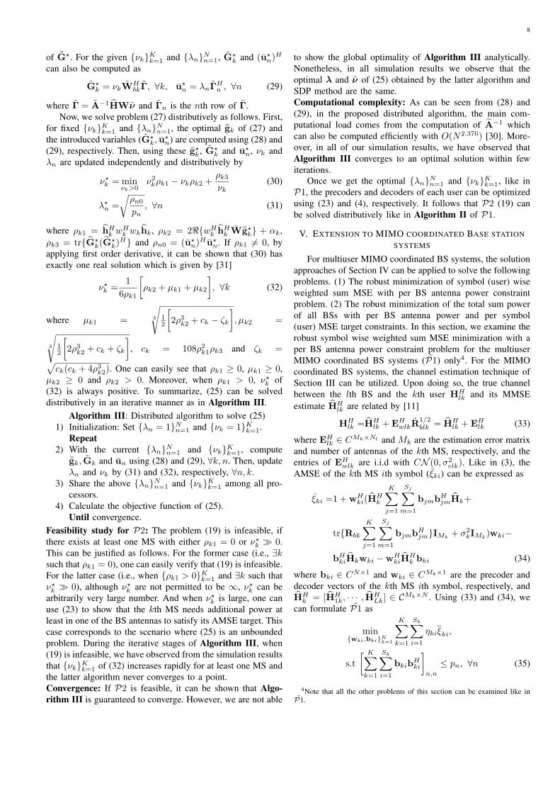
Fig. 2. The average power utilized by the first antenna of BS2 for therobust centralized, robust distributed, non-robust centralized [17] and non-robust distributed [20] designs when ρb11 = 0.25, ρb12 = 0.5, ρb13 =0.2, ρb14 = 0.4, ρb21 = 0.6, ρb22 = 0.1, ρb23 = 0.8 and ρb24 = 0.15.

A. Simulation results for P1

In this subsection, we consider a system with L = 2 BSswhere each BS has 2 antennas and K = 4 MSs. We use ρb11 =0.25, ρb12 = 0.5, ρb13 = 0.2, ρb14 = 0.4, ρb21 = 0.6, ρb22 =0.1, ρb23 = 0.8 and ρb24 = 0.15, and σ2

e1 = 0.01, σ2e2 = 0.02,

σ2e3 = 0.03 and σ2

e4 = 0.04. It is assumed that {σ2k = σ2}Kk=1,

{pn = 2}4n=1 and {ηk = 1}Kk=1. All simulation results of thissubsection are averaged over 100 randomly chosen channelrealizations.

The optimal transmit power of the first antenna of BS2 asa function of the noise power is plotted in Fig. 2. This figureshows that the power utilized by the centralized algorithmsof the robust and non-robust/naive designs are the same asthat of the distributed algorithms of the robust and non-robustdesigns, respectively. The non-robust/naive design refers tothe design in which the estimated channel is considered asperfect [17], [20]. The latter figure also shows that all antennasdo not necessarily utilize their full powers to minimize thetotal sum AMSE of the system in the robust and non-robustdesigns5. Furthermore, the power utilized by the first antenna

5This behavior has also been observed in [17] and [20] where the sum MSEminimization with per BS antenna power constraint problem is examined.

10

of BS2 for both of these designs are not necessarily the same.Although the robust and non-robust designs do not use thesame power at each antenna, we have noticed at all SNRvalues that the average total sum power of all antennas of thelatter designs are almost the same. In the sequel, we comparethe performance of the robust centralized, robust distributed,non-robust centralized and non-robust distributed algorithms interms of sum AMSE. For this purpose, we define the signal-to-noise ratio (SNR) as Psum/σ

2, where Psum is the total sumpower utilized by all BS antennas of the robust distributedalgorithm and σ2 is the noise variance. The SNR is controlledby varying σ2.

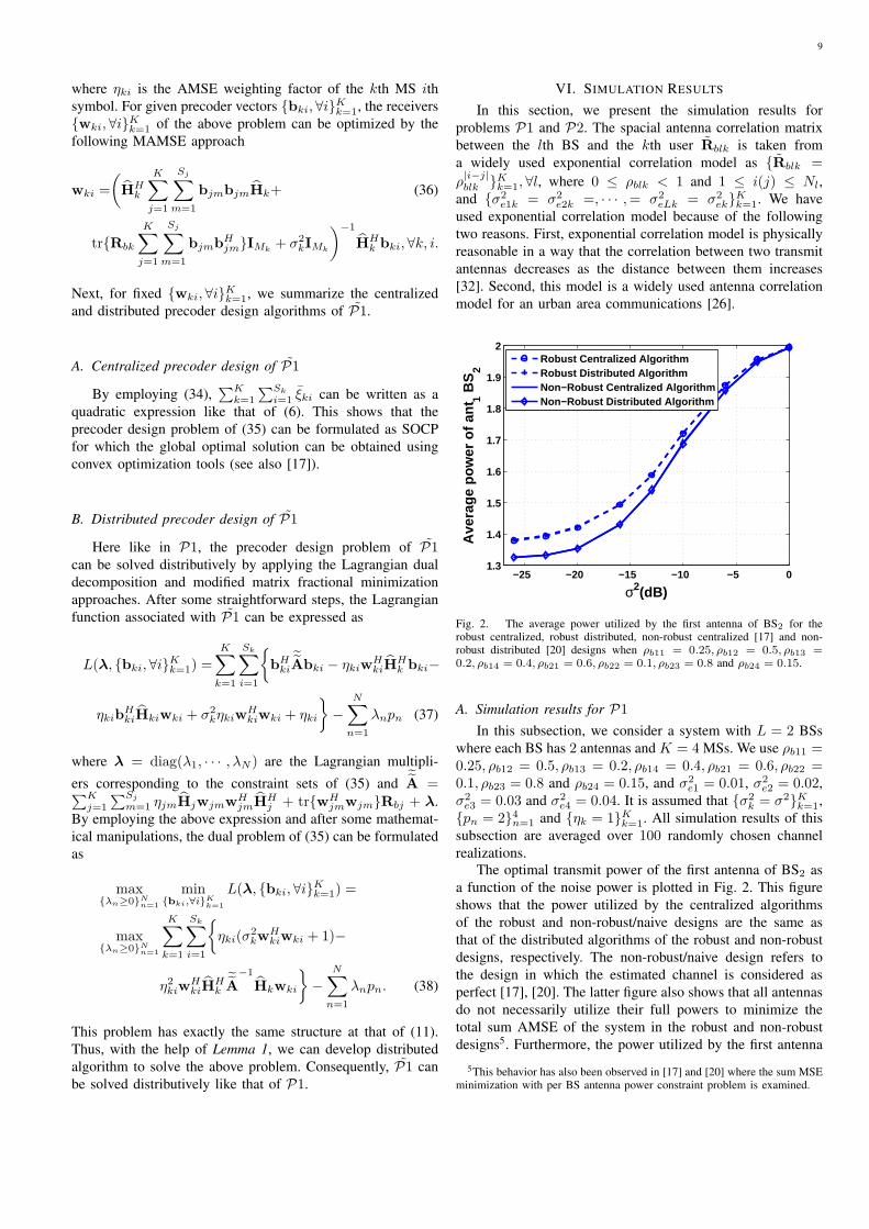
We first compare the performance of the robust centralizedand robust distributed algorithms in terms of sum AMSE.Fig. 3 shows that the robust centralized and distributed al-gorithms achieve the same sum AMSE. Next, we comparethe performance of the robust and non-robust/naive designs.In [20], we have shown that [17] and [20] achieve the samesum MSE. Thus, it is sufficient to compare the performanceof our robust designs with the non-robust design of [20].As can be seen from Fig. 3, the proposed robust designshave better performance than that of the non-robust designin [20] and this improvement is better at high SNR regions.As can be seen from the second equality of (3), when SNR ishigh (i.e., when σ2

k = σ2 is low), σ2 is negligible comparedto

∑Ll=1 σ

2elktr{R

1/2blk BlB

Hl R

1/2blk } (the term due to channel

estimation error). Thus, in the high SNR region, since thenon-robust design does not take into account the effect of∑L

l=1 σ2elktr{R

1/2blk BlB

Hl R

1/2blk } which is the dominant term,

the sum AMSE of this design increases significantly. Thesediscussions help us to understand why the performance ofnon-robust design worsens in the high SNR region. From thisexplanation, we can imply that the sum AMSE gap betweenrobust and non-robust designs increases as the SNR increases.

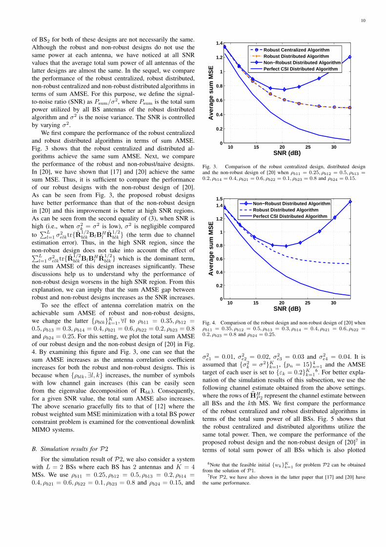
To see the effect of antenna correlation matrix on theachievable sum AMSE of robust and non-robust designs,we change the latter {ρblk}Kk=1,∀l to ρb11 = 0.35, ρb12 =0.5, ρb13 = 0.3, ρb14 = 0.4, ρb21 = 0.6, ρb22 = 0.2, ρb23 = 0.8and ρb24 = 0.25. For this setting, we plot the total sum AMSEof our robust design and the non-robust design of [20] in Fig.4. By examining this figure and Fig. 3, one can see that thesum AMSE increases as the antenna correlation coefficientincreases for both the robust and non-robust designs. This isbecause when {ρblk,∃l, k} increases, the number of symbolswith low channel gain increases (this can be easily seenfrom the eigenvalue decomposition of Rbk). Consequently,for a given SNR value, the total sum AMSE also increases.The above scenario gracefully fits to that of [12] where therobust weighted sum MSE minimization with a total BS powerconstraint problem is examined for the conventional downlinkMIMO systems.

B. Simulation results for P2

For the simulation result of P2, we also consider a systemwith L = 2 BSs where each BS has 2 antennas and K = 4MSs. We use ρb11 = 0.25, ρb12 = 0.5, ρb13 = 0.2, ρb14 =0.4, ρb21 = 0.6, ρb22 = 0.1, ρb23 = 0.8 and ρb24 = 0.15, and

10 15 20 25 300

0.2

0.4

0.6

0.8

1

1.2

1.4

SNR (dB)

Ave

rage

sum

MS

E

Robust Centralized AlgorithmRobust Distributed AlgorithmNon−Robust Distributed AlgorithmPerfect CSI Distributed Algorithm

Fig. 3. Comparison of the robust centralized design, distributed designand the non-robust design of [20] when ρb11 = 0.25, ρb12 = 0.5, ρb13 =0.2, ρb14 = 0.4, ρb21 = 0.6, ρb22 = 0.1, ρb23 = 0.8 and ρb24 = 0.15.

10 15 20 25 300

0.2

0.4

0.6

0.8

1

1.2

1.41.5

SNR (dB)

Ave

rage

sum

MS

E

Non−Robust Distributed AlgorithmRobust Distributed AlgorithmPerfect CSI Distributed Algorithm

Fig. 4. Comparison of the robust design and non-robust design of [20] whenρb11 = 0.35, ρb12 = 0.5, ρb13 = 0.3, ρb14 = 0.4, ρb21 = 0.6, ρb22 =0.2, ρb23 = 0.8 and ρb24 = 0.25.

σ2e1 = 0.01, σ2

e2 = 0.02, σ2e3 = 0.03 and σ2

e4 = 0.04. It isassumed that {σ2

k = σ2}Kk=1, {pn = 15}4n=1 and the AMSEtarget of each user is set to {εk = 0.2}Kk=1

6. For better expla-nation of the simulation results of this subsection, we use thefollowing channel estimate obtained from the above settings.where the rows of HH

P2 represent the channel estimate betweenall BSs and the kth MS. We first compare the performanceof the robust centralized and robust distributed algorithms interms of the total sum power of all BSs. Fig. 5 shows thatthe robust centralized and distributed algorithms utilize thesame total power. Then, we compare the performance of theproposed robust design and the non-robust design of [20]7 interms of total sum power of all BSs which is also plotted

6Note that the feasible initial {wk}Kk=1 for problem P2 can be obtainedfrom the solution of P1.

7For P2, we have also shown in the latter paper that [17] and [20] havethe same performance.

11

HHP2 =

0.2328− 0.0868i 0.1344 + 0.3848i 0.2407− 0.3118i −0.2276− 1.3829i1.6717 + 0.4976i 0.5254− 0.9034i 0.0206 + 0.1318i 1.1292− 0.8314i−0.0426 + 1.7262i −0.6380− 0.5663i −0.2765− 0.4716i −0.2760− 0.1349i0.3266 + 0.0882i −0.3655 + 0.8997i −0.5944− 1.1556i −0.2692− 0.6244i

(39)

in Fig. 5. This figure shows that the robust design utilizesmore power than that of the non-robust design for all noisevariances. Now, for the total power given in the latter figure,the AMSE of each user for both designs are plotted in Fig.6. This figure shows that for all noise variances, the non-robust design does not satisfy the AMSE requirement butthe proposed robust design ensures the AMSE requirementefficiently. To ensure the latter AMSE, however, the robustdesign utilizes more power than that of the non-robust design.This shows that Fig. 6 does not reveal the actual performanceof the proposed robust design. Thus, for a fair comparison, wetune {σ2

ek}Kk=1 such that the total power utilized by the robustand non-robust designs are the same (or very close to eachother)8 and then we compare the performance of these twodesigns by their achieved AMSEs of each user. For the powerrequirement of Fig. 7, the AMSE of each user is plotted inFig. 8. The latter figure shows that for the same total power,the robust design still outperforms the non-robust design.

−16 −14 −12 −10 −8 −6 −4 −2 00

5

10

15

20

25

σ2 (dB)

Tot

al s

um p

ower

Robust Centralized AlgorithmRobust Distributed AlgorithmNon−Robust Distributed Algorithm

Fig. 5. Comparison of the robust centralized algorithm, distributed algorithmand the non-robust distributed algorithm of [20].

For P2, we have noticed that for each channel estimatedifferent error variance (after numerical tuning) is required toget the same total sum powers for the robust and non-robustdesigns. However, the performance behavior exhibited in allchannel estimates fits to that of HH

P2. The detail simulationresults of this problem for the other channel estimates areomitted to reduce redundancy. Moreover, to see the effectof antenna correlation factor for P2, we use the previouslymentioned AMSE targets (i.e., {εk = 0.2}Kk=1 ). With these

8In the robust design, for each noise level, we perform numerical searchto get the appropriate {σ2

ek}Kk=1 that yields the same (or very close) total

transmit power as that of the non-robust design. This task is termed asnumerical tuning.

−16 −14 −12 −10 −8 −6 −4 −2 00.2

0.21

0.22

0.23

0.24

0.25

0.26

0.27

0.28

σ2(dB)A

MS

E o

f eac

h us

er

User 1 Non−RobustUser 1 RobustUser 2 Non−RobustUser 2 RobustUser 3 Non−RobustUser 3 RobustUser 4 Non−RobustUser 4 Robust

Fig. 6. Comparison of the AMSE achieved in each user for the robust designand non-robust design of [20].

−16 −14 −12 −10 −8 −6 −4 −2 00

5

10

15

σ2 (dB)

Tot

al s

um p

ower

Robust Distributed Algorithm with desired σek2

Non−Robust Distributed Algorithm

Fig. 7. The power utilized by the robust design and non-robust design of[20] with the desired error variances {σ2

ek}Kk=1.

AMSE targets, when we increase the antenna correlationfactor, we observe that the total power requirement of thewhole network also increases. The simulation results whichshow this fact has not been included for conciseness.

C. Convergence characteristics of Algorithm IAs we have mentioned in Section IV-A.1, the centralized

algorithm to solve (7) has limited practical interest when thenumber of BSs and/or MSs are large. Moreover, in Section IV-A.2, the computational complexity of our distributed algorithmto solve (12) (once the complexity of (12) with AlgorithmI is studied, the complexity of (7) with this algorithm is

12

−16 −14 −12 −10 −8 −6 −4 −2 00.21

0.22

0.23

0.24

0.25

0.26

0.27

0.28

0.29

σ2 (dB)

AM

SE

of e

ach

user

User 1 Non−RobustUser 1 RobustUser 2 Non−RobustUser 2 RobustUser 3 Non−RobustUser 3 RobustUser 4 Non−RobustUser 4 Robust

Fig. 8. Comparison of the AMSE achieved in each user for the robust designand non-robust design of [20] after tuning the error variance.

immediate) is provided for a single iteration (i.e., per iterationof Algorithm I). Thus, to show the computational advantageof our distributed algorithm compared to that of the centralizedalgorithm, the number of required iterations for convergenceof Algorithm I (I1) needs to be accessed for large scalenetworks. However, we are not able to compute I1 analytically.Due to this, we examine the convergence characteristics ofAlgorithm I for a 19-cell hexagonal structure coordinatedBS system as in [33]. Each BS is located at the center ofits cell, whereas each MS is located randomly inside these19-cells with uniform distribution. The propagation modelbetween each BS and MS contains two components. Oneis the path loss component decaying with distance, and theother one is the Rayleigh fading random component whichhas a zero mean and unit variance. For this simulation, weuse {ηk = 1, σ2

elk = 0.02, ρblk = 0.25,∀l}Kk=1 and all theother parameter settings are summarized as shown in Table I.For the channel realizations of these parameters, we examinethe convergence characterstics of Algorithm I at differentiterative stages of Algorithm II (i.e., with different {wk}Kk=1)as shown in Fig. 9. As can be seen from this figure, AlgorithmI converges to an optimal solution in less than 10 iterations.

TABLE ISIMULATION PARAMETERS FOR CONVERGENCE OF Algorithm I

Number of BSs 19Number of antennas at each BS 2Transmit power of each BS antenna 5WRadius of each cell 1.6kmReference distance (d0) 1.6kmPath loss exponent 3.8Mean path loss at d0 134dBChannel bandwidth 5MHzReceiver noise figure 5dBReceiver vertical antenna gain 10.3dBiReceiver temperature 300KSNR 18dB

2 4 6 8 10 12 14 16 18 2020

25

30

35

40

45

Number of Iterations

Ob

ject

ive

fun

ctio

n o

f (1

2)

Fig. 9. Convergence characteristics of Algorithm I at different iterativestages of Algorithm II.

D. Overall computational complexity to solve (7)

In Section IV-A.1, we have presented the worst-case com-putational cost of IP methods to solve (7) centrally. However,in most practical problems, IP methods require less computa-tional cost than that of their worst-case complexities. To thebest of our knowledge, computing the exact computationalcomplexity of IP methods for this problem requires immenseeffort and time. Hence, we believe that such a task is beyondthe scope of our current work. However, we have carried outextensive simulations to compare the computational time ofour proposed distributed algorithm with that of the centralizedalgorithm which uses IP method. In the following, we describethe simulation platform and methodology we have used, anddiscuss the results.

According to [34], MOSEC is a computationally efficientoptimization package which uses IP methods to solve large-scale optimization problems. Moreover, for SOCP problems,MOSEC requires less computational time than that of SeDuMi,LOQO, SDPT3 and CPLEX [35], [36]. This motivates us tocompare the computational time of Algorithm I with that ofMOSEC to solve (7). Our Matlab codes were run on a personalcomputer with 1.6 GHz, 2GB dual core processor under Win-dows XP. For comparison between these two algorithms, wehave used a coordinated BS system with L = N/2, N = K,{ρblk = 0.25, σ2

elk = 0.02, σ2k = 0.1, }Kk=1 and {pn = 2}Nn=1.

It is assumed that problem (7) has been solved by a centralcontroller with K processors and all other parameters are takenas mentioned in the first paragraph of Section VI. Table IIshows the amount of time required to solve (7) by AlgorithmI9 and MOSEC at different iterative stages of Algorithm II(i.e., for different {wk}Kk=1). As can be seen from Table II,our proposed distributed algorithm requires less computationaltime than that of MOSEC. From this table we can notice thatour distributed algorithm has practical interest especially when

9To get the computational time of Algorithm I per processor, first weget the computational time of Algorithm I by assuming one processor (i.e.,personal computer), then, we divide the latter computational time by K.

13

K(N) is large.

TABLE IICOMPUTATIONAL TIME OF Algorithm I AND MOSEC FOR (7) (IN

SECONDS)

K 4 10 20 30 40A: MOSEC 0.0031 0.0213 0.2182 0.8833 2.3598B: Algorithm I

processor0.0012 0.0020 0.0041 0.0086 0.0118

A/B 2.52 10.455 52.643 133.874 200.336

The convergence characteristics of Algorithm III and theoverall computational complexity of (20) can be studied likein Sections VI-C and VI-D, respectively.

VII. CONCLUSIONS

This paper considers the joint transceiver design for mul-tiuser MISO systems with coordinated BSs where imperfectCSI is available at the BSs and MSs. By incorporating antennacorrelation at the BSs and taking channel estimation errorsinto account, we solve two robust design problems. Theproblems are solved as follows. First, for fixed receivers,we propose centralized and novel computationally efficientdistributed algorithms to jointly optimize the precoders of allusers. The centralized algorithms employ the SOCP approach,whereas the distributed algorithms use the Lagrangian dual de-composition, modified matrix fractional minimization and aniterative method. Second, for fixed BS precoders, the receiversare updated by the MAMSE criterion. These two steps arerepeated until convergence is achieved. Computer simulationsdemonstrate that our proposed distributed algorithms achievethe same performance as that of the centralized algorithms.Simulation results also verify the superior performance ofthe stochastic robust designs compared to that of the non-robust/naive designs.

REFERENCES

[1] G. Caire and S. Shamai, “On the achievable throughput of a multi-antenna Gaussian broadcast channel,” IEEE Tran. Info. Theo, vol. 49,no. 7, pp. 1691 – 1706, Jul. 2003.

[2] S. Serbetli and A. Yener, “Transceiver optimization for multiuser MIMOsystems,” IEEE Tran. Sig. Proc., vol. 52, no. 1, pp. 214 – 226, Jan. 2004.

[3] D. P. Palomar and S. Verdu, “Gradient of mutual information in linearvector Gaussian channels,” IEEE Tran. Info. Theo., vol. 52, no. 1, pp.141 – 154, Jan. 2006.

[4] D. P. Palomar, A unified framework for communications throughMIMO channels, Ph.D. thesis, Technical University of Catalonia (UPC),Barcelona, Spain, 2003.

[5] S. Shi, M. Schubert, and H. Boche, “Downlink MMSE transceiveroptimization for multiuser MIMO systems: Duality and sum-MSEminimization,” IEEE Tran. Sig. Proc., vol. 55, no. 11, pp. 5436 – 5446,Nov. 2007.

[6] S. Shi, M. Schubert, and H. Boche, “Rate optimization for multiuserMIMO systems with linear processing,” IEEE Tran. Sig. Proc., vol. 56,no. 8, pp. 4020 – 4030, Aug. 2008.

[7] R. Hunger, M. Joham, and W. Utschick, “On the MSE-duality of thebroadcast channel and the multiple access channel,” IEEE Tran. Sig.Proc., vol. 57, no. 2, pp. 698 – 713, Feb. 2009.

[8] S. Shi, M. Schubert, and H. Boche, “Downlink MMSE transceiveroptimization for multiuser MIMO systems: MMSE balancing,” IEEETran. Sig. Proc., vol. 56, no. 8, pp. 3702 – 3712, Aug. 2008.

[9] M. B. Shenouda and T. N. Davidson, “On the design of lineartransceivers for multiuser systems with channel uncertainty,” IEEE Jour.Sel. Commun., vol. 26, no. 6, pp. 1015 – 1024, Aug. 2008.

[10] P. Ubaidulla and A. Chockalingam, “Robust joint precoder/receivefilter designs for multiuser MIMO downlink,” in 10th IEEE Workshopon Signal Processing Advances in Wireless Communications (SPAWC),Perugia, Italy, 21 – 24 Jun. 2009, pp. 136 – 140.

[11] T. Endeshaw, B. K. Chalise, and L. Vandendorpe, “MSE uplink-downlink duality of MIMO systems under imperfect CSI,” in 3rd IEEEInternational Workshop on Computational Advances in Multi-SensorAdaptive Processing (CAMSAP), Aruba, 13 – 16 Dec. 2009, pp. 384– 387.

[12] T. E. Bogale, B. K. Chalise, and L. Vandendorpe, “Robust transceiveroptimization for downlink multiuser MIMO systems,” IEEE Tran. Sig.Proc., vol. 59, no. 1, pp. 446 – 453, Jan. 2011.

[13] K. M. Karakayali, G. J. Foschini, and R. A. Valenzuela, “Networkcoordination for spectrally efficient communications in cellular systems,”IEEE. Tran. Wirel. Comm., vol. 13, no. 4, pp. 56 – 61, Aug. 2006.

[14] H. Dahrouj and W. Yu, “Coordinated beamforming for the multi-cellmulti-antenna wireless system,” IEEE Tran. Wirel. Comm., vol. 9, no.5, pp. 1748 – 1759, May 2010.

[15] E. Bjornson, R. Zakhour, D. Gesbert, and B. Ottersten, “Cooperativemulticell precoding: Rate region characterization and distributed strate-gies with instantaneous and statistical CSI,” IEEE Tran. Sig. Proc., vol.58, no. 8, pp. 4298 – 4310, Aug. 2010.

[16] E. Bjornson, R. Zakhour, D. Gesbert, and B. Ottersten, “Distributedmulticell and multiantenna precoding: Characterization and performanceevaluation,” in Proc. IEEE Global Telecommunications Conference(GLOBECOM), Honolulu, HI, USA, 30 Nov. – 4 Dec. 2009, pp. 1 – 6.

[17] S. Shi, M. Schubert, N. Vucic, and H. Boche, “MMSE optimizationwith per-base-station power constraints for network MIMO systems,”in Proc. IEEE International Conference on Communications (ICC),Beijing, China, 19 – 23 May 2008, pp. 4106 – 4110.

[18] S. Boyd and L. Vandenberghe, Convex optimization, CambridgeUniversity Press, Cambridge, 2004.

[19] T. Tamaki, K. Seong, and J. M. Cioffi, “Downlink MIMO systems usingcooperation among base stations in a slow fading channel,” in Proc.IEEE International Conference on Communications (ICC), Glasgow,UK, 24 – 28 Jun. 2007, pp. 4728 – 4733.

[20] T. E. Bogale, L. Vandendorpe, and B. K. Chalise, “MMSE transceiverdesign for coordinated base station systems: Distributive algorithm,” in44th Annual Asilomar Conference on Signals, Systems, and Computers,Pacific Grove, CA, USA, 7 – 10 Nov. 2010.

[21] J. Luo, J. R. Zeidler, and S. Mclaughlin, “Performance analysis ofcompact antenna arrays with MRC in correlated Nakagami fadingchannels,” IEEE Trans. Veh. Technol, vol. 50, pp. 267–277, 2001.

[22] B. K. Chalise, L. Haering, and A. Czylwik, “System level performanceof UMTS-FDD with covariance transformation based DL beamforming,”in Proc. IEEE Global Telecommunications Conference (GLOBECOM),San Fransisco, USA, 1 – 5 Dec. 2003, pp. 133 – 137.

[23] D. Aszetly, On antenna arrays in mobile communication systems: Fastfading and GSM base station receiver algorithm, Ph.D. thesis, RoyalInstitute Technology, Stockholm, Sweden, 1996.

[24] T. Yoo, E. Yoon, and A. Goldsmith, “MIMO capacity with channeluncertainty: Does feedback help?,” in Proc. IEEE Global Telecommu-nications Conference (GLOBECOM), Dallas, USA, 29 Nov. – 3 Dec.2004, vol. 1, pp. 96 – 100.

[25] W. Yu and T. Lan, “Transmitter optimization for the multi-antennadownlink with per-antenna power constraints,” IEEE Trans. Sig. Proc.,vol. 55, no. 6, pp. 2646 – 2660, Jun. 2007.

[26] M. Ding, Multiple-input multiple-output wireless system designs withimperfect channel knowledge, Ph.D. thesis, Queens University Kingston,Ontario, Canada, 2008.

[27] D. Ding and S. D. Blostein, “MIMO minimum total MSE transceiverdesign with imperfect CSI at both ends,” IEEE Tran. Sig. Proc., vol.57, no. 3, pp. 1141 – 1150, Mar. 2009.

[28] K. B. Petersen and M. S. Pedersen, “The matrix cookbook,” Feb. 2008.[29] M. S. Lobo, L. Vandenberghe, S. Boyd, and H. Lebret, “Applications of

second-order cone programming,” Linear algebra and its applications,vol. 284, pp. 193 – 228, 1998.

[30] D. Coppersmith and S. Winograd, “Matrix multiplication via arithmeticprogressions,” Journal of Symbolic Computation, vol. 9, pp. 251 – 280,1990.

[31] None, “Cubic function: http://en.wikipedia.org/wiki/cubic function/,” .[32] S. L. Loyka, “Channel capacity of mimo architecture using the

exponential correlation matrix,” IEEE Tran. Comm., vol. 5, no. 9, pp.369 – 371, 2001.

[33] G. J. Foschini, K. Karakayali, and R. A. Valenzuela, “Coordinating mul-tiple antenna cellular networks to achieve enormous spectral efficiency,”Communications, IEE Proceedings, vol. 153, no. 4, 2006.

14

[34] MOSEK ApS, The MOSEK optimization toolbox for MATLAB manual,Version 6.0 (Revision 103), http://www.mosek.com, 2011.

[35] H. D. Mittelmann, “An independent benchmarking of SDP and SOCPsolvers,” Mathimatical Programming, vol. 95, no. 2, pp. 407 – 430,2003.

[36] H. D. Mittelmann, SOCP (second-order cone programming) Benchmark,http://plato.asu.edu/ftp/socp.html, Feb. 2011.

Tadilo Endeshaw Bogale (S’09) was born inGondar, Ethiopia. He received his B.Sc and M.Scdegree in Electrical Engineering from Jimma Uni-versity, Jimma, Ethiopia and Karlstad University,Karlstad, Sweden in 2004 and 2008, respectively.From 2004-2007, he was working in EthiopianTelecommunications Corporation (ETC) in mobileproject department.

Since 2009 he has been working towards his PhDdegree and as an assistant researcher at the ICTEAMinstitute, University Catholique de Louvain (UCL),

Louvain-la-Neuve, Belgium. His research interests include robust (non-robust)transceiver design for multiuser MIMO systems, centralized and distributedalgorithms, and convex optimization techniques for multiuser systems.

Luc Vandendorpe (M’93-SM’99-F’06) was bornin Mouscron, Belgium, in 1962. He received theElectrical Engineering degree (summa cum laude)and the Ph.D. degree from the Universit Catholiquede Louvain (UCL), Louvain-la-Neuve, Belgium, in1985 and 1991, respectively. Since 1985, he has beenwith the Communications and Remote Sensing Lab-oratory of UCL, where he first worked in the fieldof bit rate reduction techniques for video coding. In1992, he was a Visiting Scientist and Research Fel-low at the Telecommunications and Traffic Control

Systems Group of the Delft Technical University, The Netherlands, where heworked on spread spectrum techniques for personal communications systems.From October 1992 to August 1997, he was Senior Research Associate ofthe Belgian NSF at UCL, and invited Assistant Professor. He is currentlya Professor and head of the Institute for Information and CommunicationTechnologies, Electronics and Applied Mathematics.

His current interest is in digital communication systems and more pre-cisely resource allocation for OFDM(A)-based multicell systems, MIMO anddistributed MIMO, sensor networks, turbo-based communications systems,physical layer security and UWB based positioning.

Dr. Vandendorpe was corecipient of the 1990 Biennal Alcatel-Bell Awardfrom the Belgian NSF for a contribution in the field of image coding. In2000, he was corecipient (with J. Louveaux and F. Deryck) of the BiennalSiemens Award from the Belgian NSF for a contribution about filter-bank-based multicarrier transmission. In 2004, he was co-winner (with J. Czyz)of the Face Authentication Competition, FAC 2004. He is or has beenTPC member for numerous IEEE conferences (VTC, Globecom, SPAWC,ICC, PIMRC, WCNC) and for the Turbo Symposium. He was Co-TechnicalChair (with P. Duhamel) for the IEEE ICASSP 2006. He was an Editorfor Synchronization and Equalization of the IEEE TRANSACTIONS ONCOMMUNICATIONS between 2000 and 2002, Associate Editor of the IEEETRANSACTIONS ON WIRELESS COMMUNICATIONS between 2003 and2005, and Associate Editor of the IEEE TRANSACTIONS ON SIGNALPROCESSING between 2004 and 2006. He was Chair of the IEEE Beneluxjoint chapter on Communications and Vehicular Technology between 1999 and2003. He was an elected member of the Signal Processing for Communicationscommittee between 2000 and 2005, and an elected member of the SensorArray and Multichannel Signal Processing committee of the Signal ProcessingSociety between 2006 and 2008. Currently, he is an elected member of theSignal Processing for Communications committee. He is the Editor-in-Chieffor the EURASIP Journal on Wireless Communications and Networking. L.Vandendorpe is a Fellow of the IEEE.

Batu Krishna Chalise was born in Kathmandu,Nepal. He received the B. E. degree in electronicsengineering from Tribhuvan University, Kathmandu,in 1998 and the M. S. and Ph.D. degrees in electricalengineering from the University of Duisburg-Essen,Duisburg, Germany, in 2001 and 2006, respectively.

In 1999, he was a lecturer with the Institute ofEngineering, Kathmandu. For a short period in 2001,he was a Researcher with the Fraunhofer-Institute ofMicroelectronic Circuits and Systems (IMS), Duis-burg. From 2002-2006, he was a Research Assistant

with the Department of Communication Systems, University of Duisburg-Essen, where his Ph.D. research was supported by a grant from the Ministryof Education and Science of North Rhein-Westphalia (NRW), Germany. Hewas a Postdoctoral Researcher with the Communication and Remote SensingLaboratory, Universite catholique de Louvain, Louvain La Neuve, Belgiumfrom December 2006 till June 2010. Currently, he is the Postdoctoral ResearchFellow with the Center for Advanced Communications, Villanova University,Villanova, USA. His research interests include cooperative and opportunisticwireless communications, robust algorithms for multi-antenna systems andconvex optimization.