Mispricing of S&P 500 Index Options

George M. Constantinides Jens Carsten Jackwerth Stylianos Perrakis

University of Chicago

and NBER University of Konstanz Concordia University

Abstract

We document widespread violations of stochastic dominance in the one-month S&P 500 index

options market over the period 1986-2002. These violations imply that a trader can improve her

expected utility by engaging in a zero-net-cost trade. We allow the market to be incomplete and also

imperfect by introducing transactions costs and bid-ask spreads. There is higher incidence of

violations by OTM than by ITM calls, contradicting the common inference drawn from the observed

implied volatility smile that the problem lies with the left-hand tail of the index return distribution.

Even though pre-crash option prices conform to the BSM model reasonably well, they are incorrectly

priced. Over 1997-2002, many options, particularly OTM calls, are overpriced irrespective of which

time period is used to determine the index return distribution. These results do not support the

hypothesis that the options market is becoming more rational over time. Finally, our results dispel

another common misconception, that the observed smile is too steep after the crash: most of the

violations by post-crash options are due to the options being either underpriced over 1988-1995, or

overpriced over 1997-2002.

Current draft: October 10, 2005 JEL classification: G13

Keywords: Derivative pricing; volatility smile, incomplete markets, transactions costs; index options;

stochastic dominance bounds

We thank workshop participants at the EFA 2005 Meetings, the German Finance Society Meetings

2004, the Bachelier 2004 Congress, the University of Chicago, and Concordia, Laval, New York,

Princeton and St. Gallen Universities and, in particular, Yacine Ait-Sahalia, Matthew Richardson,

Jeffrey Russell and Hersh Shefrin for their insightful comments and constructive criticism. We also

thank Michal Czerwonko for excellent research assistance. We remain responsible for errors and

omissions. Constantinides acknowledges financial support from the Center for Research in Security

Prices of the University of Chicago and Perrakis from the Social Sciences and Humanities Research

Council of Canada. E-mail addresses: gmc@ChicagoGSB.edu, Jens.Jackwerth@uni-konstanz.de, and

SPerrakis@jmsb.concordia.ca.

1 Introduction

A robust prediction of the celebrated Black and Scholes (1973) and Merton (1973)

(BSM) option pricing model is that the volatility implied by market prices of

options is constant across strike prices. Rubinstein (1994) tested this prediction on

the S&P 500 index options (SPX), traded on the Chicago Board Options Exchange,

an exchange that comes close to the dynamically complete and perfect market

assumptions underlying the BSM model. From the start of the exchange-based

trading in April 1986 until the October 1987 stock market crash, the implied

volatility is a moderately downward-sloping function of the strike price, a pattern

referred to as the “volatility smile”, also observed in international markets and to a

lesser extent on individual-stock options. Following the crash, the volatility smile is

typically more pronounced.1

An equivalent statement of the above prediction of the BSM model, that the

volatility implied by market prices of options is constant across strike prices, is that

the risk-neutral stock price distribution is lognormal. Ait-Sahalia and Lo (1998),

Jackwerth and Rubinstein (1996) and Jackwerth (2000) estimated the risk-neutral

stock price distribution from the cross section of option prices.2 Jackwerth and

Rubinstein (1996) confirmed that, prior to the October 1987 crash, the risk-neutral

stock price distribution is close to lognormal, consistent with a moderate implied

volatility smile. Thereafter, the distribution is systematically skewed to the left,

consistent with a more pronounced smile.

These findings raise several important questions. Does the BSM model work

well prior to the crash? If it does, is it because the risk-neutral probability of a

stock market crash was low and consistent with a lognormal distribution? Or, is it

because the risk-neutral probability of a stock market crash was erroneously

1 Brown and Jackwerth (2004), Jackwerth (2004), Shefrin (2005), and Whaley (2003) review the

literature and potential explanations. 2 Jackwerth (2004) reviews the parametric and non-parametric methods for estimating the risk-

neutral distribution.

1

perceived to be low by the market participants? Why does the BSM model

typically fail after the crash? Is it because the risk neutral probability of a stock

market crash increased after the crash and became inconsistent with a lognormal

distribution? Or, is it because the risk neutral probability of a stock market crash

was erroneously perceived to do so? Is the options market rational before and after

the crash?

Several no-arbitrage models have been proposed and tested that generalize

the BSM model. These models explore the effects of generalized stock price

processes including stock price jumps and stochastic volatility and typically

generate a volatility smile. Excellent discussion of these models appears in Hull

(2005) and McDonald (2003).

Whereas downward sloping implied volatility is inconsistent with the BSM

model, it is important to realize that this pattern is not inconsistent with economic

theory in general. Two fundamental assumptions of the BSM model are that the

market is dynamically complete and frictionless. We empirically investigate

whether the observed cross sections of one-month S&P 500 index option prices over

1986-2002 are consistent with various economic models that explicitly allow for a

dynamically incomplete market and also an imperfect market that recognizes

trading costs and bid-ask spreads.

Absence of arbitrage in a frictionless market implies the existence of a

risk-neutral probability measure, not necessarily unique, such that the price of

any asset equals the expectation of its payoff under the risk-neutral measure,

discounted at the risk free rate. If a risk-neutral measure exists, the ratio of the

risk-neutral probability density and the real probability density, discounted at

the risk free rate, is referred to as the pricing kernel or stochastic discount factor.

Thus, absence of arbitrage implies the existence of a strictly positive pricing

kernel.

Economic theory imposes restrictions on equilibrium models beyond merely

the ruling out of arbitrage. In a frictionless representative-agent economy, the

pricing kernel equals the representative agent’s intertemporal marginal rate of

substitution over each trading period. If the representative agent has state

2

independent (derived) utility of wealth, then the concavity of the utility function

implies that the pricing kernel is a decreasing function of wealth.

The monotonicity restriction on the pricing kernel does not critically depend

on the existence of a representative agent. If there does not exist at least one

pricing kernel that is a decreasing function of wealth over each trading period, then

there does not exist even one economic agent with state independent (derived)

utility of wealth that is a marginal investor in the market. Therefore, any economic

agent can increase her expected utility by trading in these assets. Hereafter, we

employ the term stochastic dominance violation to connote the nonexistence of even

one economic agent with increasing and concave utility that is a marginal investor

in the market.3 This means that the return of any agent’s current portfolio is

stochastically dominated (in the second degree) by the return of another feasible

portfolio.

Under the two maintained hypotheses that the marginal investor’s (derived)

utility of wealth is state independent and wealth is monotone increasing in the

market index level, the pricing kernel is a decreasing function of the market index

level. Ait-Sahalia and Lo (2000), Jackwerth (2000), and Rosenberg and Engle

(2002) estimated the pricing kernel implied by the observed cross section of prices

of S&P 500 index options as a function of wealth, where wealth is proxied by the

S&P 500 index level. Jackwerth (2000) reported that the pricing kernel is

everywhere decreasing during the pre-crash period 1986-1987 but widespread

violations occur over the post-crash period 1987-1995. Ait-Sahalia and Lo (2000)

reported violations in 1993 and Rosenberg and Engle (2002) reported violations

over the period 1991-1995.4 On the other hand, Bliss and Panigirtzoglou (2004)

estimated plausible values for the risk aversion coefficient of the representative

agent, albeit under the assumption of power utility, thus restricting the shape of the

pricing kernel to be monotone decreasing in wealth.

3 This line of research was initiated by Perrakis and Ryan (1984), Levy (1985), and Ritchken

(1985). For more recent related contributions, see Perrakis (1986, 1993), Ritchken and Kuo

(1988), and Ryan (2000, 2003). 4 Rosenberg and Engle (2002) found violations when they used an orthogonal polynomial pricing

kernel but not when they used a power pricing kernel.

3

Several theories have been suggested to explain the inconsistencies with the

BSM model and the violations of monotonicity of the pricing kernel. Brown and

Jackwerth (2004) suggested that the reported violations of the monotonicity of the

pricing kernel may be an artifact of the maintained hypothesis that the pricing

kernel is state independent but concluded that volatility cannot be the sole omitted

state variable in the pricing kernel. Bollen and Whaley (2004) suggested that

buying pressure drives the volatility smile while Han (2004) and Shefrin (2005)

provided behavioral explanations based on sentiment.

Pan (2002), Garcia, Luger and Renault (2003), and Santa-Clara and Yan

(2004), among others, obtained plausible parameter estimates in models in which

the pricing kernel is state dependent, using panel data on S&P 500 options. Others

calibrated equilibrium models that generate a volatility smile pattern observed in

option prices. Liu, Pan and Wang (2005) investigated rare-event premia driven by

uncertainty aversion in the context of a calibrated equilibrium model and

demonstrated that the model generates a volatility smile pattern observed in option

prices. Benzoni, Collin-Dufresne, and Goldstein (2005) extended the above

approach to show that uncertainty aversion is not a necessary ingredient of the

model. More significantly, they demonstrated that the model can generate the

stark regime shift that occurred at the time of the 1987 crash. While not all of the

above papers deal explicitly with the monotonicity of the pricing kernel, they do

address the problem of reconciling the option prices with the historical index record.

These results are suggestive but stop short of demonstrating absence of stochastic

dominance violations on a month-by-month basis in the cross section of S&P 500

options. This inquiry is the focus of this paper.

In estimating the statistical distribution of the S&P 500 index returns, we

refrain from adopting the BSM assumption that the index price is a Brownian

motion and, therefore, its arithmetic returns are lognormal. We do not impose a

parametric form on the distribution of the index returns but proceed in three

different ways. In the first approach, we estimate the unconditional distribution as

the histograms extracted from two different historical index data samples covering

the periods 1928-1986 and 1972-1986. In the second approach, we estimate the

unconditional distribution as the histograms extracted from two different forward-

4

looking samples, one that includes the October 1987 crash (1987-2002) and one that

excludes it (1988-2002). Finally, we model the variance of the index returns as a

GARCH (1,1) process and estimate the conditional variance over the period 1972-

2002 by the semiparametric method of Engle and Gonzalez-Rivera (1991) that does

not impose the restriction that conditional returns are normally distributed.

Based on the index return distributions extracted in the above five

approaches, we test the compliance of option prices to the predictions of models

that allow for market incompleteness, market imperfections and intermediate

trading over the life of the options. Evidence of stochastic dominance violations

means that any trader can increase her expected utility by engaging in a zero-net-

cost trade. We consider a market with heterogeneous agents and investigate the

restrictions on option prices imposed by a particular class of utility-maximizing

traders that we simply refer to as traders. We do not make the restrictive

assumption that all economic agents belong to the class of the utility-maximizing

traders. Thus, our results are robust and unaffected by the presence of agents with

beliefs, endowments, preferences, trading restrictions, and transactions costs

schedules that differ from those of the utility-maximizing traders modeled in this

paper.

Our tests accommodate at least three implications associated with state

dependence. First, each month we search for a pricing kernel to price the cross

section of one-month options without imposing restrictions on the time series

properties of the pricing kernel month by month. Thus we allow the pricing kernel

to be state dependent. Second, in the second part of our investigation, we allow for

intermediate trading; a trader’s wealth on the expiration date of the options is

generally a function not only of the price of the market index on that date but also

of the entire path of the index level, thereby rendering the pricing kernel state

dependent. Third, we allow the variance of the index return to be state dependent

and employ the forecasted conditional variance.

The paper is organized as follows. In Section 2, we present a model for

pricing options and state restrictions on the prices of options imposed by the

absence of stochastic dominance violations. One form of these restrictions is a set

of linear inequalities on the pricing kernel that can be tested by testing the

5

feasibility of a linear program. The second form of these restrictions is an upper

and lower bound on the prices of options. In Section 3, we test the compliance of

bid and ask one-month index options to these restrictions and discuss the results.

In the concluding Section 4, we summarize the empirical findings and suggest

directions for future research.

2 Restrictions on Option Prices Imposed

by Stochastic Dominance

2.1 The Market

We consider a market with heterogeneous agents and investigate the restrictions on

option prices imposed by a particular class of utility-maximizing traders that we

simply refer to as traders. We do not make the restrictive assumption that all

agents belong to the class of the utility-maximizing traders. Thus our results are

unaffected by the presence of agents with beliefs, endowments, preferences, trading

restrictions, and transactions cost schedules that differ from those of the utility-

maximizing traders.

Trading occurs at a finite number of trading dates. The utility-maximizing

traders are allowed to hold only two primary securities in the market, a bond and a

stock. The stock has the natural interpretation as the market index. The bond is

risk free and pays constant interest each period. The traders may buy and sell the

bond without incurring transactions costs. We assume that the rate of return on

the stock is identically and independently distributed over time.

Stock trades incur proportional transactions costs charged to the bond

account. There is no presumption that all agents in the economy face the same

schedule of transactions costs as the traders do. At each date, a trader chooses the

investment in the bond and stock accounts to maximize the expected utility of net

6

worth at the terminal date. We make the plausible assumption that the utility

function is increasing and concave. Note that even this weak assumption of

monotonicity and concavity of preferences is not imposed on all agents in the

economy but only on the subset of agents that we refer to as traders.

In Appendix A, we formulate this problem as a dynamic program. As

shown in Constantinides (1979), the value function is monotone increasing and

concave in the dollar values in the bond and stock accounts, properties that it

inherits from the monotonicity and concavity of the utility function. This implies

that, at any date, the marginal utility of wealth out of the bond account is strictly

positive and decreasing in the dollar value in the bond account; and the marginal

utility of wealth out of the stock account is strictly positive and decreasing in the

dollar value in the stock account. We search for marginal utilities with the above

properties that support the prices of the bond, stock and derivatives at a given

point in time.

If we fail to find such a set marginal utilities, then any trader with increasing

and concave utility can increase her expected utility by trading in the options, the

index and the risk free rate—hence equilibrium does not exist. These strategies are

termed stochastically dominant for the purposes of this paper, insofar as they would

be adopted by all traders with utility possessing the required properties, in the same

way that all risk averse investors would choose a dominant portfolio over a

dominated one in conventional second degree stochastic dominance comparisons.

We emphasize that the restriction on option prices imposed by the criterion

of the absence of stochastic dominance is motivated by the economically plausible

assumption that there exists at least one agent in the economy with the properties

that we assign to a trader. This is a substantially weaker assumption than

requiring that all agents to have the properties that we assign to traders.

Stochastic dominance then implies that at least one agent, but not necessarily all

agents, increases her expected utility by trading.5 In our empirical investigation, we

5 We also emphasize that the restriction of the absence of stochastic dominance is weaker than

the restriction that the capital asset pricing model (CAPM) holds. The CAPM requires that the

pricing kernel be linearly decreasing in the index price. The absence of stochastic dominance

merely imposes that the pricing kernel be monotone decreasing in the index price.

7

report the percentage of months for which the problem is feasible. These are

months for which stochastic dominance violations are ruled out.

2.2 Restrictions in the Single-Period Model

The single-period model does not rule out trading over the trader’s horizon after the

options expire; it just rules out trading over the one-month life of the options. In

Section 2.3, we consider the more realistic case in which traders are allowed to

trade the bond and stock at one intermediate date over the life of the options.

The stock market index has price at the beginning of the period; ex

dividend price with probability 0S

1iS π i in state =, 1, ...,i i I at the end of the period;

and cum dividend price ( )δ+ 11 iS at the end of the period. We order the states

such that is increasing in i . 1iS

We define as the marginal utility of wealth out of the bond account

at the beginning of the period;

( )0BM

( )0SM as the marginal utility of wealth out of the

stock account at the beginning of the period; ( )1BiM as the marginal utility of

wealth out of the bond account at the end of the period; and ( )1SiM as the

marginal utility of wealth out of the stock account at the end of the period.6 The

marginal utility of wealth out of the bond and stock accounts at the beginning of

the period is strictly positive:

( )0BM > 0 (2.1)

and

( )0SM > 0

. (2.2)

The marginal utility of wealth out of the bond account at the end of the period is

strictly positive: 7

6 The marginal utilities are formally defined in Appendix B. 7 Since the value of the bond account at the end of the period is independent of the state i, we

cannot impose the condition that the marginal utility of wealth out of the bond account is

decreasing in the dollar value of the bond account.

8

( )1 0, 1,...,BiM i> = I . (2.3)

Historically, the sample mean of the premium of the market return over the

risk free rate is positive. Under the assumption of positive expected premium, the

trader is long in the stock. Since the assumption in the single-period model is that

there is no trading between the bond and stock accounts over the life of the option,

the trader’s dollar value in the stock account at the end of the period is increasing

in the stock return. Note that this conclusion critically depends on the assumption

that there is no intermediate trading in the bond and stock. Since we employed the

convention that the stock return is increasing in the state i, the dollar value in the

stock account at the end of the period is increasing in the state i. Then the

condition that the marginal utility of wealth out of the stock account at the end of

the period is strictly positive and decreasing in the dollar value in the stock account

is stated as follows:

( ) ( ) ( )1 21 1 ... 1 0S S SIM M M≥ ≥ > . (2.4)

On each date, the trader may transfer funds between the bond and stock

accounts and incur transactions costs. Therefore, the marginal rate of substitution

between the bond and stock accounts differs from unity by, at most, the

transactions cost rate:

( ) ( ) ( ) ( ) ( )− ≤ ≤ +1 0 0 1B S Bk M M k M 0 (2.5)

and

( ) ( ) ( ) ( ) ( )− ≤ ≤ + =1 1 1 1 1 , 1,...,B S Bi i ik M M k M i I . (2.6)

Marginal analysis on the bond holdings leads to the following condition on

the marginal rate of substitution between the bond holdings at beginning and end

of the period:

9

( ) ( )1

0I

Bi i

iM R Mπ

== ∑ 1B . (2.7)

Marginal analysis on the stock holdings leads to the following condition on the

marginal rate of substitution between the stock holdings at the beginning of the

period and the bond and stock holdings at the end of the period:

( ) ( ) ( )1 1

0 010 1

Ii iS S

i i ii

S SM MS S

δπ=

1BM⎡ ⎤= +⎢ ⎥⎢ ⎥⎣ ⎦∑ . (2.8)

We consider J European call and put options on the index, with random

cash payoff at the end of the period in state i . At the beginning of the period,

the trader can buy the ijX

thj derivative at price j jP k+ and sell it at price j jP k− ,

net of transactions costs. Thus 2 jk is the bid-ask spread plus the round-trip

transactions cost that the trader incurs in trading the thj derivative. Note that

there is no presumption that all agents in the economy face the same bid-ask

spreads and transactions costs as the traders do.

We assume that the traders are marginal in all the J derivatives.

Furthermore, we assume that a trader has sufficiently small positions in the

derivatives relative to her holdings in the bond and stock that the monotonicity and

concavity conditions on the value function remain valid. Marginal analysis leads to

the following restrictions on the prices of options:

( ) ( ) ( ) ( ) ( )1

0 1 0 , 1,...,I

B B Bj j i i ij j j

iP k M M X P k M j Jπ

=− ≤ ≤ + =∑ . (2.9)

Conditions (2.1)-(2.9) define a linear program. In our empirical analysis,

each month we check for feasibility of conditions (2.1)-(2.9) by using the linear

programming features of the optimization toolbox of MATLAB 7.0. We report the

percentage of months in which the linear program is feasible and, therefore,

stochastic dominance is ruled out.

10

A useful way to identify the options that cause infeasibility or near-

infeasibility of the problem is to single out a “test” option, say the option, and

solve the problem

thn

( ) ( )( )1

1max , min0

I Bi

i Bi

Mor XM

π=∑ in , (2.10)

subject to conditions (2.1)-(2.9). If this problem is feasible, then the attained

maximum and minimum have the following interpretation. If one can buy the test

option for less than the minimum attained in this problem, then at least one

investor, but not necessarily all investors, increases her expected utility by trading

the test option. Likewise, if one can write the test option, for more than the

maximum attained in this problem, then again at least one investor increases her

expected utility by trading the test option.

2.3 Restrictions in the Two-Period Model

We relax the assumption of the single-period model that, over the one-month life of

the options, markets for trading are open only at the beginning and end of the

period; we allow for a third trading date in the middle of the month. We define the

marginal utility of wealth out of the bond account and out of the stock account at

each one of the three trading dates and set up the linear program as a direct

extension of the program (2.1)-(2.9) in Section 2.2. The explicit program is given in

Appendix B. In our empirical analysis, we report the percentage of months in

which the linear program is feasible and, therefore, stochastic dominance is ruled

out.

In principle, we may allow for more than one intermediate trading date over

the one-month life of the options. However, the numerical implementation becomes

tedious as both the number of constraints and variables in the linear program

increase exponentially in the number of intermediate trading dates. This

consideration motivates the development of bounds that are independent of the

11

allowed frequency of trading of the stock and bond over the life of the option.

These bounds are presented below.

2.4 The Constantinides-Perrakis Option Bounds

Constantinides and Perrakis (2002) recognized that it is possible to recursively

apply the single-period approach and derive stochastic dominance bounds on option

prices in a market with intermediate trading over the life of the options.8 The

significance of these bounds is that they are invariant to the allowed frequency of

trading the bond and stock over the life of the options.

The task of computing these bounds is easy compared to the full-fledged

investigation of the feasibility of conditions for large T for two reasons. First, the

derivation of the bounds takes advantage of the special structure of the payoff of a

call or put option, specifically the convexity of the payoff as a function of the stock

price. Second, the set of assets is limited to three assets: the bond, stock and one

option, the test option.

The upper and lower bounds on a test option have the following

interpretation. If one can buy the test option for less than the lower option bound,

then there is stochastic dominance violation between the bond, stock and the test

option. Likewise, if one can write the test option for more than the upper option

bound, then again there is stochastic dominance violation between the bond, stock

and the test option. Below, we state these bounds without proof.9

8 Constantinides and Zariphopoulou (1999, 2001) and Constantinides and Perrakis (2002, 2004)

derived bounds on option prices in the presence of transactions costs. For alternative ways to

price options with transactions costs, see Leland (1985) and Bensaid et al (1992). 9 These bounds may not be the tightest possible bounds for any given frequency of trading.

However, they are presented here because of their universality in that they do not depend on the

frequency of trading over the life of the option. For a comprehensive discussion and derivation of

these and other possibly tighter bounds that are specific to the allowed frequency of trading, see

Constantinides and Perrakis (2002). See also Constantinides and Perrakis (2004) for extensions

to American-style options and futures options.

12

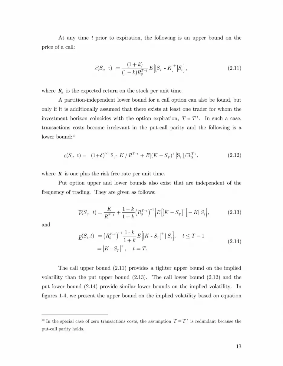
At any time t prior to expiration, the following is an upper bound on the

price of a call:

[ ]+(1 )( , t) -(1 )t T t

S

kc S E S K Sk R −

+T t

⎡ ⎤= ⎢ ⎥⎣ ⎦−, (2.11)

where SR is the expected return on the stock per unit time.

A partition-independent lower bound for a call option can also be found, but

only if it is additionally assumed that there exists at least one trader for whom the

investment horizon coincides with the option expiration, 'T T= . In such a case,

transactions costs become irrelevant in the put-call parity and the following is a

lower bound:10

( )t-T T-tt ( , t) 1+ S - / [( ) S ]/RT t

t Tc S K R E K Sδ − += + − t S , (2.12)

where is one plus the risk free rate per unit time. R

Put option upper and lower bounds also exist that are independent of the

frequency of trading. They are given as follows:

( ) [ ]11( , ) |1

T tt S TT t

K kp S t R E K S K SR k

− +−−

−t

⎡ ⎤⎡ ⎤= + − −⎢ ⎥⎢ ⎥⎣ ⎦⎣ ⎦+, (2.13)

and

( ) [ ]

[ ]

1 +1 -( , ) - | , 11

- , .

T tt S T t

T

kp S t R E K S S t Tk

K S t T

−−

+

⎡ ⎤= ≤ −⎢ ⎥⎣ ⎦+= =

(2.14)

The call upper bound (2.11) provides a tighter upper bound on the implied

volatility than the put upper bound (2.13). The call lower bound (2.12) and the

put lower bound (2.14) provide similar lower bounds on the implied volatility. In

figures 1-4, we present the upper bound on the implied volatility based on equation

10 In the special case of zero transactions costs, the assumption 'T T= is redundant because the

put-call parity holds.

13

(2.11) and the lower bound based on equation (2.12). We discuss the violation of

these bounds in Section 3.6.

3 Empirical Results

3.1 Data

We use the historical daily record of the S&P 500 index and its daily dividend

record over the period 1928-2002. The monthly index return is based on 30

calendar day (21 trading day) returns. In order to avoid difficulties with the

estimated historical mean of the returns, we demean all our samples and

reintroduce a mean 4% annualized premium over the risk free rate. The

unconditional distribution of the index is extracted from four alternative samples of

thirty-day index returns: the historical samples use returns either over the period

1928-1986 or over the period 1972-1986; the forward-looking sample inclusive of the

crash uses the returns over the period 1987-2002 and includes the 1987 stock

market crash; the forward-looking sample exclusive of the crash uses the returns

over the period 1988-2002 and excludes the stock market crash. Finally, we

estimate the conditional distribution over the period 1972-2002 by the

semiparametric GARCH (1,1) model of Engle and Gonzalez-Rivera (1991), a model

that does not impose the restriction that conditional returns are normally

distributed, as explained in Appendix D.11

11 The index return sample and the option price sample do not align. We use the conditional

volatility of the 30-day return period which starts before the option sample and covers it partly at

the beginning. We recalculated the results by using the conditional volatility of the 30-day return

period which starts during the option sample and covers it partly at the end and then continues

beyond the option sample. The two sets of results are practically indistinguishable and thus, we

do not report the latter results here.

14

For the S&P 500 index options we use two data sources. For the period

1986-1995, we use the tick-by-tick Berkeley Options Database of all quotes and

trades. We focus on the most liquid call options with K/S ratio (moneyness) in the

range 0.90-1.05. For 108 months we retain only the call option quotes for the day

corresponding to options thirty days to expiration.12 For each day retained in the

sample, we aggregate the quotes to the minute and pick the minute between 9:00-

11:00 AM with the most quotes as our cross section for the month. We present

these quotes in terms of their bid and ask implied volatilities. These are the

volatilities which would be needed in the BSM formula to price the option

exactly at the bid or ask quote, respectively. Details on this database are

provided in Appendix C, Jackwerth and Rubinstein (1996), and Jackwerth

(2000).

For the period 1997-2002, we obtain call and put option prices from the

Option Metrics Database, described in Appendix C. Note that we do not have

options data for 1996 from either data source. Only options with at least 100

traded contracts are included. We calculate a hypothetical noon option cross

section from the closing cross section and the index observed at noon and the close.

Here we assume that the implied volatilities do not change between noon and the

close. We start out with 69 raw cross sections and are left with 68 final cross

sections. The time to expiration is 29 days.

Since the Berkeley Options Database provides much cleaner data than the

Option Metrics Database, we expect a higher incidence of stochastic dominance

violations over the 1997-2002 period than over the 1986-1995 period due to data

problems. Thus we are cautious in comparing results across these two periods.

12 We lose some months for which we do not have sufficient data, i.e., months with less than five

different strike prices, months after the crash of October 1987 until June 1988, and months before

the introduction of S&P 500 index options in April 1986.

15

3.2 Assumptions on Bid-Ask Spreads and Trading Fees

There is no presumption that all agents in the economy face the same bid-ask

spreads and transactions costs as the traders do. We assume that the traders are

subject to the following bid-ask spreads and trading fees. For the index, we model

the combined one-half bid-ask spread and one-way trading fee as a one-way

proportional transactions cost rate equal to 50 bps of the index price.

For the call options obtained from the Berkeley Options Database over the

period 1986-1995, we proceed as follows. For the at-the-money call, we set the

combined one-half bid-ask spread and one-way trading fee equal to 20 (or 5, or 50)

bps of the index price. This corresponds to about 75 (or 19, or 188) cents one-way

fee per call. For any other call, the fee is proportional to the call price.

Specifically, the combined one-half bid-ask spread and one-way trading fee is equal

to the fee on the at-the-money call multiplied by the ratio of the price of the said

call and the price of the at-the-money call. Only in Table 3 do we present results

under the assumption that the fee is fixed: the combined one-half bid-ask spread

and one-way trading fee is equal to the fee on the at-the-money call.

For the call and put options obtained from the Option Metrics Database

over the period 1997-2002, we proceed as follows. For the at-the-money call, we set

the combined one-half bid-ask spread and one-way trading fee equal to 20 (or 5, or

50) bps of the index price. For any other option (call or put), the fee is

proportional to the option price.

3.3 Stochastic Dominance Violations in the Single-Period

Case

Each month we check for feasibility of conditions (2.1)-(2.9). Infeasibility of these

conditions implies stochastic dominance: any trader can improve her utility by

trading in these assets without incurring any out-of-pocket costs. If we rule out

bid-ask spreads and trading fees, we find that these conditions are violated in all

months.

16

We introduce bid-ask spreads and trading fees as described in Section 3.2.

The one-way transactions cost rate (one-way trading fee plus half the bid-ask

spread) on the index is 50 bps. For the at-the-money call, the one-way transactions

cost rate is 20 bps of the index price, or about 75 cents. For any other option, the

fee is proportional to the option price, as described in Section 3.2. The number of

calls in each (filtered) monthly cross section fluctuates between 5 and 23 with

median 10. The percentage of months without stochastic dominance violations is

displayed in Table 1. The bracketed numbers in the first row are bootstrap

standard deviations of the first-row entries, based on 1,000 samples of the 1928-2002

historical returns. The standard deviations are high and, therefore, comparisons of

the table entries across the rows and columns should be made with caution. In the

second and third rows in each cell, we display the non-violations in the cases where

the one-way transactions costs on each call equal to 5 bps and 50 bps of the index

price, respectively.

[TABLE 1]

The time series of option prices is divided into six periods and stochastic

dominance violations in each period are reported in different columns, labeled as

panels A-F. The first period extends from May 1986 to October 16, 1987, just prior

to the crash. The other five periods are all post-crash and span July 1988 to March

1991, April 1991 to August 1993, September 1993 to December 1995, February 1997

to December 1999 and February 2000 to December 2002. Note that we do not have

options data for 1996 from either data source.

The time series of index returns is divided into five samples and stochastic

dominance violations are reported in different rows for each sample. The first

sample covers 1928-1986 and excludes the crash. Since there are too many

observations, only every 6th return is recorded in building the empirical

unconditional return distribution. The second sample covers 1972-1986 and again

excludes the crash. It is shorter than the first sample to control for the

possibility of a regime shift in the return distribution. The third sample covers

1987-2002, including the crash. The fourth sample covers 1988-2002, excluding

17

the crash. The last row in the table displays the feasibility in the index sample

1972-2002, where the one-month index return distribution is conditional on

volatility and is estimated as in Appendix D. In all five samples, the mean

premium of the index return over the risk free return is adjusted to be 4%

annually.13

Most table entries are well below 100%, indicating that there are a number

of months in which the risk free rate, the price of the index, and the prices of the

cross section of calls are inconsistent with a market in which there is even one

risk-averse trader who is marginal in these securities, net of generous transactions

costs.

The top left entry of 73% refers to the index return distribution over the

period 1928-1986 and option prices over the pre-crash period from May 1986 to

October 16, 1987. In 27% of these months, conditions (2.1)-(2.9) are infeasible

and the prices imply stochastic dominance violations despite the generous

allowance for transactions costs. The next three entries to the right, panels B-D,

refer to call prices over the first three post-crash periods. There are fewer

violations in the first three post-crash periods than in the pre-crash period.

Violations dramatically increase in the last two post-crash periods, panels

E-F. However, these results should be interpreted with caution. Recall that the

quality of the option data in the 1997-2002 period is inferior to the quality in the

1986-1995 period. However, the quality of data in the 1997-1999 and 2000-2002

periods is the same and comparisons are meaningful. There are more violations

in the 2000-2002 period than in the 1997-1999 period. The later finding is

reversed in the last row where we employ the conditional index return

distribution.

We investigate the robustness of the historical estimate of the index return

distribution over the period 1928-1986 by re-estimating the historical distribution

of the index return over the more recent period 1972-1986. The results are

13 We make this adjustment in order to eschew the issues of the predictability of the equity

premium and its estimation from historical samples. Our results remain practically unchanged if

we do not make this adjustment. Essentially, the prices of one-month options are insensitive to

the expected return on the stock.

18

displayed in the second row of Table 1. The results in panels A-D remain largely

unchanged. However the incidence of violations substantially increases in the

period 1997-2002.

When we use the forward-looking index sample 1987-2002 that includes

the crash (third row) or the forward-looking index sample 1988-2002 that

excludes it (fourth row), the pre-crash options exhibit more violations (panel A).

Also, when we use the conditional index return distribution, the incidence of

violations is higher than when we use the historical index samples and

comparable to the incidence of violations when we use the forward-looking index

sample.

Our interpretation is that, before the crash, option traders were

unsophisticated and were extensively using the BSM pricing model. Recall the

stylized observation that, from the start of the exchange-based trading until the

October 1987 stock market crash, the implied volatility is a moderately

downward-sloping function of the strike price; following the crash, the volatility

smile is typically more pronounced. This means that the BSM model typically

fits the data better before the crash than after it, once the constant volatility

input is judiciously chosen as an input to the BSM formula. This does not imply

that investors were more rational before the crash than after it. In fact, our

results in panels A-D suggest that options were priced more rationally after the

crash than before it. The results contrast with the evidence in Jackwerth (2000),

that the estimated pricing kernel is monotonically decreasing (corresponding to

few, if any, violations) in the pre-crash period, but locally increasing

(corresponding to several violations) during the post-crash period.14

Looking across rows, we observe that the pre-crash call prices are more

consistent with the historical index distribution (1928-2002 and 1972-2002) than

the post-crash distribution (with or without the crash event, conditional or

unconditional). This result accords with intuition. The post-crash option prices

in 1988-1995 (panels B-D) generally have few violations. However, violations by

14 The pattern in Jackwerth (2000) does not match with Table 1 for two reasons. First, he

applies a different technique, estimating separately the smoothed risk-neutral and actual

distributions and then taking their ratio. Second, his option price sample ends in 1995.

19

option prices in 1997-2002 (panels E-F) send a mixed message. The violations

are lowest when using either the longer historical index sample 1972-1986 or the

conditional index return distribution.

3.4 Robustness in the Single-Period Case

Floor traders, institutional investors and broker-assisted investors face different

transactions cost schedules in trading options. Are the results robust under

different transactions cost schedules? In Table 1, the number in the second row

of each cell is the percentage of non-violations when the combined one-half bid-

ask spread and one-way trading fee on one option is based on 5 bps of the index

price. We observe a large percentage of violations for all index and option price

periods. Consistent with the earlier observation, there are fewer violations in the

first three post-crash periods than in the pre-crash period. The number in the

third row of each cell is the percentage of non-violations when the combined one-

half bid-ask spread and one-way trading fee on one option is based on 50 bps of

the index price. Predictably, we observe fewer violations for all index and option

price periods. There is no consistent pattern in these violations.

[TABLE 2]

Is the pattern of violation similar across the in-the-money and out-of-the-

money options? Table 2 displays the percentage of months in which stochastic

dominance is absent in the cross section of in-the-money calls (top entry) and

out-of-the-money calls (bottom entry). In all cases, there is a higher percentage

of violations by OTM calls than by ITM calls, suggesting that the mispricing is

caused by the right-hand tail of the index return distribution and not by the left-

hand tail.15 Another way to see this is by comparing the first rows in Table 1

15 This inference is subject to the criticism that it may be an artifact of sample size. The sample

of OTM calls is larger than the sample of ITM calls. Other things equal, the larger the sample,

the harder it is to find a monotone decreasing pricing kernel that prices the calls.

20

with the Table 2 OTM results: addition of the ITM calls does not decrease the

feasibility. This observation is novel and contradicts the common inference

drawn from the observed implied volatility smile that the problem lies with the

left-hand tail of the index return distribution. We revisit these violation patterns

in Section 3.6 where we discuss the violations of bounds on the prices of options.

[TABLE 3]

Table 3 displays the percentage of months in which stochastic dominance

violations are absent in the cross section of option prices but now with fixed

instead of proportional transactions costs. The one-way transactions costs rate

(one-way trading fee plus half the bid-ask spread) on the index is 50 bps. The

one-way transactions costs on each option is 20 bps of the index price. The

pattern of violations is similar to the pattern displayed in Table 1 with variable

transactions costs. With the exception of panel D, there are generally fewer

violations when the transactions costs are fixed. Recall from Table 2 that OTM

calls are responsible for more violations than ITM calls. Fixed transactions costs

imply larger transactions costs for the troublesome OTM calls, provide greater

leeway for the prices of these calls and, therefore, decrease the number of

violations.

3.5 Stochastic Dominance Violations in the Two-Period

Model

In the previous section, we considered feasibility in the context of the single-period

model. We established that there are stochastic dominance violations in a

significant percentage of the months. Does the percentage of stochastic dominance

violations increase or decrease as the allowed frequency of trading in the stock and

bond over the life of the option increases? In the special case of zero transactions

costs, i.i.d. returns and constant relative risk aversion, it can be theoretically shown

that the percentage of violations should increase as the allowed frequency of trading

21

increases. However, we cannot provide a theoretical answer if we relax any of the

above three assumptions. Therefore, we address the question empirically.

We compare the percentage of stochastic dominance violations in two

models, one with one intermediate trading date over the life of the options and

another with no intermediate trading dates over the life of the options. To this

end, we partition the 30-day horizon into two 15-day intervals and approximate the

15-day return distribution by a 21-point kernel density estimate of the 15-day

returns. We use the standard Gaussian kernel of Silverman (1986, pp. 15, 43, and

45). The assumed transactions costs are as in the base case presented in Table 1.

The one-way transactions costs rate (one-way trading fee plus half the bid-ask

spread) on the index is 50 bps. The one-way transactions cost on the at-the-money

call is 20 bps of the index price. For any other call, the fee is proportional to the

call price, as described in Section 3.2. The results are presented in Table 4.

[TABLE 4]

We may not investigate the effect of intermediate trading by directly

comparing the results in Tables 1 and 4 because the return generating process

differs in the two tables. Recall that the results in Table 1 are based on a 30-day

stock return generating process that has as many different returns as the different

observed realizations and frequency equal to the observed frequency.16 By contrast,

the results in Table 4 are based on a simplified 15-day 21-point kernel density

estimate of the 15-day returns. The coarseness of the grid is dictated by the need

to keep the problem computationally manageable. The 30-day return then is the

product of two 15-day returns treated as i.i.d. With this process of the 30-day

return, we calculate the percentage of months without stochastic dominance

violations and report the results in Table 4 in brackets.

The effect of allowing for one intermediate trading date over the life of the

one-month options is shown by the top entries in Table 4. These entries are

contrasted with the bracketed entries which represent the percentage of months

16 For the long historical sample of stock returns, we take only every sixth monthly return.

22

without stochastic dominance violations when intermediate trading is forbidden.

The comparison shows that intermediate trading has an ambiguous effect on

stochastic dominance violations in the option samples, that depends to a large

extent on the distribution used to calculate the index returns. For the long

historical sample intermediate trading slightly decreases the frequency of violations

in all panels, while it increases it, sometimes dramatically so, for the shorter

historical sample. The increase in the frequency of violations also predominates,

but not always consistently, for the remaining three samples. We conclude that

intermediate trading does not weaken, and possibly strengthens, the single-period

systematic evidence of stochastic dominance violations. In the next section, we

obtain further insights on the causes of infeasibility, by displaying the options that

violate the upper and lower bounds on option prices.

3.6 Stochastic Dominance Bounds in the Single-Period and

Multiperiod Cases

In Section 2.4, equations (2.11)-(2.14), we stated a set of stochastic dominance

bounds on option prices that apply irrespective of the permitted frequency of

trading in the bond and stock accounts over the life of the option. We calculate

these bounds and translate them as bounds on the implied volatility of option

prices. In figures 1-4, we present the upper implied volatility bound based on (2.11)

and the lower bound based on (2.12). The bid-ask spread on the option price is

taken into consideration, as we present both the bid and ask option prices,

translated into implied volatilities. A violation occurs whenever an observed option

bid price lies above the upper bound or an observed option ask price lies below the

lower bound. The upper and lower option bounds are based on the index return

distribution derived from the historical index samples 1928-1986 (figure 1) and

1972-1986 (figure 2), and the forward looking samples 1987-2002 (figure 3) and

1988-2002 (figure 4). In each figure, the six panels correspond to option prices

(implied volatilities) over the pre-crash period (panel A) and the five post-crash

23

periods (panels B-F). In all cases, the transactions costs rate on the index is 20

bps.

[FIGURES 1-4]

The downward-sloping shape of the bounds is similar across figures 1-4.

However, the upper and lower bounds in figure 1 are higher than the bounds in

figures 2-4 because the index volatility over 1928-1986 is 40% higher than the index

volatility over the index periods corresponding to figures 2-4. The pattern of

violations follows quite naturally. The flat pre-crash smile fits reasonably well

within the bounds based on the index return over 1928-1986 even though these are

downward sloping. The post-crash smiles over 1988-1995 (panels B-D) are too low

for the rather high location of these bounds.

The bounds based on the index return over the historical 1972-1986 and

forward-looking samples (figures 2-4) are located somewhat lower than the

historical 1928-1986 sample bounds. Therefore, they match the also downward-

sloping post-crash option prices in panels B-D rather well because they are located

somewhat lower too. However, they do not match very well the higher horizontal

smile of the pre-crash options.

Several option prices over the periods 1997-1999 and 2000-2002 (panels E-F)

are way above the bounds in all the figures, irrespective of whether the bounds were

calculated from historical or forward-looking index returns. This is an altogether

different pattern of violations than in the earlier panels A-D. In interpreting the

high incidence of violations of option prices over the period 1997-2002 in Tables 1-4,

we were conservative because of concerns regarding the quality of the Option

Metrics Database. The figures provide a clearer picture. If the violations were the

result of low quality of the data, then we would observe roughly as many violations

of the lower bound as we do of the upper bound. This is not the case. Most of the

violations are violations of the upper bound. Simply put, over 1997-2002, many

options, particularly OTM calls, were overpriced relative to the theoretical bounds,

irrespective of which time period is used to determine the index return distribution.

These results do not support the hypothesis that the options market is becoming

24

more rational over time, particularly after the crash. The decrease in violations

over the post-crash period 1988-1995 (panels B-D) is followed by a substantial

increase in violations over 1997-2002 (panels E-F).

Across all figures, we observe that both upper and lower bounds exhibit a

clear smile pattern. Thus the theory states that option prices should exhibit a

smile both before and after the crash. The observed pre-crash option prices (panel

A) approximately conform to the BSM model with a horizontal smile. By contrast,

the post-crash observed option prices (panels B-D) progressively show more marked

departures from horizontality, which still lie within the bounds in panel B but

violate strongly the bounds in panels C and D, even around at-the-money. This

conforms closely to the observation originally made by Rubinstein (1994) that

option prices behave differently before and after the crash, with the former

following the BSM model and the latter not. Over the period 1997-2002 (panels E-

F), option prices exhibit a mild smile. However, their predominant feature is that

they are overpriced, particularly the OTM calls.

In all figures, panel A, several pre-crash ask prices of OTM calls in panel A

fall below the lower bound. Even though pre-crash option prices follow the BSM

model reasonably well, it does not follow that these options are correctly priced.

Our novel finding is that pre-crash option prices are incorrectly priced, if the

distribution of the index return is based on the historical experience. Furthermore,

some of these prices are below the bounds, contrary to received wisdom that

historical volatility generally underprices options in the BSM model.

All figures dispel another common misconception, that the observed smile is

too steep after the crash. Our novel finding is that most of the bound violations by

post-crash options are due to the options being either underpriced (over 1988-1995,

panels B-D) or overpriced (over 1997-2002, panels E-F).

25

4 Concluding Remarks

We document widespread violations of stochastic dominance in the one-month S&P

500 index options market over the period 1986-2002, before and after the October

1987 stock market crash. We do not impose a parametric model on the index

return distribution but estimate it as the histogram of the sample distribution,

using five different index return samples: long and short samples before the crash;

two forward-looking samples, one that includes the crash and one that excludes it;

and a sample with forecasted conditional volatility. We allow the market to be

incomplete and also be imperfect by introducing generous transactions costs in

trading the index and options.

Evidence of stochastic dominance violations means that any trader can

increase her expected utility by engaging in a zero-net-cost trade. We consider a

market with heterogeneous agents and investigate the restrictions on option prices

imposed by a particular class of utility-maximizing traders that we simply refer to

as traders. We do not make the restrictive assumption that all economic agents

belong to the class of the utility-maximizing traders. Thus our results are robust

and unaffected by the presence of agents with beliefs, endowments, preferences,

trading restrictions, and transactions cost schedules that differ from those of the

utility-maximizing traders modeled in this paper.

Our empirical design allows for three implications associated with state

dependence. First, each month we search for a pricing kernel to price the cross

section of one-month options without imposing restrictions on the time series

properties of the pricing kernel month by month. Thus we allow the pricing kernel

to be state dependent. Second, we allow for intermediate trading; a trader’s wealth

on the expiration date of the options is generally a function not only of the price of

the market index on that date but also of the entire path of the index level thereby

rendering the pricing kernel state dependent. Third, we allow the variance of the

index return to be state dependent and employ the estimated conditional variance.

26

The pre-crash call prices are more consistent with the historical index

distribution than the post-crash distribution. This result accords with intuition.

The post-crash option prices in 1988-1995 generally have few violations. However,

violations by option prices in 1997-2002 send a mixed message. The violations are

lowest when using either the longer historical index sample 1972-1986 or the

conditional index return distribution. Thus, there is no systematic evidence that

investors are more rational after the crash than before it.

In all cases, there is a higher percentage of violations by OTM calls than by

ITM calls, suggesting that the right-hand tail of the index return distribution is at

least as problematic as the left-hand tail. This observation is novel and contradicts

the common inference drawn from the observed implied volatility smile that the

problem lies with the left-hand tail of the index return distribution.

Over 1997-2002, many options, particularly OTM calls, are overpriced

relative to the theoretical bounds, irrespective of which time period is used to

determine the index return distribution. One possible explanation is the poor

quality of the data over this period compared to the data over the 1986-1995

period. In any case, these results do not support the hypothesis that the options

market is becoming more rational over time.

Even though pre-crash option prices conform to the BSM model reasonably

well, it does not follow that these options are correctly priced. Our novel finding is

that pre-crash options are incorrectly priced, if the distribution of the index return

is based on the historical experience. Our interpretation of these results is that,

before the crash, option traders were extensively using the BSM pricing model.

Recall the stylized observation that, from the start of the exchange-based trading

until the October 1987 stock market crash, the implied volatility is a moderately

downward-sloping function of the strike price; following the crash, the volatility

smile is typically more pronounced. This means that the BSM model typically fits

the data better before the crash than after it, once the constant volatility input is

judiciously chosen as an input to the BSM formula. However, the fit of the BSM

model or lack of it does not speak on the rationality of option prices.

Our results dispel another common misconception, that the observed smile is

too steep after the crash. Our novel finding is that most of the bound violations by

27

post-crash options are due to the options being either underpriced over 1988-1995,

or overpriced over 1997-2002.

Finally, in many of the violations, option prices are below the bounds,

contrary to received wisdom that historical volatility generally underprices options

in the BSM model.

By providing an integrated approach to the pricing of options that allows for

incomplete and imperfect markets, we provide testable restrictions on option prices

that include the BSM model as a special case. We reviewed the empirical evidence

on the prices of S&P 500 index options. The economic restrictions are violated

surprisingly often, suggesting that the mispricing of these options cannot be entirely

attributed to the fact that the BSM model does not allow for market

incompleteness and realistic transaction costs. Whereas we allowed for a number of

implications associated with state variables, it remains an open and challenging

topic for future research to investigate whether state variables, possibly omitted in

our investigation, explain the reported month-by-month violations of stochastic

dominance.

28

Appendix A

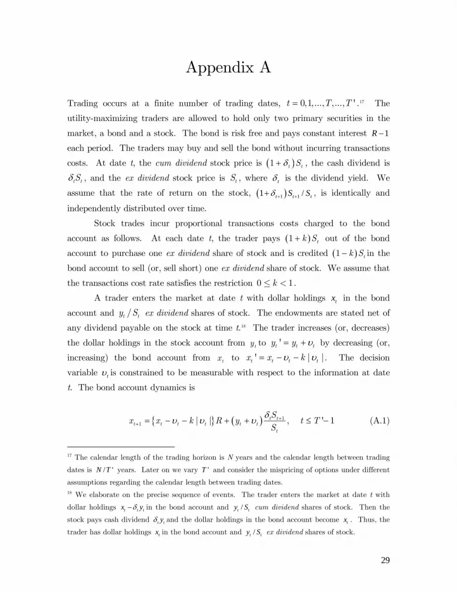
Trading occurs at a finite number of trading dates, = 0,1,..., ,..., 't T T .17 The

utility-maximizing traders are allowed to hold only two primary securities in the

market, a bond and a stock. The bond is risk free and pays constant interest 1R −

each period. The traders may buy and sell the bond without incurring transactions

costs. At date t, the cum dividend stock price is ( )δ+1 t tS , the cash dividend is

δt tS , and the ex dividend stock price is , where tS tδ is the dividend yield. We

assume that the rate of return on the stock, ( )1 11 + ++ t tS Sδ / t , is identically and

independently distributed over time.

Stock trades incur proportional transactions costs charged to the bond

account as follows. At each date t, the trader pays ( )1 tk S+ out of the bond

account to purchase one ex dividend share of stock and is credited ( in the

bond account to sell (or, sell short) one ex dividend share of stock. We assume that

the transactions cost rate satisfies the restriction 0 1.

)1 tk S−

k≤ <A trader enters the market at date t with dollar holdings tx in the bond

account and ex dividend shares of stock. The endowments are stated net of

any dividend payable on the stock at time t.

/ty St

t

18 The trader increases (or, decreases)

the dollar holdings in the stock account from to ty 't ty y υ= + by decreasing (or,

increasing) the bond account from to tx 't t t tx x k | |υ υ= − − . The decision

variable tυ is constrained to be measurable with respect to the information at date

t. The bond account dynamics is

{ } ( ) δυ υ υ ++ = − − + + ≤ −11 | | , 't t

t t t t t tt

Sx x k R y t TS

1

(A.1)

t

17 The calendar length of the trading horizon is N years and the calendar length between trading

dates is years. Later on we vary and consider the mispricing of options under different

assumptions regarding the calendar length between trading dates.

/ 'N T 'T

18 We elaborate on the precise sequence of events. The trader enters the market at date t with

dollar holdings t tx yδ− in the bond account and cum dividend shares of stock. Then the

stock pays cash dividend

/t ty S

t tyδ and the dollar holdings in the bond account become tx . Thus, the

trader has dollar holdings tx in the bond account and ex dividend shares of stock. /t ty S

29

and the stock account dynamics is

( ) 11 , 't

t t tt

Sy y t TS

υ ++ 1.= + ≤ −

T Ty

(A.2)

At the terminal date, the stock account is liquidated, ''υ = −

' |, and the net

worth is . At each date t, the trader chooses investment ' ' |T T Tx y k y+ − tυ to

maximize the expected utility of net worth, ( )' ' '| | |T T T tE u x y k y S⎡ ⎤+ −⎣ ⎦ .19 We

make the plausible assumption that the utility function, ( )u ⋅ , is increasing and

concave, and is defined for both positive and negative terminal net worth.20 Note

that even this weak assumption of monotonicity and concavity of preferences is not

imposed on all agents in the economy but only on the subset of agents that we refer

to as traders.

We recursively define the value function ( ) ( )≡ , ,t tV t V x y t as

( ) { } ( ) ( )υδυ υ υ υ+ +

⎡ ⎤⎛ ⎞= − − + + + +⎢ ⎥⎜ ⎟

⎝ ⎠⎣ ⎦1 1, , max | | , , 1 |t t t

t t t t t tt t

S SV x y t E V x k R y y t SS S

(A.3)

for and ' 1t T≤ −

( ) ( )' ' ' ' ', , ' | |T T T T TV x y T u x y k y= + − . (A.4)

19 The results extend routinely to the case that consumption occurs at each trading date and

utility is defined over consumption at each of the trading dates and over the net worth at the

terminal date. See Constantinides (1979) for details. The model with utility defined over

terminal net worth alone is a more realistic representation of the objective function of financial

institutions. 20 If utility is defined only for non-negative net worth, then the decision variable is constrained to

be a member of a convex set that ensures the non-negativity of net worth. See, Constantinides

(1979) for details. However, the derivation of bounds on the prices of derivatives requires an

entirely different approach and yields weaker bounds. This problem is studied in Constantinides

and Zariphopoulou (1999, 2001).

30

We assume that the parameters satisfy appropriate technical conditions such that

the value function exists and is once differentiable.

Equations (A.1)-(A.4) define a dynamic program that can be numerically

solved for given utility function and stock return distribution. We shall not solve

this dynamic program because our goal is to derive restrictions on the prices of

options that are independent of the specific functional form of the utility function

but solely depend on the plausible assumption that the traders’ utility function is

monotone increasing and concave in the terminal wealth.

The value function is increasing and concave in ( ),t tx y , properties that it

inherits from the assumed monotonicity and concavity of the utility function, as

proven in Constantinides (1979):

( ) ( )> >0, 0x yV t V t , = 0,..., ,..., 't T T . (A.5)

and

( ) ( )( ) ( ) ( ) ( )1 ', 1 ', , , 1 ', ',

0 1, 0,..., ,..., ' .

+ − + − > + −

< < =

α α α α α α

αt t t t t t t tV x x y y t V x y t V x y t

t T T

, (A.6)

On each date, the trader may transfer funds between the bond and stock

accounts and incur transactions costs. Therefore, the marginal rate of substitution

between the bond and stock accounts differs from unity by, at most, the

transactions cost rate:

( ) ( ) ( ) ( ) ( )− ≤ ≤ + =1 1 , 0, ..., , ..., 'x y xk V t V t k V t t T T . (A.7)

Marginal analysis on the bond holdings leads to the following condition on the

marginal rate of substitution between the bond holdings at dates t and t+1:

( ) ( )[ ]1 , 0, ..., , ..., ' 1x t xV t R E V t t T T= + = − . (A.8)

31

Finally, marginal analysis on the stock holdings leads to the following condition on

the marginal rate of substitution between the stock holdings at date t and the bond

and stock holdings at date t+1:

( ) ( ) ( )1 11 1t t ty t y x

t t

S SV t E V t V tS S

δ+ +⎡ ⎤⎥⎥

= + + +⎢⎢⎣ ⎦0,..., ,..., ' 1t T T= −, . (A.9)

32

Appendix B

We allow for three trading dates, 0,1,2t = , at the beginning, middle and end of the

month. We define the stock returns over the first sub-period as

( )δ≡ +1 1iz S1 0/i S , corresponding to the =, 1, ...,I i I states on date one. We

assume that the returns over the two sub-periods are independent. Thus, the stock

returns over the second sub-period, ( )δ≡ + =2 2 11 / , 1,...,k ik iz S S k I , are

independent of i . There are 2,I = =1,..., , 1, ...,i I k I , states on date two.

We define the state-dependent marginal utility of wealth out of the bond

account on each one of the three trading dates as ( ) ( )0 0BxM V≡ ,

and

( ) ( )1 1Bi xM V≡

( ) ( )2Bik xM V≡ 2 . Likewise, we define the state-dependent marginal utility of

wealth out of the stock account on each of the three trading dates as

( ) ( )0 0SyM V≡ , ( ) ( )1S

i yM V≡ 1 and ( ) ( )2Sik yM V≡ 2

I

I

. The conditions on positivity

and monotonicity of the marginal utility of wealth out of the bond and stock

accounts at are given by equations (2.1)-(2.4). The corresponding

conditions at are:

= 0,1t

= 2t

( )2 0, , 1,...,BikM i k> = (B.1)

and

( ) ( ) ( ) ( )1 22 2 ... 2 ... 2 0, 1,...,S S S Si i ik iIM M M M i≥ ≥ ≥ > = . (B.2)

On each date, the trader may transfer funds between the bond and stock

accounts and incur transactions costs. Conditions (2.5) and (2.6) hold. The

corresponding condition at is: = 2t

( ) ( ) ( ) ( ) ( )− ≤ ≤ + =1 2 2 1 2 , , 1,...,B S Bik ik ikk M M k M i k I . (B.3)

Conditions (2.7) and (2.8) on the marginal rate of substitution between

dates zero and one hold. The corresponding conditions between dates one and two

are as follows:

33

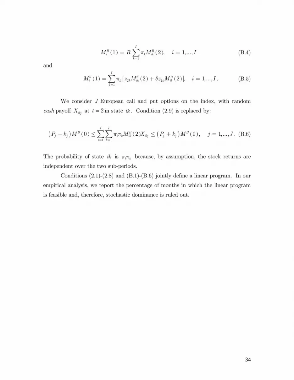
( ) ( )1

1 2 , 1,...,I

B Bi k ik

kM R M iπ

== ∑ I=

I=

J

(B.4)

and

( ) ( ) ( )[ ]2 21

1 2 2 , 1,...,I

S S Bi k k ik k ik

kM z M z M iπ δ

== +∑ . (B.5)

We consider J European call and put options on the index, with random

cash payoff at in state ik . Condition (2.9) is replaced by: ikjX = 2t

( ) ( ) ( ) ( ) ( )1 1

0 2 0 , 1,...,I I

B B Bj j i k ik ikj j j

i kP k M M X P k M jπ π

= =− ≤ ≤ + =∑∑ . (B.6)

The probability of state is because, by assumption, the stock returns are

independent over the two sub-periods.

ik i kπ π

Conditions (2.1)-(2.8) and (B.1)-(B.6) jointly define a linear program. In our

empirical analysis, we report the percentage of months in which the linear program

is feasible and, therefore, stochastic dominance is ruled out.

34

Appendix C

1. Berkeley Options Database

The Berkeley Options Database contains all minute-by-minute quotes and trades of

the European options and futures on the S&P 500 index from April 2, 1986 to

December 29, 1995. Details on this database are found in Jackwerth and

Rubinstein (1996), Jackwerth (2000) and below.

Index Level. Traders typically use the index futures market rather than the

cash market to hedge their option positions. The reason is that the cash market

prices lag futures prices by a few minutes due to lags in reporting transactions of

the constituent stocks in the index. We check this claim by regressing the index on

each of the first twenty minute lags of the futures price. The single regression with

the highest adjusted R2 is assumed to indicate the lag for a given day. The median

lag of the index over the 1542 days from 1986 to 1992 is seven minutes. Because

the index is stale, we compute a futures-based index for each minute from the

futures market as , where F is the futures price at the option

expiration. For each day, we use the median interest rate R implied by all futures

quotes and trades and the index level at that time. We approximate the dividend

yield δ by assuming that the dividend amount and timing expected by the market

were identical to the dividends actually paid on the S&P 500 index. However, some

limited tests indicate that the choice of the index does not seem to affect the results

of this paper.

( ) 10 1S Rδ −= + F

Interest Rate. We compute implied interest rates embedded in the

European put-call parity relation. Armed with option quotes, we calculate separate

lending and borrowing interest returns from put-call parity where we use the above

future-based index. For each expiration date, we assign a single lending and

borrowing rate to each day, which is the median of all daily observations across all

strike prices. We then use the average of these two interest rates as our daily spot

rate for the particular time to expiration. Finally, we obtain the interpolated

interest rates from the implied forward curve. If there is data missing, we assume

35

that the spot rate curve can be extrapolated horizontally for the shorter and longer

times-to-expiration. Again, some limited tests indicate that the results are not

affected by the exact choice of the interest rate.

Option Prices. We use only bid and ask prices on call options. For each

day retained in the sample, we aggregate the quotes to the minute and pick the

minute between 9:00-11:00 AM with the most quotes as our cross section for the

month.

We use only call options with 30 days to expiration which occur once every

month during our sample. We also trim the sample to allow for moneyness levels

between 0.90 and 1.05. Cross sections with fewer than 5 option quotes are

discarded. We also eliminate the cross sections right after the crash of 1987 as the

data is noisy and restart the sample with the cross section expiring on July 15,

1988.

Arbitrage Violations. In the process of setting up the database, we check for

a number of errors which might have been contained in the original minute-by-

minute transaction level data. We eliminate a few obvious data-entry errors as well

as a few quotes with excessive spreads—more than 200 cents for options and 20

cents for futures. General arbitrage violations are eliminated from the data set.

We also check for violations of vertical and butterfly spreads. Within each minute,

we keep the largest set of option quotes which satisfies the restriction

. (1 ) max[0, (1 ) ]i iS C Sδ δ+ ≥ ≥ + −K R

Early exercise is not an issue as the S&P 500 options are European and the

discreteness of quotes and trades only introduces a stronger upward bias in the

midpoint implied volatilities for deep-out-of-the-money puts (moneyness less than

0.6) which we do not use in our empirical work. We start out with 107 raw cross

sections and are left with 98 final cross sections.

2. Option Metrics Database

The Option Metrics Database contains indicative end-of-day European call and put

option quotes on the S&P 500 index from January 2, 1997 to December 31, 2002.

In merging the Option Metrics Database with the Berkeley Options Database, we

36

follow the above procedure as much as possible, given the closing prices data that

the Option Metrics Database provides. Therefore, only departures and innovations

from the above procedure are noted.

Index Level. As the closing (noon) index price, we use the price implied by

the closing (noon) futures price.

Interest Rate. As we cannot arrive at consistently positive interest rates

implied by option prices, we use T-bill rates instead, obtained from Federal Reserve

Bank of St. Louis Economic Research Database (FRED®).

Option Prices. In the final sample, only call and put options with at least

100 traded contracts are included. We calculate a hypothetical noon option cross

section from the closing cross section and the index observed at noon and the close.

Here we assume that the implied volatilities do not change between noon and the

close. We start out with 69 raw cross sections and are left with 68 final cross

sections. The time to expiration is 29 days.

3. S&P 500 Information Bulletin

We obtain the historical daily record of the S&P 500 index and its daily dividend

record over the period 1928-2002 from the S&P 500 Information Bulletin. Before

April 1982, dividends are estimated from monthly dividend yields.

37

Appendix D

The GARCH (1,1) special case of the Engle and Gonzalez-Rivera (1991)

semiparametric model applied to the monthly S&P 500 index return, ty , is

described by equations (D.1)-(D.3):

ε= +ty y t (D.1)

( )ε− ∼1/2 . . . 0,1th i i d g (D.2)

and

ω αε β− −= + +21t th 1th

)

, (D.3)

where is an unknown distribution with zero mean and unit variance. (0,1g

The parameters ( )ω α β, , are estimated by maximum likelihood under the

(false) assumption that ( )1/ 2 . . . 0,1th i i d Nε− ∼ . Then the time series { }ε−1/2t th is

calculated and the true density ( )0,1g is estimated as the histogram of all the time

series observations. The histogram may be smoothed by kernel methods but we do

not undertake this step in order to keep the procedure comparable to that followed

in estimating the unconditional distribution.

One may consider re-estimating the parameters ( ), ,ω α β by maximum

likelihood, replacing the assumption that ( )1/ 2 . . . 0,1th i i d Nε− ∼ with the assumption

that , where is the estimated density in the last step

above. Engle and Gonzalez-Rivera (1991) showed by simulation that this

additional step is unnecessary in practice.

(1/ 2 . . . 0,1th i i d gε− ∼ ) )(0,1g

38

REFERENCES

Ait-Sahalia, Y. and A. W. Lo, 1998. “Nonparametric Estimation of State-Price

Densities Implicit in Financial Prices.” Journal of Finance 53, 499-547.

Ait-Sahalia, Y. and A. W. Lo, 2000. “Nonparametric Risk Management and

Implied Risk Aversion.” Journal of Econometrics 94, 9-51.

Bensaid, B., J-P. Lesne, H. Pagés and J. Scheinkman, 1992. “Derivative Asset

Pricing with Transaction Costs.” Mathematical Finance 2, 63-86.

Benzoni, L., P. Collin-Dufresne, and R. S. Goldstein, 2005. “Can Standard

Preferences Explain the Prices of Out-of-the-Money S&P 500 Options?”,

Working paper, University of Minnesota.

Black, F. and M. S. Scholes, 1973. “The Pricing of Options and Corporate

Liabilities.” Journal of Political Economy 81, 637-654.

Bliss, R. R., and N. Panigirtzoglou, 2004. “Option-Implied Risk Aversion

Estimates”, The Journal of Finance 59, 407-446.

Bollen, N. and R. Whaley, 2004. “Does Net Buying Pressure Affect the Shape of

Implied Volatility Functions?” Journal of Finance 59, 711-753.

Brown, D. and J. C. Jackwerth, 2004. “The Pricing Kernel Puzzle: Reconciling

Index Option Data and Economic Theory.” Working paper, University of

Wisconsin, Madison.

Constantinides, G. M., 1979. “Multiperiod Consumption and Investment Behavior

with Convex Transactions Costs.” Management Science 25, 1127-1137.

Constantinides, G. M. and S. Perrakis, 2002. “Stochastic Dominance Bounds on

Derivatives Prices in a Multiperiod Economy with Proportional Transaction

Costs.” Journal of Economic Dynamics and Control 26, 1323-1352.

Constantinides, G. M. and S. Perrakis, 2004. “Stochastic Dominance Bounds on

American Option Prices in Markets with Frictions.” Working paper,

University of Chicago and Concordia University.

Constantinides, G. M. and T. Zariphopoulou, 1999. “Bounds on Prices of

Contingent Claims in an Intertemporal Economy with Proportional

Transaction Costs and General Preferences.” Finance and Stochastics 3,

345-369.

39

Constantinides, G. M. and T. Zariphopoulou, 2001. “Bounds on Derivative Prices

in an Intertemporal Setting with Proportional Transaction Costs and

Multiple Securities.” Mathematical Finance 11, 331-346.

Engle, R. F. and G. Gonzalez-Rivera, 1991. “Semiparametric ARCH Models.”

Journal of Business and Economic Statistics 9/4, 345-359.

Garcia, R., R. Luger and E. Renault, 2003. “Empirical Assessment of an

Intertemporal Option Pricing Model with Latent Variables.” Journal of

Econometrics 116, 49-83.

Han, B., 2004. “Limits of Arbitrage, Sentiment and Index Option Smile.”

Working paper, Ohio State University.

Hull, J. C., 2005. Options, Futures, and Other Derivatives, Prentice Hall.

Jackwerth, J. C., 2000. “Recovering Risk Aversion from Option Prices and

Realized Returns.” Review of Financial Studies 13, 433-451.

Jackwerth, J. C., 2004. “Option-Implied Risk-Neutral Distributions and Risk

Aversion.” ISBN 0-943205-66-2, Research Foundation of AIMR,

Charlottesville, USA.

Jackwerth, J. C. and M. Rubinstein, 1996. “Recovering Probability Distributions

from Option Prices.” Journal of Finance 51, 1611-1631.

Leland, H. E., 1985. “Option Pricing and Replication with Transactions Costs.”

Journal of Finance 40, 1283-1301.

Levy, H., 1985. “Upper and Lower Bounds of Put and Call Option Value:

Stochastic Dominance Approach.” Journal of Finance 40, 1197-1217.

Liu, J., J. Pan, and T. Wang, 2005. “An Equilibrium Model of Rare-event Premia

and Its Implications for Option Smirks.” Review of Financial Studies 18,

131-164.

McDonald, R. L., 2003. Derivatives Markets, Addison-Wesley.

Merton, R. C., 1973. “Theory of Rational Option Pricing.” Bell Journal of

Economics and Management Science 4, 141-183.

Pan, J., 2002. “The Jump-Risk Premia Implicit in Option Prices: Evidence from an

Integrated Time-Series Study.” Journal of Financial Economics 63, 3-50.

Perrakis, S., 1986. “Option Bounds in Discrete Time: Extensions and the Pricing

of the American Put.” Journal of Business 59, 119-141.

40

Perrakis, S., 1993. “Option Pricing for Multinomial Stock Returns in Diffusion and

Mixed Processes.” Canadian Journal of Administrative Sciences 10, 68-82.

Perrakis, S., and P. J. Ryan, 1984. “Option Pricing Bounds in Discrete Time.”

Journal of Finance 39, 519-525.

Ritchken, P. H., 1985. “On Option Pricing Bounds.” Journal of Finance 40, 1219-

1233.

Ritchken, P.H. and S. Kuo, 1988. “Option Bounds with Finite Revision

Opportunities.” Journal of Finance 43, 301-308.

Rosenberg, J. V. and R. F. Engle, 2002. “Empirical Pricing Kernels.” Journal of

Financial Economics 64, 341-372.

Rubinstein, M., 1994. “Implied Binomial Trees.” Journal of Finance 49, 771-818.

Ryan, P. J., 2000. “Tighter Option Bounds from Multiple Exercise Prices.”

Review of Derivatives Studies 4, No. 2, 155-188.

Ryan, P. J., 2003. “Progressive Option Bounds from the Sequence of Concurrently

Expiring Options.” European Journal of Operational Research 151, 193-223.

Santa-Clara, P. and S. Yan, 2004. “Jump and Volatility Risk and Risk Premia: A

New Model and Lessons from S&P 500 Options.” Working paper, UCLA.

Shefrin, H., 2005. A Behavioral Approach to Asset Pricing, Elsevier/North-

Holland, Amsterdam.

Silverman, B. W., 1986. Density Estimation, Chapman and Hall, London.

Whaley, R. E., 2003. “Derivatives.” In G. M. Constantinides, M. Harris, and R.

Stulz, eds., Financial Markets and Asset Pricing: Handbook of the

Economics of Finance, Volume 1B. Handbooks in Economics 21

Elsevier/North-Holland, Amsterdam.

41

Table 1. Percentage of Months without Stochastic Dominance Violations in the

Single-Period Case

The table displays the percentage of months in which stochastic dominance violations are absent in

the cross section of option prices. In brackets, the table displays the bootstrap standard errors of

these percentages. The one-way transactions cost rate (one-way trading fees plus half the bid-ask

spread) on the index is 50 bps. The one-way transactions cost on each option is proportional to the

index price, as explained in Section 3.2. In the second (or, third) row of each cell, the table displays

the percentage of months without violations when the one-way proportional transactions costs on

each option are equal to 5 (or, 50) bps of the index price.

Panel A:

860516-

871016

Panel B:

880715-

910315

Panel C:

910419-

930820

Panel D:

930917-

951215

Panel E:

970221-

991217

Panel F:

000218-

021220

Number of Months 15 29 28 26 35 33

Historical Index Sample

1928-1986

73 (20)

60

87

90 (13)

59

90

100 (13)

46

100

92 (30)

0

96

60 (23)

14

80

48 (19)

21

61

Historical Index Sample

1972-1986

73

33

73

76

52

90

100

50

100

92

4

96

34

6

66

27

9

48

Forward-Looking Index

Sample (including the

crash) 1987-2002

40

13

67

76

48

83

100

61

100

96

12

96

26

14

43

15

3

33

Forward-Looking Index

Sample (excluding the

crash) 1988-2002

47

20

73

76

48

86

100

54

100

92

4

96

31

3

60

24

9

36

Index Sample 1972-2002

with Conditional Index

Return Distribution

47

27

60

86

48

97

89

75

100

100

65

100

40

9

54

58

18

67

42

Table 2. Percentage of Months without Stochastic Dominance Violations in the

Single-Period Case—ITM and OTM Calls Separately

The table displays the percentage of months in which stochastic dominance violations are absent in

the cross section of in-the-money calls (top entry) and out-of-the-money calls (bottom entry). The

one-way transactions cost rate (one-way trading fees plus half the bid-ask spread) on the index is 50

bps. The one-way transactions costs on each option are proportional to the index price, as explained

in Section 3.2.

Panel A:

860516-

871016

Panel B:

880715-

910315

Panel C:

910419-

930820

Panel D:

930917-

951215

Panel E:

970221-

991217

Panel F:

000218-

021220

Number of Months 15 29 28 26 35 33

Historical Index Sample

1928-1986

93

73

90

90

100

100

100

92

74

63

58

48

Historical Index Sample

1972-1986

73

73

83

76

100

100

100

92

43

34

39

27

Forward-Looking Index

Sample (including the

crash) 1987-2002

73

40

83

76

100

100

100

96

46

26

39

15

Forward-Looking Index

Sample (excluding the

crash) 1988-2002

73

47

83

76

100

100

100

92

46

31

39

24

Index Sample 1972-2002

with Conditional Index

Return Distribution

80

47

93

86

96

89

100

100

49

40

67

58

43

Table 3. Percentage of Months without Stochastic Dominance Violations in the

Single-Period Case and Fixed Transactions Costs

The table displays the percentage of months in which stochastic dominance violations are absent in

the cross section of option prices. The one-way transactions costs rate (one-way trading fees plus

half the bid-ask spread) on the index is 50 bps. The one-way transactions costs on each option are

20 bps of the index price.

Panel A:

860516-

871016

Panel B:

880715-

910315

Panel C:

910419-

930820

Panel D:

930917-

951215

Panel E:

970221-

991217

Panel F:

000218-

021220

Number of Months 15 29 28 26 35 33

Historical Index Sample

1928-1986

73

86 86 31 66 48

Historical Index Sample

1972-1986

73

83 89 42 43 30

Forward-Looking Index

Sample (including the

crash) 1987-2002

60 79 89 50 40 33

Forward-Looking Index

Sample (excluding the

crash) 1988-2002

67 72 89 46 40 30

Index Sample 1972-2002

with Conditional Index

Return Distribution

47 93 96 100 43 64

44

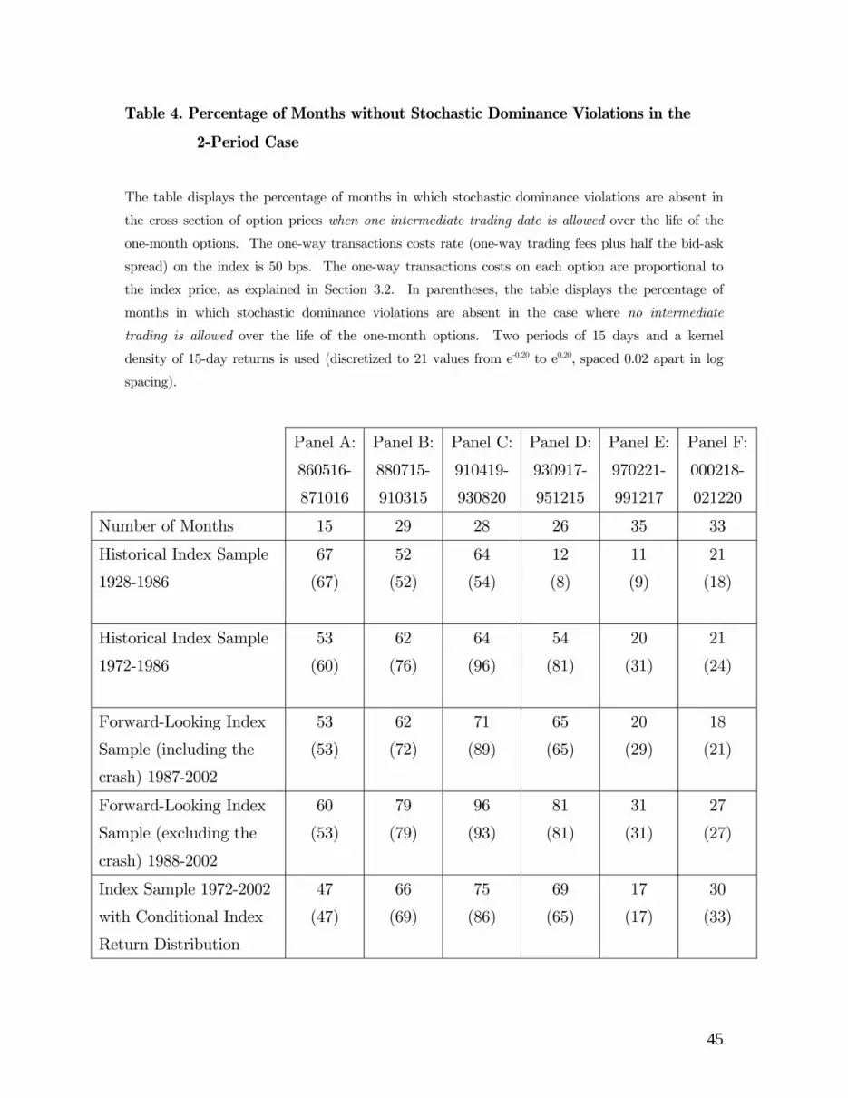
Table 4. Percentage of Months without Stochastic Dominance Violations in the

2-Period Case

The table displays the percentage of months in which stochastic dominance violations are absent in

the cross section of option prices when one intermediate trading date is allowed over the life of the

one-month options. The one-way transactions costs rate (one-way trading fees plus half the bid-ask

spread) on the index is 50 bps. The one-way transactions costs on each option are proportional to

the index price, as explained in Section 3.2. In parentheses, the table displays the percentage of

months in which stochastic dominance violations are absent in the case where no intermediate

trading is allowed over the life of the one-month options. Two periods of 15 days and a kernel

density of 15-day returns is used (discretized to 21 values from e-0.20 to e0.20, spaced 0.02 apart in log

spacing).

Panel A:

860516-

871016

Panel B:

880715-

910315

Panel C:

910419-

930820

Panel D:

930917-

951215

Panel E:

970221-

991217

Panel F:

000218-

021220

Number of Months 15 29 28 26 35 33

Historical Index Sample

1928-1986

67

(67)

52

(52)

64

(54)

12

(8)

11

(9)

21

(18)

Historical Index Sample

1972-1986

53

(60)

62

(76)

64

(96)

54

(81)

20

(31)

21

(24)

Forward-Looking Index

Sample (including the

crash) 1987-2002

53

(53)

62

(72)

71

(89)

65

(65)

20 18

(29) (21)

Forward-Looking Index

Sample (excluding the

crash) 1988-2002

60

(53)

79

(79)

96

(93)

81

(81)

31

(31)

27

(27)

Index Sample 1972-2002

with Conditional Index

Return Distribution

47

(47)

66

(69)

75

(86)

69

(65)

17

(17)

30

(33)

45

Figure 1. Bound Violations Based on the Historical Index Sample 1928-1986 The six panels display the upper and lower option bounds (implied volatilities) calculated with the

index return distribution based on the historical index sample 1928-1986, as a function of the

moneyness (K/S). The figures also display the observed bid (circles) and ask (crosses) option implied

volatilities over the pre-crash period (panel A) and the five post-crash periods (panels B-F). The

transactions costs rate on the index is 20 bps.

Panel A

0

0.1

0.2

0.3

0.4

0.5

0.9 0.95 1 1.05

Moneyness

Impl

ied

Vola

tility

Panel B

0

0.1

0.2

0.3

0.4

0.5

0.9 0.95 1 1.05

MoneynessIm

plie

d Vo

latil

ity

Panel C

0

0.1

0.2

0.3

0.4

0.5

0.9 0.95 1 1.05

Moneyness

Impl

ied

Vola

tility

Panel D

0

0.1

0.2

0.3

0.4

0.5

0.9 0.95 1 1.05

Moneyness

Impl

ied

Vola

tility

Panel E

0

0.1

0.2

0.3

0.4

0.5

0.9 0.95 1 1.05

Moneyness

Impl

ied

Vola

tility

Panel F

0

0.1

0.2

0.3

0.4

0.5

0.9 0.95 1 1.05

Moneyness

Impl

ied

Vola

tility

46

Figure 2. Bound Violations Based on the Historical Index Sample 1972-1986 The six panels display the upper and lower option bounds (implied volatilities) calculated with the

index return distribution based on the historical index sample 1972-1986, as a function of the

moneyness (K/S). The figures also display the observed bid (circles) and ask (crosses) option implied

volatilities over the pre-crash period (panel A) and the five post-crash periods (panels B-F). The

transactions costs rate on the index is 20 bps.

Panel A

0

0.1

0.2

0.3

0.4

0.5

0.9 0.95 1 1.05

Moneyness

Impl

ied

Vola

tility

Panel B

0

0.1

0.2

0.3

0.4

0.5

0.9 0.95 1 1.05

MoneynessIm

plie

d Vo

latil

ity

Panel C

0

0.1

0.2

0.3

0.4

0.5

0.9 0.95 1 1.05

Moneyness

Impl

ied

Vola

tility

Panel D

0

0.1

0.2

0.3

0.4

0.5

0.9 0.95 1 1.05

Moneyness

Impl

ied

Vola

tility

Panel E

0

0.1

0.2

0.3

0.4

0.5

0.9 0.95 1 1.05

Moneyness

Impl

ied

Vola

tility

Panel F

0

0.1

0.2

0.3

0.4

0.5

0.9 0.95 1 1.05

Moneyness

Impl

ied

Vola

tility

47

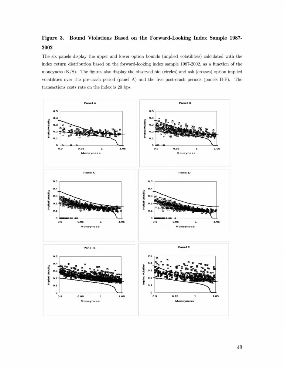
Figure 3. Bound Violations Based on the Forward-Looking Index Sample 1987-

2002 The six panels display the upper and lower option bounds (implied volatilities) calculated with the

index return distribution based on the forward-looking index sample 1987-2002, as a function of the

moneyness (K/S). The figures also display the observed bid (circles) and ask (crosses) option implied

volatilities over the pre-crash period (panel A) and the five post-crash periods (panels B-F). The

transactions costs rate on the index is 20 bps.

Panel A

0

0.1

0.2

0.3

0.4

0.5

0.9 0.95 1 1.05

Moneyness

Impl

ied

Vola

tility

Panel B

0

0.1

0.2

0.3

0.4

0.5

0.9 0.95 1 1.05

Moneyness

Impl

ied

Vola

tility

Panel C

0

0.1

0.2

0.3

0.4

0.5

0.9 0.95 1 1.05

Moneyness

Impl

ied

Vola

tility

Panel D

0

0.1

0.2

0.3

0.4

0.5

0.9 0.95 1 1.05

Moneyness

Impl

ied

Vola

tility

Panel E

0

0.1

0.2

0.3

0.4

0.5

0.9 0.95 1 1.05

Moneyness

Impl

ied

Vola

tility

Panel F

0

0.1

0.2

0.3

0.4

0.5

0.9 0.95 1 1.05

Moneyness

Impl

ied

Vola

tility

48

Figure 4. Bound Violations Based on the Forward-Looking Index Sample 1988-

2002 The six panels display the upper and lower option bounds (implied volatilities) calculated with the

index return distribution based on the forward-looking index sample 1988-2002, as a function of the

moneyness (K/S). The figures also display the observed bid (circles) and ask (crosses) option implied

volatilities over the pre-crash period (panel A) and the five post-crash periods (panels B-F). The

transactions costs rate on the index is 20 bps.

Panel A

0

0.1

0.2

0.3

0.4

0.5

0.9 0.95 1 1.05

Moneyness

Impl

ied

Vola

tility

Panel B

0

0.1

0.2

0.3

0.4

0.5

0.9 0.95 1 1.05

Moneyness

Impl

ied

Vola

tility

Panel C

0

0.1

0.2

0.3

0.4

0.5

0.9 0.95 1 1.05

Moneyness

Impl

ied

Vola

tility

Panel D

0

0.1

0.2

0.3

0.4

0.5

0.9 0.95 1 1.05

Moneyness

Impl

ied

Vola

tility

Panel F

0

0.1

0.2

0.3

0.4

0.5

0.9 0.95 1 1.05

Moneyness

Impl

ied

Vola

tility

Panel E

0

0.1

0.2

0.3

0.4

0.5

0.9 0.95 1 1.05

Moneyness

Impl

ied

Vola

tility

49