ARTICLE IN PRESS

0167-7152/$ - se

doi:10.1016/j.sp

�CorrespondE-mail addr

Statistics & Probability Letters 78 (2008) 608–615

www.elsevier.com/locate/stapro

Minimax designs for optimum mixtures

Manisha Pal, Nripes Kumar Mandal�

Department of Statistics, University of Calcutta, Kolkata 700 019, India

Received 13 March 2006; received in revised form 28 June 2006; accepted 7 September 2007

Available online 26 October 2007

Abstract

In a mixture experiment the measured response is assumed to depend only on the relative proportion of ingredients or

components present in the mixture. Scheffe [1958. Experiments with mixtures. Journal of Royal Statistical Society B 20,

pp. 344–360; 1963. Simplex-centroid design for experiments with mixtures. Journal of Royal Statistical Society B 25,

235–263] first systematically considered this problem and introduced different models and designs suitable in such

situations. Optimum designs for the estimation of parameters of different mixture models are available in the literature.

The problem of estimating the optimum proportion of mixture components is of great practical importance. Pal and

Mandal [2006. Optimum designs for optimum mixtures. Statistics and Probability Letters 76, 1369–1379] first attempted to

find a solution to this problem using the trace criterion, assuming prior knowledge about the optimum mixing proportions.

In this paper the minimax criterion has been employed to find a solution to the above problem.

r 2007 Published by Elsevier B.V.

MSC: 62K99; 62J05

Keywords: Mixture experiments; Second-order models; Non-linear function; Asymptotic efficiency; Weighted centroid designs; Partial

Loewner Ordering; Minimax criterion

1. Introduction

In a mixture experiment, the response depends on the proportions x1, x2,y,xq of a number of ingredientssatisfying xiX0;

Pqi¼1xi ¼ 1. Scheffe (1958, 1963) introduced canonical models of different degrees to

represent the response function Bx. He also introduced Simplex Lattice Designs and Simplex Centroid Designsin such situations. Optimality of mixture designs for the estimation of parameters of the response function wasconsidered by Kiefer (1961, 1975), Galil and Kiefer (1977), Liu and Neudecker (1995), among others. Draperand Pukelsheim (1999) established the optimality of Weighted Centroid Designs with respect to PartialLoewner Ordering (PLO) for two and three component mixtures.

The problem of estimating the optimum mixture combination in a mixture experiment is of great practicalimportance. In pharmaceutical research, for example, response is the potency of a new drug relative to anestablished one and the problem is to find the optimum proportion of the mixing substances so that the

e front matter r 2007 Published by Elsevier B.V.

l.2007.09.022

ing author.

ess: mandalnk2001@yahoo.co.in (N.K. Mandal).

ARTICLE IN PRESSM. Pal, N.K. Mandal / Statistics & Probability Letters 78 (2008) 608–615 609

relative potency is maximized. Pal and Mandal (2006) (henceforth to be referred as PM) probably firstattempted to find optimum designs for the estimation of optimum mixture combination. They solved theproblem under the assumption that the response function can be approximated by a second degree concavefunction in the mixture components. The optimum mixture combination g came out to be a non-linearfunction of the unknown parameters in the response function. A pseudo-Bayesian approach was pursued bywhere g was assumed to have a prior distribution with known second order raw moments and the criterionused to get the optimum design was minimization of the expected trace of MSEðgÞ.

As mentioned in PM, there are several ways of tackling the presence of unknown parameters in any measureof accuracy. In this paper, we attempt to solve the problem using minimax criterion. In Section 2 we formulatethe problem and use the concept of invariance and concavity property of the criterion function to substantiallyreduce the class of competing designs. In Section 3 the optimal designs are obtained for q ¼ 2 and 3.

2. Investigation of the problem

As in PM, we assume the response function to be quadratic concave in the components x1, x2,y,xq in thefactor space X ¼ {(x1, x2,y,xq)|xiX0, i ¼ 1(1)q,

Pxi ¼ 1} and to have the form

EðY jxÞ ¼ Bx ¼X

i

biix2i þ

Xioj

bijxixj ¼ f 0ðxÞy, (1)

where

x ¼ ðx1; x2; . . . ;xqÞ0,

f ðxÞ ¼ ðx21; x

22; . . . ;x

2q;x1x2;x1x3; . . . ;xq�1xqÞ

0,

y ¼ ðb11;b22; . . . ;bqq;b12;b13; . . . ; bq�1;qÞ0,

f(x) and y being p� 1 vectors with p ¼ ðqþ12 Þ.

The response function (1) can also be expressed in the form

Bx ¼ x0Bx

with

B ¼

b11 ð1=2Þb12 ð1=2Þb13 . . . ð1=2Þb1q

b22 ð1=2Þb23 . . . ð1=2Þb2q

. . . . . . . . . . . . . . .

bqq

0BBBB@

1CCCCA.

We assume that B is negative definite so that, subject toPq

i¼1xi ¼ 1, Bx is maximized at x ¼ g, where

g ¼ d�1B�1 1 (2)

with d ¼ 10 B�1 1. We are interested in estimating the non-linear function g given by (2) as accurately aspossible by a proper choice of a design in X.

Let x be an arbitrary design in X and MðxÞ ¼RX f ðxÞf 0ðxÞdxðxÞ, the information matrix of x. For a given

design x, we can estimate B by B, the least squares estimator of B, and hence d by d. Then, replacing d and B

by d and B respectively in (2), we get an estimate of g as

g ¼ d�1

B�1

1 . (3)

Under suitable regularity assumptions on error distribution, the standard q-method gives, for large n, anadequate approximation of the dispersion matrix of g as

E½ðg� gÞðg� gÞ0� ¼ AðgÞM�1ðxÞA0ðgÞ, (4)

ARTICLE IN PRESSM. Pal, N.K. Mandal / Statistics & Probability Letters 78 (2008) 608–615610

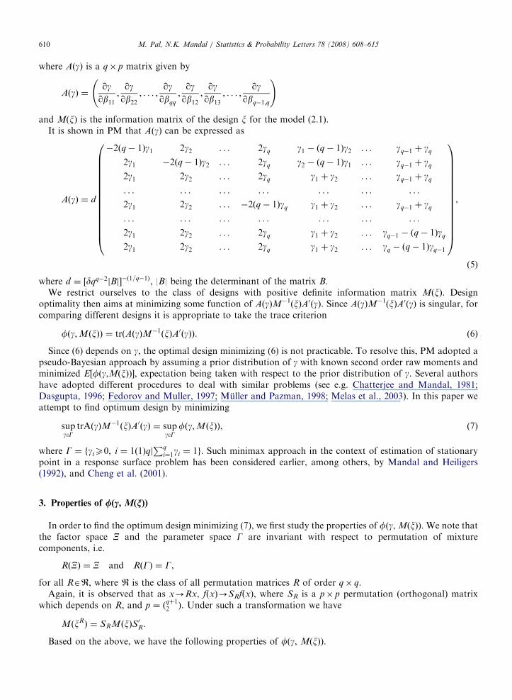
where A(g) is a q� p matrix given by

AðgÞ ¼qgqb11

;qgqb22

; . . . ;qgqbqq

;qgqb12

;qgqb13

; . . . ;qg

qbq�1;q

!

and M(x) is the information matrix of the design x for the model (2.1).It is shown in PM that A(g) can be expressed as

AðgÞ ¼ d

�2ðq� 1Þg1 2g2 . . . 2gq g1 � ðq� 1Þg2 . . . gq�1 þ gq

2g1 �2ðq� 1Þg2 . . . 2gq g2 � ðq� 1Þg1 . . . gq�1 þ gq

2g1 2g2 . . . 2gq g1 þ g2 . . . gq�1 þ gq

. . . . . . . . . . . . . . . . . . . . .

2g1 2g2 . . . �2ðq� 1Þgq g1 þ g2 . . . gq�1 þ gq

. . . . . . . . . . . . . . . . . . . . .

2g1 2g2 . . . 2gq g1 þ g2 . . . gq�1 � ðq� 1Þgq

2g1 2g2 . . . 2gq g1 þ g2 . . . gq � ðq� 1Þgq�1

0BBBBBBBBBBBBBB@

1CCCCCCCCCCCCCCA

,

(5)

where d ¼ ½dqq�2jBj��ð1=q�1Þ, |B| being the determinant of the matrix B.We restrict ourselves to the class of designs with positive definite information matrix M(x). Design

optimality then aims at minimizing some function of A(g)M�1(x)A0(g). Since A(g)M�1(x)A0(g) is singular, forcomparing different designs it is appropriate to take the trace criterion

fðg;MðxÞÞ ¼ trðAðgÞM�1ðxÞA0ðgÞÞ. (6)

Since (6) depends on g, the optimal design minimizing (6) is not practicable. To resolve this, PM adopted apseudo-Bayesian approach by assuming a prior distribution of g with known second order raw moments andminimized E[f(g,M(x))], expectation being taken with respect to the prior distribution of g. Several authorshave adopted different procedures to deal with similar problems (see e.g. Chatterjee and Mandal, 1981;Dasgupta, 1996; Fedorov and Muller, 1997; Muller and Pazman, 1998; Melas et al., 2003). In this paper weattempt to find optimum design by minimizing

supg�G

trAðgÞM�1ðxÞA0ðgÞ ¼ supg�G

fðg;MðxÞÞ, (7)

where G ¼ fgiX0; i ¼ 1ð1ÞqjPq

i¼1gi ¼ 1g: Such minimax approach in the context of estimation of stationarypoint in a response surface problem has been considered earlier, among others, by Mandal and Heiligers(1992), and Cheng et al. (2001).

3. Properties of /(c, M(n))

In order to find the optimum design minimizing (7), we first study the properties of f(g, M(x)). We note thatthe factor space X and the parameter space G are invariant with respect to permutation of mixturecomponents, i.e.

RðXÞ ¼ X and RðGÞ ¼ G,

for all RAR, where R is the class of all permutation matrices R of order q� q.Again, it is observed that as x-Rx, f(x)-SRf(x), where SR is a p� p permutation (orthogonal) matrix

which depends on R, and p ¼ ðqþ12 Þ. Under such a transformation we have

MðxRÞ ¼ SRMðxÞS0R.

Based on the above, we have the following properties of f(g, M(x)).

ARTICLE IN PRESSM. Pal, N.K. Mandal / Statistics & Probability Letters 78 (2008) 608–615 611

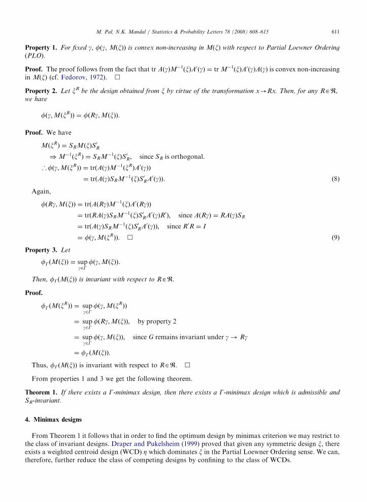
Property 1. For fixed g, f(g, M(x)) is convex non-increasing in M(x) with respect to Partial Loewner Ordering

(PLO).

Proof. The proof follows from the fact that tr A(g)M�1(x)A0(g) ¼ tr M�1(x)A0(g)A(g) is convex non-increasingin M(x) (cf. Fedorov, 1972). &

Property 2. Let xR be the design obtained from x by virtue of the transformation x-Rx. Then, for any RAR,we have

fðg;MðxRÞÞ ¼ fðRg;MðxÞÞ.

Proof. We have

MðxRÞ ¼ SRMðxÞS0R

)M�1ðxRÞ ¼ SRM�1ðxÞS0R; since SR is orthogonal.

‘fðg;MðxRÞÞ ¼ trðAðgÞM�1ðxR

ÞA0ðgÞÞ

¼ trðAðgÞSRM�1ðxÞS0RA0ðgÞÞ. ð8Þ

Again,

fðRg;MðxÞÞ ¼ trðAðRgÞM�1ðxÞA0ðRgÞÞ

¼ trðRAðgÞSRM�1ðxÞS0RA0ðgÞR0Þ; since AðRgÞ ¼ RAðgÞSR

¼ trðAðgÞSRM�1ðxÞS0RA0ðgÞÞ; since R0R ¼ I

¼ fðg;MðxRÞÞ: & ð9Þ

Property 3. Let

fGðMðxÞÞ ¼ supg2G

fðg;MðxÞÞ.

Then, fG(M(x)) is invariant with respect to RAR.

Proof.

fGðMðxRÞÞ ¼ sup

g2Gfðg;MðxR

ÞÞ

¼ supg2G

fðRg;MðxÞÞ; by property 2

¼ supg2G

fðg;MðxÞÞ; since G remains invariant under g! Rg

¼ fGðMðxÞÞ.

Thus, fG(M(x)) is invariant with respect to RAR. &

From properties 1 and 3 we get the following theorem.

Theorem 1. If there exists a G-minimax design, then there exists a G-minimax design which is admissible and

SR-invariant.

4. Minimax designs

From Theorem 1 it follows that in order to find the optimum design by minimax criterion we may restrict tothe class of invariant designs. Draper and Pukelsheim (1999) proved that given any symmetric design x, thereexists a weighted centroid design (WCD) Z which dominates x in the Partial Loewner Ordering sense. We can,therefore, further reduce the class of competing designs by confining to the class of WCDs.

ARTICLE IN PRESSM. Pal, N.K. Mandal / Statistics & Probability Letters 78 (2008) 608–615612

4.1. Two factors

Consider the case of two factors. Here the vertex point design Z1 and the overall centroid design Z2 aregiven by

Z11

0

� �¼ Z1

0

1

� �¼ 1

2; Z2

1212

!¼ 1. (10)

A WCD is given by Z ¼ aZ1 þ ð1� aÞZ2 with mass a/2 at each vertex point and 0pap1. From PM theinformation matrix of WCD is given by

MðZÞ ¼ ð 116Þ

1þ 7a 1� a 1� a

1þ 7a 1� a

1� a

0B@

1CA.

So,

M�1ðZÞ ¼ 2að1�aÞ

1� a 0 �ð1� aÞ

1� a �ð1� aÞ

2ð1þ 3aÞ

0B@

1CA

‘ fðg;MðZÞÞ ¼ ð2d2=að1� aÞÞg0Cg;

where

C ¼5� a �2

�2 5� a

� �and d2

¼ d2jBj�2.

Clearly C40, and hence f(g,M(Z)) is a convex function of g. So, f(g,M(Z)) is maximized at the extremepoints

g ¼0

1

� �and g ¼

1

0

� �

where f(g,M(Z)) has the same value.

‘ maxg2G

fðg;MðZÞÞ ¼2d2ð5� aÞ

að1� aÞ¼ 2d2 5

aþ

4

1� a

� �. (11)

It is easy to see that the value of a which minimizes (11) is

aopt ¼

ffiffiffi5pffiffiffi4pþ

ffiffiffi5p ¼ 0:5279

and

min0pap1

maxg2G

fðg;MðZÞÞ ¼ 35:8885d2.

4.2. Three factors

In the case of three factors, the class of WCD consists of design Z1 supported by three vertex points, designZ2 supported by three midpoints of the edges and the overall centroid design Z3:

Z1

1

0

0

0B@

1CA ¼ Z1

0

1

0

0B@

1CA ¼ Z1

0

0

1

0B@

1CA ¼ 1

3Z2

1212

0

0B@

1CA ¼ Z2

12

012

0B@

1CA ¼ Z2

01212

0B@

1CA ¼ 1

3; Z3

121212

0B@1CA ¼ 1.

ARTICLE IN PRESSM. Pal, N.K. Mandal / Statistics & Probability Letters 78 (2008) 608–615 613

Attaching weights a1, a2 and a3 respectively to Z1, Z2 and Z3 with aiX0, i ¼ 1, 2, 3 andP3

i¼1ai ¼ 1, a WCDis given by Z ¼ a1Z1+a2Z2+a3Z3. This means the design assigns mass a1/3 to each of the vertices (1, 0, 0)0,(0, 1, 0)0 and (0, 0, 1)0, mass a2/3 to each of the three midpoints of the edges (1

2, 12, 0)0, (1

2, 0, 1

2)0 and (0, 1

2, 12)0, and

mass a3 to the overall centroid point (13, 13, 13)0.

From PM the information matrix of Z is given by

MðZÞ ¼

a b b b b b

a b b c b

a c b b

b c c

b c

b

0BBBBBBBB@

1CCCCCCCCA, (12)

where a ¼ 181ð1þ 26a1 þ 19

8a2Þ, b ¼ 1

81ð1� a1 þ 11

16a2Þ and c ¼ 1

81ð1� a1 � a2Þ, and a3 is replaced by 1�a1�a2.

Clearly, M�1(Z) will be of the form

M�1ðZÞ ¼

e f f g g h

e f g h g

e h g g

k m m

k m

k

0BBBBBBBB@

1CCCCCCCCA, (13)

where e, f, g, h, k, m are as follows:

e ¼a

ðaþ 2bÞðaþ c� 2bÞ�

2bþ c

aþ 2bg; f ¼ �

2b

ðaþ 2bÞðaþ c� 2bÞ�

2bþ c

aþ 2bg,

h ¼1

aþ c� 2bþ g; k ¼ �

a� c

b� cg,

m ¼1

b� c

b� a

aþ c� 2bþ ðc� aÞg

� �; g ¼

abþ ac� 2b2

ðaþ c� 2bÞð2b2� ab� 2acþ c2Þ

. ð14Þ

Then

fðg;MðZÞÞ ¼X3i¼1

l0iM�1ðZÞli (15)

where l01, l02 and l03 are the rows of A(g).From (15), for q ¼ 3, we have

l0i ¼ g0Di; i ¼ 1; 2; 3,

where

D1 ¼ d

�4 0 0 1 1 0

0 2 0 �2 0 1

0 0 2 0 �2 1

0BB@

1CCA; D2 ¼ d

2 0 0 �2 1 0

0 �4 0 1 0 1

0 0 2 0 1 �2

0BB@

1CCA,

D3 ¼ d

2 0 0 1 �2 0

0 2 0 1 0 �2

0 0 �4 0 1 1

0BB@

1CCA.

Hence, fðg;MðZÞÞ ¼ g0ðP3

i¼1DiM�1ðZÞD0iÞg, which is a convex function of g since M�1(Z) is positive definite.

Thus, f(g,M(Z)) is maximized at some boundary point of G.

ARTICLE IN PRESSM. Pal, N.K. Mandal / Statistics & Probability Letters 78 (2008) 608–615614

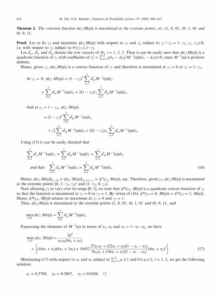
Theorem 2. The criterion function f(g,M(Z)) is maximized at the extreme points, viz. (1, 0, 0)0, (0, 1, 0)0 and

(0, 0, 1)0.

Proof. Let us fix g3 and maximize f(g,M(Z)) with respect to g1 and g2 subject to g1+g2 ¼ 1�g3, g1, g2X0,i.e. with respect to g1 subject to 0pg1p1�g3.

Let d 01i, d 02i and d 03i denote the row vectors of Di, i ¼ 1, 2, 3. Then it can be easily seen that f(g,M(Z)) is aquadratic function of g1 with coefficient of g21 ¼

P3i¼1ðd1i � d2iÞ

0M�1ðZÞðd1i � d2iÞX0, since M�1(Z) is positivedefinite.

Hence, given g3, f(g,M(Z)) is a convex function of g1 and therefore is maximized at g1 ¼ 0 or g1 ¼ 1�g3.

At g1 ¼ 0; fðg;MðZÞÞ ¼ ð1� g3Þ2X3i¼1

d 02iM�1ðZÞd2i

þX3i¼1

d 03iM�1ðZÞd3i þ 2ð1� g3Þg3

X3i¼1

d 02iM�1ðZÞd3i.

And at g1 ¼ 1� g3; fðg;MðZÞÞ

¼ ð1� g3Þ2X3i¼1

d 01iM�1ðZÞd1i

þ g23X3i¼1

d 03iM�1ðZÞd3i þ 2ð1� g3Þg3

X3i¼1

d 01iM�1ðZÞd3i.

Using (13) it can be easily checked that

X3i¼1

d 01iM�1ðZÞd1i ¼

X3i¼1

d 02iM�1ðZÞd2i ¼

X3i¼1

d 03iM�1ðZÞd3i

and thatX3i¼1

d 01iM�1ðZÞd3i ¼

X3i¼1

d 02iM�1ðZÞd3i. ð16Þ

Hence, fðg;MðZÞÞjg1¼0 ¼ fðg;MðZÞÞjg1¼1�g3 ¼ f�ðg3;MðZÞÞ, say. Therefore, given g3, f(g,M(Z)) is maximizedat the extreme points (0, 1�g3, g3)0 and (1�g3, 0, g3)0.

Now allowing g3 to vary over its range [0, 1], we note that f*(g3, M(Z)) is a quadratic convex function of g3so that the function is maximized at g3 ¼ 0 or g3 ¼ 1. By virtue of (16), f*(g3 ¼ 0, M(Z)) ¼ f*(g3 ¼ 1, M(Z)).Hence f*(g3, M(Z)) attains its maximum at g3 ¼ 0 and g3 ¼ 1.

Thus, f(g,M(Z)) is maximized at the extreme points (1, 0, 0)0, (0, 1, 0)0 and (0, 0, 1)0, and

maxg2G

fðg;MðZÞÞ ¼X3i¼1

d 03iM�1ðZÞd3i.

Expressing the elements of M�1(Z) in terms of a1, a2 and a3 ¼ 1�a1�a2, we have

maxg2G

fðg;MðZÞÞ ¼3d2

a1a2ð8a1 þ a2Þ

� ð16a1 þ a2Þð8a1 þ 3a2Þ þ 1843227a1a2 þ ð32a1 þ a2Þð1� a1 � a2Þ9a1a2 þ ð16a1 þ a2Þð1� a1 � a2Þ

ð4a1 þ a2Þ2

� �. ð17Þ

Minimizing (17) with respect to a1 and a2 subject toP2

i¼1aip1 and 0paip1, i ¼ 1, 2, we get the followingsolution:

a1 ¼ 0:3789; a2 ¼ 0:5867; a3 ¼ 0:0344: &

ARTICLE IN PRESSM. Pal, N.K. Mandal / Statistics & Probability Letters 78 (2008) 608–615 615

5. Conclusion

In selecting the design, we have used the criterion of minimizing

maxg2G

Trace E½ðg� gÞðg� gÞ0�.

It has been noted that the optimum designs obtained by PM and the minimax criterion are members of theclass of WCD. However, the design given by PM puts positive mass at the vertices and the midpoints of theedges and zero mass at the overall centroid point. On the other hand, the minimax criterion leads to a designwhich assigns positive mass to all the support points of WCD.

The present paper deals with mixture experiments involving only two- and three-factors. Attempt may bemade to extend it to the case of general q-component mixture.

Acknowledgments

The authors thank the referee for his valuable comments which improved the presentation of the paper.

References

Chatterjee, S.K., Mandal, N.K., 1981. Response surface designs for estimating the optimal point. Calcutta Statistical Association Bulletin

30, 145–169.

Cheng, R.C.H., Melas, V.B., Pepelyshev, A.N., 2001. Optimal designs for the evaluation of an extremum point. In: Atkinson, A.,

Bogacka, B., Zhigljavsky, A. (Eds.), Optimum Design 2000. Kluwer Academic Publishers, Dordrecht, pp. 15–24.

Dasgupta, A., 1996. Review of optimal Bayes designs. In: Ghosh, S., Rao, C.R. (Eds.), Handbook of Statistics, vol. 13, p. 1099.

Draper, N.R., Pukelsheim, F., 1999. Kiefer ordering of simplex designs for first and second degree mixture models. Journal of Statististical

Planning & Inference 79, 325–348.

Fedorov, V.V., 1972. Theory of Optimal Experiments. Academic Press, New York.

Fedorov, V.V., Muller, W.G., 1997. Another view on optimal design for estimating the point of extremum in quadratic regression.

Metrika 46, 147–157.

Galil, Z., Kiefer, J., 1977. Comparison of simplex designs for quadratic mixture models. Technometrics 19, 445–453.

Kiefer, J., 1961. Optimum designs in regression problems II. Annuls of Mathematical Statistics 32, 298–325.

Kiefer, J., 1975. Optimum design: variation in structure and performance under change of criterion. Biometrika 62, 277–288.

Liu, S., Neudecker, H., 1995. Experiments with mixtures: optimal allocation for Becker’s models. Metrika 45, 53–66.

Mandal, N.K., Heiligers, B., 1992. Minimax designs for estimating the optimum point in a quadratic response surface. Journal of

Statististical Planning & Inference 31, 235–244.

Melas, V.B., Pepelyshev, A., Cheng, R.C.H., 2003. Designs for estimating an extremal point of quadratic regression models in a

hyper-ball. Metrika 58, 193–208.

Muller, Ch.H., Pazman, A., 1998. Applications of necessary and sufficient conditions for maximin efficient designs. Metrika 48, 1–19.

Pal, M., Mandal, N.K., 2006. Optimum designs for optimum mixtures. Statistics and Probability Letters 76, 1369–1379.

Scheffe, H., 1958. Experiments with mixtures. Journal of Royal Statistical Society B 20, 344–360.

Scheffe, H., 1963. Simplex-centroid design for experiments with mixtures. Journal of Royal Statistical Society B 25, 235–263.