Embed Size (px)
Citation preview
arX
iv:1
703.
0019
7v2
[m
ath.
GR
] 4
Dec
201
7
Minimal and canonical images
Christopher Jefferson, Eliza Jonauskyte, Markus Pfeiffer
University of St Andrews
School of Computer Science
North Haugh
St Andrews
KY16 9SX
Scotland
Rebecca Waldecker
Martin-Luther-Universitat Halle-Wittenberg
Institut fur Mathematik
06099 Halle
Germany
Abstract
We describe a family of new algorithms for finding the canonical image of a set
of points under the action of a permutation group. This family of algorithms
makes use of the orbit structure of the group, and a chain of subgroups of
the group, to efficiently reduce the amount of search that must be performed
to find a canonical image.
We present a formal proof of correctness of our algorithms and describe
experiments on different permutation groups that compare our algorithms
with the previous state of the art.
Keywords: Minimal Images, Canonical Images, Computation, Group
Email addresses: [email protected] (Christopher Jefferson),[email protected] (Eliza Jonauskyte), [email protected](Markus Pfeiffer), [email protected] (RebeccaWaldecker)
URL: http://caj.host.cs.st-andrews.ac.uk/ (Christopher Jefferson),https://www.morphism.de/~markusp/ (Markus Pfeiffer),http://conway1.mathematik.uni-halle.de/~waldecker/index-english.html
(Rebecca Waldecker)
Preprint submitted to Journal of Algebra November 19, 2021

Theory, Permutation Groups.
1. Background
Many combinatorial and group theoretical problems [14, 4, 2] are equiv-
alent to finding, given a group G that acts on a finite set Ω and a subset
X Ď Ω, a partition of X into subsets that are in the same orbit of G.
We can solve such problems by taking two elements of X and searching
for an element of G that maps one to the other. However, this requires a
possible Op|X|2q checks, if all elements of X are in different orbits.
Given a group G acting on a set Ω, a canonical labelling function maps
each element of Ω to a distinguished element of its orbit under G. Using a
canonical labelling function we can check if two members of Ω are in the same
orbit by applying the canonical labelling function to both and checking if the
results are equal. More importantly, we can solve the problem of partitioning
X into orbit-equivalent subsets by performing Op|X|q canonical image calcu-
lations. Once we have the canonical image of each element, we can organize
the canonical images into equivalence classes by sorting in Op|X|logp|X|qqcomparisons, or expected Op|X|q time by placing them into a hash table.
This is because checking if two elements are in the same equivalence class is
equivalent to checking if their canonical images are equal.
The canonical image problem has a long history. Jeffrey Leon [9] discusses
three types of problems on permutation groups – subgroup-type problems
(finding the intersection of several groups), coset-type problems (deciding
whether or not the intersection of a series of cosets is empty, and if not, finding
their intersection) and canonical-representative-type problems. He claims to
have an algorithm to efficiently solve the canonical-representative problem,
but does not discuss it further. His comments have inspired mathematicians
and computer scientists to work on questions related to minimal images and
canonical images.
One of the most well-studied canonical-image problems is the canonical
graph problem. Current practical systems derive from partition refinement
techniques, which were first practically used for graph automorphisms by
McKay [11] in the Nauty system. There have been a series of improvements to
2

this technique, including Saucy [1], Bliss [8] and Traces [12]. A comparison
of these systems can be found in [12].
We cannot, however, directly apply the existing work for graph isomor-
phism to finding canonical images in arbitrary groups. The reason is that
McKay’s Graph Isomorphism algorithm only considers finding the canonical
image of a graph under the action of the full symmetric group on the set of
vertices. Many applications require finding canonical images under the action
of subgroups of the full symmetric group.
One example of a canonical labelling function is, given a total ordering
on X , to map each value of X to the smallest element in its orbit under
G. This Minimal image problem has been treated by Linton in [10]. Pech
and Reichard [13] apply techniques similar to Linton’s to enumerate orbit
representatives of subsets of Ω under the action of a permutation group
on Ω. Linton gives a practical algorithm for finding the smallest image of
a set under the action of a given permutation group. Our new algorithm,
inspired by Linton’s work, is designed to find canonical images: we extend and
generalize Linton’s technique using a new orbit-based counting technique. In
this paper we first introduce some notation and explain the concepts that
go into the algorithm, then we prove the necessary results and finish with
experiments that demonstrate how this new algorithm is superior to the
previously published techniques.
2. Minimal and Canonical Images
Throughout this paper, Ω will be a finite set, G a subgroup of SympΩq,and Ω will be ordered by some (not necessarily total) order ď. If α P Ω, then
we denote the orbit of α under G by αG. Simlarly, if A Ď Ω and g P G, then
Ag :“ tag | a P Au and AG :“ tAg | g P Gu.In this paper, we want to efficiently solve the problem of deciding, given
two subsets A,B Ď Ω, if A P BG. We do this by defining a canonical image:
Definition 2.1. A canonical labelling function C for the action of G
on a set Ω is a function C : PpΩq Ñ PpΩq such that, for all A Ď Ω, it is
true that
• CpAq P AG, and
3
• CpAgq “ CpAq for all g P G.
In this situation we call CpAq the canonical image of A Ď Ω (with
respect to G in this particular action).
Further, we say that gA P G is a canonizing element for A if and only
if AgA “ CpAq.
A canonical image can be seen as a well-defined representative of a G-
orbit on Ω with respect to the defined action. While in this paper we will
only consider the action of G on a set of subsets of Ω, canonical images
are defined similarly for any group and action. In practice we want to be
able to find canonical images effectively and efficiently. In some situations
we are interested in computing the canonizing element, which might not
be uniquely determined. Our algorithms will always produce a canonizing
element as a byproduct of search. We choose to make this explicit here to
make the exposition clearer.
Minimal images are a special type of canonical image.
Remark 2.2. Suppose that ď is a partial order on Ω such that any two
elements in the same orbit can be compared by ď.
Let Minď denote the function that, for all ω P Ω, maps ω to the smallest
element in its orbit. Then Minď is a canonical labelling function.
In practical applications we are interested in more structure, namely in
structures that G can act on naturally via the action on a given set Ω. These
structures include subsets of Ω, graphs with vertex set Ω, sets of maps with
domain or range Ω, and so on.
In this paper, our main application will be finding canonical images when
acting on a set of subsets of Ω.
Definition 2.3. Suppose that ď is a total order of Ω. Then we introduce a
total order ď on PpΩq as follows:
We say that A is less than B and write A ď B if and only if A contains
an element a such that a R B and a ď b for all b P BzA.
Example 2.4. Let Ω :“ t1, 2, 3, 4, 5, 6, 7u with the natural order and let
A :“ t1, 3, 4u, B :“ t3, 5, 7u, C :“ t3, 6, 7u, D :“ t1, 3u and E :“ t2u.
4
Now A ď B, because 1 P A, 1 R B and 1 is smaller than all the elements
in B, in particular those not in A. Moreover A ď C for the same reason.
Furthermore, B ď C, because 5 P B, 5 R C, and if we look at CzB, then this
only contains the element 6 and 5 is smaller.
Next we consider A and D. As 4 P AzD and DzA “ ∅, we see that
A ď D. Also A ď E because 1 P AzE and 1 is smaller than all elements in
EzA “ E. Finally E ď B because 2 P EzB “ E and 2 is smaller than all
elements in BzE “ B.
Remark 2.5. The example illustrates that this new order introduced above
reduces to lexicographical order for sets of the same size. But for sets of
different sizes, it might seem counter-intuitive. Our reason for choosing this
different ordering is that it satisfies the following property:
If n P N and if A and B are sets of integers, then A X t1, . . . , nu ăB X t1, . . . , nu implies A ă B. This means that, when building A and B
incrementally, we know the order of A and B as soon as we find the first
integer that is contained in one of the sets but not in the other. This is not true
for lexicographic ordering of sets, as t1u ă t1, 2u but t1, 1000u ą t1, 2, 1000u.
If G is a subgroup of SympΩq and ω P Ω, then we denote by Gω the point
stabilizer of ω in G. For distinct elements x, y P Ω, we denote by Gx ÞÑy the
set of all elements of G that map x to y. This set may be empty.
We remark that the above information is readily available from a stabilizer
chain for the group G, which can be calculated efficiently. For further details
we refer the reader to [5]. We now introduce some notation and then prove
a basic result about cosets.
Definition 2.6. Let G be a permutation group acting on a totally ordered
set pΩ,ďq, and let ď denote the induced ordering as explained in Definition
2.3. Let H be a subgroup of G and S Ď Ω. Then we define the minimal
image of S under H to be the smallest element in the set tSh | h P Huwith respect to ď.
In order to simplify notation, we will from now on write ď for the induced
order and then we write MinpH,S,ďq for the minimal image of S under H.
5
Lemma 2.7. Let G be a permutation group acting on a totally ordered set
pΩ,ďq, and let H be a subgroup of G and S Ď Ω. Then the following hold for
all x, y P Ω:
(i) For all σ P Hx ÞÑy it is true that σ ¨ Hy “ Hx ÞÑy “ Hx ¨ σ.
(ii) If σ P Hx ÞÑy, then Minpσ ¨ H,S,ďq “ MinpH,Sσ,ďq.
Proof. If σ P Hx ÞÑy, then multiplication by σ from the right or left is a
bijection on H , respectively. For all α P Hx we have that α ¨ σ maps x to y
and for all β P Hy we see that σ ¨ β also maps x to y. This implies the first
statement.
For (ii) we just look at the definition: Minpσ ¨H,S,ďq denotes the smallest
element in the set tSσ¨h | h P Hu and MinpH,Sσ,ďq denotes the smallest
element in the set tpSσqh | h P Hu, which is the same set.
2.1. Worked Example
We will find minimal, and later canonical, images using similar techniques
to Linton in [10]. This algorithm splits the problem into small sub-problems,
by splitting a group into the cosets of a point stabilizer. We will begin by
demonstrating this general technique with a worked example.
Example 2.8. In the following example we will look at Ω “ t1, 2, 3, 4, 5, 6u,the subgroup G “ xp14qp23qp56q, p126qy ď S6, and S “ t2, 3, 5u. We intend
to find the minimal image MinpG, S,ďq, where the ordering on subsets of Ω
is the induced ordering from ď on Ω as explained in Definition 2.3.
We split our problem into pieces by looking at cosets of G1 “ xp3, 4, 5qy.The minimal image of S under G will be realized by an element contained in
(at least) one of the cosets of G1, so if we find the minimal image of S under
elements in each coset, and then take the minimum of these, we will find the
global minimum.
Lemma 2.7 gives that, for all g P G, it holds that Minpg ¨ G1, S,ďq “MinpG1, S
g,ďq, and so we can change our problem from looking for the min-
imal image of S with respect to cosets of G1 to looking at images of Sg under
elements of G1 where g runs over a set of coset representatives of G1 in G.
For each i P t1, . . . , 6u we need an element gi P Gi ÞÑ1 (where any exist),
so that we can then consider Sgi.
6
We choose the elements id, p162q, p146523q, p14qp23qp56q, p142365q and
p126q and obtain six images of S:
t2, 3, 5u, t1, 3, 5u, t3, 1, 2u, t3, 2, 6u, t3, 6, 1u, t6, 3, 5u.
As we are looking at the images of these sets under G1, we know that
all images of a set containing 1 will contain 1, and all images of a set not
containing 1 will not contain 1. From Definition 2.3, all subsets of t1, . . . , 6ucontaining 1 are smaller than all subsets not containing 1. This means that
we can filter our list down to t1, 3, 5u, t3, 1, 2u and t3, 6, 1u.Furthermore, G1 fixes 2, so by the same argument we can filter our list of
sets not containing 2, leaving only t3, 1, 2u. The minimal image of this under
G1 is clearly t3, 1, 2u (in this particular case we could of course also have
stopped as soon as we saw t3, 1, 2u, as this is the smallest possible set of size
3).
Now, let us consider what would happen if the ordering of the integers was
reversed, so we are looking for MinpG, S,ěq, again with the induced ordering.
For the same reasons as above, we begin by calculating G6 “ xp3, 5, 4qyand by finding images of S for some element from each coset of G6 in G.
An example of six images is
t1, 5, 4u, t6, 5, 3u, t4, 6, 1u, t5, 1, 2u, t3, 2, 6u, t2, 3, 5u.
We can ignore anything that does not contain 6, so we are left with:
t6, 5, 3u, t4, 6, 1u, t3, 2, 6u.
As 5 is not fixed by G6, we can not reason about the presence or absence
of 5 in our sets. There is an image of every set that contains 5, and there
are even two distinct images of t6, 5, 3u that contain 5. Therefore we must
continue our search by considering G6,5.
Application of an element from each coset of G6,5 to S generates nine sets,
of which four contain the element 5. In fact we reach t6, 3, 5u, t6, 5, 4u from
the set t6, 4, 3u, we reach t5, 6, 1u from the set t4, 6, 1u and we reach t5, 2, 6ufrom the set t3, 2, 6u. From these we extract the minimal image t6, 5, 4u.
In this example, different orderings of t1, 2, 3, 4, 5, 6u produced different
sized searches, with different numbers of levels of search required.
7
3. Minimal Images under alternative orderings of Ω
As was demonstrated in Example 2.8, the choice of ordering of the set our
group acts on influences the size of the search for a minimal image. In this
section we will show how to create orderings of Ω that, on average, reduce
the size of search for a minimal image.
We begin by showing how large a difference different orderings can make.
We do this by proving that, for any choice ď of ordering of Ω, group G and
any input set S, we can construct a minimal image problem that is as hard
as finding MinpG, S,ďq, but where reversing the ordering on Ω makes the
problem trivial.
We make this more precise: Given n P N, a permutation group G on
t1, . . . , nu with some ordering ď and a subset S Ď t1, . . . , nu, we construct a
group H and a set T such that MinpG, S,ďq “ MinpH, T,ďq X t1..nu, whichshows that finding MinpH, T,ďq is at least as hard as finding MinpG, S,ďq.On the other hand, we will show that MinpH, T,ěq “ T and that this can
be deduced without search. This is done in Lemma 3.5. An example along
the way will illustrate the construction.
Definition 3.1. We fix n P N and we let k P N. For all j P N we define
qpjq P N (where q stands for “quotient”) and rpjq P t1, . . . , nu (where r
stands for “remainder”) such that j “ qpjq ¨ n ` rpjq.Let ext : G Ñ Sk¨n be the following map: For all g P G and all j P
t1, . . . , k ¨ nu, the element extpgq maps j to qpjq ¨ n ` rpjqg.
Example 3.2. Let n “ 4 and G “ S4. Then we extend the action of G to
the set t1, . . . , 12u using the map ext.
For example g “ p134q maps 4 to 1. We write 12 “ 2 ¨ 4 ` 4 and then
it follows that extpgq maps 12 to 2 ¨ 4 ` 4g “ 8 ` 1 “ 9. In fact g acts
simultaneously on the three tuples p1, 2, 3, 4q, p5, 6, 7, 8q and p9, 10, 11, 12q as
it does on p1, 2, 3, 4q.
Definition 3.3. Fixing n, k P N and a subgroup G of Sn, and using the map
ext defined above, we say that H is the extension of G on t1, . . . , k ¨ nuif and only if H “ textpgq | g P Gu is the image of G under the map ext.
8
The extension H of G on a set t1, . . . , k ¨ nu is a subset of Sk¨n. We show
now that even more is true:
Lemma 3.4. Let n, k P N and G ď Sn. Then the extension of G onto
t1, . . . , k ¨ nu is a subgroup of Sk¨n that is isomorphic to G.
Proof. Let H :“ extpGq be the image of G under the map ext and let a, b P G
be distinct. Then let j P t1, . . . , nu be such that ja ‰ jb. By definition
extpaq and extpbq map j in the same way that a and b do, so we see that
extpaq ‰ extpbq. Hence the map ext is injective. Therefore ext : G Ñ H is
bijective.
Next we let a, b P G be arbitrary and we let j P t1, . . . , k ¨ nu. Then the
composition ab is mapped to extpabq, which maps j to qpjq ¨ n ` rpjqab. Nowrpjqab “ prpjqaqb and therefore the composition extpaq extpbq P Sk¨n maps j to
pqpjq ¨ n ` rpjqaqextpbq “ qpjq ¨ n ` prpjqaqb. This is because rpjqa P t1, . . . , nu.Hence extpabq “ extpaq extpbq. That implies ext is a group homomorphism
and hence that G and its image are isomorphic.
Lemma 3.5. Let n P N and G ď Sn. Let H denote the extension of G on
t1, . . . , pn` 1q ¨nu and let S Ď t1, . . . , nu. Let T :“ S Y tl ¨n` l | l P t1..nuu,let ď denote the natural ordering of the integers, and let ě denote its reverse.
For simplicity we use the same symbols for the ordering induced on PpΩq,respectively. Then
• MinpH, T,ďq X t1, . . . , nu “ MinpG, S,ďq.
• MinpH, T,ěq “ T .
Proof. Let h P H . Then by construction h stabilizes the partition
r1, . . . , n|n ` 1, . . . , 2n| . . . |n ¨ n, . . . , pn ` 1q ¨ ns.
Moreover, for all i P t1, . . . , nu and g P G we have that ig “ iextpgq and so
Lemma 3.4 implies that
9
MinpG, S,ďq “ minď
tSg | g P Gu X t1, . . . , nu
“ minď
tSextpgq | g P Gu X t1, . . . , nu
“ minď
tSh | h P Hu X t1, . . . , nu
“ MinpH, T,ďq X t1, . . . , nu.
This proves the first statement.
For the second statement we notice that pn ` 1q ¨ n is now the smallest
element of T , and it cannot be mapped to anything smaller, because it also
is the smallest element available. So if we let h P H be such that T h “MinpH, T,ěq, then h fixes the point npn` 1q. By definition of the extension,
it follows that h also fixes k ¨n for all k P t1 . . . nu. The next point of T under
the ordering is n2 ´ 1. It cannot be mapped by h to n2, because n2 is already
fixed, hence h has to fix n2 ´ 1, too.
Arguing as above it follows that all points are fixed by h, thus in partic-
ular MinpH, T,ěq “ T , as stated. Furthermore, any algorithm that stepped
through the elements of T in the order we describe would find this smallest
element without having to perform a branching search, as at each step there
is no choice on which element of T is the next smallest.
3.1. Comparing Minimal Images Cheaply
We describe some important aspects of Linton’s algorithm for computing
the minimal image of a subset of Ω.
Definition 3.6. Suppose that pΩ,ďq is a totally ordered set and that G ďSympΩq. Then OrbpGq denotes the list of orbits of G on Ω. This list of orbits
is ordered with respect to the smallest element in each orbit under ď.
A G-orbit will be called a singleton if and only if it has size 1.
If S Ď Ω, then we say that a G-orbit is empty in S if and only if it is
disjoint from S as a set, and we say that it is full in S if and only if it is
completely contained in S.
Example 3.7. Let Ω :“ t1, . . . , 8u, with the natural ordering on the integers,
let G :“ xp1, 4q, p2, 8q, p5, 6q, p7, 8qy and let S :“ t1, 3, 5, 6u.
10
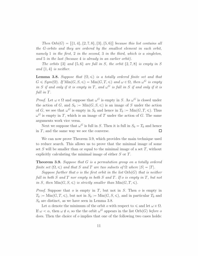
Then OrbpGq “ rt1, 4u, t2, 7, 8u, t3u, t5, 6us because this list contains all
the G-orbits and they are ordered by the smallest element in each orbit,
namely 1 in the first, 2 in the second, 3 in the third, which is a singleton,
and 5 in the last (because 4 is already in an earlier orbit).
The orbits t3u and t5, 6u are full in S, the orbit t2, 7, 8u is empty in S
and t1, 4u is neither.
Lemma 3.8. Suppose that pΩ,ďq is a totally ordered finite set and that
G ď SympΩq. If MinpG, S,ďq “ MinpG, T,ďq and ω P Ω, then ωG is empty
in S if and only if it is empty in T , and ωG is full in S if and only if it is
full in T .
Proof. Let ω P Ω and suppose that ωG is empty in S. As ωG is closed under
the action of G, and S0 :“ MinpG, S,ďq is an image of S under the action
of G, we see that ωG is empty in S0 and hence in T0 :“ MinpG, T,ďq. ThusωG is empty in T , which is an image of T under the action of G. The same
arguments work vice versa.
Next we suppose that ωG is full in S. Then it is full in S0 “ T0 and hence
in T , and the same way we see the converse.
We can now prove Theorem 3.9, which provides the main technique used
to reduce search. This allows us to prove that the minimal image of some
set S will be smaller than or equal to the minimal image of a set T , without
explicitly calculating the minimal image of either S or T .
Theorem 3.9. Suppose that G is a permutation group on a totally ordered
finite set pΩ,ďq and that S and T are two subsets of Ω where |S| “ |T |.Suppose further that o is the first orbit in the list OrbpGq that is neither
full in both S and T nor empty in both S and T . If o is empty in T , but not
in S, then MinpG, S,ďq is strictly smaller than MinpG, T,ďq.
Proof. Suppose that o is empty in T , but not in S. Then o is empty in
T0 :“ MinpG, T,ďq, but not in S0 :“ MinpG, S,ďq, and in particular T0 and
S0 are distinct, as we have seen in Lemma 3.8.
Let α denote the minimum of the orbit o with respect to ď and let ω P Ω.
If ω ă α, then ω R o, so the the orbit ωG appears in the list OrbpGq before o
does. Then the choice of o implies that one of the following two cases holds:
11
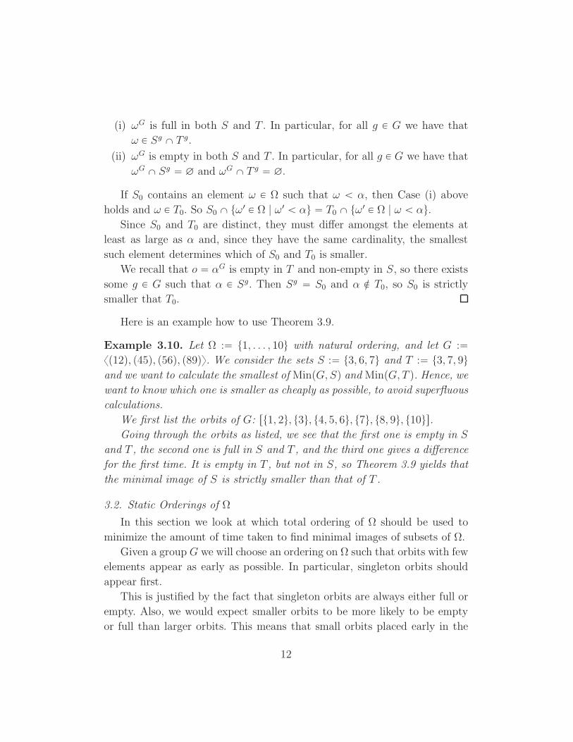
(i) ωG is full in both S and T . In particular, for all g P G we have that
ω P Sg X T g.
(ii) ωG is empty in both S and T . In particular, for all g P G we have that
ωG X Sg “ ∅ and ωG X T g “ ∅.
If S0 contains an element ω P Ω such that ω ă α, then Case (i) above
holds and ω P T0. So S0 X tω1 P Ω | ω1 ă αu “ T0 X tω1 P Ω | ω ă αu.Since S0 and T0 are distinct, they must differ amongst the elements at
least as large as α and, since they have the same cardinality, the smallest
such element determines which of S0 and T0 is smaller.
We recall that o “ αG is empty in T and non-empty in S, so there exists
some g P G such that α P Sg. Then Sg “ S0 and α R T0, so S0 is strictly
smaller that T0.
Here is an example how to use Theorem 3.9.
Example 3.10. Let Ω :“ t1, . . . , 10u with natural ordering, and let G :“xp12q, p45q, p56q, p89qy. We consider the sets S :“ t3, 6, 7u and T :“ t3, 7, 9uand we want to calculate the smallest of MinpG, Sq and MinpG, T q. Hence, wewant to know which one is smaller as cheaply as possible, to avoid superfluous
calculations.
We first list the orbits of G: rt1, 2u, t3u, t4, 5, 6u, t7u, t8, 9u, t10us.Going through the orbits as listed, we see that the first one is empty in S
and T , the second one is full in S and T , and the third one gives a difference
for the first time. It is empty in T , but not in S, so Theorem 3.9 yields that
the minimal image of S is strictly smaller than that of T .
3.2. Static Orderings of Ω
In this section we look at which total ordering of Ω should be used to
minimize the amount of time taken to find minimal images of subsets of Ω.
Given a group G we will choose an ordering on Ω such that orbits with few
elements appear as early as possible. In particular, singleton orbits should
appear first.
This is justified by the fact that singleton orbits are always either full or
empty. Also, we would expect smaller orbits to be more likely to be empty
or full than larger orbits. This means that small orbits placed early in the
12
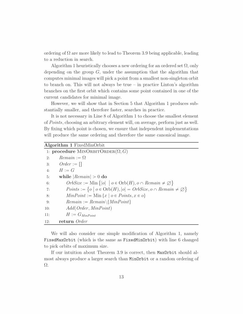
ordering of Ω are more likely to lead to Theorem 3.9 being applicable, leading
to a reduction in search.
Algorithm 1 heuristically chooses a new ordering for an ordered set Ω, only
depending on the group G, under the assumption that the algorithm that
computes minimal images will pick a point from a smallest non-singleton orbit
to branch on. This will not always be true – in practice Linton’s algorithm
branches on the first orbit which contains some point contained in one of the
current candidates for minimal image.
However, we will show that in Section 5 that Algorithm 1 produces sub-
stantially smaller, and therefore faster, searches in practice.
It is not necessary in Line 8 of Algorithm 1 to choose the smallest element
of Points , choosing an arbitrary element will, on average, perform just as well.
By fixing which point is chosen, we ensure that independent implementations
will produce the same ordering and therefore the same canonical image.
Algorithm 1 FixedMinOrbit
1: procedure MinOrbitOrder(Ω, G)
2: Remain :“ Ω
3: Order :“ rs4: H :“ G
5: while |Remain| ą 0 do
6: OrbSize :“ Min
|o|ˇ
ˇ o P OrbpHq, o X Remain ‰ H(
7: Points :“
oˇ
ˇ o P OrbpHq, |o| “ OrbSize, o X Remain ‰ H(
8: MinPoint :“ Min tx | o P Points , x P ou9: Remain :“ RemainztMinPointu10: AddpOrder ,MinPointq11: H :“ GMinPoint
12: return Order
We will also consider one simple modification of Algorithm 1, namely
FixedMaxOrbit (which is the same as FixedMinOrbit) with line 6 changed
to pick orbits of maximum size.
If our intuition about Theorem 3.9 is correct, then MaxOrbit should al-
most always produce a larger search than MinOrbit or a random ordering of
Ω.
13
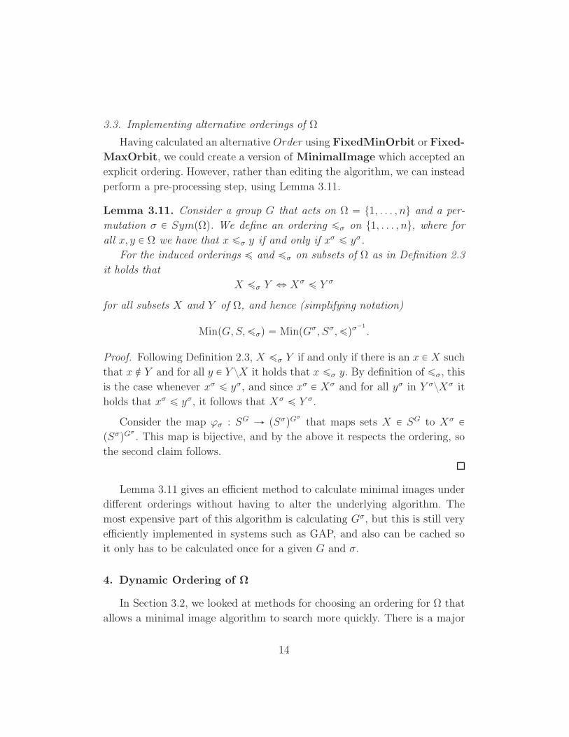
3.3. Implementing alternative orderings of Ω
Having calculated an alternative Order using FixedMinOrbit or Fixed-
MaxOrbit, we could create a version of MinimalImage which accepted an
explicit ordering. However, rather than editing the algorithm, we can instead
perform a pre-processing step, using Lemma 3.11.
Lemma 3.11. Consider a group G that acts on Ω “ t1, . . . , nu and a per-
mutation σ P SympΩq. We define an ordering ďσ on t1, . . . , nu, where for
all x, y P Ω we have that x ďσ y if and only if xσ ď yσ.
For the induced orderings ď and ďσ on subsets of Ω as in Definition 2.3
it holds that
X ďσ Y ô Xσď Y σ
for all subsets X and Y of Ω, and hence (simplifying notation)
MinpG, S,ďσq “ MinpGσ, Sσ,ďqσ´1
.
Proof. Following Definition 2.3, X ďσ Y if and only if there is an x P X such
that x R Y and for all y P Y zX it holds that x ďσ y. By definition of ďσ, this
is the case whenever xσ ď yσ, and since xσ P Xσ and for all yσ in Y σzXσ it
holds that xσ ď yσ, it follows that Xσď Y σ.
Consider the map ϕσ : SG Ñ pSσqGσ
that maps sets X P SG to Xσ PpSσqG
σ
. This map is bijective, and by the above it respects the ordering, so
the second claim follows.
Lemma 3.11 gives an efficient method to calculate minimal images under
different orderings without having to alter the underlying algorithm. The
most expensive part of this algorithm is calculating Gσ, but this is still very
efficiently implemented in systems such as GAP, and also can be cached so
it only has to be calculated once for a given G and σ.
4. Dynamic Ordering of Ω
In Section 3.2, we looked at methods for choosing an ordering for Ω that
allows a minimal image algorithm to search more quickly. There is a major
14
limitation to this technique – it does not make use of the sets whose canonical
image we wish to find.
In this section, instead of producing an ordering ahead of time, we will
incrementally define the ordering of Ω as the algorithm progresses. At each
stage we will consider exactly which extension of our partially constructed
ordering will lead to the smallest increase in the number of sets we must
consider.
We are not free to choose our ordering arbitrarily as we must still map
two sets in the same orbit of G to the same canonical image. However, we
can use different orderings for sets that are in different orbits of G.
Firstly, we will explain how we build the orderings that our algorithm
uses.
4.1. Orderings
When building canonical images, we build orderings as the algorithm
progresses. We represent these partially built orderings as ordered partitions.
Definition 4.1. Let k P N and let P “ rX1, . . . , Xks be an ordered partition
of PpΩq. Then, given two subsets S and T of Ω, we write S ăP T if and only
if the cell that contains S occurs before the cell that contains T in P .
We say that P is G-invariant if and only if for all i P t1, . . . , ku and g P G
it holds that S P Xi if and only if Sg P Xi.
A refinement of an ordered partition rX1, . . . , Xks is an ordered partition
rY1,1, Y1,2, . . . , Yk,ls where l P N and such that, for all i P t1, . . . , ku and
j P t1, . . . , lu, we have that Yi,j Ď Xi.
A completion of an ordered partition X “ rX1, . . . , Xks is a refinement
where every cell is of size one. Given an ordering for Ω, the standard com-
pletion of an ordered partition X orders the members of each cell of X using
the ordering on sets from Definition 2.3.
In our algorithm we need a completion of an ordered partition, but the
exact completion is unimportant – it is only important that, given an ordered
partition X , we always return the same completion. For this reason we define
the standard completion of an ordered partition.
15
Example 4.2. Let G :“ xp12qy ď S3 and Ω :“ t1, 2, 3u. Moreover let
P :“ rtu, t1u, t2u, t1, 3u, t2, 3u | t3u, t1, 2u, t1, 2, 3us be an ordered parti-
tion of PpΩq.The orbits of G on Ω are t1, 2u and t3u. In particular all elements of G
stabilize the partition P .
The ordered partition Q :“ rt1, 3u, t2u | tu, t1u, t2, 3u | t3u, t1, 2u, t1, 2, 3usis a refinement of P that is not G-invariant.
To see this, we let g :“ p12q P G. We have that t1, 3u is in the first cell
of Q, but t1, 3ug “ t2, 3u is not in the first cell.
In Example 4.2 we only considered a very small group, because the size
of PpΩq is 2|Ω|. In practice we will not explicitly create ordered partitions of
PpΩq, but instead store a compact description of them from which we can
deduce the cell that any particular set is in.
In this paper, we will consider two methods of building and refining or-
dered partitions. We first define the orbit count of a set, which we will use
when building refiners.
Definition 4.3. Let G be a group acting on an ordered set Ω, and S Ď Ω.
Define the orbit count of S in G, denoted OrbcountpG, Sq as follows: Given
the list OrbpGq of orbits of G on Ω sorted by the their smallest member, the
list OrbcountpG, Sq contains the size of the intersection |o X S| in place of
o P OrbpGq.
We will see the practical use of Orbcount in Lemma 5.1.
Lemma 4.4. Suppose that pΩ,ďq is a totally ordered finite set and that
G ď SympΩq. Suppose further that S, T Ď Ω and that there is some g P G
such that Sg “ T . Then OrbcountpG, Sq “ OrbcountpG, T q.
Proof. Let o P OrbpGq and g P G with Sg “ T . Then og “ o and α P po X Sqif and only if αg P po X Sqg, if and only if αg P pog X Sgq “ po X T q.
Definition 4.5. Let P be an ordered partition of PpΩq.
• If α P Ω, then the point refinement of P by α is the ordered partition
Q defined in the following way: Each cell Xi of P is split into two cells,
16
namely the cell tS | S P Xi, α P Su, and the cell tS | S P Xi, α R Su. Ifone of these sets is empty, then Xi is not split.
• If G ď SympΩq and C “ OrbcountpG, T q for some set T Ď Ω, then
the orbit refinement of P by C is the ordered partition Q defined
as follows: Each cell Xi of P is split into two cells, namely tS | S PXi,OrbcountpG, Sq “ Cu, and tS | S P Xi,OrbcountpG, Sq ‰ Cu. Ifone of these sets is empty, Xi is not split.
4.2. Algorithm
We will now present our algorithm. First, we give a technical definition
which will be used in proving the correctness of our algorithm.
Definition 4.6. For all n P N we define Ln to be the set of lists of length n
whose entries are non-empty subsets of Ω. If X P Ln, then as a convention
we write X1, . . . , Xn for the entries of the list X.
If X P Ln and H ď G ď Sn is such that |G : H | “ k P N and Q “tq1, . . . , qku is a set of coset representatives of H in G, then we define XQ
to be the list whose first k entries are Xq11 , . . . , X
qk1 , followed by X
q12 , . . . , X
qk2
until the last k entries are Xq1n , . . . , Xqk
n . We note that XQ P Ln¨k.
Let X, Y P Ln. We say that X and Y are G-equivalent if and only if there
exist a permutation σ of t1, . . . , nu and group elements g1, . . . , gn P G such
that, for all i P t1, . . . , nu, it holds that Yi “ Xgiiσ .
We now prove a series of three lemmas about coset representatives, which
form the basis for the correctness proof of our algorithm. They are used to
perform the recursive step, moving from a group to a subgroup.
Lemma 4.7. Suppose that G is a permutation group on a set Ω, that H is a
subgroup of G of index k P N and that T is a set of left coset representatives
of H in G.
Then the following are true:
(i) |T | “ k.
(ii) If T “ tt1, . . . , tku and g P G and if, for all i P t1, . . . , ku, we define
qi :“ gti, then Q :“ tq1, . . . , qku is also a set of coset representatives
of H in G. In particular there is a bijection from Q to any set of left
coset representatives of H in G.
17
Proof. By definition the index of H in G is the number of (left or right)
cosets of H in G.
For the second statement we let i, j P t1, . . . , ku be such that qiH “ qjH ,
hence gtiH “ gtjH . Then t´1
j ti “ t´1
j g´1gti P H and hence tiH “ tjH . Hence
i “ j because ti and tj are from a set of coset representatives.
Lemma 4.8. Suppose that G is a permutation group on a set Ω and that
S, T Ď Ω are such that the lists rSs and rT s are G-equivalent.
Let H be a subgroup of G of index k P N and let P “ tp1, . . . , pku and
Q :“ tq1, . . . , qku be sets of left coset representatives of H in G.
Then rSsP and rT sQ are H-equivalent.
Proof. As rSs and rT s are G-equivalent, we know that there exists a group
element g P G such that Sg “ T .
We fix g, for all i P t1, . . . , ku we let ti :“ gqi and we consider the set
T :“ tti | i P t1, . . . , kuu. Then T is also a set of left coset representatives of
H in G, by Lemma 4.7. As P is also a set of left coset representatives, we
know that T and P have the same size, so there is a bijection from P to T .
This can be expressed in the following way:
There is a permutation σ P Sk such that, for all i P t1, .., ku, it is true
that piσH “ tiH . That means there is a unique hi P H such that piσhi “ ti.
Let now Si :“ Spi and Ti :“ T qi for i P t1, . . . , ku, then
Ti “ T qi “ pSgqqi “ Sti “ Spiσhi “ pSpiσ qhi “ pSiσqhi,
hence rSsP and rT sQ are H-equivalent.
Lemma 4.9. Suppose that G is a permutation group on a set Ω, that n P N
and that X, Y P Ln are G-equivalent. Let H be a subgroup of G of index
k P N and let P “ tp1, . . . , pku and Q :“ tq1, . . . , qku be sets of left coset
representatives of H in G.
Then XP and Y Q are H-equivalent.
Proof. As X and Y are G-equivalent, we know that there exist a permutation
σ P Sn and g1, . . . , gn P G such that Yi “ Xgiiσ for all i P t1, . . . , nu. We fix
this permutation σ.
18
If i P t1, . . . , nu, then rXiσs and rYis satisfy the hypothesis of Lemma 4.8,
so it follows that rXiσsP and rYisQ are H-equivalent.
So we find a permutation αi P Sk and group elements hi1, . . . , hik P H
such that pXpjαi
iσ qhij “ Yqii for all j P t1, . . . , ku.
Using σ and α1, . . . , αk we define a permutation γ on 1, . . . , n ¨ k.First we express l P t1, . . . , n ¨ ku uniquely as l “ cl ¨ k ` rl where cl P
t0, . . . , n ´ 1u and rl P t1, . . . , ku and we define
lγ :“ pcl ` 1qσ ¨ k ` rαcl`1
l .
This is well-defined because of the ranges of cl and rl and it is a permuta-
tion because of the uniqueness of the expression and because σ and α1, . . . , αn
are permutations.
Then, for each l P t1, . . . , n ¨ ku, expressed as l “ cl ¨ k ` rl as we did
above, we set h :“ hcl`1,rl, X1l :“ X
prlcl`1
and Y 1l :“ Y
qrlcl`1
.
Then XP “ rX 11, . . . , X
1n¨ks and Y Q “ rY 1
1 , . . . , Y1n¨ks.
If we set p :“ pracl`1
l
and q :“ qrl, then we have, for all l “ cl ¨ k ` rl, that
X 1hlγ “ pXp
pcl`1qσqh “ ppXσcl`1
qpqh “ Yqcl`1 “ Y 1
l .
This is H-equivalence.
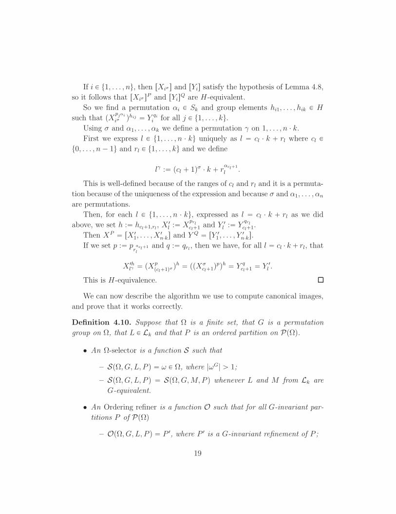
We can now describe the algorithm we use to compute canonical images,
and prove that it works correctly.
Definition 4.10. Suppose that Ω is a finite set, that G is a permutation
group on Ω, that L P Lk and that P is an ordered partition on PpΩq.
• An Ω-selector is a function S such that
– SpΩ, G, L, P q “ ω P Ω, where |ωG| ą 1;
– SpΩ, G, L, P q “ SpΩ, G,M, P q whenever L and M from Lk are
G-equivalent.
• An Ordering refiner is a function O such that for all G-invariant par-
titions P of PpΩq
– OpΩ, G, L, P q “ P 1, where P 1 is a G-invariant refinement of P ;
19
– OpΩ, G, L, P q “ OpΩ, G,M, P q whenever L and M from Lk are
G-equivalent.
An ordering refiner cannot return a total ordering, unless G acts triv-
ially, because the partial ordering cannot distinguish between values that are
contained in the same orbit of G.
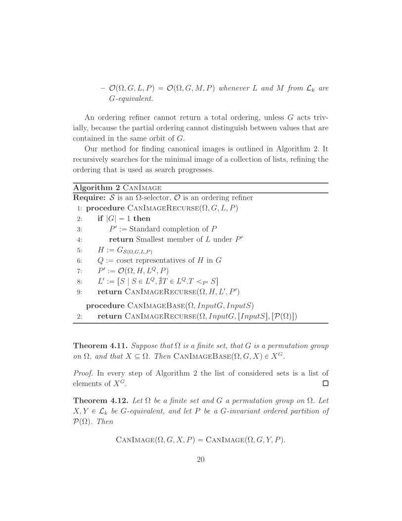
Our method for finding canonical images is outlined in Algorithm 2. It
recursively searches for the minimal image of a collection of lists, refining the
ordering that is used as search progresses.
Algorithm 2 CanImage
Require: S is an Ω-selector, O is an ordering refiner
1: procedure CanImageRecurse(Ω, G, L, P )
2: if |G| “ 1 then
3: P 1 :“ Standard completion of P
4: return Smallest member of L under P 1
5: H :“ GSpΩ,G,L,P q
6: Q :“ coset representatives of H in G
7: P 1 :“ OpΩ, H, LQ, P q8: L1 :“ rS | S P LQ, ET P LQ.T ăP 1 Ss9: return CanImageRecurse(Ω, H, L1, P 1)
procedure CanImageBase(Ω, InputG, InputS)
2: return CanImageRecurse(Ω, InputG, rInputSs, rPpΩqs)
Theorem 4.11. Suppose that Ω is a finite set, that G is a permutation group
on Ω, and that X Ď Ω. Then CanImageBasepΩ, G,Xq P XG.
Proof. In every step of Algorithm 2 the list of considered sets is a list of
elements of XG.
Theorem 4.12. Let Ω be a finite set and G a permutation group on Ω. Let
X, Y P Lk be G-equivalent, and let P be a G-invariant ordered partition of
PpΩq. Then
CanImagepΩ, G,X, P q “ CanImagepΩ, G, Y, P q.
20

Proof. We proceed by induction on the size of G.
The base case is |G| “ 1. As X and Y are G-equivalent, X and Y contain
the same sets, possibly in a different order. For a given P and Ω, there is only
one standard completion of P that gives a complete ordering on PpΩq, andso X and Y have the same smallest element under the standard completion
of P and so the claim follows.
Consider now any non-trivial group G, and suppose for our induction
hypothesis that the claim holds for all groups H where |H | ă |G|.Definition 4.10 and the fact that S is an Ω-selector imply that
H “ GSpΩ,G,X,P q “ GSpΩ,G,Y,P q.
Moreover, H is a proper subgroup of G. We take two sets Q1 and Q2 of coset
representatives of H in G, which are not necessarily equal.
Since O is an ordering refiner, it holds that
P 1 “ OpΩ, H,X, P q “ OpΩ, H, Y, P q
By Lemma 4.9, XQ1 and Y Q2 are H-equivalent, and by definition P 1 is G-
invariant. If we identify the cell P 1i of P 1 that contains the smallest element
of XQ1, then L1X contains those elements of XQ1 that are in P 1
i . Each of
these elements is H-equivalent to an element of Y Q2, and therefore L1X is
H-equivalent to L1Y . Then the induction hypothesis yields that
CanImagepΩ, H,X 1, P q “ CanImagepΩ, G, Y 1, P q,
so the claim follows by induction.
We see from Theorem 4.11 and 4.12 that
CanImagepΩ, G,X, P q “ CanImagepΩ, G, Y, P q if and only if Y P XG.
We note that Algorithm 2 can easily be adapted to return an element
g of G such that Xg “ CanImagepΩ, G,X, P q. This happens by attaching
to each set, when it is created, the permutation that maps it to the original
input S. We omit this addition for readability.
21
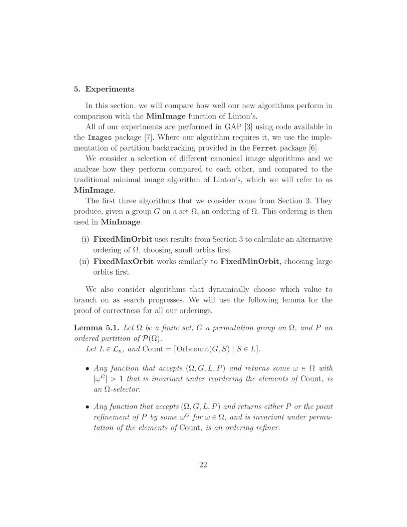
5. Experiments
In this section, we will compare how well our new algorithms perform in
comparison with the MinImage function of Linton’s.
All of our experiments are performed in GAP [3] using code available in
the Images package [7]. Where our algorithm requires it, we use the imple-
mentation of partition backtracking provided in the Ferret package [6].
We consider a selection of different canonical image algorithms and we
analyze how they perform compared to each other, and compared to the
traditional minimal image algorithm of Linton’s, which we will refer to as
MinImage.
The first three algorithms that we consider come from Section 3. They
produce, given a group G on a set Ω, an ordering of Ω. This ordering is then
used in MinImage.
(i) FixedMinOrbit uses results from Section 3 to calculate an alternative
ordering of Ω, choosing small orbits first.
(ii) FixedMaxOrbit works similarly to FixedMinOrbit, choosing large
orbits first.
We also consider algorithms that dynamically choose which value to
branch on as search progresses. We will use the following lemma for the
proof of correctness for all our orderings.
Lemma 5.1. Let Ω be a finite set, G a permutation group on Ω, and P an
ordered partition of PpΩq.Let L P Ln, and Count “ rOrbcountpG, Sq | S P Ls.
• Any function that accepts pΩ, G, L, P q and returns some ω P Ω with
|ωG| ą 1 that is invariant under reordering the elements of Count, is
an Ω-selector.
• Any function that accepts pΩ, G, L, P q and returns either P or the point
refinement of P by some ωG for ω P Ω, and is invariant under permu-
tation of the elements of Count, is an ordering refiner.
22
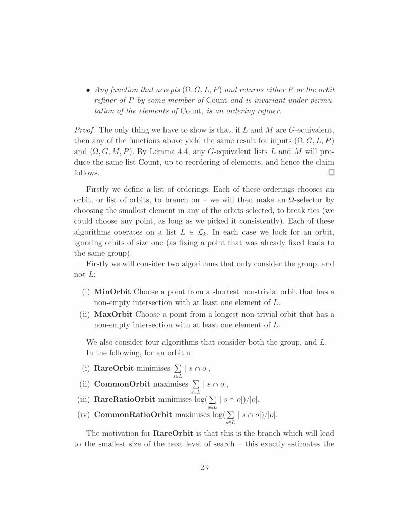
• Any function that accepts pΩ, G, L, P q and returns either P or the orbit
refiner of P by some member of Count and is invariant under permu-
tation of the elements of Count, is an ordering refiner.
Proof. The only thing we have to show is that, if L and M are G-equivalent,
then any of the functions above yield the same result for inputs pΩ, G, L, P qand pΩ, G,M, P q. By Lemma 4.4, any G-equivalent lists L and M will pro-
duce the same list Count, up to reordering of elements, and hence the claim
follows.
Firstly we define a list of orderings. Each of these orderings chooses an
orbit, or list of orbits, to branch on – we will then make an Ω-selector by
choosing the smallest element in any of the orbits selected, to break ties (we
could choose any point, as long as we picked it consistently). Each of these
algorithms operates on a list L P Lk. In each case we look for an orbit,
ignoring orbits of size one (as fixing a point that was already fixed leads to
the same group).
Firstly we will consider two algorithms that only consider the group, and
not L:
(i) MinOrbit Choose a point from a shortest non-trivial orbit that has a
non-empty intersection with at least one element of L.
(ii) MaxOrbit Choose a point from a longest non-trivial orbit that has a
non-empty intersection with at least one element of L.
We also consider four algorithms that consider both the group, and L.
In the following, for an orbit o
(i) RareOrbit minimisesř
sPL
| s X o|,
(ii) CommonOrbit maximisesř
sPL
| s X o|,
(iii) RareRatioOrbit minimises logpř
sPL
| s X o|q|o|,
(iv) CommonRatioOrbit maximises logpř
sPL
| s X o|q|o|.
The motivation for RareOrbit is that this is the branch which will lead
to the smallest size of the next level of search – this exactly estimates the
23
size of the next level if our ordering refiner only fixed a point in orbit o.
We therefore expect, conversely, CommonOrbit to perform badly and to
produce very large searches.
One limitation of RareOrbit is that it will favour smaller orbits – in
general we want to minimize the size of the whole search. The idea here is
that if we have two levels of search where we split on an orbit of size two,
and each time create 10 times more sets is equivalent to splitting once on
an orbit of size four, and creating 100 times more sets. RareRatioOrbit
compensates for this. We expect that CommonRatioOrbit is the inverse
of this, so we also expect it to perform badly.
For each of these orderings, we use the ordering refiner that takes each
fixed point of G in their order in Ω, and performs a point refinement by
each recursively in turn. By repeated application of Lemma 4.4, this is a
G-invariant ordering refiner.
We also have a set of orderings which make use of orbit counting. To keep
the number of experiments under control, we used the RareOrbit strategy
in each case to choose which point to branch on next, and we also build an
orbit refiner.
Given an unordered list of orbit counts,
(i) RareOrbitPlusMin chooses the lexicographically smallest one.
(ii) RareOrbitPlusRare chooses the least frequently occurring orbit count
list (using the lexicographically smallest to break ties).
(iii) RareOrbitPlusCommon chooses the most frequently occurring orbit
count list (using the lexicographically smallest to break ties).
5.1. Experiments
In this section we perform a practical comparison of our algorithms, and
the MinImage algorithm of Linton, for three different families of problems:
grid groups, m-sets, and primitive groups.
5.2. Experimental Design
We will consider three sets of benchmarks in our testing. In each exper-
iment, given a permutation group that acts on t1, . . . , nu, we will run an
24
experiment with each of our orderings to find the canonical image of a set of
sizeX
n2
\
,X
n4
\
andX
n8
\
.
We run our algorithms on a randomly chosen conjugate of each primitive
group, to randomize the initial ordering of the integers the group is defined
over. The same conjugate is used of each group in all experiments, and when
choosing a random subset of size x from a set S, we always choose the same
random subset. We use a timeout of five minutes for each experiment. We
force GAP to build a stabilizer chain for each of our groups before we begin
our algorithm, because this can in some cases take a long time.
For each size of set and each ordering, we measure three things. The
total number of problems solved, the total time taken to solve all problems,
counting timeouts as 5 minutes, and the number of moved points of the
largest group solved. Our experiments were all performed on an Intel(R)
Xeon(R) CPU E5-2640 v4 running at 2.40GHz, with twenty cores. Each
copy of GAP was allowed a maximum of 6GB of RAM.
5.2.1. Grid Groups
In this experiment, we look for canonical images of sets in grid groups.
Definition 5.2. Let n P N. The direct product Sn ˆ Sn acts on the set
t1, . . . , nu ˆ t1, . . . , nu of pairs in the following way:
For all pi, jq P t1, . . . , nu ˆ t1, . . . , nu and all pσ, τq P Sn ˆ Sn we define
pi, jqpσ,τq :“ piσ, jτq.
The subgroup G ď Sympt1, . . . , nu ˆ t1, . . . , nuq defined by this action is
called the n ˆ n grid group.
We note that, while the construction of the grid group is done by starting
with an n by n grid of points and permuting rows or columns independently
of each other, we actually represent this group as a subgroup of Sn¨n, and we
do not assume prior knowledge of the grid structure of the action.
We ran experiments on the grid groups for grids of size 5ˆ5 to 100ˆ100.
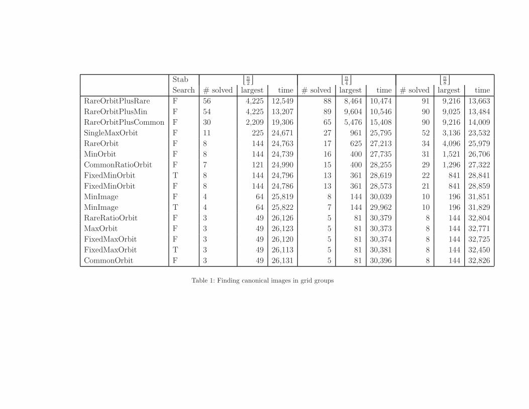
The results of this experiment are given in Table 1.
The basic algorithm, MinImage, is only able to solve 22 problems within
the timeout. FixedMinOrbit solves 43 problems, while being implemented
25
as a simple pre-processing step to MinImage. The dynamic MinOrbit is
able to solve 55 problems, and the best orbit-based strategy, SingleMax-
Orbit, solves 70 problems. However the advanced techniques, which filter by
orbit lists, perform much better. Even ordering by the most common orbit
list leads to solving over 185 problems, and the best strategy, RareOrbit-
PlusRare, solves 235 out of the total 288 problems.
Furthermore, for these large groups, the algorithms are still performing
very small searches: For example FixedMinOrbit, on its largest solved prob-
lem with sizeX
n2
\
sets and a grid of size 12 ˆ 12, generates 793, 124 search
nodes, while RareOrbitPlusMin produces only 183, 579 search nodes on
its largest solved problem withX
n2
\
sets (65 ˆ 65).
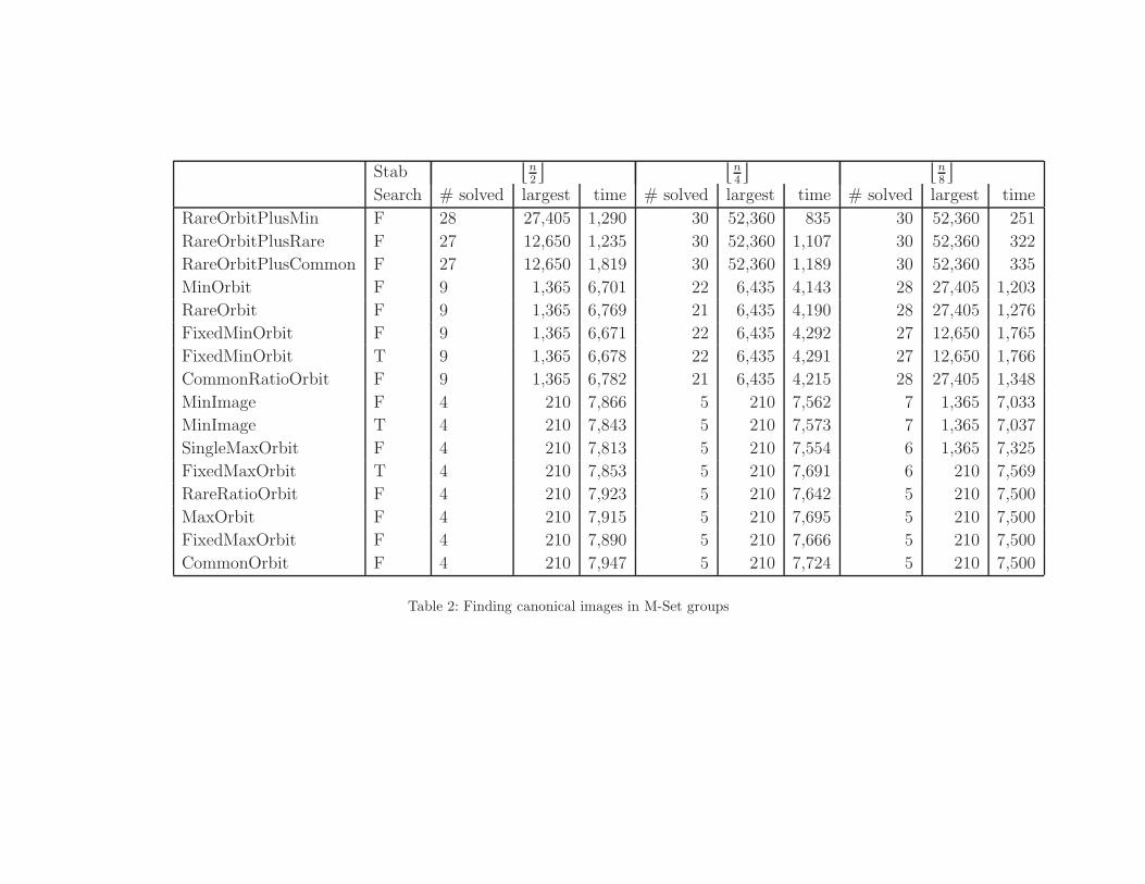
5.2.2. M-Sets
Linton [10] considers, given integers n and m, defining a permutation
group on the set T of all subsets of size m of t1, . . . , nu under the action on T
of Sn acting on the members of the m-sets. He then looks for minimal images
of randomly chosen subsets of T of size k, under the standard lexicographic
ordering on sets.
We ran experiments for m “ 2 and n P t10, 15, . . . , 100u, for m “ 4 and
n P t10, 15, . . . , 35u, for m “ 6 and n P t10, 15, 20u and finally m “ 8, n “ 10
as described in Section 5.2. We choose these 30 experiments as these were the
problems that any of our techniques were able to solve in under 5 minutes.
The results of our experiments are shown in Table 2.
Similarly to our experiments on grid groups, we find that the standard
MinImage algorithm is only able to solve a very small set of benchmarks.
Some of the better algorithms, including FixedMinOrbit, are able to solve 9
problems. In particular, once againMinOrbit is not significantly better than
FixedMinOrbit, although it is slightly faster on average over all problems.
However, the orbit-based strategies do much better, solving all the prob-
lems which we set. In the case of sets that contain an eighth of all m-sets, the
best technique is able to solve all problems any technique can solve, in under
5 minutes. The largest solved problem, which was instance n “ 35, m “ 4
for a set on an eighth of all m-sets, is solved in only 6, 594 search nodes
by RareOrbitPlusMin, while the largest solved problem of MinImage,
n “ 15, m “ 4 takes 631, 144 search nodes.
26
StabX
n2
\ X
n4
\ X
n8
\
Search # solved largest time # solved largest time # solved largest time
RareOrbitPlusRare F 56 4,225 12,549 88 8,464 10,474 91 9,216 13,663
RareOrbitPlusMin F 54 4,225 13,207 89 9,604 10,546 90 9,025 13,484
RareOrbitPlusCommon F 30 2,209 19,306 65 5,476 15,408 90 9,216 14,009
SingleMaxOrbit F 11 225 24,671 27 961 25,795 52 3,136 23,532
RareOrbit F 8 144 24,763 17 625 27,213 34 4,096 25,979
MinOrbit F 8 144 24,739 16 400 27,735 31 1,521 26,706
CommonRatioOrbit F 7 121 24,990 15 400 28,255 29 1,296 27,322
FixedMinOrbit T 8 144 24,796 13 361 28,619 22 841 28,841
FixedMinOrbit F 8 144 24,786 13 361 28,573 21 841 28,859
MinImage F 4 64 25,819 8 144 30,039 10 196 31,851
MinImage T 4 64 25,822 7 144 29,962 10 196 31,829
RareRatioOrbit F 3 49 26,126 5 81 30,379 8 144 32,804
MaxOrbit F 3 49 26,123 5 81 30,373 8 144 32,771
FixedMaxOrbit F 3 49 26,120 5 81 30,374 8 144 32,725
FixedMaxOrbit T 3 49 26,113 5 81 30,381 8 144 32,450
CommonOrbit F 3 49 26,131 5 81 30,396 8 144 32,826
Table 1: Finding canonical images in grid groups
StabX
n2
\ X
n4
\ X
n8
\
Search # solved largest time # solved largest time # solved largest time
RareOrbitPlusMin F 28 27,405 1,290 30 52,360 835 30 52,360 251
RareOrbitPlusRare F 27 12,650 1,235 30 52,360 1,107 30 52,360 322
RareOrbitPlusCommon F 27 12,650 1,819 30 52,360 1,189 30 52,360 335
MinOrbit F 9 1,365 6,701 22 6,435 4,143 28 27,405 1,203
RareOrbit F 9 1,365 6,769 21 6,435 4,190 28 27,405 1,276
FixedMinOrbit F 9 1,365 6,671 22 6,435 4,292 27 12,650 1,765
FixedMinOrbit T 9 1,365 6,678 22 6,435 4,291 27 12,650 1,766
CommonRatioOrbit F 9 1,365 6,782 21 6,435 4,215 28 27,405 1,348
MinImage F 4 210 7,866 5 210 7,562 7 1,365 7,033
MinImage T 4 210 7,843 5 210 7,573 7 1,365 7,037
SingleMaxOrbit F 4 210 7,813 5 210 7,554 6 1,365 7,325
FixedMaxOrbit T 4 210 7,853 5 210 7,691 6 210 7,569
RareRatioOrbit F 4 210 7,923 5 210 7,642 5 210 7,500
MaxOrbit F 4 210 7,915 5 210 7,695 5 210 7,500
FixedMaxOrbit F 4 210 7,890 5 210 7,666 5 210 7,500
CommonOrbit F 4 210 7,947 5 210 7,724 5 210 7,500
Table 2: Finding canonical images in M-Set groups
5.2.3. Comparison to Graph Canonical Image
A set of 2-sets can be viewed as an undirected graph, where the two sets
represent the edges. The problem of finding the canonical image of this set
of 2-sets is equivalent to the traditional problem of finding a canonical image
of this graph. We can therefore perform a comparison between our technique
and Nauty, for these problems. Nauty is able to a find canonical image for
all our 2-set problems almost instantly. We investigated why Nauty was able
to outperform us by such a large margin, and found three problems. We list
the most important one first.
• The central algorithm of Nauty makes use of properties of the form
“vertices with i neighbors can only map to other vertices with i neigh-
bors”. Our algorithm does not make use of this property, as it represents
a much more complex condition when considered on m-sets. Further,
while we could add a special case specifically for when the group we
are considering is the symmetric group operating on m-sets, we would
prefer to find a more general technique.
• Our algorithm spends a large proportion of its time calculating stabi-
lizer chains, and mapping sets through elements of the group. This is
not required for the graphs.
• Our algorithm is written in GAP rather than highly optimized C.
The most important results to draw from this comparison is that our
algorithms should not be viewed as a replacement for graph isomorphism
algorithms. We are investigating how to close this performance gap, without
special casing.
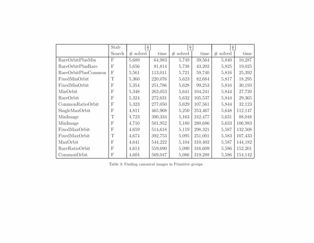
5.2.4. Primitive Groups
In this experiment we look for canonical images of sets under the action
of primitive groups which move between 2 and 1, 000 points. We remove the
natural alternating and symmetric groups, as finding minimal and canonical
images in these groups is trivial and can be easily special-cased. So we look
at a total number of 5, 845 groups, each of which was successfully treated by
at least one algorithm.
29
We perform the experiment as described in Section 5.2. The results are
given in Table 3.
All algorithms are able to solve a large number of problems. This is un-
surprising as many primitive groups are quite small (for example the cyclic
groups), so any technique is able to brute-force search many problems. How-
ever, we can still see that, for the hardest problemsX
n2
\
, many algorithms
outperform MinImage, and the techniques that use extra orbit-counting
filtering solve 300 more problems, and they run much faster.
For the easiest set of problems,X
n8
\
, we see that the algorithm RareOr-
bitPlusMin, which usually performs best, solves slightly fewer problems.
This is because there are a small number of groups where the extra filtering
provides no search reduction, but still requires a small overhead in time. How-
ever, the total time taken is still much smaller, and the algorithm only fails to
solve five problems. These five problems involve groups that are isomorphic to
the affine general linear groups AGLp8, 2q, AGLp6, 3q and AGLp9, 2q, and the
projective linear group PSLp9, 2q. This suggests that the linear groups may
be a source of hard problems for canonical image algorithms in the future.
5.2.5. Experimental Conclusions
Our experiments show that using FixedMinOrbit is almost always su-
perior to MinImage. As implementing FixedMinOrbit requires a fairly
small amount of code and time over MinImage, this suggests that any im-
plementations of Linton’s algorithm should have FixedMinOrbit added,
because this provides a substantial performance boost, for relatively little
extra coding.
Algorithms that dynamically order the underlying set, such asMinOrbit
and RareOrbit provide only a small benefit over FixedMinOrbit. Algo-
rithms which add orbit counting provide a much bigger gain, often allowing
solving problems on groups many orders of magnitude larger than before,
thereby greatly advancing the state of the art.
6. Conclusions
We present a general framework and a new set of algorithms for finding
the canonical image of a set under the action of a permutation group. Our
30
StabX
n2
\ X
n4
\ X
n8
\
Search # solved time # solved time # solved time
RareOrbitPlusMin F 5,689 64,983 5,749 39,564 5,840 10,287
RareOrbitPlusRare F 5,656 81,814 5,738 43,202 5,825 19,025
RareOrbitPlusCommon F 5,561 113,011 5,721 59,740 5,816 25,392
FixedMinOrbit T 5,360 220,076 5,623 82,684 5,817 18,295
FixedMinOrbit F 5,354 251,786 5,628 99,253 5,816 30,193
MinOrbit F 5,348 263,053 5,641 104,241 5,844 27,720
RareOrbit F 5,324 272,631 5,632 105,537 5,844 29,365
CommonRatioOrbit F 5,323 277,050 5,629 107,561 5,844 32,123
SingleMaxOrbit F 4,811 465,908 5,250 253,467 5,648 112,147
MinImage T 4,723 390,334 5,163 242,477 5,631 88,048
MinImage F 4,710 501,952 5,180 280,686 5,633 106,983
FixedMaxOrbit F 4,659 514,618 5,119 298,321 5,587 132,508
FixedMaxOrbit T 4,674 392,753 5,095 251,001 5,583 107,433
MaxOrbit F 4,641 544,222 5,104 310,402 5,587 144,182
RareRatioOrbit F 4,614 559,690 5,090 316,609 5,586 152,201
CommonOrbit F 4,604 569,047 5,086 319,288 5,586 154,142
Table 3: Finding canonical images in Primitive groups
experiments show that our new algorithms outperform the previous state of
the art, often by orders of magnitude.
Our basic framework runs on the concept of refiners and selectors and
is not limited to finding only canonical images of subsets of Ω. In future
work we will investigate families of refiners and selectors that allow finding
canonical images for many other combinatorial objects.
Acknowledgements.
All authors thank the DFG (Wa 3089/6-1) and the EPSRC CCP CoDiMa
(EP/M022641/1) for supporting this work. The first author would like to
thank the Royal Society, and the EPSRC (EP/M003728/1). The third
author would like to acknowledge support from the OpenDreamKit Hori-
zon 2020 European Research Infrastructures Project (#676541). The first
and third author thank the Algebra group at the Martin-Luther Univer-
sitat Halle-Wittenberg for the hospitality and the inspiring environment.
The fourth author wishes to thank the Computer Science Department of
the University of St Andrews for its hospitality during numerous visits.
References
[1] P. T. Darga, K. A. Sakallah, and I. L. Markov. Faster symmetry dis-
covery using sparsity of symmetries. In 2008 45th ACM/IEEE Design
Automation Conference, pages 149–154, June 2008.
[2] Andreas Distler, Chris Jefferson, Tom Kelsey, and Lars Kotthoff. The
Semigroups of Order 10, pages 883–899. Springer Berlin Heidelberg,
Berlin, Heidelberg, 2012.
[3] The GAP Group. GAP – Groups, Algorithms, and Programming, Ver-
sion 4.8.4, 2016.
[4] Ian P Gent and Barbara M Smith. Symmetry breaking in constraint pro-
gramming. In Proceedings of the 14th European conference on artificial
intelligence, pages 599–603. IOS press, 2000.
32
[5] Derek F. Holt, Bettina Eick, and Eamonn A. O’Brien. Handbook of Com-
putational Group Theory. Discrete Mathematics and its Applications.
Chapman & Hall/CRC, Boca Raton, 2005.
[6] Christopher Jefferson. Ferret - GAP Package, 2016.
[7] Christopher Jefferson and Eliza Jonauskyte. Images - GAP Package,
2016.
[8] Tommi Junttila and Petteri Kaski. Engineering an efficient canoni-
cal labeling tool for large and sparse graphs. In David Applegate,
Gerth Stølting Brodal, Daniel Panario, and Robert Sedgewick, editors,
Proceedings of the Ninth Workshop on Algorithm Engineering and Ex-
periments and the Fourth Workshop on Analytic Algorithms and Com-
binatorics, pages 135–149. SIAM, 2007.
[9] Jeffrey S. Leon. Permutation group algorithms based on partitions, I:
Theory and algorithms. Journal of Symbolic Computation, 12(4):533–
583, 1991.
[10] Steve Linton. Finding the smallest image of a set. In Proceedings of the
2004 International Symposium on Symbolic and Algebraic Computation,
ISSAC ’04, pages 229–234, New York, NY, USA, 2004. ACM.
[11] Brendan D. McKay. Practical graph isomorphism. Congr. Numer.,
(30):45–87, 1980.
[12] Brendan D. McKay and Adolfo Piperno. Practical graph isomorphism,
II. Journal of Symbolic Computation, 60:94–112, 2014.
[13] Christian Pech and Sven Reichard. Enumerating Set Orbits, pages 137–
150. Springer Berlin Heidelberg, Berlin, Heidelberg, 2009.
[14] Leonard H. Soicher. On the structure and classification of somas: Gen-
eralizations of mutually orthogonal latin squares. Electr. J. Comb., 6,
1999.
33


