Migrant Networks and Foreign Direct Investment

Beata S. Javorcik,* Çağlar Özden,* Mariana Spatareanu** & Cristina Neagu*

Abstract

While there exists a sizeable literature documenting the importance of ethnic networks for international trade, little attention has been devoted to studying the effects of networks on foreign direct investment (FDI). The existence of ethnic networks may positively affect FDI by promoting information flows across international borders and by serving as a contract enforcement mechanism. This paper investigates the link between the presence of migrants in the United States and U.S. FDI in the migrants’ countries of origin, taking into account the potential endogeneity concerns. The results suggest that US FDI abroad is positively correlated with the presence of migrants from the host country. The data further indicate that the relationship between FDI and migration is driven by the presence of migrants with a college education. World Bank Policy Research Working Paper 4046, November 2006

The Policy Research Working Paper Series disseminates the findings of work in progress to encourage the exchange of ideas about development issues. An objective of the series is to get the findings out quickly, even if the presentations are less than fully polished. The papers carry the names of the authors and should be cited accordingly. The findings, interpretations, and conclusions expressed in this paper are entirely those of the authors. They do not necessarily represent the view of the World Bank, its Executive Directors, or the countries they represent. Policy Research Working Papers are available online at http://econ.worldbank.org.

* Development Economics Research Group (DECRG), World Bank MC3-303, 1818 H Street, NW, Washington, DC 20433; Email: bjavorcik@worldbank.org, cozden@worldbank.org and ineagu@worldbank.org, respectively. ** Department of Economics, Rutgers University, 801 Hill Hall, Newark, NJ 07102. Email: marianas@andromeda.rutgers.edu. The authors would like to thank David McKenzie for sharing the data on passport fees and Torfinn Harding, Molly Lipscomb and participants of the World Bank international trade seminar for helpful comments and suggestions.

WPS4046

1

1. Introduction

The decline in transportation and communications costs and the reduction in policy

induced barriers have led to a rapid increase in the flow of goods, capital, people and knowledge

across international boundaries. There exists an extensive literature exploring the effects of these

forces, but much less attention has been paid to more subtle linkages and feedback mechanisms

which are shaping the global economy. One of such linkages is the influence of migration on

foreign direct investment (FDI), which is the focus of this study.

While a growing literature has documented a positive association between the presence of

ethnic networks and international trade, the link between migration and FDI remains relatively

unexplored. The main premise of the existing literature is that international transactions are

plagued with informal trade barriers, in addition to formal trade barriers such as transportation

costs and tariffs. Among these barriers are the difficulties associated with provision of

information on many issues, including potential market opportunities, and with enforcing

contracts across national boundaries. As shown by Gould (1994), Head and Ries (1998), Rauch

and Trindade (2002) and Combes et al. (2003), the presence of people with the same ethnic

background on both sides of a border may alleviate these problems. Their language skills and

familiarity with a foreign country can significantly lower communication costs. They possess

valuable information about the market structure, consumer preferences, business ethics and

commercial codes in both economies. They decrease the costs of negotiating and enforcing a

contract through their social links, networking skills and knowledge of the local legal regime. In

short, business and social networks that span national borders can help to overcome many

contractual and informational barriers and carry out mutually beneficial international

transactions.1

Foreign direct investment activities may face even larger information asymmetries than

international trade transactions. Direct investment generally requires long-term focus and

interactions with diverse group of economic agents from suppliers and workers to government

1 Gould (1994) finds that both US exports and imports are positively correlated with the stock of migrants from the partner country present in the US. Head and Ries (1998) reach a similar conclusion when examining Canadian data, as do Combes et al. (2003) using information on intra-regional economic activity in France. Rauch and Trindade (2002) distinguish between the effect of networks as a conduit of information and a contract enforcement mechanism. They show that the presence of ethnic Chinese networks matters more for trade in differentiated products than for trade in homogenous commodities. Given that it is harder to assess the attributes of differentiated products, these findings suggests that in addition to serving as an information channel, ethnic networks may provide implicit contract guarantees and deter opportunistic behavior among its members. See a survey of the literature by Rauch (2001) for more details.

2

officials. The investor needs to have detailed knowledge of the consumer, the labor and input

markets and the legal and regulatory regimes in the host country. Contractual and informational

problems can be quite severe and that is why variables related to governance and legal regimes

are found to be among the most important determinants of FDI flows into a country.2 Thus, it is

natural to expect a positive relationship between migration and FDI, yet surprisingly this is a

relatively unexplored area.3 The only studies examining this question are unpublished papers by

Bhattacharya and Groznik (2003) and Buch et al. (2003), which find a positive relationship

between migration and FDI flows, and a forthcoming study by Kugler and Rapoport (2006),

whose results suggest that migration and FDI inflows are negatively correlated

contemporaneously but that skilled migration is associated with an increase in future FDI.4

This paper contributes to the literature by explicitly taking into account the endogeneity

problem that has been ignored in the existing studies.5 Endogeneity arises since migration and

FDI flows may influence each other. On the one hand, as FDI inflows bring capital, new

technologies and know-how to host countries, they may lead to faster economic growth (provided

some conditions are fulfilled, see Alfaro et al. 2004). Entry of multinationals also tends to

produce better employment opportunities and higher paying jobs (Lipsey and Sjoholm 2004).

Therefore, FDI inflows may lower the incentives to migrate. On the other hand, the presence of

FDI may have a positive effect on migration as local employees may be transferred by their 2 See for instance, Wei (2000) and Smarzynska and Wei (2000). 3 The importance of migrant networks for FDI flows is reflected in anecdotal evidence. For instance, Singh (2003) reports: “Many times top management of Indian origin in the U.S. was asked to start up the offices in India, usually in emerging industrialized cities such as Bangalore and Hyderabad. For example, a return migrant who had worked for Yahoo office in the U.S. for five years set up Yahoo’s development center in Bangalore. This returnee had made the personal decision of moving back to India with his family but ideally wanted to do the same work in India he was currently doing with Yahoo in the San Francisco Bay Area. His managers at Yahoo created a proposal for a new development center in Bangalore to be run by this returnee. After some negotiations the proposal was accepted by the executives of Yahoo and he soon was in charge of opening up a Yahoo development in India. This happened because Yahoo management in the U.S. valued his work and recognized his potential in creating a development center in India." The results of a recent survey of Indian software industry show that 14% of firms received investment from Indians domiciled in a developed country and in a quarter of those cases, such investment accounted for over half of new investment (Commander et al. 2004). 4 Kugler and Rapoport regress the growth in capital financed with US FDI in country k in the 1990s on the stock of migrants from country k present in the US in year 1990 and the change in this stock taking place between 1990 and 2000. They use three dependent variables: total FDI, FDI in manufacturing and FDI in services. They also distinguish between migrants with primary, secondary and tertiary education. They use information on 55 countries and find a positive relationship between total US FDI and the 1990 stock of migrants with primary and tertiary education and no significant relationship for the change in migrant stocks. When FDI in manufacturing is considered, the 1990 stock of migrants with tertiary education appears to have a positive effect, while the change in the stock of migrants with secondary education is associated with lower FDI. In the case of services, the stock of migrants with tertiary education appears to have a positive effect on FDI, and the change in this stock negatively affects FDI. 5 To assess causality Buch et al. (2003) use the Arellano-Bond approach, however, the tests of overidentifying restrictions reject the validity of this approach.

3

foreign employer to the company headquarters abroad or their experience of working for a

multinational may later facilitate their move to the foreign employer’s home country. These

effects are likely to be stronger for highly educated workers who have the skills to work for

foreign multinationals and this would explain, the stronger relationship between FDI flows and

skilled migration. Yet none of the existing studies mentioned above has addressed this potentially

critical issue.

In this study, we examine the relationship between the presence of migrants in the United

States and US foreign direct investment in 56 countries around the world. To address the potential

endogeneity of migration with respect to FDI, we employ the instrumental variable approach. Our

instruments include the stock of migrants in the European Union (EU), the costs of acquiring a

national passport in the migrants’ country of origin and the population density in themigrants’

country of origin. As stocks of migrants in major destination countries tend to be correlated, the

first instrument is likely to be a good predictor of migrant presence in the US. As for the second

instrument, McKenzie shows (2005) that high passport costs are associated with lower levels of

outward migration and tend be correlated with other emigration barriers imposed by countries.

Finally, population density has been shown to be an important push factor stimulating emigration

as argued by Lucas (2005).

Our results can be summarized as follows. The data suggest that the presence of migrants

in the US increases the volume of US FDI in their country of origin. The effect appears to be

stronger for skilled migrants, that is, those with at least a college education. The magnitude of the

effect is economically meaningful, as a one percent increase in the migrant stock is associated

with a 0.3 percent increase in the FDI stock. A similar increase in the number of migrants with

tertiary education increases FDI by 0.4 percent. Furthermore, a 10 percent rise in the share of

tertiary educated migrants (while keeping total number of migrants constant) increases the FDI

stock in their country of origin by an additional 0.5 percent. Our analysis also suggests that

ignoring the endogeneity issue tends to underestimate the effect of migration on FDI thus

suggesting that foreign investment may reduce the incentives to emigrate.

Migration of educated people (the so-called brain-drain), particularly from developing

countries to developed ones, is generally perceived as having a negative effect on the home

country. This effect may be somewhat mitigated by flows of remittances from migrants, which

generate significant income for many developing countries. Our results suggest that there may

exist another positive effect of migration; migrant diaspora may serve as a channel of information

transfer across international borders and thus may contribute to greater integration of their home

country with the global economy through larger presence of FDI.

4

We also contribute to the literature on the linkages between factor mobility and

international trade. Factor mobility and trade emerge as substitutes or complements in various

models depending on the underlying assumptions on technology, factor endowments and

mobility.6 Our results indicate that the relationships between the movements of the underlying

factors of production – labor and capital in this case – also need to be taken into account and in

this case appear to be complements.

The following section describes the data and the empirical strategy. Next we discuss the

results. The final section presents the conclusion.

2. Estimation Strategy

The basic question we seek to address is whether, aside from the general determinants of

FDI flows, such as partner country specific characteristics, the volume of US FDI abroad is also

influenced by the stock of migrants from the partner country present in the US. To examine this

question we start with a basic specification:

ln FDIct =α + δ1 ln Migrantsct + Xct Π + αt + εct

where the dependent variable is the stock of US FDI in country c at time t measured in terms of

(i) the value of total assets of non-bank affiliates of non-bank US parents, or (ii) the volume of

sales of non-bank affiliates of non-bank US parents. The dependent variable enters the equation

in the log form. The explanatory variable of interest is the logarithm of the stock of migrants from

country c present in the US at time t. Depending on the specification, we use the information on

the total stock of migrants, the stock of migrants with at least tertiary education or both the total

stock of migrants and the share of migrants with tertiary education.7 The information on FDI and

migrants is available for two years: 1990 and 2000.

We include several partner country specific control variables commonly used in the

literature on FDI determinants. These are: log of population size to capture the potential market

size of the country, log of GDP per capita to proxy the purchasing power of consumers in the

country, the average inflation during the 5 year period to control for macroeconomic stability, an

index of the quality of the business climate, a dummy for the presence of armed conflict in the

1990s, log of distance to the US to capture the transaction costs related to travel, communications

costs and cultural distance and a dummy for the year 1990 (αt ).

6 For example, Markusen (1986) argues that substitutability is a special case of factor proportions models. 7 Since taking the logarithm would lead to losing all observations for which the total stock of migrants or the stock of migrants with tertiary education take the value of zero, we add one before taking the log.

5

As we are concerned about the endogeneity of the migrant stock, we employ the

instrumental variable approach. Our first instrument is the stock of migrants from country c living

in the European Union (EU) at time t. Given that both the US and the EU are major destinations

for migration flows, the stocks of migrants in the US and EU will be correlated. However, there is

less reason to suspect that the stock of migrants in the EU is correlated with the error term in the

regression.8 The definition of this instrument corresponds to the definition of the variable for

which it is instrumenting. An aggregate migrant stock in the US is instrumented using the

aggregate migrant stock in the EU, and the stock of college educated migrants in the US is

instrumented with the stock of college educated migrants in the EU.

Our second instrument is the cost of obtaining a national passport in the partner country

c, normalized by the country’s GDP per capita. High passport fees are likely to constitute a

barrier to emigration, particularly for the poorer segment of the population. Indeed, McKenzie

(2005) finds that high passport fees are associated with lower levels of outward migration.

As the third instrument, we use the log of population density in the partner country c.

Earlier migration research has shown that population density is an important push factor,

especially in countries with significant rural populations, as it reflects the absence of adequate

land ownership.

We also experiment with two additional instruments capturing legal barriers to obtaining

a passport and traveling out of the country faced by citizens of some countries. For instance, in

some countries married women need to obtain permission from their husband and unmarried

women need to obtain permission from their father or an adult relative in order to travel abroad.

Such legal restrictions are often accompanied by a social disapproval of women migrating alone.

As McKenzie (2005) shows, the presence of such restrictions is negatively correlated with the

number of migrants relative to the population size. The second set of restrictions pertains to the

need to obtain government permission or an exit visa to travel abroad and to travel restrictions

imposed on citizens of national service age. Although the permission to travel may be granted in

most cases, the existence of restrictions adds to the costs and uncertainty of the migration

decision. Moreover, the restrictions imposed on citizens of national service age may constrain the

population in the age range at which individuals have the greatest propensity to migrate

(McKenzie 2005).

8 While countries experiencing a military conflict or a major economic crisis are likely to experience both an increase in emigration and a decline in FDI inflows, this phenomenon would be captured by the other control variables in our regression.

6

3. Data

The data used in this study come from several sources. The source of migration figures is

the US Census, which includes very detailed information on the social and economic status and

the country of origin of foreign-born individuals living in the United States. We use the

information from the 1% sample of the 1990 and the 2000 Census.9 Each individual observation

in the Census has a population weight attached to it, which captures the proportion of the overall

US population the observation represents. Thus, foreign-born individuals in our data represent

around 4.5 million people in the US. The data also contain information about the individual’s

industry of employment and the education level. There are 9 separate education levels listed in

the Census, and we divide them into two main categories: (i) college or above and (ii) less than

college education. Thus we are able to calculate the stock of migrants from each country of origin

in each educational category present in the US in 1990 and 2000.

As a robustness check, we also use information on the migrant’s industry of employment.

There are close to 300 industries listed in the Census, and we aggregate them into ten sectors to

match the sectoral FDI data. Based on the information on an individual’s age and year of arrival,

we construct their date of entry into the US labor market.10 In this way, we construct the migrant

stock for each industry, year and country of origin.

Information on US FDI abroad comes from the Bureau of Economic Analysis, which

collects figures on total assets and sales volume of non-bank affiliates of non-bank US

companies. In our main specification, we focus on aggregate figures for each host country but in a

robustness check we also estimate a model at the sectoral level. The data can be disaggregated

into 10 industries which are finance, food, information technology, chemicals, electronic and

electrical equipment, machinery, fabricated metals, wholesale trade, transportation equipment,

and services. As the industry classification changed in 1998, we include only those industries that

were present throughout the whole period. To match the availability of the Census information on

the country of origin as well as the timing of the Census data, we focus on figures for 57 host

countries for the years 1990 and 2000.

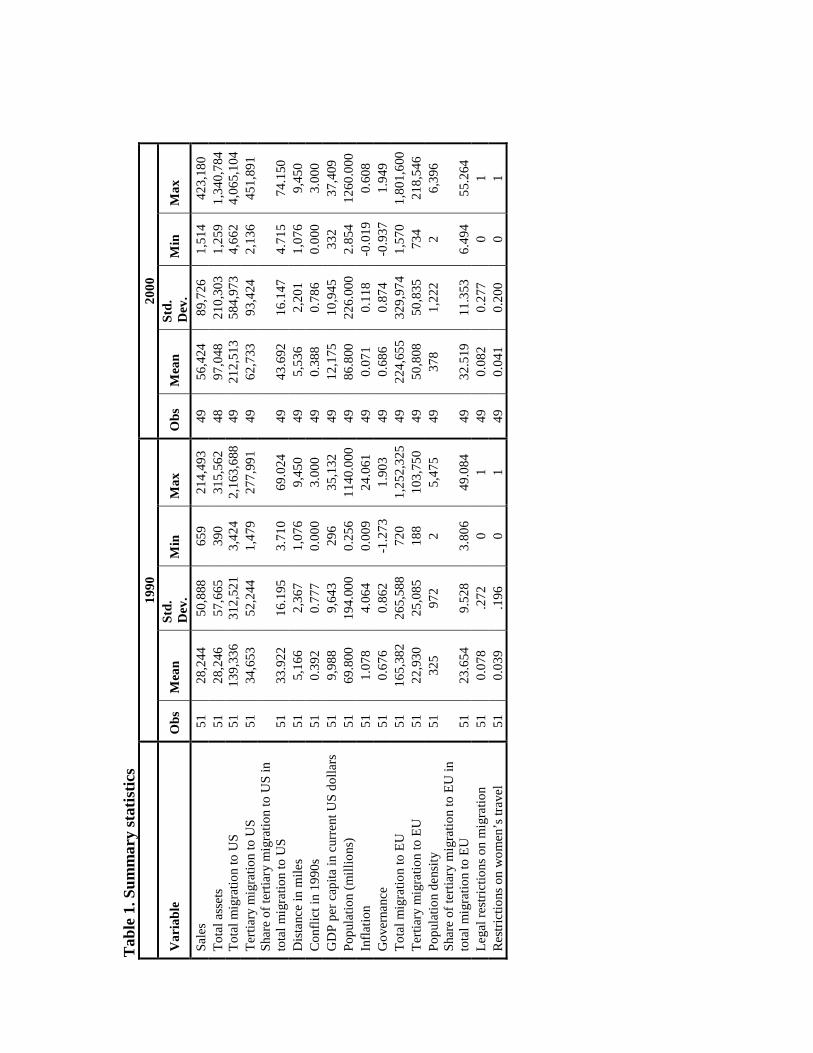
Turning to other host country characteristics, figures on the population size, GDP per

capita in current US dollars and consumer price inflation have been taken from the World Bank’s

World Development Indicators. For 1990 we use the average of inflation from 1988 through

9 Extracts from the Census samples are made available through IPUMS (Integrated Public Use Microdata Series), which is a database maintained by Minnesota Population Center at University of Minnesota (http://beta.ipums.org/usa/index.html). 10 We consider the year of arrival and the year of the completion of the highest education degree and take the larger of the two numbers as the year of entry into the US labor market.

7

1992, and for 2000 the average from 1998 through 2002. Quality of the business climate is

measured using the average of the following governance indicators developed by Kaufman,

Kraay and Mastruzzi (2004): voice and accountability, political stability, government

effectiveness, regulatory quality, rule of law, and control of corruption. The indicators are

available for alternating years in the 1996-2004 period. They range from –2.5 to 2.5 with higher

numbers corresponding to higher quality of governance in the country. For 1990 we use the 1996

data and for 2000 we use 2000 data. The conflict indicator is an index constructed based on

information available at www.prio.no, “Armed Conflict Version 2.1.” by Gleditsch, Wallensteen,

Eriksson, Sollenberg and Strand (2002). The index takes on values from 0 (no conflict) to 3

(severe conflict) depending on the depth of the conflicts in which the country was

involved during the 1990s. The distance between the US and the partner country is measured in

miles and comes from Andrew Rose’s dataset available at http://faculty.haas.berkeley.edu/arose/.

In our instrumental variables approach, we use data on migrant stocks in the 15 countries

of the European Union disaggregated by country of origin and education level, taken from

Docquier and Marfouk (2005). We employ the information on passport fees from McKenzie

(2005). We normalize the fees by the country’s GDP per capita expressed in US dollars.11 Finally,

we use the data on population density from the World Development Indicators database.

As additional instruments, we employ a dummy variable taking the value of one for

countries in which women face restrictions on foreign travel and a dummy variable taking the

value of one for countries placing other legal restrictions on emigration. There are only two

countries in the sample which employ the first type of restrictions (Egypt and Saudi Arabia) and

four countries with the second type of restrictions (Ecuador, Equatorial Guinea, Israel where

government permission is required to travel and Singapore which restricts travel of citizens of

national service age). Moreover, due to a regrettable mismatch in timing, as these variables

pertain to year 2004/5, we use these additional instruments only in a robustness check. Both

variables come from McKenzie (2005).

Table 1 presents summary statistics of all variables used in the study.

11 The information on fees pertains to 2005. To make the figures comparable to the GDP per capita data we express the fees in 1990 and 2000 US dollars, as appropriate.

8

4. Results

4.1. OLS specification

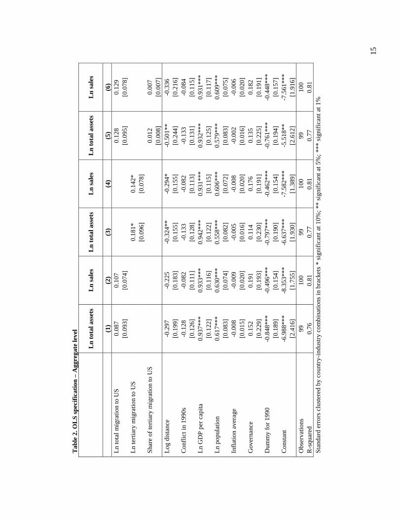
We begin our analysis with a basic OLS model and present the results for three sets of

regressions. Each set uses a different definition of the migration variable and within each set we

employ two alternative dependent variables: total assets of US affiliates abroad and sales of US

affiliates abroad. In the first set of regressions (columns 1 and 2 in Table 2), the variable of

interest is the total stock of migrants from the partner country c present in the US at time t. The

second set uses the stock of country c’s migrants with tertiary education living in the US at time t

(columns 3 and 4), and the third set employs both the aggregate stock of migrants from the

partner country c present in the US at time t as well as the share of tertiary educated migrants in

the total stock of migrants from the partner country c present in the US at time t (5 and 6).

The presence of migrants with a college education appears to be positively correlated

with US FDI in their country of origin. This effect is significant at the 10 percent level in both

specifications. In contrast, the aggregate stock of migrants does not have a statistically significant

effect on either of the FDI variables. When two indicators of migration (total migrant stock and

the share of college educated migrants) are entered into the same model, both bear positive signs

but neither variable reaches conventional significance levels.

Based on the OLS regression, it could be inferred that the presence of tertiary educated

migrants in US plays a role in FDI flows from the US to the origin countries of the migrants.

Total migration seems to have no discernible effect on FDI. However, these estimations are likely

to distort the true effect of migration on FDI, because they ignore the endogeneity that may be

present between FDI stocks and migration. To account for this possible endogeneity, we use the

instrumental variable approach in the following section.

The other control variables have the expected signs. We find that countries with large

markets (in terms of population size and GDP per capita) attract more FDI. Both variables are

significant at the one percent level. The same is true of countries located closer to the US, albeit

this variable is not significant in all specifications. While the other control variables bear the

anticipated signs, they are not statistically significant with the exception of the time dummy

which suggests that FDI stock in 2000 exceeded that of a decade earlier. The regressions have a

satisfactory explanatory power with the R-squared ranging from .76 to .81.

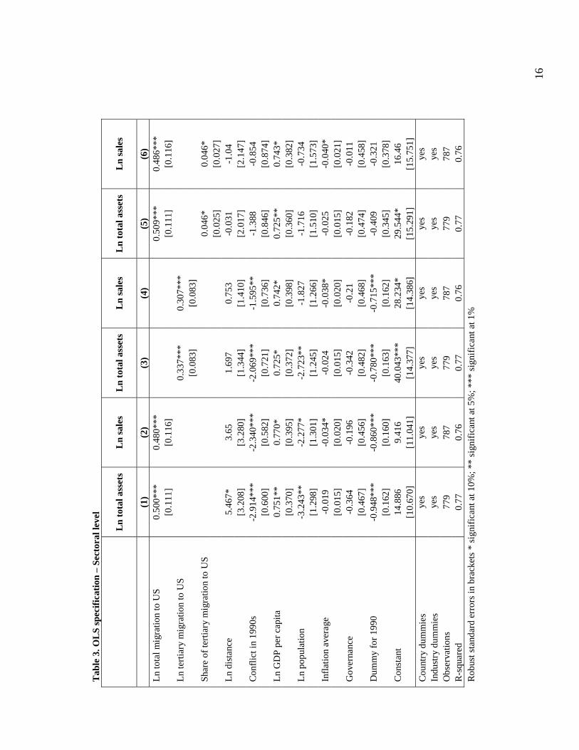
Our data also allow us to repeat the above exercise at the sectoral level.12 More precisely,

we regress the stock of FDI in sector s in country c at time t on the presence of migrants from

12 Recall the anecdotal evidence mentioned in footnote 3.

9

country c employed in sector s in the US at time t. The model includes partner country and

industry fixed effects. Standard errors are clustered at the country-industry level. The results,

presented in Table 3, differ from those obtained earlier. In all six regressions, we find a positive

and significant coefficient on the stock of migrants employed in the sector. This is the case for the

stock of migrants regardless of their educational background as well as for the stock of migrants

with tertiary education. Moreover, when the total sectoral stock is entered jointly with the share

of educated migrants, we find that both variables bear positive and statistically significant

coefficients.

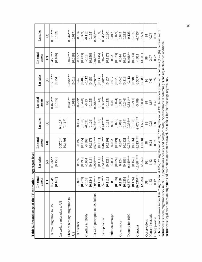
4.2. Instrumental variable approach

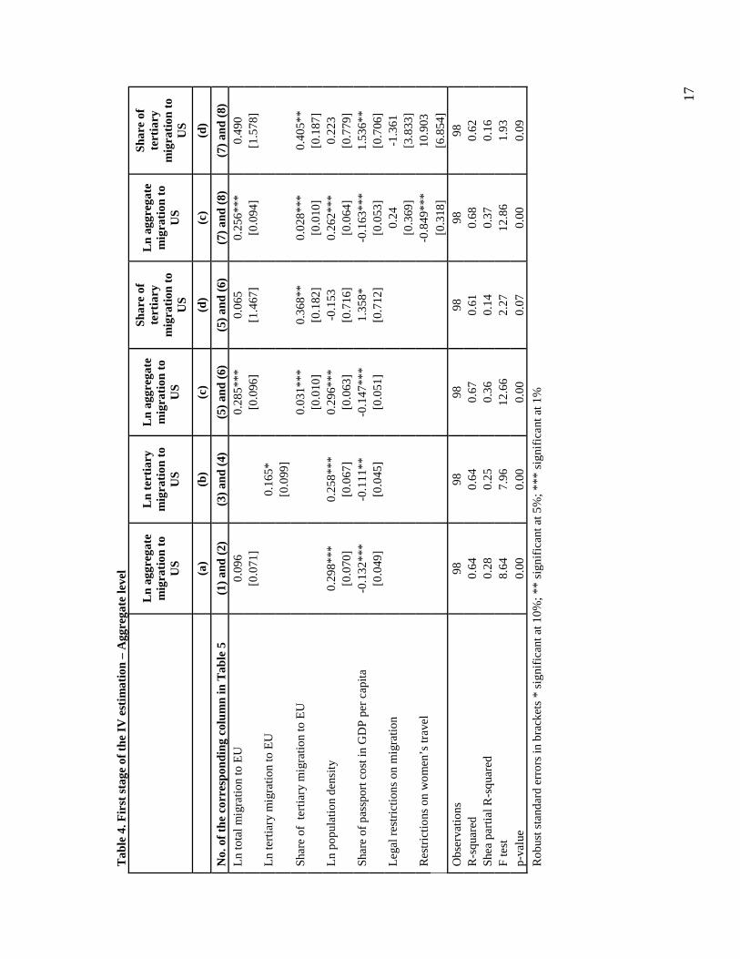
Next we employ the instrumental variable approach and present the first and the second

stage results in Tables 4 and 5, respectively. Our baseline set of instruments includes: the

presence of migrants in the EU (total stock, stock of tertiary educated migrants or share of tertiary

educated migrants in total stock, depending on the specification), population density in the

migrants’ country of origin and the cost of obtaining a national passport normalized by GDP per

capita in the migrants’ country of origin. As a robustness check, in the last two specifications we

also present results with additional instruments (restrictions on womens’ travel and other legal

restrictions on emigration).

As illustrated in Table 4, our instruments perform quite well as they can explain a

significant portion, between 14% and 36%, of the variable they are instrumenting for, i.e. the

aggregate stock of migrants or the stock of migrants with tertiary education. Their suitability is

also confirmed by the test of excluded instruments and the overidentification tests. All

instruments have the expected sign. While a higher population density and a larger migrant stock

in the EU are positively correlated with the presence of migrants in the US, a negative correlation

is found between the passport cost, restrictions on women’s travel and the migration variable.

The partner country specific control variables in the second stage (Table 5) exhibit the

same sign and significance pattern as in the OLS specification. The only exception is the distance,

which has ceased to be statistically significant in all but one specification.

Large differences, however, appear with respect to migration. As we have corrected for

the endogeneity of the migration variables, their coefficients should reflect reality to a greater

extent than the coefficients in the OLS regressions. We find that both aggregate migrant stock as

well as the stock of migrants with tertiary education are positively correlated with the stock of US

FDI in the migrants’ country of origin. The coefficients on migrant stocks are statistically

significant in all 8 specifications. The elasticity of FDI with respect to migration is higher for

10

skilled migrants, which is intuitive as college educated migrants may be better positioned both

financially and socially to assist US companies and entrepreneurs in investing abroad. This

pattern is confirmed in the last four specifications where both the aggregate migrant stock and the

share of skilled migrants have positive and statistically significant coefficients.

The magnitudes of these effects are economically meaningful. A one percent increase in

the total migrant stock is associated with a .3 percent increase in the FDI stock. In the case of

skilled migrants, the corresponding effect is higher reaching about .4 percent. Using the last two

specifications as the basis for inference, we find that a 10 percent rise in the share of tertiary

educated migrants in the migrant population increases the FDI stock in their country of origin by

an additional .57 percent.

We conclude that there exists a positive correlation between the presence of migrants in

the US and the stock of FDI in their country of origin. This correlation is particularly strong in the

case of migrants with college education. Our analysis also suggests that ignoring the endogeneity

issue tends to underestimate the effect of migration on FDI.

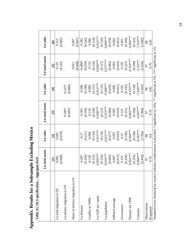
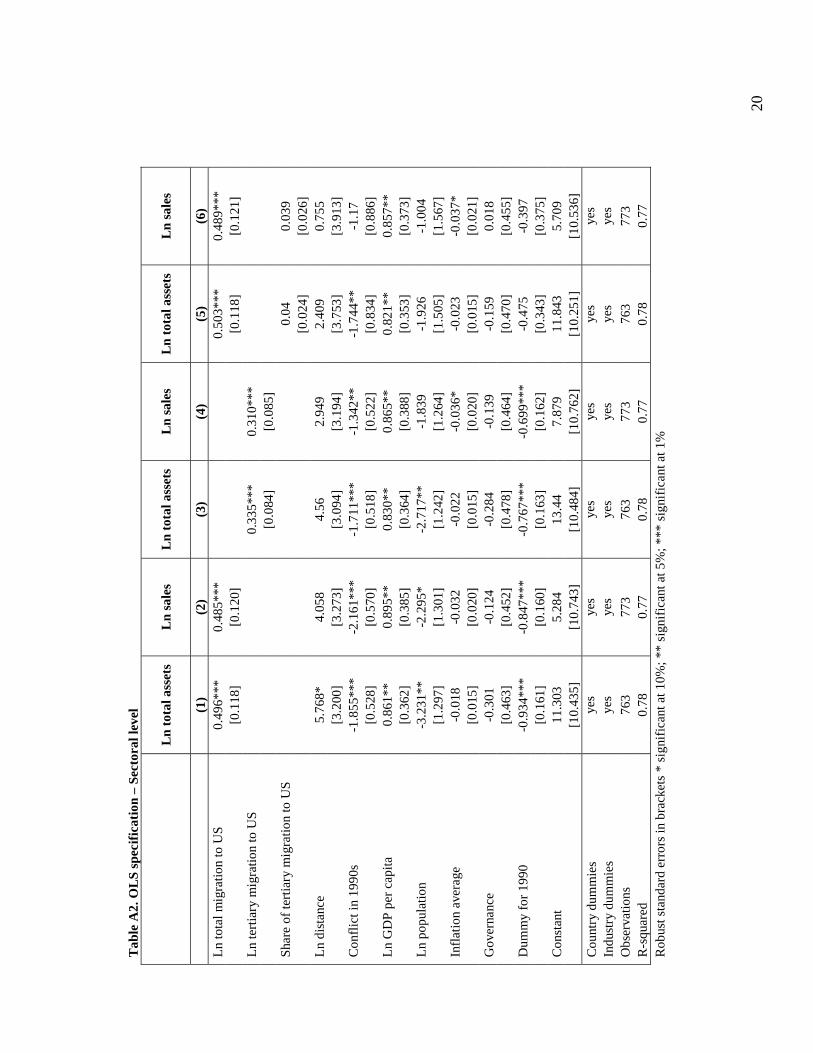
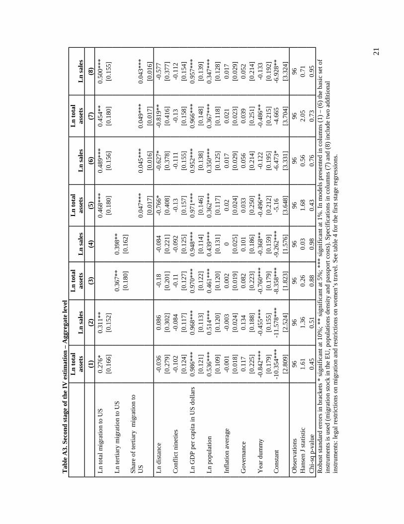
4.3. Robustness checks

To check the robustness of our results, we reestimated all regressions excluding Mexico,

which has a special status vis-à-vis the US relative to other destination countries included in the

analysis, both as a sender of migratory flows and as a recipient of FDI. The special relationship

between the US and Mexico is due to their geographic proximity, membership in NAFTA as well

as from a large differential in the level of economic development between the two neighbors

which prompts a large number of Mexicans to cross the border in search of a better life. The

results, presented in Appendix Tables A1 (OLS – aggregate FDI flows), Table A2 (OLS – sector-

level FDI flows) and Table A3 (IV regressions) do not differ significantly from the results of the

orginal model. Therefore, we conclude that our findings are not driven by the figures for Mexico.

5. Conclusions

The purpose of this study was to examine whether migrant networks have a positive

effect on flows of foreign direct investment to the migrants’ country of origin. To study this

question, we used data on US FDI abroad and the presence of migrants in the US. To take into

account the potential simultaneity between FDI and migrant flows, we instrumented for the

migrant presence in the US using information on the stock of migrants from the country of origin

11

present in the EU, population density in the migrants’ country of origin, the cost of obtaining a

national passport and other legal barriers to emigration in the migrants’ country of origin.

Our results suggest that US FDI abroad is positively correlated with the presence of

migrants from the host country. This finding is consistent with the hypothesis that ethnic

networks serve as an important channel of information about business conditions and

opportunities abroad, which was postulated and confirmed in the context of the international trade

literature. Our findings further indicate that the relationship between FDI and migration is driven

by the presence of migrants with a college education, thus suggesting that the presence of an

educated diaspora may have a positive effect on the integration its country of origin with the

global economy.

12

6. Bibliography

Alfaro, Laura, Areendam Chanda, Sebnem Kalemli-Ozcan, and Selin Sayek. 2004. "FDI and Economic Growth: The Role of Local Financial Markets," Journal of International Economics 64(1).

Buch, Claudia, Jörn Kleinert and Farid Toubal. 2003. “Where Enterprises Lead, People Follow? Links Between Migration and German FDI,” Kiel Working Paper No. 1190.

Bhattacharya, Utpal and Peter Groznik. 2003. “Melting Pot or Salad Bowl: Some Evidence from U.S. Investments Abroad,”. EFA 2003 Annual Conference Paper No.650.

Commander, Simon, Rupa Chanda and L. Alan Winters. 2004. “Who Gains from Skilled Migration? Evidence from the Software Industry,” London Business School mimeo.

Docquier, Frederic and Abdeslam Marfouk. 2005. “Measuring the international mobility of skilled workers (1990-2000),” World Bank Policy Research Working Paper No. 3381.

Gleditsch, Nils Petter, Peter Wallensteen, Mikael Eriksson, Margareta Sollenberg & Håvard Strand. 2002. “Armed Conflict 1946–2001: A New Dataset,” Journal of Peace Research 39(5): 615–637.

Gould, David M. 1994. “Immigrant Links to the Home Country: Empirical Implications for U.S. Bilateral Trade Flows,” Review of Economics and Statistics, 76: 302-16.

Head, Keith and John Ries. 1998. “Immigration and Trade Creation: Econometric Evidence from Canada,” Canadian Journal of Economics, 31(1): 47-62.

Kaufmann, Daniel; Kraay, Aart; Mastruzzi, Massimo. 2004. „Governance matters IV: governance indicators for 1996-2004,” World Bank Policy Research Working Paper No. 3630.

Kugler, Maurice and Hillel Rapoport. 2006. “Skilled Emigration, Business Networks and Foreign Direct Investment,” Economic Letters, forthcoming.

Lipsey, Robert E. and Fredrik Sjoholm. 2004. Foreign direct investment, education and wages in Indonesian manufacturing Journal of Development Economics, 73(1): 415-422.

Lucas, Robert E.B. 2005. International Migration and Economic Development: Lessons from Low Income Countries, Regeringskanliet, Sweden.

Markusen, James. 1986. “Explaining the Volume of Trade: An Eclectic Approach,” American Economic Review, 76(5): 1002-1011.

McKenzie, David. 2005. “Paper Wall Are Easier to Tear Down: Passport Costs and Legal Barriers to Emigration,” World Bank Policy Research Working Paper No. 3783.

Rauch, James. 2001. “Business and Social Networks in International Trade,” Journal of Economic Literature, XXXIX: 1177-1203.

Rauch, James and Vitor Trindade. 2002. “Ethnic Chinese Networks In International Trade, Review of Economics and Statistics 84(1): 116-130

Singh, Shinu. “Economic Impact of Return Migration of Highly-Skilled IT Professionals from the United States to India," Draft Thesis, Massachusetts Institute of Technology (downloaded on August 18, 2006 from http://web.mit.edu/nruiz/www/Documents/Shinu's%20Thesis%20Draft.pdf#search=%22Shinu%20Singh%20india%20migration%22)

13

Smarzynska, Beata and Shang-Jin Wei. 2000. “Corruption and Composition of Foreign Direct Investment: Firm Level Evidence” with Shang-Jin Wei, World Bank Policy Research Working Paper No. 2360.

Wei, Shang-Jin. 2000. "How Taxing Is Corruption on International Investors?" Review of Economics and Statistics. 82 (1): 1-11.

Tab

le 1

. Sum

mar

y st

atis

tics

1990

20

00

Var

iabl

e O

bs

Mea

n St

d.

Dev

. M

in

Max

O

bs

Mea

n St

d.

Dev

. M

in

Max

Sale

s 51

28

,244

50

,888

65

9 21

4,49

3 49

56

,424

89

,726

1,

514

423,

180

Tot

al a

sset

s 51

28

,246

57

,665

39

0 31

5,56

2 48

97

,048

21

0,30

3 1,

259

1,34

0,78

4 T

otal

mig

ratio

n to

US

51

139,

336

312,

521

3,42

4 2,

163,

688

49

212,

513

584,

973

4,66

2 4,

065,

104

Ter

tiary

mig

ratio

n to

US

51

34,6

53

52,2

44

1,47

9 27

7,99

1 49

62

,733

93

,424

2,

136

451,

891

Shar

e of

tert

iary

mig

ratio

n to

US

in

tota

l mig

ratio

n to

US

51

33.9

22

16.1

95

3.71

0 69

.024

49

43

.692

16

.147

4.

715

74.1

50

Dis

tanc

e in

mile

s 51

5,

166

2,36

7 1,

076

9,45

0 49

5,

536

2,20

1 1,

076

9,45

0 C

onfl

ict i

n 19

90s

51

0.39

2 0.

777

0.00

0 3.

000

49

0.38

8 0.

786

0.00

0 3.

000

GD

P p

er c

apita

in c

urre

nt U

S do

llars

51

9,

988

9,64

3 29

6 35

,132

49

12

,175

10

,945

33

2 37

,409

P

opul

atio

n (m

illi

ons)

51

69

.800

19

4.00

0 0.

256

1140

.000

49

86

.800

22

6.00

0 2.

854

1260

.000

In

flat

ion

51

1.

078

4.06

4 0.

009

24.0

61

49

0.07

1 0.

118

-0.0

19

0.60

8 G

over

nanc

e 51

0.

676

0.86

2 -1

.273

1.

903

49

0.68

6 0.

874

-0.9

37

1.94

9 T

otal

mig

ratio

n to

EU

51

16

5,38

2 26

5,58

8 72

0 1,

252,

325

49

224,

655

329,

974

1,57

0 1,

801,

600

Ter

tiary

mig

ratio

n to

EU

51

22

,930

25

,085

18

8 10

3,75

0 49

50

,808

50

,835

73

4 21

8,54

6 P

opul

atio

n de

nsit

y 51

32

5 97

2 2

5,47

5 49

37

8 1,

222

2 6,

396

Shar

e of

tert

iary

mig

ratio

n to

EU

in

tota

l mig

ratio

n to

EU

51

23

.654

9.

528

3.80

6 49

.084

49

32

.519

11

.353

6.

494

55.2

64

Leg

al r

estr

ictio

ns o

n m

igra

tion

51

0.07

8 .2

72

0 1

49

0.08

2 0.

277

0 1

Res

tric

tions

on

wom

en’s

trav

el

51

0.03

9 .1

96

0 1

49

0.04

1 0.

200

0 1

15

Tab

le 2

. OL

S sp

ecif

icat

ion

– A

ggre

gate

leve

l

L

n to

tal a

sset

s L

n sa

les

Ln

tota

l ass

ets

Ln

sale

s L

n to

tal a

sset

s L

n sa

les

(1

) (2

) (3

) (4

) (5

) (6

) L

n to

tal m

igra

tion

to U

S 0.

087

0.10

7

0.

128

0.12

9

[0.0

93]

[0.0

74]

[0.0

95]

[0.0

78]

Ln

tert

iary

mig

ratio

n to

US

0.18

1*

0.14

2*

[0

.096

] [0

.078

]

Sh

are

of te

rtia

ry m

igra

tion

to U

S

0.

012

0.00

7

[0.0

08]

[0.0

07]

Log

dis

tanc

e -0

.297

-0

.225

-0

.324

**

-0.2

94*

-0.5

01**

-0

.336

[0.1

99]

[0.1

83]

[0.1

55]

[0.1

55]

[0.2

44]

[0.2

16]

Con

flic

t in

1990

s -0

.128

-0

.082

-0

.133

-0

.082

-0

.133

-0

.084

[0.1

26]

[0.1

11]

[0.1

28]

[0.1

13]

[0.1

31]

[0.1

15]

Ln

GD

P p

er c

apita

0.

937*

**

0.93

3***

0.

942*

**

0.93

1***

0.

932*

**

0.93

1***

[0.1

22]

[0.1

16]

[0.1

22]

[0.1

15]

[0.1

25]

[0.1

17]

Ln

popu

latio

n 0.

617*

**

0.63

0***

0.

558*

**

0.60

6***

0.

579*

**

0.60

9***

[0.0

83]

[0.0

74]

[0.0

82]

[0.0

72]

[0.0

83]

[0.0

75]

Infl

atio

n av

erag

e

-0.0

08

-0.0

09

-0.0

05

-0.0

08

-0.0

02

-0.0

06

[0

.015

] [0

.020

] [0

.016

] [0

.020

] [0

.016

] [0

.020

] G

over

nanc

e 0.

152

0.19

1 0.

114

0.17

6 0.

135

0.18

2

[0.2

29]

[0.1

93]

[0.2

30]

[0.1

91]

[0.2

25]

[0.1

91]

Dum

my

for

1990

-0

.848

***

-0.4

96**

* -0

.797

***

-0.4

62**

* -0

.761

***

-0.4

48**

*

[0.1

89]

[0.1

54]

[0.1

90]

[0.1

54]

[0.1

94]

[0.1

57]

Con

stan

t -6

.988

***

-8.3

53**

* -6

.637

***

-7.5

82**

* -5

.518

**

-7.5

61**

*

[2.4

16]

[1.7

55]

[1.9

30]

[1.3

89]

[2.6

12]

[1.9

16]

Obs

erva

tions

99

10

0 99

10

0 99

10

0 R

-squ

ared

0.

76

0.81

0.

77

0.81

0.

77

0.81

St

anda

rd e

rror

s cl

uste

red

by c

ount

ry-i

ndus

try

com

bina

tion

s in

bra

cket

s *

sign

ific

ant a

t 10%

; **

sign

ific

ant a

t 5%

; ***

sig

nifi

cant

at 1

%

16

T

able

3. O

LS

spec

ific

atio

n –

Sect

oral

leve

l

L

n to

tal a

sset

s L

n sa

les

Ln

tota

l ass

ets

Ln

sale

s L

n to

tal a

sset

s L

n sa

les

(1

) (2

) (3

) (4

) (5

) (6

) L

n to

tal m

igra

tion

to U

S 0.

500*

**

0.48

0***

0.

509*

**

0.48

6***

[0.1

11]

[0.1

16]

[0.1

11]

[0.1

16]

Ln

tert

iary

mig

ratio

n to

US

0.33

7***

0.

307*

**

[0

.083

] [0

.083

]

Sh

are

of te

rtia

ry m

igra

tion

to U

S

0.

046*

0.

046*

[0.0

25]

[0.0

27]

Ln

dist

ance

5.

467*

3.

65

1.69

7 0.

753

-0.0

31

-1.0

4

[3.2

08]

[3.2

80]

[1.3

44]

[1.4

10]

[2.0

17]

[2.1

47]

Con

flic

t in

1990

s -2

.914

***

-2.3

40**

* -2

.069

***

-1.5

95**

-1

.388

-0

.854

[0.6

00]

[0.5

82]

[0.7

21]

[0.7

36]

[0.8

46]

[0.8

74]

Ln

GD

P p

er c

apita

0.

751*

* 0.

770*

0.

725*

0.

742*

0.

725*

* 0.

743*

[0.3

70]

[0.3

95]

[0.3

72]

[0.3

98]

[0.3

60]

[0.3

82]

Ln

popu

latio

n -3

.243

**

-2.2

77*

-2.7

23**

-1

.827

-1

.716

-0

.734

[1.2

98]

[1.3

01]

[1.2

45]

[1.2

66]

[1.5

10]

[1.5

73]

Infl

atio

n av

erag

e

-0.0

19

-0.0

34*

-0.0

24

-0.0

38*

-0.0

25

-0.0

40*

[0

.015

] [0

.020

] [0

.015

] [0

.020

] [0

.015

] [0

.021

] G

over

nanc

e -0

.364

-0

.196

-0

.342

-0

.21

-0.1

82

-0.0

11

[0

.467

] [0

.456

] [0

.482

] [0

.468

] [0

.474

] [0

.458

] D

umm

y fo

r 19

90

-0.9

48**

* -0

.860

***

-0.7

80**

* -0

.715

***

-0.4

09

-0.3

21

[0

.162

] [0

.160

] [0

.163

] [0

.162

] [0

.345

] [0

.378

] C

onst

ant

14.8

86

9.41

6 40

.043

***

28.2

34*

29.5

44*

16.4

6

[10.

670]

[1

1.04

1]

[14.

377]

[1

4.38

6]

[15.

291]

[1

5.75

1]

Cou

ntry

dum

mie

s ye

s ye

s ye

s ye

s ye

s ye

s In

dust

ry d

umm

ies

yes

yes

yes

yes

yes

yes

Obs

erva

tions

77

9 78

7 77

9 78

7 77

9 78

7 R

-squ

ared

0.

77

0.76

0.

77

0.76

0.

77

0.76

R

obus

t sta

ndar

d er

rors

in b

rack

ets

* si

gnif

ican

t at 1

0%; *

* si

gnif

ican

t at 5

%; *

** s

igni

fica

nt a

t 1%

17

Tab

le 4

. Fir

st s

tage

of

the

IV e

stim

atio

n –

Agg

rega

te le

vel

L

n ag

greg

ate

mig

rati

on t

o U

S

Ln

tert

iary

m

igra

tion

to

US

Ln

aggr

egat

e m

igra

tion

to

US

Shar

e of

te

rtia

ry

mig

rati

on t

o U

S

Ln

aggr

egat

e m

igra

tion

to

US

Shar

e of

te

rtia

ry

mig

rati

on t

o U

S

(a

) (b

) (c

) (d

) (c

) (d

)

No.

of

the

corr

espo

ndin

g co

lum

n in

Tab

le 5

(1

) an

d (2

) (3

) an

d (4

) (5

) an

d (6

) (5

) an

d (6

) (7

) an

d (8

) (7

) an

d (8

) L

n to

tal m

igra

tion

to E

U

0.09

6

0.28

5***

0.

065

0.25

6***

0.

490

[0

.071

]

[0.0

96]

[1.4

67]

[0.0

94]

[1.5

78]

Ln

tert

iary

mig

ratio

n to

EU

0.16

5*

[0.0

99]

Shar

e of

ter

tiary

mig

ratio

n to

EU

0.

031*

**

0.36

8**

0.02

8***

0.

405*

*

[0.0

10]

[0.1

82]

[0.0

10]

[0.1

87]

Ln

popu

latio

n de

nsit

y 0.

298*

**

0.25

8***

0.

296*

**

-0.1

53

0.26

2***

0.

223

[0

.070

] [0

.067

] [0

.063

] [0

.716

] [0

.064

] [0

.779

] Sh

are

of p

assp

ort c

ost i

n G

DP

per

cap

ita

-0.1

32**

* -0

.111

**

-0.1

47**

* 1.

358*

-0

.163

***

1.53

6**

[0

.049

] [0

.045

] [0

.051

] [0

.712

] [0

.053

] [0

.706

] L

egal

res

tric

tions

on

mig

ratio

n

0.

24

-1.3

61

[0

.369

] [3

.833

] R

estr

ictio

ns o

n w

omen

’s tr

avel

-0

.849

***

10.9

03

[0

.318

] [6

.854

] O

bser

vatio

ns

98

98

98

98

98

98

R-s

quar

ed

0.64

0.

64

0.67

0.

61

0.68

0.

62

Shea

par

tial R

-squ

ared

0.

28

0.25

0.

36

0.14

0.

37

0.16

F

test

8.

64

7.96

12

.66

2.27

12

.86

1.93

p-

valu

e 0.

00

0.00

0.

00

0.07

0.

00

0.09

Rob

ust s

tand

ard

erro

rs in

bra

cket

s *

sign

ific

ant a

t 10%

; **

sign

ific

ant a

t 5%

; ***

sig

nifi

cant

at 1

%

18

Tab

le 5

. Sec

ond

stag

e of

the

IV

est

imat

ion

– A

ggre

gate

leve

l

L

n to

tal

asse

ts

Ln

sale

s L

n to

tal

asse

ts

Ln

sale

s L

n to

tal

asse

ts

Ln

sale

s L

n to

tal

asse

ts

Ln

sale

s

(1

) (2

) (3

) (4

) (5

) (6

) (7

) (8

)

Ln

tota

l mig

ratio

n to

US

0.28

4*

0.32

6**

0.46

3***

0.

501*

**

0.45

0***

0.

511*

**

[0

.162

] [0

.153

]

[0

.165

] [0

.151

] [0

.166

] [0

.152

] L

n te

rtia

ry m

igra

tion

to U

S

0.

370*

* 0.

412*

*

[0.1

80]

[0.1

67]

Shar

e of

tert

iary

mig

ratio

n to

0.

045*

* 0.

046*

**

0.04

7***

0.

044*

**

US

[0

.018

] [0

.018

] [0

.018

] [0

.017

] L

n di

stan

ce

-0.0

03

0.07

6 -0

.197

-0

.153

-0

.709

* -0

.671

-0

.777

* -0

.614

[0.2

79]

[0.2

95]

[0.1

75]

[0.1

90]

[0.4

28]

[0.4

09]

[0.4

33]

[0.3

99]

Con

flic

t in

1990

s -0

.103

-0

.084

-0

.109

-0

.091

-0

.13

-0.1

12

-0.1

3 -0

.112

[0.1

24]

[0.1

18]

[0.1

27]

[0.1

26]

[0.1

55]

[0.1

56]

[0.1

56]

[0.1

55]

Ln

GD

P p

er c

apita

in U

S do

llars

0.

983*

**

0.97

6***

0.

974*

**

0.96

4***

0.

968*

**

0.95

9***

0.

963*

**

0.96

3***

[0.1

19]

[0.1

11]

[0.1

21]

[0.1

13]

[0.1

43]

[0.1

38]

[0.1

45]

[0.1

39]

Ln

popu

latio

n 0.

526*

**

0.51

1***

0.

463*

**

0.44

7***

0.

363*

**

0.34

8***

0.

367*

**

0.34

5***

[0.1

11]

[0.1

21]

[0.1

20]

[0.1

31]

[0.1

15]

[0.1

27]

[0.1

17]

[0.1

30]

Infl

atio

n av

erag

e 0

-0.0

03

0.00

2 -0

.001

0.

02

0.01

7 0.

02

0.01

7

[0.0

18]

[0.0

24]

[0.0

19]

[0.0

25]

[0.0

24]

[0.0

29]

[0.0

23]

[0.0

29]

Gov

erna

nce

0.11

8 0.

124

0.07

7 0.

082

0.03

9 0.

045

0.04

4 0.

043

[0

.225

] [0

.186

] [0

.222

] [0

.184

] [0

.246

] [0

.213

] [0

.247

] [0

.212

] D

umm

y fo

r 19

90

-0.8

37**

* -0

.449

***

-0.7

51**

* -0

.356

**

-0.5

11**

-0

.113

-0

.498

**

-0.1

25

[0

.176

] [0

.152

] [0

.176

] [0

.158

] [0

.211

] [0

.201

] [0

.213

] [0

.196

] C

onst

ant

-10.

536*

**

-11.

684*

**

-8.3

15**

* -9

.078

***

-5.4

89

-6.3

07*

-4.9

11

-6.7

93*

[2

.834

] [2

.556

] [1

.808

] [1

.535

] [3

.838

] [3

.606

] [3

.881

] [3

.559

] O

bser

vatio

ns

98

98

98

98

98

98

98

98

Han

sen

J st

atis

tic

1.53

1.

42

0.28

0.

26

1.67

0.

61

2.07

0.

76

Chi

-sq

p-va

lue

0.47

0.

49

0.87

0.

88

0.43

0.

74

0.72

0.

94

Rob

ust s

tand

ard

erro

rs in

bra

cket

s *

sign

ific

ant a

t 10%

; **

sign

ific

ant a

t 5%

; ***

sig

nifi

cant

at 1

%. I

n m

odel

s pr

esen

ted

in c

olum

ns (

1) –

(6)

the

basi

c se

t of

inst

rum

ents

is u

sed

(mig

ratio

n st

ock

in th

e E

U, p

opul

atio

ns d

ensi

ty a

nd p

assp

ort c

osts

). S

peci

fica

tions

in c

olum

ns (

7) a

nd (

8) in

clud

e tw

o ad

ditio

nal

inst

rum

ents

: leg

al r

estr

ictio

ns o

n m

igra

tion

and

rest

rict

ions

on

wom

en’s

trav

el. S

ee ta

ble

4 fo

r th

e fi

rst s

tage

reg

ress

ions

.

19

App

endi

x. R

esul

ts fo

r a

Subs

ampl

e E

xclu

ding

Mex

ico

Tab

le A

1. O

LS

spec

ific

atio

n –

Agg

rega

te le

vel

L

n to

tal a

sset

s L

n sa

les

Ln

tota

l ass

ets

Ln

sale

s L

n to

tal a

sset

s L

n sa

les

(1

) (2

) (3

) (4

) (5

) (6

) L

n to

tal m

igra

tion

to U

S 0.

085

0.09

1

0.

125

0.11

3

[0.0

98]

[0.0

79]

[0.1

01]

[0.0

82]

Ln

tert

iary

mig

ratio

n to

US

0.18

0*

0.13

7*

[0

.097

] [0

.080

]

Sh

are

of te

rtia

ry m

igra

tion

to U

S

0.

012

0.00

7

[0.0

08]

[0.0

07]

Ln

dist

ance

-0

.287

-0

.17

-0.3

03

-0.2

08

-0.4

90*

-0.2

82

[0

.220

] [0

.211

] [0

.194

] [0

.194

] [0

.259

] [0

.241

] C

onfl

ict i

n 19

90s

-0.1

28

-0.0

84

-0.1

34

-0.0

86

-0.1

33

-0.0

86

[0

.125

] [0

.110

] [0

.128

] [0

.112

] [0

.130

] [0

.114

] L

n G

DP

per

cap

ita

0.93

5***

0.

915*

**

0.93

8***

0.

912*

**

0.92

8***

0.

912*

**

[0

.124

] [0

.118

] [0

.123

] [0

.115

] [0

.127

] [0

.120

] L

n po

pula

tion

0.61

6***

0.

621*

**

0.55

3***

0.

588*

**

0.57

7***

0.

600*

**

[0

.083

] [0

.077

] [0

.084

] [0

.076

] [0

.083

] [0

.078

] In

flat

ion

aver

age

-0

.007

-0

.007

-0

.005

-0

.006

-0

.002

-0

.004

[0.0

15]

[0.0

20]

[0.0

16]

[0.0

21]

[0.0

16]

[0.0

21]

Gov

erna

nce

0.15

5 0.

21

0.11

8 0.

194

0.13

9 0.

202

[0

.230

] [0

.196

] [0

.231

] [0

.192

] [0

.227

] [0

.194

] D

umm

y fo

r 19

90

-0.8

51**

* -0

.504

***

-0.8

02**

* -0

.470

***

-0.7

63**

* -0

.454

***

[0

.193

] [0

.158

] [0

.194

] [0

.158

] [0

.199

] [0

.161

] C

onst

ant

-6.9

94**

* -8

.363

***

-6.6

97**

* -7

.818

***

-5.5

22**

-7

.553

***

[2

.418

] [1

.764

] [1

.964

] [1

.410

] [2

.618

] [1

.945

] O

bser

vatio

ns

97

98

97

98

97

98

R-s

quar

ed

0.76

0.

8 0.

76

0.81

0.

76

0.81

St

anda

rd e

rror

s cl

uste

red

by c

ount

ry-i

ndus

try

com

bina

tion

s in

bra

cket

s *

sign

ific

ant a

t 10%

; **

sign

ific

ant a

t 5%

; ***

sig

nifi

cant

at 1

%

20

T

able

A2.

OL

S sp

ecif

icat

ion

– Se

ctor

al le

vel

L

n to

tal a

sset

s L

n sa

les

Ln

tota

l ass

ets

Ln

sale

s L

n to

tal a

sset

s L

n sa

les

(1

) (2

) (3

) (4

) (5

) (6

) L

n to

tal m

igra

tion

to U

S 0.

496*

**

0.48

5***

0.

503*

**

0.48

9***

[0.1

18]

[0.1

20]

[0.1

18]

[0.1

21]

Ln

tert

iary

mig

ratio

n to

US

0.33

5***

0.

310*

**

[0

.084

] [0

.085

]

Sh

are

of te

rtia

ry m

igra

tion

to U

S

0.

04

0.03

9

[0.0

24]

[0.0

26]

Ln

dist

ance

5.

768*

4.

058

4.56

2.

949

2.40

9 0.

755

[3

.200

] [3

.273

] [3

.094

] [3

.194

] [3

.753

] [3

.913

] C

onfl

ict i

n 19

90s

-1.8

55**

* -2

.161

***

-1.7

11**

* -1

.342

**

-1.7

44**

-1

.17

[0

.528

] [0

.570

] [0

.518

] [0

.522

] [0

.834

] [0

.886

] L

n G

DP

per

cap

ita

0.86

1**

0.89

5**

0.83

0**

0.86

5**

0.82

1**

0.85

7**

[0

.362

] [0

.385

] [0

.364

] [0

.388

] [0

.353

] [0

.373

] L

n po

pula

tion

-3.2

31**

-2

.295

* -2

.717

**

-1.8

39

-1.9

26

-1.0

04

[1

.297

] [1

.301

] [1

.242

] [1

.264

] [1

.505

] [1

.567

] In

flat

ion

aver

age

-0

.018

-0

.032

-0

.022

-0

.036

* -0

.023

-0

.037

*

[0.0

15]

[0.0

20]

[0.0

15]

[0.0

20]

[0.0

15]

[0.0

21]

Gov

erna

nce

-0.3

01

-0.1

24

-0.2

84

-0.1

39

-0.1

59

0.01

8

[0.4

63]

[0.4

52]

[0.4

78]

[0.4

64]

[0.4

70]

[0.4

55]

Dum

my

for

1990

-0

.934

***

-0.8

47**

* -0

.767

***

-0.6

99**

* -0

.475

-0

.397

[0.1

61]

[0.1

60]

[0.1

63]

[0.1

62]

[0.3

43]

[0.3

75]

Con

stan

t 11

.303

5.

284

13.4

4 7.

879

11.8

43

5.70

9

[10.

435]

[1

0.74

3]

[10.

484]

[1

0.76

2]

[10.

251]

[1

0.53

6]

Cou

ntry

dum

mie

s ye

s ye

s ye

s ye

s ye

s ye

s In

dust

ry d

umm

ies

yes

yes

yes

yes

yes

yes

Obs

erva

tions

76

3 77

3 76

3 77

3 76

3 77

3 R

-squ

ared

0.

78

0.77

0.

78

0.77

0.

78

0.77

R

obus

t sta

ndar

d er

rors

in b

rack

ets

* si

gnif

ican

t at 1

0%; *

* si

gnif

ican

t at 5

%; *

** s

igni

fica

nt a

t 1%

21

Tab

le A

3. S

econ

d st

age

of t

he I

V e

stim

atio

n –

Agg

rega

te le

vel

L

n to

tal

asse

ts

Ln

sale

s L

n to

tal

asse

ts

Ln

sale

s L

n to

tal

asse

ts

Ln

sale

s L

n to

tal

asse

ts

Ln

sale

s

(1

) (2

) (3

) (4

) (5

) (6

) (7

) (8

)

Ln

tota

l mig

ratio

n to

US

0.27

6*

0.31

1**

0.46

8***

0.

489*

**

0.45

4**

0.50

0***

[0.1

66]

[0.1

52]

[0.1

80]

[0.1

56]

[0.1

80]

[0.1

55]

Ln

tert

iary

mig

ratio

n to

US

0.36

7**

0.39

8**

[0

.180

] [0

.162

]

Sh

are

of te

rtia

ry m

igra

tion

to

US

0.04

7***

0.

045*

**

0.04

9***

0.

043*

**

[0

.017

] [0

.016

] [0

.017

] [0

.016

] L

n di

stan

ce

-0.0

36

0.08

6 -0

.18

-0.0

84

-0.7

66*

-0.6

27*

-0.8

19**

-0

.577

[0.2

79]

[0.3

02]

[0.2

01]

[0.2

21]

[0.4

08]

[0.3

78]

[0.4

16]

[0.3

77]

Con

flic

t nin

etie

s -0

.102

-0

.084

-0

.11

-0.0

92

-0.1

3 -0

.111

-0

.13

-0.1

12

[0

.124

] [0

.117

] [0

.127

] [0

.125

] [0

.157

] [0

.155

] [0

.158

] [0

.154

] L

n G

DP

per

cap

ita in

US

dolla

rs

0.98

6***

0.

968*

**

0.97

0***

0.

948*

**

0.97

1***

0.

952*

**

0.96

6***

0.

957*

**

[0

.121

] [0

.113

] [0

.122

] [0

.114

] [0

.146

] [0

.138

] [0

.148

] [0

.139

] L

n po

pula

tion

0.53

6***

0.

514*

**

0.46

1***

0.

439*

**

0.36

2***

0.

350*

**

0.36

7***

0.

347*

**

[0

.109

] [0

.120

] [0

.120

] [0

.131

] [0

.117

] [0

.125

] [0

.118

] [0

.128

] In

flat

ion

aver

age

-0.0

01

-0.0

03

0.00

2 0

0.02

0.

017

0.02

1 0.

017

[0

.018

] [0

.024

] [0

.019

] [0

.025

] [0

.024

] [0

.029

] [0

.023

] [0

.029

] G

over

nanc

e 0.

117

0.13

4 0.

082

0.10

1 0.

033

0.05

6 0.

039

0.05

2

[0.2

25]

[0.1

88]

[0.2

23]

[0.1

86]

[0.2

50]

[0.2

14]

[0.2

51]

[0.2

14]

Yea

r du

mm

y -0

.842

***

-0.4

55**

* -0

.760

***

-0.3

68**

-0

.496

**

-0.1

22

-0.4

86**

-0

.133

[0.1

79]

[0.1

55]

[0.1

79]

[0.1

59]

[0.2

12]

[0.1

95]

[0.2

15]

[0.1

92]

Con

stan

t -1

0.35

4***

-1

1.57

8***

-8

.358

***

-9.2

62**

* -5

.16

-6.4

73*

-4.6

65

-6.9

28**

[2.8

09]

[2.5

24]

[1.8

23]

[1.5

76]

[3.6

48]

[3.3

31]

[3.7

04]

[3.3

24]

Obs

erva

tions

96

96

96

96

96

96

96

96

H

anse

n J

stat

istic

1.

61

1.36

0.

26

0.03

1.

68

0.56

2.

05

0.71

C

hi-s

q p-

valu

e 0.

45

0.51

0.

88

0.98

0.

43

0.76

0.

73

0.95

R

obus

t sta

ndar

d er

rors

in b

rack

ets

* si

gnif

ican

t at 1

0%; *

* si

gnif

ican

t at 5

%; *

** s

igni

fica

nt a

t 1%

. In

mod

els

pres

ente

d in

col

umns

(1)

– (

6) th

e ba

sic

set o

f in

stru

men

ts is

use

d (m

igra

tion

stoc

k in

the

EU

, pop

ulat

ions

den

sity

and

pas

spor

t cos

ts).

Spe

cifi

catio

ns in

col

umns

(7)

and

(8)

incl

ude

two

addi

tiona

l in

stru

men

ts: l

egal

res

tric

tions

on

mig

ratio

n an

d re

stri

ctio

ns o

n w

omen

’s tr

avel

. See

tabl

e 4

for

the

firs

t sta

ge r

egre

ssio

ns.

22