Microsatellite analysis of population structure and genetic variability in peregrine falcons (Falco peregrinus)

CBS Pollock workshop June 2005 WP-10

1

Microsatellite analysis of the population structure of the Bering Sea pollock

Shubina E.A.1, Ponomareva E.V.1, Glubokov A.I.2

1 Belozersky Institute, Department of Biology, Moscow State University, Russia 2 Russian Federal Research Institute of Fisheries and Oceanography, Moscow, Russia

The study continues a series of effort aimed at genetic certification of the spawning

concentrations of the Bering Sea pollock using microsatellite markers. The numerous microsatellite loci

are relatively evenly distributed throughout the genomes and, as a rule, are marked by a high allele

polymorphism. Such polymorphism emerges thanks to the DNA-polymerase sliding through along one

of the chains in the process of replication. The allele variants are inherited according to Mendel laws,

and are customarily considered to be selectively neutral. Despite the very low values of differentiation

indices caused by the large effective population size and a high level of gene flow, the sea fishes,

including pollock, are weakly but significantly genetically structured by neutral loci within a vast

spatial scale (Bailey et al., 1999, DeWoody&Avise, 2000, Bentzen et al., 1996). The Bering Sea

pollock was analyzed previously using Karagin, Olutor, Koryak, Navarin and North Kuril concentration

samples. It was shown, however, that the genetic distances between the territorially separated spawning

concentrations are short, and the dendrograms founded on those distances are not stable. The

microsatellite DNA molecular features marked by homoplastics (i.e. differences in the ways of

evolution of the same allele variants), and the high probability of reverse mutations slow down the

allele frequencies becoming divergent among various spawning concentrations, and entail discrepancies

between the results obtained from the samples separated by considerable time intervals (Olsen et al.,

2002). The minimum size of sample for the sea fish species of little variance is 70-150 fish depending

on the number of allele variants. The number of preparations examined from each sample must not be

less than 50. The specimens from territorially distant spawning stocks of an established population

status should be introduced into the analysis.

Our study involved the analysis of 306 specimens from six regions of the Bering Sea (Fig. 1):

Karagin, Olutor, Shirshov Ridge, Navarin, North Kuril and East Bering Sea. The pollock samples from

the East Bering Sea were provided by the courtesy of N. Williamson (Alaska Fisheries Research

Center).


2

N

E W Fig. 1. Sites of genetic sampling.

Materials and methods

Nine microsatellite loci identified by O’Reilly (O’Reilly et al.., 2000) were selected for

analysis: Tch5, Tch10, Tch12, Tch13, Tch14, Tch15, Tch18, Tch19 and Tch22. The sequences of

nine microsatellite sites and their primers are given in Figure 2.


3

Tch5 (GATA)14 F: gcc tta ata tca cgc aca R: tcg cat tga gcc tag ttt Tch10 (GGCT)6CTCT (GTCT)2 F: gtc tct atg tct gtc ttt cta ttt g R: acg aaa ccc aac cct gat t Tch12 (GGTT)22 F: caa ttt gtc agc ctс tgt tac c R: agt aca gct tga ttg ttt ctg gg Tch13 (GT)9 F: ttt ccg atg agg tca tgg R: agt aca gct tga ttg ttt ctg gg Tch14 (GAAA)31 F: cat aca ttg gtc act ctt tct tac R: aaa ctg ata tac gcc caa ct Tch15 (GA)3(CA)2GACA (GA)5CAGATA(GA)8 F: aaa ctt cac ctg acc aac R: gca aca caa ctt aat cat ct Tch18 (GT)15 F: gga gat ggt gct aac tgg R: aac gca cat gca cat acg. Tch19 (GTCT)15 F: tat gct gat tgg tta ggc R: gat cat ttg ttt cag aga gc

Tch22 (GACA)6 F: atc ata tct ggc caa gtt c R: ctc tct ctg aat ccc tct g

Fig. 2. The sequences of nine microsatellite sites and their primers (F-forward; R-reverse).

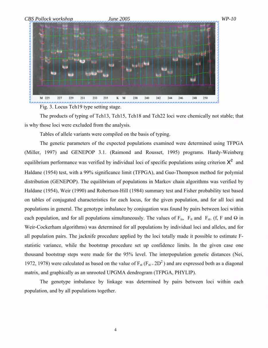
Electrophoretic subdivision of allele variants and genotyping The PCR products containing microsatellite fragments were divided in a 6% or 8%

polyacrylamid gel in TB acetate. Upon the completion of electrophoresis the gels were colored with

ethidium bromide and photographed in UV light. Allele variants were typed with KODAK 1D Image

analysis software. When data on marker fragment size is introduced this program allowed us to

determine the absolute size of microsatellite alleles. An example of stage of typing process is given in

the Figure 3.


4

Fig. 3. Locus Tch19 type setting stage.

The products of typing of Tch13, Tch15, Tch18 and Tch22 loci were chemically not stable; that

is why those loci were excluded from the analysis.

Tables of allele variants were compiled on the basis of typing.

The genetic parameters of the expected populations examined were determined using TFPGA

(Miller, 1997) and GENEPOP 3.1. (Raimond and Rousset, 1995) programs. Hardy-Weinberg

equilibrium performance was verified by individual loci of specific populations using criterion Χ2 and

Haldane (1954) test, with a 99% significance limit (TFPGA), and Guo-Thompson method for polymial

distribution (GENEPOP). The equilibrium of populations in Markov chain algorithms was verified by

Haldane (1954), Weir (1990) and Robertson-Hill (1984) summary test and Fisher probability test based

on tables of conjugated characteristics for each locus, for the given population, and for all loci and

populations in general. The genotype imbalance by conjugation was found by pairs between loci within

each population, and for all populations simultaneously. The values of Fis, Fit and Fst. (f, F and O in

Weir-Cockerham algorithms) was determined for all populations by individual loci and alleles, and for

all population pairs. The jacknife procedure applied by the loci totally made it possible to estimate F-

statistic variance, while the bootstrap procedure set up confidence limits. In the given case one

thousand bootstrap steps were made for the 95% level. The interpopulation genetic distances (Nei,

1972, 1978) were calculated as based on the value of Fst (Fst = 2D2 ) and are expressed both as a diagonal

matrix, and graphically as an unrooted UPGMA dendrogram (TFPGA, PHYLIP).

The genotype imbalance by linkage was determined by pairs between loci within each

population, and by all populations together.


5

Results and discussion

The results of genotyping of DNA preparations by loci are represented in histograms. The

height of tiers corresponds to the absolute values of allele frequencies in the given sample; X-axis

shows the allele variants of loci while the Y-axis shows the frequency of their occurrence.


6

Small differences in histograms from various samples were recorded in locus Tch5 (Fig. 4).

North Kuril

0

1

2

3

4

5

6

7

8

9

1 2 3 4 5 6 7 8 9 10 11 12 13 14 15 16 17 18 19 20 21 22 23 24 25 26 27 28 29 30

Karagin

0

1

2

3

4

5

6

7

1 2 3 4 5 6 7 8 9 10 11 12 13 14 15 16 17 18 19 20 21 22 23 24 25 26 27 28 29 30

Olutor

0

2

4

6

8

10

12

14

1 2 3 4 5 6 7 8 9 10 11 12 13 14 15 16 17 18 19 20 21 22 23 24 25 26 27 28 29 30

Shirshov

0

2

4

6

8

10

12

14

16

18

20

1 2 3 4 5 6 7 8 9 10 11 12 13 14 15 16 17 18 19 20 21 22 23 24 25 26 27 28 29 30

East Bering Sea

0

2

4

6

8

10

12

14

16

1 2 3 4 5 6 7 8 9 10 11 12 13 14 15 16 17 18 19 20 21 22 23 24 25 26 27 28 29 30

Navarin

0

2

4

6

8

10

12

1 2 3 4 5 6 7 8 9 10 11 12 13 14 15 16 17 18 19 20 21 22 23 24 25 26 27 28 29 30

Total

0

10

20

30

40

50

60

1 2 3 4 5 6 7 8 9 10 11 12 13 14 15 16 17 18 19 20 21 22 23 24 25 26 27 28 29 30

Fig. 4. Distribution of allele frequencies in locus Tch5.


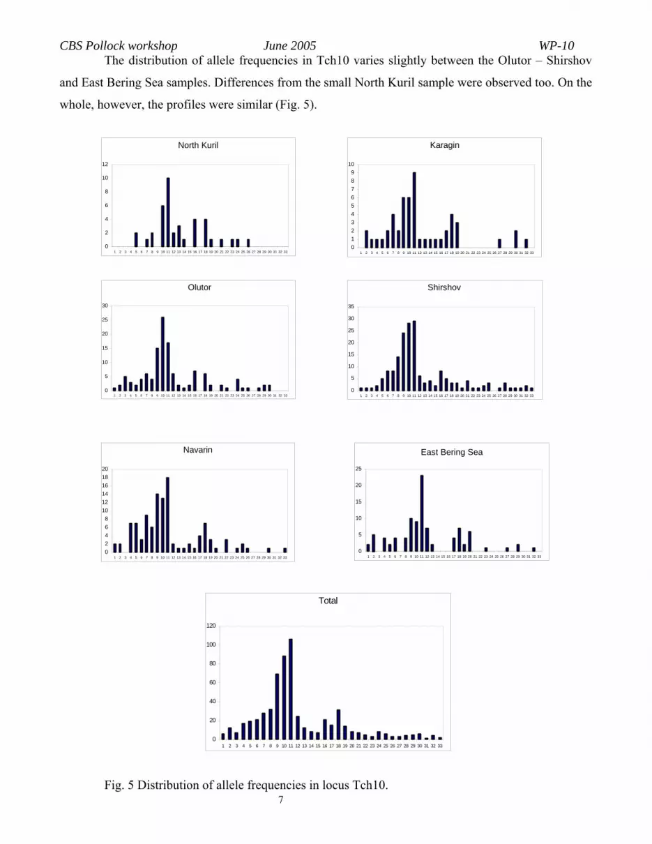
7 Fig. 5 Distribution of allele frequencies in locus Tch10.

The distribution of allele frequencies in Tch10 varies slightly between the Olutor – Shirshov

and East Bering Sea samples. Differences from the small North Kuril sample were observed too. On the

whole, however, the profiles were similar (Fig. 5).

Karagin

0123456789

10

1 2 3 4 5 6 7 8 9 10 11 12 13 14 15 16 17 18 19 20 21 22 23 24 25 26 27 28 29 30 31 32 33

North Kuril

0

2

4

6

8

10

12

1 2 3 4 5 6 7 8 9 10 11 12 13 14 15 16 17 18 19 20 21 22 23 24 25 26 27 28 29 30 31 32 33

Shirshov

0

5

10

15

20

25

30

35

1 2 3 4 5 6 7 8 9 10 11 12 13 14 15 16 17 18 19 20 21 22 23 24 25 26 27 28 29 30 31 32 33

Olutor

0

5

10

15

20

25

30

1 2 3 4 5 6 7 8 9 10 11 12 13 14 15 16 17 18 19 20 21 22 23 24 25 26 27 28 29 30 31 32 33

Navarin

02468

101214161820

1 2 3 4 5 6 7 8 9 10 11 12 13 14 15 16 17 18 19 20 21 22 23 24 25 26 27 28 29 30 31 32 33

East Bering Sea

0

5

10

15

20

25

1 2 3 4 5 6 7 8 9 10 11 12 13 14 15 16 17 18 19 20 21 22 23 24 25 26 27 28 29 30 31 32 33

Total

0

20

40

60

80

100

120

1 2 3 4 5 6 7 8 9 10 11 12 13 14 15 16 17 18 19 20 21 22 23 24 25 26 27 28 29 30 31 32 33

CBS Pollock workshop WP-10

8

orth Kuril and Karagin samples only

which may result from the insufficient volume of these samples (Fig. 6).

Fig. 6. Distribution of allele frequencies in locus Tch12.

June 2005 For locus 12 differences were obtained between the N

North Kuril

789

10

0123456

1 2 3 4 5 6 7 8 9 10 11

Karagin

20

25

0

5

10

15

1 2 3 4 5 6 7 8 9 10 11

Shirshov

50

60

0

10

20

30

40

1 2 3 4 5 6 7 8 9 10 11

Olutor

50

60

0

10

20

30

40

1 2 3 4 5 6 7 8 9 10 11

Navarin

0

5

10

15

20

25

30

35

40

1 2 3 4 5 6 7 8 9 10 11

East Bering Sea

0

5

10

15

20

25

30

35

40

1 2 3 4 5 6 7 8 9 10 11

Total

0

50

100

150

200

250

1 2 3 4 5 6 7 8 9 10 11

CBS Pollock workshop WP-10

9

T

rin – East Bering Sea samples

(Fig. 7). Totally, the sample’s distribution is close to normal.

ig. 7. Distribution of allele frequencies in locus Tch14.

rin – East Bering Sea samples

(Fig. 7). Totally, the sample’s distribution is close to normal.

ig. 7. Distribution of allele frequencies in locus Tch14.

June 2005 here is some bias in distribution of allele frequencies in the East Bering Sea sample but it

occurs smoothly in the series of the Karagin – Olutor – Shirshov– Nava

ere is some bias in distribution of allele frequencies in the East Bering Sea sample but it

occurs smoothly in the series of the Karagin – Olutor – Shirshov– Nava

FF

Shirshov

0

5

10

15

20

25

1 2 3 4 5 6 7 8 9 10 11 12 13 14 15 16 17 18 19 20 21 22 23 24 25 26 27

Olutor

2

4

6

8

10

12

14

16

01 2 3 4 5 6 7 8 9 10 11 12 13 14 15 16 17 18 19 20 21 22 23 24 25 26 27

North Kuril

0123456789

10

1 2 3 4 5 6 7 8 9 10 11 12 13 14 15 16 17 18 19 20 21 22 23 24 25 26 27

Karagin

0

1

2

3

4

5

6

7

8

1 2 3 4 5 6 7 8 9 10 11 12 13 14 15 16 17 18 19 20 21 22 23 24 25 26 27

Navarin

0

2

4

6

8

10

12

14

16

1 2 3 4 5 6 7 8 9 10 11 12 13 14 15 16 17 18 19 20 21 22 23 24 25 26 27

East Bering Sea

0

5

10

15

20

25

1 2 3 4 5 6 7 8 9 10 11 12 13 14 15 16 17 18 19 20 21 22 23 24 25 26 27

Total

01020304050607080

1 2 3 4 5 6 7 8 9 10 11 12 13 14 15 16 17 18 19 20 21 22 23 24 25 26 27


10

No not

Fig. 8. Distribution of allele

able differences were observed in allele frequency distribution in locus Tch19 (Fig. 8).

frequencies in locus Tch19.

Shirshov

0

5

10

15

20

25

1 2 3 4 5 6 7 8 9 10 11 12 13 14 15 16 17 18 19

North Kuril

0

1

2

3

4

5

6

7

8

1 2 3 4 5 6 7 8 9 10 11 12 13 14 15 16 17 18 19

Navarin

0

2

4

6

8

10

12

1 2 3 4 5 6 7 8 9 10 11 12 13 14 15 16 17 18 19

Olutor

0

5

10

15

20

1 2 3 4 5 6 7 8 9 10 11 12 13 14 15 16 17 18 19

Karagin

0

2

4

6

8

10

1 2 3 4 5 6 7 8 9 10 11 12 13 14 15 16 17 18 19

East Bering Sea

0

2

4

6

8

10

12

1 2 3 4 5 6 7 8 9 10 11 12 13 14 15 16 17 18 19

Total

01020304050607080

1 3 5 7 9 11 13 15 17 19


11

he main genetic indicators of the pollock samples examined and the characteristics of the

microsatellite markers used for that are given in Table 1. It includes the volume of the summary

samples examined, for each locus, the number of alleles in locus, the allele size pitch in nucleotide

pairs, the expected and observed heterozygosity. The most deviant loci are marked with asterisks. The

Hardy-Weinberg equilibrium is followed in loci Tch5 and Tch10 only.

Table 1. Characteristics of the main genetic indicators of samples and microsatellite loci.

Notation: N – number of specimens examined; Na – number of alleles in locus; R – allele size pitch in

nucleotide pairs; He – expected heterozygosity; Ho – heterozygosity observed.

Sample Loci

T

Tch 5 Tch 10 Tch 12 Tch 14 Tch 19 North Kuril N 20 20 20 20 19

Na 16 15 10 13 12 R 186-274 145-187 118-154 116-212 106-162 He 0,90 0,88 0,84 0,90 0,88 Ho 0,90 0,85 0,60* 0,60*** 0,74

Karagin N 25 26 26 25 26 Na 19 21 7 16 16 R 198-302 139-209 126-150 144-204 94-162 He 0,93 0,92 0,70 0,90 0,91 Ho 0,96 1,00 0,65 0,56*** 0,81

Olutor N 63 63 63 63 62 Na 25 26 8 22 15 R 186-294 137-199 126-158 116-220 106-166 He 0,94 0,91 0,75 0,93 0,91 Ho 0,83 0,87 0,48*** 0,75*** 0,66***

Shirshov N 90 90 89 89 90 Na 29 33 7 24 17 R 190-302 137-213 126-150 124-224 90-166 He 0,95 0,91 0,79 0,93 0,92 Ho 0,89 0,81 0,61* 0,65*** 0,63***

Navarin N 56 56 56 54 54 Na 26 25 8 21 18 R 186-290 139-209 126-154 112-220 90-162 He 0,94 0,92 0,77 0,92 0,93 Ho 0,85 0,84* 0,57** 0,70*** 0,57***

East Bering Sea N 49 49 48 49 49 Na 25 19 8 22 15 R 194-290 137-209 122-150 119-224 106-166 He 0,93 0,90 0,78 0,90 0,92 Ho 0,80** 0,76 0,69 0,71* 0,45***


12

The analysis of this table shows that heterozygote deficiency of some degree is a feature of all

tion alleles in

polymorphous loci. O’Reilly and others who have deve sed in

this paper recognize that in a number

low (O’Reilly et al., 2004). However, they ascribe sking in

electrophoresis of long alleles by the short ones, a utations in

flanking sequences – Blankenship thods of

n from

equilibrium make it possible to track down additi

The population differences were an

frequency variance. The North Kuril sample is a s of

genotypic and allele variants. The second ranking sa om the

East Bering Sea. The concentrations from th

differentiation. The error in summary

12, for which Hardy-Weinberg law correspondence was

The quantitative measure of the degree of diff

variance of gene frequencies. It is calculated as difference between

population and the intrapopulation varian

two software which apply different algorithms. Fit

sample; Fis is the intrapopulation variance; Fst is the stand egree

of differentiation which we revealed was very low, though the two estimates of this value obtained by

using two software agreed alm all differences

were recorded.

the samples examined. There is no correla with the size of samples or the number of

loped the set of microsatellite markers u

of loci (including Tch14 and Tch19) the level of heterozygosity is

that to technical causes, namely to ma

nd to a greater number of O-alleles (m

et al., 2002), and they believe that the “other me

electrophoresis” and involvement of programs accounting for the probability of deviatio

onal alleles which raises the heterozygosity.

alyzed by the genotype variants, allele diversity, and gene

significantly differentiated one both in term

mple showing loci differentiation comes fr

e Northwest Bering Sea do not show any significant

testing of loci for genotype and allele differentiation is 0.0226

and 0.000 respectively. It is noteworthy that genotype differentiation was found only in loci 5, 10 and

shown (Tch12 has a marginal deviation value).

erentiation in a population is a standardized

the variance in an undivided total

ce. Table 2 represents the values of variances calculated using

is variance of allele frequencies in the total undivided

ardized interpopulation variance. The d

ost fully. Locus Tch14 is the only exception where sm


13

Table 2. F – statistics estimates obtained with GENEPOP and TFPGA software reflecting

allele frequency distribution in five microsatellite loci of pollock. * - Locus where differences in

variance estimates were recorded.

Software

GENEPOP

TFPGA

FIS Estimates Loci

FIT

FST

FIS

FIT

FST

ch5T

0 092

,0015

907

,092

0015

908 , 193 0 42 0,0 91 0 2 0, 0,00

Tch10*

64

02

61

085

026

34 0,0 332 0,0 922 0,0 589 0, 8 0,0 0,08

Tch12 449

,00289

,2427

,246

031 436

0,2 32 0 3 0 41 0 0 0,0

0,2

7059

0,00366

0,26790

0,2706

0,0037

2679 Tch14 0,2 0 3 8 0,

Tch19

16

000

17

331

007

18 0,3 928 -0, 785 0,3 464 0, 3 -0, 0,33

average ,196

0,0020

0,1945

0,203

020 020

0 1 6 0,0

0,2

A precise te or su vision of samples in general by applying TFPGA program using

Markov chains concurrently for each of the five loci showed lack of difference for Tch5 locus only

(Raimond and Rouss 99

ultilocus test p ed the of Χ 21 ber of degrees of freedom

being equal to the 10 d 10

st f bdi

et, 1 5).

The m roduc value 2 as 60.5 3, the num

% an 0% probability of differentiation.


14

able 3. Pairs of genetic Nei distances (original ones above the diagonal; unbias ones below

the diag

T

onal) between various groups of pollock by five microsatellite loci

Concantration Shirshov Olutor North Kuril Karagin Navarin East Bering Sea

Shirshov ***

0,0701 0,2206 0,1128 0,0708 0,1137

Olutor 0,0121 ***

0,2375 0,1061 0,0906 0,1148

North Kuril 0,0890 0,0987 ***

0,3331 0,2492 0,3042

Karagin 0,0150 0,0011 0,1545 ***

0,11185 0,1441

Navarin 0,0045 0,0172 0,1022 0,0053 ***

0,1445

East Bering Sea 0,0473 0,0412 0,1570 0,0307 0,0627 ***

As is known, Nei distances are functions of the distances expressed in Fst units. That is why it

is only the unbias values adjusted by the size of sample that are of interest in Table 3.

The major source of being subdivided in the samples analyzed by genetic distances is the set of

the Nort

by all the markers used.

h Kuril samples. The difference between the size of Nei distances for the Bering Sea samples is

very small; still, there is some correlation with the sites of samples. At any rate, the East Bering Sea

and Navarin samples are genetically somewhat more distant than the Navarin and West Bering Sea

ones. The UPGMA cluster based on Nei genetic distances is shown in Figure 9. The bootstrap analysis

of the cluster showed that the linkpoint uniting the Shirshov and Olutor samples has a 51% bootstrap

coefficient, and is supported by 3 loci; linkpoints 2 and 3 (Navarin and Karagin samples respectively)

have bootstrap coefficient of 78% and 66%. Finally, the East Bering Sea and North Kuril samples were

100% supported


15

UPG ro

Sample rshov; . il ; 5 n; 6 ring

The unrooted dendrogram constructed on the basis of Nei distances shows the degree of

genetic distance of pollock groupings from er agre wit eographic

distances between them ).

F 9.ig MA dend gram of pollock concentrations based on Nei genetic distances.

s; 1. Shi 2. Olutor, 3 North Kur ; 4. Karagin . Navari East Be Sea.

one anoth wh ch i es ellw h t e gh

(Fig. 10


16

Fig 10. UPGMA dendrogram of pollock concentrations based on Nei genetic distances

(unrooted)

NorthKuril

Conclusions

1. Hardy-Weinberg law test confirmed the genetic equilibrium of all the groupings examined.

2. The allele frequency analysis was used as basis for the conclusion regarding the existence of a

genetic structure in the sample considered.

3. A quantitative evaluation of the difference showed similarity among the West Bering Sea

concentrations, Navarin inclusive. The East Bering Sea samples are very disparate in terms of

genetic distances. The North Kuril Grouping stands expressly aside.

4. The genetic distances between the samples on the whole reflect the geographic remoteness of

concentrations. The Karagin grouping is an exception. This might result from the insufficiency

of the sample.

Refernces

Bailey, K.M., T.J.Quinn, P.Bentzen & W.S.Grant. 1999. Population structure and dynamics of walleye

pollock, Theragra chalcogramma. Advances in Marine Biology. v.37:p.179-255.

0.1

Navarin

Shirshov ridge

Olyutor

EBS

Karagin


17

Bentzen, P., C.T.Taggart, D.E.Ruzzante , D.Cook. 1996. Microsatellite polymorphism and the

population structure of Atlantic cod (Gadus morhua) in the northwest Atlantic. 1996.

Can.J.Fish.Aquat.Sci., v.53, p.2706-2721.

Blankenship, S.M., B.May, D.Hedgecock. 2002. Evolution of a perfect simple sequence repeat locus in

the context of its flanking sequence. Mol.Biol.Evol. , v.19 (11), 1943-1951.

DeWoody, J.A. & J.C.Avise. Microsatellite variation in marine, freshwater and anadromous fishes

compared with other animals. 2000. J.of Fish Biol., v.56, p.461-473.

Holdane, J.B.S. 1954. An exact test for randomness of mating. J.Genet., v.52, p.631-635.

S.T.Kalinowski. 2005. Do polymorphic loci require large sample sizes to estimate genetic distances?

Heredity, v.94, p.33-36.

Miller, M.P. 1997. Tools for population genetic analysis (TFPGA) 1.3: A windows program for the

analysis

3-292.

Nei, M. 1978. Estimation of average heterozygosity and genetic distance from a small number of

individu

ramma) using allozyme, mitochondrial DNA, and microsatellite

data. Fish.Bull. v.100, p.752-764.

O'Reilly, P., M. Canino, K. Bailey & P. Bentzen. 2000. Isolation of twenty low stutter di- and

tetranucleotide microsatellites for population analyses of walleye pollock and other gadoids. J. Fish

Biol. V.56:p. 1074-1086.

O’Reilly, P.T., F.Canino, K.M. Bailey, P.Bentzen. 2004. Inverse relationship between Fst and

microsatellite polymorphism in the marine fish, walleye pollock (Theragra chalcogramma):

implications for resolving weak population structure. Molecular Ecology, v.13, p. 1799- 1814.

PHYLIP (Phylogeny Inference Package) Version 3.5c. Executables for Windows95, 98, NT systems.

Copyright 1986-1999 by Joseph Felsenstein and the University of Washington.

Raimond, M. & F. Rousset. 1995 An exact test for population differentiation. Evolution. v. 49: p.1280-

1283

Robertson, A. & W.G Hill. 1984. Deviations from Hardy-Weinberg proportions: sampling variances

and use in estimation of inbreeding coefficients. Genetics. v.107, p.713-718.

Ruzzante, D.E. 1998. A comparison of several measures of genetic distance and population structure

with microsatellite data: bias and sampling variance. Can. J. Fish. Aquat. Sci., v.55, p.1-14.

Weir, B.S. 1990. Analysis of genetic data. Moscow. Mir. P.399.

of allozyme and molecular population genetic data. Computer software distributed by author.

Nei, M. 1972. Genetic distance between population. American Naturalist, v.106 (949), p.28

al. Genetics, v.89, p.583-590.

Olsen, J.B., S.E.Merkouris, J.E.Seeb. 2002. An examination of spatial and temporal variation in

walleye pollock (Theragra chalcog

Documents

Microsatellite analysis of population structure and genetic variability in peregrine falcons (Falco peregrinus)