METALLIC PLASTICITY MODELLING – ABAQUS FEM CODE

METALLIC PLASTICITY MODELLING – ABAQUS FEM CODE

ISM2006

18/03/2016

Issue 2

Compiled by: Álvaro José Martínez / María Romero Menéndez 18/03/2016

Supervised by: María Romero Menéndez 18/03/2016

Approved by: Álvaro José Martínez 18/03/2016

Pág. 1 / 27

METALLIC PLASTICITY MODELLING – ABAQUS

FEM CODE


ISM2006

18/03/2016

Issue 2

Pág. 2 / 27

List of Document Changes

Issue Date Remarks

1 20/01/2015 First Issue.

2 18/03/2016 K formula (page 13) has been corrected


ISM2006

18/03/2016

Issue 2

Pág. 3 / 27

CONTENTS

REFERENCES ................................................................................................................................... 5

1. INTRODUCTION ................................................................................................................. 6

2. MATERIAL STRENGTH PARAMETERS ........................................................................... 7

2.1. YOUNG’S MODULUS, E ..................................................................................................... 8

2.2. YIELD STRENGTH - FTY ..................................................................................................... 8

2.3. ULTIMATE TENSILE STRENGTH - FTU ............................................................................. 8

2.4. PERCENT ELONGATION - % E ......................................................................................... 8

3. MATERIAL MODELLING IN ABAQUS .............................................................................. 9

3.1. TRUE STRESS AND LOGARITHMIC STRAIN (TRUE STRAIN) ....................................... 9

3.2. PLASTIC ENTRIES IN ABAQUS CODE ............................................................................. 9

3.3. IDEALIZATION OF THE STRESS-STRAIN CURVE ........................................................ 10

3.3.1. Elastic-Plastic Idealization ................................................................................................. 10

3.3.2. Elastic-Linear strain hardening Idealization ....................................................................... 11

3.3.3. Ramberg-Osgood Idealization ........................................................................................... 12

3.3.4. Ramberg-Osgood Idealization for ABAQUS Code ............................................................ 14

4. DEFINING MATERIAL DATA IN ABAQUS ENVIROMENT ............................................ 19

5. DFEM MODELLING GUIDELINES FOR NON-LINEAR ANALYSIS WITH ABAQUS (PLASTICITY) ................................................................................................................... 20

5.1. SHELL AND SOLID ELEMENT TYPES ............................................................................ 20

5.1.1. BENDING DOMINANT PROBLEMS ................................................................................. 20

5.1.2. CONTACT DOMINANT PROBLEMS WITHOUT BENDING ............................................ 20

5.1.3. CONTACT DOMINANT PROBLEMS WITH BENDING .................................................... 20

5.2. MESH DENSITY ................................................................................................................ 20

5.2.1. STRESS DISCONTINUITY ............................................................................................... 20

5.2.2. FILLET RADIUS ................................................................................................................ 20

6. POST-PROCESSING OF NON-LINEAR PLASTICITY ANALYSIS ................................ 22

6.1. RESERVE FACTOR .......................................................................................................... 22

6.2. PLASTIC ONSET FOR RAMBERG – OSGOOD IDEALIZATION .................................... 22

7. EXAMPLE ......................................................................................................................... 23

7.1. GEOMETRY ...................................................................................................................... 23

7.2. MESH ................................................................................................................................ 23

7.3. MATERIAL ......................................................................................................................... 24

7.4. LOAD ................................................................................................................................. 24

7.5. BOUNDARY CONDITIONS ............................................................................................... 24

7.6. RESULTS .......................................................................................................................... 25

7.6.1. MODEL 01 – Material Idealization: Elastic-Linear strain hardening .................................. 25


ISM2006

18/03/2016

Issue 2

Pág. 4 / 27

7.6.2. MODEL 02 – Material Idealization: Ramberg – Osgood ................................................... 25

7.6.3. Neuber Plasticity Correction .............................................................................................. 25

7.6.4. Summary ........................................................................................................................... 26

8. APPENDIX ........................................................................................................................ 27


ISM2006

18/03/2016

Issue 2

Pág. 5 / 27

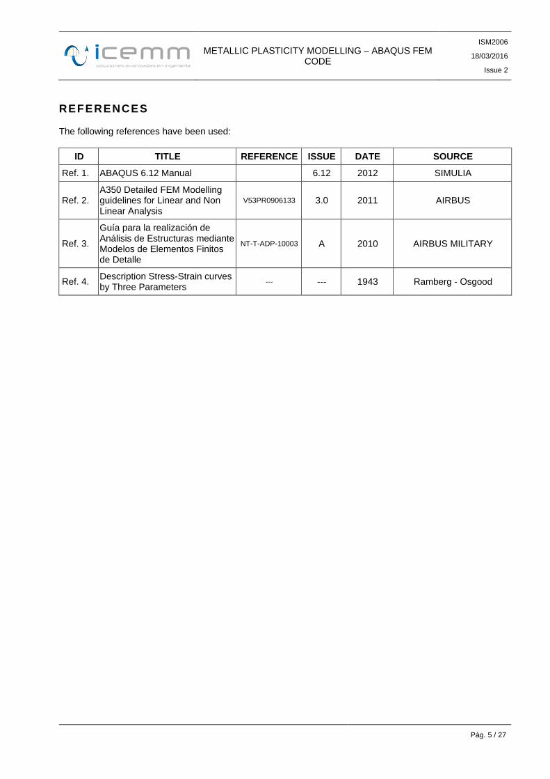
REFERENCES

The following references have been used:

ID TITLE REFERENCE ISSUE DATE SOURCE

Ref. 1. ABAQUS 6.12 Manual 6.12 2012 SIMULIA

Ref. 2. A350 Detailed FEM Modelling guidelines for Linear and Non Linear Analysis

V53PR0906133 3.0 2011 AIRBUS

Ref. 3.

Guía para la realización de Análisis de Estructuras mediante Modelos de Elementos Finitos de Detalle

NT-T-ADP-10003 A 2010 AIRBUS MILITARY

Ref. 4. Description Stress-Strain curves by Three Parameters

--- --- 1943 Ramberg - Osgood


ISM2006

18/03/2016

Issue 2

Pág. 6 / 27

1. INTRODUCTION

This document presents the different ways to model the plasticity behavior in ductile metals and its implementation in the FEM ABAQUS Code.

All concepts are based in the engineering tension test, which is widely used to provide basic design information on the strength of materials and as an acceptance test for the specification of materials.

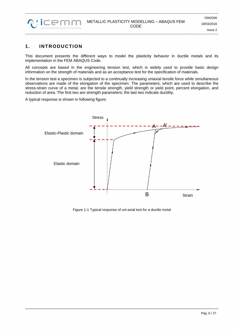
In the tension test a specimen is subjected to a continually increasing uniaxial tensile force while simultaneous observations are made of the elongation of the specimen. The parameters, which are used to describe the stress-strain curve of a metal, are the tensile strength, yield strength or yield point, percent elongation, and reduction of area. The first two are strength parameters; the last two indicate ductility.

A typical response is shown in following figure:

Figure 1-1 Typical response of uni-axial test for a ductile metal

Stress

Strain

Elastic-Plastic domain

Elastic domain


ISM2006

18/03/2016

Issue 2

Pág. 7 / 27

2. MATERIAL STRENGTH PARAMETERS

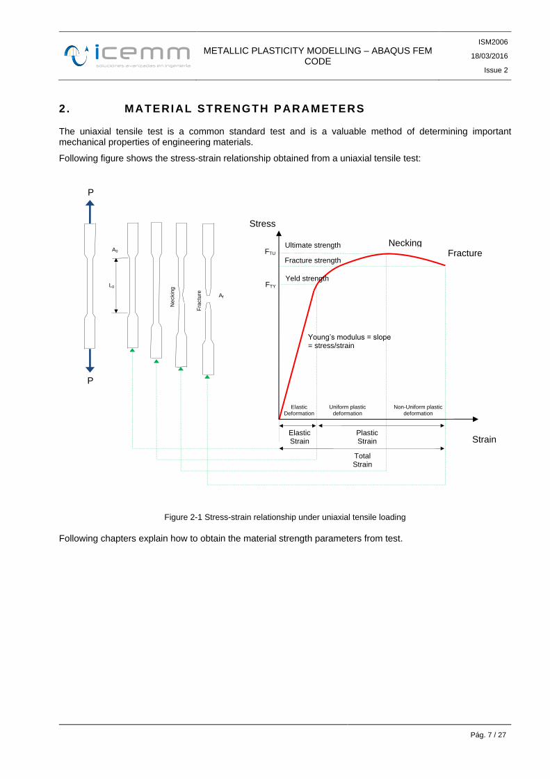
The uniaxial tensile test is a common standard test and is a valuable method of determining important mechanical properties of engineering materials.

Following figure shows the stress-strain relationship obtained from a uniaxial tensile test:

Figure 2-1 Stress-strain relationship under uniaxial tensile loading

Following chapters explain how to obtain the material strength parameters from test.

Stress

Strain

Necking Fracture

Yeld strength

Fracture strength

Ultimate strength

Young’s modulus = slope = stress/strain

Neckin

g

Fra

ctu

re

Af

A0

L0

Elastic Strain

Plastic Strain

Total Strain

Elastic Deformation

Uniform plastic deformation

Non-Uniform plastic deformation

P

P

FTY

FTU


ISM2006

18/03/2016

Issue 2

Pág. 8 / 27

2.1. YOUNG’S MODULUS, E

During elastic deformation, the engineering stress-strain relationship follows the Hooke's Law and the slope of the curve indicates the Young's modulus (E)

E

2.2. YIELD STRENGTH - FTY

The stress at which a material exhibits a specified permanent deformation.

This stress is usually determined by the offset method, where the strain departs from the linear portion of the actual stress–strain diagram by an offset unit strain of 0.002.

0

0002setstrain_off

TYA

PF

Where:

A0 = Original cross sectional area

P(strain_offset=0.002) = Load at 0.2% strain

2.3. ULTIMATE TENSILE STRENGTH - FTU

The ultimate strength of a material in uniaxial tension is the maximum tensile stress that the material can sustain calculated on the basis of the greatest load achieved prior to fracture.

0

MAXTU

A

PF

Where:

A0 = Original cross sectional area

PMAX = Maximum load

2.4. PERCENT ELONGATION - % E

Percent elongation is the increase in gage length, measured after fracture of the tensile specimen within the gage length, expressed as a percentage of the original gage length:

100L

L-Le %

0

0f

Where:

L0 = Initial gage length

Lf = Length of the gage section at fracture


ISM2006

18/03/2016

Issue 2

Pág. 9 / 27

3. MATERIAL MODELLING IN ABAQUS

Ductile metallic materials are usually modeled as plastic behavior with isotropic hardening (the yield surface changes size uniformly in all directions such that the yield stress increases or decreases in all stress directions as plastic straining occurs).

Yield data should always be given in ABAQUS as TRUE STRESS VERSUS LOGARITHMIC STRAIN.

3.1. TRUE STRESS AND LOGARITHMIC STRAIN (TRUE STRAIN)

Logarithmic strain (or true strain), ε, is defined as:

0

0

nom

0

L

L

L

L-L

ε1lnL

Lln

L

dLε

0

nom

Where:

L = Current gage length

L0 = Original gage length

εnom = engineering or nominal strain

There are two ways to define stress:

Engineering or nominal stress, σnom

: the force at any time during the test divided by the initPLASial

area of the test piece A0; σnom = F/A0

True stress, σ: The force at any time divided by the instantaneous area of the test piece; σ = F/Ai, Ai is

the instantaneous cross section of a test piece

Assuming that the piece volume is constant during deformation, Ai can be defined as a function of A0 and εnom

:

nom0

i

nom

0

0i

0

i

i

0

00ii

1

AA

L

LL1

L

L1

A

A

LALA

Therefore, the true stress is defined as:

nomnom

0i

11A

F

A

F nom

3.2. PLASTIC ENTRIES IN ABAQUS CODE

Material entries for plastic behavior with isotropic hardening in ABAQUS code are defined as following:

*****************************************

** Elastic behavior

*****************************************

*Material, name=material_name

*Elastic

young's module, poisson coefficient

*****************************************

** Plastic behavior


ISM2006

18/03/2016

Issue 2

Pág. 10 / 27

*****************************************

*Plastic

true_stress_1, logarithmic_plastic_strain_1



...

Where the logarithmic plastic strain is defined as the total logarithmic strain minus the elastic logarithmic strain:

E

11ln

E1ln

nomnomnom

ln

nompl

3.3. IDEALIZATION OF THE STRESS-STRAIN CURVE

Because of the complex nature of the stress-strain curve, it has become customary to idealize this curve in various ways.

Following chapters shows typical idealizations for ductile metallic plastic behavior.

3.3.1. Elastic-Plastic Idealization

Figure 3-1 Elastic-plastic idealization

This stress-strain curve is defined through the following entries:

*****************************************

** Elastic behavior

*****************************************


*Elastic

E, ν *****************************************

** Plastic behavior

*****************************************

*Plastic

0.0 , E

F1F

ty

ty


ISM2006

18/03/2016

Issue 2

Pág. 11 / 27

E

Fe1ln ,

E

F1F

truety,ty

ty

Where:

elongation e

E

F1FF

tytytruety,

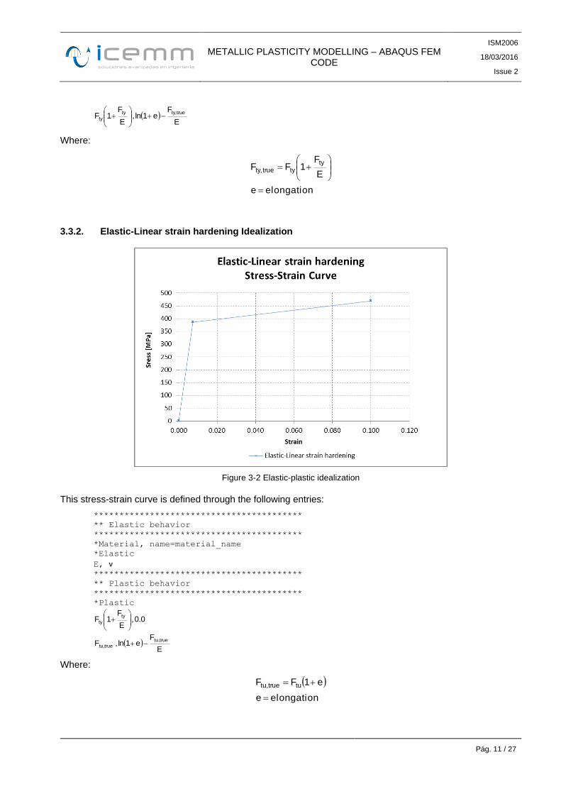
3.3.2. Elastic-Linear strain hardening Idealization

Figure 3-2 Elastic-plastic idealization

This stress-strain curve is defined through the following entries:

*****************************************

** Elastic behavior

*****************************************


*Elastic

E, ν *****************************************

** Plastic behavior

*****************************************

*Plastic

0.0 , E

F1F

ty

ty

E

Fe1ln , F

truetu,

truetu,

Where:

elongation e

e1FF tutruetu,


ISM2006

18/03/2016

Issue 2

Pág. 12 / 27

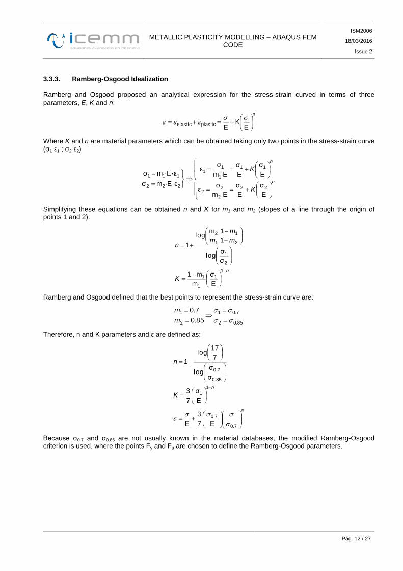
3.3.3. Ramberg-Osgood Idealization

Ramberg and Osgood proposed an analytical expression for the stress-strain curved in terms of three parameters, E, K and n:

n

plasticelasticE

KE

Where K and n are material parameters which can be obtained taking only two points in the stress-strain curve (σ1 ε1 ; σ2 ε2)

n

n

K

K

E

σ

E

σ

·Em

σε

E

σ

E

σ

·Em

σε

·E·εmσ

·E·εmσ

22

2

22

11

1

11

222

111

Simplifying these equations can be obtained n and K for m1 and m2 (slopes of a line through the origin of points 1 and 2):

n

K

m

m

mn

1

1

1

1

2

1

2

1

1

2

E

σ

m

m1

σ

σ log

1

1m log

1

Ramberg and Osgood defined that the best points to represent the stress-strain curve are:

85.02

7.01

2

1

85.0

7.0

m

m

Therefore, n and K parameters and ε are defined as:

n

7.0

7.0

1

1

0.85

0.7

E7

3

E

E

σ

7

3

σ

σ log

7

17 log

1

n

K

n

Because σ0.7 and σ0.85 are not usually known in the material databases, the modified Ramberg-Osgood criterion is used, where the points Fy and Fu are chosen to define the Ramberg-Osgood parameters.


ISM2006

18/03/2016

Issue 2

Pág. 13 / 27

n

y

u

u

K

F

F

E

Fe

n

yF

E 002.0

log

002.0 log

Where Fu is the ultimate strength, Fy is the yield strength and e the elongation.

Modified Ramberg-Osgood formulae for different stress behavior are defined as following:

Tension:

tn

002.0E

log

002.0 log

ty

ty

tu

t

tu

t

F

F

F

E

Fe

n

Compression:

cn

002.0E

log

002.0 log

cy

cy

tu

c

tu

c

F

F

F

E

Fe

n

Shear:

sn

3002.0G

2

sy

tcs

F

nnn


ISM2006

18/03/2016

Issue 2

Pág. 14 / 27

3.3.4. Ramberg-Osgood Idealization for ABAQUS Code

Material modelling in Abaqus FEM Code of Ramberg-Osgood idealization is shown through an example to facilitate its practical application.

Material: Al 2024 T351 – B – LT – Range: [25.43 < t < 38.10]

E = 73774 N/mm2 (Young Modulus)

Ftu= 441.3 N/mm2 (Ultimate strength)

Fty= 303.4 N/mm2 (Yield strength)

e = 7 % (strain at rupture)

Off. Strain = 0.01 % (Plastic onset in Ramberg-Osgood curve)

Plastic material behavior in ABAQUS code is defined with entries *ELASTIC and *PLASTIC.

*ELASTIC entry defines the elastic response of the material. The elastic response is defined in terms of constant (with respect to strain) moduli, such as Young’s modulus and Poisson’s ratio for an isotropic material.

Because Fty is defined for an offset unit strain of 0.002 in the stress–strain diagram, it is necessary to define

plastic behavior in a previous stress point, σref, in order to avoid discontinuities in plastic stress-strain diagram.

σref is calculated for a fixed ratio (Offset Strain) between the elastic strain and the Ramberg-Osgood strain, in

order to achieve the plastic onset in the Ramberg-Osgood curve. Following equation shows how to calculate

the σref:

n

tyref

ref

ty

refref

ref

StrainOff

F

E

StrainOff

FE

E

StrainOff

1

002.0

100.

100

.002.0

100

.

Offset Strain equal to 0.01 is recommended.

3.3.4.1. Ramberg-Osgood Coefficient

25.9

4.303

3.441 log

002.0

73774

3.44107.0

log

log

002.0 log

ty

tu

t

tu

t

F

F

E

Fe

n

3.3.4.2. σref

MPa

StrainOff

F

n

tyref 5.219002.0

10001.0

4.303002.0

100. 25.9

11


ISM2006

18/03/2016

Issue 2

Pág. 15 / 27

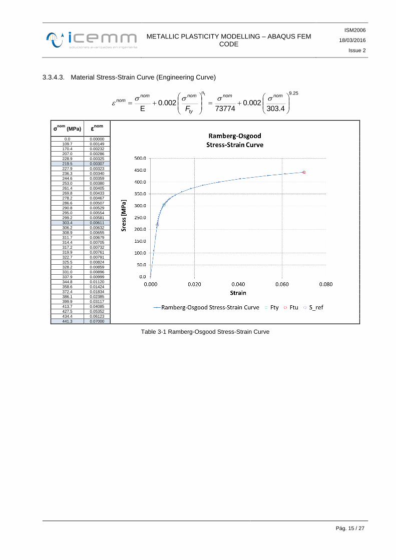
3.3.4.3. Material Stress-Strain Curve (Engineering Curve)

9.25n

4.303 002.0

73774 002.0

E

t

nomnom

ty

nomnomnom

F

σnom (MPa) εnom

0.0 0.00000

109.7 0.00149

170.4 0.00232

207.0 0.00286

228.9 0.00325

219.5 0.00307

227.9 0.00323

236.3 0.00340

244.6 0.00359

253.0 0.00380

261.4 0.00405

269.8 0.00433

278.2 0.00467

286.6 0.00507

290.8 0.00529

295.0 0.00554

299.2 0.00581

303.4 0.00611

306.2 0.00632

308.9 0.00655

311.7 0.00679

314.4 0.00705

317.2 0.00732

319.9 0.00761

322.7 0.00791

325.5 0.00824

328.2 0.00859

331.0 0.00896

337.9 0.00999

344.8 0.01120

358.6 0.01424

372.4 0.01834

386.1 0.02385

399.9 0.03117

413.7 0.04085

427.5 0.05352

434.4 0.06123

441.3 0.07000

Table 3-1 Ramberg-Osgood Stress-Strain Curve


ISM2006

18/03/2016

Issue 2

Pág. 16 / 27

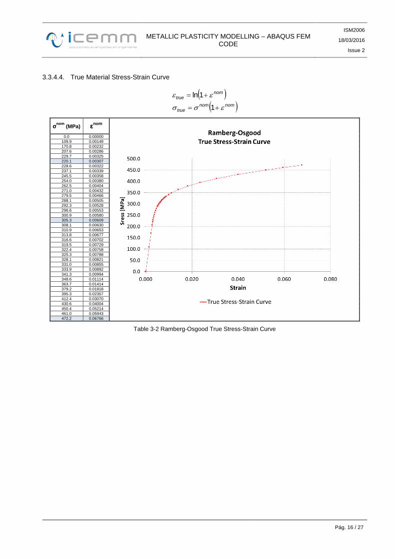
3.3.4.4. True Material Stress-Strain Curve

nomnom

true

nomtrue

1

1ln

σnom (MPa) εnom

0.0 0.00000

109.9 0.00149

170.8 0.00232

207.6 0.00286

229.7 0.00325

220.1 0.00307

228.6 0.00322

237.1 0.00339

245.5 0.00358

254.0 0.00380

262.5 0.00404

271.0 0.00432

279.5 0.00466

288.1 0.00505

292.3 0.00528

296.6 0.00553

300.9 0.00580

305.3 0.00609

308.1 0.00630

310.9 0.00653

313.8 0.00677

316.6 0.00702

319.5 0.00729

322.4 0.00758

325.3 0.00788

328.1 0.00821

331.0 0.00855

333.9 0.00892

341.3 0.00994

348.6 0.01114

363.7 0.01414

379.2 0.01818

395.3 0.02357

412.4 0.03070

430.6 0.04004

450.4 0.05214

461.0 0.05943

472.2 0.06766

Table 3-2 Ramberg-Osgood True Stress-Strain Curve


ISM2006

18/03/2016

Issue 2

Pág. 17 / 27

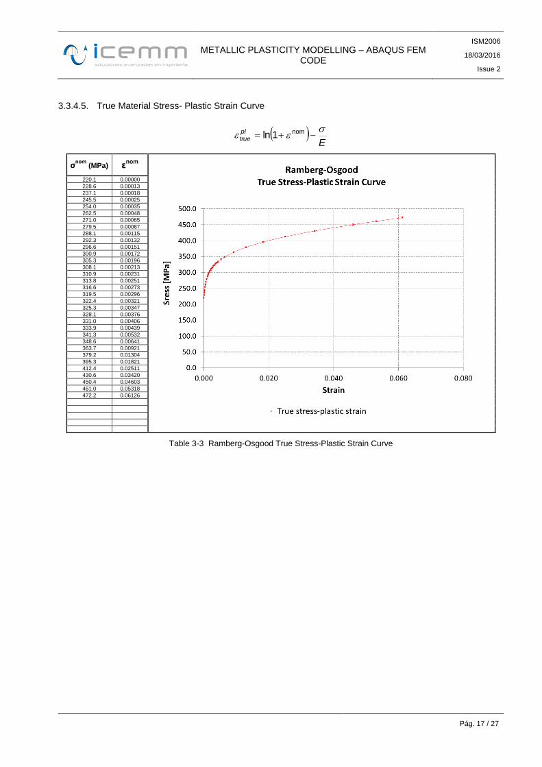
3.3.4.5. True Material Stress- Plastic Strain Curve

E

pltrue

nom1ln

σnom (MPa) εnom

220.1 0.00000

228.6 0.00013

237.1 0.00018

245.5 0.00025

254.0 0.00035

262.5 0.00048

271.0 0.00065

279.5 0.00087

288.1 0.00115

292.3 0.00132

296.6 0.00151

300.9 0.00172

305.3 0.00196

308.1 0.00213

310.9 0.00231

313.8 0.00251

316.6 0.00273

319.5 0.00296

322.4 0.00321

325.3 0.00347

328.1 0.00376

331.0 0.00406

333.9 0.00439

341.3 0.00532

348.6 0.00641

363.7 0.00921

379.2 0.01304

395.3 0.01821

412.4 0.02511

430.6 0.03420

450.4 0.04603

461.0 0.05318

472.2 0.06126

Table 3-3 Ramberg-Osgood True Stress-Plastic Strain Curve


ISM2006

18/03/2016

Issue 2

Pág. 18 / 27

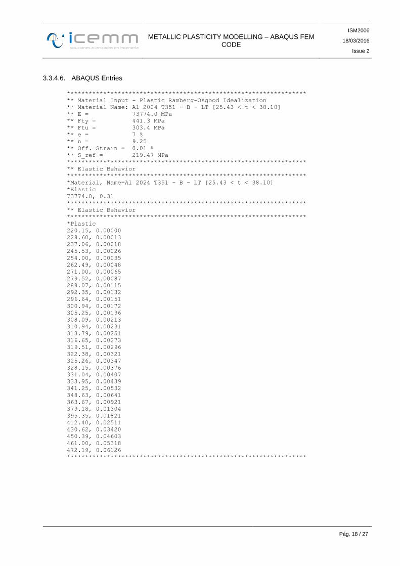
3.3.4.6. ABAQUS Entries

******************************************************************

** Material Input - Plastic Ramberg-Osgood Idealization

** Material Name: Al 2024 T351 - B - LT [25.43 < t < 38.10]

** E = 73774.0 MPa

** Fty = 441.3 MPa

** Ftu = 303.4 MPa

** e = 7 %

** n = 9.25

** Off. Strain = 0.01 %

** S_ref = 219.47 MPa

******************************************************************

** Elastic Behavior

******************************************************************

*Material, Name=Al 2024 T351 - B - LT [25.43 < t < 38.10]

*Elastic

73774.0, 0.31

******************************************************************

** Elastic Behavior

******************************************************************

*Plastic

220.15, 0.00000

228.60, 0.00013

237.06, 0.00018

245.53, 0.00026

254.00, 0.00035

262.49, 0.00048

271.00, 0.00065

279.52, 0.00087

288.07, 0.00115

292.35, 0.00132

296.64, 0.00151

300.94, 0.00172

305.25, 0.00196

308.09, 0.00213

310.94, 0.00231

313.79, 0.00251

316.65, 0.00273

319.51, 0.00296

322.38, 0.00321

325.26, 0.00347

328.15, 0.00376

331.04, 0.00407

333.95, 0.00439

341.25, 0.00532

348.63, 0.00641

363.67, 0.00921

379.18, 0.01304

395.35, 0.01821

412.40, 0.02511

430.62, 0.03420

450.39, 0.04603

461.00, 0.05318

472.19, 0.06126

******************************************************************


ISM2006

18/03/2016

Issue 2

Pág. 19 / 27

4. DEFINING MATERIAL DATA IN ABAQUS ENVIROMENT

ABAQUS has no built-in system of units, and therefore, all input data must be specified in consistent units.

This is the reason why there are not material libraries loaded in ABAQUS environment.

If the system of units used for the analysis is always the same can be useful to modify the ABAQUS environment to define a material database with the common material used in analysis.

ABAQUS env file have to be modified with the following sentences:

def onCaeStartup(): execfile('C:\\material.py')

Where, the “material.py” file contains the material database.


ISM2006

18/03/2016

Issue 2

Pág. 20 / 27

5. DFEM MODELLING GUIDELINES FOR NON -LINEAR ANALYSIS WITH ABAQUS (PLASTIC ITY)

5.1. SHELL AND SOLID ELEMENT TYPES

5.1.1. BENDING DOMINANT PROBLEMS

SHELL

S4 if out-of-plane bending

S8 if in-plane bending (to avoid shear-locking effects)

SOLID

C3D8I if very regular mesh (no distortion), C3D20

C3D10 (to be used without projection of edge nodes on the geometry)

5.1.2. CONTACT DOMINANT PROBLEMS WITHOUT BENDING

SHELL

S4

SOLID

C3D8

C3D10 (to be used without projection of edge nodes on the geometry)

5.1.3. CONTACT DOMINANT PROBLEMS WITH BENDING

SOLID

C3D8I (if very regular mesh)

5.2. MESH DENSITY

5.2.1. STRESS DISCONTINUITY

Because the stress and strain are discontinuous between adjacent elements, the level of stress or strain discontinuity is a level of accuracy:

Very accurate : d<5%

Accurate : 5%<d<10%

Medium : 10%<d<20%

Coarse : 20%<d

5.2.2. FILLET RADIUS

To define peak stress or plastic behavior in fillet radius, the level of accuracy must be very accurate. It is necessary to define minimum 8 elements (90º) in the radius path.

Because the integration points in 3D solid elements are defined inside of element, stress and strain are calculated by extrapolating the data from the integration points to the nodes.


ISM2006

18/03/2016

Issue 2

Pág. 21 / 27

This extrapolation depends on element type (shape functions), and the accuracy results depend on mesh density and stress/strain gradient

It is recommended to use shell elements in the external side to achieve accurately the peak stress/strain and the plastic behavior.


ISM2006

18/03/2016

Issue 2

Pág. 22 / 27

6. POST-PROCESSING OF NON -LINEAR PLASTICITY ANALYSIS

6.1. RESERVE FACTOR

The post-processing of non-linear finite element plasticity analyses must be done with care, especially with respect to Reserve Factors calculation.

RF must be based on the following formula:

LoadApplied

LoadAllowableR.F.

Where the Allowable Load is the load for which the criterion in allowable plastic strain is reached.

Allowable Load is obtained loading the FE Model with a given load level above Ultimate Load that produce the ultimate strength in the structure.

Following expressions for plastic analysis are also used, although they are not strictly right and non-conservative results could be obtained:

FEM

FEM

tu

elongationR.F.

FR.F.

6.2. PLASTIC ONSET FOR RAMBERG – OSGOOD IDEALIZATION

For Ramberg-Osgood material idealization, plastic onset is defined in a stress point below of Fty. Therefore plastic strains are obtained in finite element analysis for stresses lower than Fty.

Because these strains are lower than 0.002 (offset unit strain for Fty), plastic behavior can be considered as negligible and elastic response can be assumed.


ISM2006

18/03/2016

Issue 2

Pág. 23 / 27

7. EXAMPLE

In this chapter a simply example has been developed in order to evaluate the influence of the different material idealizations and the ways to obtain the ultimate reserve factor.

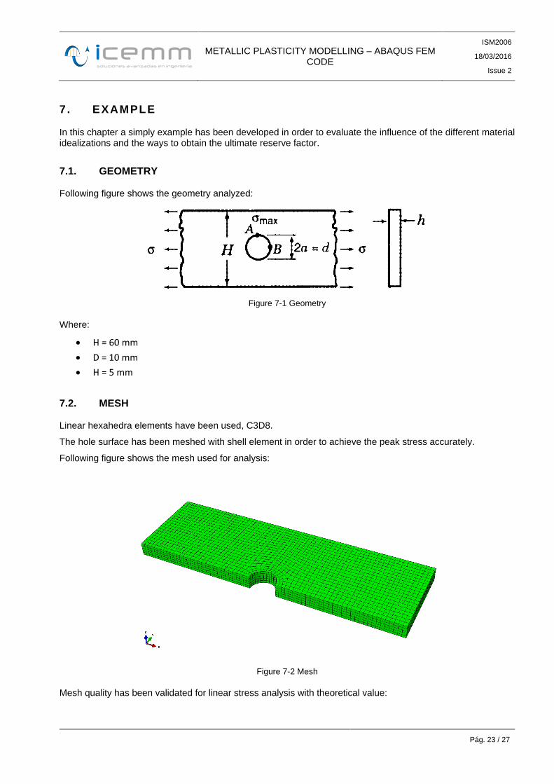
7.1. GEOMETRY

Following figure shows the geometry analyzed:

Figure 7-1 Geometry

Where:

H = 60 mm

D = 10 mm

H = 5 mm

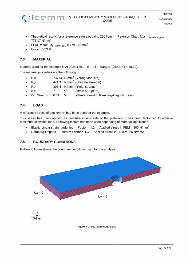
7.2. MESH

Linear hexahedra elements have been used, C3D8.

The hole surface has been meshed with shell element in order to achieve the peak stress accurately.

Following figure shows the mesh used for analysis:

Figure 7-2 Mesh

Mesh quality has been validated for linear stress analysis with theoretical value:


ISM2006

18/03/2016

Issue 2

Pág. 24 / 27

Theoretical results for a reference stress equal to 250 N/mm2 (Peterson Chart 4.1) - σpeak,max_ppal =

775,17 N/mm2

FEM Result - σpeak,max_ppal = 779,2 N/mm2

Error = 0.53 %

7.3. MATERIAL

Material used for the example is Al 2024 T351 – B – LT – Range: [25.43 < t < 38.10].

The material properties are the following:

E = 73774 N/mm2

(Young Modulus)

Ftu= 441.3 N/mm2

(Ultimate strength)

Fty= 303.4 N/mm2 (Yield strength)

e = 7 % (strain at rupture)

Off. Strain = 0.01 % (Plastic onset in Ramberg-Osgood curve)

7.4. LOAD

A reference stress of 250 N/mm2 has been used for the example.

This stress has been applied as pressure in one side of the plate and it has been factorized to achieve maximum allowable load. Following factors has been used depending of material idealization:

Elastic-Linear strain hardening – Factor = 1.2 → Applied stress in FEM = 300 N/mm2

Ramberg-Osgood – Factor = Factor = 1.3 → Applied stress in FEM = 325 N/mm2

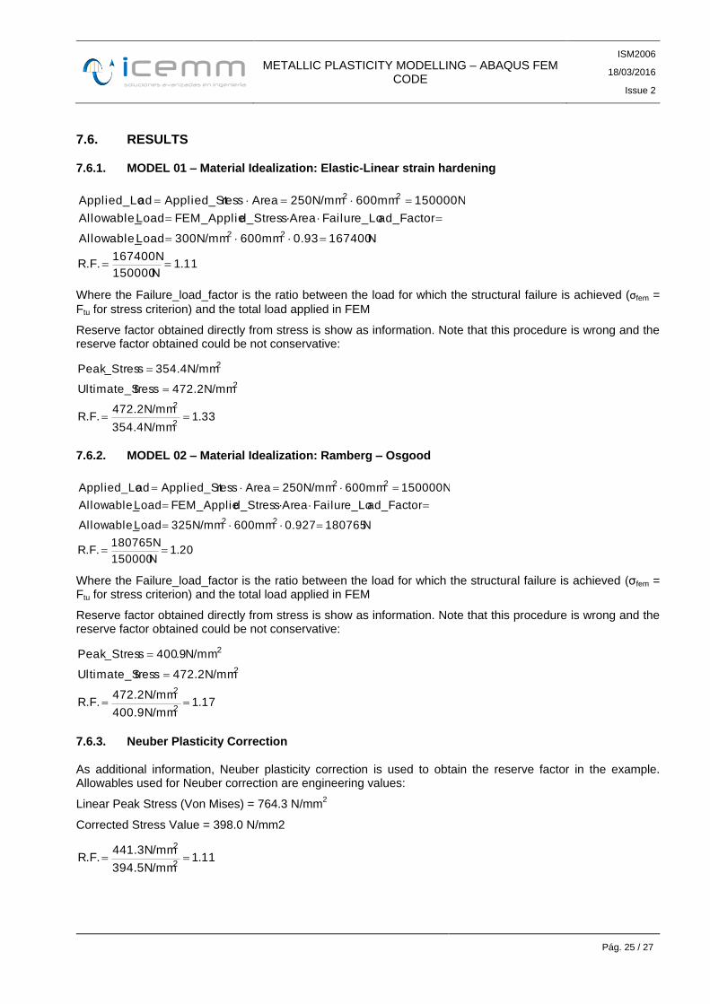
7.5. BOUNDARY CONDITIONS

Following figure shows the boundary conditions used for the analysis:

Figure 7-3 Boundary conditions

Ux = 0

Uy = 0


ISM2006

18/03/2016

Issue 2

Pág. 25 / 27

7.6. RESULTS

7.6.1. MODEL 01 – Material Idealization: Elastic-Linear strain hardening

11.1N150000

167400N R.F.

N1674000.93600mm300N/mmLoadAllowable_

ad_FactorFailure_Loread_Stress·AFEM_ApplieLoadAllowable_

150000N600mm250N/mmArearessApplied_StadApplied_Lo

22

22

Where the Failure_load_factor is the ratio between the load for which the structural failure is achieved (σfem =

Ftu for stress criterion) and the total load applied in FEM

Reserve factor obtained directly from stress is show as information. Note that this procedure is wrong and the reserve factor obtained could be not conservative:

33.1354.4N/mm

472.2N/mm R.F.

472.2N/mmtressUltimate_S

354.4N/mmsPeak_Stres

2

2

2

2

7.6.2. MODEL 02 – Material Idealization: Ramberg – Osgood

20.1N150000

180765N R.F.

N1807650.927600mm325N/mmLoadAllowable_

ad_FactorFailure_Loread_Stress·AFEM_ApplieLoadAllowable_

150000N600mm250N/mmArearessApplied_StadApplied_Lo

22

22

Where the Failure_load_factor is the ratio between the load for which the structural failure is achieved (σfem = Ftu for stress criterion) and the total load applied in FEM

Reserve factor obtained directly from stress is show as information. Note that this procedure is wrong and the reserve factor obtained could be not conservative:

17.1400.9N/mm

472.2N/mm R.F.

472.2N/mmtressUltimate_S

N/mm9.400sPeak_Stres

2

2

2

2

7.6.3. Neuber Plasticity Correction

As additional information, Neuber plasticity correction is used to obtain the reserve factor in the example. Allowables used for Neuber correction are engineering values:

Linear Peak Stress (Von Mises) = 764.3 N/mm2

Corrected Stress Value = 398.0 N/mm2

11.1394.5N/mm

441.3N/mm R.F.

2

2


ISM2006

18/03/2016

Issue 2

Pág. 26 / 27

7.6.4. Summary

MATERIAL IDEALIZATION LoadApplied

LoadAllowableR.F.

FEM

tuFR.F.

Elastic-Linear strain hardening 1.11 1.33

Ramberg – Osgood 1.20 1.17

Neuber Plasticity Correction --- 1.11

Table 7-1 RF Summary


ISM2006

18/03/2016

Issue 2

Pág. 27 / 27

8. APPENDIX

ID TITLE

1. ISM2006-01_Ramberg-Osgood_Idealization_v1.xls

2. ISM2006_Example_Ch7_Model_01_LinearElastPlasticHard.inp

3. ISM2006_Example_Ch7_Model_02_RambergOsgood.inp

4. ISM2006_Example_Ch7_Model_03_Linear.inp

5. ISM2006_Example_Ch7_Plate_Hole.cae

6. ISM2006_Example_Ch7_Neuber_Correction.xls

7. ISM2006_Example_Ch7_Ramberg-Osgood_Idealization.xls

Documents

METALLIC PLASTICITY MODELLING – ABAQUS FEM CODE