University of Windsor University of Windsor

Scholarship at UWindsor Scholarship at UWindsor

Electronic Theses and Dissertations Theses, Dissertations, and Major Papers

2014

Mechanical Analyses of Multi-piece Mining Vehicle Wheels to Mechanical Analyses of Multi-piece Mining Vehicle Wheels to

Enhance Safety Enhance Safety

Zhanbiao Li University of Windsor

Follow this and additional works at: https://scholar.uwindsor.ca/etd

Recommended Citation Recommended Citation Li, Zhanbiao, "Mechanical Analyses of Multi-piece Mining Vehicle Wheels to Enhance Safety" (2014). Electronic Theses and Dissertations. 5197. https://scholar.uwindsor.ca/etd/5197

This online database contains the full-text of PhD dissertations and Masters’ theses of University of Windsor students from 1954 forward. These documents are made available for personal study and research purposes only, in accordance with the Canadian Copyright Act and the Creative Commons license—CC BY-NC-ND (Attribution, Non-Commercial, No Derivative Works). Under this license, works must always be attributed to the copyright holder (original author), cannot be used for any commercial purposes, and may not be altered. Any other use would require the permission of the copyright holder. Students may inquire about withdrawing their dissertation and/or thesis from this database. For additional inquiries, please contact the repository administrator via email (scholarship@uwindsor.ca) or by telephone at 519-253-3000ext. 3208.

Mechanical Analyses of Multi-piece Mining Vehicle

Wheels to Enhance Safety

By

Zhanbiao Li

A Dissertation

Submitted to the Faculty of Graduate Studies

through Mechanical, Automotive, and Materials Engineering Department

in Partial Fulfillment of the Requirements for

the Degree of Doctor of Philosophy

at the University of Windsor

Windsor, Ontario, Canada

2014

© 2014 Zhanbiao Li

Mechanical Analyses of Multi-piece Mining Vehicle Wheels to Enhance Safety

By

Zhanbiao Li

APPROVED BY:

__________________________________________________

Dr. R. Hall, External Examiner

University of British Columbia

__________________________________________________

Dr. S. Das

Department of Civil and Environmental Engineering

__________________________________________________

Dr. N. Zamani

Department of Mechanical, Automotive and Materials Engineering

__________________________________________________

Dr. D. Green

Department of Mechanical, Automotive and Materials Engineering

__________________________________________________

Dr. W. Altenhof, Advisor

Department of Mechanical, Automotive and Materials Engineering

September 4, 2014

iii

DECLARATION OF PREVIOUS PUBLICATION

This dissertation includes four (4) original papers that have been previously published in

peer reviewed journals, as follows:

Dissertation

Chapter Publication title/full citation Publication status*

Chapter 4

Tonkovich A., Li Z., DiCecco S., Altenhof W.,

Banting R., and Hu H. (2012) “Experimental

Observations of tire Deformation Characteristics on

Heavy Mining Vehicles under static and Quasi-

Static Loading”. Journal of Terramechanics, Vol.

49, No. 3-4, pp. 215-231.

Published

Chapter 5 and

Chapter 6

Li Z., Tonkovich A., DiCecco S., Altenhof W.,

Banting R., and Hu H. (2013) “Development and

validation of a FE model of a mining vehicle tire”.

International Journal of Vehicle Design, Vol.65,

No.2/3, pp.176 – 201.

Published

Chapter 8 and

Chapter 9

Li Z., DiCecco S., Tonkovich A., Altenhof W.,

Banting R., and Hu H. (2013) “A threaded-

connection locking mechanism integrated into a

multi-piece mining wheel for enhanced structural

performance and safety”. Journal of

Terramechanics, Vol. 50, No. 4, pp. 245-264.

Published

Chapter 8 and

Chapter 9

Li Z., DiCecco S., Altenhof W., Thomas M.,

Banting R., and Hu H. (2014) “Stress and Fatigue

Life Analyses of a Five-piece Rim and the Proposed

Optimization with a Two-piece Rim”. Journal of

Terramechanics, Vol. 52, pp. 31-45.

Published

I certify that I have obtained a written permission from the copyright owner(s) to include

the above published material(s) in my dissertation. I certify that the above material describes

work completed during my registration as graduate student at the University of Windsor.

I declare that, to the best of my knowledge, my dissertation does not infringe upon

anyone’s copyright nor violate any proprietary rights and that any ideas, techniques, quotations,

or any other material from the work of other people included in my dissertation, published or

otherwise, are fully acknowledged in accordance with the standard referencing practices.

iv

Furthermore, to the extent that I have included copyrighted material that surpasses the bounds of

fair dealing within the meaning of the Canada Copyright Act, I certify that I have obtained a

written permission from the copyright owner(s) to include such material(s) in my dissertation.

I declare that this is a true copy of my dissertation, including any final revisions, as

approved by my dissertation committee and the Graduate Studies office, and that this dissertation

has not been submitted for a higher degree to any other University or Institution.

.

v

CLAIMS TO ORIGINALITY

Aspects of this work constitute, in the author’s opinion, new and distinct contributions to

the technical knowledge pertaining to enhancing the safety of multi-piece wheels. These include:

(i) Analyses of fatality reports associated with multi-piece wheel failures. Through many

fatality incident analyses, the root cause for the multi-piece wheel failures was

identified to associate with the lock ring. This finding defined the focuses of this

research and gave a clear direction for innovative designs. In the public domain, no

literature was found to conduct systemic analysis of fatality incidents to identity the

cause of multi-piece wheel failures, in the off-the-road (OTR) wheel design’s point of

view.

(ii) Experimental testing of OTR tire/wheel assemblies. In-field tire deflection tests were

conducted on heavy-duty underground mining vehicles. Linear relationships were

found between the vertical wheel displacement and the maximum lateral tire deflection

for linear static and quasi-static loading conditions. No literature was found in public

domain to conduct in-field OTR tire deflection tests. The testing methods and findings

are unique in this area. The in-field OTR tire testing led to the successful tire modeling

and inclusion in the OTR tire/wheel assembly models, which were used for numerical

predications of wheel performances and design improvements.

(iii) Development of the finite element (FE) model of a five-piece OTR tire/wheel

assemblies. A robust and high fidelity FE model of the assembly was developed using

simplified yet efficient modeling approaches and validated using in-field experimental

test data.

(iv) Investigation of geometry and material degradation effect on fatigue life of a five-piece

wheel. This research numerically investigated the effects of geometry degradation

(material wear out in critical regions) and material property degradation (corrosion on

wheels) on multi-piece wheel performances and fatigue lives.

(v) BS (bead seat) band pull-out numerical testing method. This numerical testing is

unique in determining the capability of the multi-piece wheel locking mechanism in

holding the tire and wheel components in proper engaging positions under severe

loading conditions.

vi

(vi) The threaded-connection mechanism design to replace the lock ring mechanism in the

conventional five-piece wheel. This threaded-connection four-piece design reduced

the possibility of failure due to the mismatched wheel components. The BS band pull-

out simulation revealed that the threaded-connection design was twice as strong as the

conventional five-piece design in holding wheel components and the tire together. The

progressive failure mode of the threaded-connection had a much safer failure mode,

compared to the instantaneous failure mode of the conventional five-piece lock ring

design. The fatigue lives on the critical regions of the rim base were over two orders of

magnitude higher than the fatigue lives of the rim base of the conventional five-piece

wheel.

(vii) The innovative two-piece wheel design. The two-piece wheel design completely

removed the possibility of wheel failure due to mismatched wheel components that

existed in other multi-piece wheels with a lock ring mechanism. It also reduced the

numbers of pieces of the wheel. The fatigue lives at critical regions were increased by

over two orders of magnitude, compared to the conventional five-piece wheel.

vii

ABSTRACT

In this research, experimental and numerical methods were used to analyse the

performance of multi-piece wheel structures and two proposed innovative designs to enhance

safety were validated by computer simulations. Fatality report analyses revealed that the majority

(90%) of the multi-piece wheel failures were caused by use of lock rings.

Experimental tire and rim base tests were conducted to understand the deflection

characteristics of off-the-road tires and to validate the finite element model of a five-piece

wheel/tire (sized 29.5-29) assembly. A linear relationship was found between the vertical

displacement of the wheel and the maximum lateral deflection of the tire for both static and

quasi-static loading tests. A robust tire model was validated with an average accumulative error

of 9.7% and an average validation metric of 0.96 for tire deflections, compared to the

experimental tests. The rim base model was validated with an average error of 7.6% and an

average validation metric of 0.93 for wheel deformations, and an average accumulative error of

12.7% and an average validation metric of 0.88 for strains, compared to experimental tests.

Based on validated FE model of the five-piece wheel/tire assembly, geometry

degradation (material wear out at critical regions) and material degradation (fatigue and corrosion)

were studied to estimate their effects on fatigue lives. Two design innovations were proposed to

enhance safety and fatigue life of the five-piece wheel. The threaded-connection design reduced

the possibility of failure due to the mismatched wheel components. The BS band pull-out

simulation revealed that the threaded-connection design was twice as strong as the conventional

five-piece design in holding wheel components and the tire together, and the wheel may fail in a

safer mode. The fatigue lives of the rim base were two orders of magnitude higher than those of

the conventional five-piece wheel. The two-piece wheel design completely removed the

possibility of wheel failure due to mismatched wheel components; the fatigue lives were

increased by over two orders of magnitude, compared to the conventional five-piece wheel.

viii

DEDICATION

This dissertation is dedicated to my wife, Helen Yu, for her patience and support, to my

parents-in-law (Lanfang Liu and Xigang Yu) for their support by taking care of our children

during these several years, and to my daughter Lena and my son Leeming for their sacrifice of

their play time with me.

ix

ACKNOWLEDGEMENTS

The author would like to express his great appreciation to Dr. William Altenhof, his

academic advisor, for his patience, understanding, encouragement, and guidance in the courses of

this research and accomplishing the dissertation. There were ups and downs on the way, but they

finally went through it and they both feel accomplished. The author would also like to thank

Aleksander Tonkovich and Sante DiCecco, the other two members of Dr. Altenhof’s research

team, for their help and cooperation. The author would like to acknowledge the financial support

from the Workplace Safety Insurance Board (WSIB) of Ontario, the Natural Sciences and

Engineering Research Council of Canada (NSERC), and the Ministry of Training, Colleges and

Universities (TCU) of Ontario. The author is obliged to the support and help from the industrial

partners: North Shore Industry Wheel Mfg. (NSIW), Goldcorp Musselwhite Mine, Glencore

Xstrata Nickel Sudbury Operations, Glencore Xstrata Copper Kidd Mine, Vale Inco., Goodyear

Canada Inc., Royal Tire Sudbury, Fountain Tire Sudbury, and Workplace Safety North (WSN) of

Ontario, with special thanks to the following individuals: Darrell Brown, Mark Thomas, Brent

Tarini, Jude deCastro, and Rick Banking.

x

TABLE OF CONTENTS

DECLARATION OF PREVIOUS PUBLICATION ...................................................................... iii

CLAIMS TO ORIGINALITY ......................................................................................................... v

ABSTRACT……………………………………………………………………………………...vii

DEDICATION .............................................................................................................................. viii

ACKNOWLEDGEMENTS ............................................................................................................ ix

LIST OF TABLES ....................................................................................................................... xvii

LIST OF FIGURES .................................................................................................................... xviii

LIST OF APPENDICES ............................................................................................................. xxiv

LIST OF ABBREVIATIONS ...................................................................................................... xxv

LIST OF NOMENCLATURE ................................................................................................... xxvii

Chapter 1. Introduction and Motivation .................................................................................... 1

1.1. Mining Industry in Canada .................................................................................................. 1

1.2. The Differences between a Wheel and a Rim ...................................................................... 2

1.3. On-the-road Wheels and Off-the-road (OTR) Wheels......................................................... 3

1.3.1. The Size Difference ..................................................................................................... 3

1.3.2. The Wheel Structure and Tire Mounting Differences .................................................. 4

1.3.3. Manufacturing Materials and Maintenance Differences .............................................. 5

1.4. Rationale for the Use of Multi-piece Wheels ....................................................................... 6

1.5. Procedures and Regulations on Handling Multi-piece Wheel/Tire Assemblies .................. 8

1.6. Motivation for Multi-piece Wheel Research ..................................................................... 10

Chapter 2. Literature Review ................................................................................................... 12

2.1. Multi-piece Wheels and OTR Tires ................................................................................... 12

2.1.1. On-the-road Single-piece Wheel and Tire Codes ...................................................... 12

2.1.2. Multi-piece Wheel Structures .................................................................................... 13

2.1.2.1. Names and Size Specifications of Multi-piece Wheel Components ...................... 13

2.1.2.2. Other Multi-piece Wheel Structures ...................................................................... 15

2.1.3. Off-the-road (OTR) Tires........................................................................................... 17

2.1.3.1. OTR Tires Structures and Materials ...................................................................... 17

2.1.3.2. Radial Tires and Bias Tires .................................................................................... 18

2.1.3.3. The OTR Tire Deflections and Dimensions........................................................... 20

2.1.3.4. Tire Load and Pressure Relationship ..................................................................... 22

xi

2.1.3.5. OTR Tire Size and Code Designations .................................................................. 22

2.1.3.5.1. Tire Size Designations ...................................................................................... 22

2.1.3.5.2. Tire Industry Codes .......................................................................................... 23

2.2. Fatalities Caused by Multi-piece Wheel/Tire Failures....................................................... 24

2.2.1. Fatalities in Canada since 1998 .................................................................................. 25

2.2.2. Fatalities in the United States since 1998 .................................................................. 26

2.2.3. Fatalities in Australia since 1998 ............................................................................... 27

2.2.4. Analysis and Summary of the Fatality Incidents ....................................................... 28

2.2.4.1. Tire Explosions ...................................................................................................... 28

2.2.4.2. Tire Zipper Ruptures .............................................................................................. 29

2.2.4.3. Tire Blow-outs ....................................................................................................... 29

2.2.4.3.1. Tire Blow-out Fatality Incident Analysis ......................................................... 30

2.2.4.3.2. Lock Ring Improper Seating ............................................................................ 31

2.2.4.3.3. Wear, Corrosion, and Fatigue Cracks in the Gutter Region ............................. 32

2.2.4.4. Tire Failures for on-the-road Tires ......................................................................... 33

2.2.5. Working with Multi-piece Wheel and OTR Tire ....................................................... 33

2.3. Fatigue Life Analysis Theory ............................................................................................ 34

2.3.1. Mechanism of Fatigue Failure ................................................................................... 34

2.3.1.1. Crack Initiation Stage............................................................................................. 35

2.3.1.2. Crack Propagation Stage ........................................................................................ 36

2.3.1.3. Fracture .................................................................................................................. 36

2.3.2. The Stress-life (S-N) Approach .................................................................................. 38

2.3.2.1. Fatigue Loads ......................................................................................................... 38

2.3.2.2. Material Fatigue Test ............................................................................................. 39

2.3.2.3. Factors Influencing Fatigue Life ............................................................................ 40

2.3.2.4. The Influence of Mean Stress ................................................................................ 41

2.3.3. Strain-life (-N) Approach ......................................................................................... 44

2.3.3.1. Monotonic Stress-Strain Behaviour ....................................................................... 44

2.3.3.2. Cyclic Stress-Strain Behaviour .............................................................................. 45

2.3.3.3. The Strain-life (-N) Response .............................................................................. 46

2.3.3.4. Determination of Cyclic Fatigue Properties ........................................................... 47

2.3.3.5. The Effect of Mean Stress ...................................................................................... 49

2.3.3.5.1. The Morrow mean stress correction ................................................................. 49

2.3.3.5.2. The Smith-Watson-Topper mean stress correction .......................................... 50

xii

2.3.3.6. Factors Influencing Fatigue Strain Life ................................................................. 50

2.3.3.7. Elastic-Plastic Corrections ..................................................................................... 50

2.3.4. Multi-axial Loading in Fatigue .................................................................................. 52

2.3.4.1. Fatigue Life Prediction in Simple Multiaxial Stress/Strain Situations .................. 52

2.3.4.2. Fatigue Life Prediction in Complex Multiaxial Stress/Strain Conditions .............. 54

2.3.4.3. Critical Plane Approach ......................................................................................... 55

2.3.5. Accumulated Fatigue Assessment ............................................................................. 57

2.4. Wheel Fatigue Testing Standards ...................................................................................... 58

2.4.1. Dynamic Cornering Fatigue Testing .......................................................................... 59

2.4.2. Dynamic Radial Fatigue Testing ................................................................................ 60

2.5. FE-based Wheel Fatigue Testing ....................................................................................... 61

2.5.1. FE-based Wheel Dynamic Cornering Fatigue Testing .............................................. 62

2.5.2. FE-based Wheel Dynamic Radial Fatigue Testing .................................................... 63

2.5.3. FE-Based Fatigue Testing on Other Vehicle Structures ............................................ 64

Chapter 3. Scope of Research .................................................................................................. 66

3.1. Testing Methods Used in Multi-piece Wheel Fatigue Assessment ................................... 66

3.1.1. Experimental Testing ................................................................................................. 66

3.1.2. The Finite Element (FE) Method ............................................................................... 67

3.1.3. Fatigue Life Assessment Methods ............................................................................. 67

3.2. Innovative Designs ............................................................................................................. 68

3.3. Computer Software Used for This Research ...................................................................... 68

Chapter 4. Tire and Wheel Experimental Testing ................................................................... 70

4.1. Experimental Testing of a Five-piece Wheel/Tire Assembly ............................................ 70

4.1.1. Experimental Procedure ............................................................................................. 71

4.1.1.1. Testing Information ............................................................................................... 72

4.1.1.2. Tire Physical and Engineering Data ....................................................................... 72

4.1.1.3. Testing Apparatus .................................................................................................. 73

4.1.1.4. Static Deflection Scale Testing .............................................................................. 76

4.1.2. Results and Discussions ............................................................................................. 77

4.1.2.1. Above Ground Quasi-Static Testing Observations ................................................ 77

4.1.2.2. Underground Static Testing Observations ............................................................. 83

4.2. Rim Base Laboratory Tests ................................................................................................ 85

4.2.1. Rim Base Testing Procedure ...................................................................................... 86

4.2.2. Experimental Rim Base Testing Observations .......................................................... 89

xiii

Chapter 5. Finite Element Model Development ...................................................................... 91

5.1. Tire Model Development ................................................................................................... 91

5.1.1. On-the-road Tire Modeling in the Open Literature .................................................... 91

5.1.2. Tire Model Development for the Tire 29.5-29 ........................................................... 92

5.1.2.1. Tire Discretization ................................................................................................. 93

5.1.2.1.1. The Bead ........................................................................................................... 95

5.1.2.1.2. The Chafer ........................................................................................................ 95

5.1.2.1.3. The Apex, Sidewall, Shoulder, Sidetread, Undertread, Tread, and Liner ........ 95

5.1.2.1.4. The Body Plies ................................................................................................. 97

5.1.2.2. Tire Pressure Modelling ......................................................................................... 99

5.1.2.3. Other Critical Modelling Features ....................................................................... 100

5.1.2.4. Static and Quasi-static Deflection Testing Simulations ....................................... 101

5.1.2.4.1. Static Loading Simulations ............................................................................. 102

5.1.2.4.2. Quasi-Static Loading Simulations .................................................................. 102

5.1.2.5. The Computer Used for the Simulations and Simulation Time ........................... 104

5.2. Numerical Rim Base Model Development ...................................................................... 104

Chapter 6. Stress and Fatigue Life Analyses ......................................................................... 108

6.1. FE Model Validation ........................................................................................................ 108

6.1.1. FE Model Validation for Tire 29.5-29 ..................................................................... 108

6.1.1.1. Validation Procedures .......................................................................................... 108

6.1.1.1.1. Static Loading Behaviour Validation ............................................................. 108

6.1.1.1.2. Quasi-Static Loading Behaviour Validation ................................................... 109

6.1.1.2. Results and Discussions ....................................................................................... 110

6.1.1.2.1. Static Loading Behaviour ............................................................................... 110

6.1.1.2.2. Quasi-Static Loading Behaviour .................................................................... 112

6.1.2. Rim Base FE Model Validation ............................................................................... 118

6.2. Geometry Degradation Modeling .................................................................................... 120

6.2.1. The OEM Wheel Information and Wear Conditions ............................................... 120

6.2.2. New and Worn Wheel Dimensions .......................................................................... 122

6.2.3. The Heave-duty HT2000 Rim Base ......................................................................... 123

6.2.4. FE Model Development ........................................................................................... 125

6.3. Determination of Cyclic Fatigue Properties. .................................................................... 127

6.3.1. Mechanical Properties of the Rim Base from Monotonic Tensile Tests .................. 127

6.3.1.1. Tensile Test Results of Specimens Extracted from Rim Base ............................. 127

xiv

6.3.1.2. Yield Criteria under Multiaxial Loading ............................................................. 129

6.3.1.2.1. Maximum Shear Stress Yield Criterion (Tresca) ........................................... 129

6.3.1.2.2. Maximum Distortion-Energy or von Mises Criterion .................................... 129

6.3.1.2.3. Determination of Yield Shear Stress under Multiaxial Loading .................... 130

6.3.2. Cyclic Fatigue Properties for Stress-life Approach ................................................. 130

6.3.2.1. Introduction of the Stress-Based Fatigue Tests .................................................... 130

6.3.2.2. Cyclic Fatigue Properties for Stress-Based Tests ................................................ 131

6.3.3. Cyclic Fatigue Properties for Strain-life Approach ................................................. 134

Chapter 7. Discussions on Simulation Results ...................................................................... 138

7.1. Geometry Degradation ..................................................................................................... 138

7.1.1. Maximum von Mises and Maximum Shear Stress Analyses ................................... 138

7.1.2. Fatigue Life Analyses .............................................................................................. 139

7.2. Material Degradation ....................................................................................................... 140

Chapter 8. Innovative Multi-piece Wheel Designs ................................................................ 142

8.1. The Threaded-connection Design .................................................................................... 142

8.1.1. The Proposed Threaded-Connection Locking Mechanism ...................................... 142

8.1.2. Assessment Approaches for the Proposed Design ................................................... 144

8.1.2.1. BS Band Pull-out Simulations ............................................................................. 145

8.1.2.2. Wheel Stress and Fatigue Life Assessments ........................................................ 146

8.1.2.2.1. Simulated Loading and Boundary Conditions for Stress and Fatigue Life

Assessments .................................................................................................... 147

8.2. The Two-piece Wheel Design.......................................................................................... 147

8.2.1. The Proposed Two-piece Wheel Design .................................................................. 147

8.2.2. The Tire and Wheel Model Development ................................................................ 149

8.2.2.1. The Tire Model Development .............................................................................. 149

8.2.2.1.1. Tire Discretization .......................................................................................... 150

8.2.2.1.2. Modelling of Steel Bead Coils and Body Pliers ............................................. 152

8.2.2.1.3. Other Critical Modelling Features .................................................................. 153

8.2.2.2. Wheel Model Development ................................................................................. 154

8.2.2.2.1. Five-piece Wheel Model Development .......................................................... 154

8.2.2.2.2. Two-piece Wheel Model Development .......................................................... 156

8.2.3. Loading and Boundary Conditions for Tire Validation ........................................... 156

8.2.4. Tire Model Validation through Static Load Simulation .......................................... 157

8.2.5. Numerical Testing of the Multi-Piece Wheel Assemblies ....................................... 159

xv

8.2.5.1. Loading and Bounding Conditions for FE Simulations ....................................... 159

8.2.5.2. Modelling Approaches for the Focused Regions ................................................. 162

8.2.5.3. Selection of Material Properties for Numerical Fatigue Assessment .................. 163

Chapter 9. Discussions on Innovative Designs ...................................................................... 164

9.1. Discussions on Threaded-connection Design .................................................................. 164

9.1.1. BS Band Pull-out Simulation Results ...................................................................... 164

9.1.2. Wheel Stress and Fatigue Life Analyses .................................................................. 166

9.2. Discussions on Two-piece Wheel Numerical Testing ..................................................... 167

9.2.1. Stress Analysis ......................................................................................................... 167

9.2.2. Connecting Beam Element Forces ........................................................................... 171

9.2.3. Fatigue Life Simulation Results. .............................................................................. 173

Chapter 10. Summaries and Conclusions ................................................................................ 174

10.1. Summary on the Analyses of the Fatality Reports ........................................................... 174

10.2. Conclusions on Experimental Tire Testing and Rim Base Testing ................................. 174

10.2.1. Experimental Tire Testing ................................................................................... 174

10.2.2. Laboratory Rim Base Testing .............................................................................. 175

10.3. Conclusions on the FE Model Developments .................................................................. 176

10.3.1. Tire Model Development ..................................................................................... 176

10.3.2. Rim Base Model Development ............................................................................ 176

10.4. Geometry Degradation Analysis of the Rim Base ........................................................... 176

10.5. Material Degradation Analysis of the Rim Base ............................................................. 177

10.6. Conclusions on Innovative Design Improvements to Enhance Safety ............................ 177

10.6.1. Conclusions on the Threaded-connection wheel Design ..................................... 177

10.6.2. Conclusions on the Two-piece Wheel Design ..................................................... 178

Chapter 11. Limitations of the Study and Future Work .......................................................... 180

11.1. Limitations of the Study ................................................................................................... 180

11.2. Future work ...................................................................................................................... 180

11.2.1. Future Work on the Threaded-connection Design ............................................... 180

11.2.2. Future Work on the Two-piece Wheel Design .................................................... 180

11.2.3. Experimental Testing of Prototype Wheels for the New Designs ....................... 181

11.2.4. Geometry Optimization of the Multi-piece Wheels ............................................. 181

References……………………………………………………………………………………….182

Appendix A: Fatigue Analysis within nCode DesignLife ........................................................... 194

Appendix B: Quasi-static Testing Observations for Event 2 and Event 3 ................................... 197

xvi

Appendix C: Experimental Observations from the Rim Base Testing ........................................ 202

Appendix D: Tire Quasi-static Testing Results Comparisons between Experimental Tests and

Computer Simulations for Test Event 2 and Event 3 Conditions .......................... 204

Appendix E: Partial Input Files Used for FE Simulations ........................................................... 210

E.1 Partial Input File Used of Tire Model Validation ............................................................ 210

E.2 Partial Input File Used for Tire Quasi-static Loading ...................................................... 216

E.3 Partial Input File Used for Rim Base Model Validation .................................................. 225

E.4 Partial Input File Used for BS Band Pull-out Simulation ................................................ 227

E.5 Partial Input File Used for Threaded-connection Design at Quasi-static Loading Condition

…………………………………………………………………………………………...228

E.6 Partial Input File Used for Two-piece wheel Traveling and Steering Simulation ........... 234

Appendix F: Copyright Permissions ............................................................................................ 245

VITA AUCTORIS ....................................................................................................................... 287

xvii

LIST OF TABLES

Table 1.1 Lost-tie injuries and fatality in Canada and Ontario from 2009-2011. ....................... 2

Table 2.1 Standard tire industry code. ...................................................................................... 23

Table 2.2 Standard tread code, depth, and type. ....................................................................... 24

Table 4.1 Test vehicle information. .......................................................................................... 72

Table 4.2 Tire physical data as given in Goodyear’s OTR Engineering Data Book [28]. ........ 72

Table 4.3 Tire deflection characteristics based on Goodyear OTR data [28]. .......................... 73

Table 4.4 Tire wear based on mine site tire measurements. ..................................................... 73

Table 4.5 Tire stiffness comparison of experimental static loading and Goodyear OTR data. 84

Table 4.6 Tire deflection observations comparing experimental static loading to Goodyear

OTR data. .................................................................................................................. 85

Table 5.1 Liner elastic modulus change effects ........................................................................ 96

Table 6.1 Vertical and Lateral Deflections for static loading condition. ................................ 110

Table 6.2 Slope comparisons for vertical and lateral deflections versus load. ....................... 111

Table 6.3 Errors and validation metrics between experimental test and simulation for event 1.

................................................................................................................................. 117

Table 6.4 Deflection (mm), strain (microstrain, με), errors, and validation metricsfor

simulations and experimental tests under static load condition. ............................. 119

Table 6.5 Elastic moduli, engineering and true data for the three tests. ................................. 129

Table 6.6 S-N fatigue properties generated from fatigue tests. ................................................ 133

Table 7.1 Maximum von Mises stresses/maximum shear stresses (MPa) on the shell elements

at front gutter and back section regions. ................................................................. 139

Table 7.3 Fatigue life comparisons between new gutter and corroded gutter materials. ......... 140

Table 8.1 Tire deflection comparisons. ................................................................................... 158

Table 9.1 The maximum von Mises stress/maximum shear stress at the front regions of shell

elements for the lock ring design and the threaded-connection design. .................. 167

Table 9.2 Fatigue life predictions (cycles) and comparisons. ................................................. 167

Table 9.3 Maximum effective/maximum shear stresses (MPa) at different focused regions. 170

Table 9.4 Minimum fatigue S-N/-N life (cycle) comparisons on focused regions. ............... 173

xviii

LIST OF FIGURES

Figure 1.1 A single-piece wheel (a) and a five- wheel (b) [5]. ..................................................... 3

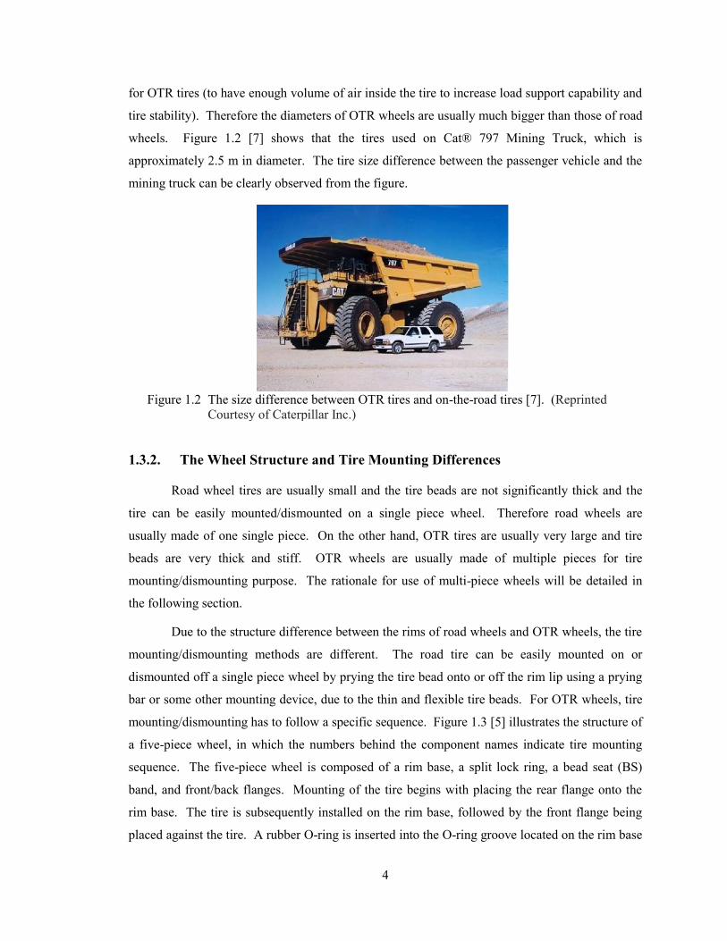
Figure 1.2 The size difference between OTR tires and on-the-road tires [7]. (Reprinted

Courtesy of Caterpillar Inc.) ....................................................................................... 4

Figure 1.3 A five-piece wheel wheel structure and tire mounting sequence [5]. ......................... 5

Figure 1.4 Severe cuts and wear on an OTR tire. ......................................................................... 7

Figure 1.5 Schematic view of the rationale for use of multi-piece wheel for OTR vehicles. ...... 7

Figure 1.6 Multi-piece wheel failures kill people [9]. .................................................................. 8

Figure 1.7 Trajectory of multi-piece wheel parts in different scenarios [10]. .............................. 9

Figure 1.8 Place wheel and tire in a safety cage during tire inflation [11]. .................................. 9

Figure 2.1 The side view of a single piece wheel (a) [16] and tire codes for on-the-road tire (b)

[17]. ........................................................................................................................... 13

Figure 2.2 Names and specifications of three-piece wheel components [18]. ........................... 14

Figure 2.3 Names and specifications of five-piece wheel components [18]. ............................. 14

Figure 2.4 Names of the components of a five-piece wheel involving an out board driver [18].

................................................................................................................................... 15

Figure 2.5 A two-piece wheel with a split lock ring (a) [19, 20] and a two-piece wheel with

connecting bolts. ....................................................................................................... 15

Figure 2.6 Two different structures of four-piece wheels [21]. .................................................. 16

Figure 2.7 The structure of a seven-piece wheel [22]. ............................................................... 16

Figure 2.8 Tire construction features of a radial tire (a) and a bias tire (b) [25]. ....................... 17

Figure 2.9 Radial structure tire and bias structure tire [26]. ....................................................... 19

Figure 2.10 Tire deflections and tire dimensions under static load [28]. ..................................... 21

Figure 2.11 Tire size designations. ............................................................................................... 23

Figure 2.12 Illustrations of sidewall markings of a Goodyear tire. .............................................. 24

Figure 2.13 Detailed tire failure reasons specified in the incident reports in the failure mode of

tire blow-out. ........................................................................................................... 30

Figure 2.14 A sprung lock ring (left) and a good lock ring (right) [18]. ...................................... 31

Figure 2.15 Correct installation (left) and lock ring installed backward (right) [18]. .................. 32

Figure 2.16 Wear and Fatigue cracks in the gutter region [5]. ..................................................... 32

Figure 2.17 Three common rotation loads. ................................................................................... 38

Figure 2.18 Fatigue strength versus the numbers of cycle to failure diagram. ............................. 39

xix

Figure 2.19 Estimated S-N response for HCF regime (a) materials with an endurance limit

(b) material without an endurance limit. ................................................................... 41

Figure 2.20 High cycle fatigue data showing the influence of mean stress. ................................. 42

Figure 2.21 Various failure lines for fluctuating stresses. ............................................................ 43

Figure 2.22 True stress versus true strain diagram. ...................................................................... 45

Figure 2.23 Strain amplitude as a function of reversals to failure. ............................................... 47

Figure 2.24 Log stress versus log plastic strain line. .................................................................... 48

Figure 2.25 Effect of mean stress on the strain-life curve. ........................................................... 49

Figure 2.26 The Neuber’s method for estimating elastic-plastic strain and stress at a notch. ...... 51

Figure 2.27 Dynamic cornering fatigue testing set-up [81]. (Reprinted with permission from

SAE J328 Feb 2005 © 2005SAE International. Further use or distribution is not

permitted without permission from SAE.) ................................................................ 59

Figure 2.28 Dynamic radial fatigue testing set-up. [81] (Reprinted with permission from

SAE J328 Feb 2005 © 2005SAE International. Further use or distribution is not

permitted without permission from SAE.) ................................................................ 60

Figure 4.1 Wheel assembly displacement measurement apparatus for R29.5-29 tire. Note:

Positive vertical displacement is downwards in the z-axis direction, positive

lateral/sidewall displacement is inwards in the x-axis direction, and positive

longitudinal is towards the front of the vehicle in the y-axis direction. .................... 75

Figure 4.2 Excitation of the R2900G using the Caterpillar 990 front load scoop. ..................... 76

Figure 4.3 Quasi-static testing tire responses for test event 1, exhibiting maximum deflection in

the (a) vertical and lateral directions as well as (b) lateral deflection versus vertical

deflection. .................................................................................................................. 78

Figure 4.4 Plot of validation metric, V, given in Equation (4.2) as a function of relative error.

................................................................................................................................... 80

Figure 4.5 Vertical displacement comparisons for test event 1 between laser displacement

transducer measurements and high-speed camera image tracking using ProAnalyst.

................................................................................................................................... 80

Figure 4.6 Location of points tracked on the physical tire 29.5-29. ........................................... 81

Figure 4.7 Vertical deflection responses for tracked nodes for test event 1. .............................. 82

Figure 4.8 Horizontal deflection responses for tracked nodes for test event 1. .......................... 83

Figure 4.9 Static load-deflection data for the tire 29.5-29 showing a) vertical deflection versus

load force and b) lateral deflection versus load force compared to the corresponding

Goodyear engineering data point. ............................................................................. 84

Figure 4.10 Testing apparatus and setup used during static rim base testing. .............................. 87

Figure 4.11 Locations of strain and displacement measurement on the rim base ......................... 88

xx

Figure 4.12 Experimental observations (a) lateral deflections at location ‘B’ and ...................... 90

(b) circumferential strain at location ‘1’. .................................................................. 90

Figure 5.1 Five-piece wheel assembly model. ........................................................................... 93

Figure 5.2 Tire region definitions and discretization. ................................................................ 94

Figure 5.3 Deformed tire (a) sidetread too soft, (b) shoulder too soft. ....................................... 96

Table 5.1 Liner elastic modulus change effects ........................................................................ 96

Figure 5.4 (a) beam elements added and (b) deformation of the tire at the bottom contact patch.

................................................................................................................................... 98

Figure 5.5 Tire region definitions and the associated elastic moduli assigned (in MPa). .......... 98

Figure 5.6 Set-up for simulating tire inflation. ........................................................................... 99

Figure 5.7 Load applications for static load simulation. .......................................................... 102

Figure 5.8 Load applications for quasi-static simulation. ........................................................ 103

Figure 5.9 Half rim base model illustrating mesh discretization. ............................................. 104

Figure 6.1 Location of points tracked on the physical test apparatus (a) and numerical model (b).

................................................................................................................................. 110

Figure 6.2 (a) Vertical deflection/load response and (b) lateral deflection/load response for tire

29.5-29. ................................................................................................................... 111

Figure 6.3 (a) Lateral deflection versus time for event 1, (b) lateral versus vertical deflection for

event 1, (c) lateral deflection versus time for event 2, (d) lateral versus vertical

deflection for event 2, (e) lateral deflection versus time for event 3, (f) lateral versus

vertical deflection for event 3. ................................................................................ 113

Figure 6.4 Deflection comparisons at H points for event 1, (a) Vertical deflection versus time

for H-in location, (b) horizontal deflection versus time for H-in location, (c) vertical

deflection versus time for H-out location, (b) horizontal deflection versus time for

H-out location. ........................................................................................................ 114

Figure 6.5 Deflection comparisons at D points for event 1, (a) Vertical deflection versus time

for D-in location, (b) horizontal deflection versus time for D-in location, (c) vertical

deflection versus time for D-out location, (b) horizontal deflection versus time for

D-out location. ........................................................................................................ 115

Figure 6.6 Deflection comparisons at V points for event 1, (a) Vertical deflection versus time

for V-in location, (b) horizontal deflection versus time for V-in location, (c) vertical

deflection versus time for V-out location, (b) horizontal deflection versus time for

V-out location. ........................................................................................................ 116

Figure 6.7 Comparison of experimental and numerical (a) vertical displacements and (b) lateral

displacements measured from locations ‘A’ and ‘B’, respectively. ........................ 118

xxi

Figure 6.8 Comparison of experimental and numerical circumferential strains at (a) locations 1,

2 and 5 and (b) locations 3 and 4. ........................................................................... 119

Figure 6.9 Gauges are used to check the back section. ............................................................ 121

Figure 6.10 Gauges is used to check front gutter region. ......................................................... 122

Figure 6.11 Profiles of back (a) and front (b) section of rim base – new (blue) and worn (red).

................................................................................................................................. 123

Figure 6.12 Cross section comparison between the OEM rim base and the HT2000 rim base.

................................................................................................................................. 123

Figure 6.13 Front gutter region comparisons between the OEM rim base and the HT2000 rim

base. ........................................................................................................................ 124

Figure 6.14 The lock ring dislodged under “push out” simulation for the OEM rim. ................ 125

Figure 6.15 The FE model of the rim/tire assembly of the OEM new rim. ................................ 126

Figure 6.16 Load application histories and illustrations of applied loads for fatigue life analysis –

the OEM wheel assembly. ...................................................................................... 127

Figure 6.17 Engineering stress/strain behavior of the 29-25.00/3.5 rim base. ............................ 128

Figure 6.18 R. R. Moore rotating beam fatigue testing machine. .............................................. 131

Figure 6.19 High cycle fatigue (HCF) behaviors for specimens extracted from new gutter, back

section, and corroded gutter regions. ...................................................................... 132

Figure 6.20 Total strain-life curve and elastic strain-life curve deduced using universal slope

approximations, and elastic strain- life curve transformed from stress-life testing. 135

Figure 6.21 The curves of total strain life, elastic strain life and plastic strain life for the new

gutter region. ........................................................................................................... 136

Figure 6.22 The total strain life curves for the three conditions. ................................................ 137

Figure 7.1 Maximum von Mises stress contours for the three different rims, (a) the HT2000

new, (b) the OEM new, and (c) the OEM worn. ..................................................... 138

Figure 8.1 Schematic of a 29-25 five-piece wheel, illustrating rim width, flange height, and rim

diameter. .................................................................................................................. 143

Figure 8.2 Illustrations of (a) O-ring placement and the BS band mating with the threaded rim

base and (b) the threaded rim base and BS band, and the installation process. ...... 143

Figure 8.3 (a) Feature lines of a conventional rim base and a threaded rim base and (b) critical

dimension of the threaded BS band region. .......................................................... 144

Figure 8.4 Cross-section of the wheel/tire FE model illustrating the BS band pull-out simulation

for the five-piece wheel/tire assembly. ................................................................... 145

Figure 8.5 (a) five-piece wheel structure and (b) Kalmar ContChamp 42-45 tonnes container

handler [128]. .......................................................................................................... 148

Figure 8.6 The proposed two-piece wheel design. ................................................................... 149

xxii

Figure 8.7 The FE model of the five-piece tire/rim assembly. ................................................. 150

Figure 8.8 Discretization of the tire showing elastic moduli (MPa) at different regions. ........ 151

Figure 8.9 (a) Beam elements in the liner region and (b) beam elements in bead and chafer

regions. .................................................................................................................... 153

Figure 8.10 Modelling of the five-piece wheel for tire validation purpose. ............................... 155

Figure 8.11 Modelling of bolt connection for two-piece wheel. ................................................ 156

Figure 8.12 Load application histories for tire FE model validation. ......................................... 157

Figure 8.13 Simulated tire deformation of the half model at 16,650 kg static load. ................. 158

Figure 8.14 FE model set-ups for travelling (rotation) and steering (turning) simulation. ....... 159

Figure 8.15 Load application histories for 24.14 km/h. ............................................................. 161

Figure 8.16 Analysis focused regions for the five-piece and two-piece wheels. ....................... 162

Figure 9.1 Simulation deformation predictions of the BS band disengagements of (a) the lock

ring design and (b) the threaded-connection design................................................ 164

Figure 9.2 Predicted pull-out (a) force/displacement response and (b) energy/displacement

response of the conventional and proposed wheel designs. .................................... 165

Figure 9.3 von Mises stress contours of the lock ring design (a) and the threaded-connection

design (b) during quasi-static loading simulations. ................................................. 166

Figure 9.4 Initial and final positions of the tires, and moving traces of the axles with

approximate dimensions (a) 8.05 km/h and (b) 24.14 km/h. .................................. 168

Figure 9.5 von Mises stress time histories for the shell elements on lock ring groove – 24.14

km/h. ....................................................................................................................... 169

Figure 9.6 Maximum shear stress contours at lock ring groove (FR1-1) (a) and at the FR2-1 and

FR2-3 regions of the two-piece wheel (b) at t = 1.65 s under 24.14 km/h. ............. 170

Figure 9.7 Axial forces on the 4 beam elements – 8.05 km/h. ................................................. 172

Figure A.1 The fatigue analysis “5-Boxes Trick” [105]. .......................................................... 194

Figure A.2 A simple example of DesignLife-based fatigue life analysis process. .................... 196

Figure B.1 Quasi-static testing tire responses for test event 2 (a) vertical and lateral directions as

well as (b) lateral deflection versus vertical deflection. .......................................... 197

Figure B.2 Quasi-static testing tire responses for test event 3 (a) vertical and lateral directions as

well as (b) lateral deflection versus vertical deflection. .......................................... 197

Figure B.3 Vertical displacement comparisons between laser displacement transducer

measurements and high-speed camera image tracking using ProAnalyst (a) test event

2 and (b) test event 3. .............................................................................................. 198

Figure B.4 Vertical deflection responses for tracked nodes for test event 2. ............................ 198

Figure B.5 Horizontal deflection responses for tracked nodes for test event 2. ........................ 199

xxiii

Figure B.6 Vertical deflection responses for tracked nodes for test event 3. ............................ 200

Figure B.7 Horizontal deflection responses for tracked nodes for test event 3. ........................ 201

Figure D.1 Deflection comparisons at H points for event 2, (a) Vertical deflection versus time

for H-in location, (b) horizontal deflection versus time for H-in location, (c) vertical

deflection versus time for H-out location, (b) horizontal deflection versus time for

H-out location. ........................................................................................................ 204

Figure D.2 Deflection comparisons at D points for event 2, (a) Vertical deflection versus time

for D-in location, (b) horizontal deflection versus time for D-in location, (c) vertical

deflection versus time for D-out location, (b) horizontal deflection versus time for

D-out location. ........................................................................................................ 205

Figure D.3 Deflection comparisons at D points for event 2, (a) Vertical deflection versus time

for V-in location, (b) horizontal deflection versus time for V-in location, (c) vertical

deflection versus time for V-out location, (b) horizontal deflection versus time for

V-out location. ........................................................................................................ 206

Figure D.4 Deflection comparisons at H points for event 3, (a) Vertical deflection versus time

for H-in location, (b) horizontal deflection versus time for H-in location, (c) vertical

deflection versus time for H-out location, (b) horizontal deflection versus time for

H-out location. ........................................................................................................ 207

Figure D.5 Deflection comparisons at D points for event 3, (a) Vertical deflection versus time

for D-in location, (b) horizontal deflection versus time for D-in location, (c) vertical

deflection versus time for D-out location, (b) horizontal deflection versus time for

D-out location. ........................................................................................................ 208

Figure D.6 Deflection comparisons at D points for event 3, (a) Vertical deflection versus time

for V-in location, (b) horizontal deflection versus time for V-in location, (c) vertical

deflection versus time for V-out location, (b) horizontal deflection versus time for

V-out location. ........................................................................................................ 209

xxiv

LIST OF APPENDICES

Appendix A: Fatigue Analysis within nCode DesignLife

Appendix B: Quasi-static Testing Observations for Event 2 and Event 3

Appendix C: Experimental Observations from the Rim Base Testing

Appendix D: Tire Quasi-static Testing Results Comparisons Between Experimental Tests and

Computer Simulations for Test Event 2 and Event 3 Conditions

Appendix E: Partial Input Files Used for FE Simulations

Appendix F: Copyright Permissions

xxv

LIST OF ABBREVIATIONS

AR aspect ratio

BS bead seat

CAD computer aided design

CAE computer aided engineering

CPU center processing unit

DIC digital image correlation

GPD gross domestic product

GUI graphical user interface

FE finite element

FEA finite element analysis

FR free radius

HCF high cycle fatigue

HSLA high strength low alloy

ICAM incident cause analysis method

LCF low cycle fatigue

LD lateral deflection

LTI lost time injury

LTA less than adequate

LHD Load-haul-dump

LSG loaded section growth

LSTC Livermore Software Technology Corporation

LSW loaded section width

NDT non-destructive testing

NSIW North Shore Industrial Wheel Mfg.

OD overall diameter

OEM original equipment manufacturer

OTR off-the-road

OW overall width

PR ply rating

SAE Society of Automotive Engineers

SH section height

SLR static load radius

xxvi

SW section width

TRA Tire and Rim Association

TSA tire standards associations

TW tread width

VD vertical deflection

WSIB Workplace Safety and Insurance Board

xxvii

LIST OF NOMENCLATURE

a fatigue strength factor

A0 initial cross section area of the specimen

b fatigue strength exponent

b1 slope of the S-N response after 106 cycles

Β stiffness proportional damping constants

c fatigue ductility exponent

C damping matrix

Cload load factor

Cm constant related to the specific material

Creliab reliability factor

Csize size factor

Csurf surface factor

Ctemp temperature factor

d inset or outset of the wheel

DC decay coefficient

D pij plastic component of the rate of deformation tensor

e elongation of the specimen

E modulus of elasticity

Ev experimental measurement

Fdamp system damping force

K strength coefficient

Kf accelerated test factor

Ks stiffness matrix

K’ cyclic strength coefficient

l final length of the specimen

L load rating of the wheel

l0 initial length of the specimen

m nodal mass

M bending moment

Mm mass matrix

N fatigue life

Ni life to crack initiation

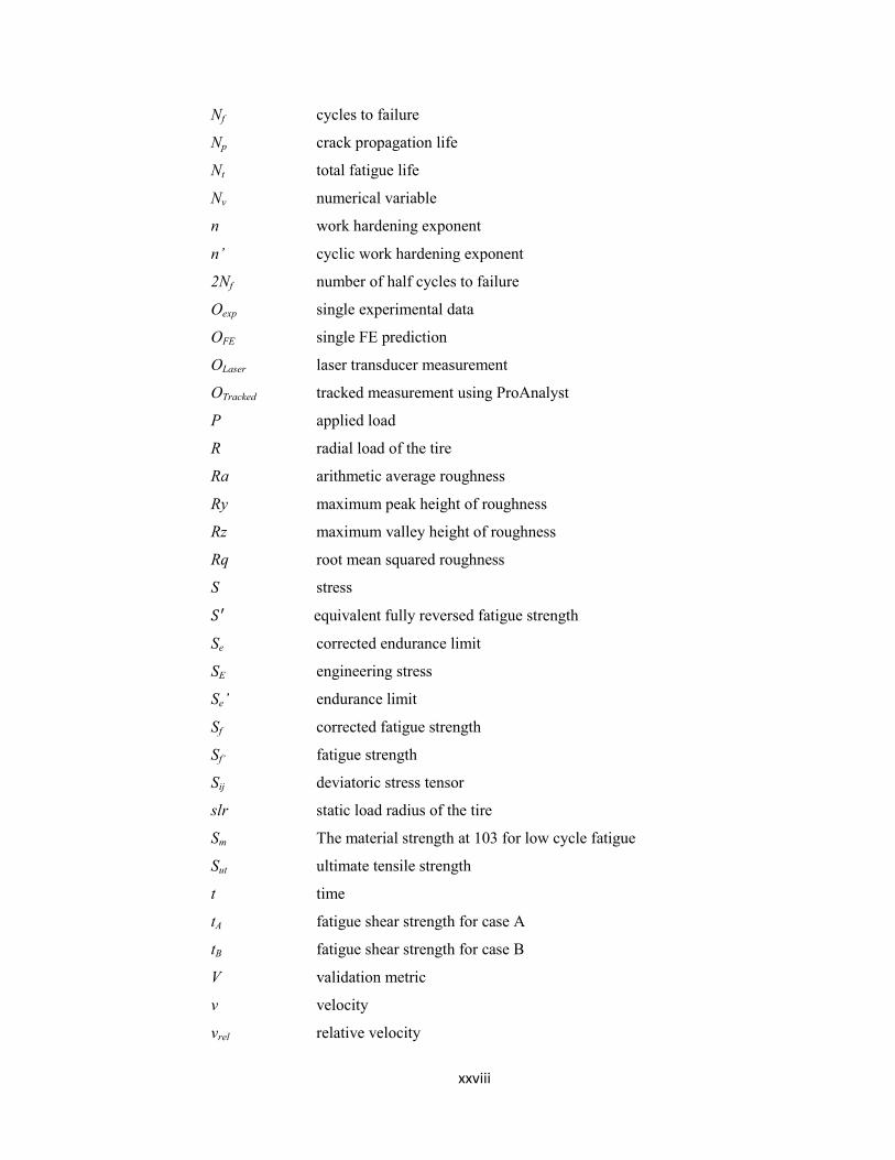
xxviii

Nf cycles to failure

Np crack propagation life

Nt total fatigue life

Nv numerical variable

n work hardening exponent

n’ cyclic work hardening exponent

2Nf number of half cycles to failure

Oexp single experimental data

OFE single FE prediction

OLaser laser transducer measurement

OTracked tracked measurement using ProAnalyst

P applied load

R radial load of the tire

Ra arithmetic average roughness

Ry maximum peak height of roughness

Rz maximum valley height of roughness

Rq root mean squared roughness

S stress

equivalent fully reversed fatigue strength

Se corrected endurance limit

SE engineering stress

Se’ endurance limit

Sf corrected fatigue strength

Sf’ fatigue strength

Sij deviatoric stress tensor

slr static load radius of the tire

Sm The material strength at 103 for low cycle fatigue

Sut ultimate tensile strength

t time

tA fatigue shear strength for case A

tB fatigue shear strength for case B

V validation metric

v velocity

vrel relative velocity

xxix

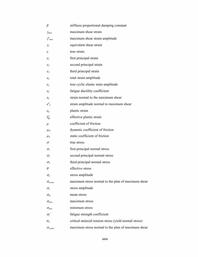
β stiffness proportional damping constant

max maximum shear strain

amax maximum shear strain amplitude

e equivalent shear strain

true strain

1 first principal strain

2 second principal strain

3 third principal strain

a total strain amplitude

e true cyclic elastic stain amplitude

f’ fatigue ductility coefficient

n strain normal to the maximum shear

an strain amplitude normal to maximum shear

p plastic strain

effective plastic strain

µ coefficient of friction

µD dynamic coefficient of friction

µS static coefficient of friction

true stress

1 first principal normal stress

2 second principal normal stress

3 third principal normal stress

effective stress

a stress amplitude

a,max maximum stress normal to the plan of maximum shear

e stress amplitude

m mean stress

max maximum stress

min minimum stress

f’ fatigue strength coefficient

o critical uniaxial tension stress (yield normal stress)

n,max maximum stress normal to the plan of maximum shear

xxx

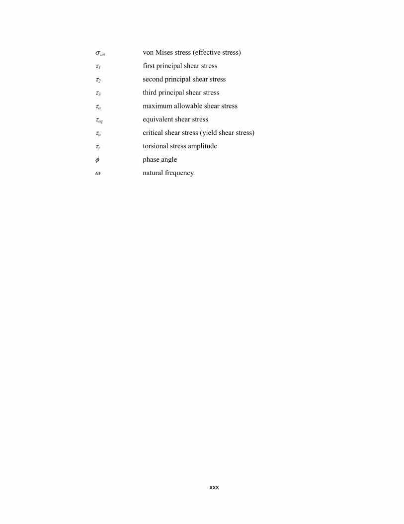
vm von Mises stress (effective stress)

1 first principal shear stress

2 second principal shear stress

3 third principal shear stress

a maximum allowable shear stress

eq equivalent shear stress

o critical shear stress (yield shear stress)

t torsional stress amplitude

phase angle

natural frequency

1

Chapter 1. Introduction and Motivation

1.1. Mining Industry in Canada

Mining impacts our everyday lives, not only from a broader economic and employment

perspective, but in our day-to-day living. From mining come the highways, electrical and

communications networks, clean-energy technologies, housing, automobiles, consumer

electronics and other products and infrastructure essential to modern life.

Mining is one of Canada's most important economic sectors and is a major driver of our

country's prosperity. According to Facts and Figures of The Canadian Mining Industry 2012 [1],

in 2011, the industry contributed $35.6 billion to the gross domestic product (GDP) and employed

320,000 workers in the sectors of mineral extraction, processing and manufacturing. It is an

industry that stimulates and supports economic growth both in large urban centres and in remote

rural communities, including numerous First Nations communities; mining is an important

employer of Aboriginal Canadians.

Mining accounts for 22.8% of Canadian goods exports and $9 billion in taxes and

royalties paid to federal, provincial, and territorial governments [1]. The industry also generates

considerable economic spin-off activity: there are more than 3,200 companies that provide the

industry with services ranging from engineering consulting to drilling equipment. In addition,

over half the freight revenues of Canada's railroads are generated by mining.

Globally, Canada remains the top destination for mining exploration, attracting 18% of

the world's spending in this sector [1]. In the same vein, Canada is recognized internationally as a

source of mining leadership and related finance expertise: there are approximately 1,000

Canadian exploration companies active in over 100 countries.

Ontario is the largest producer in Canada of gold, nickel, copper, platinum group metals,

copper, salt, and structural materials [2]. The value of mineral production was $6.3 billion in

2009, $7.7 billion in 2010, and $10.7 billion in 2011. This represented almost 25% of all

Canadian nonfuel mineral production in 2011 and accounted directly for more than 1.6% of total

Ontario GDP.

However, some factors hamper the development to mining industry. One of which is the

injuries in the mining industry. Injuries have a tendency of decreasing due to technology

advancement, stringent government safety regulations, and employee training. However, mining

injuries and fatalities are still occurring around the world every year as regular occurrences.

2

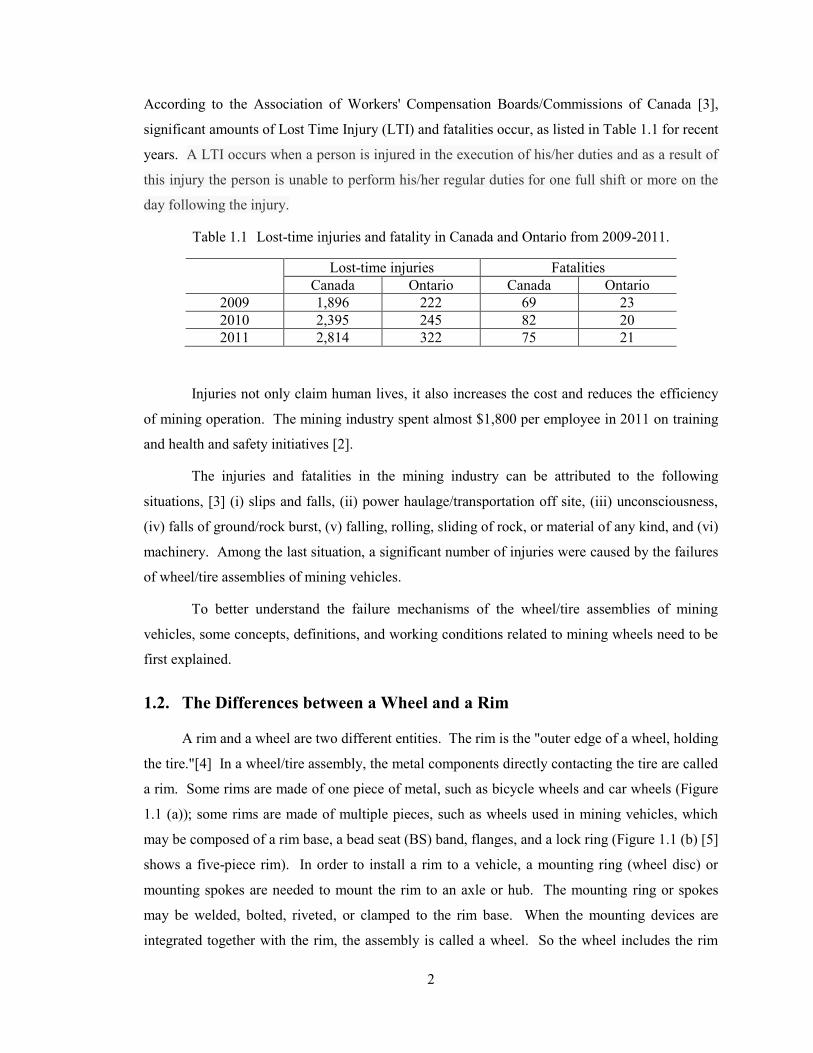
According to the Association of Workers' Compensation Boards/Commissions of Canada [3],

significant amounts of Lost Time Injury (LTI) and fatalities occur, as listed in Table 1.1 for recent

years. A LTI occurs when a person is injured in the execution of his/her duties and as a result of

this injury the person is unable to perform his/her regular duties for one full shift or more on the

day following the injury.

Table 1.1 Lost-time injuries and fatality in Canada and Ontario from 2009-2011.

Lost-time injuries Fatalities

Canada Ontario Canada Ontario

2009 1,896 222 69 23

2010 2,395 245 82 20

2011 2,814 322 75 21

Injuries not only claim human lives, it also increases the cost and reduces the efficiency

of mining operation. The mining industry spent almost $1,800 per employee in 2011 on training

and health and safety initiatives [2].

The injuries and fatalities in the mining industry can be attributed to the following

situations, [3] (i) slips and falls, (ii) power haulage/transportation off site, (iii) unconsciousness,

(iv) falls of ground/rock burst, (v) falling, rolling, sliding of rock, or material of any kind, and (vi)

machinery. Among the last situation, a significant number of injuries were caused by the failures

of wheel/tire assemblies of mining vehicles.

To better understand the failure mechanisms of the wheel/tire assemblies of mining

vehicles, some concepts, definitions, and working conditions related to mining wheels need to be

first explained.

1.2. The Differences between a Wheel and a Rim

A rim and a wheel are two different entities. The rim is the "outer edge of a wheel, holding

the tire."[4] In a wheel/tire assembly, the metal components directly contacting the tire are called

a rim. Some rims are made of one piece of metal, such as bicycle wheels and car wheels (Figure

1.1 (a)); some rims are made of multiple pieces, such as wheels used in mining vehicles, which

may be composed of a rim base, a bead seat (BS) band, flanges, and a lock ring (Figure 1.1 (b) [5]

shows a five-piece rim). In order to install a rim to a vehicle, a mounting ring (wheel disc) or

mounting spokes are needed to mount the rim to an axle or hub. The mounting ring or spokes

may be welded, bolted, riveted, or clamped to the rim base. When the mounting devices are

integrated together with the rim, the assembly is called a wheel. So the wheel includes the rim

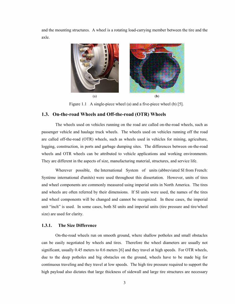
3

and the mounting structures. A wheel is a rotating load-carrying member between the tire and the

axle.

1.3. On-the-road Wheels and Off-the-road (OTR) Wheels

The wheels used on vehicles running on the road are called on-the-road wheels, such as

passenger vehicle and haulage truck wheels. The wheels used on vehicles running off the road

are called off-the-road (OTR) wheels, such as wheels used in vehicles for mining, agriculture,

logging, construction, in ports and garbage dumping sites. The differences between on-the-road

wheels and OTR wheels can be attributed to vehicle applications and working environments.

They are different in the aspects of size, manufacturing material, structures, and service life.

Wherever possible, the International System of units (abbreviated SI from French:

Système international d'unités) were used throughout this dissertation. However, units of tires

and wheel components are commonly measured using imperial units in North America. The tires

and wheels are often referred by their dimensions. If SI units were used, the names of the tires

and wheel components will be changed and cannot be recognized. In these cases, the imperial

unit “inch” is used. In some cases, both SI units and imperial units (tire pressure and tire/wheel

size) are used for clarity.

1.3.1. The Size Difference

On-the-road wheels run on smooth ground, where shallow potholes and small obstacles

can be easily negotiated by wheels and tires. Therefore the wheel diameters are usually not

significant, usually 0.45 meters to 0.6 meters [6] and they travel at high speeds. For OTR wheels,

due to the deep potholes and big obstacles on the ground, wheels have to be made big for

continuous traveling and they travel at low speeds. The high tire pressure required to support the

high payload also dictates that large thickness of sidewall and large tire structures are necessary

(a) (b)

Figure 1.1 A single-piece wheel (a) and a five-piece wheel (b) [5].

4

for OTR tires (to have enough volume of air inside the tire to increase load support capability and

tire stability). Therefore the diameters of OTR wheels are usually much bigger than those of road

wheels. Figure 1.2 [7] shows that the tires used on Cat® 797 Mining Truck, which is

approximately 2.5 m in diameter. The tire size difference between the passenger vehicle and the

mining truck can be clearly observed from the figure.

1.3.2. The Wheel Structure and Tire Mounting Differences

Road wheel tires are usually small and the tire beads are not significantly thick and the

tire can be easily mounted/dismounted on a single piece wheel. Therefore road wheels are

usually made of one single piece. On the other hand, OTR tires are usually very large and tire

beads are very thick and stiff. OTR wheels are usually made of multiple pieces for tire

mounting/dismounting purpose. The rationale for use of multi-piece wheels will be detailed in

the following section.

Due to the structure difference between the rims of road wheels and OTR wheels, the tire

mounting/dismounting methods are different. The road tire can be easily mounted on or

dismounted off a single piece wheel by prying the tire bead onto or off the rim lip using a prying

bar or some other mounting device, due to the thin and flexible tire beads. For OTR wheels, tire

mounting/dismounting has to follow a specific sequence. Figure 1.3 [5] illustrates the structure of

a five-piece wheel, in which the numbers behind the component names indicate tire mounting

sequence. The five-piece wheel is composed of a rim base, a split lock ring, a bead seat (BS)

band, and front/back flanges. Mounting of the tire begins with placing the rear flange onto the

rim base. The tire is subsequently installed on the rim base, followed by the front flange being

placed against the tire. A rubber O-ring is inserted into the O-ring groove located on the rim base

Figure 1.2 The size difference between OTR tires and on-the-road tires [7]. (Reprinted

Courtesy of Caterpillar Inc.)

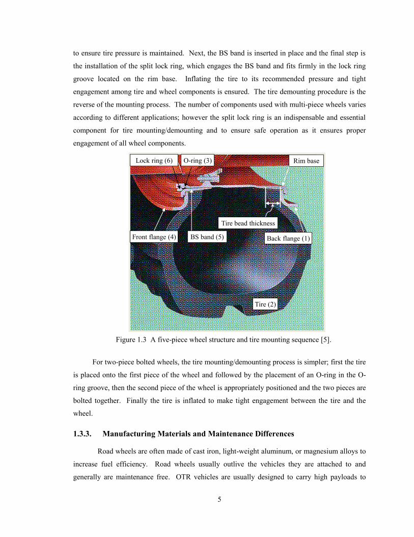
5

to ensure tire pressure is maintained. Next, the BS band is inserted in place and the final step is

the installation of the split lock ring, which engages the BS band and fits firmly in the lock ring

groove located on the rim base. Inflating the tire to its recommended pressure and tight

engagement among tire and wheel components is ensured. The tire demounting procedure is the

reverse of the mounting process. The number of components used with multi-piece wheels varies

according to different applications; however the split lock ring is an indispensable and essential

component for tire mounting/demounting and to ensure safe operation as it ensures proper

engagement of all wheel components.

For two-piece bolted wheels, the tire mounting/demounting process is simpler; first the tire

is placed onto the first piece of the wheel and followed by the placement of an O-ring in the O-

ring groove, then the second piece of the wheel is appropriately positioned and the two pieces are

bolted together. Finally the tire is inflated to make tight engagement between the tire and the

wheel.

1.3.3. Manufacturing Materials and Maintenance Differences

Road wheels are often made of cast iron, light-weight aluminum, or magnesium alloys to

increase fuel efficiency. Road wheels usually outlive the vehicles they are attached to and

generally are maintenance free. OTR vehicles are usually designed to carry high payloads to

Rim base

Back flange (1)

Tire (2)

Front flange (4) BS band (5)

Lock ring (6) O-ring (3)

Tire bead thickness

Figure 1.3 A five-piece wheel structure and tire mounting sequence [5].

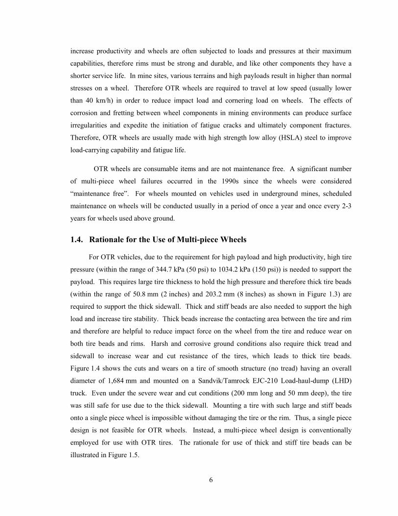
6

increase productivity and wheels are often subjected to loads and pressures at their maximum

capabilities, therefore rims must be strong and durable, and like other components they have a

shorter service life. In mine sites, various terrains and high payloads result in higher than normal

stresses on a wheel. Therefore OTR wheels are required to travel at low speed (usually lower

than 40 km/h) in order to reduce impact load and cornering load on wheels. The effects of

corrosion and fretting between wheel components in mining environments can produce surface

irregularities and expedite the initiation of fatigue cracks and ultimately component fractures.

Therefore, OTR wheels are usually made with high strength low alloy (HSLA) steel to improve

load-carrying capability and fatigue life.

OTR wheels are consumable items and are not maintenance free. A significant number

of multi-piece wheel failures occurred in the 1990s since the wheels were considered

“maintenance free”. For wheels mounted on vehicles used in underground mines, scheduled

maintenance on wheels will be conducted usually in a period of once a year and once every 2-3

years for wheels used above ground.

1.4. Rationale for the Use of Multi-piece Wheels

For OTR vehicles, due to the requirement for high payload and high productivity, high tire

pressure (within the range of 344.7 kPa (50 psi) to 1034.2 kPa (150 psi)) is needed to support the

payload. This requires large tire thickness to hold the high pressure and therefore thick tire beads

(within the range of 50.8 mm (2 inches) and 203.2 mm (8 inches) as shown in Figure 1.3) are

required to support the thick sidewall. Thick and stiff beads are also needed to support the high

load and increase tire stability. Thick beads increase the contacting area between the tire and rim

and therefore are helpful to reduce impact force on the wheel from the tire and reduce wear on

both tire beads and rims. Harsh and corrosive ground conditions also require thick tread and

sidewall to increase wear and cut resistance of the tires, which leads to thick tire beads.

Figure 1.4 shows the cuts and wears on a tire of smooth structure (no tread) having an overall

diameter of 1,684 mm and mounted on a Sandvik/Tamrock EJC-210 Load-haul-dump (LHD)

truck. Even under the severe wear and cut conditions (200 mm long and 50 mm deep), the tire

was still safe for use due to the thick sidewall. Mounting a tire with such large and stiff beads

onto a single piece wheel is impossible without damaging the tire or the rim. Thus, a single piece

design is not feasible for OTR wheels. Instead, a multi-piece wheel design is conventionally

employed for use with OTR tires. The rationale for use of thick and stiff tire beads can be

illustrated in Figure 1.5.

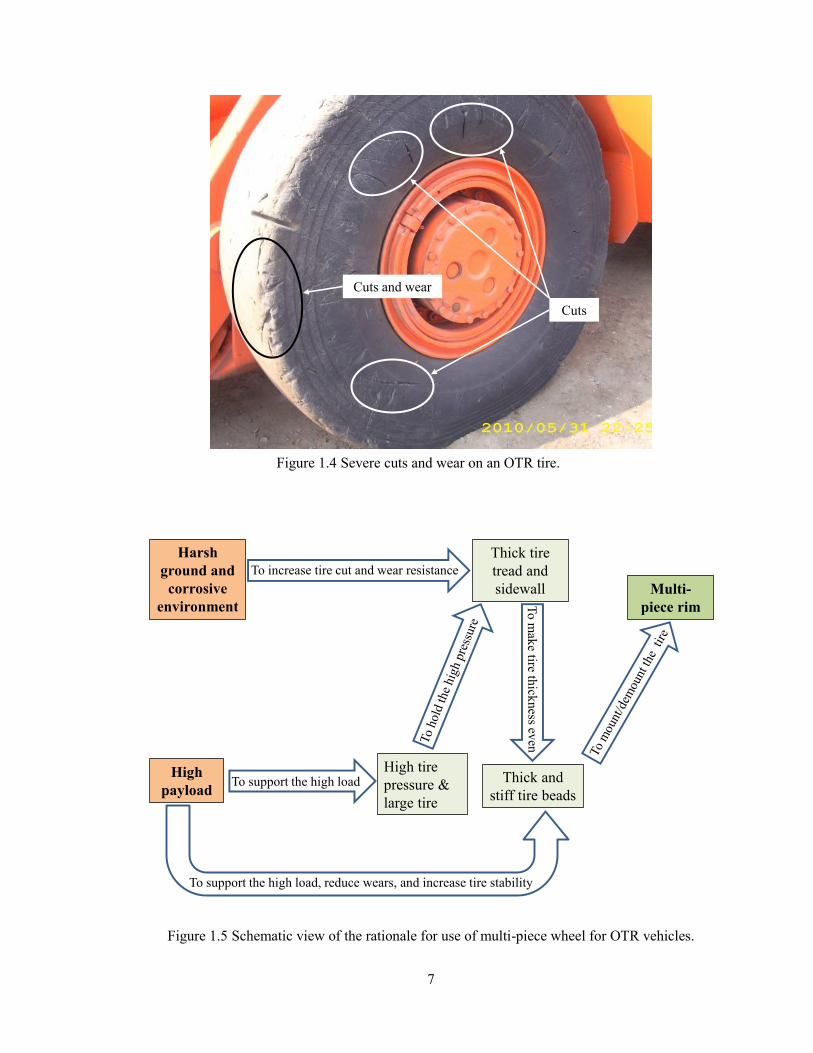
7

Cuts and wear

Cuts

Figure 1.4 Severe cuts and wear on an OTR tire.

High

payload

High tire

pressure &

large tire

Thick and

stiff tire beads

Harsh

ground and

corrosive

environment

Thick tire

tread and

sidewall

To increase tire cut and wear resistance

To support the high load

To support the high load, reduce wears, and increase tire stability

Multi-

piece rim

Figure 1.5 Schematic view of the rationale for use of multi-piece wheel for OTR vehicles.

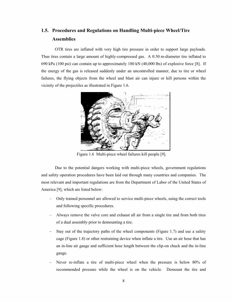
8

1.5. Procedures and Regulations on Handling Multi-piece Wheel/Tire

Assemblies

OTR tires are inflated with very high tire pressure in order to support large payloads.

Thus tires contain a large amount of highly-compressed gas. A 0.50 m-diameter tire inflated to

690 kPa (100 psi) can contain up to approximately 180 kN (40,000 lbs) of explosive force [8]. If

the energy of the gas is released suddenly under an uncontrolled manner, due to tire or wheel

failures, the flying objects from the wheel and blast air can injure or kill persons within the

vicinity of the projectiles as illustrated in Figure 1.6.

Due to the potential dangers working with multi-piece wheels, government regulations

and safety operation procedures have been laid out through many countries and companies. The

most relevant and important regulations are from the Department of Labor of the United States of

America [9], which are listed below:

– Only trained personnel are allowed to service multi-piece wheels, using the correct tools

and following specific procedures.

– Always remove the valve core and exhaust all air from a single tire and from both tires

of a dual assembly prior to demounting a tire.

– Stay out of the trajectory paths of the wheel components (Figure 1.7) and use a safety

cage (Figure 1.8) or other restraining device when inflate a tire. Use an air hose that has

an in-line air gauge and sufficient hose length between the clip-on chuck and the in-line

gauge.

– Never re-inflate a tire of multi-piece wheel when the pressure is below 80% of

recommended pressure while the wheel is on the vehicle. Demount the tire and

Figure 1.6 Multi-piece wheel failures kill people [9].

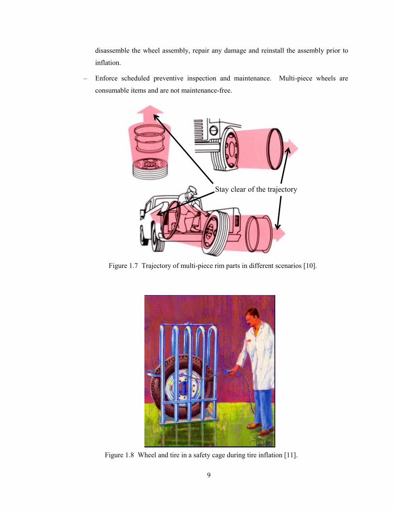
9

disassemble the wheel assembly, repair any damage and reinstall the assembly prior to

inflation.

– Enforce scheduled preventive inspection and maintenance. Multi-piece wheels are

consumable items and are not maintenance-free.

Stay clear of the trajectory

Figure 1.7 Trajectory of multi-piece rim parts in different scenarios [10].

Figure 1.8 Wheel and tire in a safety cage during tire inflation [11].

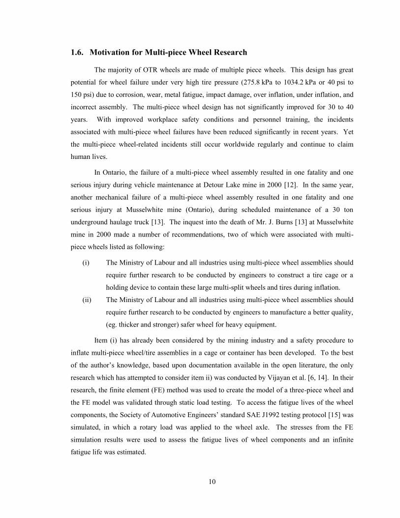
10

1.6. Motivation for Multi-piece Wheel Research

The majority of OTR wheels are made of multiple piece wheels. This design has great

potential for wheel failure under very high tire pressure (275.8 kPa to 1034.2 kPa or 40 psi to

150 psi) due to corrosion, wear, metal fatigue, impact damage, over inflation, under inflation, and

incorrect assembly. The multi-piece wheel design has not significantly improved for 30 to 40

years. With improved workplace safety conditions and personnel training, the incidents

associated with multi-piece wheel failures have been reduced significantly in recent years. Yet

the multi-piece wheel-related incidents still occur worldwide regularly and continue to claim

human lives.

In Ontario, the failure of a multi-piece wheel assembly resulted in one fatality and one

serious injury during vehicle maintenance at Detour Lake mine in 2000 [12]. In the same year,

another mechanical failure of a multi-piece wheel assembly resulted in one fatality and one

serious injury at Musselwhite mine (Ontario), during scheduled maintenance of a 30 ton

underground haulage truck [13]. The inquest into the death of Mr. J. Burns [13] at Musselwhite

mine in 2000 made a number of recommendations, two of which were associated with multi-

piece wheels listed as following:

(i) The Ministry of Labour and all industries using multi-piece wheel assemblies should

require further research to be conducted by engineers to construct a tire cage or a

holding device to contain these large multi-split wheels and tires during inflation.

(ii) The Ministry of Labour and all industries using multi-piece wheel assemblies should

require further research to be conducted by engineers to manufacture a better quality,

(eg. thicker and stronger) safer wheel for heavy equipment.

Item (i) has already been considered by the mining industry and a safety procedure to

inflate multi-piece wheel/tire assemblies in a cage or container has been developed. To the best

of the author’s knowledge, based upon documentation available in the open literature, the only

research which has attempted to consider item ii) was conducted by Vijayan et al. [6, 14]. In their

research, the finite element (FE) method was used to create the model of a three-piece wheel and

the FE model was validated through static load testing. To access the fatigue lives of the wheel

components, the Society of Automotive Engineers’ standard SAE J1992 testing protocol [15] was

simulated, in which a rotary load was applied to the wheel axle. The stresses from the FE

simulation results were used to assess the fatigue lives of wheel components and an infinite

fatigue life was estimated.

11

However, literature and documented incident reports indicate that multi-piece wheels

have limited fatigue lives. In the research conducted by Vijayan et al. [6,14], geometry

degradation due to wear and impact damage and material degradation due to corrosive

environmental conditions were not considered, which led to the conclusion of infinite fatigue life

prediction. Another limitation in [6] and [14] was the exclusion of OTR tires in the structural

analysis. All these factors affect the accuracy of the analysis results.

Supported by Workplace Safety and Insurance Board (WSIB) of Ontario, further research

was conducted by the University of Windsor research team, led by Dr. Altenhof, to consider the

aforementioned factors affecting fatigue life of multi-piece wheels. In this research, innovative

designs were also proposed to make multi-piece wheels safer.

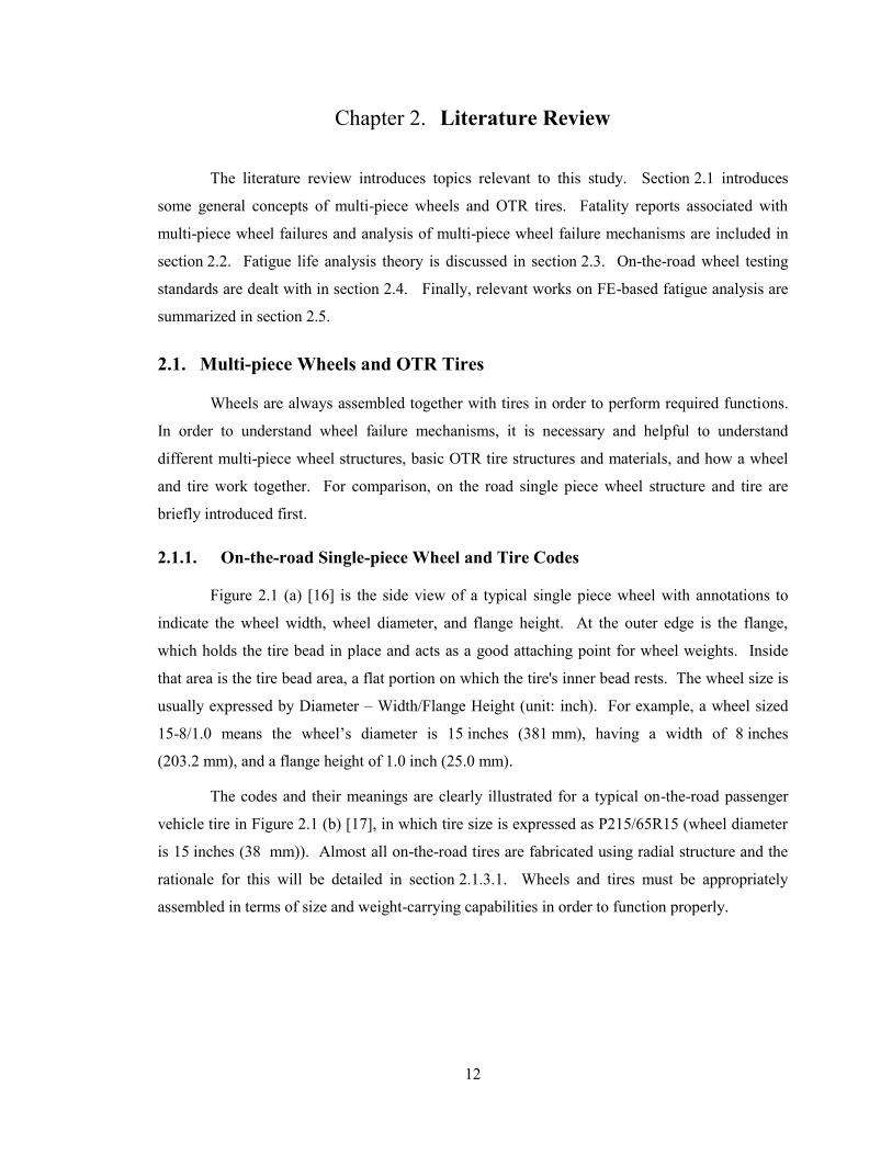
12

Chapter 2. Literature Review

The literature review introduces topics relevant to this study. Section 2.1 introduces

some general concepts of multi-piece wheels and OTR tires. Fatality reports associated with

multi-piece wheel failures and analysis of multi-piece wheel failure mechanisms are included in

section 2.2. Fatigue life analysis theory is discussed in section 2.3. On-the-road wheel testing

standards are dealt with in section 2.4. Finally, relevant works on FE-based fatigue analysis are

summarized in section 2.5.

2.1. Multi-piece Wheels and OTR Tires

Wheels are always assembled together with tires in order to perform required functions.

In order to understand wheel failure mechanisms, it is necessary and helpful to understand

different multi-piece wheel structures, basic OTR tire structures and materials, and how a wheel

and tire work together. For comparison, on the road single piece wheel structure and tire are

briefly introduced first.

2.1.1. On-the-road Single-piece Wheel and Tire Codes

Figure 2.1 (a) [16] is the side view of a typical single piece wheel with annotations to

indicate the wheel width, wheel diameter, and flange height. At the outer edge is the flange,

which holds the tire bead in place and acts as a good attaching point for wheel weights. Inside

that area is the tire bead area, a flat portion on which the tire's inner bead rests. The wheel size is

usually expressed by Diameter – Width/Flange Height (unit: inch). For example, a wheel sized

15-8/1.0 means the wheel’s diameter is 15 inches (381 mm), having a width of 8 inches

(203.2 mm), and a flange height of 1.0 inch (25.0 mm).

The codes and their meanings are clearly illustrated for a typical on-the-road passenger

vehicle tire in Figure 2.1 (b) [17], in which tire size is expressed as P215/65R15 (wheel diameter

is 15 inches (38 mm)). Almost all on-the-road tires are fabricated using radial structure and the

rationale for this will be detailed in section 2.1.3.1. Wheels and tires must be appropriately

assembled in terms of size and weight-carrying capabilities in order to function properly.

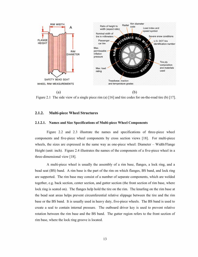
13

2.1.2. Multi-piece Wheel Structures

2.1.2.1. Names and Size Specifications of Multi-piece Wheel Components

Figure 2.2 and 2.3 illustrate the names and specifications of three-piece wheel

components and five-piece wheel components by cross section views [18]. For multi-piece

wheels, the sizes are expressed in the same way as one-piece wheel: Diameter – Width/Flange

Height (unit: inch). Figure 2.4 illustrates the names of the components of a five-piece wheel in a

three-dimensional view [18].

A multi-piece wheel is usually the assembly of a rim base, flanges, a lock ring, and a

bead seat (BS) band. A rim base is the part of the rim on which flanges, BS band, and lock ring

are supported. The rim base may consist of a number of separate components, which are welded

together, e.g. back section, center section, and gutter section (the front section of rim base, where

lock ring is seated on). The flanges help hold the tire on the rim. The knurling on the rim base at

the bead seat areas helps prevent circumferential relative slippage between the tire and the rim

base or the BS band. It is usually used in heavy duty, five-piece wheels. The BS band is used to

create a seal to contain internal pressure. The outboard driver key is used to prevent relative

rotation between the rim base and the BS band. The gutter region refers to the front section of

rim base, where the lock ring groove is located.

(a) (b)

Figure 2.1 The side view of a single piece rim (a) [16] and tire codes for on-the-road tire (b) [17].

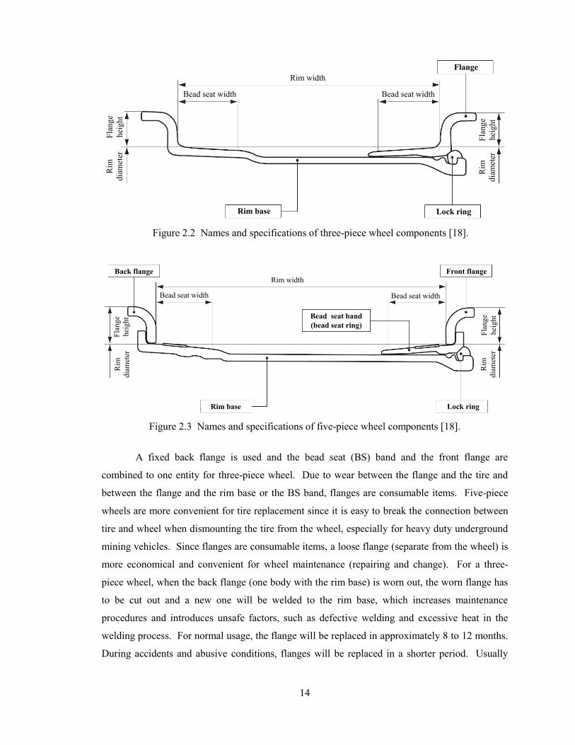
14

A fixed back flange is used and the bead seat (BS) band and the front flange are

combined to one entity for three-piece wheel. Due to wear between the flange and the tire and

between the flange and the rim base or the BS band, flanges are consumable items. Five-piece

wheels are more convenient for tire replacement since it is easy to break the connection between

tire and wheel when dismounting the tire from the wheel, especially for heavy duty underground

mining vehicles. Since flanges are consumable items, a loose flange (separate from the wheel) is

more economical and convenient for wheel maintenance (repairing and change). For a three-

piece wheel, when the back flange (one body with the rim base) is worn out, the worn flange has

to be cut out and a new one will be welded to the rim base, which increases maintenance

procedures and introduces unsafe factors, such as defective welding and excessive heat in the

welding process. For normal usage, the flange will be replaced in approximately 8 to 12 months.

During accidents and abusive conditions, flanges will be replaced in a shorter period. Usually

Flange

Lock ringRim base

Rim width

Bead seat width Bead seat width

Fla

nge

hei

ght

Rim

dia

met

er

Fla

nge

hei

gh

t

Rim

dia

met

er

Figure 2.2 Names and specifications of three-piece wheel components [18].

Front flangeBack flange

Lock ringRim base

Rim width

Bead seat width Bead seat width

Rim

dia

met

er

Fla

nge

hei

ght

Rim

dia

met

er

Fla

nge

hei

ght Bead seat band

(bead seat ring)

Figure 2.3 Names and specifications of five-piece wheel components [18].

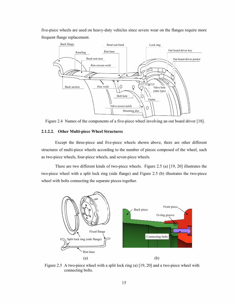
15

five-piece wheels are used on heavy-duty vehicles since severe wear on the flanges require more

frequent flange replacement.

2.1.2.2. Other Multi-piece Wheel Structures

Except the three-piece and five-piece wheels shown above, there are other different

structures of multi-piece wheels according to the number of pieces composed of the wheel, such

as two-piece wheels, four-piece wheels, and seven-piece wheels.

There are two different kinds of two-piece wheels. Figure 2.5 (a) [19, 20] illustrates the

two-piece wheel with a split lock ring (side flange) and Figure 2.5 (b) illustrates the two-piece

wheel with bolts connecting the separate pieces together.

Back pieceFront piece

O-ring groove

Connecting bolts

Rim base

Fixed flange

Split lock ring (side flange)

(a) (b)

Figure 2.5 A two-piece wheel with a split lock ring (a) [19, 20] and a two-piece wheel with

connecting bolts.

\bolts.

Back flange

Knurling

Bead seat band Lock ring

Out board driver key

Out board driver pocket

Rim base

Bead seat area

Rim circum-weld

Back section Disc weld

Bolt hole

Valve access notch

Valve hole

(tube type)

Gutter

Mounting disc

Figure 2.4 Names of the components of a five-piece wheel involving an out board driver [18].

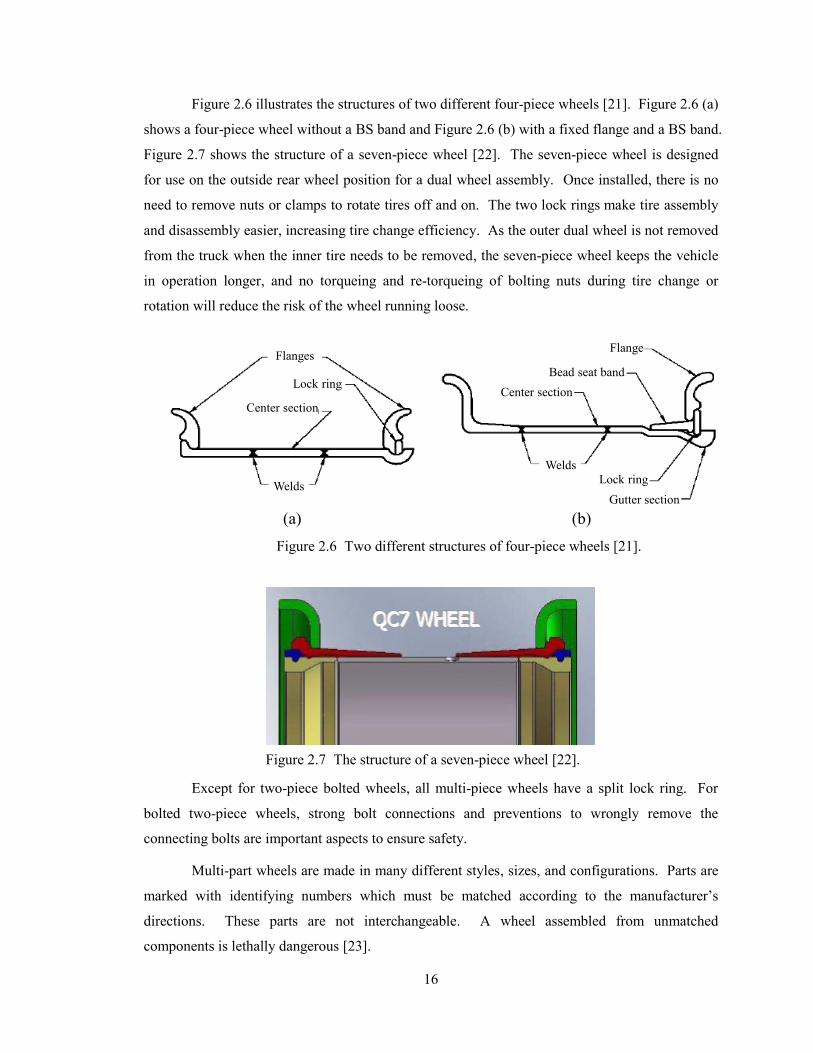
16

Figure 2.6 illustrates the structures of two different four-piece wheels [21]. Figure 2.6 (a)

shows a four-piece wheel without a BS band and Figure 2.6 (b) with a fixed flange and a BS band.

Figure 2.7 shows the structure of a seven-piece wheel [22]. The seven-piece wheel is designed

for use on the outside rear wheel position for a dual wheel assembly. Once installed, there is no

need to remove nuts or clamps to rotate tires off and on. The two lock rings make tire assembly

and disassembly easier, increasing tire change efficiency. As the outer dual wheel is not removed

from the truck when the inner tire needs to be removed, the seven-piece wheel keeps the vehicle

in operation longer, and no torqueing and re-torqueing of bolting nuts during tire change or

rotation will reduce the risk of the wheel running loose.

Except for two-piece bolted wheels, all multi-piece wheels have a split lock ring. For

bolted two-piece wheels, strong bolt connections and preventions to wrongly remove the

connecting bolts are important aspects to ensure safety.

Multi-part wheels are made in many different styles, sizes, and configurations. Parts are

marked with identifying numbers which must be matched according to the manufacturer’s

directions. These parts are not interchangeable. A wheel assembled from unmatched

components is lethally dangerous [23].

(a) (b)

FlangesFlange

Lock ring

Center section

Welds

Welds

Lock ring

Center section

Gutter section

Bead seat band

Figure 2.6 Two different structures of four-piece wheels [21].

Figure 2.7 The structure of a seven-piece wheel [22].

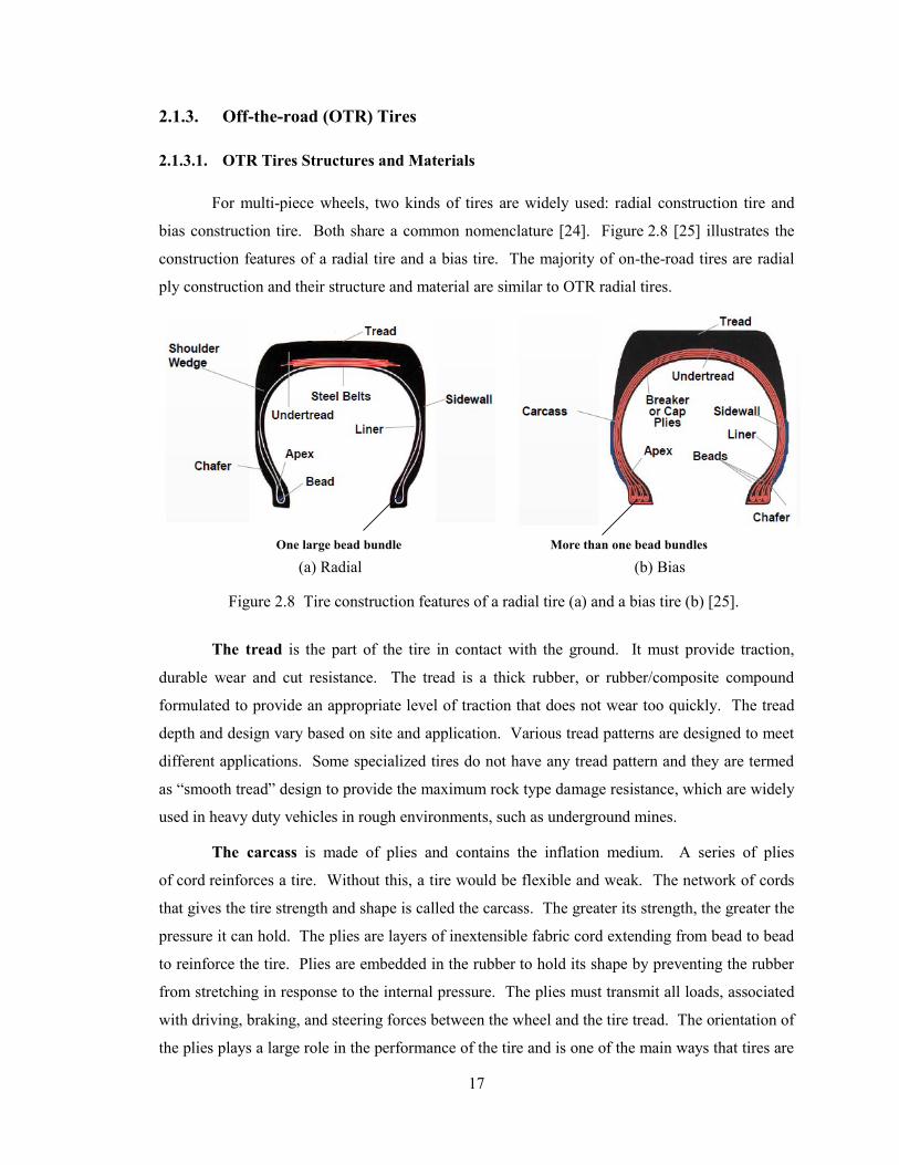
17

2.1.3. Off-the-road (OTR) Tires

2.1.3.1. OTR Tires Structures and Materials

For multi-piece wheels, two kinds of tires are widely used: radial construction tire and

bias construction tire. Both share a common nomenclature [24]. Figure 2.8 [25] illustrates the

construction features of a radial tire and a bias tire. The majority of on-the-road tires are radial

ply construction and their structure and material are similar to OTR radial tires.

The tread is the part of the tire in contact with the ground. It must provide traction,

durable wear and cut resistance. The tread is a thick rubber, or rubber/composite compound

formulated to provide an appropriate level of traction that does not wear too quickly. The tread

depth and design vary based on site and application. Various tread patterns are designed to meet

different applications. Some specialized tires do not have any tread pattern and they are termed

as “smooth tread” design to provide the maximum rock type damage resistance, which are widely

used in heavy duty vehicles in rough environments, such as underground mines.

The carcass is made of plies and contains the inflation medium. A series of plies

of cord reinforces a tire. Without this, a tire would be flexible and weak. The network of cords

that gives the tire strength and shape is called the carcass. The greater its strength, the greater the

pressure it can hold. The plies are layers of inextensible fabric cord extending from bead to bead

to reinforce the tire. Plies are embedded in the rubber to hold its shape by preventing the rubber

from stretching in response to the internal pressure. The plies must transmit all loads, associated

with driving, braking, and steering forces between the wheel and the tire tread. The orientation of

the plies plays a large role in the performance of the tire and is one of the main ways that tires are

More than one bead bundlesOne large bead bundle

(a) Radial (b) Bias

Figure 2.8 Tire construction features of a radial tire (a) and a bias tire (b) [25].

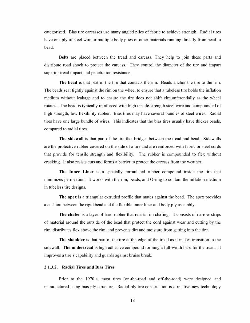
18

categorized. Bias tire carcasses use many angled plies of fabric to achieve strength. Radial tires

have one ply of steel wire or multiple body plies of other materials running directly from bead to

bead.

Belts are placed between the tread and carcass. They help to join these parts and

distribute road shock to protect the carcass. They control the diameter of the tire and impart

superior tread impact and penetration resistance.

The bead is that part of the tire that contacts the rim. Beads anchor the tire to the rim.

The beads seat tightly against the rim on the wheel to ensure that a tubeless tire holds the inflation

medium without leakage and to ensure the tire does not shift circumferentially as the wheel

rotates. The bead is typically reinforced with high tensile-strength steel wire and compounded of

high strength, low flexibility rubber. Bias tires may have several bundles of steel wires. Radial

tires have one large bundle of wires. This indicates that the bias tires usually have thicker beads,

compared to radial tires.

The sidewall is that part of the tire that bridges between the tread and bead. Sidewalls

are the protective rubber covered on the side of a tire and are reinforced with fabric or steel cords

that provide for tensile strength and flexibility. The rubber is compounded to flex without

cracking. It also resists cuts and forms a barrier to protect the carcass from the weather.

The Inner Liner is a specially formulated rubber compound inside the tire that

minimizes permeation. It works with the rim, beads, and O-ring to contain the inflation medium

in tubeless tire designs.

The apex is a triangular extruded profile that mates against the bead. The apex provides

a cushion between the rigid bead and the flexible inner liner and body ply assembly.

The chafer is a layer of hard rubber that resists rim chafing. It consists of narrow strips

of material around the outside of the bead that protect the cord against wear and cutting by the

rim, distributes flex above the rim, and prevents dirt and moisture from getting into the tire.

The shoulder is that part of the tire at the edge of the tread as it makes transition to the

sidewall. The undertread is high adhesive compound forming a full-width base for the tread. It

improves a tire’s capability and guards against bruise break.

2.1.3.2. Radial Tires and Bias Tires

Prior to the 1970’s, most tires (on-the-road and off-the-road) were designed and

manufactured using bias ply structure. Radial ply tire construction is a relative new technology

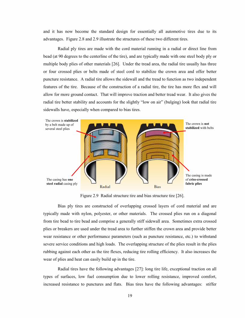
19

and it has now become the standard design for essentially all automotive tires due to its

advantages. Figure 2.8 and 2.9 illustrate the structures of these two different tires.

Radial ply tires are made with the cord material running in a radial or direct line from

bead (at 90 degrees to the centerline of the tire), and are typically made with one steel body ply or

multiple body plies of other materials [26]. Under the tread area, the radial tire usually has three

or four crossed plies or belts made of steel cord to stabilize the crown area and offer better

puncture resistance. A radial tire allows the sidewall and the tread to function as two independent

features of the tire. Because of the construction of a radial tire, the tire has more flex and will

allow for more ground contact. That will improve traction and better tread wear. It also gives the

radial tire better stability and accounts for the slightly “low on air” (bulging) look that radial tire

sidewalls have, especially when compared to bias tires.

Bias ply tires are constructed of overlapping crossed layers of cord material and are

typically made with nylon, polyester, or other materials. The crossed plies run on a diagonal

from tire bead to tire bead and comprise a generally stiff sidewall area. Sometimes extra crossed

plies or breakers are used under the tread area to further stiffen the crown area and provide better

wear resistance or other performance parameters (such as puncture resistance, etc.) to withstand

severe service conditions and high loads. The overlapping structure of the plies result in the plies

rubbing against each other as the tire flexes, reducing tire rolling efficiency. It also increases the

wear of plies and heat can easily build up in the tire.

Radial tires have the following advantages [27]: long tire life, exceptional traction on all

types of surfaces, low fuel consumption due to lower rolling resistance, improved comfort,

increased resistance to punctures and flats. Bias tires have the following advantages: stiffer

The crown is not

stabilized with belts

The casing is made

of criss-crossed

fabric plies

The crown is stabilized

by a belt made up of

several steel plies

The casing has one

steel radial casing ply

Figure 2.9 Radial structure tire and bias structure tire [26].

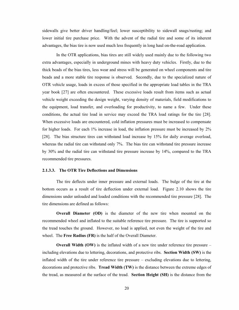
20

sidewalls give better driver handling/feel; lower susceptibility to sidewall snags/rusting; and

lower initial tire purchase price. With the advent of the radial tire and some of its inherent

advantages, the bias tire is now used much less frequently in long haul on-the-road application.

In the OTR applications, bias tires are still widely used mainly due to the following two

extra advantages, especially in underground mines with heavy duty vehicles. Firstly, due to the

thick beads of the bias tires, less wear and stress will be generated on wheel components and tire

beads and a more stable tire response is observed. Secondly, due to the specialized nature of

OTR vehicle usage, loads in excess of those specified in the appropriate load tables in the TRA

year book [27] are often encountered. These excessive loads result from items such as actual

vehicle weight exceeding the design weight, varying density of materials, field modifications to

the equipment, load transfer, and overloading for productivity, to name a few. Under these

conditions, the actual tire load in service may exceed the TRA load ratings for the tire [28].

When excessive loads are encountered, cold inflation pressures must be increased to compensate

for higher loads. For each 1% increase in load, the inflation pressure must be increased by 2%

[28]. The bias structure tires can withstand load increase by 15% for daily average overload,

whereas the radial tire can withstand only 7%. The bias tire can withstand tire pressure increase

by 30% and the radial tire can withstand tire pressure increase by 14%, compared to the TRA

recommended tire pressures.

2.1.3.3. The OTR Tire Deflections and Dimensions

The tire deflects under inner pressure and external loads. The bulge of the tire at the

bottom occurs as a result of tire deflection under external load. Figure 2.10 shows the tire

dimensions under unloaded and loaded conditions with the recommended tire pressure [28]. The

tire dimensions are defined as follows:

Overall Diameter (OD) is the diameter of the new tire when mounted on the

recommended wheel and inflated to the suitable reference tire pressure. The tire is supported so

the tread touches the ground. However, no load is applied, not even the weight of the tire and

wheel. The Free Radius (FR) is the half of the Overall Diameter.

Overall Width (OW) is the inflated width of a new tire under reference tire pressure –

including elevations due to lettering, decorations, and protective ribs. Section Width (SW) is the

inflated width of the tire under reference tire pressure – excluding elevations due to lettering,

decorations and protective ribs. Tread Width (TW) is the distance between the extreme edges of

the tread, as measured at the surface of the tread. Section Height (SH) is the distance from the

21

bead seat to the outer tread contour of the inflated tire at its central line. SH is half of the

difference between the tire overall diameter and rim diameter.

Static Loaded Radius (SLR) is the distance from centre of wheel to the ground on a

vehicle under reference load and pressure at static loading condition. Vertical Deflection (VD)

is the difference between the Free Radius and Static Loaded Radius. Static Loaded Width

(LSW) is the maximum width of the tire under reference load and pressure at static condition.

The difference between Static Loaded Width and Overall Width is the Loaded Section Growth

(LSG). In this research, Loaded Section Growth is also referred as tire Lateral Deflection (LD).

Another important tire size parameter is Aspect Ratio (AR), which is defined as the ratio of the

tire Section Height (SH) to its Section Width (SW) expressed as a percentage.

Tread Width (TW)

Section Width (SW)

Overall Width (OW)

Fre

e R

adiu

s (F

R)

Over

all

Dia

met

er (

OD

)

Static Loaded Width (SLW)

Sec

tio

n H

eigh

t (S

H)

Sta

tic

Lo

aded

Rad

ius

(SL

R)Vertical Deflection (VD)

PressurePressure

Pressure Pressure

Static Load

Unloaded Loaded

Figure 2.10 Tire deflections and tire dimensions under static load [28].

22

2.1.3.4. Tire Load and Pressure Relationship

Each tire is designed to carry a specific load at a specific inflation pressure. In tire

manufacturers’ engineering data books, load/inflation tables are listed [28] for each tire. When

the tire is inflated to the correct pressure for the load, deflection will be within design limits.

Loading a tire above the specified limit will result in over-deflection. Inflating a tire above the

specified limit will result in over-inflation. Over-inflation and/or over-loading can reduce tire

performance and reduce tire life, which leads directly to a higher cost per ton mile (or kilometer).

Overloading may lead to premature tire failure. If the inflation pressure is not adjusted

for heavier loads, tires will become unserviceable due to tread and ply separation, disintegration

of the carcass and inner linear, radial sidewall cracking, and excessive bead chafing. Overloads

with the inflation adjusted accordingly may exceed the carcass strength, which will result in

impact breaks and cuts, rapid wear, and fabric fatigue. Under extreme conditions, this can lead to

a tire rupture, which can cause property damage, serious injury, or even death.

For a given tire size, inflation pressure determines how much load can be carried (the

inflation medium can be air or nitrogen). There are factors other than inflation pressure which

affect tire load capacity [24]. Larger tires (with larger internal air volumes) can carry higher

loads at the same pressure. Load capacity also varies with speed. The Tire Standards

Associations (TSA) and tire manufacturers publish tables of maximum loads at specified speeds

in order to reduce heat buildup inside the tires.

The tire’s pressure capacity is determined by its carcass strength. Carcass strength is

indicated by a ply rating (PR) for bias tires. Symbols or star ratings are used to indicate radial tire

strength. Some OTR tires are marked with Load Indexes and Speed Symbols.

2.1.3.5. OTR Tire Size and Code Designations

2.1.3.5.1. Tire Size Designations

Categorized by the aspect ratio, there are three different kinds of tires: conventional

(narrow base), wide base, and “65 series” tires. The tire size designations have minor differences

between different tire manufacturers. Figure 2.11 illustrates the tire size designations for the

three different kinds of tires. Based on the Goodyear OTR Engineering Data Book [28], the

definitions of the three different tires are as follows:

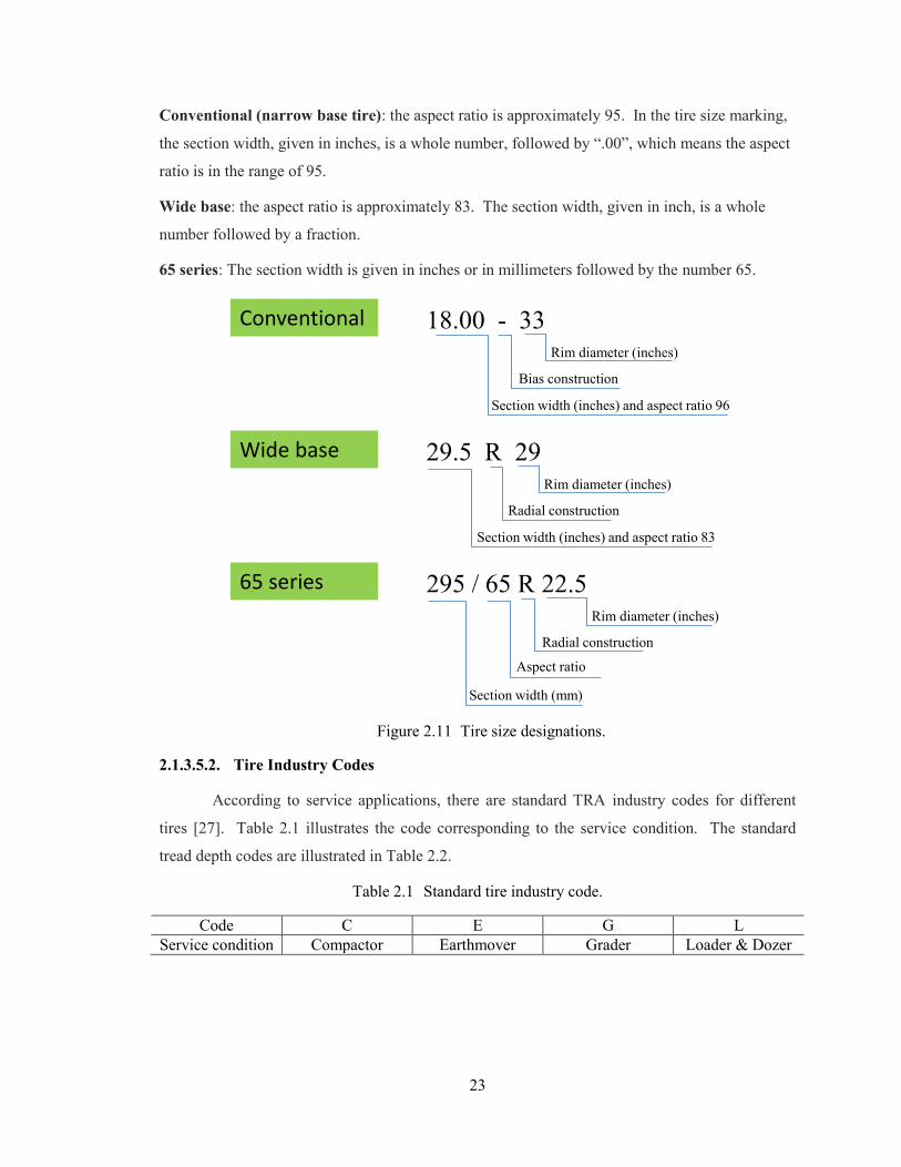
23

Conventional (narrow base tire): the aspect ratio is approximately 95. In the tire size marking,

the section width, given in inches, is a whole number, followed by “.00”, which means the aspect

ratio is in the range of 95.

Wide base: the aspect ratio is approximately 83. The section width, given in inch, is a whole

number followed by a fraction.

65 series: The section width is given in inches or in millimeters followed by the number 65.

2.1.3.5.2. Tire Industry Codes

According to service applications, there are standard TRA industry codes for different

tires [27]. Table 2.1 illustrates the code corresponding to the service condition. The standard

tread depth codes are illustrated in Table 2.2.

Table 2.1 Standard tire industry code.

Code C E G L

Service condition Compactor Earthmover Grader Loader & Dozer

29.5 R 29Rim diameter (inches)

Radial construction

Section width (inches) and aspect ratio 83

18.00 - 33Rim diameter (inches)

Bias construction

Section width (inches) and aspect ratio 96

295 / 65 R 22.5Rim diameter (inches)

Radial construction

Section width (mm)

Aspect ratio

Conventional

Wide base

65 series

Figure 2.11 Tire size designations.

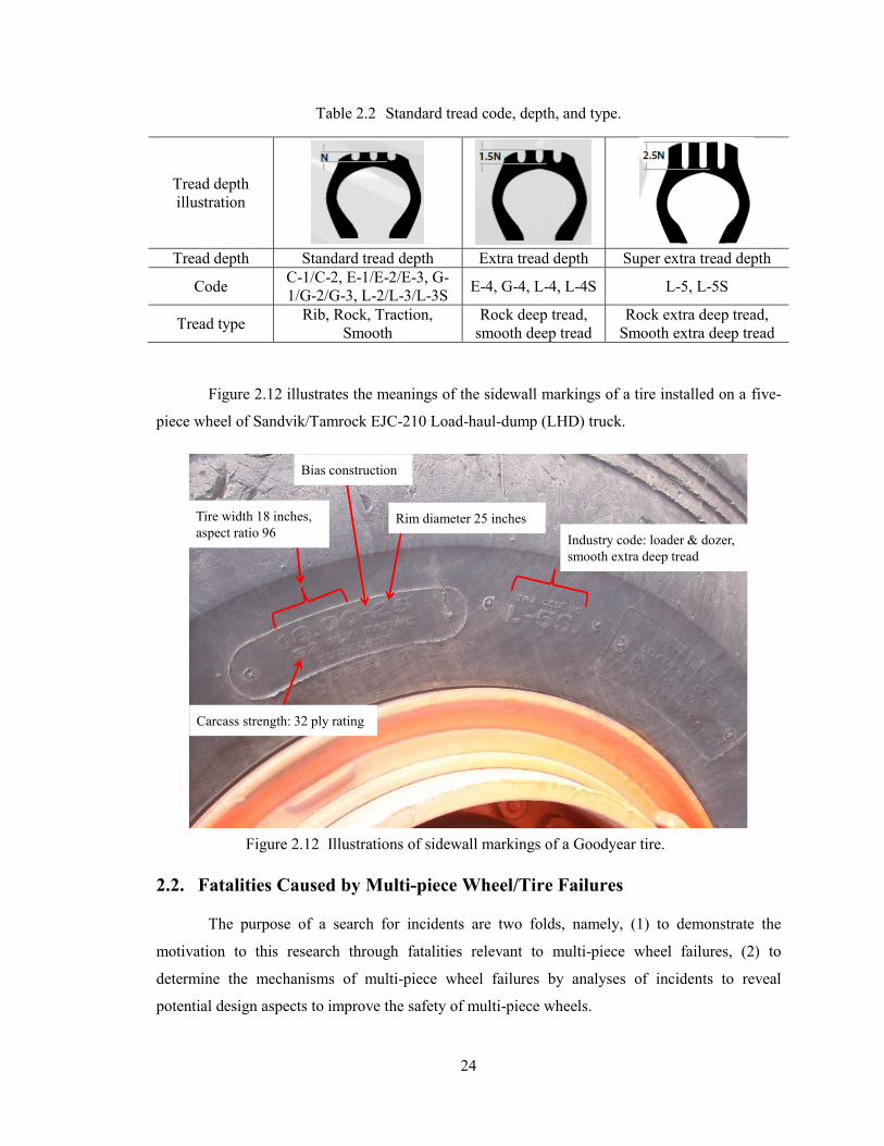
24

Table 2.2 Standard tread code, depth, and type.

Tread depth

illustration

Tread depth Standard tread depth Extra tread depth Super extra tread depth

Code C-1/C-2, E-1/E-2/E-3, G-

1/G-2/G-3, L-2/L-3/L-3S E-4, G-4, L-4, L-4S L-5, L-5S

Tread type Rib, Rock, Traction,

Smooth

Rock deep tread,

smooth deep tread

Rock extra deep tread,

Smooth extra deep tread

Figure 2.12 illustrates the meanings of the sidewall markings of a tire installed on a five-

piece wheel of Sandvik/Tamrock EJC-210 Load-haul-dump (LHD) truck.

2.2. Fatalities Caused by Multi-piece Wheel/Tire Failures

The purpose of a search for incidents are two folds, namely, (1) to demonstrate the

motivation to this research through fatalities relevant to multi-piece wheel failures, (2) to

determine the mechanisms of multi-piece wheel failures by analyses of incidents to reveal

potential design aspects to improve the safety of multi-piece wheels.

Tire width 18 inches,

aspect ratio 96

Bias construction

Rim diameter 25 inches

Carcass strength: 32 ply rating

Industry code: loader & dozer,

smooth extra deep tread

Figure 2.12 Illustrations of sidewall markings of a Goodyear tire.

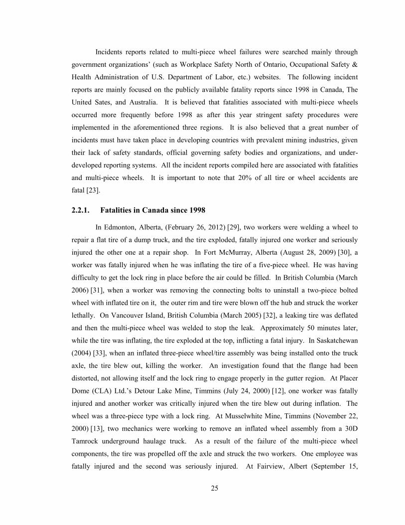
25

Incidents reports related to multi-piece wheel failures were searched mainly through

government organizations’ (such as Workplace Safety North of Ontario, Occupational Safety &

Health Administration of U.S. Department of Labor, etc.) websites. The following incident

reports are mainly focused on the publicly available fatality reports since 1998 in Canada, The

United Sates, and Australia. It is believed that fatalities associated with multi-piece wheels

occurred more frequently before 1998 as after this year stringent safety procedures were

implemented in the aforementioned three regions. It is also believed that a great number of

incidents must have taken place in developing countries with prevalent mining industries, given

their lack of safety standards, official governing safety bodies and organizations, and under-

developed reporting systems. All the incident reports compiled here are associated with fatalities

and multi-piece wheels. It is important to note that 20% of all tire or wheel accidents are

fatal [23].

2.2.1. Fatalities in Canada since 1998

In Edmonton, Alberta, (February 26, 2012) [29], two workers were welding a wheel to

repair a flat tire of a dump truck, and the tire exploded, fatally injured one worker and seriously

injured the other one at a repair shop. In Fort McMurray, Alberta (August 28, 2009) [30], a

worker was fatally injured when he was inflating the tire of a five-piece wheel. He was having

difficulty to get the lock ring in place before the air could be filled. In British Columbia (March

2006) [31], when a worker was removing the connecting bolts to uninstall a two-piece bolted

wheel with inflated tire on it, the outer rim and tire were blown off the hub and struck the worker

lethally. On Vancouver Island, British Columbia (March 2005) [32], a leaking tire was deflated

and then the multi-piece wheel was welded to stop the leak. Approximately 50 minutes later,

while the tire was inflating, the tire exploded at the top, inflicting a fatal injury. In Saskatchewan

(2004) [33], when an inflated three-piece wheel/tire assembly was being installed onto the truck

axle, the tire blew out, killing the worker. An investigation found that the flange had been

distorted, not allowing itself and the lock ring to engage properly in the gutter region. At Placer

Dome (CLA) Ltd.’s Detour Lake Mine, Timmins (July 24, 2000) [12], one worker was fatally

injured and another worker was critically injured when the tire blew out during inflation. The

wheel was a three-piece type with a lock ring. At Musselwhite Mine, Timmins (November 22,

2000) [13], two mechanics were working to remove an inflated wheel assembly from a 30D

Tamrock underground haulage truck. As a result of the failure of the multi-piece wheel

components, the tire was propelled off the axle and struck the two workers. One employee was

fatally injured and the second was seriously injured. At Fairview, Albert (September 15,

26

2000) [34], two tire service technicians were mounting a 60-centimetre-wheel tire onto a grader.

When they started to inflate the tire, the tire blew out and struck both workers. One worker

received minor injuries, and the other 23-year-old worker received head injuries and died the next

day. In Saskatchewan (February 14, 1998) [35], a mechanic was killed while removing the left

rear wheel from a Toro 35D underground haul truck. As the mechanic removed the last nut

holding the wheel assembly onto the axle, the wheel failed and the out bolting flange was

projected away by air pressure, which struck the mechanic in the chest.

2.2.2. Fatalities in the United States since 1998

In Newport News, Virginia (January 17, 2011) [36], when a worker inflated a Modin

Nylon Tube Type N500 tire on a 24-inch multi-piece wheel, the wheel failed and killed the

worker. The tire/wheel assembly was mounted on a 1975 Chevrolet C60 Dump Truck. In Clyde,

Ohio (October 14, 2010) [37], when a 58-year-old male contract auto detailer was cleaning the

wheel assembly of a commercial truck in preparation for the vehicle's eventual sale, the assembly

(known as a multi-piece wheel) exploded, sending sharp metal fragments and other material deep

into the employee's forehead and left arm. The resulting injuries killed him. In Norco, California

(January 18, 2010) [38], a worker was killed when he was inflating a split wheel tire of a

Mitsubishi fork lift. In Hazard, Kentucky (January 23, 2009) [39], a worker was killed when he

was inflating a three-piece wheel tire and the wheel explosively separated and struck him in the

head. In Elk Grove Village, Illinois (August 28, 2009) [40], a truck tire technician was killed

when he was installing a wheel with inflated tire. The wheel exploded and struck him in the head.

In Woodruff, Wisconsin (December 9, 2008) [41], a mechanic was fatally struck when he was

inflating a tire and the tire blew out.

In New York (December 2007) [42], a male equipment operator was fatally injured by a

metal lock ring propelled from a three-piece wheel tire assembly he was inflating. The victim

operated a front-end loader that was a 1985 model with tire size of 17.5-25. After the victim

started his loader, he noticed that the left front tire on his loader was “soft” or under-inflated.

When the worker was inflating the tire, the tire blew out and the lock ring was propelled out and

struck his head and he was fatally injured. The investigation found that the possible reason for

the incident was the dislodged lock ring. The investigation suggested that if the pressure in a

multi-piece wheel tire is reduced to 80% of the recommended operating pressure, the tire

assembly shall be completely deflated, removed from the vehicle, disassembled, inspected and

reassembled prior to inflation. If a tire mounted on multi-piece wheel loses a significant amount

of air, the wheel components that are secured in the rim base under the normal tire air pressure

27

may be offset or dislodged. When the flat tire is inflated, due to the rapid increase of the air

pressure and volume, the dislodged wheel components can be propelled at great distances with

great forces and can cause serious injury or death to anyone in the trajectory area.

In Massachusetts (December 31, 2007) [10], a 59-year-old male mechanic was fatally

injured while changing a container handler’s dual front inner tire that was mounted on a five-

piece wheel. The investigation found there had been a crack in the lock ring groove and severe

wear, rust, and pitting were found on the rim base. The tire should have been completely deflated

prior to demounting and a routine inspection of wheel would have detected the crack. In Marietta,

Georgia (April 19, 2007) [43], a mechanic at a lumber company was performing two tire changes

on a forklift truck that incorporated two-piece wheel assemblies. The wheel blew apart under

pressure and the top portion of the wheel was blown toward the mechanic, fatally striking him in

the face. In Cullman, Alabama (December 13, 2007) [44], a worker was reinstalling a split wheel

tire on a lowboy trailer. He initially placed the tire/wheel assembly onto the lowboy. As he took

the tire/rim assembly off and laid it down, there was an explosion. The failed wheel fatally struck

the worker.

The above mentioned ten fatality incidents occurred from 2007 to 2011. There are another

twenty-eight fatality incidents that occurred from 1998 to 2006, in which one incident [19]

occurred in Alaska in 2006 and the other twenty-seven [45-71] occurred in continental USA.

Totally, there are 38 fatalities involved with multi-piece wheels in the United States during this

period, based on available reports.

2.2.3. Fatalities in Australia since 1998

In Queensland (2005) [72], while removing a tire and wheel assembly from a drive axle

bogey of an off-highway coal transport prime mover, the operator suffered fatal injuries when the

five-piece wheel failed and blew parts of the wheel assembly toward the worker. In Queensland

(February 2004) [73], two workers were changing wheels on a 170-tonne truck when the split

lock ring became dislodged and caused the tire to move uncontrollably, projecting the tire

assembly about 15 meters away. It struck one person who sustained a broken jaw. The second

person, who was pinned under the tire assembly, suffered fatal injuries. The other two incidents

[74, 75] that occurred during this period did not cause death. An incident [74] occurred in 2002

due to tire zipper rupture and another incident [75] was caused by installing the lock ring

backward.

28

2.2.4. Analysis and Summary of the Fatality Incidents

Totally there were forty-nine fatality incidents cited in the previous sections which

occurred from 1998 to 2012; 9 in Canada, 38 in the USA, and 2 in Australia. The majority of the

fatalities were caused by the failure to follow correct procedures of handling multi-piece

wheel/tire assemblies. Multi-piece wheels are high-risk assemblies and need to be treated

accordingly. Many serious and fatal accidents can be attributed to poor removal and fitting

practices, inadequate inspection regimes, and a lack of training for personnel involved in tire and

wheel maintenance tasks.

In 2006, Rasche et al. [76] compiled and analyzed 82 OTR wheel/tire assembly failure

incident reports of earthmover vehicles which occurred in the United States, Canada, and

Australia from 1987 to 2006. It was found that 33% of the cases resulted in the death of the tire

serviceman or personnel involved in the work. A further 50% of all other incidents were

classified as potential fatalities based on their similarity to other fatality cases. The actual and

potential fatalities accounted for 83% of the cases. Using the Incident Cause Analysis Method

(ICAM), the analyses show that the leading cause of the incidents is the LTA (less than adequate)

material testing and fatigue NDT (non-destructive testing). Multi-piece wheels are consumable

items and rigorous, systematic, and reliable wheel component testing and maintenance are

required in order to ensure safe operation. The other main causes of failure include heating of

wheel assembly, LTA matching of assembly components, LTA wheel integrity, and LTA

deflation practice.

Analyses of the forty-nine fatality incidents referenced in the previous sections reveal the

similar causes as Rasche et al. [76] did. Multi-piece wheel/tire assembly failures can be classified

in three failure modes: tire explosion, tire rupture, and tire blow-out [77]. This classification is

helpful to find the direct causes of the multi-piece wheel/tire assembly failures to provide

directions for design improvement of multi-piece wheels.

2.2.4.1. Tire Explosions

Tire explosion is caused by the rapid buildup of tire pressure due to fire inside the tire.

The heat and the flame of the fire weaken the tire’s integrity, resulting in the tire bursting through

the affected sidewall or tread area. Before the tire explodes, the internal pressure is much higher

than the recommended working pressure. A tire explosion is a chemical reaction involving

energy many orders of magnitude greater than that of a tire blow-out or zipper rupture. A shock

wave will create pressures typically in excess of 6894.8 kPa (1,000 psi) during tire explosion [78].

29

Therefore tire explosion is more violent than other two tire failure modes. The explosion can

propel the tire, the wheel components, and the axle components as far as 500 m (1500 feet) or

more from the machine [78]. Both the force of the explosion and the flying objects can cause

property damage, personal injury, or death. A tire explosion may occur when the truck is in

motion or stationary [78]. In the 49 fatality incidents, two incidents [29, 32] were caused by tire

explosion.

In some cases, the buildup of flammable gases results from pyrolysis, the decomposition

of a chemical (the tire rubber) by extreme heat. Pyrolysis can occur if the vehicle's wheel/tire

components have been heated. This can occur after the vehicle comes near or touches a high

voltage power line [79], after a brake has been heated, after the wheel has been heated with a

torch, after a stud has been cut off a wheel or by welding on the wheel [29, 32], and when the

truck is struck by lightning [80]. Under-inflation (pressure is 20% lower than the recommended

pressure) or overload can also cause pyrolysis since tire extreme deformation and wear between

wheel components may cause heat buildup and accelerate the decomposing of the tire rubber

under this condition.

2.2.4.2. Tire Zipper Ruptures

Another hazard is the failure of the tire sidewall, either because of weakening during

service under fatigue loading and corrosive environments or from an overpressure [77]. This type

of tire failure is called a "zipper rupture" in steel cord radial tires. The steel wires in the sidewall

of a radial tire may be weakened by corrosion, under inflation, over inflation, overloading, an

operational damage or a result of a manufacturing defect. The blast of air can cause direct

injuries or blow pieces of the tire and wheel assembly towards the worker during inflation of the

tire. A tire zipper rupture usually occurs when a truck is in motion.

In the 49 fatalities, two incidents [52, 53] were caused by tire zipper rupture due to over

inflation by using a faulty pressure gauge or not using a pressure regulator. The tire rupture in

incident [74] was caused by a previous tire tear.

2.2.4.3. Tire Blow-outs

When the tire is not strong enough to hold the high internal pressure, tire failure will

occur in the mode of explosion or zipper rupture. When the metal multi-piece wheel is not strong

enough to hold the internal pressure, or the wheel’s integrity is weakened, the failure is referred to

as tire blow-out. Incorrect assembly, metal fatigue, corrosion, wear, impact damage, over

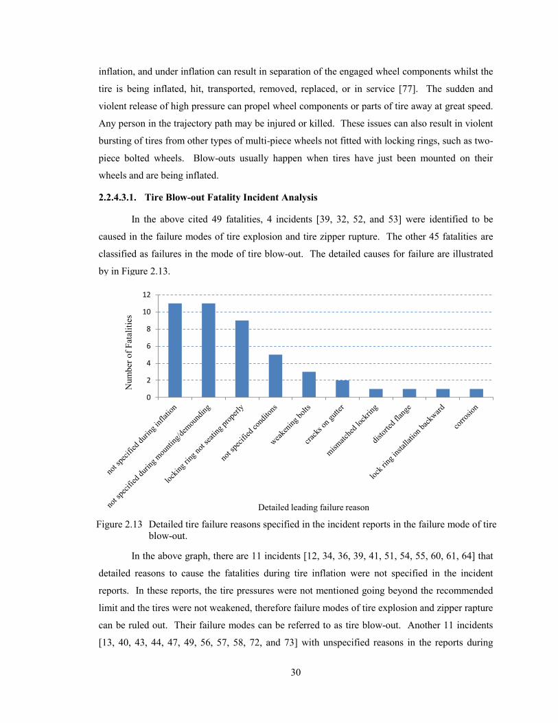
30

inflation, and under inflation can result in separation of the engaged wheel components whilst the

tire is being inflated, hit, transported, removed, replaced, or in service [77]. The sudden and

violent release of high pressure can propel wheel components or parts of tire away at great speed.

Any person in the trajectory path may be injured or killed. These issues can also result in violent

bursting of tires from other types of multi-piece wheels not fitted with locking rings, such as two-

piece bolted wheels. Blow-outs usually happen when tires have just been mounted on their

wheels and are being inflated.

2.2.4.3.1. Tire Blow-out Fatality Incident Analysis

In the above cited 49 fatalities, 4 incidents [39, 32, 52, and 53] were identified to be

caused in the failure modes of tire explosion and tire zipper rupture. The other 45 fatalities are

classified as failures in the mode of tire blow-out. The detailed causes for failure are illustrated

by in Figure 2.13.

In the above graph, there are 11 incidents [12, 34, 36, 39, 41, 51, 54, 55, 60, 61, 64] that

detailed reasons to cause the fatalities during tire inflation were not specified in the incident

reports. In these reports, the tire pressures were not mentioned going beyond the recommended

limit and the tires were not weakened, therefore failure modes of tire explosion and zipper rapture

can be ruled out. Their failure modes can be referred to as tire blow-out. Another 11 incidents

[13, 40, 43, 44, 47, 49, 56, 57, 58, 72, and 73] with unspecified reasons in the reports during

0

2

4

6

8

10

12

Nu

mb

er o

f F

atal

itie

s

Detailed leading failure reason

Figure 2.13 Detailed tire failure reasons specified in the incident reports in the failure mode of tire

blow-out.

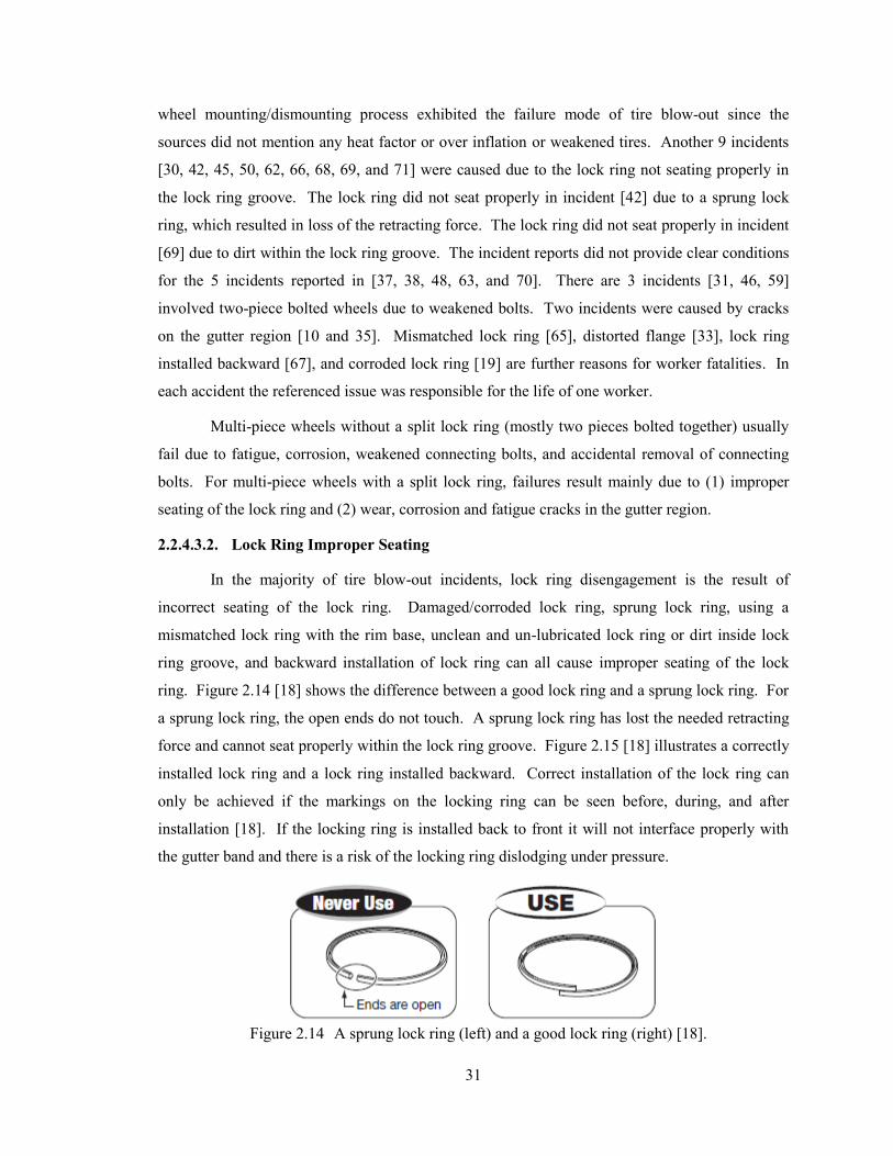
31

wheel mounting/dismounting process exhibited the failure mode of tire blow-out since the

sources did not mention any heat factor or over inflation or weakened tires. Another 9 incidents

[30, 42, 45, 50, 62, 66, 68, 69, and 71] were caused due to the lock ring not seating properly in

the lock ring groove. The lock ring did not seat properly in incident [42] due to a sprung lock

ring, which resulted in loss of the retracting force. The lock ring did not seat properly in incident

[69] due to dirt within the lock ring groove. The incident reports did not provide clear conditions

for the 5 incidents reported in [37, 38, 48, 63, and 70]. There are 3 incidents [31, 46, 59]

involved two-piece bolted wheels due to weakened bolts. Two incidents were caused by cracks

on the gutter region [10 and 35]. Mismatched lock ring [65], distorted flange [33], lock ring

installed backward [67], and corroded lock ring [19] are further reasons for worker fatalities. In

each accident the referenced issue was responsible for the life of one worker.

Multi-piece wheels without a split lock ring (mostly two pieces bolted together) usually

fail due to fatigue, corrosion, weakened connecting bolts, and accidental removal of connecting

bolts. For multi-piece wheels with a split lock ring, failures result mainly due to (1) improper

seating of the lock ring and (2) wear, corrosion and fatigue cracks in the gutter region.

2.2.4.3.2. Lock Ring Improper Seating

In the majority of tire blow-out incidents, lock ring disengagement is the result of

incorrect seating of the lock ring. Damaged/corroded lock ring, sprung lock ring, using a

mismatched lock ring with the rim base, unclean and un-lubricated lock ring or dirt inside lock

ring groove, and backward installation of lock ring can all cause improper seating of the lock

ring. Figure 2.14 [18] shows the difference between a good lock ring and a sprung lock ring. For

a sprung lock ring, the open ends do not touch. A sprung lock ring has lost the needed retracting

force and cannot seat properly within the lock ring groove. Figure 2.15 [18] illustrates a correctly

installed lock ring and a lock ring installed backward. Correct installation of the lock ring can

only be achieved if the markings on the locking ring can be seen before, during, and after

installation [18]. If the locking ring is installed back to front it will not interface properly with

the gutter band and there is a risk of the locking ring dislodging under pressure.

Figure 2.14 A sprung lock ring (left) and a good lock ring (right) [18].

32

2.2.4.3.3. Wear, Corrosion, and Fatigue Cracks in the Gutter Region

Corrosion, wear, and fatigue are other factors responsible for the deteriorating of the

integrity of wheel components, especially the gutter region, where the lock ring groove is located,

as shown in Figure 2.16 [5]. Under high internal pressure and high load, stress concentration can

be easily generated in the small region of lock ring groove on the rim, inducing fatigue cracks in

the gutter region. When fatigue crack propagation occurs, the engagement of the wheel

components can suddenly break down, resulting in separation of wheel components under great

speed. Additionally, the sliding and galling of the lock ring can wear away material in the lock

ring groove. Loss of material in the groove can impair the engagement of wheel components and

accelerate the initiation and propagation of cracks. Harsh working conditions in the mine sites

with corrosive environments have synergistic effects on accelerating material wear and crack

related failures.

Markings

are visible

Markings are

not visible

Figure 2.15 Correct installation (left) and lock ring installed backward (right) [18].

Figure 2.16 Wear and Fatigue cracks in the gutter region [5].

33

2.2.4.4. Tire Failures for on-the-road Tires

Tire explosion and zipper rupture occur for on-the-road tires used on passenger vehicles

and haulage trucks too. Due to the lower tire pressure, smaller tire size, and favorable service

conditions, the energy released by on-the-road tires when explosion or rupture happens is much

lower, compared to the OTR tires. Tire blow-out is very common for OTR tires and very rare for

on-the-road tires since a single-piece wheel is used.

Tire explosion and zipper rupture are initiated from the tires. Tire blow-out starts with

multi-piece wheel components. The above incident report analysis shows that over 90% of the

fatalities occurred in the mode of tire blow-out. Tire blow-outs are actually caused due to the

multi-piece wheel design. This research is focused on improving the design of multi-piece

wheels to minimize or completely remove the occurrence of tire blow-out.

2.2.5. Working with Multi-piece Wheel and OTR Tire

Wheel dimensions are standardized by the Tire and Rim Association [27] for size and

contour only, and particular tire and wheel combinations are designated to ensure proper

mounting and fit of the tire. The load and cold inflation pressure imposed on the wheel must not

exceed the wheel manufacturers' recommendations even though the tire may be approved for a

higher load or inflation.

Wheels and tires represent one of the major direct expenses in OTR equipment

operations [24]. They are consumable items and regular maintenance will not only help them last

longer, but will also reduce the incident rates. For underground mines, the rule of thumb for

wheel life before recertification/intensive inspection is 1 year or 3,000 service hours; and 8,000

service hours for wheels used above ground. Tires used above ground last typically for one year,

and tires used underground last for 3 to 8 months.

Over-inflation can reduce tire’s service time. Under-inflation is more detrimental.

Under-inflation can lead to irregular or uneven tread wear, sidewall radial cracks, ply separation,

loose or broken cords inside the tire, fabric carcass fatigue, and belt edge separation. Low

pressure can accelerate the wear of the wheel component and reduce service time. Most severely,

tires with less than optimum air pressure are very dangerous. Under-inflation may damage the

engagement among wheel components, causing tire blow-outs. Tires with less than 80% working

pressure should be safely deflated and serviced [23]. Checking tire pressure regularly is an

34

important precaution for safety operations. In some mine sites, tire pressure is checked every

shift.

Since the 1950’s, the OTR wheel assemblies (rim and tire, geometry and structure) has not

changed, but the payloads and travel speeds of the OTR vehicles have increased tremendously.

For example, the 26.5×25 tire was previously in LHD trucks with a capacity of 7 yard3 (5.35 m

3),

however such a tire is now used in 9 yard3 (6.88 m

3) truck at higher travel speeds and rougher

conditions. The mass density of the ore also has a great effect on load (with nickel and gold ores

being heavier). In order to catch up with the load increase, the tire pressure has increased from

344.7 to 689.5 kPa (50 psi to 100 psi). The increased pressure accelerates the failure of multi-

piece wheel/tire assembly and is dangerous to human life.

Given the criticality of correct fitment, severe loading and working environment, and the

much higher inflation pressures, working with OTR wheel assemblies carries much higher risks

than working with on-the-road tires where risks have largely been mitigated due to lower

individual wheel loads and smooth road conditions. The hazardous characteristics and incident

preventions require strict controls at the management and operational level, and by the individuals

carrying out the task.

2.3. Fatigue Life Analysis Theory

Most failures in machinery are due to time-varying loads [84]. These failures typically

occur at stress levels significantly lower than the yield strengths of the materials. This kind of

failure is termed “fatigue failure”. Fatigue is defined as the progressive and localized structural

damage that occurs when a material is subjected to cyclic loading [84]. The fatigue failure

phenomenon was first noticed in the 1800s when railroad-car axles began failing after only

limited service in Europe. The axles were made of ductile steel but exhibited sudden, brittle-like

failures due to fatigue. Research within the area of fatigue failure is less than two hundred years

old and research efforts continue.

2.3.1. Mechanism of Fatigue Failure

Fatigue failures always begin at a crack [85]. Fischer and Yen [86] have shown that

virtually all structural members contain discontinuities, ranging from microscopic (<0.25 mm) to

macroscopic, introduced in the manufacturing or fabricating process. There are three stages of

fatigue failure, namely, crack initiation, crack propagation, and sudden fracture due to unstable

35

crack growth. The first stage can be of short duration, the second stage involves most of the life

of the part, and the third stage is instantaneous.

2.3.1.1. Crack Initiation Stage

At a microscopic scale, all metals are heterogeneous and anisotropic [86]. Metals are

composed of groups of small crystal grains. For each grain, its behavior is anisotropic due to the

crystal planes and if a grain boundary is crossed, the orientation of these planes changes.

Inhomogeneities also exist due to the presence of tiny voids or particles of a different chemical

composition than the bulk of the material, such as hard silicate or alumina inclusions in steel [86].

Stress concentrations may cause local yielding, even though the nominal stress in the section is

well below the yield strength of the material. The localized yielding causes distortion and creates

slip bands (regions of intense deformation due to shear deformation) along the crystal boundaries.

When more slip bands occur due to cyclic loading, the slip bands coalesce into microscopic

cracks. Pre-existing voids or inclusions will serve as stress raisers to initiate the crack.

It is almost universally agreed that fatigue failures start at the surface of a specimen or

component [87]. This is true whether the test is carried out in a rotating-beam machine where the

maximum stress is always at the surface, or in a push-pull machine which gives a simple tensile-

compressive stress cycle. The mechanism of surface crack initiation can be accounted for in the

following three aspects.

Firstly, all structures experience some degree of bending under cyclic loading, even in

uniaxial loading conditions, due to imperfect geometries of the structures and inexact uniaxial

loading. This creates uneven stress distributions in the structures, with the maximum at the

surface of the structures. Secondly, all structure surfaces have, to some extent, defects, including

dents, pitting, scratches, wear, corrosion, and surface roughness caused in the machining

processes. These defects act as stress-raisers to cause local yielding under maximum tensile

stresses at the surface. Finally, compared to the material inside the structure, the material at the

surface only has half side of materials to resist deformation under loading, allowing for

deformation to happen at the surface with more ease at lower stress levels.

It is very important to understand the surface crack initiation mechanism in FE modeling

of fatigue structures. To accurately predict the surface stresses, shell elements have to be used on

the surfaces of structures since solid elements cannot accurately capture the stress levels on the

surfaces.

36

2.3.1.2. Crack Propagation Stage

In the beginning of micro-crack propagation, micro-cracks move along shear planes thus

having a tendency to form an angle of 45 degree to the surfaces [86]. During this stage, the

micro-cracks can enlarge freely until micro-structural barriers stop them. The micro-structural

barriers include grain boundaries and other hard material faces. If the micro-cracks do not have

enough energy (at low stress levels) to overcome the barriers, the micro-cracks will stop

propagation. Knowledge of micro-cracks propagation can be used to prolong this stage by

introducing compressive residual stresses through several types of treatments of structures,

namely, thermal treatments, surface treatments (shot peening and cold forming), and mechanical

prestressing.

Once a micro-crack is established, the prolonged crack creates stress concentrations at the

front tip. The crack begins to propagate in the direction perpendicular to the applied stress. Each

time a tensile stress opens the crack, the crack grows a small amount. When the stress cycles to a

compressive-stress regime, or to zero, or to a sufficiently lower tensile stress, the crack closes.

Crack growth is due to tensile stress and the crack grows along planes normal to the maximum

tensile stress. Therefore, fatigue failure is considered to be due to the tensile stress, even though

shear stress initializes the crack in ductile materials. Cyclic stresses that are always compressive

will not cause crack growth, as they tend to close the crack. The crack propagation growth rate is

very small, but this adds up over a large number of cycles.

If a part containing a crack is in a corrosive environment, the crack will grow under static

stress. The combination of stress and corrosive environment has a synergistic effect and the

material corrodes more rapidly than if unstressed. If the part is cyclically stressed in a corrosive

environment, the crack will grow more rapidly than from either factor alone. This is called

corrosion fatigue. While the frequency of stress cycling appears to have no detrimental effect on

crack growth in a noncorrosive environment, it does in corrosive environments. Lower cyclic

frequencies allow the environment more time to act on the stressed crack tip while it is held open

under tensile stress, and this substantially increases the rate of the crack growth per cycle.

2.3.1.3. Fracture

The crack will continue to grow as long as the cyclical tensile stress and/or corrosion

factors of sufficient severity are present. At some point, the crack size becomes large enough that

the amount of undamaged material is insufficient to carry the maximum load, and an abrupt,

brittle failure occurs.

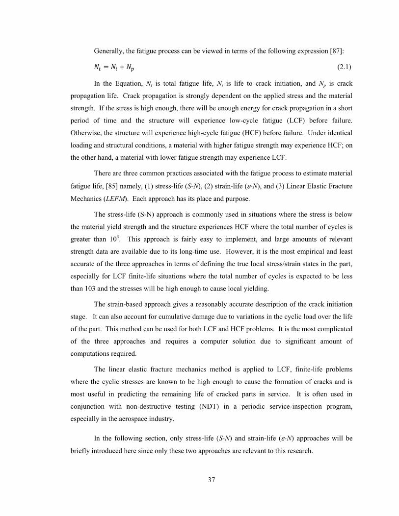
37

Generally, the fatigue process can be viewed in terms of the following expression [87]:

(2.1)

In the Equation, Nt is total fatigue life, Ni is life to crack initiation, and Np is crack

propagation life. Crack propagation is strongly dependent on the applied stress and the material

strength. If the stress is high enough, there will be enough energy for crack propagation in a short

period of time and the structure will experience low-cycle fatigue (LCF) before failure.

Otherwise, the structure will experience high-cycle fatigue (HCF) before failure. Under identical

loading and structural conditions, a material with higher fatigue strength may experience HCF; on

the other hand, a material with lower fatigue strength may experience LCF.

There are three common practices associated with the fatigue process to estimate material

fatigue life, [85] namely, (1) stress-life (S-N), (2) strain-life (-N), and (3) Linear Elastic Fracture

Mechanics (LEFM). Each approach has its place and purpose.

The stress-life (S-N) approach is commonly used in situations where the stress is below

the material yield strength and the structure experiences HCF where the total number of cycles is

greater than 103. This approach is fairly easy to implement, and large amounts of relevant

strength data are available due to its long-time use. However, it is the most empirical and least

accurate of the three approaches in terms of defining the true local stress/strain states in the part,

especially for LCF finite-life situations where the total number of cycles is expected to be less

than 103 and the stresses will be high enough to cause local yielding.

The strain-based approach gives a reasonably accurate description of the crack initiation

stage. It can also account for cumulative damage due to variations in the cyclic load over the life

of the part. This method can be used for both LCF and HCF problems. It is the most complicated

of the three approaches and requires a computer solution due to significant amount of

computations required.

The linear elastic fracture mechanics method is applied to LCF, finite-life problems

where the cyclic stresses are known to be high enough to cause the formation of cracks and is

most useful in predicting the remaining life of cracked parts in service. It is often used in

conjunction with non-destructive testing (NDT) in a periodic service-inspection program,

especially in the aerospace industry.

In the following section, only stress-life (S-N) and strain-life (-N) approaches will be

briefly introduced here since only these two approaches are relevant to this research.

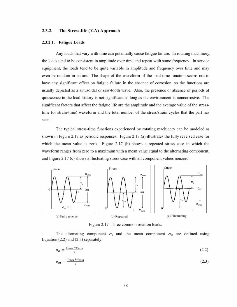
38

2.3.2. The Stress-life (S-N) Approach

2.3.2.1. Fatigue Loads

Any loads that vary with time can potentially cause fatigue failure. In rotating machinery,

the loads tend to be consistent in amplitude over time and repeat with some frequency. In service

equipment, the loads tend to be quite variable in amplitude and frequency over time and may

even be random in nature. The shape of the waveform of the load-time function seems not to

have any significant effect on fatigue failure in the absence of corrosion, so the functions are

usually depicted as a sinusoidal or saw-tooth wave. Also, the presence or absence of periods of

quiescence in the load history is not significant as long as the environment is noncorrosive. The

significant factors that affect the fatigue life are the amplitude and the average value of the stress-

time (or strain-time) waveform and the total number of the stress/strain cycles that the part has

seen.

The typical stress-time functions experienced by rotating machinery can be modeled as

shown in Figure 2.17 as periodic responses. Figure 2.17 (a) illustrates the fully reversed case for

which the mean value is zero. Figure 2.17 (b) shows a repeated stress case in which the

waveform ranges from zero to a maximum with a mean value equal to the alternating component,

and Figure 2.17 (c) shows a fluctuating stress case with all component values nonzero.

The alternating component a and the mean component m are defined using

Equation (2.2) and (2.3) separately.

(2.2)

(2.3)

-1.5

-1

-0.5

0

0.5

1

1.5

0 5E-09 1E-08 1.5E-08

Stress

t

0

0.5

1

1.5

2

2.5

0 5E-09 1E-08 1.5E-08

Stress

t0

0.5

1

1.5

2

2.5

3

0 5E-09 1E-08 1.5E-08

Stress

t

0

0 0

a

max

minim = 0

(a) Fully reverse

a

max

mini

m

(b) Repeated

a

max

mini

m

(c) Fluctuating

Figure 2.17 Three common rotation loads.

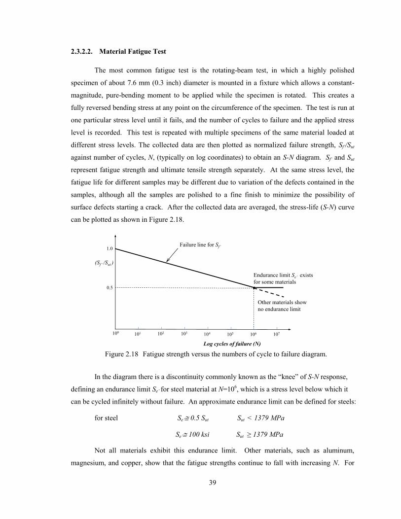
39

2.3.2.2. Material Fatigue Test

The most common fatigue test is the rotating-beam test, in which a highly polished

specimen of about 7.6 mm (0.3 inch) diameter is mounted in a fixture which allows a constant-

magnitude, pure-bending moment to be applied while the specimen is rotated. This creates a

fully reversed bending stress at any point on the circumference of the specimen. The test is run at

one particular stress level until it fails, and the number of cycles to failure and the applied stress

level is recorded. This test is repeated with multiple specimens of the same material loaded at

different stress levels. The collected data are then plotted as normalized failure strength, Sf’/Sut

against number of cycles, N, (typically on log coordinates) to obtain an S-N diagram. Sf’ and Sut

represent fatigue strength and ultimate tensile strength separately. At the same stress level, the

fatigue life for different samples may be different due to variation of the defects contained in the

samples, although all the samples are polished to a fine finish to minimize the possibility of

surface defects starting a crack. After the collected data are averaged, the stress-life (S-N) curve

can be plotted as shown in Figure 2.18.

In the diagram there is a discontinuity commonly known as the “knee” of S-N response,

defining an endurance limit Se’ for steel material at N=106, which is a stress level below which it

can be cycled infinitely without failure. An approximate endurance limit can be defined for steels:

for steel Se’ 0.5 Sut Sut < 1379 MPa

Se’ 100 ksi Sut ≥ 1379 MPa

Not all materials exhibit this endurance limit. Other materials, such as aluminum,

magnesium, and copper, show that the fatigue strengths continue to fall with increasing N. For

100 102 103 104 105 106 107101

0.5

1.0

(Sf ’ /Sut )

Log cycles of failure (N)

Endurance limit Se’ exists

for some materials

Failure line for Sf ’

Other materials show

no endurance limit

Figure 2.18 Fatigue strength versus the numbers of cycle to failure diagram.

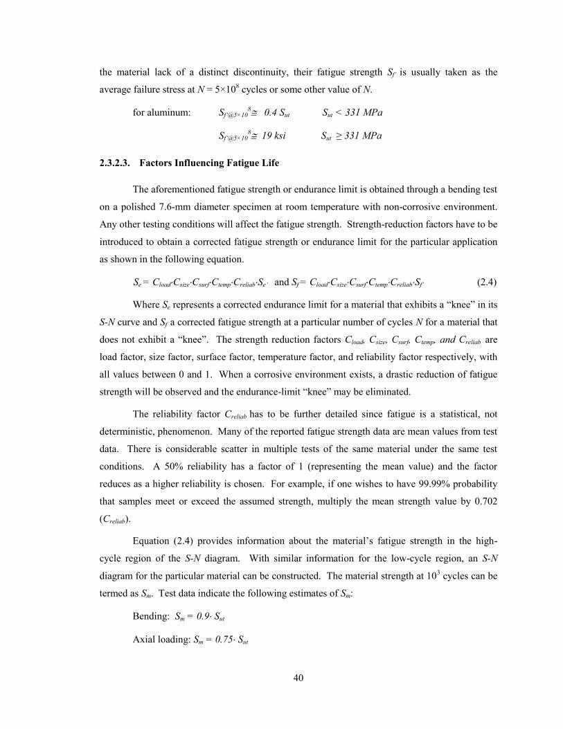
40

the material lack of a distinct discontinuity, their fatigue strength Sf’ is usually taken as the

average failure stress at N = 5×108 cycles or some other value of N.

for aluminum: Sf’@5×108 0.4 Sut Sut < 331 MPa

Sf’@5×108 19 ksi Sut ≥ 331 MPa

2.3.2.3. Factors Influencing Fatigue Life

The aforementioned fatigue strength or endurance limit is obtained through a bending test

on a polished 7.6-mm diameter specimen at room temperature with non-corrosive environment.

Any other testing conditions will affect the fatigue strength. Strength-reduction factors have to be

introduced to obtain a corrected fatigue strength or endurance limit for the particular application

as shown in the following equation.

Se = CloadCsizeCsurfCtempCreliabSe’ and Sf = CloadCsizeCsurfCtempCreliabSf’ (2.4)

Where Se represents a corrected endurance limit for a material that exhibits a “knee” in its

S-N curve and Sf a corrected fatigue strength at a particular number of cycles N for a material that

does not exhibit a “knee”. The strength reduction factors Cload, Csize, Csurf, Ctemp, and Creliab are

load factor, size factor, surface factor, temperature factor, and reliability factor respectively, with

all values between 0 and 1. When a corrosive environment exists, a drastic reduction of fatigue

strength will be observed and the endurance-limit “knee” may be eliminated.

The reliability factor Creliab has to be further detailed since fatigue is a statistical, not

deterministic, phenomenon. Many of the reported fatigue strength data are mean values from test

data. There is considerable scatter in multiple tests of the same material under the same test

conditions. A 50% reliability has a factor of 1 (representing the mean value) and the factor

reduces as a higher reliability is chosen. For example, if one wishes to have 99.99% probability

that samples meet or exceed the assumed strength, multiply the mean strength value by 0.702

(Creliab).

Equation (2.4) provides information about the material’s fatigue strength in the high-

cycle region of the S-N diagram. With similar information for the low-cycle region, an S-N

diagram for the particular material can be constructed. The material strength at 103 cycles can be

termed as Sm. Test data indicate the following estimates of Sm:

Bending: Sm = 0.9 Sut

Axial loading: Sm = 0.75 Sut

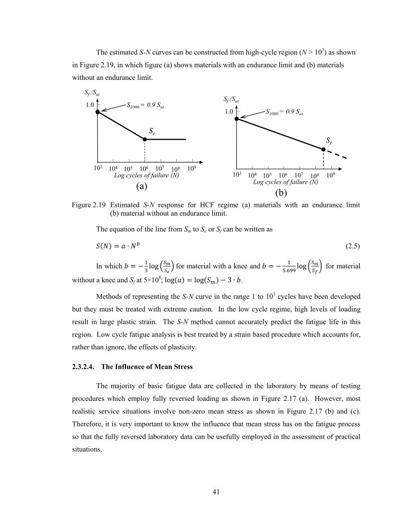
41

The estimated S-N curves can be constructed from high-cycle region (N > 103) as shown

in Figure 2.19, in which figure (a) shows materials with an endurance limit and (b) materials

without an endurance limit.

The equation of the line from Sm to Se or Sf can be written as

( ) (2.5)

In which

(

) for material with a knee and

(

) for material

without a knee and Sf at 5×108; ( ) ( ) .

Methods of representing the S-N curve in the range 1 to 103 cycles have been developed

but they must be treated with extreme caution. In the low cycle regime, high levels of loading

result in large plastic strain. The S-N method cannot accurately predict the fatigue life in this

region. Low cycle fatigue analysis is best treated by a strain based procedure which accounts for,

rather than ignore, the effects of plasticity.

2.3.2.4. The Influence of Mean Stress

The majority of basic fatigue data are collected in the laboratory by means of testing

procedures which employ fully reversed loading as shown in Figure 2.17 (a). However, most

realistic service situations involve non-zero mean stress as shown in Figure 2.17 (b) and (c).

Therefore, it is very important to know the influence that mean stress has on the fatigue process

so that the fully reversed laboratory data can be usefully employed in the assessment of practical

situations.

105

Sf

103 107 109108

1.0

Sf /Sut

Log cycles of failure (N)

S1000 = 0.9 Sut

Se

(a)

104 106

105103 107 109108

1.0

Sf /Sut

Log cycles of failure (N)

S1000 = 0.9 Sut

(b)

104 106

Figure 2.19 Estimated S-N response for HCF regime (a) materials with an endurance limit

(b) material without an endurance limit.

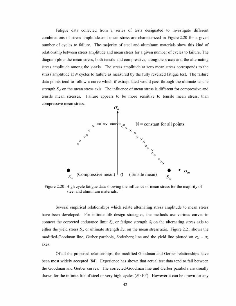
42

Fatigue data collected from a series of tests designated to investigate different

combinations of stress amplitude and mean stress are characterized in Figure 2.20 for a given

number of cycles to failure. The majority of steel and aluminum materials show this kind of

relationship between stress amplitude and mean stress for a given number of cycles to failure. The

diagram plots the mean stress, both tensile and compressive, along the x-axis and the alternating

stress amplitude among the y-axis. The stress amplitude at zero mean stress corresponds to the

stress amplitude at N cycles to failure as measured by the fully reversed fatigue test. The failure

data points tend to follow a curve which if extrapolated would pass through the ultimate tensile

strength Sut on the mean stress axis. The influence of mean stress is different for compressive and

tensile mean stresses. Failure appears to be more sensitive to tensile mean stress, than

compressive mean stress.

Several empirical relationships which relate alternating stress amplitude to mean stress

have been developed. For infinite life design strategies, the methods use various curves to

connect the corrected endurance limit Se, or fatigue strength Sf on the alternating stress axis to

either the yield stress Sy, or ultimate strength Sut, on the mean stress axis. Figure 2.21 shows the

modified-Goodman line, Gerber parabola, Soderberg line and the yield line plotted on m – a

axes.

Of all the proposed relationships, the modified-Goodman and Gerber relationships have

been most widely accepted [84]. Experience has shown that actual test data tend to fail between

the Goodman and Gerber curves. The corrected-Goodman line and Gerber parabola are usually

drawn for the infinite-life of steel or very high-cycles (N>106). However it can be drawn for any

Sut- Sut

m

a

0 (Tensile mean)(Compressive mean)

N = constant for all points

Figure 2.20 High cycle fatigue data showing the influence of mean stress for the majority of

steel and aluminum materials.

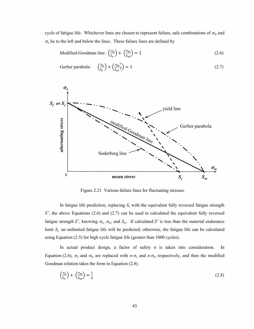
43

cycle of fatigue life. Whichever lines are chosen to represent failure, safe combinations of m and

a lie to the left and below the lines. These failure lines are defined by

Modified-Goodman line: (

) (

) (2.6)

Gerber parabola: (

) (

) (2.7)

In fatigue life prediction, replacing Se with the equivalent fully reversed fatigue strength

, the above Equations (2.6) and (2.7) can be used to calculated the equivalent fully reversed

fatigue strength , knowing a, m, and Sut. If calculated is less than the material endurance

limit Se, an unlimited fatigue life will be predicted; otherwise, the fatigue life can be calculated

using Equation (2.5) for high cycle fatigue life (greater than 1000 cycles).

In actual product design, a factor of safety n is taken into consideration. In

Equation (2.6), a and m are replaced with na and nm respectively, and then the modified

Goodman relation takes the form in Equation (2.8).

(

) (

)

(2.8)

0

Sf or Se

mean stress

yield line

Soderberg line

Gerber parabola

alt

ern

ati

ng s

tres

s

Sy Sut

m

a

Figure 2.21 Various failure lines for fluctuating stresses.

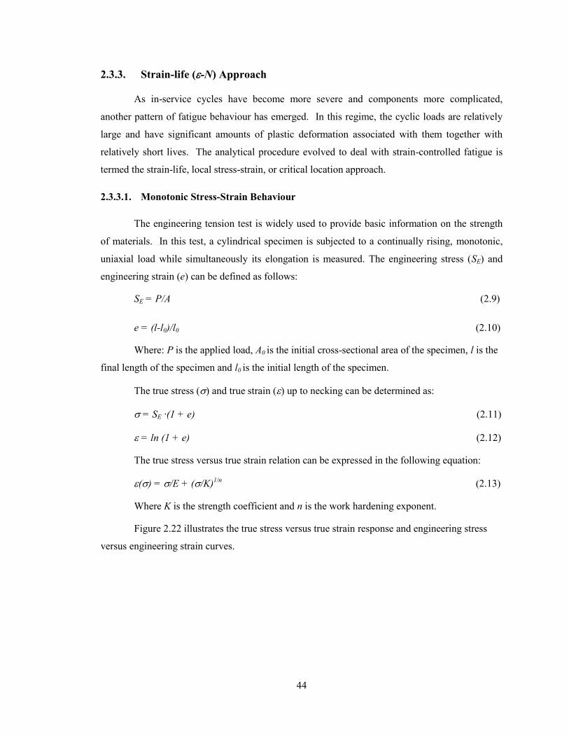
44

2.3.3. Strain-life (-N) Approach

As in-service cycles have become more severe and components more complicated,

another pattern of fatigue behaviour has emerged. In this regime, the cyclic loads are relatively

large and have significant amounts of plastic deformation associated with them together with

relatively short lives. The analytical procedure evolved to deal with strain-controlled fatigue is

termed the strain-life, local stress-strain, or critical location approach.

2.3.3.1. Monotonic Stress-Strain Behaviour

The engineering tension test is widely used to provide basic information on the strength

of materials. In this test, a cylindrical specimen is subjected to a continually rising, monotonic,

uniaxial load while simultaneously its elongation is measured. The engineering stress (SE) and

engineering strain (e) can be defined as follows:

SE = P/A (2.9)

e = (l-l0)/l0 (2.10)

Where: P is the applied load, A0 is the initial cross-sectional area of the specimen, l is the

final length of the specimen and l0 is the initial length of the specimen.

The true stress () and true strain () up to necking can be determined as:

= SE ∙(1 + e) (2.11)

= ln (1 + e) (2.12)

The true stress versus true strain relation can be expressed in the following equation:

() = /E + (/K)1/n

(2.13)

Where K is the strength coefficient and n is the work hardening exponent.

Figure 2.22 illustrates the true stress versus true strain response and engineering stress

versus engineering strain curves.

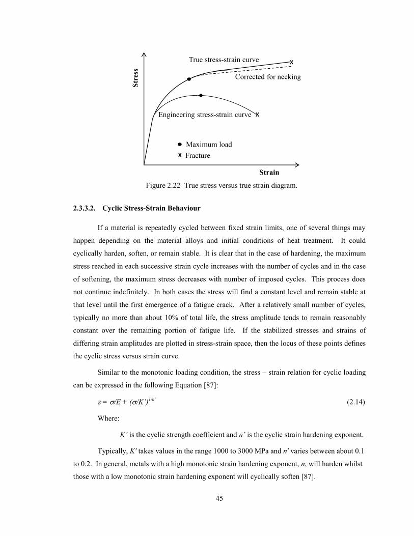
45

2.3.3.2. Cyclic Stress-Strain Behaviour

If a material is repeatedly cycled between fixed strain limits, one of several things may

happen depending on the material alloys and initial conditions of heat treatment. It could

cyclically harden, soften, or remain stable. It is clear that in the case of hardening, the maximum

stress reached in each successive strain cycle increases with the number of cycles and in the case

of softening, the maximum stress decreases with number of imposed cycles. This process does

not continue indefinitely. In both cases the stress will find a constant level and remain stable at

that level until the first emergence of a fatigue crack. After a relatively small number of cycles,

typically no more than about 10% of total life, the stress amplitude tends to remain reasonably

constant over the remaining portion of fatigue life. If the stabilized stresses and strains of

differing strain amplitudes are plotted in stress-strain space, then the locus of these points defines

the cyclic stress versus strain curve.

Similar to the monotonic loading condition, the stress – strain relation for cyclic loading

can be expressed in the following Equation [87]:

= /E + (/K’)1/n’

(2.14)

Where:

K’ is the cyclic strength coefficient and n’ is the cyclic strain hardening exponent.

Typically, K' takes values in the range 1000 to 3000 MPa and n' varies between about 0.1

to 0.2. In general, metals with a high monotonic strain hardening exponent, n, will harden whilst

those with a low monotonic strain hardening exponent will cyclically soften [87].

True stress-strain curve

X

X

X

Maximum load

Fracture

Engineering stress-strain curve

Corrected for necking

Str

ess

Strain

Figure 2.22 True stress versus true strain diagram.

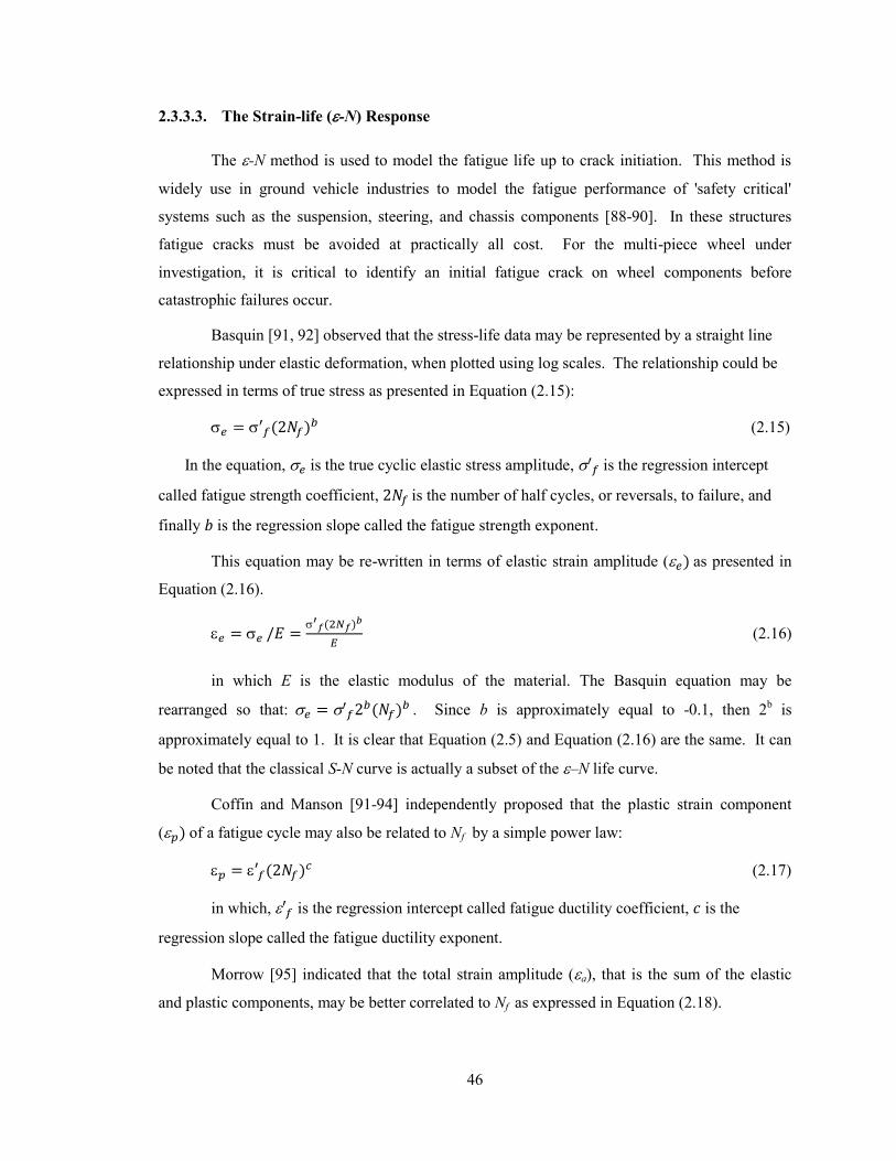
46

2.3.3.3. The Strain-life (-N) Response

The -N method is used to model the fatigue life up to crack initiation. This method is

widely use in ground vehicle industries to model the fatigue performance of 'safety critical'

systems such as the suspension, steering, and chassis components [88-90]. In these structures

fatigue cracks must be avoided at practically all cost. For the multi-piece wheel under

investigation, it is critical to identify an initial fatigue crack on wheel components before

catastrophic failures occur.

Basquin [91, 92] observed that the stress-life data may be represented by a straight line

relationship under elastic deformation, when plotted using log scales. The relationship could be

expressed in terms of true stress as presented in Equation (2.15):

( )

(2.15)

In the equation, is the true cyclic elastic stress amplitude, is the regression intercept

called fatigue strength coefficient, is the number of half cycles, or reversals, to failure, and

finally is the regression slope called the fatigue strength exponent.

This equation may be re-written in terms of elastic strain amplitude ( ) as presented in

Equation (2.16).

( )

(2.16)

in which E is the elastic modulus of the material. The Basquin equation may be

rearranged so that:

( ) . Since b is approximately equal to -0.1, then 2

b is

approximately equal to 1. It is clear that Equation (2.5) and Equation (2.16) are the same. It can

be noted that the classical S-N curve is actually a subset of the –N life curve.

Coffin and Manson [91-94] independently proposed that the plastic strain component

( ) of a fatigue cycle may also be related to Nf by a simple power law:

( ) (2.17)

in which, is the regression intercept called fatigue ductility coefficient, is the

regression slope called the fatigue ductility exponent.

Morrow [95] indicated that the total strain amplitude (a), that is the sum of the elastic

and plastic components, may be better correlated to Nf as expressed in Equation (2.18).

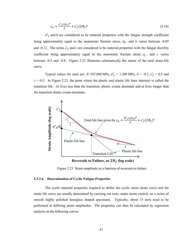
47

( )

( )

(2.18)

and are considered to be material properties with the fatigue strength coefficient

being approximately equal to the monotonic fracture stress, , and b varies between -0.05

and -0.12. The terms and are considered to be material properties with the fatigue ductility

coefficient being approximately equal to the monotonic fracture strain , and c varies

between -0.5 and -0.8. Figure 2.23 illustrates schematically the nature of the total strain-life

curve.

Typical values for steel are: E=207,000 MPa, = 1,300 MPa, b = -0.1, = 0.5 and

c = -0.5. In Figure 2.23, the point where the plastic and elastic life lines intersect is called the

transition life. At lives less than the transition, plastic events dominate and at lives longer than

the transition elastic events dominate.

2.3.3.4. Determination of Cyclic Fatigue Properties

The cyclic material properties required to define the cyclic stress strain curve and the

strain life curve are usually determined by carrying out tests, under strain control, on a series of

smooth highly polished hourglass shaped specimens. Typically, about 15 tests need to be

performed at differing strain amplitudes. The properties can then be calculated by regression

analysis on the following curves:

Plastic life line

/E

Str

ain

Am

pli

tud

e (l

og s

cale

)

Reversals to Failure, or (log scale)

1

1

b

c

Elastic life line

Total life line given by

Transition Life

Figure 2.23 Strain amplitude as a function of reversals to failure.

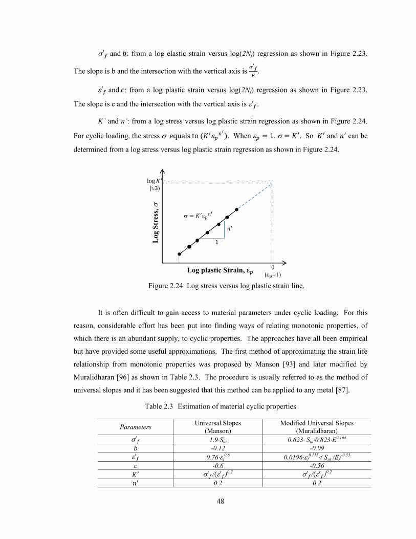
48

and : from a log elastic strain versus log(2Nf) regression as shown in Figure 2.23.

The slope is b and the intersection with the vertical axis is

and : from a log plastic strain versus log(2Nf) regression as shown in Figure 2.23.

The slope is c and the intersection with the vertical axis is .

K’ and n’: from a log stress versus log plastic strain regression as shown in Figure 2.24.

For cyclic loading, the stress (

). When , . So and can be

determined from a log stress versus log plastic strain regression as shown in Figure 2.24.

It is often difficult to gain access to material parameters under cyclic loading. For this

reason, considerable effort has been put into finding ways of relating monotonic properties, of

which there is an abundant supply, to cyclic properties. The approaches have all been empirical

but have provided some useful approximations. The first method of approximating the strain life

relationship from monotonic properties was proposed by Manson [93] and later modified by

Muralidharan [96] as shown in Table 2.3. The procedure is usually referred to as the method of

universal slopes and it has been suggested that this method can be applied to any metal [87].

Table 2.3 Estimation of material cyclic properties

Parameters Universal Slopes

(Manson)

Modified Universal Slopes

(Muralidharan)

1.9Sut 0.623 Sut0.823E0.168

-0.12 -0.09

0.76f0.6

0.0196f0.115( Sut /E)

-0.53

-0.6 -0.56

/( )

0.2

/( )0.2

0.2 0.2

Log S

tres

s,

Log plastic Strain,

1

0

( =1)

(3)

Figure 2.24 Log stress versus log plastic strain line.

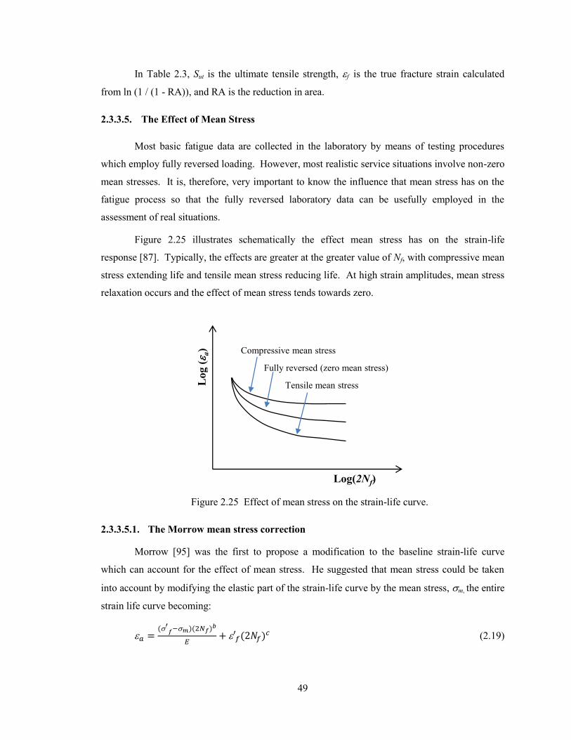
49

In Table 2.3, Sut is the ultimate tensile strength, f is the true fracture strain calculated

from ln (1 / (1 - RA)), and RA is the reduction in area.

2.3.3.5. The Effect of Mean Stress

Most basic fatigue data are collected in the laboratory by means of testing procedures

which employ fully reversed loading. However, most realistic service situations involve non-zero

mean stresses. It is, therefore, very important to know the influence that mean stress has on the

fatigue process so that the fully reversed laboratory data can be usefully employed in the

assessment of real situations.

Figure 2.25 illustrates schematically the effect mean stress has on the strain-life

response [87]. Typically, the effects are greater at the greater value of Nf, with compressive mean

stress extending life and tensile mean stress reducing life. At high strain amplitudes, mean stress

relaxation occurs and the effect of mean stress tends towards zero.

2.3.3.5.1. The Morrow mean stress correction

Morrow [95] was the first to propose a modification to the baseline strain-life curve

which can account for the effect of mean stress. He suggested that mean stress could be taken

into account by modifying the elastic part of the strain-life curve by the mean stress, m, the entire

strain life curve becoming:

(

)( )

( )

(2.19)

Log ( a

)

Log(2Nf)

Compressive mean stress

Fully reversed (zero mean stress)

Tensile mean stress

Figure 2.25 Effect of mean stress on the strain-life curve.

50

The Morrow equation is consistent with observation that mean stress effects are

significant at low values of plastic strain and little effect at high plastic strains.

2.3.3.5.2. The Smith-Watson-Topper mean stress correction

Smith, Watson and Topper [97] have proposed a slightly different approach to account

for mean stress through consideration of the maximum stress present in any given cycle. In this

case the damage parameter is taken to be the product of the maximum stress, max, and the strain

amplitude, a, of a cycle.

For fully reversed loading the maximum stress is given by ( )

and

multiplying the strain-life Equation (2.18) yields the following equation

( )

( )( ) (2.20)

The Smith-Watson-Topper equation predicts that no fatigue damage can accrue when the

maximum stress becomes zero or negative, which is not strictly true.

It is difficult to categorically select one procedure in preference to the other to determine

the effect of mean stress. However, for loading sequences which are predominantly tensile in

nature the Smith-Watson-Topper approach is more conservative and is, therefore, recommended.

In the case where the loading is predominantly compressive, particularly for wholly compressive

cycles, the Morrow correction can be used to provide more realistic life estimates.

2.3.3.6. Factors Influencing Fatigue Strain Life

A standardized, fully reversed, strain controlled, fatigue test is used to determine the

baseline strain-life relationship for a polished specimen of approximately 6 mm diameter. As

with the S-N method, similar fatigue strength reduction factors can be used to modify the fatigue

strength to account for variations of component size, the type of loading, the effect of surface

finish, and the effect of surface treatment [87].

2.3.3.7. Elastic-Plastic Corrections

The local strain approach requires total (elastic-plastic) strain as well as stress, yet for

efficiency reasons, calculations often have to be based on linear elastic FE calculations. Notch

corrections allow elastic-plastic strains and stresses to be estimated based on elastic FE results.

The Neuber method [98] provides a simple way of estimating the total elastic-plastic

strain and stress at an “average” stress concentration, based on the local elastic stress/strain.

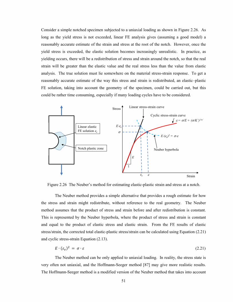
51

Consider a simple notched specimen subjected to a uniaxial loading as shown in Figure 2.26. As

long as the yield stress is not exceeded, linear FE analysis gives (assuming a good model) a

reasonably accurate estimate of the strain and stress at the root of the notch. However, once the

yield stress is exceeded, the elastic solution becomes increasingly unrealistic. In practice, as

yielding occurs, there will be a redistribution of stress and strain around the notch, so that the real

strain will be greater than the elastic value and the real stress less than the value from elastic

analysis. The true solution must lie somewhere on the material stress-strain response. To get a

reasonably accurate estimate of the way this stress and strain is redistributed, an elastic–plastic

FE solution, taking into account the geometry of the specimen, could be carried out, but this

could be rather time consuming, especially if many loading cycles have to be considered.

The Neuber method provides a simple alternative that provides a rough estimate for how

the stress and strain might redistribute, without reference to the real geometry. The Neuber

method assumes that the product of stress and strain before and after redistribution is constant.

This is represented by the Neuber hyperbola, where the product of stress and strain is constant

and equal to the product of elastic stress and elastic strain. From the FE results of elastic

stress/strain, the corrected total elastic-plastic stress/strain can be calculated using Equation (2.21)

and cyclic stress-strain Equation (2.13).

( ) (2.21)

The Neuber method can be only applied to uniaxial loading. In reality, the stress state is

very often not uniaxial, and the Hoffmann-Seeger method [87] may give more realistic results.

The Hoffmann-Seeger method is a modified version of the Neuber method that takes into account

Linear elastic

FE solution e

Notch plastic zone

Stress

Strain

Cyclic stress-strain curve

Neuber hyperbola

e

Ee

E

1

E(e)2 =

Linear stress-strain curve

= /E + (/K’)1/n’

Figure 2.26 The Neuber’s method for estimating elastic-plastic strain and stress at a notch.

52

the state of stress, allowing it to be extended to proportional multiaxial loadings (the orientation

of the principal axes remain fixed). When multi-axial loading is not proportional, the Hoffmann-

Seeger method is not applicable. If the input from the FE analysis is elastic-plastic strain and

stress, the notch corrections will not be used. A suitable plasticity model will have to be

implemented in the FE calculation so that there is no need to use a notch/plasticity correction in

the fatigue calculation to estimate the redistribution of stress and strain.

2.3.4. Multi-axial Loading in Fatigue

The previous discussions were limited to cases in which the loading produced uniaxial

stresses in the part. However, most practical situations, including rotating shafts, connecting

links, automotive and aircraft components and many mechanical components involve a multiaxial

state of cyclic stress. This often means that, at any point, both the directions and the magnitudes

of the principal stresses can vary during the loading cycle and, therefore, as a function of time.

The multiple time-varying loads may be periodic, random, or some combination of the two. If

periodic, they can be mutually synchronous, or asynchronous. If synchronous, they may have

phase relationships from in-phase to 180 out-of-phase or anything in between. The possible

combinations are quite varied, and only a few simple combinations have been studied to

determine their effects on fatigue failure. Collins [99] suggests that the assumption that loads are

synchronous and in-phase is usually accurate for machine design and usually, but not always,

conservative.

The most-studied cases are those of periodic, synchronous, in-phase loads that cause

combined stresses/strains whose principal directions do not change with time. This is referred to

as simple multiaxial stress/strain. Other situations, in which the directions of the principal

stresses/strains vary with time, or stresses/strains are asynchronous or out-of-phase, are called

complex multiaxial stress/strain and are still being studied.

2.3.4.1. Fatigue Life Prediction in Simple Multiaxial Stress/Strain Situations

Traditionally, the approach to the design of components subjected to multiaxial loading is

to make the fundamental assertion by using an equivalent modulus. The assertion states that

failure under multiaxial loading is predicted to occur if and when the cyclically induced

magnitude of that modulus is sufficiently large that failure would occur in the uniaxial state for an

identical magnitude of the same modulus. The modulus is a measurable quantity such as

principal stress, principal shear stress, or distortion energy. This philosophy has led to what is

usually referred to as the equivalent stress-strain approach, where an equivalent stress or strain

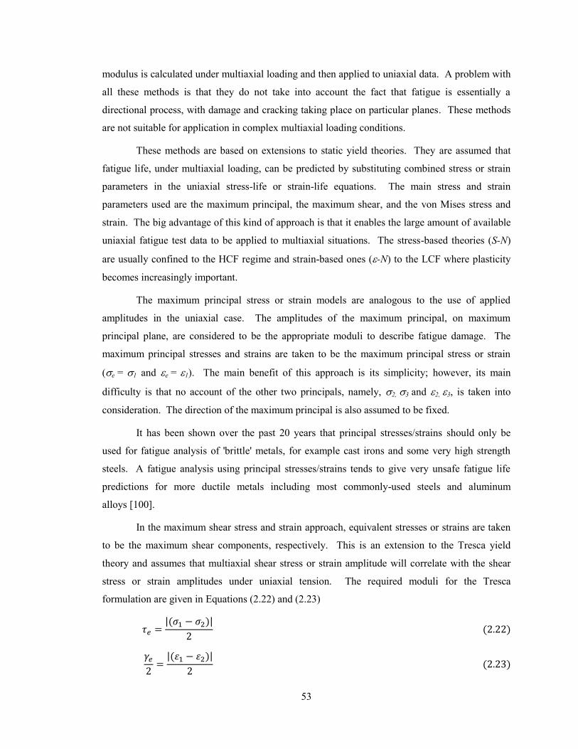
53

modulus is calculated under multiaxial loading and then applied to uniaxial data. A problem with

all these methods is that they do not take into account the fact that fatigue is essentially a

directional process, with damage and cracking taking place on particular planes. These methods

are not suitable for application in complex multiaxial loading conditions.

These methods are based on extensions to static yield theories. They are assumed that

fatigue life, under multiaxial loading, can be predicted by substituting combined stress or strain

parameters in the uniaxial stress-life or strain-life equations. The main stress and strain

parameters used are the maximum principal, the maximum shear, and the von Mises stress and

strain. The big advantage of this kind of approach is that it enables the large amount of available

uniaxial fatigue test data to be applied to multiaxial situations. The stress-based theories (S-N)

are usually confined to the HCF regime and strain-based ones (-N) to the LCF where plasticity

becomes increasingly important.

The maximum principal stress or strain models are analogous to the use of applied

amplitudes in the uniaxial case. The amplitudes of the maximum principal, on maximum

principal plane, are considered to be the appropriate moduli to describe fatigue damage. The

maximum principal stresses and strains are taken to be the maximum principal stress or strain

(e = 1 and e = 1). The main benefit of this approach is its simplicity; however, its main

difficulty is that no account of the other two principals, namely, 2, 3 and 2, 3, is taken into

consideration. The direction of the maximum principal is also assumed to be fixed.

It has been shown over the past 20 years that principal stresses/strains should only be

used for fatigue analysis of 'brittle' metals, for example cast irons and some very high strength

steels. A fatigue analysis using principal stresses/strains tends to give very unsafe fatigue life

predictions for more ductile metals including most commonly-used steels and aluminum

alloys [100].

In the maximum shear stress and strain approach, equivalent stresses or strains are taken

to be the maximum shear components, respectively. This is an extension to the Tresca yield

theory and assumes that multiaxial shear stress or strain amplitude will correlate with the shear

stress or strain amplitudes under uniaxial tension. The required moduli for the Tresca

formulation are given in Equations (2.22) and (2.23)

|( )|

( )

|( )|

( )

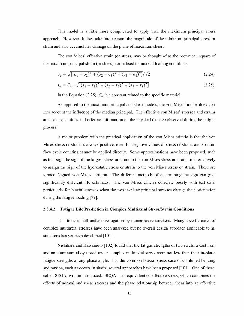
54

This model is a little more complicated to apply than the maximum principal stress

approach. However, it does take into account the magnitude of the minimum principal stress or

strain and also accumulates damage on the plane of maximum shear.

The von Mises’ effective strain (or stress) may be thought of as the root-mean square of

the maximum principal strain (or stress) normalised to uniaxial loading conditions.

√[( ) ( )

( ) ] √ (2.24)

√[( ) ( )

( ) ] (2.25)

In the Equation (2.25), Cm is a constant related to the specific material.

As opposed to the maximum principal and shear models, the von Mises’ model does take

into account the influence of the median principal. The effective von Mises’ stresses and strains

are scalar quantities and offer no information on the physical damage observed during the fatigue

process.

A major problem with the practical application of the von Mises criteria is that the von

Mises stress or strain is always positive, even for negative values of stress or strain, and so rain-

flow cycle counting cannot be applied directly. Some approximations have been proposed, such

as to assign the sign of the largest stress or strain to the von Mises stress or strain, or alternatively

to assign the sign of the hydrostatic stress or strain to the von Mises stress or strain. These are

termed ‘signed von Mises’ criteria. The different methods of determining the sign can give

significantly different life estimates. The von Mises criteria correlate poorly with test data,

particularly for biaxial stresses when the two in-plane principal stresses change their orientation

during the fatigue loading [99].

2.3.4.2. Fatigue Life Prediction in Complex Multiaxial Stress/Strain Conditions

This topic is still under investigation by numerous researchers. Many specific cases of

complex multiaxial stresses have been analyzed but no overall design approach applicable to all

situations has yet been developed [101].

Nishihara and Kawamoto [102] found that the fatigue strengths of two steels, a cast iron,

and an aluminum alloy tested under complex multiaxial stress were not less than their in-phase

fatigue strengths at any phase angle. For the common biaxial stress case of combined bending

and torsion, such as occurs in shafts, several approaches have been proposed [101]. One of these,

called SEQA, will be introduced. SEQA is an equivalent or effective stress, which combines the

effects of normal and shear stresses and the phase relationship between them into an effective

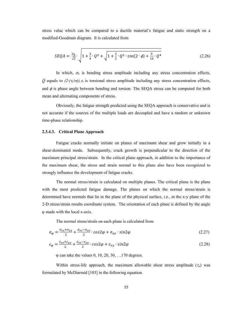
55

stress value which can be compared to a ductile material’s fatigue and static strength on a

modified-Goodman diagram. It is calculated from

√ √

√

( )

(2.26)

In which, b is bending stress amplitude including any stress concentration effects,

Q equals to (2(t/)),t is torsional stress amplitude including any stress concentration effects,

and is phase angle between bending and torsion. The SEQA stress can be computed for both

mean and alternating components of stress.

Obviously, the fatigue strength predicted using the SEQA approach is conservative and is

not accurate if the sources of the multiple loads are decoupled and have a random or unknown

time-phase relationship.

2.3.4.3. Critical Plane Approach

Fatigue cracks normally initiate on planes of maximum shear and grow initially in a

shear-dominated mode. Subsequently, crack growth is perpendicular to the direction of the

maximum principal stress/strain. In the critical plane approach, in addition to the importance of

the maximum shear, the stress and strain normal to this plane also have been recognized to

strongly influence the development of fatigue cracks.

The normal stress/strain is calculated on multiple planes. The critical plane is the plane

with the most predicted fatigue damage. The planes on which the normal stress/strain is

determined have normals that lie in the plane of the physical surface, i.e., in the x-y plane of the

2-D stress/strain results coordinate system. The orientation of each plane is defined by the angle

made with the local x-axis.

The normal stress/strain on each plane is calculated from

(2.27)

(2.28)

can take the values 0, 10, 20, 30, …170 degrees.

Within stress-life approach, the maximum allowable shear stress amplitude (a) was

formulated by McDiarmid [103] in the following equation.

56

(2.29)

The reversed shear fatigue strength, tA or tB, is used depending on whether case A or case

B crack exists. In case A, cracks grow along the surface; in case B, cracks grow into the surface.

The variable is the maximum normal stress on the critical plane of maximum shear stress

amplitude (a). Sut is the tensile strength of the material. If then a = tA,B, the

maximum allowable shear stress amplitude is equal to the reversed shear fatigue strength.

In the stage of product design, the above equation can be used to calculate the fatigue

factor of safety by multiplying the left side of the equation with the safety factor ncp, the above

equation can be transformed to:

(2.30)

In fatigue life prediction, the McDiarmid equation can be used to calculate the equivalent

shear stress teq using critical plane approach and then the uniaxial shear stress fatigue life data can

be used.

(2.31)

Within strain-life approach, Brown and Miller [104] presented a two parameter

formulation as:

max = f (n) (2.32)

Where max is the maximum shear strain and n is the strain normal to max.

The maximum shear strain is the primary force in crack initiation and the strain normal to

the plane of the maximum shear is a modifying factor. This approach is similar to the maximum

shear stress and strain approach (Tresca), but with normal strain component added. With these

ideas, the strain-life equation becomes:

( )

( )

(2.33)

In which, is the maximum shear strain amplitude and

is the strain amplitude

normal to the plane of maximum shear.

In situations of non-proportional loading, the direction of the principal stresses or strains

can vary with time. The plane of maximum shear has a fixed relationship, to the plane on which

the maximum principals are located and so the plane of maximum shear itself will rotate. Under

57

these circumstances, even the Miller Brown damage parameter will fail to account for this effect.

The net result of this is an averaging or smoothing out of the damage estimate and almost

certainly an underestimate of the actual damage.

A strategy for accounting for these effects is to calculate fatigue damage across a range of

orientations of the shear plane in an effort to identify the most damaging [87]. The effect of the

applied loading on a particular plane is determined by a tensor rotation of the stresses and strains

to that plane and estimating the damage that accumulates on it. This process is continued until a

number of planes have been analyzed, and the most damaging plane identified. Typically, under

conditions of plane stress, possibly 18 calculations, in increments of 10 degrees, would need to be

made. For tri-axial stress states, which occur on surfaces under pressure (e.g. bearings) or inside

of components, many more planes have to be considered. The normal vectors of all the planes

form a hemisphere (e.g. about 200 planes with about 10 degree angular separation). With the

advancement of computer technology, this method is becoming more effective in computer

simulation.

2.3.5. Accumulated Fatigue Assessment

In practice, a mechanical part is often exposed to a complex, random, sequence of loads,

large and small. When the cyclic load level varies during the fatigue process, a cumulative

damage model is often hypothesized. According to Miner’s rule [87], a linear damage concept

can be used to assess the fatigue life of the part. Miner’s rule states that cycles act together

linearly to cause “damage” and consume the fatigue life. Failure occurs when damage sums to 1

(load sequence effects are not accounted for). Mathematically, it can be expressed as follows:

Fatigue failure occurs when

∑

( )

Where “m” represents the number of different stress/strain levels in the complex load, ni

represents the cycles at stress i or strain i, and Nfi represents the number of cycles to failure

under stress i or strain i only. The term

can be assumed as the fractional damage at stress i

or strain i.

In a practical situation, the sequence of the different levels of load is random. In order to

count the cycles in different stress/strain levels for assessing fatigue life using Miner’s rule, the

rain-flow counting method is used to find the fatigue cycles in the stress/strain history.

58

2.4. Wheel Fatigue Testing Standards

Great efforts were taken to find testing standards associated with multi-piece wheel

design and durability analyses in the open literature. Unfortunately only one manuscript by

Vijayan et al. [14] was found which deals with the fatigue analysis of a three-piece wheel, whose

structure is similar to that as shown in Figure 2.2. In the three-piece wheel analysis, the testing

method used (SAE J1992) is for military bolted two-piece wheels, not for three-piece wheels with

a lock ring. As stated in Section 1.6, this analysis has some limitations without including a tire in

the model and the consideration of geometry and material degradation. To the best of the

author’s knowledge, no other testing standards or manuscripts relevant to this topic have been

published.

There are a limited number of fatigue testing standards and abundant manuscripts

available in the open literature about passenger car and truck wheels (single-piece). As stated in

Section 2.1, OTR tires and on-the-road tires have similar structures and materials and multi-piece

and single-piece wheels have a common fundamental structure. Therefore, the methods used to

assess the fatigue life of single piece wheel can be useful for the fatigue life estimate of multi-

piece wheels.

In automotive engineering, wheels are one of the most critical components and their

function is of vital importance in human safety. In the fatigue evaluation of a wheel design, the

commonly accepted procedure for wheel manufacturers is to pass two durability tests, namely the

cornering fatigue test and the radial fatigue test [80]. There are several Society of Automotive

Engineers (SAE) testing standards for different kinds of on-the-road wheels. SAE J328 [81]

provides minimum performance requirements and procedures for fatigue testing of wheels

intended for normal highway use and temporary use on passenger cars, light trucks, and multi-

purpose vehicles. SAE 267 [82] provides procedures and minimum performances required for

fatigue testing of wheels and demountable wheels intended for normal highway use on heavy

trucks, buses, truck-trailers and multipurpose vehicles. SAE J1992 [83] provides laboratory

procedures for fatigue testing certain production disc wheels, demountable rims, and bolt-together

divided wheels intended for normal highway use on military trucks, buses, truck-trailers and

multi-purposed passenger vehicles. Each standard provides two fatigue testing procedures,

namely, cornering and radial fatigue testing. These three testing standards provide almost

identical cornering and radial testing procedures.

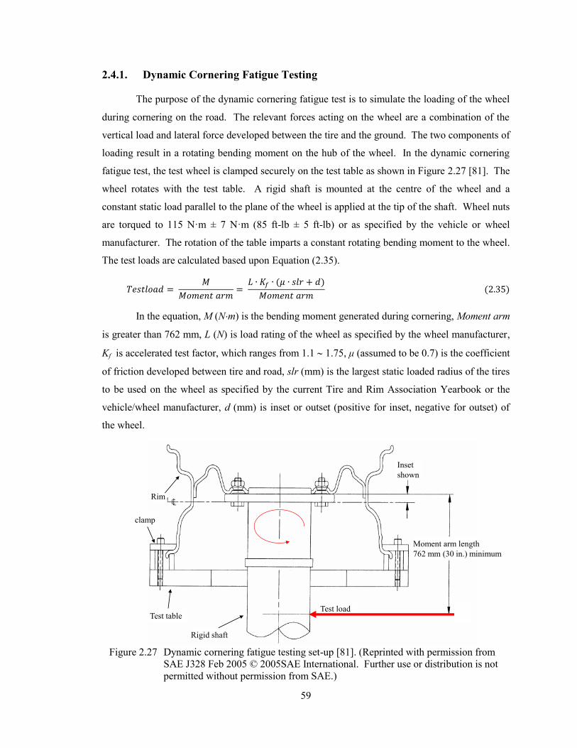
59

2.4.1. Dynamic Cornering Fatigue Testing

The purpose of the dynamic cornering fatigue test is to simulate the loading of the wheel

during cornering on the road. The relevant forces acting on the wheel are a combination of the

vertical load and lateral force developed between the tire and the ground. The two components of

loading result in a rotating bending moment on the hub of the wheel. In the dynamic cornering

fatigue test, the test wheel is clamped securely on the test table as shown in Figure 2.27 [81]. The

wheel rotates with the test table. A rigid shaft is mounted at the centre of the wheel and a

constant static load parallel to the plane of the wheel is applied at the tip of the shaft. Wheel nuts

are torqued to 115 N·m ± 7 N·m (85 ft-lb ± 5 ft-lb) or as specified by the vehicle or wheel

manufacturer. The rotation of the table imparts a constant rotating bending moment to the wheel.

The test loads are calculated based upon Equation (2.35).

( )

( )

In the equation, M (Nm) is the bending moment generated during cornering, Moment arm

is greater than 762 mm, L (N) is load rating of the wheel as specified by the wheel manufacturer,

Kf is accelerated test factor, which ranges from 1.1 1.75, μ (assumed to be 0.7) is the coefficient

of friction developed between tire and road, slr (mm) is the largest static loaded radius of the tires

to be used on the wheel as specified by the current Tire and Rim Association Yearbook or the

vehicle/wheel manufacturer, d (mm) is inset or outset (positive for inset, negative for outset) of

the wheel.

Inset

shown

Moment arm length

762 mm (30 in.) minimum

Rim

Test loadTest table

clamp

Rigid shaft

Figure 2.27 Dynamic cornering fatigue testing set-up [81]. (Reprinted with permission from

SAE J328 Feb 2005 © 2005SAE International. Further use or distribution is not

permitted without permission from SAE.)

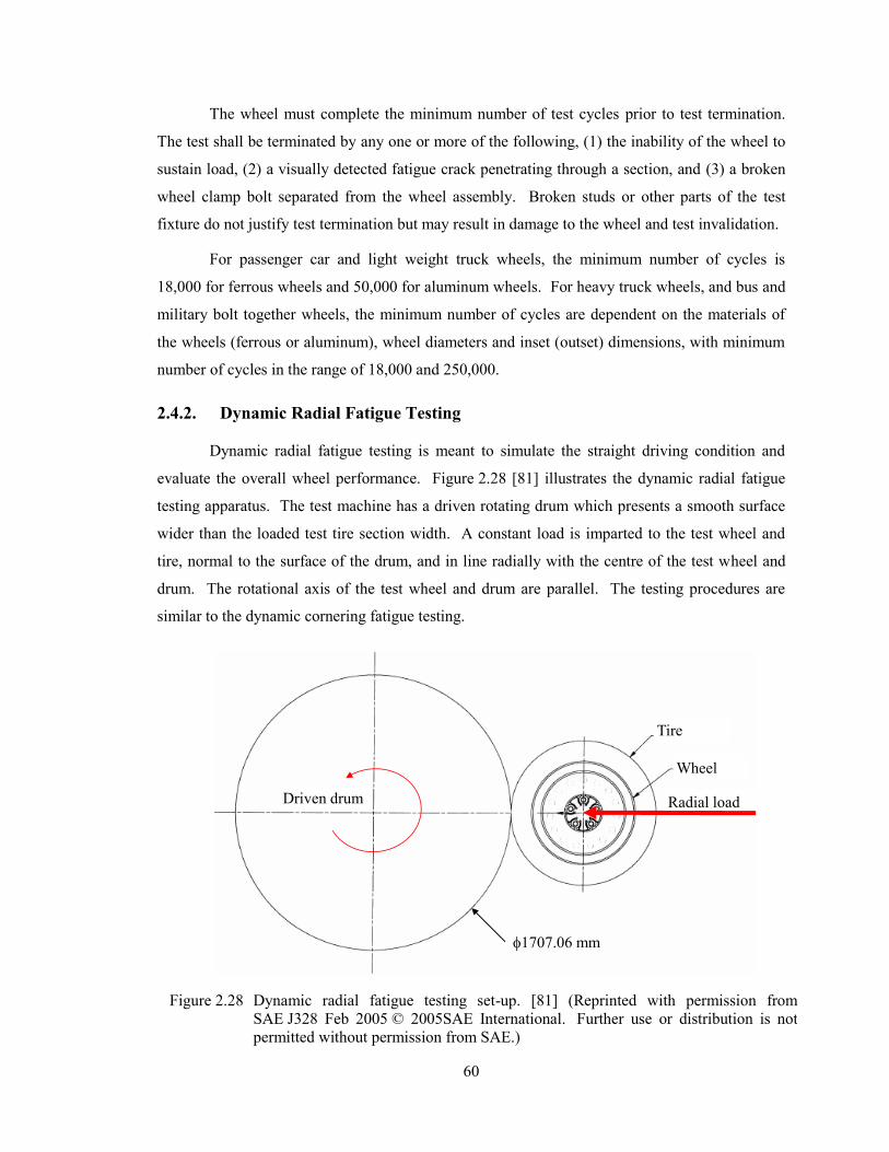
60

The wheel must complete the minimum number of test cycles prior to test termination.

The test shall be terminated by any one or more of the following, (1) the inability of the wheel to

sustain load, (2) a visually detected fatigue crack penetrating through a section, and (3) a broken

wheel clamp bolt separated from the wheel assembly. Broken studs or other parts of the test

fixture do not justify test termination but may result in damage to the wheel and test invalidation.

For passenger car and light weight truck wheels, the minimum number of cycles is

18,000 for ferrous wheels and 50,000 for aluminum wheels. For heavy truck wheels, and bus and

military bolt together wheels, the minimum number of cycles are dependent on the materials of

the wheels (ferrous or aluminum), wheel diameters and inset (outset) dimensions, with minimum

number of cycles in the range of 18,000 and 250,000.

2.4.2. Dynamic Radial Fatigue Testing

Dynamic radial fatigue testing is meant to simulate the straight driving condition and

evaluate the overall wheel performance. Figure 2.28 [81] illustrates the dynamic radial fatigue

testing apparatus. The test machine has a driven rotating drum which presents a smooth surface

wider than the loaded test tire section width. A constant load is imparted to the test wheel and

tire, normal to the surface of the drum, and in line radially with the centre of the test wheel and

drum. The rotational axis of the test wheel and drum are parallel. The testing procedures are

similar to the dynamic cornering fatigue testing.

Driven drum

Tire

Wheel

Radial load

1707.06 mm

Figure 2.28 Dynamic radial fatigue testing set-up. [81] (Reprinted with permission from

SAE J328 Feb 2005 © 2005SAE International. Further use or distribution is not

permitted without permission from SAE.)

61

The radial load (R) to be applied to the wheel is determined using Equation (2.36)

(2.36)

The parameters in the equation have the same meanings as in Equation (2.35).

2.5. FE-based Wheel Fatigue Testing

Fatigue analysis can be determined using field testing, laboratory testing and/or analytical

methods. Traditional methods for fatigue analysis are based on field testing and/or laboratory

testing, while analytical approaches have been increasingly integrated over the last decade due to

the advancement of computer technology. On-the-road wheel fatigue life can be assessed using

the aforementioned SAE testing standards within the laboratory. Traditionally, in the new wheel

development stage, experimental testing can only be conducted when prototype wheels are

available. If the performance does not meet the cycle of life requirements, the wheel design will

be modified and new prototype wheels be fabricated and the fatigue testing repeated. This

repetitive process continues until the wheel meets the fatigue life requirements before mass

production. This process is very costly and time-consuming. Analytical fatigue life analysis is

limited to simply structure under simply loading conditions due to the massive, prohibitive

calculations required.

With the advancement of computer technology, computer-aided engineering (CAE) is

widely used in the early stage of product development, testing, and manufacturing. The use of

calculations and simulations is a key feature of the modern design process. Several properties

such as strength, stiffness, durability, handling, ride comfort and crash resistance can today be

numerically analyzed with varying levels of accuracy. Development time can be shortened by

ensuring that some, or all, of these properties fulfill established requirements even before the first

prototype is built.

To reduce the cost and time of product development, iterations must be reduced at the

physical prototype stage and a reliable methodology to predict the durability parameters, such as

fatigue life and fatigue factors of safety, is critical in the early virtual prototype stage. The most

appropriate product development process is to test as few prototypes as possible, preferably only

one of any finalized model. The FE-based fatigue analyses, feeding stress/strain data from FE

analysis to fatigue prediction software to estimate fatigue parameters, are widely used in the

automotive industry. Calculations based on fatigue theory and accurate loading histories permit

structures and components to be optimized for durability without the need for expensive and

time-consuming testing of series of prototypes. Thus, designs can be obtained that are less

62

conservative (i.e. better optimized) than those based on traditional criteria, such as maximum load

or stress for a series of standard load cases.

2.5.1. FE-based Wheel Dynamic Cornering Fatigue Testing

Wang et al. [106] simulated the dynamic cornering fatigue test of a steel passenger car

disc wheel, according to SAE J328. A linear transient dynamic FE analysis was conducted to

obtain the stress/strain data and the local strain approach was used to predict fatigue life of the

wheel. HyperMesh was used to create the FE model and the linear solver OptiStruct was used to

solve the FE model. In the FE model, the wheel was mounted to a rotating table by clamping its

rim and a shaft was attached to the center of the wheel, and a constant normal force was applied

to the tip of the shaft in order to create a rotatory moment. FE results showed that the critical

(high stress) areas were located around the cooling (ventilation) holes and the centre of the disc.

The FE model was validated with experimental measurements of strains at five locations using

five 45 strain rosettes. The strain history of the element was applied to predict the fatigue life of

the critical element with local strain approach, which was quite close to the test results.

Following SAE J328 protocol, Shang et al. [107] assessed the safety factors for a newly

designed forged magnesium wheel with ten spokes, using FE analysis. The wheel model was

developed using the commercial software HyperMesh and was solved using the explicit FE code

LS-DYNA. In their study, a fatigue analysis post-processor, developed in the programming

language Java was used to calculate the safety factors of each element. Experimental tests found

that the location of the crack initiation on the spoke was identical to the location of the element

with the minimum safety factor calculated numerically. A design modification, namely,

increasing the thickness of the spokes, was incorporated and both the experiment tests and

numerical simulations on the modified wheel passed the SAE J328 fatigue test requirements.

Based on SAE J1992, Vijayan et al. [5] investigated the fatigue factors of safety of a

three-piece mining wheel. A FE model of the three-piece wheel was developed and validated

under static bending loading conditions by comparing strain values between experiment testing

and FE simulation at various locations on the rim. The model predicted strains, for the majority

of locations, within 15% error in comparison to experimental results. Numerical tests of the SAE

J1992 fatigue loading condition using LS-DYNA were performed on the validated model by

applying a rotatory bending force of 22 kN. Stresses predicted from these simulations were used

to calculate the element-based fatigue factor of safety utilizing four different methods, namely

von Mises (Goodman), Sines (Goodman), damage mechanics, and critical plane approaches. The

63

least fatigue factors of safety estimated were 1.9140, 1.9345, 1.1570 and 1.8770, respectively.

These fatigue factors of safety imply that an infinite life of the mining wheel existed. The

experimental and numerical tests both showed that the maximum stresses/strains were located at

the lock ring groove region, correspondingly, the least fatigue factors of safety were also located

in the same region. The infinite fatigue life prediction deviated from the in-field observation of

the limited fatigue life of the three-piece wheel. The difference was attributed to the difference in

loading conditions between SAE J1922 testing protocol and in-field use of the three-piece wheel,

specifically, the loading condition specified in SAE J1992 underestimates the severity of the

loading condition experienced by the three-piece wheel in normal service. The lack of wear,

material degradation due to corrosion, and localized damage of the three-piece wheel in

numerical simulation efforts were hypothesized to contribute towards the limited fatigue life

observed in service condition.

2.5.2. FE-based Wheel Dynamic Radial Fatigue Testing

Topac et al. [108] investigated the fatigue failure on the cooling holes of a newly

designed heavy commercial vehicle steel wheel under dynamic radial fatigue according to SAE

J267 standards. The stress/strain analysis was performed through the commercial FE software

code ANSYS. In the FE model, the tire was not included and the radial forces were applied

statically at the tire bead-rim contact region. Tire pressure was uniformly applied along the outer

circumference of the wheel flange. Any effect of centrifugal force was ignored. The material

properties of the wheel were determined through coupon tensile tests and hardness tests. To

predict the minimum number of wheel turns before fatigue crack initiation, the stress life

approach was utilized. The estimated S-N diagram was constructed using the ultimate tensile

strength of the processed wheel material which was determined through hardness tests. The

effects of factors such as surface roughness, size and stress concentration were also taken into

account using endurance-limit modifying factors. The Gerber approach was used to predict the

fatigue life of the wheel. The results obtained correspond to the results of radial fatigue tests. To

obtain an extended fatigue life, a design enhancement solution, including both increasing the

local thickness and the cross-sectional radius at the critical regions was applied. Stress analyses

showed that by using this solution, it was possible to decrease the equivalent von Mises stress at

these regions.

Firat et al. [109] simulated dynamic radial fatigue testing according to SAE J328 on a

disc-type truck wheel. In their analysis, a linear elastic wheel FE model was created and analyzed

using ANSYS. In the model, the tire was not included and spring elements were used to simulate

64

vertical and horizontal loads from the tire. Centrifugal forces acting on the wheel were modeled

with distributed body forces at a constant rotational speed. The experimental fatigue test cycles

and failure locations were predicted using effective strain, Smith–Watson–Topper and Fatemi–

Socie parameters using computed stress–strain histories. Nodal points on the cooling hole and

the rim-well welding were identified as the fatigue critical locations. Favorable correlations were

obtained with the critical plane parameters involving mean stress correction terms when

compared with strain gauges. Fatigue test cycles predicted using Fatemi–Socie damage

parameter was observed to be conservative and considerably close to actual test cycles for all

camber angles.

2.5.3. FE-Based Fatigue Testing on Other Vehicle Structures

Many other investigations in the open literature have considered structural fatigue testing,

which are very useful for this multi-piece wheel fatigue life analyses.

In Llano-Vizcaya et al.’s [110] work, multiaxial fatigue and failure of helical

compression springs were investigated. A linear stress analysis was carried out in the FE code

ANSYS and the stresses on the spring surface were transferred to the nCode module DesignLife.

A local strain life approach was used to assess the fatigue life. The strain life material properties

were estimated using monotonic uniaxial tensile strength as shown in Table 2.3 of Section 2.3.3.4.

To deal with multiaxial loading fatigue, the critical plane approach was used to conduct fatigue

life analysis. Experimental fatigue findings were compared with multiaxial fatigue criteria

predictions using the approaches of Fatemi–Socie, Wang–Brown, and the Coffin–Manson method

based on shear deformation. The Fatemi–Socie critical plane approach predicted a good estimate

of the fatigue life. The Wang–Brown criterion overestimated spring fatigue life, the Coffin–

Mason model provided conservative results. It was noted that the universal slopes method to

estimate strain-life properties from the monotonic uniaxial tension test, gave better predictions of

the spring fatigue life than the modified universal slopes method.

Conle and Chu [111] introduced the development of fatigue analysis and the local stress–

strain approach in complex vehicular structures in the last 20 years. The strain-life fatigue

analysis has achieved the status of industry standard in automotive, truck and earth moving

industries. Although the fundamental concepts of the method are quite simple, the recent

advancement of massive computerization technology has made it viable by creating fatigue

simulation software. Linear elastic FE models are widely used to obtain stress/strain data for

fatigue life estimates. The multiaxial Neuber type of plasticity correction method must be used to

translate the elastic local stress estimates into approximations that are corrected for elastic/plastic

65

stress–strain behaviour. Conle and Chu found that the traditional uniaxial parameters and the

equivalent stress/strain type parameters do not work well under multiaxial conditions for which

an all-encompassing damage algorithm must search for the most damaging plane at the critical

location (termed “the critical plane approach”) and utilize both normal stress/strain and shear

stress/strain on the critical plane.

66

Chapter 3. Scope of Research

The prime goal of this study is to improve the integrity of multi-piece wheel for safety.

The fatigue failure of wheel components is a major cause of the breakdown of wheel integrity.

To extend fatigue life, numerical computer simulations, assisted with experimental testing, were

used to improve multi-piece wheel design.

The literature in the aforementioned wheel fatigue tests show that the road wheels fail

mostly in the spoke region and bolt connection region [106-109]. The critical stress regions on a

disc type wheel are disc-rim weld, cooling hole, and lug bolt contact area [112]. Based on the

incident report analyses, the fatigue failure region on the multi-piece wheel with a lock ring is

mainly focused on the gutter (lock ring groove). Due to the differences between on-the-road

wheels (single-piece) and multi-piece OTR wheels in terms of structures, applications, and

loading conditions, the SAE testing protocols used to assess the fatigue parameters of on-the-road

wheels are not applicable to assess the fatigue behavior of multi-piece wheels.

3.1. Testing Methods Used in Multi-piece Wheel Fatigue Assessment

Due to the large structure and high tire pressure of multi-piece wheel assemblies,

experimental fatigue testing of OTR wheels is costly and safety prohibitive. Computer

simulations are used to assess stresses and fatigue parameters of wheel components. For the

simulated loading conditions to be realistic and representative to service conditions, in-field

experimental tests are needed. The experiment testing serves two purposes, namely, providing

loading data for numerical simulations and FE model validations.

3.1.1. Experimental Testing

In the early stage of this research, the research team made trips to several mine sites, a

mine equipment provider, two OTR wheel and tire manufacturers and suppliers in Northern

Ontario to educate the author on multi-piece wheels. In June 2011, static and quasi-static tire

tests were conducted at MusselWhite underground mine and above ground mechanic shops. The

static loading tests were conducted on a R2900 LHD vehicle through weighing the vehicle and

measuring tire deflections (Section 4.1.1) in a variety of loading conditions. The quasi-static tests

were conducted on the same vehicle to obtain tire deflection characteristics under severe loading

conditions. The tested severe loading conditions were used to validate tire models and to assess

OTR wheels’ strength and fatigue performance.

67

To validate the wheel model, laboratory rim base tests were conducted under static

loading conditions. Laser displacement measuring devices, force measuring devices, and strain

gauges were used to obtain the deformation information of the rim base. Detailed descriptions of

the tire and rim base experimental tests are in the following chapter.

3.1.2. The Finite Element (FE) Method

In the previous cited works conducting fatigue assessment, FE modeling was used for all

cases. As pointed out by Conle and Chu [111], plastic modeling gives poor quality of

stress/strain assessment when faced with reversals in loading direction. In this research, a linear

elastic model was created to simulate the static and quasi-static tests for fatigue life analysis.

Using linear elastic FEA to obtain stress/strain data is a common acceptable practice for

durability study. During fatigue life analyses, stresses/strains were corrected to elastic-plastic

stresses/strains using the Hoffmann-Seeger method. To simulate BS bank pull-out tests, an

elastic-plastic material model was used to model large deformation, non-cyclic loading condition,

which was detailed in Section 8.1.2.1.

In this study, a unique OTR tire was modelled and validated through experimental testing.

The methodology used for the tire modelling was published in an international journal. This OTR

tire modelling is the first to be found in open literature.

3.1.3. Fatigue Life Assessment Methods

The S-N approach is a traditional and well developed and accepted method to conduct

fatigue estimates. The S-N fatigue material properties can be easily obtained by conducting

fatigue testing. Strain life is more suitable to simulate crack initiation and has become greatly

incorporated in practice. It accounts for material plasticity and usually gives more appropriate

(less conservative) results. The multi-piece wheels are safety critical components and it is

important to detect fatigue cracks before failures. Therefore in this study, both methods were

used to estimate fatigue lives of multi-piece wheel components. The S-N responses were

generated by experimental fatigue testing of the extracted samples from multi-piece wheel

components. Due to the high investment to perform tests to get the strain-life material parameters,

the strain life material properties were estimated using monotonic ultimate tensile stress

according to Table 2.3 [96] of Section 2.3.3.4.

In both fatigue assessment approaches, the critical plane fatigue failure theory was used

to account for multiaxial loading conditions. Given the past practical implementation of

68

durability analyses, this is the most accurate approach to simulate fatigue life, although it

demands more computational efforts.

3.2. Innovative Designs

Based on the stress/strain and fatigue life assessments, innovative designs were proposed

and tested numerically. The primary criterion to assess the efficiency of the new designs is

fatigue performance. By comparing the fatigue lives between the new and original designs, the

durability enhancement of proposed new designs were investigated. In the new designs,

installation convenience and fail-safe mechanisms were considered to ensure the viability of the

new designs.

In the open literature, no information relevant to OTR wheel modifications was found. In

this research, two innovative OTR wheel design modifications were proposed and their durability

performances were investigated using numerical methods. The proposed threaded-connection

four-piece wheel and two-piece wheel show significant durability improvement.

3.3. Computer Software Used for This Research

The software used for this FE-based fatigue assessment was HyperMesh [113], LS-

DYNA [114], LS-PrePost [115], and nCode DesignLife [87].

HyperMesh is one module inside HyperWorks, created by Altair Incorporated.

HyperMesh is a high-performance FE pre-processor to generate FE models, starting from import

of CAD geometry to exporting a FE input file. HyperMesh enables engineers to generate high

quality meshes with maximum accuracy in the shortest time possible. A complete set of

geometry editing tools helps to efficiently prepare CAD models for the meshing process.

Additionally, meshing algorithms for shell and solid elements provide full discretization control.

LS-DYNA is an advanced general-purpose multi-physics simulation software package

developed by the Livermore Software Technology Corporation (LSTC). While the package

continues to contain more and more possibilities for the calculation of many complex real world

problems, its origins and core-competency lie in highly nonlinear transient FE analysis using

explicit time integration. The code can model contacts among structures with great accuracy and

simulate large deformation in transient states. LS-DYNA possesses many analysis capabilities,

including nonlinear dynamics, quasi-static simulations, linear statics, and many more. LS-DYNA

is widely used by the automotive industry to analyze vehicle designs.

69

LS-PrePost is an advanced pre- and post-processor designed specifically for LS-DYNA.

Here it is mainly used for post-processing simulation results from LS-DYNA. It was used to

create simulation animation files, contours of various parameters (displacement, stress, and strain),

curve plotting, and to output simulation data.

nCode DesignLife provides fatigue life prediction from FE results even before a

prototype product is available. It directly supports many FEA result data including LS-DYNA. It

has a wide range of fatigue analysis capabilities including stress-life, strain-life, multiaxial, weld

analysis, and more. nCode DesignLife was used to assess the fatigue lives of the multi-piece

wheels in this research. A brief introduction to the nCode DesignLife is explained in Appendix A.

Other software was used for data acquisition and analysis. During experimental testing,

LabVIEW was used for data acquisition and synchronization of transducer data to high speed

images. Sigmaplot was used to generate high quality plots. ProAnalyst was used to track the

motion of the tires and wheels in the video footage recorded using high speed camera during the

experimental tests. Using ProAnalyst, translational and angular displacements and velocities at

specific points were tracked and quantified.

70

Chapter 4. Tire and Wheel Experimental Testing

The purposes of the experimental tests are to understand the characteristics of the

deflection versus loading of the multi-piece wheel/tire assemblies, to provide realistic

loading/boundary data for the FE models of the tire/wheel assemblies for fatigue life assessments,

and to validate the FE models. The scale tests and quasi-static tests were conducted at a mine site.

The laboratory rim base tests were performed at the University of Windsor.

4.1. Experimental Testing of a Five-piece Wheel/Tire Assembly

Given the complex nature and physical dimensions of OTR tire structures, great

challenges arise in accurately modelling and predicting their dynamic performance under load

and in-use, when applying computer-aided engineering (CAE) methods. One significant

challenge in OTR tire modelling is the lack of experimental data pertinent for model validation.

A literature review on the topic of OTR tires reveals that there is no extensive information

available regarding the load-deflection behaviour of OTR tires. Fortunately, the tire manufacturer

Goodyear OTR does provide limited load-deflection tire data, however, the data is specified for

only a single loading condition. Therefore, OTR tire testing is required to obtain high fidelity in-

field data, encompassing the general and localized vertical and side-wall deformation of the OTR

tire as a function of load, for FE model validation purposes.

OTR tire modelling and experimentation has been primarily restricted to tire

manufacturers and this kind of information is not available in the public domain. The

methodologies used to study on-the-road tires are equally applicable to study OTR tires since the

structures and basic materials are similar between OTR tires and on-the-road tires.

In the study of Burke et al. [116], a model of a 195/65R15 car tire was created using

Nastran to investigate the static tire/road interaction. To validate the predictive capabilities of the

model, a downward force was applied to the wheel hub using an electro/hydraulic actuator and

displacement as a function of load was recorded using the actuator controller and an externally

mounted dial test indicator. Testing was carried out over a range of loads and inflation pressures

for comprehensive validation of the numerical tire model.

Neves et al. [117] created a model of a 175/65R 14 82T tire used on passenger vehicles.

The purpose of their model was to investigate tire performance under sudden impact loadings.

Model validation was completed by performing full wheel/tire impact tests. The velocity of the

indenter was measured using a laser Doppler Polytec OFV-323, which was subsequently time

71

differentiated to obtain acceleration and impact force data. Other instrumentation included the

OFV-3020 laser capturing system and a high-speed camera which recorded the impact events at a

rate of 10,000 frames per second. Indenter mass and tire inflation pressure were varied

throughout experimentation for a greater range of testing conditions.

In the study of Nguyen et al. [118], the behaviour of aircraft tires undergoing indentation

due to runway debris was recorded using digital image correlation (DIC) techniques. In the study,

the load-indentation behaviour of the tires was obtained for a C-130 Hercules nose wheel and a

Goodyear flight custom 6.50-10 tire. The wheel-tire assembly was mounted in an Instron TT-DM

testing machine fitted with a 5 kN load cell, to track indentation loads. In parallel, an Aramis

DIC system was setup using two 1.3 megapixel cameras for acquiring strain measurements. Each

tire was coloured with a stochastic pattern of white dots for DIC calibration and tracking.

Cameras were maintained at a safe operating distance away from the testing apparatus, which

prevented data acquisition within the immediate proximity of the indenter, in the tire grooves and

close to the tire shoulders. Testing was performed for a series of tire pressures with results

demonstrating a good correlation between tire inflation pressure and released indentation energy.

In the aforementioned literatures, experimental tests were conducted to help build and

validate numerical FE models. Once the FE models were validated, they were further used to

investigate tire performance under other scenarios. In this multi-piece wheel research, similar

procedures were utilized.

4.1.1. Experimental Procedure

Detailed mechanical characteristics of off-the-road tires used on heavy mining vehicles

are unavailable in open literature, with little information available from manufacturers. Since the

tire of interest in this study is of the Goodyear brand, the Goodyear Off-The-Road Tire

Engineering Data Book [28] is referenced for comparison and validation purposes and discussed

in future sections. To gain a better understanding of tire behaviour and characteristics, a variety

of measurements were taken using different approaches to excite the test vehicles. Testing on

underground heavy vehicle scale was done to acquire the static load-deflection behaviour of the

tire, while above-ground testing consisted of severe vehicle excitation for the purpose of

obtaining the quasi-static relationship between vertical and lateral sidewall tire deflection

behaviour.

72

4.1.1.1. Testing Information

Over the course of several days, testing was conducted at a remote Canadian underground

mine site where several vehicles were instrumented and tested in the summer of 2011. All test

vehicles were Caterpillar brand equipment and were either load-haul-dump (LHD) scoop vehicles

or an underground articulated truck. Only one wheel assembly was measured during the course

of each vehicle test, with the specific machine, tire, and wheel information of interest summarized

in Table 4.1. All tests on the three vehicles yielded similar tire deflection data. In this

dissertation, discussion is limited to the tire/wheel assembly with the tire sized 29.5-29 since this

tire/wheel assembly will be the focus for mechanical analysis for enhanced safety.

Table 4.1 Test vehicle information.

Machine Tire Specification Tire Rim Specification

Caterpillar AD45B

Truck (equipped with

push box)

Goodyear 29.5R29 RL-5K; L-5 Type 6SCold

Tire Pressure: 660 kPa Radial

5-piece wheel

NSIW Model

HT2000

Caterpillar R2900G

LHD Scoop

Goodyear 29.5-29 SMO; D/L-5D Type 6SCold

Tire Pressure: 591 kPa Bias

5-piece wheel;

Unknown

manufacturer

Caterpillar R1700G

LHD Scoop

Goodyear 26.5-25 SMO; D/L-5D Type 6SCold

Tire Pressure: 646 kPa Bias

5-piece wheel;

Unknown

Manufacturer

4.1.1.2. Tire Physical and Engineering Data

The tire under study is of bias-ply construction. Table 4.2 lists the engineering data for

this tire according to the Goodyear Engineering Data Book [28]. Where applicable, the U.S.

Imperial system of measurements was used as it is the base standard for tire and wheel, however,

where possible, data is based on the SI system of units or presented in both. All observations are

based on SI unit measurements.

Table 4.2 Tire physical data as given in Goodyear’s OTR Engineering Data Book [28].

Tire

Model

Inflated

Overall

Diameter

(inch/mm)

Inflated

Overall

Width

(inch/mm)

Static

Loaded

Width

(inch/mm)

Static

Loaded

Radius

(inch/mm)

Mass

(kg)

Static

load

(kN)

Inflated

Pressure Rim

Width -

Flange

height

(inch) PSI kPa

29.5-29 78.9/2004 30.1/765 33.0/838 36.3/922 1304 230kN 91 627 25.00 -

3.5

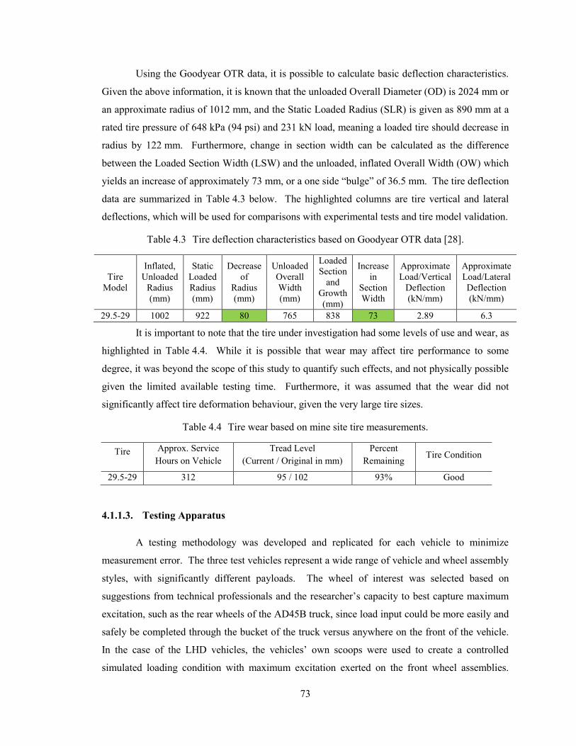
73

Using the Goodyear OTR data, it is possible to calculate basic deflection characteristics.

Given the above information, it is known that the unloaded Overall Diameter (OD) is 2024 mm or

an approximate radius of 1012 mm, and the Static Loaded Radius (SLR) is given as 890 mm at a

rated tire pressure of 648 kPa (94 psi) and 231 kN load, meaning a loaded tire should decrease in

radius by 122 mm. Furthermore, change in section width can be calculated as the difference

between the Loaded Section Width (LSW) and the unloaded, inflated Overall Width (OW) which

yields an increase of approximately 73 mm, or a one side “bulge” of 36.5 mm. The tire deflection

data are summarized in Table 4.3 below. The highlighted columns are tire vertical and lateral

deflections, which will be used for comparisons with experimental tests and tire model validation.

Table 4.3 Tire deflection characteristics based on Goodyear OTR data [28].

Tire

Model

Inflated,

Unloaded

Radius

(mm)

Static

Loaded

Radius

(mm)

Decrease

of

Radius

(mm)

Unloaded

Overall

Width

(mm)

Loaded

Section

and

Growth

(mm)

Increase

in

Section

Width

Approximate

Load/Vertical

Deflection

(kN/mm)

Approximate

Load/Lateral

Deflection

(kN/mm)

29.5-29 1002 922 80 765 838 73 2.89 6.3

It is important to note that the tire under investigation had some levels of use and wear, as

highlighted in Table 4.4. While it is possible that wear may affect tire performance to some

degree, it was beyond the scope of this study to quantify such effects, and not physically possible

given the limited available testing time. Furthermore, it was assumed that the wear did not

significantly affect tire deformation behaviour, given the very large tire sizes.

Table 4.4 Tire wear based on mine site tire measurements.

Tire Approx. Service

Hours on Vehicle

Tread Level

(Current / Original in mm)

Percent

Remaining Tire Condition

29.5-29 312 95 / 102 93% Good

4.1.1.3. Testing Apparatus

A testing methodology was developed and replicated for each vehicle to minimize

measurement error. The three test vehicles represent a wide range of vehicle and wheel assembly

styles, with significantly different payloads. The wheel of interest was selected based on

suggestions from technical professionals and the researcher’s capacity to best capture maximum

excitation, such as the rear wheels of the AD45B truck, since load input could be more easily and

safely be completed through the bucket of the truck versus anywhere on the front of the vehicle.

In the case of the LHD vehicles, the vehicles’ own scoops were used to create a controlled

simulated loading condition with maximum excitation exerted on the front wheel assemblies.

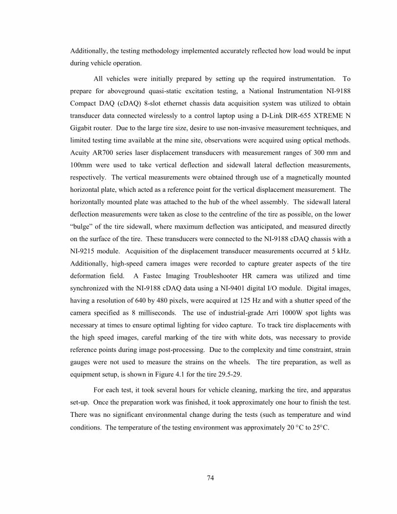
74

Additionally, the testing methodology implemented accurately reflected how load would be input

during vehicle operation.

All vehicles were initially prepared by setting up the required instrumentation. To

prepare for aboveground quasi-static excitation testing, a National Instrumentation NI-9188

Compact DAQ (cDAQ) 8-slot ethernet chassis data acquisition system was utilized to obtain

transducer data connected wirelessly to a control laptop using a D-Link DIR-655 XTREME N

Gigabit router. Due to the large tire size, desire to use non-invasive measurement techniques, and

limited testing time available at the mine site, observations were acquired using optical methods.

Acuity AR700 series laser displacement transducers with measurement ranges of 300 mm and

100mm were used to take vertical deflection and sidewall lateral deflection measurements,

respectively. The vertical measurements were obtained through use of a magnetically mounted

horizontal plate, which acted as a reference point for the vertical displacement measurement. The

horizontally mounted plate was attached to the hub of the wheel assembly. The sidewall lateral

deflection measurements were taken as close to the centreline of the tire as possible, on the lower

“bulge” of the tire sidewall, where maximum deflection was anticipated, and measured directly

on the surface of the tire. These transducers were connected to the NI-9188 cDAQ chassis with a

NI-9215 module. Acquisition of the displacement transducer measurements occurred at 5 kHz.

Additionally, high-speed camera images were recorded to capture greater aspects of the tire

deformation field. A Fastec Imaging Troubleshooter HR camera was utilized and time

synchronized with the NI-9188 cDAQ data using a NI-9401 digital I/O module. Digital images,

having a resolution of 640 by 480 pixels, were acquired at 125 Hz and with a shutter speed of the

camera specified as 8 milliseconds. The use of industrial-grade Arri 1000W spot lights was

necessary at times to ensure optimal lighting for video capture. To track tire displacements with

the high speed images, careful marking of the tire with white dots, was necessary to provide

reference points during image post-processing. Due to the complexity and time constraint, strain

gauges were not used to measure the strains on the wheels. The tire preparation, as well as

equipment setup, is shown in Figure 4.1 for the tire 29.5-29.

For each test, it took several hours for vehicle cleaning, marking the tire, and apparatus

set-up. Once the preparation work was finished, it took approximately one hour to finish the test.

There was no significant environmental change during the tests (such as temperature and wind

conditions. The temperature of the testing environment was approximately 20 C to 25C.

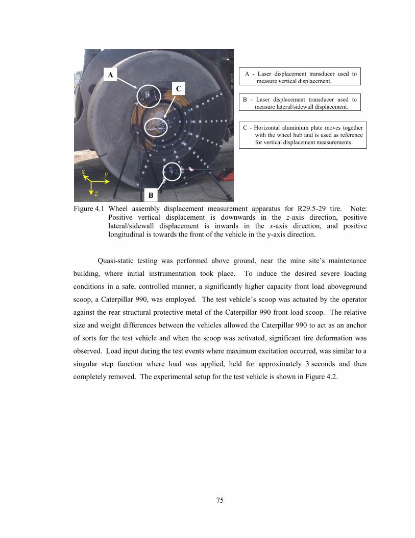
75

Quasi-static testing was performed above ground, near the mine site’s maintenance

building, where initial instrumentation took place. To induce the desired severe loading

conditions in a safe, controlled manner, a significantly higher capacity front load aboveground

scoop, a Caterpillar 990, was employed. The test vehicle’s scoop was actuated by the operator

against the rear structural protective metal of the Caterpillar 990 front load scoop. The relative

size and weight differences between the vehicles allowed the Caterpillar 990 to act as an anchor

of sorts for the test vehicle and when the scoop was activated, significant tire deformation was

observed. Load input during the test events where maximum excitation occurred, was similar to a

singular step function where load was applied, held for approximately 3 seconds and then

completely removed. The experimental setup for the test vehicle is shown in Figure 4.2.

A - Laser displacement transducer used to

measure vertical displacement.A

B

C

x

z

y

B - Laser displacement transducer used to

measure lateral/sidewall displacement.

C - Horizontal aluminium plate moves together

with the wheel hub and is used as reference

for vertical displacement measurements.

Figure 4.1 Wheel assembly displacement measurement apparatus for R29.5-29 tire. Note:

Positive vertical displacement is downwards in the z-axis direction, positive

lateral/sidewall displacement is inwards in the x-axis direction, and positive

longitudinal is towards the front of the vehicle in the y-axis direction.

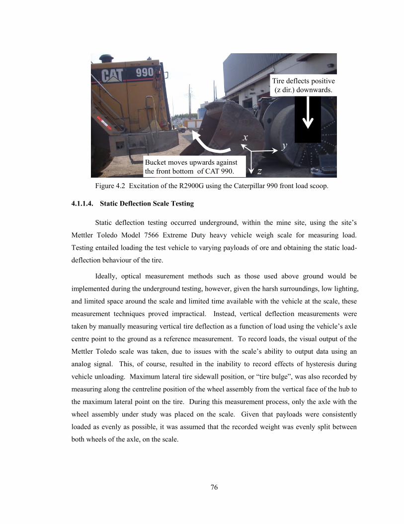
76

4.1.1.4. Static Deflection Scale Testing

Static deflection testing occurred underground, within the mine site, using the site’s

Mettler Toledo Model 7566 Extreme Duty heavy vehicle weigh scale for measuring load.

Testing entailed loading the test vehicle to varying payloads of ore and obtaining the static load-

deflection behaviour of the tire.

Ideally, optical measurement methods such as those used above ground would be

implemented during the underground testing, however, given the harsh surroundings, low lighting,

and limited space around the scale and limited time available with the vehicle at the scale, these

measurement techniques proved impractical. Instead, vertical deflection measurements were

taken by manually measuring vertical tire deflection as a function of load using the vehicle’s axle

centre point to the ground as a reference measurement. To record loads, the visual output of the

Mettler Toledo scale was taken, due to issues with the scale’s ability to output data using an

analog signal. This, of course, resulted in the inability to record effects of hysteresis during

vehicle unloading. Maximum lateral tire sidewall position, or “tire bulge”, was also recorded by

measuring along the centreline position of the wheel assembly from the vertical face of the hub to

the maximum lateral point on the tire. During this measurement process, only the axle with the

wheel assembly under study was placed on the scale. Given that payloads were consistently

loaded as evenly as possible, it was assumed that the recorded weight was evenly split between

both wheels of the axle, on the scale.

x

z

y

Tire deflects positive

(z dir.) downwards.

Bucket moves upwards against

the front bottom of CAT 990.

Figure 4.2 Excitation of the R2900G using the Caterpillar 990 front load scoop.

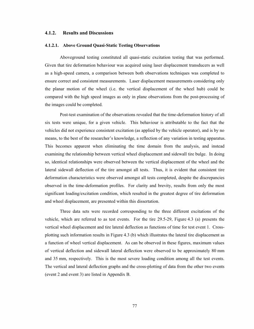
77

4.1.2. Results and Discussions

4.1.2.1. Above Ground Quasi-Static Testing Observations

Aboveground testing constituted all quasi-static excitation testing that was performed.

Given that tire deformation behaviour was acquired using laser displacement transducers as well

as a high-speed camera, a comparison between both observations techniques was completed to

ensure correct and consistent measurements. Laser displacement measurements considering only

the planar motion of the wheel (i.e. the vertical displacement of the wheel hub) could be

compared with the high speed images as only in plane observations from the post-processing of

the images could be completed.

Post-test examination of the observations revealed that the time-deformation history of all

six tests were unique, for a given vehicle. This behaviour is attributable to the fact that the

vehicles did not experience consistent excitation (as applied by the vehicle operator), and is by no

means, to the best of the researcher’s knowledge, a reflection of any variation in testing apparatus.

This becomes apparent when eliminating the time domain from the analysis, and instead

examining the relationship between vertical wheel displacement and sidewall tire bulge. In doing

so, identical relationships were observed between the vertical displacement of the wheel and the

lateral sidewall deflection of the tire amongst all tests. Thus, it is evident that consistent tire

deformation characteristics were observed amongst all tests completed, despite the discrepancies

observed in the time-deformation profiles. For clarity and brevity, results from only the most

significant loading/excitation condition, which resulted in the greatest degree of tire deformation

and wheel displacement, are presented within this dissertation.

Three data sets were recorded corresponding to the three different excitations of the

vehicle, which are referred to as test events. For the tire 29.5-29, Figure 4.3 (a) presents the

vertical wheel displacement and tire lateral deflection as functions of time for test event 1. Cross-

plotting such information results in Figure 4.3 (b) which illustrates the lateral tire displacement as

a function of wheel vertical displacement. As can be observed in these figures, maximum values

of vertical deflection and sidewall lateral deflection were observed to be approximately 80 mm

and 35 mm, respectively. This is the most severe loading condition among all the test events.

The vertical and lateral deflection graphs and the cross-plotting of data from the other two events

(event 2 and event 3) are listed in Appendix B.

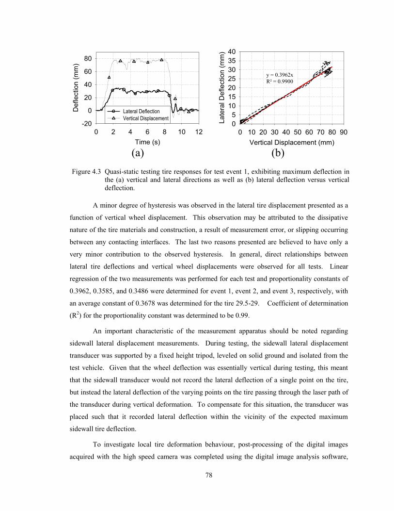
78

A minor degree of hysteresis was observed in the lateral tire displacement presented as a

function of vertical wheel displacement. This observation may be attributed to the dissipative

nature of the tire materials and construction, a result of measurement error, or slipping occurring

between any contacting interfaces. The last two reasons presented are believed to have only a

very minor contribution to the observed hysteresis. In general, direct relationships between

lateral tire deflections and vertical wheel displacements were observed for all tests. Linear

regression of the two measurements was performed for each test and proportionality constants of

0.3962, 0.3585, and 0.3486 were determined for event 1, event 2, and event 3, respectively, with

an average constant of 0.3678 was determined for the tire 29.5-29. Coefficient of determination

(R2) for the proportionality constant was determined to be 0.99.

An important characteristic of the measurement apparatus should be noted regarding

sidewall lateral displacement measurements. During testing, the sidewall lateral displacement

transducer was supported by a fixed height tripod, leveled on solid ground and isolated from the

test vehicle. Given that the wheel deflection was essentially vertical during testing, this meant

that the sidewall transducer would not record the lateral deflection of a single point on the tire,

but instead the lateral deflection of the varying points on the tire passing through the laser path of

the transducer during vertical deformation. To compensate for this situation, the transducer was

placed such that it recorded lateral deflection within the vicinity of the expected maximum

sidewall tire deflection.

To investigate local tire deformation behaviour, post-processing of the digital images

acquired with the high speed camera was completed using the digital image analysis software,

Vertical Displacement (mm)

0 10 20 30 40 50 60 70 80 90

La

tera

l D

efle

ctio

n (

mm

)

0

5

10

15

20

25

30

35

40

Time (s)

0 2 4 6 8 10 12

De

fle

ctio

n (

mm

)

-20

0

20

40

60

80

Lateral Deflection

Vertical Displacement

y = 0.3962x

R² = 0.9900

(b)(a)

Figure 4.3 Quasi-static testing tire responses for test event 1, exhibiting maximum deflection in

the (a) vertical and lateral directions as well as (b) lateral deflection versus vertical

deflection.

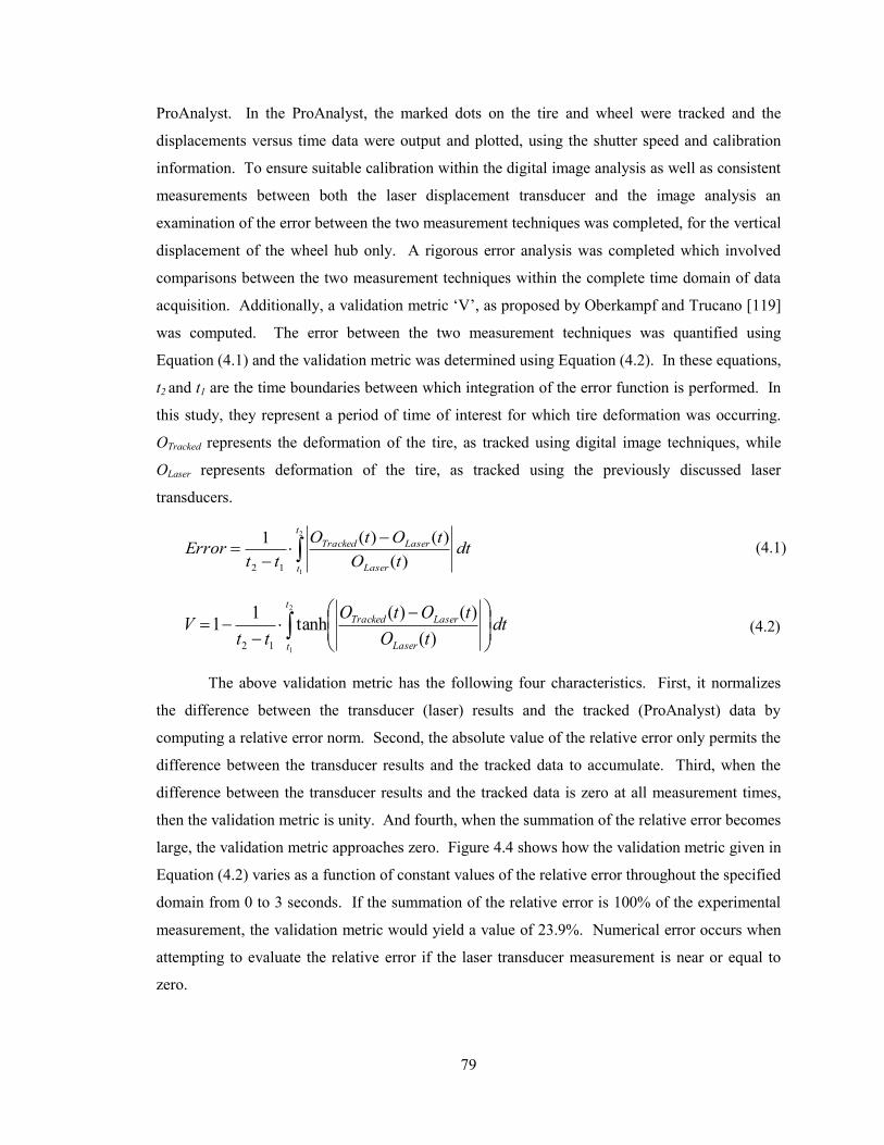
79

ProAnalyst. In the ProAnalyst, the marked dots on the tire and wheel were tracked and the

displacements versus time data were output and plotted, using the shutter speed and calibration

information. To ensure suitable calibration within the digital image analysis as well as consistent

measurements between both the laser displacement transducer and the image analysis an

examination of the error between the two measurement techniques was completed, for the vertical

displacement of the wheel hub only. A rigorous error analysis was completed which involved

comparisons between the two measurement techniques within the complete time domain of data

acquisition. Additionally, a validation metric ‘V’, as proposed by Oberkampf and Trucano [119]

was computed. The error between the two measurement techniques was quantified using

Equation (4.1) and the validation metric was determined using Equation (4.2). In these equations,

t2 and t1 are the time boundaries between which integration of the error function is performed. In

this study, they represent a period of time of interest for which tire deformation was occurring.

OTracked represents the deformation of the tire, as tracked using digital image techniques, while

OLaser represents deformation of the tire, as tracked using the previously discussed laser

transducers.

dttO

tOtO

ttError

t

t Laser

LaserTracked )(

)()(1 2

112

(4.1)

dttO

tOtO

ttV

t

t Laser

LaserTracked )(

)()(tanh

11

2

112

(4.2)

The above validation metric has the following four characteristics. First, it normalizes

the difference between the transducer (laser) results and the tracked (ProAnalyst) data by

computing a relative error norm. Second, the absolute value of the relative error only permits the

difference between the transducer results and the tracked data to accumulate. Third, when the

difference between the transducer results and the tracked data is zero at all measurement times,

then the validation metric is unity. And fourth, when the summation of the relative error becomes

large, the validation metric approaches zero. Figure 4.4 shows how the validation metric given in

Equation (4.2) varies as a function of constant values of the relative error throughout the specified

domain from 0 to 3 seconds. If the summation of the relative error is 100% of the experimental

measurement, the validation metric would yield a value of 23.9%. Numerical error occurs when

attempting to evaluate the relative error if the laser transducer measurement is near or equal to

zero.

80

Figure 4.5 illustrates the vertical displacement comparison for test event 1 between laser

displacement transducer measurements and digital image analysis tracking. The error and

validation metric were determined to be 2.31% and 0.979 respectively. The plot comparisons for

test event 2 and 3 are listed in Appendix B with errors and validation metrics of 1.25% and 0.985,

1.12% and 0.989, respectively. This analysis ensured confidence with regards to the optical

measurement techniques applied within this research.

Determination of local tire deformation behaviour occurred after the error analysis was

completed. Six locations amongst all markings applied to the tire were considered for tracking.

Figure 4.6 illustrates the locations of these points for the 29.5-29 tire. The selection of these

points was based upon the desire to eliminate any excessive analyses, yet provide a thorough

understanding of the local tire deformation. As a result points H-in and H-out, which pass

through the wheel center horizontally, D-in and D-out, which pass through wheel center

Figure 4.4 Plot of validation metric, V, given in Equation (4.2) as a function of relative error.

Time (s)

0 2 4 6 8 10 12

Ve

rtic

al D

efle

ctio

n (

mm

)

-100

102030405060708090

Laser Measurement

ProAnalyst Tracked

Figure 4.5 Vertical displacement comparisons for test event 1 between laser displacement

transducer measurements and high-speed camera image tracking using

ProAnalyst.

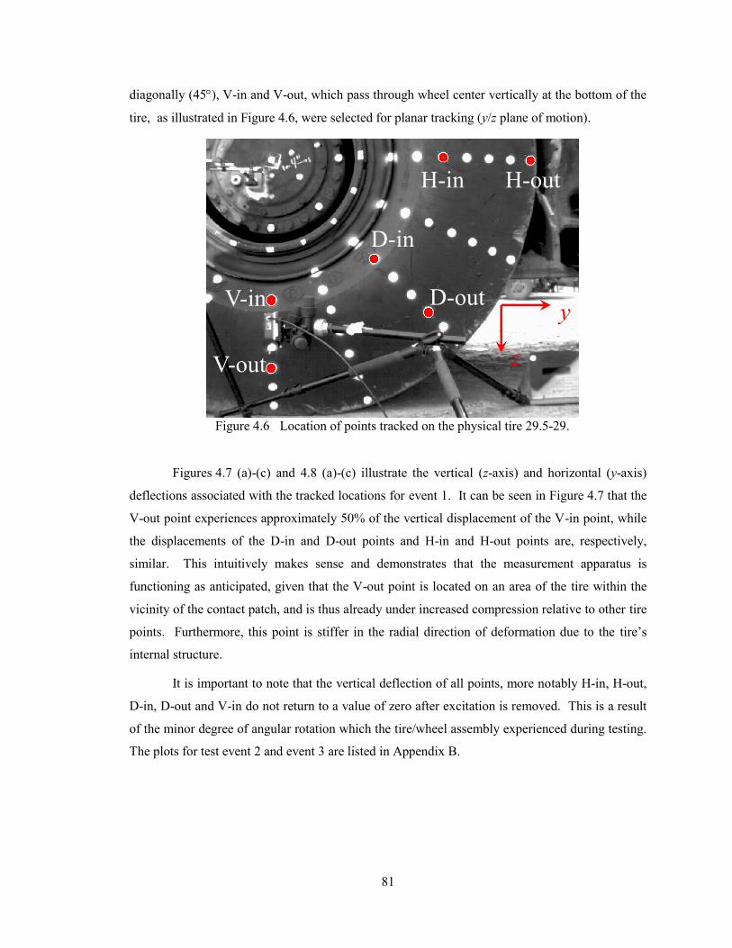
81

diagonally (45), V-in and V-out, which pass through wheel center vertically at the bottom of the

tire, as illustrated in Figure 4.6, were selected for planar tracking (y/z plane of motion).

Figures 4.7 (a)-(c) and 4.8 (a)-(c) illustrate the vertical (z-axis) and horizontal (y-axis)

deflections associated with the tracked locations for event 1. It can be seen in Figure 4.7 that the

V-out point experiences approximately 50% of the vertical displacement of the V-in point, while

the displacements of the D-in and D-out points and H-in and H-out points are, respectively,

similar. This intuitively makes sense and demonstrates that the measurement apparatus is

functioning as anticipated, given that the V-out point is located on an area of the tire within the

vicinity of the contact patch, and is thus already under increased compression relative to other tire

points. Furthermore, this point is stiffer in the radial direction of deformation due to the tire’s

internal structure.

It is important to note that the vertical deflection of all points, more notably H-in, H-out,

D-in, D-out and V-in do not return to a value of zero after excitation is removed. This is a result

of the minor degree of angular rotation which the tire/wheel assembly experienced during testing.

The plots for test event 2 and event 3 are listed in Appendix B.

H-in H-out

D-in

D-outV-in

V-out z

y

Figure 4.6 Location of points tracked on the physical tire 29.5-29.

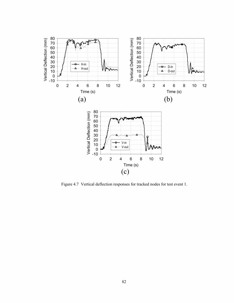
82

Time (s)

0 2 4 6 8 10 12

Vert

ica

l D

eflectio

n (

mm

)

-100

1020304050607080

H-in

H-out

Time (s)

0 2 4 6 8 10 12

Vert

ica

l D

eflectio

n (

mm

)

-100

1020304050607080

D-in

D-out

Time (s)

0 2 4 6 8 10 12

Vert

ica

l D

eflectio

n (

mm

)

-100

1020304050607080

V-in

V-out

(b)(a)

(c)

Figure 4.7 Vertical deflection responses for tracked nodes for test event 1.

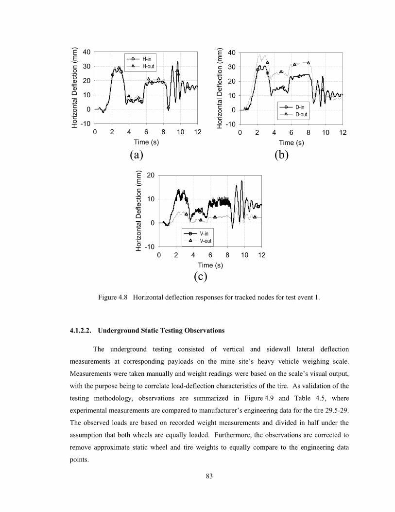
83

4.1.2.2. Underground Static Testing Observations

The underground testing consisted of vertical and sidewall lateral deflection

measurements at corresponding payloads on the mine site’s heavy vehicle weighing scale.

Measurements were taken manually and weight readings were based on the scale’s visual output,

with the purpose being to correlate load-deflection characteristics of the tire. As validation of the

testing methodology, observations are summarized in Figure 4.9 and Table 4.5, where

experimental measurements are compared to manufacturer’s engineering data for the tire 29.5-29.

The observed loads are based on recorded weight measurements and divided in half under the

assumption that both wheels are equally loaded. Furthermore, the observations are corrected to

remove approximate static wheel and tire weights to equally compare to the engineering data

points.

Time (s)

0 2 4 6 8 10 12

Hori

zo

nta

l D

eflectio

n (

mm

)

-10

0

10

20

30

40H-in

H-out

Time (s)

0 2 4 6 8 10 12

Hori

zo

nta

l D

eflectio

n (

mm

)

-10

0

10

20

30

40

D-in

D-out

Time (s)

0 2 4 6 8 10 12

Hori

zo

nta

l D

eflectio

n (

mm

)

-10

0

10

20

V-in

V-out

(b)(a)

(c)

Figure 4.8 Horizontal deflection responses for tracked nodes for test event 1.

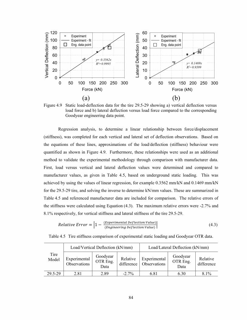
84

Regression analysis, to determine a linear relationship between force/displacement

(stiffness), was completed for each vertical and lateral set of deflection observations. Based on

the equations of these lines, approximations of the load/deflection (stiffness) behaviour were

quantified as shown in Figure 4.9. Furthermore, these relationships were used as an additional

method to validate the experimental methodology through comparison with manufacturer data.

First, load versus vertical and lateral deflection values were determined and compared to

manufacturer values, as given in Table 4.5, based on underground static loading. This was

achieved by using the values of linear regression, for example 0.3562 mm/kN and 0.1469 mm/kN

for the 29.5-29 tire, and solving the inverse to determine kN/mm values. These are summarized in

Table 4.5 and referenced manufacturer data are included for comparison. The relative errors of

the stiffness were calculated using Equation (4.3). The maximum relative errors were -2.7% and

8.1% respectively, for vertical stiffness and lateral stiffness of the tire 29.5-29.

| ( )

( )| (4.3)

Table 4.5 Tire stiffness comparison of experimental static loading and Goodyear OTR data.

Tire

Model

Load/Vertical Deflection (kN/mm) Load/Lateral Deflection (kN/mm)

Experimental

Observations

Goodyear

OTR Eng.

Data

Relative

difference

Experimental

Observations

Goodyear

OTR Eng.

Data

Relative

difference

29.5-29 2.81 2.89 -2.7% 6.81 6.30 8.1%

Force (kN)

0 50 100 150 200 250 300

Ve

rtic

al D

efle

ctio

n (

mm

)

0

20

40

60

80

100

120Experiment

Experiment - fit

Eng. data point

(a)

Force (kN)

0 50 100 150 200 250 300

La

tera

l D

efle

ctio

n (

mm

)

0

10

20

30

40

50

60Experiment

Experiment - fit

Eng. data point

(b)

y= 0.3562x

R2=0.9995 y= 0.1469x

R2=0.9399

(a) (b)Figure 4.9 Static load-deflection data for the tire 29.5-29 showing a) vertical deflection versus

load force and b) lateral deflection versus load force compared to the corresponding

Goodyear engineering data point.

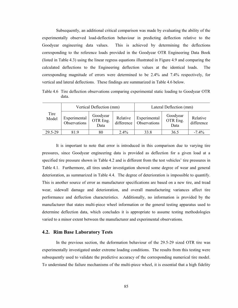
85

Subsequently, an additional critical comparison was made by evaluating the ability of the

experimentally observed load-deflection behaviour in predicting deflection relative to the

Goodyear engineering data values. This is achieved by determining the deflections

corresponding to the reference loads provided in the Goodyear OTR Engineering Data Book

(listed in Table 4.3) using the linear regress equations illustrated in Figure 4.9 and comparing the

calculated deflections to the Engineering deflection values at the identical loads. The

corresponding magnitude of errors were determined to be 2.4% and 7.4% respectively, for

vertical and lateral deflections. These findings are summarized in Table 4.6 below.

Table 4.6 Tire deflection observations comparing experimental static loading to Goodyear OTR

data.

Tire

Model

Vertical Deflection (mm) Lateral Deflection (mm)

Experimental

Observations

Goodyear

OTR Eng.

Data

Relative

difference

Experimental

Observations

Goodyear

OTR Eng.

Data

Relative

difference

29.5-29 81.9 80 2.4% 33.8 36.5 -7.4%

It is important to note that error is introduced in this comparison due to varying tire

pressures, since Goodyear engineering data is provided as deflection for a given load at a

specified tire pressure shown in Table 4.2 and is different from the test vehicles’ tire pressures in

Table 4.1. Furthermore, all tires under investigation showed some degree of wear and general

deterioration, as summarized in Table 4.4. The degree of deterioration is impossible to quantify.

This is another source of error as manufacturer specifications are based on a new tire, and tread

wear, sidewall damage and deterioration, and overall manufacturing variances affect tire

performance and deflection characteristics. Additionally, no information is provided by the

manufacturer that states multi-piece wheel information or the general testing apparatus used to

determine deflection data, which concludes it is appropriate to assume testing methodologies

varied to a minor extent between the manufacturer and experimental observations.

4.2. Rim Base Laboratory Tests

In the previous section, the deformation behaviour of the 29.5-29 sized OTR tire was

experimentally investigated under extreme loading conditions. The results from this testing were

subsequently used to validate the predictive accuracy of the corresponding numerical tire model.

To understand the failure mechanisms of the multi-piece wheel, it is essential that a high fidelity

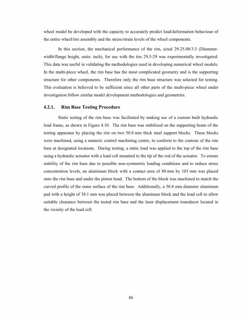
86

wheel model be developed with the capacity to accurately predict load/deformation behaviour of

the entire wheel/tire assembly and the stress/strain levels of the wheel components.

In this section, the mechanical performance of the rim, sized 29-25.00/3.5 (Diameter-

width/flange height, units: inch), for use with the tire 29.5-29 was experimentally investigated.

This data was useful in validating the methodologies used in developing numerical wheel models.

In the multi-piece wheel, the rim base has the most complicated geometry and is the supporting

structure for other components. Therefore only the rim base structure was selected for testing.

This evaluation is believed to be sufficient since all other parts of the multi-piece wheel under

investigation follow similar model development methodologies and geometries.

4.2.1. Rim Base Testing Procedure

Static testing of the rim base was facilitated by making use of a custom built hydraulic

load frame, as shown in Figure 4.10. The rim base was stabilized on the supporting beam of the

testing apparatus by placing the rim on two 50.8 mm thick steel support blocks. These blocks

were machined, using a numeric control machining centre, to conform to the contour of the rim

base at designated locations. During testing, a static load was applied to the top of the rim base

using a hydraulic actuator with a load cell mounted to the tip of the rod of the actuator. To ensure

stability of the rim base due to possible non-symmetric loading conditions and to reduce stress

concentration levels, an aluminum block with a contact area of 80 mm by 103 mm was placed

onto the rim base and under the piston head. The bottom of the block was machined to match the

curved profile of the outer surface of the rim base. Additionally, a 50.8 mm diameter aluminum

pad with a height of 38.1 mm was placed between the aluminum block and the load cell to allow

suitable clearance between the tested rim base and the laser displacement transducer located in

the vicinity of the load cell.

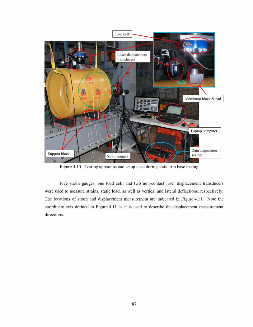
87

Five strain gauges, one load cell, and two non-contact laser displacement transducers

were used to measure strains, static load, as well as vertical and lateral deflections, respectively.

The locations of strain and displacement measurement are indicated in Figure 4.11. Note the

coordinate axis defined in Figure 4.11 as it is used to describe the displacement measurement

directions.

Laptop computer

Data acquisition

systemSupport blocksStrain gauges

Aluminum block & pad

Load cell

Laser displacement

transducers

Figure 4.10 Testing apparatus and setup used during static rim base testing.

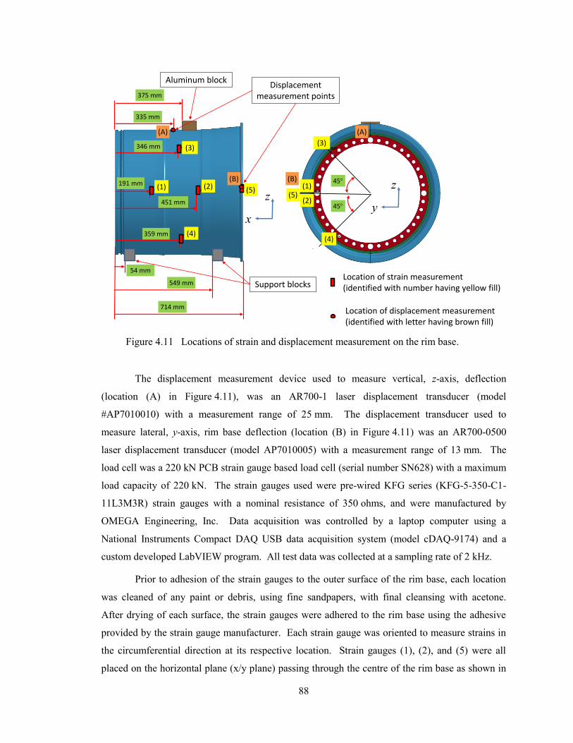
88

The displacement measurement device used to measure vertical, z-axis, deflection

(location (A) in Figure 4.11), was an AR700-1 laser displacement transducer (model

#AP7010010) with a measurement range of 25 mm. The displacement transducer used to

measure lateral, y-axis, rim base deflection (location (B) in Figure 4.11) was an AR700-0500

laser displacement transducer (model AP7010005) with a measurement range of 13 mm. The

load cell was a 220 kN PCB strain gauge based load cell (serial number SN628) with a maximum

load capacity of 220 kN. The strain gauges used were pre-wired KFG series (KFG-5-350-C1-

11L3M3R) strain gauges with a nominal resistance of 350 ohms, and were manufactured by

OMEGA Engineering, Inc. Data acquisition was controlled by a laptop computer using a

National Instruments Compact DAQ USB data acquisition system (model cDAQ-9174) and a

custom developed LabVIEW program. All test data was collected at a sampling rate of 2 kHz.

Prior to adhesion of the strain gauges to the outer surface of the rim base, each location

was cleaned of any paint or debris, using fine sandpapers, with final cleansing with acetone.

After drying of each surface, the strain gauges were adhered to the rim base using the adhesive

provided by the strain gauge manufacturer. Each strain gauge was oriented to measure strains in

the circumferential direction at its respective location. Strain gauges (1), (2), and (5) were all

placed on the horizontal plane (x/y plane) passing through the centre of the rim base as shown in

(1)191 mm

346 mm

359 mm

451 mm

54 mm

549 mm

(2)

(3)

(4)

(5)

335 mm

375 mm

714 mm

45

45

(1)

(2)(5)

Aluminum blockDisplacement

measurement points

Support blocks

(4)

(3)

y

z

(A)

(B)

(A)

(B)

Location of strain measurement (identified with number having yellow fill)

Location of displacement measurement (identified with letter having brown fill)

x

z

Figure 4.11 Locations of strain and displacement measurement on the rim base.

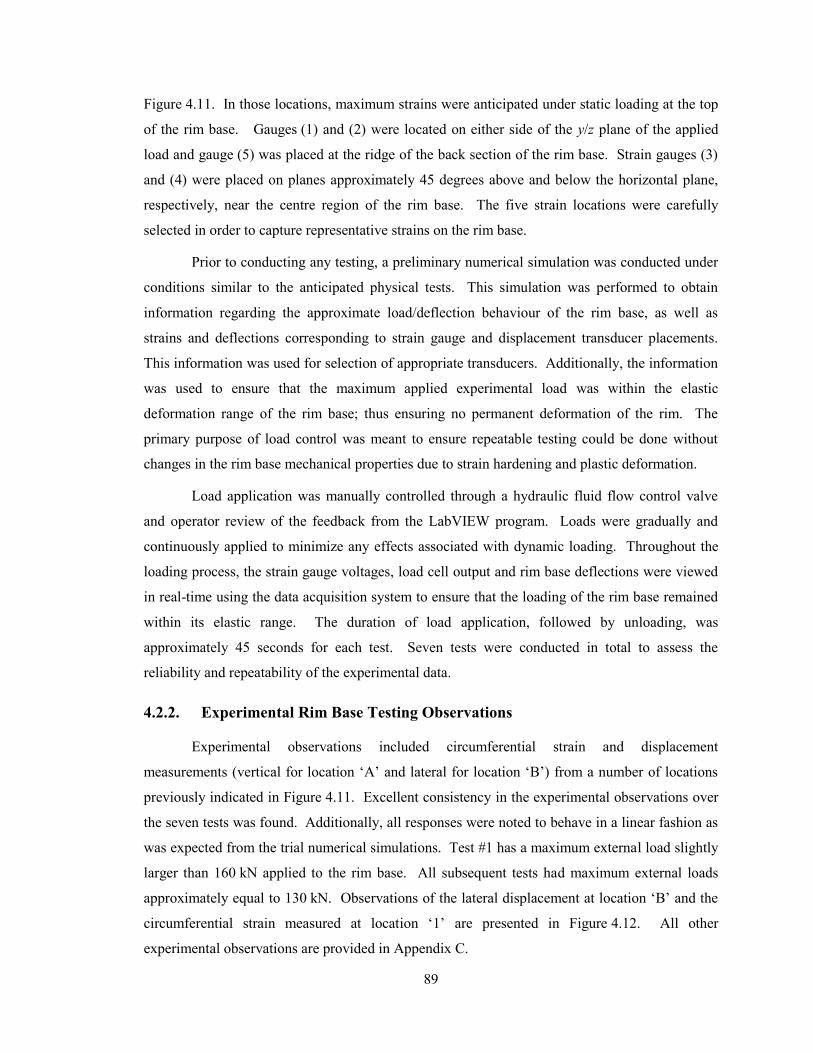
89

Figure 4.11. In those locations, maximum strains were anticipated under static loading at the top

of the rim base. Gauges (1) and (2) were located on either side of the y/z plane of the applied

load and gauge (5) was placed at the ridge of the back section of the rim base. Strain gauges (3)

and (4) were placed on planes approximately 45 degrees above and below the horizontal plane,

respectively, near the centre region of the rim base. The five strain locations were carefully

selected in order to capture representative strains on the rim base.

Prior to conducting any testing, a preliminary numerical simulation was conducted under

conditions similar to the anticipated physical tests. This simulation was performed to obtain

information regarding the approximate load/deflection behaviour of the rim base, as well as

strains and deflections corresponding to strain gauge and displacement transducer placements.

This information was used for selection of appropriate transducers. Additionally, the information

was used to ensure that the maximum applied experimental load was within the elastic

deformation range of the rim base; thus ensuring no permanent deformation of the rim. The

primary purpose of load control was meant to ensure repeatable testing could be done without

changes in the rim base mechanical properties due to strain hardening and plastic deformation.

Load application was manually controlled through a hydraulic fluid flow control valve

and operator review of the feedback from the LabVIEW program. Loads were gradually and

continuously applied to minimize any effects associated with dynamic loading. Throughout the

loading process, the strain gauge voltages, load cell output and rim base deflections were viewed

in real-time using the data acquisition system to ensure that the loading of the rim base remained

within its elastic range. The duration of load application, followed by unloading, was

approximately 45 seconds for each test. Seven tests were conducted in total to assess the

reliability and repeatability of the experimental data.

4.2.2. Experimental Rim Base Testing Observations

Experimental observations included circumferential strain and displacement

measurements (vertical for location ‘A’ and lateral for location ‘B’) from a number of locations

previously indicated in Figure 4.11. Excellent consistency in the experimental observations over

the seven tests was found. Additionally, all responses were noted to behave in a linear fashion as

was expected from the trial numerical simulations. Test #1 has a maximum external load slightly

larger than 160 kN applied to the rim base. All subsequent tests had maximum external loads

approximately equal to 130 kN. Observations of the lateral displacement at location ‘B’ and the

circumferential strain measured at location ‘1’ are presented in Figure 4.12. All other

experimental observations are provided in Appendix C.

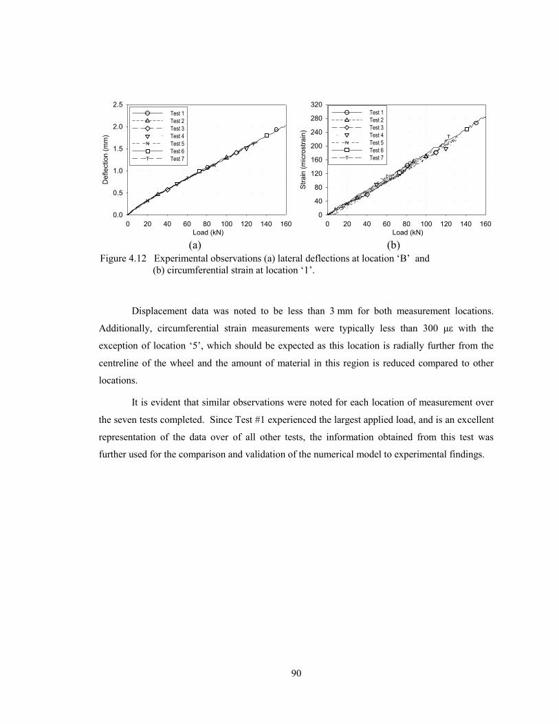
90

Displacement data was noted to be less than 3 mm for both measurement locations.

Additionally, circumferential strain measurements were typically less than 300 με with the

exception of location ‘5’, which should be expected as this location is radially further from the

centreline of the wheel and the amount of material in this region is reduced compared to other

locations.

It is evident that similar observations were noted for each location of measurement over

the seven tests completed. Since Test #1 experienced the largest applied load, and is an excellent

representation of the data over of all other tests, the information obtained from this test was

further used for the comparison and validation of the numerical model to experimental findings.

Load (kN)

0 20 40 60 80 100 120 140 160

Deflection (

mm

)

0.0

0.5

1.0

1.5

2.0

2.5

N

N

T

T

Test 1

Test 2

Test 3

Test 4

Test 5N

Test 6

Test 7T

Load (kN)

0 20 40 60 80 100 120 140 160

Str

ain

(m

icro

str

ain

)

0

40

80

120

160

200

240

280

320

N

N

T

T

Test 1

Test 2

Test 3

Test 4

Test 5N

Test 6

Test 7T

(a) (b)

Figure 4.12 Experimental observations (a) lateral deflections at location ‘B’ and

(b) circumferential strain at location ‘1’.

91

Chapter 5. Finite Element Model Development

5.1. Tire Model Development

5.1.1. On-the-road Tire Modeling in the Open Literature

Tire modeling and experimentation has been primarily restricted to tire manufacturers,

with no studies known to be available regarding the simulation of mining wheel tires in the open

literature. Regardless, studies of on-the-road tires are applicable to a reasonable degree, since the

structures and materials of the two different types of tires are similar, despite significant

differences in bead and sidewall thickness when compared proportionally.

To create a detailed tire model for crash applications, Reid et al. [120] conducted two

types of tire tests, namely, single-sided compression and double-sided compression. The first test

was achieved by placing a flat rigid ground type surface below the tire and subsequently

prescribing a displacement to the centre of the wheel. The second test follows similar

methodology to the first, except the prescribed motion was made in reference to a solid plate

placed on top of the tire; thus resulting in double-sided compression. In both tests load-deflection

curves were obtained and were used to improve the accuracy of the tire model. The researchers

took a unique approach to the model development, which avoided the discretization of all

structures of the tire and wheel; however, the majority of the components which influenced the

response of the tire and wheel assembly were carefully modelled such that good predictive

capabilities of the model existed under a number of testing conditions.

In the work of Orengo et al., [121] tire blow-out of a passenger vehicle in roadside

hardware simulations was modelled using the commercial software LS-DYNA. In their

numerical tire model, the modelling of different tire components was simplified to shell, beam

and solid elements. The model was subsequently verified against experimental observations and

found to correlate well; thus validating the model simplifications.

Neves et al. [117] created a model of a 175/65R 14 82T tire used on passenger vehicles,

to investigate the tire performance under sudden impact loadings. The researchers used the FE

software Abaqus for their investigations. To validate their model, impact tests were conducted on

the tire and deformation was tracked using laser displacement transducers and a high speed

camera.

In the study of Burke and Olatunbosun [116], a model of a 195/65R15 tire was created

using Nastran to investigate the static tire/road interaction. In their research, a gap formulation

92

was implemented to model the interaction so that the contact patch area, shape and deflection

were automatically accounted for under a given load and inflation pressure. To validate their

model, a downward force was applied to the wheel centre and tire displacement as a function of

load was recorded and compared against model behaviour. This simplistic approach was used to

assess the predictive capabilities of the numerical model.

5.1.2. Tire Model Development for the Tire 29.5-29

The OTR tire modeled was the tire sized 29.5-29, used on the mining vehicle Caterpillar

R2900G LHD Scoop, which was experimentally tested. Detailed tire physical and deflection

information were listed in Table 4.2 and 4.3 in Chapter 4. This tire has a bias structure and

smooth tread pattern.

Great efforts were taken to obtain more detailed information about the tire structure and

material properties than information presented in previous sections, however, only geometric

dimensions, such as bead and sidewall thickness by manually measuring a physical tire, could be

obtained due to the proprietary and confidential nature of the tire design. A lack of specific

material properties also arose for Reid et al. [120] while modelling a Chevrolet C2500 pickup

truck tire. In their study, a C2500 pickup truck tire was cut in half and the detailed tire geometry

was obtained. Similar methodologies were sought to be used in this investigation, however, it

was found unfeasible to obtain relevant tire cross-sections, primarily due to the size and the

weight of the tire and the availability of cutting equipment, without causing significant

degradation to the tire near the potentially cut regions. Instead, acknowledgement is made that

the model of this study seeks to simulate overall tire performance rather than the detailed, highly

localized structural performance of the tire components. As such, a simplified tire model meeting

the overall performance of the tire was chosen as the basis of model development.

Since the tire and wheel always work together, the tire and wheel assembly was tested

and modeled together. Prior to tire model development, a basic wheel model was established.

The wheel structure was composed of seven pieces, namely, the rim base, bead seat (BS) band,

locking ring, front and back flanges, support disc and mounting disc as shown in Figure 5.1. In

real-world operation the mounting disc’s deformation is minimal and is not of primary interest to

this study. Correspondingly, a rigid material property was assigned to this part of the model. The

remaining wheel components were modelled using the elastic material properties of steel.

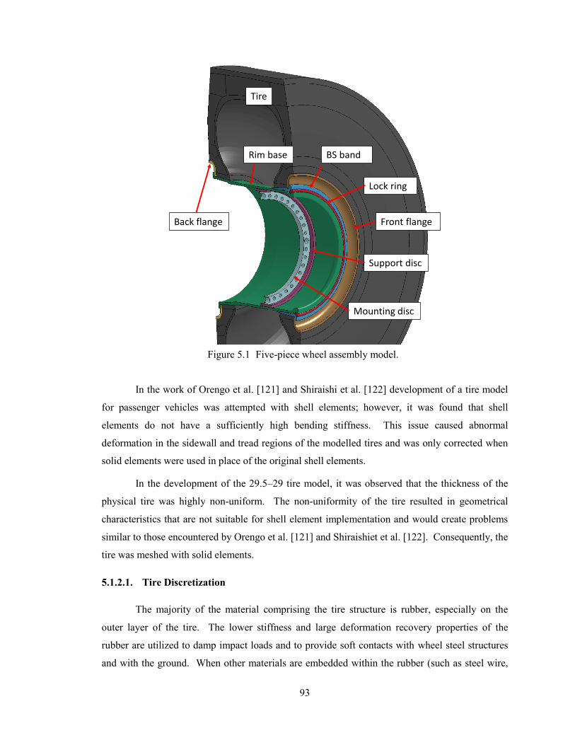
93

In the work of Orengo et al. [121] and Shiraishi et al. [122] development of a tire model

for passenger vehicles was attempted with shell elements; however, it was found that shell

elements do not have a sufficiently high bending stiffness. This issue caused abnormal

deformation in the sidewall and tread regions of the modelled tires and was only corrected when

solid elements were used in place of the original shell elements.

In the development of the 29.5–29 tire model, it was observed that the thickness of the

physical tire was highly non-uniform. The non-uniformity of the tire resulted in geometrical

characteristics that are not suitable for shell element implementation and would create problems

similar to those encountered by Orengo et al. [121] and Shiraishiet et al. [122]. Consequently, the

tire was meshed with solid elements.

5.1.2.1. Tire Discretization

The majority of the material comprising the tire structure is rubber, especially on the

outer layer of the tire. The lower stiffness and large deformation recovery properties of the

rubber are utilized to damp impact loads and to provide soft contacts with wheel steel structures

and with the ground. When other materials are embedded within the rubber (such as steel wire,

Tire

Back flange Front flange

Rim base

Support disc

Mounting disc

Lock ring

BS band

Figure 5.1 Five-piece wheel assembly model.

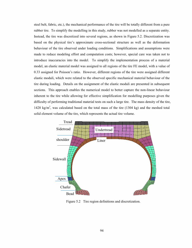
94

steel belt, fabric, etc.), the mechanical performance of the tire will be totally different from a pure

rubber tire. To simplify the modelling in this study, rubber was not modelled as a separate entity.

Instead, the tire was discretized into several regions, as shown in Figure 5.2. Discretization was

based on the physical tire’s approximate cross-sectional structure as well as the deformation

behaviour of the tire observed under loading conditions. Simplifications and assumptions were

made to reduce modeling effort and computation costs; however, special care was taken not to

introduce inaccuracies into the model. To simplify the implementation process of a material

model, an elastic material model was assigned to all regions of the tire FE model, with a value of

0.33 assigned for Poisson’s ratio. However, different regions of the tire were assigned different

elastic moduli, which were related to the observed specific mechanical material behaviour of the

tire during loading. Details on the assignment of the elastic moduli are presented in subsequent

sections. This approach enables the numerical model to better capture the non-linear behaviour

inherent to the tire while allowing for effective simplification for modelling purposes given the

difficulty of performing traditional material tests on such a large tire. The mass density of the tire,

1428 kg/m3, was calculated based on the total mass of the tire (1304 kg) and the meshed total

solid element volume of the tire, which represents the actual tire volume.

Liner

Chafer

Sidewall

shoulder

Sidetread

Tread

Bead

Undertread

Apex

Figure 5.2 Tire region definitions and discretization.

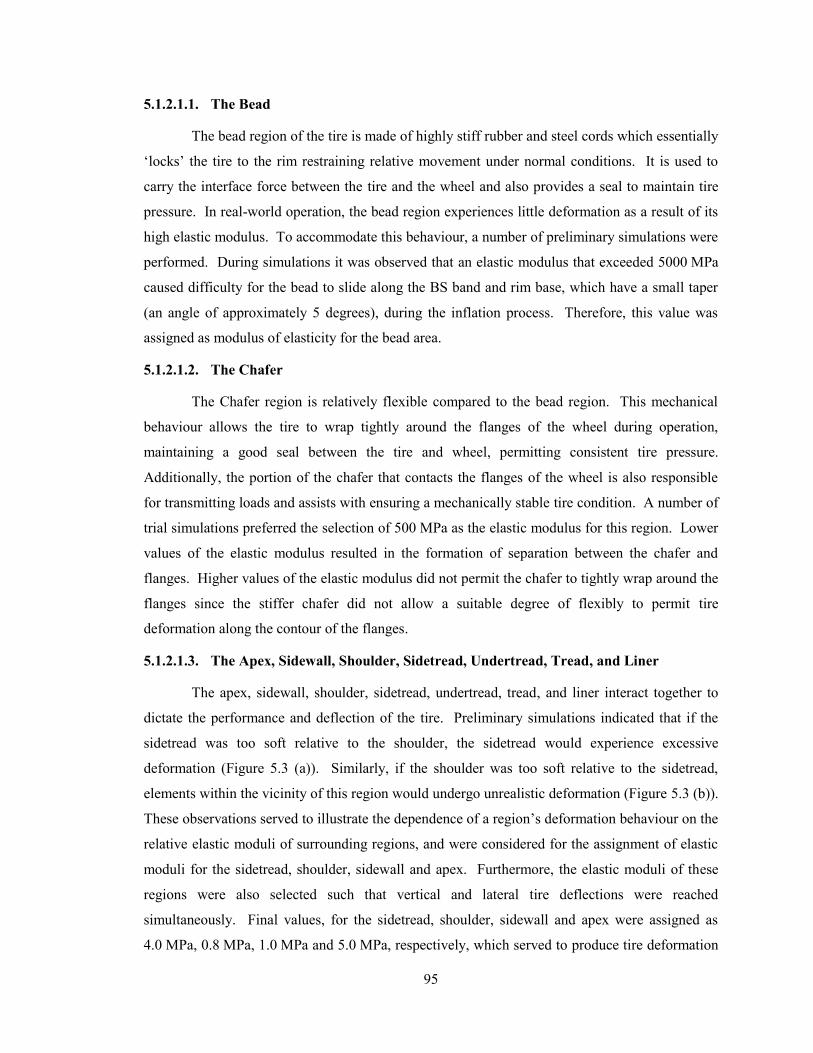
95

5.1.2.1.1. The Bead

The bead region of the tire is made of highly stiff rubber and steel cords which essentially

‘locks’ the tire to the rim restraining relative movement under normal conditions. It is used to

carry the interface force between the tire and the wheel and also provides a seal to maintain tire

pressure. In real-world operation, the bead region experiences little deformation as a result of its

high elastic modulus. To accommodate this behaviour, a number of preliminary simulations were

performed. During simulations it was observed that an elastic modulus that exceeded 5000 MPa

caused difficulty for the bead to slide along the BS band and rim base, which have a small taper

(an angle of approximately 5 degrees), during the inflation process. Therefore, this value was

assigned as modulus of elasticity for the bead area.

5.1.2.1.2. The Chafer

The Chafer region is relatively flexible compared to the bead region. This mechanical

behaviour allows the tire to wrap tightly around the flanges of the wheel during operation,

maintaining a good seal between the tire and wheel, permitting consistent tire pressure.

Additionally, the portion of the chafer that contacts the flanges of the wheel is also responsible

for transmitting loads and assists with ensuring a mechanically stable tire condition. A number of

trial simulations preferred the selection of 500 MPa as the elastic modulus for this region. Lower

values of the elastic modulus resulted in the formation of separation between the chafer and

flanges. Higher values of the elastic modulus did not permit the chafer to tightly wrap around the

flanges since the stiffer chafer did not allow a suitable degree of flexibly to permit tire

deformation along the contour of the flanges.

5.1.2.1.3. The Apex, Sidewall, Shoulder, Sidetread, Undertread, Tread, and Liner

The apex, sidewall, shoulder, sidetread, undertread, tread, and liner interact together to

dictate the performance and deflection of the tire. Preliminary simulations indicated that if the

sidetread was too soft relative to the shoulder, the sidetread would experience excessive

deformation (Figure 5.3 (a)). Similarly, if the shoulder was too soft relative to the sidetread,

elements within the vicinity of this region would undergo unrealistic deformation (Figure 5.3 (b)).

These observations served to illustrate the dependence of a region’s deformation behaviour on the

relative elastic moduli of surrounding regions, and were considered for the assignment of elastic

moduli for the sidetread, shoulder, sidewall and apex. Furthermore, the elastic moduli of these

regions were also selected such that vertical and lateral tire deflections were reached

simultaneously. Final values, for the sidetread, shoulder, sidewall and apex were assigned as

4.0 MPa, 0.8 MPa, 1.0 MPa and 5.0 MPa, respectively, which served to produce tire deformation

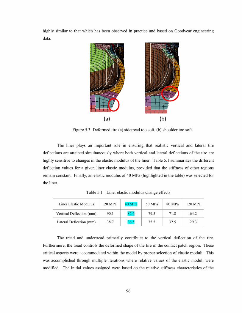
96

highly similar to that which has been observed in practice and based on Goodyear engineering

data.

The liner plays an important role in ensuring that realistic vertical and lateral tire

deflections are attained simultaneously where both vertical and lateral deflections of the tire are

highly sensitive to changes in the elastic modulus of the liner. Table 5.1 summarizes the different

deflection values for a given liner elastic modulus, provided that the stiffness of other regions

remain constant. Finally, an elastic modulus of 40 MPa (highlighted in the table) was selected for

the liner.

Table 5.1 Liner elastic modulus change effects

Liner Elastic Modulus 20 MPa 40 MPa 50 MPa 80 MPa 120 MPa

Vertical Deflection (mm) 90.1 82.6 79.5 71.8 64.2

Lateral Deflection (mm) 38.7 36.5 35.5 32.5 29.3

The tread and undertread primarily contribute to the vertical deflection of the tire.

Furthermore, the tread controls the deformed shape of the tire in the contact patch region. These

critical aspects were accommodated within the model by proper selection of elastic moduli. This

was accomplished through multiple iterations where relative values of the elastic moduli were

modified. The initial values assigned were based on the relative stiffness characteristics of the

(a) (b)

Figure 5.3 Deformed tire (a) sidetread too soft, (b) shoulder too soft.

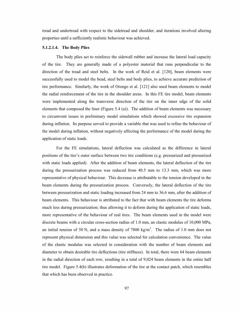
97

tread and undertread with respect to the sidetread and shoulder, and iterations involved altering

properties until a sufficiently realistic behaviour was achieved.

5.1.2.1.4. The Body Plies

The body plies act to reinforce the sidewall rubber and increase the lateral load capacity

of the tire. They are generally made of a polyester material that runs perpendicular to the

direction of the tread and steel belts. In the work of Reid et al. [120], beam elements were

successfully used to model the bead, steel belts and body plies, to achieve accurate prediction of

tire performance. Similarly, the work of Orengo et al. [121] also used beam elements to model

the radial reinforcement of the tire in the shoulder areas. In this FE tire model, beam elements

were implemented along the transverse direction of the tire on the inner edge of the solid

elements that composed the liner (Figure 5.4 (a)). The addition of beam elements was necessary

to circumvent issues in preliminary model simulations which showed excessive tire expansion

during inflation. Its purpose served to provide a variable that was used to refine the behaviour of

the model during inflation, without negatively affecting the performance of the model during the

application of static loads.

For the FE simulations, lateral deflection was calculated as the difference in lateral

positions of the tire’s outer surface between two tire conditions (e.g. pressurized and pressurized

with static loads applied). After the addition of beam elements, the lateral deflection of the tire

during the pressurization process was reduced from 40.5 mm to 13.3 mm, which was more

representative of physical behaviour. This decrease is attributable to the tension developed in the

beam elements during the pressurization process. Conversely, the lateral deflection of the tire

between pressurization and static loading increased from 24 mm to 36.6 mm, after the addition of

beam elements. This behaviour is attributed to the fact that with beam elements the tire deforms

much less during pressurization; thus allowing it to deform during the application of static loads,

more representative of the behaviour of real tires. The beam elements used in the model were

discrete beams with a circular cross-section radius of 1.0 mm, an elastic modulus of 10,000 MPa,

an initial tension of 50 N, and a mass density of 7800 kg/m3. The radius of 1.0 mm does not

represent physical dimension and this value was selected for calculation convenience. The value

of the elastic modulus was selected in consideration with the number of beam elements and

diameter to obtain desirable tire deflections (tire stiffness). In total, there were 64 beam elements

in the radial direction of each row, resulting in a total of 9,024 beam elements in the entire half

tire model. Figure 5.4(b) illustrates deformation of the tire at the contact patch, which resembles

that which has been observed in practice.

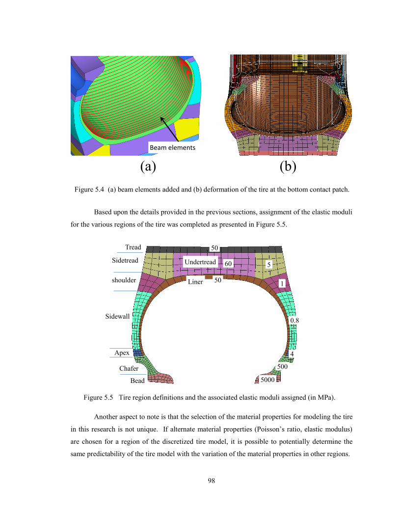
98

Based upon the details provided in the previous sections, assignment of the elastic moduli

for the various regions of the tire was completed as presented in Figure 5.5.

Another aspect to note is that the selection of the material properties for modeling the tire

in this research is not unique. If alternate material properties (Poisson’s ratio, elastic modulus)

are chosen for a region of the discretized tire model, it is possible to potentially determine the

same predictability of the tire model with the variation of the material properties in other regions.

Liner

60

50

5

5000

500

501

0.8

4

Chafer

Sidewall

shoulder

Sidetread

Tread

Bead

Undertread

Apex

Figure 5.5 Tire region definitions and the associated elastic moduli assigned (in MPa).

Beam elements

(a) (b)

Figure 5.4 (a) beam elements added and (b) deformation of the tire at the bottom contact patch.

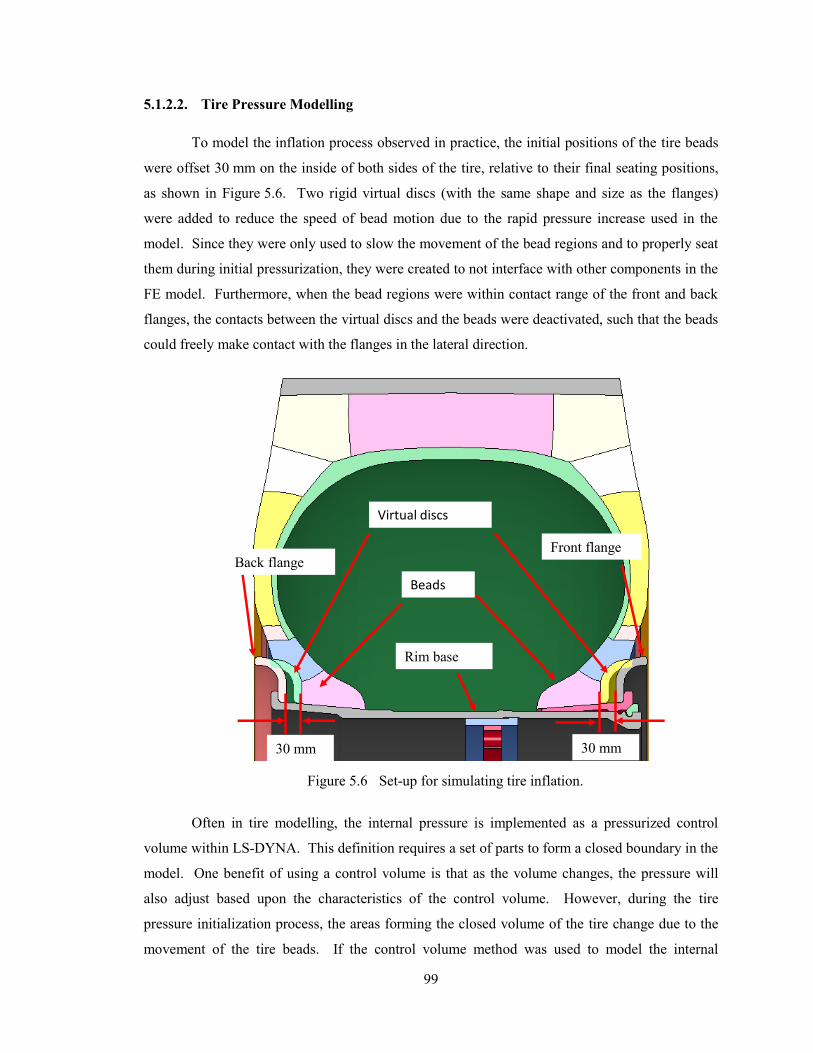
99

5.1.2.2. Tire Pressure Modelling

To model the inflation process observed in practice, the initial positions of the tire beads

were offset 30 mm on the inside of both sides of the tire, relative to their final seating positions,

as shown in Figure 5.6. Two rigid virtual discs (with the same shape and size as the flanges)

were added to reduce the speed of bead motion due to the rapid pressure increase used in the

model. Since they were only used to slow the movement of the bead regions and to properly seat

them during initial pressurization, they were created to not interface with other components in the

FE model. Furthermore, when the bead regions were within contact range of the front and back

flanges, the contacts between the virtual discs and the beads were deactivated, such that the beads

could freely make contact with the flanges in the lateral direction.

Often in tire modelling, the internal pressure is implemented as a pressurized control

volume within LS-DYNA. This definition requires a set of parts to form a closed boundary in the

model. One benefit of using a control volume is that as the volume changes, the pressure will

also adjust based upon the characteristics of the control volume. However, during the tire

pressure initialization process, the areas forming the closed volume of the tire change due to the

movement of the tire beads. If the control volume method was used to model the internal

30 mm

Virtual discs

Back flangeFront flange

Beads

Rim base

30 mm

Figure 5.6 Set-up for simulating tire inflation.

100

pressure, it would be difficult to define the control volume due to the inconsistent enclosed

boundary resulting from large bead movement. Under load conditions considered in this study,

the enclosed volume was assumed to experience negligible volume change and the temperature of

air inside the tire was similarly assumed constant, therefore the pressure inside the tire was

assumed unchanged. In an effort to reduce the complexity of the tire model in this study, the tire

pressure was modelled with constant surface pressure applied on the tire inner surface.

5.1.2.3. Other Critical Modelling Features

A penalty based surface to surface contact definition was applied to model the interaction

between all tire and wheel components. For contacts amongst wheel components, which were

modelled as steel, a coefficient of static friction of 0.35 was used. A coefficient of static friction

of 0.2 was applied to contact areas between the bead region and the BS band and rim, to reflect

the fact that in practice a lubricant is applied to the bead region to ensure it can slide along the BS

band/rim with ease during the inflation process.

At the interface between the chafer and the front/back flanges, where no lubricant was

applied and to ensure the tight contact within this region, a coefficient of friction varying from

0.85 to 1.0 was considered in the model development. Observations regarding the relative

movement of this portion of the tire and the wheel indicated no separation at this interface

throughout all testing. This range of the coefficient of friction was realistic given that the

coefficient of static friction between rubber and solids has been noted to range from 1.0 to 4.0

under dry conditions [123] and from 0.6 to 0.9 between steel and rubber [124]. A final value of

unity for the coefficient of friction was used within this investigation.

A stationary rigid wall was created below the bottom of the tire to model the contact

between the tire and the ground, with a friction of coefficient of 1.0 to prevent tire slip.

During early model development, the application of static forces resulted in tire

deformation hysteresis and tire vibrations. These traits are attributable to the interior pressure of

the tire. To address the presence of deformation hysteresis and tire vibrations within the model,

mass weighted nodal damping and second order objective stress updates were applied to the

model [120]. The force vector (Fdamp) due to system damping was determined from Equation (5.1)

according to LS-DYNA [114].

(5.1)

101

In the equation, is the natural frequency (given in radians per unit time), m is the nodal

mass, and is the nodal velocity. This is done to achieve the effect of damping both rigid body

motion as well as tire vibration. To assess the amount of damping required for the model, an

eigenvalue analysis was conducted to find the natural frequency of the model. This allowed

determination of damping constants suitable for the tire pressurization process and static force

application which were selected as 35 and 39, respectively. With these damping constants, the

damping energy was less than 25% of the internal energy of the model, thus validating the use of

damping.

To circumvent hourglass deformation, the Flanagan-Belytschko stiffness hourglass

control with a coefficient of 0.1 was employed for the entire tire [114]. Hourglass modes are

nonphysical, zero-energy modes of deformation that produce zero strain and no

stress. Hourglass modes occur only in under-integrated solid, shell, and thick shell elements.

LS-DYNA has various algorithms for inhibiting hourglass modes. Hourglass control introduces

non-physical energy in the FE analysis and this energy is referred to as hourglass energy.

Hourglass energy should be kept as low as possible, typically less than 10% of the system’s peak

internal energy. For the simulations conducted in this research, the maximum hourglass energy

was found to be 6.29% of the peak internal energy of the simulation.

Mass scaling and time scaling techniques were used to improve the computational

efficiency of the model. The time periods of the excitations of the tire during the experimental

deflection testing were approximately 10 seconds. These time durations were reduced by one

order of magnitude when used in the FE model in order to expedite the simulations, without

affecting the acceptable levels of accuracy. In order to maximize the time step during simulations,

a constant time step of 1.8 μs was used, with the majority of the mass added to the lock ring

portion of the wheel, as most of the small elements are located in this part due to geometric

constraints. Trial simulations without mass scaling were conducted and compared to simulations

with mass scaling where results indicated a negligible difference in model behaviour. The FE

keywords used in tire modeling was illustrated in Appendix E.1, with important parameters of FE

modeling included.

5.1.2.4. Static and Quasi-static Deflection Testing Simulations

Due to the symmetry of geometry and boundary conditions, only half of the wheel

assembly was modelled and symmetric boundary conditions were applied along the plane of

symmetry, for static load simulations. The half wheel assembly model contained 65,520

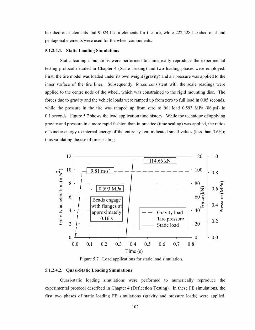
102

hexahedronal elements and 9,024 beam elements for the tire, while 222,528 hexahedronal and

pentagonal elements were used for the wheel components.

5.1.2.4.1. Static Loading Simulations

Static loading simulations were performed to numerically reproduce the experimental

testing protocol detailed in Chapter 4 (Scale Testing) and two loading phases were employed.

First, the tire model was loaded under its own weight (gravity) and air pressure was applied to the

inner surface of the tire liner. Subsequently, forces consistent with the scale readings were

applied to the centre node of the wheel, which was constrained to the rigid mounting disc. The

forces due to gravity and the vehicle loads were ramped up from zero to full load in 0.05 seconds,

while the pressure in the tire was ramped up from zero to full load 0.593 MPa (86 psi) in

0.1 seconds. Figure 5.7 shows the load application time history. While the technique of applying

gravity and pressure in a more rapid fashion than in practice (time scaling) was applied, the ratios

of kinetic energy to internal energy of the entire system indicated small values (less than 3.6%);

thus validating the use of time scaling.

5.1.2.4.2. Quasi-Static Loading Simulations

Quasi-static loading simulations were performed to numerically reproduce the

experimental protocol described in Chapter 4 (Deflection Testing). In these FE simulations, the

first two phases of static loading FE simulations (gravity and pressure loads) were applied,

Time (s)

0.0 0.1 0.2 0.3 0.4 0.5 0.6 0.7 0.8

Gra

vit

y a

ccel

erat

ion

(m

/s2

)

0

2

4

6

8

10

12

Pre

ssu

re (

MP

a)

0.0

0.2

0.4

0.6

0.8

1.0

Fo

rce

(kN

)

0

20

40

60

80

100

120

Gravity load

Tire pressure

Static load

0.593 MPa

114.66 kN

9.81 m/s2

Beads engage

with flanges at

approximately

0.16 s

Figure 5.7 Load applications for static load simulation.

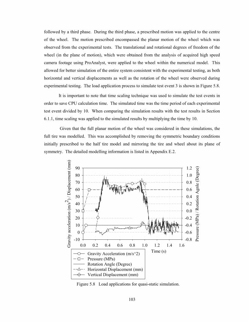
103

followed by a third phase. During the third phase, a prescribed motion was applied to the centre

of the wheel. The motion prescribed encompassed the planar motion of the wheel which was

observed from the experimental tests. The translational and rotational degrees of freedom of the

wheel (in the plane of motion), which were obtained from the analysis of acquired high speed

camera footage using ProAnalyst, were applied to the wheel within the numerical model. This

allowed for better simulation of the entire system consistent with the experimental testing, as both

horizontal and vertical displacements as well as the rotation of the wheel were observed during

experimental testing. The load application process to simulate test event 3 is shown in Figure 5.8.

It is important to note that time scaling technique was used to simulate the test events in

order to save CPU calculation time. The simulated time was the time period of each experimental

test event divided by 10. When comparing the simulation results with the test results in Section

6.1.1, time scaling was applied to the simulated results by multiplying the time by 10.

Given that the full planar motion of the wheel was considered in these simulations, the

full tire was modelled. This was accomplished by removing the symmetric boundary conditions

initially prescribed to the half tire model and mirroring the tire and wheel about its plane of

symmetry. The detailed modelling information is listed in Appendix E.2.

Time (s)

0.0 0.2 0.4 0.6 0.8 1.0 1.2 1.4 1.6Gra

vit

y a

ccel

erat

ion

(m

/s2

) /

Dis

pla

cem

ent

(mm

)

-10

0

10

20

30

40

50

60

70

80

90

Pre

ssu

re (

MP

a) /

Ro

tati

on

Ag

nle

(D

egre

e)

-0.8

-0.6

-0.4

-0.2

0.0

0.2

0.4

0.6

0.8

1.0

1.2

Gravity Acceleration (m/s^2)

Pressure (MPa)

Rotation Angle (Degree)

Horizontal Displacement (mm)

Vertical Displacement (mm)

Figure 5.8 Load applications for quasi-static simulation.

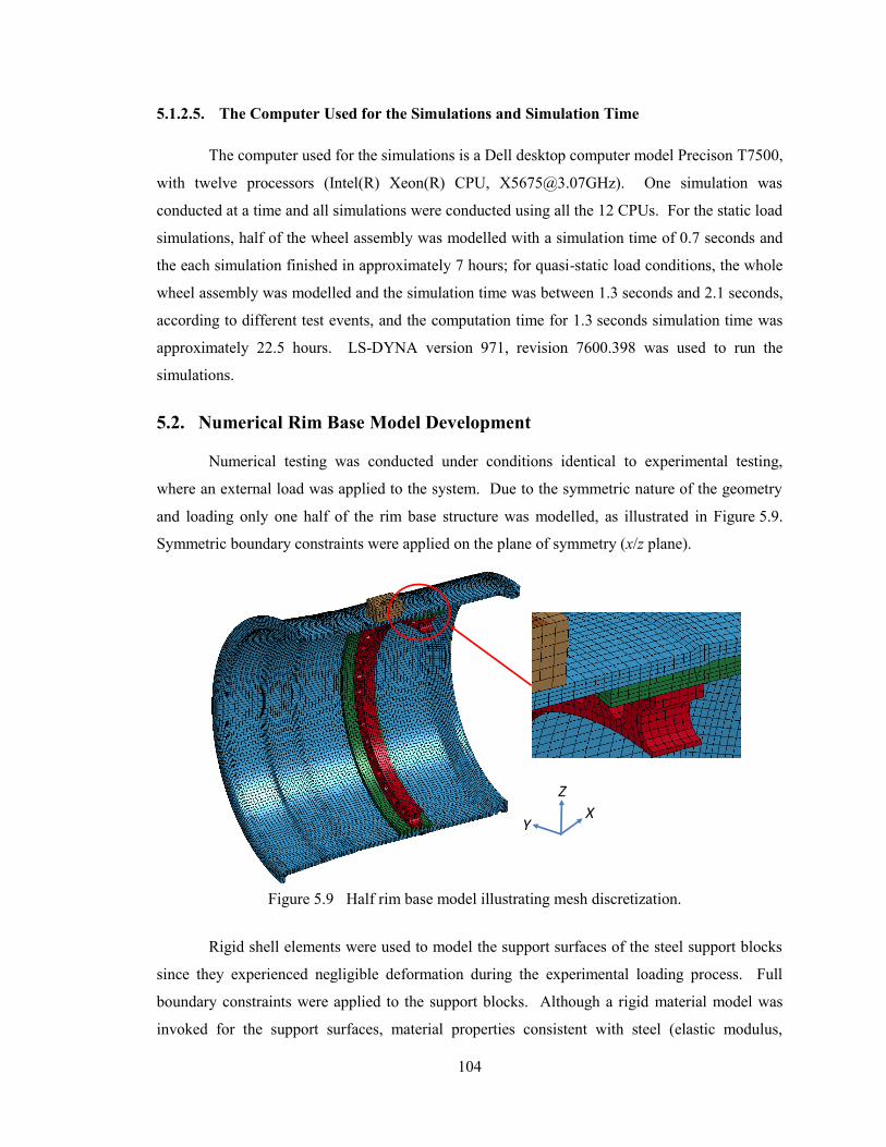
104

5.1.2.5. The Computer Used for the Simulations and Simulation Time

The computer used for the simulations is a Dell desktop computer model Precison T7500,

with twelve processors (Intel(R) Xeon(R) CPU, X5675@3.07GHz). One simulation was

conducted at a time and all simulations were conducted using all the 12 CPUs. For the static load

simulations, half of the wheel assembly was modelled with a simulation time of 0.7 seconds and

the each simulation finished in approximately 7 hours; for quasi-static load conditions, the whole

wheel assembly was modelled and the simulation time was between 1.3 seconds and 2.1 seconds,

according to different test events, and the computation time for 1.3 seconds simulation time was

approximately 22.5 hours. LS-DYNA version 971, revision 7600.398 was used to run the

simulations.

5.2. Numerical Rim Base Model Development

Numerical testing was conducted under conditions identical to experimental testing,

where an external load was applied to the system. Due to the symmetric nature of the geometry

and loading only one half of the rim base structure was modelled, as illustrated in Figure 5.9.

Symmetric boundary constraints were applied on the plane of symmetry (x/z plane).

Rigid shell elements were used to model the support surfaces of the steel support blocks

since they experienced negligible deformation during the experimental loading process. Full

boundary constraints were applied to the support blocks. Although a rigid material model was

invoked for the support surfaces, material properties consistent with steel (elastic modulus,

Z

XY

Figure 5.9 Half rim base model illustrating mesh discretization.

105

density, and Poisson’s ratio equal to 210 GPa, 7800 kg/m3 and 0.28, respectively) were applied

within the rigid material definition. Although no deformation of the elements occurs, such

information is needed for the contact definitions which contain the support surfaces.

The 50.8 mm diameter aluminum pad was modelled with rigid shell elements and used to

apply the external load to the system. Single point boundary constraints were applied to the

aluminum pad to permit motion in only the z-axis direction. The rigid material model utilized for

the aluminum pad incorporated material properties consistent with aluminum (elastic modulus,

density, and Poisson’s ratio equal to 72 GPa, 2700 kg/m3 and 0.33, respectively).

The rectangular aluminum block, which conformed to the curved profile of the rim base,

was modelled using single point quadrature solid elements having elastic material properties. The

elastic modulus, density, and Poisson’s ratio of the rectangular aluminum block was prescribed as

72 GPa, 2700 kg/m3 and 0.33, respectively. No permanent deformations of the block were noted

in any of the experimental tests. Under-integrated solid elements were utilized for the aluminum

block, with 384 elements used to discretize this structure. The aspect ratio of the elements within

this portion of the model was approximately 1.2.

Surface to surface contact definitions were used to establish interfaces between (1) the

rigid disc and the aluminum block, (2) the aluminum block and the rim, and (3) the rim and

support blocks. The coefficient of friction, within these contact algorithms, is a function of the

static and dynamic coefficients of friction as well as the relative sliding velocity between surfaces

and a decay coefficient as expressed in Equation (5.2) [114].

( ) | | (5.2)

No relative motion was noted to occur within the experimental testing and thus a

consistent coefficient of friction equal to 0.3 was applied. This occurs if μS = μD = 0.3 and DC =

0 as was implemented into the model. This coefficient of friction was determined from simple

experimental testing completed between the interacting surfaces. Gravity was also applied to the

system, with a local acceleration due to gravity of 9.807 m/s2 prescribed.

The cross-section of the rim base (within the x/z plane), excluding the mounting ring, was

first meshed using shell elements, which were then revolved about the centreline of the rim to

form the three dimensional FE model of the structure. Careful discretization of the cross-section

was completed to ensure that a suitably sized mesh was constructed with interior angles

approximately equal to 90 degrees. Furthermore, a uniform and consistent mesh through the

cross-section was developed. Following this process the shell elements were revolved about the

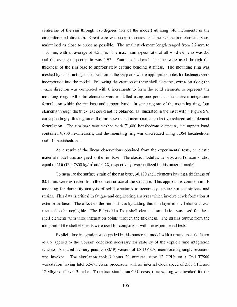
106

centreline of the rim through 180 degrees (1/2 of the model) utilizing 140 increments in the

circumferential direction. Great care was taken to ensure that the hexahedron elements were

maintained as close to cubes as possible. The smallest element length ranged from 2.2 mm to

11.0 mm, with an average of 4.5 mm. The maximum aspect ratio of all solid elements was 3.6

and the average aspect ratio was 1.92. Four hexahedronal elements were used through the

thickness of the rim base to appropriately capture bending stiffness. The mounting ring was

meshed by constructing a shell section in the y/z plane where appropriate holes for fasteners were

incorporated into the model. Following the creation of these shell elements, extrusion along the

x-axis direction was completed with 6 increments to form the solid elements to represent the

mounting ring. All solid elements were modelled using one point constant stress integration

formulation within the rim base and support band. In some regions of the mounting ring, four

elements through the thickness could not be obtained, as illustrated in the inset within Figure 5.9,

correspondingly, this region of the rim base model incorporated a selective reduced solid element

formulation. The rim base was meshed with 71,680 hexahedrons elements, the support band

contained 9,800 hexahedrons, and the mounting ring was discretized using 5,064 hexahedrons

and 144 pentahedrons.

As a result of the linear observations obtained from the experimental tests, an elastic

material model was assigned to the rim base. The elastic modulus, density, and Poisson’s ratio,

equal to 210 GPa, 7800 kg/m3 and 0.28, respectively, were utilized in this material model.

To measure the surface strain of the rim base, 36,120 shell elements having a thickness of

0.01 mm, were extracted from the outer surface of the structure. This approach is common in FE

modeling for durability analysis of solid structures to accurately capture surface stresses and

strains. This data is critical in fatigue and engineering analyses which involve crack formation at

exterior surfaces. The effect on the rim stiffness by adding this thin layer of shell elements was

assumed to be negligible. The Belytschko-Tsay shell element formulation was used for these

shell elements with three integration points through the thickness. The strains output from the

midpoint of the shell elements were used for comparison with the experimental tests.

Explicit time integration was applied in this numerical model with a time step scale factor

of 0.9 applied to the Courant condition necessary for stability of the explicit time integration

scheme. A shared memory parallel (SMP) version of LS-DYNA, incorporating single precision

was invoked. The simulation took 3 hours 30 minutes using 12 CPUs on a Dell T7500

workstation having Intel X5675 Xeon processors with an internal clock speed of 3.07 GHz and

12 Mbytes of level 3 cache. To reduce simulation CPU costs, time scaling was invoked for the

107

structural analyses. Loading was prescribed to the 50.8 mm diameter aluminum pad starting from

zero to 100 kN, in a manner consistent with the experimental tests. However, within the

numerical simulation, the time which the load was increased from zero to 100 kN was over a

period of 1 second. Following the completion of the simulation two critical observations were

investigated to ensure the appropriateness of the time scaled (quasi-static) solution. Firstly, it was

determined that the kinetic energy was found to be negligible (less than 1%) when compared to

the internal energy. Secondly, no significant differences between the applied external load at the

top of the rim base and the sum of the support loads at the two support bases was found.

Correspondingly, a quasi-static simulation was completed and the use of time scaling was

appropriately justified. Detailed modelling information is listed in the input file of Appendix E.3.

108

Chapter 6. Stress and Fatigue Life Analyses

The tire and rim base models were validated based on the comparisons of the results

between experimental tests and numerical simulations. The validated tire/wheel assembly model

was used to conduct stress and fatigue life assessment of the wheel components at critical regions

under severe loading conditions and the further design improvements of the multi-piece wheels

were based on the validated tire/wheel assembly model.

6.1. FE Model Validation

6.1.1. FE Model Validation for Tire 29.5-29

6.1.1.1. Validation Procedures

6.1.1.1.1. Static Loading Behaviour Validation

Validation of the numerical tire model was performed in three steps. First, the ability of

the tire model to correctly predict centre wheel deflection and maximum lateral sidewall

deflection for a prescribed centre wheel load was verified based on Goodyear engineering data.

As previously discussed (Table 4.2 and 4.3), the Goodyear data indicated that for tire 29.5-29,

under a static load equivalent to approximately 230 kN at wheel centre, the tire would experience

a vertical deflection of 80 mm and a maximum lateral sidewall deflection of 36.5 mm (one side),

when pressurized to 627 kPa (91 psi).

In the next step of validation, the static deflections of the simulated tire model under

various loads were compared with the experimentally obtained scale testing deflection

measurements in Chapter 4. This step is considered a comparison of static load deflection

behaviour of the tire, in which the gross vehicle weight was input into the FE model and the

vertical and maximum lateral sidewall deflections were output for comparison. Furthermore, as

the experimental tire pressure was 86 psi (0.593 MPa), this step is also used to validate the

effectiveness of the model at simulating pressure different from that which is referenced in the

Goodyear data.

The percentage error, calculated using Equation (6.1), was used to assess the predictive

capabilities of the numerical model relative to the experimental observation. In Equation (6.1)

‘Nv” represents the value of the numerical variable and ‘Ev’ represents the corresponding

experimental measurement.

109

(

) (6.1)

6.1.1.1.2. Quasi-Static Loading Behaviour Validation

The final step in the tire model validation consisted of comparing the deflections of the

model under the quasi-static loading conditions against the measurements recorded during the

deflection testing. In this step, two separate comparisons were able to be made, due to the

amount of data collected during the deflection testing; thus allowing for a more thorough

validation of the model in the most computationally intensive simulation regime of this study.

In the first comparison, the maximum lateral sidewall deflections of the tire were

compared to those experimentally obtained using the 100 mm Acuity AR700 series displacement

transducer. Data points were first plotted in the time domain to illustrate the lateral deflection as

a function of time and were subsequently plotted as a function of the vertical deflection of the

wheel centre.

In the physical tests, the laser displacement transducer was supported by a fixed height

tripod positioned on the ground. Due to the vertical deflections of the tire during loadings, the

measured lateral sidewall deflections were not of a fixed point on the tire, but instead of a

continuous vertical line, based on the amount of vertical tire deflection experienced at the

maximum lateral sidewall points. To account for these measurement variations, three nodal

points in the FE tire model were tracked within the vicinity of the area which was recorded by the

transducer. Results from tracking the three nodes indicated a difference in lateral deflection of 2-

3 mm per node. Therefore, the average of the three nodal measurements was taken for each

simulation, and was used to compare with the experimental testing data.

In the second comparison, the vertical (z-direction) and longitudinal (y-direction)

deflections of selected points on the tire was compared. As previously discussed, the

experimental deflection of these points were determined through acquisition of high speed

photographs, using a Fastec high speed camera followed by motion tracking of the various

highlighted locations in Figure 6.1(H-in, H-out, D-in, D-out, V-in, and V-out) using ProAnalyst.

The locations of the tracked points on the physical tire and the corresponding nodes tracked in the

FE model are illustrated in Figures 6.1 (a) and 6.1 (b).

For the quasi-static comparisons, maximum relative errors calculated using Equation (6.1)

and more rigorous accumulative errors and validation metrics using Equations (4.1) and (4.2)

were conducted.

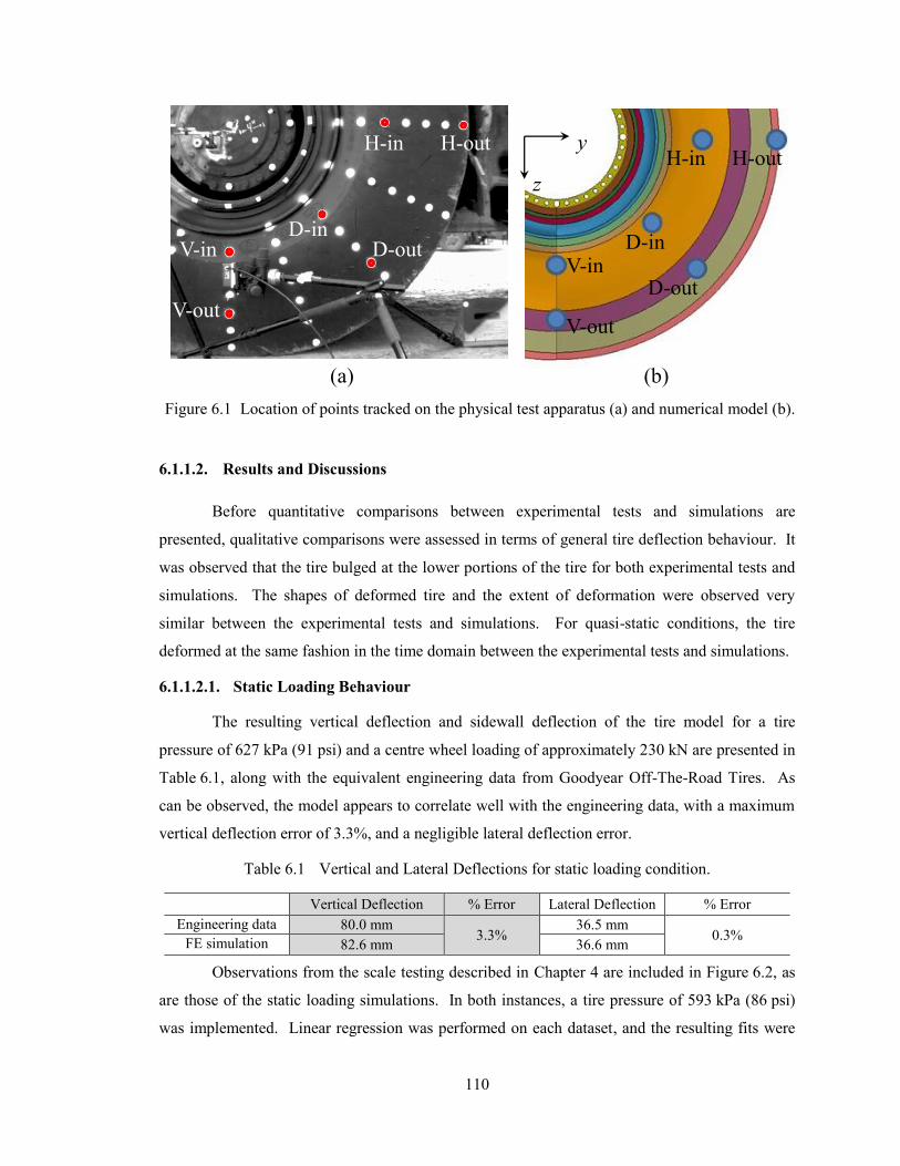
110

6.1.1.2. Results and Discussions

Before quantitative comparisons between experimental tests and simulations are

presented, qualitative comparisons were assessed in terms of general tire deflection behaviour. It

was observed that the tire bulged at the lower portions of the tire for both experimental tests and

simulations. The shapes of deformed tire and the extent of deformation were observed very

similar between the experimental tests and simulations. For quasi-static conditions, the tire

deformed at the same fashion in the time domain between the experimental tests and simulations.

6.1.1.2.1. Static Loading Behaviour

The resulting vertical deflection and sidewall deflection of the tire model for a tire

pressure of 627 kPa (91 psi) and a centre wheel loading of approximately 230 kN are presented in

Table 6.1, along with the equivalent engineering data from Goodyear Off-The-Road Tires. As

can be observed, the model appears to correlate well with the engineering data, with a maximum

vertical deflection error of 3.3%, and a negligible lateral deflection error.

Table 6.1 Vertical and Lateral Deflections for static loading condition.

Vertical Deflection % Error Lateral Deflection % Error

Engineering data 80.0 mm 3.3%

36.5 mm 0.3%

FE simulation 82.6 mm 36.6 mm

Observations from the scale testing described in Chapter 4 are included in Figure 6.2, as

are those of the static loading simulations. In both instances, a tire pressure of 593 kPa (86 psi)

was implemented. Linear regression was performed on each dataset, and the resulting fits were

H-in H-out

D-inD-outV-in

V-out

H-in H-out

D-in

D-outV-in

V-out

z

y

(a) (b)

Figure 6.1 Location of points tracked on the physical test apparatus (a) and numerical model (b).

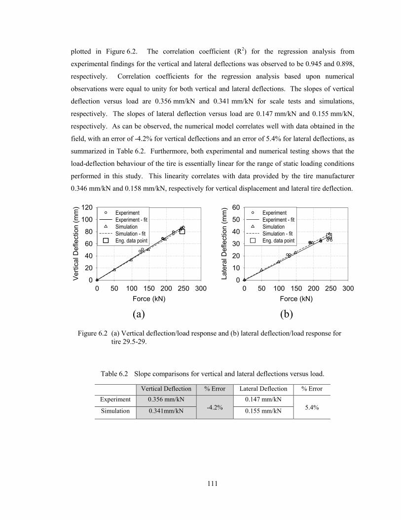
111

plotted in Figure 6.2. The correlation coefficient (R2) for the regression analysis from

experimental findings for the vertical and lateral deflections was observed to be 0.945 and 0.898,

respectively. Correlation coefficients for the regression analysis based upon numerical

observations were equal to unity for both vertical and lateral deflections. The slopes of vertical

deflection versus load are 0.356 mm/kN and 0.341 mm/kN for scale tests and simulations,

respectively. The slopes of lateral deflection versus load are 0.147 mm/kN and 0.155 mm/kN,

respectively. As can be observed, the numerical model correlates well with data obtained in the

field, with an error of -4.2% for vertical deflections and an error of 5.4% for lateral deflections, as

summarized in Table 6.2. Furthermore, both experimental and numerical testing shows that the

load-deflection behaviour of the tire is essentially linear for the range of static loading conditions

performed in this study. This linearity correlates with data provided by the tire manufacturer

0.346 mm/kN and 0.158 mm/kN, respectively for vertical displacement and lateral tire deflection.

Table 6.2 Slope comparisons for vertical and lateral deflections versus load.

Vertical Deflection % Error Lateral Deflection % Error

Experiment 0.356 mm/kN

-4.2%

0.147 mm/kN

5.4% Simulation 0.341mm/kN 0.155 mm/kN

Force (kN)

0 50 100 150 200 250 300

Ve

rtic

al D

efle

ctio

n (

mm

)

0

20

40

60

80

100

120Experiment

Experiment - fit

Simulation

Simulation - fit

Eng. data point

Force (kN)

0 50 100 150 200 250 300

La

tera

l D

efle

ctio

n (

mm

)

0

10

20

30

40

50

60Experiment

Experiment - fit

Simulation

Simulation - fit

Eng. data point

(a) (b)

Figure 6.2 (a) Vertical deflection/load response and (b) lateral deflection/load response for

tire 29.5-29.

112

6.1.1.2.2. Quasi-Static Loading Behaviour

Maximum Lateral Sidewall Deflection

The results from experimental deflection test events as described in Chapter 4 are

presented in in Figures 6.3 to 6.6, as well as the numerical results from the quasi-static loading

simulations described in Chapter 5. Event 1, with observations presented in Figure 6.3 (a) and

6.3 (b), was the most severe loading condition on the tire, resulting in a maximum vertical

deflection of approximately 80 mm. The corresponding lateral deflection for this event was noted

to be maximized, having a value of approximately 35 mm, when the vertical deflections were

most significant. A linear relationship between lateral and vertical deflections was noted for all

events for both experimental and numerical findings. A regression analysis of the lateral/vertical

deflection relationship resulted in slopes for event 1, 2, and 3, of 0.396 mm/mm, 0.359 mm/mm,

and 0.346 mm/mm, respectively. This finding indicates that the lateral deflections were typically

37% of the vertical deflections and consistency amongst all tests was noted. Differences in the

slopes of the lateral/vertical deflection relationship from experimental findings to numerical

predictions were typically less than 13%, with the average slope for numerical findings being

equal to 0.39 mm/mm. A minor degree of hysteresis was noted in both testing methods, with the

experimental observations being slightly greater on this aspect of the lateral/vertical deflection

relationship.

For the time domain comparisons, the numerical results demonstrate good correlation

with tire deflections obtained experimentally for all test events. For event 1, there exists a

difference of approximately 17% between the numerical and experimental findings, from 1.8 s to

3.5 s. However, for the remainder of the simulation, the percentage error is almost negligible

between the two responses. Results from events 2 and 3 also demonstrate good correlation

between numerical and experimental findings, with the numerical models only over-predicting

the experimental findings by a maximum of 10% during the entire duration of each event.

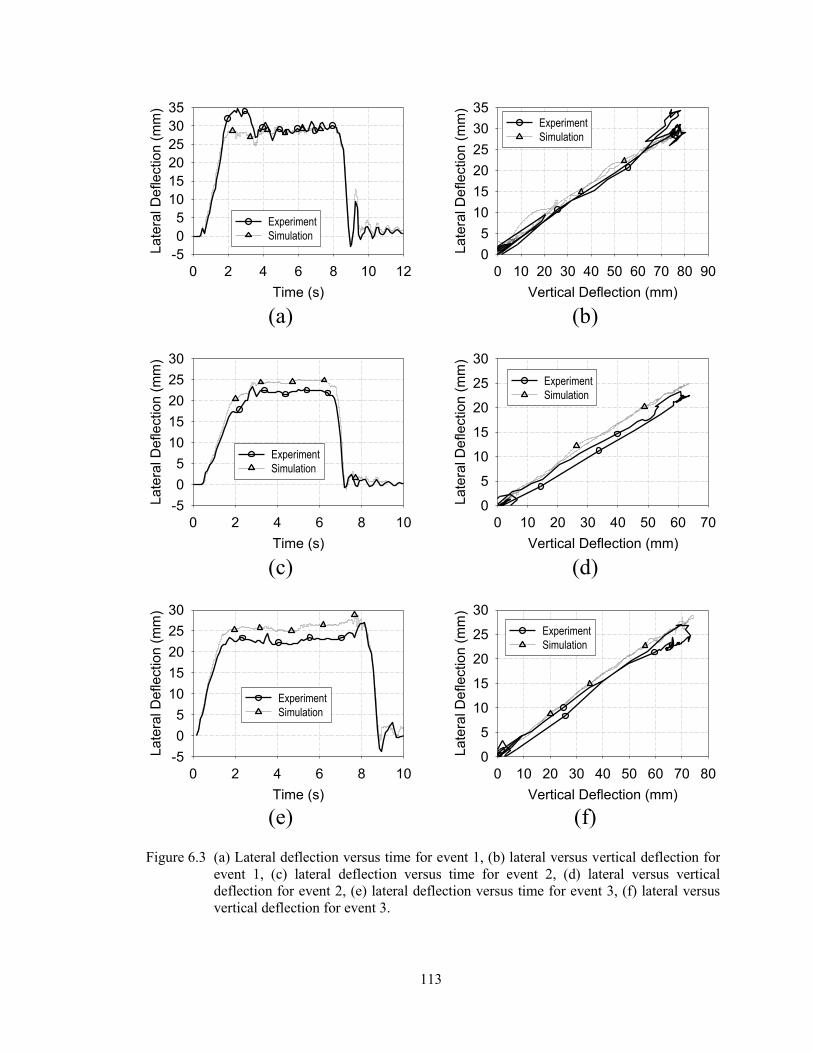
113

Time (s)

0 2 4 6 8 10 12

Late

ral D

eflection (

mm

)

-5

0

5

10

15

20

25

30

35

Experiment

Simulation

Vertical Deflection (mm)

0 10 20 30 40 50 60 70 80 90

Late

ral D

eflection (

mm

)

0

5

10

15

20

25

30

35Experiment

Simulation

(a) (b)

Time (s)

0 2 4 6 8 10

Late

ral D

eflection (

mm

)

-5

0

5

10

15

20

25

30

Experiment

Simulation

Vertical Deflection (mm)

0 10 20 30 40 50 60 70 80

Late

ral D

eflection (

mm

)

0

5

10

15

20

25

30

Experiment

Simulation

(e) (f)

Time (s)

0 2 4 6 8 10

Late

ral D

eflection (

mm

)

-5

0

5

10

15

20

25

30

Experiment

Simulation

Vertical Deflection (mm)

0 10 20 30 40 50 60 70

Late

ral D

eflection (

mm

)

0

5

10

15

20

25

30

Experiment

Simulation

(c) (d)

Figure 6.3 (a) Lateral deflection versus time for event 1, (b) lateral versus vertical deflection for

event 1, (c) lateral deflection versus time for event 2, (d) lateral versus vertical

deflection for event 2, (e) lateral deflection versus time for event 3, (f) lateral versus

vertical deflection for event 3.

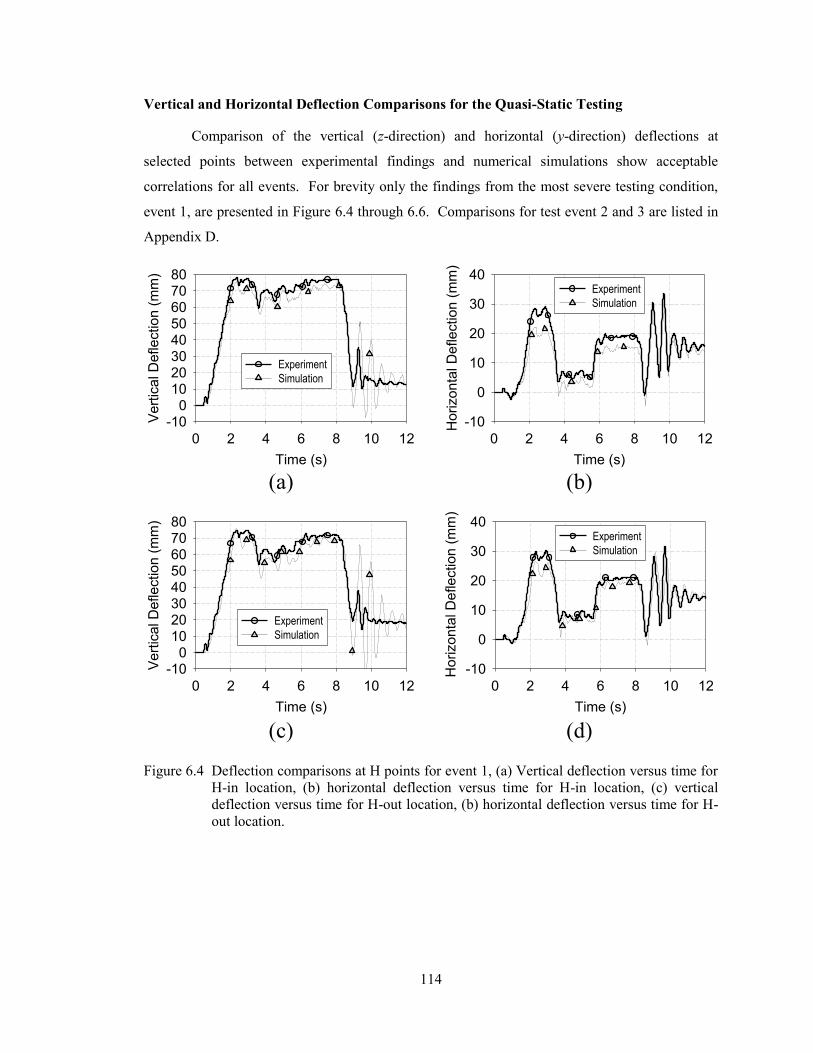
114

Vertical and Horizontal Deflection Comparisons for the Quasi-Static Testing

Comparison of the vertical (z-direction) and horizontal (y-direction) deflections at

selected points between experimental findings and numerical simulations show acceptable

correlations for all events. For brevity only the findings from the most severe testing condition,

event 1, are presented in Figure 6.4 through 6.6. Comparisons for test event 2 and 3 are listed in

Appendix D.

Time (s)

0 2 4 6 8 10 12

Vert

ical D

eflection (

mm

)

-100

1020304050607080

Experiment

Simulation

Time (s)

0 2 4 6 8 10 12H

orizonta

l D

eflection (

mm

)

-10

0

10

20

30

40Experiment

Simulation

Time (s)

0 2 4 6 8 10 12

Vert

ical D

eflection (

mm

)

-100

1020304050607080

Experiment

Simulation

Time (s)

0 2 4 6 8 10 12

Horizonta

l D

eflection (

mm

)

-10

0

10

20

30

40Experiment

Simulation

(a) (b)

(c) (d)

Figure 6.4 Deflection comparisons at H points for event 1, (a) Vertical deflection versus time for

H-in location, (b) horizontal deflection versus time for H-in location, (c) vertical

deflection versus time for H-out location, (b) horizontal deflection versus time for H-

out location.

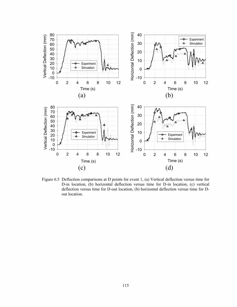
115

Time (s)

0 2 4 6 8 10 12

Ve

rtic

al D

efle

ctio

n (

mm

)

-100

1020304050607080

Experiment

Simulation

Time (s)

0 2 4 6 8 10 12

Ho

rizo

nta

l D

efle

ctio

n (

mm

)

-10

0

10

20

30

40Experiment

Simulation

Time (s)

0 2 4 6 8 10 12

Ho

rizo

nta

l D

efle

ctio

n (

mm

)

-10

0

10

20

30

40

Experiment

Simulation

(a) (b)

(c) (d)Time (s)

0 2 4 6 8 10 12

Vert

ical D

eflection (

mm

)

-100

1020304050607080

Experiment

Simulation

Figure 6.5 Deflection comparisons at D points for event 1, (a) Vertical deflection versus time for

D-in location, (b) horizontal deflection versus time for D-in location, (c) vertical

deflection versus time for D-out location, (b) horizontal deflection versus time for D-

out location.

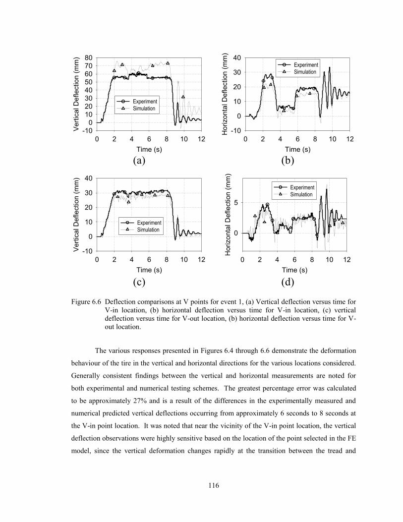
116

The various responses presented in Figures 6.4 through 6.6 demonstrate the deformation

behaviour of the tire in the vertical and horizontal directions for the various locations considered.

Generally consistent findings between the vertical and horizontal measurements are noted for

both experimental and numerical testing schemes. The greatest percentage error was calculated

to be approximately 27% and is a result of the differences in the experimentally measured and

numerical predicted vertical deflections occurring from approximately 6 seconds to 8 seconds at

the V-in point location. It was noted that near the vicinity of the V-in point location, the vertical

deflection observations were highly sensitive based on the location of the point selected in the FE

model, since the vertical deformation changes rapidly at the transition between the tread and

Time (s)

0 2 4 6 8 10 12

Ve

rtic

al D

efle

ctio

n (

mm

)

-100

1020304050607080

Experiment

Simulation

Time (s)

0 2 4 6 8 10 12

Ho

rizo

nta

l D

efle

ctio

n (

mm

)

-10

0

10

20

30

40Experiment

Simulation

Time (s)

0 2 4 6 8 10 12

Ve

rtic

al D

efle

ctio

n (

mm

)

-10

0

10

20

30

40

Experiment

Simulation

Time (s)

0 2 4 6 8 10 12

Ho

rizo

nta

l D

efle

ction

(m

m)

0

5

Experiment

Simulation

(a) (b)

(c) (d)

Figure 6.6 Deflection comparisons at V points for event 1, (a) Vertical deflection versus time for

V-in location, (b) horizontal deflection versus time for V-in location, (c) vertical

deflection versus time for V-out location, (b) horizontal deflection versus time for V-

out location.

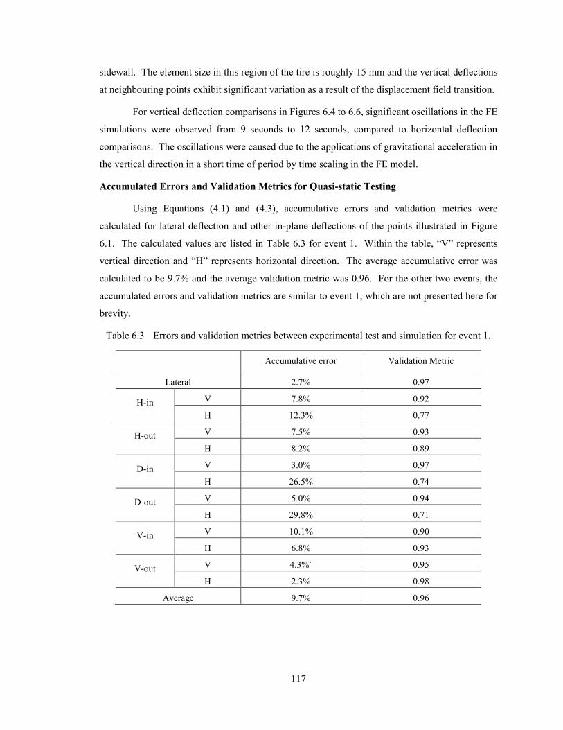
117

sidewall. The element size in this region of the tire is roughly 15 mm and the vertical deflections

at neighbouring points exhibit significant variation as a result of the displacement field transition.

For vertical deflection comparisons in Figures 6.4 to 6.6, significant oscillations in the FE

simulations were observed from 9 seconds to 12 seconds, compared to horizontal deflection

comparisons. The oscillations were caused due to the applications of gravitational acceleration in

the vertical direction in a short time of period by time scaling in the FE model.

Accumulated Errors and Validation Metrics for Quasi-static Testing

Using Equations (4.1) and (4.3), accumulative errors and validation metrics were

calculated for lateral deflection and other in-plane deflections of the points illustrated in Figure

6.1. The calculated values are listed in Table 6.3 for event 1. Within the table, “V” represents

vertical direction and “H” represents horizontal direction. The average accumulative error was

calculated to be 9.7% and the average validation metric was 0.96. For the other two events, the

accumulated errors and validation metrics are similar to event 1, which are not presented here for

brevity.

Table 6.3 Errors and validation metrics between experimental test and simulation for event 1.

Accumulative error Validation Metric

Lateral 2.7% 0.97

H-in V 7.8% 0.92

H 12.3% 0.77

H-out V 7.5% 0.93

H 8.2% 0.89

D-in V 3.0% 0.97

H 26.5% 0.74

D-out V 5.0% 0.94

H 29.8% 0.71

V-in V 10.1% 0.90

H 6.8% 0.93

V-out V 4.3%` 0.95

H 2.3% 0.98

Average 9.7% 0.96

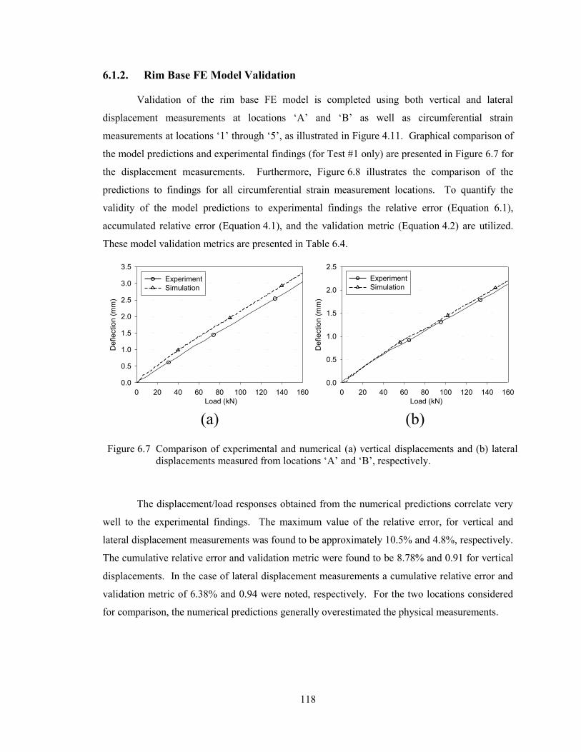
118

6.1.2. Rim Base FE Model Validation

Validation of the rim base FE model is completed using both vertical and lateral

displacement measurements at locations ‘A’ and ‘B’ as well as circumferential strain

measurements at locations ‘1’ through ‘5’, as illustrated in Figure 4.11. Graphical comparison of

the model predictions and experimental findings (for Test #1 only) are presented in Figure 6.7 for

the displacement measurements. Furthermore, Figure 6.8 illustrates the comparison of the

predictions to findings for all circumferential strain measurement locations. To quantify the

validity of the model predictions to experimental findings the relative error (Equation 6.1),

accumulated relative error (Equation 4.1), and the validation metric (Equation 4.2) are utilized.

These model validation metrics are presented in Table 6.4.

The displacement/load responses obtained from the numerical predictions correlate very

well to the experimental findings. The maximum value of the relative error, for vertical and

lateral displacement measurements was found to be approximately 10.5% and 4.8%, respectively.

The cumulative relative error and validation metric were found to be 8.78% and 0.91 for vertical

displacements. In the case of lateral displacement measurements a cumulative relative error and

validation metric of 6.38% and 0.94 were noted, respectively. For the two locations considered

for comparison, the numerical predictions generally overestimated the physical measurements.

Load (kN)

0 20 40 60 80 100 120 140 160

Defle

ctio

n (

mm

)

0.0

0.5

1.0

1.5

2.0

2.5

3.0

3.5

Experiment

Simulation

Load (kN)

0 20 40 60 80 100 120 140 160

Defle

ctio

n (

mm

)

0.0

0.5

1.0

1.5

2.0

2.5

Experiment

Simulation

(a) (b)

Figure 6.7 Comparison of experimental and numerical (a) vertical displacements and (b) lateral

displacements measured from locations ‘A’ and ‘B’, respectively.

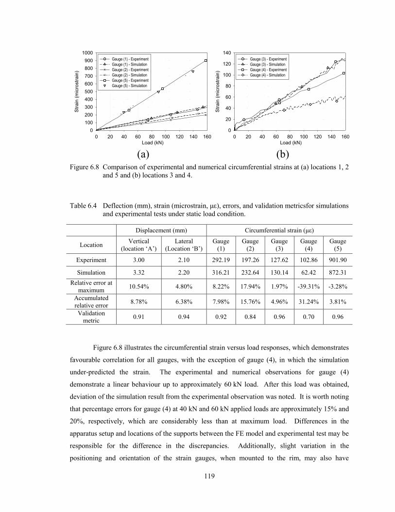
119

Table 6.4 Deflection (mm), strain (microstrain, με), errors, and validation metricsfor simulations

and experimental tests under static load condition.

Displacement (mm) Circumferential strain (με)

Location Vertical

(location ‘A’)

Lateral

(Location ‘B’)

Gauge

(1)

Gauge

(2)

Gauge

(3)

Gauge

(4)

Gauge

(5)

Experiment 3.00 2.10 292.19 197.26 127.62 102.86 901.90

Simulation 3.32 2.20 316.21 232.64 130.14 62.42 872.31

Relative error at

maximum 10.54% 4.80% 8.22% 17.94% 1.97% -39.31% -3.28%

Accumulated

relative error 8.78% 6.38% 7.98% 15.76% 4.96% 31.24% 3.81%

Validation

metric 0.91 0.94 0.92 0.84 0.96 0.70 0.96

Figure 6.8 illustrates the circumferential strain versus load responses, which demonstrates

favourable correlation for all gauges, with the exception of gauge (4), in which the simulation

under-predicted the strain. The experimental and numerical observations for gauge (4)

demonstrate a linear behaviour up to approximately 60 kN load. After this load was obtained,

deviation of the simulation result from the experimental observation was noted. It is worth noting

that percentage errors for gauge (4) at 40 kN and 60 kN applied loads are approximately 15% and

20%, respectively, which are considerably less than at maximum load. Differences in the

apparatus setup and locations of the supports between the FE model and experimental test may be

responsible for the difference in the discrepancies. Additionally, slight variation in the

positioning and orientation of the strain gauges, when mounted to the rim, may also have

Load (kN)

0 20 40 60 80 100 120 140 160

Str

ain

(m

icro

str

ain

)

0

100

200

300

400

500

600

700

800

900

1000

X

X

X

U

U

U

Gauge (1) - Experiment

Gauge (1) - Simulation

Gauge (2) - ExperimentX

Gauge (2) - SimulationU

Gauge (5) - Experiment

Gauge (5) - Simulation

Load (kN)

0 20 40 60 80 100 120 140 160

Str

ain

(m

icro

str

ain

)

0

20

40

60

80

100

120

140

Gauge (3) - Experiment

Gauge (3) - Simulation

Gauge (4) - Experiment

Gauge (4) - Simulation

(a) (b)Figure 6.8 Comparison of experimental and numerical circumferential strains at (a) locations 1, 2

and 5 and (b) locations 3 and 4.

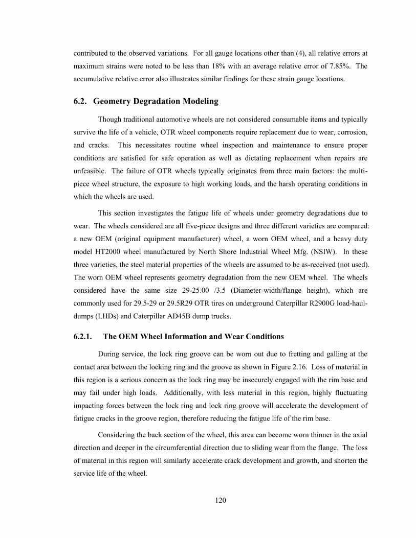
120

contributed to the observed variations. For all gauge locations other than (4), all relative errors at

maximum strains were noted to be less than 18% with an average relative error of 7.85%. The

accumulative relative error also illustrates similar findings for these strain gauge locations.

6.2. Geometry Degradation Modeling

Though traditional automotive wheels are not considered consumable items and typically

survive the life of a vehicle, OTR wheel components require replacement due to wear, corrosion,

and cracks. This necessitates routine wheel inspection and maintenance to ensure proper

conditions are satisfied for safe operation as well as dictating replacement when repairs are

unfeasible. The failure of OTR wheels typically originates from three main factors: the multi-

piece wheel structure, the exposure to high working loads, and the harsh operating conditions in

which the wheels are used.

This section investigates the fatigue life of wheels under geometry degradations due to

wear. The wheels considered are all five-piece designs and three different varieties are compared:

a new OEM (original equipment manufacturer) wheel, a worn OEM wheel, and a heavy duty

model HT2000 wheel manufactured by North Shore Industrial Wheel Mfg. (NSIW). In these

three varieties, the steel material properties of the wheels are assumed to be as-received (not used).

The worn OEM wheel represents geometry degradation from the new OEM wheel. The wheels

considered have the same size 29-25.00 /3.5 (Diameter-width/flange height), which are

commonly used for 29.5-29 or 29.5R29 OTR tires on underground Caterpillar R2900G load-haul-

dumps (LHDs) and Caterpillar AD45B dump trucks.

6.2.1. The OEM Wheel Information and Wear Conditions

During service, the lock ring groove can be worn out due to fretting and galling at the

contact area between the locking ring and the groove as shown in Figure 2.16. Loss of material in

this region is a serious concern as the lock ring may be insecurely engaged with the rim base and

may fail under high loads. Additionally, with less material in this region, highly fluctuating

impacting forces between the lock ring and lock ring groove will accelerate the development of

fatigue cracks in the groove region, therefore reducing the fatigue life of the rim base.

Considering the back section of the wheel, this area can become worn thinner in the axial

direction and deeper in the circumferential direction due to sliding wear from the flange. The loss

of material in this region will similarly accelerate crack development and growth, and shorten the

service life of the wheel.

121

In order to ensure the safety of OTR wheels, NSIW tracks most in-service wheels at mine

sites and carries out routine check-ups and maintenance as required. To facilitate inspections,

tolerance “GO/NO-GO” gauges were designed and used to check critical regions of the wheel.

Figure 6.9 shows the use of these gauges in the back section of the rim base. A “GO” condition

signifies the wear is not significant enough to warrant repair or replacement, whereas “NO-GO”

conditions means the wear in the particular region is too large and out of tolerance, meaning the

region has to be replaced or repaired in order to maintain safe working conditions. In

Figure 6.9(a), the gauge checks the thickness of the back section; in Figure 6.9(b), the gauge

checks the wear in the radial direction.

Figure 6.10 illustrates the use of a gauge in the front gutter region of the rim. Given a

“GO” condition, the wear in the groove is negligible whereas a “NO-GO” condition indicates

wear is significant enough for the gauge to fit in the groove. In this condition, the gutter region

must be replaced or the whole rim base must be discarded.

1 23

(a) (b)

GO GO

NO - GO NO - GO

Figure 6.9 Gauges are used to check the back section.

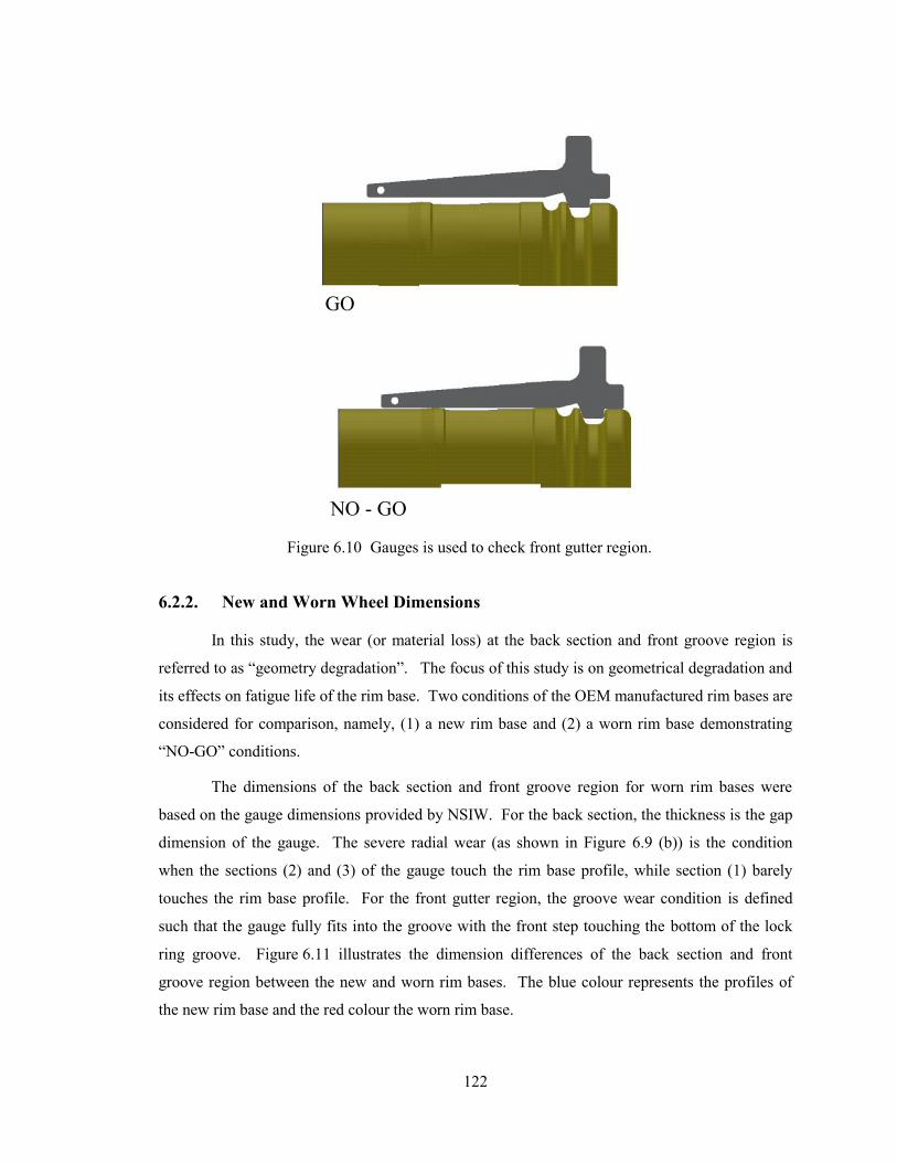
122

6.2.2. New and Worn Wheel Dimensions

In this study, the wear (or material loss) at the back section and front groove region is

referred to as “geometry degradation”. The focus of this study is on geometrical degradation and

its effects on fatigue life of the rim base. Two conditions of the OEM manufactured rim bases are

considered for comparison, namely, (1) a new rim base and (2) a worn rim base demonstrating

“NO-GO” conditions.

The dimensions of the back section and front groove region for worn rim bases were

based on the gauge dimensions provided by NSIW. For the back section, the thickness is the gap

dimension of the gauge. The severe radial wear (as shown in Figure 6.9 (b)) is the condition

when the sections (2) and (3) of the gauge touch the rim base profile, while section (1) barely

touches the rim base profile. For the front gutter region, the groove wear condition is defined

such that the gauge fully fits into the groove with the front step touching the bottom of the lock

ring groove. Figure 6.11 illustrates the dimension differences of the back section and front

groove region between the new and worn rim bases. The blue colour represents the profiles of

the new rim base and the red colour the worn rim base.

GO

NO - GO

Figure 6.10 Gauges is used to check front gutter region.

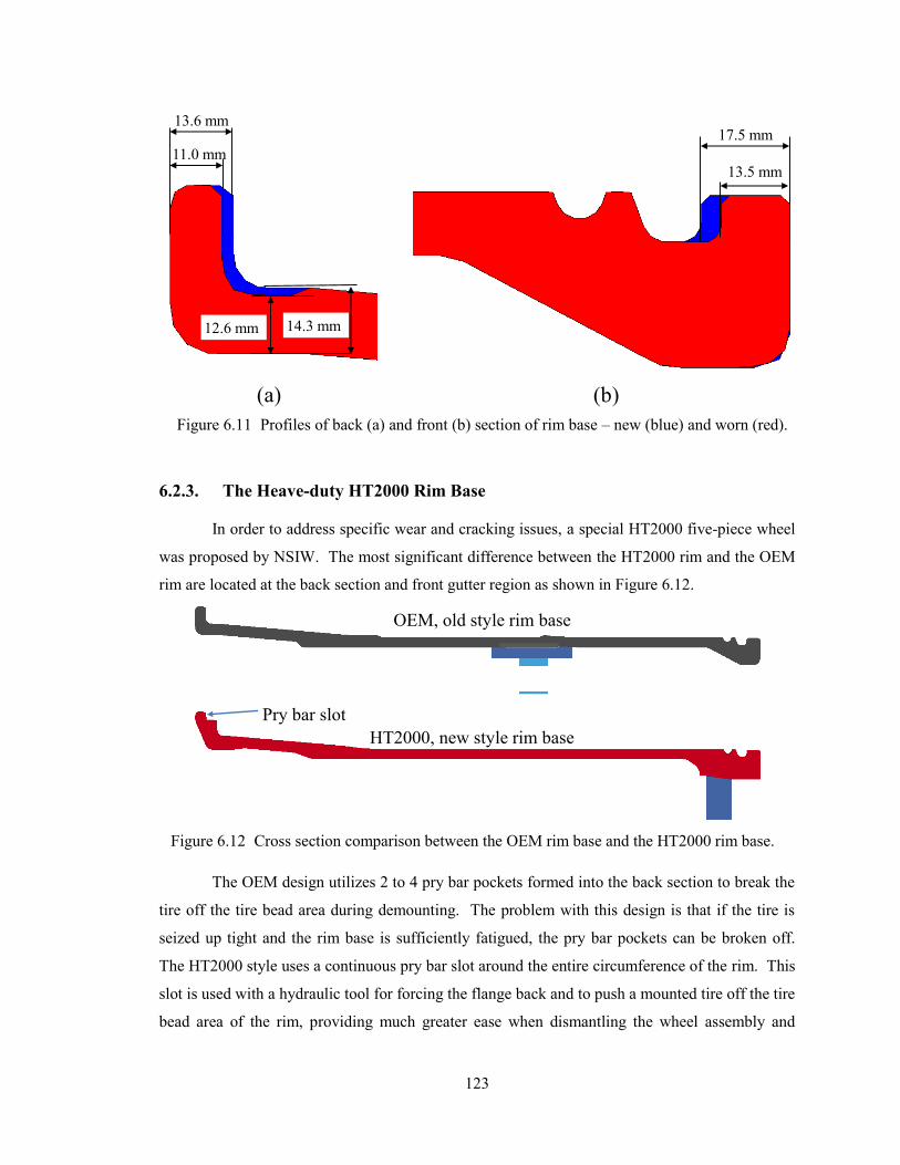
123

6.2.3. The Heave-duty HT2000 Rim Base

In order to address specific wear and cracking issues, a special HT2000 five-piece wheel

was proposed by NSIW. The most significant difference between the HT2000 rim and the OEM

rim are located at the back section and front gutter region as shown in Figure 6.12.

The OEM design utilizes 2 to 4 pry bar pockets formed into the back section to break the

tire off the tire bead area during demounting. The problem with this design is that if the tire is

seized up tight and the rim base is sufficiently fatigued, the pry bar pockets can be broken off.

The HT2000 style uses a continuous pry bar slot around the entire circumference of the rim. This

slot is used with a hydraulic tool for forcing the flange back and to push a mounted tire off the tire

bead area of the rim, providing much greater ease when dismantling the wheel assembly and

OEM, old style rim base

HT2000, new style rim base

Pry bar slot

Figure 6.12 Cross section comparison between the OEM rim base and the HT2000 rim base.

13.6 mm

14.3 mm

11.0 mm

12.6 mm

17.5 mm

13.5 mm

(a) (b)

Figure 6.11 Profiles of back (a) and front (b) section of rim base – new (blue) and worn (red).

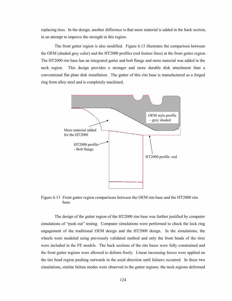
124

replacing tires. In the design, another difference is that more material is added in the back section,

in an attempt to improve the strength in this region.

The front gutter region is also modified. Figure 6.13 illustrates the comparison between

the OEM (shaded grey color) and the HT2000 profiles (red feature lines) at the front gutter region.

The HT2000 rim base has an integrated gutter and bolt flange and more material was added in the

neck region. This design provides a stronger and more durable disk attachment than a

conventional flat plate disk installation. The gutter of this rim base is manufactured as a forged

ring from alloy steel and is completely machined.

The design of the gutter region of the HT2000 rim base was further justified by computer

simulations of “push out” testing. Computer simulations were performed to check the lock ring

engagement of the traditional OEM design and the HT2000 design. In the simulations, the

wheels were modeled using previously validated method and only the front beads of the tires

were included in the FE models. The back sections of the rim bases were fully constrained and

the front gutter regions were allowed to deform freely. Linear increasing forces were applied on

the tire bead region pushing outwards in the axial direction until failures occurred. In these two

simulations, similar failure modes were observed in the gutter regions: the neck regions deformed

HT2000 profile -red

OEM style profile

– grey shaded

HT2000 profile

- Bolt flange

More material added

for the HT2000

Figure 6.13 Front gutter region comparisons between the OEM rim base and the HT2000 rim

base.

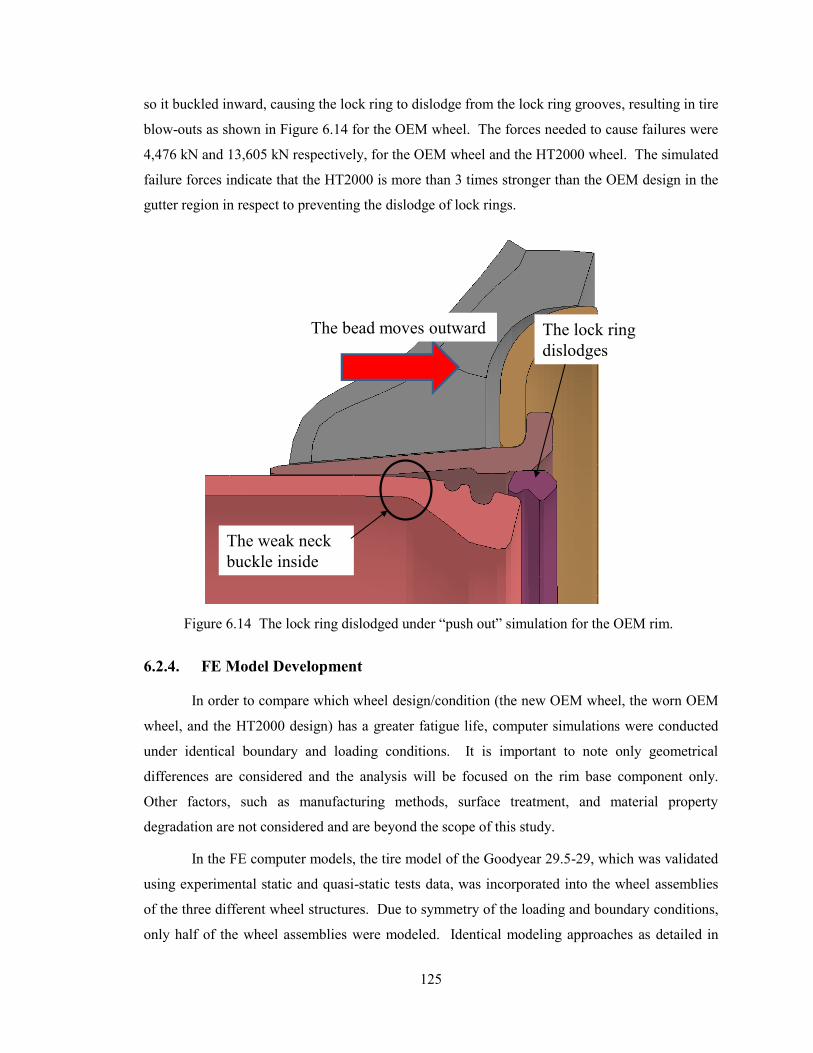
125

so it buckled inward, causing the lock ring to dislodge from the lock ring grooves, resulting in tire

blow-outs as shown in Figure 6.14 for the OEM wheel. The forces needed to cause failures were

4,476 kN and 13,605 kN respectively, for the OEM wheel and the HT2000 wheel. The simulated

failure forces indicate that the HT2000 is more than 3 times stronger than the OEM design in the

gutter region in respect to preventing the dislodge of lock rings.

6.2.4. FE Model Development

In order to compare which wheel design/condition (the new OEM wheel, the worn OEM

wheel, and the HT2000 design) has a greater fatigue life, computer simulations were conducted

under identical boundary and loading conditions. It is important to note only geometrical

differences are considered and the analysis will be focused on the rim base component only.

Other factors, such as manufacturing methods, surface treatment, and material property

degradation are not considered and are beyond the scope of this study.

In the FE computer models, the tire model of the Goodyear 29.5-29, which was validated

using experimental static and quasi-static tests data, was incorporated into the wheel assemblies

of the three different wheel structures. Due to symmetry of the loading and boundary conditions,

only half of the wheel assemblies were modeled. Identical modeling approaches as detailed in

The weak neck

buckle inside

The bead moves outward The lock ring

dislodges

Figure 6.14 The lock ring dislodged under “push out” simulation for the OEM rim.

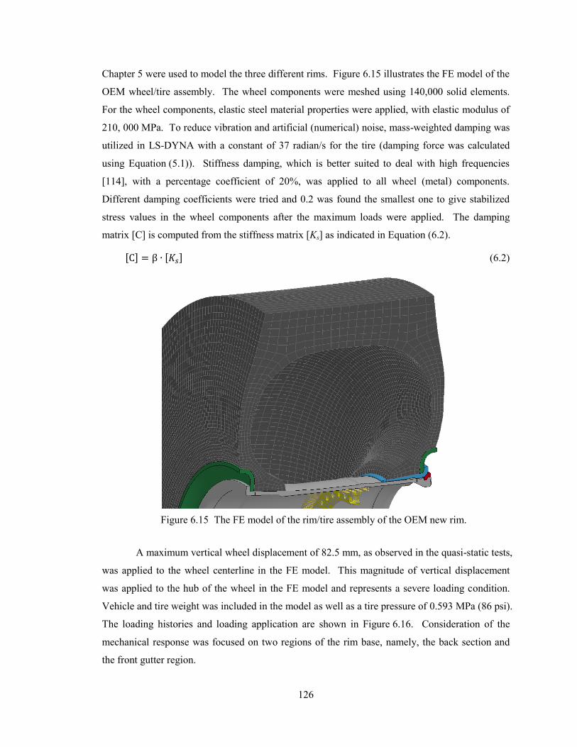
126

Chapter 5 were used to model the three different rims. Figure 6.15 illustrates the FE model of the

OEM wheel/tire assembly. The wheel components were meshed using 140,000 solid elements.

For the wheel components, elastic steel material properties were applied, with elastic modulus of

210, 000 MPa. To reduce vibration and artificial (numerical) noise, mass-weighted damping was

utilized in LS-DYNA with a constant of 37 radian/s for the tire (damping force was calculated

using Equation (5.1)). Stiffness damping, which is better suited to deal with high frequencies

[114], with a percentage coefficient of 20%, was applied to all wheel (metal) components.

Different damping coefficients were tried and 0.2 was found the smallest one to give stabilized

stress values in the wheel components after the maximum loads were applied. The damping

matrix [C] is computed from the stiffness matrix [Ks] as indicated in Equation (6.2).

[ ] [ ] (6.2)

A maximum vertical wheel displacement of 82.5 mm, as observed in the quasi-static tests,

was applied to the wheel centerline in the FE model. This magnitude of vertical displacement

was applied to the hub of the wheel in the FE model and represents a severe loading condition.

Vehicle and tire weight was included in the model as well as a tire pressure of 0.593 MPa (86 psi).

The loading histories and loading application are shown in Figure 6.16. Consideration of the

mechanical response was focused on two regions of the rim base, namely, the back section and

the front gutter region.

Figure 6.15 The FE model of the rim/tire assembly of the OEM new rim.

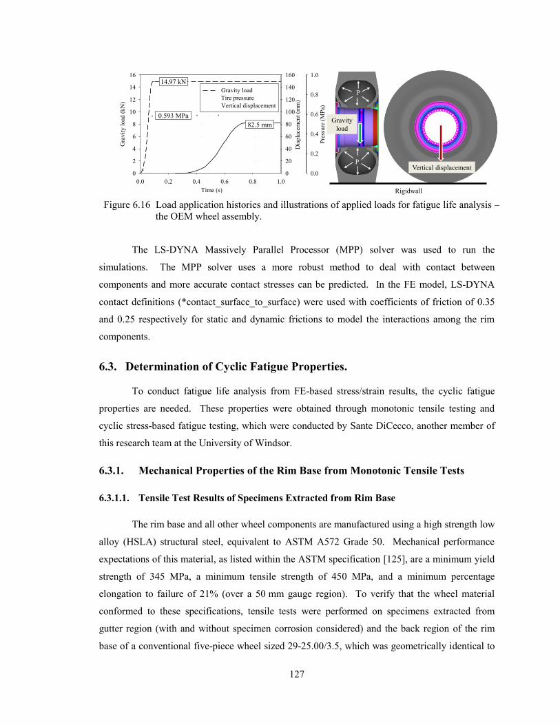
127

The LS-DYNA Massively Parallel Processor (MPP) solver was used to run the

simulations. The MPP solver uses a more robust method to deal with contact between

components and more accurate contact stresses can be predicted. In the FE model, LS-DYNA

contact definitions (*contact_surface_to_surface) were used with coefficients of friction of 0.35

and 0.25 respectively for static and dynamic frictions to model the interactions among the rim

components.

6.3. Determination of Cyclic Fatigue Properties.

To conduct fatigue life analysis from FE-based stress/strain results, the cyclic fatigue

properties are needed. These properties were obtained through monotonic tensile testing and

cyclic stress-based fatigue testing, which were conducted by Sante DiCecco, another member of

this research team at the University of Windsor.

6.3.1. Mechanical Properties of the Rim Base from Monotonic Tensile Tests

6.3.1.1. Tensile Test Results of Specimens Extracted from Rim Base

The rim base and all other wheel components are manufactured using a high strength low

alloy (HSLA) structural steel, equivalent to ASTM A572 Grade 50. Mechanical performance

expectations of this material, as listed within the ASTM specification [125], are a minimum yield

strength of 345 MPa, a minimum tensile strength of 450 MPa, and a minimum percentage

elongation to failure of 21% (over a 50 mm gauge region). To verify that the wheel material

conformed to these specifications, tensile tests were performed on specimens extracted from

gutter region (with and without specimen corrosion considered) and the back region of the rim

base of a conventional five-piece wheel sized 29-25.00/3.5, which was geometrically identical to

Time (s)

0.0 0.2 0.4 0.6 0.8 1.0

Gra

vit

y l

oad

(k

N)

0

2

4

6

8

10

12

14

16

Pre

ssu

re (

MP

a)

0.0

0.2

0.4

0.6

0.8

1.0

Dis

pla

cem

ent

(mm

)

0

20

40

60

80

100

120

140

160

Gravity load

Tire pressure

Vertical displacement

82.5 mm

0.593 MPa

14.97 kN

P

P

Gravity

load

Vertical displacement

Rigidwall

Figure 6.16 Load application histories and illustrations of applied loads for fatigue life analysis –

the OEM wheel assembly.

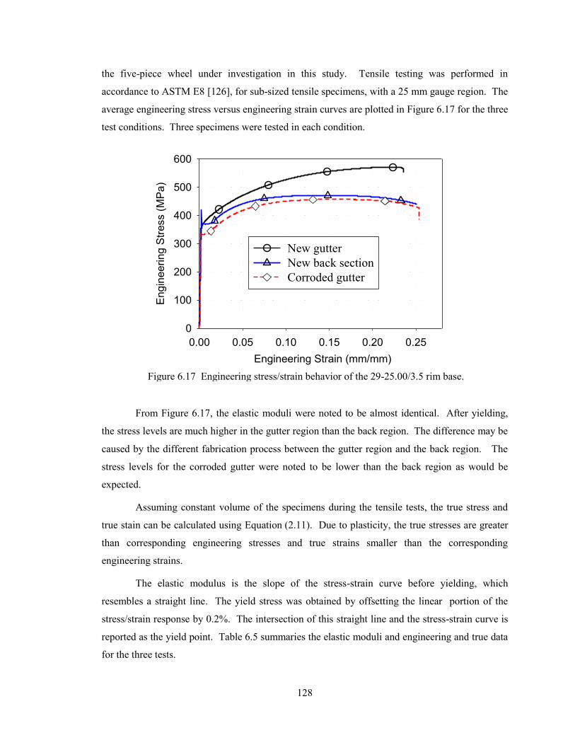
128

the five-piece wheel under investigation in this study. Tensile testing was performed in

accordance to ASTM E8 [126], for sub-sized tensile specimens, with a 25 mm gauge region. The

average engineering stress versus engineering strain curves are plotted in Figure 6.17 for the three

test conditions. Three specimens were tested in each condition.

From Figure 6.17, the elastic moduli were noted to be almost identical. After yielding,

the stress levels are much higher in the gutter region than the back region. The difference may be

caused by the different fabrication process between the gutter region and the back region. The

stress levels for the corroded gutter were noted to be lower than the back region as would be

expected.

Assuming constant volume of the specimens during the tensile tests, the true stress and

true stain can be calculated using Equation (2.11). Due to plasticity, the true stresses are greater

than corresponding engineering stresses and true strains smaller than the corresponding

engineering strains.

The elastic modulus is the slope of the stress-strain curve before yielding, which

resembles a straight line. The yield stress was obtained by offsetting the linear portion of the

stress/strain response by 0.2%. The intersection of this straight line and the stress-strain curve is

reported as the yield point. Table 6.5 summaries the elastic moduli and engineering and true data

for the three tests.

Engineering Strain (mm/mm)

0.00 0.05 0.10 0.15 0.20 0.25

En

gin

ee

rin

g S

tress (

MP

a)

0

100

200

300

400

500

600

New gutter

New back section

Corroded gutter

Figure 6.17 Engineering stress/strain behavior of the 29-25.00/3.5 rim base.

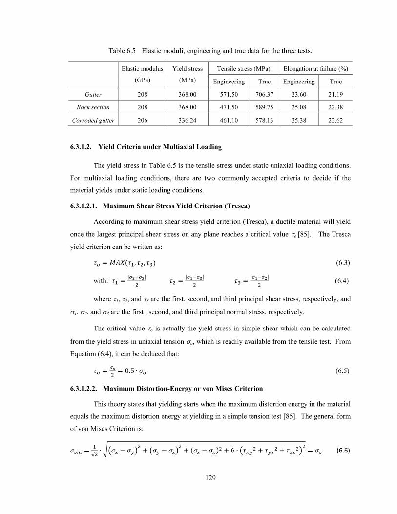
129

Table 6.5 Elastic moduli, engineering and true data for the three tests.

Elastic modulus

(GPa)

Yield stress

(MPa)

Tensile stress (MPa) Elongation at failure (%)

Engineering True Engineering True

Gutter 208 368.00 571.50 706.37 23.60 21.19

Back section 208 368.00 471.50 589.75 25.08 22.38

Corroded gutter 206 336.24 461.10 578.13 25.38 22.62

6.3.1.2. Yield Criteria under Multiaxial Loading

The yield stress in Table 6.5 is the tensile stress under static uniaxial loading conditions.

For multiaxial loading conditions, there are two commonly accepted criteria to decide if the

material yields under static loading conditions.

6.3.1.2.1. Maximum Shear Stress Yield Criterion (Tresca)

According to maximum shear stress yield criterion (Tresca), a ductile material will yield

once the largest principal shear stress on any plane reaches a critical value o [85]. The Tresca

yield criterion can be written as:

( ) (6.3)

with: | |

| |

| |

(6.4)

where 1, 2, and 3 are the first, second, and third principal shear stress, respectively, and

1, 2, and 3 are the first , second, and third principal normal stress, respectively.

The critical value o is actually the yield stress in simple shear which can be calculated

from the yield stress in uniaxial tension o, which is readily available from the tensile test. From

Equation (6.4), it can be deduced that:

(6.5)

6.3.1.2.2. Maximum Distortion-Energy or von Mises Criterion

This theory states that yielding starts when the maximum distortion energy in the material

equals the maximum distortion energy at yielding in a simple tension test [85]. The general form

of von Mises Criterion is:

√ √( )

( )

( )

(

)

(6.6)

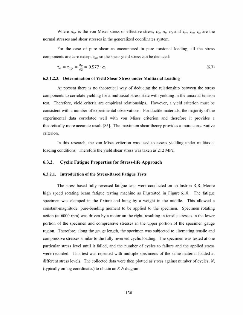
130

Where vm is the von Mises stress or effective stress, x, y, z and xy, yz, zx are the

normal stresses and shear stresses in the generalized coordinates system.

For the case of pure shear as encountered in pure torsional loading, all the stress

components are zero except xy, so the shear yield stress can be deduced:

√ (6.7)

6.3.1.2.3. Determination of Yield Shear Stress under Multiaxial Loading

At present there is no theoretical way of deducing the relationship between the stress

components to correlate yielding for a multiaxial stress state with yielding in the uniaxial tension

test. Therefore, yield criteria are empirical relationships. However, a yield criterion must be

consistent with a number of experimental observations. For ductile materials, the majority of the

experimental data correlated well with von Mises criterion and therefore it provides a

theoretically more accurate result [85]. The maximum shear theory provides a more conservative

criterion.

In this research, the von Mises criterion was used to assess yielding under multiaxial

loading conditions. Therefore the yield shear stress was taken as 212 MPa.

6.3.2. Cyclic Fatigue Properties for Stress-life Approach

6.3.2.1. Introduction of the Stress-Based Fatigue Tests

The stress-based fully reversed fatigue tests were conducted on an Instron R.R. Moore

high speed rotating beam fatigue testing machine as illustrated in Figure 6.18. The fatigue

specimen was clamped in the fixture and hung by a weight in the middle. This allowed a

constant-magnitude, pure-bending moment to be applied to the specimen. Specimen rotating

action (at 6000 rpm) was driven by a motor on the right, resulting in tensile stresses in the lower

portion of the specimen and compressive stresses in the upper portion of the specimen gauge

region. Therefore, along the gauge length, the specimen was subjected to alternating tensile and

compressive stresses similar to the fully reversed cyclic loading. The specimen was tested at one

particular stress level until it failed, and the number of cycles to failure and the applied stress

were recorded. This test was repeated with multiple specimens of the same material loaded at

different stress levels. The collected data were then plotted as stress against number of cycles, N,

(typically on log coordinates) to obtain an S-N diagram.

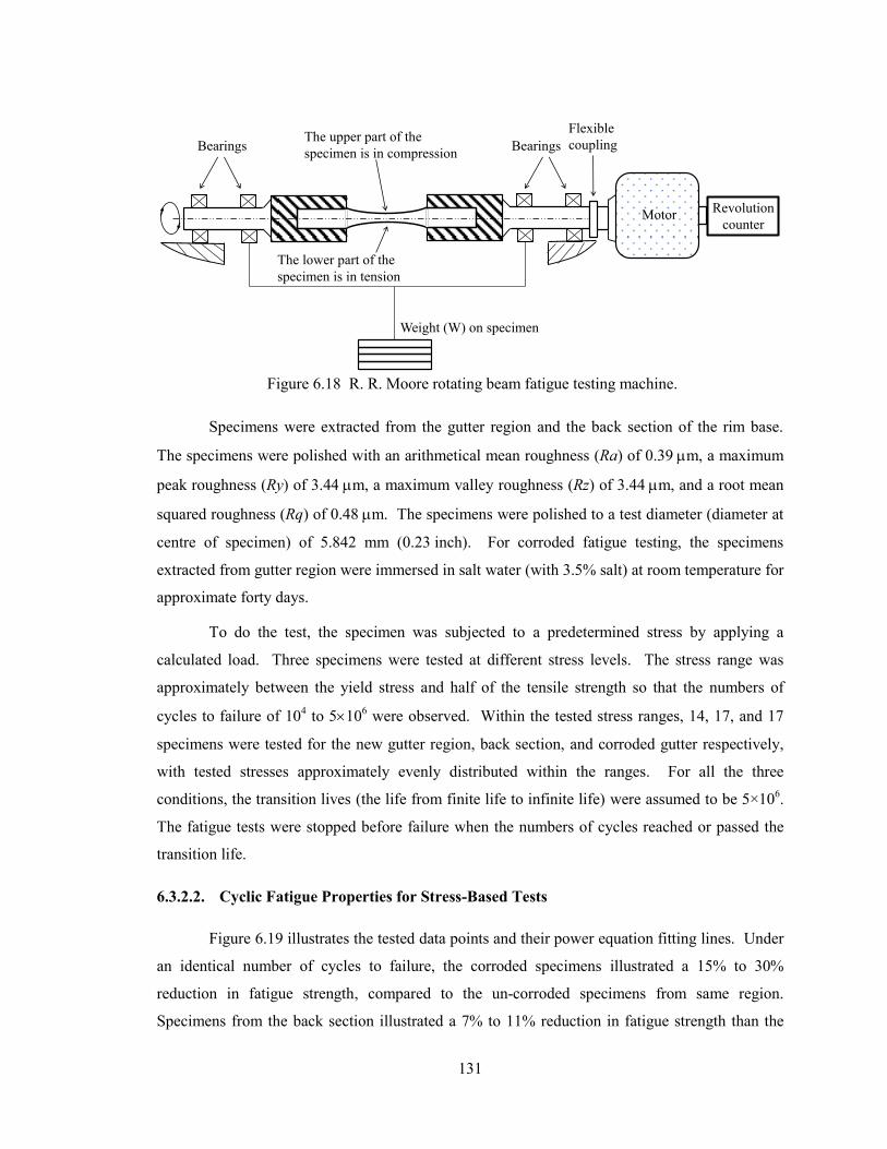
131

Specimens were extracted from the gutter region and the back section of the rim base.

The specimens were polished with an arithmetical mean roughness (Ra) of 0.39 m, a maximum

peak roughness (Ry) of 3.44 m, a maximum valley roughness (Rz) of 3.44 m, and a root mean

squared roughness (Rq) of 0.48 m. The specimens were polished to a test diameter (diameter at

centre of specimen) of 5.842 mm (0.23 inch). For corroded fatigue testing, the specimens

extracted from gutter region were immersed in salt water (with 3.5% salt) at room temperature for

approximate forty days.

To do the test, the specimen was subjected to a predetermined stress by applying a

calculated load. Three specimens were tested at different stress levels. The stress range was

approximately between the yield stress and half of the tensile strength so that the numbers of

cycles to failure of 104 to 510

6 were observed. Within the tested stress ranges, 14, 17, and 17

specimens were tested for the new gutter region, back section, and corroded gutter respectively,

with tested stresses approximately evenly distributed within the ranges. For all the three

conditions, the transition lives (the life from finite life to infinite life) were assumed to be 5×106.

The fatigue tests were stopped before failure when the numbers of cycles reached or passed the

transition life.

6.3.2.2. Cyclic Fatigue Properties for Stress-Based Tests

Figure 6.19 illustrates the tested data points and their power equation fitting lines. Under

an identical number of cycles to failure, the corroded specimens illustrated a 15% to 30%

reduction in fatigue strength, compared to the un-corroded specimens from same region.

Specimens from the back section illustrated a 7% to 11% reduction in fatigue strength than the

Bearings Bearings

Weight (W) on specimen

The upper part of the

specimen is in compression

The lower part of the

specimen is in tension

Motor

Flexible

coupling

Revolution

counter

Figure 6.18 R. R. Moore rotating beam fatigue testing machine.

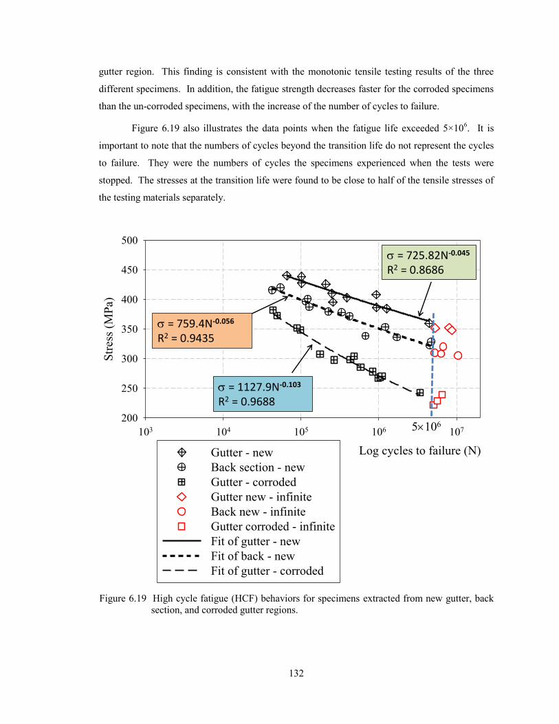
132

gutter region. This finding is consistent with the monotonic tensile testing results of the three

different specimens. In addition, the fatigue strength decreases faster for the corroded specimens

than the un-corroded specimens, with the increase of the number of cycles to failure.

Figure 6.19 also illustrates the data points when the fatigue life exceeded 5×106. It is

important to note that the numbers of cycles beyond the transition life do not represent the cycles

to failure. They were the numbers of cycles the specimens experienced when the tests were

stopped. The stresses at the transition life were found to be close to half of the tensile stresses of

the testing materials separately.

Log cycles to failure (N)

103 104 105 106 107

Str

ess

(MP

a)

200

250

300

350

400

450

500

Gutter - new

Back section - new

Gutter - corroded

Gutter new - infinite

Back new - infinite

Gutter corroded - infinite

Fit of gutter - new

Fit of back - new

Fit of gutter - corroded

= 725.82N-0.045

R2 = 0.8686

= 1127.9N-0.103

R2 = 0.9688

= 759.4N-0.056

R2 = 0.9435

5106

Figure 6.19 High cycle fatigue (HCF) behaviors for specimens extracted from new gutter, back

section, and corroded gutter regions.

133

Using a power equation curve fit, with R2 values illustrated in Figure 6.19, the stresses

(in MPa) versus the numbers of cycle to failure can be expressed as follows:

( ) (6.8)

( ) (6.9)

( ) (6.10)

Combining the information from tensile tests and fatigue tests, the Stress-life (S-N)

fatigue properties were calculated (as listed in Table 6.6) and used within nCode DesignLife to

assess fatigue life based on the linear FE simulation stress/strain results.

Table 6.6 S-N fatigue properties generated from fatigue tests.

Gutter - new Back section - new Gutter - corroded Description

YS 368.00 368.00 336.24 Yield Strength (MPa)

UTS 571.50 471.50 461.10 Ultimate Tensile Strength (MPa)

E 2.076×105 2.076×10

5 2.059×10

5 Elastic Modulus (MPa)

SRI1 725.82 759.4 1127.90 Stress Range Intercept (MPa)

b1 -0.045 -0.056 -0.103 First Fatigue Strength Exponent

Nc1 5×106 5×10

6 5×10

6 Fatigue Transition Point (cycles)

b2 -0.045 -0.056 -0.103 Second Fatigue Strength Exponent

SE 0.1 0.1 0.1 Standard Error of Log (N)

RR -1 -1 -1 R-ratio of Test

Nfc 1×1030

1×1030

1×1030

Fatigue CutOff

For steel materials, the fatigue life is assumed infinite beyond the transition life on the

S-N life profile and the second portion of the S-N relationship is a straight horizontal line with the

second fatigue strength exponent (the slope b2) equivalent to zero. If the predicted lives for the

original design and the proposed design are both infinite, then the two designs are not

quantitatively comparable. To circumvent this issue, the second slope b2 was assumed to be

equivalent to the first slope b1, as highlighted in Table 6.6. These modifications were

recommended by DesignLife [127] and allowed for a comparison on the fatigue lives of the

different wheel designs. Obviously, the fatigue life estimated beyond transition life does not

reflect real fatigue life. It is used for comparison only between different design iterations. If the

predicted life is greater than the Fatigue CutOff (Nfc), an infinite fatigue life will be given.

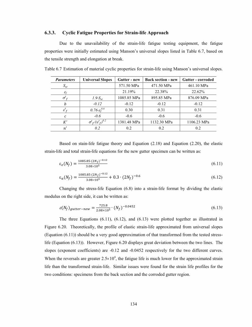
134

6.3.3. Cyclic Fatigue Properties for Strain-life Approach

Due to the unavailability of the strain-life fatigue testing equipment, the fatigue

properties were initially estimated using Manson’s universal slopes listed in Table 6.7, based on

the tensile strength and elongation at break.

Table 6.7 Estimation of material cyclic properties for strain-life using Manson’s universal slopes.

Parameters Universal Slopes Gutter - new Back section - new Gutter - corroded

Sut 571.50 MPa 471.50 MPa 461.10 MPa

f 21.19% 22.38% 22.62%

1.9Sut 1085.85 MPa 895.85 MPa 876.09 MPa

-0.12 -0.12 -0.12 -0.12

0.76f0.6

0.30 0.31 0.31

-0.6 -0.6 -0.6 -0.6

/( )

0.2 1381.48 MPa 1132.30 MPa 1106.23 MPa

0.2 0.2 0.2 0.2

Based on stain-life fatigue theory and Equation (2.18) and Equation (2.20), the elastic

strain-life and total strain-life equations for the new gutter specimen can be written as:

( ) ( )

(6.11)

( ) ( )

( ) (6.12)

Changing the stress-life Equation (6.8) into a strain-life format by dividing the elastic

modulus on the right side, it can be written as:

( )

( ) (6.13)

The three Equations (6.11), (6.12), and (6.13) were plotted together as illustrated in

Figure 6.20. Theoretically, the profile of elastic strain-life approximated from universal slopes

(Equation (6.11)) should be a very good approximation of that transformed from the tested stress-

life (Equation (6.13)). However, Figure 6.20 displays great deviation between the two lines. The

slopes (exponent coefficients) are -0.12 and -0.0452 respectively for the two different curves.

When the reversals are greater 2.5104, the fatigue life is much lower for the approximated strain

life than the transformed strain-life. Similar issues were found for the strain life profiles for the

two conditions: specimens from the back section and the corroded gutter region.

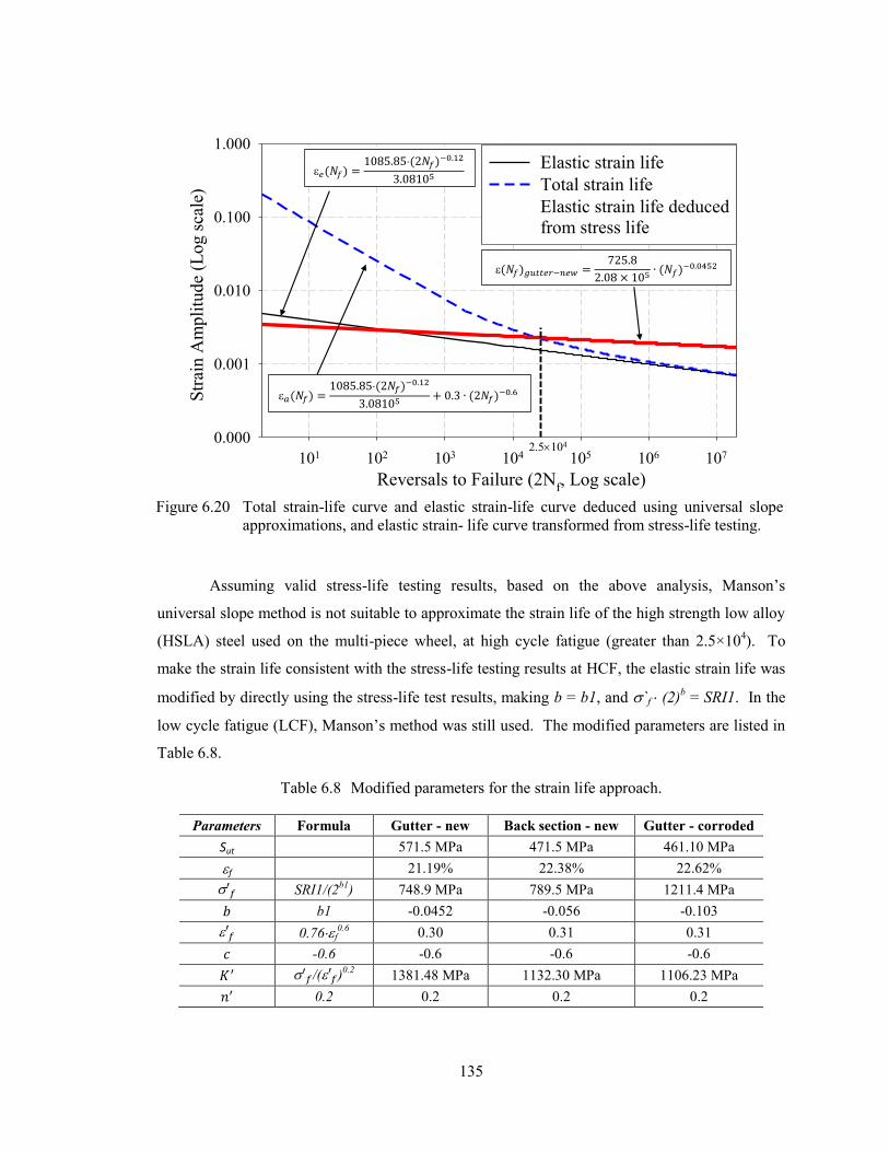
135

Assuming valid stress-life testing results, based on the above analysis, Manson’s

universal slope method is not suitable to approximate the strain life of the high strength low alloy

(HSLA) steel used on the multi-piece wheel, at high cycle fatigue (greater than 2.5×104). To

make the strain life consistent with the stress-life testing results at HCF, the elastic strain life was

modified by directly using the stress-life test results, making b = b1, and `f (2)b = SRI1. In the

low cycle fatigue (LCF), Manson’s method was still used. The modified parameters are listed in

Table 6.8.

Table 6.8 Modified parameters for the strain life approach.

Parameters Formula Gutter - new Back section - new Gutter - corroded

Sut 571.5 MPa 471.5 MPa 461.10 MPa

f 21.19% 22.38% 22.62%

SRI1/(2

b1) 748.9 MPa 789.5 MPa 1211.4 MPa

b1 -0.0452 -0.056 -0.103

0.76f0.6

0.30 0.31 0.31

-0.6 -0.6 -0.6 -0.6

/( )

0.2 1381.48 MPa 1132.30 MPa 1106.23 MPa

0.2 0.2 0.2 0.2

Reversals to Failure (2Nf, Log scale)

101 102 103 104 105 106 107

Str

ain

Am

pli

tud

e (L

og s

cale

)

0.000

0.001

0.010

0.100

1.000

Elastic strain life

Total strain life

Elastic strain life deduced

from stress life

2.5104

Figure 6.20 Total strain-life curve and elastic strain-life curve deduced using universal slope

approximations, and elastic strain- life curve transformed from stress-life testing.

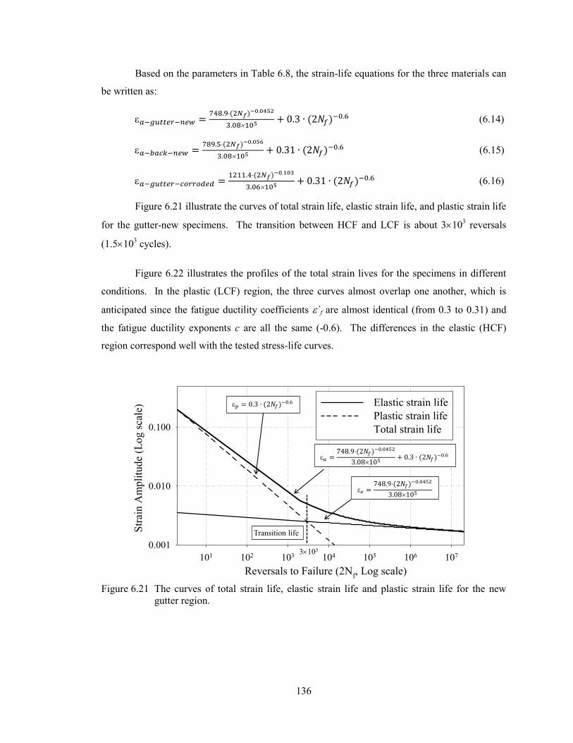
136

Based on the parameters in Table 6.8, the strain-life equations for the three materials can

be written as:

( )

( ) (6.14)

( )

( ) (6.15)

( )

( ) (6.16)

Figure 6.21 illustrate the curves of total strain life, elastic strain life, and plastic strain life

for the gutter-new specimens. The transition between HCF and LCF is about 3103 reversals

(1.5103 cycles).

Figure 6.22 illustrates the profiles of the total strain lives for the specimens in different

conditions. In the plastic (LCF) region, the three curves almost overlap one another, which is

anticipated since the fatigue ductility coefficients `f are almost identical (from 0.3 to 0.31) and

the fatigue ductility exponents c are all the same (-0.6). The differences in the elastic (HCF)

region correspond well with the tested stress-life curves.

Reversals to Failure (2Nf, Log scale)

101 102 103 104 105 106 107

Str

ain

Am

pli

tud

e (L

og s

cale

)

0.001

0.010

0.100

Elastic strain life

Plastic strain life

Total strain life

3103

Transition life

Figure 6.21 The curves of total strain life, elastic strain life and plastic strain life for the new

gutter region.

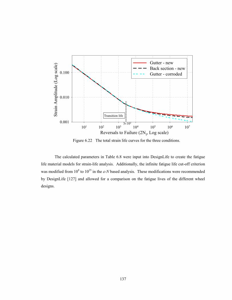
137

The calculated parameters in Table 6.8 were input into DesignLife to create the fatigue

life material models for strain-life analysis. Additionally, the infinite fatigue life cut-off criterion

was modified from 108 to 10

25 in the -N based analysis. These modifications were recommended

by DesignLife [127] and allowed for a comparison on the fatigue lives of the different wheel

designs.

Reversals to Failure (2Nf, Log scale)

101 102 103 104 105 106 107

Str

ain

Am

pli

tud

e (L

og s

cale

)

0.001

0.010

0.100

Gutter - new

Back section - new

Gutter - corroded

3103

Transition life

Figure 6.22 The total strain life curves for the three conditions.

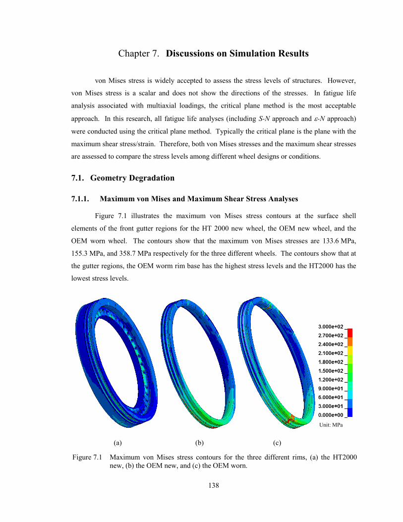
138

Chapter 7. Discussions on Simulation Results

von Mises stress is widely accepted to assess the stress levels of structures. However,

von Mises stress is a scalar and does not show the directions of the stresses. In fatigue life

analysis associated with multiaxial loadings, the critical plane method is the most acceptable

approach. In this research, all fatigue life analyses (including S-N approach and -N approach)

were conducted using the critical plane method. Typically the critical plane is the plane with the

maximum shear stress/strain. Therefore, both von Mises stresses and the maximum shear stresses

are assessed to compare the stress levels among different wheel designs or conditions.

7.1. Geometry Degradation

7.1.1. Maximum von Mises and Maximum Shear Stress Analyses

Figure 7.1 illustrates the maximum von Mises stress contours at the surface shell

elements of the front gutter regions for the HT 2000 new wheel, the OEM new wheel, and the

OEM worn wheel. The contours show that the maximum von Mises stresses are 133.6 MPa,

155.3 MPa, and 358.7 MPa respectively for the three different wheels. The contours show that at

the gutter regions, the OEM worm rim base has the highest stress levels and the HT2000 has the

lowest stress levels.

(a) (b)

Unit: MPa

(c)

Figure 7.1 Maximum von Mises stress contours for the three different rims, (a) the HT2000

new, (b) the OEM new, and (c) the OEM worn.

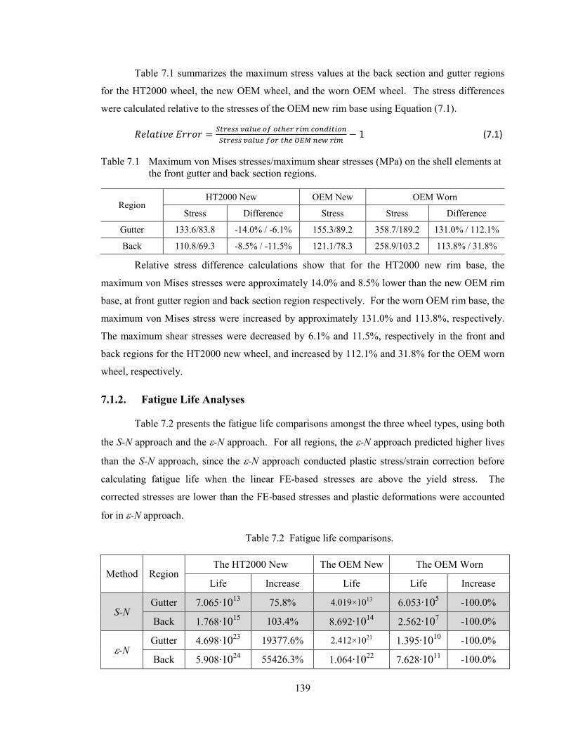
139

Table 7.1 summarizes the maximum stress values at the back section and gutter regions

for the HT2000 wheel, the new OEM wheel, and the worn OEM wheel. The stress differences

were calculated relative to the stresses of the OEM new rim base using Equation (7.1).

(7.1)

Table 7.1 Maximum von Mises stresses/maximum shear stresses (MPa) on the shell elements at

the front gutter and back section regions.

Region HT2000 New OEM New OEM Worn

Stress Difference Stress Stress Difference

Gutter 133.6/83.8 -14.0% / -6.1% 155.3/89.2 358.7/189.2 131.0% / 112.1%

Back 110.8/69.3 -8.5% / -11.5% 121.1/78.3 258.9/103.2 113.8% / 31.8%

Relative stress difference calculations show that for the HT2000 new rim base, the

maximum von Mises stresses were approximately 14.0% and 8.5% lower than the new OEM rim

base, at front gutter region and back section region respectively. For the worn OEM rim base, the

maximum von Mises stress were increased by approximately 131.0% and 113.8%, respectively.

The maximum shear stresses were decreased by 6.1% and 11.5%, respectively in the front and

back regions for the HT2000 new wheel, and increased by 112.1% and 31.8% for the OEM worn

wheel, respectively.

7.1.2. Fatigue Life Analyses

Table 7.2 presents the fatigue life comparisons amongst the three wheel types, using both

the S-N approach and the -N approach. For all regions, the -N approach predicted higher lives

than the S-N approach, since the -N approach conducted plastic stress/strain correction before

calculating fatigue life when the linear FE-based stresses are above the yield stress. The

corrected stresses are lower than the FE-based stresses and plastic deformations were accounted

for in -N approach.

Table 7.2 Fatigue life comparisons.

Method Region The HT2000 New The OEM New The OEM Worn

Life Increase Life Life Increase

S-N Gutter 7.065∙10

13 75.8% 4.019×10

13 6.053∙105 -100.0%

Back 1.768∙1015

103.4% 8.692∙1014

2.562∙107 -100.0%

-N Gutter 4.698∙10

23 19377.6% 2.412×10

21 1.395∙1010

-100.0%

Back 5.908∙1024

55426.3% 1.064∙1022

7.628∙1011

-100.0%

140

Based on the fatigue life prediction using S-N approach, finite fatigue lives were

predicted at the gutter region (6.053105) of the OEM worn wheel. Infinite lives (greater than

transition life 5×106) were predicted for other regions using S-N approach and all the regions

using -N approach. Using Equation 7.1, the calculated relative differences of the fatigue life

between different situations are also listed in Table 7.2. The predicted fatigue lives for the OEM

worn wheel were over several orders of magnitude lower than the predicted lives for the OEM

new wheel, on the corresponding regions. On the other hand, the predicted fatigue lives for the

HT2000 new wheel were over 75% higher than the lives of the OEM new wheel, on the

corresponding regions.

7.2. Material Degradation

It was initially planned to compare the fatigue lives between OEM new wheel and OEM

used wheel, in order to investigate the material degradation effects. Tensile and fatigue tests were

conducted on specimens extracted from new OEM wheel and used OEM wheel and the testing

results showed almost identical yield stresses, tensile stresses, elongations, and fatigue data

between the specimens. For the used wheel, the material property degradations mostly happened

on the outer surfaces of the wheel components. After polishing the specimens before testing, the

degraded materials were removed, which explains why the testing results were almost identical

between the specimens extracted from the two different wheels. In this study, therefore, the

material property degradation effects were investigated using material properties of specimens

extracted from the new OEM wheel, corroded in salted water and non-corroded.

In order to investigate the effects of material degradation, fatigue life estimations were

conducted on the OEM new wheel base structure without considering geometry degradation.

The fatigue life estimations were only focused on the gutter region of the rim base since the gutter

region is the most critical region. The FE stress/strain results were obtained with the loading

conditions illustrated in Figure 6.16. The cyclic fatigue properties (listed in Table 6.6 and 6.8)

from specimens of new gutter and corroded gutter were used to compare the fatigue life.

Table 7.3 lists the fatigue life calculation results using nCode DesignLife.

Table 7.3 Fatigue life comparisons between new gutter and corroded gutter materials.

Method Region New gutter Corroded gutter Increase

S-N Gutter 4.019×1013

6.197∙105 -100.0%

-N Gutter 2.412×1021

9.735∙108 -100.0%

141

It is observed that both S-N and -N methods predicted higher fatigue life for the new

specimen than the corroded specimen in the gutter region, with the -N method predicting much

longer fatigue life than the S-N method. No matter what methods were used, the fatigue lives of

the corroded materials were significantly reduced by several orders of magnitude.

From a microscopic point of view, corrosion takes away the external material and creates

highly irregular micro-structure on the surface of the component. Significant stress

concentrations are induced in localized areas of the component during service. Therefore,

massive fatigue life reductions were predicted. This is an important finding which was

hypothesized by Vijayan et al. [6, 14].

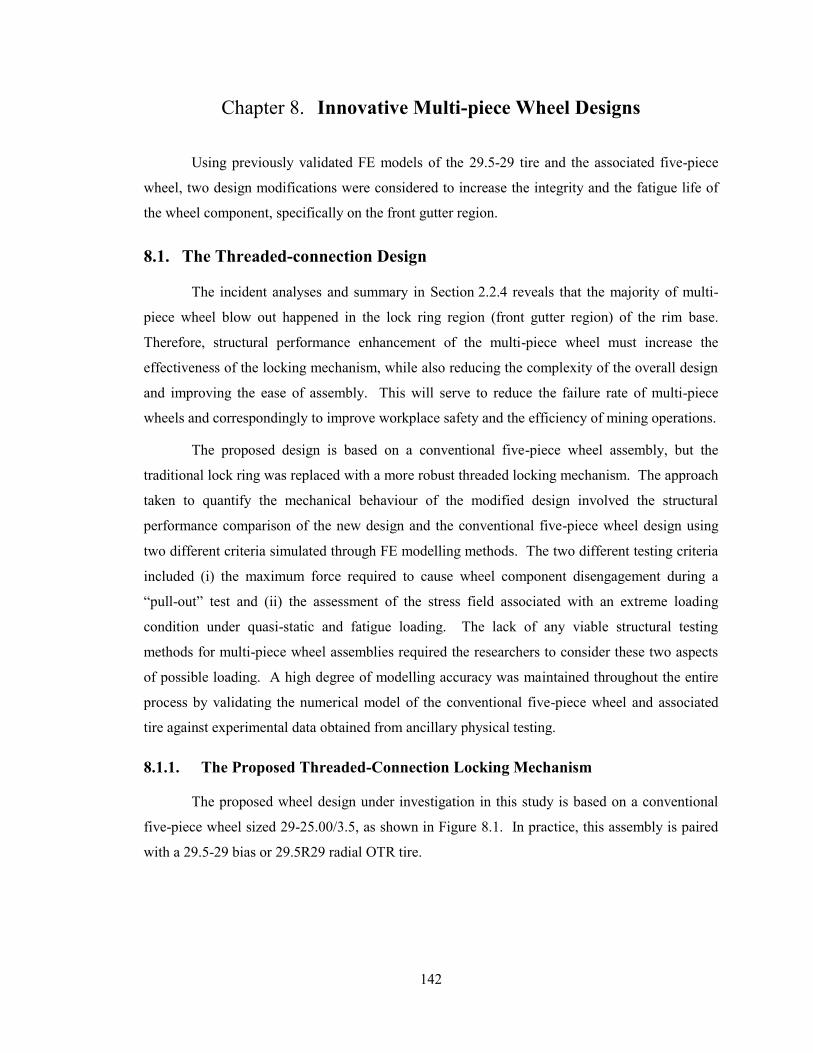
142

Chapter 8. Innovative Multi-piece Wheel Designs

Using previously validated FE models of the 29.5-29 tire and the associated five-piece

wheel, two design modifications were considered to increase the integrity and the fatigue life of

the wheel component, specifically on the front gutter region.

8.1. The Threaded-connection Design

The incident analyses and summary in Section 2.2.4 reveals that the majority of multi-

piece wheel blow out happened in the lock ring region (front gutter region) of the rim base.

Therefore, structural performance enhancement of the multi-piece wheel must increase the

effectiveness of the locking mechanism, while also reducing the complexity of the overall design

and improving the ease of assembly. This will serve to reduce the failure rate of multi-piece

wheels and correspondingly to improve workplace safety and the efficiency of mining operations.

The proposed design is based on a conventional five-piece wheel assembly, but the

traditional lock ring was replaced with a more robust threaded locking mechanism. The approach

taken to quantify the mechanical behaviour of the modified design involved the structural

performance comparison of the new design and the conventional five-piece wheel design using

two different criteria simulated through FE modelling methods. The two different testing criteria

included (i) the maximum force required to cause wheel component disengagement during a

“pull-out” test and (ii) the assessment of the stress field associated with an extreme loading

condition under quasi-static and fatigue loading. The lack of any viable structural testing

methods for multi-piece wheel assemblies required the researchers to consider these two aspects

of possible loading. A high degree of modelling accuracy was maintained throughout the entire

process by validating the numerical model of the conventional five-piece wheel and associated

tire against experimental data obtained from ancillary physical testing.

8.1.1. The Proposed Threaded-Connection Locking Mechanism

The proposed wheel design under investigation in this study is based on a conventional

five-piece wheel sized 29-25.00/3.5, as shown in Figure 8.1. In practice, this assembly is paired

with a 29.5-29 bias or 29.5R29 radial OTR tire.

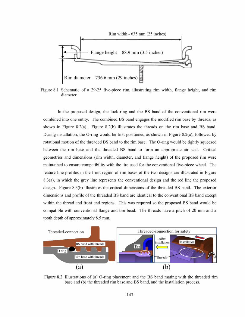
143

In the proposed design, the lock ring and the BS band of the conventional rim were

combined into one entity. The combined BS band engages the modified rim base by threads, as

shown in Figure 8.2(a). Figure 8.2(b) illustrates the threads on the rim base and BS band.

During installation, the O-ring would be first positioned as shown in Figure 8.2(a), followed by

rotational motion of the threaded BS band to the rim base. The O-ring would be tightly squeezed

between the rim base and the threaded BS band to form an appropriate air seal. Critical

geometries and dimensions (rim width, diameter, and flange height) of the proposed rim were

maintained to ensure compatibility with the tire used for the conventional five-piece wheel. The

feature line profiles in the front region of rim bases of the two designs are illustrated in Figure

8.3(a), in which the grey line represents the conventional design and the red line the proposed

design. Figure 8.3(b) illustrates the critical dimensions of the threaded BS band. The exterior

dimensions and profile of the threaded BS band are identical to the conventional BS band except

within the thread and front end regions. This was required so the proposed BS band would be

compatible with conventional flange and tire bead. The threads have a pitch of 20 mm and a

tooth depth of approximately 8.5 mm.

Rim width - 635 mm (25 inches)

Flange height – 88.9 mm (3.5 inches)

Rim diameter – 736.6 mm (29 inches)

Figure 8.1 Schematic of a 29-25 five-piece rim, illustrating rim width, flange height, and rim

diameter.

BS band with threads

Rim base with threads

Threaded-connection

O ring

Threaded-connection for safety

After

installation

Threads

Installation

Tire

(a) (b)

Figure 8.2 Illustrations of (a) O-ring placement and the BS band mating with the threaded rim

base and (b) the threaded rim base and BS band, and the installation process.

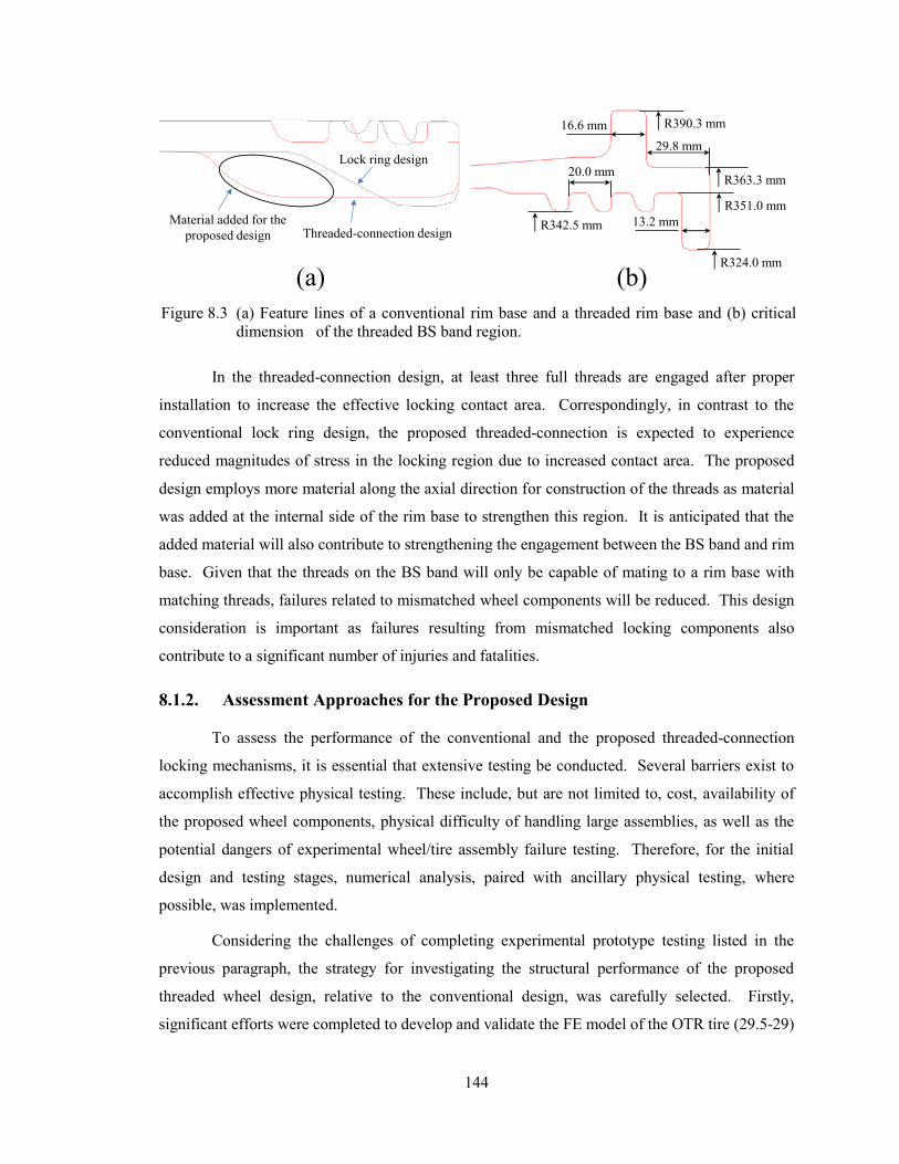
144

In the threaded-connection design, at least three full threads are engaged after proper

installation to increase the effective locking contact area. Correspondingly, in contrast to the

conventional lock ring design, the proposed threaded-connection is expected to experience

reduced magnitudes of stress in the locking region due to increased contact area. The proposed

design employs more material along the axial direction for construction of the threads as material

was added at the internal side of the rim base to strengthen this region. It is anticipated that the

added material will also contribute to strengthening the engagement between the BS band and rim

base. Given that the threads on the BS band will only be capable of mating to a rim base with

matching threads, failures related to mismatched wheel components will be reduced. This design

consideration is important as failures resulting from mismatched locking components also

contribute to a significant number of injuries and fatalities.

8.1.2. Assessment Approaches for the Proposed Design

To assess the performance of the conventional and the proposed threaded-connection

locking mechanisms, it is essential that extensive testing be conducted. Several barriers exist to

accomplish effective physical testing. These include, but are not limited to, cost, availability of

the proposed wheel components, physical difficulty of handling large assemblies, as well as the

potential dangers of experimental wheel/tire assembly failure testing. Therefore, for the initial

design and testing stages, numerical analysis, paired with ancillary physical testing, where

possible, was implemented.

Considering the challenges of completing experimental prototype testing listed in the

previous paragraph, the strategy for investigating the structural performance of the proposed

threaded wheel design, relative to the conventional design, was carefully selected. Firstly,

significant efforts were completed to develop and validate the FE model of the OTR tire (29.5-29)

Threaded-connection design

Lock ring design

Material added for the

proposed design

R324.0 mm

R363.3 mm

R390.3 mm

13.2 mmR342.5 mm

R351.0 mm

20.0 mm

16.6 mm

29.8 mm

(a) (b)

Figure 8.3 (a) Feature lines of a conventional rim base and a threaded rim base and (b) critical

dimension of the threaded BS band region.

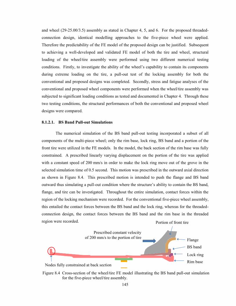
145

and wheel (29-25.00/3.5) assembly as stated in Chapter 4, 5, and 6. For the proposed threaded-

connection design, identical modelling approaches to the five-piece wheel were applied.

Therefore the predictability of the FE model of the proposed design can be justified. Subsequent

to achieving a well-developed and validated FE model of both the tire and wheel, structural

loading of the wheel/tire assembly were performed using two different numerical testing

conditions. Firstly, to investigate the ability of the wheel’s capability to contain its components

during extreme loading on the tire, a pull-out test of the locking assembly for both the

conventional and proposed designs was completed. Secondly, stress and fatigue analyses of the

conventional and proposed wheel components were performed when the wheel/tire assembly was

subjected to significant loading conditions as tested and documented in Chapter 4. Through these

two testing conditions, the structural performances of both the conventional and proposed wheel

designs were compared.

8.1.2.1. BS Band Pull-out Simulations

The numerical simulation of the BS band pull-out testing incorporated a subset of all

components of the multi-piece wheel; only the rim base, lock ring, BS band and a portion of the

front tire were utilized in the FE models. In the model, the back section of the rim base was fully

constrained. A prescribed linearly varying displacement on the portion of the tire was applied

with a constant speed of 200 mm/s in order to make the lock ring move out of the grove in the

selected simulation time of 0.5 second. This motion was prescribed in the outward axial direction

as shown in Figure 8.4. This prescribed motion is intended to push the flange and BS band

outward thus simulating a pull-out condition where the structure’s ability to contain the BS band,

flange, and tire can be investigated. Throughout the entire simulation, contact forces within the

region of the locking mechanism were recorded. For the conventional five-piece wheel assembly,

this entailed the contact forces between the BS band and the lock ring, whereas for the threaded-

connection design, the contact forces between the BS band and the rim base in the threaded

region were recorded.

Flange

BS band

Lock ring

Rim baseNodes fully constrained at back section

Portion of front tire

Prescribed constant velocity

of 200 mm/s to the portion of tire

Figure 8.4 Cross-section of the wheel/tire FE model illustrating the BS band pull-out simulation

for the five-piece wheel/tire assembly.

146

Since this simulated testing condition involves plasticity of the wheel component, an

elastic-plastic material model was developed and incorporated into all portions of the wheel FE

model. The model selected was type 24 within LS-DYNA [114] which incorporates the von

Mises yield criterion, and the equivalent von Mises stress is calculated in terms of the deviatoric

stress tensor as presented in Equation (8.1). Furthermore, the equivalent plastic strain is

calculated through time integration of the rate of deformation tensor as presented in

Equation (8.2).

21

2

3

ijij SS (8.1)

t

ijp

ijp

p dtDD0

21

3

2

(8.2)

To be conservative in the numerical analyses, the minimum values of the yield strength

(345 MPa), ultimate tensile strength (450 MPa) and percent elongation (21%) of the ASTM A572

Grade 50 steel were used within the development of the material model. Failure of finite

elements was considered by implementing a simple effective plastic strain failure criterion where

any elements which the effective plastic strain exceeded 0.21 would be removed from the

calculations and no longer able to support any stress. No material strain rate effects were

considered in the model since the load was applied in a slow fashion.

Contact between the rim components as well as between the tire and wheel components

(specifically the flange and BS band) was modelled using a surface to surface contact algorithm

within LS-DYNA. The coefficients of static and dynamic friction as well as the decay coefficient

for contact associated with the wheel components was defined as 0.35, 0.25 and 1000,

respectively. This large value of the decay coefficient results in a very abrupt change from the

static to the dynamic coefficient of friction as shown in Equation (5.2). The coefficients of static

and dynamic friction and the decay coefficient for contact between the tire portion and the flange

and BS band were specified as 0.35, 0, and 0, respectively. These values resulted in a constant

coefficient of friction between interacting surfaces regardless of whether or not relative motion

occurs. The input file used for the pull-out testing is listed in Appendix E.4.

8.1.2.2. Wheel Stress and Fatigue Life Assessments

As previously identified, an anticipated benefit of the proposed threaded-connection

wheel design is reduced magnitudes of stress within the locking region resulting from an increase

147

in the overall contact area between the rim base and the BS band. Through numerical simulation

efforts, the effective (von Mises) stress and the 1st principal stress magnitudes were compared

between the conventional five-piece wheel and the proposed wheel under identical loading

conditions. Subsequently, the fatigue life of each wheel was evaluated based on FE simulated

stress/strain results using the commercial software DesignLife. In these simulation conditions a

complete wheel/tire assembly was considered.

8.1.2.2.1. Simulated Loading and Boundary Conditions for Stress and Fatigue Life

Assessments

The quasi-static loading condition considered in the numerical simulation was based

upon the previously detailed experimental testing in Chapter 4. This loading condition was

identified by mine operators and supervisors as representing an extreme loading condition on the

wheel/tire assembly. In this condition the centre of the wheel obtained a maximum vertical

displacement of 82.5 mm.

The numerical implementation of this loading condition involved the application of a

vertical (downward) displacement of the centre of the wheel as well as the application of internal

pressure within the tire and the appropriately distributed vehicle weight to one of the wheel/tire

assemblies. Therefore, within the numerical simulations application of gravity (14.97 kN) and

internal pressure (86 psi) were first applied and allowed to reach a steady state deformation

condition. Following this loading, a vertical downward displacement (82.5 mm) was prescribed

to the centre of the wheel/tire assembly. The load applications were identical to the load

application as in the geometry degradation study described shown in Figure 6.16. The FE input

file is in Appendix E.5.

8.2. The Two-piece Wheel Design

8.2.1. The Proposed Two-piece Wheel Design

The Kalmar ContChamp 42-45 tonnes container handler uses five-piece wheels, as shown

in Figure 8.5 (a). The numbers in the brackets show the mounting sequence, which is the same as

conventional five-piece wheels. Figure 8.5 (b) shows the container handler on which the five-

piece wheels are installed [128]. This five-piece wheel has the similar structures of the HT 2000

enhanced mining wheel.

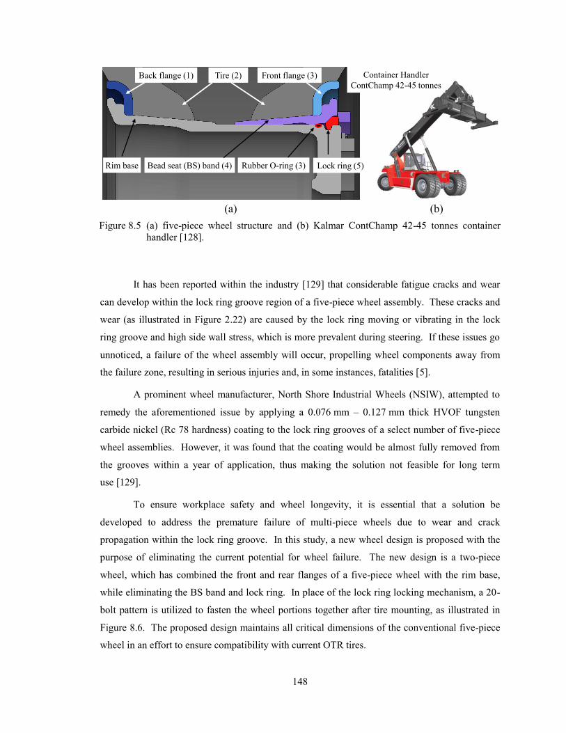
148

It has been reported within the industry [129] that considerable fatigue cracks and wear

can develop within the lock ring groove region of a five-piece wheel assembly. These cracks and

wear (as illustrated in Figure 2.22) are caused by the lock ring moving or vibrating in the lock

ring groove and high side wall stress, which is more prevalent during steering. If these issues go

unnoticed, a failure of the wheel assembly will occur, propelling wheel components away from

the failure zone, resulting in serious injuries and, in some instances, fatalities [5].

A prominent wheel manufacturer, North Shore Industrial Wheels (NSIW), attempted to

remedy the aforementioned issue by applying a 0.076 mm – 0.127 mm thick HVOF tungsten

carbide nickel (Rc 78 hardness) coating to the lock ring grooves of a select number of five-piece

wheel assemblies. However, it was found that the coating would be almost fully removed from

the grooves within a year of application, thus making the solution not feasible for long term

use [129].

To ensure workplace safety and wheel longevity, it is essential that a solution be

developed to address the premature failure of multi-piece wheels due to wear and crack

propagation within the lock ring groove. In this study, a new wheel design is proposed with the

purpose of eliminating the current potential for wheel failure. The new design is a two-piece

wheel, which has combined the front and rear flanges of a five-piece wheel with the rim base,

while eliminating the BS band and lock ring. In place of the lock ring locking mechanism, a 20-

bolt pattern is utilized to fasten the wheel portions together after tire mounting, as illustrated in

Figure 8.6. The proposed design maintains all critical dimensions of the conventional five-piece

wheel in an effort to ensure compatibility with current OTR tires.

(a) (b)

Rim base

Tire (2)Back flange (1) Front flange (3)

Bead seat (BS) band (4) Lock ring (5)Rubber O-ring (3)

Container Handler

ContChamp 42-45 tonnes

Figure 8.5 (a) five-piece wheel structure and (b) Kalmar ContChamp 42-45 tonnes container

handler [128].

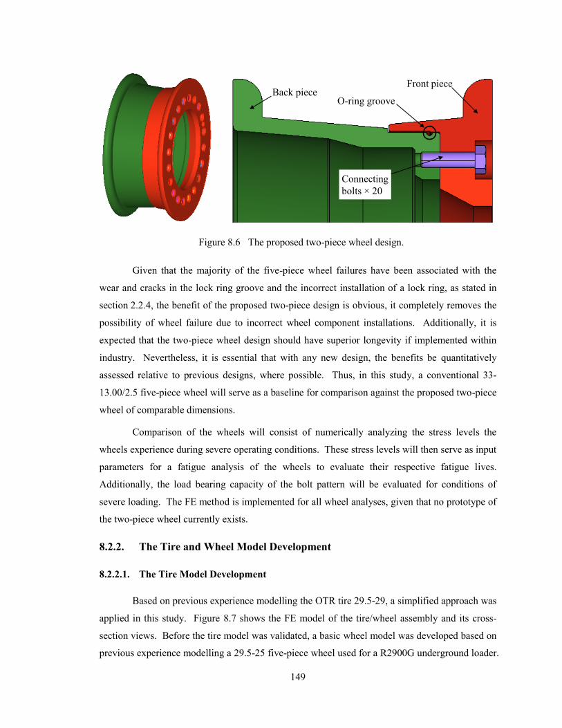
149

Given that the majority of the five-piece wheel failures have been associated with the

wear and cracks in the lock ring groove and the incorrect installation of a lock ring, as stated in

section 2.2.4, the benefit of the proposed two-piece design is obvious, it completely removes the

possibility of wheel failure due to incorrect wheel component installations. Additionally, it is

expected that the two-piece wheel design should have superior longevity if implemented within

industry. Nevertheless, it is essential that with any new design, the benefits be quantitatively

assessed relative to previous designs, where possible. Thus, in this study, a conventional 33-

13.00/2.5 five-piece wheel will serve as a baseline for comparison against the proposed two-piece

wheel of comparable dimensions.

Comparison of the wheels will consist of numerically analyzing the stress levels the

wheels experience during severe operating conditions. These stress levels will then serve as input

parameters for a fatigue analysis of the wheels to evaluate their respective fatigue lives.

Additionally, the load bearing capacity of the bolt pattern will be evaluated for conditions of

severe loading. The FE method is implemented for all wheel analyses, given that no prototype of

the two-piece wheel currently exists.

8.2.2. The Tire and Wheel Model Development

8.2.2.1. The Tire Model Development

Based on previous experience modelling the OTR tire 29.5-29, a simplified approach was

applied in this study. Figure 8.7 shows the FE model of the tire/wheel assembly and its cross-

section views. Before the tire model was validated, a basic wheel model was developed based on

previous experience modelling a 29.5-25 five-piece wheel used for a R2900G underground loader.

Back pieceFront piece

O-ring groove

Connecting

bolts 20

Figure 8.6 The proposed two-piece wheel design.

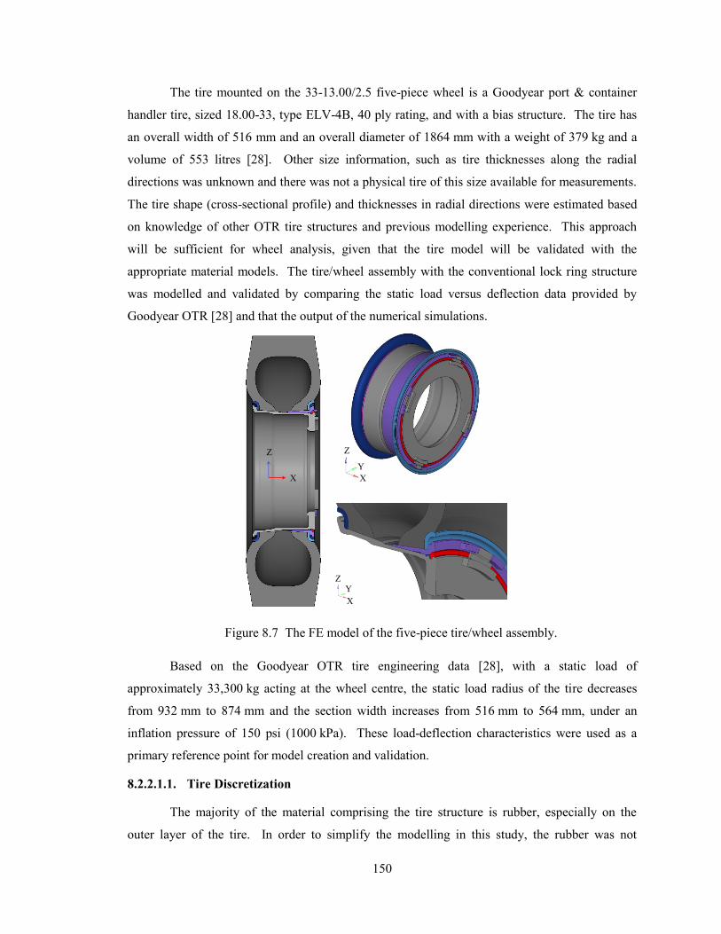
150

The tire mounted on the 33-13.00/2.5 five-piece wheel is a Goodyear port & container

handler tire, sized 18.00-33, type ELV-4B, 40 ply rating, and with a bias structure. The tire has

an overall width of 516 mm and an overall diameter of 1864 mm with a weight of 379 kg and a

volume of 553 litres [28]. Other size information, such as tire thicknesses along the radial

directions was unknown and there was not a physical tire of this size available for measurements.

The tire shape (cross-sectional profile) and thicknesses in radial directions were estimated based

on knowledge of other OTR tire structures and previous modelling experience. This approach

will be sufficient for wheel analysis, given that the tire model will be validated with the

appropriate material models. The tire/wheel assembly with the conventional lock ring structure

was modelled and validated by comparing the static load versus deflection data provided by

Goodyear OTR [28] and that the output of the numerical simulations.

Based on the Goodyear OTR tire engineering data [28], with a static load of

approximately 33,300 kg acting at the wheel centre, the static load radius of the tire decreases

from 932 mm to 874 mm and the section width increases from 516 mm to 564 mm, under an

inflation pressure of 150 psi (1000 kPa). These load-deflection characteristics were used as a

primary reference point for model creation and validation.

8.2.2.1.1. Tire Discretization

The majority of the material comprising the tire structure is rubber, especially on the

outer layer of the tire. In order to simplify the modelling in this study, the rubber was not

X

Y

Z

X

YZ

X

Z

Figure 8.7 The FE model of the five-piece tire/wheel assembly.

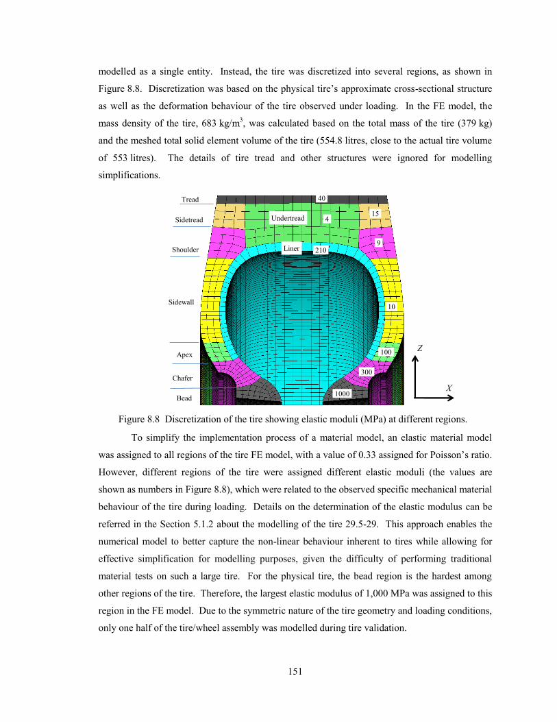
151

modelled as a single entity. Instead, the tire was discretized into several regions, as shown in

Figure 8.8. Discretization was based on the physical tire’s approximate cross-sectional structure

as well as the deformation behaviour of the tire observed under loading. In the FE model, the

mass density of the tire, 683 kg/m3, was calculated based on the total mass of the tire (379 kg)

and the meshed total solid element volume of the tire (554.8 litres, close to the actual tire volume

of 553 litres). The details of tire tread and other structures were ignored for modelling

simplifications.

To simplify the implementation process of a material model, an elastic material model

was assigned to all regions of the tire FE model, with a value of 0.33 assigned for Poisson’s ratio.

However, different regions of the tire were assigned different elastic moduli (the values are

shown as numbers in Figure 8.8), which were related to the observed specific mechanical material

behaviour of the tire during loading. Details on the determination of the elastic modulus can be

referred in the Section 5.1.2 about the modelling of the tire 29.5-29. This approach enables the

numerical model to better capture the non-linear behaviour inherent to tires while allowing for

effective simplification for modelling purposes, given the difficulty of performing traditional

material tests on such a large tire. For the physical tire, the bead region is the hardest among

other regions of the tire. Therefore, the largest elastic modulus of 1,000 MPa was assigned to this

region in the FE model. Due to the symmetric nature of the tire geometry and loading conditions,

only one half of the tire/wheel assembly was modelled during tire validation.

Liner 210

4

9

1000

300

15

40

10

Chafer

Sidewall

Shoulder

Sidetread

Tread

Bead

Undertread

Apex 100

X

Z

Figure 8.8 Discretization of the tire showing elastic moduli (MPa) at different regions.

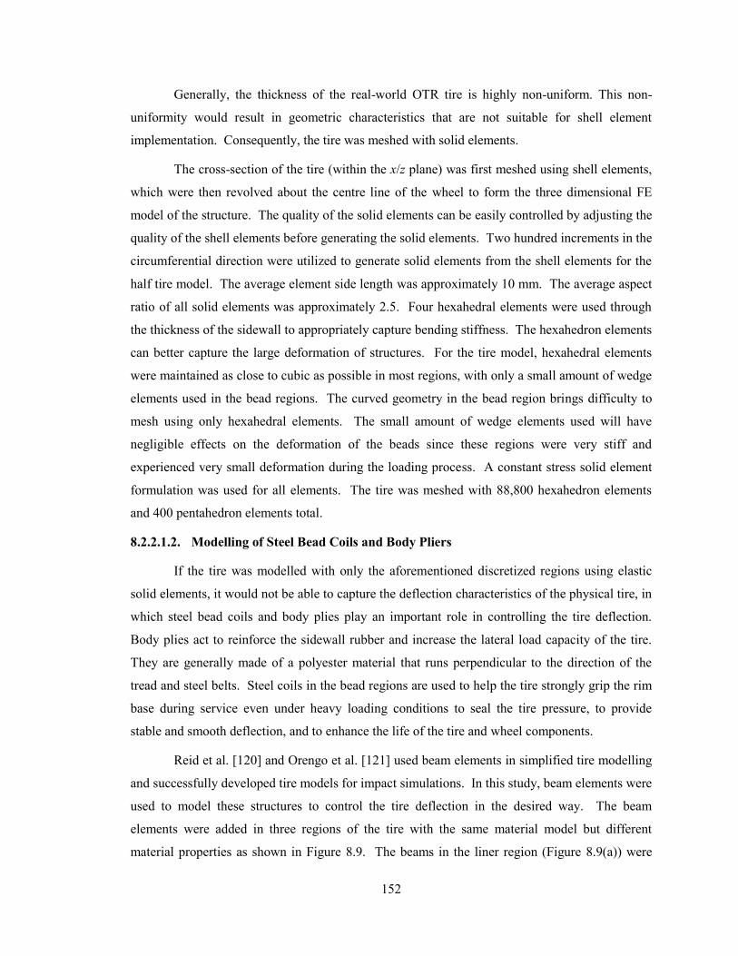
152

Generally, the thickness of the real-world OTR tire is highly non-uniform. This non-

uniformity would result in geometric characteristics that are not suitable for shell element

implementation. Consequently, the tire was meshed with solid elements.

The cross-section of the tire (within the x/z plane) was first meshed using shell elements,

which were then revolved about the centre line of the wheel to form the three dimensional FE

model of the structure. The quality of the solid elements can be easily controlled by adjusting the

quality of the shell elements before generating the solid elements. Two hundred increments in the

circumferential direction were utilized to generate solid elements from the shell elements for the

half tire model. The average element side length was approximately 10 mm. The average aspect

ratio of all solid elements was approximately 2.5. Four hexahedral elements were used through

the thickness of the sidewall to appropriately capture bending stiffness. The hexahedron elements

can better capture the large deformation of structures. For the tire model, hexahedral elements

were maintained as close to cubic as possible in most regions, with only a small amount of wedge

elements used in the bead regions. The curved geometry in the bead region brings difficulty to

mesh using only hexahedral elements. The small amount of wedge elements used will have

negligible effects on the deformation of the beads since these regions were very stiff and

experienced very small deformation during the loading process. A constant stress solid element

formulation was used for all elements. The tire was meshed with 88,800 hexahedron elements

and 400 pentahedron elements total.

8.2.2.1.2. Modelling of Steel Bead Coils and Body Pliers

If the tire was modelled with only the aforementioned discretized regions using elastic

solid elements, it would not be able to capture the deflection characteristics of the physical tire, in

which steel bead coils and body plies play an important role in controlling the tire deflection.

Body plies act to reinforce the sidewall rubber and increase the lateral load capacity of the tire.

They are generally made of a polyester material that runs perpendicular to the direction of the

tread and steel belts. Steel coils in the bead regions are used to help the tire strongly grip the rim

base during service even under heavy loading conditions to seal the tire pressure, to provide

stable and smooth deflection, and to enhance the life of the tire and wheel components.

Reid et al. [120] and Orengo et al. [121] used beam elements in simplified tire modelling

and successfully developed tire models for impact simulations. In this study, beam elements were

used to model these structures to control the tire deflection in the desired way. The beam

elements were added in three regions of the tire with the same material model but different

material properties as shown in Figure 8.9. The beams in the liner region (Figure 8.9(a)) were

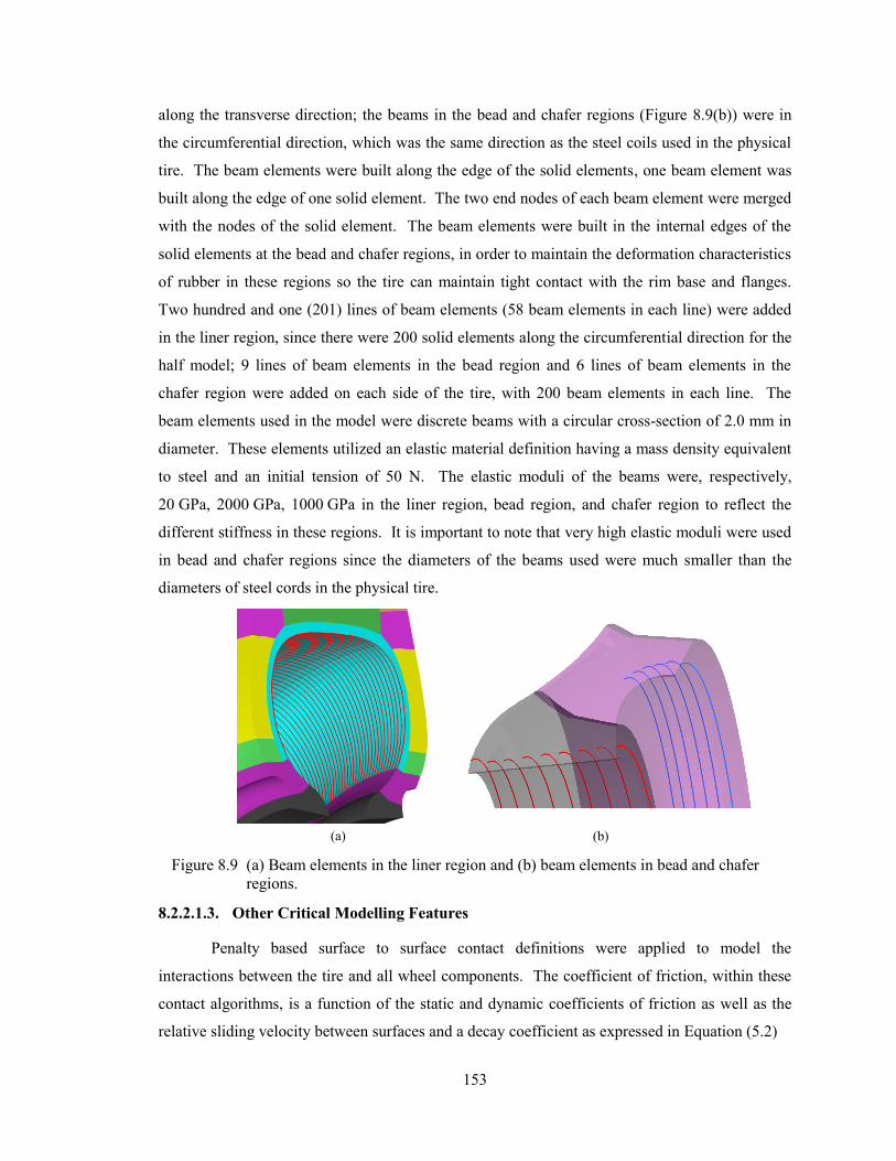
153

along the transverse direction; the beams in the bead and chafer regions (Figure 8.9(b)) were in

the circumferential direction, which was the same direction as the steel coils used in the physical

tire. The beam elements were built along the edge of the solid elements, one beam element was

built along the edge of one solid element. The two end nodes of each beam element were merged

with the nodes of the solid element. The beam elements were built in the internal edges of the

solid elements at the bead and chafer regions, in order to maintain the deformation characteristics

of rubber in these regions so the tire can maintain tight contact with the rim base and flanges.

Two hundred and one (201) lines of beam elements (58 beam elements in each line) were added

in the liner region, since there were 200 solid elements along the circumferential direction for the

half model; 9 lines of beam elements in the bead region and 6 lines of beam elements in the

chafer region were added on each side of the tire, with 200 beam elements in each line. The

beam elements used in the model were discrete beams with a circular cross-section of 2.0 mm in

diameter. These elements utilized an elastic material definition having a mass density equivalent

to steel and an initial tension of 50 N. The elastic moduli of the beams were, respectively,

20 GPa, 2000 GPa, 1000 GPa in the liner region, bead region, and chafer region to reflect the

different stiffness in these regions. It is important to note that very high elastic moduli were used

in bead and chafer regions since the diameters of the beams used were much smaller than the

diameters of steel cords in the physical tire.

8.2.2.1.3. Other Critical Modelling Features

Penalty based surface to surface contact definitions were applied to model the

interactions between the tire and all wheel components. The coefficient of friction, within these

contact algorithms, is a function of the static and dynamic coefficients of friction as well as the

relative sliding velocity between surfaces and a decay coefficient as expressed in Equation (5.2)

(b)(a)

Figure 8.9 (a) Beam elements in the liner region and (b) beam elements in bead and chafer

regions.

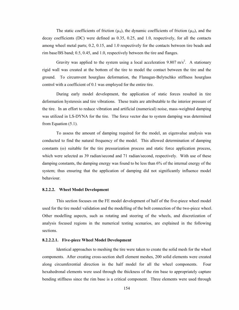
154

The static coefficients of friction (µS), the dynamic coefficients of friction (µD), and the

decay coefficients (DC) were defined as 0.35, 0.25, and 1.0, respectively, for all the contacts

among wheel metal parts; 0.2, 0.15, and 1.0 respectively for the contacts between tire beads and

rim base/BS band; 0.5, 0.45, and 1.0, respectively between the tire and flanges.

Gravity was applied to the system using a local acceleration 9.807 m/s2. A stationary

rigid wall was created at the bottom of the tire to model the contact between the tire and the

ground. To circumvent hourglass deformation, the Flanagan-Belytschko stiffness hourglass

control with a coefficient of 0.1 was employed for the entire tire.

During early model development, the application of static forces resulted in tire

deformation hysteresis and tire vibrations. These traits are attributable to the interior pressure of

the tire. In an effort to reduce vibration and artificial (numerical) noise, mass-weighted damping

was utilized in LS-DYNA for the tire. The force vector due to system damping was determined

from Equation (5.1).

To assess the amount of damping required for the model, an eigenvalue analysis was

conducted to find the natural frequency of the model. This allowed determination of damping

constants () suitable for the tire pressurization process and static force application process,

which were selected as 39 radian/second and 71 radian/second, respectively. With use of these

damping constants, the damping energy was found to be less than 6% of the internal energy of the

system; thus ensuring that the application of damping did not significantly influence model

behaviour.

8.2.2.2. Wheel Model Development

This section focuses on the FE model development of half of the five-piece wheel model

used for the tire model validation and the modelling of the bolt connection of the two-piece wheel.

Other modelling aspects, such as rotating and steering of the wheels, and discretization of

analysis focused regions in the numerical testing scenarios, are explained in the following

sections.

8.2.2.2.1. Five-piece Wheel Model Development

Identical approaches to meshing the tire were taken to create the solid mesh for the wheel

components. After creating cross-section shell element meshes, 200 solid elements were created

along circumferential direction in the half model for all the wheel components. Four

hexahedronal elements were used through the thickness of the rim base to appropriately capture

bending stiffness since the rim base is a critical component. Three elements were used through

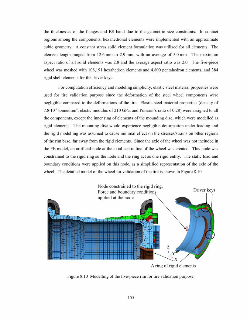
155

the thicknesses of the flanges and BS band due to the geometric size constraints. In contact

regions among the components, hexahedronal elements were implemented with an approximate

cubic geometry. A constant stress solid element formulation was utilized for all elements. The

element length ranged from 12.6 mm to 2.9 mm, with an average of 5.0 mm. The maximum

aspect ratio of all solid elements was 2.8 and the average aspect ratio was 2.0. The five-piece

wheel was meshed with 108,191 hexahedron elements and 4,800 pentahedron elements, and 384

rigid shell elements for the driver keys.

For computation efficiency and modeling simplicity, elastic steel material properties were

used for tire validation purpose since the deformation of the steel wheel components were

negligible compared to the deformations of the tire. Elastic steel material properties (density of

7.8∙10-9

tonne/mm3, elastic modulus of 210 GPa, and Poisson’s ratio of 0.28) were assigned to all

the components, except the inner ring of elements of the mounding disc, which were modelled as

rigid elements. The mounting disc would experience negligible deformation under loading and

the rigid modelling was assumed to cause minimal effect on the stresses/strains on other regions

of the rim base, far away from the rigid elements. Since the axle of the wheel was not included in

the FE model, an artificial node at the axial centre line of the wheel was created. This node was

constrained to the rigid ring so the node and the ring act as one rigid entity. The static load and

boundary conditions were applied on this node, as a simplified representation of the axle of the

wheel. The detailed model of the wheel for validation of the tire is shown in Figure 8.10.

Node constrained to the rigid ring.

Force and boundary conditions

applied at the node

A ring of rigid elements

Driver keys

X

Y

Z

Figure 8.10 Modelling of the five-piece rim for tire validation purpose.

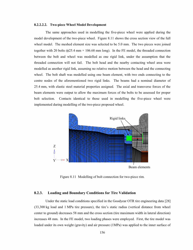
156

8.2.2.2.2. Two-piece Wheel Model Development

The same approaches used in modelling the five-piece wheel were applied during the

model development of the two-piece wheel. Figure 8.11 shows the cross section view of the full

wheel model. The meshed element size was selected to be 5.0 mm. The two pieces were joined

together with 20 bolts (25.4 mm × 106.68 mm long). In the FE model, the threaded connection

between the bolt and wheel was modelled as one rigid link, under the assumption that the

threaded connection will not fail. The bolt head and the nearby contacting wheel area were

modelled as another rigid link, assuming no relative motion between the head and the connecting

wheel. The bolt shaft was modelled using one beam element, with two ends connecting to the

centre nodes of the aforementioned two rigid links. The beams had a nominal diameter of

25.4 mm, with elastic steel material properties assigned. The axial and transverse forces of the

beam elements were output to allow the maximum forces of the bolts to be assessed for proper

bolt selection. Contacts identical to those used in modelling the five-piece wheel were

implemented during modelling of the two-piece proposed wheel.

8.2.3. Loading and Boundary Conditions for Tire Validation

Under the static load conditions specified in the Goodyear OTR tire engineering data [28]

(33,300 kg load and 1 MPa tire pressure), the tire’s static radius (vertical distance from wheel

center to ground) decreases 58 mm and the cross section (tire maximum width in lateral direction)

increases 48 mm. In the FE model, two loading phases were employed. First, the tire model was

loaded under its own weight (gravity) and air pressure (1MPa) was applied to the inner surface of

Beam elements

Rigid links

XY

Z

Figure 8.11 Modelling of bolt connection for two-piece rim.

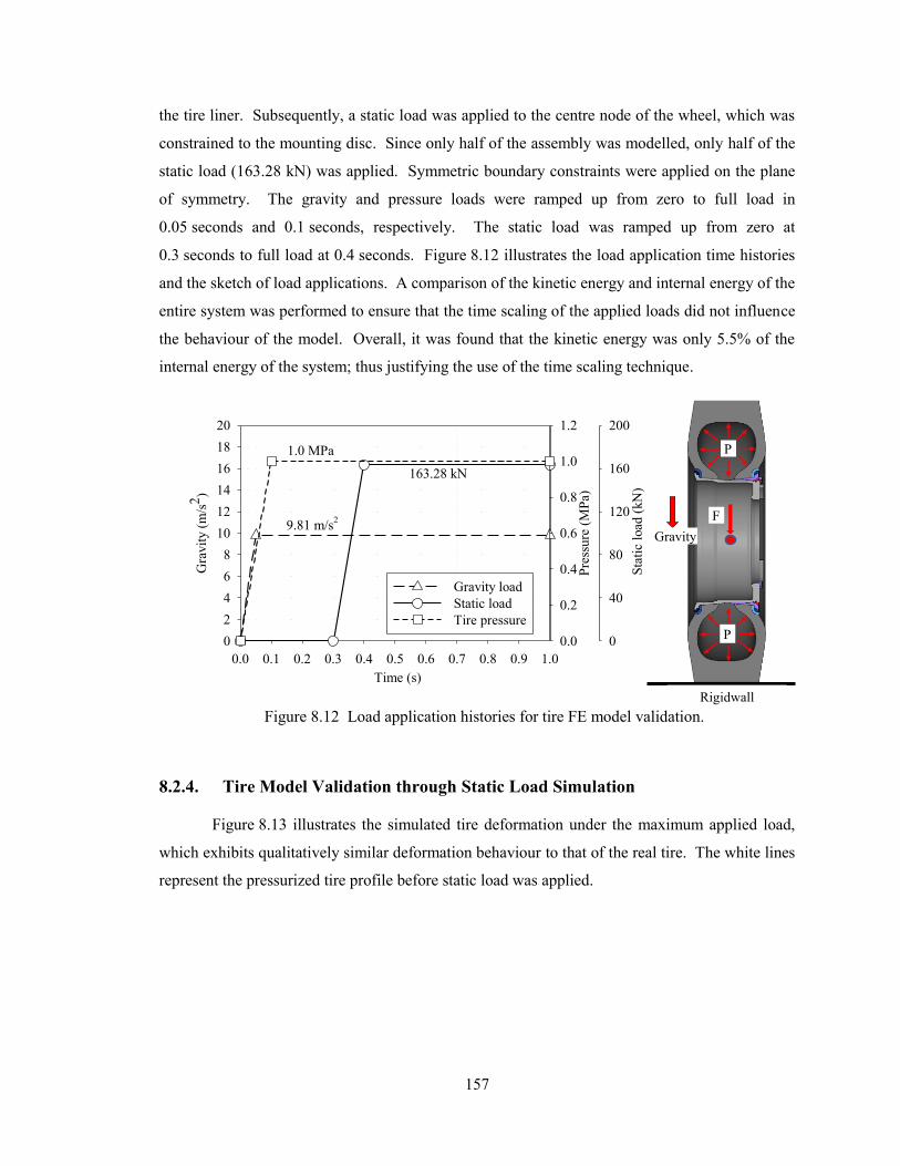
157

the tire liner. Subsequently, a static load was applied to the centre node of the wheel, which was

constrained to the mounting disc. Since only half of the assembly was modelled, only half of the

static load (163.28 kN) was applied. Symmetric boundary constraints were applied on the plane

of symmetry. The gravity and pressure loads were ramped up from zero to full load in

0.05 seconds and 0.1 seconds, respectively. The static load was ramped up from zero at

0.3 seconds to full load at 0.4 seconds. Figure 8.12 illustrates the load application time histories

and the sketch of load applications. A comparison of the kinetic energy and internal energy of the

entire system was performed to ensure that the time scaling of the applied loads did not influence

the behaviour of the model. Overall, it was found that the kinetic energy was only 5.5% of the

internal energy of the system; thus justifying the use of the time scaling technique.

8.2.4. Tire Model Validation through Static Load Simulation

Figure 8.13 illustrates the simulated tire deformation under the maximum applied load,

which exhibits qualitatively similar deformation behaviour to that of the real tire. The white lines

represent the pressurized tire profile before static load was applied.

P

P

F

Gravity

Rigidwall

Time (s)

0.0 0.1 0.2 0.3 0.4 0.5 0.6 0.7 0.8 0.9 1.0

Gra

vit

y (

m/s

2)

0

2

4

6

8

10

12

14

16

18

20

Sta

tic

load

(kN

)0

40

80

120

160

200

Pre

ssu

re (

MP

a)

0.0

0.2

0.4

0.6

0.8

1.0

1.2

Gravity load

Static load

Tire pressure

9.81 m/s2

163.28 kN

1.0 MPa

Figure 8.12 Load application histories for tire FE model validation.

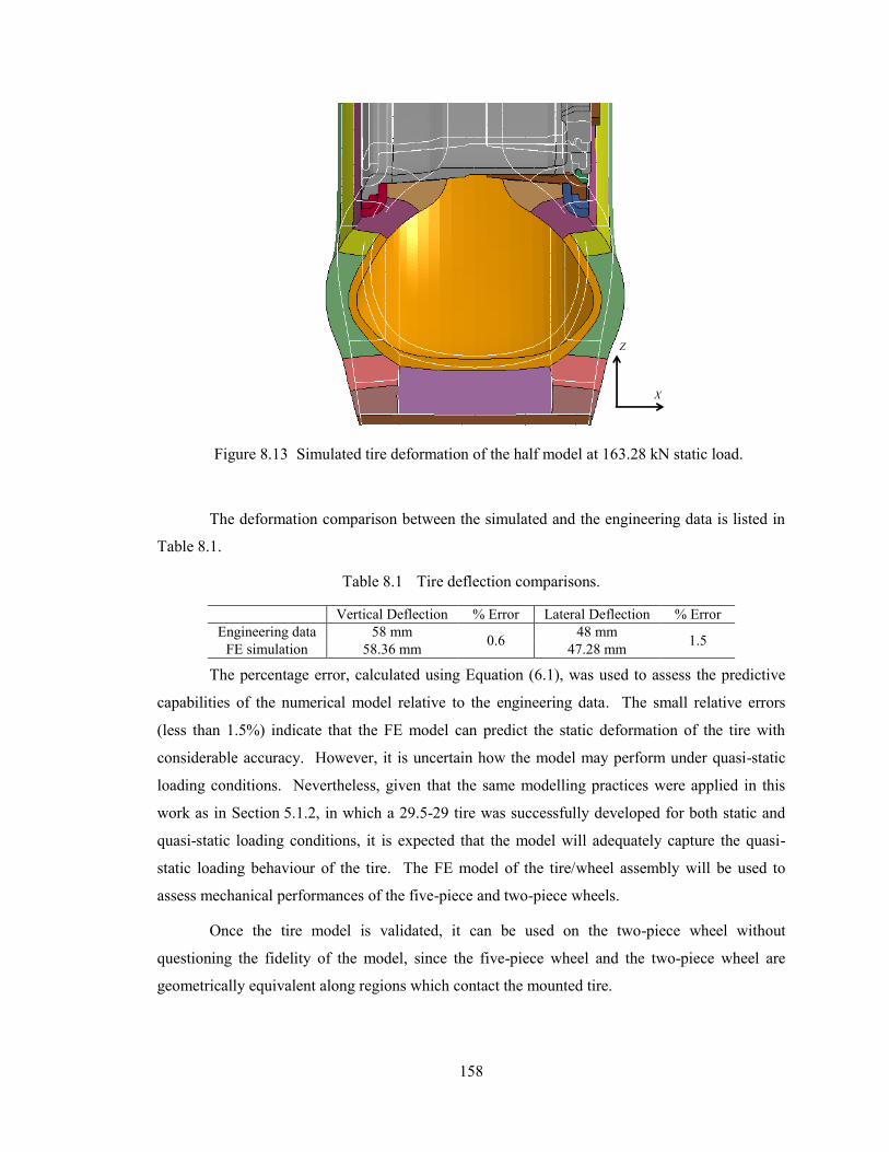
158

The deformation comparison between the simulated and the engineering data is listed in

Table 8.1.

Table 8.1 Tire deflection comparisons.

Vertical Deflection % Error Lateral Deflection % Error

Engineering data 58 mm 0.6

48 mm 1.5

FE simulation 58.36 mm 47.28 mm

The percentage error, calculated using Equation (6.1), was used to assess the predictive

capabilities of the numerical model relative to the engineering data. The small relative errors

(less than 1.5%) indicate that the FE model can predict the static deformation of the tire with

considerable accuracy. However, it is uncertain how the model may perform under quasi-static

loading conditions. Nevertheless, given that the same modelling practices were applied in this

work as in Section 5.1.2, in which a 29.5-29 tire was successfully developed for both static and

quasi-static loading conditions, it is expected that the model will adequately capture the quasi-

static loading behaviour of the tire. The FE model of the tire/wheel assembly will be used to

assess mechanical performances of the five-piece and two-piece wheels.

Once the tire model is validated, it can be used on the two-piece wheel without

questioning the fidelity of the model, since the five-piece wheel and the two-piece wheel are

geometrically equivalent along regions which contact the mounted tire.

X

Z

Figure 8.13 Simulated tire deformation of the half model at 163.28 kN static load.

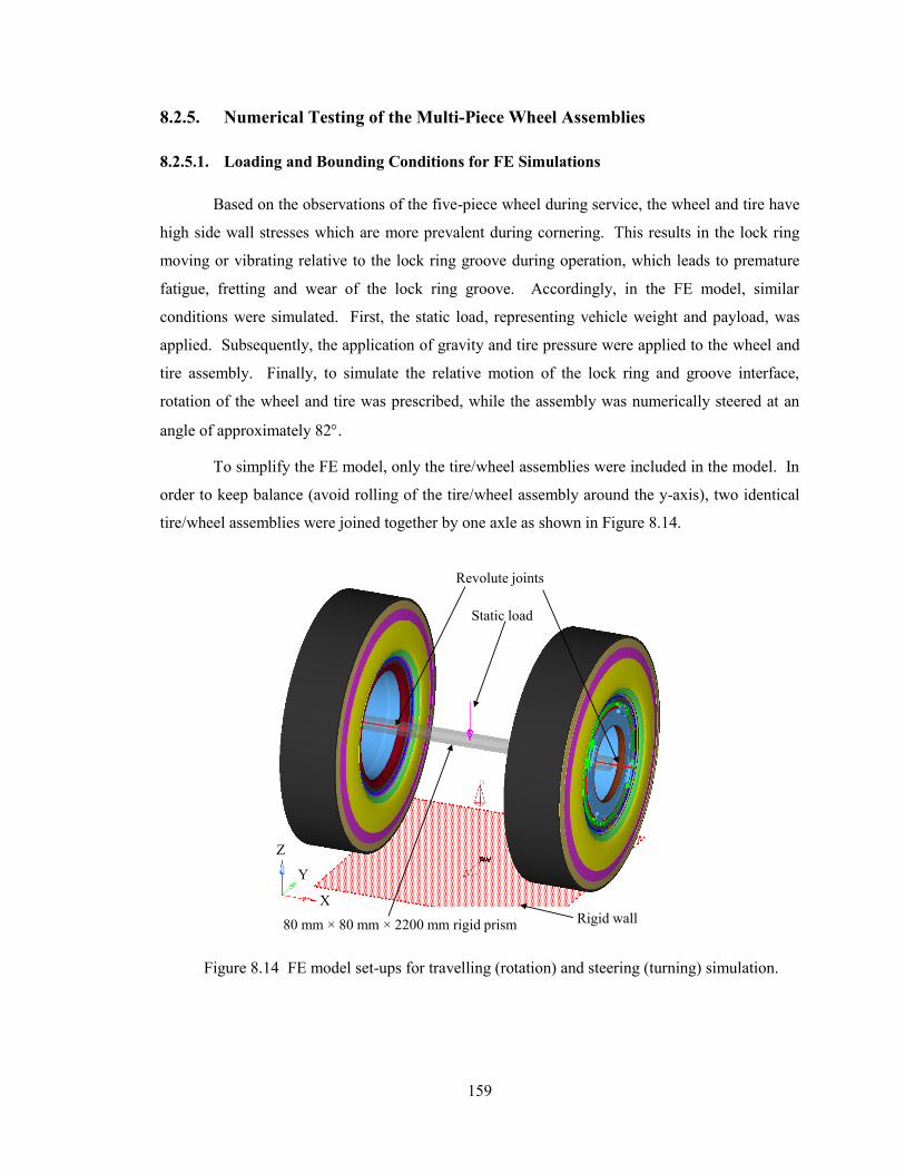
159

8.2.5. Numerical Testing of the Multi-Piece Wheel Assemblies

8.2.5.1. Loading and Bounding Conditions for FE Simulations

Based on the observations of the five-piece wheel during service, the wheel and tire have

high side wall stresses which are more prevalent during cornering. This results in the lock ring

moving or vibrating relative to the lock ring groove during operation, which leads to premature

fatigue, fretting and wear of the lock ring groove. Accordingly, in the FE model, similar

conditions were simulated. First, the static load, representing vehicle weight and payload, was

applied. Subsequently, the application of gravity and tire pressure were applied to the wheel and

tire assembly. Finally, to simulate the relative motion of the lock ring and groove interface,

rotation of the wheel and tire was prescribed, while the assembly was numerically steered at an

angle of approximately 82.

To simplify the FE model, only the tire/wheel assemblies were included in the model. In

order to keep balance (avoid rolling of the tire/wheel assembly around the y-axis), two identical

tire/wheel assemblies were joined together by one axle as shown in Figure 8.14.

Revolute joints

80 mm 80 mm 2200 mm rigid prism

Static load

Rigid wall

X

Y

Z

Figure 8.14 FE model set-ups for travelling (rotation) and steering (turning) simulation.

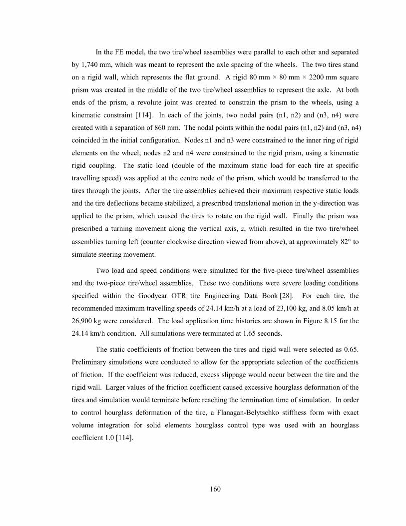
160

In the FE model, the two tire/wheel assemblies were parallel to each other and separated

by 1,740 mm, which was meant to represent the axle spacing of the wheels. The two tires stand

on a rigid wall, which represents the flat ground. A rigid 80 mm × 80 mm × 2200 mm square

prism was created in the middle of the two tire/wheel assemblies to represent the axle. At both

ends of the prism, a revolute joint was created to constrain the prism to the wheels, using a

kinematic constraint [114]. In each of the joints, two nodal pairs (n1, n2) and (n3, n4) were

created with a separation of 860 mm. The nodal points within the nodal pairs (n1, n2) and (n3, n4)

coincided in the initial configuration. Nodes n1 and n3 were constrained to the inner ring of rigid

elements on the wheel; nodes n2 and n4 were constrained to the rigid prism, using a kinematic

rigid coupling. The static load (double of the maximum static load for each tire at specific

travelling speed) was applied at the centre node of the prism, which would be transferred to the

tires through the joints. After the tire assemblies achieved their maximum respective static loads

and the tire deflections became stabilized, a prescribed translational motion in the y-direction was

applied to the prism, which caused the tires to rotate on the rigid wall. Finally the prism was

prescribed a turning movement along the vertical axis, z, which resulted in the two tire/wheel

assemblies turning left (counter clockwise direction viewed from above), at approximately 82 to

simulate steering movement.

Two load and speed conditions were simulated for the five-piece tire/wheel assemblies

and the two-piece tire/wheel assemblies. These two conditions were severe loading conditions

specified within the Goodyear OTR tire Engineering Data Book [28]. For each tire, the

recommended maximum travelling speeds of 24.14 km/h at a load of 23,100 kg, and 8.05 km/h at

26,900 kg were considered. The load application time histories are shown in Figure 8.15 for the

24.14 km/h condition. All simulations were terminated at 1.65 seconds.

The static coefficients of friction between the tires and rigid wall were selected as 0.65.

Preliminary simulations were conducted to allow for the appropriate selection of the coefficients

of friction. If the coefficient was reduced, excess slippage would occur between the tire and the

rigid wall. Larger values of the friction coefficient caused excessive hourglass deformation of the

tires and simulation would terminate before reaching the termination time of simulation. In order

to control hourglass deformation of the tire, a Flanagan-Belytschko stiffness form with exact

volume integration for solid elements hourglass control type was used with an hourglass

coefficient 1.0 [114].

161

For the five-piece wheel, four drive keys were used to prevent the relative rotation

between the rim base and BS band and to evenly distribute the reaction forces at the driver key

regions. In conditions of rotation, there is a greater tendency for the BS band to rotate relative to

the rim base, compared to static load conditions. The modeling technique for the driver key using

rigid shell elements in the static load condition did not work efficiently for the rotation condition,

causing contact penetration between the driver key and wheel, and between the driver key and BS

band, resulting in excess relative rotation of the components. In the rotation loading condition,

the driver keys were modeled as solid elements as one entity with the rim base and contacts were

established between the rim base and BS band at driver key locations. The relative rotation

between the two components was prevented using this approach. To prevent the relative rotation

between the flange and BS band/rim base, a static coefficient of friction of 0.80 was used for the

contacts between these parts. The static coefficients of friction between the tire and wheel

components were selected as 0.95. The static coefficients of friction among the wheel

components were selected as 0.35.

To reduce the artificial (numerical) noise effects on stress levels, stiffness damping was

implemented. This type of damping is more effective for high frequencies [114]. The damping

coefficient (β) of 20% was applied to all wheel (metal) components. The damping matrix was

computed from the stiffness matrix as indicated in Equation (6.2). Detailed modelling parameters

are included in Appendix E.5.

As pointed out by Conle et al. [130], plastic modeling gives poor quality of stress/strain

assessment when faced with reversals in loading direction. In this research, a linear elastic model

Time (s)

0.0 0.2 0.4 0.6 0.8 1.0 1.2 1.4 1.6 1.8 2.0

Gra

vit

y (

m/s

2)

/Tra

vel

ling s

pee

d (

km

/h)

0

5

10

15

20

25

30

35

40

45

50

Sta

tic

load

(kN

)

0

100

200

300

400

500

Pre

ssure

(M

Pa)

0.0

0.2

0.4

0.6

0.8

1.0

1.2

1.4

Ste

erin

g s

pee

d (

o/s

)

0

40

80

120

160

200

240

Gravity load

Static load

Tire pressure

Travelling speed

Steering speed

453.1 kN

1.0 MPa

9.81 m/s2

24.14 km/h

180o/s

Figure 8.15 Load application histories for 24.14 km/h transverse travelling condition.

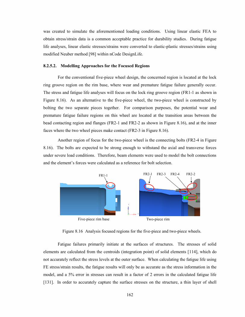
162

was created to simulate the aforementioned loading conditions. Using linear elastic FEA to

obtain stress/strain data is a common acceptable practice for durability studies. During fatigue

life analyses, linear elastic stresses/strains were converted to elastic-plastic stresses/strains using

modified Neuber method [98] within nCode DesignLife.

8.2.5.2. Modelling Approaches for the Focused Regions

For the conventional five-piece wheel design, the concerned region is located at the lock

ring groove region on the rim base, where wear and premature fatigue failure generally occur.

The stress and fatigue life analyses will focus on the lock ring groove region (FR1-1 as shown in

Figure 8.16). As an alternative to the five-piece wheel, the two-piece wheel is constructed by

bolting the two separate pieces together. For comparison purposes, the potential wear and

premature fatigue failure regions on this wheel are located at the transition areas between the

bead contacting region and flanges (FR2-1 and FR2-2 as shown in Figure 8.16), and at the inner

faces where the two wheel pieces make contact (FR2-3 in Figure 8.16).

Another region of focus for the two-piece wheel is the connecting bolts (FR2-4 in Figure

8.16). The bolts are expected to be strong enough to withstand the axial and transverse forces

under severe load conditions. Therefore, beam elements were used to model the bolt connections

and the element’s forces were calculated as a reference for bolt selection.

Fatigue failures primarily initiate at the surfaces of structures. The stresses of solid

elements are calculated from the centroids (integration point) of solid elements [114], which do

not accurately reflect the stress levels at the outer surface. When calculating the fatigue life using

FE stress/strain results, the fatigue results will only be as accurate as the stress information in the

model, and a 5% error in stresses can result in a factor of 2 errors in the calculated fatigue life

[131]. In order to accurately capture the surface stresses on the structure, a thin layer of shell

FR1-1 FR2-1

Five-piece rim base Two-piece rim

FR2-2FR2-3 FR2-4

Figure 8.16 Analysis focused regions for the five-piece and two-piece wheels.

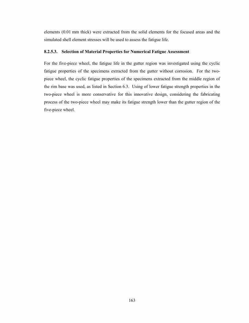
163

elements (0.01 mm thick) were extracted from the solid elements for the focused areas and the

simulated shell element stresses will be used to assess the fatigue life.

8.2.5.3. Selection of Material Properties for Numerical Fatigue Assessment

For the five-piece wheel, the fatigue life in the gutter region was investigated using the cyclic

fatigue properties of the specimens extracted from the gutter without corrosion. For the two-

piece wheel, the cyclic fatigue properties of the specimens extracted from the middle region of

the rim base was used, as listed in Section 6.3. Using of lower fatigue strength properties in the

two-piece wheel is more conservative for this innovative design, considering the fabricating

process of the two-piece wheel may make its fatigue strength lower than the gutter region of the

five-piece wheel.

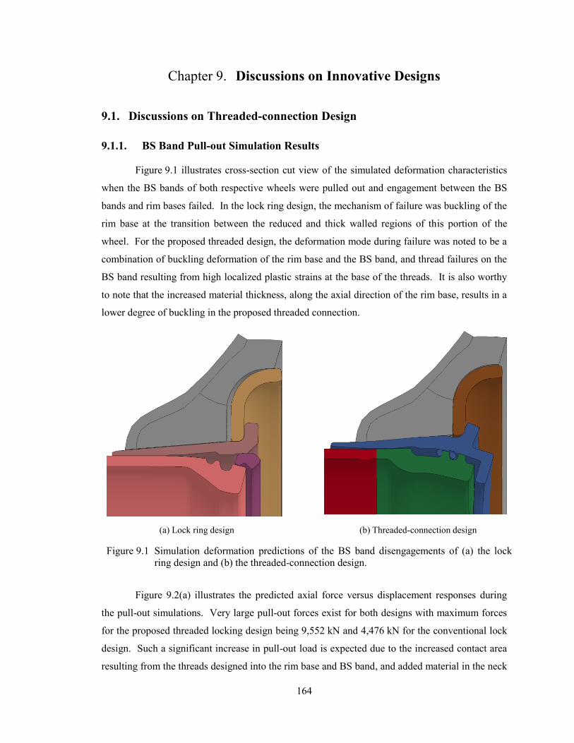
164

Chapter 9. Discussions on Innovative Designs

9.1. Discussions on Threaded-connection Design

9.1.1. BS Band Pull-out Simulation Results

Figure 9.1 illustrates cross-section cut view of the simulated deformation characteristics

when the BS bands of both respective wheels were pulled out and engagement between the BS

bands and rim bases failed. In the lock ring design, the mechanism of failure was buckling of the

rim base at the transition between the reduced and thick walled regions of this portion of the

wheel. For the proposed threaded design, the deformation mode during failure was noted to be a

combination of buckling deformation of the rim base and the BS band, and thread failures on the

BS band resulting from high localized plastic strains at the base of the threads. It is also worthy

to note that the increased material thickness, along the axial direction of the rim base, results in a

lower degree of buckling in the proposed threaded connection.

Figure 9.2(a) illustrates the predicted axial force versus displacement responses during

the pull-out simulations. Very large pull-out forces exist for both designs with maximum forces

for the proposed threaded locking design being 9,552 kN and 4,476 kN for the conventional lock

design. Such a significant increase in pull-out load is expected due to the increased contact area

resulting from the threads designed into the rim base and BS band, and added material in the neck

(a) Lock ring design (b) Threaded-connection design

Figure 9.1 Simulation deformation predictions of the BS band disengagements of (a) the lock

ring design and (b) the threaded-connection design.

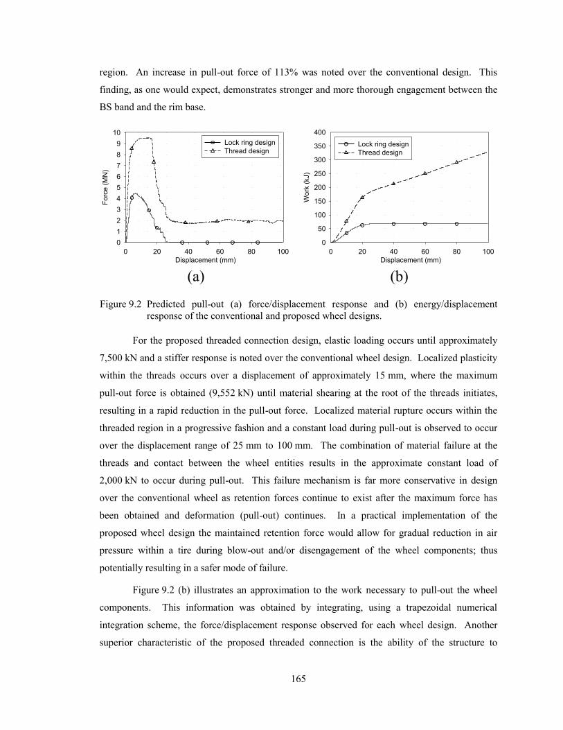
165

region. An increase in pull-out force of 113% was noted over the conventional design. This

finding, as one would expect, demonstrates stronger and more thorough engagement between the

BS band and the rim base.

For the proposed threaded connection design, elastic loading occurs until approximately

7,500 kN and a stiffer response is noted over the conventional wheel design. Localized plasticity

within the threads occurs over a displacement of approximately 15 mm, where the maximum

pull-out force is obtained (9,552 kN) until material shearing at the root of the threads initiates,

resulting in a rapid reduction in the pull-out force. Localized material rupture occurs within the

threaded region in a progressive fashion and a constant load during pull-out is observed to occur

over the displacement range of 25 mm to 100 mm. The combination of material failure at the

threads and contact between the wheel entities results in the approximate constant load of

2,000 kN to occur during pull-out. This failure mechanism is far more conservative in design

over the conventional wheel as retention forces continue to exist after the maximum force has

been obtained and deformation (pull-out) continues. In a practical implementation of the

proposed wheel design the maintained retention force would allow for gradual reduction in air

pressure within a tire during blow-out and/or disengagement of the wheel components; thus

potentially resulting in a safer mode of failure.

Figure 9.2 (b) illustrates an approximation to the work necessary to pull-out the wheel

components. This information was obtained by integrating, using a trapezoidal numerical

integration scheme, the force/displacement response observed for each wheel design. Another

superior characteristic of the proposed threaded connection is the ability of the structure to

(a)

Displacement (mm)

0 20 40 60 80 100

Forc

e (

MN

)

0

1

2

3

4

5

6

7

8

9

10

Lock ring design

Thread design

(b)

Displacement (mm)

0 20 40 60 80 100

Wo

rk (

kJ)

0

50

100

150

200

250

300

350

400

Lock ring design

Thread design

Figure 9.2 Predicted pull-out (a) force/displacement response and (b) energy/displacement

response of the conventional and proposed wheel designs.

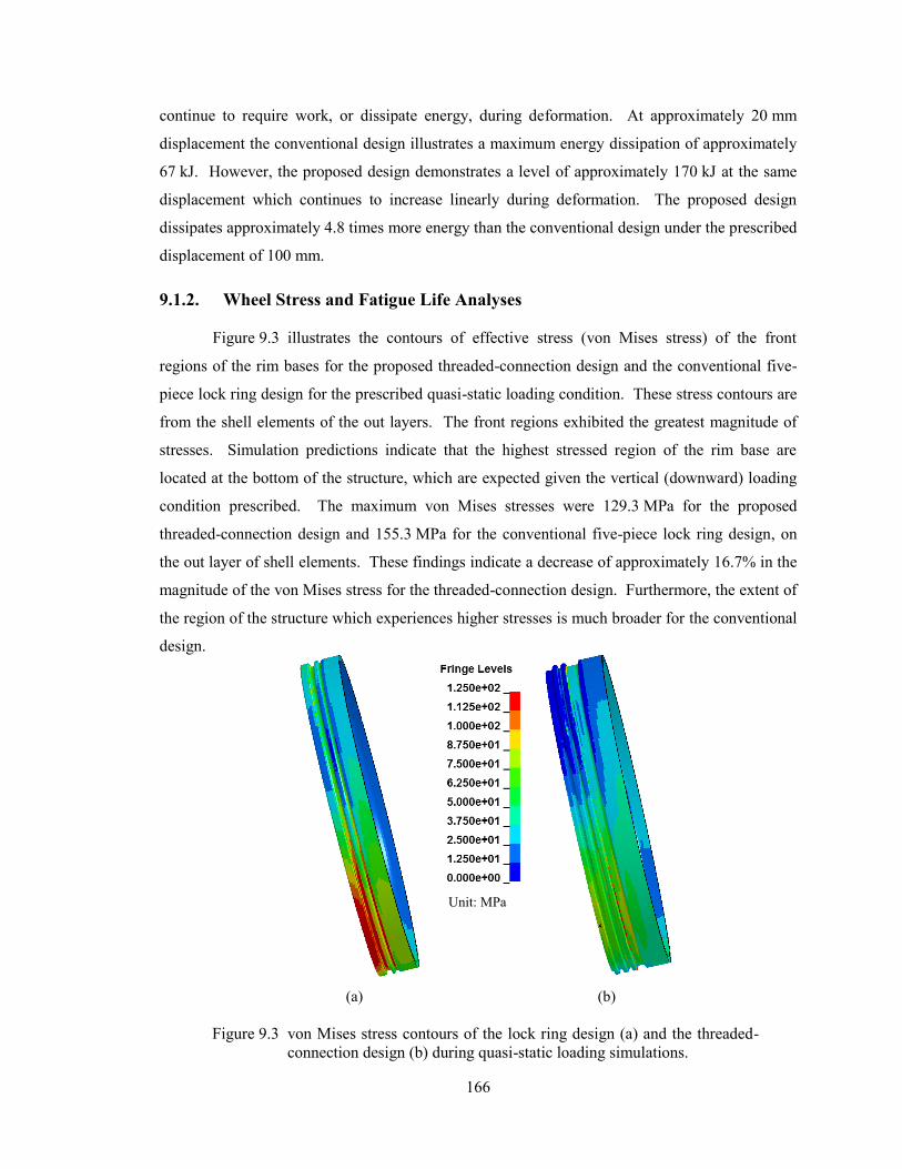
166

continue to require work, or dissipate energy, during deformation. At approximately 20 mm

displacement the conventional design illustrates a maximum energy dissipation of approximately

67 kJ. However, the proposed design demonstrates a level of approximately 170 kJ at the same

displacement which continues to increase linearly during deformation. The proposed design

dissipates approximately 4.8 times more energy than the conventional design under the prescribed

displacement of 100 mm.

9.1.2. Wheel Stress and Fatigue Life Analyses

Figure 9.3 illustrates the contours of effective stress (von Mises stress) of the front

regions of the rim bases for the proposed threaded-connection design and the conventional five-

piece lock ring design for the prescribed quasi-static loading condition. These stress contours are

from the shell elements of the out layers. The front regions exhibited the greatest magnitude of

stresses. Simulation predictions indicate that the highest stressed region of the rim base are

located at the bottom of the structure, which are expected given the vertical (downward) loading

condition prescribed. The maximum von Mises stresses were 129.3 MPa for the proposed

threaded-connection design and 155.3 MPa for the conventional five-piece lock ring design, on

the out layer of shell elements. These findings indicate a decrease of approximately 16.7% in the

magnitude of the von Mises stress for the threaded-connection design. Furthermore, the extent of

the region of the structure which experiences higher stresses is much broader for the conventional

design.

Unit: MPa

(a) (b)

Figure 9.3 von Mises stress contours of the lock ring design (a) and the threaded-

connection design (b) during quasi-static loading simulations.

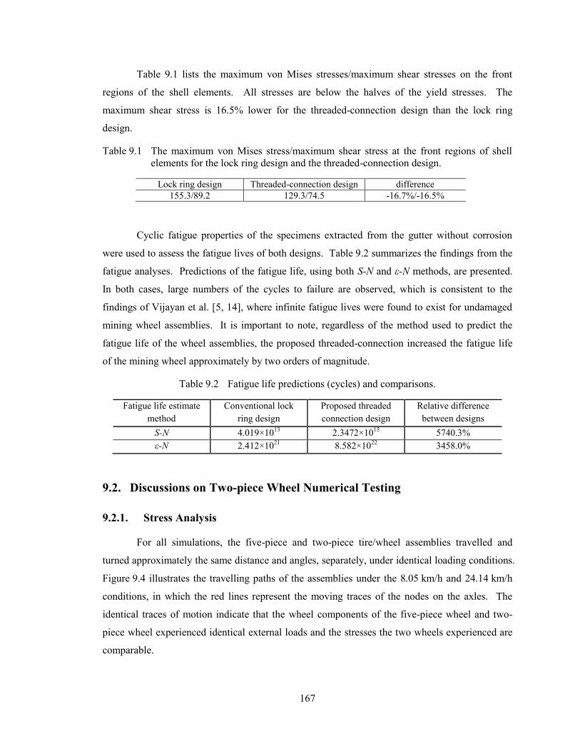
167

Table 9.1 lists the maximum von Mises stresses/maximum shear stresses on the front

regions of the shell elements. All stresses are below the halves of the yield stresses. The

maximum shear stress is 16.5% lower for the threaded-connection design than the lock ring

design.

Table 9.1 The maximum von Mises stress/maximum shear stress at the front regions of shell

elements for the lock ring design and the threaded-connection design.

Lock ring design Threaded-connection design difference

155.3/89.2 129.3/74.5 -16.7%/-16.5%

Cyclic fatigue properties of the specimens extracted from the gutter without corrosion

were used to assess the fatigue lives of both designs. Table 9.2 summarizes the findings from the

fatigue analyses. Predictions of the fatigue life, using both S-N and ε-N methods, are presented.

In both cases, large numbers of the cycles to failure are observed, which is consistent to the

findings of Vijayan et al. [5, 14], where infinite fatigue lives were found to exist for undamaged

mining wheel assemblies. It is important to note, regardless of the method used to predict the

fatigue life of the wheel assemblies, the proposed threaded-connection increased the fatigue life

of the mining wheel approximately by two orders of magnitude.

Table 9.2 Fatigue life predictions (cycles) and comparisons.

Fatigue life estimate

method

Conventional lock

ring design

Proposed threaded

connection design

Relative difference

between designs

S-N 4.019×1013

2.3472×1015

5740.3%

ε-N 2.412×1021

8.582×1022

3458.0%

9.2. Discussions on Two-piece Wheel Numerical Testing

9.2.1. Stress Analysis

For all simulations, the five-piece and two-piece tire/wheel assemblies travelled and

turned approximately the same distance and angles, separately, under identical loading conditions.

Figure 9.4 illustrates the travelling paths of the assemblies under the 8.05 km/h and 24.14 km/h

conditions, in which the red lines represent the moving traces of the nodes on the axles. The

identical traces of motion indicate that the wheel components of the five-piece wheel and two-

piece wheel experienced identical external loads and the stresses the two wheels experienced are

comparable.

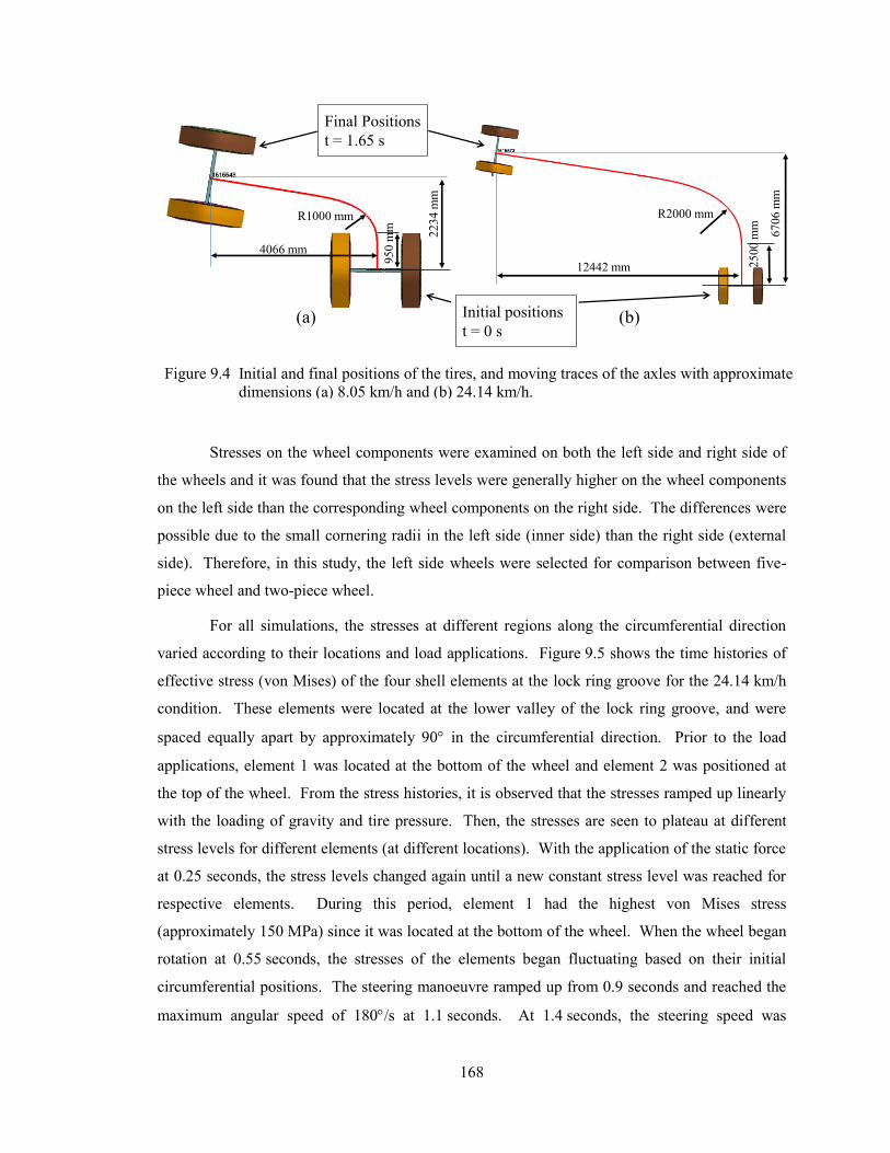
168

Stresses on the wheel components were examined on both the left side and right side of

the wheels and it was found that the stress levels were generally higher on the wheel components

on the left side than the corresponding wheel components on the right side. The differences were

possible due to the small cornering radii in the left side (inner side) than the right side (external

side). Therefore, in this study, the left side wheels were selected for comparison between five-

piece wheel and two-piece wheel.

For all simulations, the stresses at different regions along the circumferential direction

varied according to their locations and load applications. Figure 9.5 shows the time histories of

effective stress (von Mises) of the four shell elements at the lock ring groove for the 24.14 km/h

condition. These elements were located at the lower valley of the lock ring groove, and were

spaced equally apart by approximately 90 in the circumferential direction. Prior to the load

applications, element 1 was located at the bottom of the wheel and element 2 was positioned at

the top of the wheel. From the stress histories, it is observed that the stresses ramped up linearly

with the loading of gravity and tire pressure. Then, the stresses are seen to plateau at different

stress levels for different elements (at different locations). With the application of the static force

at 0.25 seconds, the stress levels changed again until a new constant stress level was reached for

respective elements. During this period, element 1 had the highest von Mises stress

(approximately 150 MPa) since it was located at the bottom of the wheel. When the wheel began

rotation at 0.55 seconds, the stresses of the elements began fluctuating based on their initial

circumferential positions. The steering manoeuvre ramped up from 0.9 seconds and reached the

maximum angular speed of 180/s at 1.1 seconds. At 1.4 seconds, the steering speed was

95

0 m

m

R1000 mm

22

34

mm

4066 mm

R2000 mm

67

06

mm

12442 mm 25

00

mm

(a) (b)Initial positions

t = 0 s

Final Positions

t = 1.65 s

Figure 9.4 Initial and final positions of the tires, and moving traces of the axles with approximate

dimensions (a) 8.05 km/h and (b) 24.14 km/h.

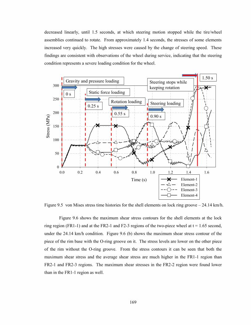
169

decreased linearly, until 1.5 seconds, at which steering motion stopped while the tire/wheel

assemblies continued to rotate. From approximately 1.4 seconds, the stresses of some elements

increased very quickly. The high stresses were caused by the change of steering speed. These

findings are consistent with observations of the wheel during service, indicating that the steering

condition represents a severe loading condition for the wheel.

Figure 9.6 shows the maximum shear stress contours for the shell elements at the lock

ring region (FR1-1) and at the FR2-1 and F2-3 regions of the two-piece wheel at t = 1.65 second,

under the 24.14 km/h condition. Figure 9.6 (b) shows the maximum shear stress contour of the

piece of the rim base with the O-ring groove on it. The stress levels are lower on the other piece

of the rim without the O-ring groove. From the stress contours it can be seen that both the

maximum shear stress and the average shear stress are much higher in the FR1-1 region than

FR2-1 and FR2-3 regions. The maximum shear stresses in the FR2-2 region were found lower

than in the FR1-1 region as well.

Time (s)

0.0 0.2 0.4 0.6 0.8 1.0 1.2 1.4 1.6

Str

ess

(MP

a)

0

50

100

150

200

250

300

Element-1

Element-2

Element-3

Element-4

Static force loading

Gravity and pressure loading

Rotation loading Steering loading

Steering stops while

keeping rotation

0 s

0.25 s

0.55 s0.90 s

1.50 s

Figure 9.5 von Mises stress time histories for the shell elements on lock ring groove – 24.14 km/h.

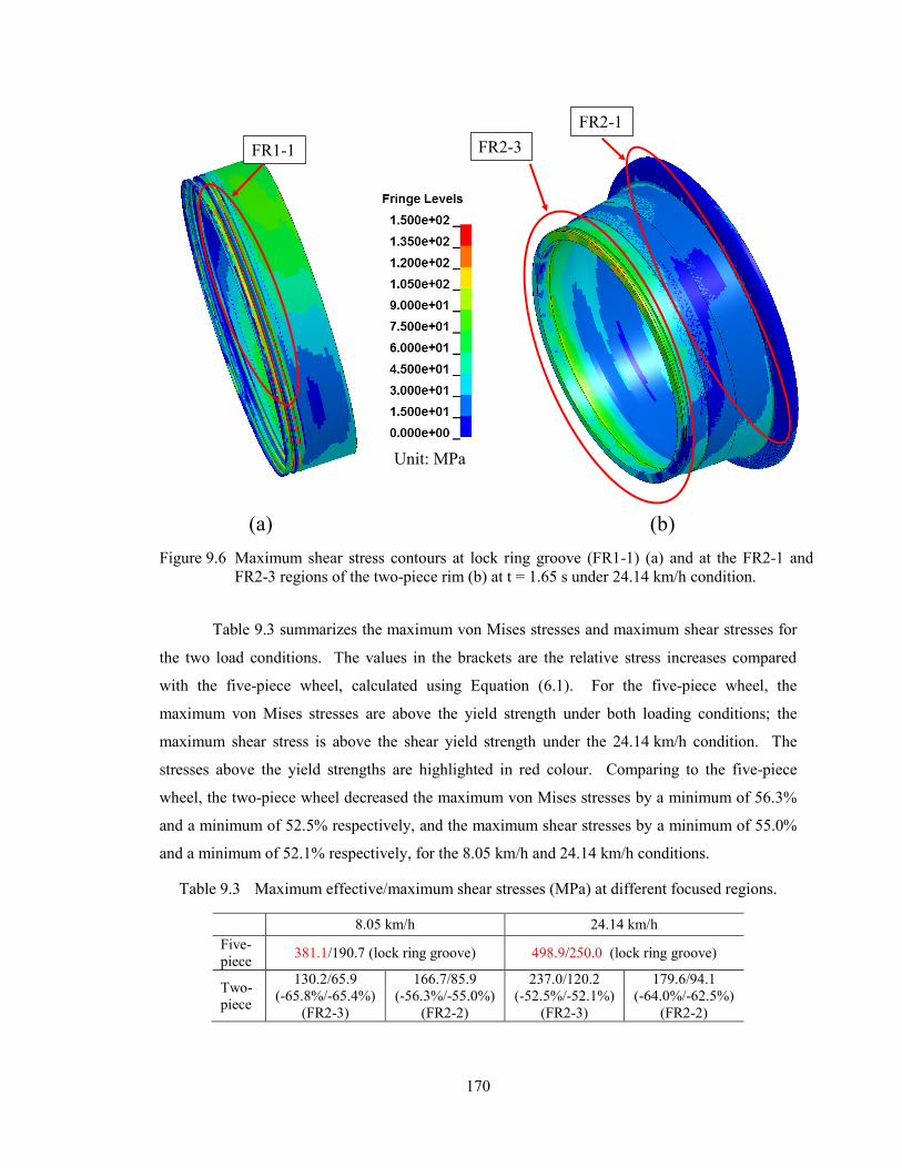
170

Table 9.3 summarizes the maximum von Mises stresses and maximum shear stresses for

the two load conditions. The values in the brackets are the relative stress increases compared

with the five-piece wheel, calculated using Equation (6.1). For the five-piece wheel, the

maximum von Mises stresses are above the yield strength under both loading conditions; the

maximum shear stress is above the shear yield strength under the 24.14 km/h condition. The

stresses above the yield strengths are highlighted in red colour. Comparing to the five-piece

wheel, the two-piece wheel decreased the maximum von Mises stresses by a minimum of 56.3%

and a minimum of 52.5% respectively, and the maximum shear stresses by a minimum of 55.0%

and a minimum of 52.1% respectively, for the 8.05 km/h and 24.14 km/h conditions.

Table 9.3 Maximum effective/maximum shear stresses (MPa) at different focused regions.

8.05 km/h 24.14 km/h

Five-

piece 381.1/190.7 (lock ring groove) 498.9/250.0 (lock ring groove)

Two-

piece

130.2/65.9

(-65.8%/-65.4%)

(FR2-3)

166.7/85.9

(-56.3%/-55.0%)

(FR2-2)

237.0/120.2

(-52.5%/-52.1%)

(FR2-3)

179.6/94.1

(-64.0%/-62.5%)

(FR2-2)

Unit: MPa

(a) (b)

FR1-1 FR2-3

FR2-1

Figure 9.6 Maximum shear stress contours at lock ring groove (FR1-1) (a) and at the FR2-1 and

FR2-3 regions of the two-piece rim (b) at t = 1.65 s under 24.14 km/h condition.

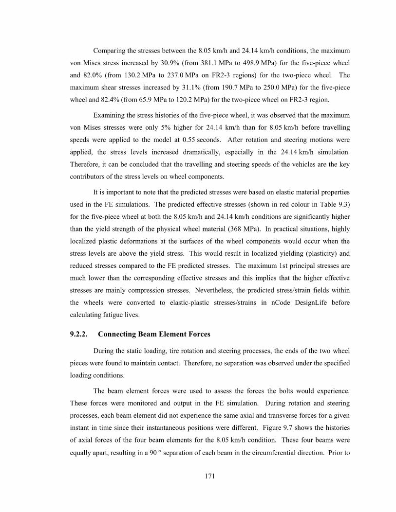
171

Comparing the stresses between the 8.05 km/h and 24.14 km/h conditions, the maximum

von Mises stress increased by 30.9% (from 381.1 MPa to 498.9 MPa) for the five-piece wheel

and 82.0% (from 130.2 MPa to 237.0 MPa on FR2-3 regions) for the two-piece wheel. The

maximum shear stresses increased by 31.1% (from 190.7 MPa to 250.0 MPa) for the five-piece

wheel and 82.4% (from 65.9 MPa to 120.2 MPa) for the two-piece wheel on FR2-3 region.

Examining the stress histories of the five-piece wheel, it was observed that the maximum

von Mises stresses were only 5% higher for 24.14 km/h than for 8.05 km/h before travelling

speeds were applied to the model at 0.55 seconds. After rotation and steering motions were

applied, the stress levels increased dramatically, especially in the 24.14 km/h simulation.

Therefore, it can be concluded that the travelling and steering speeds of the vehicles are the key

contributors of the stress levels on wheel components.

It is important to note that the predicted stresses were based on elastic material properties

used in the FE simulations. The predicted effective stresses (shown in red colour in Table 9.3)

for the five-piece wheel at both the 8.05 km/h and 24.14 km/h conditions are significantly higher

than the yield strength of the physical wheel material (368 MPa). In practical situations, highly

localized plastic deformations at the surfaces of the wheel components would occur when the

stress levels are above the yield stress. This would result in localized yielding (plasticity) and

reduced stresses compared to the FE predicted stresses. The maximum 1st principal stresses are

much lower than the corresponding effective stresses and this implies that the higher effective

stresses are mainly compression stresses. Nevertheless, the predicted stress/strain fields within

the wheels were converted to elastic-plastic stresses/strains in nCode DesignLife before

calculating fatigue lives.

9.2.2. Connecting Beam Element Forces

During the static loading, tire rotation and steering processes, the ends of the two wheel

pieces were found to maintain contact. Therefore, no separation was observed under the specified

loading conditions.

The beam element forces were used to assess the forces the bolts would experience.

These forces were monitored and output in the FE simulation. During rotation and steering

processes, each beam element did not experience the same axial and transverse forces for a given

instant in time since their instantaneous positions were different. Figure 9.7 shows the histories

of axial forces of the four beam elements for the 8.05 km/h condition. These four beams were

equally apart, resulting in a 90 separation of each beam in the circumferential direction. Prior to

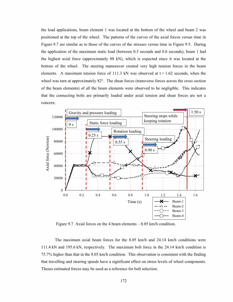
172

the load applications, beam element 1 was located at the bottom of the wheel and beam 2 was

positioned at the top of the wheel. The patterns of the curves of the axial forces versus time in

Figure 9.7 are similar as to those of the curves of the stresses versus time in Figure 9.5. During

the application of the maximum static load (between 0.3 seconds and 0.6 seconds), beam 1 had

the highest axial force (approximately 88 kN), which is expected since it was located at the

bottom of the wheel. The steering manoeuver created very high tension forces in the beam

elements. A maximum tension force of 111.3 kN was observed at t = 1.62 seconds, when the

wheel was turn at approximately 82. The shear forces (transverse forces across the cross section

of the beam elements) of all the beam elements were observed to be negligible. This indicates

that the connecting bolts are primarily loaded under axial tension and shear forces are not a

concern.

The maximum axial beam forces for the 8.05 km/h and 24.14 km/h conditions were

111.4 kN and 195.6 kN, respectively. The maximum bolt force in the 24.14 km/h condition is

75.7% higher than that in the 8.05 km/h condition. This observation is consistent with the finding

that travelling and steering speeds have a significant effect on stress levels of wheel components.

Theses estimated forces may be used as a reference for bolt selection.

Time (s)

0.0 0.2 0.4 0.6 0.8 1.0 1.2 1.4 1.6

Ax

ial

forc

e (N

ewto

n)

0

20000

40000

60000

80000

100000

120000

Beam-1

Beam-2

Beam-3

Beam-4

Static force loading

Gravity and pressure loading

Rotation loading

Steering loading

Steering stops while

keeping rotation0 s

0.25 s

0.55 s

0.90 s

1.50 s

Figure 9.7 Axial forces on the 4 beam elements – 8.05 km/h condition.

173

9.2.3. Fatigue Life Simulation Results.

Table 9.4 summarizes the findings from the fatigue life analyses. Predictions of the

fatigue life, using both S-N and ε-N methods, are presented. In both cases, a large number of

cycles are observed except on the five-piece wheel under the 24.14 km/h condition, which

indicates a finite number of cycles (8.346×105), lower than the transition life (5×10

6). For all the

regions considered, due to the consideration of plasticity and stress correction from linear FE

results, the ε-N approach predicted higher fatigue life than the S-N method. For the five-piece

wheel under the 8.05 km/h condition, although the maximum von Mises stress is above yield, a

very large number of cycles to failure was predicted. This implies that the stresses are typically

under compressive state.

Table 9.4 Minimum fatigue S-N/-N life (cycle) comparisons on focused regions.

Fatigue life

estimate method Wheel 8.05 km/h 24.14 km/h

S - N Five-piece

4.946×1010

(lock ring groove)

8.346×105

(lock ring groove)

Proposed

two-piece

1.091×1014

(FR2-3)

2.843×1012

(FR2-2)

7.203×1011

(FR2-3)

1.941×1011

(FR2-2)

ε - N Five-piece

2.834×1017

(lock ring groove)

3.828×1012

(lock ring groove)

Proposed

two-piece 6.861×10

19

(FR2-3)

2.620×1017

(FR2-2)

4.918×1017

(FR2-3)

7.805×1015

(FR2-2)

Corresponding to the stress levels, the fatigue lives for the five-piece wheel are over four

orders of magnitude higher under the 8.05 km/h condition than those under the 24.14 km/h

condition, and ten times higher for the two-piece wheel. Under identical steering condition, high

traveling speed caused much high stresses, consequently much lower fatigue live were predicted

on the wheel components. Using the S-N approach, the fatigue lives for the two-piece are at least

two orders of magnitude higher than the five-piece wheel under both loading conditions. Using

the ε-N approach, the fatigue lives are almost identical between the five-piece and the proposed

two-piece wheel under the 8.05 km/h condition, and the fatigue life for the two-piece wheel is at

least two orders of magnitude higher than the five-piece wheel under the 24.14 km/h condition.

Due to the similar structure between the mining vehicle five piece wheel (29-25) and the

port container handler vehicle five-piece wheel, the proposed two-piece wheel can be used in

mining industry without compromising its advantages described above.

174

Chapter 10. Summaries and Conclusions

A thorough research investigation was conducted on safety issues of multi-piece wheels

for OTR vehicles, especially for heavy-duty mining vehicles. The wheel and tire performance of

a five-piece wheel was tested both experimentally and numerically. The fatigue lives of the

wheel base were investigated in different conditions, namely, new condition, geometry

degradation condition, and material degradation condition. Two innovative designs were

proposed to enhance the performance and durability of the multi-piece wheels. The following

conclusions can be drawn from this research.

10.1. Summary on the Analyses of the Fatality Reports

Forty-nine fatality reports, associated with multi-piece wheel failure in Canada, the

United States, and Australia during 2008-2012, were analyzed. Multi-piece wheel/tire assembly

failures can be classified in three failure modes, namely, tire explosion, tire rupture, and tire

blow-out. Of the forty-nine fatality incidents, two incidents were caused due to tire explosion and

another two incidents were caused due to tire zipper rupture. The remaining fatality incidents

were caused due to tire blow-outs, which were associated with failure of multi-piece wheels to

hold the tire pressure.

Blow-outs are usually caused by incorrect assembly, metal fatigue, corrosion, wear,

impact damage, over inflation, and under inflation. In those situations, the sudden separation of

the engaged wheel components under high pressure can caused property damages and human

injuries. The majority of the blow-outs were a result of the incorrect use of the split lock ring;

either by incorrect installation in the gutter region or by corrosion, wear, and fatigue cracks in the

gutter region. This discovery reveals the appropriate direction of design improvement to enhance

the safety of multi-piece wheel wheels through the removal of the lock ring locking mechanism.

10.2. Conclusions on Experimental Tire Testing and Rim Base Testing

10.2.1. Experimental Tire Testing

This study investigated the deflection response of a five-piece wheel and tire assembly on

a heavy mining vehicle HLD R2900G when subjected to excitation. The Goodyear tire 29.5-29

was experimentally tested to determine its deflection performance and planar deformation

characteristics. Based upon the work completed within this study the following conclusions can

be made:

175

1) For each quasi-static test, linear relationships were experimentally observed between tire

lateral deflections versus wheel vertical displacements. The average proportionality

constant between the two measurements of 0.3678 mm/mm for the tire 29.5-29 was

determined.

2) For the most aggressive loading conditions considered within this study, maximum wheel

vertical displacement and tire sidewall lateral deflection were observed to be

approximately equal to 80 mm and 35 mm, respectively.

3) For each static test, linear relationships were observed for the vertical wheel displacement

and the lateral tire deflection versus tire load. Approximate values of 2.81 kN/mm and

6.81 kN/mm were observed for the vertical displacement and the lateral deflection

respectively.

4) Based on a static loading condition, good correlation between engineering data and the

experimental findings was found with respect to load versus vertical displacement and

lateral deflection with errors of 2.7% and 8.1% respectively.

10.2.2. Laboratory Rim Base Testing

Static load tests were conducted on the rim base of a five-piece wheel, sized 29-25.00/3.5

and commonly used for 29.5-29 or 29.5R29 OTR tires. The applied load was controlled so the

rim base experienced elastic deformation. Based on experimental observations, the following

conclusions can be drawn:

1) The measured deflection and strain data from experimental tests showed approximately

identical results for multiple tests under identical boundary and testing conditions.

Consistency in testing observations was obtained.

2) Linear relationships were observed for the deflection/load and strain/load responses of the

rim base for all regions monitored during the testing.

3) Maximum rim deflections at the top and side locations were experimentally observed to be

3.0 mm and 2.1 mm, respectively. Maximum strain measurements at gauge locations (1)

through (5) were found to be 292.210-6

, 197.310-6

, 127.610-6

, 102.910-6

, and

901.910-6

, respectively.

176

10.3. Conclusions on the FE Model Developments

10.3.1. Tire Model Development

Validation of the tire model to experimental findings was completed through examination

of the displacement field of various regions on the tire. The relative errors of the simulation

results were within 5.4% compared with the experimental findings under static loading condition.

The average accumulative error and average validation metric were 9.7% and 0.96 respectively

under quasi-static condition. Based upon the work completed in this study, it can be concluded

that The FE model of the tire 29.5-29 can predict the tire deflection characteristics with

acceptable accuracies, which are normally 15%.

10.3.2. Rim Base Model Development

The very good degree of predictability of the displacement and circumferential strain

from the numerical model and the thorough error analyses of these observations provide a strong

degree of confidence in model capabilities. Correspondingly, the numerical model of the rim

base combined with the rest of the wheel components, which were modeled following consistent

discretization procedures, as well as the numerical model of the tire were used for subsequent

structural analyses.

10.4. Geometry Degradation Analysis of the Rim Base

In this study, the geometrical differences and fatigue lives were compared amongst a new

OEM rim base, a worn OEM rim base, and a new heavy duty HT2000 rim base, which have the

same rim size. The dimensions of the worn OEM rim base were established based on the “NO

GO” gauges invented by NSIW to facilitate the inspection of the wheel components. Computer

simulations were used to assess the stress levels and fatigue lives in critical regions. Under

identical loading conditions (displacing the rim base 82.5 mm downward quasi-statically), the

predicted fatigue lives for the OEM worn wheel are 100% lower than the predicted lives for the

OEM new wheel, on the corresponding regions; the predicted fatigue lives for the HT2000 new

wheel are over 75% higher than the lives of the OEM new wheel, on the corresponding regions.

The simulation results suggest the dimensions determined by the NSIW “GO/NO-GO”

gauges are effectively designed to identify wheel geometries which exhibit a reduced fatigue life

condition and should be considered for maintenance. The use of the gauges or similar

methodologies to facilitate the inspection of wheel components is highly recommended to ensure

177

the safety. The stress and fatigue life comparisons among the three different wheels suggest that

material wear (geometry degradation) is a significant concern in the wheel’s fatigue life.

10.5. Material Degradation Analysis of the Rim Base

Using tested stress-based cyclic material properties and estimated strain-based cyclic

material properties for the new and corroded gutter specimens, the material property degradation

effect on the fatigue life was investigated. It was found the fatigue lives of the corroded materials

were significantly reduced by at least six (6) orders of magnitude.

10.6. Conclusions on Innovative Design Improvements to Enhance Safety

Based on the validated FE model of the five-piece wheel/tire assembly, two innovative

design improvements were proposed and their mechanical performance and fatigue lives were

numerical assessed.

10.6.1. Conclusions on the Threaded-connection wheel Design

This study proposed a threaded-connection locking design between wheel components in

place of the conventional lock ring mechanism, in an effort to improve the engagement capability

of wheel components and thus enhance structural performance and safety. The proposed

threaded-connection was incorporated into the validated FE model of the wheel/tire assembly and

two structural tests were conducted to evaluate the mechanical performance in the regions where

the locks of the wheel components occur. The following conclusions regarding the proposed

threaded-connection design can be made:

1) The numerical BS band pull-out tests showed that the maximum force required to pull out

the BS band of the threaded-connection was 9,552 kN, or nearly double (113%) the force

required to pull out the BS band of the conventional five-piece design (4,476 kN). This

finding demonstrates the enhanced engagement ability of the threaded-connection

locking mechanism. Additionally, the simulation predictions illustrated a safer failure

deformation mode for the proposed thread locking mechanism.

2) The quasi-static load simulations demonstrated that the maximum von Mises stresses

were 129.3 MPa and 155.3 MPa, the maximum shear stresses 89.2 MPa and 72.5 MPa,

respectively at the front regions of the threaded-connection design and conventional lock

ring design respectively. Furthermore, a much broader region of the conventional wheel

178

structure experiences higher magnitudes of stress compared to the proposed threaded

connection design.

3) The fatigue analyses predicted a significant enhancement in the fatigue life of the

proposed threaded wheel design over the conventional lock ring structure. The fatigue

life was noted to increase at least by two orders of magnitude when utilizing a threaded

connection design.

10.6.2. Conclusions on the Two-piece Wheel Design

In this study, the FE model of a tire sized 18.00-33, used for the container handler vehicle,

was developed and validated using engineering data obtained from the tire manufacturer’s

engineering data. The conventional five-piece wheel and proposed two-piece wheel, sized

33-13.00/2.5, compatible with the tire, were modeled using previously validated approaches.

Using the validated FE models, the rims were numerically investigated under severe loading and

manoeuvre conditions – static loading followed by rotation travelling and steering of the rims.

The two simulated conditions encompassed the wheel and tire assemblies travelling at speeds of

8.05 km/h with 26,900 kg load and 24.14 km/h with 23,100 kg load, respectively. The

performances of the wheel components were assessed in terms of stresses, fatigue lives, and, for

the two-piece wheel, bolt connection forces. Based on the analyses, the following conclusions

were drawn.

1) Comparing to the conventional five-piece wheel, the proposed two-piece wheel decreased

the maximum von Mises stresses by over 56.3% and 52.5%, the maximum shear stresses

by over 55.0% and 52.1%, respectively, for the 8.05 km/h and 24.14 km/h conditions.

Consequently, the fatigue lives for the two-piece wheel were increased by over two

orders of magnitude except under the 8.05 km/h condition using ε-N approach, where

almost identical fatigue life was predicted to the five-piece wheel.

2) Comparing the stresses between the 8.05 km/h and 24.14 km/h conditions, the maximum

von Mises stress increased by 30.9% (from 381.1 MPa to 498.9 MPa) for the five-piece

wheel and 82.0% (from 130.2 MPa to 237.0 MPa on FR2-3 regions) for the two-piece

wheel. The maximum shear stresses increased by 31.1% (from 190.7 MPa to 250.0 MPa)

for the five-piece wheel and 82.4% (from 65.9 MPa to 120.2 MPa) for the two-piece

wheel on FR2-3 region. The durability analysis shows that the fatigue life was

significantly decreased under the 24.14 km/h condition for both the five-piece wheel and

the two-piece wheel, using both S-N and -N approaches, compared to the 8.05 km/h

condition.

179

3) The bolt forces were assessed from the beam elements in the FE model of the two-piece

wheel. The shear forces (transverse direction) were found to be negligible. The

maximum axial forces were 111.4 kN and 195.7 kN, for the 8.05 km/h and 24.14 km/h

conditions, respectively.

4) Although the magnitude of the static load contributes to increasing the stresses on the

wheel components and the bolt connecting forces, driving and steering speeds are the key

factors in high stresses and high bolt connection forces. This is most notable during hard

cornering of the wheels.

180

Chapter 11. Limitations of the Study and Future Work

11.1. Limitations of the Study

In this study, all materials were assumed isotropic and homogenous. In the practical

situation, the material properties may very well be different in different directions, resulting in

anisotropy caused by forming and product manufacturing processes.

Structural fatigue is a statistic phenomenon, due to inconsistency of the material fatigue

properties and the existence of micro-cracks in any structure. There are considerable scatter in

values in multiple tests of the same material under the same test conditions. The standard

deviations of endurance strengths of steels seldom exceed 8% of their mean values [85]. The

fatigue test data presented in this study represents the mean values of the steel fatigue strength

and has a reliability of 50%. If a 99.99% reliability is desired, the tested fatigue strength values

have to be reduced by a factor of 0.702. Correspondently, the calculated fatigue lives will be

reduced based on this 99.99% reliability.

11.2. Future work

11.2.1. Future Work on the Threaded-connection Design

In the threaded-connection design, the combined BS band is screwed onto the rim base.

To prevent over-screwing or loose during driving forward or backward conditions of the vehicle,

a lock mechanism needs to be incorporated into the design to prevent the relative rotation

between the BS band and the rim base. The function of this device is similar to the drive keys,

currently used in multi-piece wheels, which prevent relative rotation between BS band and rim

base.

11.2.2. Future Work on the Two-piece Wheel Design

The proposed two pieces are bolted together using twenty bolts. Another way to join the

two pieces together is thread connection, similar to the proposed threaded-connection four-piece

wheel design. The threaded-connections replace the bolt connections, avoiding the occurrences

of bolt failures or accidental removal of the bolts. In the future, the durability performance of the

threaded-connected two-piece wheel may be investigated.

181

11.2.3. Experimental Testing of Prototype Wheels for the New Designs

Any product design must experience the validation of final prototype testing before

putting into mass production. The prototype testing for the threaded-connection four-piece wheel

and the bolted-together two-piece wheel can be conducted by collaboration with industry partners.

11.2.4. Geometry Optimization of the Multi-piece Wheels

Using advanced computer software, the shapes of wheel components can be optimized to

minimize weight of the wheel and maximize the fatigue life, especially on the front gutter regions

of multi-piece wheels with a lock ring.

182

References

[1] The Mining Association of Canada (2013). Facts and Figures of The Canadian Mining

Industry 2012.

<http://www.mining.ca/www/media_lib/MAC_Documents/Publications/2013/Facts%20an

d%20Figures/FactsandFigures2012Eng.pdf> accessed on May 13, 2013.

[2] Ontario Mining Association, Facts & Figures (2013).

<http://www.oma.on.ca/en/ontariomining/facts_figures.asp> accessed on May 14, 2013.

[3] Workplace Safety North, Injury and Occupational Disease Treads in the Mining industry,

Workplace Safety North Mining Health and Safety Conference, April 16 - 18, 2013,

Sudbury, Ontario.

<http://www.workplacesafetynorth.ca/sites/default/files/Injury%20and%20Occupational%

20Disease%20Trends%20in%20the%20Mining%20Industry%202013.pdf> accessed on

May 15, 2013.

[4] Jewel, Elizabeth (2006). The Pocket Oxford Dictionary and Thesaurus. Oxford University

Press. pp. 722. ISBN 978-0-19-530715-3.

[5] North Shore Industry Wheel Manufacturing (2010). Wheel Safety, Maintenance and

Inspection, Presentation on the Technical Advisory Committee meeting, June, 2010,

Sudbury, Ontario, Canada.

[6] Vijayan V. (2008). Numerical model development of a heavy mining vehicle multi-piece

wheel assembly for structural analysis, M.A.Sc.thesis, University of Windsor, Windsor,

Ontario, Canada.

[7] < http://www.caterpillar.com/> accessed on June 13, 2013.

[8] WORK SAFE ALBERTA (2004). Workplace Health and Safety Bulletin - Servicing Tires

Safely, Alberta Human Resources and Employment, Canada, GS003 – General Safety, 7

pages.

[9] U.S. Department of Labor, Mine Safety and Health Administration, National Mine Health

and Safety Academy (1996). Tire and Rim Safety Awareness Program, Instruction Guide

Series, MSHA IG 60. <http://www.msha.gov/S&HINFO/IG60.PDF> accessed on June 5,

2013.

[10] Fatality Assessment and Control Evaluation (FACE) Program, U.S. Department of Health

and Human Services (2007). Mechanic Dies while Changing a Tire Mounted on a Multi-

piece Split Rim Wheel, Massachusetts Case Report: 07-MA-058.

<http://www.cdc.gov/niosh/face/stateface/ma/07ma058.html> accessed on June 5, 2013.

[11] Workplace Safety North (2000). Multi-piece Rim – Controlling the Hazards.

<http://www.workplacesafetynorth.ca/sites/default/files/resources/Multi-

Piece%20Rims%20Presentation.pdf> accessed on June 17, 2013.

[12] Workplace Safety North, Ontario, Fatality Reports.

<http://www.masha.on.ca/fatality_details.aspx?fatality_id=9> accessed on

September 7, 2012.

183

[13] Ministry of The Solicitor General, Office of the Chief Coroner, Canada (2003). Verdict of

Coroner’s jury serving on the inquest into the death of Jerome Burns.

[14] Vijayan V., Altenhof W., and Banting R. (2010). A finite element approach to estimation

of fatigue life for a three-piece mining vehicle wheel, International Journal of Heavy

Vehicle Systems, Vol. 17, No. 2, pp. 159 - 178.

[15] Society of Automotive Engineers (1993). Wheel Cornering Fatigue Test Standard - SAE

J1992 Nov. 93, SAE Handbook, 2000, 400 Commonwealth Drive, Warrendale, PA.

[16] <http://www.secondchancegarage.com/public/265.cfm> accessed on June 12, 2013.

[17] <http://en.wikipedia.org/wiki/File:Tire_code_-_en.svg> accessed on June 12, 2013.

[18] Topy Industries Limited (2008). Multi-piece Rims for Industrial and Construction

Vehicles RIM INSTRUCTION MANUAL, vision 1, 2008.

<http://www.topy.co.jp/english/dept/wheel/pdf/71424250-e.pdf> accessed on

June 13, 2013.

[19] Fatality Assessment and Control Evaluation (FACE) Program, U.S. Department of Health

and Human Services (2003). Worker Struck by Multi-piece Rim during Wheel Installation,

Alaska Case Report: 03AK006.

<http://www.cdc.gov/niosh/FACE/stateface/ak/03ak006.html> accessed on June 7, 2013.

[20] Occupational Health and Safety, Alberta Employment and Immigration (2004). Servicing

Tires Safely, Workplace Health and Safety Bulletin.

<http://humanservices.alberta.ca/documents/WHS-PUB_gs003.pdf> accessed on

June 7, 2013.

[21] North Shore Industry Wheel Mfg. (2011). Earthmover and Construction Products Catalog.

<http://www.nsiw.com/UploadedFiles/File/nsiw%20em%20catalogue.pdf> accessed on

June 10, 2011.

[22] North Shore Industry Wheel Mfg. (2013). QC7 – 7-piece quick changing wheel.

<http://www.nsiw.com/UploadedFiles/File/qc7%20quick%20change%20wheel%20broc.p

df> accessed on June 12, 2013.

[23] Workplace Safety North (2000). Take Ten for Safety, Multi-piece Rims Controlling The

Hazards, Version 2.0.

<http://www.workplacesafetynorth.ca/sites/default/files/resources/Multi-

Piece%20Rims%20Leader%20Guide_0.pdf> accessed on June 17, 2013.

[24] The Goodyear Tire & Rubber Company (2008). Goodyear off-the-road Tire Maintenance

Manual. <http://www.goodyearotr.com/cfmx/web/otr/info/pdf/otr_MaintenanceManual.pdf>

accessed on June 10, 2010.

[25] deCastro J. (Goodyear Canada Inc.) (2010). ABC’s of OTR, presentation on the Technical

Advisory Meeting of Workplace Safety North (MSN), Sault Ste. Marie, Ontario,

June 1, 2010.

184

[26] The Goodyear Tire & Rubber Company (2003). Radial Truck Tire & Retread Service

Manual. <http://www.goodyear.ca/truck/pdf/radialretserv/Retread_All_V.pdf> accessed on

June 13, 2013.

[27] The Tire and Rim Association (2013). 2013 Year Book. <http://www.gobookee.net/tire-

and-rim-yearbook/> accessed on June 17, 2013.

[28] The Goodyear Tire & Rubber Company (2008). Goodyear OTR Tire Engineering Data

Book. <http://www.goodyearotr.com/cfmx/web/otr/info/pdf/otrdatabook.pdf> accessed on

June 17, 2013.

[29] Albert Government (2012). Workplace Incident Fatalities Accepted by the Workers’

Compensation Board in 2012. <http://www.humanservices.alberta.ca/documents/2012-

workplace-fatalities-accepted-wcb.pdf> and

<http://www.edmontonsun.com/2012/02/26/exploding-tire-kills-worker> accessed on

June 22, 2013.

[30] Occupational Health and Safety, Alberta Employment and Immigration (2009). WORKER

FATALLY INJURED WHEN TIRE COMPONENTS SEPARATE, Occupational Health

and Safety Fatality Report, File #: F-256084.

<http://humanservices.alberta.ca/documents/FR-2009-08-28.pdf> accessed on

June 22, 2013.

[31] WorkSafeBC, Workers’ Compensation Board of BC (2006). Hazard Alert - Removing

inflated tire leads to fatal explosion, Alert #: Fatality 06-03.

<http://www2.worksafebc.com/i/posters/pdfs/2006/ha0603.pdf> accessed on June 13, 2013.

[32] WorkSafety BC, Workers’ Compensation Board of BC (2005). Welding on assembled

wheel results in explosion, Incident Investigation Report, 2005.

<http://www2.worksafebc.com/PDFs/investigations/IIR2005108320019.pdf> accessed on

June 15, 2013.

[33] Occupational health and safety, Saskatchewan Labour (2004). Truck tire explosions claim

two more lives, November 2004. <http://www.lrws.gov.sk.ca/truck-tire-explosions-claim-

two-more-lives> accessed on September 5, 2012.

[34] Alberta Human Resources and Employment, Workplace Health & Safety, Alberta (2002).

Occupational Health & Safety Magazine, Work Struck by Tire Rim. Volume 25, Number 3,

September 2002. <http://humanservices.alberta.ca/documents/WHS-

PUB_ohsmag_0902.pdf> accessed on June 20, 2013.

[35] Occupational Health and Safety, Saskatchewan Ministry of Labor Relations and

Workplace Safety (1999). Hazard Alerts – Tire Mound/Demound on Heavy Vehicles.

<http://www.lrws.gov.sk.ca/tire-mount-demount-heavy-vehicles> accessed on

June 28, 2013.

185

[36] Occupational Safety & Health Administration, U.S. Department of Labor (2011).

Mechanic Dies After Wheel Failure During Tire Inflation, Report ID: 0729300.

<http://www.osha.gov/pls/imis/accidentsearch.accident_detail?id=200012912> accessed

on June 20, 2013.

[37] Occupational Safety and Health Administration, U.S. Department of Labor (2010).

Exploding Multi-piece Wheel Rim Kills Auto Dealer Worker, Report ID: 0524700.

<http://www.osha.gov/pls/imis/accidentsearch.accident_detail?id=202089462> accessed

on June 11, 2013.

[38] Occupational Safety & Health Administration, U.S. Department of Labor (2010).

Employee Is Killed From Head Injury While Inflating Tire, Report ID: 0950633.

<http://www.osha.gov/pls/imis/accidentsearch.accident_detail?id=202609129> accessed

on June 11, 2013.

[39] Occupational Safety and Health Administration, U.S. Department of Labor (2009). Tire

Service Worker Is Killed In Rim Wheel Explosion, Report ID: 0452110.

<http://www.osha.gov/pls/imis/accidentsearch.accident_detail?id=201859931> accessed

on June 11, 2013.

[40] Occupational Safety and Health Administration, U.S. Department of Labor (2009).

Worker Is Killed When Multi-Piece Rim Explodes, Report ID: 0521700.

<http://www.osha.gov/pls/imis/accidentsearch.accident_detail?id=200033496> accessed

on June 11, 2013.

[41] Occupational Safety & Health Administration, U.S. Department of Labor (2008).

Employee Is Killed When Struck In The Head By Tire Rim, Report ID: 0521100.

<http://www.osha.gov/pls/imis/accidentsearch.accident_detail?id=200651529> accessed

on June 11, 2013.

[42] Fatality Assessment and Control Evaluation (FACE) Program, U.S. Department of Health

and Human Services (2007). Equipment Operator Killed by a Lock Ring Propelled from a

Multi piece Rim Wheel, New York State Case Report: 07NY137.

<http://www.health.ny.gov/environmental/investigations/face/07ny137.htm> accessed on

June 7, 2013.

[43] Occupational Safety & Health Administration, U.S. Department of Labor (2007).

Employee Killed When Struck By Exploding Multi-Piece Wheel, Report ID: 0524200.

<http://www.osha.gov/pls/imis/accidentsearch.accident_detail?id=201262177> accessed

on June 11, 2013.

[44] Occupational Safety & Health Administration, U.S. Department of Labor (2007).

Employee Is killed By Exploding Split Rim Tire, Report ID: 0418300.

<http://www.osha.gov/pls/imis/accidentsearch.accident_detail?id=201272689> accessed

on June 11, 2013.

186

[45] Occupational Safety & Health Administration, U.S. Department of Labor (2006).

Employee IS Killed When Split Ring Rim Blows Off Tire, Report ID: 0453710.

<http://www.osha.gov/pls/imis/accidentsearch.accident_detail?id=200355576> accessed

on June 11, 2013.

[46] Fatality Assessment and Control Evaluation (FACE) Program, U.S. Department of Health

and Human Services (2006). An apprentice mechanic died when the truck tire he was

standing over exploded, FACE 05CA007.

<http://www.cdc.gov/niosh/face/stateface/ca/05ca007.html> accessed on June 13, 2012.

[47] Occupational Safety & Health Administration, United States Department of Labor (2004).

Employee Is Killed While Repairing Multi-Piece Wheel, Report ID: 0316700.

<http://www.osha.gov/pls/imis/accidentsearch.accident_detail?id=14319248> accessed on

June 11, 2013.

[48] Occupational Safety & Health Administration, United States Department of Labor (2004).

Employee Is Killed During Tire Rim Failure, Report ID: 0751910.

<http://www.osha.gov/pls/imis/accidentsearch.accident_detail?id=200528883> accessed

on June 11, 2013.

[49] Occupational Safety & Health Administration, U.S. Department of Labor (2004). Tire

Explosion Kills Employee, Report ID: 0420600.

<http://www.osha.gov/pls/imis/accidentsearch.accident_detail?id=202344396> accessed

on June 11, 2013.

[50] Occupational Safety & Health Administration, U.S. Department of Labor (2004).

Employee Is Killed When Struck By Wheel Ring Shot From Wheel, Report ID: 0950625.

<http://www.osha.gov/pls/imis/accidentsearch.accident_detail?id=201086105> accessed

on June 11, 2013.

[51] Occupational Safety & Health Administration, United States Department of Labor (2003).

Employee Killed After Tire He Was Inflating Exploded, Report ID: <0453720.

http://www.osha.gov/pls/imis/accidentsearch.accident_detail?id=200071850> accessed on

June 11, 2013.

[52] Occupational Safety & Health Administration, U.S. Department of Labor (2003).

Employee Died After Explosion While Recapping Truck Tire, Report ID: 0453710.

<http://www.osha.gov/pls/imis/accidentsearch.accident_detail?id=200352896> accessed

on June 11, 2013.

[53] FACE Facts, Massachusetts Department of Public Health (2004). Worker Killed While

Inflating a Tire Mounted on a Multi-Piece Rim - Massachusetts Fatality Investigation

Report, August 2004, Vol. 7, No. 2. <http://www.mass.gov/eohhs/docs/dph/occupational-

health/face-facts/face-fact-rim.pdf> accessed on June 7, 2013.

[54] Occupational Safety & Health Administration, U.S. Department of Labor (2003). One

Employee Died, One Injured When Struck By Truck Tire Rim, Report ID: 0729700.

187

<http://www.osha.gov/pls/imis/accidentsearch.accident_detail?id=201343381> accessed

on June 11, 2013.

[55] Occupational Safety & Health Administration, U.S. Department of Labor (2004). Multi-

Piece Rim Wheel Explodes Killing Employee, Report ID: 0950621.

<http://www.osha.gov/pls/imis/accidentsearch.accident_detail?id=201174026> accessed

on June 13, 2013.

[56] Occupational Safety & Health Administration, U.S. Department of Labor (2003).

Empolyee Killed When Struck In The Head By Flying Split Rims, Report ID: 1050210.

<http://www.osha.gov/pls/imis/accidentsearch.accident_detail?id=201681376> accessed

on June 11, 2013.

[57] Occupational Safety & Health Administration, U.S. Department of Labor (2002).

Employee Killed When Tire And Rim Assembly Exploded, Report ID: 0214200.

<http://www.osha.gov/pls/imis/accidentsearch.accident_detail?id=200022697> accessed

on June 11, 2013.

[58] Occupational Safety & Health Administration, United States Department of Labor (2002).

Employee Struck By A Flying Wheel Rim, Report ID: 0257230.

<http://www.osha.gov/pls/imis/accidentsearch.accident_detail?id=202260584> accessed

on June 11, 2013.

[59] Occupational Safety & Health Administration, U.S. Department of Labor (2002).

Employee Killed When Struck By Multipiece Tire Rim, Report ID: 0522300.

<http://www.osha.gov/pls/imis/accidentsearch.accident_detail?id=200101319> accessed

on June 11, 2013.

[60] Occupational Safety & Health Administration, U.S. Department of Labor (2002).

Employee Struck By A Split Rim Tire, Report ID: 0418100.

<http://www.osha.gov/pls/imis/accidentsearch.accident_detail?id=201281334> accessed

on June 11, 2013.

[61] Occupational Safety & Health Administration, U.S. Department of Labor (2002).

Employee Dies When Struck In His Head By Exploding Wheel Rim, Report ID: 0420600.

<http://www.osha.gov/pls/imis/accidentsearch.accident_detail?id=202327854> accessed

on June 11, 2013.

[62] Occupational Safety & Health Administration, U.S. Department of Labor (2001).

Employee Killed When Struck By A Ring And Wheel, Report ID: 0627400.

<http://www.osha.gov/pls/imis/accidentsearch.accident_detail?id=200811081> accessed

on June 11, 2013.

[63] Occupational Safety & Health Administration, U.S. Department of Labor (2001).

Employee Killed When Struck By A Piece From Tire Rim, Report ID: 0418300.

<http://www.osha.gov/pls/imis/accidentsearch.accident_detail?id=201271368> accessed

on June 11, 2013.

188

[64] Occupational Safety & Health Administration, U.S. Department of Labor (2000).

Employee Dies After Tire Assembly Accident, report ID: 1054116.

<http://www.osha.gov/pls/imis/accidentsearch.accident_detail?id=201620374> accessed

on June 11, 2013.

[65] Division of Occupational Safety and Health, Department of Labour, North Carolina (2000).

Hazard Alert – Multi-piece Rims.

<http://www.nclabor.com/osha/etta/hazard_alerts/MultiRims.pdf> accessed June 8, 2013.

[66] Occupational Safety & Health Administration, U.S. Department of Labor (2000).

Employee Killed When Struck By Tire Rim Lock Ring, report ID: 0453730.

<http://www.osha.gov/pls/imis/accidentsearch.accident_detail?id=202074530> accessed

on June 11, 2013.

[67] Mine Safety and Health Administration (MSHA), U.S. Department of Labor (2002).

MSHA's Accident Prevention Program Miner's Tip - Multi-Piece Rim Wheels.

<http://www.msha.gov/accident_prevention/Tips/rimwheel.pdf> accessed on

June 26, 2013.

[68] Occupational Safety & Health Administration, U. S. Department of Labor (1998).

Employee Killed When Truck Crane Tire Explodes, report ID: 0316400.

<http://www.osha.gov/pls/imis/accidentsearch.accident_detail?id=200630259> accessed

on June 11, 2013.

[69] Occupational Safety & Health Administration, U. S. Department of Labor (1998).

Employee Killed Tire Explodes During Mounting, report ID: 0627100.

<http://www.osha.gov/pls/imis/accidentsearch.accident_detail?id=200260495> accessed

on June 11, 2013.

[70] Occupational Safety & Health Administration, U. S. Department of Labor (1998).

Employee Killed When Wheel Rim Blows Apart, Report ID: 0728500.

<http://www.osha.gov/pls/imis/accidentsearch.accident_detail?id=200000495> accessed

on June 11, 2013.

[71] Occupational Safety & Health Administration, U. S. Department of Labor (1998).

Employee Killed When Struck By Split Rim Tire Locking Ring, report ID: 0419400.

<http://www.osha.gov/pls/imis/accidentsearch.accident_detail?id=201360518> accessed

on June 11, 2013.

[72] Natural Resources and Mines, Queensland Government (2005). Fatal Injury To Prime

Mover Operator As Rim Assembly Fails, Safety Alert No. 136, 2005.

<http://mines.industry.qld.gov.au/assets/inspectorate/safety_alert136.pdf> accessed on

June 7, 2013.

[73] Mineral Resources, New South Wales (2004). Safety Alert - QUEENSLAND FATALITY

DURING WHEEL REMOVAL, Report No: SA 04 01.

189

<http://www.dpi.nsw.gov.au/data/assets/pdf_file/0010/66853/Safety-Alert-04-01-QLD-

fatality-during-wheel1.pdf> accessed on June 7, 2013.

[74] Natural Resources and Mines, Queensland Government (2002). Safety Alert - Violent Tire

Rupture on Dump Truck, Alert No. 83, 2002.

<http://mines.industry.qld.gov.au/assets/inspectorate/safety_alert083.pdf> accessed on

June 13, 2012.

[75] Natural Resources and Mines, Queensland Government (2000). Tire Rim Assembly Blew

Apart, Mines Inspectorate Safety Alert No. 29, 2000.

<http://mines.industry.qld.gov.au/assets/inspectorate/safety_alert029.pdf> accessed on

June 8, 2013.

[76] Rasche T. and Lkinge T. (2006). Review and Analysis of tire Related Accidents and

Incidents – an ACARP Study to Improve tire & Rim Maintenance and Operational Safety

of Rubber tired Earthmover Equipment.

<http://www.qrc.org.au/conference/_dbase_upl/rasche_Tyre%20Related%20Accidents%2

0and%20Incidents.pdf> accessed on June 26, 2013.

[77] Workplace Safety North, Ontario (2013). Tires and Rims - MOL Guideline-Section 107 –

Working With Tires and Wheel Assemblies.

<http://www.workplacesafetynorth.ca/resources/multi-piece-rims-controlling-hazards>

accessed on June 5, 2013.

[78] Cutler T. (2004). Final Report to Hamersley Iron on Catastrophic Tire Incident on

Haultruck 06H1 at Channar on April 10, 2004.

<http://www.otraco.com.au/Libraries/Technical_Papers/Tyre_Explosion_Investigation_-

_Lightning_Strike.sflb.ashx> accessed on June 26, 2013.

[79] Workers’ Compensation Board of British Columbia, Canada (2003). Hazard Alert – Tire

explodes when truck contacts overhead power line.

<http://www2.worksafebc.com/i/posters/2003/ha0317_tire.htm> accessed on June 26, 2013.

[80] Kocabicak U. and Firat M. (2001). Numerical analysis of wheel cornering fatigue tests.

Engineering Failure Analysis, vol. 8, pp. 339 - 354.

[81] SAE (Society of Automotive Engineers) International (2005). SURFACE VEHICLE

RECOMMENDED PRACTICE - Wheels - Passenger Car and Light Truck

PerformanceRequirements and Test Procedures- SAE J328, Rev. Feb. 2005, 400

Commonwealth Drive, Warrendale, PA. < http://standards.sae.org/j328_200502/> accessed

on July 11, 2013.

[82] SAE (Society of Automotive Engineers) International (2007). SURFACE VEHICLE

RECOMMENDED PRACTICE - Wheels/Rims - Performance Requirements and Test

Procedures - Truck and Bus- SAE J267, Rev. Dec. 2007, 400 Commonwealth Drive,

Warrendale, PA. <http://standards.sae.org/j328_200502/> accessed on July 11, 2013.

190

[83] SAE (Society of Automotive Engineers) International (2007). SURFACE VEHICLE

RECOMMENDED PRACTICE -Wheels/Rims—Military Vehicles—Test Procedures and

Performance Requirements- SAE J1992, Rev. Mar. 2001, 400 Commonwealth Drive,

Warrendale, PA.

<http://www.autoparts-standard.org/index/images/userfiles/media/SAE%20J1992-2001.pdf>

accessed on July 11, 2013.

[84] <http://en.wikipedia.org/wiki/Fatigue_(material)> accessed November 1, 2012.

[85] Norton R. L. (2006). Machine Design-An Integrated Approach, third edition, Pearson

Prentice Hall, pp. 302.

[86] J. W. Fischer and B. T. Yen (1972). Design, Structural details, and Discontinuities in Steel,

Safety and Reliability of Metal Structures, American Society of Civil Engineers, Nov. 2.

[87] HBM-nCode United Kingdom Limited (2012). nCode Book of Fatigue Theory.

[88] Chu C. (1997). Multiaxial fatigue life prediction method in the ground vehicle industry,

International Journal of Fatigue, Vol. 19, No. 1, pp. S325 - S330.

[89] Conle F.A. and Chu C.-C. (1997). Fatigue analysis and the local stress-strain approach in

complex vehicular structures, International Journal of Fatigue, Vol. 19, Supp. No. 1, pp.

S317 - S323.

[90] Grujicic M., Arakere, G., Bell W.C., Harvi H., Yalavarthy H. V., Pandurangan B., Haque I.,

and Fadel G. M. (2010). Reliability-Based Design Optimization for Durability of Ground

Vehicle Suspension System Components, ASM International, Journal of Material

Engineerng and Performance, vol. 19, pp.301 - 313.

[91] Mitchell M. R. (1996). Fundamentals of modern fatigue analysis for design, In: Lampman

Steven R., editor, ASM Handbook, Materials Park: ASM International, pp. 229 - 49.

[92] Basquin OH. (1910). The exponential law of endurance tests, Proceedings – American

Society for Testing Materials, Vol. 10, pp. 625 - 30.

[93] Manson SS. (1965). Fatigue: a complex subject – some simple approximation,

Experimental Mechanics, Vol. 5, pp. 193 - 226.

[94] Coffin LF. (1954). A study of the effect of cyclic thermal stresses on a ductile metal,

Transactions of the American Society of Mechanical Engineers, Vol. 76, pp. 931 - 950.

[95] Morrow J. (1968). Fatigue properties of metals, section 3.2., In: Fatigue Design Handbook,

Pub. No. AE-4, SAE, Warrendale, PA.

[96] Muralidharan U, Manson SS. (1988). Modified universal slopes equation for estimation of

fatigue characteristics, Journal of Engineering Materials and Technology - Transactions of

the American Society of Mechanical Engineers, Vol. 10, pp. 55 - 58.

191

[97] Smith, K. N., Watson, P. and Topper, T. H. (1970). A stress-strain function for the fatigue

of materials, Journal of Materials, Vol. 5, pp. 767 - 778.

[98] HBM-nCode United Kingdom Limited (2013). DesignLife Theory Guide.

[99] Collins, J. A. (1993). Failure of Material in Mechanical Design, 2nd edition, John Wiley &

Sons Inc., New York, pp. 238 - 254,.

[100] Mercer I., Malton G., and Draper J. (2003). Investigating fatigue failures using analysis

and testing – some do’s and don’ts, Safe Technology Limited, EIS Seminar.

[101] Tipton S. M. and Nelson D. V. (1985). Fatigue Life Predictions for a Notched Shaft in

Combined Bending and Torsion, in Multiaxial Fatigue, K. J. Miller and M. W. Brown,

Editors. SATM: Philadephia, PA. pp. 514 - 550.

[102] Nishihara T. and Kawamoto M. (1945). The strength of Metals under Combined

Alternating Bending and Torsion with Phase Difference, Memoirs College of Engineering,

Kyoto Univ., Japan, 11(85).

[103] McDiarmid D. L. (1991). A general criterion for high cycle multiaxial fatigue failure,

Fatigue and Fracture of Engineering Materials and Structures, Vol. 14(4), pp. 429 - 453.

[104] Brown M. W. and Miller K. J. (1973). A theory for fatigue failure under multiaxial stress

strain conditions, Proceeding of the Institute of Mechanical Engineers, Vol. 187, pp. 745 -

755.

[105] HBM-nCode United Kingdom Limited (2012).Pratical Fatigue Theory.

[106] Wang X. and Zhang X. (2010). Simulation of dynamic cornering fatigue test of a steel

passenger car wheel, International Journal of Fatigue, Vol. 32, pp. 434 - 442.

[107] Shang R, Altenhof W, Hu H, Li N. (2008). Rotary fatigue analysis of forged magnesium

road wheels, SAE technical paper, No. 2008-01-0211.

[108] Topac M.M., Ercan S., and Kuralay N.S. (2012). Fatigue life prediction of a heavy vehicle

steel wheel under radial loads by using finite element analysis, Engineering Failure

Analysis, Vol. 20, pp. 67 - 79.

[109] Firat M., Kozan R., Ozsoy M., and Mete O.H. (2009). Numerical modeling and simulation

of wheel radial fatigue tests, Engineering Failure Analysis, Vol. 16, pp. 1533 - 1541.

[110] Llano-Vizcaya L., Rubio-Gonza´lez C., Mesmacque G., and Cervantes-Herna´ndez T.

(2006). Multiaxial fatigue and failure analysis of helical compression springs, Engineering

Failure Analysis, Vol. 13, pp. 1303 - 1313.

[111] Conle F.A. and Chu C.-C. (1997). Fatigue analysis and the local stress-strain approach in

complex vehicular structures, International Journal of Fatigue, Vol. 19, Supp. No. 1, pp.

S317 - S323.

192

[112] Kocabicak U. and Firat M. (2001). Numerical analysis of wheel cornering fatigue tests,

Eenineering Failure Anlsyiss, Vol. 8, pp. 339 – 354.

[113] Altair Incorporated (2006). HyperMesh 8.0 User’s Guide, July 2006.

[114] Livermore Software Technology Corporation (LSTC), LS-DYNA Keyword User’s Manual,

Version 971/Rev5, May 2010.

[115] Livermore Software Technology Corporation (LSTC) (2012). Introduction to LS-PrePost

3.2, July 31, 2012.

[116] Burke A.M. and Olatunbosun O.A. (1997). Static tire/Road Interaction Modelling,

Meccanica, Vol. 32, pp. 472 - 479.

[117] Neves R.R. V., Micheli G.B., Alves, M. (2010). An experimental and numerical

investigation on tire impact, International Journal of Impact Engineering, Vol. 37, pp 685 -

693.

[118] Nguyen S., Greenhalgh E.S., Iannucci L., Longstaff S., Olsson R. and Curtis P. T.

(2011). Experimental Characterisation of tire Indentation by Simulated Runway Debris,

Strain: An International Journal for Experimental Mechanics, Vol. 47, pp. 343 - 350.

[119] Oberkampf W. and Trucano T. (2002). Verification and validation in computational fluid

dynamics, Progress in Aerospace Science, Vol. 38, pp. 209 - 272.

[120] Reid J. D., Boesch D. A. and Bielenberg R.W. (2007). Detailed tire modeling for crash

applications, International Journal of Crashworthiness, Vol. 12, No. 5, pp. 521 - 529.

[121] Orengo F., Ray M. H., and Plaxico C.A. (2003). Modeling tire blow-out in roadside

hardware simulations using LS-DYNA, Proceedings of IMECE’03, 2003 ASME

International Mechanical Engineering Congress & Exposition, Washington, DC,

November 16 - 21.

[122] Shiraishi M., Iwasaki N., Saruwatari T., and Hayashi K. (2002). Developing FE-Tire

Model Library for Durability and Crash Simulations, the 7th International LS-DYNA

Users Conference, Dearborn, Michigan, Vol. 13, pp.29 - 36.

[123] Coefficient of Friction –RoyMech.

<http://www.roymech.co.uk/Useful_Tables/Tribology/co_of_frict.htm> accessed on

June 15, 2010.

[124] Burton, W.E. (1949). Engineering With Rubber, McGraw Hill Book Company Inc., New

York, New York.

[125] ASTM Standard A572/A572M – 12a, Standard Specification for High-Strength Low-Alloy

Columbium Vanadium Structural Steel, ASTM International, West Conshohocken, PA,

2013, DOI: 10.1520/A0572_A0572M-12A, www. astm.org.

193

[126] ASTM Standard E8/E8M − 11, Standard Test Methods for Tension Testing of Metallic

Materials1, ASTM International, West Conshohocken, PA, 2012, DOI:

10.1520/E0008_E0008M-11, www. astm.org.

[127] Mentley J. (2013). nCode DesignLife, personal communication.

[128] Kalmar Industries, Technical Information – Container Handler – ContChamp 42-45

Tonnes (2012).

<http://www.kalmarind.nl/source.php/38881/Products%20Tech%20doc%20DRF%20Topli

ft.pdf> accessed on October 15, 2013.

[129] Zhang Y. (2008). Metallurgical Failure Analysis of Cracked Wheel Rim, Bodycote

Materials Testing Canada Inc., Ref #: G807288.

[130] Conle F.A. and Chu C. (1997). Fatigue analysis and the local stress–strain approach in

complex vehicular structures, International Journal of Fatigue, Vol. 19-1, pp. 317 - 323.

[131] Draper J. and Aveline R., (2004). How to achieve valid results in durability analysis from

FEA software, ANSYS World User Conference, Bergamo, Italy, pp. 8 - 14.

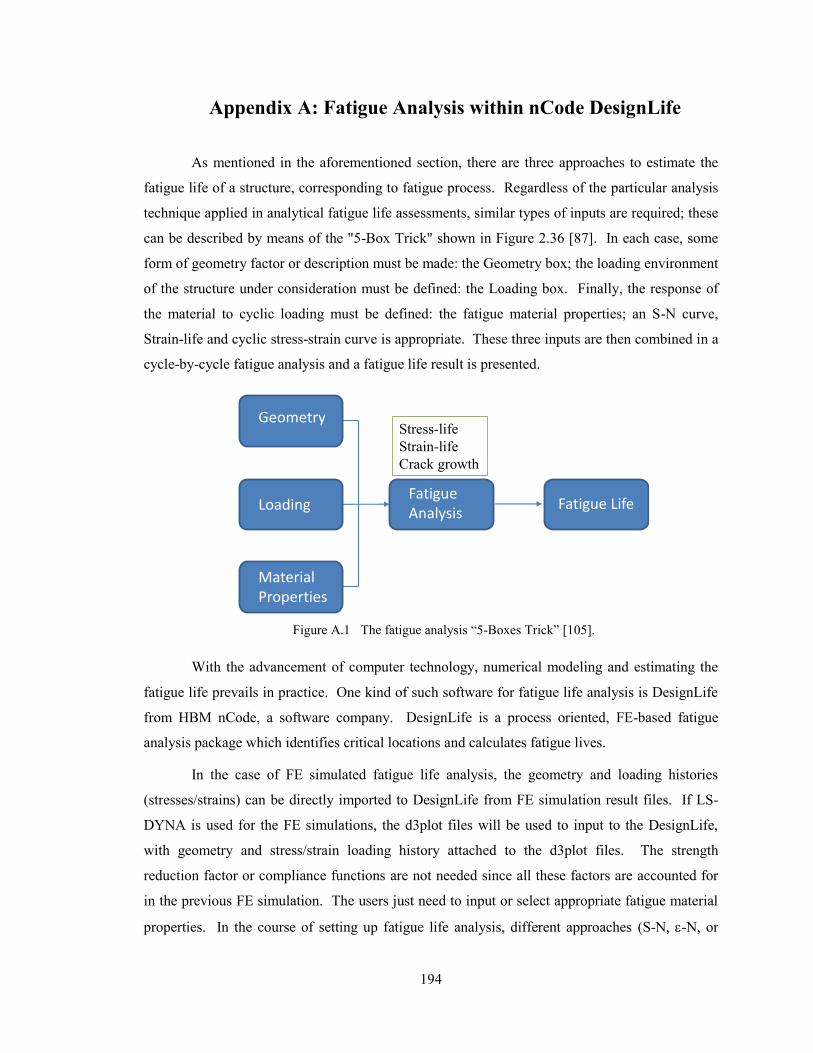
194

Appendix A: Fatigue Analysis within nCode DesignLife

As mentioned in the aforementioned section, there are three approaches to estimate the

fatigue life of a structure, corresponding to fatigue process. Regardless of the particular analysis

technique applied in analytical fatigue life assessments, similar types of inputs are required; these

can be described by means of the "5-Box Trick" shown in Figure 2.36 [87]. In each case, some

form of geometry factor or description must be made: the Geometry box; the loading environment

of the structure under consideration must be defined: the Loading box. Finally, the response of

the material to cyclic loading must be defined: the fatigue material properties; an S-N curve,

Strain-life and cyclic stress-strain curve is appropriate. These three inputs are then combined in a

cycle-by-cycle fatigue analysis and a fatigue life result is presented.

With the advancement of computer technology, numerical modeling and estimating the

fatigue life prevails in practice. One kind of such software for fatigue life analysis is DesignLife

from HBM nCode, a software company. DesignLife is a process oriented, FE-based fatigue

analysis package which identifies critical locations and calculates fatigue lives.

In the case of FE simulated fatigue life analysis, the geometry and loading histories

(stresses/strains) can be directly imported to DesignLife from FE simulation result files. If LS-

DYNA is used for the FE simulations, the d3plot files will be used to input to the DesignLife,

with geometry and stress/strain loading history attached to the d3plot files. The strength

reduction factor or compliance functions are not needed since all these factors are accounted for

in the previous FE simulation. The users just need to input or select appropriate fatigue material

properties. In the course of setting up fatigue life analysis, different approaches (S-N, -N, or

Geometry

MaterialProperties

LoadingFatigueAnalysis

Fatigue Life

Stress-life

Strain-life

Crack growth

Figure A.1 The fatigue analysis “5-Boxes Trick” [105].

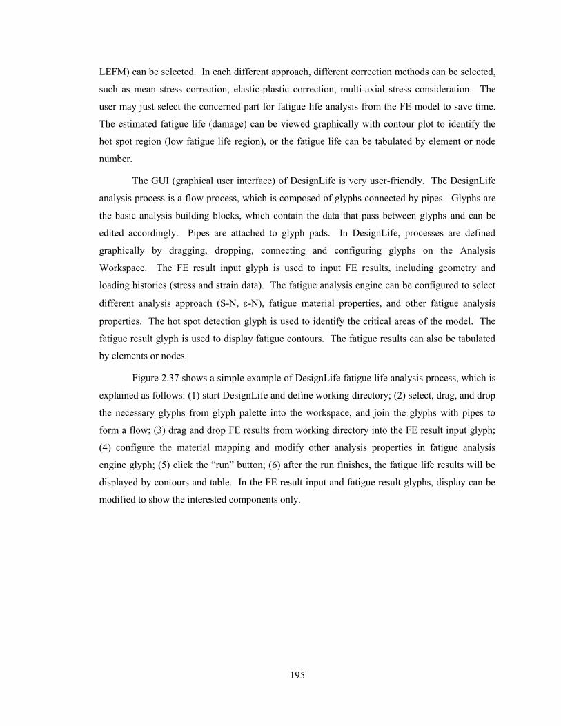
195

LEFM) can be selected. In each different approach, different correction methods can be selected,

such as mean stress correction, elastic-plastic correction, multi-axial stress consideration. The

user may just select the concerned part for fatigue life analysis from the FE model to save time.

The estimated fatigue life (damage) can be viewed graphically with contour plot to identify the

hot spot region (low fatigue life region), or the fatigue life can be tabulated by element or node

number.

The GUI (graphical user interface) of DesignLife is very user-friendly. The DesignLife

analysis process is a flow process, which is composed of glyphs connected by pipes. Glyphs are

the basic analysis building blocks, which contain the data that pass between glyphs and can be

edited accordingly. Pipes are attached to glyph pads. In DesignLife, processes are defined

graphically by dragging, dropping, connecting and configuring glyphs on the Analysis

Workspace. The FE result input glyph is used to input FE results, including geometry and

loading histories (stress and strain data). The fatigue analysis engine can be configured to select

different analysis approach (S-N, -N), fatigue material properties, and other fatigue analysis

properties. The hot spot detection glyph is used to identify the critical areas of the model. The

fatigue result glyph is used to display fatigue contours. The fatigue results can also be tabulated

by elements or nodes.

Figure 2.37 shows a simple example of DesignLife fatigue life analysis process, which is

explained as follows: (1) start DesignLife and define working directory; (2) select, drag, and drop

the necessary glyphs from glyph palette into the workspace, and join the glyphs with pipes to

form a flow; (3) drag and drop FE results from working directory into the FE result input glyph;

(4) configure the material mapping and modify other analysis properties in fatigue analysis

engine glyph; (5) click the “run” button; (6) after the run finishes, the fatigue life results will be

displayed by contours and table. In the FE result input and fatigue result glyphs, display can be

modified to show the interested components only.

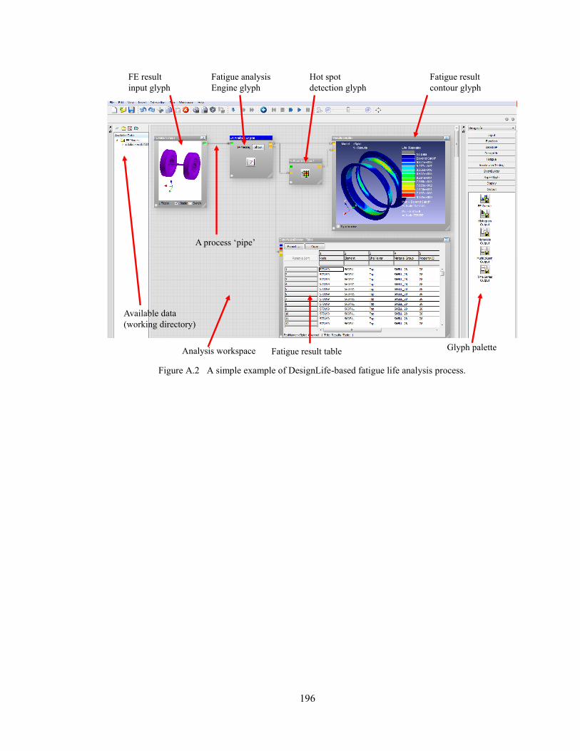
196

A process ‘pipe’

Fatigue result

contour glyph

Fatigue result table Glyph palette

Available data

(working directory)

FE result

input glyph

Fatigue analysis

Engine glyph

Hot spot

detection glyph

Analysis workspace

Figure A.2 A simple example of DesignLife-based fatigue life analysis process.

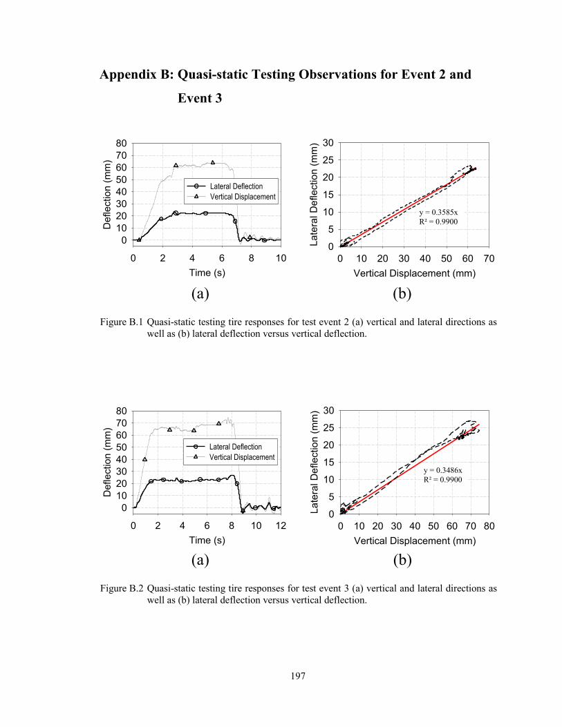
197

Appendix B: Quasi-static Testing Observations for Event 2 and

Event 3

Vertical Displacement (mm)

0 10 20 30 40 50 60 70

La

tera

l D

efle

ctio

n (

mm

)

0

5

10

15

20

25

30

Time (s)

0 2 4 6 8 10

De

flectio

n (

mm

)

0

10

20

30

40

50

60

70

80

Lateral Deflection

Vertical Displacement

y = 0.3585x

R² = 0.9900

(b)(a)

Figure B.1 Quasi-static testing tire responses for test event 2 (a) vertical and lateral directions as

well as (b) lateral deflection versus vertical deflection.

Time (s)

0 2 4 6 8 10 12

De

fle

ctio

n (

mm

)

0

10

20

30

40

50

60

70

80

Lateral Deflection

Vertical Displacement

Vertical Displacement (mm)

0 10 20 30 40 50 60 70 80

La

tera

l D

efle

ctio

n (

mm

)

0

5

10

15

20

25

30

y = 0.3486x

R² = 0.9900

(b)(a)

Figure B.2 Quasi-static testing tire responses for test event 3 (a) vertical and lateral directions as

well as (b) lateral deflection versus vertical deflection.

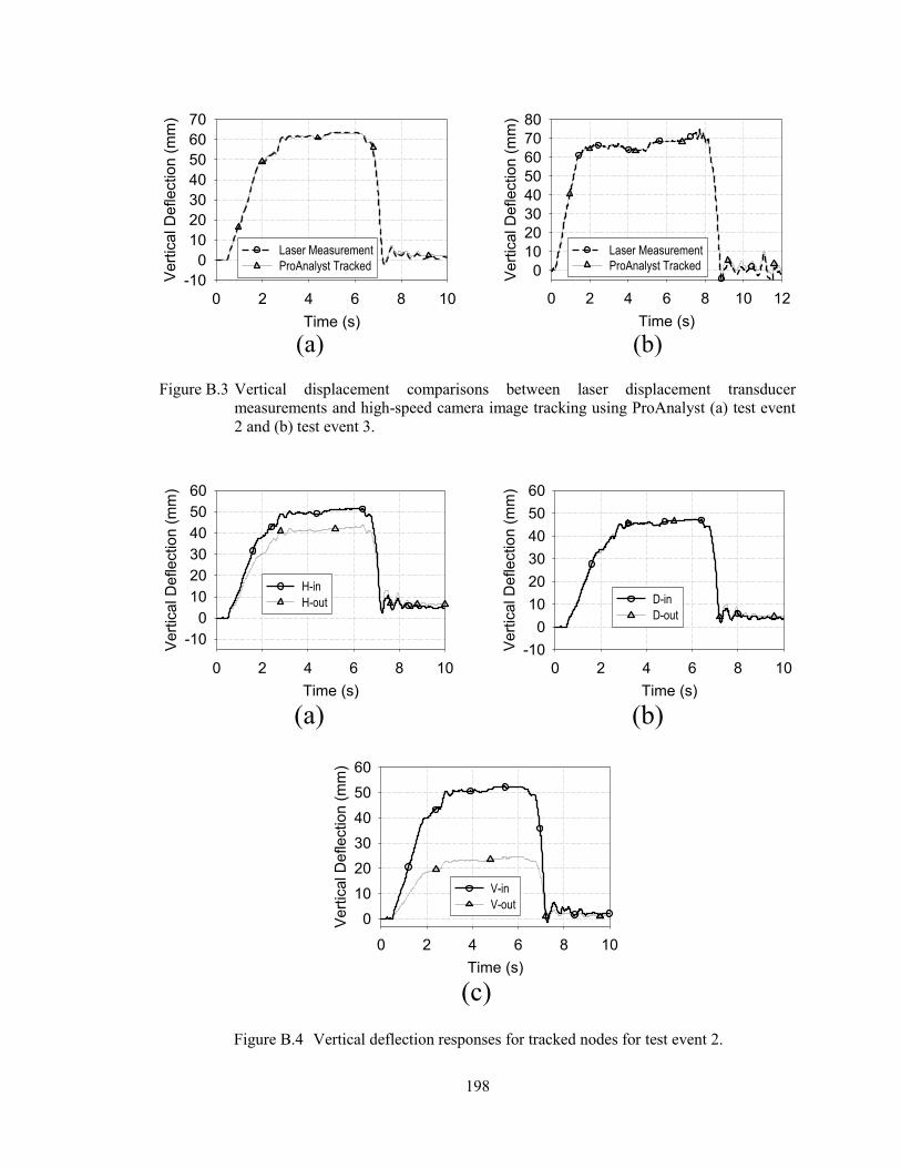
198

Time (s)

0 2 4 6 8 10 12

Ve

rtic

al D

efle

ctio

n (

mm

)

0

10

20

30

40

50

60

70

80

Laser Measurement

ProAnalyst Tracked

Time (s)

0 2 4 6 8 10

Ve

rtic

al D

efle

ctio

n (

mm

)

-10

0

10

20

30

40

50

60

70

Laser Measurement

ProAnalyst Tracked

(b)(a)

Figure B.3 Vertical displacement comparisons between laser displacement transducer

measurements and high-speed camera image tracking using ProAnalyst (a) test event

2 and (b) test event 3.

Time (s)

0 2 4 6 8 10

Ve

rtic

al D

efle

ctio

n (

mm

)

-10

0

10

20

30

40

50

60

H-in

H-out

Time (s)

0 2 4 6 8 10

Ve

rtic

al D

efle

ctio

n (

mm

)

-10

0

10

20

30

40

50

60

D-in

D-out

Time (s)

0 2 4 6 8 10

Ve

rtic

al D

efle

ctio

n (

mm

)

0

10

20

30

40

50

60

V-in

V-out

(b)(a)

(c)

Figure B.4 Vertical deflection responses for tracked nodes for test event 2.

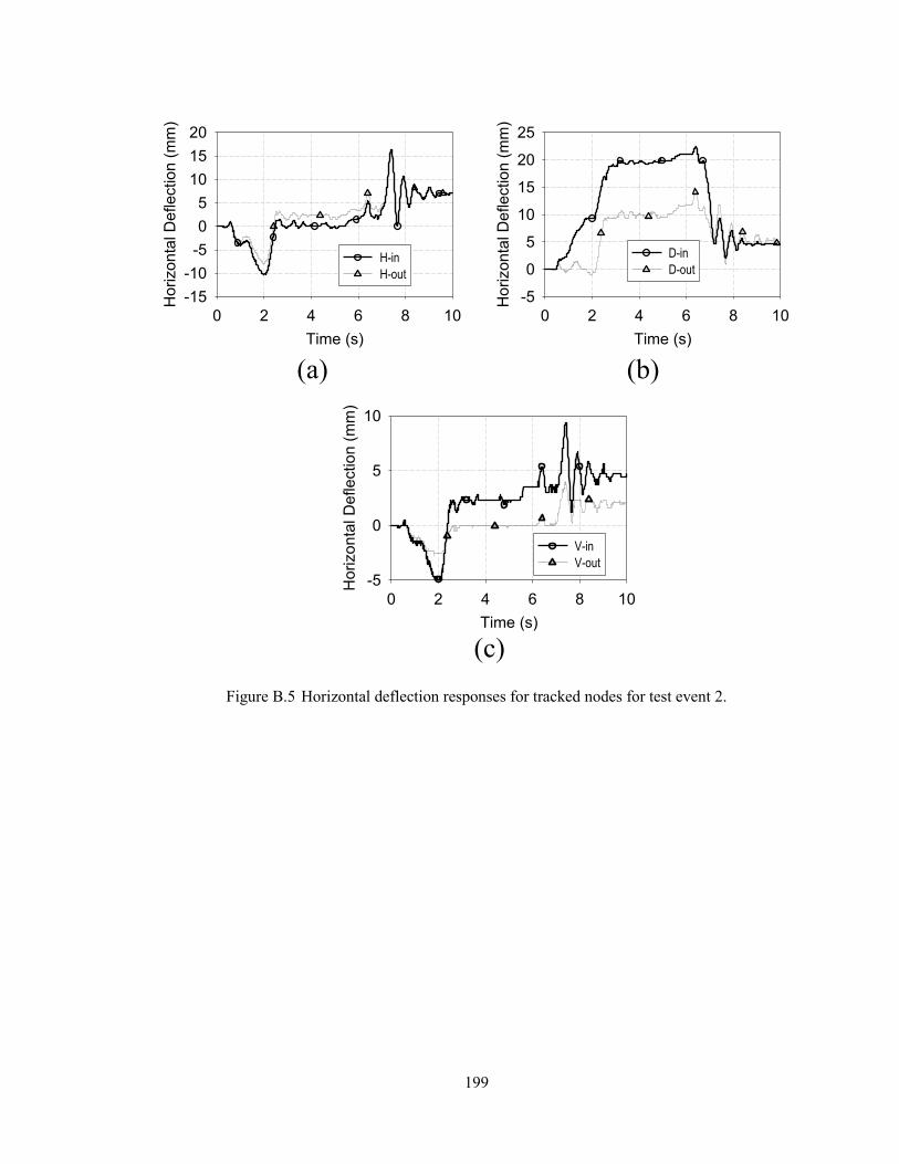
199

Time (s)

0 2 4 6 8 10

Hori

zo

nta

l D

eflectio

n (

mm

)

-15

-10

-5

0

5

10

15

20

H-in

H-out

Time (s)

0 2 4 6 8 10

Hori

zo

nta

l D

efle

ctio

n (

mm

)

-5

0

5

10

15

20

25

D-in

D-out

Time (s)

0 2 4 6 8 10

Hori

zo

nta

l D

efle

ctio

n (

mm

)

-5

0

5

10

V-in

V-out

(b)(a)

(c)

Figure B.5 Horizontal deflection responses for tracked nodes for test event 2.

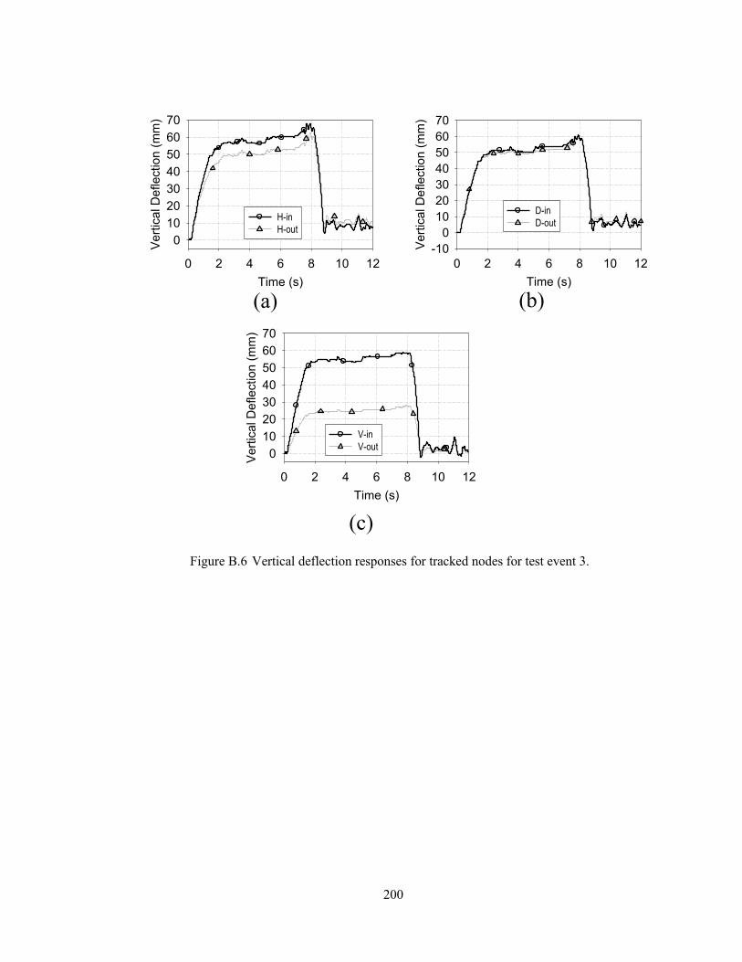
200

Time (s)

0 2 4 6 8 10 12

Ve

rtic

al D

efle

ctio

n (

mm

)

0

10

20

30

40

50

60

70

H-in

H-out

(a)

Time (s)

0 2 4 6 8 10 12

Ve

rtic

al D

efle

ctio

n (

mm

)

-10

0

10

20

30

40

50

60

70

D-in

D-out

(b)

Time (s)

0 2 4 6 8 10 12

Ve

rtic

al D

efle

ctio

n (

mm

)

0

10

20

30

40

50

60

70

V-in

V-out

(c)

(a)

(c)

(b)

Figure B.6 Vertical deflection responses for tracked nodes for test event 3.

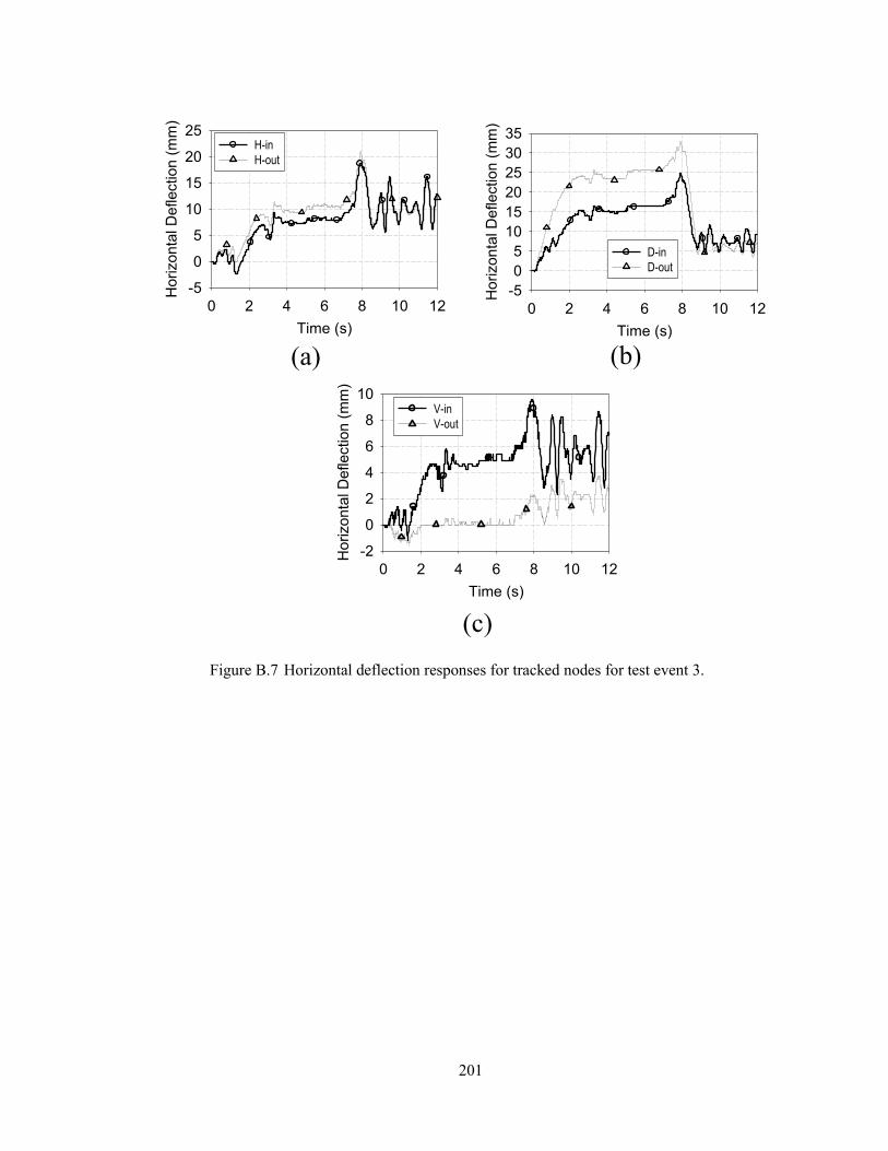
201

(a)

(c)

(b)

Time (s)

0 2 4 6 8 10 12

Ho

rizo

nta

l D

efle

ctio

n (

mm

)

-5

0

5

10

15

20

25H-in

H-out

(a)

Time (s)

0 2 4 6 8 10 12

Hori

zon

tal D

eflectio

n (

mm

)

-5

0

5

10

15

20

25

30

35

D-in

D-out

(b)

Time (s)

0 2 4 6 8 10 12

Hori

zon

tal D

eflection

(m

m)

-2

0

2

4

6

8

10V-in

V-out

(c)

Figure B.7 Horizontal deflection responses for tracked nodes for test event 3.

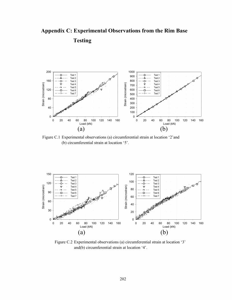
202

Appendix C: Experimental Observations from the Rim Base

Testing

Load (kN)

0 20 40 60 80 100 120 140 160

Str

ain

(m

icro

str

ain

)

0

40

80

120

160

200

N

T

T

Test 1

Test 2

Test 3

Test 4

Test 5N

Test 6

Test 7T

Load (kN)

0 20 40 60 80 100 120 140 160

Str

ain

(m

icro

str

ain

)

0

100

200

300

400

500

600

700

800

900

1000

N

N

T

T

Test 1

Test 2

Test 3

Test 4

Test 5N

Test 6

Test 7T

(a) (b)

Figure C.1 Experimental observations (a) circumferential strain at location ‘2’and

(b) circumferential strain at location ‘5’.

Load (kN)

0 20 40 60 80 100 120 140 160

Str

ain

(m

icro

str

ain

)

0

30

60

90

120

150

N

N

T

T

Test 1

Test 2

Test 3

Test 4

Test 5N

Test 6

Test 7T

Load (kN)

0 20 40 60 80 100 120 140 160

Str

ain

(m

icro

str

ain

)

0

20

40

60

80

100

120

N

T

T

Test 1

Test 2

Test 3

Test 4

Test 5N

Test 6

Test 7T

(a) (b)

Figure C.2 Experimental observations (a) circumferential strain at location ‘3’

and(b) circumferential strain at location ‘4’.

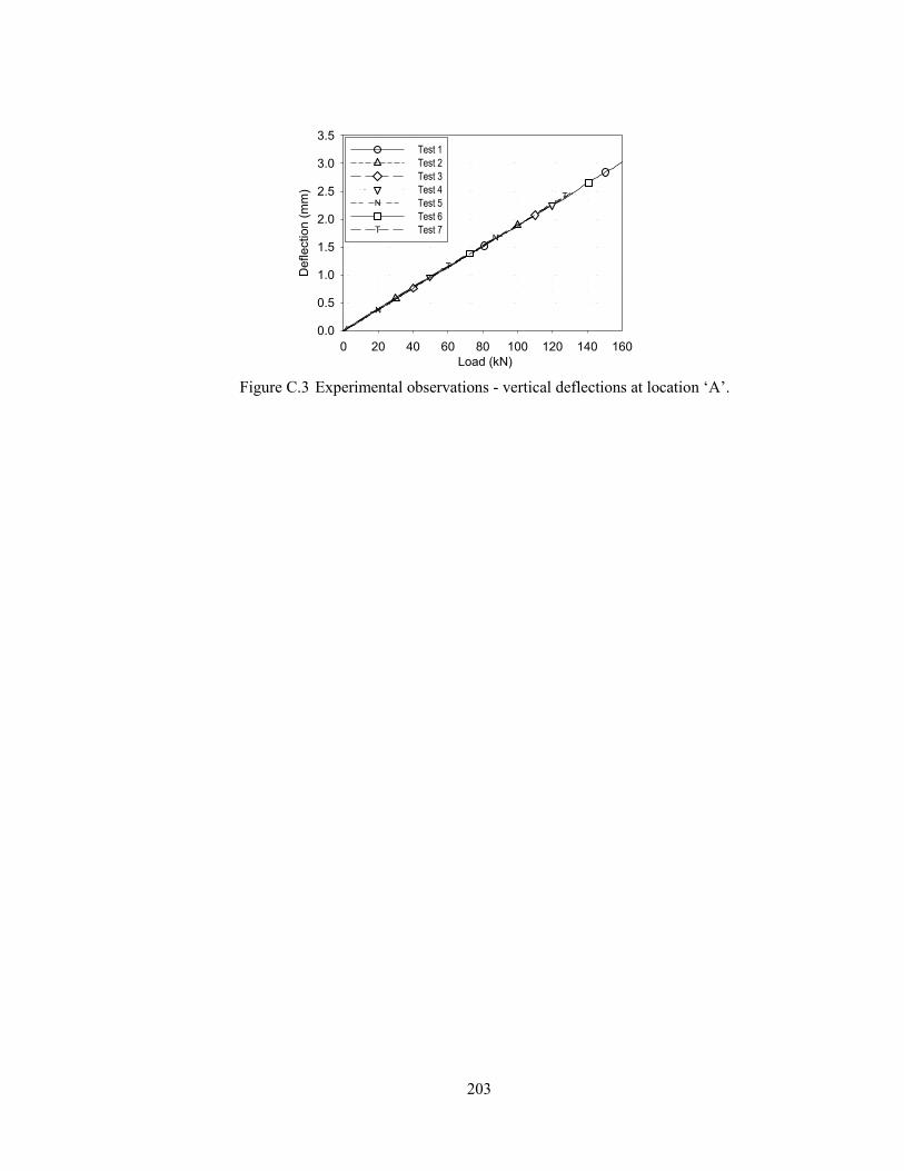
203

Load (kN)

0 20 40 60 80 100 120 140 160

De

fle

ctio

n (

mm

)

0.0

0.5

1.0

1.5

2.0

2.5

3.0

3.5

N

N

T

T

Test 1

Test 2

Test 3

Test 4

Test 5N

Test 6

Test 7T

Figure C.3 Experimental observations - vertical deflections at location ‘A’.

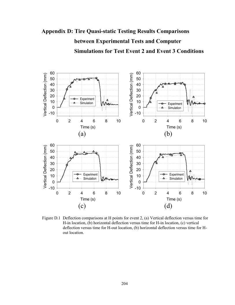
204

Appendix D: Tire Quasi-static Testing Results Comparisons

between Experimental Tests and Computer

Simulations for Test Event 2 and Event 3 Conditions

Time (s)

0 2 4 6 8 10

Vert

ical D

eflection (

mm

)

-10

0

10

20

30

40

50

60

Experiment

Simulation

Time (s)

0 2 4 6 8 10

Vert

ical D

eflection (

mm

)

-10

0

10

20

30

40

50

60

Experiment

Simulation

(b)(a)

Time (s)

0 2 4 6 8 10

Vert

ical D

eflection (

mm

)

-10

0

10

20

30

40

50

60

Experiment

Simulation

Time (s)

0 2 4 6 8 10

Vert

ical D

eflection (

mm

)

-10

0

10

20

30

40

50

60

Experiment

Simulation

(d)(c)

Figure D.1 Deflection comparisons at H points for event 2, (a) Vertical deflection versus time for

H-in location, (b) horizontal deflection versus time for H-in location, (c) vertical

deflection versus time for H-out location, (b) horizontal deflection versus time for H-

out location.

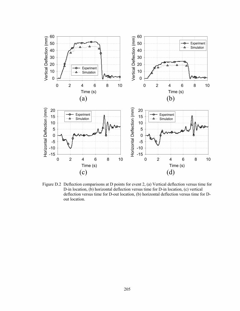
205

Time (s)

0 2 4 6 8 10

Ve

rtic

al D

efle

ctio

n (

mm

)

0

10

20

30

40

50

60

Experiment

Simulation

Time (s)

0 2 4 6 8 10

Ve

rtic

al D

efle

ctio

n (

mm

)

0

10

20

30

40

50

60

Experiment

Simulation

Time (s)

0 2 4 6 8 10

Ho

rizo

nta

l D

efle

ctio

n (

mm

)

-15

-10

-5

0

5

10

15

20Experiment

Simulation

Time (s)

0 2 4 6 8 10

Ho

rizo

nta

l D

efle

ctio

n (

mm

)

-15

-10

-5

0

5

10

15

20Experiment

Simulation

(b)(a)

(d)(c)

Figure D.2 Deflection comparisons at D points for event 2, (a) Vertical deflection versus time for

D-in location, (b) horizontal deflection versus time for D-in location, (c) vertical

deflection versus time for D-out location, (b) horizontal deflection versus time for D-

out location.

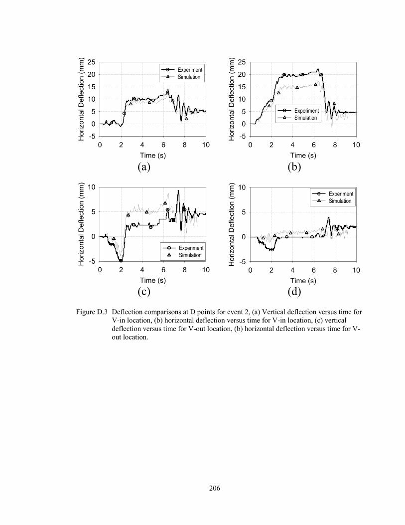
206

Time (s)

0 2 4 6 8 10

Ho

rizo

nta

l D

efle

ctio

n (

mm

)

-5

0

5

10

15

20

25Experiment

Simulation

Time (s)

0 2 4 6 8 10

Ho

rizo

nta

l D

efle

ctio

n (

mm

)

-5

0

5

10

15

20

25

Experiment

Simulation

(b)(a)

(d)(c)Time (s)

0 2 4 6 8 10

Ho

rizo

nta

l D

efle

ctio

n (

mm

)

-5

0

5

10

Experiment

Simulation

Time (s)

0 2 4 6 8 10

Ho

rizo

nta

l D

efle

ctio

n (

mm

)

-5

0

5

10Experiment

Simulation

Figure D.3 Deflection comparisons at D points for event 2, (a) Vertical deflection versus time for

V-in location, (b) horizontal deflection versus time for V-in location, (c) vertical

deflection versus time for V-out location, (b) horizontal deflection versus time for V-

out location.

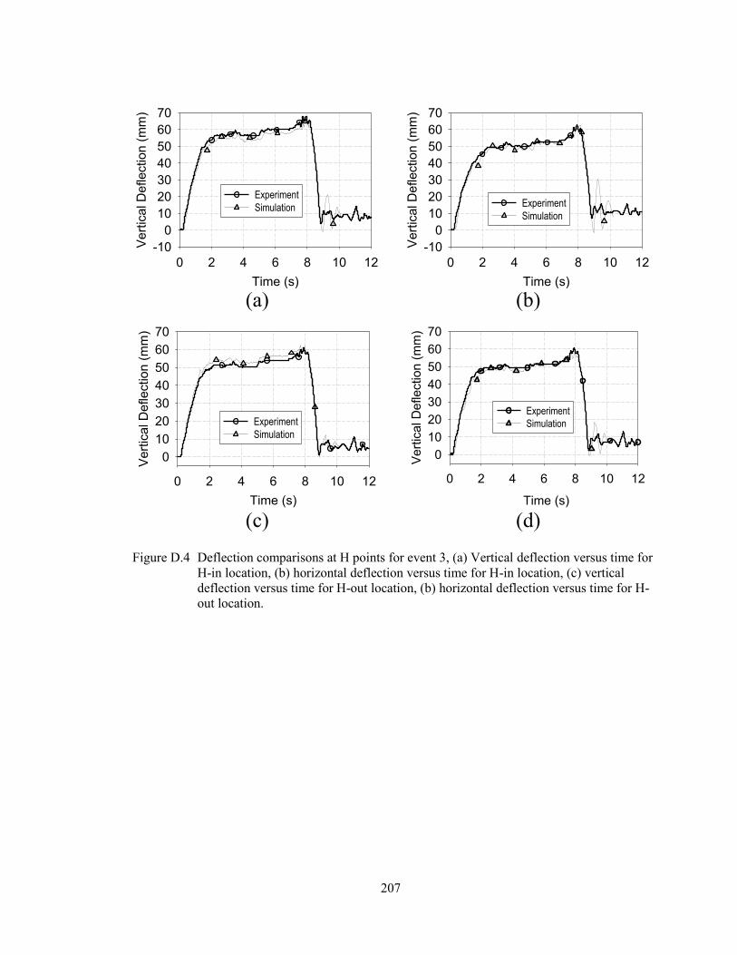
207

Time (s)

0 2 4 6 8 10 12

Vert

ica

l D

eflection (

mm

)

-10

0

10

20

30

40

50

60

70

Experiment

Simulation

Time (s)

0 2 4 6 8 10 12

Vert

ica

l D

eflection (

mm

)

-10

0

10

20

30

40

50

60

70

Experiment

Simulation

(b)(a)

(d)(c)Time (s)

0 2 4 6 8 10 12

Ve

rtic

al D

efle

ctio

n (

mm

)

0

10

20

30

40

50

60

70

Experiment

Simulation

Time (s)

0 2 4 6 8 10 12

Ve

rtic

al D

efle

ctio

n (

mm

)

0

10

20

30

40

50

60

70

Experiment

Simulation

Figure D.4 Deflection comparisons at H points for event 3, (a) Vertical deflection versus time for

H-in location, (b) horizontal deflection versus time for H-in location, (c) vertical

deflection versus time for H-out location, (b) horizontal deflection versus time for H-

out location.

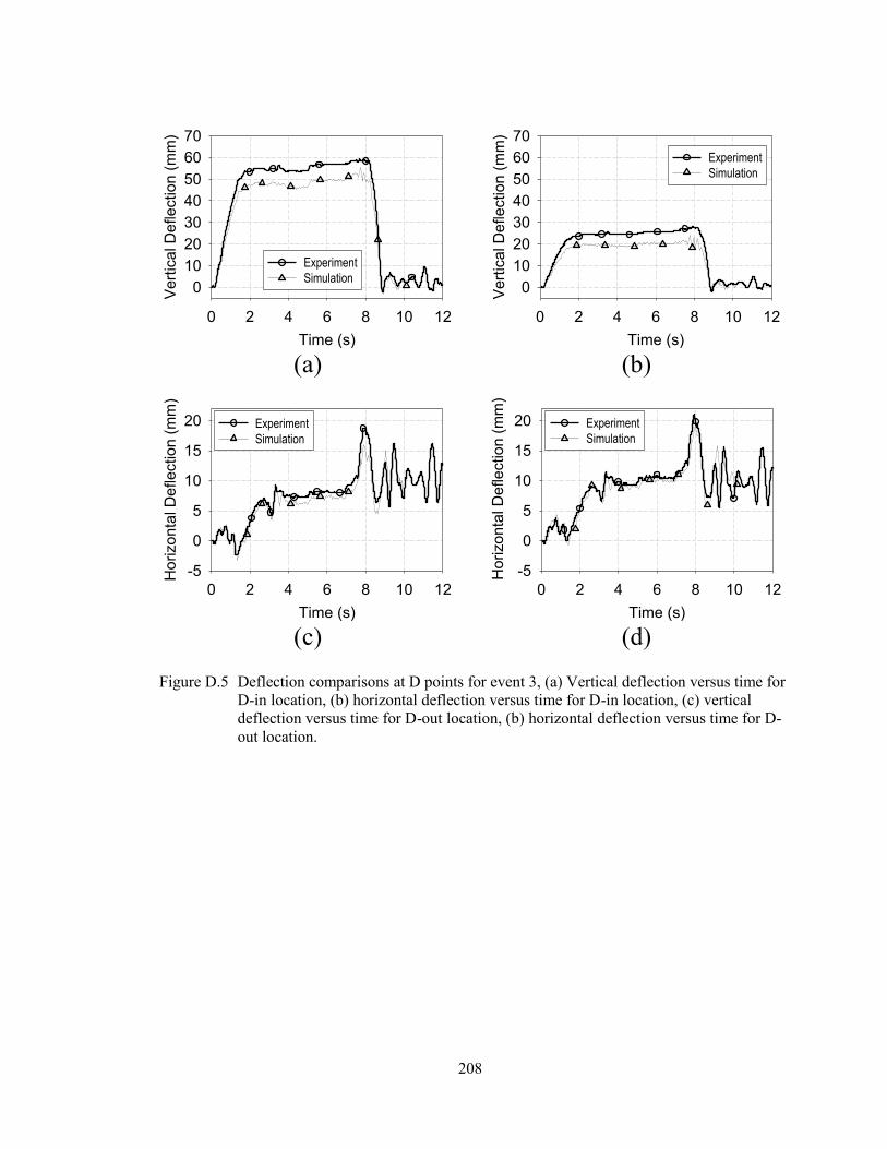
208

Time (s)

0 2 4 6 8 10 12

Ve

rtic

al D

efle

ctio

n (

mm

)

0

10

20

30

40

50

60

70

Experiment

Simulation

Time (s)

0 2 4 6 8 10 12

Ve

rtic

al D

efle

ctio

n (

mm

)

0

10

20

30

40

50

60

70

Experiment

Simulation

(b)(a)

(d)(c)Time (s)

0 2 4 6 8 10 12

Ho

rizo

nta

l D

efle

ctio

n (

mm

)

-5

0

5

10

15

20 Experiment

Simulation

Time (s)

0 2 4 6 8 10 12

Ho

rizo

nta

l D

efle

ctio

n (

mm

)

-5

0

5

10

15

20 Experiment

Simulation

Figure D.5 Deflection comparisons at D points for event 3, (a) Vertical deflection versus time for

D-in location, (b) horizontal deflection versus time for D-in location, (c) vertical

deflection versus time for D-out location, (b) horizontal deflection versus time for D-

out location.

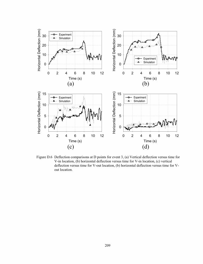
209

Time (s)

0 2 4 6 8 10 12

Ho

rizo

nta

l D

efle

ctio

n (

mm

)

0

10

20

30 Experiment

Simulation

Time (s)

0 2 4 6 8 10 12

Ho

rizo

nta

l D

efle

ctio

n (

mm

)

0

10

20

30

Experiment

Simulation

(b)(a)

(d)(c)Time (s)

0 2 4 6 8 10 12

Ho

rizo

nta

l D

efle

ctio

n (

mm

)

0

5

10

15Experiment

Simulation

Time (s)

0 2 4 6 8 10 12

Ho

rizo

nta

l D

efle

ctio

n (

mm

)

0

5

10

15Experiment

Simulation

Figure D.6 Deflection comparisons at D points for event 3, (a) Vertical deflection versus time for

V-in location, (b) horizontal deflection versus time for V-in location, (c) vertical

deflection versus time for V-out location, (b) horizontal deflection versus time for V-

out location.

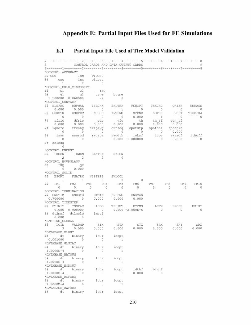
210

Appendix E: Partial Input Files Used for FE Simulations

E.1 Partial Input File Used of Tire Model Validation

$---+----1----+----2----+----3----+----4----+----5----+----6----+----7----+----8

$ CONTROL CARDS AND DATA OUTPUT CARDS $

$---+----1----+----2----+----3----+----4----+----5----+----6----+----7----+----8

*CONTROL_ACCURACY

$$ OSU INN PIDOSU

$# osu inn pidosu

1 2 0

*CONTROL_BULK_VISCOSITY

$$ Q1 Q2 IBQ

$# q1 q2 type btype

1.500000 0.060000 -2 0

*CONTROL_CONTACT

$$ SLSFAC RWPNAL ISLCHK SHLTHK PENOPT THKCHG ORIEN ENMASS

0.000 0.000 0 1 0 0 0 0

$$ USRSTR USRFRC NSBCS INTERM XPENE SSTHK ECDT TIEDPRJ

0 0 0 0 0.000 1 0 0

$# sfric dfric edc vfc th th_sf pen_sf

0.000 0.000 0.000 0.000 0.000 0.000 0.000

$# ignore frceng skiprwg outseg spotstp spotdel spothin

0 0 0 0 0 0 0.000

$# isym nserod rwgaps rwgdth rwksf icov swradf ithoff

0 0 0 0.000 1.000000 0 0.000 0

$# shledg

0

*CONTROL_ENERGY

$$ HGEN RWEN SLNTEN RYLEN

2 2 2 0

*CONTROL_HOURGLASS

$$ IHQ QH

6 0.000

*CONTROL_SOLID

$$ ESORT FMATRX NIPTETS SWLOCL

1 1 0 0 0

$$ PM1 PM2 PM3 PM4 PM5 PM6 PM7 PM8 PM9 PM10

0 0 0 0 0 0 0 0 0 0

*CONTROL_TERMINATION

$$ ENDTIM ENDCYC DTMIN ENDENG ENDMAS

0.700000 0 0.000 0.000 0.000

*CONTROL_TIMESTEP

$$ DTINIT TSSFAC ISDO TSLIMT DT2MS LCTM ERODE MSIST

0.000 0.900000 0 0.000 -2.000E-6 0 0 0

$# dt2msf dt2mslc imscl

0.000 0 0

*DAMPING_GLOBAL

$$ LCID VALDMP STX STR STZ SRX SRY SRZ

3 0.000 0.000 0.000 0.000 0.000 0.000 0.000

*DATABASE_ELOUT

$# dt binary lcur ioopt

0.001000 0 0 1

*DATABASE_GLSTAT

$# dt binary lcur ioopt

1.0000E-4 0 0 1

*DATABASE_MATSUM

$# dt binary lcur ioopt

1.0000E-4 0 0 1

*DATABASE_NODOUT

$# dt binary lcur ioopt dthf binhf

1.0000E-4 0 0 1 0.000 0

*DATABASE_RCFORC

$# dt binary lcur ioopt

1.0000E-4 0 0 1

*DATABASE_RWFORC

$# dt binary lcur ioopt

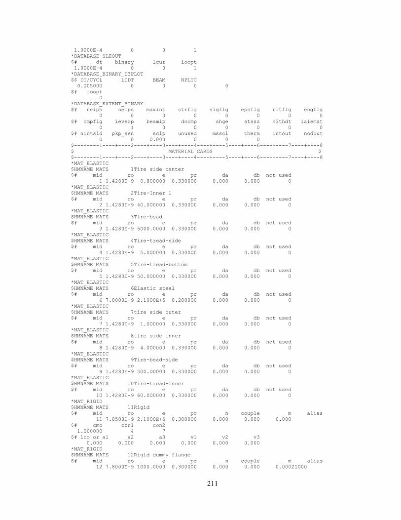
211

1.0000E-4 0 0 1

*DATABASE_SLEOUT

$# dt binary lcur ioopt

1.0000E-4 0 0 1

*DATABASE_BINARY_D3PLOT

$$ DT/CYCL LCDT BEAM NPLTC

0.005000 0 0 0 0

$# ioopt

0

*DATABASE_EXTENT_BINARY

$# neiph neips maxint strflg sigflg epsflg rltflg engflg

0 0 0 0 0 0 0 0

$# cmpflg ieverp beamip dcomp shge stssz n3thdt ialemat

0 1 0 0 0 0 0 0

$# nintsld pkp_sen sclp unused msscl therm intout nodout

0 0 0.000 0 0 0

$---+----1----+----2----+----3----+----4----+----5----+----6----+----7----+----8

$ MATERIAL CARDS $

$---+----1----+----2----+----3----+----4----+----5----+----6----+----7----+----8

*MAT_ELASTIC

$HMNAME MATS 1Tire side center

$# mid ro e pr da db not used

1 1.4280E-9 0.800000 0.330000 0.000 0.000 0

*MAT_ELASTIC

$HMNAME MATS 2Tire-Inner 1

$# mid ro e pr da db not used

2 1.4280E-9 40.000000 0.330000 0.000 0.000 0

*MAT_ELASTIC

$HMNAME MATS 3Tire-bead

$# mid ro e pr da db not used

3 1.4280E-9 5000.0000 0.330000 0.000 0.000 0

*MAT_ELASTIC

$HMNAME MATS 4Tire-tread-side

$# mid ro e pr da db not used

4 1.4280E-9 5.000000 0.330000 0.000 0.000 0

*MAT_ELASTIC

$HMNAME MATS 5Tire-tread-bottom

$# mid ro e pr da db not used

5 1.4280E-9 50.000000 0.330000 0.000 0.000 0

*MAT_ELASTIC

$HMNAME MATS 6Elastic steel

$# mid ro e pr da db not used

6 7.8000E-9 2.1000E+5 0.280000 0.000 0.000 0

*MAT_ELASTIC

$HMNAME MATS 7tire side outer

$# mid ro e pr da db not used

7 1.4280E-9 1.000000 0.330000 0.000 0.000 0

*MAT_ELASTIC

$HMNAME MATS 8tire side inner

$# mid ro e pr da db not used

8 1.4280E-9 4.000000 0.330000 0.000 0.000 0

*MAT_ELASTIC

$HMNAME MATS 9Tire-bead-side

$# mid ro e pr da db not used

9 1.4280E-9 500.00000 0.330000 0.000 0.000 0

*MAT_ELASTIC

$HMNAME MATS 10Tire-tread-inner

$# mid ro e pr da db not used

10 1.4280E-9 60.000000 0.330000 0.000 0.000 0

*MAT_RIGID

$HMNAME MATS 11Rigid

$# mid ro e pr n couple m alias

11 7.8500E-9 2.1000E+5 0.300000 0.000 0.000 0.000

$# cmo con1 con2

1.000000 4 7

$# lco or a1 a2 a3 v1 v2 v3

0.000 0.000 0.000 0.000 0.000 0.000

*MAT_RIGID

$HMNAME MATS 12Rigid dummy flange

$# mid ro e pr n couple m alias

12 7.8000E-9 1000.0000 0.300000 0.000 0.000 0.00021000

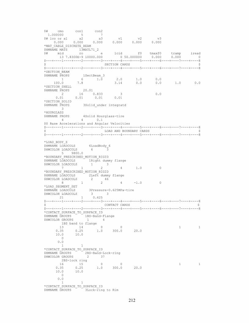
212

$# cmo con1 con2

1.000000 5 7

$# lco or a1 a2 a3 v1 v2 v3

0.000 0.000 0.000 0.000 0.000 0.000

*MAT_CABLE_DISCRETE_BEAM

$HMNAME MATS 13MATL71_2

$# mid ro e lcid f0 tmaxf0 tramp iread

13 7.8300E-9 10000.000 0 50.000000 0.000 0.000 0

$---+----1----+----2----+----3----+----4----+----5----+----6----+----7----+----8

$ SECTION CARDS $

$---+----1----+----2----+----3----+----4----+----5----+----6----+----7----+----8

*SECTION_BEAM

$HMNAME PROPS 1SectBeam_3

1 6 1.0 2.0 1.0 0.0

100.0 7.8 3.14 0.0 0.0 1.0 0.0

*SECTION_SHELL

$HMNAME PROPS 20.01

2 16 0.833 3 0.0

0.01 0.01 0.01 0.01

*SECTION_SOLID

$HMNAME PROPS 3Solid_under integratd

3

*HOURGLASS

$HMNAME PROPS 4Solid Hourglass-tire

4 4 0.1

$$ Base Accelerations and Angular Velocities

$---+----1----+----2----+----3----+----4----+----5----+----6----+----7----+----8

$ LOAD AND BOUNDARY CARDS $

$---+----1----+----2----+----3----+----4----+----5----+----6----+----7----+----8

*LOAD_BODY_Z

$HMNAME LOADCOLS 6LoadBody_6

$HWCOLOR LOADCOLS 6 3

5 9800.0

*BOUNDARY_PRESCRIBED_MOTION_RIGID

$HMNAME LOADCOLS 1Right dummy flange

$HWCOLOR LOADCOLS 1 3

7 1 2 4 1.0 0

*BOUNDARY_PRESCRIBED_MOTION_RIGID

$HMNAME LOADCOLS 2Left dummy flange

$HWCOLOR LOADCOLS 2 46

8 1 2 4 -1.0 0

*LOAD_SEGMENT_SET

$HMNAME LOADCOLS 3Pressure-0.625MPa-tire

$HWCOLOR LOADCOLS 3 3

21 1 0.625

$---+----1----+----2----+----3----+----4----+----5----+----6----+----7----+----8

$ CONTACT CARDS $

$---+----1----+----2----+----3----+----4----+----5----+----6----+----7----+----8

*CONTACT_SURFACE_TO_SURFACE_ID

$HMNAME GROUPS 1BS-Band-Flange

$HWCOLOR GROUPS 1 4

1BS band to flange

13 14 0 0 1 1

0.35 0.25 1.0 300.0 20.0

10.0 10.0

0

0.0

1 1

*CONTACT_SURFACE_TO_SURFACE_ID

$HMNAME GROUPS 2BS-Band-Lock-ring

$HWCOLOR GROUPS 2 37

2BS-lock ring

16 15 0 0 1 1

0.35 0.25 1.0 300.0 20.0

10.0 10.0

0

0.0

1 1

*CONTACT_SURFACE_TO_SURFACE_ID

$HMNAME GROUPS 3Lock-ring to Rim

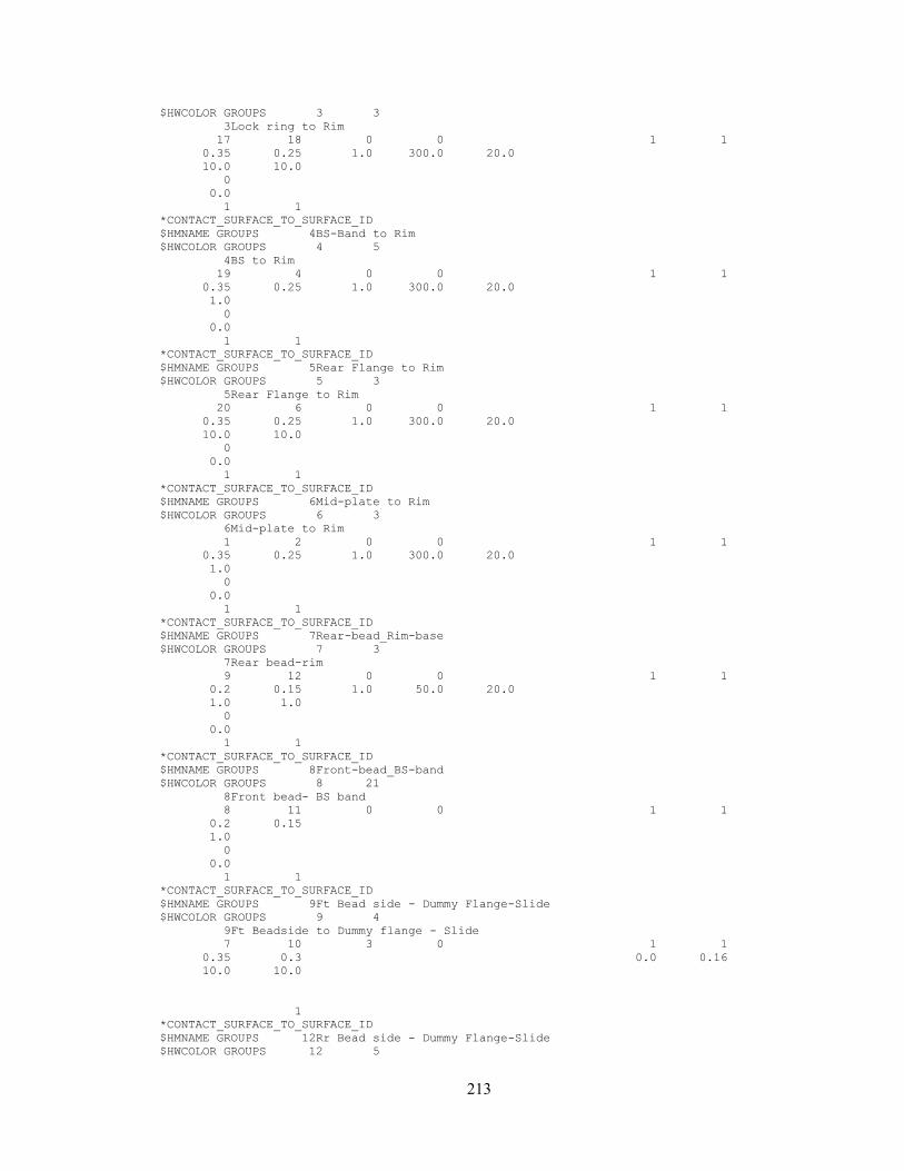
213

$HWCOLOR GROUPS 3 3

3Lock ring to Rim

17 18 0 0 1 1

0.35 0.25 1.0 300.0 20.0

10.0 10.0

0

0.0

1 1

*CONTACT_SURFACE_TO_SURFACE_ID

$HMNAME GROUPS 4BS-Band to Rim

$HWCOLOR GROUPS 4 5

4BS to Rim

19 4 0 0 1 1

0.35 0.25 1.0 300.0 20.0

1.0

0

0.0

1 1

*CONTACT_SURFACE_TO_SURFACE_ID

$HMNAME GROUPS 5Rear Flange to Rim

$HWCOLOR GROUPS 5 3

5Rear Flange to Rim

20 6 0 0 1 1

0.35 0.25 1.0 300.0 20.0

10.0 10.0

0

0.0

1 1

*CONTACT_SURFACE_TO_SURFACE_ID

$HMNAME GROUPS 6Mid-plate to Rim

$HWCOLOR GROUPS 6 3

6Mid-plate to Rim

1 2 0 0 1 1

0.35 0.25 1.0 300.0 20.0

1.0

0

0.0

1 1

*CONTACT_SURFACE_TO_SURFACE_ID

$HMNAME GROUPS 7Rear-bead_Rim-base

$HWCOLOR GROUPS 7 3

7Rear bead-rim

9 12 0 0 1 1

0.2 0.15 1.0 50.0 20.0

1.0 1.0

0

0.0

1 1

*CONTACT_SURFACE_TO_SURFACE_ID

$HMNAME GROUPS 8Front-bead_BS-band

$HWCOLOR GROUPS 8 21

8Front bead- BS band

8 11 0 0 1 1

0.2 0.15

1.0

0

0.0

1 1

*CONTACT_SURFACE_TO_SURFACE_ID

$HMNAME GROUPS 9Ft Bead side - Dummy Flange-Slide

$HWCOLOR GROUPS 9 4

9Ft Beadside to Dummy flange - Slide

7 10 3 0 1 1

0.35 0.3 0.0 0.16

10.0 10.0

1

*CONTACT_SURFACE_TO_SURFACE_ID

$HMNAME GROUPS 12Rr Bead side - Dummy Flange-Slide

$HWCOLOR GROUPS 12 5

214

12Rr Beadside to Dummy flange -Slide

8 24 3 0 1 1

0.35 0.3 0.0 0.16

10.0 10.0

1

*CONTACT_SURFACE_TO_SURFACE_ID

$HMNAME GROUPS 14Rr Bead side - Flange-No-Slide

$HWCOLOR GROUPS 14 7

14Rr Bead side - Flange-No-Slide

13 24 3 0 1 1

1.0 0.9

10.0 10.0

1

*CONTACT_SURFACE_TO_SURFACE_ID

$HMNAME GROUPS 15Ft Bead side - Flange-No-Slide

$HWCOLOR GROUPS 15 7

15Ft Bead side - Flange-No-Slide

11 10 3 0 1 1

1.0 0.9

10.0 10.0

1

*CONTACT_NODES_TO_SURFACE_ID

$HMNAME GROUPS 20Ft Bead side - Flange-Slide

$HWCOLOR GROUPS 20 36

20Ft Bead side - Flange-Slide

2 25 4 0 1 1

0.1 0.05

100.0 100.0

1

*CONTACT_NODES_TO_SURFACE_ID

$HMNAME GROUPS 19Rr Bead side - Flange-Slide

$HWCOLOR GROUPS 19 4

19Rr Bead side - Flange-Slide

3 26 4 0 1 1

0.1 0.05

100.0 100.0

1

*CONTACT_NODES_TO_SURFACE_ID

$HMNAME GROUPS 22Ft flange to chafer

$HWCOLOR GROUPS 22 4

22Ft flange to chafer

4 22 4 0

0.1 0.05

100.0 100.0

*CONTACT_NODES_TO_SURFACE_ID

$HMNAME GROUPS 23bk flange to chafer

$HWCOLOR GROUPS 23 4

23bk flange to chafer

5 23 4 0

0.1 0.05

100.0 100.0

*CONSTRAINED_EXTRA_NODES_NODE

$HMNAME GROUPS 21load center

$HWCOLOR GROUPS 21 4

4 179915

215

*RIGIDWALL_PLANAR_FORCES_ID

$HMNAME GROUPS 17Ground

$HWCOLOR GROUPS 17 5

17

1

721.0049364.2432E-05-994.50025721.0049363.2308E-04-993.50025

0 0 0 0 0 0

$---+----1----+----2----+----3----+----4----+----5----+----6----+----7----+----8

$ DEFINE CURVE CARDS $

$---+----1----+----2----+----3----+----4----+----5----+----6----+----7----+----8

*DEFINE_CURVE

$HMNAME CURVES 1LoadCurve_1

$HWCOLOR CURVES 1 3

$HMCURVE 2 2 LoadCurve1

1 0 1.0 1.0 0.0 0.0 0

0.0 0.0

0.1 1.0

10.0 1.0

*DEFINE_CURVE

$HMNAME CURVES 2LoadCurve_2

$HWCOLOR CURVES 2 4

$HMCURVE 3 3 LoadCurve2

2 0 1.0 1.0 0.0 0.0 0

0.0 0.0

0.35 0.0

0.4 1.0

10.0 1.0

*DEFINE_CURVE

$HMNAME CURVES 3LoadCurve_3

$HWCOLOR CURVES 3 3

$HMCURVE 1 1 LoadCurve3

3 0 1.0 1.0 0.0 0.0 0

0.0 35.0

0.35 35.0

0.36 39.0

10.0 39.0

*DEFINE_CURVE

$HMNAME CURVES 4curve1

$HWCOLOR CURVES 4 3

$HMCURVE 1 2 curve1

4 0 1.0 1.0

0.0 0.0

0.15 30.0

10.0 600.0

*DEFINE_CURVE

$HMNAME CURVES 5curve2

$HWCOLOR CURVES 5 3

$HMCURVE 1 3 curve2

5 0 1.0 1.0

0.0 0.0

0.05 1.0

10.0 1.0

216

E.2 Partial Input File Used for Tire Quasi-static Loading

$---+----1----+----2----+----3----+----4----+----5----+----6----+----7----+----8

$ LOAD AND BOUNDARY CARDS $

$---+----1----+----2----+----3----+----4----+----5----+----6----+----7----+----8

*LOAD_BODY_Z

$HMNAME LOADCOLS 7LoadBody_9

$HWCOLOR LOADCOLS 7 4

5 9800.0

*BOUNDARY_PRESCRIBED_MOTION_RIGID

$HMNAME LOADCOLS 1Right dummy flange

$HWCOLOR LOADCOLS 1 7

7 1 2 4 1.0 0

*BOUNDARY_PRESCRIBED_MOTION_RIGID

$HMNAME LOADCOLS 2Left dummy flange

$HWCOLOR LOADCOLS 2 46

8 1 2 4 -1.0 0

*BOUNDARY_PRESCRIBED_MOTION_RIGID_LOCAL

$HMNAME LOADCOLS 3rotation

$HWCOLOR LOADCOLS 3 38

4 5 2 8 1.0 0 0.7

*LOAD_SEGMENT_SET

$HMNAME LOADCOLS 6Pressure-0.593MPa-tire

$HWCOLOR LOADCOLS 6 24

19 1 0.593

*LOAD_NODE_POINT

$HMNAME LOADCOLS 8LoadNode_3

$HWCOLOR LOADCOLS 8 63

179915 3 2 -130000.0 0

*BOUNDARY_PRESCRIBED_MOTION_NODE

$HMNAME LOADCOLS 4Vertical movement

$HWCOLOR LOADCOLS 4 3

179915 3 2 6 1.0 0.7

*BOUNDARY_PRESCRIBED_MOTION_NODE

$HMNAME LOADCOLS 5Longitudinal movement

$HWCOLOR LOADCOLS 5 51

179915 2 2 7 1.0 0.7

$---+----1----+----2----+----3----+----4----+----5----+----6----+----7----+----8

$ DEFINE CURVE CARDS $

$---+----1----+----2----+----3----+----4----+----5----+----6----+----7----+----8

*DEFINE_CURVE

$HMNAME CURVES 1LoadCurve_1

$HWCOLOR CURVES 1 3

$HMCURVE 2 2 LoadCurve1

1 0 1.0 1.0 0.0 0.0 0

0.0 0.0

0.1 1.0

10.0 1.0

*DEFINE_CURVE

$HMNAME CURVES 2LoadCurve_2

$HWCOLOR CURVES 2 4

$HMCURVE 3 3 LoadCurve2

2 0 1.0 1.0 0.0 0.0 0

0.0 0.0

0.35 0.0

0.4 1.0

10.0 1.0

*DEFINE_CURVE

$HMNAME CURVES 3LoadCurve_3

$HWCOLOR CURVES 3 3

$HMCURVE 1 1 LoadCurve3

3 0 1.0 1.0 0.0 0.0 0

0.0 35.0

0.35 35.0

0.36 39.0

10.0 39.0

*DEFINE_CURVE

$HMNAME CURVES 4curve1

$HWCOLOR CURVES 4 3

$HMCURVE 1 2 curve1

217

4 0 1.0 1.0

0.0 0.0

0.15 30.0

10.0 600.0

*DEFINE_CURVE

$HMNAME CURVES 5curve2

$HWCOLOR CURVES 5 3

$HMCURVE 1 3 curve2

5 0 1.0 1.0

0.0 0.0

0.05 1.0

10.0 1.0

*DEFINE_CURVE

$HMNAME CURVES 6LoadCurve_6

$HWCOLOR CURVES 6 3

$HMCURVE 1 1 LoadCurve6

6 0 1.0 -1.0 0.0 0.0 0

0.0 0.0

0.007 0.2341

0.015 1.405

0.023 2.809

0.031 3.511

0.039 4.214

0.047 5.384

0.055 6.086

0.063 6.555

0.071 6.555

0.079 8.427

0.087 8.427

0.095 8.896

0.103 10.07

0.111 10.77

0.119 10.77

0.127 11.7

0.135 12.64

0.143 11.94

0.151 11.7

0.159 11.7

0.167 11.94

0.175 11.94

0.183 14.05

0.191 16.39

0.199 18.03

0.207 20.13

0.215 22.24

0.223 24.35

0.231 26.69

0.239 28.56

0.247 30.43

0.255 31.84

0.263 33.48

0.271 35.11

0.279 36.75

0.287 38.39

0.295 40.26

0.303 41.2

0.311 42.37

0.319 43.54

0.327 44.48

0.335 44.71

0.343 44.95

0.351 44.95

0.359 44.71

0.367 45.18

0.375 45.88

0.383 45.88

0.391 46.35

0.399 48.22

0.407 50.56

0.415 50.1

0.423 51.27

218

0.431 54.08

0.439 53.37

0.447 52.44

0.455 54.08

0.463 53.37

0.471 51.5

0.479 52.44

0.487 52.91

0.495 51.97

0.503 51.5

0.511 51.97

0.519 51.73

0.527 51.5

0.535 51.97

0.543 51.73

0.551 51.5

0.559 50.8

0.567 51.5

0.575 51.27

0.583 51.27

0.591 51.5

0.599 51.5

0.607 51.03

0.615 51.03

0.623 51.03

0.631 51.03

0.639 51.03

0.647 51.03

0.655 51.03

0.663 51.03

0.671 51.03

0.679 51.03

0.687 51.03

0.695 51.03

0.703 50.56

0.711 50.8

0.719 50.8

0.727 50.8

0.735 50.56

0.743 50.56

0.751 50.56

0.759 50.56

0.767 50.56

0.775 50.56

0.783 50.56

0.791 50.56

0.799 50.56

0.807 50.56

0.815 50.56

0.823 50.56

0.831 50.56

0.839 50.56

0.847 50.56

0.855 50.56

0.863 50.56

0.871 50.56

0.879 50.56

0.887 50.56

0.895 50.56

0.903 50.56

0.911 50.56

0.919 50.56

0.927 50.56

0.935 50.56

0.943 50.56

0.951 50.56

0.959 50.56

0.967 49.63

0.975 48.22

0.983 47.76

0.991 46.35

219

0.999 44.95

1.007 41.9

1.015 39.8

1.023 36.52

1.031 31.6

1.039 26.69

1.047 22.71

1.055 19.2

1.063 14.05

1.071 11.7

1.079 9.598

1.087 6.086

1.095 2.809

1.103 2.575

1.111 3.043

1.119 3.746

1.127 4.448

1.135 4.682

1.143 3.746

1.151 2.575

1.159 2.575

1.167 3.277

1.175 3.511

1.183 2.809

1.191 2.809

1.199 1.639

1.207 1.405

1.215 2.107

1.223 2.809

1.231 2.809

1.239 2.107

1.247 1.639

1.255 1.405

1.263 1.873

1.271 3.043

1.279 2.809

1.287 2.341

1.295 1.405

1.303 1.405

1.311 1.405

1.319 1.405

1.327 1.873

1.335 2.107

1.343 1.405

1.351 1.17

1.359 1.405

1.367 1.405

1.375 1.405

1.383 1.639

1.391 1.405

1.399 0.9364

*DEFINE_CURVE

$HMNAME CURVES 7LoadCurve_7

$HWCOLOR CURVES 7 4

$HMCURVE 2 2 LoadCurve7

7 0 1.0 1.0 0.0 0.0 0

0.0 0.0

0.007 0.2341

0.015 0.9364

0.023 0.4682

0.031 0.0

0.039 -0.4682

0.047 -0.7023

0.055 -0.2341

0.063 -0.4682

0.071 -0.4682

0.079 0.0

0.087 0.7023

0.095 2.341

0.103 3.98

0.111 4.448

220

0.119 3.511

0.127 2.341

0.135 2.341

0.143 2.341

0.151 2.341

0.159 2.341

0.167 2.341

0.175 2.341

0.183 2.575

0.191 2.341

0.199 2.341

0.207 2.107

0.215 1.405

0.223 0.7023

0.231 0.0

0.239 -0.9364

0.247 -0.7023

0.255 -0.9364

0.263 -1.17

0.271 -1.17

0.279 -1.405

0.287 -1.639

0.295 -1.873

0.303 -2.341

0.311 -2.341

0.319 -2.341

0.327 -2.341

0.335 -3.043

0.343 -2.341

0.351 -2.341

0.359 -2.575

0.367 -3.043

0.375 -2.341

0.383 -2.341

0.391 -4.682

0.399 -4.682

0.407 -3.511

0.415 -4.682

0.423 -6.555

0.431 -5.384

0.439 -4.682

0.447 -4.682

0.455 -4.916

0.463 -5.15

0.471 -4.682

0.479 -4.448

0.487 -4.682

0.495 -4.682

0.503 -4.682

0.511 -4.682

0.519 -4.682

0.527 -4.682

0.535 -4.682

0.543 -4.916

0.551 -4.682

0.559 -4.682

0.567 -4.682

0.575 -5.15

0.583 -5.15

0.591 -4.682

0.599 -4.682

0.607 -5.15

0.615 -5.15

0.623 -5.15

0.631 -5.15

0.639 -5.15

0.647 -5.15

0.655 -5.15

0.663 -5.15

0.671 -5.15

0.679 -5.15

221

0.687 -5.15

0.695 -5.15

0.703 -4.916

0.711 -5.618

0.719 -5.618

0.727 -5.618

0.735 -5.618

0.743 -5.618

0.751 -5.618

0.759 -5.618

0.767 -5.618

0.775 -5.618

0.783 -5.618

0.791 -5.618

0.799 -5.618

0.807 -5.618

0.815 -5.618

0.823 -5.618

0.831 -5.618

0.839 -5.618

0.847 -5.618

0.855 -5.852

0.863 -5.852

0.871 -5.852

0.879 -5.852

0.887 -5.852

0.895 -5.852

0.903 -5.852

0.911 -5.852

0.919 -5.852

0.927 -5.852

0.935 -5.852

0.943 -5.852

0.951 -5.852

0.959 -5.852

0.967 -6.789

0.975 -7.959

0.983 -10.53

0.991 -14.05

0.999 -17.32

1.007 -20.37

1.015 -18.73

1.023 -14.28

1.031 -11.94

1.039 -10.53

1.047 -8.427

1.055 -6.555

1.063 -5.384

1.071 -4.682

1.079 -3.511

1.087 -2.341

1.095 -2.107

1.103 -0.9364

1.111 -0.7023

1.119 -1.639

1.127 -2.809

1.135 -2.341

1.143 -1.639

1.151 -0.4682

1.159 -0.4682

1.167 -1.17

1.175 -2.341

1.183 -2.107

1.191 -1.405

1.199 -0.9364

1.207 -0.9364

1.215 -0.9364

1.223 -1.639

1.231 -1.873

1.239 -1.873

1.247 -1.405

222

1.255 -0.9364

1.263 -0.9364

1.271 -1.405

1.279 -2.341

1.287 -2.341

1.295 -1.17

1.303 -0.2341

1.311 -0.2341

1.319 -1.17

1.327 -1.873

1.335 -1.873

1.343 -1.17

1.351 -1.17

1.359 -0.2341

1.367 -0.9364

1.375 -1.405

1.383 -1.405

1.391 -1.17

1.399 -1.17

*DEFINE_CURVE

$HMNAME CURVES 8LoadCurve_8

$HWCOLOR CURVES 8 4

$HMCURVE 2 2 LoadCurve7

8 0 1.0 1.0 0.0 0.0 0

0.0 0.0

0.007 -6.221000000000E-04

0.015 -6.040000000000E-04

0.023 6.1690000000000E-04

0.031 -3.672000000000E-10

0.039 0.002452

0.047 0.001826

0.055 0.001226

0.063 0.002452

0.071 0.002452

0.079 6.1690000000000E-04

0.087 0.00121

0.095 -0.001231

0.103 -0.002452

0.111 -0.001842

0.119 -6.040000000000E-04

0.127 -2.936000000000E-09

0.135 -6.161000000000E-04

0.143 -0.001231

0.151 -0.001846

0.159 -0.001846

0.167 -0.001231

0.175 -0.00246

0.183 -0.001842

0.191 -4.404000000000E-09

0.199 6.1690000000000E-04

0.207 0.001226

0.215 0.00305

0.223 0.003656

0.231 0.003667

0.239 0.003667

0.247 0.004298

0.255 0.004286

0.263 0.006131

0.271 0.006131

0.279 0.006116

0.287 0.006721

0.295 0.009187

0.303 0.009151

0.311 0.009771

0.319 0.009771

0.327 0.009771

0.335 0.01097

0.343 0.01039

0.351 0.01039

0.359 0.009771

0.367 0.01222

223

0.375 0.01101

0.383 0.009771

0.391 0.01037

0.399 0.01037

0.407 0.01349

0.415 0.01164

0.423 0.01346

0.431 0.01282

0.439 0.01342

0.447 0.01164

0.455 0.01162

0.463 0.01284

0.471 0.01162

0.479 0.01284

0.487 0.01286

0.495 0.01101

0.503 0.01164

0.511 0.01164

0.519 0.01101

0.527 0.0116

0.535 0.01164

0.543 0.01099

0.551 0.01164

0.559 0.01039

0.567 0.01101

0.575 0.01097

0.583 0.01222

0.591 0.01164

0.599 0.01164

0.607 0.01222

0.615 0.01222

0.623 0.01222

0.631 0.01222

0.639 0.01222

0.647 0.01222

0.655 0.01222

0.663 0.01222

0.671 0.01222

0.679 0.01222

0.687 0.01222

0.695 0.01222

0.703 0.01099

0.711 0.01279

0.719 0.01279

0.727 0.01279

0.735 0.01217

0.743 0.01217

0.751 0.01279

0.759 0.01217

0.767 0.0122

0.775 0.0122

0.783 0.0122

0.791 0.01282

0.799 0.01282

0.807 0.0116

0.815 0.01222

0.823 0.01222

0.831 0.01222

0.839 0.01222

0.847 0.01284

0.855 0.01222

0.863 0.01222

0.871 0.01344

0.879 0.01344

0.887 0.01222

0.895 0.01284

0.903 0.01222

0.911 0.01162

0.919 0.01224

0.927 0.01346

0.935 0.01224

224

0.943 0.01224

0.951 0.01224

0.959 0.01164

0.967 0.0116

0.975 0.01097

0.983 0.01464

0.991 0.01714

0.999 0.01905

1.007 0.01776

1.015 0.01654

1.023 0.01349

1.031 0.01226

1.039 0.009828

1.047 0.007978

1.055 0.009187

1.063 0.006736

1.071 0.005511

1.079 0.004274

1.087 0.001234

1.095 0.002443

1.103 0.001835

1.111 0.001218

1.119 0.001835

1.127 0.003071

1.135 0.002472

1.143 0.001835

1.151 6.0940000000000E-04

1.159 0.001835

1.167 0.001835

1.175 0.002452

1.183 0.001844

1.191 0.001844

1.199 0.002443

1.207 0.002443

1.215 0.002462

1.223 0.00306

1.231 0.003071

1.239 0.003667

1.247 0.002452

1.255 0.001835

1.263 0.001844

1.271 0.001235

1.279 0.001835

1.287 0.002452

1.295 0.001226

1.303 0.001226

1.311 0.001226

1.319 6.1690000000000E-04

1.327 0.002452

1.335 0.00306

1.343 0.001226

1.351 0.001826

1.359 0.001235

1.367 0.001835

1.375 0.001226

1.383 0.001844

1.391 0.001226

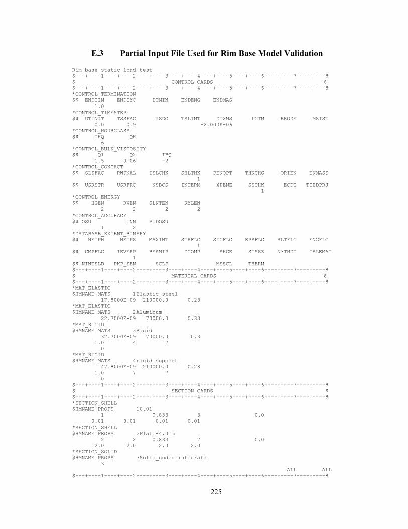
225

E.3 Partial Input File Used for Rim Base Model Validation

Rim base static load test

$---+----1----+----2----+----3----+----4----+----5----+----6----+----7----+----8

$ CONTROL CARDS $

$---+----1----+----2----+----3----+----4----+----5----+----6----+----7----+----8

*CONTROL_TERMINATION

$$ ENDTIM ENDCYC DTMIN ENDENG ENDMAS

1.0

*CONTROL_TIMESTEP

$$ DTINIT TSSFAC ISDO TSLIMT DT2MS LCTM ERODE MSIST

0.0 0.9 -2.000E-06

*CONTROL_HOURGLASS

$$ IHQ QH

6

*CONTROL_BULK_VISCOSITY

$$ Q1 Q2 IBQ

1.5 0.06 -2

*CONTROL_CONTACT

$$ SLSFAC RWPNAL ISLCHK SHLTHK PENOPT THKCHG ORIEN ENMASS

1

$$ USRSTR USRFRC NSBCS INTERM XPENE SSTHK ECDT TIEDPRJ

1

*CONTROL_ENERGY

$$ HGEN RWEN SLNTEN RYLEN

2 2 2 2

*CONTROL_ACCURACY

$$ OSU INN PIDOSU

1 2

*DATABASE_EXTENT_BINARY

$$ NEIPH NEIPS MAXINT STRFLG SIGFLG EPSFLG RLTFLG ENGFLG

1

$$ CMPFLG IEVERP BEAMIP DCOMP SHGE STSSZ N3THDT IALEMAT

1

$$ NINTSLD PKP_SEN SCLP MSSCL THERM

$---+----1----+----2----+----3----+----4----+----5----+----6----+----7----+----8

$ MATERIAL CARDS $

$---+----1----+----2----+----3----+----4----+----5----+----6----+----7----+----8

*MAT_ELASTIC

$HMNAME MATS 1Elastic steel

17.8000E-09 210000.0 0.28

*MAT_ELASTIC

$HMNAME MATS 2Aluminum

22.7000E-09 70000.0 0.33

*MAT_RIGID

$HMNAME MATS 3Rigid

32.7000E-09 70000.0 0.3

1.0 4 7

0

*MAT_RIGID

$HMNAME MATS 4rigid support

47.8000E-09 210000.0 0.28

1.0 7 7

0

$---+----1----+----2----+----3----+----4----+----5----+----6----+----7----+----8

$ SECTION CARDS $

$---+----1----+----2----+----3----+----4----+----5----+----6----+----7----+----8

*SECTION_SHELL

$HMNAME PROPS 10.01

1 0.833 3 0.0

0.01 0.01 0.01 0.01

*SECTION_SHELL

$HMNAME PROPS 2Plate-4.0mm

2 2 0.833 2 0.0

2.0 2.0 2.0 2.0

*SECTION_SOLID

$HMNAME PROPS 3Solid_under integratd

3

ALL ALL

$---+----1----+----2----+----3----+----4----+----5----+----6----+----7----+----8

226

$ lOAD CARDS $

$---+----1----+----2----+----3----+----4----+----5----+----6----+----7----+----8

*LOAD_BODY_Z

$HMNAME LOADCOLS 3LoadBody_3

$HWCOLOR LOADCOLS 3 3

2 9800.0

*LOAD_RIGID_BODY

$HMNAME LOADCOLS 1Load-rigid-body

$HWCOLOR LOADCOLS 1 3

5 3 1 -100000.0

$---+----1----+----2----+----3----+----4----+----5----+----6----+----7----+----8

$ CONTACT CARDS $

$---+----1----+----2----+----3----+----4----+----5----+----6----+----7----+----8

*CONTACT_SURFACE_TO_SURFACE_ID

$HMNAME GROUPS 1pad to Aluminum

$HWCOLOR GROUPS 1 29

1Pad to Aluminum

5 3 3 0 1 1

0.3 0.0

1 1

*CONTACT_SURFACE_TO_SURFACE_ID

$HMNAME GROUPS 2Rim to stands

$HWCOLOR GROUPS 2 29

2Rim to Support 2

5 6 0 3 1 1

0.2 0.1

20 20

1 1

*CONTACT_SURFACE_TO_SURFACE_ID

$HMNAME GROUPS 3Aluminum to Rim

$HWCOLOR GROUPS 3 29

3Aluminum to Rim

4 1 0 0 1 1

0.6 0.15

1 1

*CONTACT_SURFACE_TO_SURFACE_ID

$HMNAME GROUPS 4Rim to support 1

$HWCOLOR GROUPS 4 29

4Rim to support 1

2 11 0 3 1 1

0.2 0.1

20.0 20.0

1 1

$---+----1----+----2----+----3----+----4----+----5----+----6----+----7----+----8

$ DEFINE CURVE CARDS $

$---+----1----+----2----+----3----+----4----+----5----+----6----+----7----+----8

*DEFINE_CURVE

$HMNAME CURVES 1LoadCurve_2

$HWCOLOR CURVES 1 4

$HMCURVE 3 3 LoadCurve2

1 0 1.0 1.0 0.0 0.0 0

0.0 0.0

1.0 1.0

*DEFINE_CURVE

$HMNAME CURVES 2curve2

$HWCOLOR CURVES 2 3

$HMCURVE 1 3 curve2

2 0 1.0 1.0

0.0 0.0

0.05 1.0

227

E.4 Partial Input File Used for BS Band Pull-out Simulation

$---+----1----+----2----+----3----+----4----+----5----+----6----+----7----+----8

$ MATERIAL CARDS $

$---+----1----+----2----+----3----+----4----+----5----+----6----+----7----+----8

*MAT_ELASTIC

$HMNAME MATS 16Tire-bead.1

161.4280E-09 1000.0 0.33

*MAT_ELASTIC

$HMNAME MATS 17Tire-bead-side

171.4280E-09 1000.0 0.33

*MAT_RIGID

$HMNAME MATS 15Rigid inner

151.4280E-09 2000.0 0.3

1.0 5 7

0

*MAT_PIECEWISE_LINEAR_PLASTICITY

$HMNAME MATS 6Elastic steel

67.8000E-09 210000.0 0.28 345.0 550.0 0.21

$$ HM Entries in Stress-Strain Curve =

*MAT_PIECEWISE_LINEAR_PLASTICITY

$HMNAME MATS 18front flange

187.8000E-09 210000.0 0.28 345.0 550.0

$$ HM Entries in Stress-Strain Curve =

$---+----1----+----2----+----3----+----4----+----5----+----6----+----7----+----8

$ SECTION CARDS $

$---+----1----+----2----+----3----+----4----+----5----+----6----+----7----+----8

*SECTION_BEAM

$HMNAME PROPS 3Beam

3 2 1.0 2.0 1.0

3.14 1.0 1.0 2.0 0.0

*SECTION_SHELL

$HMNAME PROPS 10.01

1 1 0.0

0.01 0.01 0.01 0.01

*SECTION_SOLID

$HMNAME PROPS 2Solid_under integratd

2

$HMNAME PROPS 4Solid_under integratd.1

4

*HOURGLASS

$HMNAME PROPS 5Solid Hourglass-tire

5 4 0.1

$---+----1----+----2----+----3----+----4----+----5----+----6----+----7----+----8

$ BOUNDARY CARDS $

$---+----1----+----2----+----3----+----4----+----5----+----6----+----7----+----8

*BOUNDARY_PRESCRIBED_MOTION_RIGID

$HMNAME LOADCOLS 1Prescribed displacement

$HWCOLOR LOADCOLS 1 3

33 1 2 1 50.0 0

*DEFINE_CURVE

$HMNAME CURVES 1LoadCurve_1

$HWCOLOR CURVES 1 3

$HMCURVE 2 2 LoadCurve1

1 0 1.0 1.0 0.0 0.0 0

0.0 0.0

0.5 2.0

228

E.5 Partial Input File Used for Threaded-connection Design at

Quasi-static Loading Condition

$---+----1----+----2----+----3----+----4----+----5----+----6----+----7----+----8

$ MATERIAL CARDS $

$---+----1----+----2----+----3----+----4----+----5----+----6----+----7----+----8

*MAT_ELASTIC

$HMNAME MATS 1Tire side center

11.4280E-09 0.8 0.33

*MAT_ELASTIC

$HMNAME MATS 2Tire-Inner 1

21.4280E-09 40.0 0.33

*MAT_ELASTIC

$HMNAME MATS 3Tire-bead

31.4280E-09 5000.0 0.33

*MAT_ELASTIC

$HMNAME MATS 4Tire-tread-side

41.4280E-09 5.0 0.33

*MAT_ELASTIC

$HMNAME MATS 5Tire-tread-bottom

51.4280E-09 50.0 0.33

*MAT_ELASTIC

$HMNAME MATS 6Elastic steel

67.8000E-09 210000.0 0.28

*MAT_ELASTIC

$HMNAME MATS 7tire side outer

71.4280E-09 1.0 0.33

*MAT_ELASTIC

$HMNAME MATS 8tire side inner

81.4280E-09 4.0 0.33

*MAT_ELASTIC

$HMNAME MATS 9Tire-bead-side

91.4280E-09 500.0 0.33

*MAT_ELASTIC

$HMNAME MATS 10Tire-tread-inner

101.4280E-09 60.0 0.33

*MAT_RIGID

$HMNAME MATS 11Rigid

117.8500E-09 210000.0 0.3

1.0 1 4

0

*MAT_RIGID

$HMNAME MATS 12Rigid dummy flange

127.8000E-09 1000.0 0.3 21000

1.0 5 7

0

*MAT_RIGID

$HMNAME MATS 13rigid driver key

137.8000E-09 210000.0 0.28

0.0

0

*MAT_CABLE_DISCRETE_BEAM

$HMNAME MATS 14MATL71_2

147.8300E-09 10000.0 0 50.0 0

$---+----1----+----2----+----3----+----4----+----5----+----6----+----7----+----8

$ SECTION CARDS $

$---+----1----+----2----+----3----+----4----+----5----+----6----+----7----+----8

*SECTION_BEAM

$HMNAME PROPS 1SectBeam_3

1 6 1.0 2.0 1.0 0.0

100.0 7.8 3.14 0.0 0.0 1.0 0.0

*SECTION_SHELL

$HMNAME PROPS 20.01

2 0.833 3 0.0

0.01 0.01 0.01 0.01

*SECTION_SHELL

$HMNAME PROPS 3Driver key

3 0 0.833 2 0.0

229

2.0 2.0 2.0 2.0

*SECTION_SOLID

$HMNAME PROPS 4Solid_under integratd

4

*HOURGLASS

$HMNAME PROPS 5Solid Hourglass-tire

5 4 0.1

$---+----1----+----2----+----3----+----4----+----5----+----6----+----7----+----8

$ LOAD AND BOUNDARY CARDS $

$---+----1----+----2----+----3----+----4----+----5----+----6----+----7----+----8

*LOAD_BODY_Z

$HMNAME LOADCOLS 6LoadBody_6

$HWCOLOR LOADCOLS 6 3

1 9800.0

*BOUNDARY_PRESCRIBED_MOTION_RIGID

$HMNAME LOADCOLS 1Right dummy flange

$HWCOLOR LOADCOLS 1 7

8 1 2 4 1.0 0

*BOUNDARY_PRESCRIBED_MOTION_RIGID

$HMNAME LOADCOLS 2Left dummy flange

$HWCOLOR LOADCOLS 2 46

9 1 2 4 -1.0 0

*LOAD_SEGMENT_SET

$HMNAME LOADCOLS 4Pressure-0.593MPa-tire

$HWCOLOR LOADCOLS 4 24

15 1 0.593

$HMNAME LOADCOLS 5Pressure-rim base

$HWCOLOR LOADCOLS 5 3

3 1 0.593

*SET_SEGMENT

$HMNAME CSURFS 1Mid plate

$HWCOLOR CSURFS 1 4

1

368 370 224862 224863

*BOUNDARY_PRESCRIBED_MOTION_NODE

$HMNAME LOADCOLS 3Vertical movement

$HWCOLOR LOADCOLS 3 3

69812 3 2 6 -82.5 0.3

*DATABASE_HISTORY_NODE

$HMNAME OUTPUTBLOCKS 1TimeHistory1

69812 71479 90144 90166 90168 90169 90184 90187

90191 90192 103050 74468 96701 111654 113436 90174

90141 113440

$---+----1----+----2----+----3----+----4----+----5----+----6----+----7----+----8

$ CONTACT CARDS $

$---+----1----+----2----+----3----+----4----+----5----+----6----+----7----+----8

*CONTACT_SURFACE_TO_SURFACE_ID

$HMNAME GROUPS 1BS-Band-Flange

$HWCOLOR GROUPS 1 4

1BS band to flange

11 12 0 0 1 1

0.35 0.25 1.0 300.0 20.0

10.0 10.0

0

0.0

1 1

*CONTACT_SURFACE_TO_SURFACE_ID

$HMNAME GROUPS 2BS END - Rin front end

$HWCOLOR GROUPS 2 37

2BS END - Rin front end

22 24 0 0 1 1

0.35 0.25 1.0 300.0 20.0

10.0 10.0

0

0.0

1 1

*CONTACT_SURFACE_TO_SURFACE_ID

$HMNAME GROUPS 3Rim thread - BS thread

$HWCOLOR GROUPS 3 3

3Rim thread - BS thread

21 23 0 0 1 1

230

0.35 0.25 1.0 300.0 20.0

10.0 10.0

0

0.0

1 1

*CONTACT_SURFACE_TO_SURFACE_ID

$HMNAME GROUPS 4BS-Band to Rim

$HWCOLOR GROUPS 4 5

4BS to Rim

13 4 0 0 1 1

0.35 0.25 1.0 300.0 20.0

10.0 10.0

0

0.0

1 1

*CONTACT_SURFACE_TO_SURFACE_ID

$HMNAME GROUPS 5Rear Flange to Rim

$HWCOLOR GROUPS 5 3

5Rear Flange to Rim

14 5 0 0 1 1

0.35 0.25 1.0 300.0 20.0

10.0 10.0

0

0.0

1 1

*CONTACT_SURFACE_TO_SURFACE_ID

$HMNAME GROUPS 6Mid-plate to Rim

$HWCOLOR GROUPS 6 3

6Mid-plate to Rim

1 2 0 0 1 1

0.35 0.25 1.0 300.0 20.0

1.0

0

0.0

1 1

*CONTACT_SURFACE_TO_SURFACE_ID

$HMNAME GROUPS 7Rear-bead_Rim-base

$HWCOLOR GROUPS 7 3

7Rear bead-rim

7 10 0 0 1 1

0.35 0.25 1.0 50.0 20.0

1.0 1.0

0

0.0

1 1

*CONTACT_SURFACE_TO_SURFACE_ID

$HMNAME GROUPS 8Front-bead_BS-band

$HWCOLOR GROUPS 8 21

8Front bead- BS band

6 9 0 0 1 1

0.35 0.25

1.0

0

0.0

1 1

*CONTACT_SURFACE_TO_SURFACE_ID

$HMNAME GROUPS 9Ft Bead side - Dummy Flange-Slide

$HWCOLOR GROUPS 9 4

9Ft Beadside to Dummy flange - Slide

8 8 3 0 1 1

0.35 0.3 0.0 0.16

10.0 10.0

1

*CONTACT_SURFACE_TO_SURFACE_ID

$HMNAME GROUPS 10Rr Bead side - Dummy Flange-Slide

$HWCOLOR GROUPS 10 5

10Rr Beadside to Dummy flange -Slide

9 18 3 0 1 1

0.35 0.3 0.0 0.16

231

10.0 10.0

1

*CONTACT_SURFACE_TO_SURFACE_ID

$HMNAME GROUPS 11Rr Bead side - Flange-No-Slide

$HWCOLOR GROUPS 11 7

11Rr Bead side - Flange-No-Slide

13 18 3 0 1 1

1.0 0.9

10.0 10.0

1

*CONTACT_SURFACE_TO_SURFACE_ID

$HMNAME GROUPS 12Ft Bead side - Flange-No-Slide

$HWCOLOR GROUPS 12 7

12Ft Bead side - Flange-No-Slide

12 8 3 0 1 1

1.0 0.9

10.0 10.0

1

*CONTACT_NODES_TO_SURFACE_ID

$HMNAME GROUPS 13Ft Bead side - Flange-Slide

$HWCOLOR GROUPS 13 36

13Ft Bead side - Flange-Slide

2 19 4 0 1 1

0.1 0.05

100.0 100.0

1

*CONTACT_NODES_TO_SURFACE_ID

$HMNAME GROUPS 14Rr Bead side - Flange-Slide

$HWCOLOR GROUPS 14 4

14Rr Bead side - Flange-Slide

3 20 4 0 1 1

0.1 0.05

100.0 100.0

1

*CONSTRAINED_EXTRA_NODES_SET

$HMNAME GROUPS 16load center

$HWCOLOR GROUPS 16 4

6 4

*SET_NODE_LIST

$HMSET

$HMNAME SETS 4local system

4 0.0 0.0 0.0 0.0

69812 165761 165762

*RIGIDWALL_PLANAR_FORCES_ID

$HMNAME GROUPS 15Ground

$HWCOLOR GROUPS 15 5

15

1

721.0049364.2432E-05-994.50025721.0049363.2308E-04-993.50025 1.0

0 0 0 0 0 0

$---+----1----+----2----+----3----+----4----+----5----+----6----+----7----+----8

$ DEFINE CURVE CARDS $

$---+----1----+----2----+----3----+----4----+----5----+----6----+----7----+----8

*DEFINE_CURVE

$HMNAME CURVES 1LoadCurve_1

$HWCOLOR CURVES 1 3

$HMCURVE 2 2 LoadCurve1

1 0 0.02 1.0 0.0 0.0 0

0.0 0.0

0.2632 0.005

0.5263 0.015

232

0.7895 0.035

1.0526 0.055

1.3158 0.09

1.5789 0.133

1.8421 0.195

2.1053 0.275

2.3684 0.37

2.6316 0.475

2.8947 0.59

3.1579 0.7

3.4211 0.81

3.6842 0.905

3.9474 0.96

4.2105 0.985

4.4737 0.995

4.7368 0.999

5.0 1.0

100.0 1.0

*DEFINE_CURVE

$HMNAME CURVES 2LoadCurve_2

$HWCOLOR CURVES 2 4

$HMCURVE 3 3 LoadCurve2

2 0 1.0 15000.0 0.0 0.0 0

0.0 1.0

2.0 1.0

*DEFINE_CURVE

$HMNAME CURVES 3LoadCurve_3

$HWCOLOR CURVES 3 3

$HMCURVE 1 1 LoadCurve3

3 0 1.0 1.0 0.0 0.0 0

0.0 35.0

0.35 35.0

0.36 39.0

10.0 39.0

*DEFINE_CURVE

$HMNAME CURVES 4curve1

$HWCOLOR CURVES 4 3

$HMCURVE 1 2 curve1

4 0 1.0 1.0

0.0 0.0

0.06 24.0

0.07 26.0

0.08 27.3

0.09 28.2

0.1 28.85

0.12 29.75

0.14 30.3

0.15 30.5

2.0 400.0

*DEFINE_CURVE

$HMNAME CURVES 5curve2

$HWCOLOR CURVES 5 3

$HMCURVE 1 3 curve2

5 0 0.01 1.0

0.0 0.0

0.2632 0.005

0.5263 0.015

0.7895 0.035

1.0526 0.055

1.3158 0.09

1.5789 0.133

1.8421 0.195

2.1053 0.275

2.3684 0.37

2.6316 0.475

2.8947 0.59

3.1579 0.7

3.4211 0.81

3.6842 0.905

3.9474 0.96

4.2105 0.985

233

4.4737 0.995

4.7368 0.999

5.0 1.0

200.0 1.0

*DEFINE_CURVE

$HMNAME CURVES 6LoadCurve_6

$HWCOLOR CURVES 6 3

$HMCURVE 1 1 LoadCurve6

6 0 0.6 1.0 0.0 0.0 0

0.0 0.0

0.05632 0.005

0.08263 0.015

0.10895 0.035

0.13526 0.055

0.16158 0.09

0.18789 0.133

0.21421 0.195

0.24053 0.275

0.26684 0.37

0.29316 0.475

0.31947 0.59

0.34579 0.7

0.37211 0.81

0.39842 0.905

0.42474 0.96

0.45105 0.985

0.47737 0.995

0.50368 0.999

0.5 1.0

2.0 1.0

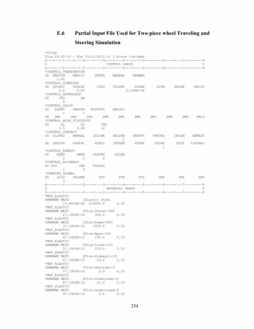
234

E.6 Partial Input File Used for Two-piece wheel Traveling and

Steering Simulation

*TITLE

Tire 18.00-33 - Rim 33-13.00/2.5- 2 piece rim-5mph

$---+----1----+----2----+----3----+----4----+----5----+----6----+----7----+----8

$ CONTROL CARDS $

$---+----1----+----2----+----3----+----4----+----5----+----6----+----7----+----8

*CONTROL_TERMINATION

$$ ENDTIM ENDCYC DTMIN ENDENG ENDMAS

1.65

*CONTROL_TIMESTEP

$$ DTINIT TSSFAC ISDO TSLIMT DT2MS LCTM ERODE MSIST

0.0 0.67 -2.000E-06

*CONTROL_HOURGLASS

$$ IHQ QH

6

*CONTROL_SOLID

$$ ESORT FMATRX NIPTETS SWLOCL

1 1

$$ PM1 PM2 PM3 PM4 PM5 PM6 PM7 PM8 PM9 PM10

*CONTROL_BULK_VISCOSITY

$$ Q1 Q2 IBQ

1.5 0.06 -2

*CONTROL_CONTACT

$$ SLSFAC RWPNAL ISLCHK SHLTHK PENOPT THKCHG ORIEN ENMASS

1

$$ USRSTR USRFRC NSBCS INTERM XPENE SSTHK ECDT TIEDPRJ

1

*CONTROL_ENERGY

$$ HGEN RWEN SLNTEN RYLEN

2 2 2

*CONTROL_ACCURACY

$$ OSU INN PIDOSU

1 2

*DAMPING_GLOBAL

$$ LCID VALDMP STX STR STZ SRX SRY SRZ

3

$---+----1----+----2----+----3----+----4----+----5----+----6----+----7----+----8

$ MATERIAL CARDS $

$---+----1----+----2----+----3----+----4----+----5----+----6----+----7----+----8

*MAT_ELASTIC

$HMNAME MATS 1Elastic steel

17.8000E-09 210000.0 0.28

*MAT_ELASTIC

$HMNAME MATS 2Tire-Chafer-300

27.1900E-10 300.0 0.33

*MAT_ELASTIC

$HMNAME MATS 3Tire-bead-1000

37.1900E-10 1000.0 0.33

*MAT_ELASTIC

$HMNAME MATS 4Tire-Apex-100

47.1900E-10 100.0 0.33

*MAT_ELASTIC

$HMNAME MATS 5Tire-Liner-210

57.1900E-10 210.0 0.33

*MAT_ELASTIC

$HMNAME MATS 6Tire-Sidewall-10

67.1900E-10 10.0 0.33

*MAT_ELASTIC

$HMNAME MATS 7Tire-Shoulder-9

77.1900E-10 9.0 0.33

*MAT_ELASTIC

$HMNAME MATS 8Tire-Sidetread-15

87.1900E-10 15.0 0.33

*MAT_ELASTIC

$HMNAME MATS 9Tire-undertread-4

97.1900E-10 4.0 0.33

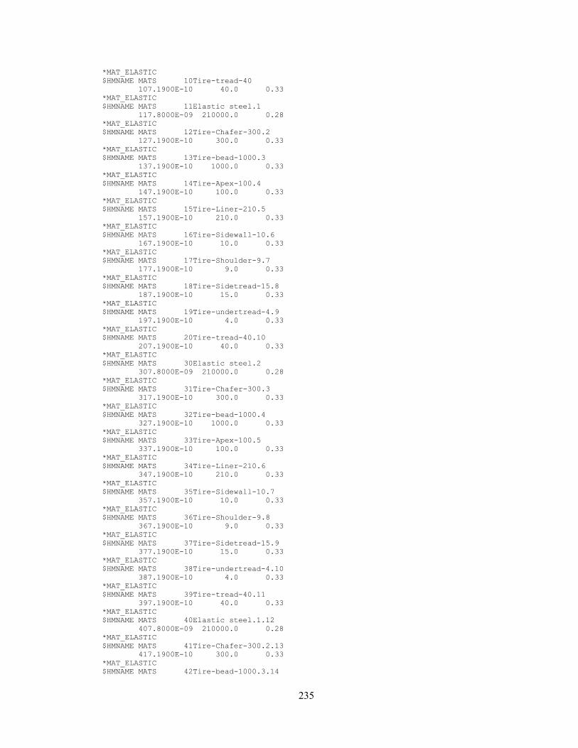
235

*MAT_ELASTIC

$HMNAME MATS 10Tire-tread-40

107.1900E-10 40.0 0.33

*MAT_ELASTIC

$HMNAME MATS 11Elastic steel.1

117.8000E-09 210000.0 0.28

*MAT_ELASTIC

$HMNAME MATS 12Tire-Chafer-300.2

127.1900E-10 300.0 0.33

*MAT_ELASTIC

$HMNAME MATS 13Tire-bead-1000.3

137.1900E-10 1000.0 0.33

*MAT_ELASTIC

$HMNAME MATS 14Tire-Apex-100.4

147.1900E-10 100.0 0.33

*MAT_ELASTIC

$HMNAME MATS 15Tire-Liner-210.5

157.1900E-10 210.0 0.33

*MAT_ELASTIC

$HMNAME MATS 16Tire-Sidewall-10.6

167.1900E-10 10.0 0.33

*MAT_ELASTIC

$HMNAME MATS 17Tire-Shoulder-9.7

177.1900E-10 9.0 0.33

*MAT_ELASTIC

$HMNAME MATS 18Tire-Sidetread-15.8

187.1900E-10 15.0 0.33

*MAT_ELASTIC

$HMNAME MATS 19Tire-undertread-4.9

197.1900E-10 4.0 0.33

*MAT_ELASTIC

$HMNAME MATS 20Tire-tread-40.10

207.1900E-10 40.0 0.33

*MAT_ELASTIC

$HMNAME MATS 30Elastic steel.2

307.8000E-09 210000.0 0.28

*MAT_ELASTIC

$HMNAME MATS 31Tire-Chafer-300.3

317.1900E-10 300.0 0.33

*MAT_ELASTIC

$HMNAME MATS 32Tire-bead-1000.4

327.1900E-10 1000.0 0.33

*MAT_ELASTIC

$HMNAME MATS 33Tire-Apex-100.5

337.1900E-10 100.0 0.33

*MAT_ELASTIC

$HMNAME MATS 34Tire-Liner-210.6

347.1900E-10 210.0 0.33

*MAT_ELASTIC

$HMNAME MATS 35Tire-Sidewall-10.7

357.1900E-10 10.0 0.33

*MAT_ELASTIC

$HMNAME MATS 36Tire-Shoulder-9.8

367.1900E-10 9.0 0.33

*MAT_ELASTIC

$HMNAME MATS 37Tire-Sidetread-15.9

377.1900E-10 15.0 0.33

*MAT_ELASTIC

$HMNAME MATS 38Tire-undertread-4.10

387.1900E-10 4.0 0.33

*MAT_ELASTIC

$HMNAME MATS 39Tire-tread-40.11

397.1900E-10 40.0 0.33

*MAT_ELASTIC

$HMNAME MATS 40Elastic steel.1.12

407.8000E-09 210000.0 0.28

*MAT_ELASTIC

$HMNAME MATS 41Tire-Chafer-300.2.13

417.1900E-10 300.0 0.33

*MAT_ELASTIC

$HMNAME MATS 42Tire-bead-1000.3.14

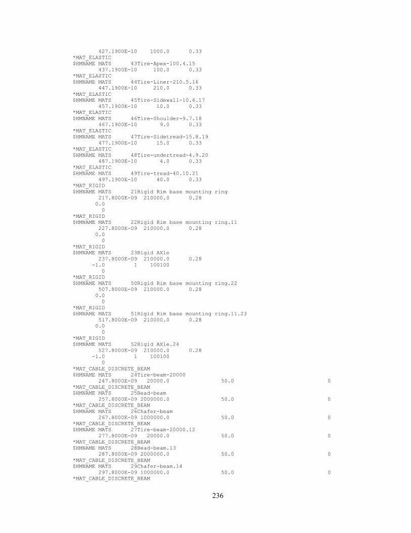
236

427.1900E-10 1000.0 0.33

*MAT_ELASTIC

$HMNAME MATS 43Tire-Apex-100.4.15

437.1900E-10 100.0 0.33

*MAT_ELASTIC

$HMNAME MATS 44Tire-Liner-210.5.16

447.1900E-10 210.0 0.33

*MAT_ELASTIC

$HMNAME MATS 45Tire-Sidewall-10.6.17

457.1900E-10 10.0 0.33

*MAT_ELASTIC

$HMNAME MATS 46Tire-Shoulder-9.7.18

467.1900E-10 9.0 0.33

*MAT_ELASTIC

$HMNAME MATS 47Tire-Sidetread-15.8.19

477.1900E-10 15.0 0.33

*MAT_ELASTIC

$HMNAME MATS 48Tire-undertread-4.9.20

487.1900E-10 4.0 0.33

*MAT_ELASTIC

$HMNAME MATS 49Tire-tread-40.10.21

497.1900E-10 40.0 0.33

*MAT_RIGID

$HMNAME MATS 21Rigid Rim base mounting ring

217.8000E-09 210000.0 0.28

0.0

0

*MAT_RIGID

$HMNAME MATS 22Rigid Rim base mounting ring.11

227.8000E-09 210000.0 0.28

0.0

0

*MAT_RIGID

$HMNAME MATS 23Rigid AXle

237.8000E-09 210000.0 0.28

-1.0 1 100100

0

*MAT_RIGID

$HMNAME MATS 50Rigid Rim base mounting ring.22

507.8000E-09 210000.0 0.28

0.0

0

*MAT_RIGID

$HMNAME MATS 51Rigid Rim base mounting ring.11.23

517.8000E-09 210000.0 0.28

0.0

0

*MAT_RIGID

$HMNAME MATS 52Rigid AXle.24

527.8000E-09 210000.0 0.28

-1.0 1 100100

0

*MAT_CABLE_DISCRETE_BEAM

$HMNAME MATS 24Tire-beam-20000

247.8000E-09 20000.0 50.0 0

*MAT_CABLE_DISCRETE_BEAM

$HMNAME MATS 25Bead-beam

257.8000E-09 2000000.0 50.0 0

*MAT_CABLE_DISCRETE_BEAM

$HMNAME MATS 26Chafer-beam

267.8000E-09 1000000.0 50.0 0

*MAT_CABLE_DISCRETE_BEAM

$HMNAME MATS 27Tire-beam-20000.12

277.8000E-09 20000.0 50.0 0

*MAT_CABLE_DISCRETE_BEAM

$HMNAME MATS 28Bead-beam.13

287.8000E-09 2000000.0 50.0 0

*MAT_CABLE_DISCRETE_BEAM

$HMNAME MATS 29Chafer-beam.14

297.8000E-09 1000000.0 50.0 0

*MAT_CABLE_DISCRETE_BEAM

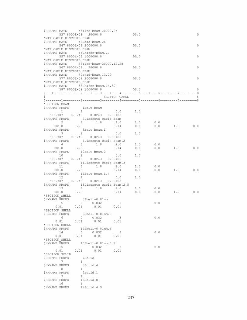
237

$HMNAME MATS 53Tire-beam-20000.25

537.8000E-09 20000.0 50.0 0

*MAT_CABLE_DISCRETE_BEAM

$HMNAME MATS 54Bead-beam.26

547.8000E-09 2000000.0 50.0 0

*MAT_CABLE_DISCRETE_BEAM

$HMNAME MATS 55Chafer-beam.27

557.8000E-09 1000000.0 50.0 0

*MAT_CABLE_DISCRETE_BEAM

$HMNAME MATS 56Tire-beam-20000.12.28

567.8000E-09 20000.0 50.0 0

*MAT_CABLE_DISCRETE_BEAM

$HMNAME MATS 57Bead-beam.13.29

577.8000E-09 2000000.0 50.0 0

*MAT_CABLE_DISCRETE_BEAM

$HMNAME MATS 58Chafer-beam.14.30

587.8000E-09 1000000.0 50.0 0

$---+----1----+----2----+----3----+----4----+----5----+----6----+----7----+----8

$ SECTION CARDS $

$---+----1----+----2----+----3----+----4----+----5----+----6----+----7----+----8

*SECTION_BEAM

$HMNAME PROPS 1Bolt beam

1 2 0.0 1.0

506.707 0.0243 0.0243 0.00405

$HMNAME PROPS 2Discrete cable Beam

2 6 1.0 2.0 1.0 0.0

100.0 7.8 3.14 0.0 0.0 1.0 0.0

$HMNAME PROPS 3Bolt beam.1

3 2 0.0 1.0

506.707 0.0243 0.0243 0.00405

$HMNAME PROPS 4Discrete cable Beam.2

4 6 1.0 2.0 1.0 0.0

100.0 7.8 3.14 0.0 0.0 1.0 0.0

$HMNAME PROPS 10Bolt beam.2

10 2 0.0 1.0

506.707 0.0243 0.0243 0.00405

$HMNAME PROPS 11Discrete cable Beam.3

11 6 1.0 2.0 1.0 0.0

100.0 7.8 3.14 0.0 0.0 1.0 0.0

$HMNAME PROPS 12Bolt beam.1.4

12 2 0.0 1.0

506.707 0.0243 0.0243 0.00405

$HMNAME PROPS 13Discrete cable Beam.2.5

13 6 1.0 2.0 1.0 0.0

100.0 7.8 3.14 0.0 0.0 1.0 0.0

*SECTION_SHELL

$HMNAME PROPS 5Shell-0.01mm

5 0 0.832 3 0.0

0.01 0.01 0.01 0.01

*SECTION_SHELL

$HMNAME PROPS 6Shell-0.01mm.3

6 0 0.832 3 0.0

0.01 0.01 0.01 0.01

*SECTION_SHELL

$HMNAME PROPS 14Shell-0.01mm.6

14 0 0.832 3 0.0

0.01 0.01 0.01 0.01

*SECTION_SHELL

$HMNAME PROPS 15Shell-0.01mm.3.7

15 0 0.832 3 0.0

0.01 0.01 0.01 0.01

*SECTION_SOLID

$HMNAME PROPS 7Solid

7 1

$HMNAME PROPS 8Solid.4

8 1

$HMNAME PROPS 9Solid.1

9 1

$HMNAME PROPS 16Solid.8

16 1

$HMNAME PROPS 17Solid.4.9

238

17 1

$HMNAME PROPS 18Solid.1.10

18 1

*HOURGLASS

$HMNAME PROPS 10Solid Hourglass control

10 4 0.1

$HMNAME PROPS 11Solid Hourglass control.5

11 4 0.1

$HMNAME PROPS 12Solid Hourglass control.11

12 4 0.1

$HMNAME PROPS 13Solid Hourglass control.5.12

13 4 0.1

$HMNAME PROPS 19Tire hourglass

19 5 1.0

$---+----1----+----2----+----3----+----4----+----5----+----6----+----7----+----8

$ CONTACT CARDS $

$---+----1----+----2----+----3----+----4----+----5----+----6----+----7----+----8

*CONTACT_SURFACE_TO_SURFACE_ID

$HMNAME GROUPS 1Rim1 End-Rim2 End

$HWCOLOR GROUPS 1 29

1Rim1 End-Rim2 End

2 1 0 0 1 1

0.35 0.25 1.0 300.0 200.0

1.0 1.0

0

1 1

*CONTACT_SURFACE_TO_SURFACE_ID

$HMNAME GROUPS 2Rim1-Rim2

$HWCOLOR GROUPS 2 29

2Rim1-Rim2

4 3 0 0 1 1

0.35 0.25 1.0 300.0 200.0

1.0 1.0

0

1 1

*CONTACT_SURFACE_TO_SURFACE_ID

$HMNAME GROUPS 3Front rim-Bead

$HWCOLOR GROUPS 3 29

3Front rim-Bead

5 9 0 0 1 1

0.95 0.9 1.0 5.0 20.0

1 1

*CONTACT_SURFACE_TO_SURFACE_ID

$HMNAME GROUPS 4Back rim - Rear Bead

$HWCOLOR GROUPS 4 29

4Back rim - Rear Bead

7 10 0 0 1 1

0.95 0.9 1.0 5.0 20.0

1 1

*CONTACT_SURFACE_TO_SURFACE_ID

$HMNAME GROUPS 5Front rim - Chafer

$HWCOLOR GROUPS 5 29

5Front Rim - Chafer

6 11 0 0 1 1

0.95 0.9 1.0 5.0 20.0

10.0 10.0

0

1 1

*CONTACT_SURFACE_TO_SURFACE_ID

$HMNAME GROUPS 6Back Rim - Chafer

$HWCOLOR GROUPS 6 29

6Back Rim - Chafer

239

8 12 0 0 1 1

0.95 0.9 1.0 5.0 20.0

10.0 10.0

0

1 1

*CONTACT_SURFACE_TO_SURFACE_ID

$HMNAME GROUPS 18Back Rim - Chafer.6

$HWCOLOR GROUPS 18 29

18Back Rim - Chafer

21 25 0 0 1 1

0.95 0.9 1.0 5.0 20.0

10.0 10.0

0

1 1

*CONTACT_SURFACE_TO_SURFACE_ID

$HMNAME GROUPS 17Front rim - Chafer.5

$HWCOLOR GROUPS 17 29

17Front Rim - Chafer

19 24 0 0 1 1

0.95 0.9 1.0 5.0 20.0

10.0 10.0

0

1 1

*CONTACT_SURFACE_TO_SURFACE_ID

$HMNAME GROUPS 16Back rim - Rear Bead.4

$HWCOLOR GROUPS 16 29

16Back rim - Rear Bead

20 23 0 0 1 1

0.95 0.9 1.0 5.0 20.0

1 1

*CONTACT_SURFACE_TO_SURFACE_ID

$HMNAME GROUPS 15Front rim-Bead.3

$HWCOLOR GROUPS 15 29

15Front rim-Bead

18 22 0 0 1 1

0.95 0.9 1.0 5.0 20.0

1 1

*CONTACT_SURFACE_TO_SURFACE_ID

$HMNAME GROUPS 14Rim1-Rim2.2

$HWCOLOR GROUPS 14 29

14Rim1-Rim2

17 16 0 0 1 1

0.35 0.25 1.0 300.0 200.0

1.0 1.0

0

1 1

*CONTACT_SURFACE_TO_SURFACE_ID

$HMNAME GROUPS 13Rim1 End-Rim2 End.1

$HWCOLOR GROUPS 13 29

13Rim1 End-Rim2 End

15 14 0 0 1 1

0.35 0.25 1.0 300.0 200.0

1.0 1.0

0

1 1

*CONTACT_AUTOMATIC_GENERAL_ID

$HMNAME GROUPS 19Beam contacts.7

$HWCOLOR GROUPS 19 29

19Beam contacts

89 2 1 1

240

0

1 1

*CONTACT_AUTOMATIC_GENERAL_ID

$HMNAME GROUPS 7Beam contacts

$HWCOLOR GROUPS 7 29

7Beam contacts

43 2 1 1

0

1 1

*CONSTRAINED_EXTRA_NODES_SET

$HMNAME GROUPS 22Back Joint

$HWCOLOR GROUPS 22 29

31 45

*SET_NODE_LIST

$HMSET

$HMNAME SETS 45Back joint

45 0.0 0.0 0.0 0.0

534877 534880

*CONSTRAINED_EXTRA_NODES_SET

$HMNAME GROUPS 21Front Joint

$HWCOLOR GROUPS 21 29

8 44

*SET_NODE_LIST

$HMSET

$HMNAME SETS 44Front joint

44 0.0 0.0 0.0 0.0

534876 534882

*CONSTRAINED_EXTRA_NODES_SET

$HMNAME GROUPS 23Axle

$HWCOLOR GROUPS 23 29

21 46

*SET_NODE_LIST

$HMSET

$HMNAME SETS 46Axle joint

46 0.0 0.0 0.0 0.0

534878 534879 534881 534883

*RIGIDWALL_PLANAR_ID

$HMNAME GROUPS 8Ground

$HWCOLOR GROUPS 8 3

8

41

81.994-4.243E-05-927.02024 81.994-4.243E-05-926.02024 0.65

*RIGIDWALL_PLANAR_ID

$HMNAME GROUPS 20Ground.9

$HWCOLOR GROUPS 20 3

20

87

81.994-4.243E-05-927.02024 81.994-4.243E-05-926.02024 0.65

*CONSTRAINED_NODAL_RIGID_BODY

$HMNAME COMPS 24Mounting disc-1.1

$HWCOLOR COMPS 24 54

47 0 0 0

*SET_NODE_LIST

$HMSET

$HMNAME SETS 47rigid719909nodeset.1

47 0.0 0.0 0.0 0.0

861810 612593 612594 612595 612596 612597 612598 612599

$---+----1----+----2----+----3----+----4----+----5----+----6----+----7----+----8

$ LOAD AND BOUNDARY CARDS $

$---+----1----+----2----+----3----+----4----+----5----+----6----+----7----+----8

*LOAD_BODY_Z

$HMNAME LOADCOLS 7LoadBody_7

$HWCOLOR LOADCOLS 7 3

2 9810.0

*BOUNDARY_PRESCRIBED_MOTION_RIGID_LOCAL

241

$HMNAME LOADCOLS 1Constrained x movement-local

$HWCOLOR LOADCOLS 1 20

21 1 2 15 0.0 0

*BOUNDARY_PRESCRIBED_MOTION_RIGID

$HMNAME LOADCOLS 2Moving 5mile/hour

$HWCOLOR LOADCOLS 2 3

21 2 0 15 2235.0 0 0.55

*BOUNDARY_PRESCRIBED_MOTION_RIGID

$HMNAME LOADCOLS 3Turn 90 degree/second

$HWCOLOR LOADCOLS 3 20

21 7 0 30 3.142 0 0.9

*LOAD_SEGMENT_SET

$HMNAME LOADCOLS 4Tire-pressure-145PSI-10Bar-1.0MPa

$HWCOLOR LOADCOLS 4 5

13 1 1.0

$HMNAME LOADCOLS 5Tire-pressure-145PSI-10Bar-1.0MPa.1

$HWCOLOR LOADCOLS 5 5

26 16 1.0

*SET_SEGMENT

$HMNAME CSURFS 1Rim-1-end

$HWCOLOR CSURFS 1 6

1

2179 1754 180632 180632

*LOAD_NODE_POINT

$HMNAME LOADCOLS 6Force 527778N

$HWCOLOR LOADCOLS 6 8

532871 3 14 -527778.0 0

$---+----1----+----2----+----3----+----4----+----5----+----6----+----7----+----8

$ DEFINE CURVE CARDS $

$---+----1----+----2----+----3----+----4----+----5----+----6----+----7----+----8

*DEFINE_CURVE

$HMNAME CURVES 1Pressure load

$HWCOLOR CURVES 1 3

$HMCURVE 1 2 curve1

1 0 1.0 1.0

0.0 0.0

0.1 1.0

3.0 1.0

*DEFINE_CURVE

$HMNAME CURVES 2Gravity

$HWCOLOR CURVES 2 4

$HMCURVE 1 3 curve1

2 0 1.0 1.0

0.0 0.0

0.05 1.0

3.0 1.0

*DEFINE_CURVE

$HMNAME CURVES 3Global damping-39-71

$HWCOLOR CURVES 3 5

$HMCURVE 1 1 curve1

3 0 1.0 1.0

0.0 39.0

0.2 39.0

0.201 71.0

3.0 71.0

*DEFINE_CURVE

$HMNAME CURVES 4Force curve

$HWCOLOR CURVES 4 6

$HMCURVE 1 2 curve1

4 0 1.0 1.0

0.0 0.0

0.2 0.0

0.3 1.0

3.0 1.0

*DEFINE_CURVE

$HMNAME CURVES 5Rotation + Turn

$HWCOLOR CURVES 5 7

$HMCURVE 1 3 curve1

5 0 1.0 1.0

0.0 0.0

0.2 1.0

242

3.0 1.0

*DEFINE_CURVE

$HMNAME CURVES 6Pressure load.1

$HWCOLOR CURVES 6 3

$HMCURVE 1 2 curve1

6 0 1.0 1.0

0.0 0.0

0.1 1.0

3.0 1.0

*DEFINE_CURVE

$HMNAME CURVES 7Gravity.2

$HWCOLOR CURVES 7 4

$HMCURVE 1 3 curve1

7 0 1.0 1.0

0.0 0.0

0.05 1.0

3.0 1.0

*DEFINE_CURVE

$HMNAME CURVES 8Global damping-39-71.3

$HWCOLOR CURVES 8 5

$HMCURVE 1 1 curve1

8 0 1.0 1.0

0.0 39.0

0.2 39.0

0.201 71.0

3.0 71.0

*DEFINE_CURVE

$HMNAME CURVES 9Force curve.4

$HWCOLOR CURVES 9 6

$HMCURVE 1 2 curve1

9 0 1.0 1.0

0.0 0.0

0.2 0.0

0.3 1.0

3.0 1.0

*DEFINE_CURVE

$HMNAME CURVES 10Rotation + Turn.5

$HWCOLOR CURVES 10 7

$HMCURVE 1 3 curve1

10 0 1.0 1.0

0.0 0.0

0.2 1.0

3.0 1.0

*DEFINE_CURVE

$HMNAME CURVES 11Pressure load.2

$HWCOLOR CURVES 11 3

$HMCURVE 1 2 curve1

11 0 1.0 1.0

0.0 0.0

0.1 1.0

3.0 1.0

*DEFINE_CURVE

$HMNAME CURVES 12Gravity.3

$HWCOLOR CURVES 12 4

$HMCURVE 1 3 curve1

12 0 1.0 1.0

0.0 0.0

0.05 1.0

3.0 1.0

*DEFINE_CURVE

$HMNAME CURVES 13Global damping-39-71.4

$HWCOLOR CURVES 13 5

$HMCURVE 1 1 curve1

13 0 1.0 1.0

0.0 39.0

0.2 39.0

0.201 71.0

3.0 71.0

*DEFINE_CURVE

$HMNAME CURVES 14Force curve.5

$HWCOLOR CURVES 14 6

243

$HMCURVE 1 2 curve1

14 0 1.0 1.0

0.0 0.0

0.25 0.0

0.35 1.0

3.0 1.0

*DEFINE_CURVE

$HMNAME CURVES 15Rotation + Turn.6

$HWCOLOR CURVES 15 7

$HMCURVE 1 3 curve1

15 0 1.0 1.0

0.0 0.0

0.2 1.0

3.0 1.0

*DEFINE_CURVE

$HMNAME CURVES 16Pressure load.3

$HWCOLOR CURVES 16 3

$HMCURVE 1 2 curve1

16 0 1.0 1.0

0.0 0.0

0.1 1.0

3.0 1.0

*DEFINE_CURVE

$HMNAME CURVES 17Gravity.4

$HWCOLOR CURVES 17 4

$HMCURVE 1 3 curve1

17 0 1.0 1.0

0.0 0.0

0.05 1.0

3.0 1.0

*DEFINE_CURVE

$HMNAME CURVES 18Global damping-39-71.5

$HWCOLOR CURVES 18 5

$HMCURVE 1 1 curve1

18 0 1.0 1.0

0.0 39.0

0.2 39.0

0.201 71.0

3.0 71.0

*DEFINE_CURVE

$HMNAME CURVES 19Force curve.6

$HWCOLOR CURVES 19 6

$HMCURVE 1 2 curve1

19 0 1.0 1.0

0.0 0.0

0.2 0.0

0.3 1.0

3.0 1.0

*DEFINE_CURVE

$HMNAME CURVES 20Rotation + Turn.7

$HWCOLOR CURVES 20 7

$HMCURVE 1 3 curve1

20 0 1.0 1.0

0.0 0.0

0.2 1.0

3.0 1.0

*DEFINE_CURVE

$HMNAME CURVES 21Pressure load.1.8

$HWCOLOR CURVES 21 3

$HMCURVE 1 2 curve1

21 0 1.0 1.0

0.0 0.0

0.1 1.0

3.0 1.0

*DEFINE_CURVE

$HMNAME CURVES 22Gravity.2.9

$HWCOLOR CURVES 22 4

$HMCURVE 1 3 curve1

22 0 1.0 1.0

0.0 0.0

0.05 1.0

244

3.0 1.0

*DEFINE_CURVE

$HMNAME CURVES 23Global damping-39-71.3.10

$HWCOLOR CURVES 23 5

$HMCURVE 1 1 curve1

23 0 1.0 1.0

0.0 39.0

0.2 39.0

0.201 71.0

3.0 71.0

*DEFINE_CURVE

$HMNAME CURVES 24Force curve.4.11

$HWCOLOR CURVES 24 6

$HMCURVE 1 2 curve1

24 0 1.0 1.0

0.0 0.0

0.2 0.0

0.3 1.0

3.0 1.0

*DEFINE_CURVE

$HMNAME CURVES 25Rotation + Turn.5.12

$HWCOLOR CURVES 25 7

$HMCURVE 1 3 curve1

25 0 1.0 1.0

0.0 0.0

0.2 1.0

3.0 1.0

*DEFINE_CURVE

$HMNAME CURVES 26Pressure load.2.13

$HWCOLOR CURVES 26 3

$HMCURVE 1 2 curve1

26 0 1.0 1.0

0.0 0.0

0.1 1.0

3.0 1.0

*DEFINE_CURVE

$HMNAME CURVES 27Gravity.3.14

$HWCOLOR CURVES 27 4

$HMCURVE 1 3 curve1

27 0 1.0 1.0

0.0 0.0

0.05 1.0

3.0 1.0

*DEFINE_CURVE

$HMNAME CURVES 28Global damping-39-71.4.15

$HWCOLOR CURVES 28 5

$HMCURVE 1 1 curve1

28 0 1.0 1.0

0.0 39.0

0.2 39.0

0.201 71.0

3.0 71.0

*DEFINE_CURVE

$HMNAME CURVES 29Force curve.5.16

$HWCOLOR CURVES 29 6

$HMCURVE 1 2 curve1

29 0 1.0 1.0

0.0 0.0

0.25 0.0

0.35 1.0

3.0 1.0

*DEFINE_CURVE

$HMNAME CURVES 30Rotation + Turn.6.17

$HWCOLOR CURVES 30 7

$HMCURVE 1 3 curve1

30 0 1.0 1.0

0.0 0.0

0.2 1.0

0.5 1.0

0.6 0.0

3.0 0.0

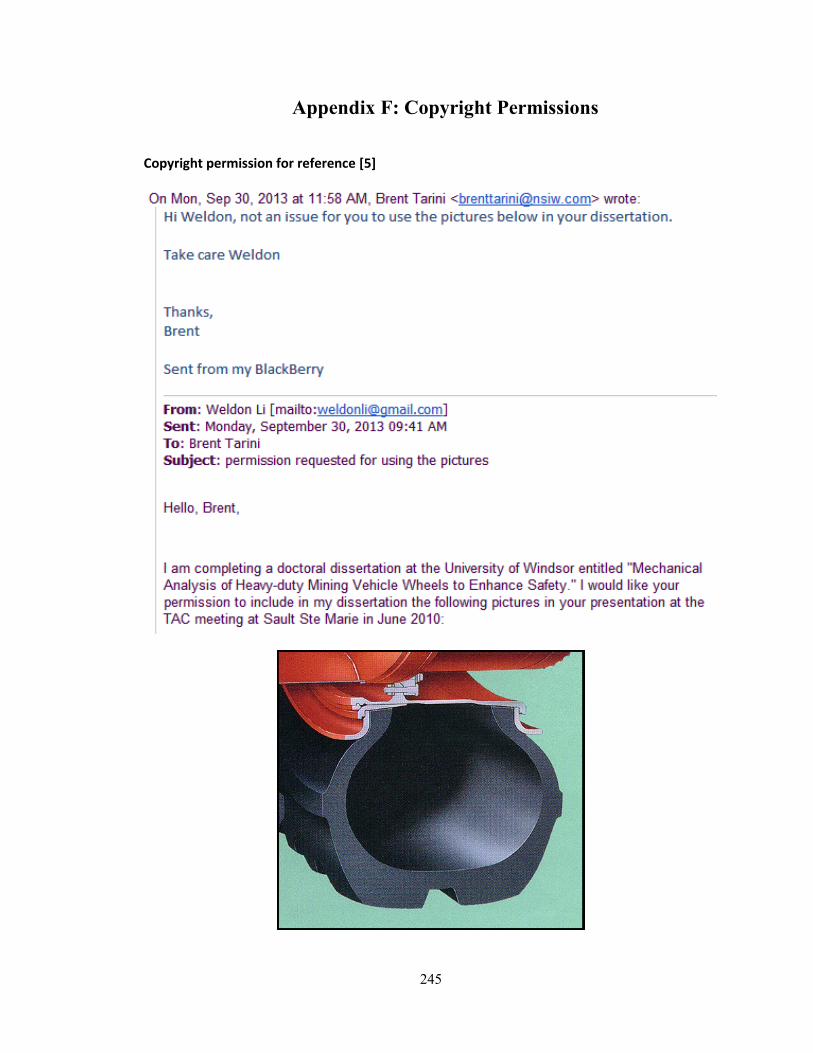
245

Appendix F: Copyright Permissions

Copyright permission for reference [5]

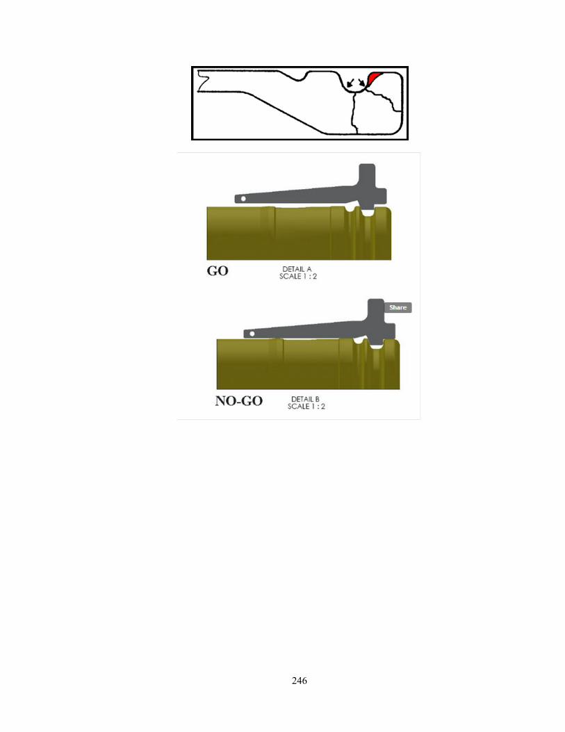
246

247

248

Copyright permission for reference [7]

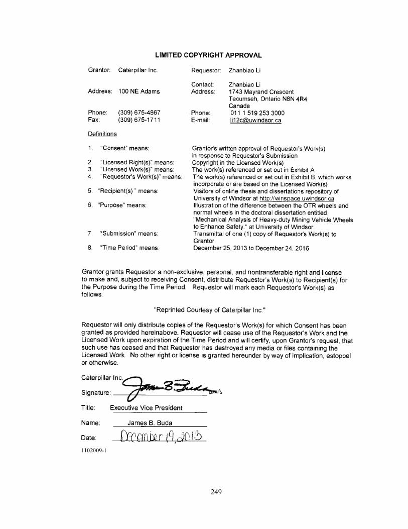
249

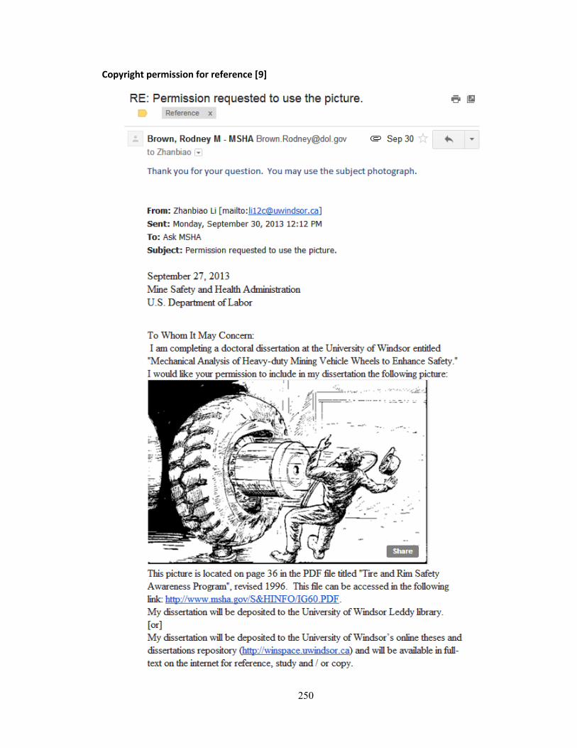
250

Copyright permission for reference [9]

251

252

Copyright permission for reference [10]

253

254

255

256

Copyright permission for reference [11]

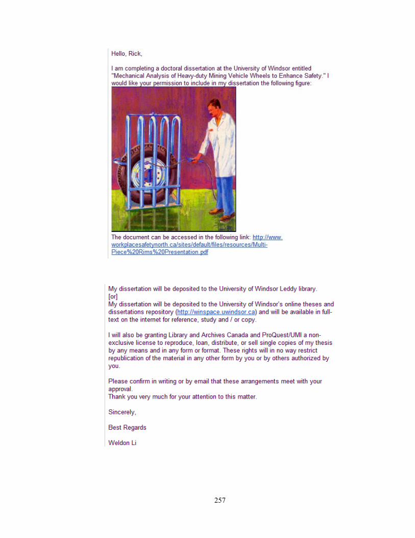
257

258

Copyright permission for reference [16]

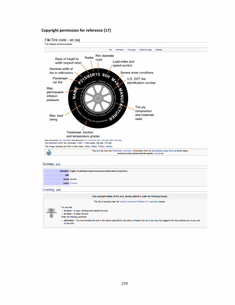
259

Copyright permission for reference [17]

260

Copyright permission for reference [18]

261

262

263

Copyright permission for reference [19]

264

265

Copyright permission for reference [20] [30]

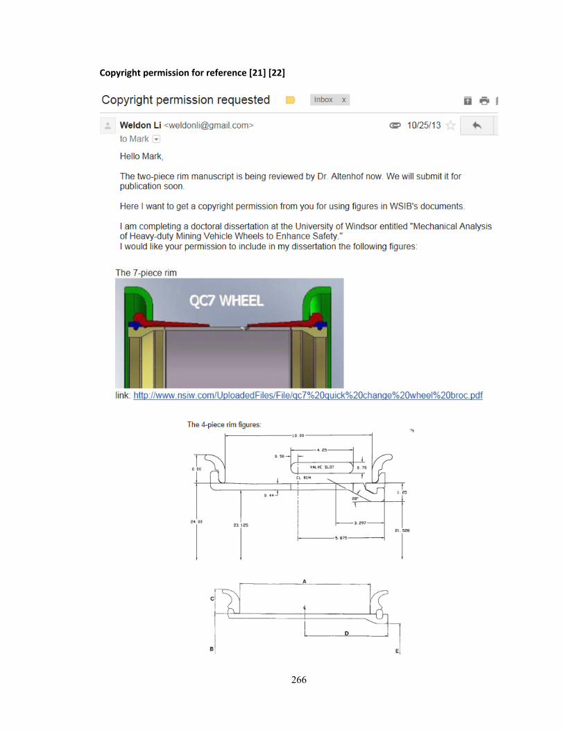
266

Copyright permission for reference [21] [22]

267

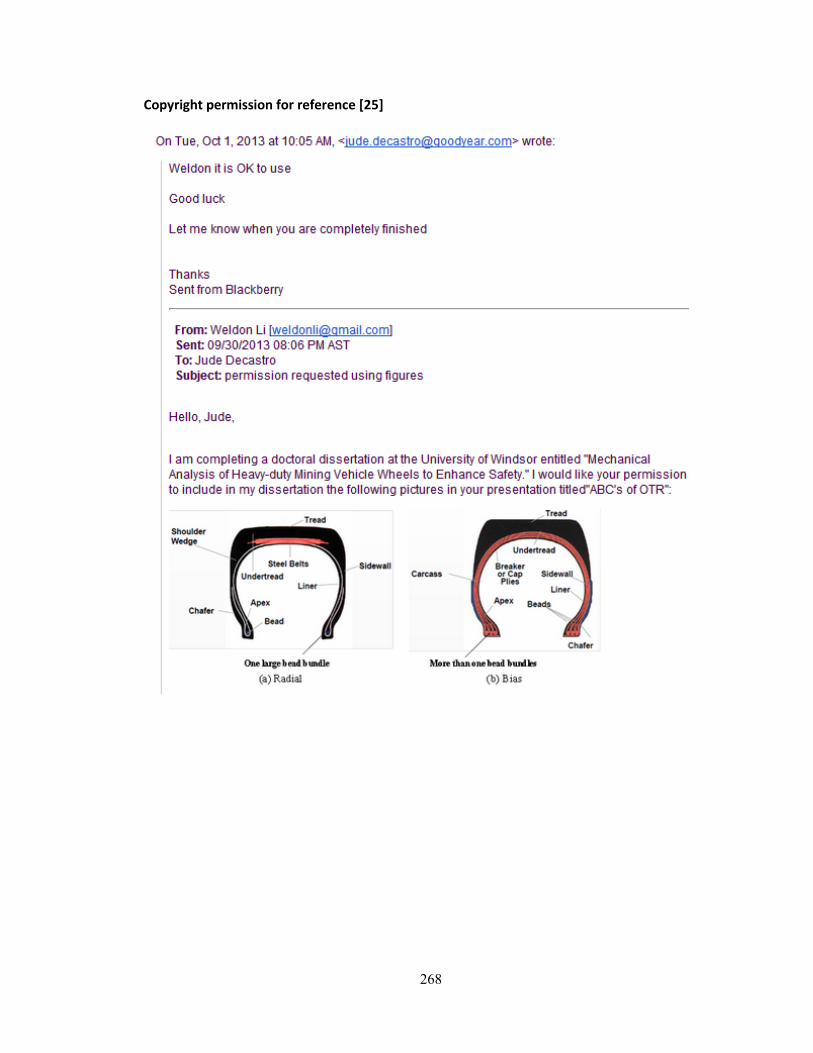
268

Copyright permission for reference [25]

269

270

Copyright permission for reference [26] [28]

271

272

Copyright permission for reference [32]

273

274

275

276

Copyright permission for reference [33]

277

Copyright permission for reference [81]

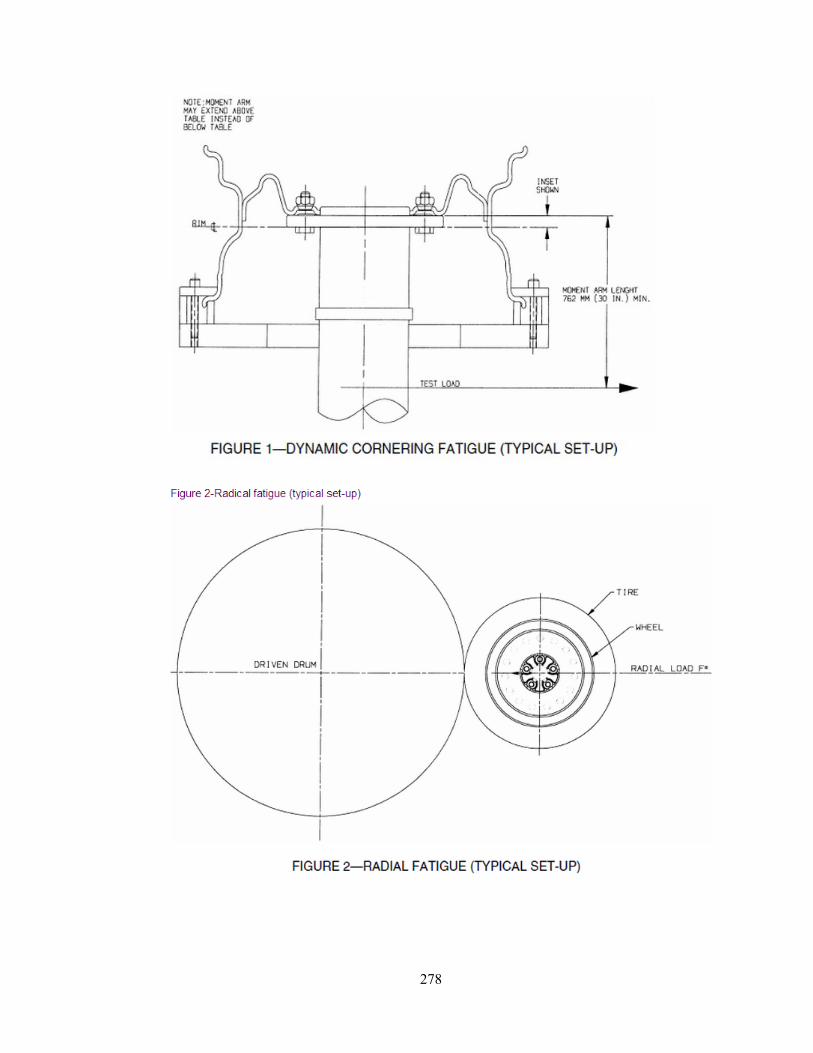
278

279

280

Copyright permission for reference [105]

281

282

Copyright permission for reference [128]

283

284

285

286

287

VITA AUCTORIS

NAME: Zhanbiao Li

PLACE OF BIRTH:

Honghu, China

YEAR OF BIRTH:

1966

EDUCATION:

University of Windsor, Ph. D. in mechanical

engineering, Windsor, ON, 2014

University of Windsor, M. A. Sc. in mechanical

engineering, Windsor, ON, 2003

Huazhong University of Science & Technology,

B. Sc. in mechanical engineering, Wuhan, China,

1987