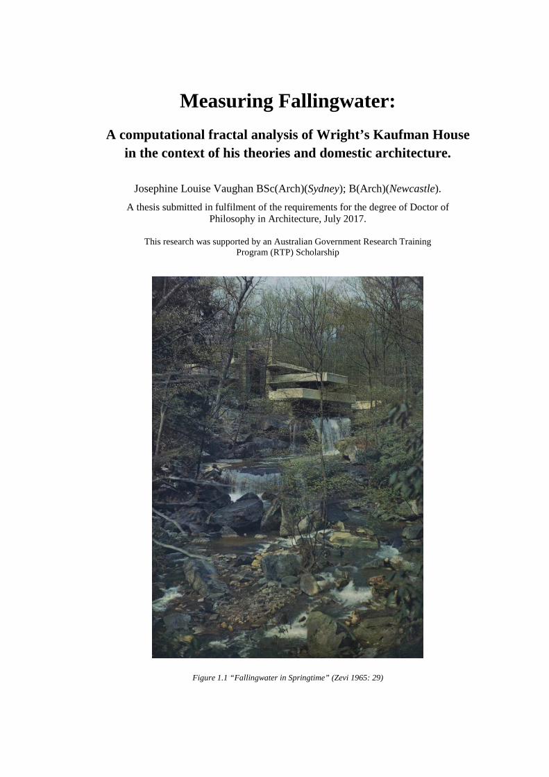
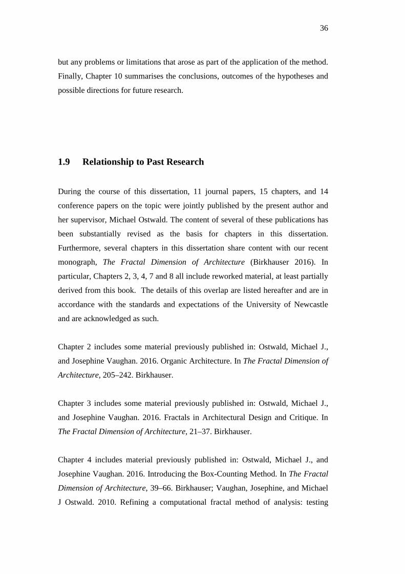
Measuring Fallingwater: A computational fractal analysis of Wright’s Kaufman House

in the context of his theories and domestic architecture.

Josephine Louise Vaughan BSc(Arch)(Sydney); B(Arch)(Newcastle).

A thesis submitted in fulfilment of the requirements for the degree of Doctor of Philosophy in Architecture, July 2017.

This research was supported by an Australian Government Research Training

Program (RTP) Scholarship

Figure 1.1 “Fallingwater in Springtime” (Zevi 1965: 29)

2

Statement of Originality I hereby certify that the work embodied in the thesis is my own work, conducted under normal supervision.

The thesis contains no material which has been accepted for the award of any other degree or diploma in any university or other tertiary institution and, to the best of my knowledge and belief, contains no material previously published or written by another person, except where due reference has been made in the text. I give consent to the final version of my thesis being made available worldwide when deposited in the University’s Digital Repository, subject to the provisions of the Copyright Act 1968.

Josephine Vaughan Statement of Collaboration I hereby certify that the work embodied in this thesis has been done in collaboration with other researchers. I have included below, as part of the thesis, a statement clearly outlining the extent of collaboration, with whom and under what auspices.

Statement of Authorship I hereby certify that the work embodied in this thesis contains published papers/scholarly work of which I am a joint author. I have included below, as part of the thesis a written statement, endorsed by my supervisor, attesting to my contribution to the joint publications/scholarly work.

Between 2009 and 2016, Josephine Vaughan (the candidate) and Professor Michael J. Ostwald (primary supervisor), jointly published 25 papers and a co-authored monograph, developing the basic analytical method and some of the arguments used in this dissertation. Sections of these jointly authored publications form the basis for several chapters in this dissertation, although all have been modified and revised for this purpose.

In accordance with the University of Newcastle policy, this statement is to confirm that the sections of these past publications which are used in this dissertation are those for which the candidate led the primary authoring and/or intellectual development. Notwithstanding this general statement, Chapter 1 provides a complete list of the sources for any sections or ideas, fully referenced to the original authorship and place of publication. Furthermore, for Hypothesis 1, the method was jointly developed, and the results were solely produced and analyzed by the candidate. For Hypothesis 2, the candidate solely developed the method, the results and completed the subsequent analysis.

Josephine Vaughan (candidate) Professor Michael J. Ostwald (supervisor)

3

Table of Contents

Front matter Statements of Originality, Collaboration and Authorship 2

Abstract 6

Prelude 8

PART I: Frank Lloyd Wright and Fallingwater

1 Introduction 10

1.1 History and Setting of Fallingwater 12

1.2 A Unique House in Wright’s Oeuvre? 16

1.3 A House Which Reflects its Natural Setting? 18

1.4 Hypotheses 20

1.5 Significance and Rationale 23

1.6 Approach and Method 26

1.7 Limitations 28

1.8 Dissertation Summary 31

1.9 Relationship to Past Research 36

2 Frank Lloyd Wright and Fallingwater 40

2.1 A Background to Frank Lloyd Wright 42

2.2 Style and Philosophy of the Era: Organic Modernity 52

2.3 Identifying Separate Definitions of Landscape and Nature 54

2.4 Scholarly Interpretation of Fallingwater 67

2.5 Strategies at Fallingwater 92

Conclusion 95

PART II: Methodological Considerations 96

3 Fractals and Architecture 97

3.1 Defining a Fractal 98

3.2 Fractals in Architectural Design and Critique 104

3.3 Frank Lloyd Wright and Fractal Geometry 109

Conclusion 113

4

4 Measuring Buildings and the Box-counting Method 115

4.1 Measuring Wright 115

4.2 Fractal Dimensions 119

4.3 Measuring Fractal Dimensions 120

4.4 The Box-counting Method 121

4.5 Fractal Analysis and the Built Environment 129

4.6 Box-counting Analysis of Wright’s Architecture 140

Conclusion 142

5 Variables in the Box-counting Method 143

5.1 Representation Challenges: Measuring 144

5.2 Methodological Variables 154

5.3 Image Challenges: Pre-processing Settings 156

5.4 Methodological Challenges: Processing Settings 161

5.5 Revisiting the Robie House 167

Conclusion 168

6 Comparing Architecture and Nature 170

6.1 Relationships Between Nature and Architecture 171

6.2 Finding the Similarities Between Nature and Architecture 173

6.3 Fractal Analysis of Nature 175

6.4 Comparing Natural and Built Forms 176

6.5 Testing Comparisons Between Architecture and Ecology 178

6.6 Image Requirements for Comparing Fractal Dimensions 186

6.7 A Data Selection Methodology 190

6.8 Selecting Data for Fallingwater and its Natural Setting 200

Conclusion 206

7 Methodology 207

7.1 Research Description 208

7.2 Data Selection and Scope 210

7.3 Data Source, Data Settings and Image Texture 213

7.4 Dissertation Research Method 220

7.5 Definitions and Coding Method 220

7.6 Comparative Analysis 226

7.7 Interpretation of Results 228

Conclusion 229

5

PART III: Results 230 8 Comparing Fallingwater with Wright’s Architecture 231

8.1 Interpreting the Data 232

8.2 Analysis of Fallingwater 234

8.3 House Sets for Comparison with Fallingwater 239

8.4 The Visual Complexity of Fallingwater Compared 261

8.5 The Similarity of Fallingwater to Wright’s Other Houses 265

Conclusion 269

9 Comparing Fallingwater with its Natural Setting 272

9.1 Scholarly Approaches to Fallingwater and 273 its Natural Setting 9.2 Analysis of the Fallingwater House 275

9.3 Analysis of the Fallingwater Site 282

9.4 The Visual Complexity of Fallingwater House and 289 Site Compared Conclusion 293

10 Conclusion 296

10.1 Results for Hypothesis 1 298

10.2 Results for Hypothesis 2 300

10.3 Other Observations Arising from the Research 302

10.4 Future Research 304

Conclusion 305

End Matter 307 Bibliography 308

List of Figures 338

Acknowledgements 341

6

Abstract

Sited above a waterfall on Bear Run stream, in a wooded gulley in Mill Run,

Pennsylvania, the Kaufman house, or Fallingwater as it is commonly known, is

one of the most famous buildings in the world. This house, which Frank Lloyd

Wright commenced designing in 1934, has been the subject of enduring scholarly

analysis and speculation for many reasons, two of which are the subject of this

dissertation. The first is associated with the positioning of the design in Wright’s

larger body of work. Across 70 years of his architectural practice, most of

Wright’s domestic work can be categorised into three distinct stylistic periods—

the Prairie, Textile-block and Usonian. Compared to the houses that belong to

those three periods, Fallingwater appears to defy such a simple classification and

is typically regarded as representing a break from Wright’s usual approach to

creating domestic architecture. A second, and more famous argument about

Fallingwater, is that it is the finest example of one of Wright’s key design

propositions, Organic architecture. In particular, Wright’s Fallingwater allegedly

exhibits clear parallels between its form and that of the surrounding natural

landscape. Both theories about Fallingwater—that it is different from his other

designs and that it is visually similar to its setting—seem to be widely accepted by

scholars, although there is relatively little quantitative evidence in support of

either argument. These theories are reframed in the present dissertation as two

hypotheses.

Using fractal dimension analysis, a computational method that mathematically

measures the characteristic visual complexity of an object, this dissertation tests

two hypotheses about the visual properties of Frank Lloyd Wright's Fallingwater.

These hypotheses are only used to define the testable goals of the dissertation, as

due to the many variables in the way architectural historians and theorists develop

arguments, the hypotheses cannot be framed in a pure scientific sense.

7

To test Hypothesis 1, the computational method is applied to fifteen houses from

three of Wright’s well-documented domestic design periods, and the results are

compared with measures that are derived from Fallingwater. Through this process

a mathematical determination can be made about the relationship between the

formal expressions of Fallingwater and that of Wright’s other domestic

architecture. To test Hypothesis 2, twenty analogues of the natural landscape

surrounding Fallingwater are measured using the same computational method,

and the results compared to the broader formal properties of the house. Such a

computational and mathematical analysis has never before been undertaken of

Fallingwater or its surrounding landscape.

The dissertation concludes by providing an assessment of the two hypotheses, and

through this process demonstrates the usefulness of fractal analysis in the

interpretation of architecture, and the natural environment. The numerical results

for Hypothesis 1 do not have a high enough percentage difference to suggest that

Fallingwater is atypical of his houses, confirming that Hypothesis 1 is false. Thus

the outcome does not support the general scholarly consensus that Fallingwater is

different to Wright’s other domestic works. The results for Hypothesis 2 found a

mixed level of similarity in characteristic complexity between Fallingwater and

its natural setting. However, the background to this hypothesis suggests that the

results should be convincingly positive and while some of the results are

supportive, this was not the dominant outcome and thus Hypothesis 2 could

potentially be considered disproved. This second outcome does not confirm the

general view that Fallingwater is visually similar to its surrounding landscape.

8

Prelude

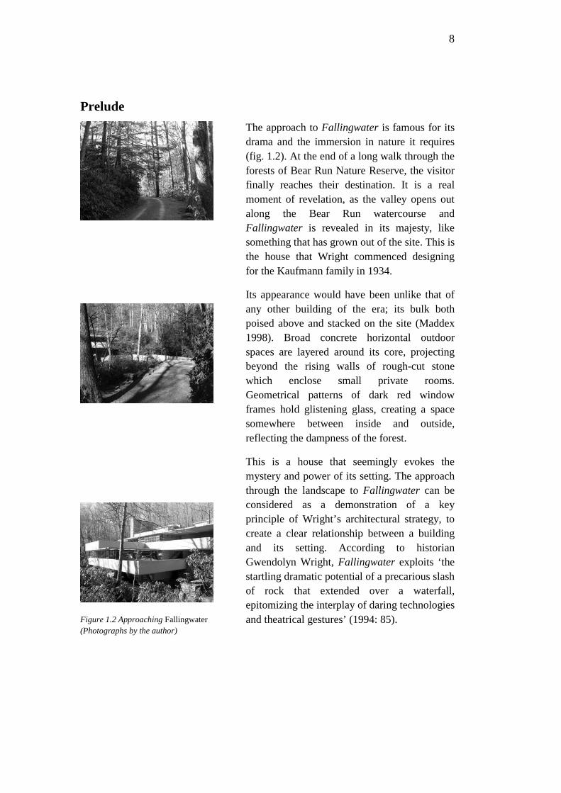
The approach to Fallingwater is famous for its drama and the immersion in nature it requires (fig. 1.2). At the end of a long walk through the forests of Bear Run Nature Reserve, the visitor finally reaches their destination. It is a real moment of revelation, as the valley opens out along the Bear Run watercourse and Fallingwater is revealed in its majesty, like something that has grown out of the site. This is the house that Wright commenced designing for the Kaufmann family in 1934.

Its appearance would have been unlike that of any other building of the era; its bulk both poised above and stacked on the site (Maddex 1998). Broad concrete horizontal outdoor spaces are layered around its core, projecting beyond the rising walls of rough-cut stone which enclose small private rooms. Geometrical patterns of dark red window frames hold glistening glass, creating a space somewhere between inside and outside, reflecting the dampness of the forest.

This is a house that seemingly evokes the mystery and power of its setting. The approach through the landscape to Fallingwater can be considered as a demonstration of a key principle of Wright’s architectural strategy, to create a clear relationship between a building and its setting. According to historian Gwendolyn Wright, Fallingwater exploits ‘the startling dramatic potential of a precarious slash of rock that extended over a waterfall, epitomizing the interplay of daring technologies and theatrical gestures’ (1994: 85).

Figure 1.2 Approaching Fallingwater (Photographs by the author)

9

Part I: Frank Lloyd Wright and Fallingwater

10

Chapter 1

Introduction

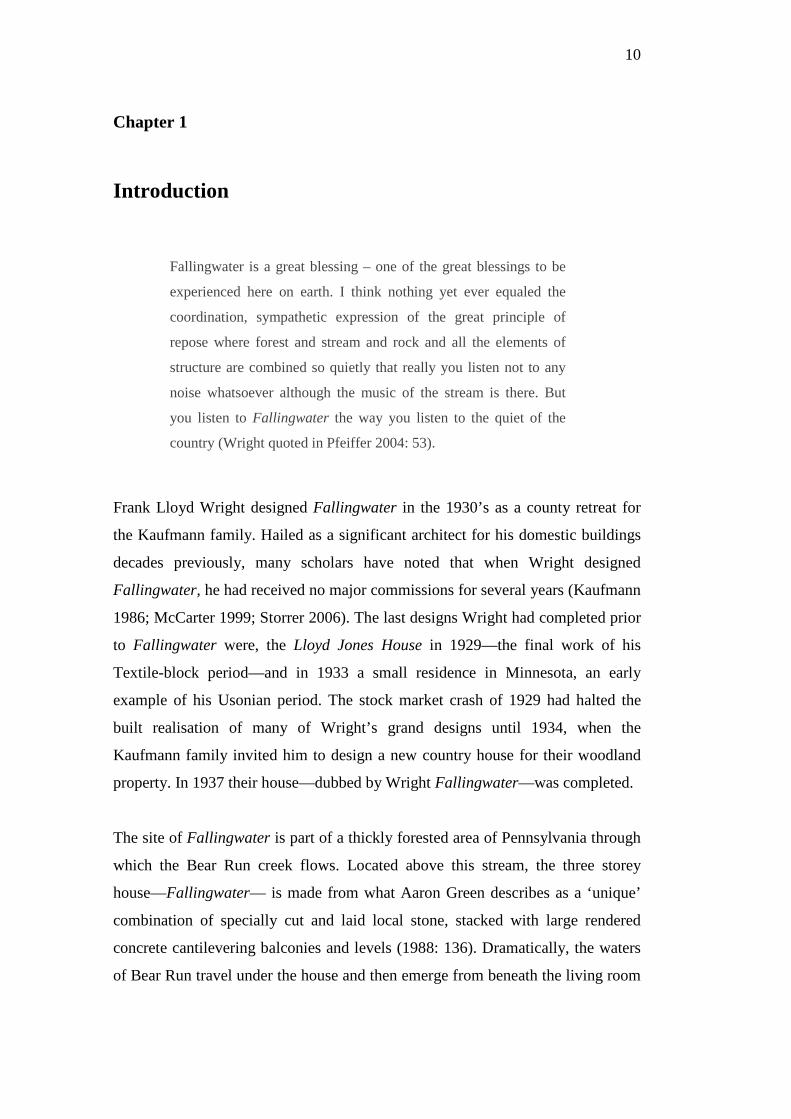
Fallingwater is a great blessing – one of the great blessings to be

experienced here on earth. I think nothing yet ever equaled the

coordination, sympathetic expression of the great principle of

repose where forest and stream and rock and all the elements of

structure are combined so quietly that really you listen not to any

noise whatsoever although the music of the stream is there. But

you listen to Fallingwater the way you listen to the quiet of the

country (Wright quoted in Pfeiffer 2004: 53).

Frank Lloyd Wright designed Fallingwater in the 1930’s as a county retreat for

the Kaufmann family. Hailed as a significant architect for his domestic buildings

decades previously, many scholars have noted that when Wright designed

Fallingwater, he had received no major commissions for several years (Kaufmann

1986; McCarter 1999; Storrer 2006). The last designs Wright had completed prior

to Fallingwater were, the Lloyd Jones House in 1929—the final work of his

Textile-block period—and in 1933 a small residence in Minnesota, an early

example of his Usonian period. The stock market crash of 1929 had halted the

built realisation of many of Wright’s grand designs until 1934, when the

Kaufmann family invited him to design a new country house for their woodland

property. In 1937 their house—dubbed by Wright Fallingwater—was completed.

The site of Fallingwater is part of a thickly forested area of Pennsylvania through

which the Bear Run creek flows. Located above this stream, the three storey

house—Fallingwater— is made from what Aaron Green describes as a ‘unique’

combination of specially cut and laid local stone, stacked with large rendered

concrete cantilevering balconies and levels (1988: 136). Dramatically, the waters

of Bear Run travel under the house and then emerge from beneath the living room

11

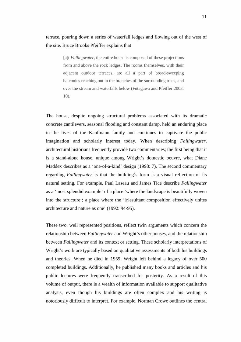
terrace, pouring down a series of waterfall ledges and flowing out of the west of

the site. Bruce Brooks Pfeiffer explains that

[a]t Fallingwater, the entire house is composed of these projections

from and above the rock ledges. The rooms themselves, with their

adjacent outdoor terraces, are all a part of broad-sweeping

balconies reaching out to the branches of the surrounding trees, and

over the stream and waterfalls below (Futagawa and Pfeiffer 2003:

10).

The house, despite ongoing structural problems associated with its dramatic

concrete cantilevers, seasonal flooding and constant damp, held an enduring place

in the lives of the Kaufmann family and continues to captivate the public

imagination and scholarly interest today. When describing Fallingwater,

architectural historians frequently provide two commentaries; the first being that it

is a stand-alone house, unique among Wright’s domestic oeuvre, what Diane

Maddex describes as a ‘one-of-a-kind’ design (1998: 7). The second commentary

regarding Fallingwater is that the building’s form is a visual reflection of its

natural setting. For example, Paul Laseau and James Tice describe Fallingwater

as a ‘most splendid example’ of a place ‘where the landscape is beautifully woven

into the structure’; a place where the ‘[r]esultant composition effectively unites

architecture and nature as one’ (1992: 94-95).

These two, well represented positions, reflect twin arguments which concern the

relationship between Fallingwater and Wright’s other houses, and the relationship

between Fallingwater and its context or setting. These scholarly interpretations of

Wright’s work are typically based on qualitative assessments of both his buildings

and theories. When he died in 1959, Wright left behind a legacy of over 500

completed buildings. Additionally, he published many books and articles and his

public lectures were frequently transcribed for posterity. As a result of this

volume of output, there is a wealth of information available to support qualitative

analysis, even though his buildings are often complex and his writing is

notoriously difficult to interpret. For example, Norman Crowe outlines the central

12

problem of studying Wright’s work, as that his ‘architecture is clouded by details

of his life, his clients, the times in which he worked, his own misleading rhetoric,

and by an elaborate taxonomy of his stylistic inventions and their subsequent

influences on later architects and architecture’ (Crowe 1992: vii).

The following section introduces Fallingwater and its background, before these

two scholarly arguments about Fallingwater are examined in more detail. While

the mathematical and computational analysis used in the present dissertation are

based on quantitative data, the broad range of qualitative information and

interpretation of Wright’s work serves as a guide for this research, providing a

basis from which to draw the framework of the methodology.

1.1 History and Setting of Fallingwater

In the aftermath of the great depression, Wright maintained an income by setting

up the ‘Taliesin Fellowship’ in 1932, where fee-paying students worked alongside

Wright in his architectural practice, absorbing his architecture, philosophy and

lifestyle. One member of this ‘fellowship’ was Edgar Kaufmann Junior, who

joined the group in early 1934. Not particularly interested in becoming an

architect, Edgar Junior—like his parents Liliane and Edgar Kaufmann—had an

interest in contemporary art, architecture, design and philosophy, and he joined

the fellowship to round out his education. Edgar Junior, full of enthusiasm for

Wright’s architecture, introduced his own family to the philosophy and

architecture of Frank Lloyd Wright. The Kaufmanns shared many similar

philosophical views with Wright, including the enjoyment of spending time in

nature (Cleary 1999). To this end the Kaufmanns would regularly visit their own

holiday cabin in the woods, near a locality called Mill Run, about 100km

southwest of their home in Pittsburgh, Pennsylvania. In the early 1930s the

Kaufmanns began thinking of building a more refined holiday home, and with

Edgar Junior’s encouragement, they invited Wright to inspect the site, which he

did in December 1934.

13

It is cold in Mill Run in December, the average temperature at that time of year in

the 1930s was a high of 3ºC and a low of around -7 ºC. The tall trees, mostly

deciduous, lose their leaves in December, and the Great Laurel Rhododendrons

are some of the few plants in the understory to hold their greenery in the winter

months. At that time of year snow can blanket the area and the creek can freeze

over. The effect of winter is that the landscape is less clothed in greenery, and the

shape of the land can be seen more easily than in the deeply forested valley in

spring. Edgar Kaufmann Junior recalls the day Wright came to their site when the

‘mountains put on their best repertoire to him—sun, rain and hail alternated; the

masses of native rhododendrons were in bloom’ (1983: 69), and he remembers

how the weather that day ‘accentuated the rugged terrain’ (1986: 36).

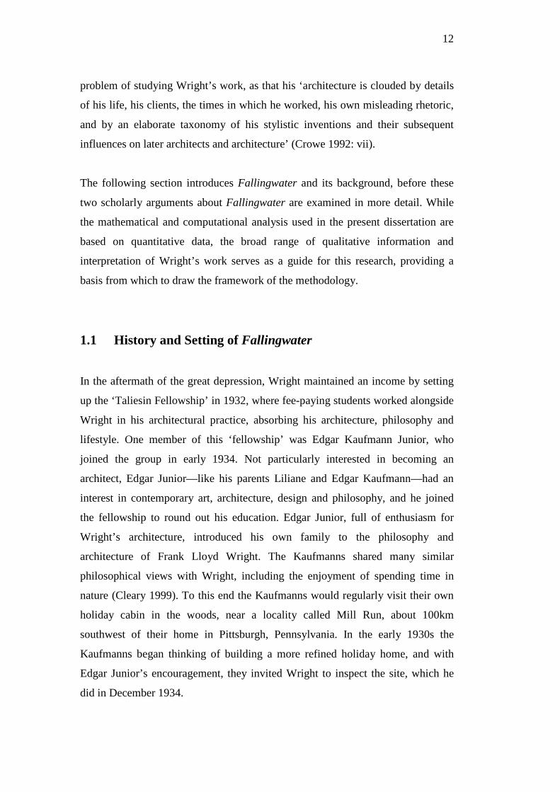
Figure 1.3 Bear Run stream in its forested setting (Photograph by the author)

14

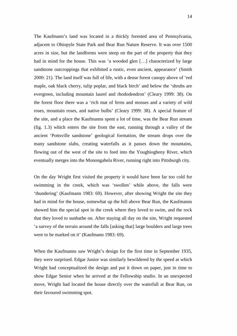
The Kaufmann’s land was located in a thickly forested area of Pennsylvania,

adjacent to Ohiopyle State Park and Bear Run Nature Reserve. It was over 1500

acres in size, but the landforms were steep on the part of the property that they

had in mind for the house. This was ‘a wooded glen […] characterized by large

sandstone outcroppings that exhibited a rustic, even ancient, appearance’ (Smith

2000: 21). The land itself was full of life, with a dense forest canopy above of ‘red

maple, oak black cherry, tulip poplar, and black birch’ and below the ‘shrubs are

evergreen, including mountain laurel and rhododendron’ (Cleary 1999: 38). On

the forest floor there was a ‘rich mat of ferns and mosses and a variety of wild

roses, mountain roses, and native bulbs’ (Cleary 1999: 38). A special feature of

the site, and a place the Kaufmanns spent a lot of time, was the Bear Run stream

(fig. 1.3) which enters the site from the east, running through a valley of the

ancient ‘Pottsville sandstone’ geological formation, the stream drops over the

many sandstone slabs, creating waterfalls as it passes down the mountains,

flowing out of the west of the site to feed into the Youghiogheny River, which

eventually merges into the Monongahela River, running right into Pittsburgh city.

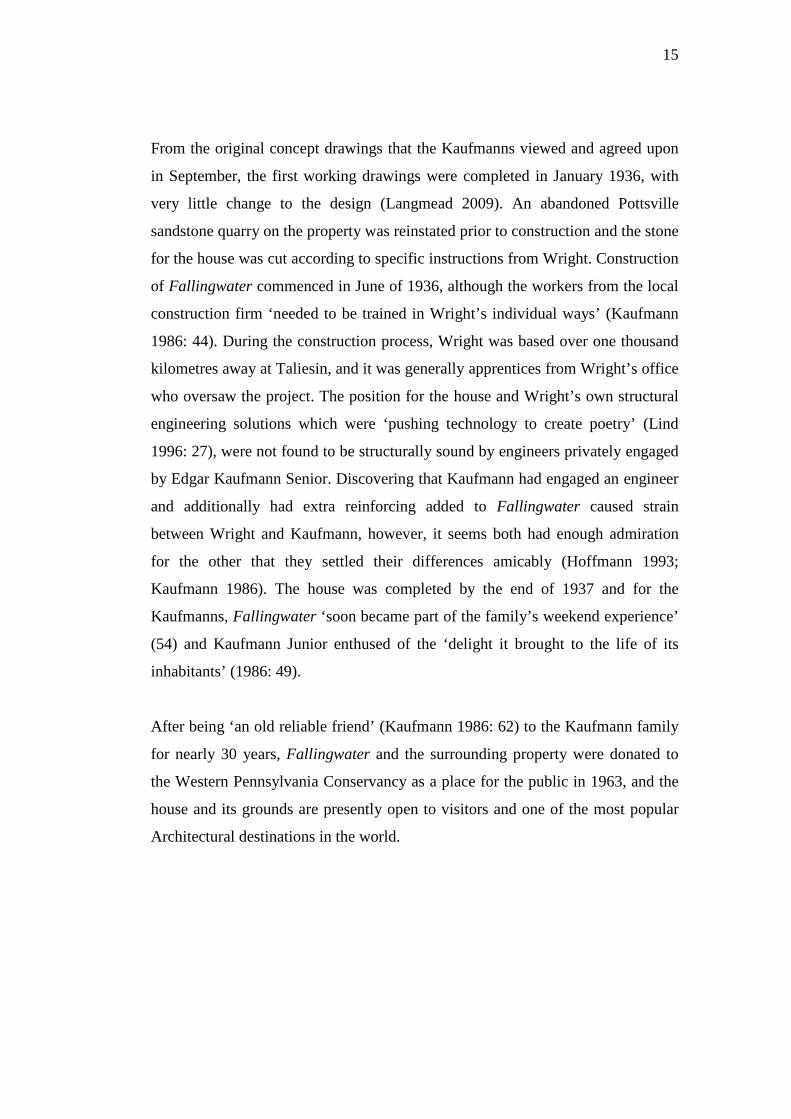
On the day Wright first visited the property it would have been far too cold for

swimming in the creek, which was ‘swollen’ while above, the falls were

‘thundering’ (Kaufmann 1983: 69). However, after showing Wright the site they

had in mind for the house, somewhat up the hill above Bear Run, the Kaufmanns

showed him the special spot in the creek where they loved to swim, and the rock

that they loved to sunbathe on. After staying all day on the site, Wright requested

‘a survey of the terrain around the falls [asking that] large boulders and large trees

were to be marked on it’ (Kaufmann 1983: 69).

When the Kaufmanns saw Wright’s design for the first time in September 1935,

they were surprised. Edgar Junior was similarly bewildered by the speed at which

Wright had conceptualized the design and put it down on paper, just in time to

show Edgar Senior when he arrived at the Fellowship studio. In an unexpected

move, Wright had located the house directly over the waterfall at Bear Run, on

their favoured swimming spot.

15

From the original concept drawings that the Kaufmanns viewed and agreed upon

in September, the first working drawings were completed in January 1936, with

very little change to the design (Langmead 2009). An abandoned Pottsville

sandstone quarry on the property was reinstated prior to construction and the stone

for the house was cut according to specific instructions from Wright. Construction

of Fallingwater commenced in June of 1936, although the workers from the local

construction firm ‘needed to be trained in Wright’s individual ways’ (Kaufmann

1986: 44). During the construction process, Wright was based over one thousand

kilometres away at Taliesin, and it was generally apprentices from Wright’s office

who oversaw the project. The position for the house and Wright’s own structural

engineering solutions which were ‘pushing technology to create poetry’ (Lind

1996: 27), were not found to be structurally sound by engineers privately engaged

by Edgar Kaufmann Senior. Discovering that Kaufmann had engaged an engineer

and additionally had extra reinforcing added to Fallingwater caused strain

between Wright and Kaufmann, however, it seems both had enough admiration

for the other that they settled their differences amicably (Hoffmann 1993;

Kaufmann 1986). The house was completed by the end of 1937 and for the

Kaufmanns, Fallingwater ‘soon became part of the family’s weekend experience’

(54) and Kaufmann Junior enthused of the ‘delight it brought to the life of its

inhabitants’ (1986: 49).

After being ‘an old reliable friend’ (Kaufmann 1986: 62) to the Kaufmann family

for nearly 30 years, Fallingwater and the surrounding property were donated to

the Western Pennsylvania Conservancy as a place for the public in 1963, and the

house and its grounds are presently open to visitors and one of the most popular

Architectural destinations in the world.

16

1.2 A Unique House in Wright’s Oeuvre?

If one building appears to have consistent formal or material qualities which are

similar to those of another building—or of a set of buildings—these properties are

collectively defined as a style. Often, architects develop distinctive formal or

material qualities across a set of designs, thereby creating their own particular

style. Furthermore, if the architect practices over several years, they may even

develop several distinguishable styles, or periods, that their buildings can be

categorised into. While the term ‘style’, and its derivatives such as ‘stylistic’, may

have other meanings, in this dissertation the use of the term ‘style’ refers to an

architectural period wherein a pattern of formal or material qualities is evident.

During his career, Wright worked in periods of distinctive styles. For example,

Wright initially gained international recognition with his Prairie style houses,

long, low-lying buildings which were designed as a reflection of the broad

expanse of the Prairie plains. All of these Prairie style houses are characterized by

strong horizontal lines, over-extended eaves, low-pitched roofs, open floor plan

and a central hearth. Wright’s Robie House is widely regarded as the ultimate

example of this approach.

In the period 1910-1920, Wright became involved in several large-scale

developments, including his American System Built Homes, a standardised,

affordable housing type, and the Ravine Bluffs Development, in Glencoe, Illinois.

During this period he was also invited to Japan to design Tokyo’s Imperial Hotel,

and he designed several houses and a school which were also built in Japan.

Wright expanded his practice in California in the early 1920’s and during the

following decade he designed many buildings although only five houses were

constructed. These five houses have since become known as the Textile-block

homes. Appearing as imposing, ageless structures, these houses were typically

constructed from a double skin of pre-cast patterned and plain exposed concrete

blocks held together by Wright’s patented system of steel rods and concrete grout.

17

The plain square blocks of the houses are generally punctuated by ornamented

blocks and for each house a different pattern was employed. The last house of this

period, the Lloyd Jones House in Tulsa (1929), is notably less ornamental than the

others in the sequence with Wright rejecting richly decorated blocks ‘in favor of

an alternating pattern of piers and slots’ (Frampton 2005: 170). The Lloyd Jones

House was Wright’s last major completed commission before Fallingwater.

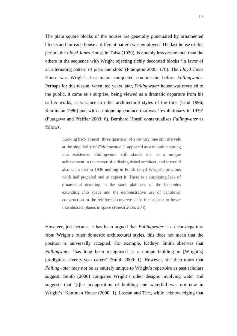
Perhaps for this reason, when, ten years later, Fallingwater house was revealed to

the public, it came as a surprise, being viewed as a dramatic departure from his

earlier works, at variance to other architectural styles of the time (Lind 1996;

Kaufmann 1986) and with a unique appearance that was ‘revolutionary in 1939’

(Futagawa and Pfeiffer 2003: 6). Bernhard Hoesli contextualises Fallingwater as

follows.

Looking back almost [three quarters] of a century, one still marvels

at the singularity of Fallingwater. It appeared as a mutation sprung

into existence. Fallingwater still stands out as a unique

achievement in the career of a distinguished architect, and it would

also seem that in 1936 nothing in Frank Lloyd Wright’s previous

work had prepared one to expect it. There is a surprising lack of

ornamental detailing in the stark plainness of the balconies

extending into space and the demonstrative use of cantilever

construction in the reinforced-concrete slabs that appear to hover

like abstract planes in space (Hoesli 2005: 204).

However, just because it has been argued that Fallingwater is a clear departure

from Wright’s other domestic architectural styles, this does not mean that the

position is universally accepted. For example, Kathryn Smith observes that

Fallingwater ‘has long been recognized as a unique building in [Wright’s]

prodigious seventy-year career’ (Smith 2000: 1). However, she then notes that

Fallingwater may not be as entirely unique to Wright’s repertoire as past scholars

suggest. Smith (2000) compares Wright’s other designs involving water and

suggests that ‘[t]he juxtaposition of building and waterfall was not new in

Wright’s’ Kaufman House (2000: 1). Laseau and Tice, while acknowledging that

18

Fallingwater is unique in many respects, also propose that ‘[s]everal houses

among Wright’s earlier work could provide plausible prototypes for Fallingwater’

(1992: 72). Robert McCarter (2002) also identifies a selection of Wright’s

previous designs which may have influenced Fallingwater and supports his

argument with the following quote from Wright.

The ideas involved [in Fallingwater] are in no wise changed from

those of early work. The materials and methods of construction

come through them. The affects you see in this house are not

superficial effects, and are entirely consistent with the prairie

houses of 1901-10 (Wright 1941, qtd in McCarter 2002: 6).

Thomas Doremus (1992) also offers the unusual opinion that Fallingwater’s

‘abrupt break with earlier work’ (35) occurred because Wright was influenced at

the time by the work of Le Corbusier. In particular, Doremus (1992) suggests that

Fallingwater is directly influenced by the Villa Savoye.

Such debates, about the position of Fallingwater in Wright’s larger domestic

canon, can be traced in many histories and scholarly critiques. Certainly there are

elements in Fallingwater which recall his previous designs, and which seem to

prefigure his later Usonian works. As such, claims that it is unique in his oeuvre

are readily disputed, but questions remain about its connection to both earlier and

later styles. Was it a transition design, from the Textile-block to the Usonian

period, or was it a throwback to the Prairie style?

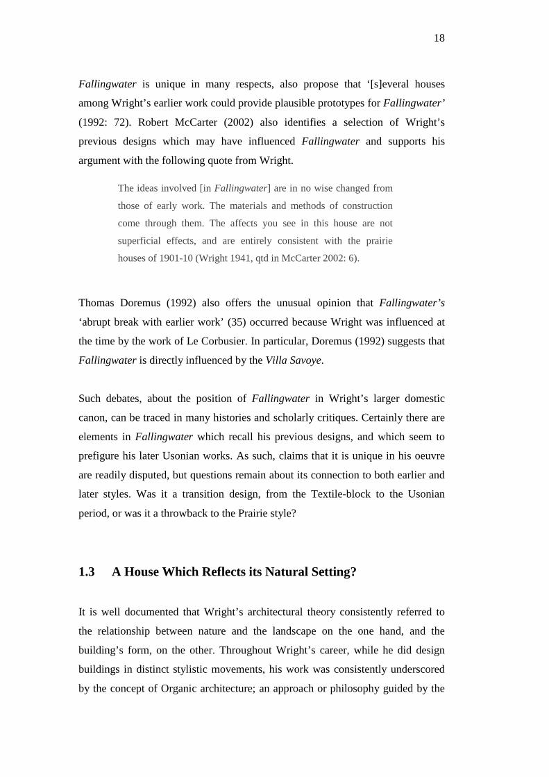
1.3 A House Which Reflects its Natural Setting?

It is well documented that Wright’s architectural theory consistently referred to

the relationship between nature and the landscape on the one hand, and the

building’s form, on the other. Throughout Wright’s career, while he did design

buildings in distinct stylistic movements, his work was consistently underscored

by the concept of Organic architecture; an approach or philosophy guided by the

19

principles of nature (Wright’s approach to Organic architecture is explained in

section 2.2). For Wright, this was not necessarily the physical form of nature, as

he differentiated between two primary forms; the physical natural landscape and a

transcendent ‘inner nature’ (Wright 1957: 89; Cronin 1994; Spirn 2000i). The

second form, ‘inner nature’, described architecture which was a spiritual

incarnation of nature, an Emersonian concept by which ‘the correlation of

physical form to nature would elevate the spiritual condition of humankind’

(Alofsin 1994:32). Indeed, Wright often referred to ‘Nature spelled with a capital

“N” the way you spell God with a capital “G”’ (Wright qtd in Pfeiffer 2004: 12).

However, Wright’s understanding of the physical form of nature was derived from

the tangible surrounding landscapes, around which Wright typically designed

buildings to achieve ‘an absolutely symbiotic integration with nature’ (Antoniades

1992: 243). Wright used several recurring strategies to create the impression that a

building is closely related to its site and these included approaches to the design of

the building as well as his interpretation and often, manipulation, of the landscape

(Moholy-Nagy 1959; Frazier 1995; De Long 1996).

Fallingwater is described as one of the foremost examples of Wright’s houses that

appear to be a part of nature, or even as a natural object itself. For example,

McCarter describes the design as having ‘grown out of the ground and into the

light’ (1999: 220). Fallingwater also allegedly contains many clear examples of

the design strategies linking landscape and building that Wright typically used

(Kaufmann 1986; Hoffmann 1993; Levine 1996). Despite the overwhelming

quantity of literature supporting or repeating this claim, that Fallingwater echoes

its natural setting, there are those who disagree, prompting an ongoing debate

amongst historians and architectural scholars. For example, Donald Hoffmann

accuses Fallingwater of being ‘an intruder in the forest’ (1995: 85), and Kenneth

Frampton considers Fallingwater’s purpose is to ‘juxtapose nature and culture as

explicitly as possible’ (1994: 72). Smith suggests that the house ‘differentiates

itself from its surroundings and retains its identity’ (2000: 25).

20

Famous for acknowledging the influence of nature in his personal and

architectural philosophy, Wright differentiated between the physical and spiritual

aspects of nature. Examining the various examples of Wright’s approach to

nature—provided by Wright and successive scholars—it is possible to discover

specific references to how his buildings relate to their physical, tangible setting.

While most scholars, and Wright himself, insist this is the case for Fallingwater,

others disagree, suggesting the house is more of a Modernist spaceship, landed in

a pristine forest. Significantly, both sets of views are from reputed, experienced

Wrightian scholars, but which, if any, are correct?

1.4 Hypotheses In scientific research a hypothetico-deductive approach is typically used to

examine phenomena from the perspective of logic and causation, with the

resulting hypothesis formulated by an inductive argument. However, this

dissertation can not employ such a scientific approach to developing hypotheses,

as there is no pre-existing or logical evidence to support the ideas being tested. In

essence, these ideas are based on theories and suppositions proposed by previous

scholars. Furthermore, the complexity of the possible iterations and variables in

this thesis also make it inappropriate to develop and apply hypotheses in a

scientific sense. Instead, the hypotheses presented here are used to carefully define

the testable goals of the dissertation.

This dissertation tests two hypotheses that reflect dominant scholarly

interpretations of Fallingwater’s visual and formal properties, as set out in the

previous two sections.

• Hypothesis 1: That the formal and visual properties of Frank Lloyd

Wright’s Fallingwater are atypical of his early and mid-career housing

(1901-1955).

21

• Hypothesis 2: That the formal and visual properties of Frank Lloyd

Wright’s Fallingwater strongly reflect its natural setting.

While historians typically frame both of these hypotheses as true, almost

suggesting that one necessarily follows the other, the present research treats these

hypotheses as parallel or disconnected propositions. Both could be true, both false

or some combination of one true and the other false. Furthermore, unlike most

scholarly assessments of Wright’s work, this dissertation uses a quantitative

approach: a computational variation of the fractal analysis method for measuring

visual complexity. In Chapter 7, these hypotheses are reframed around the

mathematical indicators that will be used to test their veracity in Chapters 8 and 9.

The proposed quantitative approach will make a new range of information about

Wright’s architecture, and especially Fallingwater, available to support future

research. Rather than relying on the diverse views of scholars or Wright’s own—

often rambling—discourse, a quantitative study provides numerical, comparable

results. Wright’s architectural history and various scholarly viewpoints will assist

in the interpretation of results, however, the sets of computed fractal dimensions

deliver definite information on levels of visual complexity in Wright’s

architecture. As an approach to this dissertation, when used with a rigorous

methodology, the results will illuminate the hypotheses with a solid basis of data.

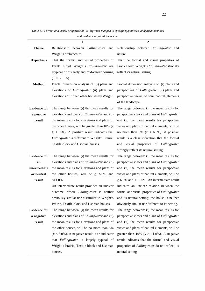
Table 1.0 aligns the hypotheses with the analytical method used to test them and

the indicators that will be used to determine the validity of each hypothesis. The

details of these processes and indicative range percentages chosen for this

purpose, are explained in Part II.

22

Table 1.0 Formal and visual properties of Fallingwater mapped to specific hypotheses, analytical methods

and evidence required for results

1 2

Theme Relationship between Fallingwater and

Wright’s architecture.

Relationship between Fallingwater and

nature.

Hypothesis That the formal and visual properties of

Frank Lloyd Wright’s Fallingwater are

atypical of his early and mid-career housing

(1901-1955).

That the formal and visual properties of

Frank Lloyd Wright’s Fallingwater strongly

reflect its natural setting.

Method Fractal dimension analysis of: (i) plans and

elevations of Fallingwater (ii) plans and

elevations of fifteen other houses by Wright.

Fractal dimension analysis of: (i) plans and

perspectives of Fallingwater (ii) plans and

perspective views of four natural elements

of the landscape

Evidence for

a positive

result

The range between: (i) the mean results for

elevations and plans of Fallingwater and (ii)

the mean results for elevations and plans of

the other houses, will be greater than 10% (x

≥ 11.0%). A positive result indicates that

Fallingwater is different to Wright’s Prairie,

Textile-block and Usonian houses.

The range between: (i) the mean results for

perspective views and plans of Fallingwater

and (ii) the mean results for perspective

views and plans of natural elements, will be

no more than 5% (x < 6.0%). A positive

result is a clear indication that the formal

and visual properties of Fallingwater

strongly reflect its natural setting

Evidence for

an

intermediate

or neutral

result

The range between: (i) the mean results for

elevations and plans of Fallingwater and (ii)

the mean results for elevations and plans of

the other houses, will be ≥ 6.0% and

<11.0%.

An intermediate result provides an unclear

outcome, where Fallingwater is neither

obviously similar nor dissimilar to Wright’s

Prairie, Textile-block and Usonian houses.

The range between: (i) the mean results for

perspective views and plans of Fallingwater

and (ii) the mean results for perspective

views and plans of natural elements, will be

≥ 6.0% and < 11.0%. An intermediate result

indicates an unclear relation between the

formal and visual properties of Fallingwater

and its natural setting; the house is neither

obviously similar nor different to its setting.

Evidence for

a negative

result

The range between: (i) the mean results for

elevations and plans of Fallingwater and (ii)

the mean results for elevations and plans of

the other houses, will be no more than 5%

(x < 6.0%). A negative result is an indicator

that Fallingwater is largely typical of

Wright’s Prairie, Textile-block and Usonian

houses.

The range between: (i) the mean results for

perspective views and plans of Fallingwater

and (ii) the mean results for perspective

views and plans of natural elements, will be

greater than 10% (x ≥ 11.0%). A negative

result indicates that the formal and visual

properties of Fallingwater do not reflect its

natural setting

23

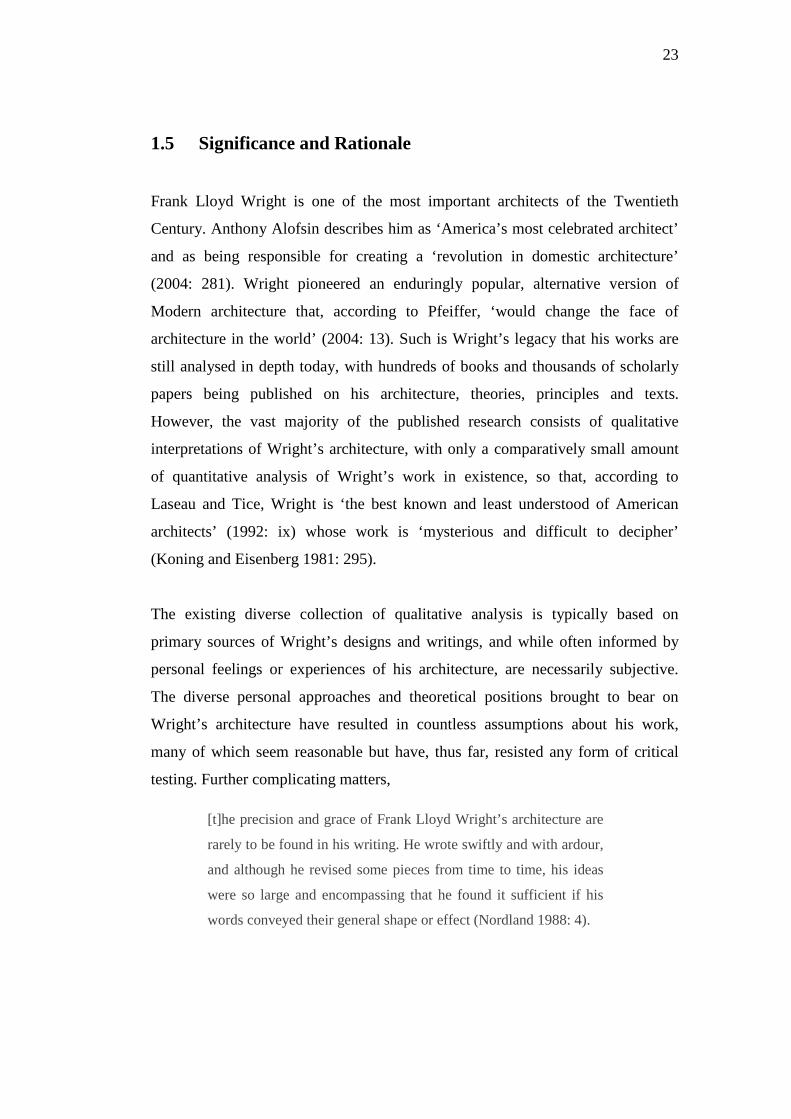
1.5 Significance and Rationale

Frank Lloyd Wright is one of the most important architects of the Twentieth

Century. Anthony Alofsin describes him as ‘America’s most celebrated architect’

and as being responsible for creating a ‘revolution in domestic architecture’

(2004: 281). Wright pioneered an enduringly popular, alternative version of

Modern architecture that, according to Pfeiffer, ‘would change the face of

architecture in the world’ (2004: 13). Such is Wright’s legacy that his works are

still analysed in depth today, with hundreds of books and thousands of scholarly

papers being published on his architecture, theories, principles and texts.

However, the vast majority of the published research consists of qualitative

interpretations of Wright’s architecture, with only a comparatively small amount

of quantitative analysis of Wright’s work in existence, so that, according to

Laseau and Tice, Wright is ‘the best known and least understood of American

architects’ (1992: ix) whose work is ‘mysterious and difficult to decipher’

(Koning and Eisenberg 1981: 295).

The existing diverse collection of qualitative analysis is typically based on

primary sources of Wright’s designs and writings, and while often informed by

personal feelings or experiences of his architecture, are necessarily subjective.

The diverse personal approaches and theoretical positions brought to bear on

Wright’s architecture have resulted in countless assumptions about his work,

many of which seem reasonable but have, thus far, resisted any form of critical

testing. Further complicating matters,

[t]he precision and grace of Frank Lloyd Wright’s architecture are

rarely to be found in his writing. He wrote swiftly and with ardour,

and although he revised some pieces from time to time, his ideas

were so large and encompassing that he found it sufficient if his

words conveyed their general shape or effect (Nordland 1988: 4).

24

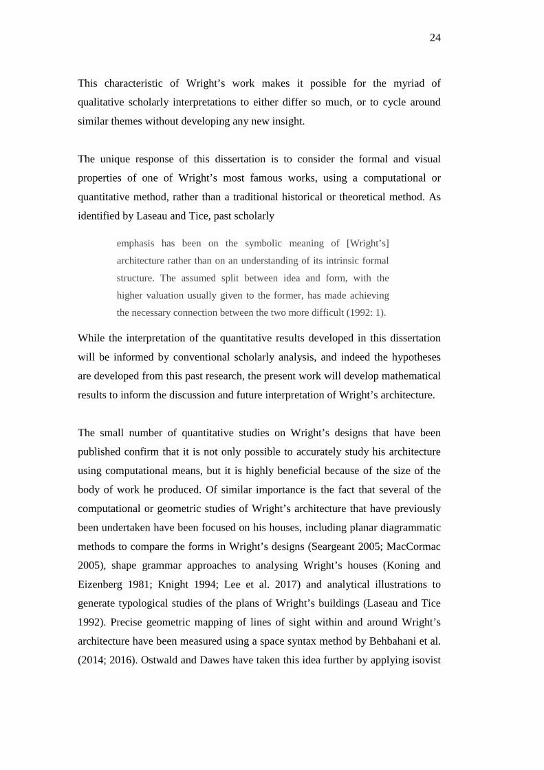
This characteristic of Wright’s work makes it possible for the myriad of

qualitative scholarly interpretations to either differ so much, or to cycle around

similar themes without developing any new insight.

The unique response of this dissertation is to consider the formal and visual

properties of one of Wright’s most famous works, using a computational or

quantitative method, rather than a traditional historical or theoretical method. As

identified by Laseau and Tice, past scholarly

emphasis has been on the symbolic meaning of [Wright’s]

architecture rather than on an understanding of its intrinsic formal

structure. The assumed split between idea and form, with the

higher valuation usually given to the former, has made achieving

the necessary connection between the two more difficult (1992: 1).

While the interpretation of the quantitative results developed in this dissertation

will be informed by conventional scholarly analysis, and indeed the hypotheses

are developed from this past research, the present work will develop mathematical

results to inform the discussion and future interpretation of Wright’s architecture.

The small number of quantitative studies on Wright’s designs that have been

published confirm that it is not only possible to accurately study his architecture

using computational means, but it is highly beneficial because of the size of the

body of work he produced. Of similar importance is the fact that several of the

computational or geometric studies of Wright’s architecture that have previously

been undertaken have been focused on his houses, including planar diagrammatic

methods to compare the forms in Wright’s designs (Seargeant 2005; MacCormac

2005), shape grammar approaches to analysing Wright’s houses (Koning and

Eizenberg 1981; Knight 1994; Lee et al. 2017) and analytical illustrations to

generate typological studies of the plans of Wright’s buildings (Laseau and Tice

1992). Precise geometric mapping of lines of sight within and around Wright’s

architecture have been measured using a space syntax method by Behbahani et al.

(2014; 2016). Ostwald and Dawes have taken this idea further by applying isovist

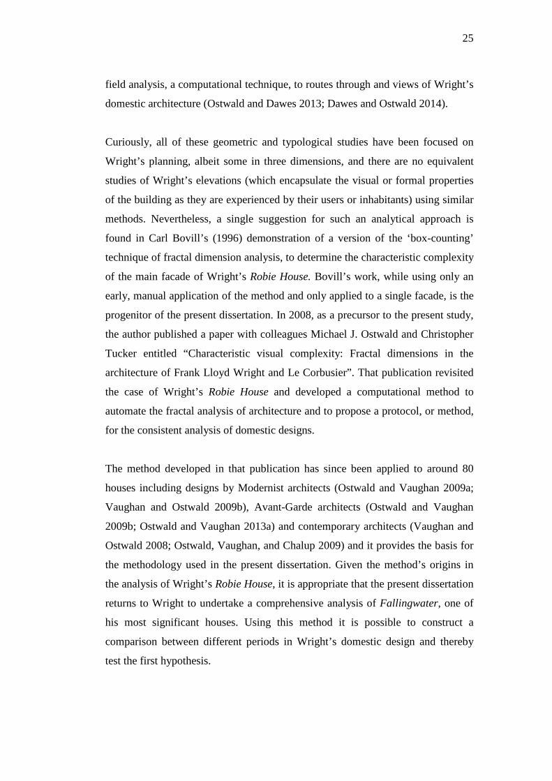
25

field analysis, a computational technique, to routes through and views of Wright’s

domestic architecture (Ostwald and Dawes 2013; Dawes and Ostwald 2014).

Curiously, all of these geometric and typological studies have been focused on

Wright’s planning, albeit some in three dimensions, and there are no equivalent

studies of Wright’s elevations (which encapsulate the visual or formal properties

of the building as they are experienced by their users or inhabitants) using similar

methods. Nevertheless, a single suggestion for such an analytical approach is

found in Carl Bovill’s (1996) demonstration of a version of the ‘box-counting’

technique of fractal dimension analysis, to determine the characteristic complexity

of the main facade of Wright’s Robie House. Bovill’s work, while using only an

early, manual application of the method and only applied to a single facade, is the

progenitor of the present dissertation. In 2008, as a precursor to the present study,

the author published a paper with colleagues Michael J. Ostwald and Christopher

Tucker entitled “Characteristic visual complexity: Fractal dimensions in the

architecture of Frank Lloyd Wright and Le Corbusier”. That publication revisited

the case of Wright’s Robie House and developed a computational method to

automate the fractal analysis of architecture and to propose a protocol, or method,

for the consistent analysis of domestic designs.

The method developed in that publication has since been applied to around 80

houses including designs by Modernist architects (Ostwald and Vaughan 2009a;

Vaughan and Ostwald 2009b), Avant-Garde architects (Ostwald and Vaughan

2009b; Ostwald and Vaughan 2013a) and contemporary architects (Vaughan and

Ostwald 2008; Ostwald, Vaughan, and Chalup 2009) and it provides the basis for

the methodology used in the present dissertation. Given the method’s origins in

the analysis of Wright’s Robie House, it is appropriate that the present dissertation

returns to Wright to undertake a comprehensive analysis of Fallingwater, one of

his most significant houses. Using this method it is possible to construct a

comparison between different periods in Wright’s domestic design and thereby

test the first hypothesis.

26

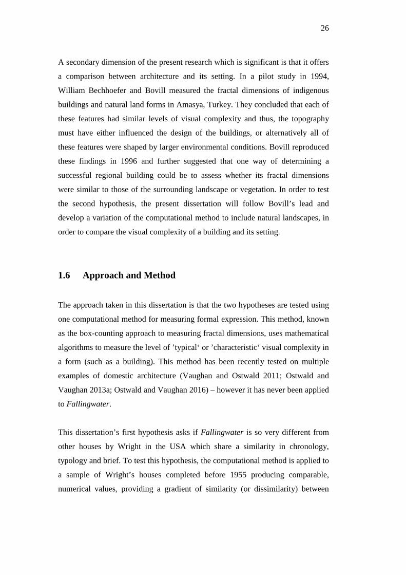
A secondary dimension of the present research which is significant is that it offers

a comparison between architecture and its setting. In a pilot study in 1994,

William Bechhoefer and Bovill measured the fractal dimensions of indigenous

buildings and natural land forms in Amasya, Turkey. They concluded that each of

these features had similar levels of visual complexity and thus, the topography

must have either influenced the design of the buildings, or alternatively all of

these features were shaped by larger environmental conditions. Bovill reproduced

these findings in 1996 and further suggested that one way of determining a

successful regional building could be to assess whether its fractal dimensions

were similar to those of the surrounding landscape or vegetation. In order to test

the second hypothesis, the present dissertation will follow Bovill’s lead and

develop a variation of the computational method to include natural landscapes, in

order to compare the visual complexity of a building and its setting.

1.6 Approach and Method

The approach taken in this dissertation is that the two hypotheses are tested using

one computational method for measuring formal expression. This method, known

as the box-counting approach to measuring fractal dimensions, uses mathematical

algorithms to measure the level of ’typical‘ or ’characteristic‘ visual complexity in

a form (such as a building). This method has been recently tested on multiple

examples of domestic architecture (Vaughan and Ostwald 2011; Ostwald and

Vaughan 2013a; Ostwald and Vaughan 2016) – however it has never been applied

to Fallingwater.

This dissertation’s first hypothesis asks if Fallingwater is so very different from

other houses by Wright in the USA which share a similarity in chronology,

typology and brief. To test this hypothesis, the computational method is applied to

a sample of Wright’s houses completed before 1955 producing comparable,

numerical values, providing a gradient of similarity (or dissimilarity) between

27

Fallingwater and his other houses. The method for testing hypothesis one is as

follows.

a. The computational method—fractal analysis (which will be described later

in Chapter 4)—is applied to measuring the characteristic complexity of the

four cardinal elevations, three floor plans and one roof plan of

Fallingwater.

b. The computational method is then applied to 58 elevations and 46 plans of

15 of Wright’s built houses, from three significant periods in his career.

The 15 houses are the Robie, Evans, Zeigler, Tomek and Henderson

Houses from Wright’s Prairie Style period; the Ennis, Millard, Storrer,

Freeman and Lloyd-Jones Houses from Wright’s textile block period; and

the Palmer, Dobkins, Reisley, Fawcett and Chahroudi Houses from his

Usonian period.

c. A numerical comparison using mean dimensions and comparative ranges

is undertaken between 112 major and approximately 1000 minor data

points generated by the 15 houses and the equivalent data from

Fallingwater.

The second hypothesis asks if Fallingwater is visually similar to its natural

setting. By using a variation in the application of the computational method, the

form and complexity of Wright’s Fallingwater can be compared with its

surrounding landscape. The method for testing the second hypothesis is as

follows.

a. The computational method is applied to four perspective drawings of

Fallingwater (generated from Wright’s original chosen viewpoints), and to

the four plans of the building.

b. Sixteen views of four natural features and four site plans of those features

are selected from the Bear Run site and analysed using the same

computational method.

28

c. The fractal dimension measurements for Fallingwater are compared with

equivalent measurements derived from the nature analogues. The results

are analysed by comparing mean values and the gaps between them.

The results of both tests are presented as charted mathematical data, in tabular and

graphical format. The data is analysed and discussed in its historical context, and

interpreted with an informed theoretical reading, by comparing the results with

past published research and scholarly theories on Wright’s work. The

interpretation of the results will also be informed by past results of research into

the fractal dimensions of domestic architecture (Bovill 1996; Zarnowieka 1998;

Debailleux 2010; Lorenz 2003; Ostwald and Vaughan 2016).

1.7 Limitations

The methodological scope of the research is defined by four limits: characteristic

complexity and fractal dimensions; the selection of subjects for analysis; the

representation of the images for analysis; and the variables of the computational

method.

1. Characteristic Complexity and Fractal Dimensions

In a way, the most significant limitation is that this dissertation uses characteristic

complexity—measured using fractal dimensions—to compare objects. Fractal

dimensions are a statistical approximation of the spread of geometric detail or

information in an image. Fractal dimensions do not provide information on any

other visual properties such as proportion, composition or color.

2. Subject selection.

The computational method is carried out on two-dimensional images, and to

reduce the possible number of external variables that can have an impact on the

data, these images are selected from a pool of similar types. The buildings

analysed are only domestic structures designed by Frank Lloyd Wright. Of the

29

several hundred houses Wright designed in his lifetime, only 16 are selected for

analysis. The reason for this limited sample of houses is to maximize the potential

reliability and consistency of the results, while including his major works from

each period. To narrow the selection, completed houses, in preference to unbuilt

works, and designs from a similar time frame and geographic distribution are

selected. Thus, only domestic buildings by Frank Lloyd Wright completed in the

USA after the beginning of his Prairie style (1901), or before the end of his

Usonian period (1959) are considered for inclusion.

Since Bovill first undertook a fractal dimension analysis of Wright’s Robie House

in 1996, houses have been a regular subject of this research approach (Zarnowieka

1998; Lorenz 2003; Wen and Kao 2005; Debailleux 2010; Ostwald and Vaughan

2016). Houses are appropriate analytical subjects because they typically possess

scale, program and materiality that are comparable to other houses. Because the

architectural brief conventionally shapes the form and complexity of the design,

conducting a comparison between different building types (such as a church, an

apartment building and stadium) would produce results that are largely a

reflection of the function of the building.

Wright designed houses of many different sizes, from tiny cottages to large

housing complexes. He designed many ‘modest’ sized homes, single freestanding

domestic type buildings with one main living area and 2-3 bedrooms.

Fallingwater fits into this size category, and therefore all of the other houses

selected for comparison also do so.

3. Image representation boundaries.

Once the buildings are selected for analysis, there must be a consideration of

which representations of these buildings will be analysed. For the architectural

images, only re-drawn line drawings from existing original drawings that are

publically available, but not photographs or archival facsimiles, are used for

analysis. Following the method published by Bovill (1996) and work completed in

part by Ostwald, Chalup, Tucker and the present author (2008) for the first

30

hypothesis, it will be one pixel-width line drawings of elevations and plans of

buildings which will be analysed, rather than sections, perspectives etc. For the

second hypothesis, other drawings types, for example perspectives and landscape

views, will also be considered. In this way the analysis can be done in a

standardised manner, and the lines selected to include in the analysis will not

include a large amount of detail, only the significant lines will be reproduced.

These approaches are described in more detail in Chapter 6.

4. Computational limits.

The final limitation concerns the method being used. The box-counting method

has only been developed in detail for architectural research in the last decade, with

many of the most significant advances occurring in the last few years (Ben-

Hamouche 2009). There are several variations of the method, and some known

inconsistencies. While the box-counting method was traditionally a manual

exercise, the variation used in this dissertation will follow the version published

extensively in the last few years (Ostwald and Vaughan 2016). This method uses a

computer program (in this case, Archimage, a program co-developed by Ostwald,

Chalup, Nicklin and the present author). The known limitations of the method are

described in detail in Chapter 5.

There are three further non-methodological limitations to this dissertation; the first

being the age of the buildings. This study is focussed on the visual appearance of

buildings and landscapes, and the dissertation seeks to understand Wright’s

original influences, which are apparent in the buildings and setting at the time

they were built. The houses studied range from 62 to over 100 years old today,

with Fallingwater being 80 years old and, as such, many changes have occurred

over time to these buildings. To ensure a similar state between all buildings

studied, the original images produced by Wright are analysed, rather than any

modifications or additions that have been subsequently designed. This applies to a

particular aspect of Fallingwater, where detached guest quarters were later

designed by Wright. As they were designed and constructed after Fallingwater

was originally competed they are not included in the present analysis.

31

The second non-methodological limitation is that the distance between Australia

and the USA, and the diverse location of Wright’s buildings across the USA

(many of which are private homes), means that the majority of the buildings

studied are impossible to visit. However, a site visit was undertaken in 2012 to

Fallingwater—and to many of Wright’s publicly accessible Prairie Houses—to

gather data for this dissertation. Finally, language provides a limitation, and

written sources will be limited to those published in English.

1.8 Dissertation Summary

The dissertation is divided into three parts. Part I presents the hypotheses of this

dissertation and provides an introduction to Frank Lloyd Wright and his

architectural design and theory. Part II provides an explanation of the

computational method used to test the hypotheses and Part III reports the results

generated, and discusses the results and their implications, before reaching a

conclusion. These three parts, and the chapters they comprise, are summarised

hereafter.

Part I: Frank Lloyd Wright and Fallingwater

The present chapter, the introduction to Part I, covers the context to the research

project, focussing on scholarly analyses of Wright’s work which suggest clear

parallels between his architectural forms and the surrounding natural landscape. In

particular, the proposals of architectural theorists and historians regarding

Fallingwater, as emblematic of a site-related building, are described, in addition

to claims that Fallingwater is a unique work among Wright’s sizeable oeuvre.

This scholarly context leads to the formulation of the two hypotheses. The two

hypotheses regarding Wright and Fallingwater are stated and explained, and the

significance of this dissertation is outlined. This is followed by a brief outline of

32

the computational method, and the methodological and other boundaries or

limitations of this work.

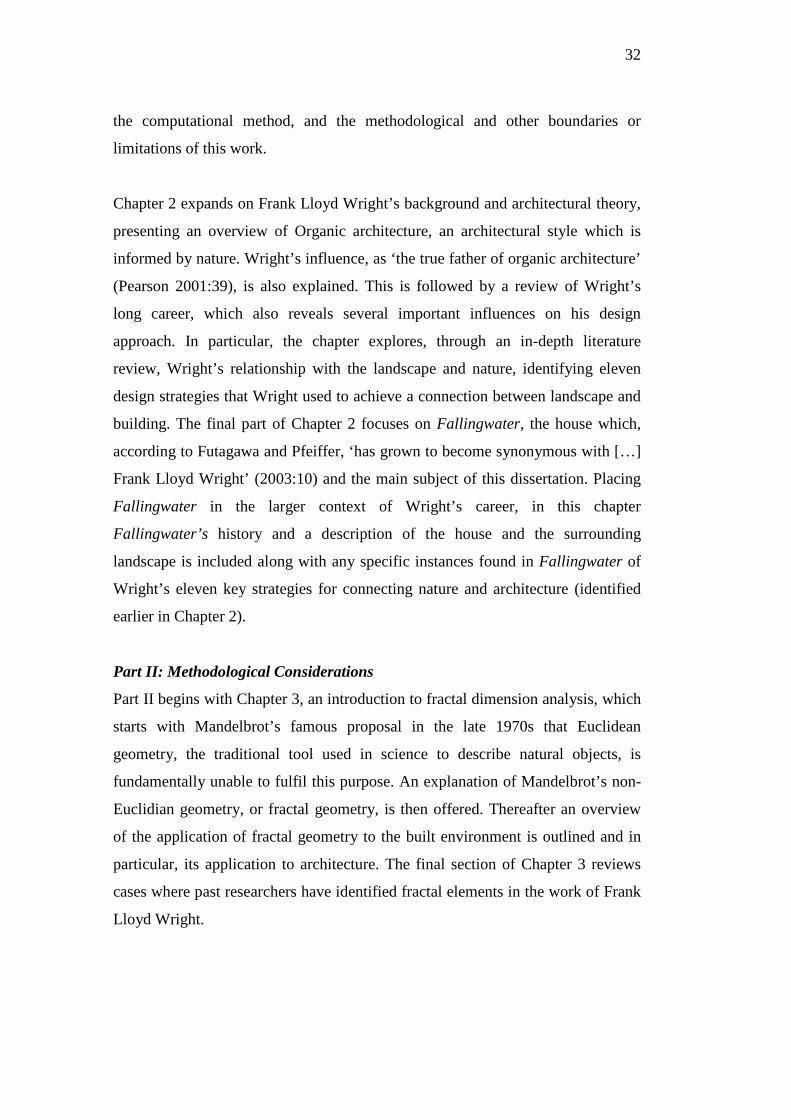
Chapter 2 expands on Frank Lloyd Wright’s background and architectural theory,

presenting an overview of Organic architecture, an architectural style which is

informed by nature. Wright’s influence, as ‘the true father of organic architecture’

(Pearson 2001:39), is also explained. This is followed by a review of Wright’s

long career, which also reveals several important influences on his design

approach. In particular, the chapter explores, through an in-depth literature

review, Wright’s relationship with the landscape and nature, identifying eleven

design strategies that Wright used to achieve a connection between landscape and

building. The final part of Chapter 2 focuses on Fallingwater, the house which,

according to Futagawa and Pfeiffer, ‘has grown to become synonymous with […]

Frank Lloyd Wright’ (2003:10) and the main subject of this dissertation. Placing

Fallingwater in the larger context of Wright’s career, in this chapter

Fallingwater’s history and a description of the house and the surrounding

landscape is included along with any specific instances found in Fallingwater of

Wright’s eleven key strategies for connecting nature and architecture (identified

earlier in Chapter 2).

Part II: Methodological Considerations

Part II begins with Chapter 3, an introduction to fractal dimension analysis, which

starts with Mandelbrot’s famous proposal in the late 1970s that Euclidean

geometry, the traditional tool used in science to describe natural objects, is

fundamentally unable to fulfil this purpose. An explanation of Mandelbrot’s non-

Euclidian geometry, or fractal geometry, is then offered. Thereafter an overview

of the application of fractal geometry to the built environment is outlined and in

particular, its application to architecture. The final section of Chapter 3 reviews

cases where past researchers have identified fractal elements in the work of Frank

Lloyd Wright.

33

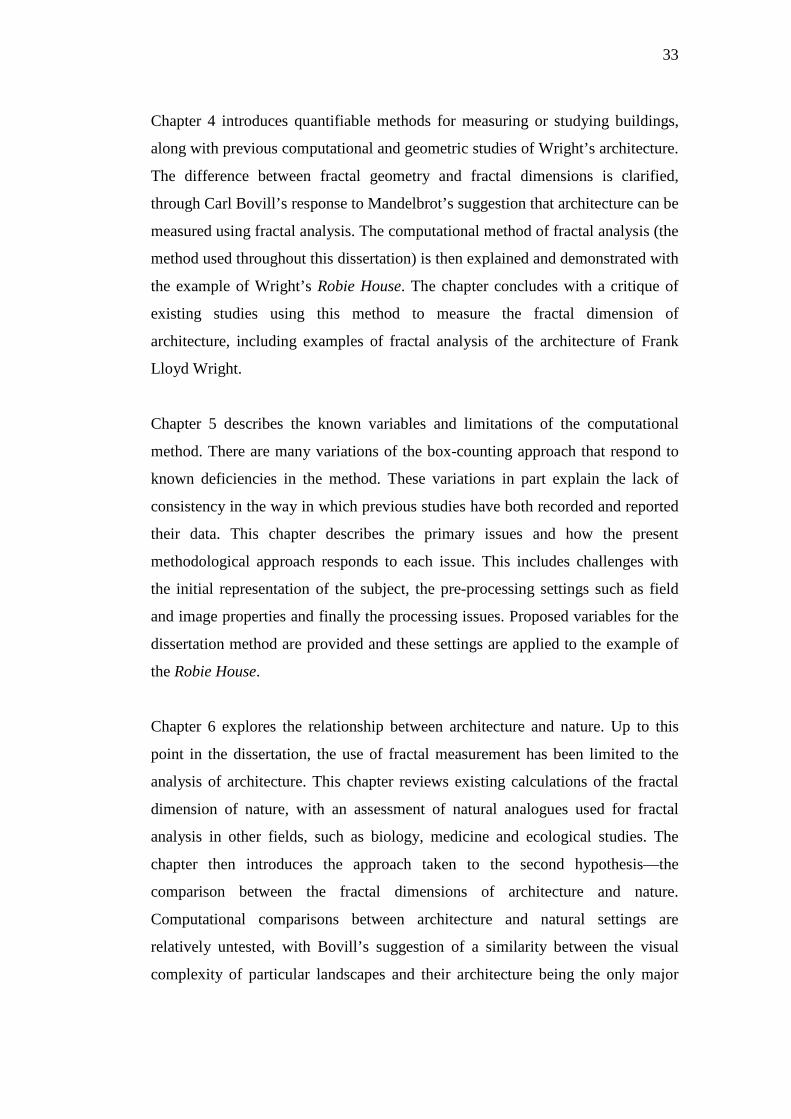
Chapter 4 introduces quantifiable methods for measuring or studying buildings,

along with previous computational and geometric studies of Wright’s architecture.

The difference between fractal geometry and fractal dimensions is clarified,

through Carl Bovill’s response to Mandelbrot’s suggestion that architecture can be

measured using fractal analysis. The computational method of fractal analysis (the

method used throughout this dissertation) is then explained and demonstrated with

the example of Wright’s Robie House. The chapter concludes with a critique of

existing studies using this method to measure the fractal dimension of

architecture, including examples of fractal analysis of the architecture of Frank

Lloyd Wright.

Chapter 5 describes the known variables and limitations of the computational

method. There are many variations of the box-counting approach that respond to

known deficiencies in the method. These variations in part explain the lack of

consistency in the way in which previous studies have both recorded and reported

their data. This chapter describes the primary issues and how the present

methodological approach responds to each issue. This includes challenges with

the initial representation of the subject, the pre-processing settings such as field

and image properties and finally the processing issues. Proposed variables for the

dissertation method are provided and these settings are applied to the example of

the Robie House.

Chapter 6 explores the relationship between architecture and nature. Up to this

point in the dissertation, the use of fractal measurement has been limited to the

analysis of architecture. This chapter reviews existing calculations of the fractal

dimension of nature, with an assessment of natural analogues used for fractal

analysis in other fields, such as biology, medicine and ecological studies. The

chapter then introduces the approach taken to the second hypothesis—the

comparison between the fractal dimensions of architecture and nature.

Computational comparisons between architecture and natural settings are

relatively untested, with Bovill’s suggestion of a similarity between the visual

complexity of particular landscapes and their architecture being the only major

34

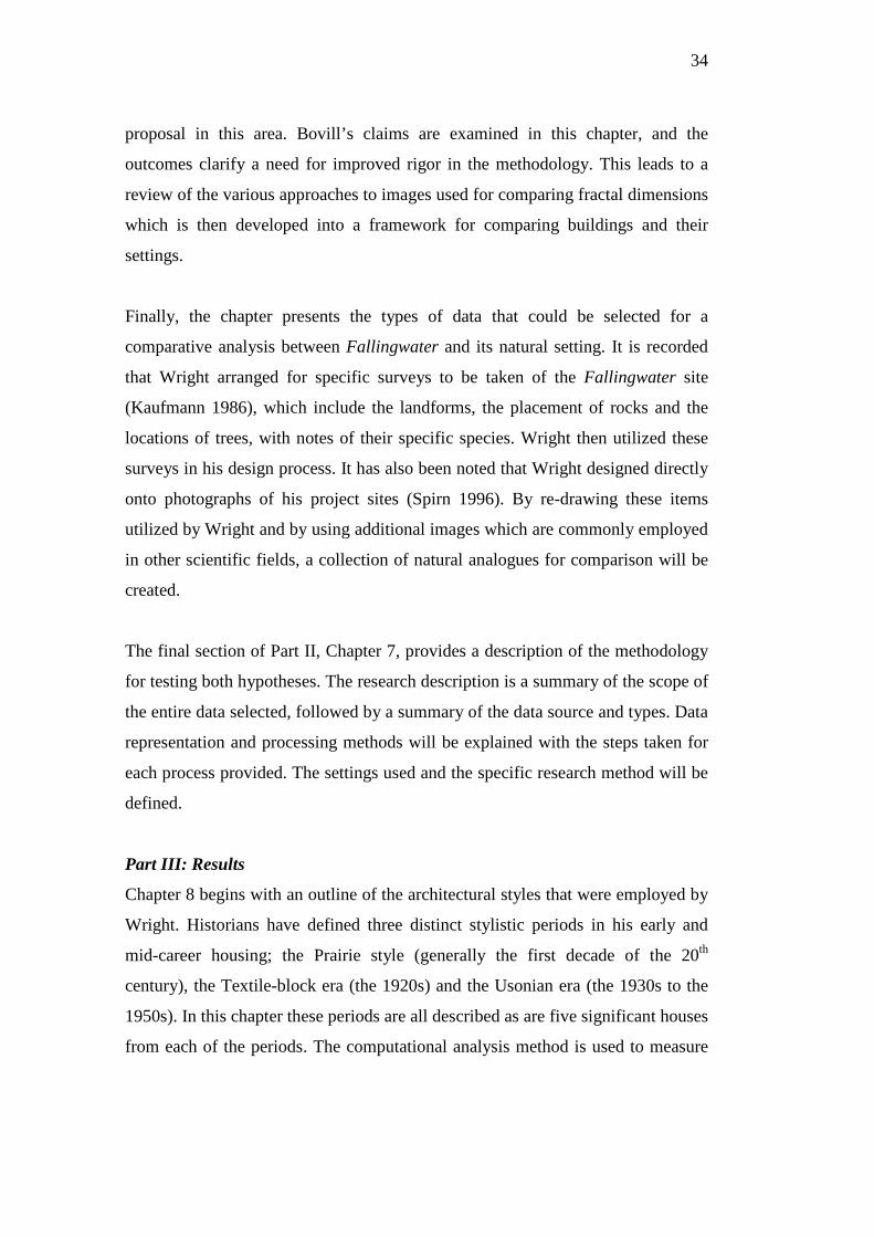
proposal in this area. Bovill’s claims are examined in this chapter, and the

outcomes clarify a need for improved rigor in the methodology. This leads to a

review of the various approaches to images used for comparing fractal dimensions

which is then developed into a framework for comparing buildings and their

settings.

Finally, the chapter presents the types of data that could be selected for a

comparative analysis between Fallingwater and its natural setting. It is recorded

that Wright arranged for specific surveys to be taken of the Fallingwater site

(Kaufmann 1986), which include the landforms, the placement of rocks and the

locations of trees, with notes of their specific species. Wright then utilized these

surveys in his design process. It has also been noted that Wright designed directly

onto photographs of his project sites (Spirn 1996). By re-drawing these items

utilized by Wright and by using additional images which are commonly employed

in other scientific fields, a collection of natural analogues for comparison will be

created.

The final section of Part II, Chapter 7, provides a description of the methodology

for testing both hypotheses. The research description is a summary of the scope of

the entire data selected, followed by a summary of the data source and types. Data

representation and processing methods will be explained with the steps taken for

each process provided. The settings used and the specific research method will be

defined.

Part III: Results

Chapter 8 begins with an outline of the architectural styles that were employed by

Wright. Historians have defined three distinct stylistic periods in his early and

mid-career housing; the Prairie style (generally the first decade of the 20th

century), the Textile-block era (the 1920s) and the Usonian era (the 1930s to the

1950s). In this chapter these periods are all described as are five significant houses

from each of the periods. The computational analysis method is used to measure

35

the fractal dimensions of four elevations of each of these houses, in addition to

four elevations of Fallingwater. The results for all houses are then tabulated.

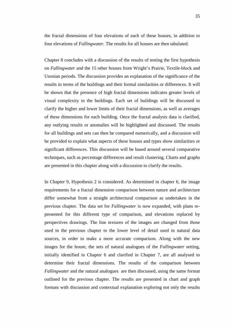
Chapter 8 concludes with a discussion of the results of testing the first hypothesis

on Fallingwater and the 15 other houses from Wright’s Prairie, Textile-block and

Usonian periods. The discussion provides an explanation of the significance of the

results in terms of the buildings and their formal similarities or differences. It will

be shown that the presence of high fractal dimensions indicates greater levels of

visual complexity in the buildings. Each set of buildings will be discussed to

clarify the higher and lower limits of their fractal dimensions, as well as averages

of these dimensions for each building. Once the fractal analysis data is clarified,

any outlying results or anomalies will be highlighted and discussed. The results

for all buildings and sets can then be compared numerically, and a discussion will

be provided to explain what aspects of these houses and types show similarities or

significant differences. This discussion will be based around several comparative

techniques, such as percentage differences and result clustering. Charts and graphs

are presented in this chapter along with a discussion to clarify the results.

In Chapter 9, Hypothesis 2 is considered. As determined in chapter 6, the image

requirements for a fractal dimension comparison between nature and architecture

differ somewhat from a straight architectural comparison as undertaken in the

previous chapter. The data set for Fallingwater is now expanded, with plans re-

presented for this different type of comparison, and elevations replaced by

perspectives drawings. The line textures of the images are changed from those

used in the previous chapter to the lower level of detail used in natural data

sources, in order to make a more accurate comparison. Along with the new

images for the house, the sets of natural analogues of the Fallingwater setting,

initially identified in Chapter 6 and clarified in Chapter 7, are all analysed to

determine their fractal dimensions. The results of the comparison between

Fallingwater and the natural analogues are then discussed, using the same format

outlined for the previous chapter. The results are presented in chart and graph

formats with discussion and contextual explanation exploring not only the results

36

but any problems or limitations that arose as part of the application of the method.

Finally, Chapter 10 summarises the conclusions, outcomes of the hypotheses and

possible directions for future research.

1.9 Relationship to Past Research

During the course of this dissertation, 11 journal papers, 15 chapters, and 14

conference papers on the topic were jointly published by the present author and

her supervisor, Michael Ostwald. The content of several of these publications has

been substantially revised as the basis for chapters in this dissertation.

Furthermore, several chapters in this dissertation share content with our recent

monograph, The Fractal Dimension of Architecture (Birkhauser 2016). In

particular, Chapters 2, 3, 4, 7 and 8 all include reworked material, at least partially

derived from this book. The details of this overlap are listed hereafter and are in

accordance with the standards and expectations of the University of Newcastle

and are acknowledged as such.

Chapter 2 includes some material previously published in: Ostwald, Michael J.,

and Josephine Vaughan. 2016. Organic Architecture. In The Fractal Dimension of

Architecture, 205–242. Birkhauser.

Chapter 3 includes some material previously published in: Ostwald, Michael J.,

and Josephine Vaughan. 2016. Fractals in Architectural Design and Critique. In

The Fractal Dimension of Architecture, 21–37. Birkhauser.

Chapter 4 includes material previously published in: Ostwald, Michael J., and

Josephine Vaughan. 2016. Introducing the Box-Counting Method. In The Fractal

Dimension of Architecture, 39–66. Birkhauser; Vaughan, Josephine, and Michael

J Ostwald. 2010. Refining a computational fractal method of analysis: testing

37

Bovill’s architectural data. In New Frontiers: Proceedings of the 15th

International Conference on Computer Aided Architectural Design Research in

Asia, 29–38. Hong Kong: CAADRIA.

Chapter 5 includes material previously published in: Ostwald, Michael J, and

Josephine Vaughan. 2013. Representing Architecture for Fractal Analysis: A

Framework for Identifying Significant Lines. Architectural Science Review 56:

242–251; Ostwald, Michael J, and Josephine Vaughan. 2013. Limits and Errors

Optimising Image Pre-Processing Standards for Architectural Fractal Analysis.

ArS Architecture Science 7: 1–19; Ostwald, Michael J., and Josephine Vaughan.

2016. Measuring Architecture. In The Fractal Dimension of Architecture, 67–85.

Birkhauser; Ostwald, Michael J., and Josephine Vaughan. 2016. Refining the

Method. In The Fractal Dimension of Architecture, 87–131. Birkhauser;

Vaughan, Josephine and Michael J. Ostwald. 2009. Refining the Computational

Method for the Evaluation of Visual Complexity in Architectural Images:

Significant Lines in the Early Architecture of Le Corbusier. In Computation: The

New Realm of Architectural Design: Proceedings of eCAADe27. 689-698.

Istanbul, Turkey: eCAADe.

Chapter 6 includes material previously published in: Vaughan, Josephine, and

Michael J Ostwald. 2017. The Comparative Numerical Analysis Of Nature And

Architecture: A New Framework. International Journal of Design & Nature and

Ecodynamics 12: 156–166; Vaughan, Josephine, and Michael J Ostwald. 2009.

Nature and architecture: revisiting the fractal connection in Amasya and Sea

Ranch. In Performative Ecologies in the Built Environment: Sustainability

Research Across Disciplines, 42. Launceston, Tasmania; Vaughan, Josephine, and

Michael J Ostwald. 2010. Using fractal analysis to compare the characteristic

complexity of nature and architecture: re-examining the evidence. Architectural

Science Review 53: 323–332.

38

Chapter 7 includes material previously published in: Ostwald, Michael J., and

Josephine Vaughan. 2016. Analysing the Twentieth-Century House. In The

Fractal Dimension of Architecture, 135–157. Birkhauser.

Chapter 8 includes material previously published in: Vaughan, Josephine and

Michael J. Ostwald. 2011. The Relationship Between the Fractal Dimension of

Plans and Elevations in the. Architecture of Frank Lloyd Wright: Comparing The

Prairie Style, Textile Block and Usonian Periods. Architectural Science Research:

ArS. 4: 21-44; Vaughan, Josephine and Michael J. Ostwald. 2010. A Quantitative

Comparison between Wright’s Prairie Style and Triangle-Plan Usonian Houses

Using Fractal Analysis. Design Principles and Practices: An International

Journal, 4: 333 – 344.

Methodological refinements described in the following works are also

accommodated in the approach taken in this dissertation: Vaughan, Josephine. and

Michael J. Ostwald. 2014. Measuring the significance of façade transparency in

Australian regionalist architecture: A computational analysis of 10 designs by

Glenn Murcutt. Architectural Science Review 57: 249-259; Vaughan, Josephine

and Michael J. Ostwald. 2009. A Quantitative Comparison between the Formal

Complexity of Le Corbusier’s Pre-Modern (1905-1912) and Early Modern (1922-

1928) Architecture. Design Principles and Practices: An International Journal, 3:

359 – 371; Vaughan, Josephine and Michael J. Ostwald, 2014. Quantifying the

changing visual experience of architecture: Combining Movement with Visual

Complexity. In. Across: Architectural Research through to Practice: Proceedings

of the 48th International Conference of the Architectural Science Association:

557–568. Genoa, Italy: ANZAScA; Vaughan, Josephine and Michael J. Ostwald

2010. Refining a computational fractal method of analysis: testing Bovill’s

architectural data. In Proceedings of the 15th International Conference on

Computer Aided Architectural Design Research in Asia: 29-38. Hong Kong:

CAADRIA; Vaughan, Josephine and Michael J. Ostwald. 2008. Approaching

Euclidean Limits: A Fractal Analysis of the Architecture of Kazuyo Sejima. In

39

Innovation Inspiration and Instruction: New Knowledge in the Architectural

Sciences, ANZAScA 08: 285-294. Newcastle, Australia: ANZAScA.

40

Chapter 2

Frank Lloyd Wright and Fallingwater

Accounts of Frank Lloyd Wright’s architecture and design philosophy often

include claims about connections to the natural world and his veneration of the

landscape. Indeed, scholarly readings of the relationship between Wright’s

architecture and nature, combined with Wright’s own, often unclear,

pronouncements on the metaphysical properties of the natural world, have

resulted in a general view that ‘Wright regarded nature in almost mystical terms’

(Pfeiffer 2004: 12). So strong was his nature-oriented doctrine that Wright would

eventually claim a thread of the Modernist style almost entirely to himself, being

known as the ‘father of organic architecture’ (Pearson 2001: 39). While the words

nature, organic and landscape are often conflated when scholars talk about

Wright’s influence, there are important distinctions between them. For example,

popular thought in the early years of the twentieth century may have conceived of

nature as a spiritual, transcendent or poetic presence (Hoffmann 1995; Miller

2009), but there was also interest in the physical forms and ecological operations

of the natural landscape (Olsberg 1996). The terms ‘landscape’ and ‘nature’ are

pivotal to the arguments developed in this thesis and the intricacies of these terms

are unpacked throughout the chapter. The essential difference between nature and

landscape is significant because it has been argued that Wright typically

differentiated landscape from nature (Cronon 1994: 14; Spirn 2000a: 17). This

distinction is at the core of the present chapter.

This chapter commences with an overview of Wright’s attitudes to nature and

how they developed throughout his career. Beginning with Wright’s views about

landscape and how these evolved during his early years on the family farm, this

chapter presents some of the history of Wright’s career, focusing on those

moments when the natural landscape became a driving force in his personal and

architectural identity. The first section of the chapter effectively provides a

background to his design philosophy, and it is included here in part as

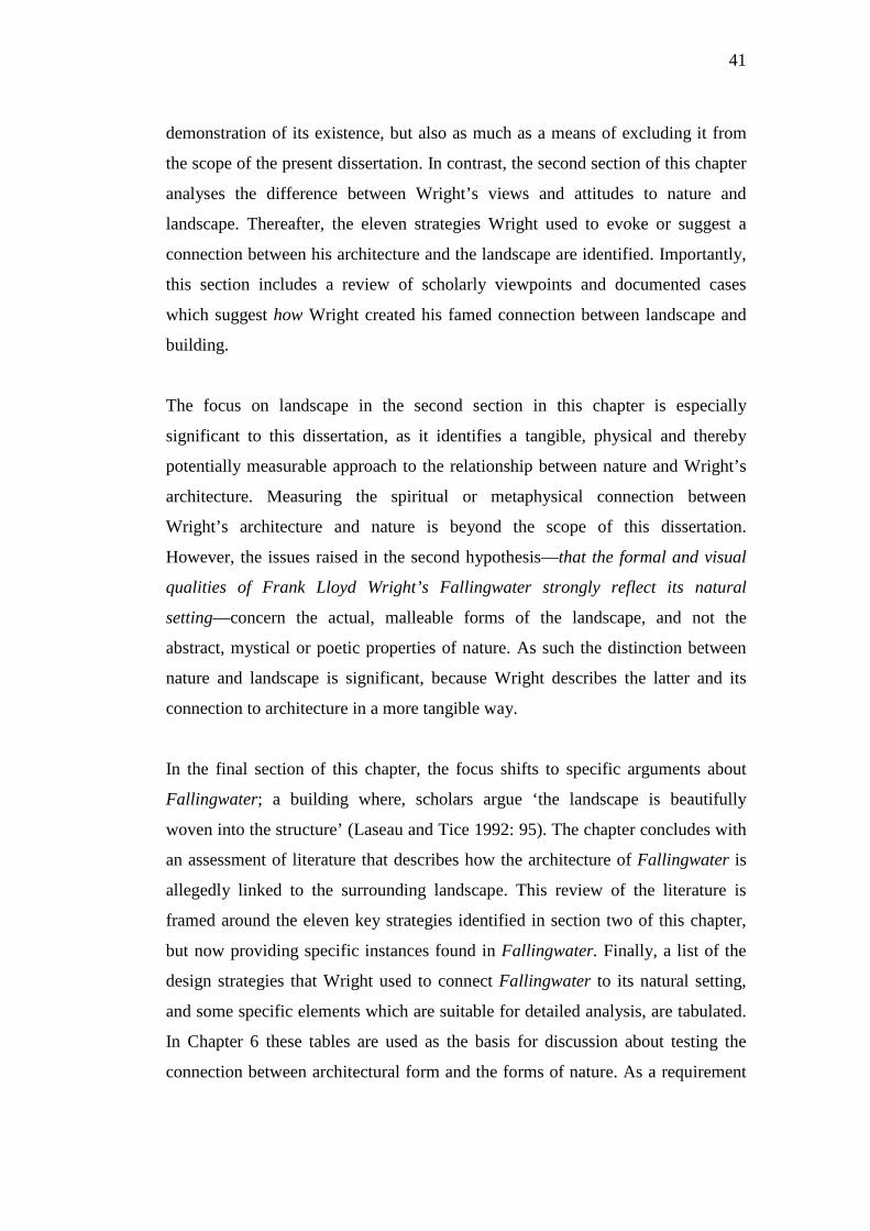
41

demonstration of its existence, but also as much as a means of excluding it from

the scope of the present dissertation. In contrast, the second section of this chapter

analyses the difference between Wright’s views and attitudes to nature and

landscape. Thereafter, the eleven strategies Wright used to evoke or suggest a

connection between his architecture and the landscape are identified. Importantly,

this section includes a review of scholarly viewpoints and documented cases

which suggest how Wright created his famed connection between landscape and

building.

The focus on landscape in the second section in this chapter is especially

significant to this dissertation, as it identifies a tangible, physical and thereby

potentially measurable approach to the relationship between nature and Wright’s

architecture. Measuring the spiritual or metaphysical connection between

Wright’s architecture and nature is beyond the scope of this dissertation.

However, the issues raised in the second hypothesis—that the formal and visual

qualities of Frank Lloyd Wright’s Fallingwater strongly reflect its natural

setting—concern the actual, malleable forms of the landscape, and not the

abstract, mystical or poetic properties of nature. As such the distinction between

nature and landscape is significant, because Wright describes the latter and its

connection to architecture in a more tangible way.

In the final section of this chapter, the focus shifts to specific arguments about

Fallingwater; a building where, scholars argue ‘the landscape is beautifully

woven into the structure’ (Laseau and Tice 1992: 95). The chapter concludes with

an assessment of literature that describes how the architecture of Fallingwater is

allegedly linked to the surrounding landscape. This review of the literature is

framed around the eleven key strategies identified in section two of this chapter,

but now providing specific instances found in Fallingwater. Finally, a list of the

design strategies that Wright used to connect Fallingwater to its natural setting,

and some specific elements which are suitable for detailed analysis, are tabulated.

In Chapter 6 these tables are used as the basis for discussion about testing the

connection between architectural form and the forms of nature. As a requirement

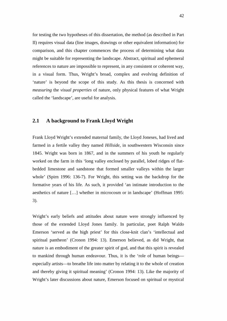
42

for testing the two hypotheses of this dissertation, the method (as described in Part

II) requires visual data (line images, drawings or other equivalent information) for

comparison, and this chapter commences the process of determining what data

might be suitable for representing the landscape. Abstract, spiritual and ephemeral

references to nature are impossible to represent, in any consistent or coherent way,

in a visual form. Thus, Wright’s broad, complex and evolving definition of

‘nature’ is beyond the scope of this study. As this thesis is concerned with

measuring the visual properties of nature, only physical features of what Wright

called the ‘landscape’, are useful for analysis.

2.1 A background to Frank Lloyd Wright

Frank Lloyd Wright’s extended maternal family, the Lloyd Joneses, had lived and

farmed in a fertile valley they named Hillside, in southwestern Wisconsin since

1845. Wright was born in 1867, and in the summers of his youth he regularly

worked on the farm in this ‘long valley enclosed by parallel, lobed ridges of flat-

bedded limestone and sandstone that formed smaller valleys within the larger

whole’ (Spirn 1996: 136-7). For Wright, this setting was the backdrop for the

formative years of his life. As such, it provided ‘an intimate introduction to the

aesthetics of nature […] whether in microcosm or in landscape’ (Hoffman 1995:

3).

Wright’s early beliefs and attitudes about nature were strongly influenced by

those of the extended Lloyd Jones family. In particular, poet Ralph Waldo

Emerson ‘served as the high priest’ for this close-knit clan’s ‘intellectual and

spiritual pantheon’ (Cronon 1994: 13). Emerson believed, as did Wright, that

nature is an embodiment of the greater spirit of god, and that this spirit is revealed

to mankind through human endeavour. Thus, it is the ‘role of human beings—

especially artists—to breathe life into matter by relating it to the whole of creation

and thereby giving it spiritual meaning’ (Cronon 1994: 13). Like the majority of

Wright’s later discussions about nature, Emerson focused on spiritual or mystical

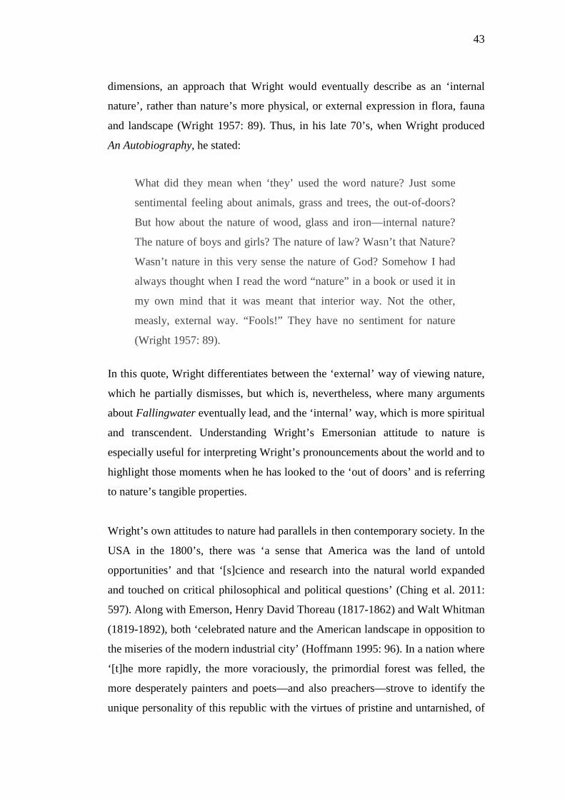
43

dimensions, an approach that Wright would eventually describe as an ‘internal

nature’, rather than nature’s more physical, or external expression in flora, fauna

and landscape (Wright 1957: 89). Thus, in his late 70’s, when Wright produced

An Autobiography, he stated:

What did they mean when ‘they’ used the word nature? Just some

sentimental feeling about animals, grass and trees, the out-of-doors?

But how about the nature of wood, glass and iron—internal nature?

The nature of boys and girls? The nature of law? Wasn’t that Nature?

Wasn’t nature in this very sense the nature of God? Somehow I had

always thought when I read the word “nature” in a book or used it in

my own mind that it was meant that interior way. Not the other,

measly, external way. “Fools!” They have no sentiment for nature

(Wright 1957: 89).

In this quote, Wright differentiates between the ‘external’ way of viewing nature,

which he partially dismisses, but which is, nevertheless, where many arguments

about Fallingwater eventually lead, and the ‘internal’ way, which is more spiritual

and transcendent. Understanding Wright’s Emersonian attitude to nature is

especially useful for interpreting Wright’s pronouncements about the world and to

highlight those moments when he has looked to the ‘out of doors’ and is referring

to nature’s tangible properties.

Wright’s own attitudes to nature had parallels in then contemporary society. In the

USA in the 1800’s, there was ‘a sense that America was the land of untold

opportunities’ and that ‘[s]cience and research into the natural world expanded

and touched on critical philosophical and political questions’ (Ching et al. 2011:

597). Along with Emerson, Henry David Thoreau (1817-1862) and Walt Whitman

(1819-1892), both ‘celebrated nature and the American landscape in opposition to

the miseries of the modern industrial city’ (Hoffmann 1995: 96). In a nation where

‘[t]he more rapidly, the more voraciously, the primordial forest was felled, the

more desperately painters and poets—and also preachers—strove to identify the

unique personality of this republic with the virtues of pristine and untarnished, of

44

“romantic,” Nature’ (Miller 2009: 207). The writings of Emerson, Thoreau and

Whitman shaped the American psyche of the time and its response to nature.

In addition to being influenced by figures from literature and philosophy,

Wright’s architectural thinking was also shaped by Eugène Emmanuel Viollet-le-

Duc (1814-1879) and John Ruskin (1819-1900), both of whom held nature-based

beliefs, promoted honesty in materials and felt that a spiritual or moral imperative

was required in design. Thomas Jefferson (1743-1826), not only the third

president of the United States but an architect and philosopher, also influenced

Wright’s early ideas about how ‘architecture was directly related to social reform’

(Ching et al. 2011: 619). Thus Wright, living at a time and in a place that

supported specific approaches of family, spirituality, philosophy, literature and the

arts, was influenced towards a particular life-view. This ‘philosophy’ was

underscored by a hands-on experience on the land and Wright reflected that this

approach ‘came to me gradually and mostly by way of the farm’ (1943: 243). The

combination of practical and theoretical aspects of this context assisted Wright to

develop an understanding of ‘the mysterious beauties and obvious cruelties of

Nature—interlocking interchanges of the universe’, these natural elements were

emphasised in Wright’s view when connected to architecture, as he concluded:

‘these began to fascinate me more when I began to build’ (243).

2.1.1 Wright’s Architectural Career

Wright began his architectural education in 1885 working for Joseph Silsbee—

whose ‘Queen Anne designs were very fashionable’ at the time (Storrer 2006:

3)—and then found a like-minded mentor under the employment of Louis

Sullivan from 1888 to 1893. Sullivan, a key figure in the development of large-

scale urban buildings of the late 1800’s, espoused ‘an emphatic rejection of any

autonomous form in building which failed to take account of function and

construction’ (Seidlein 1997: 326). Sullivan also famously advocated that ideally,

‘form [is] derived from nature’ (326). Through these attitudes and beliefs,

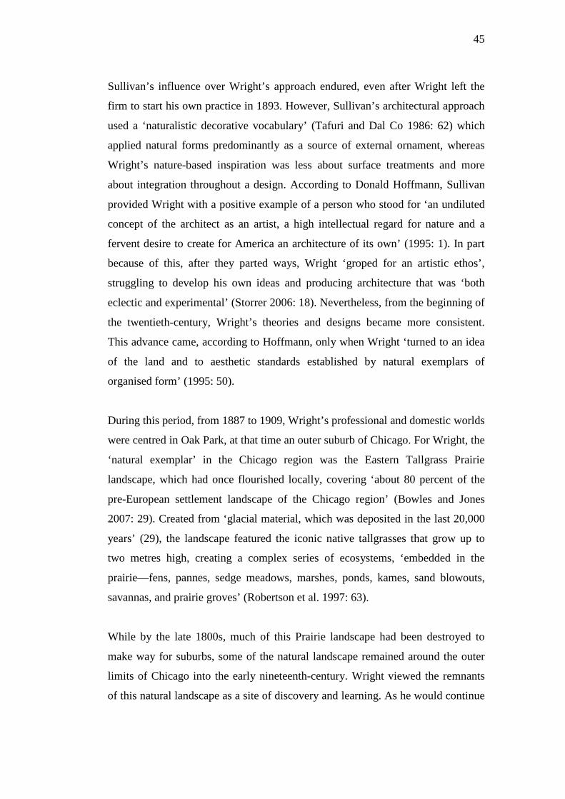
45

Sullivan’s influence over Wright’s approach endured, even after Wright left the

firm to start his own practice in 1893. However, Sullivan’s architectural approach

used a ‘naturalistic decorative vocabulary’ (Tafuri and Dal Co 1986: 62) which

applied natural forms predominantly as a source of external ornament, whereas

Wright’s nature-based inspiration was less about surface treatments and more

about integration throughout a design. According to Donald Hoffmann, Sullivan

provided Wright with a positive example of a person who stood for ‘an undiluted

concept of the architect as an artist, a high intellectual regard for nature and a

fervent desire to create for America an architecture of its own’ (1995: 1). In part

because of this, after they parted ways, Wright ‘groped for an artistic ethos’,

struggling to develop his own ideas and producing architecture that was ‘both

eclectic and experimental’ (Storrer 2006: 18). Nevertheless, from the beginning of

the twentieth-century, Wright’s theories and designs became more consistent.

This advance came, according to Hoffmann, only when Wright ‘turned to an idea

of the land and to aesthetic standards established by natural exemplars of

organised form’ (1995: 50).

During this period, from 1887 to 1909, Wright’s professional and domestic worlds

were centred in Oak Park, at that time an outer suburb of Chicago. For Wright, the

‘natural exemplar’ in the Chicago region was the Eastern Tallgrass Prairie

landscape, which had once flourished locally, covering ‘about 80 percent of the

pre-European settlement landscape of the Chicago region’ (Bowles and Jones

2007: 29). Created from ‘glacial material, which was deposited in the last 20,000

years’ (29), the landscape featured the iconic native tallgrasses that grow up to

two metres high, creating a complex series of ecosystems, ‘embedded in the

prairie—fens, pannes, sedge meadows, marshes, ponds, kames, sand blowouts,

savannas, and prairie groves’ (Robertson et al. 1997: 63).

While by the late 1800s, much of this Prairie landscape had been destroyed to

make way for suburbs, some of the natural landscape remained around the outer

limits of Chicago into the early nineteenth-century. Wright viewed the remnants

of this natural landscape as a site of discovery and learning. As he would continue

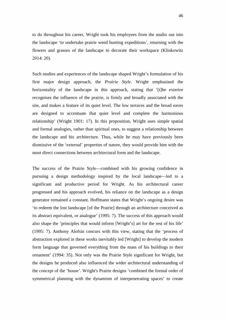
46

to do throughout his career, Wright took his employees from the studio out into

the landscape ‘to undertake prairie weed hunting expeditions’, returning with the

flowers and grasses of the landscape to decorate their workspace (Klinkowitz

2014: 20).

Such studies and experiences of the landscape shaped Wright’s formulation of his

first major design approach, the Prairie Style. Wright emphasised the

horizontality of the landscape in this approach, stating that ‘[t]he exterior

recognises the influence of the prairie, is firmly and broadly associated with the

site, and makes a feature of its quiet level. The low terraces and the broad eaves

are designed to accentuate that quiet level and complete the harmonious

relationship’ (Wright 1901: 17). In this proposition, Wright uses simple spatial

and formal analogies, rather than spiritual ones, to suggest a relationship between

the landscape and his architecture. Thus, while he may have previously been

dismissive of the ‘external’ properties of nature, they would provide him with the

most direct connections between architectural form and the landscape.

The success of the Prairie Style—combined with his growing confidence in

pursuing a design methodology inspired by the local landscape—led to a

significant and productive period for Wright. As his architectural career

progressed and his approach evolved, his reliance on the landscape as a design

generator remained a constant. Hoffmann states that Wright’s ongoing desire was

‘to redeem the lost landscape [of the Prairie] through an architecture conceived as

its abstract equivalent, or analogue’ (1995: 7). The success of this approach would

also shape the ‘principles that would inform [Wright’s] art for the rest of his life’

(1995: 7). Anthony Alofsin concurs with this view, stating that the ‘process of

abstraction explored in these works inevitably led [Wright] to develop the modern

form language that governed everything from the mass of his buildings to their

ornament’ (1994: 35). Not only was the Prairie Style significant for Wright, but

the designs he produced also influenced the wider architectural understanding of

the concept of the ‘house’. Wright's Prairie designs ‘combined the formal order of

symmetrical planning with the dynamism of interpenetrating spaces’ to create

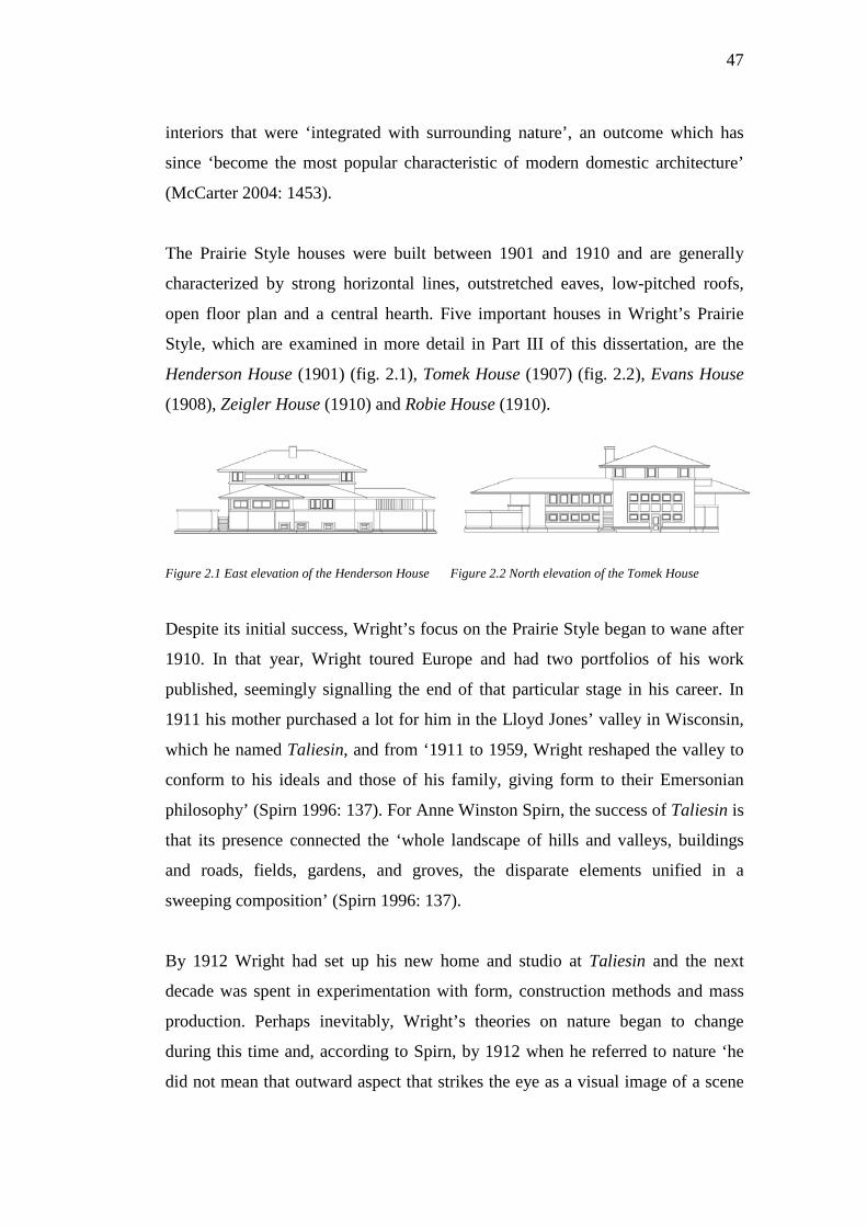
47

interiors that were ‘integrated with surrounding nature’, an outcome which has

since ‘become the most popular characteristic of modern domestic architecture’

(McCarter 2004: 1453).

The Prairie Style houses were built between 1901 and 1910 and are generally

characterized by strong horizontal lines, outstretched eaves, low-pitched roofs,

open floor plan and a central hearth. Five important houses in Wright’s Prairie

Style, which are examined in more detail in Part III of this dissertation, are the

Henderson House (1901) (fig. 2.1), Tomek House (1907) (fig. 2.2), Evans House

(1908), Zeigler House (1910) and Robie House (1910).

Figure 2.1 East elevation of the Henderson House Figure 2.2 North elevation of the Tomek House

Despite its initial success, Wright’s focus on the Prairie Style began to wane after

1910. In that year, Wright toured Europe and had two portfolios of his work

published, seemingly signalling the end of that particular stage in his career. In

1911 his mother purchased a lot for him in the Lloyd Jones’ valley in Wisconsin,

which he named Taliesin, and from ‘1911 to 1959, Wright reshaped the valley to

conform to his ideals and those of his family, giving form to their Emersonian

philosophy’ (Spirn 1996: 137). For Anne Winston Spirn, the success of Taliesin is

that its presence connected the ‘whole landscape of hills and valleys, buildings

and roads, fields, gardens, and groves, the disparate elements unified in a

sweeping composition’ (Spirn 1996: 137).

By 1912 Wright had set up his new home and studio at Taliesin and the next

decade was spent in experimentation with form, construction methods and mass

production. Perhaps inevitably, Wright’s theories on nature began to change

during this time and, according to Spirn, by 1912 when he referred to nature ‘he

did not mean that outward aspect that strikes the eye as a visual image of a scene

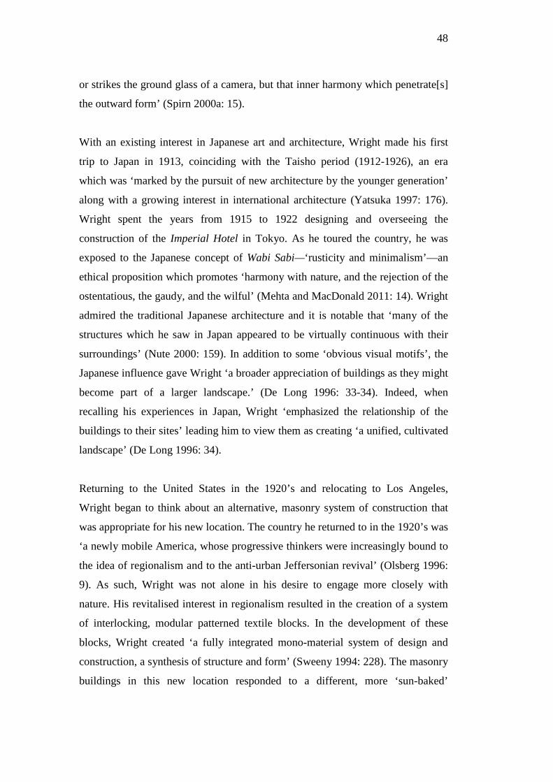
48

or strikes the ground glass of a camera, but that inner harmony which penetrate[s]

the outward form’ (Spirn 2000a: 15).

With an existing interest in Japanese art and architecture, Wright made his first

trip to Japan in 1913, coinciding with the Taisho period (1912-1926), an era

which was ‘marked by the pursuit of new architecture by the younger generation’

along with a growing interest in international architecture (Yatsuka 1997: 176).

Wright spent the years from 1915 to 1922 designing and overseeing the

construction of the Imperial Hotel in Tokyo. As he toured the country, he was

exposed to the Japanese concept of Wabi Sabi—‘rusticity and minimalism’—an

ethical proposition which promotes ‘harmony with nature, and the rejection of the

ostentatious, the gaudy, and the wilful’ (Mehta and MacDonald 2011: 14). Wright

admired the traditional Japanese architecture and it is notable that ‘many of the

structures which he saw in Japan appeared to be virtually continuous with their

surroundings’ (Nute 2000: 159). In addition to some ‘obvious visual motifs’, the

Japanese influence gave Wright ‘a broader appreciation of buildings as they might

become part of a larger landscape.’ (De Long 1996: 33-34). Indeed, when

recalling his experiences in Japan, Wright ‘emphasized the relationship of the

buildings to their sites’ leading him to view them as creating ‘a unified, cultivated

landscape’ (De Long 1996: 34).

Returning to the United States in the 1920’s and relocating to Los Angeles,

Wright began to think about an alternative, masonry system of construction that

was appropriate for his new location. The country he returned to in the 1920’s was

‘a newly mobile America, whose progressive thinkers were increasingly bound to

the idea of regionalism and to the anti-urban Jeffersonian revival’ (Olsberg 1996:

9). As such, Wright was not alone in his desire to engage more closely with

nature. His revitalised interest in regionalism resulted in the creation of a system

of interlocking, modular patterned textile blocks. In the development of these

blocks, Wright created ‘a fully integrated mono-material system of design and

construction, a synthesis of structure and form’ (Sweeny 1994: 228). The masonry

buildings in this new location responded to a different, more ‘sun-baked’

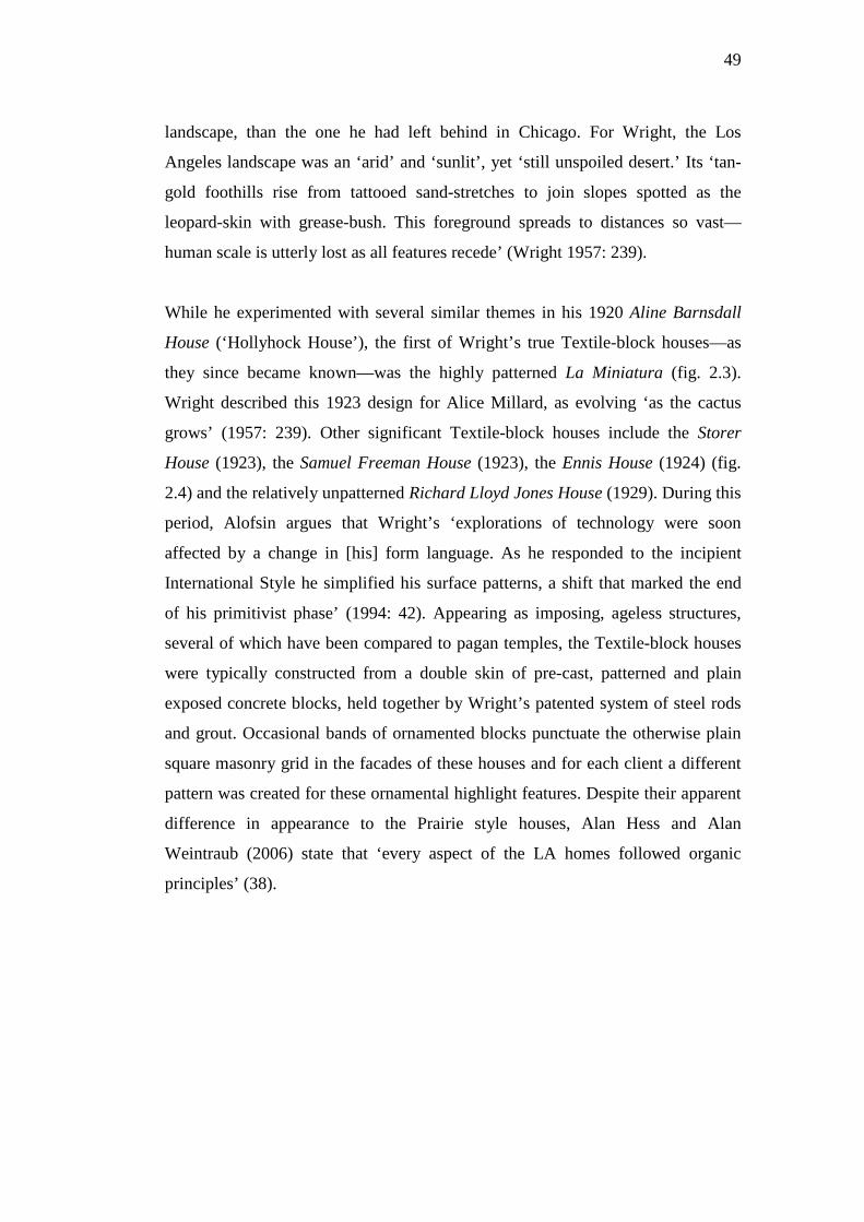
49

landscape, than the one he had left behind in Chicago. For Wright, the Los

Angeles landscape was an ‘arid’ and ‘sunlit’, yet ‘still unspoiled desert.’ Its ‘tan-

gold foothills rise from tattooed sand-stretches to join slopes spotted as the

leopard-skin with grease-bush. This foreground spreads to distances so vast—

human scale is utterly lost as all features recede’ (Wright 1957: 239).

While he experimented with several similar themes in his 1920 Aline Barnsdall

House (‘Hollyhock House’), the first of Wright’s true Textile-block houses—as

they since became known—was the highly patterned La Miniatura (fig. 2.3).

Wright described this 1923 design for Alice Millard, as evolving ‘as the cactus

grows’ (1957: 239). Other significant Textile-block houses include the Storer

House (1923), the Samuel Freeman House (1923), the Ennis House (1924) (fig.

2.4) and the relatively unpatterned Richard Lloyd Jones House (1929). During this

period, Alofsin argues that Wright’s ‘explorations of technology were soon

affected by a change in [his] form language. As he responded to the incipient

International Style he simplified his surface patterns, a shift that marked the end

of his primitivist phase’ (1994: 42). Appearing as imposing, ageless structures,

several of which have been compared to pagan temples, the Textile-block houses

were typically constructed from a double skin of pre-cast, patterned and plain

exposed concrete blocks, held together by Wright’s patented system of steel rods

and grout. Occasional bands of ornamented blocks punctuate the otherwise plain

square masonry grid in the facades of these houses and for each client a different

pattern was created for these ornamental highlight features. Despite their apparent

difference in appearance to the Prairie style houses, Alan Hess and Alan

Weintraub (2006) state that ‘every aspect of the LA homes followed organic

principles’ (38).

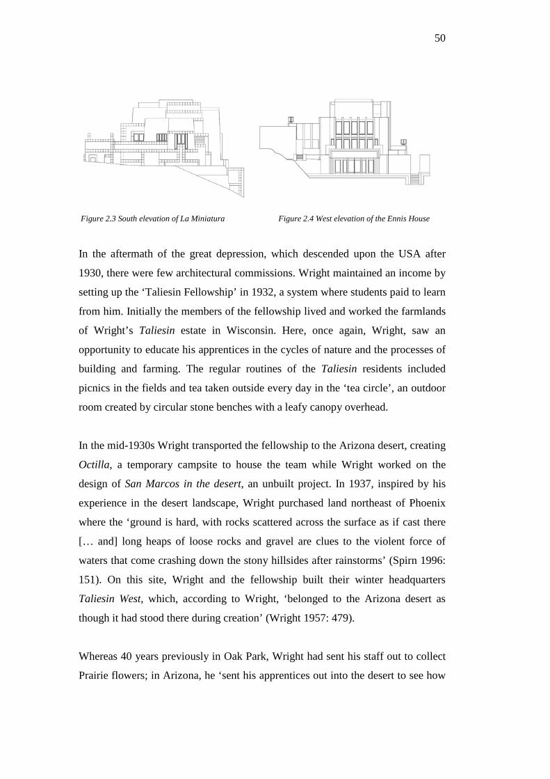
50

Figure 2.3 South elevation of La Miniatura Figure 2.4 West elevation of the Ennis House

In the aftermath of the great depression, which descended upon the USA after

1930, there were few architectural commissions. Wright maintained an income by

setting up the ‘Taliesin Fellowship’ in 1932, a system where students paid to learn

from him. Initially the members of the fellowship lived and worked the farmlands

of Wright’s Taliesin estate in Wisconsin. Here, once again, Wright, saw an

opportunity to educate his apprentices in the cycles of nature and the processes of

building and farming. The regular routines of the Taliesin residents included

picnics in the fields and tea taken outside every day in the ‘tea circle’, an outdoor

room created by circular stone benches with a leafy canopy overhead.

In the mid-1930s Wright transported the fellowship to the Arizona desert, creating

Octilla, a temporary campsite to house the team while Wright worked on the

design of San Marcos in the desert, an unbuilt project. In 1937, inspired by his

experience in the desert landscape, Wright purchased land northeast of Phoenix

where the ‘ground is hard, with rocks scattered across the surface as if cast there

[… and] long heaps of loose rocks and gravel are clues to the violent force of

waters that come crashing down the stony hillsides after rainstorms’ (Spirn 1996:

151). On this site, Wright and the fellowship built their winter headquarters

Taliesin West, which, according to Wright, ‘belonged to the Arizona desert as

though it had stood there during creation’ (Wright 1957: 479).

Whereas 40 years previously in Oak Park, Wright had sent his staff out to collect

Prairie flowers; in Arizona, he ‘sent his apprentices out into the desert to see how

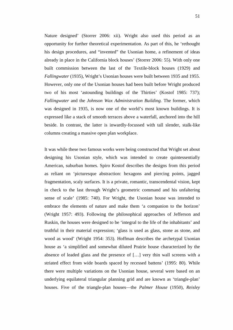
51

Nature designed’ (Storrer 2006: xii). Wright also used this period as an

opportunity for further theoretical experimentation. As part of this, he ‘rethought

his design procedures, and “invented” the Usonian home, a refinement of ideas

already in place in the California block houses’ (Storrer 2006: 55). With only one

built commission between the last of the Textile-block houses (1929) and

Fallingwater (1935), Wright’s Usonian houses were built between 1935 and 1955.

However, only one of the Usonian houses had been built before Wright produced

two of his most ‘astounding buildings of the Thirties’ (Kostof 1985: 737);

Fallingwater and the Johnson Wax Administration Building. The former, which

was designed in 1935, is now one of the world’s most known buildings. It is

expressed like a stack of smooth terraces above a waterfall, anchored into the hill

beside. In contrast, the latter is inwardly-focussed with tall slender, stalk-like

columns creating a massive open plan workplace.

It was while these two famous works were being constructed that Wright set about

designing his Usonian style, which was intended to create quintessentially

American, suburban homes. Spiro Kostof describes the designs from this period

as reliant on ‘picturesque abstraction: hexagons and piercing points, jagged

fragmentation, scaly surfaces. It is a private, romantic, transcendental vision, kept

in check to the last through Wright’s geometric command and his unfaltering

sense of scale’ (1985: 740). For Wright, the Usonian house was intended to

embrace the elements of nature and make them ‘a companion to the horizon’

(Wright 1957: 493). Following the philosophical approaches of Jefferson and

Ruskin, the houses were designed to be ‘integral to the life of the inhabitants’ and

truthful in their material expression; ‘glass is used as glass, stone as stone, and

wood as wood’ (Wright 1954: 353). Hoffman describes the archetypal Usonian

house as ‘a simplified and somewhat diluted Prairie house characterized by the

absence of leaded glass and the presence of […] very thin wall screens with a

striated effect from wide boards spaced by recessed battens’ (1995: 80). While

there were multiple variations on the Usonian house, several were based on an

underlying equilateral triangular planning grid and are known as ‘triangle-plan’

houses. Five of the triangle-plan houses—the Palmer House (1950), Reisley

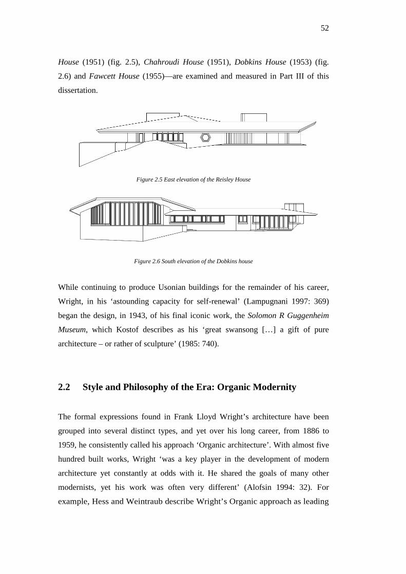
52

House (1951) (fig. 2.5), Chahroudi House (1951), Dobkins House (1953) (fig.

2.6) and Fawcett House (1955)—are examined and measured in Part III of this

dissertation.

Figure 2.5 East elevation of the Reisley House

Figure 2.6 South elevation of the Dobkins house

While continuing to produce Usonian buildings for the remainder of his career,

Wright, in his ‘astounding capacity for self-renewal’ (Lampugnani 1997: 369)

began the design, in 1943, of his final iconic work, the Solomon R Guggenheim

Museum, which Kostof describes as his ‘great swansong […] a gift of pure

architecture – or rather of sculpture’ (1985: 740).

2.2 Style and Philosophy of the Era: Organic Modernity

The formal expressions found in Frank Lloyd Wright’s architecture have been

grouped into several distinct types, and yet over his long career, from 1886 to

1959, he consistently called his approach ‘Organic architecture’. With almost five

hundred built works, Wright ‘was a key player in the development of modern

architecture yet constantly at odds with it. He shared the goals of many other

modernists, yet his work was often very different’ (Alofsin 1994: 32). For

example, Hess and Weintraub describe Wright’s Organic approach as leading

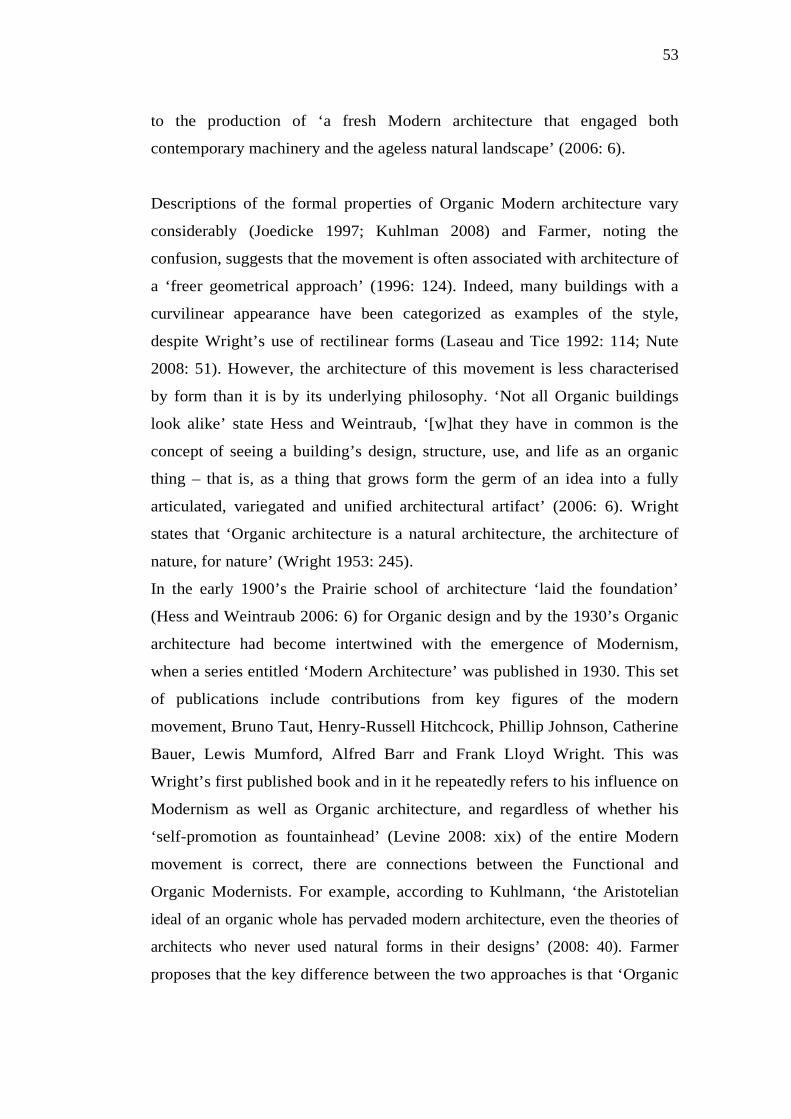
53

to the production of ‘a fresh Modern architecture that engaged both

contemporary machinery and the ageless natural landscape’ (2006: 6).

Descriptions of the formal properties of Organic Modern architecture vary

considerably (Joedicke 1997; Kuhlman 2008) and Farmer, noting the

confusion, suggests that the movement is often associated with architecture of

a ‘freer geometrical approach’ (1996: 124). Indeed, many buildings with a

curvilinear appearance have been categorized as examples of the style,

despite Wright’s use of rectilinear forms (Laseau and Tice 1992: 114; Nute

2008: 51). However, the architecture of this movement is less characterised

by form than it is by its underlying philosophy. ‘Not all Organic buildings

look alike’ state Hess and Weintraub, ‘[w]hat they have in common is the

concept of seeing a building’s design, structure, use, and life as an organic

thing – that is, as a thing that grows form the germ of an idea into a fully

articulated, variegated and unified architectural artifact’ (2006: 6). Wright

states that ‘Organic architecture is a natural architecture, the architecture of

nature, for nature’ (Wright 1953: 245).

In the early 1900’s the Prairie school of architecture ‘laid the foundation’

(Hess and Weintraub 2006: 6) for Organic design and by the 1930’s Organic

architecture had become intertwined with the emergence of Modernism,

when a series entitled ‘Modern Architecture’ was published in 1930. This set

of publications include contributions from key figures of the modern

movement, Bruno Taut, Henry-Russell Hitchcock, Phillip Johnson, Catherine

Bauer, Lewis Mumford, Alfred Barr and Frank Lloyd Wright. This was

Wright’s first published book and in it he repeatedly refers to his influence on

Modernism as well as Organic architecture, and regardless of whether his

‘self-promotion as fountainhead’ (Levine 2008: xix) of the entire Modern

movement is correct, there are connections between the Functional and

Organic Modernists. For example, according to Kuhlmann, ‘the Aristotelian

ideal of an organic whole has pervaded modern architecture, even the theories of

architects who never used natural forms in their designs’ (2008: 40). Farmer

proposes that the key difference between the two approaches is that ‘Organic

54

theories had sources not only in science but in poetic thinking too’ (1996:

124). While Organic architecture is often considered ‘synonymous with the

buildings and writings of Frank Lloyd Wright’ (Farmer and Richardson

1996: 124), there were several other key proponents of the style in the

United States who had worked with Wright. These include Rudolph

Schindler, Bruce Goff, John Lautner, Alden Dow and Frank Lloyd Wright’s

son, Lloyd Wright.

2.3 Identifying Separate Definitions of Landscape and Nature

Identifying precisely what Wright meant when he spoke of ‘nature’ can be

difficult. As Spirn observes, ‘Wright used the word “nature” in several senses’

including as ‘an essential quality, material reality and divine force’. Indeed, he

‘often moved from one sense of the word to another without transition’ (2000b:

15). Wright practiced architecture and published many written works over a

period of seven decades. This extended period provided ample time for him to

develop and then revise his thoughts about nature (Hoffmann 1995). For example,

Wright’s proclamations about Organic architecture clearly change throughout his

long career. Another substantial difficulty in interpreting Wright’s thoughts on

nature is that his written words, and transcripts of his lectures and interviews, are

notoriously ambiguous and tend to ramble in vague or ill-defined ways. Sibyl

Moholy-Nagy describes Wright’s verbal expression as being a ‘well-known

mixture of poetic pantheism […] ranting attack […and] unabashed self-

glorification’ (1959: 319). Wright’s ideas and arguments were often so extensive

that he ‘found it sufficient if his words conveyed their general shape or effect’ and

not their specifics (Nordland 1988: 4). The consequence of this approach is that a

complex mythology has grown around Wright and his philosophy of nature. For

example, a common argument is that for Wright, the ‘central idea often came from

nature’ (Bovill 1996: 6). Such a description, while useful and valid when forming

an overall understanding about Wright’s theory and design, is neither specific nor

tangible enough for the purpose of this present study. However, whereas Wright’s

55

proclamations about nature are difficult to decipher and interpret, he had a

different attitude to the landscape, which he tended to describe in more concise

terms. For example, according to Spirn, ‘Wright revered nature, not landscape,

and his use of the two words was distinctly different. When Wright spoke of

nature, he spoke of principles, of authority for architectural form, and his words

were abstract. He rarely mentioned landscape; when he did describe a landscape,

his language focused upon recurrent features or pattern rather than idiosyncratic

variables’ (2000b: 15). The following sections in this chapter focus on Wright’s

approaches to designing in response to nature’s most tangible presence, the

landscape.

2.3.1 Wright’s Methods for Designing Buildings with Landscapes

By setting aside Wright’s somewhat spiritual and often nonspecific views on

nature and focusing instead on the more defined topic of landscape, particular

methods that he employed to create the ‘building-of-nature’ effect have been

consistently observed by scholars. However, even this process is not without its

challenges. For example, Nicholas Olsberg suggests that Wright has a strong

‘discipline with which he analysed […the] forms and processes’ of the American

wilderness. Unfortunately, Olsberg does not provide a detailed description of

Wright’s ‘deep reading of terrain’ (1996: 10). Nevertheless, some authors have

attempted to identify the precise design strategies which Wright used to contribute

to the impression that his buildings are directly connected to their settings. This

section looks at two of these responses to the landscape: design strategies and site

integration.

Design strategies

Six interconnected and recurring design strategies, for linking Wright’s

architecture to nature, have been identified by historians, scholars and critics. The

six are: his approach to the ground; the formal mass of the building; the roof; the

openings; any intersections with natural features of the location; and the material

palette. Each of these are examined hereafter.

56

• The first of Wright’s recurring design strategies involves the relationship

between the ground floor and the landscape. The ‘ground-hugging’ (Frazier

1995: forward) appearance of many of Wright’s buildings is a property which

has been repeatedly emphasised by scholars (Richards 1970; Hoffmann 1995;

Frazier 1995; McCarter 2004). While there are several common ways of

providing foundation support for a building—such as being set up on piers,

stilts or cantilevered—Wright’s buildings were generally built using a slab-

on-ground technique. This approach typically involves ‘a concrete slab with

integral edge beams’ being ‘placed on the ground’, where it ‘provides the

base and floor structure for the building’ (Milton 1994: 227). This common

building method does not, in itself, provide strong evidence of a special

connection of the building to the landscape. If this was the case, the frequency

of its use would mean that most architects today could be regarded as

‘building with nature’. What is specific to Wright is the creation (and

expression) of a wide, firm, concrete, rock or earth-berm like firmament, as

an integral element. This element is often emphasised by long, low masonry

walls along with porches, terraces and horizontal planters. The effect can be

seen in his Prairie Style houses, and especially the Robie House. The

extended and emphasised solid plinth for a design, often executed in a

contrasting color or material to the walls, usually results in the lowest floor

level being raised above ground level, but still being firmly connected to it.

This design strategy expressed a ‘grip on the earth’ (Hoffmann 1995: 10), a

sense which was further emphasised by Wright’s use of accentuated linear

form—particularly parallel horizontal lines—throughout his buildings, not

just on the surface or facade (Hoffmann 1995; Maddex 1998). In

combination, these formal strategies created the sense of a building that

‘embraced the ground of which it should seem to grow’ (Frazier 1995:

forward).

• The second of Wright’s design strategies that sought to emphasise the

connection to nature involves massing. One of Wright’s most common

57

approaches to architectural form was to shift the planes of his buildings, to

dissolve their footprints, rooflines, and general massing, such that they seem

to ‘penetrate the landscape even as the landscape penetrates the building’

(Moholy-Nagy 1959: 327). This approach can be seen in many of Wright’s

plans, which appear to have sections cut out of them, and at the same time,

other sections extrude beyond a typical perimeter (Giedion 1959; McCarter

2004). This effect can be seen in Taliesin West, which is ‘notched, and knit’

into the landscape, with walls that are ‘cut into, extend above [and] reach out

to the immediate terrain’ (Spirn 1996: 152). While less specific, Paul Laseau

and James Tice suggest that when the formal symmetry of Wright’s work is

broken up in accordance with this strategy, it gives a building a more

‘natural’ feel (1992: 70). Wright’s approach to massing, in which the

landscape and building work together as physical volumes interacting or

intersecting in three dimensions, is what scholars (and Wright himself) refer

to as an architectural ‘weave’. Laseau and Tice observe this geometric

tapestry in Wright’s buildings where typically the ‘predominantly horizontal

spatial weave was complimented by a vertical spatial weave’ (1992: 94). John

Sergeant highlights Wright’s strong development of this ‘warp and woof’

approach to form in the Textile-block houses, which were usually set on

steep sites, thus enhancing Wright’s three-dimensional weave, which ‘allows

nature in the form of the demands of the site to penetrate Wright’s geometric

grid […] and to coexist there with the solid elements of the house’ (Sergeant

2005: 195).

• The third of Wright’s recurring design strategies involves the extension of his

rooflines into the landscape. This strategy, which often involves extensive

cantilevered roofs, surprised many, including Wright’s clients the Tomeks,

who requested that posts be added to their cantilevered roof because it looked

too precarious. When he first developed this strategy during his Prairie Style

period, Wright stated that ‘the broad eaves are designed to accentuate that

quiet level [of the prairie] and complete the harmonious relationship’ (Wright

1901: 17) between the building and the landscape. The effect, suggests

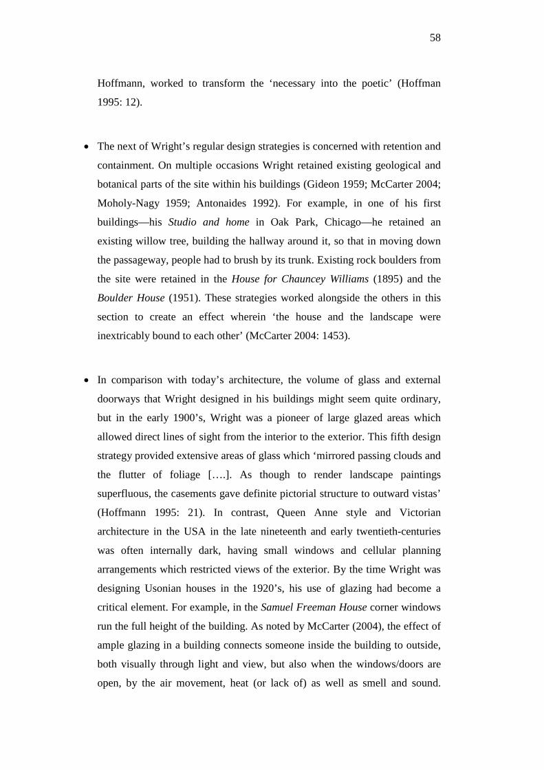
58

Hoffmann, worked to transform the ‘necessary into the poetic’ (Hoffman

1995: 12).

• The next of Wright’s regular design strategies is concerned with retention and

containment. On multiple occasions Wright retained existing geological and

botanical parts of the site within his buildings (Gideon 1959; McCarter 2004;

Moholy-Nagy 1959; Antonaides 1992). For example, in one of his first

buildings—his Studio and home in Oak Park, Chicago—he retained an

existing willow tree, building the hallway around it, so that in moving down

the passageway, people had to brush by its trunk. Existing rock boulders from

the site were retained in the House for Chauncey Williams (1895) and the

Boulder House (1951). These strategies worked alongside the others in this

section to create an effect wherein ‘the house and the landscape were

inextricably bound to each other’ (McCarter 2004: 1453).

• In comparison with today’s architecture, the volume of glass and external

doorways that Wright designed in his buildings might seem quite ordinary,

but in the early 1900’s, Wright was a pioneer of large glazed areas which

allowed direct lines of sight from the interior to the exterior. This fifth design

strategy provided extensive areas of glass which ‘mirrored passing clouds and

the flutter of foliage [….]. As though to render landscape paintings

superfluous, the casements gave definite pictorial structure to outward vistas’

(Hoffmann 1995: 21). In contrast, Queen Anne style and Victorian

architecture in the USA in the late nineteenth and early twentieth-centuries

was often internally dark, having small windows and cellular planning

arrangements which restricted views of the exterior. By the time Wright was

designing Usonian houses in the 1920’s, his use of glazing had become a

critical element. For example, in the Samuel Freeman House corner windows

run the full height of the building. As noted by McCarter (2004), the effect of

ample glazing in a building connects someone inside the building to outside,

both visually through light and view, but also when the windows/doors are

open, by the air movement, heat (or lack of) as well as smell and sound.

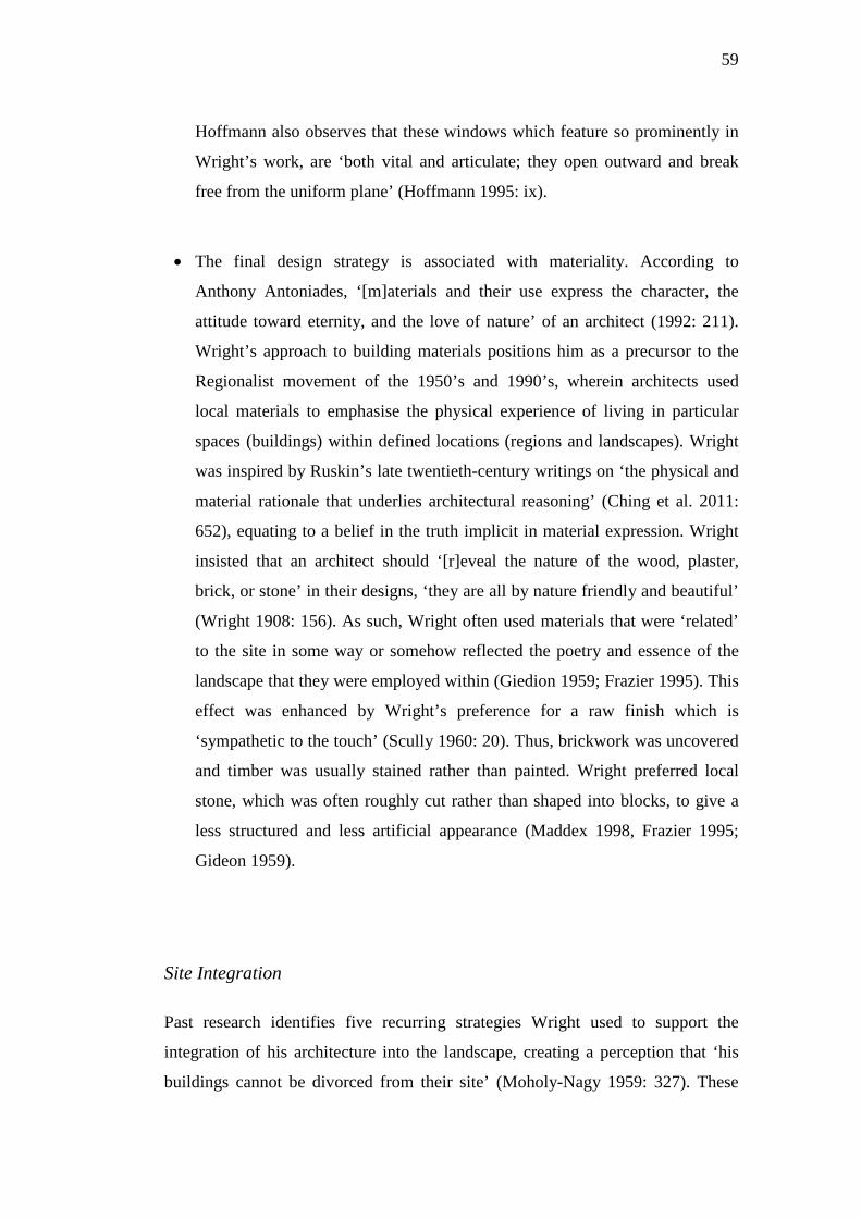
59

Hoffmann also observes that these windows which feature so prominently in

Wright’s work, are ‘both vital and articulate; they open outward and break

free from the uniform plane’ (Hoffmann 1995: ix).

• The final design strategy is associated with materiality. According to

Anthony Antoniades, ‘[m]aterials and their use express the character, the

attitude toward eternity, and the love of nature’ of an architect (1992: 211).

Wright’s approach to building materials positions him as a precursor to the

Regionalist movement of the 1950’s and 1990’s, wherein architects used

local materials to emphasise the physical experience of living in particular

spaces (buildings) within defined locations (regions and landscapes). Wright

was inspired by Ruskin’s late twentieth-century writings on ‘the physical and

material rationale that underlies architectural reasoning’ (Ching et al. 2011:

652), equating to a belief in the truth implicit in material expression. Wright

insisted that an architect should ‘[r]eveal the nature of the wood, plaster,

brick, or stone’ in their designs, ‘they are all by nature friendly and beautiful’

(Wright 1908: 156). As such, Wright often used materials that were ‘related’

to the site in some way or somehow reflected the poetry and essence of the

landscape that they were employed within (Giedion 1959; Frazier 1995). This

effect was enhanced by Wright’s preference for a raw finish which is

‘sympathetic to the touch’ (Scully 1960: 20). Thus, brickwork was uncovered

and timber was usually stained rather than painted. Wright preferred local

stone, which was often roughly cut rather than shaped into blocks, to give a

less structured and less artificial appearance (Maddex 1998, Frazier 1995;

Gideon 1959).

Site Integration

Past research identifies five recurring strategies Wright used to support the

integration of his architecture into the landscape, creating a perception that ‘his

buildings cannot be divorced from their site’ (Moholy-Nagy 1959: 327). These

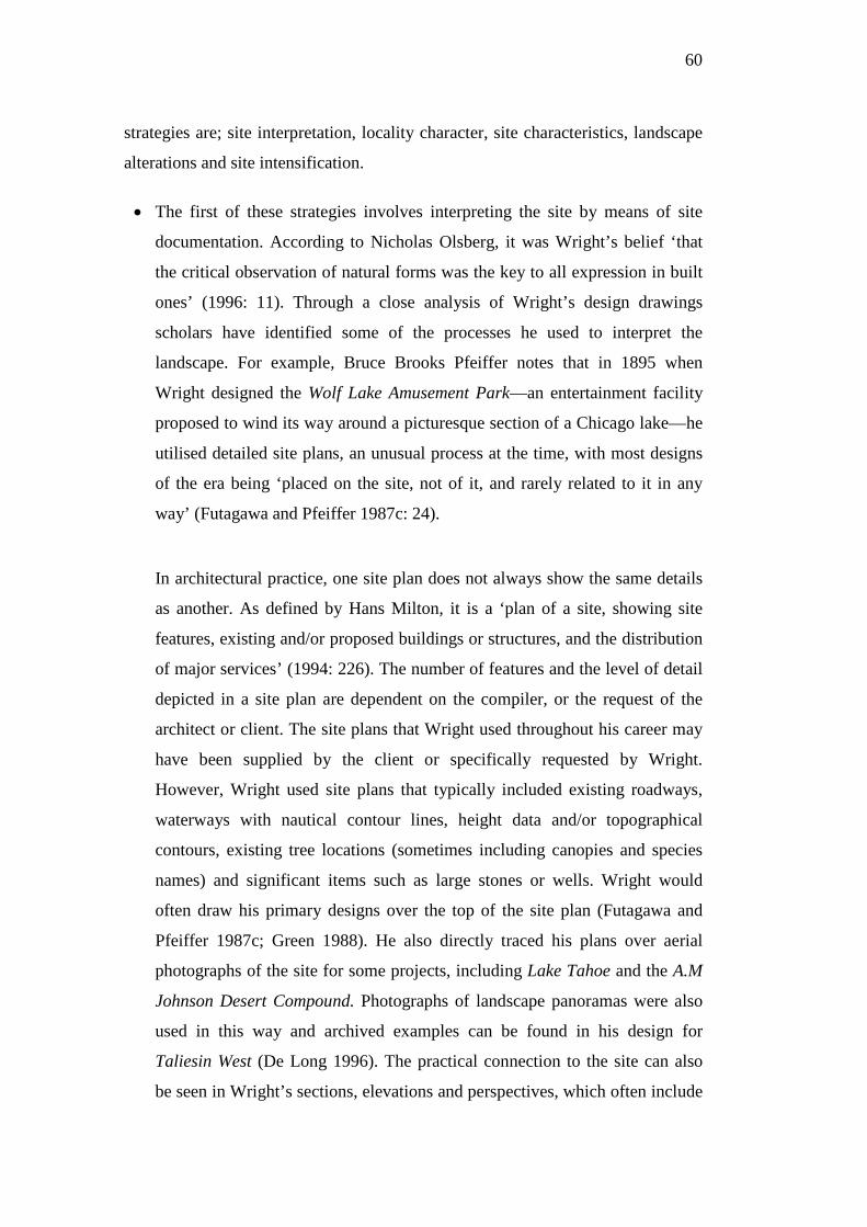
60

strategies are; site interpretation, locality character, site characteristics, landscape

alterations and site intensification.

• The first of these strategies involves interpreting the site by means of site

documentation. According to Nicholas Olsberg, it was Wright’s belief ‘that

the critical observation of natural forms was the key to all expression in built

ones’ (1996: 11). Through a close analysis of Wright’s design drawings

scholars have identified some of the processes he used to interpret the

landscape. For example, Bruce Brooks Pfeiffer notes that in 1895 when

Wright designed the Wolf Lake Amusement Park—an entertainment facility

proposed to wind its way around a picturesque section of a Chicago lake—he

utilised detailed site plans, an unusual process at the time, with most designs

of the era being ‘placed on the site, not of it, and rarely related to it in any

way’ (Futagawa and Pfeiffer 1987c: 24).

In architectural practice, one site plan does not always show the same details

as another. As defined by Hans Milton, it is a ‘plan of a site, showing site

features, existing and/or proposed buildings or structures, and the distribution

of major services’ (1994: 226). The number of features and the level of detail

depicted in a site plan are dependent on the compiler, or the request of the

architect or client. The site plans that Wright used throughout his career may

have been supplied by the client or specifically requested by Wright.

However, Wright used site plans that typically included existing roadways,

waterways with nautical contour lines, height data and/or topographical

contours, existing tree locations (sometimes including canopies and species

names) and significant items such as large stones or wells. Wright would

often draw his primary designs over the top of the site plan (Futagawa and

Pfeiffer 1987c; Green 1988). He also directly traced his plans over aerial

photographs of the site for some projects, including Lake Tahoe and the A.M

Johnson Desert Compound. Photographs of landscape panoramas were also

used in this way and archived examples can be found in his design for

Taliesin West (De Long 1996). The practical connection to the site can also

be seen in Wright’s sections, elevations and perspectives, which often include

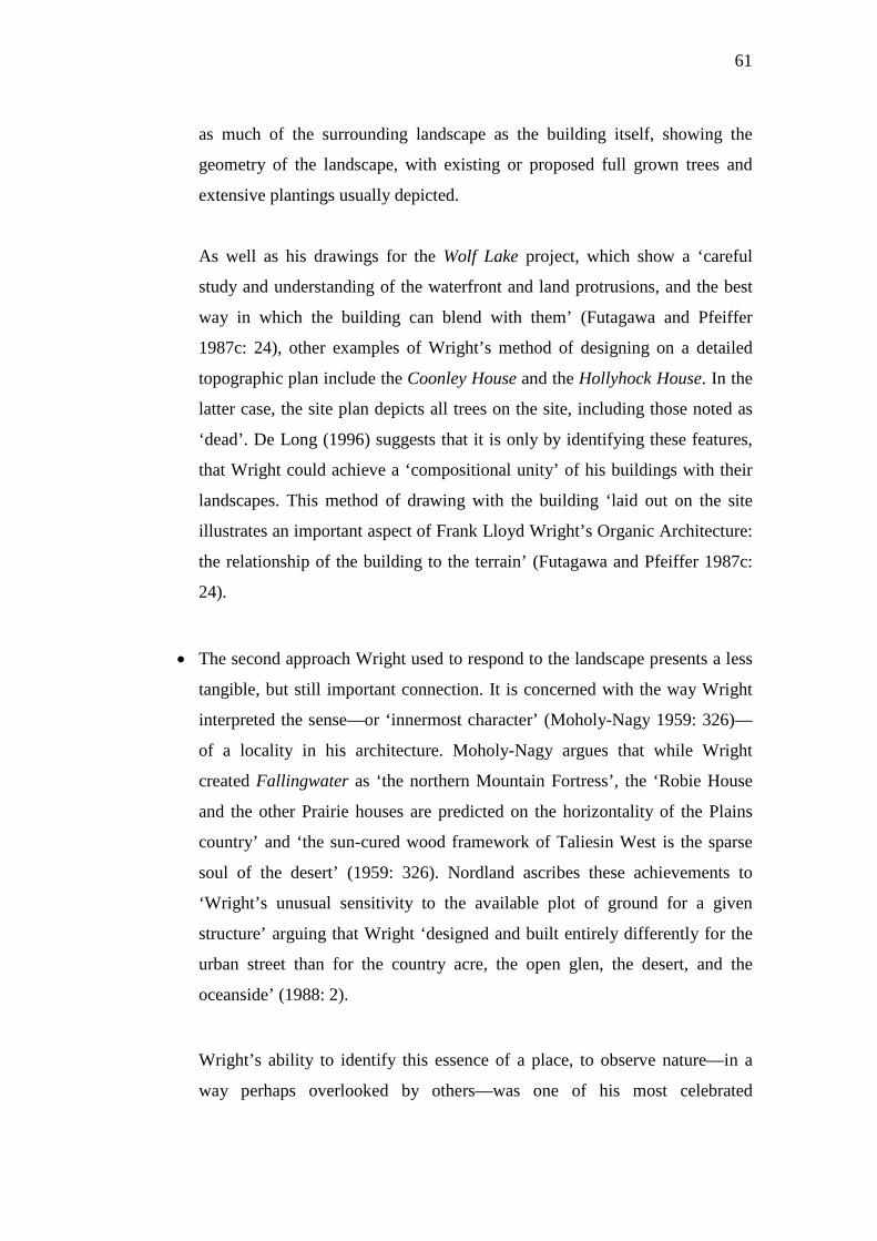
61

as much of the surrounding landscape as the building itself, showing the

geometry of the landscape, with existing or proposed full grown trees and

extensive plantings usually depicted.

As well as his drawings for the Wolf Lake project, which show a ‘careful

study and understanding of the waterfront and land protrusions, and the best

way in which the building can blend with them’ (Futagawa and Pfeiffer

1987c: 24), other examples of Wright’s method of designing on a detailed

topographic plan include the Coonley House and the Hollyhock House. In the

latter case, the site plan depicts all trees on the site, including those noted as

‘dead’. De Long (1996) suggests that it is only by identifying these features,

that Wright could achieve a ‘compositional unity’ of his buildings with their

landscapes. This method of drawing with the building ‘laid out on the site

illustrates an important aspect of Frank Lloyd Wright’s Organic Architecture:

the relationship of the building to the terrain’ (Futagawa and Pfeiffer 1987c:

24).

• The second approach Wright used to respond to the landscape presents a less

tangible, but still important connection. It is concerned with the way Wright

interpreted the sense—or ‘innermost character’ (Moholy-Nagy 1959: 326)—

of a locality in his architecture. Moholy-Nagy argues that while Wright

created Fallingwater as ‘the northern Mountain Fortress’, the ‘Robie House

and the other Prairie houses are predicted on the horizontality of the Plains

country’ and ‘the sun-cured wood framework of Taliesin West is the sparse

soul of the desert’ (1959: 326). Nordland ascribes these achievements to

‘Wright’s unusual sensitivity to the available plot of ground for a given

structure’ arguing that Wright ‘designed and built entirely differently for the

urban street than for the country acre, the open glen, the desert, and the

oceanside’ (1988: 2).

Wright’s ability to identify this essence of a place, to observe nature—in a

way perhaps overlooked by others—was one of his most celebrated

62

achievements. From Wright’s own recollections, this way of interpreting the

landscape was something he could do since childhood. In the opening

paragraph of An Autobiography—which Wright published at the age of 76—

he remembers his impressions of the landscape, from his early years on his

uncle’s farm.

A light blanket of snow fresh-fallen over sloping fields, gleaming

in the morning sun. Clusters of pod-topped weeds woven of bronze

here and there sprinkling the spotless expanse of white. Dark

sprays of slender metallic straight lines, tipped with quivering dots.

Pattern to the eye of the sun, as the sun spread delicate network of

more patterns in blue shadows on the white beneath (Wright 1957:

3).

In such accounts, Wright interprets the landscape as a set of abstracted

patterns, or as a painting or collage, interwoven, dimensional and coloured.

Reinforcing this notion is the content of Wright’s 1943 letter to Jens Jensen,

an influential Prairie Style ‘natural’ landscape designer. In the letter, Wright

explains his own ‘experience in the study of structural Form as interpretation

of nature’, stating that he is ‘an abstractionist seeking the pattern behind the

realism’ (Wright 1984: 104). This leads to his third strategy for designing

buildings, wherein Wright identified individual aspects of the site which

might be reinterpreted, re-used or reflected back to the viewer in the

appearance of the building.

• Wright’s third strategy emphasised the importance of unity between the

visual appearance of the landscape and the built form, often drawing

inspiration for colours, materials, forms and imagery from each individual

site. He proposed using building materials which reflect the features of the

site, creating the impression of houses ‘growing from their site in native

materials, no more “deciduous” than the native rock ledges of the hills, or the

fir trees rooted in the ground, all taking on the character of the individual in

perpetual bewildering variety’ (Wright 1927, qtd in De Long 1996: 61).

63

The physical shape of the landscape surrounding the building was also to play

an important role in Wright’s design methodology. He was adamant that a

‘building should appear to grow easily from its site and be shaped to

harmonize with its surroundings if Nature is manifest there, and if not, try to

make it as quiet, substantial and organic as She would have been were the

opportunity Hers’ (Wright 1908: 156). Wright proposed several rules for

achieving this outcome, including that ‘no house should ever be on any hill or

on anything. It should be of the hill, belonging to it’ (Wright 1957: 225). He

argued that the house ‘should appear to be part of the site and not a foreign

element set up boxwise on edge to the utter humiliation of every natural thing

in sight’ (Wright 1894: qtd in Hoffmann 1995: 10). The characteristic shapes

found in the locality could be adapted or applied directly in the design, as in

the temporary Octilla, where the geometry of the surrounding mountain

ranges, and the talus at their junctures, formed a one-two proportioned

triangle. This geometry was then ‘used in planning the camp, […] in the

general form of all the cabins as well as their general plan’ and in their

‘eccentric gable’ decoration which was scarlet coloured, to reflect the

‘ocatillo bloom’ (Wright 1957: 311). Here, as he did elsewhere, Wright used

the colors of the local ecological landscape in his design, just as he had done

earlier in his career when he advised architects to ‘go to the woods and fields

for color schemes’ (Wright 1908: 156).

• The fourth strategy for Wright’s approach to landscape integration is his

attitude towards landscaping. In the majority of cases, scholarly

interpretations of Wright’s buildings tend to discuss the manner in which the

character of the site is reflected in the architecture. However, some critical

thinkers, including Olsberg (1996), David DeLong (1996) and Spirn (1998;

2000a), suggest an alternative. They argue that Wright shaped the landscape

around the building, dramatically increasing the way the landscape seems to

fit the architecture. These authors argue that Wright’s particular talent in

connecting buildings and landscapes lies in his underemphasised abilities as a

64

landscape architect. It was not just Wright’s eye for mass and volume, line

and colour and their effect on the viewer that made his buildings appear to fit

so well. Wright massaged his sites so that they melded into the architecture. It

was this combined capacity, arising from the way he read the shape of the

land, that allowed the building to become, in effect, a harmonious addition to

the landscape, or as Jodidio suggests of Fallingwater, a ‘feature of the

landscape’ (2006: 7). According to Spirn, ‘Wright saw “land as architecture”

and shaped its outward appearance to express his vision of its inner structure’,

which explains the fact that ‘some of Wright’s greatest works are large

compositions of buildings and gardens, roads and waterways, fields and

groves’ (Spirn 1998: 127). This alternative reading of Wright’s strategy

suggests that he not only designed a building within its constructed footprint,

but designed the entire setting—building, landscape and beyond—‘as

contributing elements in the larger order of both the landscape and the city’

(McCarter 2004: 1453). This desire to shape and enhance the natural

landscape is in accordance with Wright’s Emersonian values and lessons,

which proscribed that ‘the purpose of art and architecture was not slavishly to

copy external nature, but to use it […] as the occasion for exploring inner

nature and thereby expressing universal spirit. For the artist, nature was raw

material awaiting transformation into some greater vision of a still more

divine ideal’ (Cronon 1994: 14).

• Not only did Wright design the landscape, but in his final site strategy, he

employed a particular approach to enhance the qualities of the site by means

of emphasis in his architecture. Thus, Wright proposed that his designs for the

Prairie should ‘accentuate this natural beauty, its quiet level’ (Wright 1901:

17, author’s italics). Olsberg notes that from the design of Fallingwater

onwards, Wright left ‘behind his earlier attempts to build in sympathy with

the land’ and within the landscape, instead his ‘built forms that would indeed

“intensify,” and perhaps complete, the natural structures’ (1996: 10). In a

similar way, McCarter notes that even in an urban setting ‘the outriding walls

and overhanging eaves’ serve to ‘layer the house into the earth, giving the

65

suburban site a geometric order so that the house and the landscape were

inextricably bound to each other’ (2004: 1453).

2.3.2 Summary of Identified Design Approaches In total, eleven of Wright’s strategies for connecting architecture to the landscape

are identified in the preceding sections and these are summarised hereafter (Table

2.1). These are not only informative for understanding the basis on which claims

and about Wright and nature have been made, but they also provide a basis for the

analytical methodology used in Part II of this dissertation.

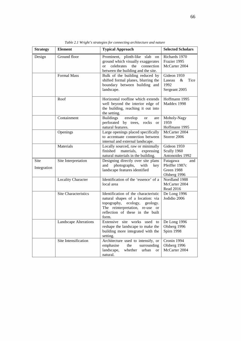
66

Table 2.1 Wright’s strategies for connecting architecture and nature

Strategy Element Typical Approach Selected Scholars

Design Ground floor Prominent, plinth-like slab on ground which visually exaggerates or celebrates the connection between the building and the site.

Richards 1970 Frazier 1995 McCarter 2004

Formal Mass Bulk of the building reduced by shifted formal planes, blurring the boundary between building and landscape.

Gideon 1959 Laseau & Tice 1992 Sergeant 2005

Roof Horizontal roofline which extends well beyond the interior edge of the building, reaching it out into the setting.

Hoffmann 1995 Maddex 1998

Containment Buildings envelop or are perforated by trees, rocks or natural features.

Moholy-Nagy 1959 Hoffmann 1995

Openings Large openings placed specifically to accentuate connection between internal and external landscape.

McCarter 2004 Storrer 2006

Materials Locally sourced, raw or minimally finished materials, expressing natural materials in the building.

Gideon 1959 Scully 1960 Antonoides 1992

Site

Integration

Site Interpretation Designing directly over site plans and photographs, with key landscape features identified

Futagawa and Pfeiffer 1987c Green 1988 Olsberg 1996

Locality Character Identification of the ‘essence’ of a local area

Nordland 1988 McCarter 2004 Read 2016

Site Characteristics Identification of the characteristic natural shapes of a location: via topography, ecology, geology. The reinterpretation, re-use or reflection of these in the built form.

De Long 1996 Jodidio 2006

Landscape Alterations Extensive site works used to reshape the landscape to make the building more integrated with the setting.

De Long 1996 Olsberg 1996 Spirn 1998

Site Intensification Architecture used to intensify, or emphasise the surrounding landscape, whether urban or natural.

Cronin 1994 Olsberg 1996 McCarter 2004

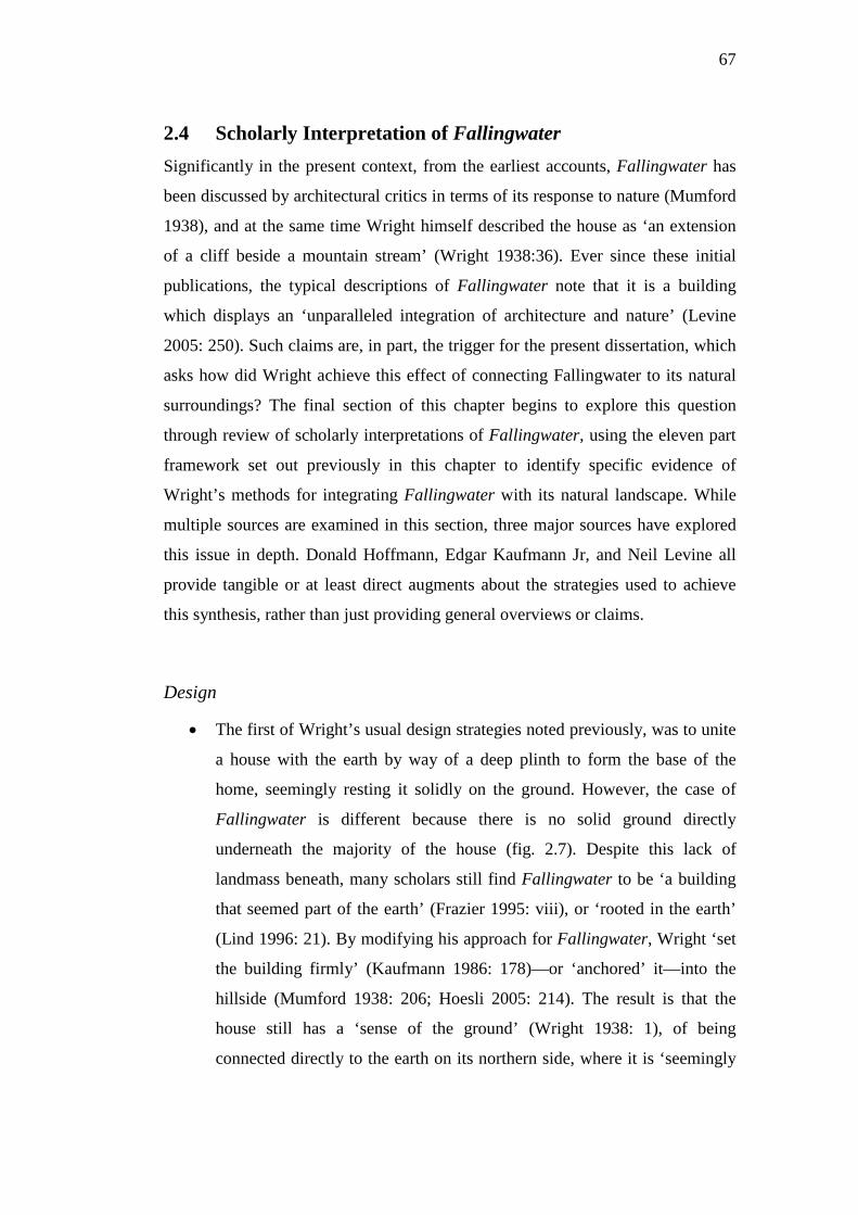
67

2.4 Scholarly Interpretation of Fallingwater Significantly in the present context, from the earliest accounts, Fallingwater has

been discussed by architectural critics in terms of its response to nature (Mumford

1938), and at the same time Wright himself described the house as ‘an extension

of a cliff beside a mountain stream’ (Wright 1938:36). Ever since these initial

publications, the typical descriptions of Fallingwater note that it is a building

which displays an ‘unparalleled integration of architecture and nature’ (Levine

2005: 250). Such claims are, in part, the trigger for the present dissertation, which

asks how did Wright achieve this effect of connecting Fallingwater to its natural

surroundings? The final section of this chapter begins to explore this question

through review of scholarly interpretations of Fallingwater, using the eleven part

framework set out previously in this chapter to identify specific evidence of

Wright’s methods for integrating Fallingwater with its natural landscape. While

multiple sources are examined in this section, three major sources have explored

this issue in depth. Donald Hoffmann, Edgar Kaufmann Jr, and Neil Levine all

provide tangible or at least direct augments about the strategies used to achieve

this synthesis, rather than just providing general overviews or claims.

Design

• The first of Wright’s usual design strategies noted previously, was to unite

a house with the earth by way of a deep plinth to form the base of the

home, seemingly resting it solidly on the ground. However, the case of

Fallingwater is different because there is no solid ground directly

underneath the majority of the house (fig. 2.7). Despite this lack of

landmass beneath, many scholars still find Fallingwater to be ‘a building

that seemed part of the earth’ (Frazier 1995: viii), or ‘rooted in the earth’

(Lind 1996: 21). By modifying his approach for Fallingwater, Wright ‘set

the building firmly’ (Kaufmann 1986: 178)—or ‘anchored’ it—into the

hillside (Mumford 1938: 206; Hoesli 2005: 214). The result is that the

house still has a ‘sense of the ground’ (Wright 1938: 1), of being

connected directly to the earth on its northern side, where it is ‘seemingly

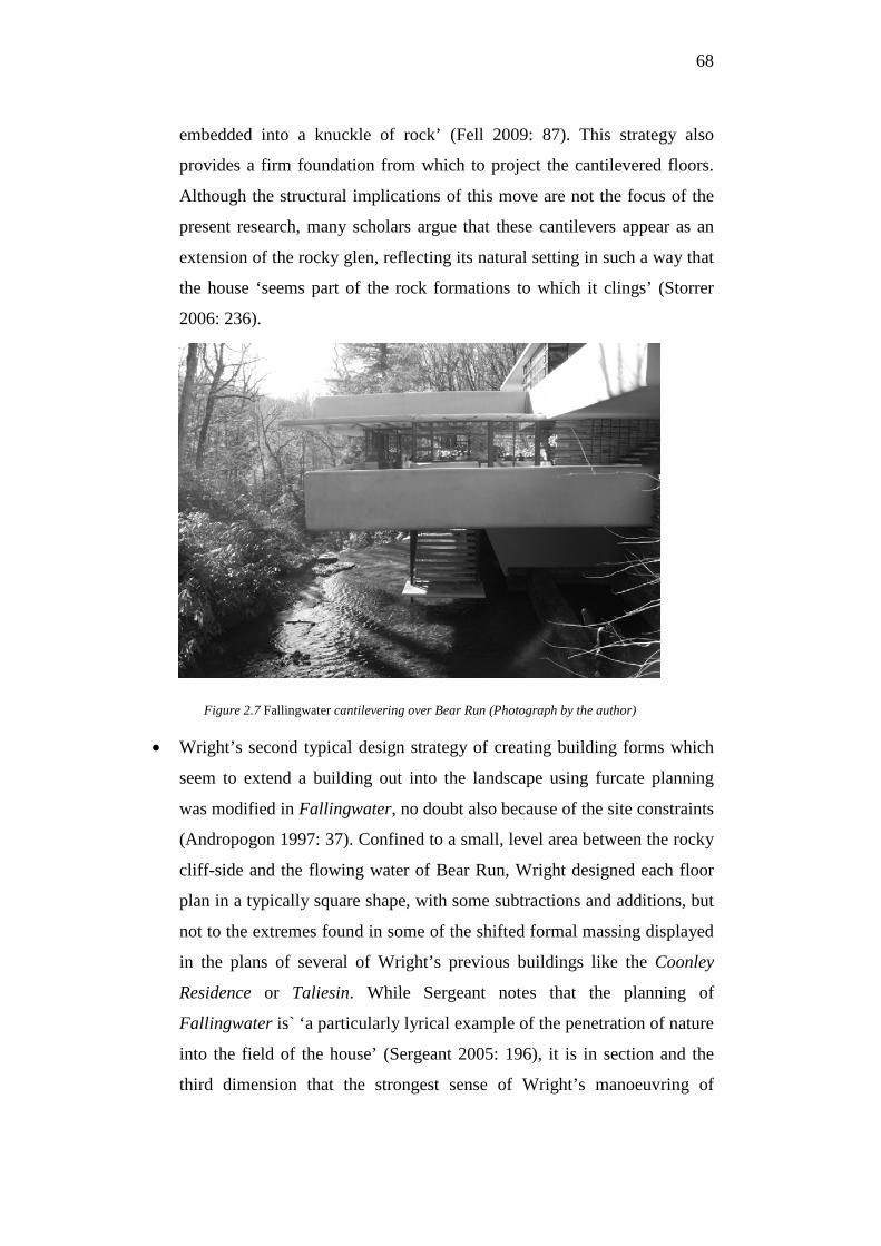
68

embedded into a knuckle of rock’ (Fell 2009: 87). This strategy also

provides a firm foundation from which to project the cantilevered floors.

Although the structural implications of this move are not the focus of the

present research, many scholars argue that these cantilevers appear as an

extension of the rocky glen, reflecting its natural setting in such a way that

the house ‘seems part of the rock formations to which it clings’ (Storrer

2006: 236).

Figure 2.7 Fallingwater cantilevering over Bear Run (Photograph by the author)

• Wright’s second typical design strategy of creating building forms which

seem to extend a building out into the landscape using furcate planning

was modified in Fallingwater, no doubt also because of the site constraints

(Andropogon 1997: 37). Confined to a small, level area between the rocky

cliff-side and the flowing water of Bear Run, Wright designed each floor

plan in a typically square shape, with some subtractions and additions, but

not to the extremes found in some of the shifted formal massing displayed

in the plans of several of Wright’s previous buildings like the Coonley

Residence or Taliesin. While Sergeant notes that the planning of

Fallingwater is` ‘a particularly lyrical example of the penetration of nature

into the field of the house’ (Sergeant 2005: 196), it is in section and the

third dimension that the strongest sense of Wright’s manoeuvring of

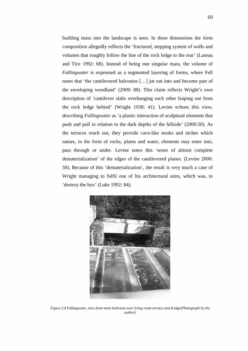
69

building mass into the landscape is seen. In three dimensions the form

composition allegedly reflects the ‘fractured, stepping system of walls and

volumes that roughly follow the line of the rock ledge to the rear’ (Laseau

and Tice 1992: 68). Instead of being one singular mass, the volume of

Fallingwater is expressed as a segmented layering of forms, where Fell

notes that ‘the cantilevered balconies […] jut out into and become part of

the enveloping woodland’ (2009: 88). This claim reflects Wright’s own

description of ‘cantilever slabs overhanging each other leaping out from

the rock ledge behind’ (Wright 1938: 41). Levine echoes this view,

describing Fallingwater as ‘a plastic interaction of sculptural elements that

push and pull in relation to the dark depths of the hillside’ (2000:50). As

the terraces reach out, they provide cave-like nooks and niches which

nature, in the form of rocks, plants and water, elements may enter into,

pass through or under. Levine notes this ‘sense of almost complete

dematerialization’ of the edges of the cantilevered planes. (Levine 2000:

50). Because of this ‘dematerialization’, the result is very much a case of

Wright managing to fulfil one of his architectural aims, which was, to

‘destroy the box’ (Luke 1992: 84).

Figure 2.8 Fallingwater, view from main bedroom over living room terrace and bridge(Photograph by the author)

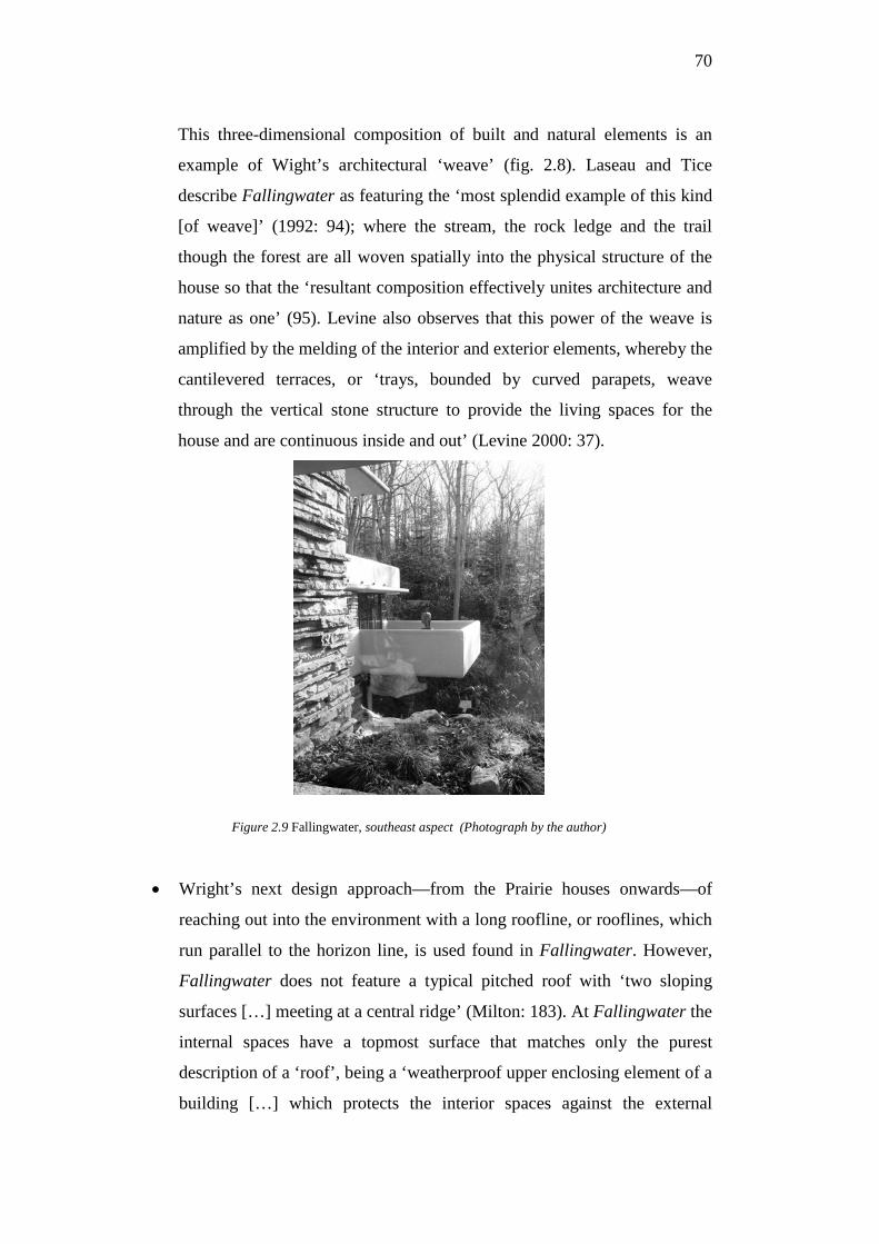
70

This three-dimensional composition of built and natural elements is an

example of Wight’s architectural ‘weave’ (fig. 2.8). Laseau and Tice

describe Fallingwater as featuring the ‘most splendid example of this kind

[of weave]’ (1992: 94); where the stream, the rock ledge and the trail

though the forest are all woven spatially into the physical structure of the

house so that the ‘resultant composition effectively unites architecture and

nature as one’ (95). Levine also observes that this power of the weave is

amplified by the melding of the interior and exterior elements, whereby the

cantilevered terraces, or ‘trays, bounded by curved parapets, weave

through the vertical stone structure to provide the living spaces for the

house and are continuous inside and out’ (Levine 2000: 37).

Figure 2.9 Fallingwater, southeast aspect (Photograph by the author)

• Wright’s next design approach—from the Prairie houses onwards—of

reaching out into the environment with a long roofline, or rooflines, which

run parallel to the horizon line, is used found in Fallingwater. However,

Fallingwater does not feature a typical pitched roof with ‘two sloping

surfaces […] meeting at a central ridge’ (Milton: 183). At Fallingwater the

internal spaces have a topmost surface that matches only the purest

description of a ‘roof’, being a ‘weatherproof upper enclosing element of a

building […] which protects the interior spaces against the external

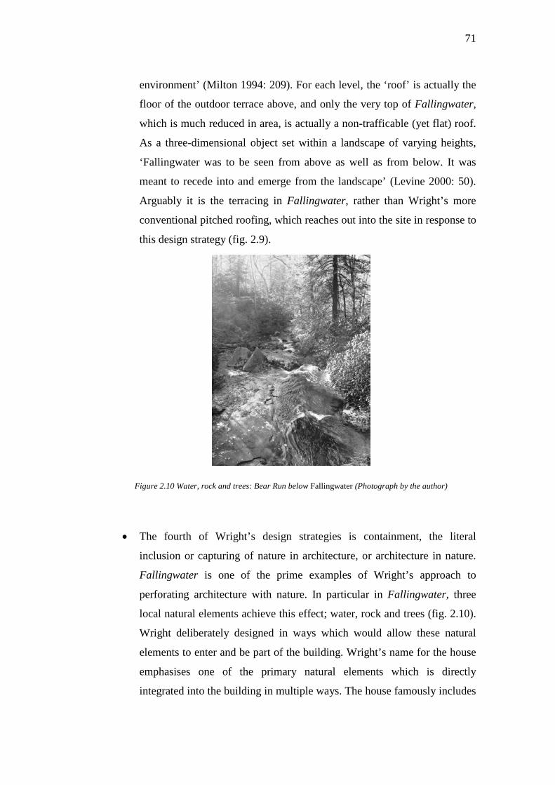
71

environment’ (Milton 1994: 209). For each level, the ‘roof’ is actually the

floor of the outdoor terrace above, and only the very top of Fallingwater,

which is much reduced in area, is actually a non-trafficable (yet flat) roof.

As a three-dimensional object set within a landscape of varying heights,

‘Fallingwater was to be seen from above as well as from below. It was

meant to recede into and emerge from the landscape’ (Levine 2000: 50).

Arguably it is the terracing in Fallingwater, rather than Wright’s more

conventional pitched roofing, which reaches out into the site in response to

this design strategy (fig. 2.9).

Figure 2.10 Water, rock and trees: Bear Run below Fallingwater (Photograph by the author)

• The fourth of Wright’s design strategies is containment, the literal

inclusion or capturing of nature in architecture, or architecture in nature.

Fallingwater is one of the prime examples of Wright’s approach to

perforating architecture with nature. In particular in Fallingwater, three

local natural elements achieve this effect; water, rock and trees (fig. 2.10).

Wright deliberately designed in ways which would allow these natural

elements to enter and be part of the building. Wright’s name for the house

emphasises one of the primary natural elements which is directly

integrated into the building in multiple ways. The house famously includes

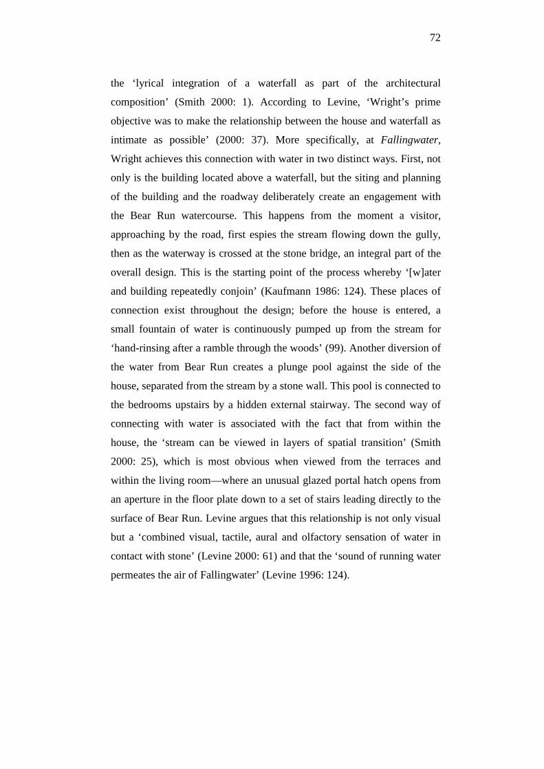
72

the ‘lyrical integration of a waterfall as part of the architectural

composition’ (Smith 2000: 1). According to Levine, ‘Wright’s prime

objective was to make the relationship between the house and waterfall as

intimate as possible’ (2000: 37). More specifically, at Fallingwater,

Wright achieves this connection with water in two distinct ways. First, not

only is the building located above a waterfall, but the siting and planning

of the building and the roadway deliberately create an engagement with

the Bear Run watercourse. This happens from the moment a visitor,

approaching by the road, first espies the stream flowing down the gully,

then as the waterway is crossed at the stone bridge, an integral part of the

overall design. This is the starting point of the process whereby ‘[w]ater

and building repeatedly conjoin’ (Kaufmann 1986: 124). These places of

connection exist throughout the design; before the house is entered, a

small fountain of water is continuously pumped up from the stream for

‘hand-rinsing after a ramble through the woods’ (99). Another diversion of

the water from Bear Run creates a plunge pool against the side of the

house, separated from the stream by a stone wall. This pool is connected to

the bedrooms upstairs by a hidden external stairway. The second way of

connecting with water is associated with the fact that from within the

house, the ‘stream can be viewed in layers of spatial transition’ (Smith

2000: 25), which is most obvious when viewed from the terraces and

within the living room—where an unusual glazed portal hatch opens from

an aperture in the floor plate down to a set of stairs leading directly to the

surface of Bear Run. Levine argues that this relationship is not only visual

but a ‘combined visual, tactile, aural and olfactory sensation of water in

contact with stone’ (Levine 2000: 61) and that the ‘sound of running water

permeates the air of Fallingwater’ (Levine 1996: 124).

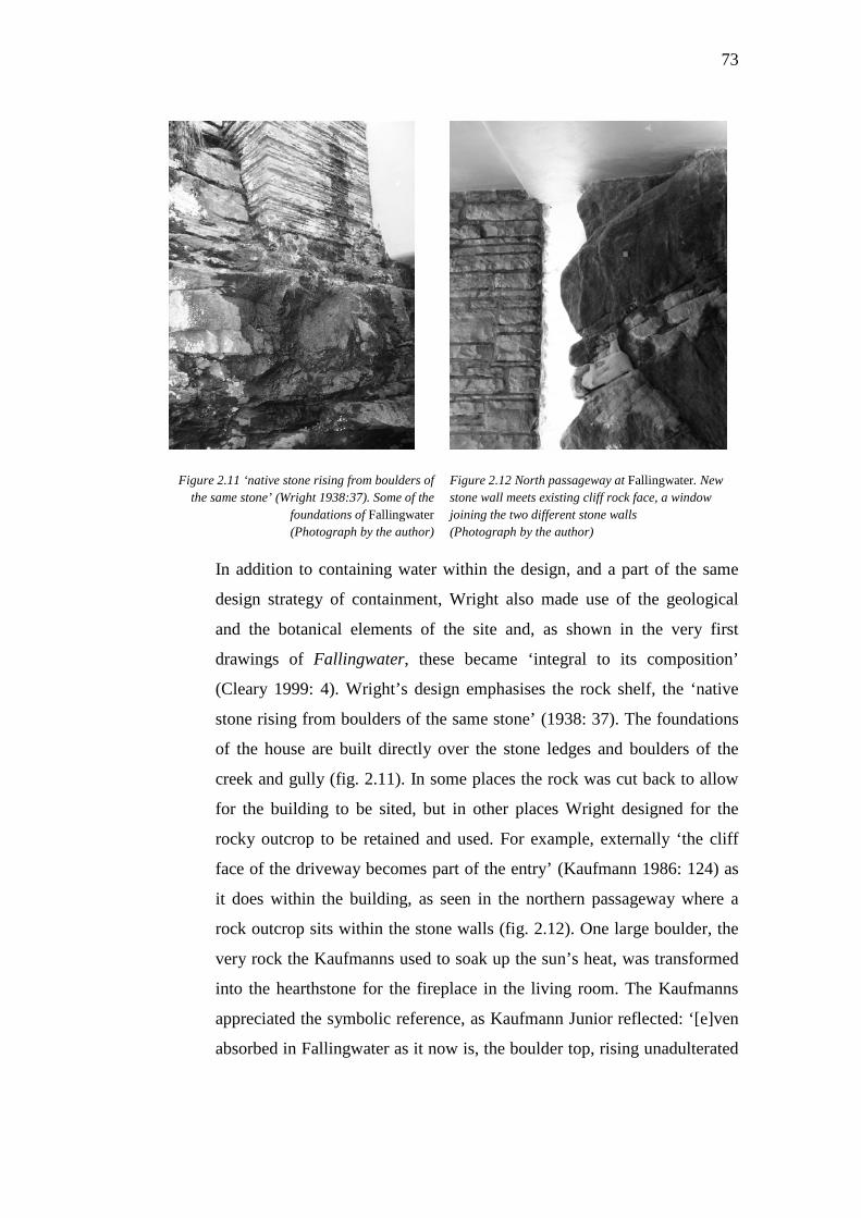
73

Figure 2.11 ‘native stone rising from boulders of the same stone’ (Wright 1938:37). Some of the

foundations of Fallingwater (Photograph by the author)

Figure 2.12 North passageway at Fallingwater. New stone wall meets existing cliff rock face, a window joining the two different stone walls (Photograph by the author)

In addition to containing water within the design, and a part of the same

design strategy of containment, Wright also made use of the geological

and the botanical elements of the site and, as shown in the very first

drawings of Fallingwater, these became ‘integral to its composition’

(Cleary 1999: 4). Wright’s design emphasises the rock shelf, the ‘native

stone rising from boulders of the same stone’ (1938: 37). The foundations

of the house are built directly over the stone ledges and boulders of the

creek and gully (fig. 2.11). In some places the rock was cut back to allow

for the building to be sited, but in other places Wright designed for the

rocky outcrop to be retained and used. For example, externally ‘the cliff

face of the driveway becomes part of the entry’ (Kaufmann 1986: 124) as

it does within the building, as seen in the northern passageway where a

rock outcrop sits within the stone walls (fig. 2.12). One large boulder, the

very rock the Kaufmanns used to soak up the sun’s heat, was transformed

into the hearthstone for the fireplace in the living room. The Kaufmanns

appreciated the symbolic reference, as Kaufmann Junior reflected: ‘[e]ven

absorbed in Fallingwater as it now is, the boulder top, rising unadulterated

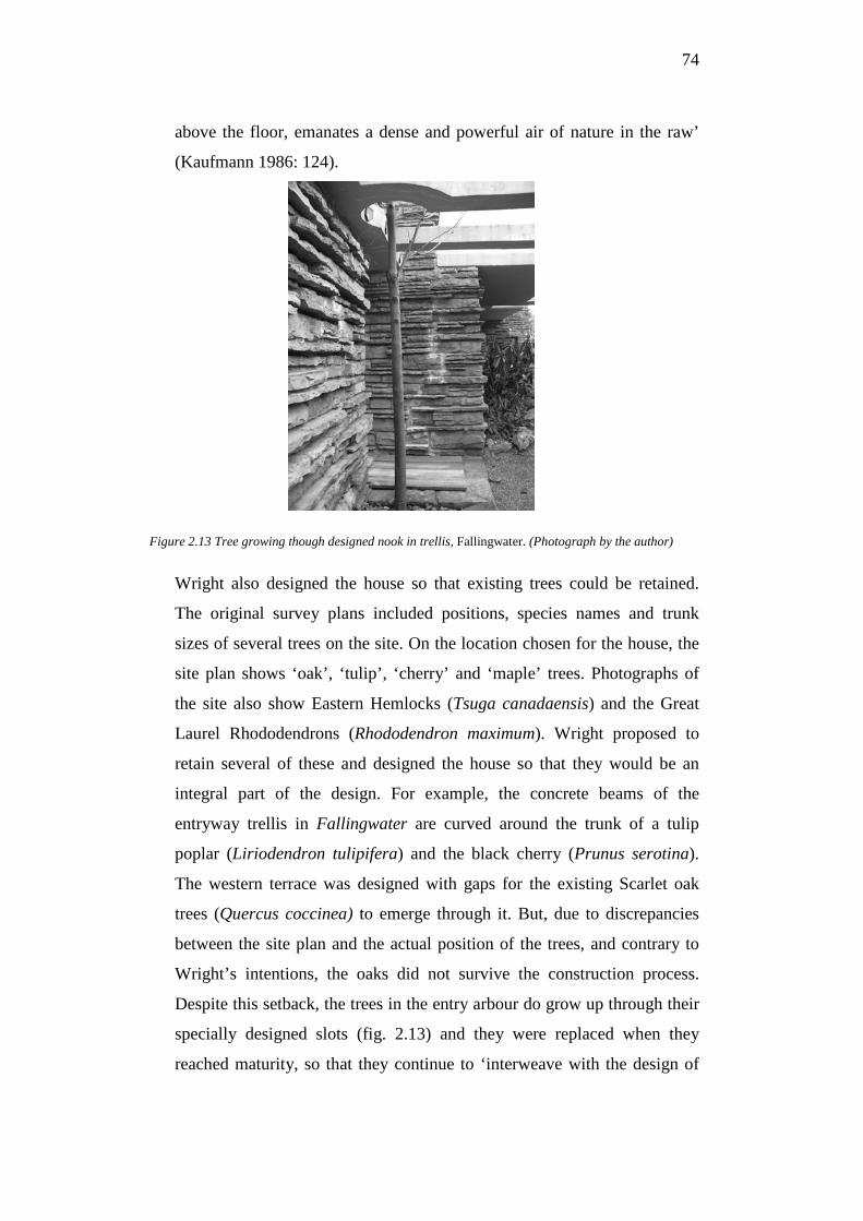
74

above the floor, emanates a dense and powerful air of nature in the raw’

(Kaufmann 1986: 124).

Figure 2.13 Tree growing though designed nook in trellis, Fallingwater. (Photograph by the author)

Wright also designed the house so that existing trees could be retained.

The original survey plans included positions, species names and trunk

sizes of several trees on the site. On the location chosen for the house, the

site plan shows ‘oak’, ‘tulip’, ‘cherry’ and ‘maple’ trees. Photographs of

the site also show Eastern Hemlocks (Tsuga canadaensis) and the Great

Laurel Rhododendrons (Rhododendron maximum). Wright proposed to

retain several of these and designed the house so that they would be an

integral part of the design. For example, the concrete beams of the

entryway trellis in Fallingwater are curved around the trunk of a tulip

poplar (Liriodendron tulipifera) and the black cherry (Prunus serotina).

The western terrace was designed with gaps for the existing Scarlet oak

trees (Quercus coccinea) to emerge through it. But, due to discrepancies

between the site plan and the actual position of the trees, and contrary to

Wright’s intentions, the oaks did not survive the construction process.

Despite this setback, the trees in the entry arbour do grow up through their

specially designed slots (fig. 2.13) and they were replaced when they

reached maturity, so that they continue to ‘interweave with the design of

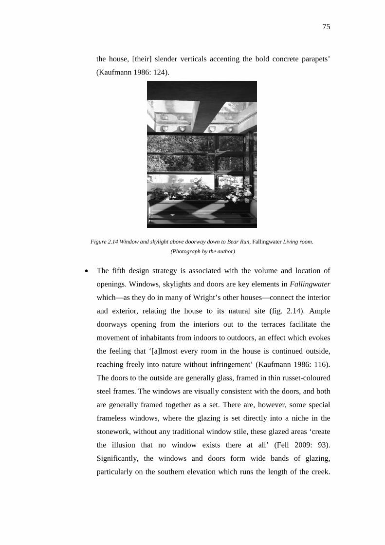
75

the house, [their] slender verticals accenting the bold concrete parapets’

(Kaufmann 1986: 124).

Figure 2.14 Window and skylight above doorway down to Bear Run, Fallingwater Living room.

(Photograph by the author)

• The fifth design strategy is associated with the volume and location of

openings. Windows, skylights and doors are key elements in Fallingwater

which—as they do in many of Wright’s other houses—connect the interior

and exterior, relating the house to its natural site (fig. 2.14). Ample

doorways opening from the interiors out to the terraces facilitate the

movement of inhabitants from indoors to outdoors, an effect which evokes

the feeling that ‘[a]lmost every room in the house is continued outside,

reaching freely into nature without infringement’ (Kaufmann 1986: 116).

The doors to the outside are generally glass, framed in thin russet-coloured

steel frames. The windows are visually consistent with the doors, and both

are generally framed together as a set. There are, however, some special

frameless windows, where the glazing is set directly into a niche in the

stonework, without any traditional window stile, these glazed areas ‘create

the illusion that no window exists there at all’ (Fell 2009: 93).

Significantly, the windows and doors form wide bands of glazing,

particularly on the southern elevation which runs the length of the creek.

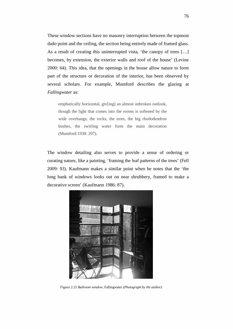
76

These window sections have no masonry interruption between the topmost

dado point and the ceiling, the section being entirely made of framed glass.

As a result of creating this uninterrupted vista, ‘the canopy of trees […]

becomes, by extension, the exterior walls and roof of the house’ (Levine

2000: 64). This idea, that the openings in the house allow nature to form

part of the structure or decoration of the interior, has been observed by

several scholars. For example, Mumford describes the glazing at

Fallingwater as:

emphatically horizontal, giv[ing] an almost unbroken outlook,

though the light that comes into the rooms is softened by the

wide overhangs; the rocks, the trees, the big rhododendron

bushes, the swirling water form the main decoration

(Mumford 1938: 207).

The window detailing also serves to provide a sense of ordering or

curating nature, like a painting, ‘framing the leaf patterns of the trees’ (Fell

2009: 93). Kaufmann makes a similar point when he notes that the ‘the

long bank of windows looks out on near shrubbery, framed to make a

decorative screen’ (Kaufmann 1986: 87).

Figure 2.15 Bedroom window, Fallingwater (Photograph by the author)

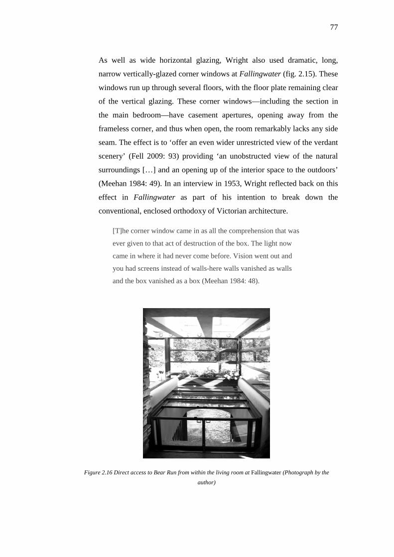
77

As well as wide horizontal glazing, Wright also used dramatic, long,

narrow vertically-glazed corner windows at Fallingwater (fig. 2.15). These

windows run up through several floors, with the floor plate remaining clear

of the vertical glazing. These corner windows—including the section in

the main bedroom—have casement apertures, opening away from the

frameless corner, and thus when open, the room remarkably lacks any side

seam. The effect is to ‘offer an even wider unrestricted view of the verdant

scenery’ (Fell 2009: 93) providing ‘an unobstructed view of the natural

surroundings […] and an opening up of the interior space to the outdoors’

(Meehan 1984: 49). In an interview in 1953, Wright reflected back on this

effect in Fallingwater as part of his intention to break down the

conventional, enclosed orthodoxy of Victorian architecture.

[T]he corner window came in as all the comprehension that was

ever given to that act of destruction of the box. The light now

came in where it had never come before. Vision went out and

you had screens instead of walls-here walls vanished as walls

and the box vanished as a box (Meehan 1984: 48).

Figure 2.16 Direct access to Bear Run from within the living room at Fallingwater (Photograph by the

author)

78

Other openings in Fallingwater that have received more specific

treatments include a glazed portal to the creek below, through the living

room floor (fig. 2.16). This allows direct access to the water, but also

provides a visual and aural connection to it. Looking straight at this

stairway, a view is provided of the water below, and looking through the

glazing immediately ahead, the tree line can also be seen, so that ‘both sky

and water are brought simultaneously into the house’ (Kaufmann 1986:

80). Likewise, Levine notes that this opening ‘links the tree/leaf imagery

to the stone/water imagery at the point where the house is most fully

understood as being suspended between earth and sky’ (Levine 2000: 64).

Several unusual windows are also located halfway over planter boxes, so

in a passageway, half an ornamental garden is inside the house, and then

separated by a pane of glass, the same garden appears to carry on outside.

In the living room, a planter box sits just inside a window, so looking

through it, one sees the live plants inside, and the living landscape beyond.

Upstairs, the technique is reversed; a planter is set just on the outside of

the window. The slight variations in this strategy might be evidence of

Wright’s intention to constantly challenge the relationship between the

inside and outside, or the synthetic and the natural, using a range of

opening types.

• The final design strategy is associated with use of materials. In

Fallingwater Wright repeats his general approach to building materials.

The predominant building elements in the house are stone, concrete, glass,

timber and steel. These materials are allegedly ‘appropriate’ in a structural

or pragmatic sense, but they are also used to ‘develop a poetic sensibility’

(Laseau and Tice 1992: 66). Describing the house, Wright stated that

‘shelter took on a definite masonry form while still preserving protection

overhead for extensive glass surface[s]’ (1938: 36). Scholars argue that the

materials chosen by Wright represent his distillation of the overall essence

of a site. According to Alofsin, ‘[e]ach material—stone, glass, concrete—

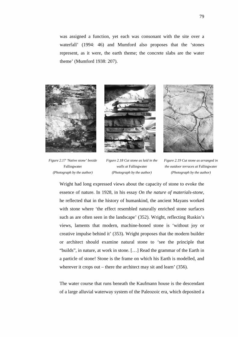
79

was assigned a function, yet each was consonant with the site over a

waterfall’ (1994: 46) and Mumford also proposes that the ‘stones

represent, as it were, the earth theme; the concrete slabs are the water

theme’ (Mumford 1938: 207).

Figure 2.17 ‘Native stone’ beside

Fallingwater

(Photograph by the author)

Figure 2.18 Cut stone as laid in the

walls at Fallingwater

(Photograph by the author)

Figure 2.19 Cut stone as arranged in

the outdoor terraces at Fallingwater

(Photograph by the author)

Wright had long expressed views about the capacity of stone to evoke the

essence of nature. In 1928, in his essay On the nature of materials-stone,

he reflected that in the history of humankind, the ancient Mayans worked

with stone where ‘the effect resembled naturally enriched stone surfaces

such as are often seen in the landscape’ (352). Wright, reflecting Ruskin’s

views, laments that modern, machine-honed stone is ‘without joy or

creative impulse behind it’ (353). Wright proposes that the modern builder

or architect should examine natural stone to ‘see the principle that

“builds”, in nature, at work in stone. […] Read the grammar of the Earth in

a particle of stone! Stone is the frame on which his Earth is modelled, and

wherever it crops out – there the architect may sit and learn’ (356).

The water course that runs beneath the Kaufmann house is the descendant

of a large alluvial waterway system of the Paleozoic era, which deposited a

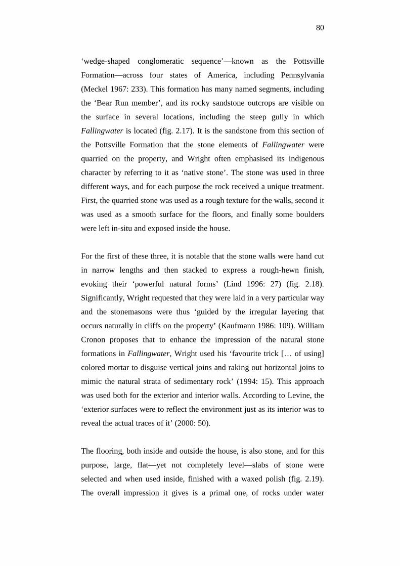
80

‘wedge-shaped conglomeratic sequence’—known as the Pottsville

Formation—across four states of America, including Pennsylvania

(Meckel 1967: 233). This formation has many named segments, including

the ‘Bear Run member’, and its rocky sandstone outcrops are visible on

the surface in several locations, including the steep gully in which

Fallingwater is located (fig. 2.17). It is the sandstone from this section of

the Pottsville Formation that the stone elements of Fallingwater were

quarried on the property, and Wright often emphasised its indigenous

character by referring to it as ‘native stone’. The stone was used in three

different ways, and for each purpose the rock received a unique treatment.

First, the quarried stone was used as a rough texture for the walls, second it

was used as a smooth surface for the floors, and finally some boulders

were left in-situ and exposed inside the house.

For the first of these three, it is notable that the stone walls were hand cut

in narrow lengths and then stacked to express a rough-hewn finish,

evoking their ‘powerful natural forms’ (Lind 1996: 27) (fig. 2.18).

Significantly, Wright requested that they were laid in a very particular way

and the stonemasons were thus ‘guided by the irregular layering that

occurs naturally in cliffs on the property’ (Kaufmann 1986: 109). William

Cronon proposes that to enhance the impression of the natural stone

formations in Fallingwater, Wright used his ‘favourite trick [… of using]

colored mortar to disguise vertical joins and raking out horizontal joins to

mimic the natural strata of sedimentary rock’ (1994: 15). This approach

was used both for the exterior and interior walls. According to Levine, the

‘exterior surfaces were to reflect the environment just as its interior was to

reveal the actual traces of it’ (2000: 50).

The flooring, both inside and outside the house, is also stone, and for this

purpose, large, flat—yet not completely level—slabs of stone were

selected and when used inside, finished with a waxed polish (fig. 2.19).

The overall impression it gives is a primal one, of rocks under water

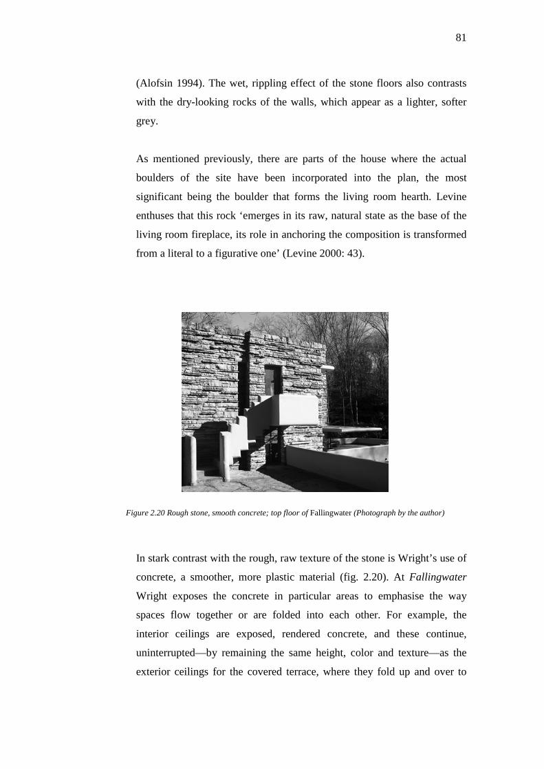
81

(Alofsin 1994). The wet, rippling effect of the stone floors also contrasts

with the dry-looking rocks of the walls, which appear as a lighter, softer

grey.

As mentioned previously, there are parts of the house where the actual

boulders of the site have been incorporated into the plan, the most

significant being the boulder that forms the living room hearth. Levine

enthuses that this rock ‘emerges in its raw, natural state as the base of the

living room fireplace, its role in anchoring the composition is transformed

from a literal to a figurative one’ (Levine 2000: 43).

Figure 2.20 Rough stone, smooth concrete; top floor of Fallingwater (Photograph by the author)

In stark contrast with the rough, raw texture of the stone is Wright’s use of

concrete, a smoother, more plastic material (fig. 2.20). At Fallingwater

Wright exposes the concrete in particular areas to emphasise the way

spaces flow together or are folded into each other. For example, the

interior ceilings are exposed, rendered concrete, and these continue,

uninterrupted—by remaining the same height, color and texture—as the

exterior ceilings for the covered terrace, where they fold up and over to

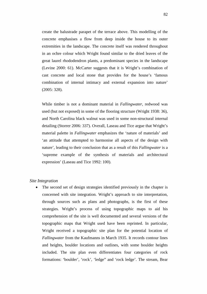
82

create the balustrade parapet of the terrace above. This modelling of the

concrete emphasises a flow from deep inside the house to its outer

extremities in the landscape. The concrete itself was rendered throughout

in an ochre colour which Wright found similar to the dried leaves of the

great laurel rhododendron plants, a predominant species in the landscape

(Levine 2000: 61). McCarter suggests that it is Wright’s combination of

cast concrete and local stone that provides for the house’s ‘famous

combination of internal intimacy and external expansion into nature’

(2005: 328).

While timber is not a dominant material in Fallingwater, redwood was

used (but not exposed) in some of the flooring structure (Wright 1938: 36),

and North Carolina black walnut was used in some non-structural internal

detailing (Storrer 2006: 337). Overall, Laseau and Tice argue that Wright’s

material palette in Fallingwater emphasizes the ‘nature of materials’ and

‘an attitude that attempted to harmonise all aspects of the design with

nature’, leading to their conclusion that as a result of this Fallingwater is a

‘supreme example of the synthesis of materials and architectural

expression’ (Laseau and Tice 1992: 100).

Site Integration • The second set of design strategies identified previously in the chapter is

concerned with site integration. Wright’s approach to site interpretation,

through sources such as plans and photographs, is the first of these

strategies. Wright’s process of using topographic maps to aid his

comprehension of the site is well documented and several versions of the

topographic maps that Wright used have been reprinted. In particular,

Wright received a topographic site plan for the potential location of

Fallingwater from the Kaufmanns in March 1935. It records contour lines

and heights, boulder locations and outlines, with some boulder heights

included. The site plan even differentiates four categories of rock

formations: ‘boulder’, ‘rock’, ‘ledge” and ‘rock ledge’. The stream, Bear

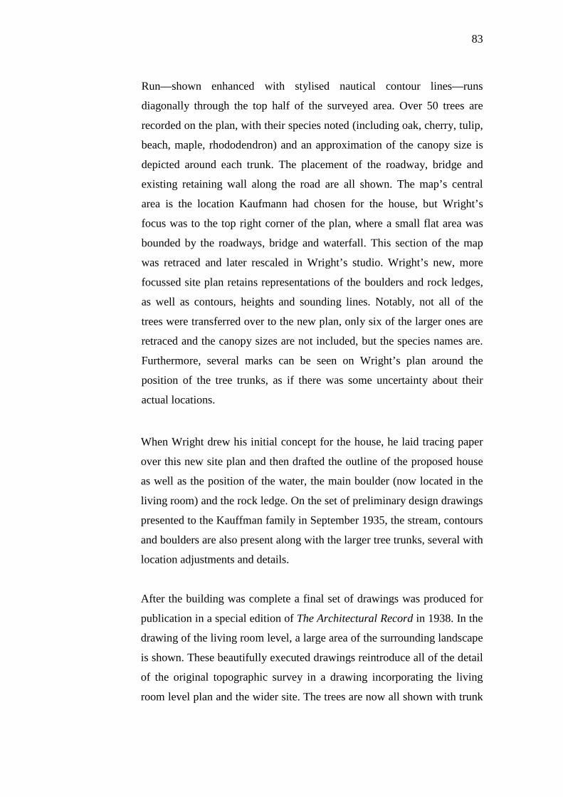
83

Run—shown enhanced with stylised nautical contour lines—runs

diagonally through the top half of the surveyed area. Over 50 trees are

recorded on the plan, with their species noted (including oak, cherry, tulip,

beach, maple, rhododendron) and an approximation of the canopy size is

depicted around each trunk. The placement of the roadway, bridge and

existing retaining wall along the road are all shown. The map’s central

area is the location Kaufmann had chosen for the house, but Wright’s

focus was to the top right corner of the plan, where a small flat area was

bounded by the roadways, bridge and waterfall. This section of the map

was retraced and later rescaled in Wright’s studio. Wright’s new, more

focussed site plan retains representations of the boulders and rock ledges,

as well as contours, heights and sounding lines. Notably, not all of the

trees were transferred over to the new plan, only six of the larger ones are

retraced and the canopy sizes are not included, but the species names are.

Furthermore, several marks can be seen on Wright’s plan around the

position of the tree trunks, as if there was some uncertainty about their

actual locations.

When Wright drew his initial concept for the house, he laid tracing paper

over this new site plan and then drafted the outline of the proposed house

as well as the position of the water, the main boulder (now located in the

living room) and the rock ledge. On the set of preliminary design drawings

presented to the Kauffman family in September 1935, the stream, contours

and boulders are also present along with the larger tree trunks, several with

location adjustments and details.

After the building was complete a final set of drawings was produced for

publication in a special edition of The Architectural Record in 1938. In the

drawing of the living room level, a large area of the surrounding landscape

is shown. These beautifully executed drawings reintroduce all of the detail

of the original topographic survey in a drawing incorporating the living

room level plan and the wider site. The trees are now all shown with trunk

84

diameter and canopies rendered in different styles to represent their

species: however, the information is all transmitted graphically; the names

of trees, contour heights and any other nomenclature are not included.

While the Kaufmanns were initially surprised at the alternative location

Wright had identified for the house, Wright must have started to

conceptualise the building on the alternative location on the first day he

visited the site. As Cleary notes, ‘Wright’s schematic drawings shed light

on his design process’ (1999: 41). Importantly, Wright requested that the

area around the falls, well away from the original site suggested by the

Kaufmanns, be included in the contour plans. He similarly made it clear

that he wanted the large trees and boulders to be included in the first

contour plan in great detail, as if he was already considering their

incorporation in the design. Cleary also suggests that ‘Wright’s awareness

of the [...] trees as three-dimensional entities is demonstrated by

indications of their canopies as well as their trunks in the plans. Their

importance was in the initial conceptualisation of the house rather than in

the construction’ (41).

• As well as using externally sourced documentation to gain an insight into

the landscape, Wright’s second site strategy involved extracting the more

ephemeral properties of the site, including its ‘essence’. This approach

involves Wright’s ‘sensitivity’ to nature (Nordland 1988: 2) and is harder

to assess. In Fallingwater, Wright allegedly sought to create a building

that was ‘radiant and right for its forest place’ (Hoffmann 1993: 3) and

where ‘the dynamic spirit of the building is in keeping with the spirit of

the wild and rugged woodland’ (Simonds 1983: 21). Likewise, Charles

and Berdeana Aguar find that ‘Fallingwater evokes a responsive sense-of-

place absolutely in keeping with the rugged character of the massive rocks,

the turbulence of the waterfall, and the natural persona of the forested site’

(2002: 230). Perhaps, as suggested, this strategy involves determining an

overall character of the locality, and it is Wright’s next strategy, which

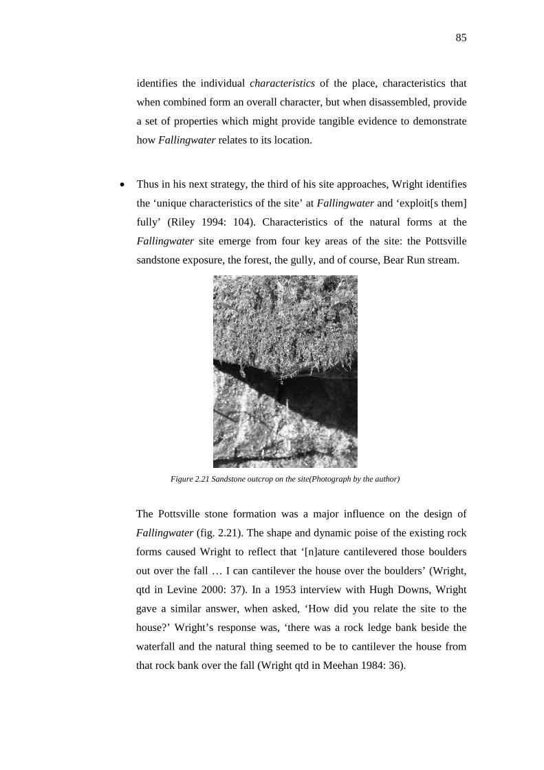
85

identifies the individual characteristics of the place, characteristics that

when combined form an overall character, but when disassembled, provide

a set of properties which might provide tangible evidence to demonstrate

how Fallingwater relates to its location.

• Thus in his next strategy, the third of his site approaches, Wright identifies

the ‘unique characteristics of the site’ at Fallingwater and ‘exploit[s them]

fully’ (Riley 1994: 104). Characteristics of the natural forms at the

Fallingwater site emerge from four key areas of the site: the Pottsville

sandstone exposure, the forest, the gully, and of course, Bear Run stream.

Figure 2.21 Sandstone outcrop on the site(Photograph by the author)

The Pottsville stone formation was a major influence on the design of

Fallingwater (fig. 2.21). The shape and dynamic poise of the existing rock

forms caused Wright to reflect that ‘[n]ature cantilevered those boulders

out over the fall … I can cantilever the house over the boulders’ (Wright,

qtd in Levine 2000: 37). In a 1953 interview with Hugh Downs, Wright

gave a similar answer, when asked, ‘How did you relate the site to the

house?’ Wright’s response was, ‘there was a rock ledge bank beside the

waterfall and the natural thing seemed to be to cantilever the house from

that rock bank over the fall (Wright qtd in Meehan 1984: 36).

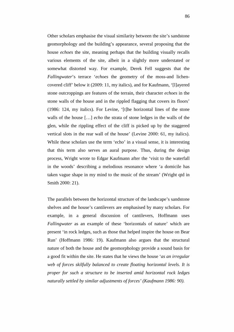
86

Other scholars emphasise the visual similarity between the site’s sandstone

geomorphology and the building’s appearance, several proposing that the

house echoes the site, meaning perhaps that the building visually recalls

various elements of the site, albeit in a slightly more understated or

somewhat distorted way. For example, Derek Fell suggests that the

Fallingwater’s terrace ‘echoes the geometry of the moss-and lichen-

covered cliff’ below it (2009: 11, my italics), and for Kaufmann, ‘[l]ayered

stone outcroppings are features of the terrain, their character echoes in the

stone walls of the house and in the rippled flagging that covers its floors’

(1986: 124, my italics). For Levine, ‘[t]he horizontal lines of the stone

walls of the house […] echo the strata of stone ledges in the walls of the

glen, while the rippling effect of the cliff is picked up by the staggered

vertical slots in the rear wall of the house’ (Levine 2000: 61, my italics).

While these scholars use the term ‘echo’ in a visual sense, it is interesting

that this term also serves an aural purpose. Thus, during the design

process, Wright wrote to Edgar Kaufmann after the ‘visit to the waterfall

in the woods’ describing a melodious resonance where ‘a domicile has

taken vague shape in my mind to the music of the stream’ (Wright qtd in

Smith 2000: 21).

The parallels between the horizontal structure of the landscape’s sandstone

shelves and the house’s cantilevers are emphasised by many scholars. For

example, in a general discussion of cantilevers, Hoffmann uses

Fallingwater as an example of these ‘horizontals of nature’ which are

present ‘in rock ledges, such as those that helped inspire the house on Bear

Run’ (Hoffmann 1986: 19). Kaufmann also argues that the structural

nature of both the house and the geomorphology provide a sound basis for

a good fit within the site. He states that he views the house ‘as an irregular

web of forces skilfully balanced to create floating horizontal levels. It is

proper for such a structure to be inserted amid horizontal rock ledges

naturally settled by similar adjustments of forces’ (Kaufmann 1986: 90).

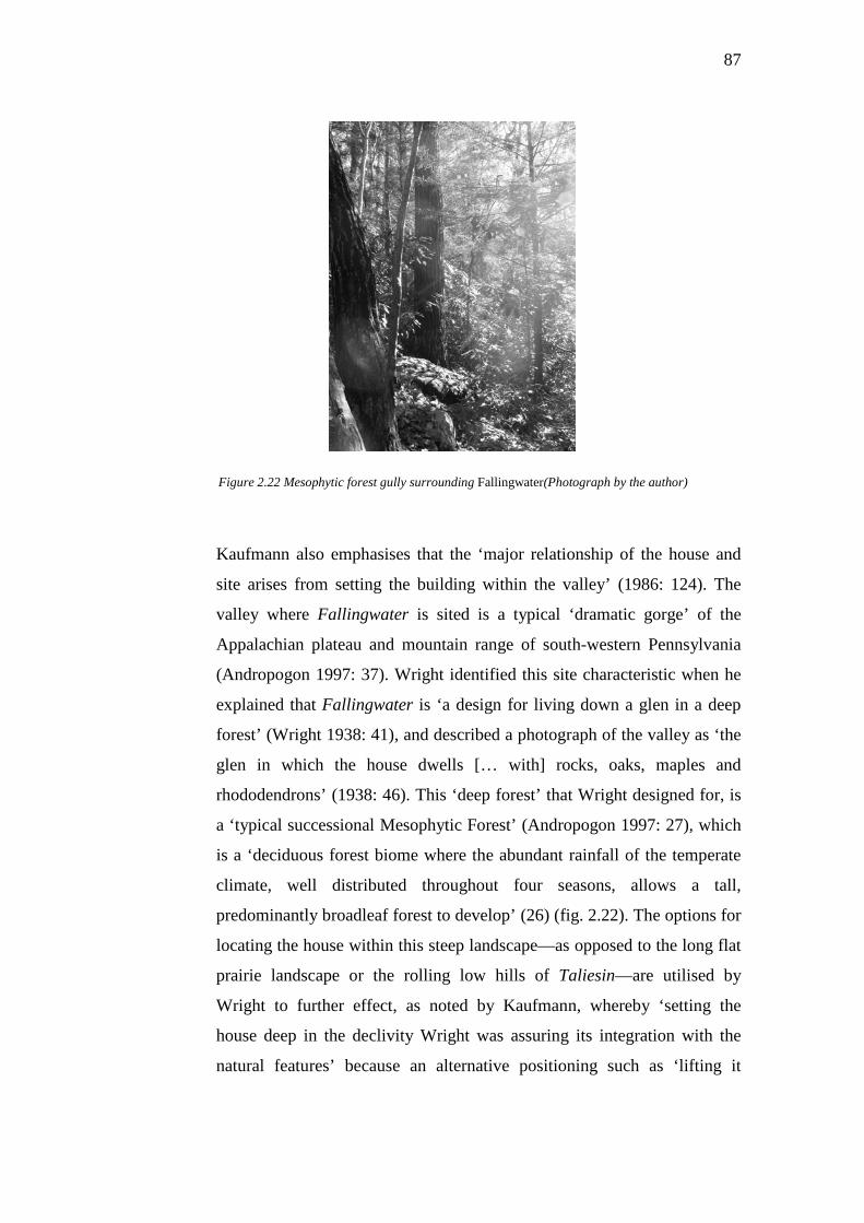
87

Figure 2.22 Mesophytic forest gully surrounding Fallingwater(Photograph by the author)

Kaufmann also emphasises that the ‘major relationship of the house and

site arises from setting the building within the valley’ (1986: 124). The

valley where Fallingwater is sited is a typical ‘dramatic gorge’ of the

Appalachian plateau and mountain range of south-western Pennsylvania

(Andropogon 1997: 37). Wright identified this site characteristic when he

explained that Fallingwater is ‘a design for living down a glen in a deep

forest’ (Wright 1938: 41), and described a photograph of the valley as ‘the

glen in which the house dwells [… with] rocks, oaks, maples and

rhododendrons’ (1938: 46). This ‘deep forest’ that Wright designed for, is

a ‘typical successional Mesophytic Forest’ (Andropogon 1997: 27), which

is a ‘deciduous forest biome where the abundant rainfall of the temperate

climate, well distributed throughout four seasons, allows a tall,

predominantly broadleaf forest to develop’ (26) (fig. 2.22). The options for

locating the house within this steep landscape—as opposed to the long flat

prairie landscape or the rolling low hills of Taliesin—are utilised by

Wright to further effect, as noted by Kaufmann, whereby ‘setting the

house deep in the declivity Wright was assuring its integration with the

natural features’ because an alternative positioning such as ‘lifting it

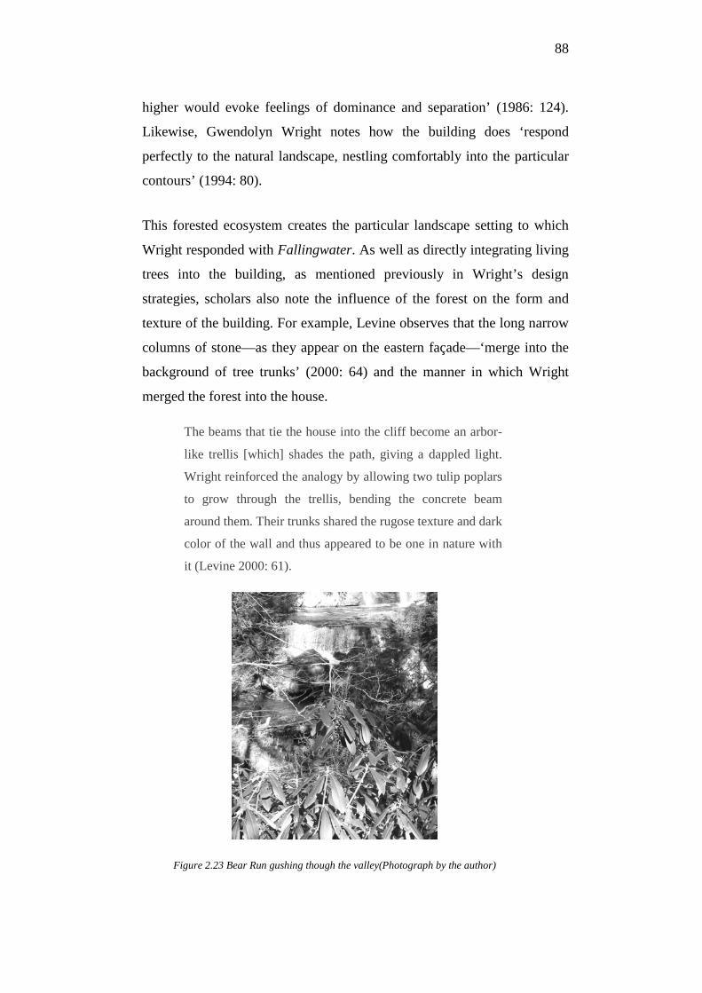
88

higher would evoke feelings of dominance and separation’ (1986: 124).

Likewise, Gwendolyn Wright notes how the building does ‘respond

perfectly to the natural landscape, nestling comfortably into the particular

contours’ (1994: 80).

This forested ecosystem creates the particular landscape setting to which

Wright responded with Fallingwater. As well as directly integrating living

trees into the building, as mentioned previously in Wright’s design

strategies, scholars also note the influence of the forest on the form and

texture of the building. For example, Levine observes that the long narrow

columns of stone—as they appear on the eastern façade—‘merge into the

background of tree trunks’ (2000: 64) and the manner in which Wright

merged the forest into the house.

The beams that tie the house into the cliff become an arbor-

like trellis [which] shades the path, giving a dappled light.

Wright reinforced the analogy by allowing two tulip poplars

to grow through the trellis, bending the concrete beam

around them. Their trunks shared the rugose texture and dark

color of the wall and thus appeared to be one in nature with

it (Levine 2000: 61).

Figure 2.23 Bear Run gushing though the valley(Photograph by the author)

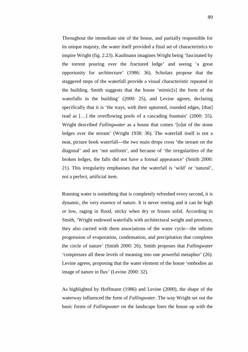
89

Throughout the immediate site of the house, and partially responsible for

its unique majesty, the water itself provided a final set of characteristics to

inspire Wright (fig. 2.23). Kaufmann imagines Wright being ‘fascinated by

the torrent pouring over the fractured ledge’ and seeing ‘a great

opportunity for architecture’ (1986: 36). Scholars propose that the

staggered steps of the waterfall provide a visual characteristic repeated in

the building. Smith suggests that the house ‘mimic[s] the form of the

waterfalls in the building’ (2000: 25), and Levine agrees, declaring

specifically that it is ‘the trays, with their upturned, rounded edges, [that]

read as […] the overflowing pools of a cascading fountain’ (2000: 55).

Wright described Fallingwater as a house that comes ‘[o]ut of the stone

ledges over the stream’ (Wright 1938: 36). The waterfall itself is not a

neat, picture book waterfall—the two main drops cross ‘the stream on the

diagonal’ and are ‘not uniform’, and because of ‘the irregularities of the

broken ledges, the falls did not have a formal appearance’ (Smith 2000:

21). This irregularity emphasises that the waterfall is ‘wild’ or ‘natural’,

not a perfect, artificial item.

Running water is something that is completely refreshed every second, it is

dynamic, the very essence of nature. It is never resting and it can be high

or low, raging in flood, sticky when dry or frozen solid. According to

Smith, ‘Wright endowed waterfalls with architectural weight and presence,

they also carried with them associations of the water cycle—the infinite

progression of evaporation, condensation, and precipitation that completes

the circle of nature’ (Smith 2000: 26). Smith proposes that Fallingwater

‘compresses all these levels of meaning into one powerful metaphor’ (26).

Levine agrees, proposing that the water element of the house ‘embodies an

image of nature in flux’ (Levine 2000: 32).

As highlighted by Hoffmann (1986) and Levine (2000), the shape of the

waterway influenced the form of Fallingwater. The way Wright set out the

basic forms of Fallingwater on the landscape lines the house up with the

90

angle of the stream, producing an ‘oblique orientation’ (Cleary 1999: 41)

to which Wright draws attention in his captioning of a plan, ‘showing

relation of building to bank, bridge and stream’ (Wright 1938: 45). Smith

suggests that this positioning strategy, wherein Fallingwater was placed

in-line with the directions of the geological fissures, creates a fascinating

effect (fig. 2.24)

[where]when viewed from a central vantage point downstream,

the two waterfalls appear to flow at ninety-degree angles to

each other. This configuration in repeated in the projecting

living-room and bedroom parapets, which crisscross at a ninety-

degree angle echoing the waterfalls below (Smith 2000: 25).

Figure 2.24 Relationship of terrace angles to waterfall, Fallingwater(Photograph by the author)

• The next strategy Wright typically used to integrate a building into a site,

was ‘a willingness to modify the landscape to conform to a pattern of

work’ (Riley 1994: 99). This strategy of altering the landscape to help the

building to ‘fit in’ was not the case at Fallingwater, where Wright did little

91

landscape alteration as ‘there are practically no gardens or special

plantings; nature is the garden’ (Kaufmann 1986: 127). Fell notes Wright’s

use of large-scale landscaping in many previous designs, but says that for

Fallingwater it was different. ‘Wright considered the building so skilfully

integrated with its surroundings, he advised [the Kaufmanns] not to

change the natural landscape since it could not be improved upon’ (Fell

2009: 18). Instead, as far as landscape considerations go, Wright focused

on his final strategy of using architecture to emphasise or intensify various

properties of the site of Fallingwater. In this situation, with such a

powerful landscape, Wright did not need to manipulate the site physically

as he had done with other projects. For Fallingwater, Wright enhanced the

characteristics of the site with the building. As Fell argues,

it is the artful way Wright dovetailed his design for human

shelter into a pristine natural environment that makes

Fallingwater iconoclastic and a landscaping triumph. At

Fallingwater it is the brilliant—and revolutionary—placement

of the house itself that constitutes the landscaping (2009: 91).

Kaufmann specifically points to the terraces, which ‘seem to sublimate the

great native rock ledges, echoing, completing, and ordering them’ (1986:

124). Other scholars suggest it is the boldness of the architecture that

emphasises the landscape, so that it is the building that ‘reveals and

dramatizes the forms and functions of the place’ (Andropgon 1997: 36). In

this way, Gwendolyn Wright notes that Fallingwater ‘assert[s] a strong

architectural statement that heightens the effect of the surroundings’

(1994: 80) and Smith suggests that while Fallingwater ‘retains its identity

as a man-made object, it is perceived as a compliment to nature; and a

result, each ennobles the other by its presence’ (2000: 25).

92

2.5 Strategies at Fallingwater

Tables 2.2 and 2.3 list the design and site strategies that Wright typically used to

connect a building to a site and summarises the particular connections found in

Fallingwater. Table 2.2 describes the six design strategies and Table 2.3 the five

site strategies. For both tables, the typical elements and approach that connect

landscape and architecture in Wright’s work—as identified initially in this

chapter—are presented in conjunction with a summary of how this approach was

(or was not) applied by Wright at Fallingwater. In addition to these summaries,

the table’s ‘evidence’ column proposes a verification of how much (or little) the

strategy is demonstrated at Fallingwater, including a symbol to represent the

degree to which this evidence can be found, where ‘–’ refers to very little if any at

all, ‘+’ indicates some evidence, and ‘++’ shows that Fallingwater is a prime

example of the strategy. As Hypothesis 2 of this dissertation analyses features of

the landscape surrounding Fallingwater and compares the results to aspects of the

building, the final ‘data’ column considers if the element has any features that

could be analysed by measuring and comparing fractal dimensions. The initial

process of of analysing Wright’s approach to designing with nature is to identify

pairs of forms, natural and synthetic, which historians, critics or Wright himself

have linked together. In order for these features to be analysed using fractal

dimensions, the data sources for pairing need to be quantifiable and comparable.

The ‘data’ column proposes the usefulness of the element for fractal analysis, with

three options. First are those elements which are eliminated due to lack of

evidence at Fallingwater ‘–’. Second are those for which no specific items could

be compared using fractal analysis, ‘x’. The final data type, ‘’, indicates the

potential for the element to be analysed using fractal analysis (see Part II).

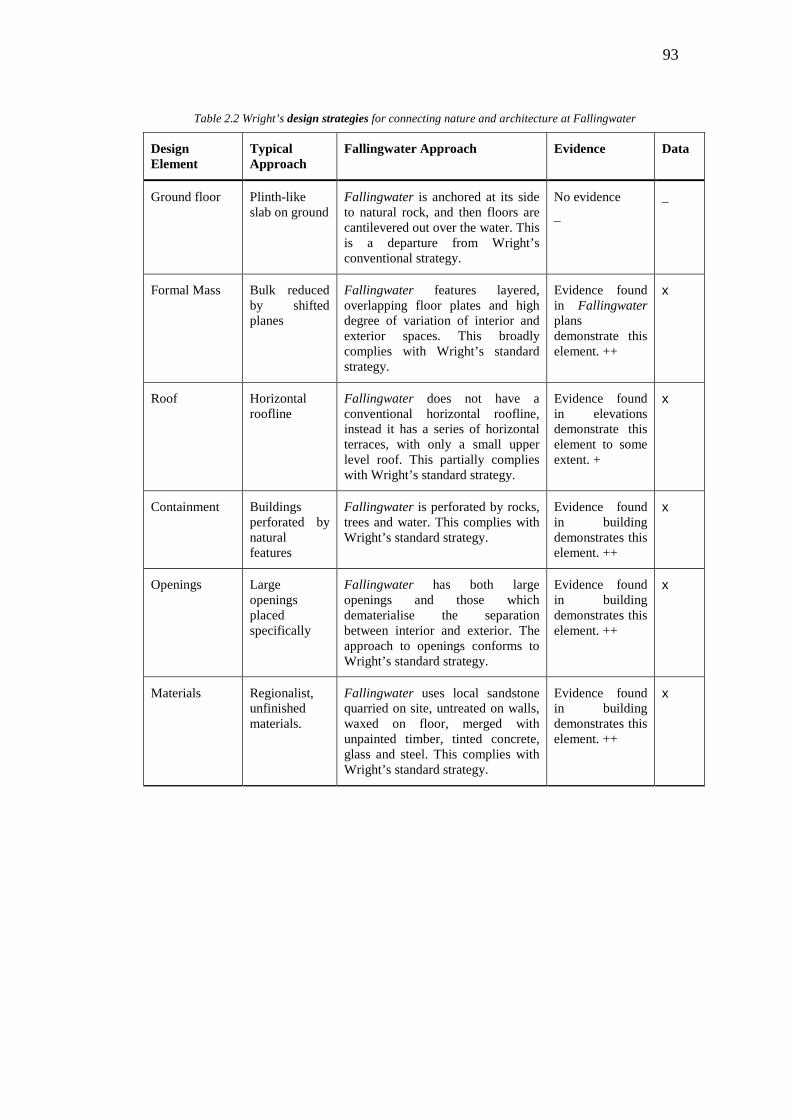
93

Table 2.2 Wright’s design strategies for connecting nature and architecture at Fallingwater

Design Element

Typical Approach

Fallingwater Approach Evidence Data

Ground floor Plinth-like slab on ground

Fallingwater is anchored at its side to natural rock, and then floors are cantilevered out over the water. This is a departure from Wright’s conventional strategy.

No evidence

–

_

Formal Mass Bulk reduced by shifted planes

Fallingwater features layered, overlapping floor plates and high degree of variation of interior and exterior spaces. This broadly complies with Wright’s standard strategy.

Evidence found in Fallingwater plans demonstrate this element. ++

x

Roof Horizontal roofline

Fallingwater does not have a conventional horizontal roofline, instead it has a series of horizontal terraces, with only a small upper level roof. This partially complies with Wright’s standard strategy.

Evidence found in elevations demonstrate this element to some extent. +

x

Containment Buildings perforated by natural features

Fallingwater is perforated by rocks, trees and water. This complies with Wright’s standard strategy.

Evidence found in building demonstrates this element. ++

x

Openings Large openings placed specifically

Fallingwater has both large openings and those which dematerialise the separation between interior and exterior. The approach to openings conforms to Wright’s standard strategy.

Evidence found in building demonstrates this element. ++

x

Materials Regionalist, unfinished materials.

Fallingwater uses local sandstone quarried on site, untreated on walls, waxed on floor, merged with unpainted timber, tinted concrete, glass and steel. This complies with Wright’s standard strategy.

Evidence found in building demonstrates this element. ++

x

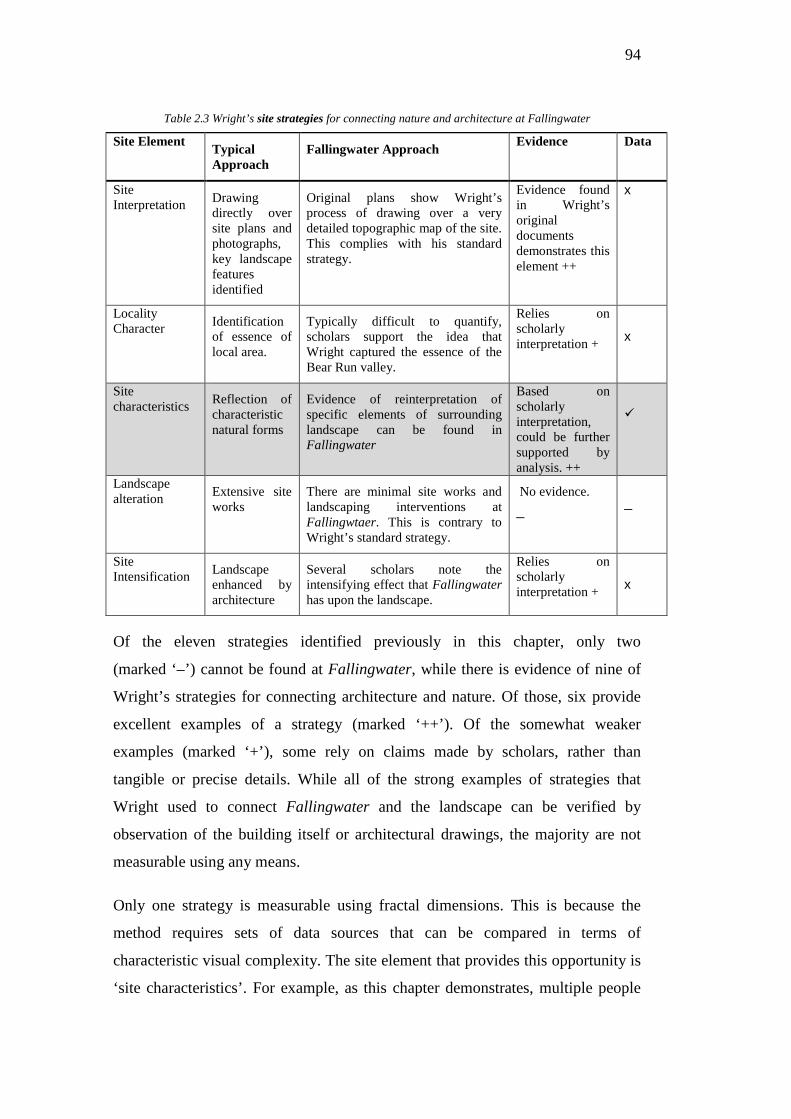
94

Table 2.3 Wright’s site strategies for connecting nature and architecture at Fallingwater

Site Element Typical Approach

Fallingwater Approach Evidence Data

Site Interpretation Drawing

directly over site plans and photographs, key landscape features identified

Original plans show Wright’s process of drawing over a very detailed topographic map of the site. This complies with his standard strategy.

Evidence found in Wright’s original documents demonstrates this element ++

x

Locality Character Identification

of essence of local area.

Typically difficult to quantify, scholars support the idea that Wright captured the essence of the Bear Run valley.

Relies on scholarly interpretation +

x

Site characteristics Reflection of

characteristic natural forms

Evidence of reinterpretation of specific elements of surrounding landscape can be found in Fallingwater

Based on scholarly interpretation, could be further supported by analysis. ++

Landscape alteration Extensive site

works There are minimal site works and landscaping interventions at Fallingwtaer. This is contrary to Wright’s standard strategy.

No evidence.

–

–

Site Intensification Landscape

enhanced by architecture

Several scholars note the intensifying effect that Fallingwater has upon the landscape.

Relies on scholarly interpretation +

x

Of the eleven strategies identified previously in this chapter, only two

(marked ‘–’) cannot be found at Fallingwater, while there is evidence of nine of

Wright’s strategies for connecting architecture and nature. Of those, six provide

excellent examples of a strategy (marked ‘++’). Of the somewhat weaker

examples (marked ‘+’), some rely on claims made by scholars, rather than

tangible or precise details. While all of the strong examples of strategies that

Wright used to connect Fallingwater and the landscape can be verified by

observation of the building itself or architectural drawings, the majority are not

measurable using any means.

Only one strategy is measurable using fractal dimensions. This is because the

method requires sets of data sources that can be compared in terms of

characteristic visual complexity. The site element that provides this opportunity is

‘site characteristics’. For example, as this chapter demonstrates, multiple people

95

have drawn direct connections between the appearance of the steep topography of

the valley, with its layered, projecting rock outcrops, and the form of

Fallingwater, with its cantilevered, horizontal terraces, tied to its steep vertical

stone walls. Similarly, Fallingwater’s profile, massing or silhouette, has been

likened to that of the valley. Such features of both the architecture and the

landscape are measurable using fractal analysis, and claims of their similarities are

therefore testable, and suited to this study.

Conclusion Throughout his life, Wright consistently espoused an Emersonian philosophy of

nature, which in turn had a profound influence on his own approach to designing

in response to the natural landscape. It was in Wright’s development of the Prairie

style, in the early 1900’s, where he used an abstracted reference to the natural

landscape, that Wright truly found his design style. For the rest of his career,

Wright typically used these abilities to delve into the natural, or even urban

setting, capturing its essence and reflecting this back in his architecture.

This chapter has defined the approaches—classified into eleven strategies—that

Wright took in order to achieve the effect of integrating a building with its setting.

The previous section of this chapter examined the evidence that Wright used these

approaches in Fallingwater to create a house that has become emblematic of a

building that fits with its natural setting. The chapter concluded with an

assessment of the features identified as ‘site characteristics’ that might be able to

be measured and tested to assess arguments that have been made about

Fallingwater. These features will be further investigated in Chapter 6.

The following chapters form Part II of this dissertation. They will describe the

methodological considerations for analysing several periods of Wright’s

architecture, as well as the approach to a specific study of the characteristic

complexity of Fallingwater and its natural setting.

96

Part II Methodological Considerations

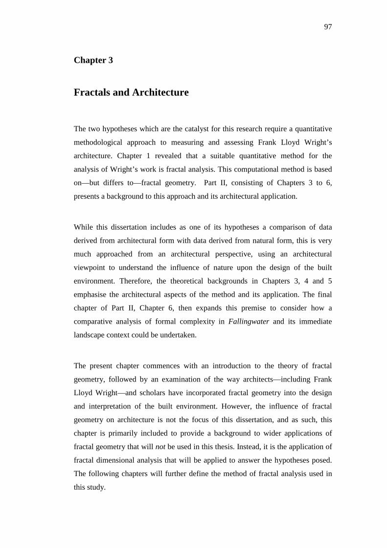
97

Chapter 3

Fractals and Architecture

The two hypotheses which are the catalyst for this research require a quantitative

methodological approach to measuring and assessing Frank Lloyd Wright’s

architecture. Chapter 1 revealed that a suitable quantitative method for the

analysis of Wright’s work is fractal analysis. This computational method is based

on—but differs to—fractal geometry. Part II, consisting of Chapters 3 to 6,

presents a background to this approach and its architectural application.

While this dissertation includes as one of its hypotheses a comparison of data

derived from architectural form with data derived from natural form, this is very

much approached from an architectural perspective, using an architectural

viewpoint to understand the influence of nature upon the design of the built

environment. Therefore, the theoretical backgrounds in Chapters 3, 4 and 5

emphasise the architectural aspects of the method and its application. The final

chapter of Part II, Chapter 6, then expands this premise to consider how a

comparative analysis of formal complexity in Fallingwater and its immediate

landscape context could be undertaken.

The present chapter commences with an introduction to the theory of fractal

geometry, followed by an examination of the way architects—including Frank

Lloyd Wright—and scholars have incorporated fractal geometry into the design

and interpretation of the built environment. However, the influence of fractal

geometry on architecture is not the focus of this dissertation, and as such, this

chapter is primarily included to provide a background to wider applications of

fractal geometry that will not be used in this thesis. Instead, it is the application of

fractal dimensional analysis that will be applied to answer the hypotheses posed.

The following chapters will further define the method of fractal analysis used in

this study.

98

3.1 Defining a Fractal

The word ‘fractal’ is derived from the Latin word frangere, meaning to break or

fragment. In mathematics the word ‘fraction’ is derived from the Latin fractus,

which is the past participle of frangere (Mandelbrot 1977). A fraction is both a

number produced by dividing one into another, and a fragment of a larger whole.

The meaning of the word fractal is drawn from both the original Latin and the

mathematical variant. In conventional use, the word fractal is used in two

contexts, the first to describe a type of irregular dimensionality and the second an

infinitely deep geometric set. In order to understand what a fractal dimension is,

and the difference between fractal dimensions (the topic of this dissertation) and

fractal geometry (the shapes often adopted by architectural designers), it is

necessary to briefly delve into the theory of dimensions and the history of fractals.

Architects and designers conventionally talk about and conceptualise shape and

form in both two and three dimensions. That is, from the first stages in their

education, designers understand that objects (including cities, buildings and

furniture) are three-dimensional, although their properties are typically described

using two-dimensional representations (plans, elevations, sections and various

perspective and isometric views). While this way of thinking about flat

representations as ‘two-dimensional’ and physical objects as ‘three-dimensional’

is in common use in society, the theory of dimensionality is actually much more

intricate and diverse (Aull and Lowen 2011). As a starting point to understanding

this theory, it is first necessary to clarify some of the basic terminology and

concepts used.

Mathematicians and scientists sometimes call the world in which we physically

exist ‘Euclidean space’, philosophers describe it as the ‘material world’ and

architectural theorists define it as ‘lived space’ or ‘experiential space’ (Juhos

1976). This dimension is physically tangible (it can be touched and otherwise

sensed) and it has practical material and scale limits, meaning it cannot be

99

infinitely divided or enlarged. To use an architectural example, a building in the

material world can be touched, it provides physical shelter and it is made of

substances that lose their structure if they are sufficiently weathered. In contrast,

the theorised or imagined world is described by mathematicians as ‘topological

space’, by philosophers as ‘abstract space’ and by architectural theorists as

‘geometric space’ (Wagner 2006). This imagined space has no direct physicality

and no practical limits, but it can still be studied in valuable ways. To use another

architectural example, a computer model of a building cannot be touched, it has

no capacity to provide shelter from the elements and it can be made infinitely

small, or large, without any impact on its geometry. Both the material world (of

the building) and the abstract world (of the CAD model) are rigorously defined,

dimensional spaces, but as we will see, while architects view them both as three

dimensional, mathematicians and scientists see them differently.

Technically, a dimension is a topological measure of the space-filling properties

of an object (Manning 1956). Thus, a dimension is an abstract but still accurate

gauge of the extent to which an object occupies space. While architects talk about

only two different dimensions—two-dimensional representations and three-

dimensional objects—for a mathematician, a large number of hypothetical

dimensions (n) exist in topological space. Mathematically, the relative

membership of an object in a dimensional set is determined by calculating the

number of coordinates required to define the location of a point on that object.

Thus, for example, the corner of a planar surface can be located in space with only

an x and y coordinate, while the corner of a cube requires x, y and z coordinates.

For the first of these examples n = 2 and for the second n = 3; that is, they are

respectively in two-dimensional and three-dimensional space (Sommerville 1958).

Because infinite mathematical dimensions are possible, mathematicians typically

talk of space as being n-dimensional (Pierpont 1930; Manning 1956).

Until the early 1970s, mathematicians accepted that n was necessarily a whole

number (for example, 1, 2 or 3). Moreover, the Euclidean world was thought of as

necessarily a geometrical three-dimensional space, with all other dimensions

100

existing only in abstract space. However, the idea that multiple dimensions may

exist simultaneously in Euclidean space has become known as the ‘theory of

general dimensions’ (Edgar 2008; Pears 2008). One of the catalysts for this

development was the growing realisation that whole number or integer

dimensions are incapable of describing the full complexity of the material world.

Probably the most famous of the general dimensions, and the first to methodically

develop non-integer values, is the fractal dimension.

In Les Objects Fractals, Benoît Mandelbrot (1975) built on the work of Gaston

Julia (1918) to suggest that Euclidean geometry, the traditional tool used in

science to describe natural objects, is fundamentally unable to fulfil this purpose.

While historically science considered roughness and irregularity to be an

aberration disguising underlying systems with finite values, Mandelbrot suggests

that the fragmentation of all naturally occurring phenomena cannot be so easily

disregarded. In order to solve this dilemma Mandelbrot (1982) proposed that

certain natural structures may be interpreted as lying in the range between

traditional whole number dimensions. He argues that, for example, if we look at a

snowflake under a microscope, it fills more space than a line (n > 1.0), yet far less

than a surface (n < 2.0), therefore its actual dimension is a fraction which is more

than one but less than two. Mandelbrot calls such fractional, non-integer

dimensions, fractal dimensions. Mandelbrot’s (1977) technical definition of a

fractal has been widely paraphrased as a set for which one has Hausdorff-

Besicovitch dimension greater than topological dimension and he demonstrated

this definition of a type of irregularity using a series of geometric constructions

which parametrically repeat themselves to produce evocative and infinitely

complex images. In this process Mandelbrot used fractal geometric sets to explain

fractal dimensions and vice versa.

It is this early combination of fractal dimensions and fractal geometry that caused

much of the later confusion and even forced Mandelbrot to revise his definition.

In hindsight, this misunderstanding was almost to be expected, because for a

mathematician dimensions are necessarily topological or abstract and should not

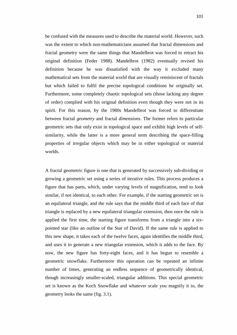
101

be confused with the measures used to describe the material world. However, such

was the extent to which non-mathematicians assumed that fractal dimensions and

fractal geometry were the same things that Mandelbrot was forced to retract his

original definition (Feder 1988). Mandelbrot (1982) eventually revised his

definition because he was dissatisfied with the way it excluded many

mathematical sets from the material world that are visually reminiscent of fractals

but which failed to fulfil the precise topological conditions he originally set.

Furthermore, some completely chaotic topological sets (those lacking any degree

of order) complied with his original definition even though they were not in its

spirit. For this reason, by the 1980s Mandelbrot was forced to differentiate

between fractal geometry and fractal dimensions. The former refers to particular

geometric sets that only exist in topological space and exhibit high levels of self-

similarity, while the latter is a more general term describing the space-filling

properties of irregular objects which may be in either topological or material

worlds.

A fractal geometric figure is one that is generated by successively sub-dividing or

growing a geometric set using a series of iterative rules. This process produces a

figure that has parts, which, under varying levels of magnification, tend to look

similar, if not identical, to each other. For example, if the starting geometric set is

an equilateral triangle, and the rule says that the middle third of each face of that

triangle is replaced by a new equilateral triangular extension, then once the rule is

applied the first time, the starting figure transforms from a triangle into a six-

pointed star (like an outline of the Star of David). If the same rule is applied to

this new shape, it takes each of the twelve faces, again identifies the middle third,

and uses it to generate a new triangular extension, which it adds to the face. By

now, the new figure has forty-eight faces, and it has begun to resemble a

geometric snowflake. Furthermore this operation can be repeated an infinite

number of times, generating an endless sequence of geometrically identical,

though increasingly smaller-scaled, triangular additions. This special geometric

set is known as the Koch Snowflake and whatever scale you magnify it to, the

geometry looks the same (fig. 3.1).

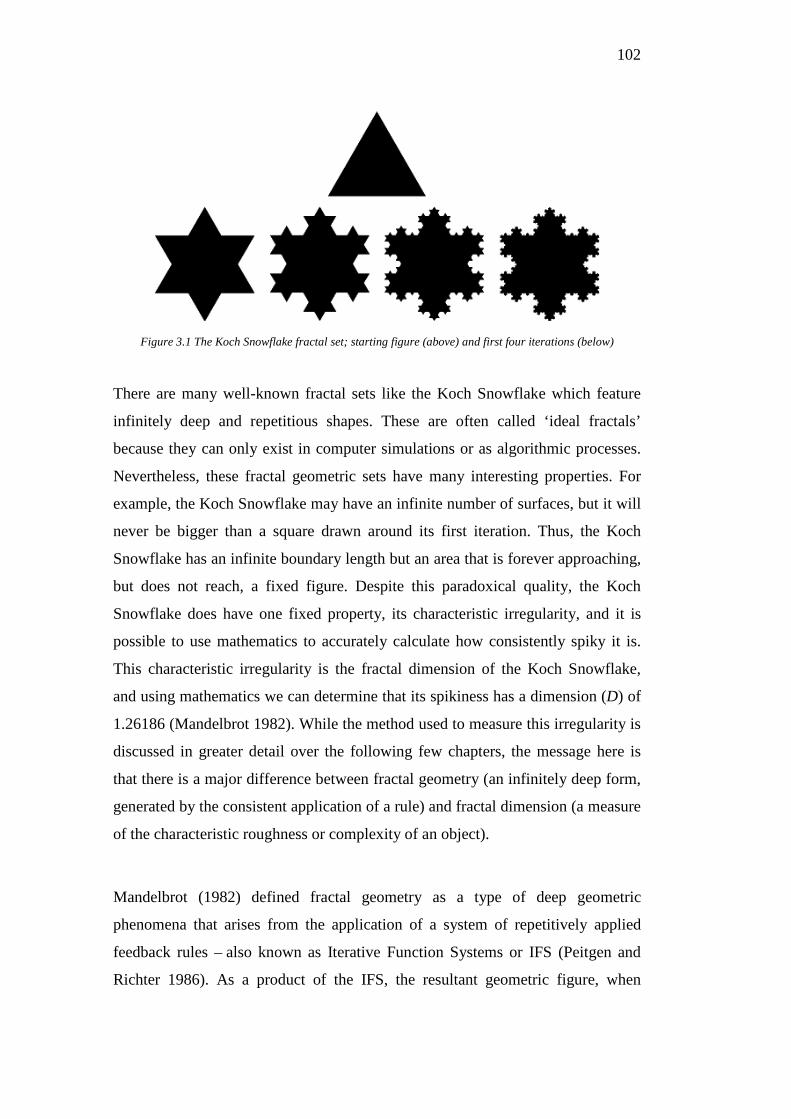
102

Figure 3.1 The Koch Snowflake fractal set; starting figure (above) and first four iterations (below)

There are many well-known fractal sets like the Koch Snowflake which feature

infinitely deep and repetitious shapes. These are often called ‘ideal fractals’

because they can only exist in computer simulations or as algorithmic processes.

Nevertheless, these fractal geometric sets have many interesting properties. For

example, the Koch Snowflake may have an infinite number of surfaces, but it will

never be bigger than a square drawn around its first iteration. Thus, the Koch

Snowflake has an infinite boundary length but an area that is forever approaching,

but does not reach, a fixed figure. Despite this paradoxical quality, the Koch

Snowflake does have one fixed property, its characteristic irregularity, and it is

possible to use mathematics to accurately calculate how consistently spiky it is.

This characteristic irregularity is the fractal dimension of the Koch Snowflake,

and using mathematics we can determine that its spikiness has a dimension (D) of

1.26186 (Mandelbrot 1982). While the method used to measure this irregularity is

discussed in greater detail over the following few chapters, the message here is

that there is a major difference between fractal geometry (an infinitely deep form,

generated by the consistent application of a rule) and fractal dimension (a measure

of the characteristic roughness or complexity of an object).

Mandelbrot (1982) defined fractal geometry as a type of deep geometric

phenomena that arises from the application of a system of repetitively applied

feedback rules – also known as Iterative Function Systems or IFS (Peitgen and

Richter 1986). As a product of the IFS, the resultant geometric figure, when

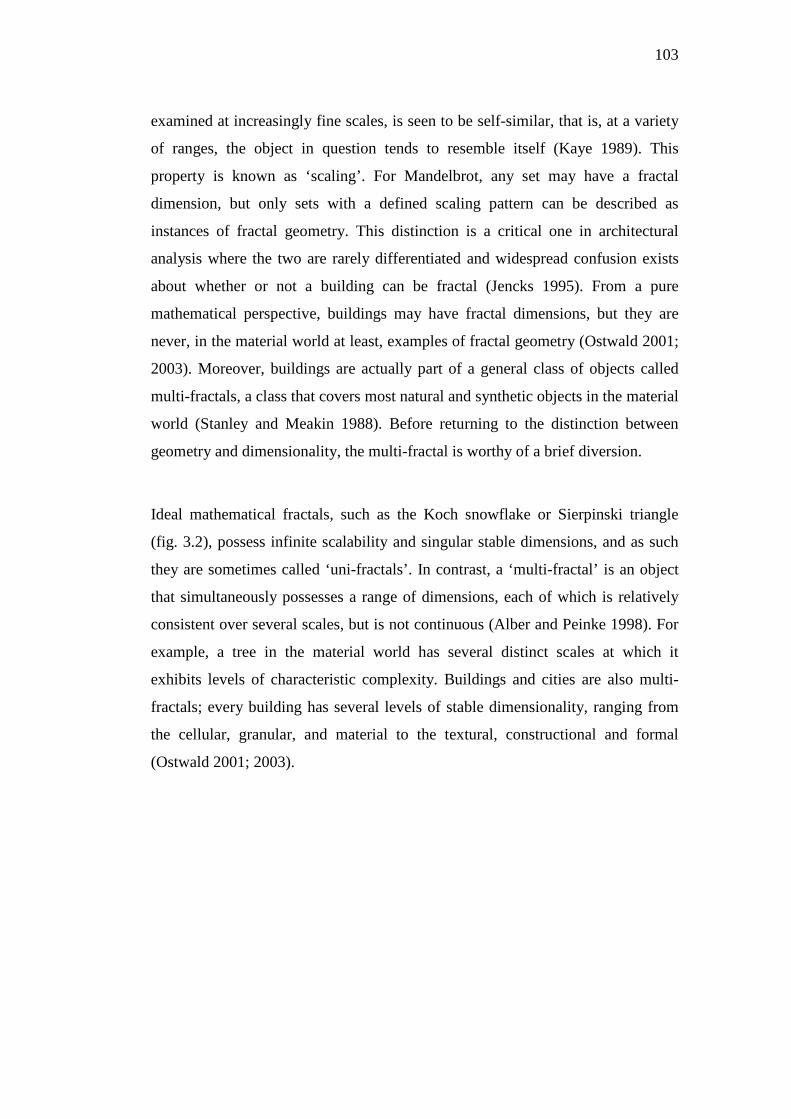
103

examined at increasingly fine scales, is seen to be self-similar, that is, at a variety

of ranges, the object in question tends to resemble itself (Kaye 1989). This

property is known as ‘scaling’. For Mandelbrot, any set may have a fractal

dimension, but only sets with a defined scaling pattern can be described as

instances of fractal geometry. This distinction is a critical one in architectural

analysis where the two are rarely differentiated and widespread confusion exists

about whether or not a building can be fractal (Jencks 1995). From a pure

mathematical perspective, buildings may have fractal dimensions, but they are

never, in the material world at least, examples of fractal geometry (Ostwald 2001;

2003). Moreover, buildings are actually part of a general class of objects called

multi-fractals, a class that covers most natural and synthetic objects in the material

world (Stanley and Meakin 1988). Before returning to the distinction between

geometry and dimensionality, the multi-fractal is worthy of a brief diversion.

Ideal mathematical fractals, such as the Koch snowflake or Sierpinski triangle

(fig. 3.2), possess infinite scalability and singular stable dimensions, and as such

they are sometimes called ‘uni-fractals’. In contrast, a ‘multi-fractal’ is an object

that simultaneously possesses a range of dimensions, each of which is relatively

consistent over several scales, but is not continuous (Alber and Peinke 1998). For

example, a tree in the material world has several distinct scales at which it

exhibits levels of characteristic complexity. Buildings and cities are also multi-

fractals; every building has several levels of stable dimensionality, ranging from

the cellular, granular, and material to the textural, constructional and formal

(Ostwald 2001; 2003).

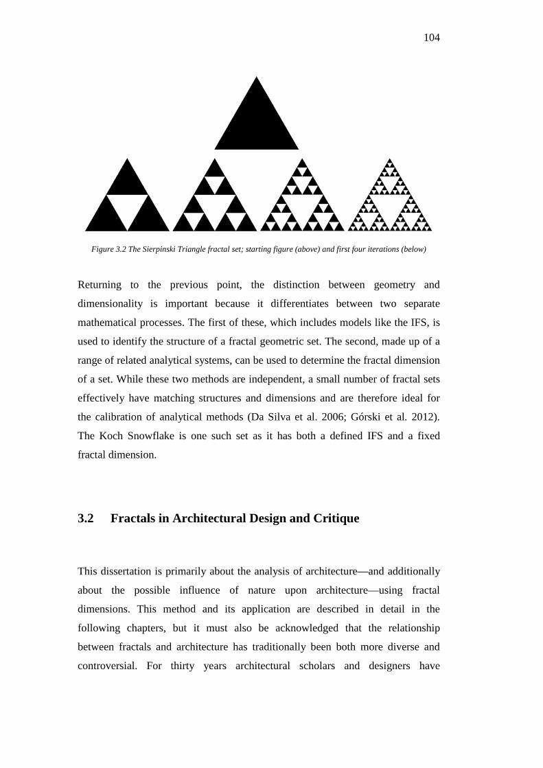
104

Figure 3.2 The Sierpinski Triangle fractal set; starting figure (above) and first four iterations (below)

Returning to the previous point, the distinction between geometry and

dimensionality is important because it differentiates between two separate

mathematical processes. The first of these, which includes models like the IFS, is

used to identify the structure of a fractal geometric set. The second, made up of a

range of related analytical systems, can be used to determine the fractal dimension

of a set. While these two methods are independent, a small number of fractal sets

effectively have matching structures and dimensions and are therefore ideal for

the calibration of analytical methods (Da Silva et al. 2006; Górski et al. 2012).

The Koch Snowflake is one such set as it has both a defined IFS and a fixed

fractal dimension.

3.2 Fractals in Architectural Design and Critique

This dissertation is primarily about the analysis of architecture—and additionally

about the possible influence of nature upon architecture—using fractal

dimensions. This method and its application are described in detail in the

following chapters, but it must also be acknowledged that the relationship

between fractals and architecture has traditionally been both more diverse and

controversial. For thirty years architectural scholars and designers have

105

opportunistically appropriated images and ideas from fractal geometry along with

concepts broadly related to fractal dimensions and non-linear dynamics, and used

them for a wide variety of purposes. Some of these appropriations have been

motivated by the desire to advance architecture or to offer new ways of

understanding design, but many others have a seemingly more superficial or

expeditious agenda (Ostwald 1998). There are sometimes frustrating connections

that have been proposed between architecture and fractals, however likewise there

are a large number of examples where architecture and fractal geometry have been

used as a catalyst for discussion of the broader nature of this complex and creative

association.

Fascinated by its mathematics and imagery, or drawn to possible natural or

mystical connections, some architectural writers and designers have promulgated

a range of often idiosyncratic interpretations of fractal geometry. Because of the

diverse range of motives for adopting fractal geometry, there is neither an agreed

upon definition nor a common title for works that use fractals for inspiration,

design rationale or form generation. For example, several portmanteau descriptors

exist which merge multiple, often dissimilar properties. Probably the best known

of these is Charles Jencks’s (1995) ‘Architecture of the Jumping Universe’, an

evocative title for an eclectic set of ideas cherry-picked from science, philosophy

and art. Similarly, the ‘New Baroque’ (Kipnis 1993) and the ‘Architecture of the

Fold’ (Eisenman 1993) freely merge concepts from fractal geometry with themes

from the writings of Deleuze and Guattari, philosophers who once used fractal

geometry as a metaphor for political theory (Ostwald 2000; 2006). The repeated

use of other classifications including ‘Fractalism’, ‘Complexitism’, ‘Complexity

Architecture’ and ‘Non-linear Architecture’ have led scholars like Yannick Joye

to argue that ‘a systematic, encompassing, scholarly treatment of the use and

presence of this geometrical language in architecture is missing’ (2011: 814).

Despite ongoing confusion over definitions, there are many examples of possible

connections between fractal geometry and architectural design, ranging from

inspiration to structure, from construction to surface treatment and from applied

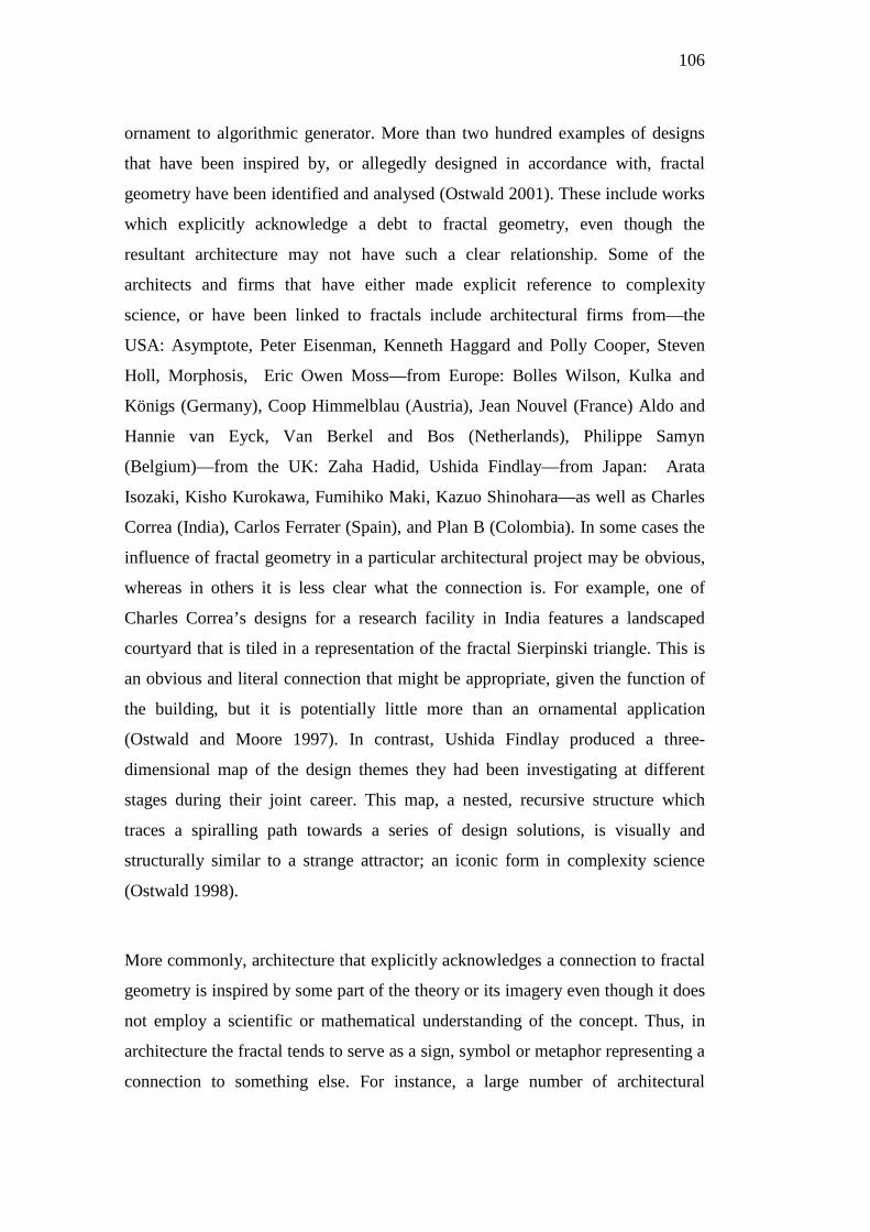
106

ornament to algorithmic generator. More than two hundred examples of designs

that have been inspired by, or allegedly designed in accordance with, fractal

geometry have been identified and analysed (Ostwald 2001). These include works

which explicitly acknowledge a debt to fractal geometry, even though the

resultant architecture may not have such a clear relationship. Some of the

architects and firms that have either made explicit reference to complexity

science, or have been linked to fractals include architectural firms from—the

USA: Asymptote, Peter Eisenman, Kenneth Haggard and Polly Cooper, Steven

Holl, Morphosis, Eric Owen Moss—from Europe: Bolles Wilson, Kulka and

Königs (Germany), Coop Himmelblau (Austria), Jean Nouvel (France) Aldo and

Hannie van Eyck, Van Berkel and Bos (Netherlands), Philippe Samyn

(Belgium)—from the UK: Zaha Hadid, Ushida Findlay—from Japan: Arata

Isozaki, Kisho Kurokawa, Fumihiko Maki, Kazuo Shinohara—as well as Charles

Correa (India), Carlos Ferrater (Spain), and Plan B (Colombia). In some cases the

influence of fractal geometry in a particular architectural project may be obvious,

whereas in others it is less clear what the connection is. For example, one of

Charles Correa’s designs for a research facility in India features a landscaped

courtyard that is tiled in a representation of the fractal Sierpinski triangle. This is

an obvious and literal connection that might be appropriate, given the function of

the building, but it is potentially little more than an ornamental application

(Ostwald and Moore 1997). In contrast, Ushida Findlay produced a three-

dimensional map of the design themes they had been investigating at different

stages during their joint career. This map, a nested, recursive structure which

traces a spiralling path towards a series of design solutions, is visually and

structurally similar to a strange attractor; an iconic form in complexity science

(Ostwald 1998).

More commonly, architecture that explicitly acknowledges a connection to fractal

geometry is inspired by some part of the theory or its imagery even though it does

not employ a scientific or mathematical understanding of the concept. Thus, in

architecture the fractal tends to serve as a sign, symbol or metaphor representing a

connection to something else. For instance, a large number of architectural

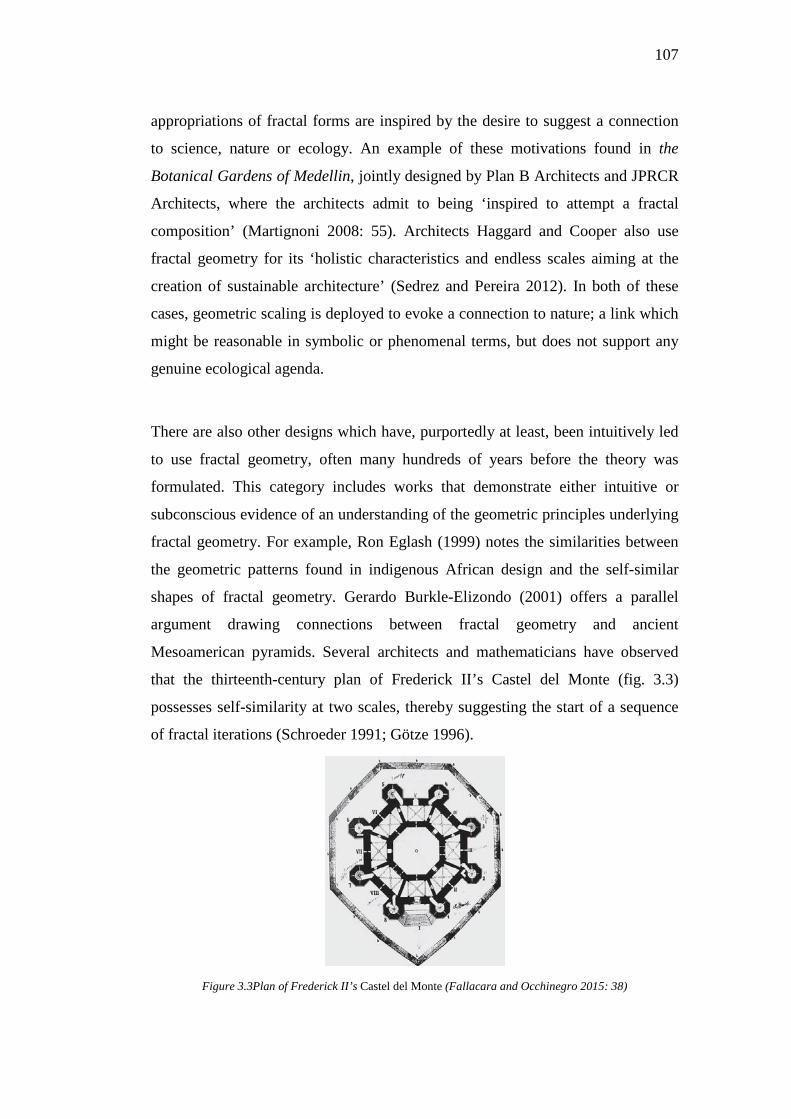
107

appropriations of fractal forms are inspired by the desire to suggest a connection

to science, nature or ecology. An example of these motivations found in the

Botanical Gardens of Medellin, jointly designed by Plan B Architects and JPRCR

Architects, where the architects admit to being ‘inspired to attempt a fractal

composition’ (Martignoni 2008: 55). Architects Haggard and Cooper also use

fractal geometry for its ‘holistic characteristics and endless scales aiming at the

creation of sustainable architecture’ (Sedrez and Pereira 2012). In both of these

cases, geometric scaling is deployed to evoke a connection to nature; a link which

might be reasonable in symbolic or phenomenal terms, but does not support any

genuine ecological agenda.

There are also other designs which have, purportedly at least, been intuitively led

to use fractal geometry, often many hundreds of years before the theory was

formulated. This category includes works that demonstrate either intuitive or

subconscious evidence of an understanding of the geometric principles underlying

fractal geometry. For example, Ron Eglash (1999) notes the similarities between

the geometric patterns found in indigenous African design and the self-similar

shapes of fractal geometry. Gerardo Burkle-Elizondo (2001) offers a parallel

argument drawing connections between fractal geometry and ancient

Mesoamerican pyramids. Several architects and mathematicians have observed

that the thirteenth-century plan of Frederick II’s Castel del Monte (fig. 3.3)

possesses self-similarity at two scales, thereby suggesting the start of a sequence

of fractal iterations (Schroeder 1991; Götze 1996).

Figure 3.3Plan of Frederick II’s Castel del Monte (Fallacara and Occhinegro 2015: 38)

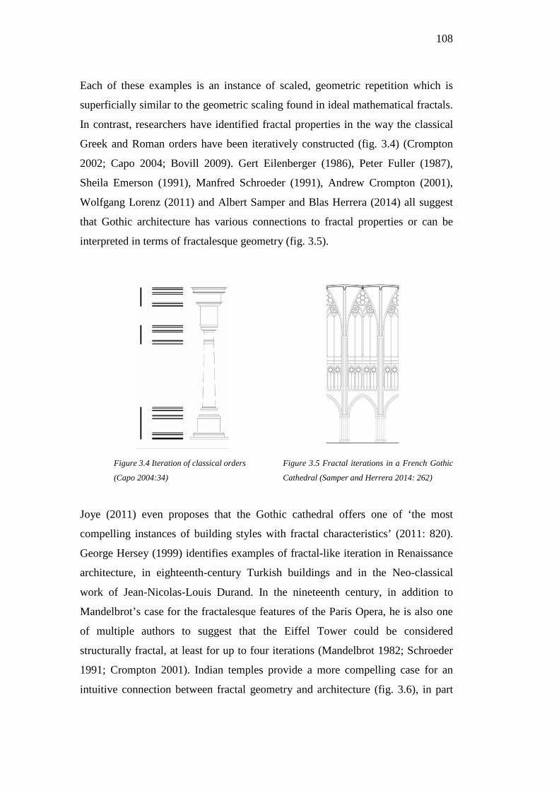
108

Each of these examples is an instance of scaled, geometric repetition which is

superficially similar to the geometric scaling found in ideal mathematical fractals.

In contrast, researchers have identified fractal properties in the way the classical

Greek and Roman orders have been iteratively constructed (fig. 3.4) (Crompton

2002; Capo 2004; Bovill 2009). Gert Eilenberger (1986), Peter Fuller (1987),

Sheila Emerson (1991), Manfred Schroeder (1991), Andrew Crompton (2001),

Wolfgang Lorenz (2011) and Albert Samper and Blas Herrera (2014) all suggest

that Gothic architecture has various connections to fractal properties or can be

interpreted in terms of fractalesque geometry (fig. 3.5).

Figure 3.4 Iteration of classical orders Figure 3.5 Fractal iterations in a French Gothic

(Capo 2004:34) Cathedral (Samper and Herrera 2014: 262)

Joye (2011) even proposes that the Gothic cathedral offers one of ‘the most

compelling instances of building styles with fractal characteristics’ (2011: 820).

George Hersey (1999) identifies examples of fractal-like iteration in Renaissance

architecture, in eighteenth-century Turkish buildings and in the Neo-classical

work of Jean-Nicolas-Louis Durand. In the nineteenth century, in addition to

Mandelbrot’s case for the fractalesque features of the Paris Opera, he is also one

of multiple authors to suggest that the Eiffel Tower could be considered

structurally fractal, at least for up to four iterations (Mandelbrot 1982; Schroeder

1991; Crompton 2001). Indian temples provide a more compelling case for an

intuitive connection between fractal geometry and architecture (fig. 3.6), in part

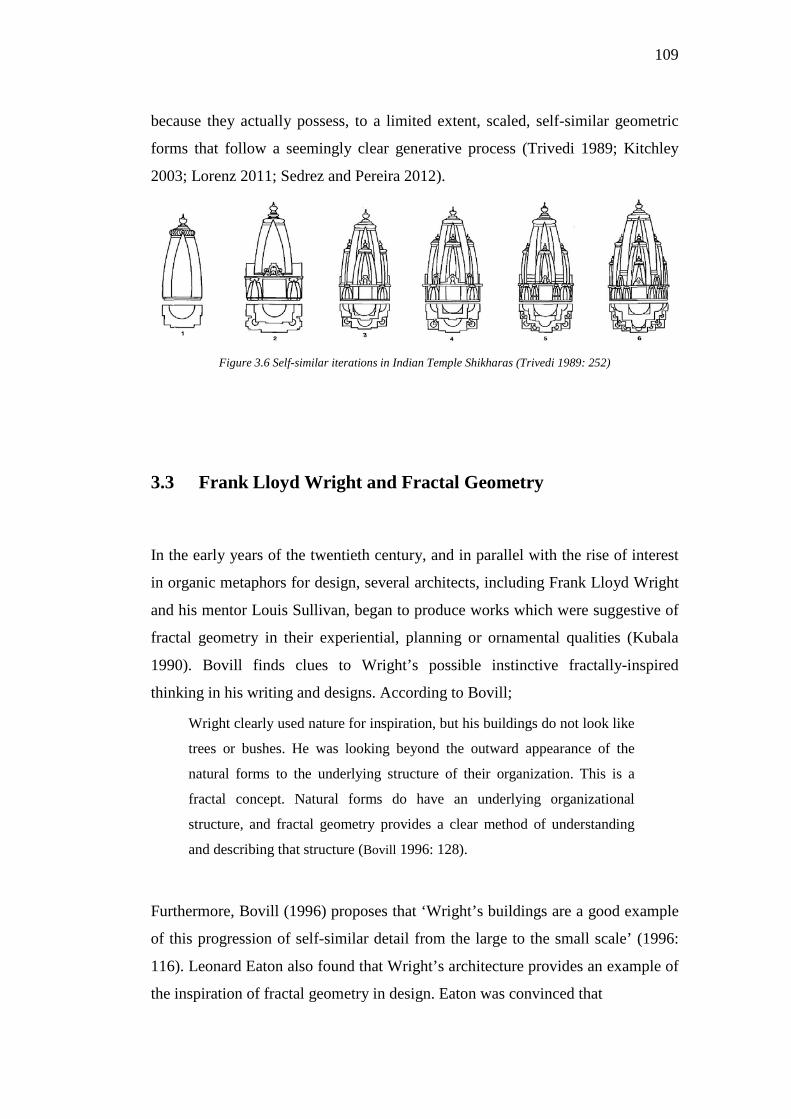
109

because they actually possess, to a limited extent, scaled, self-similar geometric

forms that follow a seemingly clear generative process (Trivedi 1989; Kitchley

2003; Lorenz 2011; Sedrez and Pereira 2012).

Figure 3.6 Self-similar iterations in Indian Temple Shikharas (Trivedi 1989: 252)

3.3 Frank Lloyd Wright and Fractal Geometry

In the early years of the twentieth century, and in parallel with the rise of interest

in organic metaphors for design, several architects, including Frank Lloyd Wright

and his mentor Louis Sullivan, began to produce works which were suggestive of

fractal geometry in their experiential, planning or ornamental qualities (Kubala

1990). Bovill finds clues to Wright’s possible instinctive fractally-inspired

thinking in his writing and designs. According to Bovill;

Wright clearly used nature for inspiration, but his buildings do not look like

trees or bushes. He was looking beyond the outward appearance of the

natural forms to the underlying structure of their organization. This is a

fractal concept. Natural forms do have an underlying organizational

structure, and fractal geometry provides a clear method of understanding

and describing that structure (Bovill 1996: 128).

Furthermore, Bovill (1996) proposes that ‘Wright’s buildings are a good example

of this progression of self-similar detail from the large to the small scale’ (1996:

116). Leonard Eaton also found that Wright’s architecture provides an example of

the inspiration of fractal geometry in design. Eaton was convinced that

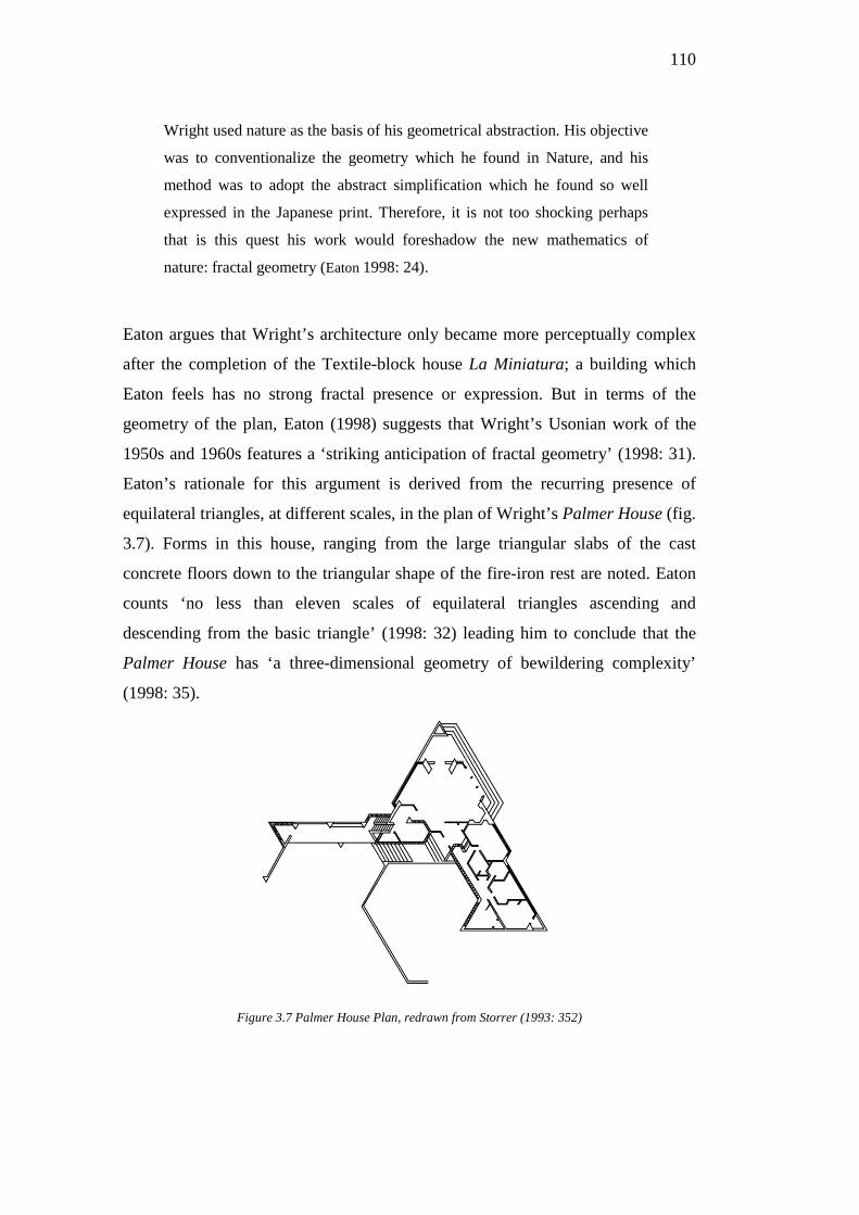
110

Wright used nature as the basis of his geometrical abstraction. His objective

was to conventionalize the geometry which he found in Nature, and his

method was to adopt the abstract simplification which he found so well

expressed in the Japanese print. Therefore, it is not too shocking perhaps

that is this quest his work would foreshadow the new mathematics of

nature: fractal geometry (Eaton 1998: 24).

Eaton argues that Wright’s architecture only became more perceptually complex

after the completion of the Textile-block house La Miniatura; a building which

Eaton feels has no strong fractal presence or expression. But in terms of the

geometry of the plan, Eaton (1998) suggests that Wright’s Usonian work of the

1950s and 1960s features a ‘striking anticipation of fractal geometry’ (1998: 31).

Eaton’s rationale for this argument is derived from the recurring presence of

equilateral triangles, at different scales, in the plan of Wright’s Palmer House (fig.

3.7). Forms in this house, ranging from the large triangular slabs of the cast

concrete floors down to the triangular shape of the fire-iron rest are noted. Eaton

counts ‘no less than eleven scales of equilateral triangles ascending and

descending from the basic triangle’ (1998: 32) leading him to conclude that the

Palmer House has ‘a three-dimensional geometry of bewildering complexity’

(1998: 35).

Figure 3.7 Palmer House Plan, redrawn from Storrer (1993: 352)

111

Yannick Joye agrees with Eaton’s assertion that the ‘Palmer House seems to be

the culmination point’ (Joye 2007: 312) of Wright’s intuitive use of fractal

geometry in architecture. In a similar vein, Daniele Capo (2004) uses Eaton’s

analysis of Wright’s domestic architecture to build on his own fractal analysis of

architecture, suggesting that Wright’s architecture combined smaller elements to

create larger works which show fractal similarities to Palladio’s architectural

orders. Giovanni Ferrero, Celestina Cotti, Michela Rossi, and Cecilia Tedeschi

also accept Eaton’s conclusion that fractals can be found in the Palmer House

(Ferrero et al. 2009). However, before Eaton’s work was published, Michael

Ostwald and John Moore (1996) rhetorically demonstrated that even the most

Euclidean of buildings, like Mies Van Der Rohe’s Seagram Building, can have

more than 12 scales of conscious self-similarity and that this does not make them,

or the Palmer House, fractal (Ostwald 2003). James Harris also disagrees with

Eaton’s simplified analysis of the Palmer House, saying that Eaton’s paper ‘points

out the misconception that a repetition of a form, the triangle in this case,

constitutes a fractal quality. It is not the repetition of the form or motif but the

manner in which it is repeated or its structure and nesting characteristics which

are important’ (Harris 2007: 98). Harris proceeds to apply an iteration method

(IFS) to a triangle, in an attempt to produce a similar plan to the Palmer House,

finally creating a design with some similarities in plan to the final design by

Wright. Harris concludes that Wright’s architecture may not be as strongly

generated by fractal geometry as Eaton suggests. However he finds the

relationship to be ‘analogous’ (Harris 2007:98). The word analogous is

appropriate because Eaton proposes the existence of a symbolic or metaphoric

relationship between fractal geometry and repetitious forms in the plan of the

Palmer House. Grant Hildebrand’s (2007) analysis of the Palmer House also

effectively dismisses Eaton’s argument about scaling and triangular geometry,

preferring to stress the more phenomenal or experiential connections to nature and

complexity.

112

While these scholars write directly about Wright’s possible relationship with

fractal geometry, there are others (including Wright himself) whose words do not

mention fractals but do suggest a fractalesque approach to design, particularly

noting repeated, scaled iterations, or pattern-seeking geometry, and this is based

on natural pattern. These proposals emerge from Wright’s source of inspiration in

nature, and the manner of his design process, where according to Carla Lind,

Wright ‘dipped into the stream, looked into the treetops, stretched out like

branches from a tree, and used nature’s own color palette’ (1996: 21). Neil Levine

provides an example of this process in Fallingwater, which he describes as being

‘ultimately about the cumulative effect of stone, water, trees, leaves, mist, clouds,

and sky as they interact over time’ (2000: 57-58).

Many authors emphasise Wright’s own declarations that ‘design is abstraction of

nature-elements in purely geometric terms’ (Wright 1957: 181). For example,

Diane Maddex considers Wright’s architecture as an expression where ‘geometry

synthesized nature to its very essence’ (1998: 9), and David Hertz also notes

Wright’s ‘careful observation of natural pattern’ (1993: 2). According to Olsberg,

Wright was attempting ‘to discover an abstract language of forms—a language in

sympathy with natural laws’ the output of which did not have to necessarily

present as ‘naturalistic’ (1996: 11).

While the observation of a pattern in nature may lead to the development of

fractal-like geometry, as David De Long points out, it is just as possible to find

Euclidean patterns and geometry this way:

For Wright, the ideal order of the universe was thus Euclidian by nature,

and this order could be represented by combinations of Euclidian shapes

organized according to a larger field of gridded modules. (1996: 119)

The change from Euclidean to fractal geometry can be found in the repetition or

iteration of the forms, over different levels of physical dimension. This idea of

‘scaling’, while not mentioned in conjunction with fractals, is alluded to by many

113

Wright scholars, so that while De Long finds Wright’s work to be extracted

Euclidean shapes, his description of their use could be considered fractal.

[Wright] sought universal meaning though attachment to place, varying his

geometries not only to achieve an indivisible bond with each specific

location, but, more importantly, to complete that locations underlying

structure, so that each place became more fully revealed as an indivisible

part of an ordered cosmos (De Long 1996: 120).

Other authors describe the scaling effect more clearly, explaining that Wright

‘developed the notion of inner geometries, concealed within larger forms’

(Olsberg 1996: 12). According to Jeanne Rubin, ‘[f]rom the smallest interior

detail to the largest exterior statement, Wright is well known to have developed

his structures outward from within, through repetitive extensions of a central

motif’ (2002: 111). Howard Robertson defines Wright’s Organic style as an

architecture where ‘everything in and about the building should be fully

integrated, part of the design […] It means that the expression, the exterior details,

the planning for requirements, are all built-in and built-up, producing an organic

whole’ (1952: 174). Finally, whether or not evidence of fractal properties can be

detected, Wright himself, in his usual rambling way, declared that:

Reality is spirit—the essence brooding just behind all aspect. Seize it! And–

after all you will see that the pattern of reality is supergeometric, casting a

spell or a charm over any geometry, and is such a spell in itself. Yes, so it

seems to me as I draw with T-square, triangle and scale. That is what it

means to be an artist—to seize the essence brooding everywhere in

everything, just behind aspect (1957: 157).

Conclusion

Despite the fascinating possibility that Wright may have developed an instinctual

understanding of the fractal geometry present in nature, this dissertation does not

explore this avenue of research any further. While this chapter has been concerned

with the way fractal geometry and associated imagery and ideas have been used

114

by architectural designers and scholars, this notion has been presented as a

precursor to this study’s more rigorous basis, the application of a quantifiable

approach to measuring and analysing Wright’s architecture using fractal

dimensions. The two approaches offer different ways of considering the

relationship between design and geometry, for there is no explicit connection

between fractal measurement and a design that seeks to evoke—through form,

texture or tectonics—fractal geometry. Thus, while it is possible to measure the

fractal dimension of a building that is inspired by fractal geometry, the two

processes, measurement and inspiration, are fundamentally unrelated. The former,

measurement, is a universal set of actions, following a strict protocol, which can

be repeated for multiple similar objects. The latter, inspiration, is an intricate and

potentially poetic process, which is typically unique to an individual. Both of

these processes are valid and useful, but they should not be confused.

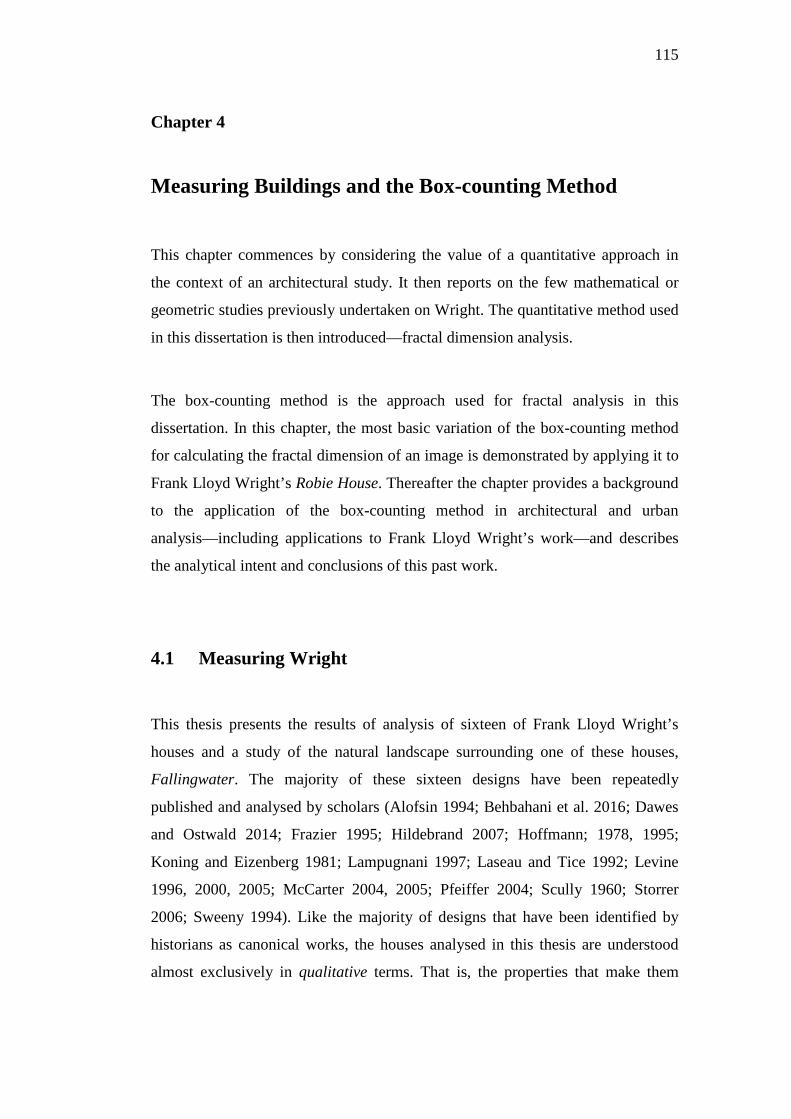
115

Chapter 4

Measuring Buildings and the Box-counting Method

This chapter commences by considering the value of a quantitative approach in

the context of an architectural study. It then reports on the few mathematical or

geometric studies previously undertaken on Wright. The quantitative method used

in this dissertation is then introduced—fractal dimension analysis.

The box-counting method is the approach used for fractal analysis in this

dissertation. In this chapter, the most basic variation of the box-counting method

for calculating the fractal dimension of an image is demonstrated by applying it to

Frank Lloyd Wright’s Robie House. Thereafter the chapter provides a background

to the application of the box-counting method in architectural and urban

analysis—including applications to Frank Lloyd Wright’s work—and describes

the analytical intent and conclusions of this past work.

4.1 Measuring Wright

This thesis presents the results of analysis of sixteen of Frank Lloyd Wright’s

houses and a study of the natural landscape surrounding one of these houses,

Fallingwater. The majority of these sixteen designs have been repeatedly

published and analysed by scholars (Alofsin 1994; Behbahani et al. 2016; Dawes

and Ostwald 2014; Frazier 1995; Hildebrand 2007; Hoffmann; 1978, 1995;

Koning and Eizenberg 1981; Lampugnani 1997; Laseau and Tice 1992; Levine

1996, 2000, 2005; McCarter 2004, 2005; Pfeiffer 2004; Scully 1960; Storrer

2006; Sweeny 1994). Like the majority of designs that have been identified by

historians as canonical works, the houses analysed in this thesis are understood

almost exclusively in qualitative terms. That is, the properties that make them

116

special or significant are documented and communicated using textual

descriptions, supplemented by photographic or graphic media. In these cases, the

media is not usually scrutinised or analysed, it only provides a visual reference for

the house, rather than an explanatory reference, leaving the descriptive text to

provide the reader with an understanding of these designs. Such texts are

invariably presented using a combination of comparative and denotative terms.

Thus, these designs are characterised by historians and scholars as having, ‘wider

eaves’, ‘deeper balconies’ and ‘natural materials’ (Alofsin 1994; De Long 1996;

Storrer 2006). They are ‘richly textured’ and ‘grow out of their sites’ (Kaufmann

1986; Maddex 1998). These examples are typical of the qualitative descriptions

used to explain the characteristics of architecture and the significance of these

buildings in a larger historical context. Variations of these phrases are repeated in

almost every major architectural reference work. They represent a combination of

professional judgment, informed personal opinion and received wisdom (Koning

and Eisenberg 1981; Stamps 1999; Laseau and Tice 1992). For example, Koning

and Eisenberg emphasise that ‘such descriptions do not explicitly inform us as to

how […] houses are constructed, and consequently provide little help in

designing’ (1981:295). There is nothing wrong with this way of constructing the

history and theory of architecture, but there are valuable alternative approaches

that can be used to question the traditional classification of these buildings and

promote a new way of understanding them.

Frank Lloyd Wright’s architecture is a perfect example of a body of work which

has been extensively documented by twentieth century historians using qualitative

techniques (Futagawa and Pfeiffer 1984; 1985a; 1985b; 1985c; 1987a; 1987b;

Cronon 1994; De Long 1996; Cleary 1999; Storrer 2006; Hoffmann 1978; 1993;

1995; Levine 2005; Fell 2009). Despite such examples, Wright’s architecture has

only rarely been subjected to any type of quantitative—generally computational or

mathematical—analysis. Even though researchers have repeatedly identified

Wright’s predilection for geometric systems and have carefully quantified and

categorized his works into clear stylistic period (Koning and Eizenberg 1981;

MacCormac 2005; Dawes and Ostwald 2014; Behbahani et al. 2016; Lee et al.

117

2017), the vast majority of what is known about Wright’s architecture remains

qualitative in nature. Nevertheless, a small number of quantitative studies do exist

and they confirm that it is not only possible to study Wright’s architecture using

computational means, but it is highly beneficial because of the size of the body of

work he produced. Importantly, several of the computational or geometric studies

of Wright’s architecture that have previously been undertaken have been focused

on his houses. For example, John Sergeant proposes that Wright’s flexible use of

planning grids is the common link between the Prairie Style, the Textile-block

period and the Usonian house period. Sergeant suggests that the Prairie Style

houses were designed on a ‘tartan grid’ where a ‘vocabulary of forms was used to

translate or express the grid at all points – the solid rather than pierced balconies,

planters, bases of flower urns, clustered piers, even built-in seats were evocations

of the underlying structure of a house’ (2005: 192). The Textile-block houses,

typically set in the steep topography of the Los Angeles foothills, necessitated a

development in Wright’s use of the grid which signals, according to Sergeant, the

moment when Wright first extended his planning grid into a vertical axis.

Richard MacCormac uses a different, but equally planar diagrammatic method to

compare the forms of 11 of Wright’s early buildings with the shapes of the

Froebel’s Gifts; a three-dimensional educational device which Wright used as a

child. MacCormac concludes that the Froebel discipline can be found in all of

Wright’s early work as a ‘certain continuity of principle’ (2005: 132). Hank

Koning and Julie Eizenberg agree that ‘MacCormac was right in the idea that

there is a consistent underlying structure informing Wright’s work’ however, they

find MacCormac’s method and approach to be limited by a sense of order ‘as if

order must in some way be tied up with measurable geometry’(Koning and

Eizenberg 1981: 296). Koning and Eizenberg propose that a shape grammar

approach is more suitable to the analysis and modelling of Wright’s organic

design approach. Utilizing the shape grammar approach to analyse six of Wright’s

prairie houses, Koning and Eizenberg conclude that ‘the composition of Wright’s

prairie-style houses is based on a few simple spatial relations between

parameterized three-dimensional building blocks of the Froebelean type’ (Koning

118

and Eizenberg 1981: 296). They further propose a three-dimensional parametric

shape grammar to demonstrate the design of new ‘Wright-style’ buildings. Terry

Knight builds on the work of Koning and Eizenberg with a comparative shape

grammar analysis of Wright’s Prairie and Usonian styles. Knight believes that the

elemental ‘composition of Prairie houses provide[s] the basis for the basic

composition of the later Usonian houses’ (1994: 222). Knight produces a shape

grammar for six of Wright’s Usonian houses, and compares these with ‘a

simplified version of Koning and Eizenberg’s earlier [Prairie] grammar’ (1994:

224), concluding that ‘[a]lthough the outward appearance and spatial organization

of Usonian houses seems substantially different from that of the Prairie houses,

the underlying composition of Usonian designs is closely related to that of Prairie

designs’ (1994: 236). Most recently, Lee et al. (2017) have returned to Koning’s

and Eizenberg’s original grammatical reading of the Prairie Style, and using a

combined syntactical and grammatical method, identified a statistical archetype

for this period of Wright’s architecture.

In the largest plan-analysis study undertaken into Wright’s works, Paul Laseau

and James Tice reject the standard historical focus on ‘underlying principles’ and

aim for a balanced approach that employs analytical illustrations to generate

typological studies of the plans of 131 of Wright’s buildings. Laseau and Tice’s

formal analysis demonstrates a categorisation of Wright’s work into three

typological, rather than chronological, thematic groups; the atrium, the hearth and

the tower (1992).

Precise geometric mapping of lines of sight within and around Wright’s

architecture have been measured using a space syntax method by Behbahani et al.

(2014; 2016). Ostwald and Dawes have taken this idea further by applying isovist

field analysis, a computational technique, to investigate Hildebrand’s architectural

version of Prospect-Refuge theory as applied to routes through and views of

Wright’s domestic architecture (Ostwald and Dawes 2013; Dawes and Ostwald

2014).

119

4.2 Fractal Dimensions

The quantitative methods described in the previous section all provide calculable,

comparable results, which broaden the techniques available to architectural

scholars. Another, similarly rigorous method—fractal analysis—is the

quantitative, mathematical and computational approach chosen for the present

study, giving it a distinctive starting point from which to selectively rethink the

properties of some of Wright’s most famous buildings.

Fractal analysis measures the fractal dimension of a plan, elevation or other

representation of a design. A fractal dimension is a rigorous measure of the

relative density and diversity of geometric information in an image or object. This

property, which is described as either ‘characteristic complexity’ or ‘statistical

roughness’, is simply a determination of the amount (meaning volume) and

distribution (meaning how it is spread over many scales) of geometry in a form. In

architectural terms, it could be seen as a mathematical calculation of the extent to

which lines, regardless of their purpose, are both present in, and dispersed across,

an elevation or plan.

The method for calculating the fractal dimension of an object was first proposed

by mathematicians in the 1980s (Eilenberger 1986; Peitgen and Richter 1986;

Keller et al. 1987; Feder 1988; Vos 1988; Kaye 1989). Many hundreds of

scientific and medical studies (for example, Peebles 1989; Chen et al. 1993;

Asvestas et al. 2000; De Vico et al. 2009) have been published using variations of

the fractal analysis method to measure and compare complex objects, but it is

still—despite important past research—poorly understood by architectural

scholars and almost completely unknown amongst design students and

practitioners. Part of the reason for this situation is that these other fields

(engineering, biology, astronomy, geology and medicine) have had a long-term

interest in measuring the properties of complex objects and have thus developed

stable versions of the method. However, in architecture and design, despite

120

progress in the 1990s, the most accurate and useful variant has only recently been

identified. For this reason, Part II contains a clear description of the process of

using fractal dimensions for measuring, along with a demonstration of its

application, a review of its methodological variables and a discussion of its limits.

4.3 Measuring Fractal Dimensions

There are multiple ways of mathematically calculating the fractal dimension of an

image (where 1.0 < D < 2.0) or object (where 2.0 < D < 3.0). For example,

Mandelbrot (1982) describes three alternatives, the first of which, the box-

counting approach, relies on overlaying different scales of grids and comparing

the amount of detail present in each. Often credited to Richard Voss (1986; 1988),

technically the box-counting method calculates the Minkowski–Bouligant

dimension. In practice though, the method has become so widely accepted that the

result is described as either the box-counting dimension or the fractal dimension.

Mandelbrot (1982) also presented a second way of calculating the approximate

fractal dimension of an image using overlapping circles of different radii and a

comparison between the capacities of these circles to cover the outline of an

image. The third method described by Mandelbrot was the packing dimension

which is based on the capacity of a series of circles to cover an irregular line

around an image. This third version imagines that a range of circles, of

increasingly reducing size, are iteratively packed inside the borders of that image.

A comparison is then constructed between the number of circles, of different

scales, needed to ‘fill’ the object.

Since Mandelbrot first proposed that fractal dimensions were measurable, seven

major permutations or approaches have been identified. The first two are the box-

counting method and the differential box-counting method. The other five are the

power spectrum method, the power differentiation method, the difference

statistics method, the Kth nearest neighbour method and the covering blanket

121

approach (Ostwald 2013). All of these versions have been evaluated and

compared with the outcome that, for most results (1.2 < D < 1.8) the box-counting

method is the most accurate and useful (Asvestas et al. 2000; Li et al. 2009).

Nirupam Sarker and B.B. Chaudhuri (1994) concur, arguing that despite some

known issues with higher range (D > 1.8) results, the box-counting method

remains the most reliable approach. This particular issue arises from the fact that

for very complex dimensions, the box-counting method begins to lose accuracy at

the most complex extreme (Asvestas et al. 2000). This observation is of less

concern for architectural analysis than for some other fields, because architecture

and most correctly pre-processed urban forms, do not fall into the range where D

> 1.8 and if they do, the level of error does not become substantial until D >1.9

(Ostwald et al. 2009; Ostwald and Vaughan 2013a) and the majority of past

research into methods of measuring fractal dimensions have confirmed that the

box-counting approach is the most accurate and useful (Xie and Xie 1997; Yu et

al. 2005).

4.4 The Box-counting Method

The box-counting method for determining the fractal dimension of an image is

probably the best-known approach, in any discipline, for quantifying

characteristic visual complexity. This method has been studied extensively and

applied in the sciences and mathematics and, over time, several variations of it

have been developed for use in different fields. While there are different ways of

measuring fractal dimensions, the box-counting variant is the most stable and

repeatable, and thus, over time, it has become synonymous with ‘fractal

analysis’.For example, specific versions have been developed for biology (De

Vico et al. 2005), neuroscience (Jelinek et al. 2005), mineralogy (Blenkinsop and

Sanderson 1999), geology (Grau et al. 2006) and physics (Kruger 1996). The

reason these variations exist is that the box-counting method is known to have

particular strengths and weaknesses in certain ranges of dimensions and for

122

particular image types. As a result of this, scientists and mathematicians have

identified several mathematical refinements, along with a range of methodological

and data variables that, in combination, can be optimised to meet the needs of

different disciplines.

The box-counting method was first adopted for architectural and urban analysis in

the 1990s (Batty and Longley 1994) and since that time has been used for the

analysis of a growing number of buildings, ranging from ancient structures to

twentieth century designs (Bovill 1996; Burkle-Elizondo 2001; Rian et al. 2007;

Ostwald and Vaughan 2009; 2010; 2013). A stable computational version was

first presented in 2008 (Ostwald et al. 2008) and the box counting method is now

the accepted version in architectural scholarship as it is ‘easy to use and an

appropriate method for measuring works of architecture with regard to continuity

of roughness over a specific scale-range (coherence of scales)’ (Lorenz 2009:

703). However, architectural researchers, like the scientists and mathematicians

before them, have also noted that the method has some weaknesses and have

identified several specific factors which can dramatically affect the accuracy of

the calculation (Bovill 1996; Benguigui et al. 2000; Ostwald et al. 2008; Lorenz

2012). Despite this, it is only in the last few years that solutions to these problems

have been identified and their impacts determined (Ostwald 2013; Ostwald and

Vaughan 2013b; 2013c).

Using this stable computational version of the method, which is described in

detail in the present dissertation, it is now possible to measure the fractal

dimensions of the plans and elevations of a wide range of buildings. The data

points extracted from these views can then be synthesised into sets of values that

are in turn compiled in various ways to produce a series of composite results

describing the fractal dimension of a complete building. Once this process is

complete the data may be coded with additional information producing a set of

mathematical results that describe the properties of a design, or a set of buildings,

or changing formal and spatial patterns over time.

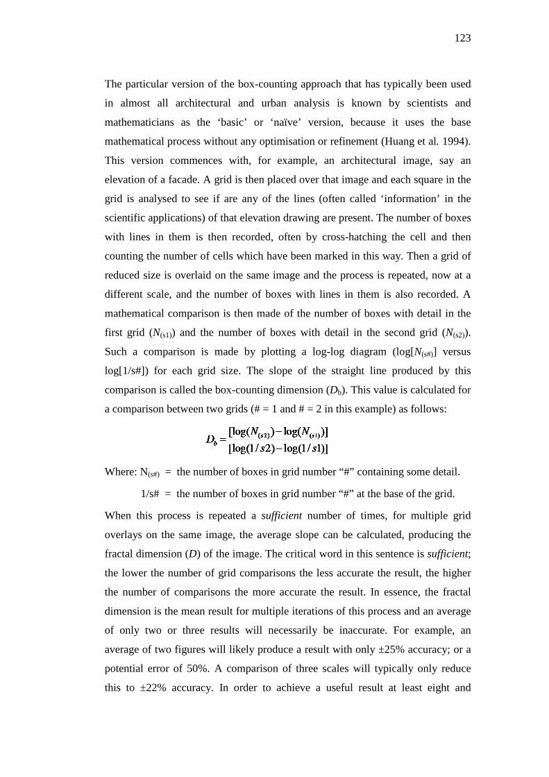
123

The particular version of the box-counting approach that has typically been used

in almost all architectural and urban analysis is known by scientists and

mathematicians as the ‘basic’ or ‘naïve’ version, because it uses the base

mathematical process without any optimisation or refinement (Huang et al. 1994).

This version commences with, for example, an architectural image, say an

elevation of a facade. A grid is then placed over that image and each square in the

grid is analysed to see if are any of the lines (often called ‘information’ in the

scientific applications) of that elevation drawing are present. The number of boxes

with lines in them is then recorded, often by cross-hatching the cell and then

counting the number of cells which have been marked in this way. Then a grid of

reduced size is overlaid on the same image and the process is repeated, now at a

different scale, and the number of boxes with lines in them is also recorded. A

mathematical comparison is then made of the number of boxes with detail in the

first grid (N(s1)) and the number of boxes with detail in the second grid (N(s2)).

Such a comparison is made by plotting a log-log diagram (log[N(s#)] versus

log[1/s#]) for each grid size. The slope of the straight line produced by this

comparison is called the box-counting dimension (Db). This value is calculated for

a comparison between two grids (# = 1 and # = 2 in this example) as follows:

Where: N(s#) = the number of boxes in grid number “#” containing some detail.

1/s# = the number of boxes in grid number “#” at the base of the grid.

When this process is repeated a sufficient number of times, for multiple grid

overlays on the same image, the average slope can be calculated, producing the

fractal dimension (D) of the image. The critical word in this sentence is sufficient;

the lower the number of grid comparisons the less accurate the result, the higher

the number of comparisons the more accurate the result. In essence, the fractal

dimension is the mean result for multiple iterations of this process and an average

of only two or three results will necessarily be inaccurate. For example, an

average of two figures will likely produce a result with only ±25% accuracy; or a

potential error of 50%. A comparison of three scales will typically only reduce

this to ±22% accuracy. In order to achieve a useful result at least eight and

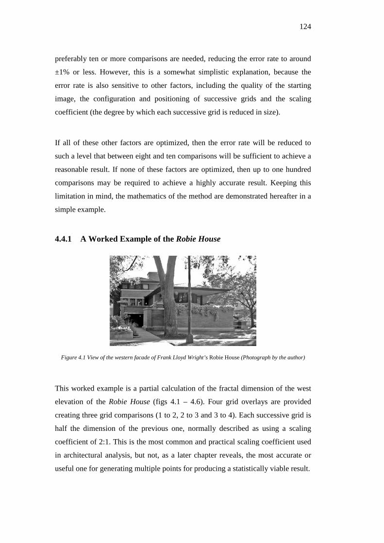
124

preferably ten or more comparisons are needed, reducing the error rate to around

±1% or less. However, this is a somewhat simplistic explanation, because the

error rate is also sensitive to other factors, including the quality of the starting

image, the configuration and positioning of successive grids and the scaling

coefficient (the degree by which each successive grid is reduced in size).

If all of these other factors are optimized, then the error rate will be reduced to

such a level that between eight and ten comparisons will be sufficient to achieve a

reasonable result. If none of these factors are optimized, then up to one hundred

comparisons may be required to achieve a highly accurate result. Keeping this

limitation in mind, the mathematics of the method are demonstrated hereafter in a

simple example.

4.4.1 A Worked Example of the Robie House

Figure 4.1 View of the western facade of Frank Lloyd Wright’s Robie House (Photograph by the author)

This worked example is a partial calculation of the fractal dimension of the west

elevation of the Robie House (figs 4.1 – 4.6). Four grid overlays are provided

creating three grid comparisons (1 to 2, 2 to 3 and 3 to 4). Each successive grid is

half the dimension of the previous one, normally described as using a scaling

coefficient of 2:1. This is the most common and practical scaling coefficient used

in architectural analysis, but not, as a later chapter reveals, the most accurate or

useful one for generating multiple points for producing a statistically viable result.

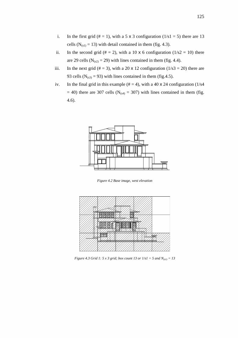
125

i. In the first grid (# = 1), with a 5 x 3 configuration (1/s1 = 5) there are 13

cells (N(s1) = 13) with detail contained in them (fig. 4.3).

ii. In the second grid (# = 2), with a 10 x 6 configuration (1/s2 = 10) there

are 29 cells (N(s2) = 29) with lines contained in them (fig. 4.4).

iii. In the next grid (# = 3), with a 20 x 12 configuration (1/s3 = 20) there are

93 cells (N(s3) = 93) with lines contained in them (fig.4.5).

iv. In the final grid in this example (# = 4), with a 40 x 24 configuration (1/s4

= 40) there are 307 cells (N(s4) = 307) with lines contained in them (fig.

4.6).

Figure 4.2 Base image, west elevation

Figure 4.3 Grid 1: 5 x 3 grid; box count 13 or 1/s1 = 5 and N(s1) = 13

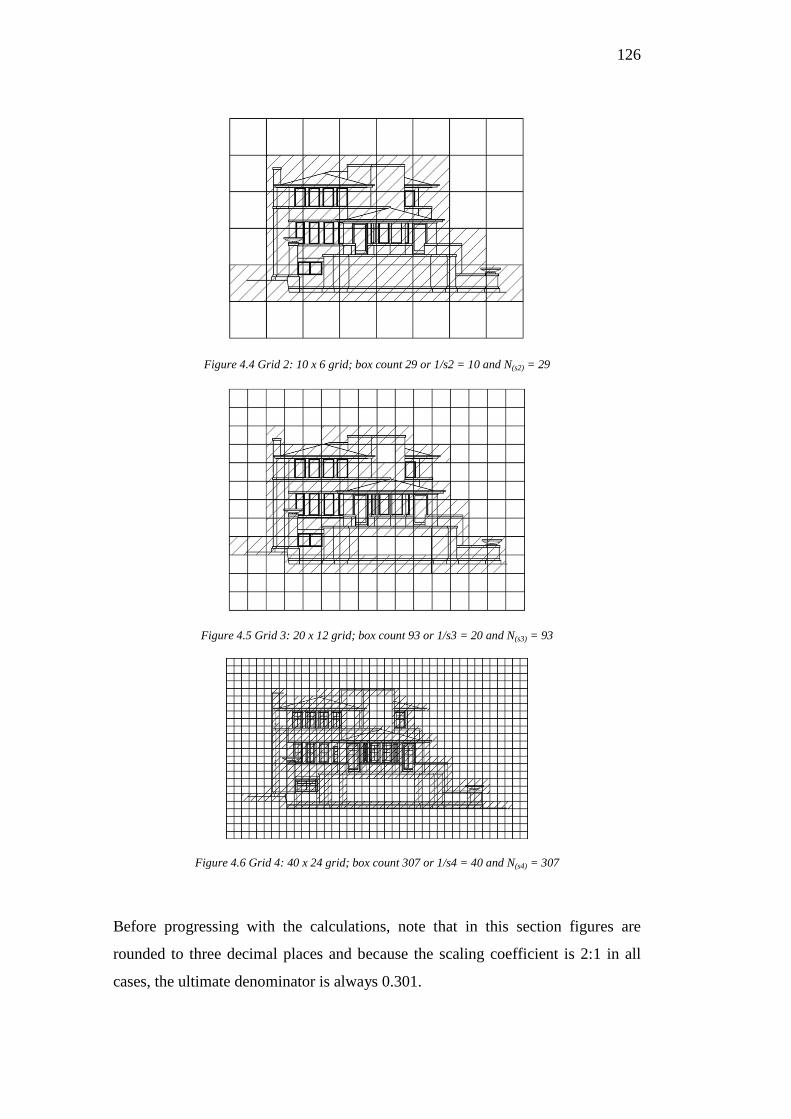
126

Figure 4.4 Grid 2: 10 x 6 grid; box count 29 or 1/s2 = 10 and N(s2) = 29

Figure 4.5 Grid 3: 20 x 12 grid; box count 93 or 1/s3 = 20 and N(s3) = 93

Figure 4.6 Grid 4: 40 x 24 grid; box count 307 or 1/s4 = 40 and N(s4) = 307

Before progressing with the calculations, note that in this section figures are

rounded to three decimal places and because the scaling coefficient is 2:1 in all

cases, the ultimate denominator is always 0.301.

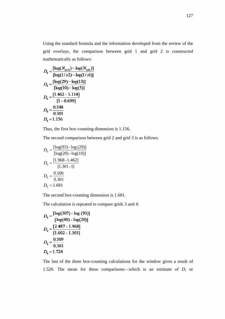
127

Using the standard formula and the information developed from the review of the

grid overlays, the comparison between grid 1 and grid 2 is constructed

mathematically as follows:

Thus, the first box-counting dimension is 1.156.

The second comparison between grid 2 and grid 3 is as follows:

The second box-counting dimension is 1.681.

The calculation is repeated to compare grids 3 and 4:

The last of the three box-counting calculations for the window gives a result of

1.520. The mean for these comparisons—which is an estimate of D, or

681.1301.0

0.506]1 - 1.301[

]1.462 - 1.968[]log(10) - log(20)[](29) log - log(93)[

=

=

=

=

b

b

b

b

D

D

D

D

128

alternatively a D calculation with a high error rate as a result of such a limited

data set—is therefore:

The set of results are then graphed in a log-log graph (that is, both scales are

logarithmic), with the box-count (y axis) against the box size (x axis). In this

example, the three comparison results appear relatively close to the mean (fig.4.7).

Figure 4.7 Log-log graph for the first three comparisions of the Robie House elevation

D = 1 . 1 56 + 1 . 681 + 1 . 724 3

D = 1 . 520

129

4.5 Fractal Analysis and the Built Environment

The following section provides an overview of past research that has been

undertaken using the box-counting method to measure the fractal dimension of the

built environment. The scale of these studies varies from the analysis of city plans

(Masucci et al. 2012) to measurements of individual buildings and architectural

details (Zarnowiecka 2002). Many of these studies were undertaken using a

manual version of the method which, much like the worked examples in the

present section, rely on a person physically counting the number of details in

various grids, then using formulas to calculate the fractal dimension of an image.

The more recent examples tend to use purpose-designed or authored software to

undertake much larger and more accurate applications of the method. Despite this

difference, the basic approach remains the same. However, as several comments

in the present section indicate, not all of the results of this basic variation of the

method are useful or accurate. Thus, despite an increase in the application of this

method, surprisingly few of these past studies include details about the particular

variation they employ, or the settings and raw data they use for their calculations.

This means that the results of most of these studies are impossible to replicate.

Furthermore, there are some serious methodological flaws in a few of the past

applications along with more subtle problems with the way authors have

interpreted their results. While a small number of these concerns are noted in the

next section, its primary purpose is not to be critical of these works, but to

describe the breadth of applications of the method.

This section divides past research using the box-counting approach broadly by

application, starting with research that is focussed on urban forms and then

considering those that focus on architecture, and then finally on fractal analysis of

the architecture of Frank Lloyd Wright. While many of the results of these studies

are described in the text, most cannot legitimately be compared with each other

because they use different starting points (from photographs to sketches and line

drawings) and different data extraction and processing procedures (from manual

techniques to software supported ones). Furthermore, several past publications co-

130

authored by the present author are also included in the discussion as they use box-

counting to investigate various buildings (Vaughan and Ostwald 2008; 2011;

Ostwald and Vaughan 2013a).

4.5.1 Urban Analysis

Studies of cities using fractal analysis range from a consideration of urban

morphology to measurements of the plans of streets, transport networks and green

spaces. As noted by Lachlan Robertson, fractal analysis ‘can potentially be the

tool that allows us to describe accurately [...] “organic” urban form’ (1995: 13).

Observations about the potential fractal dimension of urban forms began to be

published in the late 1980s (Yamagishi et al. 1988) and since then a growing

number of different approaches to the fractal analysis of urban plans have been

proposed (Oku 1990; Mizuno and Kakei 1990; Rodin and Rodina 2000; Ben-

Hamouche 2009). However, the earliest research to specifically use the box-

counting method in urban analysis can be traced to Michael Batty and Paul

Longley (1994) who employed a variation of the method, which they called ‘cell-

counting’, to examine changes in the growth and form of urban boundaries.

Following their work, fractal analysis continued to be used to measure changing

urban forms including studies of Tel Aviv (Benguigui et al. 2000) and London

(Masucci et al. 2012), along with shifting settlement patterns in Mayan cities

(Brown and Witschey 2003). The application of the box-counting method to the

analysis of urban form has also been undertaken by Mauro Barros-Filho and

Fabiano Sobreira (2005), who examined, amongst other areas, slums in Brazil.

The box-counting method has since been used to compare the fractal dimension of

street patterns in more than twenty cities (Cardillo et al. 2006) and a worldwide

urban classification system using fractal dimensions has been proposed

(Encarnação et al. 2012).

In a variation of these urban approaches, the box-counting method has also been

used to analyse transportation networks and their impact on settlement patterns,

131

including a comparison between Seoul and Paris (Kim et al. 2003). Yongmei Lu

and Junmei Tang (2004) used the method to analyse the connection between city

size and transportation networks in Texas, while Isabelle Thomas and Pierre

Frankhauser (2013) compared the dimensions of developed spaces and roadways

in Belgium. At a smaller scale Ron Eglash (1999) examined plans of part of a

Mofou settlement in Cameroon and the urban core of the Turkish city of Amasya,

the latter of which has been the subject of several studies about the relationship

between the fractal dimension of traditional urban centres and of their surrounding

natural context (Bovill 1996; Lorenz 2003; Vaughan and Ostwald 2009a;

Bourchtein et al. 2014). Green spaces, typically urban parks, have also been

measured using box-counting to develop a model for sustainable development

(Wang et al. 2011) and to compare the porosity of parks in the USA, China and

Argentina (Liang et al. 2013). Jon Cooper has led a series of detailed studies of

streetscape quality in Oxford (Cooper and Oskrochi 2008; Cooper et al. 2010) and

Taipei (Cooper et al. 2013) using the box-counting method. Distant views of city

skylines have also been analysed by Stamps (2002) and the visual qualities of city

skylines in Amsterdam, Sydney and Suzhou have been measured and compared

(Chalup et al. 2008).

In the majority of these examples of urban dimensional analysis, the box-counting

method has been used to quantify the characteristic complexity of a city, including

its growth patterns, road and rail networks, open spaces and skylines. Several of

the studies (Benguigui et al. 2000; Stamps 2002; Bourchtein et al. 2014) also

display an awareness that fractal dimensions are more informative when used for

comparative purposes, or for classifying different types of patterns against a

standard value or measure.

4.5.2 Architectural Analysis

The earliest serious attempt to calculate the fractal dimension of architecture using

the box-counting method is found in the work of Carl Bovill, whose publication

Fractal Geometry in Architecture and Design (1996) provided the first major

132

exploration of the relationship between fractal geometry and art, music, design

and architecture. In that work Bovill not only demonstrated the box-counting

method in detail, he also used it to measure the fractal properties of plans and

elevations of several canonical buildings, including the south elevation of

Wright’s Robie House and the west elevation of Le Corbusier’s Villa Savoye.

Bovill concluded from this analysis that the Robie House elevation is in the order

of 10% more visually complex than the Villa Savoye elevation. This comparison

seems to confirm the intuitive interpretation that architects have historically

offered, that Wright’s design, with its elaborate windows, modelling and raked

rooflines, has greater and more consistent levels of visual complexity than Le

Corbusier’s white, geometric facade.

More controversially, Bovill also used the box-counting method to compare

architecture and its surrounding context by calculating the fractal dimensions of a

row of houses and their mountainous setting. He suggests that the 14% difference

in characteristic visual complexity between these two sets of results demonstrates

that ‘the indigenous builders somehow applied the rhythms of nature to their

housing site layout and elevation design’ (1996: 145)—this claim will be further

explored in Chapter 6. While the efficacy of such claims have been examined and

criticised (Vaughan and Ostwald 2009a), Bovill’s clear and detailed explanation

of the method paved the way for many scholars to use this method for measuring

architecture. The remainder of this section reviews the application of the box-

counting method to both historic and more contemporary buildings.

Clifford Brown et al. argue that the box-counting method is useful for

archaeologists because ‘it is always important to identify, describe, and quantify

variation in material culture’ (2005: 54). These concerns are of similar

significance for architectural historians who, like archaeologists, are often

interested in both the form of a cultural artefact and symbolic meaning. However,

applications of the box-counting method to historic buildings also contain a high

proportion of arguments which seem to confuse fractal dimensions with fractal

geometry, as well as those which try to conflate measured dimensions with

133

mystical or symbolic properties. Within papers which otherwise contain rigorous

mathematical analysis (Oleschko et al. 2000; Burkle-Elizondo and Valdez-Cepeda

2001) , an unexpected range of misleading conclusions are recorded, including

several which are not supported by the method or its results.

The most common historic buildings that have been the subject of fractal analysis

are temples and pyramids. In the latter category, a team led by Klaudia Oleschko

analysed three major Teotihuacan pyramids and six ancient complexes (100 BC–

700 AD), as well as four recent buildings in modern day Teotihuacan. The

computational analysis was based on digitized black and white aerial photographs

of these buildings. The results grouped the images in three fractal dimension

ranges, with pyramids 1.8876< D <1.8993, complexes 1.8755< D <1.883 and

modern buildings 1.7805< D <1.8243 (Oleschko et al. 2000). Despite the fact that

these results only determine fractal dimensions, and not necessarily that the

buildings have any fractal geometric qualities, Oleschko’s team claims that ‘this

technique, […] confirms the supposition that Teotihuacan was laid out according

to a master plan, where each small building may be considered to be a replica of

the whole complex’ (Oleschko et al. 2000: 1015). Notwithstanding the serious

methodological problems inherent in extracting data from aerial photographs

(where countless additional features artificially raise the D result), a common

range of dimensions does not necessarily mean that all of the buildings in a given

set were designed in accordance with a similar formal schema; there are other

more plausible explanations. For instance, a large number of Gothic church

elevations have similar fractal dimensions but this does not mean that the

architects responsible for them were all involved in a cult to replicate this form

across Europe (Samper and Herrera 2014). Instead, common crafting techniques,

materials and details, along with similar technology and iconography, means that

a level of consistency would naturally exist.

Two studies of Mesoamerican pyramids and temples (Burkle-Elizondo 2001;

Burkle-Elizondo and Valdez-Cepeda 2001) feature interpretations that, like the

Teotihuacan case, may be debatable. These studies use the box-counting method

134

to measure the dimension of scanned images of elevations of Mayan, Aztec and

Toltec monuments (300 BC–1110 AD). These results superficially suggest that

these monuments are ornate, visually complex structures with an average D of

1.92. However, before considering Gerardo Burkle-Elizondo’s conclusion, it is

worth noting that a D of 1.92 would be amongst the highest dimensions ever

recorded in architecture, being comparable with the dimension of an intricate

vascular network or dense tree structure, but in this case it is only for a set of

stepped pyramids and some decorative panels. A close review of the images used

for the analysis reveals that they are scanned, grey-scale images, which when

converted into line drawings, generate a large amount of visual ‘noise’, including

a large number of features which are not actually present in the architecture. Thus,

the D results are exaggerated by the nature of the starting images. Regardless of

the results, Burkle-Elizondo’s conclusion, which echoes that of Oleschko, is that,

based on the results, ‘we think that there undoubtedly existed a mathematical

system and a deep geometrical development in Mesoamerican art and architecture,

and that they used patterns and ‘golden units’ (2001: 212). Because the Golden

Mean is actually a ‘primitive’ or ‘trivial’ fractal, it has a ‘known’ fractal

dimension which is far less than D = 1.92. Furthermore, that a culture promulgates

a recurring set of geometric patterns is not unexpected, but this is not necessarily a

reflection of any deeper level of understanding or significance. These two facts

mean that the spirit of Burkle-Elizondo’s conclusion may be correct, but the

fractal dimension results are insufficient, in and of themselves, to support this

position.

Iasef Rian et al. (2007) consider both fractal geometry and fractal dimensions as

two distinct and separate aspects of the Kandariya Mahadev, an eleventh-century

Hindu temple in Northern India. They use the box-counting method to confirm the

characteristic complexity of plans, elevations and details of the temple, and a

separate diagrammatic analysis provides a breakdown of the monument’s fractal-

like geometric construction. Their research also reports important information

regarding the method used, the results of which identify a close range of high

135

dimensions (1.7 < D <1.8) in the plans, elevations, details and ceiling panels of

the ancient temple.

Both Wolfgang Lorenz and Daniele Capo have used the box-counting method to

analyse classical Greek and Roman orders. Lorenz (2003) investigated a set of

line drawings of the entry elevations of four ancient Grecian temples and found

that of the set, the Treasury of Athens (c. 490 BC) in Delphi had the lowest fractal

dimension (D = 1.494) and the Erechtheion (c. 400 BC) in Athens had the highest

(D = 1.710). Lorenz concluded that the dimensions confirmed an intuitive visual

reading of the complexity of the different building elements of the temples. Capo

(2004) used a modified version of the box-counting method (described as the

‘information dimension’) to compare the Doric, Corinthian and Composite orders

of architecture (600 BC–100 BC). Capo did not publish the resulting dimensions,

but concluded that they ‘showed a fundamental coherence’ (2004: 35).

Architecture of the sixteenth-century Ottoman period in Turkey has been the

subject of fractal analysis by several authors. For example, William Bechoefer

and Carl Bovill analysed a set of Ottoman houses in the ancient city of Amasya

which were an example ‘of the most important remaining assemblage of

waterfront houses in Anatolia’ (1994: 5). They used a limited, manual version of

the box-counting method to measure the elevation of the group of five houses,

producing a result of D = 1.717. This same strip of housing was re-analysed using

the manual method by Lorenz in 2003 with a different result (D = 1.546) and a

third result (D = 1.505) has also been calculated using a computational version of

the method (Vaughan and Ostwald 2010). The houses were further analysed by

Bourchtein et al. in 2014 using a different computational method and with error

correction filtering applied and they found the row of houses had a D value of

1.58. The geometric properties of another group of eight traditional Ottoman

houses were measured by Gulen Cagdas, Gaye Gozubuyuk and Özgür Ediz

(2005). Three different facets of these houses, in the Chora district of Istanbul,

were considered. First, their combined roof plans (D = 1.7) then their building

outline (D = 1.2) and finally their street elevation (D = 1.2).

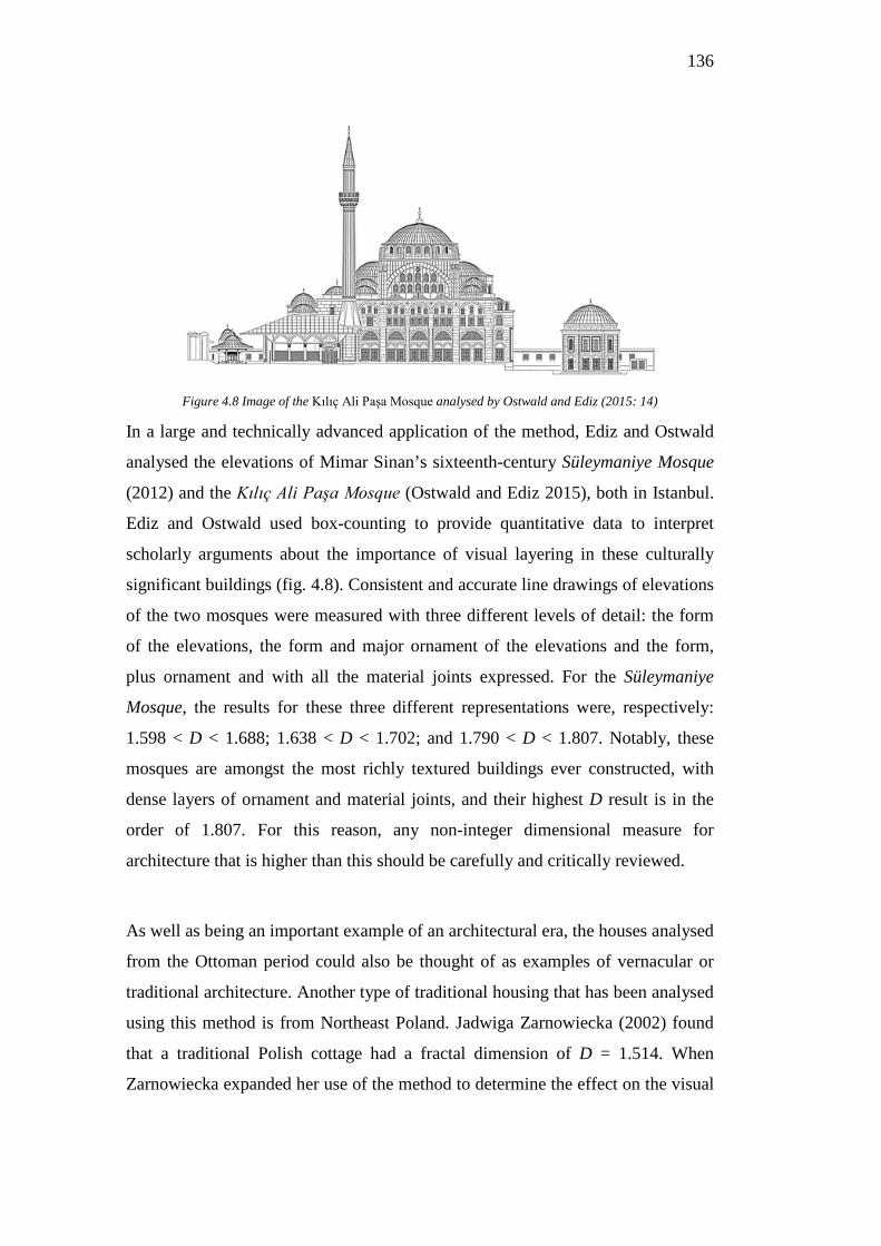
136

Figure 4.8 Image of the Kılıç Ali Paşa Mosque analysed by Ostwald and Ediz (2015: 14)

In a large and technically advanced application of the method, Ediz and Ostwald

analysed the elevations of Mimar Sinan’s sixteenth-century Süleymaniye Mosque

(2012) and the Kılıç Ali Paşa Mosque (Ostwald and Ediz 2015), both in Istanbul.

Ediz and Ostwald used box-counting to provide quantitative data to interpret

scholarly arguments about the importance of visual layering in these culturally

significant buildings (fig. 4.8). Consistent and accurate line drawings of elevations

of the two mosques were measured with three different levels of detail: the form

of the elevations, the form and major ornament of the elevations and the form,

plus ornament and with all the material joints expressed. For the Süleymaniye

Mosque, the results for these three different representations were, respectively:

1.598 < D < 1.688; 1.638 < D < 1.702; and 1.790 < D < 1.807. Notably, these

mosques are amongst the most richly textured buildings ever constructed, with

dense layers of ornament and material joints, and their highest D result is in the

order of 1.807. For this reason, any non-integer dimensional measure for

architecture that is higher than this should be carefully and critically reviewed.

As well as being an important example of an architectural era, the houses analysed

from the Ottoman period could also be thought of as examples of vernacular or

traditional architecture. Another type of traditional housing that has been analysed

using this method is from Northeast Poland. Jadwiga Zarnowiecka (2002) found

that a traditional Polish cottage had a fractal dimension of D = 1.514. When

Zarnowiecka expanded her use of the method to determine the effect on the visual

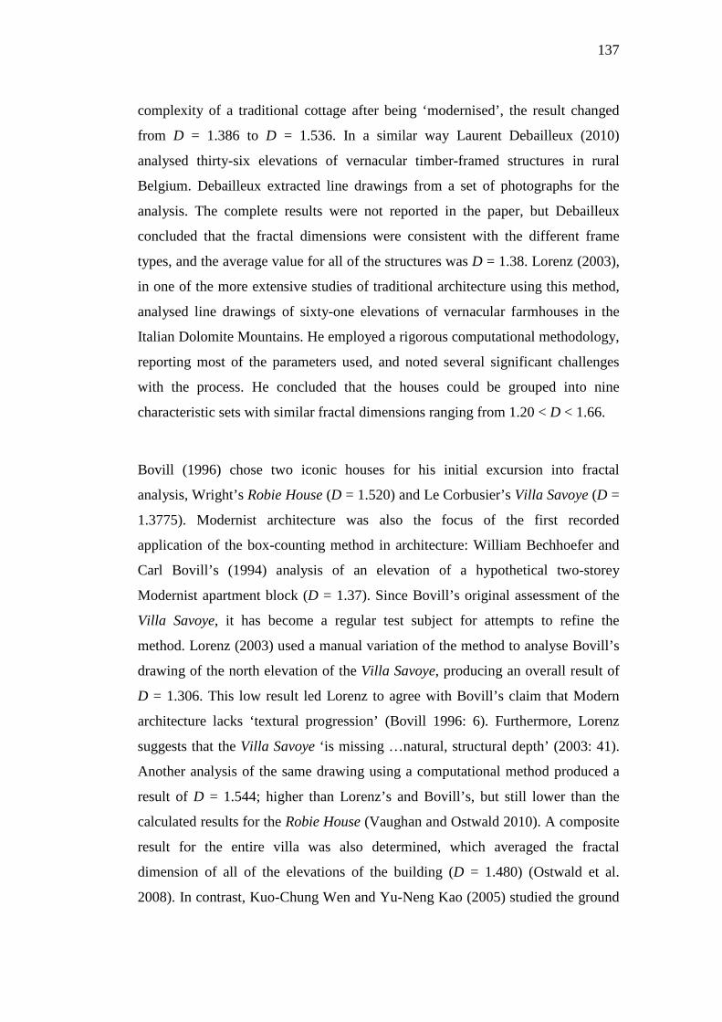
137

complexity of a traditional cottage after being ‘modernised’, the result changed

from D = 1.386 to D = 1.536. In a similar way Laurent Debailleux (2010)

analysed thirty-six elevations of vernacular timber-framed structures in rural

Belgium. Debailleux extracted line drawings from a set of photographs for the

analysis. The complete results were not reported in the paper, but Debailleux

concluded that the fractal dimensions were consistent with the different frame

types, and the average value for all of the structures was D = 1.38. Lorenz (2003),

in one of the more extensive studies of traditional architecture using this method,

analysed line drawings of sixty-one elevations of vernacular farmhouses in the

Italian Dolomite Mountains. He employed a rigorous computational methodology,

reporting most of the parameters used, and noted several significant challenges

with the process. He concluded that the houses could be grouped into nine

characteristic sets with similar fractal dimensions ranging from 1.20 < D < 1.66.

Bovill (1996) chose two iconic houses for his initial excursion into fractal

analysis, Wright’s Robie House (D = 1.520) and Le Corbusier’s Villa Savoye (D =

1.3775). Modernist architecture was also the focus of the first recorded

application of the box-counting method in architecture: William Bechhoefer and

Carl Bovill’s (1994) analysis of an elevation of a hypothetical two-storey

Modernist apartment block (D = 1.37). Since Bovill’s original assessment of the

Villa Savoye, it has become a regular test subject for attempts to refine the

method. Lorenz (2003) used a manual variation of the method to analyse Bovill’s

drawing of the north elevation of the Villa Savoye, producing an overall result of

D = 1.306. This low result led Lorenz to agree with Bovill’s claim that Modern

architecture lacks ‘textural progression’ (Bovill 1996: 6). Furthermore, Lorenz

suggests that the Villa Savoye ‘is missing …natural, structural depth’ (2003: 41).

Another analysis of the same drawing using a computational method produced a

result of D = 1.544; higher than Lorenz’s and Bovill’s, but still lower than the

calculated results for the Robie House (Vaughan and Ostwald 2010). A composite

result for the entire villa was also determined, which averaged the fractal

dimension of all of the elevations of the building (D = 1.480) (Ostwald et al.

2008). In contrast, Kuo-Chung Wen and Yu-Neng Kao (2005) studied the ground

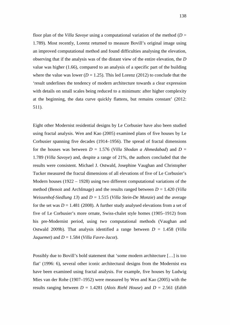
138

floor plan of the Villa Savoye using a computational variation of the method (D =

1.789). Most recently, Lorenz returned to measure Bovill’s original image using

an improved computational method and found difficulties analysing the elevation,

observing that if the analysis was of the distant view of the entire elevation, the D

value was higher (1.66), compared to an analysis of a specific part of the building

where the value was lower (D = 1.25). This led Lorenz (2012) to conclude that the

‘result underlines the tendency of modern architecture towards a clear expression

with details on small scales being reduced to a minimum: after higher complexity

at the beginning, the data curve quickly flattens, but remains constant’ (2012:

511).

Eight other Modernist residential designs by Le Corbusier have also been studied

using fractal analysis. Wen and Kao (2005) examined plans of five houses by Le

Corbusier spanning five decades (1914–1956). The spread of fractal dimensions

for the houses was between D = 1.576 (Villa Shodan a Ahmedabad) and D =

1.789 (Villa Savoye) and, despite a range of 21%, the authors concluded that the

results were consistent. Michael J. Ostwald, Josephine Vaughan and Christopher

Tucker measured the fractal dimensions of all elevations of five of Le Corbusier’s

Modern houses (1922 – 1928) using two different computational variations of the

method (Benoit and ArchImage) and the results ranged between D = 1.420 (Villa

Weissenhof-Siedlung 13) and D = 1.515 (Villa Stein-De Monzie) and the average

for the set was D = 1.481 (2008). A further study analysed elevations from a set of

five of Le Corbusier’s more ornate, Swiss-chalet style homes (1905–1912) from

his pre-Modernist period, using two computational methods (Vaughan and

Ostwald 2009b). That analysis identified a range between D = 1.458 (Villa

Jaquemet) and D = 1.584 (Villa Favre-Jacot).

Possibly due to Bovill’s bold statement that ‘some modern architecture […] is too

flat’ (1996: 6), several other iconic architectural designs from the Modernist era

have been examined using fractal analysis. For example, five houses by Ludwig

Mies van der Rohe (1907–1952) were measured by Wen and Kao (2005) with the

results ranging between D = 1.4281 (Alois Riehl House) and D = 2.561 (Edith

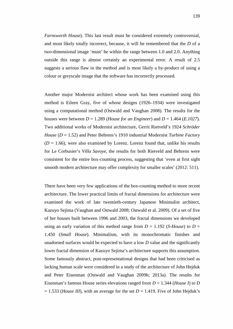
139

Farnsworth House). This last result must be considered extremely controversial,

and most likely totally incorrect, because, it will be remembered that the D of a

two-dimensional image ‘must’ be within the range between 1.0 and 2.0. Anything

outside this range is almost certainly an experimental error. A result of 2.5

suggests a serious flaw in the method and is most likely a by-product of using a

colour or greyscale image that the software has incorrectly processed.

Another major Modernist architect whose work has been examined using this

method is Eileen Gray, five of whose designs (1926–1934) were investigated

using a computational method (Ostwald and Vaughan 2008). The results for the

houses were between D = 1.289 (House for an Engineer) and D = 1.464 (E.1027).

Two additional works of Modernist architecture, Gerrit Rietveld’s 1924 Schröder

House (D = 1.52) and Peter Behrens’s 1910 industrial Modernist Turbine Factory

(D = 1.66), were also examined by Lorenz. Lorenz found that, unlike his results

for Le Corbusier’s Villa Savoye, the results for both Rietveld and Behrens were

consistent for the entire box-counting process, suggesting that ‘even at first sight

smooth modern architecture may offer complexity for smaller scales’ (2012: 511).

There have been very few applications of the box-counting method to more recent

architecture. The lower practical limits of fractal dimensions for architecture were

examined the work of late twentieth-century Japanese Minimalist architect,

Kazuyo Sejima (Vaughan and Ostwald 2008; Ostwald et al. 2009). Of a set of five

of her houses built between 1996 and 2003, the fractal dimensions we developed

using an early variation of this method range from D = 1.192 (S-House) to D =

1.450 (Small House). Minimalism, with its monochromatic finishes and

unadorned surfaces would be expected to have a low D value and the significantly

lower fractal dimension of Kazuyo Sejima’s architecture supports this assumption.

Some famously abstract, post-representational designs that had been criticised as

lacking human scale were considered in a study of the architecture of John Hejduk

and Peter Eisenman (Ostwald and Vaughan 2009b; 2013a). The results for

Eisenman’s famous House series elevations ranged from D = 1.344 (House I) to D

= 1.533 (House III), with an average for the set D = 1.419. Five of John Hejduk’s

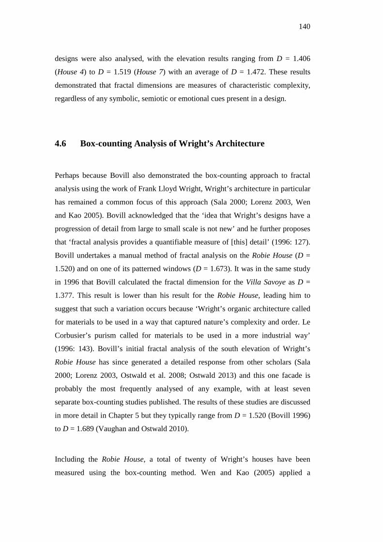
140

designs were also analysed, with the elevation results ranging from D = 1.406

(House 4) to D = 1.519 (House 7) with an average of D = 1.472. These results

demonstrated that fractal dimensions are measures of characteristic complexity,

regardless of any symbolic, semiotic or emotional cues present in a design.

4.6 Box-counting Analysis of Wright’s Architecture

Perhaps because Bovill also demonstrated the box-counting approach to fractal

analysis using the work of Frank Lloyd Wright, Wright’s architecture in particular

has remained a common focus of this approach (Sala 2000; Lorenz 2003, Wen

and Kao 2005). Bovill acknowledged that the ‘idea that Wright’s designs have a

progression of detail from large to small scale is not new’ and he further proposes

that ‘fractal analysis provides a quantifiable measure of [this] detail’ (1996: 127).

Bovill undertakes a manual method of fractal analysis on the Robie House (D =

1.520) and on one of its patterned windows (D = 1.673). It was in the same study

in 1996 that Bovill calculated the fractal dimension for the Villa Savoye as D =

1.377. This result is lower than his result for the Robie House, leading him to

suggest that such a variation occurs because ‘Wright’s organic architecture called

for materials to be used in a way that captured nature’s complexity and order. Le

Corbusier’s purism called for materials to be used in a more industrial way’

(1996: 143). Bovill’s initial fractal analysis of the south elevation of Wright’s

Robie House has since generated a detailed response from other scholars (Sala

2000; Lorenz 2003, Ostwald et al. 2008; Ostwald 2013) and this one facade is

probably the most frequently analysed of any example, with at least seven

separate box-counting studies published. The results of these studies are discussed

in more detail in Chapter 5 but they typically range from D = 1.520 (Bovill 1996)

to D = 1.689 (Vaughan and Ostwald 2010).

Including the Robie House, a total of twenty of Wright’s houses have been

measured using the box-counting method. Wen and Kao (2005) applied a

141

computational version of the method to plans of five houses by Wright spanning

from 1890 to 1937. The houses studied were the Frank Lloyd Wright House (D =

1.436), the Harley Brandley House (D = 1.626) the Avery Coonley House (D =

1.589), the Sherman M. Booth house (D = 1.609) and the Herbert Jacobs house

(D = 1.477). The elevations of five of Wright’s Prairie Houses (1901–1910) have

also been examined using two different computational variations of the box-

counting method (Ostwald et al. 2008). The range of fractal dimensions which

were recorded is between D = 1.505 (Zeigler House) and D = 1.580 (Evans

House). Past research has also examined Wright’s Usonian houses and Textile-

block houses (Vaughan and Ostwald 2011). While these results are revised and

refined later in this dissertation, the original range for the Usonian houses was

between D = 1.350 (Fawcett House) and D = 1.486 (Palmer House) and the

average for the set was D = 1.425. The fractal dimensions for the Textile-block

houses were between D = 1.506 (Freeman House) and D = 1.614 (La Miniatura)

and the average for the set was D = 1.538.

The Unity Temple (1905) in Chicago is the only non-domestic building designed

by Wright which has been analysed using this method. The fractal dimension of

the north elevation of the Unity Temple has been the subject of three separate

studies. In his 1996 publication, Bovill undertook fractal analysis on several

features of the north elevation of the Unity Temple, believing this particular

building ‘should help explain Wright’s ability to grasp the underlying structure of

a natural form and translate it into a building form’ (128). Bovill proposes the

Unity Temple as a demonstration because he considered Wright’s admiration of

the effect of light in a forest to be translated into a building which Bovill

considers to be—in its levels of visual complexity—akin to the forest itself (128).

Bovill explains that ‘The forest displays a form that is complex at the ground

plane, simpler in the zone of the tree trunks, and complex again in the branching

structure of the tree canopy’ (128). Bovill found that the results from this manual

fractal analysis were ‘as expected for a design with forest imagery as a base idea.

The upper part (D = 1.415) and base (D = 1.678) of the building have higher

fractal dimensions than the middle (D = 1.223) of the building’ (132). Bovill’s

142

overall results for the facade of the Unity Temple (D = 1.550) have been retested

using the same image by others including Lorenz who also used a manual method,

D = 1.513 (2003) and with a computational variation, producing a relatively

similar measure, D = 1.574 (Vaughan and Ostwald 2010).

Conclusion

As demonstrated in this chapter, the box-counting method is deceptively simple to

apply, and this is why there are a growing number of examples of its application

in urban and architectural analysis. Conversely though, the method has multiple

complicating factors that have undermined the usefulness and validity of many

early studies. These problems are readily apparent in the review of past results,

where multiple applications of the method to the same facades have produced

often-divergent results, and where a large number of completely counter-intuitive

outcomes have been published (Oleschko et al. 2000; Burkle-Elizondo and

Valdez-Cepeda 2001; Wen and Kao 2005). The three major concerns facing those

seeking to use the method are about image representation standards, data pre-

processing standards and methodological considerations.

The first of these concerns arises from the fact that the box-counting method

measures information contained in an image. Obviously, if this image is a

photograph, then the information contained in it will be very different from the

information in a line drawing. Shadows, textures and perspective are all part of

the way in which we experience the world, but they also complicate and

undermine the process of measurement to such a degree that they are typically

removed from any consideration of questions of form. For example, unless a

person was specifically interested in the visual impact of plants, trees or shadows,

all of these features will completely dominate any analysis of visual complexity in

a building facade. Furthermore, when studying a building, the question must be

asked, what data is relevant? That is, which lines in a plan or elevation should be

measured and why? These questions are addressed over the following chapters.

143

Chapter 5

Variables in the Box-counting Method

In the last two decades a growing body of research has been published which uses

the box-counting method to measure the fractal dimensions of architectural or

urban forms. However, much of this research displays only a low level of

awareness of the sensitivities or limits of the method. As a consequence, often

widely varying results have been produced using the same mathematical approach

and, in some cases, exactly the same images. It is only recently that these

limitations have been determined and a range of optimal standards and settings to

overcome many of these limitations have been proposed and accepted (Ostwald

and Vaughan 2012; Ostwald 2013; Ostwald and Vaughan 2013; 2016).

The challenges associated with the accuracy and accountability of the box-

counting method are threefold. The first challenge, which is associated with image

representation, is to determine, in a consistent and reasoned manner, the lines in

an image which are significant for analysis. Inconsistent representational

standards will render the results of most studies meaningless, and this chapter

begins by describing a uniform approach to the presentation of images to be

analysed. If a consistent rationale for the correct starting image information and

representation is applied, then the second challenge is to determine the correct

way to present or prepare that data prior to mathematical or computational

analysis. For example, how large should the starting image be, what line weights

should architecture be depicted in, and how much space should be left around the

image for a reasonable starting grid to be drawn. The third challenge is found

once the image is being analysed, when it is necessary to ensure that all of the

computational variables are set to an optimal standard. These methodological

standards include the ratio by which successive grids are reduced in size—the

‘scaling coefficient’—and the position from which these grids are generated—the

‘grid disposition’. This chapter describes these three areas of limitation in detail,

144

and considers the range of settings and options available for all of these variables

with reference to the latest information and suitability of these options.

Based on the results of this past experimental research—some of which was co-

written by the present author—the optimal settings or variables for the method are

determined and then applied to the south elevation of the Robie House, the

standard test subject of multiple previous studies. Finally, a summary of the ideal

settings and standards selected for fractal analysis of images in this dissertation

will then be presented.

5.1 Representation Challenges: Measuring

All of the main computational methods of formal and spatial analysis used in

architecture rely on measured representations of buildings or spaces. Thus, they

derive data from orthographic projections (plans, elevations and sections), CAD

models and photographic surveys. For two of the most established computational

methods the rationale describing which part of a building plan to analyse and how

the analysis is undertaken is relatively straightforward. Space Syntax research

typically analyses habitable space, being rigorous in its geometric mapping of

lines of sight, visually defined space or permeability (access) in a plan (Hillier and

Hanson 1984; Hillier 1996). Shape grammar researchers have a different but

similarly meticulous way of extracting geometric and topological properties from

a building plan before any analysis is undertaken (Stiny 1975; Knight 1992).

While the logic underlying these approaches to measurement continues to be

debated, there are accepted standards in each field.

Like architectural analysis using Zipf’s law or Van der Laan septaves and pixel

counts, fractal analysis provides a measure of the distribution of information (lines

or details) in an object across multiple scales (Stamps 1999; Crompton and Brown

2008; Crompton 2012). Unlike Space syntax and Shape Grammar, there is no

145

standardised guideline to identify which parts of a building facade or plan should

be the subject of fractal analysis measurement. Despite early attempts to clarify

which parts of a building should be analysed (Bovill 1996), researchers have

repeatedly noted that there is a lack of consistency in the field (Lorenz 2003;

Ostwald et al. 2008). Moreover, it has been demonstrated that different measures

can be derived from an analysis of the same elevation of a building, depending on

which lines are chosen for consideration (Zarnowiecka 2002; Vaughan and

Ostwald 2009b). Consider the example of Frank Lloyd Wright’s Robie House, a

design which has been the subject of seven separate applications of fractal

analysis (Bovill 1996; Sala 2000; Lorenz 2003; Ostwald et al. 2008; Vaughan and

Ostwald 2011; Ostwald 2013; Lorenz 2013). Across these studies, the variation in

the measurements recorded is in the order of 17%. This is because these studies

have multiple mathematical and methodological differences.

The most obvious explanation for the 17% anomaly is simply that computational

methods like fractal analysis do not measure buildings; rather, they extract

measures from representations of buildings. The primary representational media

used for architectural analysis is the orthographic drawing and there are many

variations in how a building can be represented in such a drawing (Hewitt 1985;

Leupen et al. 1997) For example, in Bovill’s original (1996) study of the south

elevation of the Robie House (fig. 5.1), he chose to analyse an image in which

only major changes in form were delineated. Using a limited range of graphic

standards, Bovill predominantly represented the geometrical forms of the

architecture. For example, the line-work in the elevation is highly simplified, with

the elevation reduced to a collection of Euclidian shapes, lacking in the

architectural details that exist in the actual building, including guttering and

window mullions. Architects understand that such graphic conventions are

representative of a form; they are not meant to be taken literally. In contrast, the

2008 analysis of the same facade by Ostwald et al. is derived from a tracing of a

similar drawing, wherein a greater level of detail is included (fig. 5.2). In this

study, guttering is shown, the glazing panels are shown in detail, with mullions

depicted; however, the full amount of detail in the ornately glazed windows is not

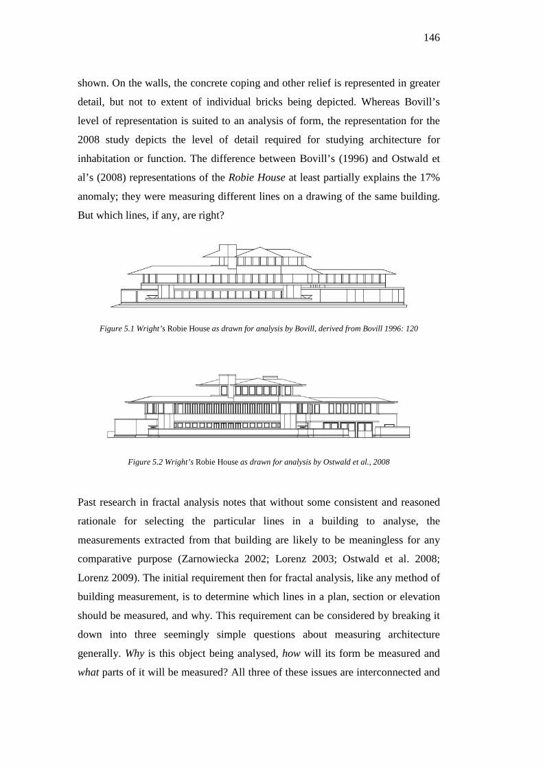
146

shown. On the walls, the concrete coping and other relief is represented in greater

detail, but not to extent of individual bricks being depicted. Whereas Bovill’s

level of representation is suited to an analysis of form, the representation for the

2008 study depicts the level of detail required for studying architecture for

inhabitation or function. The difference between Bovill’s (1996) and Ostwald et

al’s (2008) representations of the Robie House at least partially explains the 17%

anomaly; they were measuring different lines on a drawing of the same building.

But which lines, if any, are right?

Figure 5.1 Wright’s Robie House as drawn for analysis by Bovill, derived from Bovill 1996: 120

Figure 5.2 Wright’s Robie House as drawn for analysis by Ostwald et al., 2008

Past research in fractal analysis notes that without some consistent and reasoned

rationale for selecting the particular lines in a building to analyse, the

measurements extracted from that building are likely to be meaningless for any

comparative purpose (Zarnowiecka 2002; Lorenz 2003; Ostwald et al. 2008;

Lorenz 2009). The initial requirement then for fractal analysis, like any method of

building measurement, is to determine which lines in a plan, section or elevation

should be measured, and why. This requirement can be considered by breaking it

down into three seemingly simple questions about measuring architecture

generally. Why is this object being analysed, how will its form be measured and

what parts of it will be measured? All three of these issues are interconnected and

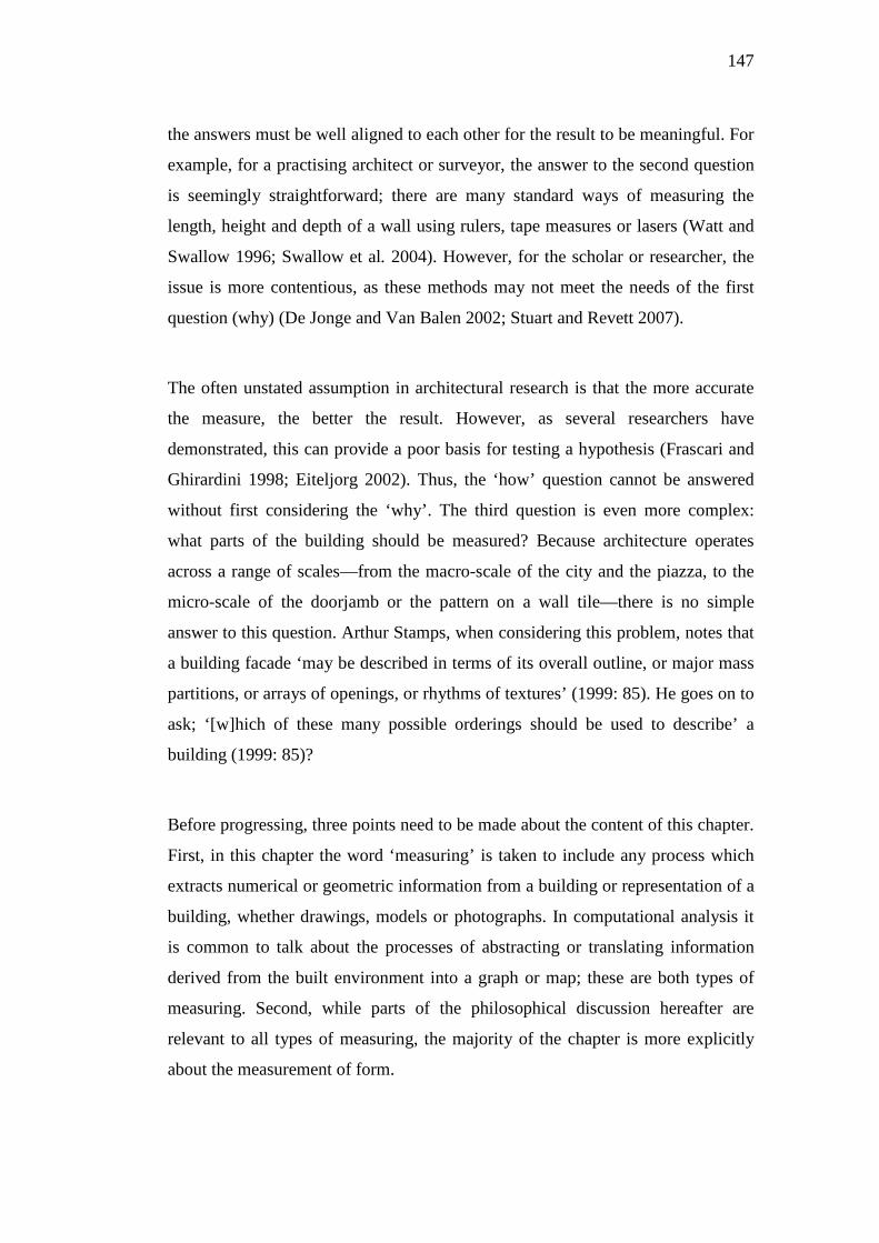
147

the answers must be well aligned to each other for the result to be meaningful. For

example, for a practising architect or surveyor, the answer to the second question

is seemingly straightforward; there are many standard ways of measuring the

length, height and depth of a wall using rulers, tape measures or lasers (Watt and

Swallow 1996; Swallow et al. 2004). However, for the scholar or researcher, the

issue is more contentious, as these methods may not meet the needs of the first

question (why) (De Jonge and Van Balen 2002; Stuart and Revett 2007).

The often unstated assumption in architectural research is that the more accurate

the measure, the better the result. However, as several researchers have

demonstrated, this can provide a poor basis for testing a hypothesis (Frascari and

Ghirardini 1998; Eiteljorg 2002). Thus, the ‘how’ question cannot be answered

without first considering the ‘why’. The third question is even more complex:

what parts of the building should be measured? Because architecture operates

across a range of scales—from the macro-scale of the city and the piazza, to the

micro-scale of the doorjamb or the pattern on a wall tile—there is no simple

answer to this question. Arthur Stamps, when considering this problem, notes that

a building facade ‘may be described in terms of its overall outline, or major mass

partitions, or arrays of openings, or rhythms of textures’ (1999: 85). He goes on to

ask; ‘[w]hich of these many possible orderings should be used to describe’ a

building (1999: 85)?

Before progressing, three points need to be made about the content of this chapter.

First, in this chapter the word ‘measuring’ is taken to include any process which

extracts numerical or geometric information from a building or representation of a

building, whether drawings, models or photographs. In computational analysis it

is common to talk about the processes of abstracting or translating information

derived from the built environment into a graph or map; these are both types of

measuring. Second, while parts of the philosophical discussion hereafter are

relevant to all types of measuring, the majority of the chapter is more explicitly

about the measurement of form.

148

5.1.1 Image Delineation: ‘Texture’

A legitimate system of inquiry for investigating the formal properties of buildings

must have a clearly aligned method of measurement and research purpose. Thus,

the research question or hypothesis must be one for which measurements can

provide useful evidence. While this may seem obvious, it is less common to

observe that the particular architectural features being measured must also be

appropriate for the research purpose. In computational analysis this is a question

of representation or delineation. For example, it is possible to delineate the facade

of a building, in a drawing or model, using many different combinations of lines

or textures. However, in all of these cases the act of measuring is reliant on the

conventions of representation. This is because, regardless of whether field

dimensions are taken using a laser scanner or tape measure, the dimensions have

to be transcribed into a representational system, be it a drawing, CAD or BIM

model, for it to be analysed.

The particular question of how much texture to include when measuring a facade

or plan is one of the more controversial ones in fractal analysis. When considering

an image, the ‘texture’ is considered as the amount of detail depicted. Bovill

(1996) argues that the geometric patterns produced by repetitive materials (like

the horizontal lines of floorboards) should not be measured; this would increase

the amount of visible texture. However, Joye (2011) has at least partially rejected

the proposal to discard this level of image texture. Jadwiga Zarnowiecka in

particular offers a balanced account of this issue. She originally disagreed with

Bovill’s proposition that, for example, the horizontal lines in a facade made by

timber siding should be ignored. Zarnowiecka notes that if this is the case, then

‘one must make a decision if a decorated top roof boarding is still a siding or a

detail. Should this decision depend on the width of the planks being used in

boarding?’ (2002: 343). However, after measuring the difference between the

elevation with planks, and without, she realised that the ‘concentration of the lines

on the facade’ changes the measured result even though they are not an important

feature (2002: 344). When considering a simple regional house in Poland,

Zarnowiecka notes that the addition of window mullions ‘change[s] the results of

149

the measurement, even though aesthetically they are quite meaningless’ (2002:

344). Zarnowiecka’s problem may be traced to the fact that measuring texture (to

use the terminology of the current chapter) skews the results of the analysis,

effectively making it unusable. The lack of a consistent set of guidelines for what

level of information, or linear texture to include in an image for testing, may

affect the results of the analysis. It has been found that—on an analysis of the

same building—the fractal dimension increases with each additional layer of

information included in the representation (Ostwald and Vaughan 2013c).

In order to accommodate this need, a framework of five cumulative levels of

representation have been defined and mapped against comparable research

purposes (Ostwald and Vaughan 2013c). This framework shows that, for instance,

it is not reasonable to study the impact of material texture on a building when only

the footprint of a plan is measured. Conversely, if the impact of planning

decisions regarding site amalgamation is to be studied, then measuring the

geometry of material textures in a facade will be counter-productive. This

framework, aligning level of representation with research intent, is also inherently

cumulative. That is, it relies on the fact that the building outline is required as a

precursor to defining primary forms. Thereafter, secondary forms can only be

added if the boundaries of the primary forms are already present, and so on. Thus,

the framework is described in terms of what is added with each level of

representation, as shown in Table 5.1

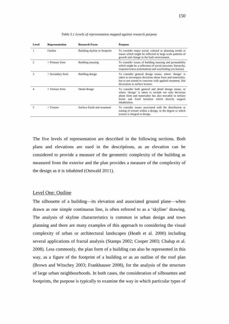
150

Table 5.1 Levels of representation mapped against research purpose

Level Representation Research Focus Purpose

1 Outline Building skyline or footprint To consider major social, cultural or planning trends or issues which might be reflected in large scale patterns of growth and change in the built environment.

2 + Primary form Building massing To consider issues of building massing and permeability which might be a reflection of social structure, hierarchy, responsiveness (orientation) and wayfinding (occlusion).

3 + Secondary form Building design To consider general design issues, where ‘design’ is taken to encompass decisions about form and materiality, but to not extend to concerns with applied ornament, fine decoration or surface texture.

4 + Tertiary form Detail design To consider both general and detail design issues, or where ‘design’ is taken to include not only decisions about form and materiality but also movable or tertiary forms and fixed furniture which directly support inhabitation.

5 + Texture Surface finish and ornament To consider issues associated with the distribution or zoning of texture within a design, or the degree to which texture is integral to design.

The five levels of representation are described in the following sections. Both

plans and elevations are used in the descriptions, as an elevation can be

considered to provide a measure of the geometric complexity of the building as

measured from the exterior and the plan provides a measure of the complexity of

the design as it is inhabited (Ostwald 2011).

Level One: Outline

The silhouette of a building—its elevation and associated ground plane—when

drawn as one simple continuous line, is often referred to as a ‘skyline’ drawing.

The analysis of skyline characteristics is common in urban design and town

planning and there are many examples of this approach to considering the visual

complexity of urban or architectural landscapes (Heath et al. 2000) including

several applications of fractal analysis (Stamps 2002; Cooper 2003; Chalup et al.

2008). Less commonly, the plan form of a building can also be represented in this

way, as a figure of the footprint of a building or as an outline of the roof plan

(Brown and Witschey 2003; Frankhauser 2008), for the analysis of the structure

of large urban neighbourhoods. In both cases, the consideration of silhouettes and

footprints, the purpose is typically to examine the way in which particular types of

151

construction create distinctive patterns, which in turn are thought to reflect the

individual social and cultural characteristics of a region. This strategy is used

where the large-scale patterns found in the built environment are thought to be a

reflection of distinct differences between regions or groups (Brown and Witschey

2003). If this approach is taken, the silhouette retains much of the character of the

aggregate geometry of the design, with the roof outline, showing and details such

as hips, gables and chimneys. Features such as the windows, through which the

sky cannot be seen, are not shown.

Level Two: Outline + Primary form

The second level of detail that could be considered for analysis is the formal

massing of the building as a whole; what might be termed its primary form. This

level is focussed on major formal gestures, not secondary forms, detail or

ornament. The building is represented by the outline but now with the addition of

massing elements, including openings. Smaller scale formal changes within these

elements, such as individual stair treads or brick corbels, would not be included.

All windows and doors are shown as portals but with no indication of fenestration

or detail. Window openings of all sizes can be included at this stage as they

represent a significant impact on the three-dimensional form of the building. In

elevation specifically, gross changes in form, such as protruding walls,

significantly advancing and receding elements (which measure greater than 250

mm) and the roof planes, are also delineated. Likewise in plan, the walls and

major changes in floor level are shown. This level of representation was selected

by Bovill (1996), for a fractal analysis of Frank Lloyd Wright’s Robie House to

gain a sense of the geometry of the major formal gestures in the plan.

Level Three: Outline + Primary form + Secondary form

In combination, the elements which make up the overall massing in a design along

with major changes in materials could be considered secondary forms. By

including secondary forms—in addition to the information previously provided by

the outline and massing of the building—the primary geometric gestures that

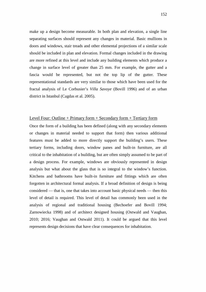
152

make up a design become measurable. In both plan and elevation, a single line

separating surfaces should represent any changes in material. Basic mullions in

doors and windows, stair treads and other elemental projections of a similar scale

should be included in plan and elevation. Formal changes included in the drawing

are more refined at this level and include any building elements which produce a

change in surface level of greater than 25 mm. For example, the gutter and a

fascia would be represented, but not the top lip of the gutter. These

representational standards are very similar to those which have been used for the

fractal analysis of Le Corbusier’s Villa Savoye (Bovill 1996) and of an urban

district in Istanbul (Cagdas et al. 2005).

Level Four: Outline + Primary form + Secondary form + Tertiary form

Once the form of a building has been defined (along with any secondary elements

or changes in material needed to support that form) then various additional

features must be added to more directly support the building’s users. These

tertiary forms, including doors, window panes and built-in furniture, are all

critical to the inhabitation of a building, but are often simply assumed to be part of

a design process. For example, windows are obviously represented in design

analysis but what about the glass that is so integral to the window’s function.

Kitchens and bathrooms have built-in furniture and fittings which are often

forgotten in architectural formal analysis. If a broad definition of design is being

considered — that is, one that takes into account basic physical needs — then this

level of detail is required. This level of detail has commonly been used in the

analysis of regional and traditional housing (Bechoefer and Bovill 1994;

Zarnowiecka 1998) and of architect designed housing (Ostwald and Vaughan,

2010; 2016; Vaughan and Ostwald 2011). It could be argued that this level

represents design decisions that have clear consequences for inhabitation.

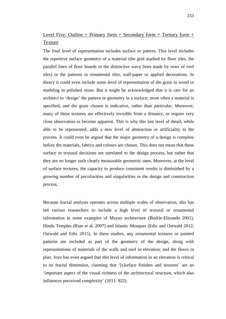
153

Level Five: Outline + Primary form + Secondary form + Tertiary form + Texture

The final level of representation includes surface or pattern. This level includes

the repetitive surface geometry of a material (the grid marked by floor tiles, the

parallel lines of floor boards or the distinctive wavy lines made by rows of roof

tiles) or the patterns in ornamental tiles, wall-paper or applied decorations. In

theory it could even include some level of representation of the grain in wood or

marbling in polished stone. But it might be acknowledged that it is rare for an

architect to ‘design’ the pattern or geometry in a surface; more often a material is

specified, and the grain chosen is indicative, rather than particular. Moreover,

many of these textures are effectively invisible from a distance, or require very

close observation to become apparent. This is why this last level of detail, while

able to be represented, adds a new level of abstraction or artificiality to the

process. It could even be argued that the major geometry of a design is complete

before the materials, fabrics and colours are chosen. This does not mean that these

surface or textural decisions are unrelated to the design process, but rather that

they are no longer such clearly measurable geometric ones. Moreover, at the level

of surface textures, the capacity to produce consistent results is diminished by a

growing number of peculiarities and singularities in the design and construction

process.

Because fractal analysis operates across multiple scales of observation, this has

led various researchers to include a high level of textural or ornamental

information in some examples of Mayan architecture (Burkle-Elizondo 2001),

Hindu Temples (Rian et al. 2007) and Islamic Mosques (Ediz and Ostwald 2012;

Ostwald and Ediz 2015). In these studies, any ornamental textures or painted

patterns are included as part of the geometry of the design, along with

representations of materials of the walls and roof in elevation, and the floors in

plan. Joye has even argued that this level of information in an elevation is critical

to its fractal dimension, claiming that ‘[s]urface finishes and textures’ are an

‘important aspect of the visual richness of the architectural structure, which also

influences perceived complexity’ (2011: 822).

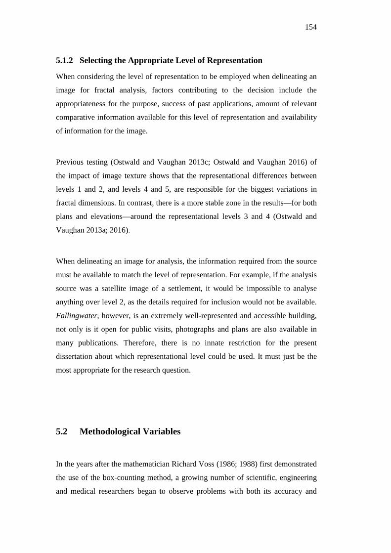
154

5.1.2 Selecting the Appropriate Level of Representation

When considering the level of representation to be employed when delineating an

image for fractal analysis, factors contributing to the decision include the

appropriateness for the purpose, success of past applications, amount of relevant

comparative information available for this level of representation and availability

of information for the image.

Previous testing (Ostwald and Vaughan 2013c; Ostwald and Vaughan 2016) of

the impact of image texture shows that the representational differences between

levels 1 and 2, and levels 4 and 5, are responsible for the biggest variations in

fractal dimensions. In contrast, there is a more stable zone in the results—for both

plans and elevations—around the representational levels 3 and 4 (Ostwald and

Vaughan 2013a; 2016).

When delineating an image for analysis, the information required from the source

must be available to match the level of representation. For example, if the analysis

source was a satellite image of a settlement, it would be impossible to analyse

anything over level 2, as the details required for inclusion would not be available.

Fallingwater, however, is an extremely well-represented and accessible building,

not only is it open for public visits, photographs and plans are also available in

many publications. Therefore, there is no innate restriction for the present

dissertation about which representational level could be used. It must just be the

most appropriate for the research question.

5.2 Methodological Variables

In the years after the mathematician Richard Voss (1986; 1988) first demonstrated

the use of the box-counting method, a growing number of scientific, engineering

and medical researchers began to observe problems with both its accuracy and

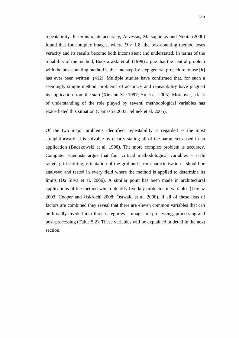
155

repeatability. In terms of its accuracy, Asvestas, Matsopoulos and Nikita (2000)

found that for complex images, where D > 1.8, the box-counting method loses

veracity and its results become both inconsistent and understated. In terms of the

reliability of the method, Buczkowski et al. (1998) argue that the central problem

with the box-counting method is that ‘no step-by-step general procedure to use [it]

has ever been written’ (412). Multiple studies have confirmed that, for such a

seemingly simple method, problems of accuracy and repeatability have plagued

its application from the start (Xie and Xie 1997; Yu et al. 2005). Moreover, a lack

of understanding of the role played by several methodological variables has

exacerbated this situation (Camastra 2003; Jelinek et al. 2005).

Of the two major problems identified, repeatability is regarded as the most

straightforward; it is solvable by clearly stating all of the parameters used in an

application (Buczkowski et al. 1998). The more complex problem is accuracy.

Computer scientists argue that four critical methodological variables – scale

range, grid shifting, orientation of the grid and error characterisation – should be

analysed and tested in every field where the method is applied to determine its

limits (Da Silva et al. 2006). A similar point has been made in architectural

applications of the method which identify five key problematic variables (Lorenz

2003; Cooper and Oskrochi 2008; Ostwald et al. 2008). If all of these lists of

factors are combined they reveal that there are eleven common variables that can

be broadly divided into three categories – image pre-processing, processing and

post-processing (Table 5.2). These variables will be explained in detail in the next

section.

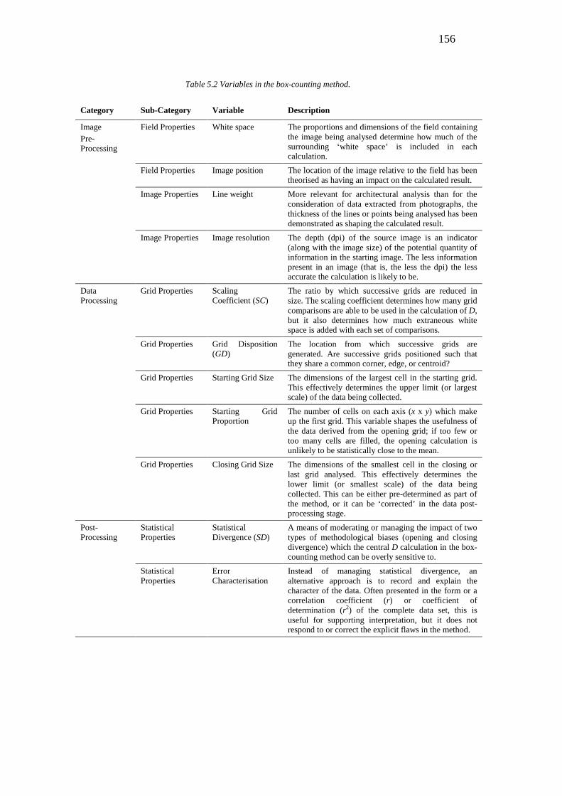
156

Table 5.2 Variables in the box-counting method.

Category Sub-Category Variable Description

Image Pre-Processing

Field Properties White space The proportions and dimensions of the field containing the image being analysed determine how much of the surrounding ‘white space’ is included in each calculation.

Field Properties Image position The location of the image relative to the field has been theorised as having an impact on the calculated result.

Image Properties Line weight More relevant for architectural analysis than for the consideration of data extracted from photographs, the thickness of the lines or points being analysed has been demonstrated as shaping the calculated result.

Image Properties Image resolution The depth (dpi) of the source image is an indicator (along with the image size) of the potential quantity of information in the starting image. The less information present in an image (that is, the less the dpi) the less accurate the calculation is likely to be.

Data Processing

Grid Properties Scaling Coefficient (SC)

The ratio by which successive grids are reduced in size. The scaling coefficient determines how many grid comparisons are able to be used in the calculation of D, but it also determines how much extraneous white space is added with each set of comparisons.

Grid Properties Grid Disposition (GD)

The location from which successive grids are generated. Are successive grids positioned such that they share a common corner, edge, or centroid?

Grid Properties Starting Grid Size The dimensions of the largest cell in the starting grid. This effectively determines the upper limit (or largest scale) of the data being collected.

Grid Properties Starting Grid Proportion

The number of cells on each axis (x x y) which make up the first grid. This variable shapes the usefulness of the data derived from the opening grid; if too few or too many cells are filled, the opening calculation is unlikely to be statistically close to the mean.

Grid Properties Closing Grid Size The dimensions of the smallest cell in the closing or last grid analysed. This effectively determines the lower limit (or smallest scale) of the data being collected. This can be either pre-determined as part of the method, or it can be ‘corrected’ in the data post-processing stage.

Post-Processing

Statistical Properties

Statistical Divergence (SD)

A means of moderating or managing the impact of two types of methodological biases (opening and closing divergence) which the central D calculation in the box-counting method can be overly sensitive to.

Statistical Properties

Error Characterisation

Instead of managing statistical divergence, an alternative approach is to record and explain the character of the data. Often presented in the form or a correlation coefficient (r) or coefficient of determination (r2) of the complete data set, this is useful for supporting interpretation, but it does not respond to or correct the explicit flaws in the method.

157

5.3 Image Challenges: Pre-processing Settings

While the statistical validity of the fractal analysis method is largely reliant on the

later data processing variables, image pre-processing factors also have the

potential to cause substantial errors. For example, these variables could cause

four seemingly identical elevations, all derived from the same CAD file, to

produce different results, due to the way they have each been saved or positioned.

Four types of image pre-processing properties are significant for understanding

the limits of the box-counting method. The first pair, white space and image

position, are associated with the field on which the starting image is positioned

and the relationship between the field and the image being analysed. The second

pair of factors, line weight and image resolution, are properties of the image itself,

being literally the lines which make up the image being analysed and the size and

sharpness of the image.

5.3.1 Image Pre-processing: Field Properties

The background on which the image being analysed is placed is called the field.

Two initially important properties of the field are its size and proportion. Size is

measured in pixels (the length and breadth of the image) to accommodate

different image densities. The field size is the first determinant of the practical

limits of the analytical process. Ideally, the larger the field and image, the more

grid comparisons may be constructed and the better the result. The proportion of

the field is important because it determines the field’s capacity to be neatly

divided by grids. As the box-counting method uses regular grids, it is obvious, but

almost never stated, that the dimensions of the field should be multiples of the

same figure. Thus, a 1000 pixel high by 2000 pixel wide field will accommodate

several ideal starting grid configurations including a 500p grid (2 x 4 cells), a

250p grid (4 x 8 cells) and a 200p grid (5 x 10 cells). However, Foroutan-Pour,

Dutilleul and Smith (1999) have demonstrated that the ideal starting proportion

158

for the grid is a multiple of four on the shortest side. This starting configuration

limits the volume of white space included in the first calculation and in doing so,

reduces the need for post-processing corrections (see the discussion of statistical

divergence in section 5.4.2 of this chapter). If the field does not have an ideal

proportion, then it must be cropped or enlarged to achieve such a configuration.

The field comprises three components: white space, image space and empty

space. The descriptor ‘white space’ refers to the region surrounding the image;

‘image space’ refers to the lines that make up the image itself; and ‘empty space’

is any region enclosed by the lines (fig. 5.3). The image space and the empty

space are effectively fixed quantities, but the initial amount of white space is

determined when the image is positioned or cropped on the ‘canvas’ prior to

analysis. Why is this seemingly trivial feature so significant? Because,

hypothetically, the more white space there is around an image the more the results

of the calculation will be skewed by factors that are not intrinsic to the elevation

or plan being analysed. Alternatively, if there is almost no white space (that is, the

image is tightly cropped), then the first few grid comparisons may be statistically

biased because every cell may have information in it. Results from previous

testing on the effect of white space suggest that the best image pre-processing

setting was to have either 40% or 50% of the image size added around the image

as white space (Ostwald and Vaughan 2013b).

Just as the area of white space surrounding the image has an impact on the result,

so too does the location of the white space relative to the image space (the image

position). If, for example, the field is twice as large as the image on it, then the

image could be positioned in a range of alternative locations on that field. If it was

placed to the left side of the field, a large amount of white space will appear to the

right. However, if the image space is primarily on the top right of the field, the

white space on the lower left will be counted in a different iteration of the box-

counting process, with both architectural images essentially the same but possibly

resulting in different fractal dimensions. Previous studies found image position to

be the least consistent of any of the four pre-processing variables examined

159

(Ostwald and Vaughan 2013b). With no clear pattern, the centre-centre position,

identified as the most stable, is adopted for the target value for this study.

Figure 5.3 Defining the parts of the image

5.3.2 Image Pre-processing: Image Properties

Starting images for analysis may potentially be in colour (32 bit), greyscale (16

bit) or black and white (2 bit), but the analytical method only handles black and

white lines or points. Data is either present in a grid cell (black) and can be

unequivocally counted, or it is not (white). Without exception, every application

of the box-counting method in architectural or urban analysis which uses

photographs has relied on the application of multiple additional filters (often

hidden in the software being used and possibly not even obvious to the

researchers) to reduce greyscale and colour gradients to simple black and white

lines and points. This factor also explains many of the false or grossly exaggerated

results that have been reported in the past. To the human eye, a greyscale

photographic image may seem to clearly represent a building form, but by the

160

time the greyscale has been converted to a two-bit image, it has lost resemblance

to the original.

One of the critical image variables for architectural analysis, the line weight or

thickness factor, relates to the width of the lines in the image being analysed. The

box-counting method will incorrectly calculate the dimension of solid black

sections of images and even thickened lines will be artificially counted twice, with

each reduction in grid scale, leading to high error rates (Taylor and Taylor 1991;

Chen et al. 2010). The standard solution to this problem is that all images must be

pre-processed with edge detection software to convert them into one-pixel-wide

lines (Chalup et al. 2009). Alternatively, it has been suggested that all images

should be pre-processed in a CAD program to choose the finest practical line that

the software can produce. Previous testing on line weight shows that as the line

weight increases, so too does the calculated result (Ostwald and Vaughan 2013b;

2016). The line weight to be used for this dissertation was therefore the thinnest,

1pt, as this cannot be counted multiple times in an analysis of the same box-

counting grid; a 1pt line is either emphatically inside or outside a 1pt grid-shifted

line, whereas a 20pt thickness line can be partially inside (say, 8pts) and partially

outside (12pts) a grid line which means that it will be counted twice at that scale.

Too often in architectural computational analysis the size of the image being

analysed is given as a metric measure; for example, ‘200mm x 100mm’. This

description is often meaningless because it is the resolution of the image—its

‘dots per inch’ or ‘dpi’—and its size in pixels that is relevant, not its physical size.

The same image, printed at the same physical size, will be very blurry at 75dpi but

very sharp at 500dpi. Thus, the field size of a digital image must be understood as

its length and breadth measured in pixels. The field size is important because it is

the first determinant of the practical limits of the analytical process. The larger the

field, the more grid comparisons may be constructed and the more accurate the

result. However, increasing the image size multiplies the computer processing

power needed and there are practical limits to all current software, and previous

studies have shown has a clear practical upper and lower limit beyond which a

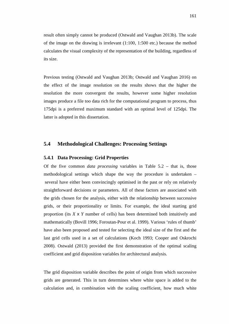
161

result often simply cannot be produced (Ostwald and Vaughan 2013b). The scale

of the image on the drawing is irrelevant (1:100, 1:500 etc.) because the method

calculates the visual complexity of the representation of the building, regardless of

its size.

Previous testing (Ostwald and Vaughan 2013b; Ostwald and Vaughan 2016) on

the effect of the image resolution on the results shows that the higher the

resolution the more convergent the results, however some higher resolution

images produce a file too data rich for the computational program to process, thus

175dpi is a preferred maximum standard with an optimal level of 125dpi. The

latter is adopted in this dissertation.

5.4 Methodological Challenges: Processing Settings

5.4.1 Data Processing: Grid Properties

Of the five common data processing variables in Table 5.2 – that is, those

methodological settings which shape the way the procedure is undertaken –

several have either been convincingly optimised in the past or rely on relatively

straightforward decisions or parameters. All of these factors are associated with

the grids chosen for the analysis, either with the relationship between successive

grids, or their proportionality or limits. For example, the ideal starting grid

proportion (its X x Y number of cells) has been determined both intuitively and

mathematically (Bovill 1996; Foroutan-Pour et al. 1999). Various ‘rules of thumb’

have also been proposed and tested for selecting the ideal size of the first and the

last grid cells used in a set of calculations (Koch 1993; Cooper and Oskrochi

2008). Ostwald (2013) provided the first demonstration of the optimal scaling

coefficient and grid disposition variables for architectural analysis.

The grid disposition variable describes the point of origin from which successive

grids are generated. This in turn determines where white space is added to the

calculation and, in combination with the scaling coefficient, how much white

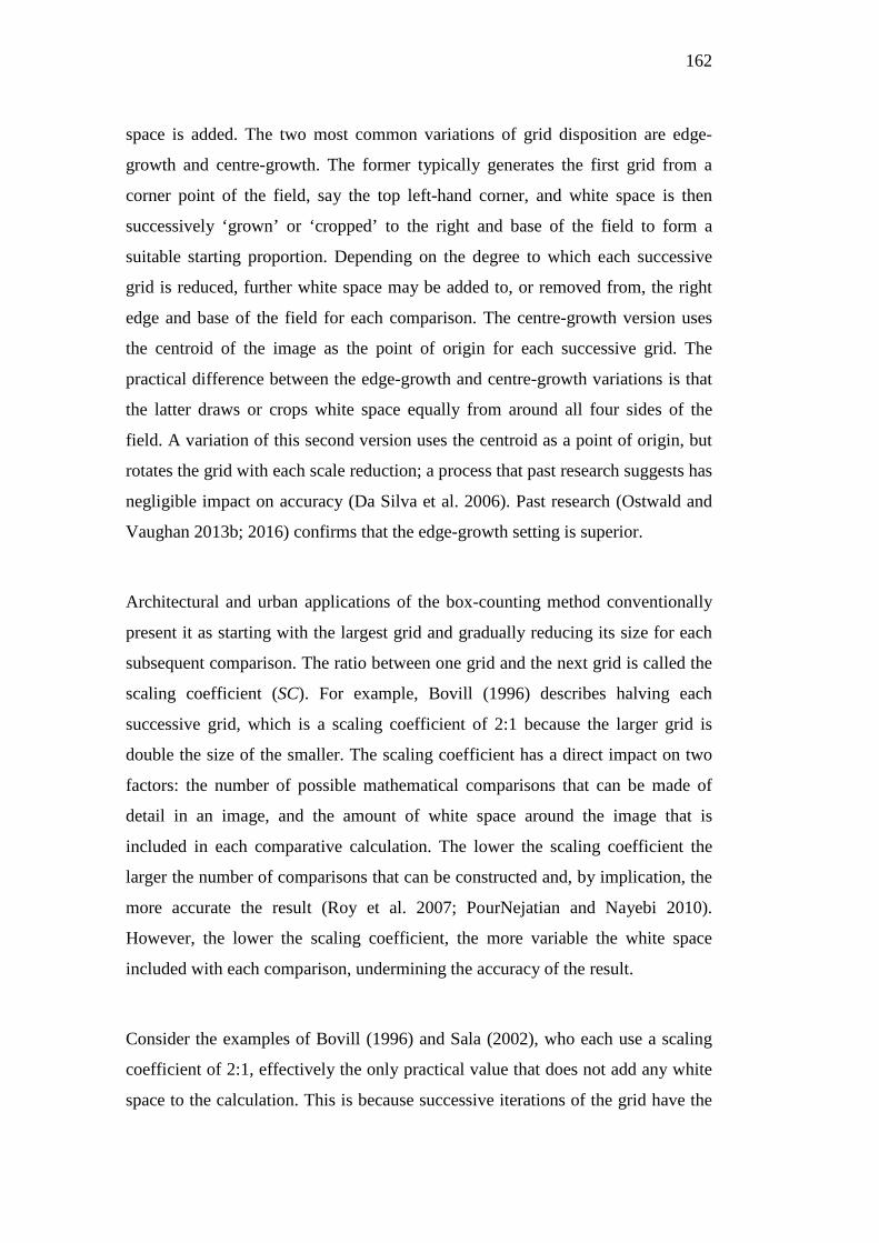
162

space is added. The two most common variations of grid disposition are edge-

growth and centre-growth. The former typically generates the first grid from a

corner point of the field, say the top left-hand corner, and white space is then

successively ‘grown’ or ‘cropped’ to the right and base of the field to form a

suitable starting proportion. Depending on the degree to which each successive

grid is reduced, further white space may be added to, or removed from, the right

edge and base of the field for each comparison. The centre-growth version uses

the centroid of the image as the point of origin for each successive grid. The

practical difference between the edge-growth and centre-growth variations is that

the latter draws or crops white space equally from around all four sides of the

field. A variation of this second version uses the centroid as a point of origin, but

rotates the grid with each scale reduction; a process that past research suggests has

negligible impact on accuracy (Da Silva et al. 2006). Past research (Ostwald and

Vaughan 2013b; 2016) confirms that the edge-growth setting is superior.

Architectural and urban applications of the box-counting method conventionally

present it as starting with the largest grid and gradually reducing its size for each

subsequent comparison. The ratio between one grid and the next grid is called the

scaling coefficient (SC). For example, Bovill (1996) describes halving each

successive grid, which is a scaling coefficient of 2:1 because the larger grid is

double the size of the smaller. The scaling coefficient has a direct impact on two

factors: the number of possible mathematical comparisons that can be made of

detail in an image, and the amount of white space around the image that is

included in each comparative calculation. The lower the scaling coefficient the

larger the number of comparisons that can be constructed and, by implication, the

more accurate the result (Roy et al. 2007; PourNejatian and Nayebi 2010).

However, the lower the scaling coefficient, the more variable the white space

included with each comparison, undermining the accuracy of the result.

Consider the examples of Bovill (1996) and Sala (2002), who each use a scaling

coefficient of 2:1, effectively the only practical value that does not add any white

space to the calculation. This is because successive iterations of the grid have the

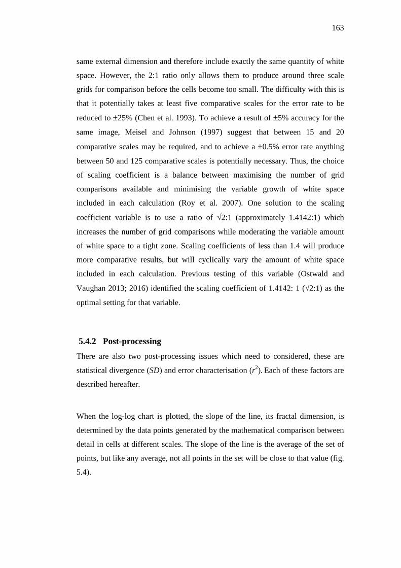
163

same external dimension and therefore include exactly the same quantity of white

space. However, the 2:1 ratio only allows them to produce around three scale

grids for comparison before the cells become too small. The difficulty with this is

that it potentially takes at least five comparative scales for the error rate to be

reduced to ±25% (Chen et al. 1993). To achieve a result of ±5% accuracy for the

same image, Meisel and Johnson (1997) suggest that between 15 and 20

comparative scales may be required, and to achieve a ±0.5% error rate anything

between 50 and 125 comparative scales is potentially necessary. Thus, the choice

of scaling coefficient is a balance between maximising the number of grid

comparisons available and minimising the variable growth of white space

included in each calculation (Roy et al. 2007). One solution to the scaling

coefficient variable is to use a ratio of √2:1 (approximately 1.4142:1) which

increases the number of grid comparisons while moderating the variable amount

of white space to a tight zone. Scaling coefficients of less than 1.4 will produce

more comparative results, but will cyclically vary the amount of white space

included in each calculation. Previous testing of this variable (Ostwald and

Vaughan 2013; 2016) identified the scaling coefficient of 1.4142: 1 (√2:1) as the

optimal setting for that variable.

5.4.2 Post-processing

There are also two post-processing issues which need to considered, these are

statistical divergence (SD) and error characterisation (r2). Each of these factors are

described hereafter.

When the log-log chart is plotted, the slope of the line, its fractal dimension, is

determined by the data points generated by the mathematical comparison between

detail in cells at different scales. The slope of the line is the average of the set of

points, but like any average, not all points in the set will be close to that value (fig.

5.4).

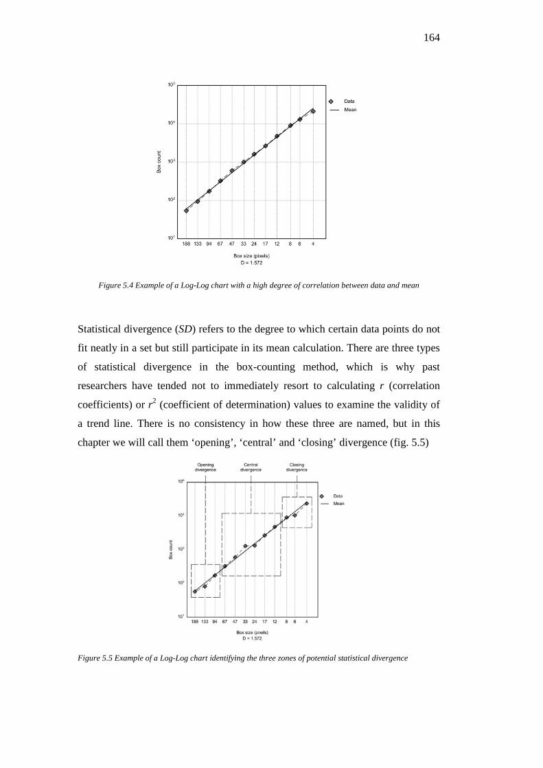
164

Figure 5.4 Example of a Log-Log chart with a high degree of correlation between data and mean

Statistical divergence (SD) refers to the degree to which certain data points do not

fit neatly in a set but still participate in its mean calculation. There are three types

of statistical divergence in the box-counting method, which is why past

researchers have tended not to immediately resort to calculating r (correlation

coefficients) or r2 (coefficient of determination) values to examine the validity of

a trend line. There is no consistency in how these three are named, but in this

chapter we will call them ‘opening’, ‘central’ and ‘closing’ divergence (fig. 5.5)

Figure 5.5 Example of a Log-Log chart identifying the three zones of potential statistical divergence

165

Opening divergence occurs in the first few grid comparisons for one of three

common reasons. First, because the proportionality of the opening grid is poor;

second, because excessive white space surrounds the image; finally, because the

image fills the entire first grid. All of these problems are associated with poor

starting field and image settings. Central divergence occurs in the ‘stable’, middle

part of the graph and it represents an inconsistent shift in detail in the image itself

(meaning that the image is a multi-fractal). Such a shift is not an anomaly; it is an

important property of the image. Closing divergence occurs when the analytical

grids have become so small that they are mostly counting empty space within the

image (Chen et al. 1993). The first and the third types are flaws which can be

minimised or controlled in various ways. The second type is a quality of the

image itself, representing the scale at which the characteristic irregularity begins

to break down. Some software allows for the tactical removal of particular points

in the ‘central’ range, but such a process alters the measured character of the

object, so it should be avoided unless the user has a clear reason for making such

a decision.

While central divergence is critical for the calculation, opening and closing

divergence can be controlled. For example, past research suggests that an ideal

proportion for the opening field and associated first or largest grid cell is 0.25l,

where l is the length of the shortest side (Foroutan-Pour et al. 1999). Conversely,

the smallest grid that should be considered has a cell size of 0.03l (Koch 1993;

Cooper and Oskrochi 2008).

Another way to approach this problem is to post-process the results to control the

extent to which divergence is allowed. For example, to limit the impact of

opening divergence, the overall result for all grid comparisons is first calculated

and then the first data point is removed and the result recalculated. If the

difference between the original and the revised result is greater than a particular

threshold level (called the SD value), then the first point is removed. Then the

process is repeated for the second point and potentially for the third, if a large

166

enough data set is available. The same process also occurs with the last point or

two in the line, to limit the impact of closing diversity.

The ideal SD value is relative to two factors: the accuracy of the other variables in

the method and the purpose of the analysis. In the first instance, there is no need

to choose an SD of 0.5% (a value which will remove data points which deviate

from the average by more than ±0.25% relative to the log-log result), if the

accuracy of data produced by the scaling coefficient is at best ±5%. In the second

instance, for example in architecture, the human eye will readily differentiate

between dimensions with around 4% difference (Stamps 2002; Ostwald and

Vaughan 2010; Vaughan and Ostwald 2010), so for some limited purposes, an SD

of less than ±2.0% may be unnecessary. However, Westheimer’s (1991) research

into the capacity of the human eye to differentiate between different types of

fractal lines (mathematical ‘random walks’) finds that a less than 1% variation is

readily perceived by the human mind for similar objects. Thus, if there are two

similar forms (say two different elevations of the Villa Savoye), the human eye is

likely to be able to detect which one is more visually complex, even if the

difference is only in the order of 1%. However, if the images are stylistically

dissimilar (say an elevation of the Villa Savoye and one of the Robie House), then

the human eye will readily identify the more complex image, but have a much

lower ability to determine how much more complex it is. For this reason, and the

results of previous testing (Ostwald and Vaughan 2013b; 2016), for architectural

analysis, a ±1% SD value is potentially sufficient for most analyses, although for

some specific purposes higher or lower values might be more appropriate.

167

5.5 Revisiting the Robie House

The Robie House (figs 5.1 and 5.2) is one of the canonical works of twentieth

century architecture that Bovill (1996) chose an elevation of to demonstrate that

the box-counting approach could be used in architectural studies. Lorenz (2003)

and Ostwald (et al. 2008; Ostwald 2013) have repeated variations of this analysis,

however none of these studies were undertaken using the standard and settings

proposed in this chapter.

In his original study, Bovill (1996) undertook three comparative calculations

(over four scales with SC = 2.0) for the south elevation, recording D results of

1.645, 1.485 and 1.441; average D = 1.520. Lorenz (2003) used the same image

over the same range of scales and the same SC value but produced an overall

calculation of D = 1.57. Ostwald, Vaughan and Tucker (2008) undertook eleven

comparative calculations over twelve scales of grid with SC = 1.41 and using

image pre-processing to convert all lines to one-pixel-width; the result was D =

1.62. Ostwald’s (2013) result of D = 1.572 was produced using an SC of 1.4142:1,

and the same elevation image, with a base width of 2900p wide, centred in a 3000

x 1500p field, with edge-growth grid disposition and a 50% Sobel-gradient. SD

was also used with a ±1.5% threshold.

If the south elevation if the Robie House is retested, using all of the optimal

settings identified in this chapter for both data processing and pre-processing, a

new result is produced, D = 1.5708. When the percentage difference between the

past results and the new results is calculated, a maximum difference is found of

5.08%, reducing down to the more recent result difference of 0.12%. In effect, this

process could be viewed as a record of the growing accuracy and accountability of

the method.

168

Conclusion

Previous attempts to refine the box-counting method have noted that it is both

more subtle and complex than most users realise. This chapter highlights the

groups of variables which need to be addressed for consistent analysis of images

using the box-counting method. These variables need to be considered in a

particular order according to their impact on the process. The first variable comes

into play prior to analysis—when the amount of information (texture) is selected

for inclusion in an image which is to be analysed. The possible outcomes of this

variable are acknowledged in this chapter by providing a classification of levels of

texture and corresponding meaning, and a suggested approach to representing an

image in the selected level is provided. Next, there is a set of methodological

variables—similar to the texture representation issue, the methodological

variables also involve image presentation, in this case it is the impact of an image

positioned on the ‘page’ and any settings used for a digitised drawing. To provide

consistent analysis, these aspects must match between images, and this chapter

presents a range of optimal image settings to be used in box-counting analysis.

The next set of variables described in this chapter relate to the computational

process, and again, consistent settings across the data analysed in required. The

box-counting calculations for this dissertation are calculated with the

computational program ArchImage, which allows for these settings to be entered

prior to the calculations being undertaken. The Final variable is considered after

the analysis, and this is the effect of statistical properties or error characterisation.

The methodological settings used in the present dissertation are set out in Table

5.3.

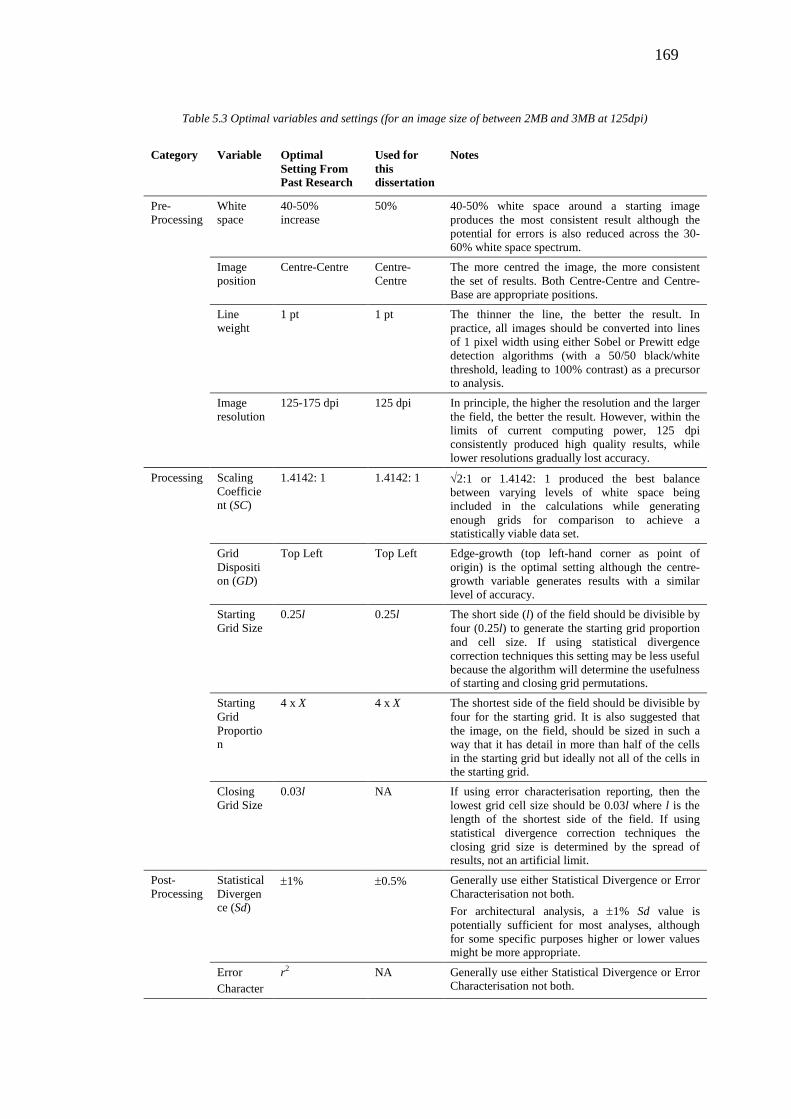
169

Table 5.3 Optimal variables and settings (for an image size of between 2MB and 3MB at 125dpi)

Category Variable Optimal Setting From Past Research

Used for this dissertation

Notes

Pre-Processing

White space

40-50% increase

50% 40-50% white space around a starting image produces the most consistent result although the potential for errors is also reduced across the 30-60% white space spectrum.

Image position

Centre-Centre Centre-Centre

The more centred the image, the more consistent the set of results. Both Centre-Centre and Centre-Base are appropriate positions.

Line weight

1 pt 1 pt The thinner the line, the better the result. In practice, all images should be converted into lines of 1 pixel width using either Sobel or Prewitt edge detection algorithms (with a 50/50 black/white threshold, leading to 100% contrast) as a precursor to analysis.

Image resolution

125-175 dpi 125 dpi In principle, the higher the resolution and the larger the field, the better the result. However, within the limits of current computing power, 125 dpi consistently produced high quality results, while lower resolutions gradually lost accuracy.

Processing Scaling Coefficient (SC)

1.4142: 1 1.4142: 1 √2:1 or 1.4142: 1 produced the best balance between varying levels of white space being included in the calculations while generating enough grids for comparison to achieve a statistically viable data set.

Grid Disposition (GD)

Top Left Top Left Edge-growth (top left-hand corner as point of origin) is the optimal setting although the centre-growth variable generates results with a similar level of accuracy.

Starting Grid Size

0.25l 0.25l The short side (l) of the field should be divisible by four (0.25l) to generate the starting grid proportion and cell size. If using statistical divergence correction techniques this setting may be less useful because the algorithm will determine the usefulness of starting and closing grid permutations.

Starting Grid Proportion

4 x X 4 x X The shortest side of the field should be divisible by four for the starting grid. It is also suggested that the image, on the field, should be sized in such a way that it has detail in more than half of the cells in the starting grid but ideally not all of the cells in the starting grid.

Closing Grid Size

0.03l NA If using error characterisation reporting, then the lowest grid cell size should be 0.03l where l is the length of the shortest side of the field. If using statistical divergence correction techniques the closing grid size is determined by the spread of results, not an artificial limit.

Post-Processing

Statistical Divergence (Sd)

±1% ±0.5% Generally use either Statistical Divergence or Error Characterisation not both. For architectural analysis, a ±1% Sd value is potentially sufficient for most analyses, although for some specific purposes higher or lower values might be more appropriate.

Error Character

r2 NA Generally use either Statistical Divergence or Error Characterisation not both.

170

Chapter 6

Comparing Architecture and Nature

According to Anthony Antoniades, ‘[n]ature is everywhere […] it touches

everything, giving the blow of life and shaping the prerequisites for the existence

and the growth of things’ (1992: 233). An enduring interest in nature’s influence

upon architectural design and theory has resulted in many projects and

publications, some of which claim a connection between architecture and nature

using only the most whimsical of logic and circular of arguments. Thus,

connections between nature and architecture are common, but the rationales for

these connections, and the manner in which they are presented or actualised, are

highly variable and often unconvincing.

This chapter commences with a brief overview of the application of fractal

analysis to nature, and then a review of past cases where the fractal dimensions of

architectural and natural forms have been compared. The problems or challenges

raised by these past applications of the method are then examined. The second

half of the chapter seeks to solve the problem—of a lack of a logical basis for

comparing architecture and nature—by categorising methodological examples

from both natural and architectural fractal analysis approaches. Specifically, the

type of image delineation and the level of information contained in it are

compared and ranked for their usefulness. Through this process, the chapter

provides a critical overview of the past application of fractal analysis to images of

nature and architecture, and provides a framework for developing a methodology

for comparing the built and natural environments of Frank Lloyd Wright’s

Fallingwater.

171

6.1 Relationships Between Nature and Architecture

It would be difficult to argue that any architecture can be produced without some

recognition of nature. As buildings are created of the earth’s resources, and are

subject to the effects of its weathering, Philip Jodidio (2006) argues that all

architects must be subject to the influence of nature. According to Antoniades,

architects are well-placed to accommodate nature into their work, as

nobody sees nature in more dynamic ways than architects, because

they are looking at it from so many more points of view. They care

about the ways and laws of the construction of the various natural

elements, and they care equally about […] the dynamism of natural

phenomenon (1992: 241).

Furthermore, beyond the general presence of the natural environment in

architects’ lives, there have been several aesthetic styles or movements which

have been inspired by nature, along with philosophers and designers who have

cited nature as a direct influence on their work.

Throughout the early human history of the need for shelter, vernacular built forms

have been influenced by familiarity with natural elements and forces, and a need

to build by hand, using locally sourced materials. While such examples are

inevitably closely influenced by nature, it is only in more recent history that

architectural movements have specifically claimed a connection to ‘nature’,

whether this is through concepts, forms, materials or climate. For example, around

the mid-eighteenth century, the Arts and Crafts movement (c 1860-1915)—

influenced by the thinking of John Ruskin and William Morris—rejected the early

impact of the mechanised age and proposed a shift away from industrialisation

and back to hand crafting and natural materials. In the late 1800’s, the Art

Nouveau style (c 1890-1910) of architecture emerged, the curling, curving tendrils

of its ornamentation reflecting the forms of nature. In this era, within the more

industrial Chicago Style, Louis Sullivan also used natural motifs in a decorative

manner in his buildings. Sullivan promoted an ‘architecture which shall speak

172

with cleanness, with eloquence, and with warmth, of the fullness, the

completeness of man’s intercourse with nature’ (Sullivan 1979: 200).

Some designers and scholars, including James Wines, argue that ‘the Arts and

Crafts Movement and Art Nouveau became the last architectural styles to

celebrate the building arts and natural forms’ (2000:22). After this time, the

emergence of Functional and later International Modernism more generally, and

some would say famously, ignored the natural environment. Wines laments that at

that time, ‘the battle was lost—Modern Design swept the slate clean with its

persuasive arguments about the relevance of industrial imagery’ (Wines 2000:

22). However, despite Wines’ lamentation, many architects of the Modern style

were fascinated and inspired by nature. As discussed previously in Chapter 2,

Frank Lloyd Wright followed Sullivan’s teachings to create a Modern style that

produced buildings which did not necessarily replicate the ‘look’ of nature, but

whose forms emerged from a design language that respected the rules of nature.

Another Modernist architect, Richard Neutra, ‘felt a fundamental obligation to

build houses and their surroundings in close harmony with the landscape […]

without resorting to naturalistic mannerism’ (Sack 1992: 21). Louis Kahn was

also awed by the processes of nature and said that ‘[i]t must be considered nothing

short of a human miracle to have thought of a building which doesn’t in any way

resemble what is in nature and which could not have been done if nature hadn’t

approved its making’ (Kahn and Wurman 1986: 1).

Wentworth D’arcy Thompson’s On Growth and Form (1917), presented elements

of nature in the context of biomathematics (mathematical and theoretical biology),

inspiring many thinkers of the day, including architects, who looked to the forms

of nature as a structural guide. In more recent times, Philip Steadman (2008)

examined and criticised the use of nature as an analogy for the way natural

structures might describe architecture (Groat and Wang 2002). The study of the

shapes and forms of nature has led several architects to pursue a type of bio-

morphic architecture, where the designer employ shapes which metaphorically

reflect or evoke nature, as seen in the late nineteenth century in the work of

173

Antoni Gaudí. While Wright did not always directly reflect the forms of nature in

his designs, many who were influenced by his work extended his Organic

Modernism to become a Biomorphic style, typically involving designs with

flowing, naturalistic forms. This type of Organic architecture continued

throughout the late twentieth century to the present day, with Bruce Goff, Bart

Prince, Helena Arahuette and Gregory Burgess having produced designs in this

style. A further variation of these themes is found in the Critical Regionalist

movement, which considers the natural environment in terms of site and materials.

A broad spectrum of current design activity considers the natural environment as

part of the desire to produce Sustainable architecture. This approach ‘combine[s]

environmental responsibility with formal ambition’ (Genevro 2000: 4). While

there are no consistent formal or aesthetic responses found in Sustainable or Eco-

Architecture, there is a consideration of nature in the design process of most

buildings that are called ‘sustainable’. This consideration might manifest in a

building through a response to embodied energy, climatic control or ecological

sensitivity. It might also be expressed through a visual connection, or geometric

similarity, between the appearance of a building and nature (Makhzoumi and

Pungetti 1999; Hagan 2001; Williams 2007).

6.2 Finding the Similarities Between Nature and Architecture

Qualitative connections between architecture and nature are typically made using

visual simile or metaphor, symbolism or semiotics. Such methods consciously or

subconsciously evoke—through the poetry of form, the use of materials, or the

icons and messages embedded in a design—connections to nature. While such

qualitative methods have been used to argue for the visual similarities, or

differences, between architecture and nature, there are a limited number of

quantitative approaches to this issue. Fractal analysis provides one of very few

methods available to analyse and compare the characteristic complexity of diverse

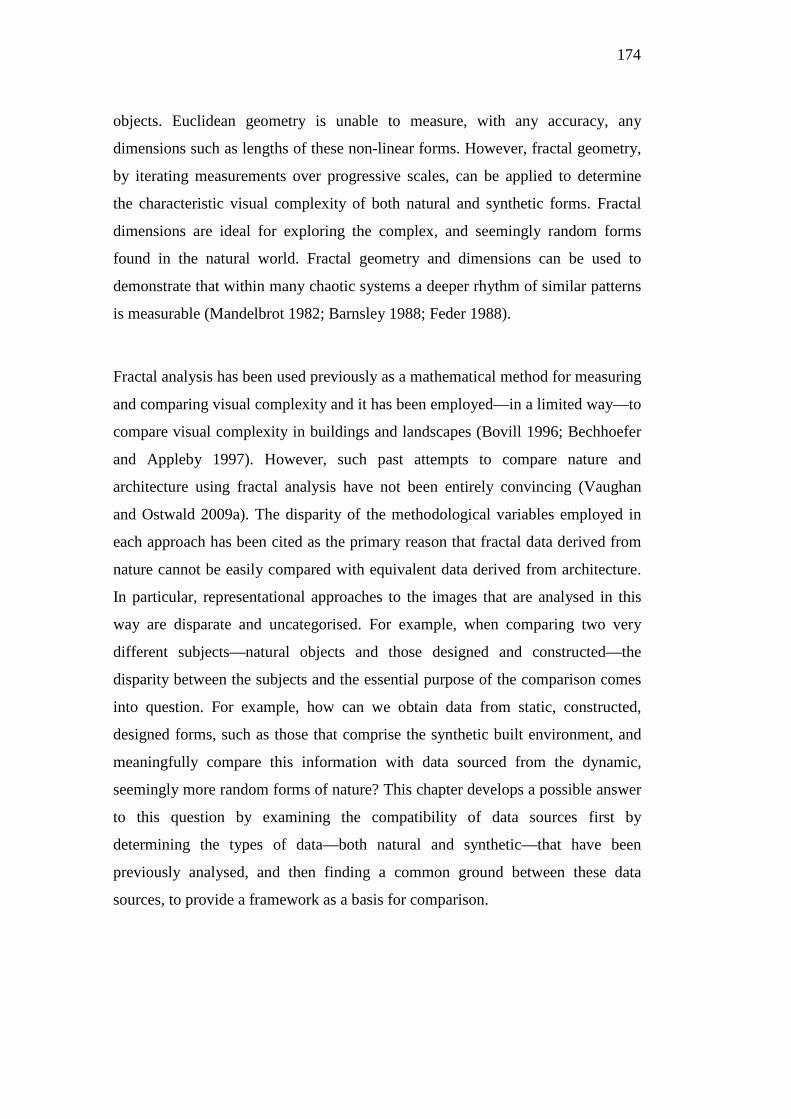
174

objects. Euclidean geometry is unable to measure, with any accuracy, any

dimensions such as lengths of these non-linear forms. However, fractal geometry,

by iterating measurements over progressive scales, can be applied to determine

the characteristic visual complexity of both natural and synthetic forms. Fractal

dimensions are ideal for exploring the complex, and seemingly random forms

found in the natural world. Fractal geometry and dimensions can be used to

demonstrate that within many chaotic systems a deeper rhythm of similar patterns

is measurable (Mandelbrot 1982; Barnsley 1988; Feder 1988).

Fractal analysis has been used previously as a mathematical method for measuring

and comparing visual complexity and it has been employed—in a limited way—to

compare visual complexity in buildings and landscapes (Bovill 1996; Bechhoefer

and Appleby 1997). However, such past attempts to compare nature and

architecture using fractal analysis have not been entirely convincing (Vaughan

and Ostwald 2009a). The disparity of the methodological variables employed in

each approach has been cited as the primary reason that fractal data derived from

nature cannot be easily compared with equivalent data derived from architecture.

In particular, representational approaches to the images that are analysed in this

way are disparate and uncategorised. For example, when comparing two very

different subjects—natural objects and those designed and constructed—the

disparity between the subjects and the essential purpose of the comparison comes

into question. For example, how can we obtain data from static, constructed,

designed forms, such as those that comprise the synthetic built environment, and

meaningfully compare this information with data sourced from the dynamic,

seemingly more random forms of nature? This chapter develops a possible answer

to this question by examining the compatibility of data sources first by

determining the types of data—both natural and synthetic—that have been

previously analysed, and then finding a common ground between these data

sources, to provide a framework as a basis for comparison.

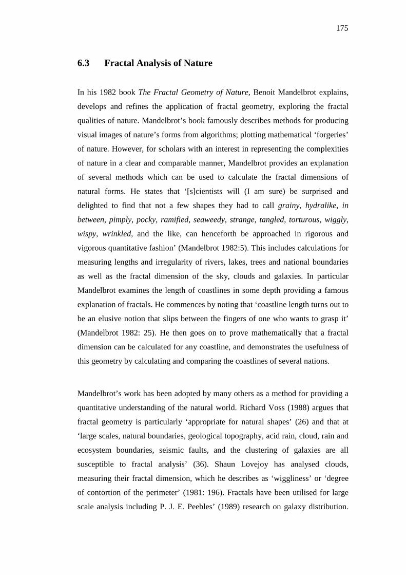
175

6.3 Fractal Analysis of Nature

In his 1982 book The Fractal Geometry of Nature, Benoit Mandelbrot explains,

develops and refines the application of fractal geometry, exploring the fractal

qualities of nature. Mandelbrot’s book famously describes methods for producing

visual images of nature’s forms from algorithms; plotting mathematical ‘forgeries’

of nature. However, for scholars with an interest in representing the complexities

of nature in a clear and comparable manner, Mandelbrot provides an explanation

of several methods which can be used to calculate the fractal dimensions of

natural forms. He states that ‘[s]cientists will (I am sure) be surprised and

delighted to find that not a few shapes they had to call grainy, hydralike, in

between, pimply, pocky, ramified, seaweedy, strange, tangled, torturous, wiggly,

wispy, wrinkled, and the like, can henceforth be approached in rigorous and

vigorous quantitative fashion’ (Mandelbrot 1982:5). This includes calculations for

measuring lengths and irregularity of rivers, lakes, trees and national boundaries

as well as the fractal dimension of the sky, clouds and galaxies. In particular

Mandelbrot examines the length of coastlines in some depth providing a famous

explanation of fractals. He commences by noting that ‘coastline length turns out to

be an elusive notion that slips between the fingers of one who wants to grasp it’

(Mandelbrot 1982: 25). He then goes on to prove mathematically that a fractal

dimension can be calculated for any coastline, and demonstrates the usefulness of

this geometry by calculating and comparing the coastlines of several nations.

Mandelbrot’s work has been adopted by many others as a method for providing a

quantitative understanding of the natural world. Richard Voss (1988) argues that

fractal geometry is particularly ‘appropriate for natural shapes’ (26) and that at

‘large scales, natural boundaries, geological topography, acid rain, cloud, rain and

ecosystem boundaries, seismic faults, and the clustering of galaxies are all

susceptible to fractal analysis’ (36). Shaun Lovejoy has analysed clouds,

measuring their fractal dimension, which he describes as ‘wiggliness’ or ‘degree

of contortion of the perimeter’ (1981: 196). Fractals have been utilised for large

scale analysis including P. J. E. Peebles’ (1989) research on galaxy distribution.

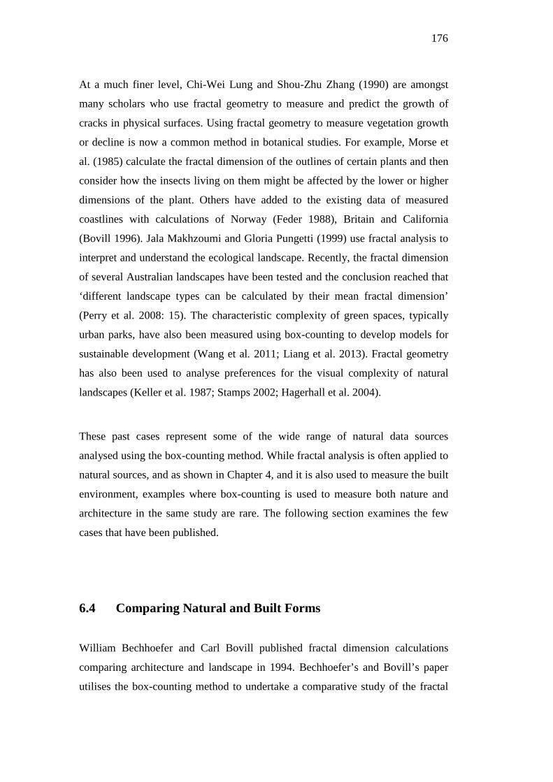
176

At a much finer level, Chi-Wei Lung and Shou-Zhu Zhang (1990) are amongst

many scholars who use fractal geometry to measure and predict the growth of

cracks in physical surfaces. Using fractal geometry to measure vegetation growth

or decline is now a common method in botanical studies. For example, Morse et

al. (1985) calculate the fractal dimension of the outlines of certain plants and then

consider how the insects living on them might be affected by the lower or higher

dimensions of the plant. Others have added to the existing data of measured

coastlines with calculations of Norway (Feder 1988), Britain and California

(Bovill 1996). Jala Makhzoumi and Gloria Pungetti (1999) use fractal analysis to

interpret and understand the ecological landscape. Recently, the fractal dimension

of several Australian landscapes have been tested and the conclusion reached that

‘different landscape types can be calculated by their mean fractal dimension’

(Perry et al. 2008: 15). The characteristic complexity of green spaces, typically

urban parks, have also been measured using box-counting to develop models for

sustainable development (Wang et al. 2011; Liang et al. 2013). Fractal geometry

has also been used to analyse preferences for the visual complexity of natural

landscapes (Keller et al. 1987; Stamps 2002; Hagerhall et al. 2004).

These past cases represent some of the wide range of natural data sources

analysed using the box-counting method. While fractal analysis is often applied to

natural sources, and as shown in Chapter 4, and it is also used to measure the built

environment, examples where box-counting is used to measure both nature and

architecture in the same study are rare. The following section examines the few

cases that have been published.

6.4 Comparing Natural and Built Forms

William Bechhoefer and Carl Bovill published fractal dimension calculations

comparing architecture and landscape in 1994. Bechhoefer’s and Bovill’s paper

utilises the box-counting method to undertake a comparative study of the fractal

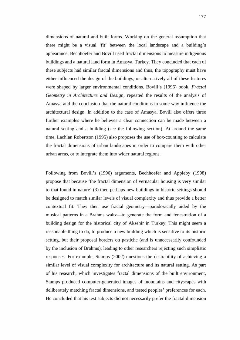
177

dimensions of natural and built forms. Working on the general assumption that

there might be a visual ‘fit’ between the local landscape and a building’s

appearance, Bechhoefer and Bovill used fractal dimensions to measure indigenous

buildings and a natural land form in Amasya, Turkey. They concluded that each of

these subjects had similar fractal dimensions and thus, the topography must have

either influenced the design of the buildings, or alternatively all of these features

were shaped by larger environmental conditions. Bovill’s (1996) book, Fractal

Geometry in Architecture and Design, repeated the results of the analysis of

Amasya and the conclusion that the natural conditions in some way influence the

architectural design. In addition to the case of Amasya, Bovill also offers three

further examples where he believes a clear connection can be made between a

natural setting and a building (see the following section). At around the same

time, Lachlan Robertson (1995) also proposes the use of box-counting to calculate

the fractal dimensions of urban landscapes in order to compare them with other

urban areas, or to integrate them into wider natural regions.

Following from Bovill’s (1996) arguments, Bechhoefer and Appleby (1998)

propose that because ‘the fractal dimension of vernacular housing is very similar

to that found in nature’ (3) then perhaps new buildings in historic settings should

be designed to match similar levels of visual complexity and thus provide a better

contextual fit. They then use fractal geometry—paradoxically aided by the

musical patterns in a Brahms waltz—to generate the form and fenestration of a

building design for the historical city of Aksehir in Turkey. This might seem a

reasonable thing to do, to produce a new building which is sensitive to its historic

setting, but their proposal borders on pastiche (and is unnecessarily confounded

by the inclusion of Brahms), leading to other researchers rejecting such simplistic

responses. For example, Stamps (2002) questions the desirability of achieving a

similar level of visual complexity for architecture and its natural setting. As part

of his research, which investigates fractal dimensions of the built environment,

Stamps produced computer-generated images of mountains and cityscapes with

deliberately matching fractal dimensions, and tested peoples’ preferences for each.

He concluded that his test subjects did not necessarily prefer the fractal dimension

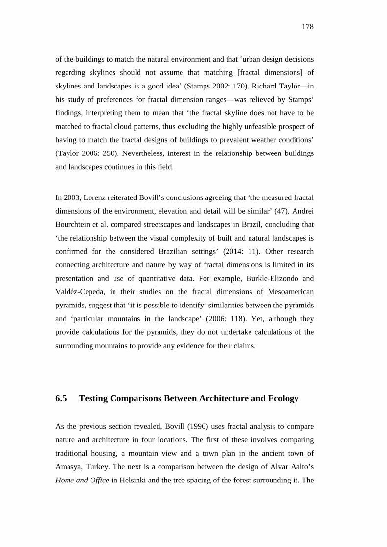
178

of the buildings to match the natural environment and that ‘urban design decisions

regarding skylines should not assume that matching [fractal dimensions] of

skylines and landscapes is a good idea’ (Stamps 2002: 170). Richard Taylor—in

his study of preferences for fractal dimension ranges—was relieved by Stamps’

findings, interpreting them to mean that ‘the fractal skyline does not have to be

matched to fractal cloud patterns, thus excluding the highly unfeasible prospect of

having to match the fractal designs of buildings to prevalent weather conditions’

(Taylor 2006: 250). Nevertheless, interest in the relationship between buildings

and landscapes continues in this field.

In 2003, Lorenz reiterated Bovill’s conclusions agreeing that ‘the measured fractal

dimensions of the environment, elevation and detail will be similar’ (47). Andrei

Bourchtein et al. compared streetscapes and landscapes in Brazil, concluding that

‘the relationship between the visual complexity of built and natural landscapes is

confirmed for the considered Brazilian settings’ (2014: 11). Other research

connecting architecture and nature by way of fractal dimensions is limited in its

presentation and use of quantitative data. For example, Burkle-Elizondo and

Valdéz-Cepeda, in their studies on the fractal dimensions of Mesoamerican

pyramids, suggest that ‘it is possible to identify’ similarities between the pyramids

and ‘particular mountains in the landscape’ (2006: 118). Yet, although they

provide calculations for the pyramids, they do not undertake calculations of the

surrounding mountains to provide any evidence for their claims.

6.5 Testing Comparisons Between Architecture and Ecology

As the previous section revealed, Bovill (1996) uses fractal analysis to compare

nature and architecture in four locations. The first of these involves comparing

traditional housing, a mountain view and a town plan in the ancient town of

Amasya, Turkey. The next is a comparison between the design of Alvar Aalto’s

Home and Office in Helsinki and the tree spacing of the forest surrounding it. The

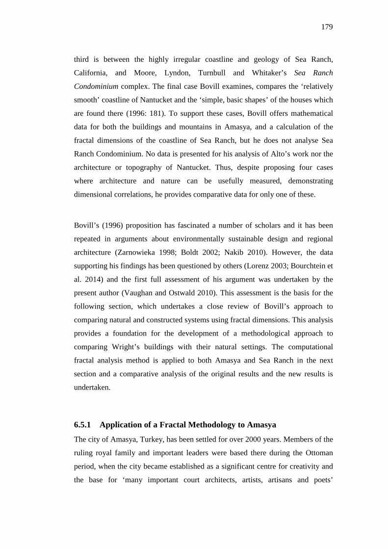
179

third is between the highly irregular coastline and geology of Sea Ranch,

California, and Moore, Lyndon, Turnbull and Whitaker’s Sea Ranch

Condominium complex. The final case Bovill examines, compares the ‘relatively

smooth’ coastline of Nantucket and the ‘simple, basic shapes’ of the houses which

are found there (1996: 181). To support these cases, Bovill offers mathematical

data for both the buildings and mountains in Amasya, and a calculation of the

fractal dimensions of the coastline of Sea Ranch, but he does not analyse Sea

Ranch Condominium. No data is presented for his analysis of Alto’s work nor the

architecture or topography of Nantucket. Thus, despite proposing four cases

where architecture and nature can be usefully measured, demonstrating

dimensional correlations, he provides comparative data for only one of these.

Bovill’s (1996) proposition has fascinated a number of scholars and it has been

repeated in arguments about environmentally sustainable design and regional

architecture (Zarnowieka 1998; Boldt 2002; Nakib 2010). However, the data

supporting his findings has been questioned by others (Lorenz 2003; Bourchtein et

al. 2014) and the first full assessment of his argument was undertaken by the

present author (Vaughan and Ostwald 2010). This assessment is the basis for the

following section, which undertakes a close review of Bovill’s approach to

comparing natural and constructed systems using fractal dimensions. This analysis

provides a foundation for the development of a methodological approach to

comparing Wright’s buildings with their natural settings. The computational

fractal analysis method is applied to both Amasya and Sea Ranch in the next

section and a comparative analysis of the original results and the new results is

undertaken.

6.5.1 Application of a Fractal Methodology to Amasya

The city of Amasya, Turkey, has been settled for over 2000 years. Members of the

ruling royal family and important leaders were based there during the Ottoman

period, when the city became established as a significant centre for creativity and

the base for ‘many important court architects, artists, artisans and poets’

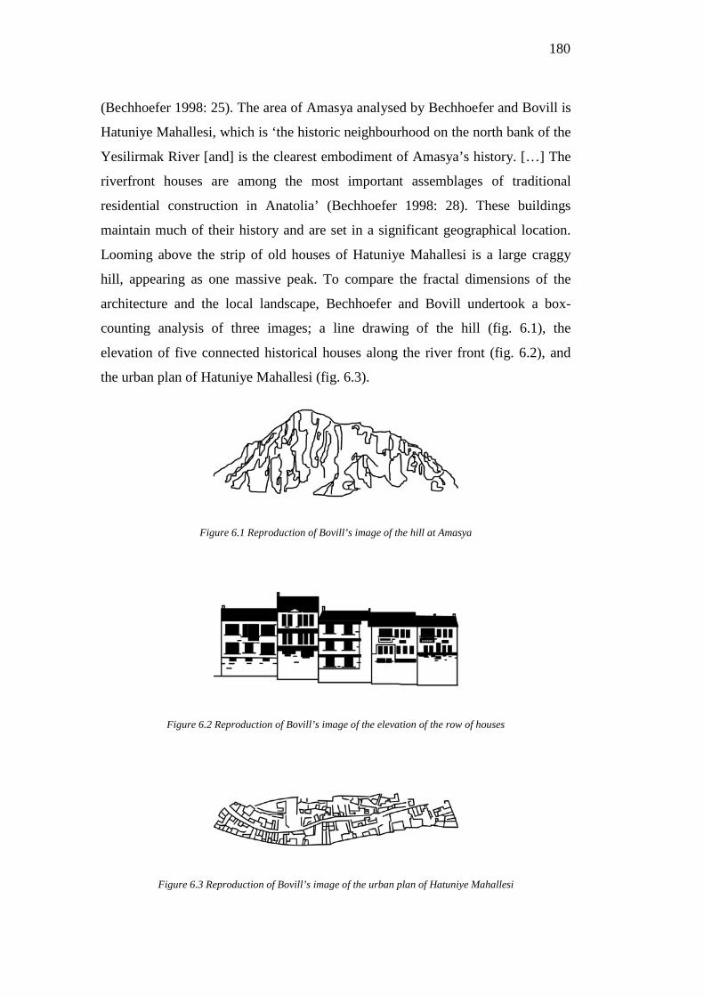
180

(Bechhoefer 1998: 25). The area of Amasya analysed by Bechhoefer and Bovill is

Hatuniye Mahallesi, which is ‘the historic neighbourhood on the north bank of the

Yesilirmak River [and] is the clearest embodiment of Amasya’s history. […] The

riverfront houses are among the most important assemblages of traditional

residential construction in Anatolia’ (Bechhoefer 1998: 28). These buildings

maintain much of their history and are set in a significant geographical location.

Looming above the strip of old houses of Hatuniye Mahallesi is a large craggy

hill, appearing as one massive peak. To compare the fractal dimensions of the

architecture and the local landscape, Bechhoefer and Bovill undertook a box-

counting analysis of three images; a line drawing of the hill (fig. 6.1), the

elevation of five connected historical houses along the river front (fig. 6.2), and

the urban plan of Hatuniye Mahallesi (fig. 6.3).

Figure 6.1 Reproduction of Bovill’s image of the hill at Amasya

Figure 6.2 Reproduction of Bovill’s image of the elevation of the row of houses

Figure 6.3 Reproduction of Bovill’s image of the urban plan of Hatuniye Mahallesi

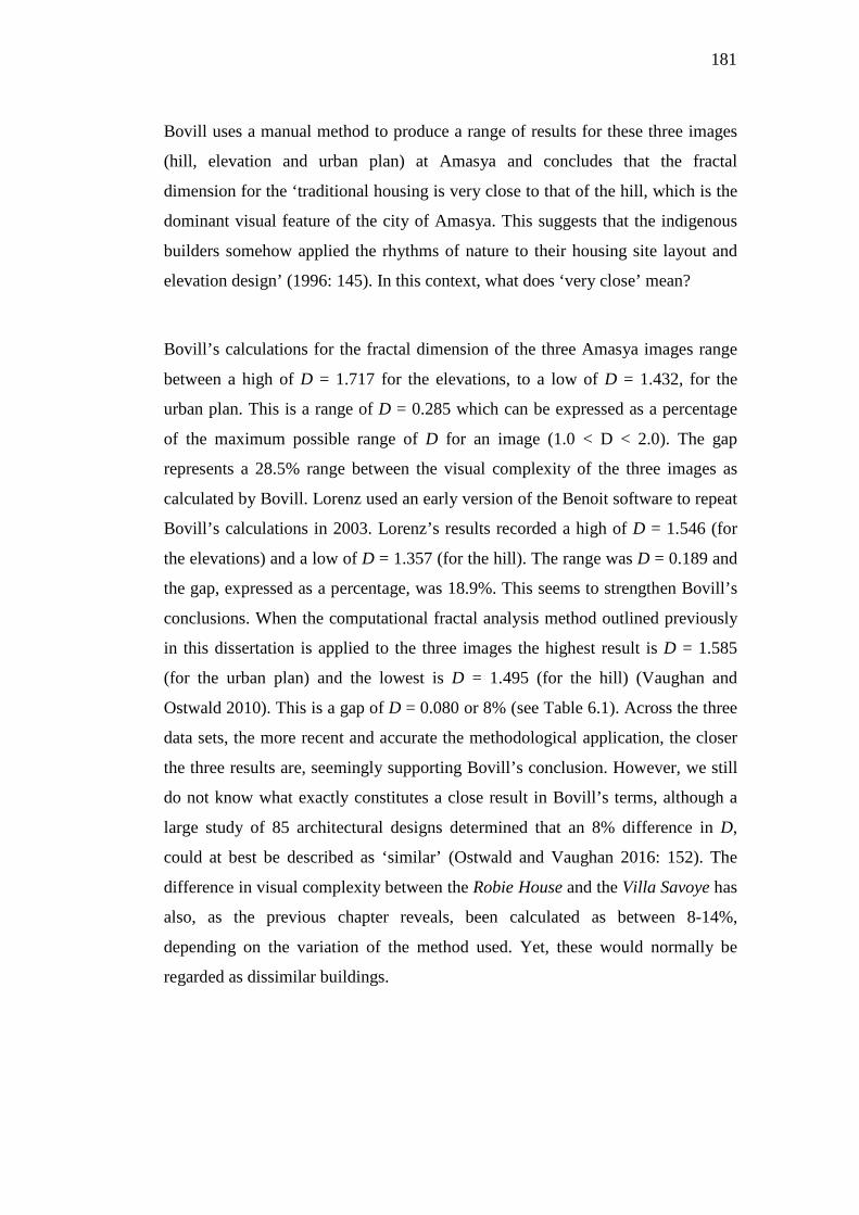
181

Bovill uses a manual method to produce a range of results for these three images

(hill, elevation and urban plan) at Amasya and concludes that the fractal

dimension for the ‘traditional housing is very close to that of the hill, which is the

dominant visual feature of the city of Amasya. This suggests that the indigenous

builders somehow applied the rhythms of nature to their housing site layout and

elevation design’ (1996: 145). In this context, what does ‘very close’ mean?

Bovill’s calculations for the fractal dimension of the three Amasya images range

between a high of D = 1.717 for the elevations, to a low of D = 1.432, for the

urban plan. This is a range of D = 0.285 which can be expressed as a percentage

of the maximum possible range of D for an image (1.0 < D < 2.0). The gap

represents a 28.5% range between the visual complexity of the three images as

calculated by Bovill. Lorenz used an early version of the Benoit software to repeat

Bovill’s calculations in 2003. Lorenz’s results recorded a high of D = 1.546 (for

the elevations) and a low of D = 1.357 (for the hill). The range was D = 0.189 and

the gap, expressed as a percentage, was 18.9%. This seems to strengthen Bovill’s

conclusions. When the computational fractal analysis method outlined previously

in this dissertation is applied to the three images the highest result is D = 1.585

(for the urban plan) and the lowest is D = 1.495 (for the hill) (Vaughan and

Ostwald 2010). This is a gap of D = 0.080 or 8% (see Table 6.1). Across the three

data sets, the more recent and accurate the methodological application, the closer

the three results are, seemingly supporting Bovill’s conclusion. However, we still

do not know what exactly constitutes a close result in Bovill’s terms, although a

large study of 85 architectural designs determined that an 8% difference in D,

could at best be described as ‘similar’ (Ostwald and Vaughan 2016: 152). The

difference in visual complexity between the Robie House and the Villa Savoye has

also, as the previous chapter reveals, been calculated as between 8-14%,

depending on the variation of the method used. Yet, these would normally be

regarded as dissimilar buildings.

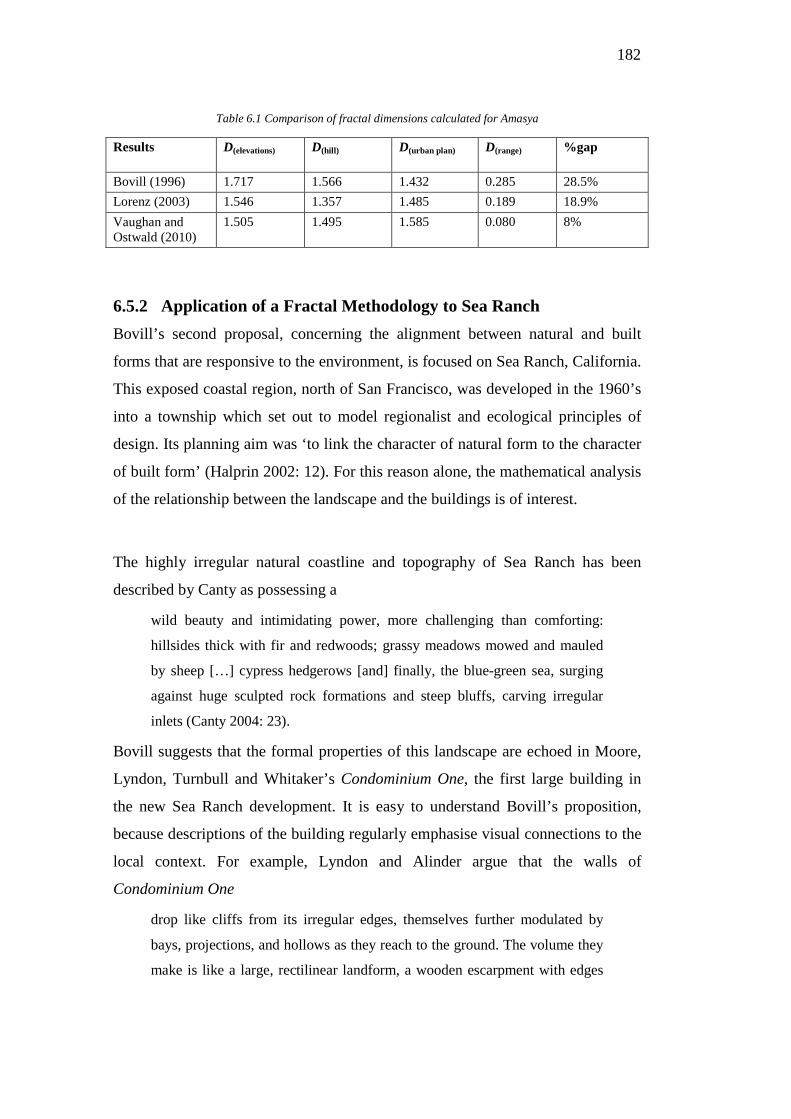
182

Table 6.1 Comparison of fractal dimensions calculated for Amasya

Results D(elevations) D(hill) D(urban plan) D(range) %gap

Bovill (1996) 1.717 1.566 1.432 0.285 28.5% Lorenz (2003) 1.546 1.357 1.485 0.189 18.9% Vaughan and Ostwald (2010)

1.505 1.495 1.585 0.080 8%

6.5.2 Application of a Fractal Methodology to Sea Ranch Bovill’s second proposal, concerning the alignment between natural and built

forms that are responsive to the environment, is focused on Sea Ranch, California.

This exposed coastal region, north of San Francisco, was developed in the 1960’s

into a township which set out to model regionalist and ecological principles of

design. Its planning aim was ‘to link the character of natural form to the character

of built form’ (Halprin 2002: 12). For this reason alone, the mathematical analysis

of the relationship between the landscape and the buildings is of interest.

The highly irregular natural coastline and topography of Sea Ranch has been

described by Canty as possessing a

wild beauty and intimidating power, more challenging than comforting:

hillsides thick with fir and redwoods; grassy meadows mowed and mauled

by sheep […] cypress hedgerows [and] finally, the blue-green sea, surging

against huge sculpted rock formations and steep bluffs, carving irregular

inlets (Canty 2004: 23).

Bovill suggests that the formal properties of this landscape are echoed in Moore,

Lyndon, Turnbull and Whitaker’s Condominium One, the first large building in

the new Sea Ranch development. It is easy to understand Bovill’s proposition,

because descriptions of the building regularly emphasise visual connections to the

local context. For example, Lyndon and Alinder argue that the walls of

Condominium One

drop like cliffs from its irregular edges, themselves further modulated by

bays, projections, and hollows as they reach to the ground. The volume they

make is like a large, rectilinear landform, a wooden escarpment with edges

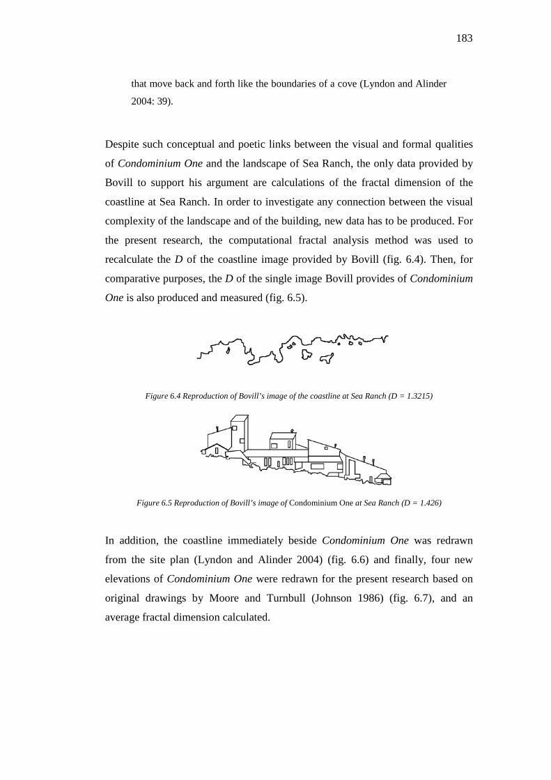
183

that move back and forth like the boundaries of a cove (Lyndon and Alinder

2004: 39).

Despite such conceptual and poetic links between the visual and formal qualities

of Condominium One and the landscape of Sea Ranch, the only data provided by

Bovill to support his argument are calculations of the fractal dimension of the

coastline at Sea Ranch. In order to investigate any connection between the visual

complexity of the landscape and of the building, new data has to be produced. For

the present research, the computational fractal analysis method was used to

recalculate the D of the coastline image provided by Bovill (fig. 6.4). Then, for

comparative purposes, the D of the single image Bovill provides of Condominium

One is also produced and measured (fig. 6.5).

Figure 6.4 Reproduction of Bovill’s image of the coastline at Sea Ranch (D = 1.3215)

Figure 6.5 Reproduction of Bovill’s image of Condominium One at Sea Ranch (D = 1.426)

In addition, the coastline immediately beside Condominium One was redrawn

from the site plan (Lyndon and Alinder 2004) (fig. 6.6) and finally, four new

elevations of Condominium One were redrawn for the present research based on

original drawings by Moore and Turnbull (Johnson 1986) (fig. 6.7), and an

average fractal dimension calculated.

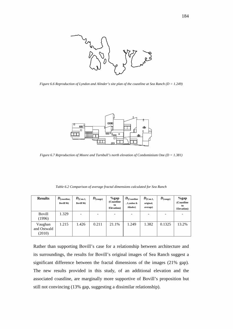
184

Figure 6.6 Reproduction of Lyndon and Alinder’s site plan of the coastline at Sea Ranch (D = 1.249)

Figure 6.7 Reproduction of Moore and Turnbull’s north elevation of Condominium One (D = 1.381)

Table 6.2 Comparison of average fractal dimensions calculated for Sea Ranch

Results D(coastline,

Bovill 96) D(Con.1,

Bovill 96) D(range) %gap

(Coastline to

Elevation)

D(Coastline

, Lyndon &

Alinder)

D(Con.1,

original,

average)

D(range) %gap (Coastline

to Elevation)

Bovill (1996)

1.329 - - - - - - -

Vaughan and Ostwald

(2010)

1.215 1.426 0.211 21.1% 1.249 1.382 0.1325 13.2%

Rather than supporting Bovill’s case for a relationship between architecture and

its surroundings, the results for Bovill’s original images of Sea Ranch suggest a

significant difference between the fractal dimensions of the images (21% gap).

The new results provided in this study, of an additional elevation and the

associated coastline, are marginally more supportive of Bovill’s proposition but

still not convincing (13% gap, suggesting a dissimilar relationship).

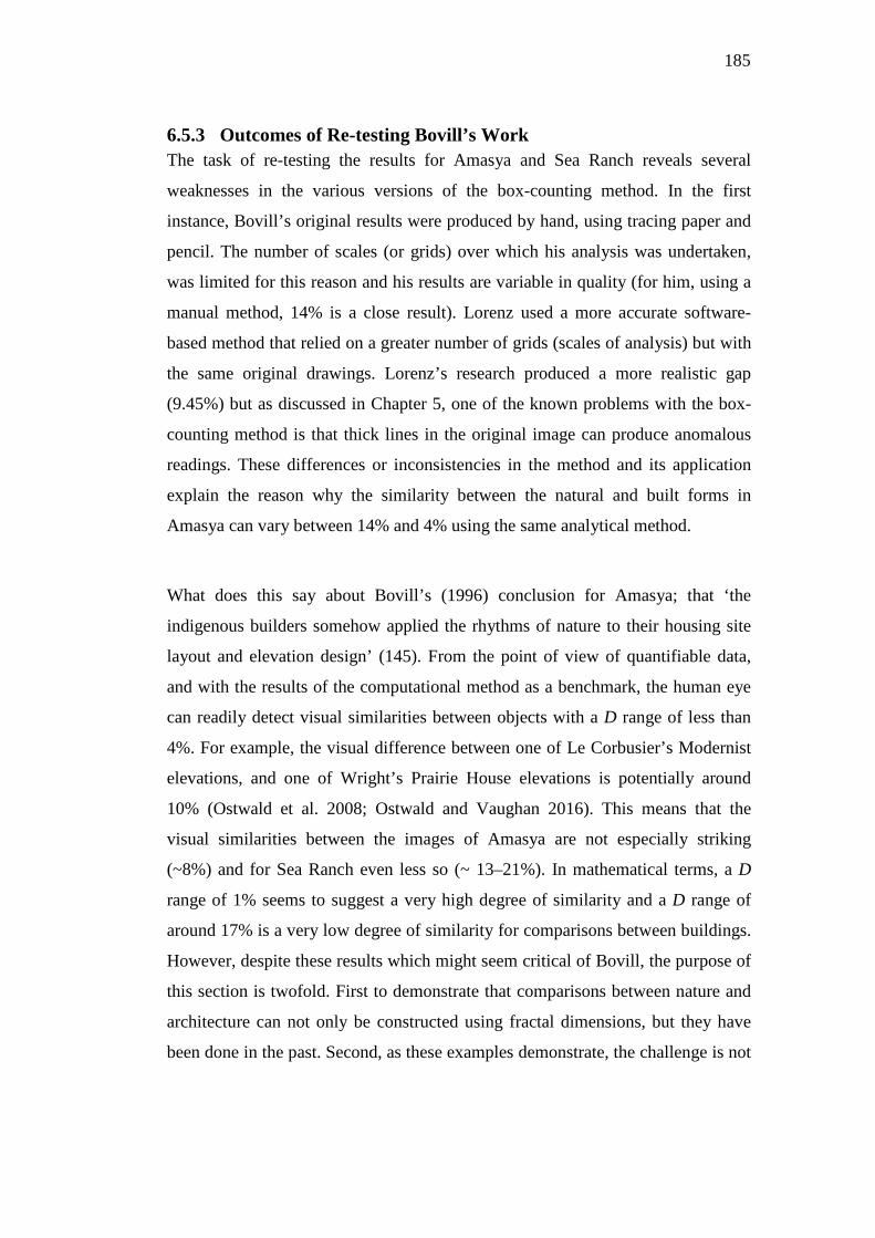
185

6.5.3 Outcomes of Re-testing Bovill’s Work The task of re-testing the results for Amasya and Sea Ranch reveals several

weaknesses in the various versions of the box-counting method. In the first

instance, Bovill’s original results were produced by hand, using tracing paper and

pencil. The number of scales (or grids) over which his analysis was undertaken,

was limited for this reason and his results are variable in quality (for him, using a

manual method, 14% is a close result). Lorenz used a more accurate software-

based method that relied on a greater number of grids (scales of analysis) but with

the same original drawings. Lorenz’s research produced a more realistic gap

(9.45%) but as discussed in Chapter 5, one of the known problems with the box-

counting method is that thick lines in the original image can produce anomalous

readings. These differences or inconsistencies in the method and its application

explain the reason why the similarity between the natural and built forms in

Amasya can vary between 14% and 4% using the same analytical method.

What does this say about Bovill’s (1996) conclusion for Amasya; that ‘the

indigenous builders somehow applied the rhythms of nature to their housing site

layout and elevation design’ (145). From the point of view of quantifiable data,

and with the results of the computational method as a benchmark, the human eye

can readily detect visual similarities between objects with a D range of less than

4%. For example, the visual difference between one of Le Corbusier’s Modernist

elevations, and one of Wright’s Prairie House elevations is potentially around

10% (Ostwald et al. 2008; Ostwald and Vaughan 2016). This means that the

visual similarities between the images of Amasya are not especially striking

(~8%) and for Sea Ranch even less so (~ 13–21%). In mathematical terms, a D

range of 1% seems to suggest a very high degree of similarity and a D range of

around 17% is a very low degree of similarity for comparisons between buildings.

However, despite these results which might seem critical of Bovill, the purpose of

this section is twofold. First to demonstrate that comparisons between nature and

architecture can not only be constructed using fractal dimensions, but they have

been done in the past. Second, as these examples demonstrate, the challenge is not

186

so much ‘can we compare nature and architecture using fractal dimensions’, but

‘how can a valid (useful, consistent and logical) comparison be undertaken’?

Bovill’s results were limited by the number of images he tested, the selection of

images he chose and the manual version of the analytical method he used. He

didn’t provide any clear rationale or guidelines for the data source or type required

to make such a comparison. This problem can be traced to the often-overlooked

fact that computational methods, like fractal analysis, do not measure ‘nature’ or

‘architecture’ per se, rather they extract measures from representations of natural

objects, landscapes or buildings. Images such as geological landform drawings

and architectural elevation drawings are ‘secondary representations of artefacts’

(Hewitt 1985: 3), and there exists a vast range of typical representation options

and standards available for scholars analysing such subjects (Leupen et al. 1997).

Rather than rejecting the whole concept outright, it is proposed that the potential

validity of a computational comparison of the complexity of nature and

architecture could be further developed if a more rigorous methodology could be

applied to the data selected for analysis. This idea, which follows from the various

precedents outlined in the present chapter, is developed in the following section.

6.6 Image Requirements for Comparing Fractal Dimensions

As discussed in Chapters 4 and 5, the fractal analysis method has many variables

and failing to apply them in a consistent manner can mean that results are difficult

to compare between different studies. Previous research has identified optimal

settings for fractal analysis which ensure consistent, repeatable results (Koch

1993; Buczkowski et al. 1998; Foroutan-pour et al. 1999; Cooper and Oskrochi

2008; Ostwald 2013; Ostwald and Vaughan 2013b). As Chapter 5 reveals, the

usefulness of any data is also reliant on the two-dimensional representation which

is subject to analysis (Vaughan and Ostwald 2010; Ostwald and Vaughan 2012).

However, while the framework presented in Chapter 5 can be used to select the

187

right level of representation for various architectural research topics or questions,

what happens when we want to compare two very different subjects, say a

building and a landform?

When fractal analysis is used to make comparisons, for example, in biological

sciences to establish a difference in complexity between two forest types, this

could be considered a legitimate or reasonable comparison of natural data (Zeide

and Pfeifer 1991). Or in the built environment, to compare the changes in design

complexity during an architect’s career, this could be considered a legitimate or

reasonable comparison using synthetic data (Vaughan and Ostwald 2009b).

While each of these separate cases are potentially reasonable (such as the

correlation between multiple natural forms and between different buildings), when

the data from two different sources—the natural and the synthetic—is compared,

this raises questions regarding the basis for such a comparison. This section

develops an approach to images as a type of data that represent (in several

different ways) an object in reality.

Mark Hewitt emphasises the importance of distinguishing and categorising

aspects of an image noting that for analysis of images we need to ‘consider

drawings, models, and other representational devices both as works […] and as

ideas’ (1985:6). To approach the comparison of images of nature and images of

architecture in a consistent and useful way, four practical elements, or

categorising groups, are proposed to be considered.

• First, the images need to be similar in the topic they depict; what might be

called the theme of the research. This doesn’t necessarily imply that only

identical subjects may be compared, but rather that there needs to be a

reasoned approach to comparing subjects. For example, if it has been

argued that the silhouette of a mountain range inspired local architects to

create elevations which reflected its geometry, then both the geometry of

the mountain’s silhouette, and that of the local architecture, may

reasonably be considered part of the same theme or topic.

188

• Second, knowing the attributes of the subject will clarify the practical

capacity to compare subjects by acknowledging their difference and

finding a common ground between different data sources. In this study, the

attributes are considered to be either synthetic (static, constructed,

designed forms, such as those that comprise the built environment) or

natural (the dynamic, natural, seemingly random forms found in nature).

• Third, not only do the images need a cohesive topic, they must have a

similar representation method; that is, the physical presentation, be it a

photograph or a line drawing for example. In art terms, this would be

called the ‘medium’ (Lucie-Smith 2003: 136). When undertaking a fractal

analysis, comparing line drawings of nature or architecture is more likely

to produce a viable result than comparing photographs of one with line

drawings of the other.

• Fourth, they need to be homogeneous in their data type. This refers to the

many typical modes of presentation of a particular set of information used

in the attribute’s field, whether it be an architectural elevation, or a

geographic strata map. Having a homogeneous type means that it is

reasonable to—for example—compare site plans or compare perspective

drawings, but that comparing site drawings with perspective drawings will

not provide a valid basis for comparison.

Figure 6.8 provides an example of what these four terms or concepts might mean

in practice. For the purposes of the table, the topic could be the comparison of a

house and its setting. The data is divided into two columns, synthetic and natural.

The image is then defined for its representation (method of presentation) and its

type (mode of presentation).

189

Figure 6.8 Examples of representations and types of synthetic and natural data

These four considerations are important because knowing the topic, attribute,

representation and type means that we can approach a comparative method in a

logical manner. For example, within a fractal dimension study of one subject, say

a study of house facades on a street, the images being compared need to relate to

each other. Thus, for an analysis of housing in this street (being the ‘topic’), the

data could be a collection of photographs (‘representation’) of house frontages

(‘types’). In this case, the fractal analysis would be based on synthetic images

(‘attribute’). The data from the study would be compatible as the topic, attributes,

representation and type would all be similar, at least in terms of the hypothesis

being tested. A different fractal study might be based on a tree species (‘topic’).

190

The D values for which could be found from a set of line-drawn tracings

(‘representation’) of natural (‘attribute’) leaves (‘type’) from particular trees.

Again, the data will correlate for a meaningful outcome. However, if we wished to

compare the trees on the street with the houses on that same street, we need to

approach the relationship between the topics (houses/trees), their attributes

(synthetic/natural), the method of representation (photograph/line drawing) and

their type (house frontages/leaf tracings). Given the disparity of these image

variables, the results of two studies would be difficult to meaningfully compare

unless some of the variables were somehow made analogous. While we may not

want to change the natural/synthetic attributes in the example study, we could

change the topic to the study of a particular streetscape. The method would then

require an appropriate representation and type for all of the images being

analysed. The next section develops a guideline for making such a comparison.

6.7 A Data Selection Methodology

While there are multiple image variations commonly used for various box-

counting applications, no guidelines exist for matching the representation and type

of images for analysis (Vaughan and Ostwald 2010). Thus, the following sections

of this chapter describe an approach to achieving homogeneity of representation

and type in the data selection process. First, existing cases of representation and

type which are found in box-counting analyses of nature, and then the built

environment, are explored and tabulated (Tables 6.3 and 6.4). Thereafter, the idea

that these images might have different data gradients—depending on what they

depict and how they display it—is introduced and an approach for matching data

gradients to increase the likelihood of a more realistic or useful quantitative

comparison is proposed. Next, a discussion of the reasoning behind the selection

of data considers data grouping of previous fractal analysis data sets, forming a

framework of criteria for data section. Finally, these criteria are applied to the

possible data available from sources relating to Fallingwater and a set of potential

191

data is described in terms of its type and representation, which will be developed

in the following chapter into a set of final data ready for analysis and comparison.

6.7.1 Reviewing Natural Data Representation and Type The standard box-counting method of fractal dimension analysis, used for both

natural and synthetic objects, utilises base data in several standard forms. Despite

concerns that ‘no single photograph can represent the diversity readily seen from a

particular viewpoint’ (Palmer and Hoffman 2001: 159), black and white binary

photographs have been used to calculate the fractal dimension of top down, close-

up views of plants (Morse et al. 1985) and pebbles (Yang and Juo 2001), and the

box-counting fractal dimension has been calculated from photographs framing

abstract views for a range of plants, landforms and celestial bodies (Spehar et al.

2003). However, photographs generally produce a high fractal dimension due to

the large amount of data in the image, a factor that is complicated by shadows,

reflections, textures and depth of field. In contrast, a silhouette extracted from a

photograph using edge-detection reduces this volume of extraneous ‘noise’

making the image processing more consistent and the process more repeatable

(Chalup et al. 2008; Chen et al. 2010), partially due to the fact that silhouette

extraction by software doesn’t require personal judgement (Hagerhall et al. 2004).

James Keller et al. (1987) initiated much of the methodology used for silhouette

detection for fractal analysis, and the results of their research demonstrate that

fractal dimension ranges of silhouettes can be used to distinguish between

different elements in nature. Edge-detected photographic silhouettes have been

used as raw data for the box counting-method for studies of vista outlooks and

natural landscapes (Hagerhall et al. 2004; Chen et al. 2010; Wang and Ogawa

2015), top down views of outlines of leaf collections (Tucek et al. 2011) and

aerial views of natural landscapes (Wang and Ogawa 2015). Osmond (2010)

presents a novel approach by using a fisheye lens to photograph overhead

landscapes, using edge detection to produce a hemispheric skyline for analysis.

Other linear plan type images used for box-counting analysis include line

drawings of landscape plans (Perry 2012) and vegetation cover (Ingegnoli 2013).

Nautical charts (Simon and Simon 1995) and geographic maps (Wahl et al. 1994;

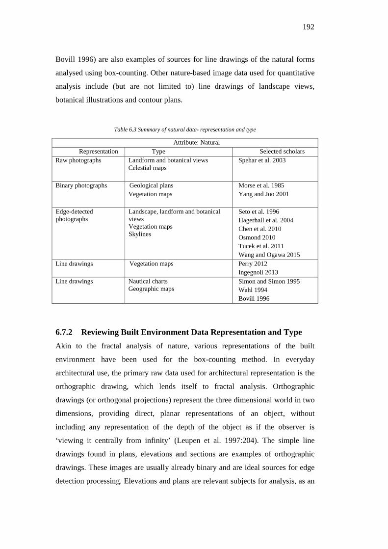
192

Bovill 1996) are also examples of sources for line drawings of the natural forms

analysed using box-counting. Other nature-based image data used for quantitative

analysis include (but are not limited to) line drawings of landscape views,

botanical illustrations and contour plans.

Table 6.3 Summary of natural data- representation and type

Attribute: Natural Representation Type Selected scholars

Raw photographs Landform and botanical views Celestial maps

Spehar et al. 2003

Binary photographs Geological plans Vegetation maps

Morse et al. 1985 Yang and Juo 2001

Edge-detected photographs

Landscape, landform and botanical views Vegetation maps Skylines

Seto et al. 1996 Hagerhall et al. 2004 Chen et al. 2010 Osmond 2010 Tucek et al. 2011 Wang and Ogawa 2015

Line drawings Vegetation maps Perry 2012 Ingegnoli 2013

Line drawings Nautical charts Geographic maps

Simon and Simon 1995 Wahl 1994 Bovill 1996

6.7.2 Reviewing Built Environment Data Representation and Type Akin to the fractal analysis of nature, various representations of the built

environment have been used for the box-counting method. In everyday

architectural use, the primary raw data used for architectural representation is the

orthographic drawing, which lends itself to fractal analysis. Orthographic

drawings (or orthogonal projections) represent the three dimensional world in two

dimensions, providing direct, planar representations of an object, without

including any representation of the depth of the object as if the observer is

‘viewing it centrally from infinity’ (Leupen et al. 1997:204). The simple line

drawings found in plans, elevations and sections are examples of orthographic

drawings. These images are usually already binary and are ideal sources for edge

detection processing. Elevations and plans are relevant subjects for analysis, as an

193

elevation can be considered to provide a measure of the geometric complexity of

the building as viewed from the exterior and the plan provides a measure of the

complexity of the design as it is inhabited (Ostwald 2011). In the past, box-

counting has been applied to line drawings of building plans (Rian et al. 2007;

Wen and Kao 2005; Vaughan and Ostwald 2011; Ostwald and Vaughan 2016),

simple line elevations of houses (Bovill 1996; Cagdas et al. 2005; Vaughan and

Ostwald 2013; Ostwald and Vaughan 2016) and detailed linear elevations

(Zarnowiecka 2002; Ediz and Ostwald 2012). Single line, digitised tracings of site

plans showing the outlines of buildings have been taken from maps of both

ancient (Brown and Witschey 2003) and contemporary cases (Benguigui et al.

2000).

Orthographic views provide a solution to creating a specific, repeatable approach

to preparing architectural drawings, and this drawing representation is particularly

suited to comparing stylistic or formal qualities in sets of architectural images

using fractal analysis. However, there are a small number of phenomenological

studies—that investigate the experience of a building—which have calculated the

fractal dimensions of digitally drawn, pre-processed perspective images of built

forms, as the perspective images are potentially more suited to the ‘perceptual’

research subject than orthographic images (Hewitt 1985: 6). A study of the

suggestion of depth in the facades of Glenn Murcutt’s buildings tested twelve

perspectival images of the Marie Short House (Vaughan and Ostwald 2014a) and

a study of spatio-visual experience was also carried out using a set of 52 computer

generated perspective views charting the progress into and though Frank Lloyd

Wright’s Robie House (Vaughan and Ostwald 2014b).

Like the studies of D values of natural landscapes, edge-detected outlines from

photographs are also have been converted to binary images and used to study the

fractal dimension of buildings. For example, Klaudia Oleschko et al. (2000) used

edge-detected photographs to calculate the D of aerial, top-down views of ancient

buildings. Frankhauser used this image representation method for studies of

European housing layouts (2008), and others have used the approach for frontal

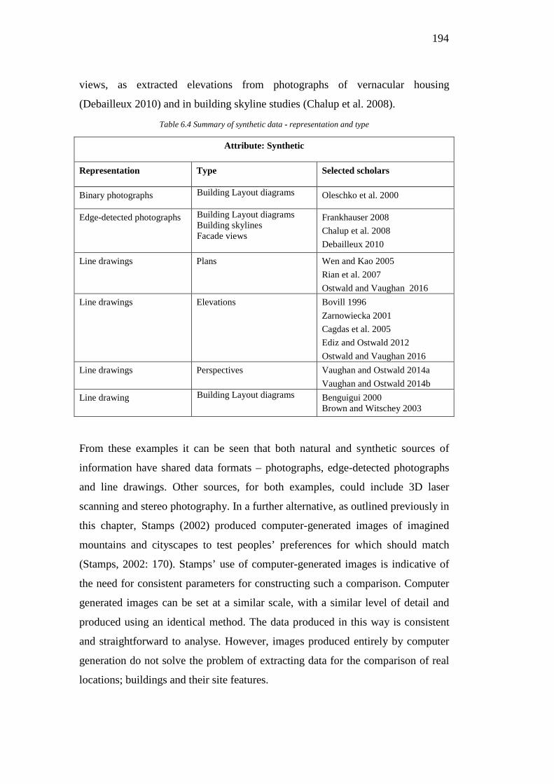
194

views, as extracted elevations from photographs of vernacular housing

(Debailleux 2010) and in building skyline studies (Chalup et al. 2008).

Table 6.4 Summary of synthetic data - representation and type

Attribute: Synthetic

Representation Type Selected scholars

Binary photographs Building Layout diagrams Oleschko et al. 2000

Edge-detected photographs Building Layout diagrams Building skylines Facade views

Frankhauser 2008 Chalup et al. 2008 Debailleux 2010

Line drawings Plans Wen and Kao 2005 Rian et al. 2007 Ostwald and Vaughan 2016

Line drawings Elevations Bovill 1996 Zarnowiecka 2001 Cagdas et al. 2005 Ediz and Ostwald 2012 Ostwald and Vaughan 2016

Line drawings Perspectives Vaughan and Ostwald 2014a Vaughan and Ostwald 2014b

Line drawing Building Layout diagrams

Benguigui 2000 Brown and Witschey 2003

From these examples it can be seen that both natural and synthetic sources of

information have shared data formats – photographs, edge-detected photographs

and line drawings. Other sources, for both examples, could include 3D laser

scanning and stereo photography. In a further alternative, as outlined previously in

this chapter, Stamps (2002) produced computer-generated images of imagined

mountains and cityscapes to test peoples’ preferences for which should match

(Stamps, 2002: 170). Stamps’ use of computer-generated images is indicative of

the need for consistent parameters for constructing such a comparison. Computer

generated images can be set at a similar scale, with a similar level of detail and

produced using an identical method. The data produced in this way is consistent

and straightforward to analyse. However, images produced entirely by computer

generation do not solve the problem of extracting data for the comparison of real

locations; buildings and their site features.

195

6.7.3 Data Gradients of Realism and Quantitative Potential

The methodology proposed in this section seeks to determine which of the cases

of natural and synthetic images result in compatible sources of raw data. This

process begins by categorising the different raw data sources with regard to the

way in which they represent reality. The examples of previously analysed,

extracted synthetic and natural data provide a breakdown of not only how—via a

particular representation method (say, a line drawing or photograph)—the subject

is presented, but also what—via the decision on type (say, a plan or a skyline)—is

expressed in the image. This data can be further classified in two ways – the level

of realism perceived in the image, and the amount of potentially quantifiable

information found in the image.

The first of these two classifications, the realism, is based on the notion that

images ‘give only a limited picture of what they represent; they are an abstraction

of reality’ (Leupen et al. 1997: 204). This categorisation ranks the ‘quality’ of

information present in the image, relative to the realism of the image or data, a

criterion which relates to our worldview. The level of realism indicates how much

the image looks like the actual object being represented (Table 6.5 column a).

• A ‘high’ level of quality is the closest level to visual reality; for example, a

high resolution, 3D colour laser scan might fulfil this criteria. The purpose

of depicting objects or places as images in this way is often to reproduce a

visual image as close as possible to that which is seen by the observer.

• A ‘Medium’ level of quality relates to images which are broadly connected

to the visual properties of their originals, such as a silhouette extracted

from a photograph.

• ‘Low’ quality images do not strongly correspond to forms as we perceive

them. For example, we do not view a hillside as being covered in lines at

regular intervals, despite what a contour plan suggests. Stan Allen

describes this effect whereby a plan drawing can ‘describe’ a building very

effectively, but when one is in the building, these plans ‘vanish’ (Allen

2009: 46).

196

Whereas the category of realism may show an object as it appears to the eye, there

are many additional ways we might gain an understanding of an object via its

representation (Foucault 1970). The next data classification considers what else an

image might convey, so that ‘[i]nstead of tangible objects floating in measureless

space, space itself can be measured and precisely represented’ (Allen 2009: 12).

Many image types used in architectural drawings and natural analysis serve a

purpose to transmit information to the viewer and different images provide

different levels of information. The next classification of the data here grades the

quantitative potential of the data, by categorising the degree of accuracy to which

the data in a representation reflects the original object (Table 6.5, column b).

• A ‘high’ level of quantity or accuracy might be found in a 3D laser scan or

a site plan, such as a contour plan, both of which are metrically accurate,

but the former has a high level of ‘realism[, and the latter a low level.

Nevertheless, while a site plan has a ‘low’ level of realism of

representation—as we rarely perceive our surroundings as abstracted plan

views—they can provide a high quantity of information when analysed,

due to the amount of extractable data, and the relationship between

information and the actual site. This is a case where, ‘[p]aradoxically, the

dry, dispassionate form of notation, which makes no attempt to approach

reality through resemblance, is better able to anticipate the experience of

the real’ (Allen 2009: 45). Topographical maps are examples of technical,

convention-based drawings, which have a general standard of

representation (you would expect to see single curved lines for contours,

dots or small circles for tree trunks), making them more data rich, yet less

realistic (Leupen et al. 1997).

• A ‘medium’ level of quantity or accuracy is found in images that, when

compared to the previous examples, have a less specific amount of

information, but can provide quantitative data nonetheless. Perspective

drawings would have a medium degree of accuracy, particularly the

mechanical projection method of setting-out a perspective. Arthur Drexler

emphasis that ‘this laborious process ensures that a building be represented

in its true proportions’, this method being a more accurate transmission of

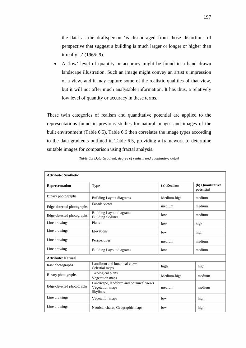
197

the data as the draftsperson ‘is discouraged from those distortions of

perspective that suggest a building is much larger or longer or higher than

it really is’ (1965: 9).

• A ‘low’ level of quantity or accuracy might be found in a hand drawn

landscape illustration. Such an image might convey an artist’s impression

of a view, and it may capture some of the realistic qualities of that view,

but it will not offer much analysable information. It has thus, a relatively

low level of quantity or accuracy in these terms.

These twin categories of realism and quantitative potential are applied to the

representations found in previous studies for natural images and images of the

built environment (Table 6.5). Table 6.6 then correlates the image types according

to the data gradients outlined in Table 6.5, providing a framework to determine

suitable images for comparison using fractal analysis.

Table 6.5 Data Gradient: degree of realism and quantitative detail

Attribute: Synthetic

Representation Type (a) Realism (b) Quantitative potential

Binary photographs Building Layout diagrams Medium-high medium

Edge-detected photographs Facade views medium medium

Edge-detected photographs Building Layout diagrams Building skylines low medium

Line drawings Plans low high

Line drawings Elevations low high

Line drawings Perspectives medium medium

Line drawing Building Layout diagrams low medium

Attribute: Natural

Raw photographs Landform and botanical views Celestial maps high high

Binary photographs Geological plans Vegetation maps Medium-high medium

Edge-detected photographs Landscape, landform and botanical views Vegetation maps Skylines

medium medium

Line drawings Vegetation maps low high

Line drawings Nautical charts, Geographic maps low high

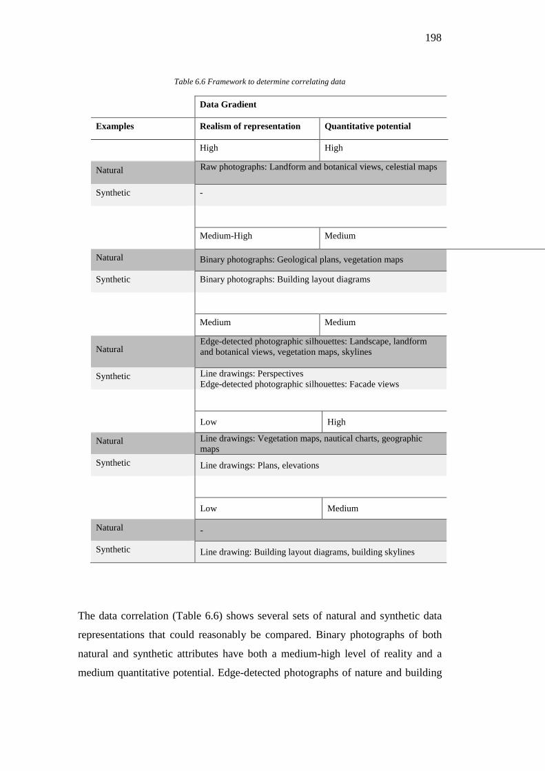
198

Table 6.6 Framework to determine correlating data

Data Gradient

Examples Realism of representation Quantitative potential

High High

Natural Raw photographs: Landform and botanical views, celestial maps

Synthetic -

Medium-High Medium

Natural Binary photographs: Geological plans, vegetation maps

Synthetic Binary photographs: Building layout diagrams

Medium Medium

Natural Edge-detected photographic silhouettes: Landscape, landform and botanical views, vegetation maps, skylines

Synthetic Line drawings: Perspectives Edge-detected photographic silhouettes: Facade views

Low High

Natural Line drawings: Vegetation maps, nautical charts, geographic maps

Synthetic Line drawings: Plans, elevations

Low Medium

Natural -

Synthetic Line drawing: Building layout diagrams, building skylines

The data correlation (Table 6.6) shows several sets of natural and synthetic data

representations that could reasonably be compared. Binary photographs of both

natural and synthetic attributes have both a medium-high level of reality and a

medium quantitative potential. Edge-detected photographs of nature and building

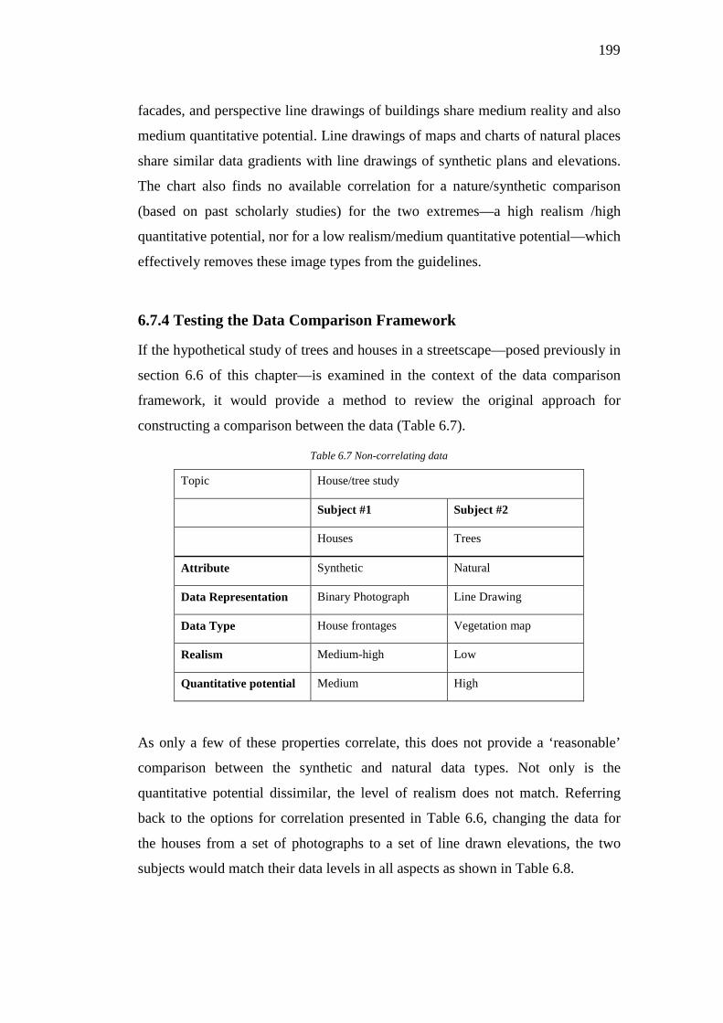
199

facades, and perspective line drawings of buildings share medium reality and also

medium quantitative potential. Line drawings of maps and charts of natural places

share similar data gradients with line drawings of synthetic plans and elevations.

The chart also finds no available correlation for a nature/synthetic comparison

(based on past scholarly studies) for the two extremes—a high realism /high

quantitative potential, nor for a low realism/medium quantitative potential—which

effectively removes these image types from the guidelines.

6.7.4 Testing the Data Comparison Framework

If the hypothetical study of trees and houses in a streetscape—posed previously in

section 6.6 of this chapter—is examined in the context of the data comparison

framework, it would provide a method to review the original approach for

constructing a comparison between the data (Table 6.7).

Table 6.7 Non-correlating data

Topic House/tree study

Subject #1 Subject #2

Houses Trees

Attribute Synthetic Natural

Data Representation Binary Photograph Line Drawing

Data Type House frontages Vegetation map

Realism Medium-high Low

Quantitative potential Medium High

As only a few of these properties correlate, this does not provide a ‘reasonable’

comparison between the synthetic and natural data types. Not only is the

quantitative potential dissimilar, the level of realism does not match. Referring

back to the options for correlation presented in Table 6.6, changing the data for

the houses from a set of photographs to a set of line drawn elevations, the two

subjects would match their data levels in all aspects as shown in Table 6.8.

200

Table 6.8 Correlating data

Topic Streetscape study

Subject #1 Subject #2

Houses Trees

Attribute Synthetic Natural

Data Representation Line Drawing Line Drawing

Data Type Elevations Vegetation map

Realism Low Low

Quantitative

potential High High

6.8 Selecting Data for Fallingwater and its Natural Setting

This final part of the chapter considers the types of synthetic and natural data that

could be obtained for the comparative analysis of Fallingwater and its natural

setting. The strategies identified at the end of Chapter 2, as connecting elements

between Fallingwater and its surrounding natural landscape, will be considered in

combination with the framework developed in the present chapter. Potential data

sources are then tested with the suggested framework to determine if they provide

a reasonable basis for comparison.

6.8.1 Data Selection

Section 6.6 of this chapter sets out the criteria to be identified in order to identify

correlating data for analysis. These criteria are; the topic, the subjects and their

attributes, the data representation, data type, and data gradients (both realism and

quantitative). This section applies that criteria to determine the images required

for a comparative study between architecture and nature for Fallingwater.

201

Topic, Subjects, Attributes

The topic of the study is provided by the second hypothesis: a comparison of the

formal and visual qualities of Fallingwater and its natural setting. Next, the

subjects and their attributes need to be identified. We already know that the

attributes will be either natural or synthetic. The sole synthetic subject is already

identified as Frank Lloyd Wright’s Fallingwater. The counterpoint of this

analysis—the landscape surrounding Fallingwater—is broken down into four

natural subjects; these are the ‘site characteristics’ of Fallingwater’s surroundings,

identified in Chapter 2 as four main features of the landscape, which many

scholars claim are directly reflected in the built form of Fallingwater. The four

natural subjects are: the Pottsville sandstone outcrop, the Mesophytic forest, the

gully setting and Bear Run stream. Having determined the topic, subjects and their

attributes, the representation and type of the data must be next considered for

analysis and comparison in Part III of this dissertation.

Data Type and Representation

In answering the first hypothesis, the formal properties of houses analysed

(including Fallingwater) are found in architectural drawings of their elevations

and plans. It would make sense to analyse Fallingwater for the second hypothesis

from the same sorts of viewpoints as the first hypothesis, from a top-down, plan

type view and from a frontal view, perpendicular to the dominant geometry of the

ground plane. Would it then be suitable to re-use the fractal dimensions calculated

for the Fallingwater plans and elevations from the architecture-architecture

hypothesis and compare them to the natural elements? This can be answered by

considering the framework for correlating data (Table 6.6). Starting with the idea

of comparing plans; the framework shows the only natural/synthetic

correspondence for plans to be architectural line drawing plans of a building

compared to line drawing plan-based views of vegetation, geology and water

systems. These image representations and types of both subjects share low levels

of realism and high levels of quantitative data. This suits the data sources and will

be the approach for comparing natural and synthetic plans of Fallingwater and its

surrounding landscape.

202

When the proposal to compare Fallingwater’s synthetic elevations to natural

views is applied to the framework, the ‘view’ is considered to be a formal

expression of a building or natural element, which is visible from points which are

external to the structure and are largely perpendicular to the dominant geometry of

the ground plane. When looking at the synthetic elevation view, in the low/high

category which it belongs, there is no corresponding natural image view. The

natural view representations and types all depict a greater sense of the ‘real world’

than architectural elevations. A line drawing of the elevation of a building has

only a low level of realism in this sense – it is only with great difficulty that we

could ever see a building that looks exactly as it does in elevation. However, an

elevation is full of information about a building, which means it has high

quantitative potential. In both respects, the elevation differs from one of the most

widely used natural image types—a line image extracted from a photograph of

nature—as line drawings extracted from photographs appear more alike to the

original object depicted (medium level of realism) but at the same time, they have

less quantitative potential than an elevation. For this reason, it is not possible to

extract as much useful data or information from line detected photograph of

nature as we could from an elevation.

Thus, it is not appropriate to compare architectural elevations of Fallingwater

with natural analogue views. The framework shows instead two options, both

falling in the medium realism/medium quantitative category. These are the

comparison of edge-detected photographs of natural elements with either edge-

detected photographs of building facades or with line drawings of architectural

perspectives. The option to use edge-detected photographs of Fallingwater, while

valid, does have some sourcing issues. This study is focused on the original

design of Fallingwater, as it was first built, and photographs from that era of full

facades of the house from all angles are limited, not only by small primary source

collections but also by the siting of Fallingwater – its position ‘anchored […] in

the wooded hillside above stream and waterfall’ (Hoesli 2005: 214) makes it very

difficult to obtain frontal photographs of facades. Additionally, photographs of the

203

house would inevitably include trees in front of the building, however the fractal

analysis method—as outlined in Chapter 5—does not include trees and other

plants in the image used for architectural analysis.

Perspective drawings of Fallingwater, on the other hand, have several supportive

reasons to be included in this analysis. The comparison for the second hypothesis

is at least partially based on the understanding that Wright spent time at the

Kaufmann’s Bear Run property, observed the landscape (Kaufmann 1986) and

then made his design for Fallingwater based on his own visual observations, as

well as interpretations provided from technical drawings (Cleary 1999). In this

case images derived from a visual experience need to be included in the analysis.

Orthographic images for example, do not perceptually relate to visual experience,

as it is impossible to actually experience an elevation in the same way that it is

drawn, because while an elevation or plan is drawn in parallax, the human eye

read the world through a type of perspective lens, and cannot see the ‘real world’

in parallax: we never see two lines as parallel, we see them as converging. Thus,

while plans and elevations are universal modes of representation and this is why

they are useful for fractal analysis comparisons between buildings, they do not

replicate the way we view the world.

The analysis for the second hypothesis is not concerned with a comparison

between buildings, but interested in the way a specific object or building is

visually experienced from different positions in space. Carl Bovill alludes to the

measuring of changing fractal dimensions in response to the viewer’s experience

(1996). He effectively asks: why don’t we measure the fractal dimensions of

perspective views of buildings? Bovill proposes that architecture is necessarily

produced through the manipulation of rhythmic forms. He expands this idea to

argue that fractal geometry allows the development of a ‘quantifiable measure of

the mixture of order and surprise’ (1996: 3) in architecture and, moreover, that

this measure reveals an essence of a building’s formal composition. For Bovill,

‘[a]rchitectural composition is concerned with the progressions of interesting

forms from the distant view of the facade to the intimate details’ (1996: 3). Bovill

204

suggests a method of measuring fractal dimensions in response to the shifting

position of the viewer. If we wanted to measure the visual experience of Wright as

he imagined a building in three dimensions, then perspective drawings are an

accepted method for representing a building, generally to convey an impression to

the viewer of how the building will actually appear (Leupen et al. 1997; Vaughan

and Ostwald 2014b).

According to Arthur Drexler, Wright’s ‘drawings are valuable beyond their

intrinsic beauty; they are a clue to the process of this thought’ (1965: 9). It is

known that Wright typically designed buildings in his mind before committing his

thoughts to paper (Kaufmann 1986; MacCormac 2005). It was Wright’s advice

that one should ‘[c]onceive the building in the imagination, not on paper but in the

mind, thoroughly - before touching paper (Wright 1928: 49). It is also known that

Wright had strong three-dimensional visualisation skills and used perspectives as

a design tool. In 1925, before beginning the design of Fallingwater, Wright

emphasised that in practice, ‘schemes are conceived in three dimensions as

organic entities’ (Wright 1992:18) and to achieve this, Wright and ‘his office staff

designed almost from the start using perspective drawings as study sketches’

(Hewitt 1985:3). Drexler observes that ‘Wright’s [perspective] drawings were

very much part of the day to day process of design. This fact is revealed not only

by the preliminary sketches for perspective drawings that are now famous, […]

and by certain unpublished perspective studies’ (1965: 9). In the design and

presentation process for Fallingwater, Wright used perspective drawings, some

from different directions and some variations on one viewpoint. These

perspectives can be used to set the angles for digital line drawing perspectives of

Fallingwater, suitable for analysis.

Considering the options for representing Fallingwater and its surrounding

landscape for this dissertation’s second hypothesis, the most suitable images for

the plan comparisons will be line drawings of plans of both the house and the four

features of the landscape. For the views of the house and its surroundings,

perspective line drawings of Fallingwater will be compared with line drawings

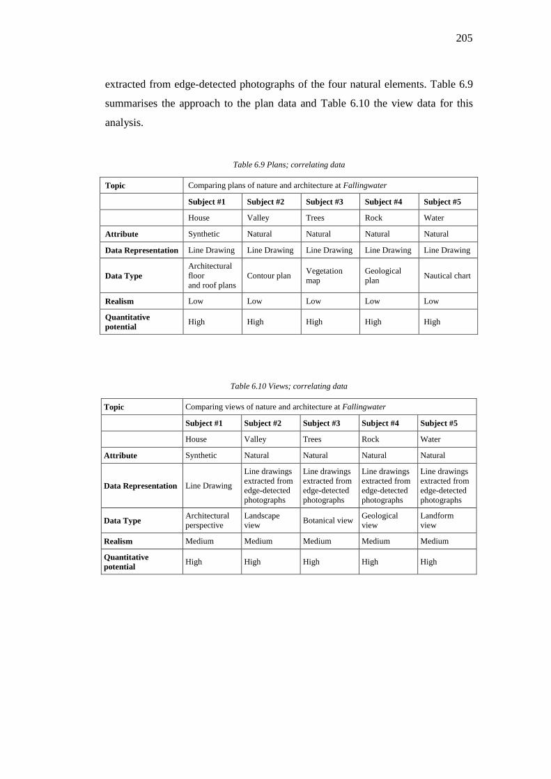
205

extracted from edge-detected photographs of the four natural elements. Table 6.9

summarises the approach to the plan data and Table 6.10 the view data for this

analysis.

Table 6.9 Plans; correlating data

Topic Comparing plans of nature and architecture at Fallingwater Subject #1 Subject #2 Subject #3 Subject #4 Subject #5

House Valley Trees Rock Water

Attribute Synthetic Natural Natural Natural Natural

Data Representation Line Drawing Line Drawing Line Drawing Line Drawing Line Drawing

Data Type Architectural floor and roof plans

Contour plan Vegetation map

Geological plan Nautical chart

Realism Low Low Low Low Low Quantitative potential High High High High High

Table 6.10 Views; correlating data

Topic Comparing views of nature and architecture at Fallingwater

Subject #1 Subject #2 Subject #3 Subject #4 Subject #5

House Valley Trees Rock Water

Attribute Synthetic Natural Natural Natural Natural

Data Representation Line Drawing

Line drawings extracted from edge-detected photographs

Line drawings extracted from edge-detected photographs

Line drawings extracted from edge-detected photographs

Line drawings extracted from edge-detected photographs

Data Type Architectural perspective

Landscape view Botanical view Geological

view Landform view

Realism Medium Medium Medium Medium Medium

Quantitative potential High High High High High

206

Conclusion

The second hypothesis in this dissertation requires a comparison between the

forms of nature and architecture in Fallingwater, carried out using the box-

counting method of fractal dimension analysis. The first part of this chapter

examines a sample of existing cases of box-counting analysis of nature, and of

architecture, and the handful of comparative studies of nature and architecture.

An overview of the data types and presentation opportunities available is then

extrapolated from the past examples. A set of methodological frameworks to

determine which of these data types exactly could be compared in order to answer

the second hypothesis are then provided and tested.

Reviewing the many data presentation methods and types available through the

framework finally provides the analysis of Fallingwater and nature with a

rationale of suitable data for analysis. The synthetic subject, the Fallingwater

house, is already known. The natural data subjects are the valley, the forest, the

watercourse and the stone outcrops. Knowing the data subject, the first step to

select the representation method is to consider the background information,

suitability for purpose and greatest data validity. The present chapter ends with the

suggestion of data selected for comparison to be represented in two main ways,

outlines of natural views to be compared with architectural perspective line

drawings and architectural plans to be compared with site plans.

207

Chapter 7

Methodology

This chapter describes the method used in this dissertation to examine the two

hypotheses and the rationale, limitations and scope of the method. The chapter

includes a detailed discussion of the stages in the research process and the use of

calculated and derived measures to characterise and compare the properties of

individual designs, sets of designs and natural analogues.

It should now be clear that a different approach is required for the images used to

test the two hypotheses. The data analysed in Chapter 8 provides results for the

first hypothesis, which is focused on an architecture-architecture comparison. This

follows the standard protocols used for architectural image analysis. In contrast,

Chapter 9 tests the second hypothesis; an architecture-nature comparison. The

requirements for the latter analysis have been developed exclusively for this study

and—as shown in the previous sections—those requirements are different to those

used for the former analysis. While acknowledging that all of the drawings

analysed are artificially abstracted views, the aim of every decision taken in the

re-drawing and re-representation of the subjects being analysed is to limit the

impact of artificial graphic conventions and to standardise representational

systems such that reasonable comparisons can be made between them.

The two-dimensional variation of the box-counting method can be used to

measure the fractal dimension of a wide range of objects, as represented in

images, including such diverse forms as arterial networks (Thomas and

Frankhauser 2013), forest perimeters (Zeide and Pfeifer 1991), cityscapes (Chalup

et al. 2008) and star clusters in galaxies (Peebles 1989). For every application of

the method there are two different aspects of the experimental design that must be

considered and described. The first, the optimisation of factors that are innate to

the mathematical basis of the approach, is described in Chapter 5. The second, a

208

considered approach to using that method to interrogate, interpret and understand

Wright’s architecture and its natural analogues, is contained in the present chapter.

The first step in this approach builds on material presented in previous chapters

and involves setting the rationale for selecting the data source, image texture

levels and data settings. A comprehensive list of all of the designs that are

analysed in Part III is also provided in this chapter, as are the representational

standards employed to prepare the data for analysis. In the second part of this

chapter, the stages of the research method are described. The last stages include

deriving comparative indicators of the consistency of the data (or lack thereof).

7.1 Research Description

This dissertation uses fractal dimensions to examine two hypotheses about Frank

Lloyd Wright’s Fallingwater. A fractal dimension provides a measure of the

characteristic visual complexity of a subject. Because fractal dimension data is

numerical, it can be rigorously compared, provided the original subjects are all

selected and prepared for analysis in a consistent manner.

The first hypothesis investigates if Fallingwater looks similar to Wright’s other

architectural designs, or if it is unique in its appearance in comparison to them.

Wright’s stylistic consistency, throughout various defined periods of his

architectural career, has been previously demonstrated using multiple

computational methods including syntactical analysis (Dawes and Ostwald 2014;

2015; Behbahani et al. 2016), shape grammars (Koning and Eizenberg 1981) and

justified graph grammars (Lee et al. 2017). Fractal dimensions have also been

used to mathematically differentiate the properties of Wright’s three great stylistic

periods; the Prairie, Textile-block and Usonian works (Vaughan and Ostwald

2011). The results of these computational studies demonstrate that Wright’s

architecture can be mathematically categorised into different styles, and it can be

applied to analyse and differentiate the character of both plans and elevations. In

209

the present context, by comparing the fractal dimensions of plans and elevations

of Fallingwater with those of fifteen houses selected from three of Wright’s well

known architectural periods, encompassing a timeframe that includes

Fallingwater’s construction, any differences in visual complexity between

Fallingwater and the other houses should be uncovered in the numerical results of

the fractal analysis. The method using this process is described in the present

chapter and the results of the analysis of these sixteen houses are presented in

Chapter 8.

The second hypothesis uses fractal dimensions to compare the characteristic

complexity of eight line drawings of Fallingwater with twenty line drawings of its

natural setting. As Chapter 6 reveals, fractal analysis has been successfully used to

analyse and compare natural forms in many past research projects, however the

comparison of landscape (natural data) and architecture (synthetic data) is

relatively untested. The natural data sets for this second study, the results of which

are presented in Chapter 9, comprise of plans and views of the valley, the trees,

rocks and water extracted from the landscape surrounding Fallingwater. The

synthetic sets are made of plans and perspectives of Fallingwater. This chapter

will provide details of how the method will be applied for this comparison of

nature and architecture.

The methodology presented in this chapter first looks at the selection, scope,

interpretation, representation and processing used for the data selected for the first

hypothesis, then the respective data for the second hypothesis is provided. All of

the results in Part III of this book were produced using software to undertake both

the box-counting procedure and the calculation of fractal dimensions. That

software, called ArchImage (Version 1.16) is used for all of the fractal dimension

calculations undertaken for this dissertation.

210

7.2 Data Selection and Scope

7.2.1 Architecture

The argument that Fallingwater is distinctly different from any other works in

Wright’s oeuvre could be tested by comparing the house to any of his buildings;

public or domestic. A study of commercial, urban or religious designs is possible

using fractal dimensions, however, none of these building types have the same

potential for producing consistent and, within reason, statistically valid results for

comparisons with other designs. Houses are an ideal subject for an application of

fractal analysis because, as a type, they possess similar scale, program and

materiality. Thus, three sets of domestic designs by Wright have been selected for

comparison with Fallingwater in this dissertation. Famous houses have been

chosen because, by definition, they have been extensively researched in the past

and thereby offer an opportunity for comparing the quantitative results derived

from the present study with past qualitative interpretations. Indeed, in the analysis

provided in Part III, the measured results are tested against specific arguments

about these houses that have been suggested by historians, theorists and critics.

To maintain a level of consistency across each set of houses several guiding

parameters have been chosen. The first of these is the general goal that no more

than ten years should separate the earliest design in a set from the last design.

Another consideration in grouping the entire fifteen houses into sets based on a

time period means that the sets can be drawn from the three distinct stylistic shifts

that occurred in Wright career (spanning, 1901 to 1910, 1923 to 1929 and 1950 to

1956) (Koning and Eizenberg 1981; MacCormac 2005; Dawes and Ostwald 2014;

Behbahani et al. 2016; Lee et al. 2017). By using these defined styles, which both

historians and computational researchers have previously validated, it is possible

to use existing scholarly discourse on these periods to frame and interpret the

results. A second parameter shaping the selection process is that single houses

(rather than pavilions or estates) were chosen, to limit the impact of dramatically

divergent scale projects. The third parameter is that completed works rather than

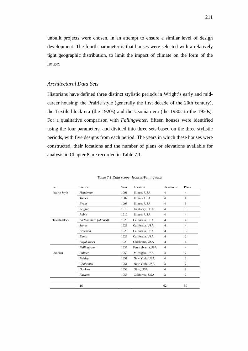
211

unbuilt projects were chosen, in an attempt to ensure a similar level of design

development. The fourth parameter is that houses were selected with a relatively

tight geographic distribution, to limit the impact of climate on the form of the

house.

Architectural Data Sets

Historians have defined three distinct stylistic periods in Wright’s early and mid-

career housing; the Prairie style (generally the first decade of the 20th century),

the Textile-block era (the 1920s) and the Usonian era (the 1930s to the 1950s).

For a qualitative comparison with Fallingwater, fifteen houses were identified

using the four parameters, and divided into three sets based on the three stylistic

periods, with five designs from each period. The years in which these houses were

constructed, their locations and the number of plans or elevations available for

analysis in Chapter 8 are recorded in Table 7.1.

Table 7.1 Data scope: Houses/Fallingwater

Set Source Year Location Elevations Plans

Prairie Style Henderson 1901 Illinois, USA 4 4

Tomek 1907 Illinois, USA 4 4

Evans 1908 Illinois, USA 4 3

Zeigler 1910 Kentucky, USA 4 3

Robie 1910 Illinois, USA 4 4

Textile-block La Miniatura (Millard) 1923 California, USA 4 4

Storer 1923 California, USA 4 4

Freeman 1923 California, USA 4 3

Ennis 1923 California, USA 4 2

Lloyd-Jones 1929 Oklahoma, USA 4 4

Fallingwater 1937 Pennsylvania,USA 4 4

Usonian Palmer 1950 Michigan, USA 4 2

Reisley 1951 New York, USA 4 3

Chahroudi 1951 New York, USA 3 2

Dobkins 1953 Ohio, USA 4 2

Fawcett 1955 California, USA 3 2

16 62 50

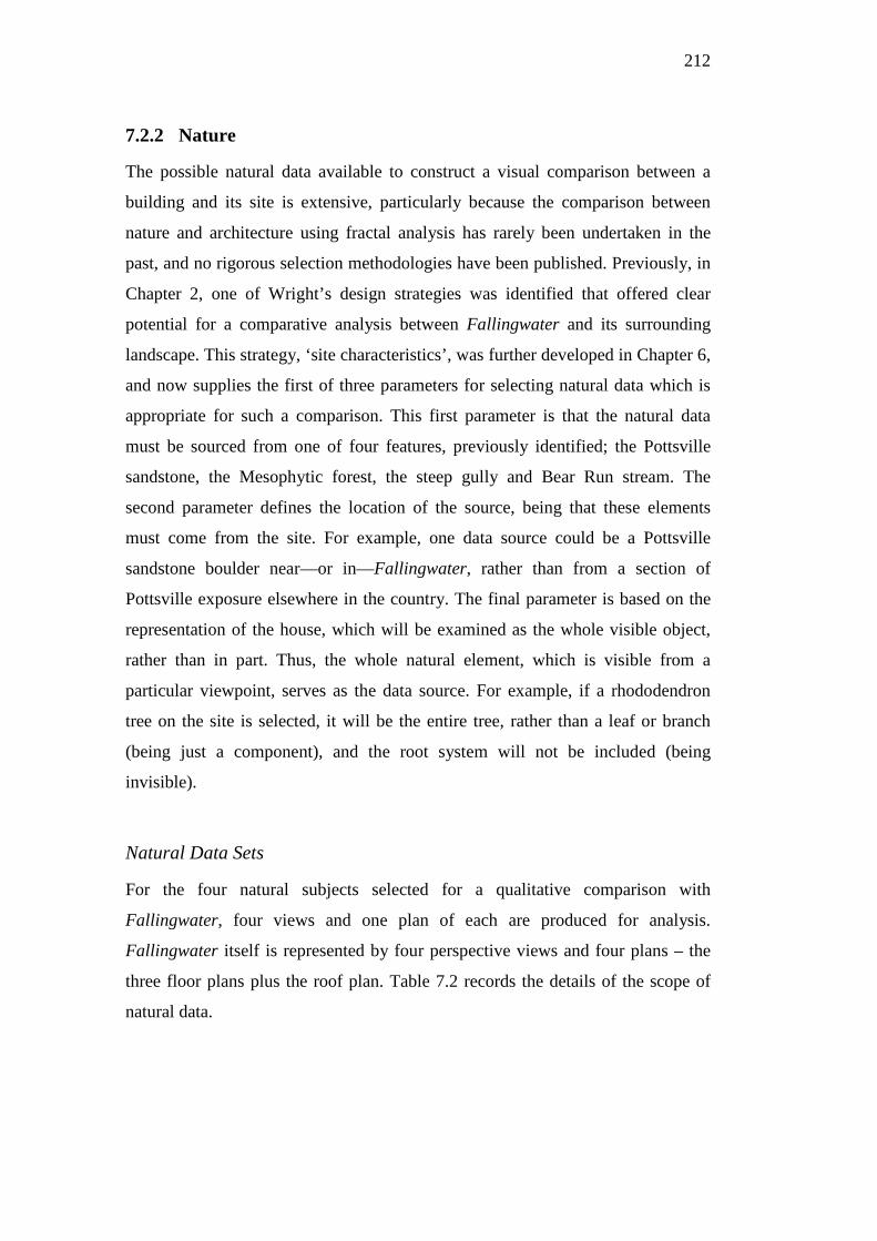
212

7.2.2 Nature

The possible natural data available to construct a visual comparison between a

building and its site is extensive, particularly because the comparison between

nature and architecture using fractal analysis has rarely been undertaken in the

past, and no rigorous selection methodologies have been published. Previously, in

Chapter 2, one of Wright’s design strategies was identified that offered clear

potential for a comparative analysis between Fallingwater and its surrounding

landscape. This strategy, ‘site characteristics’, was further developed in Chapter 6,

and now supplies the first of three parameters for selecting natural data which is

appropriate for such a comparison. This first parameter is that the natural data

must be sourced from one of four features, previously identified; the Pottsville

sandstone, the Mesophytic forest, the steep gully and Bear Run stream. The

second parameter defines the location of the source, being that these elements

must come from the site. For example, one data source could be a Pottsville

sandstone boulder near—or in—Fallingwater, rather than from a section of

Pottsville exposure elsewhere in the country. The final parameter is based on the

representation of the house, which will be examined as the whole visible object,

rather than in part. Thus, the whole natural element, which is visible from a

particular viewpoint, serves as the data source. For example, if a rhododendron

tree on the site is selected, it will be the entire tree, rather than a leaf or branch

(being just a component), and the root system will not be included (being

invisible).

Natural Data Sets

For the four natural subjects selected for a qualitative comparison with

Fallingwater, four views and one plan of each are produced for analysis.

Fallingwater itself is represented by four perspective views and four plans – the

three floor plans plus the roof plan. Table 7.2 records the details of the scope of

natural data.

213

Table 7.2 Data scope: Nature/Fallingwater

Set Source Views Plans

Natural element Rocks 4 1

Valley 4 1

Forest 4 1

Water 4 1

House Fallingwater 4 4

20 8

7.3 Data Source, Data Settings and Image Texture

All of the images analysed in this dissertation are based on specific primary

sources relevant to the study. The parameters and limitation for selection of these

sources are discussed for all data sets in this section. Once the sources are

selected, the images being for analysis are derived from these sources following

the pre-processing standards described in Chapter 5. The specific pre-processing

standards for all images—summarised in Table 5.3—including image position,

line weight, white space and image depth are all standardised using Photoshop

(Adobe) prior to importing the files into ArchImage for analysis.

Chapter 5 also describes the framework for the levels of image

texture/information to be included in the representation of the source (Table 5.1).

Applying the research focus and purpose to that framework determines the level

of information to be included in the images for analysis. A comparison between

fractal analysis studies is difficult to achieve when the studies compared are

conducted by different scholars. This is due to the range of variables, whereas

having other studies in a similar representation type provides a rough guide for

judging similarities or differences. The two hypotheses presented in this

dissertation do not necessarily have the same research focus. Hypothesis 1

compares sets of buildings while Hypothesis 2 compares natural and built

elements, and the levels of texture to be included in each approach are determined

in this section.

214

7.3.1 Comparing Architecture with Architecture (Hypothesis 1)

The most productive images to use for measuring the fractal dimensions of an

architectural design are line drawings of orthogonal plans and elevations (Ostwald

and Vaughan 2016). Although elevations and plans are less realistic, they offer a

universal system of representation that can be independently validated and used to

construct reasonable comparisons between buildings (Leupen et al. 1997). The

majority of all computational techniques for investigating architecture rely on

plans and elevations, and this includes almost all past applications of fractal

analysis listed in Chapter 4. Therefore, for the purposes of this research, the basic

formal properties of these sixteen buildings are assumed to be sufficiently

encapsulated in their 62 elevations and 50 plans.

Data Source

The first step in the house comparison process is to source an authoritative set of

working drawings (or measured drawings if the former are not available) for each

building being analysed. All the sources for Wright’s architecture used in this

thesis were predominantly reconstructed from his original working drawings

reproduced by Storrer (2006) and Futagawa and Pfeiffer (1984, 1985a, 1985b,

1985c, 1986, 1987a, 1987b, 1987c) All of the elevations and plans are scanned

and traced using ArchiCAD (Graphisoft) software. Provided the plans and

elevations match, and overall dimensions are consistent, these documents are

accepted as the primary data. If there are inconsistencies, the dimensions on the

drawings or surveys are used to reconcile the views and then the design drawings

and photographs are employed as a final means of interpreting and correcting any

discrepancies. If any sets of drawings are incomplete, missing views are

reconstructed using information from other sources (including sections or

axonometrics) along with any photographs of the houses. In some situations

where the design has since been altered—as is the case with several of Wright’s

houses—it is the original design that is analysed, not any later alterations.

215

For most designs analysed four elevations are typically produced; however, in the

case of the Usonian houses, due to their triangular planning, three elevations are

more practical. Whether there are four or three elevations, they are regarded as

collectively constituting what might be called the ‘perimeter’ or ‘boundary’

facades of the building, that is, the formal expression of the building which is

visible from points which are external to the structure and are largely

perpendicular to the dominant geometry of the plan. In addition, some building

plans are sufficiently complex that small facade surfaces may not be visible on

any elevation or may be distorted. Such hidden elevations are also excluded from

the analysis.

House plans used for analysis include the ground floor and any upper, habitable

levels (which may include functional spaces in an attic level) and the roof plan.

Basements are only drawn and analysed if they were clearly designed to contain

habitable floor space. This means that plant or boiler rooms and wood storage

spaces, which are on a separate floor plan and serve no other habitable function,

are excluded from the analysis.

Image Texture

When producing the images for analysis, the level of ‘texture’ in the image

delineation must be considered in accordance with the levels of representation in

Table 5.1. For all the plans and elevations for every building analysed in Chapter

8, the building outline and primary, secondary and tertiary forms are digitally

traced, but any material representation is excluded. This follows the guidelines for

level 4 of the levels of representation framework in Chapter 5. In practice, this

means that all tracing is undertaken using single lines, with no textures or infills.

All changes in form and between materials are depicted using a single line

separating the surfaces. As the delineated images represent a ‘real’ view of the

building, dotted lines indicating hidden surfaces and forms are not shown.

Typically included in the traced representation are any building elements that

would produce a change in the surface level of more than 1 cm. Thus, a gutter and

216

a fascia would be drawn, but not the top lip of the gutter. In plans, any change in

floor material with a single line to divide them is traced, but, as in the elevations,

the material is not indicated. Any built-in furniture, such as bathroom items and

built-in benches are delineated with a simple outline of the furniture item. For the

representation of doors and windows in elevations, the main frame, plus any

secondary sash details or mullions are included, but not secondary leadlight or

ornate moulds and joinery. Glass is depicted as opaque unless otherwise stated. In

plan, doors are all drawn open at 90°, while all windows are depicted closed. No

‘swings’ are shown on doors or windows.

There are many architectural graphic conventions for representing voids, stair runs

and roofs in plan but none of these could be used for the present analysis. To

assist in the decision of how to represent the form of a plan, the building is

imagined with its upper part sliced off, just below each ceiling line, and the view

is drawn as if looking down into it. In a multi-level house this is especially

significant because all stair treads up to the top of the level or floor being depicted

in a plan are drawn. Again, no hidden detail lines for forms that are not visible are

shown. However, any details that would be seen through void spaces and on the

roof plan any features (such as lower roof levels) that would be seen below the

roof, are all shown. Using a similar logic, it should be obvious that dotted ‘roof-

lines above’ on a plan, or landscape contour lines, paths or paving are not

depicted. The edge of a building is the limit of the drawing, with engaged steps

and the balconies included, but not site works. If in elevation, the garden walls are

a clear extension of the building form, and are integral to the visual appearance of

a house, they are retained. Any internal construction details which would not be

visible when built are not depicted. No vegetation, shadows or other entourage

elements or textures are included in the analysis of the architecture.

217

7.3.2 Comparing Architecture with Nature (Hypothesis 2)

As described in the previous chapter, the most suitable images of nature are those

that will provide correlating data with synthetic subjects (Keller et al. 1987;

Chalup et al. 2008; Chen et al. 2010). For the view analyses in this study, the

images for the natural subjects are simple linear representations, derived from

edge-detected photographs (linear detail extraction), and the matching images for

views of Fallingwater are simple line drawings of architectural perspectives. In

plan view, the natural subjects are represented by scientifically specific—yet not

overly detailed—line drawn plans (technical site drawings), and Fallingwater is

represented by a line drawn architectural plans.

Data Source

The primary sources for the perspective images of Fallingwater are sourced from

reproductions of Wright’s original perspective drawings found in Drexler (1965)

and Futagawa and Pfeiffer (1987c). These images were first scanned and then

using ArchiCAD (Graphisoft) software, the original images were used to set the

location and viewing cone to generate new the digital perspective drawings

generated from a CAD model of Fallingwater. The CAD model was reconstructed

from Wright’s original working drawings reproduced by Storrer (2006) and

Futagawa and Pfeiffer (1986). The plan images for Fallingwater are derived in the

same way as those in section 7.3.1.

The source for views of three of the elements of the natural landscape (the trees,

rocks and water) are from photographs taken by the author when visiting

Fallingwater to undertake fieldwork for this dissertation in 2012. The

photographs were scanned into Photoshop (Adobe) and the relevant natural

element was extracted by converting it into a single line drawing using the edge

detection function. Just as buildings are shown in their entirety—without nearby

objects included in the analysed images—this process is applied to the natural

elements. In extracting the elements from the source there may be parts of the

object that are hidden from view because they have something in front of them in

218

the photograph, but if you could walk into and around the scene you could see the

part obscured in the photograph. Thus, in this case, the hidden part is

reconstructed based on other evidence from other photographs or videos. For

example, a boulder might have a tree branch partially obscuring it in an original

photograph, and in its representation for analysis, this branch is removed and the

missing section of the boulder is reconstructed. A different scenario is presented

when parts of an element are hidden in the photograph because they can never be

seen by a viewer, even if in the actual landscape. For example, the roots of a tree

are hidden by the earth and the base of a boulder may also be completely hidden

by the earth. In such cases, the part of the object which is never visible is ignored

in the analysis.

Photographs capturing the views of the valley are problematic for analysis due to

the thick forest and the house obscuring the essential information required for the

analysis. To resolve this issue, the source for the valley images were selected from

2D still shots of 3D Google Earth views, which were then edge detected and

converted to line drawings.

The source for the plan views of the natural elements is a combination of the

original site plan produced for the Kaufmanns and the site plan produced by

Wright’s apprentices. These plans were scanned into Photoshop (Adobe) and line

detection function used to isolate the four elements in plan form, generating four

line drawings of the plans.

Image Texture

The approach to the level of texture included in past examples of image

representation for fractal analysis of natural objects is typically equivalent to level

three. A further consideration about the data presentation method used in this

dissertation is based on the results of the previous comparative fractal studies

between nature and architecture; being Bovill’s (1996) analysis of Amasya, and

his proposals for analyses at Sea Ranch, Nantucket and Helsinki. In these studies,

219

he used linear, minimally detailed images, also equivalent to level three in the

gradients of texture representation provided in Chapter 5. This level of

representation is appropriate for general design issues, where ‘design’ is taken to

encompass decisions about form and materiality, these being the main elements

scholars use to describe Fallingwater. Typically, the house and its surroundings

are described in terms of overall shape, form and aspect—such as the primary

geometric gestures that make up the landscape and the building design—criteria

that all fit under the notion of ‘site characteristics’. In this way, it is proposed that

the analysis in this study is of line-based imagery, using level three representation

for the nature-architecture study.

The architectural perspectives and plans, edge-detected views of the natural

elements and plans of the natural landscape, are all depicted with the image

outline and primary and secondary forms, but any tertiary form or material

representation is excluded, in accordance with the level 3 framework. This is an

important consideration because typically, some architecturally-rendered

perspective images can be highly detailed. In this case, much of that fine detail

will not be considered. In practice, this means that all tracing is undertaken using

single lines, with no textures or infills. In plan, perspective and line-detected

images, all changes in form and between materials are depicted using a single line

separating the surfaces. Typically included in the traced representation are any

elements that would produce a change in surface level of greater than 25 mm. For

example, when depicting a tree on the site, if it had small changes at the base of

the tree, with less than 30 mm of modulation where the roots descend into the

earth, these lesser details are not depicted. However, if the tree had a deeply

buttressed trunk, then these changes in form are shown.

Apart from the level of texture depicted in the architectural images, most of the

other considerations for representing architecture listed in the previous section

apply to the representation of Fallingwater in this second approach. This includes

not representing shadows, vegetation or other transient of unbuilt details around

the building. For example, while the waterfall is a key element in the house, it is

220

not included in the perspective images, as it will be included as a stand-alone

element and its individual fractal dimension calculated for comparison with the

house. As in previous section, typical drawing conventions, such as door swings,

dotted lines etc., will not be included in the depictions for testing the second

hypothesis.

7.4 Dissertation Research Method

There are six stages to the standard research method used, each of which are

described in detail over the following sections. These stages are:

i. Identifying and coding data (source images).

ii. Box-counting fractal analysis of each building or natural feature in

isolation to determine D values and derive mean values and a ‘composite’

mean for the entire item.

iii. For the comparative sets, analysis of each set to determine mean results as

well as an ‘aggregate’ result for the entire set.

iv. Comparative analysis of all results.

v. Presentation of results.

In the context of this research, the ‘set’ of buildings is a group of five houses

designed by Wright and defined by a particular style. The two sets for

Fallingwater comprise the plans and elevations reproduced at level 4 for

Hypothesis 1, and the plans and perspectives reproduced at level 3 for Hypothesis

2.

7.5 Definitions and Coding Method

The terminology and coding procedure for all the raw data analysed in Part III of

the dissertation is described in the following two sections, each relating to the

221

particular hypothesis it is focussed on, and the particular data which serves the

test. The first section describes the terminology and coding method for the

approach taken to the data in Chapter 8, first explaining how it is applied for

individual buildings and then specifically the approach to the building sets

(Prairie, Textile-block and Usonian). The second section describes the definitions

and coding method to derive data for Chapter 9, the views and plans of

Fallingwater and the natural elements

7.5.1 Definitions and Coding Method: Hypothesis 1

i. The elevations of each house are either numbered (E1-4) in accordance with

the conventions used in past research.

ii. The ground floor plan is numbered zero (P0) and any floors above ground

level are numbered consecutively from 1 (P1, P2 ,…). If one or more

basement levels, are present in a design, they are designated with negative

integers (P-1, P-2 ,…).

iii. The roof is separately labelled (PR) although it is grouped with the plan set

for determining mean values.

Analysis of Each Building (15 houses + Fallingwater)

Fractal dimension measures are calculated for each view of a particular house,

along with some derived measures from this raw data (Table 7.3). The following

steps describe the way a series of fractal dimension results for elevations and

plans are determined and then combined to create a ‘composite’ value for a

building.

i. Each elevation is measured using ArchImage software to determine its

fractal dimension (DE1-4).

ii. The mean DE value for the house is determined (μE). This value is a measure

of the typical level of visual complexity observable in the exterior of the

house.

iii. Each plan is measured using ArchImage software to determine its fractal

dimension (DP# or DPR).

222

iv. The mean of the DP# and DPR results for the house is determined (μP). This

value is a measure of the typical level of formal complexity present in the

spatial arrangement of the plan and its corresponding exterior expression in

the roof.

v. The DE1-4 and DP#-PR results for the house are combined into a mean for the

entire house (μE+P). This is a composite measure of the typical level of

characteristic complexity present in the building.

Table 7.3 Summary of definitions relating to the analysis of an individual house

Abbreviation Meaning Explanation

D Fractal Dimension Fractal dimension (D) is a measure of the formal complexity of a design and the consistency with which it is distributed across all scales of a design. For an image, D is a value between 1.0 and 2.0. The fractal dimension of an architectural elevation is DE. The fractal dimension of an architectural plan is DP.

DE D for a specific elevation.

DP D for a specific plan.

μE Mean D for the visible elevations of a building.

A ‘mean’ is the average of a set of values (the sum of the values divided by their number). It is expressed here as a ‘population’ mean (μ) because the findings of this research are generally not extrapolated to comment on anything other than the actual houses being analysed. The mean D for all of the elevations of a single building is μE. This value reflects the typical level of characteristic formal complexity visible in the exterior of a design. The mean D for all of the plans of a single building is μP. This value reflects the typical level of characteristic complexity present in the spatial and formal properties of the interior and the expression of its roof. The ‘composite’ result, μE+P, is the mean for the plans and elevations of a single building.

μP Mean D result for the habitable plans of a building.

μE+P. Mean D result for all of the plans and elevations of a building.

Analysis of a Set of Buildings (5 houses of one style)

The group of five houses in each of Wright’s stylistic periods—the Prairie,

Textile-block and Usonian—can each be called a set of houses that provide a

point of comparison for the results of Fallingwater. Thus the five Prairie style

houses can be grouped together and considered as the Prairie set etc. The results

of sets are signified in this research by the presence of curly brackets {…}. The

following steps describe the process for combining a series of fractal dimension

measures derived from five individual houses to develop results for the set. Table

7.4 shows the summary of definitions used regarding these sets.

i. The five μE results in the set are averaged together to create an aggregate

result for the set (μ{E}) which is a measure of the typical level of

characteristic visual complexity present across all facades in the set.

ii. The median fractal dimension for all elevations in the set is calculated for

comparative purposes (M{E}).

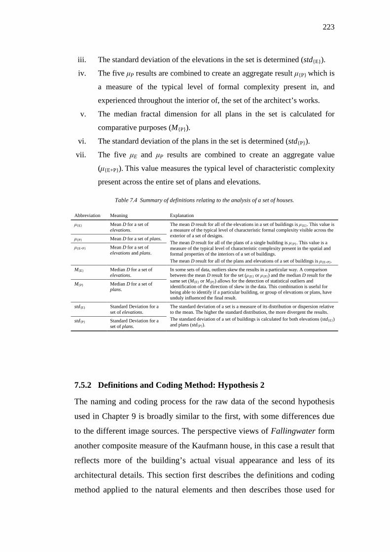
223

iii. The standard deviation of the elevations in the set is determined (std{E}).

iv. The five μP results are combined to create an aggregate result μ{P} which is

a measure of the typical level of formal complexity present in, and

experienced throughout the interior of, the set of the architect’s works.

v. The median fractal dimension for all plans in the set is calculated for

comparative purposes (M{P}).

vi. The standard deviation of the plans in the set is determined (std{P}).

vii. The five μE and μP results are combined to create an aggregate value

(μ{E+P}). This value measures the typical level of characteristic complexity

present across the entire set of plans and elevations.

Table 7.4 Summary of definitions relating to the analysis of a set of houses.

Abbreviation Meaning Explanation

μ{E} Mean D for a set of elevations.

The mean D result for all of the elevations in a set of buildings is μ{E}. This value is a measure of the typical level of characteristic formal complexity visible across the exterior of a set of designs. The mean D result for all of the plans of a single building is μ{P}. This value is a measure of the typical level of characteristic complexity present in the spatial and formal properties of the interiors of a set of buildings. The mean D result for all of the plans and elevations of a set of buildings is μ{E+P}.

μ{P} Mean D for a set of plans.

μ{E+P} Mean D for a set of elevations and plans.

M{E} Median D for a set of elevations.

In some sets of data, outliers skew the results in a particular way. A comparison between the mean D result for the set (μ{E} or μ{P}) and the median D result for the same set (M{E} or M{P}) allows for the detection of statistical outliers and identification of the direction of skew in the data. This combination is useful for being able to identify if a particular building, or group of elevations or plans, have unduly influenced the final result.

M{P} Median D for a set of plans.

std{E} Standard Deviation for a set of elevations.

The standard deviation of a set is a measure of its distribution or dispersion relative to the mean. The higher the standard distribution, the more divergent the results. The standard deviation of a set of buildings is calculated for both elevations (std{E}) and plans (std{P}).

std{P} Standard Deviation for a set of plans.

7.5.2 Definitions and Coding Method: Hypothesis 2

The naming and coding process for the raw data of the second hypothesis

used in Chapter 9 is broadly similar to the first, with some differences due

to the different image sources. The perspective views of Fallingwater form

another composite measure of the Kaufmann house, in this case a result that

reflects more of the building’s actual visual appearance and less of its

architectural details. This section first describes the definitions and coding

method applied to the natural elements and then describes those used for

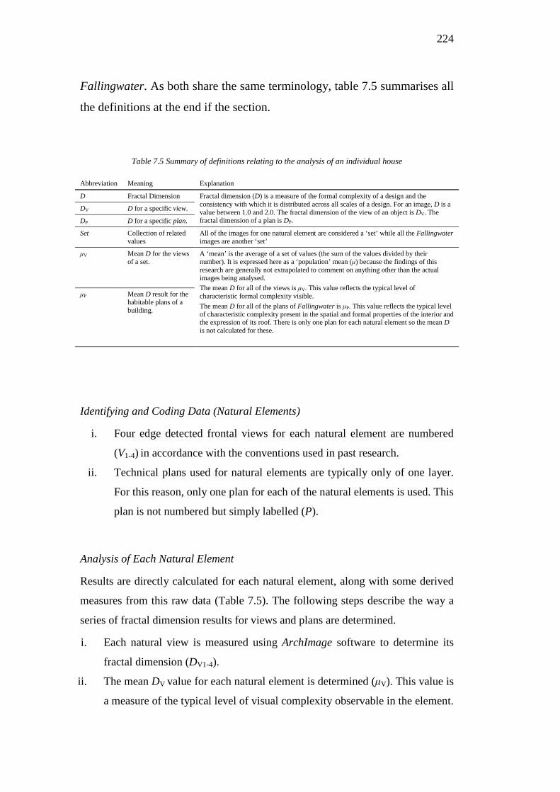
224

Fallingwater. As both share the same terminology, table 7.5 summarises all

the definitions at the end if the section.

Table 7.5 Summary of definitions relating to the analysis of an individual house

Abbreviation Meaning Explanation

D Fractal Dimension Fractal dimension (D) is a measure of the formal complexity of a design and the consistency with which it is distributed across all scales of a design. For an image, D is a value between 1.0 and 2.0. The fractal dimension of the view of an object is DV. The fractal dimension of a plan is DP.

DV D for a specific view.

DP D for a specific plan.

Set Collection of related values

All of the images for one natural element are considered a ‘set’ while all the Fallingwater images are another ‘set’

μV Mean D for the views of a set.

A ‘mean’ is the average of a set of values (the sum of the values divided by their number). It is expressed here as a ‘population’ mean (μ) because the findings of this research are generally not extrapolated to comment on anything other than the actual images being analysed. The mean D for all of the views is μV. This value reflects the typical level of characteristic formal complexity visible. The mean D for all of the plans of Fallingwater is μP. This value reflects the typical level of characteristic complexity present in the spatial and formal properties of the interior and the expression of its roof. There is only one plan for each natural element so the mean D is not calculated for these.

μP Mean D result for the habitable plans of a building.

Identifying and Coding Data (Natural Elements)

i. Four edge detected frontal views for each natural element are numbered

(V1-4) in accordance with the conventions used in past research.

ii. Technical plans used for natural elements are typically only of one layer.

For this reason, only one plan for each of the natural elements is used. This

plan is not numbered but simply labelled (P).

Analysis of Each Natural Element

Results are directly calculated for each natural element, along with some derived

measures from this raw data (Table 7.5). The following steps describe the way a

series of fractal dimension results for views and plans are determined.

i. Each natural view is measured using ArchImage software to determine its

fractal dimension (DV1-4).

ii. The mean DV value for each natural element is determined (μV). This value is

a measure of the typical level of visual complexity observable in the element.

225

iii. Each plan is measured using ArchImage software to determine its fractal

dimension (DP).

Identifying and Coding Data (Fallingwater)

i. Four perspective views of Fallingwater are numbered (V1-4) in accordance

with the conventions used in past research.

ii. The ground floor plan is numbered zero (P0) and the floors above ground

level are numbered consecutively from 1 (P1, P2)

iii. The roof is separately labelled (PR) although it is grouped with the plan set

for determining mean values.

Analysis of Fallingwater

Results are directly calculated for Fallingwater, along with some derived

measures from this raw data (Table 7.5). The following steps describe the way a

series of fractal dimension results for views and plans are determined.

i. Each perspective view is measured using ArchImage software to determine

its fractal dimension (DV1-4).

ii. The mean DV value for Fallingwater is determined (μV). This value is a

measure of the typical level of visual complexity observable from the

viewpoints suggested by Wright.

iii. Each plan is measured using ArchImage software to determine its fractal

dimension (DP# or DPR).

iv. The mean of the DP# and DPR results for Fallingwater are determined (μP).

This value is a measure of the typical level of formal complexity present in

the spatial arrangement of the plan and its corresponding exterior expression

in the roof.

226

7.6 Comparative Analysis

The difference between two fractal dimensions is defined as the Range (R) and it

can be expressed in two ways. First, the difference can be measured in terms of

absolute fractal dimensions (RD) where the subtraction of one D result from

another determines the positive or negative difference in terms of D.

Alternatively, because the fractal dimension of an image is necessarily between

1.00 and 2.00, the difference between two dimensions can also be expressed as a

percentage (R%). Importantly, while both expressions are useful for the analysis of

results, R% is simply RD with the decimal point moved two places to the right. In

general R% is more useful for considering large sets of results, whereas RD is more

commonly used for individual comparisons (Table 7.7). Range is handled as

follows.

i. The range between the highest and the lowest DE result in an

individual house is calculated (RE (D or %)).

ii. The range between the highest and the lowest DE results in a set of

houses is calculated (R{E} (D or %)).

iii. The range between the highest and the lowest DP result in an

individual house or natural element is calculated (RP (D or %)).

iv. The range between the highest and the lowest DP results in a set of

houses or the set of natural elements is calculated (R{P} (D or %)).

v. The range between the highest μE+P and the lowest μE+P result in a set is

calculated (R{μE+P} + (D or %)). This measure reflects the degree of

diversity within the μ{E+P} result.

vi. The range between the μE of Fallingwater and the μ{E} of a stylistic set

of houses (R μE (D or %)) reflecting the diversity between elevations of

Fallingwater and elevations of Wright’s other houses of distinctive

stylistic periods.

vii. The range between the μP of Fallingwater and the μ{P} of a set (R μP (D or

%)) reflecting the diversity between Fallingwater and any set of plans

studied.

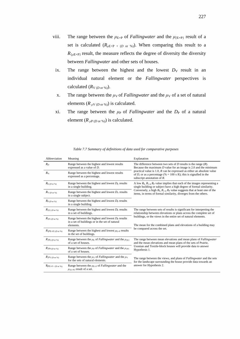
227

viii. The range between the μE+P of Fallingwater and the μ{E+P} result of a

set is calculated (RμE+P + (D or %)). When comparing this result to a

R{μE+P} result, the measure reflects the degree of diversity the diversity

between Fallingwater and other sets of houses.

ix. The range between the highest and the lowest DV result in an

individual natural element or the Fallingwater perspectives is

calculated (RV (D or %)).

x. The range between the μV of Fallingwater and the μV of a set of natural

elements (R μV (D or %)) is calculated.

xi. The range between the μP of Fallingwater and the DP of a natural

element (R μP (D or %)) is calculated.

Table 7.7 Summary of definitions of data used for comparative purposes

Abbreviation Meaning Explanation

RD Range between the highest and lowest results expressed as a value of D.

The difference between two sets of D results is the range (R). Because the maximum D value for an image is 2.0 and the minimum practical value is 1.0, R can be expressed as either an absolute value of D, or as a percentage (% = 100 x R); this is signalled in the subscript annotation of R.

R% Range between the highest and lowest results expressed as a percentage.

RE (D or %) Range between the highest and lowest DE results in a single building.

A low RE, Rv or RP value implies that each of the images representing a single building or subject have a high degree of formal similarity. Conversely, a high RE, Rv or RP value suggests that at least one of the items, in terms of formal similarity, diverges from the others. RV (D or %) Range between the highest and lowest DV results

in a single subject.

RP (D or %) Range between the highest and lowest DP results in a single building.

R{E} (D or %) Range between the highest and lowest DE results in a set of buildings.

The range between sets of results is significant for interpreting the relationship between elevations or plans across the complete set of buildings, or the views in the entire set of natural elements. The mean for the combined plans and elevations of a building may be compared across the set.

R{P} (D or %) Range between the highest and lowest DP results in a set of buildings or in the set of natural elements.

R{μE+P} (D or %) Range between the highest and lowest μE+P results in the set of buildings.

R μE (D or %) Range between the μE of Fallingwater and the μ{E} of a set of houses.

The range between mean elevations and mean plans of Fallingwater and the mean elevations and mean plans of the sets of Prairie, Usonian and Textile-block houses will provide data to answer Hypothesis 1. The range between the views, and plans of Fallingwater and the sets for the landscape surrounding the house provide data towards an answer for Hypothesis 2.

R μP (D or %) Range between the μP of Fallingwater and the μ{P} of a set of houses.

R μV (D or %) Range between the μV of Fallingwater and the μV for the sets of natural elements.

RμE+P + (D or %). Range between the μE+P of Fallingwater and the μ{E+P} result of a set.

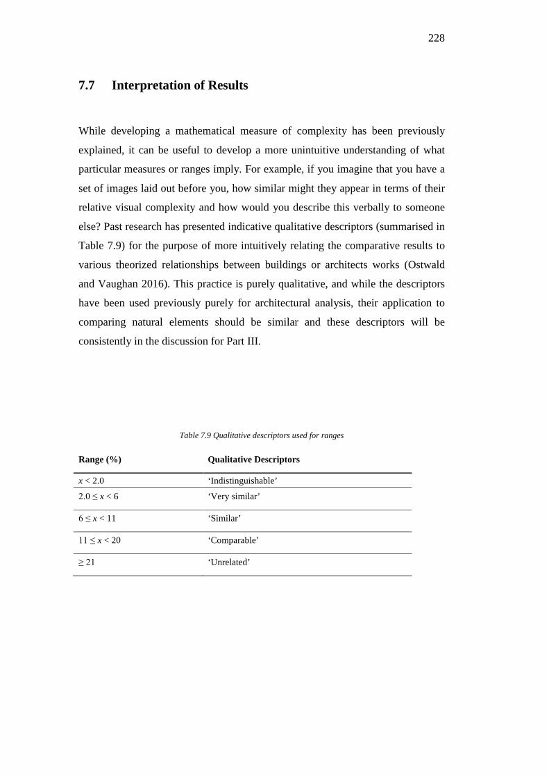
228

7.7 Interpretation of Results

While developing a mathematical measure of complexity has been previously

explained, it can be useful to develop a more unintuitive understanding of what

particular measures or ranges imply. For example, if you imagine that you have a

set of images laid out before you, how similar might they appear in terms of their

relative visual complexity and how would you describe this verbally to someone

else? Past research has presented indicative qualitative descriptors (summarised in

Table 7.9) for the purpose of more intuitively relating the comparative results to

various theorized relationships between buildings or architects works (Ostwald

and Vaughan 2016). This practice is purely qualitative, and while the descriptors

have been used previously purely for architectural analysis, their application to

comparing natural elements should be similar and these descriptors will be

consistently in the discussion for Part III.

Table 7.9 Qualitative descriptors used for ranges

Range (%) Qualitative Descriptors

x < 2.0 ‘Indistinguishable’

2.0 ≤ x < 6 ‘Very similar’

6 ≤ x < 11 ‘Similar’

11 ≤ x < 20 ‘Comparable’

≥ 21 ‘Unrelated’

229

Conclusion

The methodology for sourcing and preparing the final versions of images selected

for analysis in this dissertation is covered in this chapter, as well as the approach

to presenting and analysing the numerical data produced by the fractal analysis of

all 144 images tested.

The large number of measures presented in this chapter might seem complex at

first, but there are really only two basic things being measured in all cases: the

first is the difference between Fallingwater and the other houses, via the fractal

dimensions of elevations and plans; and the second is the difference between

Fallingwater and its surrounding landscape, via the fractal dimensions of views

and plans. To compare the various measures derived in this way, the difference or

range between the results is determined. If the range is relatively small, then the

images are visually similar. If the range is large, then they are dissimilar.

Ultimately, in most cases, a small range implies a degree of consistency in the

way a designer works, even though various site and program-specific differences

might occasionally confound the data.

230

PART III Results

231

Chapter 8

Comparing Fallingwater with Wright’s Architecture

To answer the first hypothesis of this dissertation, the present chapter uses fractal

dimensions to analyse the characteristic complexity of Fallingwater and of fifteen

other houses by Frank Lloyd Wright, focusing on how they relate to each other. It

commences by treating architecture as a special type of dimensional data, which

can be measured in individual designs, and then compared. However, it is not

productive to examine architecture solely using numbers. Buildings serve human

functions, they enable critical social structures and they embody cultural values.

Architecture is not just space and form divorced from purpose, geography or

human aspiration. Therefore, previous chapters have provided a social and

historical context for Fallingwater, and this chapter also provides a brief

background to the fifteen additional houses, prior to undertaking a mathematical

analysis of each. Once the analysis is complete, the resultant data is then

interpreted in terms of both simple statistical patterns and accepted historical and

theoretical readings. In this way the chapter shifts between qualitative and

quantitative approaches, using the former to ground or frame the research and the

latter to give it a unique lens through which to study the claim that Fallingwater is

different to other houses by Wright.

The chapter commences by using fractal dimensions to analyse four plans and

four elevations of Fallingwater. The results for the house are then critically

assessed, demonstrating the way such information can be used to test a more

traditional interpretation of the building. The houses used as a point of

comparison with Fallingwater were identified in the previous chapter, being five

houses each from Wright’s Prairie, Textile-block and Usonian styles. The next

section of the present chapter calculates the fractal dimensions of the plans and

elevations of each of the houses in each stylistic set, and these results are also

presented in the context of an overall stylistic interpretation of the houses and

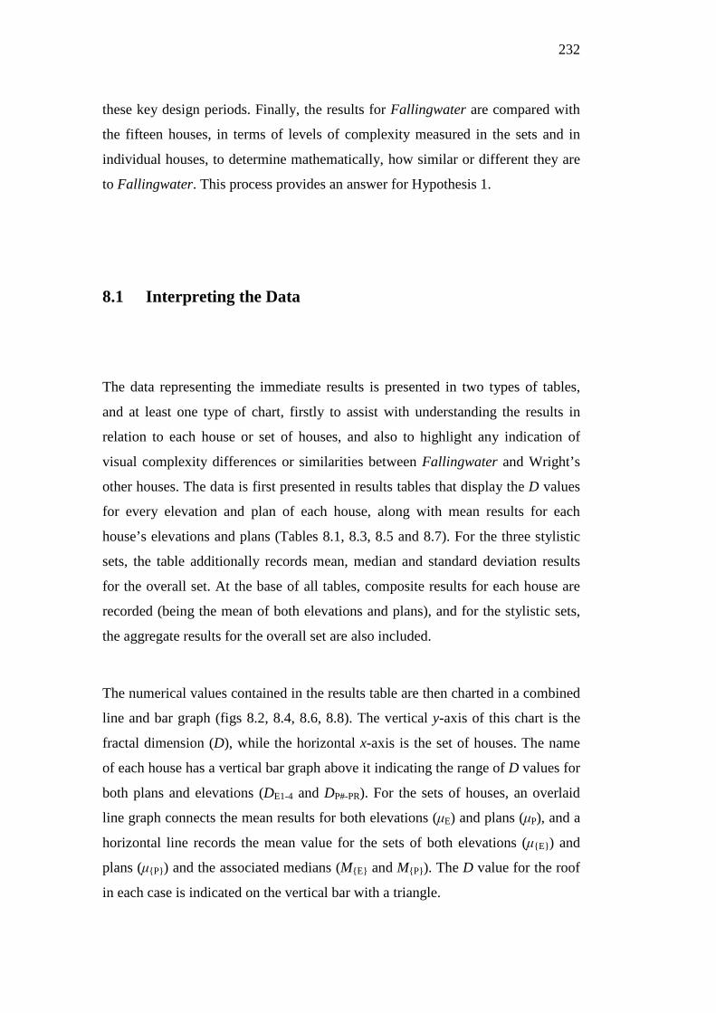
232

these key design periods. Finally, the results for Fallingwater are compared with

the fifteen houses, in terms of levels of complexity measured in the sets and in

individual houses, to determine mathematically, how similar or different they are

to Fallingwater. This process provides an answer for Hypothesis 1.

8.1 Interpreting the Data

The data representing the immediate results is presented in two types of tables,

and at least one type of chart, firstly to assist with understanding the results in

relation to each house or set of houses, and also to highlight any indication of

visual complexity differences or similarities between Fallingwater and Wright’s

other houses. The data is first presented in results tables that display the D values

for every elevation and plan of each house, along with mean results for each

house’s elevations and plans (Tables 8.1, 8.3, 8.5 and 8.7). For the three stylistic

sets, the table additionally records mean, median and standard deviation results

for the overall set. At the base of all tables, composite results for each house are

recorded (being the mean of both elevations and plans), and for the stylistic sets,

the aggregate results for the overall set are also included.

The numerical values contained in the results table are then charted in a combined

line and bar graph (figs 8.2, 8.4, 8.6, 8.8). The vertical y-axis of this chart is the

fractal dimension (D), while the horizontal x-axis is the set of houses. The name

of each house has a vertical bar graph above it indicating the range of D values for

both plans and elevations (DE1-4 and DP#-PR). For the sets of houses, an overlaid

line graph connects the mean results for both elevations (μE) and plans (μP), and a

horizontal line records the mean value for the sets of both elevations (μ{E}) and

plans (μ{P}) and the associated medians (M{E} and M{P}). The D value for the roof

in each case is indicated on the vertical bar with a triangle.

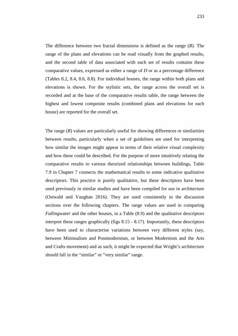
233

The difference between two fractal dimensions is defined as the range (R). The

range of the plans and elevations can be read visually from the graphed results,

and the second table of data associated with each set of results contains these

comparative values, expressed as either a range of D or as a percentage difference

(Tables 8.2, 8.4, 8.6, 8.8). For individual houses, the range within both plans and

elevations is shown. For the stylistic sets, the range across the overall set is

recorded and at the base of the comparative results table, the range between the

highest and lowest composite results (combined plans and elevations for each

house) are reported for the overall set.

The range (R) values are particularly useful for showing differences or similarities

between results, particularly when a set of guidelines are used for interpreting

how similar the images might appear in terms of their relative visual complexity

and how these could be described. For the purpose of more intuitively relating the

comparative results to various theorized relationships between buildings, Table

7.9 in Chapter 7 connects the mathematical results to some indicative qualitative

descriptors. This practice is purely qualitative, but these descriptors have been

used previously in similar studies and have been compiled for use in architecture

(Ostwald and Vaughan 2016). They are used consistently in the discussion

sections over the following chapters. The range values are used in comparing

Fallingwater and the other houses, in a Table (8.9) and the qualitative descriptors

interpret these ranges graphically (figs 8.15 - 8.17). Importantly, these descriptors

have been used to characterise variations between very different styles (say,

between Minimalism and Postmodernism, or between Modernism and the Arts

and Crafts movement) and as such, it might be expected that Wright’s architecture

should fall in the “similar” or “very similar” range.

234

8.2 Analysis of Fallingwater

This section first presents the images of Fallingwater that were analysed using the

box-counting method. The first table and chart show the results for the level of

characteristic complexity (D) in the elevations and plans, and the mean

calculations of these (Table 8.2). The comparative values table shows the range

between the results (Table 8.3). All of these results are then interpreted in the

overall discussion that follows, on the complete set of fractal dimension measures

for Fallingwater.

a. South Elevation

b. East Elevation

c. North Elevation

d. West Elevation

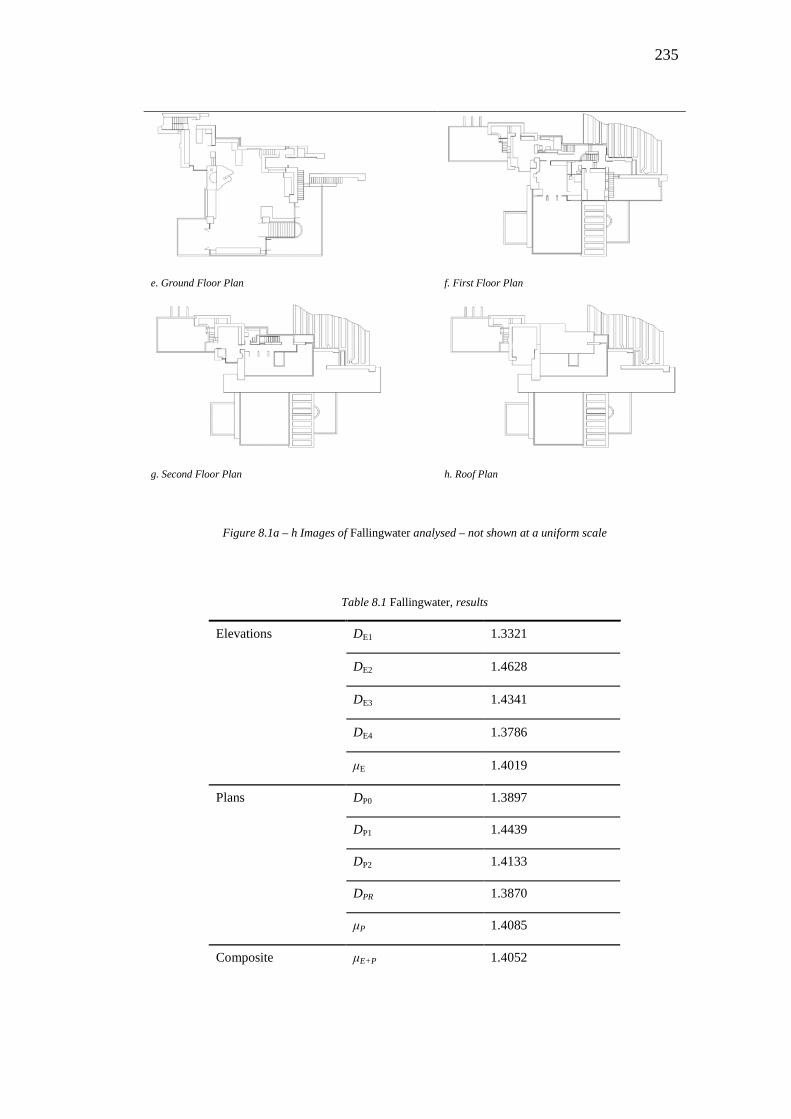
235

e. Ground Floor Plan

f. First Floor Plan

g. Second Floor Plan

h. Roof Plan

Figure 8.1a – h Images of Fallingwater analysed – not shown at a uniform scale

Table 8.1 Fallingwater, results

Elevations DE1 1.3321

DE2 1.4628

DE3 1.4341

DE4 1.3786

μE 1.4019

Plans DP0 1.3897

DP1 1.4439

DP2 1.4133

DPR 1.3870

μP 1.4085

Composite μE+P 1.4052

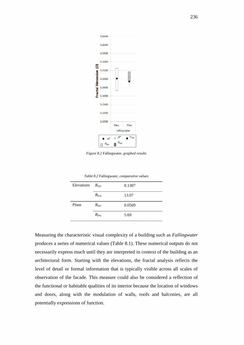
236

Figure 8.2 Fallingwater, graphed results

Table 8.2 Fallingwater, comparative values

Elevations RED 0.1307

RE% 13.07

Plans RPD 0.0569

RP% 5.69

Measuring the characteristic visual complexity of a building such as Fallingwater

produces a series of numerical values (Table 8.1). These numerical outputs do not

necessarily express much until they are interpreted in context of the building as an

architectural form. Starting with the elevations, the fractal analysis reflects the

level of detail or formal information that is typically visible across all scales of

observation of the facade. This measure could also be considered a reflection of

the functional or habitable qualities of its interior because the location of windows

and doors, along with the modulation of walls, roofs and balconies, are all

potentially expressions of function.

237

The fractal dimension results for the Fallingwater elevations indicate that the

facade with the lowest result—or least amount of visible characteristic

complexity—is the north (DE1 = 1.3321). This is the side facing the cliff and hill,

without much outlook. In the northern hemisphere, the northern side gets no direct

sun, and as Wright designed houses to address the sun (Hoppen 1998; Hess and

Weintraub 2012) it is no surprise that this elevation has less fenestration than the

other facades, and correspondingly, less visual complexity. On the opposite side

of the house is the south elevation, the features of which are prominent in

photographs commonly used as the cover of many publications on Wright or

Fallingwater (Kauffmann 1986; Hoffmann 1993; Fell 2009; Menocal 2000). This

south elevation is parallel to the Bear Run stream and it reflects or expresses much

of the program of the house, with its layered balconies, their projecting roof

overhangs, and the windows and doors that vary according to location and

purpose. These details add up to a visually complex elevation and the results show

it is the most geometrically expressive facade of the house (DE2 = 1.4628). The

east elevation is the second most visually complex (DE3 = 1.4341) with the end

view of the many stacked stone walls contributing to the visual complexity.

Overall, these results contribute to the mean outcome for the elevations of the

overall house (μE = 1.4019).

Plan analysis requires a different interpretation of the meaning of the fractal

dimension of architecture. The fractal analysis of a building plan measures the

formal and spatial complexity of a design, not as it can be seen in its totality, but

as it can be experienced through movement or inhabitation (Ostwald 2011a).

While an elevation is potentially close to the experience of viewing a facade

(albeit through a telephoto lens and using perspective correction), the plan view

assumes that part of the building has been completely removed to reveal a more

abstract spatial relationship within, one which is never really seen in this way, but

is experienced. Hillier and Hanson have demonstrated that this experience of

space and form, as a reflection of the social structure implicit in a building, is a

significant property (Hillier and Hanson 1984; Hillier 1996).

238

The floor plans of Fallingwater show a mean value of μP = 1.4085. Perhaps

surprisingly, the ground floor plan—which contains the entry and living room and

includes visually complex items such as the existing boulder retained as the hearth

for the fire and several stairways—has the lowest value (P0 = 1.3897). The

greatest amount of formal information can be found on the first floor (P1 =

1.4439). In comparison to the open planning of the ground floor, this next level up

features a veritable warren of rooms and passageways. This planning reflects the

era, wealth and lifestyle of the Kaufmann family, with bedroom arrangements that

appear unusual today. This floor has one room each for Edgar and Liliane, each

with a person bathroom, and a guest bedroom and another bathroom. The

combination of all these small rooms, several staircases in different directions and

more outdoor terraces, creates increased formal complexity in this plan.

In architectural research, the roof plan poses a different dilemma for

interpretation, as it is shaped by both the facade expression of a building and its

interior planning. In theory, it is neither clearly separate from the set of elevations

and plans nor does it fit with either set perfectly. Nevertheless, it is notable that

with a few exceptions, relatively few roof plans resemble their elevations so much

as they resemble their internal plans (Leupen 1997; Ostwald and Vaughan 2016).

This is because roof plans are typically either a product of expediency (weather-

proofing the form of the plan) or a by-product of other decisions about massing

and expression. Therefore, despite the roof-scape being described in various

architectural primers as the ‘fifth facade’ of a building, in this case it is treated as

a special type of plan.

While the roof plan of Fallingwater has the lowest complexity of all the plans (PR

= 1.3870) this is only slightly less complex than the second floor, in the order of

0.3%, an extremely small variation. Unlike many houses that have a simple roof

covering the entire house—and a correspondingly low PR—Fallingwater’s

cantilevering terraces, overhangs and outdoor staircases all add greatly to the

complexity of its aerial view. In particular many of the living spaces of

239

Fallingwater are outdoors, and these are captured in the roof plan, which shows

all parts of the building down to the ground.

Comparing all four elevations of Fallingwater to each other produces a range of

RE% = 13.07. According to the gradients provided in Table 7.9, the elevations only

show some correspondence to each other visually, but are not as similar to each

other as the plans are. The plans of Fallingwater could be considered to be very

similar to each other RP% = 5.69. The mean result of all the plans and elevations

provides a composite result for the house (μE+P = 1.4052). While this result

describes the overall house, in order to derive some meaning from it, it needs to

be compared with other house values. The next section analyses fifteen other

houses by Wright from which a comparison can be made.

8.3 House Sets for Comparison with Fallingwater

During his lengthy career Wright pioneered many architectural design strategies

for housing. The houses selected for analysis in this chapter are drawn from the

three most distinct periods, marking significant early, mid and late eras in

Wright’s domestic architecture. The first five of Wright’s early house designs

analysed in this chapter were completed between 1901 and 1910 and are from his

Prairie style period, the next set of houses analysed are from his mid-career

Textile-block period (1922 -1932) and the last set are from Wright’s Usonian

period (1950 - 1955).

8.3.1 Prairie Style Houses

Wright’s Prairie Style is an approach inspired by the long flat reaches of the

American prairie plains and the houses he designed during this period likewise

have strong horizontal lines, dramatically wide eaves and low-pitched roofs. Hess

and Weintraub describe the style as ‘a fully formulated Modern architecture

240

rooted in the American Midwest’ (2006: 12). In these houses, ‘a vocabulary of

forms was used to translate or express the grid at all points - the solid rather than

pierced balconies, planters, bases of flower urns, clustered piers, even built in

seats were evocations of the underlying structure of a house’ (Sergeant 2005:

192).

The five Prairie style houses by Wright were constructed between 1901 and 1910.

Four of the five are in the state of Illinois and the fifth is in the neighboring state

of Kentucky. All the houses display the characteristics of Wright’s Prairie style.

Importantly, the five houses span the period between the first publication of

Wright’s Prairie Style, in the Ladies Home Journal in 1901, and what is widely

regarded as the ultimate example of this approach, the Robie House (fig. 8.3e).

The first Prairie style design analysed in this chapter is the Henderson House in

Elmhurst, Illinois which was completed in 1901 (fig. 8.3a). The house is a timber,

two-storey structure with plaster rendered elevations. A range of additions were

made to the house in the years following its completion until, in 1975, the house

was restored to its original form. The Tomek House, completed in 1907, in

Riverside, Illinois, is also a two-storey house although it possesses a basement and

is sited on a large city lot (fig 8.3b). This house is finished with pale, rendered

brickwork, dark timber trim and a red tile roof. Storrer notes that, in response to

the Tomek family’s needs, Wright later allowed posts to be placed beneath the

cantilevered roof to heighten the sense of support and enclosure (Storrer 1993:

128). As the posts were not required for structural reasons, and Wright found

them personally unnecessary, they have been omitted from the analysis. The

Evans House (fig 8.3c), completed in Chicago, Illinois in 1908, features a formal

diagram wherein the ‘basic square’ found in earlier Prairie style houses is

‘extended into a cruciform plan’ (Thomson 1999: 100). The house is set on a

sloping site and possesses a plan similar to the one Wright proposed in 1907 for a

‘fireproof house for $5000’. The Evans House was later altered to enclose the

porch area and the stucco finish on the facade was also cement rendered. The

Zeigler House in Frankfort, Kentucky was constructed in 1910 and has a similar

241

plan to the Evans House. Designed as a home for a Presbyterian minister, this

two-storey house is sited on a small, city lot and it was constructed while Wright

was in Europe (fig 8.3d). After a decade of development and refinement, the

quintessential example of the Prairie Style—the Robie House—was constructed in

Chicago, Illinois in 1910. Designed as a family home, the three storey structure

fills most of its corner site. Unlike many of Wright’s other houses of the era, the

Robie House features a facade of exposed Roman bricks with horizontal raked

joints and is described by Alofsin as ‘a startling image of sliding parallel

horizontal masses hugging the ground’ (1994: 36).

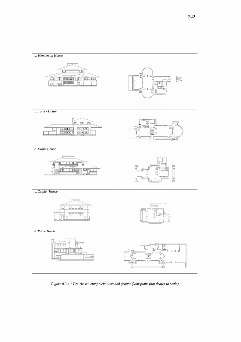
242

a. Henderson House

b. Tomek House

c. Evans House

d. Zeigler House

e. Robie House

Figure 8.3 a-e Prairie set, entry elevations and ground floor plans (not drawn to scale)

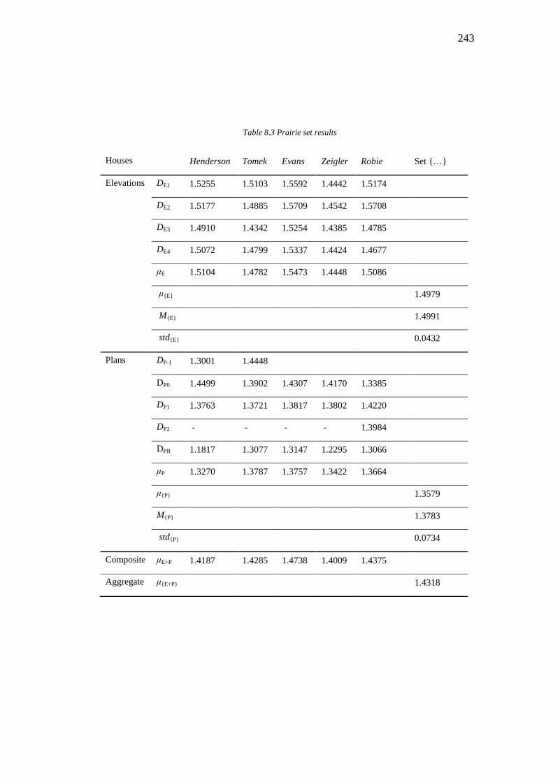
243

Table 8.3 Prairie set results

Houses Henderson Tomek Evans Zeigler Robie Set {…}

Elevations DE1 1.5255 1.5103 1.5592 1.4442 1.5174

DE2 1.5177 1.4885 1.5709 1.4542 1.5708

DE3 1.4910 1.4342 1.5254 1.4385 1.4785

DE4 1.5072 1.4799 1.5337 1.4424 1.4677

μE 1.5104 1.4782 1.5473 1.4448 1.5086

μ{E} 1.4979

M{E} 1.4991

std{E} 0.0432

Plans DP-1 1.3001 1.4448

DP0 1.4499 1.3902 1.4307 1.4170 1.3385

DP1 1.3763 1.3721 1.3817 1.3802 1.4220

DP2 - - - - 1.3984

DPR 1.1817 1.3077 1.3147 1.2295 1.3066

μP 1.3270 1.3787 1.3757 1.3422 1.3664

μ{P} 1.3579

M{P} 1.3783

std{P} 0.0734

Composite μE+P 1.4187 1.4285 1.4738 1.4009 1.4375

Aggregate μ{E+P} 1.4318

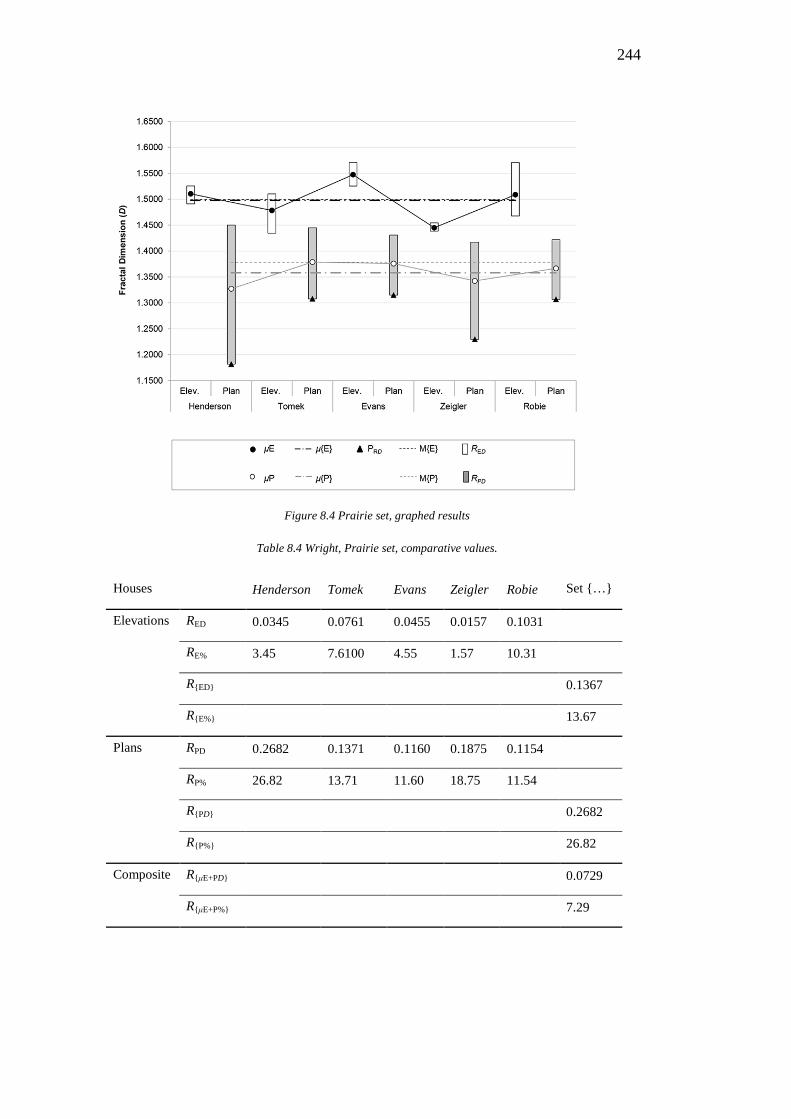
244

Figure 8.4 Prairie set, graphed results

Table 8.4 Wright, Prairie set, comparative values.

Houses Henderson Tomek Evans Zeigler Robie Set {…}

Elevations RED 0.0345 0.0761 0.0455 0.0157 0.1031

RE% 3.45 7.6100 4.55 1.57 10.31

R{ED} 0.1367

R{E%} 13.67

Plans RPD 0.2682 0.1371 0.1160 0.1875 0.1154

RP% 26.82 13.71 11.60 18.75 11.54

R{PD} 0.2682

R{P%} 26.82

Composite R{μE+PD} 0.0729

R{μE+P%} 7.29

245

In the set of Wright’s Prairie works, the Zeigler House has the lowest average

elevation result (μE = 1.4448) and the highest is found in the Evans House (μE =

1.5473). The median elevation result is 1.4991, the mean 1.4979 and the standard

deviation is 0.0432. Results for the plan means show the lowest is the Henderson

House (μP = 1.3270) while the Tomek House has the highest (μP = 1.3787). The

median for the set of plan results is 1.3783, the mean is 1.3579 and the standard

deviation is 0.0734 (Table 8.3, fig.8.4).

The entire set of five prairie houses have a close, comparable range of complexity

across all twenty elevations (R{E%} = 13.67), and while the degree of complexity

of all thirteen plans could still be considered related (R{P%} = 26.82), there is no

clear visual correspondence between them. This situation is further amplified

when the individual house results are observed. The Zeigler House has a

remarkably tight range of fractal dimensions in elevation (RE% = 1.57) which

suggests the four elevations for this house are identical in their level of visual

complexity. The range of complexity for the plans of the Zeigler House however

(RP% = 18.75), while offering more visual correspondence than the range for the

group of five Prairie houses, are only comparable rather than indistinguishable

(Table 8.4, fig. 8.4).

The graphed results show the Henderson House to be diverse in planning, but

alike in facade treatment. The set of fractal dimensions for the elevations (1.4910

< DE < 1.5255) corresponds with the even distribution of detail on the exterior of

the house, where each elevation has around fifteen windows and similar wall

detailing. The plans have a different purpose on each level, with the most complex

of the plans being the ground floor (DP0 = 1.4499) which includes flexible living

spaces and outdoor terracing. The roof plan being the least complex (DPR =

1.1817), reflects the fundamental simplicity of the layout of the Henderson House.

The Tomek House is the only house in the set of prairie houses to have an

overlapping level of detailing found in the plans and elevations. This only occurs

246

in the least complex east elevation (DE3 = 1.3432) and the most complex plan (DP-

1 = 1.4448). The east facade is smaller and dominated by a typical Prairie style,

externally expressed, wide chimney and has less remaining space for fenestration

or any other typical details found in the other three elevations. The most complex

plan is that of the entry level and includes the additional details of the stonework

mouldings which Wright used in many of his Prairie houses to anchor them to the

ground.

The Evans House and the Robie House share a similar pattern of results, both with

highly complex elevations and a very similar set of results for their plans. The

Evans House has a more similar set of elevations, in terms of complexity (RE% =

4.5) than the Robie House (RE% =10.3), and the Evans House results for elevations

all fall within those of the Robie House (1.4677 < DE < 1.5708). Likewise, the

Evans House maximum plan dimension is very similar to that of the Robie House

(DP0 = 1.4307 and DP1 = 1.4220 respectively) and the minimum plan value is also

similar for the Evans House (DPR = 1.3147) and Robie House, (DPR = 1.3066).

Overall, the results from the analysis show the elevations of Wright’s Prairie

houses to be generally more complex than the plans. Furthermore, the Median and

the Mean of all elevations are almost identical.

8.3.2 Textile-block Houses

Wright expanded his practice into Los Angeles in the early 1920’s and during the

following decade he designed many buildings, although only five houses were

built. These five houses, which share some of the character of Wright’s famous

Hollyhock House, have since become known as the Textile-block houses.

Appearing as imposing, ageless structures, these houses were typically

constructed from a double skin of pre-cast patterned and plain exposed concrete

blocks held together by Wright’s patented system of steel rods and concrete grout.

Ornamented blocks generally punctuate the plain square blocks of the houses and

for each house a different pattern is employed. Despite the difference in

247

appearance to the Prairie Style houses, Hess states that ‘every aspect of the LA

homes followed organic principles’ (Hess and Weintraub 2006: 38).

The first of the set, the Millard House or “La Miniatura” was completed in

Pasadena, California, in 1923 (fig 8.5a). This house is the only one of the Textile-

block works not to feature a secondary structure of steel rods. Reflecting on La

Miniatura, Wright wrote that in this project he ‘would take that despised outcast

of the building industry – the concrete block – out from underfoot or from the

gutter – find a hitherto unsuspected soul in it – make it live as a thing of beauty

textured like the trees’ (Wright 1960: 216-217). The second of the Textile-block

houses, the Storer House, was completed in Hollywood, California, in 1923 (fig

8.5b). It is a three-storey residence with views across Los Angeles. The Freeman

House in Los Angeles, California, was also completed in 1923 (fig 8.5c). It is

regarded as the third Textile-block house and the first to use mitred glass in the

corner windows of the house; all the previous works in this style have solid

corners. It is a two-storey, compact, flat roofed house made from both patterned

and plain textile-block and with eucalyptus timber detailing. The fourth Textile-

block house, the Ennis House, is probably the most famous of Wright’s works of

this era (fig 8.5d). Also completed in 1923 and overlooking Los Angeles, it is

regarded as the ‘most monumental’ (Storrer 1974: 222) of the houses of this era. It

has been described as ‘looking more like a Mayan temple than any other Wright

building except [the] Hollyhock House’ (222). The Ennis House is conspicuously

sited and is made of neutral coloured blocks with teak detailing. Some of the

windows feature art glass designed by Wright in an abstraction of wisteria plants.

The final design in this sequence, the Lloyd-Jones House, is in Tulsa, Oaklahoma.

Completed in 1929, it is the only non-Californian Textile-block house (fig 8.5e).

Designed for Wright’s cousin, it is a large house with extensive entertaining areas

and a four-car garage. The Lloyd-Jones House is notably less ornamental than the

others in the sequence with Wright rejecting richly decorated blocks ‘in favor of

an alternating pattern of piers and slots’ (Frampton 2005: 170).

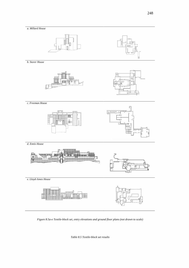
248

a. Millard House

b. Storer House

c. Freeman House

d. Ennis House

e. Lloyd-Jones House

Figure 8.5a-e Textile-block set, entry elevations and ground floor plans (not drawn to scale)

Table 8.5 Textile-block set results

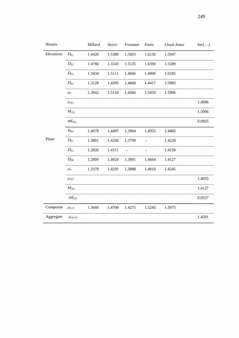
249

Houses Millard Storer Freeman Ennis Lloyd-Jones Set{…}

Elevations

Plans

DE1 1.4420 1.5389 1.3603 1.6130 1.5947

DE2 1.4786 1.5543 1.5125 1.6390 1.5589

DE3 1.3434 1.5111 1.4666 1.4900 1.6105

DE4 1.3128 1.4395 1.4868 1.4417 1.5983

μE 1.3942 1.5110 1.4566 1.5459 1.5906

μ{E} 1.4996

M{E} 1.5006

std{E} 0.0925

DP0 1.4078 1.4497 1.3964 1.4955 1.4465

DP1 1.3801 1.4330 1.3799 - 1.4228

DP2 1.2826 1.4311 - - 1.4158

DPR 1.2809 1.4024 1.3901 1.4664 1.4127

μP 1.3379 1.4291 1.3888 1.4810 1.4245

μ{P} 1.4055

M{P} 1.4127

std{P} 0.0557

Composite μE+P 1.3660 1.4700 1.4275 1.5243 1.5075

Aggregate μ{E+P} 1.4591

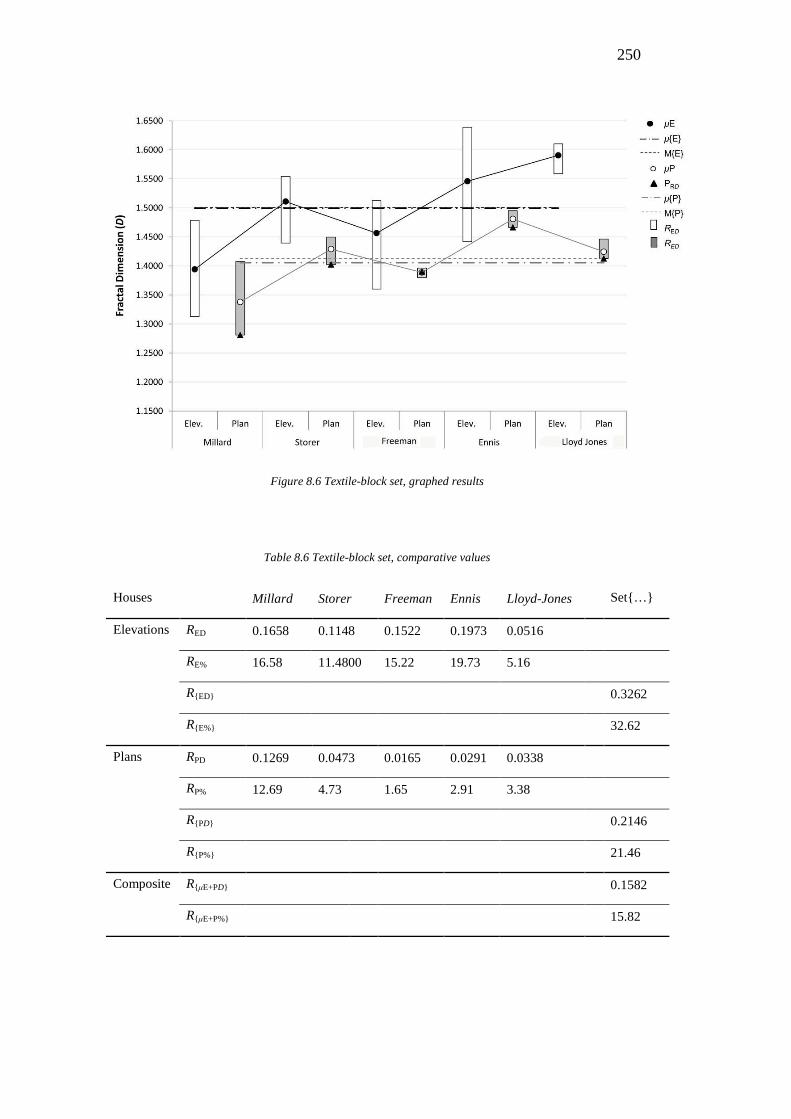
250

Figure 8.6 Textile-block set, graphed results

Table 8.6 Textile-block set, comparative values

Houses Millard Storer Freeman Ennis Lloyd-Jones Set{…}

Elevations RED 0.1658 0.1148 0.1522 0.1973 0.0516

RE% 16.58 11.4800 15.22 19.73 5.16

R{ED} 0.3262

R{E%} 32.62

Plans RPD 0.1269 0.0473 0.0165 0.0291 0.0338

RP% 12.69 4.73 1.65 2.91 3.38

R{PD} 0.2146

R{P%} 21.46

Composite R{μE+PD} 0.1582

R{μE+P%} 15.82

251

In the set of Wright’s Textile-block houses, the first house in the set, the Millard

House, has the lowest average elevation result (μE = 1.3942) and the highest is

found in the Lloyd-Jones House, the last house of the set (μE = 1.5006). The mean

elevation result is 1.4996 and median elevation result 1.5006, with the standard

deviation 0.0925. Thus, there is very little skew in the results, although the

deviation in the data is higher than it was for the Prairie style works. Results for

the plans show the lowest average is also from the Millard House (μP = 1.3379)

while the Ennis House has the highest (μP = 1.4810). The mean for the set of plans

is 1.4055, the median is 1.4127 and the standard deviation is 0.0557 (Table 8.5,

fig. 8.6).

The entire set of results of the seventeen Textile-block house plans have a familial

relationship, however the results are not closely enough related that they can be

considered “comparable” (R{P%} = 21.46). The range of complexity across all

twenty elevations (R{E%} = 32.62) is even wider and when presented with a view

of all elevations in this set, the complexity between each view is dissimilar and

unrelated (Table 8.5, fig. 8.6).

The Millard House results are lower than expected, with all results for the

elevation and most results for the plans falling below their respective averages.

The textured, ornamental blocks covering this house all have the same pattern and

this texture is treated as one surface in the representation of the elevations for

analysis, lowering the expected result. This approach does not affect the planning

however, and the Millard House results do generally show a simple type of plan.

The Storer House fits neatly into the overall results, with the overall median and

average for all the Textile-block houses set falling within the results for both plans

and elevations of the Storer House. As expected, most roof plans provide the

lowest result for each house in the Textile-block houses set, however for the

Freeman House it is the first floor which has the least visual complexity (DP1 =

1.3799). As a house designed with terraced levels, the view of the roof includes a

252

roof garden and a view of the collection of roofs below, increasing the visual

complexity of this roof plan (DPR = 1.3901).

The Ennis House could be considered as the most complex house in the Textile-

block houses set with the highest results for all plans (DP0 = 1.4955 and DR =

1.4664), and its north (DE1 = 1.6130) and south Elevations (DE2 = 1.6390) being

the most visually complex of the Textile-block houses set. However, the average

elevation result for the Lloyd-Jones House is the highest overall (μE = 1.5906).

The elevations for this house have a high fractal dimension due to the window

framing used by Wright in this building, where each panel of glass is framed to

match the blockwork. This house has an unusual result for its plans and

elevations, which are distinctly different, where the elevations are far more

complex than the plans (μP = 1.4245). All other houses in this set however, have

some overlap in complexity for the plan and elevations of the houses.

The results for the Textile-block houses set overall suggest a set of visually

complex dwellings in elevation and particularly in planning, with a broad

relationship between the complexity of the plan and elevations. Furthermore, over

the six-year period from the first to the last, the complexity of the house designs

increased. This result partially confirms the typical descriptions of these houses

provided by historians, who argue that Wright’s architecture became more

visually complex, heavy and ornate throughout this time, largely as a property of

the decoration embedded in the blocks. However, some historians disagree with

this, suggesting that in the Lloyd-Jones House Wright moved away from the

‘primitivism’ or ‘Mayan-revivalism’ found in the first four to produce a much

simpler formal expression. For example, Alofsin (1994) argues that as Wright

‘responded to the incipient International Style he simplified his surface patterns, a

shift that marked the end of his primitivist phase’ (42). Yet, the total level of

formal complexity in the work did not fall; instead, the level of ornamental detail

fell in the final house, whereas the formal modelling reached its most attenuated

expression. This interpretation of the data supports the views of those critics and

historians who see the Lloyd-Jones House as triggering a shift from vertical to

253

horizontal modelling, rather than being less ornamental in its expression

(Sweeney 1994).

8.3.3 Usonian Houses

More than twenty years were to pass before Wright developed his third major

sequence of domestic works; the Usonian houses. Wright explains that the

Usonian house is intended to be ‘integral to the life of the inhabitants’, be truthful

in its material expression (‘glass is used as glass, stone as stone, wood as wood’)

and embrace the elements of nature (1954: 353). Hoffman describes the Usonian

house as ‘a simplified and somewhat diluted prairie house characterized by the

absence of leaded glass and the presence of […] very thin wall screens with a

striated effect from wide boards spaced by recessed battens’ (Hoffmann 1995:

80). While there were multiple variations on the Usonian house, the five works

featured in the present chapter are all based on an underlying equilateral triangular

grid and were constructed between 1950 and 1956.

The first of the triangle-plan Usonian Houses, the Palmer House is located in Ann

Arbour, Michigan and was completed in 1950 (fig 8.7a). The house is a two-

storey brick structure, set into a sloping site, with wide, timber-lined eaves, giving

the viewer an impression of a low, single level house. The brick walls include

bands of patterned, perforated blocks, in the same colour as the brickwork. The

repeatedly scaled triangle motif in the Palmer house has made it the subject of

fractal studies by others (Eaton 1998; Joye 2006; Harris 2007).

The second house, the Riesley House, was the last of Wright’s Usonian houses

built in Pleasantville, New York; it was completed in 1951 (fig 8.7b). This single

level home with a small basement is constructed from local stone with timber

panelling and is set on a hillside site. In contrast, in the same year the Chahroudi

House was built on an island in Lake Mahopac, New York, and constructed using

Wright’s desert masonry rubblestone technique with some timber cladding and

detailing (fig 8.7c). Wright originally designed the cottage as the guest quarters

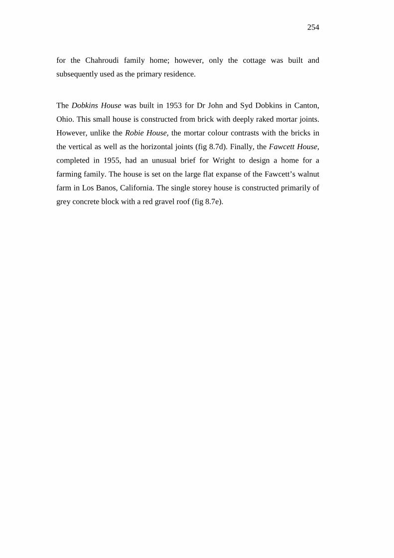
254

for the Chahroudi family home; however, only the cottage was built and

subsequently used as the primary residence.

The Dobkins House was built in 1953 for Dr John and Syd Dobkins in Canton,

Ohio. This small house is constructed from brick with deeply raked mortar joints.

However, unlike the Robie House, the mortar colour contrasts with the bricks in

the vertical as well as the horizontal joints (fig 8.7d). Finally, the Fawcett House,

completed in 1955, had an unusual brief for Wright to design a home for a

farming family. The house is set on the large flat expanse of the Fawcett’s walnut

farm in Los Banos, California. The single storey house is constructed primarily of

grey concrete block with a red gravel roof (fig 8.7e).

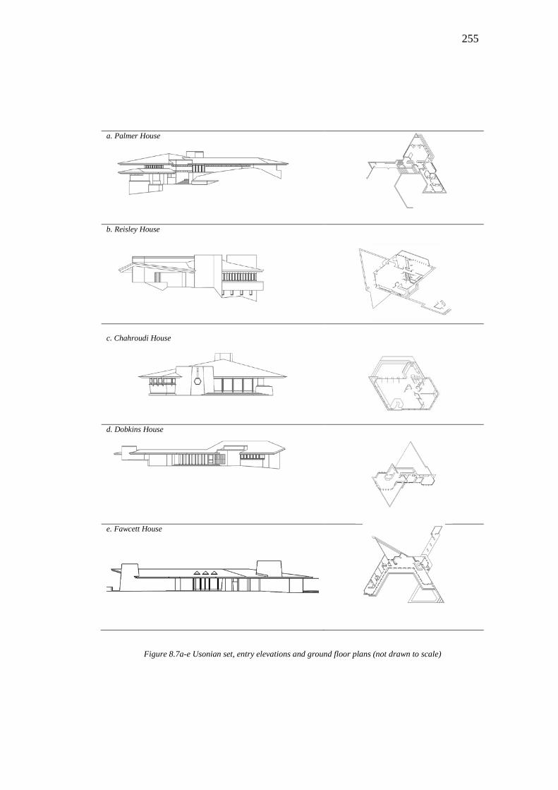
255

a. Palmer House

b. Reisley House

c. Chahroudi House

d. Dobkins House

e. Fawcett House

Figure 8.7a-e Usonian set, entry elevations and ground floor plans (not drawn to scale)

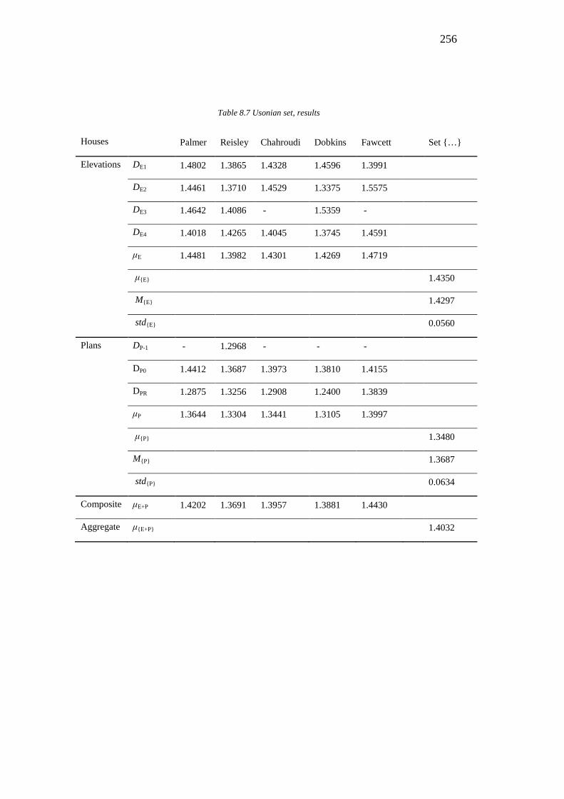
256

Table 8.7 Usonian set, results

Houses Palmer Reisley Chahroudi Dobkins Fawcett Set {…}

Elevations DE1 1.4802 1.3865 1.4328 1.4596 1.3991

DE2 1.4461 1.3710 1.4529 1.3375 1.5575

DE3 1.4642 1.4086 - 1.5359 -

DE4 1.4018 1.4265 1.4045 1.3745 1.4591

μE 1.4481 1.3982 1.4301 1.4269 1.4719

μ{E} 1.4350

M{E} 1.4297

std{E} 0.0560

Plans DP-1 - 1.2968 - - -

DP0 1.4412 1.3687 1.3973 1.3810 1.4155

DPR 1.2875 1.3256 1.2908 1.2400 1.3839

μP 1.3644 1.3304 1.3441 1.3105 1.3997

μ{P} 1.3480

M{P} 1.3687

std{P} 0.0634

Composite μE+P 1.4202 1.3691 1.3957 1.3881 1.4430

Aggregate μ{E+P} 1.4032

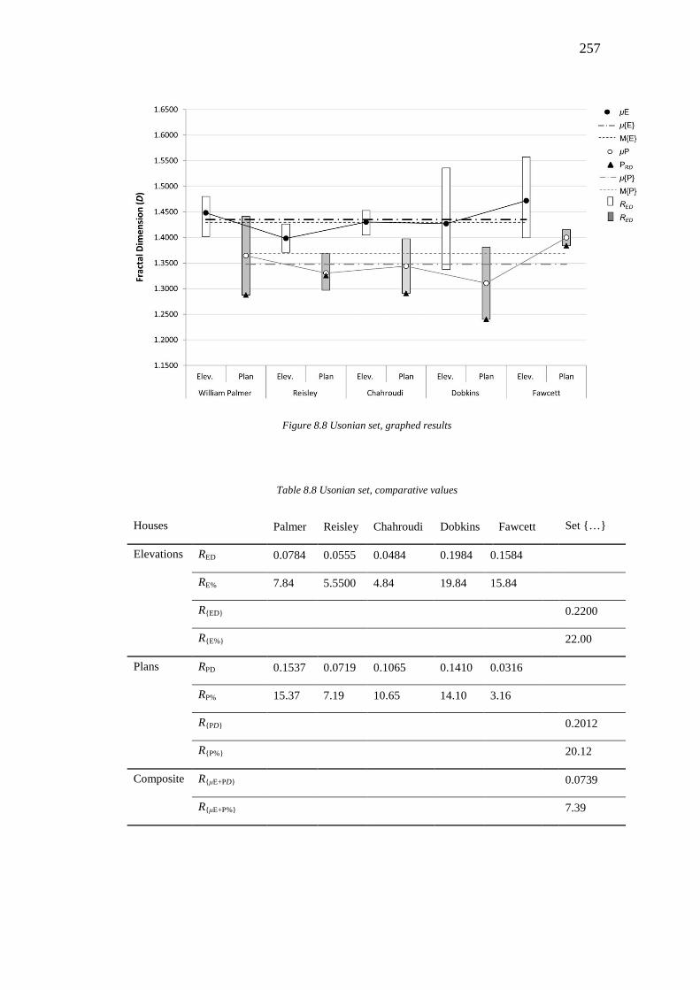
257

Figure 8.8 Usonian set, graphed results

Table 8.8 Usonian set, comparative values

Houses Palmer Reisley Chahroudi Dobkins Fawcett Set {…}

Elevations RED 0.0784 0.0555 0.0484 0.1984 0.1584

RE% 7.84 5.5500 4.84 19.84 15.84

R{ED} 0.2200

R{E%} 22.00

Plans RPD 0.1537 0.0719 0.1065 0.1410 0.0316

RP% 15.37 7.19 10.65 14.10 3.16

R{PD} 0.2012

R{P%} 20.12

Composite R{μE+PD} 0.0739

R{μE+P%} 7.39

258

The results indicate that a typical house of the Usonian period is a simple

dwelling, without a great degree of complexity in elevation. The fractal

dimensions of all five of Wright’s Usonian houses show that the lowest mean

elevation is found in the Reisley House (μE = 1.3982) and the highest in the

Fawcett House (μE = 1.4719). The highest individual elevation result is also from

the Fawcett House (DE2 = 1.5575), the complete set of results from this house

suggesting it is highly complex in both plan and elevation. The median for all

elevations in the Usonian set is 1.4297, the mean 1.4350, and the standard

deviation 0.0560. The highest plan average is also from the Reisley House (μP =

1.3997), however the highest individual plan was the ground floor of the Palmer

House (DP1 = 1.4412) and the lowest plan average is from the Dobkins House (μP

= 1.3105). The range of all the plans (R{P%} = 20.12) was in a close percentile to

that of the elevations (R{E%} = 22.00). The median for all plans is 1.3687, the mean

1.3480, and the standard deviation 0.0634. The aggregate result for all plans and

elevations is μ{E+P} = 1.4032 and the composite range is R{μE+P%} = 7.39 (Tables

8.7 and 8.8, fig. 8.8).

The ground floor plan of the Palmer House (DP0 = 1.4412) is higher than the mean

of all the elevations in the set (μ{E} = 1.4350), and in the Fawcett House all plan

results (1.3839 < DP < 1.4155) are higher than the mean of the other plans of the

Usonian set (μ{P} = 1.3480). These two houses and the Dobkins House all have

ground floor plans which share corresponding levels of visual complexity with at

least one of their elevations. The other two houses in the Usonian set, the Reisley

House and the Chahroudi House, present a ground floor fractal dimension which

is very close to, but not as complex, as the least complex of their elevations.

Due to the triangular planning system that Wright employed with these houses,

the Chahroudi House and the Fawcett House have only three elevations in

representational form. This lesser number of data points however does not appear

to affect the results, as the two houses still appear typical when compared with the

others. Indeed, the Chaharoudi House provides balanced results with the extent of

259

the D values falling neatly above and below the mean average in the case of both

the plan and elevations.

8.3.4 Wright’s Stylistic Continuity

When architectural historians review the career of Frank Lloyd Wright they

generally agree that throughout his life, his buildings display a consistent set of

design principles even though his works have varied in appearance across several

distinct stylistic periods (Hoffmann 1995; McCarter 1999; Frampton 2005).

Historians tend to acknowledge such obvious visual and stylistic differences while

focusing on similarities in the underlying tactics and theories which shape

Wright’s work. For example, Robert Sweeny concedes that Wright’s ability to

‘renew himself repeatedly throughout his career’ (1994: 1) is a characteristic of

his approach, but argues that it does not change his underlying values. David De

Long supports this view when he proposes that over time, Wright ‘was able to

retain allegiance to earlier principles while arriving at markedly different

conclusions’ (1994: xii). Kenneth Frampton similarly maintains that there is a

constant thread throughout Wright’s work which is related to a modular system of

planning and construction that ‘varied according to local circumstance’ (2005:

178). Frampton defines this continuous thread as a ‘plaited approach to

architectonic space’ that ‘prevailed throughout Wright’s long career’ (2005: 178).

Robert McCarter, who claims that Wright’s Usonian houses are derivations of his

Prairie house ideals, argues that Wright’s ‘architectural designs were a continuous

reinvention or rediscovery of the same fundamental principles’ (1999: 249).

Finally, Donald Hoffmann supports this argument confirming that ‘the language

of Wright’s buildings continued to change, but the logic did not; once he grasped

the principles, his work no longer evolved’ (1995: 52). To support this assertion

Hoffman quotes Wright stating that ‘I am pleased by the thread of structural

consistency I see inspiring the complete texture of the work revealed in my

designs and plans, […] from the beginning, 1893, to this time, 1957’ (qtd. in

Hoffman1995: 52).

260

While the preceding quotes provide interpretations of the reasons why Wright’s

architecture remained so consistent over his various stylistic periods, when

looking at the data for Wright’s Prairie, Textile-block houses and Usonian

periods, the scholarly view is generally supported. By comparing the average

complexity for the elevations of Wright’s houses over these three periods, the

largest variation is 6.4%, between the Usonian and Prairie elevations. Starting

with the first of Wright’s stylistic periods analysed, the Prairie houses have an

average fractal dimension for all elevations of μ{E} = 1.4979. This level of

complexity remains virtually unchanged in Wright’s Textile-block houses period

(μ{E} = 1.4996) before decreasing slightly in the Usonian period (μ{E} = 1.4350). In

plan form, Wright appears to have gone full circle in complexity starting from the

Prairie style (μ{P} = 1.3579) then increasing in the Textile-block houses (μ{P} =

1.4055), before returning to the lower levels in the Usonian houses (μ{P} =

1.3480). Comparing the aggregate results of the three periods of Wright’s

architecture, the Textile-block buildings are generally the most complex (μ{E+P} =

1.4591), the Usonians are the least (μ{E+P} = 1. 4032) and the Prairie houses are

midway between the two (μ{E+P} = 1. 4318) (Tables 8.3, 8.5, 8.7).

Comparing sets of fractal dimensions is one method of assessing similarities

between the elevations and plans of a building. Another is to use the Range to

determine the level of correspondence between the visual complexity of the

elevations and of the plans. The composite, or overall ranges for each set show

that the Prarie (R{μE+P%} = 7.29) and Usonian (R{μE+P%} = 7.39) have a similar level

of complexity across all plans and elevations for the sets. However, the range is

higher (R{μE+P%} = 15.82) for the Textile-block houses set, which suggests the

representations of these buildings have only some visual correspondence, and

could not be described as similar (Tables 8.4, 8.6, 8.8).

261

8.4 The Visual Complexity of Fallingwater Compared

The consistency in the appearance of Wright’s stylistic periods, especially the

Usonian and Prairie styles—as proposed academically and verified by the fractal

dimension study—implies that an unusual house such as Fallingwater might stand

out amongst the others. As discussed in Chapter 1, the proposal that this

‘revolutionary’ (Fell 2009: 91) building was formally ‘unexpected and unique in

the work of Wright’ (Hoesli 2005: 204) is supported by many histories and

scholarly critiques (Lind 1996; Kaufmann 1986; Futagawa and Pfeiffer 2003;

Hoesli 2005; Fell 2009). Yet other scholars claim there are formal elements in

Fallingwater which recall his previous designs, and which seem to prefigure his

later Usonian works (McCarter 1999; Smith 2000; Lesau and Tice 2000). As such,

claims that Fallingwater is unique in Wright’s oeuvre are contestable.

This section compares the level of characteristic visual complexity of

Fallingwater with the other fifteen houses analysed. The analysis is first

approached in stylistic groups and then individual houses are also considered.

Figures 8.9 - 8.11 demonstrate with linear trendlines for each period which

describe how Wright’s works evolved over the course of five projects. For

example, just considering elevations, visual complexity is relatively constant

across the works of Wright’s Prairie and Usonian houses, while it rises more

noticeably over time in his Textile-block houses. For the plans of the sets of

houses, the same pattern occurs, with the Prairie and Usonian houses remaining

similar in their complexity and the Textile-blocks increasing over time. Finally,

when elevations and plans are combined, these trends are confirmed, with the

Prairie houses remaining extremely stable, the Usonian houses increase in

complexity slightly over time and there is a dramatic increase in the results for the

Textile-block houses. Along with these linear indicators, a triangle is included

with each graph, representing the mean fractal dimension of Fallingwater’s plans,

elevation and the composite of the plans and elevations.

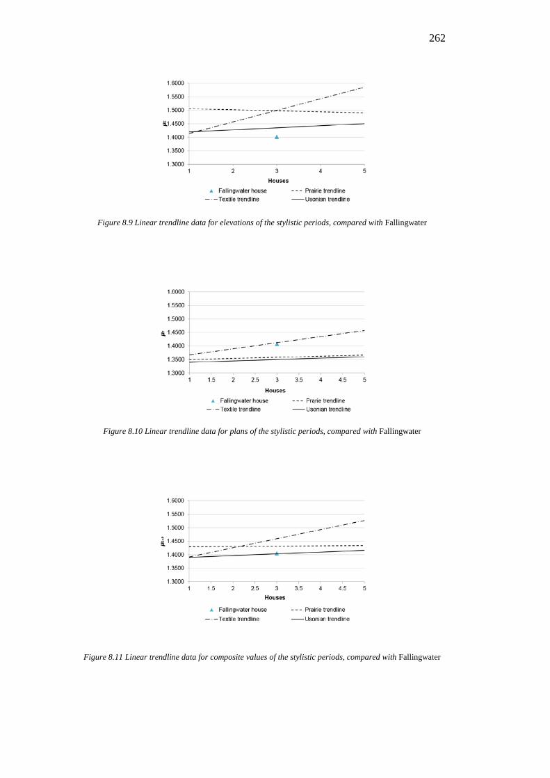
262

Figure 8.9 Linear trendline data for elevations of the stylistic periods, compared with Fallingwater

Figure 8.10 Linear trendline data for plans of the stylistic periods, compared with Fallingwater

Figure 8.11 Linear trendline data for composite values of the stylistic periods, compared with Fallingwater

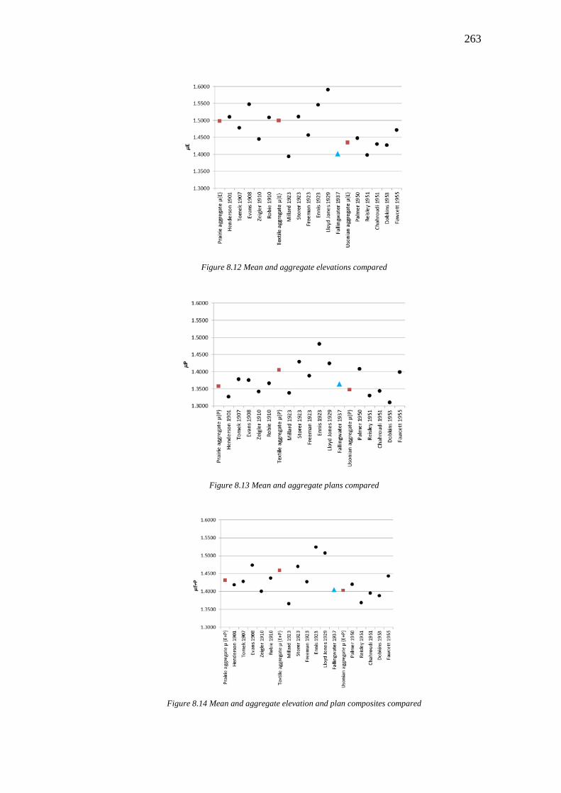
263

Figure 8.12 Mean and aggregate elevations compared

Figure 8.13 Mean and aggregate plans compared

Figure 8.14 Mean and aggregate elevation and plan composites compared

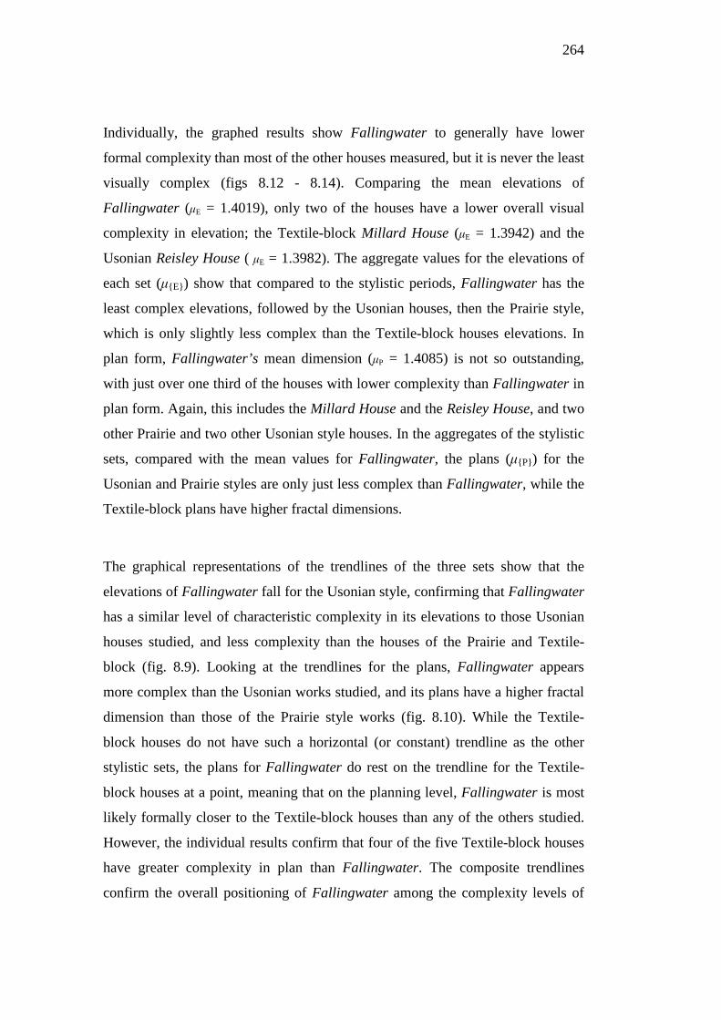
264

Individually, the graphed results show Fallingwater to generally have lower

formal complexity than most of the other houses measured, but it is never the least

visually complex (figs 8.12 - 8.14). Comparing the mean elevations of

Fallingwater (μE = 1.4019), only two of the houses have a lower overall visual

complexity in elevation; the Textile-block Millard House (μE = 1.3942) and the

Usonian Reisley House ( μE = 1.3982). The aggregate values for the elevations of

each set (μ{E}) show that compared to the stylistic periods, Fallingwater has the

least complex elevations, followed by the Usonian houses, then the Prairie style,

which is only slightly less complex than the Textile-block houses elevations. In

plan form, Fallingwater’s mean dimension (μP = 1.4085) is not so outstanding,

with just over one third of the houses with lower complexity than Fallingwater in

plan form. Again, this includes the Millard House and the Reisley House, and two

other Prairie and two other Usonian style houses. In the aggregates of the stylistic

sets, compared with the mean values for Fallingwater, the plans (μ{P}) for the

Usonian and Prairie styles are only just less complex than Fallingwater, while the

Textile-block plans have higher fractal dimensions.

The graphical representations of the trendlines of the three sets show that the

elevations of Fallingwater fall for the Usonian style, confirming that Fallingwater

has a similar level of characteristic complexity in its elevations to those Usonian

houses studied, and less complexity than the houses of the Prairie and Textile-

block (fig. 8.9). Looking at the trendlines for the plans, Fallingwater appears

more complex than the Usonian works studied, and its plans have a higher fractal

dimension than those of the Prairie style works (fig. 8.10). While the Textile-

block houses do not have such a horizontal (or constant) trendline as the other

stylistic sets, the plans for Fallingwater do rest on the trendline for the Textile-

block houses at a point, meaning that on the planning level, Fallingwater is most

likely formally closer to the Textile-block houses than any of the others studied.

However, the individual results confirm that four of the five Textile-block houses

have greater complexity in plan than Fallingwater. The composite trendlines

confirm the overall positioning of Fallingwater among the complexity levels of

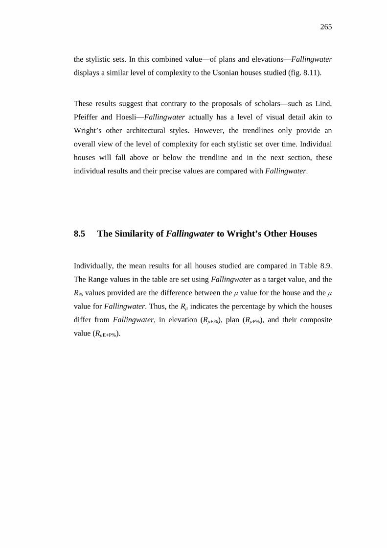
265

the stylistic sets. In this combined value—of plans and elevations—Fallingwater

displays a similar level of complexity to the Usonian houses studied (fig. 8.11).

These results suggest that contrary to the proposals of scholars—such as Lind,

Pfeiffer and Hoesli—Fallingwater actually has a level of visual detail akin to

Wright’s other architectural styles. However, the trendlines only provide an

overall view of the level of complexity for each stylistic set over time. Individual

houses will fall above or below the trendline and in the next section, these

individual results and their precise values are compared with Fallingwater.

8.5 The Similarity of Fallingwater to Wright’s Other Houses

Individually, the mean results for all houses studied are compared in Table 8.9.

The Range values in the table are set using Fallingwater as a target value, and the

R% values provided are the difference between the μ value for the house and the μ

value for Fallingwater. Thus, the Rμ indicates the percentage by which the houses

differ from Fallingwater, in elevation (RμE%), plan (RμP%), and their composite

value (RμE+P%).

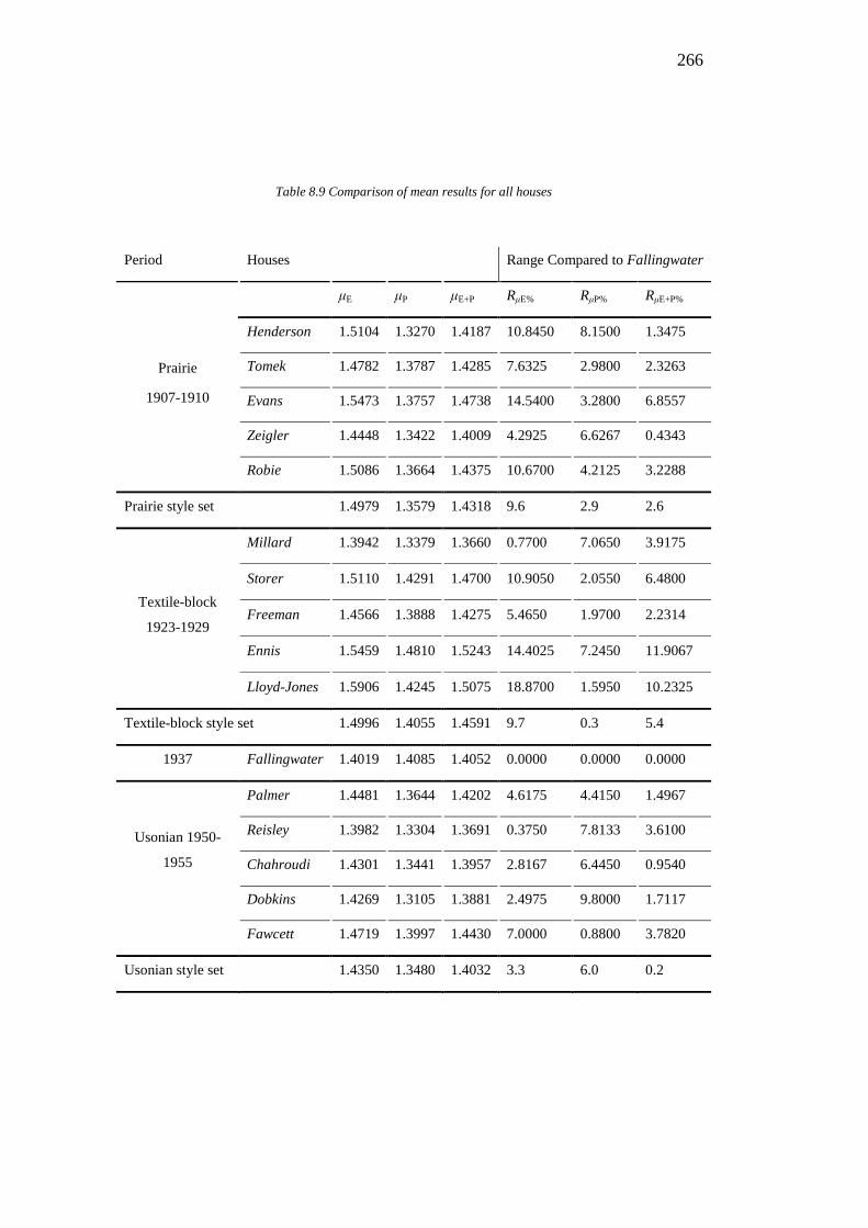
266

Table 8.9 Comparison of mean results for all houses

Period Houses Range Compared to Fallingwater

Prairie

1907-1910

μE μP μE+P RμE% RμP% RμE+P%

Henderson 1.5104 1.3270 1.4187 10.8450 8.1500 1.3475

Tomek 1.4782 1.3787 1.4285 7.6325 2.9800 2.3263

Evans 1.5473 1.3757 1.4738 14.5400 3.2800 6.8557

Zeigler 1.4448 1.3422 1.4009 4.2925 6.6267 0.4343

Robie 1.5086 1.3664 1.4375 10.6700 4.2125 3.2288

Prairie style set 1.4979 1.3579 1.4318 9.6 2.9 2.6

Textile-block

1923-1929

Millard 1.3942 1.3379 1.3660 0.7700 7.0650 3.9175

Storer 1.5110 1.4291 1.4700 10.9050 2.0550 6.4800

Freeman 1.4566 1.3888 1.4275 5.4650 1.9700 2.2314

Ennis 1.5459 1.4810 1.5243 14.4025 7.2450 11.9067

Lloyd-Jones 1.5906 1.4245 1.5075 18.8700 1.5950 10.2325

Textile-block style set 1.4996 1.4055 1.4591 9.7 0.3 5.4

1937 Fallingwater 1.4019 1.4085 1.4052 0.0000 0.0000 0.0000

Usonian 1950-

1955

Palmer 1.4481 1.3644 1.4202 4.6175 4.4150 1.4967

Reisley 1.3982 1.3304 1.3691 0.3750 7.8133 3.6100

Chahroudi 1.4301 1.3441 1.3957 2.8167 6.4450 0.9540

Dobkins 1.4269 1.3105 1.3881 2.4975 9.8000 1.7117

Fawcett 1.4719 1.3997 1.4430 7.0000 0.8800 3.7820

Usonian style set 1.4350 1.3480 1.4032 3.3 6.0 0.2

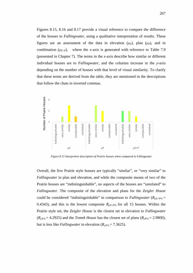
267

Figures 8.15, 8.16 and 8.17 provide a visual reference to compare the difference

of the houses to Fallingwater, using a qualitative interpretation of results. These

figures are an assessment of the data in elevation (μE), plan (μP), and in

combination (μE+P), where the x-axis is generated with reference to Table 7.9

(presented in Chapter 7). The terms in the x-axis describe how similar or different

individual houses are to Fallingwater, and the columns increase in the y-axis

depending on the number of houses with that level of visual similarity. To clarify

that these terms are derived from the table, they are mentioned in the descriptions

that follow the chats in inverted commas.

Figure 8.15 Interpretive description of Prairie houses when compared to Fallingwater

Overall, the five Prairie style houses are typically “similar”, or “very similar” to

Fallingwater in plan and elevation, and while the composite means of two of the

Prairie houses are “indistinguishable”, no aspects of the houses are “unrelated” to

Fallingwater. The composite of the elevation and plans for the Zeigler House

could be considered “indistinguishable” in comparison to Fallingwater (RμE+P% =

0.4343), and this is the lowest composite RμE+P% for all 15 houses. Within the

Prairie style set, the Zeigler House is the closest set in elevation to Fallingwater

(RμE% = 4.2925) and the Tomek House has the closest set of plans (RμP% = 2.9800),

but is less like Fallingwater in elevation (RμE% = 7.3625).

0

2

4

Indi

stin

guish

able

very

sim

ilar

simila

r

com

para

ble

unre

late

d

Indi

stin

guish

able

very

sim

ilar

simila

r

com

para

ble

unre

late

d

Indi

stin

guish

able

very

sim

ilar

simila

r

com

para

ble

unre

late

dμE μP μE+P

Num

ber o

f Pra

irie

Hou

ses

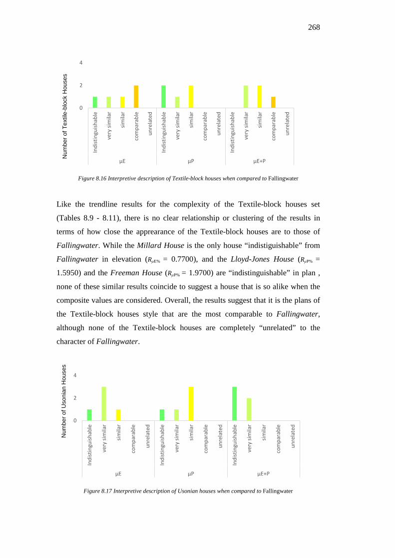
268

Figure 8.16 Interpretive description of Textile-block houses when compared to Fallingwater

Like the trendline results for the complexity of the Textile-block houses set

(Tables 8.9 - 8.11), there is no clear relationship or clustering of the results in

terms of how close the apprearance of the Textile-block houses are to those of

Fallingwater. While the Millard House is the only house “indistiguishable” from

Fallingwater in elevation (RμE% = 0.7700), and the Lloyd-Jones House (RμP% =

1.5950) and the Freeman House (RμP% = 1.9700) are “indistinguishable” in plan ,

none of these similar results coincide to suggest a house that is so alike when the

composite values are considered. Overall, the results suggest that it is the plans of

the Textile-block houses style that are the most comparable to Fallingwater,

although none of the Textile-block houses are completely “unrelated” to the

character of Fallingwater.

Figure 8.17 Interpretive description of Usonian houses when compared to Fallingwater

0

2

4

Indi

stin

guish

able

very

sim

ilar

simila

r

com

para

ble

unre

late

d

Indi

stin

guish

able

very

sim

ilar

simila

r

com

para

ble

unre

late

d

Indi

stin

guish

able

very

sim

ilar

simila

r

com

para

ble

unre

late

d

μE μP μE+P

0

2

4

Indi

stin

guish

able

very

sim

ilar

simila

r

com

para

ble

unre

late

d

Indi

stin

guish

able

very

sim

ilar

simila

r

com

para

ble

unre

late

d

Indi

stin

guish

able

very

sim

ilar

simila

r

com

para

ble

unre

late

d

μE μP μE+P

Num

ber o

f Tex

tile-

bloc

k H

ouse

s N

umbe

r of U

soni

an H

ouse

s

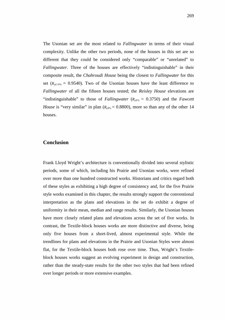
269

The Usonian set are the most related to Fallingwater in terms of their visual

complexity. Unlike the other two periods, none of the houses in this set are so

different that they could be considered only “comparable” or “unrelated” to

Fallingwater. Three of the houses are effectively “indistinguishable” in their

composite result, the Chahroudi House being the closest to Fallingwater for this

set (RμE+P% = 0.9540). Two of the Usonian houses have the least difference to

Fallingwater of all the fifteen houses tested; the Reisley House elevations are

“indistinguishable” to those of Fallingwater (RμE% = 0.3750) and the Fawcett

House is “very similar” in plan (RμP% = 0.8800), more so than any of the other 14

houses.

Conclusion

Frank Lloyd Wright’s architecture is conventionally divided into several stylistic

periods, some of which, including his Prairie and Usonian works, were refined

over more than one hundred constructed works. Historians and critics regard both

of these styles as exhibiting a high degree of consistency and, for the five Prairie

style works examined in this chapter, the results strongly support the conventional

interpretation as the plans and elevations in the set do exhibit a degree of

uniformity in their mean, median and range results. Similarly, the Usonian houses

have more closely related plans and elevations across the set of five works. In

contrast, the Textile-block houses works are more distinctive and diverse, being

only five houses from a short-lived, almost experimental style. While the

trendlines for plans and elevations in the Prairie and Usonian Styles were almost

flat, for the Textile-block houses both rose over time. Thus, Wright’s Textile-

block houses works suggest an evolving experiment in design and construction,

rather than the steady-state results for the other two styles that had been refined

over longer periods or more extensive examples.

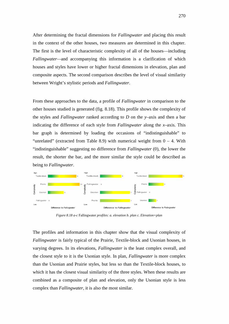
270

After determining the fractal dimensions for Fallingwater and placing this result

in the context of the other houses, two measures are determined in this chapter.

The first is the level of characteristic complexity of all of the houses—including

Fallingwater—and accompanying this information is a clarification of which

houses and styles have lower or higher fractal dimensions in elevation, plan and

composite aspects. The second comparison describes the level of visual similarity

between Wright’s stylistic periods and Fallingwater.

From these approaches to the data, a profile of Fallingwater in comparison to the

other houses studied is generated (fig. 8.18). This profile shows the complexity of

the styles and Fallingwater ranked according to D on the y–axis and then a bar

indicating the difference of each style from Fallingwater along the x–axis. This

bar graph is determined by loading the occasions of “indistinguishable” to

“unrelated” (extracted from Table 8.9) with numerical weight from 0 – 4. With

“indistinguishable” suggesting no difference from Fallingwater (0), the lower the

result, the shorter the bar, and the more similar the style could be described as

being to Fallingwater.

Figure 8.18 a-c Fallingwater profiles: a. elevation b. plan c. Elevation+plan

The profiles and information in this chapter show that the visual complexity of

Fallingwater is fairly typical of the Prairie, Textile-block and Usonian houses, in

varying degrees. In its elevations, Fallingwater is the least complex overall, and

the closest style to it is the Usonian style. In plan, Fallingwater is more complex

than the Usonian and Prairie styles, but less so than the Textile-block houses, to

which it has the closest visual similarity of the three styles. When these results are

combined as a composite of plan and elevation, only the Usonian style is less

complex than Fallingwater, it is also the most similar.

271

In addition to building on the scholarly information available on Fallingwater, the

information in this chapter provides a response to hypothesis 1, which is: that the

formal and visual qualities of Frank Lloyd Wright’s Fallingwater are atypical of

his early and mid-career housing (1901-1955). This chapter shows this hypothesis

to be false.

272

Chapter 9

Comparing Fallingwater with its Natural Setting

To examine the second hypothesis outlined at the start of this dissertation, the

present chapter uses the box-counting method to measure and compare the

characteristic complexity of Fallingwater and four natural elements within its

surrounding landscape. Chapters 2 and 6 provide the background to the analytical

method and the testing rationale required to decide which images are analysed in

this chapter. The specific images of Fallingwater which are measured in the

present chapter are four perspective views and four plan views of the house. These

eight measures are compared with those derived from sixteen line drawn views

and four site plans of four different natural subjects, collectively encapsulating

one possible reading of the geometric complexity of Fallingwater’s setting.

The methodological approach used in the previous chapter has been extensively

tested, refined and validated in the past (Ostwald and Vaughan 2016). In contrast,

the methodological approach used for the present chapter is largely untested and

as such, the results of its comparison between architecture and nature could be

regarded as akin to a pilot study or preliminary examination. Indeed, the data

presented in this chapter may serve more to provide an indicator that the method

might (or might not) work, rather than simply providing evidence that

Fallingwater does (or does not) have a connection to its setting. Thus, while this

chapter aims to determine if there is a correlation in terms of characteristic

complexity between Wright’s architecture and its natural setting, the results

cannot be taken as a definitive proof.

The images used for fractal analysis in this chapter are taken from the following

sources. The perspective drawings which are analysed in this chapter are based on

273

Wright’s original drawings reproduced by Drexler (1965) and Futagawa and

Pfeiffer (1987c; 2003). The plans for Fallingwater are traced from those

published by Storrer (2006) and Futagawa and Pfeiffer (1986). Except for the

views of the valley, the views of the natural elements are edge-detected line

drawings extracted from photographs taken by the present Author of the

landscape surrounding Fallingwater on a field trip in 2012. The views of the

valley are taken from 2D still images of the site generated using Google Earth.

The plans for the natural elements are all derived from a combination of two

primary sources, the site plan prepared for the Kaufmanns in March 1935

(McCarter 2002: 5) and the map traced over this site plan by Wright’s apprentices,

as reproduced by Kaufmann (1986: 39). The results developed in this chapter are

presented and analysed in the same way as those in Chapter 8, using the

terminology defined in Chapter 7.

9.1 Scholarly Approaches to Fallingwater and its Natural

Setting

The broad range of scholarly views that traditionally provide insight into

Fallingwater’s strong connection to its natural setting are presented in Chapter 2,

where it is shown that this house is generally regarded by architectural scholars as

being ‘part of the enveloping woodland’ (Fell 2009: 88). Chapter 2 also

demonstrates that for Wright, the intent for a house like Fallingwater is that ‘the

building with landscape and site became inevitably one’ (Wright 1955: 84).

Architectural scholars have repeatedly identified the particular strategies used by

Wright in the design of Fallingwater to connect it to the site. These include:

cantilevering the house into the landscape from a stone firmament (Mumford

1938; Wright 1938; Frazier 1995; Hoesli 2005; Storrer 2006); an interplay of

internal and external space (Wright 1938; Laseau and Tice 1992; Andropogon

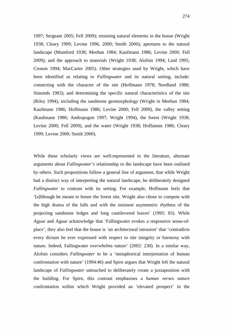
274

1997; Sergeant 2005; Fell 2009); retaining natural elements in the house (Wright

1938; Cleary 1999; Levine 1996, 2000; Smith 2000); apertures to the natural

landscape (Mumford 1938; Meehan 1984; Kaufmann 1986; Levine 2000; Fell

2009); and the approach to materials (Wright 1938; Alofsin 1994; Lind 1995;

Cronon 1994; MacCarter 2005). Other strategies used by Wright, which have

been identified as relating to Fallingwater and its natural setting, include:

connecting with the character of the site (Hoffmann 1978; Nordland 1988;

Simonds 1983); and determining the specific natural characteristics of the site

(Riley 1994), including the sandstone geomorphology (Wright in Meehan 1984;

Kaufmann 1986; Hoffmann 1986; Levine 2000; Fell 2009), the valley setting

(Kaufmann 1986; Andropogon 1997; Wright 1994), the forest (Wright 1938;

Levine 2000; Fell 2009), and the water (Wright 1938; Hoffamnn 1986; Cleary

1999; Levine 2000; Smith 2000).

While these scholarly views are well-represented in the literature, alternate

arguments about Fallingwater’s relationship to the landscape have been outlined

by others. Such propositions follow a general line of argument, that while Wright

had a distinct way of interpreting the natural landscape, he deliberately designed

Fallingwater to contrast with its setting. For example, Hoffmann feels that

‘[a]lthough he meant to honor the forest site, Wright also chose to compete with

the high drama of the falls and with the insistent asymmetric rhythms of the

projecting sandstone ledges and long cantilevered leaves’ (1995: 83). While

Aguar and Aguar acknowledge that ‘Fallingwater evokes a responsive sense-of-

place’, they also feel that the house is ‘an architectural intrusion’ that ‘contradicts

every dictum he ever expressed with respect to site integrity or harmony with

nature. Indeed, Fallingwater overwhelms nature’ (2002: 230). In a similar way,

Alofsin considers Fallingwater to be a ‘metaphorical interpretation of human

confrontation with nature’ (1994:46) and Spirn argues that Wright left the natural

landscape of Fallingwater untouched to deliberately create a juxtaposition with

the building. For Spirn, this contrast emphasises a human verses nature

confrontation within which Wright provided an ‘elevated prospect’ in the

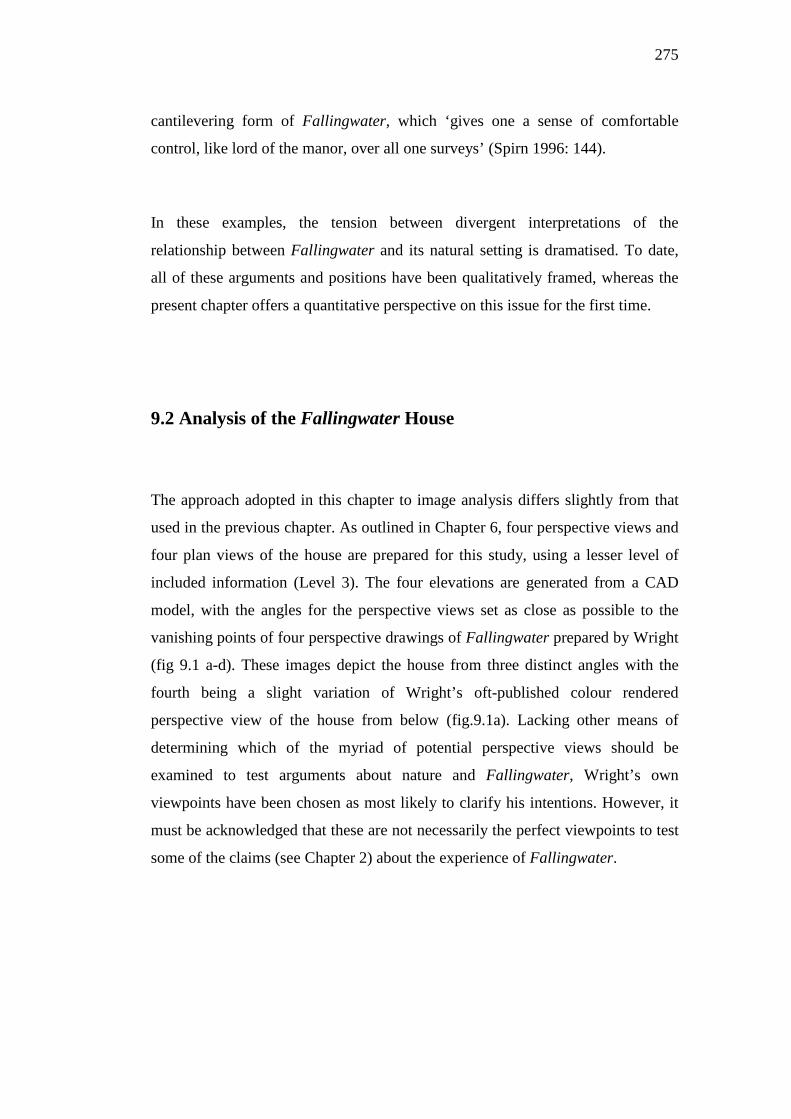
275

cantilevering form of Fallingwater, which ‘gives one a sense of comfortable

control, like lord of the manor, over all one surveys’ (Spirn 1996: 144).

In these examples, the tension between divergent interpretations of the

relationship between Fallingwater and its natural setting is dramatised. To date,

all of these arguments and positions have been qualitatively framed, whereas the

present chapter offers a quantitative perspective on this issue for the first time.

9.2 Analysis of the Fallingwater House

The approach adopted in this chapter to image analysis differs slightly from that

used in the previous chapter. As outlined in Chapter 6, four perspective views and

four plan views of the house are prepared for this study, using a lesser level of

included information (Level 3). The four elevations are generated from a CAD

model, with the angles for the perspective views set as close as possible to the

vanishing points of four perspective drawings of Fallingwater prepared by Wright

(fig 9.1 a-d). These images depict the house from three distinct angles with the

fourth being a slight variation of Wright’s oft-published colour rendered

perspective view of the house from below (fig.9.1a). Lacking other means of

determining which of the myriad of potential perspective views should be

examined to test arguments about nature and Fallingwater, Wright’s own

viewpoints have been chosen as most likely to clarify his intentions. However, it

must be acknowledged that these are not necessarily the perfect viewpoints to test

some of the claims (see Chapter 2) about the experience of Fallingwater.

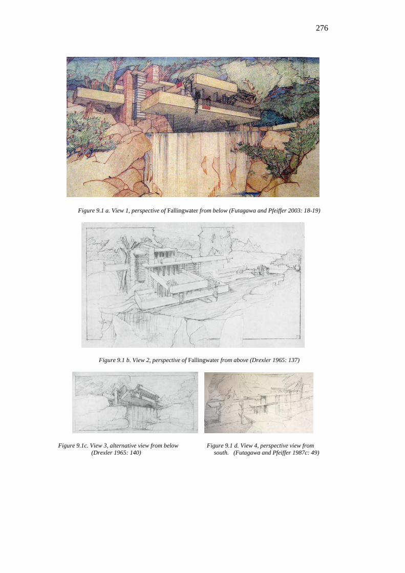
276

Figure 9.1 a. View 1, perspective of Fallingwater from below (Futagawa and Pfeiffer 2003: 18-19)

Figure 9.1 b. View 2, perspective of Fallingwater from above (Drexler 1965: 137)

Figure 9.1c. View 3, alternative view from below Figure 9.1 d. View 4, perspective view from (Drexler 1965: 140) south. (Futagawa and Pfeiffer 1987c: 49)

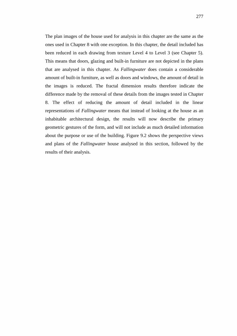
277

The plan images of the house used for analysis in this chapter are the same as the

ones used in Chapter 8 with one exception. In this chapter, the detail included has

been reduced in each drawing from texture Level 4 to Level 3 (see Chapter 5).

This means that doors, glazing and built-in furniture are not depicted in the plans

that are analysed in this chapter. As Fallingwater does contain a considerable

amount of built-in furniture, as well as doors and windows, the amount of detail in

the images is reduced. The fractal dimension results therefore indicate the

difference made by the removal of these details from the images tested in Chapter

8. The effect of reducing the amount of detail included in the linear

representations of Fallingwater means that instead of looking at the house as an

inhabitable architectural design, the results will now describe the primary

geometric gestures of the form, and will not include as much detailed information

about the purpose or use of the building. Figure 9.2 shows the perspective views

and plans of the Fallingwater house analysed in this section, followed by the

results of their analysis.

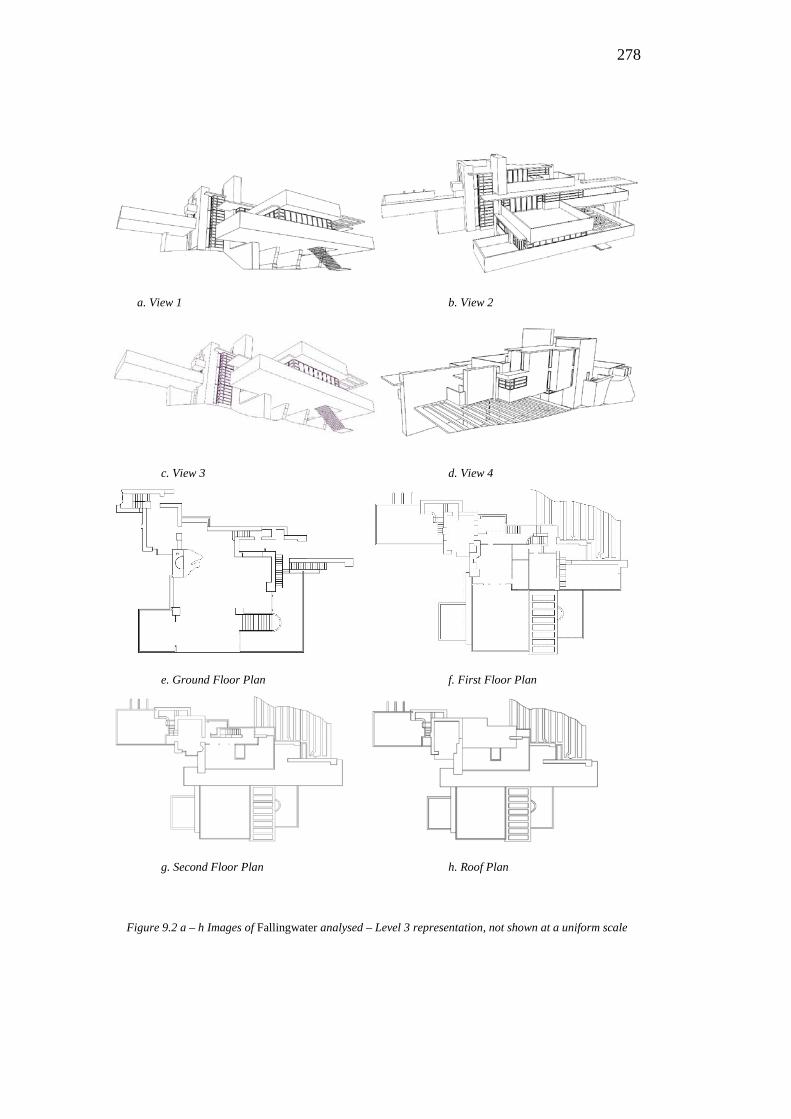
278

a. View 1 b. View 2

c. View 3 d. View 4

e. Ground Floor Plan f. First Floor Plan

g. Second Floor Plan h. Roof Plan

Figure 9.2 a – h Images of Fallingwater analysed – Level 3 representation, not shown at a uniform scale

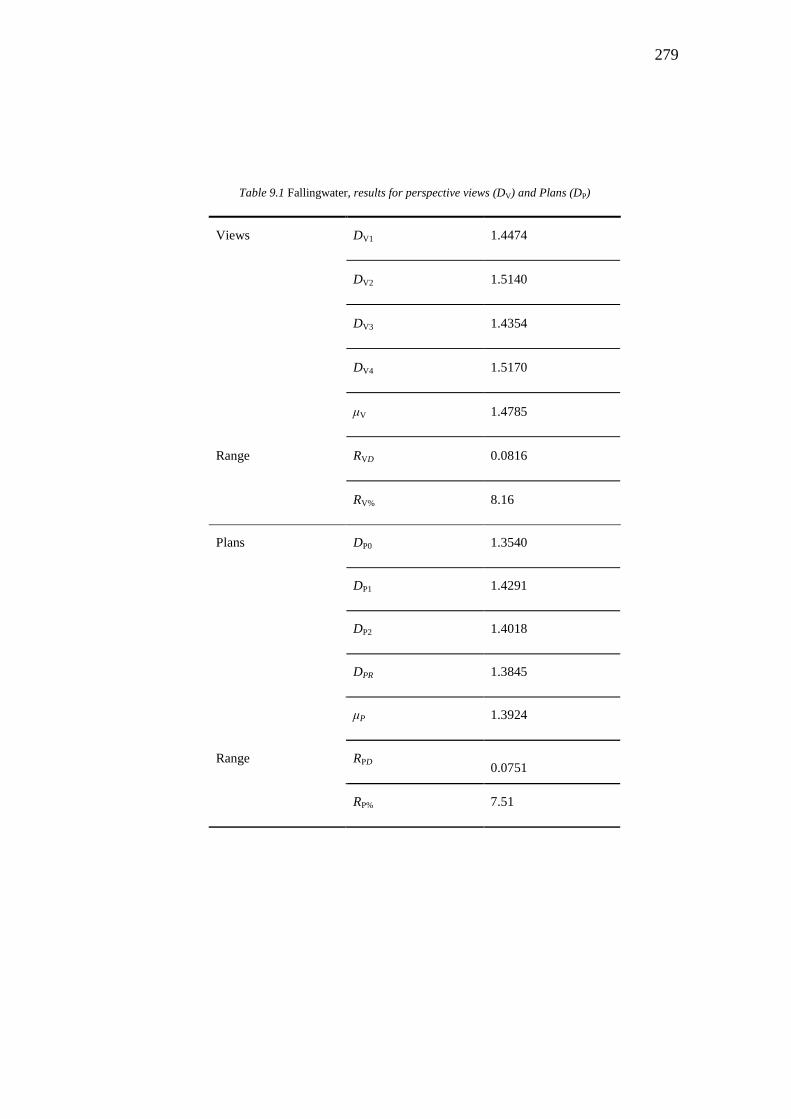
279

Table 9.1 Fallingwater, results for perspective views (DV) and Plans (DP)

Views DV1 1.4474

DV2 1.5140

DV3 1.4354

DV4 1.5170

μV 1.4785

Range RVD 0.0816

RV% 8.16

Plans DP0 1.3540

DP1 1.4291

DP2 1.4018

DPR 1.3845

μP 1.3924

Range RPD 0.0751

RP% 7.51

280

Figure 9.3 Fallingwater, graphed results for perspective views (DV) and Plans (DP)

The cardinal directions from which the perspective views are predominantly

framed are from the south and south-west (looking towards the north and north-

east), with only one perspective view from the north (looking south towards the

side of the house facing the steep slope behind). Of the elevations analysed in

Chapter 8, this northern facade has the lowest level of visual complexity, however

in the perspective views studied in this chapter, this northern perspective has the

highest fractal dimension result of all the perspective views of the house (DV4 =

1.5170). This may be because in elevation, the orthographic view of the house

flattens out what is actually a formally complex facade. Compared to the long,

cantilevered planes of the southern facade, the northern facade is stepped and

notched on both the horizontal and vertical planes, as it responds to the angle of

the driveway and to Wright’s internal planning. Of the southern perspectives, the

treetop view looking down onto the southern balconies from above has the

second-highest fractal dimension (DV2 = 1.5140), a result which is quite close to

that of the northern perspective. The two views looking up from the water of Bear

Run at the southern facade of the house vary only slightly in their perspectival

construction, and likewise their results are relatively similar (DV1 = 1.4474 and

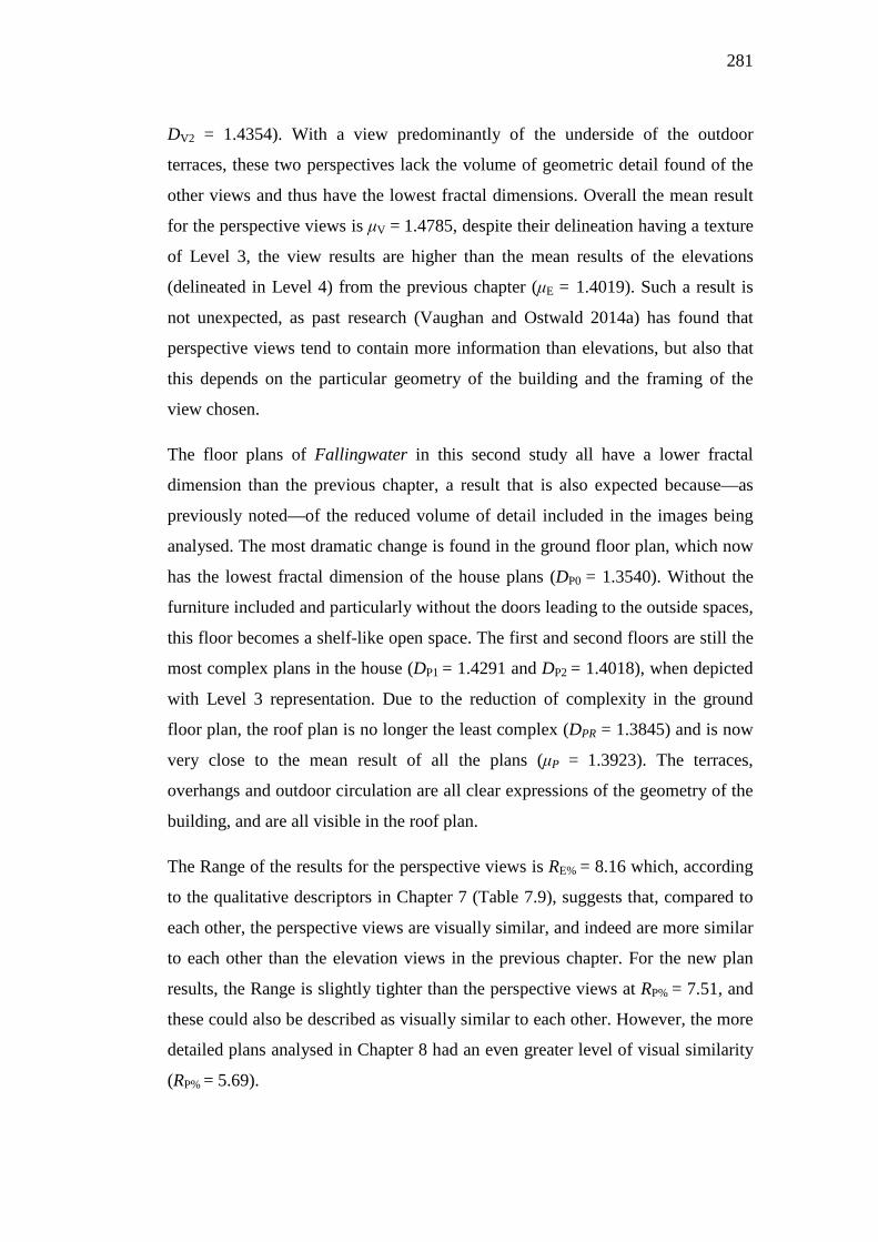
281

DV2 = 1.4354). With a view predominantly of the underside of the outdoor

terraces, these two perspectives lack the volume of geometric detail found of the

other views and thus have the lowest fractal dimensions. Overall the mean result

for the perspective views is μV = 1.4785, despite their delineation having a texture

of Level 3, the view results are higher than the mean results of the elevations

(delineated in Level 4) from the previous chapter (μE = 1.4019). Such a result is

not unexpected, as past research (Vaughan and Ostwald 2014a) has found that

perspective views tend to contain more information than elevations, but also that

this depends on the particular geometry of the building and the framing of the

view chosen.

The floor plans of Fallingwater in this second study all have a lower fractal

dimension than the previous chapter, a result that is also expected because—as

previously noted—of the reduced volume of detail included in the images being

analysed. The most dramatic change is found in the ground floor plan, which now

has the lowest fractal dimension of the house plans (DP0 = 1.3540). Without the

furniture included and particularly without the doors leading to the outside spaces,

this floor becomes a shelf-like open space. The first and second floors are still the

most complex plans in the house (DP1 = 1.4291 and DP2 = 1.4018), when depicted

with Level 3 representation. Due to the reduction of complexity in the ground

floor plan, the roof plan is no longer the least complex (DPR = 1.3845) and is now

very close to the mean result of all the plans (μP = 1.3923). The terraces,

overhangs and outdoor circulation are all clear expressions of the geometry of the

building, and are all visible in the roof plan.

The Range of the results for the perspective views is RE% = 8.16 which, according

to the qualitative descriptors in Chapter 7 (Table 7.9), suggests that, compared to

each other, the perspective views are visually similar, and indeed are more similar

to each other than the elevation views in the previous chapter. For the new plan

results, the Range is slightly tighter than the perspective views at RP% = 7.51, and

these could also be described as visually similar to each other. However, the more

detailed plans analysed in Chapter 8 had an even greater level of visual similarity

(RP% = 5.69).

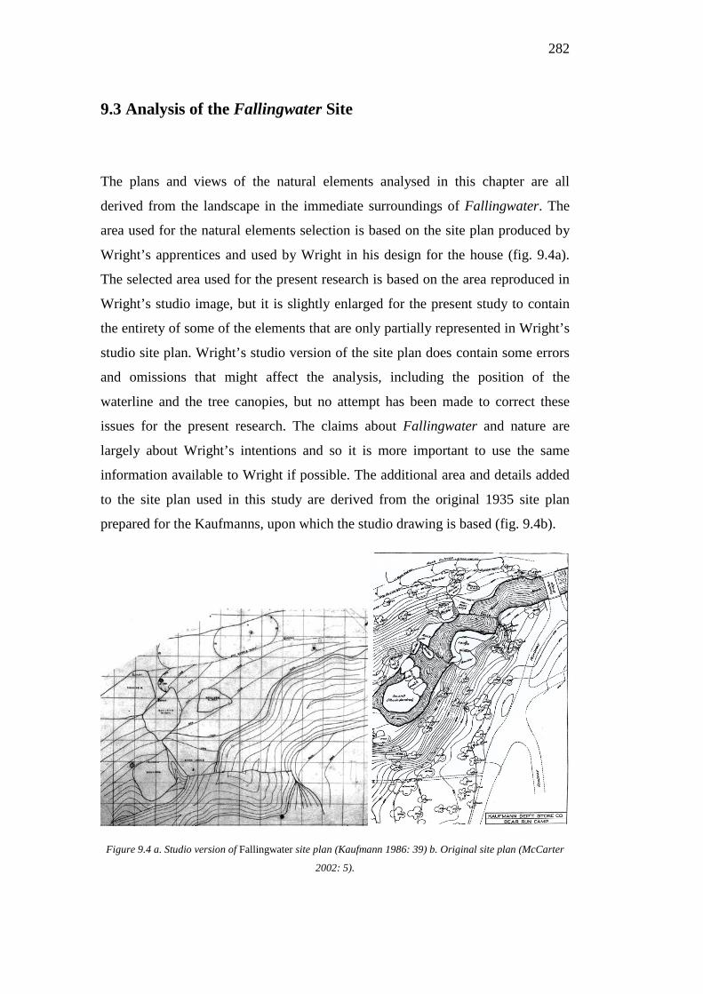
282

9.3 Analysis of the Fallingwater Site

The plans and views of the natural elements analysed in this chapter are all

derived from the landscape in the immediate surroundings of Fallingwater. The

area used for the natural elements selection is based on the site plan produced by

Wright’s apprentices and used by Wright in his design for the house (fig. 9.4a).

The selected area used for the present research is based on the area reproduced in

Wright’s studio image, but it is slightly enlarged for the present study to contain

the entirety of some of the elements that are only partially represented in Wright’s

studio site plan. Wright’s studio version of the site plan does contain some errors

and omissions that might affect the analysis, including the position of the

waterline and the tree canopies, but no attempt has been made to correct these

issues for the present research. The claims about Fallingwater and nature are

largely about Wright’s intentions and so it is more important to use the same

information available to Wright if possible. The additional area and details added

to the site plan used in this study are derived from the original 1935 site plan

prepared for the Kaufmanns, upon which the studio drawing is based (fig. 9.4b).

Figure 9.4 a. Studio version of Fallingwater site plan (Kaufmann 1986: 39) b. Original site plan (McCarter

2002: 5).

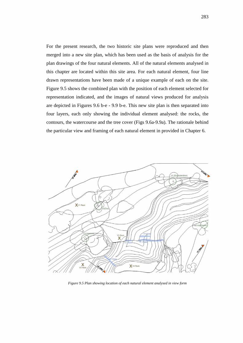
283

For the present research, the two historic site plans were reproduced and then

merged into a new site plan, which has been used as the basis of analysis for the

plan drawings of the four natural elements. All of the natural elements analysed in

this chapter are located within this site area. For each natural element, four line

drawn representations have been made of a unique example of each on the site.

Figure 9.5 shows the combined plan with the position of each element selected for

representation indicated, and the images of natural views produced for analysis

are depicted in Figures 9.6 b-e - 9.9 b-e. This new site plan is then separated into

four layers, each only showing the individual element analysed: the rocks, the

contours, the watercourse and the tree cover (Figs 9.6a-9.9a). The rationale behind

the particular view and framing of each natural element in provided in Chapter 6.

Figure 9.5 Plan showing location of each natural element analysed in view form

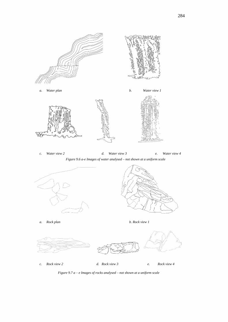
284

a. Water plan b. Water view 1

c. Water view 2 d. Water view 3 e. Water view 4

Figure 9.6 a-e Images of water analysed – not shown at a uniform scale

a. Rock plan b. Rock view 1

c. Rock view 2 d. Rock view 3 e. Rock view 4

Figure 9.7 a – e Images of rocks analysed – not shown at a uniform scale

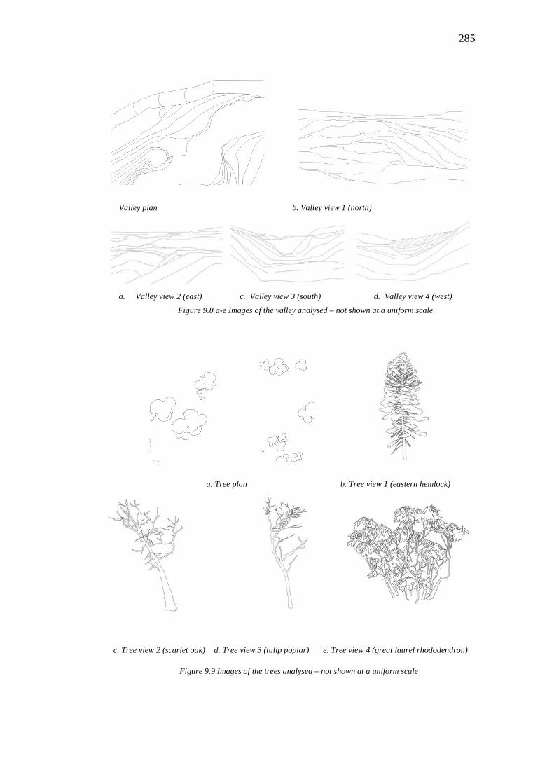
285

Valley plan b. Valley view 1 (north)

a. Valley view 2 (east) c. Valley view 3 (south) d. Valley view 4 (west)

Figure 9.8 a-e Images of the valley analysed – not shown at a uniform scale

a. Tree plan b. Tree view 1 (eastern hemlock)

c. Tree view 2 (scarlet oak) d. Tree view 3 (tulip poplar) e. Tree view 4 (great laurel rhododendron)

Figure 9.9 Images of the trees analysed – not shown at a uniform scale

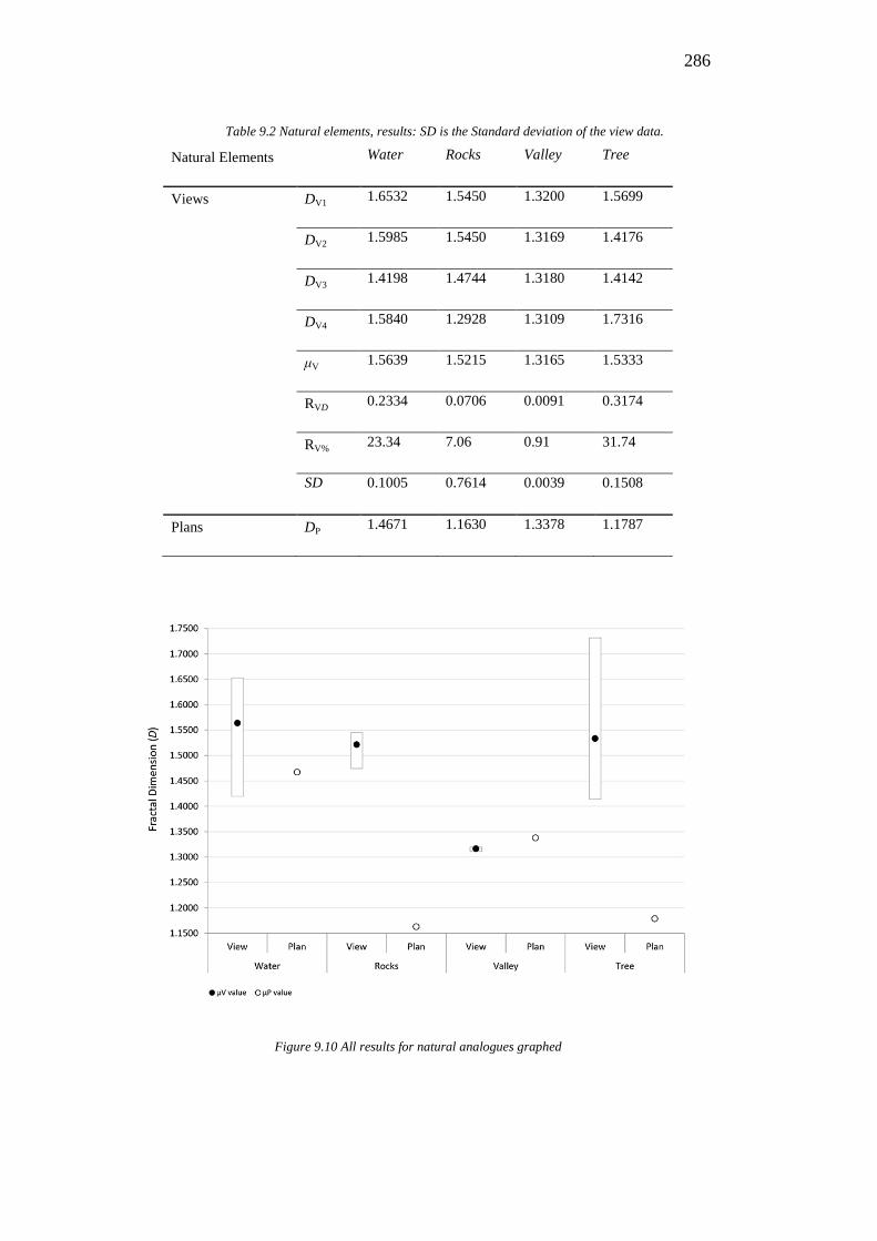
286

Table 9.2 Natural elements, results: SD is the Standard deviation of the view data. Natural Elements Water Rocks Valley Tree

Views DV1 1.6532 1.5450 1.3200 1.5699

DV2 1.5985 1.5450 1.3169 1.4176

DV3 1.4198 1.4744 1.3180 1.4142

DV4 1.5840 1.2928 1.3109 1.7316

μV 1.5639 1.5215 1.3165 1.5333

RVD 0.2334 0.0706 0.0091 0.3174

RV% 23.34 7.06 0.91 31.74

SD 0.1005 0.7614 0.0039 0.1508

Plans DP 1.4671 1.1630 1.3378 1.1787

Figure 9.10 All results for natural analogues graphed

287

The views of the water are taken from four different photographs of the waterfalls

created by the stepping down of the rock shelf in the Bear Run stream. Of these,

the main drop, during heavy rains or after the snow has melted, creates a wall of

falling water, parallel to the southern facade of the house and the image of this fall

has the highest visual complexity of all the water images (DV1 = 1.6532). The least

complex water image is of the same waterfall, but from a line drawing extracted

from a photograph taken when there was a lower water level in the Bear Run

stream (DV3 = 1.4198).

At the time of Wright’s first visit to the site of Fallingwater in 1934, it was winter

and most of the trees would have been bare of leaves except for the evergreen

Great Laurel Rhododendrons and the Eastern Hemlocks, both of which grow in

abundance around the house site. One each of these evergreens has been

reproduced for analysis along with two of the deciduous trees which also grow on

the site—the Tulip Poplar and the Scarlet Oak. Of the tree views, the Great Laurel

Rhododendron has the highest fractal dimension (DV4 = 1.7316) this is also the

highest dimension of all of the natural views analysed. The other evergreen tree

analysed, the Eastern Hemlock, has the second highest dimension (DV1 = 1.5699),

this is the expected result, as the leaves add visual detail to the images. The

deciduous trees, the Scarlet Oak (DV2 = 1.4176) and the Tulip Poplar (DV3 =

1.4142) have a similar result to each other, but lower than the evergreens.

The four rocks analysed are all examples of the Pottsville Sandstone found in the

Bear Run creek bed or near the house. The results for the first two are interesting

because they have exactly the same fractal dimension (DV1 = 1.5450; DV2 =

1.5450). These two may also be outcrops of the same rockface: the view 1 rock is

the large outcrop that supports the western terrace of the house, and the view 2

rock is of the cliffside along part of the stream, below the western terrace. Those

two rocks have the highest complexity of the four rocks analysed. The next most

complex section of rock is the cliffside underneath the southern terraces of the

house (DV3 = 1.4744), a result not too dissimilar to the others. The least complex

288

result is for a group of boulders that sit mid-stream, just below the house (DV4 =

1.2928). Perhaps because they are subject to continual water erosion they are less

fissured than the cliff edges or the boulders above the water level, hence they have

a lower fractal dimension.

The views of the valley are the least complex of all the natural elements analysed,

and rather than representing just one object such as a tree or a rock, these images

are landscape views over a greater distribution of area. While all the results for the

valley views are relatively similar, the highest is the view from the north (DV1 =

1.3200), which looks across the Bear Run gully to the road used to approach the

house. The least complex view is the view from the west (DV4 = 1.3109), which is

taken from a viewpoint down in the stream which is constrained by the steep gully

sides.

Of the plan views, the nautical chart of the water has the highest fractal dimension

(DP = 1.4671) and the rocks have the lowest level of complexity in plan (DP =

1.1630). The plan of the rocks which was analysed lacks detail and while it

provides some qualitative information, as it is an aerial view, many complex

aspects of the rock outcrop, such as the cliffline, are represented by a single line,

and thus the image is not overly complex or representative. Likewise, the tree

plans which have a similar level of representational detail to the rocks, have only

a slightly higher fractal dimension (DP = 1.1787); while the contour drawing used

to measure the valley in plan has a higher level of complexity which is closer to

those of the waterway (DP = 1.3378).

Excluding the plans from the mean view results, the water set has the highest

fractal dimension (μV = 1.5639), followed by the trees (μV = 1.5363) and then the

rocks (μV = 1.5215); while the valley has a noticeably lower level of visual

complexity (μV = 1.3165). The Range of the results for the four views of the valley

show the images to be visually indistinguishable (RV% = 0.91) and the standard

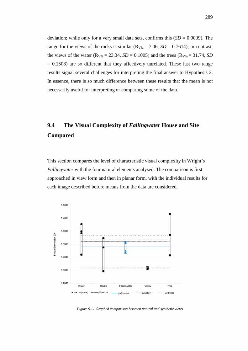
289

deviation; while only for a very small data sets, confirms this (SD = 0.0039). The

range for the views of the rocks is similar (RV% = 7.06, SD = 0.7614); in contrast,

the views of the water (RV% = 23.34, SD = 0.1005) and the trees (RV% = 31.74, SD

= 0.1508) are so different that they affectively unrelated. These last two range

results signal several challenges for interpreting the final answer to Hypothesis 2.

In essence, there is so much difference between these results that the mean is not

necessarily useful for interpreting or comparing some of the data.

9.4 The Visual Complexity of Fallingwater House and Site

Compared

This section compares the level of characteristic visual complexity in Wright’s

Fallingwater with the four natural elements analysed. The comparison is first

approached in view form and then in planar form, with the individual results for

each image described before means from the data are considered.

Figure 9.11 Graphed comparison between natural and synthetic views

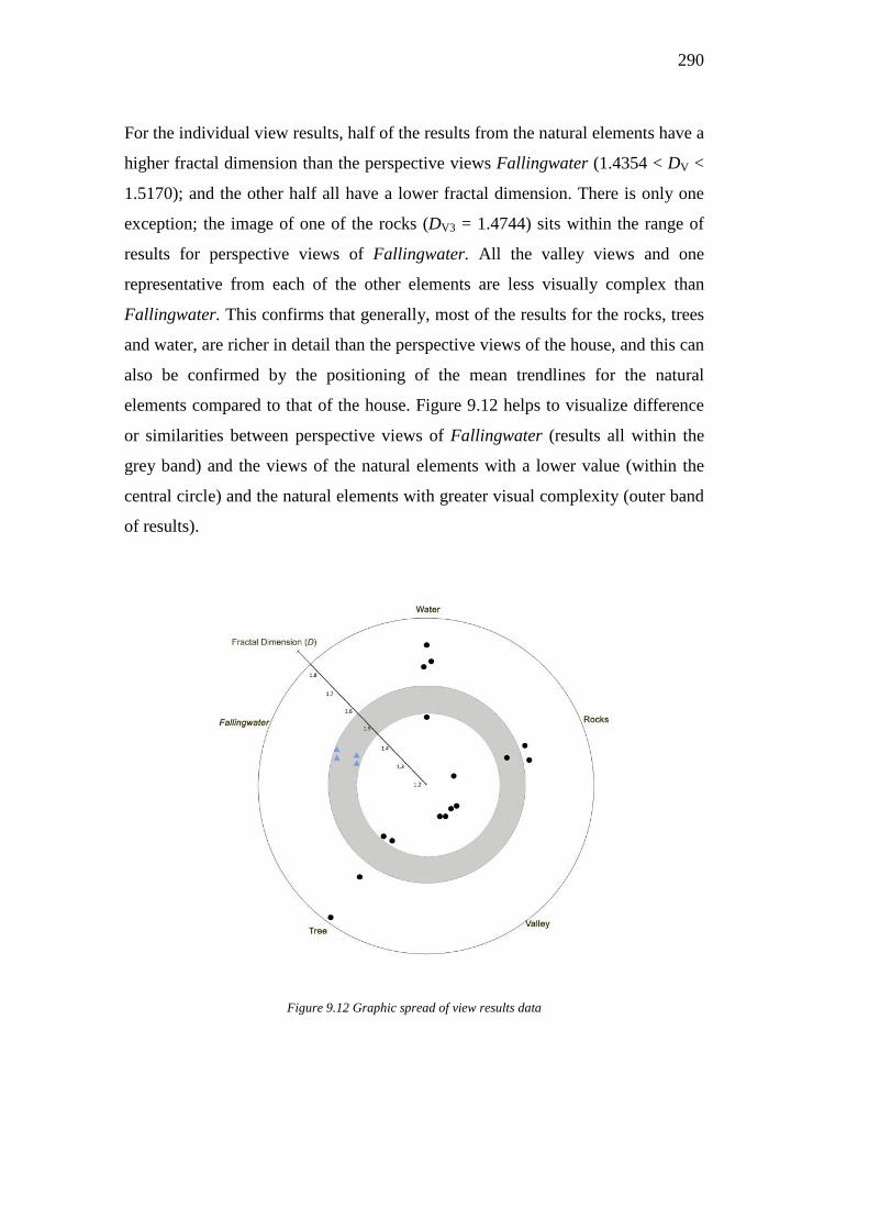
290

For the individual view results, half of the results from the natural elements have a

higher fractal dimension than the perspective views Fallingwater (1.4354 < DV <

1.5170); and the other half all have a lower fractal dimension. There is only one

exception; the image of one of the rocks (DV3 = 1.4744) sits within the range of

results for perspective views of Fallingwater. All the valley views and one

representative from each of the other elements are less visually complex than

Fallingwater. This confirms that generally, most of the results for the rocks, trees

and water, are richer in detail than the perspective views of the house, and this can

also be confirmed by the positioning of the mean trendlines for the natural

elements compared to that of the house. Figure 9.12 helps to visualize difference

or similarities between perspective views of Fallingwater (results all within the

grey band) and the views of the natural elements with a lower value (within the

central circle) and the natural elements with greater visual complexity (outer band

of results).

Figure 9.12 Graphic spread of view results data

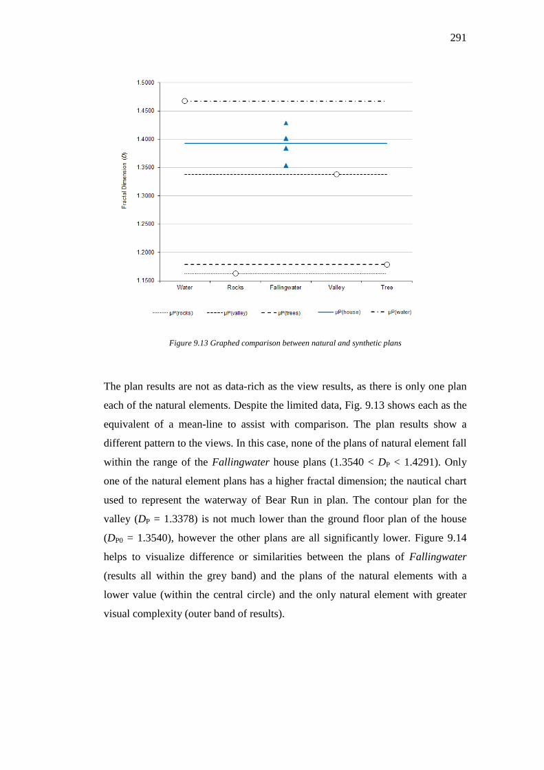
291

Figure 9.13 Graphed comparison between natural and synthetic plans

The plan results are not as data-rich as the view results, as there is only one plan

each of the natural elements. Despite the limited data, Fig. 9.13 shows each as the

equivalent of a mean-line to assist with comparison. The plan results show a

different pattern to the views. In this case, none of the plans of natural element fall

within the range of the Fallingwater house plans (1.3540 < DP < 1.4291). Only

one of the natural element plans has a higher fractal dimension; the nautical chart

used to represent the waterway of Bear Run in plan. The contour plan for the

valley (DP = 1.3378) is not much lower than the ground floor plan of the house

(DP0 = 1.3540), however the other plans are all significantly lower. Figure 9.14

helps to visualize difference or similarities between the plans of Fallingwater

(results all within the grey band) and the plans of the natural elements with a

lower value (within the central circle) and the only natural element with greater

visual complexity (outer band of results).

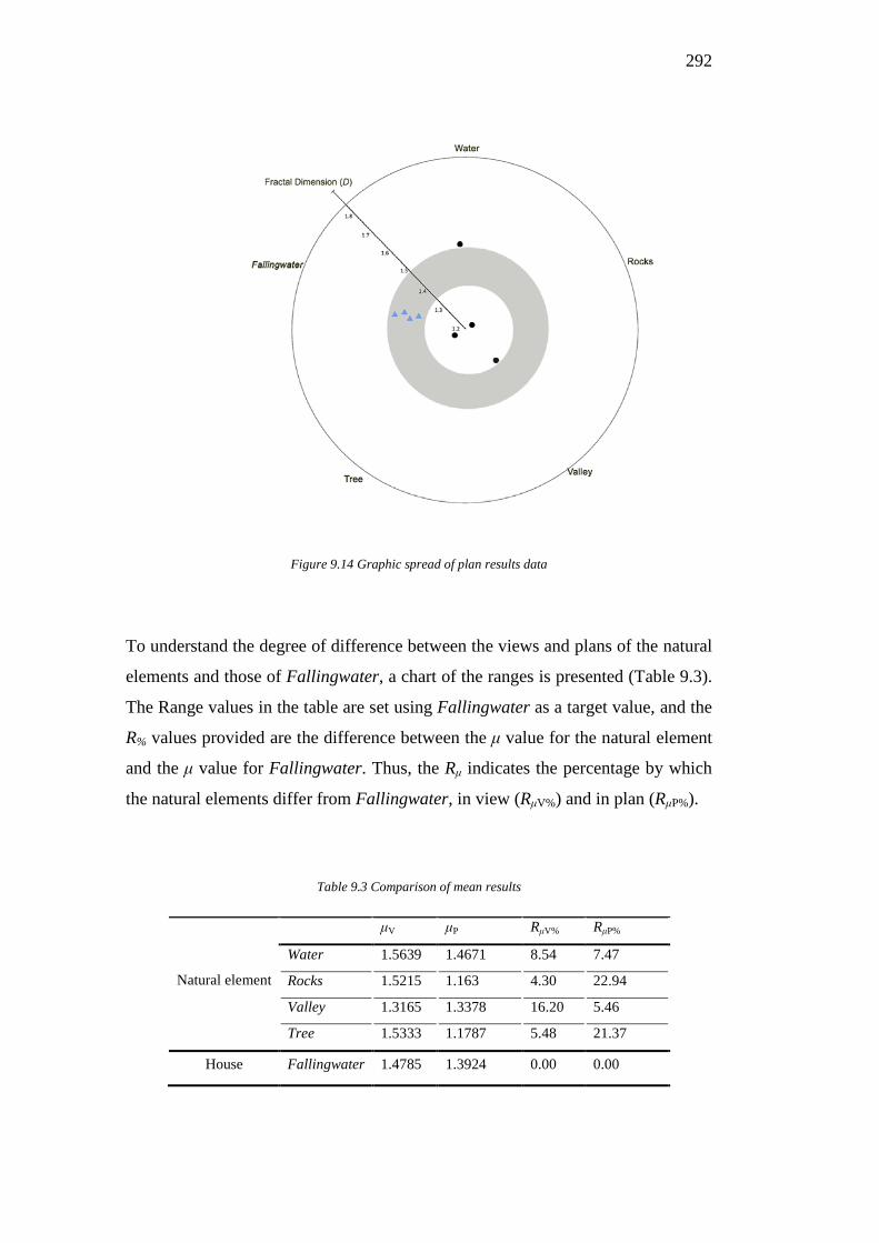
292

Figure 9.14 Graphic spread of plan results data

To understand the degree of difference between the views and plans of the natural

elements and those of Fallingwater, a chart of the ranges is presented (Table 9.3).

The Range values in the table are set using Fallingwater as a target value, and the

R% values provided are the difference between the μ value for the natural element

and the μ value for Fallingwater. Thus, the Rμ indicates the percentage by which

the natural elements differ from Fallingwater, in view (RμV%) and in plan (RμP%).

Table 9.3 Comparison of mean results

Natural element

μV μP RμV% RμP%

Water 1.5639 1.4671 8.54 7.47

Rocks 1.5215 1.163 4.30 22.94

Valley 1.3165 1.3378 16.20 5.46

Tree 1.5333 1.1787 5.48 21.37

House Fallingwater 1.4785 1.3924 0.00 0.00

293

Notwithstanding the statistical problem with several of the means discussed

previously, if we accept them as reasonable reflections of the data they are

developed from, then two of the views and one of the plans of the natural

elements could be considered to be “very similar” to those of the house. These are

the view sets of the rocks (RμV%= 4.30) and the trees (RμV%= 5.48), and the

contour plan of the valley (RμP% = 5.46). In both view (RμV%= 8.54) and plan (RμP%

= 7.47), the water can be considered broadly “similar” to Fallingwater, which

seems fitting considering the name of the house and the significance Wright

accorded Bear Run in the design (Wright 1938; Cleary 1999; Levine 2000). The

complexity of the valley views are possibly “comparable” to the house views

(RμV%= 16.20); however the plans of the rocks and trees cannot justifiably be

compared to the plans of Fallingwater, as they are visually “unrelated” (RμP% =

22.94, RμP% = 21.37). However, as very few of the mean results are for data sets

with low standard deviations, such an interpretation would be simplistic. Indeed,

of the 15 natural analogue views, only one is within the same range as the views

of Fallingwater and of the four natural plan views, none are within the same range

as the plans of Fallingwater.

Conclusion

The proposal that the form of Fallingwater strongly reflects its natural setting is a

claim made by many scholars but it is certainly not universally accepted. Using

fractal dimension analysis, this chapter measures the visual complexity of

Fallingwater and of several parts of its natural setting, to see if there is evidence

for, or against, this famous argument. While this may be the primary goal of the

chapter, it is also effectively a test of the method itself, and for this reason, the

results cannot be used to emphatically provide an end to this debate.

294

This chapter adapts the method used previously in Chapter 8 by determining the

fractal dimension of perspectives and modified plans of Fallingwater and

comparing them to fractal dimensions of views and plans of four natural elements

found in the landscape at Fallingwater (rocks, trees, water and the valley). This is

not the first time that architecture has been compared with nature in a fractal

analysis study. The most recent, detailed study on the effectiveness of

comparisons made between architecture and nature (Vaughan and Ostwald 2010)

measured the difference between the highest and lowest values of three

supposedly similar images identified by Bovill: one set of elevations, one site plan

and one image of a mountain. The resulting ‘gap’, of 28.5% was identified by

Bovill (1996) as indicating a degree of similarity between natural and synthetic

forms. However, the later analysis of Bovill’s claims (Vaughan and Ostwald

2010) found that this ‘gap’ (from highest to lowest result) not only implies a

dissimilar relationship but that a comparison of the range between mean values,

for a larger data set, would be more meaningful. Indeed, if we adopt Bovill’s

approach to calculating the nature-to-architecture gap for the entire set of data

used in the present chapter, it would be 56%. While this figure seems to

completely quash any argument that the forms of Fallingwater are visually similar

to those of its natural setting, a comparison constructed solely around outliers in a

set of data (the highest and lowest values) ignores most of the properties of the

complete set. Furthermore, Bovill’s (1996) gap approach to comparing nature and

architecture using fractal dimensions was always presented as a suggestion, which

should be tested and developed, to illustrate potential uses of the box-counting

method in architecture.

This present chapter is the first to develop Bovill’s original suggestions about

comparing nature and architecture, using a more rigorous (although still

imperfect) approach. This chapter uses more examples (of nature and architecture)

leading to more data and the capacity to use some basic statistical approaches. A

more detailed and consistent rationale is also used for the selection process for

identifying appropriate images (for testing specific claims about Wright and

Fallingwater). However, despite the larger volume of data, and the more carefully

295

chosen sets, a perfect result was never anticipated. Thus, when the data is

examined and compared in methodologically corresponding sets—as the present

chapter does—a better measure of difference is produced, but it is still not

compelling. Certainly, when the methods derived from this thesis are applied to

specific sets of images for correlation studies, the % range between the building

and nature is reduced to between 5.46% < R < 22.94%, which is an improvement

over earlier approaches, although it can still not offer a definitive proof of either

of the conflicting positions taken by Wright scholars to the relationship between

Fallingwater and its setting. Nevertheless, within the limits of the method and the

images chosen, this chapter shows a varying degree of visual correlation between

Fallingwater and its natural setting. However, given the many scholars who are

adamant that Fallingwater is inextricably entwined with its landscape, it would be

expected that the results of this study would show that the house was

predominantly “indistinguishable” or at least “very similar” to the natural setting.

As such the hypothesis, as it is framed for testing using fractal dimensions, could

potentially be considered disproved.

296

Chapter 10

Conclusion

Typical approaches in the architectural scholarship of the last few decades include

interpretation, analysis and assessment of the architecture of Frank Lloyd Wright,

and these are equally pivotal to the present dissertation. While such approaches

have been used in the past to understand Wright’s architecture—many of which

are discussed herein—this dissertation takes a slightly different path, which offers

a new opportunity to interpret the architecture and philosophy of Frank Lloyd

Wright. New approaches of this type are especially significant, as Donald

Hoffmann observes, because ‘[t]o begin afresh with Wright is to reject the

accumulated burden of received opinion, all the academic theories that pretend to

explain his architecture from presumed methods and sources’ (1995: 85). For

example, Wright’s architecture could be examined through the lens of the Arts

and Crafts movement, or in terms of the manipulation of geometric grids, shape

grammars and three-dimensional Froebel blocks. Interpretations of Wright’s

architecture in terms of ‘archetypal memories or sophomoric Freudian symbols,

arcane literary illusions or even dreamlike condensations of motifs’ (Hoffmann

1995: 85) are also common. But to perpetuate these existing ideas, rather than to

pursue new approaches, is unlikely to break new ground or resolve existing

disagreements in Wrightian scholarship. As Hoffman argues, to ‘respond to each

of these theories would only compound the pedantry beyond which Wright never

fails to soar’ (1995: 85). Thus, the present dissertation does not propose new

theories for explaining Wright’s architecture, or generates forms which are akin to

Wright’s. Instead, it applies a unique system of measuring to Wright’s most

famous house, and uses this to test several conflicting views about its properties.

This house is Fallingwater—the remarkable structure Wright designed over a

rocky waterfall in a deeply forested valley of the Pennsylvanian wilderness. It has

been the subject of wide-reaching scholarly interest for the 80 years of its

existence, but of the many different interpretations of this house, there are two

297

proposals that are of interest for this dissertation. The first is the proposition that

Fallingwater is a unique design amongst Wright’s architecture, being unlike his

three major housing styles - Prairie, Textile-block and Usonian. The second is that

Fallingwater is a house that strongly reflects its natural setting.

In this dissertation these two propositions are examined on the basis of new

evidence which is developed using fractal dimensions. Fractal dimensional

analysis is a repeatable, quantitative method for measuring the characteristic

visual complexity of a subject. In this case, the subjects are the physical forms and

the visual details of buildings and natural objects. Because fractal dimensions of

(a) Fallingwater’s natural setting, (b) Fallingwater itself and (c) Wright’s

domestic architecture, can be separately determined and compared in any

configuration, fractal analysis has been selected as the computational method

which is most likely to contribute to resolving, or at least illuminating, the two

propositions.

These two propositions, raised by architectural critics, historians and theorists, are

reframed as hypotheses for the present dissertation.

• Hypothesis 1: That the formal and visual properties of Frank Lloyd

Wright’s Fallingwater are atypical of his early and mid-career housing

(1901-1955).

• Hypothesis 2: That the formal and visual properties of Frank Lloyd

Wright’s Fallingwater strongly reflect its natural setting.

The data and associated analysis for Hypothesis 1 are contained in Chapter 8,

while Chapter 9 covers Hypothesis 2. However, before summarising the key

findings of this research, it is important to reiterate the limitations of the method

and the approaches used.

Fractal analysis is a rigorous method which is accepted throughout the sciences,

but it can only provide information about the subject being analysed and even

then, its primary use is typically for constructing comparisons. A fractal

298

dimension is a statistical approximation of the spread of detail or geometric

information across an image. Fractal dimensions do not provide information about

any other visual properties such as proportion, composition or color.

The fractal analysis method has several known limitations which can affect the

accuracy of results. For example, as a method that uses mathematical algorithms

to analyse images, its outcomes can be greatly affected by the quality and

consistency of the data input sources. A consistent method for selecting images,

determining which data to include (levels of representation) and how to process

this data is therefore a necessity. Furthermore, there are inconsistencies in the

mathematical and statistical aspects of the box-counting method which are

described in detail in Chapter 5. These methodological limitations have been

addressed where possible through careful decisions about data sources and

processing methods. However they still do have an occasional impact on the

results, and where this occurs it is noted in the text. Furthermore, like any study

that interprets numerical data, the volume of data available shapes the accuracy of

the outcome, and this study was limited by the number of sources available. A

larger number of data sets (source images) for this study would have provided

greater surety in the results, and may have assisted in interpretation of results as

additional data points might display clustering patterns more clearly.

10.1 Results for Hypothesis 1

The fractal analysis method for architecture has been progressively developed and

refined over more than two decades (Bovill 1996). Significantly, this method—

while very recently used for the analysis of Frank Lloyd Wright’s architecture

(Ostwald and Vaughan 2016)—has never been used to calculate the visual

complexity of Fallingwater, ‘the most celebrated [building] of his entire career’

(Hoffmann 1995: 83). Using the fractal analysis method it is possible to construct

299

a numerical comparison between different periods in Wright’s domestic designs

and thereby test the first hypothesis.

To test Hypothesis 1, the characteristic complexity of all four elevations and four

plans of Fallingwater are measured. Then the same method is applied to plans and

elevations of 15 of Wright’s other houses, built between 1901 and 1955,

producing results for 58 elevations and 46 plans. These 15 houses include five

representatives each from three of Wright’s key stylistic periods, the Prairie,

Textile-block and Usonian periods. The results were sorted and tabulated into

different options for comparison—numerical comparisons using individual

results, mean dimensions and comparative ranges—between the 112 major and

over 1000 minor measures produced. This numerical information is then

interpreted in combination with past scholarly arguments about Wright’s work,

combining the quantitative and qualitative to produce a nuanced assessment of the

data.

The results for the first hypothesis show that, when compared to elevations of

other houses by Wright, Fallingwater’s elevations generally have lower formal

complexity than most of the other houses measured. Moreover, Fallingwater’s

mean elevation dimension is less complex than the means of all the other sets.

Despite these results, Fallingwater is very similar to the Usonian houses in terms

of the characteristic complexity of elevations. In plan form, Fallingwater typically

has a similar level of complexity to the majority of the other houses. For the mean

plan results, Fallingwater has higher complexity than the Usonian and Prairie

houses, and shares a similar level of complexity to the Textile-block homes. Thus,

within the limits of the method, the results indicate that the visual complexity of

Fallingwater is largely typical of Wright’s Prairie, Textile-block and Usonian

houses and indeed, that in terms of formal expression, it is broadly similar to the

latter group. Collectively these results suggest that Hypothesis 1 is false,

demonstrating that—within the parameters of this dissertation— Fallingwater is

visually similar to Wright’s Prairie, Textile-block and Usonian houses.

300

The indicators of a positive, neutral or negative result for the hypothesis are

described in Chapter 1. A positive result for Hypothesis 1 would be justified if the

compared sets have a high degree of difference. This would be indicated by the

mean elevation and plan values of Fallingwater and of each of the other stylistic

sets, having a higher range than 10% (x ≥ 11.0 %) when compared. However,

none of the mean values of any of the stylistic sets have a percentage difference

from Fallingwater that is over 10%, suggesting that Hypothesis 1 is false (Table

8.9). However, as outlined in Chapter 1, the answers to the hypotheses are not

necessarily a straightforward true/false dichotomy and we can further investigate

the data for indicators of a neutral or positive outcome. The indicator of an

intermediate or neutral result would be a range that is 10% or less (x < 11.0%), but

greater than 5% (x ≥ 6.0 %). For the mean elevation results, the Prairie and

Textile-block houses all have a percentage difference from Fallingwater’s mean

elevations that match this neutral outcome, while the Usonian meets this result in

plan. The rest of the results—the Prairie and Textile-block house plans and the

Usonian elevations—are all so similar to Fallingwater (x < 6.0%) that they

emphatically show that Hypothesis 1 is false.

10.2 Results for Hypothesis 2

While the box-counting method of fractal analysis has been widely used to

measure architecture, and separately to analyse natural elements and systems, the

use of fractal analysis to compare architecture and nature has only rarely been

attempted (Bovill 1996; Lorenz 2003; Vaughan and Ostwald 2010; Bourchestein

et al 2014). However, to determine if the form of Fallingwater is similar to that of

its surrounding natural setting—and thus provide an answer to the second

hypothesis—a variation to the architectural approach has been created. This

methodological variation relies on a rationale or framework for selecting images

for comparison. Thus, prior to testing Hypothesis 2, a literature review of

Wright’s philosophy of nature and architecture was carried out, and possible

301

source images were investigated, until finally sixteen edge-detected drawings of

views of natural elements and four plans derived from the original site surveys of

the location, and four perspective views and four simplified plans of Fallingwater

house were identified as appropriate. The views of the natural elements were

extracted from photographs of Fallingwater’s setting, including its rocks, trees,

water and the valley itself. Despite the underlying image-selection framework

being consistently applied, it must be acknowledged that the final images used

represent only a small number of the myriad of potential natural images available

for this purpose. As such, they have been chosen to test arguments about the

formal relationship between nature and Fallingwater and they are not necessarily

perfect to test some other claims.

With the images selected and prepared, the second hypothesis was tested by

comparing the fractal dimension measures for the sets of images of Fallingwater

to the measures derived from sets of images of the natural elements. The results

were tabled and sorted into different options for comparison—numerical

correlations using individual results, mean dimensions and comparative ranges—

between the 28 major data points and approximately 300 minor data points. As it

was for the first hypothesis, this numerical information was then examined in

combination with past scholarly interpretations of Wright’s approach to nature

and architecture, particularly in the case of Fallingwater, combining quantitative

and qualitative to produce a meaningful reading of the data.

To determine the outcome for Hypothesis 2, the indicators presented in Chapter 1

are used. A positive result for Hypothesis 2 could be justified if the sets of natural

elements—when compared with Fallingwater—have a low degree of difference.

This would be indicated as a positive result if the mean elevation and plan have

lower range values than 5% (x < 6.0%) when compared. A negative outcome

would be indicated if the results were higher than 10% (x ≥ 11.0%), and a neutral

result would be between the two extremities (6.0% ≤ x < 11.0%). The results for

the test of the second hypothesis (Table 9.3) are less straightforward than the

results for Hypothesis 1. The mean elevations for the rocks and the trees, and the

302

plan of the valley, all have a percentage difference under 6.0%, meaning that

Hypothesis 2 could be considered valid in these cases. However contrary to this,

the plans of the rocks and trees and the elevations of the valley all have a

percentage difference from the Fallingwater results by over 10%, so that these

sets suggest Hypothesis 2 to be false. Both the results of the elevations and plan

for the water lie between these ranges, providing an intermediate, or neutral

response to Hypothesis 2 for the comparison between the house and the water.

These results do suggest—within the limits of the method and the images

chosen—a level of similarity between the forms of Fallingwater and some of

those found in its natural setting. However, given the many scholars who are

adamant that Fallingwater is an example of Wright’s aim ‘to achieve an

indivisible bond’ between architecture and landscape (De Long 1996: 120), it

would be expected that the results of this study would show that the house was

predominantly “indistinguishable” or at least “very similar” to the natural setting,

with the hypothesis outcomes being predominantly true, perhaps minimally

neutral and with no false response. Instead, the results show a more mixed or

neutral result, and as such the second hypothesis, as it is framed for testing using

fractal dimensions, could potentially be considered false and indicate that the

formal and visual properties of Fallingwater do not reflect its natural setting.

10.3 Other Observations Arising from the Research

In addition to testing the two hypotheses, the present dissertation also uncovers

some interesting aspects of Wright’s approach to design. For example, it can be

seen from the literature that there is a consistent thread wherein Wright refers to

‘nature’, throughout his lifetime. While this is not a new observation, on

examining the terminology that Wright uses to describe ‘nature’, it is clear that

he—whether consciously or not—took one particular approach to nature, which

he regarded in ‘almost mystical terms’ (Pfeiffer 2004: 12) and another to

303

landscape, which he referred to as the physical ‘features or pattern’ of the natural

world (Spirn 2000b: 15). Wright’s clear distinction between nature and landscape

is rarely mentioned in the scholarship, although it provides a valuable point of

departure from which to study Wright’s approach to landscape and natural

forms—being tangible subjects which can be analysed using fractal analysis—

rather than the more spiritual aspects of nature.

A detailed examination of literature describing Wright’s own views (and scholarly

arguments) about the relationship between design and landscape resulted in

further findings. The first of these is the identification of a set of eleven

interconnected and recurring strategies that Wright frequently employed to

connect his architecture to the landscape. These eleven strategies are composed of

five site strategies—site interpretation, locality character, site characteristics,

landscape alterations and site intensification—and six design strategies—

approach to the ground, the formal mass of the building, the roof, the openings,

any intersections with natural features of the location and the material palette.

These approaches, which Wright took when integrating a building with its setting,

are used in the present research to investigate claims about Fallingwater. This

application revealed further information about Wright’s design process and all but

two of the strategies were found to be used in Fallingwater. A summary of how

these strategies were (or were not) applied by Wright at Fallingwater is presented

at the end of Chapter 2. In addition to these summaries, the dissertation proposes a

reading of how much (or little) each strategy is demonstrated at Fallingwater.

Significantly, while some examples of strategies that Wright used to connect

Fallingwater and the landscape can be verified by observation of either the

building itself or architectural drawings, the majority are not measurable using

any means. Only one strategy, ‘site characteristics’, was found to be measurable

using fractal dimensions (or is likely to be measurable using any computational

means). Pinpointing this strategy was useful because it identified the natural

elements in the landscape surrounding Fallingwater, the water, the rocks, trees

and the valley, as suitable subjects for comparison with Fallingwater in order to

test Hypothesis 2.

304

A further observation was made in Part III, as a result of calculating the fractal

dimensions of the 15 other houses by Wright. The mathematical analysis of visual

complexity of 15 of Wright’s domestic designs shows that—despite some stylistic

differences—there is a notable degree of visual consistency across Wright’s

housing designs (the largest variation being 6.4%), an outcome that supports the

arguments of a several historians (Hoffman 1995; McCarter 1999; Frampton

2005). For the mean elevation data, the Prairie and Textile-block houses have an

almost identical fractal dimension, and the Usonian result is only slightly lower.

In plan form, Wright appears to have gone full circle in terms of spatial

complexity over time, starting from the Prairie style then increasing in the Textile-

block houses, before returning to the lower levels in the Usonian houses.

Comparing the aggregate results of the three periods of Wright’s architecture, the

Textile-block buildings are generally the most complex, the Usonians are the least

and the Prairie houses are midway between the two.

10.4 Future Research

Both hypotheses in this dissertation signal opportunities for further research.

Firstly, the mathematical methods presented in this chapter for the first

hypothesis, along with the comprehensive data for 16 houses, can be used to assist

historians and design scholars to ground their analysis of Wright’s architecture

and to promote future, more detailed computational analysis of historic buildings.

The second hypothesis also offers new research opportunities. With an increased

sample size in a comparative nature-architecture study, more statistically reliable

and robust results could be gained. Although, there is no guarantee that including

additional cases in the analysis will produce a better outcome, it might allow a

higher degree of confidence in the results to be developed.

305

There are also many potential future research topics which involve comparing

natural and architectural forms. Starting with Wright, some of his other houses

and their settings could be tested. For example, the Robie house could be

compared with the Prairie landscape surrounding Chicago in the early 1900’s. As

well as historic buildings, more recent designs (or unbuilt proposals) could be

studied using this method. Environmentally sustainable design theories often

involve claims that such buildings should ‘fit’ within the landscape. Developing

this method further might result in a process to assist with determining whether a

building is a sympathetic (meaning visually similar) addition to a landscape or

offers a point of contrast or juxtaposition.

Conclusion

Hoffman argues that Wright’s ‘words need to be sifted and weighted with care,

sifted again and always tested again against the evidence of the eye’ (1995: ix). It

is only through the careful application of such a rigorous form of visual

examination that researchers ‘will help to identify the principles that gave

[Wright’s] architecture not only its extraordinary vigor of structure and form,

expression and meaning, but its surprising continuity’ (Hoffmann 1995: x).

Taking Hoffmann’s advice, this dissertation has studied the work of Frank Lloyd

Wright, applying a combination of approaches, based around the quantitative

method of fractal analysis. The limitations of this method mean that the

interpretations of the data are neither definitive nor irrefutable. The data, Wright’s

words, his designs and the arguments of various scholars, can be thought of as a

guide. When combined and approached in different ways they offer a new way of

interpreting the architecture and theory of Frank Lloyd Wright.

Ultimately, this dissertation provides new information and resources that not only

contribute to our understanding of Frank Lloyd Wright’s architecture and design

306

theory, but also to the understanding of a unique house. The dissertation

summarises the strategies Wright used to connect Fallingwater with its setting,

providing data on the visual complexity of its plans, elevations and perspectives

along with views and plans of its setting. Historical and scholarly inputs suggested

that Fallingwater would be different from Wright’s other houses and be strongly

connected to the site, however the outcomes of the hypotheses did not support

these expectations. In conclusion, this dissertation echoes Hoffmann’s words, that

‘[t]he house on Bear Run defied every expectation […] In short, Fallingwater

flouted all the rules’ (Hoffmann 1995: 85).

307

End Matter

308

Bibliography

Aguar, Charles E, and Berdeana Aguar. 2002. Wrightscapes: Frank Lloyd

Wright’s landscape designs. New York: McGraw-Hill.

Alber, Markus, and Joachim Peinke. 1998. Improved multifractal box-counting

algorithm, virtual phase transitions, and negative dimensions.

Physical Review E 57: 5489–5493.

Allen, Stan. 2009. Practice: architecture, technique + representation. London:

Routledge.

Alofsin, Anthony. 1994. Frank Lloyd Wright and Modernism. In Frank Lloyd

Wright, architect, ed. Terence Riley, Anthony Alofsin, Museum of

Modern Art (New York), and Frank Lloyd Wright Foundation, 32–

57. New York: Museum of Modern Art.

Alofsin, Anthony. 2004. Wright, influence, and the world at large. In American

architectural history: a contemporary reader, ed. Keith Eggener,

281-293. New York: Routledge.

Andropogon Associates. Ltd. 1997. Interpretation and management plan for the

landscape of Fallingwater. Western Pennsylvania Conservancy.

Antoniades, Anthony C. 1992. Poetics of Architecture: Theory of Design. New

York: John Wiley & Sons.

Asvestas, Pantelis, George Matsopoulos, and Konstantina Nikita. 2000.

Applications of fractal theory on medical data processing. In

Advanced Infrastructures for Future Healthcare, ed. A. Marsh, L.

Grandinetti, and T. Kauranne, 425–411. Amsterdam: IOS Press.

Aull, Charles E, and Robert Lowen. 2011. Handbook of the history of general

topology. London: Springer.

309

Barnsley, Michael F. 1988. Fractals everywhere. Boston: Academic Press.

Barros Filho, Mauro, and Fabiano Sobreira. 2005. Assessing texture pattern in

slum across scales: an unsupervised approach. CASA Working Papers 87.

Batty, Michael, and Paul Longley. 1994. Fractal Cities: A Geometry of Form and

Function. San Diego: Academic Press.

Bechhoefer, William. 1998. Surviving Tourism: Report from Amasya.

Preservation of the Vernacular Built Environment in Development

Projects 114. Working Paper Series.

Bechhoefer, William, and Marylin Appleby. 1997. Fractals, music and vernacular

architecture: An experiment in contextual design. Critical Methodologies

in the Study of Traditional Environments. 97: 1–33.

Bechhoefer, William, and Carl Bovill. 1994. Fractal analysis of traditional

housing in Amasya, Turkey. Traditional Dwellings and Settlements

Working Paper Series 61: 1–21.

Behbahani, Peiman A., Ning Gu, and Michael J. Ostwald. 2014. Comparing the

properties of different space syntax techniques for analysing interiors. In

Across: Architectural Research through to Practice: 48th International

Conference of the Architectural Science Association 2014, ed. Francesca

Madeo and Marc Aurel Schnabel, 683–694. Genoa: The

Architectural Science Association & Genova University Press.

Behbahani, Peiman Amini, Michael J. Ostwald, and Ning Gu. 2016. A syntactical

comparative analysis of the spatial properties of Prairie style and

Victorian domestic architecture. The Journal of Architecture 21: 348–

374.

Benguigui, Lucien, Daniel Czamanski, Maria Marinov, and Yuval Portugali.

2000. When and where is a city fractal? Environment and Planning B:

Planning and Design 27: 507 – 519.

310

Ben-Hamouche, Mustapha. 2009. Can chaos theory explain complexity in urban

fabric? Applications in traditional muslim settlements. Nexus Network

Journal 11: 217–242.

Blenkinsop, Tom G, and David J Sanderson. 1999. Are gold deposits in the crust

fractals? A study of gold mines in the Zimbabwe craton. Geological

Society, London, Special Publications 155: 141–151.

Bourchtein, Andrei, Ludmila Bourchtein, and Natalia Naoumova. 2014. On

Fractal Complexity of Built and Natural Landscapes. In Computational

Science and Its Applications – ICCSA 2014, ed. Beniamino Murgante,

Sanjay Misra, Ana Maria A. C. Rocha, Carmelo Torre, Jorge Gustavo

Rocha, Maria Irene Falcão, David Taniar, Bernady O. Apduhan, and

Osvaldo Gervasi, 437–452. Lecture Notes in Computer Science 8580:

Springer International Publishing.

Boldt, Douglas. 2002. Fractal architecture: shaping a new century. Friends of

Kebyar 20.1: 4–16.

Bovill, Carl. 1996. Fractal geometry in architecture and design. Design Science

Collection. Boston: Birkhäuser.

Bovill, Carl. 2009. The Doric order as a fractal. In Nexus Network Journal, ed.

Stephen R. Wassell and Kim Williams, 10:283–289. Basel: Birkhäuser

Basel.

Bowles, Marlin, and Michael Jones. 2007. The Prairie-wetland vegetation

continuum in the Chicago region of Northeastern Illinois. Ecological

Restoration 25: 29–39.

Brown, Clifford T., and Walter R.T. Witschey. 2003. The fractal geometry of

ancient Maya settlement. Journal of Archaeological Science 30: 1619–

1632.

Brown, Clifford.T., Walter R.T. Witschey, and Larry .S. Liebovitch. 2005. The

broken past: Fractals in archaeology. Journal of Archaeological Method

and Theory 12: 37–78.

311

Buczkowski, Stéphane, Soula Kyriacos, Fahima Nekka, and Louis Cartilier. 1998.

The modified box-counting method: Analysis of some characteristic

parameters. Pattern Recognition 31: 411–418.

Burkle-Elizondo, Gerardo. 2001. Fractal geometry in Mesoamerica. Symmetry:

Culture and Science 12: 201–214.

Burkle-Elizondo, Gerardo, and Ricardo David Valdez-Cepeda. 2001. Do the

Mesoamerican artistic and architectural works have fractal dimension? In

Emergent Nature: Patterns, Growth and Scaling in the Sciences, ed.

Miroslav Michal Novak, 431–432. Singapore: World Scientific.

Burkle-Elizondo, Gerardo, and Ricardo David Valdez-Cepeda. 2006. Fractal

analysis of Mesoamerican pyramids. Nonlinear Dynamics, Psychology,

and Life Sciences 10: 105–122.

Cagdas, Gulen, Gaye Gozubuyuk, and Ozgur Ediz. 2005. Fractal based generative

design for harmony between old and new. In Generative Art 2005:

Proceedings of 8th Generative Art conference, ed. Celeste Soddu, 150–

159. Milan: Domus Argenia.

Camastra, Francesco. 2003. Data dimensionality estimation methods: a survey.

Pattern Recognition 36: 2945–2954.

Canty, Donald. 2004. Origins, evolutions, and ironies. In The Sea Ranch, ed.

Donlyn Lyndon and James Alinder. New York: Princeton Architectural

Press.

Capo, Daniele. 2004. The fractal nature of the architectural orders. Nexus Network

Journal 6: 30–40.

Cardillo, Alessio, Salvatore Scellato, Vito Latora, and Sergio Porta. 2006.

Structural properties of planar graphs of urban street patterns. Physical

Review. E, Statistical, Nonlinear, and Soft Matter Physics 73: 066107.

312

Chalup, Stephan, Naomi Henderson, Michael J Ostwald, and Lukasz Wiklendt.

2008. A method for cityscape analysis by determining the fractal

dimension of its skyline. In Innovation Inspiration and Instruction: New

Knowledge in the Architectural Sciences., ed. Ning Gu, Lehman Figen

Gul, Michael J. Ostwald, and Anthony Williams, 337–344. Newcastle,

NSW, Australia.

Chalup, Stephan, Naomi Henderson, Michael J Ostwald, and Lukasz Wiklendt.

2009. Box-counting dimension analysis of edge images detected with

classical edge detector. Architectural Science Review 52: 126–134.

Chen, Susan S., James M. Keller, and Richard M. Crownover. 1993. On the

calculation of fractal features from images. IEEE, Transactions on

Pattern Analysis and Machine Intelligence 15: 1087–1090.

Chen, Wei, Xing-xin Chen, and Li Zhou. 2010. Box-counting dimension analysis

of edge images detected with classical edge detector. In 2010

International Conference on Measuring Technology and Mechatronics

Automation, 756–758. Changsha City, China.

Ching, Frank, Mark Jarzombek, and Vikramaditya Prakash. 2011. A global

history of architecture. Hoboken, N.J: Wiley.

Cleary, Richard Louis. 1999. Merchant prince and master builder: Edgar J.

Kaufmann and Frank Lloyd Wright. Pittsburgh: Heinz Architectural

Center.

Cooper, Jon. 2003. Fractal assessment of street-level skylines: A possible means

of assessing and comparing character. Urban Morphology 7: 73–82.

Cooper, Jon, and Reza Oskrochi. 2008. Fractal analysis of street vistas: A

potential tool for assessing levels of visual variety in everyday street

scenes. Environment and Planning B: Planning and Design 35: 349–363.

Cooper, Jon, David Watkinson, and Reza Oskrochi. 2010. Fractal analysis and

perception of visual quality in everyday street vistas. Environment and

Planning B: Planning and Design 37: 808–822.

313

Cooper, Jon, Mei-lin Su, and Reza Oskrochi. 2013. The influence of fractal

dimension and vegetation on the perceptions of streetscape quality

in Taipei: with comparative comments made in relation to two

British case studies. Environment and Planning B: Planning and

Design 40: 43 – 62.

Crompton, Andrew. 2001. The fractal nature of the everyday environment.

Environment and Planning B: Planning and Design 28: 243 – 254.

Crompton, Andrew. 2002. Fractals and picturesque composition. Environment

and Planning B: Planning and Design 29: 451 – 459.

Crompton, Andrew. 2012. The entropy of LEGO®. Environment and Planning B:

Planning and Design 39: 174 – 182.

Crompton, Andrew, and Frank Brown. 2008. A statistical examination of visual

depth in building elevations. Environment and Planning B:

Planning and Design 35: 337 – 348.

Cronon, William. 1994. Inconstant unity: The passion of Frank Lloyd Wright. In

Frank Lloyd Wright Architect, ed. Terence Riley and Peter Reed,

8–31. New York: Museum of Modern Art.

Da Silva, David, Frédéric Boudon, Christophe Godin, Olivier Puech, Colin Smith,

and Hervé Sinoquet. 2006. A critical appraisal of the box counting

method to assess the fractal dimension of tree crowns. Lecture

Notes in Computer Science 4291: 751–760.

Dawes, Michael J, and Michael J Ostwald. 2014. Prospect-Refuge theory and the

textile-block houses of Frank Lloyd Wright: An analysis of spatio-

visual characteristics using isovists. Building and Environment 80:

228–240.

Dawes, Michael , and Michael J. Ostwald. 2015. Testing the Wright Space: Using

isovists to analyse Prospect-Refuge characteristics in Usonian

architecture. The Journal of Architecture. 19, 645-666

Debailleux, Laurent. 2010. Complementary approach for vernacular wooden

frame structures reconstruction. In Digital Heritage, 441–449.

Springer.

314

De Jonge, Krista, and Koen Van Balen, ed. 2002. Preparatory architectural

investigation in the restoration of historical buildings. Leuven:

Leuven University Press.

De Long, David Gilson, ed. 1996. Frank Lloyd Wright: Designs for an American

landscape, 1922-1932. New York: Harry N. Abrams.

De Vico, G, V Peretti, and GA Losa. 2009. Fractal organization of feline oocyte

cytoplasm. European Journal of Histochemistry 49: 151–156.

Drexler, Arthur. 1965. The drawings of Frank Lloyd Wright. New York:

Published for the Museum of Modern Art by Horizon Press.

Eaton, Leonard. 1998. Fractal geometry in the late work of Frank Lloyd Wright.

In Nexus II: Architecture and Mathematics, ed. Kim Williams, 23–

38. Fucecchio: Edizioni dell’Erba.

Edgar, Derald. 2008. Measure, topology, and fractal geometry. New York:

Springer.

Ediz, Özgür, and Michael J. Ostwald. 2012. The Süleymaniye Mosque: a

computational fractal analysis of visual complexity and layering in

Sinan’s masterwork. arq: Architectural Research Quarterly 16:

171–182.

Eglash, Ron. 1999. African fractals: modern computing and indigenous design.

New Brunswick: Rutgers University Press.

Eilenberger, Gert. 1986. Freedom, science, and aesthetics. In The beauty of

fractals, ed. Heinz-Otto Peitgen and Peter H. Richter, 175–180.

New York: Springer-Verlag.

Eisenman, Peter. 1993. Folding in time. Architectural design profile: Folding in

architecture 102: 22–25.

Eiteljorg, Harrison. 2002. How should we measure an ancient structure? Nexus

Network Journal 4: 14–20.

Emerson, Sheila. 1991. The authorisation of form: Ruskin and the science of

chaos. In chaos and order: Complex dynamics in Literature and

Science, ed. Katherine N. Hayles, 149–166. Chicago: University of

Chicago Press.

315

Encarnação, Sara, Marcos Gaudiano, Francisco C. Santos, José A. Tenedório, and

Jorge M. Pacheco. 2012. Fractal cartography of urban areas.

Scientific Reports 2: 527.

Fallacara, Giuseppe, and Ubaldo Occhinegro, ed. 2015. Castel del Monte: Inedite

indagini scientifiche. Atti del primo convegno 18-19 Giugno 2015.

Rome: Gangemi Editore

Farmer, John, and Kenneth Richardson. 1996. Green shift: towards a green

sensibility in architecture. Boston: Butterworth-Heinemann.

Feder, Jens. 1988. Fractals. New York: Plenum Press.

Fell, Derek. 2009. The gardens of Frank Lloyd Wright. London: Frances Lincoln.

Ferrero, Giovanni, Celestina Cotti, Michela Rossi, and Cecilia Tedeschi. 2009.

Geometries of imaginary space: Architectural developments of the

ideas of M. C. Escher and Buckminster Fuller. Nexus Network

Journal 11: 305–316.

Foroutan-pour, Kayhan., Pierre Dutilleul, and Donald L. Smith. 1999. Advances

in the implementation of the box-counting method of fractal

dimension estimation. Applied Mathematical. Computing 105:

195–210.

Foucault, Michel. 1970. The Order of things: an archaeology of the human

sciences. London: Routledge.

Frankhauser, Pierre. 2008. Fractal geometry for measuring and modelling urban

patterns. In The dynamics of complex urban systems, ed. Sergio

Albeverio, Denise Andrey, Paolo Giordano, and Alberto Vancheri,

213–243. Heidelberg: Physica-Verlag HD.

Frascari, Marco, and Livio Volpi Ghirardini. 1998. Contra Divinam Proportion. In

Nexus II: Architecture and Mathematics., ed. Kim Williams, 65–

74. Florence: Edizioni dell’Erba.

Frampton, Kenneth. 2005. The text-tile tectonic. In On and by Frank Lloyd

Wright: A primer of architectural principles. ed. Robert McCarter,

170–189. London: Phaidon.

316

Frazier, Nancy. 1995. Foreward. In Frank Lloyd Wright: Early visions, vii–x.

New York: Gramercy Books.

Fuller, Peter. 1987. Towards a new nature for the gothic. In Art and Design

Profile: The Post Modern Object, ed. Andreas Papadakis, 5–10.

Cambridge: Harvard University Press.

Futagawa, Yukio, and Bruce Brooks Pfeiffer. 1984. Frank Lloyd Wright

monograph 1942-1950. Vol. 7. Tokyo: A.D.A. Edita.

Futagawa, Yukio, and Bruce Brooks Pfeiffer. 1985a. Frank Lloyd Wright

monograph 1914-1923. Vol. 4. Tokyo: A.D.A. Edita.

Futagawa, Yukio, and Bruce Brooks Pfeiffer. 1985b. Frank Lloyd Wright

monograph 1924-1936. Vol. 5. Tokyo: A.D.A. Edita.

Futagawa, Yukio, and Bruce Brooks Pfeiffer. 1985c. Frank Lloyd Wright

monograph 1951-1959. Vol. 8. Tokyo: A.D.A. Edita.

Futagawa, Yukio, and Bruce Brooks Pfeiffer. 1986. Frank Lloyd Wright

monograph. 1937-1941. Vol 6. Tokyo: ADA.

Futagawa, Yukio, and Bruce Brooks Pfeiffer. 1987a. Frank Lloyd Wright

monograph 1887-1901. Vol. 1. Tokyo: A.D.A. Edita.

Futagawa, Yukio, and Bruce Brooks Pfeiffer. 1987b. Frank Lloyd Wright

monograph 1907-1913. Vol. 3. Tokyo: A.D.A. Edita.

Futagawa, Yukio, and Bruce Brooks Pfeiffer. 1987c. Frank Lloyd Wright

preliminary studies. Vol 11, 1933-1959. Tokyo: ADA Edita.

Futagawa, Yukio, and Bruce Brooks Pfeiffer 2009. Fallingwater. Tokyo: A.D.A.

Giedion, Sigfried. 1959. Space, time and architecture; the growth of a new

tradition. London: Oxford University Press.

Genevro, Rosalie. 2000. Preface. In Ten shades of green: an exhibition organized

by the Architectural League of New York, ed. Peter Buchanan, 4.

New York, NY: Architectural League of New York.

Gorski, A. Z, S. Drozdz, A. Mokrzycka, and J. Pawlik. 2012. Accuracy analysis

of the box-counting algorithm. Acta Physica Polonica A 121: B28–

B30.

317

Götze, Heinz. 1996. Friedrich II and the love of geometry. In Nexus: Architecture

and Mathematics, ed. Kim Williams. Florence: Edizioni dell’Erba.

Grau, Juan B., Valeriano Mendeza, Ana M. Tarquis, M. Cruz Diaz, and A Saab.

2006. Comparison of gliding box and box-counting methods in soil

image analysis. Geoderma 134: 349–359.

Green, Aaron G. 1988. Organic architecture: The principles of Frank Lloyd

Wright. In Frank Lloyd Wright in the Realm of Ideas, ed. Gerald

Nordland and Bruce Brooks Pfeiffer, 133–142. Carbondale:

Southern Illinois University Press.

Groat, Linda, and David Wang. 2002. Architectural research methods. New York:

John Wiley and Sons.

Hagan, Susannah. 2001. Taking shape: A new contract between architecture and

nature. Oxford: Architectural Press.

Hagerhall, Caroline M, Terry Purcell, and Richard P Taylor. 2004. Fractal

dimension of landscape silhouette outlines as a predictor of

landscape preference. Journal of Environmental Psychology 24:

247–255.

Halprin, Lawrence. 2002. The Sea-Ranch ...: Diary of an Idea. Berkeley, CA:

Spacemaker Press.

Harris, James. 2007. Integrated function systems and organic architecture from

Wright to Mondrian. Nexus Network Journal 9: 93–102.

Heath, Tom, Sandy G Smith, and Bill Lim. 2000. Tall buildings and the urban

skyline: The effect of visual complexity on preferences.

Environment and Behavior 32: 541–556.

Hersey, George L. 1999. The monumental impulse: Architecture’s biological

roots. Cambridge: The MIT Press.

Hertz, David Michael. 1993. Angels of reality. Carbondale: Southern Illonois

University Press.

Hess, Alan, and Alan Weintraub. 2006. Organic architecture: the other

modernism. Layton, Utah: Gibbs Smith.

318

Hess, Alan, and Alan Weintraub. 2012. Frank Lloyd Wright natural design:

Organic architecture : Lessons for building green from an

American original. New York: Rizzoli International Publications.

Hewitt, Mark. 1985. Representational forms and modes of conception: An

approach to the history of architectural drawing. Journal of

Architectural Education. 39: 2–9.

Hildebrand, Grant. 2007. Frank Lloyd Wright's Palmer house. Seattle: University

of Washington Press.

Hillier, Bill. 1996. Space is the machine. Cambridge: Cambridge University Press.

Hillier, Bill, and Julienne Hanson. 1984. The social logic of space. New York:

Cambridge University Press.

Hoesli, Bernhard. 2005. From the Prairie house to Fallingwater. In On and by

Frank Lloyd Wright: A primer of architectural principles, ed.

Robert McCarter, 204–215. London: Phaidon.

Hoffmann, Donald. 1993. Frank Lloyd Wright’s Fallingwater: The house and its

history. Dover Books on Architecture. New York: Dover

Publications.

Hoffmann, Donald. 1995. Understanding Frank Lloyd Wright’s architecture. New

York: Dover Publications.

Hoppen, Donald W. 1998. The seven ages of Frank Lloyd Wright: The creative

process. New York: Dover Publications.

Huang, Qian, Jacob R Lorch, and Richard C Dubes. 1994. Can the fractal

dimension of images be measured? Pattern Recognition 27: 339–

349.

Ingegnoli, Vittorio. 2013. Landscape ecology: A widening foundation. Springer

Science & Business Media.

Jelinek, Herbert F, Guy N. Elston, and B Zietsch. 2005. Fractal analysis: Pitfalls

and revelations in neuroscience. Fractals in biology and medicine

IV: 85–94.

319

Jencks, Charles. 1995. The architecture of the jumping universe: a polemic : how

complexity science is changing architecture and culture. London:

Academy Editions.

Jodidio, Philip. 2006. Architecture: Nature. Munich: Prestel.

Joedicke, Jurgen. 1997. Organic architecture. In The Thames and Hudson

dictionary of 20th-century architecture, Vittorio Magnago

Lampugnani, 253–255. London: Thames and Hudson.

Johnson, Eugene J. 1986. Charles Moore: Buildings and projects 1949-1986.

New York: Rizzoli.

Joye, Yannick. 2006. An interdisciplinary argument for natural morphologies in

architectural design. Environment and Planning B: Planning and

Design 33(2): 239–252.

Joye, Yannick. 2007. Fractal architecture could be good for you. Nexus Network

Journal 9: 311–320.

Joye, Yannick. 2011. A review of the presence and use of fractal geometry in

architectural design. Environment and Planning B: Planning and

Design 38: 814 – 828.

Juhos, Bela. 1976. Data of conciousness-logico-mathematical constructions-

methods of empirical content. In Selected Papers on Epistemology

and Physics, ed. Gerhard Frey. Boston: D. Reidel Publishing

Company.

Julia, Gaston. 1918. Memoire sur l’iteration des fonctions rationnelles. Journal de

Mathematica 7: 47–245.

Kahn, Louis Isadore, and Richard Saul Wurman. 1986. The notebooks and

drawings of Louis I. Kahn. Cambridge, Mass. ; London: M.I.T.

Press.

Kaufmann, Edgar. 1983. The house on the waterfall (1936/1962). In Writings on

Wright: Selected comment on Frank Lloyd Wright, ed. H. Allen

Brooks. Cambridge: MIT Press.

Kaufmann, Edgar. 1986. Fallingwater, a Frank Lloyd Wright country house.

New York: Abbeville Press.

320

Kaye, B H. 1989. A random walk through fractal dimensions. Cambridge: VCH

Publishers.

Keller, James M., Richard M. Crownover, and Robert Yu Chen. 1987.

Characteristics of natural scenes related to the fractal dimension.

IEEE Transactions on Pattern Analysis and Machine Intelligence,

PAMI-9: 621–627.

Kim, Kwang Sik, Lucien Benguigui, and Maria Marinov. 2003. The fractal

structure of Seoul’s public transportation system. Cities 20: 31–39.

Kipnis, Jeffrey. 1993. Towards a new architecture. Architectural Design Profile:

Folding in Architecture 102: 40–49.

Kitchley, Jinu Louishidha. 2003. Fractals in architecture. Architecture & design

20: 42–48.

Klinkowitz, Jerome. 2014. Frank Lloyd Wright and his manner of thought.

Madison, Wisconsin: The University of Wisconsin Press.

Knight, Terry Weissman. 1992. Designing with grammars. In Computer-aided

architectural design, ed. Gerhard N. Schmitt. 33-48. Wiesbaden:

Verlag Viewag

Knight, Terry Weissman. 1994. Transformations in design: A formal approach to

stylistic change and innovation in the visual arts. Cambridge:

Cambridge University Press.

Koch, Heinrich P. 1993. The concept of fractals in the pharmaceutical sciences.

Die Pharmazie 48: 643–659.

Koning, Hank, and Julie Eizenberg. 1981. The language of the prairie: Frank

Lloyd Wright’s prairie houses. Environment and Planning B:

Planning and Design 8: 295 – 323.

Kostof, Spiro. 1985. A history of architecture: Settings and rituals. New York:

Oxford University Press.

Kruger, Anton. 1996. Implementation of a fast box-counting algorithm. Computer

Physics Communications 98: 224–234.

Kubala, Thomas. 1990. Finding Sullivan’s thread. Progressive Architecture 71:

102–104.

321

Kuhlmann, Dorte. 2008. Old and new organicism in architecture: The

metamorphoses of an aesthetic idea. In On growth and form:

organic architecture and beyond, ed. Sarah Bonnemaison

and Philip Beesley. Halifax: TUNS Press.

Lampugnani, Vittorio Magnago. 1997b. Wright. In The Thames and Hudson

dictionary of 20th-century architecture, Vittorio Magnago

Lampugnani, 363–370. London: Thames and Hudson.

Langmead, Donald. 2009. Icons of American architecture: From the Alamo to the

World Trade Center. Westport: Greenwood Publishing Group.

Laseau, Paul, and James Tice. 1992. Frank Lloyd Wright: Between principle and

form. New York: Van Nostrand Reinhold.

Lee, Ju Hyun, Michael J. Ostwald and Ning Gu, 2017. A combined plan graph

and massing grammar approach to Frank Lloyd Wright’s Prairie

architecture. Nexus Network Journal. Feb: 1–21.

Leupen, Bernard, Christoph Grafe, Nicola Körnig Marc Lamp and Peter de

Zeeuw. 1997. Design and analysis. New York : Van Nostrand

Reinhold.

Levine, Neil. 1996. The architecture of Frank Lloyd Wright. Princeton, N.J.:

Princeton University Press.

Levine, Neil. 2000. The temporal dimension of Fallingwater. In Fallingwater and

Pittsburgh, ed. Narciso G. Menocal, 32–79. Carbondale: SIU

Press.

Levine, Neil.2005. Frank Lloyd Wright’s diagonal planning revisited. In On and

by Frank Lloyd Wright: A primer of architectural principles, edited

by Robert McCarter, 232–63. London: Phaidon.

Levine, Neil. 2008. Introduction. In Modern architecture being the Kahn lectures

for 1930, Frank Lloyd Wright Levine, Neil, ix–xxi. Princeton:

Princeton University Press.

Liang, Jiang, Yanqin Hu, and Hui Sun. 2013. The design evaluation of the green

space layout of urban squares based on fractal theory. Nexus

Network Journal 15: 33–49.

322

Li, Jian, Qian Du, and Caixin Sun. 2009. An improved box-counting method for

image fractal dimension estimation. Pattern Recognition 42: 2460–

2469.

Lind, Carla. 1996. Frank Lloyd Wright’s Fallingwater. San Francisco:

Pomegranate.

Lorenz, Wolfgang. 2003. Fractals and fractal architecture. Masters Diss. Vienna

University of Technology.

Lorenz, Wolfgang E. 2009. Fractal geometry of architecture: Implementation of

the box-counting method in a CAD-software. Computation: The

New Realm of Architectural Design [27th eCAADe Conference

Proceedings] Istanbul (Turkey) 16-19 September 2009, pp. 697-

704.

Lorenz, Wolfgang. 2011. Fractal geometry of architecture. In Biomimetics -

Materials, Structures and Processes: Examples, Ideas and Case

Studies, ed. Dietmar Bruckner, P. Gruber, C. Hellmich, H. B.

Schmiedmayer, H. Stachelberger, and I. C. Gebeshuber, 179–200.

Berlin: Springer.

Lorenz, Wolfgang. 2012. Estimating the fractal dimension of architecture: Using

two measurement methods implemented in AutoCAD by VBA. In

Digital Physicality - Proceedings of the 30th eCAADe Conference,

ed. Henri Achten, Jiri Pavlicak, Jaroslav Hulin, and Dana

Matejdan, 1:505–513. Prague: Czech Technical University in

Prague.

Lorenz, Wolfgang E. 2013. Combining complexity and harmony by the box-

counting method – A comparison between entrance façades of the

Pantheon in Rome and Il Redentore by Palladio. In Languages of

Design Vol 2: Computation and Performance. Proceedings of the

31st eCAADe Conference, ed. Rudi Stouffs and Sevil Sariyildiz.

667-676. Delft: The Netherlands: Delft University of Technology.

Lovejoy, Shaun. 1982. Area-perimeter relation for rain and cloud areas. Science

216. New Series: 185–187.

323

Lu, Yongmei, and Junmei Tang. 2004. Fractal dimension of a transportation

network and its relationship with urban growth: a study of the

Dallas - Fort Worth area. Environment and Planning B: Planning

and Design 31: 895 – 911.

Lucie-Smith, Edward. 2003. The Thames and Hudson dictionary of art terms.

New ed. World of Art. London: Thames & Hudson.

Luke, Timothy W. 1992. Shows of force: power, politics, and ideology in art

exhibitions. Durham: Duke University Press.

Lung, Chi-Wei, and Shou-Zhu Zhang. 1990. Fractal dimension of the fractured

surface of materials. In Fractals in Physics: Essays in Honour of

Benoit B. Mandelbrot. ed. Jens Feder and Amnon Aharony, 242–

245. Amsterdam: North-Holland.

Lyndon, Donlyn, and James Alinder. 2004. The Sea Ranch. New York: Princeton

Architectural Press.

MacCormac, Richard. 2005. Form and philosophy : Froebel’s kindergarten

training and Wright’s early work. In On and by Frank Lloyd

Wright: A Primer of Architectural Principles, ed. Robert McCarter,

124–143. London: Phaidon.

Maddex, Diane. 1998. 50 favourite rooms by Frank Lloyd Wright. London:

Thames & Hudson.

Makhzoumi, Jala, and Gloria Pungetti. 1999. Ecological landscape design and

planning: the Mediterranean context. New York: E&FN Spon.

Mandelbrot, Benoît B. 1975. Les objects fractals: forme, hasard et dimension.

Paris: Flammarion.

Mandelbrot, Benoit B. 1977. The fractal geometry of nature. New York: W.H.

Freeman.

Mandelbrot, Benoît B. 1982. The Fractal Geometry of Nature. Updated and

augmented. San Francisco: Freeman.

Manning, Henry Parker. 1956. Geometry of four dimensions. New York: Dover

Publications.

324

Martignoni, Jimena. 2008. Fractals of nature: the renovated Botanical Gardens of

Medellín meld with the city and play with natural forms.

Landscape architecture 98: 52.

Masucci, Paolo, Kiril Stanilov, and Michael Batty. 2012. Simple laws of urban

growth. arXiv:1206.5298.

McCarter, Robert. 1999. Frank Lloyd Wright. London: Phaidon

McCarter, Robert. 2002. Fallingwater. London: Phaidon

McCarter, Robert. 2004. Wright, Frank Lloyd 1867-1959. In Encyclopedia of 20th

century architecture, ed. R.Stephen Sennott, 1453. New York:

Fitzroy Dearborn.

McCarter, Robert, ed. 2005. On and by Frank Lloyd Wright: A Primer of

Architectural Principles. London: Phaidon.

Meckel, Lawrence D. 1967. Origin of Pottsville Conglomerates (Pennsylvanian)

in the Central Appalachians. Geological Society of America

Bulletin 78: 223–258.

Mehta, Geeta K, and Deanna MacDonald. 2011. New Japan architecture: recent

works by the world’s leading architects. Tokyo: Tuttle.

Meisel, Lawrence V., and Mark A. Johnson. 1997. Convergence of numerical

box-counting and correlation integral multifractal analysis

techniques. Pattern Recognition 30: 1565–1570.

Meehan, Patrick Joseph. 1984. The master architect: conversations with Frank

Lloyd Wright. New York: Wiley.

Menocal, Narciso G. 2000. Wright studies, volume two: Fallingwater and

Pittsburgh. Carbondale: Southern Illinois University Press.

Milton, Hans. 1994. Glossary of building terms. Sydney: NCRB, Standards

Australia and Suppliers Index.

Mizuno, Setsuko, and Hidekazu Kakei. 1990. Fractal analysis of street forms.

Journal of architecture, planning and environmental engineering 8:

103–108.

325

Miller, Perry. 2009. Errand into the wilderness. Cambridge: Harvard University

Press.

Moholy-Nagy, Sibyl. 1959. Frank Lloyd Wright’s testament. College Art Journal

18: 319–329.

Morse, D.R., J.H. Lawton, M.M. Dodson, and M.H. Williamson. 1985. Fractal

dimension of vegetation and the distribution of arthropod body

lengths. Nature 314: 731–733.

Mumford, Lewis. 1938. The Sky Line: at home, indoors and out. In Sidewalk

Critic: Lewis Mumford’s Writings on New York (1998), ed. Robert

Wojtowicz, 206-209. New York: Princeton Architectural Press.

Nakib, F. 2010. Fractal geometry: a tool for adaptability and ‘evolutionability.’ In

Eco-architecture III: Harmonisation Between Architecture and

Nature, ed. Santiago Hernández, C. Brebbia, and W. De Wilde,

39–47. Ashurst: WIT Press.

Nordland, Gerald. 1988. Introduction. In Frank Lloyd Wright in the Realm of

Ideas, ed. Bruce Brooks Pfeiffer and Gerald Nordland, 1–4.

Carbondale: Southern Illinois University Press.

Nute, Kevin. 2000. Frank Lloyd Wright and Japan: the role of traditional

Japanese art and architecture in the work of Frank Lloyd Wright.

London; New York: Routledge.

Nute, Kevin. 2008. Functional versus purposive in the Organic forms of Louis

Sullivan and Frank Lloyd Wright. In On growth and form: organic

architecture and beyond, ed. Sarah Bonnemaison and Philip

Beesley. Halifax: TUNS Press.

Oku, Toshinobu. 1990. On visual complexity on the urban skyline. Journal of

Planning, Architecture and Environmental Engineering 6: 61–71.

Oleschko, Klaudia, Rosa Brambila, Fernando Brambila, Jean-Francois Parrot, and

Pedro López. 2000. Fractal analysis of Teotihuacan, Mexico.

Journal of Archaeological Science 27: 1007–1016.

326

Olsberg, Nicholas. 1996. Introduction. In Frank Lloyd Wright: Designs for an

American Landscape, 1922-1932, ed. David Gilson De Long, 9–

13. New York: Harry N. Abrams.

Osmond, Paul. 2010. Hemispherical photography as a tool for urban sustainability

evaluation and design. SSRN Scholarly Paper ID 1676326.

Rochester, NY: Social Science Research Network.

Ostwald, Michael J. 1998. Fractal traces: Geometry and the architecture of Ushida

Findlay. In Ushida Findlay, Leon van Schaik, 136–143. Barcelona:

2G.

Ostwald, Michael J. 2000. Movements in Twentieth Century architecture: A

reader in architectural theory. Sydney: Archadia Press.

Ostwald, Michael J. 2001a. “Fractal architecture”: Late twentieth century

connections between architecture and fractal geometry. Nexus

Network Journal, Architecture and Mathematics 3: 73–84.

Ostwald, Michael J. 2003. Fractal architecture: The philosophical implications of

an iterative design process. Communciation and Cognition 36:

263–295.

Ostwald, Michael J. 2006. The Architecture of the New Baroque: A Comparative

Study of the Historic and New Baroque Movements in Architecture.

Singapore: Global Arts.

Ostwald, Michael J. 2011. Examining the relationship between topology and

geometry: a configurational analysis of the rural houses (1984-

2005) of Glenn Murcutt. The Journal of Space Syntax 2: 223–246.

Ostwald, Michael J. 2013. The fractal analysis of architecture: calibrating the box-

counting method using scaling coefficient and grid disposition

variables. Environment and Planning B: Planning and Design 40:

644–663.

Ostwald, Michael J., and Michael Dawes. 2013. Prospect-refuge patterns in Frank

Lloyd Wright’s Prairie houses: Using isovist fields to examine the

evidence. The Journal of Space Syntax 4: 136–159.

327

Ostwald, Michael J., and Özgür Ediz. 2015. Measuring form, ornament and

materiality in Sinan’s Kılıç Ali Paşa Mosque: An analysis using

fractal dimensions. Nexus Network Journal 17: 5–22.

Ostwald, Michael J., and R. John Moore. 1996. Fractalesque architecture: an

analysis of the grounds for excluding Mies van der Rohe from the

oeuvre. In Traditions and Modernity in Asia, ed. A. Kelly, K.

Bieda, J. F. Zhu, and W. Dewanto, 437–453. Jakarta: Mercu Buana

University.

Ostwald, Michael J., and R. John Moore. 1997. Unravelling the weave: An

analysis of architectural metaphors in nonlinear dynamics.

Interstices 4: 1–25.

Ostwald, Michael J, and Josephine Vaughan. 2008. Determining the fractal

dimension of the architecture of Eileen Gray. In Innovation,

Inspiration and Instruction, 9–16. Newcastle, NSW, Australia:

ANZAScA.

Ostwald, Michael J, and Josephine Vaughan. 2009a. Visual qualities in early

modern and late modern architecture: A mathematical comparison

of formal complexity in the houses of Gray and Sejima. In

Computing, Cognition and Education: Recent Research in the

Architectural Sciences, ed. Ning Gu, Michael J. Ostwald, and

Anthony Williams, 9–32. Newcastle: ANZAScA.

Ostwald, Michael J, and Josephine Vaughan. 2009b. Calculating Visual

Complexity in Peter Eisenman’s Architecture. In CAADRIA

2009:Between Man and Machine Integration/Intuition/Intelligence,

ed. Teng-Wen Chang, Eric Champion, and Sheng-Fen Chien, 75–

84. Yunlin, Taiwan: National Yunlin University of Science &

Technology Department of Digital Media Design.

328

Ostwald, Michael J, and Josephine Vaughan. 2010. The mathematics of style in

the architecture of Frank Lloyd Wright: A computational, fractal

analysis of formal complexity in fifteen domestic designs. In Built

Environment: Design Management and Applications, ed. Paul S.

Geller, 63–88. Hauppauge: NOVA Science Publishers.

Ostwald, Michael J, and Josephine Vaughan. 2012. Significant Lines:

Representing Architecture for Computational Analysis. In From

principles to practice in architectural science. 45th Annual

Conference of the Australian and New Zealand Architectural

Science Association.(CDROM). Sydney: Faculty of Architecture,

Design and Planning: Sydney.

Ostwald, Michael J, and Josephine Vaughan. 2013a. Differentiating the Whites:

Using fractal analysis to investigate the visual properties of the

architecture of John Hejduk and Peter Eisenman. Empirical Studies

of the Arts 31: 21–43.

Ostwald, Michael J, and Josephine Vaughan. 2013b. Limits and errors:

Optimising image pre-processing standards for architectural fractal

analysis. ArS Architecture Science 7: 1–19.

Ostwald, Michael J, and Josephine Vaughan. 2013c. Representing architecture for

fractal analysis: A framework for identifying significant lines.

Architectural Science Review 56: 242–251.

Ostwald, Michael J., and Josephine Vaughan. 2016. The fractal dimension of

architecture. Basel: Springer International Publishing.

Ostwald, Michael J., Josephine Vaughan, and Stephan Chalup. 2009. A

computational investigation into the fractal dimensions of the

architecture of Kazuyo Sejima. Design Principles and Practices:

An International Journal 3: 231–244.

329

Ostwald, Michael J., Josephine Vaughan, and Christopher Tucker. 2008.

Characteristic visual complexity: Fractal dimensions in the

architecture of Frank Lloyd Wright and Le Corbusier. In Nexus

VII: Architecture and Mathematics, 217–231. Turin: Kim Williams

Books.

Palmer, James F, and Robin E Hoffman. 2001. Rating reliability and

representation validity in scenic landscape assessments. Landscape

and Urban Planning 54: 149–161.

Pears, A. R. 2008. Dimension theory of general spaces. Cambridge: Cambridge

University Press.

Pearson, David. 2001. The breaking wave: New Organic architecture. Stroud:

Gaia.

Peebles, P. 1989. The fractal galaxy distribution. In Fractals in Physics, ed. Jens

Feder and Amnon Aharony, 273–278. Amsterdam: North-Holland.

Peitgen, Heinz-Otto, and Peter H. Richter. 1986. The beauty of fractals: Images of

complex dynamical systems. New York: Springer-Verlag.

Perry, Stephen G., Robert W. Reeves, and Jean C. Sim. 2008. Landscape design

and the language of nature. Landscape Review 12(2): 3–18.

Perry, Stephen G. 2012. The unfinished landscape fractal geometry and the

aesthetics of ecological design. Thesis, Queensland University of

Technology.

Pfeiffer, Bruce Brooks. 2004. Frank Lloyd Wright, 1867-1959: building for

democracy. Köln: Taschen.

Pierpont, James. 1930. Non-Euclidean geometry, a retrospect. Bulletin of the

American Mathematical Society 36: 66–76.

PourNejatian, Nima M, and Mohammad Mahdi Nayebi. 2010. Fractal based

detection using blind box-counting method in high resolution

radars. In Proceedings of the 7th European Radar Conference,

407–410. Paris.

330

Rian, Iasef Md, Jin-Ho Park, Hyung Uk Ahn, and Dongkuk Chang. 2007. Fractal

geometry as the synthesis of Hindu cosmology in Kandariya

Mahadev temple, Khajuraho. Building and Environment 42: 4093–

4107.

Richards, James Maude. 1970. An introduction to modern architecture.

Harmodsworth: Penguin books.

Riley, Terence. 1994. The landscapes of Frank Lloyd Wright: A pattern of work.

In Frank Lloyd Wright, architect, ed. Terence Riley and Peter

Reed, 96–108. New York: Museum of Modern Art.

Robertson, Howard. 1952. Modern architectural design. London: The

Architectural Press.

Robertson, Kenneth R., Roger C. Anderson, and Mark W. Schwartz. 1997. The

tallgrass prairie mosaic. In Conservation in Highly Fragmented

Landscapes, ed. Mark W. Schwartz, 55–87. Springer New York.

Robertson, Lachlan. 1995. A new theory for urban design. Urban Design 56: 11–

13.

Rodin, Vladimir, and Elena Rodina. 2000. The fractal dimension of Tokyo’s

streets. Fractals 8: 413–418.

Roy, Ankur, Edmund Perfect, William M.Dunne, and Larry McKay. 2007. Fractal

characterization of fracture networks: An improved box-counting

technique. Journal of Geophysical Research 112:1-9.

Rubin, Jeanne Spielman. 2002. Intimate triangle: architecture of crystals, Frank

Lloyd Wright, and the Froebel kindergarten. Huntsville, Ala.:

Polycrystal Book Service.

Sack, Manfred. 1992. Richard Neutra. Studiopaperback. Zürich: Verlag für

Architektur.

Sala, Nicoletta. 2000. Fractal models in architecture: a case of study. In

Proceedings of the International Conference on Mathematics

Education into the 21st Century: Mathematics for Living, ed. Alan

Rogerson, n.p. Amman, Jordan: The Third World Forum.

331

Sala, Nicoletta. 2002. Fractals in architecture: some examples. In Fractals in

Biology and Medicine, ed. Gabriele A. Losa, Merlini Danilo, Theo

F. Nonnenmacher, and Ewald R. Weibel, III:347–358. Basel:

Birkhäuser.

Samper, Albert, and Blas Herrera. 2014. The fractal pattern of the French Gothic

cathedrals. Nexus Network Journal 16: 251–271.

Sarker, Nirupam, and B. B. Chaudhuri. 1994. An efficient differential box-

counting approach to compute fractal dimension of image. IEEE

Transactions on Systems, Man and Cybernetics 24: 115–120.

Sarra, Valentino. 1938. Cover photograph. Time: the Weekly Newsmagazine

XXXI.

Schroeder, Manfred Robert. 1991. Fractals, chaos, power laws: Minutes from an

infinite paradise. New York: W.H. Freeman.

Scully, Vincent. 1960. Frank Lloyd Wright. London: Mayflower.

Sedrez, Maycon, and Alice Pereira. 2012. Fractal shape. Nexus Network Journal

14: 97–107.

Seidlein, Peter C. Von. 1997. Sullivan. In The Thames and Hudson encyclopaedia

of 20th century architecture, ed. Vittorio Magnago Lampugnani,

323–326. London: Thames and Hudson.

Sergeant, John. 2005. Warp and woof: a spatial analysis of Wright’s Usonian

houses. In On and by Frank Lloyd Wright: A Primer of

Architectural Principles, ed. Robert McCarter. London: Phaidon.

Simon, Richard M., and Richard H. Simon. 1995. Mid-Atlantic Salt-Marsh

shorelines: mathematical commonalities. Estuaries 18: 199–206.

Simonds, John Ormsbee. 1998. Landscape architecture: A manual of site

planning and design. New York: McGraw Hill Professional.

332

Smith, Kathryn. 2000. A beat of the rhythmic clock of nature: Frank Lloyd

Wright’s waterfall buildings. In Wright Studies, Volume Two:

Fallingwater and Pittsburgh, ed. Professor Narciso G. Menocal, 1–

31. Southern Illinois University Press.

Sommerville Duncan M’Laren Young. 1958. An introduction to the geometry of n

dimensions. New York: Dover.

Spehar, Branka, Colin W. G. Clifford, Ben R. Newell, and Richard P. Taylor.

2003. Universal aesthetic of fractals. Computers & Graphics 27:

813–820.

Spirn, Anne Whiston. 1996. Frank Lloyd Wright: Designs for an American

Landscape, 1922-1932. New York: Harry N. Adams.

Spirn, Anne Whiston. 1998. The language of landscape. New Haven, Conn: Yale

University Press.

Spirn, Anne Whiston. 2000a. Frank Lloyd Wright: Architect of landscape, part I.

Frank Lloyd Wright Quarterly 11: 3–25.

Spirn, Anne Whiston. 2000b. Frank Lloyd Wright: Architect of landscape part II.

Frank Lloyd Wright Quarterly 11: 4–25.

Stamps, Arthur Earl. 1999. Architectural detail, Van der Laan septaves and pixel

counts. Design Studies 20: 83–97.

Stamps, Arthur Earl. 2002. Fractals, skylines, nature and beauty. Landscape and

Urban Planning 60: 163–184.

Stanley, Eugene H., and Paul Meakin. 1988. Multifractal phenomena in physics

and chemistry. Nature 335: 405–409.

Stiny, George. 1975. Pictorial and formal aspects of shapes and shape grammars.

Basel: Birkhäuser.

Steadman, Philip. 2008. The evolution of designs: biological analogy in

architecture and the applied arts. London; New York: Routledge.

Storrer, William Allin. 2006. The Frank Lloyd Wright companion. Chicago:

University of Chicago Press.

333

Stuart, James, and Nicholas Revett. 2007. The antiquities of Athens: Measured

and delineated. New York: Princeton Architectural Press.

Sullivan, Louis H. 1979. Kindergarten chats and other writings. New York:

Dover Publications.

Swallow, P, D Watt, and R Ashton. 2004. Measurement and recording of historic

buildings. Shaftsbury: Donhead.

Sweeney, Robert L. 1994. Wright in Hollywood: Visions of a new architecture.

New York: Architectural History Foundation.

Tafuri, Manfredo, and Francesco Dal Co. 1986. Modern architecture. New York:

Electa/Rizzoli.

Taylor, Charles C., and S. James Taylor. 1991. Estimating the dimension of a

fractal. Journal of the Royal Statistical Society. Series B

(Methodological) 53: 353–364.

Taylor, Richard P. 2006. Reduction of physiological stress using fractal art and

architecture. Leonardo 39: 245–251.

Thomas, Isabelle, and Pierre Frankhauser. 2013. Fractal dimensions of the built-

up footprint: buildings versus roads. Fractal evidence from

Antwerp (Belgium). Environment and Planning B: Planning and

Design 40: 310 – 329.

Thomson, Iain. 1999. Frank Lloyd Wright: A visual encyclopaedia. London: PRC.

Thompson, Wentworth D’Arcy. 1917. On Growth and form. Cambridge:

University Press.

Trivedi, Kirti. 1989. Hindu temples: Models of a fractal universe. The Visual

Computer 5: 243–258.

Tucek, P, L Marek, V Paszto, Z Janoska, and M Dancak. 2011. Fractal

perspectives of GIScience based on the leaf shape analysis.

GeoComputation 2011: 169–176.

334

Vaughan, Josephine, and Michael J Ostwald. 2008. Approaching Euclidean limits:

a fractal analysis of the architecture of Kazuyo Sejima. In

Proceedings of the 42nd Annual Conference of the Australian and

New Zealand Architectural Science Association., ed. Ning Gu,

Figen Gul Leman, Michael J. Ostwald, and Anthony Williams,

285–294.

Vaughan, Josephine, and Michael J. Ostwald. 2009a. Nature and architecture:

revisiting the fractal connection in Amasya and Sea Ranch. In

Performative Ecologies in the Built Environment: Sustainability

Research Across Disciplines, 42. Launceston, Tasmania.

Vaughan, Josephine, and Michael J Ostwald. 2009b. A quantitative comparison

between the formal complexity of Le Corbusier’s Pre-Modern

(1905-1912) and Early Modern (1922-1928) architecture. Design

Principles and Practices: An international journal 3: 359–372.

Vaughan, Josephine, and Michael J Ostwald. 2010. Using fractal analysis to

compare the characteristic complexity of nature and architecture:

re-examining the evidence. Architectural Science Review 53: 323–

332.

Vaughan, Josephine, and Michael J Ostwald. 2011. The relationship between the

fractal dimension of plans and elevations in the architecture of

Frank Lloyd Wright: Comparing the Prairie style, Textile-block

and Usonian periods. ArS Architecture Science 4: 21–44.

Vaughan, Josephine, and Michael J Ostwald. 2014a. Measuring the significance

of façade transparency in Australian regionalist architecture: A

computational analysis of 10 designs by Glenn Murcutt.

Architectural Science Review 57: 249–259.

Vaughan, Josephine, and Michael J. Ostwald. 2014b. Quantifying the changing

visual experience of architecture: combining movement with visual

complexity. In Across: Architectural Research through to Practice:

Proceedings of the 48th International Conference of the

Architectural Science Association, 557–568. Genoa (Italy).

335

Voss, Richard F. 1986. Characterization and measurement of random fractals.

Physica Scripta T13: 27–32.

Voss, Richard F. 1988. Fractals in nature: From characterization to simulation. In

The Science of fractal images, ed. Heinz-Otto Peitgen, Dietmar

Saupe, and Michael F. Barnsley, 21–70. New York: Springer-

Verlag.

Wagner, Mark. 2006. The geometries of visual space. New Jersey: Psychology

Press.

Wahl, Bernt, Michael Larsen, and Peter Van Roy. 1994. Exploring fractals on the

MacIntosh. Boston, MA, USA: Addison-Wesley Longman

Publishing Co., Inc.

Wang, Haowei, Xiaodan Su, Cuiping Wang, and Rencai Dong. 2011. Fractal

analysis of urban form as a tool for improving environmental

quality. International Journal of Sustainable Development &

World Ecology 18: 548–552.

Wang, Jianhua, and Susumu Ogawa. 2015. fractal analysis of colors and shapes

for natural and urbanscapes. ISPRS - International Archives of the

Photogrammetry, Remote Sensing and Spatial Information

Sciences XL-7/W3: 1431–1438.

Watt, D, and P Swallow. 1996. Surveying historic buildings. Shaftsbury:

Donhead.

Westheimer, Gerald. 1991. Visual discrimination of fractal borders. Proceedings:

Biological Sciences 243: 215–219.

Wen, Kuo-Chung, and Yu-Neng Kao. 2005. An analytic study of architectural

design style by fractal dimension method. In 2005 Proceedings of

the 22nd ISARC, 1–6. Ferrara, Italy.

Williams, Daniel E. 2007. Sustainable design: Ecology, architecture, and

planning. John Wiley & Sons.

Wines, James. 2000. Green architecture. Köln; New York: Taschen.

Wright, Frank Lloyd. 1901. A home in a Prairie town. Ladies Home Journal

February: 17.

336

Wright, Frank Lloyd. 1908. In the cause of architecture. The Architectural Record

March: 155–220.

Wright, Frank Lloyd. 1928. In the cause of architecture: Logic of the Plan. The

Architectural Record January: 49–57.

Wright, Frank Lloyd. 1931. Modern architecture: being the Kahn lectures for

1930. Princeton: Princeton University Press.

Wright, Frank Lloyd. 1938. Frank Lloyd Wright. The Architectural Forum 68:

supplimentary section, pages 1-102.

Wright, Frank Lloyd. 1941. Frank Lloyd Wright on Architecture: Selected

Writings, 1894-1940. New York: Duel, Sloan and Pearce.

Wright, Frank Lloyd. 1943. An autobiography: book six. In Frank Lloyd Wright

Collected Writings. Vol. 4, ed. Bruce Brooks Pfeiffer. 241–255.

New York: Rizzoli 

Wright, Frank Lloyd. 1953. The future of architecture. New York: Horizon Press.

Wright, Frank Lloyd. 1954. The natural House. New York: Horizon Press.

Wright, Frank Lloyd. 1955. An American architecture. New York: Horizon Press.

Wright, Frank Lloyd. 1957. An autobiography. 6th ed. New York: Duell, Sloan

and Pearce.

Wright, Frank Lloyd. 1984. Letters to Architects. London: The Architectural

Press.

Wright, Frank Lloyd. 1992. Frank Lloyd Wright: The complete 1925

“Wendingen” series. New York: Dover.

Wright, Gwendolyn. 1994. Frank Lloyd Wright and the domestic landscape. In

Frank Lloyd Wright, architect, ed. Terence Riley and Peter Reed,

80–95. New York: Museum of Modern Art.

Xie, W, and W Xie. 1997. Fractal-based analysis of time series data and features

extraction. Xinhao Chuli (Journal of Signal Processing) 13: 98–

104.

337

Yang, Zon-Yee, and Jian-Liang Juo. 2001. Interpretation of sieve analysis data

using the box-counting method for gravelly cobbles. Canadian

Geotechnical Journal 38: 1201–1212.

Yamagishi, Ryoichi, Shigeru Uchida, and Shin-Ichi Kuga. 1988. An experimental

study of complexity and order of street-vista. Journal of architecture,

planning and environmental engineering 2: 27–35.

Yatsuka, Hijame. 1997. Japan. In The Thames and Hudson dictionary of 20th-

century architecture, Vittorio Magnago Lampugnani, 176–180.

London: Thames and Hudson.

Yu, L, D Zhang, K Wang, and W Yang. 2005. Coarse iris classification using

box-counting to estimate fractal dimensions. Pattern Recognition 38:

1791–1798.

Zarnowiecka, Jadwiga C. 1998. Chaos, databases and fractal dimension of

regional architecture. In Computerised Craftsmanship in Architectural

Education, 267–270. Paris: eCAADe

Zarnowiecka, Jadwiga C. 2002. In search of new computer tools: what does

Bovill really measure in architecture? In Connecting the Real and the

Virtual - design e-ducation 20th eCAADe Conference Proceedings,

342–345. Warsaw Poland.

Zeide, Boris, and Peter Pfeifer. 1991. A method for estimation of fractal

dimension of tree crowns. Forest Science 37: 1253–1265.

Zevi, Bruno. 1965. F. Lloyd Wright’s Fallingwater. Milan: Etas Kompass.

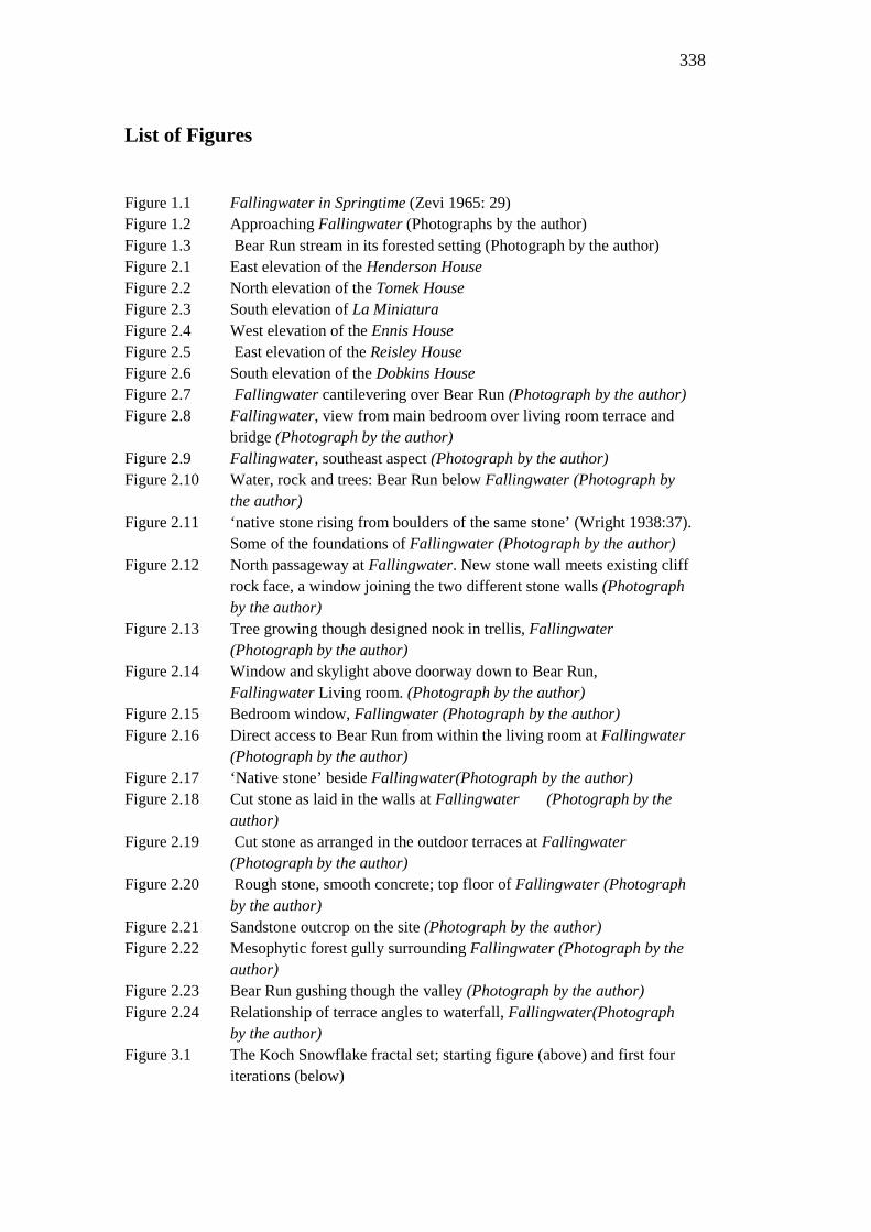
338

List of Figures

Figure 1.1 Fallingwater in Springtime (Zevi 1965: 29) Figure 1.2 Approaching Fallingwater (Photographs by the author) Figure 1.3 Bear Run stream in its forested setting (Photograph by the author) Figure 2.1 East elevation of the Henderson House Figure 2.2 North elevation of the Tomek House Figure 2.3 South elevation of La Miniatura Figure 2.4 West elevation of the Ennis House Figure 2.5 East elevation of the Reisley House Figure 2.6 South elevation of the Dobkins House Figure 2.7 Fallingwater cantilevering over Bear Run (Photograph by the author) Figure 2.8 Fallingwater, view from main bedroom over living room terrace and bridge (Photograph by the author) Figure 2.9 Fallingwater, southeast aspect (Photograph by the author) Figure 2.10 Water, rock and trees: Bear Run below Fallingwater (Photograph by the author) Figure 2.11 ‘native stone rising from boulders of the same stone’ (Wright 1938:37). Some of the foundations of Fallingwater (Photograph by the author) Figure 2.12 North passageway at Fallingwater. New stone wall meets existing cliff rock face, a window joining the two different stone walls (Photograph by the author) Figure 2.13 Tree growing though designed nook in trellis, Fallingwater (Photograph by the author) Figure 2.14 Window and skylight above doorway down to Bear Run, Fallingwater Living room. (Photograph by the author) Figure 2.15 Bedroom window, Fallingwater (Photograph by the author) Figure 2.16 Direct access to Bear Run from within the living room at Fallingwater (Photograph by the author) Figure 2.17 ‘Native stone’ beside Fallingwater(Photograph by the author) Figure 2.18 Cut stone as laid in the walls at Fallingwater (Photograph by the author) Figure 2.19 Cut stone as arranged in the outdoor terraces at Fallingwater (Photograph by the author) Figure 2.20 Rough stone, smooth concrete; top floor of Fallingwater (Photograph by the author) Figure 2.21 Sandstone outcrop on the site (Photograph by the author) Figure 2.22 Mesophytic forest gully surrounding Fallingwater (Photograph by the author) Figure 2.23 Bear Run gushing though the valley (Photograph by the author) Figure 2.24 Relationship of terrace angles to waterfall, Fallingwater(Photograph by the author) Figure 3.1 The Koch Snowflake fractal set; starting figure (above) and first four iterations (below)

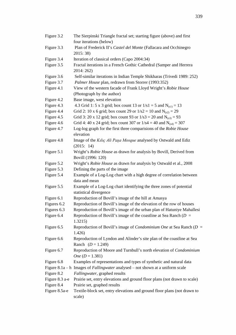
339

Figure 3.2 The Sierpinski Triangle fractal set; starting figure (above) and first four iterations (below) Figure 3.3 Plan of Frederick II’s Castel del Monte (Fallacara and Occhinegro 2015: 38) Figure 3.4 Iteration of classical orders (Capo 2004:34) Figure 3.5 Fractal iterations in a French Gothic Cathedral (Samper and Herrera 2014: 262) Figure 3.6 Self-similar iterations in Indian Temple Shikharas (Trivedi 1989: 252) Figure 3.7 Palmer House plan, redrawn from Storrer (1993:352) Figure 4.1 View of the western facade of Frank Lloyd Wright’s Robie House (Photograph by the author) Figure 4.2 Base image, west elevation Figure 4.3 4.3 Grid 1: 5 x 3 grid; box count 13 or 1/s1 = 5 and N(s1) = 13 Figure 4.4 Grid 2: 10 x 6 grid; box count 29 or 1/s2 = 10 and N(s2) = 29 Figure 4.5 Grid 3: 20 x 12 grid; box count 93 or 1/s3 = 20 and N(s3) = 93 Figure 4.6 Grid 4: 40 x 24 grid; box count 307 or 1/s4 = 40 and N(s4) = 307 Figure 4.7 Log-log graph for the first three comparisions of the Robie House elevation Figure 4.8 Image of the Kılıç Ali Paşa Mosque analysed by Ostwald and Ediz (2015: 14) Figure 5.1 Wright’s Robie House as drawn for analysis by Bovill, Derived from Bovill (1996: 120) Figure 5.2 Wright’s Robie House as drawn for analysis by Ostwald et al., 2008 Figure 5.3 Defining the parts of the image Figure 5.4 Example of a Log-Log chart with a high degree of correlation between data and mean Figure 5.5 Example of a Log-Log chart identifying the three zones of potential statistical divergence Figure 6.1 Reproduction of Bovill’s image of the hill at Amasya Figures 6.2 Reproduction of Bovill’s image of the elevation of the row of houses Figures 6.3 Reproduction of Bovill’s image of the urban plan of Hatuniye Mahallesi Figure 6.4 Reproduction of Bovill’s image of the coastline at Sea Ranch (D = 1.3215) Figure 6.5 Reproduction of Bovill’s image of Condominium One at Sea Ranch (D = 1.426) Figure 6.6 Reproduction of Lyndon and Alinder’s site plan of the coastline at Sea Ranch (D = 1.249) Figure 6.7 Reproduction of Moore and Turnbull’s north elevation of Condominium One (D = 1.381) Figure 6.8 Examples of representations and types of synthetic and natural data Figure 8.1a – h Images of Fallingwater analysed – not shown at a uniform scale Figure 8.2 Fallingwater, graphed results Figure 8.3 a-e Prairie set, entry elevations and ground floor plans (not drawn to scale) Figure 8.4 Prairie set, graphed results Figure 8.5a-e Textile-block set, entry elevations and ground floor plans (not drawn to scale)

340

Figure 8.6 Textile-block set, graphed results Figure 8.7a-e Usonian set, entry elevations and ground floor plans (not drawn to scale) Figure 8.8 Usonian set, graphed results Figure 8.9 Linear trendline data for elevations of the stylistic periods, compared with Fallingwater Figure 8.10 Linear trendline data for plans of the stylistic periods, compared with Fallingwater Figure 8.11 Linear trendline data for composite values of the stylistic periods, compared with Fallingwater Figure 8.12 Mean and aggregate elevations compared Figure 8.13 Mean and aggregate plans compared Figure 8.14 Mean and aggregate elevation and plan composites compared Figure 8.15 Interpretive description of Prairie houses when compared to Fallingwater Figure 8.16 Interpretive description of Textile-block houses when compared to Fallingwater Figure 8.17 Interpretive description of Usonian houses when compared to Fallingwater Figure 8.18 a-c Fallingwater profiles: a. elevation b. plan c. Elevation+plan Figure 9.1 a. View 1, perspective of Fallingwater from below (Futagawa and Pfeiffer 2003:18-19) Figure 9.1 b. View 2, perspective of Fallingwater from above (Drexler 1965: 137) Figure 9.1c. View 3, alternative view from below (Drexler 1965: 140) Figure 9.1 d. View 4, perspective view from south. (Futagawa and Pfeiffer 1987c: 49) Figure 9.2 a – h Images of Fallingwater analysed – Level 3 representation, not shown at a uniform scale Figure 9.3 Fallingwater, graphed results for perspective views (DV) and Plans (DP) Figure 9.4 a. Studio version of Fallingwater site plan (Kaufmann 1986: 39) b. Original site plan (McCarter 2002: 5). Figure 9.5 Plan showing location of each natural element analysed in view form Figure 9.6 a-e Images of water analysed – not shown at a uniform scale Figure 9.7 a – e Images of rocks analysed – not shown at a uniform scale Figure 9.8 a-e Images of the valley analysed – not shown at a uniform scale Figure 9.9 Images of the trees analysed – not shown at a uniform scale Figure 9.10 All results for natural analogues graphed Figure 9.11 Graphed comparison between natural and synthetic views Figure 9.12 Graphic spread of view results data Figure 9.13 Graphed comparison between natural and synthetic plans Figure 9.14 Graphic spread of plan results data

341

Acknowledgements This research was supported by an Australian Government Research Training Program

(RTP) Scholarship

ArchImage software was used for the majority of calculations in this book. Naomi

Henderson authored the prototype version of this software with Michael Ostwald and

Stephen Chalup, Steven Nicklin wrote the final version of ArchImage with Stephan

Chalup, Michael Ostwald and myself.

Thank you to Shiloh Aderhold of the Frank Lloyd Wright Preservation Trust for hosting

me in the Research Centre on my visit to Chicago, and to the Research Librarians of

Auchmuty Library, University of Newcastle for obtaining originals of 80 year old

journals for my perusal.

Thank you to Michael Dawes for your assistance with section 4 of chapter 4.

Thank you to Tessa Morrison, my co-supervisor for excellent advice.

Thank you most of all to Michael Ostwald, surely one of the most excellent supervisors

of all time, whose professional, sensible and highly intelligent insights made this process

relatively painless and has grown my ability to write, analyse and find confidence in my

own voice.

Dedication

This work is dedicated to Mother Earth, for her continuous inspiration.

….