Mean Field Variational Approximation for Continuous-Time BayesianNetworks

Ido Cohn Tal El-Hay Nir FriedmanSchool of Computer Science

The Hebrew University{ido cohn,tale,nir}@cs.huji.ac.il

Raz KupfermanInstitute of MathematicsThe Hebrew University

raz@math.huji.ac.il

Abstract

Continuous-time Bayesian networks is a natu-ral structured representation language for multi-component stochastic processes that evolve con-tinuously over time. Despite the compact repre-sentation, inference in such models is intractableeven in relatively simple structured networks.Here we introduce a mean field variational ap-proximation in which we use a product of in-homogeneous Markov processes to approximatea distribution over trajectories. This variationalapproach leads to a globally consistent distribu-tion, which can be efficiently queried. Addition-ally, it provides a lower bound on the probabil-ity of observations, thus making it attractive forlearning tasks. We provide the theoretical foun-dations for the approximation, an efficient imple-mentation that exploits the wide range of highlyoptimized ordinary differential equations (ODE)solvers, experimentally explore characterizationsof processes for which this approximation is suit-able, and show applications to a large-scale real-world inference problem.

1 Introduction

Many real-life processes can be naturally thought of asevolving continuously in time. Examples cover a di-verse range, including server availability, changes in socio-economic status, and genetic sequence evolution. To realis-tically model such processes, we need to reason about sys-tems that are composed of multiple components (e.g., manyservers in a server farm, multiple residues in a protein se-quence) and evolve in continuous time. Continuous-timeBayesian networks (CTBNs) provide a representation lan-guage for such processes, which allows to naturally exploitsparse patterns of interactions to compactly represent thedynamics of such processes [9].

Inference in multi-component temporal models is a no-toriously hard problem [1]. Similar to the situation in dis-

crete time processes, inference is exponential in the num-ber of components, even in a CTBN with sparse interac-tions [9]. Thus, we have to resort to approximate inferencemethods. The recent literature has adapted several strate-gies from discrete graphical models to CTBNs. These in-clude sampling-based approaches, where Fan and Shelton[5] introduced a likelihood-weighted sampling scheme, andmore recently we [4] introduced a Gibbs-sampling proce-dure. Such sampling-based approaches yield more accu-rate answers with the investment of additional computa-tion. However, it is hard to bound the required time in ad-vance, tune the stopping criteria, or estimate the error ofthe approximation. An alternative class of approximationsis based on variational principles.

Recently, Nodelman et al. [11] introduced an Expec-tation Propagation approach, which can be roughly de-scribed as a local message passing scheme, where eachmessage describes the dynamics of a single componentover an interval. This message passing procedure can auto-matically refine the number of intervals according to thecomplexity of the underlying system [14]. Nonetheless,it does suffer from several caveats. On the formal level,the approximation has no convergence guaranties. Second,upon convergence, the computed marginals do not nec-essarily form a globally consistent distribution. Third, itis restricted to approximations in the form of piecewise-homogeneous messages on each interval. Thus, the re-finement of the number of intervals depends on the fit ofsuch homogeneous approximations to the target process.Finally, the approximation of Nodelman et al does not pro-vide a provable approximation on the likelihood of theobservation—a crucial component in learning procedures.

Here, we develop an alternative variational approxima-tion, which provides a different trade-off. We use the strat-egy of structured variational approximations in graphicalmodels [8], and specifically by the variational approach ofOpper and Sanguinetti [12] for approximate inference inMarkov Jump Processes, a related class of models (see be-low). The resulting procedure approximates the posteriordistribution of the CTBN as a product of independent com-ponents, each of which is an inhomogeneous continuous-

time Markov process. As we show, by using a natural rep-resentation of these processes, we derive a variational pro-cedure that is both efficient, and provides a good approxi-mation both for the likelihood of the evidence and for theexpected sufficient statistics. In particular, the approxima-tion provides a lower-bound on the likelihood, and thus isattractive for use in learning.

2 Continuous-Time Bayesian Networks

Consider a D-component Markov process X(t) =(X(t)

1 , X(t)2 , . . . X

(t)D ) with state space S = S1×S2×· · ·×

SD. A notational convention: vectors are denoted by bold-face symbols, e.g., X , and matrices are denoted by black-board style characters, e.g., Q. The states in S are denotedby vectors of indexes, x = (x1, . . . , xD). We use indexes1 ≤ i, j ≤ D for enumerating components and X(t) andX

(t)i to denote the random variable describing the state of

the process and its i’th components at time t.The dynamics of a time-homogeneous continuous-time

Markov process are fully determined by the Markov transi-tion function,

px,y(t) = Pr(X(t+s) = y|X(s) = x),

where time-homogeneity implies that the right-hand sidedoes not depend on s. These dynamics are fully cap-tured by a matrix Q—the rate matrix with non-negative off-diagonal entries qx,y and diagonal qx,x = −

∑y 6=x qx,y .

This rate matrix defines the transition probabilities

px,y(h) = δx,y + qx,y · h+ o(h)

where δx,y is a multivariate Kronecker delta and o(·)means decay to zero faster than its argument. Using therate matrix Q, we can express the Markov transition func-tion as px,y(t) = [exp(tQ)]x,y where exp(tQ) is a matrixexponential [2, 7].

A continuous-time Bayesian network is defined by as-signing each component i a set of components Pai ⊆{1, . . . , D} \ {i}, which are its parents in the network [9].With each component i we then associate a set of condi-tional rate matrix Qi|Pai

·|ui for each state ui of Pai. The

off-diagonal entries qi|Paixi,yi|ui represent the rate at which Xi

transitions from state xi to state yi given that its parents arein state ui. The dynamics of X(t) are defined by a ratematrix Q with entries qx,y , which amalgamates the condi-tional rate matrices as follows:

qx,y =

qi|Paixi,yi|ui δ(x,y) = {i}∑i qi|Paixi,xi|ui x = y

0 otherwise,

(1)

where δ(x,y) = {i|xi 6= yi}. This definition implies thatchanges are one component at a time.

Given a continuous-time Bayesian network, we wouldlike to evaluate the likelihood of evidence, to compute the

probability of various events given the evidence (e.g., thatthe state of the system at time t is x), and to compute con-ditional expectations (e.g., the expected amount of time Xi

was in state xi). Direct computations of these quantitiesinvolve matrix exponentials of the rate matrix Q, whosesize is exponential in the number of components, makingthis approach infeasible beyond a modest number of com-ponents. We therefore have to resort to approximations.

3 Variational Principle for Continuous TimeMarkov Processes

We start by defining a variational approximations princi-ple in terms of a general continuous-time Markov process(that is, without assuming any network structure). For con-venience we restrict our treatment to a time interval [0, T ]with end-point evidence X(0) = e0 and X(T ) = eT . Wediscuss more general types of evidence below. Here weaim to define a lower bound on lnPQ(eT |e0) as well as toapproximate the posterior probability PQ(· | e0, eT ).

Marginal Density Representation Variational approxi-mations cast inference as an optimization problem of afunctional which approximates the log probability of theevidence by introducing an auxiliary set of variational pa-rameters. Here we define the optimization problem over aset of mean parameters [15], representing possible valuesof expected sufficient statistics.

As discussed above, the prior distribution of the processcan be characterized by a time-independent rate matrix Q.It is easy to show that if the prior is a Markov process, thenthe posterior is also a Markov process, albeit not necessar-ily a homogeneous one. Such a process can be representedby a time-dependent rate matrix that describes the instan-taneous transition rates. Here, rather than representing thetarget distribution by a time-dependent rate matrix, we con-sider a representation that is more natural for variationalapproximations. Let Pr be the distribution of a Markovprocess. We define a family of functions:

µx(t) = Pr(X(t) = x)

γx,y(t) = limh↓0

Pr(X(t) = x,X(t+h) = y)h

, x 6= y

γx,x(t) = −∑y 6=x

γx,y(t).

(2)

The function µx(t) is the probability that X(t) = x.The function γx,y(t) is the probability density that X tran-sitions from state x to y at time t. Note that this parame-ter is not a transition rate, but rather a product of a point-wise probability with the point-wise transition rate of theapproximating probability, i.e., γx,y(t)/µx(t) is the x,yentry of the time-dependent rate matrix. Hence, unlike the(inhomogeneous) rate matrix at time t, γx,y(t) takes intoaccount the probability of being in state x and not only the

rate of transitions. This definition implies that

Pr(X(t) = x,X(t+h) = y) = µx(t)δx,y+γx,y(t)h+o(h),

We aim to use the family of functions µ and γ as arepresentation of a Markov process. To do so, we needto characterize the set of constraints that these functionsshould satisfy.

Definition 3.1: A family η = {µx(t), γx,y(t) : 0 ≤ t ≤T} of continuous functions is a Markov-consistent densityset if the following constraints are fulfilled:

µx(t) ≥ 0,∑x

µx(0) = 1,

γx,y(t) ≥ 0 ∀y 6= x,

γx,x(t) = −∑y 6=x

γx,y(t),

d

dtµx(t) =

∑y

γy,x(t).

LetM be the set of all Markov-consistent densities.

Using standard arguments we can show that there ex-ists a correspondence between (generally inhomogeneous)Markov processes and density sets η. Specifically:

Lemma 3.2: Let η = {µx(t), γx,y(t)}. If η ∈ M, thenthere exists a continuous-time Markov process Pη for whichµx and γx,y satisfy (2).

The processes we are interested in, however, have addi-tional structure, as they correspond to the posterior distri-bution of a time-homogeneous process with end-point ev-idence. This additional structure implies that we shouldonly consider a subset ofM:

Lemma 3.3: Let Q be a rate matrix, and e0, eT be statesof X . Then the representation η corresponding to the pos-terior distribution PQ(·|e0, eT ) is in the setMe ⊂M thatcontains Markov-consistent density sets satisfying µx(0) =δx,e0 , µx(T ) = δx,eT .

Thus, from now on we can restrict our attention to den-sity sets from Me. The constraint that µx(0) and µx(T )also has consequences on γx,y at these points.

Lemma 3.4: If η ∈ Me then γx,y(0) = 0 for all x 6= e0

and γx,y(T ) = 0 for all y 6= eT .

Variational Principle We can now state the variationalprinciple for continuous processes, which closely trackssimilar principles for discrete processes.

We define a free energy functional,

F(η; Q) = E(η; Q) +H(η),

which, as we will see, measures the quality of η as an ap-proximation of PQ(·|e). (For succinctness, we will assumethat the evidence e is clear from the context.) The two

terms in the continuous functional correspond to an en-tropy,

H(η) =∫ T

0

∑x

∑y 6=x

γx,y(t)[1 + lnµx(t)− ln γx,y(t)]dt,

and an energy,

E(η; Q) =∫ T

0

∑x

µx(t)qx,x +∑y 6=x

γx,y(t) ln qx,y

dt.Theorem 3.5: Let Q be a rate matrix, e = (e0, eT ) bestates of X , and η ∈Me. Then

F(η; Q) = lnPQ(eT |e0)− ID(Pη(·)||PQ(·|e))

where ID(Pη(·||PQ(·|e)) is the KL divergence between thetwo processes.

We conclude that F(η; Q) is a lower bound of the log-likelihood of the evidence, and that the closer the approxi-mation to the target posterior, the tighter the bound.

Proof Outline The basic idea is to consider discrete ap-proximations of the functional. Let K be an integer. Wedefine the K-sieve XK to be the set of random variablesX(t0),X(t1), . . . ,X(tK) where tk = kT

K . We can usethe variational principle [8] on the marginal distributionsPQ(XK |e) and Pη(XK). More precisely, define

FK(η; Q) = EPη

[lnPQ(XK , eT | e0)

Pη(XK)

],

which can, by using simple arithmetic manipulations, berecast as

FK(η; Q) = lnPQ(eT |e0)− ID(Pη(XK)||PQ(XK |e)).

We get the desired result by letting K →∞. By definition limK→∞ ID(Pη(XK)||PQ(XK |e)) isID(Pη(·)||PQ(·|e)). The crux of the proof is in proving thefollowing lemma.

Lemma 3.6: F(η; Q) = limK→∞ FK(η; Q).

Proof: Since both PQ and Pη are Markov processes,

FK(η; Q) =K−1∑k=0

EPη[lnPQ(X(tk+1)|X(tk))

]−K−1∑k=0

EPη[lnPη(X(tk),X(tk+1))

]+K−1∑k=1

EPη[lnPη(X(tk))

]We now express these terms as functions of µx(t), γx,y(t)and qx,y . By definition, Pη(X(tk) = x) = µx(tk). Each

of the expectations either depend on this term, or on thejoint distribution Pη(X(tk−1),X(tk)). Using the continu-ity of γx,y(t) we write

Pη(X(tk) = x,X(tk+1) = y) = δx,yµx(tk)+ ∆K · γx,y(tk) + o(∆K)

where ∆K = T/K. Similarly, we can also write

PQ(X(tk+1) = y|X(tk) = x) = δx,y +∆K ·qx,y +o(∆K)

Finally, using properties of logarithms we have that

ln (1 + ∆K · z + o(∆K)) = ∆K · z + o(∆K).

Using these relations, we can rewrite after tedious yetstraightforward manipulations,

FK(η; Q) = EK(η; Q) +HK(η),

where

EK(η; Q) =K−1∑k=0

∆KeK(tk), HK(η) =K−1∑k=0

∆KhK(tk),

and

eK(t) =∑x

∑y 6=x

γx,y(t)[1 + lnµx(t)− ln γx,y(t)] + o(∆K)

hK(t) =∑x

µx(t)qxx +∑y 6=x

γx,y(t) log qx,y

+ o(∆K)

Letting K → ∞ we have that∑k ∆k[f(tk) + o(∆K)] →∫ T

0f(t)dt, hence EK(η; Q) and HK(η) converge to

E(η; Q) andH(η), respectively.

4 Factored ApproximationThe variational principle we discussed is based on a rep-resentation that is as complex as the original process—thenumber of functions γx,y(t) we consider is equal to the sizeof the original rate matrix Q. To get a tractable inferenceprocedure we make additional simplifying assumptions onthe approximating distribution.

Given a D-component process we consider approx-imations that factor into products of independent pro-cesses. More precisely, we define Mi

e to be the contin-uous Markov-consistent density sets over the componentXi, that are consistent with the evidence on Xi at times0 and T . Given a collection of density sets η1, . . . , ηD

for the different components, the product density set η =η1 × · · · × ηD is defined as

µx(t) =∏i

µixi(t)

γx,y(t) =

γixi,yi(t)µ

\ix (t) δ(x,y) = {i}∑

i γixi,xi(t)µ

\ix (t) x = y

0 otherwise

where µ\ix (t) =∏j 6=i µ

jxj (t) is the joint distribution at time

t of all the components other than the i’th. (It is not hard tosee that if ηi ∈ Mi

e for all i, then η ∈ Me.) We define thesetMF

e to contain all factored density sets. From now onwe assume that η = η1 × · · · × ηD ∈MF

e .Assuming that Q is defined by a CTBN, and that η is a

factored density set, we can rewrite

E(η; Q) =∑i

∫ T

0

∑xi

µixi(t)Eµ\i(t)[qxi,xi|Ui

]dt

+∑i

∫ T

0

∑xi,yi 6=xi

γixi,yi(t)Eµ\i(t)[ln qxi,yi|Ui

]dt,

andH(η) =

∑i

H(ηi).

This decomposition involves only local terms that eitherinclude the i’th component, or include the i’th componentand its parents in the CTBN defining Q. Note that termssuch as Eµ\i(t)

[qxi,xi|Ui

]involve only µj(t) for j ∈ Pai.

To make the factored nature of the approximation ex-plicit in the notation, we write henceforth,

F(η; Q) = FF (η1, . . . , ηD; Q).

Fixed Point Characterization We can now pose the op-timization problem we wish to solve:

Fixing i, and given η1, . . . , ηi−1, ηi+1, . . . , ηD,in M1

e, . . .Mi−1e ,Mi+1

e , . . . ,MDe , respec-

tively, find arg maxηi∈MieFF (η1, . . . , ηD; Q).

If for all i, we have a µi ∈ Mie, which is a solution

to this optimization problem with respect to each compo-nent, then we have a (local) stationary point of the energyfunctional withinMF

e .To solve this optimization problem, we define a La-

grangian, which includes the constraints in the form ofDef. 3.1. The Lagrangian is a functional of the functionsµixi(t) and γixi,yi(t) and Lagrange multipliers (which arefunctions of t as well). The stationary point of the func-tional satisfies the Euler-Lagrange equations, namely thefunctional derivatives of L vanish. Writing these equationsin explicit form we get a fixed point characterization of thesolution in term of the following set of ODEs:

d

dtµixi(t) =

∑yi 6=xi

(γiyi,xi(t)− γ

ixi,yi(t)

)d

dtρixi(t) = −ρixi(t)(q̄

ixi,xi(t) + ψixi(t))

−∑yi 6=xi

ρiyi(t)q̃ixi,yi(t)

(3)

where ρi are the exponents of the Lagrange multipliers.

In addition we have the following algebraic constraint

ρixi(t)γixi,yi(t) = µixi(t)q̃

ixi,yi(t)ρ

iyi(t), xi 6= yi. (4)

In these equations we use the following shorthand notationsfor the average rates

q̄ixi,yi(t) = Eµ\i(t)[qi|Paixi,yi|Ui

]q̄ixi,yi|xj (t) = Eµ\i(t)

[qi|Paixi,yi|Ui

| xj],

Similarly, we have the following shorthand notations forthe geometrically-averaged rates,

q̃ixi,yi(t) = exp{Eµ\i(t)

[ln qi|Pai

xi,yi|Ui

]}q̃ixi,yi|xj (t) = exp

{Eµ\i(t)

[ln qi|Pai

xi,yi|Ui| xj]}

,

The last auxiliary term is

ψixi(t) =∑

j∈Childreni

∑xj

µjxj (t)q̄jxj ,xj |xi(t)+∑

j∈Childreni

∑xj 6=yj

γjxj ,yj (t) ln q̃jxj ,yj |xi(t).

The two differential equations (3) for µixi(t) and ρixi(t)describe, respectively, the progression of µixi forward, andthe progression of ρixi backward. To uniquely solve theseequations we need to set the boundary conditions. Theboundary condition for µixi is defined explicitly inMF

e as

µixi(0) = δxi,ei,0 (5)

The boundary condition at T is slightly more involved. Theconstraints inMF

e imply that µixi(T ) = δxi,ei,T . As statedby Lemma 3.4, we have that γiei,T ,xi(T ) = 0 when xi 6=ei,T . Plugging these values into (4), and assuming that Qis irreducible we get that ρxi(T ) = 0 for all xi 6= ei,T .In addition, we notice that ρei,T (T ) 6= 0, for otherwise thewhole system of equations for ρ will collapse to 0. Finally,notice that the solution of (3) for µi and γi is insensitiveto the multiplication of ρi by a constant. Thus, we canarbitrarily set ρei,T (T ) = 1, and get the boundary condition

ρixi(T ) = δxi,ei,T . (6)

Theorem 4.1: ηi ∈ Mie is a stationary point (e.g., local

maxima) of FF (η1, . . . , ηD; Q) subject to the constraintsof Def. 3.1 if and only if it satisfies (3–6).

It is straightforward to extend this result to show that at amaximum with respect to all the component densities, thisfixed-point characterization must hold for all componentssimultaneously.

Example 4.2: Consider the case of a single component,for which our procedure should be exact, as no simplifyingassumptions are made on the density set. In this case, the

averaged rates q̄i and the geometrically-averaged rates q̃i

both reduce to the unaveraged rates q, and ψ ≡ 0. Thus,the system of equations to be solved is

d

dtµx(t) =

∑y 6=x

(γy,x(t)− γx,y(t))

d

dtρx(t) = −

∑y

qx,yρy(t),

along with the algebraic equation

ρx(t)γx,y(t) = qx,yµx(t)ρy(t), y 6= x.

In this case, it is straightforward to show that the back-ward propagation rule for ρx implies that

ρx(t) = Pr(eT |X(t)).

This system of ODEs is similar to forward-backward prop-agation, except that unlike classical forward propagation(which would use a function such as αx(t) = Pr(X(t) =x|e0)), here the forward propagation already takes into ac-count the backward messages, to directly compute the pos-terior. Given this interpretation, it is clear that integratingρx(t) from T to 0 followed by integrating µx(t) from 0 toT computes the exact posterior of the processes.

This interpretation of ρx(t) also allows us to understandthe role of γx,y(t). Recall that γx,y(t)/µx(t) is the instan-taneous rate of transition from x to y at time t. Thus,

γx,y(t)µx(t)

= qx,yρy(t)ρx(t)

.

That is, the instantaneous rate combines the original ratewith the relative likelihood of the evidence at T given y andx. If y is much more likely to lead to the final state, thenthe rates are biased toward y. Conversely, if y is unlikelyto lead to the evidence the rate of transitions to it are lower.This observation also explains why the forward propaga-tion of µx will reach the observed µx(T ) even though wedid not impose it explicitly.

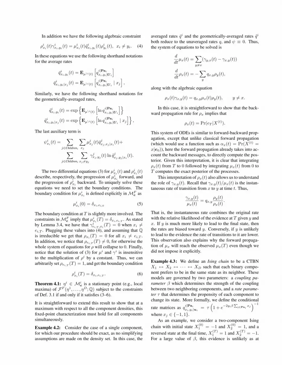
Example 4.3: We define an Ising chain to be a CTBNX1 ↔ X2 ↔ · · · ↔ XD such that each binary compo-nent prefers to be in the same state as its neighbor. Thesemodels are governed by two parameters: a coupling pa-rameter β which determines the strength of the couplingbetween two neighboring components, and a rate parame-ter τ that determines the propensity of each component tochange its state. More formally, we define the conditional

rate matrices as qi|Paixi,yi|ui = τ

(1 + e−2yiβ

P∈Pai

xj)−1

where xj ∈ {−1, 1}.As an example, we consider a two-component Ising

chain with initial state X(0)1 = −1 and X(0)

2 = 1, and areversed state at the final time, X(T )

1 = 1 and X(T )2 = −1.

For a large value of β, this evidence is unlikely as at

Figure 1: Numerical results for the two-component Ising chaindescribed in Example 4.3 where the first component starts in state−1 and ends at time T = 1 in state 1. The second componenthas the opposite behavior. (top) Two likely trajectories depictingthe two modes of the model. (middle) Exact (solid) and approx-imate (dashed/dotted) marginals µi

1(t). (bottom) The log ratiolog ρi

1(t)/ρi0(t).

both end points the components are in a undesired con-figurations. The exact posterior is one that assigns higherprobabilities to trajectories where one of the componentsswitches relatively fast to match the other, and then towardthe end of the interval, they separate to match the evidence.Since the model is symmetric, these trajectories are eitherones in which both components are most of the time instate −1, or ones where both are most of the time in state 1(Fig. 1 top). Due to symmetry, the marginal probability ofeach component is around 0.5 throughout most of the inter-val (Fig. 1 middle). The variational approximation cannotcapture the dependency between the two components, andthus converges to one of two local maxima, correspondingto the two potential subsets of trajectories. Examining thevalue of ρi, we see that close to the end of the interval theybias the instantaneous rates significantly (Fig. 1 bottom).

This example also allows to examine the implicationsof modeling the posterior by inhomogeneous Markov pro-cesses. In principle, we might have used as an approxima-tion Markov processes with homogeneous rates, and con-ditioned on the evidence. To examine whether our approx-

imation behaves in this manner, we notice that in the singlecomponent case we have

qx,y =ρx(t)γx,y(t)ρy(t)µx(t)

,

which should be constant. Consider the analogous quantityin the multi-component case: q̃ixi,yi(t), the geometric aver-age of the rate of Xi, given the probability of parents state.Not surprisingly, this is exactly a mean field approximation,where the influence of interacting components is approxi-mated by their average influence. Since the distribution ofthe parents (in the two-component system, the other com-ponent) changes in time, these rates change continuously,especially near the end of the time interval. This suggeststhat a piecewise homogeneous approximation cannot cap-ture the dynamics without a loss in accuracy.

Optimization Procedure If Q is irreducible, then ρixiand µxi are non-zero throughout the open interval (0, T ).As a result, we can solve (4) to express γixi,yi as a functionof µi and ρi, thus eliminating it from (3) to get evolutionequations solely in terms of µi and ρi. Abstracting the de-tails, we obtain a set of ODEs of the form

d

dtµi(t) = α(µi(t), ρi(t), µ\i(t)) µi(0) = given

d

dtρi(t) = −β(ρi(t), µ\i(t)) ρi(T ) = given.

where α and β can be inferred from (3) and (4). Since theevolution of ρi does not depend on µi, we can integratebackward from time T to solve for ρi. Then, integratingforward from time 0, we compute µi. After performing asingle iteration of backward-forward integration, we obtaina solution that satisfies the fixed-point equation (3) for thei’th component. (This is not surprising once we have iden-tified our procedure to be a variation of a standard forward-backward algorithm for a single component.) Such a solu-tion will be a local maximum of the functional w.r.t. to ηi

(reaching a local minimum or a saddle point requires veryspecific initialization points).

This suggests that we can use the standard procedureof asynchronous update, where we update each compo-nent in a round-robin fashion. Since each of these single-component updates converges in one backward-forwardstep, and since it reaches a local maximum, each step im-proves the value of the free energy over the previous one.Since the free energy functional is bounded by the proba-bility of the evidence, this procedure will always converge.

Another issue is the initialization of this procedure.Since the iteration on the i’th component depends on µ\i,we need to initialize µ by some legal assignment. To doso, we create a fictional rate matrix Q̃i for each componentand initialize µi to be the posterior of the process giventhe evidence ei,0 and ei,T . As a reasonable initial guess,we choose at random one of the conditional rates in Q todetermine the fictional rate matrix.

Figure 2: (a) Relative error as a function of the coupling parameter β (x-axis) and transition rates τ (y-axis) for an 8-component Isingchain. (b) Comparison of true vs. estimated likelihood as a function of the rate parameter τ . (c) Comparison of true vs. likelihood as afunction of the coupling parameter β.

The continuous time update equations allow us to usestandard ODE methods with an adaptive step size (here weuse the Runge-Kutta-Fehlberg (4,5) method). At the priceof some overhead, these procedure automatically tune thetrade-off between error and time granularity.

5 Perspective & Related Works

Variational approximations for different types ofcontinuous-time processes have been recently pro-posed [12, 13]. Our approach is motivated by results ofOpper and Sanguinetti [12] who developed a variationalprinciple for a related model. Their model, which they calla Markov jump process, is similar to an HMM, in whichthe hidden chain is a continuous-time Markov process andthere are (noisy) observations at discrete points along theprocess. They describe a variational principle and discussthe form of the functional when the approximation is aproduct of independent processes. There are two maindifferences between the setting of Opper and Sanguinettiand ours. First, we show how to exploit the structure of thetarget CTBN to reduce the complexity of the approxima-tion. These simplifications imply that the update of the i’thprocess depends only on its Markov blanket in the CTBN,allowing us to develop efficient approximations for largemodels. Second, and more importantly, the structure ofthe evidence in our setting is quite different, as we assumedeterministic evidence at the end of intervals. This settingtypically leads to a posterior Markov process in whichthe instantaneous rates used by Opper and Sanguinettidiverge toward the end point—the rates of transition intothe observed state go to infinity, leading to numericalproblems at the end points. We circumvent this problem byusing the marginal density representation which is muchmore stable numerically.

Taking the general perspective of Wainwright and Jor-dan [15], the representation of the distribution uses the nat-ural sufficient statistics. In the case of a continuous-timeMarkov process, the sufficient statistics are Tx, the time

spent in state x, and Mx,y , the number of transitions fromstate x to y. In a discrete-time model, we can capture thestatistics for every random variable. In a continuous-timemodel, however, we need to consider the time derivative ofthe statistics. Indeed, it is not hard to show that

d

dtE [Tx(t)] = µx(t) and

d

dtE [Mx,y(t)] = γx,y(t).

Thus, our marginal density sets η provide what we con-sider a natural formulation for variational approaches tocontinuous-time Markov processes.

Our presentation focused on evidence at two ends ofan interval. Our formulation easily extends to deal withmore elaborate types of evidence: (1) If we do not observethe initial state of the i’th component, we can set µix(0)to be the prior probability of X(0) = x. Similarly, if wedo not observe Xi at time T , we set ρix(T ) = 1 as ini-tial data for the backward step. (2) In a CTBN where one(or more) components are fully observed, we simply set µi

for these components to be a distribution that assigns allthe probability mass to the observed trajectory. Similarly,if we observe different components at different times, wemay update each component on a different time interval.Consequently, maintaining for each component a marginaldistribution µi throughout the interval of interest, we canupdate the other ones using their evidence patterns.

6 Experimental EvaluationTo gain better insight into the quality of our procedure, weperformed numerical tests on models that challenge the ap-proximation. Specifically, we use Ising chains where weexplore regimes defined by the degree of coupling betweenthe components (the parameter β) and the rate of transitions(the parameter τ ). We evaluate the error in two ways. Thefirst is by the difference between the true log-likelihood andour estimate. The second is by the average relative error inthe estimate of different expected sufficient statistics de-fined by

∑j|θ̂j−θj |θj

where θj is exact value of the j’th ex-

pected sufficient statistics and θ̂j is the approximation.Applying our procedure on an Ising chain with 8

components, for which we can still perform exact in-ference, we evaluated the relative error for differentchoices of β and τ . The evidence in this experiment ise0 = {+,+,+,+,+,+,−,−}, T = 0.64 and eT ={−,−,−,+,+,+,+,+}. As shown in Fig. 2a, the erroris larger when τ and β are large. In the case of a weak cou-pling (small β), the posterior is almost independent, andour approximation is accurate. In models with few transi-tions (small τ ), most of the mass of the posterior is concen-trated on a few canonical “types” of trajectories that canbe captured by the approximation (as in Example 4.3). Athigh transition rates, the components tend to transition of-ten, and in a coordinated manner, which leads to a pos-terior that is hard to approximate by a product distribution.Moreover, the resulting free energy landscape is rough withmany local maxima. Examining the error in likelihood es-timates (Fig. 2b,c) we see a similar trend.

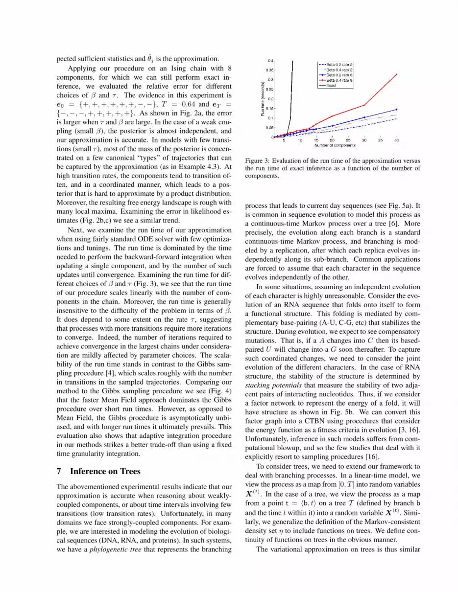
Next, we examine the run time of our approximationwhen using fairly standard ODE solver with few optimiza-tions and tunings. The run time is dominated by the timeneeded to perform the backward-forward integration whenupdating a single component, and by the number of suchupdates until convergence. Examining the run time for dif-ferent choices of β and τ (Fig. 3), we see that the run timeof our procedure scales linearly with the number of com-ponents in the chain. Moreover, the run time is generallyinsensitive to the difficulty of the problem in terms of β.It does depend to some extent on the rate τ , suggestingthat processes with more transitions require more iterationsto converge. Indeed, the number of iterations required toachieve convergence in the largest chains under considera-tion are mildly affected by parameter choices. The scala-bility of the run time stands in contrast to the Gibbs sam-pling procedure [4], which scales roughly with the numberin transitions in the sampled trajectories. Comparing ourmethod to the Gibbs sampling procedure we see (Fig. 4)that the faster Mean Field approach dominates the Gibbsprocedure over short run times. However, as opposed toMean Field, the Gibbs procedure is asymptotically unbi-ased, and with longer run times it ultimately prevails. Thisevaluation also shows that adaptive integration procedurein our methods strikes a better trade-off than using a fixedtime granularity integration.

7 Inference on Trees

The abovementioned experimental results indicate that ourapproximation is accurate when reasoning about weakly-coupled components, or about time intervals involving fewtransitions (low transition rates). Unfortunately, in manydomains we face strongly-coupled components. For exam-ple, we are interested in modeling the evolution of biologi-cal sequences (DNA, RNA, and proteins). In such systems,we have a phylogenetic tree that represents the branching

Figure 3: Evaluation of the run time of the approximation versusthe run time of exact inference as a function of the number ofcomponents.

process that leads to current day sequences (see Fig. 5a). Itis common in sequence evolution to model this process asa continuous-time Markov process over a tree [6]. Moreprecisely, the evolution along each branch is a standardcontinuous-time Markov process, and branching is mod-eled by a replication, after which each replica evolves in-dependently along its sub-branch. Common applicationsare forced to assume that each character in the sequenceevolves independently of the other.

In some situations, assuming an independent evolutionof each character is highly unreasonable. Consider the evo-lution of an RNA sequence that folds onto itself to forma functional structure. This folding is mediated by com-plementary base-pairing (A-U, C-G, etc) that stabilizes thestructure. During evolution, we expect to see compensatorymutations. That is, if a A changes into C then its based-paired U will change into a G soon thereafter. To capturesuch coordinated changes, we need to consider the jointevolution of the different characters. In the case of RNAstructure, the stability of the structure is determined bystacking potentials that measure the stability of two adja-cent pairs of interacting nucleotides. Thus, if we considera factor network to represent the energy of a fold, it willhave structure as shown in Fig. 5b. We can convert thisfactor graph into a CTBN using procedures that considerthe energy function as a fitness criteria in evolution [3, 16].Unfortunately, inference in such models suffers from com-putational blowup, and so the few studies that deal with itexplicitly resort to sampling procedures [16].

To consider trees, we need to extend our framework todeal with branching processes. In a linear-time model, weview the process as a map from [0, T ] into random variablesX(t). In the case of a tree, we view the process as a mapfrom a point t = 〈b, t〉 on a tree T (defined by branch b

and the time t within it) into a random variable X(t). Simi-larly, we generalize the definition of the Markov-consistentdensity set η to include functions on trees. We define con-tinuity of functions on trees in the obvious manner.

The variational approximation on trees is thus similar

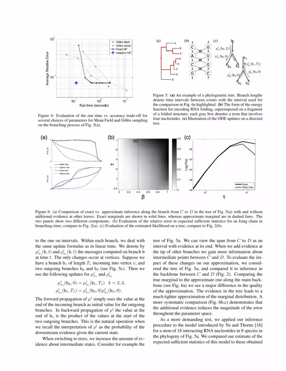
Figure 4: Evaluation of the run time vs. accuracy trade-off forseveral choices of parameters for Mean Field and Gibbs samplingon the branching process of Fig. 5(a).

Figure 5: (a) An example of a phylogenetic tree. Branch lengthsdenote time intervals between events with the interval used forthe comparison in Fig. 6a highlighted. (b) The form of the energyfunction for encoding RNA folding, superimposed on a fragmentof a folded structure; each gray box denotes a term that involvesfour nucleotides. (c) Illustration of the ODE updates on a directedtree.

Figure 6: (a) Comparison of exact vs. approximate inference along the branch from C to D in the tree of Fig. 5(a) with and withoutadditional evidence at other leaves. Exact marginals are shown in solid lines, whereas approximate marginal are in dashed lines. Thetwo panels show two different components. (b) Evaluation of the relative error in expected sufficient statistics for an Ising chain inbranching-time; compare to Fig. 2(a). (c) Evaluation of the estimated likelihood on a tree; compare to Fig. 2(b).

to the one on intervals. Within each branch, we deal withthe same update formulas as in linear time. We denote byµixi(b, t) and ρixi(b, t) the messages computed on branch bat time t. The only changes occur at vertices. Suppose wehave a branch b1 of length T1 incoming into vertex v, andtwo outgoing branches b2 and b3 (see Fig. 5c). Then weuse the following updates for µixi and ρixi

µixi(bk, 0) = µixi(b1, T1) k = 2, 3,

ρixi(b1, T1) = ρixi(b2, 0)ρixi(b3, 0).

The forward propagation of µi simply uses the value at theend of the incoming branch as initial value for the outgoingbranches. In backward propagation of ρi the value at theend of b1 is the product of the values at the start of thetwo outgoing branches. This is the natural operation whenwe recall the interpretation of ρi as the probability of thedownstream evidence given the current state.

When switching to trees, we increase the amount of ev-idence about intermediate states. Consider for example the

tree of Fig. 5a. We can view the span from C to D as aninterval with evidence at its end. When we add evidence atthe tip of other branches we gain more information aboutintermediate points between C and D. To evaluate the im-pact of these changes on our approximation, we consid-ered the tree of Fig. 5a, and compared it to inference inthe backbone between C and D (Fig. 2). Comparing thetrue marginal to the approximate one along the main back-bone (see Fig. 6a) we see a major difference in the qualityof the approximation. The evidence in the tree leads to amuch tighter approximation of the marginal distribution. Amore systematic comparison (Fig. 6b,c) demonstrates thatthe additional evidence reduces the magnitude of the errorthroughout the parameter space.

As a more demanding test, we applied our inferenceprocedure to the model introduced by Yu and Thorne [16]for a stem of 18 interacting RNA nucleotides in 8 species inthe phylogeny of Fig. 5a. We compared our estimate of theexpected sufficient statistics of this model to these obtained

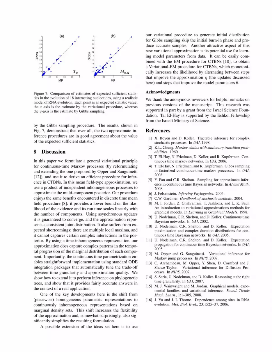
Figure 7: Comparison of estimates of expected sufficient statis-tics in the evolution of 18 interacting nucleotides, using a realisticmodel of RNA evolution. Each point is an expected statistic value;the x-axis is the estimate by the variational procedure, whereasthe y-axis is the estimate by Gibbs sampling.

by the Gibbs sampling procedure. The results, shown inFig. 7, demonstrate that over all, the two approximate in-ference procedures are in good agreement about the valueof the expected sufficient statistics.

8 Discussion

In this paper we formulate a general variational principlefor continuous-time Markov processes (by reformulatingand extending the one proposed by Opper and Sanguinetti[12]), and use it to derive an efficient procedure for infer-ence in CTBNs. In this mean field-type approximation, weuse a product of independent inhomogeneous processes toapproximate the multi-component posterior. Our procedureenjoys the same benefits encountered in discrete time meanfield procedure [8]: it provides a lower-bound on the like-lihood of the evidence and its run time scales linearly withthe number of components. Using asynchronous updatesit is guaranteed to converge, and the approximation repre-sents a consistent joint distribution. It also suffers from ex-pected shortcomings: there are multiple local maxima, andit cannot captures certain complex interactions in the pos-terior. By using a time-inhomogeneous representation, ourapproximation does capture complex patterns in the tempo-ral progression of the marginal distribution of each compo-nent. Importantly, the continuous time parametrization en-ables straightforward implementation using standard ODEintegration packages that automatically tune the trade-offbetween time granularity and approximation quality. Weshow how to extend it to perform inference on phylogenetictrees, and show that it provides fairly accurate answers inthe context of a real application.

One of the key developments here is the shift from(piecewise) homogeneous parametric representations tocontinuously inhomogeneous representations based onmarginal density sets. This shift increases the flexibilityof the approximation and, somewhat surprisingly, also sig-nificantly simplifies the resulting formulation.

A possible extension of the ideas set here is to use

our variational procedure to generate initial distributionfor Gibbs sampling skip the initial burn-in phase and pro-duce accurate samples. Another attractive aspect of thisnew variational approximation is its potential use for learn-ing model parameters from data. It can be easily com-bined with the EM procedure for CTBNs [10], to obtaina Variational-EM procedure for CTBNs, which monotoni-cally increases the likelihood by alternating between stepsthat improve the approximation η (the updates discussedhere) and steps that improve the model parameters θ.

Acknowledgments

We thank the anonymous reviewers for helpful remarks onprevious versions of the manuscript. This research wassupported in part by a grant from the Israel Science Foun-dation. Tal El-Hay is supported by the Eshkol fellowshipfrom the Israeli Ministry of Science.

References[1] X. Boyen and D. Koller. Tractable inference for complex

stochastic processes. In UAI, 1998.[2] K.L. Chung. Markov chains with stationary transition prob-

abilities. 1960.[3] T. El-Hay, N. Friedman, D. Koller, and R. Kupferman. Con-

tinuous time markov networks. In UAI, 2006.[4] T. El-Hay, N. Friedman, and R. Kupferman. Gibbs sampling

in factorized continuous-time markov processes. In UAI,2008.

[5] Y. Fan and C.R. Shelton. Sampling for approximate infer-ence in continuous time Bayesian networks. In AI and Math,2008.

[6] J. Felsenstein. Inferring Phylogenies. 2004.[7] C.W. Gardiner. Handbook of stochastic methods. 2004.[8] M. I. Jordan, Z. Ghahramani, T. Jaakkola, and L. K. Saul.

An introduction to variational approximations methods forgraphical models. In Learning in Graphical Models. 1998.

[9] U. Nodelman, C.R. Shelton, and D. Koller. Continuous timeBayesian networks. In UAI, 2002.

[10] U. Nodelman, C.R. Shelton, and D. Koller. Expectationmaximization and complex duration distributions for con-tinuous time Bayesian networks. In UAI, 2005.

[11] U. Nodelman, C.R. Shelton, and D. Koller. Expectationpropagation for continuous time Bayesian networks. In UAI,2005.

[12] M. Opper and G. Sanguinetti. Variational inference forMarkov jump processes. In NIPS, 2007.

[13] C. Archambeau, M. Opper, Y. Shen, D. Cornford and J.Shawe-Taylor. Variational inference for Diffusion Pro-cesses. In NIPS, 2007.

[14] S. Saria, U. Nodelman, and D. Koller. Reasoning at the righttime granularity. In UAI, 2007.

[15] M. J. Wainwright and M. Jordan. Graphical models, expo-nential families, and variational inference. Found. TrendsMach. Learn., 1:1–305, 2008.

[16] J. Yu and J. L Thorne. Dependence among sites in RNAevolution. Mol. Biol. Evol., 23:1525–37, 2006.