Embed Size (px)
Citation preview
Maximizing Social Welfare in a Competitive Diffusion ModelPrithu Banerjee
University of British Columbia
Vancouver, Canada
Wei Chen
Microsoft Research
Beijing, China
Laks V.S. Lakshmanan
University of British Columbia
Vancouver, Canada
ABSTRACTInfluence maximization (IM) has garnered a lot of attention in
the literature owing to applications such as viral marketing and
infection containment. It aims to select a small number of seed users
to adopt an item such that adoption propagates to a large number
of users in the network. Competitive IM focuses on the propagation
of competing items in the network. Existing works on competitive
IM have several limitations. (1) They fail to incorporate economic
incentives in users’ decision making in item adoptions. (2) Majority
of the works aim to maximize the adoption of one particular item,
and ignore the collective role that different items play. (3) They
focus mostly on one aspect of competition – pure competition. To
address these concerns we study competitive IM under a utility-
driven propagation model called UIC, and study social welfare
maximization. The problem in general is not only NP-hard but also
NP-hard to approximate within any constant factor. We, therefore,
devise instant dependent efficient approximation algorithms for the
general case as well as a (1 − 1/e − ϵ)-approximation algorithm for
a restricted setting. Our algorithms outperform different baselines
on competitive IM, both in terms of solution quality and running
time on large real networks under both synthetic and real utility
configurations.
PVLDB Reference Format:Prithu Banerjee, Wei Chen, and Laks V.S. Lakshmanan. Maximizing Social
Welfare in a Competitive Diffusion Model. PVLDB, 14(4): 613 - 625, 2021.
doi:10.14778/3436905.3436920
1 INTRODUCTIONInfluence maximization (IM) on social and information networks is
a well-studied problem that has gained a lot of traction since it was
introduced by Kempe et al. [28]. Given a network, modeled as a
probabilistic graph where users are represented by nodes and their
connections by edges, the problem is to identify a small set of kseed nodes, such that by starting a campaign from those nodes, the
expected number of users who will be influenced by the campaign,
termed influence spread, is maximized. Here, the expectation is
w.r.t. an underlying stochastic diffusion model that governs how
the influence propagates from one node to another. The “item”
being promoted by the campaign may be a product, a digital good,
an innovative idea, or an opinion.
This work is licensed under the Creative Commons BY-NC-ND 4.0 International
License. Visit https://creativecommons.org/licenses/by-nc-nd/4.0/ to view a copy of
this license. For any use beyond those covered by this license, obtain permission by
emailing [email protected]. Copyright is held by the owner/author(s). Publication rights
licensed to the VLDB Endowment.
Proceedings of the VLDB Endowment, Vol. 14, No. 4 ISSN 2150-8097.
doi:10.14778/3436905.3436920
Existing works on IM typically focus on two types of diffusion
models – single item diffusion and diffusion of multiple items underpure competition. The two classic diffusion models, Independent
Cascade (IC) and Linear Threshold (LT), were proposed in [28].
Advances on these lines of research have led to better scalable ap-
proximation algorithms and heuristics [18, 43, 44]. Most studies
on multiple-item diffusion focus on two items in pure competi-
tion [20, 35, 41, 45], that is, every node would only adopt at most
one item, never both. The typical objective is to select seeds for
the second item (the follower item) to maximize its number of
adoptions, or minimize the spread of the first item [20].
There are a number of key issues on multiple item diffusion that
are not satisfactorily addressed in most prior studies. First, most
propagation models are purely stochastic, in which if a node v is
influenced by a neighboring node u on certain item, it will either
deterministically or probabilistically adopt the item, without any
consideration of the utility of that item for the node. This fails
to incorporate economic incentives into the user adoption behav-
ior. Second, most studies focus on pure competition, where each
node adopts at most one item, and ignore the possibility of nodes
adopting multiple items. For instance, when items are involved
in a partial competition, their combined utility may still be more
than the individual utility, although it may be less than the sum
of their utilities. Third, most studies on competition focus on the
objective of maximizing the influence of one item given other items,
or minimizing the influence of existing items, and do not consider
maximizing the overall welfare caused by all item adoptions.
The study by Banerjee et al. [6] is unique in addressing the
above issues. It proposes the utility-based independent cascade
model UIC, in which: (a) each item has a utility determined by its
value, price and a noise term, and each node selects the best item or
itemset that offers the highest utility among all items that the node
becomes aware of thanks to its neighbors’ influence; and (b) the
utility-based adoption naturally models the adoption of multiple
items, in a framework that allows arbitrary interactions between
items, based on chosen value functions. Banerjee et al. [6] study
the maximization of expected social welfare, defined as the the
total sum of the utilities of items adopted by all network nodes, in
expectation. However, their study is confined to the complementaryitem scenario, where item utilities increase when bundled together.
In this paper, we complement the study in [6] by considering
the social welfare maximization problem in the UIC model when
items are purely or partially competitive. Partial (pure) competition
means adopting an item makes a user less likely (resp., impossible)
to adopt another item. To motivate the problem, we note that for a
social network platform owner (also called the host), one naturalobjective might be to optimize the advertising revenue, as studied
by Chalermsook et al. [15], or a proxy thereof, such as expected
number of item adoptions. On the other hand, one of the key assets
613
of a network host is the loyalty and engagement of its user base,
on which the host relies for its revenue from advertising and other
means. Thus, while launching campaigns, it is equally natural for
the host to take into account users’ satisfaction by making users
aware of itemsets that increase their utility. Social Welfare, being
the sum of utilities of itemsets adopted by users, is directly in line
with this objective.
As a real application, consider a music streaming platform such
as the Last.fm. Benson et al. [7] using their discrete choice model
showed existence of competition across different genres of songs
in the Last.fm dataset. In a platform such as Last.fm, the platform
owner (i.e., host) completely controls the promotion of songs and
the host would like to keep making engaging recommendations
to the users. Even when there are multiple competing songs from
different genres, the host should recommend based on users’ pref-
erences, i.e., the users’ utility. A similar idea extends to different
competing products that an e-retailer like Amazon sells directly.
Those products are already procured by the e-retailer and it has
full control over how it wants to sell them. Once again, in this set-
ting, keeping users’ satisfaction from adopting these products high
helps maintain a loyal and engaged user base. Thus maximizing
the overall social welfare is in line with the goal of the platform.
While [6] studies this problem for complementary items, social
welfare maximization under competing products is open. Moreover,
under pure competition, the bundling algorithm of [6] would lead
to nodes adopting at most one of several competing items, leading
to poor social welfare.
Compared to [6], we also consider a more flexible setting where
the allocation of some items has been fixed (e.g., the items had the
seeds selected by the host earlier) and the host is only allocating
seeds for the remaining items. Once again, the objective is still to
maximize the total social welfare of all users in the network. We call
this the CWelMax problem (for Competitive Welfare Maximization).
As it turns out, CWelMax under UIC is significantly more difficultthan the welfare maximization problem in the complementary set-ting studied in [6]. We show that when treating the allocation as
a set of item-node pairs, the welfare objective function is neither
monotone nor submodular. Moreover, with a non-trivial reduction,
we prove that CWelMax is in general NP-hard to approximate to
within any constant factor. In contrast a constant approximation
was possible in the setting considered in [6].
Despite all these difficulties, we design several algorithms that
either provide an instance-dependent approximation guarantee in
the general case, or better (constant) approximation guarantee in
some special cases. In particular, we first design algorithm SeqGRD
which provides aumin
umax
(1 − 1
e − ϵ)-approximation guarantee for the
general CWelMax setting, where umin is the minimum expected
utility among all individual items, umax is the expected maximum
utility among all item bundles, and ϵ > 0 is any small positive
number. Next, when the fixed itemset is empty, we complement Se-
qGRDwithMaxGRD, which guarantees1
m (1−1
e −ϵ)-approximation,
where m is the total number of items. Thus, when SeqGRD and
MaxGRDwork together, we can guaranteemax(umin
umax
, 1m )(1−1
e −ϵ)-
approximation when there are no prior allocated items. We can
see that when the utility difference among items is not high or
the number of items is small, the above algorithms can achieve a
reasonable approximation performance. Finally, in the special case
where we have a unique superior item with utility better than all
other items, all other items have had their allocations fixed, and
items exhibit pure competition, we design an efficient algorithm
that achieves (1 − 1
e − ϵ)-approximation.
We extensively test our algorithms against state-of-the-art IM
algorithms under seven different utility configurations including
both real and synthetic ones, which capture different aspects of
competition. Our results on real networks show that our algorithms
produce social welfare up to five times higher than the baselines.
Furthermore, they easily scale to large networks with millions of
nodes and billions of edges. We also empirically test the effect
of social welfare maximization on adoption count and show that
whereas the overall adoption count remains the same, social welfare
is maximized by reducing adoption of just the inferior items. To
summarize, our major contributions are as follows:
• We are the first to study the competitive social welfare max-
imization problem CWelMax under the utility-based UIC
model (§3).
• We show that social welfare is neither monotone, submod-
ular, nor supermodular; furthermore, it is NP-hard to ap-
proximate CWelMax within any constant factor, in general
(§4).
• We provide several algorithms that either solve the CWel-
Max in the general setting with a utility-dependent approxi-
mation guarantee, or have better (constant) approximation
guarantees in special cases (§5).
• We conducted an extensive experimental evaluation over
several real social networks comparing our algorithms with
existing algorithms. Our results show that our algorithms
significantly dominate existing algorithms and validate that
our algorithms both deliver good quality and scale to large
networks (§6).
Background and related work are discussed in §2. We conclude the
paper and discuss future work in §7. Proofs compressed or omitted
for lack of space can be found in [5].
2 BACKGROUND & RELATEDWORKOne Item IM: A directed graph G = (V , E,p) represents a socialnetwork with users V and a set of connections (edges) E. The func-tion p : E → [0, 1] specifies influence probabilities between users.
Independent cascade (IC) model is a commonly used discrete time
diffusion model [20, 28]. Given a seed set S ⊂ V , at time t = 0, only
the seed nodes in S are active. For t > 0, if a node u becomes active
at t − 1, then it makes one attempt to activate its every inactive out-
neighbor v , with success probability puv := p(u,v). The diffusionstops when no more nodes can become active.
For a seed set S ⊂ V , we use σ (S) to denote the influence spreadof S , i.e., the expected number of active nodes at the end of diffusion
from S . For a seed budget k and a diffusion model, influence maxi-mization (IM) problem is to find a seed set S ⊂ V with |S | ≤ k such
that the influence spread σ (S) under the model is maximized [28].
A set function f : 2V → R ismonotone if f (S) ≤ f (T )whenever
S ⊆ T ⊆ V ; submodular if for any S ⊆ T ⊆ V and any x ∈V \T , f (S ∪ {x}) − f (S) ≥ f (T ∪ {x}) − f (T ); f is supermodular if−f is submodular; and f is modular if it is both submodular and
supermodular.
614
Under the IC model, IM is intractable [18, 19, 28]. However σ (·)is monotone and submodular. Hence, using Monte Carlo simulation
for estimating the spread, a simple greedy algorithm delivers a
(1−1/e−ϵ)-approximation to the optimal solution, for any ϵ > 0 [26–
28]. The concept of reverse reachable (RR) sets proposed by Borgs et
al. [11], has led to a family of scalable state-of-the-art approximation
algorithms such as IMM and SSA for IM [16, 25, 31, 39, 44].
Multiple item competitive IM: More recently, IM has been stud-
ied involving independent items [21], and competing items [8, 12,
24, 35, 45]. In [34] authors study the problem under pure compe-
tition, whereas [23] aims to maximize balanced exposure in the
network for two competing ideas, and [37] addresses fairness in the
adoption of competing items. These works, however, are restricted
to specific types of competition. The Com-IC model proposed by Lu
et al. [36] can model any arbitrary degree of interaction between a
pair of items. Their main study is thus restricted to the diffusion of
two items. Li et al. [33] look into different facets of items (e.g., topics
of documents) to compute influence. However, unlike our work,
they do not consider item utility in adoption decisions made by
users. Furthermore, their objective function is based on traditional
(expected) number of item adoptions. Our objective is to maximize
the social welfare that none of these papers have studied. A more
comprehensive survey on competitive influence models, can be
found in [20, 32].
Social welfaremaximization: Utility driven adoptions have beenstudied in economics [2, 10, 38, 40]. Given items and users, and the
utility functions of users for various subsets of items, the problem is
to find an allocation of items to users such that the sum of utilities
of users, is maximized. Since the problem is intractable, approxima-
tion algorithms have been developed [22, 27, 29]. Benson et al.[7]
propose a discrete choice model to learn the utilities of itemsets
from the users’ adoption logs. Learning utility is complementary
to our work, and is used in our experiments. Moreover none of
these works consider a social network and the effect of recursive
propagation on item adoptions by its users.
Host’s perspective in the context of IM have been studied. Aslay
et al. [4] directly maximize the revenue earned by a network host,
whereas [3] minimizes the regret of seed selection. These works
do not consider the overall social welfare. Utility based adoption
decisions of users are also not part of their formalism. Welfare
maximization on social networks has been studied in a few recent
papers[9, 42]. Bhattacharya et al. [9] consider item allocations
to nodes for welfare maximization in a network with network
externalities. Their model does not consider the effect of recursive
propagation nor competition. In addition, they do not consider
budget constraints. In contrast, our focus is on competition, with
budget constraints on every item.
Banerjee et al. [6] studied welfare maximization under viral mar-
keting using the UIC propagation model that we also use. However,
their work focuses strictly on complementary items, with super-
modular value functions. As a result, their objective is monotone,
and further satisfies a nice “reachability” property (details in §4),
which paved the way for efficient approximation. However, such
complementary-only setting ignores many real world scenarios
where competing items are present, as highlighted in the intro-
duction. We instead focus on competing items. Consequently, the
objective becomes not only non-monotone, non-submdular, and
non-supermodular, but unlike in [6], is inapproximable within any
constant factor. In spite of this, we develop utility dependent approx-
imation algorithms as well as a constant approximation algorithm
for special cases.
In summary, to our knowledge, our study is the first to addresssocial welfare maximization in a network with influence propaga-tion, competing items, and budget constraints, where item adoptionis driven by utility.
3 UIC MODEL UNDER COMPETITIONIn this section, we first briefly review the utility driven independentcascade model (UIC for short) proposed in [6]. Then we describe
the competitive setting of UIC studied in this paper and formally
state the new problem we address.
Review of UIC Model: UIC integrates utility driven adoption
decision of nodes, with item propagation. Every node has two sets
of items – desire set and adoption set. Desire set is the set of items
that the node has been informed about (and thus potentially desires),
via propagation or seeding. Adoption set, is the subset of the desire
set that has the highest utility, and is adopted by the user. The utility
of an itemset I ⊆ I is derived asU(I ) = V(I ) − P(I ) +N(I ), whereV(·) denotes users’ latent valuation for an itemset, P(·) denotes
the price that user needs to pay, and N(·) is a random noise term
that denotes our uncertainty in users’ valuation.
Budget vector®b = (b1, ...,b |I |) represents the budgets associated
with the items, i.e., the number of seed nodes that can be allocated
with that item. An allocation is a relation 𝒮 ⊂ V × I such that
∀i ∈ I : |{(v, i) | v ∈ V }| ≤ bi . S𝒮i := {v | (v, i) ∈ 𝒮} denotes the
seed nodes of 𝒮 for item i and S𝒮 :=⋃i ∈I S
𝒮i . When the allocation
𝒮 is clear from the context, we write S (resp., Si ) to denote S𝒮
(resp., S𝒮i ).
Before a diffusion begins, the noise terms of all items are sam-
pled, and they are used until the end of that diffusion. The diffusion
proceeds in discrete time steps, starting from t = 1. R𝒮 (v, t) andA𝒮 (v, t) denote the desire and adoption sets of node v at time t .At t = 1, the seed nodes have their desire sets initialized according
to the allocation 𝒮 as, R𝒮 (v, 1) = {i | (v, i) ∈ 𝒮}, ∀v ∈ S𝒮 . Theseseed nodes then adopt the subset of items from the desire set that
maximizes the utility. The propagation then unfolds recursively for
t ≥ 2 in the following way. Once a node u ′ adopts an item i attime t − 1, it influences its out-neighbor u with probability pu′u ,and if it succeeds, then i is added to the desire set of u at time t .Subsequently u adopts the subset of items from the desire set of
u that maximizes the utility. Adoption is progressive, i.e., once a
node adopts an item, it cannot unadopt it later. Thus A𝒮 (u, t) =argmaxT ⊆R𝒮 (u ,t ){U(T ) | T ⊇ A
𝒮 (u, t − 1) ∧ U(T ) ≥ 0}. The
propagation converges when there is no new adoption in the net-
work. For more details readers are referred to [6].
Social welfare maximization relative to a fixed seed set: Let
G = (V , E,p) be a social network, I the universe of items under
consideration. We consider a utility-based objective called socialwelfare, which is the sum of all users’ utilities of itemsets adopted
by them after the propagation converges. Formally, E[U(A𝒮 (u))]is the expected utility that a user u attains for a seed allocation
𝒮 after the propagation ends. The expected social welfare for 𝒮 , is
615
ρ(𝒮) =∑u ∈V E[U(A
𝒮 (u))], where the expectation is over both
the randomness of propagation and noise terms N(.)
In a social network, a campaign may often be launched on top
of other existing campaigns, where the seeds for some items I1 ⊂ Imay already be fixed. Let 𝒮P
be this fixed allocation for items in
I1. Then I2 = I \ I1 is the set of items for which the seeds are to
be selected. We define the problem of maximizing expected social
welfare, on top of a fixed seed allocation as follows.
Welfare maximization under competition: Motivated by eco-
nomics theory [13], to model competition, we assume that V is
submodular, i.e., as I contains more items, the marginal value of an
item with respect to an itemset I ⊂ I decreases. We also assumeV
is monotone and thatV(∅) = 0, since it is a natural property for
valuations. For i ∈ I, N(i) ∼ Di denotes the noise term associated
with item i , where the noise may be drawn from any distribution
Di having a zero mean. Every item has an independent noise dis-
tribution. For a set of items I ⊆ I, we assume the noise and price
to be additive. Since noise is drawn from a zero mean distribution,
E[U(I )] = V(I ) − P(I ). Below, we refer to V,P, {Di }i ∈I, as themodel parameters and denote them collectively as Param.
We now illustrate using a toy example how our framework mod-
els competition.
Example 1. Suppose a user wants to buy a phone and desires (be-cause of influence) an iPhone (ip) and an Android Phone (ap). Sincethe user does not own a phone yet, she enjoys no valuation, which iscaptured byV(∅) = 0. However after she adopts one phone, then al-though the overall value increases by adopting a second phone (V(.)is monotone), the marginal value gain decreases (V(.) is submodu-lar). FormallyV({ip,ap}) = V({ip})+V({ap} | {ip}). Since valueis monotone and submodular, 0 ≤ V({ap} | {ip}) ≤ V({ap}),hence V({ip}) ≤ V({ip,ap}) ≤ V({ip}) +V({ap}). Finally pricedetermines the exact adoption set of a user. The itemset that offersthe highest utility is adopted by the user. If the second phone hasa low price (i.e., P({ap}) ≤ V({ap} | {ip})), then the user maystill adopt both the phones (partial competition). Otherwise (i.e.,P({ap}) > V({ap} | {ip})), a user who has already adopted ipwill not adopt ap.
Problem 1 (CWelMax). GivenG = (V , E,p), the set of model pa-rameters Param, an existing fixed allocation 𝒮P , and budget vector®b, find a seed allocation𝒮∗ for items I2, such that ∀i ∈ I2, |S𝒮
∗
i | ≤ biand 𝒮∗ = argmax𝒮 ρ(𝒮 ∪ 𝒮P ).
Note that this problem subsumes the typical "fresh campaigns"
setting as a special case where I1 = ∅ (and hence 𝒮p = ∅).
An equivalent possible world model: In [6], the authors pro-
posed an equivalent possible world interpretation of the diffusion
under UIC, which we will find useful. We briefly review this below.
Let ⟨G, Param⟩ be an instance of CWelMax, where G = (V , E,p). Apossible world w = (w1,w2), consists an edge possible world (edge
world) w1, and a noise possible world (noise world) w2: w1 is a de-
terministic graph sampled from the distribution associated with
G, where each edge (u,v) ∈ E is sampled in with an independent
probability of puv ; and w2 is a sample of noise terms for items
in I, drawn from noise distributions in Param. Note that propaga-
tion and adoption in w is fully deterministic. In a possible world
w , Nw (i) is the noise for item i and Uw (I ) is the (deterministic)
utility of itemset I . The social welfare of an allocation 𝒮 in w is
ρw (𝒮) :=∑v ∈V U(A
𝒮w (v)), whereA
𝒮w (v) is the adoption set of v
at the end of the propagation in worldw . The expected social welfareof an allocation 𝒮 is ρ(𝒮) := Ew [ρw (𝒮)] = Ew1
[Ew2[ρw (𝒮)]] =
Ew2[Ew1[ρw (𝒮)]].
4 PROPERTIES OF UICIt is easy to see that CWelMax is NP-hard.
Proposition 1. CWelMax in the UIC model is NP-hard.
Sketch. Classic IM is a special case of CWelMax. �
Given the hardness, we examine whether social welfare satisfies
monotonicity, submodularity or supermodularity.
Item blocking. Under the complementary setting in [6] leveraged
the reachability property: if a node v adopts an item i in any possi-
ble worldw , then all the other nodes that are reachable from v in
w will also adopt i . This property does not hold under the competi-
tive setting. In fact, adoption of one particular item can block the
propagation of another item, making social welfare non-monotone
and non-submodular.
Theorem 4.1. Expected social welfare is not monotone, and nei-ther submodular nor supermodular, with respect to sets of node-itemallocation pairs.
Proof. We show a counterexample for each of the three prop-
erties. Consider a simple network with two nodes u and v , anda directed edge (u,v) with probability 1. Assume that there is no
noise, i.e., noise is 0. There are three items in propagation whose
utility configuration is shown in Table 1.
Item V P U
∅ 0 0 0
i1 5 1 4
i2 7 4 3
i3 5 1 4
i1, i2 7 5 2
i1, i3 7 2 5
i2, i3 7 5 2
i1, i2, i3 7 6 1
Table 1: Utility configuration used in Theorem 4.1
Monotonicity. Consider two allocations 𝒮1 = {(u, i1)} and 𝒮2 =
{(u, i1), (v, i2)}. Clearly 𝒮1 ⊂ 𝒮2. Under 𝒮1
, both u and v adopt
i1, thus ρ(𝒮1) = 8. However under 𝒮2, u adopts i1 but v adopts i2.
Thus ρ(𝒮2) = 7 < ρ(𝒮1).
Submodularity. Consider 𝒮1 = {(v, i2)}, 𝒮2 = {(v, i2), (v, i3)}and (u, i1). Clearly 𝒮1 ⊂ 𝒮2
and (u, i1) < 𝒮2. Under 𝒮1
, only vadopts i2. Under𝒮1∪{(u, i1)},u adopts i1 andv adopts i2. So ρ(𝒮1∪
{(u, i1)}) − ρ(𝒮1) = 4. Under 𝒮2, v adopts i3. Under 𝒮2 ∪ {(u, i1)},
u adopts i1 and v adopts i1 and i3. So ρ(𝒮2 ∪ {(u, i1)}) − ρ(𝒮2) =
5 > ρ(𝒮1 ∪ {(u, i1)}) − ρ(𝒮1).
Supermodularity. Consider 𝒮1 = ∅, 𝒮2 = {(v, i2)} and (u, i1).Clearly 𝒮1 ⊂ 𝒮2
and (u, i1) < 𝒮2. Under 𝒮1
, there is no adoption
by any node. Under 𝒮1 ∪ {(u, i1)}, u andv both adopt i1. So ρ(𝒮1 ∪
{(u, i1)}) − ρ(𝒮1) = 8. Under 𝒮2, v adopts i2. Under 𝒮2 ∪ {(u, i1)},
u adopts i1 and v adopts i2 . So ρ(𝒮2 ∪ {(u, i1)}) − ρ(𝒮2) = 4 <
ρ(𝒮1 ∪ {(u, i1)}) − ρ(𝒮1). �
616
The absence of these properties makes CWelMax really hard to
approximate. In fact, there is no PT IME approximation algorithm
within any constant, for the general version of CWelMax.
Theorem 4.2. No PT IME algorithm can approximate CWelMaxwithin any constant factor c , 0 < c ≤ 1, unless P = NP.
Proof. We prove the theorem by a gap introducing reduction
from SET COVER. Suppose there is a PTIME c-approximation al-
gorithm A for CWelMax, for some 0 < c ≤ 1. Given an instance
I = (F ,X ) of SET COVER, where F = {S1, ..., Sr } is a collection ofsubsets over a set of ground elementsX = {д1, ...,дn }, and a number
k (k < r < n), the question is whether there exist k subsets from F
that cover all the ground elements, i.e., whether ∃C ⊂ F : |C| = k
and ∪kS ∈CS = X . We can transform I in polynomial time to an
instance J of CWelMax.
As an overview, our reduction shows that for a YES-instance of
SET COVER, the optimal expected welfare in the corresponding
CWelMax instance is high and for a NO-instance, it is low. More
precisely, letx∗y (resp.,x∗n ) be the optimal welfare on the transformed
instance J whenever the given instance I is a YES-instance (resp.,
NO-instance). Our reduction ensures that x∗n < cx∗y . In this case,
running A on J will clearly allow us to decide if I is a YES-
instance or not, which is impossible unless P = NP. The complete
proof requires several non-trivial gadgets which are omitted here
for the space constraint. It can be found in our full report [5] �
5 APPROXIMATION ALGORITHMSSince the CWelMax problem cannot be approximated within any
constant factor in general, in this section we propose several ap-
proximation algorithms that either produce a non-constant approx-
imation guarantee dependent on the problem instance or a constant
approximation guarantee for a special case of CWelMax. We first
define some important notions.
Truncated utility. For accounting the social welfare of an alloca-
tion, we develop the notion of truncated utility of an item. Recall
that when the noise of an item makes its utility negative, no node
adopts the item. Hence what contributes to the final expected social
welfare is the set of non-negative contributions to utility. We call
this the truncated utility, denotedU+(I ) :=max(0,U(I )). Thus fora (node, item) allocation pair (v, i), its expected social welfare (whenthere are no other allocations) is ρ(v, i) = E[U+(i)]σ ({v}), whereσ ({v}) is the influence spread of {v}.
Minimum and maximum utility bundle. We define umin =
mini ∈I E[U+(i)] as the minimum expected truncated utility of any
item in I, and umax = E[maxI ⊆IU+(I )] as the expected maximum
truncated utility of any item bundle in I. Note that the definitions ofumin andumax are not symmetric: (a)umin takes the minimum of an
expectation, while umax takes the expectation of a maximum; and
(b)umin takes minimum on single items whileumax takes maximum
among all bundles. The reason of this asymmetry will be clear in
our analysis.
Superior and inferior item. A given itemset I is said to have a
superior item im , if the least possible utility of im is strictly higher
than the highest possible utility of any item in I \ {im }. Notice thedefinition of superior item entails that the noise distribution should
be bounded in some way. We discuss a practical way to bound the
noise in our experiments (§6). Given a superior item, all the other
items of the itemset are called inferior items.
In what follows, we present three different algorithms with
progressively better theoretical guarantees, under progressively
stronger assumptions. As a preview, our first algorithm SeqGRD pro-
vides aumin
umax
(1− 1
e )-approximation in the most general case. Our sec-
ond algorithm, MaxGRD, assumes no prior allocations, i.e., 𝒮p = ∅.
Under this assumption, it provides a1
m (1−1
e )-approximation, where
m is the number of items. By simply returning the better of the
two allocations produced by SeqGRD and MaxGRD, the bound is
improved to max{ umin
umax
, 1m }(1 −1
e ), when 𝒮p = ∅. Our final al-
gorithm SupGRD assumes that there exists a superior item in the
itemset, the allocations for all inferior items are fixed, and that items
exhibit pure competition. Under these assumptions, it provides a
(1 − 1
e )-approximation.
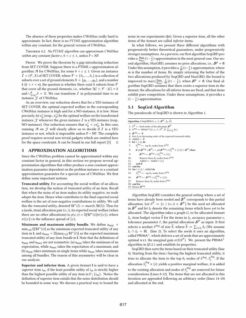
5.1 SeqGrd AlgorithmThe pseudocode of SeqGRD is shown in Algorithm 1.
Algorithm 1 SeqGRD(G , ϵ , ℓ,𝒮P , I2, ®b)
1: SP ← Seed nodes of the allocation𝒮P
2: SSeq ← PRIMA+(G , ϵ , ℓ, SP , ®b ,∑i∈I
2bi )
3: 𝒮Seq ← ∅4: Sort I2 in decreasing order of the expected truncated utility
5: Added ← ∅6: for i ∈ I2 do7: SSeqi ← top bi nodes from SSeq
8: if ρ(𝒮Seq | 𝒮P ) < ρ((𝒮Seq ∪ (SSeqi × {i })) | 𝒮P ) then
9: 𝒮Seq ← 𝒮Seq ∪ (SSeqi × {i })10: Remove those bi nodes from SSeq11: Added ← Added ∪ {i }12: end if13: end for14: for i ∈ I2 \ Added do
15: SSeqi ← top bi nodes from SSeq
16: 𝒮Seq ← 𝒮Seq ∪ (SSeqi × {i })17: Remove those bi nodes from SSeq18: end for19: Return𝒮Seq
Algorithm SeqGRD considers the general setting where a set of
items have already been seeded and 𝒮Pcorresponds to this partial
allocation. Let SP := {v | (v, i) ∈ 𝒮P } be the seed set allocated
in 𝒮Pand let I2 denote the remaining items which have yet to be
allocated. The algorithm takes a graph G, to-be-allocated itemset
I2, item budget vector®b for the items in I2, accuracy parameter ϵ ,
tolerance parameter ℓ, the partial allocation 𝒮Pas input. It first
selects a seedset SSeq of size b, where b :=∑i ∈I2 bi (We assume
I1 ∩ I2 = ∅). (line 2). To select the seeds it uses an algorithm,
called PRIMA+, which delivers a set of seeds that are approximately
optimal w.r.t. the marginal gain σ (S |SP ). We present the PRIMA+
algorithm in §5.2.1 and establish its properties.
SeqGRD then sorts the items based on their truncated utility (line
4). Starting from the item i having the highest truncated utility, it
tries to allocate the item to the top bi nodes of SSeq
, SSeqi . If the
allocation SSeqi × {i} yields a positive marginal welfare, it is added
to the existing allocation and nodes of SSeqi are removed for future
considerations (Lines 8-12). The items that are not allocated in this
iteration are appended following an arbitrary order (lines 14-18)
and allocated at the end.
617
Let Γw (S) be the set of nodes reachable from a seed set S in the
possible worldw . Then we get the following lemma.
Lemma 1. Let 𝒮 be an allocation, S be its seedset, letw be a ran-dom possible world. Then for any node v ∈ V , we have
umin ≤ Ew
[Uw (A
𝒮w (v)) | v ∈ Γw (S)
]≤ umax.
Lemma 2. Let 𝒮 be an allocation and S its corresponding seednodes. Then umin · σ (S) ≤ ρ(𝒮) ≤ umax · σ (S).
Using the lemmas, we get the following bound for SeqGRD.
Theorem 5.1. Let 𝒮Seq be the allocation returned by the Algo-rithm SeqGRD. Given ϵ, ℓ > 0, we have ρ(𝒮Seq ∪ 𝒮P ) ≥ umin
umax
(1 −
1
e − ϵ)ρ(𝒮A ∪𝒮P ) w.p. at least 1− 1
|V |ℓ , where 𝒮A is any arbitrary
allocation of items in I2 respecting the budget constraint.
We note that the property of PRIMA+ that is exploited in the
proof above is its ability to select seed nodes S such that they are
approximately optimal w.r.t. the marginal gain over an existing seed
set SP . The prefix preserving on marginals property of PRIMA+
is not needed in the above proof. However, our next algorithm
MaxGRD relies on the prefix-preserving property.
SeqGRD-NM AlgorithmThe proof of the approximation bound above does not rely on
marginal check (Algorithm 1, line 8). We call the version of SeqGRD
that does not perform marginal check SeqGRD-NM (No Marginal).
Specifically, SeqGRD-NM simply sorts the items based on their
truncated utility, allocates item i to the first bi nodes of SGrd
, where
SGrd is selected using PRIMA+, and removes those bi nodes from
SGrd .Computing marginals involves sampling, which takes signif-
icant time in large networks. On the other hand, the marginal
check avoids the phenomenon of items with lower (truncated) util-
ity blocking those with higher utility, to some extent. Thus even
though SeqGRD-NM is faster than SeqGRD and has the same ap-
proximation guarantee, under certain utility configurations, the
welfare produced by SeqGRD-NM can be worse than that of Seq-
GRD. We explore this in our experiments in §6. On the other hand,
we still append all items in the end to exhaust the budget in Se-
qGRD (lines 14–18). To really discard a certain itemset, we need
to exhaustively search through all itemset combinations, which is
time-consuming. So we only do a simple marginal check in SeqGRD,
and append all items at the end to ensure the theoretical guarantee.
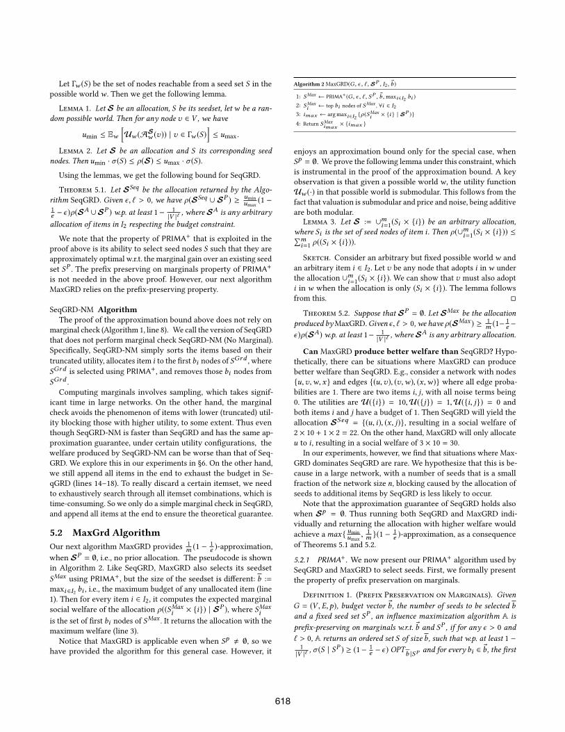
5.2 MaxGrd AlgorithmOur next algorithm MaxGRD provides
1
m (1 −1
e )-approximation,
when 𝒮P = ∅, i.e., no prior allocation. The pseudocode is shown
in Algorithm 2. Like SeqGRD, MaxGRD also selects its seedset
SMaxusing PRIMA+, but the size of the seedset is different: b :=
maxi ∈I2 bi , i.e., the maximum budget of any unallocated item (line
1). Then for every item i ∈ I2, it computes the expected marginal
social welfare of the allocation ρ((SMaxi × {i}) | 𝒮P ), where SMax
iis the set of first bi nodes of S
Max. It returns the allocation with the
maximum welfare (line 3).
Notice that MaxGRD is applicable even when Sp , ∅, so we
have provided the algorithm for this general case. However, it
Algorithm 2MaxGRD(G , ϵ , ℓ,𝒮P , I2, ®b)
1: SMax ← PRIMA+(G , ϵ , ℓ, SP , ®b ,maxi∈I2bi )
2: SMaxi ← top bi nodes of SMax
, ∀i ∈ I23: imax ← argmaxi∈I
2
{ρ(SMaxi × {i } | 𝒮P )}
4: Return SMaximax
× {imax }
enjoys an approximation bound only for the special case, when
Sp = ∅. We prove the following lemma under this constraint, which
is instrumental in the proof of the approximation bound. A key
observation is that given a possible world w , the utility function
Uw (·) in that possible world is submodular. This follows from the
fact that valuation is submodular and price and noise, being additive
are both modular.
Lemma 3. Let 𝒮 := ∪mi=1(Si × {i}) be an arbitrary allocation,where Si is the set of seed nodes of item i . Then ρ(∪mi=1(Si × {i})) ≤∑mi=1 ρ((Si × {i})).
Sketch. Consider an arbitrary but fixed possible worldw and
an arbitrary item i ∈ I2. Let v be any node that adopts i inw under
the allocation ∪mi=1(Si × {i}). We can show that v must also adopt
i in w when the allocation is only (Si × {i}). The lemma follows
from this. �
Theorem 5.2. Suppose that 𝒮P = ∅. Let 𝒮Max be the allocationproduced byMaxGRD. Given ϵ, ℓ > 0, we have ρ(𝒮Max ) ≥ 1
m (1−1
e −
ϵ)ρ(𝒮A) w.p. at least 1− 1
|V |ℓ , where𝒮A is any arbitrary allocation.
Can MaxGRD produce better welfare than SeqGRD? Hypo-thetically, there can be situations where MaxGRD can produce
better welfare than SeqGRD. E.g., consider a network with nodes
{u,v,w, x} and edges {(u,v), (v,w), (x,w)} where all edge proba-bilities are 1. There are two items i, j, with all noise terms being
0. The utilities are U({i}) = 10,U({j}) = 1,U({i, j}) = 0 and
both items i and j have a budget of 1. Then SeqGRD will yield the
allocation 𝒮Seq = {(u, i), (x, j)}, resulting in a social welfare of
2 × 10 + 1 × 2 = 22. On the other hand, MaxGRD will only allocate
u to i , resulting in a social welfare of 3 × 10 = 30.
In our experiments, however, we find that situations where Max-
GRD dominates SeqGRD are rare. We hypothesize that this is be-
cause in a large network, with a number of seeds that is a small
fraction of the network size n, blocking caused by the allocation of
seeds to additional items by SeqGRD is less likely to occur.
Note that the approximation guarantee of SeqGRD holds also
when 𝒮p = ∅. Thus running both SeqGRD and MaxGRD indi-
vidually and returning the allocation with higher welfare would
achieve amax{ umin
umax
, 1m }(1 −1
e )-approximation, as a consequence
of Theorems 5.1 and 5.2.
5.2.1 PRIMA+. We now present our PRIMA+ algorithm used by
SeqGRD and MaxGRD to select seeds. First, we formally present
the property of prefix preservation on marginals.
Definition 1. (Prefix Preservation on Marginals). GivenG = (V , E,p), budget vector ®b, the number of seeds to be selected band a fixed seed set SP , an influence maximization algorithm A isprefix-preserving on marginals w.r.t. ®b and SP , if for any ϵ > 0 andℓ > 0, A returns an ordered set S of size b, such that w.p. at least 1 −1
|V |ℓ , σ (S | SP ) ≥ (1− 1
e − ϵ) OPTb |SP and for every bi ∈ ®b, the first
618
bi nodes of S , denoted Si , satisfies σ (Si | SP ) ≥ (1− 1
e −ϵ) OPTbi |SP ,where OPTb |SP is the optimal marginal expected spread of b nodeson top the existing seeds SP .
In [6], the authors proposed a seed selection algorithm called
PRIMA that is prefix-preserving in spread, using the Reverse Reach-
able Sets (RR-sets), as proposed in IMM [44]. Here, we modify the
standard RR-set construction slightly to account for the presence of
existing seed set SP : Given an existing allocation 𝒮P, we construct
a marginal RR-set as follows. Choose a root node v ∈ V uniformly
at random, add it to Rv and start a BFS from v . Whenever u ∈ Rv ,sample each incoming edge (u ′,u) w.p. pu′u and add it to Rv . Stopwhen no new nodes are added to Rv ; if at any stage Rv overlaps SP ,i.e., if Rv ∩ S
P , ∅, then set Rv := ∅. That is, whenever a generated
RR-set “hits" SP , just set it to ∅.PRIMA+ achieves the property of prefix preservation onmarginals
and it runs in time O((b + ℓ + logn |®b |)(n +m) log n · ϵ−2), where
b :=maxi ∈I2bi , is the maximum budget of any item in I2. The algo-rithm and the proof its correctness mainly follow that of PRIMA.Hence we omit the details here for space constraints, which can be
found in our full report [5].
5.3 SupGrd AlgorithmOur third algorithm SupGRDprovides a constant (1− 1
e )-approximation.
The bound holds under more restrictive conditions as given below.
Conditions required for SupGRD approximation bound. (i)There exists a superior item (defined in §5) im in the item set: i.e.,
under any noise possible worldw2,Uw2(im ) > Uw2
(i),∀i ∈ I\{im }.(ii) Seeds for all the inferior items are fixed: that is, I2 = {im } is theonly item for which an allocation needs to be found; and (iii) There
is pure competition between all items: every node can adopt at
most one item. Under these conditions, the following two lemmas
show that the social welfare is monotone and submodular.
Lemma 4. Given𝒮P and I2, let𝒮1 and𝒮2 be two allocations overI2 such that 𝒮1 ⊆ 𝒮2. Then ρ(𝒮1 ∪ 𝒮P ) ≤ ρ(𝒮2 ∪ 𝒮P ).
Lemma 5. Given𝒮P and I2, let𝒮1 and𝒮2 be two allocations overI2 such that 𝒮1 ⊆ 𝒮2. Let s = (u, im ) < 𝒮2 be an allocation pair.Then ρ(s | 𝒮1 ∪ 𝒮P ) ≥ ρ(s | 𝒮2 ∪ 𝒮P ).
Since social welfare is monotone and submodular, a standard
greedy selection based on the marginal welfare will have (1 − 1
e )-
approximation. However since computing spread itself is #P-hard,
computing the exact marginal is not feasible. In IM, sampling using
RR-sets has been used to achieve state of the art performance.
In what follows, by extending IMM [44], we adopt a martingale
approach for seed selection in SupGRD. Given ϵ and ℓ, SupGRD
returns a seed set that has a (1 − 1
e − ϵ)-approximation w.p. at least
1 − 1
nℓ .
In the classical setting, RR-set samples are used to compute an
unbiased estimation of the spread. In our case we need to estimate
the marginal welfare using the RR-sets. Towards that we define
a notion of weight for every RR-set. The weight of an RR-set Rvdenotes the marginal gain in the expected social welfare achieved
by activating the root v of the RR-set Rv . Thus it is the differencebetween the expected truncated utility of the item that the root vadopts under the existing partial allocation 𝒮P
and that of im . To
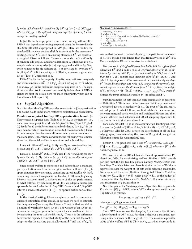
Algorithm 3 NodeSelect ion(R, b′)
1: Initialize Sb′ = ∅, i = 1
2: while i ≤ b′ do3: Select v ∈ V \ Sb′ which has the highestMR (Sb′ ∪ v) −MR (Sb′ )4: Sb′ ← Sb′ ∪ {v }5: Remove R from R if v ∈ R6: end while7: return Sb′ as the final seed set
ensure that the root v indeed adopts im , the path from some seed
of im to v should be no longer than that from any seed of 𝒮Pto v .
Thus, a weighted RR-set is constructed as follows.
Definition 2. (Weighted Reverse Reachable Set). For a given fixedallocation 𝒮P and a node v ∈ G, a weighted RR-set of v , Rv is ob-tained by starting with Rv = {v} and starting a BFS from v suchthat: for u ∈ Rv , sample each incoming edge (u ′,u) w.p. pu′,u andadd it to Rv ; stop when either no new nodes are added or Rv overlapsSP (so the distance from any node in Rv tov along the reversely gen-erated edges is at most the distance from SP to v). Then, the weightof Rv is w(Rv ) = U+({im }) −maxi ∈I s |s ∈SP∩R(v)U
+(i), where I s
denotes the items allocated to node s in the allocation 𝒮P .
SupGRD samples RR-sets using an early termination as described
in Definition 2. This construction ensures that if any member of
a weighted RR-set is seeded with im , the root of the RR-set, v ,will adopt im . In what follows, we first establish the connection
between marginal social welfare and weighted RR-sets and then
present efficient seed selection and RR-set sampling algorithms to
maximize the marginal social welfare.
For a node set S , let I[.] be an indicator function denotingwhetherS covers the (weighted) RR set R, i.e., I(S ∩R , ∅) = 1, if S ∩Rv , ∅,0 otherwise. Also let L(G) denote the distribution of all the live
edge graphs, then extending the result of Borg et al., we get the
following lemma for weighted RR-sets.
Lemma 6. For given seed sets S and SP , we have Ew1∼G [ρw1(S |
SP )] = n · Ev∼V ,w1∼G [I(S ∩ Rv , ∅) ·w(Rv )] where n = |V | is thenumber of nodes in G.
We now extend the RR-set based efficient approximation IM
algorithm, IMM, for maximizing welfare. Similar to IMM, our al-
gorithm SupGRD has two key phases, namely, NodeSelection and
Samplinд. The NodeSelection phase is similar to that of IMM, ex-
cept we consider the weight of RR-sets while selecting seed nodes.
For a node set S and a collection of weighted RR-sets R, define
MR (S) :=∑R∈R I[S ∩ R , ∅] ·w(R). Let b
′ = bim be the budget of
the superior item im . Given a set R, NodeSelection selects b ′ seedsthat maximizesMR (Algorithm 3).
Next, the goal of the Samplinд phase (Algorithm 4) is to generate
R such that |R | ≥ λ/OPT , where OPT is the optimal welfare, and
λ is defined as follows,
λ = 2n · ((1 − 1/e) · α + β)2 · ϵ−2, (1)
where, α =√ℓ logn + log 2 and
β =√(1 − 1/e) · (log
(nb′)+ ℓ log n + log 2).
Since OPT is unknown, the Samplinд first ensures that it finds
a lower bound to OPT w.h.p. For that it deploys a statistical test
using a binary search on the range ofOPT . The maximum possible
value of the welfare OPT is UB = n × umax, when every node in
619
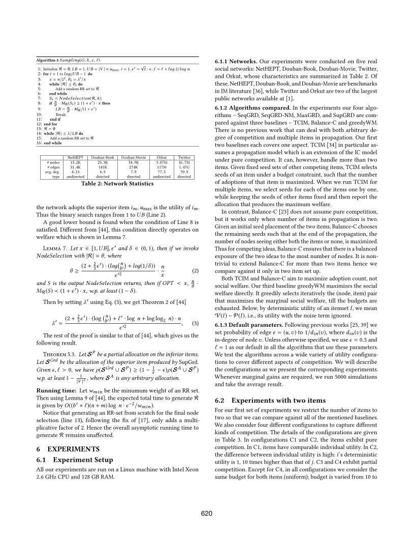
Algorithm 4 Samplinд(G , k , ϵ , ℓ)
1: Initialize R = ∅, LB = 1,U B = |V | × umax , i = 1, ϵ ′ =√2 · ϵ , ℓ = ℓ + loд 2/loд n.
2: for i = 1 to loд2U B − 1 do3: x = n/2i , θi = λ′/x4: while |R | ≤ θi do5: Add a random RR set to R
6: end while7: Si = NodeSelect ion(R, k )8: if n
θ ·MR (Si ) ≥ (1 + ϵ′) · x then
9: LB = nθ ·MR/(1 + ϵ
′)
10: Break;
11: end if12: end for13: R = ∅14: while |R | ≤ λ/LB do15: Add a random RR set to R
16: end while
NetHEPT Douban-Book Douban-Movie Orkut Twitter
# nodes 15.2K 23.3K 34.9K 3.07M 41.7M# edges 31.4K 141K 274K 117M 1.47G
avg. deg. 4.13 6.5 7.9 77.5 70.5type undirected directed directed undirected directed
Table 2: Network Statistics
the network adopts the superior item im , umax is the utility of im .
Thus the binary search ranges from 1 toUB (Line 2).
A good lower bound is found when the condition of Line 8 is
satisfied. Different from [44], this condition directly operates on
welfare which is shown in Lemma 7.
Lemma 7. Let x ∈ [1,UB], ϵ ′ and δ ∈ (0, 1), then if we invokeNodeSelection with |R | = θ , where
θ ≥(2 + 2
3ϵ ′) · (loд
(nb′)+ loд(1/δ ))
ϵ ′2·n
x(2)
and S is the output NodeSelection returns, then if OPT < x , nθ ·
MR (S) < (1 + ϵ′) · x , w.p. at least (1 − δ ).
Then by setting λ′ using Eq. (3), we get Theorem 2 of [44]
λ′ =(2 + 2
3ϵ ′) · (log
(nb′)+ ℓ′ · log n + log log
2n) · n
ϵ ′2, (3)
The rest of the proof is similar to that of [44], which gives us the
following result.
Theorem 5.3. Let𝒮P be a partial allocation on the inferior items.Let 𝒮Grd be the allocation of the superior item produced by SupGrd.Given ϵ, ℓ > 0, we have ρ(𝒮Grd ∪ 𝒮P ) ≥ (1 − 1
e − ϵ)ρ(𝒮A ∪ 𝒮P )
w.p. at least 1 − 1
|V |ℓ , where 𝒮A is any arbitrary allocation.
Running time: Let wmin be the minumum weight of an RR set.
Then using Lemma 9 of [44], the expected total time to generate R
is given by O((b ′ + ℓ)(n +m) log n · ϵ−2/wmin ).
Notice that generating an RR-set from scratch for the final node
selection (line 13), following the fix of [17], only adds a multi-
plicative factor of 2. Hence the overall asymptotic running time to
generate R remains unaffected.
6 EXPERIMENTS6.1 Experiment SetupAll our experiments are run on a Linux machine with Intel Xeon
2.6 GHz CPU and 128 GB RAM.
6.1.1 Networks. Our experiments were conducted on five real
social networks: NetHEPT, Douban-Book, Douban-Movie, Twitter,
and Orkut, whose characteristics are summarized in Table 2. Of
these, NetHEPT, Douban-Book, andDouban-Movie are benchmarks
in IM literature [36], while Twitter and Orkut are two of the largest
public networks available at [1].
6.1.2 Algorithms compared. In the experiments our four algo-
rithms – SeqGRD, SeqGRD-NM, MaxGRD, and SupGRD are com-
pared against three baselines – TCIM, Balance-C and greedyWM.
There is no previous work that can deal with both arbitrary de-
gree of competition and multiple items in propagation. Our first
two baselines each covers one aspect. TCIM [34] in particular as-
sumes a propagation model which is an extension of the IC model
under pure competition. It can, however, handle more than two
items. Given fixed seed sets of other competing items, TCIM selects
seeds of an item under a budget constraint, such that the number
of adoptions of that item is maximized. When we run TCIM for
multiple items, we select seeds for each of the items one by one,
while keeping the seeds of other items fixed and then report the
allocation that produces the maximum welfare.
In contrast, Balance-C [23] does not assume pure competition,
but it works only when number of items in propagation is two.
Given an initial seed placement of the two items, Balance-C chooses
the remaining seeds such that at the end of the propagation, the
number of nodes seeing either both the items or none, is maximized.
Thus for competing ideas, Balance-C ensures that there is a balanced
exposure of the two ideas to the most number of nodes. It is non-
trivial to extend Balance-C for more than two items hence we
compare against it only in two item set up.
Both TCIM and Balance-C aim to maximize adoption count, not
social welfare. Our third baseline greedyWM maximizes the social
welfare directly. It greedily selects iteratively the (node, item) pair
that maximizes the marginal social welfare, till the budgets are
exhausted. Below, by deterministic utility of an itemset I , we mean
V(I ) − P(I ), i.e., its utility with the noise term ignored.
6.1.3 Default parameters. Following previous works [25, 39] we
set probability of edge e = (u,v) to 1/din (v), where din (v) is thein-degree of node v . Unless otherwise specified, we use ϵ = 0.5 and
ℓ = 1 as our default in all the algorithms that use these parameters.
We test the algorithms across a wide variety of utility configura-
tions to cover different aspects of competition. We will describe
the configurations as we present the corresponding experiments.
Whenever marginal gains are required, we run 5000 simulations
and take the average result.
6.2 Experiments with two itemsFor our first set of experiments we restrict the number of items to
two so that we can compare against all of the mentioned baselines.
We also consider four different configurations to capture different
kinds of competition. The details of the configurations are given
in Table 3. In configurations C1 and C2, the items exhibit pure
competition. In C1, items have comparable individual utility. In C2,
the difference between individual utility is high: i’s deterministic
utility is 1, 10 times higher than that of j . C3 and C4 exhibit partial
competition. Except for C4, in all configurations we consider the
same budget for both items (uniform); budget is varied from 10 to
620
No Price Value Noise Budget
C1 i = 3
j = 4
{i, j} = 7
i = 4, j = 4.9
{i, j} = 4.9i : N (0, 1)
j : N (0, 1)
Uniform
C2
i = 4, j = 4.1
{i, j} = 4.1Uniform
C3 i = 4, j = 4.9
{i, j} = 8.7
Uniform
C4 Nonuniform
Table 3: Two item configurations
U(i) = 2 U({i, j}) < 0
U({j}) = 0.11 U({j,k}) < 0
U({k}) = 0.1 U({i, j,k})< 0U({i,k}) = 2.1
Table 4: Three item configuration
item p q UD{indie} 0.107 na 7.0
{rock} 0.091 na 6.8
{industrial} 0.015 na 5.0
{proдressive_metal} 0.011 na 4.7
Table 5: Learned parameters
10 30 50
Budget
10−1
100
101
102
103
104
105
Runn
ing
Tim
e(s
ec)
10 30 50
Budget
10−1
100
101
102
103
104
105
Runn
ing
Tim
e(s
ec)
10 30 50
Budget
10−1
100
101
102
103
104
105
Runn
ing
Tim
e(s
ec)
greedyWM BALANCE-C TCIM MaxGRD SeqGRD SeqGRD-NM
10 30 50
Budget
101
102
103
104
Runn
ing
Tim
e(s
ec)
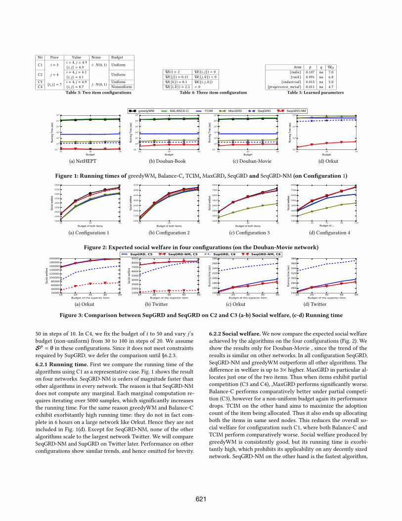
(a) NetHEPT (b) Douban-Book (c) Douban-Movie (d) Orkut
Figure 1: Running times of greedyWM, Balance-C, TCIM,MaxGRD, SeqGRD and SeqGRD-NM (on Configuration 1)
10 30 50
Budget of both items
1000
1500
2000
2500
3000
3500
4000
4500
5000
Soci
alwe
lfare
10 30 50
Budget of both items
1000
1500
2000
2500
3000
3500
4000
4500
Soci
alwe
lfare
10 30 50
Budget of both items
1000
2000
3000
4000
5000
6000
7000
8000
Soci
alwe
lfare
30 50 70 90 110Budget of i2
1000
2000
3000
4000
5000
6000
7000
8000
Soci
alwe
lfare
(a) Configuration 1 (b) Configuration 2 (c) Configuration 3 (d) Configuration 4
Figure 2: Expected social welfare in four configurations (on the Douban-Movie network)
10 20 30 40 50Budget of the superior item
20000
40000
60000
80000
100000
120000
140000
160000
180000
200000
Soci
al w
elfa
re
SupGRD, C5 SeqGRD-NM, C5 SupGRD, C6 SeqGRD-NM, C6
10 20 30 40 50Budget of the superior item
1000
2000
3000
4000
5000
6000
7000
8000
9000
Soci
al w
elfa
re
10 20 30 40 50Budget of the superior item
140
160
180
200
220
240
260
280
Runn
ing
time
(sec
)
10 20 30 40 50Budget of the superior item
240
260
280
300
320
340
360
380
Runn
ing
time
(sec
)
(a) Orkut (b) Twitter (c) Orkut (d) Twitter
Figure 3: Comparison between SupGRD and SeqGRD on C2 and C3 (a-b) Social welfare, (c-d) Running time
50 in steps of 10. In C4, we fix the budget of i to 50 and vary j’sbudget (non-uniform) from 30 to 100 in steps of 20. We assume
𝒮p = ∅ in these configurations. Since it does not meet constraints
required by SupGRD, we defer the comparison until §6.2.3.
6.2.1 Running time. First we compare the running time of the
algorithms using C1 as a representative case. Fig. 1 shows the result
on four networks. SeqGRD-NM is orders of magnitude faster than
other algorithms in every network. The reason is that SeqGRD-NM
does not compute any marginal. Each marginal computation re-
quires iterating over 5000 samples, which significantly increases
the running time. For the same reason greedyWM and Balance-C
exhibit exorbitantly high running time: they do not in fact com-
plete in 6 hours on a large network like Orkut. Hence they are not
included in Fig. 1(d). Except for SeqGRD-NM, none of the other
algorithms scale to the largest network Twitter. We will compare
SeqGRD-NM and SupGRD on Twitter later. Performance on other
configurations show similar trends, and hence omitted for brevity.
6.2.2 Social welfare.We now compare the expected social welfare
achieved by the algorithms on the four configurations (Fig. 2). We
show the results only for Douban-Movie , since the trend of the
results is similar on other networks. In all configuration SeqGRD,
SeqGRD-NM and greedyWM outperform all other algorithms. The
difference in welfare is up to 3× higher. MaxGRD in particular al-
locates just one of the two items. Thus when items exhibit partial
competition (C3 and C4), ,MaxGRD performs significantly worse.
Balance-C performs comparatively better under partial competi-
tion (C3), however for a non-uniform budget again its performance
drops. TCIM on the other hand aims to maximize the adoption
count of the item being allocated. Thus it also ends up allocating
both the items in same seed nodes. This reduces the overall so-
cial welfare for configuration such C1, where both Balance-C and
TCIM perform comparatively worse. Social welfare produced by
greedyWM is consistently good, but its running time is exorbi-
tantly high, which prohibits its applicability on any decently sized
network. SeqGRD-NM on the other hand is the fastest algorithm,
621
1 2 3 4 5 6 7 8 9 10
Number of items
10−1
100
101
102
103
104
105
106
Runn
ing
time
(sec
)
1 2 3 4 5 6 7 8 9 10
Number of items
700
800
900
1000
1100
1200
1300
1400
1500
1600
Socia
lwel
fare
greedyWM TCIM MaxGRD SeqGRD SeqGRD-NM
100 150 200 250 300 350 400 450 500
Budget of inferior items
3400
3500
3600
3700
3800
3900
4000
Socia
lwel
fare
50 60 70 80 90 100
Percentage network size
0
50
100
150
200
250
300
Runn
ing
Tim
e(s
ec)
SeqGRD-NM, time 1 SeqGRD-NM, time 2
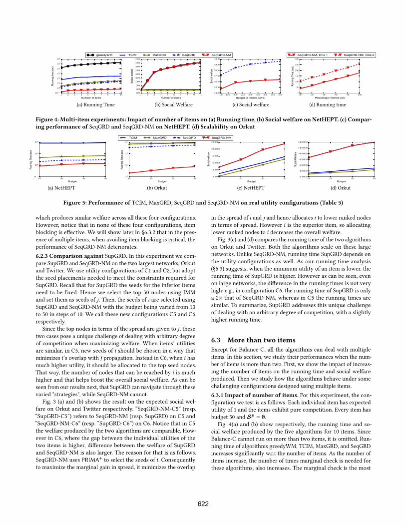
(a) Running Time (b) Social Welfare (c) Social welfare (d) Running time
Figure 4: Multi-item experiments: Impact of number of items on (a) Running time, (b) Social welfare on NetHEPT. (c) Compar-ing performance of SeqGRD and SeqGRD-NM on NetHEPT. (d) Scalability on Orkut
10 20 30 40
Budget
10−1
100
101
102
Runn
ing
Tim
e(s
ec)
10 20 30 40
Budget
101
102
103
104
Runn
ing
Tim
e(s
ec)
10 20 30 40
Budget
2000
4000
6000
8000
10000
12000
Socia
lwel
fare
TCIM MaxGRD SeqGRD SeqGRD-NM
10 20 30 40
Budget
200000
400000
600000
800000
1000000
1200000
1400000
Socia
lWel
fare
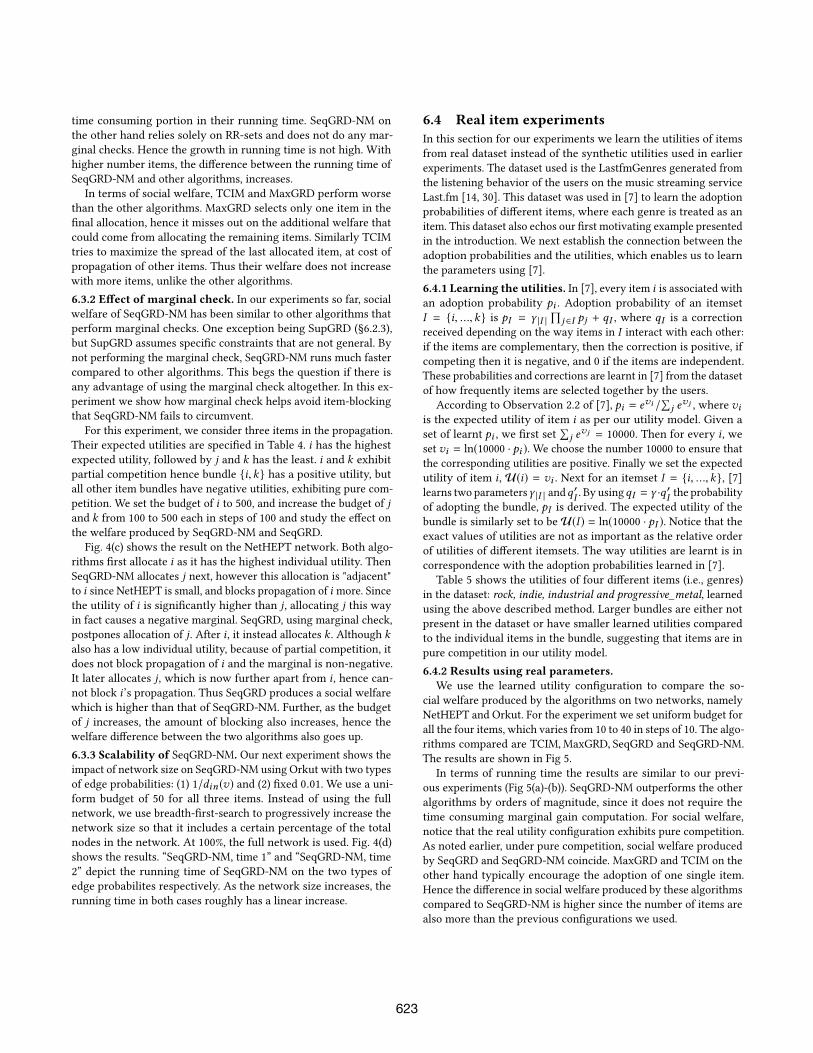
(a) NetHEPT (b) Orkut (c) NetHEPT (d) Orkut
Figure 5: Performance of TCIM,MaxGRD, SeqGRD and SeqGRD-NM on real utility configurations (Table 5)
which produces similar welfare across all these four configurations.
However, notice that in none of these four configurations, item
blocking is effective. We will show later in §6.3.2 that in the pres-
ence of multiple items, when avoiding item blocking is critical, the
performance of SeqGRD-NM deteriorates.
6.2.3 Comparison against SupGRD. In this experiment we com-
pare SupGRD and SeqGRD-NM on the two largest networks, Orkut
and Twitter. We use utility configurations of C1 and C2, but adopt
the seed placements needed to meet the constraints required for
SupGRD. Recall that for SupGRD the seeds for the inferior items
need to be fixed. Hence we select the top 50 nodes using IMM
and set them as seeds of j. Then, the seeds of i are selected using
SupGRD and SeqGRD-NM with the budget being varied from 10
to 50 in steps of 10. We call these new configurations C5 and C6
respectively.
Since the top nodes in terms of the spread are given to j, thesetwo cases pose a unique challenge of dealing with arbitrary degree
of competition when maximizing welfare. When items’ utilities
are similar, in C5, new seeds of i should be chosen in a way that
minimizes i’s overlap with j propagation. Instead in C6, when i hasmuch higher utility, it should be allocated to the top seed nodes.
That way, the number of nodes that can be reached by i is much
higher and that helps boost the overall social welfare. As can be
seen from our results next, that SupGRD can navigate through these
varied "strategies", while SeqGRD-NM cannot.
Fig. 3 (a) and (b) shows the result on the expected social wel-
fare on Orkut and Twitter respectively. “SeqGRD-NM-C5” (resp.
“SupGRD-C5”) refers to SeqGRD-NM (resp. SupGRD) on C5 and
“SeqGRD-NM-C6” (resp. “SupGRD-C6”) on C6. Notice that in C5
the welfare produced by the two algorithms are comparable. How-
ever in C6, where the gap between the individual utilities of the
two items is higher, difference between the welfare of SupGRD
and SeqGRD-NM is also larger. The reason for that is as follows.
SeqGRD-NM uses PRIMA+ to select the seeds of i . Consequentlyto maximize the marginal gain in spread, it minimizes the overlap
in the spread of i and j and hence allocates i to lower ranked nodes
in terms of spread. However i is the superior item, so allocating
lower ranked nodes to i decreases the overall welfare.Fig. 3(c) and (d) compares the running time of the two algorithms
on Orkut and Twitter. Both the algorithms scale on these large
networks. Unlike SeqGRD-NM, running time SupGRD depends on
the utility configurations as well. As our running time analysis
(§5.3) suggests, when the minimum utility of an item is lower, the
running time of SupGRD is higher. However as can be seen, even
on large networks, the difference in the running times is not very
high: e.g., in configuration C6, the running time of SupGRD is only
a 2× that of SeqGRD-NM, whereas in C5 the running times are
similar. To summarize, SupGRD addresses this unique challenge
of dealing with an arbitrary degree of competition, with a slightly
higher running time.
6.3 More than two itemsExcept for Balance-C, all the algorithms can deal with multiple
items. In this section, we study their performances when the num-
ber of items is more than two. First, we show the impact of increas-
ing the number of items on the running time and social welfare
produced. Then we study how the algorithms behave under some
challenging configurations designed using multiple items.
6.3.1 Impact of number of items. For this experiment, the con-
figuration we test is as follows. Each individual item has expected
utility of 1 and the items exhibit pure competition. Every item has
budget 50 and 𝒮p = ∅.
Fig. 4(a) and (b) show respectively, the running time and so-
cial welfare produced by the five algorithms for 10 items. Since
Balance-C cannot run on more than two items, it is omitted. Run-
ning time of algorithms greedyWM, TCIM, MaxGRD, and SeqGRD
increases significantly w.r.t the number of items. As the number of
items increase, the number of times marginal check is needed for
these algorithms, also increases. The marginal check is the most
622
time consuming portion in their running time. SeqGRD-NM on
the other hand relies solely on RR-sets and does not do any mar-
ginal checks. Hence the growth in running time is not high. With
higher number items, the difference between the running time of
SeqGRD-NM and other algorithms, increases.
In terms of social welfare, TCIM and MaxGRD perform worse
than the other algorithms. MaxGRD selects only one item in the
final allocation, hence it misses out on the additional welfare that
could come from allocating the remaining items. Similarly TCIM
tries to maximize the spread of the last allocated item, at cost of
propagation of other items. Thus their welfare does not increase
with more items, unlike the other algorithms.
6.3.2 Effect of marginal check. In our experiments so far, social
welfare of SeqGRD-NM has been similar to other algorithms that
perform marginal checks. One exception being SupGRD (§6.2.3),
but SupGRD assumes specific constraints that are not general. By
not performing the marginal check, SeqGRD-NM runs much faster
compared to other algorithms. This begs the question if there is
any advantage of using the marginal check altogether. In this ex-
periment we show how marginal check helps avoid item-blocking
that SeqGRD-NM fails to circumvent.
For this experiment, we consider three items in the propagation.
Their expected utilities are specified in Table 4. i has the highestexpected utility, followed by j and k has the least. i and k exhibit
partial competition hence bundle {i,k} has a positive utility, butall other item bundles have negative utilities, exhibiting pure com-
petition. We set the budget of i to 500, and increase the budget of jand k from 100 to 500 each in steps of 100 and study the effect on
the welfare produced by SeqGRD-NM and SeqGRD.
Fig. 4(c) shows the result on the NetHEPT network. Both algo-
rithms first allocate i as it has the highest individual utility. ThenSeqGRD-NM allocates j next, however this allocation is "adjacent"
to i since NetHEPT is small, and blocks propagation of i more. Since
the utility of i is significantly higher than j, allocating j this wayin fact causes a negative marginal. SeqGRD, using marginal check,
postpones allocation of j. After i , it instead allocates k . Although kalso has a low individual utility, because of partial competition, it
does not block propagation of i and the marginal is non-negative.
It later allocates j, which is now further apart from i , hence can-not block i’s propagation. Thus SeqGRD produces a social welfare
which is higher than that of SeqGRD-NM. Further, as the budget
of j increases, the amount of blocking also increases, hence the
welfare difference between the two algorithms also goes up.
6.3.3 Scalability of SeqGRD-NM. Our next experiment shows the
impact of network size on SeqGRD-NM using Orkut with two types
of edge probabilities: (1) 1/din (v) and (2) fixed 0.01. We use a uni-
form budget of 50 for all three items. Instead of using the full
network, we use breadth-first-search to progressively increase the
network size so that it includes a certain percentage of the total
nodes in the network. At 100%, the full network is used. Fig. 4(d)
shows the results. “SeqGRD-NM, time 1” and “SeqGRD-NM, time
2” depict the running time of SeqGRD-NM on the two types of
edge probabilites respectively. As the network size increases, the
running time in both cases roughly has a linear increase.
6.4 Real item experimentsIn this section for our experiments we learn the utilities of items
from real dataset instead of the synthetic utilities used in earlier
experiments. The dataset used is the LastfmGenres generated from
the listening behavior of the users on the music streaming service
Last.fm [14, 30]. This dataset was used in [7] to learn the adoption
probabilities of different items, where each genre is treated as an
item. This dataset also echos our first motivating example presented
in the introduction. We next establish the connection between the
adoption probabilities and the utilities, which enables us to learn
the parameters using [7].
6.4.1 Learning the utilities. In [7], every item i is associated withan adoption probability pi . Adoption probability of an itemset
I = {i, ...,k} is pI = γ |I |∏
j ∈I pj + qI , where qI is a correction
received depending on the way items in I interact with each other:
if the items are complementary, then the correction is positive, if
competing then it is negative, and 0 if the items are independent.
These probabilities and corrections are learnt in [7] from the dataset
of how frequently items are selected together by the users.
According to Observation 2.2 of [7], pi = evi /∑j e
vj, where vi
is the expected utility of item i as per our utility model. Given a
set of learnt pi , we first set∑j e
vj = 10000. Then for every i , weset vi = ln(10000 · pi ). We choose the number 10000 to ensure that
the corresponding utilities are positive. Finally we set the expected
utility of item i , U(i) = vi . Next for an itemset I = {i, ...,k}, [7]learns two parametersγ |I | andq
′I . By usingqI = γ ·q
′I the probability
of adopting the bundle, pI is derived. The expected utility of the
bundle is similarly set to beU(I ) = ln(10000 · pI ). Notice that theexact values of utilities are not as important as the relative order
of utilities of different itemsets. The way utilities are learnt is in
correspondence with the adoption probabilities learned in [7].
Table 5 shows the utilities of four different items (i.e., genres)
in the dataset: rock, indie, industrial and progressive_metal, learnedusing the above described method. Larger bundles are either not
present in the dataset or have smaller learned utilities compared
to the individual items in the bundle, suggesting that items are in
pure competition in our utility model.
6.4.2 Results using real parameters.We use the learned utility configuration to compare the so-
cial welfare produced by the algorithms on two networks, namely
NetHEPT and Orkut. For the experiment we set uniform budget for
all the four items, which varies from 10 to 40 in steps of 10. The algo-
rithms compared are TCIM,MaxGRD, SeqGRD and SeqGRD-NM.
The results are shown in Fig 5.
In terms of running time the results are similar to our previ-
ous experiments (Fig 5(a)-(b)). SeqGRD-NM outperforms the other
algorithms by orders of magnitude, since it does not require the
time consuming marginal gain computation. For social welfare,
notice that the real utility configuration exhibits pure competition.
As noted earlier, under pure competition, social welfare produced
by SeqGRD and SeqGRD-NM coincide.MaxGRD and TCIM on the
other hand typically encourage the adoption of one single item.
Hence the difference in social welfare produced by these algorithms
compared to SeqGRD-NM is higher since the number of items are
also more than the previous configurations we used.
623
Network Budget Algorithm
Real Utility Configuration (as shown in Table 5) Synthetic Utility Configuration (as shown in Table 4)
indie rock industrial progressive_metal welfare i j k welfare
NetHEPT 10
RR 203 217 191 196 4473.08 277 244 234 513.2
Snake 204(+0.005) 201(-0.081) 207(+0.083) 195(-0.005) 4458.64(-0.003) 258(-0.068) 246(+0.008) 261(+0.115) 478.4(-0.068)
SGRD-NM 255(+0.252) 199(-0.082) 188(-0.016) 165(-0.158) 4951.8 (+0.112) 306(+0.105) 220(-0.098) 227(-0.030) 577.4(+0.125)
NetHEPT 40
RR 496 493 491 475 10795.3 667 576 645 1227.3
Snake 483(-0.026) 496(+0.006) 488(-0.004) 488(+0.027) 10758.2(-0.003) 648(-0.028) 581(+0.009) 669(+0.037) 1194.5(-0.027)
SGRD-NM 673(+0.357) 499(+0.012) 419(-0.147) 365(-0.189) 11264.5(+0.043) 800(+0.199) 510(-0.114) 514(-0.203) 1510.6(+0.230)
Orkut 10
RR 37790 38888 38331 34711 828368.2 69151 49730 67405 110032.5
Snake 38241(+0.012) 37401(-0.038) 39818(+0.039) 34260(-0.013) 828235.4(-0.002) 67648(-0.021) 50511(+0.016) 68510(+0.016) 107227.7(-0.026)
SGRD-NM 50800(+0.344) 40837(+0.050) 31189(-0.186) 26895(-0.225) 864154.3(+0.040) 76784(+0.110) 50219(+0.010) 57199(-0.151) 124210.9(+0.129)
Orkut 40
RR 58142 58586 59939 54607 1276650.6 119039 83291 113359 183853.2
Snake 57211(-0.016) 56922(-0.028) 61603(+0.028) 55538(+0.017) 1272190.7(-0.035) 117454(-0.013) 82937(-0.043) 115338(+0.018) 180269.4(-0.020)
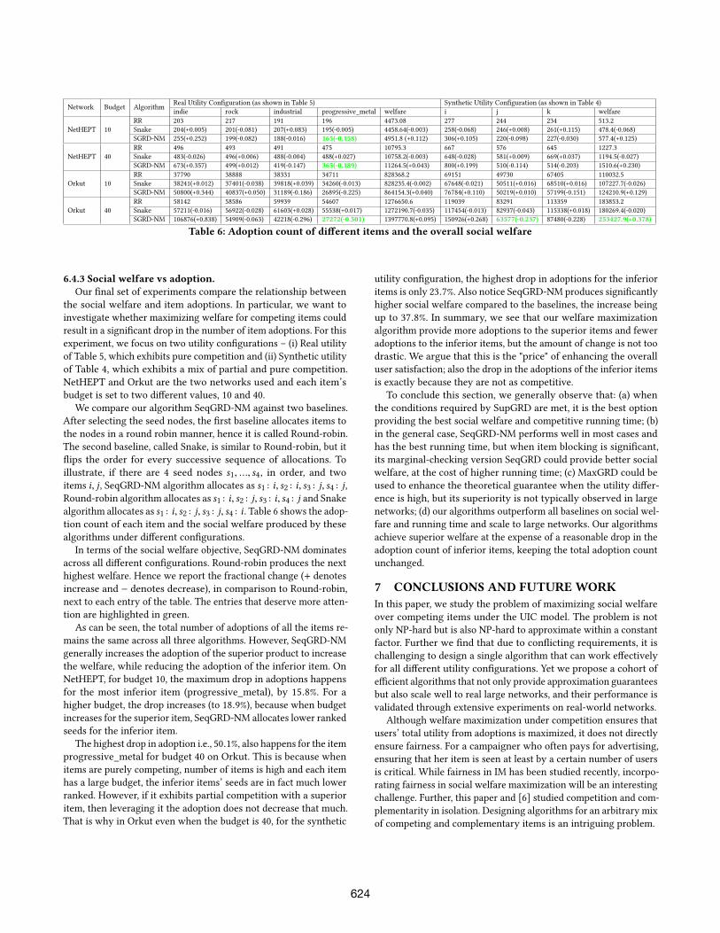
SGRD-NM 106876(+0.838) 54909(-0.063) 42218(-0.296) 27272(-0.501) 1397770.8(+0.095) 150926(+0.268) 63577(-0.237) 87480(-0.228) 253427.9(+0.378)
Table 6: Adoption count of different items and the overall social welfare
6.4.3 Social welfare vs adoption.Our final set of experiments compare the relationship between
the social welfare and item adoptions. In particular, we want to
investigate whether maximizing welfare for competing items could
result in a significant drop in the number of item adoptions. For this
experiment, we focus on two utility configurations – (i) Real utility
of Table 5, which exhibits pure competition and (ii) Synthetic utility
of Table 4, which exhibits a mix of partial and pure competition.
NetHEPT and Orkut are the two networks used and each item’s
budget is set to two different values, 10 and 40.
We compare our algorithm SeqGRD-NM against two baselines.
After selecting the seed nodes, the first baseline allocates items to
the nodes in a round robin manner, hence it is called Round-robin.
The second baseline, called Snake, is similar to Round-robin, but it
flips the order for every successive sequence of allocations. To
illustrate, if there are 4 seed nodes s1, ..., s4, in order, and two
items i, j , SeqGRD-NM algorithm allocates as s1 : i, s2 : i, s3 : j, s4 : j ,Round-robin algorithm allocates as s1 : i, s2 : j, s3 : i, s4 : j and Snakealgorithm allocates as s1 : i, s2 : j, s3 : j, s4 : i . Table 6 shows the adop-tion count of each item and the social welfare produced by these
algorithms under different configurations.
In terms of the social welfare objective, SeqGRD-NM dominates
across all different configurations. Round-robin produces the next
highest welfare. Hence we report the fractional change (+ denotes
increase and − denotes decrease), in comparison to Round-robin,
next to each entry of the table. The entries that deserve more atten-
tion are highlighted in green.
As can be seen, the total number of adoptions of all the items re-
mains the same across all three algorithms. However, SeqGRD-NM
generally increases the adoption of the superior product to increase
the welfare, while reducing the adoption of the inferior item. On
NetHEPT, for budget 10, the maximum drop in adoptions happens
for the most inferior item (progressive_metal), by 15.8%. For a
higher budget, the drop increases (to 18.9%), because when budget
increases for the superior item, SeqGRD-NM allocates lower ranked
seeds for the inferior item.
The highest drop in adoption i.e., 50.1%, also happens for the item
progressive_metal for budget 40 on Orkut. This is because when
items are purely competing, number of items is high and each item
has a large budget, the inferior items’ seeds are in fact much lower
ranked. However, if it exhibits partial competition with a superior
item, then leveraging it the adoption does not decrease that much.
That is why in Orkut even when the budget is 40, for the synthetic
utility configuration, the highest drop in adoptions for the inferior
items is only 23.7%. Also notice SeqGRD-NM produces significantly
higher social welfare compared to the baselines, the increase being
up to 37.8%. In summary, we see that our welfare maximization
algorithm provide more adoptions to the superior items and fewer
adoptions to the inferior items, but the amount of change is not too
drastic. We argue that this is the "price" of enhancing the overall
user satisfaction; also the drop in the adoptions of the inferior items
is exactly because they are not as competitive.
To conclude this section, we generally observe that: (a) when
the conditions required by SupGRD are met, it is the best option
providing the best social welfare and competitive running time; (b)
in the general case, SeqGRD-NM performs well in most cases and
has the best running time, but when item blocking is significant,
its marginal-checking version SeqGRD could provide better social
welfare, at the cost of higher running time; (c) MaxGRD could be
used to enhance the theoretical guarantee when the utility differ-
ence is high, but its superiority is not typically observed in large
networks; (d) our algorithms outperform all baselines on social wel-
fare and running time and scale to large networks. Our algorithms
achieve superior welfare at the expense of a reasonable drop in the
adoption count of inferior items, keeping the total adoption count
unchanged.
7 CONCLUSIONS AND FUTUREWORKIn this paper, we study the problem of maximizing social welfare
over competing items under the UIC model. The problem is not
only NP-hard but is also NP-hard to approximate within a constant
factor. Further we find that due to conflicting requirements, it is
challenging to design a single algorithm that can work effectively
for all different utility configurations. Yet we propose a cohort of
efficient algorithms that not only provide approximation guarantees
but also scale well to real large networks, and their performance is
validated through extensive experiments on real-world networks.
Although welfare maximization under competition ensures that
users’ total utility from adoptions is maximized, it does not directly
ensure fairness. For a campaigner who often pays for advertising,
ensuring that her item is seen at least by a certain number of users
is critical. While fairness in IM has been studied recently, incorpo-
rating fairness in social welfare maximization will be an interesting
challenge. Further, this paper and [6] studied competition and com-
plementarity in isolation. Designing algorithms for an arbitrary mix
of competing and complementary items is an intriguing problem.
624
REFERENCES[1] [n. d.]. Twitter and Orkut Dataset. https://snap.stanford.edu/data/. Accessed:
2020-05-30.
[2] Ben Abramowitz and Elliot Anshelevich. 2018. Utilitarians Without Utilities:
Maximizing Social Welfare for Graph Problems Using Only Ordinal Preferences.
In AAAI. 894–901.[3] Cigdem Aslay, Wei Lu3 Francesco Bonchi, Amit Goyal, and Laks VS Lakshmanan.
2015. Viral Marketing Meets Social Advertising: Ad Allocation with Minimum
Regret. Proceedings of the VLDB Endowment 8, 7 (2015).[4] Cigdem Aslay, Francesco Bonchi Laks VS Lakshmanan, and Wei Lu. 2017. Rev-
enue Maximization in Incentivized Social Advertising. Proceedings of the VLDBEndowment 10, 11 (2017).
[5] Prithu Banerjee et al. [n. d.]. Maximizing SocialWelfare in a Competitive Diffusion
Model. https://arxiv.org/abs/2012.03354.
[6] Prithu Banerjee et al. 2019. Maximizing Welfare in Social Networks under A
Utility Driven Influence Diffusion model. In SIGMOD.[7] Austin R Benson, Ravi Kumar, and Andrew Tomkins. 2018. A discrete choice
model for subset selection. In Proceedings of the Eleventh ACM InternationalConference on Web Search and Data Mining. 37–45.
[8] Shishir Bharathi et al. 2007. Competitive influence maximization in social net-
works. In IWWIE.[9] Sayan Bhattacharya et al. 2017. Welfare Maximization with Friends-of-Friends
Network Externalities. Theory of Computing Systems 61, 4 (2017), 948–986.[10] Robin W Boadway and Neil Bruce. 1984. Welfare economics. B. Blackwell New
York.
[11] Christian Borgs et al. 2014. Maximizing social influence in nearly optimal time.
In SODA.[12] Ceren Budak et al. 2011. Limiting the spread of misinformation in social networks.
In WWW.
[13] Robert Carbaugh. 2016. Contemporary Economics: An Applications Approach (8th
ed.). Routledge.
[14] O. Celma. 2010. Last.fm Dataset – 1K users. http://www.dtic.upf.edu/~ocelma/
MusicRecommendationDataset/lastfm-1K.html.
[15] Parinya Chalermsook et al. 2015. Social network monetization via sponsored
viral marketing. In SIGMETRICS.[16] Shuo Chen et al. 2015. Online topic-aware influence maximization. In VLDB.
666–677.
[17] Wei Chen. 2018. An Issue in the Martingale Analysis of the Influence Maximiza-
tion Algorithm IMM. arXiv preprint arXiv:1808.09363 (2018).[18] Wei Chen et al. 2010. Scalable influence maximization for prevalent viral market-
ing in large-scale social networks. In KDD.[19] Wei Chen et al. 2010. Scalable influence maximization in social networks under
the linear threshold model. In ICDM.
[20] Wei Chen et al. 2013. Information and influence propagation in social networks.Morgan & Claypool Publishers.
[21] Samik Datta et al. 2010. Viral marketing for multiple products. In ICDM.
[22] Uriel Feige and Jan Vondrák. 2010. The Submodular Welfare Problem with
Demand Queries. TOC (2010).
[23] Kiran Garimella, Aristides Gionis, Nikos Parotsidis, and Nikolaj Tatti. 2017. Bal-
ancing information exposure in social networks. In Advances in Neural Informa-tion Processing Systems. 4663–4671.
[24] Xinran He et al. 2012. Influence blocking maximization in social networks under
the competitive linear threshold model. In ICDM.
[25] Keke Huang et al. 2017. Revisiting the Stop-and-stare Algorithms for Influence
Maximization. VLDB (2017).
[26] Kyomin Jung et al. 2012. Irie: Scalable and robust influence maximization in
social networks. In ICDM.
[27] Michael Kapralov et al. 2013. Online Submodular Welfare Maximization: Greedy
is Optimal. In SODA.[28] David Kempe et al. 2003. Maximizing the spread of influence through a social
network. In KDD.[29] Nitish Korula et al. 2015. Online submodular welfare maximization: Greedy beats
1/2 in random order. In TOC.[30] Paul Lamere. 2008. LastFM-ArtistTags2007 dataset. http://musicmachinery.com/
2010/11/10/lastfm-artisttags2007/.
[31] Hui Li et al. 2015. Conformity-aware influence maximization in online social
networks. In VLDB. 117–141.[32] Yuchen Li et al. 2018. Influence Maximization on Social Graphs: A Survey. TKDE
(2018).
[33] Yuchen Li, Ju Fan, George Ovchinnikov, and Panagiotis Karras. 2019. Maximizing
multifaceted network influence. In 2019 IEEE 35th International Conference onData Engineering (ICDE). IEEE, 446–457.
[34] Yishi Lin and John CS Lui. 2015. Analyzing competitive influence maximization
problems with partial information: An approximation algorithmic framework.
Performance Evaluation 91 (2015), 187–204.
[35] Wei Lu et al. 2013. The bang for the buck: fair competitive viral marketing from
the host perspective. In KDD.[36] Wei Lu et al. 2016. FromCompetition to Complementarity: Comparative Influence
Diffusion and Maximization. In VLDB.[37] Wei Lu, Francesco Bonchi, Amit Goyal, and Laks VS Lakshmanan. 2013. The
bang for the buck: fair competitive viral marketing from the host perspective.
In Proceedings of the 19th ACM SIGKDD international conference on Knowledgediscovery and data mining. 928–936.
[38] Roger B Myerson. 1981. Optimal auction design. Mathematics of operationsresearch (1981).
[39] Hung T Nguyen et al. 2016. Stop-and-stare: Optimal sampling algorithms for
viral marketing in billion-scale networks. In SIGMOD.[40] Noam Nisan et al. 2007. Algorithmic game theory. Cambridge university press.
[41] Nishith Pathak et al. 2010. A generalized linear threshold model for multiple
cascades. In ICDM.
[42] Tao Sun et al. 2011. Participation Maximization Based on Social Influence in
Online Discussion Forums. In ICWSM.
[43] Jing Tang et al. 2018. Online Processing Algorithms for Influence Maximization.
In SIGMOD.[44] Youze Tang et al. 2015. Influence maximization in near-linear time: A martingale
approach. In SIGMOD.[45] Yuqing Zhu et al. 2016. Minimum cost seed set for competitive social influence.
In INFOCOM.
625