Manual Issue 6.3

Analysis Software

ibaAnalyzer

Manufacturer

iba AG

Koenigswarterstr. 44

90762 Fuerth

Germany

Contacts

Main office +49 911 97282-0

Fax +49 911 97282-33

Support +49 911 97282-14

Engineering +49 911 97282-13

E-Mail iba@iba-ag.com

Web www.iba-ag.com

This manual must not be circulated or copied, or its contents utilized and disseminated, without our express written permission. Any breach or infringement of this provision will result in liability for damages.

©iba AG 2014, All Rights Reserved

The content of this publication has been checked for compliance with the described hardware and software. Nevertheless, deviations cannot be excluded completely so that the full compliance is not guaranteed. However, the information in this publication is updated regularly. Required corrections are contained in the following regulations or can be downloaded on the Internet.

The current version is available for download on our web site http://www.iba-ag.com.

Protection note

Windows® is a label and registered trademark of the Microsoft Corporation. Other product and company names mentioned in this manual can be labels or registered trademarks of the corresponding owners.

Issue Date Revision Author Version SW

6.3 06.08.2014 Revisions since 5.21.5 RM 6.3.1

ibaAnalyzer Manual

Issue 6.3 i

Table of Contents 1 About this manual ........................................................................................... 12

1.1 Target group .................................................................................................. 12 1.2 Notations ....................................................................................................... 12 1.3 Used symbols ................................................................................................ 13

2 Welcome to ibaAnalyzer – an overview ........................................................ 14 2.1 The ibaAnalyzer standard functions (not subject to license fees) ................... 15 2.2 ibaAnalyzer functions subject to licensing ...................................................... 16

3 Operation and settings ................................................................................... 17 3.1 Starting ibaAnalyzer ....................................................................................... 17 3.1.1 Starting in Windows ....................................................................................... 17 3.1.2 Starting with command line ............................................................................ 17 3.1.2.1 Command line syntax ................................................................................................... 18 3.1.2.2 Using the postprocessing command ............................................................................ 19 3.1.2.3 Using the switches in the command line ...................................................................... 19 3.2 The screen..................................................................................................... 25 3.2.1 Smart Docking ............................................................................................... 25 3.2.2 Generating and moving tabs .......................................................................... 27 3.2.3 Hide window manually ................................................................................... 27 3.2.4 Hide window automatically ............................................................................. 28 3.2.5 Scale window automatically ........................................................................... 29 3.3 The menu bar ................................................................................................ 30 3.3.1 The menu file ................................................................................................. 30 3.3.2 The database menu ....................................................................................... 32 3.3.3 The historical data menu ................................................................................ 33 3.3.4 The edit menu ................................................................................................ 34 3.3.5 The setup menu ............................................................................................. 35 3.3.6 The graph mode menu................................................................................... 37 3.3.7 The file group menu ....................................................................................... 39 3.3.8 The view menu .............................................................................................. 39 3.3.9 The help menu ............................................................................................... 41 3.4 The toolbar .................................................................................................... 42 3.4.1 The tool bar ................................................................................................... 42 3.4.2 Adjust tool bars .............................................................................................. 43 3.5 Mouse and key commands ............................................................................ 45 3.5.1 Drag & Drop ................................................................................................... 45 3.5.2 Context menus .............................................................................................. 45 3.5.3 Hotkeys ......................................................................................................... 46 3.5.4 Combined mouse and key operation.............................................................. 47 3.5.5 Tooltips .......................................................................................................... 48 3.6 The signal tree window .................................................................................. 49 3.6.1 "Signals" tab: tree of data file(s) and signals .................................................. 49

Manual ibaAnalyzer

ii Issue 6.3

3.6.1.1 Presentation with module name or linear numbering .................................................. 50 3.6.1.2 Presentation of expressions......................................................................................... 51 3.6.1.3 Other channel types ..................................................................................................... 52 3.6.1.4 The context menu ........................................................................................................ 53 3.6.1.5 Alternative signal names .............................................................................................. 56 3.6.2 “Search” tab: Function for searching signals .................................................. 56 3.6.3 Presentation of characteristic values on the "Report info" tab ........................ 57 3.6.3.1 Presentation of an image on the "Report info" tab ....................................................... 57 3.6.4 Fast access to analysis files via "Analysis" tab .............................................. 57 3.7 The signal table ............................................................................................. 59 3.7.1 Signal definitions tab ..................................................................................... 59 3.7.1.1 Context menu ............................................................................................................... 60 3.7.2 Markers tab ................................................................................................... 61 3.7.2.1 Context menu ............................................................................................................... 63 3.7.3 Statistics tab .................................................................................................. 63 3.7.4 Harmonic markers tab ................................................................................... 63 3.7.5 Navigator tab ................................................................................................. 64 3.7.6 Overview tab ................................................................................................. 65 3.8 The recorder window ..................................................................................... 66 3.8.1 Context menus .............................................................................................. 68 3.9 Status bar ...................................................................................................... 70 3.10 Setup ............................................................................................................. 71 3.10.1 Preferences / graph settings .......................................................................... 71 3.10.1.1 Preferences .................................................................................................................. 71 3.10.1.2 Graph setup ................................................................................................................. 71 3.10.2 X axis ............................................................................................................ 72 3.10.2.1 Time tab ....................................................................................................................... 72 3.10.2.2 Length tab .................................................................................................................... 74 3.10.2.3 Frequency tab .............................................................................................................. 75 3.10.2.4 Tab 1/Length ................................................................................................................ 76 3.10.3 Y axis ............................................................................................................ 77 3.10.3.1 Preferences .................................................................................................................. 77 3.10.3.2 Strip settings ................................................................................................................ 78 3.10.4 Fast Fourier ................................................................................................... 80 3.10.5 2D view ......................................................................................................... 82 3.10.6 3D view ......................................................................................................... 84 3.10.7 Colors ............................................................................................................ 85 3.10.8 Font settings .................................................................................................. 86 3.10.9 Hardcopy ....................................................................................................... 87 3.10.10 Miscellaneous ............................................................................................... 88 3.10.11 Database ....................................................................................................... 91 3.10.12 Signal tree ..................................................................................................... 91 3.10.13 Signal grid ..................................................................................................... 93 3.10.14 PDO database storage .................................................................................. 95 3.10.15 ibaCapture ..................................................................................................... 97 3.10.16 Overview ....................................................................................................... 99 3.10.17 Export/import settings .................................................................................... 99

ibaAnalyzer Manual

Issue 6.3 iii

3.10.18 HD Server .................................................................................................... 101

4 Working with ibaAnalyzer ............................................................................ 103 4.1 The data file ................................................................................................. 103 4.1.1 What is a data file? ...................................................................................... 103 4.1.2 Opening a data file ....................................................................................... 104 4.1.3 Opening several data files ........................................................................... 107 4.1.4 Defining groups of data files ......................................................................... 108 4.1.5 Appending data files .................................................................................... 110 4.1.6 Advanced search for data files ..................................................................... 112 4.1.7 Slide show ................................................................................................... 114 4.1.8 Closing data files ......................................................................................... 114 4.1.9 Online analysis ............................................................................................ 114 4.1.10 Time shift of data files .................................................................................. 115 4.1.11 Export/import file tree ................................................................................... 118 4.2 The analysis ................................................................................................ 119 4.2.1 What is an analysis? .................................................................................... 119 4.2.2 Create new analysis .................................................................................... 120 4.2.3 Open analysis .............................................................................................. 120 4.2.4 Save analysis .............................................................................................. 122 4.2.5 Analysis Password Protection ...................................................................... 123 4.2.6 Fast access to preferred analyses and more (analysis tree) ........................ 124 4.2.6.1 Create a new analysis tree: ........................................................................................ 124 4.2.6.2 Groups and subgroups ............................................................................................... 126 4.2.6.3 Analyses (.pdo files) ................................................................................................... 128 4.2.6.4 Signal shortcuts .......................................................................................................... 129 4.2.6.5 Expression shortcuts .................................................................................................. 131 4.2.6.6 Marker shortcuts ......................................................................................................... 133 4.2.6.7 SQL query................................................................................................................... 135 4.2.6.8 SQL trend query ......................................................................................................... 135 4.2.6.9 Import and export of analysis trees ............................................................................ 136 4.2.7 Default analysis file ...................................................................................... 136 4.3 Presenting signals ....................................................................................... 137 4.3.1 Signal information in the signal tree ............................................................. 137 4.3.2 Selecting and presenting signals ................................................................. 138 4.3.3 Searching for signals ................................................................................... 142 4.3.4 Move signals ................................................................................................ 143 4.3.5 Hide signals ................................................................................................. 144 4.3.6 Remove signals ........................................................................................... 144 4.3.7 Move signal strips ........................................................................................ 146 4.3.8 Hide signal strips ......................................................................................... 147 4.3.9 Remove signal strips ................................................................................... 147 4.3.10 Scale signals ............................................................................................... 147 4.3.11 Y axis ........................................................................................................... 147 4.3.12 Shift scales .................................................................................................. 147 4.3.13 Compress and stretch scales ....................................................................... 148 4.3.14 Formatting the legend .................................................................................. 148

Manual ibaAnalyzer

iv Issue 6.3

4.3.15 Zoom in and out .......................................................................................... 149 4.3.16 Using the navigator ..................................................................................... 150 4.3.16.1 Navigator X-range ...................................................................................................... 150 4.3.17 Autoscrolling ................................................................................................ 152 4.4 X axis modes (reference axes) .................................................................... 153 4.4.1 Time based and length based ..................................................................... 153 4.4.2 X - Y ............................................................................................................ 154 4.4.3 FFT ............................................................................................................. 156 4.5 Views .......................................................................................................... 158 4.5.1 Standard view .............................................................................................. 158 4.5.2 2D top view ................................................................................................. 158 4.5.2.1 Settings ...................................................................................................................... 159 4.5.2.2 Setting when using zone widths ................................................................................ 162 4.5.3 3D wire frame .............................................................................................. 164 4.5.3.1 Settings ...................................................................................................................... 164 4.5.4 3D surface ................................................................................................... 167 4.6 Create new signals ...................................................................................... 169 4.6.1 Add signal in the signal table ....................................................................... 169 4.6.2 Logical signal definitions .............................................................................. 172 4.6.2.1 Dialog window ............................................................................................................ 172 4.6.2.2 Generating a simple signal ........................................................................................ 174 4.6.2.3 Creating vector signals (arrays) ................................................................................. 175 4.6.2.4 Zone control with vector signals................................................................................. 178 4.6.2.5 Import / Export function .............................................................................................. 182 4.7 Print function (hardcopy) ............................................................................. 183 4.7.1 Requirements and setup ............................................................................. 183 4.7.2 Creating an analysis report using the print preview ..................................... 183 4.8 Exporting data ............................................................................................. 186 4.8.1 Purpose ....................................................................................................... 186 4.8.2 Selecting the export mode ........................................................................... 188 4.8.2.1 Binary (PDA compressed file format *.dat) ................................................................ 188 4.8.2.2 ASCII or text file ......................................................................................................... 189 4.8.2.3 COMTRADE............................................................................................................... 190 4.8.3 Selecting the time criteria ............................................................................ 191 4.8.3.1 Time span .................................................................................................................. 191 4.8.3.2 Time base .................................................................................................................. 192 4.8.4 Signal selection ........................................................................................... 193 4.8.5 Export of text channels into an ASCII file ..................................................... 194 4.9 Documenting with HTML and graphic objects .............................................. 196 4.9.1 Exchange of curves and tables via the Windows clipboard .......................... 196 4.9.2 Exchanging graphs as image file ................................................................. 198 4.10 Markers ....................................................................................................... 199 4.10.1 Classic markers ........................................................................................... 199 4.10.2 Markers independent of the X axis .............................................................. 199 4.10.3 Harmonic markers ....................................................................................... 200 4.10.4 X-axis markers ............................................................................................ 203

ibaAnalyzer Manual

Issue 6.3 v

4.11 ibaCapture ................................................................................................... 206 4.11.1 ibaCapture-CAM .......................................................................................... 206 4.11.2 ibaCapture-HMI ........................................................................................... 211 4.12 Text Channels .............................................................................................. 213 4.12.1 Text channels ............................................................................................... 213 4.12.2 Presentation ................................................................................................ 213 4.12.3 Processing ................................................................................................... 213 4.12.4 Text channel function ................................................................................... 214 4.12.5 Application with ibaCapture ......................................................................... 214 4.13 Query HD server .......................................................................................... 215 4.13.1 Menu and tool bar ........................................................................................ 215 4.13.2 The HD query dialog .................................................................................... 216 4.13.2.1 Configuring HD server connection ............................................................................. 216 4.13.2.2 Select time range for the query .................................................................................. 218 4.13.2.3 Select the preferred time base ................................................................................... 221 4.13.3 HD query results (pseudo data files) ............................................................ 224 4.13.4 Drill-down function ....................................................................................... 224 4.13.5 Export/import of an HD query....................................................................... 227

5 Expression builder ........................................................................................ 228 5.1 Function and use ......................................................................................... 228 5.1.1 Configuration ............................................................................................... 228 5.1.2 How the expression builder works ............................................................... 230 5.1.3 Diagnosis / syntax error detection ................................................................ 232 5.2 Logical functions .......................................................................................... 234 5.2.1 Comparative operations >, >=, <, <=, <>, = ................................................. 234 5.2.2 Boolean algebra AND, OR, NOT, XOR ........................................................ 235 5.2.3 Boolean algebra bitwise (bit-by-bit) bw_AND, bw_OR, bw_XOR, bw_NOT . 235 5.2.4 Branching .................................................................................................... 238 5.2.4.1 If .................................................................................................................................. 238 5.2.4.2 IsData ......................................................................................................................... 238 5.2.5 Edge Detection ............................................................................................ 240 5.2.5.1 OneShot...................................................................................................................... 240 5.2.5.2 SetReset ..................................................................................................................... 240 5.2.5.3 TP (Timer pulse, IEC 61131-3) .................................................................................. 241 5.2.5.4 TON (Timer ON delay, IEC 61131-3) ......................................................................... 241 5.2.5.5 TOF (Timer OFF delay, IEC 61131-3) ........................................................................ 242 5.3 Mathematical functions ................................................................................ 243 5.3.1 Fundamental arithmetic operations .............................................................. 243 5.3.1.1 Fundamental arithmetic operations +, -, *, / ............................................................... 243 5.3.1.2 Abs .............................................................................................................................. 243 5.3.1.3 Mod ............................................................................................................................. 244 5.3.1.4 Ceil, Floor, Round ....................................................................................................... 244 5.3.2 Integral and differential calculation ............................................................... 245 5.3.2.1 Int ................................................................................................................................ 245 5.3.2.2 Dif ............................................................................................................................... 246 5.3.3 Powers and square roots ............................................................................. 247

Manual ibaAnalyzer

vi Issue 6.3

5.3.3.1 Pow ............................................................................................................................ 247 5.3.3.2 Sqrt ............................................................................................................................. 247 5.3.4 e functions and logarithms ........................................................................... 247 5.3.4.1 Exp ............................................................................................................................. 248 5.3.4.2 Log ............................................................................................................................. 248 5.3.4.3 Log10 ......................................................................................................................... 248 5.3.5 PI ................................................................................................................ 248 5.3.6 Sum ............................................................................................................. 248 5.4 Trigonometrical functions ............................................................................. 249 5.4.1 Cos .............................................................................................................. 249 5.4.2 Sin ............................................................................................................... 249 5.4.3 Tan .............................................................................................................. 249 5.4.4 Acos ............................................................................................................ 249 5.4.5 Asin ............................................................................................................. 250 5.4.6 Atan ............................................................................................................. 250 5.4.7 ATAN2 ......................................................................................................... 250 5.5 Statistical functions ...................................................................................... 251 5.5.1 Average value ............................................................................................. 251 5.5.1.1 Avg ............................................................................................................................. 251 5.5.1.2 AvgInTime .................................................................................................................. 251 5.5.1.3 Mavg .......................................................................................................................... 251 5.5.1.4 AvgValid ..................................................................................................................... 252 5.5.2 Maxima ....................................................................................................... 252 5.5.2.1 Max ............................................................................................................................ 252 5.5.2.2 Max2 .......................................................................................................................... 252 5.5.2.3 MaxInTime ................................................................................................................. 252 5.5.2.4 MaxValid .................................................................................................................... 253 5.5.2.5 Mmax ......................................................................................................................... 253 5.5.3 Minima ........................................................................................................ 253 5.5.3.1 Min ............................................................................................................................. 253 5.5.3.2 Min2 ........................................................................................................................... 253 5.5.3.3 MinInTime .................................................................................................................. 254 5.5.3.4 MinValid ..................................................................................................................... 254 5.5.3.5 Mmin .......................................................................................................................... 254 5.5.4 Standard deviation ....................................................................................... 254 5.5.4.1 StdDev ....................................................................................................................... 254 5.5.4.2 MstdDev ..................................................................................................................... 255 5.5.4.3 StdDevInTime ............................................................................................................ 255 5.5.4.4 StdDevValid ............................................................................................................... 255 5.5.5 Percentiles .................................................................................................. 256 5.5.5.1 Percentiles ................................................................................................................. 256 5.5.5.2 VectorPercentile ......................................................................................................... 258 5.5.5.3 PercentileValid ........................................................................................................... 258 5.5.6 Correlation and Covariance ......................................................................... 259 5.5.6.1 Correl ......................................................................................................................... 259 5.5.6.2 Mcorrel ....................................................................................................................... 259 5.5.6.3 CoVar ......................................................................................................................... 259 5.5.6.4 McoVar ....................................................................................................................... 259

ibaAnalyzer Manual

Issue 6.3 vii

5.5.7 Kurtosis ....................................................................................................... 260 5.5.7.1 Kurtosis ....................................................................................................................... 261 5.5.7.2 KurtosisInTime ............................................................................................................ 261 5.5.7.3 MKurtosis .................................................................................................................... 261 5.5.7.4 KurtosisValid ............................................................................................................... 261 5.5.7.5 VectorKurtosis ............................................................................................................ 261 5.5.8 Skewness .................................................................................................... 262 5.5.8.1 Skewness ................................................................................................................... 262 5.5.8.2 SkewnessInTime ........................................................................................................ 262 5.5.8.3 MSkewness ................................................................................................................ 262 5.5.8.4 SkewnessValid ........................................................................................................... 263 5.5.8.5 VetorSkewness ........................................................................................................... 263 5.6 Counting and sorting .................................................................................... 264 5.6.1 CountSamples ............................................................................................. 264 5.6.2 Sort .............................................................................................................. 265 5.7 Time / length functions ................................................................................. 266 5.7.1 Convert and resample ................................................................................. 266 5.7.1.1 ConvertBase ............................................................................................................... 266 5.7.1.2 Resample.................................................................................................................... 266 5.7.2 Shift along the X axis ................................................................................... 268 5.7.2.1 Shl ............................................................................................................................... 268 5.7.2.2 Shr .............................................................................................................................. 268 5.7.3 Time ............................................................................................................ 269 5.7.3.1 Time ............................................................................................................................ 269 5.7.4 Conversion from time to length reference .................................................... 270 5.7.4.1 TimeToLength ............................................................................................................ 270 5.7.4.2 TimeToLengthL .......................................................................................................... 271 5.8 X axis operations ......................................................................................... 272 5.8.1 Shift along the X axis ................................................................................... 272 5.8.1.1 SHL and SHR ............................................................................................................. 272 5.8.2 XAlignFft ...................................................................................................... 272 5.8.3 XCut functions ............................................................................................. 275 5.8.3.1 XCutRange ................................................................................................................. 275 5.8.3.2 XCutValid .................................................................................................................... 275 5.8.4 XMark functions ........................................................................................... 276 5.8.4.1 XMarkRange ............................................................................................................... 276 5.8.4.2 XMarkValid ................................................................................................................. 276 5.8.5 XMirror / XStretch ........................................................................................ 278 5.8.5.1 XMirror ........................................................................................................................ 278 5.8.5.2 XStretch ...................................................................................................................... 279 5.8.5.3 XStretchScale ............................................................................................................. 284 5.8.6 XFirst / XLast ............................................................................................... 284 5.8.6.1 XFirst .......................................................................................................................... 284 5.8.6.2 XLast ........................................................................................................................... 284 5.8.7 XSize / XSumValid / XValues ....................................................................... 286 5.8.7.1 XSize .......................................................................................................................... 286 5.8.7.2 XSumValid .................................................................................................................. 286 5.8.7.3 XValues, ..................................................................................................................... 287

Manual ibaAnalyzer

viii Issue 6.3

5.8.8 VarDelay ...................................................................................................... 287 5.8.9 XY ............................................................................................................... 288 5.8.10 XMarker1 / XMarker2 .................................................................................. 289 5.8.11 XBase / xoffset ............................................................................................ 289 5.8.11.1 XBase ......................................................................................................................... 289 5.8.11.2 XOffset ....................................................................................................................... 290 5.9 Vector operations ........................................................................................ 291 5.9.1 GetFirstIndex and GetLastIndex (‘Expression’)............................................ 291 5.9.2 GetRows ..................................................................................................... 292 5.9.3 GetZoneCenters .......................................................................................... 294 5.9.4 GetZoneOffset ............................................................................................. 294 5.9.5 GetZoneWidths ........................................................................................... 295 5.9.6 MakeVector ................................................................................................. 295 5.9.7 SetZoneWidths ............................................................................................ 296 5.9.8 VectorAvg .................................................................................................... 297 5.9.9 VectorKurtosis ............................................................................................. 297 5.9.10 VectorMarkRange ........................................................................................ 297 5.9.11 VectorMax ................................................................................................... 298 5.9.12 VectorMin .................................................................................................... 298 5.9.13 VectorPercentile .......................................................................................... 299 5.9.14 VectorSkewness .......................................................................................... 299 5.9.15 VectorStdDev .............................................................................................. 300 5.9.16 VectorSum ................................................................................................... 300 5.9.17 VectorToSignal ............................................................................................ 301 5.10 Electrical functions ...................................................................................... 303 5.10.1 Common functions ...................................................................................... 303 5.10.1.1 Eff ............................................................................................................................... 303 5.10.2 Delta functions ............................................................................................. 304 5.10.2.1 DeltaCollectiveUeff .................................................................................................... 304 5.10.2.2 DeltaCollectiveIeff ...................................................................................................... 304 5.10.2.3 DeltaActiveP............................................................................................................... 305 5.10.2.4 DeltaApparentP .......................................................................................................... 305 5.10.2.5 DeltaReactiveP .......................................................................................................... 305 5.10.2.6 DeltaReactivePS ........................................................................................................ 305 5.10.2.7 DeltaActivePFactor .................................................................................................... 306 5.10.2.8 DeltaReactivePFactor ................................................................................................ 306 5.10.2.9 DeltaReactivePFactorS .............................................................................................. 306 5.10.3 Star functions .............................................................................................. 307 5.10.3.1 StarCollectiveUeff ...................................................................................................... 307 5.10.3.2 StarCollectiveIeff ........................................................................................................ 308 5.10.3.3 StarActiveP ................................................................................................................ 308 5.10.3.4 StarApparentP ........................................................................................................... 308 5.10.3.5 StarReactiveP ............................................................................................................ 308 5.10.3.6 StarReactivePS .......................................................................................................... 308 5.10.3.7 StarActivePFactor ...................................................................................................... 309 5.10.3.8 StarReactivePFactor .................................................................................................. 309 5.10.3.9 StarReactivePFactorS ............................................................................................... 309

ibaAnalyzer Manual

Issue 6.3 ix

5.10.4 Harmonic functions ...................................................................................... 310 5.10.4.1 HarmEff....................................................................................................................... 310 5.10.4.2 HarmPhase ................................................................................................................. 310 5.10.4.3 StarHarmUGeff ........................................................................................................... 310 5.10.4.4 StarHarmUMeff ........................................................................................................... 311 5.10.4.5 StarHarmUnSym ........................................................................................................ 311 5.10.4.6 WeightedDistortionFactor ........................................................................................... 311 5.10.4.7 UnweightedDistortionFactor ....................................................................................... 311 5.10.4.8 TIF .............................................................................................................................. 312 5.10.5 Examples ..................................................................................................... 313 5.10.5.1 Dreieck ........................................................................................................................ 313 5.10.5.2 Star ............................................................................................................................. 316 5.11 Miscellaneous functions ............................................................................... 319 5.11.1 Count ........................................................................................................... 319 5.11.2 Debounce .................................................................................................... 320 5.11.3 Envelope ..................................................................................................... 321 5.11.4 False and True ............................................................................................. 321 5.11.5 GetBit .......................................................................................................... 322 5.11.6 GetBitMask .................................................................................................. 323 5.11.7 HighPrecision .............................................................................................. 324 5.11.8 InfoField ....................................................................................................... 324 5.11.9 ChannelInfoField.......................................................................................... 325 5.11.10 LimitAlarm.................................................................................................... 326 5.11.11 ManY ........................................................................................................... 327 5.11.12 RAND .......................................................................................................... 328 5.11.13 Sign ............................................................................................................. 328 5.11.14 Technostring ................................................................................................ 329 5.11.15 WindowAlarm .............................................................................................. 330 5.11.16 YatX ............................................................................................................. 330 5.12 Filter functions ............................................................................................. 332 5.12.1 LP ................................................................................................................ 332 5.12.2 Filter functions of the filter editor .................................................................. 333 5.12.2.1 Low-pass filter ............................................................................................................ 334 5.12.2.2 High-pass filter ............................................................................................................ 335 5.12.2.3 Band-pass filter ........................................................................................................... 335 5.12.2.4 Band-stop filter ........................................................................................................... 336 5.13 Technological ............................................................................................... 337 5.13.1 ChebyCoef................................................................................................... 337 5.13.2 CubicSpline.................................................................................................. 338 5.13.3 LSQPolyCoef ............................................................................................... 340 5.13.4 Polynomial ................................................................................................... 343 5.14 Spectrum analysis (FT operations)............................................................... 344 5.14.1 FftInTimeAmpl / FftInTimePower .................................................................. 344 5.14.2 FftOrderAnalysisAmpl / FftOrderAnalysisPower ........................................... 345 5.14.3 FftPeaksInTimeAmpl / FftPeaksInTimePower .............................................. 346 5.14.4 FftAmpl ........................................................................................................ 348

Manual ibaAnalyzer

x Issue 6.3

5.14.5 FftPower ...................................................................................................... 348 5.14.6 FftComplex .................................................................................................. 348 5.14.7 FftReal......................................................................................................... 349 5.14.8 FftRealInverse ............................................................................................. 351 5.15 Text functions .............................................................................................. 352 5.15.1 InfofieldText ................................................................................................. 352 5.15.2 ChannelInfoFieldText ................................................................................... 354 5.15.3 TextCompare ............................................................................................... 355 5.15.4 ToText .......................................................................................................... 357 5.15.5 TrimText ...................................................................................................... 358 5.16 Macros ........................................................................................................ 359 5.16.1 Generating a macro ..................................................................................... 360 5.16.1.1 The input dialog ......................................................................................................... 363 5.16.1.2 The intermediate values dialog .................................................................................. 364 5.16.2 Applying macros in the expression builder ................................................... 365 5.16.2.1 Example 1: Calculating the area within a hysteresis curve ....................................... 366 5.16.2.2 Example 2: Calculation head – fillet – tail of an aluminum strip ................................ 368 5.16.3 Import and export macros ............................................................................ 370 5.16.3.1 Export and import global macros ............................................................................... 371 5.16.3.2 Export and import local macros ................................................................................. 371 5.16.4 Protect macros ............................................................................................ 372

6 Filter editor .................................................................................................... 374 6.1 Creating digital filters using the graphic editor ............................................. 374 6.1.1 Dialog window of the filter editor .................................................................. 374 6.1.1.1 Filter archive............................................................................................................... 375 6.1.1.2 Signal selection .......................................................................................................... 376 6.1.1.3 Filter types.................................................................................................................. 377 6.1.1.4 Filter implementation .................................................................................................. 378 6.1.1.5 Filter characteristic ..................................................................................................... 378 6.1.1.6 Curve field and display options .................................................................................. 378 6.1.2 How to create a filter ................................................................................... 380 6.1.2.1 Example: implementing a bandstop filter for 50 Hz. .................................................. 380 6.2 Exporting and importing filters ..................................................................... 384 6.2.1 Exporting and importing global filters ........................................................... 384 6.2.2 Exporting and importing local filters ............................................................. 385

7 Report generator ........................................................................................... 386 7.1 What is an analysis report? ......................................................................... 386 7.2 Requirements, installation and starting ........................................................ 386 7.2.1 Requirements .............................................................................................. 386 7.2.2 Installation ................................................................................................... 386 7.2.3 Starting the report generator ........................................................................ 386 7.3 Data interface .............................................................................................. 388 7.3.1 "Report settings" tab .................................................................................... 388 7.3.2 "Info columns" tab........................................................................................ 390 7.3.3 "Computed columns" tab ............................................................................. 393 7.3.4 Chart fields .................................................................................................. 394

ibaAnalyzer Manual

Issue 6.3 xi

7.3.5 Table data .................................................................................................... 395 7.3.6 Text variables ............................................................................................... 395 7.3.7 "Notifications" tab ......................................................................................... 397 7.3.8 “E-mail report” tab ........................................................................................ 398 7.3.9 Video objects ............................................................................................... 399 7.4 Report example ........................................................................................... 400 7.4.1 Report editor ................................................................................................ 400 7.5 Report output ............................................................................................... 403 7.5.1 Generating a report manually ...................................................................... 403 7.5.1.1 Available file types ...................................................................................................... 404 7.5.2 Automatic output via command line commands ........................................... 405 7.5.2.1 Program call syntax .................................................................................................... 405 7.5.2.2 /report[:filename] switch .............................................................................................. 405 7.5.3 Info window .................................................................................................. 406

8 Installation ..................................................................................................... 407 8.1 System requirements ................................................................................... 407 8.2 Installation ................................................................................................... 407

9 Database interface (option) .......................................................................... 408

10 Analysis of text or csv files (option) ............................................................ 409 10.1 Introduction .................................................................................................. 409 10.2 Opening txt, csv or dat files .......................................................................... 409

11 Classified Index ............................................................................................. 410

12 Support and contact ..................................................................................... 414

Manual ibaAnalyzer

12 Issue 6.3

1 About this manual This documentation describes the function, the design and the application of the software ibaAnalyzer.

1.1 Target group This manual addresses in particular the qualified professionals who are familiar with handling electrical and electronic modules as well as communication and measurement technology. A person is regarded as professional if he/she is capable of assessing safety and recognizing possible consequences and risks on the basis of his/her specialist training, knowledge and experience and knowledge of the standard regulations.

This documentation addresses in particular professionals who are in charge of analyzing measured data and process data. Because the data is supplied by other iba products the following knowledge is required or at least helpful when working with ibaAnalyzer:

Operating system Windows

ibaPDA-V6 (creation and structure of the measuring data files)

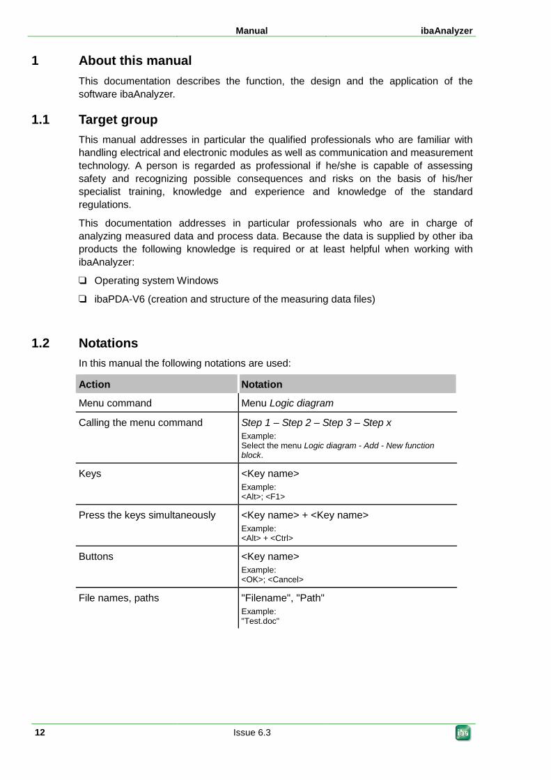
1.2 Notations In this manual the following notations are used:

Action Notation

Menu command Menu Logic diagram

Calling the menu command Step 1 – Step 2 – Step 3 – Step x Example: Select the menu Logic diagram - Add - New function block.

Keys <Key name> Example: <Alt>; <F1>

Press the keys simultaneously <Key name> + <Key name> Example: <Alt> + <Ctrl>

Buttons <Key name> Example: <OK>; <Cancel>

File names, paths "Filename", "Path" Example: "Test.doc"

ibaAnalyzer Manual

Issue 6.3 13

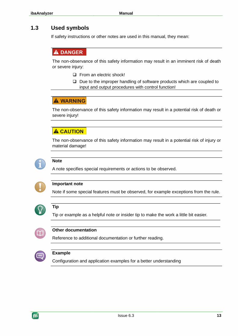
1.3 Used symbols If safety instructions or other notes are used in this manual, they mean:

The non-observance of this safety information may result in an imminent risk of death or severe injury:

From an electric shock! Due to the improper handling of software products which are coupled to

input and output procedures with control function!

The non-observance of this safety information may result in a potential risk of death or severe injury!

The non-observance of this safety information may result in a potential risk of injury or material damage!

Note

A note specifies special requirements or actions to be observed.

Important note

Note if some special features must be observed, for example exceptions from the rule.

Tip

Tip or example as a helpful note or insider tip to make the work a little bit easier.

Other documentation

Reference to additional documentation or further reading.

Example

Configuration and application examples for a better understanding

Manual ibaAnalyzer

14 Issue 6.3

2 Welcome to ibaAnalyzer – an overview ibaAnalyzer is a powerful tool for analyzing complex data which was recorded using the ibaPDA, ibaScope, ibaQDR, ibaLogic recording programs or products from other manufacturers (such as VISTA).

Analyzing large data volumes can be very time-consuming. Often, special algorithms are required for correlating measured data from a process and for its meaningful interpretation. During the development of ibaAnalyzer, special attention was thus paid to its capability of ensuring quick analyses.

In view of the wide-spread use of the program, many customers and users voiced wishes and new ideas, some of which were implemented in new functions of ibaAnalyzer. In this way, ibaAnalyzer is optimized and adapted to changing needs on an ongoing basis.

Besides the traditional task of enabling the presentation of measuring values during a process for the purpose of fault analysis or machine evaluation, a new application emerged in recent years:

ibaAnalyzer increasingly turns out to be a powerful tool for quality data management and for analyzing product-relevant data. With the upgraded functions of the database interface and of the report generator, ibaAnalyzer constitutes the fully integrated link between process-based and time-based measuring data ("Level 1") on the one hand and product-related quality data ("Level 2/3") on the other. Thanks to the underlying concept, quality data management systems can be implemented in this way which can cover a plant or machine as well as plant-spanning, factory-wide networks.

Yet, what never changes is the full upward compatibility. The newest ibaAnalyzer is always capable of analyzing the oldest data files, e.g. old EDAS data.

Buyers of an online data acquisition system receive, as before, a free copy of ibaAnalyzer which is not subject to any restrictions in terms of copying or number of installations. License fees are only payable for certain upgraded or additional functions enabling the use of the program for data extraction to files or databases or the processing of data from external sources.

ibaAnalyzer Manual

Issue 6.3 15

2.1 The ibaAnalyzer standard functions (not subject to license fees) Easy to use and intuitive user interface with smart docking windows and drag &

drop function Any number of signal strips, each enabling the selection of the following views: Time-based view (X axis = time axis)

Length-based view X axis = length axis)

X-Y view of two or more signals

FFT view

Simple placement of any number of signals in the signal strips using the drag & drop functionality (IEC1131-conforming)

Combination of data originating from different measuring processes or data sources Automatic or manual selection of colors for the curves. Individual scales for every signal within a signal strip, or scaling of a signal in

relation to any other signal on the same Y axis within a strip. Permanent display of the X/Y values for two rulers as well as for the most important

statistical values (min, max, average, standard deviation) for all the signals displayed

Zooming and moving of the section in a Navigator window 3D view and 2D top view (profile view) Powerful mathematical and technological functions for manipulating, combining,

calculating and creating signals. Generation of virtual signals, even multi-dimensional ones (vectors) A powerful digital, graphic filter designer with integrated signal generator for filter

testing. Flexible export function for generating new iba data files (for example, with

combined or mathematically modified signals) and for generating text or COMTRADE files (.txt, .csv) for further processing by other programs (for example, document generation, spreadsheet processing, etc.)

Powerful report generator for the free design and layout of analysis, quality, production and fault reports with different output formats

Information window: large-sized and alphanumeric display of important, calculated parameters or technostring information is possible

Macro function for simplifying and reusing comprehensive analysis functions and calculations.

Versatile marker functions for highlighting special measured values Use of text channels in signal strips Efficient management of the analyses for flexible use Multilingual program surface, switchable ibaHD-Server query (pseudo data file)

Manual ibaAnalyzer

16 Issue 6.3

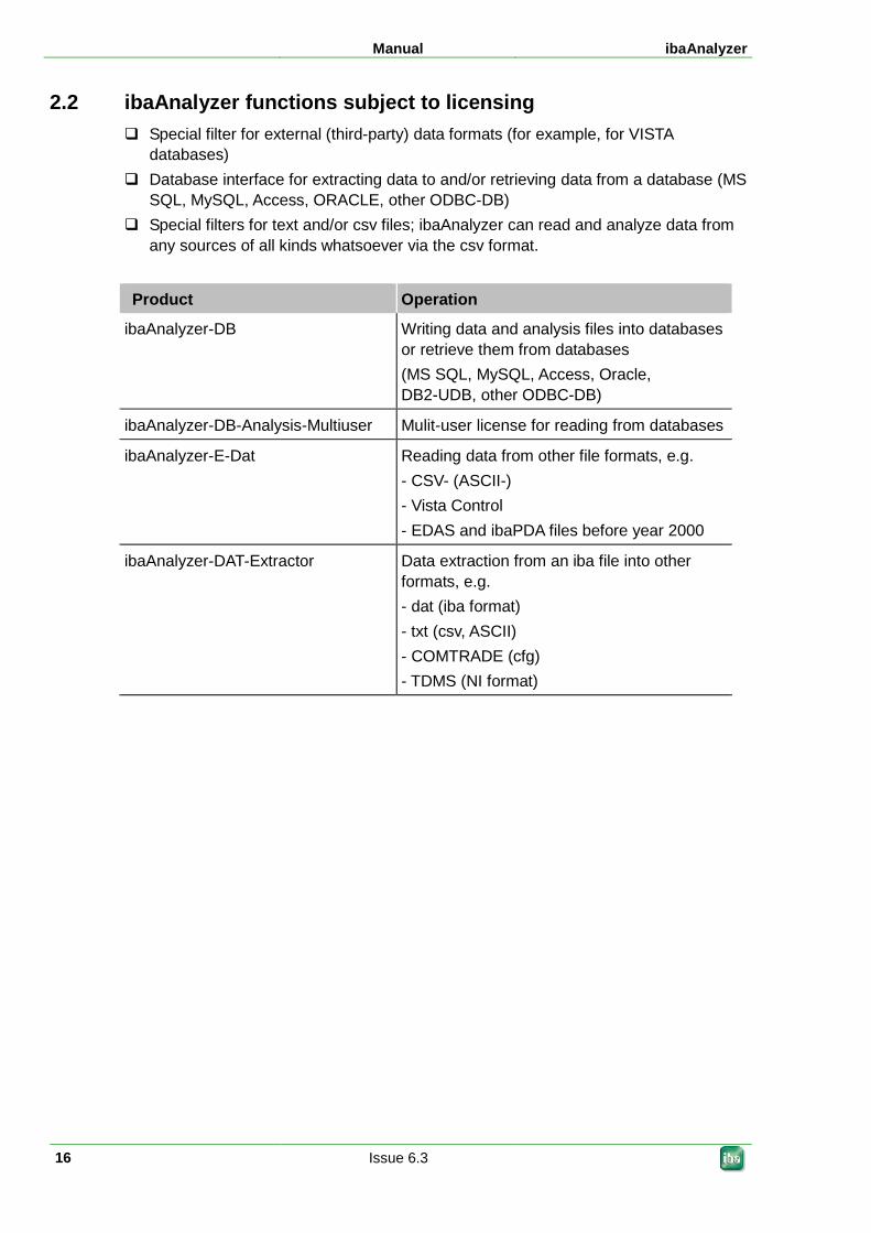
2.2 ibaAnalyzer functions subject to licensing Special filter for external (third-party) data formats (for example, for VISTA

databases) Database interface for extracting data to and/or retrieving data from a database (MS

SQL, MySQL, Access, ORACLE, other ODBC-DB) Special filters for text and/or csv files; ibaAnalyzer can read and analyze data from

any sources of all kinds whatsoever via the csv format.

Product Operation

ibaAnalyzer-DB Writing data and analysis files into databases or retrieve them from databases (MS SQL, MySQL, Access, Oracle, DB2-UDB, other ODBC-DB)

ibaAnalyzer-DB-Analysis-Multiuser Mulit-user license for reading from databases

ibaAnalyzer-E-Dat Reading data from other file formats, e.g. - CSV- (ASCII-) - Vista Control - EDAS and ibaPDA files before year 2000

ibaAnalyzer-DAT-Extractor Data extraction from an iba file into other formats, e.g. - dat (iba format) - txt (csv, ASCII) - COMTRADE (cfg) - TDMS (NI format)

ibaAnalyzer Manual

Issue 6.3 17

3 Operation and settings 3.1 Starting ibaAnalyzer 3.1.1 Starting in Windows

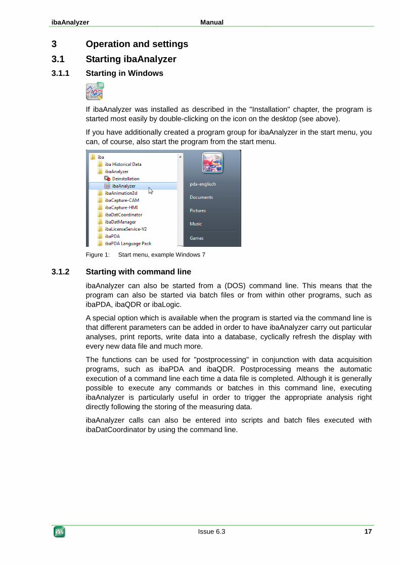
If ibaAnalyzer was installed as described in the "Installation" chapter, the program is started most easily by double-clicking on the icon on the desktop (see above).

If you have additionally created a program group for ibaAnalyzer in the start menu, you can, of course, also start the program from the start menu.

Figure 1: Start menu, example Windows 7

3.1.2 Starting with command line ibaAnalyzer can also be started from a (DOS) command line. This means that the program can also be started via batch files or from within other programs, such as ibaPDA, ibaQDR or ibaLogic.

A special option which is available when the program is started via the command line is that different parameters can be added in order to have ibaAnalyzer carry out particular analyses, print reports, write data into a database, cyclically refresh the display with every new data file and much more.

The functions can be used for "postprocessing" in conjunction with data acquisition programs, such as ibaPDA and ibaQDR. Postprocessing means the automatic execution of a command line each time a data file is completed. Although it is generally possible to execute any commands or batches in this command line, executing ibaAnalyzer is particularly useful in order to trigger the appropriate analysis right directly following the storing of the measuring data.

ibaAnalyzer calls can also be entered into scripts and batch files executed with ibaDatCoordinator by using the command line.

Manual ibaAnalyzer

18 Issue 6.3

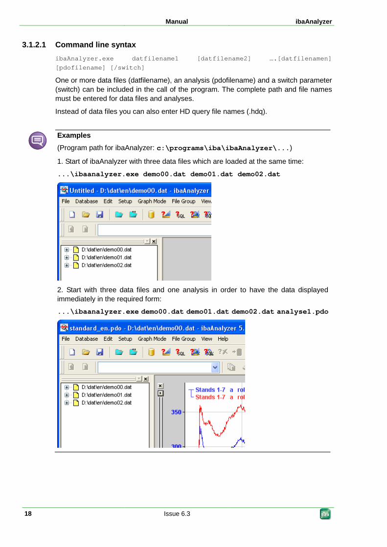
3.1.2.1 Command line syntax ibaAnalyzer.exe datfilename1 [datfilename2] ….[datfilenamen] [pdofilename] [/switch]

One or more data files (datfilename), an analysis (pdofilename) and a switch parameter (switch) can be included in the call of the program. The complete path and file names must be entered for data files and analyses.

Instead of data files you can also enter HD query file names (.hdq).

Examples (Program path for ibaAnalyzer: c:\programs\iba\ibaAnalyzer\...)

1. Start of ibaAnalyzer with three data files which are loaded at the same time:

...\ibaanalyzer.exe demo00.dat demo01.dat demo02.dat

2. Start with three data files and one analysis in order to have the data displayed immediately in the required form:

...\ibaanalyzer.exe demo00.dat demo01.dat demo02.dat analyse1.pdo

ibaAnalyzer Manual

Issue 6.3 19

3.1.2.2 Using the postprocessing command Since postprocessing is an automatic function which is controlled by the data acquisition program, such as ibaPDA, a placeholder must be used here instead of the data file name in order to access the most recent data file:

ibaAnalyzer.exe %f [pdofilename] [/switch]

%f: Last data file, complete path and file name (e.g. d:\dat\pda001.dat)

%g: Last data file, only data file name (e.g. pda001.dat)

%h: Last data file, file name without suffix (e.g. pda001)

Tip

For regular and automated calls of ibaAnalyzer depending on the data file generation, we recommend using the ibaDatCoordinator. Compared to the postprocessing, the application free of charge offers higher ease of use as well as higher flexibility and functional reliability.

3.1.2.3 Using the switches in the command line The switches are particularly important in conjunction with postprocessing because they can be used to automate complete analysis processes. It is, however, also possible to use the switches in conjunction with a manual program start.

Switch /reuse If this switch is included in the program call, ibaAnalyzer starts, loads the specified data files and, if applicable, displays the results as determined by an analysis. If another program call with /reuse switches follows, the new data files and, if applicable, also a new analysis are loaded into the existing instance of ibaAnalyzer with the old data being overwritten. This means that the existing instance is reused. Opening of further instances is prevented.

By automating this process, for example, e.g. by using the postprocessing command, it is possible to permanently update an analysis display with the latest measuring data.

If ibaAnalyzer is started with the /reuse switch, a key button in the upper left corner of the toolbar appears . Clicking this button stops the automatic update function, so that you can take your time to view data. Clicking the button again re-enables the update function.

Switch /append This switch enables the appending of several data files specified in the call. These files are then coherently shown one after another in the X direction. (An example is given below).

In connection with the /sql switch, the results from database queries are appended to each other.

Manual ibaAnalyzer

20 Issue 6.3

Switch /print This switch ensures that the measuring data can be printed as a record or log in the format defined in the selected analysis. The Windows default printer is used.

When the printing process is completed or after the print job has been triggered, ibaAnalyzer is closed again. In the case of an error, however, ibaAnalyzer remains open in order to display the error message. (An example is given below).

Switch /extract[:filename] This switch can only be used in conjunction with the license for the database interface (ibaAnalyzer DB-Extractor). The /extract switch means that ibaAnalyzer starts and loads the specified data file. Thereafter, the measuring data is processed in accordance with the specified analysis and extracted into a database. During this process, no ibaAnalyzer window is opened on the screen, i.e. the extracting process takes place in the background. The database connection must have been configured beforehand and is part of the analysis. (An example is given below).

You may also extract the data into a file. In this case, the desired file name is to be added as parameter. For extracting data into a file, a particular license is required (ibaAnalyzer DAT-Extractor).

For further information, please also refer to Database interface (option), Page 408 and/or to the additional documentation.

Switch /report[:filename] This switch will only be available with ibaAnalyzer version 3.52 and higher. With this switch, ibaAnalyzer starts, loads a specified data file and performs an analysis in accordance with the specified analysis rule. Thereafter, the integrated report generator is started and the data is printed on the Windows default printer using a report layout specified in the analysis rule if the [:filename] option was not used with the switch.

If the [:filename] switch option is used, the report can be written into a file rather than being printed. The desired file type is determined by the file name extension. Many customary formats are supported, including, for example, .pdf, .htm, .rtf, .tiff, .jpg, .xls, etc. (an example is given below).

For further information, please also refer to Report generator, Page 386.

/sql:filename.sql[;sync:”syncFieldName”] switch This switch will only be available with ibaAnalyzer version 3.57 and higher. Its use is subject to the license for the database interface. This switch is used for database queries. The :filename.sql argument can be used to transfer SQL statements as a basis for the database query. The additional, optional [;sync:...] parameter can be used to specify a grouping criterion for the query data.

For further information, please also refer to Database interface (option), Page 408 and/or to the additional documentation.

/trendsql:filename.sql[;sync:”syncFieldName”] switch This switch is available with ibaAnalyzer version 5.10.0 and higher. Its use is subject to the license for the database interface. Unlike the previous switch, it is used to query info fields and/or computed columns from a database. The "filename.sql" parameter can be used to transfer SQL statements as a basis for the database query.

ibaAnalyzer Manual

Issue 6.3 21

The query results, i.e. signals with measuring points from the time stamp column as well as info fields and/or computed columns, are displayed in the "Trend query result" branch and can be used in the analysis.

The "filename.sql" file must be a text file compliant with the SQL language as is supported by the database specified in the analysis (.pdo) (e.g. Oracle SQL server, DB2-UDB, etc.). You can load and execute this file by means of the trendquery builder.

Moreover, the execution of the SQL statement should lead to a result set with a time stamp field and at least one numerical field. Moreover, the statement should contain a sort ORDER BY clause on the time stamp.

Optionally, a synchronization field can be transferred with the "sync:" parameter for the query.

Example:

C:\Program Files\iba\ibaAnalyzer\ibaanalyzer.exe c:\pdo_for_sql\ sql.pdo /trendsql:getlastcoil.sql

Further documentation

Detailed information on the database functions are contained in the ibaAnalyzer-DB product manual.

Switch /overviewsql:filename.sql This switch has the same function as the one described before. However, the result of the trend query is not displayed in the signal tree, but in the "Overview" window or tab.

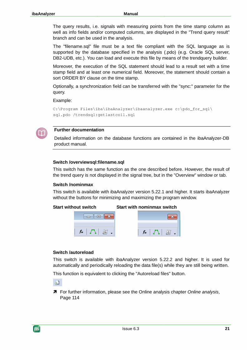
Switch /nominmax This switch is available with ibaAnalyzer version 5.22.1 and higher. It starts ibaAnalyzer without the buttons for minimizing and maximizing the program window.

Start without switch Start with nominmax switch

Switch /autoreload This switch is available with ibaAnalyzer version 5.22.2 and higher. It is used for automatically and periodically reloading the data file(s) while they are still being written.

This function is equivalent to clicking the "Autoreload files" button.

For further information, please see the Online analysis chapter Online analysis,

Page 114

Manual ibaAnalyzer

22 Issue 6.3

Switch /loadnewfiles This switch is available with ibaAnalyzer version 5.22.2 and higher. It is used for automatically and periodically reloading the data file(s) while they are still being written.

The function is equivalent to clicking the "Automatically load new data files from specified directory" button.

For further information, please see the Online analysis chapter Online analysis,

Page 114

Switch /dbPDO:AnalysisName This switch is available with ibaAnalyzer version 5.13.1 and higher. It opens analyses (*.pdo) which had been stored in a database. This database is created once and set in the preferences, PDO database storage tab.

Only add the desired analysis name – as it was stored in the database – after the colon.

Switch /filetree:conf.txt This switch is available with ibaAnalyzer version 5.21.0 and higher. It starts ibaAnalyzer with a predefined signal or file tree. Thus, several data files can be opened both on the same level and appended to each other.

The desired configuration of the file tree has to be exported as text file (here conf.txt) before. This file is transferred as parameter with the switch.

Information on the export/import of a file tree can be found in the chapter Export/import file tree, Page 118

Switch /language This switch is available from ibaAnalyzer version 6.0.0 and higher and only works in combination with Windows versions Vista or higher. It starts ibaAnalyzer in the specified language. If no language is specified, ibaAnalyzer starts in the system language or in English.

At the moment, the following variants are available:

/english

/german

/french

/spanish

/russian

/chinese

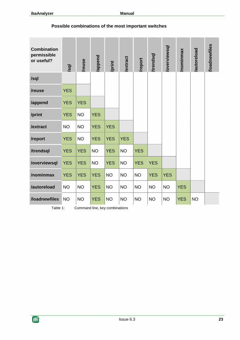
ibaAnalyzer Manual

Issue 6.3 23

Possible combinations of the most important switches

Combination permissible or useful?

/sql

/reus

e

/app

end

/prin

t

/ext

ract

/repo

rt

/tren

dsql

/ove

rvie

wsq

l

/nom

inm

ax

/aut

orel

oad

/load

new

files

/sql

/reuse YES

/append YES YES

/print YES NO YES

/extract NO NO YES YES

/report YES NO YES YES YES

/trendsql YES YES NO YES NO YES

/overviewsql YES YES NO YES NO YES YES

/nominmax YES YES YES NO NO NO YES YES

/autoreload NO NO YES NO NO NO NO NO YES

/loadnewfiles NO NO YES NO NO NO NO NO YES NO

Table 1: Command line, key combinations

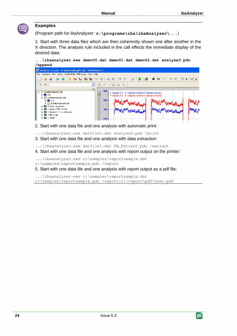
Manual ibaAnalyzer

24 Issue 6.3

Examples (Program path for ibaAnalyzer: c:\programs\iba\ibaAnalyzer\...)

1. Start with three data files which are then coherently shown one after another in the X direction. The analysis rule included in the call effects the immediate display of the desired data. ...\ibaanalyzer.exe demo00.dat demo01.dat demo02.dat analyse3.pdo /append

2. Start with one data file and one analysis with automatic print: ...\ibaanalyzer.exe datfile1.dat analyse2.pdo /print

3. Start with one data file and one analysis with data extraction: ...\ibaanalyzer.exe datfile1.dat DB_Extract.pdo /extract

4. Start with one data file and one analysis with report output on the printer: ...\ibaanalyzer.exe c:\samples\reportsample.dat c:\samples\reportsample.pdo /report

5. Start with one data file and one analysis with report output as a pdf file: ...\ibaanalyzer.exe c:\samples\reportsample.dat c:\samples\reportsample.pdo /report:c:\report\pdf\test.pdf

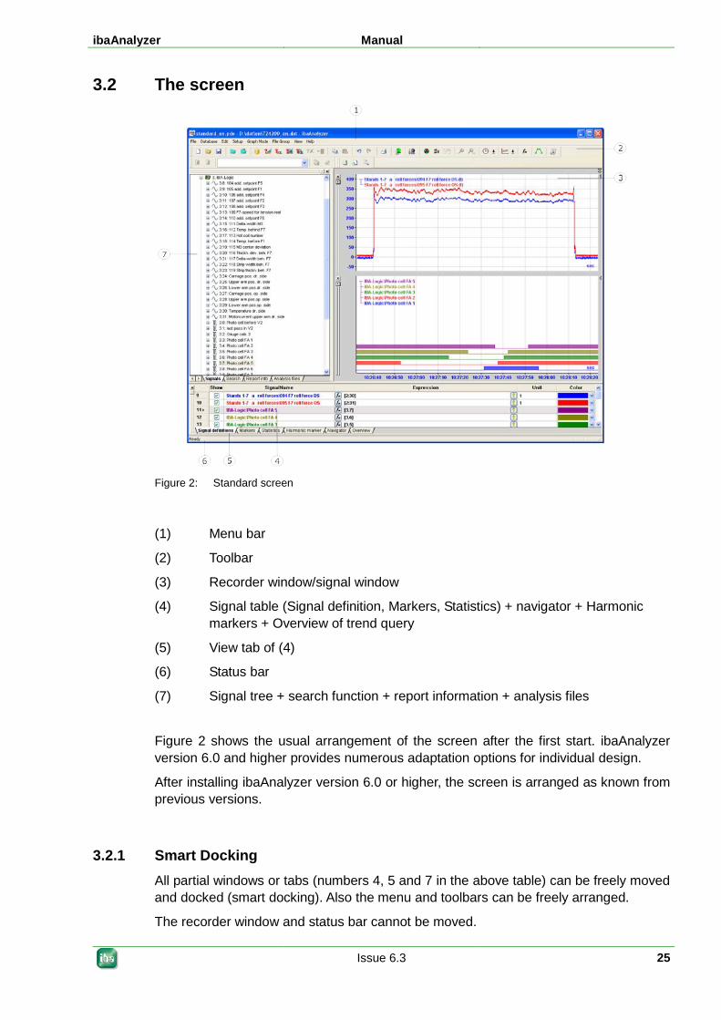
ibaAnalyzer Manual

Issue 6.3 25

3.2 The screen

Figure 2: Standard screen

(1) Menu bar

(2) Toolbar

(3) Recorder window/signal window

(4) Signal table (Signal definition, Markers, Statistics) + navigator + Harmonic markers + Overview of trend query

(5) View tab of (4)

(6) Status bar

(7) Signal tree + search function + report information + analysis files

Figure 2 shows the usual arrangement of the screen after the first start. ibaAnalyzer version 6.0 and higher provides numerous adaptation options for individual design.

After installing ibaAnalyzer version 6.0 or higher, the screen is arranged as known from previous versions.

3.2.1 Smart Docking All partial windows or tabs (numbers 4, 5 and 7 in the above table) can be freely moved and docked (smart docking). Also the menu and toolbars can be freely arranged.

The recorder window and status bar cannot be moved.

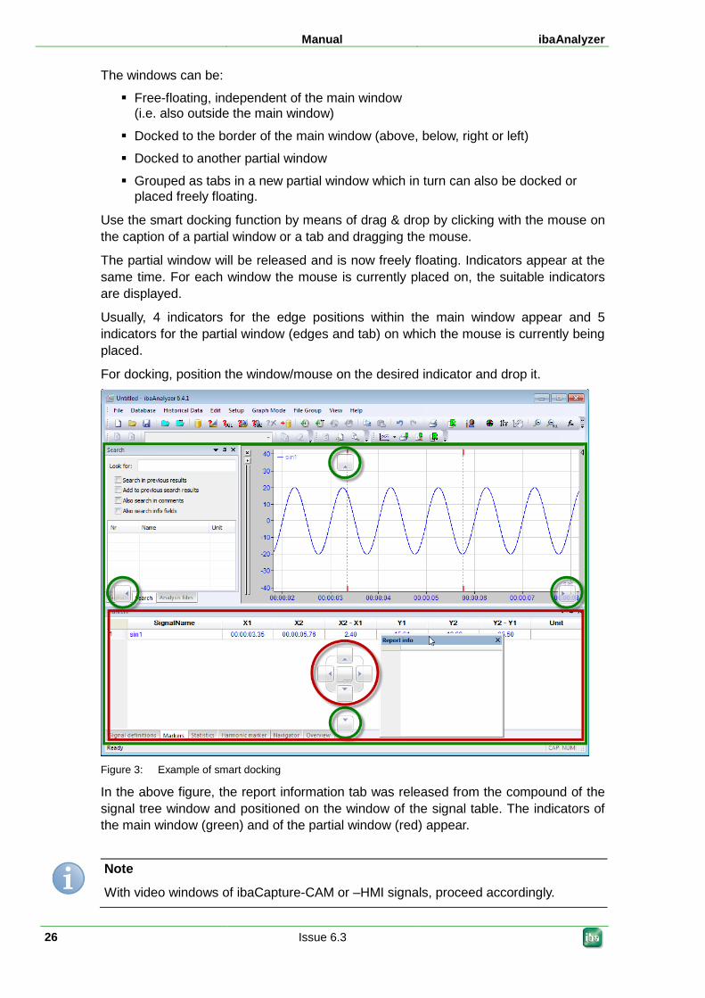
Manual ibaAnalyzer

26 Issue 6.3

The windows can be:

Free-floating, independent of the main window (i.e. also outside the main window)

Docked to the border of the main window (above, below, right or left)

Docked to another partial window

Grouped as tabs in a new partial window which in turn can also be docked or placed freely floating.

Use the smart docking function by means of drag & drop by clicking with the mouse on the caption of a partial window or a tab and dragging the mouse.

The partial window will be released and is now freely floating. Indicators appear at the same time. For each window the mouse is currently placed on, the suitable indicators are displayed.

Usually, 4 indicators for the edge positions within the main window appear and 5 indicators for the partial window (edges and tab) on which the mouse is currently being placed.

For docking, position the window/mouse on the desired indicator and drop it.

Figure 3: Example of smart docking

In the above figure, the report information tab was released from the compound of the signal tree window and positioned on the window of the signal table. The indicators of the main window (green) and of the partial window (red) appear.

Note

With video windows of ibaCapture-CAM or –HMI signals, proceed accordingly.

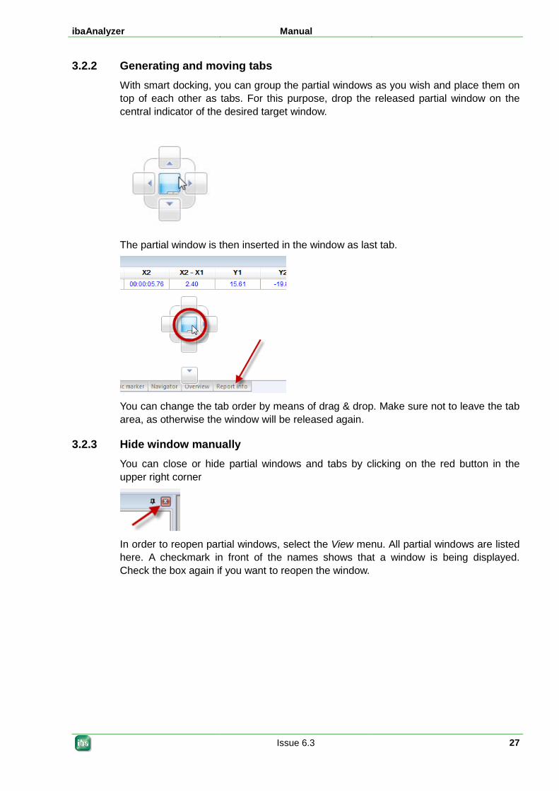
ibaAnalyzer Manual

Issue 6.3 27

3.2.2 Generating and moving tabs With smart docking, you can group the partial windows as you wish and place them on top of each other as tabs. For this purpose, drop the released partial window on the central indicator of the desired target window.

The partial window is then inserted in the window as last tab.

You can change the tab order by means of drag & drop. Make sure not to leave the tab area, as otherwise the window will be released again.

3.2.3 Hide window manually You can close or hide partial windows and tabs by clicking on the red button in the upper right corner

In order to reopen partial windows, select the View menu. All partial windows are listed here. A checkmark in front of the names shows that a window is being displayed. Check the box again if you want to reopen the window.

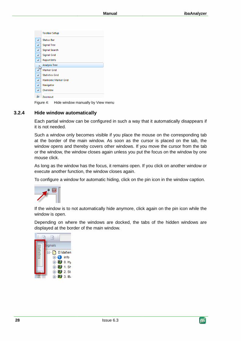
Manual ibaAnalyzer

28 Issue 6.3

Figure 4: Hide window manually by View menu

3.2.4 Hide window automatically Each partial window can be configured in such a way that it automatically disappears if it is not needed.

Such a window only becomes visible if you place the mouse on the corresponding tab at the border of the main window. As soon as the cursor is placed on the tab, the window opens and thereby covers other windows. If you move the cursor from the tab or the window, the window closes again unless you put the focus on the window by one mouse click.

As long as the window has the focus, it remains open. If you click on another window or execute another function, the window closes again.

To configure a window for automatic hiding, click on the pin icon in the window caption.

If the window is to not automatically hide anymore, click again on the pin icon while the window is open.

Depending on where the windows are docked, the tabs of the hidden windows are displayed at the border of the main window.

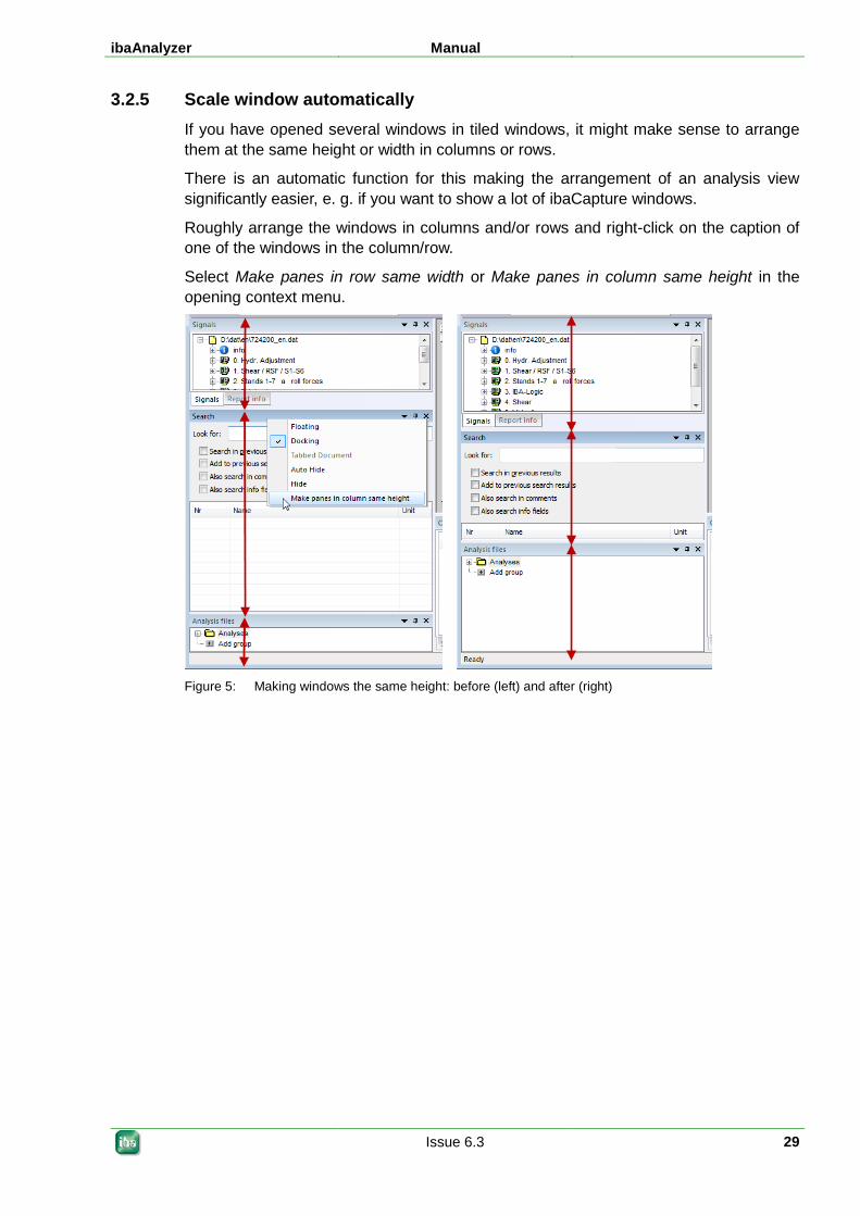
ibaAnalyzer Manual

Issue 6.3 29

3.2.5 Scale window automatically If you have opened several windows in tiled windows, it might make sense to arrange them at the same height or width in columns or rows.

There is an automatic function for this making the arrangement of an analysis view significantly easier, e. g. if you want to show a lot of ibaCapture windows.

Roughly arrange the windows in columns and/or rows and right-click on the caption of one of the windows in the column/row.

Select Make panes in row same width or Make panes in column same height in the opening context menu.

Figure 5: Making windows the same height: before (left) and after (right)

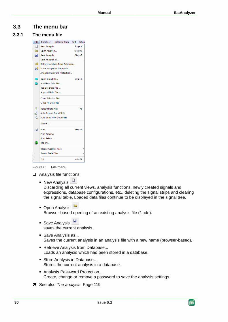
Manual ibaAnalyzer

30 Issue 6.3

3.3 The menu bar 3.3.1 The menu file

Figure 6: File menu

Analysis file functions

New Analysis Discarding all current views, analysis functions, newly created signals and expressions, database configurations, etc., deleting the signal strips and clearing the signal table. Loaded data files continue to be displayed in the signal tree.

Open Analysis Browser-based opening of an existing analysis file (*.pdo).

Save Analysis saves the current analysis.

Save Analysis as... Saves the current analysis in an analysis file with a new name (browser-based).

Retrieve Analysis from Database... Loads an analysis which had been stored in a database.

Store Analysis in Database… Stores the current analysis in a database.

Analysis Password Protection... Create, change or remove a password to save the analysis settings.

See also The analysis, Page 119

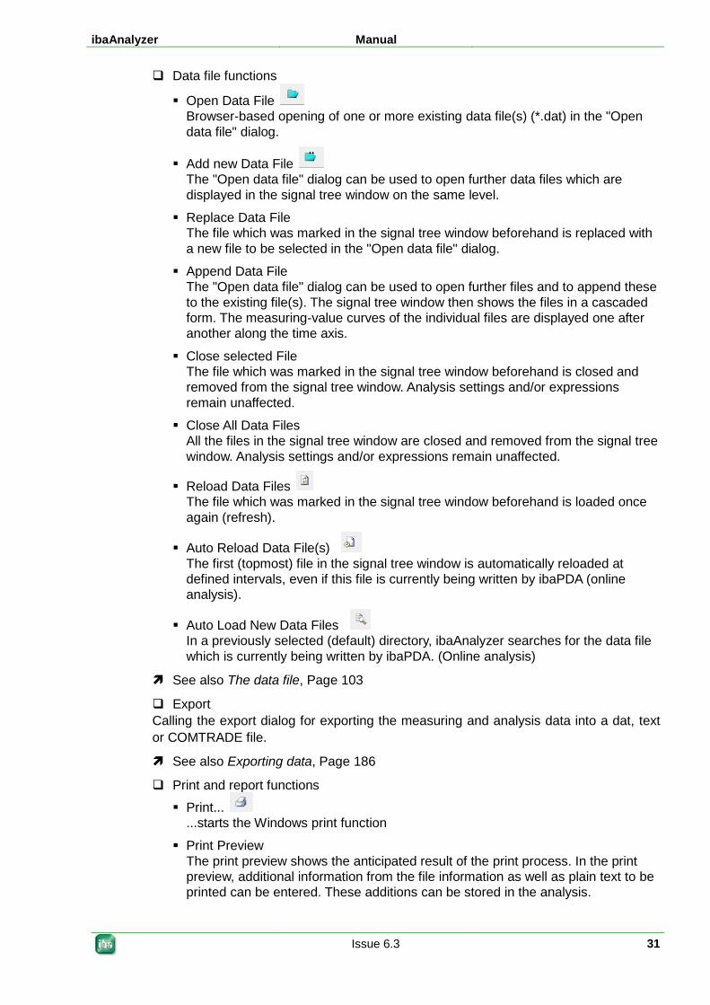
ibaAnalyzer Manual

Issue 6.3 31

Data file functions

Open Data File Browser-based opening of one or more existing data file(s) (*.dat) in the "Open data file" dialog.

Add new Data File The "Open data file" dialog can be used to open further data files which are displayed in the signal tree window on the same level.

Replace Data File The file which was marked in the signal tree window beforehand is replaced with a new file to be selected in the "Open data file" dialog.

Append Data File The "Open data file" dialog can be used to open further files and to append these to the existing file(s). The signal tree window then shows the files in a cascaded form. The measuring-value curves of the individual files are displayed one after another along the time axis.

Close selected File The file which was marked in the signal tree window beforehand is closed and removed from the signal tree window. Analysis settings and/or expressions remain unaffected.

Close All Data Files All the files in the signal tree window are closed and removed from the signal tree window. Analysis settings and/or expressions remain unaffected.

Reload Data Files The file which was marked in the signal tree window beforehand is loaded once again (refresh).

Auto Reload Data File(s) The first (topmost) file in the signal tree window is automatically reloaded at defined intervals, even if this file is currently being written by ibaPDA (online analysis).

Auto Load New Data Files In a previously selected (default) directory, ibaAnalyzer searches for the data file which is currently being written by ibaPDA. (Online analysis)

See also The data file, Page 103

Export Calling the export dialog for exporting the measuring and analysis data into a dat, text or COMTRADE file.

See also Exporting data, Page 186

Print and report functions

Print... ...starts the Windows print function

Print Preview The print preview shows the anticipated result of the print process. In the print preview, additional information from the file information as well as plain text to be printed can be entered. These additions can be stored in the analysis.

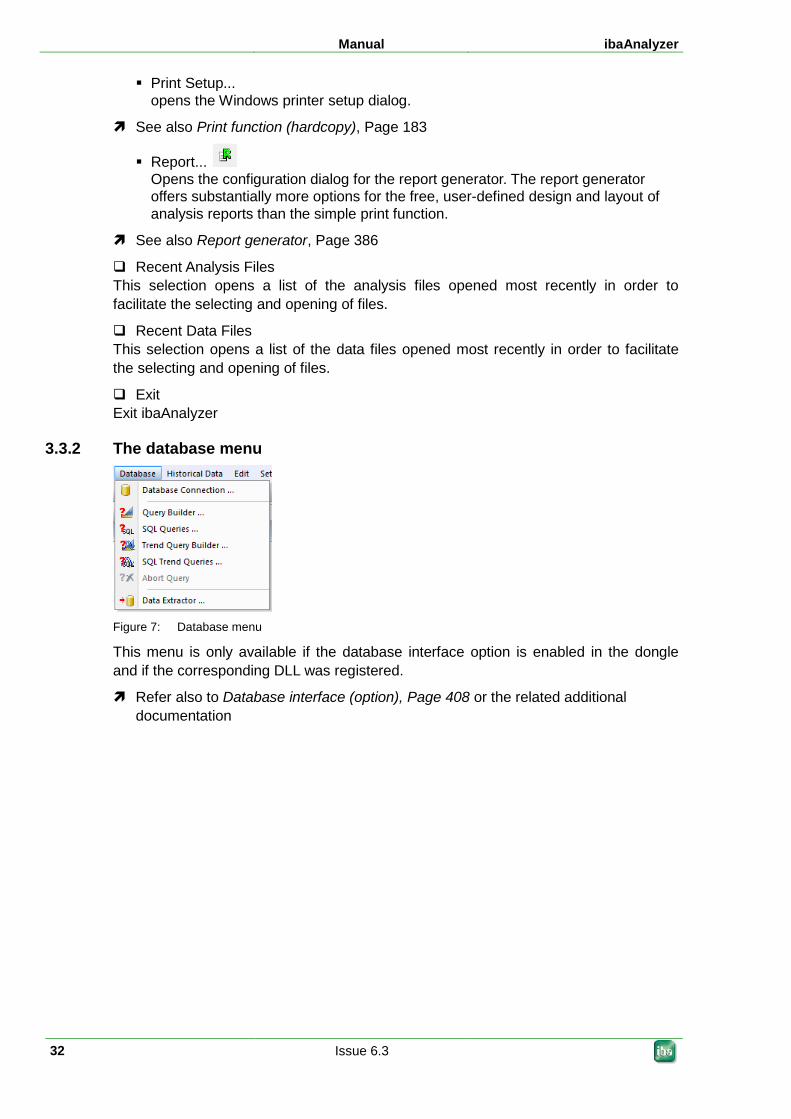
Manual ibaAnalyzer

32 Issue 6.3

Print Setup... opens the Windows printer setup dialog.

See also Print function (hardcopy), Page 183

Report... Opens the configuration dialog for the report generator. The report generator offers substantially more options for the free, user-defined design and layout of analysis reports than the simple print function.

See also Report generator, Page 386

Recent Analysis Files This selection opens a list of the analysis files opened most recently in order to facilitate the selecting and opening of files.

Recent Data Files This selection opens a list of the data files opened most recently in order to facilitate the selecting and opening of files.

Exit Exit ibaAnalyzer

3.3.2 The database menu

Figure 7: Database menu

This menu is only available if the database interface option is enabled in the dongle and if the corresponding DLL was registered.

Refer also to Database interface (option), Page 408 or the related additional documentation

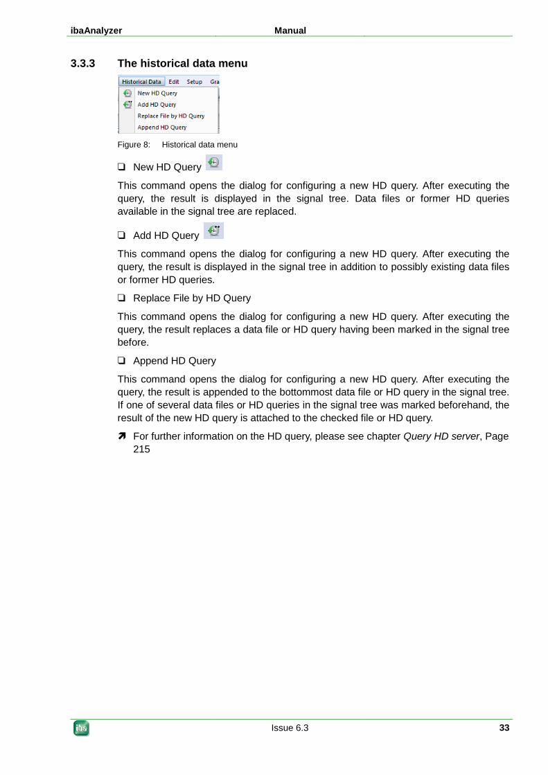
ibaAnalyzer Manual

Issue 6.3 33

3.3.3 The historical data menu

Figure 8: Historical data menu

New HD Query

This command opens the dialog for configuring a new HD query. After executing the query, the result is displayed in the signal tree. Data files or former HD queries available in the signal tree are replaced.

Add HD Query

This command opens the dialog for configuring a new HD query. After executing the query, the result is displayed in the signal tree in addition to possibly existing data files or former HD queries.

Replace File by HD Query

This command opens the dialog for configuring a new HD query. After executing the query, the result replaces a data file or HD query having been marked in the signal tree before.

Append HD Query

This command opens the dialog for configuring a new HD query. After executing the query, the result is appended to the bottommost data file or HD query in the signal tree. If one of several data files or HD queries in the signal tree was marked beforehand, the result of the new HD query is attached to the checked file or HD query.

For further information on the HD query, please see chapter Query HD server, Page 215

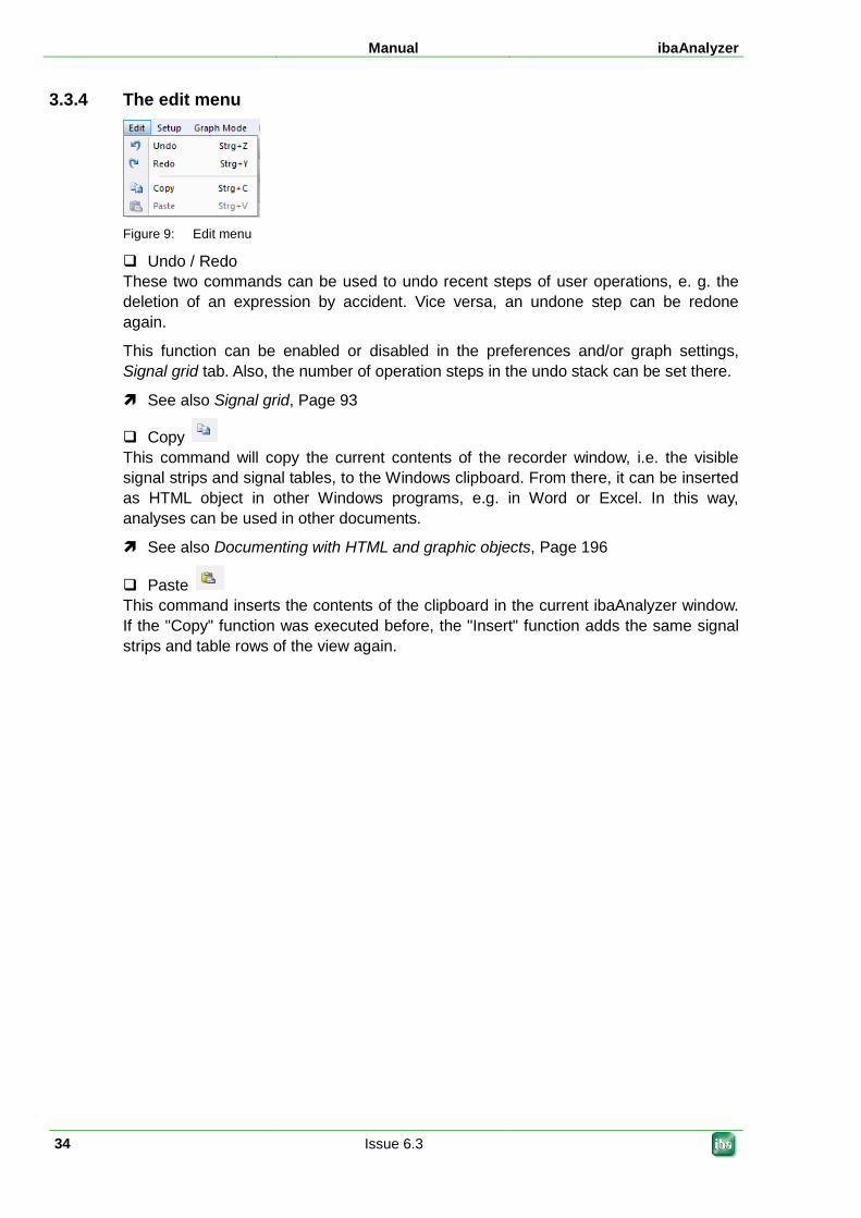
Manual ibaAnalyzer

34 Issue 6.3

3.3.4 The edit menu

Figure 9: Edit menu

Undo / Redo These two commands can be used to undo recent steps of user operations, e. g. the deletion of an expression by accident. Vice versa, an undone step can be redone again.

This function can be enabled or disabled in the preferences and/or graph settings, Signal grid tab. Also, the number of operation steps in the undo stack can be set there.

See also Signal grid, Page 93

Copy This command will copy the current contents of the recorder window, i.e. the visible signal strips and signal tables, to the Windows clipboard. From there, it can be inserted as HTML object in other Windows programs, e.g. in Word or Excel. In this way, analyses can be used in other documents.

See also Documenting with HTML and graphic objects, Page 196

Paste This command inserts the contents of the clipboard in the current ibaAnalyzer window. If the "Copy" function was executed before, the "Insert" function adds the same signal strips and table rows of the view again.

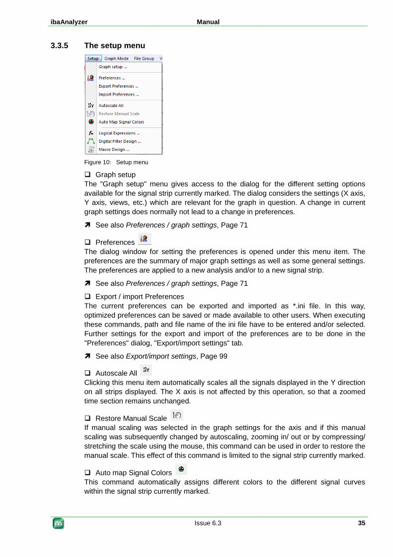
ibaAnalyzer Manual

Issue 6.3 35

3.3.5 The setup menu

Figure 10: Setup menu

Graph setup The "Graph setup" menu gives access to the dialog for the different setting options available for the signal strip currently marked. The dialog considers the settings (X axis, Y axis, views, etc.) which are relevant for the graph in question. A change in current graph settings does normally not lead to a change in preferences.

See also Preferences / graph settings, Page 71

Preferences The dialog window for setting the preferences is opened under this menu item. The preferences are the summary of major graph settings as well as some general settings. The preferences are applied to a new analysis and/or to a new signal strip.

See also Preferences / graph settings, Page 71

Export / import Preferences The current preferences can be exported and imported as *.ini file. In this way, optimized preferences can be saved or made available to other users. When executing these commands, path and file name of the ini file have to be entered and/or selected. Further settings for the export and import of the preferences are to be done in the "Preferences" dialog, "Export/import settings" tab.

See also Export/import settings, Page 99

Autoscale All Clicking this menu item automatically scales all the signals displayed in the Y direction on all strips displayed. The X axis is not affected by this operation, so that a zoomed time section remains unchanged.

Restore Manual Scale If manual scaling was selected in the graph settings for the axis and if this manual scaling was subsequently changed by autoscaling, zooming in/ out or by compressing/ stretching the scale using the mouse, this command can be used in order to restore the manual scale. This effect of this command is limited to the signal strip currently marked.

Auto map Signal Colors This command automatically assigns different colors to the different signal curves within the signal strip currently marked.

Manual ibaAnalyzer

36 Issue 6.3

Logical Expressions This command opens the dialog for the logical signal definitions. It serves for the definition of artificial or "virtual" signals. Furthermore, it is also possible to define multi-dimensional signals (arrays) here.

See also Logical signal definitions, Page 172

Digital Filter Design This menu item opens the graphic editor for digital filter design.

See also Filter editor, Page 374

Macro Design This command opens the dialog for generating macros. By means of macros, comprehensive computations and complex analysis functions can be encapsulated to be able to handle them more easily and use them more than once.

See also Macros, Page 359

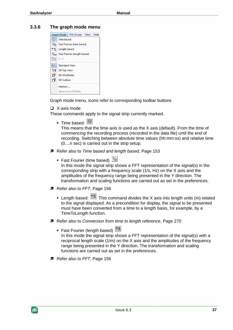
ibaAnalyzer Manual

Issue 6.3 37

3.3.6 The graph mode menu

Graph mode menu, icons refer to corresponding toolbar buttons

X-axis mode These commands apply to the signal strip currently marked.

Time based: This means that the time axis is used as the X axis (default). From the time of commencing the recording process (recorded in the data file) until the end of recording. Switching between absolute time values (hh:mm:ss) and relative time (0....n sec) is carried out in the strip setup.

Refer also to Time based and length based, Page 153

Fast Fourier (time based) In this mode the signal strip shows a FFT representation of the signal(s) in the corresponding strip with a frequency scale (1/s, Hz) on the X axis and the amplitudes of the frequency range being presented in the Y direction. The transformation and scaling functions are carried out as set in the preferences.

Refer also to FFT, Page 156

Length based: This command divides the X axis into length units (m) related to the signal displayed. As a precondition for display, the signal to be presented must have been converted from a time to a length basis, for example, by a TimeToLength function.

Refer also to Conversion from time to length reference, Page 270

Fast Fourier (length based) In this mode the signal strip shows a FFT representation of the signal(s) with a reciprocal length scale (1/m) on the X axis and the amplitudes of the frequency range being presented in the Y direction. The transformation and scaling functions are carried out as set in the preferences.

Refer also to FFT, Page 156

Manual ibaAnalyzer

38 Issue 6.3

X – Y This presentation mode is only offered if a strip contains at least two signals. If this mode is selected, the time or length axis is ignored and one signal is plotted above the other. In this way, it is possible to show dependencies of one or more signals on another signal. Using the mouse, the user selects the signal to be plotted on the X axis and the signal to be plotted on the Y axis by arranging the signals accordingly on the strip. The function is available for both time and length based signals.

Refer also to X - Y, Page 154

Views Standard View

The standard view is the default setting. It leads to a two-dimensional curve presentation.

Refer also to Standard view, Page 158

2D Top View Despite two-dimensional presentation, this view also offers information on a third dimension in that a color code is used for displaying the amplitudes of the signals measured. This view is particularly suitable for the presentation of profiles (temperature, thickness, shape profiles, etc.).

Refer also to 2D top view, Page 158

3D Wire Frame This view shows the signals measured as a three-dimensional mountain which solely consists of lines which connect the samples to each other. The resolution of this line mesh (B-Splines) can be varied in the setup for the 3D display (preferences or graph setup).

Refer also to 3D wire frame, Page 164

3D Surface This view offers a three-dimensional false-color presentation of the signals measured. Different colors (as selected in the setup) are assigned to amplitudes of the signals measured. The spaces between the signals measured can be sharply separated or they can be displayed with smooth color transitions as required. These preferences are also set in the 3D setup.

Refer also to 3D surface, Page 167

Markers…: Behind this item you’ll find the configuration dialog for markers.

Refer also to Markers, Page 199

Show Cross Profiles: This option is only available in the 2D top view. It enables the activation or deactivation of the display of cross profiles.

Refer also to 2D top view, Page 158

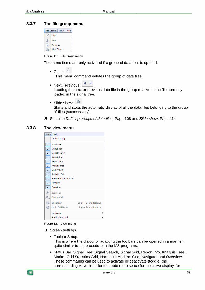
ibaAnalyzer Manual

Issue 6.3 39

3.3.7 The file group menu

Figure 11: File group menu

The menu items are only activated if a group of data files is opened.

Clear: This menu command deletes the group of data files.

Next / Previous: Loading the next or previous data file in the group relative to the file currently loaded in the signal tree.

Slide show: Starts and stops the automatic display of all the data files belonging to the group of files (successively).

See also Defining groups of data files, Page 108 and Slide show, Page 114

3.3.8 The view menu

Figure 12: View menu

Screen settings

Toolbar Setup: This is where the dialog for adapting the toolbars can be opened in a manner quite similar to the procedure in the MS programs.

Status Bar, Signal Tree, Signal Search, Signal Grid, Report Info, Analysis Tree, Marker Grid Statistics Grid, Harmonic Markers Grid, Navigator and Overview: These commands can be used to activate or deactivate (toggle) the corresponding views in order to create more space for the curve display, for

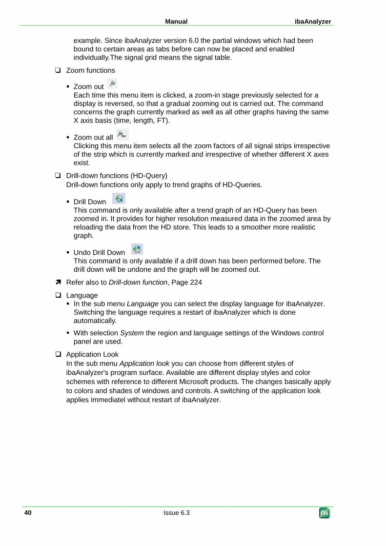
Manual ibaAnalyzer

40 Issue 6.3

example. Since ibaAnalyzer version 6.0 the partial windows which had been bound to certain areas as tabs before can now be placed and enabled individually.The signal grid means the signal table.

Zoom functions

Zoom out Each time this menu item is clicked, a zoom-in stage previously selected for a display is reversed, so that a gradual zooming out is carried out. The command concerns the graph currently marked as well as all other graphs having the same X axis basis (time, length, FT).

Zoom out all Clicking this menu item selects all the zoom factors of all signal strips irrespective of the strip which is currently marked and irrespective of whether different X axes exist.

Drill-down functions (HD-Query) Drill-down functions only apply to trend graphs of HD-Queries.

Drill Down This command is only available after a trend graph of an HD-Query has been zoomed in. It provides for higher resolution measured data in the zoomed area by reloading the data from the HD store. This leads to a smoother more realistic graph.

Undo Drill Down This command is only available if a drill down has been performed before. The drill down will be undone and the graph will be zoomed out.

Refer also to Drill-down function, Page 224

Language In the sub menu Language you can select the display language for ibaAnalyzer.

Switching the language requires a restart of ibaAnalyzer which is done automatically.

With selection System the region and language settings of the Windows control panel are used.

Application Look In the sub menu Application look you can choose from different styles of ibaAnalyzer's program surface. Available are different display styles and color schemes with reference to different Microsoft products. The changes basically apply to colors and shades of windows and controls. A switching of the application look applies immediatel without restart of ibaAnalyzer.

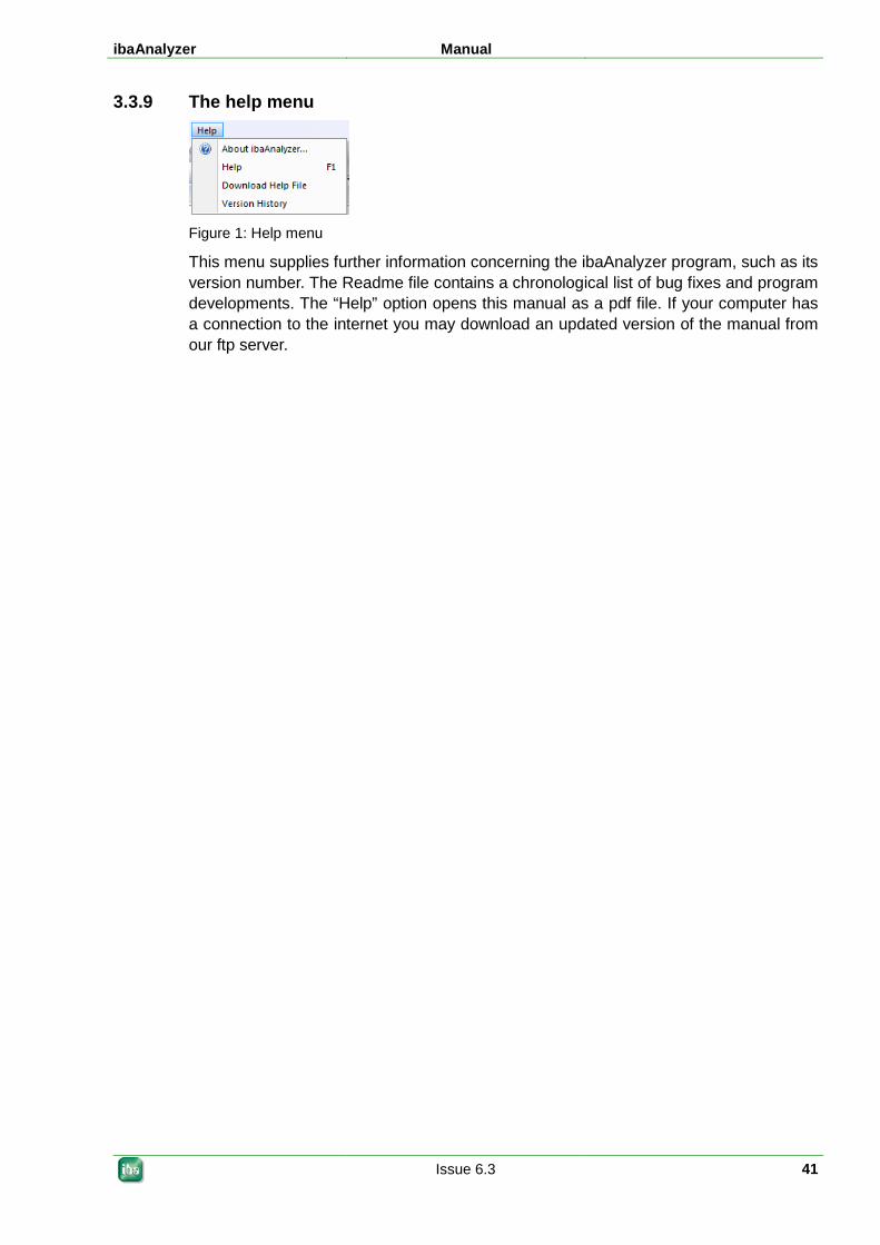
ibaAnalyzer Manual

Issue 6.3 41

3.3.9 The help menu

Figure 1: Help menu

This menu supplies further information concerning the ibaAnalyzer program, such as its version number. The Readme file contains a chronological list of bug fixes and program developments. The “Help” option opens this manual as a pdf file. If your computer has a connection to the internet you may download an updated version of the manual from our ftp server.

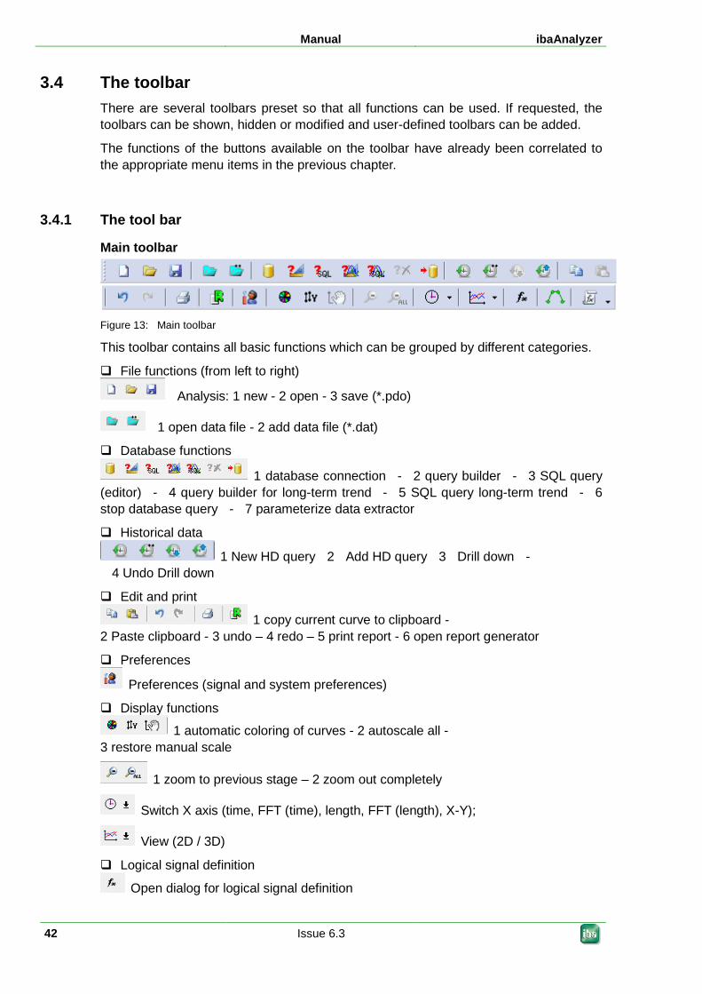
Manual ibaAnalyzer

42 Issue 6.3

3.4 The toolbar There are several toolbars preset so that all functions can be used. If requested, the toolbars can be shown, hidden or modified and user-defined toolbars can be added.

The functions of the buttons available on the toolbar have already been correlated to the appropriate menu items in the previous chapter.

3.4.1 The tool bar

Main toolbar

Figure 13: Main toolbar

This toolbar contains all basic functions which can be grouped by different categories.

File functions (from left to right)

Analysis: 1 new - 2 open - 3 save (*.pdo)

1 open data file - 2 add data file (*.dat)

Database functions

1 database connection - 2 query builder - 3 SQL query (editor) - 4 query builder for long-term trend - 5 SQL query long-term trend - 6 stop database query - 7 parameterize data extractor

Historical data

1 New HD query 2 Add HD query 3 Drill down - 4 Undo Drill down

Edit and print

1 copy current curve to clipboard - 2 Paste clipboard - 3 undo – 4 redo – 5 print report - 6 open report generator

Preferences

Preferences (signal and system preferences)

Display functions

1 automatic coloring of curves - 2 autoscale all - 3 restore manual scale

1 zoom to previous stage – 2 zoom out completely

Switch X axis (time, FFT (time), length, FFT (length), X-Y);

View (2D / 3D)

Logical signal definition

Open dialog for logical signal definition

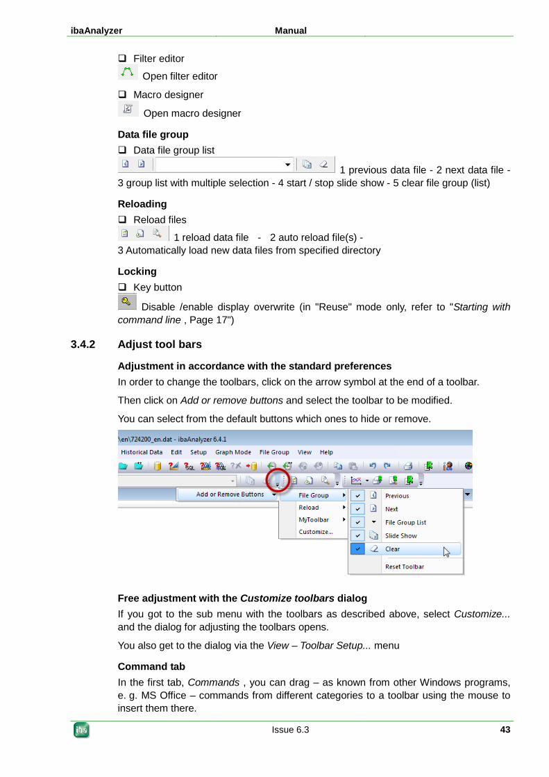
ibaAnalyzer Manual

Issue 6.3 43

Filter editor

Open filter editor

Macro designer

Open macro designer

Data file group Data file group list

1 previous data file - 2 next data file - 3 group list with multiple selection - 4 start / stop slide show - 5 clear file group (list)

Reloading Reload files

1 reload data file - 2 auto reload file(s) - 3 Automatically load new data files from specified directory

Locking Key button

Disable /enable display overwrite (in "Reuse" mode only, refer to "Starting with command line , Page 17")

3.4.2 Adjust tool bars

Adjustment in accordance with the standard preferences In order to change the toolbars, click on the arrow symbol at the end of a toolbar.

Then click on Add or remove buttons and select the toolbar to be modified.

You can select from the default buttons which ones to hide or remove.

Free adjustment with the Customize toolbars dialog If you got to the sub menu with the toolbars as described above, select Customize... and the dialog for adjusting the toolbars opens.

You also get to the dialog via the View – Toolbar Setup... menu

Command tab In the first tab, Commands , you can drag – as known from other Windows programs, e. g. MS Office – commands from different categories to a toolbar using the mouse to insert them there.

Manual ibaAnalyzer

44 Issue 6.3

As long as the Customize dialog is open, you can add or remove toolbar commands.

You remove toolbar commands by dragging them out of the toolbar using the mouse. By doing so, you can also change the main toolbar, e. g. in order to remove commands not being required.

Toolbars tab In the Toolbars tab, you can define which toolbars to be shown or hidden.

Moreover, you can reset the toolbars to factory settings.

You can also create your own toolbars. Proceed as follows:

1. Click on <New...>

2. Enter a name for the toolbar and click <OK>.

3. A freely floating toolbar without commands occurs.

4. Drag the toolbar to the toolbar area using the mouse.

5. Then go to the Commands tab and drag the desired commands to the new toolbar using the mouse.

Keyboard tab In the Keyboard tab, you can assign key combinations to toolbar commands.

1. First, select the command category and then the command you want to assign access keys to. If there already is an assignment, the access key is shown in the field on the right.

2. Click on the "Press New Shortcut Key" field and press the desired keys.

3. Click on <Assign>.

Menu tab In this tab, you can reset the menus to the factory settings and set the animation when opening the menus. The differences regarding animation, however, are only noticeable on close inspection, as this is very quick.

You can also set whether or not an open menu is to cast a drop shadow.

Options tab In the Options tab, you can set whether quick info (tooltips) is to be activated on the toolbar and with which contents.

You can also activate large icons.

ibaAnalyzer Manual

Issue 6.3 45

3.5 Mouse and key commands 3.5.1 Drag & Drop

The intuitive Drag&Drop functionality is available at many points in the ibaAnalyzer program. Simply click and mark the object (file name, signal name, signal strip, etc.) and then drag and drop it, keeping the mouse key depressed, where you need it. The Drag&Drop function is, for example, available for the following operations.

Moving a data file from the Windows Explorer to ibaAnalyzer's signal tree window. Moving one or more data files into the group window within the "Open data file"

dialog. Moving signals from the signal tree to a new signal strip or adding signals to an

existing signal strip. Moving signals within the same signal strip or between different signal strips. Moving signal strips.

3.5.2 Context menus In the different screen areas, ibaAnalyzer also offers context menus which contain commands that can be applied to the area in which the cursor is currently located. These areas are:

the signal tree window signal strips (recorder window) scales the signal table A click with the right mouse key opens the context menu.

Just have a try!

Manual ibaAnalyzer

46 Issue 6.3

3.5.3 Hotkeys Certain key combinations can be used instead of the mouse. In ibaAnalyzer, however, these combinations are almost exclusively limited to the usual Windows functions.

Additional key combinations, if available, are also displayed in the quick info (tooltips). If required, you can assign individual access keys via the menu View – Toolbar Setup... – Keyboard tab.

Key combinations Operation

<Ctrl>+<C> The contents currently displayed in the recorder window are copied to the Windows clipboard.

<Ctrl>+<V> The content having been copied into the clipboard before is pasted to the recorder window.

<Ctrl>+<N> New analysis (analysis file *.pdo).

<Ctrl>+<O> Open existing analysis.

<Ctrl>+<P> Print current view.

<Ctrl>+<S> Save current analysis.

<Ctrl>+<Z> Undo

<Ctrl>+<Y> Repeat

>Ctrl>+<D> Open data file

<F5> Reload data file

<Ctrl>+<P> Opens the print dialog to print out the current view.

<Alt>+<F4> Exit ibaAnalyzer Table 2: Key combinations (hot keys)

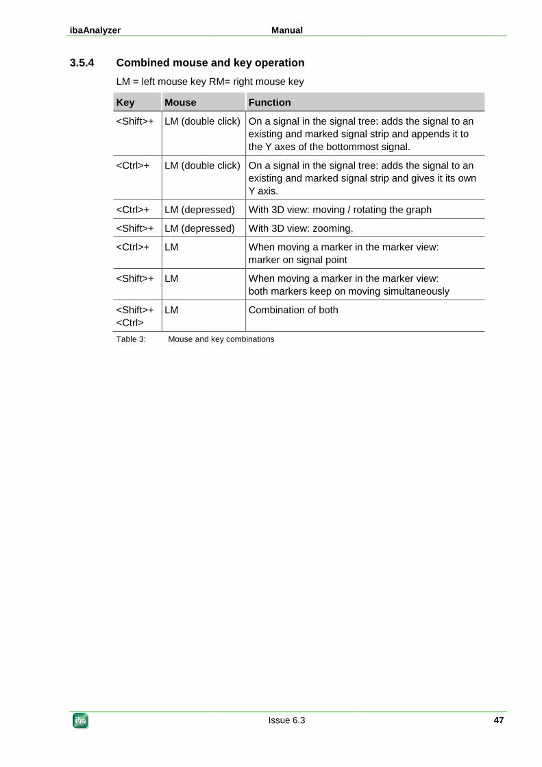
ibaAnalyzer Manual

Issue 6.3 47

3.5.4 Combined mouse and key operation LM = left mouse key RM= right mouse key

Key Mouse Function

<Shift>+ LM (double click) On a signal in the signal tree: adds the signal to an existing and marked signal strip and appends it to the Y axes of the bottommost signal.

<Ctrl>+ LM (double click) On a signal in the signal tree: adds the signal to an existing and marked signal strip and gives it its own Y axis.

<Ctrl>+ LM (depressed) With 3D view: moving / rotating the graph

<Shift>+ LM (depressed) With 3D view: zooming.

<Ctrl>+ LM When moving a marker in the marker view: marker on signal point

<Shift>+ LM When moving a marker in the marker view: both markers keep on moving simultaneously

<Shift>+<Ctrl>

LM Combination of both

Table 3: Mouse and key combinations

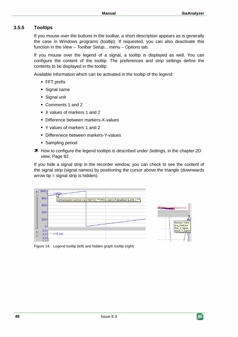
Manual ibaAnalyzer

48 Issue 6.3

3.5.5 Tooltips If you mouse over the buttons in the toolbar, a short description appears as is generally the case in Windows programs (tooltip). If requested, you can also deactivate this function in the View – Toolbar Setup... menu – Options tab.

If you mouse over the legend of a signal, a tooltip is displayed as well. You can configure the content of the tooltip. The preferences and strip settings define the contents to be displayed in the tooltip.

Available information which can be activated in the tooltip of the legend:

FFT prefix

Signal name

Signal unit

Comments 1 and 2

X values of markers 1 and 2

Difference between markers-X-values

Y values of markers 1 and 2

Differenece between markers-Y-values

Sampling period

How to configure the legend tooltips is described under Settings, in the chapter 2D view, Page 82.

If you hide a signal strip in the recorder window, you can check to see the content of the signal strip (signal names) by positioning the cursor above the triangle (downwards arrow tip = signal strip is hidden).

Figure 14: Legend tooltip (left) and hidden graph tooltip (right)

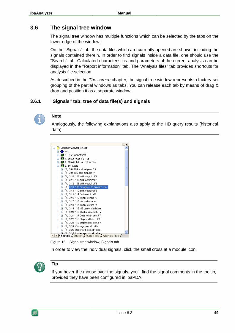
ibaAnalyzer Manual

Issue 6.3 49

3.6 The signal tree window The signal tree window has multiple functions which can be selected by the tabs on the lower edge of the window:

On the "Signals" tab, the data files which are currently opened are shown, including the signals contained therein. In order to find signals inside a data file, one should use the “Search” tab. Calculated characteristics and parameters of the current analysis can be displayed in the "Report information" tab. The “Analysis files” tab provides shortcuts for analysis file selection.

As described in the The screen chapter, the signal tree window represents a factory-set grouping of the partial windows as tabs. You can release each tab by means of drag & drop and position it as a separate window.

3.6.1 "Signals" tab: tree of data file(s) and signals

Note

Analogously, the following explanations also apply to the HD query results (historical data).

Figure 15: Signal tree window, Signals tab

In order to view the individual signals, click the small cross at a module icon.

Tip

If you hover the mouse over the signals, you’ll find the signal comments in the tooltip, provided they have been configured in ibaPDA.

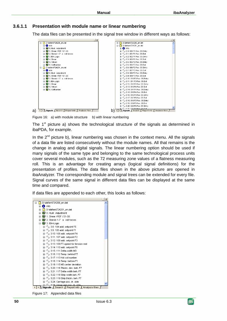
Manual ibaAnalyzer

50 Issue 6.3

3.6.1.1 Presentation with module name or linear numbering The data files can be presented in the signal tree window in different ways as follows:

a) b) Figure 16: a) with module structure b) with linear numbering

The 1st picture a) shows the technological structure of the signals as determined in ibaPDA, for example.

In the 2nd picture b), linear numbering was chosen in the context menu. All the signals of a data file are listed consecutively without the module names. All that remains is the change in analog and digital signals. The linear numbering option should be used if many signals of the same type and belonging to the same technological process units cover several modules, such as the 72 measuring zone values of a flatness measuring roll. This is an advantage for creating arrays (logical signal definitions) for the presentation of profiles. The data files shown in the above picture are opened in ibaAnalyzer. The corresponding module and signal trees can be extended for every file. Signal curves of the same signal in different data files can be displayed at the same time and compared.

If data files are appended to each other, this looks as follows:

Figure 17: Appended data files

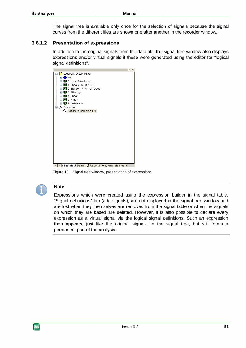
ibaAnalyzer Manual

Issue 6.3 51

The signal tree is available only once for the selection of signals because the signal curves from the different files are shown one after another in the recorder window.

3.6.1.2 Presentation of expressions In addition to the original signals from the data file, the signal tree window also displays expressions and/or virtual signals if these were generated using the editor for "logical signal definitions".

Figure 18: Signal tree window, presentation of expressions

Note

Expressions which were created using the expression builder in the signal table, "Signal definitions" tab (add signals), are not displayed in the signal tree window and are lost when they themselves are removed from the signal table or when the signals on which they are based are deleted. However, it is also possible to declare every expression as a virtual signal via the logical signal definitions. Such an expression then appears, just like the original signals, in the signal tree, but still forms a permanent part of the analysis.

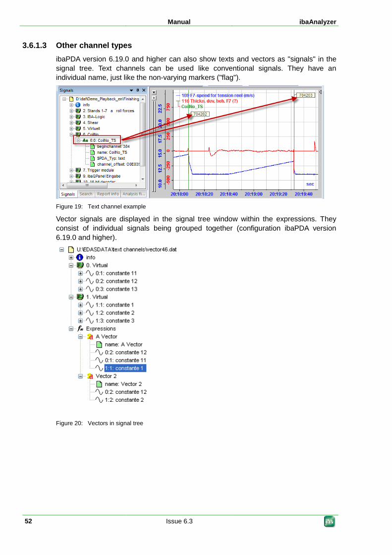
Manual ibaAnalyzer

52 Issue 6.3

3.6.1.3 Other channel types ibaPDA version 6.19.0 and higher can also show texts and vectors as "signals" in the signal tree. Text channels can be used like conventional signals. They have an individual name, just like the non-varying markers ("flag").

Figure 19: Text channel example

Vector signals are displayed in the signal tree window within the expressions. They consist of individual signals being grouped together (configuration ibaPDA version 6.19.0 and higher).

Figure 20: Vectors in signal tree

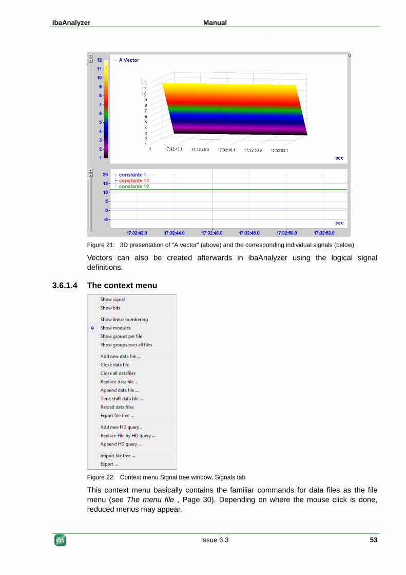
ibaAnalyzer Manual

Issue 6.3 53

Figure 21: 3D presentation of "A vector" (above) and the corresponding individual signals (below)

Vectors can also be created afterwards in ibaAnalyzer using the logical signal definitions.

3.6.1.4 The context menu

Figure 22: Context menu Signal tree window, Signals tab

This context menu basically contains the familiar commands for data files as the file menu (see The menu file , Page 30). Depending on where the mouse click is done, reduced menus may appear.

Manual ibaAnalyzer

54 Issue 6.3

Menu commands referring to data files or HD queries usually apply to the file or HD query in which the context menu was opened or which was marked at the time the context menu was opened.

However, certain special features exist in addition:

Show signal This command will cause the signal, which was right-clicked with the mouse, to be displayed in a signal strip.

Show bits This command – applied to an analog signal – will cause the display of all bits of the analog signal as separate digital signals. Thus, digital information which has been “packed” for transmission e. g. in a 16 bit integer can be displayed again as individual signals.

This works for 32 bit floating point values, too.

Linear numbering, display modules These functions are described in the preceding section of this chapter.

Show groups / individual files, .../ all files These display options are only applicable if the signals have been grouped before in the configuration of ibaPDA (or formerly in ibaScope). The signal-group-assignments are stored in the data file.

"Show groups / individual files" displays the data files as the topmost structure level in the signal tree window, with the pertinent signal groups being displayed below.

"Show groups / all files" displays the signal groups on the topmost structure level in the signal tree window.

The benefit of this approach: It is possible to define signal groups which show the signals necessary for a particular analytical purpose at a glance in the signal tree, irrespective of their physical module assignment. This means that the information concerning the technological affiliation does not necessarily have to be included in the signal name as a precondition for identifying a signal.

Show length and timebased signals separately (ibaQDR-V6) This option is only visible if a data file from an ibaQDR system with length-based and time-based signals is opened. By checking this option, the nodes of the measuring locations in the signal tree are divided into nodes for length-based signals (L) and time-based signals (T). The nodes of the measuring locations with length-based signals automatically receive the numbers x, the nodes of the measuring locations with time-based signals receive the numbers x + 1. Precondition: an archiving profile with length-based and time-based storage must have been used in the ibaQDR data recording.

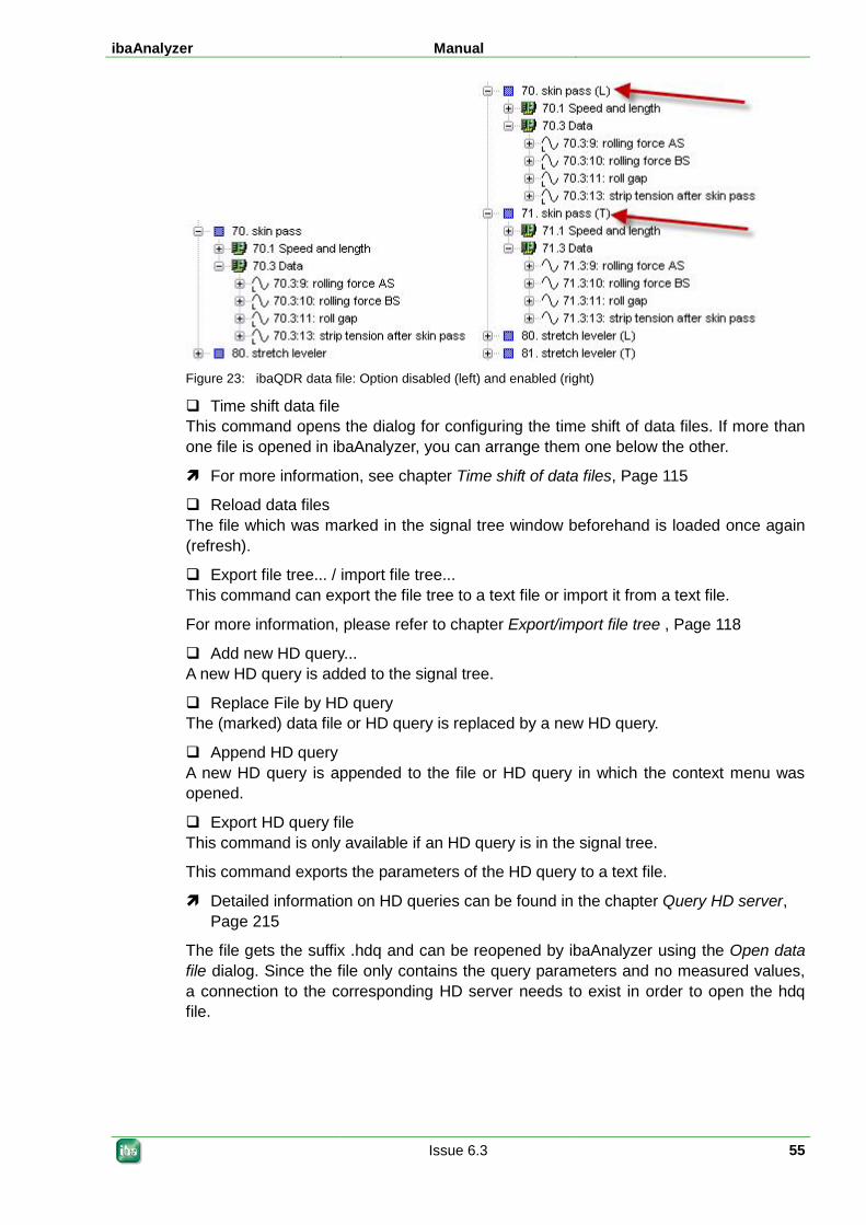
ibaAnalyzer Manual

Issue 6.3 55

Figure 23: ibaQDR data file: Option disabled (left) and enabled (right)

Time shift data file This command opens the dialog for configuring the time shift of data files. If more than one file is opened in ibaAnalyzer, you can arrange them one below the other.

For more information, see chapter Time shift of data files, Page 115

Reload data files The file which was marked in the signal tree window beforehand is loaded once again (refresh).

Export file tree... / import file tree... This command can export the file tree to a text file or import it from a text file.

For more information, please refer to chapter Export/import file tree , Page 118

Add new HD query... A new HD query is added to the signal tree.

Replace File by HD query The (marked) data file or HD query is replaced by a new HD query.

Append HD query A new HD query is appended to the file or HD query in which the context menu was opened.

Export HD query file This command is only available if an HD query is in the signal tree.

This command exports the parameters of the HD query to a text file.

Detailed information on HD queries can be found in the chapter Query HD server, Page 215

The file gets the suffix .hdq and can be reopened by ibaAnalyzer using the Open data file dialog. Since the file only contains the query parameters and no measured values, a connection to the corresponding HD server needs to exist in order to open the hdq file.

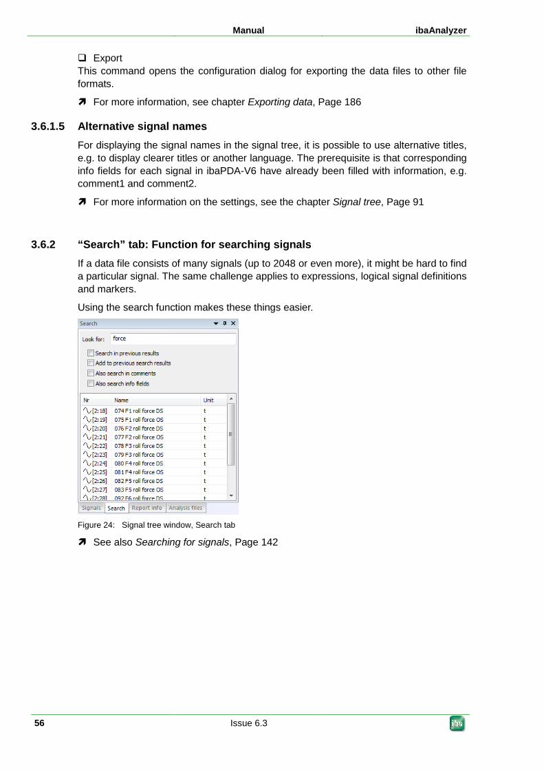
Manual ibaAnalyzer

56 Issue 6.3

Export This command opens the configuration dialog for exporting the data files to other file formats.

For more information, see chapter Exporting data, Page 186

3.6.1.5 Alternative signal names For displaying the signal names in the signal tree, it is possible to use alternative titles, e.g. to display clearer titles or another language. The prerequisite is that corresponding info fields for each signal in ibaPDA-V6 have already been filled with information, e.g. comment1 and comment2.

For more information on the settings, see the chapter Signal tree, Page 91

3.6.2 “Search” tab: Function for searching signals If a data file consists of many signals (up to 2048 or even more), it might be hard to find a particular signal. The same challenge applies to expressions, logical signal definitions and markers.

Using the search function makes these things easier.

Figure 24: Signal tree window, Search tab

See also Searching for signals, Page 142

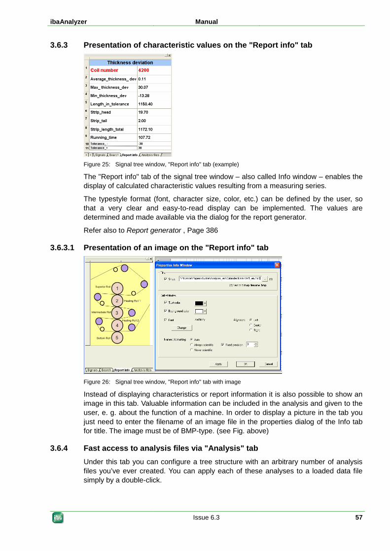
ibaAnalyzer Manual

Issue 6.3 57

3.6.3 Presentation of characteristic values on the "Report info" tab

Figure 25: Signal tree window, "Report info" tab (example)

The "Report info" tab of the signal tree window – also called Info window – enables the display of calculated characteristic values resulting from a measuring series.

The typestyle format (font, character size, color, etc.) can be defined by the user, so that a very clear and easy-to-read display can be implemented. The values are determined and made available via the dialog for the report generator.

Refer also to Report generator , Page 386

3.6.3.1 Presentation of an image on the "Report info" tab

Figure 26: Signal tree window, "Report info" tab with image

Instead of displaying characteristics or report information it is also possible to show an image in this tab. Valuable information can be included in the analysis and given to the user, e. g. about the function of a machine. In order to display a picture in the tab you just need to enter the filename of an image file in the properties dialog of the Info tab for title. The image must be of BMP-type. (see Fig. above)

3.6.4 Fast access to analysis files via "Analysis" tab Under this tab you can configure a tree structure with an arbitrary number of analysis files you’ve ever created. You can apply each of these analyses to a loaded data file simply by a double-click.

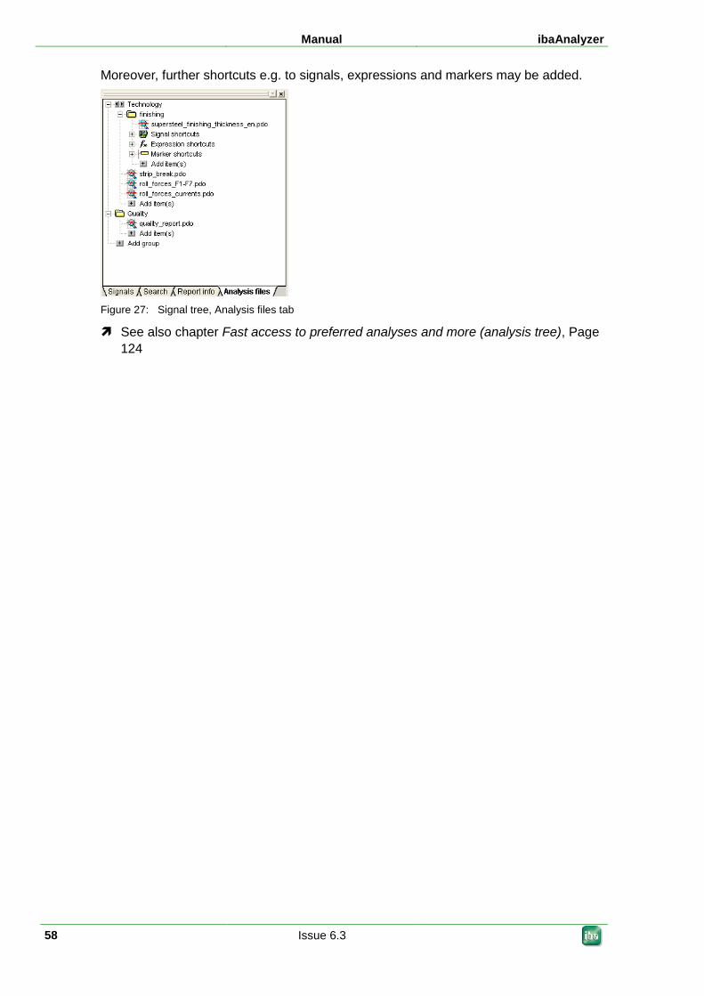
Manual ibaAnalyzer

58 Issue 6.3

Moreover, further shortcuts e.g. to signals, expressions and markers may be added.

Figure 27: Signal tree, Analysis files tab

See also chapter Fast access to preferred analyses and more (analysis tree), Page 124

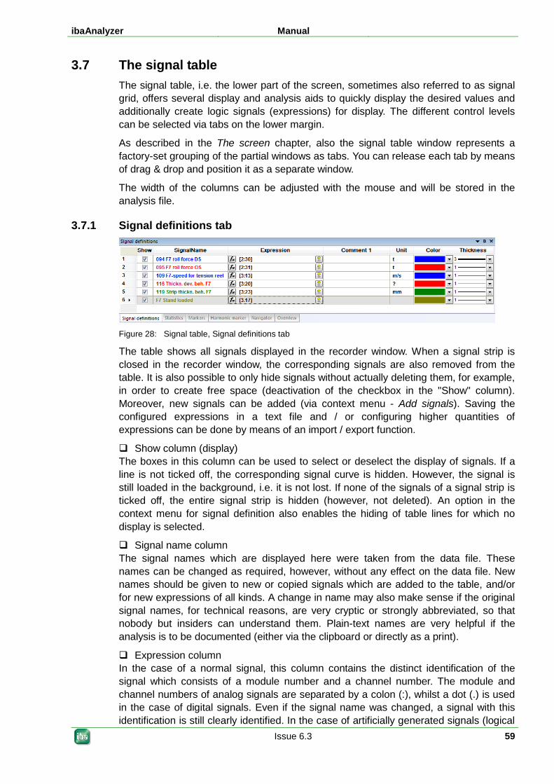
ibaAnalyzer Manual

Issue 6.3 59

3.7 The signal table The signal table, i.e. the lower part of the screen, sometimes also referred to as signal grid, offers several display and analysis aids to quickly display the desired values and additionally create logic signals (expressions) for display. The different control levels can be selected via tabs on the lower margin.

As described in the The screen chapter, also the signal table window represents a factory-set grouping of the partial windows as tabs. You can release each tab by means of drag & drop and position it as a separate window.

The width of the columns can be adjusted with the mouse and will be stored in the analysis file.

3.7.1 Signal definitions tab

Figure 28: Signal table, Signal definitions tab

The table shows all signals displayed in the recorder window. When a signal strip is closed in the recorder window, the corresponding signals are also removed from the table. It is also possible to only hide signals without actually deleting them, for example, in order to create free space (deactivation of the checkbox in the "Show" column). Moreover, new signals can be added (via context menu - Add signals). Saving the configured expressions in a text file and / or configuring higher quantities of expressions can be done by means of an import / export function.

Show column (display) The boxes in this column can be used to select or deselect the display of signals. If a line is not ticked off, the corresponding signal curve is hidden. However, the signal is still loaded in the background, i.e. it is not lost. If none of the signals of a signal strip is ticked off, the entire signal strip is hidden (however, not deleted). An option in the context menu for signal definition also enables the hiding of table lines for which no display is selected.

Signal name column The signal names which are displayed here were taken from the data file. These names can be changed as required, however, without any effect on the data file. New names should be given to new or copied signals which are added to the table, and/or for new expressions of all kinds. A change in name may also make sense if the original signal names, for technical reasons, are very cryptic or strongly abbreviated, so that nobody but insiders can understand them. Plain-text names are very helpful if the analysis is to be documented (either via the clipboard or directly as a print).

Expression column In the case of a normal signal, this column contains the distinct identification of the signal which consists of a module number and a channel number. The module and channel numbers of analog signals are separated by a colon (:), whilst a dot (.) is used in the case of digital signals. Even if the signal name was changed, a signal with this identification is still clearly identified. In the case of artificially generated signals (logical

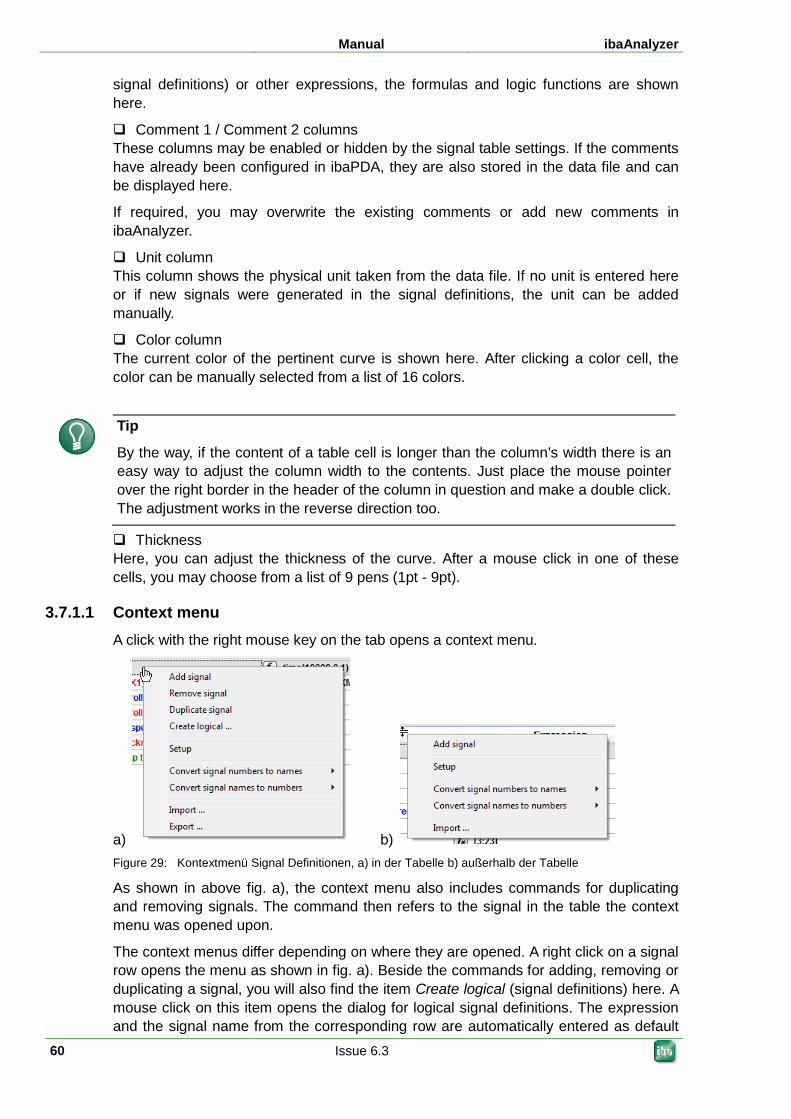
Manual ibaAnalyzer

60 Issue 6.3

signal definitions) or other expressions, the formulas and logic functions are shown here.

Comment 1 / Comment 2 columns These columns may be enabled or hidden by the signal table settings. If the comments have already been configured in ibaPDA, they are also stored in the data file and can be displayed here.

If required, you may overwrite the existing comments or add new comments in ibaAnalyzer.

Unit column This column shows the physical unit taken from the data file. If no unit is entered here or if new signals were generated in the signal definitions, the unit can be added manually.

Color column The current color of the pertinent curve is shown here. After clicking a color cell, the color can be manually selected from a list of 16 colors.

Tip

By the way, if the content of a table cell is longer than the column’s width there is an easy way to adjust the column width to the contents. Just place the mouse pointer over the right border in the header of the column in question and make a double click. The adjustment works in the reverse direction too.

Thickness Here, you can adjust the thickness of the curve. After a mouse click in one of these cells, you may choose from a list of 9 pens (1pt - 9pt).

3.7.1.1 Context menu A click with the right mouse key on the tab opens a context menu.

a) b) Figure 29: Kontextmenü Signal Definitionen, a) in der Tabelle b) außerhalb der Tabelle

As shown in above fig. a), the context menu also includes commands for duplicating and removing signals. The command then refers to the signal in the table the context menu was opened upon.

The context menus differ depending on where they are opened. A right click on a signal row opens the menu as shown in fig. a). Beside the commands for adding, removing or duplicating a signal, you will also find the item Create logical (signal definitions) here. A mouse click on this item opens the dialog for logical signal definitions. The expression and the signal name from the corresponding row are automatically entered as default

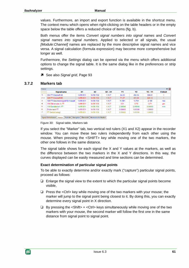
ibaAnalyzer Manual

Issue 6.3 61

values. Furthermore, an import and export function is available in the shortcut menu. The context menu which opens when right-clicking on the table headers or in the empty space below the table offers a reduced choice of items (fig. b).

Both menus offer the items Convert signal numbers into signal names and Convert signal names into signal numbers. Applied to selected or all signals, the usual [Module:Channel] names are replaced by the more descriptive signal names and vice versa. A signal calculation (formula expression) may become more comprehensive but longer as well.

Furthermore, the Settings dialog can be opened via the menu which offers additional options to change the signal table. It is the same dialog like in the preferences or strip settings.

See also Signal grid, Page 93

3.7.2 Markers tab

Figure 30: Signal table, Markers tab

If you select the "Marker" tab, two vertical red rulers (X1 and X2) appear in the recorder window. You can move these two rulers independently from each other using the mouse. When pressing the <SHIFT> key while moving one of the two markers, the other one follows in the same distance.

The signal table shows for each signal the X and Y values at the markers, as well as the difference between the two markers in the X and Y directions. In this way, the curves displayed can be easily measured and time sections can be determined.

Exact determination of particular signal points To be able to exactly determine and/or exactly mark ("capture") particular signal points, proceed as follows:

Enlarge the signal view to the extent to which the particular signal points become visible,

Press the <Ctrl> key while moving one of the two markers with your mouse; the marker will jump to the signal point being closest to it. By doing this, you can exactly determine every signal point in X direction.

By pressing the <Shift> + <Ctrl> keys simultaneously while moving one of the two markers with your mouse, the second marker will follow the first one in the same distance from signal point to signal point.

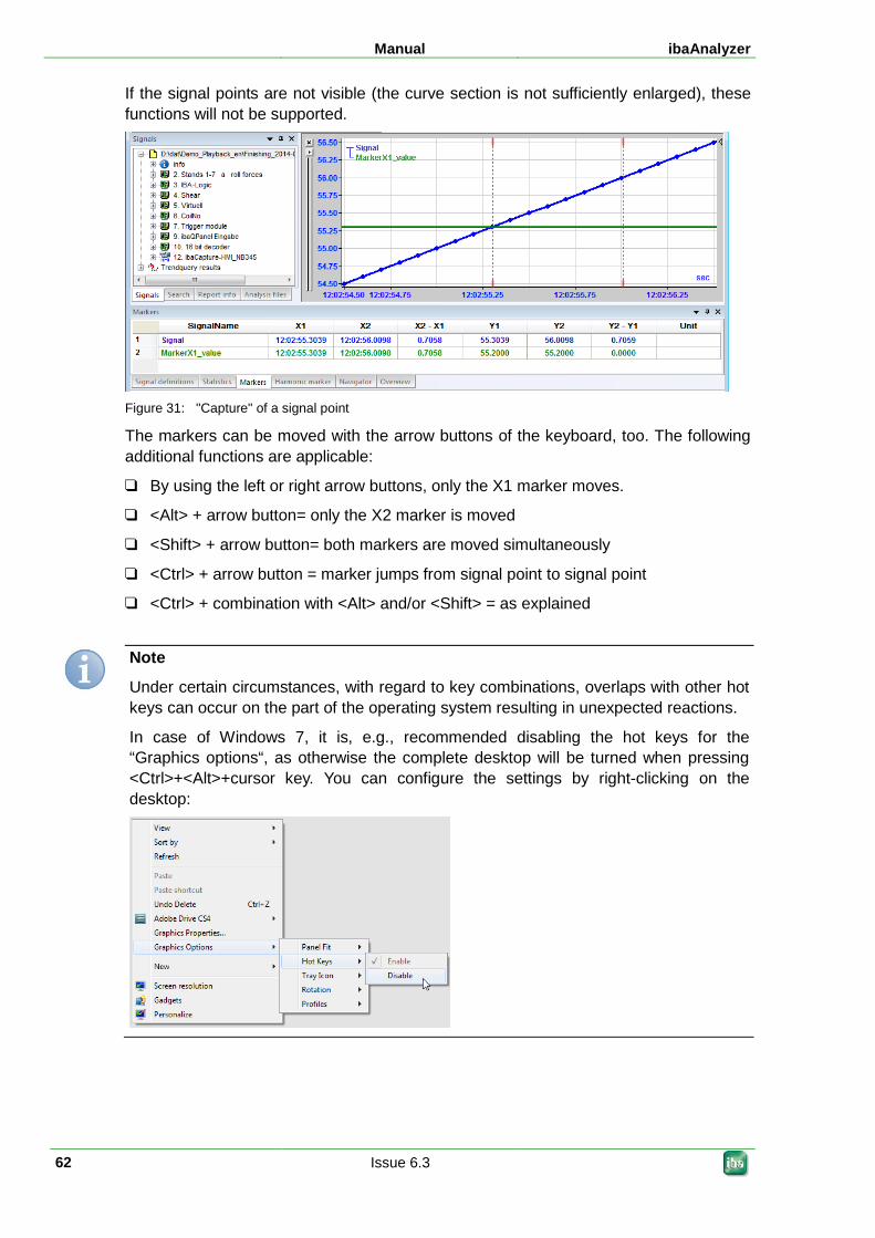
Manual ibaAnalyzer

62 Issue 6.3

If the signal points are not visible (the curve section is not sufficiently enlarged), these functions will not be supported.

Figure 31: "Capture" of a signal point

The markers can be moved with the arrow buttons of the keyboard, too. The following additional functions are applicable:

By using the left or right arrow buttons, only the X1 marker moves.

<Alt> + arrow button= only the X2 marker is moved

<Shift> + arrow button= both markers are moved simultaneously

<Ctrl> + arrow button = marker jumps from signal point to signal point

<Ctrl> + combination with <Alt> and/or <Shift> = as explained

Note

Under certain circumstances, with regard to key combinations, overlaps with other hot keys can occur on the part of the operating system resulting in unexpected reactions.

In case of Windows 7, it is, e.g., recommended disabling the hot keys for the “Graphics options“, as otherwise the complete desktop will be turned when pressing <Ctrl>+<Alt>+cursor key. You can configure the settings by right-clicking on the desktop:

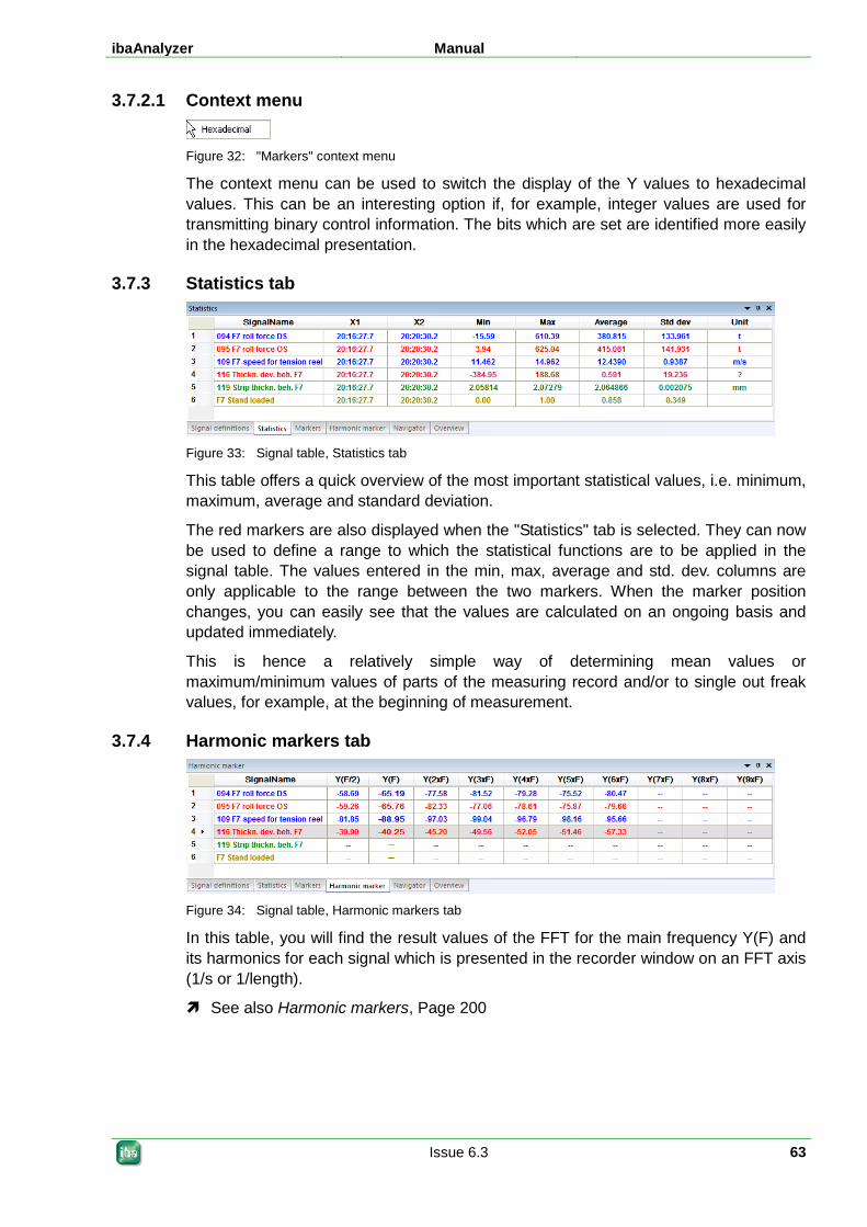
ibaAnalyzer Manual

Issue 6.3 63

3.7.2.1 Context menu

Figure 32: "Markers" context menu

The context menu can be used to switch the display of the Y values to hexadecimal values. This can be an interesting option if, for example, integer values are used for transmitting binary control information. The bits which are set are identified more easily in the hexadecimal presentation.

3.7.3 Statistics tab

Figure 33: Signal table, Statistics tab

This table offers a quick overview of the most important statistical values, i.e. minimum, maximum, average and standard deviation.

The red markers are also displayed when the "Statistics" tab is selected. They can now be used to define a range to which the statistical functions are to be applied in the signal table. The values entered in the min, max, average and std. dev. columns are only applicable to the range between the two markers. When the marker position changes, you can easily see that the values are calculated on an ongoing basis and updated immediately.

This is hence a relatively simple way of determining mean values or maximum/minimum values of parts of the measuring record and/or to single out freak values, for example, at the beginning of measurement.

3.7.4 Harmonic markers tab

Figure 34: Signal table, Harmonic markers tab

In this table, you will find the result values of the FFT for the main frequency Y(F) and its harmonics for each signal which is presented in the recorder window on an FFT axis (1/s or 1/length).

See also Harmonic markers, Page 200

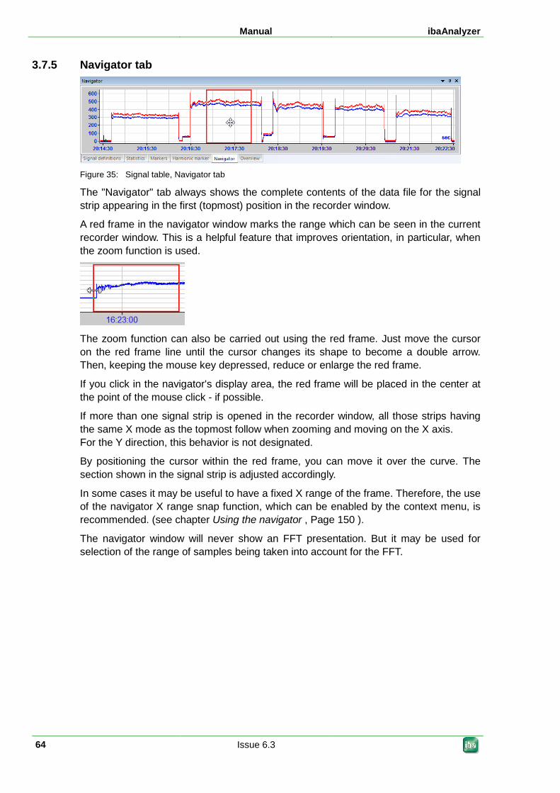
Manual ibaAnalyzer

64 Issue 6.3

3.7.5 Navigator tab

Figure 35: Signal table, Navigator tab

The "Navigator" tab always shows the complete contents of the data file for the signal strip appearing in the first (topmost) position in the recorder window.

A red frame in the navigator window marks the range which can be seen in the current recorder window. This is a helpful feature that improves orientation, in particular, when the zoom function is used.

The zoom function can also be carried out using the red frame. Just move the cursor on the red frame line until the cursor changes its shape to become a double arrow. Then, keeping the mouse key depressed, reduce or enlarge the red frame.

If you click in the navigator's display area, the red frame will be placed in the center at the point of the mouse click - if possible.

If more than one signal strip is opened in the recorder window, all those strips having the same X mode as the topmost follow when zooming and moving on the X axis. For the Y direction, this behavior is not designated.

By positioning the cursor within the red frame, you can move it over the curve. The section shown in the signal strip is adjusted accordingly.

In some cases it may be useful to have a fixed X range of the frame. Therefore, the use of the navigator X range snap function, which can be enabled by the context menu, is recommended. (see chapter Using the navigator , Page 150 ).

The navigator window will never show an FFT presentation. But it may be used for selection of the range of samples being taken into account for the FFT.

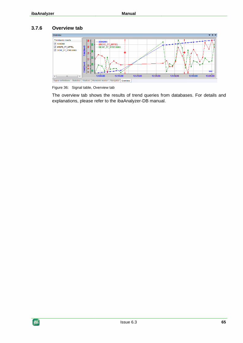
ibaAnalyzer Manual

Issue 6.3 65

3.7.6 Overview tab

Figure 36: Signal table, Overview tab

The overview tab shows the results of trend queries from databases. For details and explanations, please refer to the ibaAnalyzer-DB manual.

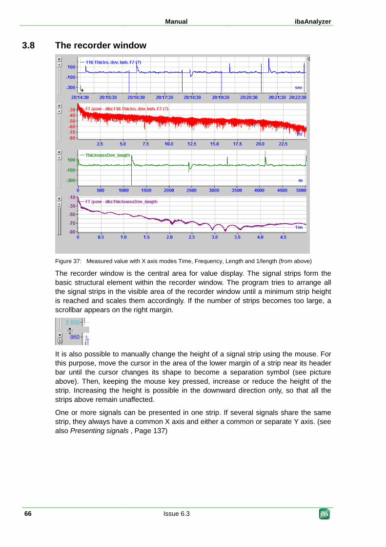
Manual ibaAnalyzer

66 Issue 6.3

3.8 The recorder window

Figure 37: Measured value with X axis modes Time, Frequency, Length and 1/length (from above)

The recorder window is the central area for value display. The signal strips form the basic structural element within the recorder window. The program tries to arrange all the signal strips in the visible area of the recorder window until a minimum strip height is reached and scales them accordingly. If the number of strips becomes too large, a scrollbar appears on the right margin.

It is also possible to manually change the height of a signal strip using the mouse. For this purpose, move the cursor in the area of the lower margin of a strip near its header bar until the cursor changes its shape to become a separation symbol (see picture above). Then, keeping the mouse key pressed, increase or reduce the height of the strip. Increasing the height is possible in the downward direction only, so that all the strips above remain unaffected.

One or more signals can be presented in one strip. If several signals share the same strip, they always have a common X axis and either a common or separate Y axis. (see also Presenting signals , Page 137)

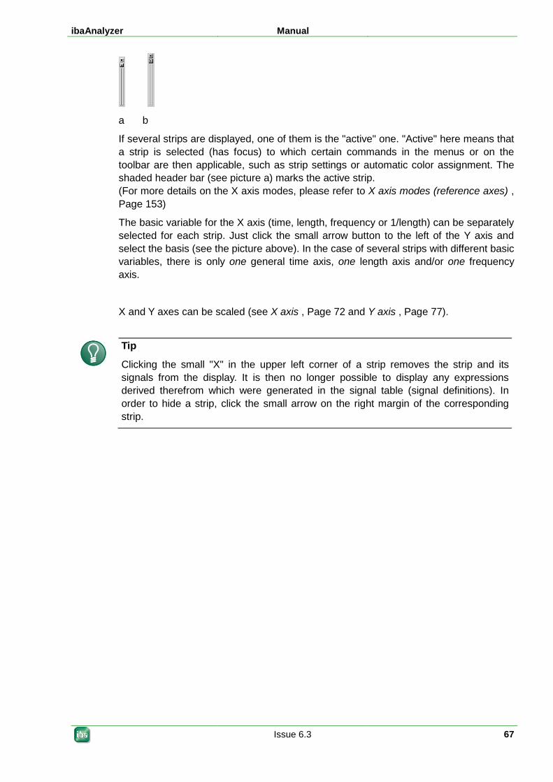
ibaAnalyzer Manual

Issue 6.3 67

a b

If several strips are displayed, one of them is the "active" one. "Active" here means that a strip is selected (has focus) to which certain commands in the menus or on the toolbar are then applicable, such as strip settings or automatic color assignment. The shaded header bar (see picture a) marks the active strip. (For more details on the X axis modes, please refer to X axis modes (reference axes) , Page 153)

The basic variable for the X axis (time, length, frequency or 1/length) can be separately selected for each strip. Just click the small arrow button to the left of the Y axis and select the basis (see the picture above). In the case of several strips with different basic variables, there is only one general time axis, one length axis and/or one frequency axis.

X and Y axes can be scaled (see X axis , Page 72 and Y axis , Page 77).

Tip

Clicking the small "X" in the upper left corner of a strip removes the strip and its signals from the display. It is then no longer possible to display any expressions derived therefrom which were generated in the signal table (signal definitions). In order to hide a strip, click the small arrow on the right margin of the corresponding strip.

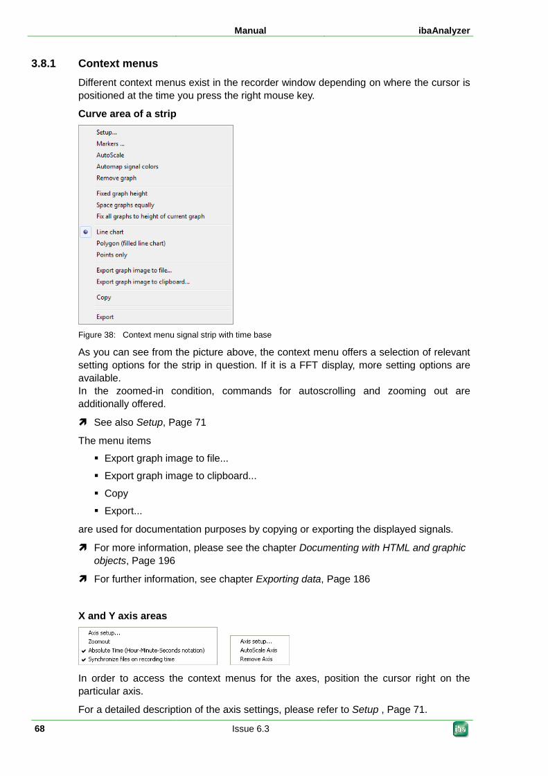
Manual ibaAnalyzer

68 Issue 6.3

3.8.1 Context menus Different context menus exist in the recorder window depending on where the cursor is positioned at the time you press the right mouse key.

Curve area of a strip

Figure 38: Context menu signal strip with time base

As you can see from the picture above, the context menu offers a selection of relevant setting options for the strip in question. If it is a FFT display, more setting options are available. In the zoomed-in condition, commands for autoscrolling and zooming out are additionally offered.

See also Setup, Page 71

The menu items

Export graph image to file...

Export graph image to clipboard...

Copy

Export...

are used for documentation purposes by copying or exporting the displayed signals.

For more information, please see the chapter Documenting with HTML and graphic objects, Page 196

For further information, see chapter Exporting data, Page 186

X and Y axis areas

In order to access the context menus for the axes, position the cursor right on the particular axis.

For a detailed description of the axis settings, please refer to Setup , Page 71.

ibaAnalyzer Manual

Issue 6.3 69

Options in the context menu of the time axis (picture on the next page b):

Hours - minutes - seconds Toggling between absolute and relative time display on the scale.

Synchronize data files with recording time This option is important in the case of appended files. If this option is selected, the signal curves are not necessarily appended to each other in direct succession, but are rather arranged on the time axis in accordance with their time stamp. In this way, it is possible to detect and show recording gaps between two data files.

See also Appending data files, Page 110

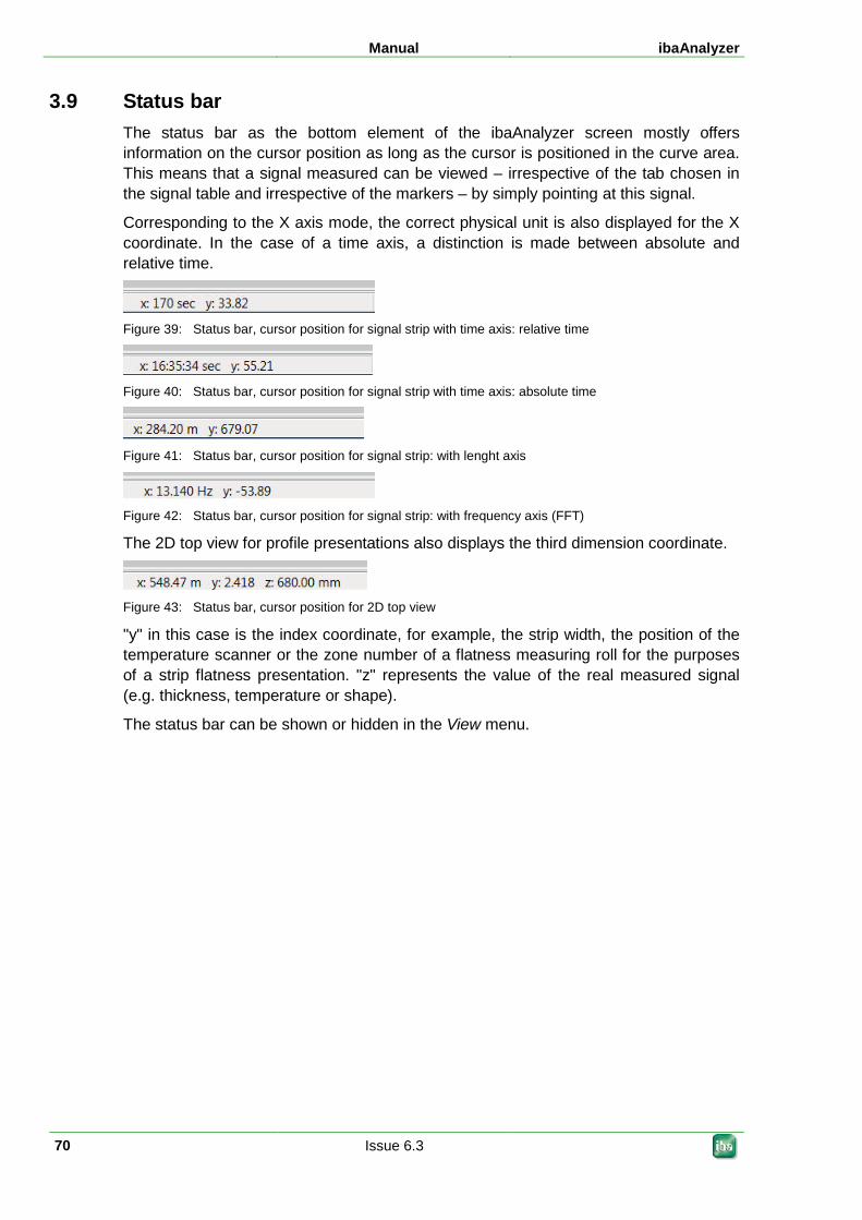
Manual ibaAnalyzer

70 Issue 6.3

3.9 Status bar The status bar as the bottom element of the ibaAnalyzer screen mostly offers information on the cursor position as long as the cursor is positioned in the curve area. This means that a signal measured can be viewed – irrespective of the tab chosen in the signal table and irrespective of the markers – by simply pointing at this signal.

Corresponding to the X axis mode, the correct physical unit is also displayed for the X coordinate. In the case of a time axis, a distinction is made between absolute and relative time.

Figure 39: Status bar, cursor position for signal strip with time axis: relative time

Figure 40: Status bar, cursor position for signal strip with time axis: absolute time

Figure 41: Status bar, cursor position for signal strip: with lenght axis

Figure 42: Status bar, cursor position for signal strip: with frequency axis (FFT)

The 2D top view for profile presentations also displays the third dimension coordinate.

Figure 43: Status bar, cursor position for 2D top view

"y" in this case is the index coordinate, for example, the strip width, the position of the temperature scanner or the zone number of a flatness measuring roll for the purposes of a strip flatness presentation. "z" represents the value of the real measured signal (e.g. thickness, temperature or shape).

The status bar can be shown or hidden in the View menu.

ibaAnalyzer Manual

Issue 6.3 71

3.10 Setup 3.10.1 Preferences / graph settings

There is generally no difference between the dialog window for the preferences and for the strip settings. Only the number of tabs is different. This is why the following explanations will be limited to the different intentions first. Thereafter, the setting options will be explained on the basis of the dialogs for the preferences.

3.10.1.1 Preferences

(Menu Setup - Preferences...)

The preferences determine the form of presentation when a new analysis is created or when a new signal strip is opened. A change in preferences has no immediate influence on the signal strips which are currently displayed unless the "Apply to analysis" option (in the dialog window in the lower left corner) is activated before the change is applied.

The preferences are saved in an initialization file of ibaAnalyzer rather than in the analysis, and are hence independent of an analysis file.

3.10.1.2 Graph setup (Setup - Graph setup... menu or in the context menu of a strip under Setup...)

The difference between the signal strip settings and preferences is that the strip settings only apply to the signal strip which is currently active (see "The recorder window , Page 66") and/or to the strip in which the context menu was opened. The strip setting dialog always offers only a subset of the tabs available for the preferences, i.e. only those tabs which are relevant for the strip in question.

On the other hand, the dialog boxes differ between preferences and strip settings. Thus, e.g. the X axis settings of the strip in the time, length, frequency and 1/length tabs also show the markers which is not the case with the preferences.

A change in the strip settings immediately affects the strip in question when the <Apply> button is clicked. Such a change has no effect on the preferences unless the "Apply to preferences" option was activated beforehand (in the dialog window in the lower left corner).

The strip settings are saved in the analysis.

Note

Formatting of numerical data such as time, date, etc., for example on the time axis, in tables or in the export dialog, is based on the regional and language settings under Windows.

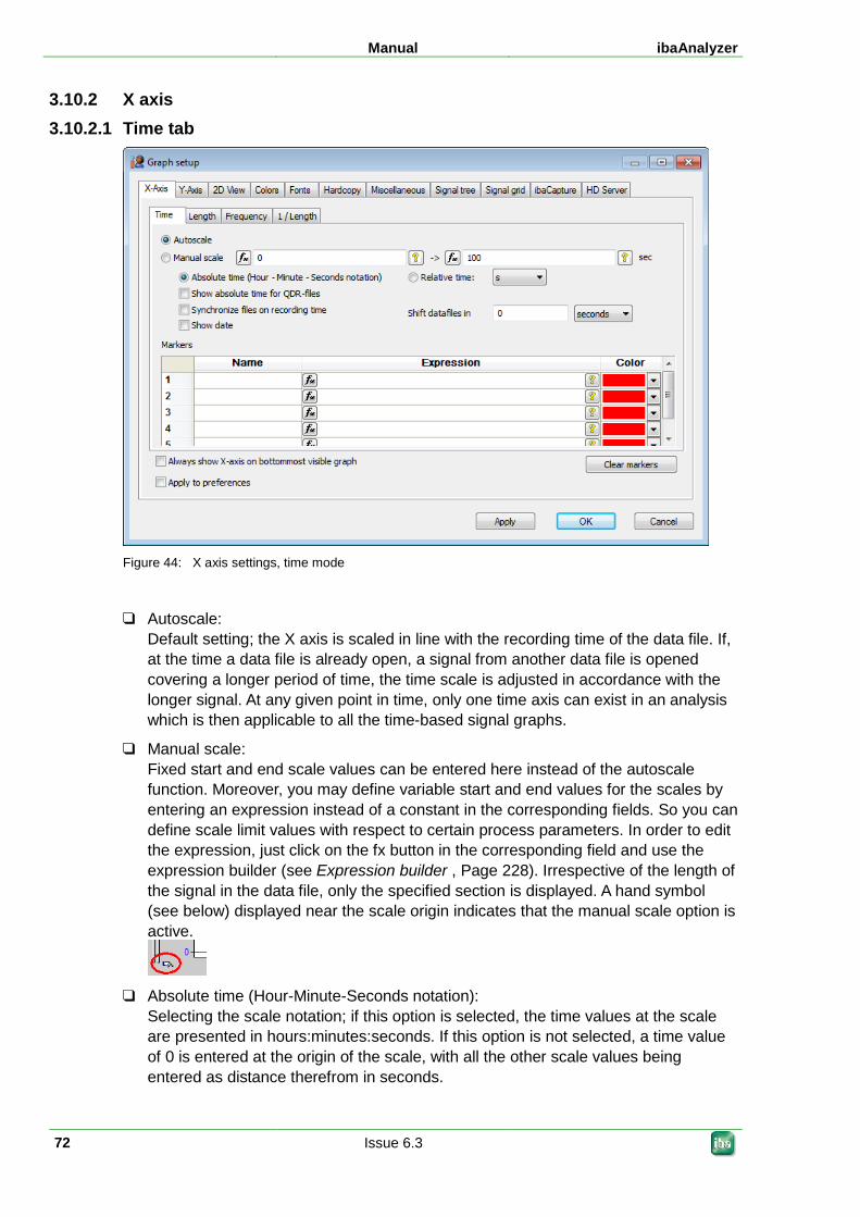
Manual ibaAnalyzer

72 Issue 6.3

3.10.2 X axis 3.10.2.1 Time tab

Figure 44: X axis settings, time mode

Autoscale: Default setting; the X axis is scaled in line with the recording time of the data file. If, at the time a data file is already open, a signal from another data file is opened covering a longer period of time, the time scale is adjusted in accordance with the longer signal. At any given point in time, only one time axis can exist in an analysis which is then applicable to all the time-based signal graphs.

Manual scale: Fixed start and end scale values can be entered here instead of the autoscale function. Moreover, you may define variable start and end values for the scales by entering an expression instead of a constant in the corresponding fields. So you can define scale limit values with respect to certain process parameters. In order to edit the expression, just click on the fx button in the corresponding field and use the expression builder (see Expression builder , Page 228). Irrespective of the length of the signal in the data file, only the specified section is displayed. A hand symbol (see below) displayed near the scale origin indicates that the manual scale option is active.

Absolute time (Hour-Minute-Seconds notation):

Selecting the scale notation; if this option is selected, the time values at the scale are presented in hours:minutes:seconds. If this option is not selected, a time value of 0 is entered at the origin of the scale, with all the other scale values being entered as distance therefrom in seconds.

ibaAnalyzer Manual

Issue 6.3 73

Show absolute time for QDR-files: This option is only applicable to data files which were generated by the ibaQDR system. Both the length reference and the time reference are stored in these files. Usually, also in time-based presentation the signals are scaled to the overall X axis. Thus, the measuring signals are "stretched" to the entire runtime of the strip in the plant. In terms of quality, you get a trend over time, however, the assignment of the Y values to the time axis is not correct. By enabling this option, the signal curve is correctly presented on the X axis in terms of time. This shows very clearly as to when and how long a measuring signal has been recorded for the corresponding strip.

Synchronize files on recording time: This option is important for the presentation of appending data files. This option must be selected as a precondition for arranging the individual signal records on the time axis in accordance with the recording data of the data file. (see Appending data files , Page 110)

Show date: When selecting the absolute time, the date can be additionally displayed on the scale. Particularly in case of data files covering several days or the time around a date line, the additional data display serves as orientation.

Relative time: For the relative time reference, you can choose between presentation in seconds, minutes : seconds or hour : minute : second.

Shift datafiles in...(time) With this setting, you can perform a strip-specific shifting of the curves, for example, to align them with curves in other strips. This setting can also be configured in addition to a general time shift, as described in chapter Time shift of data files , Page 115.

Marker table The marker table shows all X axis markers currently defined for the time axis. Here, you can define or delete markers. The table shows the marker pool which you can also access via Markers... in the context menu of a strip. You decide at a later time as to whether a marker is displayed in the strip in question by dragging it from the signal tree to the strip.

For more information about the markers, see chapter X-axis markers, Page 203.

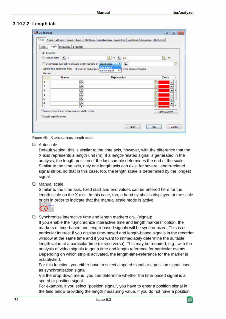
Manual ibaAnalyzer

74 Issue 6.3

3.10.2.2 Length tab

Figure 45: X axis settings, length mode

Autoscale: Default setting; this is similar to the time axis, however, with the difference that the X axis represents a length unit (m). If a length-related signal is generated in the analysis, the length position of the last sample determines the end of the scale. Similar to the time axis, only one length axis can exist for several length-related signal strips, so that in this case, too, the length scale is determined by the longest signal.

Manual scale: Similar to the time axis, fixed start and end values can be entered here for the length scale on the X axis. In this case, too, a hand symbol is displayed at the scale origin in order to indicate that the manual scale mode is active.

Synchronize interactive time and length markers on...(signal):

If you enable the "Synchronize interactive time and length markers" option, the markers of time-based and length-based signals will be synchronized. This is of particular interest if you display time-based and length-based signals in the recorder window at the same time and if you want to immediately determine the suitable length value at a particular time (or vice versa). This may be required, e.g., with the analysis of video signals to get a time and length reference for particular events. Depending on which strip is activated, the length-time-reference for the marker is established. For this function, you either have to select a speed signal or a position signal used as synchronization signal. Via the drop-down menu, you can determine whether the time-based signal is a speed or position signal. For example, if you select "position signal", you have to enter a position signal in the field below providing the length measuring value. If you do not have a position

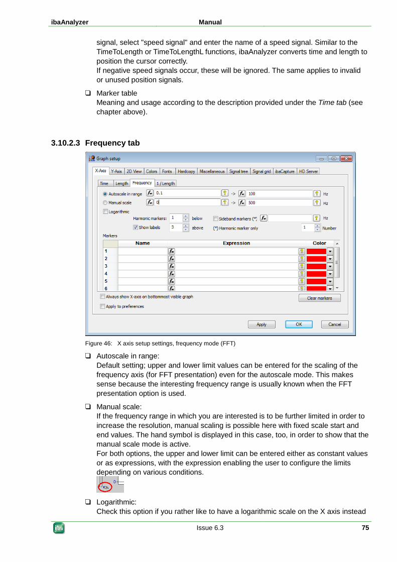
ibaAnalyzer Manual

Issue 6.3 75

signal, select "speed signal" and enter the name of a speed signal. Similar to the TimeToLength or TimeToLengthL functions, ibaAnalyzer converts time and length to position the cursor correctly. If negative speed signals occur, these will be ignored. The same applies to invalid or unused position signals.

Marker table Meaning and usage according to the description provided under the Time tab (see chapter above).

3.10.2.3 Frequency tab

Figure 46: X axis setup settings, frequency mode (FFT)

Autoscale in range: Default setting; upper and lower limit values can be entered for the scaling of the frequency axis (for FFT presentation) even for the autoscale mode. This makes sense because the interesting frequency range is usually known when the FFT presentation option is used.

Manual scale: If the frequency range in which you are interested is to be further limited in order to increase the resolution, manual scaling is possible here with fixed scale start and end values. The hand symbol is displayed in this case, too, in order to show that the manual scale mode is active. For both options, the upper and lower limit can be entered either as constant values or as expressions, with the expression enabling the user to configure the limits depending on various conditions.

Logarithmic:

Check this option if you rather like to have a logarithmic scale on the X axis instead

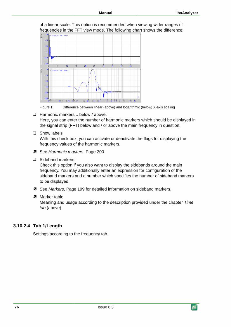
Manual ibaAnalyzer

76 Issue 6.3

of a linear scale. This option is recommended when viewing wider ranges of frequencies in the FFT view mode. The following chart shows the difference:

Figure 1: Difference between linear (above) and logarithmic (below) X-axis scaling

Harmonic markers... below / above: Here, you can enter the number of harmonic markers which should be displayed in the signal strip (FFT) below and / or above the main frequency in question.

Show labels With this check box, you can activate or deactivate the flags for displaying the frequency values of the harmonic markers.

See Harmonic markers, Page 200

Sideband markers: Check this option if you also want to display the sidebands around the main frequency. You may additionally enter an expression for configuration of the sideband markers and a number which specifies the number of sideband markers to be displayed.

See Markers, Page 199 for detailed information on sideband markers.

Marker table Meaning and usage according to the description provided under the chapter Time tab (above).

3.10.2.4 Tab 1/Length Settings according to the frequency tab.

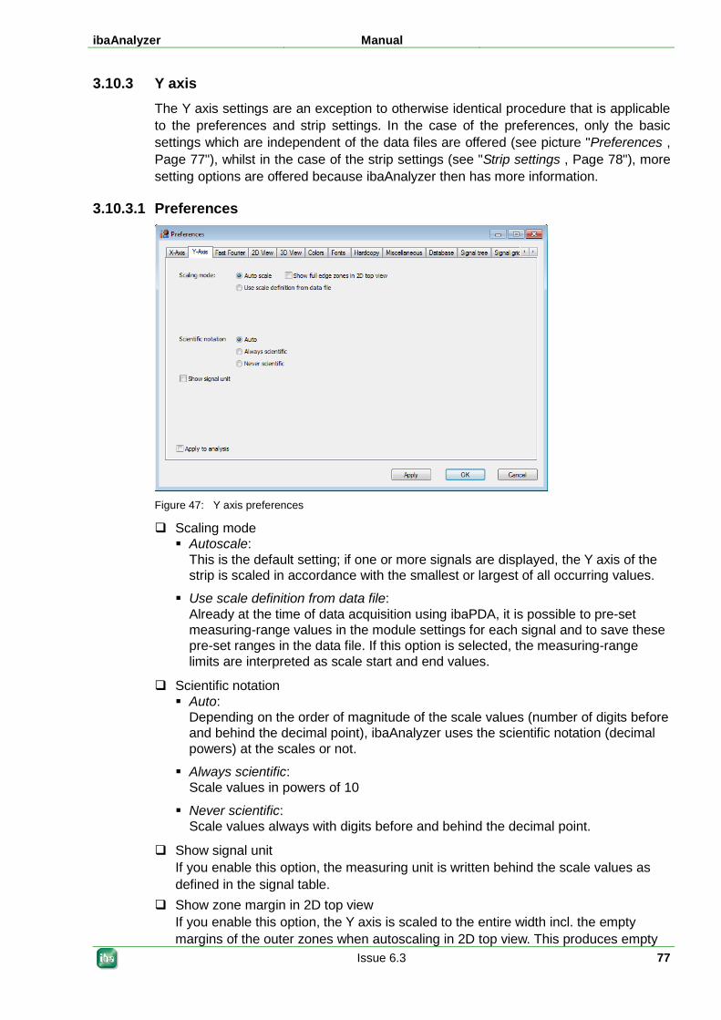
ibaAnalyzer Manual

Issue 6.3 77

3.10.3 Y axis The Y axis settings are an exception to otherwise identical procedure that is applicable to the preferences and strip settings. In the case of the preferences, only the basic settings which are independent of the data files are offered (see picture "Preferences , Page 77"), whilst in the case of the strip settings (see "Strip settings , Page 78"), more setting options are offered because ibaAnalyzer then has more information.

3.10.3.1 Preferences

Figure 47: Y axis preferences

Scaling mode Autoscale:

This is the default setting; if one or more signals are displayed, the Y axis of the strip is scaled in accordance with the smallest or largest of all occurring values.

Use scale definition from data file: Already at the time of data acquisition using ibaPDA, it is possible to pre-set measuring-range values in the module settings for each signal and to save these pre-set ranges in the data file. If this option is selected, the measuring-range limits are interpreted as scale start and end values.

Scientific notation Auto:

Depending on the order of magnitude of the scale values (number of digits before and behind the decimal point), ibaAnalyzer uses the scientific notation (decimal powers) at the scales or not.

Always scientific: Scale values in powers of 10

Never scientific: Scale values always with digits before and behind the decimal point.

Show signal unit If you enable this option, the measuring unit is written behind the scale values as defined in the signal table.

Show zone margin in 2D top view If you enable this option, the Y axis is scaled to the entire width incl. the empty margins of the outer zones when autoscaling in 2D top view. This produces empty

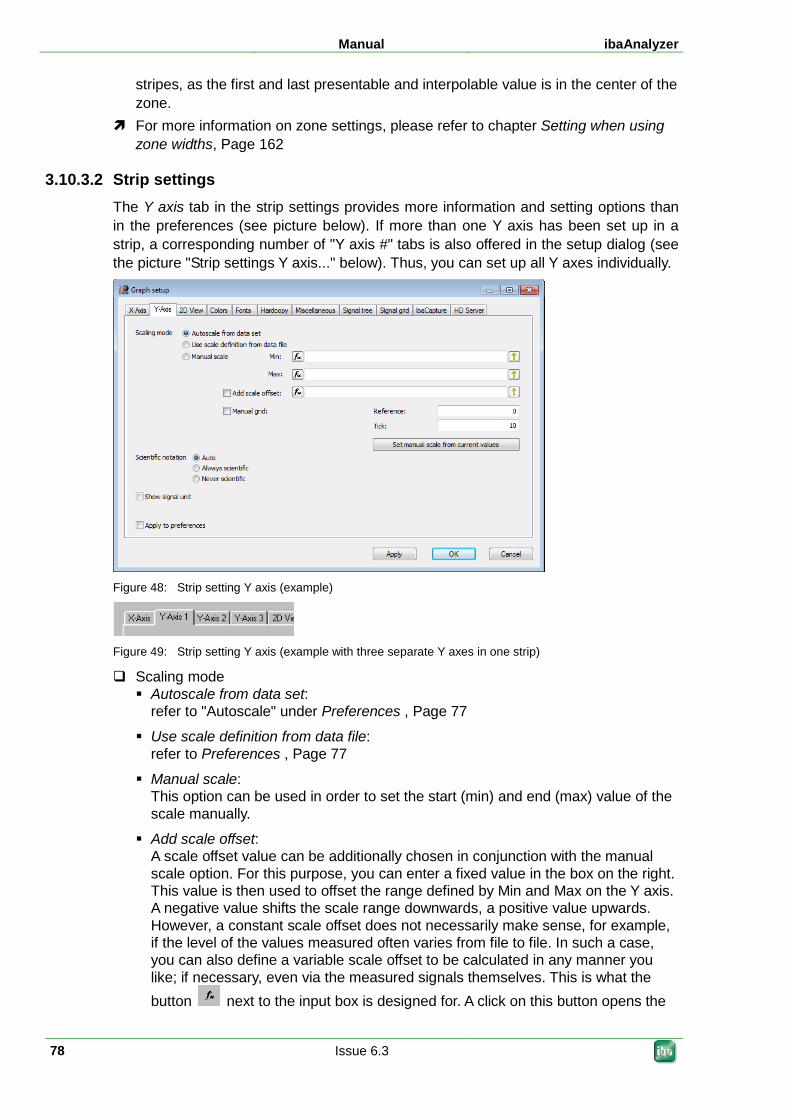
Manual ibaAnalyzer

78 Issue 6.3

stripes, as the first and last presentable and interpolable value is in the center of the zone.

For more information on zone settings, please refer to chapter Setting when using zone widths, Page 162

3.10.3.2 Strip settings The Y axis tab in the strip settings provides more information and setting options than in the preferences (see picture below). If more than one Y axis has been set up in a strip, a corresponding number of "Y axis #" tabs is also offered in the setup dialog (see the picture "Strip settings Y axis..." below). Thus, you can set up all Y axes individually.

Figure 48: Strip setting Y axis (example)

Figure 49: Strip setting Y axis (example with three separate Y axes in one strip)

Scaling mode Autoscale from data set:

refer to "Autoscale" under Preferences , Page 77

Use scale definition from data file: refer to Preferences , Page 77

Manual scale: This option can be used in order to set the start (min) and end (max) value of the scale manually.

Add scale offset: A scale offset value can be additionally chosen in conjunction with the manual scale option. For this purpose, you can enter a fixed value in the box on the right. This value is then used to offset the range defined by Min and Max on the Y axis. A negative value shifts the scale range downwards, a positive value upwards. However, a constant scale offset does not necessarily make sense, for example, if the level of the values measured often varies from file to file. In such a case, you can also define a variable scale offset to be calculated in any manner you like; if necessary, even via the measured signals themselves. This is what the button next to the input box is designed for. A click on this button opens the

ibaAnalyzer Manual

Issue 6.3 79

expression builder which you can then use to create any expressions the result of which then gives the scale offset.

See also Expression builder, Page 228.

Manual grid: Furthermore, it is also possible to divide the Y axis and/or the grid in a certain manner in conjunction with the manual scale option. Two values must be entered in the appropriate boxes for the manual grid: Reference: The reference value is the basis for determining the position of the grid. The reference value does not necessarily have to be identical to the minimum or maximum value of the manual scale. It can be within or outside the range determined by min and max. The reference value determines the place where the first grid line appears. Tick: The "Tick" value represents the step width of the grid lines. Based on the reference value, grid lines and scale values are displayed at always the same distance (tick mark). For example, in order to divide the Y axis (and the grid) in steps of 1/16, enter 0.0625 for the tick mark value.

Note

ibaAnalyzer will nevertheless adjust the scale in order to optimize the display. This mainly depends on the value range, i.e. on the min and max values. If the grid would become too narrow, the grid lines are displayed at integral multiples of the tick value.

<Set manual scale from current values> button

If you press this button while the autoscale mode is active, the current settings in the strip display are used for the fields for manual scaling. This simplifies the setting of a manual scale because the Y axis in the recorder window can also be adjusted graphically using the mouse.

Scientific notation see Preferences , Page 77

Show signal unit see Preferences , Page 77

Show zone margin in 2D top view (only with strips in 2D top view) see Preferences , Page 77

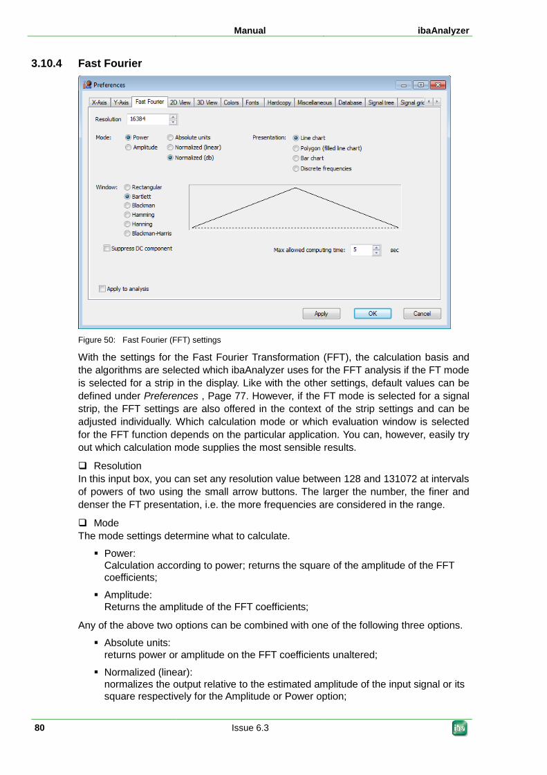
Manual ibaAnalyzer

80 Issue 6.3

3.10.4 Fast Fourier

Figure 50: Fast Fourier (FFT) settings

With the settings for the Fast Fourier Transformation (FFT), the calculation basis and the algorithms are selected which ibaAnalyzer uses for the FFT analysis if the FT mode is selected for a strip in the display. Like with the other settings, default values can be defined under Preferences , Page 77. However, if the FT mode is selected for a signal strip, the FFT settings are also offered in the context of the strip settings and can be adjusted individually. Which calculation mode or which evaluation window is selected for the FFT function depends on the particular application. You can, however, easily try out which calculation mode supplies the most sensible results.

Resolution In this input box, you can set any resolution value between 128 and 131072 at intervals of powers of two using the small arrow buttons. The larger the number, the finer and denser the FT presentation, i.e. the more frequencies are considered in the range.

Mode The mode settings determine what to calculate.

Power: Calculation according to power; returns the square of the amplitude of the FFT coefficients;

Amplitude: Returns the amplitude of the FFT coefficients;

Any of the above two options can be combined with one of the following three options.

Absolute units: returns power or amplitude on the FFT coefficients unaltered;

Normalized (linear): normalizes the output relative to the estimated amplitude of the input signal or its square respectively for the Amplitude or Power option;

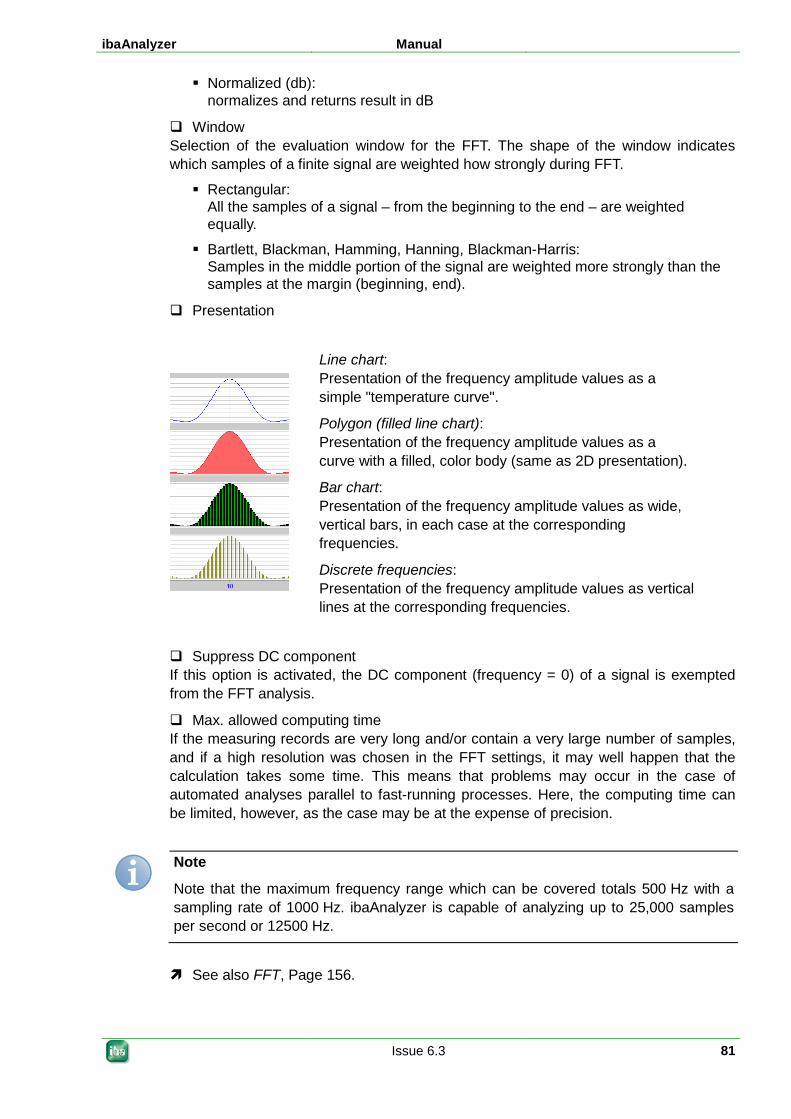
ibaAnalyzer Manual

Issue 6.3 81

Normalized (db): normalizes and returns result in dB

Window Selection of the evaluation window for the FFT. The shape of the window indicates which samples of a finite signal are weighted how strongly during FFT.

Rectangular: All the samples of a signal – from the beginning to the end – are weighted equally.

Bartlett, Blackman, Hamming, Hanning, Blackman-Harris: Samples in the middle portion of the signal are weighted more strongly than the samples at the margin (beginning, end).

Presentation

Line chart: Presentation of the frequency amplitude values as a simple "temperature curve".

Polygon (filled line chart): Presentation of the frequency amplitude values as a curve with a filled, color body (same as 2D presentation).

Bar chart: Presentation of the frequency amplitude values as wide, vertical bars, in each case at the corresponding frequencies.

Discrete frequencies: Presentation of the frequency amplitude values as vertical lines at the corresponding frequencies.

Suppress DC component If this option is activated, the DC component (frequency = 0) of a signal is exempted from the FFT analysis.

Max. allowed computing time If the measuring records are very long and/or contain a very large number of samples, and if a high resolution was chosen in the FFT settings, it may well happen that the calculation takes some time. This means that problems may occur in the case of automated analyses parallel to fast-running processes. Here, the computing time can be limited, however, as the case may be at the expense of precision.

Note

Note that the maximum frequency range which can be covered totals 500 Hz with a sampling rate of 1000 Hz. ibaAnalyzer is capable of analyzing up to 25,000 samples per second or 12500 Hz.

See also FFT, Page 156.

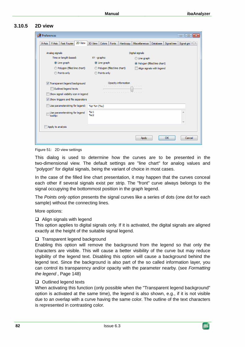
Manual ibaAnalyzer

82 Issue 6.3

3.10.5 2D view

Figure 51: 2D view settings

This dialog is used to determine how the curves are to be presented in the two-dimensional view. The default settings are "line chart" for analog values and "polygon" for digital signals, being the variant of choice in most cases.

In the case of the filled line chart presentation, it may happen that the curves conceal each other if several signals exist per strip. The "front" curve always belongs to the signal occupying the bottommost position in the graph legend.

The Points only option presents the signal curves like a series of dots (one dot for each sample) without the connecting lines.

More options:

Align signals with legend This option applies to digital signals only. If it is activated, the digital signals are aligned exactly at the height of the suitable signal legend.

Transparent legend background Enabling this option will remove the background from the legend so that only the characters are visible. This will cause a better visibility of the curve but may reduce legibility of the legend text. Disabling this option will cause a background behind the legend text. Since the background is also part of the so called information layer, you can control its transparency and/or opacity with the parameter nearby. (see Formatting the legend , Page 148)

Outlined legend texts When activating this function (only possible when the "Transparent legend background" option is activated at the same time), the legend is also shown, e.g., if it is not visible due to an overlap with a curve having the same color. The outline of the text characters is represented in contrasting color.

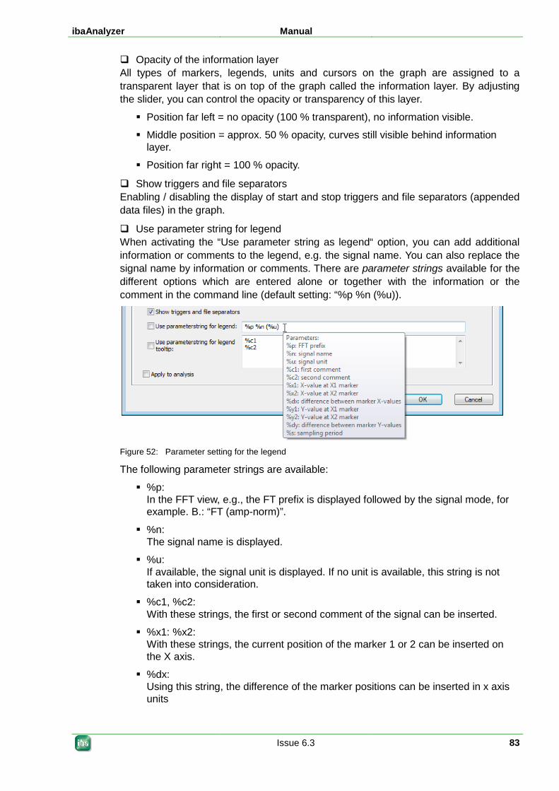
ibaAnalyzer Manual

Issue 6.3 83

Opacity of the information layer All types of markers, legends, units and cursors on the graph are assigned to a transparent layer that is on top of the graph called the information layer. By adjusting the slider, you can control the opacity or transparency of this layer.

Position far left = no opacity (100 % transparent), no information visible.

Middle position = approx. 50 % opacity, curves still visible behind information layer.

Position far right = 100 % opacity.

Show triggers and file separators Enabling / disabling the display of start and stop triggers and file separators (appended data files) in the graph.

Use parameter string for legend When activating the “Use parameter string as legend“ option, you can add additional information or comments to the legend, e.g. the signal name. You can also replace the signal name by information or comments. There are parameter strings available for the different options which are entered alone or together with the information or the comment in the command line (default setting: “%p %n (%u)).

Figure 52: Parameter setting for the legend

The following parameter strings are available:

%p: In the FFT view, e.g., the FT prefix is displayed followed by the signal mode, for example. B.: “FT (amp-norm)”.

%n: The signal name is displayed.

%u: If available, the signal unit is displayed. If no unit is available, this string is not taken into consideration.

%c1, %c2: With these strings, the first or second comment of the signal can be inserted.

%x1: %x2: With these strings, the current position of the marker 1 or 2 can be inserted on the X axis.

%dx: Using this string, the difference of the marker positions can be inserted in x axis units

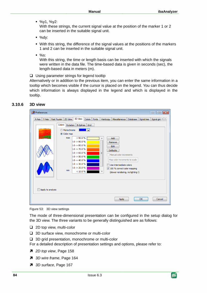
Manual ibaAnalyzer

84 Issue 6.3

%y1, %y2: With these strings, the current signal value at the position of the marker 1 or 2 can be inserted in the suitable signal unit.

%dy:

With this string, the difference of the signal values at the positions of the markers 1 and 2 can be inserted in the suitable signal unit.

%s: With this string, the time or length basis can be inserted with which the signals were written in the data file. The time-based data is given in seconds (sec), the length-based data in meters (m).

Using parameter strings for legend tooltip Alternatively or in addition to the previous item, you can enter the same information in a tooltip which becomes visible if the cursor is placed on the legend. You can thus decide which information is always displayed in the legend and which is displayed in the tooltip.

3.10.6 3D view

Figure 53: 3D view settings

The mode of three-dimensional presentation can be configured in the setup dialog for the 3D view. The three variants to be generally distinguished are as follows:

2D top view, multi-color 3D surface view, monochrome or multi-color 3D grid presentation, monochrome or multi-color For a detailed description of presentation settings and options, please refer to:

2D top view, Page 158

3D wire frame, Page 164

3D surface, Page 167

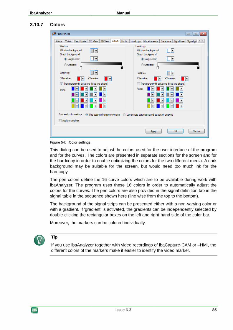
ibaAnalyzer Manual

Issue 6.3 85

3.10.7 Colors

Figure 54: Color settings

This dialog can be used to adjust the colors used for the user interface of the program and for the curves. The colors are presented in separate sections for the screen and for the hardcopy in order to enable optimizing the colors for the two different media. A dark background may be suitable for the screen, but would need too much ink for the hardcopy.

The pen colors define the 16 curve colors which are to be available during work with ibaAnalyzer. The program uses these 16 colors in order to automatically adjust the colors for the curves. The pen colors are also provided in the signal definition tab in the signal table in the sequence shown here (line wise from the top to the bottom).

The background of the signal strips can be presented either with a non-varying color or with a gradient. If 'gradient' is activated, the gradients can be independently selected by double-clicking the rectangular boxes on the left and right-hand side of the color bar.

Moreover, the markers can be colored individually.

Tip

If you use ibaAnalyzer together with video recordings of ibaCapture-CAM or –HMI, the different colors of the markers make it easier to identify the video marker.

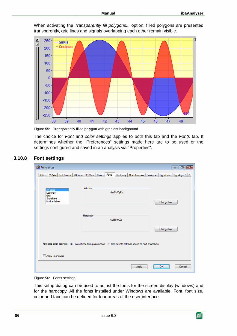
Manual ibaAnalyzer

86 Issue 6.3

When activating the Transparently fill polygons... option, filled polygons are presented transparently, grid lines and signals overlapping each other remain visible.

Figure 55: Transparently filled polygon with gradient background

The choice for Font and color settings applies to both this tab and the Fonts tab. It determines whether the "Preferences" settings made here are to be used or the settings configured and saved in an analysis via "Properties".

3.10.8 Font settings

Figure 56: Fonts settings

This setup dialog can be used to adjust the fonts for the screen display (windows) and for the hardcopy. All the fonts installed under Windows are available. Font, font size, color and face can be defined for four areas of the user interface.

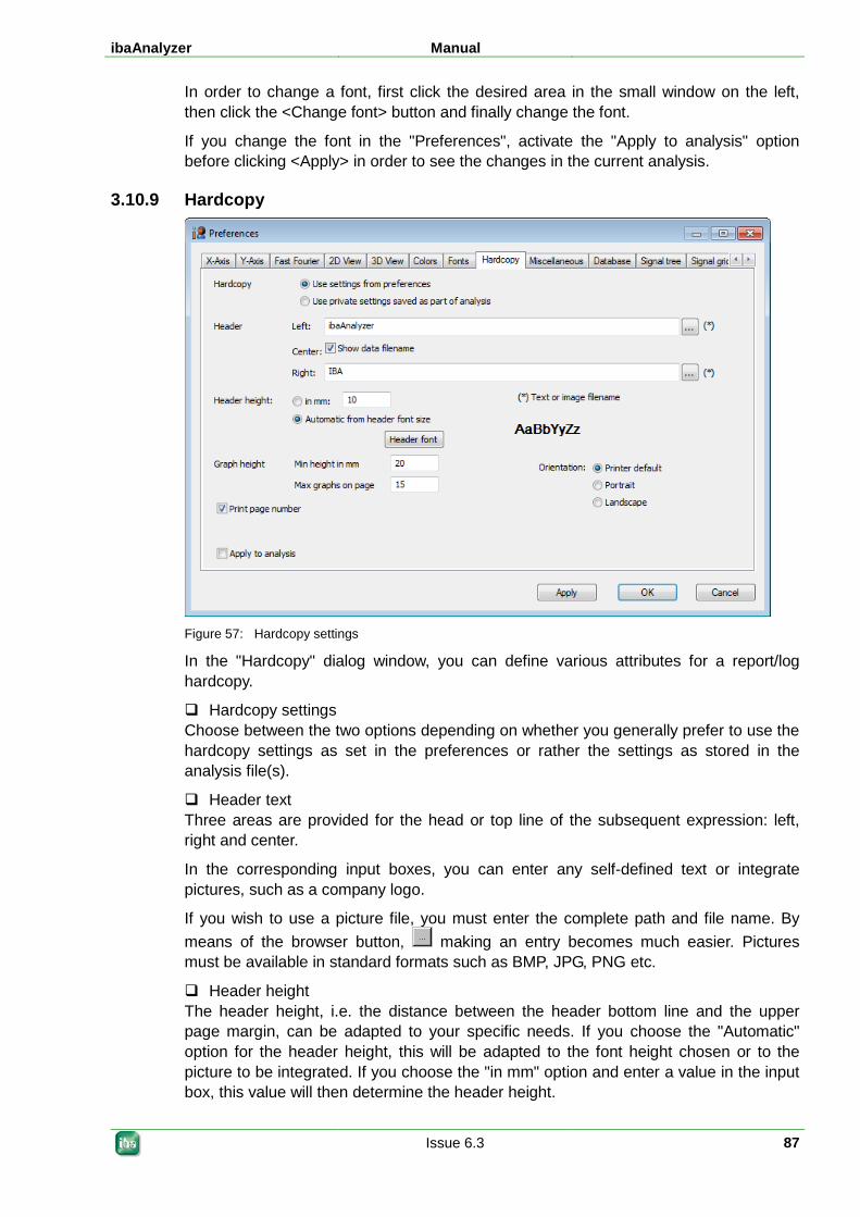
ibaAnalyzer Manual

Issue 6.3 87

In order to change a font, first click the desired area in the small window on the left, then click the <Change font> button and finally change the font.

If you change the font in the "Preferences", activate the "Apply to analysis" option before clicking <Apply> in order to see the changes in the current analysis.

3.10.9 Hardcopy

Figure 57: Hardcopy settings

In the "Hardcopy" dialog window, you can define various attributes for a report/log hardcopy.

Hardcopy settings Choose between the two options depending on whether you generally prefer to use the hardcopy settings as set in the preferences or rather the settings as stored in the analysis file(s).

Header text Three areas are provided for the head or top line of the subsequent expression: left, right and center.

In the corresponding input boxes, you can enter any self-defined text or integrate pictures, such as a company logo.

If you wish to use a picture file, you must enter the complete path and file name. By means of the browser button, making an entry becomes much easier. Pictures must be available in standard formats such as BMP, JPG, PNG etc.

Header height The header height, i.e. the distance between the header bottom line and the upper page margin, can be adapted to your specific needs. If you choose the "Automatic" option for the header height, this will be adapted to the font height chosen or to the picture to be integrated. If you choose the "in mm" option and enter a value in the input box, this value will then determine the header height.

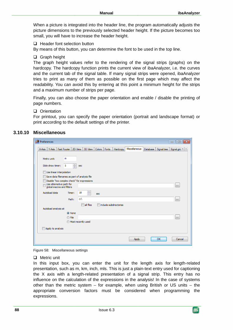
Manual ibaAnalyzer

88 Issue 6.3

When a picture is integrated into the header line, the program automatically adjusts the picture dimensions to the previously selected header height. If the picture becomes too small, you will have to increase the header height.

Header font selection button By means of this button, you can determine the font to be used in the top line.

Graph height The graph height values refer to the rendering of the signal strips (graphs) on the hardcopy. The hardcopy function prints the current view of ibaAnalyzer, i.e. the curves and the current tab of the signal table. If many signal strips were opened, ibaAnalyzer tries to print as many of them as possible on the first page which may affect the readability. You can avoid this by entering at this point a minimum height for the strips and a maximum number of strips per page.

Finally, you can also choose the paper orientation and enable / disable the printing of page numbers.

Orientation For printout, you can specify the paper orientation (portrait and landscape format) or print according to the default settings of the printer.

3.10.10 Miscellaneous

Figure 58: Miscellaneous settings

Metric unit In this input box, you can enter the unit for the length axis for length-related presentation, such as m, km, inch, mls. This is just a plain-text entry used for captioning the X axis with a length-related presentation of a signal strip. This entry has no influence on the calculation of the expressions in the analysis! In the case of systems other than the metric system – for example, when using British or US units – the appropriate conversion factors must be considered when programming the expressions.

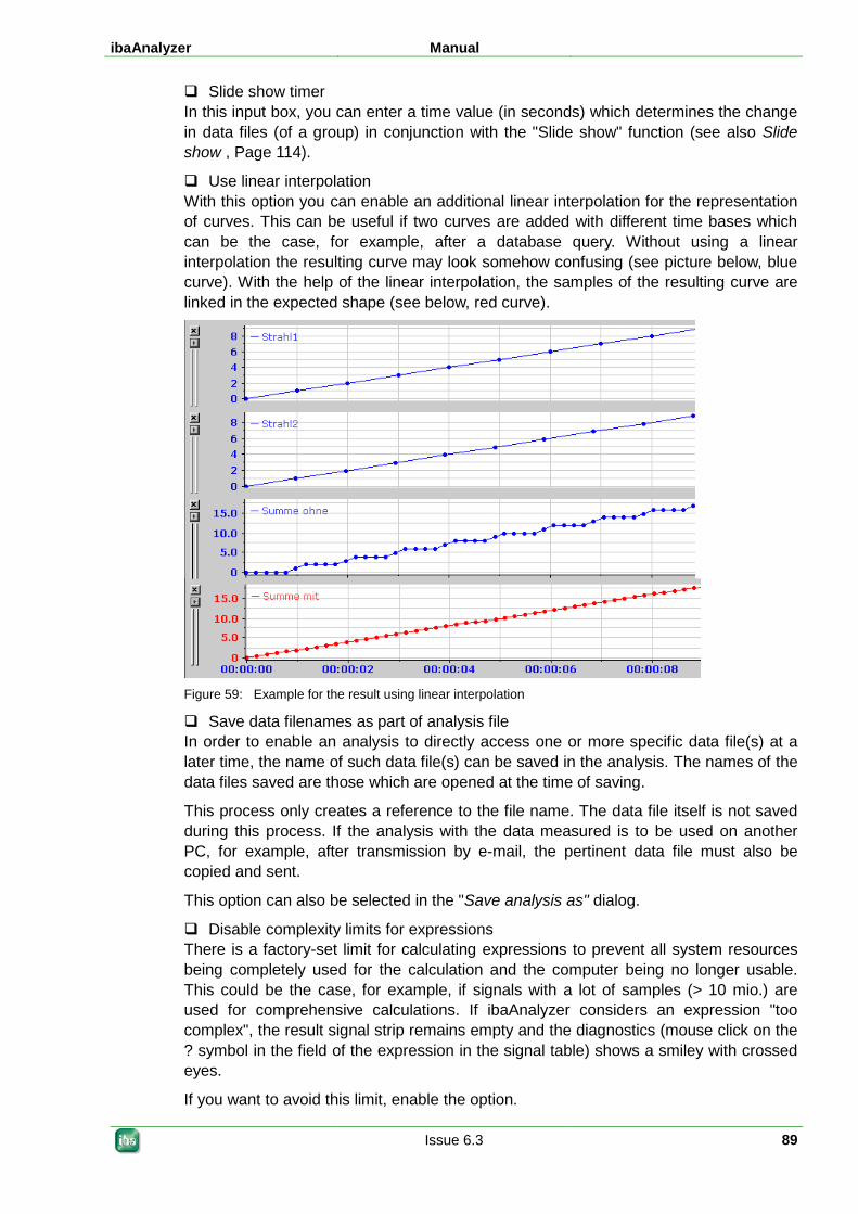
ibaAnalyzer Manual

Issue 6.3 89

Slide show timer In this input box, you can enter a time value (in seconds) which determines the change in data files (of a group) in conjunction with the "Slide show" function (see also Slide show , Page 114).

Use linear interpolation With this option you can enable an additional linear interpolation for the representation of curves. This can be useful if two curves are added with different time bases which can be the case, for example, after a database query. Without using a linear interpolation the resulting curve may look somehow confusing (see picture below, blue curve). With the help of the linear interpolation, the samples of the resulting curve are linked in the expected shape (see below, red curve).

Figure 59: Example for the result using linear interpolation

Save data filenames as part of analysis file In order to enable an analysis to directly access one or more specific data file(s) at a later time, the name of such data file(s) can be saved in the analysis. The names of the data files saved are those which are opened at the time of saving.

This process only creates a reference to the file name. The data file itself is not saved during this process. If the analysis with the data measured is to be used on another PC, for example, after transmission by e-mail, the pertinent data file must also be copied and sent.

This option can also be selected in the "Save analysis as" dialog.

Disable complexity limits for expressions There is a factory-set limit for calculating expressions to prevent all system resources being completely used for the calculation and the computer being no longer usable. This could be the case, for example, if signals with a lot of samples (> 10 mio.) are used for comprehensive calculations. If ibaAnalyzer considers an expression "too complex", the result signal strip remains empty and the diagnostics (mouse click on the ? symbol in the field of the expression in the signal table) shows a smiley with crossed eyes.

If you want to avoid this limit, enable the option.

Manual ibaAnalyzer

90 Issue 6.3

Note

Functions such as “resample“, “margin“ and “time“ can also lead to exhaustion of the resources if parameters being too large are indicated. There is also a limit for these functions, however, it cannot be disabled.

Use other path for global macros and filters If global macros and/or filters are used in an analysis, it can happen that they do not work anymore, e.g., after opening the analysis in another environment than that of their original configuration.

This might be the case, for example, if analyses and data were sent via e-mail for reasons of support or diagnostics and are to be analyzed in another environment on another computer. The receiver stores global macros and filters on another path.

By enabling this option and indicating the new path at this point, global macros and filters are automatically found.

Autoload data files, timer In this box, you will have to enter an appropriate time value in [s] if ibaAnalyzer is to analyze a data file in online mode. The data file which is currently being written by ibaPDA is then reloaded at this interval, so that new data generated in the meantime will be included in the analysis.

Autoload data files, Path In order to enable the automatic detection of open data files, enter in this box the name of the path in which ibaPDA stores the data files. If you click the symbol key during operation, ibaAnalyzer will search for an open data file in this specified path (online mode).

All files This option applies to the case that several files are opened at a time in ibaAnalyzer which are written simultaneously by one ibaPDA system, different ibaPDA systems and / or other systems, e. g. ibaLogic. If you do not check this option, only the first data file (on top in the signal tree) will be reloaded automatically.

Including subdirectories This option should be chosen if the file system of ibaPDA is organized in such a manner that further subdirectories – for example, per hour or per day – are created under the above-mentioned path.

Autoload analysis at startup This option should be used if you prefer a certain analysis being executed when starting ibaAnalyzer. Click File and enter the path and file name of the requested analysis into the box next to it or use the browser function. Or check most recently used if you prefer to start with the analysis most recently used.

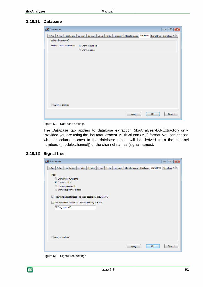
ibaAnalyzer Manual

Issue 6.3 91

3.10.11 Database

Figure 60: Database settings

The Database tab applies to database extraction (ibaAnalyzer-DB-Extractor) only. Provided you are using the ibaDataExtractor MultiColumn (MC) format, you can choose whether column names in the database tables will be derived from the channel numbers ([module:channel]) or the channel names (signal names).

3.10.12 Signal tree

Figure 61: Signal tree settings

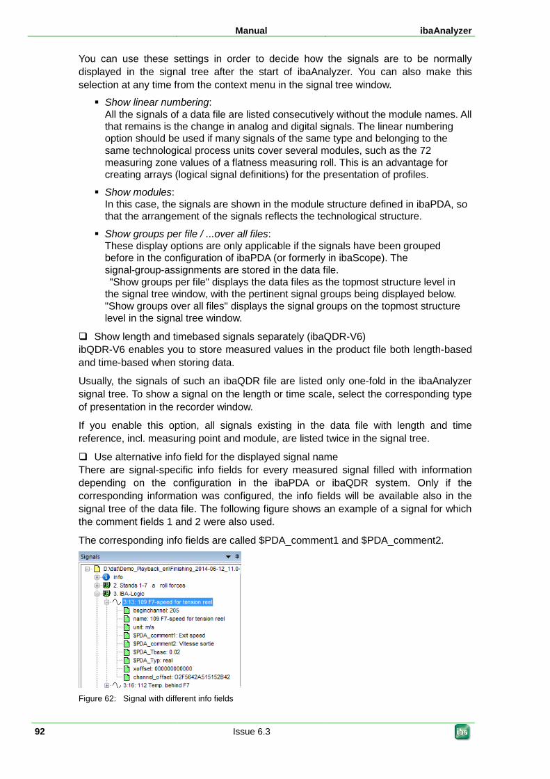
Manual ibaAnalyzer

92 Issue 6.3

You can use these settings in order to decide how the signals are to be normally displayed in the signal tree after the start of ibaAnalyzer. You can also make this selection at any time from the context menu in the signal tree window.

Show linear numbering: All the signals of a data file are listed consecutively without the module names. All that remains is the change in analog and digital signals. The linear numbering option should be used if many signals of the same type and belonging to the same technological process units cover several modules, such as the 72 measuring zone values of a flatness measuring roll. This is an advantage for creating arrays (logical signal definitions) for the presentation of profiles.

Show modules: In this case, the signals are shown in the module structure defined in ibaPDA, so that the arrangement of the signals reflects the technological structure.

Show groups per file / ...over all files: These display options are only applicable if the signals have been grouped before in the configuration of ibaPDA (or formerly in ibaScope). The signal-group-assignments are stored in the data file. "Show groups per file" displays the data files as the topmost structure level in the signal tree window, with the pertinent signal groups being displayed below. "Show groups over all files" displays the signal groups on the topmost structure level in the signal tree window.

Show length and timebased signals separately (ibaQDR-V6) ibQDR-V6 enables you to store measured values in the product file both length-based and time-based when storing data.

Usually, the signals of such an ibaQDR file are listed only one-fold in the ibaAnalyzer signal tree. To show a signal on the length or time scale, select the corresponding type of presentation in the recorder window.

If you enable this option, all signals existing in the data file with length and time reference, incl. measuring point and module, are listed twice in the signal tree.

Use alternative info field for the displayed signal name There are signal-specific info fields for every measured signal filled with information depending on the configuration in the ibaPDA or ibaQDR system. Only if the corresponding information was configured, the info fields will be available also in the signal tree of the data file. The following figure shows an example of a signal for which the comment fields 1 and 2 were also used.

The corresponding info fields are called $PDA_comment1 and $PDA_comment2.

Figure 62: Signal with different info fields

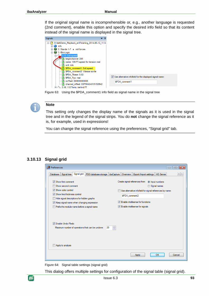
ibaAnalyzer Manual

Issue 6.3 93

If the original signal name is incomprehensible or, e.g., another language is requested (2nd comment), enable this option and specify the desired info field so that its content instead of the signal name is displayed in the signal tree.

Figure 63: Using the $PDA_comment1 info field as signal name in the signal tree

Note

This setting only changes the display name of the signals as it is used in the signal tree and in the legend of the signal strips. You do not change the signal reference as it is, for example, used in expressions!

You can change the signal reference using the preferences, “Signal grid” tab.

3.10.13 Signal grid

Figure 64: Signal table settings (signal grid)

This dialog offers multiple settings for configuration of the signal table (signal grid).

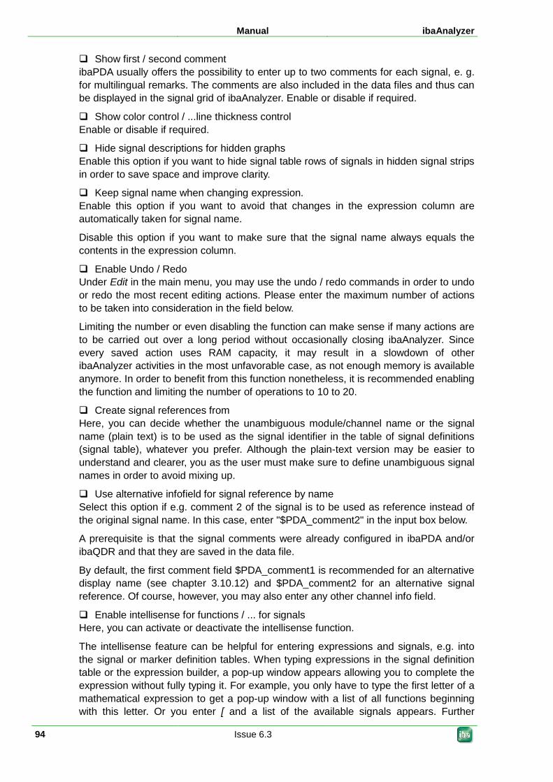
Manual ibaAnalyzer

94 Issue 6.3

Show first / second comment ibaPDA usually offers the possibility to enter up to two comments for each signal, e. g. for multilingual remarks. The comments are also included in the data files and thus can be displayed in the signal grid of ibaAnalyzer. Enable or disable if required.

Show color control / ...line thickness control Enable or disable if required.

Hide signal descriptions for hidden graphs Enable this option if you want to hide signal table rows of signals in hidden signal strips in order to save space and improve clarity.

Keep signal name when changing expression. Enable this option if you want to avoid that changes in the expression column are automatically taken for signal name.

Disable this option if you want to make sure that the signal name always equals the contents in the expression column.

Enable Undo / Redo Under Edit in the main menu, you may use the undo / redo commands in order to undo or redo the most recent editing actions. Please enter the maximum number of actions to be taken into consideration in the field below.

Limiting the number or even disabling the function can make sense if many actions are to be carried out over a long period without occasionally closing ibaAnalyzer. Since every saved action uses RAM capacity, it may result in a slowdown of other ibaAnalyzer activities in the most unfavorable case, as not enough memory is available anymore. In order to benefit from this function nonetheless, it is recommended enabling the function and limiting the number of operations to 10 to 20.

Create signal references from Here, you can decide whether the unambiguous module/channel name or the signal name (plain text) is to be used as the signal identifier in the table of signal definitions (signal table), whatever you prefer. Although the plain-text version may be easier to understand and clearer, you as the user must make sure to define unambiguous signal names in order to avoid mixing up.

Use alternative infofield for signal reference by name Select this option if e.g. comment 2 of the signal is to be used as reference instead of the original signal name. In this case, enter "$PDA_comment2" in the input box below.

A prerequisite is that the signal comments were already configured in ibaPDA and/or ibaQDR and that they are saved in the data file.

By default, the first comment field $PDA_comment1 is recommended for an alternative display name (see chapter 3.10.12) and $PDA_comment2 for an alternative signal reference. Of course, however, you may also enter any other channel info field.

Enable intellisense for functions / ... for signals Here, you can activate or deactivate the intellisense function.

The intellisense feature can be helpful for entering expressions and signals, e.g. into the signal or marker definition tables. When typing expressions in the signal definition table or the expression builder, a pop-up window appears allowing you to complete the expression without fully typing it. For example, you only have to type the first letter of a mathematical expression to get a pop-up window with a list of all functions beginning with this letter. Or you enter [ and a list of the available signals appears. Further

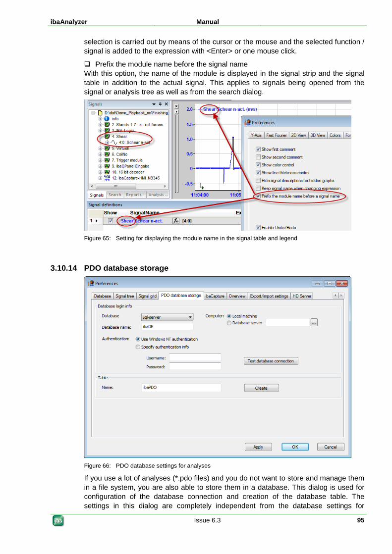
ibaAnalyzer Manual

Issue 6.3 95

selection is carried out by means of the cursor or the mouse and the selected function / signal is added to the expression with <Enter> or one mouse click.

Prefix the module name before the signal name With this option, the name of the module is displayed in the signal strip and the signal table in addition to the actual signal. This applies to signals being opened from the signal or analysis tree as well as from the search dialog.

Figure 65: Setting for displaying the module name in the signal table and legend

3.10.14 PDO database storage

Figure 66: PDO database settings for analyses

If you use a lot of analyses (*.pdo files) and you do not want to store and manage them in a file system, you are also able to store them in a database. This dialog is used for configuration of the database connection and creation of the database table. The settings in this dialog are completely independent from the database settings for

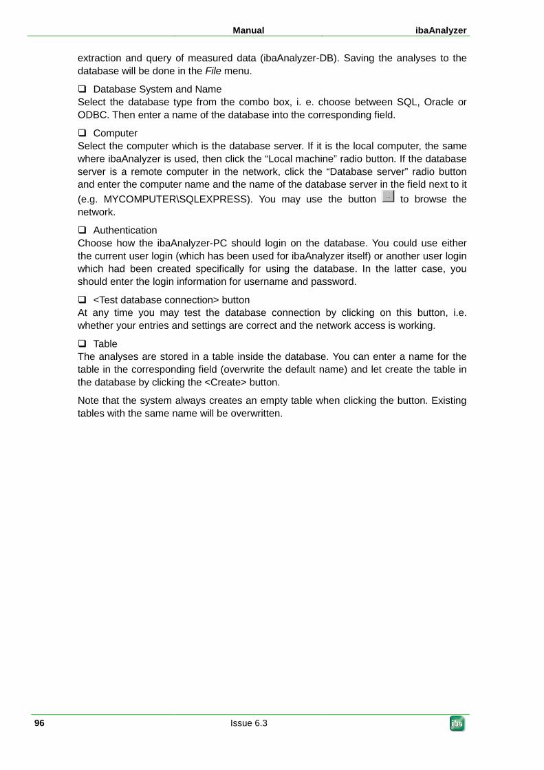
Manual ibaAnalyzer

96 Issue 6.3

extraction and query of measured data (ibaAnalyzer-DB). Saving the analyses to the database will be done in the File menu.

Database System and Name Select the database type from the combo box, i. e. choose between SQL, Oracle or ODBC. Then enter a name of the database into the corresponding field.

Computer Select the computer which is the database server. If it is the local computer, the same where ibaAnalyzer is used, then click the “Local machine” radio button. If the database server is a remote computer in the network, click the “Database server” radio button and enter the computer name and the name of the database server in the field next to it (e.g. MYCOMPUTER\SQLEXPRESS). You may use the button to browse the network.

Authentication Choose how the ibaAnalyzer-PC should login on the database. You could use either the current user login (which has been used for ibaAnalyzer itself) or another user login which had been created specifically for using the database. In the latter case, you should enter the login information for username and password.

<Test database connection> button At any time you may test the database connection by clicking on this button, i.e. whether your entries and settings are correct and the network access is working.

Table The analyses are stored in a table inside the database. You can enter a name for the table in the corresponding field (overwrite the default name) and let create the table in the database by clicking the <Create> button.

Note that the system always creates an empty table when clicking the button. Existing tables with the same name will be overwritten.

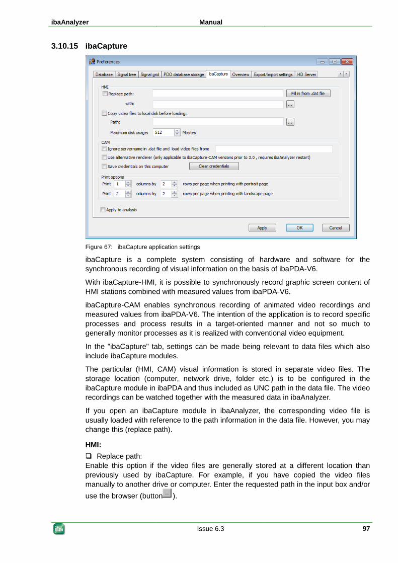
ibaAnalyzer Manual

Issue 6.3 97

3.10.15 ibaCapture

Figure 67: ibaCapture application settings

ibaCapture is a complete system consisting of hardware and software for the synchronous recording of visual information on the basis of ibaPDA-V6.

With ibaCapture-HMI, it is possible to synchronously record graphic screen content of HMI stations combined with measured values from ibaPDA-V6.

ibaCapture-CAM enables synchronous recording of animated video recordings and measured values from ibaPDA-V6. The intention of the application is to record specific processes and process results in a target-oriented manner and not so much to generally monitor processes as it is realized with conventional video equipment.

In the "ibaCapture" tab, settings can be made being relevant to data files which also include ibaCapture modules.

The particular (HMI, CAM) visual information is stored in separate video files. The storage location (computer, network drive, folder etc.) is to be configured in the ibaCapture module in ibaPDA and thus included as UNC path in the data file. The video recordings can be watched together with the measured data in ibaAnalyzer.

If you open an ibaCapture module in ibaAnalyzer, the corresponding video file is usually loaded with reference to the path information in the data file. However, you may change this (replace path).

HMI: Replace path: Enable this option if the video files are generally stored at a different location than previously used by ibaCapture. For example, if you have copied the video files manually to another drive or computer. Enter the requested path in the input box and/or use the browser (button ).

Manual ibaAnalyzer

98 Issue 6.3

Copy video files to local drive before loading: Enable this option if you want to play the video files on the local drive. The video can be played faster and smoother and the network load can be reduced. ibaAnalyzer first creates a copy of the video file to be watched on the local hard disk in the folder which had been specified by you in the “Folder” field. In order to prevent the local hard disk being filled up with video files, you should set a limit of disk space for the video files. If the limit of this space is about to be reached, the oldest video files will be deleted and overwritten.

You may enable both options in combination.

CAM: Ignore server name in .dat file and load video files from: For video playback, ibaAnalyzer and/or the integrated ibaCapture-CAM player must have a connection to the ibaCapture-CAM server where the videos are stored (except for exported dat files with embedded videos). For this purpose, the default settings use the server name which is stored in the data file. If, in the meantime, the name of the ibaCapture-CAM server has been changed or the video files have been transferred to another server, this option can refer to the new server name. The videos will then be loaded from the selected server. Also on the new server, the ibaCapture-CAM server service has to run to be able to play the videos.

Use alternative renderer (recommended for Windows 7,…): If you work with Windows 7, it is recommended checking the box to use the Windows graphic library for the screen layout. If you want to use the default mode (usage of the preinstalled iba renderer), maintain the default settings.

Save credentials on this computer If the user management was activated in ibaCapture-CAM and the rights were limited with regard to video viewing, a user has to log in entering his user name and password when opening a camera channel in ibaAnalyzer. If this user is not authorized to view videos, no videos will be displayed. This registration is required once per ibaAnalyzer session.

If you enable this option, the login information is stored on your local computer; after a restart of ibaAnalyzer, it is not required to log in again.

With the <Clear credentials> button, you can remove this information from the computer.

Print options With these settings, you determine as to how video images are to be printed if you use the print function in the File menu.

The number of columns determines how many images are to be printed side by side on one page. The images are scaled accordingly. The number of rows determines how many images are to be printed one below the other on one page.

For printing in the portrait and landscape format, these settings can be made separately.

The settings apply to video images of ibaCapture-CAM and ibaCapture-HMI.

To activate the settings with an analysis being currently open, enable the "Apply to analysis" option and click <OK>.

You can control your settings under menu File – Print preview.

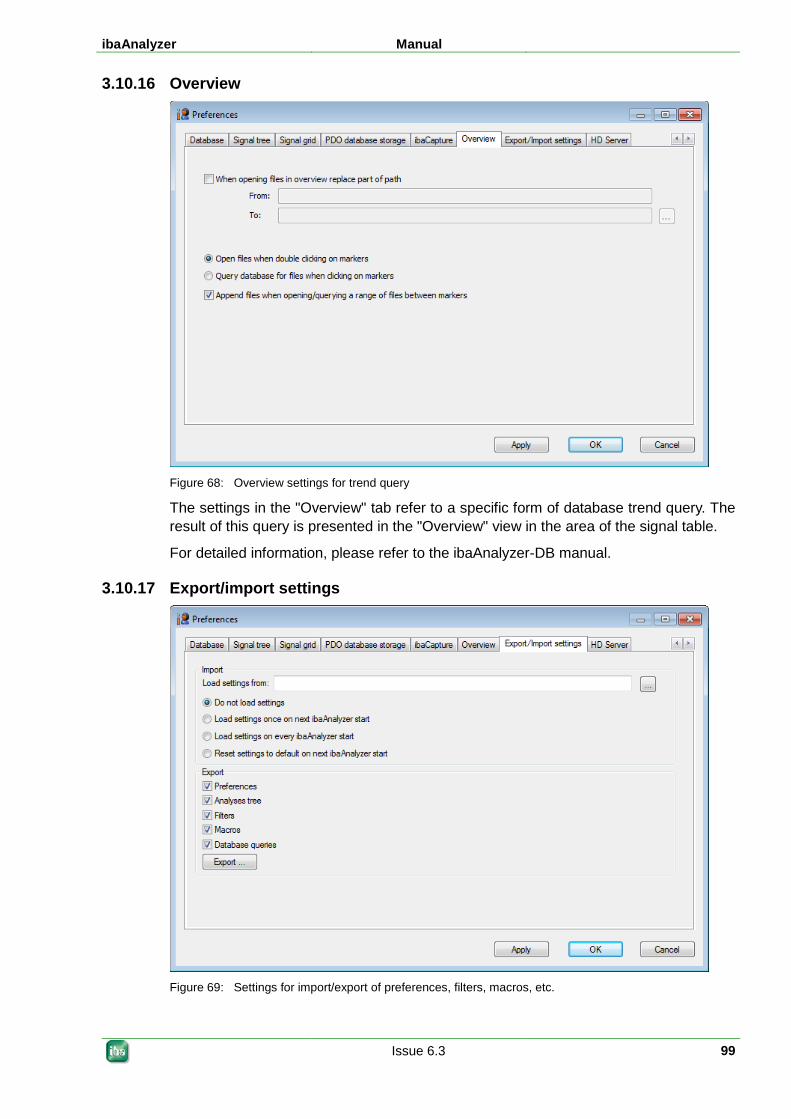
ibaAnalyzer Manual

Issue 6.3 99

3.10.16 Overview

Figure 68: Overview settings for trend query

The settings in the "Overview" tab refer to a specific form of database trend query. The result of this query is presented in the "Overview" view in the area of the signal table.

For detailed information, please refer to the ibaAnalyzer-DB manual.

3.10.17 Export/import settings

Figure 69: Settings for import/export of preferences, filters, macros, etc.

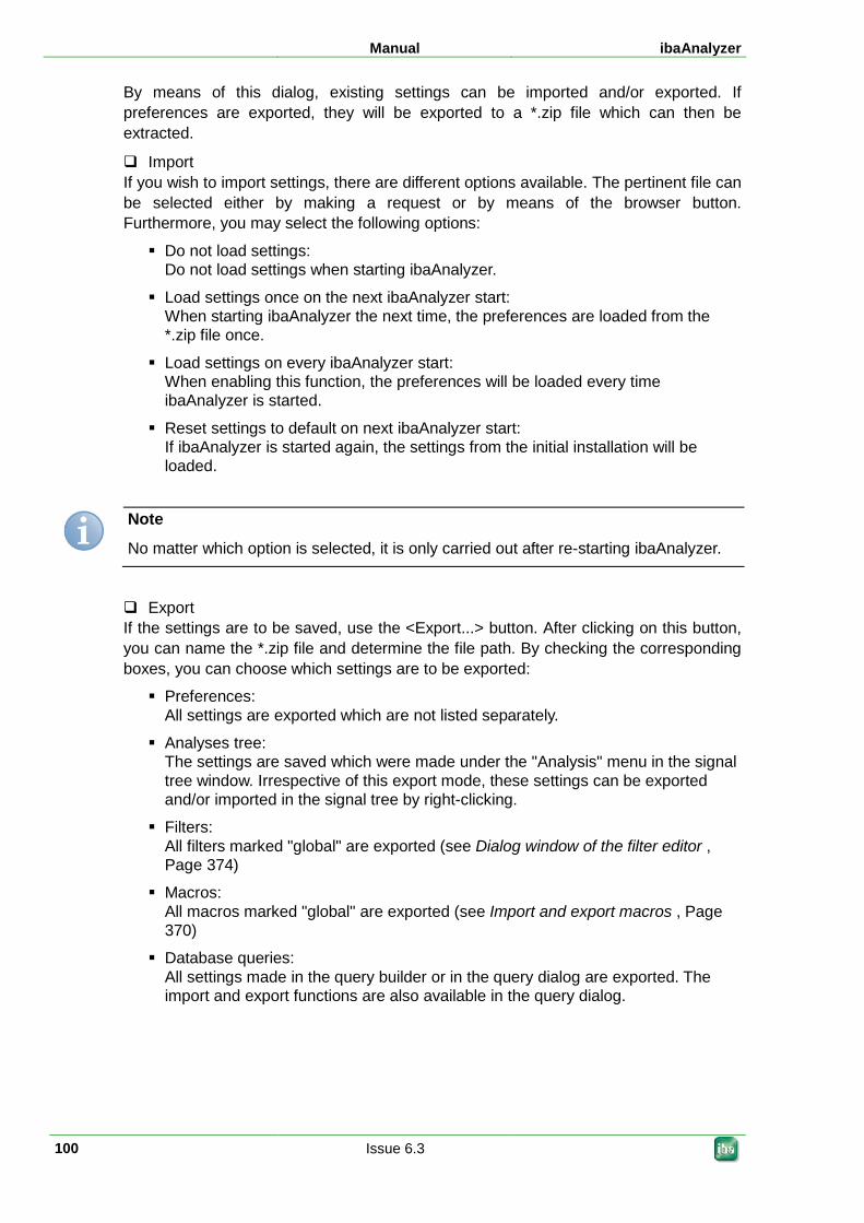
Manual ibaAnalyzer

100 Issue 6.3

By means of this dialog, existing settings can be imported and/or exported. If preferences are exported, they will be exported to a *.zip file which can then be extracted.

Import If you wish to import settings, there are different options available. The pertinent file can be selected either by making a request or by means of the browser button. Furthermore, you may select the following options:

Do not load settings: Do not load settings when starting ibaAnalyzer.

Load settings once on the next ibaAnalyzer start: When starting ibaAnalyzer the next time, the preferences are loaded from the *.zip file once.

Load settings on every ibaAnalyzer start: When enabling this function, the preferences will be loaded every time ibaAnalyzer is started.

Reset settings to default on next ibaAnalyzer start: If ibaAnalyzer is started again, the settings from the initial installation will be loaded.

Note

No matter which option is selected, it is only carried out after re-starting ibaAnalyzer.

Export If the settings are to be saved, use the <Export...> button. After clicking on this button, you can name the *.zip file and determine the file path. By checking the corresponding boxes, you can choose which settings are to be exported:

Preferences: All settings are exported which are not listed separately.

Analyses tree: The settings are saved which were made under the "Analysis" menu in the signal tree window. Irrespective of this export mode, these settings can be exported and/or imported in the signal tree by right-clicking.

Filters: All filters marked "global" are exported (see Dialog window of the filter editor , Page 374)

Macros: All macros marked "global" are exported (see Import and export macros , Page 370)

Database queries: All settings made in the query builder or in the query dialog are exported. The import and export functions are also available in the query dialog.

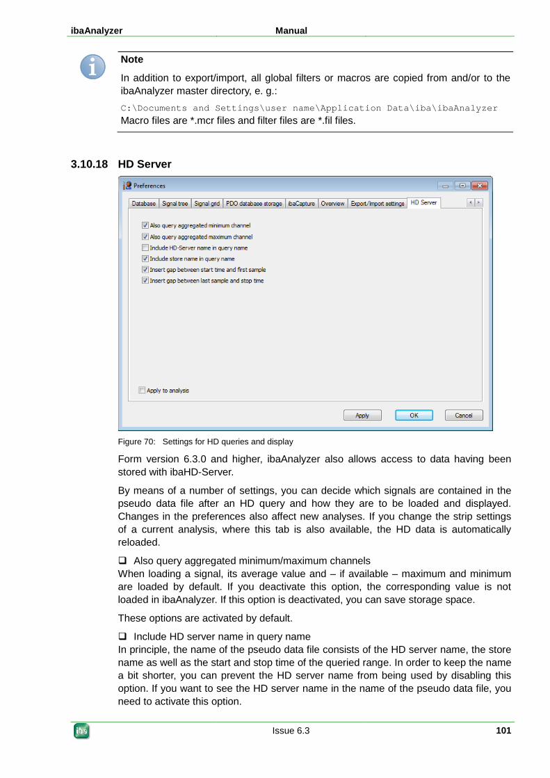
ibaAnalyzer Manual

Issue 6.3 101

Note

In addition to export/import, all global filters or macros are copied from and/or to the ibaAnalyzer master directory, e. g.: C:\Documents and Settings\user name\Application Data\iba\ibaAnalyzer

Macro files are *.mcr files and filter files are *.fil files.

3.10.18 HD Server

Figure 70: Settings for HD queries and display

Form version 6.3.0 and higher, ibaAnalyzer also allows access to data having been stored with ibaHD-Server.

By means of a number of settings, you can decide which signals are contained in the pseudo data file after an HD query and how they are to be loaded and displayed. Changes in the preferences also affect new analyses. If you change the strip settings of a current analysis, where this tab is also available, the HD data is automatically reloaded.

Also query aggregated minimum/maximum channels When loading a signal, its average value and – if available – maximum and minimum are loaded by default. If you deactivate this option, the corresponding value is not loaded in ibaAnalyzer. If this option is deactivated, you can save storage space.

These options are activated by default.

Include HD server name in query name In principle, the name of the pseudo data file consists of the HD server name, the store name as well as the start and stop time of the queried range. In order to keep the name a bit shorter, you can prevent the HD server name from being used by disabling this option. If you want to see the HD server name in the name of the pseudo data file, you need to activate this option.

Manual ibaAnalyzer

102 Issue 6.3

This option is disabled by default.

Include store name in query name Similar as to what is described above, the name of the HD store can also be used in the name of the pseudo data file. If you enable this option in addition to the previous option, the name of the pseudo data file becomes even shorter.

This option is enabled by default.

Insert gab between... It might happen that there are no values available at the beginning or end of the specified query range.

If you enable this option, there is a gap displayed in the graph between the starting point and the first measuring value and the last measuring value and the stopping time, respectively. The X axis exactly corresponds to the specified time range.

If you disable this option, no gaps will be displayed and the X axis starts with the first value measured and ends with the last value measured.

These options are enabled by default.

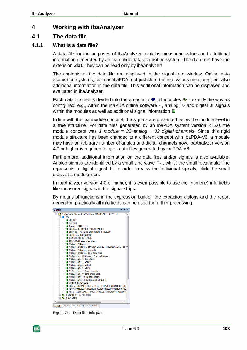
ibaAnalyzer Manual

Issue 6.3 103

4 Working with ibaAnalyzer 4.1 The data file 4.1.1 What is a data file?

A data file for the purposes of ibaAnalyzer contains measuring values and additional information generated by an iba online data acquisition system. The data files have the extension .dat. They can be read only by ibaAnalyzer!

The contents of the data file are displayed in the signal tree window. Online data acquisition systems, such as ibaPDA, not just store the real values measured, but also additional information in the data file. This additional information can be displayed and evaluated in ibaAnalyzer.

Each data file tree is divided into the areas info , all modules - exactly the way as configured, e.g., within the ibaPDA online software - , analog and digital signals within the modules as well as additional signal information

In line with the iba module concept, the signals are presented below the module level in a tree structure. For data files generated by an ibaPDA system version < 6.0, the module concept was 1 module = 32 analog + 32 digital channels. Since this rigid module structure has been changed to a different concept with ibaPDA-V6, a module may have an arbitrary number of analog and digital channels now. ibaAnalyzer version 4.0 or higher is required to open data files generated by ibaPDA-V6.

Furthermore, additional information on the data files and/or signals is also available. Analog signals are identified by a small sine wave , whilst the small rectangular line represents a digital signal . In order to view the individual signals, click the small cross at a module icon.

In ibaAnalyzer version 4.0 or higher, it is even possible to use the (numeric) info fields like measured signals in the signal strips.

By means of functions in the expression builder, the extraction dialogs and the report generator, practically all info fields can be used for further processing.

Figure 71: Data file, Info part

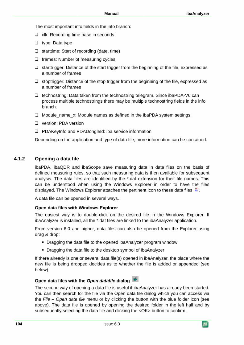
Manual ibaAnalyzer

104 Issue 6.3

The most important info fields in the info branch:

clk: Recording time base in seconds

type: Data type

starttime: Start of recording (date, time)

frames: Number of measuring cycles

starttrigger: Distance of the start trigger from the beginning of the file, expressed as a number of frames

stoptrigger: Distance of the stop trigger from the beginning of the file, expressed as a number of frames

technostring: Data taken from the technostring telegram. Since ibaPDA-V6 can process multiple technostrings there may be multiple technostring fields in the info branch.

Module_name_x: Module names as defined in the ibaPDA system settings.

version: PDA version

PDAKeyInfo and PDADongleId: iba service information

Depending on the application and type of data file, more information can be contained.

4.1.2 Opening a data file ibaPDA, ibaQDR and ibaScope save measuring data in data files on the basis of defined measuring rules, so that such measuring data is then available for subsequent analysis. The data files are identified by the *.dat extension for their file names. This can be understood when using the Windows Explorer in order to have the files displayed. The Windows Explorer attaches the pertinent icon to these data files .

A data file can be opened in several ways.

Open data files with Windows Explorer The easiest way is to double-click on the desired file in the Windows Explorer. If ibaAnalyzer is installed, all the *.dat files are linked to the ibaAnalyzer application.

From version 6.0 and higher, data files can also be opened from the Explorer using drag & drop:

Dragging the data file to the opened ibaAnalyzer program window

Dragging the data file to the desktop symbol of ibaAnalyzer

If there already is one or several data file(s) opened in ibaAnalyzer, the place where the new file is being dropped decides as to whether the file is added or appended (see below).

Open data files with the Open datafile dialog The second way of opening a data file is useful if ibaAnalyzer has already been started. You can then search for the file via the Open data file dialog which you can access via the File – Open data file menu or by clicking the button with the blue folder icon (see above). The data file is opened by opening the desired folder in the left half and by subsequently selecting the data file and clicking the <OK> button to confirm.

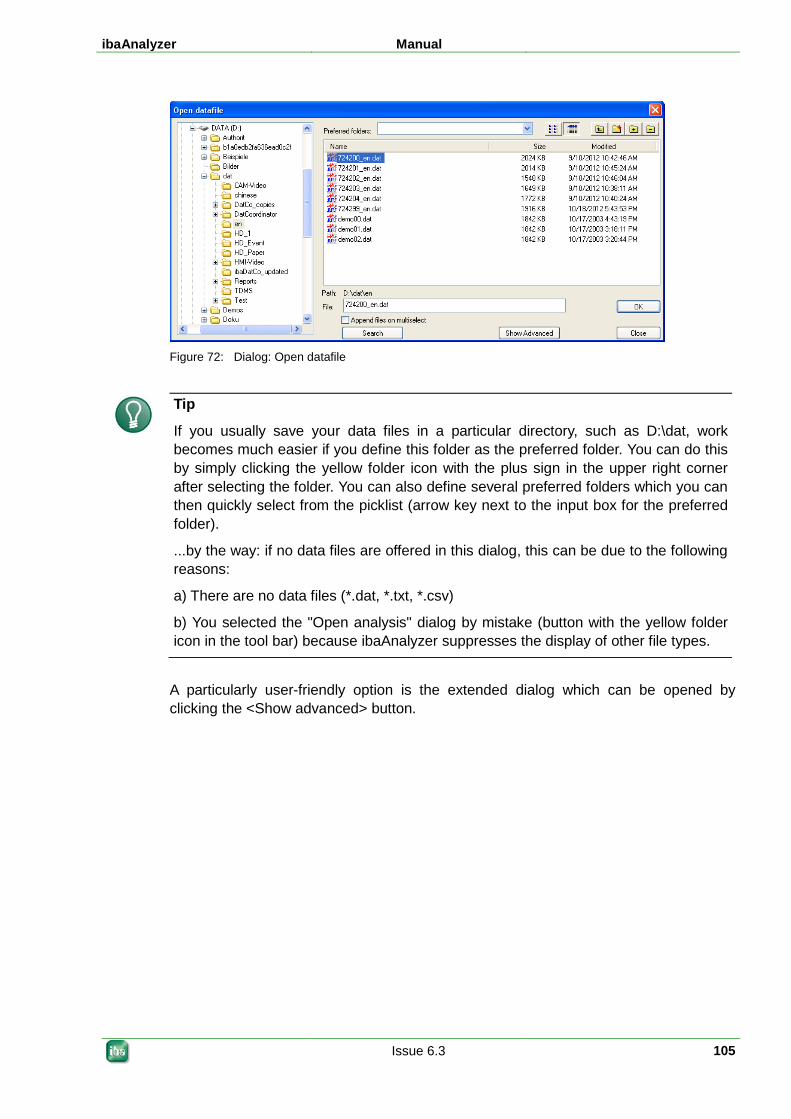
ibaAnalyzer Manual

Issue 6.3 105

Figure 72: Dialog: Open datafile

Tip

If you usually save your data files in a particular directory, such as D:\dat, work becomes much easier if you define this folder as the preferred folder. You can do this by simply clicking the yellow folder icon with the plus sign in the upper right corner after selecting the folder. You can also define several preferred folders which you can then quickly select from the picklist (arrow key next to the input box for the preferred folder).

...by the way: if no data files are offered in this dialog, this can be due to the following reasons:

a) There are no data files (*.dat, *.txt, *.csv)

b) You selected the "Open analysis" dialog by mistake (button with the yellow folder icon in the tool bar) because ibaAnalyzer suppresses the display of other file types.

A particularly user-friendly option is the extended dialog which can be opened by clicking the <Show advanced> button.

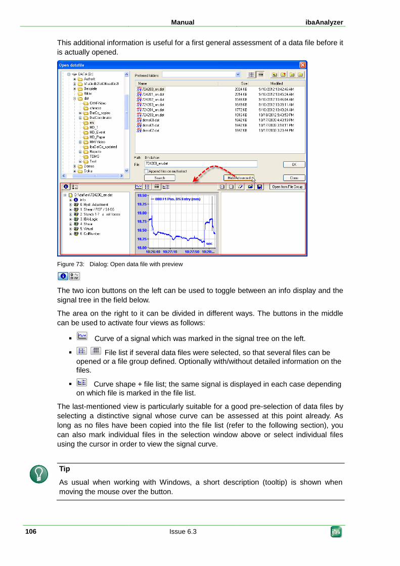
Manual ibaAnalyzer

106 Issue 6.3

This additional information is useful for a first general assessment of a data file before it is actually opened.

Figure 73: Dialog: Open data file with preview

The two icon buttons on the left can be used to toggle between an info display and the signal tree in the field below.

The area on the right to it can be divided in different ways. The buttons in the middle can be used to activate four views as follows:

Curve of a signal which was marked in the signal tree on the left.

File list if several data files were selected, so that several files can be opened or a file group defined. Optionally with/without detailed information on the files.

Curve shape + file list; the same signal is displayed in each case depending on which file is marked in the file list.

The last-mentioned view is particularly suitable for a good pre-selection of data files by selecting a distinctive signal whose curve can be assessed at this point already. As long as no files have been copied into the file list (refer to the following section), you can also mark individual files in the selection window above or select individual files using the cursor in order to view the signal curve.

Tip

As usual when working with Windows, a short description (tooltip) is shown when moving the mouse over the button.

ibaAnalyzer Manual

Issue 6.3 107

4.1.3 Opening several data files ibaAnalyzer enables the simultaneous opening of any number of data files. Opening several data files at the same time is, for example, useful if you wish to compare the curves of a signal from several data files which were stored at different times.

The blue folder icon with the two ++ signs (see above) allows for adding further data files to previously selected data files in order to analyze signals from different sources. The same command can also be executed via the File - Add new data file menu.

With ibaAnalyzer version 4.1 or higher, you can also enter wildcards * and ? in the file name field of the Open datafile dialog in order to open multiple data files at the same time.

To open several data files from the Windows Explorer, you have the following options:

Drag files one after another in the ibaAnalyzer program window. If you drag the files into the signal tree window, make sure the mouse is not placed on a data file while the files are being dropped. Otherwise, the new data file is appended (see below).

Select several files (all files in the directory using <Ctrl>+<A>) and drag them into the program window using drag & drop.

Note

Selecting several files and then pressing the <Return> key does not lead to the desired result. Instead, ibaAnalyzer opens each file in its own instance.

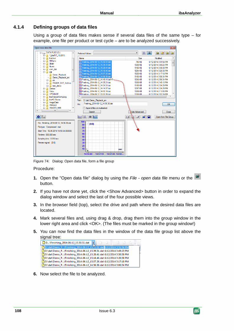
Manual ibaAnalyzer

108 Issue 6.3

4.1.4 Defining groups of data files Using a group of data files makes sense if several data files of the same type – for example, one file per product or test cycle – are to be analyzed successively.

Figure 74: Dialog: Open data file, form a file group

Procedure:

1. Open the "Open data file" dialog by using the File - open data file menu or the button.

2. If you have not done yet, click the <Show Advanced> button in order to expand the dialog window and select the last of the four possible views.

3. In the browser field (top), select the drive and path where the desired data files are located.

4. Mark several files and, using drag & drop, drag them into the group window in the lower right area and click <OK>. (The files must be marked in the group window!)

5. You can now find the data files in the window of the data file group list above the signal tree:

6. Now select the file to be analyzed.

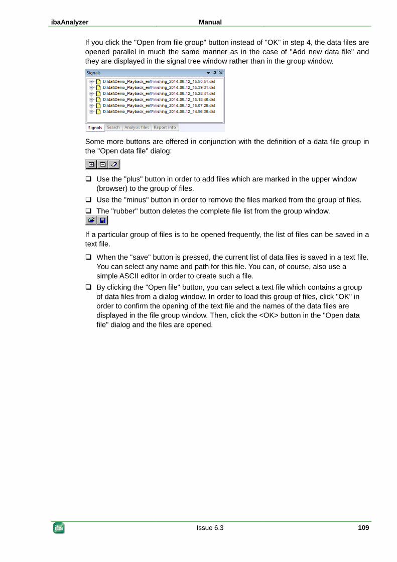
ibaAnalyzer Manual

Issue 6.3 109

If you click the "Open from file group" button instead of "OK" in step 4, the data files are opened parallel in much the same manner as in the case of "Add new data file" and they are displayed in the signal tree window rather than in the group window.

Some more buttons are offered in conjunction with the definition of a data file group in the "Open data file" dialog:

Use the "plus" button in order to add files which are marked in the upper window

(browser) to the group of files. Use the "minus" button in order to remove the files marked from the group of files. The "rubber" button deletes the complete file list from the group window.

If a particular group of files is to be opened frequently, the list of files can be saved in a text file.

When the "save" button is pressed, the current list of data files is saved in a text file. You can select any name and path for this file. You can, of course, also use a simple ASCII editor in order to create such a file.

By clicking the "Open file" button, you can select a text file which contains a group of data files from a dialog window. In order to load this group of files, click "OK" in order to confirm the opening of the text file and the names of the data files are displayed in the file group window. Then, click the <OK> button in the "Open data file" dialog and the files are opened.

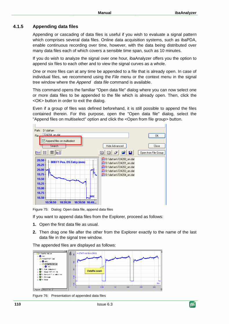
Manual ibaAnalyzer

110 Issue 6.3

4.1.5 Appending data files Appending or cascading of data files is useful if you wish to evaluate a signal pattern which comprises several data files. Online data acquisition systems, such as ibaPDA, enable continuous recording over time, however, with the data being distributed over many data files each of which covers a sensible time span, such as 10 minutes.

If you do wish to analyze the signal over one hour, ibaAnalyzer offers you the option to append six files to each other and to view the signal curves as a whole.

One or more files can at any time be appended to a file that is already open. In case of individual files, we recommend using the File menu or the context menu in the signal tree window where the Append data file command is available.

This command opens the familiar "Open data file" dialog where you can now select one or more data files to be appended to the file which is already open. Then, click the <OK> button in order to exit the dialog.

Even if a group of files was defined beforehand, it is still possible to append the files contained therein. For this purpose, open the "Open data file" dialog, select the "Append files on multiselect" option and click the <Open from file group> button.

Figure 75: Dialog: Open data file, append data files

If you want to append data files from the Explorer, proceed as follows:

1. Open the first data file as usual.

2. Then drag one file after the other from the Explorer exactly to the name of the last data file in the signal tree window.

The appended files are displayed as follows:

Figure 76: Presentation of appended data files

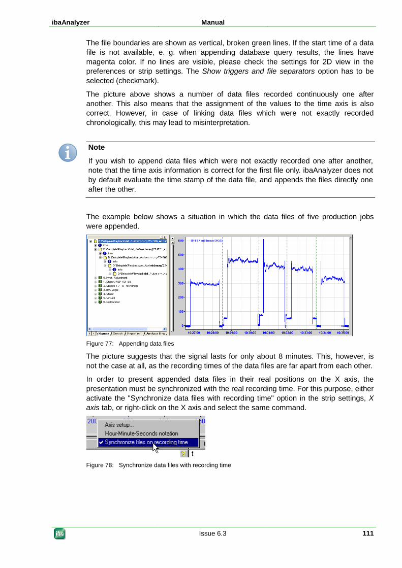
ibaAnalyzer Manual

Issue 6.3 111

The file boundaries are shown as vertical, broken green lines. If the start time of a data file is not available, e. g. when appending database query results, the lines have magenta color. If no lines are visible, please check the settings for 2D view in the preferences or strip settings. The Show triggers and file separators option has to be selected (checkmark).

The picture above shows a number of data files recorded continuously one after another. This also means that the assignment of the values to the time axis is also correct. However, in case of linking data files which were not exactly recorded chronologically, this may lead to misinterpretation.

Note

If you wish to append data files which were not exactly recorded one after another, note that the time axis information is correct for the first file only. ibaAnalyzer does not by default evaluate the time stamp of the data file, and appends the files directly one after the other.

The example below shows a situation in which the data files of five production jobs were appended.

Figure 77: Appending data files

The picture suggests that the signal lasts for only about 8 minutes. This, however, is not the case at all, as the recording times of the data files are far apart from each other.

In order to present appended data files in their real positions on the X axis, the presentation must be synchronized with the real recording time. For this purpose, either activate the "Synchronize data files with recording time" option in the strip settings, X axis tab, or right-click on the X axis and select the same command.

Figure 78: Synchronize data files with recording time

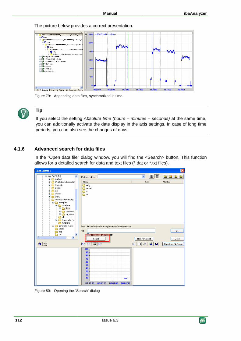
Manual ibaAnalyzer

112 Issue 6.3

The picture below provides a correct presentation.

Figure 79: Appending data files, synchronized in time

Tip

If you select the setting Absolute time (hours – minutes – seconds) at the same time, you can additionally activate the date display in the axis settings. In case of long time periods, you can also see the changes of days.

4.1.6 Advanced search for data files In the "Open data file" dialog window, you will find the <Search> button. This function allows for a detailed search for data and text files (*.dat or *.txt files).

Figure 80: Opening the "Search" dialog

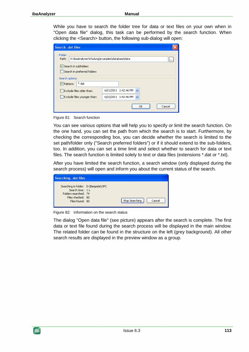
ibaAnalyzer Manual

Issue 6.3 113

While you have to search the folder tree for data or text files on your own when in "Open data file" dialog, this task can be performed by the search function. When clicking the <Search> button, the following sub-dialog will open:

Figure 81: Search function

You can see various options that will help you to specify or limit the search function. On the one hand, you can set the path from which the search is to start. Furthermore, by checking the corresponding box, you can decide whether the search is limited to the set path/folder only ("Search preferred folders") or if it should extend to the sub-folders, too. In addition, you can set a time limit and select whether to search for data or text files. The search function is limited solely to text or data files (extensions *.dat or *.txt).

After you have limited the search function, a search window (only displayed during the search process) will open and inform you about the current status of the search.

Figure 82: Information on the search status

The dialog "Open data file" (see picture) appears after the search is complete. The first data or text file found during the search process will be displayed in the main window. The related folder can be found in the structure on the left (grey background). All other search results are displayed in the preview window as a group.

Manual ibaAnalyzer

114 Issue 6.3

4.1.7 Slide show The so-called "slide show" function enables the consecutive opening of the data files of a group in ibaAnalyzer, so that these files can be viewed for a time span which you can define. This function can be helpful if you wish to successively view many files with the same analysis in order to obtain an overview.

As described in Defining groups of data files , Page 108 , you can select any files of a group from the picklist via the symbol bar for the data file group list.

The two arrow keys enable switching between the data files of the group.

In order to start the slide show, just click the button. ibaAnalyzer will then successively open the data files of the group at an interval which you can select under "Automatic slide show" on the "Miscellaneous" tab of the "Preferences".

Click the button once again in order to exit the slide show.

4.1.8 Closing data files Just as much as files can be opened in several ways, several methods are also available for closing a file.

When a new data file is opened (rather than being added or appended), the current data file is closed.

If several data files are open, mark the file(s) to be closed in the signal tree and use the "Close selected data file" command in the context menu of the signal tree window (right mouse key) or in the File menu.

In order to close all the data files which are currently open, use the "Close all data files" command in the File menu or in the context menu of the signal tree window.

4.1.9 Online analysis ibaAnalyzer enables the opening even of data files which are currently being created by ibaPDA, so that the data recorded so far can be analyzed. By selecting the appropriate preferences, as described in Miscellaneous , Page 88 the data file in question can be reloaded at cyclic intervals, so that the analysis is completed step by step.

Procedure

1. Data files are written into the path chosen under "Preferences".

2. Click on the button in ibaAnalyzer and wait until a data file appears in the signal tree window.

3. To activate the cyclic reload function, click the button .

4. Both buttons must be kept depressed for the permanent online analysis mode:

5. If you prefer to reload the data file manually, click the button once again in order to deactivate the automatic mode and subsequently use the button .

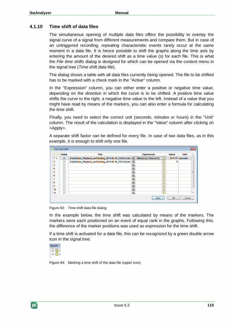
ibaAnalyzer Manual

Issue 6.3 115

4.1.10 Time shift of data files The simultaneous opening of multiple data files offers the possibility to overlay the signal curve of a signal from different measurements and compare them. But in case of an untriggered recording, repeating characteristic events rarely occur at the same moment in a data file. It is hence possible to shift the graphs along the time axis by entering the amount of the desired shift as a time value (s) for each file. This is what the File time shifts dialog is designed for which can be opened via the context menu in the signal tree (Time shift data file).

The dialog shows a table with all data files currently being opened. The file to be shifted has to be marked with a check mark in the "Active" column.

In the "Expression" column, you can either enter a positive or negative time value, depending on the direction in which the curve is to be shifted. A positive time value shifts the curve to the right, a negative time value to the left. Instead of a value that you might have read by means of the markers, you can also enter a formula for calculating the time shift.

Finally, you need to select the correct unit (seconds, minutes or hours) in the "Unit" column. The result of the calculation is displayed in the "Value" column after clicking on <Apply>.

A separate shift factor can be defined for every file. In case of two data files, as in this example, it is enough to shift only one file.

Figure 83: Time shift data file dialog

In the example below, the time shift was calculated by means of the markers. The markers were each positioned on an event of equal rank in the graphs. Following this, the difference of the marker positions was used as expression for the time shift.

If a time shift is activated for a data file, this can be recognized by a green double arrow icon in the signal tree:

Figure 84: Marking a time shift of the data file (upper icon)

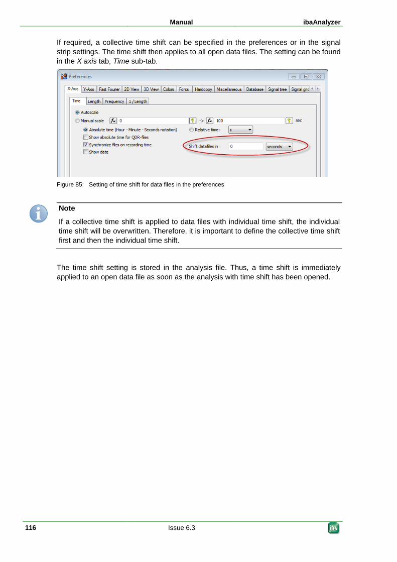
Manual ibaAnalyzer

116 Issue 6.3

If required, a collective time shift can be specified in the preferences or in the signal strip settings. The time shift then applies to all open data files. The setting can be found in the X axis tab, Time sub-tab.

Figure 85: Setting of time shift for data files in the preferences

Note

If a collective time shift is applied to data files with individual time shift, the individual time shift will be overwritten. Therefore, it is important to define the collective time shift first and then the individual time shift.

The time shift setting is stored in the analysis file. Thus, a time shift is immediately applied to an open data file as soon as the analysis with time shift has been opened.

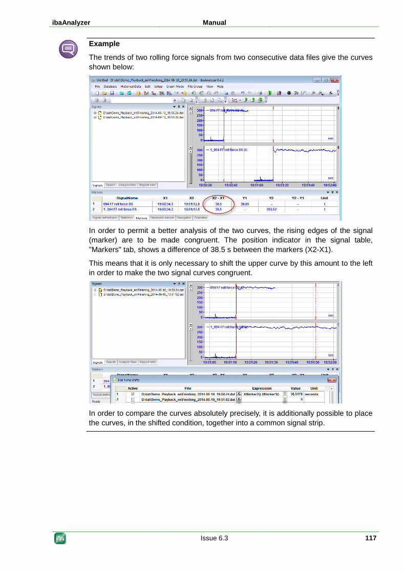
ibaAnalyzer Manual

Issue 6.3 117

Example

The trends of two rolling force signals from two consecutive data files give the curves shown below:

In order to permit a better analysis of the two curves, the rising edges of the signal (marker) are to be made congruent. The position indicator in the signal table, "Markers" tab, shows a difference of 38.5 s between the markers (X2-X1).

This means that it is only necessary to shift the upper curve by this amount to the left in order to make the two signal curves congruent.

In order to compare the curves absolutely precisely, it is additionally possible to place the curves, in the shifted condition, together into a common signal strip.

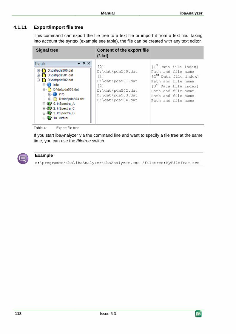
Manual ibaAnalyzer

118 Issue 6.3

4.1.11 Export/import file tree This command can export the file tree to a text file or import it from a text file. Taking into account the syntax (example see table), the file can be created with any text editor.

Signal tree Content of the export file (*.txt)

[0] D:\dat\pda500.dat [1] D:\dat\pda501.dat [2] D:\dat\pda502.dat D:\dat\pda503.dat D:\dat\pda504.dat

[1st Data file index] Path and file name [2nd Data file index] Path and file name [3rd Data file index] Path and file name Path and file name Path and file name

Table 4: Export file tree

If you start ibaAnalyzer via the command line and want to specify a file tree at the same time, you can use the /filetree switch.

Example c:\programme\iba\ibaAnalyzer\ibaAnalyzer.exe /filetree:MyFileTree.txt

ibaAnalyzer Manual

Issue 6.3 119

4.2 The analysis 4.2.1 What is an analysis?

An analysis is the compilation of all the settings of the user interface and additional items which are relevant for the analysis, such as expressions or virtual signals. An analysis can be applied to any number of data files.

The analysis is stored as a file with the extension .pdo on the hard disk. Every use can store and retrieve at any time the analysis which he or she is interested in under a user-defined name.

The following information is saved in the analysis:

Number, sequence and size of the signal strips Signal composition (module and channel number) Strip settings, such as axis scaling, type of presentation, colors Mathematical and logic functions (expressions) Logic (virtual) signals Settings for the hardcopy, including additional text fields Setup for report/log generator If the database interface is used: all settings for data extraction (archiving profiles,

technostring, etc.) and/or for data exporting Any other settings made under "Graph setup" The selected tab in the signal tree window

Note

Since the referencing of signals is based on the module and channel numbers, it is also possible to apply an analysis to data file which actually do not match this analysis. This means that values are displayed without an error message being generated.

Since also the analysis files with the .pdo extension are linked to the ibaAnalyzer program under Windows, it is also possible to start ibaAnalyzer by double-clicking a pdo file in the Windows Explorer. ibaAnalyzer will then start with the settings saved in the analysis, however, without any measured data unless the name of a data file was also saved in the analysis (refer to Save analysis , Page 122)

Manual ibaAnalyzer

120 Issue 6.3

4.2.2 Create new analysis If you start ibaAnalyzer directly or via a data file, the signal table (signal definition) and the recorder window are empty.

On the basis of a data file which contains the data you wish to analyze, you can now step by step set up your analysis, i.e. signal strips are opened in the recorder window, calculations (expressions) are programmed, virtual signals are created, logs and reports are configured, and so forth. These steps are described in the following chapters.

Once you have achieved the desired work progress, you can then save this latest condition as an analysis file.

If you have already made settings or arrangements which you wish to discard in order to start anew, you can create a new analysis via the File - New analysis menu or by clicking the corresponding icon (see above).

Data files which have been loaded continue to be displayed in the signal tree window. The new analysis does not yet have a name (i.e. it is unnamed).

4.2.3 Open analysis

In order to open an existing analysis, use the File - Open analysis menu or click the corresponding button (see left) in order to access the "Open analysis" dialog.

Tip

... By the way: If no analysis files are offered in this dialog, this can be due to the following reasons:

a) There are no analysis files ( *.pdo).

b) You selected the "Open data file" dialog by mistake (button with the blue folder icon) because ibaAnalyzer suppresses the display of other file types.

Retrieve analysis from database

Beside the usual way to store the analysis files in a file system, it is also possible to store an analysis in a database (see next chapter). The command for retrieving an analysis from the database is located in the File - Retrieve analysis from database... menu. A window opens showing the content of the database, i.e. the available analyses.

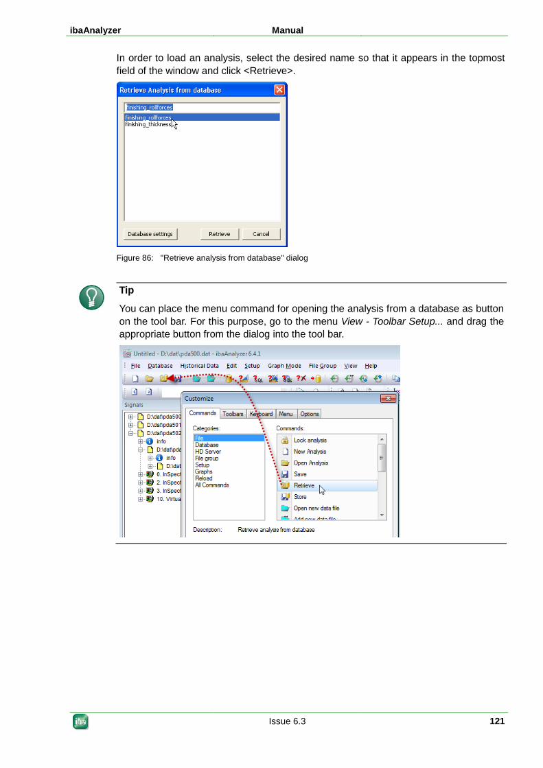
ibaAnalyzer Manual

Issue 6.3 121

In order to load an analysis, select the desired name so that it appears in the topmost field of the window and click <Retrieve>.

Figure 86: "Retrieve analysis from database" dialog

Tip

You can place the menu command for opening the analysis from a database as button on the tool bar. For this purpose, go to the menu View - Toolbar Setup... and drag the appropriate button from the dialog into the tool bar.

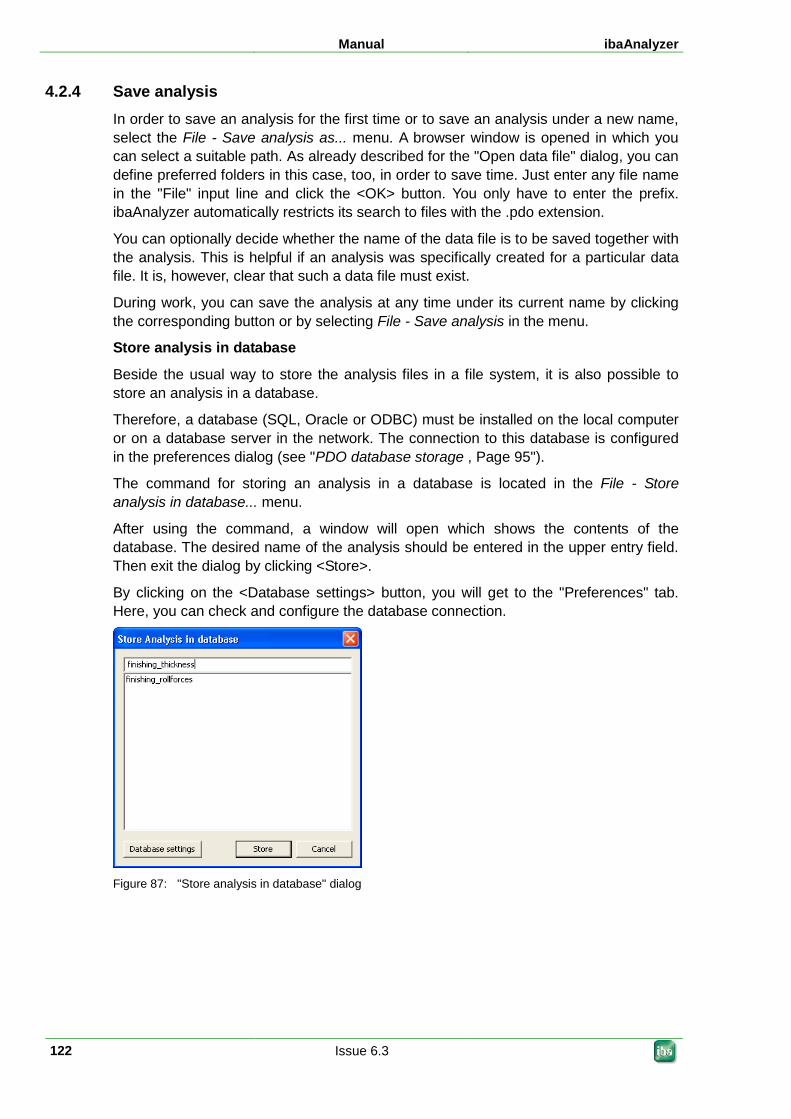
Manual ibaAnalyzer

122 Issue 6.3

4.2.4 Save analysis In order to save an analysis for the first time or to save an analysis under a new name, select the File - Save analysis as... menu. A browser window is opened in which you can select a suitable path. As already described for the "Open data file" dialog, you can define preferred folders in this case, too, in order to save time. Just enter any file name in the "File" input line and click the <OK> button. You only have to enter the prefix. ibaAnalyzer automatically restricts its search to files with the .pdo extension.

You can optionally decide whether the name of the data file is to be saved together with the analysis. This is helpful if an analysis was specifically created for a particular data file. It is, however, clear that such a data file must exist.

During work, you can save the analysis at any time under its current name by clicking the corresponding button or by selecting File - Save analysis in the menu.

Store analysis in database

Beside the usual way to store the analysis files in a file system, it is also possible to store an analysis in a database.

Therefore, a database (SQL, Oracle or ODBC) must be installed on the local computer or on a database server in the network. The connection to this database is configured in the preferences dialog (see "PDO database storage , Page 95").

The command for storing an analysis in a database is located in the File - Store analysis in database... menu.

After using the command, a window will open which shows the contents of the database. The desired name of the analysis should be entered in the upper entry field. Then exit the dialog by clicking <Store>.

By clicking on the <Database settings> button, you will get to the "Preferences" tab. Here, you can check and configure the database connection.

Figure 87: "Store analysis in database" dialog

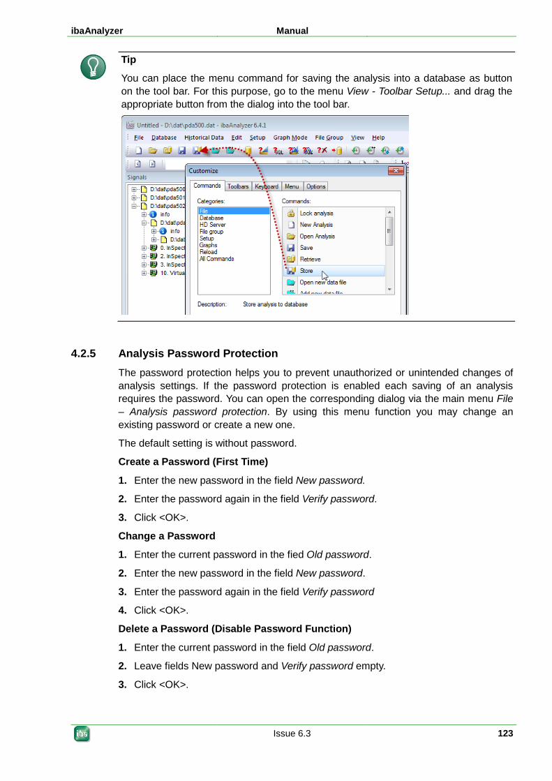
ibaAnalyzer Manual

Issue 6.3 123

Tip

You can place the menu command for saving the analysis into a database as button on the tool bar. For this purpose, go to the menu View - Toolbar Setup... and drag the appropriate button from the dialog into the tool bar.

4.2.5 Analysis Password Protection The password protection helps you to prevent unauthorized or unintended changes of analysis settings. If the password protection is enabled each saving of an analysis requires the password. You can open the corresponding dialog via the main menu File – Analysis password protection. By using this menu function you may change an existing password or create a new one.

The default setting is without password.

Create a Password (First Time)

1. Enter the new password in the field New password.

2. Enter the password again in the field Verify password.

3. Click <OK>.

Change a Password

1. Enter the current password in the fied Old password.

2. Enter the new password in the field New password.

3. Enter the password again in the field Verify password

4. Click <OK>.

Delete a Password (Disable Password Function)

1. Enter the current password in the field Old password.

2. Leave fields New password and Verify password empty.

3. Click <OK>.

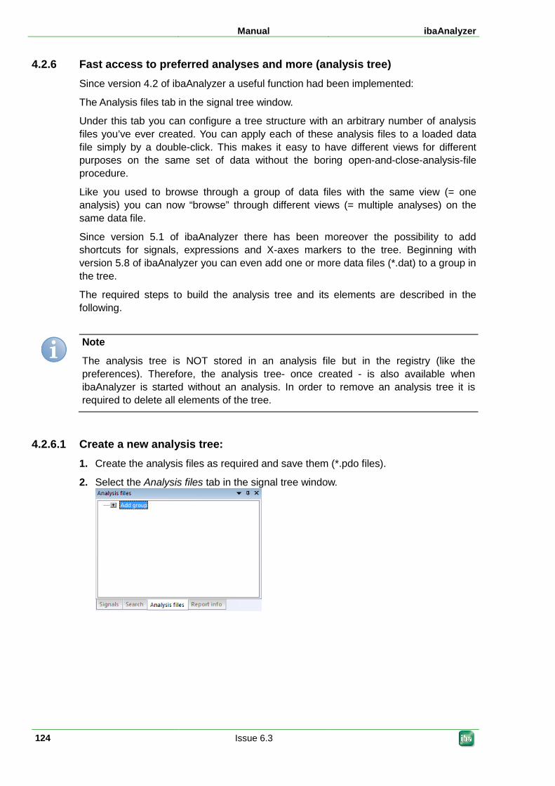
Manual ibaAnalyzer

124 Issue 6.3

4.2.6 Fast access to preferred analyses and more (analysis tree) Since version 4.2 of ibaAnalyzer a useful function had been implemented:

The Analysis files tab in the signal tree window.

Under this tab you can configure a tree structure with an arbitrary number of analysis files you’ve ever created. You can apply each of these analysis files to a loaded data file simply by a double-click. This makes it easy to have different views for different purposes on the same set of data without the boring open-and-close-analysis-file procedure.

Like you used to browse through a group of data files with the same view (= one analysis) you can now “browse” through different views (= multiple analyses) on the same data file.

Since version 5.1 of ibaAnalyzer there has been moreover the possibility to add shortcuts for signals, expressions and X-axes markers to the tree. Beginning with version 5.8 of ibaAnalyzer you can even add one or more data files (*.dat) to a group in the tree.

The required steps to build the analysis tree and its elements are described in the following.

Note

The analysis tree is NOT stored in an analysis file but in the registry (like the preferences). Therefore, the analysis tree- once created - is also available when ibaAnalyzer is started without an analysis. In order to remove an analysis tree it is required to delete all elements of the tree.

4.2.6.1 Create a new analysis tree: 1. Create the analysis files as required and save them (*.pdo files).

2. Select the Analysis files tab in the signal tree window.

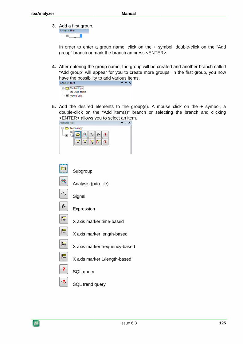
ibaAnalyzer Manual

Issue 6.3 125

3. Add a first group.

In order to enter a group name, click on the + symbol, double-click on the “Add group” branch or mark the branch an press <ENTER>.

4. After entering the group name, the group will be created and another branch called "Add group" will appear for you to create more groups. In the first group, you now have the possibility to add various items.

5. Add the desired elements to the group(s). A mouse click on the + symbol, a

double-click on the "Add item(s)" branch or selecting the branch and clicking <ENTER> allows you to select an item.

Subgroup

Analysis (pdo-file)

Signal

Expression

X axis marker time-based

X axis marker length-based

X axis marker frequency-based

X axis marker 1/length-based

SQL query

SQL trend query

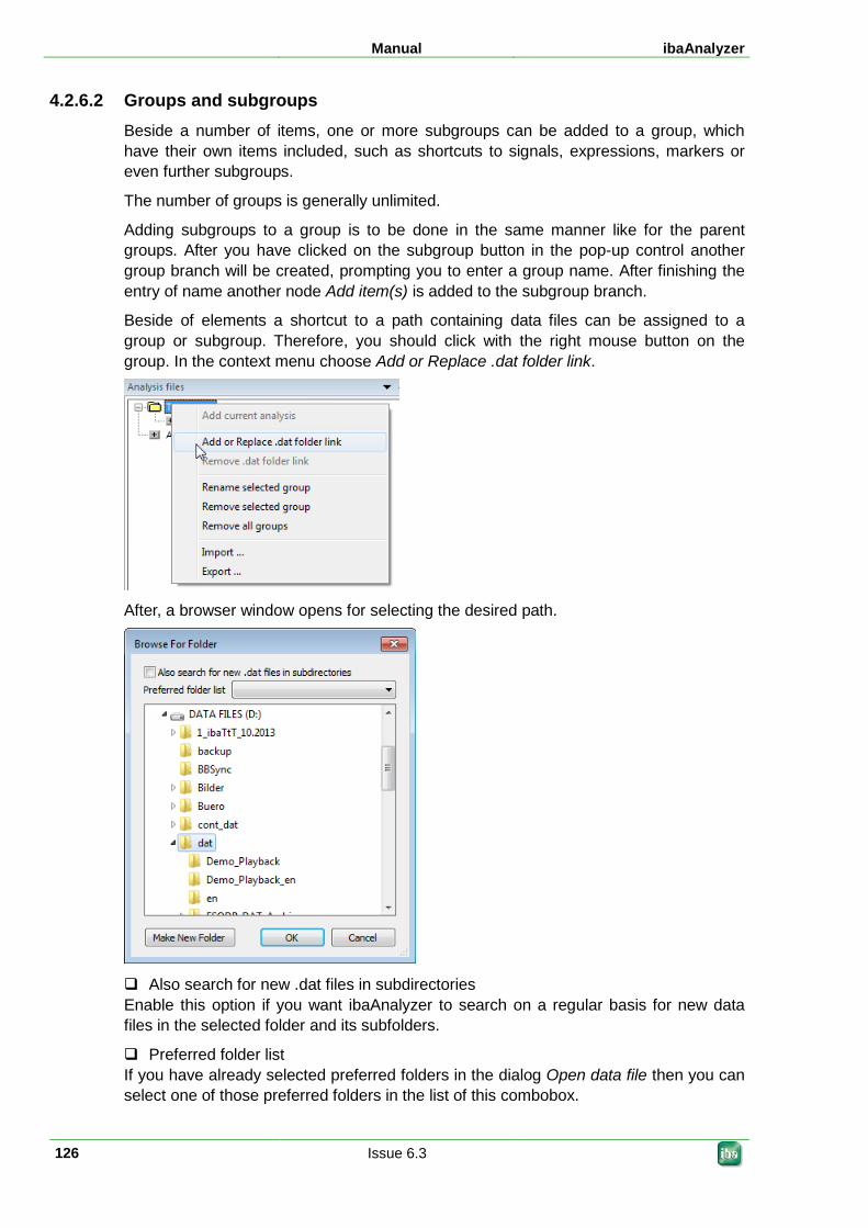
Manual ibaAnalyzer

126 Issue 6.3

4.2.6.2 Groups and subgroups Beside a number of items, one or more subgroups can be added to a group, which have their own items included, such as shortcuts to signals, expressions, markers or even further subgroups.

The number of groups is generally unlimited.

Adding subgroups to a group is to be done in the same manner like for the parent groups. After you have clicked on the subgroup button in the pop-up control another group branch will be created, prompting you to enter a group name. After finishing the entry of name another node Add item(s) is added to the subgroup branch.

Beside of elements a shortcut to a path containing data files can be assigned to a group or subgroup. Therefore, you should click with the right mouse button on the group. In the context menu choose Add or Replace .dat folder link.

After, a browser window opens for selecting the desired path.

Also search for new .dat files in subdirectories Enable this option if you want ibaAnalyzer to search on a regular basis for new data files in the selected folder and its subfolders.

Preferred folder list If you have already selected preferred folders in the dialog Open data file then you can select one of those preferred folders in the list of this combobox.

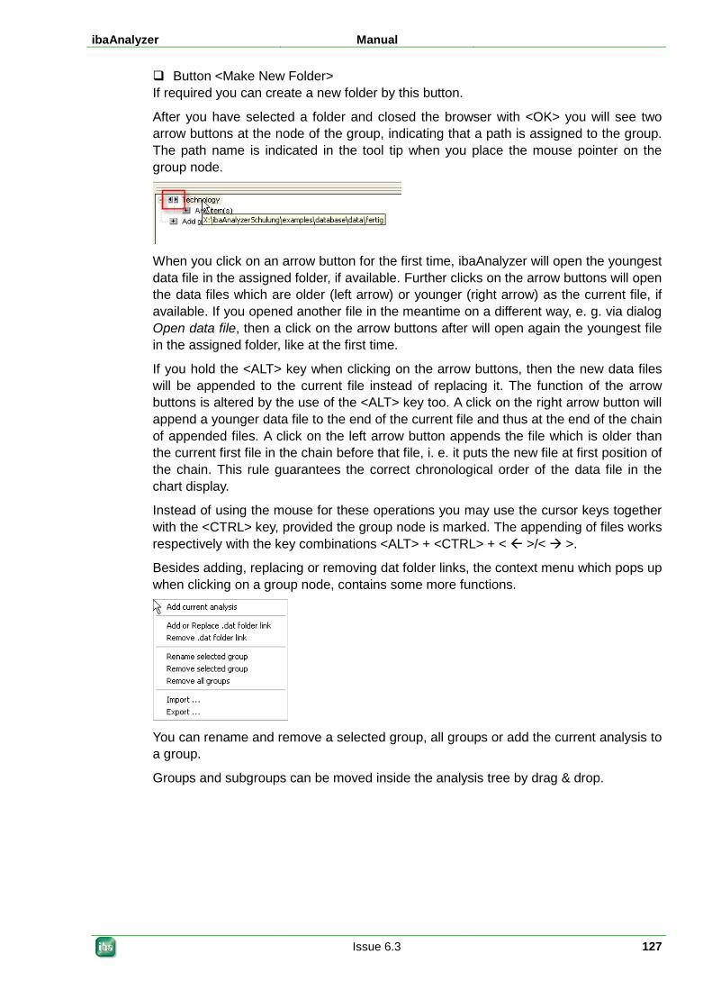
ibaAnalyzer Manual

Issue 6.3 127

Button <Make New Folder> If required you can create a new folder by this button.

After you have selected a folder and closed the browser with <OK> you will see two arrow buttons at the node of the group, indicating that a path is assigned to the group. The path name is indicated in the tool tip when you place the mouse pointer on the group node.

When you click on an arrow button for the first time, ibaAnalyzer will open the youngest data file in the assigned folder, if available. Further clicks on the arrow buttons will open the data files which are older (left arrow) or younger (right arrow) as the current file, if available. If you opened another file in the meantime on a different way, e. g. via dialog Open data file, then a click on the arrow buttons after will open again the youngest file in the assigned folder, like at the first time.

If you hold the <ALT> key when clicking on the arrow buttons, then the new data files will be appended to the current file instead of replacing it. The function of the arrow buttons is altered by the use of the <ALT> key too. A click on the right arrow button will append a younger data file to the end of the current file and thus at the end of the chain of appended files. A click on the left arrow button appends the file which is older than the current first file in the chain before that file, i. e. it puts the new file at first position of the chain. This rule guarantees the correct chronological order of the data file in the chart display.

Instead of using the mouse for these operations you may use the cursor keys together with the <CTRL> key, provided the group node is marked. The appending of files works respectively with the key combinations <ALT> + <CTRL> + < >/< >.

Besides adding, replacing or removing dat folder links, the context menu which pops up when clicking on a group node, contains some more functions.

You can rename and remove a selected group, all groups or add the current analysis to a group.

Groups and subgroups can be moved inside the analysis tree by drag & drop.

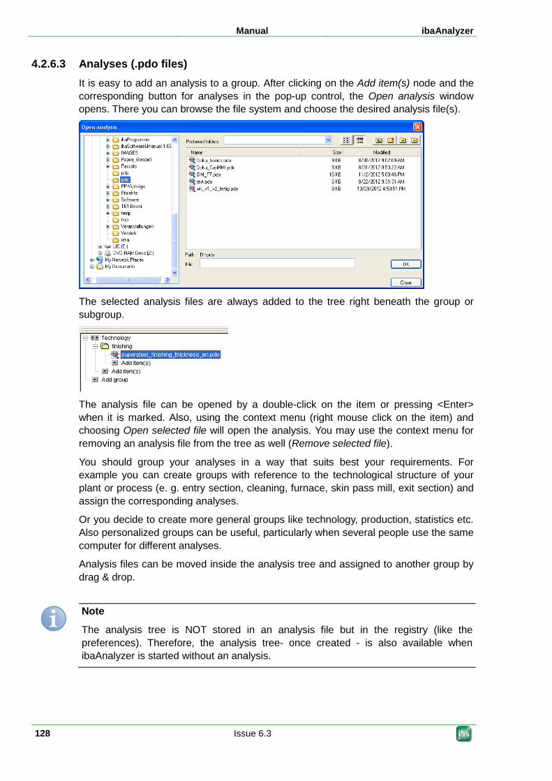
Manual ibaAnalyzer

128 Issue 6.3

4.2.6.3 Analyses (.pdo files) It is easy to add an analysis to a group. After clicking on the Add item(s) node and the corresponding button for analyses in the pop-up control, the Open analysis window opens. There you can browse the file system and choose the desired analysis file(s).

The selected analysis files are always added to the tree right beneath the group or subgroup.

The analysis file can be opened by a double-click on the item or pressing <Enter> when it is marked. Also, using the context menu (right mouse click on the item) and choosing Open selected file will open the analysis. You may use the context menu for removing an analysis file from the tree as well (Remove selected file).

You should group your analyses in a way that suits best your requirements. For example you can create groups with reference to the technological structure of your plant or process (e. g. entry section, cleaning, furnace, skin pass mill, exit section) and assign the corresponding analyses.

Or you decide to create more general groups like technology, production, statistics etc. Also personalized groups can be useful, particularly when several people use the same computer for different analyses.

Analysis files can be moved inside the analysis tree and assigned to another group by drag & drop.

Note

The analysis tree is NOT stored in an analysis file but in the registry (like the preferences). Therefore, the analysis tree- once created - is also available when ibaAnalyzer is started without an analysis.

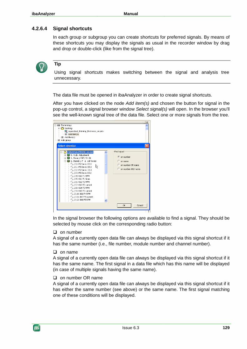
ibaAnalyzer Manual

Issue 6.3 129

4.2.6.4 Signal shortcuts In each group or subgroup you can create shortcuts for preferred signals. By means of these shortcuts you may display the signals as usual in the recorder window by drag and drop or double-click (like from the signal tree).

Tip

Using signal shortcuts makes switching between the signal and analysis tree unnecessary.

The data file must be opened in ibaAnalyzer in order to create signal shortcuts.

After you have clicked on the node Add item(s) and chosen the button for signal in the pop-up control, a signal browser window Select signal(s) will open. In the browser you’ll see the well-known signal tree of the data file. Select one or more signals from the tree.

In the signal browser the following options are available to find a signal. They should be selected by mouse click on the corresponding radio button:

on number A signal of a currently open data file can always be displayed via this signal shortcut if it has the same number (i.e., file number, module number and channel number).

on name A signal of a currently open data file can always be displayed via this signal shortcut if it has the same name. The first signal in a data file which has this name will be displayed (in case of multiple signals having the same name).

on number OR name A signal of a currently open data file can always be displayed via this signal shortcut if it has either the same number (see above) or the same name. The first signal matching one of these conditions will be displayed.

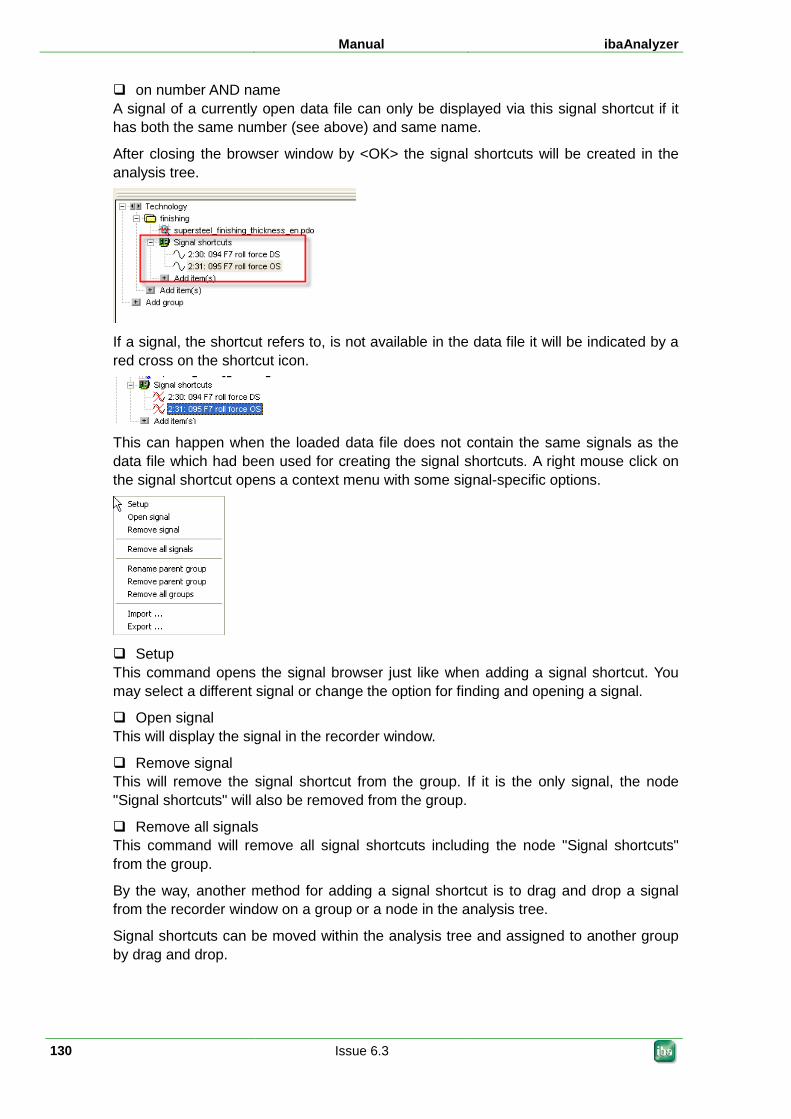
Manual ibaAnalyzer

130 Issue 6.3

on number AND name A signal of a currently open data file can only be displayed via this signal shortcut if it has both the same number (see above) and same name.

After closing the browser window by <OK> the signal shortcuts will be created in the analysis tree.

If a signal, the shortcut refers to, is not available in the data file it will be indicated by a red cross on the shortcut icon.

This can happen when the loaded data file does not contain the same signals as the data file which had been used for creating the signal shortcuts. A right mouse click on the signal shortcut opens a context menu with some signal-specific options.

Setup This command opens the signal browser just like when adding a signal shortcut. You may select a different signal or change the option for finding and opening a signal.

Open signal This will display the signal in the recorder window.

Remove signal This will remove the signal shortcut from the group. If it is the only signal, the node "Signal shortcuts" will also be removed from the group.

Remove all signals This command will remove all signal shortcuts including the node "Signal shortcuts" from the group.

By the way, another method for adding a signal shortcut is to drag and drop a signal from the recorder window on a group or a node in the analysis tree.

Signal shortcuts can be moved within the analysis tree and assigned to another group by drag and drop.

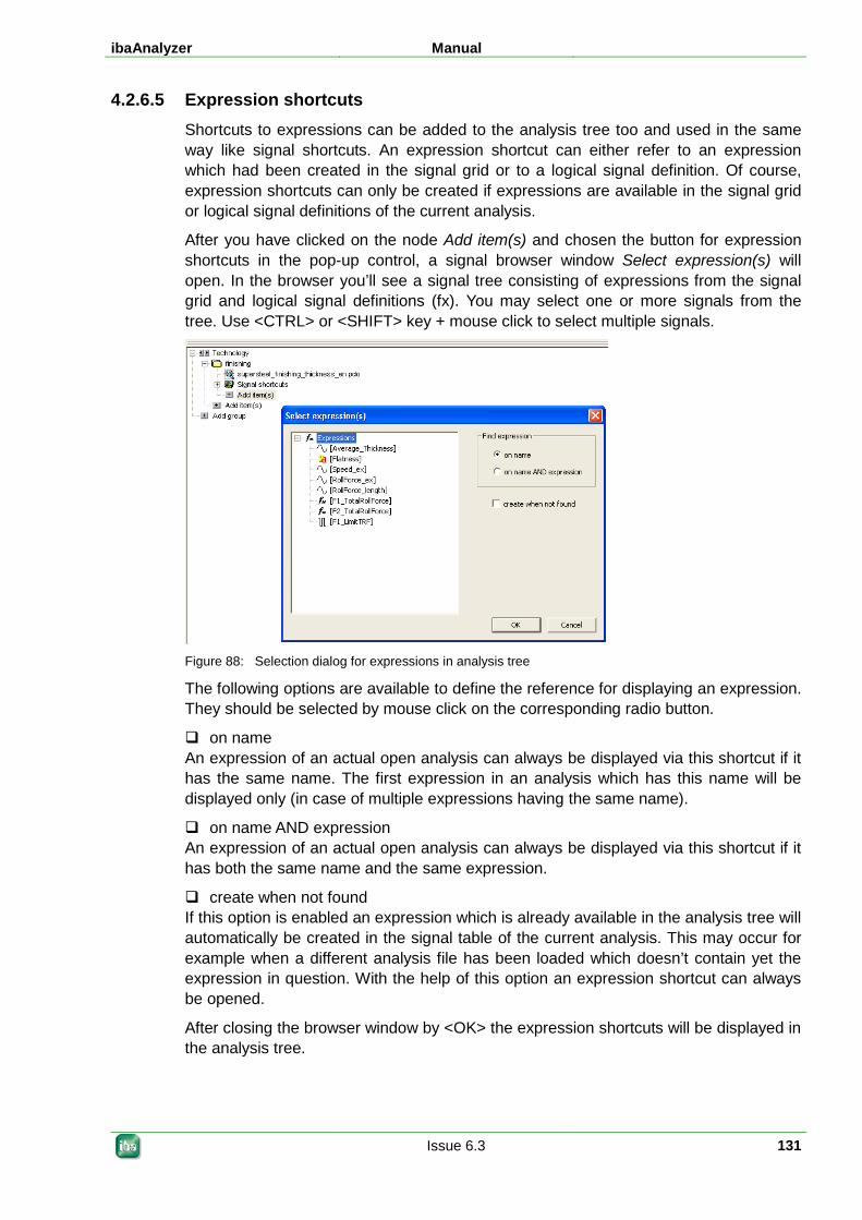
ibaAnalyzer Manual

Issue 6.3 131

4.2.6.5 Expression shortcuts Shortcuts to expressions can be added to the analysis tree too and used in the same way like signal shortcuts. An expression shortcut can either refer to an expression which had been created in the signal grid or to a logical signal definition. Of course, expression shortcuts can only be created if expressions are available in the signal grid or logical signal definitions of the current analysis.

After you have clicked on the node Add item(s) and chosen the button for expression shortcuts in the pop-up control, a signal browser window Select expression(s) will open. In the browser you’ll see a signal tree consisting of expressions from the signal grid and logical signal definitions (fx). You may select one or more signals from the tree. Use <CTRL> or <SHIFT> key + mouse click to select multiple signals.

Figure 88: Selection dialog for expressions in analysis tree

The following options are available to define the reference for displaying an expression. They should be selected by mouse click on the corresponding radio button.

on name An expression of an actual open analysis can always be displayed via this shortcut if it has the same name. The first expression in an analysis which has this name will be displayed only (in case of multiple expressions having the same name).

on name AND expression An expression of an actual open analysis can always be displayed via this shortcut if it has both the same name and the same expression.

create when not found If this option is enabled an expression which is already available in the analysis tree will automatically be created in the signal table of the current analysis. This may occur for example when a different analysis file has been loaded which doesn’t contain yet the expression in question. With the help of this option an expression shortcut can always be opened.

After closing the browser window by <OK> the expression shortcuts will be displayed in the analysis tree.

Manual ibaAnalyzer

132 Issue 6.3

If an expression, the shortcut refers to, is not available in the analysis file it will be indicated by a red cross on the shortcut icon.

This can happen when the current open analysis does not contain the same expressions like already available in the analysis tree. A right mouse click on the expression shortcut opens a context menu with some expression-specific options.

Setup This command opens the expression browser like for adding an expression shortcut before. You may select a different expression or change the option for finding an expression.

Open expression This will display the expression in the recorder window. Opening an expression will not necessarily open a new signal strip in the recorder window. It may be displayed in a signal strip with other signals, depending on where it was created.

Remove expression This will remove the expression shortcut from the group. If it is the only expression the node "Expression shortcuts" will also be removed from the group.

Remove all expressions This command will remove all expression shortcuts including the node "Expression shortcuts" from the group.

By the way, another method for adding an expression shortcut is to drag and drop a currently displayed expression from the recorder window on a group or a node in the analysis tree. Expression shortcuts can be moved inside the analysis tree and assigned to another group by drag & drop.

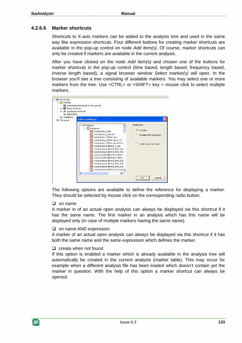
ibaAnalyzer Manual

Issue 6.3 133

4.2.6.6 Marker shortcuts Shortcuts to X-axis markers can be added to the analysis tree and used in the same way like expression shortcuts. Four different buttons for creating marker shortcuts are available in the pop-up control on node Add item(s). Of course, marker shortcuts can only be created if markers are available in the current analysis.

After you have clicked on the node Add item(s) and chosen one of the buttons for marker shortcuts in the pop-up control (time based, length based, frequency based, inverse length based), a signal browser window Select marker(s) will open. In the browser you’ll see a tree consisting of available markers. You may select one or more markers from the tree. Use <CTRL> or <SHIFT> key + mouse click to select multiple markers.

The following options are available to define the reference for displaying a marker. They should be selected by mouse click on the corresponding radio button.

on name A marker in of an actual open analysis can always be displayed via this shortcut if it has the same name. The first marker in an analysis which has this name will be displayed only (in case of multiple markers having the same name).

on name AND expression A marker of an actual open analysis can always be displayed via this shortcut if it has both the same name and the same expression which defines the marker.

create when not found If this option is enabled a marker which is already available in the analysis tree will automatically be created in the current analysis (marker table). This may occur for example when a different analysis file has been loaded which doesn’t contain yet the marker in question. With the help of this option a marker shortcut can always be opened.

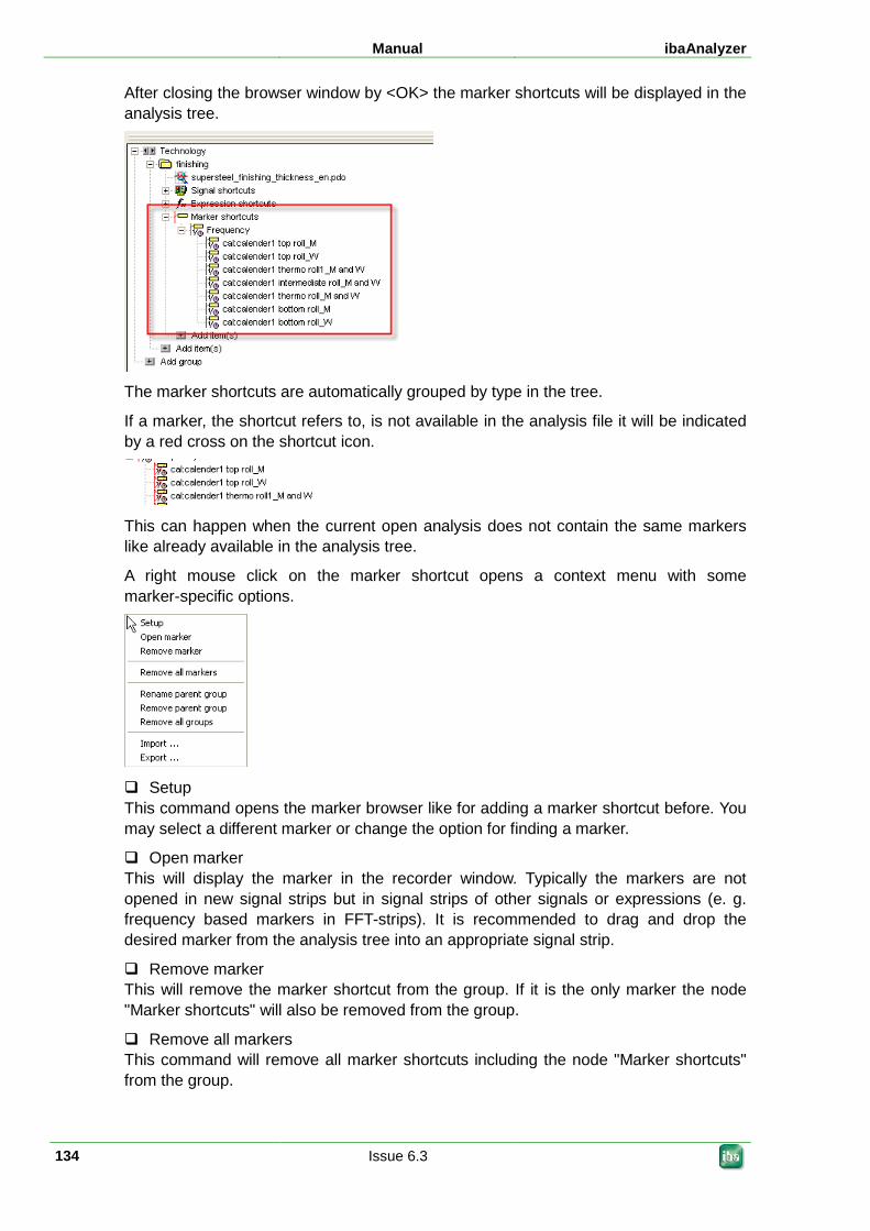
Manual ibaAnalyzer

134 Issue 6.3

After closing the browser window by <OK> the marker shortcuts will be displayed in the analysis tree.

The marker shortcuts are automatically grouped by type in the tree.

If a marker, the shortcut refers to, is not available in the analysis file it will be indicated by a red cross on the shortcut icon.

This can happen when the current open analysis does not contain the same markers like already available in the analysis tree.

A right mouse click on the marker shortcut opens a context menu with some marker-specific options.

Setup This command opens the marker browser like for adding a marker shortcut before. You may select a different marker or change the option for finding a marker.

Open marker This will display the marker in the recorder window. Typically the markers are not opened in new signal strips but in signal strips of other signals or expressions (e. g. frequency based markers in FFT-strips). It is recommended to drag and drop the desired marker from the analysis tree into an appropriate signal strip.

Remove marker This will remove the marker shortcut from the group. If it is the only marker the node "Marker shortcuts" will also be removed from the group.

Remove all markers This command will remove all marker shortcuts including the node "Marker shortcuts" from the group.

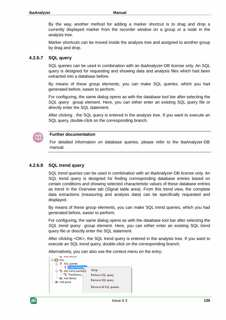
ibaAnalyzer Manual

Issue 6.3 135

By the way, another method for adding a marker shortcut is to drag and drop a currently displayed marker from the recorder window on a group or a node in the analysis tree.

Marker shortcuts can be moved inside the analysis tree and assigned to another group by drag and drop.

4.2.6.7 SQL query SQL queries can be used in combination with an ibaAnalyzer-DB license only. An SQL query is designed for requesting and showing data and analysis files which had been extracted into a database before.

By means of these group elements, you can make SQL queries, which you had generated before, easier to perform.

For configuring, the same dialog opens as with the database tool bar after selecting the SQL query group element. Here, you can either enter an existing SQL query file or directly enter the SQL statement.

After clicking , the SQL query is entered in the analysis tree. If you want to execute an SQL query, double-click on the corresponding branch.

Further documentation

For detailed information on database queries, please refer to the ibaAnalyzer-DB manual.

4.2.6.8 SQL trend query SQL trend queries can be used in combination with an ibaAnalyzer-DB license only. An SQL trend query is designed for finding corresponding database entries based on certain conditions and showing selected characteristic values of these database entries as trend in the Overview tab (Signal table area). From this trend view, the complete data extractions (measuring and analysis data) can be specifically requested and displayed.

By means of these group elements, you can make SQL trend queries, which you had generated before, easier to perform.

For configuring, the same dialog opens as with the database tool bar after selecting the SQL trend query group element. Here, you can either enter an existing SQL trend query file or directly enter the SQL statement.

After clicking <OK>, the SQL trend query is entered in the analysis tree. If you want to execute an SQL trend query, double-click on the corresponding branch.

Alternatively, you can also use the context menu on the entry:

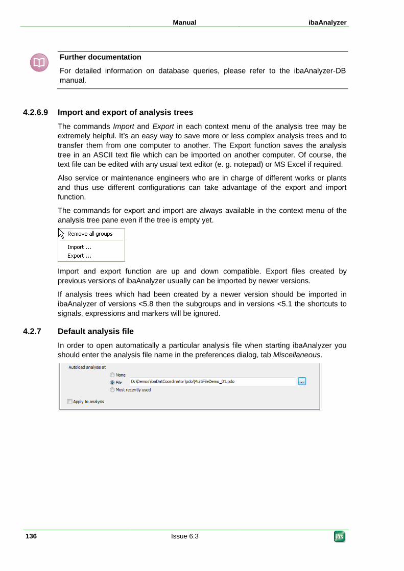
Manual ibaAnalyzer

136 Issue 6.3

Further documentation

For detailed information on database queries, please refer to the ibaAnalyzer-DB manual.

4.2.6.9 Import and export of analysis trees The commands Import and Export in each context menu of the analysis tree may be extremely helpful. It’s an easy way to save more or less complex analysis trees and to transfer them from one computer to another. The Export function saves the analysis tree in an ASCII text file which can be imported on another computer. Of course, the text file can be edited with any usual text editor (e. g. notepad) or MS Excel if required.

Also service or maintenance engineers who are in charge of different works or plants and thus use different configurations can take advantage of the export and import function.

The commands for export and import are always available in the context menu of the analysis tree pane even if the tree is empty yet.

Import and export function are up and down compatible. Export files created by previous versions of ibaAnalyzer usually can be imported by newer versions.

If analysis trees which had been created by a newer version should be imported in ibaAnalyzer of versions <5.8 then the subgroups and in versions <5.1 the shortcuts to signals, expressions and markers will be ignored.

4.2.7 Default analysis file In order to open automatically a particular analysis file when starting ibaAnalyzer you should enter the analysis file name in the preferences dialog, tab Miscellaneous.

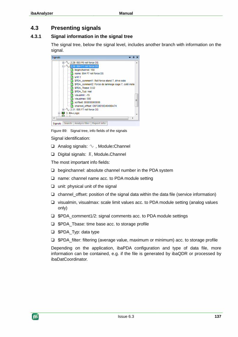
ibaAnalyzer Manual

Issue 6.3 137

4.3 Presenting signals 4.3.1 Signal information in the signal tree

The signal tree, below the signal level, includes another branch with information on the signal.

Figure 89: Signal tree, info fields of the signals

Signal identification:

Analog signals: , Module:Channel

Digital signals: , Module.Channel

The most important info fields:

beginchannel: absolute channel number in the PDA system

name: channel name acc. to PDA module setting

unit: physical unit of the signal

channel_offset: position of the signal data within the data file (service information)

visualmin, visualmax: scale limit values acc. to PDA module setting (analog values only)

$PDA_comment1/2: signal comments acc. to PDA module settings

$PDA_Tbase: time base acc. to storage profile

$PDA_Typ: data type

$PDA_filter: filtering (average value, maximum or minimum) acc. to storage profile

Depending on the application, ibaPDA configuration and type of data file, more information can be contained, e.g. if the file is generated by ibaQDR or processed by ibaDatCoordinator.

Manual ibaAnalyzer

138 Issue 6.3

4.3.2 Selecting and presenting signals If the data file is open, you can select any signals to be displayed in the recorder window, for example, in order to carry out an analysis.

There are three general ways available for selecting a signal.

Make a right mouse click on the signal you want to display and select Open signal in the context menu.

Double-clicking the desired signal in the signal tree – this operation then also opens a new signal strip in which this signal is presented.

Alternatively, you can also use the Drag&Drop function in order to drag the signal into the recorder window (click the signal with the left mouse key and keep the key depressed until the target position is reached).

These methods can be further refined in order to address the requirements of day-to-day use even better.

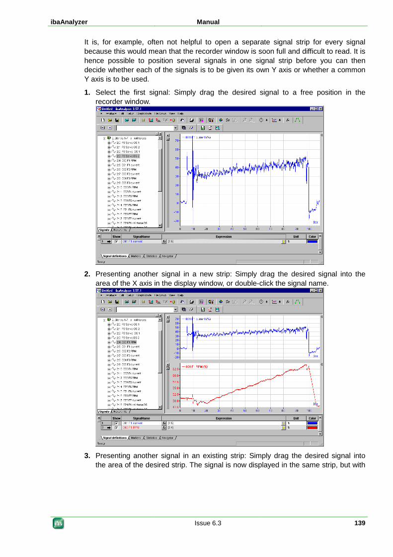
ibaAnalyzer Manual

Issue 6.3 139

It is, for example, often not helpful to open a separate signal strip for every signal because this would mean that the recorder window is soon full and difficult to read. It is hence possible to position several signals in one signal strip before you can then decide whether each of the signals is to be given its own Y axis or whether a common Y axis is to be used.

1. Select the first signal: Simply drag the desired signal to a free position in the recorder window.

2. Presenting another signal in a new strip: Simply drag the desired signal into the

area of the X axis in the display window, or double-click the signal name.

3. Presenting another signal in an existing strip: Simply drag the desired signal into

the area of the desired strip. The signal is now displayed in the same strip, but with

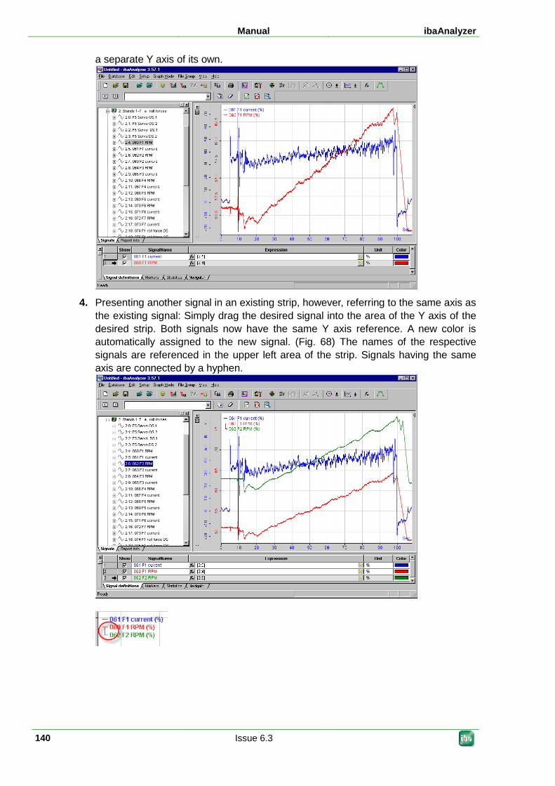
Manual ibaAnalyzer

140 Issue 6.3

a separate Y axis of its own.

4. Presenting another signal in an existing strip, however, referring to the same axis as

the existing signal: Simply drag the desired signal into the area of the Y axis of the desired strip. Both signals now have the same Y axis reference. A new color is automatically assigned to the new signal. (Fig. 68) The names of the respective signals are referenced in the upper left area of the strip. Signals having the same axis are connected by a hyphen.

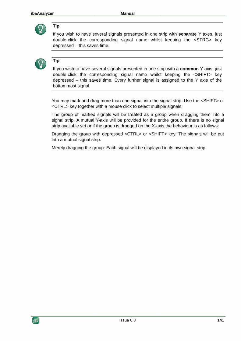
ibaAnalyzer Manual

Issue 6.3 141

Tip

If you wish to have several signals presented in one strip with separate Y axes, just double-click the corresponding signal name whilst keeping the <STRG> key depressed – this saves time.

Tip

If you wish to have several signals presented in one strip with a common Y axis, just double-click the corresponding signal name whilst keeping the <SHIFT> key depressed – this saves time. Every further signal is assigned to the Y axis of the bottommost signal.

You may mark and drag more than one signal into the signal strip. Use the <SHIFT> or <CTRL> key together with a mouse click to select multiple signals.

The group of marked signals will be treated as a group when dragging them into a signal strip. A mutual Y-axis will be provided for the entire group. If there is no signal strip available yet or if the group is dragged on the X-axis the behaviour is as follows:

Dragging the group with depressed <CTRL> or <SHIFT> key: The signals will be put into a mutual signal strip.

Merely dragging the group: Each signal will be displayed in its own signal strip.

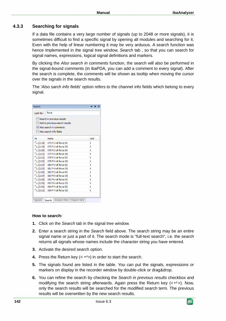
Manual ibaAnalyzer

142 Issue 6.3

4.3.3 Searching for signals If a data file contains a very large number of signals (up to 2048 or more signals), it is sometimes difficult to find a specific signal by opening all modules and searching for it. Even with the help of linear numbering it may be very arduous. A search function was hence implemented in the signal tree window, Search tab , so that you can search for signal names, expressions, logical signal definitions and markers.

By clicking the Also search in comments function, the search will also be performed in the signal-bound comments (in ibaPDA, you can add a comment to every signal). After the search is complete, the comments will be shown as tooltip when moving the cursor over the signals in the search results.

The 'Also sarch info fields' option refers to the channel info fields which belong to every signal.

How to search:

1. Click on the Search tab in the signal tree window.

2. Enter a search string in the Search field above. The search string may be an entire signal name or just a part of it. The search mode is "full-text search", i.e. the search returns all signals whose names include the character string you have entered.

3. Activate the desired search option.

4. Press the Return key (< >) in order to start the search.

5. The signals found are listed in the table. You can put the signals, expressions or markers on display in the recorder window by double-click or drag&drop.

6. You can refine the search by checking the Search in previous results checkbox and modifying the search string afterwards. Again press the Return key (< >). Now, only the search results will be searched for the modified search term. The previous results will be overwritten by the new search results.

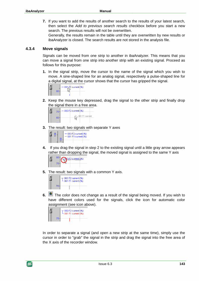
ibaAnalyzer Manual

Issue 6.3 143

7. If you want to add the results of another search to the results of your latest search, then select the Add to previous search results checkbox before you start a new search. The previous results will not be overwritten. Generally, the results remain in the table until they are overwritten by new results or ibaAnalyzer is closed. The search results are not stored in the analysis file.

4.3.4 Move signals Signals can be moved from one strip to another in ibaAnalyzer. This means that you can move a signal from one strip into another strip with an existing signal. Proceed as follows for this purpose:

1. In the signal strip, move the cursor to the name of the signal which you wish to move. A sine-shaped line for an analog signal, respectively a pulse-shaped line for a digital signal, at the cursor shows that the cursor has gripped the signal.

2. Keep the mouse key depressed, drag the signal to the other strip and finally drop

the signal there in a free area.

3. The result: two signals with separate Y axes

4. If you drag the signal in step 2 to the existing signal until a little gray arrow appears

rather than dropping the signal, the moved signal is assigned to the same Y axis

5. The result: two signals with a common Y axis.

6. The color does not change as a result of the signal being moved. If you wish to have different colors used for the signals, click the icon for automatic color assignment (see icon above).

In order to separate a signal (and open a new strip at the same time), simply use the cursor in order to "grab" the signal in the strip and drag the signal into the free area of the X axis of the recorder window.

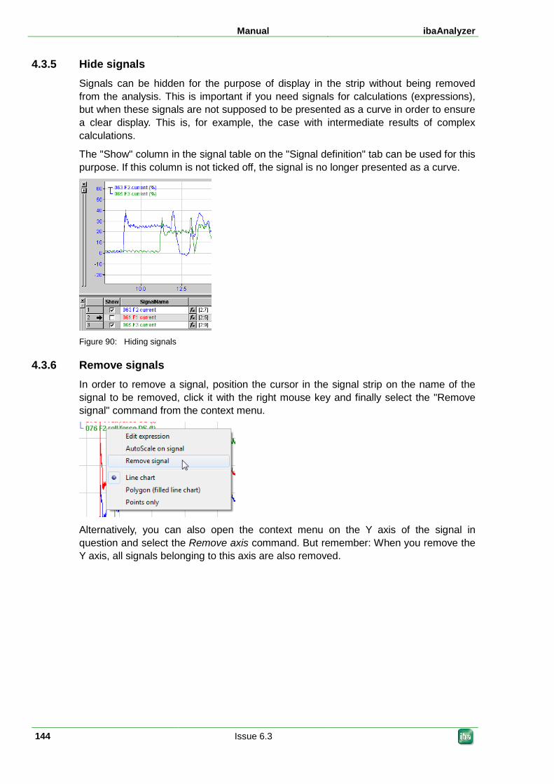
Manual ibaAnalyzer

144 Issue 6.3

4.3.5 Hide signals Signals can be hidden for the purpose of display in the strip without being removed from the analysis. This is important if you need signals for calculations (expressions), but when these signals are not supposed to be presented as a curve in order to ensure a clear display. This is, for example, the case with intermediate results of complex calculations.

The "Show" column in the signal table on the "Signal definition" tab can be used for this purpose. If this column is not ticked off, the signal is no longer presented as a curve.

Figure 90: Hiding signals

4.3.6 Remove signals In order to remove a signal, position the cursor in the signal strip on the name of the signal to be removed, click it with the right mouse key and finally select the "Remove signal" command from the context menu.

Alternatively, you can also open the context menu on the Y axis of the signal in question and select the Remove axis command. But remember: When you remove the Y axis, all signals belonging to this axis are also removed.

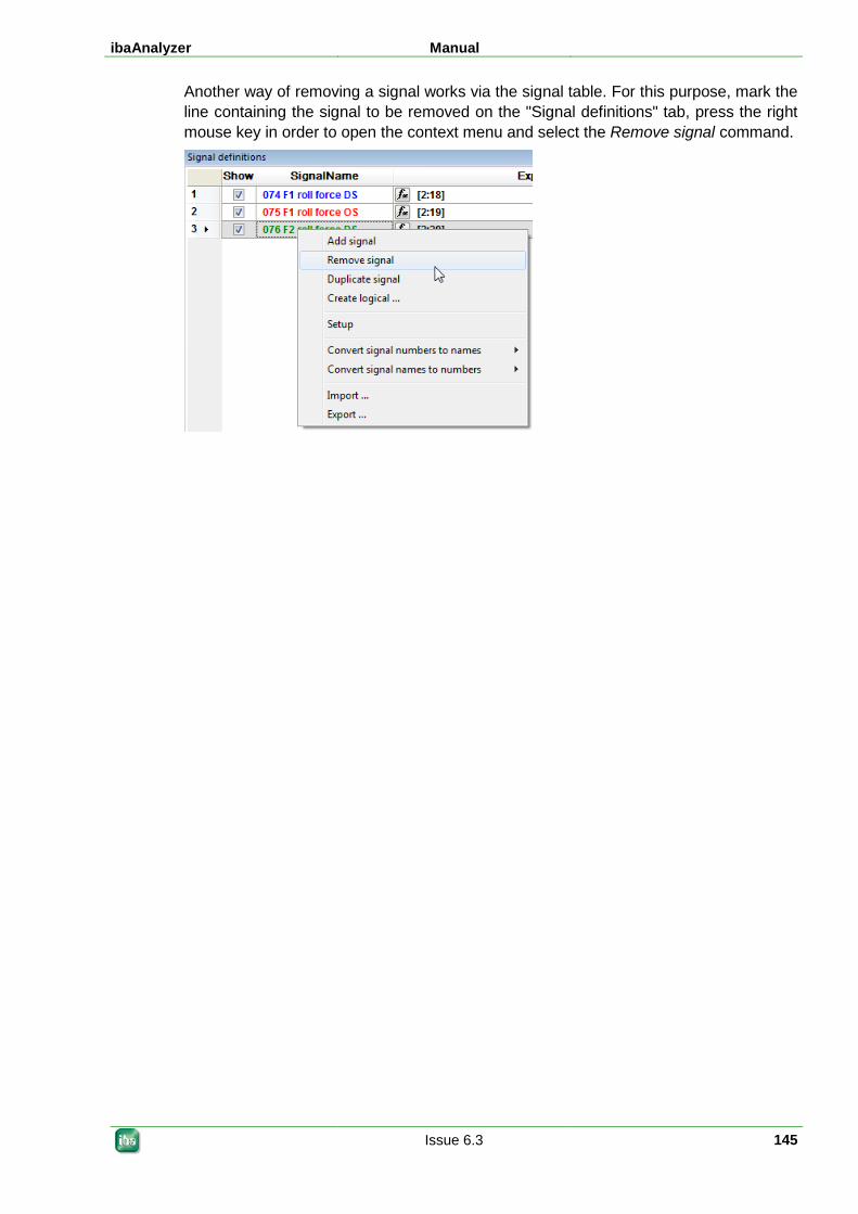
ibaAnalyzer Manual

Issue 6.3 145

Another way of removing a signal works via the signal table. For this purpose, mark the line containing the signal to be removed on the "Signal definitions" tab, press the right mouse key in order to open the context menu and select the Remove signal command.

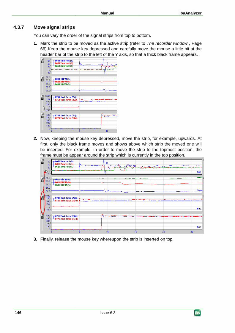
Manual ibaAnalyzer

146 Issue 6.3

4.3.7 Move signal strips You can vary the order of the signal strips from top to bottom.

1. Mark the strip to be moved as the active strip (refer to The recorder window , Page 66).Keep the mouse key depressed and carefully move the mouse a little bit at the header bar of the strip to the left of the Y axis, so that a thick black frame appears.

2. Now, keeping the mouse key depressed, move the strip, for example, upwards. At

first, only the black frame moves and shows above which strip the moved one will be inserted. For example, in order to move the strip to the topmost position, the frame must be appear around the strip which is currently in the top position.

3. Finally, release the mouse key whereupon the strip is inserted on top.

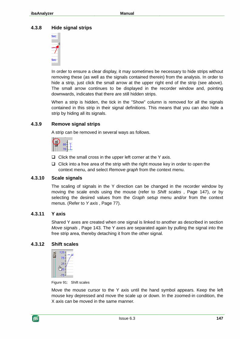
ibaAnalyzer Manual

Issue 6.3 147

4.3.8 Hide signal strips

In order to ensure a clear display, it may sometimes be necessary to hide strips without removing these (as well as the signals contained therein) from the analysis. In order to hide a strip, just click the small arrow at the upper right end of the strip (see above). The small arrow continues to be displayed in the recorder window and, pointing downwards, indicates that there are still hidden strips.

When a strip is hidden, the tick in the "Show" column is removed for all the signals contained in this strip in their signal definitions. This means that you can also hide a strip by hiding all its signals.

4.3.9 Remove signal strips A strip can be removed in several ways as follows.

Click the small cross in the upper left corner at the Y axis. Click into a free area of the strip with the right mouse key in order to open the

context menu, and select Remove graph from the context menu.

4.3.10 Scale signals The scaling of signals in the Y direction can be changed in the recorder window by moving the scale ends using the mouse (refer to Shift scales , Page 147), or by selecting the desired values from the Graph setup menu and/or from the context menus. (Refer to Y axis , Page 77).

4.3.11 Y axis Shared Y axes are created when one signal is linked to another as described in section Move signals , Page 143. The Y axes are separated again by pulling the signal into the free strip area, thereby detaching it from the other signal.

4.3.12 Shift scales

Figure 91: Shift scales

Move the mouse cursor to the Y axis until the hand symbol appears. Keep the left mouse key depressed and move the scale up or down. In the zoomed-in condition, the X axis can be moved in the same manner.

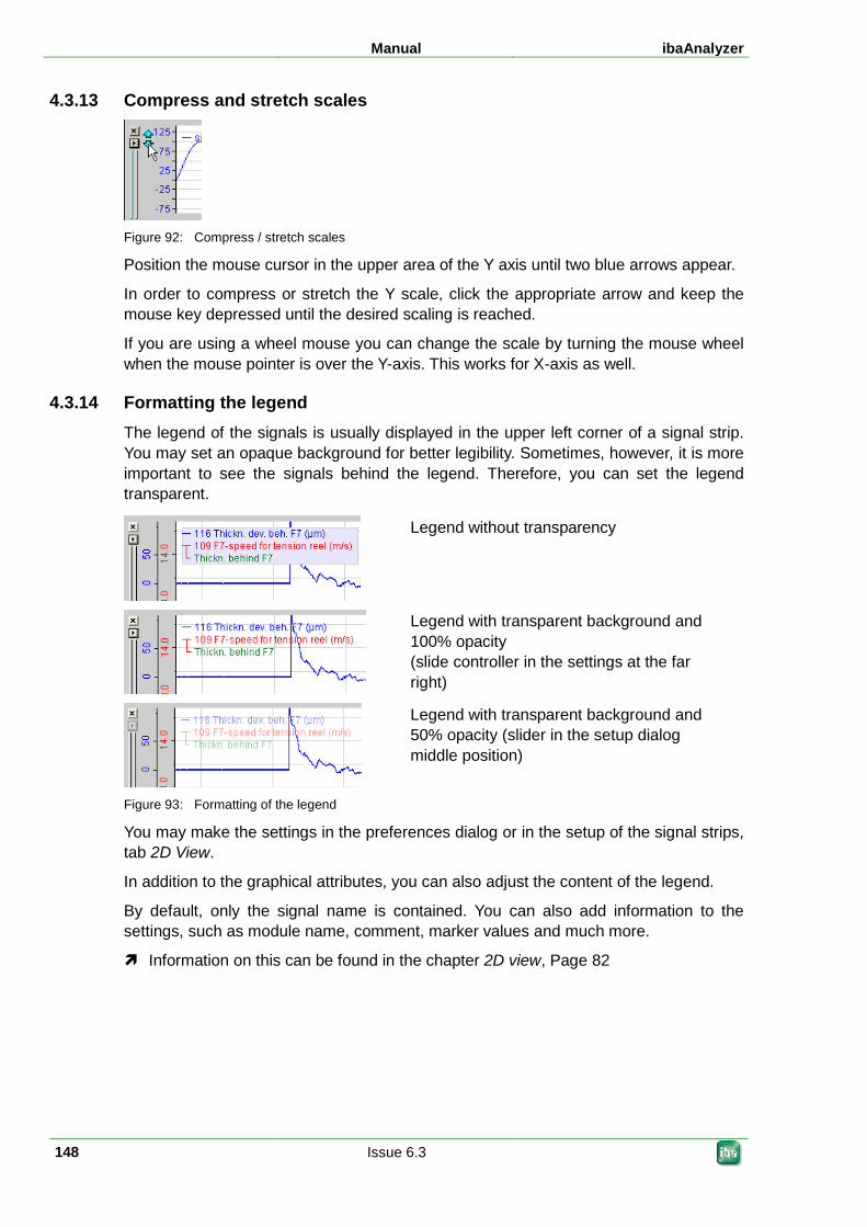
Manual ibaAnalyzer

148 Issue 6.3

4.3.13 Compress and stretch scales

Figure 92: Compress / stretch scales

Position the mouse cursor in the upper area of the Y axis until two blue arrows appear.

In order to compress or stretch the Y scale, click the appropriate arrow and keep the mouse key depressed until the desired scaling is reached.

If you are using a wheel mouse you can change the scale by turning the mouse wheel when the mouse pointer is over the Y-axis. This works for X-axis as well.

4.3.14 Formatting the legend The legend of the signals is usually displayed in the upper left corner of a signal strip. You may set an opaque background for better legibility. Sometimes, however, it is more important to see the signals behind the legend. Therefore, you can set the legend transparent.

Legend without transparency

Legend with transparent background and 100% opacity (slide controller in the settings at the far right)

Legend with transparent background and 50% opacity (slider in the setup dialog middle position)

Figure 93: Formatting of the legend

You may make the settings in the preferences dialog or in the setup of the signal strips, tab 2D View.

In addition to the graphical attributes, you can also adjust the content of the legend.

By default, only the signal name is contained. You can also add information to the settings, such as module name, comment, marker values and much more.

Information on this can be found in the chapter 2D view, Page 82

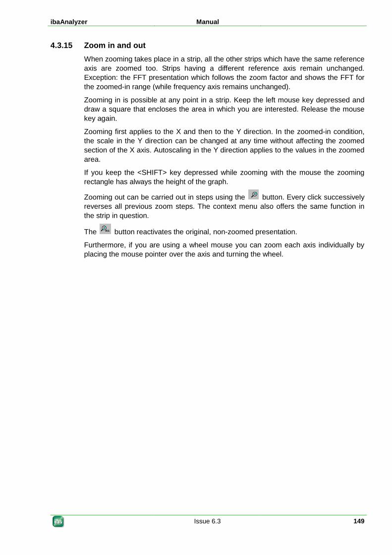
ibaAnalyzer Manual

Issue 6.3 149

4.3.15 Zoom in and out When zooming takes place in a strip, all the other strips which have the same reference axis are zoomed too. Strips having a different reference axis remain unchanged. Exception: the FFT presentation which follows the zoom factor and shows the FFT for the zoomed-in range (while frequency axis remains unchanged).

Zooming in is possible at any point in a strip. Keep the left mouse key depressed and draw a square that encloses the area in which you are interested. Release the mouse key again.

Zooming first applies to the X and then to the Y direction. In the zoomed-in condition, the scale in the Y direction can be changed at any time without affecting the zoomed section of the X axis. Autoscaling in the Y direction applies to the values in the zoomed area.

If you keep the <SHIFT> key depressed while zooming with the mouse the zooming rectangle has always the height of the graph.

Zooming out can be carried out in steps using the button. Every click successively reverses all previous zoom steps. The context menu also offers the same function in the strip in question.

The button reactivates the original, non-zoomed presentation.

Furthermore, if you are using a wheel mouse you can zoom each axis individually by placing the mouse pointer over the axis and turning the wheel.

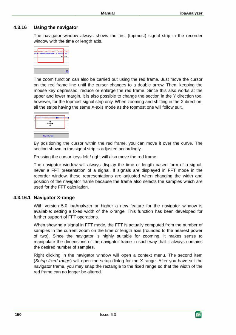
Manual ibaAnalyzer

150 Issue 6.3

4.3.16 Using the navigator The navigator window always shows the first (topmost) signal strip in the recorder window with the time or length axis.

The zoom function can also be carried out using the red frame. Just move the cursor on the red frame line until the cursor changes to a double arrow. Then, keeping the mouse key depressed, reduce or enlarge the red frame. Since this also works at the upper and lower margin, it is also possible to change the section in the Y direction too, however, for the topmost signal strip only. When zooming and shifting in the X direction, all the strips having the same X-axis mode as the topmost one will follow suit.

By positioning the cursor within the red frame, you can move it over the curve. The section shown in the signal strip is adjusted accordingly.

Pressing the cursor keys left / right will also move the red frame.

The navigator window will always display the time or length based form of a signal, never a FFT presentation of a signal. If signals are displayed in FFT mode in the recorder window, these representations are adjusted when changing the width and position of the navigator frame because the frame also selects the samples which are used for the FFT calculation.

4.3.16.1 Navigator X-range With version 5.0 ibaAnalyzer or higher a new feature for the navigator window is available: setting a fixed width of the x-range. This function has been developed for further support of FFT operations.

When showing a signal in FFT mode, the FFT is actually computed from the number of samples in the current zoom on the time or length axis (rounded to the nearest power of two). Since the navigator is highly suitable for zooming, it makes sense to manipulate the dimensions of the navigator frame in such way that it always contains the desired number of samples.

Right clicking in the navigator window will open a context menu. The second item (Setup fixed range) will open the setup dialog for the X-range. After you have set the navigator frame, you may snap the rectangle to the fixed range so that the width of the red frame can no longer be altered.

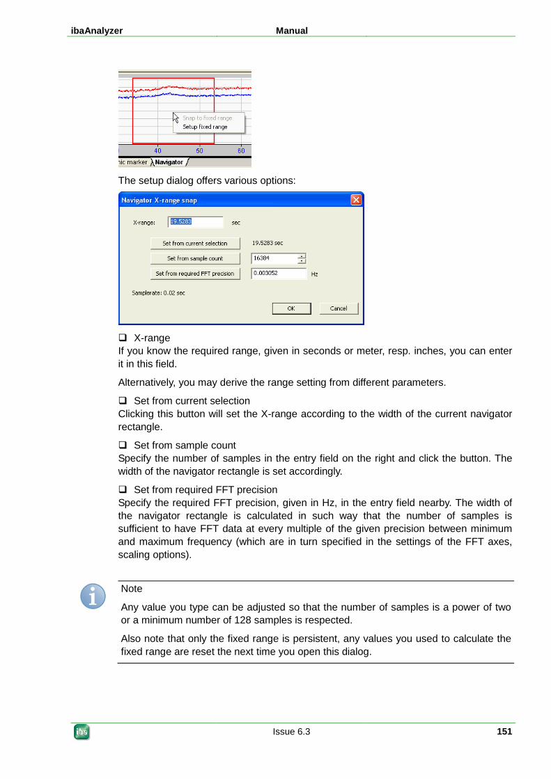
ibaAnalyzer Manual

Issue 6.3 151

The setup dialog offers various options:

X-range If you know the required range, given in seconds or meter, resp. inches, you can enter it in this field.

Alternatively, you may derive the range setting from different parameters.

Set from current selection Clicking this button will set the X-range according to the width of the current navigator rectangle.

Set from sample count Specify the number of samples in the entry field on the right and click the button. The width of the navigator rectangle is set accordingly.

Set from required FFT precision Specify the required FFT precision, given in Hz, in the entry field nearby. The width of the navigator rectangle is calculated in such way that the number of samples is sufficient to have FFT data at every multiple of the given precision between minimum and maximum frequency (which are in turn specified in the settings of the FFT axes, scaling options).

Note

Any value you type can be adjusted so that the number of samples is a power of two or a minimum number of 128 samples is respected.

Also note that only the fixed range is persistent, any values you used to calculate the fixed range are reset the next time you open this dialog.

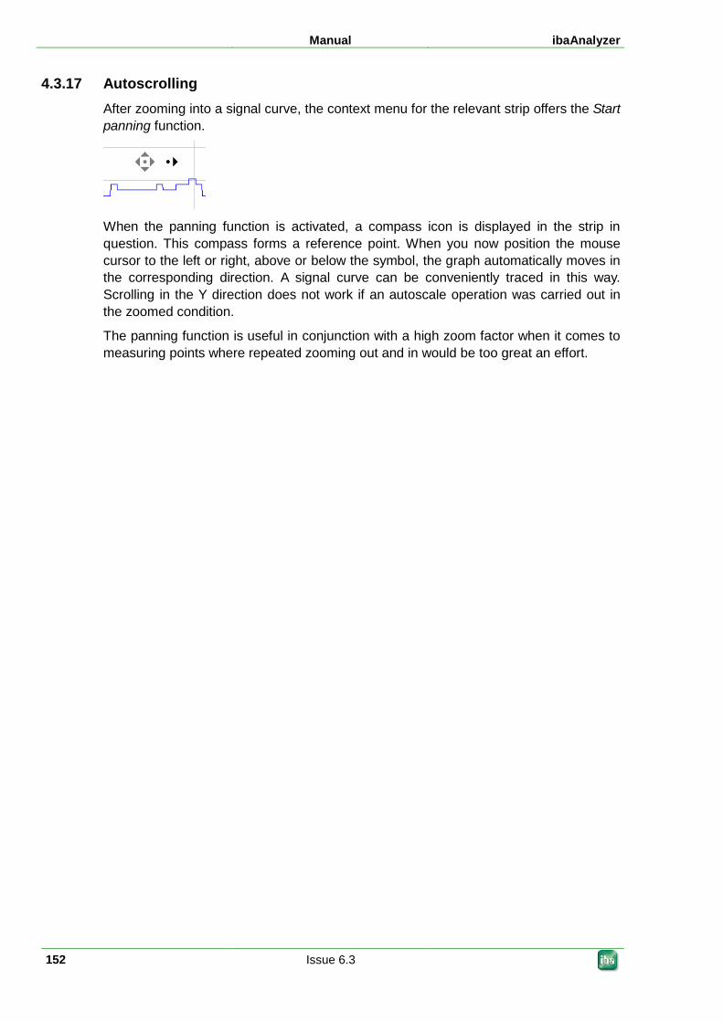
Manual ibaAnalyzer

152 Issue 6.3

4.3.17 Autoscrolling After zooming into a signal curve, the context menu for the relevant strip offers the Start panning function.

When the panning function is activated, a compass icon is displayed in the strip in question. This compass forms a reference point. When you now position the mouse cursor to the left or right, above or below the symbol, the graph automatically moves in the corresponding direction. A signal curve can be conveniently traced in this way. Scrolling in the Y direction does not work if an autoscale operation was carried out in the zoomed condition.

The panning function is useful in conjunction with a high zoom factor when it comes to measuring points where repeated zooming out and in would be too great an effort.

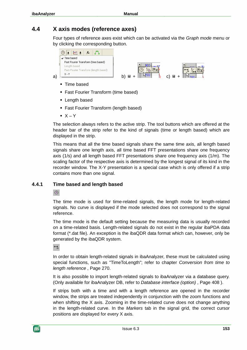
ibaAnalyzer Manual

Issue 6.3 153

4.4 X axis modes (reference axes) Four types of reference axes exist which can be activated via the Graph mode menu or by clicking the corresponding button.

a) b) + c) +

Time based

Fast Fourier Transform (time based)

Length based

Fast Fourier Transform (length based)

X – Y

The selection always refers to the active strip. The tool buttons which are offered at the header bar of the strip refer to the kind of signals (time or length based) which are displayed in the strip.

This means that all the time based signals share the same time axis, all length based signals share one length axis, all time based FFT presentations share one frequency axis (1/s) and all length based FFT presentations share one frequency axis (1/m). The scaling factor of the respective axis is determined by the longest signal of its kind in the recorder window. The X-Y presentation is a special case which is only offered if a strip contains more than one signal.

4.4.1 Time based and length based

The time mode is used for time-related signals, the length mode for length-related signals. No curve is displayed if the mode selected does not correspond to the signal reference.

The time mode is the default setting because the measuring data is usually recorded on a time-related basis. Length-related signals do not exist in the regular ibaPDA data format (*.dat file). An exception is the ibaQDR data format which can, however, only be generated by the ibaQDR system.

In order to obtain length-related signals in ibaAnalyzer, these must be calculated using special functions, such as "TimeToLength"; refer to chapter Conversion from time to length reference , Page 270.

It is also possible to import length-related signals to ibaAnalyzer via a database query. (Only available for ibaAnalyzer DB, refer to Database interface (option) , Page 408 ).

If strips both with a time and with a length reference are opened in the recorder window, the strips are treated independently in conjunction with the zoom functions and when shifting the X axis. Zooming in the time-related curve does not change anything in the length-related curve. In the Markers tab in the signal grid, the correct cursor positions are displayed for every X axis.

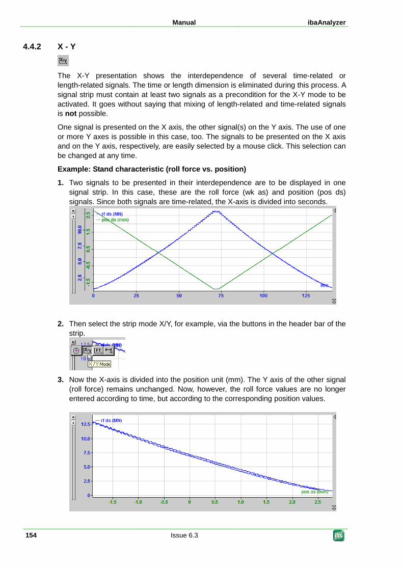
Manual ibaAnalyzer

154 Issue 6.3

4.4.2 X - Y

The X-Y presentation shows the interdependence of several time-related or length-related signals. The time or length dimension is eliminated during this process. A signal strip must contain at least two signals as a precondition for the X-Y mode to be activated. It goes without saying that mixing of length-related and time-related signals is not possible.

One signal is presented on the X axis, the other signal(s) on the Y axis. The use of one or more Y axes is possible in this case, too. The signals to be presented on the X axis and on the Y axis, respectively, are easily selected by a mouse click. This selection can be changed at any time.

Example: Stand characteristic (roll force vs. position)

1. Two signals to be presented in their interdependence are to be displayed in one signal strip. In this case, these are the roll force (wk as) and position (pos ds) signals. Since both signals are time-related, the X-axis is divided into seconds.

2. Then select the strip mode X/Y, for example, via the buttons in the header bar of the strip.

3. Now the X-axis is divided into the position unit (mm). The Y axis of the other signal

(roll force) remains unchanged. Now, however, the roll force values are no longer entered according to time, but according to the corresponding position values.

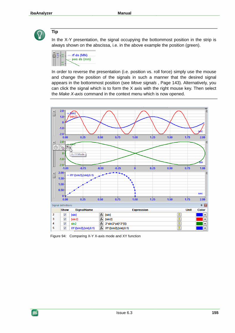
ibaAnalyzer Manual

Issue 6.3 155

Tip

In the X-Y presentation, the signal occupying the bottommost position in the strip is always shown on the abscissa, i.e. in the above example the position (green).

In order to reverse the presentation (i.e. position vs. roll force) simply use the mouse and change the position of the signals in such a manner that the desired signal appears in the bottommost position (see Move signals , Page 143). Alternatively, you can click the signal which is to form the X axis with the right mouse key. Then select the Make X-axis command in the context menu which is now opened.

Figure 94: Comparing X-Y X-axis mode and XY function

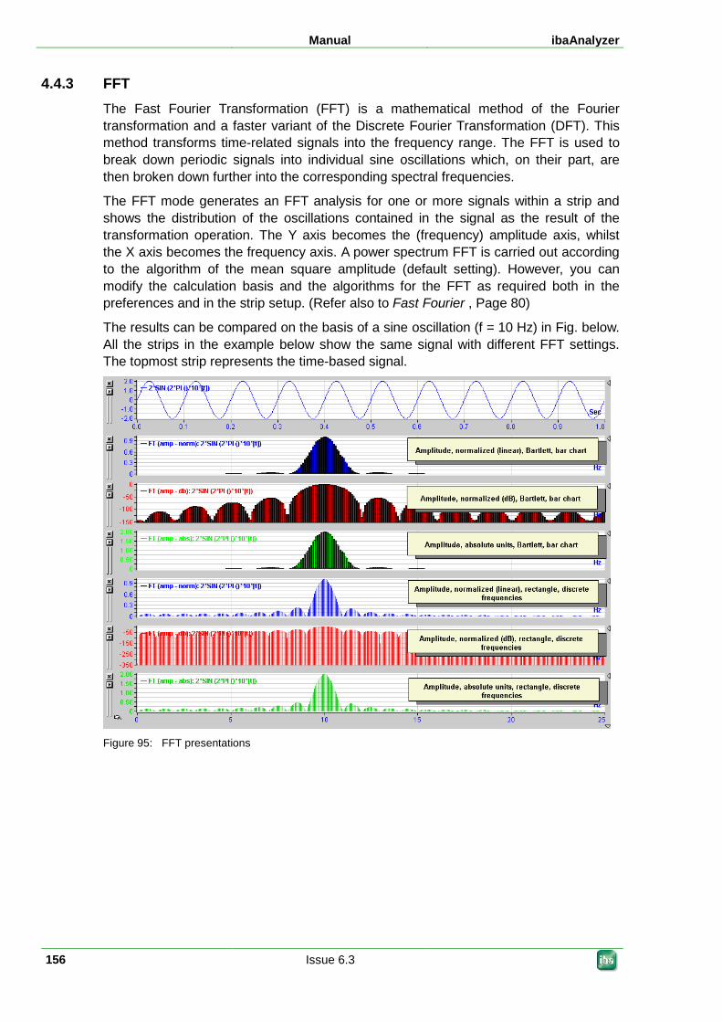
Manual ibaAnalyzer

156 Issue 6.3

4.4.3 FFT The Fast Fourier Transformation (FFT) is a mathematical method of the Fourier transformation and a faster variant of the Discrete Fourier Transformation (DFT). This method transforms time-related signals into the frequency range. The FFT is used to break down periodic signals into individual sine oscillations which, on their part, are then broken down further into the corresponding spectral frequencies.

The FFT mode generates an FFT analysis for one or more signals within a strip and shows the distribution of the oscillations contained in the signal as the result of the transformation operation. The Y axis becomes the (frequency) amplitude axis, whilst the X axis becomes the frequency axis. A power spectrum FFT is carried out according to the algorithm of the mean square amplitude (default setting). However, you can modify the calculation basis and the algorithms for the FFT as required both in the preferences and in the strip setup. (Refer also to Fast Fourier , Page 80)

The results can be compared on the basis of a sine oscillation (f = 10 Hz) in Fig. below. All the strips in the example below show the same signal with different FFT settings. The topmost strip represents the time-based signal.

Figure 95: FFT presentations

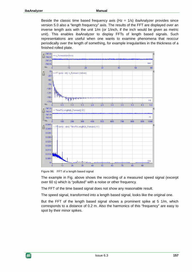
ibaAnalyzer Manual

Issue 6.3 157

Beside the classic time based frequency axis (Hz = 1/s) ibaAnalyzer provides since version 5.0 also a “length frequency” axis. The results of the FFT are displayed over an inverse length axis with the unit 1/m (or 1/inch, if the inch would be given as metric unit). This enables ibaAnalyzer to display FFTs of length based signals. Such representations are useful when one wants to examine phenomena that reoccur periodically over the length of something, for example irregularities in the thickness of a finished rolled plate.

Figure 96: FFT of a length based signal

The example in Fig. above shows the recording of a measured speed signal (excerpt over 60 s) which is “polluted” with a noise or other frequency.

The FFT of the time based signal does not show any reasonable result.

The speed signal, transformed into a length based signal, looks like the original one.

But the FFT of the length based signal shows a prominent spike at 5 1/m, which corresponds to a distance of 0.2 m. Also the harmonics of this “frequency” are easy to spot by their minor spikes.

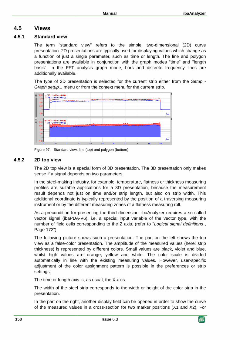
Manual ibaAnalyzer

158 Issue 6.3

4.5 Views 4.5.1 Standard view

The term "standard view" refers to the simple, two-dimensional (2D) curve presentation. 2D presentations are typically used for displaying values which change as a function of just a single parameter, such as time or length. The line and polygon presentations are available in conjunction with the graph modes "time" and "length basis". In the FFT analysis graph mode, bars and discrete frequency lines are additionally available.

The type of 2D presentation is selected for the current strip either from the Setup - Graph setup... menu or from the context menu for the current strip.

Figure 97: Standard view, line (top) and polygon (bottom)

4.5.2 2D top view The 2D top view is a special form of 3D presentation. The 3D presentation only makes sense if a signal depends on two parameters.

In the steel-making industry, for example, temperature, flatness or thickness measuring profiles are suitable applications for a 3D presentation, because the measurement result depends not just on time and/or strip length, but also on strip width. This additional coordinate is typically represented by the position of a traversing measuring instrument or by the different measuring zones of a flatness measuring roll.

As a precondition for presenting the third dimension, ibaAnalyzer requires a so called vector signal (ibaPDA-V6), i.e. a special input variable of the vector type, with the number of field cells corresponding to the Z axis. (refer to "Logical signal definitions , Page 172").

The following picture shows such a presentation. The part on the left shows the top view as a false-color presentation. The amplitude of the measured values (here: strip thickness) is represented by different colors. Small values are black, violet and blue, whilst high values are orange, yellow and white. The color scale is divided automatically in line with the existing measuring values. However, user-specific adjustment of the color assignment pattern is possible in the preferences or strip settings.

The time or length axis is, as usual, the X-axis.

The width of the steel strip corresponds to the width or height of the color strip in the presentation.

In the part on the right, another display field can be opened in order to show the curve of the measured values in a cross-section for two marker positions (X1 and X2). For

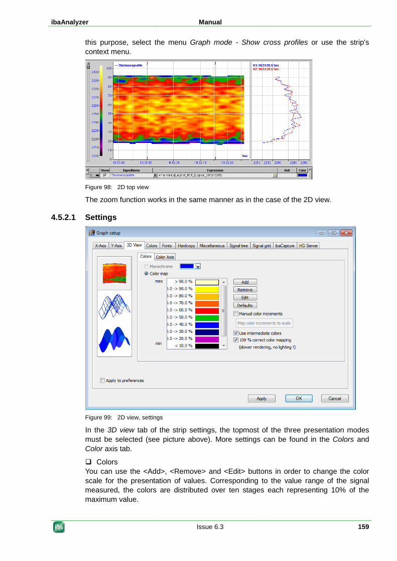
ibaAnalyzer Manual

Issue 6.3 159

this purpose, select the menu Graph mode - Show cross profiles or use the strip's context menu.

Figure 98: 2D top view

The zoom function works in the same manner as in the case of the 2D view.

4.5.2.1 Settings

Figure 99: 2D view, settings

In the 3D view tab of the strip settings, the topmost of the three presentation modes must be selected (see picture above). More settings can be found in the Colors and Color axis tab.

Colors You can use the <Add>, <Remove> and <Edit> buttons in order to change the color scale for the presentation of values. Corresponding to the value range of the signal measured, the colors are distributed over ten stages each representing 10% of the maximum value.

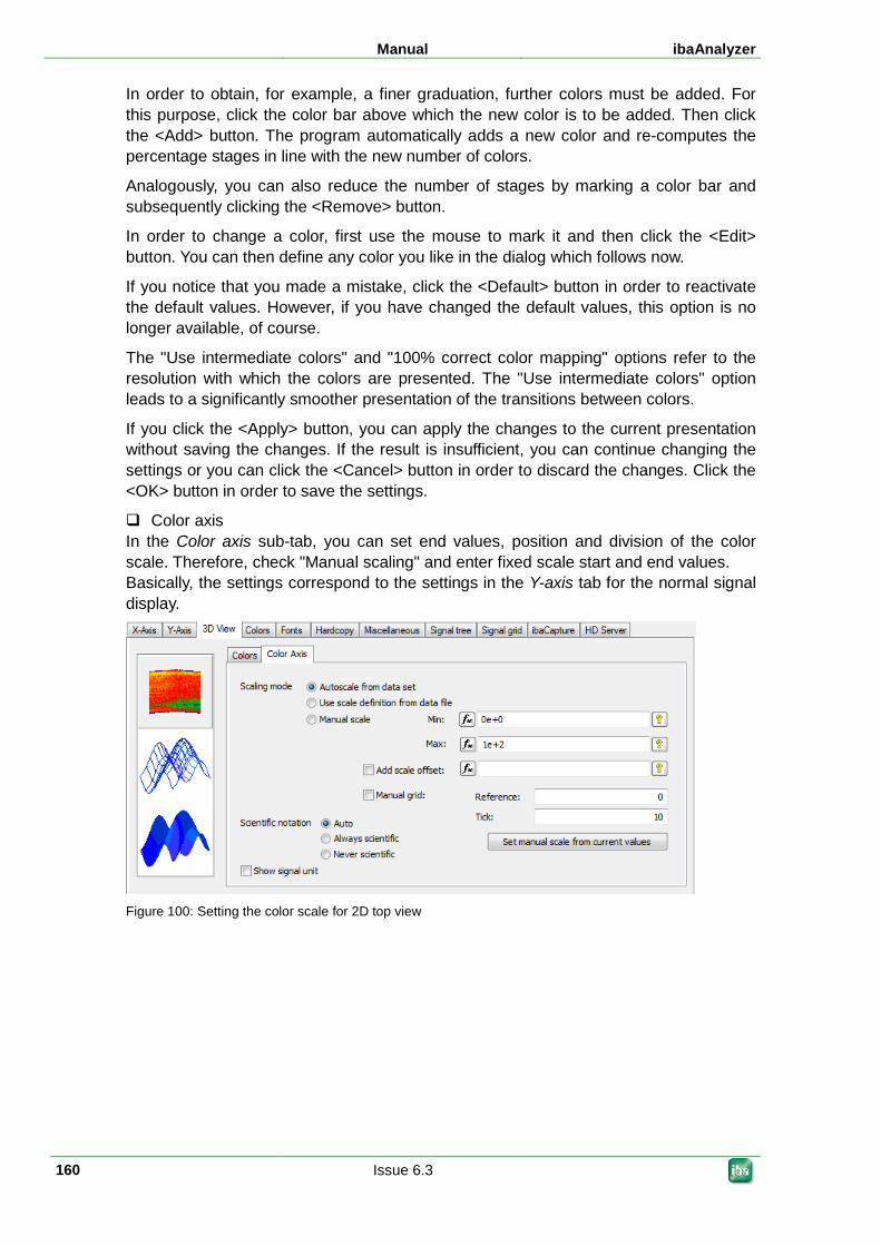
Manual ibaAnalyzer

160 Issue 6.3

In order to obtain, for example, a finer graduation, further colors must be added. For this purpose, click the color bar above which the new color is to be added. Then click the <Add> button. The program automatically adds a new color and re-computes the percentage stages in line with the new number of colors.

Analogously, you can also reduce the number of stages by marking a color bar and subsequently clicking the <Remove> button.

In order to change a color, first use the mouse to mark it and then click the <Edit> button. You can then define any color you like in the dialog which follows now.

If you notice that you made a mistake, click the <Default> button in order to reactivate the default values. However, if you have changed the default values, this option is no longer available, of course.

The "Use intermediate colors" and "100% correct color mapping" options refer to the resolution with which the colors are presented. The "Use intermediate colors" option leads to a significantly smoother presentation of the transitions between colors.

If you click the <Apply> button, you can apply the changes to the current presentation without saving the changes. If the result is insufficient, you can continue changing the settings or you can click the <Cancel> button in order to discard the changes. Click the <OK> button in order to save the settings.

Color axis In the Color axis sub-tab, you can set end values, position and division of the color scale. Therefore, check "Manual scaling" and enter fixed scale start and end values. Basically, the settings correspond to the settings in the Y-axis tab for the normal signal display.

Figure 100: Setting the color scale for 2D top view

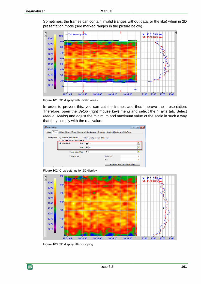
ibaAnalyzer Manual

Issue 6.3 161

Sometimes, the frames can contain invalid (ranges without data, or the like) when in 2D presentation mode (see marked ranges in the picture below).

Figure 101: 2D display with invalid areas

In order to prevent this, you can cut the frames and thus improve the presentation. Therefore, open the Setup (right mouse key) menu and select the Y axis tab. Select Manual scaling and adjust the minimum and maximum value of the scale in such a way that they comply with the real value.

Figure 102: Crop settings for 2D display

Figure 103: 2D display after cropping

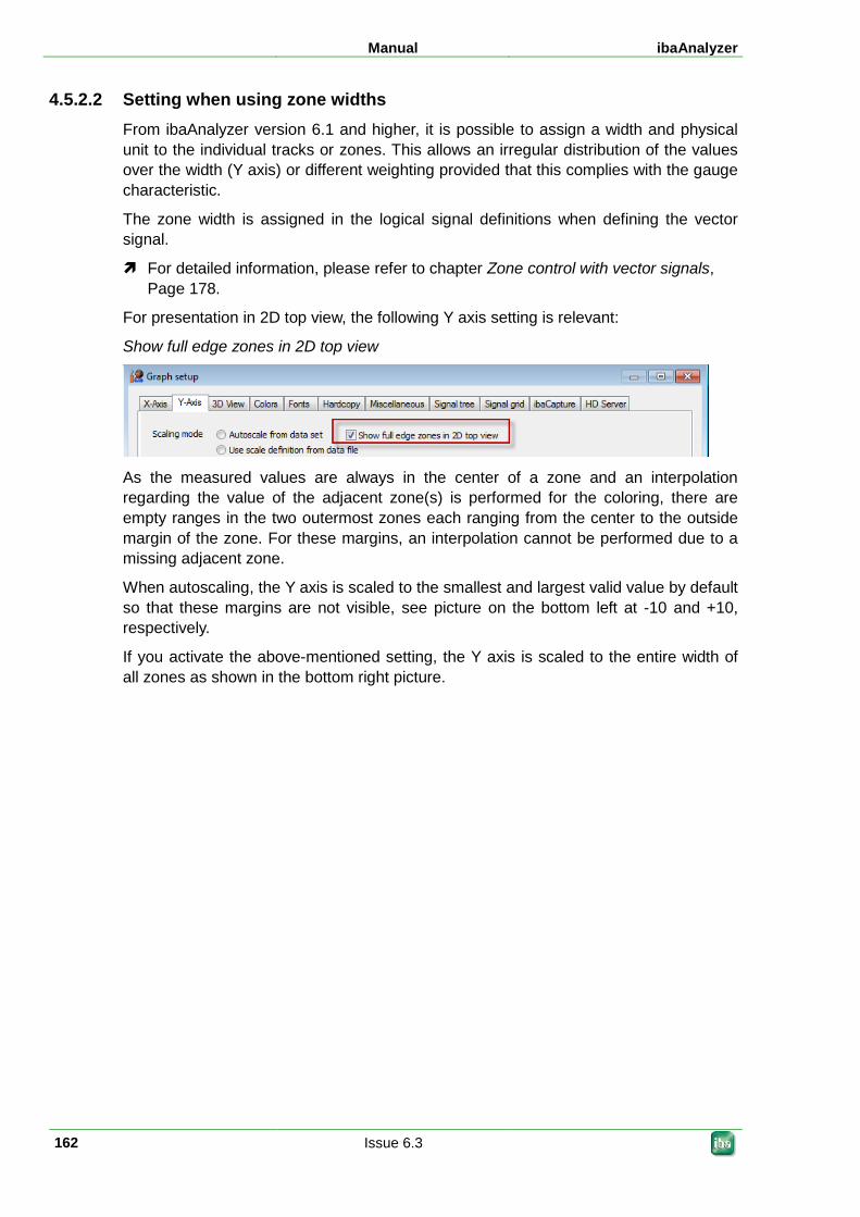
Manual ibaAnalyzer

162 Issue 6.3

4.5.2.2 Setting when using zone widths From ibaAnalyzer version 6.1 and higher, it is possible to assign a width and physical unit to the individual tracks or zones. This allows an irregular distribution of the values over the width (Y axis) or different weighting provided that this complies with the gauge characteristic.

The zone width is assigned in the logical signal definitions when defining the vector signal.

For detailed information, please refer to chapter Zone control with vector signals, Page 178.

For presentation in 2D top view, the following Y axis setting is relevant:

Show full edge zones in 2D top view

As the measured values are always in the center of a zone and an interpolation regarding the value of the adjacent zone(s) is performed for the coloring, there are empty ranges in the two outermost zones each ranging from the center to the outside margin of the zone. For these margins, an interpolation cannot be performed due to a missing adjacent zone.

When autoscaling, the Y axis is scaled to the smallest and largest valid value by default so that these margins are not visible, see picture on the bottom left at -10 and +10, respectively.

If you activate the above-mentioned setting, the Y axis is scaled to the entire width of all zones as shown in the bottom right picture.

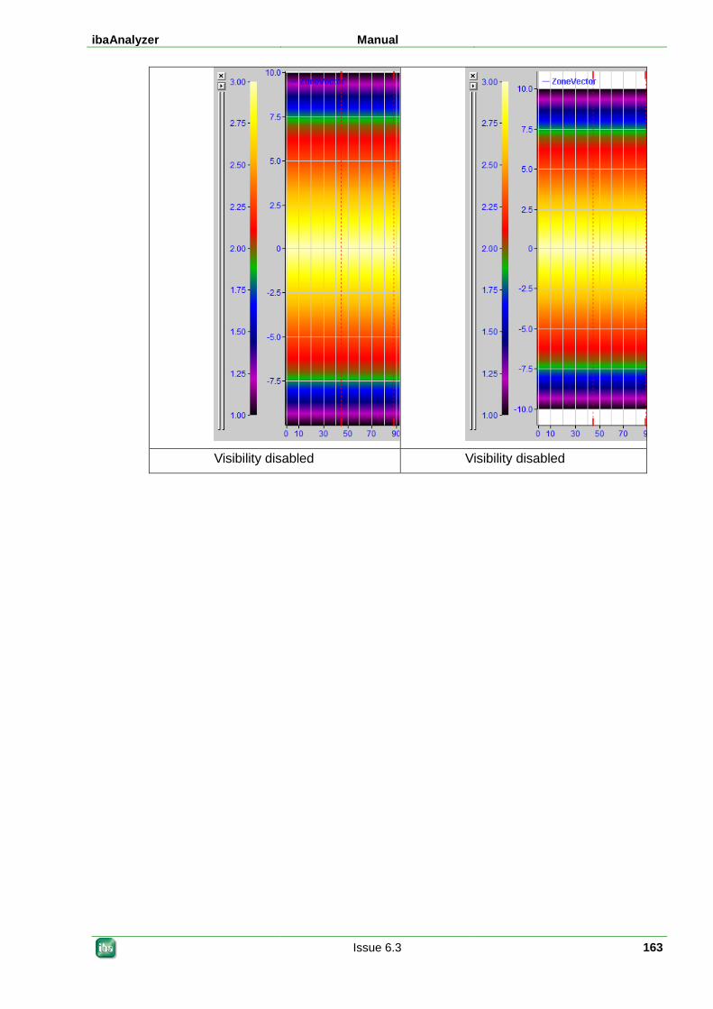
ibaAnalyzer Manual

Issue 6.3 163

Visibility disabled Visibility disabled

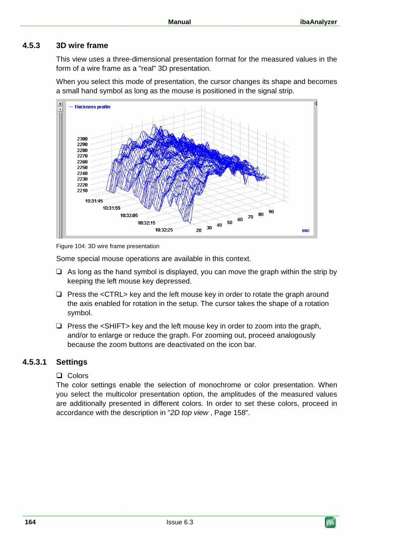
Manual ibaAnalyzer

164 Issue 6.3

4.5.3 3D wire frame This view uses a three-dimensional presentation format for the measured values in the form of a wire frame as a "real" 3D presentation.

When you select this mode of presentation, the cursor changes its shape and becomes a small hand symbol as long as the mouse is positioned in the signal strip.

Figure 104: 3D wire frame presentation

Some special mouse operations are available in this context.

As long as the hand symbol is displayed, you can move the graph within the strip by keeping the left mouse key depressed.

Press the <CTRL> key and the left mouse key in order to rotate the graph around the axis enabled for rotation in the setup. The cursor takes the shape of a rotation symbol.

Press the <SHIFT> key and the left mouse key in order to zoom into the graph, and/or to enlarge or reduce the graph. For zooming out, proceed analogously because the zoom buttons are deactivated on the icon bar.

4.5.3.1 Settings Colors The color settings enable the selection of monochrome or color presentation. When you select the multicolor presentation option, the amplitudes of the measured values are additionally presented in different colors. In order to set these colors, proceed in accordance with the description in "2D top view , Page 158".

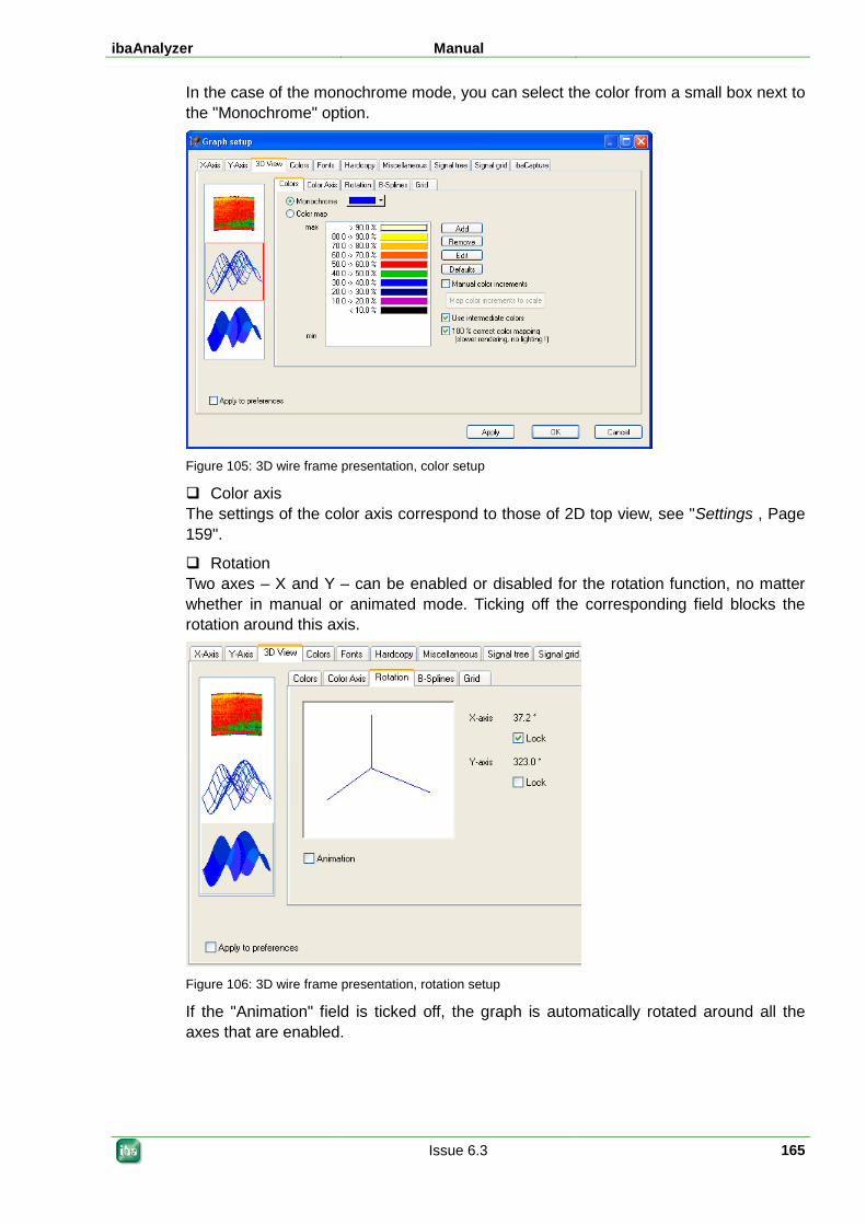
ibaAnalyzer Manual

Issue 6.3 165

In the case of the monochrome mode, you can select the color from a small box next to the "Monochrome" option.

Figure 105: 3D wire frame presentation, color setup

Color axis The settings of the color axis correspond to those of 2D top view, see "Settings , Page 159".

Rotation Two axes – X and Y – can be enabled or disabled for the rotation function, no matter whether in manual or animated mode. Ticking off the corresponding field blocks the rotation around this axis.

Figure 106: 3D wire frame presentation, rotation setup

If the "Animation" field is ticked off, the graph is automatically rotated around all the axes that are enabled.

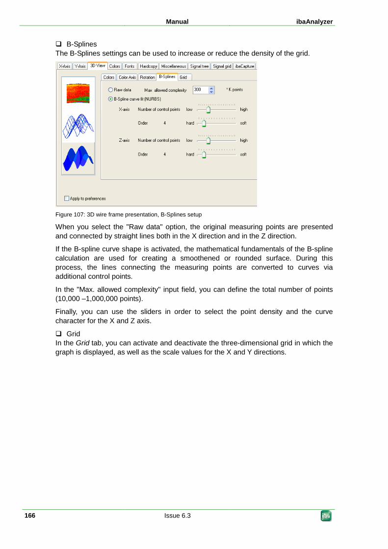
Manual ibaAnalyzer

166 Issue 6.3

B-Splines The B-Splines settings can be used to increase or reduce the density of the grid.

Figure 107: 3D wire frame presentation, B-Splines setup

When you select the "Raw data" option, the original measuring points are presented and connected by straight lines both in the X direction and in the Z direction.

If the B-spline curve shape is activated, the mathematical fundamentals of the B-spline calculation are used for creating a smoothened or rounded surface. During this process, the lines connecting the measuring points are converted to curves via additional control points.

In the "Max. allowed complexity" input field, you can define the total number of points (10,000 –1,000,000 points).

Finally, you can use the sliders in order to select the point density and the curve character for the X and Z axis.

Grid In the Grid tab, you can activate and deactivate the three-dimensional grid in which the graph is displayed, as well as the scale values for the X and Y directions.

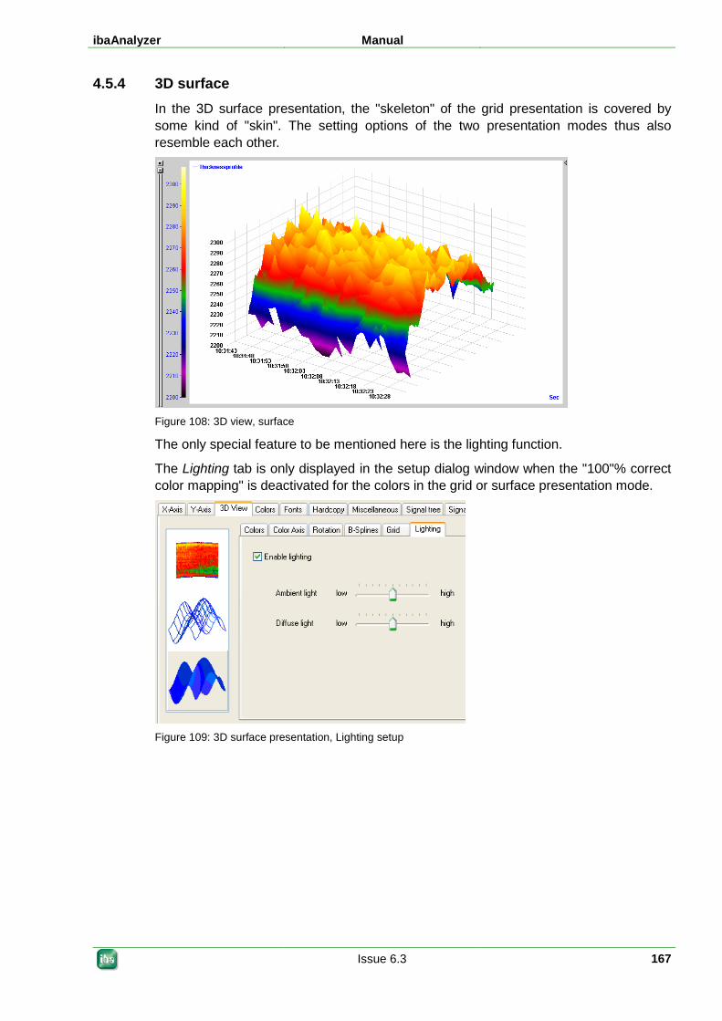
ibaAnalyzer Manual

Issue 6.3 167

4.5.4 3D surface In the 3D surface presentation, the "skeleton" of the grid presentation is covered by some kind of "skin". The setting options of the two presentation modes thus also resemble each other.

Figure 108: 3D view, surface

The only special feature to be mentioned here is the lighting function.

The Lighting tab is only displayed in the setup dialog window when the "100"% correct color mapping" is deactivated for the colors in the grid or surface presentation mode.

Figure 109: 3D surface presentation, Lighting setup

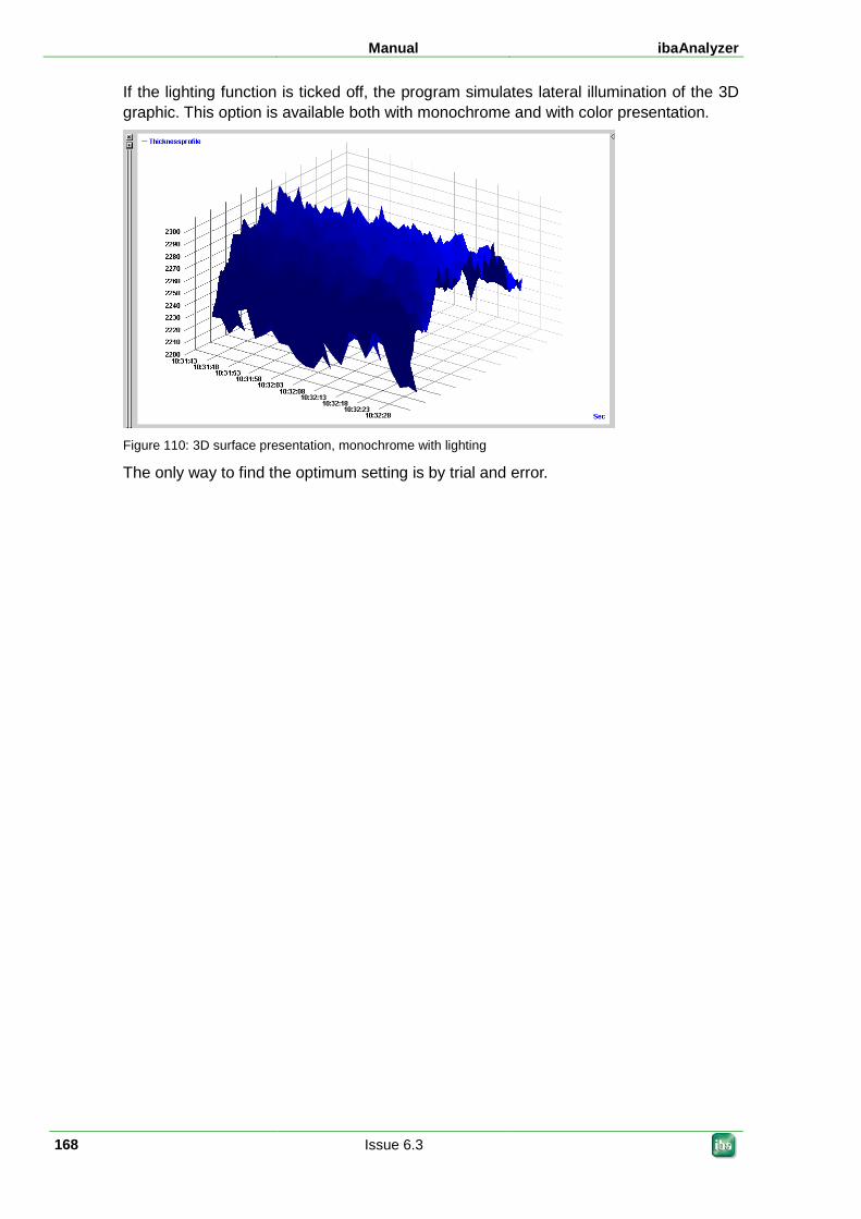
Manual ibaAnalyzer

168 Issue 6.3

If the lighting function is ticked off, the program simulates lateral illumination of the 3D graphic. This option is available both with monochrome and with color presentation.

Figure 110: 3D surface presentation, monochrome with lighting

The only way to find the optimum setting is by trial and error.

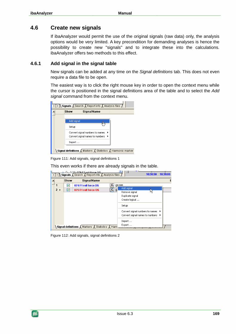
ibaAnalyzer Manual

Issue 6.3 169

4.6 Create new signals If ibaAnalyzer would permit the use of the original signals (raw data) only, the analysis options would be very limited. A key precondition for demanding analyses is hence the possibility to create new "signals" and to integrate these into the calculations. ibaAnalyzer offers two methods to this effect.

4.6.1 Add signal in the signal table New signals can be added at any time on the Signal definitions tab. This does not even require a data file to be open.

The easiest way is to click the right mouse key in order to open the context menu while the cursor is positioned in the signal definitions area of the table and to select the Add signal command from the context menu.

Figure 111: Add signals, signal definitions 1

This even works if there are already signals in the table.

Figure 112: Add signals, signal definitions 2

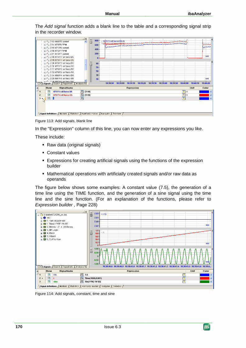
Manual ibaAnalyzer

170 Issue 6.3

The Add signal function adds a blank line to the table and a corresponding signal strip in the recorder window.

Figure 113: Add signals, blank line

In the "Expression" column of this line, you can now enter any expressions you like.

These include:

Raw data (original signals)

Constant values

Expressions for creating artificial signals using the functions of the expression builder

Mathematical operations with artificially created signals and/or raw data as operands

The figure below shows some examples: A constant value (7.5), the generation of a time line using the TIME function, and the generation of a sine signal using the time line and the sine function. (For an explanation of the functions, please refer to Expression builder , Page 228)

Figure 114: Add signals, constant, time and sine

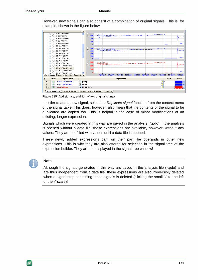
ibaAnalyzer Manual

Issue 6.3 171

However, new signals can also consist of a combination of original signals. This is, for example, shown in the figure below.

Figure 115: Add signals, addition of two original signals

In order to add a new signal, select the Duplicate signal function from the context menu of the signal table. This does, however, also mean that the contents of the signal to be duplicated are copied too. This is helpful in the case of minor modifications of an existing, longer expression.

Signals which were created in this way are saved in the analysis (*.pdo). If the analysis is opened without a data file, these expressions are available, however, without any values. They are not filled with values until a data file is opened.

These newly added expressions can, on their part, be operands in other new expressions. This is why they are also offered for selection in the signal tree of the expression builder. They are not displayed in the signal tree window!

Note

Although the signals generated in this way are saved in the analysis file (*.pdo) and are thus independent from a data file, these expressions are also irreversibly deleted when a signal strip containing these signals is deleted (clicking the small 'x' to the left of the Y scale)!

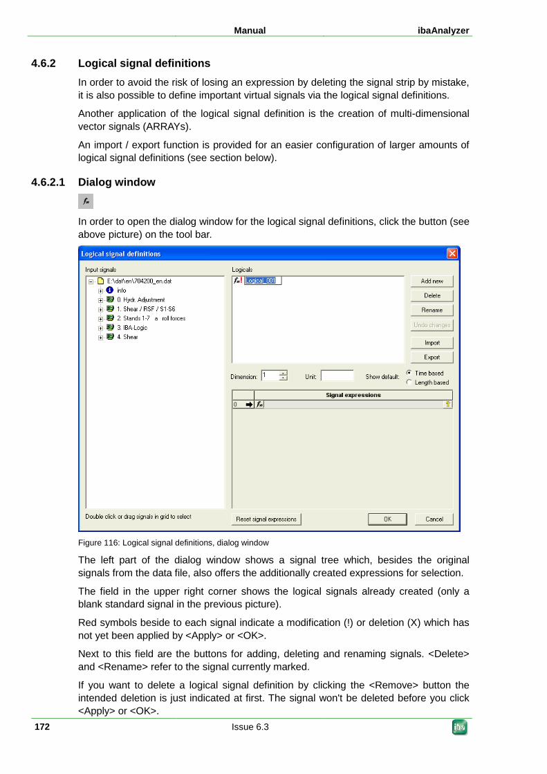
Manual ibaAnalyzer

172 Issue 6.3

4.6.2 Logical signal definitions In order to avoid the risk of losing an expression by deleting the signal strip by mistake, it is also possible to define important virtual signals via the logical signal definitions.

Another application of the logical signal definition is the creation of multi-dimensional vector signals (ARRAYs).

An import / export function is provided for an easier configuration of larger amounts of logical signal definitions (see section below).

4.6.2.1 Dialog window

In order to open the dialog window for the logical signal definitions, click the button (see above picture) on the tool bar.

Figure 116: Logical signal definitions, dialog window

The left part of the dialog window shows a signal tree which, besides the original signals from the data file, also offers the additionally created expressions for selection.

The field in the upper right corner shows the logical signals already created (only a blank standard signal in the previous picture).

Red symbols beside to each signal indicate a modification (!) or deletion (X) which has not yet been applied by <Apply> or <OK>.

Next to this field are the buttons for adding, deleting and renaming signals. <Delete> and <Rename> refer to the signal currently marked.

If you want to delete a logical signal definition by clicking the <Remove> button the intended deletion is just indicated at first. The signal won't be deleted before you click <Apply> or <OK>.

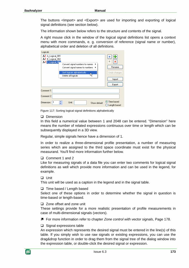
ibaAnalyzer Manual

Issue 6.3 173

The buttons <Import> and <Export> are used for importing and exporting of logical signal definitions (see section below).

The information shown below refers to the structure and contents of the signal.

A right mouse click in the window of the logical signal definitions list opens a context menu with more commands, e. g. conversion of reference (signal name or number), alphabetical order and deletion of all definitions.

Figure 117: Sorting logical signal definitions alphabetically

Dimension In this field a numerical value between 1 and 2048 can be entered. "Dimension" here means the number of related expressions continuous over time or length which can be subsequently displayed in a 3D view.

Regular, simple signals hence have a dimension of 1.

In order to realize a three-dimensional profile presentation, a number of measuring series which are assigned to the third space coordinate must exist for the physical measurand. You'll find more information further below.

Comment 1 and 2 Like for measuring signals of a data file you can enter two comments for logical signal definitions as well which provide more information and can be used in the legend, for example.

Unit This unit will be used as a caption in the legend and in the signal table.

Time based / Length based Select one of these options in order to determine whether the signal in question is time-based or length-based.

Zone offset and zone unit These settings provide for a more realistic presentation of profile measurements in case of multi-dimensional signals (vectors).

For more information refer to chapter Zone control with vector signals, Page 178.

Signal expressions table An expression which represents the desired signal must be entered in the line(s) of this table. If you simply wish to use raw signals or existing expressions, you can use the drag&drop function in order to drag them from the signal tree of the dialog window into the expression table, or double-click the desired signal or expression.

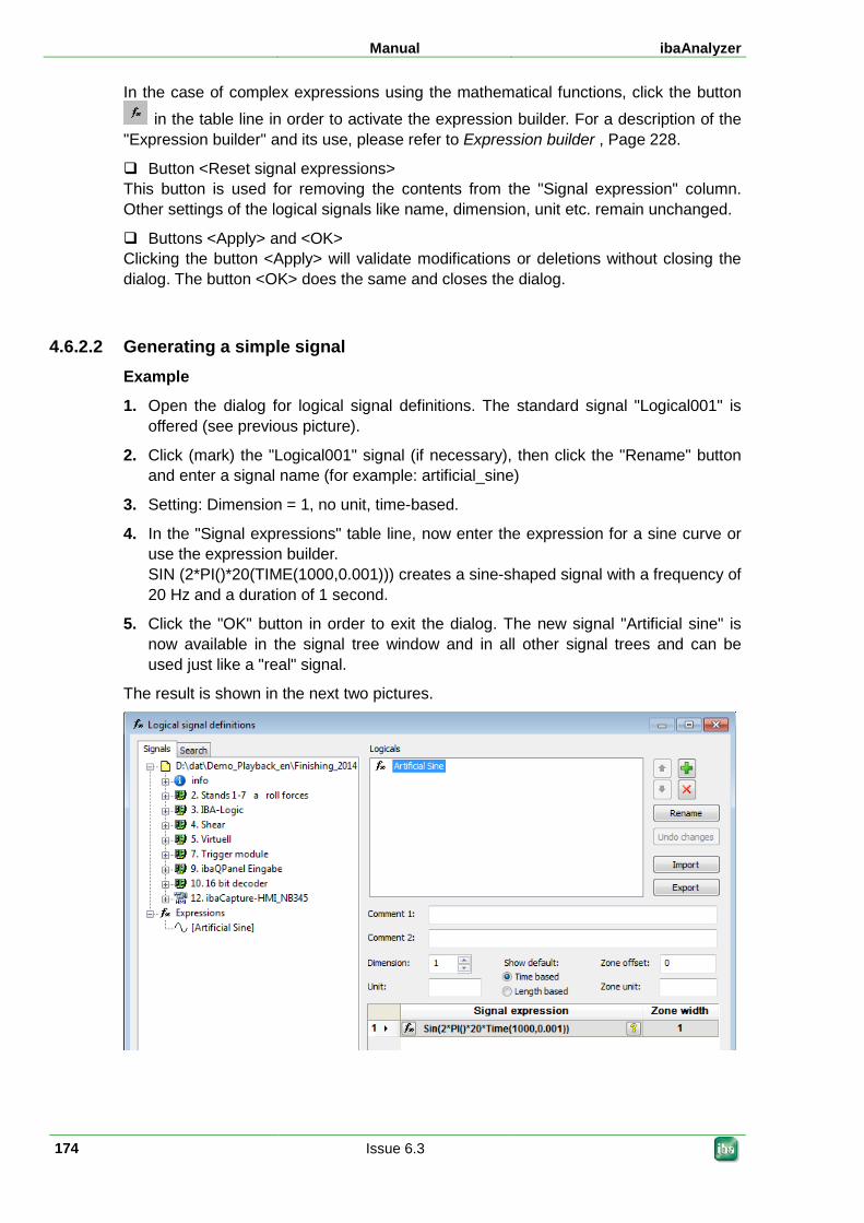
Manual ibaAnalyzer

174 Issue 6.3

In the case of complex expressions using the mathematical functions, click the button

in the table line in order to activate the expression builder. For a description of the "Expression builder" and its use, please refer to Expression builder , Page 228.

Button <Reset signal expressions> This button is used for removing the contents from the "Signal expression" column. Other settings of the logical signals like name, dimension, unit etc. remain unchanged.

Buttons <Apply> and <OK> Clicking the button <Apply> will validate modifications or deletions without closing the dialog. The button <OK> does the same and closes the dialog.

4.6.2.2 Generating a simple signal Example

1. Open the dialog for logical signal definitions. The standard signal "Logical001" is offered (see previous picture).

2. Click (mark) the "Logical001" signal (if necessary), then click the "Rename" button and enter a signal name (for example: artificial_sine)

3. Setting: Dimension = 1, no unit, time-based.

4. In the "Signal expressions" table line, now enter the expression for a sine curve or use the expression builder. SIN (2*PI()*20(TIME(1000,0.001))) creates a sine-shaped signal with a frequency of 20 Hz and a duration of 1 second.

5. Click the "OK" button in order to exit the dialog. The new signal "Artificial sine" is now available in the signal tree window and in all other signal trees and can be used just like a "real" signal.

The result is shown in the next two pictures.

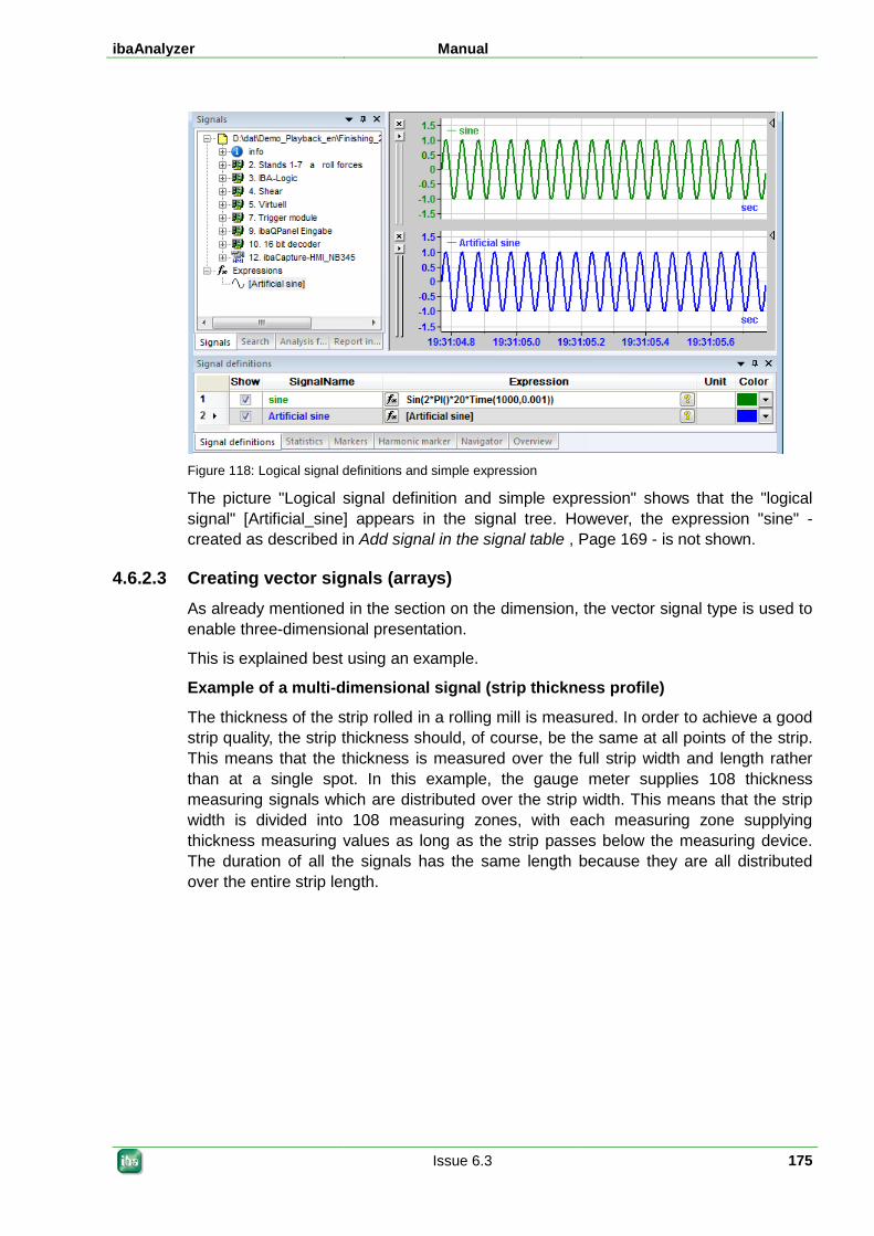
ibaAnalyzer Manual

Issue 6.3 175

Figure 118: Logical signal definitions and simple expression

The picture "Logical signal definition and simple expression" shows that the "logical signal" [Artificial_sine] appears in the signal tree. However, the expression "sine" - created as described in Add signal in the signal table , Page 169 - is not shown.

4.6.2.3 Creating vector signals (arrays) As already mentioned in the section on the dimension, the vector signal type is used to enable three-dimensional presentation.

This is explained best using an example.

Example of a multi-dimensional signal (strip thickness profile)

The thickness of the strip rolled in a rolling mill is measured. In order to achieve a good strip quality, the strip thickness should, of course, be the same at all points of the strip. This means that the thickness is measured over the full strip width and length rather than at a single spot. In this example, the gauge meter supplies 108 thickness measuring signals which are distributed over the strip width. This means that the strip width is divided into 108 measuring zones, with each measuring zone supplying thickness measuring values as long as the strip passes below the measuring device. The duration of all the signals has the same length because they are all distributed over the entire strip length.

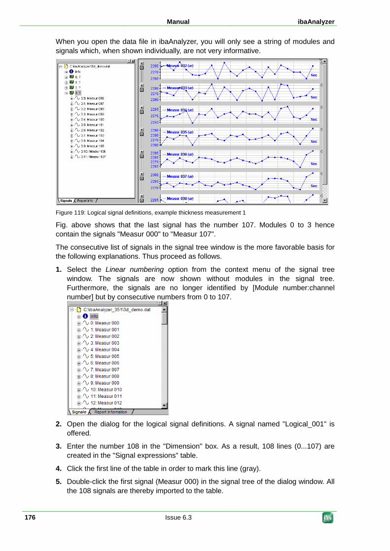
Manual ibaAnalyzer

176 Issue 6.3

When you open the data file in ibaAnalyzer, you will only see a string of modules and signals which, when shown individually, are not very informative.

Figure 119: Logical signal definitions, example thickness measurement 1

Fig. above shows that the last signal has the number 107. Modules 0 to 3 hence contain the signals "Measur 000" to "Measur 107".

The consecutive list of signals in the signal tree window is the more favorable basis for the following explanations. Thus proceed as follows.

1. Select the Linear numbering option from the context menu of the signal tree window. The signals are now shown without modules in the signal tree. Furthermore, the signals are no longer identified by [Module number:channel number] but by consecutive numbers from 0 to 107.

2. Open the dialog for the logical signal definitions. A signal named "Logical_001" is

offered.

3. Enter the number 108 in the "Dimension" box. As a result, 108 lines (0...107) are created in the "Signal expressions" table.

4. Click the first line of the table in order to mark this line (gray).

5. Double-click the first signal (Measur 000) in the signal tree of the dialog window. All the 108 signals are thereby imported to the table.

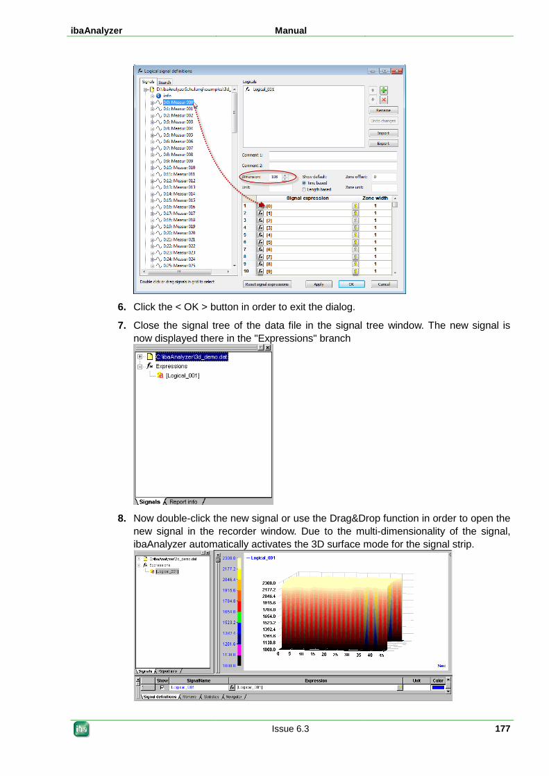
ibaAnalyzer Manual

Issue 6.3 177

6. Click the < OK > button in order to exit the dialog.

7. Close the signal tree of the data file in the signal tree window. The new signal is now displayed there in the "Expressions" branch

8. Now double-click the new signal or use the Drag&Drop function in order to open the

new signal in the recorder window. Due to the multi-dimensionality of the signal, ibaAnalyzer automatically activates the 3D surface mode for the signal strip.

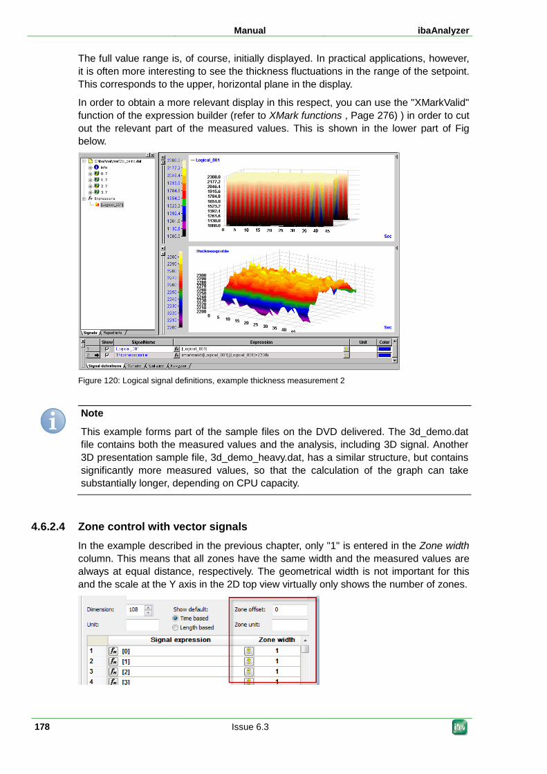
Manual ibaAnalyzer

178 Issue 6.3

The full value range is, of course, initially displayed. In practical applications, however, it is often more interesting to see the thickness fluctuations in the range of the setpoint. This corresponds to the upper, horizontal plane in the display.

In order to obtain a more relevant display in this respect, you can use the "XMarkValid" function of the expression builder (refer to XMark functions , Page 276) ) in order to cut out the relevant part of the measured values. This is shown in the lower part of Fig below.

Figure 120: Logical signal definitions, example thickness measurement 2

Note

This example forms part of the sample files on the DVD delivered. The 3d_demo.dat file contains both the measured values and the analysis, including 3D signal. Another 3D presentation sample file, 3d_demo_heavy.dat, has a similar structure, but contains significantly more measured values, so that the calculation of the graph can take substantially longer, depending on CPU capacity.

4.6.2.4 Zone control with vector signals In the example described in the previous chapter, only "1" is entered in the Zone width column. This means that all zones have the same width and the measured values are always at equal distance, respectively. The geometrical width is not important for this and the scale at the Y axis in the 2D top view virtually only shows the number of zones.

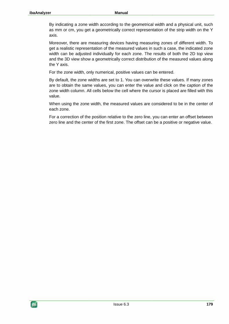
ibaAnalyzer Manual

Issue 6.3 179

By indicating a zone width according to the geometrical width and a physical unit, such as mm or cm, you get a geometrically correct representation of the strip width on the Y axis.

Moreover, there are measuring devices having measuring zones of different width. To get a realistic representation of the measured values in such a case, the indicated zone width can be adjusted individually for each zone. The results of both the 2D top view and the 3D view show a geometrically correct distribution of the measured values along the Y axis.

For the zone width, only numerical, positive values can be entered.

By default, the zone widths are set to 1. You can overwrite these values. If many zones are to obtain the same values, you can enter the value and click on the caption of the zone width column. All cells below the cell where the cursor is placed are filled with this value.

When using the zone width, the measured values are considered to be in the center of each zone.

For a correction of the position relative to the zero line, you can enter an offset between zero line and the center of the first zone. The offset can be a positive or negative value.

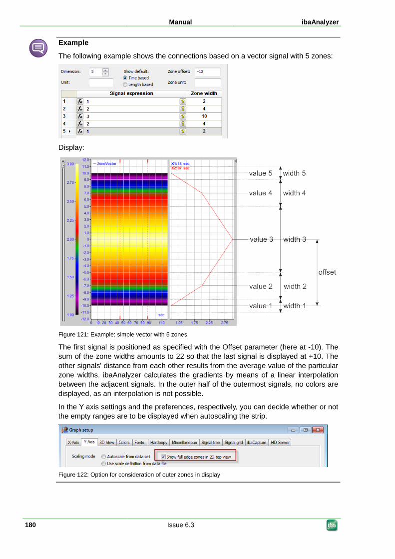
Manual ibaAnalyzer

180 Issue 6.3

Example

The following example shows the connections based on a vector signal with 5 zones:

Display:

Figure 121: Example: simple vector with 5 zones

The first signal is positioned as specified with the Offset parameter (here at -10). The sum of the zone widths amounts to 22 so that the last signal is displayed at +10. The other signals' distance from each other results from the average value of the particular zone widths. ibaAnalyzer calculates the gradients by means of a linear interpolation between the adjacent signals. In the outer half of the outermost signals, no colors are displayed, as an interpolation is not possible.

In the Y axis settings and the preferences, respectively, you can decide whether or not the empty ranges are to be displayed when autoscaling the strip.

Figure 122: Option for consideration of outer zones in display

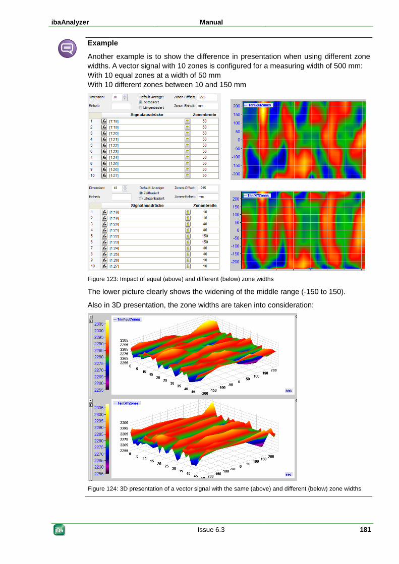
ibaAnalyzer Manual

Issue 6.3 181

Example

Another example is to show the difference in presentation when using different zone widths. A vector signal with 10 zones is configured for a measuring width of 500 mm: With 10 equal zones at a width of 50 mm With 10 different zones between 10 and 150 mm

Figure 123: Impact of equal (above) and different (below) zone widths

The lower picture clearly shows the widening of the middle range (-150 to 150).

Also in 3D presentation, the zone widths are taken into consideration:

Figure 124: 3D presentation of a vector signal with the same (above) and different (below) zone widths

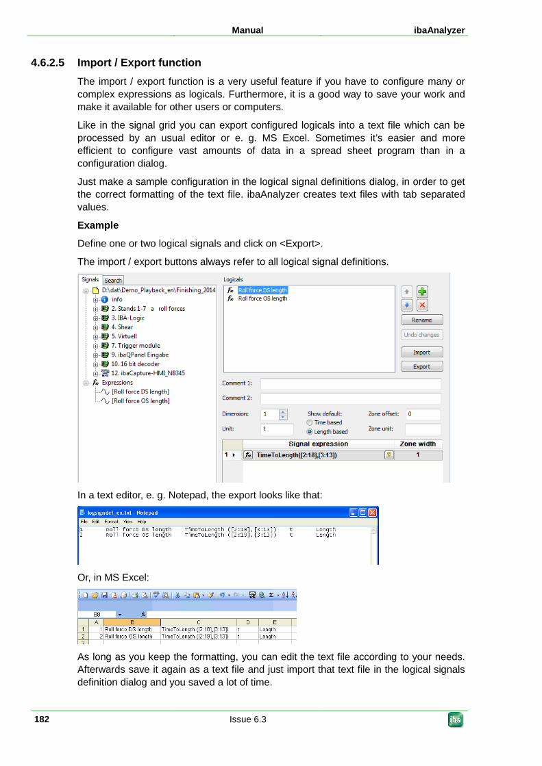
Manual ibaAnalyzer

182 Issue 6.3

4.6.2.5 Import / Export function The import / export function is a very useful feature if you have to configure many or complex expressions as logicals. Furthermore, it is a good way to save your work and make it available for other users or computers.

Like in the signal grid you can export configured logicals into a text file which can be processed by an usual editor or e. g. MS Excel. Sometimes it’s easier and more efficient to configure vast amounts of data in a spread sheet program than in a configuration dialog.

Just make a sample configuration in the logical signal definitions dialog, in order to get the correct formatting of the text file. ibaAnalyzer creates text files with tab separated values.

Example

Define one or two logical signals and click on <Export>.

The import / export buttons always refer to all logical signal definitions.

In a text editor, e. g. Notepad, the export looks like that:

Or, in MS Excel:

As long as you keep the formatting, you can edit the text file according to your needs. Afterwards save it again as a text file and just import that text file in the logical signals definition dialog and you saved a lot of time.

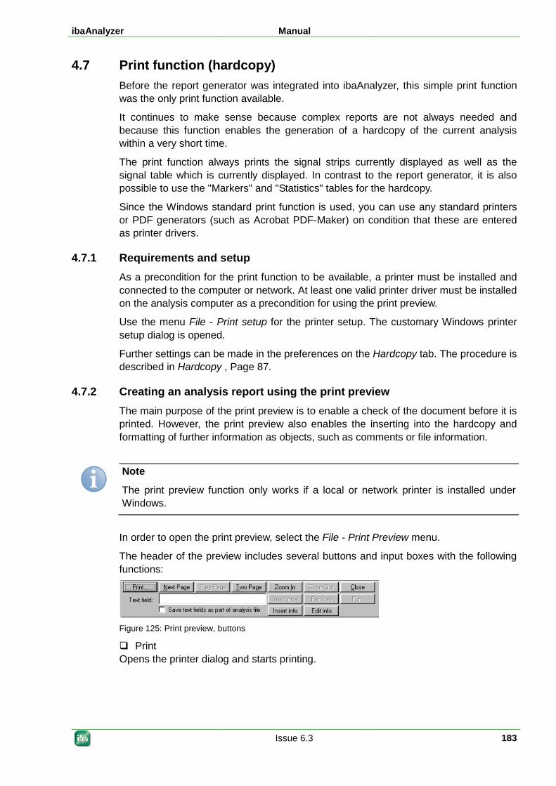
ibaAnalyzer Manual

Issue 6.3 183

4.7 Print function (hardcopy) Before the report generator was integrated into ibaAnalyzer, this simple print function was the only print function available.

It continues to make sense because complex reports are not always needed and because this function enables the generation of a hardcopy of the current analysis within a very short time.

The print function always prints the signal strips currently displayed as well as the signal table which is currently displayed. In contrast to the report generator, it is also possible to use the "Markers" and "Statistics" tables for the hardcopy.

Since the Windows standard print function is used, you can use any standard printers or PDF generators (such as Acrobat PDF-Maker) on condition that these are entered as printer drivers.

4.7.1 Requirements and setup As a precondition for the print function to be available, a printer must be installed and connected to the computer or network. At least one valid printer driver must be installed on the analysis computer as a precondition for using the print preview.

Use the menu File - Print setup for the printer setup. The customary Windows printer setup dialog is opened.

Further settings can be made in the preferences on the Hardcopy tab. The procedure is described in Hardcopy , Page 87.

4.7.2 Creating an analysis report using the print preview The main purpose of the print preview is to enable a check of the document before it is printed. However, the print preview also enables the inserting into the hardcopy and formatting of further information as objects, such as comments or file information.

Note

The print preview function only works if a local or network printer is installed under Windows.

In order to open the print preview, select the File - Print Preview menu.

The header of the preview includes several buttons and input boxes with the following functions:

Figure 125: Print preview, buttons

Print Opens the printer dialog and starts printing.

Manual ibaAnalyzer

184 Issue 6.3

Next page Open the next page.

This button is only active if one page only is displayed but if more than two pages exist, or if two pages are displayed and if more than two pages exist.

Page preview Open the previous page.

This button is only active if one page only is displayed but if more than two pages exist, or if two pages are displayed and if more than two pages exist.

One page / two pages This toggle function can be used to decide whether the print preview is to show one or two pages.

Zoom in Slightly enlarges the page displayed (by one step).

Zoom out Reduces the page displayed until it is completely displayed in the window, or until two pages are displayed in the window, respectively.

Close Closes the print preview and returns to ibaAnalyzer.

Text field In this input box, you can enter any text and comment you like. Just click into the field and then enter the text. Thereafter, click <Insert new>. The text is added to the sheet and the input line is cleared for the next entries.

Insert new Entering the text line on the sheet.

The text inserted is initially positioned in the middle of the first page or of the sheet displayed. Use the mouse in order to move the text to wherever you like.

Remove Removes a previously marked object from the print sheet (text and information only).

Font Opens a dialog window where you can select the font to be used for a previously marked object (text and information only).

Insert info You can use this button in order to select information from the "Info" branch of the data file and to insert this information in the hardcopy, for example, the start time of the recording process.

Just mark the desired information and click < OK >.

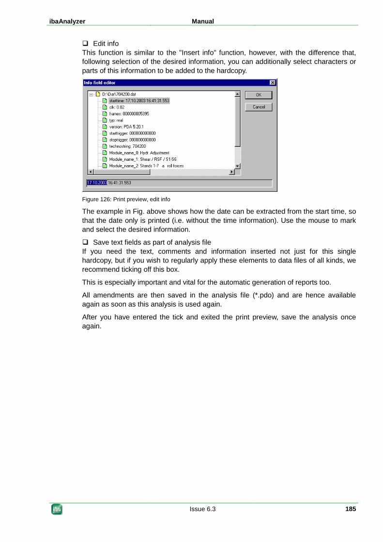
ibaAnalyzer Manual

Issue 6.3 185

Edit info This function is similar to the "Insert info" function, however, with the difference that, following selection of the desired information, you can additionally select characters or parts of this information to be added to the hardcopy.

Figure 126: Print preview, edit info

The example in Fig. above shows how the date can be extracted from the start time, so that the date only is printed (i.e. without the time information). Use the mouse to mark and select the desired information.

Save text fields as part of analysis file If you need the text, comments and information inserted not just for this single hardcopy, but if you wish to regularly apply these elements to data files of all kinds, we recommend ticking off this box.

This is especially important and vital for the automatic generation of reports too.

All amendments are then saved in the analysis file (*.pdo) and are hence available again as soon as this analysis is used again.

After you have entered the tick and exited the print preview, save the analysis once again.

Manual ibaAnalyzer

186 Issue 6.3

4.8 Exporting data 4.8.1 Purpose

Exporting data from an analysis offers many advantages. The most important advantage is probably the focus on the key elements of an analysis, especially in cases in which the analysis is to be documented or passed on to other users.

Since the recipients of such data do not necessarily or not exclusively use ibaAnalyzer, you can use the export function in order to convert the measuring data to a generally readable standard format, such as a text file. The ASCII file which is generated by the export function can be imported by practically every other program, no matter whether spreadsheet (such as MS Excel), analysis (such as MatLab), database (such as MS Access) or word processing (such as MS Word).

Furthermore, the COMTRADE format was created for special evaluations, for example, in the field of energy technology.

If the further analysis is to be carried out with ibaAnalyzer again, select the option of exporting the data to a *.dat file. Users of this export data can then use the full functionality of ibaAnalyzer for the further processing of this data. Furthermore, it is also possible to add the analysis to the export file, so that the recipient has the correct display immediately on opening the data file.

If, for example, a malfunction in a plant is analyzed and if you have finally identified and analyzed the cause of the problem, including all its boundary conditions, then it may be very helpful if the relevant measuring data and/or time intervals can be singled out from many thousand irrelevant measuring points and saved in a new file. This form of data reduction obviously also drastically reduces the size of the file which can hence be easily sent by e-mail.

Any original signals, expressions and virtual signals visible in ibaAnalyzer can be exported.

When using ibaCapture-CAM in conjunction with ibaAnalyzer even the relevant video scenes can be exported either as part of the new data file or as separate video file.

Note

The export function described in this chapter can only be used manually, i.e. each export procedure must be configured and triggered manually.

For an automated export, e.g. with ibaDatCoordinator, there is a so-called data extraction function available. This function requires a license and can be configured in the same dialog like the data base extraction. Instead of a database the export target is just a file. Similar options like for Export and more functions are available for extraction.

The product name of the extractor license is ibaAnalyzer-Dat-Extractor.

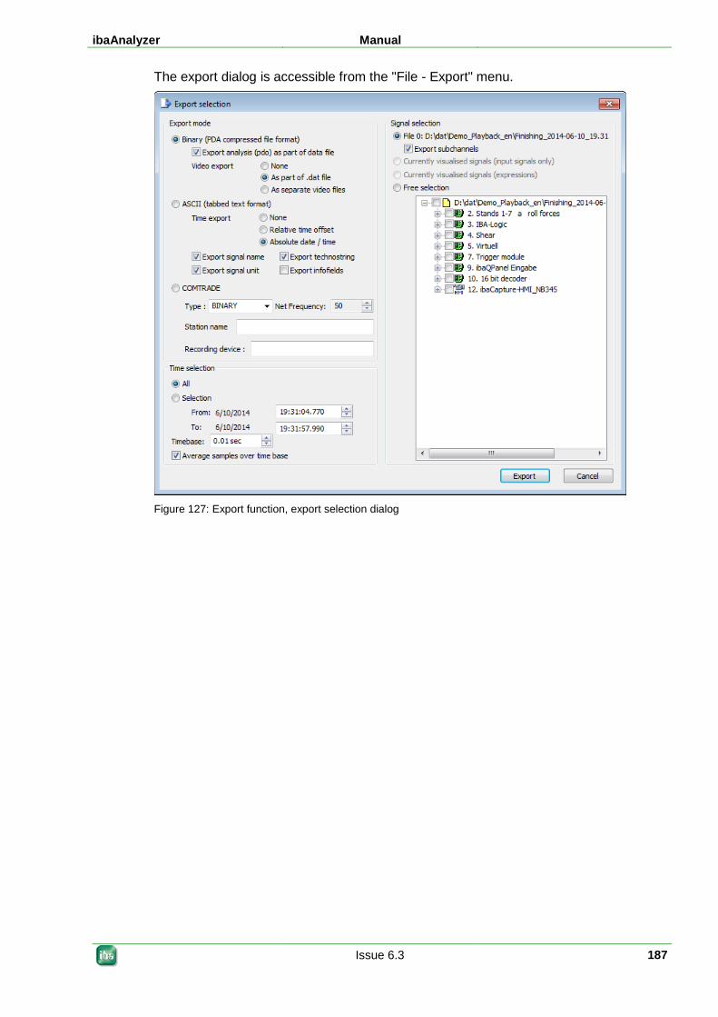
ibaAnalyzer Manual

Issue 6.3 187

The export dialog is accessible from the "File - Export" menu.

Figure 127: Export function, export selection dialog

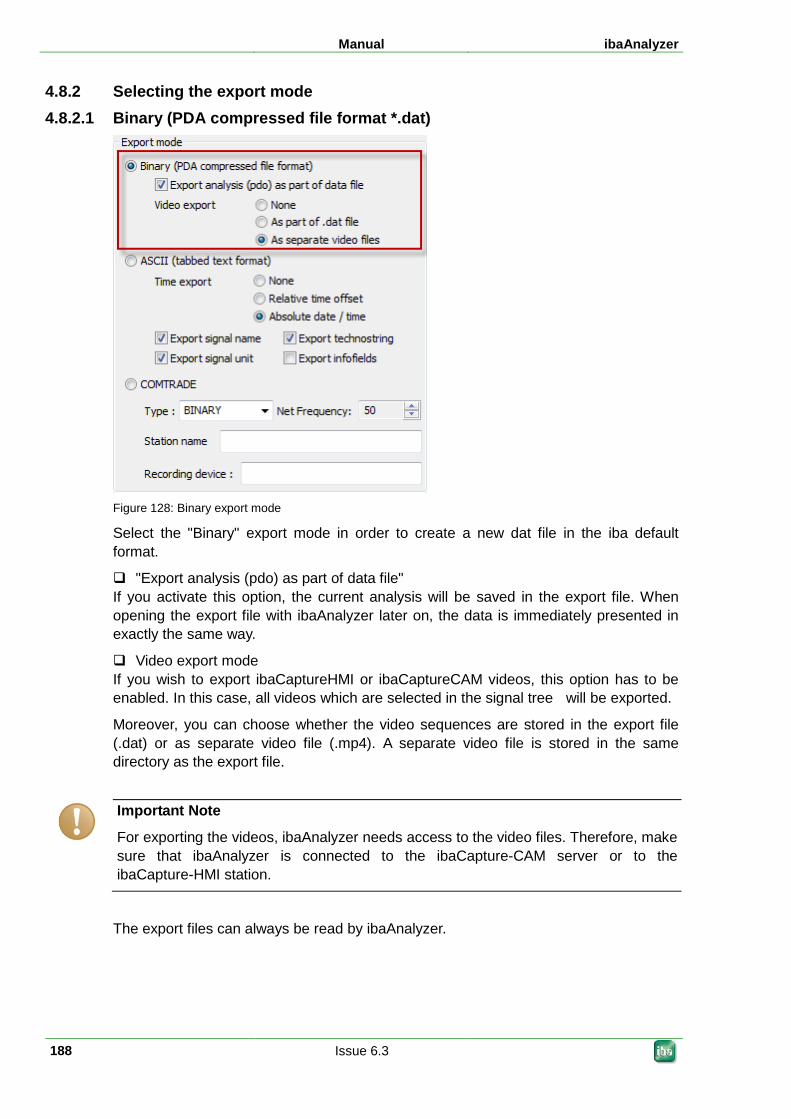
Manual ibaAnalyzer

188 Issue 6.3

4.8.2 Selecting the export mode 4.8.2.1 Binary (PDA compressed file format *.dat)

Figure 128: Binary export mode

Select the "Binary" export mode in order to create a new dat file in the iba default format.

"Export analysis (pdo) as part of data file" If you activate this option, the current analysis will be saved in the export file. When opening the export file with ibaAnalyzer later on, the data is immediately presented in exactly the same way.

Video export mode If you wish to export ibaCaptureHMI or ibaCaptureCAM videos, this option has to be enabled. In this case, all videos which are selected in the signal tree will be exported.

Moreover, you can choose whether the video sequences are stored in the export file (.dat) or as separate video file (.mp4). A separate video file is stored in the same directory as the export file.

Important Note

For exporting the videos, ibaAnalyzer needs access to the video files. Therefore, make sure that ibaAnalyzer is connected to the ibaCapture-CAM server or to the ibaCapture-HMI station.

The export files can always be read by ibaAnalyzer.

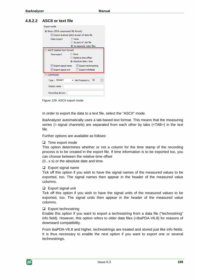
ibaAnalyzer Manual

Issue 6.3 189

4.8.2.2 ASCII or text file

Figure 129: ASCII export mode

In order to export the data to a text file, select the "ASCII" mode.

ibaAnalyzer automatically uses a tab-based text format. This means that the measuring series (= signal channels) are separated from each other by tabs (<TAB>) in the text file.

Further options are available as follows:

Time export mode This option determines whether or not a column for the time stamp of the recording process is to be created in the export file. If time information is to be exported too, you can choose between the relative time offset (0...x s) or the absolute date and time.

Export signal name Tick off this option if you wish to have the signal names of the measured values to be exported, too. The signal names then appear in the header of the measured value columns.

Export signal unit Tick off this option if you wish to have the signal units of the measured values to be exported, too. The signal units then appear in the header of the measured value columns.

Export technostring Enable this option if you want to export a technostring from a data file ("technostring" info field). However, this option refers to older data files (<ibaPDA-V6.8) for reasons of downward compatibility.

From ibaPDA-V6.8 and higher, technostrings are treated and stored just like info fields. It is thus necessary to enable the next option if you want to export one or several technostrings.

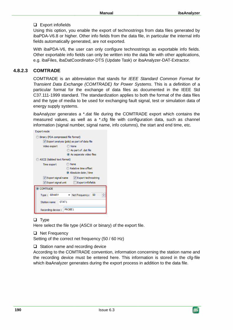
Manual ibaAnalyzer

190 Issue 6.3

Export infofields Using this option, you enable the export of technostrings from data files generated by ibaPDA-V6.8 or higher. Other info fields from the data file, in particular the internal info fields automatically generated, are not exported.

With ibaPDA-V6, the user can only configure technostrings as exportable info fields. Other exportable info fields can only be written into the data file with other applications, e.g. ibaFiles, ibaDatCoordinator-DTS (Update Task) or ibaAnalyzer-DAT-Extractor.

4.8.2.3 COMTRADE COMTRADE is an abbreviation that stands for IEEE Standard Common Format for Transient Data Exchange (COMTRADE) for Power Systems. This is a definition of a particular format for the exchange of data files as documented in the IEEE Std C37.111-1999 standard. The standardization applies to both the format of the data files and the type of media to be used for exchanging fault signal, test or simulation data of energy supply systems.

ibaAnalyzer generates a *.dat file during the COMTRADE export which contains the measured values, as well as a *.cfg file with configuration data, such as channel information (signal number, signal name, info columns), the start and end time, etc.

Type Here select the file type (ASCII or binary) of the export file.

Net Frequency Setting of the correct net frequency (50 / 60 Hz)

Station name and recording device According to the COMTRADE convention, information concerning the station name and the recording device must be entered here. This information is stored in the cfg-file which ibaAnalyzer generates during the export process in addition to the data file.

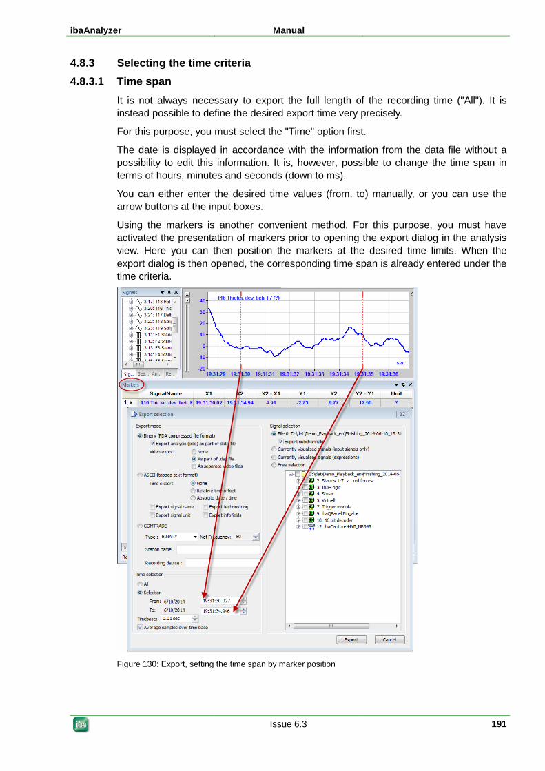
ibaAnalyzer Manual

Issue 6.3 191

4.8.3 Selecting the time criteria 4.8.3.1 Time span

It is not always necessary to export the full length of the recording time ("All"). It is instead possible to define the desired export time very precisely.

For this purpose, you must select the "Time" option first.

The date is displayed in accordance with the information from the data file without a possibility to edit this information. It is, however, possible to change the time span in terms of hours, minutes and seconds (down to ms).

You can either enter the desired time values (from, to) manually, or you can use the arrow buttons at the input boxes.

Using the markers is another convenient method. For this purpose, you must have activated the presentation of markers prior to opening the export dialog in the analysis view. Here you can then position the markers at the desired time limits. When the export dialog is then opened, the corresponding time span is already entered under the time criteria.

Figure 130: Export, setting the time span by marker position

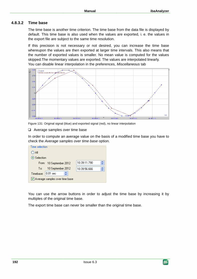
Manual ibaAnalyzer

192 Issue 6.3

4.8.3.2 Time base The time base is another time criterion. The time base from the data file is displayed by default. This time base is also used when the values are exported, i. e. the values in the export file are subject to the same time resolution.

If this precision is not necessary or not desired, you can increase the time base whereupon the values are then exported at larger time intervals. This also means that the number of exported values is smaller. No mean value is computed for the values skipped.The momentary values are exported. The values are interpolated linearly. You can disable linear interpolation in the preferences, Miscellaneous tab

Figure 131: Original signal (blue) and exported signal (red), no linear interpolation

Average samples over time base

In order to compute an average value on the basis of a modified time base you have to check the Average samples over time base option.

You can use the arrow buttons in order to adjust the time base by increasing it by multiples of the original time base.

The export time base can never be smaller than the original time base.

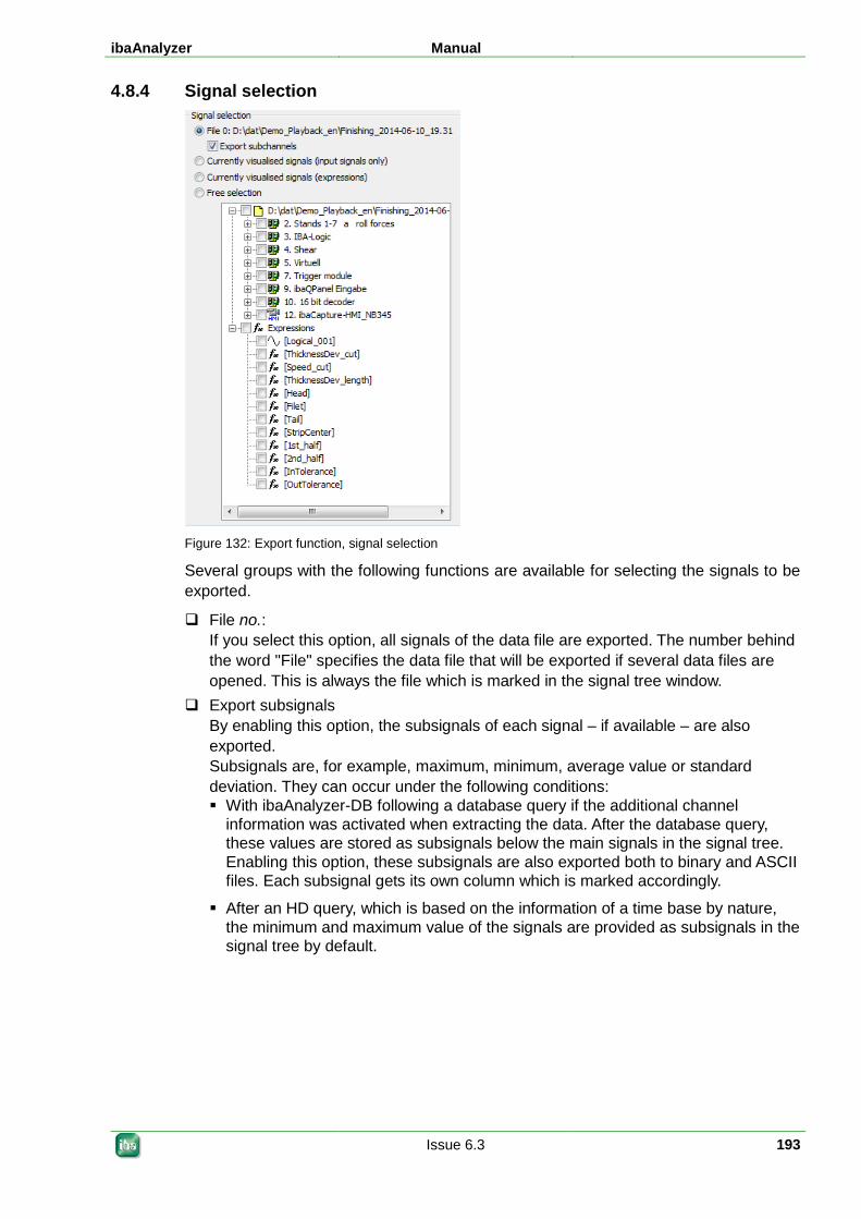
ibaAnalyzer Manual

Issue 6.3 193

4.8.4 Signal selection

Figure 132: Export function, signal selection

Several groups with the following functions are available for selecting the signals to be exported.

File no.: If you select this option, all signals of the data file are exported. The number behind the word "File" specifies the data file that will be exported if several data files are opened. This is always the file which is marked in the signal tree window.

Export subsignals By enabling this option, the subsignals of each signal – if available – are also exported. Subsignals are, for example, maximum, minimum, average value or standard deviation. They can occur under the following conditions: With ibaAnalyzer-DB following a database query if the additional channel

information was activated when extracting the data. After the database query, these values are stored as subsignals below the main signals in the signal tree. Enabling this option, these subsignals are also exported both to binary and ASCII files. Each subsignal gets its own column which is marked accordingly.

After an HD query, which is based on the information of a time base by nature, the minimum and maximum value of the signals are provided as subsignals in the signal tree by default.

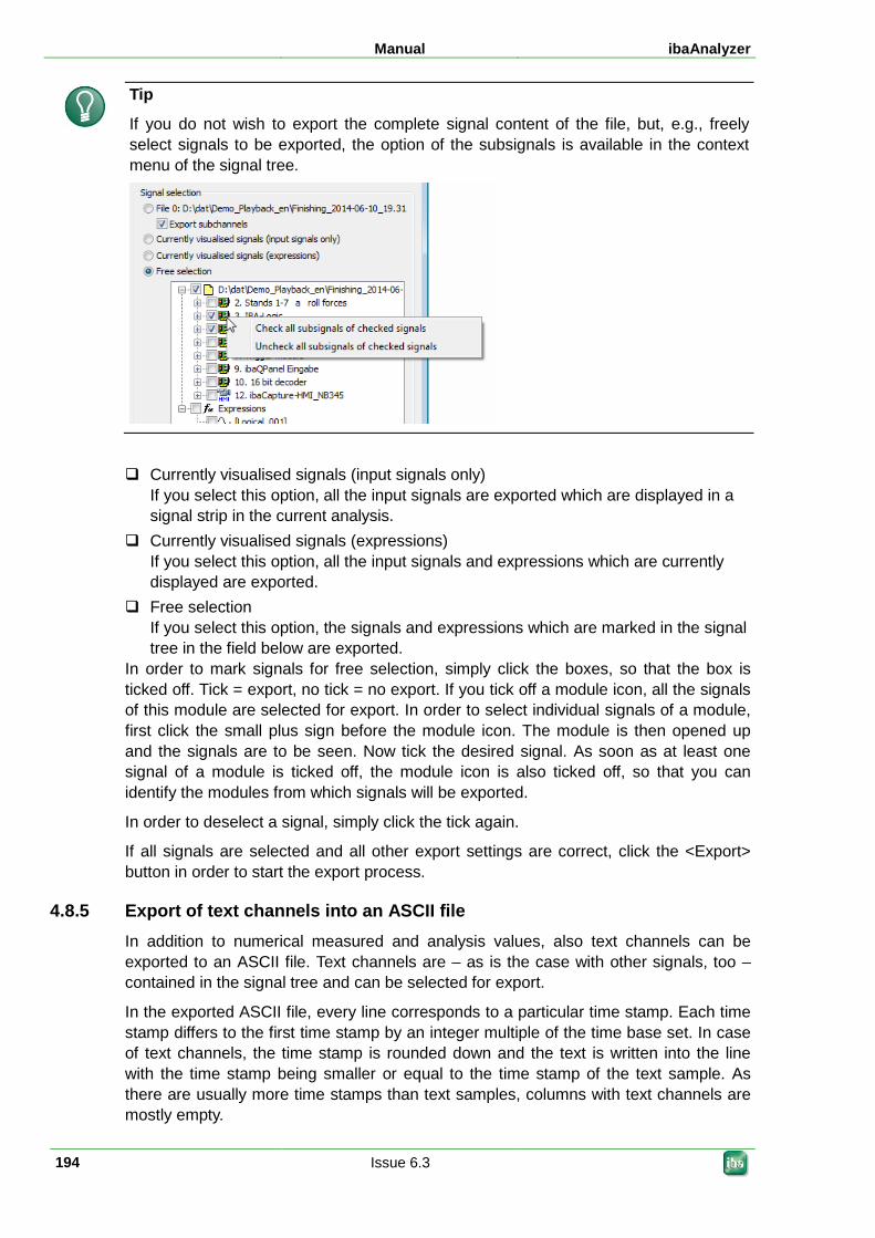
Manual ibaAnalyzer

194 Issue 6.3

Tip

If you do not wish to export the complete signal content of the file, but, e.g., freely select signals to be exported, the option of the subsignals is available in the context menu of the signal tree.

Currently visualised signals (input signals only) If you select this option, all the input signals are exported which are displayed in a signal strip in the current analysis.

Currently visualised signals (expressions) If you select this option, all the input signals and expressions which are currently displayed are exported.

Free selection If you select this option, the signals and expressions which are marked in the signal tree in the field below are exported.

In order to mark signals for free selection, simply click the boxes, so that the box is ticked off. Tick = export, no tick = no export. If you tick off a module icon, all the signals of this module are selected for export. In order to select individual signals of a module, first click the small plus sign before the module icon. The module is then opened up and the signals are to be seen. Now tick the desired signal. As soon as at least one signal of a module is ticked off, the module icon is also ticked off, so that you can identify the modules from which signals will be exported.

In order to deselect a signal, simply click the tick again.

If all signals are selected and all other export settings are correct, click the <Export> button in order to start the export process.

4.8.5 Export of text channels into an ASCII file In addition to numerical measured and analysis values, also text channels can be exported to an ASCII file. Text channels are – as is the case with other signals, too – contained in the signal tree and can be selected for export.

In the exported ASCII file, every line corresponds to a particular time stamp. Each time stamp differs to the first time stamp by an integer multiple of the time base set. In case of text channels, the time stamp is rounded down and the text is written into the line with the time stamp being smaller or equal to the time stamp of the text sample. As there are usually more time stamps than text samples, columns with text channels are mostly empty.

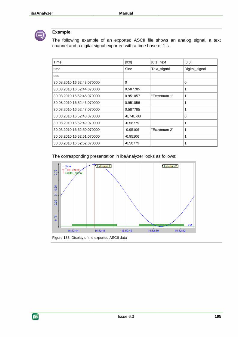
ibaAnalyzer Manual

Issue 6.3 195

Example

The following example of an exported ASCII file shows an analog signal, a text channel and a digital signal exported with a time base of 1 s.

Time [0:0] [0:1]_text [0.0]

time Sine Text_signal Digital_signal

sec

30.08.2010 16:52:43.070000 0 0

30.08.2010 16:52:44.070000 0.587785 1

30.08.2010 16:52:45.070000 0.951057 "Extremum 1" 1

30.08.2010 16:52:46.070000 0.951056 1

30.08.2010 16:52:47.070000 0.587785 1

30.08.2010 16:52:48.070000 -8,74E-08 0

30.08.2010 16:52:49.070000 -0.58779 1

30.08.2010 16:52:50.070000 -0.95106 "Extremum 2" 1

30.08.2010 16:52:51.070000 -0.95106 1

30.08.2010 16:52:52.070000 -0.58779 1

The corresponding presentation in ibaAnalyzer looks as follows:

Figure 133: Display of the exported ASCII data

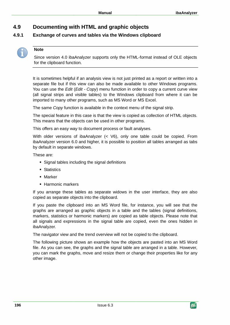
Manual ibaAnalyzer

196 Issue 6.3

4.9 Documenting with HTML and graphic objects 4.9.1 Exchange of curves and tables via the Windows clipboard

Note

Since version 4.0 ibaAnalyzer supports only the HTML-format instead of OLE objects for the clipboard function.

It is sometimes helpful if an analysis view is not just printed as a report or written into a separate file but if this view can also be made available to other Windows programs. You can use the Edit (Edit - Copy) menu function in order to copy a current curve view (all signal strips and visible tables) to the Windows clipboard from where it can be imported to many other programs, such as MS Word or MS Excel.

The same Copy function is available in the context menu of the signal strip.

The special feature in this case is that the view is copied as collection of HTML objects. This means that the objects can be used in other programs.

This offers an easy way to document process or fault analyses.

With older versions of ibaAnalyzer (< V6), only one table could be copied. From ibaAnalyzer version 6.0 and higher, it is possible to position all tables arranged as tabs by default in separate windows.

These are:

Signal tables including the signal definitions

Statistics

Marker

Harmonic markers

If you arrange these tables as separate widows in the user interface, they are also copied as separate objects into the clipboard.

If you paste the clipboard into an MS Word file, for instance, you will see that the graphs are arranged as graphic objects in a table and the tables (signal definitions, markers, statistics or harmonic markers) are copied as table objects. Please note that all signals and expressions in the signal table are copied, even the ones hidden in ibaAnalyzer.

The navigator view and the trend overview will not be copied to the clipboard.

The following picture shows an example how the objects are pasted into an MS Word file. As you can see, the graphs and the signal table are arranged in a table. However, you can mark the graphs, move and resize them or change their properties like for any other image.

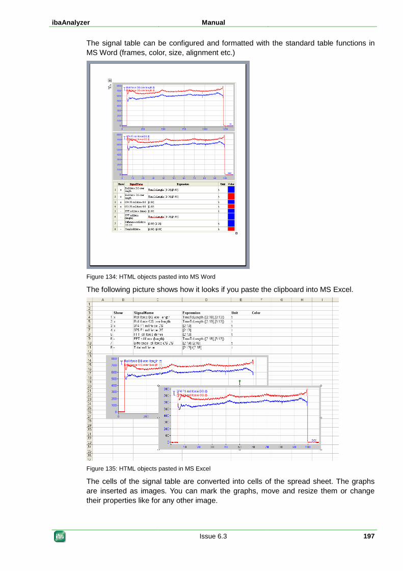
ibaAnalyzer Manual

Issue 6.3 197

The signal table can be configured and formatted with the standard table functions in MS Word (frames, color, size, alignment etc.)

Figure 134: HTML objects pasted into MS Word

The following picture shows how it looks if you paste the clipboard into MS Excel.

Figure 135: HTML objects pasted in MS Excel

The cells of the signal table are converted into cells of the spread sheet. The graphs are inserted as images. You can mark the graphs, move and resize them or change their properties like for any other image.

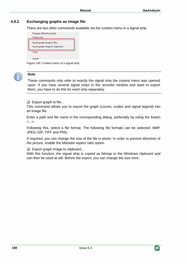
Manual ibaAnalyzer

198 Issue 6.3

4.9.2 Exchanging graphs as image file There are two other commands available via the context menu in a signal strip.

Figure 136: Context menu of a signal strip

Note

These commands only refer to exactly the signal strip the context menu was opened upon. If you have several signal strips in the recorder window and want to export them, you have to do this for each strip separately.

Export graph to file... This command allows you to export the graph (curves, scales and signal legend) into an image file.

Enter a path and file name in the corresponding dialog, preferably by using the button <...>.

Following this, select a file format. The following file formats can be selected: BMP, JPEG, GIF, TIFF and PNG.

If required, you can change the size of the file in pixels. In order to prevent distortion of the picture, enable the Maintain aspect ratio option.

Export graph image to clipboard... With this function, the signal strip is copied as bitmap to the Windows clipboard and can then be used at will. Before the export, you can change the size here.

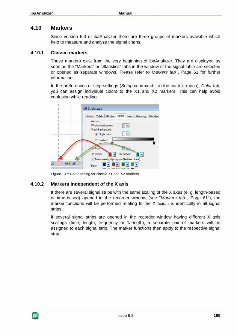
ibaAnalyzer Manual

Issue 6.3 199

4.10 Markers Since version 5.0 of ibaAnalyzer there are three groups of markers available which help to measure and analyze the signal charts.

4.10.1 Classic markers These markers exist from the very beginning of ibaAnalyzer. They are displayed as soon as the "Markers" or "Statistics" tabs in the window of the signal table are selected or opened as separate windows. Please refer to Markers tab , Page 61 for further information.

In the preferences or strip settings (Setup command... in the context menu), Color tab, you can assign individual colors to the X1 and X2 markers. This can help avoid confusion while reading.

Figure 137: Color setting for classic X1 and X2 markers

4.10.2 Markers independent of the X axis If there are several signal strips with the same scaling of the X axes (e. g. length-based or time-based) opened in the recorder window (see "Markers tab , Page 61"), the marker functions will be performed relating to the X axis, i.e. identically in all signal strips.

If several signal strips are opened in the recorder window having different X axis scalings (time, length, frequency or 1/length), a separate pair of markers will be assigned to each signal strip. The marker functions then apply to the respective signal strip.

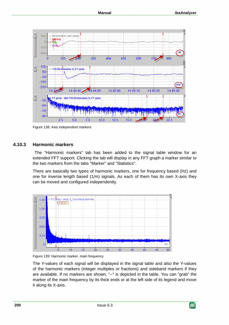
Manual ibaAnalyzer

200 Issue 6.3

Figure 138: Axis independent markers

4.10.3 Harmonic markers The "Harmonic markers" tab has been added to the signal table window for an extended FFT support. Clicking the tab will display in any FFT graph a marker similar to the two markers from the tabs "Marker" and "Statistics".

There are basically two types of harmonic markers, one for frequency based (Hz) and one for inverse length based (1/m) signals. As each of them has its own X-axis they can be moved and configured independently.

Figure 139: Harmonic marker, main frequency

The Y-values of each signal will be displayed in the signal table and also the Y-values of the harmonic markers (integer multiples or fractions) and sideband markers if they are available. If no markers are shown, “--“ is depicted in the table. You can "grab" the marker of the main frequency by its thick ends or at the left side of its legend and move it along its X-axis.

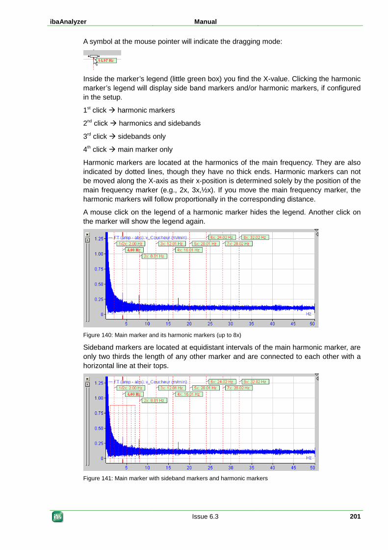
ibaAnalyzer Manual

Issue 6.3 201

A symbol at the mouse pointer will indicate the dragging mode:

Inside the marker’s legend (little green box) you find the X-value. Clicking the harmonic marker’s legend will display side band markers and/or harmonic markers, if configured in the setup.

1st click harmonic markers

2nd click harmonics and sidebands

3rd click sidebands only

4th click main marker only

Harmonic markers are located at the harmonics of the main frequency. They are also indicated by dotted lines, though they have no thick ends. Harmonic markers can not be moved along the X-axis as their x-position is determined solely by the position of the main frequency marker (e.g., 2x, 3x,½x). If you move the main frequency marker, the harmonic markers will follow proportionally in the corresponding distance.

A mouse click on the legend of a harmonic marker hides the legend. Another click on the marker will show the legend again.

Figure 140: Main marker and its harmonic markers (up to 8x)

Sideband markers are located at equidistant intervals of the main harmonic marker, are only two thirds the length of any other marker and are connected to each other with a horizontal line at their tops.

Figure 141: Main marker with sideband markers and harmonic markers

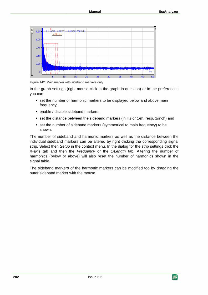
Manual ibaAnalyzer

202 Issue 6.3

Figure 142: Main marker with sideband markers only

In the graph settings (right mouse click in the graph in question) or in the preferences you can:

set the number of harmonic markers to be displayed below and above main frequency,

enable / disable sideband markers,

set the distance between the sideband markers (in Hz or 1/m, resp. 1/inch) and

set the number of sideband markers (symmetrical to main frequency) to be shown.

The number of sideband and harmonic markers as well as the distance between the individual sideband markers can be altered by right clicking the corresponding signal strip. Select then Setup in the context menu. In the dialog for the strip settings click the X-axis tab and then the Frequency or the 1/Length tab. Altering the number of harmonics (below or above) will also reset the number of harmonics shown in the signal table.

The sideband markers of the harmonic markers can be modified too by dragging the outer sideband marker with the mouse.

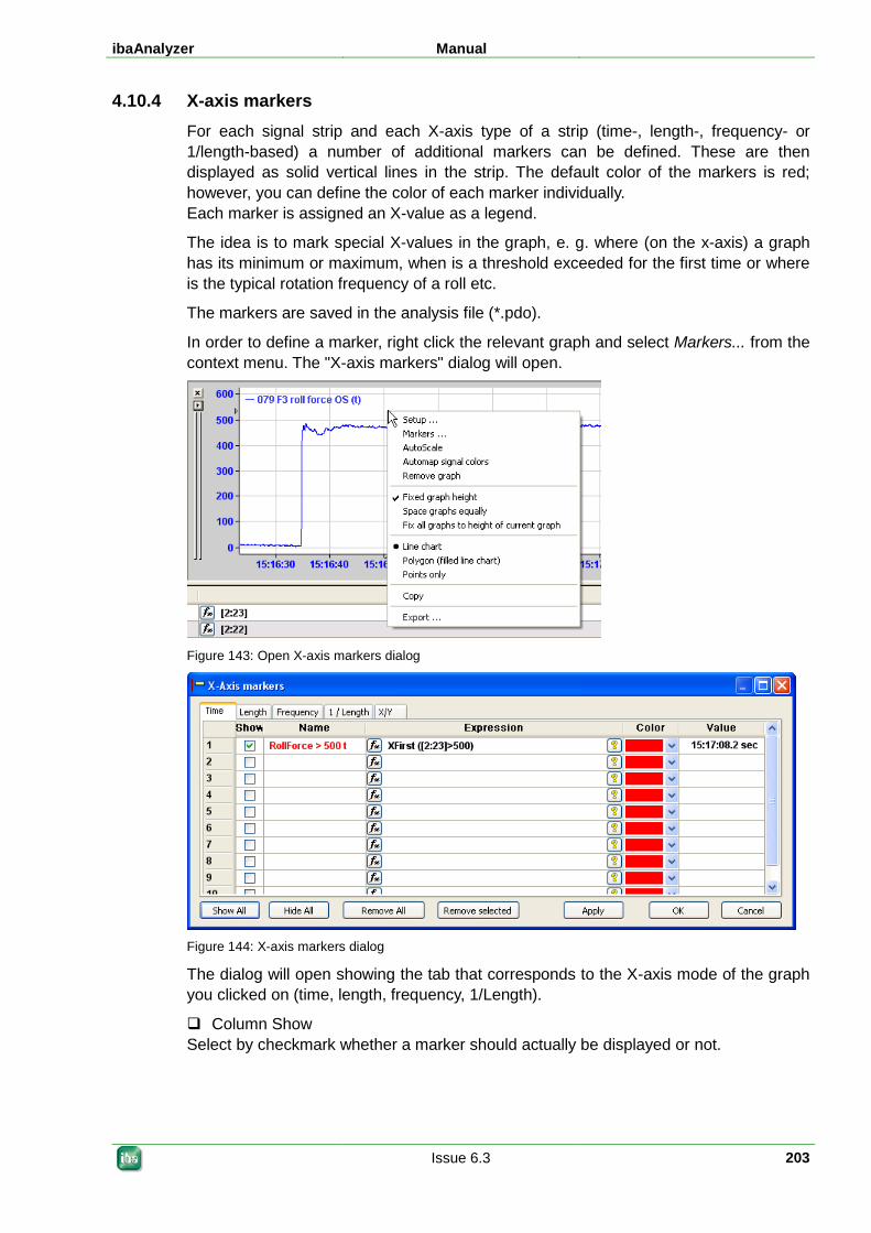
ibaAnalyzer Manual

Issue 6.3 203

4.10.4 X-axis markers For each signal strip and each X-axis type of a strip (time-, length-, frequency- or 1/length-based) a number of additional markers can be defined. These are then displayed as solid vertical lines in the strip. The default color of the markers is red; however, you can define the color of each marker individually. Each marker is assigned an X-value as a legend.

The idea is to mark special X-values in the graph, e. g. where (on the x-axis) a graph has its minimum or maximum, when is a threshold exceeded for the first time or where is the typical rotation frequency of a roll etc.

The markers are saved in the analysis file (*.pdo).

In order to define a marker, right click the relevant graph and select Markers... from the context menu. The "X-axis markers" dialog will open.

Figure 143: Open X-axis markers dialog

Figure 144: X-axis markers dialog

The dialog will open showing the tab that corresponds to the X-axis mode of the graph you clicked on (time, length, frequency, 1/Length).

Column Show Select by checkmark whether a marker should actually be displayed or not.

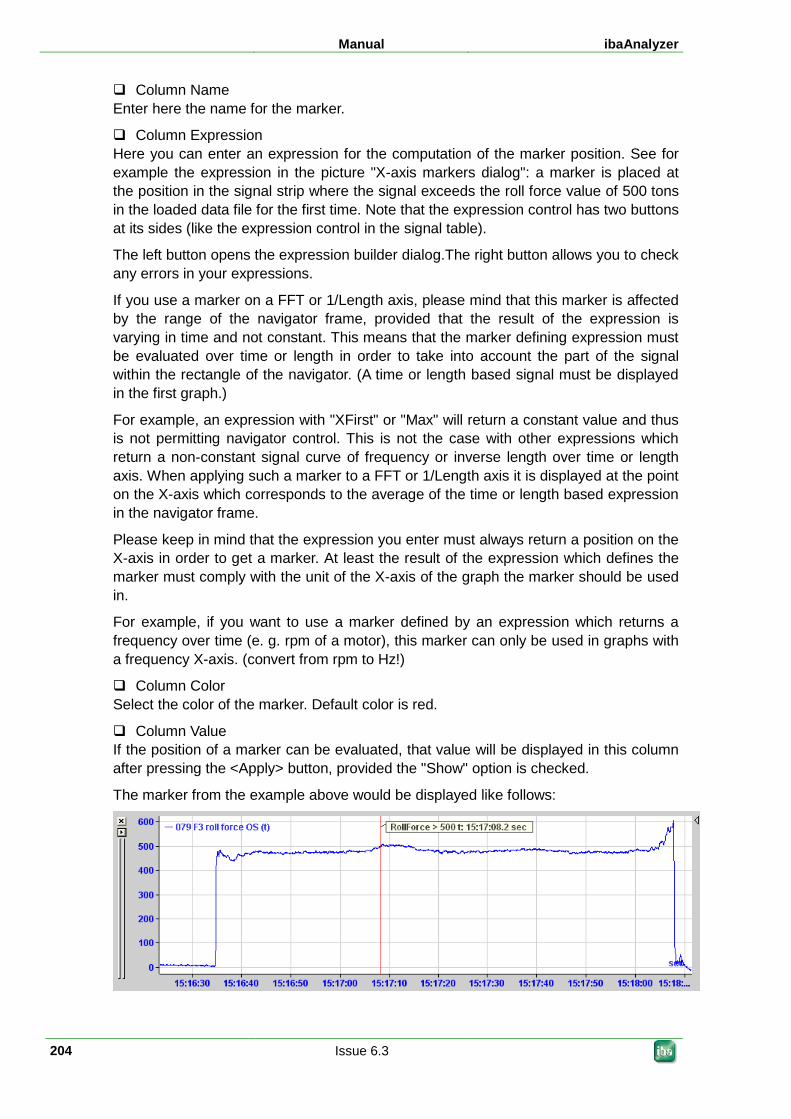
Manual ibaAnalyzer

204 Issue 6.3

Column Name Enter here the name for the marker.

Column Expression Here you can enter an expression for the computation of the marker position. See for example the expression in the picture "X-axis markers dialog": a marker is placed at the position in the signal strip where the signal exceeds the roll force value of 500 tons in the loaded data file for the first time. Note that the expression control has two buttons at its sides (like the expression control in the signal table).

The left button opens the expression builder dialog.The right button allows you to check any errors in your expressions.

If you use a marker on a FFT or 1/Length axis, please mind that this marker is affected by the range of the navigator frame, provided that the result of the expression is varying in time and not constant. This means that the marker defining expression must be evaluated over time or length in order to take into account the part of the signal within the rectangle of the navigator. (A time or length based signal must be displayed in the first graph.)

For example, an expression with "XFirst" or "Max" will return a constant value and thus is not permitting navigator control. This is not the case with other expressions which return a non-constant signal curve of frequency or inverse length over time or length axis. When applying such a marker to a FFT or 1/Length axis it is displayed at the point on the X-axis which corresponds to the average of the time or length based expression in the navigator frame.

Please keep in mind that the expression you enter must always return a position on the X-axis in order to get a marker. At least the result of the expression which defines the marker must comply with the unit of the X-axis of the graph the marker should be used in.

For example, if you want to use a marker defined by an expression which returns a frequency over time (e. g. rpm of a motor), this marker can only be used in graphs with a frequency X-axis. (convert from rpm to Hz!)

Column Color Select the color of the marker. Default color is red.

Column Value If the position of a marker can be evaluated, that value will be displayed in this column after pressing the <Apply> button, provided the "Show" option is checked.

The marker from the example above would be displayed like follows:

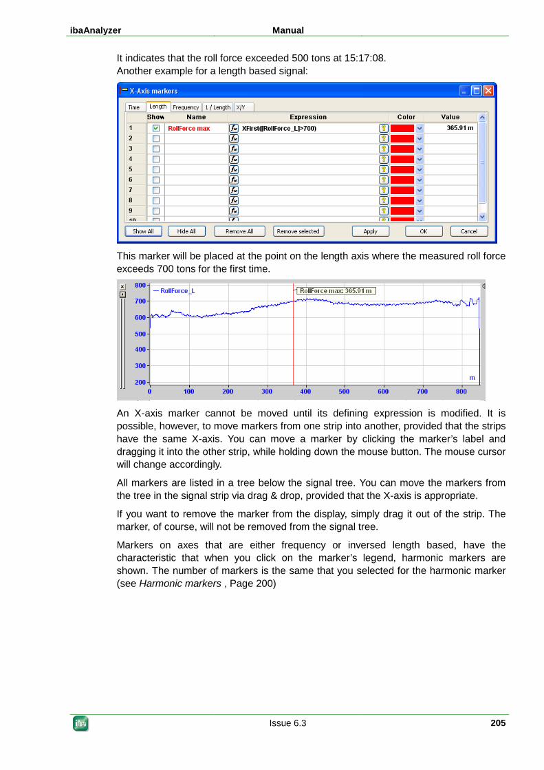
ibaAnalyzer Manual

Issue 6.3 205

It indicates that the roll force exceeded 500 tons at 15:17:08. Another example for a length based signal:

This marker will be placed at the point on the length axis where the measured roll force exceeds 700 tons for the first time.

An X-axis marker cannot be moved until its defining expression is modified. It is possible, however, to move markers from one strip into another, provided that the strips have the same X-axis. You can move a marker by clicking the marker’s label and dragging it into the other strip, while holding down the mouse button. The mouse cursor will change accordingly.

All markers are listed in a tree below the signal tree. You can move the markers from the tree in the signal strip via drag & drop, provided that the X-axis is appropriate.

If you want to remove the marker from the display, simply drag it out of the strip. The marker, of course, will not be removed from the signal tree.

Markers on axes that are either frequency or inversed length based, have the characteristic that when you click on the marker’s legend, harmonic markers are shown. The number of markers is the same that you selected for the harmonic marker (see Harmonic markers , Page 200)

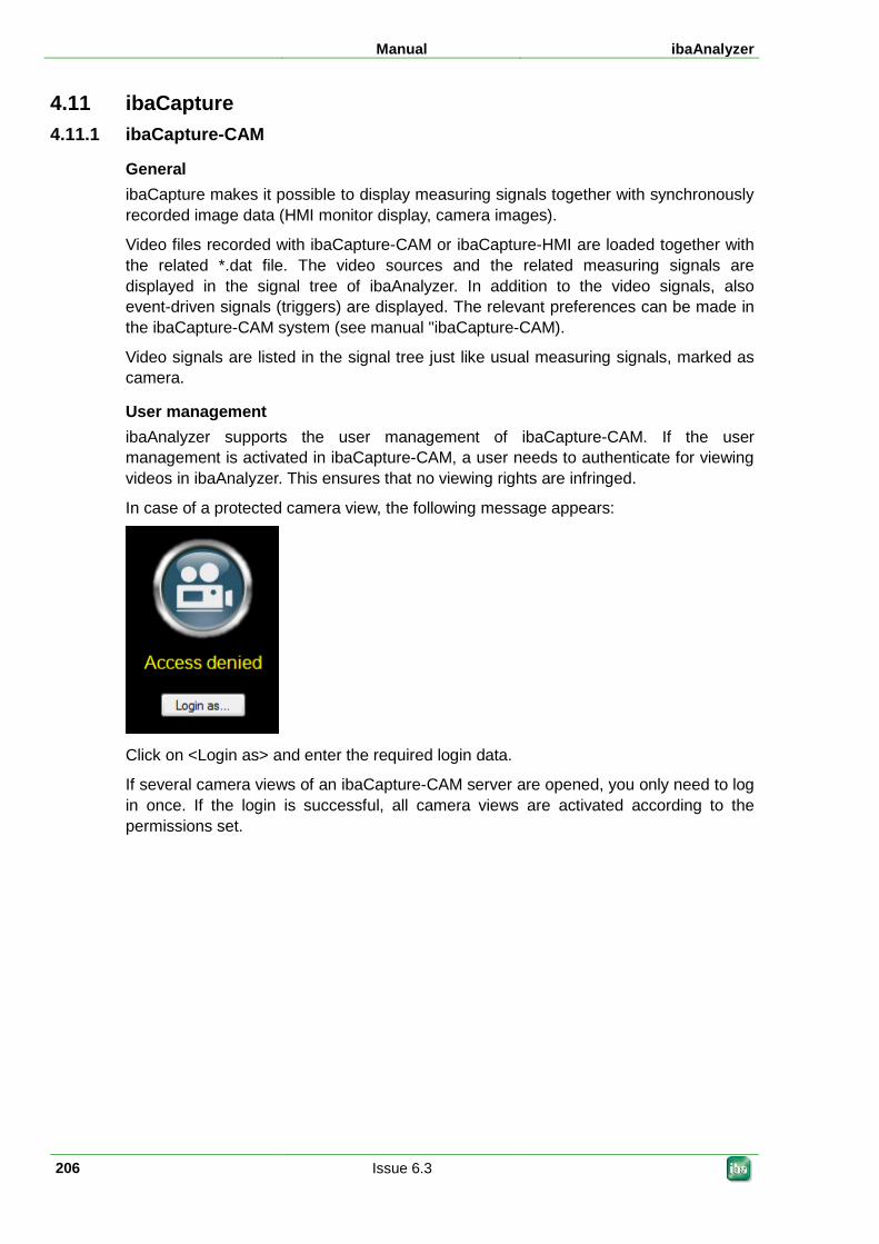
Manual ibaAnalyzer

206 Issue 6.3

4.11 ibaCapture 4.11.1 ibaCapture-CAM

General ibaCapture makes it possible to display measuring signals together with synchronously recorded image data (HMI monitor display, camera images).

Video files recorded with ibaCapture-CAM or ibaCapture-HMI are loaded together with the related *.dat file. The video sources and the related measuring signals are displayed in the signal tree of ibaAnalyzer. In addition to the video signals, also event-driven signals (triggers) are displayed. The relevant preferences can be made in the ibaCapture-CAM system (see manual "ibaCapture-CAM).

Video signals are listed in the signal tree just like usual measuring signals, marked as camera.

User management ibaAnalyzer supports the user management of ibaCapture-CAM. If the user management is activated in ibaCapture-CAM, a user needs to authenticate for viewing videos in ibaAnalyzer. This ensures that no viewing rights are infringed.

In case of a protected camera view, the following message appears:

Click on <Login as> and enter the required login data.

If several camera views of an ibaCapture-CAM server are opened, you only need to log in once. If the login is successful, all camera views are activated according to the permissions set.

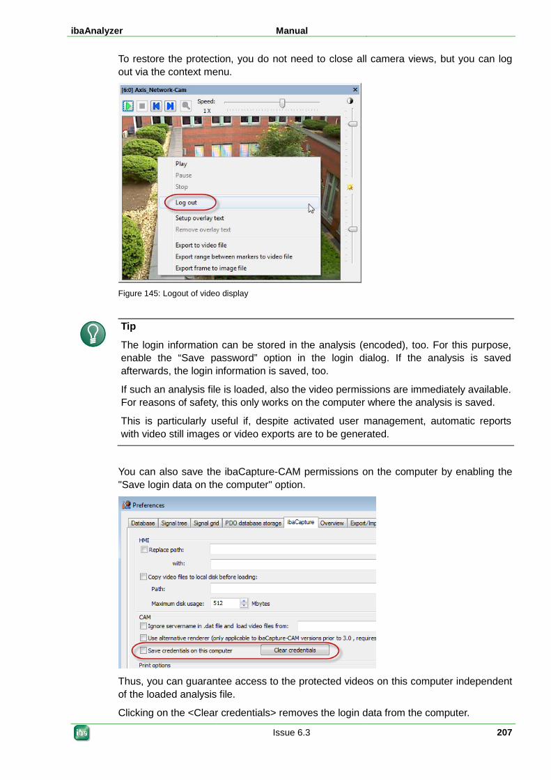
ibaAnalyzer Manual

Issue 6.3 207

To restore the protection, you do not need to close all camera views, but you can log out via the context menu.

Figure 145: Logout of video display

Tip

The login information can be stored in the analysis (encoded), too. For this purpose, enable the “Save password” option in the login dialog. If the analysis is saved afterwards, the login information is saved, too.

If such an analysis file is loaded, also the video permissions are immediately available. For reasons of safety, this only works on the computer where the analysis is saved.

This is particularly useful if, despite activated user management, automatic reports with video still images or video exports are to be generated.

You can also save the ibaCapture-CAM permissions on the computer by enabling the "Save login data on the computer" option.

Thus, you can guarantee access to the protected videos on this computer independent of the loaded analysis file.

Clicking on the <Clear credentials> removes the login data from the computer.

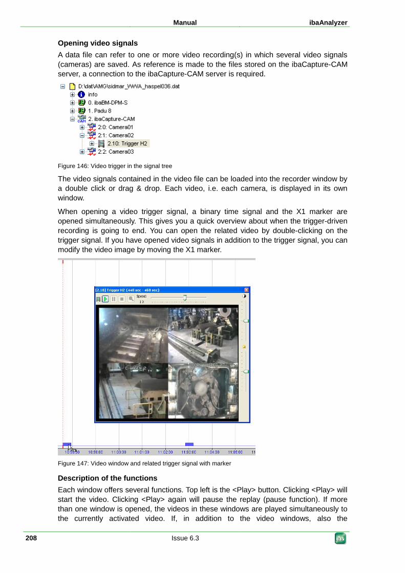
Manual ibaAnalyzer

208 Issue 6.3

Opening video signals A data file can refer to one or more video recording(s) in which several video signals (cameras) are saved. As reference is made to the files stored on the ibaCapture-CAM server, a connection to the ibaCapture-CAM server is required.

Figure 146: Video trigger in the signal tree

The video signals contained in the video file can be loaded into the recorder window by a double click or drag & drop. Each video, i.e. each camera, is displayed in its own window.

When opening a video trigger signal, a binary time signal and the X1 marker are opened simultaneously. This gives you a quick overview about when the trigger-driven recording is going to end. You can open the related video by double-clicking on the trigger signal. If you have opened video signals in addition to the trigger signal, you can modify the video image by moving the X1 marker.

Figure 147: Video window and related trigger signal with marker

Description of the functions Each window offers several functions. Top left is the <Play> button. Clicking <Play> will start the video. Clicking <Play> again will pause the replay (pause function). If more than one window is opened, the videos in these windows are played simultaneously to the currently activated video. If, in addition to the video windows, also the

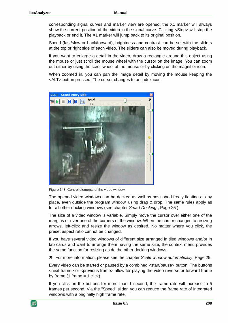
ibaAnalyzer Manual

Issue 6.3 209

corresponding signal curves and marker view are opened, the X1 marker will always show the current position of the video in the signal curve. Clicking <Stop> will stop the playback or end it. The X1 marker will jump back to its original position.

Speed (fast/slow or back/forward), brightness and contrast can be set with the sliders at the top or right side of each video. The sliders can also be moved during playback.

If you want to enlarge a detail in the video, draw a rectangle around this object using the mouse or just scroll the mouse wheel with the cursor on the image. You can zoom out either by using the scroll wheel of the mouse or by clicking on the magnifier icon.

When zoomed in, you can pan the image detail by moving the mouse keeping the <ALT> button pressed. The cursor changes to an index icon.

Figure 148: Control elements of the video window

The opened video windows can be docked as well as positioned freely floating at any place, even outside the program window, using drag & drop. The same rules apply as for all other docking windows (see chapter Smart Docking , Page 25 ).

The size of a video window is variable. Simply move the cursor over either one of the margins or over one of the corners of the window. When the cursor changes to resizing arrows, left-click and resize the window as desired. No matter where you click, the preset aspect ratio cannot be changed.

If you have several video windows of different size arranged in tiled windows and/or in tab cards and want to arrange them having the same size, the context menu provides the same function for resizing as do the other docking windows.

For more information, please see the chapter Scale window automatically, Page 29

Every video can be started or paused by a combined <start/pause> button. The buttons <next frame> or <previous frame> allow for playing the video reverse or forward frame by frame (1 frame = 1 click).

If you click on the buttons for more than 1 second, the frame rate will increase to 5 frames per second. Via the "Speed" slider, you can reduce the frame rate of integrated windows with a originally high frame rate.

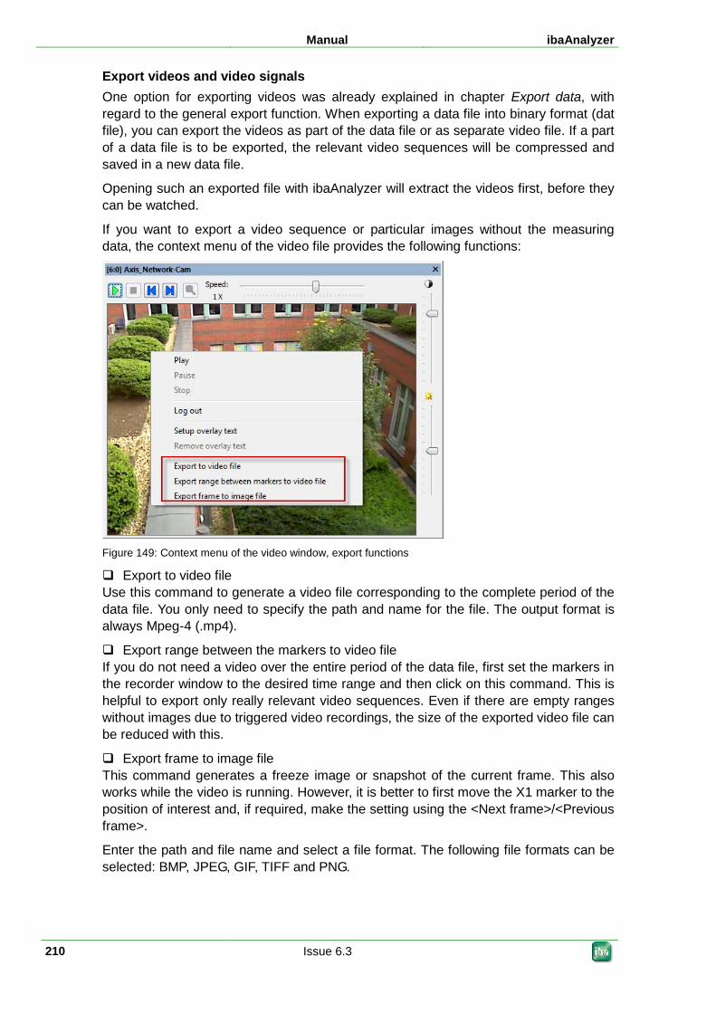
Manual ibaAnalyzer

210 Issue 6.3

Export videos and video signals One option for exporting videos was already explained in chapter Export data, with regard to the general export function. When exporting a data file into binary format (dat file), you can export the videos as part of the data file or as separate video file. If a part of a data file is to be exported, the relevant video sequences will be compressed and saved in a new data file.

Opening such an exported file with ibaAnalyzer will extract the videos first, before they can be watched.

If you want to export a video sequence or particular images without the measuring data, the context menu of the video file provides the following functions:

Figure 149: Context menu of the video window, export functions

Export to video file Use this command to generate a video file corresponding to the complete period of the data file. You only need to specify the path and name for the file. The output format is always Mpeg-4 (.mp4).

Export range between the markers to video file If you do not need a video over the entire period of the data file, first set the markers in the recorder window to the desired time range and then click on this command. This is helpful to export only really relevant video sequences. Even if there are empty ranges without images due to triggered video recordings, the size of the exported video file can be reduced with this.

Export frame to image file This command generates a freeze image or snapshot of the current frame. This also works while the video is running. However, it is better to first move the X1 marker to the position of interest and, if required, make the setting using the <Next frame>/<Previous frame>.

Enter the path and file name and select a file format. The following file formats can be selected: BMP, JPEG, GIF, TIFF and PNG.

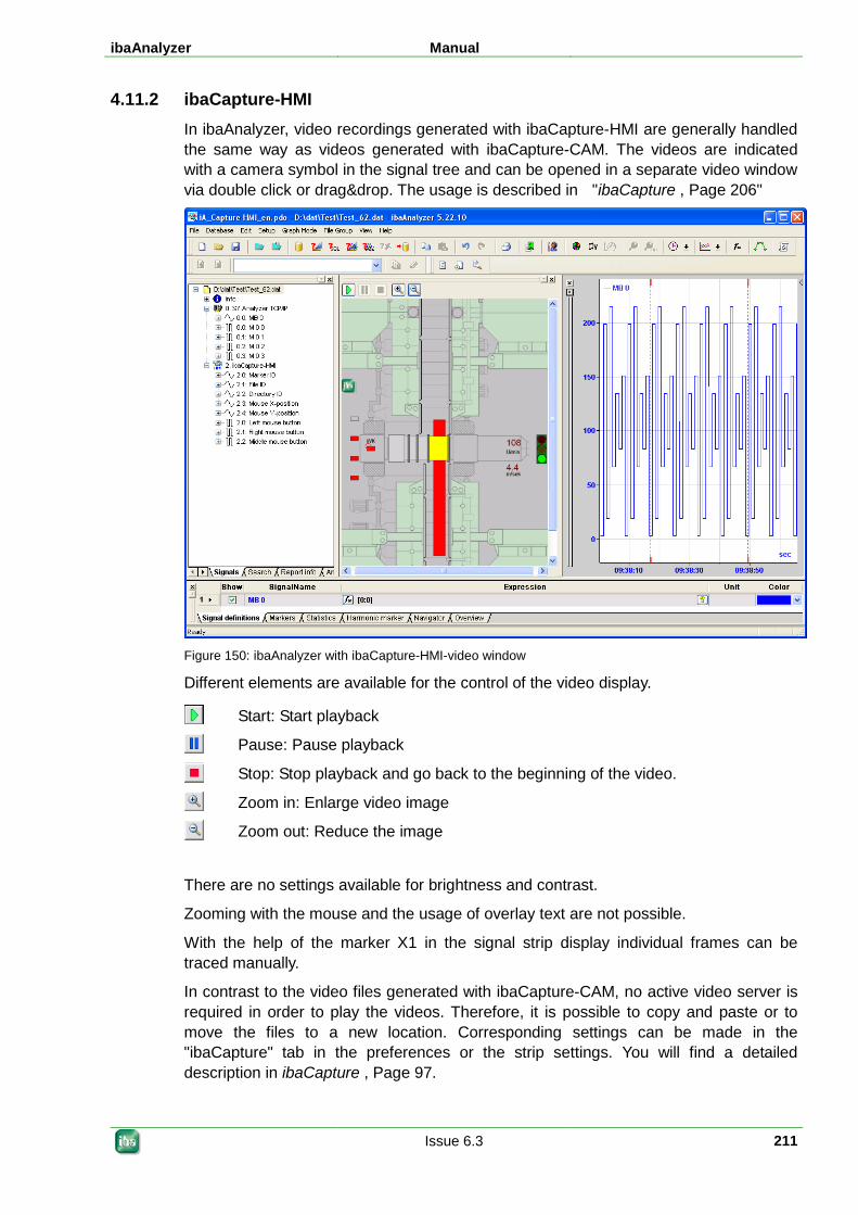
ibaAnalyzer Manual

Issue 6.3 211

4.11.2 ibaCapture-HMI In ibaAnalyzer, video recordings generated with ibaCapture-HMI are generally handled the same way as videos generated with ibaCapture-CAM. The videos are indicated with a camera symbol in the signal tree and can be opened in a separate video window via double click or drag&drop. The usage is described in "ibaCapture , Page 206"

Figure 150: ibaAnalyzer with ibaCapture-HMI-video window

Different elements are available for the control of the video display.

Start: Start playback

Pause: Pause playback

Stop: Stop playback and go back to the beginning of the video.

Zoom in: Enlarge video image

Zoom out: Reduce the image

There are no settings available for brightness and contrast.

Zooming with the mouse and the usage of overlay text are not possible.

With the help of the marker X1 in the signal strip display individual frames can be traced manually.

In contrast to the video files generated with ibaCapture-CAM, no active video server is required in order to play the videos. Therefore, it is possible to copy and paste or to move the files to a new location. Corresponding settings can be made in the "ibaCapture" tab in the preferences or the strip settings. You will find a detailed description in ibaCapture , Page 97.

Manual ibaAnalyzer

212 Issue 6.3

In case you want to print ibaCapture-HMI videos, particular settings are available. You will find a detailed description in ibaCapture , Page 97.

If you want to integrate ibaCapture-HMI videos in a report, proceed the same way as when working with ibaCapture-CAM videos. (see Video objects , Page 399)

If you want to export ibaCapture-HMI videos from a dat file, activate the "Free selection" module in the signal selection of the export mode. Subsequently mark the relevant video signals. If you tick off the "Export video as part of a data file" option in the export mode and subsequently reload the exported file, the "Replace path..." and "Copy video files to local disk before loading" options in the Preferences/Signal strip settings will be ignored. (see picture below for setting items)

For more information, please refer to ibaCapture, Page 97.

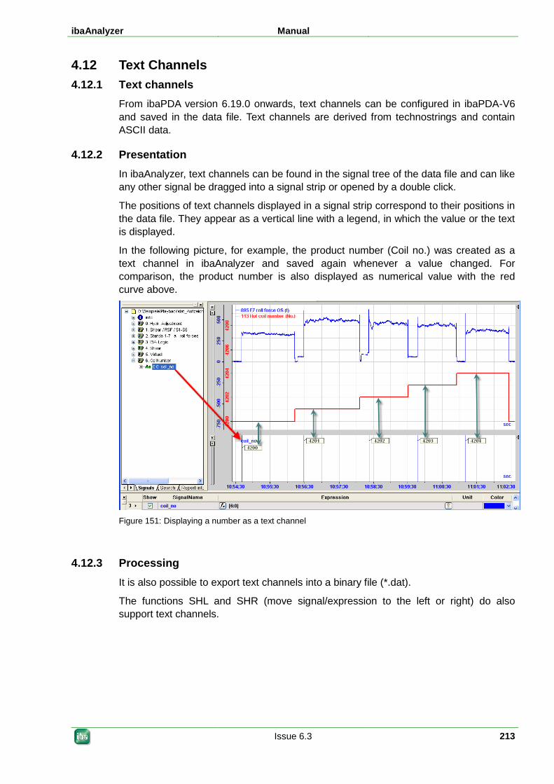
ibaAnalyzer Manual

Issue 6.3 213

4.12 Text Channels 4.12.1 Text channels

From ibaPDA version 6.19.0 onwards, text channels can be configured in ibaPDA-V6 and saved in the data file. Text channels are derived from technostrings and contain ASCII data.

4.12.2 Presentation In ibaAnalyzer, text channels can be found in the signal tree of the data file and can like any other signal be dragged into a signal strip or opened by a double click.

The positions of text channels displayed in a signal strip correspond to their positions in the data file. They appear as a vertical line with a legend, in which the value or the text is displayed.

In the following picture, for example, the product number (Coil no.) was created as a text channel in ibaAnalyzer and saved again whenever a value changed. For comparison, the product number is also displayed as numerical value with the red curve above.

Figure 151: Displaying a number as a text channel

4.12.3 Processing It is also possible to export text channels into a binary file (*.dat).

The functions SHL and SHR (move signal/expression to the left or right) do also support text channels.

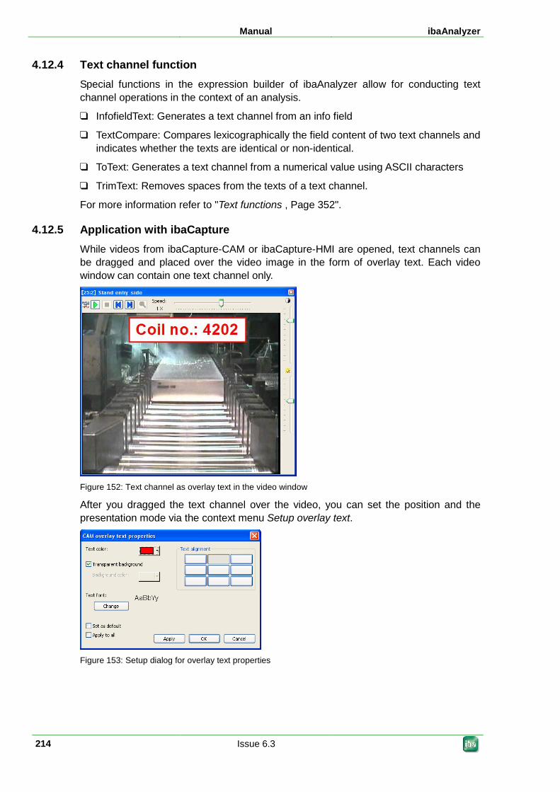
Manual ibaAnalyzer

214 Issue 6.3

4.12.4 Text channel function Special functions in the expression builder of ibaAnalyzer allow for conducting text channel operations in the context of an analysis.

InfofieldText: Generates a text channel from an info field

TextCompare: Compares lexicographically the field content of two text channels and indicates whether the texts are identical or non-identical.

ToText: Generates a text channel from a numerical value using ASCII characters

TrimText: Removes spaces from the texts of a text channel.

For more information refer to "Text functions , Page 352".

4.12.5 Application with ibaCapture While videos from ibaCapture-CAM or ibaCapture-HMI are opened, text channels can be dragged and placed over the video image in the form of overlay text. Each video window can contain one text channel only.

Figure 152: Text channel as overlay text in the video window

After you dragged the text channel over the video, you can set the position and the presentation mode via the context menu Setup overlay text.

Figure 153: Setup dialog for overlay text properties

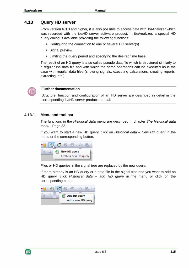
ibaAnalyzer Manual

Issue 6.3 215

4.13 Query HD server From version 6.3.0 and higher, it is also possible to access data with ibaAnalyzer which was recorded with the ibaHD server software product. In ibaAnalyzer, a special HD query dialog is available providing the following functions:

Configuring the connection to one or several HD server(s)

Signal preview

Limiting the query period and specifying the desired time base

The result of an HD query is a so-called pseudo data file which is structured similarly to a regular iba data file and with which the same operations can be executed as is the case with regular data files (showing signals, executing calculations, creating reports, extracting, etc.).

Further documentation

Structure, function and configuration of an HD server are described in detail in the corresponding ibaHD server product manual.

4.13.1 Menu and tool bar The functions in the Historical data menu are described in chapter The historical data menu , Page 33.

If you want to start a new HD query, click on Historical data – New HD query in the menu or the corresponding button.

Files or HD queries in the signal tree are replaced by the new query.

If there already is an HD query or a data file in the signal tree and you want to add an HD query, click Historical data – add HD query in the menu or click on the corresponding button.

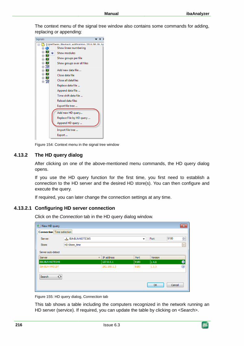
Manual ibaAnalyzer

216 Issue 6.3

The context menu of the signal tree window also contains some commands for adding, replacing or appending:

Figure 154: Context menu in the signal tree window

4.13.2 The HD query dialog After clicking on one of the above-mentioned menu commands, the HD query dialog opens.

If you use the HD query function for the first time, you first need to establish a connection to the HD server and the desired HD store(s). You can then configure and execute the query.

If required, you can later change the connection settings at any time.

4.13.2.1 Configuring HD server connection Click on the Connection tab in the HD query dialog window.

Figure 155: HD query dialog, Connection tab

This tab shows a table including the computers recognized in the network running an HD server (service). If required, you can update the table by clicking on <Search>.

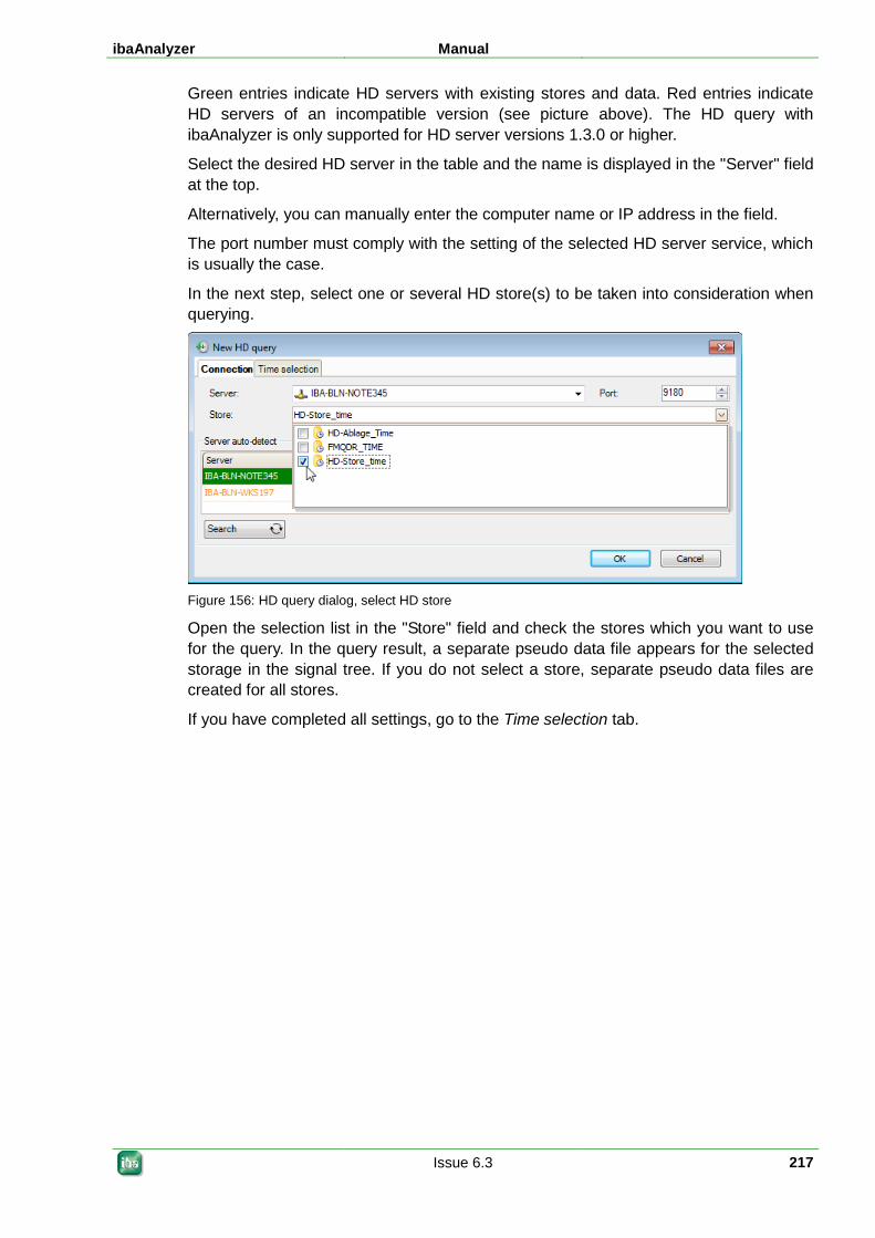
ibaAnalyzer Manual

Issue 6.3 217

Green entries indicate HD servers with existing stores and data. Red entries indicate HD servers of an incompatible version (see picture above). The HD query with ibaAnalyzer is only supported for HD server versions 1.3.0 or higher.

Select the desired HD server in the table and the name is displayed in the "Server" field at the top.

Alternatively, you can manually enter the computer name or IP address in the field.

The port number must comply with the setting of the selected HD server service, which is usually the case.

In the next step, select one or several HD store(s) to be taken into consideration when querying.

Figure 156: HD query dialog, select HD store

Open the selection list in the "Store" field and check the stores which you want to use for the query. In the query result, a separate pseudo data file appears for the selected storage in the signal tree. If you do not select a store, separate pseudo data files are created for all stores.

If you have completed all settings, go to the Time selection tab.

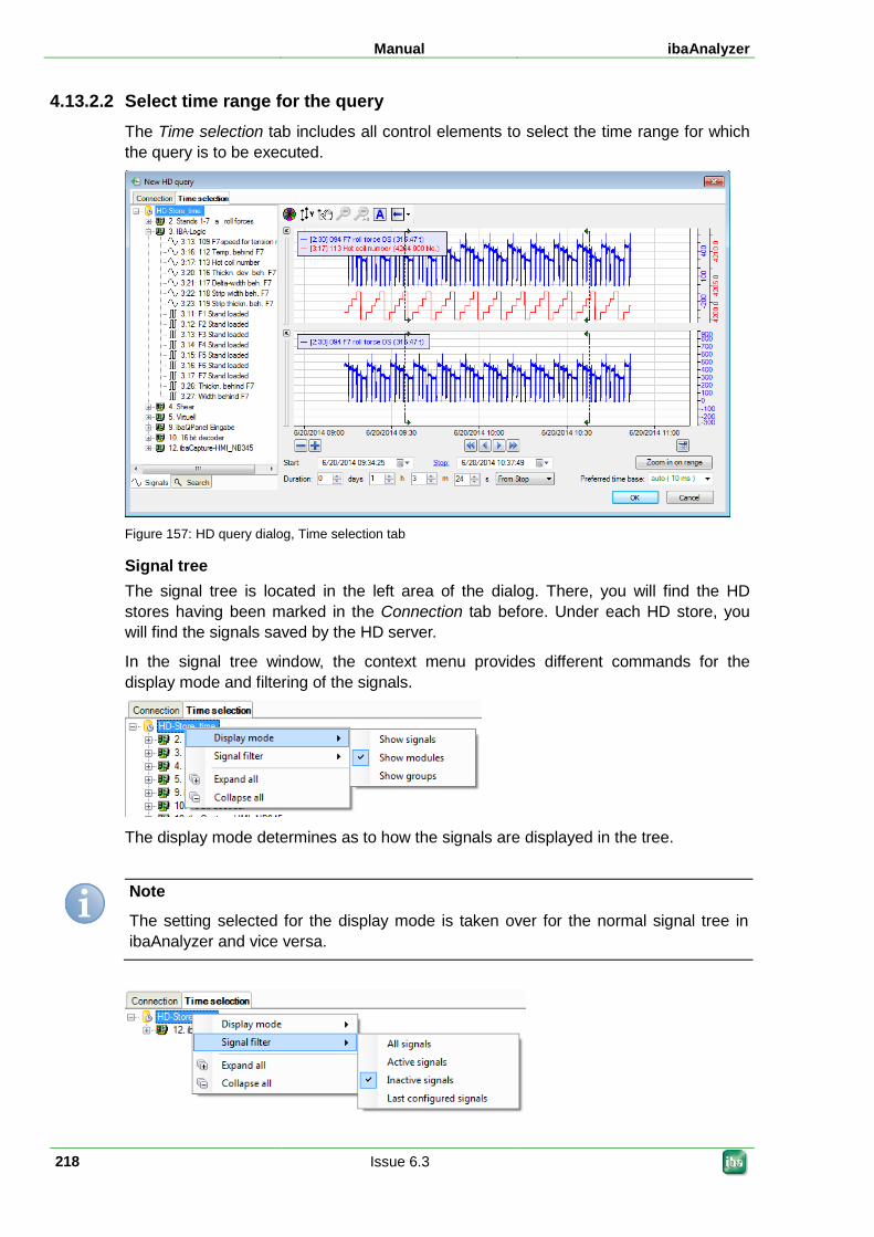
Manual ibaAnalyzer

218 Issue 6.3

4.13.2.2 Select time range for the query The Time selection tab includes all control elements to select the time range for which the query is to be executed.

Figure 157: HD query dialog, Time selection tab

Signal tree The signal tree is located in the left area of the dialog. There, you will find the HD stores having been marked in the Connection tab before. Under each HD store, you will find the signals saved by the HD server.

In the signal tree window, the context menu provides different commands for the display mode and filtering of the signals.

The display mode determines as to how the signals are displayed in the tree.

Note

The setting selected for the display mode is taken over for the normal signal tree in ibaAnalyzer and vice versa.

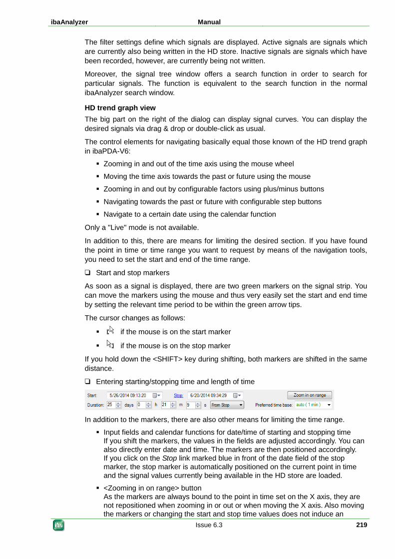
ibaAnalyzer Manual

Issue 6.3 219

The filter settings define which signals are displayed. Active signals are signals which are currently also being written in the HD store. Inactive signals are signals which have been recorded, however, are currently being not written.

Moreover, the signal tree window offers a search function in order to search for particular signals. The function is equivalent to the search function in the normal ibaAnalyzer search window.

HD trend graph view The big part on the right of the dialog can display signal curves. You can display the desired signals via drag & drop or double-click as usual.

The control elements for navigating basically equal those known of the HD trend graph in ibaPDA-V6:

Zooming in and out of the time axis using the mouse wheel

Moving the time axis towards the past or future using the mouse

Zooming in and out by configurable factors using plus/minus buttons

Navigating towards the past or future with configurable step buttons

Navigate to a certain date using the calendar function

Only a "Live" mode is not available.

In addition to this, there are means for limiting the desired section. If you have found the point in time or time range you want to request by means of the navigation tools, you need to set the start and end of the time range.

Start and stop markers

As soon as a signal is displayed, there are two green markers on the signal strip. You can move the markers using the mouse and thus very easily set the start and end time by setting the relevant time period to be within the green arrow tips.

The cursor changes as follows:

if the mouse is on the start marker

if the mouse is on the stop marker

If you hold down the <SHIFT> key during shifting, both markers are shifted in the same distance.

Entering starting/stopping time and length of time

In addition to the markers, there are also other means for limiting the time range.

Input fields and calendar functions for date/time of starting and stopping time If you shift the markers, the values in the fields are adjusted accordingly. You can also directly enter date and time. The markers are then positioned accordingly. If you click on the Stop link marked blue in front of the date field of the stop marker, the stop marker is automatically positioned on the current point in time and the signal values currently being available in the HD store are loaded.

<Zooming in on range> button As the markers are always bound to the point in time set on the X axis, they are not repositioned when zooming in or out or when moving the X axis. Also moving the markers or changing the start and stop time values does not induce an

Manual ibaAnalyzer

220 Issue 6.3

automatic adjustment of the zoom factor. Thus, they can be very close to each other or they can be outside the window. By clicking on the button, the zoom factor and position are set in such a way that the selected time range is displayed in the center of the signal strip. Start and stop markers are always positioned at one quarter or three quarters of the visible X axis segment.

Duration input fields The duration, i.e. the width of the time range, is displayed in these fields. The values are adjusted accordingly while shifting the markers. However, you can also directly enter the time in days, hours, minutes and seconds. If you change the time values by entering or using the up and down buttons, the markers will be positioned according to the button nearby. - "From stop": stop marker fixed, start marker is shifted - "From start": start marker fixed, stop marker is shifted - "Centered": the center of the selected range is stationary, both markers are shifted symmetrically to this. If you change a time value using the up and down buttons while holding down the <Ctrl> key, the other values are set to zero. If you directly enter the numerical values, hold down the <Ctrl> key and press <Enter> to apply the value and to set the other values to zero.

Preferred time base You can select from the preferred time base drop-down list a time base with which the data is to be loaded if possible. The ibaHD server automatically tries to find a time base as suitable as possible. There is more information on this topic in the next chapter.

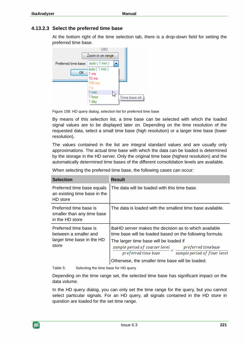
ibaAnalyzer Manual

Issue 6.3 221

4.13.2.3 Select the preferred time base At the bottom right of the time selection tab, there is a drop-down field for setting the preferred time base.

Figure 158: HD query dialog, selection list for preferred time base

By means of this selection list, a time base can be selected with which the loaded signal values are to be displayed later on. Depending on the time resolution of the requested data, select a small time base (high resolution) or a larger time base (lower resolution).

The values contained in the list are integral standard values and are usually only approximations. The actual time base with which the data can be loaded is determined by the storage in the HD server. Only the original time base (highest resolution) and the automatically determined time bases of the different consolidation levels are available.

When selecting the preferred time base, the following cases can occur:

Selection Result

Preferred time base equals an existing time base in the HD store

The data will be loaded with this time base.

Preferred time base is smaller than any time base in the HD store

The data is loaded with the smallest time base available.

Preferred time base is between a smaller and larger time base in the HD store

ibaHD server makes the decision as to which available time base will be loaded based on the following formula: The larger time base will be loaded if

Otherwise, the smaller time base will be loaded.

Table 5: Selecting the time base for HD query

Depending on the time range set, the selected time base has significant impact on the data volume.

In the HD query dialog, you can only set the time range for the query, but you cannot select particular signals. For an HD query, all signals contained in the HD store in question are loaded for the set time range.

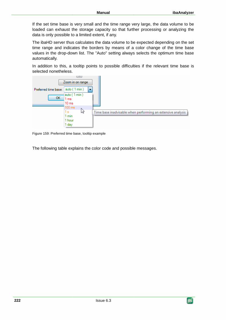
Manual ibaAnalyzer

222 Issue 6.3

If the set time base is very small and the time range very large, the data volume to be loaded can exhaust the storage capacity so that further processing or analyzing the data is only possible to a limited extent, if any.

The ibaHD server thus calculates the data volume to be expected depending on the set time range and indicates the borders by means of a color change of the time base values in the drop-down list. The "Auto" setting always selects the optimum time base automatically.

In addition to this, a tooltip points to possible difficulties if the relevant time base is selected nonetheless.

Figure 159: Preferred time base, tooltip example

The following table explains the color code and possible messages.

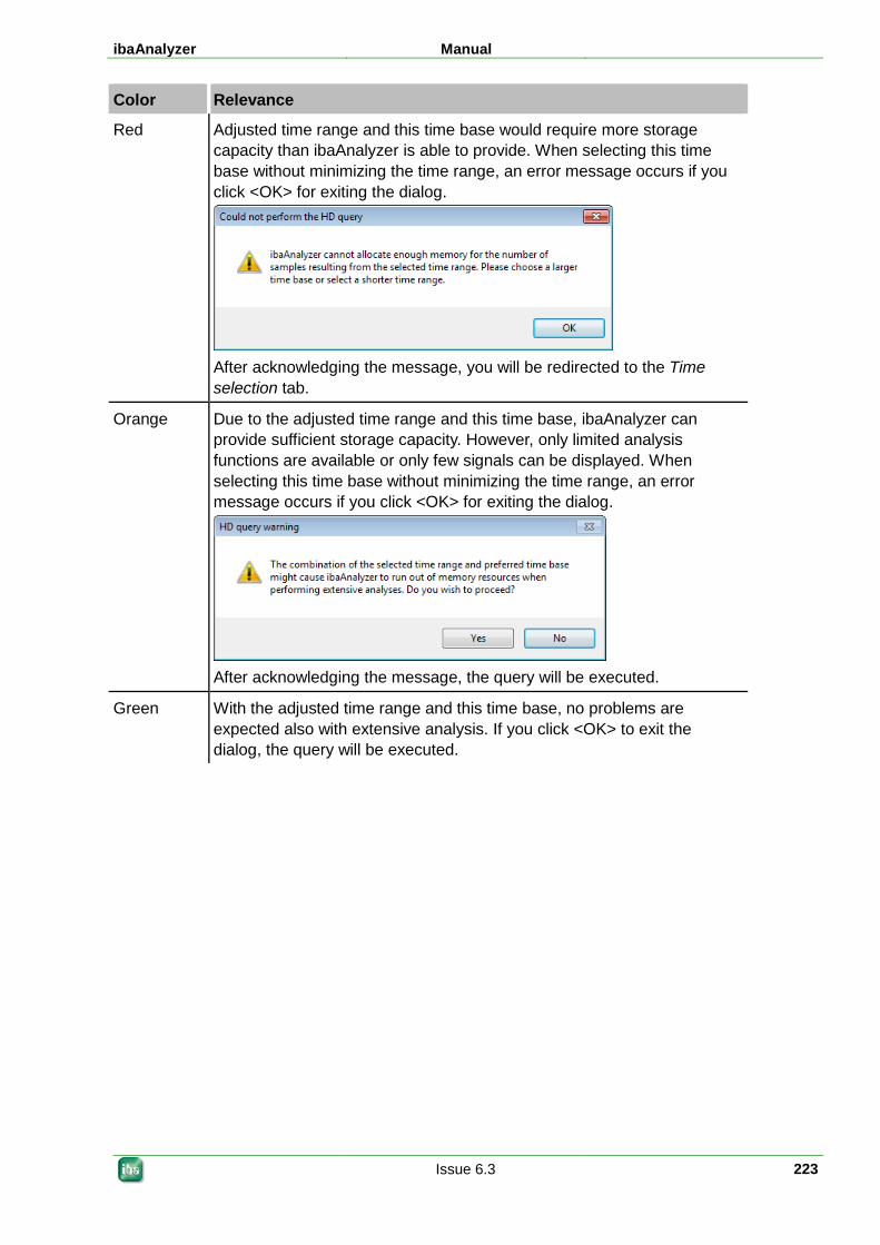
ibaAnalyzer Manual

Issue 6.3 223

Color Relevance

Red Adjusted time range and this time base would require more storage capacity than ibaAnalyzer is able to provide. When selecting this time base without minimizing the time range, an error message occurs if you click <OK> for exiting the dialog.

After acknowledging the message, you will be redirected to the Time selection tab.

Orange Due to the adjusted time range and this time base, ibaAnalyzer can provide sufficient storage capacity. However, only limited analysis functions are available or only few signals can be displayed. When selecting this time base without minimizing the time range, an error message occurs if you click <OK> for exiting the dialog.

After acknowledging the message, the query will be executed.

Green With the adjusted time range and this time base, no problems are expected also with extensive analysis. If you click <OK> to exit the dialog, the query will be executed.

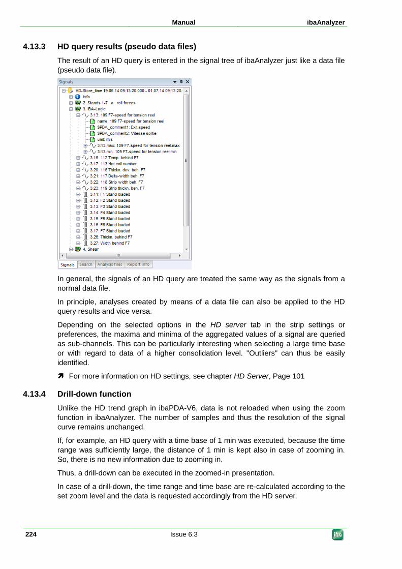
Manual ibaAnalyzer

224 Issue 6.3

4.13.3 HD query results (pseudo data files) The result of an HD query is entered in the signal tree of ibaAnalyzer just like a data file (pseudo data file).

In general, the signals of an HD query are treated the same way as the signals from a normal data file.

In principle, analyses created by means of a data file can also be applied to the HD query results and vice versa.

Depending on the selected options in the HD server tab in the strip settings or preferences, the maxima and minima of the aggregated values of a signal are queried as sub-channels. This can be particularly interesting when selecting a large time base or with regard to data of a higher consolidation level. "Outliers" can thus be easily identified.

For more information on HD settings, see chapter HD Server, Page 101

4.13.4 Drill-down function Unlike the HD trend graph in ibaPDA-V6, data is not reloaded when using the zoom function in ibaAnalyzer. The number of samples and thus the resolution of the signal curve remains unchanged.

If, for example, an HD query with a time base of 1 min was executed, because the time range was sufficiently large, the distance of 1 min is kept also in case of zooming in. So, there is no new information due to zooming in.

Thus, a drill-down can be executed in the zoomed-in presentation.

In case of a drill-down, the time range and time base are re-calculated according to the set zoom level and the data is requested accordingly from the HD server.

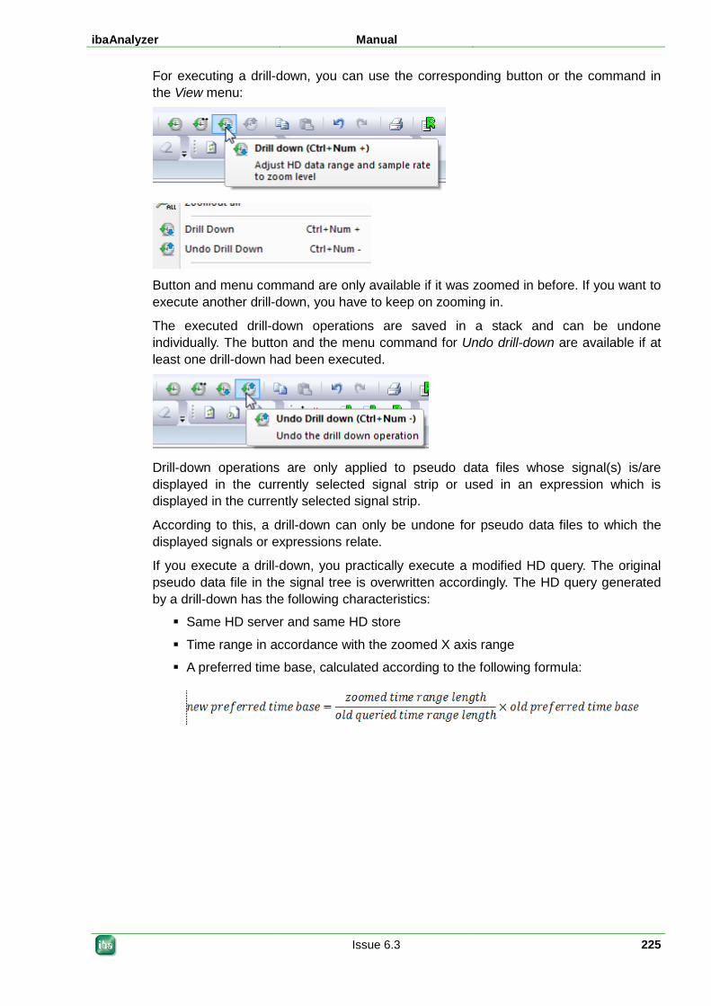
ibaAnalyzer Manual

Issue 6.3 225

For executing a drill-down, you can use the corresponding button or the command in the View menu:

Button and menu command are only available if it was zoomed in before. If you want to execute another drill-down, you have to keep on zooming in.

The executed drill-down operations are saved in a stack and can be undone individually. The button and the menu command for Undo drill-down are available if at least one drill-down had been executed.

Drill-down operations are only applied to pseudo data files whose signal(s) is/are displayed in the currently selected signal strip or used in an expression which is displayed in the currently selected signal strip.

According to this, a drill-down can only be undone for pseudo data files to which the displayed signals or expressions relate.

If you execute a drill-down, you practically execute a modified HD query. The original pseudo data file in the signal tree is overwritten accordingly. The HD query generated by a drill-down has the following characteristics:

Same HD server and same HD store

Time range in accordance with the zoomed X axis range

A preferred time base, calculated according to the following formula:

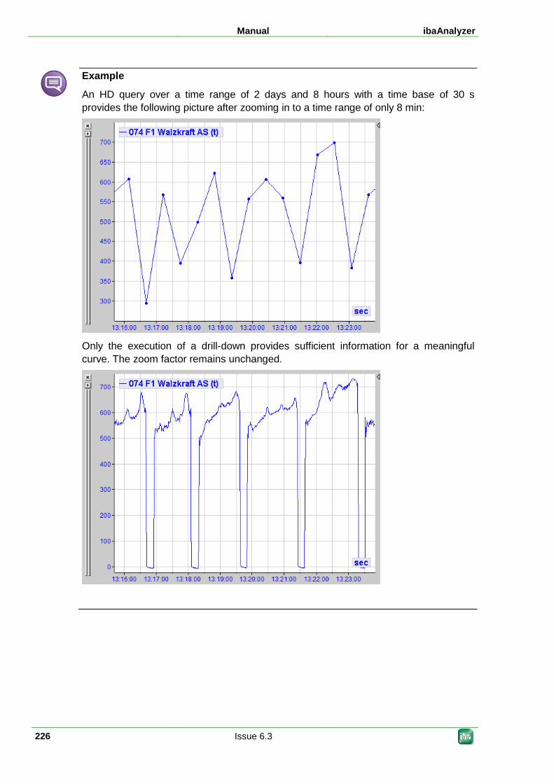
Manual ibaAnalyzer

226 Issue 6.3

Example

An HD query over a time range of 2 days and 8 hours with a time base of 30 s provides the following picture after zooming in to a time range of only 8 min:

Only the execution of a drill-down provides sufficient information for a meaningful curve. The zoom factor remains unchanged.

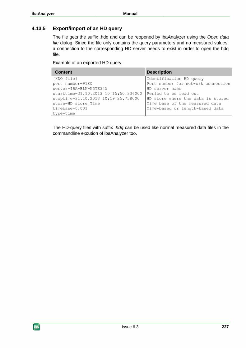
ibaAnalyzer Manual

Issue 6.3 227

4.13.5 Export/import of an HD query The file gets the suffix .hdq and can be reopened by ibaAnalyzer using the Open data file dialog. Since the file only contains the query parameters and no measured values, a connection to the corresponding HD server needs to exist in order to open the hdq file.

Example of an exported HD query:

Content Description [HDQ file] port number=9180 server=IBA-BLN-NOTE345 starttime=31.10.2013 10:15:50.336000 stoptime=31.10.2013 10:19:25.758000 store=HD store_Time timebase=0.001 type=time

Identification HD query Port number for network connection HD server name Period to be read out HD store where the data is stored Time base of the measured data Time-based or length-based data

The HD-query files with suffix .hdq can be used like normal measured data files in the commandline excution of ibaAnalyzer too.

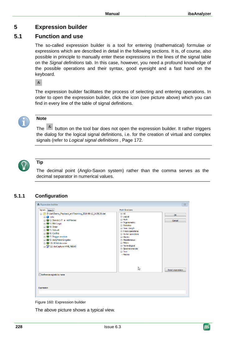
Manual ibaAnalyzer

228 Issue 6.3

5 Expression builder 5.1 Function and use

The so-called expression builder is a tool for entering (mathematical) formulae or expressions which are described in detail in the following sections. It is, of course, also possible in principle to manually enter these expressions in the lines of the signal table on the Signal definitions tab. In this case, however, you need a profound knowledge of the possible operations and their syntax, good eyesight and a fast hand on the keyboard.

The expression builder facilitates the process of selecting and entering operations. In order to open the expression builder, click the icon (see picture above) which you can find in every line of the table of signal definitions.

Note

The button on the tool bar does not open the expression builder. It rather triggers the dialog for the logical signal definitions, i.e. for the creation of virtual and complex signals (refer to Logical signal definitions , Page 172.

Tip

The decimal point (Anglo-Saxon system) rather than the comma serves as the decimal separator in numerical values.

5.1.1 Configuration

Figure 160: Expression builder

The above picture shows a typical view.

ibaAnalyzer Manual

Issue 6.3 229

The part on the left shows a signal tree which is very similar to the one in the signal tree window. However, in contrast to the signal tree window, this window here contains not just the original signals but also all the expressions which were already created using the expression builder. From this signal tree, you can now select the desired signals or expressions to be used in the calculations.

The right part of the dialog window contains a function tree view with a collection of the available mathematical operations and other functions according to subjects. The command line in which you enter the desired expression is located below these two selection fields. The gray area above this line shows a short note concerning the syntax of an operation if this operation is marked in the function tree.

The <Reset expression> button removes all entries from the command line.

You can enable the "Reference signals by name" check box if you want to use the signal names in the expressions instead of the usual signal designations consisting of [module number:signal number].

Note

When using the signal names as signal reference, it must be guaranteed that the signal names are unambiguous!

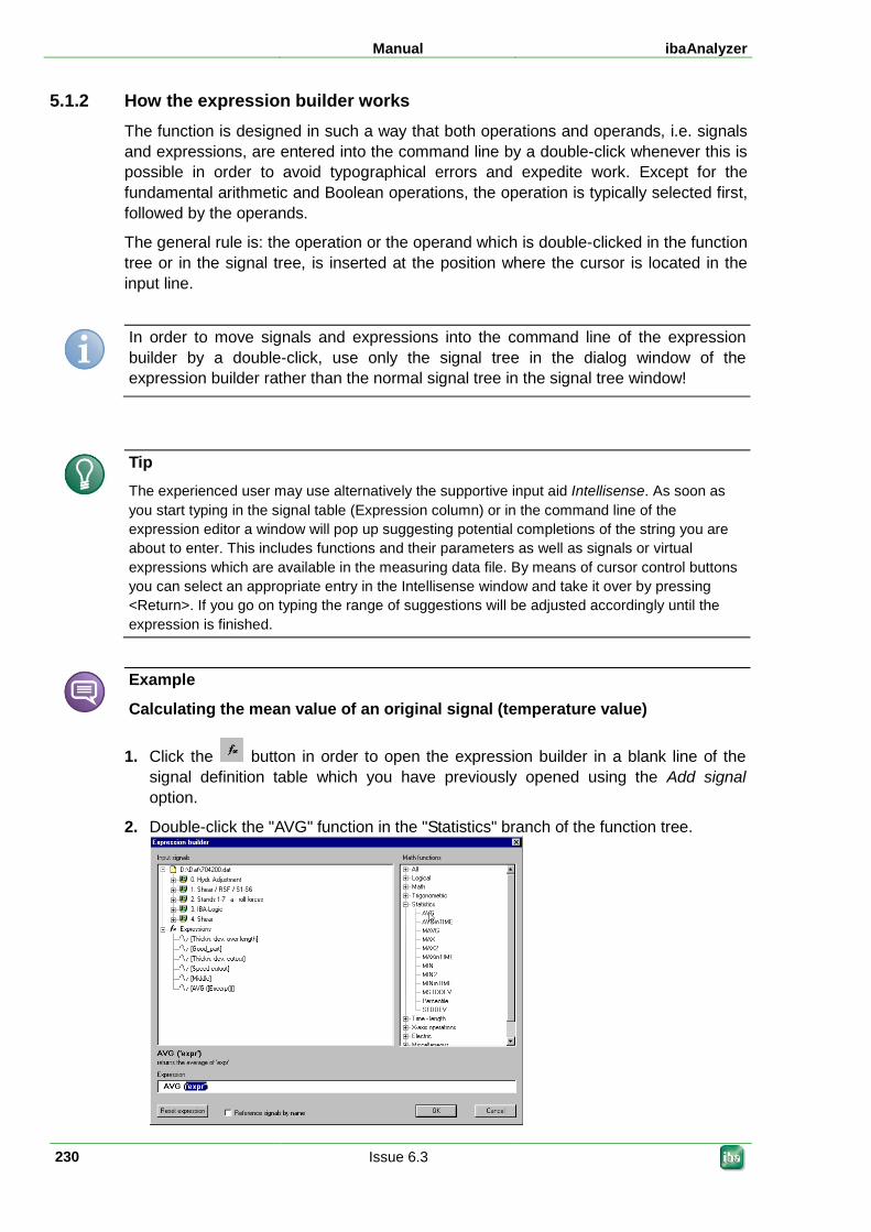
Manual ibaAnalyzer

230 Issue 6.3

5.1.2 How the expression builder works The function is designed in such a way that both operations and operands, i.e. signals and expressions, are entered into the command line by a double-click whenever this is possible in order to avoid typographical errors and expedite work. Except for the fundamental arithmetic and Boolean operations, the operation is typically selected first, followed by the operands.

The general rule is: the operation or the operand which is double-clicked in the function tree or in the signal tree, is inserted at the position where the cursor is located in the input line.

In order to move signals and expressions into the command line of the expression builder by a double-click, use only the signal tree in the dialog window of the expression builder rather than the normal signal tree in the signal tree window!

Tip

The experienced user may use alternatively the supportive input aid Intellisense. As soon as you start typing in the signal table (Expression column) or in the command line of the expression editor a window will pop up suggesting potential completions of the string you are about to enter. This includes functions and their parameters as well as signals or virtual expressions which are available in the measuring data file. By means of cursor control buttons you can select an appropriate entry in the Intellisense window and take it over by pressing <Return>. If you go on typing the range of suggestions will be adjusted accordingly until the expression is finished.

Example

Calculating the mean value of an original signal (temperature value)

1. Click the button in order to open the expression builder in a blank line of the signal definition table which you have previously opened using the Add signal option.

2. Double-click the "AVG" function in the "Statistics" branch of the function tree.

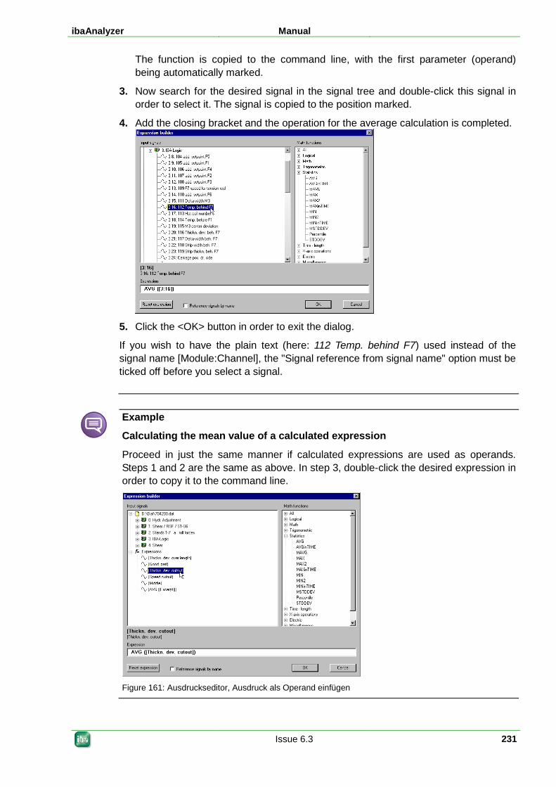
ibaAnalyzer Manual

Issue 6.3 231

The function is copied to the command line, with the first parameter (operand) being automatically marked.

3. Now search for the desired signal in the signal tree and double-click this signal in order to select it. The signal is copied to the position marked.

4. Add the closing bracket and the operation for the average calculation is completed.

5. Click the <OK> button in order to exit the dialog.

If you wish to have the plain text (here: 112 Temp. behind F7) used instead of the signal name [Module:Channel], the "Signal reference from signal name" option must be ticked off before you select a signal.

Example

Calculating the mean value of a calculated expression

Proceed in just the same manner if calculated expressions are used as operands. Steps 1 and 2 are the same as above. In step 3, double-click the desired expression in order to copy it to the command line.

Figure 161: Ausdruckseditor, Ausdruck als Operand einfügen

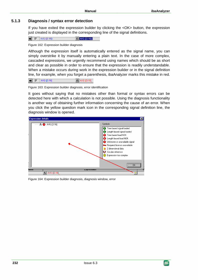
Manual ibaAnalyzer

232 Issue 6.3

5.1.3 Diagnosis / syntax error detection If you have exited the expression builder by clicking the <OK> button, the expression just created is displayed in the corresponding line of the signal definitions.

Figure 162: Expression builder diagnosis

Although the expression itself is automatically entered as the signal name, you can simply overstrike it by manually entering a plain text. In the case of more complex, cascaded expressions, we urgently recommend using names which should be as short and clear as possible in order to ensure that the expression is readily understandable. When a mistake occurs during work in the expression builder or in the signal definition line, for example, when you forget a parenthesis, ibaAnalyzer marks this mistake in red.

Figure 163: Expression builder diagnosis, error identification

It goes without saying that no mistakes other than formal or syntax errors can be detected here with which a calculation is not possible. Using the diagnosis functionality is another way of obtaining further information concerning the cause of an error. When you click the yellow question mark icon in the corresponding signal definition line, the diagnosis window is opened.

Figure 164: Expression builder diagnosis, diagnosis window, error

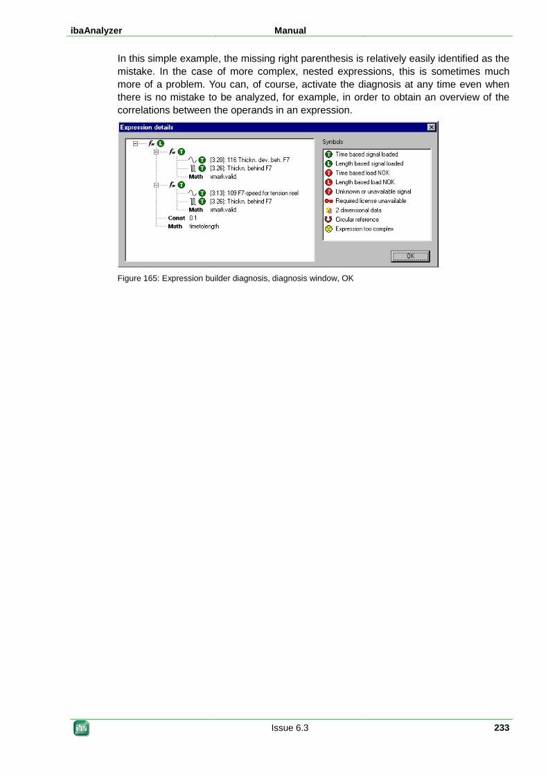
ibaAnalyzer Manual

Issue 6.3 233

In this simple example, the missing right parenthesis is relatively easily identified as the mistake. In the case of more complex, nested expressions, this is sometimes much more of a problem. You can, of course, activate the diagnosis at any time even when there is no mistake to be analyzed, for example, in order to obtain an overview of the correlations between the operands in an expression.

Figure 165: Expression builder diagnosis, diagnosis window, OK

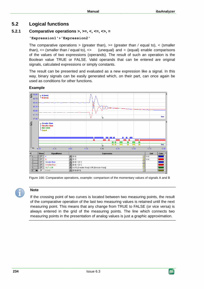
Manual ibaAnalyzer

234 Issue 6.3

5.2 Logical functions 5.2.1 Comparative operations >, >=, <, <=, <>, =

'Expression1'>'Expression2'

The comparative operations > (greater than), >= (greater than / equal to), < (smaller than), <= (smaller than / equal to), <> (unequal) and = (equal) enable comparisons of the values of two expressions (operands). The result of such an operation is the Boolean value TRUE or FALSE. Valid operands that can be entered are original signals, calculated expressions or simply constants.

The result can be presented and evaluated as a new expression like a signal. In this way, binary signals can be easily generated which, on their part, can once again be used as conditions for other functions.

Example

Figure 166: Comparative operations, example: comparison of the momentary values of signals A and B

Note

If the crossing point of two curves is located between two measuring points, the result of the comparative operation of the last two measuring values is retained until the next measuring point. This means that any change from TRUE to FALSE (or vice versa) is always entered in the grid of the measuring points. The line which connects two measuring points in the presentation of analog values is just a graphic approximation.

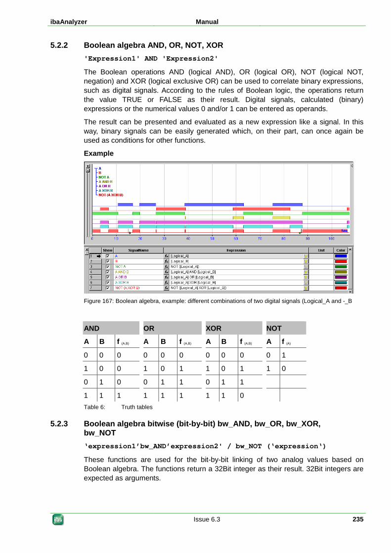
ibaAnalyzer Manual

Issue 6.3 235

5.2.2 Boolean algebra AND, OR, NOT, XOR 'Expression1' AND 'Expression2'

The Boolean operations AND (logical AND), OR (logical OR), NOT (logical NOT, negation) and XOR (logical exclusive OR) can be used to correlate binary expressions, such as digital signals. According to the rules of Boolean logic, the operations return the value TRUE or FALSE as their result. Digital signals, calculated (binary) expressions or the numerical values 0 and/or 1 can be entered as operands.

The result can be presented and evaluated as a new expression like a signal. In this way, binary signals can be easily generated which, on their part, can once again be used as conditions for other functions.

Example

Figure 167: Boolean algebra, example: different combinations of two digital signals (Logical_A and -_B

AND OR XOR NOT

A B f (A,B) A B f (A,B) A B f (A,B) A f (A)

0 0 0 0 0 0 0 0 0 0 1

1 0 0 1 0 1 1 0 1 1 0

0 1 0 0 1 1 0 1 1

1 1 1 1 1 1 1 1 0 Table 6: Truth tables

5.2.3 Boolean algebra bitwise (bit-by-bit) bw_AND, bw_OR, bw_XOR, bw_NOT ‘expression1’bw_AND’expression2' / bw_NOT (‘expression‘)

These functions are used for the bit-by-bit linking of two analog values based on Boolean algebra. The functions return a 32Bit integer as their result. 32Bit integers are expected as arguments.

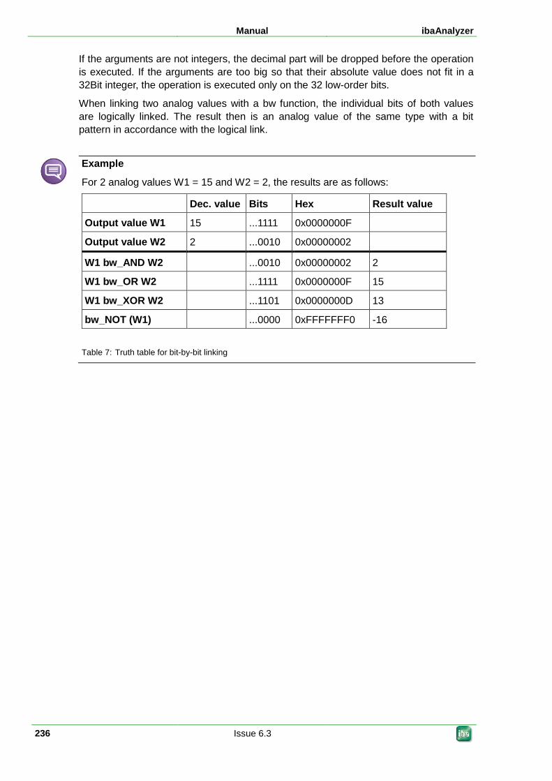
Manual ibaAnalyzer

236 Issue 6.3

If the arguments are not integers, the decimal part will be dropped before the operation is executed. If the arguments are too big so that their absolute value does not fit in a 32Bit integer, the operation is executed only on the 32 low-order bits.

When linking two analog values with a bw function, the individual bits of both values are logically linked. The result then is an analog value of the same type with a bit pattern in accordance with the logical link.

Example

For 2 analog values W1 = 15 and W2 = 2, the results are as follows:

Dec. value Bits Hex Result value

Output value W1 15 ...1111 0x0000000F

Output value W2 2 ...0010 0x00000002

W1 bw_AND W2 ...0010 0x00000002 2

W1 bw_OR W2 ...1111 0x0000000F 15

W1 bw_XOR W2 ...1101 0x0000000D 13

bw_NOT (W1) ...0000 0xFFFFFFF0 -16

Table 7: Truth table for bit-by-bit linking

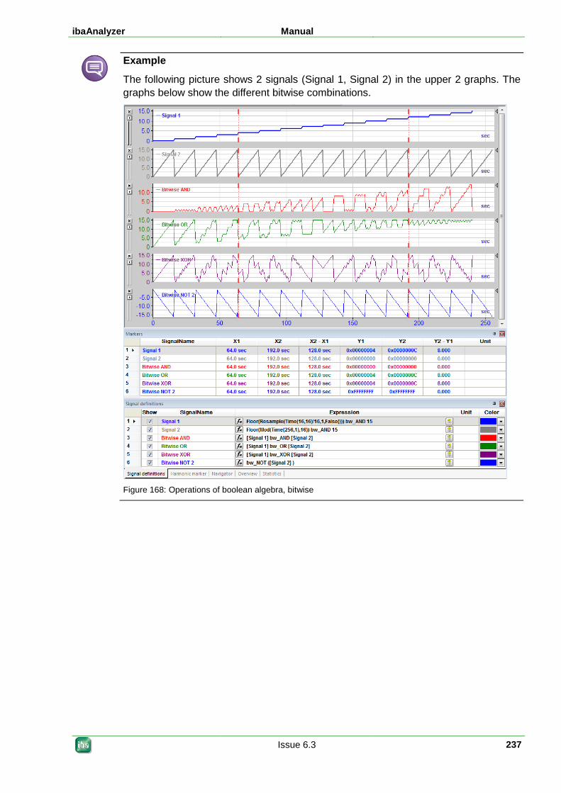
ibaAnalyzer Manual

Issue 6.3 237

Example

The following picture shows 2 signals (Signal 1, Signal 2) in the upper 2 graphs. The graphs below show the different bitwise combinations.

Figure 168: Operations of boolean algebra, bitwise

Manual ibaAnalyzer

238 Issue 6.3

5.2.4 Branching 5.2.4.1 If

If ('condition', 'true expr', 'false expr')

The If function can be used for a conditioned execution of further calculations. Depending on the Boolean result of a ‘condition’, which can be an operation itself, the operation ‘true expr’ will be executed in case of TRUE, the operation ‘false expr’ in case of FALSE.

Hence, different calculations can be executed in a process-controlled manner. Of course, you can use this function in a nested matter and thus realize further branches.

5.2.4.2 IsData IsData (‘expression’,’end')

The result of this operation is TRUE if measured values are available for 'expression'. The result is FALSE if measured values are missing or signals are empty.

This function, for example, can be used as condition for other calculations.

Optionally, the 'End' parameter can be entered. With this parameter, you can reduce or extent the result signal of the function so that it complies with other signals and can be used for further links. If you do not specify the 'End' parameter, the length of the result signal complies with that of the input signal (incl. invalid samples).

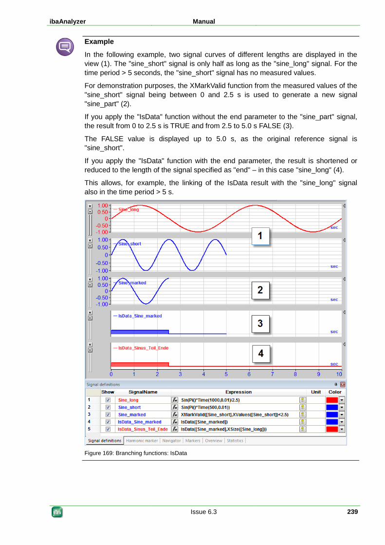
ibaAnalyzer Manual

Issue 6.3 239

Example

In the following example, two signal curves of different lengths are displayed in the view (1). The "sine_short" signal is only half as long as the "sine_long" signal. For the time period > 5 seconds, the "sine_short" signal has no measured values.

For demonstration purposes, the XMarkValid function from the measured values of the "sine_short" signal being between 0 and 2.5 s is used to generate a new signal "sine_part" (2).

If you apply the "IsData" function without the end parameter to the "sine_part" signal, the result from 0 to 2.5 s is TRUE and from 2.5 to 5.0 s FALSE (3).

The FALSE value is displayed up to 5.0 s, as the original reference signal is "sine_short".

If you apply the "IsData" function with the end parameter, the result is shortened or reduced to the length of the signal specified as "end" – in this case "sine_long" (4).

This allows, for example, the linking of the IsData result with the "sine_long" signal also in the time period > 5 s.

Figure 169: Branching functions: IsData

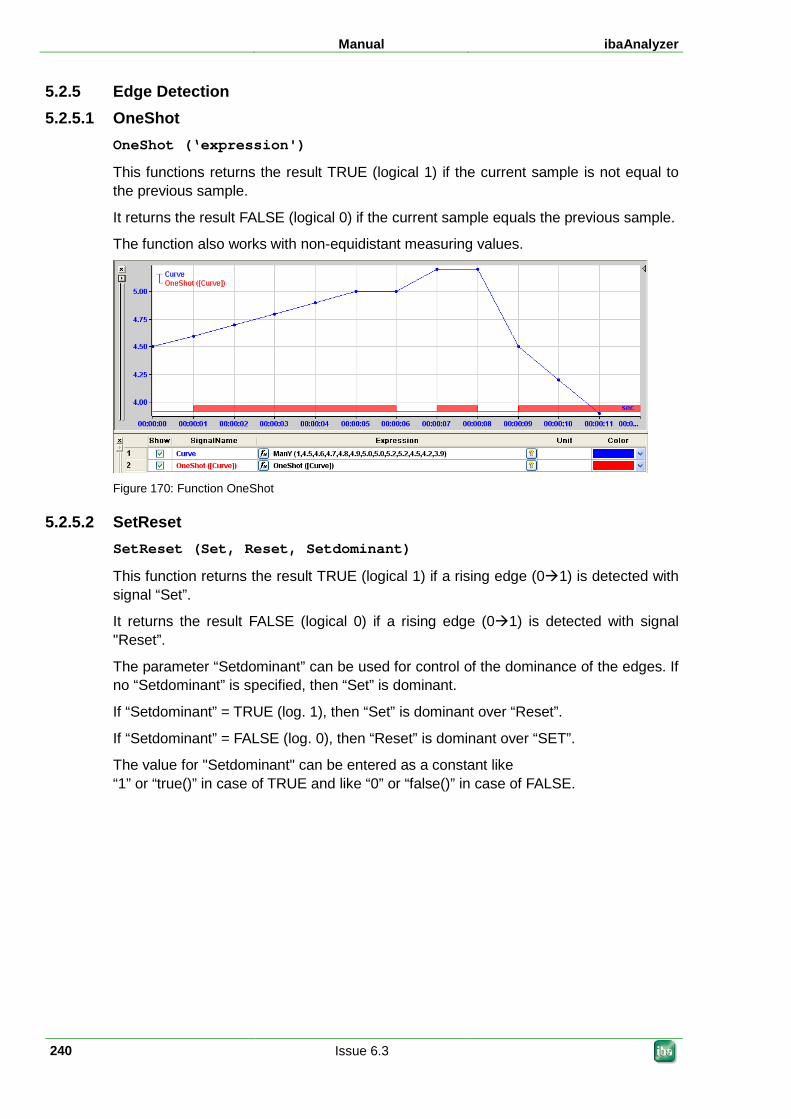
Manual ibaAnalyzer

240 Issue 6.3

5.2.5 Edge Detection 5.2.5.1 OneShot

OneShot (‘expression')

This functions returns the result TRUE (logical 1) if the current sample is not equal to the previous sample.

It returns the result FALSE (logical 0) if the current sample equals the previous sample.

The function also works with non-equidistant measuring values.

Figure 170: Function OneShot

5.2.5.2 SetReset SetReset (Set, Reset, Setdominant)

This function returns the result TRUE (logical 1) if a rising edge (01) is detected with signal “Set”.

It returns the result FALSE (logical 0) if a rising edge (01) is detected with signal "Reset”.

The parameter “Setdominant” can be used for control of the dominance of the edges. If no “Setdominant” is specified, then “Set” is dominant.

If “Setdominant” = TRUE (log. 1), then “Set” is dominant over “Reset”.

If “Setdominant” = FALSE (log. 0), then “Reset” is dominant over “SET”.

The value for "Setdominant" can be entered as a constant like “1” or “true()” in case of TRUE and like “0” or “false()” in case of FALSE.

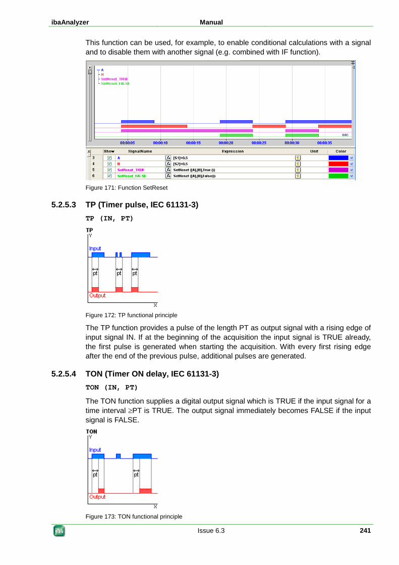
ibaAnalyzer Manual

Issue 6.3 241

This function can be used, for example, to enable conditional calculations with a signal and to disable them with another signal (e.g. combined with IF function).

Figure 171: Function SetReset

5.2.5.3 TP (Timer pulse, IEC 61131-3) TP (IN, PT)

Figure 172: TP functional principle

The TP function provides a pulse of the length PT as output signal with a rising edge of input signal IN. If at the beginning of the acquisition the input signal is TRUE already, the first pulse is generated when starting the acquisition. With every first rising edge after the end of the previous pulse, additional pulses are generated.

5.2.5.4 TON (Timer ON delay, IEC 61131-3) TON (IN, PT)

The TON function supplies a digital output signal which is TRUE if the input signal for a time interval ≥PT is TRUE. The output signal immediately becomes FALSE if the input signal is FALSE.

Figure 173: TON functional principle

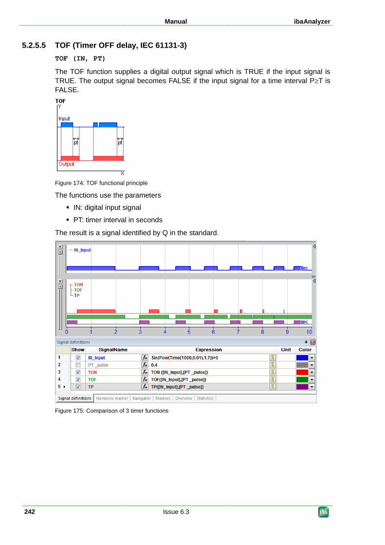
Manual ibaAnalyzer

242 Issue 6.3

5.2.5.5 TOF (Timer OFF delay, IEC 61131-3) TOF (IN, PT)

The TOF function supplies a digital output signal which is TRUE if the input signal is TRUE. The output signal becomes FALSE if the input signal for a time interval P≥T is FALSE.

Figure 174: TOF functional principle

The functions use the parameters

IN: digital input signal

PT: timer interval in seconds

The result is a signal identified by Q in the standard.

Figure 175: Comparison of 3 timer functions

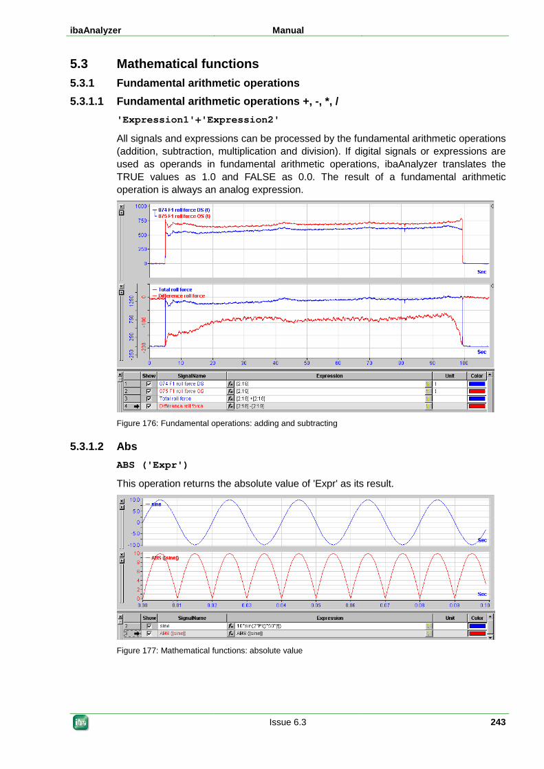
ibaAnalyzer Manual

Issue 6.3 243

5.3 Mathematical functions 5.3.1 Fundamental arithmetic operations 5.3.1.1 Fundamental arithmetic operations +, -, *, /

'Expression1'+'Expression2'

All signals and expressions can be processed by the fundamental arithmetic operations (addition, subtraction, multiplication and division). If digital signals or expressions are used as operands in fundamental arithmetic operations, ibaAnalyzer translates the TRUE values as 1.0 and FALSE as 0.0. The result of a fundamental arithmetic operation is always an analog expression.

Figure 176: Fundamental operations: adding and subtracting

5.3.1.2 Abs ABS ('Expr')

This operation returns the absolute value of 'Expr' as its result.

Figure 177: Mathematical functions: absolute value

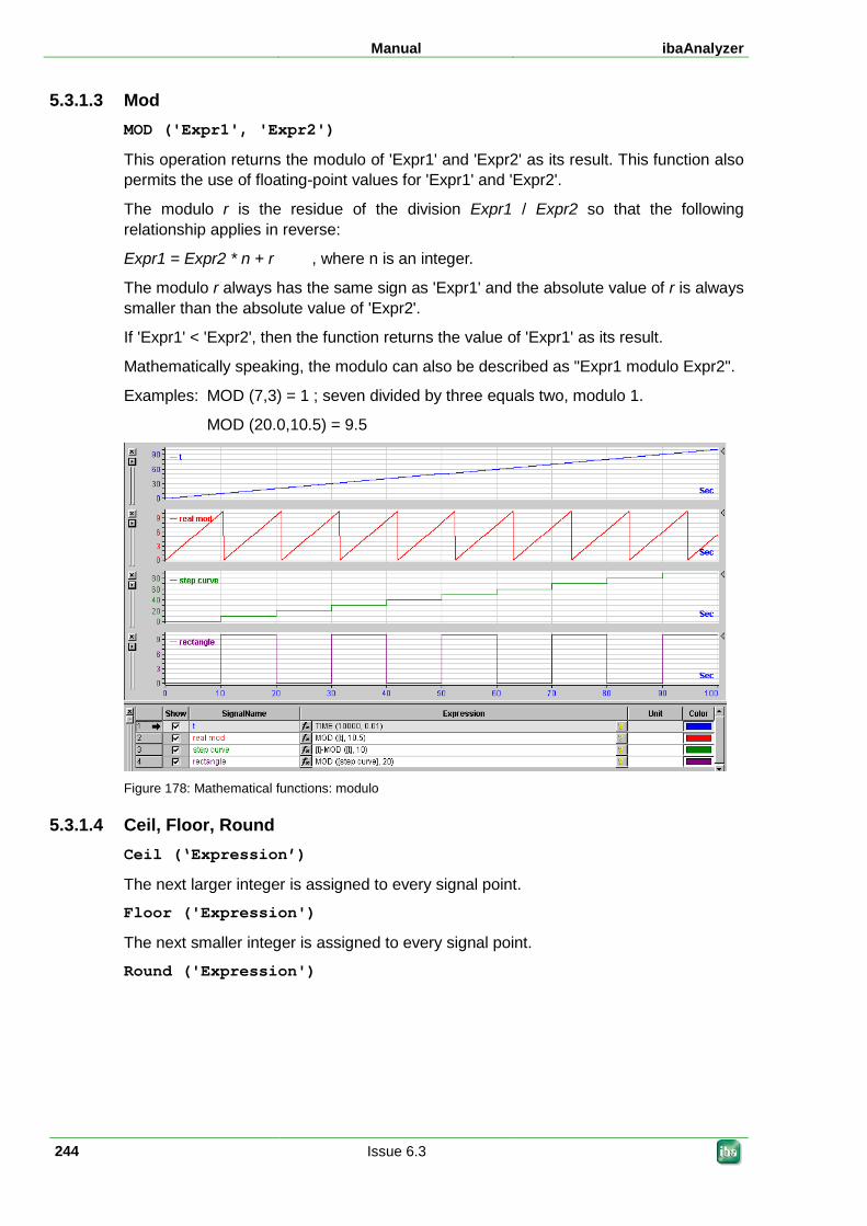
Manual ibaAnalyzer

244 Issue 6.3

5.3.1.3 Mod MOD ('Expr1', 'Expr2')

This operation returns the modulo of 'Expr1' and 'Expr2' as its result. This function also permits the use of floating-point values for 'Expr1' and 'Expr2'.

The modulo r is the residue of the division Expr1 / Expr2 so that the following relationship applies in reverse:

Expr1 = Expr2 * n + r , where n is an integer.

The modulo r always has the same sign as 'Expr1' and the absolute value of r is always smaller than the absolute value of 'Expr2'.

If 'Expr1' < 'Expr2', then the function returns the value of 'Expr1' as its result.

Mathematically speaking, the modulo can also be described as "Expr1 modulo Expr2".

Examples: MOD (7,3) = 1 ; seven divided by three equals two, modulo 1.

MOD (20.0,10.5) = 9.5

Figure 178: Mathematical functions: modulo

5.3.1.4 Ceil, Floor, Round Ceil (‘Expression’)

The next larger integer is assigned to every signal point.

Floor ('Expression')

The next smaller integer is assigned to every signal point.

Round ('Expression')

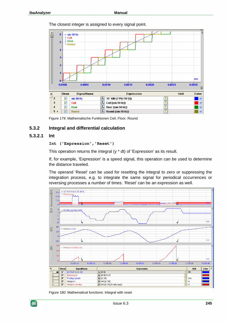
ibaAnalyzer Manual

Issue 6.3 245

The closest integer is assigned to every signal point.

Figure 179: Mathematische Funktionen Ceil, Floor, Round

5.3.2 Integral and differential calculation 5.3.2.1 Int

Int ('Expression','Reset')

This operation returns the integral (y * dt) of 'Expression' as its result.

If, for example, 'Expression' is a speed signal, this operation can be used to determine the distance traveled.

The operand ‘Reset’ can be used for resetting the integral to zero or suppressing the integration process, e.g. to integrate the same signal for periodical occurrences or reversing processes a number of times. ‘Reset’ can be an expression as well.

Figure 180: Mathematical functions: Integral with reset

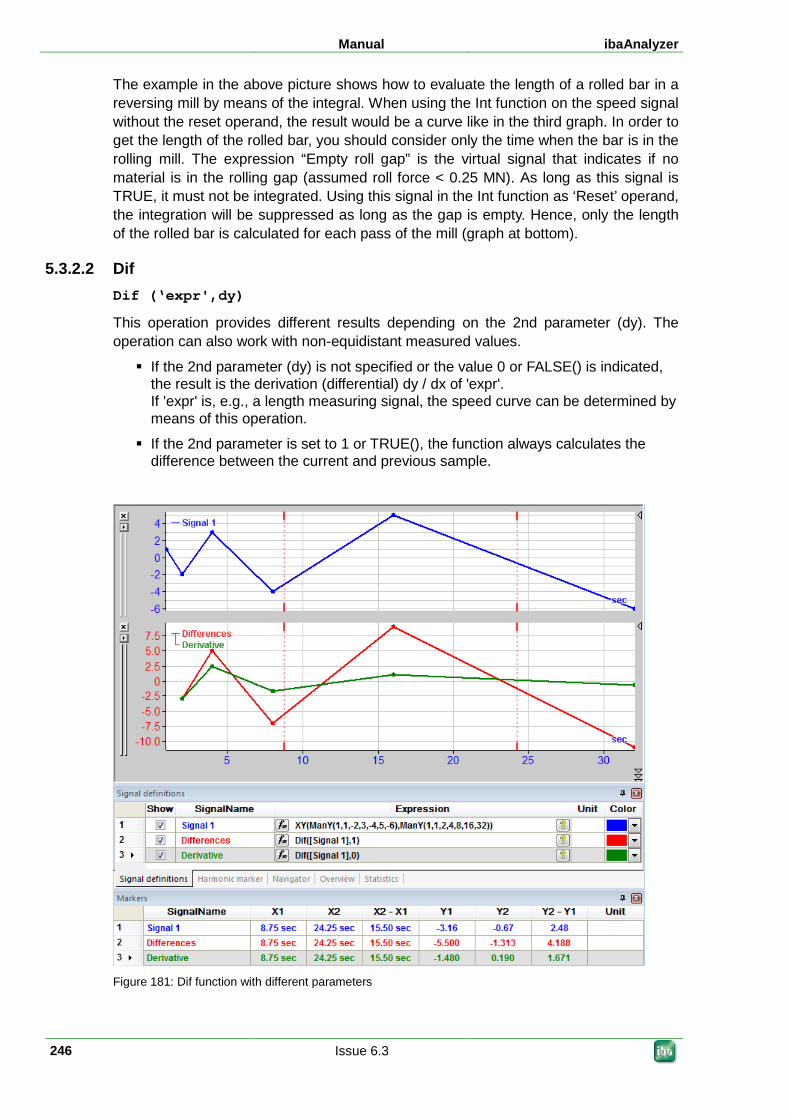
Manual ibaAnalyzer

246 Issue 6.3

The example in the above picture shows how to evaluate the length of a rolled bar in a reversing mill by means of the integral. When using the Int function on the speed signal without the reset operand, the result would be a curve like in the third graph. In order to get the length of the rolled bar, you should consider only the time when the bar is in the rolling mill. The expression “Empty roll gap” is the virtual signal that indicates if no material is in the rolling gap (assumed roll force < 0.25 MN). As long as this signal is TRUE, it must not be integrated. Using this signal in the Int function as ‘Reset’ operand, the integration will be suppressed as long as the gap is empty. Hence, only the length of the rolled bar is calculated for each pass of the mill (graph at bottom).

5.3.2.2 Dif Dif (‘expr',dy)

This operation provides different results depending on the 2nd parameter (dy). The operation can also work with non-equidistant measured values.

If the 2nd parameter (dy) is not specified or the value 0 or FALSE() is indicated, the result is the derivation (differential) dy / dx of 'expr'. If 'expr' is, e.g., a length measuring signal, the speed curve can be determined by means of this operation.

If the 2nd parameter is set to 1 or TRUE(), the function always calculates the difference between the current and previous sample.

Figure 181: Dif function with different parameters

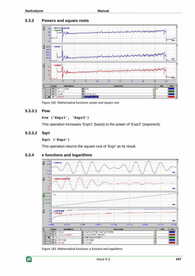
ibaAnalyzer Manual

Issue 6.3 247

5.3.3 Powers and square roots

Figure 182: Mathematical functions: power and square root

5.3.3.1 Pow Pow ('Expr1', 'Expr2')

This operation increases 'Expr1' (basis) to the power of 'Expr2' (exponent).

5.3.3.2 Sqrt Sqrt ('Expr')

This operation returns the square root of 'Expr' as its result.

5.3.4 e functions and logarithms

Figure 183: Mathematical functions: e function and logarithms

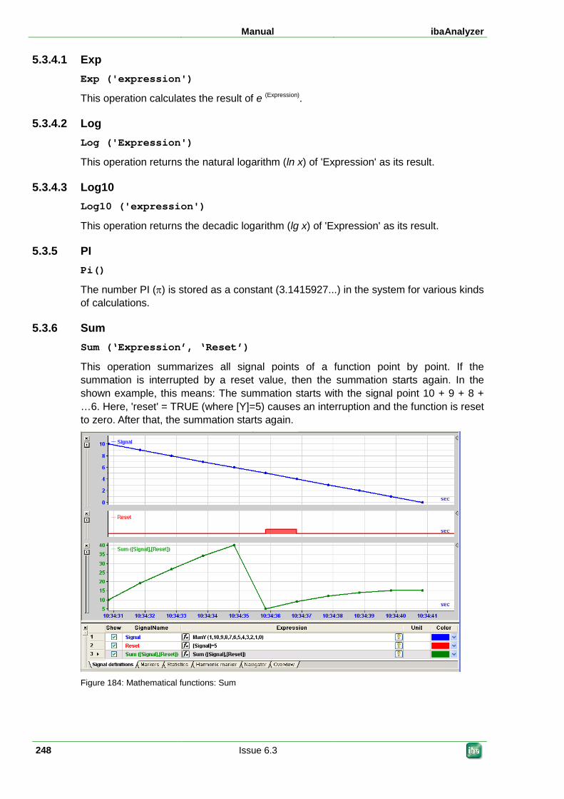
Manual ibaAnalyzer

248 Issue 6.3

5.3.4.1 Exp Exp ('expression')

This operation calculates the result of e (Expression).

5.3.4.2 Log Log ('Expression')

This operation returns the natural logarithm (ln x) of 'Expression' as its result.

5.3.4.3 Log10 Log10 ('expression')

This operation returns the decadic logarithm (lg x) of 'Expression' as its result.

5.3.5 PI Pi()

The number PI (π) is stored as a constant (3.1415927...) in the system for various kinds of calculations.

5.3.6 Sum Sum (‘Expression’, ‘Reset’)

This operation summarizes all signal points of a function point by point. If the summation is interrupted by a reset value, then the summation starts again. In the shown example, this means: The summation starts with the signal point 10 + 9 + 8 + …6. Here, 'reset' = TRUE (where [Y]=5) causes an interruption and the function is reset to zero. After that, the summation starts again.

Figure 184: Mathematical functions: Sum

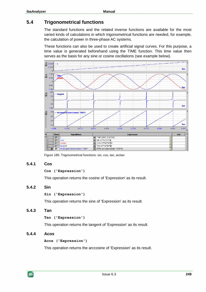
ibaAnalyzer Manual

Issue 6.3 249

5.4 Trigonometrical functions The standard functions and the related inverse functions are available for the most varied kinds of calculations in which trigonometrical functions are needed, for example, the calculation of power in three-phase AC systems.

These functions can also be used to create artificial signal curves. For this purpose, a time value is generated beforehand using the TIME function. This time value then serves as the basis for any sine or cosine oscillations (see example below).

Figure 185: Trigonometrical functions: sin, cos, tan, arctan

5.4.1 Cos Cos ('Expression')

This operation returns the cosine of 'Expression' as its result.

5.4.2 Sin Sin ('Expression')

This operation returns the sine of 'Expression' as its result.

5.4.3 Tan Tan ('Expression')

This operation returns the tangent of 'Expression' as its result.

5.4.4 Acos Acos ('Expression')

This operation returns the arccosine of 'Expression' as its result.

Manual ibaAnalyzer

250 Issue 6.3

5.4.5 Asin Asin ('Expression')

This operation returns the arcsine of 'Expression' as its result.

5.4.6 Atan Atan ('Expression')

This operation returns the arctangent of 'Expression' as its result.

5.4.7 ATAN2 Atan2 (X,Y)

This operation returns the arctangent of Y/X as its result. Signs are taken into account.

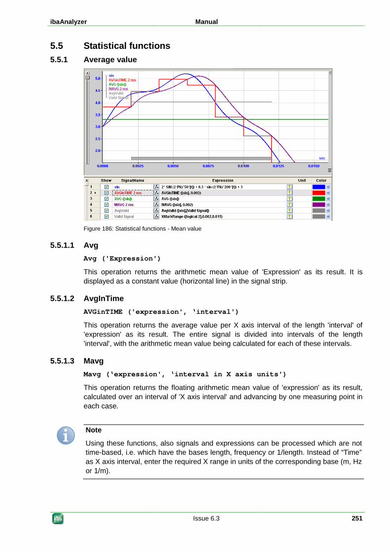
ibaAnalyzer Manual

Issue 6.3 251

5.5 Statistical functions 5.5.1 Average value

Figure 186: Statistical functions - Mean value

5.5.1.1 Avg Avg ('Expression')

This operation returns the arithmetic mean value of 'Expression' as its result. It is displayed as a constant value (horizontal line) in the signal strip.

5.5.1.2 AvgInTime AVGinTIME ('expression', ‘interval')

This operation returns the average value per X axis interval of the length 'interval' of 'expression' as its result. The entire signal is divided into intervals of the length 'interval', with the arithmetic mean value being calculated for each of these intervals.

5.5.1.3 Mavg Mavg (‘expression', ‘interval in X axis units')

This operation returns the floating arithmetic mean value of 'expression' as its result, calculated over an interval of 'X axis interval' and advancing by one measuring point in each case.

Note

Using these functions, also signals and expressions can be processed which are not time-based, i.e. which have the bases length, frequency or 1/length. Instead of “Time” as X axis interval, enter the required X range in units of the corresponding base (m, Hz or 1/m).

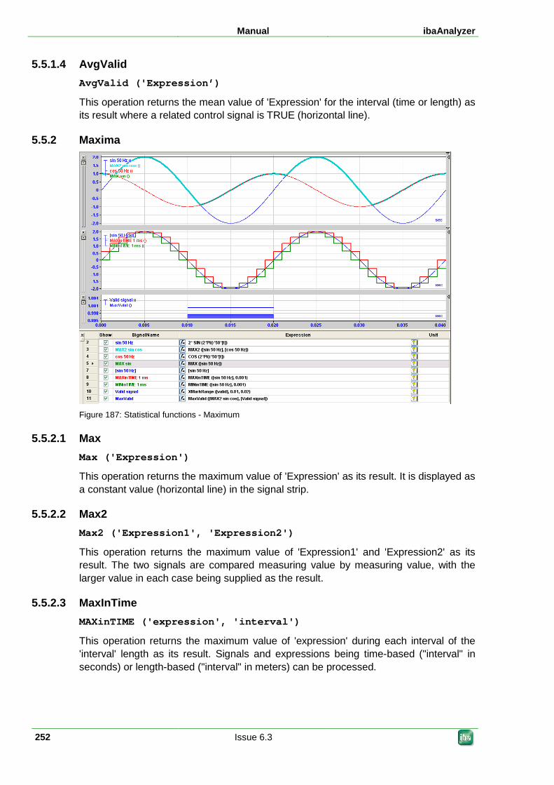
Manual ibaAnalyzer

252 Issue 6.3

5.5.1.4 AvgValid AvgValid ('Expression’)

This operation returns the mean value of 'Expression' for the interval (time or length) as its result where a related control signal is TRUE (horizontal line).

5.5.2 Maxima

Figure 187: Statistical functions - Maximum

5.5.2.1 Max Max ('Expression')

This operation returns the maximum value of 'Expression' as its result. It is displayed as a constant value (horizontal line) in the signal strip.

5.5.2.2 Max2 Max2 ('Expression1', 'Expression2')

This operation returns the maximum value of 'Expression1' and 'Expression2' as its result. The two signals are compared measuring value by measuring value, with the larger value in each case being supplied as the result.

5.5.2.3 MaxInTime MAXinTIME ('expression', 'interval')

This operation returns the maximum value of 'expression' during each interval of the 'interval' length as its result. Signals and expressions being time-based ("interval" in seconds) or length-based ("interval" in meters) can be processed.

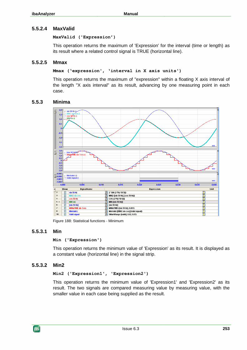
ibaAnalyzer Manual

Issue 6.3 253

5.5.2.4 MaxValid MaxValid ('Expression’)

This operation returns the maximum of 'Expression' for the interval (time or length) as its result where a related control signal is TRUE (horizontal line).

5.5.2.5 Mmax Mmax (‘expression', ‘interval in X axis units')

This operation returns the maximum of "expression" within a floating X axis interval of the length "X axis interval" as its result, advancing by one measuring point in each case.

5.5.3 Minima

Figure 188: Statistical functions - Minimum

5.5.3.1 Min Min ('Expression')

This operation returns the minimum value of 'Expression' as its result. It is displayed as a constant value (horizontal line) in the signal strip.

5.5.3.2 Min2 Min2 ('Expression1', 'Expression2')

This operation returns the minimum value of 'Expression1' and 'Expression2' as its result. The two signals are compared measuring value by measuring value, with the smaller value in each case being supplied as the result.

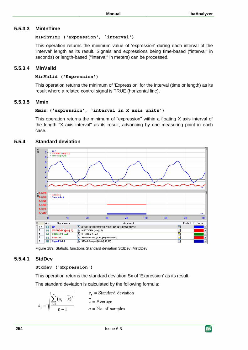
Manual ibaAnalyzer

254 Issue 6.3

5.5.3.3 MinInTime MINinTIME (‘expression', ‘interval')

This operation returns the minimum value of 'expression' during each interval of the 'interval' length as its result. Signals and expressions being time-based ("interval" in seconds) or length-based ("interval" in meters) can be processed.

5.5.3.4 MinValid MinValid ('Expression’)

This operation returns the minimum of 'Expression' for the interval (time or length) as its result where a related control signal is TRUE (horizontal line).

5.5.3.5 Mmin Mmin (‘expression', ‘interval in X axis units')

This operation returns the minimum of "expression" within a floating X axis interval of the length "X axis interval" as its result, advancing by one measuring point in each case.

5.5.4 Standard deviation

Figure 189: Statistic functions Standard deviation StdDev, MstdDev

5.5.4.1 StdDev Stddev ('Expression')

This operation returns the standard deviation Sx of 'Expression' as its result.

The standard deviation is calculated by the following formula:

1

)( 2

1

−

−=∑=

n

xxs

n

ii

x

ibaAnalyzer Manual

Issue 6.3 255

5.5.4.2 MstdDev MstdDev ('expression', 'interval')

This operation returns the floating standard deviation of 'expression' over each time interval of the length 'interval' as its result. Signals and expressions being time-based ("interval" in seconds) or length-based ("interval" in meters) can be processed.

5.5.4.3 StdDevInTime StdDevInTime (‘expression', ‘interval')

This operation returns the standard deviation of 'expression' during each interval of the length 'interval' as its result. Signals and expressions being time-based ("interval" in seconds) or length-based ("interval" in meters) can be processed.

5.5.4.4 StdDevValid StdDevValid ('Expression’)

This operation returns the standard deviation of 'Expression' for the interval (time or length) as its result where a related control signal is TRUE (horizontal line).

Manual ibaAnalyzer

256 Issue 6.3

5.5.5 Percentiles 5.5.5.1 Percentiles

Percentile ('expr', 'p')

This operation returns the "pth" percentile of 'expr' as its result.

The "pth" percentile is the smallest value of a set of measured values which is greater than p% of the number of values measured. A typical percentile is the 50% percentile, the so-called median. The median divides the set of values measured into two equal halves: 50% of all values measured are smaller than the median value, the remaining 50% are greater than or equal to it. Further typical percentiles are 25% and 75% which, together with the median, enable the division of a set of values measured into four groups, the so-called quartiles. (< 25%, <50%, <75%, ≥75%).

The "Percentile" function determines the percentile value of the total number of measuring points of a signal. The percentile 'p' must be entered as a decimal value, i.e.:

50 % --> p = 0.5 (default value)

75 % --> p = 0.75

95.9 % --> p = 0.959

This function is, for example, particularly useful when it comes to assessing the quality of a product where a particular property must comply with a defined classification.

Example: Classification of the quality of the rolling process of strip steel in terms of the thickness deviation of the finished product.

In order to determine the quality of the rolled strip, quality classes are defined for the thickness deviation as one out of several measures. The lower the thickness deviation of the strip thickness measured from the related setpoint, the higher the quality of the rolled product. The following values are assumed here for illustration purposes.

The thickness deviation must comply with the following criteria as a precondition for a finished rolled strip to be classified as marketable:

at least 95% of all the measured values of the strip must be smaller than 20 µm

at least 97.5 % of all the measured values of the strip must be smaller than 80 µm

at least 99.5 % of all the measured values of the strip must be smaller than 150 µm.

In other words, this means that, for example, only 0.5% of the values measured may be subject to a thickness deviation greater than 150 µm as a precondition for the strip not to be sorted out.

In the example shown below, the three percentiles, i.e. 95% (p = 0.95), 97.5% (p = 0.975) and 99.5% (p = 0.995) of the measuring value "116 Thickness deviation behind F7" were thus determined. Although the percentile values are not displayed in the signal strip display in order to save space, they are displayed in the "Report info" window using the report generator function. In the interest of enhanced presentation, the values determined are compared to the above-mentioned limit values and the result of the comparative operations is displayed as binary signals (color bars). All the three bars must be displayed as thick bars in order for the strip to meet the quality requirements.

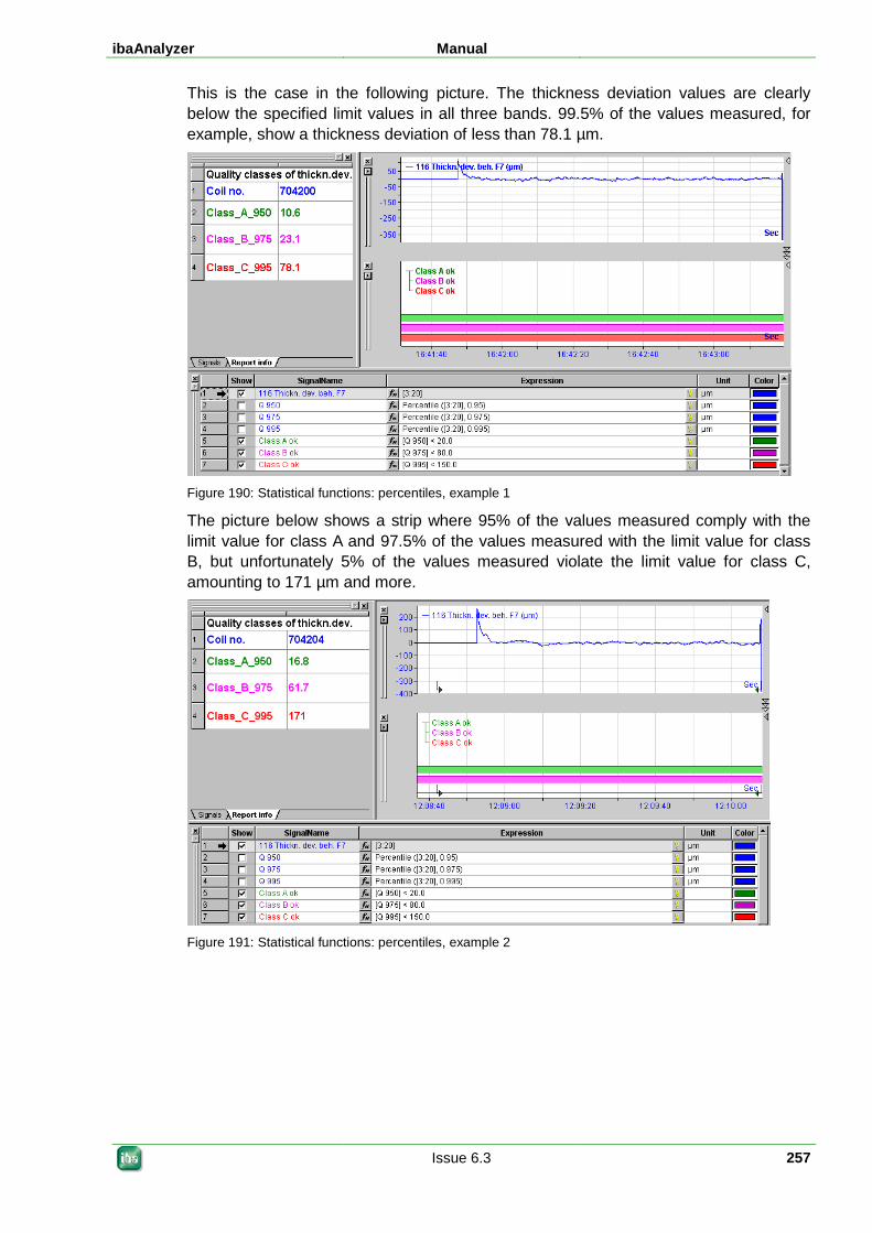
ibaAnalyzer Manual

Issue 6.3 257

This is the case in the following picture. The thickness deviation values are clearly below the specified limit values in all three bands. 99.5% of the values measured, for example, show a thickness deviation of less than 78.1 µm.

Figure 190: Statistical functions: percentiles, example 1

The picture below shows a strip where 95% of the values measured comply with the limit value for class A and 97.5% of the values measured with the limit value for class B, but unfortunately 5% of the values measured violate the limit value for class C, amounting to 171 µm and more.

Figure 191: Statistical functions: percentiles, example 2

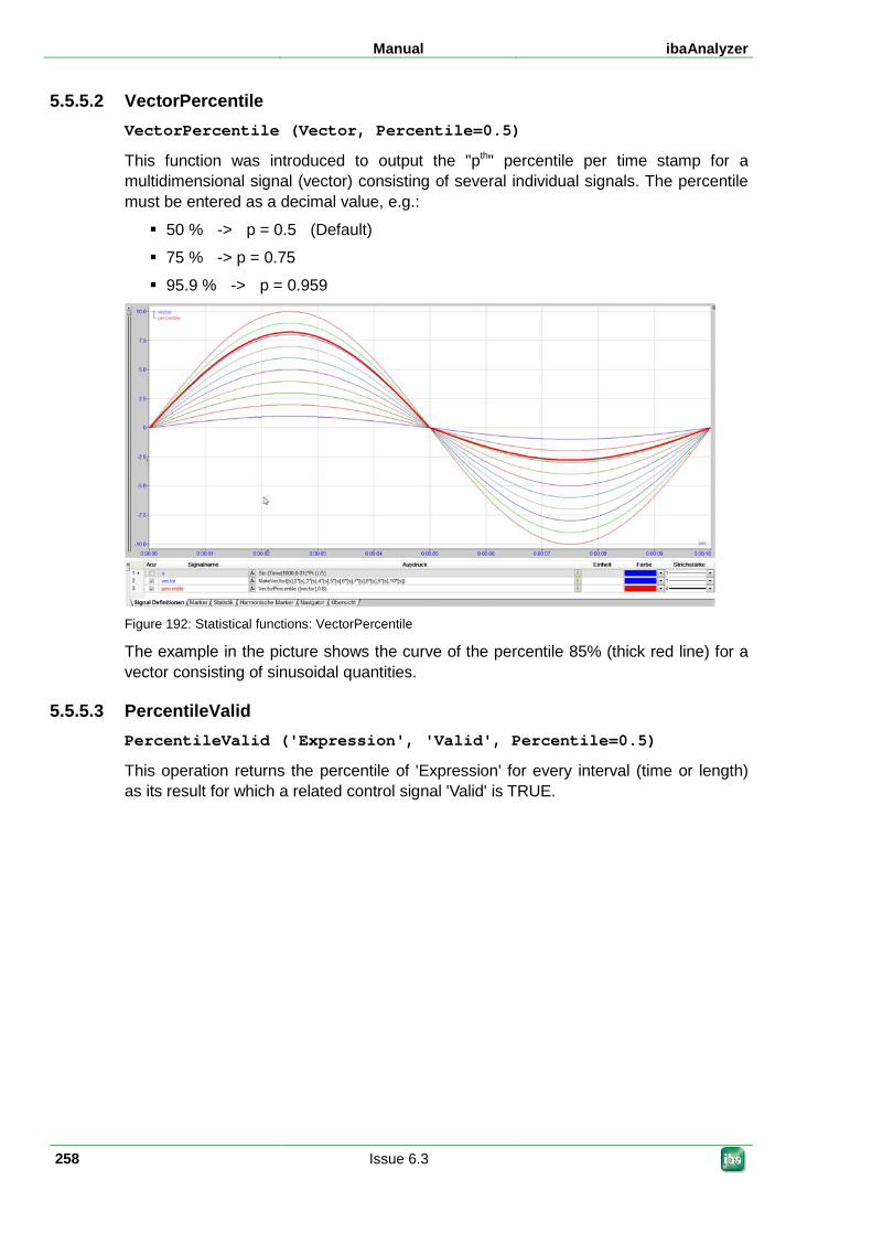
Manual ibaAnalyzer

258 Issue 6.3

5.5.5.2 VectorPercentile VectorPercentile (Vector, Percentile=0.5)

This function was introduced to output the "pth" percentile per time stamp for a multidimensional signal (vector) consisting of several individual signals. The percentile must be entered as a decimal value, e.g.:

50 % -> p = 0.5 (Default)

75 % -> p = 0.75

95.9 % -> p = 0.959

Figure 192: Statistical functions: VectorPercentile

The example in the picture shows the curve of the percentile 85% (thick red line) for a vector consisting of sinusoidal quantities.

5.5.5.3 PercentileValid PercentileValid ('Expression', 'Valid', Percentile=0.5)

This operation returns the percentile of 'Expression' for every interval (time or length) as its result for which a related control signal 'Valid' is TRUE.

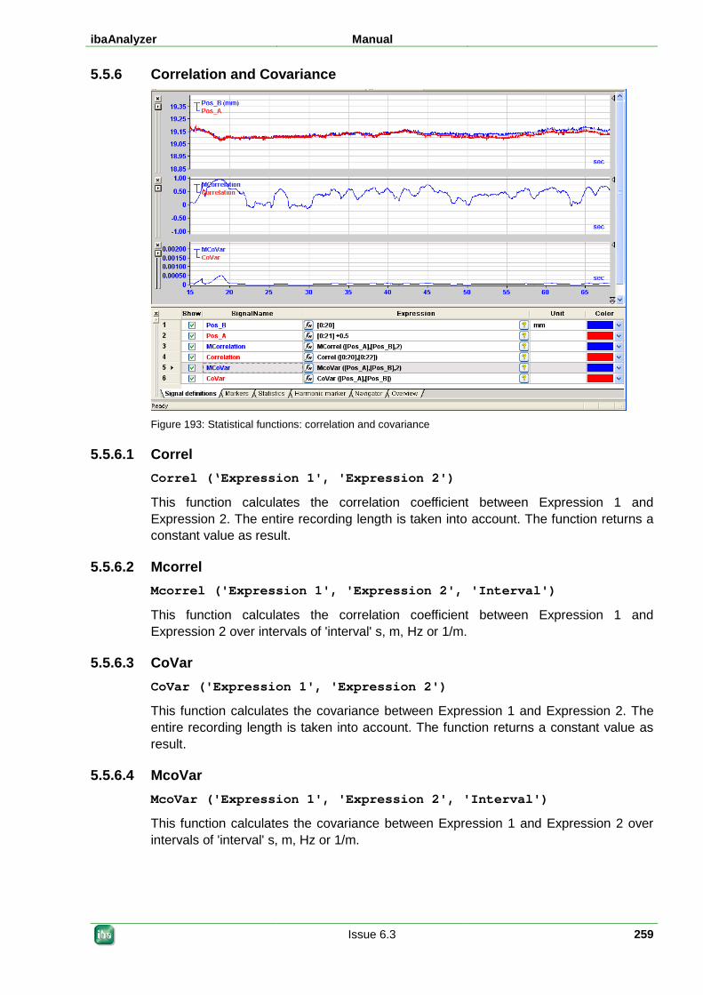
ibaAnalyzer Manual

Issue 6.3 259

5.5.6 Correlation and Covariance

Figure 193: Statistical functions: correlation and covariance

5.5.6.1 Correl Correl (‘Expression 1', 'Expression 2')

This function calculates the correlation coefficient between Expression 1 and Expression 2. The entire recording length is taken into account. The function returns a constant value as result.

5.5.6.2 Mcorrel Mcorrel ('Expression 1', 'Expression 2', 'Interval')

This function calculates the correlation coefficient between Expression 1 and Expression 2 over intervals of 'interval' s, m, Hz or 1/m.

5.5.6.3 CoVar CoVar ('Expression 1', 'Expression 2')

This function calculates the covariance between Expression 1 and Expression 2. The entire recording length is taken into account. The function returns a constant value as result.

5.5.6.4 McoVar McoVar ('Expression 1', 'Expression 2', 'Interval')

This function calculates the covariance between Expression 1 and Expression 2 over intervals of 'interval' s, m, Hz or 1/m.

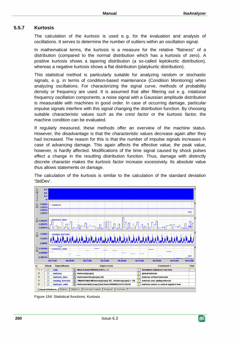
Manual ibaAnalyzer

260 Issue 6.3

5.5.7 Kurtosis The calculation of the kurtosis is used e. g. for the evaluation and analysis of oscillations. It serves to determine the number of outliers within an oscillation signal.

In mathematical terms, the kurtosis is a measure for the relative "flatness" of a distribution (compared to the normal distribution which has a kurtosis of zero). A positive kurtosis shows a tapering distribution (a so-called leptokurtic distribution), whereas a negative kurtosis shows a flat distribution (platykurtic distribution).

This statistical method is particularly suitable for analyzing random or stochastic signals, e. g. in terms of condition-based maintenance (Condition Monitoring) when analyzing oscillations. For characterizing the signal curve, methods of probability density or frequency are used. It is assumed that after filtering out e. g. rotational frequency oscillation components, a noise signal with a Gaussian amplitude distribution is measurable with machines in good order. In case of occurring damage, particular impulse signals interfere with this signal changing the distribution function. By choosing suitable characteristic values such as the crest factor or the kurtosis factor, the machine condition can be evaluated.

If regularly measured, these methods offer an overview of the machine status. However, the disadvantage is that the characteristic values decrease again after they had increased. The reason for this is that the number of impulse signals increases in case of advancing damage. This again affects the effective value, the peak value, however, is hardly affected. Modifications of the time signal caused by shock pulses effect a change in the resulting distribution function. Thus, damage with distinctly discrete character makes the kurtosis factor increase excessively. Its absolute value thus allows statements on damage.

The calculation of the kurtosis is similar to the calculation of the standard deviation 'StdDev'.

Figure 194: Statistical functions: Kurtosis

ibaAnalyzer Manual

Issue 6.3 261

5.5.7.1 Kurtosis Kurtosis (Expression')

This operation returns the kurtosis of the selected time signal as its result (expression).

5.5.7.2 KurtosisInTime KurtosisInTime ('Expression', 'Interval')

With this operation, the selected expression is divided into intervals of equal length of the quantity 'Interval'. For these intervals, the kurtosis is subsequently calculated.

5.5.7.3 MKurtosis MKurtosis ('Expression', 'interval')

This operation calculates the kurtosis of 'expression' over a fixed but floating X axis interval.

5.5.7.4 KurtosisValid KurtosisValid ('Expression', 'Valid')

This operation describes the kurtosis for those areas where a related control signal is TRUE.

5.5.7.5 VectorKurtosis VectorKurtosis('Vector')

This operation calculates the kurtosis for every signal point of a vector. Please note that at least 4 signal points must be available for this calculation.

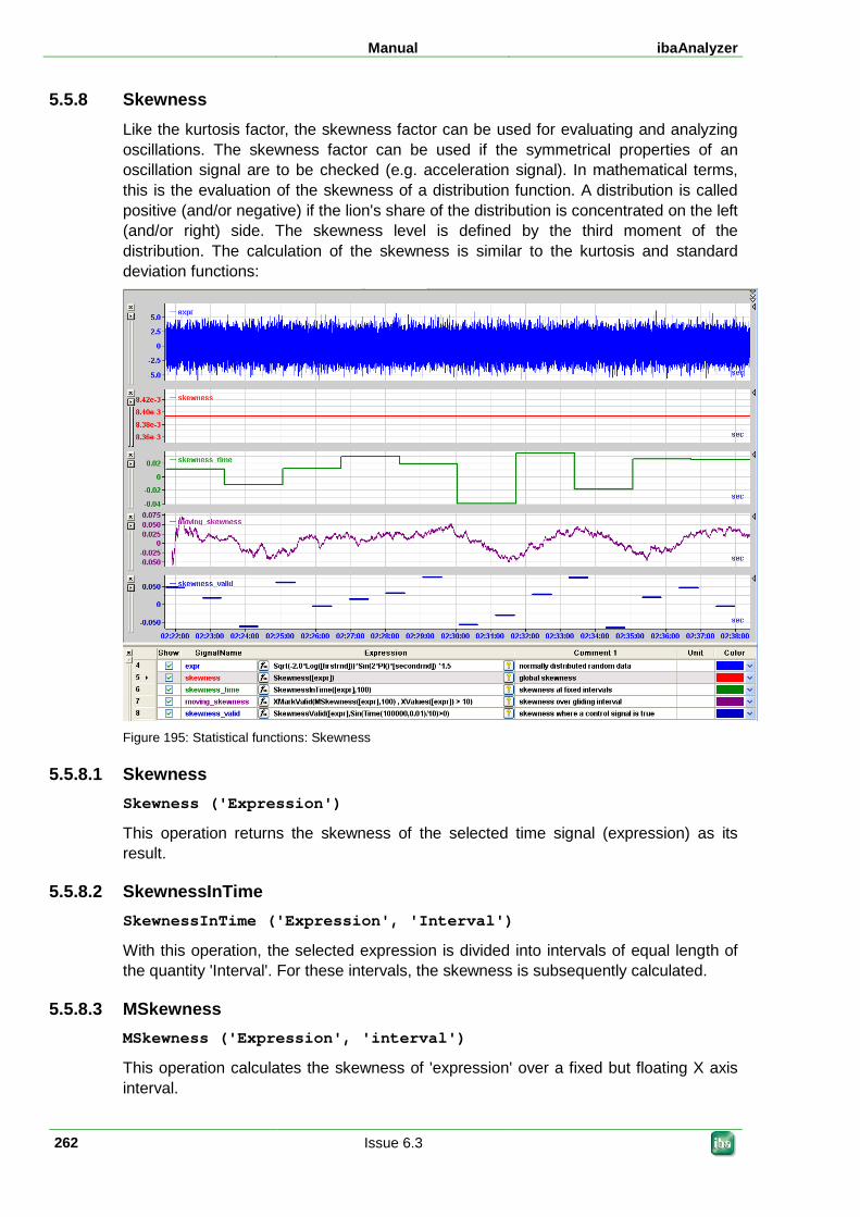
Manual ibaAnalyzer

262 Issue 6.3

5.5.8 Skewness Like the kurtosis factor, the skewness factor can be used for evaluating and analyzing oscillations. The skewness factor can be used if the symmetrical properties of an oscillation signal are to be checked (e.g. acceleration signal). In mathematical terms, this is the evaluation of the skewness of a distribution function. A distribution is called positive (and/or negative) if the lion's share of the distribution is concentrated on the left (and/or right) side. The skewness level is defined by the third moment of the distribution. The calculation of the skewness is similar to the kurtosis and standard deviation functions:

Figure 195: Statistical functions: Skewness

5.5.8.1 Skewness Skewness ('Expression')

This operation returns the skewness of the selected time signal (expression) as its result.

5.5.8.2 SkewnessInTime SkewnessInTime ('Expression', 'Interval')

With this operation, the selected expression is divided into intervals of equal length of the quantity 'Interval'. For these intervals, the skewness is subsequently calculated.

5.5.8.3 MSkewness MSkewness ('Expression', 'interval')

This operation calculates the skewness of 'expression' over a fixed but floating X axis interval.

ibaAnalyzer Manual

Issue 6.3 263

5.5.8.4 SkewnessValid SkewnessValid ('Expression', 'Valid')

This operation described the skewness for those areas where a related control signal is TRUE.

5.5.8.5 VetorSkewness VectorSkewness ('Vector')

This operation calculates the skewness for every signal point of a vector. Please note that at least 4 signal points must be available for this calculation.

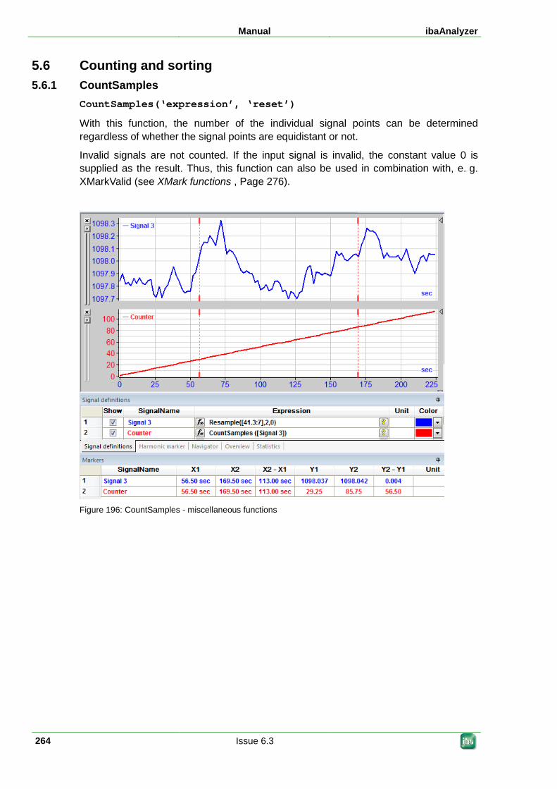
Manual ibaAnalyzer

264 Issue 6.3

5.6 Counting and sorting 5.6.1 CountSamples

CountSamples(‘expression’, ‘reset’)

With this function, the number of the individual signal points can be determined regardless of whether the signal points are equidistant or not.

Invalid signals are not counted. If the input signal is invalid, the constant value 0 is supplied as the result. Thus, this function can also be used in combination with, e. g. XMarkValid (see XMark functions , Page 276).

Figure 196: CountSamples - miscellaneous functions

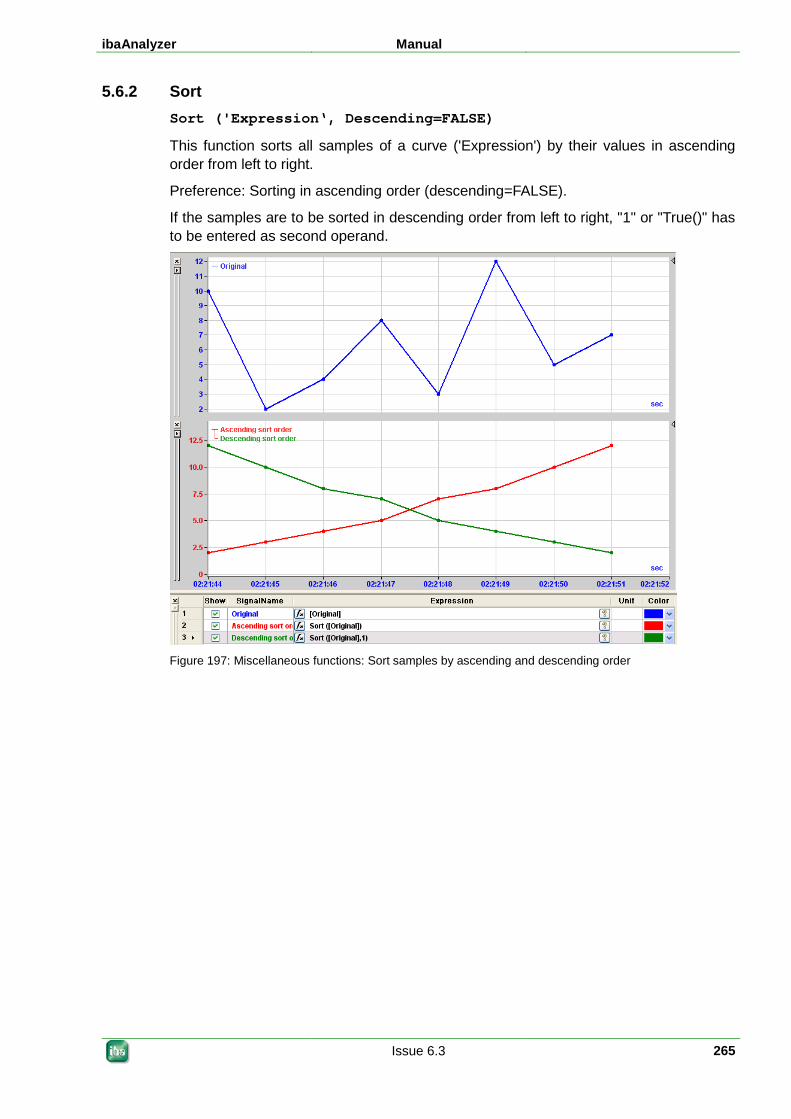
ibaAnalyzer Manual

Issue 6.3 265

5.6.2 Sort Sort ('Expression‘, Descending=FALSE)

This function sorts all samples of a curve ('Expression') by their values in ascending order from left to right.

Preference: Sorting in ascending order (descending=FALSE).

If the samples are to be sorted in descending order from left to right, "1" or "True()" has to be entered as second operand.

Figure 197: Miscellaneous functions: Sort samples by ascending and descending order

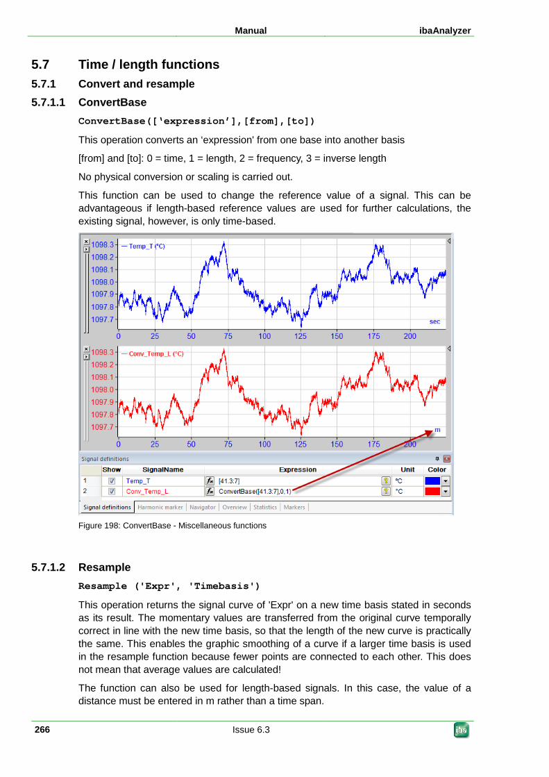
Manual ibaAnalyzer

266 Issue 6.3

5.7 Time / length functions 5.7.1 Convert and resample 5.7.1.1 ConvertBase

ConvertBase([‘expression’],[from],[to])

This operation converts an ‘expression' from one base into another basis

[from] and [to]: 0 = time, 1 = length, 2 = frequency, 3 = inverse length

No physical conversion or scaling is carried out.

This function can be used to change the reference value of a signal. This can be advantageous if length-based reference values are used for further calculations, the existing signal, however, is only time-based.

Figure 198: ConvertBase - Miscellaneous functions

5.7.1.2 Resample Resample ('Expr', 'Timebasis')

This operation returns the signal curve of 'Expr' on a new time basis stated in seconds as its result. The momentary values are transferred from the original curve temporally correct in line with the new time basis, so that the length of the new curve is practically the same. This enables the graphic smoothing of a curve if a larger time basis is used in the resample function because fewer points are connected to each other. This does not mean that average values are calculated!

The function can also be used for length-based signals. In this case, the value of a distance must be entered in m rather than a time span.

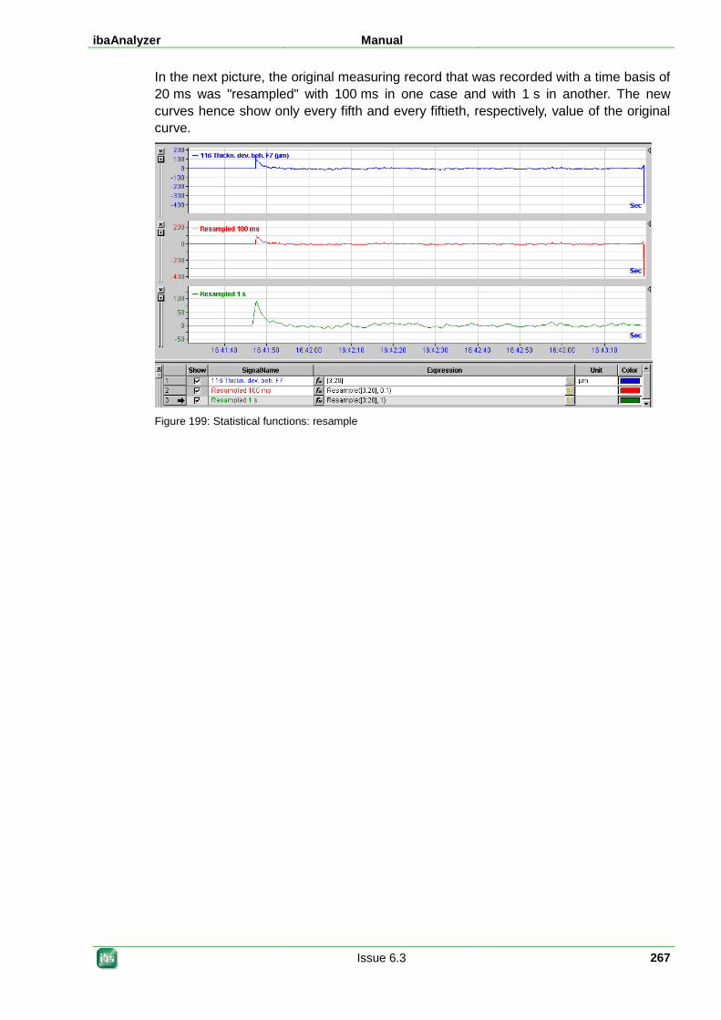
ibaAnalyzer Manual

Issue 6.3 267

In the next picture, the original measuring record that was recorded with a time basis of 20 ms was "resampled" with 100 ms in one case and with 1 s in another. The new curves hence show only every fifth and every fiftieth, respectively, value of the original curve.

Figure 199: Statistical functions: resample

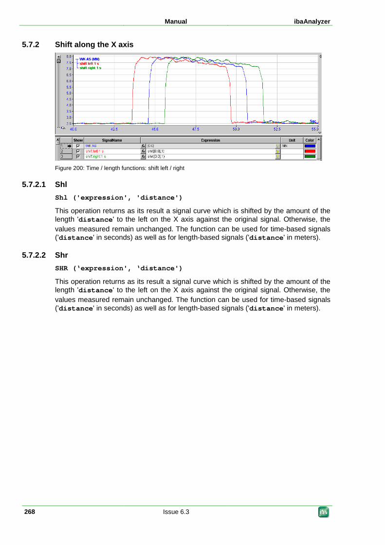
Manual ibaAnalyzer

268 Issue 6.3

5.7.2 Shift along the X axis

Figure 200: Time / length functions: shift left / right

5.7.2.1 Shl Shl ('expression', 'distance')

This operation returns as its result a signal curve which is shifted by the amount of the length 'distance' to the left on the X axis against the original signal. Otherwise, the values measured remain unchanged. The function can be used for time-based signals ('distance' in seconds) as well as for length-based signals ('distance' in meters).

5.7.2.2 Shr SHR (‘expression', ‘distance')

This operation returns as its result a signal curve which is shifted by the amount of the length 'distance' to the left on the X axis against the original signal. Otherwise, the values measured remain unchanged. The function can be used for time-based signals ('distance' in seconds) as well as for length-based signals ('distance' in meters).

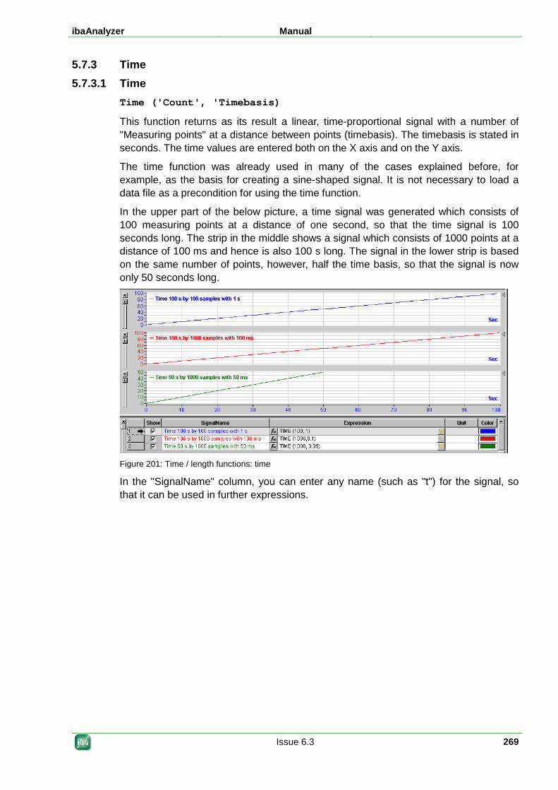
ibaAnalyzer Manual

Issue 6.3 269

5.7.3 Time 5.7.3.1 Time

Time ('Count', 'Timebasis)

This function returns as its result a linear, time-proportional signal with a number of "Measuring points" at a distance between points (timebasis). The timebasis is stated in seconds. The time values are entered both on the X axis and on the Y axis.

The time function was already used in many of the cases explained before, for example, as the basis for creating a sine-shaped signal. It is not necessary to load a data file as a precondition for using the time function.

In the upper part of the below picture, a time signal was generated which consists of 100 measuring points at a distance of one second, so that the time signal is 100 seconds long. The strip in the middle shows a signal which consists of 1000 points at a distance of 100 ms and hence is also 100 s long. The signal in the lower strip is based on the same number of points, however, half the time basis, so that the signal is now only 50 seconds long.

Figure 201: Time / length functions: time

In the "SignalName" column, you can enter any name (such as "t") for the signal, so that it can be used in further expressions.

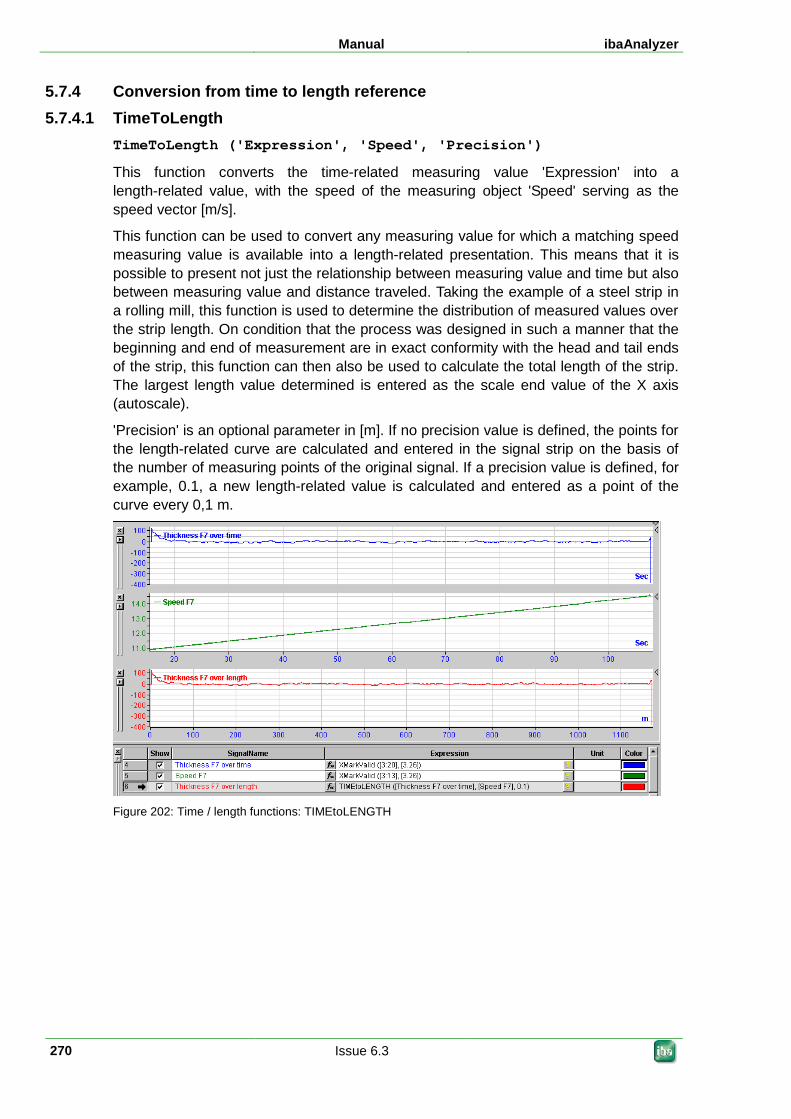
Manual ibaAnalyzer

270 Issue 6.3

5.7.4 Conversion from time to length reference 5.7.4.1 TimeToLength

TimeToLength ('Expression', 'Speed', 'Precision')

This function converts the time-related measuring value 'Expression' into a length-related value, with the speed of the measuring object 'Speed' serving as the speed vector [m/s].

This function can be used to convert any measuring value for which a matching speed measuring value is available into a length-related presentation. This means that it is possible to present not just the relationship between measuring value and time but also between measuring value and distance traveled. Taking the example of a steel strip in a rolling mill, this function is used to determine the distribution of measured values over the strip length. On condition that the process was designed in such a manner that the beginning and end of measurement are in exact conformity with the head and tail ends of the strip, this function can then also be used to calculate the total length of the strip. The largest length value determined is entered as the scale end value of the X axis (autoscale).

'Precision' is an optional parameter in [m]. If no precision value is defined, the points for the length-related curve are calculated and entered in the signal strip on the basis of the number of measuring points of the original signal. If a precision value is defined, for example, 0.1, a new length-related value is calculated and entered as a point of the curve every 0,1 m.

Figure 202: Time / length functions: TIMEtoLENGTH

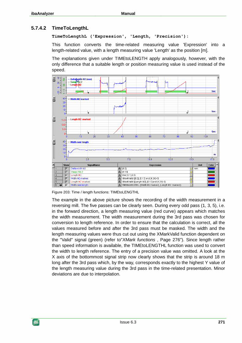
ibaAnalyzer Manual

Issue 6.3 271

5.7.4.2 TimeToLengthL TimeToLengthL ('Expression', 'Length, 'Precision'):

This function converts the time-related measuring value 'Expression' into a length-related value, with a length measuring value 'Length' as the position [m].

The explanations given under TIMEtoLENGTH apply analogously, however, with the only difference that a suitable length or position measuring value is used instead of the speed.

Figure 203: Time / length functions: TIMEtoLENGTHL

The example in the above picture shows the recording of the width measurement in a reversing mill. The five passes can be clearly seen. During every odd pass (1, 3, 5), i.e. in the forward direction, a length measuring value (red curve) appears which matches the width measurement. The width measurement during the 3rd pass was chosen for conversion to length reference. In order to ensure that the calculation is correct, all the values measured before and after the 3rd pass must be masked. The width and the length measuring values were thus cut out using the XMarkValid function dependent on the "Valid" signal (green) (refer to"XMark functions , Page 276"). Since length rather than speed information is available, the TIMEtoLENGTHL function was used to convert the width to length reference. The entry of a precision value was omitted. A look at the X axis of the bottommost signal strip now clearly shows that the strip is around 18 m long after the 3rd pass which, by the way, corresponds exactly to the highest Y value of the length measuring value during the 3rd pass in the time-related presentation. Minor deviations are due to interpolation.

Manual ibaAnalyzer

272 Issue 6.3

5.8 X axis operations 5.8.1 Shift along the X axis 5.8.1.1 SHL and SHR

See Shift along the X axis, Page 268

5.8.2 XAlignFft XAlignFft ('FixedExpr', 'AlignmentExpr', Start, End, MinScale, MaxScale, ScaleStep, QualityParam)

With this function, length-based signals with the same physical significance which were measured in different places in the process can be aligned to each other.

One example for this is the thickness-length-profile, which is recorded at the exit of a hot strip mill, and the thickness-length-profile, which is measured at the entry of the subsequent continuous pickling line.

When applying the function, different steps have to be taken into consideration that is described in the following.

Preparation of the data for an alignment (example thickness measurement)

For an automatic alignment, both of the thickness measurements (e.g. exit hot rolling – entry cold rolling or exit hot rolling – entry pickle, etc.) have to be length-related. To transform a time-related thickness measurement to length reference, three signals are required (see also "Conversion from time to length reference , Page 270"):

the time-related thickness measurement [thickness_time]

a time-related speed signal describing the speed of the strip in the thickness gauge. [speed_time]

a binary signal indicating whether a strip is present in a thickness measurement [valid]

With these three signals, the transformation can be carried out with the TimeToLength function of the ibaAnalyzer as follows:

[thickness_meter] = TimeToLength(XCutValid( [thickness_time], [valid]), XCutValid([speed_time], [valid]))

The length-related thickness measurements now have to be "mean adjusted" to exclude an existing Y shift:

[thickness_avgcln] =[thickness_meter] - Avg([thickness_meter])

If there still is an obvious Y offset due to outliers at the head or foot, both measurement series can be adjusted for the mean value of their "fillet":

[Fillet] = XmarkRange([thickness_meter], [start_fillet], [end_fillet])

[thickness_avgcln] = [thickness_meter] – Avg([Fillet])

Where applicable, one of the two strips has to be mirrored:

[thickness_mirror] = XMirror([thickness_avgcln])

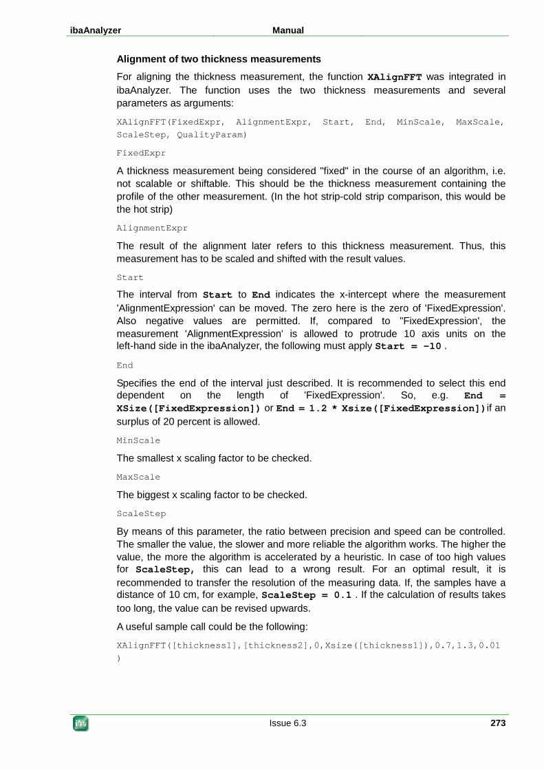
ibaAnalyzer Manual

Issue 6.3 273

Alignment of two thickness measurements

For aligning the thickness measurement, the function XAlignFFT was integrated in ibaAnalyzer. The function uses the two thickness measurements and several parameters as arguments:

XAlignFFT(FixedExpr, AlignmentExpr, Start, End, MinScale, MaxScale, ScaleStep, QualityParam)

FixedExpr

A thickness measurement being considered "fixed" in the course of an algorithm, i.e. not scalable or shiftable. This should be the thickness measurement containing the profile of the other measurement. (In the hot strip-cold strip comparison, this would be the hot strip)

AlignmentExpr

The result of the alignment later refers to this thickness measurement. Thus, this measurement has to be scaled and shifted with the result values.

Start

The interval from Start to End indicates the x-intercept where the measurement 'AlignmentExpression' can be moved. The zero here is the zero of 'FixedExpression'. Also negative values are permitted. If, compared to "FixedExpression', the measurement 'AlignmentExpression' is allowed to protrude 10 axis units on the left-hand side in the ibaAnalyzer, the following must apply Start = -10 .

End

Specifies the end of the interval just described. It is recommended to select this end dependent on the length of 'FixedExpression'. So, e.g. End = XSize([FixedExpression]) or End = 1.2 * Xsize([FixedExpression])if an surplus of 20 percent is allowed.

MinScale

The smallest x scaling factor to be checked.

MaxScale

The biggest x scaling factor to be checked.

ScaleStep

By means of this parameter, the ratio between precision and speed can be controlled. The smaller the value, the slower and more reliable the algorithm works. The higher the value, the more the algorithm is accelerated by a heuristic. In case of too high values for ScaleStep, this can lead to a wrong result. For an optimal result, it is recommended to transfer the resolution of the measuring data. If, the samples have a distance of 10 cm, for example, ScaleStep = 0.1 . If the calculation of results takes too long, the value can be revised upwards.

A useful sample call could be the following:

XAlignFFT([thickness1],[thickness2],0,Xsize([thickness1]),0.7,1.3,0.01)

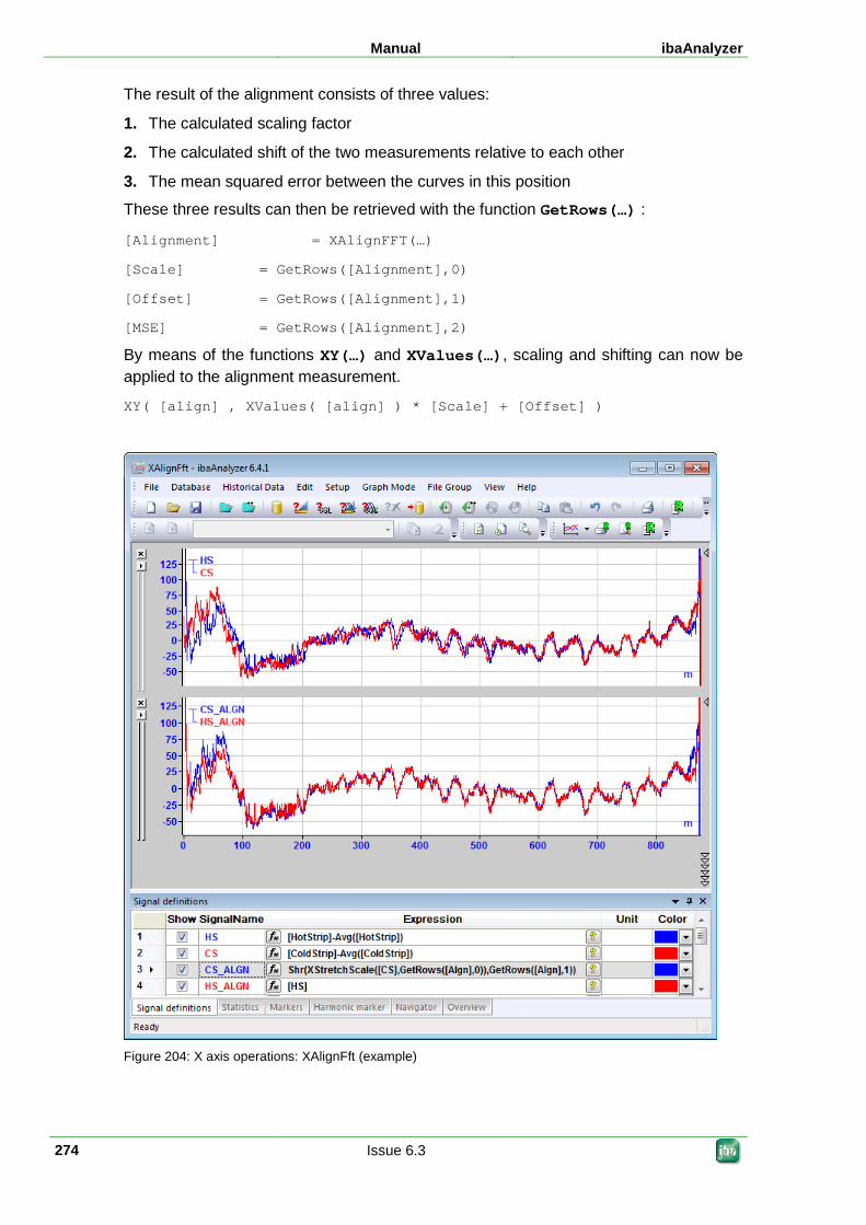
Manual ibaAnalyzer

274 Issue 6.3

The result of the alignment consists of three values:

1. The calculated scaling factor

2. The calculated shift of the two measurements relative to each other

3. The mean squared error between the curves in this position

These three results can then be retrieved with the function GetRows(…) :

[Alignment] = XAlignFFT(…)

[Scale] = GetRows([Alignment],0)

[Offset] = GetRows([Alignment],1)

[MSE] = GetRows([Alignment],2)

By means of the functions XY(…) and XValues(…), scaling and shifting can now be applied to the alignment measurement.

XY( [align] , XValues( [align] ) * [Scale] + [Offset] )

Figure 204: X axis operations: XAlignFft (example)

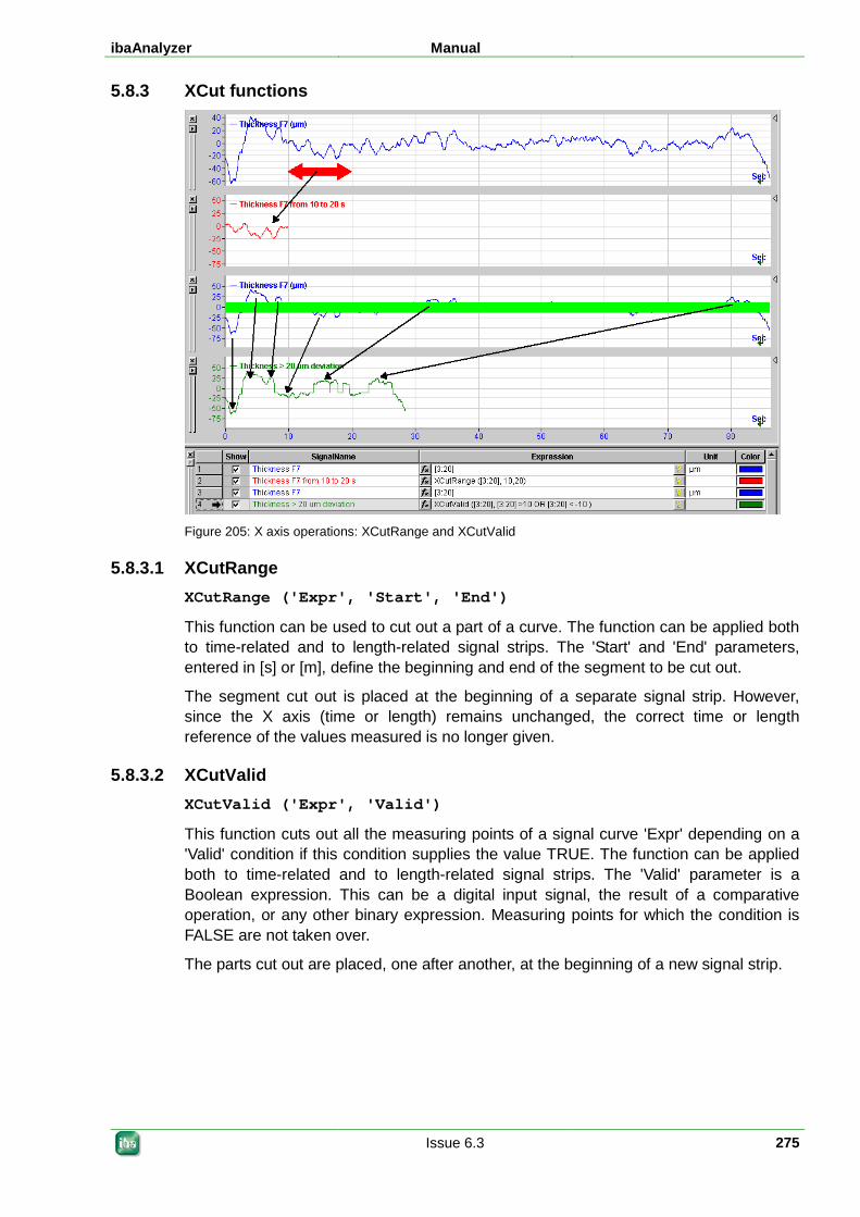
ibaAnalyzer Manual

Issue 6.3 275

5.8.3 XCut functions

Figure 205: X axis operations: XCutRange and XCutValid

5.8.3.1 XCutRange XCutRange ('Expr', 'Start', 'End')

This function can be used to cut out a part of a curve. The function can be applied both to time-related and to length-related signal strips. The 'Start' and 'End' parameters, entered in [s] or [m], define the beginning and end of the segment to be cut out.

The segment cut out is placed at the beginning of a separate signal strip. However, since the X axis (time or length) remains unchanged, the correct time or length reference of the values measured is no longer given.

5.8.3.2 XCutValid XCutValid ('Expr', 'Valid')

This function cuts out all the measuring points of a signal curve 'Expr' depending on a 'Valid' condition if this condition supplies the value TRUE. The function can be applied both to time-related and to length-related signal strips. The 'Valid' parameter is a Boolean expression. This can be a digital input signal, the result of a comparative operation, or any other binary expression. Measuring points for which the condition is FALSE are not taken over.

The parts cut out are placed, one after another, at the beginning of a new signal strip.

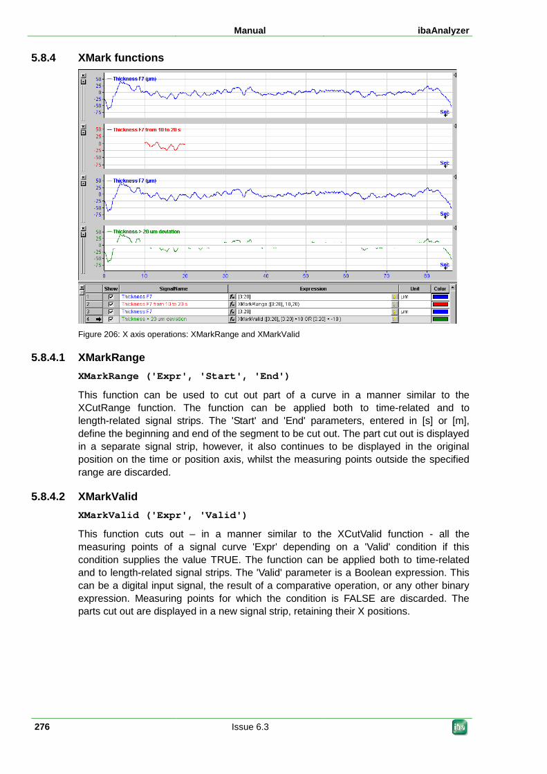
Manual ibaAnalyzer

276 Issue 6.3

5.8.4 XMark functions

Figure 206: X axis operations: XMarkRange and XMarkValid

5.8.4.1 XMarkRange XMarkRange ('Expr', 'Start', 'End')

This function can be used to cut out part of a curve in a manner similar to the XCutRange function. The function can be applied both to time-related and to length-related signal strips. The 'Start' and 'End' parameters, entered in [s] or [m], define the beginning and end of the segment to be cut out. The part cut out is displayed in a separate signal strip, however, it also continues to be displayed in the original position on the time or position axis, whilst the measuring points outside the specified range are discarded.

5.8.4.2 XMarkValid XMarkValid ('Expr', 'Valid')

This function cuts out – in a manner similar to the XCutValid function - all the measuring points of a signal curve 'Expr' depending on a 'Valid' condition if this condition supplies the value TRUE. The function can be applied both to time-related and to length-related signal strips. The 'Valid' parameter is a Boolean expression. This can be a digital input signal, the result of a comparative operation, or any other binary expression. Measuring points for which the condition is FALSE are discarded. The parts cut out are displayed in a new signal strip, retaining their X positions.

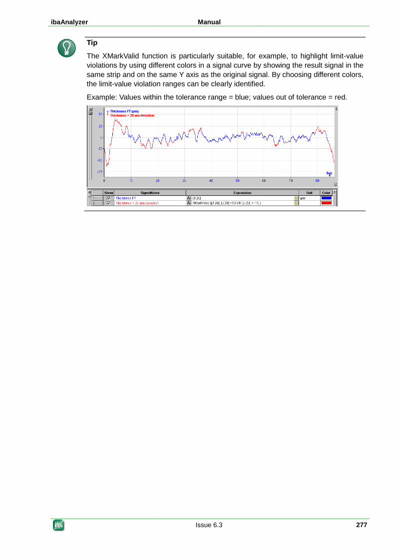
ibaAnalyzer Manual

Issue 6.3 277

Tip

The XMarkValid function is particularly suitable, for example, to highlight limit-value violations by using different colors in a signal curve by showing the result signal in the same strip and on the same Y axis as the original signal. By choosing different colors, the limit-value violation ranges can be clearly identified.

Example: Values within the tolerance range = blue; values out of tolerance = red.

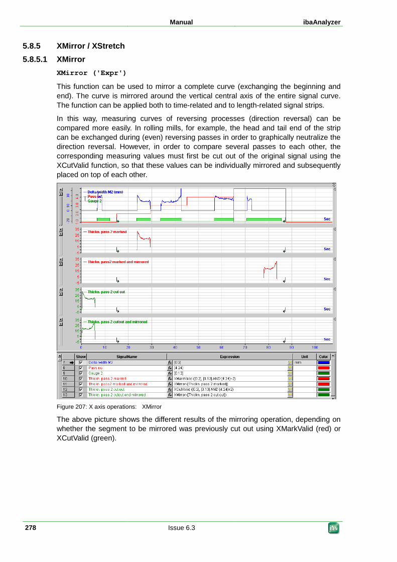
Manual ibaAnalyzer

278 Issue 6.3

5.8.5 XMirror / XStretch 5.8.5.1 XMirror

XMirror ('Expr')

This function can be used to mirror a complete curve (exchanging the beginning and end). The curve is mirrored around the vertical central axis of the entire signal curve. The function can be applied both to time-related and to length-related signal strips.

In this way, measuring curves of reversing processes (direction reversal) can be compared more easily. In rolling mills, for example, the head and tail end of the strip can be exchanged during (even) reversing passes in order to graphically neutralize the direction reversal. However, in order to compare several passes to each other, the corresponding measuring values must first be cut out of the original signal using the XCutValid function, so that these values can be individually mirrored and subsequently placed on top of each other.

Figure 207: X axis operations: XMirror

The above picture shows the different results of the mirroring operation, depending on whether the segment to be mirrored was previously cut out using XMarkValid (red) or XCutValid (green).

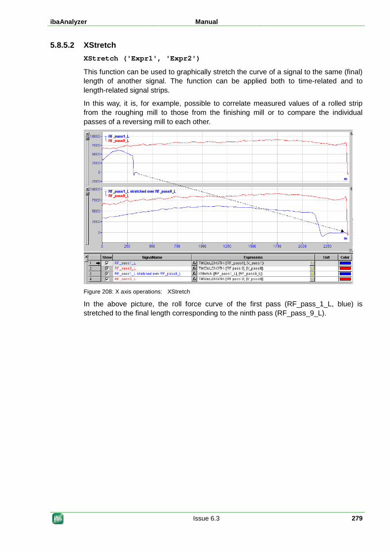
ibaAnalyzer Manual

Issue 6.3 279

5.8.5.2 XStretch XStretch ('Expr1', 'Expr2')

This function can be used to graphically stretch the curve of a signal to the same (final) length of another signal. The function can be applied both to time-related and to length-related signal strips.

In this way, it is, for example, possible to correlate measured values of a rolled strip from the roughing mill to those from the finishing mill or to compare the individual passes of a reversing mill to each other.

Figure 208: X axis operations: XStretch

In the above picture, the roll force curve of the first pass (RF_pass_1_L, blue) is stretched to the final length corresponding to the ninth pass (RF_pass_9_L).

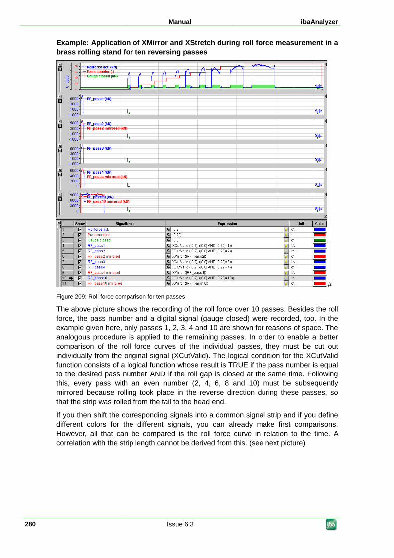
Manual ibaAnalyzer

280 Issue 6.3

Example: Application of XMirror and XStretch during roll force measurement in a brass rolling stand for ten reversing passes

# Figure 209: Roll force comparison for ten passes

The above picture shows the recording of the roll force over 10 passes. Besides the roll force, the pass number and a digital signal (gauge closed) were recorded, too. In the example given here, only passes 1, 2, 3, 4 and 10 are shown for reasons of space. The analogous procedure is applied to the remaining passes. In order to enable a better comparison of the roll force curves of the individual passes, they must be cut out individually from the original signal (XCutValid). The logical condition for the XCutValid function consists of a logical function whose result is TRUE if the pass number is equal to the desired pass number AND if the roll gap is closed at the same time. Following this, every pass with an even number (2, 4, 6, 8 and 10) must be subsequently mirrored because rolling took place in the reverse direction during these passes, so that the strip was rolled from the tail to the head end.

If you then shift the corresponding signals into a common signal strip and if you define different colors for the different signals, you can already make first comparisons. However, all that can be compared is the roll force curve in relation to the time. A correlation with the strip length cannot be derived from this. (see next picture)

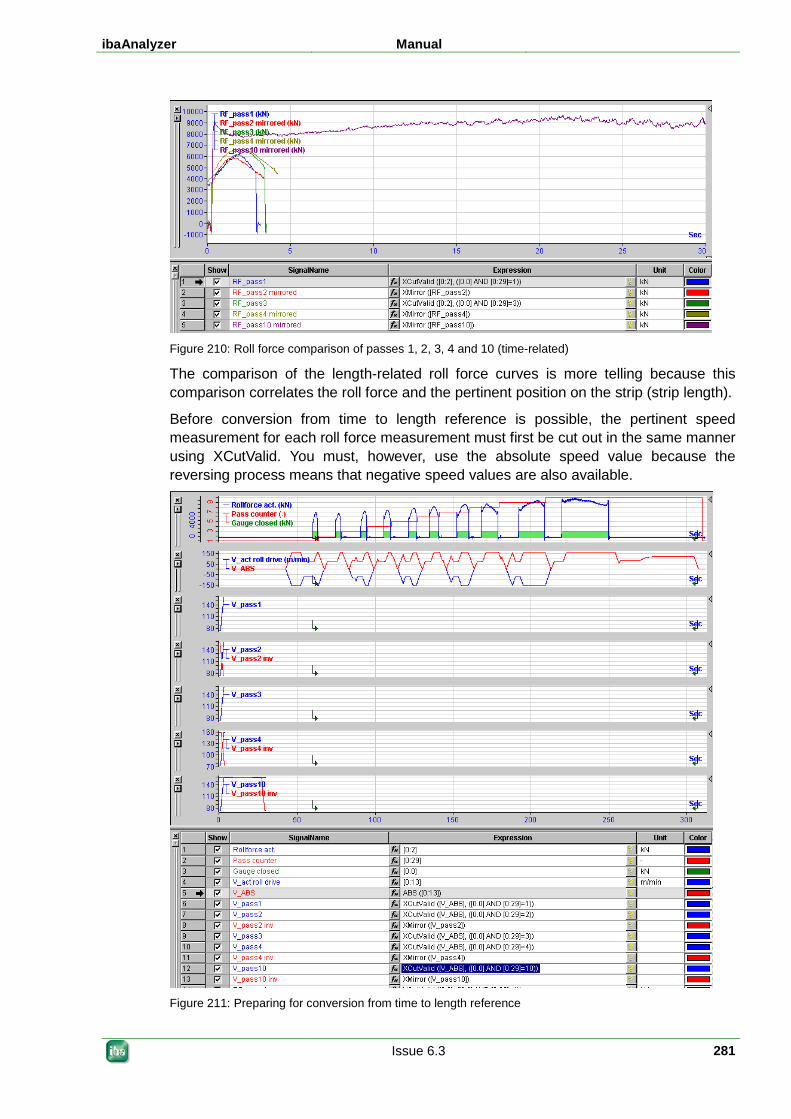
ibaAnalyzer Manual

Issue 6.3 281

Figure 210: Roll force comparison of passes 1, 2, 3, 4 and 10 (time-related)

The comparison of the length-related roll force curves is more telling because this comparison correlates the roll force and the pertinent position on the strip (strip length).

Before conversion from time to length reference is possible, the pertinent speed measurement for each roll force measurement must first be cut out in the same manner using XCutValid. You must, however, use the absolute speed value because the reversing process means that negative speed values are also available.

Figure 211: Preparing for conversion from time to length reference

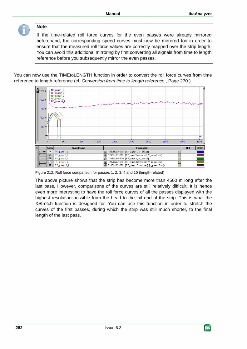
Manual ibaAnalyzer

282 Issue 6.3

Note

If the time-related roll force curves for the even passes were already mirrored beforehand, the corresponding speed curves must now be mirrored too in order to ensure that the measured roll force values are correctly mapped over the strip length. You can avoid this additional mirroring by first converting all signals from time to length reference before you subsequently mirror the even passes.

You can now use the TIMEtoLENGTH function in order to convert the roll force curves from time reference to length reference (cf. Conversion from time to length reference , Page 270 ).

Figure 212: Roll force comparison for passes 1, 2, 3, 4 and 10 (length-related)

The above picture shows that the strip has become more than 4500 m long after the last pass. However, comparisons of the curves are still relatively difficult. It is hence even more interesting to have the roll force curves of all the passes displayed with the highest resolution possible from the head to the tail end of the strip. This is what the XStretch function is designed for. You can use this function in order to stretch the curves of the first passes, during which the strip was still much shorter, to the final length of the last pass.

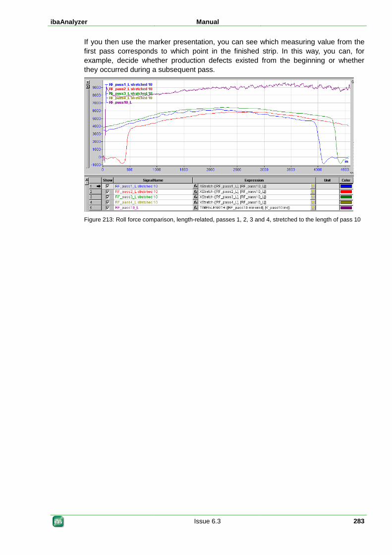
ibaAnalyzer Manual

Issue 6.3 283

If you then use the marker presentation, you can see which measuring value from the first pass corresponds to which point in the finished strip. In this way, you can, for example, decide whether production defects existed from the beginning or whether they occurred during a subsequent pass.

Figure 213: Roll force comparison, length-related, passes 1, 2, 3 and 4, stretched to the length of pass 10

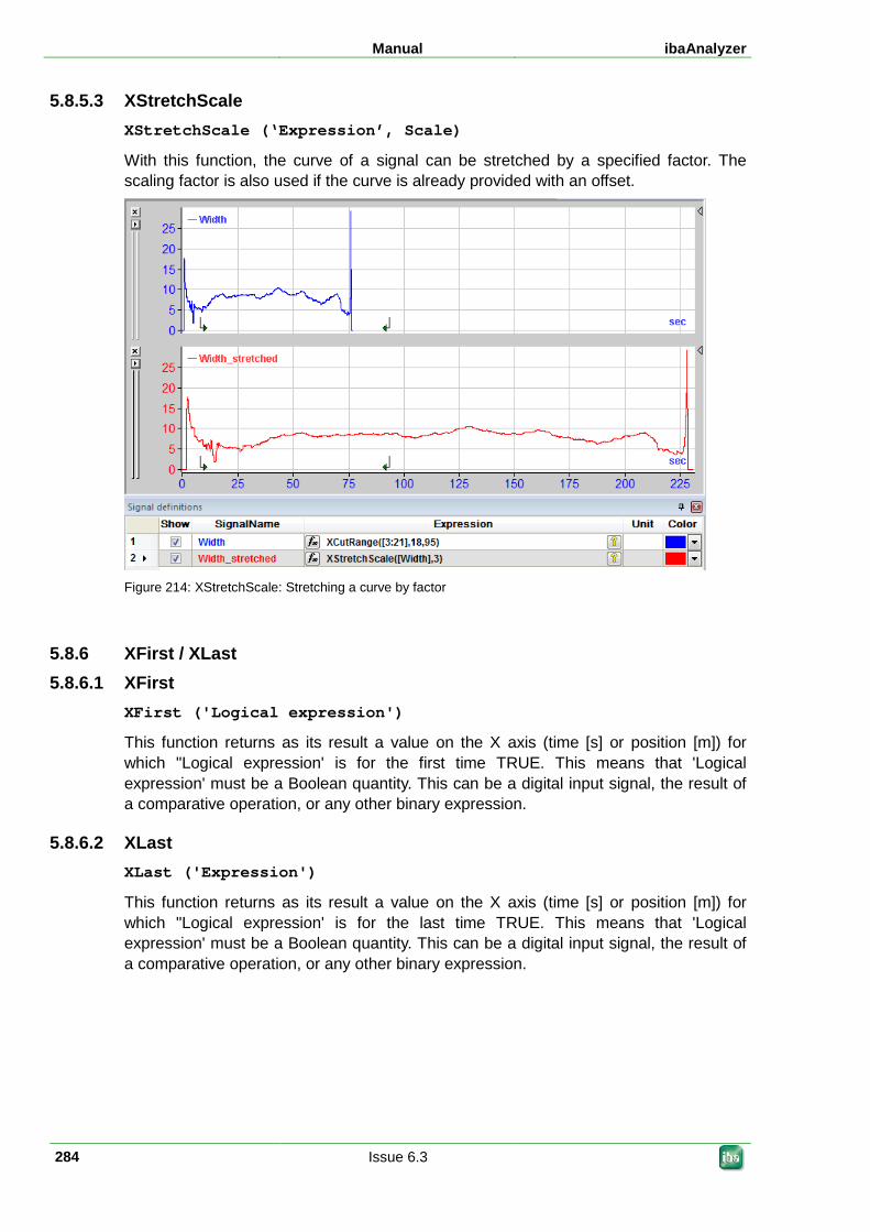
Manual ibaAnalyzer

284 Issue 6.3

5.8.5.3 XStretchScale XStretchScale (‘Expression’, Scale)

With this function, the curve of a signal can be stretched by a specified factor. The scaling factor is also used if the curve is already provided with an offset.

Figure 214: XStretchScale: Stretching a curve by factor

5.8.6 XFirst / XLast 5.8.6.1 XFirst

XFirst ('Logical expression')

This function returns as its result a value on the X axis (time [s] or position [m]) for which "Logical expression' is for the first time TRUE. This means that 'Logical expression' must be a Boolean quantity. This can be a digital input signal, the result of a comparative operation, or any other binary expression.

5.8.6.2 XLast XLast ('Expression')

This function returns as its result a value on the X axis (time [s] or position [m]) for which "Logical expression' is for the last time TRUE. This means that 'Logical expression' must be a Boolean quantity. This can be a digital input signal, the result of a comparative operation, or any other binary expression.

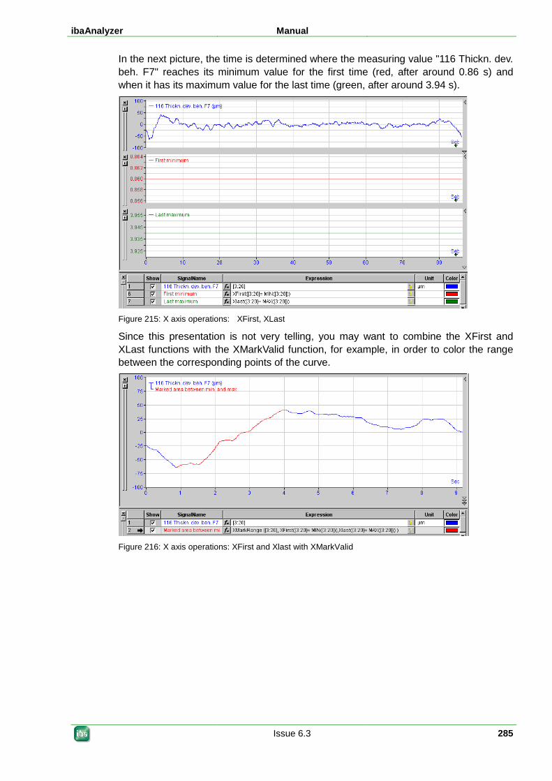
ibaAnalyzer Manual

Issue 6.3 285

In the next picture, the time is determined where the measuring value "116 Thickn. dev. beh. F7" reaches its minimum value for the first time (red, after around 0.86 s) and when it has its maximum value for the last time (green, after around 3.94 s).

Figure 215: X axis operations: XFirst, XLast

Since this presentation is not very telling, you may want to combine the XFirst and XLast functions with the XMarkValid function, for example, in order to color the range between the corresponding points of the curve.

Figure 216: X axis operations: XFirst and Xlast with XMarkValid

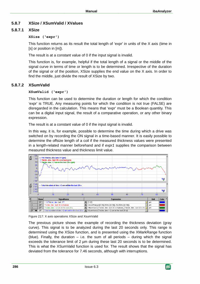
Manual ibaAnalyzer

286 Issue 6.3

5.8.7 XSize / XSumValid / XValues 5.8.7.1 XSize

XSize (‘expr')

This function returns as its result the total length of ‘expr' in units of the X axis (time in [s] or position in [m]).

The result is at a constant value of 0 if the input signal is invalid.

This function is, for example, helpful if the total length of a signal or the middle of the signal curve in terms of time or length is to be determined. Irrespective of the duration of the signal or of the position, XSize supplies the end value on the X axis. In order to find the middle, just divide the result of XSize by two.

5.8.7.2 XSumValid XSumValid (‘expr')

This function can be used to determine the duration or length for which the condition ‘expr' is TRUE. Any measuring points for which the condition is not true (FALSE) are disregarded in the calculation. This means that ‘expr' must be a Boolean quantity. This can be a digital input signal, the result of a comparative operation, or any other binary expression.

The result is at a constant value of 0 if the input signal is invalid.

In this way, it is, for example, possible to determine the time during which a drive was switched on by recording the ON signal in a time-based manner. It is easily possible to determine the offsize length of a coil if the measured thickness values were presented in a length-related manner beforehand and if expr1 supplies the comparison between measured thickness value and thickness limit value.

Figure 217: X axis operations XSize and XsumValid

The previous picture shows the example of recording the thickness deviation (gray curve). This signal is to be analyzed during the last 20 seconds only. This range is determined using the XSize function, and is presented using the XMarkRange function (blue). Finally, the duration – i.e. the sum of all periods – during which the signal exceeds the tolerance limit of 2 µm during these last 20 seconds is to be determined. This is what the XSumValid function is used for. The result shows that the signal has deviated from the tolerance for 7.46 seconds, although with interruptions.

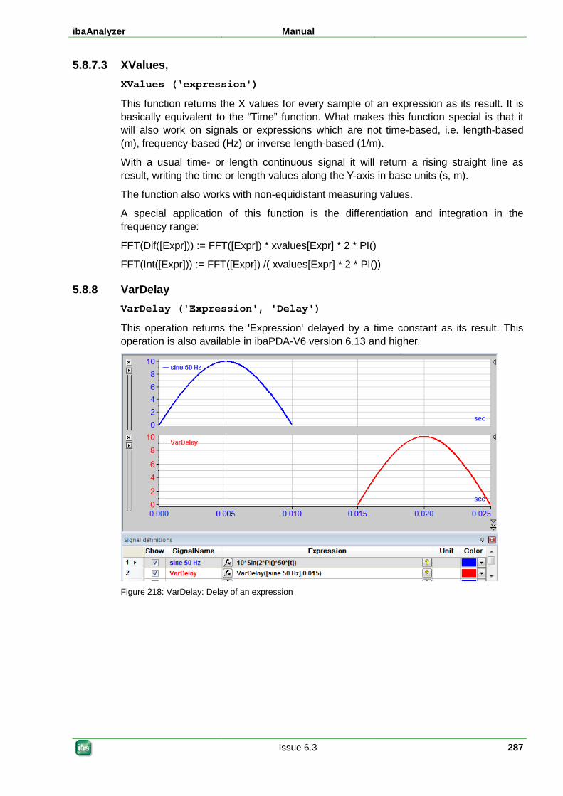
ibaAnalyzer Manual

Issue 6.3 287

5.8.7.3 XValues, XValues (‘expression')

This function returns the X values for every sample of an expression as its result. It is basically equivalent to the “Time” function. What makes this function special is that it will also work on signals or expressions which are not time-based, i.e. length-based (m), frequency-based (Hz) or inverse length-based (1/m).

With a usual time- or length continuous signal it will return a rising straight line as result, writing the time or length values along the Y-axis in base units (s, m).

The function also works with non-equidistant measuring values.

A special application of this function is the differentiation and integration in the frequency range:

FFT(Dif([Expr])) := FFT([Expr]) * xvalues[Expr] * 2 * PI()

FFT(Int([Expr])) := FFT([Expr]) /( xvalues[Expr] * 2 * PI())

5.8.8 VarDelay VarDelay ('Expression', 'Delay')

This operation returns the 'Expression' delayed by a time constant as its result. This operation is also available in ibaPDA-V6 version 6.13 and higher.

Figure 218: VarDelay: Delay of an expression

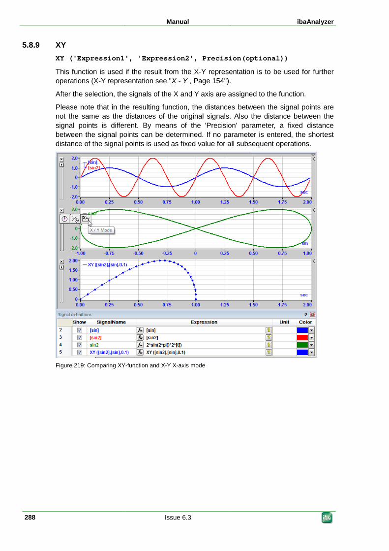
Manual ibaAnalyzer

288 Issue 6.3

5.8.9 XY XY ('Expression1', 'Expression2', Precision(optional))

This function is used if the result from the X-Y representation is to be used for further operations (X-Y representation see "X - Y , Page 154").

After the selection, the signals of the X and Y axis are assigned to the function.

Please note that in the resulting function, the distances between the signal points are not the same as the distances of the original signals. Also the distance between the signal points is different. By means of the 'Precision' parameter, a fixed distance between the signal points can be determined. If no parameter is entered, the shortest distance of the signal points is used as fixed value for all subsequent operations.

Figure 219: Comparing XY-function and X-Y X-axis mode

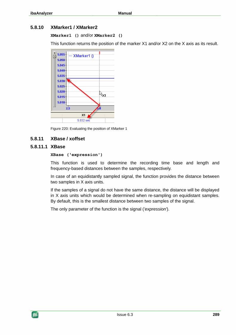
ibaAnalyzer Manual

Issue 6.3 289

5.8.10 XMarker1 / XMarker2 XMarker1 () and/or XMarker2 ()

This function returns the position of the marker X1 and/or X2 on the X axis as its result.

Figure 220: Evaluating the position of XMarker 1

5.8.11 XBase / xoffset 5.8.11.1 XBase

XBase (‘expression')

This function is used to determine the recording time base and length and frequency-based distances between the samples, respectively.

In case of an equidistantly sampled signal, the function provides the distance between two samples in X axis units.

If the samples of a signal do not have the same distance, the distance will be displayed in X axis units which would be determined when re-sampling on equidistant samples. By default, this is the smallest distance between two samples of the signal.

The only parameter of the function is the signal ('expression').

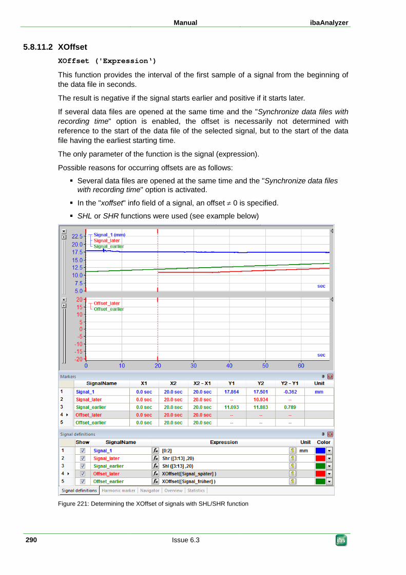
Manual ibaAnalyzer

290 Issue 6.3

5.8.11.2 XOffset XOffset ('Expression‘)

This function provides the interval of the first sample of a signal from the beginning of the data file in seconds.

The result is negative if the signal starts earlier and positive if it starts later.

If several data files are opened at the same time and the "Synchronize data files with recording time" option is enabled, the offset is necessarily not determined with reference to the start of the data file of the selected signal, but to the start of the data file having the earliest starting time.

The only parameter of the function is the signal (expression).

Possible reasons for occurring offsets are as follows:

Several data files are opened at the same time and the "Synchronize data files with recording time" option is activated.

In the "xoffset" info field of a signal, an offset ≠ 0 is specified.

SHL or SHR functions were used (see example below)

Figure 221: Determining the XOffset of signals with SHL/SHR function

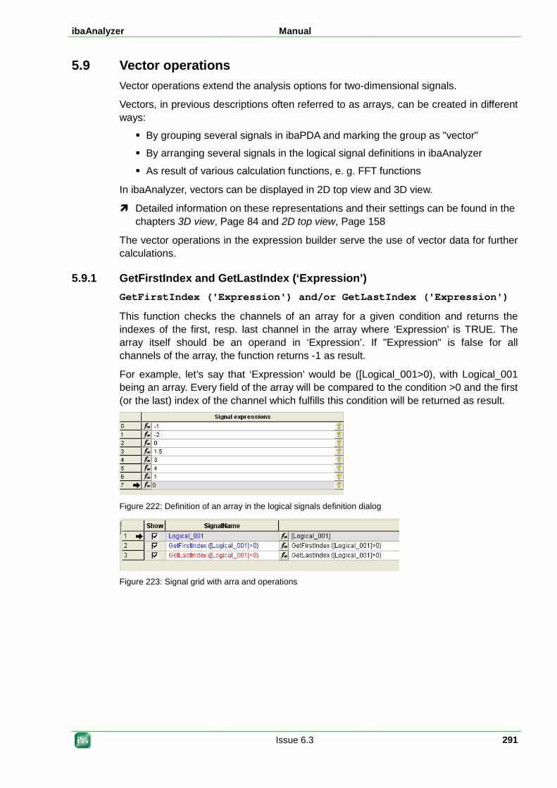
ibaAnalyzer Manual

Issue 6.3 291

5.9 Vector operations Vector operations extend the analysis options for two-dimensional signals.

Vectors, in previous descriptions often referred to as arrays, can be created in different ways:

By grouping several signals in ibaPDA and marking the group as "vector"

By arranging several signals in the logical signal definitions in ibaAnalyzer

As result of various calculation functions, e. g. FFT functions

In ibaAnalyzer, vectors can be displayed in 2D top view and 3D view.

Detailed information on these representations and their settings can be found in the chapters 3D view, Page 84 and 2D top view, Page 158

The vector operations in the expression builder serve the use of vector data for further calculations.

5.9.1 GetFirstIndex and GetLastIndex (‘Expression’) GetFirstIndex ('Expression') and/or GetLastIndex ('Expression')

This function checks the channels of an array for a given condition and returns the indexes of the first, resp. last channel in the array where ‘Expression’ is TRUE. The array itself should be an operand in ‘Expression’. If "Expression" is false for all channels of the array, the function returns -1 as result.

For example, let’s say that ‘Expression’ would be ([Logical_001>0), with Logical_001 being an array. Every field of the array will be compared to the condition >0 and the first (or the last) index of the channel which fulfills this condition will be returned as result.

Figure 222: Definition of an array in the logical signals definition dialog

Figure 223: Signal grid with arra and operations

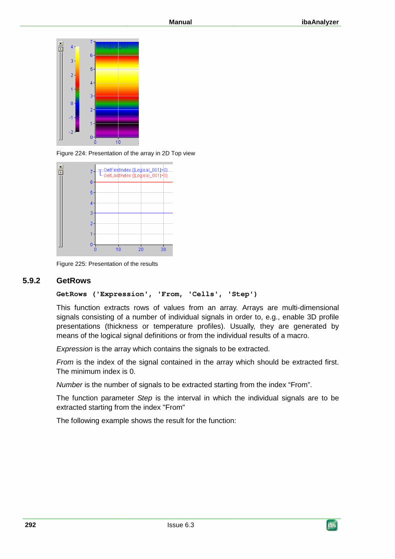
Manual ibaAnalyzer

292 Issue 6.3

Figure 224: Presentation of the array in 2D Top view

Figure 225: Presentation of the results

5.9.2 GetRows GetRows ('Expression', 'From, 'Cells', 'Step')

This function extracts rows of values from an array. Arrays are multi-dimensional signals consisting of a number of individual signals in order to, e.g., enable 3D profile presentations (thickness or temperature profiles). Usually, they are generated by means of the logical signal definitions or from the individual results of a macro.

Expression is the array which contains the signals to be extracted.

From is the index of the signal contained in the array which should be extracted first. The minimum index is 0.

Number is the number of signals to be extracted starting from the index “From”.

The function parameter Step is the interval in which the individual signals are to be extracted starting from the index "From"

The following example shows the result for the function:

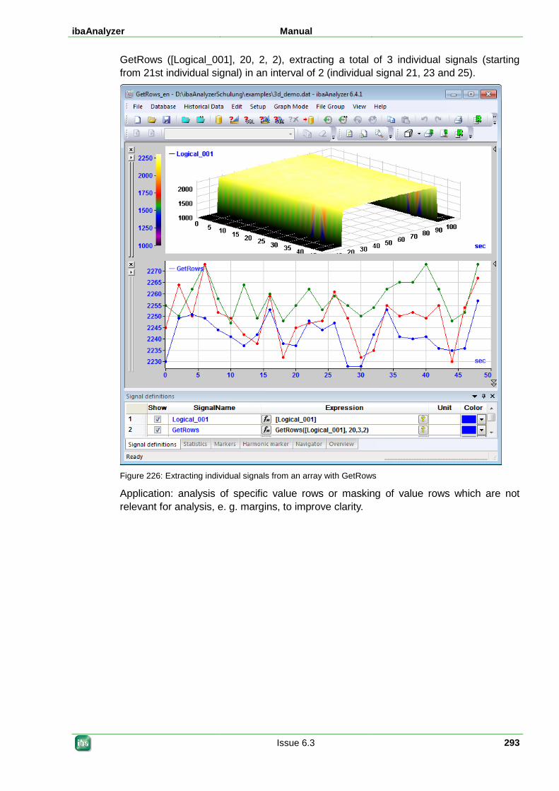
ibaAnalyzer Manual

Issue 6.3 293

GetRows ([Logical_001], 20, 2, 2), extracting a total of 3 individual signals (starting from 21st individual signal) in an interval of 2 (individual signal 21, 23 and 25).

Figure 226: Extracting individual signals from an array with GetRows

Application: analysis of specific value rows or masking of value rows which are not relevant for analysis, e. g. margins, to improve clarity.

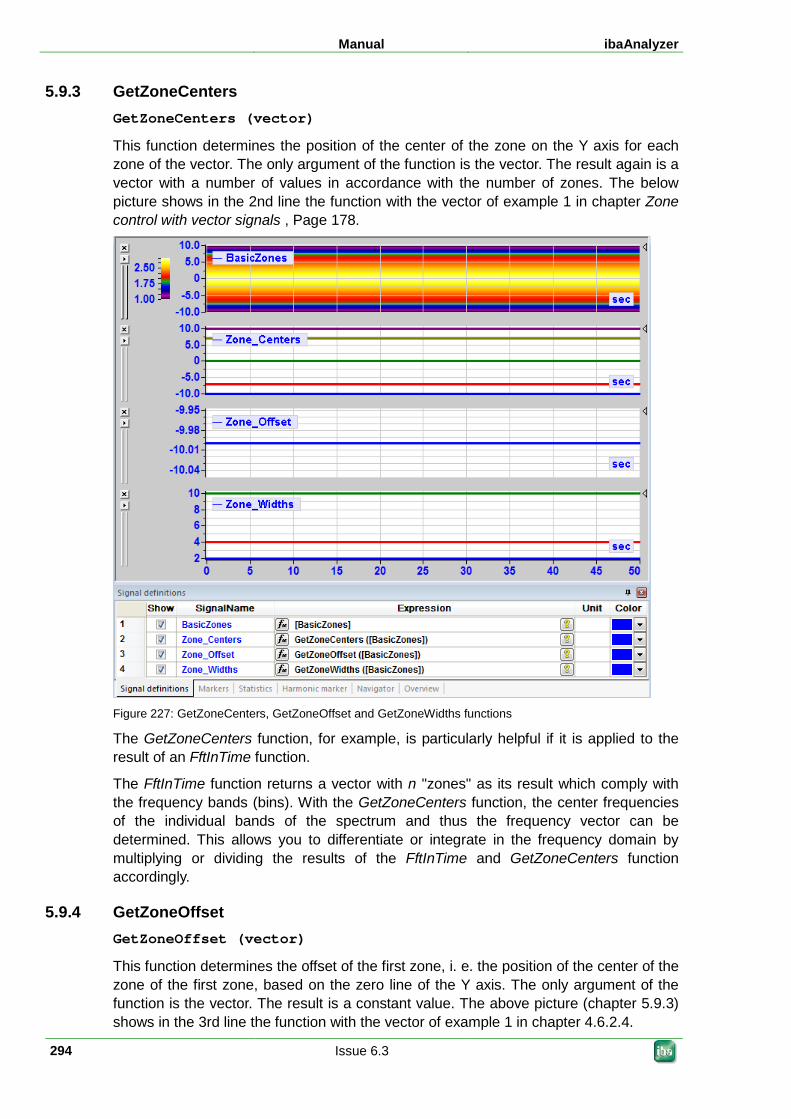
Manual ibaAnalyzer

294 Issue 6.3

5.9.3 GetZoneCenters GetZoneCenters (vector)

This function determines the position of the center of the zone on the Y axis for each zone of the vector. The only argument of the function is the vector. The result again is a vector with a number of values in accordance with the number of zones. The below picture shows in the 2nd line the function with the vector of example 1 in chapter Zone control with vector signals , Page 178.

Figure 227: GetZoneCenters, GetZoneOffset and GetZoneWidths functions

The GetZoneCenters function, for example, is particularly helpful if it is applied to the result of an FftInTime function.

The FftInTime function returns a vector with n "zones" as its result which comply with the frequency bands (bins). With the GetZoneCenters function, the center frequencies of the individual bands of the spectrum and thus the frequency vector can be determined. This allows you to differentiate or integrate in the frequency domain by multiplying or dividing the results of the FftInTime and GetZoneCenters function accordingly.

5.9.4 GetZoneOffset GetZoneOffset (vector)

This function determines the offset of the first zone, i. e. the position of the center of the zone of the first zone, based on the zero line of the Y axis. The only argument of the function is the vector. The result is a constant value. The above picture (chapter 5.9.3) shows in the 3rd line the function with the vector of example 1 in chapter 4.6.2.4.

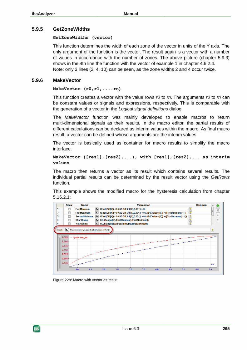
ibaAnalyzer Manual

Issue 6.3 295

5.9.5 GetZoneWidths GetZoneWidths (vector)

This function determines the width of each zone of the vector in units of the Y axis. The only argument of the function is the vector. The result again is a vector with a number of values in accordance with the number of zones. The above picture (chapter 5.9.3) shows in the 4th line the function with the vector of example 1 in chapter 4.6.2.4. Note: only 3 lines (2, 4, 10) can be seen, as the zone widths 2 and 4 occur twice.

5.9.6 MakeVector MakeVector (r0,r1,....rn)

This function creates a vector with the value rows r0 to rn. The arguments r0 to rn can be constant values or signals and expressions, respectively. This is comparable with the generation of a vector in the Logical signal definitions dialog.

The MakeVector function was mainly developed to enable macros to return multi-dimensional signals as their results. In the macro editor, the partial results of different calculations can be declared as interim values within the macro. As final macro result, a vector can be defined whose arguments are the interim values.

The vector is basically used as container for macro results to simplify the macro interface.

MakeVector ([res1],[res2],...), with [res1],[res2],... as interim values

The macro then returns a vector as its result which contains several results. The individual partial results can be determined by the result vector using the GetRows function.

This example shows the modified macro for the hysteresis calculation from chapter 5.16.2.1:

Figure 228: Macro with vector as result

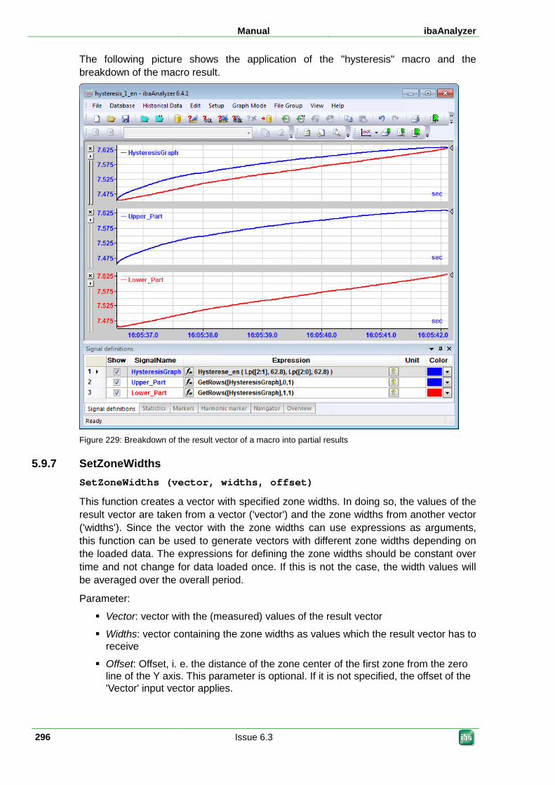
Manual ibaAnalyzer

296 Issue 6.3

The following picture shows the application of the "hysteresis" macro and the breakdown of the macro result.

Figure 229: Breakdown of the result vector of a macro into partial results

5.9.7 SetZoneWidths SetZoneWidths (vector, widths, offset)

This function creates a vector with specified zone widths. In doing so, the values of the result vector are taken from a vector ('vector') and the zone widths from another vector ('widths'). Since the vector with the zone widths can use expressions as arguments, this function can be used to generate vectors with different zone widths depending on the loaded data. The expressions for defining the zone widths should be constant over time and not change for data loaded once. If this is not the case, the width values will be averaged over the overall period.

Parameter:

Vector: vector with the (measured) values of the result vector

Widths: vector containing the zone widths as values which the result vector has to receive

Offset: Offset, i. e. the distance of the zone center of the first zone from the zero line of the Y axis. This parameter is optional. If it is not specified, the offset of the 'Vector' input vector applies.

ibaAnalyzer Manual

Issue 6.3 297

Example

The function SetZoneWidths (MakeVector(1,2,3,2,1), MakeVector(2,4,10,4,2), -10) generates the same vector as the one generated with the logical signal definitions in chapter Zone control with vector signals , Page 178.

5.9.8 VectorAvg VectorAvg (Vector)

This function calculates the average of the cross profile for each sample, i. e. the average of all vector tracks per point in time or per X axis position, respectively. The only argument of the function is the vector. The function returns a one-dimensional signal as its result showing the curve of the cross profile average value over the time/length of the vector signal with the same number of samples.

5.9.9 VectorKurtosis VectorKurtosis (Vector)

This function calculates the kurtosis of the cross profile for each sample. The only argument of the function is the vector. The function returns a one-dimensional signal as its result showing the curve of the cross profile kurtosis over the time/length of the vector signal with the same number of samples.

5.9.10 VectorMarkRange VectorMarkRange (Vector, PositionFrom, PositionTo)

This function returns a partial vector of a vector with a zone width from 'PositionFrom' (lower edge) to 'PositionTo' (upper edge) as its result.

The positions must be indicated in units of the Y axis. The positions can be both fixed values and signals or expressions and thus be dependent on the data loaded.

The expressions for defining the positions should be constant over time and not change for data loaded once. If this is not the case, the position values will be averaged over the overall period.

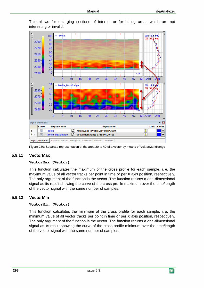
Manual ibaAnalyzer

298 Issue 6.3

This allows for enlarging sections of interest or for hiding areas which are not interesting or invalid.

Figure 230: Separate representation of the area 20 to 40 of a vector by means of VektorMarkRange

5.9.11 VectorMax VectorMax (Vector)

This function calculates the maximum of the cross profile for each sample, i. e. the maximum value of all vector tracks per point in time or per X axis position, respectively. The only argument of the function is the vector. The function returns a one-dimensional signal as its result showing the curve of the cross profile maximum over the time/length of the vector signal with the same number of samples.

5.9.12 VectorMin VectorMin (Vector)

This function calculates the minimum of the cross profile for each sample, i. e. the minimum value of all vector tracks per point in time or per X axis position, respectively. The only argument of the function is the vector. The function returns a one-dimensional signal as its result showing the curve of the cross profile minimum over the time/length of the vector signal with the same number of samples.

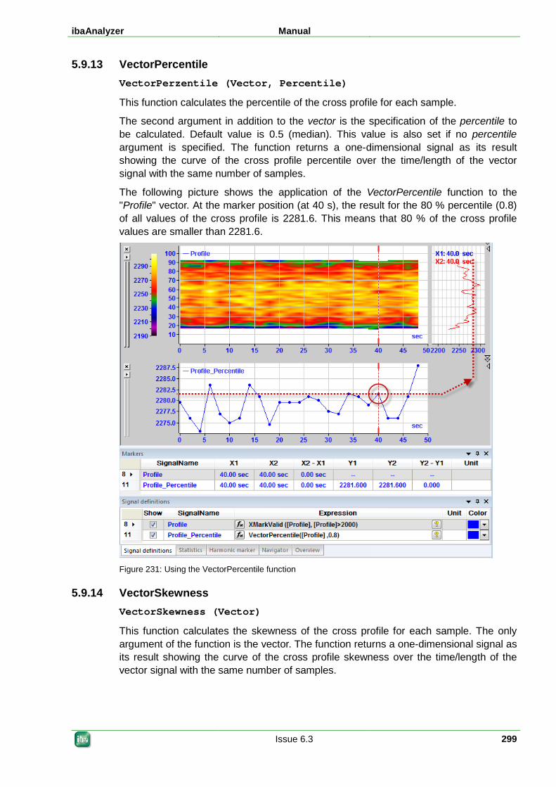
ibaAnalyzer Manual

Issue 6.3 299

5.9.13 VectorPercentile VectorPerzentile (Vector, Percentile)

This function calculates the percentile of the cross profile for each sample.

The second argument in addition to the vector is the specification of the percentile to be calculated. Default value is 0.5 (median). This value is also set if no percentile argument is specified. The function returns a one-dimensional signal as its result showing the curve of the cross profile percentile over the time/length of the vector signal with the same number of samples.

The following picture shows the application of the VectorPercentile function to the "Profile" vector. At the marker position (at 40 s), the result for the 80 % percentile (0.8) of all values of the cross profile is 2281.6. This means that 80 % of the cross profile values are smaller than 2281.6.

Figure 231: Using the VectorPercentile function

5.9.14 VectorSkewness VectorSkewness (Vector)

This function calculates the skewness of the cross profile for each sample. The only argument of the function is the vector. The function returns a one-dimensional signal as its result showing the curve of the cross profile skewness over the time/length of the vector signal with the same number of samples.

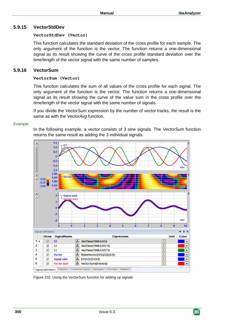
Manual ibaAnalyzer

300 Issue 6.3

5.9.15 VectorStdDev VectorStdDev (Vector)

This function calculates the standard deviation of the cross profile for each sample. The only argument of the function is the vector. The function returns a one-dimensional signal as its result showing the curve of the cross profile standard deviation over the time/length of the vector signal with the same number of samples.

5.9.16 VectorSum VectorSum (Vector)

This function calculates the sum of all values of the cross profile for each signal. The only argument of the function is the vector. The function returns a one-dimensional signal as its result showing the curve of the value sum in the cross profile over the time/length of the vector signal with the same number of signals.

If you divide the VectorSum expression by the number of vector tracks, the result is the same as with the VectorAvg function.

Example In the following example, a vector consists of 3 sine signals. The VectorSum function returns the same result as adding the 3 individual signals.

Figure 232: Using the VectorSum function for adding up signals

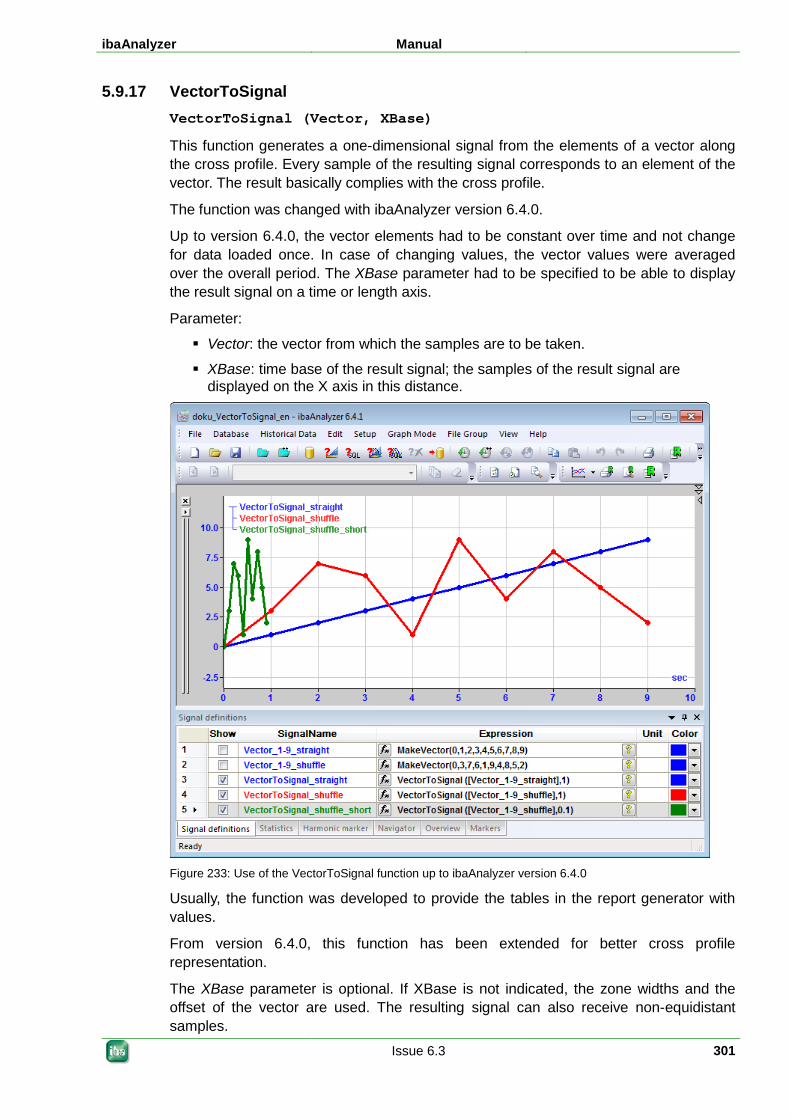
ibaAnalyzer Manual

Issue 6.3 301

5.9.17 VectorToSignal VectorToSignal (Vector, XBase)

This function generates a one-dimensional signal from the elements of a vector along the cross profile. Every sample of the resulting signal corresponds to an element of the vector. The result basically complies with the cross profile.

The function was changed with ibaAnalyzer version 6.4.0.

Up to version 6.4.0, the vector elements had to be constant over time and not change for data loaded once. In case of changing values, the vector values were averaged over the overall period. The XBase parameter had to be specified to be able to display the result signal on a time or length axis.

Parameter:

Vector: the vector from which the samples are to be taken.

XBase: time base of the result signal; the samples of the result signal are displayed on the X axis in this distance.

Figure 233: Use of the VectorToSignal function up to ibaAnalyzer version 6.4.0

Usually, the function was developed to provide the tables in the report generator with values.

From version 6.4.0, this function has been extended for better cross profile representation.

The XBase parameter is optional. If XBase is not indicated, the zone widths and the offset of the vector are used. The resulting signal can also receive non-equidistant samples.

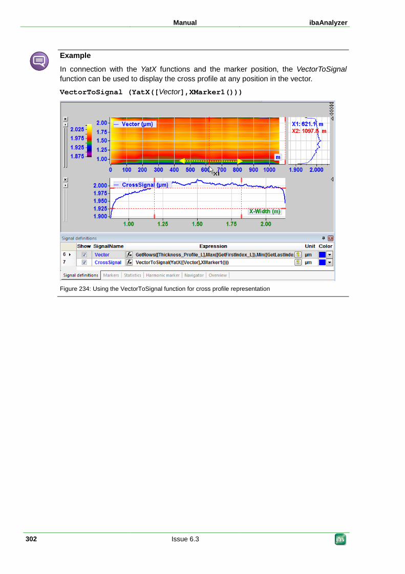
Manual ibaAnalyzer

302 Issue 6.3

Example

In connection with the YatX functions and the marker position, the VectorToSignal function can be used to display the cross profile at any position in the vector.

VectorToSignal (YatX([Vector],XMarker1()))

Figure 234: Using the VectorToSignal function for cross profile representation

ibaAnalyzer Manual

Issue 6.3 303

5.10 Electrical functions If reasonable, the following functions apply to both fixed and variable power line frequencies, e.g. in test stands.

Eff

DeltaCollectiveUeff

DeltaCollectiveIeff

DeltaActiveP

DeltaApparentP

DeltaReactiveP

DeltaActivePFactor

DeltaReactivePFactor

StarCollectiveUeff

StarCollectiveIeff

StarActiveP

StarApparentP

StarReactiveP

StarActivePFactor

StarReactivePFactor

According to definition, the following functions require fixed power line frequencies:

DeltaReactivePS

DeltaReactivePFactorS

StarReactivePS

StarReactivePFactorS

TIF

5.10.1 Common functions 5.10.1.1 Eff

Eff('expr', 'freq')

This function calculates the effective value of ‘expr’ with a fundamental frequency of ‘freq’. The default fundamental frequency is 50 Hz like in all the electrical functions of ibaAnalyzer. The following formula is used to calculate the effective value:

∑=

=N

1n

2eff )n(e

N1E

e(n) : sample n of signal e (‘expr’) N : the number of samples in a period

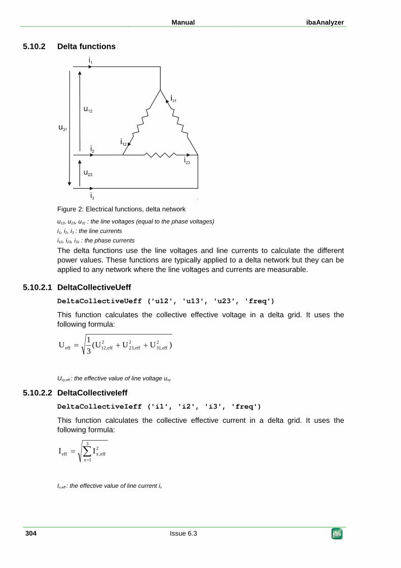
Manual ibaAnalyzer

304 Issue 6.3

5.10.2 Delta functions

Figure 2: Electrical functions, delta network

u12, u23, u31 : the line voltages (equal to the phase voltages) i1, i2, i3 : the line currents i12, i23, i31 : the phase currents

The delta functions use the line voltages and line currents to calculate the different power values. These functions are typically applied to a delta network but they can be applied to any network where the line voltages and currents are measurable.

5.10.2.1 DeltaCollectiveUeff DeltaCollectiveUeff ('u12', 'u13', 'u23', 'freq')

This function calculates the collective effective voltage in a delta grid. It uses the following formula:

)UUU(31U 2

eff,312

eff,232

eff,12eff ++=

Uxy,eff : the effective value of line voltage uxy

5.10.2.2 DeltaCollectiveIeff DeltaCollectiveIeff ('i1', 'i2', 'i3', 'freq')

This function calculates the collective effective current in a delta grid. It uses the following formula:

∑=

=3

1x

2eff,xeff II

Ix,eff : the effective value of line current ix

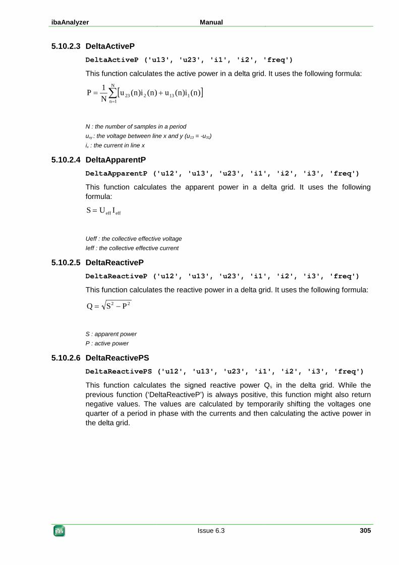
ibaAnalyzer Manual

Issue 6.3 305

5.10.2.3 DeltaActiveP DeltaActiveP ('u13', 'u23', 'i1', 'i2', 'freq')

This function calculates the active power in a delta grid. It uses the following formula:

[ ]∑=

+=N

1n113223 )n(i)n(u)n(i)n(u

N1P

N : the number of samples in a period uxy : the voltage between line x and y (u13 = -u31) ix : the current in line x

5.10.2.4 DeltaApparentP DeltaApparentP ('u12', 'u13', 'u23', 'i1', 'i2', 'i3', 'freq')

This function calculates the apparent power in a delta grid. It uses the following formula:

effeff IUS = Ueff : the collective effective voltage Ieff : the collective effective current

5.10.2.5 DeltaReactiveP DeltaReactiveP ('u12', 'u13', 'u23', 'i1', 'i2', 'i3', 'freq')

This function calculates the reactive power in a delta grid. It uses the following formula:

22 PSQ −= S : apparent power P : active power

5.10.2.6 DeltaReactivePS DeltaReactivePS ('u12', 'u13', 'u23', 'i1', 'i2', 'i3', 'freq')

This function calculates the signed reactive power QS in the delta grid. While the previous function (‘DeltaReactiveP’) is always positive, this function might also return negative values. The values are calculated by temporarily shifting the voltages one quarter of a period in phase with the currents and then calculating the active power in the delta grid.

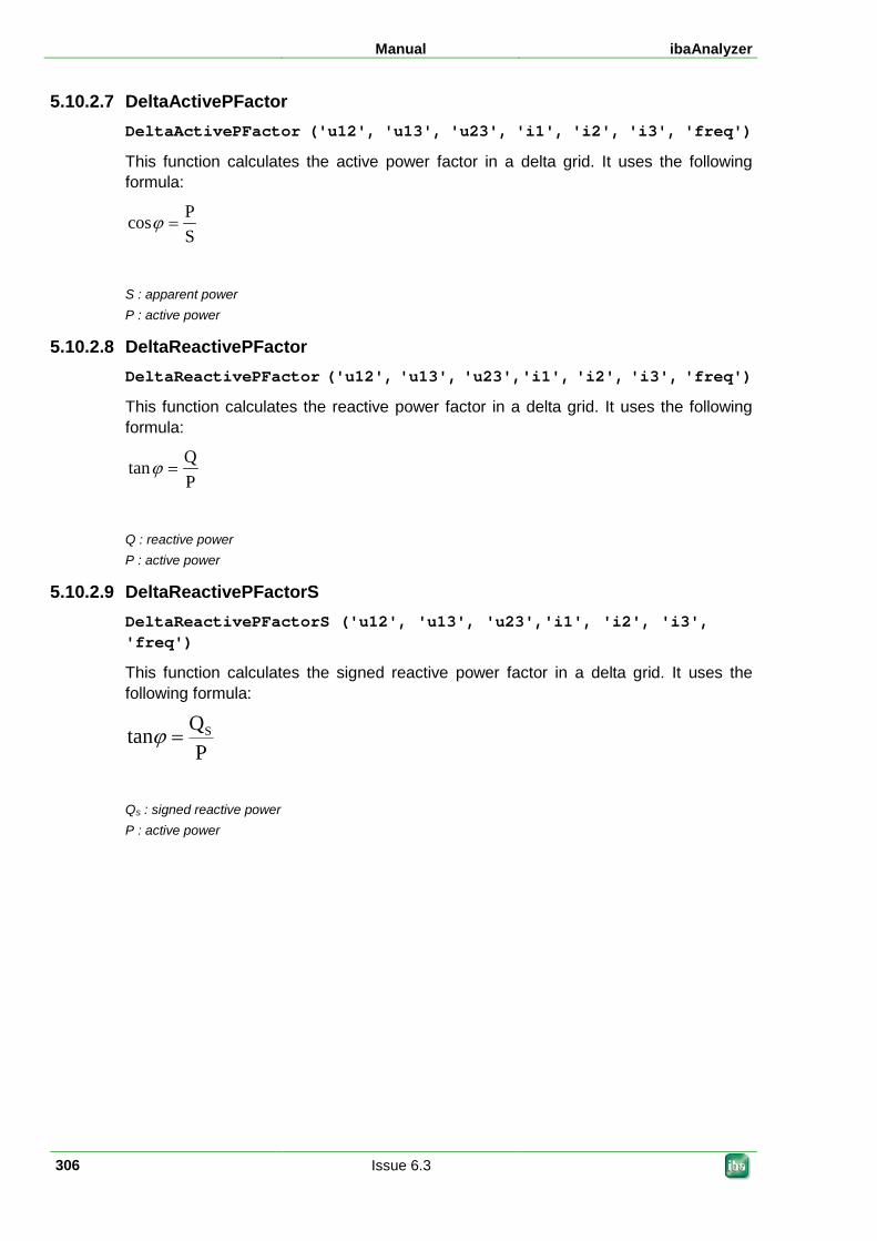
Manual ibaAnalyzer

306 Issue 6.3

5.10.2.7 DeltaActivePFactor DeltaActivePFactor ('u12', 'u13', 'u23', 'i1', 'i2', 'i3', 'freq')

This function calculates the active power factor in a delta grid. It uses the following formula:

SPcos =ϕ

S : apparent power P : active power

5.10.2.8 DeltaReactivePFactor DeltaReactivePFactor ('u12', 'u13', 'u23','i1', 'i2', 'i3', 'freq')

This function calculates the reactive power factor in a delta grid. It uses the following formula:

PQtan =ϕ

Q : reactive power P : active power

5.10.2.9 DeltaReactivePFactorS DeltaReactivePFactorS ('u12', 'u13', 'u23','i1', 'i2', 'i3', 'freq')

This function calculates the signed reactive power factor in a delta grid. It uses the following formula:

PQtan S=ϕ

QS : signed reactive power P : active power

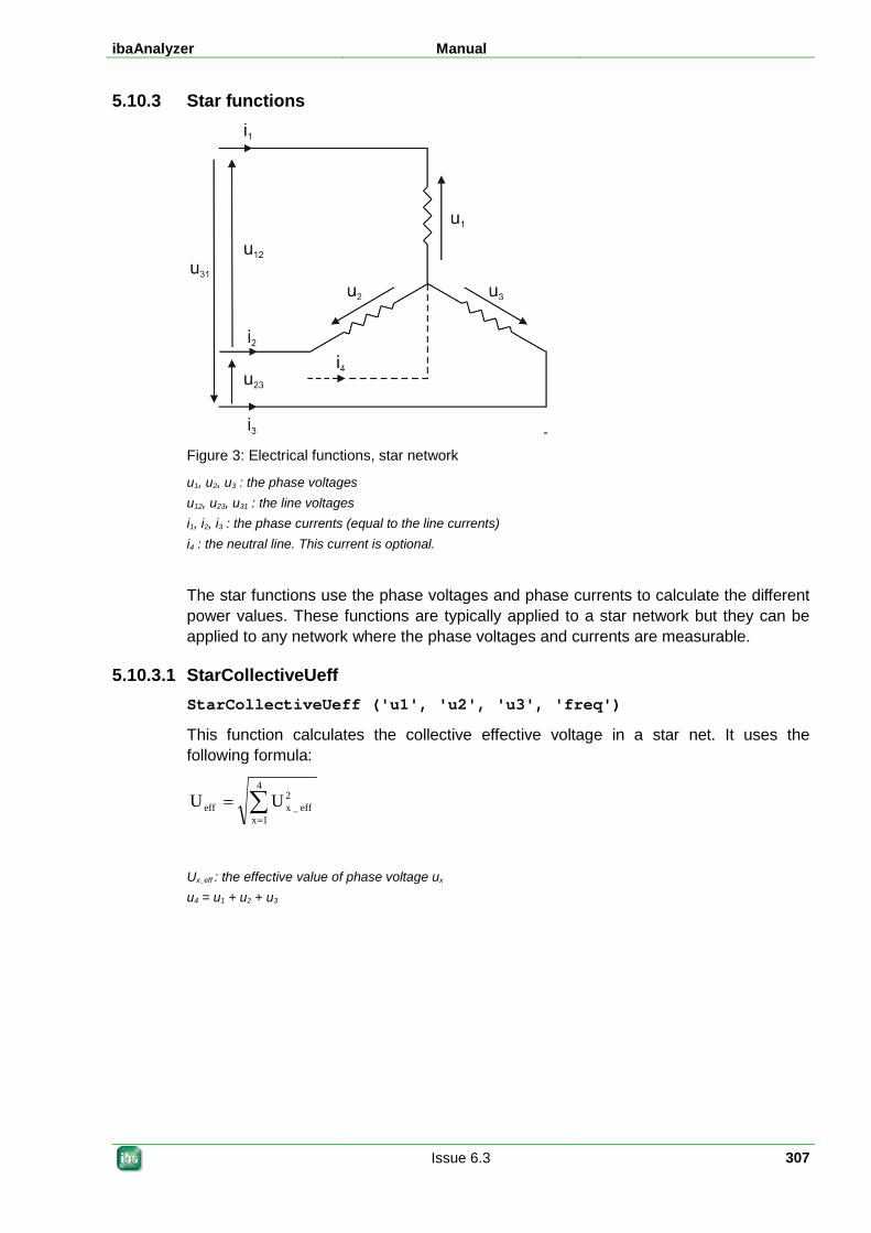
ibaAnalyzer Manual

Issue 6.3 307

5.10.3 Star functions

Figure 3: Electrical functions, star network

u1, u2, u3 : the phase voltages u12, u23, u31 : the line voltages i1, i2, i3 : the phase currents (equal to the line currents) i4 : the neutral line. This current is optional.

The star functions use the phase voltages and phase currents to calculate the different power values. These functions are typically applied to a star network but they can be applied to any network where the phase voltages and currents are measurable.

5.10.3.1 StarCollectiveUeff StarCollectiveUeff ('u1', 'u2', 'u3', 'freq')

This function calculates the collective effective voltage in a star net. It uses the following formula:

∑=

=4

1x

2eff_xeff UU

Ux_eff : the effective value of phase voltage ux u4 = u1 + u2 + u3

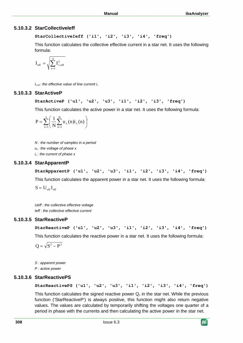
Manual ibaAnalyzer

308 Issue 6.3

5.10.3.2 StarCollectiveIeff StarCollectiveIeff ('i1', 'i2', 'i3', 'i4', 'freq')

This function calculates the collective effective current in a star net. It uses the following formula:

∑=

=4

1x

2eff,xeff II

Ix,eff : the effective value of line current ix

5.10.3.3 StarActiveP StarActiveP ('u1', 'u2', 'u3', 'i1', 'i2', 'i3', 'freq')

This function calculates the active power in a star net. It uses the following formula:

∑ ∑= =

=

3

1x

N

1nxx )n(i)n(u

N1P

N : the number of samples in a period ux : the voltage of phase x ix : the current of phase x

5.10.3.4 StarApparentP StarApparentP ('u1', 'u2', 'u3', 'i1', 'i2', 'i3', 'i4', 'freq')

This function calculates the apparent power in a star net. It uses the following formula:

effeff IUS = Ueff : the collective effective voltage Ieff : the collective effective current

5.10.3.5 StarReactiveP StarReactiveP ('u1', 'u2', 'u3', 'i1', 'i2', 'i3', 'i4', 'freq')

This function calculates the reactive power in a star net. It uses the following formula:

22 PSQ −= S : apparent power P : active power

5.10.3.6 StarReactivePS StarReactivePS ('u1', 'u2', 'u3', 'i1', 'i2', 'i3', 'i4', 'freq')

This function calculates the signed reactive power QS in the star net. While the previous function (‘StarReactiveP’) is always positive, this function might also return negative values. The values are calculated by temporarily shifting the voltages one quarter of a period in phase with the currents and then calculating the active power in the star net.

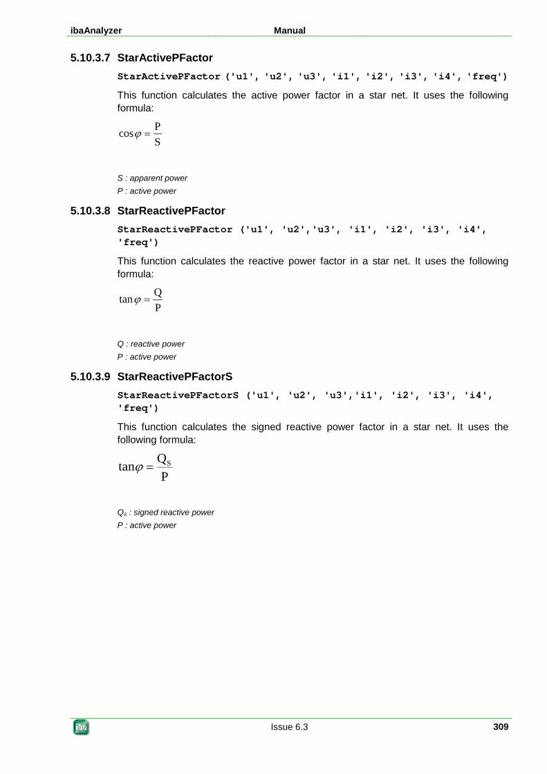
ibaAnalyzer Manual

Issue 6.3 309

5.10.3.7 StarActivePFactor StarActivePFactor ('u1', 'u2', 'u3', 'i1', 'i2', 'i3', 'i4', 'freq')

This function calculates the active power factor in a star net. It uses the following formula:

SPcos =ϕ

S : apparent power P : active power

5.10.3.8 StarReactivePFactor StarReactivePFactor ('u1', 'u2','u3', 'i1', 'i2', 'i3', 'i4', 'freq')

This function calculates the reactive power factor in a star net. It uses the following formula:

PQtan =ϕ

Q : reactive power P : active power

5.10.3.9 StarReactivePFactorS StarReactivePFactorS ('u1', 'u2', 'u3','i1', 'i2', 'i3', 'i4', 'freq')

This function calculates the signed reactive power factor in a star net. It uses the following formula:

PQtan S=ϕ

QS : signed reactive power P : active power

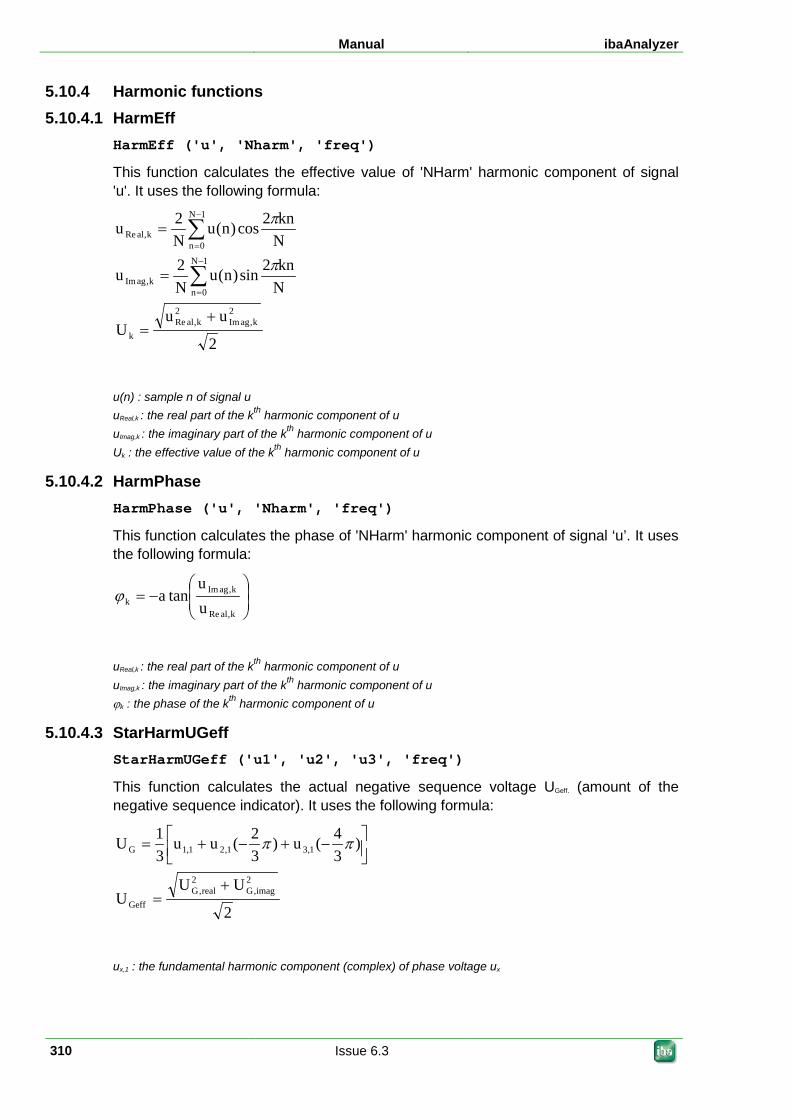
Manual ibaAnalyzer

310 Issue 6.3

5.10.4 Harmonic functions 5.10.4.1 HarmEff

HarmEff ('u', 'Nharm', 'freq')

This function calculates the effective value of 'NHarm' harmonic component of signal 'u'. It uses the following formula:

2

uuU

Nkn2sin)n(u

N2u

Nkn2cos)n(u

N2u

2k,agIm

2k,alRe

k

1N

0nk,agIm

1N

0nk,alRe

+=

=

=

∑

∑−

=

−

=

π

π

u(n) : sample n of signal u uReal,k : the real part of the kth harmonic component of u uImag,k : the imaginary part of the kth harmonic component of u Uk : the effective value of the kth harmonic component of u

5.10.4.2 HarmPhase HarmPhase ('u', 'Nharm', 'freq')

This function calculates the phase of 'NHarm' harmonic component of signal ‘u’. It uses the following formula:

−=

k,alRe

k,agImk u

utanaϕ

uReal,k : the real part of the kth harmonic component of u uImag,k : the imaginary part of the kth harmonic component of u ϕk : the phase of the kth harmonic component of u

5.10.4.3 StarHarmUGeff StarHarmUGeff ('u1', 'u2', 'u3', 'freq')

This function calculates the actual negative sequence voltage UGeff. (amount of the negative sequence indicator). It uses the following formula:

2

UUU

)34(u)

32(uu

31U

2imag,G

2real,G

Geff

1,31,21,1G

+=

−+−+= ππ

ux,1 : the fundamental harmonic component (complex) of phase voltage ux

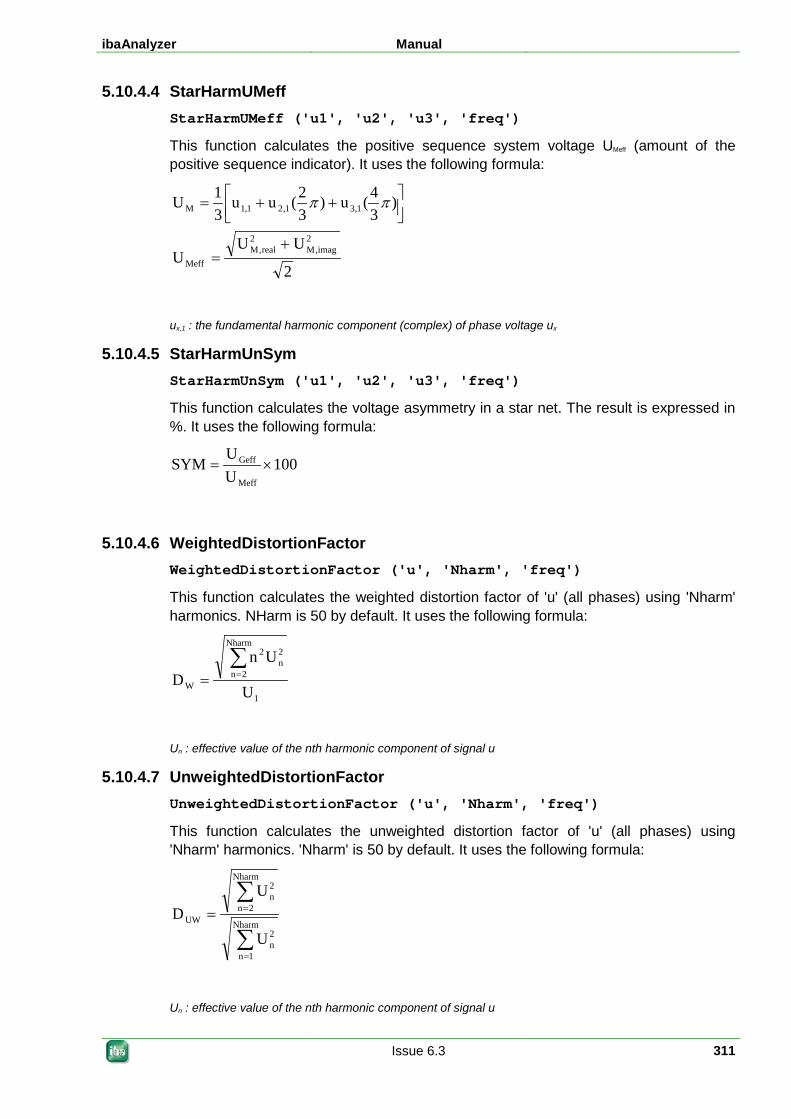
ibaAnalyzer Manual

Issue 6.3 311

5.10.4.4 StarHarmUMeff StarHarmUMeff ('u1', 'u2', 'u3', 'freq')

This function calculates the positive sequence system voltage UMeff (amount of the positive sequence indicator). It uses the following formula:

2

UUU

)34(u)

32(uu

31U

2imag,M

2real,M

Meff

1,31,21,1M

+=

++= ππ

ux,1 : the fundamental harmonic component (complex) of phase voltage ux

5.10.4.5 StarHarmUnSym StarHarmUnSym ('u1', 'u2', 'u3', 'freq')

This function calculates the voltage asymmetry in a star net. The result is expressed in %. It uses the following formula:

100UU

SYMMeff

Geff ×=

5.10.4.6 WeightedDistortionFactor WeightedDistortionFactor ('u', 'Nharm', 'freq')

This function calculates the weighted distortion factor of 'u' (all phases) using 'Nharm' harmonics. NHarm is 50 by default. It uses the following formula:

1

Nharm

2n

2n

2

W U

UnD

∑==

Un : effective value of the nth harmonic component of signal u

5.10.4.7 UnweightedDistortionFactor UnweightedDistortionFactor ('u', 'Nharm', 'freq')

This function calculates the unweighted distortion factor of 'u' (all phases) using 'Nharm' harmonics. 'Nharm' is 50 by default. It uses the following formula:

∑

∑

=

==Nharm

1n

2n

Nharm

2n

2n

UW

U

UD

Un : effective value of the nth harmonic component of signal u

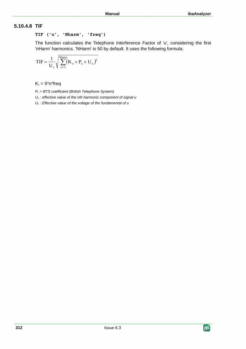
Manual ibaAnalyzer

312 Issue 6.3

5.10.4.8 TIF TIF ('u', 'Nharm', 'freq')

The function calculates the Telephone Interference Factor of 'u', considering the first 'nHarm' harmonics. 'NHarm' is 50 by default. It uses the following formula:

( )∑=

××=Nharm

2n

2nnn

1

UPKU1TIF

Kn = 5*n*freq Pn = BTS coefficient (British Telephone System) Un : effective value of the nth harmonic component of signal u U1 : Effective value of the voltage of the fundamental of u

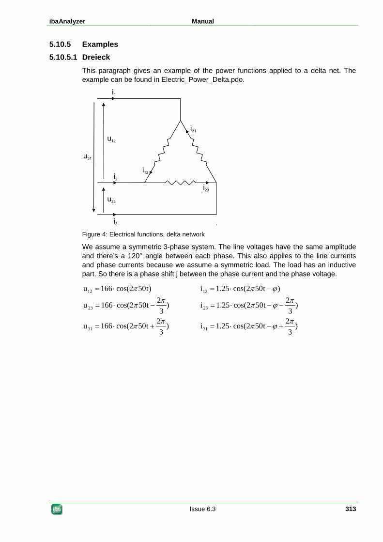
ibaAnalyzer Manual

Issue 6.3 313

5.10.5 Examples 5.10.5.1 Dreieck

This paragraph gives an example of the power functions applied to a delta net. The example can be found in Electric_Power_Delta.pdo.

Figure 4: Electrical functions, delta network

We assume a symmetric 3-phase system. The line voltages have the same amplitude and there’s a 120° angle between each phase. This also applies to the line currents and phase currents because we assume a symmetric load. The load has an inductive part. So there is a phase shift j between the phase current and the phase voltage.

)3

2t502cos(166u

)3

2t502cos(166u

)t502cos(166u

31

23

12

ππ

ππ

π

+⋅=

−⋅=

⋅=

)3

2t502cos(25.1i

)3

2t502cos(25.1i

)t502cos(25.1i

31

23

12

πϕπ

πϕπ

ϕπ

+−⋅=

−−⋅=

−⋅=

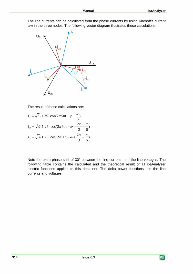
Manual ibaAnalyzer

314 Issue 6.3

The line currents can be calculated from the phase currents by using Kirchoff’s current law in the three nodes. The following vector diagram illustrates these calculations.

The result of these calculations are:

)63

2t502cos(25.13i

)63

2t502cos(25.13i

)6

t502cos(25.13i

3

2

1

ππϕπ

ππϕπ

πϕπ

−+−⋅⋅=

−−−⋅⋅=

−−⋅⋅=

Note the extra phase shift of 30° between the line currents and the line voltages. The following table contains the calculated and the theoretical result of all ibaAnalyzer electric functions applied to this delta net. The delta power functions use the line currents and voltages.

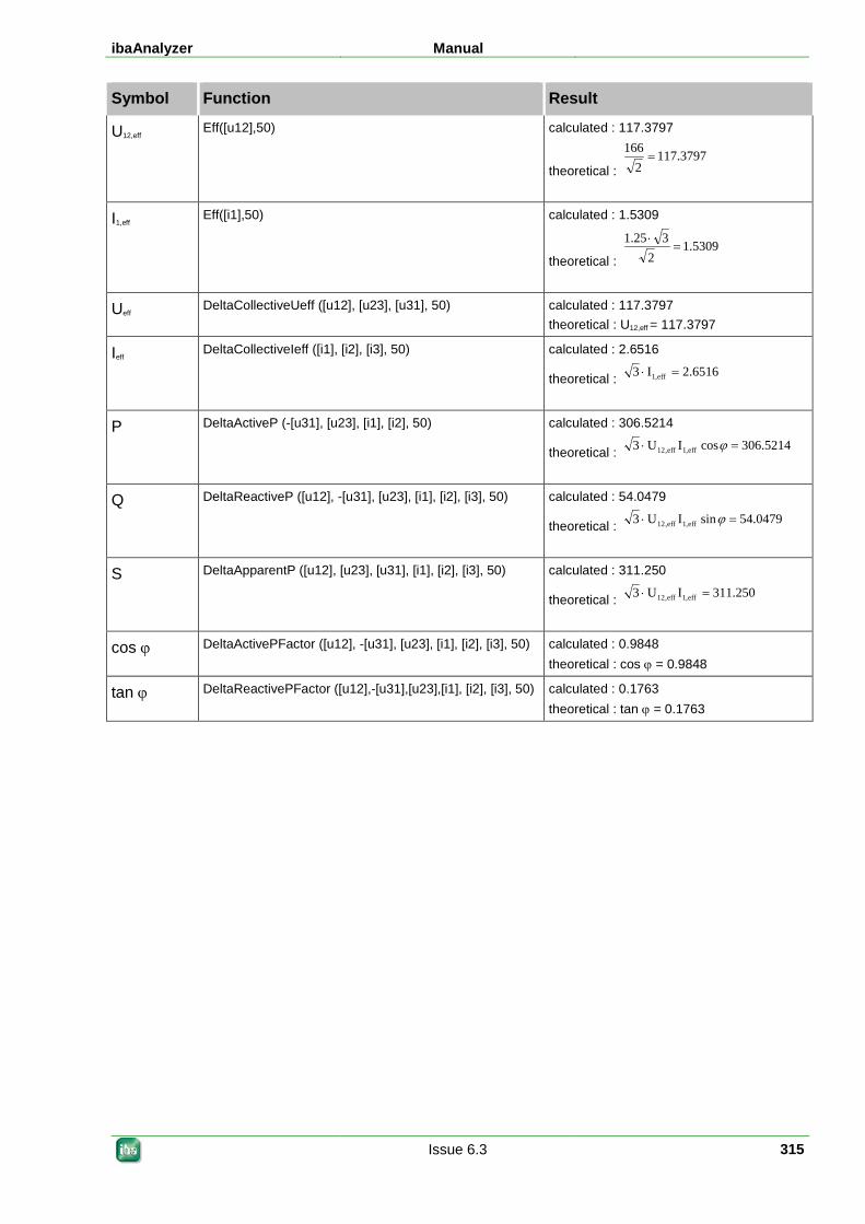
ibaAnalyzer Manual

Issue 6.3 315

Symbol Function Result

U12,eff Eff([u12],50) calculated : 117.3797

theoretical : 3797.117

2166

=

I1,eff Eff([i1],50) calculated : 1.5309

theoretical : 5309.1

2325.1=

⋅

Ueff DeltaCollectiveUeff ([u12], [u23], [u31], 50) calculated : 117.3797 theoretical : U12,eff = 117.3797

Ieff DeltaCollectiveIeff ([i1], [i2], [i3], 50) calculated : 2.6516

theoretical : 6516.2I3 eff,1 =⋅

P DeltaActiveP (-[u31], [u23], [i1], [i2], 50) calculated : 306.5214

theoretical : 5214.306cosIU3 eff,1eff,12 =⋅ ϕ

Q DeltaReactiveP ([u12], -[u31], [u23], [i1], [i2], [i3], 50) calculated : 54.0479

theoretical : 0479.54sinIU3 eff,1eff,12 =⋅ ϕ

S DeltaApparentP ([u12], [u23], [u31], [i1], [i2], [i3], 50) calculated : 311.250

theoretical : 250.311IU3 eff,1eff,12 =⋅

cos ϕ DeltaActivePFactor ([u12], -[u31], [u23], [i1], [i2], [i3], 50) calculated : 0.9848 theoretical : cos ϕ = 0.9848

tan ϕ DeltaReactivePFactor ([u12],-[u31],[u23],[i1], [i2], [i3], 50) calculated : 0.1763 theoretical : tan ϕ = 0.1763

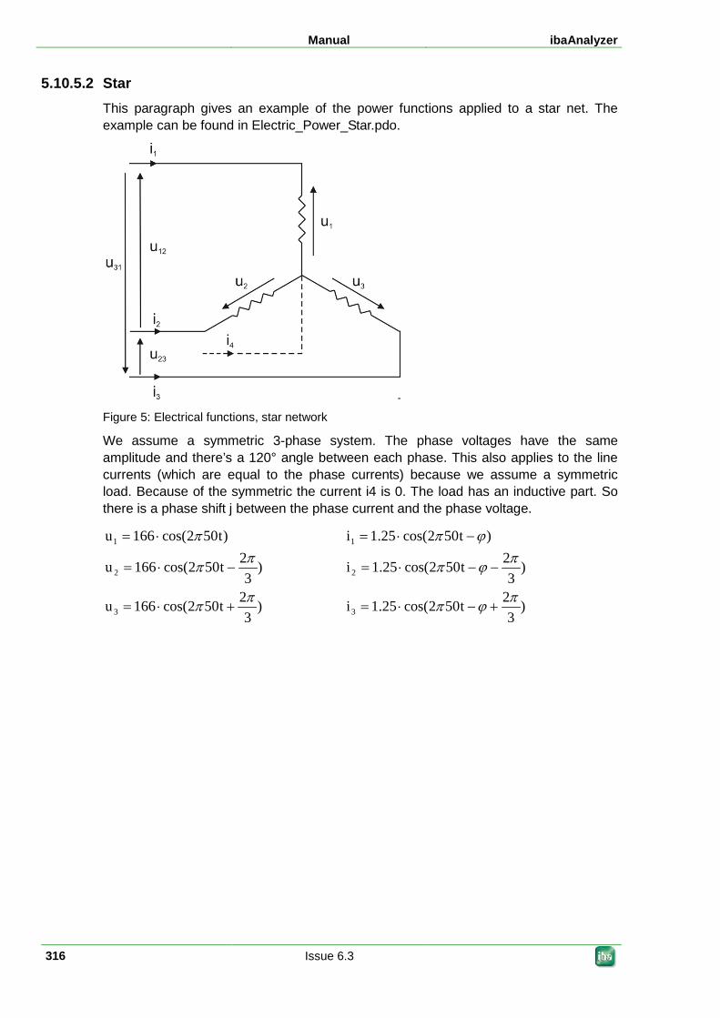
Manual ibaAnalyzer

316 Issue 6.3

5.10.5.2 Star This paragraph gives an example of the power functions applied to a star net. The example can be found in Electric_Power_Star.pdo.

Figure 5: Electrical functions, star network

We assume a symmetric 3-phase system. The phase voltages have the same amplitude and there’s a 120° angle between each phase. This also applies to the line currents (which are equal to the phase currents) because we assume a symmetric load. Because of the symmetric the current i4 is 0. The load has an inductive part. So there is a phase shift j between the phase current and the phase voltage.

)3

2t502cos(166u

)3

2t502cos(166u

)t502cos(166u

3

2

1

ππ

ππ

π

+⋅=

−⋅=

⋅=

)3

2t502cos(25.1i

)3

2t502cos(25.1i

)t502cos(25.1i

3

2

1

πϕπ

πϕπ

ϕπ

+−⋅=

−−⋅=

−⋅=

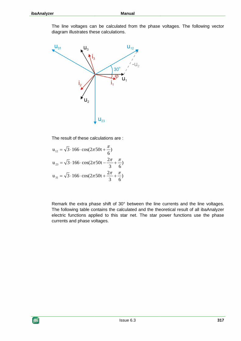
ibaAnalyzer Manual

Issue 6.3 317

The line voltages can be calculated from the phase voltages. The following vector diagram illustrates these calculations.

The result of these calculations are :

)63

2t502cos(1663u

)63

2t502cos(1663u

)6

t502cos(1663u

31

23

12

πππ

πππ

ππ

++⋅⋅=

+−⋅⋅=

+⋅⋅=

Remark the extra phase shift of 30° between the line currents and the line voltages. The following table contains the calculated and the theoretical result of all ibaAnalyzer electric functions applied to this star net. The star power functions use the phase currents and phase voltages.

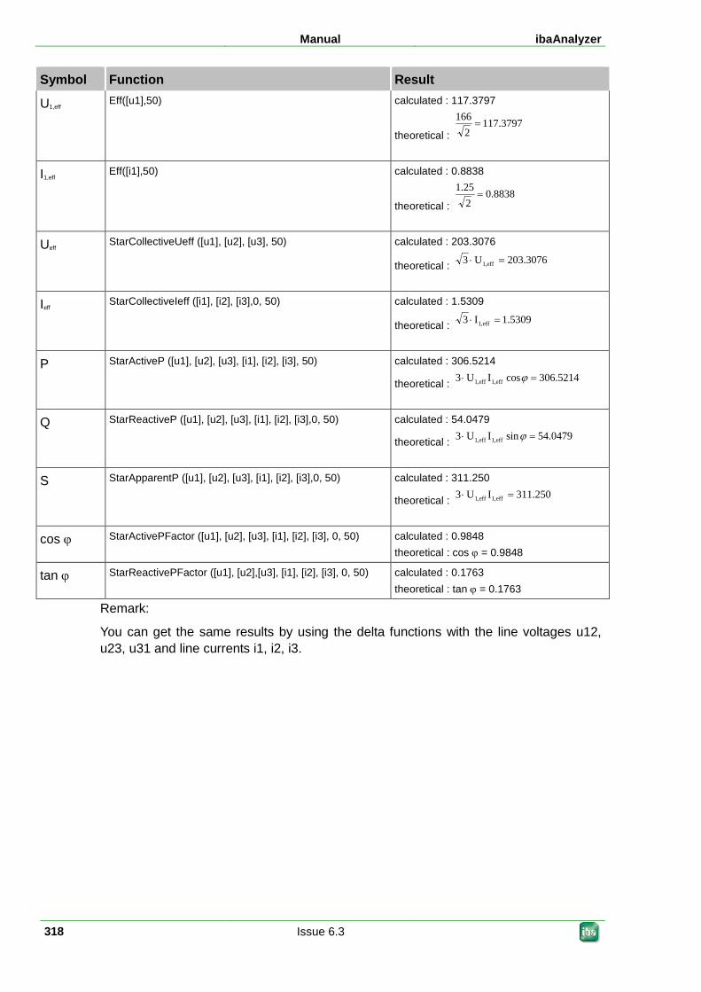
Manual ibaAnalyzer

318 Issue 6.3

Symbol Function Result

U1,eff Eff([u1],50) calculated : 117.3797

theoretical : 3797.117

2166

=

I1,eff Eff([i1],50) calculated : 0.8838

theoretical : 8838.0

225.1

=

Ueff StarCollectiveUeff ([u1], [u2], [u3], 50) calculated : 203.3076

theoretical : 3076.203U3 eff,1 =⋅

Ieff StarCollectiveIeff ([i1], [i2], [i3],0, 50) calculated : 1.5309

theoretical : 5309.1I3 eff,1 =⋅

P StarActiveP ([u1], [u2], [u3], [i1], [i2], [i3], 50) calculated : 306.5214

theoretical : 5214.306cosIU3 eff,1eff,1 =⋅ ϕ

Q StarReactiveP ([u1], [u2], [u3], [i1], [i2], [i3],0, 50) calculated : 54.0479

theoretical : 0479.54sinIU3 eff,1eff,1 =⋅ ϕ

S StarApparentP ([u1], [u2], [u3], [i1], [i2], [i3],0, 50) calculated : 311.250

theoretical : 250.311IU3 eff,1eff,1 =⋅

cos ϕ StarActivePFactor ([u1], [u2], [u3], [i1], [i2], [i3], 0, 50) calculated : 0.9848 theoretical : cos ϕ = 0.9848

tan ϕ StarReactivePFactor ([u1], [u2],[u3], [i1], [i2], [i3], 0, 50) calculated : 0.1763 theoretical : tan ϕ = 0.1763

Remark:

You can get the same results by using the delta functions with the line voltages u12, u23, u31 and line currents i1, i2, i3.

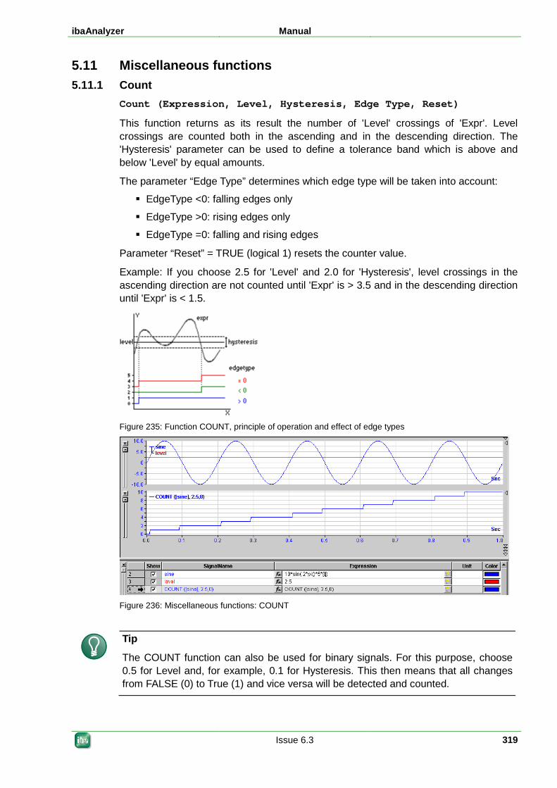
ibaAnalyzer Manual

Issue 6.3 319

5.11 Miscellaneous functions 5.11.1 Count

Count (Expression, Level, Hysteresis, Edge Type, Reset)

This function returns as its result the number of 'Level' crossings of 'Expr'. Level crossings are counted both in the ascending and in the descending direction. The 'Hysteresis' parameter can be used to define a tolerance band which is above and below 'Level' by equal amounts.

The parameter “Edge Type” determines which edge type will be taken into account:

EdgeType <0: falling edges only

EdgeType >0: rising edges only

EdgeType =0: falling and rising edges

Parameter “Reset” = TRUE (logical 1) resets the counter value.

Example: If you choose 2.5 for 'Level' and 2.0 for 'Hysteresis', level crossings in the ascending direction are not counted until 'Expr' is > 3.5 and in the descending direction until 'Expr' is < 1.5.

Figure 235: Function COUNT, principle of operation and effect of edge types

Figure 236: Miscellaneous functions: COUNT

Tip

The COUNT function can also be used for binary signals. For this purpose, choose 0.5 for Level and, for example, 0.1 for Hysteresis. This then means that all changes from FALSE (0) to True (1) and vice versa will be detected and counted.

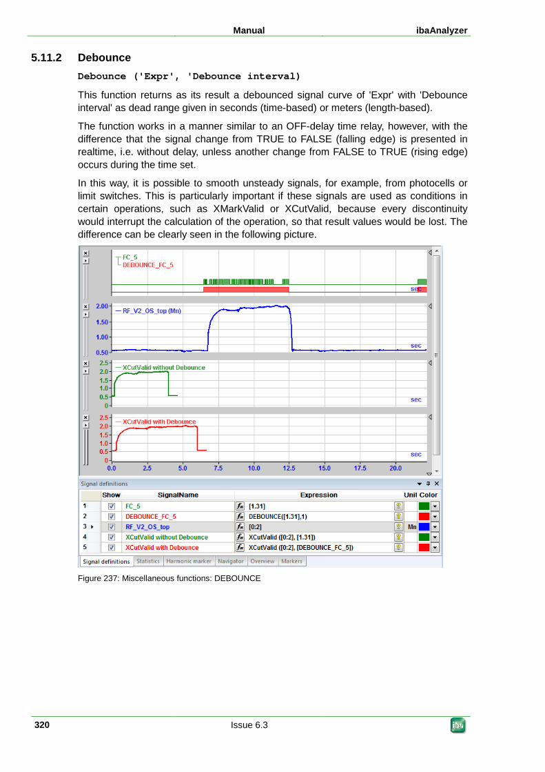
Manual ibaAnalyzer

320 Issue 6.3

5.11.2 Debounce Debounce ('Expr', 'Debounce interval)

This function returns as its result a debounced signal curve of 'Expr' with 'Debounce interval' as dead range given in seconds (time-based) or meters (length-based).

The function works in a manner similar to an OFF-delay time relay, however, with the difference that the signal change from TRUE to FALSE (falling edge) is presented in realtime, i.e. without delay, unless another change from FALSE to TRUE (rising edge) occurs during the time set.

In this way, it is possible to smooth unsteady signals, for example, from photocells or limit switches. This is particularly important if these signals are used as conditions in certain operations, such as XMarkValid or XCutValid, because every discontinuity would interrupt the calculation of the operation, so that result values would be lost. The difference can be clearly seen in the following picture.

Figure 237: Miscellaneous functions: DEBOUNCE

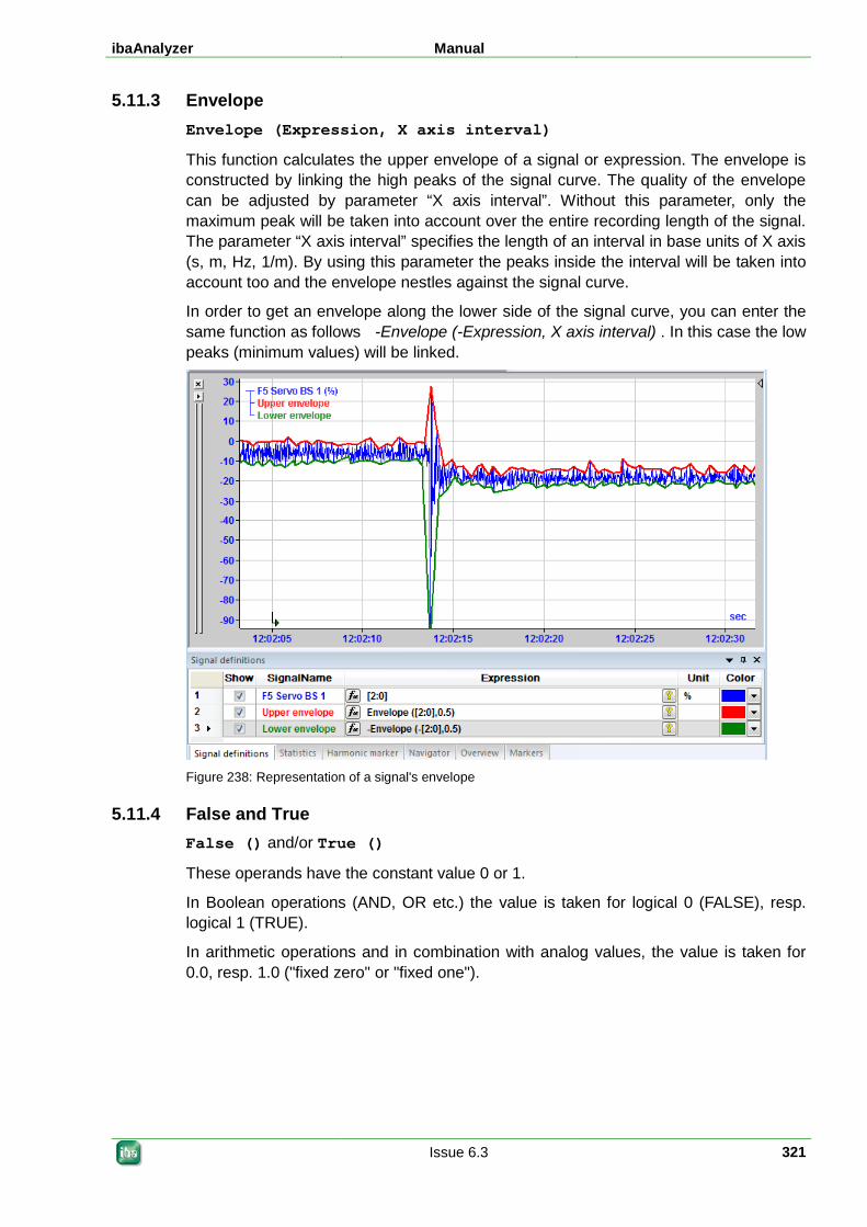
ibaAnalyzer Manual

Issue 6.3 321

5.11.3 Envelope Envelope (Expression, X axis interval)

This function calculates the upper envelope of a signal or expression. The envelope is constructed by linking the high peaks of the signal curve. The quality of the envelope can be adjusted by parameter “X axis interval”. Without this parameter, only the maximum peak will be taken into account over the entire recording length of the signal. The parameter “X axis interval” specifies the length of an interval in base units of X axis (s, m, Hz, 1/m). By using this parameter the peaks inside the interval will be taken into account too and the envelope nestles against the signal curve.

In order to get an envelope along the lower side of the signal curve, you can enter the same function as follows -Envelope (-Expression, X axis interval) . In this case the low peaks (minimum values) will be linked.

Figure 238: Representation of a signal's envelope

5.11.4 False and True False () and/or True ()

These operands have the constant value 0 or 1.

In Boolean operations (AND, OR etc.) the value is taken for logical 0 (FALSE), resp. logical 1 (TRUE).

In arithmetic operations and in combination with analog values, the value is taken for 0.0, resp. 1.0 ("fixed zero" or "fixed one").

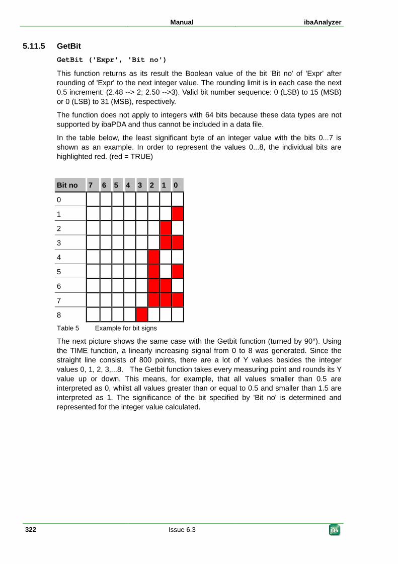
Manual ibaAnalyzer

322 Issue 6.3

5.11.5 GetBit GetBit ('Expr', 'Bit no')

This function returns as its result the Boolean value of the bit 'Bit no' of 'Expr' after rounding of 'Expr' to the next integer value. The rounding limit is in each case the next 0.5 increment. (2.48 --> 2; 2.50 -->3). Valid bit number sequence: 0 (LSB) to 15 (MSB) or 0 (LSB) to 31 (MSB), respectively.

The function does not apply to integers with 64 bits because these data types are not supported by ibaPDA and thus cannot be included in a data file.

In the table below, the least significant byte of an integer value with the bits 0...7 is shown as an example. In order to represent the values 0...8, the individual bits are highlighted red. (red = TRUE)

Bit no 7 6 5 4 3 2 1 0

0

1

2

3

4

5

6

7

8

Table 5 Example for bit signs

The next picture shows the same case with the Getbit function (turned by 90°). Using the TIME function, a linearly increasing signal from 0 to 8 was generated. Since the straight line consists of 800 points, there are a lot of Y values besides the integer values 0, 1, 2, 3,...8. The Getbit function takes every measuring point and rounds its Y value up or down. This means, for example, that all values smaller than 0.5 are interpreted as 0, whilst all values greater than or equal to 0.5 and smaller than 1.5 are interpreted as 1. The significance of the bit specified by 'Bit no' is determined and represented for the integer value calculated.

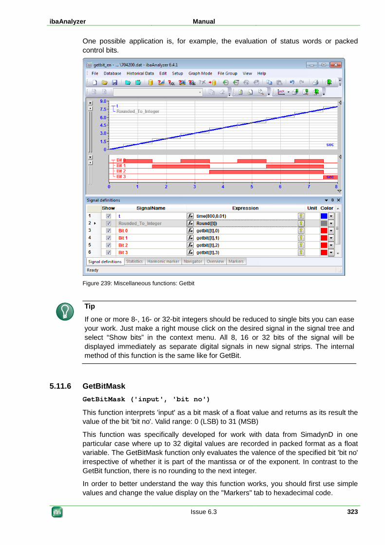
ibaAnalyzer Manual

Issue 6.3 323

One possible application is, for example, the evaluation of status words or packed control bits.

Figure 239: Miscellaneous functions: Getbit

Tip

If one or more 8-, 16- or 32-bit integers should be reduced to single bits you can ease your work. Just make a right mouse click on the desired signal in the signal tree and select “Show bits” in the context menu. All 8, 16 or 32 bits of the signal will be displayed immediately as separate digital signals in new signal strips. The internal method of this function is the same like for GetBit.

5.11.6 GetBitMask GetBitMask ('input', 'bit no')

This function interprets 'input' as a bit mask of a float value and returns as its result the value of the bit 'bit no'. Valid range: 0 (LSB) to 31 (MSB)

This function was specifically developed for work with data from SimadynD in one particular case where up to 32 digital values are recorded in packed format as a float variable. The GetBitMask function only evaluates the valence of the specified bit 'bit no' irrespective of whether it is part of the mantissa or of the exponent. In contrast to the GetBit function, there is no rounding to the next integer.

In order to better understand the way this function works, you should first use simple values and change the value display on the "Markers" tab to hexadecimal code.

Manual ibaAnalyzer

324 Issue 6.3

Tip

If one or more 32 bit floating values should be reduced to single bits you can ease your work. Just make a right mouse click on the desired signal in the signal tree and select “Show bits” in the context menu. All 32 bits of the signal will be displayed immediately as separate digital signals in new signal strip. The internal method of this function is the same like for GetBitMask.

5.11.7 HighPrecision HighPrecision (expression)

With this function, 'expression' is marked as quantity with double precision. Calculations which are then performed with 'expression' are implemented with double precision, even if the original expression only has single precision.

From version 5.21.0, ibaAnalyzer can perform calculations both with single precision (32 bit) and double precision (double precision, 64 bit).

Double precision, on the one hand, has the advantage that calculations can be performed more precisely, on the other hand, however, it also has the disadvantage that it requires twice as much storage capacity. Therefore, ibaAnalyzer automatically decides based on the input arguments which precision to be used for a calculation.

If a signal is available as 16Bit integer or 32Bit floating point value in the data file, ibaAnalyzer works with single precision.

If a signal is available as 32Bit integer or 64Bit floating point value in the data file, ibaAnalyzer works with double precision.

With the "HighPrecision" function, you can force ibaAnalyzer to perform calculations with double precision, irrespective of the precision of the input arguments.

With regard to storage capacity, ibaAnalyzer is optimized in such a way that no 64Bit copy of the argument is generated, but it is only noted that the calculations are to be performed with double precision. The results of a calculation with double precision are saved as 64Bit values.

5.11.8 InfoField Info field ('FileIndex', "'Info field'", 'Start', 'End')

This operation gets the string from any info field of a data file and supplies it for display purposes. Sole restraint: it must be a numerical string!

Parameter:

FileIndex refers to an ongoing numbering (top-down) of loaded data files, from 0 to n. If only one data file is open, use 0 for ‘Fileindex’.

"Info field": name of the info field to be read. Use quotation marks!

Start: first character of the field content to be read. Minimum value for start is 0 (=default). This parameter is optional. If no "Start" value is defined, the complete content is read.

End: last character of the field content to be read. This parameter is optional. If no "End" value is defined, it will be read from the start to the last character (end of text = default).

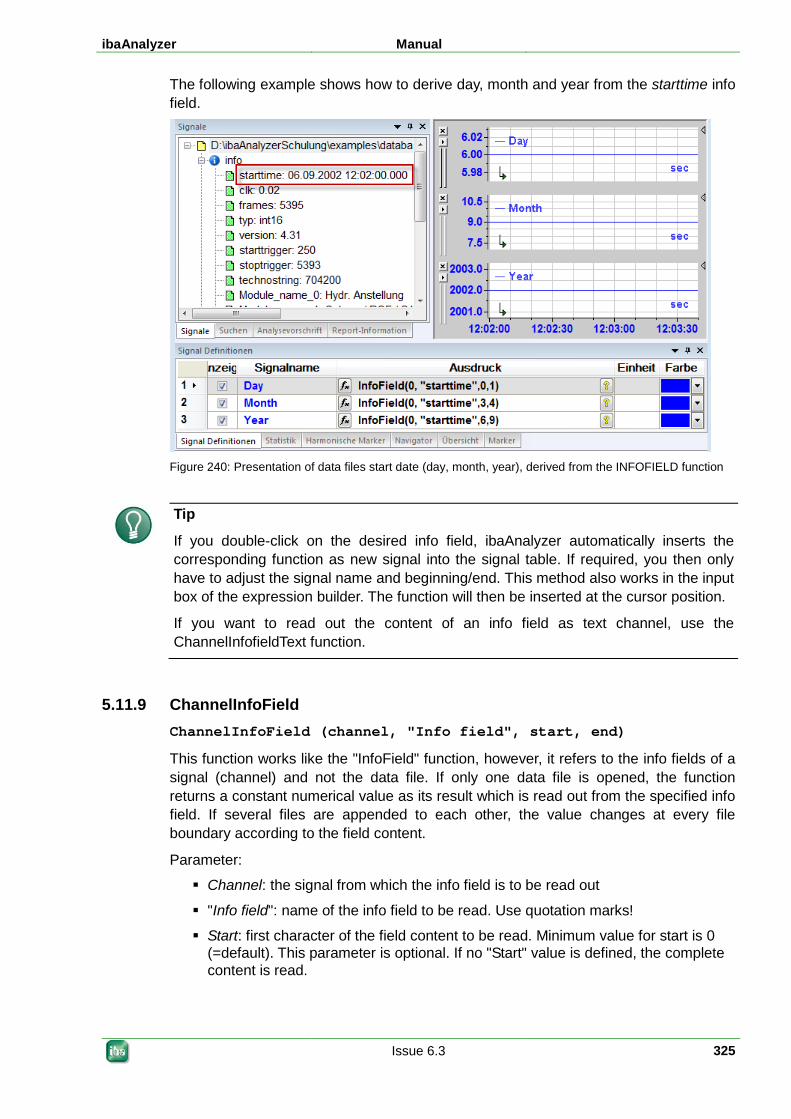
ibaAnalyzer Manual

Issue 6.3 325

The following example shows how to derive day, month and year from the starttime info field.

Figure 240: Presentation of data files start date (day, month, year), derived from the INFOFIELD function

Tip

If you double-click on the desired info field, ibaAnalyzer automatically inserts the corresponding function as new signal into the signal table. If required, you then only have to adjust the signal name and beginning/end. This method also works in the input box of the expression builder. The function will then be inserted at the cursor position.

If you want to read out the content of an info field as text channel, use the ChannelInfofieldText function.

5.11.9 ChannelInfoField ChannelInfoField (channel, "Info field", start, end)

This function works like the "InfoField" function, however, it refers to the info fields of a signal (channel) and not the data file. If only one data file is opened, the function returns a constant numerical value as its result which is read out from the specified info field. If several files are appended to each other, the value changes at every file boundary according to the field content.

Parameter:

Channel: the signal from which the info field is to be read out

"Info field": name of the info field to be read. Use quotation marks!

Start: first character of the field content to be read. Minimum value for start is 0 (=default). This parameter is optional. If no "Start" value is defined, the complete content is read.

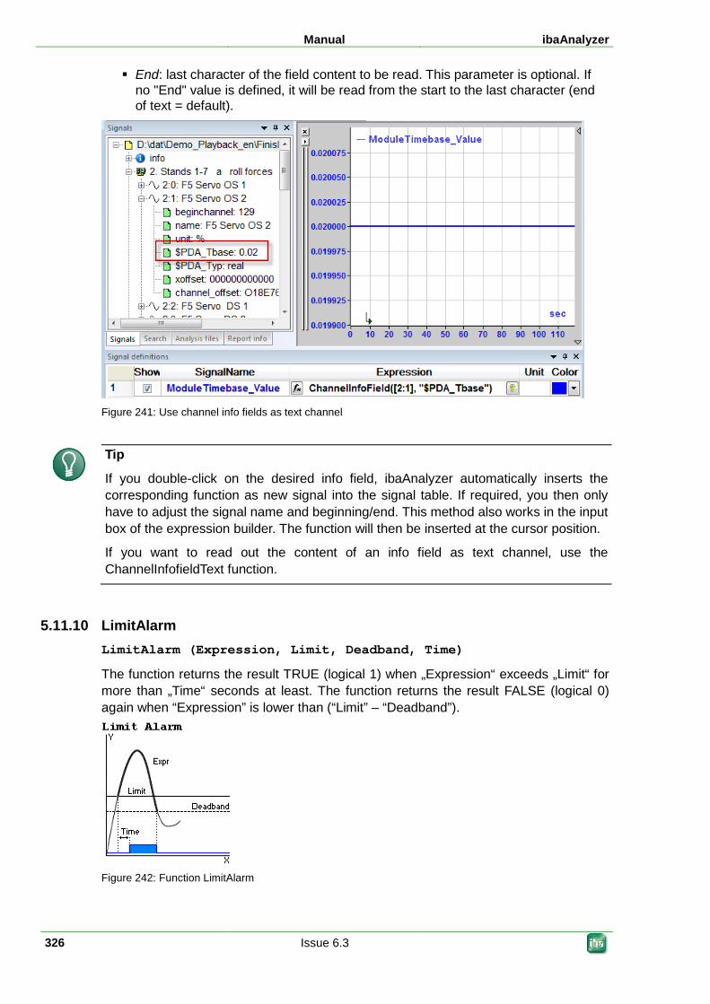
Manual ibaAnalyzer

326 Issue 6.3

End: last character of the field content to be read. This parameter is optional. If no "End" value is defined, it will be read from the start to the last character (end of text = default).

Figure 241: Use channel info fields as text channel

Tip

If you double-click on the desired info field, ibaAnalyzer automatically inserts the corresponding function as new signal into the signal table. If required, you then only have to adjust the signal name and beginning/end. This method also works in the input box of the expression builder. The function will then be inserted at the cursor position.

If you want to read out the content of an info field as text channel, use the ChannelInfofieldText function.

5.11.10 LimitAlarm LimitAlarm (Expression, Limit, Deadband, Time)

The function returns the result TRUE (logical 1) when „Expression“ exceeds „Limit“ for more than „Time“ seconds at least. The function returns the result FALSE (logical 0) again when “Expression” is lower than (“Limit” – “Deadband”).

Figure 242: Function LimitAlarm

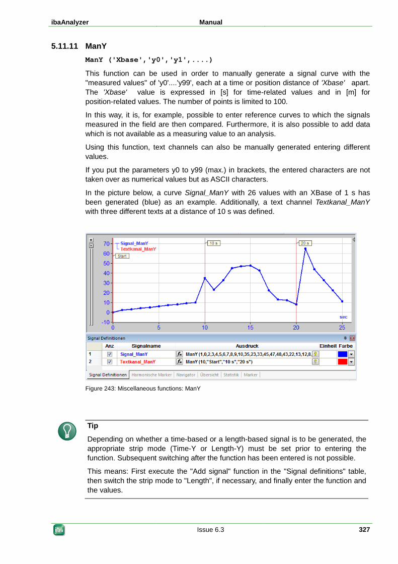
ibaAnalyzer Manual

Issue 6.3 327

5.11.11 ManY ManY ('Xbase','y0','y1',....)

This function can be used in order to manually generate a signal curve with the "measured values" of 'y0'....'y99', each at a time or position distance of 'Xbase' apart. The 'Xbase' value is expressed in [s] for time-related values and in [m] for position-related values. The number of points is limited to 100.

In this way, it is, for example, possible to enter reference curves to which the signals measured in the field are then compared. Furthermore, it is also possible to add data which is not available as a measuring value to an analysis.

Using this function, text channels can also be manually generated entering different values.

If you put the parameters y0 to y99 (max.) in brackets, the entered characters are not taken over as numerical values but as ASCII characters.

In the picture below, a curve Signal_ManY with 26 values with an XBase of 1 s has been generated (blue) as an example. Additionally, a text channel Textkanal_ManY with three different texts at a distance of 10 s was defined.

Figure 243: Miscellaneous functions: ManY

Tip

Depending on whether a time-based or a length-based signal is to be generated, the appropriate strip mode (Time-Y or Length-Y) must be set prior to entering the function. Subsequent switching after the function has been entered is not possible.

This means: First execute the "Add signal" function in the "Signal definitions" table, then switch the strip mode to "Length", if necessary, and finally enter the function and the values.

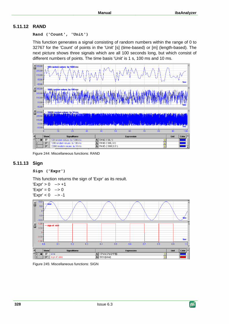
Manual ibaAnalyzer

328 Issue 6.3

5.11.12 RAND Rand ('Count', 'Unit')

This function generates a signal consisting of random numbers within the range of 0 to 32767 for the 'Count' of points in the 'Unit' [s] (time-based) or [m] (length-based). The next picture shows three signals which are all 100 seconds long, but which consist of different numbers of points. The time basis 'Unit' is 1 s, 100 ms and 10 ms.

Figure 244: Miscellaneous functions: RAND

5.11.13 Sign Sign ('Expr')

This function returns the sign of 'Expr' as its result. 'Expr' > 0 --> +1 'Expr' = 0 --> 0 'Expr' < 0 --> -1

Figure 245: Miscellaneous functions: SIGN

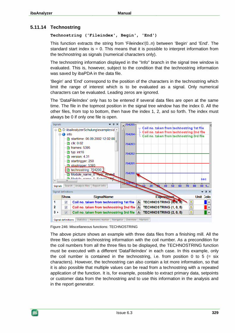
ibaAnalyzer Manual

Issue 6.3 329

5.11.14 Technostring Technostring ('Fileindex', Begin', 'End')

This function extracts the string from 'Fileindex'(0..n) between 'Begin‘ and 'End'. The standard start index is = 0. This means that it is possible to interpret information from the technostring as signals (numerical characters only).

The technostring information displayed in the "Info" branch in the signal tree window is evaluated. This is, however, subject to the condition that the technostring information was saved by ibaPDA in the data file.

'Begin' and 'End' correspond to the position of the characters in the technostring which limit the range of interest which is to be evaluated as a signal. Only numerical characters can be evaluated. Leading zeros are ignored.

The 'DataFileIndex' only has to be entered if several data files are open at the same time. The file in the topmost position in the signal tree window has the index 0. All the other files, from top to bottom, then have the index 1, 2, and so forth. The index must always be 0 if only one file is open.

Figure 246: Miscellaneous functions: TECHNOSTRING

The above picture shows an example with three data files from a finishing mill. All the three files contain technostring information with the coil number. As a precondition for the coil numbers from all the three files to be displayed, the TECHNOSTRING function must be executed with a different 'DataFileIndex' in each case. In this example, only the coil number is contained in the technostring, i.e. from position 0 to 5 (= six characters). However, the technostring can also contain a lot more information, so that it is also possible that multiple values can be read from a technostring with a repeated application of the function. It is, for example, possible to extract primary data, setpoints or customer data from the technostring and to use this information in the analysis and in the report generator.

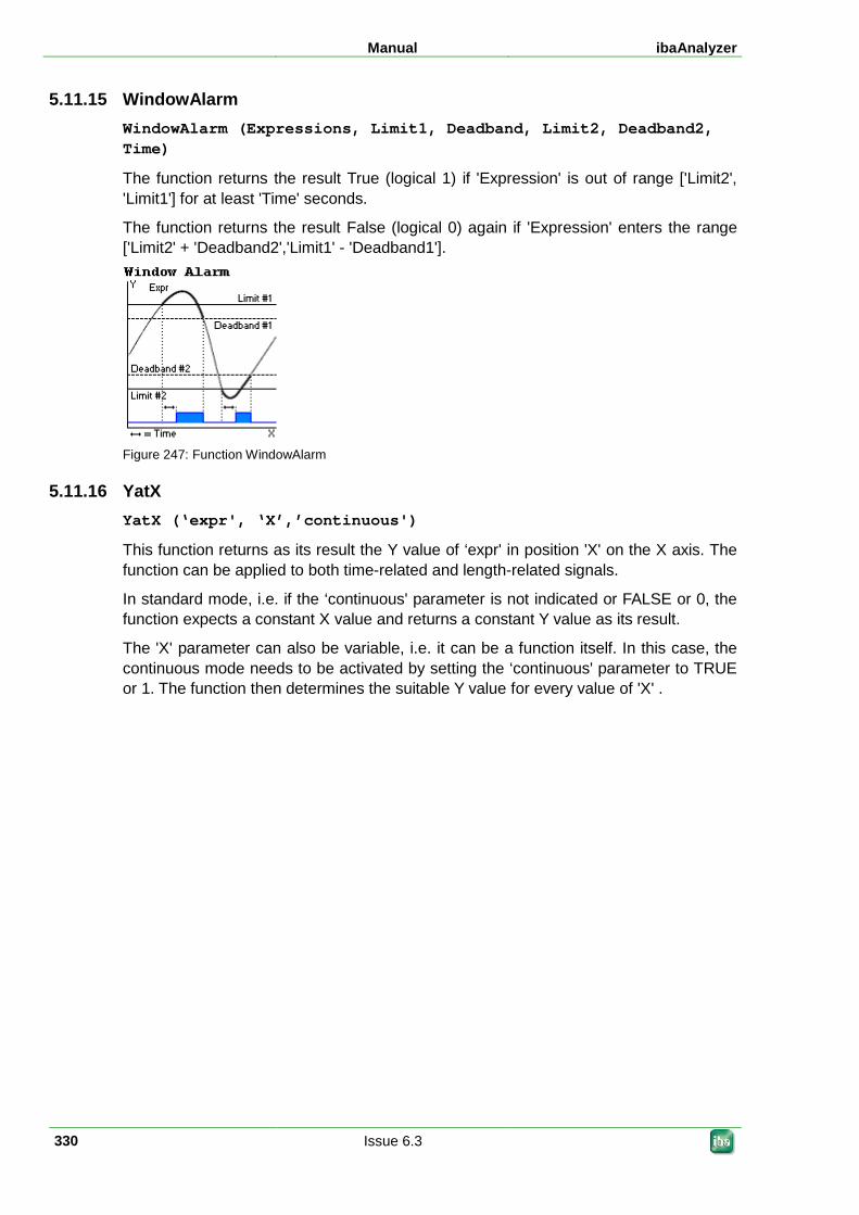
Manual ibaAnalyzer

330 Issue 6.3

5.11.15 WindowAlarm WindowAlarm (Expressions, Limit1, Deadband, Limit2, Deadband2, Time)

The function returns the result True (logical 1) if 'Expression' is out of range ['Limit2', 'Limit1'] for at least 'Time' seconds.

The function returns the result False (logical 0) again if 'Expression' enters the range ['Limit2' + 'Deadband2','Limit1' - 'Deadband1'].

Figure 247: Function WindowAlarm

5.11.16 YatX YatX (‘expr', ‘X’,’continuous')

This function returns as its result the Y value of ‘expr' in position 'X' on the X axis. The function can be applied to both time-related and length-related signals.

In standard mode, i.e. if the ‘continuous' parameter is not indicated or FALSE or 0, the function expects a constant X value and returns a constant Y value as its result.

The 'X' parameter can also be variable, i.e. it can be a function itself. In this case, the continuous mode needs to be activated by setting the ‘continuous' parameter to TRUE or 1. The function then determines the suitable Y value for every value of 'X' .

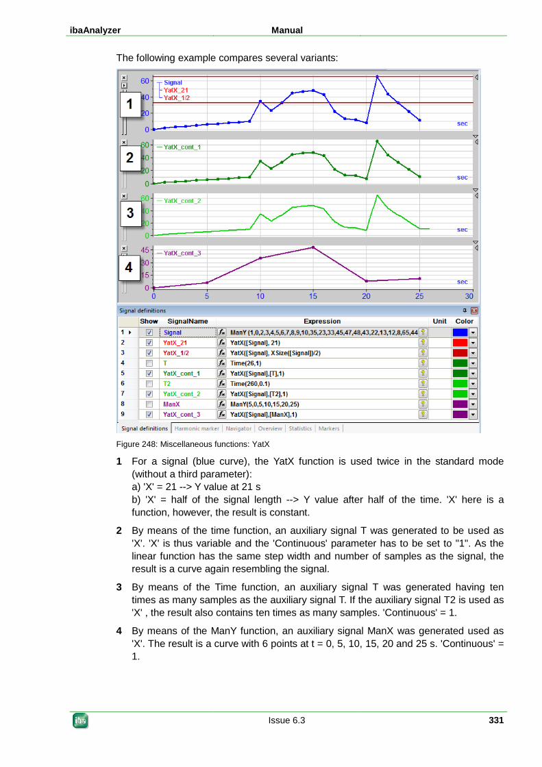
ibaAnalyzer Manual

Issue 6.3 331

The following example compares several variants:

Figure 248: Miscellaneous functions: YatX

1 For a signal (blue curve), the YatX function is used twice in the standard mode (without a third parameter): a) 'X' = 21 --> Y value at 21 s b) 'X' = half of the signal length --> Y value after half of the time. 'X' here is a function, however, the result is constant.

2 By means of the time function, an auxiliary signal T was generated to be used as 'X'. 'X' is thus variable and the 'Continuous' parameter has to be set to "1". As the linear function has the same step width and number of samples as the signal, the result is a curve again resembling the signal.

3 By means of the Time function, an auxiliary signal T was generated having ten times as many samples as the auxiliary signal T. If the auxiliary signal T2 is used as 'X' , the result also contains ten times as many samples. 'Continuous' = 1.

4 By means of the ManY function, an auxiliary signal ManX was generated used as 'X'. The result is a curve with 6 points at t = 0, 5, 10, 15, 20 and 25 s. 'Continuous' = 1.

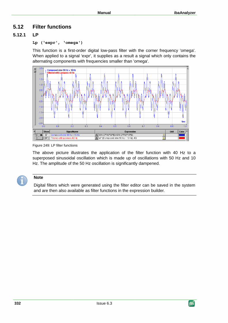
Manual ibaAnalyzer

332 Issue 6.3

5.12 Filter functions 5.12.1 LP

Lp (‘expr', ‘omega')

This function is a first-order digital low-pass filter with the corner frequency 'omega'. When applied to a signal ‘expr', it supplies as a result a signal which only contains the alternating components with frequencies smaller than 'omega'.

Figure 249: LP filter functions

The above picture illustrates the application of the filter function with 40 Hz to a superposed sinusoidal oscillation which is made up of oscillations with 50 Hz and 10 Hz. The amplitude of the 50 Hz oscillation is significantly dampened.

Note

Digital filters which were generated using the filter editor can be saved in the system and are then also available as filter functions in the expression builder.

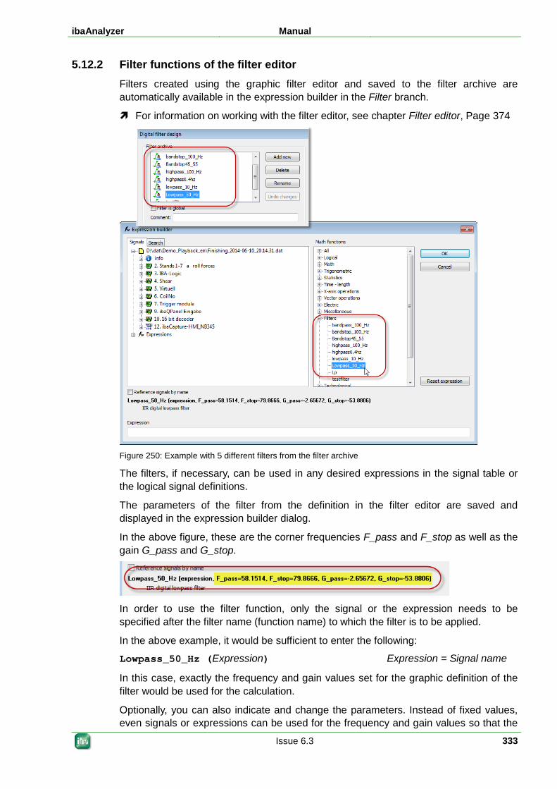
ibaAnalyzer Manual

Issue 6.3 333

5.12.2 Filter functions of the filter editor Filters created using the graphic filter editor and saved to the filter archive are automatically available in the expression builder in the Filter branch.

For information on working with the filter editor, see chapter Filter editor, Page 374

Figure 250: Example with 5 different filters from the filter archive

The filters, if necessary, can be used in any desired expressions in the signal table or the logical signal definitions.

The parameters of the filter from the definition in the filter editor are saved and displayed in the expression builder dialog.

In the above figure, these are the corner frequencies F_pass and F_stop as well as the gain G_pass and G_stop.

In order to use the filter function, only the signal or the expression needs to be specified after the filter name (function name) to which the filter is to be applied.

In the above example, it would be sufficient to enter the following:

Lowpass_50_Hz (Expression) Expression = Signal name

In this case, exactly the frequency and gain values set for the graphic definition of the filter would be used for the calculation.

Optionally, you can also indicate and change the parameters. Instead of fixed values, even signals or expressions can be used for the frequency and gain values so that the

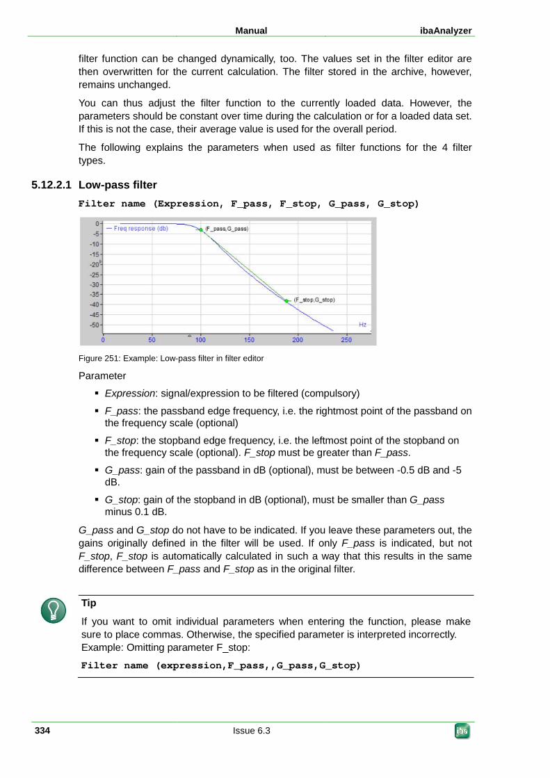
Manual ibaAnalyzer

334 Issue 6.3

filter function can be changed dynamically, too. The values set in the filter editor are then overwritten for the current calculation. The filter stored in the archive, however, remains unchanged.

You can thus adjust the filter function to the currently loaded data. However, the parameters should be constant over time during the calculation or for a loaded data set. If this is not the case, their average value is used for the overall period.

The following explains the parameters when used as filter functions for the 4 filter types.

5.12.2.1 Low-pass filter Filter name (Expression, F_pass, F_stop, G_pass, G_stop)

Figure 251: Example: Low-pass filter in filter editor

Parameter

Expression: signal/expression to be filtered (compulsory)

F_pass: the passband edge frequency, i.e. the rightmost point of the passband on the frequency scale (optional)

F_stop: the stopband edge frequency, i.e. the leftmost point of the stopband on the frequency scale (optional). F_stop must be greater than F_pass.

G_pass: gain of the passband in dB (optional), must be between -0.5 dB and -5 dB.

G_stop: gain of the stopband in dB (optional), must be smaller than G_pass minus 0.1 dB.

G_pass and G_stop do not have to be indicated. If you leave these parameters out, the gains originally defined in the filter will be used. If only F_pass is indicated, but not F_stop, F_stop is automatically calculated in such a way that this results in the same difference between F_pass and F_stop as in the original filter.

Tip

If you want to omit individual parameters when entering the function, please make sure to place commas. Otherwise, the specified parameter is interpreted incorrectly. Example: Omitting parameter F_stop:

Filter name (expression,F_pass,,G_pass,G_stop)

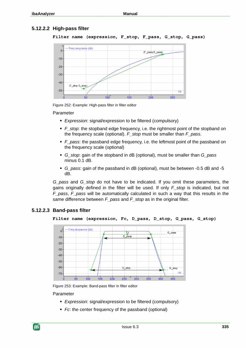
ibaAnalyzer Manual

Issue 6.3 335

5.12.2.2 High-pass filter Filter name (expression, F_stop, F_pass, G_stop, G_pass)

Figure 252: Example: High-pass filter in filter editor

Parameter

Expression: signal/expression to be filtered (compulsory)

F_stop: the stopband edge frequency, i.e. the rightmost point of the stopband on the frequency scale (optional). F_stop must be smaller than F_pass.

F_pass: the passband edge frequency, i.e. the leftmost point of the passband on the frequency scale (optional)

G_stop: gain of the stopband in dB (optional), must be smaller than G_pass minus 0.1 dB.

G_pass: gain of the passband in dB (optional), must be between -0.5 dB and -5 dB.

G_pass and G_stop do not have to be indicated. If you omit these parameters, the gains originally defined in the filter will be used. If only F_stop is indicated, but not F_pass, F_pass will be automatically calculated in such a way that this results in the same difference between F_pass and F_stop as in the original filter.

5.12.2.3 Band-pass filter Filter name (expression, Fc, D_pass, D_stop, G_pass, G_stop)

Figure 253: Example: Band-pass filter in filter editor

Parameter

Expression: signal/expression to be filtered (compulsory)

Fc: the center frequency of the passband (optional)

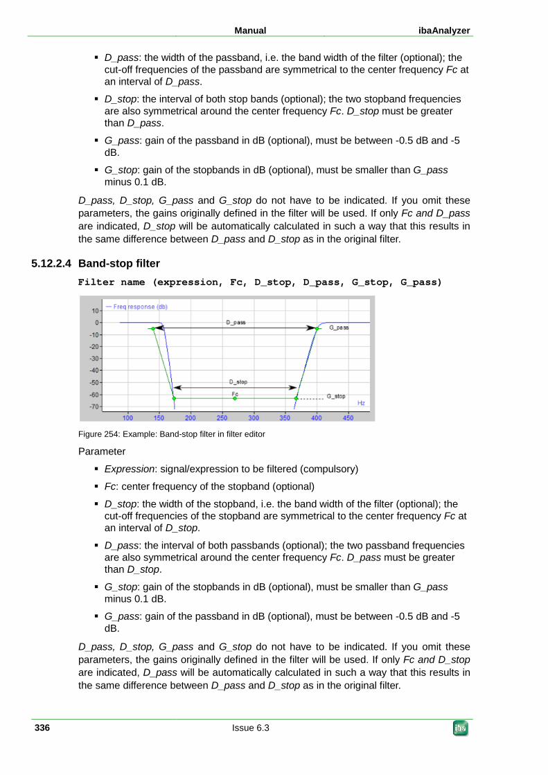
Manual ibaAnalyzer

336 Issue 6.3

D_pass: the width of the passband, i.e. the band width of the filter (optional); the cut-off frequencies of the passband are symmetrical to the center frequency Fc at an interval of D_pass.

D_stop: the interval of both stop bands (optional); the two stopband frequencies are also symmetrical around the center frequency Fc. D_stop must be greater than D_pass.

G_pass: gain of the passband in dB (optional), must be between -0.5 dB and -5 dB.

G_stop: gain of the stopbands in dB (optional), must be smaller than G_pass minus 0.1 dB.

D_pass, D_stop, G_pass and G_stop do not have to be indicated. If you omit these parameters, the gains originally defined in the filter will be used. If only Fc and D_pass are indicated, D_stop will be automatically calculated in such a way that this results in the same difference between D_pass and D_stop as in the original filter.

5.12.2.4 Band-stop filter Filter name (expression, Fc, D_stop, D_pass, G_stop, G_pass)

Figure 254: Example: Band-stop filter in filter editor

Parameter

Expression: signal/expression to be filtered (compulsory)

Fc: center frequency of the stopband (optional)

D_stop: the width of the stopband, i.e. the band width of the filter (optional); the cut-off frequencies of the stopband are symmetrical to the center frequency Fc at an interval of D_stop.

D_pass: the interval of both passbands (optional); the two passband frequencies are also symmetrical around the center frequency Fc. D_pass must be greater than D_stop.

G_stop: gain of the stopbands in dB (optional), must be smaller than G_pass minus 0.1 dB.

G_pass: gain of the passband in dB (optional), must be between -0.5 dB and -5 dB.

D_pass, D_stop, G_pass and G_stop do not have to be indicated. If you omit these parameters, the gains originally defined in the filter will be used. If only Fc and D_stop are indicated, D_pass will be automatically calculated in such a way that this results in the same difference between D_pass and D_stop as in the original filter.

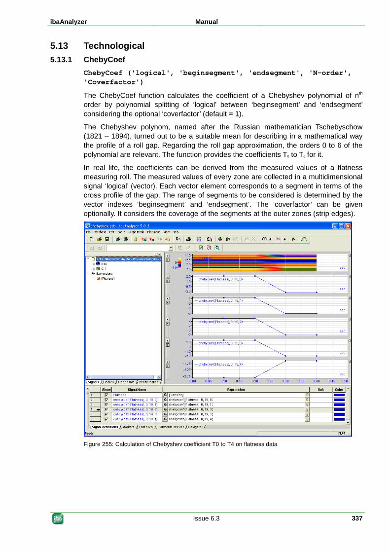
ibaAnalyzer Manual

Issue 6.3 337

5.13 Technological 5.13.1 ChebyCoef

ChebyCoef ('logical', 'beginsegment', 'endsegment', 'N-order', 'Coverfactor')

The ChebyCoef function calculates the coefficient of a Chebyshev polynomial of nth order by polynomial splitting of ‘logical’ between ‘beginsegment’ and ‘endsegment’ considering the optional ‘coverfactor’ (default = 1).

The Chebyshev polynom, named after the Russian mathematician Tschebyschow (1821 – 1894), turned out to be a suitable mean for describing in a mathematical way the profile of a roll gap. Regarding the roll gap approximation, the orders 0 to 6 of the polynomial are relevant. The function provides the coefficients T0 to T6 for it.

In real life, the coefficients can be derived from the measured values of a flatness measuring roll. The measured values of every zone are collected in a multidimensional signal ‘logical’ (vector). Each vector element corresponds to a segment in terms of the cross profile of the gap. The range of segments to be considered is determined by the vector indexes ‘beginsegment’ and ‘endsegment’. The ‘coverfactor’ can be given optionally. It considers the coverage of the segments at the outer zones (strip edges).

Figure 255: Calculation of Chebyshev coefficient T0 to T4 on flatness data

Manual ibaAnalyzer

338 Issue 6.3

5.13.2 CubicSpline CubicSpline (expression,X,Y)

The function calculates a cubic spline for a number of points and returns a smoothened signal along this spline as its result. The function can be used for interpolating a compensation curve for a signal with few samples.

Parameter:

Expression: Values to be applied at the spline

X: X coordinates of the pair of points defining the spline (knot)

Y: Y coordinates of the pair of points defining the spline (knot)

The X coordinates, by the way, do not have to be unique and sorted. If there are several value pairs with the same X coordinate, only the last value pair will be kept for calculating the spline. The remaining value pairs are sorted by X coordinates.

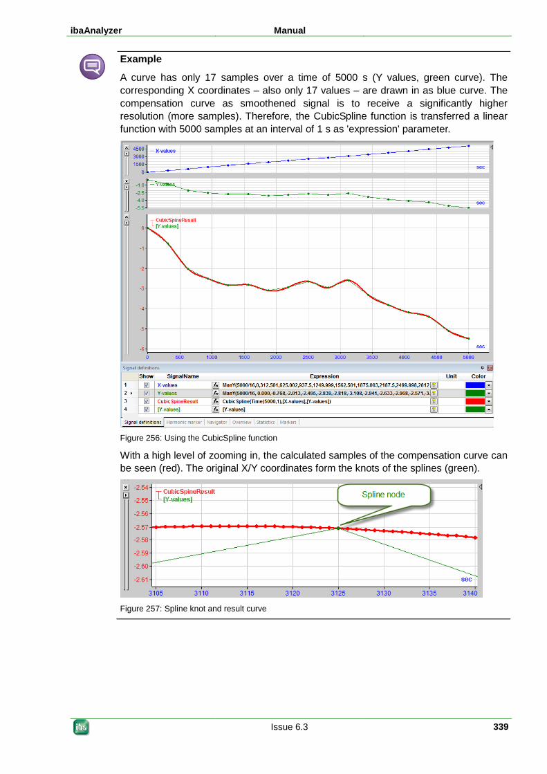
ibaAnalyzer Manual

Issue 6.3 339

Example

A curve has only 17 samples over a time of 5000 s (Y values, green curve). The corresponding X coordinates – also only 17 values – are drawn in as blue curve. The compensation curve as smoothened signal is to receive a significantly higher resolution (more samples). Therefore, the CubicSpline function is transferred a linear function with 5000 samples at an interval of 1 s as 'expression' parameter.

Figure 256: Using the CubicSpline function

With a high level of zooming in, the calculated samples of the compensation curve can be seen (red). The original X/Y coordinates form the knots of the splines (green).

Figure 257: Spline knot and result curve

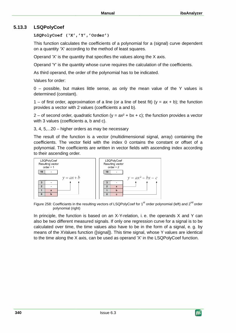
Manual ibaAnalyzer

340 Issue 6.3

5.13.3 LSQPolyCoef LSQPolyCoef (‘X’,’Y’,’Order’)

This function calculates the coefficients of a polynomial for a (signal) curve dependent on a quantity ‘X‘ according to the method of least squares.

Operand 'X' is the quantity that specifies the values along the X axis.

Operand 'Y' is the quantity whose curve requires the calculation of the coefficients.

As third operand, the order of the polynomial has to be indicated.

Values for order:

0 – possible, but makes little sense, as only the mean value of the Y values is determined (constant).

1 – of first order, approximation of a line (or a line of best fit) (y = ax + b); the function provides a vector with 2 values (coefficients a and b).

2 – of second order, quadratic function (y = ax² + bx + c); the function provides a vector with 3 values (coefficients a, b and c).

3, 4, 5,...20 – higher orders as may be necessary

The result of the function is a vector (multidimensional signal, array) containing the coefficients. The vector field with the index 0 contains the constant or offset of a polynomial. The coefficients are written in vector fields with ascending index according to their ascending order.

Figure 258: Coefficiants in the resulting vectors of LSQPolyCoef for 1st order polynomial (left) and 2nd order

polynomial (right)

In principle, the function is based on an X-Y-relation, i. e. the operands X and Y can also be two different measured signals. If only one regression curve for a signal is to be calculated over time, the time values also have to be in the form of a signal, e. g. by means of the XValues function ([signal]). This time signal, whose Y values are identical to the time along the X axis, can be used as operand 'X' in the LSQPolyCoef function.

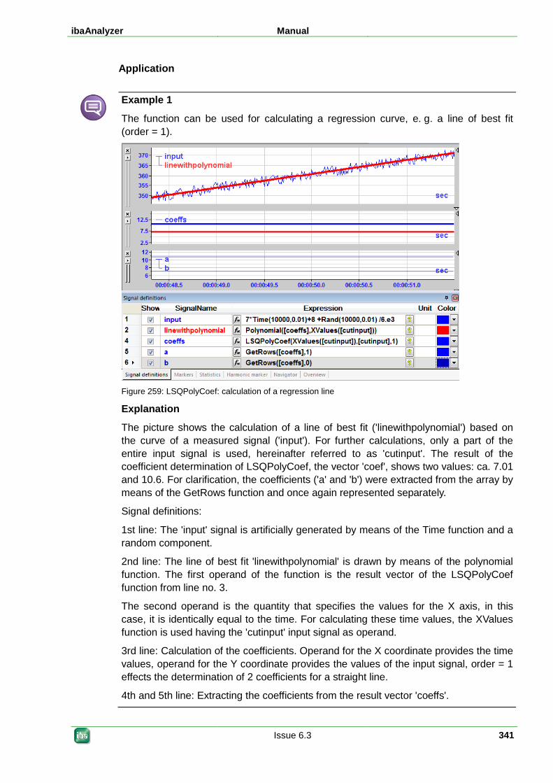
ibaAnalyzer Manual

Issue 6.3 341

Application

Example 1

The function can be used for calculating a regression curve, e. g. a line of best fit (order = 1).

Figure 259: LSQPolyCoef: calculation of a regression line

Explanation

The picture shows the calculation of a line of best fit ('linewithpolynomial') based on the curve of a measured signal ('input'). For further calculations, only a part of the entire input signal is used, hereinafter referred to as 'cutinput'. The result of the coefficient determination of LSQPolyCoef, the vector 'coef', shows two values: ca. 7.01 and 10.6. For clarification, the coefficients ('a' and 'b') were extracted from the array by means of the GetRows function and once again represented separately.

Signal definitions:

1st line: The 'input' signal is artificially generated by means of the Time function and a random component.

2nd line: The line of best fit 'linewithpolynomial' is drawn by means of the polynomial function. The first operand of the function is the result vector of the LSQPolyCoef function from line no. 3.

The second operand is the quantity that specifies the values for the X axis, in this case, it is identically equal to the time. For calculating these time values, the XValues function is used having the 'cutinput' input signal as operand.

3rd line: Calculation of the coefficients. Operand for the X coordinate provides the time values, operand for the Y coordinate provides the values of the input signal, order = 1 effects the determination of 2 coefficients for a straight line.

4th and 5th line: Extracting the coefficients from the result vector 'coeffs'.

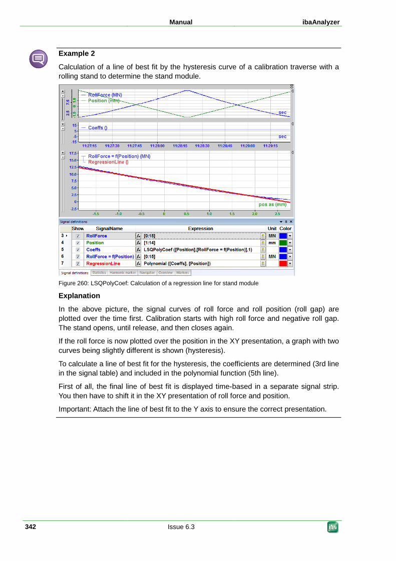
Manual ibaAnalyzer

342 Issue 6.3

Example 2

Calculation of a line of best fit by the hysteresis curve of a calibration traverse with a rolling stand to determine the stand module.

Figure 260: LSQPolyCoef: Calculation of a regression line for stand module

Explanation

In the above picture, the signal curves of roll force and roll position (roll gap) are plotted over the time first. Calibration starts with high roll force and negative roll gap. The stand opens, until release, and then closes again.

If the roll force is now plotted over the position in the XY presentation, a graph with two curves being slightly different is shown (hysteresis).

To calculate a line of best fit for the hysteresis, the coefficients are determined (3rd line in the signal table) and included in the polynomial function (5th line).

First of all, the final line of best fit is displayed time-based in a separate signal strip. You then have to shift it in the XY presentation of roll force and position.

Important: Attach the line of best fit to the Y axis to ensure the correct presentation.

ibaAnalyzer Manual

Issue 6.3 343

5.13.4 Polynomial Polynomial ('Coef', 'X')

This function calculates the polynomial value for every sample of ‘X‘ on the basis of a coefficient vector 'Coef'.

It is required for the representation of regression lines or best-fit curves whose coefficients were calculated with the LSQPolyCoef function prior to this.

Example see above picture, "LSQPolyCoef , Page 340".

Manual ibaAnalyzer

344 Issue 6.3

5.14 Spectrum analysis (FT operations) ibaAnalyzer has a range of FFT operations. The FFT operations enable the user not just to display a time-based or length-based signal in an FFT presentation mode but to create logical signals or expressions which can be used as FFT signals for further analyses.

Note

From version 5.22.6 of ibaAnalyzer and higher, the FftInTime function is no longer available in the expression editor. It was replaced by the functions FftInTimeAmpl and FftInTimePower . For reasons of downward compatibility, the function is still supported in terms of computations. Existing analyses using the FftInTime function must not be changed.

The same applies to the functions FftOrderAnalysis and FftPeaksInTime.

5.14.1 FftInTimeAmpl / FftInTimePower FfTinTimeAmpl or FftInTimePower ('Expression', 'Time', 'Number of frequencies’, 'Min frequency', 'Max frequency', 'Window', 'Overlap', 'SuppressDC')

The FftInTimeAmpl or FftInTimePower operations evaluate the FFT of ‘Expression’ every ‘Time’ seconds and deliver ‘Number of frequencies’ between ‘Min frequency’ (default = 0) and ‘Max frequency’ (default = sampling frequency / 2 of ‘expression’) the amplitude trend or the power trend in an vector as result. The FFT can use the following window types:

Rectangular (= 0), default

Bartlett (= 1)

Blackman (= 2)

Hamming (= 3)

Hanning (= 4)

Blackman-Harris (=5)

The overlap factor determines the overlapping of the frequency segments and can be between 0 (no overlapping, default) and 1 (full overlapping). By means of the FftInTime function, you can display fluctuating frequencies over time.

'SuppressDC': this argument refers to the constant part of the signal (e.g. the average value) which is often so large that the alternating component hardly carries weight. You suppress the DC component by entering 1 or True () for this argument (default = 0 or FALSE). If you want to use the default value, just close the parenthesis after the ‘window’ argument without the last comma.

Note

'SuppressDC' also applies to 'FftOrderAnalysis', 'FftAmpl', and 'FftPower'.

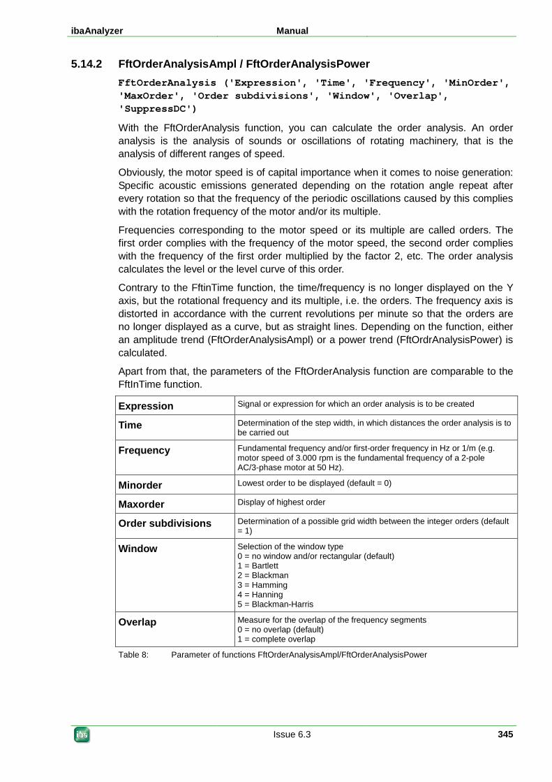
ibaAnalyzer Manual

Issue 6.3 345

5.14.2 FftOrderAnalysisAmpl / FftOrderAnalysisPower FftOrderAnalysis ('Expression', 'Time', 'Frequency', 'MinOrder', 'MaxOrder', 'Order subdivisions', 'Window', 'Overlap', 'SuppressDC')

With the FftOrderAnalysis function, you can calculate the order analysis. An order analysis is the analysis of sounds or oscillations of rotating machinery, that is the analysis of different ranges of speed.

Obviously, the motor speed is of capital importance when it comes to noise generation: Specific acoustic emissions generated depending on the rotation angle repeat after every rotation so that the frequency of the periodic oscillations caused by this complies with the rotation frequency of the motor and/or its multiple.

Frequencies corresponding to the motor speed or its multiple are called orders. The first order complies with the frequency of the motor speed, the second order complies with the frequency of the first order multiplied by the factor 2, etc. The order analysis calculates the level or the level curve of this order.

Contrary to the FftinTime function, the time/frequency is no longer displayed on the Y axis, but the rotational frequency and its multiple, i.e. the orders. The frequency axis is distorted in accordance with the current revolutions per minute so that the orders are no longer displayed as a curve, but as straight lines. Depending on the function, either an amplitude trend (FftOrderAnalysisAmpl) or a power trend (FftOrdrAnalysisPower) is calculated.

Apart from that, the parameters of the FftOrderAnalysis function are comparable to the FftInTime function.

Expression Signal or expression for which an order analysis is to be created

Time Determination of the step width, in which distances the order analysis is to be carried out

Frequency Fundamental frequency and/or first-order frequency in Hz or 1/m (e.g. motor speed of 3.000 rpm is the fundamental frequency of a 2-pole AC/3-phase motor at 50 Hz).

Minorder Lowest order to be displayed (default = 0)

Maxorder Display of highest order

Order subdivisions Determination of a possible grid width between the integer orders (default = 1)

Window Selection of the window type 0 = no window and/or rectangular (default) 1 = Bartlett 2 = Blackman 3 = Hamming 4 = Hanning 5 = Blackman-Harris

Overlap Measure for the overlap of the frequency segments 0 = no overlap (default) 1 = complete overlap

Table 8: Parameter of functions FftOrderAnalysisAmpl/FftOrderAnalysisPower

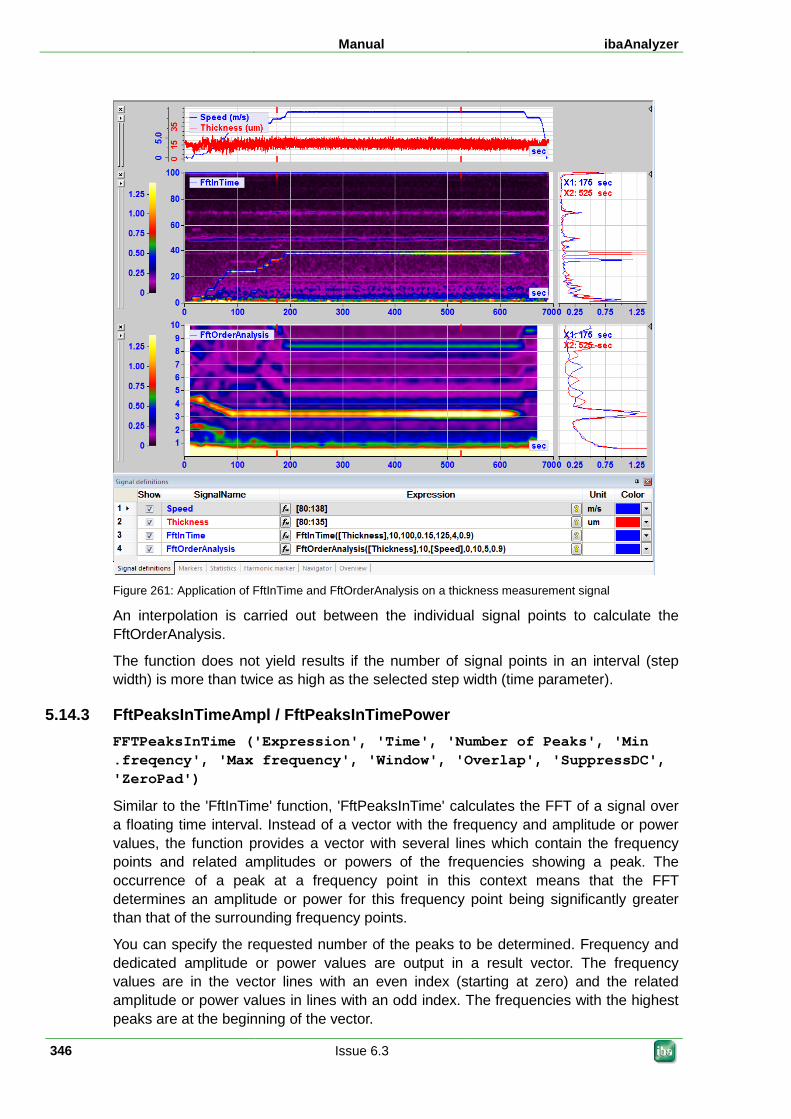
Manual ibaAnalyzer

346 Issue 6.3

Figure 261: Application of FftInTime and FftOrderAnalysis on a thickness measurement signal

An interpolation is carried out between the individual signal points to calculate the FftOrderAnalysis.

The function does not yield results if the number of signal points in an interval (step width) is more than twice as high as the selected step width (time parameter).

5.14.3 FftPeaksInTimeAmpl / FftPeaksInTimePower FFTPeaksInTime ('Expression', 'Time', 'Number of Peaks', 'Min .freqency', 'Max frequency', 'Window', 'Overlap', 'SuppressDC', 'ZeroPad')

Similar to the 'FftInTime' function, 'FftPeaksInTime' calculates the FFT of a signal over a floating time interval. Instead of a vector with the frequency and amplitude or power values, the function provides a vector with several lines which contain the frequency points and related amplitudes or powers of the frequencies showing a peak. The occurrence of a peak at a frequency point in this context means that the FFT determines an amplitude or power for this frequency point being significantly greater than that of the surrounding frequency points.

You can specify the requested number of the peaks to be determined. Frequency and dedicated amplitude or power values are output in a result vector. The frequency values are in the vector lines with an even index (starting at zero) and the related amplitude or power values in lines with an odd index. The frequencies with the highest peaks are at the beginning of the vector.

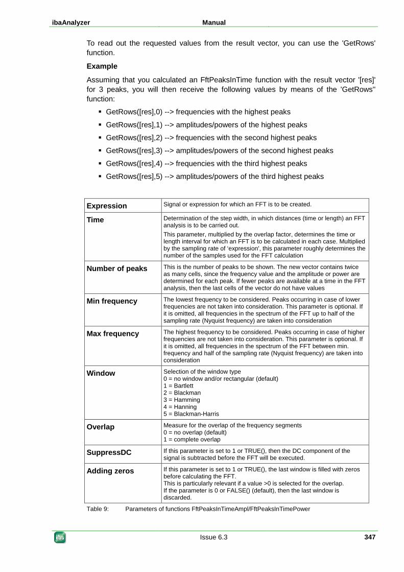
ibaAnalyzer Manual

Issue 6.3 347

To read out the requested values from the result vector, you can use the 'GetRows' function.

Example

Assuming that you calculated an FftPeaksInTime function with the result vector '[res]' for 3 peaks, you will then receive the following values by means of the 'GetRows'' function:

GetRows([res],0) --> frequencies with the highest peaks

GetRows([res],1) --> amplitudes/powers of the highest peaks

GetRows([res],2) --> frequencies with the second highest peaks

GetRows([res],3) --> amplitudes/powers of the second highest peaks

GetRows([res],4) --> frequencies with the third highest peaks

GetRows([res],5) --> amplitudes/powers of the third highest peaks

Expression Signal or expression for which an FFT is to be created.

Time Determination of the step width, in which distances (time or length) an FFT analysis is to be carried out. This parameter, multiplied by the overlap factor, determines the time or length interval for which an FFT is to be calculated in each case. Multiplied by the sampling rate of ‘expression', this parameter roughly determines the number of the samples used for the FFT calculation

Number of peaks This is the number of peaks to be shown. The new vector contains twice as many cells, since the frequency value and the amplitude or power are determined for each peak. If fewer peaks are available at a time in the FFT analysis, then the last cells of the vector do not have values

Min frequency The lowest frequency to be considered. Peaks occurring in case of lower frequencies are not taken into consideration. This parameter is optional. If it is omitted, all frequencies in the spectrum of the FFT up to half of the sampling rate (Nyquist frequency) are taken into consideration

Max frequency The highest frequency to be considered. Peaks occurring in case of higher frequencies are not taken into consideration. This parameter is optional. If it is omitted, all frequencies in the spectrum of the FFT between min. frequency and half of the sampling rate (Nyquist frequency) are taken into consideration

Window Selection of the window type 0 = no window and/or rectangular (default) 1 = Bartlett 2 = Blackman 3 = Hamming 4 = Hanning 5 = Blackman-Harris

Overlap Measure for the overlap of the frequency segments 0 = no overlap (default) 1 = complete overlap

SuppressDC If this parameter is set to 1 or TRUE(), then the DC component of the signal is subtracted before the FFT will be executed.

Adding zeros If this parameter is set to 1 or TRUE(), the last window is filled with zeros before calculating the FFT. This is particularly relevant if a value >0 is selected for the overlap. If the parameter is 0 or FALSE() (default), then the last window is discarded.

Table 9: Parameters of functions FftPeaksInTimeAmpl/FftPeaksInTimePower

Manual ibaAnalyzer

348 Issue 6.3

5.14.4 FftAmpl FftAmpl ('Expression', 'Resolution', 'Window', 'SuppressDC')

This function calculates the amplitude for each FFT component, i. e. the amount of the complex component. In contrary to "normal" FFT (i. e., the ones you get by selecting the frequency axis or 1/length axis), this function takes all samples into account and not just those in the signal strip.

'Expression': The signal or expression you wish to have an FFT from.

'Resolution': The number of desired frequencies

'Window': The window type you wish to apply before calculating the FFT. Default is 0 (no window or rectangular), although a window is usually required. Please enter one of the following numbers in order to select the window type:

None (= 0), default

Bartlett (= 1)

Blackman (= 2)

Hamming (= 3)

Hanning (= 4)

Blackman-Harris (=5)

5.14.5 FftPower FftPower ('Expression, 'Resolution', 'Window', 'SuppressDC')

This function basically equals the function FftAmpl but instead of taking the amount, it calculates the square of the real part + the square of the imaginary part.

5.14.6 FftComplex FftComplex(input,inverse,normalize)

Note

This function, just like the functions FfTReal and FftRealInverse, is designed to provide FFT results which were identified without averaging in “bins", windowing or advanced normalization. The results are therefore even more suitable for further calculations and can be used more flexibly. Advanced users can apply their own methods to averaging, windowing or normalization.

Unlike the usual FFT functions in ibaAnalyzer, the number of samples of the input signal does not necessarily have to be a power of 2.

The FftComplex function returns a two-dimensional signal (vector) as its result which contains both the real component and the imaginary component of the FFT calculation result. The function can calculate both normal FFT and inverse FFT.

The function uses the following parameters:

Input: input signal to which the FFT is to be applied. It can be both a two-dimensional signal consisting of real and imaginary components and a

ibaAnalyzer Manual

Issue 6.3 349

one-dimensional signal. In the latter case, the imaginary component is considered to be zero for the entire input signal.

Inverse: if this parameter is TRUE or 1, an inverse FFT is executed. In this case, the function expects an input signal being either frequency-based or 1/length-based. The result of the operation then is a time-based or length-based signal. If the parameter is FALSE (default) or 0 or if it is not specified, a normal FFT calculation will be performed. In this case, the function expects a time-based or length-based signal and the result is frequency-based or 1/length-based.

Normalize: for this parameter, the following values are permitted: 0 ... no normalization is performed (default). This means that if an inverse FFT is applied to a normal FFT, not the original signal is returned as result, but the original signal multiplied by the number of samples: 1: the result is divided by the number of samples if a normal FFT is executed. In case of an inverse FFT, the result remains unchanged. If an inverse FFT is applied to the result of a normal FFT, you will receive the original signal again. 2: the result is divided by the square root of the number of samples. This applies both to a normal FFT and an inverse FFT. If an inverse FFT is applied to the result of a normal FFT, you will receive the original signal again. Other values: function as with value 1. If the parameter is not specified, the function works as with the value 0 (default).

5.14.7 FftReal FftReal (input,normalize)

This function calculates the FFT of a real (one-dimensional) signal and returns a two-dimensional signal with real component and imaginary component of the FFT operation as its result. Only the positive spectrum is output, as the negative spectrum is only the conjugate gradient of the positive spectrum.

As to the number of samples N in the input signal, the following applies:

N does not have to be a power of 2.

If N is even, N/2+1 frequency points are calculated; the first (DC component) and last point are merely real.

If N is odd, (N+1)/2 frequency points are calculated; for those, the DC component is merely real.

The function uses the following parameters:

Input: real input signal to which the FFT is to be applied.

Normalize: if this parameter is TRUE or 1, a normalization is performed. If the number of samples N is odd, all frequency values except for the DC component are divided by N/2. If N is even, all frequency values except for the DC component and the last value are divided by N/2. The excluded values are divided by N instead. If this parameter is FALSE or 0 (default) or if it is not specified, no normalization is performed.

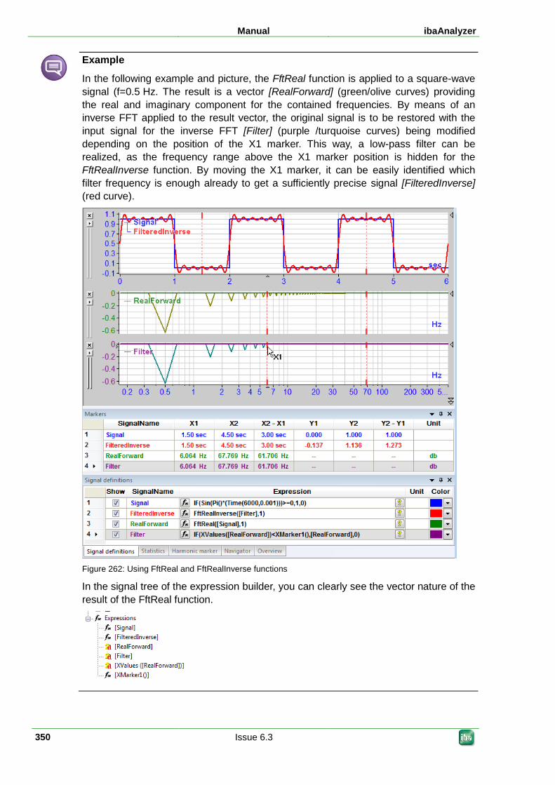
Manual ibaAnalyzer

350 Issue 6.3

Example

In the following example and picture, the FftReal function is applied to a square-wave signal (f=0.5 Hz. The result is a vector [RealForward] (green/olive curves) providing the real and imaginary component for the contained frequencies. By means of an inverse FFT applied to the result vector, the original signal is to be restored with the input signal for the inverse FFT [Filter] (purple /turquoise curves) being modified depending on the position of the X1 marker. This way, a low-pass filter can be realized, as the frequency range above the X1 marker position is hidden for the FftRealInverse function. By moving the X1 marker, it can be easily identified which filter frequency is enough already to get a sufficiently precise signal [FilteredInverse] (red curve).

Figure 262: Using FftReal and FftRealInverse functions

In the signal tree of the expression builder, you can clearly see the vector nature of the result of the FftReal function.

ibaAnalyzer Manual

Issue 6.3 351

5.14.8 FftRealInverse FftRealInverse(input,normalize)

This function calculates an inverse FFT. A two-dimensional signal (vector) is expected as input signal containing the real component and the imaginary component of the positive spectrum. The result is a real signal.

The function uses the following parameters:

Input: two-dimensional input signal (vector) to which the FFT is to be applied.

Normalize: this parameter should be set to TRUE or 1 if the input signal had been normalized before as described with the FftReal function. Otherwise, this parameter should be set to FALSE or 0. If FftRealInverse is applied to the result of a FftReal function and the Normalize parameter for both functions is TRUE, the original, real signal is displayed again. If Normalize is FALSE for both functions, the original, real signal is displayed multiplied by N.

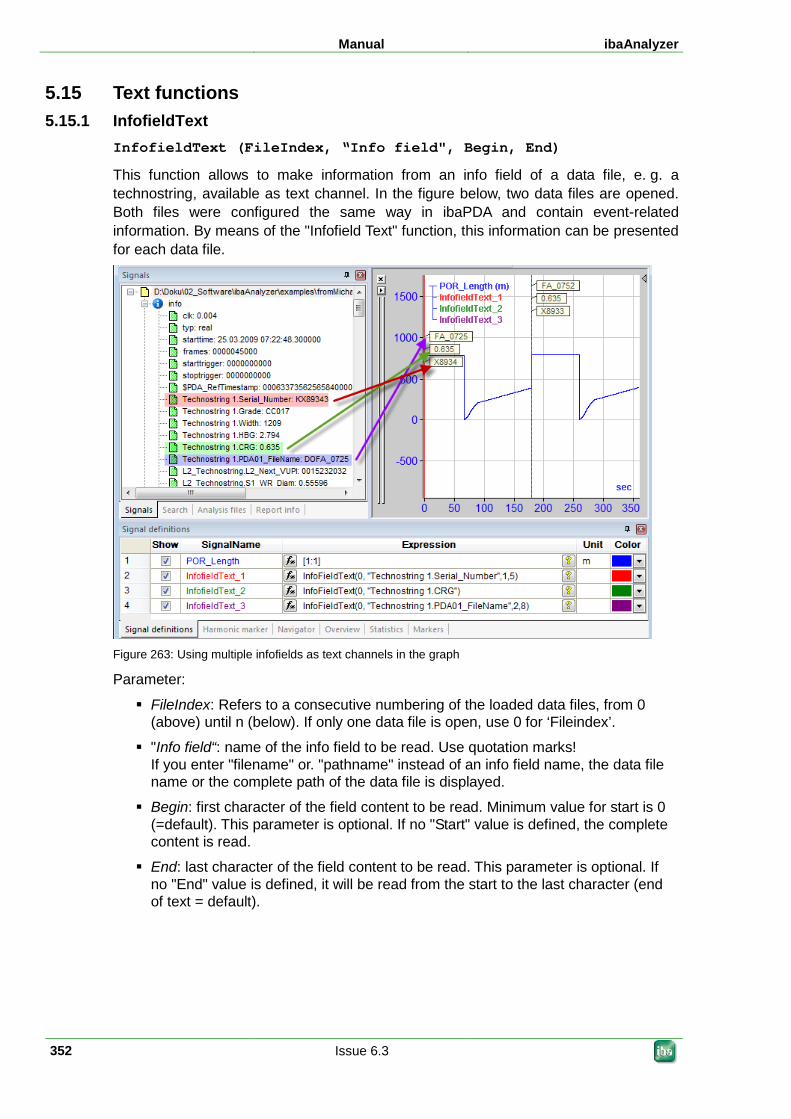
Manual ibaAnalyzer

352 Issue 6.3

5.15 Text functions 5.15.1 InfofieldText

InfofieldText (FileIndex, “Info field", Begin, End)

This function allows to make information from an info field of a data file, e. g. a technostring, available as text channel. In the figure below, two data files are opened. Both files were configured the same way in ibaPDA and contain event-related information. By means of the "Infofield Text" function, this information can be presented for each data file.

Figure 263: Using multiple infofields as text channels in the graph

Parameter:

FileIndex: Refers to a consecutive numbering of the loaded data files, from 0 (above) until n (below). If only one data file is open, use 0 for ‘Fileindex’.

"Info field“: name of the info field to be read. Use quotation marks! If you enter "filename" or. "pathname" instead of an info field name, the data file name or the complete path of the data file is displayed.

Begin: first character of the field content to be read. Minimum value for start is 0 (=default). This parameter is optional. If no "Start" value is defined, the complete content is read.

End: last character of the field content to be read. This parameter is optional. If no "End" value is defined, it will be read from the start to the last character (end of text = default).

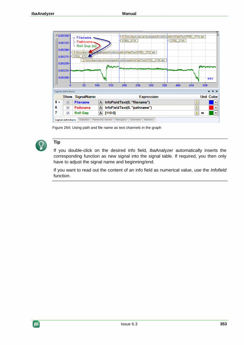
ibaAnalyzer Manual

Issue 6.3 353

Figure 264: Using path and file name as text channels in the graph

Tip

If you double-click on the desired info field, ibaAnalyzer automatically inserts the corresponding function as new signal into the signal table. If required, you then only have to adjust the signal name and beginning/end.

If you want to read out the content of an info field as numerical value, use the Infofield function.

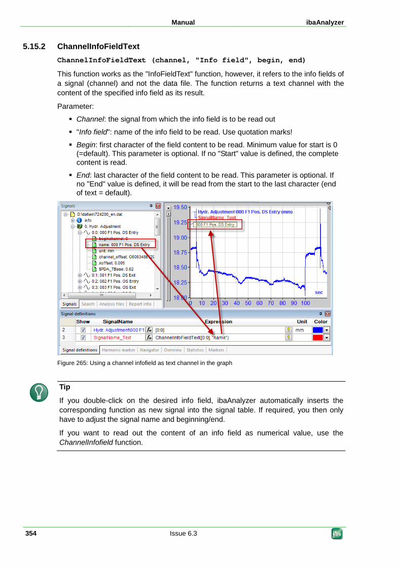
Manual ibaAnalyzer

354 Issue 6.3

5.15.2 ChannelInfoFieldText ChannelInfoFieldText (channel, "Info field", begin, end)

This function works as the "InfoFieldText" function, however, it refers to the info fields of a signal (channel) and not the data file. The function returns a text channel with the content of the specified info field as its result.

Parameter:

Channel: the signal from which the info field is to be read out

"Info field": name of the info field to be read. Use quotation marks!

Begin: first character of the field content to be read. Minimum value for start is 0 (=default). This parameter is optional. If no "Start" value is defined, the complete content is read.

End: last character of the field content to be read. This parameter is optional. If no "End" value is defined, it will be read from the start to the last character (end of text = default).

Figure 265: Using a channel infofield as text channel in the graph

Tip

If you double-click on the desired info field, ibaAnalyzer automatically inserts the corresponding function as new signal into the signal table. If required, you then only have to adjust the signal name and beginning/end.

If you want to read out the content of an info field as numerical value, use the ChannelInfofield function.

ibaAnalyzer Manual

Issue 6.3 355

5.15.3 TextCompare TextCompare (Text1, Text2, CaseSensitive)

This function allows you to compare the text information lexicographically.

The function works with contents of text channels as well as with plain text which – used with quotation marks – is directly entered in the signal definition.

Parameter:

Text1: first comparison text. It can be a text channel or a plain text. Plain text must be used with quotation marks.

Text2: second comparison text. It can be a text channel or a plain text. Plain text must be used with quotation marks.

CaseSensitive: optional parameter which can be used to specify whether case sensitivity is taken into consideration for the comparison. If this parameter is TRUE (default) or not specified, case sensitivity is taken into consideration. "aaAA" and "aaaa" are thus different texts. If this parameter is FALSE, there is no differentiation. "aaAA" and "aaaa" are identical texts.

Comparison and results:

The result is -1 if the information of the first text is to be arranged lexicographically before that of the second text. In the below picture, this is the case for the result of "time-start date comparison". The start times of the first two data files (07:22:48 and 07:34:48) are before the comparison time "07:40:00".

The result is 0 if both texts contain the same information. In the picture below, this is the case for the result of "date-start date comparison". The start date of all three data files (25.03.2009) is equal to the comparison date "25.03.2009".

The result is +1 if the information of the first text is to be arranged lexicographically after that of the second text. In the below picture, this is the case for the result of "time-start date comparison" regarding the last data file. The start time of the third data file (07:49:47) follows the comparison time "07:40:00.

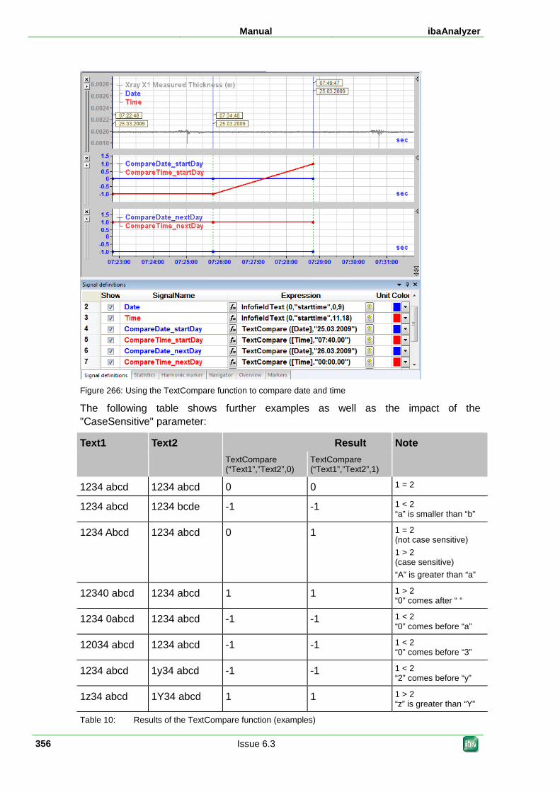
Manual ibaAnalyzer

356 Issue 6.3

Figure 266: Using the TextCompare function to compare date and time

The following table shows further examples as well as the impact of the "CaseSensitive" parameter:

Text1 Text2 Result Note

TextCompare (“Text1”,”Text2”,0)

TextCompare (“Text1”,”Text2”,1)

1234 abcd 1234 abcd 0 0 1 = 2

1234 abcd 1234 bcde -1 -1 1 < 2 “a” is smaller than “b”

1234 Abcd 1234 abcd 0 1 1 = 2 (not case sensitive) 1 > 2 (case sensitive) “A” is greater than “a”

12340 abcd 1234 abcd 1 1 1 > 2 “0” comes after “ “

1234 0abcd 1234 abcd -1 -1 1 < 2 “0” comes before “a”

12034 abcd 1234 abcd -1 -1 1 < 2 “0” comes before “3”

1234 abcd 1y34 abcd -1 -1 1 < 2 “2” comes before “y”

1z34 abcd 1Y34 abcd 1 1 1 > 2 “z” is greater than “Y”

Table 10: Results of the TextCompare function (examples)

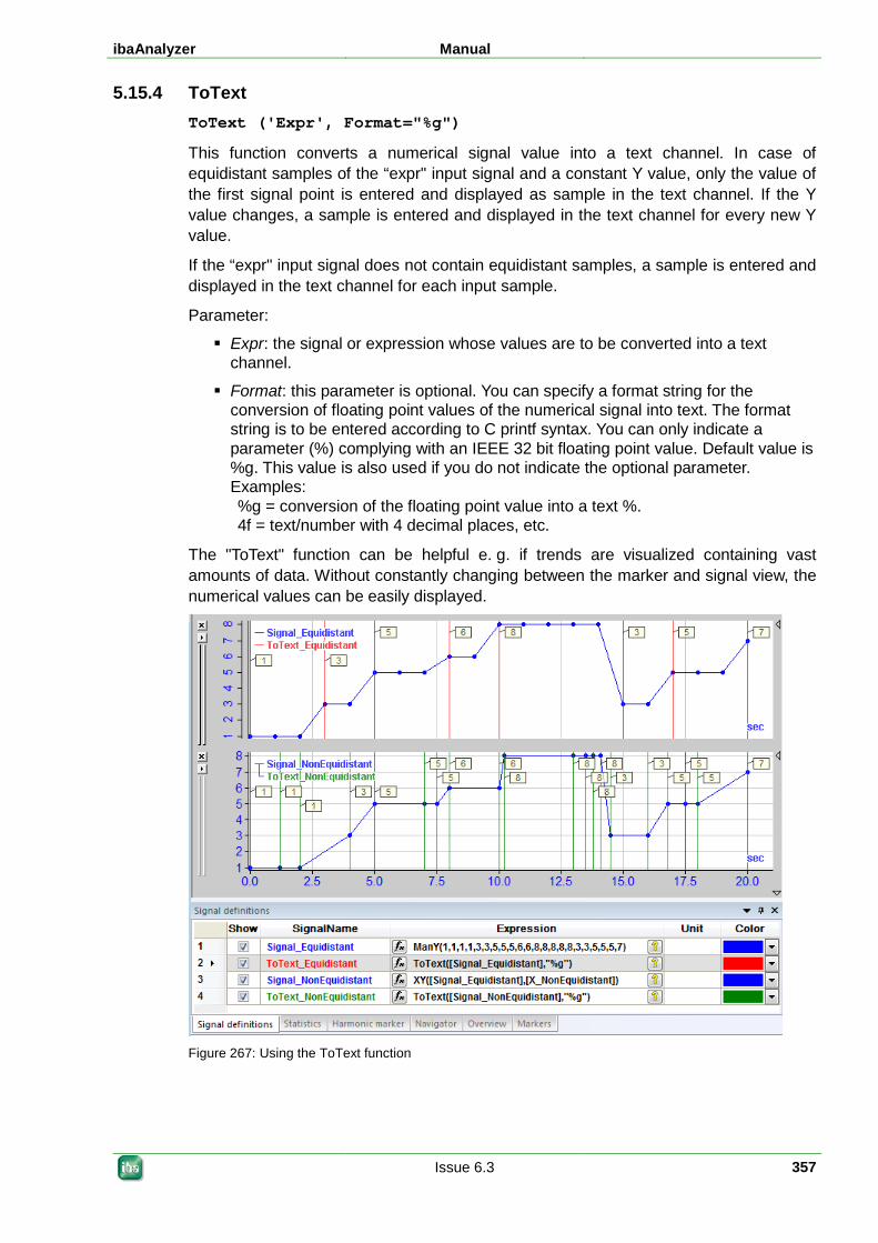
ibaAnalyzer Manual

Issue 6.3 357

5.15.4 ToText ToText ('Expr', Format="%g")

This function converts a numerical signal value into a text channel. In case of equidistant samples of the “expr" input signal and a constant Y value, only the value of the first signal point is entered and displayed as sample in the text channel. If the Y value changes, a sample is entered and displayed in the text channel for every new Y value.

If the “expr" input signal does not contain equidistant samples, a sample is entered and displayed in the text channel for each input sample.

Parameter:

Expr: the signal or expression whose values are to be converted into a text channel.

Format: this parameter is optional. You can specify a format string for the conversion of floating point values of the numerical signal into text. The format string is to be entered according to C printf syntax. You can only indicate a parameter (%) complying with an IEEE 32 bit floating point value. Default value is %g. This value is also used if you do not indicate the optional parameter. Examples: %g = conversion of the floating point value into a text %. 4f = text/number with 4 decimal places, etc.

The "ToText" function can be helpful e. g. if trends are visualized containing vast amounts of data. Without constantly changing between the marker and signal view, the numerical values can be easily displayed.

Figure 267: Using the ToText function

Manual ibaAnalyzer

358 Issue 6.3

5.15.5 TrimText TrimText (Text, RemoveOption=0)

With this function, you can remove the spaces from texts. This function can be used both in case of text channels already contained in data files and in case of results of the InfofieldText and ToText functions.

Parameter:

Text: Text channel or expression generating text from which spaces are to be removed.

RemoveOption: Parameter for setting the operating mode 0 (default): Removing spaces before and after the text 1: Removing spaces before the text only 2: Removing spaces after the text only 3: Removing all spaces, also in the text

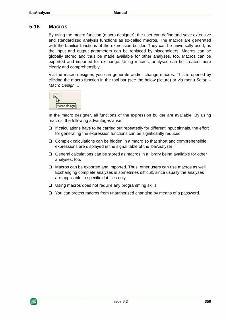
ibaAnalyzer Manual

Issue 6.3 359

5.16 Macros By using the macro function (macro designer), the user can define and save extensive and standardized analysis functions as so-called macros. The macros are generated with the familiar functions of the expression builder. They can be universally used, as the input and output parameters can be replaced by placeholders. Macros can be globally stored and thus be made available for other analyses, too. Macros can be exported and imported for exchange. Using macros, analyses can be created more clearly and comprehensibly.

Via the macro designer, you can generate and/or change macros. This is opened by clicking the macro function in the tool bar (see the below picture) or via menu Setup – Macro Design....

In the macro designer, all functions of the expression builder are available. By using macros, the following advantages arise:

If calculations have to be carried out repeatedly for different input signals, the effort for generating the expression functions can be significantly reduced

Complex calculations can be hidden in a macro so that short and comprehensible expressions are displayed in the signal table of the ibaAnalyzer

General calculations can be stored as macros in a library being available for other analyses, too.

Macros can be exported and imported. Thus, other users can use macros as well. Exchanging complete analyses is sometimes difficult, since usually the analyses are applicable to specific dat files only.

Using macros does not require any programming skills

You can protect macros from unauthorized changing by means of a password.

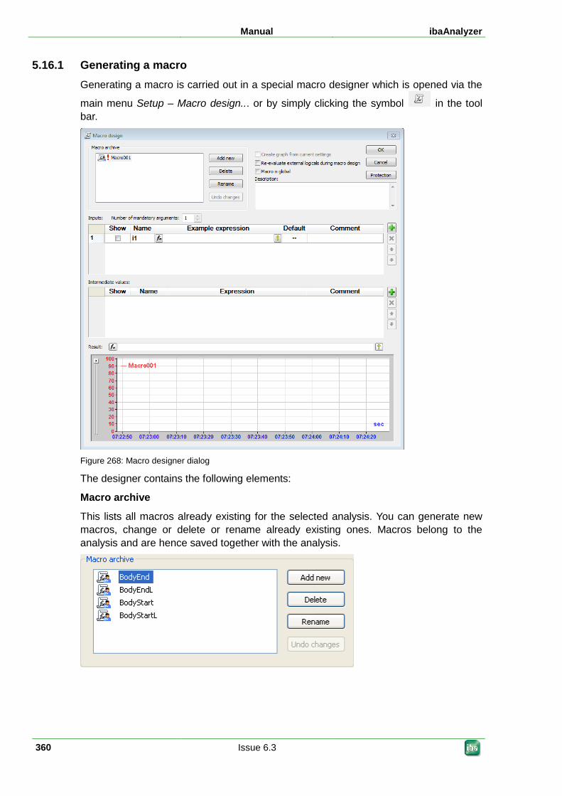
Manual ibaAnalyzer

360 Issue 6.3

5.16.1 Generating a macro Generating a macro is carried out in a special macro designer which is opened via the

main menu Setup – Macro design... or by simply clicking the symbol in the tool bar.

Figure 268: Macro designer dialog

The designer contains the following elements:

Macro archive

This lists all macros already existing for the selected analysis. You can generate new macros, change or delete or rename already existing ones. Macros belong to the analysis and are hence saved together with the analysis.

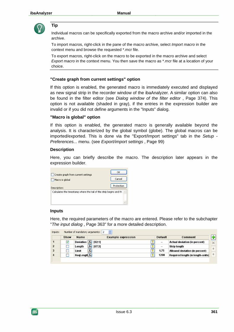
ibaAnalyzer Manual

Issue 6.3 361

Tip

Individual macros can be specifically exported from the macro archive and/or imported in the archive. To import macros, right-click in the pane of the macro archive, select Import macro in the context menu and browse the requested *.mcr file. To export macros, right-click on the macro to be exported in the macro archive and select Export macro in the context menu. You then save the macro as *.mcr file at a location of your choice.

"Create graph from current settings" option

If this option is enabled, the generated macro is immediately executed and displayed as new signal strip in the recorder window of the ibaAnalyzer. A similar option can also be found in the filter editor (see Dialog window of the filter editor , Page 374). This option is not available (shaded in gray), if the entries in the expression builder are invalid or if you did not define arguments in the "Inputs" dialog.

"Macro is global" option

If this option is enabled, the generated macro is generally available beyond the analysis. It is characterized by the global symbol (globe). The global macros can be imported/exported. This is done via the "Export/Import settings" tab in the Setup - Preferences... menu. (see Export/import settings , Page 99)

Description

Here, you can briefly describe the macro. The description later appears in the expression builder.

Inputs

Here, the required parameters of the macro are entered. Please refer to the subchapter "The input dialog , Page 363" for a more detailed description.

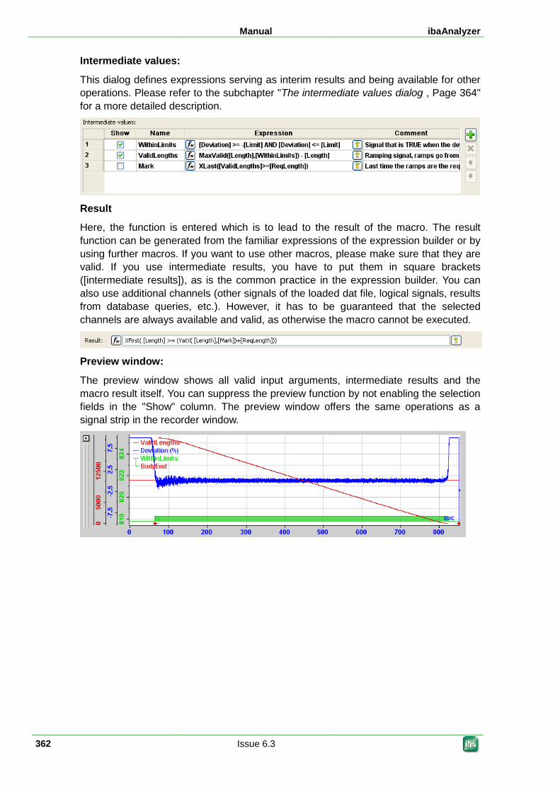
Manual ibaAnalyzer

362 Issue 6.3

Intermediate values:

This dialog defines expressions serving as interim results and being available for other operations. Please refer to the subchapter "The intermediate values dialog , Page 364" for a more detailed description.

Result

Here, the function is entered which is to lead to the result of the macro. The result function can be generated from the familiar expressions of the expression builder or by using further macros. If you want to use other macros, please make sure that they are valid. If you use intermediate results, you have to put them in square brackets ([intermediate results]), as is the common practice in the expression builder. You can also use additional channels (other signals of the loaded dat file, logical signals, results from database queries, etc.). However, it has to be guaranteed that the selected channels are always available and valid, as otherwise the macro cannot be executed.

Preview window:

The preview window shows all valid input arguments, intermediate results and the macro result itself. You can suppress the preview function by not enabling the selection fields in the "Show" column. The preview window offers the same operations as a signal strip in the recorder window.

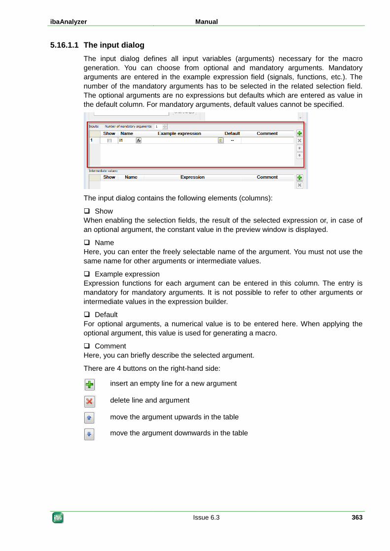
ibaAnalyzer Manual

Issue 6.3 363

5.16.1.1 The input dialog The input dialog defines all input variables (arguments) necessary for the macro generation. You can choose from optional and mandatory arguments. Mandatory arguments are entered in the example expression field (signals, functions, etc.). The number of the mandatory arguments has to be selected in the related selection field. The optional arguments are no expressions but defaults which are entered as value in the default column. For mandatory arguments, default values cannot be specified.

The input dialog contains the following elements (columns):

Show When enabling the selection fields, the result of the selected expression or, in case of an optional argument, the constant value in the preview window is displayed.

Name Here, you can enter the freely selectable name of the argument. You must not use the same name for other arguments or intermediate values.

Example expression Expression functions for each argument can be entered in this column. The entry is mandatory for mandatory arguments. It is not possible to refer to other arguments or intermediate values in the expression builder.

Default For optional arguments, a numerical value is to be entered here. When applying the optional argument, this value is used for generating a macro.

Comment Here, you can briefly describe the selected argument.

There are 4 buttons on the right-hand side:

insert an empty line for a new argument

delete line and argument

move the argument upwards in the table

move the argument downwards in the table

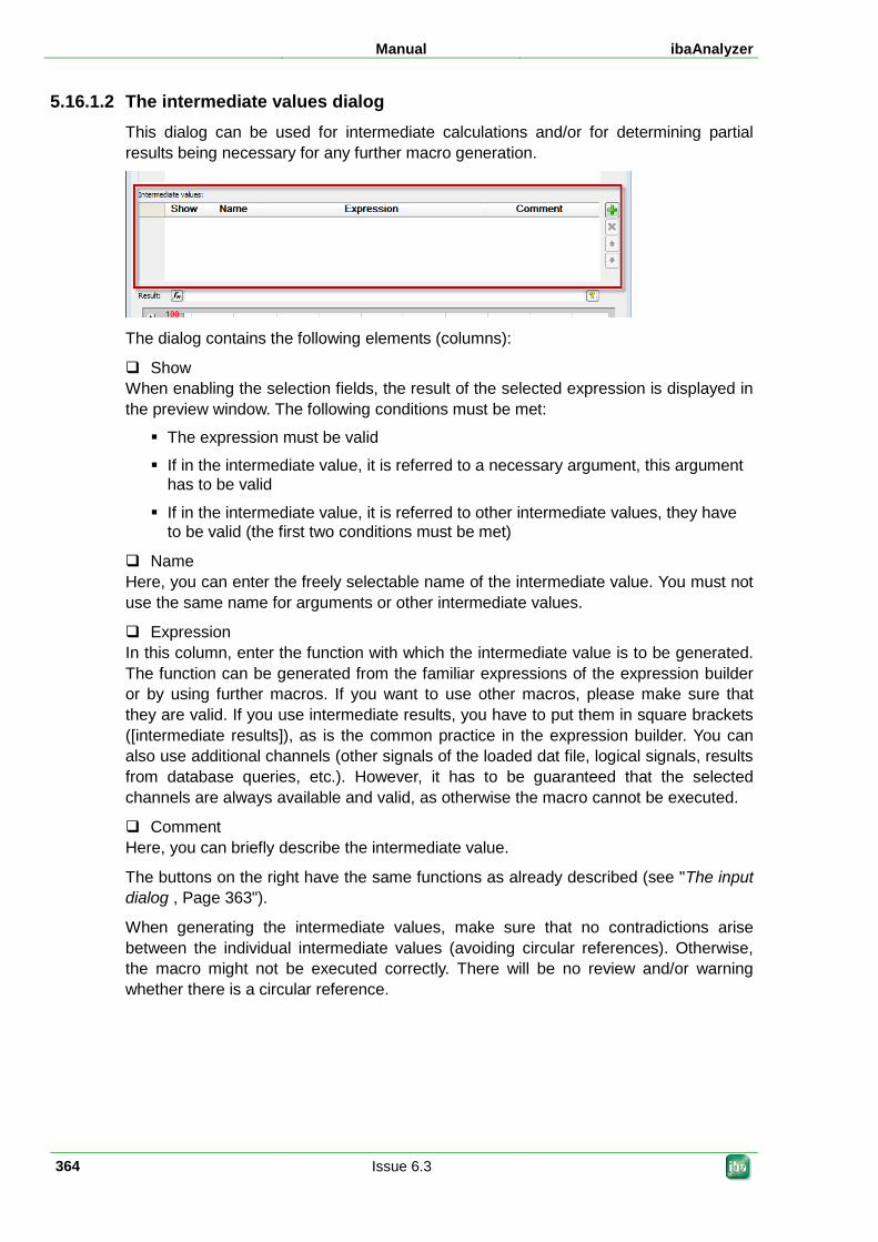
Manual ibaAnalyzer

364 Issue 6.3

5.16.1.2 The intermediate values dialog This dialog can be used for intermediate calculations and/or for determining partial results being necessary for any further macro generation.

The dialog contains the following elements (columns):

Show When enabling the selection fields, the result of the selected expression is displayed in the preview window. The following conditions must be met:

The expression must be valid

If in the intermediate value, it is referred to a necessary argument, this argument has to be valid

If in the intermediate value, it is referred to other intermediate values, they have to be valid (the first two conditions must be met)

Name Here, you can enter the freely selectable name of the intermediate value. You must not use the same name for arguments or other intermediate values.

Expression In this column, enter the function with which the intermediate value is to be generated. The function can be generated from the familiar expressions of the expression builder or by using further macros. If you want to use other macros, please make sure that they are valid. If you use intermediate results, you have to put them in square brackets ([intermediate results]), as is the common practice in the expression builder. You can also use additional channels (other signals of the loaded dat file, logical signals, results from database queries, etc.). However, it has to be guaranteed that the selected channels are always available and valid, as otherwise the macro cannot be executed.

Comment Here, you can briefly describe the intermediate value.

The buttons on the right have the same functions as already described (see "The input dialog , Page 363").

When generating the intermediate values, make sure that no contradictions arise between the individual intermediate values (avoiding circular references). Otherwise, the macro might not be executed correctly. There will be no review and/or warning whether there is a circular reference.

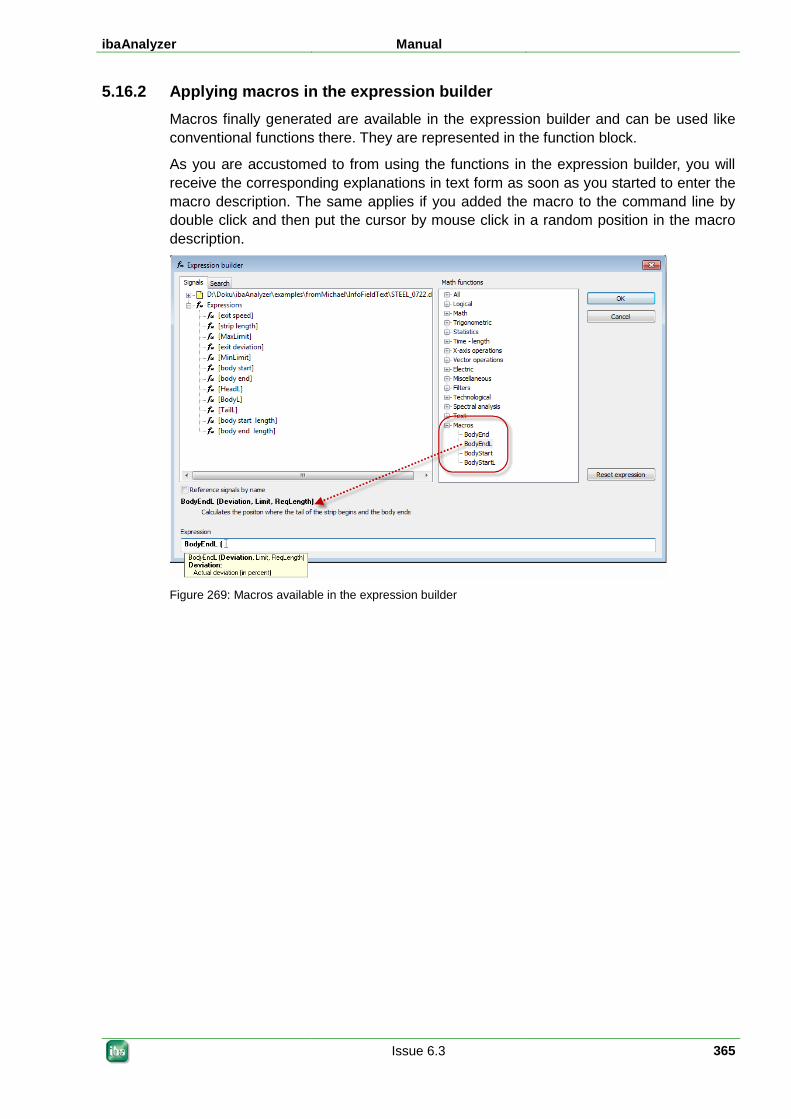
ibaAnalyzer Manual

Issue 6.3 365

5.16.2 Applying macros in the expression builder Macros finally generated are available in the expression builder and can be used like conventional functions there. They are represented in the function block.

As you are accustomed to from using the functions in the expression builder, you will receive the corresponding explanations in text form as soon as you started to enter the macro description. The same applies if you added the macro to the command line by double click and then put the cursor by mouse click in a random position in the macro description.

Figure 269: Macros available in the expression builder

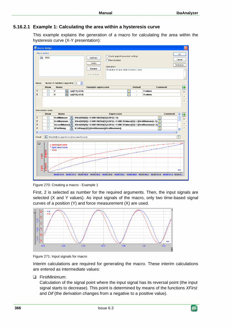
Manual ibaAnalyzer

366 Issue 6.3

5.16.2.1 Example 1: Calculating the area within a hysteresis curve This example explains the generation of a macro for calculating the area within the hysteresis curve (X-Y presentation):

Figure 270: Creating a macro - Example 1

First, 2 is selected as number for the required arguments. Then, the input signals are selected (X and Y values). As input signals of the macro, only two time-based signal curves of a position (Y) and force measurement (X) are used.

Figure 271: Input signals for macro

Interim calculations are required for generating the macro. These interim calculations are entered as intermediate values:

FirstMinimum: Calculation of the signal point where the input signal has its reversal point (the input signal starts to decrease). This point is determined by means of the functions XFirst and Dif (the derivation changes from a negative to a positive value).

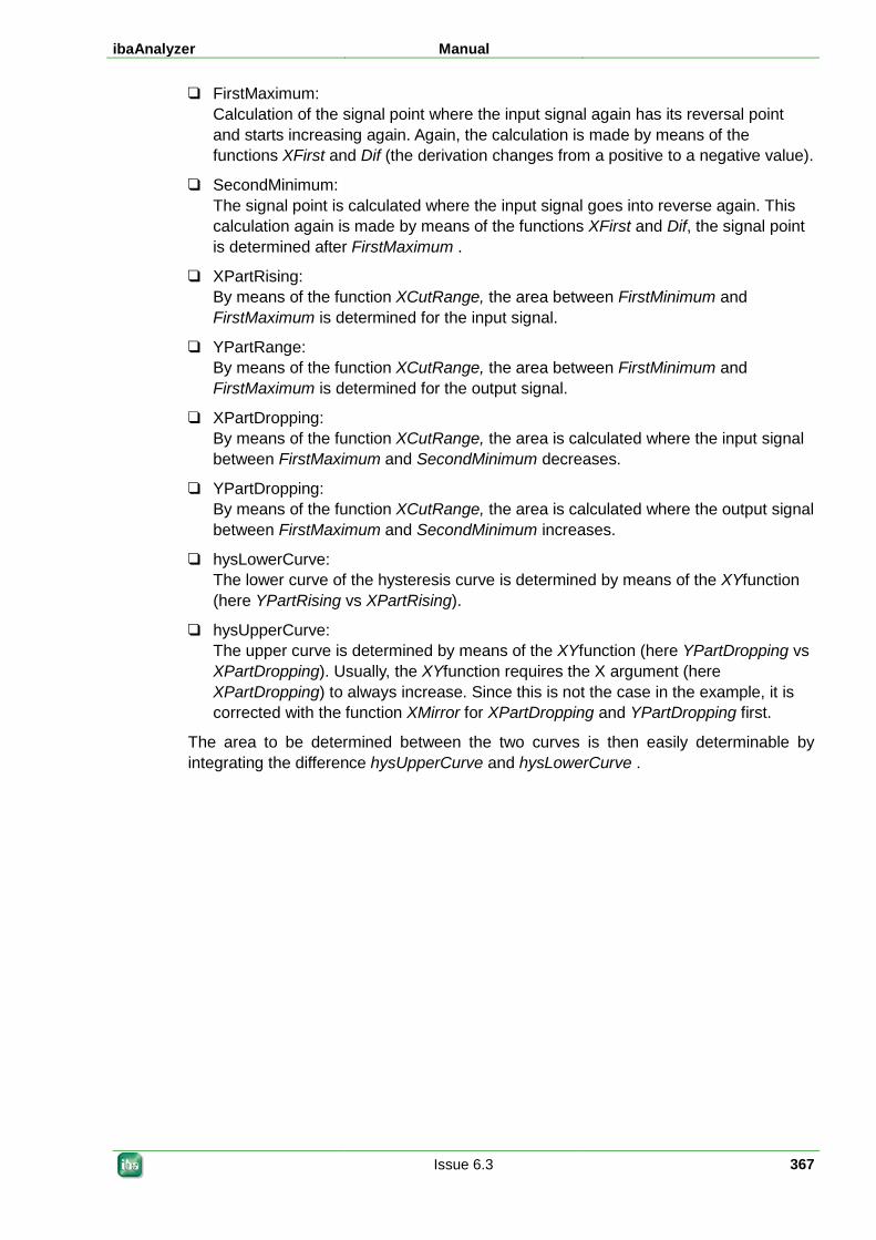
ibaAnalyzer Manual

Issue 6.3 367

FirstMaximum: Calculation of the signal point where the input signal again has its reversal point and starts increasing again. Again, the calculation is made by means of the functions XFirst and Dif (the derivation changes from a positive to a negative value).

SecondMinimum: The signal point is calculated where the input signal goes into reverse again. This calculation again is made by means of the functions XFirst and Dif, the signal point is determined after FirstMaximum .

XPartRising: By means of the function XCutRange, the area between FirstMinimum and FirstMaximum is determined for the input signal.

YPartRange: By means of the function XCutRange, the area between FirstMinimum and FirstMaximum is determined for the output signal.

XPartDropping: By means of the function XCutRange, the area is calculated where the input signal between FirstMaximum and SecondMinimum decreases.

YPartDropping: By means of the function XCutRange, the area is calculated where the output signal between FirstMaximum and SecondMinimum increases.

hysLowerCurve: The lower curve of the hysteresis curve is determined by means of the XYfunction (here YPartRising vs XPartRising).

hysUpperCurve: The upper curve is determined by means of the XYfunction (here YPartDropping vs XPartDropping). Usually, the XYfunction requires the X argument (here XPartDropping) to always increase. Since this is not the case in the example, it is corrected with the function XMirror for XPartDropping and YPartDropping first.

The area to be determined between the two curves is then easily determinable by integrating the difference hysUpperCurve and hysLowerCurve .

Manual ibaAnalyzer

368 Issue 6.3

5.16.2.2 Example 2: Calculation head – fillet – tail of an aluminum strip In general, rolled metal strips, so-called coils, can be divided into three different sections, the head, the fillet and the tail, with the fillet being far the greatest section of the strip.

First, the particular areas are to be defined:

The head section is defined as the section where significant quality parameters (e. g. thickness, width, mechanical properties) are not yet homogeneous within acceptable tolerances. The head is always at the beginning of the strip (the section which is reshaped first when rolling).

The definition also applies to the tail, however this section is the last to leave the rolling stand (reshaping is completed).

The fillet section is between head and tail, i. e. the significant quality parameters should be homogeneous in this section.

The two following macros calculate the beginning as well as the end of the fillet section.

Macro for calculating the beginning of the fillet section - macro name BodyStartL

The following input signals are determined:

Deviation: Quality parameter (here thickness deviation) which has to be within a specified tolerance. This is a length-based signal, the deviation is given in percentage).

Limit: The tolerance limit is given as a constant value. Here, it is an optional argument with a default value (here 1.75 %).

ReqLength: Specification of the required length where the thickness deviation has to be within a given tolerance. Here, it is also an optional argument with a default value (here 1.200).

The following intermediate results are required for calculating the macro:

Length: With the function XValues, the length-related signal points of the thickness deviation are determined.

WithinLimits: This expression determines whether the thickness deviation (Deviation) is within the tolerance. The expression is TRUE if: –Limit ≤ Deviation ≤ Limit.

ValidLengths: By means of the function MinValid, the smallest value is determined where the condition WithinLimits is met, i.e. is TRUE (in cases where the tolerance conditions are met for the first time).

Mark: By means of the function XFirst, both the point is determined where the condition ValidLength is met for the first time and the point where the range of validity of ReqLength is exceeded.

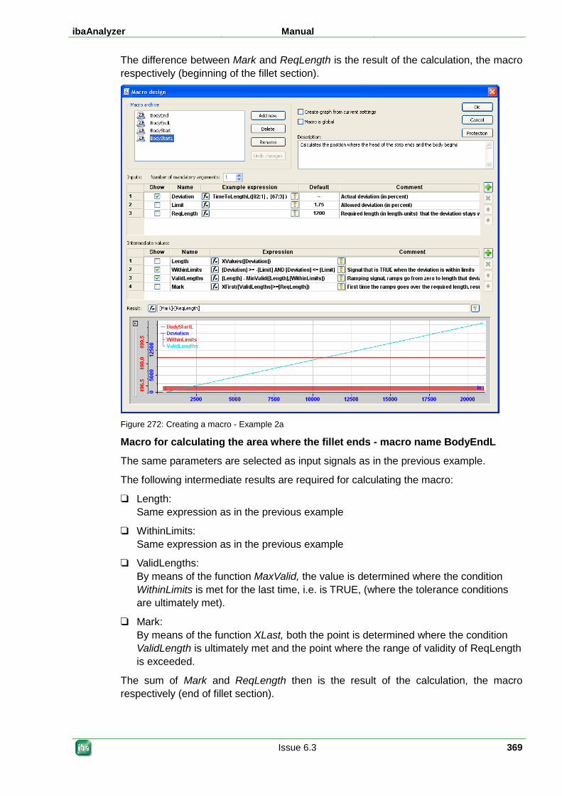
ibaAnalyzer Manual

Issue 6.3 369

The difference between Mark and ReqLength is the result of the calculation, the macro respectively (beginning of the fillet section).

Figure 272: Creating a macro - Example 2a

Macro for calculating the area where the fillet ends - macro name BodyEndL

The same parameters are selected as input signals as in the previous example.

The following intermediate results are required for calculating the macro:

Length: Same expression as in the previous example

WithinLimits: Same expression as in the previous example

ValidLengths: By means of the function MaxValid, the value is determined where the condition WithinLimits is met for the last time, i.e. is TRUE, (where the tolerance conditions are ultimately met).

Mark: By means of the function XLast, both the point is determined where the condition ValidLength is ultimately met and the point where the range of validity of ReqLength is exceeded.

The sum of Mark and ReqLength then is the result of the calculation, the macro respectively (end of fillet section).

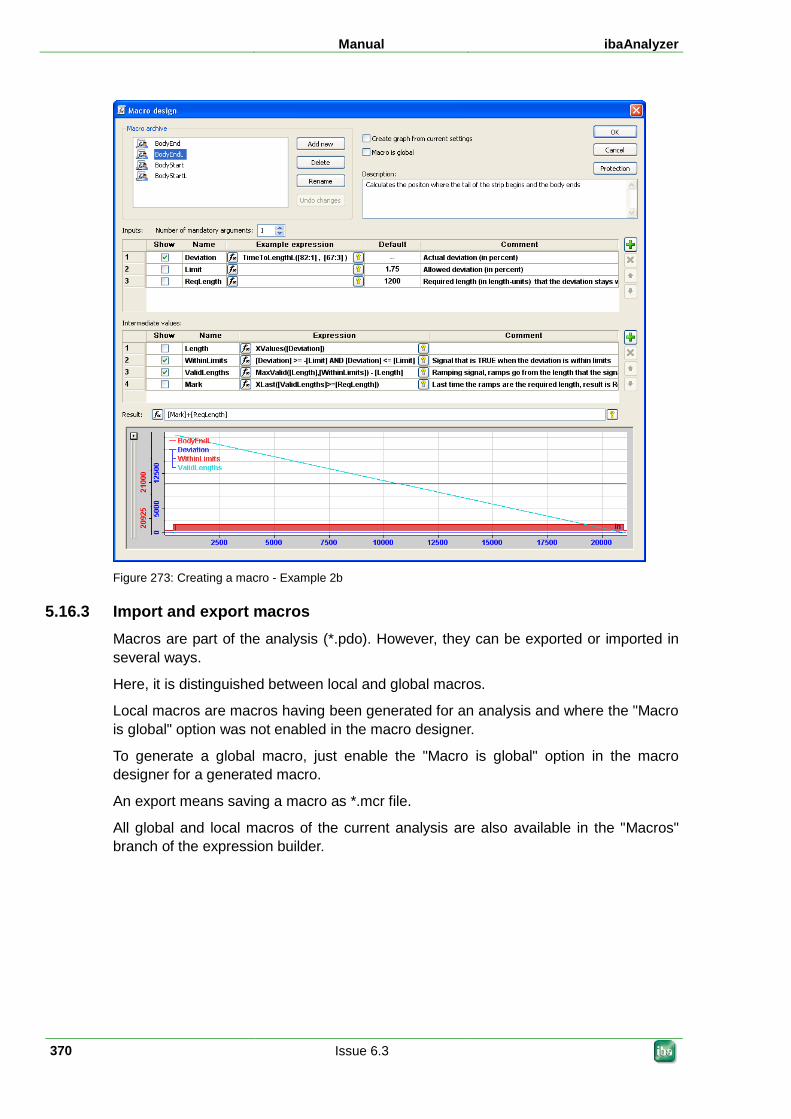
Manual ibaAnalyzer

370 Issue 6.3

Figure 273: Creating a macro - Example 2b

5.16.3 Import and export macros Macros are part of the analysis (*.pdo). However, they can be exported or imported in several ways.

Here, it is distinguished between local and global macros.

Local macros are macros having been generated for an analysis and where the "Macro is global" option was not enabled in the macro designer.

To generate a global macro, just enable the "Macro is global" option in the macro designer for a generated macro.

An export means saving a macro as *.mcr file.

All global and local macros of the current analysis are also available in the "Macros" branch of the expression builder.

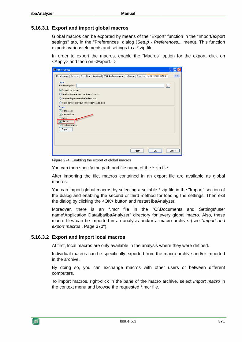
ibaAnalyzer Manual

Issue 6.3 371

5.16.3.1 Export and import global macros Global macros can be exported by means of the "Export" function in the "Import/export settings" tab, in the "Preferences" dialog (Setup - Preferences... menu). This function exports various elements and settings to a *.zip file

In order to export the macros, enable the "Macros" option for the export, click on <Apply> and then on <Export...>.

Figure 274: Enabling the export of global macros

You can then specify the path and file name of the *.zip file.

After importing the file, macros contained in an export file are available as global macros.

You can import global macros by selecting a suitable *.zip file in the "Import" section of the dialog and enabling the second or third method for loading the settings. Then exit the dialog by clicking the <OK> button and restart ibaAnalyzer.

Moreover, there is an *.mcr file in the "C:\Documents and Settings\user name\Application Data\iba\ibaAnalyzer" directory for every global macro. Also, these macro files can be imported in an analysis and/or a macro archive. (see "Import and export macros , Page 370").

5.16.3.2 Export and import local macros At first, local macros are only available in the analysis where they were defined.

Individual macros can be specifically exported from the macro archive and/or imported in the archive.

By doing so, you can exchange macros with other users or between different computers.

To import macros, right-click in the pane of the macro archive, select Import macro in the context menu and browse the requested *.mcr file.

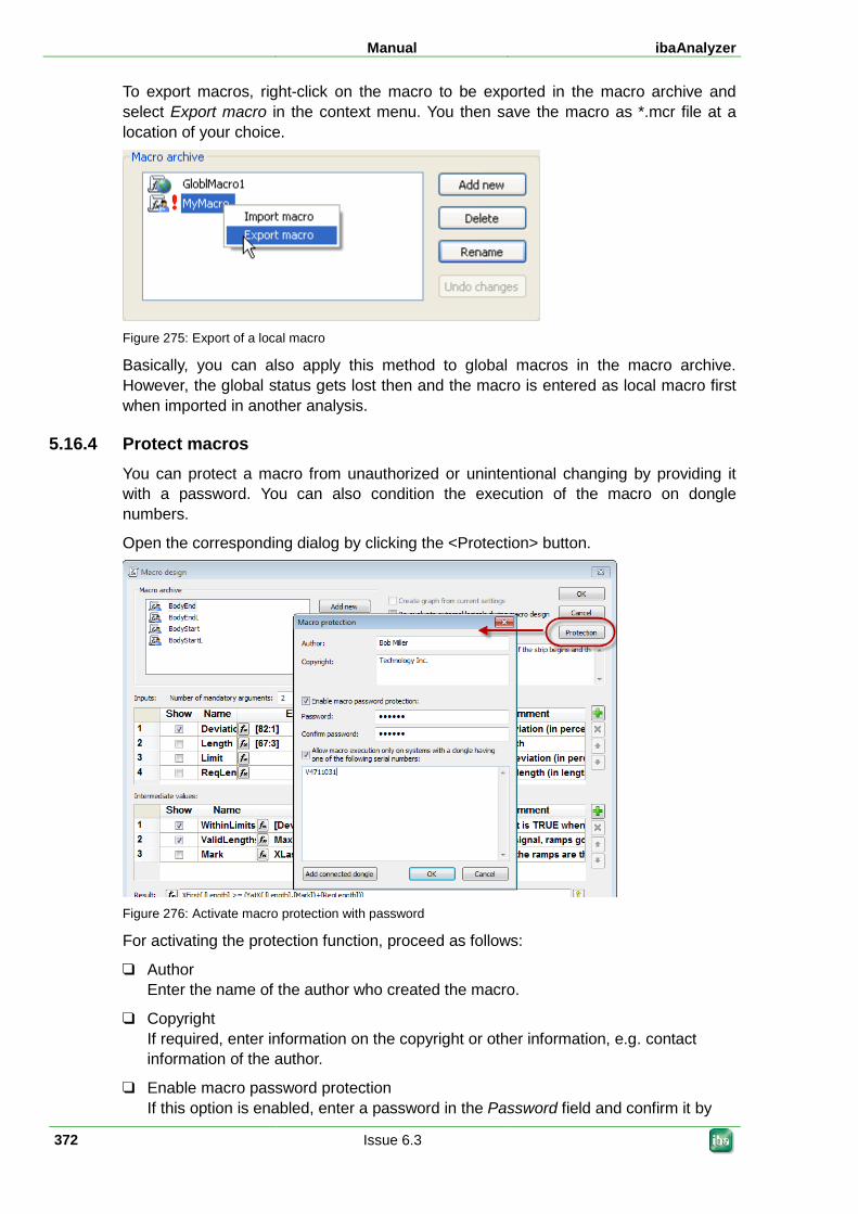
Manual ibaAnalyzer

372 Issue 6.3

To export macros, right-click on the macro to be exported in the macro archive and select Export macro in the context menu. You then save the macro as *.mcr file at a location of your choice.

Figure 275: Export of a local macro

Basically, you can also apply this method to global macros in the macro archive. However, the global status gets lost then and the macro is entered as local macro first when imported in another analysis.

5.16.4 Protect macros You can protect a macro from unauthorized or unintentional changing by providing it with a password. You can also condition the execution of the macro on dongle numbers.

Open the corresponding dialog by clicking the <Protection> button.

Figure 276: Activate macro protection with password

For activating the protection function, proceed as follows:

Author Enter the name of the author who created the macro.

Copyright If required, enter information on the copyright or other information, e.g. contact information of the author.

Enable macro password protection If this option is enabled, enter a password in the Password field and confirm it by

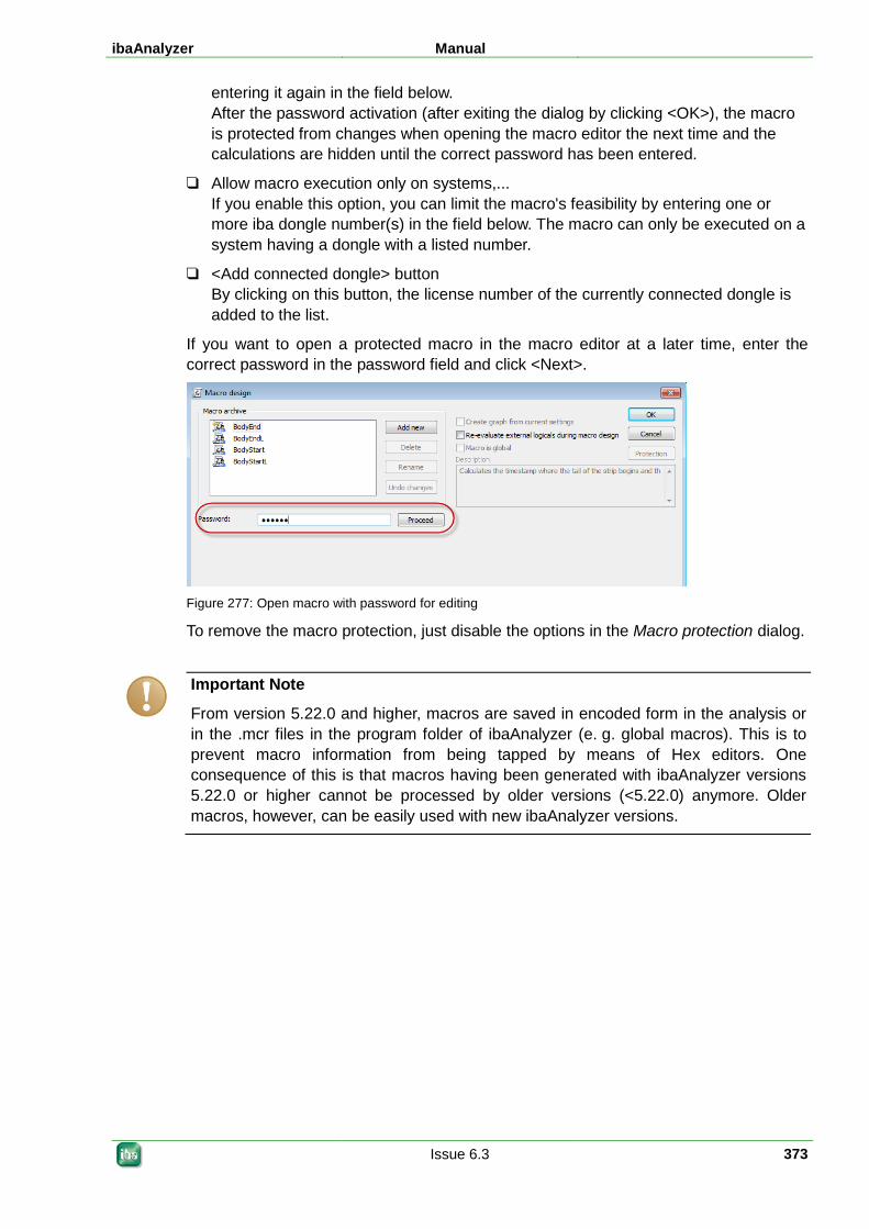
ibaAnalyzer Manual

Issue 6.3 373

entering it again in the field below. After the password activation (after exiting the dialog by clicking <OK>), the macro is protected from changes when opening the macro editor the next time and the calculations are hidden until the correct password has been entered.

Allow macro execution only on systems,... If you enable this option, you can limit the macro's feasibility by entering one or more iba dongle number(s) in the field below. The macro can only be executed on a system having a dongle with a listed number.

<Add connected dongle> button By clicking on this button, the license number of the currently connected dongle is added to the list.

If you want to open a protected macro in the macro editor at a later time, enter the correct password in the password field and click <Next>.

Figure 277: Open macro with password for editing

To remove the macro protection, just disable the options in the Macro protection dialog.

Important Note

From version 5.22.0 and higher, macros are saved in encoded form in the analysis or in the .mcr files in the program folder of ibaAnalyzer (e. g. global macros). This is to prevent macro information from being tapped by means of Hex editors. One consequence of this is that macros having been generated with ibaAnalyzer versions 5.22.0 or higher cannot be processed by older versions (<5.22.0) anymore. Older macros, however, can be easily used with new ibaAnalyzer versions.

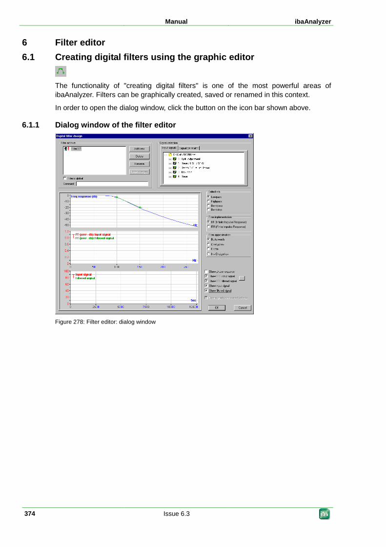
Manual ibaAnalyzer

374 Issue 6.3

6 Filter editor 6.1 Creating digital filters using the graphic editor

The functionality of "creating digital filters" is one of the most powerful areas of ibaAnalyzer. Filters can be graphically created, saved or renamed in this context.

In order to open the dialog window, click the button on the icon bar shown above.

6.1.1 Dialog window of the filter editor

Figure 278: Filter editor: dialog window

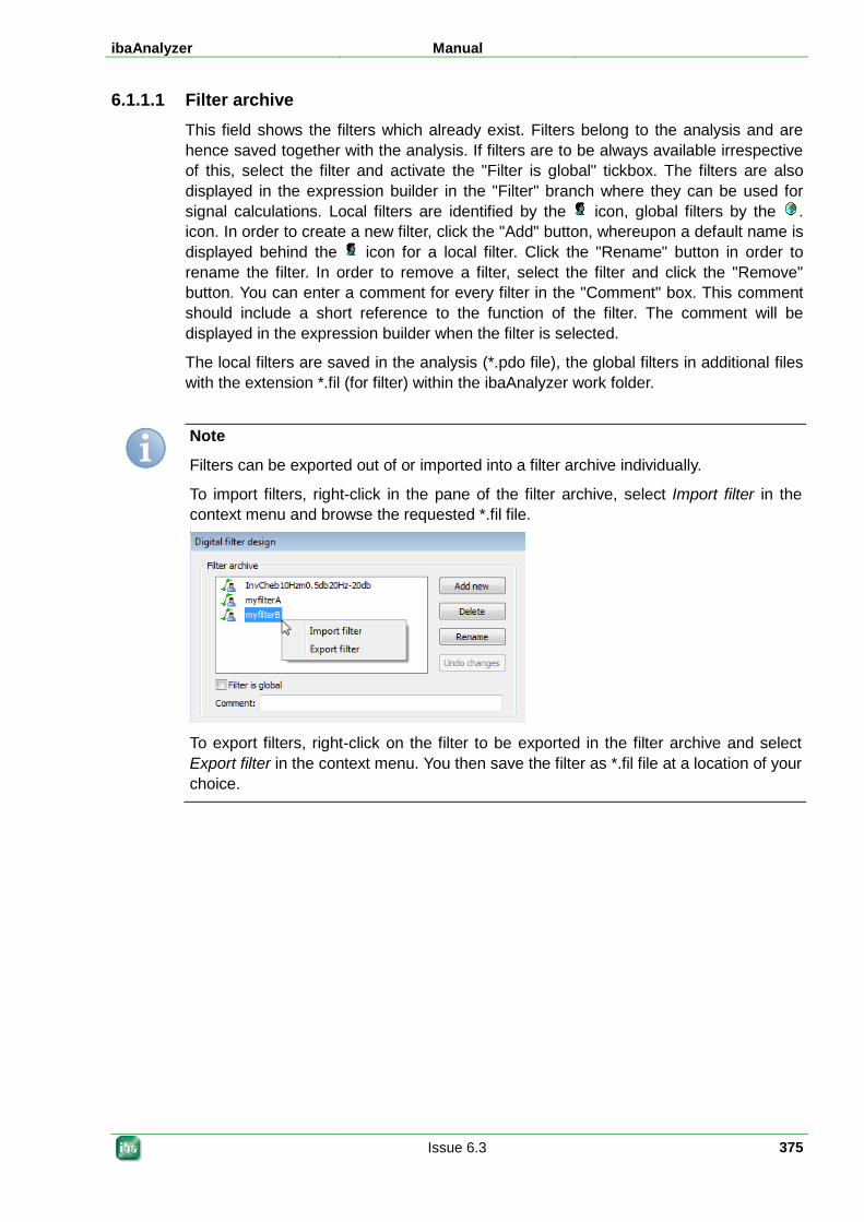
ibaAnalyzer Manual

Issue 6.3 375

6.1.1.1 Filter archive This field shows the filters which already exist. Filters belong to the analysis and are hence saved together with the analysis. If filters are to be always available irrespective of this, select the filter and activate the "Filter is global" tickbox. The filters are also displayed in the expression builder in the "Filter" branch where they can be used for signal calculations. Local filters are identified by the icon, global filters by the . icon. In order to create a new filter, click the "Add" button, whereupon a default name is displayed behind the icon for a local filter. Click the "Rename" button in order to rename the filter. In order to remove a filter, select the filter and click the "Remove" button. You can enter a comment for every filter in the "Comment" box. This comment should include a short reference to the function of the filter. The comment will be displayed in the expression builder when the filter is selected.

The local filters are saved in the analysis (*.pdo file), the global filters in additional files with the extension *.fil (for filter) within the ibaAnalyzer work folder.

Note

Filters can be exported out of or imported into a filter archive individually.

To import filters, right-click in the pane of the filter archive, select Import filter in the context menu and browse the requested *.fil file.

To export filters, right-click on the filter to be exported in the filter archive and select Export filter in the context menu. You then save the filter as *.fil file at a location of your choice.

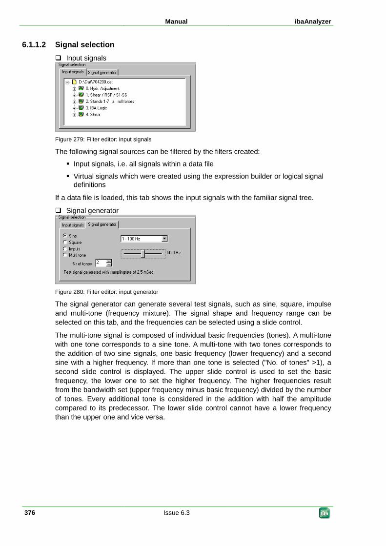
Manual ibaAnalyzer

376 Issue 6.3

6.1.1.2 Signal selection Input signals

Figure 279: Filter editor: input signals

The following signal sources can be filtered by the filters created:

Input signals, i.e. all signals within a data file

Virtual signals which were created using the expression builder or logical signal definitions

If a data file is loaded, this tab shows the input signals with the familiar signal tree.

Signal generator

Figure 280: Filter editor: input generator

The signal generator can generate several test signals, such as sine, square, impulse and multi-tone (frequency mixture). The signal shape and frequency range can be selected on this tab, and the frequencies can be selected using a slide control.

The multi-tone signal is composed of individual basic frequencies (tones). A multi-tone with one tone corresponds to a sine tone. A multi-tone with two tones corresponds to the addition of two sine signals, one basic frequency (lower frequency) and a second sine with a higher frequency. If more than one tone is selected ("No. of tones" >1), a second slide control is displayed. The upper slide control is used to set the basic frequency, the lower one to set the higher frequency. The higher frequencies result from the bandwidth set (upper frequency minus basic frequency) divided by the number of tones. Every additional tone is considered in the addition with half the amplitude compared to its predecessor. The lower slide control cannot have a lower frequency than the upper one and vice versa.

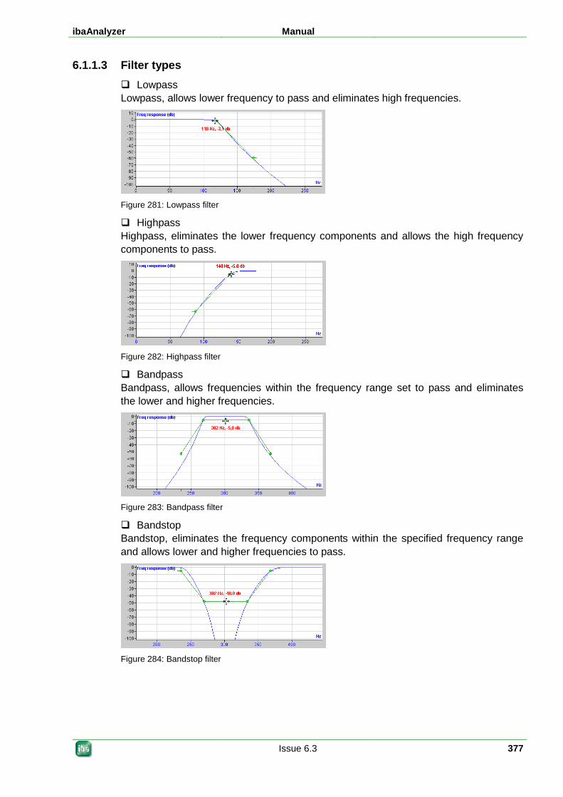
ibaAnalyzer Manual

Issue 6.3 377

6.1.1.3 Filter types Lowpass Lowpass, allows lower frequency to pass and eliminates high frequencies.

Figure 281: Lowpass filter

Highpass Highpass, eliminates the lower frequency components and allows the high frequency components to pass.

Figure 282: Highpass filter

Bandpass Bandpass, allows frequencies within the frequency range set to pass and eliminates the lower and higher frequencies.

Figure 283: Bandpass filter

Bandstop Bandstop, eliminates the frequency components within the specified frequency range and allows lower and higher frequencies to pass.

Figure 284: Bandstop filter

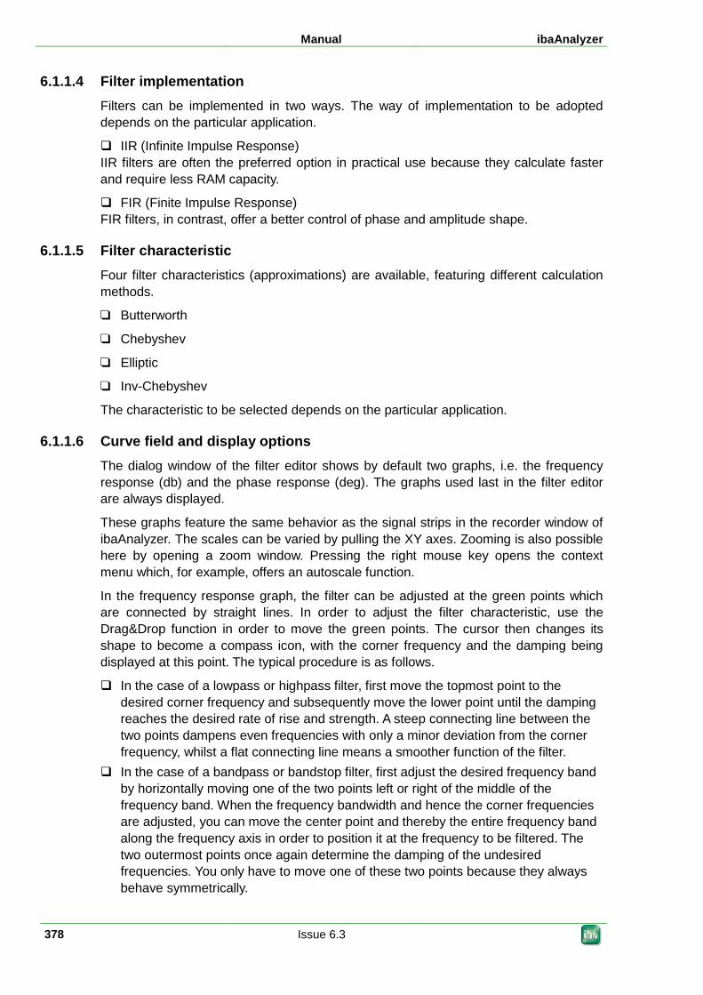
Manual ibaAnalyzer

378 Issue 6.3

6.1.1.4 Filter implementation Filters can be implemented in two ways. The way of implementation to be adopted depends on the particular application.

IIR (Infinite Impulse Response) IIR filters are often the preferred option in practical use because they calculate faster and require less RAM capacity.

FIR (Finite Impulse Response) FIR filters, in contrast, offer a better control of phase and amplitude shape.

6.1.1.5 Filter characteristic Four filter characteristics (approximations) are available, featuring different calculation methods.

Butterworth

Chebyshev

Elliptic

Inv-Chebyshev

The characteristic to be selected depends on the particular application.

6.1.1.6 Curve field and display options The dialog window of the filter editor shows by default two graphs, i.e. the frequency response (db) and the phase response (deg). The graphs used last in the filter editor are always displayed.

These graphs feature the same behavior as the signal strips in the recorder window of ibaAnalyzer. The scales can be varied by pulling the XY axes. Zooming is also possible here by opening a zoom window. Pressing the right mouse key opens the context menu which, for example, offers an autoscale function.

In the frequency response graph, the filter can be adjusted at the green points which are connected by straight lines. In order to adjust the filter characteristic, use the Drag&Drop function in order to move the green points. The cursor then changes its shape to become a compass icon, with the corner frequency and the damping being displayed at this point. The typical procedure is as follows.

In the case of a lowpass or highpass filter, first move the topmost point to the desired corner frequency and subsequently move the lower point until the damping reaches the desired rate of rise and strength. A steep connecting line between the two points dampens even frequencies with only a minor deviation from the corner frequency, whilst a flat connecting line means a smoother function of the filter.

In the case of a bandpass or bandstop filter, first adjust the desired frequency band by horizontally moving one of the two points left or right of the middle of the frequency band. When the frequency bandwidth and hence the corner frequencies are adjusted, you can move the center point and thereby the entire frequency band along the frequency axis in order to position it at the frequency to be filtered. The two outermost points once again determine the damping of the undesired frequencies. You only have to move one of these two points because they always behave symmetrically.

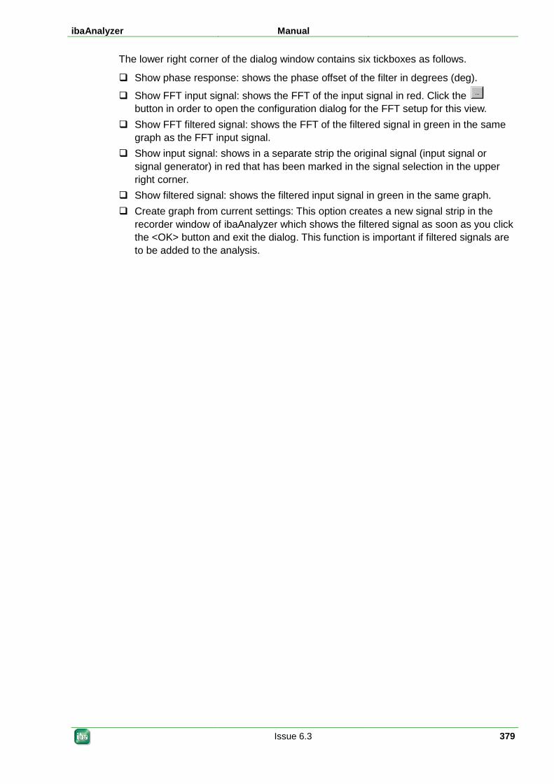
ibaAnalyzer Manual

Issue 6.3 379

The lower right corner of the dialog window contains six tickboxes as follows.

Show phase response: shows the phase offset of the filter in degrees (deg).

Show FFT input signal: shows the FFT of the input signal in red. Click the button in order to open the configuration dialog for the FFT setup for this view.

Show FFT filtered signal: shows the FFT of the filtered signal in green in the same graph as the FFT input signal.

Show input signal: shows in a separate strip the original signal (input signal or signal generator) in red that has been marked in the signal selection in the upper right corner.

Show filtered signal: shows the filtered input signal in green in the same graph. Create graph from current settings: This option creates a new signal strip in the

recorder window of ibaAnalyzer which shows the filtered signal as soon as you click the <OK> button and exit the dialog. This function is important if filtered signals are to be added to the analysis.

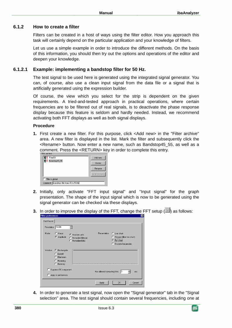
Manual ibaAnalyzer

380 Issue 6.3

6.1.2 How to create a filter Filters can be created in a host of ways using the filter editor. How you approach this task will certainly depend on the particular application and your knowledge of filters.

Let us use a simple example in order to introduce the different methods. On the basis of this information, you should then try out the options and operations of the editor and deepen your knowledge.

6.1.2.1 Example: implementing a bandstop filter for 50 Hz. The test signal to be used here is generated using the integrated signal generator. You can, of course, also use a clean input signal from the data file or a signal that is artificially generated using the expression builder.

Of course, the view which you select for the strip is dependent on the given requirements. A tried-and-tested approach in practical operations, where certain frequencies are to be filtered out of real signals, is to deactivate the phase response display because this feature is seldom and hardly needed. Instead, we recommend activating both FFT displays as well as both signal displays.

Procedure

1. First create a new filter. For this purpose, click <Add new> in the "Filter archive" area. A new filter is displayed in the list. Mark the filter and subsequently click the <Rename> button. Now enter a new name, such as Bandstop45_55, as well as a comment. Press the <RETURN> key in order to complete this entry.

2. Initially, only activate "FFT input signal" and "Input signal" for the graph

presentation. The shape of the input signal which is now to be generated using the signal generator can be checked via these displays.

3. In order to improve the display of the FFT, change the FFT setup ( ) as follows:

4. In order to generate a test signal, now open the "Signal generator" tab in the "Signal

selection" area. The test signal should contain several frequencies, including one at

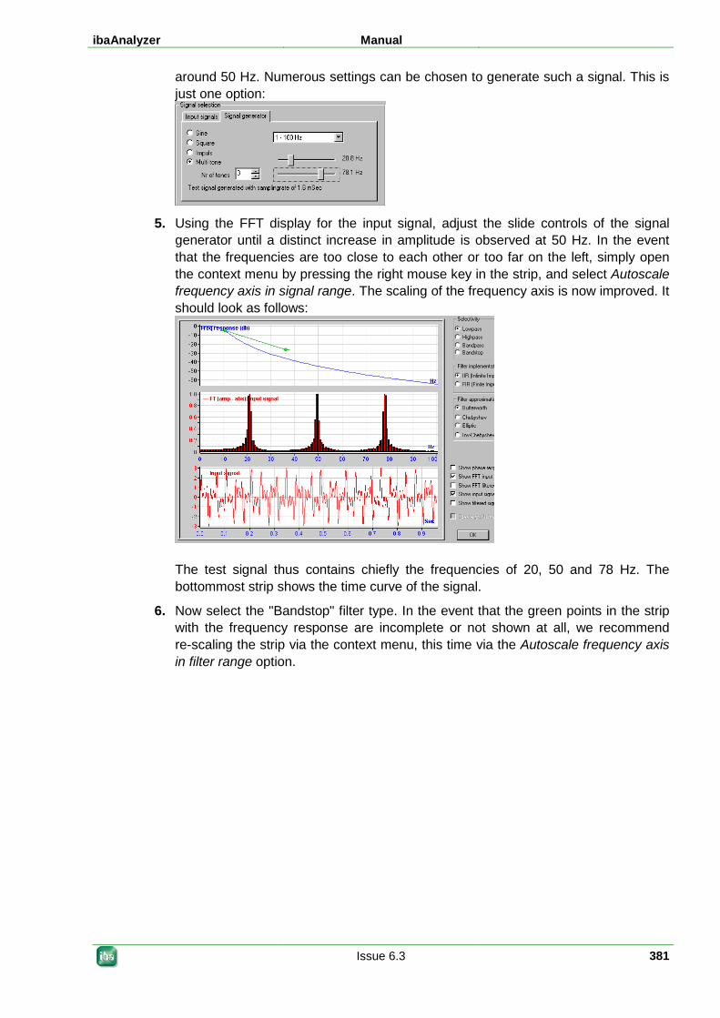
ibaAnalyzer Manual

Issue 6.3 381

around 50 Hz. Numerous settings can be chosen to generate such a signal. This is just one option:

5. Using the FFT display for the input signal, adjust the slide controls of the signal

generator until a distinct increase in amplitude is observed at 50 Hz. In the event that the frequencies are too close to each other or too far on the left, simply open the context menu by pressing the right mouse key in the strip, and select Autoscale frequency axis in signal range. The scaling of the frequency axis is now improved. It should look as follows:

The test signal thus contains chiefly the frequencies of 20, 50 and 78 Hz. The bottommost strip shows the time curve of the signal.

6. Now select the "Bandstop" filter type. In the event that the green points in the strip with the frequency response are incomplete or not shown at all, we recommend re-scaling the strip via the context menu, this time via the Autoscale frequency axis in filter range option.

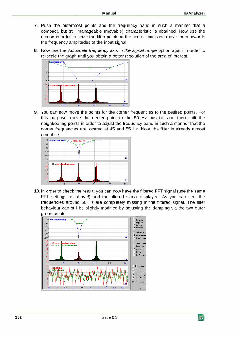
Manual ibaAnalyzer

382 Issue 6.3

7. Push the outermost points and the frequency band in such a manner that a compact, but still manageable (movable) characteristic is obtained. Now use the mouse in order to seize the filter points at the center point and move them towards the frequency amplitudes of the input signal.

8. Now use the Autoscale frequency axis in the signal range option again in order to re-scale the graph until you obtain a better resolution of the area of interest.

9. You can now move the points for the corner frequencies to the desired points. For

this purpose, move the center point to the 50 Hz position and then shift the neighbouring points in order to adjust the frequency band in such a manner that the corner frequencies are located at 45 and 55 Hz. Now, the filter is already almost complete.

10. In order to check the result, you can now have the filtered FFT signal (use the same

FFT settings as above!) and the filtered signal displayed. As you can see, the frequencies around 50 Hz are completely missing in the filtered signal. The filter behaviour can still be slightly modified by adjusting the damping via the two outer green points.

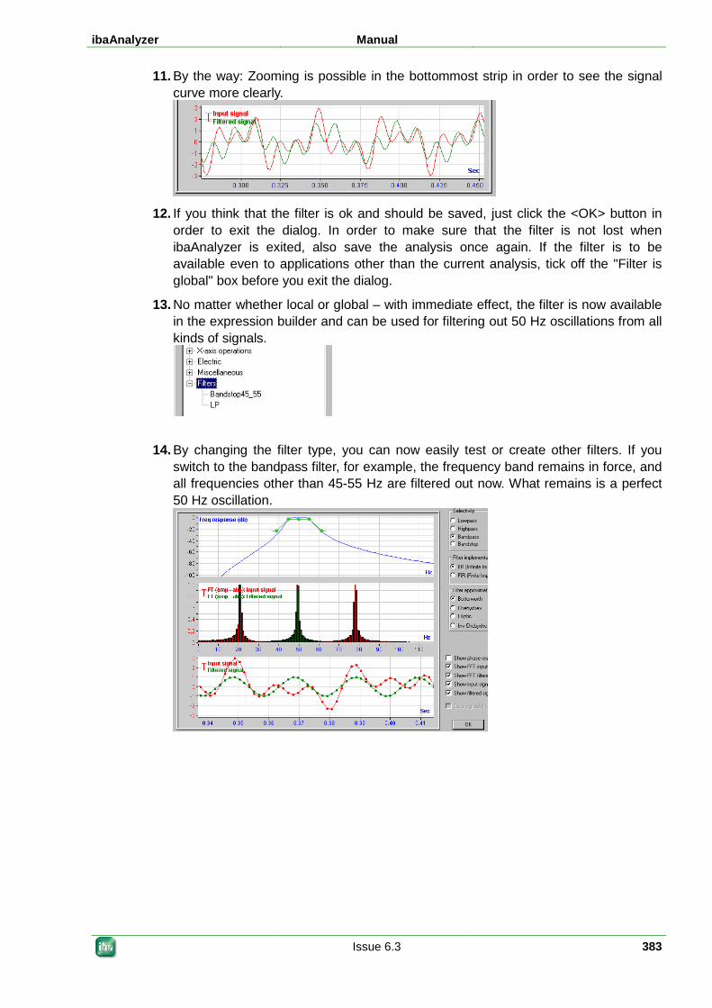
ibaAnalyzer Manual

Issue 6.3 383

11. By the way: Zooming is possible in the bottommost strip in order to see the signal curve more clearly.

12. If you think that the filter is ok and should be saved, just click the <OK> button in

order to exit the dialog. In order to make sure that the filter is not lost when ibaAnalyzer is exited, also save the analysis once again. If the filter is to be available even to applications other than the current analysis, tick off the "Filter is global" box before you exit the dialog.

13. No matter whether local or global – with immediate effect, the filter is now available in the expression builder and can be used for filtering out 50 Hz oscillations from all kinds of signals.

14. By changing the filter type, you can now easily test or create other filters. If you switch to the bandpass filter, for example, the frequency band remains in force, and all frequencies other than 45-55 Hz are filtered out now. What remains is a perfect 50 Hz oscillation.

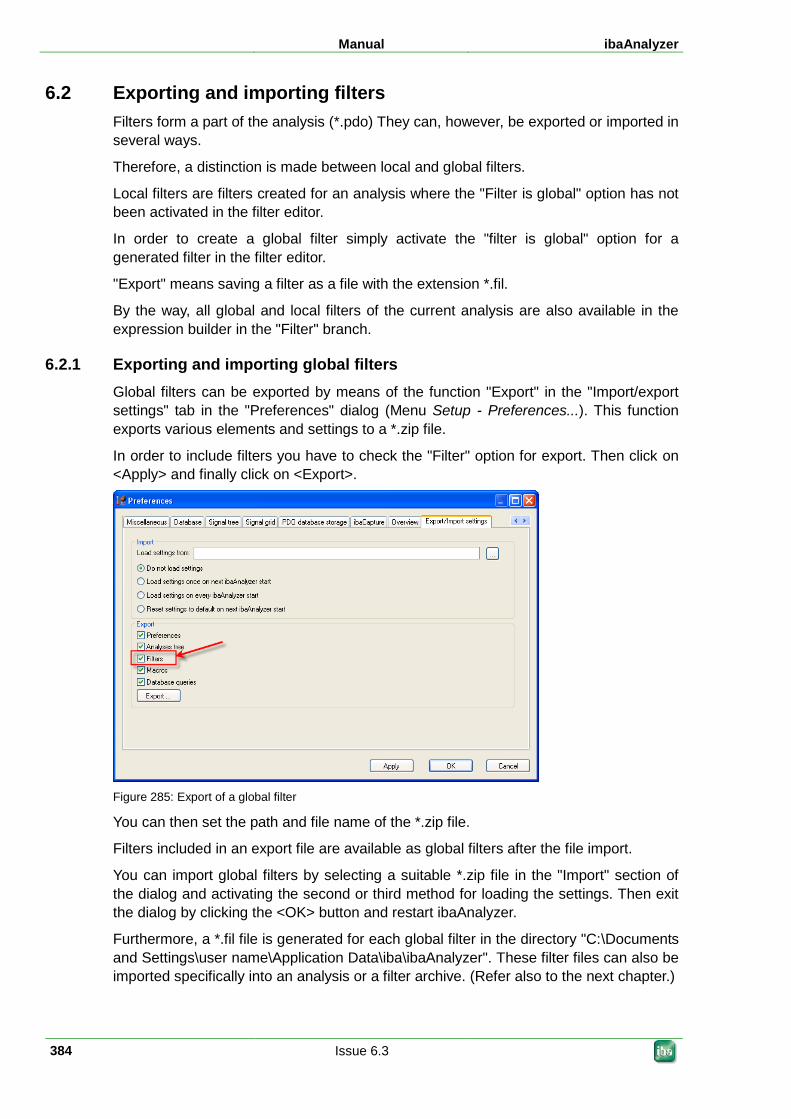
Manual ibaAnalyzer

384 Issue 6.3

6.2 Exporting and importing filters Filters form a part of the analysis (*.pdo) They can, however, be exported or imported in several ways.

Therefore, a distinction is made between local and global filters.

Local filters are filters created for an analysis where the "Filter is global" option has not been activated in the filter editor.

In order to create a global filter simply activate the "filter is global" option for a generated filter in the filter editor.

"Export" means saving a filter as a file with the extension *.fil.

By the way, all global and local filters of the current analysis are also available in the expression builder in the "Filter" branch.

6.2.1 Exporting and importing global filters Global filters can be exported by means of the function "Export" in the "Import/export settings" tab in the "Preferences" dialog (Menu Setup - Preferences...). This function exports various elements and settings to a *.zip file.

In order to include filters you have to check the "Filter" option for export. Then click on <Apply> and finally click on <Export>.

Figure 285: Export of a global filter

You can then set the path and file name of the *.zip file.

Filters included in an export file are available as global filters after the file import.

You can import global filters by selecting a suitable *.zip file in the "Import" section of the dialog and activating the second or third method for loading the settings. Then exit the dialog by clicking the <OK> button and restart ibaAnalyzer.

Furthermore, a *.fil file is generated for each global filter in the directory "C:\Documents and Settings\user name\Application Data\iba\ibaAnalyzer". These filter files can also be imported specifically into an analysis or a filter archive. (Refer also to the next chapter.)

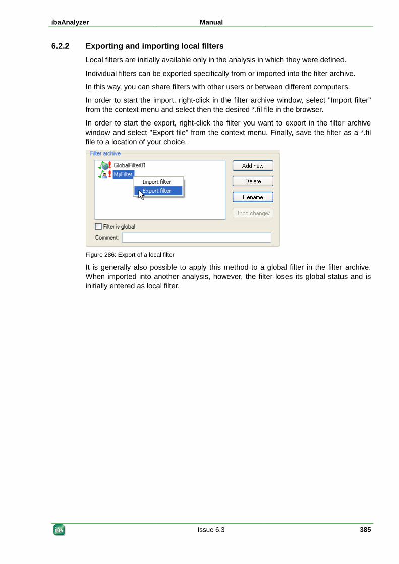
ibaAnalyzer Manual

Issue 6.3 385

6.2.2 Exporting and importing local filters Local filters are initially available only in the analysis in which they were defined.

Individual filters can be exported specifically from or imported into the filter archive.

In this way, you can share filters with other users or between different computers.

In order to start the import, right-click in the filter archive window, select "Import filter" from the context menu and select then the desired *.fil file in the browser.

In order to start the export, right-click the filter you want to export in the filter archive window and select "Export file" from the context menu. Finally, save the filter as a *.fil file to a location of your choice.

Figure 286: Export of a local filter

It is generally also possible to apply this method to a global filter in the filter archive. When imported into another analysis, however, the filter loses its global status and is initially entered as local filter.

Manual ibaAnalyzer

386 Issue 6.3

7 Report generator This chapter gives an introduction to the reporting options using the report generator. The most important aspect that will be discussed here is the data interface with the report generator in the form in which it was implemented in ibaAnalyzer.

Details concerning report layout and design, i.e. the use of combit's (http://www.combit.net/reporting/report-generator-List-Label) reporting tool "List & Label", can be found in the online documentation. We recommend booking an additional report generator training course at our company in order to learn how to use this complex tool.

Note

iba offers a standard course on the subject of the report generator. Please visit our website for course times, availability and prices, or just call us.

7.1 What is an analysis report? You as the user can choose any design and layout you like for an analysis report. The analysis report can be used to present the signal strips from ibaAnalyzer as well as all kinds of process data (such as technostrings, calculated values, etc.) and graphic objects (squares, circles, pictures, ...) and diagrams. Furthermore, text fields capable of formatting can be edited, and bar codes and charts/tables can be generated.

A report can be compiled and prepared on a workpiece-related basis and can be subsequently printed or exported into a file (for example, in the .pdf format). Furthermore, automatic generation and output of a report via a post-processing command from ibaPDA or by means of ibaDatCoordinator is also possible.

The name of the analysis file used for the report generation is available in the report generator as 'AnalysisPath' variable.

7.2 Requirements, installation and starting 7.2.1 Requirements

ibaAnalyzer V5.0 or higher A standard printer driver should be installed on the computer

7.2.2 Installation Since ibaAnalyzer V5 and higher the Report Generator is automatically installed by the ibaAnalyzer installer. A separate installation of the Report Generator is not required.

7.2.3 Starting the report generator Once the report generator is installed as described in the "Installation" section, you can

start the program via ibaAnalyzer's menu bar by clicking the icon.

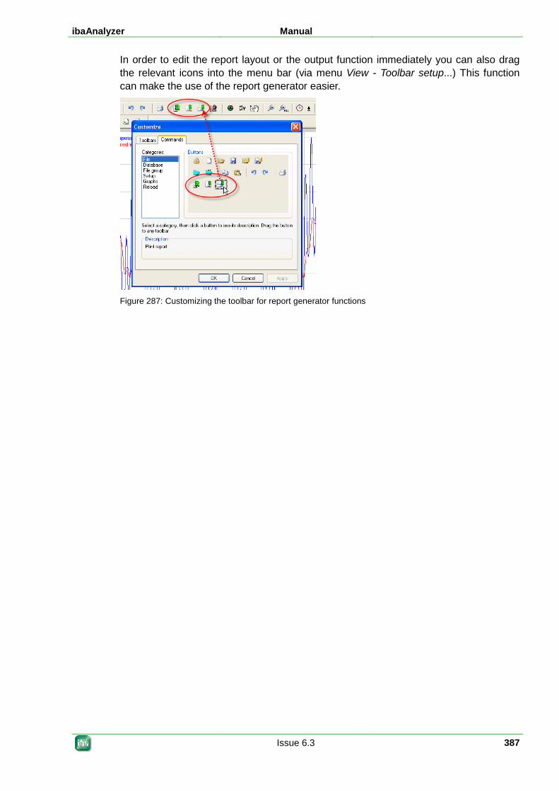
ibaAnalyzer Manual

Issue 6.3 387

In order to edit the report layout or the output function immediately you can also drag the relevant icons into the menu bar (via menu View - Toolbar setup...) This function can make the use of the report generator easier.

Figure 287: Customizing the toolbar for report generator functions

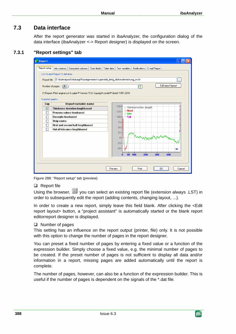
Manual ibaAnalyzer

388 Issue 6.3

7.3 Data interface After the report generator was started in ibaAnalyzer, the configuration dialog of the data interface (ibaAnalyzer <-> Report designer) is displayed on the screen.

7.3.1 "Report settings" tab

Figure 288: "Report setup" tab (preview)

Report file Using the browser, you can select an existing report file (extension always .LST) in order to subsequently edit the report (adding contents, changing layout, ...).

In order to create a new report, simply leave this field blank. After clicking the <Edit report layout> button, a "project assistant" is automatically started or the blank report editorreport designer is displayed.

Number of pages This setting has an influence on the report output (printer, file) only. It is not possible with this option to change the number of pages in the report designer.

You can preset a fixed number of pages by entering a fixed value or a function of the expression builder. Simply choose a fixed value, e.g. the minimal number of pages to be created. If the preset number of pages is not sufficient to display all data and/or information in a report, missing pages are added automatically until the report is complete.

The number of pages, however, can also be a function of the expression builder. This is useful if the number of pages is dependent on the signals of the *.dat file.

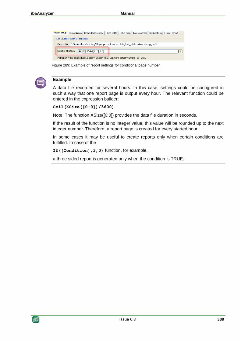
ibaAnalyzer Manual

Issue 6.3 389

Figure 289: Example of report settings for conditional page number

Example

A data file recorded for several hours. In this case, settings could be configured in such a way that one report page is output every hour. The relevant function could be entered in the expression builder:

Ceil(XSize([0:0])/3600)

Note: The function XSize([0:0]) provides the data file duration in seconds.

If the result of the function is no integer value, this value will be rounded up to the next integer number. Therefore, a report page is created for every started hour.

In some cases it may be useful to create reports only when certain conditions are fulfilled. In case of the

If([Condition],3,0) function, for example,

a three sided report is generated only when the condition is TRUE.

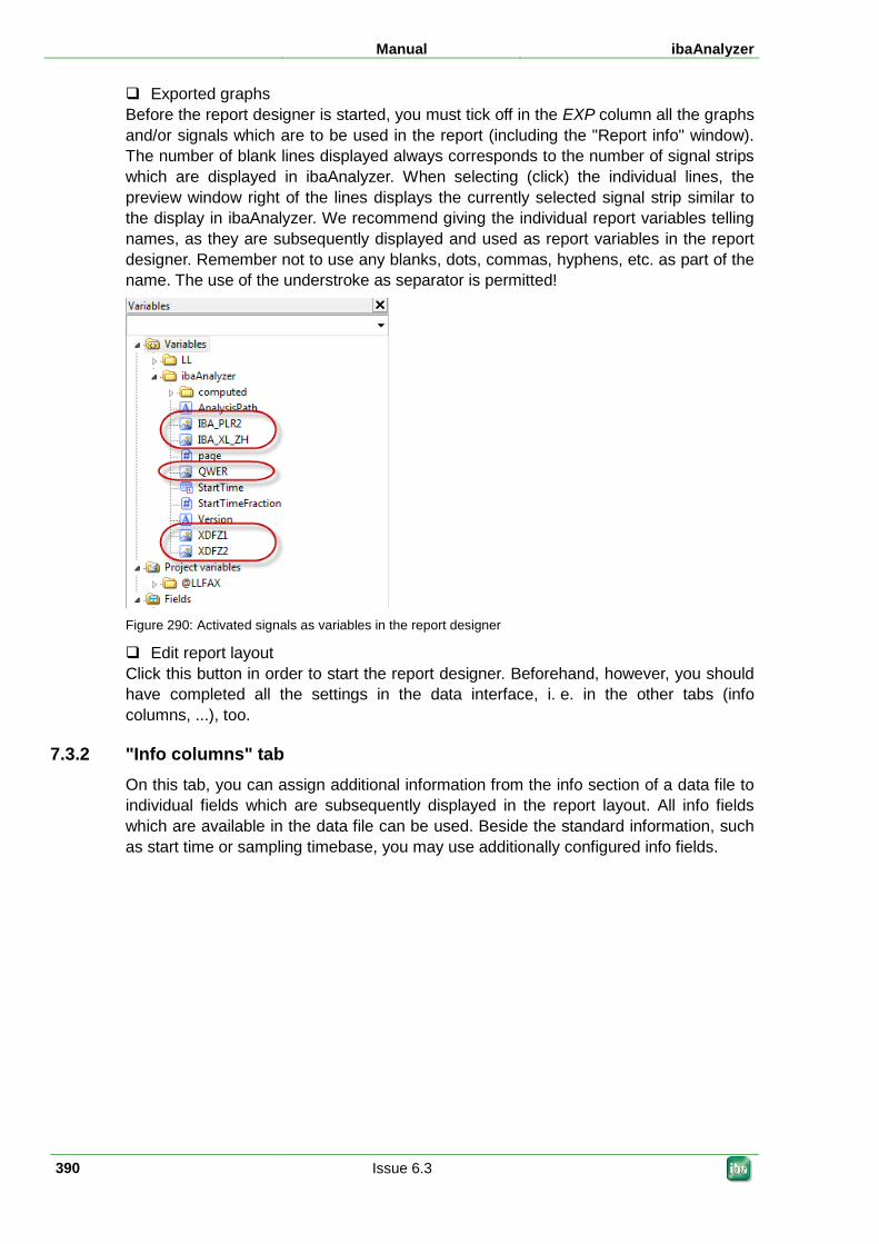
Manual ibaAnalyzer

390 Issue 6.3

Exported graphs Before the report designer is started, you must tick off in the EXP column all the graphs and/or signals which are to be used in the report (including the "Report info" window). The number of blank lines displayed always corresponds to the number of signal strips which are displayed in ibaAnalyzer. When selecting (click) the individual lines, the preview window right of the lines displays the currently selected signal strip similar to the display in ibaAnalyzer. We recommend giving the individual report variables telling names, as they are subsequently displayed and used as report variables in the report designer. Remember not to use any blanks, dots, commas, hyphens, etc. as part of the name. The use of the understroke as separator is permitted!

Figure 290: Activated signals as variables in the report designer

Edit report layout Click this button in order to start the report designer. Beforehand, however, you should have completed all the settings in the data interface, i. e. in the other tabs (info columns, ...), too.

7.3.2 "Info columns" tab On this tab, you can assign additional information from the info section of a data file to individual fields which are subsequently displayed in the report layout. All info fields which are available in the data file can be used. Beside the standard information, such as start time or sampling timebase, you may use additionally configured info fields.

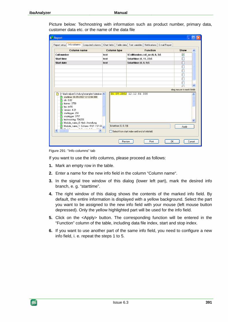
ibaAnalyzer Manual

Issue 6.3 391

Picture below: Technostring with information such as product number, primary data, customer data etc. or the name of the data file

Figure 291: "Info columns" tab

If you want to use the info columns, please proceed as follows:

1. Mark an empty row in the table.

2. Enter a name for the new info field in the column “Column name“.

3. In the signal tree window of this dialog (lower left part), mark the desired info branch, e. g. “starttime”.

4. The right window of this dialog shows the contents of the marked info field. By default, the entire information is displayed with a yellow background. Select the part you want to be assigned to the new info field with your mouse (left mouse button depressed). Only the yellow highlighted part will be used for the info field.

5. Click on the <Apply> button. The corresponding function will be entered in the “Function” column of the table, including data file index, start and stop index.

6. If you want to use another part of the same info field, you need to configure a new info field, i. e. repeat the steps 1 to 5.

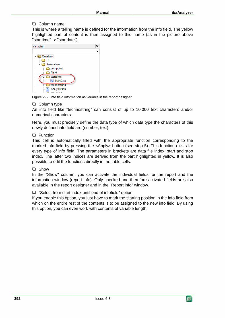
Manual ibaAnalyzer

392 Issue 6.3

Column name This is where a telling name is defined for the information from the info field. The yellow highlighted part of content is then assigned to this name (as in the picture above "starttime" -> "startdate").

Figure 292: Info field information as variable in the report designer

Column type An info field like “technostring” can consist of up to 10,000 text characters and/or numerical characters.

Here, you must precisely define the data type of which data type the characters of this newly defined info field are (number, text).

Function This cell is automatically filled with the appropriate function corresponding to the marked info field by pressing the <Apply> button (see step 5). This function exists for every type of info field. The parameters in brackets are data file index, start and stop index. The latter two indices are derived from the part highlighted in yellow. It is also possible to edit the functions directly in the table cells.

Show In the "Show" column, you can activate the individual fields for the report and the information window (report info). Only checked and therefore activated fields are also available in the report designer and in the "Report info" window.

"Select from start index until end of infofield" option If you enable this option, you just have to mark the starting position in the info field from which on the entire rest of the contents is to be assigned to the new info field. By using this option, you can even work with contents of variable length.

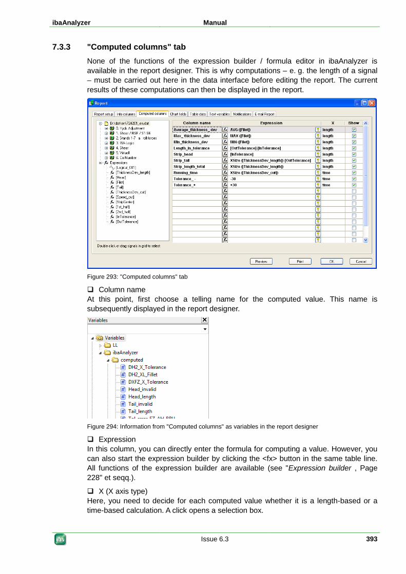
ibaAnalyzer Manual

Issue 6.3 393

7.3.3 "Computed columns" tab None of the functions of the expression builder / formula editor in ibaAnalyzer is available in the report designer. This is why computations – e. g. the length of a signal – must be carried out here in the data interface before editing the report. The current results of these computations can then be displayed in the report.

Figure 293: "Computed columns" tab

Column name At this point, first choose a telling name for the computed value. This name is subsequently displayed in the report designer.

Figure 294: Information from "Computed columns" as variables in the report designer

Expression In this column, you can directly enter the formula for computing a value. However, you can also start the expression builder by clicking the <fx> button in the same table line. All functions of the expression builder are available (see "Expression builder , Page 228" et seqq.).

X (X axis type) Here, you need to decide for each computed value whether it is a length-based or a time-based calculation. A click opens a selection box.

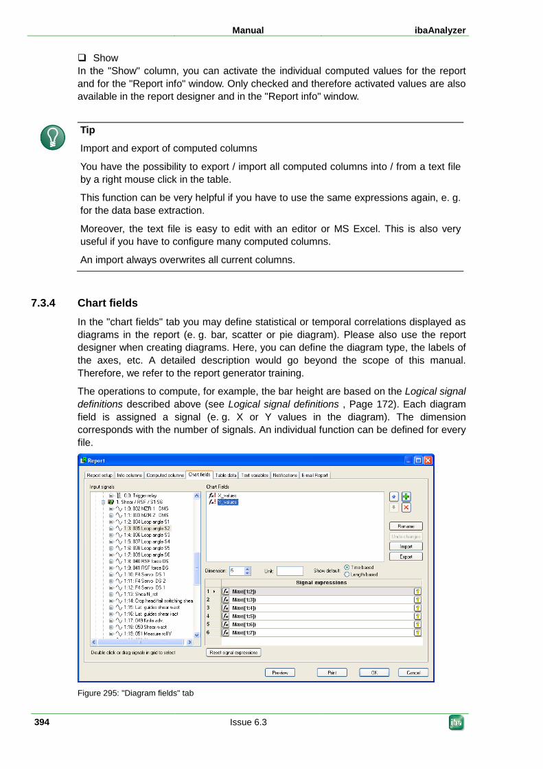
Manual ibaAnalyzer

394 Issue 6.3

Show In the "Show" column, you can activate the individual computed values for the report and for the "Report info" window. Only checked and therefore activated values are also available in the report designer and in the "Report info" window.

Tip

Import and export of computed columns

You have the possibility to export / import all computed columns into / from a text file by a right mouse click in the table.

This function can be very helpful if you have to use the same expressions again, e. g. for the data base extraction.

Moreover, the text file is easy to edit with an editor or MS Excel. This is also very useful if you have to configure many computed columns.

An import always overwrites all current columns.

7.3.4 Chart fields In the "chart fields" tab you may define statistical or temporal correlations displayed as diagrams in the report (e. g. bar, scatter or pie diagram). Please also use the report designer when creating diagrams. Here, you can define the diagram type, the labels of the axes, etc. A detailed description would go beyond the scope of this manual. Therefore, we refer to the report generator training.

The operations to compute, for example, the bar height are based on the Logical signal definitions described above (see Logical signal definitions , Page 172). Each diagram field is assigned a signal (e. g. X or Y values in the diagram). The dimension corresponds with the number of signals. An individual function can be defined for every file.

Figure 295: "Diagram fields" tab

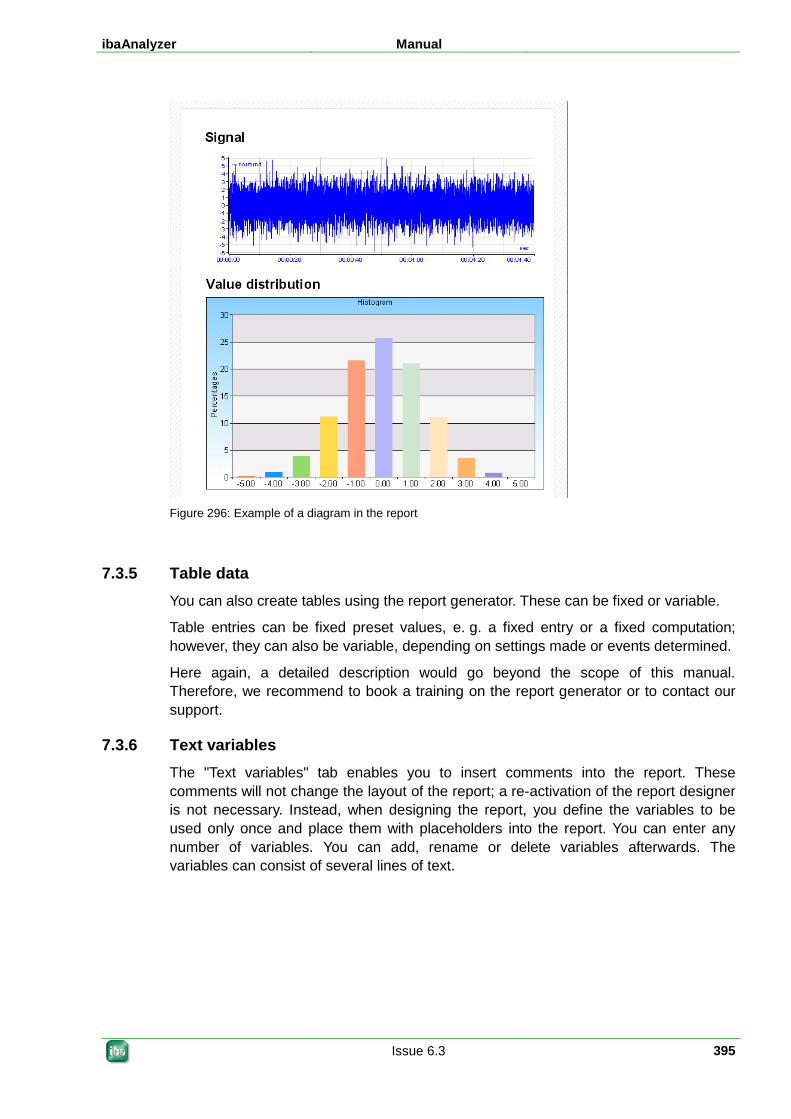
ibaAnalyzer Manual

Issue 6.3 395

Figure 296: Example of a diagram in the report

7.3.5 Table data You can also create tables using the report generator. These can be fixed or variable.

Table entries can be fixed preset values, e. g. a fixed entry or a fixed computation; however, they can also be variable, depending on settings made or events determined.

Here again, a detailed description would go beyond the scope of this manual. Therefore, we recommend to book a training on the report generator or to contact our support.

7.3.6 Text variables The "Text variables" tab enables you to insert comments into the report. These comments will not change the layout of the report; a re-activation of the report designer is not necessary. Instead, when designing the report, you define the variables to be used only once and place them with placeholders into the report. You can enter any number of variables. You can add, rename or delete variables afterwards. The variables can consist of several lines of text.

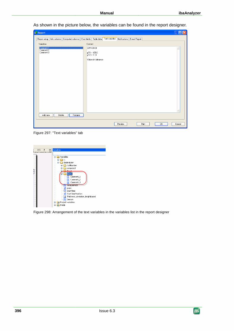
Manual ibaAnalyzer

396 Issue 6.3

As shown in the picture below, the variables can be found in the report designer.

Figure 297: "Text variables" tab

Figure 298: Arrangement of the text variables in the variables list in the report designer

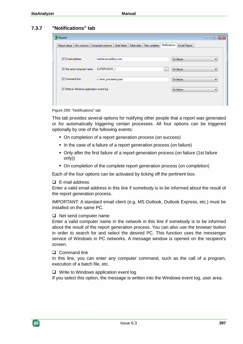
ibaAnalyzer Manual

Issue 6.3 397

7.3.7 "Notifications" tab

Figure 299: "Notifications" tab

This tab provides several options for notifying other people that a report was generated or for automatically triggering certain processes. All four options can be triggered optionally by one of the following events:

On completion of a report generation process (on success)

In the case of a failure of a report generation process (on failure)

Only after the first failure of a report generation process (on failure (1st failure only))

On completion of the complete report generation process (on completion)

Each of the four options can be activated by ticking off the pertinent box.

E-mail address Enter a valid email address in this line if somebody is to be informed about the result of the report generation process.

IMPORTANT: A standard email client (e.g. MS Outlook, Outlook Express, etc.) must be installed on the same PC.

Net send computer name Enter a valid computer name in the network in this line if somebody is to be informed about the result of the report generation process. You can also use the browser button in order to search for and select the desired PC. This function uses the messenger service of Windows in PC networks. A message window is opened on the recipient's screen.

Command line In this line, you can enter any computer command, such as the call of a program, execution of a batch file, etc.

Write to Windows application event log If you select this option, the message is written into the Windows event log, user area.

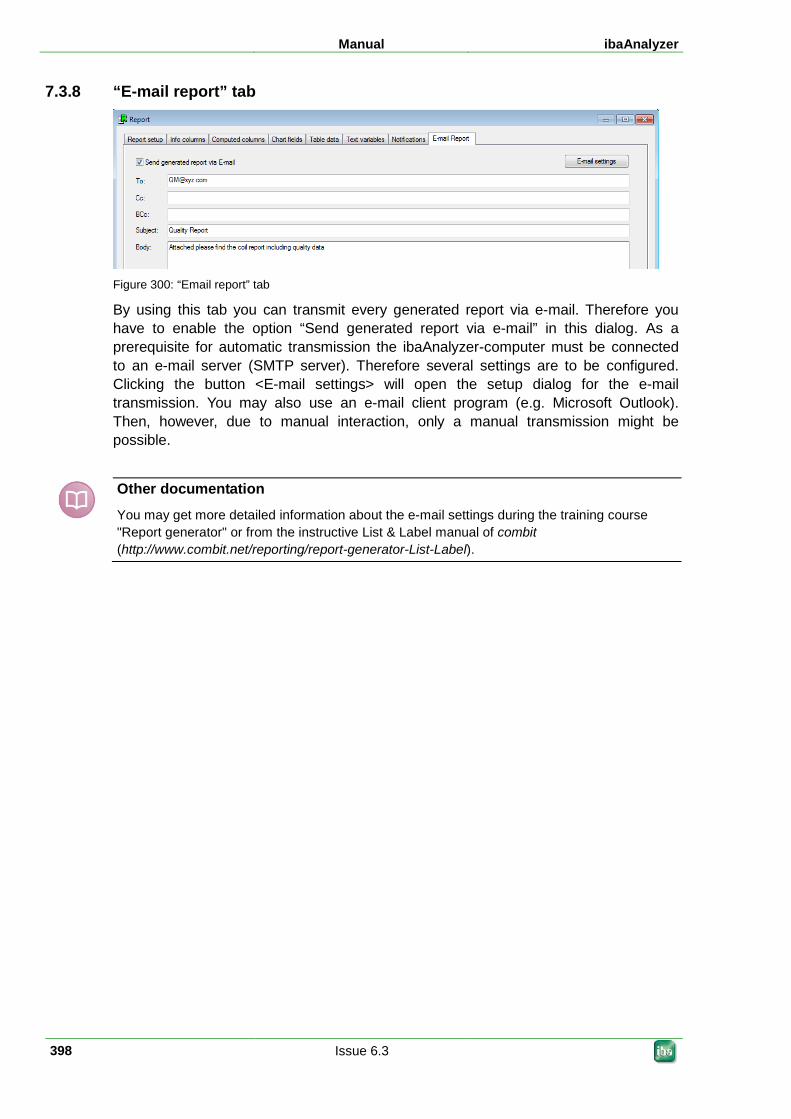
Manual ibaAnalyzer

398 Issue 6.3

7.3.8 “E-mail report” tab

Figure 300: “Email report” tab

By using this tab you can transmit every generated report via e-mail. Therefore you have to enable the option “Send generated report via e-mail” in this dialog. As a prerequisite for automatic transmission the ibaAnalyzer-computer must be connected to an e-mail server (SMTP server). Therefore several settings are to be configured. Clicking the button <E-mail settings> will open the setup dialog for the e-mail transmission. You may also use an e-mail client program (e.g. Microsoft Outlook). Then, however, due to manual interaction, only a manual transmission might be possible.

Other documentation

You may get more detailed information about the e-mail settings during the training course "Report generator" or from the instructive List & Label manual of combit (http://www.combit.net/reporting/report-generator-List-Label).

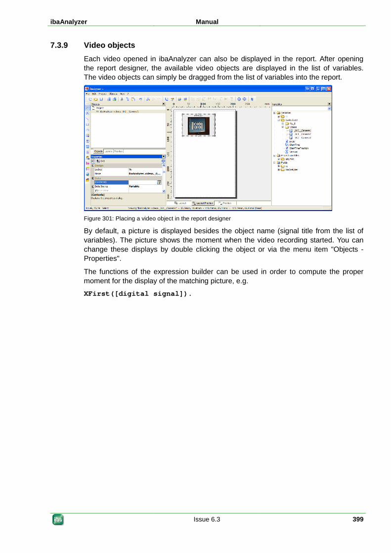
ibaAnalyzer Manual

Issue 6.3 399

7.3.9 Video objects Each video opened in ibaAnalyzer can also be displayed in the report. After opening the report designer, the available video objects are displayed in the list of variables. The video objects can simply be dragged from the list of variables into the report.

Figure 301: Placing a video object in the report designer

By default, a picture is displayed besides the object name (signal title from the list of variables). The picture shows the moment when the video recording started. You can change these displays by double clicking the object or via the menu item "Objects - Properties".

The functions of the expression builder can be used in order to compute the proper moment for the display of the matching picture, e.g.

XFirst([digital signal]).

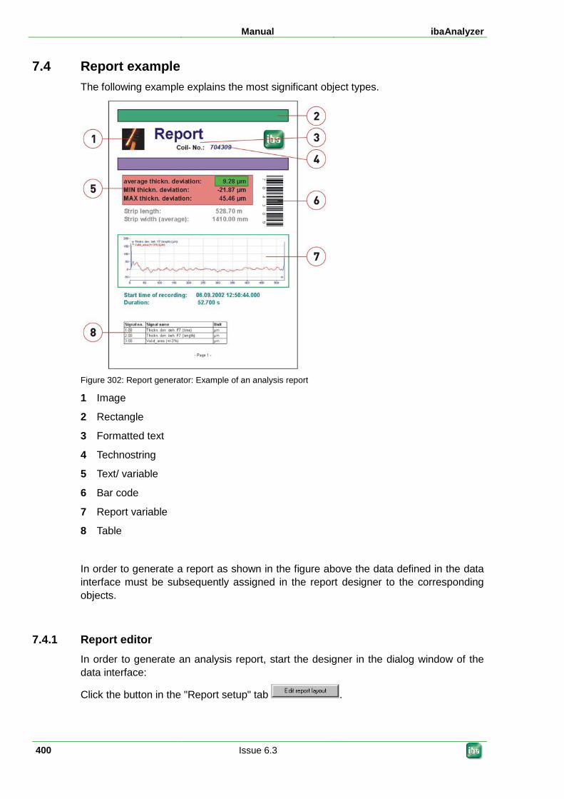
Manual ibaAnalyzer

400 Issue 6.3

7.4 Report example The following example explains the most significant object types.

Figure 302: Report generator: Example of an analysis report

1 Image

2 Rectangle

3 Formatted text

4 Technostring

5 Text/ variable

6 Bar code

7 Report variable

8 Table

In order to generate a report as shown in the figure above the data defined in the data interface must be subsequently assigned in the report designer to the corresponding objects.

7.4.1 Report editor In order to generate an analysis report, start the designer in the dialog window of the data interface:

Click the button in the "Report setup" tab .

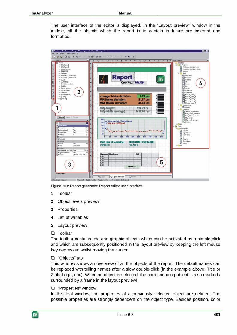
ibaAnalyzer Manual

Issue 6.3 401

The user interface of the editor is displayed. In the "Layout preview" window in the middle, all the objects which the report is to contain in future are inserted and formatted.

Figure 303: Report generator: Report editor user interface

1 Toolbar

2 Object levels preview

3 Properties

4 List of variables

5 Layout preview

Toolbar The toolbar contains text and graphic objects which can be activated by a simple click and which are subsequently positioned in the layout preview by keeping the left mouse key depressed whilst moving the cursor.

"Objects" tab This window shows an overview of all the objects of the report. The default names can be replaced with telling names after a slow double-click (in the example above: Title or Z_ibaLogo, etc.). When an object is selected, the corresponding object is also marked / surrounded by a frame in the layout preview!

"Properties" window In this tool window, the properties of a previously selected object are defined. The possible properties are strongly dependent on the object type. Besides position, color

Manual ibaAnalyzer

402 Issue 6.3

and size of an object, it is, for example, also possible to activate presentation and pagination conditions.

"Layout preview" window This is the work area where existing objects can be edited or deleted and where new objects can be added. The shape and dimensions result from the defined layout preferences.

The work area always consists of one single page only. This means that it is not possible to create further pages as you may know from other programs.

In order to create multi-page analysis reports, you have to define and assign so-called "levels".

"List of variables" window This window shows the previously defined data from the data interface of ibaAnalyzer. You can use the drag and drop function in order to position and subsequently format the variables in the work area.

These include, for example:

Report variables (signal strips)

Computed values

Technostring fields

Furthermore, other types of data are additionally made available by default:

Information from the data file (such as sample time, start trigger, time, ...)

Fields / arrays from the data file (such as signal name, unit, ...)

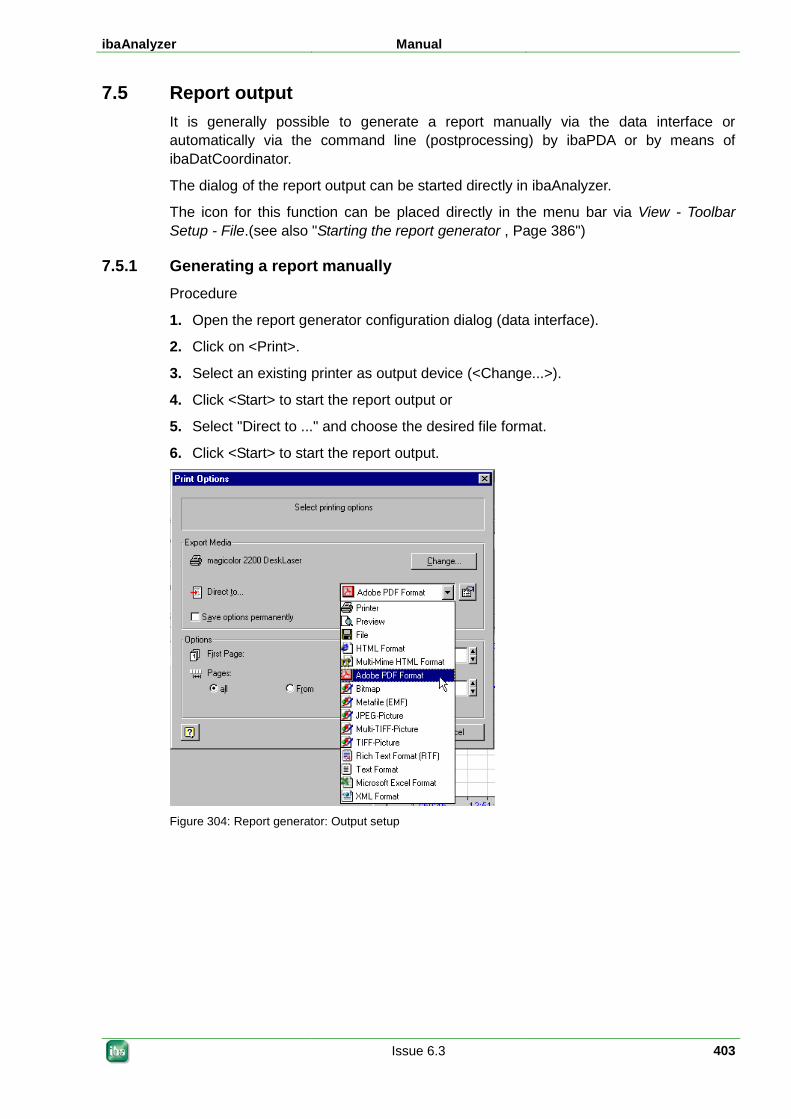
ibaAnalyzer Manual

Issue 6.3 403

7.5 Report output It is generally possible to generate a report manually via the data interface or automatically via the command line (postprocessing) by ibaPDA or by means of ibaDatCoordinator.

The dialog of the report output can be started directly in ibaAnalyzer.

The icon for this function can be placed directly in the menu bar via View - Toolbar Setup - File.(see also "Starting the report generator , Page 386")

7.5.1 Generating a report manually Procedure

1. Open the report generator configuration dialog (data interface).

2. Click on <Print>.

3. Select an existing printer as output device (<Change...>).

4. Click <Start> to start the report output or

5. Select "Direct to ..." and choose the desired file format.

6. Click <Start> to start the report output.

Figure 304: Report generator: Output setup

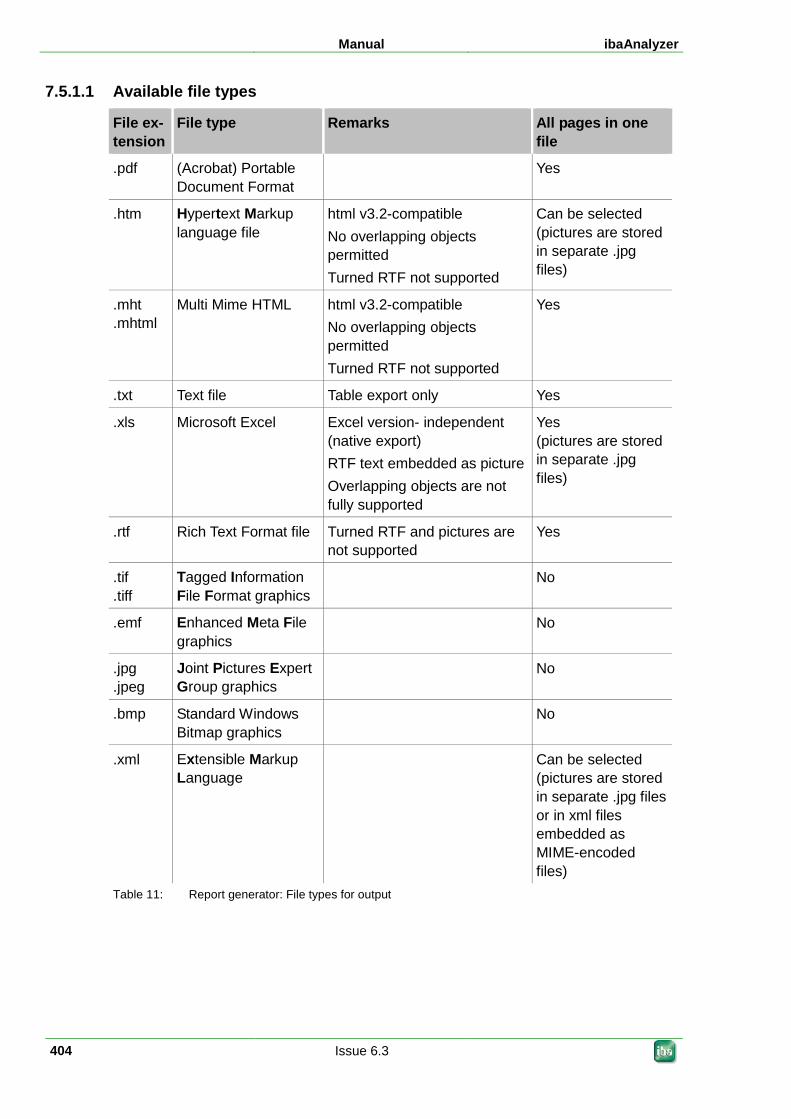
Manual ibaAnalyzer

404 Issue 6.3

7.5.1.1 Available file types

File ex- tension

File type Remarks All pages in one file

.pdf (Acrobat) Portable Document Format

Yes

.htm Hypertext Markup language file

html v3.2-compatible No overlapping objects permitted Turned RTF not supported

Can be selected (pictures are stored in separate .jpg files)

.mht

.mhtml Multi Mime HTML html v3.2-compatible

No overlapping objects permitted Turned RTF not supported

Yes

.txt Text file Table export only Yes

.xls Microsoft Excel Excel version- independent (native export) RTF text embedded as picture Overlapping objects are not fully supported

Yes (pictures are stored in separate .jpg files)

.rtf Rich Text Format file Turned RTF and pictures are not supported

Yes

.tif

.tiff Tagged Information File Format graphics

No

.emf Enhanced Meta File graphics

No

.jpg

.jpeg Joint Pictures Expert Group graphics

No

.bmp Standard Windows Bitmap graphics

No

.xml Extensible Markup Language

Can be selected (pictures are stored in separate .jpg files or in xml files embedded as MIME-encoded files)

Table 11: Report generator: File types for output

ibaAnalyzer Manual

Issue 6.3 405

7.5.2 Automatic output via command line commands As already described in chapter "Starting with command line , Page 17", you can also start ibaAnalyzer via the command line, for example, via post-processing in ibaPDA or by means of ibaDatCoordinator. In this case, several parameters and switches can be transferred together with the command, causing ibaAnalyzer to automatically carry out certain analyses, including, for example, the generation of a report and its output.

Tip

The output of reports can be automized and conveniently configured with the help of the software tool ibaDatCoordinator.

7.5.2.1 Program call syntax ...\ibaanalyzer.exe Datafile.dat Analyse.pdo /report[:File]

The data file(s) Datafile.dat must be available.

The analysis Analysis.pdo must be available. The configuration of the data interface as well as the link to a valid report layout file are saved in the analysis.

7.5.2.2 /report[:filename] switch This switch will only be available with ibaAnalyzer version 3.52 and higher. If ibaAnalyzer is started with this switch, the specified data file is loaded and an analysis is carried out in accordance with the analysis transferred. Thereafter, the integrated report generator is started and the data is printed on the Windows default printer using a report layout specified in the analysis if the :filename option was not used with the switch.

If the :filename switch option is used, the report can be written into a file rather than being printed. The desired file type is determined by the file name extension in accordance with the Available file types , Page 404.

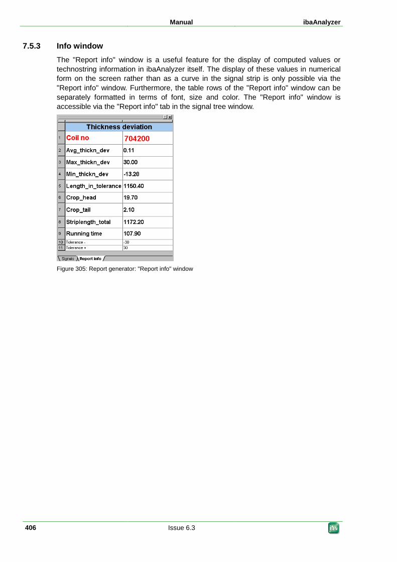
Manual ibaAnalyzer

406 Issue 6.3

7.5.3 Info window The "Report info" window is a useful feature for the display of computed values or technostring information in ibaAnalyzer itself. The display of these values in numerical form on the screen rather than as a curve in the signal strip is only possible via the "Report info" window. Furthermore, the table rows of the "Report info" window can be separately formatted in terms of font, size and color. The "Report info" window is accessible via the "Report info" tab in the signal tree window.

Figure 305: Report generator: "Report info" window

ibaAnalyzer Manual

Issue 6.3 407

8 Installation 8.1 System requirements

PC, multi-core CPU, 2 GHz or better

2048 MB RAM or more for extended analyses (with video etc.)

100 MB or more available hard disk space for the program

Additional hard disk capacity for data files and analyses, depending on your particular application

Operating system: MS Windows XP, Vista, 7, Server 2003, Server 2008 or Server 2012

Internet Explorer 6.0 or higher

8.2 Installation The CD delivered contains all the necessary program files in one directory. They can be found in the directory ..\ibaAnalyzer_Vm.n.. (m.n = Version). The installation file is available in zipped and unzipped form.

You can

a) copy the zip file to the hard disk of your computer and unzip it there or

b) run the installation file ibaAnalyzerInstall_vm.n.exe directly from CD.

When downloading the installation file from our website, you will receive a zip file which has to be saved to your hard disk and unzipped there.

Then proceed as follows:

1. Run the file ibaAnalyzerInstall_vm.n.exe. If ibaAnalyzer is already installed on your computer, you will be notified and asked to confirm the reinstallation. Click <Yes>. The installation wizard will start.

2. Click <Next> to start the installation. In the next step, you can change the target folder for the program files, if you wish.

3. Click <Next>. In the next step, you can select the type of database support. This is only necessary if you use ibaAnalyzer-DB (ibaHistorian) to extract data into a database or to read from a database. All other applications do not require database support.

4. Make your choice and click <Install>. The installation will start and a progress bar will be displayed. If interested, you can click on <Show details> in order to track the individual actions. A notification will be displayed after the installation is complete.

5. If you want to launch ibaAnalyzer immediately after the installation, then activate the checkbox "Launch ibaAnalyzer" and click <Finish>.

Manual ibaAnalyzer

408 Issue 6.3

9 Database interface (option) The added database interface feature enables the writing of measuring data into a database and/or the retrieving and analyzing of data from a database. MS SQL server, MS ACCESS, DB2-UDB and ORACLE as well as other ODBC-compatible databases are supported.

This feature enables the comprehensive integration of basic process data into your company's quality management system. The related data editing and compression as well as data extraction processes can be fully automated.

Order number Description Comment

33.010430 ibaAnalyzer-DB Writing and reading of a database

33.0104450 ibaAnalyzer-DB-Analysis-Multiuser

Retrieving database by multiple clients

Other documentation

The description of the database interface is available as a separate document (ibaAnalyzer-DB) and comes with the additional license, and/or is available on request.

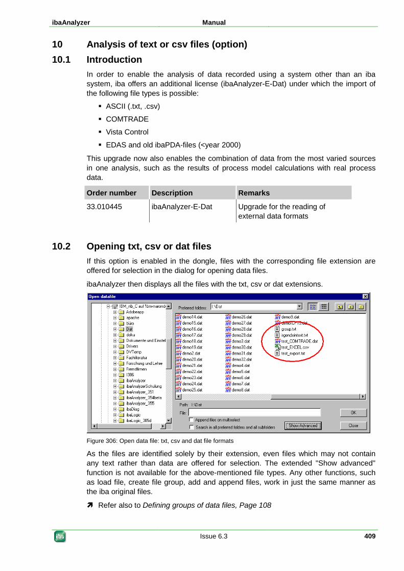
ibaAnalyzer Manual

Issue 6.3 409

10 Analysis of text or csv files (option) 10.1 Introduction

In order to enable the analysis of data recorded using a system other than an iba system, iba offers an additional license (ibaAnalyzer-E-Dat) under which the import of the following file types is possible:

ASCII (.txt, .csv)

COMTRADE

Vista Control

EDAS and old ibaPDA-files (<year 2000)

This upgrade now also enables the combination of data from the most varied sources in one analysis, such as the results of process model calculations with real process data.

Order number Description Remarks

33.010445 ibaAnalyzer-E-Dat Upgrade for the reading of external data formats

10.2 Opening txt, csv or dat files If this option is enabled in the dongle, files with the corresponding file extension are offered for selection in the dialog for opening data files.

ibaAnalyzer then displays all the files with the txt, csv or dat extensions.

Figure 306: Open data file: txt, csv and dat file formats

As the files are identified solely by their extension, even files which may not contain any text rather than data are offered for selection. The extended "Show advanced" function is not available for the above-mentioned file types. Any other functions, such as load file, create file group, add and append files, work in just the same manner as the iba original files.

Refer also to Defining groups of data files, Page 108

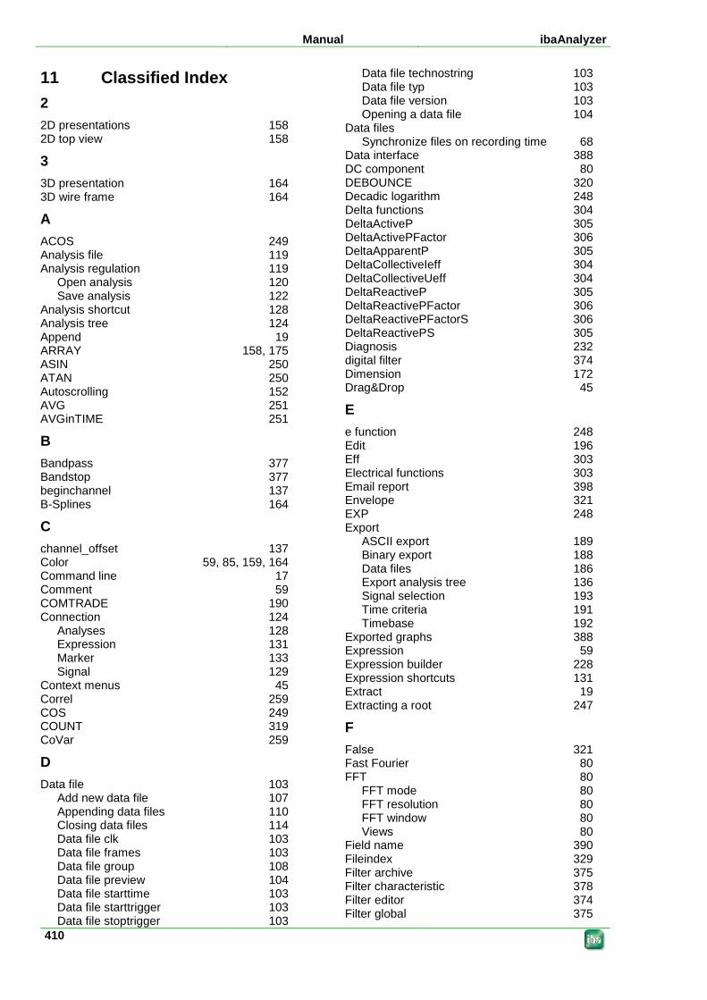
Manual ibaAnalyzer

410

11 Classified Index 2 2D presentations 158 2D top view 158

3 3D presentation 164 3D wire frame 164

A ACOS 249 Analysis file 119 Analysis regulation 119

Open analysis 120 Save analysis 122

Analysis shortcut 128 Analysis tree 124 Append 19 ARRAY 158, 175 ASIN 250 ATAN 250 Autoscrolling 152 AVG 251 AVGinTIME 251

B Bandpass 377 Bandstop 377 beginchannel 137 B-Splines 164

C channel_offset 137 Color 59, 85, 159, 164 Command line 17 Comment 59 COMTRADE 190 Connection 124

Analyses 128 Expression 131 Marker 133 Signal 129

Context menus 45 Correl 259 COS 249 COUNT 319 CoVar 259

D Data file 103

Add new data file 107 Appending data files 110 Closing data files 114 Data file clk 103 Data file frames 103 Data file group 108 Data file preview 104 Data file starttime 103 Data file starttrigger 103 Data file stoptrigger 103

Data file technostring 103 Data file typ 103 Data file version 103 Opening a data file 104

Data files Synchronize files on recording time 68

Data interface 388 DC component 80 DEBOUNCE 320 Decadic logarithm 248 Delta functions 304 DeltaActiveP 305 DeltaActivePFactor 306 DeltaApparentP 305 DeltaCollectiveIeff 304 DeltaCollectiveUeff 304 DeltaReactiveP 305 DeltaReactivePFactor 306 DeltaReactivePFactorS 306 DeltaReactivePS 305 Diagnosis 232 digital filter 374 Dimension 172 Drag&Drop 45

E e function 248 Edit 196 Eff 303 Electrical functions 303 Email report 398 Envelope 321 EXP 248 Export

ASCII export 189 Binary export 188 Data files 186 Export analysis tree 136 Signal selection 193 Time criteria 191 Timebase 192

Exported graphs 388 Expression 59 Expression builder 228 Expression shortcuts 131 Extract 19 Extracting a root 247

F False 321 Fast Fourier 80 FFT 80

FFT mode 80 FFT resolution 80 FFT window 80 Views 80

Field name 390 Fileindex 329 Filter archive 375 Filter characteristic 378 Filter editor 374 Filter global 375

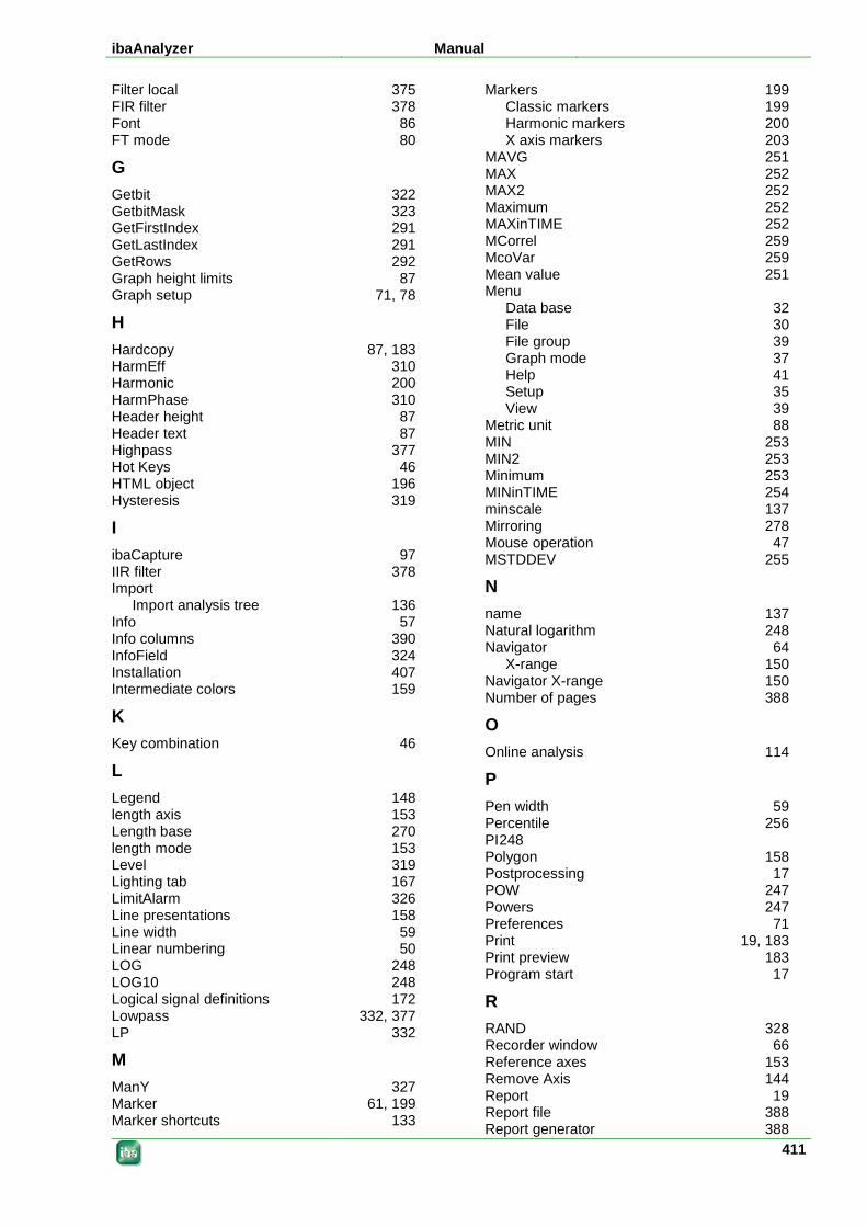
ibaAnalyzer Manual

411

Filter local 375 FIR filter 378 Font 86 FT mode 80

G Getbit 322 GetbitMask 323 GetFirstIndex 291 GetLastIndex 291 GetRows 292 Graph height limits 87 Graph setup 71, 78

H Hardcopy 87, 183 HarmEff 310 Harmonic 200 HarmPhase 310 Header height 87 Header text 87 Highpass 377 Hot Keys 46 HTML object 196 Hysteresis 319

I ibaCapture 97 IIR filter 378 Import

Import analysis tree 136 Info 57 Info columns 390 InfoField 324 Installation 407 Intermediate colors 159

K Key combination 46

L Legend 148 length axis 153 Length base 270 length mode 153 Level 319 Lighting tab 167 LimitAlarm 326 Line presentations 158 Line width 59 Linear numbering 50 LOG 248 LOG10 248 Logical signal definitions 172 Lowpass 332, 377 LP 332

M ManY 327 Marker 61, 199 Marker shortcuts 133

Markers 199 Classic markers 199 Harmonic markers 200 X axis markers 203

MAVG 251 MAX 252 MAX2 252 Maximum 252 MAXinTIME 252 MCorrel 259 McoVar 259 Mean value 251 Menu

Data base 32 File 30 File group 39 Graph mode 37 Help 41 Setup 35 View 39

Metric unit 88 MIN 253 MIN2 253 Minimum 253 MINinTIME 254 minscale 137 Mirroring 278 Mouse operation 47 MSTDDEV 255

N name 137 Natural logarithm 248 Navigator 64

X-range 150 Navigator X-range 150 Number of pages 388

O Online analysis 114

P Pen width 59 Percentile 256 PI 248 Polygon 158 Postprocessing 17 POW 247 Powers 247 Preferences 71 Print 19, 183 Print preview 183 Program start 17

R RAND 328 Recorder window 66 Reference axes 153 Remove Axis 144 Report 19 Report file 388 Report generator 388

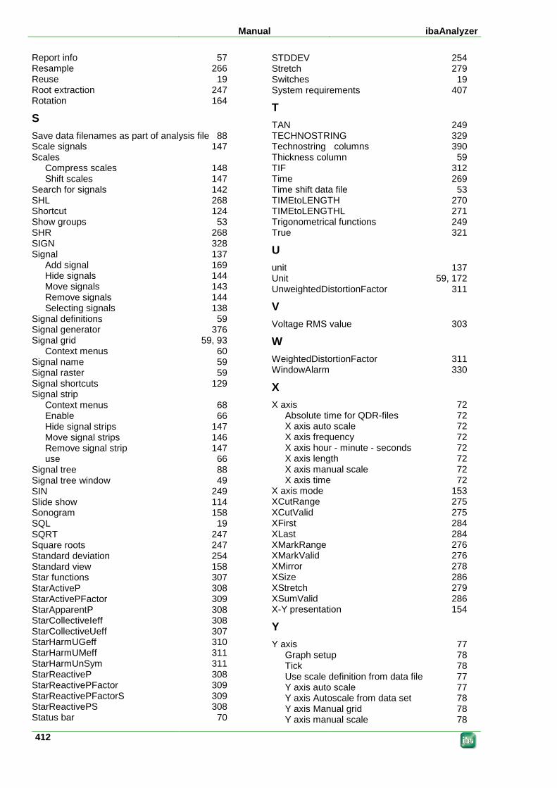
Manual ibaAnalyzer

412

Report info 57 Resample 266 Reuse 19 Root extraction 247 Rotation 164

S Save data filenames as part of analysis file 88 Scale signals 147 Scales

Compress scales 148 Shift scales 147

Search for signals 142 SHL 268 Shortcut 124 Show groups 53 SHR 268 SIGN 328 Signal 137

Add signal 169 Hide signals 144 Move signals 143 Remove signals 144 Selecting signals 138

Signal definitions 59 Signal generator 376 Signal grid 59, 93

Context menus 60 Signal name 59 Signal raster 59 Signal shortcuts 129 Signal strip

Context menus 68 Enable 66 Hide signal strips 147 Move signal strips 146 Remove signal strip 147 use 66

Signal tree 88 Signal tree window 49 SIN 249 Slide show 114 Sonogram 158 SQL 19 SQRT 247 Square roots 247 Standard deviation 254 Standard view 158 Star functions 307 StarActiveP 308 StarActivePFactor 309 StarApparentP 308 StarCollectiveIeff 308 StarCollectiveUeff 307 StarHarmUGeff 310 StarHarmUMeff 311 StarHarmUnSym 311 StarReactiveP 308 StarReactivePFactor 309 StarReactivePFactorS 309 StarReactivePS 308 Status bar 70

STDDEV 254 Stretch 279 Switches 19 System requirements 407

T TAN 249 TECHNOSTRING 329 Technostring columns 390 Thickness column 59 TIF 312 Time 269 Time shift data file 53 TIMEtoLENGTH 270 TIMEtoLENGTHL 271 Trigonometrical functions 249 True 321

U unit 137 Unit 59, 172 UnweightedDistortionFactor 311

V Voltage RMS value 303

W WeightedDistortionFactor 311 WindowAlarm 330

X X axis 72

Absolute time for QDR-files 72 X axis auto scale 72 X axis frequency 72 X axis hour - minute - seconds 72 X axis length 72 X axis manual scale 72 X axis time 72

X axis mode 153 XCutRange 275 XCutValid 275 XFirst 284 XLast 284 XMarkRange 276 XMarkValid 276 XMirror 278 XSize 286 XStretch 279 XSumValid 286 X-Y presentation 154

Y Y axis 77

Graph setup 78 Tick 78 Use scale definition from data file 77 Y axis auto scale 77 Y axis Autoscale from data set 78 Y axis Manual grid 78 Y axis manual scale 78

ibaAnalyzer Manual

413

Y axis preferences 77 Y axis reference 78 Y axis scale offset 78 Y axis scaling mode 77, 78

Y axis scaling mode 77, 78 Y axis scientific notation 77 YatX 330

Z Zoom 149

Manual ibaAnalyzer

414 Issue 6.3

12 Support and contact Support

Phone: +49 911 97282-14

Fax: +49 911 97282-33

Email: support@iba-ag.com

Note

If you require support, indicate the serial number (iba-S/N) of the product.

Contact

Headquarters

iba AG Koenigswarterstr. 44 90762 Fuerth Germany

Phone: +49 911 97282-0

Fax: +49 911 97282-33

Email: iba@iba-ag.com

Contact: Mr Harald Opel

Regional and Worldwide

For contact data of your regional iba office or representative please refer to our web site

www.iba-ag.com.