1

Magnetic Bubbles and Kinetic Alfven Waves in theHigh-Latitude Magnetopause Boundary

K. Stasiewicz1,2, C. E. Seyler3, F. S. Mozer4, G. Gustafsson1, J. Pickett5 andB. Popielawska2

1Swedish Institute of Space Physics, Uppsala, Sweden2Space Research Centre, Polish Academy of Sciences, Warsaw, Poland3Cornell University, Ithaca, USA4University of Berkeley, California, USA5Iowa University, Iowa, USA

Abstract. We present a detailed analysis of magnetic bubbles observed by thePOLAR satellite in the high-latitude magnetopause boundary. The bubbles whichrepresent holes or strong depressions (up to 98%) of the ambient magnetic fieldare filled with heated solar wind plasma elements and observed in the vicinity ofstrong magnetopause currents and possibly near the reconnection site. We analyzethe wave modes in the frequency range 0-30 Hz at the magnetopause (bubble) layerand conclude that the broadband waves in this frequency range represent mostlikely spatial turbulence of Kinetic Alfven Waves (KAW), Doppler shifted to higherfrequencies (in the satellite frame) by convective plasma flows. We present alsoresults of a numerical simulation which indicate that the bubbles are produced bya tearing mode reconnection process and the KAW fluctuations are related to theHall instability created by macroscopic pressure and magnetic field gradients. Theobserved spatial spectrum of KAW extends from several ion gyroradii (∼ 500 km)down to the electron inertial length (∼ 5 km).

1. Introduction

Satellites traversing the Earth’s magnetosheath oftenobserve strong oscillatory depressions of the magneticfield, δB/B0 ∼ 90% [Kaufmann et al., 1970; Tsurutaniet al., 1982; Fazakerley and Southwood, 1994; Lucek etal., 1999]. Similar oscillations are detected in the mag-netosheaths of Jupiter and Saturn [Tsurutani et al.,1993; Erdos and Balogh, 1996; Schwartz et al., 1996].These structures have been shown to be mirror modewaves generated in a high-beta plasma by anisotropicion distributions. In the magnetosheath such ions canbe produced either by bow shock compression or byfield-line draping close to the magnetopause [Crookerand Siscoe, 1977; Denton et al., 1994]. Description ofthe physical mechanism of the mirror instability can befound in [Hasegawa, 1969; Southwood and Kivelseon,1993; Kivelson and Southwood, 1996].

Singular, deep magnetic depressions were first ob-served in the solar wind [Turner et al., 1977]. Win-terhalter et al. [1994, 2000] reported from Ulysses datathat linear magnetic holes (without any accompanyingchange in the IMF direction) may appear either as ir-regular trains of dips, or isolated dips. Motivated by the

2

fact that magnetic holes are observed in a rather mirrormode stable environment, Baumgartel [1999] proposeda soliton solution in the frame of the Hall MHD. Tsu-rutani et al. [1999] described another type of magneticdecreases in the solar wind that are bounded by inter-planetary discontinuities and found that no good theo-retical mechanism for the whole ensemble of magneticholes/depressions does actually exist. Singular holesin the magnetic field were also observed at the low-and high-latitude magnetopause [Luhr and Klocker,1987; Treumann et al., 1990; Gosling et al., 1991] andin the outer cusp [Savin et al., 1998].

In this paper we present a detailed analysis of mag-netic holes (bubbles) observed by the POLAR satellite.We find that it is unlikely that the magnetic holes ob-served at the magnetopause boundary layer are relatedto mirror mode waves. We present results of a numericalsimulation which indicate that the bubbles may be re-lated to tearing mode instability driven by strong mag-netopause currents and the smaller scale fluctuationsrepresent kinetic Alfven waves driven by macroscopicpressure and magnetic field gradients via Hall instabil-ity. The results suggest also presence of a turbulent cas-cade where the energy of KAW cascades through widerange of spatial scales: from a few ion gyroradi ρi ∼ 500km down to the electron inertial scale λe = c/ωpe ∼ 5km (c is speed of light and ωpe is the electron plasmafrequency).

2. Observations

2.1. Overview of the event April 11, 1997

During periods of high solar wind pressure (5-10 nPa)the orbit of the POLAR spacecraft with the apogee of 9RE occasionally crosses the magnetopause current layerand enters the magnetosheath region. In 1996 and 1997during spring/summer season, when POLAR apogeewas on the dayside, the magnetopause crossings weremost common in region poleward of the cusp at high-latitudes. One such an event occurred on April 11, 1997,13:30-15:30 UT when POLAR was in the dusk sector ofthe high-latitude dayside lobe, GSM (x, y, z)=(2.8, 1.5,8.0) RE at 14:30 UT. The ISTP WIND spacecraft waslocated 230 RE in front of the Earth and registered solarwind at a steady speed of 450 km/s with the pressureincreasing from 5 to 10 nPa, due to the increase of thesolar wind number density. During this time intervalthe IMF was relatively steady with BGSM=(3, -2, 20)nT at WIND position, delayed to POLAR by 56 min.A general configuration of the POLAR orbit during thiscase can be found in Russell et al. [2000].

3

We shall now focus on the magnetometer data (cour-tesy of C. Russell) which are shown in Figure 1. The Fig 1spacecraft was in the high-latitude compressed lobe fieldof the magnitude of 110 nT until 14:28 UT, when it en-countered three Magnetic Bubbles Layers (MBL) seenbest in panel B as dropouts of the total magnetic field,marked with solid bars. The bubble layers are locatedadjacent to the magnetopause current layer best seenas reversals of Bz. The minimum field measured dur-ing this event was 1.4 nT which corresponds to 98 %depression of the ambient field of ∼ 100 nT. The firstbubble layer was followed by a prominent crossing of themagnetopause layer at 14:34 UT and entering into themagnetosheath with nearly oppositely directed mag-netic field of similar strength. A sudden change of theBz and Bx to opposite values at 14:35 UT, accompaniedby a decrease of |By|, is consistent with a high-latitudemagnetopause crossing, as the change is toward IMF-like configuration of Bz, a strongly dominating compo-nent in the solar wind.

The spacecraft re-entered the MBL during 14:43-14:46, returned to the magnetosheath and after anothercrossing of the MBL and the magnetopause at 14:52 itcontinued its journey inside the magnetosphere. Fromthe electric field measured by the EFI (Electric FieldInstrument) we compute the vE = E ×B/B2 velocityfor the time interval in Figure 1. The modulus of veloc-ity vE is shown in the lowest panel. As can be seen inFigure 1 the vE flows are highly variable (50-300 km/s)and significantly higher (∼ 200 km/s) in the bubble lay-ers compared to ∼ 80 km/s in the magnetosheath andinside the magnetosphere. The general direction of theconvective vE and the bulk plasma flow V (not shownhere) are consistent with the expected geometry of flowsassociated with magnetopause crossing. The GSM vEx

component is positive (sunward) inside the magneto-sphere and consistently negative (albeit small) in themagnetosheath ”proper” (i.e., in the MS region ousideof the outer part of the MBL, from 14:35:30 to 14:42:00UT and from 14:47:00 to 14:51:00 UT). Correspond-ingly, the GSM vEz component is negative in the mag-netosphere and consistently positive in the MS proper.The GSM vEy component is positive throughout all re-gions, consistent with the expected flow duskward in thepost-afternoon sector of the magnetopause. The bulkplasma flow in the MS proper is sub-Alfvenic, V < 170km/s, antisunward, duskward and poleward, with all 3components of equal magnitude of about 100km/s (C.Kletzing, private communication). The three bubblelayers are characterized by enhanced vE flows with in-creased kinetic energy coming presumably from the re-

4

distribution of the ambient magnetic field energy, whichcan be deduced from high correlation between B and vE

panels in Figure 1.The characteristics of the electron and ion distribu-

tions measured during this event and shown in Figure2 corroborate the presented above interpretation of the Fig 2magnetopause crossings. It is seen that the magneticdepressions in Figure 1 are filled with ions and elec-trons with energy higher than in the adjacent magne-tosheath region. The particle energization is accompa-nied by strong depressions (annihilation) of the mag-netic field. The maximum depression of the magneticfield is ∆B ≈ 100 nT which corresponds to the magneticenergy density ∆B2/2µ0 = 4 × 10−9 J/m3. This mag-netic energy is equivalent to particle energy of 800 eVper ion-electron pair at the number density of 30 cm−3.It should be noted here that contrary to our conclu-sions, some other authors [Fuselier et al., 2000; Russellet al., 2000; Le et al., 2000] do not interpret this caseas a magnetopause crossing.

The particle moments show that in the bubble layerthe parallel ion and electron pressure exceeds the per-pendicular components. This indicates that the condi-tion for the mirror instability [Southwood and Kivelseon,1993]

T⊥/T‖1 + β−1

⊥> 1 (1)

is not fulfilled. In Figure 3 we show the plot of themirror instability condition (1) derived from particlemeasurements. The plasma is found to be mirror-mode Fig.3stable in all regions. In Table I we show characteristicplasma parameters in the three main regions of Figure1: the magnetosheath, bubble layer, and the magneto-sphere. Tab I

We now focus on the first bubble layer from Figure 1which we show in Figure 4. The picture shows that thestrong depressions of the magnetic field B are associ-ated with some density variations (on logarithmic scalethey do not show very well, see Figure 5 for details), butthe very strong density gradient at 1431:15 (first verti-cal line) is not related to appreciable magnetic pertur-bations. This density gradient separates obviously theinner magnetosphere from the magnetopause boundary(bubble) layer. On the other hand the magnetic sig-natures of the magnetopause seen as reversals of Bz

at 1434:10 (second vertical line) is not associated withstrong density variation. It is, however, associated withstrong particle heating leading to a large decrease of to-tal B. In the bottom panel we show the Alfven velocity

Fig 4vA =

B0

(µ0ρ)1/2, (2)

5

where ρ = nimi is the ion mass density. The ion speciesis assumed to be hydrogen, and the number density isderived from the “satellite potential“ measured by theelectric field experiment. We have used an empirical for-mula derived by Escoubet et al. [1997], calibrated herewith the moments of the particle distributions measuredby the HYDRA instrument.

2.2. Magnetic bubbles and KAWs

The nature of the observed magnetic bubbles is re-vealed if we inspect higher resolution plot of two or-thogonal components of the magnetic and electric fieldsshown in Figure 5. High degree of correlation betweenBz andEy components is characteristic for Alfven waves.Indeed, for amplitudes δE ≈ 30 mV/m and δB ≈ 150nT, the ratio δE/δB ≈ 200 km/s, which is close tothe value for Alfven velocity vA inside the bubble layer.The bottom panel shows the electron density derivedfrom the satellite potential (solid line) with superim-posed values obtained as moments from the electronand ion measurements (asterisks). One can see goodagreement between these two techniques. Fig 5

Let us recall basic properties of Alfven waves. Theoriginal low frequency MHD wave [Alfven, 1942] is dis-persionless

ω = kzvA, (3)

where kz is the wave vector parallel to the ambientmagnetic field. Significant modifications are introducedwhen the wavelength perpendicular to the backgroundmagnetic field becomes comparable either to the ion gy-roradius at electron temperature, ρs = (Te/mi)1/2/ωci,the ion thermal gyroradius, ρi = (Ti/mi)1/2/ωci

[Hasegawa, 1976], or to the collisionless electron skindepth λe = c/ωpe [Goertz and Boswell, 1979], whereωci is ion cyclotron frequency and ωpe is electron plasmafrequency.

Recent review by Stasiewicz et al. [2000a] providesa comprehensive discussion on dispersive Alfven wavesin the ionospheric and in laboratory plasmas. In stan-dard terminology, the Inertial Alfven Waves (IAW) areω < ωci Alfven waves in a medium where the elec-tron thermal velocity, vte = (2Te/me)1/2, is less thanvA. In such a case, the parallel electric field is sup-ported by the electron inertia. Kinetic Alfven Waves(KAW) are waves in a medium where vte > vA. Inthis case, the parallel electric force is balanced by theparallel electron pressure gradient. The term Disper-sive Alfven Waves (DAW) would cover these two cases.Clearly, the IAW arises in a low-beta plasma withβ = 2µ0nT/B

20 < me/mi, whereas the KAW appear

in an intermediate beta plasma with me/mi < β < 1.

6

Here, T = (Te + Ti)/2 is the plasma temperature.The low-beta conditions and IAW occur in the top-side ionosphere below approximately 1 RE , whereas athigher altitudes the Alfven waves have kinetic proper-ties (KAW).

For ω < ωci kinetic Alfven waves, the well know dis-persion equation reads

ω = kzvA

√1 + k2

⊥(ρ2s + ρ2

i ), (4)

whereas the E/B ratio for plane, obliquely propagatingwaves can be expressed as [Stasiewicz et al., 2000a]∣∣∣∣ δEy

δBx

∣∣∣∣ =vA(1 + k2

⊥ρ2i )

[1 + k2⊥(ρ2

s + ρ2i )]1/2

≈ vA

√1 + k2

⊥ρ2i . (5)

In the above approximation we have used the experi-mental condition Ti/Te ≈ 8 which implies ρi � ρs.

An analysis of the E/B ratio performed for IAW mea-sured by FREJA at lower altitudes [Stasiewicz et al.,2000b] has demonstrated that broadband ELF waves(BB-ELF) observed in the frequency range 0-500 Hzrepresent in fact spatial turbulence of dispersive Alfvenwaves. Simply, waves ω � ωci with a spectrum of spa-tial scales ∆k (such that k = 2π/λ) are recorded on amoving spacecraft as waves in the frequency domain

∆ωd = v ·∆k, (6)

where v is velocity of the plasma structure with respectto the satellite. Distinction between true time-domainwaves ∆ω and Doppler shifted spatial waves ∆k canbe done directly with multiple probe measurements, orindirectly with the help of the polarization relation (5)as has been done by Stasiewicz et al. [2000b] for wavesmeasured by FREJA. The polarization relation for IAWis similar to (5) with collisionless electron skin depthλe instead of ion gyroradius ρi. Additional differencebetween the FREJA and POLAR cases is that the con-vective flows at FREJA altitudes (∼1500 km) are muchsmaller than the satellite velocity so v ≈ vs ≈ 7 km/sin equation (6). On the other hand at POLAR apogee,the satellite speed vs ≈ 3 km/s is much smaller thanconvective flows, and v ≈ vE ≈ 100 km/s. DAW spec-trum ∆k described by equation (5) should be observedon a spacecraft as a frequency spectrum

∣∣∣∣ δEy

δBx

∣∣∣∣ ≈ 〈vA〉√

1 +⟨

2πρi

v cos θ

⟩2

f2, (7)

where f(= k·v/2π) is an apparent Doppler frequency inthe satellite frame, θ is the angle between the k-vector

7

and the velocity v, and brackets 〈〉 represent a spatialaverage. Fig 6

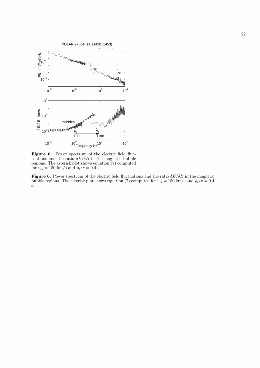
In Figure 6 we show average power spectrum of theelectric field fluctuations measured in the frequencyrange 0-104 Hz and the ratio δE/δB as a function offrequency. To make these plots we took continuous dcfield and snapshot measurements at higher frequencieswithin the bubble layers marked in Figure 1. The fre-quency spectrum is covered by three instruments. Thedc magnetic field is sampled continuously at the rate8.3 s−1, the low-frequency waveform receiver (LFWR)and high-frequency waveform receiver (HFWR) providesnapshots sampled at the rate 100 s−1, and 50,000 s−1,respectively. The plots of dc and LFWR channels over-lap completely indicating good inter-calibration. How-ever, because of the wave instrument filter character-istics the plots in Figure 6 at the transition frequencyof ∼ 50 Hz between LFWR and HFWR are not reli-able. The LFWR and HFWR snapshots are taken atdifferent locations, which can also explain the observedmismatch in the frequency spectra. Anyway, the powerspectrum and the waveforms show that the dominantmode represent broadband ELF waves 0-30 Hz with asignificant power drop above ∼30 Hz, which is near thelower hybrid range.

The asterisk curve shows equation (7) computed forvA = 150 km/s and ρi/v = 0.4 s, which is satisfied fore.g. ρi = 60 km and v = 150 km/s, 〈cos θ〉 ∼ 1. A goodagreement between approximation (7) and the measure-ments provides indirect evidence that in the frequencyrange 0-30 Hz the waves represent spatial turbulence ofDAW.

Transition from equation (5) to (7) requires knowl-edge of the angle between the convection velocity vE andthe wavevector k. Because both these vectors are ex-pected to vary significantly in time (space) we use herestatistical average of spectra which would result in anaverage value for 〈cos θ〉 and other parameters in equa-tion (7). Translation from frequency to spatial scaleλ = v/f requires the knowledge of the convective ve-locity v. For v ≈100 km/s, the frequency of 1 Hz cor-responds to λ =100 km which is on the order of iongyroradius, while 100 Hz corresponds to λ ≈ 1 km,which is about the electron inertial length. It appearsfrom Figure 6 that for scales larger than ρi waves haveδE/δB ≈ vA, while the dispersive KAW spectrum (7)extends from ρi down to λe. Above 30 Hz, or close tothe inertial electron scale, dissipative processes relatedpresumably to electron acceleration lead to the dropoutof the electric field power seen in Figure 6. The bub-ble structures correspond roughly to ∼ 0.2 Hz. It is

8

interesting to note that the ordering of scales ρi and λe

is reversed at low altitudes and DAW waves measuredon FREJA extends from λe ∼ 300 m down to ρi ∼ 20m, where they are strongly dissipated due to stochasticacceleration of ions [Stasiewicz et al., 2000b; Stasiewiczet al., 2000c].

3. Theory and simulation

The discussion on linear spectra for KAW in the pre-vious section could not address the origin of the ob-served large amplitude structures. Since the kineticAlfven wave carry a parallel and perpendicular elec-tric field they can accelerate ions and electrons along aswell as perpendicular to the magnetic field. The nonlin-ear interaction with quasi-stationary density and com-pressional magnetic field perturbations can gives rise tomodulational instability. Even the linear small ampli-tude DAW become compressional for sufficiently largek⊥. Indeed, the density fluctuations depend on thek⊥λi, where λi = vA/ωci = c/ωpi is the inertial ionlength, as [Hollweg, 1999]

δni

n0= k⊥λi

vE

vA. (8)

The above result applies both to KAW and IAW andshows that the Alfven wave becomes compressible whenperpendicular size of the structures becomes compara-ble to the inertial ion length. In our case, it is seenfrom Table I that the wave induced convective flows arecomparable to the Alfven velocity and the density per-turbations implied by (8) may be quite large, as seen inFigure 5.

The density fluctuations imply pressure fluctuationsthat drive a magnetization current, which in turn pro-duces a compressive magnetic field δBz. In the linearapproximation the density and compressional magneticfield fluctuations are related as [Hollweg, 1999]

δBz/B0

δni/n0= − c2s

v2A

, (9)

where cs is the ion sound speed. The observed valuesfor cs can be obtained from Table I as vs = vi

√Te/Ti,

i.e., they are 2-3 times smaller than vi.The parallel electric field of KAW will affect particles

which are in Landau resonance with the wave

kzvz = ω. (10)

Table I shows that both ion thermal and bulk flow ison the order of the Alfven speed. Thus, one expects

9

efficient ion heating via Landau resonance which canaccount for ion energization seen in Figure 2.

The linear theory has a limited application to thestrongly nonlinear structures seen in the measurements.We present here results from the solution of the resis-tive Hall MHD equations which are intended to modela tearing mode reconnection process leading to mag-netic bubble or island formation which are associatedwith kinetic Alfven wave fluctuations. We present thegeneral resistive Hall MHD equations then specialize tothe two-dimensional geometry that we use in the sim-ulations. The Hall instability which is related to driftAlfven waves is discussed in the context of the two-dimensional model for which it is shown that instabil-ity exists at scales smaller than the tearing mode scale.A sample simulation of high spatial resolution is pre-sented which exhibits the formation of magnetic islandsthrough the tearing mode and kinetic Alfven wave fluc-tuations through the Hall instability.

3.1. Hall MHD Model

The Hall MHD equations are:

∂tn +∇ · (nu) = 0 (11)

(∂t + u · ∇)u = −1ρ∇p +

1µ0ρ

(∇×B)×B (12)

(∂t + u · ∇) p + γp∇ · u = 0 (13)∂tB = −∇×E (14)

E+ u×B =1

µ0ne(∇×B)×B+ ηJ (15)

∇×B = µ0J (16)

where n is the number density, ρ = Mn is the massdensity, M is the mean particle mass, u is the fluidvelocity, p is the pressure, B is the magnetic field, Jis the current density, E is the electric field, η is theresistivity and γ is the adiabatic constant for which weuse γ = 2 in our simulations.

3.2. Two-dimensional dimensionless equations

The equations are nondimensionalized as follows: Thefluid velocities are normalized to the characteristic Alfvenspeed vA = B0/

√ρ0µo, mass density to the ambi-

ent mass density ρ0, length scales to a characteristiclength L and time scales to L/vA. We consider two-dimensional variations in the x−z plane where the y di-rection is ignorable. In two dimensions when expressedin term of the vector potential B = yBy − y×∇Ay theelectric field components become

Ex = uy ∂xAy + uz By −

10

ε

n

[12∂x(By)2 + ∂xAy∇2Ay

]− η∂zBy (17)

Ey = ux ∂xAy + uz ∂zAy +ε

n(∂xAy ∂zBy − ∂zAy ∂xBy)− η∇2Ay (18)

Ez = uy ∂zAy − ux By −ε

n

[12∂z(By)2 + ∂zAy∇2Ay

]+ η∂xBy, (19)

where ε = λi/L is the Hall parameter and λi = c/ωpi.The components of the momentum equation are

∂tux + (ux∂x + uz∂z)ux =

−1ρ

[∂x

(p +

12B2

y

)+ ∂xAy∇2Ay

](20)

∂tuy + (ux∂x + uz∂z)uy =1ρ

(∂xAy ∂zBy − ∂zAy ∂xBy) (21)

∂tuz + (ux∂x + uz∂z)uz =

−1ρ

[∂z

(p +

12B2

y

)+ ∂zAy∇2Ay

]. (22)

The components of Faraday’s law are

∂tAy = −Ey (23)∂tBy = ∂xEz − ∂zEx. (24)

Finally the continuity and pressure equations are

∂tρ + ∂x(ρux) + ∂z(ρuz) = 0 (25)∂tp+ ux∂xp + uz∂zp + γp (∂xux + ∂zuz) = 0. (26)

Equations (17) - (26) are the complete two-dimensionalHall MHD equations.

3.3. Hall instability

Near the magnetopause the ion temperature is largedue to the solar wind. This creates an electric field Ex

to balance ion pressure. The magnetic gradient gen-erates a cross-field current resulting in a J × B forcethat must be balanced by the pressure gradient. Thusthe equilibrium electric field is related to the magneticgradient as well as the plasma pressure which is pre-dominately the ion pressure. The resulting E × B orcurrent drift of the electrons can generate an instabil-ity. We perform a local analysis having kx = 0 of (17) -(26) assuming perturbations of the form exp[ikzz− iωt]

11

and a varying magnetic field B0z(x). To simplify theanalysis we assume incompressible perturbations andthereby neglect the fast magnetosonic wave and onlyinclude the shear dispersive Alfven wave. After consid-erable algebra we find

(ω2 − k2zv

2A)(ω − kzvB) + ω(ω2 − k2

zc2s)kzλ

2i = 0, (27)

where vB = (µ0n0e)−1∂B0z/∂x and c2s = γp0/ρ0. Equa-tion (27) has unstable roots for vB > cs and within aband limited range of wavenumbers. The local approx-imation does not allow us to consider kx = 0 since theequilibrium varies in the x direction although the sim-ulation does of course allow nonzero kx. For the ho-mogeneous case we can allow kx = 0 and we find forkzλi � 1, the dispersion relation ω2 = k2

zv2A(1 + k2ρ2

s),where k2 = k2

x + k2z , which is the kinetic Alfven wave

dispersion relation.The Hall instability has been discussed in the context

of laboratory plasma by Gordeev et al. [1994] and byMaggs and Morales [1996]. The instability given by (27)is due to the interaction between the drift mode ω =kzvB and the Alfven-ion cyclotron mode given by ω2 =k2

zv2A(1 + k2

zρ2s). The acoustic speed is stabilizing and

the threshold condition is vB > cs. A local analysiscan be misleading in a sheared magnetic field such aswe consider here. This is because the shear limits thex extent of the mode thereby significantly altering thestability properties. A nonlocal analysis is required toobtain quantitative estimates of the growth rate. Thatanalysis is beyond the scope of the present paper andwill be deferred to a future publication.

3.4. Simulation results

We present the results of one simulation to show themagnetic bubble structure and the fluctuations associ-ated with the Hall instability. The simulation is notintended to reproduce the observations in any detailbut only to show that with reasonable initial conditionsspontaneous reconnection in the form of a tearing modewill result and that instability associated with the largegradients of the bubble boundary will arise from theHall instability. This should be considered in compar-ing the simulation results to the data.

The simulation code is based upon the Fourier spec-tral method and is similar to that described in Seyler[1990]. The equations are solved in dimensionless formwith the following non-dimensional tilded variables: t =tL/vA, x = x/L, u = u/vA, B = B/B0, P = P/P0,and ρ = ρ/ρ0, where L is the characteristic scale of theequilibrium. From these one can revert from simula-tion to physical units. The simulation dimensions are

12

−π < x ≤ π and −2π < z ≤ 2π. The Hall parameter isε = 0.026. The number of grid points used are 128 in xand 256 in z. The time step is ∆t = 0.0025. The ini-tial equilibrium is of the form Jy(x) = J0 sech(−ax2),where J0 = 8 and a = 4π. The dimensionless resistivityis η = 0.002. The dimensionless current layer width awas chosen to produce an tearing mode unstable cur-rent layer that grows to form fully developed bubbles ina time comparable to the Hall instability growth time. Fig 7

The current density is shown in Figure 7. The mag-netic bubbles are the two magnetic islands formed bythe tearing mode. The kinetic Alfven wave fluctuationsare readily apparent. The contour plot of By(x, z) isshown in Figure 8. This plot clearly shows the vorticesassociated with the flow due to the Hall instability. Thefluctuations due to the Hall instability are concentratedon the bubble boundaries since that is where the mag-netic field gradient is largest. Figures 1 and 4 also showthat magnetic fluctuations are enhanced near the bub-ble boundaries. This is consistent with the interpre-tation that the fluctuations are the result of the Hallinstability which is driven by the magnetic gradient. Fig 8

The plots shown in Figures 9 and 10 are taken alongz at 4 grid points to the right of the centerline of thesimulation region. They show the relative level of varia-tion of the magnetic field, pressure and density. Figure Fig 99 shows the magnetic bubble from the perspective of aone-point satellite measurement and can be comparedto Figure 4 (of the observational section). The bestcomparison is obtained when the simulation Bx is com-pared to the POLAR observed By and when the simu-lation z coordinate has a significant component in thePOLAR x direction. Given that the POLAR GSM co-ordinates, (x, y, z) = (2.8, 1.5, 8.0)RE correspond to alocation over the cusp where the geomagnetic field has asignificant x component, this correspondence is reason-able if one recalls that the simulation coordinates areappropriate to the nose of the magnetopause locatedat approximately (x, y, z) = (10, 0, 0)RE . We shouldmention here that the real boundary layer is subject toboth rapid radial motion (oscillations in the simulationx direction) and convective flows along the boundary.In effect, the satellite trajectory corresponds to a mean-dering motion through the simulation region and can-not be directly compared to a single straight line cutthrough the region. Fig 10

Figure 10 shows that the region inside the magneticbubble or island is significantly hotter than the outsideregion. This is due to the fact that the initial pressure atx = 0 must be larger to create pressure balance with theequilibrium magnetic field. Since we chose the initial

13

density to be constant, this implies the temperature ishottest initially at x = 0. The evolution of the pressureis such that the temperature is hottest in the centerof the magnetic island. This is not surprising since thetearing mode evolves quasi-statically in that the growthtime is much less that the Alfven time. Therefore quasi-static pressure balance requires that the pressure hasa maximum where the magnetic field magnitude is aminimum. Thus the increase of the plasma pressure isdue to the compensation the magnetic field depression,so that the total pressure is approximately constant.

The tearing mode instability has been discussed bynumerous authors the list of which is too extensive togive here. Much of the relevant literature is referencedin the review article byWhite [1986]. The tearing modeis spontaneous reconnection that lowers the magneticenergy of the initial equilibrium state. The formationof magnetic islands is characteristic of the tearing mode.A magnetic island is a region of closed contours of thevector potential which typically has a lower field at thecenter of the island. Magnetic islands form as the re-sult of the reconnection flow in which the plasma isadvected towards the separatrix by the inflow and ex-hausted into the region inside the separatrix by the out-flow jets thereby filling the region inside the separatrixwith plasma and forming a magnetic bubble. The mag-netic energy is lowered and converted into kinetic energyin this process. The amount the initial magnetic en-ergy is lowered depends considerably upon the plasmaparameters and the initial conditions, but about 10%is typical [Steinholfson and Van Hoven, 1984]. Theredistribution of the magnetic energy density can varygreatly between the outside and inside regions of theisland. The POLAR observation of more than 90% isnot unreasonable and is close to what was found in thesimulation.

4. Discussion and Conclusions

A detailed analysis of electromagnetic and plasmaproperties of magnetic holes observed in the vicinityof the magnetopause layer supplemented by a numeri-cal simulation show that these are most likely related totearing mode instability which develops strongly nonlin-ear structures on the scale of the current layer width.

We have demonstrated that the δE/δB ratio for largescale features is close to the Alfven velocity, indicatingthat these can be regarded as nonlinear Alfven wavestructures, probably related to the evolution of the tear-ing mode instability. For smaller scale structures thisratio gradually increases and it is well represented bythe dispersion relation for KAWs (see Figure 6). Thus,

14

the measurements suggest that broadband waves ob-served at the magnetopause layer in the frequency range0.1-30 Hz represent most likely spatial turbulence ofnonlinear and dispersive Alfven waves (λ⊥ ≈ 1500 − 5km and ω � 1 Hz), which are Doppler shifted to the ob-served frequencies by convective plasma flows vE ∼ 150km/s.

The numerical simulation indicates that the smallscale KAW may be generated through the Hall instabil-ity on the macroscopic pressure and magnetic field gra-dients produced by the tearing mode driven by strongmagnetopause currents. The presented particle mea-surements indicate that both ions and electron are en-ergized to about twice their initial energy inside themagnetopause bubble layer. The particle energizationcould be related to kinetic Alfven waves which cover thespatial scales ranging from λi, ρi down to λe and thuscan interact and energize both with ions and electrons.The magnetic fluctuation are likely due to a drift-Alfventype instability. We have only presented a limited anal-ysis and more work is necessary to have complete un-derstanding of the fluctuations. The simulation modelis limited to two-dimensions. This in itself restricts thepossible types of instabilities. Since the current due toreconnection is in the ignorable direction of the sim-ulation, these instabilities would not accounted for inthe model. To include these would require a three di-mensional model. The solution of a three-dimensionalmodel at the required resolution is beyond our capabil-ities at this point in time. A linear stability analysis,however is tractable and will be reported upon in a fu-ture paper.

The existence of a guide magnetic field componentis inevitable near the magnetopause if the solar windmagnetic field is not strictly north or south. Our 2Dsimulations consider the y direction as the ignorablecoordinate and the magnetic islands lie in the x − zplane. In a recent paper Hau and Sonnerup [1999] ana-lyze AMPTE/IRM data using a technique for recover-ing magnetic field maps from insitu data. Of the fourevents they study, one has a magnetic island geometryin which the ignorable coordinate is along the GSM zdirection and the other three have the GSM y directionas ignorable. The results of Hau and Sonnerup [1999]appear to support our contention that magnetic bubblesare magnetic islands due to tearing modes.

The processes discussed in this paper involve trans-formations of considerable amount of energy betweenthe magnetic, electric fields and particles (thermal andtranslational). For example we observe a reduction of98% of the magnetic energy inside some bubbles. Con-

15

sequently, full understanding of the processes discussedin this paper is of fundamental importance for the en-ergetics of the solar wind - magnetosphere coupling.

Acknowledgments. The authors would like to thankC. Kletzing for providing the HYDRA data and principalinvestigators: D. Gurnett, C. T. Russell and J. Scudder formaking available the field and plasma measurements. Thework of C. E. Seyler was supported by National ScienceFoundation Grant ATM 9819661 and NASA grant NAG5-4464. Work of F.S. Mozer was partly supported by NASAgrant FDNAG5-8078 and B.Popielawska was supported byKBN grant 2.P03C.004.13.

References

Alfven, H., Existence of electromagnetic-hydromagneticwaves, Nature, 150, 405–406, 1942.

Baumgartel, K., Soliton approach to magnetic holes, J.Geophys. Res., 104, 28295, 1999.

Crooker, N. U., and G. L. Siscoe, A mechanism of pressureanisotropy and mirror instability in the dayside magne-tosheath, J. Geophys. Res., 82, 185-186, 1977.

Denton, R. E., B. J. Anderson, S. P. Gary, and S. A. Fuselier,Bounded anisotropy fluid model for ion temperatures, J.Geophys. Res., 99, 11,225-11,241, 1994.

Erdos, G., and A. Balogh, Statistical properties of mir-ror mode structures observed by Ulysses in the magne-tosheath of Jupiter, J. Geophys. Res., 101, 1–12, 1996.

Escoubet, C. P., A. Pedersen, R. Schmidt, and P. A.Lindqvist, Density in the magnetosphere inferred fromISEE 1 spacecraft potential, J. Geophys. Res., 102,17,595, 1997.

Fazakerley, A. N. and D. J. Southwood, Mirror instability inthe magnetosheath, Adv. Space Res., 14, (7)65-68, 1994.

Fuselier, S. A., K. J. Trattner, and S. M. Petrinec, Cuspobservations of high- and low-latitude reconnection fornorthward IMF, J. Geophys. Res., 105, 253-266, 2000.

Goertz, C. K., and R. W. Boswell, Magnetosphere-ionosphere coupling, J. Geophys. Res., 84, 7239–7246,1979.

Gordeev, A. V., A. S. Kinsep, and L. I. Rudakov, Electronmagnetohydrodynamics, Phys. Rep., 243, 215–315, 1994.

Gosling, J. T., M. F. Thomsen, S. J. Bame, R. C. Elphic,and C. T. Russell, Observations of reconnection of in-terplanetary and lobe magnetic field at the high-latitudemagnetopause, J. Geophys. Res., 96, 14,097-14,106, 1991.

Hasegawa, A., Drift mirror instability in the magnetosphere,Phys. Fluids., 12, 2642-2650, 1969.

Hasegawa, A., Particle acceleration by MHD surface waveand formation of aurora, J. Geophys. Res., 81, 5083–5090,1976.

Hau, L.-N. and B. U. O. Sonnerup, Two-dimensional coher-ent structures in the magnetopause: Recovery of staticequilibria from single-spacecraft data, J. Geophys. Res.,104, 6900–6917, 1999.

Hollweg, J. V., Kinetic Alfven wave revisited, J. Geophys.Res., 104, 14,811, 1999.

Kaufmann, R., J. T. Horng, and A. Wolfe, Large ampli-tude hydromagnetic waves in the inner magnetosheath,J. Geophys. Res., 75, 4666, 1970.

16

Kivelson, M. G. and D. J. Southwood, Mirror instabilityII: The mechanism of non-linear saturation, J. Geophys.Res., 101, 17,365-17,371, 1996.

Le, G., J. Raeder, C. T. Russell, G. Lu, S. M. Petrinec, andF. S. Mozer, Polar cusp and vicinity under strongly north-ward IMF on April 11, 1997: Observations and MHD sim-ulations, J. Geophys. Res., xx, in press, 2000.

Lucek, E. A., M. W. Dunlop, A. Balogh, P. Cargill, W.Baumjohann, E. Georgescu, G. Haerendel, and K.-H. For-nacon, Identification of mirror mode structures in theEquator-S magnetic field data, Ann. Geophysicae, 17,1560-1573, 1999.

Luhr, H., and N. Klocker, AMPTE IRM observations ofmagnetic cavities near the magnetopause, Geophys. Res.Lett., 14, 186, 1987.

Maggs, J. E., and G. J. Morales, Magnetic fluctuations as-sociated with field-aligned striations, Geophys. Res. Lett.,23, 633, 1996.

Russell, C. T., G. Le, and S. M. Petrinec, Cusp observa-tions of high- and low-latitude reconnection for northwardIMF: An alternate view, J. Geophys. Res., 105, 5489-5495,2000.

Savin, S. P., et al., The cusp/magnetosheath interface onMay 29, 1996: Interball-1 and Polar observations, Geo-phys. Res. Lett., 25, 2963, 1998.

Schwartz, S. J., D. Burgess, and J. J. Moses, Low-frequencywaves in the magnetosheath: present status, Ann. Geo-physicae, 14, 1134-1150, 1996.

Seyler, C. E., A mathematical model of the structure andevolution of small-scale discrete auroral arcs, J. Geophys.Res., 95, 17199, 1990.

Southwood, D. J., and M. G. Kivelson, Mirror instability 1,the physical mechanism of linear instability, J. Geophys.Res., 98, 9181, 1993.

Stasiewicz, K., P. Bellan, C. Chaston, C. Kletzing, R. Lysak,J. Maggs, O. Pokhotelov, C. Seyler, P. Shukla, L. Stenflo,A. Streltsov, and J.-E. Wahlund, Small scale Alfvenicstructure in the aurora, Space Sci. Rev., 92, 423-533,2000a.

Stasiewicz, K., Y. Khotyaintsev, M. Berthomier, and J.-E.Wahlund, Identification of widespread turbulence of dis-persive Alfven waves, Geophys. Res. Lett., 27, 173, 2000b.

Stasiewicz, K., R. Lundin, and G. Marklund, Stochastic ionheating by orbit chaotization on electrostatic waves andnonlinear structures, Phys. Scripta, T84, 60, 2000c.

Steinholfson R. S. and G. V. Van Hoven, Nonlinear Evo-lution of the Resistive Tearing Mode, Phys. Fluids, 27,1207, 1984.

Treumann, R., L. Brostrom, J. LaBelle, and N. Scopke, Theplasma wave signature of a magnetic hole in the vicinityof the magnetopause, J. Geophys. Res., 95, 19,099, 1990.

Tsurutani, B. T., E. J. Smith, R. R. Anderson, K. W.Ogilvie, J. D. Scudder, D. N. Baker, and S. J. Bame,Lion roars and nonoscillatory drift mirror waves in themagnetosheath, J. Geophys. Res., 87, 6060, 1982.

Tsurutani, B. T., D. J. Southwood, E. J. Smith, andA. Balogh, A survey of low frequency waves at Jupiter:The Ulysses encounter, J. Geophys. Res., 98, 21,203-21,216, 1993.

Tsurutani, B. T., G. S. Lakhina, D. Winterhalter, J. Arballo,G. Galvan, and R. Sukurai, Energetic particle cross-fielddiffusion: Interactions with magnetic decreases, Nonlin-

17

ear Proc. in Geophys., 6, 235, 1999.Turner, J. M., L. F. Burlaga, N. F. Ness, and J. F. Lemaire,

Magnetic holes in the solar wind, J. Geophys. Res., 82,1921, 1977.

White, R. B., Resistive Reconnection, Rev. Mod. Phys., 58,183, 1986.

Winterhalter, D., M. Neugebauer, B. E. Goldstein, E. J.Smith, S. J. Bame, and A. Balogh, Ulysses field andplasma observations of magnetic holes in the solar windand their relation to mirror-mode structures, J. Geophys.Res., 99, 23,371, 1994.

Winterhalter, D., E. J. Smith, M. Neugebauer, B. E. Gold-stein, B. T. Tsurutani, The latitudinal distribution ofsolar wind magnetic holes, Geophys. Res. Lett., 27, 1615-1618, 2000.

G. Gustafsson and K. Stasiewicz, Swedish Institute ofSpace Physics, Box 537, 75121 Uppsala, Sweden. (e-mail:gg@irfu.se, ks@irfu.se)

F. S. Mozer, Physics Department and Space Sciences Lab-oratory, University of California, Berkeley, CA. 94720 (e-mail: fmozer@ssl.berkeley.edu)

J. S. Pickett, Department of Physics and Astronomy, TheUniversity of Iowa, Iowa City, IA 52242, (e-mail: pick-ett@uiowa.edu)

B. Popielawska, Space Research Centre, Bartycka 18A,00-716 Warsaw, Poland (e-mail: bpop@cbk.waw.pl)

C. E. Seyler, School of Electrical Engineer-ing, Cornell University, Ithaca, NY 14853, (e-mail:seyler@ee.cornell.edu)

(Received July 2000; revised 2000;accepted March 2000.)

Copyright 2001 by the American Geophysical Union.

Paper number ................

Table 1. Plasma parameters in three regions of Figure 2. Parameters not defined in text are:λi = c/ωpi, fce electron gyrofrequency, fpi, fci ion (proton) plasma and gyro-frequency, fLH lower-hybrid frequency.

n B Te Ti vE vi vA λe ρi λi β fci fLH fpi

cm−3 nT eV eV km/s km/s km/s km km km Hz Hz kHzSheath 25 100 20 150 100 150 400 1 20 50 0.1 1.4 65 1Bubble 15 50 50 400 200 300 200 1 80 60 1 0.7 32 1Sphere 0.2 110 80 800 50 400 5000 10 40 500 10−3 1.5 60 0.1

18

0 10 20 30 40 50 60

−50

0

50

Bx

nT

0 10 20 30 40 50 60−80

−40

0

40

By

nT

0 10 20 30 40 50 60−100

0

100

Bz

nT

0 10 20 30 40 50 600

50

100

150

B n

T

0 10 20 30 40 50 600

100

200

300

VE k

m/s

MS MS

POLAR 97−04−11 Time [min] from 1400 UT

Figure 1. Magnetopause crossings on 11 April 1997.Three component magnetic field Bx, By, Bz in GSM co-ordinates, |B| and the convection speed vE .

Figure 1. Magnetopause crossings on 11 April 1997. Three component magnetic field Bx, By, Bz

in GSM coordinates, |B| and the convection speed vE .

Figure 2. Particle distributions measured during theanalyzed event. Three electron and three ion panelsshow particle fluxes along the magnetic field, perpen-dicular, and antiparallel to B. The magnetosheath andbubble layers are marked with MS and B, respectively.

Figure 2. Particle distributions measured during the analyzed event. Three electron and threeion panels show particle fluxes along the magnetic field, perpendicular, and antiparallel to B.The magnetosheath and bubble layers are marked with MS and B, respectively.

20

0 10 20 30 40 50 600

0.2

0.4

0.6

0.8

1

1.2

Time [min] from 1400 UT

arb.

uni

ts

mirror−mode instability threshold

Figure 3. The mirror-mode instability condition (1)derived from particle measurements. The plasma ismirror-mode stable in all regions: the magnetosheath,bubble layer and the magnetosphere.

Figure 3. The mirror-mode instability condition (1) derived from particle measurements. Theplasma is mirror-mode stable in all regions: the magnetosheath, bubble layer and the magneto-sphere.

30 31 32 33 34 35 36

−100

0

100

Bz n

T

30 31 32 33 34 35 360

50

100

B n

T

30 31 32 33 34 35 3610

−2

100

n e cm

−3

30 31 32 33 34 35 3610

2

103

104

v A k

m/s

magneto−sphere

bubble layer

magneto−sheath

MP

Alfvén resonator

POLAR 97−04−11 min from 1400 UT

21

Figure 4. Details of a bubble layer: magnetic field Bz

and B, the electron density ne, and the Alfven velocityvA.

Figure 4. Details of a bubble layer: magnetic field Bz and B, the electron density ne, and theAlfven velocity vA.

31.5 32 32.5 33−100

−50

0

50

Bz

nT

31.5 32 32.5 33−20

0

20

Ey

mV

/m

31.5 32 32.5 330

50

100

B n

T

31.5 32 32.5 330

5

10

15

ne c

m−

3

POLAR 97−04−11 [min] from 1400 UT

Figure 5. High degree of correlation between perpen-dicular components of Bz and Ey with δEy/δBz ≈ 200km/s ≈ vA indicates Alfvenic structures. The bottompanel shows the electron density derived from the satel-lite potential (solid line) and from particle measure-ments (asterisk)

Figure 5. High degree of correlation between perpendicular components of Bz and Ey withδEy/δBz ≈ 200 km/s ≈ vA indicates Alfvenic structures. The bottom panel shows the electrondensity derived from the satellite potential (solid line) and from particle measurements (asterisk)

22

10−2

100

102

104

10−5

100

POLAR 97−04−11 (1430−1453)P

E (

mV

/m)2 /H

z

10−2

100

102

104

102

104

106

δ E

/δ B

km

/s

Frequency Hz

fce

100 1 km

ρi λ

e

bubbles

Figure 6. Power spectrum of the electric field fluc-tuations and the ratio δE/δB in the magnetic bubbleregions. The asterisk plot shows equation (7) computedfor vA = 150 km/s and ρi/v = 0.4 s.

Figure 6. Power spectrum of the electric field fluctuations and the ratio δE/δB in the magneticbubble regions. The asterisk plot shows equation (7) computed for vA = 150 km/s and ρi/v = 0.4s.

23

Current Density

x

z

Figure 7. Current density contours taken at time100 showing the region of most intense current whichbounds the magnetic bubble/island region.

Figure 7. Current density contours taken at time 100 showing the region of most intense currentwhich bounds the magnetic bubble/island region.

24

By

x

z

Figure 8. Contour plot of the By magnetic field at time100 showing the fluctuations due to the drift-Alfvenmode which is also an indication of the electron flow.

Figure 8. Contour plot of the By magnetic field at time 100 showing the fluctuations due to thedrift-Alfven mode which is also an indication of the electron flow.

25

−2 0 2−1

−0.5

0

0.5

1

1.5

2

2.5

z

Bz(z

) (s

olid

), B

x(z)

(das

h) &

By(z

) (d

ot)

Magnetic Field Components

Figure 9. Magnetic field components at time 100 takenalong z at a point in x four grid points to the right ofthe centerline of the simulation. The magnetic bubbleregion is clearly revealed as the region of minimum Bz.The fluctuations in the field are due to the drift-Alfveninstability.

Figure 9. Magnetic field components at time 100 taken along z at a point in x four grid pointsto the right of the centerline of the simulation. The magnetic bubble region is clearly revealed asthe region of minimum Bz. The fluctuations in the field are due to the drift-Alfven instability.

26

−2 0 20

0.5

1

1.5

2

2.5

3

3.5

4

z

p(z)

(so

lid)

& n

(z)

(das

h)Pressure and Density

Figure 10. Pressure and density at the same time andlocation as in figure 9. The region of highest pressurecorresponds to the region within the magnetic bubbleand is where the temperature is maximum.

Figure 10. Pressure and density at the same time and location as in figure 9. The region of high-est pressure corresponds to the region within the magnetic bubble and is where the temperatureis maximum.