Embed Size (px)
Citation preview
HAL Id: tel-03698474https://tel.archives-ouvertes.fr/tel-03698474
Submitted on 18 Jun 2022
HAL is a multi-disciplinary open accessarchive for the deposit and dissemination of sci-entific research documents, whether they are pub-lished or not. The documents may come fromteaching and research institutions in France orabroad, or from public or private research centers.
L’archive ouverte pluridisciplinaire HAL, estdestinée au dépôt et à la diffusion de documentsscientifiques de niveau recherche, publiés ou non,émanant des établissements d’enseignement et derecherche français ou étrangers, des laboratoirespublics ou privés.
Machine learning for performance modelling on colossalsoftware configuration spaces
Hugo Martin
To cite this version:Hugo Martin. Machine learning for performance modelling on colossal software configuration spaces.Artificial Intelligence [cs.AI]. Université Rennes 1, 2021. English. �NNT : 2021REN1S117�. �tel-03698474�
THÈSE DE DOCTORAT DE
L’UNIVERSITÉ DE RENNES 1
ÉCOLE DOCTORALE NO 601Mathématiques et Sciences et Technologiesde l’Information et de la CommunicationSpécialité : « Informatique »
Par
Hugo MARTINMachine Learning for Performance Modelling on Colossal Soft-ware Configuration Spaces
Thèse présentée et soutenue à Rennes, le 16 Décembre 2021Unité de recherche : Equipe DiverSE, IRISA
Rapporteurs avant soutenance :
Laurence DUCHIEN Professeur à l’Université de LillesJulia LAWALL Directrice de Rercherche à INRIA - Paris
Composition du Jury :Attention, en cas d’absence d’un des membres du Jury le jour de la soutenance, la composition du jury doit être revuepour s’assurer qu’elle est conforme et devra être répercutée sur la couverture de thèse
Président : Isabelle PUAUT Professeur à l’Université de Rennes 1Examinateurs : Laurence DUCHIEN Professeur à l’Université de Lille
Julia LAWALL Directrice de Recherche à INRIA - ParisIsabelle PUAUT Professeur à l’Université de Rennes 1Klaus Schmid Professeur à l’Université de Hildesheim
Dir. de thèse : Mathieu ACHER Professeur à l’Université de Rennes 1Co-dir. de thèse : Jean-Marc JEZEQUEL Professeur à l’Université de Rennes 1


RÉSUMÉ EN FRANÇAIS
Presque tous les systèmes logiciels d’aujourd’hui sont configurables. A l’aide d’options,il est possible de modifier le comportement de ces systèmes, d’ajouter ou d’enlever cer-taines capacités pour améliorer leurs performances ou les adapter à différentes situations.Chacune de ces options est liée à certains parties de code, et s’assurer du bon fonction-nement de ces parties entre elles, ou de les empêcher d’être utilisées ensemble, est un desdéfis durant le développement et l’utilisation de ces logiciels, connus sous le nom de Lignesde Produits Logiciel (ou SPL pour Software Product Lines). Si cela peut sembler rela-tivement simple avec quelques options, certains logiciels assemblent des milliers d’optionsréparties sur des millions de lignes de code, ce qui rend la tâche autrement plus complexe.
Durant la dernière décennie, les chercheurs ont commencé a utiliser des techniquesd’apprentissage automatique afin de répondre aux problématiques des Lignes de ProduitsLogiciels. Un des problèmes clés est la prédiction des différentes propriétés de ces logiciels,comme la vitesse d’exécution d’une tâche, qui peut fortement varier selon la configurationdu logiciel utilisé. Mesurer les propriétés pour chaque configuration peut être coûteuxet complexe, voire impossible dans les cas les plus extrêmes. La création d’un modèlepermttant de prédire les propriétés du logiciel, en s’aidant des mesures sur seulementd’une faible partie des configurations possible est une tâche dans laquelle l’apprentissageautomatique excelle.
Différentes solutions ont été developées, mais elles n’ont été validées que dans descas où le nombre d’options est assez faible. Or, une part importante des SPL sontdotés de plusieurs centaines voire plusieurs milliers d’options. Sans tester les solutionsd’apprentissage automatique sur des logiciels avec autant d’options, il est impossible desavoir si ces solutions sont adaptées pour de tels cas.
La première contribution de cette thèse est l’application d’algorithmes d’apprentissageautomatique sur une ligne de produits logiciels à une échelle jamais atteinte auparavant.Le noyau Linux, avec ses 15.000 options, dépasse complètement toutes les études de cassur les Lignes de Produits Logiciels présentes dans la littérature, qui n’ont utilisé que descas d’au mieux 60 options. En évaluant la précision de plusieurs algorithmes de l’état del’art pour prédire la taille binaire du noyau Linux, nous avons pu déterminer les limites de
3

certaines techniques. Sans surprise, les algorithmes linéaires donnent de mauvais résultatsen termes de précision, car ils ne peuvent pas appréhender la complexité causée par lesinteractions entre les options. Le modèle de performance-influence, bien que développéspécifiquement pour les SPL, ne peut pas gérer autant d’options malgré les mesures prisespour réduire l’explosion combinatoire. En fin de compte, nous avons constaté que lesalgorithmes basés sur les arbres, ainsi que les réseaux de neurones, étaient capables defournir un modèle assez précis avec des ressources raisonnables en termes de temps et demémoire.
La deuxième contribution est la Feature Ranking List, une liste des options classéespar importance envers leur impact sur une propriété cible d’un logiciel, générée par uneamélioration de la sélection des caractéristiques basée sur les arbres de décisions. Nousavons évalué ses effets sur les modèles de prédiction de la taille des binaires du noyauLinux dans les mêmes conditions que pour la première contribution. L’effet souhaité et leplus connu de la sélection de caractéristiques en général est une accélération majeure dutemps d’apprentissage, le divisant par 5 pour les Gradient Boosting Trees et de 20 pour lesRandom Forests. De manière plus inattendue, nous constatons également une améliorationnotable de la précision pour la plupart des algorithmes précédemment considérés. LaFeature Ranking List est lisible par l’homme, et lorsqu’elle a été présentée à des experts,elle a été jugée assez juste. Cependant, il y a une grande divergence lorsqu’on la confronte àla documentation, principalement en raison du très faible nombre d’options explicitementdocumentées comme ayant un impact sur la taille du noyau Linux.
La troisième contribution est l’amélioration de la spécialisation automatisée des per-formances et son évaluation sur différents SPL dont Linux. La spécialisation des perfor-mances est un processus qui consiste à ajouter des contraintes sur un SPL afin de répondreà un certain seuil de performance défini par l’utilisateur, pour l’aider lors de la configu-ration du logiciel. Il est possible d’automatiser ce processus en utilisant l’apprentissageautomatique, et plus précisément des arbres de décisions classifieurs qui prédisent si uneconfiguration est acceptable ou non par rapport au seuil de performance, à partir desquelsnous pouvons extraire des règles, ensuite appliquées comme contraintes sur la SPL cible.Les améliorations portent sur deux aspects. Le premier est l’application de la sélectiondes options basée sur la Feature Ranking List, qui a permis d’améliorer à la fois la pré-cision et le temps d’apprentissage, même sur des SPL avec seulement quelques options.La seconde est la prise en compte des arbres de décisions régresseurs, qui produisent unmodèle similaire pour l’extraction de règles, mais avec l’avantage d’être conscient de la
4

performance, alors que cette dimension est réduite à un simple booléen dans un processusde classification. Nous avons développé une nouvelle technique, basée sur les arbres dedécisions régresseurs, où nous simulons un écart dans la distribution de la performancepour rendre l’algorithme conscient du seuil en ce qui concerne la fonction de perte. Enfin de compte, les trois techniques ont leurs propres forces et faiblesses, avec leurs proprescas d’utilisation, et doivent être considérées comme complémentaires.
La dernière contribution ouvre la porte à une utilisation plus durable de l’apprentissageautomatique pour les lignes de produits logiciels. Dans ce domaine, peu voire aucune at-tention n’a été accordée à la précision des modèles sur différentes versions d’un SPL. Nousavons donc pris un modèle très précis issu des travaux de notre deuxième contribution,l’avons évalué sur des versions ultérieures et avons observé deux problèmes majeurs. Lepremier est la différence d’options, car entre deux versions, certaines options apparaissentet d’autres disparaissent, créant un décalage dans l’espace de configuration. Le secondest la baisse de précision lorsque le modèle est utilisé sur une autre version que celle surlaquelle il a été entraîné. Le coût pour entraîner le premier modèle était très important, entermes de mesures de configuration et d’efforts d’entraînement, et une telle dépense n’estpas raisonnable lorsque l’on considère une nouvelle version tous les deux ou trois mois.Pour résoudre ces deux problèmes, nous avons créé Evolution-Aware Model Shifting, unetechnique d’apprentissage par transfert adaptée à l’échelle et au rythme d’évolution dunoyau Linux. Elle exploite le modèle original mais déprécié et, pour une fraction du coûtinitial, l’adapte aux nouvelles versions. Nos résultats montrent une très bonne précisionsur trois ans d’évolution, et une meilleure précision que l’apprentissage à partir de zérosur le même ensemble de données.
5

ABSTRACT
Variability is the blessing and the curse of today software development. On one hand,it allows for fast and cheap development, while offering efficient customization to preciselymeet the needs of a user. On the other hand, the increase in complexity of the systems dueto the sheer amount of possible configurations makes it hard or even impossible for usersto correctly utilize them, for developers to properly test them, or for experts to preciselygrasp their functioning.
Machine Learning is a research domain that grew in accessibility and variety of usagesover the last decades. It attracted interest from researchers from the Software Engineeringdomain for its ability to handle the complexity of Software Product Lines on problemsthey were tackling such as performance prediction or optimization. However, all studiespresenting learning-based solutions in the SPL domain failed to explore the scalability oftheir techniques on systems with colossal configuration space (> 1000 options).
In this thesis, we focus on the Linux Kernel. With more than 15.000 options, it is veryrepresentative of the complexity of systems with colossal configuration spaces. We firstapply various learning techniques to predict the kernel binary size, and report that mostof the techniques fail to produce accurate results. In particular, performance-influencemodel, a learning technique tailored for SPL problem, does not even work on such largedataset. Among the tested techniques, only Tree-based algorithms and Neural Networksare able to produce an accurate model in an acceptable time.
To mitigate the problems created by colossal configuration spaces on learning tech-niques, we propose a feature selection technique leveraging Random Forest, enhancedtoward better stability. We show that by using the feature selection, the training timecan be greatly reduced, and the accuracy can be improved. This Tree-based feature selec-tion technique is also completely automated and does not rely on prior knowledge on thesystem.
Performance specialization is a technique that constrains the configuration space ofa software system to meet a given performance criterion. It is possible to automate thespecialization process by leveraging Decision Trees. While only Decision Tree Classifierhas been used for this task, we explore the usage of Decision Tree Regressor, as well as a
7

novel hybrid approach. We test and compare the different approaches on a wide range ofsystems, as well as on Linux to ensure the scalability on colossal configuration spaces. Inmost cases, including Linux, we report at least 90% accuracy, and each approach havingtheir own particular strength compared to the others. At last, we also leverage the Tree-based feature selection, whose most notorious effect is the reduction of the training timeof Decision Trees on Linux, downing from one minute to a second or less.
The last contribution explores the sustainability of a performance model across ver-sions of a configurable system. We reused the model trained on the 4.13 version of Linuxfrom our first contribution, and measured its accuracy on six later versions up to 5.8,spanning over three years. We show that a model is quickly outdated and unusable asis. To preserve the accuracy of the model over versions, we use transfer learning withthe help of Tree-based algorithms to maintain it at a reduced cost. We tackle the prob-lem of heterogeneity of the configuration space, that is evolving with each version. Weshow that the transfer approach allows for an acceptable accuracy at low cost, and vastlyoutperforms a learning from scratch approach using the same budget.
Overall, this thesis focuses on the problems of systems with colossal configurationspaces such as Linux, and show that Tree-based algorithms are a valid solution, versatileenough to answer a wide range of problem, and accurate enough to be considered.
8

ACKNOWLEDGEMENT
My first thank go to you, reader, as a big lesson I learned during this thesis, is thatscience is valuable only if it is passed to others, and reading this thesis is as much importantas writing it.
I want to thank The University of Rennes 1 and all the professors for their teachingall along my 9 years of studies. In particular, Professor Rumen Andonov, you deserve aspecial place in my thoughts, as your decision to welcome that kind of lost student onthat first day of L3 leads to this thesis. Thank you for the trust you placed in me thatday.
Thanks to the jury members who accepted to read this thesis and review the worksdescribed in it. The feedback I received has been used, to my great pleasure, to improvethe manuscript which is, in my humble opinion, far better now than when I send it toreview.
Thanks to all master students who worked on the TuxML project, which have beenfundamental for the works realized in this thesis.
Paul, you guided me on my first steps toward machine learning and always ensured Ihad all I needed, even when I did not ask while needing it, thank you.
Juliana, you scientific excellence impressed me, and I have been very please to be giventhe opportunity to work with you on many projects during your postdoc.
Luc, we shared a lot in the last few years at DiverSE, and your expertise in statisticshelped a lot in going further in this thesis. Our discussions, about research or other topics,have always been a great pleasure and very enriching.
To all the members of the DiverSE team, too many to be all cited, you are all in mythoughts as you all marked me. I loved belonging to this group, in this constant sharingof knowledge, spanning of many domains, a true melting pot of reflection where curiositymakes science.
Mathieu, this internship you offered me opened a new path for that I thought un-reachable, and this changed my life forever. Your enthusiasm is a true driving force foranyone working with you, never let that go!
Jean-Marc, you scientific skills have been recognized many times in many ways, but
9

what impressed me the most was the degree you have been accessible to me during thisthesis. We can feel your great experience of science through your concise and highlyrelevant critics, which were able to focus Mathieu’s catching enthusiasm.
Thank you both for being an incredible duo of supervisors.Jérôme, I follow you path a little by default, and if I forked to my own path, thank
you for having been a model to follow.Maman, you always bend over backward to offer your two big boys everything they
needed, you can be proud of the result.Pap, you offered us, Jérôme and me, the education you could never access, and you
passed on us everything we needed to get the best out of it. Even if you will not be ableto assist to the completion of this thesis, know that it is dedicated to you. Thank you foreverything.
10

REMERCIEMENTS
Mes premiers remerciements vont à vous, lecteur, car une grande leçon que j’ai tiréede cette thèse, est que la science n’a de valeur que si elle est transmise, et que lire cettethèse est aussi important que de l’écrire.
Je tiens à remercier l’Université de Rennes 1 et tous les professeurs pour leurs en-seignements pendant mes 9 années d’études. En particulier, Professeur Rumen Andonov,vous méritez une place importante dans mes pensées, car de votre décision d’accueillircet étudiant un peu perdu en ce jour de rentrée en L3 découle cette thèse. Merci de laconfiance que vous m’avez accordée ce jour-là.
Merci aux membres du jury qui ont accepté de lire cette thèse et d’évaluer les travauxqui la composent. Les retours que j’ai eu ont servi à mon grand plaisir à améliorer lemanuscrit qui est, à mon humble opinion, d’une bien meilleure qualité que quand il leura été transmis.
Merci à tous les étudiants de master qui ont participé au projet TuxML, qui a étéfondamental pour les études développées dans cette thèse.
Paul, tu m’as accompagné dans mes premiers pas vers le machine learning et t’estoujours assuré que j’avais ce dont j’avais besoin pour avancer, même quand je ne ledemandais alors que j’en avais besoin, je t’en remercie.
Juliana, ton excellence scientifique m’a impressionné, et j’ai été très heureux de pouvoirtravailler avec toi sur les nombreux projets au cours de ton postdoc.
Luc, on a beaucoup partagé au cours de ces dernières années chez DiverSE, et tonexpertise en statistiques a largement participé à l’avancée de cette thèse. Les discussionsque l’on a pu avoir, à propos de la recherche ou bien d’autres sujets, ont toujours été ungrand plaisir et très enrichissantes.
A tous les membres de l’équipe DiverSE, trop nombreux pour être tous cités, mais jepense à chacun d’entre vous qui m’avez marqué. J’ai aimé faire partie de ce groupe, dansce partage de connaissances permanent, couvrant de nombreux domaines, un véritablecreuset de réflexion où la curiosité fait avancer la science.
Mathieu, ce stage que tu m’as offert a ouvert pour moi une voie que je pensais inac-cessible, et cela a changé ma vie. Ton enthousiasme permanent est un véritable moteur
11

CHAPTER 0. REMERCIEMENTS
pour quiconque travaille avec toi, ne perds jamais ça!Jean-Marc, tes compétences scientifiques ont été maintes fois reconnues de bien des
manières, mais ce qui m’a le plus impressionné est à quel point tu m’as été accessibleau cours de cette thèse. Ta grande expérience de la science se ressent par tes critiquesconcises et pertinentes qui ont su canaliser l’enthousiasme communicatif de Mathieu.
Merci à vous deux pour avoir été un excellent duo de directeurs de thèse.Jérôme, j’ai suivi ta voie un peu par défaut, et si aujourd’hui j’ai légèrement bifurqué
pour aller sur ma propre voie, merci d’avoir été un modèle à suivre.Maman, tu t’es toujours pliée en quatre pour fournir à tes deux grands garçons tout
ce dont ils avaient besoin, tu peux être fière du résultat.Papa, tu nous as offert, à Jérôme et à moi, l’éducation dont tu n’as jamais pu profiter,
et tu nous as tout transmis pour que l’on puisse en tirer le meilleur. Même si tu ne pourraspas assister à l’achèvement de cette thèse, sache qu’elle t’est dédiée. Merci pour tout.
12
TABLE OF CONTENTS
Résumé en français 3
Abstract 7
1 Introduction 17
2 Background 252.1 Software Product Lines . . . . . . . . . . . . . . . . . . . . . . . . . . . . . 25
2.1.1 The Curse of Configurability . . . . . . . . . . . . . . . . . . . . . . 272.1.2 Specialization . . . . . . . . . . . . . . . . . . . . . . . . . . . . . . 28
2.2 Machine Learning for SPL . . . . . . . . . . . . . . . . . . . . . . . . . . . 312.2.1 Machine Learning . . . . . . . . . . . . . . . . . . . . . . . . . . . . 312.2.2 Machine Learning for SPL . . . . . . . . . . . . . . . . . . . . . . . 332.2.3 Transfer Learning . . . . . . . . . . . . . . . . . . . . . . . . . . . . 362.2.4 Feature Selection . . . . . . . . . . . . . . . . . . . . . . . . . . . . 36
2.3 The Linux Kernel . . . . . . . . . . . . . . . . . . . . . . . . . . . . . . . . 382.3.1 Linux, options, and configurations . . . . . . . . . . . . . . . . . . . 382.3.2 Kernel binary size . . . . . . . . . . . . . . . . . . . . . . . . . . . . 392.3.3 Linux kernel rapid evolution . . . . . . . . . . . . . . . . . . . . . . 422.3.4 Linux and Machine Learning . . . . . . . . . . . . . . . . . . . . . . 42
2.4 Conclusion . . . . . . . . . . . . . . . . . . . . . . . . . . . . . . . . . . . . 43
3 Binary Size prediction for Linux Kernel: The Challenge of Colossal Con-figuration Space 453.1 Introduction . . . . . . . . . . . . . . . . . . . . . . . . . . . . . . . . . . . 453.2 Non-Functional Property prediction of Software Product Lines . . . . . . . 47
3.2.1 Gathering configurations’ data . . . . . . . . . . . . . . . . . . . . . 473.2.2 Statistical learning problem . . . . . . . . . . . . . . . . . . . . . . 483.2.3 Limitations of state-of-the-art solutions . . . . . . . . . . . . . . . . 49
3.3 Study design . . . . . . . . . . . . . . . . . . . . . . . . . . . . . . . . . . . 50
13
TABLE OF CONTENTS
3.3.1 Dataset . . . . . . . . . . . . . . . . . . . . . . . . . . . . . . . . . 513.3.2 Statistical learning implementation . . . . . . . . . . . . . . . . . . 523.3.3 Metrics and measurements . . . . . . . . . . . . . . . . . . . . . . . 55
3.4 Results . . . . . . . . . . . . . . . . . . . . . . . . . . . . . . . . . . . . . . 553.5 Threats to Validity . . . . . . . . . . . . . . . . . . . . . . . . . . . . . . . 56
3.5.1 Internal Validity . . . . . . . . . . . . . . . . . . . . . . . . . . . . 563.5.2 External Validity . . . . . . . . . . . . . . . . . . . . . . . . . . . . 57
3.6 Conclusion . . . . . . . . . . . . . . . . . . . . . . . . . . . . . . . . . . . . 58
4 Tree-based Feature Selection 594.1 Introduction . . . . . . . . . . . . . . . . . . . . . . . . . . . . . . . . . . . 594.2 Kernel Sizes and Documentation . . . . . . . . . . . . . . . . . . . . . . . . 614.3 Learning with Tree-based Feature Selection . . . . . . . . . . . . . . . . . . 61
4.3.1 Our Approach: Tree-based feature selection . . . . . . . . . . . . . . 624.4 Study design . . . . . . . . . . . . . . . . . . . . . . . . . . . . . . . . . . . 65
4.4.1 Metrics and measurements . . . . . . . . . . . . . . . . . . . . . . . 664.4.2 Feature Ranking List scenarios . . . . . . . . . . . . . . . . . . . . 67
4.5 Results . . . . . . . . . . . . . . . . . . . . . . . . . . . . . . . . . . . . . . 684.5.1 (RQ1) Accuracy . . . . . . . . . . . . . . . . . . . . . . . . . . . . . 694.5.2 (RQ2) Stability . . . . . . . . . . . . . . . . . . . . . . . . . . . . . 714.5.3 (RQ3) Training time . . . . . . . . . . . . . . . . . . . . . . . . . . 724.5.4 (RQ) Interpretability . . . . . . . . . . . . . . . . . . . . . . . . . . 74
4.6 Threats to Validity . . . . . . . . . . . . . . . . . . . . . . . . . . . . . . . 764.6.1 Internal Validity . . . . . . . . . . . . . . . . . . . . . . . . . . . . 76
4.7 Conclusion . . . . . . . . . . . . . . . . . . . . . . . . . . . . . . . . . . . . 77
5 Automated Performance Specialization 795.1 Introduction . . . . . . . . . . . . . . . . . . . . . . . . . . . . . . . . . . . 795.2 Performance Specialization . . . . . . . . . . . . . . . . . . . . . . . . . . . 815.3 Automated Performance Specialization . . . . . . . . . . . . . . . . . . . . 84
5.3.1 Specialization as a learning problem . . . . . . . . . . . . . . . . . . 845.3.2 Learning algorithms for specialization . . . . . . . . . . . . . . . . . 845.3.3 Learning strategies . . . . . . . . . . . . . . . . . . . . . . . . . . . 855.3.4 Tree-based Feature selection . . . . . . . . . . . . . . . . . . . . . . 87
5.4 Study Design . . . . . . . . . . . . . . . . . . . . . . . . . . . . . . . . . . 87
14
TABLE OF CONTENTS
5.4.1 Datasets . . . . . . . . . . . . . . . . . . . . . . . . . . . . . . . . . 885.4.2 Learning algorithms . . . . . . . . . . . . . . . . . . . . . . . . . . 895.4.3 Threshold influence . . . . . . . . . . . . . . . . . . . . . . . . . . . 895.4.4 Metrics . . . . . . . . . . . . . . . . . . . . . . . . . . . . . . . . . 905.4.5 Tree-based Feature selection . . . . . . . . . . . . . . . . . . . . . . 90
5.5 Results . . . . . . . . . . . . . . . . . . . . . . . . . . . . . . . . . . . . . . 915.5.1 Results RQ1 and RQ2—Accuracy . . . . . . . . . . . . . . . . . . . 935.5.2 Results RQ3—Feature selection . . . . . . . . . . . . . . . . . . . . 945.5.3 Results RQ4—Training time . . . . . . . . . . . . . . . . . . . . . . 95
5.6 Discussion . . . . . . . . . . . . . . . . . . . . . . . . . . . . . . . . . . . . 985.7 Threats to validity . . . . . . . . . . . . . . . . . . . . . . . . . . . . . . . 99
5.7.1 Internal validity . . . . . . . . . . . . . . . . . . . . . . . . . . . . . 995.7.2 External validity . . . . . . . . . . . . . . . . . . . . . . . . . . . . 100
5.8 Conclusion . . . . . . . . . . . . . . . . . . . . . . . . . . . . . . . . . . . . 100
6 Model Shifting for Performance prediction across Versions 1036.1 Introduction . . . . . . . . . . . . . . . . . . . . . . . . . . . . . . . . . . . 1036.2 Impacts of Evolution on Configuration Performance . . . . . . . . . . . . . 105
6.2.1 Experimental Settings . . . . . . . . . . . . . . . . . . . . . . . . . 1066.2.2 Results . . . . . . . . . . . . . . . . . . . . . . . . . . . . . . . . . . 110
6.3 Evolution-aware Model Shifting . . . . . . . . . . . . . . . . . . . . . . . . 1136.3.1 Heterogeneous Transfer Learning Problem . . . . . . . . . . . . . . 1136.3.2 Principles . . . . . . . . . . . . . . . . . . . . . . . . . . . . . . . . 1156.3.3 Algorithm . . . . . . . . . . . . . . . . . . . . . . . . . . . . . . . . 1166.3.4 Variant: Incremental Transfer . . . . . . . . . . . . . . . . . . . . . 116
6.4 Effectiveness of Transfer Learning . . . . . . . . . . . . . . . . . . . . . . . 1186.4.1 Experimental settings . . . . . . . . . . . . . . . . . . . . . . . . . . 1186.4.2 Baseline Methods and Parameters . . . . . . . . . . . . . . . . . . . 1196.4.3 Results . . . . . . . . . . . . . . . . . . . . . . . . . . . . . . . . . . 120
6.5 Discussions . . . . . . . . . . . . . . . . . . . . . . . . . . . . . . . . . . . 1246.6 Threats to Validity . . . . . . . . . . . . . . . . . . . . . . . . . . . . . . . 1276.7 Conclusion . . . . . . . . . . . . . . . . . . . . . . . . . . . . . . . . . . . . 128
7 Conclusion and Perspectives 1317.1 Conclusion . . . . . . . . . . . . . . . . . . . . . . . . . . . . . . . . . . . . 131
15

TABLE OF CONTENTS
7.2 Perspectives . . . . . . . . . . . . . . . . . . . . . . . . . . . . . . . . . . . 1337.2.1 Feature Selection . . . . . . . . . . . . . . . . . . . . . . . . . . . . 1337.2.2 Automated Performance Specialization . . . . . . . . . . . . . . . . 1347.2.3 Transfer Learning for Prediction across versions . . . . . . . . . . . 134
Bibliography 137
16
Chapter 1
INTRODUCTION
Variability is a concept that affects everyone, everywhere, every day. It represents theset of all choices that we can make, or imposed by external factors. Moreover, each choicecan influence others, and each combination of choices can lead to a different outcome.These choices are various, such as the different paths you will take to go to work. Eachintersection is a choice and this succession of choices creates a unique path, with its ownoutcome. An outcome we could think of is the travel time, which is obviously dependanton the paths you take, but also on your speed, and is impacted by external factors (heavytraffic, roadworks, etc.) which could be avoided with a different choice of paths. However,it is often hard to predict how a choice can impact a specific outcome. Since most of thechoices do not actually impact the outcome, or so little, they are mostly overlooked inorder to avoid to be overburdened by decision making and the analysis work it requires.One could try every possible set of choices, but if we take our previous example, given thenumber of roads that exists, the set of all possible combinations, from the straightest tothe most unexpected, is unfathomable. Such approach can only be considered in a contextwith very few choices.
In Software Engineering, variability has been introduced in order to create what wecall Software Product Lines (SPL). The idea is to answer various client needs in a singlesystem by offering them the possibility to configure that system with options to activatea part of the system that is needed. As many client can share the same needs, reusing asoftware system is a good way to avoid unnecessary costs. Variability brings out its ownproblems when used in Software Product Lines. Some options activated together mightsee their behavior change, as they can be interacting with each others. This implies thattesting an option without considering others is not enough to ensure that the systemworks as expected. Beyond simply working well, options and combinations of options canaffect performance or other non-functional properties. As Software Product Lines evolve,they become more complex, harder to understand and to profile.
Modelling the performance of a system has been the realm of experts for decades, but
17
Introduction
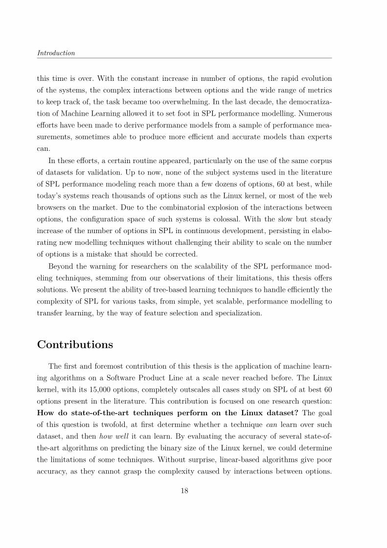
this time is over. With the constant increase in number of options, the rapid evolutionof the systems, the complex interactions between options and the wide range of metricsto keep track of, the task became too overwhelming. In the last decade, the democratiza-tion of Machine Learning allowed it to set foot in SPL performance modelling. Numerousefforts have been made to derive performance models from a sample of performance mea-surements, sometimes able to produce more efficient and accurate models than expertscan.
In these efforts, a certain routine appeared, particularly on the use of the same corpusof datasets for validation. Up to now, none of the subject systems used in the literatureof SPL performance modeling reach more than a few dozens of options, 60 at best, whiletoday’s systems reach thousands of options such as the Linux kernel, or most of the webbrowsers on the market. Due to the combinatorial explosion of the interactions betweenoptions, the configuration space of such systems is colossal. With the slow but steadyincrease of the number of options in SPL in continuous development, persisting in elabo-rating new modelling techniques without challenging their ability to scale on the numberof options is a mistake that should be corrected.
Beyond the warning for researchers on the scalability of the SPL performance mod-eling techniques, stemming from our observations of their limitations, this thesis offerssolutions. We present the ability of tree-based learning techniques to handle efficiently thecomplexity of SPL for various tasks, from simple, yet scalable, performance modelling totransfer learning, by the way of feature selection and specialization.
Contributions
The first and foremost contribution of this thesis is the application of machine learn-ing algorithms on a Software Product Line at a scale never reached before. The Linuxkernel, with its 15,000 options, completely outscales all cases study on SPL of at best 60options present in the literature. This contribution is focused on one research question:How do state-of-the-art techniques perform on the Linux dataset? The goalof this question is twofold, at first determine whether a technique can learn over suchdataset, and then how well it can learn. By evaluating the accuracy of several state-of-the-art algorithms on predicting the binary size of the Linux kernel, we could determinethe limitations of some techniques. Without surprise, linear-based algorithms give pooraccuracy, as they cannot grasp the complexity caused by interactions between options.
18
Introduction
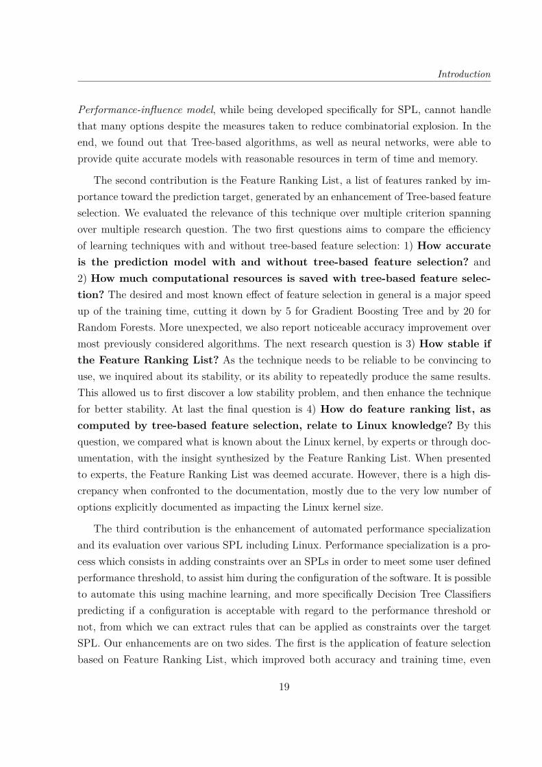
Performance-influence model, while being developed specifically for SPL, cannot handlethat many options despite the measures taken to reduce combinatorial explosion. In theend, we found out that Tree-based algorithms, as well as neural networks, were able toprovide quite accurate models with reasonable resources in term of time and memory.
The second contribution is the Feature Ranking List, a list of features ranked by im-portance toward the prediction target, generated by an enhancement of Tree-based featureselection. We evaluated the relevance of this technique over multiple criterion spanningover multiple research question. The two first questions aims to compare the efficiencyof learning techniques with and without tree-based feature selection: 1) How accurateis the prediction model with and without tree-based feature selection? and2) How much computational resources is saved with tree-based feature selec-tion? The desired and most known effect of feature selection in general is a major speedup of the training time, cutting it down by 5 for Gradient Boosting Tree and by 20 forRandom Forests. More unexpected, we also report noticeable accuracy improvement overmost previously considered algorithms. The next research question is 3) How stable ifthe Feature Ranking List? As the technique needs to be reliable to be convincing touse, we inquired about its stability, or its ability to repeatedly produce the same results.This allowed us to first discover a low stability problem, and then enhance the techniquefor better stability. At last the final question is 4) How do feature ranking list, ascomputed by tree-based feature selection, relate to Linux knowledge? By thisquestion, we compared what is known about the Linux kernel, by experts or through doc-umentation, with the insight synthesized by the Feature Ranking List. When presentedto experts, the Feature Ranking List was deemed accurate. However, there is a high dis-crepancy when confronted to the documentation, mostly due to the very low number ofoptions explicitly documented as impacting the Linux kernel size.
The third contribution is the enhancement of automated performance specializationand its evaluation over various SPL including Linux. Performance specialization is a pro-cess which consists in adding constraints over an SPLs in order to meet some user definedperformance threshold, to assist him during the configuration of the software. It is possibleto automate this using machine learning, and more specifically Decision Tree Classifierspredicting if a configuration is acceptable with regard to the performance threshold ornot, from which we can extract rules that can be applied as constraints over the targetSPL. Our enhancements are on two sides. The first is the application of feature selectionbased on Feature Ranking List, which improved both accuracy and training time, even
19
Introduction
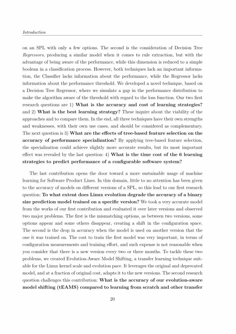
on an SPL with only a few options. The second is the consideration of Decision TreeRegressors, producing a similar model when it comes to rule extraction, but with theadvantage of being aware of the performance, while this dimension is reduced to a simpleboolean in a classification process. However, both techniques lack an important informa-tion, the Classifier lacks information about the performance, while the Regressor lacksinformation about the performance threshold. We developed a novel technique, based ona Decision Tree Regressor, where we simulate a gap in the performance distribution tomake the algorithm aware of the threshold with regard to the loss function. Our two firstresearch questions are 1) What is the accuracy and cost of learning strategies?and 2) What is the best learning strategy? These inquire about the viability of theapproaches and to compare them. In the end, all three techniques have their own strengthsand weaknesses, with their own use cases, and should be considered as complementary.The next question is 3) What are the effects of tree-based feature selection on theaccuracy of performance specialization? By applying tree-based feature selection,the specialization could achieve slightly more accurate results, but its most importanteffect was revealed by the last question: 4) What is the time cost of the 6 learningstrategies to predict performance of a configurable software system?
The last contribution opens the door toward a more sustainable usage of machinelearning for Software Product Lines. In this domain, little to no attention has been givento the accuracy of models on different versions of a SPL, so this lead to our first researchquestion: To what extent does Linux evolution degrade the accuracy of a binarysize prediction model trained on a specific version? We took a very accurate modelfrom the works of our first contribution and evaluated it over later versions and observedtwo major problems. The first is the mismatching options, as between two versions, someoptions appear and some others disappear, creating a shift in the configuration space.The second is the drop in accuracy when the model is used on another version that theone it was trained on. The cost to train the first model was very important, in terms ofconfiguration measurements and training effort, and such expense is not reasonable whenyou consider that there is a new version every two or three months. To tackle these twoproblems, we created Evolution-Aware Model Shifting, a transfer learning technique suit-able for the Linux kernel scale and evolution pace. It leverages the original and deprecatedmodel, and at a fraction of original cost, adapts it to the new versions. The second researchquestion challenges this contribution: What is the accuracy of our evolution-awaremodel shifting (tEAMS) compared to learning from scratch and other transfer
20
Introduction
learning techniques? Our results show very good accuracy over three years of evolution,and better accuracy than learning from scratch on the same dataset.
Outline
In Chapter 2, we present the state-of-the-art on Software Product Lines and SoftwareVariability concerns, as well as machine learning and its uses in Software Engineering. Wealso present the Linux kernel and its particularities given how unique it is among otherSPL.
In Chapter 3, we present our evaluation of the state-of-the-art machine learning tech-niques on the problem of predicting Linux kernel binary size. We show how we set up theevaluation, and present the dataset we used for the Linux kernel and then present theresults.
In Chapter 4, we propose the Feature Ranking List, and how to use it to performfeature selection even at the scale of Linux. We develop the concept and present howwe used Tree-based feature selection to obtain the Feature Ranking List and how weenhance it to increase its stability. By describing the limitations of the state-of-the-art,we show that this technique is the only reasonable way to deal with highly configurablesystems at this time. We show the results of using this feature selection step with thealgorithm previously explored, on both accuracy and training time. We also compare theFeature Ranking List with expert knowledge and documentation. At last, we investigatethe stability of the Feature Ranking List, and explore its influence on accuracy for modelsusing it.
In Chapter 5, we introduce new ways to perform automated performance specializa-tion. We details the concept of performance specialization, and how it was automated. Wepropose two other ways to do it, and evaluate all approaches on Linux and other popularSPL from the state-of-the-art.
In Chapter 6, we explore the accuracy of a model over different versions of Linux kernelto measure its degradation. We present evolution-aware model shifting, a transfer learningtechnique compatible with software evolution concerns, and compare the accuracy of theresulting models to learning from scratch.
At the end, the conclusion will offer a wrap up of the contributions and provide thedifferent perspectives the contributions opened in the field of machine learning applied tocolossal configuration spaces.
21
Introduction
Bibliographical notes
The research presented in this thesis reuses and extends publications of the author.The list of peer-reviewed papers is given below.
Journals
1. [91] Hugo Martin, Mathieu Acher, Juliana Alves Pereira, Luc Lesoil, Djamel Ed-dine Khelladi and Jean-Marc Jézéquel. (2021). Transfer Learning Across Variantsand Versions: The Case of Linux Kernel Size, accepted at IEEE Transactions onSoftware Engineering https://hal.inria.fr/hal-03358817
2. [114] Juliana Alves Pereira, Hugo Martin, Mathieu Acher, Jean-Marc Jézéquel,Goetz Botterweck, Anthony Ventresque. Learning Software Configuration Spaces:A Systematic Literature Review. Journal of Systems and Software, Elsevier, 2021,⟨10.1016/j.jss.2021.111044⟩ https://hal.inria.fr/hal-02148791
Conferences
3. [92] Hugo Martin, Mathieu Acher, Juliana Alves Pereira, and Jean-Marc Jézéquel.(2021). A comparison of performance specialization learning for configurable sys-tems. in:Proceedings of the 25th ACM International Systems and SoftwareProd-uct Line Conference - Volume A, SPLC ’21, Leicester, United Kingdom: Asso-ciation for Computing Machinery, 2021, pp. 46–57, (Best paper Award) https://hal.archives-ouvertes.fr/hal-03335263
4. [8] Juliana Alves Pereira, Mathieu Acher, Hugo Martin, and Jean-Marc Jézéquel.2020. Sampling Effect on Performance Prediction of Configurable Systems: A CaseStudy. In Proceedings of the ACM/SPEC International Conference on PerformanceEngineering (ICPE ’20). Association for Computing Machinery, New York, NY,USA, 277–288. (Best paper Award) https://hal.inria.fr/hal-02356290v2
Reproducible Science: Software, Data, and Tools
As part of the PhD thesis, we contributed to build datasets, to analyse data forreporting quantitative and qualitative insights, and to develop tools. The following onlineresources reference tools, data, script, documentation, models, etc. developed as part ofthe conducted studies:
— The Linux dataset: https://zenodo.org/record/4943884
22

Introduction
— A Docker image to train models and explore hyperparameters: https://github.com/HugoJPMartin/rf-analysis
— Artifacts for Automated Performance Specialization (ACM badge artifacts at SPLC):https://github.com/HugoJPMartin/SPLC2021
— Artifacts for Transfer Learning for Linux: https://github.com/HugoJPMartin/transfer-linux
— kpredict, a tool for predicting kernel binary size from .config files: https://github.com/HugoJPMartin/kpredict
23

Chapter 2
BACKGROUND
In this chapter, we present the background knowledge needed to understand this the-sis, and the state-of-the-art of the domains the thesis belongs to. At first, we detail thebackground in Software Product Lines, and the limitations that required the use of ma-chine learning, which we introduce in the following section. Then, we develop the variousefforts made to join Software Product Lines and Machine Learning in the literature. Nextwe describe Linux, a good example of a system with a colossal configuration space. At theend, we summarize the weaknesses in the state-of-the-art that this thesis aims to address.
2.1 Software Product Lines
Production line is a concept said to be created by Henry Ford in the early 1900’s, andwhile this claim can be debatable, he brought massive improvements to assembly linesand standardization. This allowed mass production of cheap and easy to maintain cars,and paired with socioeconomic developments, it undeniably led to the democratization ofcars. However, this achievement was at the cost of customization as Ford pointed it outin his famous quote: "Any customer can have a car painted any color that he wants solong as it is black".
This highlights divergence between expensive but mostly customized cars, and thecheap and massively produced cars but completely standardized ones. These two conceptsexist in all production domains as of today, though in a more nuanced way, each one beingan extremity of a spectrum. Mass production evolved to include the concept of masscustomization, which allows answering specific customers’ needs, yet still with the large-scale production requirements. This can be made through the use of options a customercan select, such as choosing a color other than black, electrical windows, or even a differentengine. All in all, the same model of car, the core, can articulate itself in various endproducts through the combination of multiple available options.
In Software Engineering, the same concept of product lines has been applied to reduce
25
Partie , Chapter 2 – Background
cost and time of development. Clemens et al. [28] define a Software Product Line (SPL)as follow:
A software product line is a set of software-intensive systems sharing acommon, managed set of features that satisfy the specific needs of a particularmarket segment or mission and that are developed from a common set of coreassets in a prescribed way.
The most particular aspect of SPL that makes it stand out from other product lineengineering is the ability to reuse software almost at will. Krueger [85] presents softwarereuse as "the process of creating a software systems from existing software rather thanbuilding software systems from scratch". Even more specifically, with the help of cus-tomization patterns like options, mentioned with cars, customization is also applied inSoftware Product Lines. It then became possible to create a software system meeting veryspecific needs without having to write a single line of code. Svahnberg et al. [140] definethis as software variability:
Software variability is the ability of a software system or artifact to beefficiently extended, changed, customized or configured for use in a particularcontext.
Nowadays, almost every software system is configurable in some way, and the numberof options tends to grow bigger over time [31]. The good side of this phenomenon is thatthe number of possible configurations grows even faster due to combinatorial explosion,leading to an increased chance that some of them would meet customers’ requirements.The bad side of this phenomenon is that the number of possible configurations grows evenfaster due to combinatorial explosion, leading to a massive increase in effort to ensure theproper functioning of every options with one another or to know the behavior of someoptions in a specific configuration.
Indeed, not all possible combinations of options are valid, due to constraints anddependencies. These represent the situations when some options do not work with oneanother, such as categorical options (SLOB, SLAB and SLUB are three different memorymanagement options, only one should be picked at a time), or when an options requiresanother one to work. In order to model these, the concept of feature models has beendeveloped [72]. Over the years, it has been improved, with support for cardinalities [32,137], or with automated reasoning based on translation to propositional formulas andSAT solving [13].
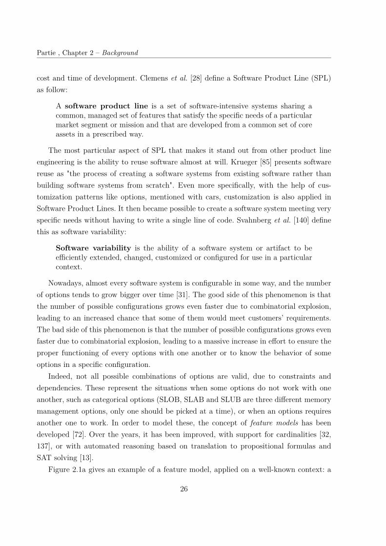
Figure 2.1a gives an example of a feature model, applied on a well-known context: a
26
2.1. Software Product Lines
(a) Full menu
(b) Vegan menu
Figure 2.1 – Example of feature model representing restaurant menu.
restaurant menu. In this case, each dish is a feature, and without constraint, 12 disheswould mean 4095 different combinations of possible dishes. However, the feature modelexpresses different conditions to make a combination valid. First, all dishes are groupedinto a category: Starters, Main and Dessert. Each of these categories is an "Or Group",meaning only one dish of each category can be taken. Then, we have optional categories, asin this menu, only the Main category is mandatory. With all these constraints, the numberof valid menus drops down to 100, in other words, only 2% of the combinations are valid.This demonstrates the need of having a clearly defined map of the valid combinations toavoid mistakes during the selection of the features.
2.1.1 The Curse of Configurability
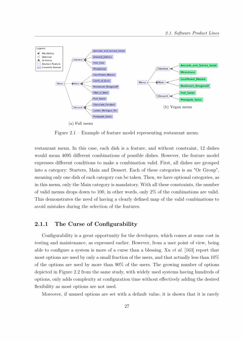
Configurability is a great opportunity for the developers, which comes at some cost intesting and maintenance, as expressed earlier. However, from a user point of view, beingable to configure a system is more of a curse than a blessing. Xu et al. [163] report thatmost options are used by only a small fraction of the users, and that actually less than 10%of the options are used by more than 90% of the users. The growing number of optionsdepicted in Figure 2.2 from the same study, with widely used systems having hundreds ofoptions, only adds complexity at configuration time without effectively adding the desiredflexibility as most options are not used.
Moreover, if unused options are set with a default value, it is shown that it is rarely
27
Partie , Chapter 2 – Background
Figure 2.2 – The increasing number of configuration parameters with software evolution(credit to Xu et al. [163])
a value well-suited for the user’s needs, meaning that every unused options would likelybloat the system and decrease its performance regarding user’s needs.
One way to alleviate the variability burden on a user is specialization.
2.1.2 Specialization
In Software Engineering, we can find the concept of specialization in many shapes.Maybe the most known example is in the class diagrams of Unified Modeling Languageswith the inheritance relationship, where specialization and generalization are the twodirections to interpret this relationship.
The work of Consel et al. [29, 94, 126] on program specialization shows the concerns
28

2.1. Software Product Lines
that generic programs can be less efficient than specialized ones, and the program spe-cialization aims to strip down parts of the program that are useless for specific tasks butthat might impact the performance.
Czarnecki et al. [33, 34] enhance features models by porting specialization, or multi-stage configuration, into them. Usually, the configuration of a system happens in onego, all the desired features are selected, in accordance with the constraints. However, itis possible to consider other cases, such as when two or more parties are involved in theconfiguration of the system, each having their own needs in term of features. For instance,a software vendor could support only a subset of the features of the software system theysell in order to reduce the cost for testing, and provide the client with a specialized system,that is still configurable in the sense that there would be more than one configurationavailable, but always within the boundaries of the vendor support. Other constraints arepossible in the limiting of the feature model expressiveness, such as forcing the activationof a feature when another is activated.
If we take the feature model in Figure 2.1a, it can be difficult to determine the veganoptions in the menu. By using specialization, we can provide the feature model in Fig-ure 2.1b, which only presents the vegan options. In this case, the client does not have toworry about choosing a wrong dish according to his needs.
Performance Specialization While the use cases of specialization proposed by Czar-necki et al. target directly features, it is possible to leverage the same principles of spe-cialization for other, less direct and usually more complex targets, such as performanceand properties (speed, energy consumption, etc.). In this case, the specialization worksaround a given performance threshold, and all configurations of the specialized systemsshould meet that threshold. To achieve that, further constraints have to be created in thefeature model, based on expert knowledge or direct measurements.
Going further with our example of restaurant menu, we annotated each dish with itscalories value in Figure 2.3a, which would allow to filter out menu variants with too manycalories, let’s say 1200 calories. The main difference with the vegan specialization is thatthe constraints on a dish will depend on other dishes, such as the constraint that theFillet of Beef (650 calories) cannot be taken with the Chocolate Fondant (600) as thispair gives 1250 calories. In this case, a specialized menu would prune the available dishesalong with the client selecting his own dishes to always respect the given threshold.
However, the calorie problem is an additive problem, meaning that you just have to
29
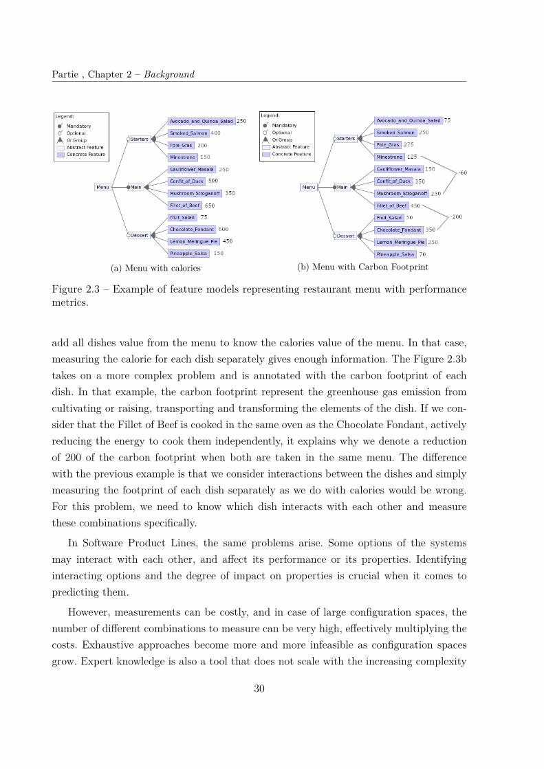
Partie , Chapter 2 – Background
(a) Menu with calories (b) Menu with Carbon Footprint
Figure 2.3 – Example of feature models representing restaurant menu with performancemetrics.
add all dishes value from the menu to know the calories value of the menu. In that case,measuring the calorie for each dish separately gives enough information. The Figure 2.3btakes on a more complex problem and is annotated with the carbon footprint of eachdish. In that example, the carbon footprint represent the greenhouse gas emission fromcultivating or raising, transporting and transforming the elements of the dish. If we con-sider that the Fillet of Beef is cooked in the same oven as the Chocolate Fondant, activelyreducing the energy to cook them independently, it explains why we denote a reductionof 200 of the carbon footprint when both are taken in the same menu. The differencewith the previous example is that we consider interactions between the dishes and simplymeasuring the footprint of each dish separately as we do with calories would be wrong.For this problem, we need to know which dish interacts with each other and measurethese combinations specifically.
In Software Product Lines, the same problems arise. Some options of the systemsmay interact with each other, and affect its performance or its properties. Identifyinginteracting options and the degree of impact on properties is crucial when it comes topredicting them.
However, measurements can be costly, and in case of large configuration spaces, thenumber of different combinations to measure can be very high, effectively multiplying thecosts. Exhaustive approaches become more and more infeasible as configuration spacesgrow. Expert knowledge is also a tool that does not scale with the increasing complexity
30
2.2. Machine Learning for SPL
of the systems. The more options there are in a system, the harder it is for an expert toidentify the rules needed for specialization.
The growing complexity of Software Product Lines makes the solutions based on ex-pert knowledge or exhaustive exploration less and less efficient with the regard to theaccuracy or the cost. This has led the SPL community to investigate machine learning asan alternative approach.
2.2 Machine Learning for SPL
2.2.1 Machine Learning
Mitchell [96] defines learning as follow:
A computer program is said to learn from experience E with respect to someclass of tasks T and performance measure P, if its performance at tasks in T,as measured by P, improves with experience E
The example given by Mitchell with checkers presents T (task) as the ability to playcheckers, P (performance) as the win ratio, and E (experience) as playing a game ofcheckers. The field of Machine Learning aims to develop and enhance algorithms thatenable computers to learn.
Machine learning algorithms come in all sorts of forms, all with their specific usage,features and complexity. James et al. [62] provide an extensive introduction to machinelearning and first separate algorithms by their purpose. Unsupervised learning aims tofind similarities between examples and create clusters; we do not use these techniques inthis thesis. For supervised learning, the learned model is a function that links the featuresto a label, such as a list of symptoms to a specific illness, or a list of options to the priceof a car. In the first case, it is specifically called classification as the label is a discretevalue from a set of classes (the known illnesses), while the latter is called regression, asthe label is a continuous value (the price).
For supervised learning, we can mention different algorithms:— Linear Regression: the most simple approach of machine learning, used for pre-
dicting quantitative value. The resulting model takes the form of y = ax + b, withx being a feature, a and b the values determined by the algorithm. Multiple LinearRegression combine these models to handle more features such as y = a1x1+a2x2+b
— Logistic Regression: the pendant of Linear Regression but for qualitative values,
31

Partie , Chapter 2 – Background
hence a classification method, despite the name. The model is similar, with thedifference that the values determined by the algorithm are probabilities.
— Decision Trees (DT): By recursively splitting the dataset, this type of algorithmobtains a set of decision rules that segment the prediction space into a number ofsimple regions. This set of rules can be organized into a Decision Tree, hence thename of the algorithm. There are actually multiple algorithms that can create aDecision Tree, and while they can all handle regression and classification tasks,they can differ in their limitations regarding the number of branches at each node(only two branches means a Binary Decision Tree) or in whether they can handlecategorical features instead of only numerical features. Decision Trees can be usedin ensembles in different ways:— Bagging: By averaging the result of multiple Decision Trees trained on different
subsets of the training set, it is possible to reduce the variance of the model.— Random Forest (RF): Similar to bagging, RF also trains the Decision Trees
on different subset of features, allowing for better use of moderately correlatedfeatures when there are strongly correlated features in the same set. It yieldsgenerally better results and lower variance.
— Boosting: This technique creates Decision Trees sequentially, always with re-gard to the previous iteration’s errors in order to fix them, hence resulting inbetter accuracy. One of the most known algorithm implementing this processis the Gradient Boosting Tree (GBT)
— Support Vector Machines (SVM): These algorithms are based on the dis-covery of an hyperplane that separates different classes. As is, it is only able tohandle linear separation, but with the help of the kernel trick to warp the problemspace, non-linear problems can be solved. They can handle both regression andclassification problems.
— Neural Network: Composed of interconnected neurons, individual nodes holdinga function weighting inputs into an output, its flexibility allows to solve a broadrange of problems, with the help of various architectures, the layout of neuronconnections in the network. It is arguably the best type of algorithm developedin the past years, at great expense of computing power and number of examplesneeded.
This is only an excerpt of all existing learning algorithms, and they all come withvariations for handling specific problems.
32
2.2. Machine Learning for SPL
2
3Learning
(RQ4: Section 4.4)Validation
(RQ5: Section 4.5)
Prediction
Model
1
4
Start
End
(Re)Sampling
(RQ2: Section 4.2)Measuring
(RQ3: Section 4.3)
NO
Active
Learning?
YES
!" !# … !$ %" %# … %&'" 1 1 … 1 56 126 … +
'# 0 1 … 0 51 167 … -
… … … … … … … … …
'( 1 0 … 0 34 113 … +
I/O
Decision
LEGEND
Step
Start/End
Stages
Flow direction
Execution
Simulation
…
Testing set
Validation set
Evaluation
Metric
Training set
Variability Model / Configurations
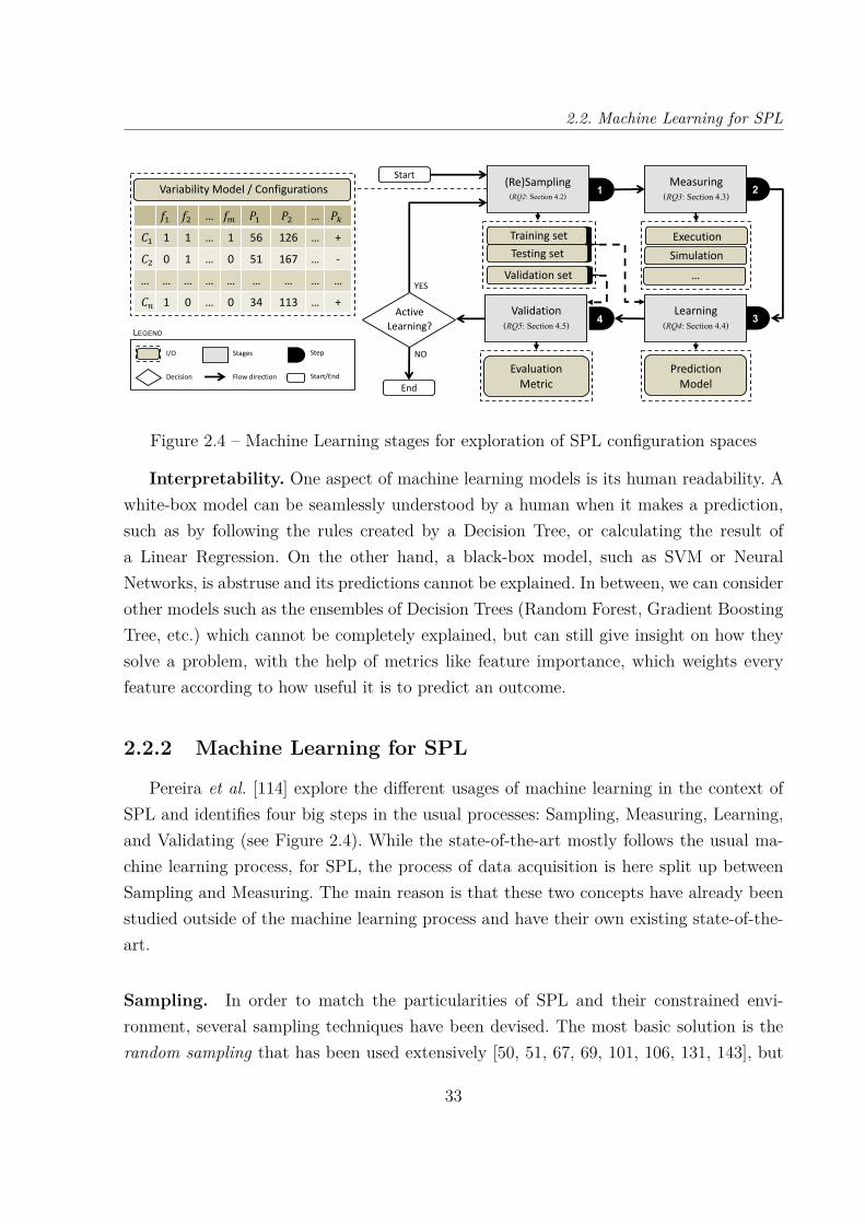
Figure 2.4 – Machine Learning stages for exploration of SPL configuration spaces
Interpretability. One aspect of machine learning models is its human readability. Awhite-box model can be seamlessly understood by a human when it makes a prediction,such as by following the rules created by a Decision Tree, or calculating the result ofa Linear Regression. On the other hand, a black-box model, such as SVM or NeuralNetworks, is abstruse and its predictions cannot be explained. In between, we can considerother models such as the ensembles of Decision Trees (Random Forest, Gradient BoostingTree, etc.) which cannot be completely explained, but can still give insight on how theysolve a problem, with the help of metrics like feature importance, which weights everyfeature according to how useful it is to predict an outcome.
2.2.2 Machine Learning for SPL
Pereira et al. [114] explore the different usages of machine learning in the context ofSPL and identifies four big steps in the usual processes: Sampling, Measuring, Learning,and Validating (see Figure 2.4). While the state-of-the-art mostly follows the usual ma-chine learning process, for SPL, the process of data acquisition is here split up betweenSampling and Measuring. The main reason is that these two concepts have already beenstudied outside of the machine learning process and have their own existing state-of-the-art.
Sampling. In order to match the particularities of SPL and their constrained envi-ronment, several sampling techniques have been devised. The most basic solution is therandom sampling that has been used extensively [50, 51, 67, 69, 101, 106, 131, 143], but
33
Partie , Chapter 2 – Background
has raised many concerns about its feasibility or its uniformity [117].Other solutions rely on heuristics. By using expert knowledge or documentation, it is
possible to find the features to focus on and the feature interactions to care of [133, 134].Coverage sampling systematically samples all combinations of feature of n order. Pair-
wise sampling (order n = 2) assumes feature interaction between every possible pair offeatures [131, 132, 133, 134]. Other works consider 3-wise sampling [71, 89, 124] or evenhigher order [165, 166].
Pereira et al. [8] compare 6 different sampling techniques while varying input workloadon subject systems and with two different performance metrics. The goal is to determinethe impact of workload and metrics on the accuracy of a learning method, when most ofthe studies comparing sampling techniques disregard these parameters. It appears thatboth workload and metrics greatly change the efficiency of all sampling techniques, andthat random sampling is the most solid technique overall.
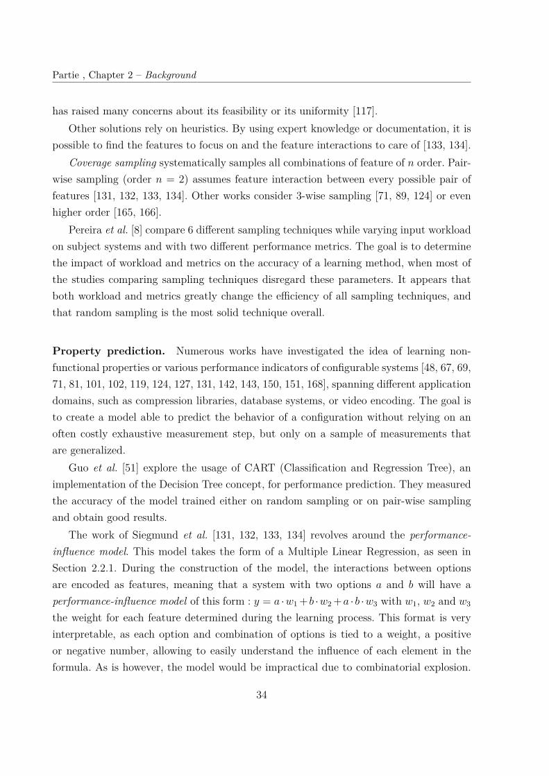
Property prediction. Numerous works have investigated the idea of learning non-functional properties or various performance indicators of configurable systems [48, 67, 69,71, 81, 101, 102, 119, 124, 127, 131, 142, 143, 150, 151, 168], spanning different applicationdomains, such as compression libraries, database systems, or video encoding. The goal isto create a model able to predict the behavior of a configuration without relying on anoften costly exhaustive measurement step, but only on a sample of measurements thatare generalized.
Guo et al. [51] explore the usage of CART (Classification and Regression Tree), animplementation of the Decision Tree concept, for performance prediction. They measuredthe accuracy of the model trained either on random sampling or on pair-wise samplingand obtain good results.
The work of Siegmund et al. [131, 132, 133, 134] revolves around the performance-influence model. This model takes the form of a Multiple Linear Regression, as seen inSection 2.2.1. During the construction of the model, the interactions between optionsare encoded as features, meaning that a system with two options a and b will have aperformance-influence model of this form : y = a ·w1 + b ·w2 +a · b ·w3 with w1, w2 and w3
the weight for each feature determined during the learning process. This format is veryinterpretable, as each option and combination of options is tied to a weight, a positiveor negative number, allowing to easily understand the influence of each element in theformula. As is however, the model would be impractical due to combinatorial explosion.
34
2.2. Machine Learning for SPL
The solution to that problem evolved over the different iterations of the algorithms tocreate the models. At first, they used expert knowledge to identify options that interactedwith each other. Then they moved to a more data-driven approach with the help ofheuristics: only the influential options are combined into features for the model. This is aprocess of feature selection which is described later in Section 2.2.4. Numerous works [39,40, 63] then used and enhanced this model on deeper problems.
Optimization. The problem of optimizing performance of configurable systems (i.e.,finding the best configuration) has attracted some attention [82, 100, 101, 114]. Despite avery similar approach as performance prediction, the details on how to reach that goal canbe almost opposed as shown by Nairet al. [102] : some models bad at predicting accuratelyperformance can be used for optimization.
White-box approaches. By pairing learning techniques with static data-flow analysisor profiling to guide the performance analysis, white-box approaches [152, 153, 156] havebeen proposed to inspect the implementation of a configurable system. They are typicallyused to help understand options and their interactions in a fine-grained way and canprovide valuable insights.
Automated Performance Specialization. For the same reasons that performancemodelling is error-prone for large configurable systems if only based on expert knowl-edge, and almost impossible by systematic measurement, performance specialization is acomplex task given how hard it is to find the right constraints.
Temple et al. [141, 143] leverage a Decision Tree Classifier and its decision rules toinfer the right constraints to obtain a specialized feature model.
Performance specialization is applicable to several domains. Temple et al. [141, 143]explore the domain of a video generator. To improve the learning process, Temple etal. [141] specifically target low confidence areas for sampling. The authors use an adver-sarial learning technique, called evasion attack, after a classifier is trained with a supportvector machine. Beyond a video generator, Temple et al. [142] explore also the domainsof web server, compiler, database system, and image processing. Acher et al. [6] explorethe domain of creating a specialized document (such as a research paper or a resume).Amand et al. [9] applied learning techniques in the 3D printing domain.
There are several works in the faulty specialization context [11, 45, 46, 84, 116, 122,143, 165]. These works explore several domains, such as software-intensive systems, combi-
35
Partie , Chapter 2 – Background
natorial models, and 3D printing. However, these works focus on mining rules for avoidinginvalid configurations, without having performance in mind.
2.2.3 Transfer Learning
West [159] gives a definition of transfer learning (also called inductive transfer):
Inductive transfer refers to any algorithmic process by which structure orknowledge derived from a learning problem is used to enhance learning on arelated problem.
Transfer learning is subject to intensive research in many domains (e.g., image process-ing, natural language processing) [110, 158, 167]. Different kinds of data, assumptions,and tasks are considered. Some of the most complex tasks handled by machine learn-ing rely on models that can take months to train, and consequently a huge amount ofresources. Transfer learning has been developed to heavily reuse models with slight modi-fication to specialize to a user needs, effectively avoiding the costs of training a new modelfrom scratch. Negative transfer is an important concern [167] in this context: divergencemeasures between source and target have been proposed as well as dedicated algorithms[35, 110, 158, 164].
Transfer Learning for SPL Transfer learning has attracted interest with the promiseto save resources by reusing the knowledge of performance under different settings (e.g.,hardware settings) [24, 61, 64, 66, 68, 78, 83, 103, 149, 150, 155].
Defect prediction Defect prediction leverages transfer learning to identify defects inprojects lacking data by reusing models created from other projects with more data [25,26, 88, 104, 154]. Particularly, they handle the problem of heterogeneous context. Themetrics used to predict the defects differ from one project to another. To use informationfrom a project in another, this heterogeneity needs to be taken in account.
2.2.4 Feature Selection
Feature selection is a terminology used both in Product Line Engineering and MachineLearning with different significations. In Product Line Engineering, the feature selectioninvolves setting a value to an option (also named feature), while in Machine Learning,it is the consideration of only a subset of the available features when learning a model.
36

2.2. Machine Learning for SPL
In this part, as well as in the remainder of this thesis, feature selection uses only itsMachine Learning signification. Chandrashekar et al. [23] provides an extensive reviewon feature selection. They describe it as helping "in understanding data, reducing com-putation requirement, reducing the effect of curse of dimensionality and improving thepredictor performance". They distinguish three main categories of feature selection: filter,wrapper and embedded methods. A filter method only works as a preprocessing step byranking features with regard to a relevance criterion and then selecting the highest ones.Wrapper methods rely on the prediction model, and by testing subsets of the featuresand comparing accuracy of the different subset, they can identify their best subset. Thismethod is highly sensitive to the number of features as the number of potential subsetsis exponential. In embedded methods, the feature selection is directly part of the modelbuilding phase, such as with decision trees where at each split, a feature is selected.
Sigmund et al. [131] rely on a forward backward feature selection algorithm. As awrapper method, it compares subsets of features by measuring the accuracy of the modeltrained on each subset. The subsets are created by adding features one by one, in theforward step, so that only individual features with positive impact on the accuracy arekept. Then, the backward step consists in taking out features one by one, and putting themin again if there is an accuracy loss. This is to avoid bias due to the order of appearanceof the features.
This usage of feature selection, backed up by heuristics, helps to reduce the combinato-rial explosion coming from the increasing number of options in software systems. However,this does not ensure the scalability of the approach when dealing with thousands of op-tions. In fact, there is no study applying machine learning on systems with more than a fewdozens of options, and this lack of information can put all the state-of-the-art techniquesat risk if they cannot deal with more complex systems.
The Linux Kernel is a perfect example of a system with a colossal configuration spacewith more than 15.000 options to date. We will thus use it as a subject to inquire aboutthe scalability of state-of-the-art techniques.
37
Partie , Chapter 2 – Background
2.3 The Linux Kernel
2.3.1 Linux, options, and configurations
The Linux Kernel is a free and open-source operating system, that is the most usedoperating system in the world. While it is almost absent in the desktop market, it isdominant in every other markets. More than 95% of the servers, the machines hostingInternet websites, run on Linux. 85% of all smartphones run on Linux. All of the Top 500supercomputers run on Linux [44]. And if the Linux kernel is omnipresent, it is partlybecause it is a highly-configurable system which can adapt to a broad range of needs andenvironments.
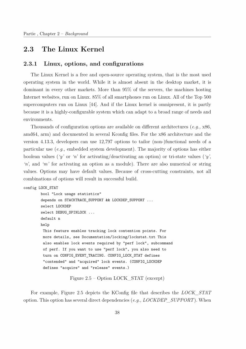
Thousands of configuration options are available on different architectures (e.g., x86,amd64, arm) and documented in several Kconfig files. For the x86 architecture and theversion 4.13.3, developers can use 12,797 options to tailor (non-)functional needs of aparticular use (e.g., embedded system development). The majority of options has eitherboolean values (‘y’ or ‘n’ for activating/deactivating an option) or tri-state values (‘y’,‘n’, and ‘m’ for activating an option as a module). There are also numerical or stringvalues. Options may have default values. Because of cross-cutting constraints, not allcombinations of options will result in successful build.config LOCK_STAT
bool "Lock usage statistics"depends on STACKTRACE_SUPPORT && LOCKDEP_SUPPORT ...select LOCKDEPselect DEBUG_SPINLOCK ...default nhelpThis feature enables tracking lock contention points. Formore details, see Documentation/locking/lockstat.txt Thisalso enables lock events required by "perf lock", subcommandof perf. If you want to use "perf lock", you also need toturn on CONFIG_EVENT_TRACING. CONFIG_LOCK_STAT defines"contended" and "acquired" lock events. (CONFIG_LOCKDEPdefines "acquire" and "release" events.)
Figure 2.5 – Option LOCK_STAT (excerpt)
For example, Figure 2.5 depicts the KConfig file that describes the LOCK_STAToption. This option has several direct dependencies (e.g., LOCKDEP_SUPPORT ). When
38
2.3. The Linux Kernel
selected, this option activates several other options such as LOCKDEP. By default, thisoption is not selected (‘n’). The documentation of this option (including the help part)does not give any indication about its impact on any property such as the kernel size.In this type of documentation, the impact of options on the different properties is oftenmissing, and always expressed in a fuzzy way.
Linux kernel builders set values to options (e.g., through a configurator [160]) andobtain a so-called .config file.
We consider that a configuration is an assignment of a value to each option, eitherby the user, or automatically with a default value. Based on a configuration, the buildprocess of a Linux kernel can start and involves different layers, tools, and languages (C,CPP, gcc, GnuMake and Kconfig).
KConfig language
The KConfig files, which index all features and their dependencies, are used to expressthe feature model, and are written in the KConfig language [73] specifically developed forthe Linux kernel. While the language suits the needs of the kernel developers, it appearsthat it is not very compatible with tools and methods developed by research in SPL andvariability for many reasons. The semantics of the languages are reported not entirelyfigured out yet [14, 15, 75, 129]. Despite many initiatives and works, KConfig does notintegrate a SAT solver [74], and the various works around it such as Undertaker [37, 147]tend to only translate the KConfig information towards another compatible format, atthe price of certain loss of integrity and mistakes [128].
2.3.2 Kernel binary size
Use cases and scenarios
There are numerous use-cases for tuning options related to binary size of the kernel inparticular [56, 107]:
— the kernel should run on very small systems (IoT) or old machines with limitedresources;
— Linux can be used as the primary bootloader. The size requirements on the first-stage bootloader are more stringent than for a traditional running operating sys-tem;
— size reduction can improve flash lifetime, spare RAM and maximize performance;
39

Partie , Chapter 2 – Background
— a supercomputing program may want to run at high performance entirely withinthe L2 cache of the processor. If the combination of kernel and program is smallenough, it can avoid accessing main memory entirely;
— the kernel should boot faster and consume less energy: though there is no empiricalevidence for how kernel size relates to other non-functional properties (e.g., energyconsumption), practitioners tend to follow the hypothesis that the higher the size,the higher the energy consumption.
— cloud providers can optimize instances of Linux kernels w.r.t. size;— in terms of security, the attack surface can be reduced when optional parts are not
really needed.When configuring a kernel, binary size is usually neither the only concern nor the ul-
timate goal. The minimization of the kernel size has no interest if the kernel is unable toboot on a specific device. Size is rather part of a suitable tradeoff between hardware con-straints, functional requirements, and other non-functional concerns (e.g., security). Thepresence of logical constraints and subtle interactions between options further complicatesthe task.
Community attempts
There exists (informal) initiatives in the Linux community that are dealing with kernelsizes.
The Wiki https://elinux.org/Kernel_Size_Tuning_Guide provides guidelines toconfigure the kernel and points out numerous important options related to size. Howeverthe page is no longer actively maintained since 2011. Tim Bird (Sony) presented "Advancedsize optimization of the Linux kernel" in 2013 [17].
Josh Triplett (Intel) introduced tinyconfig at Linux Plumbers Conference 2014 ("LinuxKernel Tinification" [146]) and described motivating use-cases.
The leitmotiv is to leave maximum configuration room for useful functionality whileexploiting opportunities to make the kernel as small as possible. It led to the creation of theproject http://tiny.wiki.kernel.org. The last modifications were made 5 years ago onLinux versions 3.X https://git.kernel.org/pub/scm/linux/kernel/git/josh/linux.git/. Pieter Smith (Philips) gave a talk about "Linux in a Lightbulb: How Far Are Weon Tinification (2015)". Michael Opdenacker (Bootlin) described the state of Linux ker-nel size in 2018. According to these experts, techniques for size reduction are broad andrelated to link-time optimization, compilers, file systems, strippers, etc. In many cases, a
40
2.3. The Linux Kernel
key challenge is that configuration options are spread out over different files of the codebase, possibly across subsystems [1, 2, 99, 16, 95, 112].
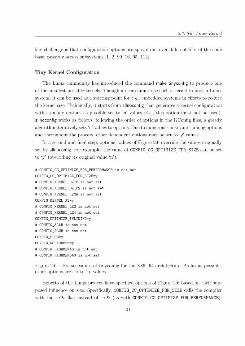
Tiny Kernel Configuration
The Linux community has introduced the command make tinyconfig to produce oneof the smallest possible kernels. Though a user cannot use such a kernel to boot a Linuxsystem, it can be used as a starting point for e.g., embedded systems in efforts to reducethe kernel size. Technically, it starts from allnoconfig that generates a kernel configurationwith as many options as possible set to ‘n’ values (i.e., this option must not be used).allnoconfig works as follows: following the order of options in the KConfig files, a greedyalgorithm iteratively sets ‘n’ values to options. Due to numerous constraints among optionsand throughout the process, other dependent options may be set to ‘y’ values.
In a second and final step, options’ values of Figure 2.6 override the values originallyset by allnoconfig. For example, the value of CONFIG_CC_OPTIMIZE_FOR_SIZE can be setto ‘y’ (overriding its original value ‘n’).
# CONFIG_CC_OPTIMIZE_FOR_PERFORMANCE is not setCONFIG_CC_OPTIMIZE_FOR_SIZE=y# CONFIG_KERNEL_GZIP is not set# CONFIG_KERNEL_BZIP2 is not set# CONFIG_KERNEL_LZMA is not setCONFIG_KERNEL_XZ=y# CONFIG_KERNEL_LZO is not set# CONFIG_KERNEL_LZ4 is not setCONFIG_OPTIMIZE_INLINING=y# CONFIG_SLAB is not set# CONFIG_SLUB is not setCONFIG_SLOB=yCONFIG_NOHIGHMEM=y# CONFIG_HIGHMEM4G is not set# CONFIG_HIGHMEM64G is not set
Figure 2.6 – Pre-set values of tinyconfig for the X86_64 architecture. As far as possible,other options are set to ‘n’ values.
Experts of the Linux project have specified options of Figure 2.6 based on their sup-posed influence on size. Specifically, CONFIG_CC_OPTIMIZE_FOR_SIZE calls the compilerwith the −Os flag instead of −O2 (as with CONFIG_CC_OPTIMIZE_FOR_PERFORMANCE).
41
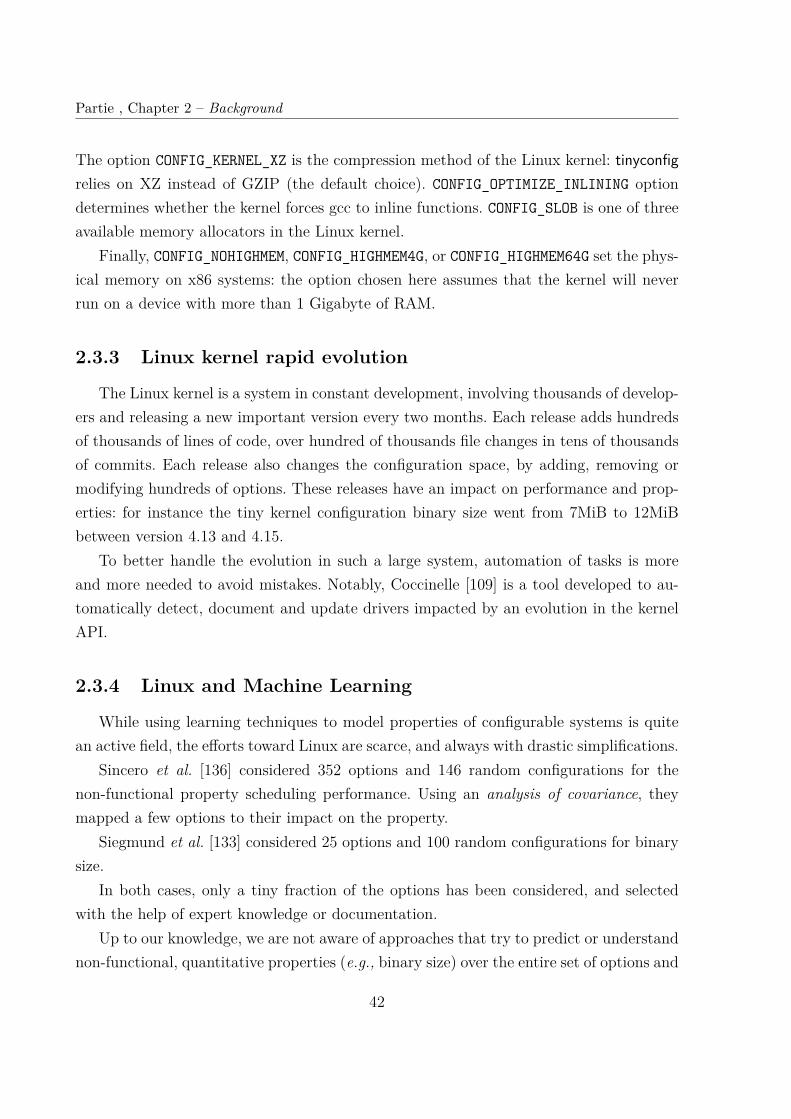
Partie , Chapter 2 – Background
The option CONFIG_KERNEL_XZ is the compression method of the Linux kernel: tinyconfigrelies on XZ instead of GZIP (the default choice). CONFIG_OPTIMIZE_INLINING optiondetermines whether the kernel forces gcc to inline functions. CONFIG_SLOB is one of threeavailable memory allocators in the Linux kernel.
Finally, CONFIG_NOHIGHMEM, CONFIG_HIGHMEM4G, or CONFIG_HIGHMEM64G set the phys-ical memory on x86 systems: the option chosen here assumes that the kernel will neverrun on a device with more than 1 Gigabyte of RAM.
2.3.3 Linux kernel rapid evolution
The Linux kernel is a system in constant development, involving thousands of develop-ers and releasing a new important version every two months. Each release adds hundredsof thousands of lines of code, over hundred of thousands file changes in tens of thousandsof commits. Each release also changes the configuration space, by adding, removing ormodifying hundreds of options. These releases have an impact on performance and prop-erties: for instance the tiny kernel configuration binary size went from 7MiB to 12MiBbetween version 4.13 and 4.15.
To better handle the evolution in such a large system, automation of tasks is moreand more needed to avoid mistakes. Notably, Coccinelle [109] is a tool developed to au-tomatically detect, document and update drivers impacted by an evolution in the kernelAPI.
2.3.4 Linux and Machine Learning
While using learning techniques to model properties of configurable systems is quitean active field, the efforts toward Linux are scarce, and always with drastic simplifications.
Sincero et al. [136] considered 352 options and 146 random configurations for thenon-functional property scheduling performance. Using an analysis of covariance, theymapped a few options to their impact on the property.
Siegmund et al. [133] considered 25 options and 100 random configurations for binarysize.
In both cases, only a tiny fraction of the options has been considered, and selectedwith the help of expert knowledge or documentation.
Up to our knowledge, we are not aware of approaches that try to predict or understandnon-functional, quantitative properties (e.g., binary size) over the entire set of options and
42
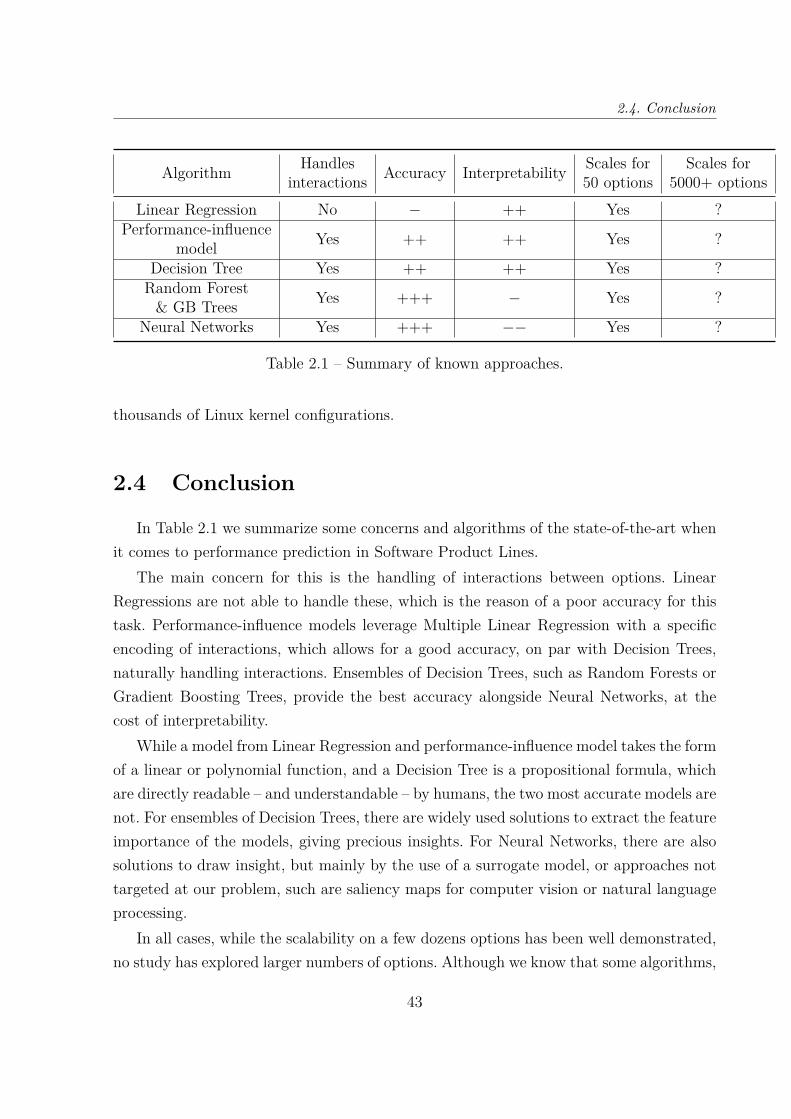
2.4. Conclusion
Algorithm Handlesinteractions Accuracy Interpretability Scales for
50 optionsScales for
5000+ optionsLinear Regression No − ++ Yes ?
Performance-influencemodel Yes ++ ++ Yes ?
Decision Tree Yes ++ ++ Yes ?Random Forest
& GB Trees Yes +++ − Yes ?
Neural Networks Yes +++ −− Yes ?
Table 2.1 – Summary of known approaches.
thousands of Linux kernel configurations.
2.4 Conclusion
In Table 2.1 we summarize some concerns and algorithms of the state-of-the-art whenit comes to performance prediction in Software Product Lines.
The main concern for this is the handling of interactions between options. LinearRegressions are not able to handle these, which is the reason of a poor accuracy for thistask. Performance-influence models leverage Multiple Linear Regression with a specificencoding of interactions, which allows for a good accuracy, on par with Decision Trees,naturally handling interactions. Ensembles of Decision Trees, such as Random Forests orGradient Boosting Trees, provide the best accuracy alongside Neural Networks, at thecost of interpretability.
While a model from Linear Regression and performance-influence model takes the formof a linear or polynomial function, and a Decision Tree is a propositional formula, whichare directly readable – and understandable – by humans, the two most accurate models arenot. For ensembles of Decision Trees, there are widely used solutions to extract the featureimportance of the models, giving precious insights. For Neural Networks, there are alsosolutions to draw insight, but mainly by the use of a surrogate model, or approaches nottargeted at our problem, such are saliency maps for computer vision or natural languageprocessing.
In all cases, while the scalability on a few dozens options has been well demonstrated,no study has explored larger numbers of options. Although we know that some algorithms,
43

Partie , Chapter 2 – Background
notably Neural Networks, are well-suited for thousands or even millions of inputs, we stilldo not know how well they handle SPL performance prediction.
The first objective of this thesis is to explore this scalability over options, and we findout that most techniques do not scale. Tree-based solutions and neural networks beingthe only techniques that we determined to be scalable and accurate, we leverage RandomForests and its partial interpretability to automate feature selection, that allows othertechniques to scale, or the already scalable technique to perform better and faster.
We then explore the different usages of Tree-based algorithms, for automated perfor-mance specialization, but also for transferring a model from one version to another at lowcost.
44
Chapter 3
BINARY SIZE PREDICTION FOR LINUX
KERNEL: THE CHALLENGE OF
COLOSSAL CONFIGURATION SPACE
3.1 Introduction
With now more than 15,000 configuration options, including more than 9,000 justfor the x86 architecture, the Linux kernel is one of the most complex configurable open-source system ever developed. If all these options were binary and independent, thatwould indeed yield 215000 possible variants of the kernel. Of course not all options areindependent (leading to fewer possible variants), but some of them have tri-states values:yes, no, or module instead of simply boolean values (leading to more possible variants).Users can thus choose values for activating options – either compiled as modules or directlyintegrated within the kernel – and deactivate options. The assignment of a specific valueto each option forms a configuration, from which a kernel can hopefully be compiled, built,and booted. Linux kernels are used in a wide variety of systems, ranging from embeddeddevices and cloud services to powerful supercomputers [145]. Many of these systems havestrong requirements on the kernel size due to constraints such as limited memory or instantboot [56, 107]. Obtaining a suitable trade off between kernel size, functionality, and othernon-functional concerns (e.g., security) is an important challenge. For instance, activatingan individual option can increase the kernel binary size so much that it becomes impossibleto deploy it. Hubaux et al. [58] report that many Linux users complained about the lack ofguidance for making configuration decisions, and the low quality of the advice provided bythe configurators. Beyond Linux and even for much smaller configurable systems, similarconfiguration issues have been reported [3, 60, 125, 161, 162, 163, 169].
A fundamental issue is that configuration options often have a significant influence
45
Partie , Chapter 3 – Binary Size prediction for Linux Kernel: The Challenge of ColossalConfiguration Space
on non-functional properties (here: binary size 1) that are hard to estimate and model apriori. There are numerous possible options values, logical constraints between options,and potential interactions among configuration options [51, 71, 114, 123, 131] that canhave an effect on quantitative properties such as size. As we will further elaborate in Sec-tion 4.2, the effort of the Linux community to document options related to kernel binarysize is highly valuable, but mostly relies on human expertise, which makes the mainte-nance of this knowledge quite challenging on the long run. Furthermore, numerous workshave showed that quantifying the performance influence of each individual option is notmeaningful in most cases [51, 71, 114, 123, 131]. That is, the performance influence of n op-tions, all jointly activated in a configuration, is not easily deducible from the performanceinfluence of each individual option. As our empirical results will show, the Linux kernel bi-nary size is not an exception: options such as CONFIG_DEBUG_* or CC_OPTIMIZE_FOR_SIZEhave cross-cutting, non-linear effects and cannot be reduced to additive effects, hence ba-sic linear regression models, which are unable to capture interactions among options, givepoorly accurate results.
Numerous works have considered the problem of learning the effects of options andtheir interactions. The process of "sampling, measuring, learning" configurations has beenapplied on several configurable systems in different domains [114, 51, 123, 131, 71]. How-ever, the number of options was limited to dozens of options. At the scale of Linux, thereare more than 9,000 options for the x86 architecture and only a fraction of possible ker-nel configurations can be measured owing to the cost of compiling and building kernels(a build typically takes about 10 minutes on a modern computer). Linux thus questionswhether learning methods used in the state of the art would scale (w.r.t. training time),provide accurate models, and provide interpretable information at such an unprecedentedscale.
In this chapter, we consider a wide range of state-of-the-art learning algorithms toexplore their behavior on a yet untested scale in term of number of options. The lack ofempirical results on this matter left by previous state-of-the-art experimentations, limitedto at most 60 options, makes it impossible to know if there is a problem or not.
The contributions of this chapter are as follows:— The design and implementation of a large study about kernels’ sizes. We compute
at scale different measures and we engineer specific methods for feature encoding
1. The terminology footprint is also used in the literature to refer to the "binary size of a generatedproduct" [133, 135]
46
3.2. Non-Functional Property prediction of Software Product Lines
and feature construction 2;— A comparison of a wide range of machine learning algorithms over prediction errors.
We analyse the amount of configurations needed for training and replicate theexperiments using different learning algorithms and measures of kernel size.
— An infrastructure, called TuxML, and a comprehensive dataset of 95,854 config-urations with measurements of size as well as learning procedures for replicationand reproducibility of the results [139].
3.2 Non-Functional Property prediction of SoftwareProduct Lines
In this section, we describe the different problems and solutions existing in the state-of-the-art when it comes to predicting the properties of specific configurations of softwaresystems. Section 3.2.1 describes the process of building a dataset of configuration mea-surements. Section 3.2.2 formalizes our problem as a statistical learning one. Section 3.2.3lists existing solutions in the state of the art and describes their limits.
3.2.1 Gathering configurations’ data
Our approach, like other learning-based performance models, requires engineering ef-fort to measure non-functional properties (here: the binary size of a Linux kernel) outof a sample of configurations. We have developed the tool TuxML to build the Linuxkernel in the large i.e., whatever options are combined. TuxML uses Docker to host thenumerous packages and tools needed to compile, build, and measure the Linux kernel.Inside Docker, a collection of Python scripts automates the build process. Docker offers areproducible and portable environment – clusters of heterogeneous machines can be usedwith the same libraries and tools (e.g., compiler versions). In particular, we can use a gridcomputing or a cloud infrastructure to build a large set of configurations.
The two main steps followed by TuxML to measure kernel binary sizes are as follows:
1. Sampling configurations. For this step, we relied on randconfig to randomly generateLinux kernel configurations. randconfig has the merit of generating valid configura-tions respecting the numerous constraints between options. It is also a mature toolthat the Linux community maintains and uses [95]. Though randconfig does not
2. We consider options and features as two separate terminology as explained in 3.4.1
47
Partie , Chapter 3 – Binary Size prediction for Linux Kernel: The Challenge of ColossalConfiguration Space
produce uniform, random samples (see Section 3.5), there is still a wide diversitywithin the values of options (being ‘y’, ‘n’, or ‘m’). We use this sample to create a.config file.
2. Kernel size measurement. Given a set of .config files, TuxML builds the corre-sponding kernels. Throughout the process, TuxML measures the size of vmlinux,a statically linked executable file containing the kernel. We saved the configurationsand the resulting sizes in a database.
The outcome is a dataset of Linux configurations together with their binary size. Eachline of the dataset is composed of a set of configuration option values and a quantitativevalue.
3.2.2 Statistical learning problem
At this step, we have built a dataset of configurations and binary sizes. Predictingthe size of a configurable system now becomes a supervised regression problem, i.e., weaim to predict a quantitative variable out of features, built from configuration options asexplained above.
Let us formalize the problem. First, we denote p the number of configuration optionsand define the configuration space C = {0, 1}p. Out of this space of configurations C, wegather a subset of d configurations, denoted CS ⊂ Cd, as explained in Section 3.2.1.
We separate CS into a training set CtrS and a test set Cte
S , so CS = CtrS
⊕CteS .
Then, we denote:— F (C,R+) the ensemble of functions of C in R+,— f : C → R+ ∈ F (C,R+) the function affecting to any configuration c ∈ C its
performance f(c) ∈ R+,— f(S) the distribution of performance of a set of configuration S, verifying: ∀ S ⊂
C, f(S) = {f(c), c ∈ S}.
With respect to these notations, the goal is to train a learning algorithm f estimatingthe function f for each measured configuration of the training set c ∈ Ctr
S , i.e., f =argmin
h∈F (C,R+)L(f(Ctr
S ), h(CtrS )), where L is a loss function.
The training set CtrS is used to obtain a prediction model, while the testing set Cte
S
only tests the prediction performances of f . The principle is to confront predicted valuesf(Cte
S ) to observed (i.e., ground truth) values f(CteS ).
48
3.2. Non-Functional Property prediction of Software Product Lines
From options to features. Due to discrepancy in vocabulary between the config-urable systems domain and the machine learning domain, we clarify how both terms,"option" and "feature" will be used in this chapter and the remaining of this thesis. Anoption is a variable in a configuration of a system. In the Linux case, every availableoption has a value in the configuration file .config 3. A feature is an independent variablegiven to a machine learning algorithm. Traditionally in Software Engineering, a featurecorresponds to one and only one option and vice versa [49, 148]. Most of the time it isactually the case for Linux. However, we found opportunities to apply feature engineeringtechniques that can alter this observation. The most frequent change is an option notbeing represented at all by a feature, because it has the same value across all examples.Another example is when several options can be merged into a single feature, since theyare logically implied or excluded. In any case, it is straightforward to trace back featuresto the corresponding options.
3.2.3 Limitations of state-of-the-art solutions
Numerous statistical learning algorithms, capable of handling a regression problem,are used in the literature of configurable systems. The most used are standard machinelearning techniques, such as linear methods for regression, decision trees (CART), or ran-dom forests [114]. These algorithms differ in terms of computational cost, expressivenessand interpretability. For instance, linear regressions are considered as easy to interpret,but are unable to capture interactions between options or to handle non-linear effects.On the opposite side of the spectrum, neural networks are blackbox models that canreach higher accuracy on larger datasets. In between, there are variants of algorithms(e.g., Lasso [144]) or ensemble methods (e.g., random forests [18]) together with hyper-parameters that have different impacts on training time, accuracy, and interpretability.For instance, max_depth, a hyperparameter of random forest, controls the maximal depthof the trees (i.e., the maximal number of times we can split the dataset) and may affectresults.
Siegmund et al. [131] introduced a learning method called performance-influence model.Feature-forward selection and multiple linear regression are used in a stepwise manner toshrink or keep terms representing options or interactions. This method aims to handleinteractions between options, limit the number of options to learn on, and provide a
3. Technically, the Linux options that are not specified in a .config file have the value ’n’.
49
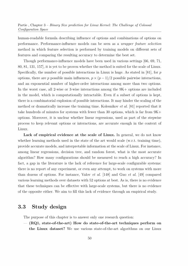
Partie , Chapter 3 – Binary Size prediction for Linux Kernel: The Challenge of ColossalConfiguration Space
human-readable formula describing influence of options and combinations of options onperformance. Performance-influence models can be seen as a wrapper feature selectionmethod in which feature selection is performed by training models on different sets offeatures and comparing the resulting accuracy to determine the best set.
Though performance-influence models have been used in various settings [66, 69, 71,80, 81, 131, 157], it is yet to be proven whether the method is suited for the scale of Linux.Specifically, the number of possible interactions in Linux is huge. As stated in [81], for p
options, there are p possible main influences, p × (p − 1)/2 possible pairwise interactions,and an exponential number of higher-order interactions among more than two options.In the worst case, all 2-wise or 3-wise interactions among the 9K+ options are includedin the model, which is computationally intractable. Even if a subset of options is kept,there is a combinatorial explosion of possible interactions. It may hinder the scaling of themethod or dramatically increase the training time. Kolesnikov et al. [81] reported that ittake hundreds of minutes for systems with fewer than 30 options, which is far from 9K+options. Moreover, it is unclear whether linear regressions, used as part of the stepwiseprocess to keep relevant options or interactions, are accurate enough in the context ofLinux.
Lack of empirical evidence at the scale of Linux. In general, we do not knowwhether learning methods used in the state of the art would scale (w.r.t. training time),provide accurate models, and interpretable information at the scale of Linux. For instance,among linear regressions, decision tree, and random forest, what is the most accuratealgorithm? How many configurations should be measured to reach a high accuracy? Infact, a gap in the literature is the lack of reference for large-scale configurable systems:there is no report of any experiment, or even any attempt, to work on systems with morethan dozens of options. For instance, Valov et al. [148] and Guo et al. [49] comparedvarious learning methods over datasets with 52 options at best. As is, there is no evidencethat these techniques can be effective with large-scale systems, but there is no evidenceof the opposite either. We aim to fill this lack of evidence through an empirical study.
3.3 Study design
The purpose of this chapter is to answer only one research question:— (RQ1, state-of-the-art) How do state-of-the-art techniques perform on
the Linux dataset? We use various state-of-the-art algorithms on our Linux
50
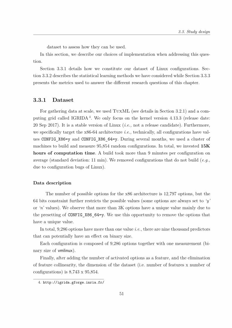
3.3. Study design
dataset to assess how they can be used.In this section, we describe our choices of implementation when addressing this ques-
tion.Section 3.3.1 details how we constitute our dataset of Linux configurations. Sec-
tion 3.3.2 describes the statistical learning methods we have considered while Section 3.3.3presents the metrics used to answer the different research questions of this chapter.
3.3.1 Dataset
For gathering data at scale, we used TuxML (see details in Section 3.2.1) and a com-puting grid called IGRIDA 4. We only focus on the kernel version 4.13.3 (release date:20 Sep 2017). It is a stable version of Linux (i.e., not a release candidate). Furthermore,we specifically target the x86-64 architecture i.e., technically, all configurations have val-ues CONFIG_X86=y and CONFIG_X86_64=y. During several months, we used a cluster ofmachines to build and measure 95,854 random configurations. In total, we invested 15Khours of computation time. A build took more than 9 minutes per configuration onaverage (standard deviation: 11 min). We removed configurations that do not build (e.g.,due to configuration bugs of Linux).
Data description
The number of possible options for the x86 architecture is 12,797 options, but the64 bits constraint further restricts the possible values (some options are always set to ‘y’or ‘n’ values). We observe that more than 3K options have a unique value mainly due tothe presetting of CONFIG_X86_64=y. We use this opportunity to remove the options thathave a unique value.
In total, 9,286 options have more than one value i.e., there are nine thousand predictorsthat can potentially have an effect on binary size.
Each configuration is composed of 9,286 options together with one measurement (bi-nary size of vmlinux).
Finally, after adding the number of activated options as a feature, and the eliminationof feature collinearity, the dimension of the dataset (i.e. number of features x number ofconfigurations) is 8,743 x 95,854.
4. http://igrida.gforge.inria.fr/
51
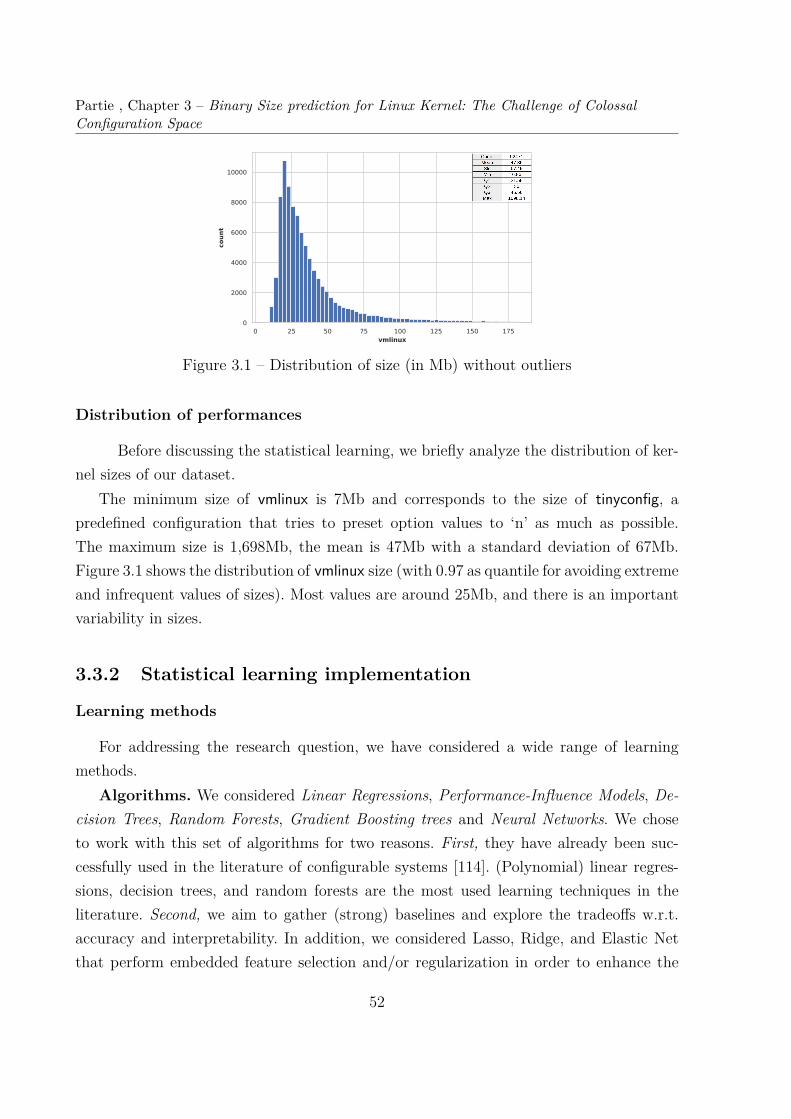
Partie , Chapter 3 – Binary Size prediction for Linux Kernel: The Challenge of ColossalConfiguration Space
0 25 50 75 100 125 150 175vmlinux
0
2000
4000
6000
8000
10000
count
Figure 3.1 – Distribution of size (in Mb) without outliers
Distribution of performances
Before discussing the statistical learning, we briefly analyze the distribution of ker-nel sizes of our dataset.
The minimum size of vmlinux is 7Mb and corresponds to the size of tinyconfig, apredefined configuration that tries to preset option values to ‘n’ as much as possible.The maximum size is 1,698Mb, the mean is 47Mb with a standard deviation of 67Mb.Figure 3.1 shows the distribution of vmlinux size (with 0.97 as quantile for avoiding extremeand infrequent values of sizes). Most values are around 25Mb, and there is an importantvariability in sizes.
3.3.2 Statistical learning implementation
Learning methods
For addressing the research question, we have considered a wide range of learningmethods.
Algorithms. We considered Linear Regressions, Performance-Influence Models, De-cision Trees, Random Forests, Gradient Boosting trees and Neural Networks. We choseto work with this set of algorithms for two reasons. First, they have already been suc-cessfully used in the literature of configurable systems [114]. (Polynomial) linear regres-sions, decision trees, and random forests are the most used learning techniques in theliterature. Second, we aim to gather (strong) baselines and explore the tradeoffs w.r.t.accuracy and interpretability. In addition, we considered Lasso, Ridge, and Elastic Netthat perform embedded feature selection and/or regularization in order to enhance the
52
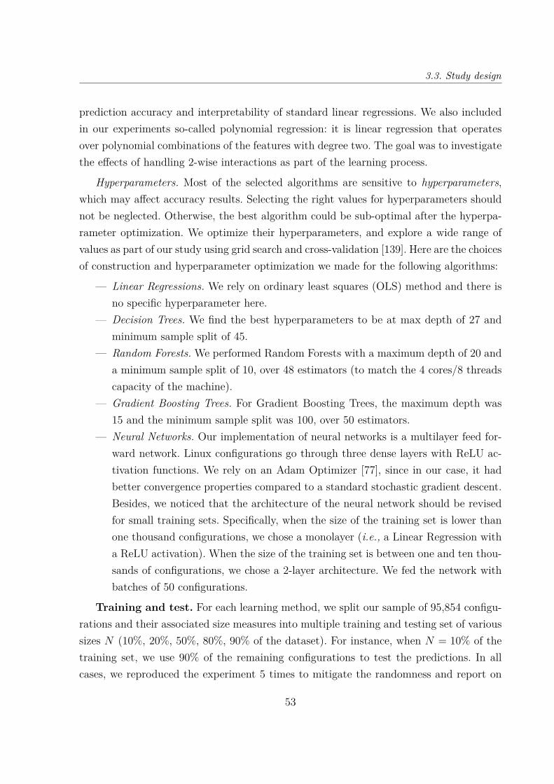
3.3. Study design
prediction accuracy and interpretability of standard linear regressions. We also includedin our experiments so-called polynomial regression: it is linear regression that operatesover polynomial combinations of the features with degree two. The goal was to investigatethe effects of handling 2-wise interactions as part of the learning process.
Hyperparameters. Most of the selected algorithms are sensitive to hyperparameters,which may affect accuracy results. Selecting the right values for hyperparameters shouldnot be neglected. Otherwise, the best algorithm could be sub-optimal after the hyperpa-rameter optimization. We optimize their hyperparameters, and explore a wide range ofvalues as part of our study using grid search and cross-validation [139]. Here are the choicesof construction and hyperparameter optimization we made for the following algorithms:
— Linear Regressions. We rely on ordinary least squares (OLS) method and there isno specific hyperparameter here.
— Decision Trees. We find the best hyperparameters to be at max depth of 27 andminimum sample split of 45.
— Random Forests. We performed Random Forests with a maximum depth of 20 anda minimum sample split of 10, over 48 estimators (to match the 4 cores/8 threadscapacity of the machine).
— Gradient Boosting Trees. For Gradient Boosting Trees, the maximum depth was15 and the minimum sample split was 100, over 50 estimators.
— Neural Networks. Our implementation of neural networks is a multilayer feed for-ward network. Linux configurations go through three dense layers with ReLU ac-tivation functions. We rely on an Adam Optimizer [77], since in our case, it hadbetter convergence properties compared to a standard stochastic gradient descent.Besides, we noticed that the architecture of the neural network should be revisedfor small training sets. Specifically, when the size of the training set is lower thanone thousand configurations, we chose a monolayer (i.e., a Linear Regression witha ReLU activation). When the size of the training set is between one and ten thou-sands of configurations, we chose a 2-layer architecture. We fed the network withbatches of 50 configurations.
Training and test. For each learning method, we split our sample of 95,854 configu-rations and their associated size measures into multiple training and testing set of varioussizes N (10%, 20%, 50%, 80%, 90% of the dataset). For instance, when N = 10% of thetraining set, we use 90% of the remaining configurations to test the predictions. In allcases, we reproduced the experiment 5 times to mitigate the randomness and report on
53
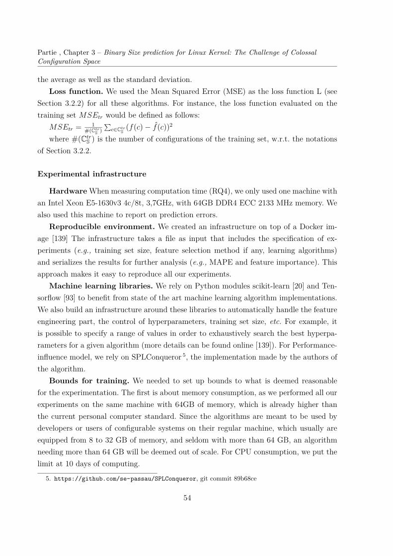
Partie , Chapter 3 – Binary Size prediction for Linux Kernel: The Challenge of ColossalConfiguration Space
the average as well as the standard deviation.Loss function. We used the Mean Squared Error (MSE) as the loss function L (see
Section 3.2.2) for all these algorithms. For instance, the loss function evaluated on thetraining set MSEtr would be defined as follows:
MSEtr = 1#(Ctr
S )∑
c∈CtrS
(f(c) − f(c))2
where #(CtrS ) is the number of configurations of the training set, w.r.t. the notations
of Section 3.2.2.
Experimental infrastructure
Hardware When measuring computation time (RQ4), we only used one machine withan Intel Xeon E5-1630v3 4c/8t, 3,7GHz, with 64GB DDR4 ECC 2133 MHz memory. Wealso used this machine to report on prediction errors.
Reproducible environment. We created an infrastructure on top of a Docker im-age [139] The infrastructure takes a file as input that includes the specification of ex-periments (e.g., training set size, feature selection method if any, learning algorithms)and serializes the results for further analysis (e.g., MAPE and feature importance). Thisapproach makes it easy to reproduce all our experiments.
Machine learning libraries. We rely on Python modules scikit-learn [20] and Ten-sorflow [93] to benefit from state of the art machine learning algorithm implementations.We also build an infrastructure around these libraries to automatically handle the featureengineering part, the control of hyperparameters, training set size, etc. For example, itis possible to specify a range of values in order to exhaustively search the best hyperpa-rameters for a given algorithm (more details can be found online [139]). For Performance-influence model, we rely on SPLConqueror 5, the implementation made by the authors ofthe algorithm.
Bounds for training. We needed to set up bounds to what is deemed reasonablefor the experimentation. The first is about memory consumption, as we performed all ourexperiments on the same machine with 64GB of memory, which is already higher thanthe current personal computer standard. Since the algorithms are meant to be used bydevelopers or users of configurable systems on their regular machine, which usually areequipped from 8 to 32 GB of memory, and seldom with more than 64 GB, an algorithmneeding more than 64 GB will be deemed out of scale. For CPU consumption, we put thelimit at 10 days of computing.
5. https://github.com/se-passau/SPLConqueror, git commit 89b68ce
54

3.4. Results
3.3.3 Metrics and measurements
To assess the accuracy of each method, we rely on the Mean Absolute PercentageError (MAPE), an interpretable and comparable metric. The MAPE of the testing setMAPEte would be defined as follows:
MAPEte = 100#(Cte
S )∑
c∈CteS
|f(c)−f(c)|f(c) %
where #(CteS ) is the number of configurations of the test set, w.r.t. the notations of
Section 3.2.2.We choose the MAPE to depict our results since:
1. it is frequently used when the quantity to predict is known to remain above zero(as in our case) [114];
2. it has the merit of being easy to understand and compare (it is a percentage);
3. it handles the wide distribution and outliers of vmlinux size (Figure 3.1);
4. it is commonly used in approaches about learning and configurable systems [114].
All reported accuracy values are made with this metric in order to have an easiercomparison, and lower is the value the better.
3.4 Results
Most of studied techniques could perform their task in the time and memory limitswe had set. We however failed to get results from two of the techniques we have tried:SPLConqueror and Polynomial regression:
— Importing the Linux dataset into SPLConqueror raises an error about insufficientmemory, so SPLConqueror cannot perform anything on the dataset 6.
— Polynomial regression integrates interactions among features (in the same vein asperformance-influence model) and does not scale for a degree 2.
Table 3.1 reports the highly variable accuracy in MAPE of all successfully testedtechniques with various training set sizes. We can distinguish multiple groups of similarperformance and techniques:
— Linear regression based techniques: OLS Regression, Ridge, ElasticNet and Lassoall present poor results, with Lasso being the only one with less than 50% MAPE,but still 34% at best. The results show that linear regressions are not suited for
6. We used SPLConqueror from commit 9b68ce on Ubuntu 20.04 LTS and got the message "Sys-tem.OutOfMemoryException: Insufficient memory to continue the execution of the program."
55
Partie , Chapter 3 – Binary Size prediction for Linux Kernel: The Challenge of ColossalConfiguration Space
Algorithm N=10 N=20 N=50 N=80 N=90OLS Regression 74.54±2.3 68.76± 1.03 61.9 ± 1.14 50.37±0.57 49.42±0.08Lasso 34.13±1.38 34.32±0.12 36.58±1.04 38.07±0.08 38.04±0.17Ridge 139.63±1.13 91.43±1.07 62.42±0.08 55.75±0.2 51.78±0.14ElasticNet 79.26±0.9 80.81±1.05 80.58±0.77 80.57±0.71 80.34±0.53Decision Tree 15.18 ± 0.13 13.21 ± 0.12 11.32±0.07 10.61± 0.10 10.48± 0.15Random Forest 12.5±0.19 10.75±0.07 9.27±0.07 8.6±0.07 8.4 ±0.07GB Tree 11.13±0.23 9.43±0.07 7.70±0.04 7.02±0.05 6.83±0.10N. Networks - 13.92 ± 0.99 9.46 ± 0.15 8.29 ± 0.18 8.08 ± 0.12Polynomial Regression - - - - -
Table 3.1 – MAPE of different learning algorithms for the prediction of vmlinux size, withN being the percentage of the dataset used as training
Linux and that the problem of predicting size cannot be trivially resolved with asimple additive, linear model (as hypothesized earlier in the chapter);
— Tree-based techniques: Decision Tree, Random Forest and Gradient Boosting Treeall show MAPE at less than 20% even with "only" 10% of the dataset, even reaching6.83% for GB Tree at 90% of the dataset. Decision trees are inferior to randomforest and GB Trees;
— Neural Networks work quite well but require much more data to be efficient com-pared to Tree-based techniques.
How does state-of-the-art techniques perform on large configurable sys-tems? At the exception of Performance-Influence model and Polynomial Regres-sion, most of the techniques studied can handle the Linux dataset in reasonabletime and memory limits. On the accuracy side, we can notice that Linear regressionbased techniques do not present very accurate results, and only Tree-based andneural network techniques are suited for Linux.
3.5 Threats to Validity
3.5.1 Internal Validity
The selection of the learning algorithms and their parameter settings may affect theaccuracy and influence interpretability. To reduce this threat, we selected the most widelyused learning algorithms that have shown promising results in this field [114] and for a fair
56
3.5. Threats to Validity
comparison we searched for their best parameters. We deliberately used random samplingover the training set for all experiments to increase internal validity. For each samplesize, we repeat the prediction process 5 times. For each process, we split the datasetinto training and testing which are independent of each other. To assess the accuracy ofthe algorithms and thus its interpretability, we used MAPE since most of the state-of-the-art works use this metric for evaluating the effectiveness of performance predictionalgorithm [114].
Another threat to validity concerns the (lack of) uniformity of randconfig. Indeedrandconfig does not provide a perfect uniform distribution over valid configurations [95].The strategy of randconfig is to randomly enable or disable options according to the orderin the Kconfig files. It is thus biased towards features higher up in the tree. The problem ofuniform sampling is fundamentally a satisfiability problem. To the best of our knowledge,there is no robust and scalable solution capable of comprehensively translating Kconfigfiles of Linux into a format usable by a SAT solver. Second, uniform sampling either doesnot scale yet or is not uniform [117, 21, 22, 42]. So we had to stick with randconfig. Wesee randconfig as a baseline widely used by the Linux community [121, 95].
3.5.2 External Validity
A threat to external validity is related to the target kernel version and architecture(x86) of Linux. Because we rely on the kernel version 4.13.3 and the non-functional prop-erty binary size, the results may be subject to this specific version and quantitative prop-erty. However, a generalization of the results for other non-functional properties (e.g.,boot time) would require additional experiments. It is actually a challenge per se to scaleup such experiments. Binary size has the merit of being independent of the hardware:we do not need to control for the heterogeneity of machines or repeat the measurements.Binary size has also proved to be a non-trivial property to learn.
Overall, we focused on a single version and property to be able to make robust andreliable statements about whether learning approaches can be used in such settings. Ourresults suggest we can now envision to perform an analysis over other versions and prop-erties to generalize our findings.
57
Partie , Chapter 3 – Binary Size prediction for Linux Kernel: The Challenge of ColossalConfiguration Space
3.6 Conclusion
Is it possible to learn the essence of a gigantic space of software configurations withrespect to a given property of interest? We addressed an instance of this problem throughthe prediction of Linux kernel sizes for the x86_64 processor architecture, dealing withover 9,000 options and thus a huge configuration space.
We invested 15K hours of computation to build and measure 95,854 Linux kernelconfigurations and found that:
— Linear regression based techniques give low accuracy results.— Polynomial regression and performance-influence models run out of memory, pos-
sibly due to the way interactions are encoded.— Tree-based algorithm and neural networks show quite a good accuracy, and Gra-
dient Boosting Trees yield the best results.The fact that performance-influence models approach, a well-established algorithm
designed especially to deal with Software Product Lines problems and maybe the mostadvanced one currently in the field, does not scale with the number of options in Linux,is a worrying discovery for the relevance of current research based on that algorithm andyet claiming their scalability to all Software Product Lines.
We believe that the limitation comes from the way interactions are encoded into thealgorithm, as each interaction is represented by a new features when presented to thealgorithm building the model. This lead to a combinatorial explosion, and this despitethe heuristics used to mitigate it. This type of encoding is used in other works aroundSPL, and thus severely limits its applicability for really large configurable systems.
Tree-based algorithm and neural networks are the best algorithms in our study andoffer a positive answer to the question about the possibility to learning on such a con-figuration space. However, the costs in term of resources needed to gather the dataset,and to a lesser extent to train the models, can be a deterrent to engage in such initiative,especially in a context of constant evolution.
58

Chapter 4
TREE-BASED FEATURE SELECTION
4.1 Introduction
Feature Selection is a well-known process in machine learning, and after consideringthe previous chapter on property prediction of Linux Kernel, we aim to follow a novelresearch direction. Instead of considering the whole set of options when training a model,we first compute a subset of influential options with tree-based algorithms. Then learningmethods can operate over a much reduced feature space.
Our hypothesis is that some configuration options of Linux have little effect on a givenproperty of interest (e.g., the kernel binary size) and thus can be removed without incur-ring much loss of information. So-called feature selection techniques are worth consideringwhen there are many features and comparatively few samples as in Linux (see e.g., Chap-ter 18 of [53]). Though we are not necessarily in extreme cases like the analysis of DNAmicroarray data [138, 23] in which there are only a few samples available, the Linux caseexhibits a very large number of options p.
The promise of feature selection is that the resulting models are easier to interpretand faster to train since only a few options are considered (i.e., p′ << p with p′ the newnumber of considered options). The danger, however, is that the accuracy might decreaseif the subset of options is badly chosen. Hence several empirical questions arise: Can tree-based feature selection identify relevant options with effects on binary size? Is featureselection competitive w.r.t. accuracy? How many configurations should be measured andwhat machine learning algorithms should be used to reach a high accuracy?
Prior works considered only a few options and configurations. Sincero et al. [136]considered 352 options and 146 random configurations for the non-functional propertyscheduling performance. Siegmund et al. [133, 135] considered 25 options and 100 randomconfigurations for binary size. In this study and in contrast to prior works, we make noassumption about the supposed influence of some options and our experiments considerthe entire 9K+ options of the Linux kernel on the x86_64 architecture. We also considered
59

Partie , Chapter 4 – Tree-based Feature Selection
a baseline of 95K+ different configurations. Beyond Linux, only dozens of options over afew configurations are usually considered in the literature of configurable systems [114].The gap with the Linux case is substantial, up to the point that some learning algorithms,including the ones proposed in the literature, do not scale (see Section 3.2.3) or have pooraccuracy (see Section 4.5). We also aim to automate the process of selecting a subset ofrelevant options prior to the training of a prediction model. Owing to the large number ofoptions (9K+), feature selection is particularly suited for Linux. Yet, it is unclear whetherfeature selection is effective at this scale. Feature selection can be done manually: someexperts chose a subset of options based on some knowledge to make the experiment lesscostly and thus affordable. We want to automate this process, thus avoiding to rely ona potentially incomplete and outdated knowledge. Feature selection can also be realizedthrough wrapper methods that determine the best set of features by comparing modelstrained on different sets [23]. Techniques such as performance-influence models [131] enterinto this category. Empirical results show that such state-of-the-art methods either do notscale or are poorly accurate at the scale of Linux. For addressing these limitations, wedevelop a two-step method that relies on tree-based feature selection. First, a learningprocess computes a so-called feature ranking list for ordering important features. Then,this list is fed to a learning algorithm that operates over a subset of predictive features. Weuse tree-based learning algorithms (e.g., random forest) to learn the feature ranking list,owing to their predictive power and interpretability. As detailed in the rest of this chapter,empirical results show that (1) tree-based learning algorithms are the most accurate amongal tested algorithms and (2) the use of tree-based feature selection outperforms learningapproaches that do not resort to feature selection.
The contributions of this chapter are as follows:
— A measurement of the effect of tree-based feature selection on a wide range ofmachine learning algorithms over prediction errors, interpretability, and trainingtime. We find that tree-based feature selection is able to identify a reduced setof options that both speeds up the training time and produces simpler and moreaccurate models;
— A qualitative analysis of identified options based on the cross-analysis of Linuxdocumentation, default options’ values and configurations, and experts’ knowledge.We find that the subset of options found by tree-based feature selection is consistentw.r.t. Linux knowledge;
60
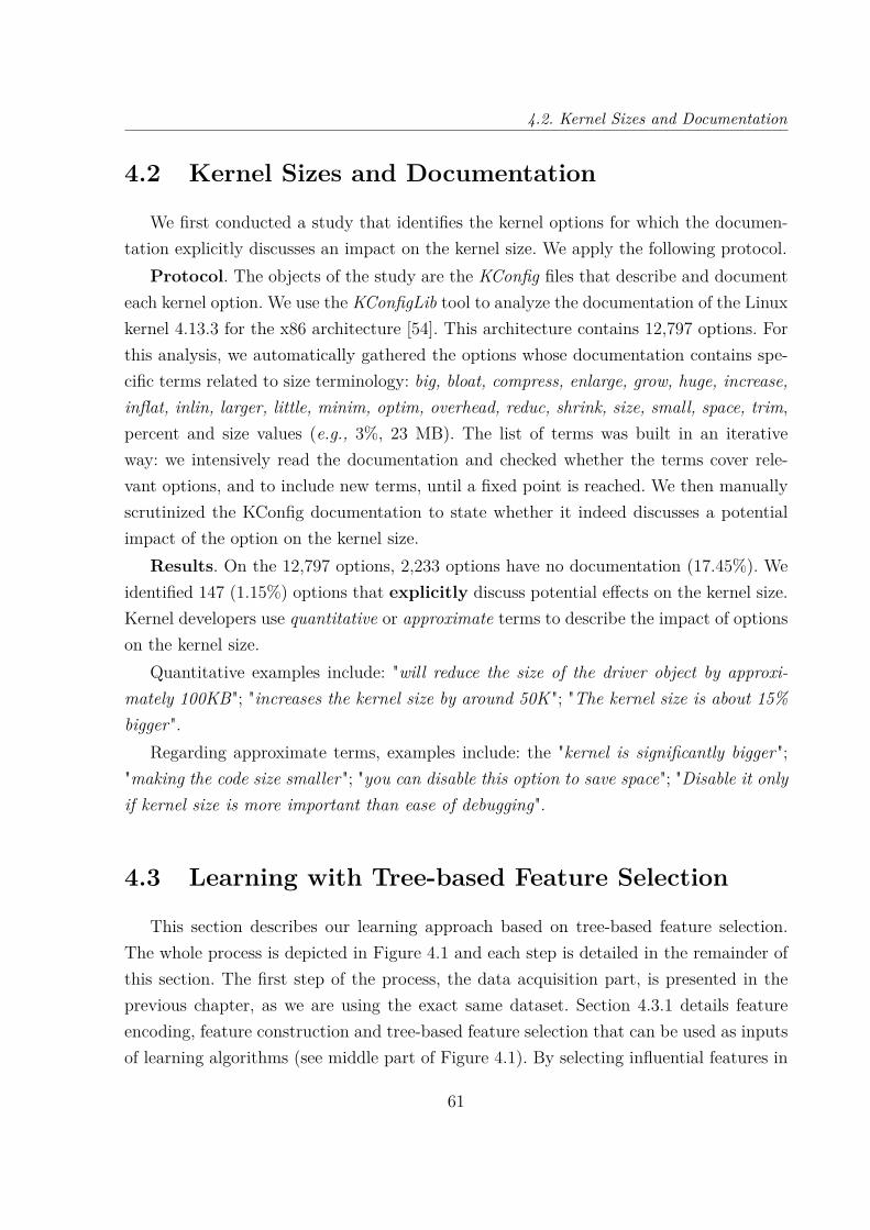
4.2. Kernel Sizes and Documentation
4.2 Kernel Sizes and Documentation
We first conducted a study that identifies the kernel options for which the documen-tation explicitly discusses an impact on the kernel size. We apply the following protocol.
Protocol. The objects of the study are the KConfig files that describe and documenteach kernel option. We use the KConfigLib tool to analyze the documentation of the Linuxkernel 4.13.3 for the x86 architecture [54]. This architecture contains 12,797 options. Forthis analysis, we automatically gathered the options whose documentation contains spe-cific terms related to size terminology: big, bloat, compress, enlarge, grow, huge, increase,inflat, inlin, larger, little, minim, optim, overhead, reduc, shrink, size, small, space, trim,percent and size values (e.g., 3%, 23 MB). The list of terms was built in an iterativeway: we intensively read the documentation and checked whether the terms cover rele-vant options, and to include new terms, until a fixed point is reached. We then manuallyscrutinized the KConfig documentation to state whether it indeed discusses a potentialimpact of the option on the kernel size.
Results. On the 12,797 options, 2,233 options have no documentation (17.45%). Weidentified 147 (1.15%) options that explicitly discuss potential effects on the kernel size.Kernel developers use quantitative or approximate terms to describe the impact of optionson the kernel size.
Quantitative examples include: "will reduce the size of the driver object by approxi-mately 100KB"; "increases the kernel size by around 50K "; "The kernel size is about 15%bigger".
Regarding approximate terms, examples include: the "kernel is significantly bigger";"making the code size smaller"; "you can disable this option to save space"; "Disable it onlyif kernel size is more important than ease of debugging".
4.3 Learning with Tree-based Feature Selection
This section describes our learning approach based on tree-based feature selection.The whole process is depicted in Figure 4.1 and each step is detailed in the remainder ofthis section. The first step of the process, the data acquisition part, is presented in theprevious chapter, as we are using the exact same dataset. Section 4.3.1 details featureencoding, feature construction and tree-based feature selection that can be used as inputsof learning algorithms (see middle part of Figure 4.1). By selecting influential features in
61
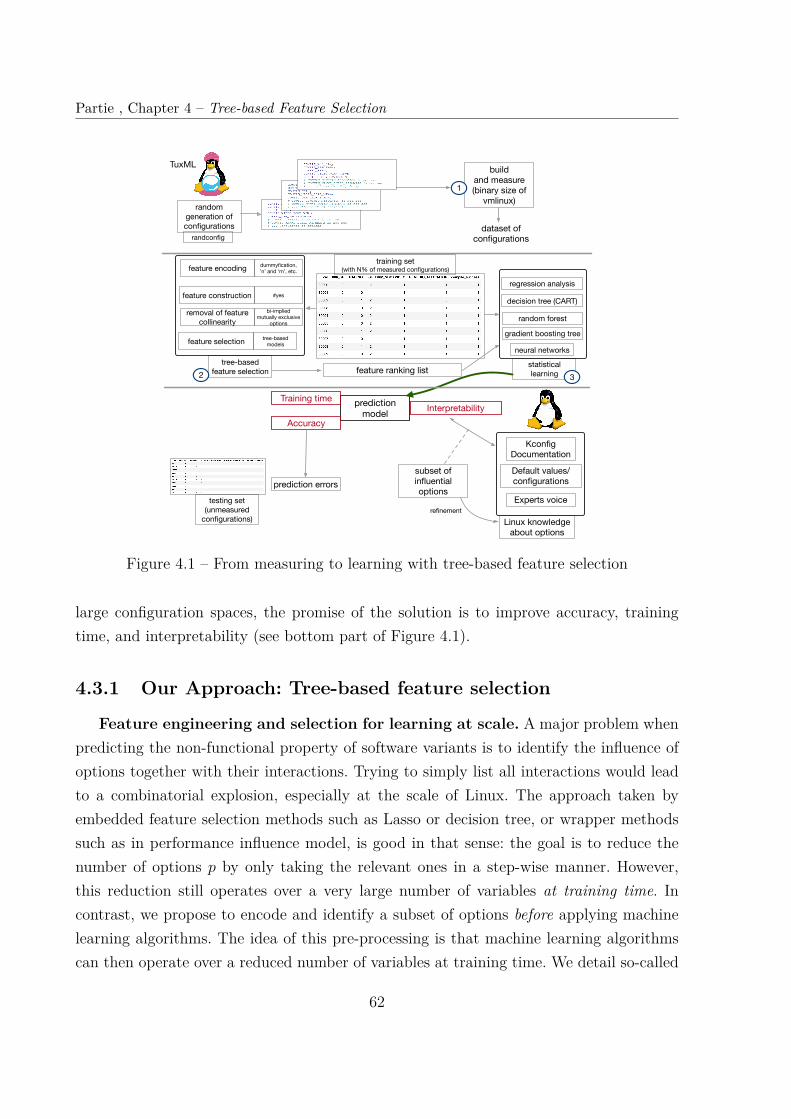
Partie , Chapter 4 – Tree-based Feature Selection
random generation of configurations
randconfig
build and measure(binary size of
vmlinux)
feature encoding
feature selection
feature construction
neural networks
decision tree (CART)
random forest
gradient boosting tree
regression analysis
statistical learning
tree-based feature selection
prediction model
AccuracyInterpretability
Kconfig Documentation
Default values/ configurations
Linux knowledge about options
Experts voiceprediction errors
training set (with N% of measured configurations)
testing set (unmeasured
configurations)
subset of influential options
dummyfication, ’n’ and ‘m’, etc.
#yes
tree-based models
1
2 3
refinement
feature ranking list
Training time
removal of feature collinearity
bi-impliedmutually exclusive
options
TuxML
dataset of configurations
Figure 4.1 – From measuring to learning with tree-based feature selection
large configuration spaces, the promise of the solution is to improve accuracy, trainingtime, and interpretability (see bottom part of Figure 4.1).
4.3.1 Our Approach: Tree-based feature selection
Feature engineering and selection for learning at scale. A major problem whenpredicting the non-functional property of software variants is to identify the influence ofoptions together with their interactions. Trying to simply list all interactions would leadto a combinatorial explosion, especially at the scale of Linux. The approach taken byembedded feature selection methods such as Lasso or decision tree, or wrapper methodssuch as in performance influence model, is good in that sense: the goal is to reduce thenumber of options p by only taking the relevant ones in a step-wise manner. However,this reduction still operates over a very large number of variables at training time. Incontrast, we propose to encode and identify a subset of options before applying machinelearning algorithms. The idea of this pre-processing is that machine learning algorithmscan then operate over a reduced number of variables at training time. We detail so-called
62

4.3. Learning with Tree-based Feature Selection
tree-based feature selection in the next section. To the best of our knowledge, the useof feature selection prior to the learning has not received attention in the literature ofconfigurable systems.
Intuition. A hypothesis is that some configuration options of Linux have littleeffects and can be removed without incurring much loss of information. Feature selectiontechniques are worth considering when there are many features and comparatively fewsamples. Though we are not necessarily in an extreme case like the analysis of DNAmicroarray data [23, 138] in which there are only a few available samples, the Linux caseexhibits a very large number of options p. The goal is to operate over a reduced numberof variables p′ ≪ p when training, ideally over a relatively small training set (e.g., lessthan 10K) to reduce the overall cost of learning.
The left middle part of Figure 4.1 lists each step of the tree-based feature selectionmethod.
Feature encoding A first way to reduce p is to properly encode options as features.Regression analysis requires that we encode three possible values of options (e.g., ‘y’, ‘n’,‘m’) into numerical values. An encoding of ‘n’ as 0, ‘y’ as 1, and ‘m’ as 2 is a first possiblesolution. However, some learning algorithms (e.g., linear regression) will assume that twonearby values are more similar than two distant values (here ‘y’ and ’m’ would be moresimilar than ‘m’ and ‘n’). This encoding will also be confusing when interpreting thenegative or positive weights of a feature. There are many techniques to encode categoricalvariables (e.g., dummy variables [41]). We observe that the ‘m’ value has no direct effecton the size since kernel modules are not compiled into the kernel and can be loaded asneeded. Therefore, we consider that ‘m’ values have the same effect as ‘n’ values, and thesevalues can be merged. As a result, the problem is simplified: an option can only take twovalues (i.e., "yes" or "no", 1 or 0 as defined in Section 3.2.2). For non-tri-state options,which are only 319, we simply discarded them. With this encoding, the hypothesis is thatthe accuracy of the prediction model is not impacted whereas the problem is simpler tohandle for learning algorithms and easier to interpret.
Feature construction. The number of ‘y’ options’ values in a configuration, denoted#yes, can have an impact on the kernel size, and has been added as a new feature in thedataset. The rationale is that the more options are included, the larger is the kernel. Atfirst glance, the inclusion of a new feature is counter-intuitive since our focus is ratherto reduce the number of variables. However, this feature is informative and may have astrong predictive power: it makes explicit the domain knowledge about the relationship
63

Partie , Chapter 4 – Tree-based Feature Selection
between binary size and number of options. By adding such a feature, the hypothesis isthat the accuracy of the prediction model can be improved.
Feature selection Knowing which configuration options are most predictive of size ispart of our goal. With that in mind, feature importance is a useful concept: it is the increasein the prediction error of the model after we permuted the feature’s values [97]. For adecision tree, the importance of a feature is computed as the (normalized) total reductionof the splitting criterion (e.g., Gini or entropy) brought by that feature. For randomforest, feature permutation importance is computed through the observation of the effecton machine learning model accuracy of randomly shuffling each predictor variable [18, 97,111].
Elimination of feature collinearity. In machine learning, feature collinearity happenswhen two (or more) features are completely correlated. Feature collinearity is in fact awell-known, general issue in machine learning, especially for model interpretability [38,18, 111, 97, 43]. Feature collinearity also becomes an issue when quantifying how much afeature is important to predict the target values. Specifically, when multiple features sharethe same values, hence all having the same information value, there is no other choice tobe made than random split between those features. It has two major consequences:
1. there is some instability: it is hard to reproduce a feature’s importance withoutsetting a random seed at all levels of the experiment, as a feature’s importancedepends on the previous splits in the tree.
2. the importance of the information held by a group of features will be distributedbetween them and considered far lower than it should be [97].
In order to mitigate feature collinearity, we grouped collinear options into a single feature.There are at least two relevant cases of collinear options: (1) some options are logicallybi-implied and have always the same values in a configuration; (2) some options aremutually exclusive and have always opposite values (e.g., CC_OPTIMIZE_FOR_SIZE andCC_OPTIMIZE_FOR_PERFORMANCE). In both cases, we create one "artificial" feature thatacts as a representative group of all involved options. It does not bring any problem forinterpretation as it is possible to retrieve which options compose one "artificial" feature.
The elimination of feature collinearity is an important step realized just before theactual feature selection. We choose to rely on a tree-based feature selection. The principleis to rely on decision trees or ensembles like random forest to produce a feature rankinglist. Such algorithms are capable of handling non-linear effects and have strong predic-tion power. (Empirical results confirm that tree-based learning algorithms are the most
64
4.4. Study design
accurate, see Section 4.5).Once the feature importance of random forests is computed, the feature ranking list can
be created. The feature ranking list orders features by importance. We use a threshold toselect a subset of relevant options (e.g., the top 500 of the list, by decreasing importance).This threshold allows one to control the reduced number of variables p′ ≪ p to considerat training time. A learning algorithm can use the subset of features to eventually traina predictive model.
Stability. It should be noted that the algorithm of random forest relies on randomselection: this can cause instability in the computation of feature importance. To mitigatethis threat, we rely on two techniques. First, we simply repeat the process several timesand compute the average of feature importance. Second, we eliminate collinear featuresbefore training the random forest (see previous explanations).
4.4 Study design
The main research question is RQ: How effective is tree-based feature selection forpredicting Linux kernel sizes?, which can be decomposed into five main research questions:
— (RQ1, accuracy) How accurate is the prediction model with and withouttree-based feature selection? Depending on e.g., training set size, feature selec-tion or hyperparameters of learning algorithms, the resulting model may producemore or fewer errors when predicting the size of unseen configurations.
— (RQ2, stability) How stable is the Feature Ranking List? Depending onthe models used to create the Feature Ranking List, the set of selected featurescan vary.
— (RQ3, training time) How much computational resources is saved withtree-based feature selection? By selecting a subset of relevant features, learningalgorithms operate on a smaller number of features at training time. Depending one.g., training set size, feature selection or hyperparameters of learning algorithms,the resulting model may need more or fewer computational resources to get trained.
— (RQ4, interpretability) How do feature ranking lists, as computed bytree-based feature selection, relate to Linux knowledge? We aim to comparethe retrieved knowledge extracted from models with knowledge from the Linuxcommunity. Linux knowledge notably comes from the Kconfig documentation andexperts’ insights.
65
Partie , Chapter 4 – Tree-based Feature Selection
In this section, we describe our choices of implementation when addressing these ques-tions. For most of the experiments, we use the same process as in the last chapter, withadditional steps when it comes to feature selection.
Tree-based feature selection
Each learning algorithm previously described can be used with tree-based featureselection. Our automated feature selection process is based on the feature ranking list,created from insights extracted from a machine learning algorithm. In our case and forRQ2, we rely on 20 random forests to compute the list. Random forests appear to reachhigh accuracy, better than decision trees. For each random forest, the importance of eachfeature is computed, then all features are sorted by their importance, the most importantfeature being the top one in the ranking. We take the average ranking across all 20 randomforests to get the final feature ranking list. As further elaborated in RQ3, we needed torely on the results of multiple random forests due to the instability of the model. Evenwith the same dataset and hyperparameters, the feature importance of two random forestwas fairly different. For example, if we take the 300 most important features of the firstrandom forest, we could only retrieve half of them in the second random forest top 300.
An important factor that can influence the accuracy of a learning method with tree-based feature selection is k, the number of selected features within the feature rankinglist. We make k vary from 50 (i.e., the 50 top influential features) to 8,743 (the size of theentire list), in steps of 50. The goal is to identify how many features are ideally needed attraining time for reaching high accuracy.
We apply all learning methods of Section 3.3.2 with and without tree-based featureselection, and report on the difference of accuracy in Section 4.5.1.
4.4.1 Metrics and measurements
Aside from the accuracy metric, Mean Absolute Percentage error which is describedin Section 3.3.3, we also measure the stability of the Feature Ranking List, the trainingtime and the quality of the List.
(RQ3) Stability
The Feature Ranking List is created using the feature importance given by a model.The Random Forest relies on random selection and this can cause inconsistency in the
66
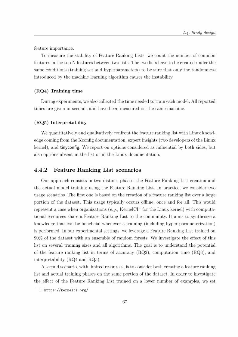
4.4. Study design
feature importance.To measure the stability of Feature Ranking Lists, we count the number of common
features in the top N features between two lists. The two lists have to be created under thesame conditions (training set and hyperparameters) to be sure that only the randomnessintroduced by the machine learning algorithm causes the instability.
(RQ4) Training time
During experiments, we also collected the time needed to train each model. All reportedtimes are given in seconds and have been measured on the same machine.
(RQ5) Interpretability
We quantitatively and qualitatively confront the feature ranking list with Linux knowl-edge coming from the Kconfig documentation, expert insights (two developers of the Linuxkernel), and tinyconfig. We report on options considered as influential by both sides, butalso options absent in the list or in the Linux documentation.
4.4.2 Feature Ranking List scenarios
Our approach consists in two distinct phases: the Feature Ranking List creation andthe actual model training using the Feature Ranking List. In practice, we consider twousage scenarios. The first one is based on the creation of a feature ranking list over a largeportion of the dataset. This usage typically occurs offline, once and for all. This wouldrepresent a case when organizations (e.g., KernelCI 1 for the Linux kernel) with computa-tional resources share a Feature Ranking List to the community. It aims to synthesize aknowledge that can be beneficial whenever a training (including hyper-parameterization)is performed. In our experimental settings, we leverage a Feature Ranking List trained on90% of the dataset with an ensemble of random forests. We investigate the effect of thislist on several training sizes and all algorithms. The goal is to understand the potentialof the feature ranking list in terms of accuracy (RQ2), computation time (RQ3), andinterpretability (RQ4 and RQ5).
A second scenario, with limited resources, is to consider both creating a feature rankinglist and actual training phases on the same portion of the dataset. In order to investigatethe effect of the Feature Ranking List trained on a lower number of examples, we set
1. https://kernelci.org/
67
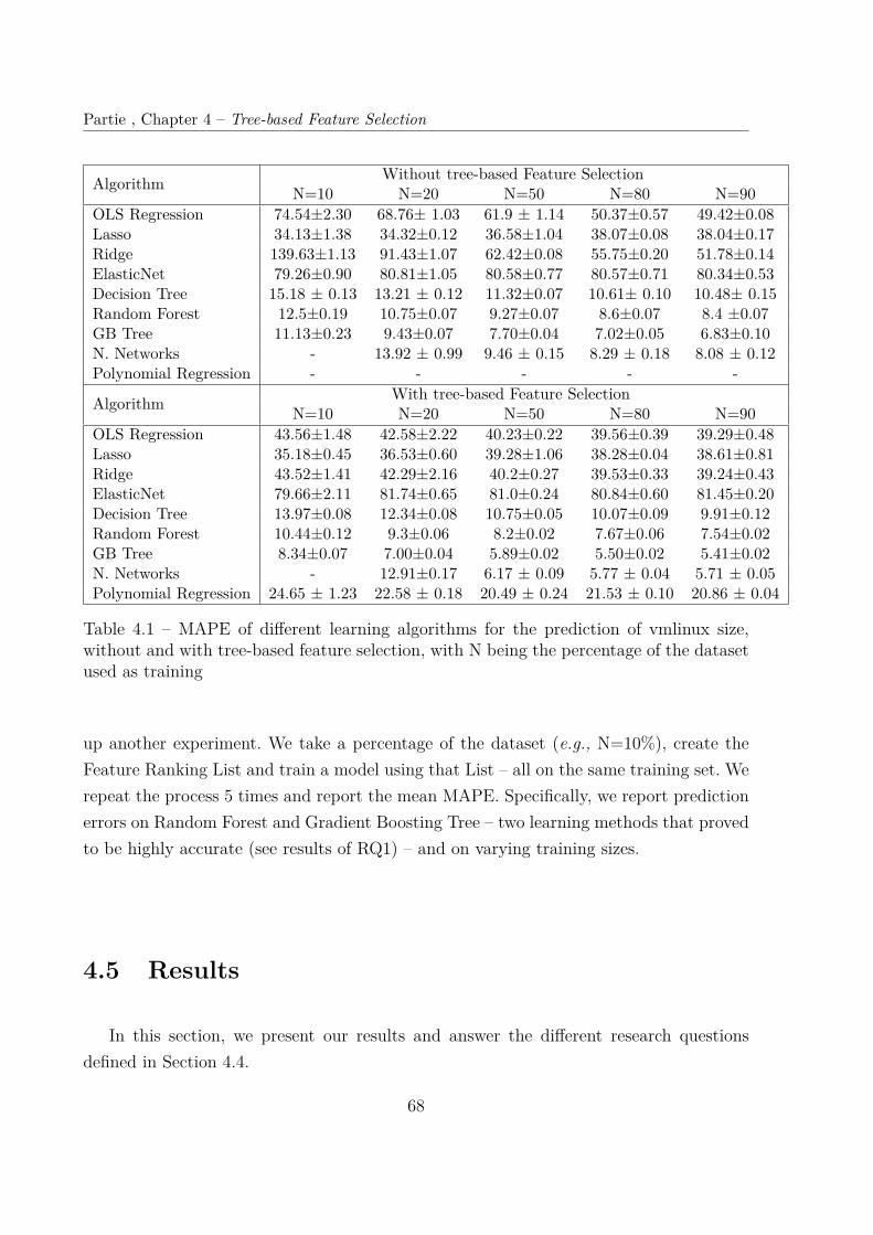
Partie , Chapter 4 – Tree-based Feature Selection
Algorithm Without tree-based Feature SelectionN=10 N=20 N=50 N=80 N=90
OLS Regression 74.54±2.30 68.76± 1.03 61.9 ± 1.14 50.37±0.57 49.42±0.08Lasso 34.13±1.38 34.32±0.12 36.58±1.04 38.07±0.08 38.04±0.17Ridge 139.63±1.13 91.43±1.07 62.42±0.08 55.75±0.20 51.78±0.14ElasticNet 79.26±0.90 80.81±1.05 80.58±0.77 80.57±0.71 80.34±0.53Decision Tree 15.18 ± 0.13 13.21 ± 0.12 11.32±0.07 10.61± 0.10 10.48± 0.15Random Forest 12.5±0.19 10.75±0.07 9.27±0.07 8.6±0.07 8.4 ±0.07GB Tree 11.13±0.23 9.43±0.07 7.70±0.04 7.02±0.05 6.83±0.10N. Networks - 13.92 ± 0.99 9.46 ± 0.15 8.29 ± 0.18 8.08 ± 0.12Polynomial Regression - - - - -
Algorithm With tree-based Feature SelectionN=10 N=20 N=50 N=80 N=90
OLS Regression 43.56±1.48 42.58±2.22 40.23±0.22 39.56±0.39 39.29±0.48Lasso 35.18±0.45 36.53±0.60 39.28±1.06 38.28±0.04 38.61±0.81Ridge 43.52±1.41 42.29±2.16 40.2±0.27 39.53±0.33 39.24±0.43ElasticNet 79.66±2.11 81.74±0.65 81.0±0.24 80.84±0.60 81.45±0.20Decision Tree 13.97±0.08 12.34±0.08 10.75±0.05 10.07±0.09 9.91±0.12Random Forest 10.44±0.12 9.3±0.06 8.2±0.02 7.67±0.06 7.54±0.02GB Tree 8.34±0.07 7.00±0.04 5.89±0.02 5.50±0.02 5.41±0.02N. Networks - 12.91±0.17 6.17 ± 0.09 5.77 ± 0.04 5.71 ± 0.05Polynomial Regression 24.65 ± 1.23 22.58 ± 0.18 20.49 ± 0.24 21.53 ± 0.10 20.86 ± 0.04
Table 4.1 – MAPE of different learning algorithms for the prediction of vmlinux size,without and with tree-based feature selection, with N being the percentage of the datasetused as training
up another experiment. We take a percentage of the dataset (e.g., N=10%), create theFeature Ranking List and train a model using that List – all on the same training set. Werepeat the process 5 times and report the mean MAPE. Specifically, we report predictionerrors on Random Forest and Gradient Boosting Tree – two learning methods that provedto be highly accurate (see results of RQ1) – and on varying training sizes.
4.5 Results
In this section, we present our results and answer the different research questionsdefined in Section 4.4.
68

4.5. Results
4.5.1 (RQ1) Accuracy
What is the best algorithm to learn the Linux kernel’s size?
In Table 4.1, we report the MAPE (and its standard deviation) of multiple statisticallearning algorithms, on various training set sizes (N), with and without tree-based featureselection.
We observe that algorithms based on linear regression (Lasso, Ridge, Elasticnet) donot work well, having a MAPE of more than 30% whatever the training set size or thefeature selection, showing that the size problem is not only an additive problem. Some donot even take advantage of a bigger training set, like Lasso which even increases its MAPEfrom 34% to 38% when the training set size goes from 10% to 90%. Tree-based algorithms(Decision Tree, Random Forest, Gradient Boosting Tree) tend to work far better (MAPEof 15% and lower) and effectively take advantage of more data to train on. As a base ofcomparison, we also report results from Neural Networks which are better than most ofalgorithms when fed with a big enough training set. 10% of the data in the training setwas not enough to make a multiple layer network converge; it led to a MAPE greater than90%. Besides, using a monolayer network would not be different from a linear regression.
How many configuration options do we need to learn the Linux kernel’s size?
Figure 4.2 aims to show the influence on the accuracy of (1) the number k of selectedfeatures and (2) the training set percentage (N) of the full dataset. In particular, it depictshow Random Forest performs when varying k and N.
We observe that for a training set size of N=10% (9,500), the accuracy peaks (i.e.,lowest error rate) when k=100 with a MAPE of 9.57, and consistently increases with morefeatures. For a training set size of N=50% (47,500), accuracy peaks when k=200 with aMAPE of 7.74. For N=90% (85,500), we reach a MAPE of 7.29 with k=250. Independentlyfrom the training set size, we consistently observe in Figure 4.2 that the MAPE is thelowest when k is in the range 100—250.
This optimal number of selected features depends on the algorithm used. Table 4.1reports the accuracy results with feature selection of the optimal number for each learningmethod. For example, for Ridge or ElasticNet, it is in the range 250—300, for Lasso, 350—400, for Gradient boosting tree, 1400–1600, for Neural Networks, 1500 (see [139] for moredetails).
Given these results, we can say that out of the thousands of options of Linux kernel,
69
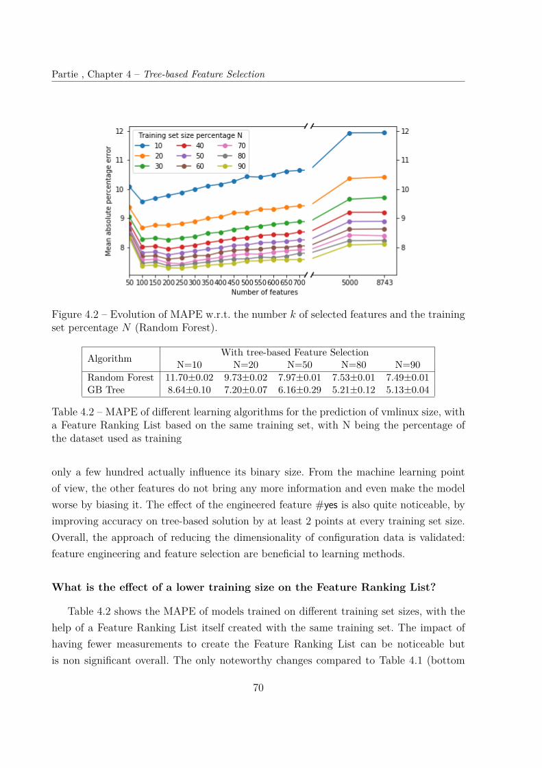
Partie , Chapter 4 – Tree-based Feature Selection
Figure 4.2 – Evolution of MAPE w.r.t. the number k of selected features and the trainingset percentage N (Random Forest).
Algorithm With tree-based Feature SelectionN=10 N=20 N=50 N=80 N=90
Random Forest 11.70±0.02 9.73±0.02 7.97±0.01 7.53±0.01 7.49±0.01GB Tree 8.64±0.10 7.20±0.07 6.16±0.29 5.21±0.12 5.13±0.04
Table 4.2 – MAPE of different learning algorithms for the prediction of vmlinux size, witha Feature Ranking List based on the same training set, with N being the percentage ofthe dataset used as training
only a few hundred actually influence its binary size. From the machine learning pointof view, the other features do not bring any more information and even make the modelworse by biasing it. The effect of the engineered feature #yes is also quite noticeable, byimproving accuracy on tree-based solution by at least 2 points at every training set size.Overall, the approach of reducing the dimensionality of configuration data is validated:feature engineering and feature selection are beneficial to learning methods.
What is the effect of a lower training size on the Feature Ranking List?
Table 4.2 shows the MAPE of models trained on different training set sizes, with thehelp of a Feature Ranking List itself created with the same training set. The impact ofhaving fewer measurements to create the Feature Ranking List can be noticeable butis non significant overall. The only noteworthy changes compared to Table 4.1 (bottom
70

4.5. Results
table, with tree-based feature selection) is that at 10% of training set size, the MAPE ofRandom Forest is 1.3 point higher (10.44% vs 11.70%). However, it is still better thanwithout feature selection (12.5%). In this practical scenario, the use of tree-based featureselection gives better accuracy results than the traditional training.
Answering RQ1
(RQ1, accuracy) How accurate is the predictive model with and withouttree-based feature selection? We find a sweet spot where only 200—300 featuresare sufficient to efficiently train a Random Forest and a Gradient Boosting Tree toobtain a prediction model that outperforms other baselines (6% prediction errors for40K configurations). We observe similar feature selection benefits for any trainingset size and tree-based learning algorithms. Overall, the use of tree-based featureselection is to be recommended when building a predictive model for Linux.
4.5.2 (RQ2) Stability
First benefit of tree-based selection: a stable Feature Ranking List
We studied the stability of the Feature Ranking List, and revised our method tocreate it. At first, we simply created a list using only one Random Forest. However, whencomparing two lists created using two different models yet trained in the same conditions,we could observe major differences already in the top 10 features, with only 9 featuresbeing in that top 10 in both. When comparing the top 300, we could only observe from100 (with feature collinearity) up to 130 (after elimination of feature collinearity) commonfeatures. This instability would be a problem so we changed the way we create the FeatureRanking List by using an ensemble of Random Forests.
By using the average feature importance of 20 Random Forests, the resulting FeatureRanking List shows a stability of 10 common features in the top 10 and 286 commonfeatures in the top 300. Despite not being perfectly stable, relying on an ensemble ofRandom Forests proves itself far more stable then using a single model.
When comparing Feature Ranking Lists with and without eliminating feature collinear-ity, we can observe its influence. For instance, the group #153 is in the 30th position, so aquite important feature, but when each of the options composing the group are taken in-dividually, namely IOSCHED_NOOP, SBITMAP, and BLOCK, they are positioned 136th, 109th,
71
Partie , Chapter 4 – Tree-based Feature Selection
and 130th, which shows a significant decrease in their computed importance.
Answering RQ2
(RQ2, stability) How stable is the Feature Ranking List? Using an ensembleof Random Forest allows the creation of a far more stable list, with more than 95%features in common among the top 300 between multiple lists.
4.5.3 (RQ3) Training time
Our obtained results show that tree-based feature selection is promising w.r.t. accuracyand interpretability. However, this is not the only observed benefit. In fact, it also has apositive impact on computational resources.
Second benefit of tree-based feature selection: a shorter training time
During the experiments, we observed that training the model without feature selectiontook a lot of time (up to 24 hours for some settings of boosting trees). To further assessthe effect of feature selection, we performed a controlled experiment. We measure thecomputation time for Random Forest and Gradient Boosting Tree, on multiple numbers offeatures and training set sizes, and report the results in Table 4.3. For Random Forest, wereport a 4,632 seconds (77 minutes) computation over 85K rows of the dataset (N=90%),with all features. With 200 features selected, we report a computation time of 97 seconds,147 seconds for 300 features and 254 seconds for 500 features. The time reduction wasrespectively 48, 31, 18 fold less than without feature selection.
With Gradient Boosting Tree, on all features and 85k rows of the dataset, we reporta computation time of 22,090 seconds (more than 6 hours). In the same conditions, fordifferent numbers of selected features, we observed a difference in time. With 500 featuresselected, we report a computation time of 1,252 seconds (21 minutes), 2,679 seconds (45minutes) for 1,000 features, and 4,350 seconds (72 minutes) for 1,500 features. The timereduction was respectively 17, 8, 5 fold less than without feature selection.
The computation time difference between Random Forest and Gradient Boosting Treeis explained by the capability of Random Forest to use multiple threads while GradientBoosting Tree is not multi-threaded. In the context of intensive search of hyperparameters,
72
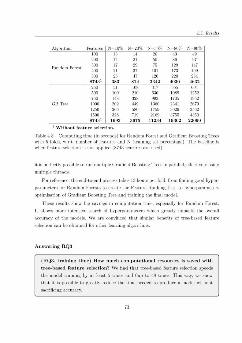
4.5. Results
Algorithm Features N=10% N=20% N=50% N=80% N=90%
Random Forest
100 13 14 26 43 49200 14 21 50 86 97300 17 29 75 129 147400 21 37 101 173 199500 25 47 126 220 254
87431 383 814 2342 4030 4632
GB Tree
250 51 108 317 555 604500 100 210 630 1089 1252750 148 328 993 1705 19521000 202 449 1360 2341 26791250 266 580 1759 3029 35621500 328 719 2169 3755 435087431 1693 3675 11234 19302 22090
1 Without feature selection.
Table 4.3 – Computing time (in seconds) for Random Forest and Gradient Boosting Treeswith 5 folds, w.r.t. number of features and N (training set percentage). The baseline iswhen feature selection is not applied (8743 features are used).
it is perfectly possible to run multiple Gradient Boosting Trees in parallel, effectively usingmultiple threads.
For reference, the end-to-end process takes 13 hours per fold, from finding good hyper-parameters for Random Forests to create the Feature Ranking List, to hyperparametersoptimisation of Gradient Boosting Tree and training the final model.
These results show big savings in computation time, especially for Random Forest.It allows more intensive search of hyperparameters which greatly impacts the overallaccuracy of the models. We are convinced that similar benefits of tree-based featureselection can be obtained for other learning algorithms.
Answering RQ3
(RQ3, training time) How much computational resources is saved withtree-based feature selection? We find that tree-based feature selection speedsthe model training by at least 5 times and 0up to 48 times. This way, we showthat it is possible to greatly reduce the time needed to produce a model withoutsacrificing accuracy.
73
Partie , Chapter 4 – Tree-based Feature Selection
4.5.4 (RQ) Interpretability
On the interpretability of the Linux documentation
Contrary to Neural networks, Gradient Boosting Tree or Random Forest are algorithmswith built-in interpretability. There, we can extract a list of features that can be orderedby their importance with respect to the property of interest (here size). So the questionis: How do feature ranking lists, as computed by tree-based feature selection, relate toLinux knowledge?
Confrontation with documentation. We confront the feature ranking list to the147 options referring to size in the Kconfig documentation (see Section 4.2). First, wenotice that 31 options have a unique value in our dataset: randconfig was unable to diversifythe values of some options and therefore the learning phase cannot infer anything. We seeit as an opportunity to further identify influential options. As a proof of concept, we samplethousands of new configurations with and without option KASAN_INLINE activated (in ouroriginal dataset, KASAN_INLINE was always set to ’n’). We did observe a size increase (20%on average), suggesting that the documentation could help identifying influential optionswe have missed due to randconfig. However, the documentation can put us on the wrongtrack: we have also tried for 5 other options and did not observe a significant effect onsize [139].
Among the resulting 116 options (147 − 31), we found that:— 7 are in the top 50, 6 are in the top 50—250, 6 are in the top 250—500, and 28 in
the top 500—1,500— 60% of options are beyond the rank 1,500, hence not considered after feature se-
lection. We identified two possible explanations. First, the effect on size is simplynegligible: It is explicitly stated as such in the documentation ("This will increasethe size of the kernelcapi module by 20 KB" or "Disabling this option saves about300 bytes"). Second, some option values are not distributed uniformly (e.g., 98% ‘y’and 2% ‘n’ value) in our dataset: the learning phase needs more diverse instances.
Finding of undocumented options. A consequence from the confrontation withKconfig is that the vast majority of influential options is either not documented or notreferring to size. In order to further understand this trend, we analyze the top 50 optionsin the feature ranking list (representing 95% of the feature importance in the RandomForest):
— only 7 options are documented as having a clear influence on size;
74
4.5. Results
— our investigations and exchanges with domain experts 2 show that the 43 remainingoptions are either (1) necessary to activate other options; (2) the underlying mem-ory used would be based on the size of the driver; (3) chip-selection configuration(you cannot run the kernel on the indicated system without activating this option);(4) related to compiler coverage instrumentation, which will affect lots (possibleall) code paths; (5) debugging features; (6) related to DRM (for Direct RenderingManager) and GPU drivers
Revisiting tinyconfig
In our dataset, we observe that tinyconfig is by far the smallest kernel (≈7Mb). Thesecond smallest configuration is ≈11Mb. That is, despite 90K+ measurements with rand-config, we were unable to get closer to 7Mb. Can our prediction model explain this signif-icant difference (≈4Mb)?
A first hypothesis is that the four pre-set options of tinyconfig have an important im-pact on the size (see Figure 2.6, page 41). We observe that our prediction model indeedranks CC_OPTIMIZE_FOR_SIZE, one of the four pre-set options, in the top 200. The otherthree remaining options have no significant effects according to our model and cannotexplain the ≈4Mb difference. In fact, there is a more simple explanation: the strategy oftinyconfig consists in minimizing #yes. According to our prediction model, #yes is highlyinfluential feature. We notice that the number of ‘y’ options of tinyconfig is 224 whilethe second smallest configuration exhibits 646 options: the difference is significant. Fur-thermore, tinyconfig deactivates many top-influential options like KASAN or DEBUG_INFOthat have a positive effect on the binary size when activated. We can conclude that theinsights of the predictive model are consistent with the heuristic of tinyconfig.
Collinearity and interpretability.
The top 50 of our feature ranking list exhibits 4 groups with collinear features.Thanks to removal of feature collinearity, we have automatically identified cases in
which some options can be grouped together (e.g., we can remove KASAN_OUTLINE andonly keep KASAN). We found that taking in account feature collinearity is beneficial for tworeasons (1) we do not miss influential features since the importance is not split amongfeatures; (2) experts only have to review a group of features instead of unrelated and
2. The full data is available on the companion web site [139]
75
Partie , Chapter 4 – Tree-based Feature Selection
supposedly independent features.
Documentation-based feature selection
Instead of using the top X features from the Features Ranking List of a tree-basedfeature selection, the 147 options referring to size in the Kconfig documentation (seeSection 4.2) can be used to form the feature list fed to the actual training. This scenariocorresponds to feature selection realized with expert knowledge. We use all the 147 optionsin the Linux documentation and only them (considering that an option is encoded as afeature).
The resulting prediction model exhibits a MAPE of 23.6% for Gradient Boosting Tree(the best learning algorithm) and over 90% of the dataset for training. It is more than4 times the error rate of using the Feature Ranking List used with tree-based featureselection. This show that documentation alone is not suited for feature selection. It isin line with previous observations: the Linux documentation is incomplete (i.e., someimportant features are missing) and describes features that have little influence on size.
Answering RQ4
(RQ4, interpretability) How do feature ranking lists, as computed bytree-based feature selection, relate to domain knowledge? Thanks to ourprediction model, we have effectively identified a list of important features thatis consistent with the options and strategy of tinyconfig, and Linux knowledge(Kconfig documentation and expert insight). We also found options that can beused to refine or augment the incomplete documentation of the Linux kernel.
4.6 Threats to Validity
4.6.1 Internal Validity
Aside from the threats describe in Section 3.5.1 about the range of algorithms con-sidered, and the sampling method used which both also affect the experiment from thischapter, we can raise another threat about the Feature Ranking List. The computation offeature importance is subject to some debate and some implementation over random for-est, including the scikit-learn’s one we rely on, may be biased [18, 43, 97, 111]. This issue
76

4.7. Conclusion
may impact our experiments e.g., we may have missed important options. To mitigate thisthreat, we have computed feature importance with repetitions (i.e., 20 times). Our ob-servation is that the top influential options then remain very similar [139] (see RQ2). Asfuture work, we plan to compare different techniques to compute feature importance [18,43, 97, 111].
4.7 Conclusion
Feature selection is a process that has proved itself efficient in the usage of machinelearning in many domains. While Software Product Lines is not an exception, the onlyprevious use was done in a way that does not scale to the number of options of Linux.
Tree-based feature selection is a technique that has been used a lot in biology whendealing with very large datasets, making it potentially suitable for SPL.
In this chapter, we explored this process, the concerns of stability and how to dealwith it.
We compared multiple state-of-the-art solutions with and without feature selectionand found that tree-based feature selection pays off:
— the accuracy is better with than without tree-based feature selection. It is possibleto reach low prediction errors (5.5% for binary kernel size);
— the training time is decreased by at least an order of magnitude;— the identification of influential options is consistent with, and can even improve, the
expert knowledge about Linux kernel configuration. Models are easy to interpret:insights can be validated and communicated;
The decrease of prediction errors is perhaps the most surprising positive result of ourempirical inquiry, since feature selection does not necessarily improve accuracy. Overall,we found a subset of options (≈500) that can achieve an interesting sweet-spot along thethree dimensions (accuracy, training time, interpretability). Furthermore, feature selectionhas the merit of being agnostic and fully automated: we did not rely on expert knowledgeto achieve this result.
77

Chapter 5
AUTOMATED PERFORMANCE
SPECIALIZATION
5.1 Introduction
More and more software systems are configurable through command-line parameters,configuration files, or compile-time options. Users can set many configuration options’values to fit their functional requirements and performance objectives. For instance, userscan change parameters’ values of the x264 encoder to obtain a video in a fast way; userscan configure Linux to obtain a kernel with a binary size below a certain threshold (e.g.,less than 20Mb).
The configuration of a configurable system is an error-prone and time-consuming task.There is a combinatorial explosion of possible configurations and the effects of optionson performance is hard to document and formalize. Numerous works have shown thatquantifying the performance influence of each individual option is not meaningful in mostcases [114]. That is, the performance influence of n options, all jointly activated in aconfiguration, is not easily deducible from the performance influence of each individualoption. We thus need to try to capture the complex interactions among options and theireffects on performance.
An approach for supporting users in the configuration process is to specialize the con-figuration space of a software system. Given a performance objective, the specializationbuilds presets or profiles through constraints over options’ values. Constraints can be onindividual options: some specific values are already preset and users can focus on theremaining options. Constraints can also be among several options to only keep combina-tions of options’ values (configurations) that have acceptable performance. For instance,the encoder x264 can be specialized to encode videos in a fast way: some options valuesare preset while the remaining options can still be configured for dealing with hardwareconstraints, output quality, or functional concerns.
79
Partie , Chapter 5 – Automated Performance Specialization
Specializing the configuration space of a software system has a long tradition since theseminal paper of Czarnecki et al. [33].
Specialization has been considered for targeting specific profiles, usages, deploymentscenarios, or hardware settings [6, 9, 32, 59, 143]. The idea is to retain only a subset ofconfigurations that meet a performance threshold (e.g., execution time below one second)and thus discard the rest. Specialization should not be confused with configuration opti-mization (tuning) where the goal is to find a unique and optimal configuration. Throughspecialization, users still have flexibility (variability) to configure their systems. The ben-efit is that some options’ value are already preset for reaching a performance threshold.A unique challenge is to identify configurations that should be kept (or, equivalently, todiscard non-acceptable configurations), which boils down to specifying constraints amongoptions’ values.
On the one hand, measuring all configurations is infeasible in practice owing to thecombinatorial explosion of possible configurations. On the other hand, the manual specifi-cation of constraints is an error-prone, time-consuming, and hardly repeatable task for anyperformance objective. It should however be possible to automate the specialization pro-cess using machine learning, i.e., measuring a sample of configurations and then learningwhat options’ values should be constrained. Even focusing on learning techniques basedon decision trees for their built-in explainability, there is still a wide range of possibleapproaches that need to be evaluated, i.e., how accurate is the specialization with regardsto sampling size, performance thresholds, and kinds of configurable systems.
In this chapter, we propose six learning techniques based on regression, classification,feature selection and a combination thereof. We first perform a study on 8 configurablesystems with dozens of options, as usually considered in the literature. We then perform astudy on a much larger configurable systems – the Linux kernel considering 9K+ options.In summary, our contributions are as follows:
— We propose a new way to use decision trees, called specialized regression andtailored toward performance specialization;
— We design and develop six performance specialization learning strategies with threevariants of Decision Trees: regression, classification, and specialized regression;
— We perform an empirical study to compare the accuracy results of these techniques.Through our experimental results, we find that Decision Tree is a very accuratealgorithm for performance specialization. However, it is sensitive to threshold vari-ation. Feature selection is a reliable way to produce more accurate results; however
80
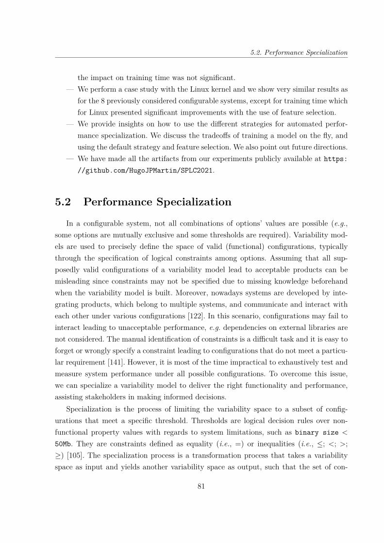
5.2. Performance Specialization
the impact on training time was not significant.— We perform a case study with the Linux kernel and we show very similar results as
for the 8 previously considered configurable systems, except for training time whichfor Linux presented significant improvements with the use of feature selection.
— We provide insights on how to use the different strategies for automated perfor-mance specialization. We discuss the tradeoffs of training a model on the fly, andusing the default strategy and feature selection. We also point out future directions.
— We have made all the artifacts from our experiments publicly available at https://github.com/HugoJPMartin/SPLC2021.
5.2 Performance Specialization
In a configurable system, not all combinations of options’ values are possible (e.g.,some options are mutually exclusive and some thresholds are required). Variability mod-els are used to precisely define the space of valid (functional) configurations, typicallythrough the specification of logical constraints among options. Assuming that all sup-posedly valid configurations of a variability model lead to acceptable products can bemisleading since constraints may not be specified due to missing knowledge beforehandwhen the variability model is built. Moreover, nowadays systems are developed by inte-grating products, which belong to multiple systems, and communicate and interact witheach other under various configurations [122]. In this scenario, configurations may fail tointeract leading to unacceptable performance, e.g. dependencies on external libraries arenot considered. The manual identification of constraints is a difficult task and it is easy toforget or wrongly specify a constraint leading to configurations that do not meet a particu-lar requirement [141]. However, it is most of the time impractical to exhaustively test andmeasure system performance under all possible configurations. To overcome this issue,we can specialize a variability model to deliver the right functionality and performance,assisting stakeholders in making informed decisions.
Specialization is the process of limiting the variability space to a subset of config-urations that meet a specific threshold. Thresholds are logical decision rules over non-functional property values with regards to system limitations, such as binary size <
50Mb. They are constraints defined as equality (i.e., =) or inequalities (i.e., ≤; <; >;≥) [105]. The specialization process is a transformation process that takes a variabilityspace as input and yields another variability space as output, such that the set of con-
81
Partie , Chapter 5 – Automated Performance Specialization
figurations denoted by the latter space is a subset of the configurations denoted by theformer space (see Figure 5.1) [32].
Figure 5.1 – Configuration of a specialized Linux kernel. Given a performance threshold(binary size < 50Mb), the specialization process identifies constraints among optionsthat preclude some (combinations of) values (in gray); users still have some flexibility toconfigure other options (in black).
The specialization of a variability space involves the addition of a set of new con-straints (rules) to options’ values. Such rules describe how performance influences thesystem options’ interactions, i.e. the variability space is restricted to only configurationssatisfying the given performance threshold. The restricted subset of configurations repre-sents the space of specialization. As an example, the Linux can be specialized to obtaina kernel binary size below 50Mb (see Figure 5.1). To meet the threshold, a set of optionsvalues (in gray) are preset to true while others to false, and the remaining options (inblack) can still be configured. This is helpful to avoid large kernels that take too muchtime to compile. Notice that we consider a threshold, thus contrary to optimization ap-proaches that aim at satisfying a specific optimization objective (e.g. minimize binarysize), we aim at specializing the configuration space to a subset of acceptable configu-rations. Although optimization is not our aim here, the specialization may highly assistthe optimization process later when deriving a suited configuration, e.g. to support thevariability at runtime.
How do we find a set of options that affect considerably performance? Op-tions can be captured by running the system and measuring performance of each config-
82
5.2. Performance Specialization
uration. However, as the configuration space is typically very large and measuring eachvalid configuration is often infeasible, the use of learning-based techniques are promis-ing for specialization. Learning techniques automatically obtain rules without exploringall possible configurations. They are used under the condition a sample of configurationmeasurements is available. The idea is to learn out of a (small) sample of configurationobservations and hopefully generalize to the whole configuration space.
The learning process consists of four main stages: (1) definition of a performancethreshold, (2) sampling, (3) measuring, and (4) learning (see Figure 5.1). The fifth stage(validation) is interesting for assessing the prediction models and their accuracy – a cen-tral research question of this chapter. First, the process starts by defining a thresholdand selecting a sample set of valid configurations. Second, the sample of configuration isbuilt, and the properties of interest are measured. Third, these measurements and theperformance threshold are used as input to accurately learn a prediction model. Finally,the validation step computes the accuracy of the prediction model.
Prediction models support stakeholders understanding the characteristics of the vari-ability space, i.e. the effects of some options and how options interact. Interpretability forspecialization is very important both for validating the insights of the learning and forencoding the knowledge into a variability model. As an example, consider learning tech-niques based on decision trees. Each branch of a tree represents a set of rules (decisions)that satisfy a threshold leaf. Thus, as a result, rules are mined by building the conjunctionof a path to reach a threshold leaf. In the example of Figure 5.1, the algorithm learnsthat by having the options CONFIG_64BIT, CONFIG_SLOB, and CONFIG_PCI deselected, andCONFIG_DEBUG_INFO_SPLIT, CONFIG_UBSAN_SANITIZE_ALL,CONFIG_OPTIMIZE_INLINING, and CONFIG_DEBUG_INFO_REDUCED selected, the binary sizethreshold is (almost) guaranteed to be respected. Thus, options are preset and no mod-ification of these option values are allowed. Without specialization, we are likely to setdifferent option values. An interesting example is "defconfig", a default configuration forLinux, in which the binary size is around 70Mb. So, in case users start the configurationwith "defconfig", they do not meet the specified threshold. Notice that learning is usefuland necessary since manually discovering such rules is tedious, error-prone, and time-consuming. Moreover, it requires expert knowledge of the system domain. The overalloutcome is constraints among options that are retrofitted into a variability model anda configurator. Constraints can either force the values of individual options or logicallyinvolve several options. Such constraints are learned out of learning models.
83
Partie , Chapter 5 – Automated Performance Specialization
5.3 Automated Performance Specialization
The key to automated specialization is the identification of constraints that can pre-clude configurations not fitting a performance threshold. We first frame the specializationproblem as a learning problem. We discuss the space of possible learning algorithms andshow that decision trees represent a good fit between accuracy and the identificationof constraints. We then present three techniques that can be combined with tree-basedfeature selection to realize performance specialization.
5.3.1 Specialization as a learning problem
We denote p the number of configuration options and define the configuration spaceC = {0, 1}p. Out of this space of configurations C, we gather a subset of d configurations,denoted CS ⊂ Cd. We separate CS into a training set Ctr
S and a test set CteS , so CS =
CtrS
⊕CteS . Let B = {0, 1} resp. for "non-acceptable" and "acceptable". Then, we denote:
— f : C → R+ the function affecting to any configuration c ∈ C its performancef(c) ∈ R+,
— p : R → B a predicate that determines whether a performance value is acceptableor non-acceptable,
— s : C × p → B the specialization function affecting to any configuration c ∈ C itsacceptability p(f(c)) ∈ B.
With respect to these notations, the goal is to train a learning algorithm s estimatingthe function s for each measured configuration of the training set c ∈ Ctr
S . The training setCtr
S is used to obtain a learning model, while the testing set CteS only tests the prediction
accuracy of s.
5.3.2 Learning algorithms for specialization
Numerous statistical learning algorithms can be used for performance specialization.These algorithms differ in terms of computational cost, expressiveness and interpretabil-ity. We now review the literature of configurable systems (based on the systematic sur-vey [114]). We discuss what algorithms are suited or not for our specific problem. Linearregressions are considered as easy to interpret, but are unable to capture interactions be-tween options or to handle non-linear effects [97]. Neural networks can reach high accuracyon large datasets. DeepPerf [52] has been developed for tackling configurable systems with
84
5.3. Automated Performance Specialization
dozens of options. Empirical results show the effectiveness of DeepPerf [52] on all systemsof our study (except Linux that has not been considered). However, neural networks areblack-box functions for which it is hard to extract rules (constraints) among options, atop requirement in the specialization problem.
Siegmund et al. [131] introduced a learning method called performance-influence model.Feature-forward selection and multiple linear regression are used in a stepwise manner toshrink or keep terms representing options or interactions. This method aims to handleinteractions between options, limit the number of options to learn on, and provide ahuman-readable formula describing influence of options and combinations of options onperformance. However, performance-influence model does not address the performancespecialization problem. First, the model addressed a regression problem while we are in-terested in predicting the class of a configuration. Second, the technique does not retrofitconstraints into a variability model. The synthesized information (a formula with coeffi-cients) is not designed for extracting rules and constraints. Third, a performance-influencemodel aims to construct a global performance model: a rewrite is necessary to take thethreshold into account. Fourth, the step-wise addition of interactions among options doesnot scale for Linux that exhibits 9K+ options (see more details hereafter).
Decision trees ( e.g., CART) are the most used technique in the literature [114]. De-cision trees have been used either for classification or regression, have reached competingaccuracy with the state-of-the-art, and are interpretable by construction [142, 148, 150].The tree structure is ideal for capturing interactions between options. Rules can easily beextracted and retrofitted into a variability model.
Random forests are an ensemble learning method that constructs a multitude of deci-sion trees at training time. As an ensemble method, the accuracy of random forests canbe better than decision trees. However the question of extracting rules out of multipletrees is still an open issue.
Overall, decision trees represent a good fit for our specialization problem. We willconsider this learning technique under different strategies in the following.
5.3.3 Learning strategies
Fundamentally, the learning problem presented in Section 5.3.1 is a supervised, binaryclassification problem. However, and which makes it noteworthy, the learning has at itsdisposal continuous values (performance measurements). In this regard, the problem isclose to a regression problem, except that one does not want to eventually predict a
85
Partie , Chapter 5 – Automated Performance Specialization
quantity but a class.
We now describe three possible techniques for performance specialization learning:classification, regression, and specialized regression.
Classification. The strategy is to use a classification tree, ie a Decision tree model wherethe target variable can take a discrete set of values (acceptable, non-acceptable). From themeasured performance of configurations and the defined threshold, it is possible to labeleach configuration as acceptable or non-acceptable. Then a classification tree is trained topredict the performance acceptability on new configurations. One of the downsides of thisapproach is that the actual performance value is lost from the dataset, as it is replacedby a simple boolean value. Not having the numerical information to indicate whether aconfiguration is close to the performance threshold, or very far from that threshold, islikely to degrade the accuracy of the learning process.
Gap in the related work. Classification trees have been considered in prior works [6, 9,142]. However, a systematic comparison with other techniques is missing and it is unclearhow the approach works for large systems like Linux.
Regression. Another way to produce a decision tree is to tackle the regression problem.In this case, a regression tree would predict directly the performance of a configurationand then a post-process step can be applied to determine if that predicted performance isacceptable. It means that the regression tree has to be rewritten for predicting the outcome(a class). The promise is to better use the performance value, unlike the classificationapproach. However, the learning is focused on minimizing the error between the predictedperformance value and the actual value independent of the threshold. As a result, aconfiguration could well have its performance value, predicted with a very low error butjust on the other side of the threshold, leading to a classification error unrecognized bythe regression algorithm. It should be noted that a regression approach is agnostic to thethreshold, meaning that the model can be used once and for all, for any threshold. Incontrast, a classification tree should be trained anytime a new performance threshold isspecified.
Gap in the related work. Although regression problems have been widely considered forperformance prediction or optimization, we are unaware of existing works that investigatetheir effectiveness in the context of specialization. As stated, specialization is in-betweena regression and classification problem, which questions the accuracy of such techniquesin this context.
86

5.4. Study Design
Specialized regression. Considering the weaknesses of the two previous approaches,we propose a novel and hybrid strategy. The training of a regression tree is performedover the dataset where all performance values higher than the performance thresholdare increased by an important amount. Intuitively, we artificially create a "gap" in theperformance distribution representing the threshold. The intent is to punish errors acrossthe border, while still being able to take advantage of the insight given by the performancevalue. We call this techniques specialized regression since the regression is aware of thespecialization criterion (performance threshold). In contrast, regression is only aware ofthe performance values of the training set and ignores the performance threshold.
5.3.4 Tree-based Feature selection
As we demonstrate in Chapter 4, the feature selection can have positive impact on per-formance prediction models, both on accuracy and training time. The idea is to decreasethe complexity of the problem, without removing too valuable information. This selectioncan be done in several ways, such as using expert knowledge, or in an automated fashion.We will reuse here the process based on extracting the feature importance of RandomForest, and ranking feature by this metric, as we showed its ability to scale on thousandsof features.
As the learning task is a classification one and not a regression one, the effects of thisfeature selection on the automated specialization process are yet to be determined.
5.4 Study Design
To investigate the proposed approaches, we elaborate four research questions to con-duct our experiment:
— RQ1: What is the accuracy and cost of learning strategies? We aim to eval-uate the prediction errors of specialization learning on nine real-world configurablesystems, with varying cost in terms of the number of configuration measurements.
— RQ2: What is the best learning strategy? There are multiple ways to usedecision trees (namely classification, regression and specialized regression) in orderto synthesize the rules needed for the specialization. With regard to accuracy, isthere a best strategy e.g., whatever the subject system?
— RQ3: What are the effects of tree-based feature selection on the accuracy
87

Partie , Chapter 5 – Automated Performance Specialization
System Features Measured Configurations
Apache 9 192Berkeley C 19 2.560Berkeley J 26 180
Dune 11 2.304HMSGP 14 3.456HIPAcc 33 13.485LLVM 11 1.024SQLite 39 4.553Linux 9.467 92.562
Table 5.1 – Datasets information, including number of features and number of measuredconfigurations
of performance specialization? We aim to investigate whether feature selectionimproves or degrades the accuracy of learning strategies and for which subjectsystems, performance thresholds, and training set size.
— RQ4: What is the time cost of the 6 learning strategies to predict per-formance of a configurable software system? This question is to evaluatethe practicality and feasibility of a proposed strategy. To answer this question, weshow the time consumed by the feature selection (if used), hyperparameter search-ing and training process on various highly configurable software systems (includingLinux). We also put in perspective the fact that some techniques are learned onceand for all, whatever the performance thresholds.
5.4.1 Datasets
In order to perform our experiments, we relied on datasets already used in the com-munity (see details in Table 5.1).
Common SE datasets
Our first part of the experiments is to train Decision Trees on reliable datasets com-monly used on numerous occasions in the past [52, 131] to observe the efficiency of learningtechniques.
88
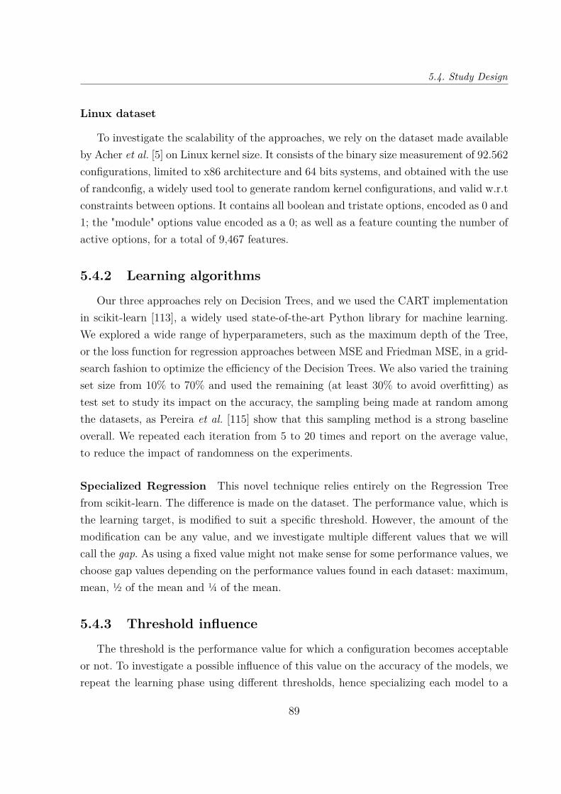
5.4. Study Design
Linux dataset
To investigate the scalability of the approaches, we rely on the dataset made availableby Acher et al. [5] on Linux kernel size. It consists of the binary size measurement of 92.562configurations, limited to x86 architecture and 64 bits systems, and obtained with the useof randconfig, a widely used tool to generate random kernel configurations, and valid w.r.tconstraints between options. It contains all boolean and tristate options, encoded as 0 and1; the "module" options value encoded as a 0; as well as a feature counting the number ofactive options, for a total of 9,467 features.
5.4.2 Learning algorithms
Our three approaches rely on Decision Trees, and we used the CART implementationin scikit-learn [113], a widely used state-of-the-art Python library for machine learning.We explored a wide range of hyperparameters, such as the maximum depth of the Tree,or the loss function for regression approaches between MSE and Friedman MSE, in a grid-search fashion to optimize the efficiency of the Decision Trees. We also varied the trainingset size from 10% to 70% and used the remaining (at least 30% to avoid overfitting) astest set to study its impact on the accuracy, the sampling being made at random amongthe datasets, as Pereira et al. [115] show that this sampling method is a strong baselineoverall. We repeated each iteration from 5 to 20 times and report on the average value,to reduce the impact of randomness on the experiments.
Specialized Regression This novel technique relies entirely on the Regression Treefrom scikit-learn. The difference is made on the dataset. The performance value, which isthe learning target, is modified to suit a specific threshold. However, the amount of themodification can be any value, and we investigate multiple different values that we willcall the gap. As using a fixed value might not make sense for some performance values, wechoose gap values depending on the performance values found in each dataset: maximum,mean, ½ of the mean and ¼ of the mean.
5.4.3 Threshold influence
The threshold is the performance value for which a configuration becomes acceptableor not. To investigate a possible influence of this value on the accuracy of the models, werepeat the learning phase using different thresholds, hence specializing each model to a
89

Partie , Chapter 5 – Automated Performance Specialization
particular threshold. For the regression approach, we do not repeat the learning process,since a regression model is threshold-agnostic. Thus, we repeated only the accuracy mea-surement. We choose 5 threshold values based on the performance distribution for eachdataset, namely 10%, 20%, 50%, 80% and 90% quantiles.
5.4.4 Metrics
To measure the accuracy of the Decision Trees classification, we use the balance accu-racy[19], which is a combination of sensitivity and specificity:
Balanced accuracy = 12
(TP
TP + FN+ TN
TN + FP
)
with TP for True Positive, TN for True Negative, FN for False Negative and TP for FalsePositive. The balanced accuracy heavily takes in account the influence of imbalanced classdistribution, which inevitably happens due to the threshold variation in the experiment.In the remaining of the chapter, we will refer to balanced accuracy as "accuracy".
5.4.5 Tree-based Feature selection
We trained 20 Random Forests on 10% of the training set and extracted a FeatureRanking List, except for Linux kernel, where we used the List provided with the dataset [5].We then repeated the learning as much as needed to find the optimal number of options.
We consider 6 different strategies:
1. Classification
2. Classification with Feature Selection
3. Regression
4. Regression with Feature Selection
5. Specialized Regression
6. Specialized Regression with Feature Selection
As mentioned, we evaluated all 6 strategies over 5 different thresholds, and with 4different training sizes.
90

5.5. Results
5.5 Results
In this section, we discuss the answers to our research questions defined in Section 5.4.
91

Partie , Chapter 5 – Automated Performance Specialization
Tabl
e5.
2–
Aver
age
accu
racy
and
stan
dard
devi
atio
npe
rsy
stem
and
lear
ning
tech
niqu
eov
eral
lthr
esho
lds
and
for
70%
trai
ning
set
size.
FSst
ands
for
Feat
ure
Selec
tion
whi
leA
llSt
rate
gies
mea
nth
atwe
syst
emat
ical
lych
oose
the
best
stra
tegy
amon
gth
e6.
Syst
emA
llst
rate
gies
Cla
ssifi
catio
nC
lass
ifica
tion
FSR
egre
ssio
nR
egre
ssio
nFS
Spec
.Reg
r.Sp
ec.R
egr.
FS
Apa
che
95.3
%(±
2.1)
94.3
%(±
2.3)
92.3
%(±
3.0)
93.1
%(±
2.7)
93.3
%(±
3.3)
92.8
%(±
2.7)
93.5
%(±
3.6)
Berk
eley
C99
.9%
(±0.
3)99
.8%
(±0.
4)99
.9%
(±0.
3)99
.8%
(±0.
4)99
.8%
(±0.
3)99
.5%
(±0.
6)99
.6%
(±0.
5)Be
rkel
eyJ
93.3
%(±
9.4)
92.9
%(±
9.2)
92.4
%(±
9.8)
92.1
%(±
9.5)
92.4
%(±
10.1
)90
.0%
(±12
.4)
91.2
%(±
10.8
)D
une
93.6
%(±
2.4)
92.8
%(±
1.7)
92.2
%(±
1.8)
91.2
%(±
3.2)
91.9
%(±
2.9)
92.7
%(±
3.2)
92.9
%(±
3.1)
HIP
Acc
97.6
%(±
0.9)
96.6
%(±
1.1)
97.1
%(±
0.7)
95.5
%(±
2.3)
95.6
%(±
2.3)
94.9
%(±
4.2)
94.9
%(±
4.4)
HM
SGP
97.3
%(±
2.1)
96.5
%(±
2.5)
96.9
%(±
2.4)
96.7
%(±
2.2)
97.2
%(±
2.0)
96.4
%(±
2.6)
97.0
%(±
2.3)
LLV
M94
.6%
(±4.
4)93
.8%
(±5.
2)94
.0%
(±5.
1)91
.8%
(±5.
5)93
.2%
(±4.
7)93
.2%
(±3.
8)93
.7%
(±4.
0)SQ
Lite
74.9
%(±
10.4
)73
.7%
(±9.
0)73
.4%
(±9.
0)70
.2%
(±8.
2)70
.6%
(±8.
4)70
.1%
(±13
.6)
70.6
%(±
13.4
)Li
nux
92.6
%(±
4.0)
91.1
%(±
2.4)
91.3
%(±
2.8)
91.2
%(±
2.9)
91.4
%(±
3.3)
91.8
%(±
4.2)
92.0
%(±
4.7)
92
5.5. Results
Figure 5.2 – Performance Distribution for BerkeleyJ
5.5.1 Results RQ1 and RQ2—Accuracy
Table 5.2 is a summary of the accuracy over all thresholds for each system with 70%training set size. With the exception of the SQLite system, we report an accuracy ofmore than 90% overall, showing that Decision Tree is able to handle the complexity ofconfigurable systems for the specialization task in most cases. We observe that the bestresults are held by the Classification strategy on 6 out of 9 systems. However, since thedifference between strategies is very slight, we can consider the 6 strategies to be accurate.Furthermore, there is no learning strategy better than another on all thresholds. For somesystems, a high standard deviation can be observed due to thresholds variations within asubject system. For instance, for BerkeleyJ 1 the accuracy for 70% T.S. (training set size)goes from 77.2% to 100%, respectively at 10% and 50% of A.C. (acceptable configurations),which is tied to the threshold variation. This can be explained by the very inconsistentperformance distribution shown in Figure 5.2.
(RQ1) Decision Tree is an accurate algorithm for performance specialization, withmore than 90% accuracy for 8 out of 9 systems, including Linux.
Strategies
In this section, we report mainly on the tables present in our supplementary material2,where we detailed results over all strategies and systems for each considered threshold andtraining size. Here, due to space limitations, we add the detailed results only for Apacheand Linux (see Tables 5.3 and 5.4). Notice that the results in Table 5.2 (for all systems)
1. https://raw.githubusercontent.com/HugoJPMartin/SPLC2021/master/tables.pdf
93
Partie , Chapter 5 – Automated Performance Specialization
refer to a 70% training set size and an average over all thresholds.
Classification. As seen previously, classification is overall the best strategy, and itsstrength resides mainly in the restrictive threshold of 10% or 20% A.C. (acceptable con-figurations). For Apache, at 10% A.C. and 10% and 20% T.S. (training set size), theaccuracy is more than 3 points higher on classification than the two other strategies. ForHIPAcc, at 10% A.C. that difference is from 4 to 5 points, while regression shows 92.2%accuracy at 70% T.S., classification shows 97.3% accuracy.
Regression. The overall accuracy of regression is very similar to specialized regression.For 1 out of 8 systems (HMSGP) it is the best solution. However, regression is a threshold-agnostic approach. It tends to be very sensitive to extreme thresholds (10% and 90% A.C.),which can be seen as a limitation. HMSGP and Linux are the exceptions, where regressionshows itself the best strategy i n many cases. For Linux, regression is the best at 50%A.C. on all T.S., and at low T.S. and A.C. We note also that regression is often betterthan classification on higher thresholds, and better than specialized regression on lowerthresholds.
Specialized Regression. This approach shines at higher thresholds, being the beststrategy in almost all cases at 80% and 90% A.C. The improvement can be very important,for instance Apache at 90% A.C. and 10% T.S., specialized regression is better by 6 and9 points over regression and classification. About the gap influence (Section 5.4.3), mostof the time the minimum value (¼ of the mean) gives the best results, and in some cases(for Berkeley C and Berkeley J) it’s the maximum value.
(RQ2) The 6 strategies are particularly sensitive to performance thresholds.Classification is the most efficient on low thresholds, specialized regression on highthresholds, while regression proves itself a good middle ground.
5.5.2 Results RQ3—Feature selection
In Tables 5.3 and 5.4, the influence of feature selection is represented by the valueinside brackets. In the vast majority of cases, the use of feature selection improves theresults, though the improvement can be very low (less than 1 point). The most significantimprovements are for LLVM (see in our supplementary material), with cases showing upto 10.3 points more than their counterpart without feature selection.
94

5.5. Results
On the other hand, some cases show that feature selection does not improve the ac-curacy (mostly for classification strategy). We report one case where the feature selectionhas a significantly negative impact with regression, while there are 21 of such cases (outof 180 possible cases per strategy) for classification.
Beside, the optimal number of options to select is very variable depending on thresholdand training set size. We did not identify particular pattern to predict that number before-hand, so the number of selected options should be considered as a new hyperparameterfor the Decision Tree.
(RQ3) Feature selection is a reliable way to produce more accurate results (im-provements up to 10%), although the increase is often insignificant. Note thatclassification-based learning sometimes does not take advantage of feature selec-tion – using all features lead to better results.
5.5.3 Results RQ4—Training time
The training time of a Decision Tree is in the order of milliseconds (except for Linux).It is up to 22 ms for Specialized Regression on HIPAcc, which is the system with thelargest configuration dataset (see Table 5.1). The training time reduction after featureselection is very slight. The most significant improvement is the reduction from 6.4 msto 3.5 ms (for Regression Decision Tree on SQLite). Proportionally, it is a 45% timereduction. However, the reduction is imperceptible for a human.
For Linux, the training time of a Decision Tree is 54 seconds for Classification, 86seconds for Regression and 93 seconds for Specialized Regression. With feature selectionhowever, these training times are reduced to 0.5 second for Classification, 2.3 secondsfor Regression and 1 second for Specialized Regression. These improvements are massive,cutting down the training time from 40 folds up to 100 folds, making them fit for areal-time usage.
(RQ4) The training time of Decision Trees is in the order of milliseconds, whichmakes it very affordable as a learning technique, except for Linux which takes aminute or more. For Linux, the use of feature selection makes it possible to cutdown that training time to the order of second(s).
95
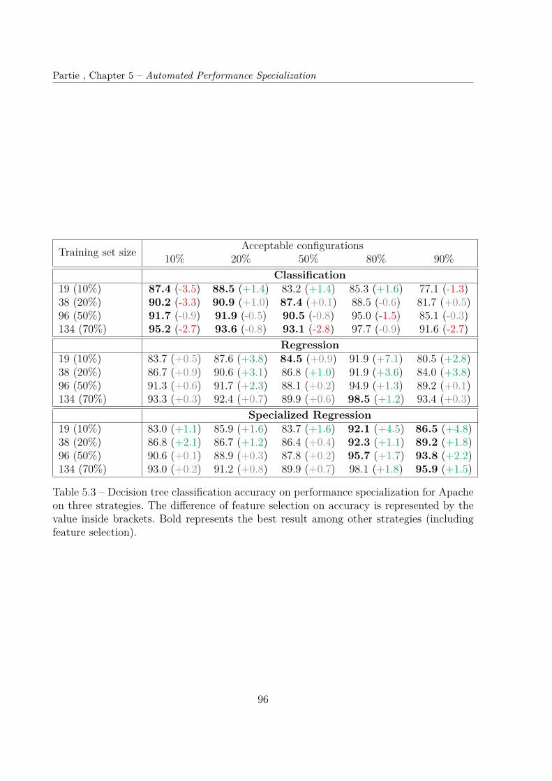
Partie , Chapter 5 – Automated Performance Specialization
Training set size Acceptable configurations10% 20% 50% 80% 90%
Classification19 (10%) 87.4 (-3.5) 88.5 (+1.4) 83.2 (+1.4) 85.3 (+1.6) 77.1 (-1.3)38 (20%) 90.2 (-3.3) 90.9 (+1.0) 87.4 (+0.1) 88.5 (-0.6) 81.7 (+0.5)96 (50%) 91.7 (-0.9) 91.9 (-0.5) 90.5 (-0.8) 95.0 (-1.5) 85.1 (-0.3)134 (70%) 95.2 (-2.7) 93.6 (-0.8) 93.1 (-2.8) 97.7 (-0.9) 91.6 (-2.7)
Regression19 (10%) 83.7 (+0.5) 87.6 (+3.8) 84.5 (+0.9) 91.9 (+7.1) 80.5 (+2.8)38 (20%) 86.7 (+0.9) 90.6 (+3.1) 86.8 (+1.0) 91.9 (+3.6) 84.0 (+3.8)96 (50%) 91.3 (+0.6) 91.7 (+2.3) 88.1 (+0.2) 94.9 (+1.3) 89.2 (+0.1)134 (70%) 93.3 (+0.3) 92.4 (+0.7) 89.9 (+0.6) 98.5 (+1.2) 93.4 (+0.3)
Specialized Regression19 (10%) 83.0 (+1.1) 85.9 (+1.6) 83.7 (+1.6) 92.1 (+4.5) 86.5 (+4.8)38 (20%) 86.8 (+2.1) 86.7 (+1.2) 86.4 (+0.4) 92.3 (+1.1) 89.2 (+1.8)96 (50%) 90.6 (+0.1) 88.9 (+0.3) 87.8 (+0.2) 95.7 (+1.7) 93.8 (+2.2)134 (70%) 93.0 (+0.2) 91.2 (+0.8) 89.9 (+0.7) 98.1 (+1.8) 95.9 (+1.5)
Table 5.3 – Decision tree classification accuracy on performance specialization for Apacheon three strategies. The difference of feature selection on accuracy is represented by thevalue inside brackets. Bold represents the best result among other strategies (includingfeature selection).
96
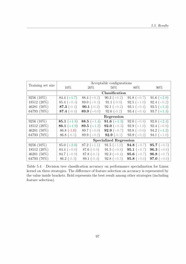
5.5. Results
Training set size Acceptable configurations10% 20% 50% 80% 90%
Classification9256 (10%) 84.4 (+1.7) 88.4 (+0.2) 90.3 (+0.2) 91.8 (+0.7) 91.6 (+2.8)18512 (20%) 85.4 (+0.4) 89.0 (+0.4) 91.1 (-0.0) 92.5 (+1.0) 92.4 (+0.2)46281 (50%) 87.3 (-0.4) 90.1 (-0.2) 92.1 (+0.2) 93.1 (+0.4) 93.5 (+1.2)64793 (70%) 87.4 (-0.4) 89.9 (+0.0) 92.6 (-0.2) 93.4 (+0.4) 93.7 (+1.3)
Regression9256 (10%) 85.1 (+1.8) 88.5 (+1.4) 91.6 (+1.3) 92.0 (+0.8) 92.0 (+2.4)18512 (20%) 86.1 (+1.9) 89.5 (+1.2) 92.0 (+0.3) 92.9 (+1.0) 92.4 (+0.8)46281 (50%) 86.8 (-1.0) 89.7 (+0.0) 92.9 (+0.7) 93.8 (+0.6) 94.2 (+1.2)64793 (70%) 86.8 (-0.5) 89.9 (+0.2) 92.9 (-0.1) 93.9 (+0.2) 94.1 (+1.0)
Specialized Regression9256 (10%) 85.0 (+2.0) 87.2 (+1.1) 91.5 (+1.0) 94.8 (+0.7) 95.7 (+0.5)18512 (20%) 84.4 (+0.6) 87.6 (-0.0) 91.5 (+0.8) 95.1 (+0.7) 96.3 (+0.6)46281 (50%) 84.7 (+0.9) 87.8 (-0.1) 92.3 (+0.4) 95.6 (+0.7) 96.8 (+0.7)64793 (70%) 86.2 (-0.3) 89.1 (-0.4) 92.8 (+0.5) 95.8 (+0.6) 97.0 (+0.6)
Table 5.4 – Decision tree classification accuracy on performance specialization for Linuxkernel on three strategies. The difference of feature selection on accuracy is represented bythe value inside brackets. Bold represents the best result among other strategies (includingfeature selection).
97
Partie , Chapter 5 – Automated Performance Specialization
5.6 Discussion
Guidelines. Using the empirical knowledge we acquired during the experiments, weaim to propose some guidelines on how to use the different strategies for automatedperformance specialization.
Due to the cost of learning, or the specialization model being shipped as is, it isnot always possible to train a new model each time it is needed ("on the fly"). Thiscomputational cost can be a barrier in terms of user experience. For instance, end-usersmay not be interested to wait almost a minute while maintainers may accept the necessarytime to hopefully get accurate specialization. There are two scenarios:
— You cannot train a model on the fly:— The default strategy is regression, as being able to handle all thresholds at
once and quite accurately.— The profile strategy is classification and specialized regression. Instead of
having one generic model, it is possible to focus on one (or more) profile, i.e.threshold. Classification is better for highly constraining specialization, whilespecialized regression is better for slightly constraining specialization.
— Note that is is possible to leverage multiple models depending on the needs,and having some particular profiles, backed up by a regression model for othercases.
— You can train a model on the fly: When the specialization model can be re-trained for a specific performance threshold, it is better not to use regression, butto use classification for highly constraining specialization and specialized regressionfor slightly constraining specialization.
Feature selection should be considered in almost every cases. When the training timeis negligible, the cost of finding the optimal number of options is negligible too with highchances to have a more accurate model. When the training time is not negligible, such asfor Linux, the reduced training time makes it worth to explore a few numbers of options.
Good regressor, bad classifier. "A good regressor should give out a good classifier"is an intuition that one could have when thinking about using a regressor to perform aclassification task based on a continuous value, such as specialization. While this happensto be true in a lot of cases, it also happens to be very wrong in some cases. During ourexperiment, we observe a lot of different regressors and computed both their balancedaccuracy and Mean Absolute Percentage Error (MAPE), a regression error metric, and
98
5.7. Threats to validity
we noticed some of them to go completely against the mentioned intuition. For instance,we have a quite good regressor, with 6% error rate, but with a quite bad balanced accuracyat just under 70%. On the other hand, on the same system, we have a very good classifier,presenting 100% balanced accuracy, but sitting at almost 45% error rate, one of the worstwe found on that system.
Safety and flexibility. If we only used the balanced accuracy as the most fair and generalmetric, some other metric can reveal interesting aspects of the classification. Precisionmeasures how much of the predicted acceptable configurations are actually acceptable, andindicates the safety of the evaluated classifier. Recall measures how much of all acceptableconfigurations are actually considered by the classifier, and indicates the flexibility. Exceptin the rare cases of finding a perfect classifier, there is always a trade-off between flexibilityand safety. One interesting aspect of the Decision Tree is that for each rule, it can delivera probability of acceptability, and this can be used to tweak the rules, either towardflexibility, or toward safety.
5.7 Threats to validity
In this section, we describe some internal and external threats to the validity of thisstudy.
5.7.1 Internal validity
Hyperparameters for Decision Trees. Just like many learning algorithms, DecisionTrees exhibit hyperparameters that can impact the performance of the algorithm (accu-racy as well as training time). To mitigate this threat, we explored a wide range of themin a grid-search fashion i.e., we test all combinations of multiple values for each of them.Complete results and scripts are available online.
Threshold variation. The performance threshold – the limit set by the user to definean acceptable configuration – can make the accuracies of the learning techniques vary alot. We considered this aspect by using different thresholds, based on the performancedistributions of each system and dataset. However, this may rise a problem: as we cansee in Figure 5.2, the 10% and 20% thresholds are very close and also very constraining,which might explain the low accuracy of the specialization models. In practical terms,these thresholds do not correspond to any realistic expectation from a user. Despite this
99
Partie , Chapter 5 – Automated Performance Specialization
threat, we did observe the phenomenon for only one system while none of the 6 learningtechniques have been favored. However, we warn that this is a threat that should beconsidered for any future work or transfer in a real use case.
Sampling. For this experiment, we focused only on random sampling to avoid spreadingourselves too much. Pereira et al. [115] shows that random sampling is a strong baseline,but also warns about the potentially strong influence of different sampling strategies, espe-cially when comparing learning techniques. The exploration of other sampling techniquesis definitely in the scope of future work.
5.7.2 External validity
Workload influence. It is well known that the input workload of a system process, forinstance the input video for a video encoder, is another source of variability that should betaken into account. As we relied on datasets shared by the community, we did not focus onthis aspect of variability at this time. Besides, not all systems are impacted by workload,such as the binary size of Linux kernel which is only dependent on the configuration.Thus, we focused on a single workload to be able to make robust and reliable statementsabout a specific strategy. We are confident that some method of transfer learning shouldbe able to tackle other workloads. Demonstrating the validity of the approach for otherworkloads is part of our future work.
System generalization. As all empirical studies, the conclusions are fully reliable onthe studied systems. Thus, we acknowledge that the use of another system may lead todifferent results. However, once we are able to demonstrate evidences of good results on aset of real-world systems widely used in the literature, including the Linux kernel, we arequite confident in the generalization of our approach. Still, conducting experiments withother systems is an important next step, which is part of our future work.
5.8 Conclusion
As software systems become more and more configurable, it becomes harder for usersto correctly configure them or to reach a certain goal, being functional or in terms ofperformance. Specialization is a technique that adds constraints to a system in order toassist users in reaching a predefined goal while sacrificing the configurability as little as
100

5.8. Conclusion
possible. However, a manual specialization process to create the constraints can be error-prone, time-consuming, and heavily dependent on a knowledge that is hard to formalizeor simply not available. The recent rise of data and machine learning appears to be a goodcandidate to automate the specialization process and complement or replace the expertknowledge.
We explored the decision tree learning algorithm, for how suited it is to extract rulesthat can be retrofitted into variability models of configurable systems. We used and com-pared both classification and regression trees, as well as a novel variant of regression treerefined toward the specialization problem, that we called specialized regression. We alsoused tree-based feature selection to investigate how well it can be combined with spe-cialization. We performed an empirical study to evaluate the ability of Decision Trees toaccurately constrain the configuration space of the systems for the specialization problemand performance properties. We used the datasets that are well known in the community,as well as taking up the challenge of the Linux kernel and its thousands of options.
Our results showed that the learning models are more than 90% accurate on 8 out9 systems, including Linux. Every strategy is efficient, but each has its own strengthsregarding different thresholds, which makes them all worth considering. Feature selectionproved itself a good and reliable way to improve accuracy, and also to reduce the trainingtime. If for most systems, the training time is very low, in the order of the milliseconds,in the case of the Linux kernel it can take more than one minute and feature selectionreduces that time to one or two seconds.
We have exposed a panorama of accurate learning techniques for the performancespecialization problem. As future work, we plan to assess how the inferred configurationknowledge relates to domain experts’ knowledge (e.g., Linux developers). It will requireto investigate how readable and comprehensible are constraints extracted from the spe-cialization process. Another research direction is how this knowledge transfers across deepvariability [86] (e.g., versions and workloads of a system).
101

Chapter 6
MODEL SHIFTING FOR PERFORMANCE
PREDICTION ACROSS VERSIONS
6.1 Introduction
We detailed previously how complex and costly modelling the performance of a con-figurable system can be, especially in systems with thousands of options. In all previouswork on performance modelling, a key aspect of software systems has been put aside tolower the complexity: evolution.
At each new release, the problem of obtaining an accurate performance model of aconfigurable system may arise again due to the variability in time. For configurable systemsevolving at a rapid pace, sampling again each new version is impractical. Since itrequires such a large amount of computational resources to measure the performance ofeach configuration to be used as input to a machine learning algorithm, this process couldeven take more time than the release period.
To overcome this issue, we propose to transfer the learning across versions. Sincethe feature space (i.e., the set of configuration options) can change across versions, ourapproach falls under the category known as heterogeneous transfer learning, opposite tohomogeneous transfer learning, that assumes the feature space remains unchanged duringevolution. Identifying how to efficiently apply transfer knowledge of the learned model asthe systems evolve is challenging. This is indeed a well-known general problem in machinelearning [110, 158], made even more difficult because of the heterogeneity of configurationspaces because it may cause bias on cross-version feature representation [36].
Existing works [24, 61, 64, 66, 67, 68, 78, 98, 103, 149, 150, 155] have attempted toinvestigate the transfer challenge. However, they investigated it in the context of homoge-neous feature spaces and not for the case of system code evolving across different versions,i.e. heterogeneous feature spaces. Thus, to the best of our knowledge, no work has shownevidence that transfer learning can model variability in space and time of configurable sys-
103

Partie , Chapter 6 – Model Shifting for Performance prediction across Versions
tems accurately. Moreover, existing works do not consider very complex systems that havethousands of options and at the same time evolve frequently with large deltas betweenreleases.
For this chapter, we purposely again consider the Linux kernel, because it is one ofthe most complex representative cases of this problem. It has thousands of options (e.g.,around 15,000 for version 5.8) and hundreds of releases over more than two decades. Weselected seven releases spanning over three years from version 4.13 (2017) to 5.8 (2020).On this dataset we first answer the following research question: RQ1. To what extentdoes Linux evolution degrade the accuracy of a performance prediction model trained ona specific version?
To this end, we first perform an experiment to quantify the impact of Linux evolution(i.e., the release of a new kernel version) on configuration performance (specifically: ker-nel binary size for a Linux configuration). To the best of our knowledge, no prior workhas attempted to check whether a learnt configuration performance model can be usedregardless of the applied system evolution over time. Our experiments show that evolutiondoes indeed impact the learnt model by degrading the prediction (by a ratio of 4 to 6)down to the point where it cannot effectively be used on subsequent releases.
After that, we propose a new automated transfer Evolution-aware Model Shifting(tEAMS) approach that consists in applying a tree-based model shifting using gradientboosting trees, backed up with feature alignment to handle the problem of heterogene-ity in configuration spaces. The goal of tEAMS, as any transfer learning technique, isto beat approaches that learn at every release ("from scratch"), as illustrated in Figure6.2. We then answer the next research question: RQ2. What is the accuracy of tEAMScompared to learning from scratch and other transfer learning techniques?
Our results show that tEAMS outperforms state-of-the-art approaches by reachinga low and constant 5.6% to 7.1% error rate rather than 8.3 to 9.2% for learning fromscratch method. Our contributions are summarized as follows:
1. We design and implement a large-scale study of the effectiveness of transfer learningto model kernels’ variability in space and time.
2. We show empirical evidence for the degradation of binary size predictions fromversion 4.13 onward.
3. We propose a novel technique (tEAMS) for transfer learning across versions, withtwo variants: one shot transfer and incremental transfer.
4. We evaluate our results over seven kernel versions and a dataset of 243K+ con-
104
6.2. Impacts of Evolution on Configuration Performance
figurations spanning over three years: tEAMS vastly outperforms the accuracyof state-of-the-art transfer learning strategies. Moreover, it is cost-effective since itworks with the addition of a reduced set of training samples over future versions.
The chapter is organized as follows. Section 6.2 investigates how performance predic-tions degrade over evolution releases. Section 6.3 presents a new approach called tEAMS.Section 6.4 evaluates tEAMS on the history of Linux kernels from 4.13 to 5.8 and com-pares it to state-of-the-art. Sections 6.5 and 6.6 discuss various aspects of the proposedsolution, and the threats to validity. Finally, Section 6.7 concludes this chapter.
We provide a replication package with all artifacts (including datasets and learningprocedures): https://zenodo.org/record/4960172.
6.2 Impacts of Evolution on Configuration Perfor-mance
In chapter 3, we show that creating a performance prediction model, or in this case abinary size prediction model, is a costly task and out of reach of most learning techniques.Moreover, this has been done on a fixed version (4.13) and we now need to inquire aboutits durability.
In this section, we aim to quantify the impact of Linux evolution (i.e., the release ofa new kernel version) on configuration binary size and prediction models.
Mühlbauer et al. [98] investigated the history of software performance to isolate whena performance shift happens over time. If we know evolution can impact the performanceof a configurable software, we do not actually know if and how much it can impact aperformance prediction model.
A hypothesis is that the evolution has no significant impact and the Linux commu-nity can effectively reuse a binary size prediction model across all versions. The counterhypothesis is that the evolution changes the binary size distributions: in this case, a mea-surable and practical consequence would be that a binary size model becomes inaccuratefor other versions. In other words, if the degradation of the accuracy of a prediction modelis to be expected, it is necessary to know whether such degradation is sharp enough tobe a problem for the Linux community. However, none of these hypotheses has been in-vestigated in the literature. Therefore, quantifying the impacts of evolution is crucial andboils down to addressing the following research question:
105
Partie , Chapter 6 – Model Shifting for Performance prediction across Versions
(RQ1) To what extent does Linux evolution degrade the accuracy of abinary size prediction model trained on a specific version? To address it, wemeasure the accuracy of a performance prediction model, specifically a binary size pre-diction model, trained in one specific version (i.e., 4.13), when applied to later versions(e.g., up to 5.8).
6.2.1 Experimental Settings
We now present the datasets we gathered on different Linux configurations and ver-sions; the learning algorithms we used to build the prediction models, as well as theaccuracy metric.
Dataset
We compiled and measured Linux kernels on seven different versions. Table 6.1 furtherdetails each considered release version:
— 4.13: this release was the starting point of our work with huge investments (buildsand measurements of 90K+ configurations);
— 4.15: the release was the first to deal with the serious chip security problems melt-down/spectre [118] that mainly apply to Intel-based processor (x86 architecture).A broad set of mitigations has been included in the kernel, which can have an effecton kernel sizes;
— 4.20: the last version before 5.0, with several x86/x86_64 optimizations. As part ofthe in-depth analysis on the evolution of core operation performance in Linux [120],Ren et al. identified several changes in latency for versions between 4.15 and 4.20;
— 5.0: an interesting version, as there has been some debate about the decrease ofkernel performance on some macro-benchmarks (e.g., see [57]);
— 5.4: it is a long term support release that will be maintained 6 years. This versionalso includes modifications for dealing with Linux performance [55, 57];
— 5.7: a recent version, more than a half-year after 5.4;— 5.8: Linus Torvalds commented 1 "IOW, 5.8 looks big. Really big." and reported
"over 14k non-merge commits (over 15k counting merges), 800k new lines, andover 14 thousand files changed", suggesting an important and challenging evolution
1. https://lore.kernel.org/lkml/CAHk-=whfuea587g8rh2DeLFFGYxiVuh-bzq22osJwz3q4SOfmA@mail.gmail.com/
106

6.2. Impacts of Evolution on Configuration Performance
to tackle.
As depicted in Table 6.1, the continuous evolution from 4.13 to 5.8 is significant interms of numbers of added/deleted options, delta of the commits and the changes files.Note that those changes are computed for each release w.r.t. 4.13.
For all versions, we specifically targeted the x86-64 architecture, i.e., technically, allconfigurations have values CONFIG_X86=y and CONFIG_X86_64=y. Overall, we spandifferent periods during 3 years, with some modifications (security enhancements, newfeatures) suggesting possible impacts on kernel non-functional properties (e.g., size).
For each version, we build thousands of random configurations (see Table 6.1 column5 - [Examples]). Owing to the computational cost, we balance the budget to measure atleast and around 20K+ configurations per version. Such data is used to test the accuracyof a prediction model. We used TuxML 2, a tool to build the Linux kernel in the largei.e., whatever options are combined.
TuxML relies on Docker to host the numerous packages needed to compile and mea-sure the Linux kernel.
Docker offers a reproducible and portable environment – clusters of heterogeneousmachines can be used with the same libraries and tools (e.g., compilers’ versions). InsideDocker, a collection of Python scripts automates the build process. We rely on randconfigto randomly generate Linux kernel configurations. randconfig has the merit of generatingvalid configurations that respect the numerous constraints between options. It is also amature tool that the Linux community maintains and uses [95]. Though randconfig doesnot produce uniform, random samples (see Section 6.6), there is a diversity within thevalues of options (being ‘y’, ‘n’, or ‘m’).
Given .config files, TuxML builds the corresponding kernels. Throughout the process,TuxML can collect various kinds of information, including the build status and the size ofthe kernel. We concretely measure vmlinux, a statically linked executable file that containsthe kernel in object file format.
The distribution of binary size in our dataset varies depending on the version. Whilethe mean binary size on version 4.13 is 47 MiB, for other versions that mean value isbetween 89 MiB and 118 MiB. The minimum size for all version is around 10 MiB andthe maximum around 2 GiB.
2. https://github.com/TuxML/tuxml
107

Partie , Chapter 6 – Model Shifting for Performance prediction across Versions
Tabl
e6.
1–
Dat
aset
prop
ertie
sfo
rea
chve
rsio
n.T
henu
mbe
rof
dele
ted/
new
feat
ures
,del
taco
mm
its,fi
les
chan
ges
are
w.r.
t.4.
13.†
forv
ersio
ns4.
13an
d4.
15,t
hebu
ildtim
e(n
umbe
rofs
econ
dsto
build
one
confi
gura
tion)
shou
ldbe
inte
rpre
ted
with
caut
ion
since
weus
edhe
tero
gene
ous
mac
hine
san
ddi
dno
tse
ekto
cont
rolt
heir
work
load
Vers
ion
Rel
ease
Dat
eLO
CFi
les
Exam
ples
Seco
nds/
confi
gO
ptio
nsFe
atur
esD
elet
edfe
atur
esN
ewfe
atur
es∆
Com
mits
File
sch
ange
s
4.13
2017
/09/
0316
,616
,534
60,5
3092
,562
271†
12,7
769,
468
--
--
4.15
2018
/01/
2817
,073
,368
62,2
4939
,391
263†
12,9
989,
425
342
299
31,0
5293
4,62
84.
2020
18/1
2/23
17,5
26,1
7162
,423
23,4
8922
513
,533
10,1
8946
81,
189
104,
691
1,97
2,02
05.
020
19/0
3/03
17,6
79,3
7263
,076
19,9
5224
713
,673
10,2
9349
41,
319
118,
778
2,17
0,93
55.
420
19/1
0/24
19,3
58,9
0367
,915
25,8
4728
514
,159
10,8
1366
32,
008
181,
308
3,82
7,02
55.
720
20/0
5/31
19,3
58,9
0367
,915
20,1
5925
814
,586
11,3
3871
52,
585
225,
804
4,39
3,11
75.
820
20/0
8/02
19,7
29,1
9769
,303
21,9
2328
914
,817
11,5
3073
02,
792
242,
381
4,68
1,31
3
108
6.2. Impacts of Evolution on Configuration Performance
Preprocessing
We distinguish between options and features, as an option is a variable in Linux kernelconfiguration, and a feature an independent variable from which the machine learningalgorithm creates a model. The distinction is important as we made some manipulationsover the dataset, in order to facilitate the learning. The first one is to put aside non-tristate options, which represent a very small subset (between 300 and 320 dependingon the version). Most Linux kernel options values are "yes", "no", or "module", hence thename "tristate" options. The second manipulation was to encode these option values intonumbers to be processed by the algorithm. We observed that the values "no" and "module"had the same effect on the kernel size, so we encoded them as 0, and "yes" as 1. That is,we do not use "module" as an option value and we are not interested in module size. Thenwe put aside the options only having one value in the whole dataset, as it would bringno information from a statistical point of view and only make it longer for a algorithmto learn. Last but not least, we added a custom feature which is the sum of all activatedoptions in the configuration, as it has proved important and helpful in a previous studyof Acher et al. [5].
Performance Prediction Models
Extensive experiments on 4.13 (the oldest version of the dataset) showed what learn-ing algorithms and hyper-parameters were effective and for which training set size [5].Specifically, we chose gradient boosting trees (GBTs) that, according to [5], obtain thebest results whatever the training set size. GBTs proved to be superior to linear regressionmodels, decision trees, random forest, and neural networks for relatively small trainingset sizes (e.g., 20K) but also for larger budgets (e.g., 80K+).
We trained GBTs with 85.000 examples on version 4.13. We took care of finding thebest hyperparameters, using grid-search, as it proved itself a quite important factor in theaccuracy of the models. We relied on scikit-learn [20], a Python library that implementsstate-of-the-art machine learning algorithms. As a performance model only matches aspecific set of features (here: the features of 4.13), we deleted features only contained infurther, target versions (e.g., 4.15).
109
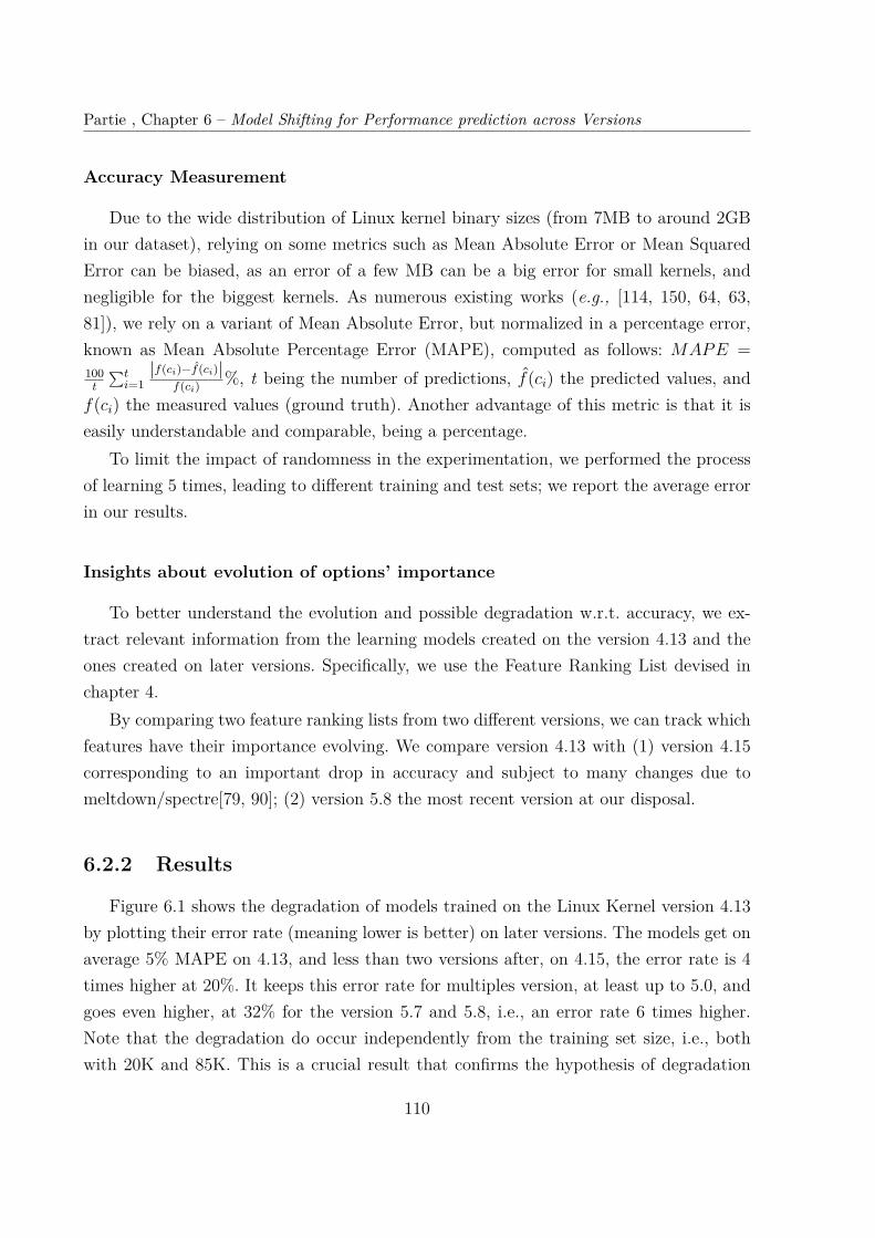
Partie , Chapter 6 – Model Shifting for Performance prediction across Versions
Accuracy Measurement
Due to the wide distribution of Linux kernel binary sizes (from 7MB to around 2GBin our dataset), relying on some metrics such as Mean Absolute Error or Mean SquaredError can be biased, as an error of a few MB can be a big error for small kernels, andnegligible for the biggest kernels. As numerous existing works (e.g., [114, 150, 64, 63,81]), we rely on a variant of Mean Absolute Error, but normalized in a percentage error,known as Mean Absolute Percentage Error (MAPE), computed as follows: MAPE =100
t
∑ti=1
|f(ci)−f(ci)|f(ci) %, t being the number of predictions, f(ci) the predicted values, and
f(ci) the measured values (ground truth). Another advantage of this metric is that it iseasily understandable and comparable, being a percentage.
To limit the impact of randomness in the experimentation, we performed the processof learning 5 times, leading to different training and test sets; we report the average errorin our results.
Insights about evolution of options’ importance
To better understand the evolution and possible degradation w.r.t. accuracy, we ex-tract relevant information from the learning models created on the version 4.13 and theones created on later versions. Specifically, we use the Feature Ranking List devised inchapter 4.
By comparing two feature ranking lists from two different versions, we can track whichfeatures have their importance evolving. We compare version 4.13 with (1) version 4.15corresponding to an important drop in accuracy and subject to many changes due tomeltdown/spectre[79, 90]; (2) version 5.8 the most recent version at our disposal.
6.2.2 Results
Figure 6.1 shows the degradation of models trained on the Linux Kernel version 4.13by plotting their error rate (meaning lower is better) on later versions. The models get onaverage 5% MAPE on 4.13, and less than two versions after, on 4.15, the error rate is 4times higher at 20%. It keeps this error rate for multiples version, at least up to 5.0, andgoes even higher, at 32% for the version 5.7 and 5.8, i.e., an error rate 6 times higher.Note that the degradation do occur independently from the training set size, i.e., bothwith 20K and 85K. This is a crucial result that confirms the hypothesis of degradation
110
6.2. Impacts of Evolution on Configuration Performance
Figure 6.1 – Accuracy of prediction models, trained on 4.13, with training set size 20Kand 85K, when applied on later versions.
over time, regardless of the training set size. Hence, we need a more sustainable solutionlike transfer learning [65, 82, 150].
It is worth noting though that the error rate stabilizes between 4.15 and 5.0. Hence,a hypothesis is that the evolution might be less costly between some versions. Unfortu-nately, a direct reuse of the prediction model is inaccurate for the early version 4.15 andsubsequent ones (4.20, and 5.0). Moreover, the degradation slightly decreases between 5.7and 5.8. A possible explanation is that the binary size distributions of 5.8 is closer to4.13, at least for the way the basic transfer is performed. It also suggests an effect of theevolution between 5.7 and 5.8. Besides model reuse with 20K is more accurate than modelreuse with much bigger training set size (85K) for all target versions, except 5.8. It is notwhat we would have expected for a learning model: a larger training set for the sourcemodel should lead to improved accuracy. This shows that despite the evolution changesboth at the code level and options between the releases (see Table 6.1), the use of modelreuse does not follow a logical or explainable reason from a machine learning point ofview. Overall, simply transferring a prediction model is neither accurate nor reliable: theevolution of the configurations binary size is not captured.
We also measured the degradation of prediction models trained on other versions with15K (see Figure 6.1). We can observe that the degradation is less immediate than withthe version 4.13 but is still happening, especially on version 5.8 as the error percentageraises to 40% - 50%.
111
Partie , Chapter 6 – Model Shifting for Performance prediction across Versions
Insights about evolution and options. We first compare feature ranking lists frommodels trained on versions 4.13 and 4.15. We notice the following evolution patterns:
— Features unchanged: Numerous influential features do not change in importancefrom one version to another. Specifically, out of the top 50 features from both list(the top 50 representing 95% of the feature importance), 29 are the same. This isa key observation that allows one to envision the use of a model from one versionto another, even partly;
— Important new features: 3 important features from the top 50 in version 4.15did not exist in 4.13, such as CHASH (ranked #18), NOUVEAU_DEBUG_MMU(#21) or BLK_MQ_RDMA (#44);
— Features losing importance: 21 features from the top 50 that were importantin 4.13 became unimportant in 4.15, meaning they do not impact kernel size any-more, such as RTL8723BE (from #48 to #8892), BT_BNEP_MC_FILTER (#38 to#4182) or AQUANTIA_PHY (#43 to #3348);
— Features gaining importance: 18 features from the top 50 that were unim-portant in 4.13 became important in 4.15, such as HIPPI (from #6882 to #27),HAMACHI (from #7197 to #50) or NFC_MEI_PHY (from #4921 to #26).
We also compare feature ranking lists from models trained on versions 4.13 and 5.8and find similar patterns:
— Features unchanged: Out of the top 50 features from both lists, 21 are the same.It is less than between versions 4.13 and 4.15, but there is still a substantial overlap;
— Appearing important features: 12 features from the top 50, such asDMA_COHERENT_POOL (ranked #12), DEBUG_INFO_COMPRESSED(#6) orAMD_MEM_ENCRYPT(#9);
— Features losing importance: 24 features from the top 50, such as ATH5K_TRACER(from #20 to #10423), DQL (#40 to #4153) or FDDI (#32 to #2532);
— Features gaining importance: 17 features from the top 50, such as LOCKDEP(#5639 to #22), PROVE_LOCKING (#2362 to #19) or SND_SOC_SI476X (#7075to #31)
Our observations show that numerous features involved in different evolution patternscan cause the degradation of a prediction model. Prediction models trained on a specificversion are challenged by 1) new features, which are unknown to old models, and 2) thechanges in importance of the known features. Interestingly, we did not find importantfeatures that were removed between version 4.13 and 4.15. Another important insight is
112
6.3. Evolution-aware Model Shifting
that a large subset of features remain important across versions: one can leverage thisknowledge for building a prediction model. Overall, there is a potential to transfer amodel from one version to another under the condition that new features together withthe effects of important features are correctly handled. In fact, the insights drive thedesign of tEAMS: more details are provided in the next section.
Evolution does impact configuration prediction and degradation quicklyoccurs: from less than 5% to 20% (after only 4 months of evolution) to upto 32% for later versions. The reuse of a prediction model on different versionsis not a satisfying solution, calling for other approaches.
6.3 Evolution-aware Model Shifting
In order to deal with the degradation issue highlighted in the previous section, wenow present evolution-aware model shifting (tEAMS), a method to transfer a predictionmodel for a given source version onto a target version.
6.3.1 Heterogeneous Transfer Learning Problem
Owing to the huge configuration space of the Linux kernel, it is impractical to re-learnat every release. To alleviate this issue, transfer learning was proposed as a new machinelearning paradigm. It transfers the knowledge of a model built for a specific source domain(where sufficient measured/labeled data are available) to a related target domain (withlittle or no additional data) [36]. Figure 6.2 gives the general principle about how transferlearning works. Here, to make predictions over the Linux kernel version 5.8, we coulddirectly reuse the performance model A built from the source version 4.13. Basically, thesource model A is adapted to consider the aligned set of features from both source andtarget domains (i.e., model A’). Finally, the target model B is trained with only a fewmeasured configurations in the target domain B plus the knowledge from the modifiedsource model A’.
However, the evolution of Linux brings a specific scenario for transfer learning: con-figuration options for the source version (e.g., 4.13) are not the same as further, targetversions (e.g., 5.8). It is worth noting in Table 6.1 that the number of options keeps in-creasing over versions. Between two versions, numerous options appear while some others
113
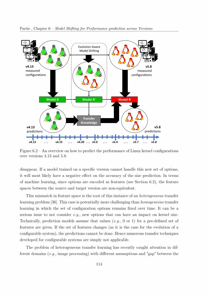
Partie , Chapter 6 – Model Shifting for Performance prediction across Versions
v4.13 . . . v4.15 . . . v4.20 . . . v5.0 . . . v5.4 . . . v5.7 . . . v5.8
Evolution-Aware Model Shifting
Model A Model B
v4.13predictions
v4.13measured configurations
v5.8measured
configurations
v5.8predictions
Model A’
TransferKnowledge
Figure 6.2 – An overview on how to predict the performance of Linux kernel configurationsover versions 4.13 and 5.8.
disappear. If a model trained on a specific version cannot handle this new set of options,it will most likely have a negative effect on the accuracy of the size prediction. In termsof machine learning, since options are encoded as features (see Section 6.2), the featurespaces between the source and target version are non-equivalent.
This mismatch in feature space is the root of this instance of an heterogeneous transferlearning problem [36]. This case is potentially more challenging than homogeneous transferlearning in which the set of configuration options remains fixed over time. It can be aserious issue to not consider e.g., new options that can have an impact on kernel size.Technically, prediction models assume that values (e.g., 0 or 1) for a pre-defined set offeatures are given. If the set of features changes (as it is the case for the evolution of aconfigurable system), the predictions cannot be done. Hence numerous transfer techniquesdeveloped for configurable systems are simply not applicable.
The problem of heterogeneous transfer learning has recently caught attention in dif-ferent domains (e.g., image processing) with different assumptions and "gap" between the
114
6.3. Evolution-aware Model Shifting
source and the target [36]. The intuition is that, for Linux, the shared set of features canbe exploited to effectively transfer predictions.
6.3.2 Principles
The major challenge is to bridge the gap between the feature spaces. We rely on twosteps: (1) feature alignment, which deals with the differences between features’ sets amongtwo versions; (2) the learning of a transfer function that map source features onto targetsize. For realizing feature alignment, we distinguish three cases:
— commonality: options that are common across versions (i.e., options have thesame names) are encoded as unique, shared features. There are two benefits: wecan reuse a prediction model obtained over a source version "as is", without hav-ing to retrain it with another feature scheme; we do not double the number offeatures, something that would increase the size of the learning model up to thepoint some learning algorithms might not scale. The anticipated risk is that someLinux options, though common across versions, may drastically differ at the im-plementation level, thus having different effects on sizes. We deal with this riskthrough the learning of a transfer function that aims to find the correspondencesbetween the source and the target (see below);
— deleted features: options that are in the source version, but no longer in thetarget version: we add features in the target version with one possible value, "0" or"1". Observations show that putting "1" as the default always gives slightly betteraccuracy.
— new features: options that are not in the source version, but only introduced inthe target version: we ignore them when predicting the performance value sincethe source model cannot handle them, but we keep them in the target dataset.
Feature alignment alone is not sufficient; it is mainly a syntactical mapping at thisstep. There is a need to capture the transfer function, i.e., the relationship between thesource features, the source labels (kernel size of each configuration under source version),the target features, and the target labels. This transfer function should be learned. Owingto the complexity of the evolution, a "simple" linear function is unlikely to be accurate –our empirical results confirm the intuition, see next section. In contrast to existing worksthat rely on linear regression models for "shifting" the prediction models [82, 150, 65], werely on more expressive learning models, capable of capturing interactions between sourceand target information.
115
Partie , Chapter 6 – Model Shifting for Performance prediction across Versions
Note that the feature alignment is a completely automated process and relies on thehigh similarity between the features spaces. In case of too disjoint features spaces, thissolution would likely fail, and other solutions should be considered [36]
6.3.3 Algorithm
Figure 6.3 outlines the process for the tEAMS algorithm that gives the four keysignificant steps:
– ➀ Target dataset and Source model acquisition: Train or acquire a robust modelon measurements from the source version and a dataset from the target version;
– ➁ Feature alignment: If the source and the target do not have the same set ofoptions, an alignment of the feature spaces is applied (e.g., as described in Sec-tion 6.3.2);
– ➂ Target prediction: Using the source model, predict the value of the target dataand add this prediction as a new feature in the target dataset;
– ➃ Shifting model training: Using the enhanced target dataset, train a new model(e.g., with a Gradient Boosting Tree algorithm capable of handling interactions).
Note that the source model is usually already trained beforehand, and its training stepcan be skipped in this case. Overall, our solution is fairly easy to implement and deploy.Moreover, once we train a source version the learning of the transfer function scales well(see next section).
6.3.4 Variant: Incremental Transfer
A possible variant of this technique is to use it in an incremental fashion, and toreplace the source model by an already transferred model for a previous version. In theend, such a model consists of a source model, shifted multiple times in a row throughmultiple intermediate target versions until the final target version.
This variant could potentially give more accurate results, since the complexity of thetransfer is spread over multiple models. The farther two versions are from each other,in terms of software evolution, the more performances-impacting changes can happen. Atransfer model that handles two distant versions has to deal with all changes betweenthese two versions at once, while in an incremental process, each model only has to dealwith a fraction of the changes. On the other hand, we know that machine learning modelsare imperfect and error prone, even if the error is limited. Relying on a series of machine
116
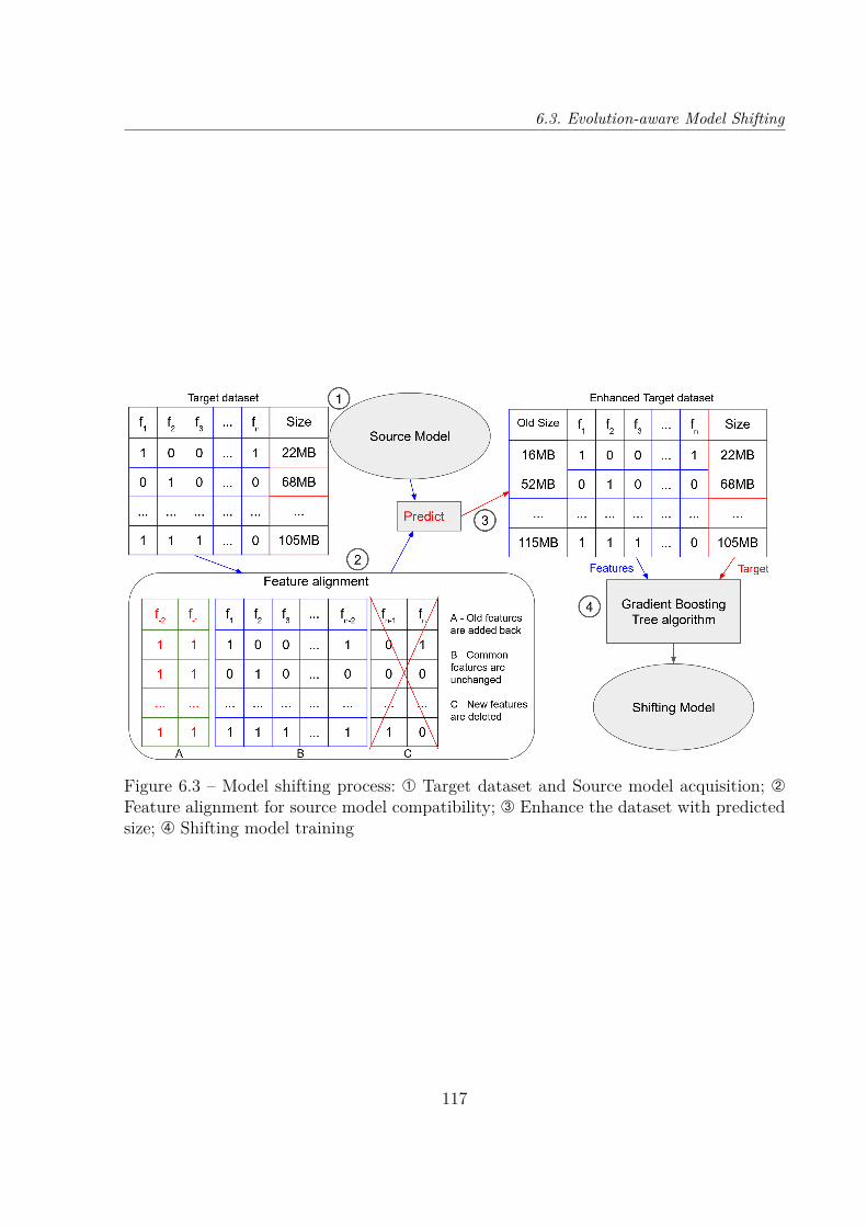
6.3. Evolution-aware Model Shifting
Figure 6.3 – Model shifting process: ➀ Target dataset and Source model acquisition; ➁
Feature alignment for source model compatibility; ➂ Enhance the dataset with predictedsize; ➃ Shifting model training
117

Partie , Chapter 6 – Model Shifting for Performance prediction across Versions
learning models can turn out to be risky, as these errors can be spread and amplified overthe multiple models.
6.4 Effectiveness of Transfer Learning
Our goal is to evaluate the cost-effectiveness of our approach tEAMS in the contextof Linux evolution. The effectiveness is the accuracy of the prediction model and its abilityto minimize prediction errors as much as possible. If the source version and the targetversion have very little in common, configuration performance knowledge may not transferwell. In such situations, transfer learning can be unsuccessful and can lead to a "negative"transfer [36]. Specifically, we consider that the transfer is negative when learning fromscratch directly onto the target version – without transfer and using only the limitedmeasured target data available for transfer – leads to better accuracy than a transfermodel with the same budget. Thus, we aim to answer the following research question:
(RQ2) What is the accuracy of our evolution-aware model shifting (tEAMS)compared to learning from scratch and other transfer learning techniques?The accuracy of tEAMS depends on the investment realized for creating or updatingthe prediction models. Specifically:
— the number of configuration measurements over the target model used to train theprediction model: non-transfer learning (i.e., from scratch) uses the same trainingset and we can compare our results;
— the number of configuration measurements over the source version used to trainthe prediction model: from large training sets to relatively small ones;
Hence, we address RQ2 through different cost scenarios and we can identify for whichinvestments tEAMS is effective.
6.4.1 Experimental settings
Dataset
For training and validating the prediction models, we use the same kernel versions andconfiguration measurements as in Section 6.2 and Table 6.1.
118
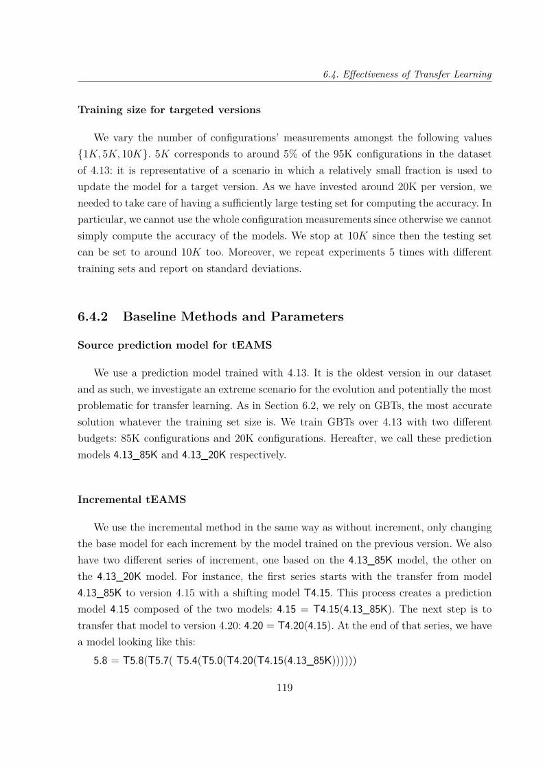
6.4. Effectiveness of Transfer Learning
Training size for targeted versions
We vary the number of configurations’ measurements amongst the following values{1K, 5K, 10K}. 5K corresponds to around 5% of the 95K configurations in the datasetof 4.13: it is representative of a scenario in which a relatively small fraction is used toupdate the model for a target version. As we have invested around 20K per version, weneeded to take care of having a sufficiently large testing set for computing the accuracy. Inparticular, we cannot use the whole configuration measurements since otherwise we cannotsimply compute the accuracy of the models. We stop at 10K since then the testing setcan be set to around 10K too. Moreover, we repeat experiments 5 times with differenttraining sets and report on standard deviations.
6.4.2 Baseline Methods and Parameters
Source prediction model for tEAMS
We use a prediction model trained with 4.13. It is the oldest version in our datasetand as such, we investigate an extreme scenario for the evolution and potentially the mostproblematic for transfer learning. As in Section 6.2, we rely on GBTs, the most accuratesolution whatever the training set size is. We train GBTs over 4.13 with two differentbudgets: 85K configurations and 20K configurations. Hereafter, we call these predictionmodels 4.13_85K and 4.13_20K respectively.
Incremental tEAMS
We use the incremental method in the same way as without increment, only changingthe base model for each increment by the model trained on the previous version. We alsohave two different series of increment, one based on the 4.13_85K model, the other onthe 4.13_20K model. For instance, the first series starts with the transfer from model4.13_85K to version 4.15 with a shifting model T4.15. This process creates a predictionmodel 4.15 composed of the two models: 4.15 = T4.15(4.13_85K). The next step is totransfer that model to version 4.20: 4.20 = T4.20(4.15). At the end of that series, we havea model looking like this:
5.8 = T5.8(T5.7( T5.4(T5.0(T4.20(T4.15(4.13_85K))))))
119

Partie , Chapter 6 – Model Shifting for Performance prediction across Versions
Learning from scratch
The most simple way to create a prediction model for a given version is to learnfrom scratch with an allocated budget. We use the GBTs algorithm to create predictionmodels from scratch, for each version of our dataset. As previously stated, the studyin [5] shows that GBTs were a scalable and accurate solution compared to other state-of-the-art solutions. Furthermore, the superiority of GBTs is more apparent when smalltraining sets are employed. This quality of GBTs is even more important when learningfor the target version where the budget for updating the model is typically limited –we investigate budget with less than 20K measurements (see above "Training size fortargeted versions"). We replicated the experiments of 4.13 on other versions: linear models,decision trees, random forests, and neural networks give inferior accuracy compared toGBTs, especially for small sampling size (e.g., 10K). Thus, we do not report results ofother learning algorithms and keep only GBTs, the strongest baselines for learning fromscratch or for transfer learning techniques.
tEAMS with linear-based transfer function
In most state-of-the-art cases, model shifting processes use a simple linear learningalgorithm to create a shifting model and they are performing quite well (e.g. [150, 61]).We rely on such a linear transfer function and also apply feature alignment as part oftEAMS.
6.4.3 Results
Figure 6.4 depicts the evolution of the MAPE for the reuse of the model 4.13_85K(i.e., 4.13 with a 85K of training set), and the 4 studied techniques trained using 5Kexamples. We can quickly see that linear model shifting has more than 40% MAPE overall versions and is not accurate at all. It is surprisingly the worst by far, in particular,in comparison with the direct reuse of the prediction model. The standard deviation forLinear model shifting is between 1.5 and 3, while all other techniques are much morestable with a standard deviation always at 0.1 or less. Moreover, learning from scratchwith 5K examples allows to create models having an MAPE between 8.2% and 9.2% quiteconsistently. On the other side, tEAMS with the same budget offers a lower MAPE from5.6% on version 4.15 to 6.8% in version 5.8 with a peak at 7.1 in version 5.7. It is worthnoting that tEAMS MAPE increases a little bit at each version. However, the increase
120
6.4. Effectiveness of Transfer Learning
Figure 6.4 – Accuracy of tEAMS 4.13_85K compared to other techniques using 5Kexamples for the target
is not significant and remains low.Comparing tEAMS with its incremental variant shows a very slight but constant
advantage over the variant, which also show better results then learning from scratch.Table 6.2 gives the results for MAPE with combinations of different models used
(4.13_20K and 4.13_85K) and training set size (1K, 5K, 10K) for the scratch base-line,tEAMS and Incremental tEAMS. The other techniques already performed poorly,Table 6.2 hence focuses on the three competing solutions in Figure 6.4. We now reporton these results.
Impact of training set size over target. As illustrated in Tables 6.2, when de-creasing the training transfer set for the newer versions to 1K example (1% of the originalset), the MAPE increases to 14.9%-16.7% depending on the version. Whereas, the MAPEfor tEAMS only increases to 6.7%-10.6%, with the same trend consistently increasingMAPE over time (and versions). For Incremental tEAMS, the error rate increases fasterup to 13.3 on version 5.8. On the other hand, if we increase the training set to 10K (10%of the original set), accuracy when learning from scratch gets better, with 7.0% to 7.7%MAPE. For tEAMS, the accuracy also gets better, from 5.2% MAPE on version 4.15 to6.1% on version 5.7 and then slightly further improves to 6.1% on version 5.8. We observe
121
Partie , Chapter 6 – Model Shifting for Performance prediction across Versions
the same trend for Incremental tEAMS, going up to 6.5% on 5.7 and then to 6.2 on 5.8.
Impact of tEAMS source model. We measured the same variations using model4.13_20K as the source model, which was built from 20,000 examples instead of 85,000.This affects tEAMS by slightly increasing the MAPE. In particular, we observe that fortEAMS: 1) with 1K, the MAPE varies from 8.5% to 11.6%, 2) With 5K, it varies from6.7% to 7.9%, and 3) with 10K, it varies from 6.2% to 6.7%. Whereas for learning fromscratch, we observe that: 1) with 1K, the MAPE varies from 14.9% to 16.7%, 2) With 5K,it varies from 8.3% to 9.2%, and 3) with 10K, it varies from 7.04% to 7.67%. Therefore,our results show that tEAMS outperforms the two baselines, regardless of the size oftraining sets. In this situation, Incremental tEAMS also shows slightly better resultsthan tEAMS in some cases. At 10k, Incremental tEAMS beats tEAMS on all versionsexcept 5.7, and at 5k, only for versions 4.20 and 5.0. Given the fair increase in error rateat 1k, Incremental tEAMS seems to be very sensitive to higher error rate from previousversions.
Computational cost of training. We performed our experiments on a machinewith an Intel Xeon 4c/8t, 3,7 GHz, 64GB memory. Training from scratch with 1K, 5Kand 10K examples take respectively 21, 195 and 407 seconds. Learning with tEAMStakes a little more time with 60, 288 and 604 seconds for the same number of examples.The training time of tEAMS for updating a prediction model is thus affordable andnegligible compared to the time taken to build and measure the kernel configurations.The overall cost of training is mainly due to the training of the source model (details canbe found in [5]) which is done only once. As a final note, building kernels and gatheringconfigurations data (see Table 6.1) is by far the most costly activity – the time needed totrain the prediction model out of data through either transfer learning or from scratch (afew minutes) is negligible.
tEAMS and Incremental tEAMS are more accurate solutions than learn-ing from scratch and linear model shifting to predict Linux Kernel size ondifferent versions. Also, Incremental tEAMS shows results mostly worse thantEAMS and without significant improvement. Even with different source modelsand training set sizes, tEAMS keeps better and acceptable accuracy with6.9% MAPE on the latest 5.8 version leveraging model trained on 3 yearsold data.
122
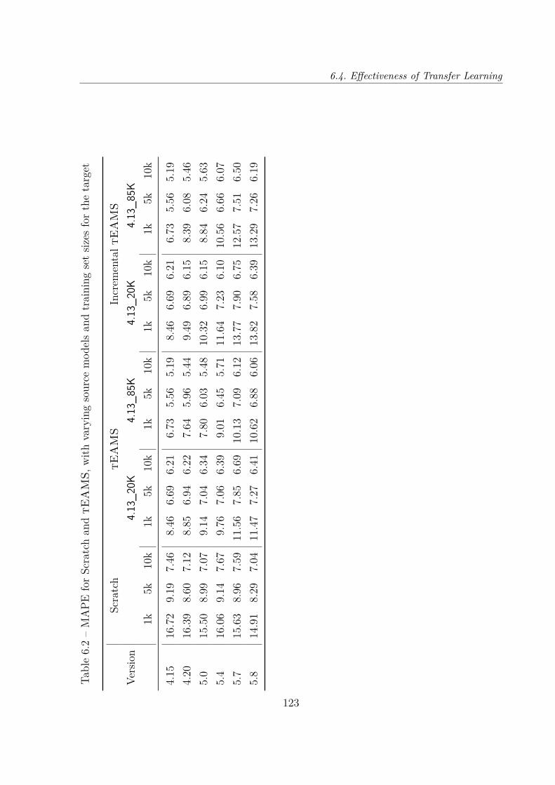
6.4. Effectiveness of Transfer LearningTa
ble
6.2
–M
APE
for
Scra
tch
and
tEA
MS,
with
vary
ing
sour
cem
odel
san
dtr
aini
ngse
tsiz
esfo
rth
eta
rget
Vers
ion
Scra
tch
tEA
MS
Incr
emen
talt
EA
MS
4.13
_20K
4.13
_85K
4.13
_20K
4.13
_85K
1k5k
10k
1k5k
10k
1k5k
10k
1k5k
10k
1k5k
10k
4.15
16.7
29.
197.
468.
466.
696.
216.
735.
565.
198.
466.
696.
216.
735.
565.
194.
2016
.39
8.60
7.12
8.85
6.94
6.22
7.64
5.96
5.44
9.49
6.89
6.15
8.39
6.08
5.46
5.0
15.5
08.
997.
079.
147.
046.
347.
806.
035.
4810
.32
6.99
6.15
8.84
6.24
5.63
5.4
16.0
69.
147.
679.
767.
066.
399.
016.
455.
7111
.64
7.23
6.10
10.5
66.
666.
075.
715
.63
8.96
7.59
11.5
67.
856.
6910
.13
7.09
6.12
13.7
77.
906.
7512
.57
7.51
6.50
5.8
14.9
18.
297.
0411
.47
7.27
6.41
10.6
26.
886.
0613
.82
7.58
6.39
13.2
97.
266.
19
123
Partie , Chapter 6 – Model Shifting for Performance prediction across Versions
6.5 Discussions
Integration of tEAMS in the Linux project. Our results suggest that we cannow provide accurate prediction tools that can be used on 7 versions spanning 3 years ofperiod. In fact, it is an additional advantage of tEAMS compared to non-transfer learningmethods that stick to a specific version. This ability is important, since older versions ofthe kernel are still widely used. Long term support (LTS) releases are particularly relevantsince (1) they are maintained over a period of 6 years (2) they are considered by otherrelated communities, like the Android one. The version 5.4 of our dataset is an LTS releaseand tEAMS can be used in this context.
Linux practitioners interested in a specific release, not present in our dataset, couldwell invest some resources to obtain a new model. For example, we have not consideredversion 4.19 (a LTS release). Non-transfer learning methods would be unable to reusetheir models while tEAMS provide state-of-the-art cost-accuracy results.
We envision to integrate tEAMS as part of the ongoing continuous integration efforton the Linux kernel. We have released a tool, called kpredict 3, that predicts the size of thekernel binary size given only a .config file. kpredict is written in Python, available on pip,and supports all kernel versions mentioned in this article. A usage example is as follows:
> curl -s http://tuxml-data.irisa.fr/data/configuration/167950/config -o .config> kpredict .config> Predicted size : 68.1MiB
whereas the actual size of the configuration (see http://tuxml-data.irisa.fr/data/configuration/167950/ for more details) is 67.82 MiB.
Recently KernelCI [76], the major community-effort supported by several organizations(Google, Redhat, etc.), has added the ability to compute kernel sizes and this functionalityis activated by default, for any build. Hence tEAMS will benefit from such data. Besides,the current focus of KernelCI and many CI effort is mostly driven by controlling that thekernels build (for different architectures and configurations). It is not incompatible withthe prediction of kernel sizes since we did not employ a sampling strategy specificallydevoted to this property. We rely on random configurations that are used to cover thekernel and find bugs (see e.g., [4]). In passing tEAMS can benefit from kernel sizes’ datawhile the CI effort continues to track bugs.
Besides, the development cost of integrating this process is fairly small and requireslittle maintenance. All steps in the process, including feature alignment and adaptation
3. https://github.com/HugoJPMartin/kpredict/
124
6.5. Discussions
of the learning model to the new version, are fully automated and do not require theintervention of kernel developers or maintainers. Our engineering experience with kpredictis that the overhead of implementing transfer learning steps is not much higher thanlearning from scratch.
Is the cost of tEAMS affordable for Linux? Under the same cost settings,tEAMS shows superior accuracy compared to non-transfer learning and other base-lines. Still, one can wonder whether measuring thousands of configurations is practicallypossible, especially when there is a new release. Specifically, results show that with 5Kmeasurements we can obtain almost stable accuracy. So, is the build of 5K affordable forLinux? To address this question, we investigated the number of builds realized by Ker-nelCI and asked the leaders of the project. At the time of the publication, KernelCI isable to build 200 kernels in one hour. We then analyze the retrospective cost of measuring5K as part of our experiments. On average, our investments sum around 260 seconds permachine whatever the version (see Table 6.1, page 108). That is, with 15 machines (16cores) full time during 24 hours, we can already measure 5K configurations. As a sidenote, the numbers should be put in perspective: Linux exhibits thousands of options (seeTable 6.1) and has a large community with many contributors and organizations involved.Overall, though the cost itself is affordable from a computational point of view, there is atradeoff to find between (1) accuracy; (2) value for the community. This tradeoff shouldbe considered for any configurable system. In any case tEAMS has demonstrated beingthe most cost-effective approach.
tEAMS versus Incremental tEAMS As we investigated the differences in accuracybetween the two techniques, we observed that both show very similar results when usinga significant amount of examples, while Incremental tEAMS drops in accuracy whenhaving a reduced training set. This shows that it is very sensitive to low accuracy modelsin series. On the other hand, if the investment in measurements is sizeable, it would bewise to consider it.
When it comes to using and sharing a model, one should consider the cost of havingan incremental solution as it comes at a cost. The first is the size of the model, as asolution composed of a multitude of models also means a larger size of the file to share.The other is the time taken to predict a value, which can be a critical point dependingon the context. If using one or two models in series usually take less than a second, anincremental solution can take few seconds. If the model is used in a user interface, suchan high response time can be considered a severe drawback.
125

Partie , Chapter 6 – Model Shifting for Performance prediction across Versions
tEAMS and transfer functions As part of tEAMS several transfer functions canbe considered for shifting a prediction model. Results show that simple linear regressionis clearly not effective. An alternative is to add interactions’ terms as part of the linearregression. As stated in [81], for p options, there are p possible main influences, p×(p−1)/2possible pairwise interactions, and an exponential number of higher-order interactionsamong more than two options. In the worst case, all 2-wise or 3-wise interactions amongthe 9K+ options are included in the model, which is computationally intractable. Evenif a subset of options is kept, there is a combinatorial explosion of possible interactions.Another possibility is to consider linear models with regularized regression. However, priorexperiments [5] for training prediction models over Linux 4.13 showed that Lasso [144] orElasticNet have severe limitations in terms of accuracy. We chose GBTs for their inherentability to capture non-linear behavior or options’ interactions and empirical results showhigh accuracy. However we do not claim that the use of GBTs is the best solution. Infact, as tEAMS is capable of handling other transfer functions, we plan to consider otherlearning techniques (e.g., neural networks) and investigate tradeoffs between accuracy,computational cost, and interpretability.
When and how should we update tEAMS? Results show that our solution oftransfer learning works well over a long period of three years from 2017 to 2020. Meaningthat up to today, transferring is better than re-learning from scratch. However, eventually,in future evolution and releases, say in 2021 or 2022, transfer learning might degrade.Therefore, at some point, one must learn a new prediction model as the source on whichto apply further transfer learning with our solution. Quantifying exactly when one mustre-learn the performance model is out of the scope of this chapter and is left for futurework. In practice, developers can set a limit of acceptable error rate under which transfercan be still applied and beyond which re-learning a prediction model is necessary.
Is tEAMS applicable to other configurable systems? We investigated in thischapter a case of heterogeneous transfer learning where our considered configurable sys-tem evolves in time and space, i.e., the set of options changes on every release over time.Therefore, other configurable systems that evolve while the set of options also changes canbe ideal candidates to leverage our results and tEAMS. For example, curl is a widelyused configurable system that has now more than 200 options. curl does evolves fre-quently[30], and has performance concerns. GCC[47] and Clang[27] (compilers), ApacheCassandra[10] (database), Amazon EC2 (Web cloud service), OpenCV [108] (image pro-cessing), Kafka[70] (distributed systems) are other examples of configurable systems that
126
6.6. Threats to Validity
continuously add or remove options, maintain their code base at a fast pace, and withstrong performance requirements. These systems have active user communities and havealready been considered in the context of performance prediction of configurable systems(see [114, 67, 142, 130, 7, 12]), but without considering the evolution of their options’ sets.In the future, we plan to replicate our study for such subject systems.
6.6 Threats to Validity
Threats to internal validity are related to the sampling used as training set forall experiments. We deliberately used random sampling to diversify our datasets of con-figurations. To mitigate any bias, for each sample size, we repeat the prediction process 5times. For each process, we split the dataset into training and testing which are indepen-dent of each other. To assess the accuracy of the algorithms, we used MAPE that has themerit of being comparable among versions and learning approaches. Most of the state-of-the-art works use this metric for evaluating the effectiveness of performance predictionalgorithms [114]. Another threat to internal validity concerns the (lack of) uniformity ofrandconfig. Indeed randconfig does not provide a perfect uniform distribution over validconfigurations [95]. The strategy of randconfig is to randomly enable or disable options ac-cording to the order in the Kconfig files. It is thus biased towards features higher up in thetree. The problem of uniform sampling is fundamentally a satisfiability (SAT) problem.However, to the best of our knowledge, there is no robust and scalable solution capableof comprehensively translating Kconfig files of Linux into a SAT formula, especially forthe new versions of Linux. Second, uniform sampling either does not scale yet or is notuniform at the scale of Linux [117, 21, 22, 42].
Looking at the decrease gap in accuracy between learning from scratch and tEAMSthe more examples are given for training, we can expect that at some point, learning fromscratch would be better than tEAMS. We did not investigate further as it would requirean important effort to gather so much more examples on all the studied versions, but itwould be interesting to know if such turning point exists and where is that turning pointin term of number of examples. While we highlight how good transfer is with limited data,we did not investigate enough how good it is with a lot of data.
Regarding the analysis with the feature ranking list, some problems may arise that canthreaten results of Section 6.2.2. First, the importance is based on a tree structure, andeven if we average the ranking out of multiple models, the way the tree is built can create
127
Partie , Chapter 6 – Model Shifting for Performance prediction across Versions
a bias. Second, the importance does not show if the feature has a positive or negativeimpact. Hence, there is a risk of having a feature evolving that gets the same importancevalue but with inverse impact from one version to another. Other interpretable techniquesare needed to gain further insights.
Threats to external validity are related to the targeted kernel versions, targetedarchitecture (x86), targeted quantitative property (size), and used compilers (gcc 6.3). Wehave spanned different periods of the kernel from 2017 to 2020, considering stable versionsand covering numerous evolutions (see Table 6.1). We could consider minor releases, butthe practical interest for the Linux community would be less obvious. We are expectingsimilar results since the evolution in minor release is mostly based on patches and bugfixings. We have considered the most popular and active architecture (x86). Another ar-chitecture could lead to different options’ effects on size. The idea of transfer learningcould well be applied in this context and is left as future work. A generalization of the re-sults for other non-functional properties (e.g., compilation time, boot time) would requireadditional experiments with further resources and engineering efforts. In contrast to e.g.,compilation time, the size of a the kernel is not subject to hardware variations and we canscale the experiments with distributed machines. Hence, we focused on a single propertyto be able to make robust and reliable statements about whether learning approachescan be used in such settings. There is also a clear interest for the Linux community (seeSection 6.5). Our results suggest we can now envision to perform an analysis over otherproperties to generalize our findings. Finally, as we used Linux kernel, we do not generalizeto all configurable systems, especially to those with few options and small-medium codesize. However, this is not the goal of this study since we purposely targeted Linux dueto its complexity (in options and LOC). Further experimentation on other case studiesremains necessary.
6.7 Conclusion
In this chapter, we showed that the evolution of Linux has a noticeable impact onkernel sizes of configurations with a large-scale study spanning 7 versions over 3 yearsand 240K+ configurations. As a result, a size prediction model learned from one specificversion quickly becomes obsolete and inaccurate, despite a huge initial investment (15Khours of computation for building a training set of 90K configurations). We developeda heterogeneous transfer evolution-aware model shifting (tEAMS) learning technique.
128

6.7. Conclusion
It is capable of handling new options that appear in new versions while learning thefunction that maps the novel effects of shared options among versions. Our results showedthat the transfer of a prediction model leads to accurate results (the prediction error(MAPE) remains low and constant) without the need of collecting a very large corpus ofmeasurements’ configurations. With only 5K configurations, we could transfer the modelmade in September 2017 for the 5.8 version released in August 2020.
Linux is an extreme case of a highly complex configurable system that rapidly evolves.Though not all systems have ≈ 14.500 options and such a frequency of commits, manysoftware systems face the same problem of dealing with variability in space (variants) andtime (versions). The increasing adoption of continuous integration in software engineeringhas exacerbated the problem of adding, removing, or maintaining configuration options(being realized as feature toggles, command line parameters, conditional compilation,etc.). The fact that transfer learning works for Linux is reassuring, which has a greatpotential impact on Linux developers and integrators. There is hope that the effort madefor one version of a software system can be reused through transfer.
129


Chapter 7
CONCLUSION AND PERSPECTIVES
7.1 Conclusion
As Software Product Lines become prevalent in many software development environ-ments and grow bigger and bigger, various problems appear. One of them is to understandthe systems well enough to predict their performances for all possible variants. Relying onexpert knowledge is limited and prone to error, especially in a context of constant evolu-tion. Over the last decade, researchers focused on leveraging machine learning techniquesto create reliable performance models. However, none of the studies evaluated their newtechniques on systems with more than a few dozens of options, leaving a grey area as toknow how such techniques would perform on colossal configurations spaces from systemswith hundreds or thousands of options.
The first contribution of this thesis was to enlighten this grey area, and we have shownthat most learning techniques are either poorly accurate, or do not scale to the thousandsof options of the Linux Kernel, in particular the learning techniques tailored to handle SPLspecifics. On the contrary, we found out that Decision Tree and its ensemble techniques,as well as neural networks, are able to handle thousands of options in input and theirinteractions at the same time.
The second contribution leverages Random Forest to create a list of features orderedby their importance, the Feature Ranking List, then used in a feature selection processto filter out the less useful features. This feature selection can be used by any algorithm,with mixed results. However, for tree-based algorithms and neural networks, the featureselection increases the accuracy of the models, and greatly decreases the training time.We also investigated the quality of the Feature Ranking List, by submitting it to expertswho approved it with respect to their knowledge. Finally we proposed to improve theFeature Ranking List stability through the use of an ensemble of Random Forest, in orderto decrease the variance in the ranking.
The third contribution compares different strategies to perform automated perfor-
131
mance specialization. The first iteration of the concept only used classification modelsto synthesize the rules needed for the specialization. We considered two new approaches.First, we used the other way to leverage Decision Trees, as a regression model. Then, weproposed an hybrid approach, tailored toward the specialization problem. We also usedthe feature selection process detailed in the second contribution and measured its influenceon accuracy and training times. All approaches gave good results on most of the subjectsystems, without any one being better than the others overall. Training time are about afew milliseconds for systems with a few dozens of options, up to more than one minutefor Linux. The feature selection gave mixed results in term of accuracy gain, though itmostly had a positive but limited impact. In term of training time reduction, it broughtthe training time on Linux to the order of the second, which is a massive improvement.
The final contribution explored the problem of maintaining the performance modelsover time, and more specifically across versions. First, we studied the model trained onthe version 4.13 of the Linux Kernel and the variation in its accuracy on six later versionsspanning 3 years from version 4.15 to 5.8, and reported that the model quickly loosesaccuracy. To mitigate the effect of evolution on the accuracy, we considered transferlearning with the model shifting approach to leverage the deprecated model knowledge tobuild a model for new versions at lower cost. We have shown that transfer learning offersa solution to maintain the prediction model at high accuracy even on versions years laterwith only a fraction of the cost of the original model, and a better accuracy than learningfrom scratch for the same cost. We also considered an incremental approach of the modelshifting that is able to give slightly better accuracy when given enough data.
In fine, we can note that systems with colossal configurations spaces such as theLinux Kernel are particularly absent from the state-of-the-art in performance predictionof Software Product Lines, and it appears that most solutions, and particularly specializedones, do not scale to such problem. We demonstrated that tree-based learning algorithmsare (1) able to scale in colossal configurations spaces and (2) able to handle the interactionproblem specific to SPL. They are also interpretable in ways that allow the creation ofa Feature Ranking List to perform a feature selection by filtering, and to extract rulesneeded to automate performance specialization. We have shown that performance modelssuffer from software evolution and proposed a transfer learning by model shifting makingpossible to maintain acceptable accuracy at low cost over at least a few years.
132
7.2 Perspectives
While this thesis answered some questions about learning on colossal configurationspaces, it also rises many more and opens perspectives for future works. The first per-spective we propose are general to the whole thesis, then we will be more specific chapterby chapter.
Beyond binary size. All along this thesis, we focused particularly on the predictionof binary size of the Linux kernel. While we defend the relevance of predicting the size ofthe kernel, this focus is mainly a technical limitation of TuxML, the tool for compiling andmeasuring the kernel, which is not mature enough yet to handle other metrics, such as boottime or energy consumption. However, binary size has one important advantage, the lowimpact of deep variability, as it is not influenced by hardware, workload or environmentinfluence. This was raised recently as a very important problem calling previous works,with fixed or undisclosed hardware, workload or environment, into question. Even though,we know that other factors can impact the binary size such as the version of the compiler,a problem we hope to tackle with the help of transfer learning.
Beyond Linux. The case of the Linux Kernel has been a central theme of the thesis,both because of the opportunity given by the TuxML project and because of the excellentuse case it is. However, Linux is not the only system with thousands of options, such asmany systems from the automotive industry that has been particularly used as subjectsystems on feature modelling research. Investigating other similar cases are needed toensure the generalization of the methods proposed.
7.2.1 Feature Selection
In Chapter 3, we saw that the wrapper methods used to select features in [131] lead toan explosion of computing time when used on thousands of options, especially given theparticular way the interactions are encoded. The tree-based feature selection explored inChapter 4 is only one of the many existing solutions [23], which should be compared interm of both accuracy gain and resources needed to perform the selection.
Stability. The stability problem of the tree-based feature selection has been a concern.While partially solved, it deserves a deeper study, with different stability metrics to betterunderstand it, but also trying out different approaches than Random Forest. The impactof the training set size is to be determined as well.
Finding the sweet spot. While the Feature Ranking list is used for feature selection,
133
we did not find an efficient way to determine the right number of features to include (thesweet spot) other than creating models with a wide range of number of features andcomparing them. A first step to improve that would be to perform a less naive approachin gradient descent. Another possibility would be to determine it a priori, which could bea long shot given that we found different sweet spots depending on the algorithm used.
7.2.2 Automated Performance Specialization
In Chapter 5, we explored the process of Automated Performance Specialization andmultiple learning strategies to synthesize the needed rules. However, we focused only onthe accuracy of the model to validate the approach and this should be taken further ondifferent aspects.
Safety and flexibility. The consideration of safety and flexibility can be very im-portant to a user. If we know it is technically possible with Decision Trees to tweak thedecision rules to tip the scale in favor of one over the other, we still need to make moreexperiments to compare cost and improvement with this process.
Going further with constraints. We only considered the extracted rules to be usedby software and dismissed their actual human readability, which could also be of inter-est for practitioners. Another research direction requiring human studies and controlledexperiments could focus on that aspect of learning-based rule synthesis. The use of fea-ture selection might also be of interest here, since rules and constraints will operate overa limited set of options. More aggressive pruning strategies can also be envisioned withtradeoffs between accuracy and interpretability.
Active learning. In our experiment, we only considered a single step of learning tocreate a model. However, we can consider multiple steps of learning, and leveraging theinterpretability of the Decision Trees to find the most error-prone rules in order to refinethem by sampling around the misclassified configurations. It is also possible to use theFeature Ranking List to focus the sampling toward the most influential options and avoidthe ones without influence.
7.2.3 Transfer Learning for Prediction across versions
While we successfully used transfer learning to create robust prediction models acrossdifferent versions in Chapter 6, there are still some doubts to dispel and improvements tobe made.
134
Minor version influence. In the study, we focused our problem space on majorversions (4.15, 5.4, 5.8 ...), but we do not know the impact of minor versions (5.8.1, 5.8.2...) on the prediction models, and especially if transfer is needed even between minorversions, which could negatively impact the viability of our approach given the costsof measurements. However, given the relatively low loss of accuracy between two closeversions outside of exceptional cases, odds are that this should not be necessary.
Targeted sampling. In [64], Jamshidi et al. use learned model to focus the samplingtoward important features when transferring between different environments. While thesolution is developed in a homogeneous context unlike the problem of transfer betweenversions, it could help in reducing the costs of measurement, and studying the feasibilityand efficiency of such approach should be a good way to improve our method.
Commit mining. When developing our method for model shifting, we took a com-plete black-box approach regarding the target system, and this sometimes leads to ar-bitrary decisions to be made. For instance, during the feature alignment, we set all theold features value to 1 as a default value. Features can evolve in many ways, such asappearing or disappearing, but also they can be locked in a specific value, split amongmultiple new features, merged into one, or even just be renamed. Our approach can onlyhandle the first two ways. By mining the commits, we hope to gather meaningful insightthat can help to better handle these evolving features. Such insight can also be leveragedfor targeted sampling as mentioned previously.
Other algorithms. In our study, we only used a Gradient Boosting Tree to builda source model. Since the proposed method for model shifting is completely algorithm-agnostic, in the sense that in theory any algorithm could be used to build both the sourceand the shifting models, we could investigate more algorithms. We could also investigatethe interaction between the source and shifting models.
Feature selection. The interaction between the feature selection and the model shift-ing method is quite uncertain. First, our approach of feature alignment should be revised,as simply putting away the features not in the source model, which only has a few selectedfeatures, could seriously impact the accuracy. Then, we could consider multiple ways totransfer the Feature ranking List: creating a new list from the target dataset, at the riskof having a less reliable list due to stability concerns, or leverage a Feature Ranking Listfrom the shifting model to update the list from the source model, which can be trickydue to the lack of expressiveness of the feature importance metric. We should also con-sider different cases, for handling cases when training the source model is possible with
135

information about the target version features, and when it is not.Multidimensional transfer. We studied the use of model shifting for the problem
of evolution in time, while other works focused on different goal, such as transfer betweenenvironments [69]. When we explored the deep variability concerns [86], we figured thatwhen we train a prediction model, we usually focus on a very specific context (versionof the systems, version of the compiler, configuration of the compiler [87], environment...) and the use of transfer learning becomes obvious. However, transferring along onlyone dimension at a time is not enough, and we should explore the use of multiple trans-fer strategies at once. Given the efficiency of the model shifting methods, a sequentialcombination of shifting could be a good initial research direction.
136

BIBLIOGRAPHY
[1] Iago Abal, Claus Brabrand, and Andrzej Wasowski, « 42 variability bugs in thelinux kernel: a qualitative analysis », in: ASE ’14, Vasteras, Sweden - September15 - 19, 2014, 2014, pp. 421–432 (cit. on p. 41).
[2] Iago Abal et al., « Variability Bugs in Highly Configurable Systems: A QualitativeAnalysis », in: TSE Methodol. 26.3 (Jan. 2018), 10:1–10:34, issn: 1049-331X (cit.on p. 41).
[3] Ebrahim Khalil Abbasi et al., « The Anatomy of a Sales Configurator: An Empir-ical Study of 111 Cases », in: Advanced Information Systems Engineering - 25thInternational Conference, CAiSE 2013, Valencia, Spain, June 17-21, 2013. Pro-ceedings, 2013, pp. 162–177 (cit. on p. 45).
[4] Mathieu Acher et al., Learning From Thousands of Build Failures of Linux KernelConfigurations, Technical Report, Inria ; IRISA, June 2019, pp. 1–12, url: https://hal.inria.fr/hal-02147012 (cit. on p. 124).
[5] Mathieu Acher et al., « Learning Very Large Configuration Spaces: What Mattersfor Linux Kernel Sizes », in: (2019) (cit. on pp. 89, 90, 109, 120, 122, 126).
[6] Mathieu Acher et al., « VaryLaTeX: Learning Paper Variants That Meet Con-straints », in: Proceedings of the 12th International Workshop on Variability Mod-elling of Software-Intensive Systems, ACM, 2018, pp. 83–88 (cit. on pp. 35, 80,86).
[7] Omid Alipourfard et al., « Cherrypick: Adaptively unearthing the best cloud con-figurations for big data analytics », in: 14th {USENIX} {NSDI} 17, 2017, pp. 469–482 (cit. on p. 127).
[8] Juliana Alves Pereira et al., « Sampling Effect on Performance Prediction of Con-figurable Systems: A Case Study », in: International Conference on PerformanceEngineering (ICPE 2020), 2020, url: https://hal.inria.fr/hal-02356290(cit. on pp. 22, 34).
137
[9] Benoit Amand et al., « Towards Learning-Aided Configuration in 3D Printing:Feasibility Study and Application to Defect Prediction », in: VaMoS 2019 - 13thInternational Workshop on Variability Modelling of Software-Intensive Systems,Leuven, Belgium, Feb. 2019, pp. 1–9, url: https://hal.inria.fr/hal-01990767(cit. on pp. 35, 80, 86).
[10] Apache Cassandra, url: https://cassandra.apache.org/doc/latest/new/index.html (cit. on p. 126).
[11] Paolo Arcaini, Angelo Gargantini, and Paolo Vavassori, « Automatic Detectionand Removal of Conformance Faults in Feature Models », in: 2016 IEEE Interna-tional Conference on Software Testing, Verification and Validation (ICST), 2016,pp. 102–112, doi: 10.1109/ICST.2016.10 (cit. on p. 35).
[12] Liang Bao et al., « AutoConfig: automatic configuration tuning for distributed mes-sage systems », in: IEEE/ACM International Conference on Automated SoftwareEngineering (ASE), ACM, 2018, pp. 29–40 (cit. on p. 127).
[13] David Benavides, Pablo Trinidad Martı*************************************n-Arroyo, and Antonio Ruiz Cortés, « Automated reasoning on feature models. », in:International Conference on Advanced Information Systems Engineering (CAiSE),vol. 5, 3520, Springer, 2005, pp. 491–503 (cit. on p. 26).
[14] Thorsten Berger et al., « A Study of Variability Models and Languages in the Sys-tems Software Domain », in: IEEE Transactions on Software Engineering 99.PrePrints(2013), p. 1, issn: 0098-5589, doi: http://doi.ieeecomputersociety.org/10.1109/TSE.2013.34 (cit. on p. 39).
[15] Thorsten Berger et al., « Variability Modeling in the Real: A Perspective from theOperating Systems Domain », in: Proceedings of the IEEE/ACM InternationalConference on Automated Software Engineering, ASE ’10, Antwerp, Belgium: As-sociation for Computing Machinery, 2010, pp. 73–82, isbn: 9781450301169, doi:10.1145/1858996.1859010, url: https://doi.org/10.1145/1858996.1859010(cit. on p. 39).
[16] Cor-Paul Bezemer et al., « An empirical study of unspecified dependencies in make-based build systems », in: EMSE 22.6 (2017), pp. 3117–3148, doi: 10.1007/s10664-017-9510-8 (cit. on p. 41).
138
[17] Tim Bird, Advanced Size Optimization of the Linux Kernel, 2013, url: https://elinux.org/images/9/9e/Bird-Kernel-Size-Optimization-LCJ-2013.pdf(cit. on p. 40).
[18] Leo Breiman, « Random forests », in: Machine learning 45.1 (2001), pp. 5–32 (cit.on pp. 49, 64, 76, 77).
[19] Kay Henning Brodersen et al., « The Balanced Accuracy and Its Posterior Dis-tribution », in: 2010 20th International Conference on Pattern Recognition, 2010,pp. 3121–3124, doi: 10.1109/ICPR.2010.764 (cit. on p. 90).
[20] Lars Buitinck et al., « API design for machine learning software: experiences fromthe scikit-learn project », in: ECML PKDD Workshop: Languages for Data Miningand Machine Learning, 2013, pp. 108–122 (cit. on pp. 54, 109).
[21] Supratik Chakraborty, Kuldeep S Meel, and Moshe Y Vardi, « A scalable andnearly uniform generator of SAT witnesses », in: International Conference on Com-puter Aided Verification, Springer, 2013, pp. 608–623 (cit. on pp. 57, 127).
[22] Supratik Chakraborty et al., « On Parallel Scalable Uniform SAT Witness Gen-eration », in: Tools and Algorithms for the Construction and Analysis of SystemsTACAS’15 2015, London, UK, April 11-18, 2015. Proceedings, 2015, pp. 304–319(cit. on pp. 57, 127).
[23] Girish Chandrashekar and Ferat Sahin, « A survey on feature selection methods »,in: Computers & Electrical Engineering 40.1 (2014), pp. 16–28 (cit. on pp. 37, 59,60, 63, 133).
[24] Haifeng Chen, Wenxuan Zhang, and Guofei Jiang, Experience transfer for theconfiguration tuning of large scale computing systems, US Patent 8,315,960, Nov.2012 (cit. on pp. 36, 103).
[25] Haowen Chen et al., « An Empirical Study on Heterogeneous Defect Prediction Ap-proaches », in: IEEE Transactions on Software Engineering (2020) (cit. on p. 36).
[26] Jinyin Chen et al., « Multiview transfer learning for software defect prediction »,in: IEEE Access 7 (2019), pp. 8901–8916 (cit. on p. 36).
[27] Clang, url: https://clang.llvm.org/ (cit. on p. 126).
[28] Paul Clements and Linda Northrop, Software product lines: practices and patterns,The SEI series in software engineering, Boston: Addison-Wesley, 2002, 563 pp.,isbn: 9780201703320 (cit. on p. 26).
139
[29] C. Consel et al., « Tempo: specializing systems applications and beyond », in: ACMComputing Surveys 30.3 (Sept. 1, 1998), 19–es, issn: 0360-0300, doi: 10.1145/289121.289140, url: https://doi.org/10.1145/289121.289140 (visited on07/22/2021) (cit. on p. 28).
[30] cURL, url: https://curl.haxx.se/docs/releases.html (cit. on p. 126).
[31] Curl Evolution, 2021, url: https://daniel.haxx.se/blog/2020/03/20/curl-22-years-in-22-pictures-and-2222-words/ (cit. on p. 26).
[32] Krzysztof Czarnecki, Simon Helsen, and Ulrich Eisenecker, « Formalizing Cardinality-based Feature Models and their Specialization », in: Software Process Improvementand Practice, 2005, pp. 7–29 (cit. on pp. 26, 80, 82).
[33] Krzysztof Czarnecki, Simon Helsen, and Ulrich Eisenecker, « Staged configurationthrough specialization and multilevel configuration of feature models », in: Soft-ware Process: Improvement and Practice 10.2 (2005), pp. 143–169 (cit. on pp. 29,80).
[34] Krzysztof Czarnecki, Simon Helsen, and Ulrich Eisenecker, « Staged ConfigurationUsing Feature Models », in: Software Product Lines, 2004, pp. 266–283, doi: 10.1007/b100081 (cit. on p. 29).
[35] Wenyuan Dai et al., « Boosting for Transfer Learning », in: Proceedings of the 24thInternational Conference on Machine Learning, ICML ’07, Corvalis, Oregon, USA:Association for Computing Machinery, 2007, pp. 193–200, isbn: 9781595937933,doi: 10.1145/1273496.1273521, url: https://doi.org/10.1145/1273496.1273521 (cit. on p. 36).
[36] Oscar Day and Taghi M Khoshgoftaar, « A survey on heterogeneous transfer learn-ing », in: Journal of Big Data 4.1 (2017), p. 29 (cit. on pp. 103, 113–116, 118).
[37] Christian Dietrich et al., « A robust approach for variability extraction from theLinux build system », in: SPLC’12, 2012, pp. 21–30 (cit. on p. 39).
[38] C.F. Dormann et al., « Collinearity: a review of methods to deal with it and a sim-ulation study evaluating their performance », English, in: Ecography 36.1 (2013),pp. 27–46, issn: 0906-7590, doi: 10.1111/j.1600-0587.2012.07348.x (cit. onp. 64).
140
[39] Johannes Dorn, Sven Apel, and Norbert Siegmund, « Generating Attributed Vari-ability Models for Transfer Learning », in: Proceedings of the 14th InternationalWorking Conference on Variability Modelling of Software-Intensive Systems, VA-MOS ’20, Magdeburg, Germany: Association for Computing Machinery, 2020,isbn: 9781450375016, doi: 10 . 1145 / 3377024 . 3377040, url: https : / / doi .org/10.1145/3377024.3377040 (cit. on p. 35).
[40] Johannes Dorn, Sven Apel, and Norbert Siegmund, « Mastering Uncertainty in Per-formance Estimations of Configurable Software Systems », in: 2020 35th IEEE/ACMInternational Conference on Automated Software Engineering (ASE), 2020, pp. 684–696 (cit. on p. 35).
[41] Norman R Draper and Harry Smith, Applied regression analysis, vol. 326, JohnWiley & Sons, 1998 (cit. on p. 63).
[42] Rafael Dutra et al., « Efficient sampling of SAT solutions for testing », in: Pro-ceedings of the 40th International Conference on Software Engineering, ICSE 2018,Gothenburg, Sweden, May 27 - June 03, 2018, 2018, pp. 549–559, doi: 10.1145/3180155.3180248, url: http://doi.acm.org/10.1145/3180155.3180248 (cit.on pp. 57, 127).
[43] Aaron Fisher, Cynthia Rudin, and Francesca Dominici, All Models are Wrong, butMany are Useful: Learning a Variable’s Importance by Studying an Entire Class ofPrediction Models Simultaneously, 2018, eprint: arXiv:1801.01489 (cit. on pp. 64,76, 77).
[44] Nick Galov, 111+ Linux Statistics and Facts, 2021, url: https://hostingtribunal.com/blog/linux-statistics (cit. on p. 38).
[45] Angelo Gargantini, Justyna Petke, and Marco Radavelli, « Combinatorial Inter-action Testing for Automated Constraint Repair », in: 2017 IEEE InternationalConference on Software Testing, Verification and Validation Workshops (ICSTW),2017, pp. 239–248, doi: 10.1109/ICSTW.2017.44 (cit. on p. 35).
[46] Angelo Gargantini, Justyna Petke, and Marco Radavelli, « Combinatorial interac-tion testing for automated constraint repair », in: 2017 IEEE International Confer-ence on Software Testing, Verification and Validation Workshops (ICSTW), IEEE,2017, pp. 239–248 (cit. on p. 35).
[47] GCC, url: https://gcc.gnu.org/releases.html (cit. on p. 126).
141
[48] Jianmei Guo et al., « Data-efficient performance learning for configurable sys-tems », in: EMSE (2017), pp. 1–42 (cit. on p. 34).
[49] Jianmei Guo et al., « Data-efficient performance learning for configurable sys-tems », in: Empirical Software Engineering 23.3 (2018), pp. 1826–1867, doi: 10.1007/s10664- 017- 9573- 6, url: https://doi.org/10.1007/s10664- 017-9573-6 (cit. on pp. 49, 50).
[50] Jianmei Guo et al., « SMTIBEA: a hybrid multi-objective optimization algorithmfor configuring large constrained software product lines », in: Software & SystemsModeling (July 2017), issn: 1619-1374, doi: 10.1007/s10270-017-0610-0, url:https://doi.org/10.1007/s10270-017-0610-0 (cit. on p. 33).
[51] Jianmei Guo et al., « Variability-aware performance prediction: A statistical learn-ing approach », in: IEEE/ACM International Conference on Automated SoftwareEngineering (ASE), IEEE, 2013, pp. 301–311 (cit. on pp. 33, 34, 46).
[52] Huong Ha and Hongyu Zhang, « DeepPerf: performance prediction for configurablesoftware with deep sparse neural network », in: Proceedings of the 41st Interna-tional Conference on Software Engineering, ICSE 2019, Montreal, QC, Canada,May 25-31, 2019, 2019, pp. 1095–1106, url: https://dl.acm.org/citation.cfm?id=3339642 (cit. on pp. 84, 85, 88).
[53] Trevor Hastie, Robert Tibshirani, and Jerome Friedman, The elements of statisti-cal learning: data mining, inference, and prediction, Springer Science & BusinessMedia, 2009 (cit. on p. 59).
[54] https://github.com/ulfalizer/Kconfiglib, A flexible Python 2/3 Kconfig implemen-tation and library, Accessed = 2019-05-08 (cit. on p. 61).
[55] https://kernelnewbies.org/Linux_5.4, TKernelNewbies: Linux_5.4, Nov.2019 (cit. on p. 106).
[56] https://tiny.wiki.kernel.org/, Linux Kernel Tinification, last access: july 2019 (cit.on pp. 39, 45).
[57] https://www.phoronix.com/scan.php?page=article&item=linux- 416-54&num=1, The Disappointing Direction Of Linux Performance From 4.16 To 5.4Kernels, Nov. 2019 (cit. on p. 106).
142
[58] Arnaud Hubaux, Yingfei Xiong, and Krzysztof Czarnecki, « A user survey of con-figuration challenges in Linux and eCos », in: Sixth International Workshop onVariability Modelling of Software-Intensive Systems, Leipzig, Germany, January25-27, 2012. Proceedings, 2012, pp. 149–155, doi: 10.1145/2110147.2110164,url: https://doi.org/10.1145/2110147.2110164 (cit. on p. 45).
[59] Arnaud Hubaux et al., « Supporting Multiple Perspectives in Feature-based Con-figuration », in: Software and Systems Modeling (2011), pp. 1–23 (cit. on p. 80).
[60] Arnaud Hubaux et al., « Supporting multiple perspectives in feature-based con-figuration », in: Software and System Modeling 12.3 (2013), pp. 641–663, doi:10.1007/s10270-011-0220-1, url: https://doi.org/10.1007/s10270-011-0220-1 (cit. on p. 45).
[61] Md Shahriar Iqbal, Lars Kotthoff, and Pooyan Jamshidi, « Transfer Learning forPerformance Modeling of Deep Neural Network Systems », in: 2019 USENIXOpML, Santa Clara, CA: USENIX Association, May 2019, pp. 43–46, isbn: 978-1-939133-00-7 (cit. on pp. 36, 103, 120).
[62] Gareth James et al., An Introduction to Statistical Learning: with Applications in R,Springer, 2013, url: https://faculty.marshall.usc.edu/gareth-james/ISL/(cit. on p. 31).
[63] Pooyan Jamshidi et al., « Learning to sample: Exploiting similarities across envi-ronments to learn performance models for configurable systems », in: Proceedingsof the 2018 26th ACM Joint Meeting on European Software Engineering Confer-ence and Symposium on the Foundations of Software Engineering, 2018, pp. 71–82(cit. on pp. 35, 110).
[64] Pooyan Jamshidi et al., « Learning to sample: exploiting similarities across envi-ronments to learn performance models for configurable systems », in: Proceedingsof the 2018 ACM ESEC/SIGSOFT, ACM, 2018, pp. 71–82 (cit. on pp. 36, 103,110, 135).
[65] Pooyan Jamshidi et al., « Learning to sample: exploiting similarities across environ-ments to learn performance models for configurable systems », in: Proceedings ofthe 2018 ACM ESEC/SIGSOFT FSE 2018, Lake Buena Vista, FL, USA, Novem-ber 04-09, 2018, 2018, pp. 71–82, doi: 10.1145/3236024.3236074 (cit. on pp. 111,115).
143
[66] Pooyan Jamshidi et al., « Machine Learning Meets Quantitative Planning: En-abling Self-Adaptation in Autonomous Robots », in: arXiv preprint arXiv:1903.03920(2019) (cit. on pp. 36, 50, 103).
[67] Pooyan Jamshidi et al., « Transfer Learning for Improving Model Predictions inHighly Configurable Software », in: Proceedings of the 12th International Sympo-sium on Software Engineering for Adaptive and Self-Managing Systems (SEAMS),Buenos Aires: IEEE Computer Society, May 2017, pp. 31–41, doi: http://dx.doi.org/10.1109/SEAMS.2017.11 (cit. on pp. 33, 34, 103, 127).
[68] Pooyan Jamshidi et al., « Transfer learning for performance modeling of con-figurable systems: An exploratory analysis », in: 2017 32nd ASE, IEEE, 2017,pp. 497–508 (cit. on pp. 36, 103).
[69] Pooyan Jamshidi et al., « Transfer learning for performance modeling of config-urable systems: an exploratory analysis », in: IEEE/ACM International Confer-ence on Automated Software Engineering (ASE), IEEE Press, 2017, pp. 497–508(cit. on pp. 33, 34, 50, 136).
[70] Kafka, url: https://cwiki.apache.org/confluence/display/KAFKA/Index(cit. on p. 126).
[71] Christian Kaltenecker et al., « Distance-Based Sampling of Software ConfigurationSpaces », in: Proceedings of the International Conference on Software Engineering(ICSE), 2019 (cit. on pp. 34, 46, 50).
[72] K. Kang et al., Feature-Oriented Domain Analysis (FODA), tech. rep. CMU/SEI-90-TR-21, SEI, Nov. 1990 (cit. on p. 26).
[73] KConfig Language, 2021, url: https://www.kernel.org/doc/html/latest/kbuild/kconfig-language.html (cit. on p. 39).
[74] KConfig Language SAT integration, 2021, url: https://kernelnewbies.org/KernelProjects/kconfig-sat (cit. on p. 39).
[75] KConfig Language Semantics, 2021, url: https://www.kernel.org/doc/html/latest / kbuild / kconfig - language . html # semantics - of - kconfig (cit. onp. 39).
[76] KernelCI, url: https://kernelci.org/ (cit. on p. 124).
[77] Diederik P. Kingma and Jimmy Ba, Adam: A Method for Stochastic Optimization,2017, arXiv: 1412.6980 [cs.LG] (cit. on p. 53).
144
[78] Ekrem Kocaguneli, Tim Menzies, and Emilia Mendes, « Transfer learning in effortestimation », in: EMSE 20.3 (2015), pp. 813–843 (cit. on pp. 36, 103).
[79] Paul Kocher et al., « Spectre Attacks: Exploiting Speculative Execution », in: 40thIEEE Symposium on Security and Privacy (S&P’19), 2019 (cit. on p. 110).
[80] Sergiy Kolesnikov et al., « On the relation of external and internal feature interac-tions: A case study », in: arXiv preprint arXiv:1712.07440 (2017) (cit. on p. 50).
[81] Sergiy Kolesnikov et al., « Tradeoffs in modeling performance of highly configurablesoftware systems », in: SoSyM 18.3 (June 2019), pp. 2265–2283, issn: 1619-1374(cit. on pp. 34, 50, 110, 126).
[82] R. Krishna et al., « Whence to Learn? Transferring Knowledge in ConfigurableSystems using BEETLE », in: IEEE Transactions on Software Engineering (2020),pp. 1–1 (cit. on pp. 35, 111, 115).
[83] Rahul Krishna, Tim Menzies, and Wei Fu, « Too much automation? The bell-wether effect and its implications for transfer learning », in: Proceedings of the31st IEEE/ACM International Conference on Automated Software Engineering,2016, pp. 122–131 (cit. on p. 36).
[84] Thomas Krismayer, Rick Rabiser, and Paul Grünbacher, « Mining Constraints forEvent-Based Monitoring in Systems of Systems », in: IEEE/ACM InternationalConference on Automated Software Engineering (ASE), IEEE Press, 2017, pp. 826–831 (cit. on p. 35).
[85] Charles W. Krueger, « Software reuse », in: ACM Computing Surveys 24.2 (June 1,1992), pp. 131–183, issn: 0360-0300, doi: 10.1145/130844.130856, url: https://doi.org/10.1145/130844.130856 (visited on 09/15/2021) (cit. on p. 26).
[86] Luc Lesoil et al., « Deep Software Variability: Towards Handling Cross-Layer Con-figuration », in: VaMoS 2021 - 15th International Working Conference on Vari-ability Modelling of Software-Intensive Systems, Krems / Virtual, Austria, Feb.2021, url: https://hal.inria.fr/hal-03084276 (cit. on pp. 101, 136).
[87] Luc Lesoil et al., « The Interplay of Compile-Time and Run-Time Options forPerformance Prediction », in: Proceedings of the 25th ACM International Sys-tems and Software Product Line Conference - Volume A, SPLC ’21, Leicester,United Kingdom: Association for Computing Machinery, 2021, pp. 100–111, isbn:
145
9781450384698, doi: 10.1145/3461001.3471149, url: https://doi.org/10.1145/3461001.3471149 (cit. on p. 136).
[88] Zhiqiang Li et al., « Cost-sensitive transfer kernel canonical correlation analysisfor heterogeneous defect prediction », in: ASE 25.2 (2018), pp. 201–245 (cit. onp. 36).
[89] Max Lillack, Johannes Müller, and Ulrich W Eisenecker, « Improved predictionof non-functional properties in software product lines with domain context », in:Software Engineering 2013 (2013) (cit. on p. 34).
[90] Moritz Lipp et al., « Meltdown: Reading Kernel Memory from User Space », in:27th USENIX Security Symposium (USENIX Security 18), 2018 (cit. on p. 110).
[91] H. Martin et al., « Transfer Learning Across Variants and Versions : The Case ofLinux Kernel Size », in: IEEE Transactions on Software Engineering 01 (Sept.5555), pp. 1–1, issn: 1939-3520, doi: 10.1109/TSE.2021.3116768 (cit. on p. 22).
[92] Hugo Martin et al., « A Comparison of Performance Specialization Learning forConfigurable Systems », in: Proceedings of the 25th ACM International Systemsand Software Product Line Conference - Volume A, SPLC ’21, Leicester, UnitedKingdom: Association for Computing Machinery, 2021, pp. 46–57, isbn: 9781450384698,doi: 10.1145/3461001.3471155, url: https://doi.org/10.1145/3461001.3471155 (cit. on p. 22).
[93] Martin Abadi et al., TensorFlow: Large-Scale Machine Learning on Heteroge-neous Systems, Software available from tensorflow.org, 2015, url: https://www.tensorflow.org/ (cit. on p. 54).
[94] Dylan McNamee et al., « Specialization tools and techniques for systematic opti-mization of system software », in: ACM Trans. Comput. Syst. 19.2 (2001), pp. 217–251, doi: 10.1145/377769.377778, url: http://doi.acm.org/10.1145/377769.377778 (cit. on p. 28).
[95] Jean Melo et al., « A quantitative analysis of variability warnings in linux », in:Proceedings of the Tenth VaMoS, ACM, 2016, pp. 3–8 (cit. on pp. 41, 47, 57, 107,127).
[96] Tom M. Mitchell, Machine Learning, New York: McGraw-Hill, 1997, isbn: 978-0-07-042807-2 (cit. on p. 31).
146
[97] Christoph Molnar, Interpretable Machine Learning, Lulu. com, 2020 (cit. on pp. 64,76, 77, 84).
[98] S. Mühlbauer, S. Apel, and N. Siegmund, « Identifying Software PerformanceChanges Across Variants and Versions », in: 2020 35th IEEE/ACM InternationalConference on Automated Software Engineering (ASE), 2020, pp. 611–622 (cit. onpp. 103, 105).
[99] Sarah Nadi et al., « Where Do Configuration Constraints Stem From? An Extrac-tion Approach and an Empirical Study », in: IEEE Trans. Software Eng. () (cit. onp. 41).
[100] Vivek Nair et al., « Finding Faster Configurations Using FLASH », in: IEEE Trans-actions on Software Engineering 46.7 (2020), pp. 794–811, doi: 10.1109/TSE.2018.2870895 (cit. on p. 35).
[101] Vivek Nair et al., « Finding Faster Configurations Using Flash », in: IEEE Trans-act. on Software Engineering (2018) (cit. on pp. 33–35).
[102] Vivek Nair et al., « Using bad learners to find good configurations », in: Pro-ceedings of the 2017 11th Joint Meeting on Foundations of Software Engineering,ESEC/FSE 2017, Paderborn, Germany, September 4-8, 2017, 2017, pp. 257–267,doi: 10.1145/3106237.3106238 (cit. on pp. 34, 35).
[103] Jaechang Nam, Sinno Jialin Pan, and Sunghun Kim, « Transfer defect learning »,in: 2013 35th ICSE, IEEE, 2013, pp. 382–391 (cit. on pp. 36, 103).
[104] Jaechang Nam et al., « Heterogeneous defect prediction », in: IEEE Transactionson Software Engineering 44.9 (2017), pp. 874–896 (cit. on p. 36).
[105] Lina Ochoa et al., « A systematic literature review on the semi-automatic con-figuration of extended product lines », in: Journal of Systems and Software 144(2018), pp. 511–532 (cit. on p. 81).
[106] Jeho Oh et al., « Finding near-optimal configurations in product lines by randomsampling », in: Proceedings of the 2017 11th Joint Meeting on Foundations of Soft-ware Engineering, ESEC/FSE 2017, Paderborn, Germany, September 4-8, 2017,2017, pp. 61–71, doi: 10.1145/3106237.3106273, url: http://doi.acm.org/10.1145/3106237.3106273 (cit. on p. 33).
[107] Michael Opdenacker, BoF: Embedded Linux Size, Embedded Linux ConferenceNorth-America, 2018 (cit. on pp. 39, 45).
147
[108] OpenCV, url: https://github.com/opencv/opencv_contrib (cit. on p. 126).
[109] Yoann Padioleau et al., « Documenting and Automating Collateral Evolutions inLinux Device Drivers », in: Proceedings of the 3rd ACM SIGOPS/EuroSys Euro-pean Conference on Computer Systems 2008, Eurosys ’08, Glasgow, Scotland UK:Association for Computing Machinery, 2008, pp. 247–260, isbn: 9781605580135,doi: 10.1145/1352592.1352618, url: https://doi.org/10.1145/1352592.1352618 (cit. on p. 42).
[110] Sinno Jialin Pan and Qiang Yang, « A survey on transfer learning », in: TKDE22.10 (2009), pp. 1345–1359 (cit. on pp. 36, 103).
[111] Terence Parr et al., Beware Default Random Forest Importances, last access: july2019, 2018 (cit. on pp. 64, 76, 77).
[112] L. Passos et al., « A Study of Feature Scattering in the Linux Kernel », in: IEEETransactions on Software Engineering (2018), pp. 1–1, issn: 0098-5589, doi: 10.1109/TSE.2018.2884911 (cit. on p. 41).
[113] F. Pedregosa et al., « Scikit-learn: Machine Learning in Python », in: Journal ofMachine Learning Research 12 (2011), pp. 2825–2830 (cit. on p. 89).
[114] Juliana Alves Pereira et al., « Learning software configuration spaces: A systematicliterature review », in: Journal of Systems and Software 182 (2021), p. 111044,issn: 0164-1212, doi: https://doi.org/10.1016/j.jss.2021.111044, url:https://www.sciencedirect.com/science/article/pii/S0164121221001412(cit. on pp. 22, 33, 35, 46, 49, 52, 55–57, 60, 79, 84, 85, 110, 127).
[115] Juliana Alves Pereira et al., « Sampling Effect on Performance Prediction of Con-figurable Systems: A Case Study », in: ICPE ’20: ACM/SPEC International Con-ference on Performance Engineering, Edmonton, AB, Canada, April 20-24, 2020,ed. by José Nelson Amaral et al., ACM, 2020, pp. 277–288, doi: 10.1145/3358960.3379137, url: https://doi.org/10.1145/3358960.3379137 (cit. on pp. 89,100).
[116] Justyna Petke et al., « Efficiency and Early Fault Detection with Lower and HigherStrength Combinatorial Interaction Testing », in: Proceedings of the 2013 9th JointMeeting on Foundations of Software Engineering, ESEC/FSE 2013, Saint Peters-burg, Russia: ACM, 2013, pp. 26–36, isbn: 978-1-4503-2237-9 (cit. on p. 35).
148
[117] Quentin Plazar et al., « Uniform Sampling of SAT Solutions for Configurable Sys-tems: Are We There Yet? », in: ICST 2019 - 12th International Conference onSoftware Testing, Verification, and Validation, Xian, China, Apr. 2019, pp. 1–12(cit. on pp. 34, 57, 127).
[118] Andrew Prout et al., « Measuring the impact of Spectre and Meltdown », in: 2018IEEE High Performance extreme Computing Conference (HPEC), IEEE, 2018,pp. 1–5 (cit. on p. 106).
[119] Clément Quinton et al., « Evolution in dynamic software product lines », in: Jour-nal of Software: Evolution and Process (2020), e2293 (cit. on p. 34).
[120] Xiang Ren et al., « An analysis of performance evolution of Linux’s core opera-tions », in: Proceedings of the 27th ACM SOSP, 2019, pp. 554–569 (cit. on p. 106).
[121] Valentin Rothberg et al., « Towards scalable configuration testing in variable soft-ware », in: ACM SIGPLAN Notices, vol. 52, 3, ACM, 2016, pp. 156–167 (cit. onp. 57).
[122] Safdar Aqeel Safdar et al., « Mining cross product line rules with multi-objectivesearch and machine learning », in: Proceedings of the Genetic and EvolutionaryComputation Conference, ACM, 2017, pp. 1319–1326 (cit. on pp. 35, 81).
[123] A. Sarkar et al., « Cost-Efficient Sampling for Performance Prediction of Config-urable Systems (T) », in: ASE’15, 2015 (cit. on p. 46).
[124] Atri Sarkar et al., « Cost-efficient sampling for performance prediction of con-figurable systems (t) », in: IEEE/ACM International Conference on AutomatedSoftware Engineering (ASE), IEEE, 2015, pp. 342–352 (cit. on p. 34).
[125] Mohammed Sayagh et al., « Software Configuration Engineering in Practice: In-terviews, Survey, and Systematic Literature Review », in: IEEE Transactions onSoftware Engineering (2018) (cit. on p. 45).
[126] Ulrik P. Schultz, Julia L. Lawall, and Charles Consel, « Automatic Program Spe-cialization for Java », in: ACM Trans. Program. Lang. Syst. 25.4 (July 2003),pp. 452–499, issn: 0164-0925, doi: 10.1145/778559.778561, url: http://doi.acm.org/10.1145/778559.778561 (cit. on p. 28).
[127] Amir Molzam Sharifloo et al., « Learning and evolution in dynamic software prod-uct lines », in: 2016 IEEE/ACM 11th Int. Symposium on Software Engineering forAdaptive and Self-Managing Systems, IEEE, 2016, pp. 158–164 (cit. on p. 34).
149

[128] Sascha El-Sharkawy, Adam Krafczyk, and Klaus Schmid, « Analysing the KconfigSemantics and Its Analysis Tools », in: SIGPLAN Not. 51.3 (Oct. 2015), pp. 45–54, issn: 0362-1340, doi: 10.1145/2936314.2814222, url: https://doi.org/10.1145/2936314.2814222 (cit. on p. 39).
[129] S. She et al., « Reverse Engineering Feature Models », in: ICSE’11, 2011 (cit. onp. 39).
[130] Norbert Siegmund, Stefan Sobernig, and Sven Apel, « Attributed Variability Mod-els: Outside the Comfort Zone », in: Proceedings of the 2017 11th Joint Meetingon Foundations of Software Engineering, ESEC/FSE 2017, Paderborn, Germany:ACM, 2017, pp. 268–278, isbn: 978-1-4503-5105-8 (cit. on p. 127).
[131] Norbert Siegmund et al., « Performance-Influence Models for Highly ConfigurableSystems », in: ESEC/FSE’15, 2015 (cit. on pp. 33, 34, 37, 46, 49, 50, 60, 85, 88,133).
[132] Norbert Siegmund et al., « Predicting performance via automated feature-interactiondetection », in: ICSE, 2012, pp. 167–177 (cit. on p. 34).
[133] Norbert Siegmund et al., « Scalable prediction of non-functional properties in soft-ware product lines », in: Software Product Line Conference (SPLC), 2011 15thInternational, 2011, pp. 160–169 (cit. on pp. 34, 42, 46, 59).
[134] Norbert Siegmund et al., « Scalable prediction of non-functional properties in soft-ware product lines: Footprint and memory consumption », in: Information andSoftware Technology 55.3 (2013), pp. 491–507 (cit. on p. 34).
[135] Norbert Siegmund et al., « Scalable prediction of non-functional properties in soft-ware product lines: Footprint and memory consumption », in: Inf. Softw. Technol.55.3 (2013), pp. 491–507, doi: 10.1016/j.infsof.2012.07.020, url: https://doi.org/10.1016/j.infsof.2012.07.020 (cit. on pp. 46, 59).
[136] Julio Sincero, Wolfgang Schroder-Preikschat, and Olaf Spinczyk, « Approachingnon-functional properties of software product lines: Learning from products », in:Software Engineering Conference (APSEC), 2010 17th Asia Pacific, 2010, pp. 147–155 (cit. on pp. 42, 59).
150
[137] Gustavo Sousa, Walter Rudametkin, and Laurence Duchien, « Extending FeatureModels with Relative Cardinalities », in: Proceedings of the 20th InternationalSystems and Software Product Line Conference, SPLC ’16, Beijing, China: As-sociation for Computing Machinery, 2016, pp. 79–88, isbn: 9781450340502, doi:10.1145/2934466.2934475, url: https://doi.org/10.1145/2934466.2934475(cit. on p. 26).
[138] Terry Speed, Statistical analysis of gene expression microarray data, Chapman andHall/CRC, 2003 (cit. on pp. 59, 63).
[139] Supplementary material (Web page), https://github.com/TuxML/size-analysis/ (cit.on pp. 47, 53, 54, 69, 74, 75, 77).
[140] Mikael Svahnberg, Jilles van Gurp, and Jan Bosch, « A taxonomy of variabilityrealization techniques: Research Articles », in: Softw. Pract. Exper. 35.8 (2005),pp. 705–754, issn: 0038-0644, doi: http://dx.doi.org/10.1002/spe.v35:8(cit. on p. 26).
[141] Paul Temple et al., « Empirical assessment of generating adversarial configurationsfor software product lines », in: Empir. Softw. Eng. 26.1 (2021), p. 6, doi: 10.1007/s10664-020-09915-7, url: https://doi.org/10.1007/s10664-020-09915-7 (cit. on pp. 35, 81).
[142] Paul Temple et al., « Learning Contextual-Variability Models », in: IEEE Software34.6 (2017), pp. 64–70 (cit. on pp. 34, 35, 85, 86, 127).
[143] Paul Temple et al., « Using Machine Learning to Infer Constraints for ProductLines », in: Software Product Line Conference (SPLC), Beijing, China, Sept. 2016(cit. on pp. 33–35, 80).
[144] Robert Tibshirani, « Regression shrinkage and selection via the lasso », in: Journalof the Royal Statistical Society: Series B (Methodological) 58.1 (1996), pp. 267–288(cit. on pp. 49, 126).
[145] Linus Torvalds, « The linux edge », in: Communications of the ACM 42.4 (1999),pp. 38–38 (cit. on p. 45).
[146] Josh Triplett, Linux Kernel Tinification, 2014, url: https://events.static.linuxfound.org/sites/events/files/slides/tiny.pdf (cit. on p. 40).
[147] Undertaker, 2021, url: http://vamos.informatik.uni-erlangen.de/trac/undertaker (cit. on p. 39).
151
[148] Pavel Valov, Jianmei Guo, and Krzysztof Czarnecki, « Empirical comparison ofregression methods for variability-aware performance prediction », in: SPLC’15,2015 (cit. on pp. 49, 50, 85).
[149] Pavel Valov, Jianmei Guo, and Krzysztof Czarnecki, « Transferring Pareto Fron-tiers across Heterogeneous Hardware Environments », in: Proceedings of the ACM/SPECICPE, ICPE ’20, Edmonton AB, Canada: Association for Computing Machinery,2020, pp. 12–23, isbn: 9781450369916 (cit. on pp. 36, 103).
[150] Pavel Valov et al., « Transferring Performance Prediction Models Across DifferentHardware Platforms », in: Proceedings of the 8th ACM/SPEC on InternationalConference on Performance Engineering, ACM, 2017, pp. 39–50 (cit. on pp. 34,36, 85, 103, 110, 111, 115, 120).
[151] Dana Van Aken et al., « Automatic database management system tuning throughlarge-scale machine learning », in: Proceedings of the 2017 ACM International Con-ference on Management of Data, ACM, 2017, pp. 1009–1024 (cit. on p. 34).
[152] Miguel Velez et al., « Configcrusher: Towards white-box performance analysis forconfigurable systems », in: Automated Software Engineering 27.3 (2020), pp. 265–300 (cit. on p. 35).
[153] Miguel Velez et al., « White-box analysis over machine learning: Modeling perfor-mance of configurable systems », in: 2021 IEEE/ACM 43rd International Confer-ence on Software Engineering (ICSE), IEEE, 2021, pp. 1072–1084 (cit. on p. 35).
[154] Aili Wang et al., « Few-shot learning based balanced distribution adaptation forheterogeneous defect prediction », in: IEEE Access 8 (2020), pp. 32989–33001 (cit.on p. 36).
[155] Xuezhi Wang, Tzu-Kuo Huang, and Jeff Schneider, « Active transfer learning undermodel shift », in: ICML, 2014, pp. 1305–1313 (cit. on pp. 36, 103).
[156] Max Weber, Sven Apel, and Norbert Siegmund, « White-Box Performance-Influencemodels: A profiling and learning approach », in: 2021 IEEE/ACM 43rd Interna-tional Conference on Software Engineering (ICSE), IEEE, 2021, pp. 1059–1071(cit. on p. 35).
152
[157] Markus Weckesser et al., « Optimal reconfiguration of dynamic software productlines based on performance-influence models », in: Proceeedings of the 22nd Inter-national Conference on Software Product Line, ACM, 2018, pp. 98–109 (cit. onp. 50).
[158] Karl Weiss, Taghi M Khoshgoftaar, and DingDing Wang, « A survey of transferlearning », in: Journal of Big data 3.1 (2016), p. 9 (cit. on pp. 36, 103).
[159] Jeremy West, A Theoretical Foundation for Inductive Transfer, 2007, url: https://web.archive.org/web/20070801120743/http://cpms.byu.edu/springresearch/abstract-entry?id=861 (visited on 08/05/2007) (cit. on p. 36).
[160] Yingfei Xiong et al., « Generating Range Fixes for Software Configuration », in:34th International Conference on Software Engineering, June 2012 (cit. on p. 39).
[161] Yingfei Xiong et al., « Generating range fixes for software configuration », in: 34thInternational Conference on Software Engineering, ICSE 2012, June 2-9, 2012,Zurich, Switzerland, 2012, pp. 58–68, doi: 10.1109/ICSE.2012.6227206, url:https://doi.org/10.1109/ICSE.2012.6227206 (cit. on p. 45).
[162] Yingfei Xiong et al., « Range Fixes: Interactive Error Resolution for Software Con-figuration », in: IEEE Trans. Software Eng. 41.6 (2015), pp. 603–619, doi: 10.1109/TSE.2014.2383381, url: https://doi.org/10.1109/TSE.2014.2383381(cit. on p. 45).
[163] Tianyin Xu et al., « Hey, you have given me too many knobs!: understanding anddealing with over-designed configuration in system software », in: Proceedings ofthe 10th Joint Meeting on Foundations of Software Engineering, ESEC/FSE 2015,2015, pp. 307–319 (cit. on pp. 27, 28, 45).
[164] Yi Yao and Gianfranco Doretto, « Boosting for transfer learning with multiplesources », in: 2010 IEEE computer society conference on computer vision and pat-tern recognition, IEEE, 2010, pp. 1855–1862 (cit. on p. 36).
[165] Cemal Yilmaz, Myra B Cohen, and Adam A Porter, « Covering Arrays for EfficientFault Characterization in Complex Configuration Spaces », in: IEEE Transactionson Software Engineering 32.1 (2006), pp. 20–34 (cit. on pp. 34, 35).
[166] Cemal Yilmaz et al., « Reducing masking effects in combinatorialinteraction test-ing: A feedback drivenadaptive approach », in: IEEE Transactions on SoftwareEngineering 40.1 (2014), pp. 43–66 (cit. on p. 34).
153

[167] Wen Zhang et al., « Overcoming negative transfer: A survey », in: arXiv preprintarXiv:2009.00909 (2020) (cit. on p. 36).
[168] Yi Zhang et al., « A mathematical model of performance-relevant feature inter-actions », in: Proceedings of the 20th International SPLC, ACM, 2016, pp. 25–34(cit. on p. 34).
[169] Wei Zheng, Ricardo Bianchini, and Thu D Nguyen, « Automatic configurationof internet services », in: ACM SIGOPS Operating Systems Review 41.3 (2007),pp. 219–229 (cit. on p. 45).
154


