LWP

Locally Weighted Polynomials toolbox for Matlab/Octave

ver. 2.2

Gints Jekabsons

http://www.cs.rtu.lv/jekabsons/

User's manual

September, 2016

Copyright © 2009-2016 Gints Jekabsons

CONTENTS

1. INTRODUCTION..........................................................................................................................3

2. AVAILABLE FUNCTIONS..........................................................................................................42.1. Function lwppredict.............................................................................................................42.2. Function lwpparams...............................................................................................................52.3. Function lwpeval...................................................................................................................72.4. Function lwpfindh.................................................................................................................9

3. EXAMPLE OF USAGE...............................................................................................................11

4. REFERENCES.............................................................................................................................14

2

1. INTRODUCTION

What is LWP

LWP is a Matlab/Octave toolbox implementing Locally Weighted Polynomial regression (alsoknown as Local Regression / Locally Weighted Scatterplot Smoothing / LOESS / LOWESS andKernel Smoothing). With this toolbox you can fit local polynomials of any degree using one of thenine kernels with metric window widths or nearest neighbor window widths to data of anydimensionality. A function for optimization of the kernel bandwidth is also available. Theoptimization can be performed using Leave-One-Out Cross-Validation, GCV, AICC, AIC, FPE, T,S, or separate validation data. Robust fitting is available as well.

Some of the original papers on locally weighted regression methods include (Cleveland et al.,1992; Cleveland & Devlin, 1988; Cleveland, 1979; Stone, 1977; Nadaraya, 1964; Watson, 1964).

This user's manual provides overview of the functions available in the LWP toolbox.LWP toolbox can be downloaded at http://www.cs.rtu.lv/jekabsons/.The toolbox code is licensed under the GNU GPL ver. 3 or any later version.

Feedback

For any feedback on the toolbox including bug reports feel free to contact me via the emailaddress given on the title page of this user's manual.

Citing the LWP toolbox

Jekabsons G., Locally Weighted Polynomials toolbox for Matlab/Octave, 2016, available athttp://www.cs.rtu.lv/jekabsons/

3

2. AVAILABLE FUNCTIONS

LWP toolbox provides the following list of functions: lwppredict – predicts response values for the given query points using Locally Weighted

Polynomial regression; lwpparams – creates configuration for LWP (the output structure is for further use with all

the other functions of the toolbox); lwpeval – evaluates predictive performance of LWP using one of the criteria; lwpfindh – finds the “best” bandwidth for a kernel.

2.1. Function lwppredict

Purpose:Predicts response values for the given query points using Locally Weighted Polynomial

regression. Can also provide the smoothing matrix L.

Call:[Yq, L] = lwppredict(Xtr, Ytr, params, Xq, weights, failSilently)

All the input arguments, except the first three, are optional. Empty values are also accepted (thecorresponding defaults will be used).

Input:Xtr, Ytr : Training data. Xtr is a matrix with rows corresponding to observations

and columns corresponding to input variables. Ytr is a column vector ofresponse values. To automatically standardize Xtr to unit standarddeviation before performing any further calculations, setparams.standardize to true.If Xq is not given or is empty, Xtr also serves as query points.If the dataset contains observations with coincident Xtr values, it isrecommended to merge the observations before using the LWP toolbox.One can simply reduce the dataset by averaging the Ytr at the tied valuesof Xtr and supplement these new observations at the unique values of Xtrwith an additional weight.

params : A structure of parameters for LWP. See function lwpparams for details.Xq : A matrix of query data points. Xq should have the same number of

columns as Xtr. If Xq is not given or is empty, query points are Xtr.weights : Observation weights for training data (which multiply the kernel weights).

The length of the vector must be the same as the number of observations inXtr and Ytr. The weights must be nonnegative.

failSilently : In case of any errors, whether to fail with an error message or just outputNaN. This is useful for functions that perform parameter optimization andcould try to wander out of ranges (e.g., lwpfindh) as well as for drawingplots even if some of the response values evaluate to NaN. Default value =false. See also argument safe of function lwpparams.

Output:Yq : A column vector of predicted response values at the query points (or NaN

where calculations failed).

4

L : Smoothing matrix. Available only if Xq is empty.

Remarks:Locally Weighted Polynomial regression is designed to address situations in which models of

global behaviour do not perform well or cannot be effectively applied without undue effort. LWP isa nonparametric regression method that is carried out by pointwise fitting of low-degreepolynomials to localized subsets of the data. The advantage of this method is that the analyst is notrequired to specify a global function. However, the method requires fairly large, densely sampleddatasets in order to produce good models and it is relatively computationally intensive.

The assumption of the LWP regression is that near the query point the value of the responsevariable changes smoothly and can be approximated using a low-degree polynomial. Thecoefficients of the polynomial are calculated using weighted least squares method giving the largestweights to the nearest data observations and the smallest or zero weights to the farthest dataobservations.

For further details on kernels, see remarks for function lwpparams.

2.2. Function lwpparams

Purpose:Creates configuration for LWP. The output structure is for further use with all the other

functions of the toolbox.

Call:params = lwpparams(kernel, degree, useKNN, h, robust, knnSumWeights,

standardize, safe)

All the input arguments of this function are optional. Empty values are also accepted (thecorresponding defaults will be used).

Input:kernel : Kernel type (string). See user's manual for details. Default value = 'TRC'.

'UNI': Uniform (rectangular)'TRI': Triangular'EPA': Epanechnikov (quadratic)'BIW': Biweight (quartic)'TRW': Triweight'TRC': Tricube'COS': Cosine'GAU': Gaussian'GAR': Gaussian modified (Rikards et al., 2006).

degree : Polynomial degree. Default value = 2. If degree is not an integer, letdegree = d1 + d2 where d1 is an integer and 0 < d2 < 1; then a “mixeddegree fit” is performed where the fit is a weighted average of the localpolynomial fits of degrees d1 and d1 + 1 with weight 1 – d2 for the formerand weight d2 for the latter (Cleveland & Loader, 1996).

useKNN : Whether the bandwidth for kernel is defined in nearest neighbors (true)or as a metric window (false). Default value = true.

h : Window size of the kernel defining its bandwidth. If useKNN = true, hdefines the number of nearest neighbors: for h <= 1, the number of nearestneighbors is the fraction h of the whole dataset; for h > 1, the number ofnearest neighbors is integer part of h. If useKNN = false, h defines metric

5

window size. More specifically, let maxDist be the distance between twoopposite corners of the hypercube defined by Xtr, then: for the first 7kernel types, h*maxDist is kernel radius; for kernel type 'GAU', h*maxDistis standard deviation; for kernel type 'GAR', h is coefficient alpha (smalleralpha means larger bandwidth; see remarks for details). In any case, h canalso be called smoothing parameter. Default value = 0.5, i.e., 50% of alldata if useKNN = true or 50% of maxDist if useKNN = false and kerneltype is not 'GAR'.Note that if useKNN = true, the farthest of the nearest neighbors will get 0weight.

robust : Whether to use robust local regression and how many iterations to use forthe robust weighting calculations. Typical values range from 2 to 5. Defaultvalue = 0 (robust version is turned off). The algorithm for the robustversion is from Cleveland (1979).

knnSumWeights : This argument is used only if useKNN = true and fitting uses observationweights or robustness weights (when robust > 0). Set to true to defineneighborhoods using a total weight content params.h (relative to sum of allweights) (Hastie et al., 2009). Set to false to define neighborhoods just bycounting observations irrespective of their weights, except if a weight is 0.Default value = true.

standardize : Whether to standardize all input variables to unit standard deviation.Default value = true.

safe : Whether to allow prediction only if the number of the available dataobservations for the polynomial at a query point is larger than or equal tothe number of its coefficients. Default value = true, i.e., the function willfail with error message or output NaN (what is the exact action to be taken,is determined by argument failSilently of the called function). If safe isset to false, coefficients will be calculated even if there is rank deficiency.To avoid these situations altogether, make the bandwidth of the kernelsufficiently wide. Note that setting safe = false is not available in Octave.

Output:params : A structure of parameters for further use with all the other functions of the

toolbox containing the provided values (or defaults, if not provided).

Remarks:Let b(X) be a vector of polynomial terms in X. At each query point solve

to produce the fit where K is a weighting function or kernel

where ||.|| is the Euclidean norm and hλ(x0) is a width function (indexed by λ) that determines thewidth of the neighborhood at x0. For metric window widths, hλ(x0) = λ is constant. For k-nearestneighborhoods, the neighborhood size k replaces λ, and we have hk(x0) = ||x0 – x[k]|| where x[k] is thefarthest of the k nearest neighbors xi to x0.

The LWP toolbox implements the following kernel functions:1. Uniform (rectangular)

6

2. Triangular

3. Epanechnikov (quadratic)

4. Biweight (quartic)

5. Triweight

6. Tricube

7. Cosine

8. Gaussian

9. Gaussian kernel modified according to (Rikards et al., 2006).

where α is coefficient controlling the locality of the fit (when α is zero, the result of the procedure isequivalent to global regression) and

.where x[n] is the farthest of the n data observations to x0.

Some additional details on the choice of bandwidth (Hastie et al., 2009): Large bandwidthimplies lower variance (averages over more observations) but higher bias. Metric window widthstend to keep the bias of the estimate constant, but the variance is inversely proportional to the localdensity. Nearest neighbors exhibit the opposite behaviour; the variance stays constant and theabsolute bias varies inversely with local density. On boundaries, the metric neighborhoods tend tocontain less observations, while the nearest-neighborhoods get wider.

Note that the behaviour of the modified Gaussian kernel is inverted – for larger α the fitting ismore local.

2.3. Function lwpeval

Purpose:Evaluates predictive performance of LWP using one of the criteria.

Call:[evaluation, df1, df2] = lwpeval(Xtr, Ytr, params, crit, Xv, Yv, weights,

failSilently, checkArguments)

7

All the input arguments, except the first four, are optional. Empty values are also accepted (thecorresponding defaults will be used).

Input:Xtr, Ytr : Training data. See description of function lwppredict for details.params : A structure of parameters for LWP. See description of function

lwpparams for details.crit : Criterion (string):

'VD': Use validation data (Xv, Yv)'CVE': Explicit Leave-One-Out Cross-Validation'CV': Closed-form expression for Leave-One-Out Cross-Validation'GCV': Generalized Cross-Validation (Craven & Wahba, 1979)'AICC1': improved version of AIC (Hurvich et al., 1998)'AICC': approximation of AICC1 (Hurvich et al., 1998)'AIC': Akaike Information Criterion (Akaike, 1973, 1974)'FPE': Final Prediction Error (Akaike, 1970)'T': (Rice, 1984)'S': (Shibata, 1981)The study by Hurvich et al. (1998) compared GCV, AICC1, AICC, AIC, andT for nonparametric regression. Overall, AICC gave the best results. It wasconcluded that AICC1, AICC, and T tend to slightly oversmooth, GCV has atendency to undersmooth, while AIC has a strong tendency to choose thesmallest bandwidth available.Note that if robust fitting or observation weights are used, the onlyavailable criteria are 'VD' and 'CVE'.

Xv, Yv : Validation data for criterion 'VD'.weights : Observation weights for training data. See description of function

lwppredict for details.failSilently : See description of function lwppredict. Default value = false.checkArguments : Whether to check if all the input arguments are provided correctly.

Default value = true. It can be useful to turn it off when calling thisfunction many times for optimization purposes.

Output:val : The calculated criterion value.df1, df2 : Degrees of freedom of the LWP fit: df1 = trace(L), df2 = trace(L'*L).

Not available if crit is 'VD' or 'CVE'.

Remarks:The criteria in the LWP toolbox is calculated as follows.Explicit Leave-One-Out Cross-Validation (Mean Squared Error):

CVE=1n∑i=1

n

( yi− ^f (−i)(x i))2

where y i is the response value for the ith training data observation, ^f (−i)(x i) is the estimate of fobtained by omitting the pair {x i , yi} , and n is the number of observations in the training data.

Closed-form expression for Leave-One-Out Cross-Validation:

CV=1n∑i=1

n

(yi− y i1−lii

)2

8

where y i is the estimated value of y i and lii is the ith diagonal element of smoothing matrix L.Generalized Cross-Validation (Craven & Wahba, 1979):

GCV=nRSS

(n−tr (L))2

where RSS is the residual sum of squares and tr (L) is the trace of L.Akaike Information Criterion (Akaike, 1973, 1974):

AIC=log(RSS /n)+2 tr(L)/n

AICC1, improved version of AIC (Hurvich et al., 1998):

AICC1=log(RSS /n)+(δ 1/δ 2)(n+ tr(L ' L))

δ 12/δ 2−2

where δ 1=tr(B) , δ 2=tr (B2) , B=(I−H) ' (I−H) , and I is the identity matrix.

AICC, approximation of AICC1 (Hurvich et al., 1998):

AICC=log (RSS/n)+1+2( tr(L)+1)n− tr(L)−2

Final Prediction Error (Akaike, 1970):

FPE=RSS (1+ tr(L)/n)n(1−tr (L)/n)

T (Rice, 1984):

T=RSSn−2 tr(L)

S (Shibata, 1981):

S=(1/n)RSS (1+2 tr (L)/n)

2.4. Function lwpfindh

Purpose:Finds the “best” bandwidth for a kernel using a simple grid search followed by fine-tuning.

Predictive performances are estimated using one of the criteria provided by function lwpeval.

Call:[hBest, critBest, results] = lwpfindh(Xtr, Ytr, params, crit, hList, Xv, Yv,

weights, finetune, verbose)

All the input arguments, except the first four, are optional. Empty values are also accepted (thecorresponding defaults will be used).

Input:Xtr, Ytr : Training data. See description of function lwppredict for details.params : A structure of parameters for LWP. See description of function

lwpparams. Parameter params.h is ignored, as it is the one parameter tooptimize.

9

crit : See description of function lwpeval.hList : A vector of non-negative window size h values to try (see description of

function lwpparams for details about h). If hList is not supplied, a grid ofvalues is created automatically depending on params.kernel. For allkernel types, except 'GAR', equidistant values between 0.05 and 1 with stepsize 0.05 are considered. For kernel type 'GAR', the values growexponentially from 0 to 100*2^10. The result from this search step is(optionally) fine-tuned (see argument finetune).

Xv, Yv : Validation data for criterion 'VD'.weights : Observation weights for training data. See description of function

lwppredict for details.finetune : Whether to fine-tune the result from the grid search. Nearest neighbor

window widths are fine-tuned using more fine-grained grid. Metric windowwidths are fine-tuned using Nelder-Mead simplex direct search. Defaultvalue = true.

verbose : Whether to print the optimization progress to the console. Default value =true.

Output:hBest : The best found value for h.critBest : Criterion value for hBest.results : A matrix with four columns. First column contains all the h values

considered in the initial grid search. Second column contains thecorresponding criterion values. Third and fourth columns contain df1 anddf2 values from function lwpeval. See function lwpeval for details.

10

3. EXAMPLE OF USAGE

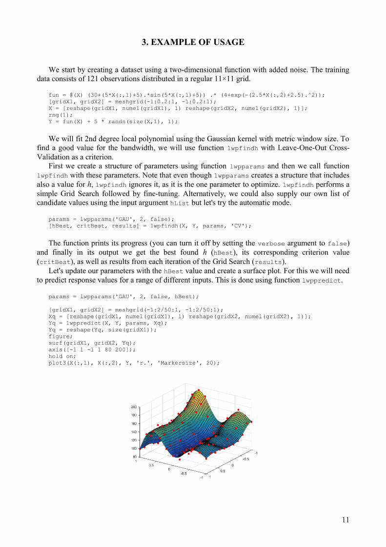
We start by creating a dataset using a two-dimensional function with added noise. The trainingdata consists of 121 observations distributed in a regular 11×11 grid.

fun = @(X) (30+(5*X(:,1)+5).*sin(5*X(:,1)+5)) .* (4+exp(-(2.5*X(:,2)+2.5).^2));[gridX1, gridX2] = meshgrid(-1:0.2:1, -1:0.2:1);X = [reshape(gridX1, numel(gridX1), 1) reshape(gridX2, numel(gridX2), 1)];rng(1);Y = fun(X) + 5 * randn(size(X,1), 1);

We will fit 2nd degree local polynomial using the Gaussian kernel with metric window size. Tofind a good value for the bandwidth, we will use function lwpfindh with Leave-One-Out Cross-Validation as a criterion.

First we create a structure of parameters using function lwpparams and then we call functionlwpfindh with these parameters. Note that even though lwpparams creates a structure that includesalso a value for h, lwpfindh ignores it, as it is the one parameter to optimize. lwpfindh performs asimple Grid Search followed by fine-tuning. Alternatively, we could also supply our own list ofcandidate values using the input argument hList but let's try the automatic mode.

params = lwpparams('GAU', 2, false);[hBest, critBest, results] = lwpfindh(X, Y, params, 'CV');

The function prints its progress (you can turn it off by setting the verbose argument to false)and finally in its output we get the best found h (hBest), its corresponding criterion value(critBest), as well as results from each iteration of the Grid Search (results).

Let's update our parameters with the hBest value and create a surface plot. For this we will needto predict response values for a range of different inputs. This is done using function lwppredict.

params = lwpparams('GAU', 2, false, hBest);

[gridX1, gridX2] = meshgrid(-1:2/50:1, -1:2/50:1);Xq = [reshape(gridX1, numel(gridX1), 1) reshape(gridX2, numel(gridX2), 1)];Yq = lwppredict(X, Y, params, Xq);Yq = reshape(Yq, size(gridX1));figure;surf(gridX1, gridX2, Yq);axis([-1 1 -1 1 80 200]);hold on;plot3(X(:,1), X(:,2), Y, 'r.', 'Markersize', 20);

11

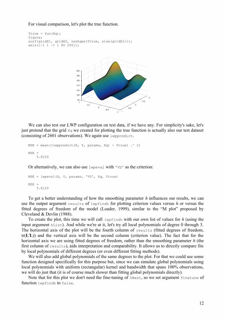
For visual comparison, let's plot the true function.

Ytrue = fun(Xq);figure;surf(gridX1, gridX2, reshape(Ytrue, size(gridX1)));axis([-1 1 -1 1 80 200]);

We can also test our LWP configuration on test data, if we have any. For simplicity's sake, let'sjust pretend that the grid Xq we created for plotting the true function is actually also our test dataset(consisting of 2601 observations). We again use lwppredict.

MSE = mean((lwppredict(X, Y, params, Xq) - Ytrue) .^ 2)

MSE = 5.8120

Or alternatively, we can also use lwpeval with 'VD' as the criterion:

MSE = lwpeval(X, Y, params, 'VD', Xq, Ytrue)

MSE = 5.8120

To get a better understanding of how the smoothing parameter h influences our results, we canuse the output argument results of lwpfindh for plotting criterion values versus h or versus thefitted degrees of freedom of the model (Loader, 1999), similar to the “M plot” proposed byCleveland & Devlin (1988).

To create the plot, this time we will call lwpfindh with our own list of values for h (using theinput argument hList). And while we're at it, let's try all local polynomials of degree 0 through 3.The horizontal axis of the plot will be the fourth column of results (fitted degrees of freedom,tr(L'L)) and the vertical axis will be the second column (criterion value). The fact that for thehorizontal axis we are using fitted degrees of freedom, rather than the smoothing parameter h (thefirst column of results), aids interpretation and comparability. It allows us to directly compare fitsby local polynomials of different degrees (or even different fitting methods).

We will also add global polynomials of the same degrees to the plot. For that we could use somefunction designed specifically for this purpose but, since we can simulate global polynomials usinglocal polynomials with uniform (rectangular) kernel and bandwidth that spans 100% observations,we will do just that (it is of course much slower than fitting global polynomials directly).

Note that for this plot we don't need the fine-tuning of hBest, so we set argument finetune offunction lwpfindh to false.

12

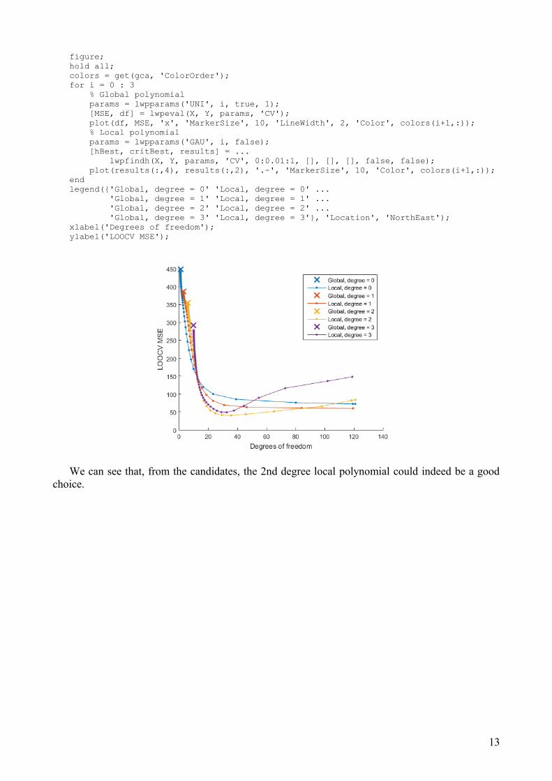
figure;hold all;colors = get(gca, 'ColorOrder');for i = 0 : 3 % Global polynomial params = lwpparams('UNI', i, true, 1); [MSE, df] = lwpeval(X, Y, params, 'CV'); plot(df, MSE, 'x', 'MarkerSize', 10, 'LineWidth', 2, 'Color', colors(i+1,:)); % Local polynomial params = lwpparams('GAU', i, false); [hBest, critBest, results] = ... lwpfindh(X, Y, params, 'CV', 0:0.01:1, [], [], [], false, false); plot(results(:,4), results(:,2), '.-', 'MarkerSize', 10, 'Color', colors(i+1,:));endlegend({'Global, degree = 0' 'Local, degree = 0' ... 'Global, degree = 1' 'Local, degree = 1' ... 'Global, degree = 2' 'Local, degree = 2' ... 'Global, degree = 3' 'Local, degree = 3'}, 'Location', 'NorthEast');xlabel('Degrees of freedom');ylabel('LOOCV MSE');

We can see that, from the candidates, the 2nd degree local polynomial could indeed be a goodchoice.

13

4. REFERENCES

1. Akaike H., Statistical predictor identification, Annals of Institute of Statistical Mathematics, 22(2), 1970, pp. 202-217.

2. Akaike H., Information theory and an extension of the maximum likelihood principle.Proceedings of 2nd International Symposium on Information Theory, eds Petrov B. N. andCsaki F., 1973, pp. 267-281.

3. Akaike H., A new look at the statistical model identification. IEEE Transactions on AutomaticControl, 19 (6), 1974, pp. 716-723.

4. Cleveland W. S., Robust Locally Weighted Regression and Smoothing Scatterplots. Journal ofthe American Statistical Association, 74 (368), 1979, pp. 829-836.

5. Cleveland W. S., Devlin S. J., Locally weighted regression: An approach to regression analysisby local fitting, Journal of the American Statistical Association, 83 (403), 1988, pp. 596-610.

6. Cleveland W. S., Grosse E., Shyu W. M., Local regression models. Chapter 8 of StatisticalModels in S, eds Chambers J. M. and Hastie T. J., Wadsworth & Brooks/Cole, 1992

7. Cleveland W. S., Loader C. L., Smoothing by Local Regression: Principles and Methods,Statistical Theory and Computational Aspects of Smoothing, eds Haerdle W. and Schimek M.G., Springer, New York, 1996, pp. 10-49.

8. Craven P., Wahba G., Smoothing noisy data with spline functions. Numer. Math., 31, 1979, pp.377-403.

9. Fan J., Gijbels I., Local polynomial modelling and its applications. Chapman & Hall, 199610. Hastie T., Tibshirani R., Friedman J., The elements of statistical learning: Data mining,

inference and prediction, 2nd edition, Springer, 200911. Hurvich C. M., Simonoff J. S., Tsai C.-L., Smoothing Parameter Selection in Nonparametric

Regression Using an Improved Akaike Information Criterion, Journal of the Royal StatisticalSociety, Series B (Statistical Methodology), 60 (2), 1998, pp. 271-293.

12. Loader C., Local Regression and Likelihood, Springer, New York, 199913. Nadaraya E. A., On Estimating Regression. Theory of Probability and its Applications, 9 (1),

1964, pp. 141-142.14. Rice J., Bandwidth choice for nonparametric regression. The Annals of Statistics, 12 (4), 1984,

pp. 1215-1230.15. Rikards R., Abramovich H., Kalnins K., Auzins J., Surrogate modeling in design optimization

of stiffened composite shells, Composite Structures, 73 (2), 2006, pp. 244–251.16. Shibata R., An Optimal Selection of Regression Variables, Biometrika, 68 (1), 1981, pp. 45-54.17. Stone C., Consistent nonparametric regression. Annals of Statistics, 5 (4), 1977, pp. 595-645.18. Watson G. S., Smooth regression analysis. Sankhyā: The Indian Journal of Statistics, Series A,

26 (4), 1964, pp. 359-372.

14