Embed Size (px)
Citation preview

Pre-print version
Published version: Hielke Buddelmeyer, Wang-Sheng Lee and Mark Wooden, ‘Low-paid Employment and Unemployment Dynamics in Australia’, The Economic Record 86(272), March 2010, pp. 28-48. [http://dx.doi.org/10.1111/j.1475-4932.2009.00595.x]
Low-paid Employment and Unemployment Dynamics in
Australia*
HIELKE BUDDELMEYER, WANG-SHENG LEE and MARK WOODEN
Melbourne Institute of Applied Economic and Social Research,
The University of Melbourne
* This paper is based on research commissioned by the Australian Government Department of Education, Employment and Workplace Relations under the Social Policy Research Services Agreement (2005-09) with the Melbourne Institute of Applied Economic and Social Research. Additional funding was also received from the Faculty of Economics and Commerce, University of Melbourne. It uses unit record data from the Household, Income and Labour Dynamics in Australia (HILDA) Survey. The HILDA Survey Project was initiated and is funded by the Australian Government Department of Families, Housing, Community Services and Indigenous Affairs and is managed by the Melbourne Institute of Applied Economic and Social Research. The findings and views reported in this paper, however, are those of the author and should not be attributed to any of the aforementioned organisations.
The data used in this paper were extracted using the Add-On package PanelWhiz v2.0 (Nov 2007) for Stata, written by Dr. John P. Haisken-DeNew ([email protected]).
Correspondence: Dr Hielke Buddelmeyer, Melbourne Institute of Applied Economic and Social Research, Level 7, Alan Gilbert Bldg, The University of Melbourne, VIC, 3010. Email: [email protected].

Low-paid Employment and Unemployment Dynamics in
Australia*
Abstract
This paper uses longitudinal data from the Household, Income and Labour Dynamics in
Australia (or HILDA) Survey to examine the extent to which the relatively high rates of
transition from low-paid employment into unemployment are the result of disadvantageous
personal characteristics or are instead a function of low-paid work itself. Dynamic random
effects probit models of the likelihood of unemployment are estimated. After controlling for
unobserved heterogeneity and initial conditions, we find that, relative to high-paid
employment, low-paid employment is associated with a higher risk of unemployment, but
this effect is only significant among women. We also find only weak evidence that low-wage
employment is a conduit for repeat unemployment.

I Introduction
Like many other countries, and notably the UK and the US, recent government policy in
Australia, especially under the Howard Coalition Government, has emphasised the
importance of getting people into work in order to reduce long-term welfare dependence and
increase workforce participation (e.g., DEWR, 2003). The guiding philosophy behind this
approach rests on the twin claims that employment is the best protection against poverty and
financial hardship, and that a low-paid job, even if it is not long lasting, can act as a bridge to
more sustained and more attractive employment opportunities. In contrast, critics of this ‘jobs
first’ approach argue that many low-paid jobs are both temporary and provide little in the
way of employment enhancing skills. As a result, many labour force participants cycle
between joblessness and low quality employment; what has been described as a ‘no pay, low
pay cycle’ (Dunlop, 2001; Perkins & Scutella, 2008).
While there is convincing descriptive evidence indicating that low-paid workers in
Australia are at much greater risk of experiencing future unemployment than workers in more
highly paid jobs (Perkins & Scutella, 2008), what is still unknown is the extent to which this
is the result of disadvantageous worker characteristics, either observed or unobserved, or a
function of low-paid work itself. In this paper we shed light on this question by using
longitudinal data from the Household, Income and Labour Dynamics in Australia (or
HILDA) Survey to model annual rates of transition between employment, distinguishing
between low-paid and high-paid jobs, and unemployment. More specifically, we estimate
dynamic random effects probit models of the likelihood of labour force participants
experiencing unemployment. In contrast to most previous research, we find little evidence to
support the conclusion that low-paid employment per se, at least during the period under
investigation (2001 to 2007), markedly increased the risk of men experiencing a spell of
1

unemployment in the future. In contrast, among women a sizeable and statistically significant
effect is found.
The paper is structured into seven sections. Following this introduction, we review
previous empirical studies that have examined the relationship between low-paid employment
and unemployment (or in some cases, joblessness). Section III then provides a short
introduction to the data, and especially the earnings and hours data that are used in defining
low pay. That definition is then set out in Section IV, along with a discussion of some of the
issues surrounding that definition. Section V provides some descriptive statistics on low pay
transitions. The centrepiece of the paper is the multivariate analyses of low pay transitions,
which are described, and for which results are presented, in Section VI. Some brief
conclusions are provided in Section VII.
II Previous Research
The issue of low pay dynamics and earnings mobility has been much studied in overseas
countries, especially in the UK. Gregory and Elias (1994), for example, used longitudinal
data collected from employers in the UK New Earnings Survey (NES) and found
considerable mobility out of the bottom of the wage distribution, especially by younger
workers. With the emergence of data from the British Household Panel Survey (BHPS),
which commenced in 1991, UK studies on this issue proliferated, all of which were largely
concerned with estimating the probability of exiting low-paid employment or, conversely, the
extent of persistence of the low pay state (Sloane & Theodossiou 1996, 1998; Gosling et al.,
1997; Stewart & Swaffield, 1997). In contrast to the earlier work based on the NES, these
studies emphasised the evidence on persistence of low pay. More recent studies, both in the
UK and elsewhere in Europe, have further advanced our understanding of low pay dynamics
by employing statistical techniques that take into account the endogeneity of the initial wage
2

state (Stewart & Swaffield, 1999; Cappellari, 2002; Sousa-Poza, 2004) and in, some cases,
panel attrition as well (Uhlendorf, 2006; Cappellari & Jenkins, 2008a).
One of the themes to emerge from this body of research is that the experience of low
pay is closely associated with subsequent episodes of joblessness. Gosling et al. (1997), for
example, reported from their analysis of the first four waves of the BHPS that men in the
bottom quartile of the earnings distribution were “almost three times as likely to move out of
employment in the 12 months following the first-wave interview as men in the top quartile”
(p. 35). This interdependence between low pay and joblessness, and the role of state
dependence, has been explored in a number of studies, though we are only aware of two –
Stewart (2007) and Cappellari and Jenkins (2008b) – that have focussed specifically on
unemployment (as distinct from all joblessness), both of which again used data from the
BHPS collected during the 1990s.
Stewart (2007) estimated probabilities of both unemployment and low-paid
employment using dynamic random effects probit models that controlled for endogenous
initial conditions and unobserved heterogeneity. He reached the striking conclusion that low-
paid employment (defined as earnings of less than ₤3.50 per hours in 1997 terms) has almost
as large an adverse impact on future employment prospects as current unemployment. This
conclusion appears to be based on the finding that the coefficients on the indicator variables
for unemployment conditional on being unemployed in the previous period and for
unemployment conditional on being in a low-wage state in the previous period were not
significantly different from each other. This result, however, was only obtained once spells of
continuing non-employment were excluded. Further, in Stewart’s preferred equation, the
estimated effect of past unemployment is still almost 1.4 times that of past low-wage
employment. The strong conclusion of Stewart (2007) appears to be driven by a pre-
occupation with statistical significance. If we focus simply on the estimated magnitudes from
3

his research we can just as reasonably draw the conclusion that the protective effects of high-
wage employment are only marginally greater than that of low-wage employment – the
predicted probability of unemployment is only 1.5 percentage points (or 28%) lower.
A different estimation approach was employed by Cappellari and Jenkins (2008b).
They modelled annual transitions between unemployment and low-paid and high-paid
employment states using a multivariate probit model that accounted for three potentially
endogenous selection processes – the initial wage state, selection into employment, and
sample attrition – and allowed for correlations between the unobserved factors in these
different processes.1 They restricted their sample to men, but like Stewart (2007) concluded
that low-paid employment is associated with a higher probability of future unemployment
than high-wage employment. The size of the effect, however, could still be argued to be
relatively small; about one percentage point in the full model, which holds constant observed
and unobserved personal attributes. And unlike the finding of Stewart, the relevant coefficient
was not statistically significant.
Research in Australia is both far less prevalent and far less well developed, in part
reflecting the paucity of longitudinal data in this country. The first significant Australian
longitudinal survey to track labour market behaviour, for example, only commenced in 1985
and only followed young people until age 24. Known as the Australian Longitudinal Survey
(and surviving today under the name, Longitudinal Surveys of Australian Youth), it formed
the basis of the first empirical investigation of low-wage dynamics in Australia. That study,
by Miller (1989), however, was only concerned with employment, and not with the
interaction with unemployment.
It would be another decade before serious empirical evidence on the relationship
between low-wage employment and unemployment, or more strictly joblessness, in Australia
would be presented. This research, by Dunlop (2000, 2001), used longitudinal data from the
4
Survey of Employment and Unemployment Patterns collected by the Australian Bureau of
Statistics (ABS) in 1995, 1996 and 1997. Based on results from the construction of simple
transition matrices, she concluded that low-paid employment (defined as earning less than
$10 per hour in September 1994, a level that was then indexed to growth in average weekly
earnings) is a temporary state for about half of the low paid. For the remaining half, low-paid
employment appears to be relatively persistent or involves churning in and out of joblessness.
Indeed, and echoing the results typically reported for the UK, she concluded that “low-paid
adults are about twice as likely as the higher paid to face spells of joblessness during the two-
year transition period” covered by the data (Dunlop, 2001, p. 105). Very similar conclusions
were drawn by Perkins and Scutella (2008) from their analysis of HILDA Survey data for the
period 2001 to 2005. They reported annual transition rates that indicate that the probability of
workers in low-paid employment being jobless a year later is around twice that of workers in
higher paid work.
Both of these studies reported descriptive data, and made no serious attempt to account
for individual heterogeneity. They also did not distinguish unemployment from other forms
of joblessness. Watson (2008), on the other hand, used the calendar data from the first six
waves of the HILDA Survey to estimate a variety of statistical models of labour market states
that control for individual heterogeneity to varying degrees, while also attempting to deal
with other statistical issues such as correlated error structures. He also explicitly separated
unemployment from other non-employment states, though not in the models that control for
unobserved heterogeneity. His key findings were twofold. First, among the sample of persons
who change jobs or enter employment over the sample period, those in the lowest earnings
quintile are, as we would expect, much more likely to have experienced a preceding spell of
non-employment. Second, and more importantly, the next transition among this group is
more likely to be a move into non-employment rather than into employment.
5

Unfortunately, the HILDA Survey data provide no information on earnings in jobs held
between interview dates, and the central conclusions of Watson (2008) are closely linked to
the assumptions he makes about the earnings of between-interview jobs. In particular,
Watson used earnings reported during the annual interview to impute earnings for between-
interview jobs. Although Watson’s attempt to use detailed job spell information from the
calendar data is commendable, the assumption he makes of assigning an average quintile
score to all jobs held in a year potentially induces a serious bias that can account for his
findings.2 Further, we suspect the earnings measure is based on either weekly or annual
earnings and thus will itself be a function of the number of hours worked.
In this study we seek to shed further light on the extent to which low-paid job holders in
Australia are at relatively high risk of experiencing future spells of unemployment, and
whether it is the characteristics of holders of low-paid jobs or characteristics intrinsic to the
low-paid jobs that explain this enhanced risk. The major innovation, at least when compared
to previous Australian work, is the more careful treatment of econometric issues concerning
unobserved heterogeneity and initial conditions. While the approach used is closely modelled
on the UK research of Stewart (2007), this study differs by providing separate estimates for
men and women. We also give consideration to the potential importance of restricting the
sample for analysis to labour force participants and how that might influence our conclusions.
III Data
The data used in this study come from the first seven waves of the HILDA Survey, a
longitudinal survey with a focus on work, income and family that has been following a
sample of Australians every year since 2001. Described in more detail in Wooden and
Watson (2007), the survey commenced in 2001 with a nationally representative sample of
Australian households. Personal interviews were completed at 7682 of the 11 693 households
identified as in scope for wave 1 (providing an initial responding sample comprising 13 969
6

people), and while non-response is considerable, the characteristics of the responding sample
appear to match the broader population quite well. The members of these participating
households form the basis of the panel pursued in the subsequent waves of interviews, which
are conducted approximately one year apart. Interviews are conducted with all adults (defined
as persons aged 15 years or older on the 30th June preceding the interview date) who are
members of the original sample, as well as any other adults who, in later waves, are residing
with an original sample member. Annual re-interview rates (the proportion of respondents
from one wave who are successfully interviewed the next) are reasonably high, rising from
87% in wave 2 to over 94% in waves 5, 6 and 7.
Following Stewart (2007), the sample used here is initially restricted to those persons
who were in the labour force (i.e., either employed or unemployed) at the time of interview.
But in contrast to Stewart (but like Cappellari and Jenkins, 2008b), we also remove from the
sample all persons who are self-employed at the time of interview, including owner managers
that might otherwise be defined as employees of their own business. Concerns about both the
general quality of income information provided by the self-employed and the way incomes
are apportioned to earnings by owner-managers argue strongly in favour of their exclusion.
We also exclude all persons under the age of 21 years and any other full-time students. The
exclusion of persons under the age of 21 years was deemed necessary given the wage
structures in many jobs (and in most awards) provide for junior rates of pay that are below
those that apply to adult employees. Certainly the inclusion of juniors would cause the low-
pay threshold (defined in Section IV) to fall and reduce the number of adults defined as low
paid.3 The working sample thus commenced with 43 262 observations on 11 152 individuals.
Only 2458 of these people, however, are observed in the labour force in all seven waves.
The unemployment indicator is constructed from questions which were intended to
produce a measure that accords with ABS / ILO definitions. Thus to be defined as
7

unemployed a respondent had to meet each of the following conditions: (i) not had a paid job
during the preceding 7 days; (ii) been actively looking for paid work during the previous 4
weeks; and (iii) been available to start work in the previous week (or was waiting to start a
new job that was expected to commence within the next 4 weeks).
The low pay and high pay indicators are based on a measure of the hourly wage in the
main job, which is in turn obtained by dividing usual gross weekly earnings by usual weekly
hours worked. The earnings measure used here is usual current total gross weekly pay in the
main job. It is derived from a sequence of questions that asks respondents to provide the
gross amount of their most recent pay, the length of that pay period, and then to indicate
whether that is their usual pay. If it is not their usual pay, details of their usual pay are then
collected. The relevant questions are based quite closely on a similar set of questions
included in the ABS Survey of Income and Housing Costs. A particular problem for many
household surveys collecting economic data is high rates of item non-response. The earnings
data in the HILDA Survey, however, do not seem to be seriously affected by this problem,
with the proportion of cases where no information on current earnings (in the main job) is
provided averaging just 2.9 per cent over the seven waves.
Hours of work is represented by the number of total hours usually worked per week in
the main job, where total hours includes any paid or unpaid overtime as well as any work
undertaken outside the workplace. While non-response is minimal, measurement error is very
likely. It is, for example, often claimed that survey-based data will tend to overstate hours of
work at the upper end of the distribution (see Robinson & Bostrom, 1994). In large part this
will simply be the result of over-reporting, a phenomenon which is especially likely in
societies where long hours of work is seen as ‘badge of courage’. It could also arise as a
result of other measurement problems, including the inclusion of time that we would not
generally consider to be work (e.g., meal breaks, time on-call, and commuting time), and in
8

the way some respondents interpret what is meant by ‘usual’. However, there is no a priori
reason to assume that the hours data for employees from the HILDA Survey are any more (or
less) biased than hours data from any other survey-based data set, an assumption that has
been confirmed by comparisons of the HILDA Survey estimates with estimates from ABS
household surveys (Wooden et al., 2007).
IV Defining Low Pay
All investigations into the concept of low pay are confronted by the question of how to define
it, and more specifically how to define the low-pay threshold. If the focus is on the
relationship between earnings and income poverty then it makes sense to define low pay in
terms of adequacy, and historically it has been this perspective that has dominated thinking
about low pay in Australia. A needs-based approach, however, is not appropriate for
examining questions relating to earnings mobility and labour market transitions. In the needs-
based approach, transitions into and out of low pay can occur because of changes in family
circumstances and relocation. In contrast, analyses of earnings mobility are not concerned
with whether earnings are adequate to support some pre-defined lifestyle. Previous research
into the dynamics of low-paid employment has thus not defined low pay by reference to some
standard of need, but relative either to the distribution of earnings or to some administrative
standard.
The choice of threshold is highly variable across studies. Some (e.g., Gregory & Elias,
1994; Gosling et al., 1997; Watson, 2008) have simply defined the low paid as those in the
bottom decile or quintile in the wage distribution, which fixes the low paid to be a
predetermined proportion of the working population. Very differently, others have set a low
pay threshold relative to some institutional norm, such as a minimum wage, and then indexed
that threshold to changes in either consumer prices or average earnings (e.g., Richardson &
Harding 1999; Dunlop 2001, 2001; Stewart 2007). More usual, however, is to define the
9
threshold relative to the distribution of hourly earnings across all workers, with two-thirds
median being perhaps most commonly used (e.g., Webb et al., 1996; Keese et al., 1998;
Sloane & Theodossiou, 1998; Uhlendorff, 2006; Capellari & Jenkins, 2008a; Perkins &
Scutella, 2008).4 In this analysis we adopt this widely used benchmark and so define a person
as low paid if their rate of pay is less than two-thirds of the median gross hourly wage.
The usual rationale for employing a threshold based on hourly rates of pay is that the
alternative – a cut-off based on weekly pay – will see some individuals defined as low paid
simply because they work relatively few hours. This is usually judged problematic, especially
when those part-time hours are the preferred working arrangement of the individual.5 On the
other hand, using hourly pay will see some people defined as low paid because of the large
numbers of hours they report usually working. According to the data set used here, for
example, around 21 per cent of all employed persons in Australia report usual weekly hours
of at least 50.6 This in itself is not necessarily a problem provided both that hours are
measured accurately and that one working hour is much like another. Neither assumption is
likely to be realistic, suggesting consideration should be given to capping working hours.
Experimentation with different caps, however, suggested that a cap made little difference to
the estimated threshold.
We also need to decide how to deal with multiple job-holders. Most studies ignore this
distinction; the hourly earnings measure is based on earnings in all jobs. Again this seems a
reasonable decision if the focus of the research is on the adequacy of incomes, but not where
the focus is on labour market transitions. Thus, and as previously noted, we only use the
earnings and hours from the main job, defined in the HILDA Survey as that which provides
the most pay each week.
A final issue concerns the treatment of casual employees who, as observed in
Buddelmeyer and Wooden (2008), account for well over one in every four Australian
10

employees. While there is no precise and consistent definition of casual employment in either
common or industrial law in Australia, it is widely accepted that a common feature of casual
employment is the absence of entitlement to paid sick leave, paid annual leave and paid
public holidays. Indeed it is this feature of casual work that has been most frequently used to
measure its incidence in Australia. More importantly for this analysis, the rates of pay of
casual employees typically include a pay loading, usually assumed to be around 20%, to
compensate for their ineligibility for these entitlements. As a result, it has been argued that
the measured hourly pay rates of casual employees needs to be discounted by 20%. This, for
example, was the approach used by Dunlop (2000, 2001). Alternatively, it could be argued
that the casual pay loading is conceptually no different than the pay loading (implicit or
explicit) that is attached to any job as compensation for some undesirable characteristic.
Casuals get a higher rate of pay to compensate for lack of access to leave entitlements in the
same way that, say, underground miners attract a pay loading to compensate for dangerous
working conditions. In this paper we take the latter approach and do not discount casual pay.
We next need to decide from which data source to draw the benchmark. Most
convenient is to use the HILDA Survey sample itself (as compared with some external
benchmark). Given the HILDA Survey is designed to provide a representative sample of all
Australian residents living in private households this seems a reasonable step. Further, it
provides a simple mechanism for automatically updating the low-pay threshold over time; we
simply tie the threshold to the observed changes in the distribution of hourly earnings within
the HILDA sample. To be more specific, we derive a median hourly wage for each survey
wave based on the weighted distribution of hourly earnings of all adult employees (aged 21
years or older) with both positive earnings and positive working hours, but excluding full-
time students. Cases where earnings have to be imputed are excluded.
11

Our estimated low-pay thresholds for each survey wave are reported in Table 1. As can
be seen, the low-pay threshold has increased steadily over time, and by wave 7 was almost
30% higher than the level in wave 1. By comparison, consumer prices over this period rose
by only 18%. This real growth in the level of the low-pay threshold reflects the growth in
average and median real earnings over this same period. As we would also expect, the weekly
equivalents of our low-pay thresholds all lie above the level of the Federal Minimum Wage
that applied at the time, though the size of this differential is not large, averaging around 7%.
We also checked the sensitivity of our estimates to different assumptions (using
earnings from all jobs instead of main jobs, capping weekly hours worked at 60, using
imputed earnings when not reported, and applying a discount to the earnings of casual
employees). For the most part the thresholds are robust, and varying the assumptions makes
little difference to the estimated threshold. The one exception here is the treatment of casual
pay, the discounting of which has a noticeable impact on the level of low-paid employment,
drawing as it does many more casual employees into the low pay category. However,
discounting casual pay does not appear to substantially affect employment dynamics and thus
would have little bearing on the conclusions reached in the analysis that follows.
V Descriptive Statistics
We begin by presenting, in Table 2, distributions of the sample by labour market state, where
we distinguish between persons who are: (i) unemployed; (ii) low paid (earning less than 2/3
median earnings); and (iii) high paid (earning more than 2/3 median). Thus we see from the
first row in this table that the unweighted unemployment rate has fallen from 6.3% at the start
of the period to just 3.6% by 2007. Note, however, that our exclusion of the self-employed
means that these rates are not directly comparable with those produced by the ABS from the
Labour Force Survey. Nevertheless, we are very confident that the composition of the sample
is broadly in line with Labour Force Survey estimates. The latter suggest ‘adjusted’
12

unemployment rates (that is, after excluding the self-employed from the population) of 7.1%
and 4.7% in November 2001 and November 2007, respectively. These rates are higher than
reported in Table 2 from the HILDA Survey, but this is to be expected given the ABS treats
owner-managers of incorporated businesses as employees whereas we do not. Much more
importantly, the level of decline in these unemployment rates over the two periods is very
similar to that recorded in our sample.
Estimates of the proportion of adult employees that would be defined as low paid in our
analysis sample are presented in the second row of Table 2. As can be seen, the proportion of
the adult labour force defined as having low-paid jobs is relatively stable over the period
covered, averaging around 11 to 12%. Further, we can see that this proportion is slightly
higher among women (averaging 12.4%) than among men (10.9%).
Even though the proportion of low-paid workers at any point in time is reasonably
stable, there is considerable movement between labour market states. This is shown in Table
3, which reports average rates of transition over both a one-period interval and a two-period
interval (with, on average, each period being about one year). Thus, of those in the low-paid
category at time 1t − , just 44% can be expected to still be low-paid by time t. The majority of
low-paid workers (53%) will instead be classified as high-paid workers by the next survey
date, leaving a small fraction (less than 2%) seeking jobs. Similarly, of those in the low-paid
category at time 2t − , only 38% will be in that same state by time t, with 59% having moved
into a high-paid state.
Table 3 also reveals that the probabilities of unemployment are higher for persons who
were in low-paid employment in the past than those who were in high-paid employment.
Indeed, the one-period conditional probability of unemployment is, among all persons,
exactly twice as great for those who were in low-paid employment last period relative to
those in high-paid employment. The comparable two-period conditional probabilities are
13

close to identical to the one-period probabilities. We can also see that this difference is
characteristic of both men and women, though the size of the differential is greater among
women.
Overall, the descriptive data from the HILDA Survey suggest little has changed since
the 1990s when the data used by Dunlop (2000, 2001) were collected. The data presented
here seem entirely consistent with her conclusion that low-paid employment is a temporary
state for about half the low-paid workforce, and is either persistent or involves churning in
and out of employment for the other half. We will now test these conclusions within a
multivariate framework that controls for personal attributes, other characteristics, and
unobserved heterogeneity.
VI Multivariate Analysis of Low Pay Dynamics
(i) Model Specification
Following Stewart (2007), we employ a dynamic random effects probit framework. The
latent equation for the dynamic random effects panel probit model can be written as:
*1 'it it it i ity y x uγ β α−= + + +
where the subscript i = 1, 2, …, N indexes individuals, the subscript t = 2, …, T indexes time
periods, *ity is the latent dependent variable identifying employment status, itx is a vector of
exogenous characteristics, iα are unobserved individual-specific random effects, and the itu
are assumed to be distributed 2(0, )uN σ . The observed binary outcome is:
*1 if 0
0 otherwiseit
ity
y ≥
=
The standard random effects model assumes that iα is uncorrelated with itx . As this is
potentially restrictive, we adopt the Mundlak-Chamberlain approach (Mundlak, 1978;
14

Chamberlain, 1984) and allow a correlation between iα and the observed characteristics in
the model by assuming a relationship between iα and the means of the time-varying x-
variables:
'i i ix aα ν= +
where iν is distributed 2(0, )N νσ .
The dynamic random effects probit model requires an auxiliary distributional
assumption on the individual-specific effects. Alternatively, a fixed effects model might be
considered. The fixed effects approach has the advantage that it requires no assumptions on
the statistical properties of the individual effects and is capable of eliminating all time-
invariant differences between individuals, even if they are unobserved. However, in non-
linear panel data models, the use of fixed effects is notoriously problematic due to the
incidental parameters problem. In general, the random effects estimator provides greater
efficiency if the auxiliary distributional assumption is valid, and is inconsistent if it is not. In
the application of dynamic random effects probit models, Arulampalam and Stewart
(forthcoming) suggest that it is advantageous to allow for correlated random effects using the
Mundlak-Chamberlain approach rather than not allowing for the correlation.
An important issue that needs to be addressed is the so-called initial conditions
problem. This problem arises because the start of the observation period (wave 1 in 2001)
does not coincide with the start of the stochastic process generating low-paid employment
experiences. Estimation of the model therefore requires a further assumption about the
relationship between 1iy and iα . If the initial conditions are correlated with iα , as is likely in
our context, not addressing the initial conditions problem will lead to overstating the level of
state dependence (i.e., the estimate of γ in will be larger than it actually should be).
15

One possible approach to solve the initial conditions problems is based on a suggestion
by Wooldridge (2005). In the Wooldridge approach, the relationship between 1iy and iα is
accounted for by modelling the distribution of iα given 1iy . The assumption in Wooldridge’s
approach is that the distribution of the individual specific effects conditional on the
exogenous individual characteristics is correctly specified. Although other approaches to deal
with the problem of initial conditions are available (Heckman, 1981; Orme, 2001), Monte
Carlo simulations reported in Arulampalam and Stewart (forthcoming) suggest that all three
estimators display similar results and perform satisfactorily, at least when T=6. We are
therefore satisfied that our chosen estimation strategy is sensible.
The dynamic panel model is most appropriate for addressing the issue of whether prior
unemployment or low-paid employment experiences exacerbate the likelihood of
experiencing unemployment in the future. It does so by decomposing the state dependence of
unemployment into true state dependence (i.e., the scarring effect of unemployment) and the
component that is due to unobserved heterogeneity across the units (i.e., differences in
individuals).
The issue of whether prior unemployment and low-paid employment experiences
exacerbate the likelihood of experiencing unemployment in the future is further examined
using a second-order dynamic random effects probit model so that employment states in both
1t − and 2t − are allowed to impact on unemployment at t. Eight dummy variables are
included as explanatory variables to account for the nine possible combination of states in
periods 1t − and 2t − in place of the lagged dependent variable. The advantage of such an
approach is that interactions of employment states in periods 1t − and 2t − can be used to
help understand the effect of certain pathways or sequences. For example, unemployment
followed by low-paid employment might be expected to be associated with a higher
16
probability of unemployment at period t than unemployment followed by high-paid
employment. Specifically, the model takes the following form:
*1 2( )( ) 'it k it it it i it
ky s s x uγ β α− −= + + +∑
*1 if 00 otherwise
itit
yy
≥=
where 1its − is a dummy variable denoting one of the three states (low pay, high pay and
unemployed) in time 1t − and 2its − is a dummy variable denoting one of the same three states
in time 2t − . The subscript i = 1, 2, … , N indexes individuals and the subscript t = 3, …, T
indexes time periods. In this model, the data are restricted to those persons in the labour force
in all seven waves.
The observable characteristics that comprise itx are listed in Table 4, along with their
summary statistics (means and standard deviations). They are intended to capture the effects
of age, education, marital status (or more strictly, partnership status), the number of
dependent children, ethnic origin (reflected in two crude dummy variables identifying
whether the respondent is of indigenous origin or was born overseas but not in one of the
major English-speaking countries7), the presence of a long-term health condition that is work
limiting, geographic location8 and the unemployment rate of the region (either a capital city
or the remainder of a State or Territory) in which the respondent lives (measured in June each
year).
(ii) Results
Results from the first-order dynamic model are reported in Tables 5 and 6. For completeness
we report results from both the simple pooled dynamic probits (Table 5) and from the panel
data (i.e., random effects) models (Table 6). We focus most of our attention, however, on the
latter given the strong evidence of unobserved heterogeneity, reflected most obviously in the
17

marked difference in the magnitude of the coefficients on the lagged employment states. As
discussed above, the panel data models are estimated using the Wooldridge method, but
coefficient estimates have been rescaled in order to provide comparability with the pooled
probit estimates.9 The variables in the tables denoted by m(.) are the means over time of the
variable in parentheses, or in other words, the Mundlak-Chamberlain time averages that
control for the correlation between the exogenous variables and iα . In all cases, we report
results for all persons (in line with Stewart, 2007) as well as for men and women separately.
It turns out that this distinction is non-trivial, with our results suggesting quite different
conclusions depending on which sex is under consideration.
From the results presented in Tables 5 and 6, two comparisons are worth highlighting:
the average partial effects (APE) and the predicted probability ratios (PPR). These are both
defined relative to the high-paid employment state at 1t − , with the former being defined as a
difference and the latter a ratio. The APEs of interest are given in the bottom of these Tables.
Thus, the pooled probit (Table 5) gives an APE of unemployment at 1t − for all persons of
0.279. After allowing for initial conditions and controlling for heterogeneity (Table 6), the
APE declines to just 0.067, indicating that the Wooldridge estimator reduces the degree of
measured persistence considerably. The PPR from the random effects model, however,
suggests that an individual unemployed at 1t − is still 8.4 times more likely to be
unemployed at t than an equivalent person in high-paid employment at 1t − . Furthermore,
our results suggest that the difference with respect to people in low-paid jobs is not that much
smaller – the PPR is 5.8. This stands in marked contrast to the results obtained for the UK by
Stewart (2007).
Even more interesting is the relativity between the indicator variables for being in high-
paid employment at 1t − and being in low-paid employment at 1t − . The relevant APE is just
0.004 while the PPR is 1.44. That is, a person in low-paid employment is 1.4 times more
18

likely, compared with a person in high-paid employment, to be unemployed next period.
Somewhat surprisingly, this result for the relativity between the effects of low-paid and high-
paid employment at 1t − is very similar to the results reported by Stewart (2007). These
results do, therefore, suggest that low-paid employment (relative to high paid employment)
enhances the likelihood of experiencing unemployment. The magnitude of this effect,
however, is only statistically significant and of any economic significance for women.
Among men the effect of low-paid employment is both very small (a PPR of 1.1) and a long
way from statistical significance (p-value = .62). In contrast, for women the PPR is quite
large (1.6) and the estimated coefficient is highly significant (p-value = .01).
Why low-paid jobs would have a greater scarring impact on women is not immediately
obvious, but would be consistent with the presence of discrimination in hiring and firing
practices at the bottom of the wages distribution. Alternatively, it might be argued that the
results reflect differences in preferences for employment emanating from the secondary
income earner status of women in many households. Such differences in preferences should,
however, have been captured by our model, and indeed estimation of separate equations for
married women and single women (but not reported in detail) finds little evidence that
married women in low-paid jobs face a markedly higher risk of future unemployment than
married women in high-paid jobs: the estimated PPR is, at just 1.04, very similar to that for
men. The gender differential appears to be largely restricted to single women. For this group
the relevant PPR summarising the effect of low-paid employment on future unemployment
relative to the effect of high-paid employment is 2.53.
As noted by Stewart (2007), the first-order model results still do not enable us to get a
good handle on whether low pay is a conduit to repeat unemployment. To get at this we turn
to our second-order model results. Again the results from the simple pooled probit (Table 7)
19

are reported mainly for completeness, and we focus here on the results from the panel data
models (Table 8).
As we would expect, the results indicate that an individual unemployed at both 1t −
and 2t − is much more likely (by 24 percentage points) to be unemployed at time t relative to
an individual who is high paid in both 1t − and 2t − . But are employed people who have
escaped unemployment recently no longer at risk of unemployment? The answer is clearly
no, with the probability of future unemployment significantly higher among employed
persons with a recent unemployment experience (i.e., at 2t − ) than among employed persons
who have not been scarred. Nevertheless, the relative size of these effects still suggests that
the scarring effect of unemployment is much reduced by an episode of employment. But most
telling, it does not appear to matter that much whether the next job is low paid or high paid;
the size of the estimated effect of unemployment (at 2t − ) is much the same in both cases –
the relevant APEs are 0.03 compared with 0.02, while the relevant PPRs are 5.0 compared
with 3.8.10
Again our conclusions differ somewhat when we focus on women and men separately.
We find that among men, low-paid employment is more likely to be a channel to repeat
unemployment – low-paid men with a recent history of unemployment are 5.9 times more
likely to be unemployed than men in high-paid jobs in both past periods, whereas men in
high-paid jobs with a history of unemployment are only 3.3 times more likely. That said, this
difference, while seemingly quite large, was not statistically significant (p-value = .32).
Among women the difference between low-paid employment and high-paid employment is
much smaller, and also statistically insignificant.
(iii) The Treatment of Sample Exits
To this point we have restricted our attention to labour force participants and thus excluded
persons not actively seeking work. As a result, all transitions from employment into non-
20

participation are excluded. This can be defended if we believe that all such transitions are
voluntary and driven by worker preferences. However, we know that discouraged worker
effects exist and that some people do not seek work because they believe a suitable job
cannot be found. It is thus possible that exclusion of these transitions out of our sample might
generate a form of selection bias in our results. Furthermore, as is often the practice with
analyses of longitudinal data, we have ignored panel attrition, effectively assuming that
persons who cease responding to the survey are no different to those that continue.
As shown in Table 9, exits out of sample are considerable. This table is a reproduction
of Table 3, but with the key difference that it reports exit from the sample as two additional
transition states at year t. As can be seen, the rate of sample exits into non-participation is
very high among the unemployed, consistent with the idea that many unemployed churn in
and out of the labour force. This type of sample exit is much less common among the
employed, but nevertheless is noticeably more common among the low-paid group than the
high-paid group. The fifth column of this table reports the rate of panel exits. These rates are
both very high, averaging 15% across the entire sample, and again exhibit a clear correlation
with labour market status – the unemployed are most likely to drop out of the panel while
high-paid employees are the least likely.
The high rate of panel attrition deserves comment, especially given it seems
inconsistent with the much lower rates of attrition usually reported for the HILDA Survey
(and discussed earlier). Panel attrition, as defined here, can arise for three basic types of
reasons: (i) sample members refusing to respond; (ii) death of sample members; and (iii) the
study design. Neither of the last two reasons are generally classified by survey administrators
as forms of panel attrition, and in the case of the HILDA Survey the last reason is of large
significance. Specifically, all persons who join sampled households after wave 1 are only
added to the sample on a temporary basis. With one exception, they only remain in the
21

sample for as long as they co-reside with an original sample member.11 This feature of the
sample design creates the appearance of a high rate of panel attrition.
The pattern of exit probabilities reported in Table 9 suggests the distinct possibility that
there may be correlations between the unobserved factors affecting exit and labour market
transitions. We thus subjected our analyses to a series of checks designed to ascertain
whether our results are robust in the face of these potential selection biases. First, we re-
estimated our dynamic probit model after extending the sample to include persons who move
out of the labour force and replacing the dependent variable with a variable identifying
joblessness (i.e., either unemployment or non-participation). Table 10 reports the summary
statistics from these estimations, which can be compared with the summary statistics reported
in Table 6. This table suggests two main conclusions. First, a focus on unemployment, rather
than joblessness, may cause us to seriously understate the extent to which non-employment
states are persistent. The probability of non-employment in period t conditional on non-
employment in period 1t − is almost 58%. The comparable estimate when the dependent
variable is unemployment was just under 8%. Second, and despite this large difference, our
conclusions regarding the relative efficacy of low-paid and high-paid employment are little
affected. The difference between low-paid jobs and high-paid jobs in terms of its effect on the
probability of future joblessness remains insignificant. In fact, the results in Table 10 would
lead us to strengthen our conclusions, with the key PPR being just 1.06, compared with the
ratio of 1.4 obtained when unemployment was the outcome.
Finally, there is the question of panel attrition. As attrition is a feature of all household
panel surveys, weights are typically provided to adjust the data for the differing propensity of
sample members to be re-interviewed. The HILDA Survey provides a rich set of weights,
including longitudinal weights for each pair of consecutive waves (i.e., they adjust for the
probability of responding at time t given response at time 1t − ). We re-estimated our pooled
22

probit models using these time varying pair-wise longitudinal weights, but results obtained
were almost identical to those reported in Table 5. Unfortunately, unlike the case of the
pooled probit, using time-varying weights in the dynamic probit model is non-trivial.
However, when we restrict the sample to those individuals observed in all waves we can use
the enumerated person longitudinal weights provided in wave 7 to adjust our data for the
propensity to be interviewed in all 7 waves. If panel attrition is an issue, then one would
expect this to be brought to light most strongly in the case of a balanced sample. As was the
case for the pooled probit, using weights resulted in almost identical parameter estimates.
Overall, therefore, and despite the considerable extent of sample attrition, we can find
no evidence to suggest that attrition biases are of large consequence for our key result. Panel
attrition does not appear to be imparting any bias to our results, and while our focus on
unemployment rather than joblessness may have caused us to seriously understate the extent
to which joblessness is persistent, it does not affect our conclusions about the relative
efficacy of low-paid employment.
VII Conclusion
The aim of this paper was to examine in detail, using the first seven waves of the HILDA
Survey data, whether low-paid jobs in Australia reduce or exacerbate the likelihood of
experiencing unemployment in the future. First and second-order dynamic random effects
probit models predicting the probability of a labour force participant experiencing
unemployment, after controlling for both unobserved heterogeneity and initial conditions,
were estimated. The results indicate that prior low-paid employment experiences have, at
most, only a modest effect on the probability of experiencing unemployment in the future vis-
à-vis high-paid employment. Indeed, among men there appears to be no significant difference
between low-paid employment and high-paid employment. We did, however, uncover some
weak evidence that men were more likely to experience repeat unemployment if the
23
intervening employment was low paid. For women we find essentially the reverse results.
The experience of low-paid employment places women at much greater risk (1.6 times more
likely) of experiencing future unemployment relative to high-paid employment, but it does
not exacerbate their likelihood of experiencing repeat unemployment. We also found that the
relatively greater risk of future unemployment faced by low-paid women is mostly restricted
to single women. Ultimately, however, the main feature of our analysis is the mainly weak
scarring effects exerted by low-paid employment. Instead, by far the best predictor of
whether someone is unemployed at time t is whether they have experienced unemployment in
the past.
An interesting question is why our results seem so different from the results obtained in
UK studies. Part of the explanation we believe lies in the way the UK results have been
interpreted. As we noted earlier, Cappellari and Jenkins (2008b), who only analysed data for
men, did not actually find significant differences between low-paid employment and high-
paid employment in terms of their effects on future unemployment. Their results are thus
entirely consistent with what is reported here. Stewart (2007), on the other hand, did obtain
quite different results, but even he still reported relative probabilities of unemployment
conditional on low-paid employment compared with high-paid employment that are close to
identical to that reported here.
Another possibility may lie in the different time periods covered by the data. The UK
studies of Stewart (2007) and Cappellari and Jenkins (2008b) both used data from the 1990s
when UK unemployment rates were very high; indeed the data period includes the recession
of the early 1990s. In contrast, the HILDA Survey data used here come from a period of
strong economic growth and record low levels of unemployment. It may be that in a period of
economic contraction with higher levels of unemployment we might obtain very different
results.
24

We also report on some intriguing differences between men and women, something that
has not been studied in the UK literature. We speculate that our results are consistent with the
presence of gender-based discrimination in hiring and firing practices, at least at the bottom
of the wages distribution. Ultimately, however, this is an issue that is not pursued at any
length in this paper, and is obviously an area ripe for further research.
Finally, there remains the question of the policy significance of our results. In our view,
the findings reported in this paper are generally supportive of the jobs-first approach to
workforce participation. While it is true that workers in low-paid jobs are at greater risk of
future unemployment (and joblessness) this is mainly due to personal characteristics that
render them less competitive in the labour market. Public policy needs to continue to
emphasise and support education and early childhood development as the key mechanisms
for ensuring labour market entrants are not disadvantaged in the labour market. In contrast,
policy makers need to be cautious in adopting and supporting measures intended to improve
the well-being of low-paid workers (such as increases in minimum wages and other minimum
award conditions) that might harm employment prospects. Anything that increases the risk of
job loss or reduces the likelihood of securing new employment will only exacerbate the
difficulties these disadvantaged workers face in building a long-term attachment to the
workforce.
25
REFERENCES
Arulampalam, W. (1999), ‘A Note on Estimated Coefficients in Random Effects Probit
Models’, Oxford Bulletin of Economics and Statistics 61, 597-602.
Arulampalam, W. and Stewart, M. (forthcoming), ‘Simplified Implementation of the
Heckman Estimator of the Dynamic Probit Model and a Comparison with Alternative
Estimators’, Oxford Bulletin of Economics and Statistics.
Australian Bureau of Statistics [ABS] (2009), Underemployed Workers, September 2008
(ABS cat. no. 6265.0). ABS, Canberra.
Buddelmeyer, H. and Wooden, M. (2008), ‘Transitions from Casual Employment in
Australia’, Melbourne Institute Working Paper no. 7/08. Melbourne Institute of Applied
Economic and Social Research, University of Melbourne.
Cappellari, L. (2002), ‘Do the ‘Working Poor’ Stay Poor? An Analysis of Low Pay
Transitions in Italy’, Oxford Bulletin of Economics and Statistics 64, 87-110.
Cappellari, L. and Jenkins, S.P. (2008a), ‘Estimating Low Pay Transition Probabilities,
Accounting for Endogenous Selection Mechanisms’, Journal of the Royal Statistical
Society, Series C 57, 165-86.
Cappellari, L. and Jenkins, S.P. (2008b), ‘Transitions between Unemployment and Low Pay’,
in Polachek S.W. and Tatsiramos, K. (eds), Work, Earnings and Other Aspects of the
Employment Relation: Research in Labor Economics, Volume 28. Emerald Group
Publishing, Bingley (UK); 57-79.
Chamberlain, G. (1984), ‘Panel Data’, in Z. Griliches and M. Intriligator (eds), Handbook of
Econometrics, Vol. II. North Holland, Amsterdam; 1247-318.
Department of Employment and Workplace Relations [DEWR] (2003), Good Jobs or Bad
Jobs: An Australian Policy and Empirical Perspective. DEWR, Canberra. Downloaded
26

on 27/2/2009 from: www.workplace.gov.au/NR/rdonlyres/5AD2F564-CAF3-45F9-A63E-
7FF67C6F2DD5/0/Good_Jobs_Bad_Jobs.pdf
Dunlop, Y. (2000), Labour Market Outcomes of Low Paid Adult Workers: An Application
Using the Survey of Employment and Unemployment Patterns, ABS Occasional Paper
6293.0.00.005, Australian Bureau of Statistics, Canberra.
Dunlop Y. (2001), ‘Low-paid Employment in the Australian Labour Market, 1995-97’, in J.
Borland, B. Gregory and P. Sheehan (eds), Work Rich, Work Poor: Inequality and
Economic Change in Australia. Centre for Strategic Economic Studies, Victoria
University, Melbourne; 95-118.
Gosling, A., Johnson, P., McCrae, J. and Paul, G. (1997), The Dynamics of Low Pay and
Unemployment in Early 1990s Britain. Institute of Fiscal Studies, London.
Gregory, M. and Elias, P. (1994), ‘Earnings Transitions of the Low Paid in Britain, 1976-91:
A Longitudinal Analysis’, International Journal of Manpower 15, 170-88.
Heckman, J.J. (1981), ‘The Incidental Parameters Problem and the Problem of Initial
Conditions in Estimating a Discrete Time-discrete Data Stochastic Process’, in C.F.
Manski and D. McFadden (eds), Structural Analysis of Discrete Data with Econometric
Applications. MIT Press, Cambridge, MA; 114-178.
Keese, M., Puymoyen, A. and Swaim, P. (1998), ‘The Incidence and Dynamics of Low-paid
Employment in OECD Countries’, in R. Asplund, P.J. Sloane and I. Theodossiou (eds),
Low Pay and Earnings Mobility in Europe. Edward Elgar, Cheltenham; 223-65.
Miller, P.W. (1989), ‘Low-wage Youth Employment: A Permanent or Transitory State?’, The
Economic Record 65, 126-35.
Mundlak, Y. (1978), ‘On the Pooling of Time Series and Cross Section Data’, Econometrica
46, 69-85.
27

Orme, C.D. (2001), ‘Two-step Inference in Dynamic Non-linear Panel Data Models’,
Unpublished mimeo, University of Manchester.
Perkins, D. and Scutella, R. (2008), ‘Improving Employment Retention and Advancement of
Low-Paid Workers’, Australian Journal of Labour Economics 11, 97-114.
Richardson, S. and Harding, A. (1999), ‘Poor Workers? The Link Between Low Wages, Low
Family Income and the Tax and Transfer Systems’, in S. Richardson (ed.), Reshaping
the Labour Market: Regulation, Efficiency and Equality in Australia. Cambridge
University Press, Cambridge; 122-58.
Robinson, J.P. and Bostrom, A. (1994), ‘The Overestimated Workweek? What Time-diary
Measures Suggest’, Monthly Labor Review 117 (August), 11-23.
Sloane, P.J. and Theodossiou, I. (1996), ‘Earnings Mobility, Family Income and Low Pay’,
The Economic Journal 106, 657-666.
Sloane, P.J. and Theodossiou, I. (1998), ‘An Econometric Analysis of Low Pay and Earnings
Mobility in Britain’, in R. Asplund, P.J. Sloane and I. Theodossiou (eds), Low Pay and
Earnings Mobility in Europe. Edward Elgar, Cheltenham; 103-15.
Sousa-Poza, A. (2004), ‘Is the Swiss Labour Market Segmented? An Analysis Using
Alternative Approaches’, Labour 18, 131-161.
Stewart, M.B. (2007), ‘The Inter-related Dynamics of Unemployment and Low Pay’, Journal
of Applied Econometrics 22, 511-31.
Stewart, M.B. and Swaffield, J.K. (1997), ‘The Dynamics of Low Pay in Britain’, in P. Gregg
(ed.), Jobs, Wages and Poverty: Patterns of Persistence and Mobility in the Flexible
Labour Market. Centre for Economic Performance, London; 36-51.
Stewart, M.B. and Swaffield, J.K. (1999), ‘Low Pay Dynamics and Transition Probabilities’,
Economica 66, 23-42.
28

Uhlendorff, A. (2006), ‘From No Pay to Low And Back Again? A Multi-State Model of Low
Pay Dynamics’, IZA Discussion Paper no. 2482, IZA (Institute for the Study of
Labour), Bonn.
Watson, I. (2008), ‘Low Paid Jobs and Unemployment: Churning in the Australian Labour
Market, 2001 to 2006’, Australian Journal of Labour Economics 11, 71-96.
Webb, S., Kemp, M. and Millar, J. (1996), ‘The Changing Face of Low Pay in Britain’,
Policy Studies 17, 255-71.
Wooden, M. and Watson, N. (2007), ‘The HILDA Survey and its Contribution to Economic
and Social Research (So Far)’, The Economic Record 83, 208-31.
Wooden, M., Wilkins, R. and McGuinness, S. (2007), ‘Minimum Wages and the Working
Poor’, Economic Papers 26, 295-307.
Wooldridge, J.M. (2005), ‘Simple Solutions to the Initial Conditions Problem in Dynamic,
Nonlinear Panel Data Models with Unobserved Heterogeneity’, Journal of Applied
Econometrics 20, 39-54.
29

FOOTNOTES
1 However, this approach comes at a cost. Specifically, they are not able to explicitly model
the individual-specific random effects and instead adopt a second-best approach by
pooling data across waves. Furthermore, their approach relies on potentially contentious
exclusion restrictions for identification.
2 Consider an individual who is not employed at two consecutive waves, but who has a job
spell in the interim. Under an average quintile score assignment strategy this job will
automatically be assigned to the lowest quintile due to the absence of earnings at the time
of interview preceding and following the job spell. This then biases the result towards
finding that a job with low earnings is preceded (and followed) by an episode of non-
employment precisely because non-employment at both waves results in low earnings
being assigned to the job in between the two interviews. Conversely, had the person been
employed with high earnings at both waves the result would have been biased towards
finding that a high earning interim job is more likely to be preceded (and followed) by
employment because employment at both waves preceding and following the current job is
a necessary condition for the current job to be assigned high earnings.
3 An alternative approach would be to follow Richardson and Harding (1999) and define a
separate low-pay threshold for juniors, and indeed for each year of age up to and including
20 years. Relatively small sample sizes, especially after exclusion of the full-time students,
however, will almost certainly mean that the estimation of such thresholds using the
approach adopted in this analysis will be highly imprecise.
4 Capellari and Jenkins (2008b) vary slightly from this norm, setting their low-pay threshold
at 60% of median hourly earnings.
5 It is well established that the majority of part-time workers do not have preferences for
more hours. According to Labour Force Survey data for September 2008 (ABS, 2009),
30

only 23 per cent of persons defined as being employed on a part-time basis indicated a
preference for longer working hours.
6 Compared with the Labour Force Survey, the HILDA Survey overstates the incidence of
long working hours. Estimates from the Labour Force Survey indicate that the proportion
of the employed workforce that usually work 50 hours or more per week during September
to November – the period of peak interviewing for the HILDA Survey – has, over the
period covered in this analysis, varied from 18.6 per cent in 2001 to 17.3 per cent in 2007.
7 These are the UK, New Zealand, Ireland, Canada, USA and South Africa.
8 We include dummy variables identifying States (with the largest State, New South Wales,
being the omitted reference group), and distinguishing between inner regional and outer
regional parts of Australia (which, in turn, are based on a categorical measure of
remoteness of Australian localities developed by the Australian Bureau of Statistics).
9 Scaling is done by multiplying coefficient of panel estimates by 2ˆ(1 )uσ− . See
Arulampalam (1999) for a detailed discussion.
10 A test of significance could not reject the hypothesis that the estimated coefficients are not
equal (p-value = .49).
11 The exception is people who have a child with an original sample member.
31

TABLE 1
Estimated Low-Pay Thresholds (Adults)
Wave 1 Wave 2 Wave 3 Wave 4 Wave 5 Wave 6 Wave 7
Low-pay threshold
Hourly earnings ($) 11.67 12.04 12.50 13.04 13.56 14.38 15.16
Weekly equivalent ($) 443.46 457.52 475.0 495.5 515.28 546.44 576.08
Sample size 6043 5760 5724 5616 5891 6039 6007
Note: Weekly equivalents are based on a 38 hour week.
TABLE 2
Employment and Pay Status by Wave and Sex (Adults)
Labour market state Wave 1 Wave 2 Wave 3 Wave 4 Wave 5 Wave 6 Wave 7
Persons
Unemployed 6.3 5.5 4.6 4.0 4.1 4.0 3.6
Low-paid employee 11.7 11.3 11.7 11.1 11.4 11.9 12.1
High-paid employee 82.0 83.2 83.7 84.9 84.5 84.2 84.5
Total 100.0 100.0 100.0 100.0 100.0 100.0 100.0
Sample size 6477 6127 6037 5879 6169 6318 6255
Males
Unemployed 7.4 5.6 4.8 3.4 4.1 3.7 3.3
Low-paid employee 10.9 10.6 11.3 10.4 10.4 11.3 11.1
High-paid employee 81.7 83.8 83.9 86.2 85.5 85.0 85.6
Total 100.0 100.0 100.0 100.0 100.0 100.0 100.0
Sample size 3384 3215 3152 3038 3159 3206 3147
Females
Unemployed 5.1 5.4 4.4 4.5 4.2 4.2 3.9
Low-paid employee 12.5 12.0 12.1 12.0 12.5 12.4 13.1
High-paid employee 82.4 82.6 83.5 83.5 83.3 83.4 83.0
Total 100.0 100.0 100.0 100.0 100.0 100.0 100.0
Sample size 3093 2912 2885 2841 3010 3112 3108
32

TABLE 3
Transitions between Labour Market States by Sex (Adults)
Labour force status at time t
Unemployed Low-paid employee
High-paid employee Total
All persons
Status at time t-1
Unemployed 36.8 14.0 49.3 100.0
Low-paid employee 2.6 44.1 53.3 100.0
High-paid employee 1.3 5.8 92.8 100.0
Status at time t-2
Unemployed 28.5 16.5 55.0 100.0
Low-paid employee 2.6 38.2 59.2 100.0
High-paid employee 1.4 6.0 92.7 100.0
Males
Status at time t-1
Unemployed 39.3 13.2 47.6 100.0
Low-paid employee 2.2 47.6 50.2 100.0
High paid employee 1.4 4.9 93.7 100.0
Status at time t-2
Unemployed 30.8 16.4 52.8 100.0
Low-paid employee 2.6 41.9 55.6 100.0
High-paid employee 1.5 5.0 93.6 100.0
Females
Status at time t-1
Unemployed 33.9 14.9 51.2 100.0
Low-paid employee 2.9 40.7 56.4 100.0
High paid employee 1.3 6.9 91.8 100.0
Status at time t-2
Unemployed 25.8 16.6 57.6 100.0
Low-paid employee 2.7 34.4 62.9 100.0
High-paid employee 1.3 7.1 91.6 100.0
33

TABLE 4
Means and Standard Deviations of Variables
Variable Mean Standard Deviation
Unemployed at t (Ut) 0.046 0.209
Low paid at t (Lt) 0.116 0.320
High paid at t (Ht) 0.838 0.368
Control variables
Year 11 and below 0.237 0.425
Year 12 0.139 0.346
Diploma / Certificate 0.336 0.472
Degree or higher 0.287 0.452
Male 0.515 0.500
Age 21 to 24 0.092 0.289
Age 25 to 34 0.254 0.435
Age 35 to 44 0.291 0.454
Age 45 to 54 0.246 0.431
Age 55 plus 0.117 0.321
Number of dependent children 0.889 1.137
Married (including de facto unions) 0.704 0.456
Aboriginal or Torres Straits Islander 0.016 0.127
Not born in English-speaking country 0.115 0.318
Long-term health condition (limits work) 0.087 0.282
Major city 0.655 0.475
Inner regional 0.225 0.418
Outer regional (and remote locations) 0.120 0.325
NSW 0.302 0.459
VIC 0.254 0.435
QLD 0.207 0.405
SA 0.086 0.280
WA 0.092 0.288
TAS 0.029 0.169
ACT / NT 0.031 0.173
Regional unemployment rate 5.436 1.288
Note: Pooled data from HILDA Survey waves 1-7 (2001-2008); N = 43 262.
34

TABLE 5
Dynamic Pooled Probit Model for Unemployment Probability
Pooled probit
(Persons)
P-value Pooled probit
(Males)
P-value Pooled probit
(Females)
P-value
Unemployed at t-1 1.711 0.000 1.726 0.000 1.660 0.000 Low paid at t-1 0.168 0.003 0.082 0.340 0.249 0.001 Male 0.026 0.488 Degree or higher 0.030 0.953 -1.002 0.030 0.570 0.343 Diploma / Certificate -0.014 0.958 -0.051 0.874 0.009 0.980 Year 12 0.425 0.184 0.207 0.622 0.564 0.190 Age 21 to 24 0.142 0.093 -0.016 0.889 0.320 0.014 Age 25 to 34 0.091 0.156 -0.036 0.654 0.224 0.036 Age 35 to 44 -0.002 0.970 -0.072 0.377 0.045 0.686 Age 45 to 54 0.006 0.926 -0.068 0.404 0.098 0.350 Number of dependent children 0.073 0.110 0.086 0.158 0.071 0.303 Married -0.072 0.475 -0.053 0.708 -0.110 0.446 Aboriginal or Torres Straits Islander 0.455 0.000 0.327 0.058 0.574 0.000 Not born in English-speaking country 0.204 0.000 0.161 0.040 0.242 0.002 Long-term health condition 0.378 0.000 0.335 0.001 0.423 0.000 Inner regional 0.152 0.442 0.123 0.643 0.168 0.562 Outer regional 0.079 0.742 0.004 0.990 0.187 0.544 VIC 0.003 0.950 -0.046 0.474 0.057 0.422 QLD -0.074 0.167 -0.164 0.036 0.035 0.641 SA -0.152 0.039 -0.153 0.123 -0.180 0.092 WA -0.194 0.010 -0.226 0.018 -0.154 0.193 TAS -0.162 0.155 -0.136 0.385 -0.216 0.172 ACT / NT -0.097 0.488 -0.235 0.228 0.047 0.808 Regional unemployment rate 0.054 0.013 0.069 0.018 0.042 0.202 m(Number of dependent children) -0.075 0.141 -0.100 0.151 -0.048 0.530 m(Degree or higher) -0.354 0.491 0.627 0.177 -0.838 0.168 m(Diploma / Certificate) -0.094 0.723 -0.150 0.645 0.003 0.993 m(Year 12) -0.634 0.052 -0.560 0.197 -0.644 0.139 m(Married) -0.203 0.071 -0.278 0.084 -0.118 0.461 m(Long-term health condition) 0.092 0.397 0.166 0.258 0.026 0.873 m(Inner regional) -0.254 0.228 -0.310 0.278 -0.169 0.584 m(Outer regional) -0.157 0.528 -0.062 0.862 -0.307 0.333 m(Regional unemployment rate) 0.021 0.586 0.033 0.497 -0.003 0.959 Constant -2.328 0.000 -2.195 0.000 -2.415 0.000 N 29433 15409 14024 Log likelihood -2675.71 -1398.47 -1257.67 Prob(Ut | Ut-1) 0.293 0.299 0.271 Prob(Ut | Lt-1) 0.021 0.017 0.024 Prob(Ut | Ht-1) 0.014 0.014 0.013 APE: Prob(Ut | Ut-1) - Prob(Ut | Ht-1) 0.279 0.285 0.258 APE: Prob(Ut | Lt-1) - Prob(Ut | Ht-1) 0.007 0.003 0.009 PPR: Prob(Ut | Ut-1) / Prob(Ut | Ht-1) 20.93 21.36 20.85 PPR: Prob(Ut | Lt-1) / Prob(Ut | Ht-1) 1.50 1.21 1.85 PPR: Prob(Ut | Ut-1) / Prob(Ut | Lt-1) 13.95 17.59 11.29
Note: Omitted reference groups are high paid at t-1, aged 55 plus, did not complete Year 12, major city, State (NSW), and female (for the All persons specification).
35

TABLE 6
Dynamic Panel Probit Model for Unemployment Probability
RE probit (Persons, rescaled)
P-value RE probit (Males,
rescaled)
P-value RE probit (Females, rescaled)
P-value
Unemployed at t-1 0.901 0.000 0.943 0.000 0.858 0.000 Low paid at t-1 0.126 0.025 0.041 0.618 0.204 0.008 Male 0.014 0.718 Degree or higher -0.026 0.958 -1.163 0.166 0.582 0.320 Diploma / Certificate -0.102 0.627 -0.229 0.562 -0.039 0.878 Year 12 0.354 0.342 0.108 0.863 0.498 0.288 Age 21 to 24 0.162 0.067 -0.049 0.697 0.397 0.003 Age 25 to 34 0.082 0.232 -0.068 0.460 0.241 0.027 Age 35 to 44 -0.018 0.803 -0.095 0.307 0.045 0.689 Age 45 to 54 -0.017 0.798 -0.105 0.259 0.090 0.392 Number of dependent children 0.079 0.091 0.087 0.164 0.088 0.240 Married -0.058 0.538 -0.043 0.737 -0.083 0.555 Aboriginal or Torres Straits Islander 0.451 0.000 0.289 0.102 0.585 0.000 Not born in English-speaking country 0.183 0.002 0.146 0.077 0.220 0.010 Long-term health condition 0.396 0.000 0.343 0.002 0.449 0.000 Inner regional 0.156 0.274 0.143 0.463 0.153 0.472 Outer regional 0.111 0.561 0.059 0.809 0.201 0.522 VIC 0.013 0.800 -0.046 0.518 0.073 0.327 QLD -0.099 0.080 -0.184 0.021 0.004 0.957 SA -0.154 0.047 -0.162 0.125 -0.165 0.160 WA -0.204 0.015 -0.240 0.034 -0.159 0.204 TAS -0.175 0.191 -0.136 0.466 -0.227 0.256 ACT / NT -0.148 0.272 -0.268 0.184 -0.010 0.956 Regional unemployment rate 0.026 0.452 0.055 0.257 -0.002 0.965 m(Number of dependent children) -0.080 0.123 -0.100 0.156 -0.063 0.438 m(Degree or higher) -0.261 0.598 0.827 0.327 -0.823 0.166 m(Diploma / Certificate) 0.025 0.908 0.069 0.864 0.061 0.819 m(Year 12) -0.528 0.163 -0.432 0.500 -0.542 0.255 m(Married) -0.201 0.060 -0.290 0.053 -0.114 0.470 m(Long-term health condition) 0.057 0.628 0.135 0.410 -0.005 0.975 m(Inner regional) -0.263 0.091 -0.327 0.125 -0.160 0.489 m(Outer regional) -0.198 0.333 -0.119 0.650 -0.336 0.314 m(Regional unemployment rate) 0.045 0.263 0.035 0.539 0.046 0.426 Initial unemployment 0.872 0.000 0.821 0.000 0.914 0.000 Constant -2.235 0.000 -2.080 0.000 -2.354 0.000 N 29433 15409 14024 Log likelihood -2592.53 -1360.92 -1211.71 Prob(Ut | Ut-1) 0.076 0.085 0.069 Prob(Ut | Lt-1) 0.013 0.011 0.016 Prob(Ut | Ht-1) 0.009 0.010 0.010 APE: Prob(Ut | Ut-1) – Prob(Ut | Ht-1) 0.067 0.075 0.059 APE: Prob(Ut | Lt-1) – Prob(Ut | Ht-1) 0.004 0.001 0.006 PPR: Prob(Ut | Ut-1) / Prob(Ut | Ht-1) 8.44 8.50 6.90 PPR: Prob(Ut | Lt-1) / Prob(Ut | Ht-1) 1.44 1.10 1.60 PPR: Prob(Ut | Ut-1) / Prob(Ut | Lt-1) 5.84 7.73 4.31
Note: Omitted reference groups are high paid at t-1, aged 55 plus, did not complete Year 12, major city, State (NSW), and female (for the All persons specification).
36

TABLE 7 Second Order Dynamic Pooled Probit Model for Unemployment Probability
Pooled probit
(Persons)
P-value Pooled probit
(Males)
P-value Pooled probit
(Females)
P-value
Unemployed at t-1, Unemployed at t-2 2.287 0.000 2.248 0.000 2.299 0.000 Unemployed at t-1, Low paid at t-2 1.387 0.000 1.598 0.000 1.157 0.001 Unemployed at t-1, High paid at t-2 1.227 0.000 1.331 0.000 1.066 0.000 Low paid at t-1, Unemployed at t-2 1.068 0.000 1.060 0.000 1.175 0.000 High paid at t-1, Unemployed at t-2 0.919 0.000 0.821 0.000 1.008 0.000 Low paid at t-1, Low paid at t-2 0.145 0.203 -0.058 0.740 0.377 0.014 Low paid at t-1, High paid at t-2 0.163 0.140 0.020 0.913 0.273 0.056 High paid at t-1, Low paid at t-2 0.189 0.063 0.266 0.047 0.083 0.593 Male 0.046 0.368 Degree or higher 0.574 0.290 -0.574 0.080 0.955 0.173 Diploma / Certificate -0.182 0.610 -0.098 0.687 -0.289 0.582 Year 12 0.059 0.888 -0.221 0.568 0.385 0.549 Age 21 to 24 -0.001 0.992 -0.067 0.678 0.079 0.713 Age 25 to 34 0.014 0.861 -0.114 0.268 0.157 0.234 Age 35 to 44 -0.117 0.159 -0.177 0.090 -0.066 0.634 Age 45 to 54 -0.002 0.976 -0.066 0.504 0.103 0.404 Number of dependent children 0.081 0.213 0.093 0.266 0.048 0.626 Married 0.009 0.947 0.135 0.482 -0.176 0.387 Aboriginal or Torres Straits Islander 0.524 0.000 0.134 0.543 0.824 0.000 Not born in English-speaking country 0.158 0.031 0.101 0.326 0.223 0.030 Long-term health condition 0.438 0.000 0.302 0.018 0.582 0.000 Inner regional 0.043 0.872 0.240 0.456 -0.225 0.575 Outer regional 0.454 0.115 0.515 0.206 0.380 0.293 VIC -0.061 0.324 -0.122 0.141 0.028 0.766 QLD -0.150 0.037 -0.211 0.033 -0.052 0.636 SA -0.240 0.020 -0.291 0.032 -0.213 0.184 WA -0.322 0.003 -0.387 0.008 -0.218 0.167 TAS -0.167 0.308 -0.097 0.628 -0.395 0.162 ACT / NT -0.202 0.226 -0.441 0.100 0.002 0.990 Regional unemployment rate 0.006 0.859 0.041 0.388 -0.032 0.537 m(Number of dependent children) -0.073 0.303 -0.070 0.444 -0.049 0.650 m(Degree or higher) -0.817 0.139 0.244 0.491 -1.083 0.128 m(Diploma / Certificate) 0.142 0.699 -0.095 0.711 0.475 0.375 m(Year 12) -0.204 0.633 -0.016 0.967 -0.420 0.515 m(Married) -0.260 0.098 -0.428 0.047 -0.041 0.853 m(Long-term health condition) -0.049 0.724 0.131 0.511 -0.255 0.178 m(Inner regional) -0.010 0.971 -0.337 0.341 0.420 0.316 m(Outer regional) -0.455 0.145 -0.522 0.245 -0.391 0.312 m(Regional unemployment rate) -0.031 0.614 -0.002 0.978 -0.074 0.441 Constant -1.942 0.000 -1.963 0.000 -1.868 0.000 N 20556 10927 9629 Log likelihood -1420.30 -772.81 -625.32 Prob(Ut | Ht-1, Ht-2) 0.010 0.010 0.009 Prob(Ut | Ut-1, Ut-2) 0.450 0.441 0.430 Prob(Ut | Ut-1, Lt-2) 0.159 0.219 0.102 Prob(Ut | Ut-1, Ht-2) 0.124 0.150 0.087 Prob(Ut | Lt-1, Ut-2) 0.095 0.097 0.105 Prob(Ut | Ht-1, Ut-2) 0.073 0.063 0.079 Prob(Ut | Lt-1, Lt-2) 0.014 0.009 0.022 Prob(Ut | Lt-1, Ht-2) 0.014 0.011 0.017 Prob(Ut | Ht-1, Lt-2) 0.015 0.020 0.011 APE: Prob(Ut | Ut-1, Ut-2) - Prob(Ut | Ht-1, Ht-2) 0.44 0.43 0.42 APE: Prob(Ut | Lt-1, Ut-2) - Prob(Ut | Ht-1, Ht-2) 0.09 0.09 0.10 APE: Prob(Ut | Ht-1, Ut-2) - Prob(Ut | Ht-1, Ht-2) 0.06 0.05 0.07 PPR: Prob(Ut | Ut-1, Ut-2) / Prob(Ut | Ht-1, Ht-2) 45.00 44.10 47.77 PPR: Prob(Ut | Lt-1, Ut-2) / Prob(Ut | Ht-1, Ht-2) 9.50 9.70 11.66 PPR: Prob(Ut | Ht-1, Ut-2) / Prob(Ut | Ht-1, Ht-2) 7.30 6.30 8.77 Note: Omitted reference groups are high paid at t-1 and high paid at t-2, aged 55 plus, did not complete Year 12, major city, State (NSW), and female (for the All persons specification).
37

TABLE 8 Second Order Dynamic Panel Probit Model for Unemployment Probability
RE probit (Persons, rescaled)
P-value RE probit (Males,
rescaled)
P-value RE probit (Females, rescaled)
P-value
Unemployed at t-1, Unemployed at t-2 1.720 0.000 1.837 0.000 1.476 0.000 Unemployed at t-1, Low paid at t-2 1.178 0.000 1.466 0.000 0.823 0.026 Unemployed at t-1, High paid at t-2 1.035 0.000 1.254 0.000 0.661 0.004 Low paid at t-1, Unemployed at t-2 0.655 0.001 0.785 0.002 0.538 0.065 High paid at t-1, Unemployed at t-2 0.515 0.000 0.500 0.007 0.485 0.008 Low paid at t-1, Low paid at t-2 0.110 0.333 -0.063 0.708 0.308 0.055 Low paid at t-1, High paid at t-2 0.142 0.195 0.004 0.983 0.237 0.101 High paid at t-1, Low paid at t-2 0.188 0.065 0.268 0.049 0.073 0.650 Male 0.042 0.411 Degree or higher 0.643 0.269 -0.569 0.681 1.038 0.133 Diploma / Certificate -0.154 0.601 -0.085 0.874 -0.233 0.521 Year 12 0.022 0.968 -0.271 0.751 0.328 0.665 Age 21 to 24 0.003 0.980 -0.083 0.655 0.132 0.531 Age 25 to 34 -0.013 0.874 -0.150 0.190 0.165 0.235 Age 35 to 44 -0.141 0.109 -0.202 0.081 -0.070 0.629 Age 45 to 54 -0.028 0.732 -0.085 0.449 0.083 0.528 Number of dependent children 0.071 0.277 0.079 0.344 0.064 0.580 Married 0.041 0.756 0.173 0.326 -0.125 0.544 Aboriginal or Torres Straits Islander 0.516 0.000 0.094 0.702 0.825 0.000 Not born in English-speaking country 0.142 0.063 0.078 0.454 0.220 0.058 Long-term health condition 0.443 0.000 0.309 0.033 0.579 0.000 Inner regional 0.059 0.763 0.331 0.203 -0.291 0.321 Outer regional 0.504 0.058 0.656 0.055 0.246 0.577 VIC -0.057 0.375 -0.121 0.160 0.029 0.770 QLD -0.179 0.019 -0.243 0.018 -0.086 0.468 SA -0.252 0.018 -0.316 0.028 -0.210 0.217 WA -0.336 0.003 -0.421 0.007 -0.226 0.204 TAS -0.156 0.398 -0.049 0.832 -0.419 0.230 ACT / NT -0.249 0.155 -0.514 0.081 -0.020 0.930 Regional unemployment rate -0.031 0.559 -0.036 0.611 -0.030 0.703 m(Number of dependent children) -0.061 0.393 -0.053 0.569 -0.060 0.625 m(Degree or higher) -0.861 0.144 0.272 0.845 -1.159 0.100 m(Diploma / Certificate) 0.139 0.645 -0.080 0.884 0.440 0.249 m(Year 12) -0.139 0.801 0.063 0.941 -0.325 0.670 m(Married) -0.284 0.054 -0.472 0.019 -0.076 0.741 m(Long-term health condition) -0.077 0.631 0.076 0.726 -0.215 0.37 m(Inner regional) -0.040 0.852 -0.418 0.147 0.455 0.152 m(Outer regional) -0.510 0.078 -0.650 0.083 -0.279 0.559 m(Regional unemployment rate) -0.003 0.967 0.040 0.647 -0.050 0.602 Initial unemployment 0.593 0.000 0.471 0.001 0.765 0.000 Constant -1.996 0.000 -1.935 0.000 -1.989 0.000 N 20556 10927 9629 Log likelihood -1400.29 -764.25 -611.15 Prob(Ut | Ht-1, Ht-2) 0.008 0.010 0.006 Prob(Ut | Ut-1, Ut-2) 0.245 0.292 0.154 Prob(Ut | Ut-1, Lt-2) 0.110 0.182 0.047 Prob(Ut | Ut-1, Ht-2) 0.085 0.133 0.033 Prob(Ut | Lt-1, Ut-2) 0.040 0.059 0.025 Prob(Ut | Ht-1, Ut-2) 0.030 0.033 0.022 Prob(Ut | Lt-1, Lt-2) 0.011 0.009 0.014 Prob(Ut | Lt-1, Ht-2) 0.012 0.010 0.012 Prob(Ut | Ht-1, Lt-2) 0.014 0.020 0.008 APE: Prob(Ut | Ut-1, Ut-2) - Prob(Ut | Ht-1, Ht-2) 0.24 0.28 0.15 APE: Prob(Ut | Lt-1, Ut-2) - Prob(Ut | Ht-1, Ht-2) 0.03 0.05 0.02 APE: Prob(Ut | Ht-1, Ut-2) - Prob(Ut | Ht-1, Ht-2) 0.02 0.02 0.02 PPR: Prob(Ut | Ut-1, Ut-2) / Prob(Ut | Ht-1, Ht-2) 30.63 29.20 25.66 PPR: Prob(Ut | Lt-1, Ut-2) / Prob(Ut | Ht-1, Ht-2) 5.00 5.90 4.17 PPR: Prob(Ut | Ht-1, Ut-2) / Prob(Ut | Ht-1, Ht-2) 3.75 3.30 3.67 Note: Omitted reference groups are high paid at t-1 and high paid at t-2, aged 55 plus, did not complete Year 12, major city, State (NSW), and female (for the All persons specification).
38
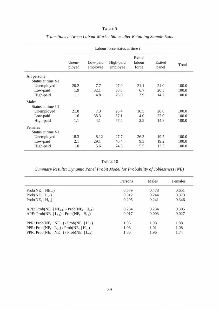
TABLE 9
Transitions between Labour Market States after Retaining Sample Exits
Labour force status at time t
Total Unem-ployed
Low-paid employee
High-paid employee
Exited labour force
Exited panel
All persons
Status at time t-1 Unemployed 20.2 7.7 27.0 21.1 24.0 100.0 Low-paid 1.9 32.1 38.8 6.7 20.5 100.0 High-paid 1.1 4.8 76.0 3.9 14.2 100.0
Males Status at time t-1 Unemployed 21.8 7.3 26.4 16.5 28.0 100.0 Low-paid 1.6 35.3 37.1 4.0 22.0 100.0 High-paid 1.1 4.1 77.5 2.5 14.8 100.0
Females Status at time t-1 Unemployed 18.3 8.12 27.7 26.3 19.5 100.0 Low-paid 2.1 29.1 40.4 9.3 19.2 100.0 High-paid 1.0 5.6 74.3 5.5 13.5 100.0
TABLE 10
Summary Results: Dynamic Panel Probit Model for Probability of Joblessness (NE)
Persons Males Females
Prob(NEt | NEt-1) 0.579 0.478 0.651 Prob(NEt | Lt-1) 0.312 0.244 0.373 Prob(NEt | Ht-1) 0.295 0.241 0.346 APE: Prob(NEt | NEt-1) - Prob(NEt | Ht-1) 0.284 0.234 0.305 APE: Prob(NEt | Lt-1) - Prob(NEt | Ht-1) 0.017 0.003 0.027 PPR: Prob(NEt | NEt-1) / Prob(NEt | Ht-1) 1.96 1.98 1.88 PPR: Prob(NEt | Lt-1) / Prob(NEt | Ht-1) 1.06 1.01 1.08 PPR: Prob(NEt | NEt-1) / Prob(NEt | Lt-1) 1.86 1.96 1.74
39