Embed Size (px)
Citation preview
Sensors 2014, 14, 22500-22524; doi:10.3390/s141222500OPEN ACCESS
sensorsISSN 1424-8220
www.mdpi.com/journal/sensors
Article
Long-Term Activity Recognition from WristwatchAccelerometer Data †
Enrique Garcia-Ceja *, Ramon F. Brena, Jose C. Carrasco-Jimenez and Leonardo Garrido
Tecnológico de Monterrey, Campus Monterrey, Av. Eugenio Garza Sada 2501 Sur,Monterrey 64849, Mexico; E-Mails: [email protected] (R.F.B.);[email protected] (J.C.C.-J.); [email protected] (L.G.)
† Expanded conference paper based on “Long-Term Activities Segmentation Using Viterbi Algorithmwith a k-Minimum-Consecutive-States Constraint”, the 5th International Conference on AmbientSystems, Networks and Technologies (ANT-2014).
* Author to whom correspondence should be addressed; E-Mail: [email protected];Tel.: +52-81-8358-2000 (ext. 5246).
External Editor: Panicos Kyriacou
Received: 30 July 2014; in revised form: 18 October 2014 / Accepted: 14 November 2014 /Published: 27 November 2014
Abstract: With the development of wearable devices that have several embedded sensors,it is possible to collect data that can be analyzed in order to understand the user’s needsand provide personalized services. Examples of these types of devices are smartphones,fitness-bracelets, smartwatches, just to mention a few. In the last years, several workshave used these devices to recognize simple activities like running, walking, sleeping, andother physical activities. There has also been research on recognizing complex activitieslike cooking, sporting, and taking medication, but these generally require the installation ofexternal sensors that may become obtrusive to the user. In this work we used accelerationdata from a wristwatch in order to identify long-term activities. We compare the use ofHidden Markov Models and Conditional Random Fields for the segmentation task. We alsoadded prior knowledge into the models regarding the duration of the activities by codingthem as constraints and sequence patterns were added in the form of feature functions. Wealso performed subclassing in order to deal with the problem of intra-class fragmentation,which arises when the same label is applied to activities that are conceptually the same butvery different from the acceleration point of view.
Sensors 2014, 14 22501
Keywords: activity recognition; long-term activities; accelerometer sensor; CRF; HMM;Viterbi; clustering; subclassing; watch; context-aware
1. Introduction
Human activity recognition is an important task for ambient intelligent systems. Being able torecognize the state of a person can provide us with valuable information that can be used as inputfor other systems. For example, in healthcare, fall detection can be used to alert the medical staff incase of an accident; in personal assistant applications, the current activity could be used to improve therecommendations and reminders. For example, in [1] a framework for activity inference is proposed,which is based on the idea that it is possible to classify activities from the handled artifacts used toperform each activity. They presented a practical case in a nursing home to characterize the activitiesthat caregivers perform in providing healthcare of elders with restricted mobility. Han et al. [2] proposeda healthcare framework to manage lifestyle diseases by monitoring long-term activities and reportingirregular and unhealthy patterns to a doctor and a caregiver.
With the development of wearable devices that have several embedded sensors, it has become possibleto collect different types of data that can be analyzed in order to understand the user’s needs andprovide personalized services. Examples of these types of devices are smartphones, fitness bracelets [3],smartwatches [4], etc. With the miniaturization of sensors, it is now possible to collect data aboutacceleration, humidity, rotation, position, magnetic field, and light intensity with small wearable devices.In recent years, simple human activity recognition has been achieved successfully; however, complexactivity recognition is still challenging and remains an active area of research. Generally, simpleactivities do not depend on the context, i.e., they can exist by themselves and they last for only a fewseconds. Examples of this type of activities are: running, walking, resting, sitting, etc. More complexand long-term activities are composed of a collection of simple activities and may include additionalcontextual information like time of the day, spatial location, interactions with other people and objects.Examples of this type of activities include: cooking, sporting, commuting, taking medication, amongother types of activities. The recognition of these activities generally requires more sensors and a fixedinfrastructure (e.g., video cameras, RFID tags, several accelerometers, magnetic sensors). In this workwe focus on the problem of recognizing sequential long-term activities from wristwatch accelerometerdata and the problem can be stated as follows: Given a sequence of accelerometer data recorded from awristwatch, the task is to recognize what long-term activities were performed by the user and the order inwhich they occurred, i.e., their segmentation. In this work, we focused on activities of daily living, suchas shopping, exercising, working, taking lunch, etc., since they are useful to living independently [5].This information could also be used by health and wellbeing applications such as Bewell [6] in order toassist individuals in maintaining a healthy lifestyle. Another potential application is that the activitiescould be further characterized in order to understand their quality. For example, when doing exercise,we may want to know if the user is guarding against injuries or performing the activity with confidence.Aung et al. [7] and Singh et al. [8] have discussed the importance of detecting the quality of activitiesto provide a more tailored support or feedback in mental and physical rehabilitation.

Sensors 2014, 14 22502
To be able to recognize the long-term activities, first we decomposed the accelerometer data into asequence of primitives [9]; thus, each long-term activity is represented as a string where each symbolis a primitive. This process is called vector quantization ([10], pp. 122–131) and will be describedin Section 5. A primitive, conceptually represents a simple activity, e.g., running, walking, etc., butthere is not necessarily a one-to-one mapping between the primitives and activities that exist in our“human vocabulary”. These primitives are automatically discovered from the data [11]. The rationalefor extracting these primitives is that the data can be represented as a sequence of characters, andthus, sequence patterns specific to each of the activities can be looked for in order to increase thediscrimination power between different activities. This type of representation is also suitable to performactivity prediction [12] (which will be left as future work). We used the Viterbi algorithm [13,14] ona Hidden Markov Model (HMM) ([10], Chapter 6) and on a Conditional Random Field (CRF) [15] toperform the segmentation and compared the results.
Within the HMMs and CRFs context, the sequence of primitives can be seen as the sequence ofobservations. For each observation we want to know the class (the activity) that generated it. The Viterbialgorithm is a dynamic programming method to find the best state sequence (in this case, the sequence ofactivities) that generated the observations (primitives) according to some optimality criterion. We useda modified version of this algorithm to add a constraint that takes into account the activities minimumlifespan. For example, if we know that the shopping activity takes at least 10 min, we can rule out statesequences that are shorter than 10 min. In our previous work of activity segmentation with an HMM, wecalled this a k-minimum consecutive states constraint [16]. In this work, we will also add informationabout sequence patterns found in the data by using a CRF.
When modeling the activities with an HMM, it is difficult to incorporate prior knowledge in theform of sequence patterns because HMMs have difficulty in modeling overlapping, non-independentfeatures [17]. A Conditional Random Field can be thought of as a more general Hidden Markov Model.With CRFs it is possible to add arbitrary features even if they overlap. We identified recurrent patternsthat occur within each activity and coded them as features in CRFs.
In this paper we present an extension of our previous work about long-term activitiessegmentation [16] with the following additions: (1) the use of real data collected with a wristwatch fromtwo subjects (21 days of data) instead of using simulated data; (2) the use of Conditional Random Fieldsin order to include more information into the models by finding sequence patterns; (3) the data and codewere made publicly available to facilitate the reproduction of the results; (4) the idea of subclassing wasintroduced in order to deal with the problem of intra-class fragmentation. We also make use of clusteringquality measures [18] in order to automatically find good subclassing groups. This problem arises duringthe activity labeling process. For example, a user could label an activity as having dinner but sometimeshe may use cutlery (for meat, soups, salads, etc.) and sometimes he may use his hands (for hamburgers,pizza, etc.). In this case, the activity label is the same for both scenarios even though both may varywidely from the acceleration point of view, making the activity having dinner implicitly fragmentedinto two classes. This phenomenon can introduce noise to the model and decrease the recognitionaccuracy. In Section 7 we will describe the process to deal with the intra-class fragmentation problemby automatically finding possibly fragmented classes and subclassing them.

Sensors 2014, 14 22503
This paper is organized as follows. Section 2 presents related works on activity recognition. Section 3presents the background theory of Hidden Markov Models and Conditional Random Fields. In Section 4we present the data collection process and the preprocessing steps. Section 5 details how the sequencesof primitives are generated from the raw accelerometer data. Section 6 explains the features used forthe CRF, which includes finding the sequence patterns. Section 7 describes the intra-class fragmentationproblem and the proposed method to reduce its effects. In Section 8 we describe the experiments andpresent the results. Section 9 directs to the sources for downloading the data and code in order toreproduce the results. Finally, in Section 10 we draw conclusions and propose future work.
2. Related Work
Recent works have taken advantage of wearable sensors to perform simple activity recognition withthem. Many of these works use motion sensors (e.g., accelerometer and gyroscope) to recognize simplephysical activities like running, walking, sleeping, cycling, among other activities [19–24]. To performsimple activity recognition, usually, the accelerometer data is divided into fixed time windows, generally2–10 s [19,23,25]. Then, time domain and/or frequency domain features [26] are extracted from thedata. The set of features of the corresponding window is known as a feature vector or an instance. Thosefeature vectors are used to train and test classification models such as Decision Trees, Naïve Bayes,Support Vector Machines, and other types of classifiers [27].
There has also been research on complex and long-term activities. Martínez-Pérez et al., implementeda system in a nursing home [1]. Their system integrates artifact behavior modeling, event interpretationand context extraction. They perform the inference based on how people handle different typesof artifacts (devices to measure blood pressure, paper towel, cream, etc.). In their use case, theycharacterized the caregivers’ activities of taking blood pressure, feeding, hygiene and medication ofan elderly patient with restricted mobility over a period of ten days, achieving an accuracy of 91.35%.Gu et al. [28] focused on recognizing sequential, interleaved and concurrent activities like makingcoffee, ironing, drinking, using phone, watching TV, etc. They conducted their experiments in a smarthome using sensors like accelerometers, temperature, humidity, light, etc. They also attached RFID tagsto rooms, cups, teaspoons, and books. Their reported overall accuracy was 88.11%. One of the recentworks in complex activity recognition is that of Cook et al. [29]. In their work, they do activity discoveryand activity recognition with data collected from three smart apartments with several installed sensorsand they deal with the interesting problem of having unlabeled activities. Each apartment housed anelderly during six months. They used infrared motion detectors and magnetic door sensors to recognize11 different activities like bathing, cooking, eating, relaxing, etc. They reported accuracies of 71.08%,59.76% and 84.89% for each of the three apartments.
There are also works that do complex activity recognition using wearable sensors. In the work ofHuynh et al. [30], they used three wearable sensors boards: one on the right wrist, one on the rightside of the hip and the last one on the right thigh. The sensor boards have 2D accelerometers andbinary tilt switches. They recorded three different high level activities (housework, morning tasks andshopping) from one user giving a total of 621 min. They tested different algorithms and achieved thebest accuracy (91.8%) when using histogram features with a Support Vector Machine. Mitchell et al.

Sensors 2014, 14 22504
used accelerometers from smartphones to classify sporting activities: five matches of soccer (15 players)and six hockey matches (17 players) [31]. They achieved a maximum F-measure accuracy of 87% bythe fusion of different classifiers and extracting features using the Discrete Wavelet Transform. One ofthe advantages of using wearable sensors for activity recognition is that it is easy to uniquely identifythe users. When using sensors installed in an environment with multiple residents, it becomes difficultto identify which user activated a specific sensor. Another advantage with wearable sensors is that therecognition can be performed almost in any place. A disadvantage of using a wearable sensor, e.g., justone accelerometer, is that it is not possible to detect activities that do not involve the movement of thepart of the body that has the sensor. For example, if the accelerometer is in the user’s pocket and heis sitting down, it may not be possible to tell whether he is working on a computer or maybe havingdinner. Installed sensors and wearable sensors are complementary approaches to perform human activityrecognition, both with strengths and weaknesses. For example, in [32] the authors used a multi-sensorapproach with wearable (accelerometer) and installed sensors (cameras).
When recognizing simple activities, the approach of extracting features from window segments isappropriate since they last for only a few seconds. However, to recognize long-term activities fromaccelerometer data, generating fixed length windows is not suitable. For example, the long-term activityworking could have small periods of the walking activity, but this does not mean that the user iscommuting to another place. If a fixed time window method is used, it may be the case that the windowincludes only data about the walking activity so the model can confuse this activity with commuting.Generally, users perform long-term activities in a continuous manner and they do not have a clearseparation boundary. In order to recognize more complex activities from accelerometer data, modelsthat can deal with temporal information are needed. Examples of such models are Hidden MarkovModels (HMMs) and Conditional Random Fields (CRFs), which have already been used extensivelyfor activity recognition. For example, Lee and Cho used hierarchical HMMs to recognize activities liketaking bus, shopping, walking, among other activities, using data collected with a smartphone [33]. Theirmethod consists of first recognizing actions using HMMs and then using these actions sequences to feedhigher level HMMs that perform the activity recognition. In [34], the authors used HMMs to recognizeactions from several inertial sensors placed in different parts of the body. They used nine sensor boardsin different parts of the body and their experiments included three subjects. In the previously mentionedwork [29], Cook et al. also used a CRF and an HMM. On the other hand, Van Kasteren et al. used HMMsand CRFs to monitor activities for elderly care from data collected from a wireless sensor network ina smart home [35]. In the work of Vinh et al., they used semi-Markov CRFs, which enabled them tomodel the duration and the interdependency of activities (dinner, commuting, lunch, office) [36]. Theirreported precision was 88.47% on the dataset from [37], which consists of data collected during sevendays using two triaxial accelerometers. Table 1 summarizes some of the related works for complexactivity recognition.
Sensors 2014, 14 22505
Table 1. Related complex activity recognition works.
Work # Activities Sensors Details
Martínez-Pérezet al. [1]
4: taking bloodpressure, feeding,
hygiene, medication
RFID, accelerometers,video cameras
91.35% accuracy, 1 patientduring 10 days. 81 instances.
Guet al. [28]
26: making coffee,ironing, using phone,washing clothes, etc.
accelerometers, temperature,humidity, light, RFID, etc.
Overall accuracy 88.11%,4 subjects over a 4 weeks
period. Collected instances 532.
Cooket al. [29]
11: bathing, cooking,sleeping, eating, relaxing,
taking medicine,hygiene, etc.
infrared motion detectorsand magnetic door sensors
Accuracies of 71.08%, 59.76%and 84.89% for each of the
3 apartments during a period of6 months.
Huynhet al. [30]
3: housework, morningtasks and shopping.
2D accelerometers andtilt switches
Accuracy of 91.8% for 1 userand period of about 10 h.
Kasterenet al. [35]
bathing, dressing,toileting, etc.
reed switches, pressure mats,mercury contacts, passive
infrared, float sensorsand temperature sensors
4 different datasets
Tolstikovet al. [38]
7: leaving, toileting,showering, sleeping,
breakfast, etc.14 binary sensors
Maximum accuracy of 95.7%for 1 subject during 27 days.
Vinhet al. [36]
4: dinner, commuting,lunch and office work
2 triaxial accelerometersPrecision of 88.47% for data
collected during 7 days.
Sunget al. [39]
12: cooking, talking onthe phone, working on
computer, etc.Microsoft Kinect
Average precision 86.5%, datacollected by 4 subjects
Gordonet al. [40]
7: drinking, gesticulating,put mug on table,
meeting, presentation,coffee break, etc.
accelerometers attachedto mugs
Average accuracy of 95% forsingle-user and maximum 96%for group activities. 3 subjects.
In total over 45 mins. ofcollected data.
This work differs from the previous ones in the following aspects. (1) We use a single accelerometerin a wristwatch to perform long-term activity segmentation; (2) We propose a method to deal withthe problem of intra-class fragmentation by finding possible subclasses of each class by means ofclustering quality indices. We found that the overall recognition accuracy was improved (within ourtested approaches) by incorporating prior knowledge such as the activities minimum lifespan and byfinding sequence patterns that are common to each of the activities. Subclassing fragmented activitiesalso helped to increase the overall recognition accuracy within our tested approaches.

Sensors 2014, 14 22506
3. Background
In this section we introduce the notations that will be used throughout this paper, as well as thebackground theory of Hidden Markov Models and Conditional Random Fields. From here on, we willuse the notation introduced by Rabiner and Juang ([10], Chapter 6).
3.1. Hidden Markov Models
A Hidden Markov Model is a probabilistic graphical model consisting of a set of observations andstates represented by random variables and can be defined as a 5-tuple 〈N,M,A,B, π〉 where:
• N is the number of states in the model indexed by {1, 2, ..., N}. The current state at time t is qt.• M is the number of distinct observation symbols denoted as V = {v1, v2, ..., vM}.• A is the state transition probability distribution. A = {aij} where
aij = P (qt+1 = j | qt = i), 1 ≤ i, j ≤ N (1)
and aij ≥ 0 ∀j, i;N∑j=1
aij = 1 ∀i
• B is the observation symbol probability distribution. B = {bj(k)} in which
bj(k) = P (ot = vk | qt = j), 1 ≤ k ≤M, (2)
defines the symbol distribution in state j, j = 1, 2, ..., N .• π is the initial state distribution π = {πi} in which
πi = P (q1 = i), 1 ≤ i ≤ N. (3)
3.2. Conditional Random Fields
Hidden Markov Models are generative models that define a joint probability distribution P (O,Q)
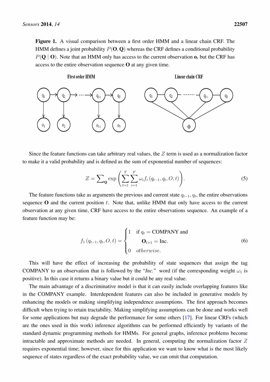
where O and Q are random variables. An observation ot may only depend on the state at time t [41](Figure 1). This is a strong assumption—in real world scenarios an observation may depend also onstates at different times. For example, in part-of-speech tagging [42] the aim is to label a sequence ofwords with tags like “PERSON”, “COMPANY”, “VERB”, etc. For example, if “Martin Inc. ....” is thesequence of words, as soon as we see “Martin” we may label it as “PERSON” but if we look at the nextobservation “Inc.” then we realize that the first tag should be “COMPANY”. This type of dependenciescan be easily modeled with a CRF.
Conditional Random Fields were first introduced by Lafferty et al. [15] to label sequenced data.Linear chain Conditional Random Fields define a conditional probability:
P (Q | O) =1
Zexp
(T∑t=1
F∑i=1
ωifi (qt−1, qt, O, t)
)(4)
where Q is the states sequence and O is the observations sequence. fi and ωi are feature functions andtheir respective weights and can take real values. F is the total number of feature functions.
Sensors 2014, 14 22507
Figure 1. A visual comparison between a first order HMM and a linear chain CRF. TheHMM defines a joint probability P (O,Q) whereas the CRF defines a conditional probabilityP (Q | O). Note that an HMM only has access to the current observation ot but the CRF hasaccess to the entire observation sequence O at any given time.
Since the feature functions can take arbitrary real values, the Z term is used as a normalization factorto make it a valid probability and is defined as the sum of exponential number of sequences:
Z =∑
Qexp
(T∑t=1
F∑i=1
ωifi (qt−1, qt, O, t)
). (5)
The feature functions take as arguments the previous and current state qt−1, qt, the entire observationssequence O and the current position t. Note that, unlike HMM that only have access to the currentobservation at any given time, CRF have access to the entire observations sequence. An example of afeature function may be:
f1 (qt−1, qt, O, t) =
1 if qt = COMPANY and
Ot+1 = Inc.
0 otherwise.
(6)
This will have the effect of increasing the probability of state sequences that assign the tagCOMPANY to an observation that is followed by the “Inc.” word (if the corresponding weight ω1 ispositive). In this case it returns a binary value but it could be any real value.
The main advantage of a discriminative model is that it can easily include overlapping features likein the COMPANY example. Interdependent features can also be included in generative models byenhancing the models or making simplifying independence assumptions. The first approach becomesdifficult when trying to retain tractability. Making simplifying assumptions can be done and works wellfor some applications but may degrade the performance for some others [17]. For linear CRFs (whichare the ones used in this work) inference algorithms can be performed efficiently by variants of thestandard dynamic programming methods for HMMs. For general graphs, inference problems becomeintractable and approximate methods are needed. In general, computing the normalization factor Zrequires exponential time; however, since for this application we want to know what is the most likelysequence of states regardless of the exact probability value, we can omit that computation.

Sensors 2014, 14 22508
To perform the activity inference, we used the Viterbi algorithm on both HMMs and CRFs. Theconstrained version of the Viterbi algorithm [16] allows to set the minimum number of consecutivestates that can occur for each state i. This requires an additional parameter κ, which is an array thatstores the minimum consecutive states for each activity:
κ(i) = n ∈ N>0, 1 ≤ i ≤ N (7)
Now we can take into account the minimum lifespan of each activity by coding this information in theκ array. This information was computed from the data by finding the minimum number of consecutivestates of each activity and dividing them by 2 (to allow some deviance).
4. Data Collection
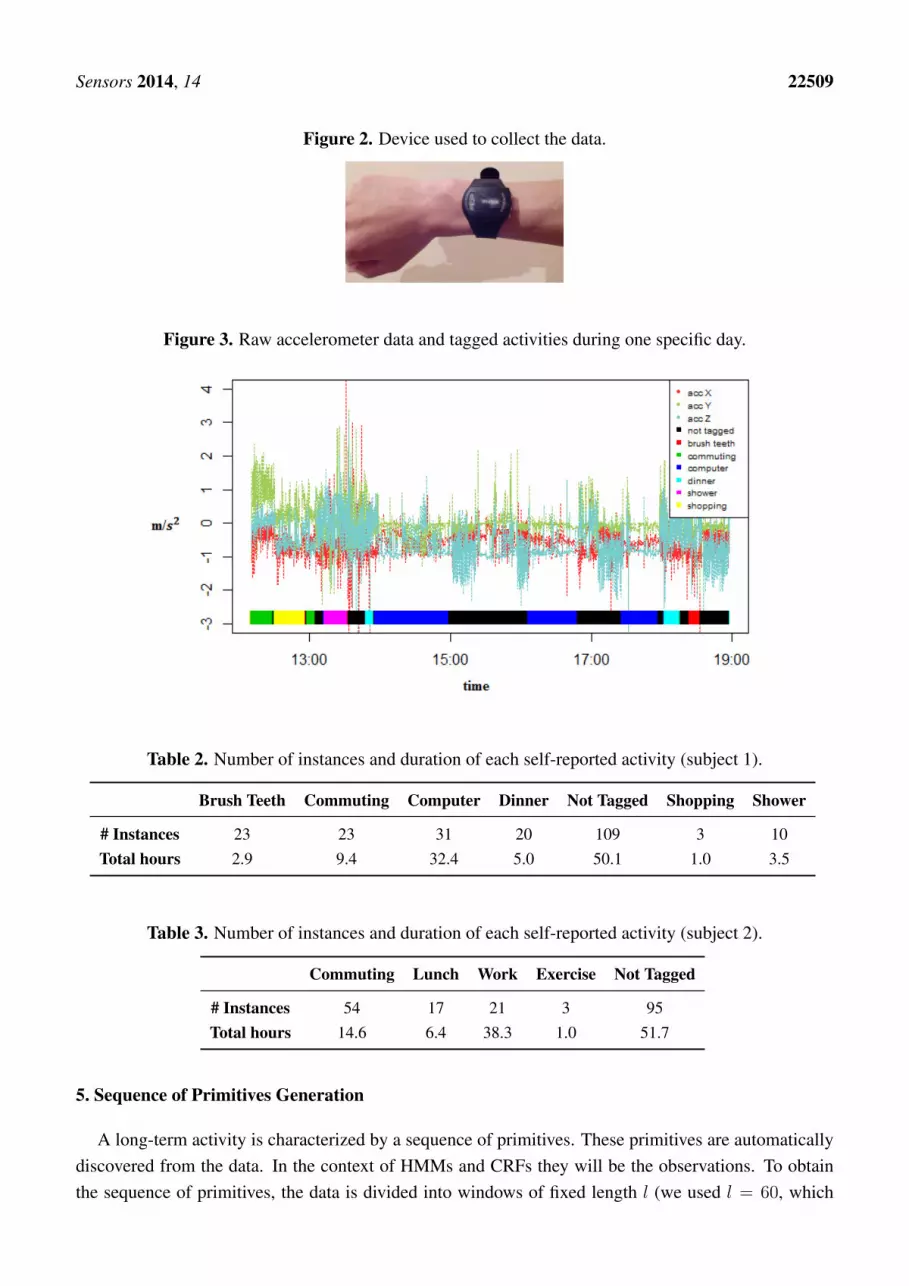
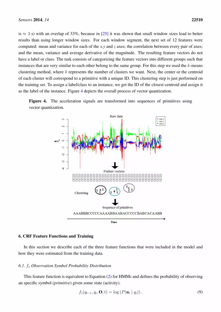
A GENEActiv [43] watch with an embedded triaxial accelerometer was used to collect the data. Thiswatch can sample at up to 100 Hz. For our experiments, the sampling rate was set at 20 Hz because it hasbeen shown that activity classification is high for sampling rates above or equal to 10 Hz but the accuracydecreases at a sampling rate of 5 Hz [44]. This watch also collects temperature and light intensity butthey were not used. The watch was placed on the dominant hand of each user (Figure 2). The usersperformed their activities of daily living and took note of the start and end time of several of them. Datawere collected by two subjects during 11 and 10 days, respectively, from approximately 9:00 to 23:00.The first subject was one of the researchers and the second subject was a volunteer that had no relationto this work. The first subject recorded 6 activities: (1) Shopping, which consists of picking and buyinggroceries at the supermarket; (2) Showering, which consists of taking a shower and dressing; (3) Dinner,which also takes into account breakfast and lunch time; (4) Working, which for most of the time isworking with a computer but also involves taking rests and going to the bathroom; (5) Commuting, whichincludes by bus, by car, or walking; (6) Brush Teeth, which consists of both brushing the teeth and usinga dental floss. Subject 2 tagged 4 activities: (1) Commuting; (2) Lunch, which also consists of breakfastand dinner time; (3) Working time, which for most of the time is office work; (4) Exercise, which consistsof walking, running, stretching, etc. There is also an activity not tagged for data that was not labeled bythe users. Figure 3 shows the raw accelerometer data and the tagged activities for one specific day ofone of the subjects. Tables 2 and 3 show the number of instances and the duration of each activity forboth subjects.
To reduce some noise, an average filter with a window length of 10 (Equation (8)) was used:
vs(t) =1
n
t−1∑i=t−n
v(i) (8)
where v is the original vector, vs is the smoothed vector and n is the window length.
Sensors 2014, 14 22509
Figure 2. Device used to collect the data.
Figure 3. Raw accelerometer data and tagged activities during one specific day.
Table 2. Number of instances and duration of each self-reported activity (subject 1).
Brush Teeth Commuting Computer Dinner Not Tagged Shopping Shower
# Instances 23 23 31 20 109 3 10Total hours 2.9 9.4 32.4 5.0 50.1 1.0 3.5
Table 3. Number of instances and duration of each self-reported activity (subject 2).
Commuting Lunch Work Exercise Not Tagged
# Instances 54 17 21 3 95Total hours 14.6 6.4 38.3 1.0 51.7
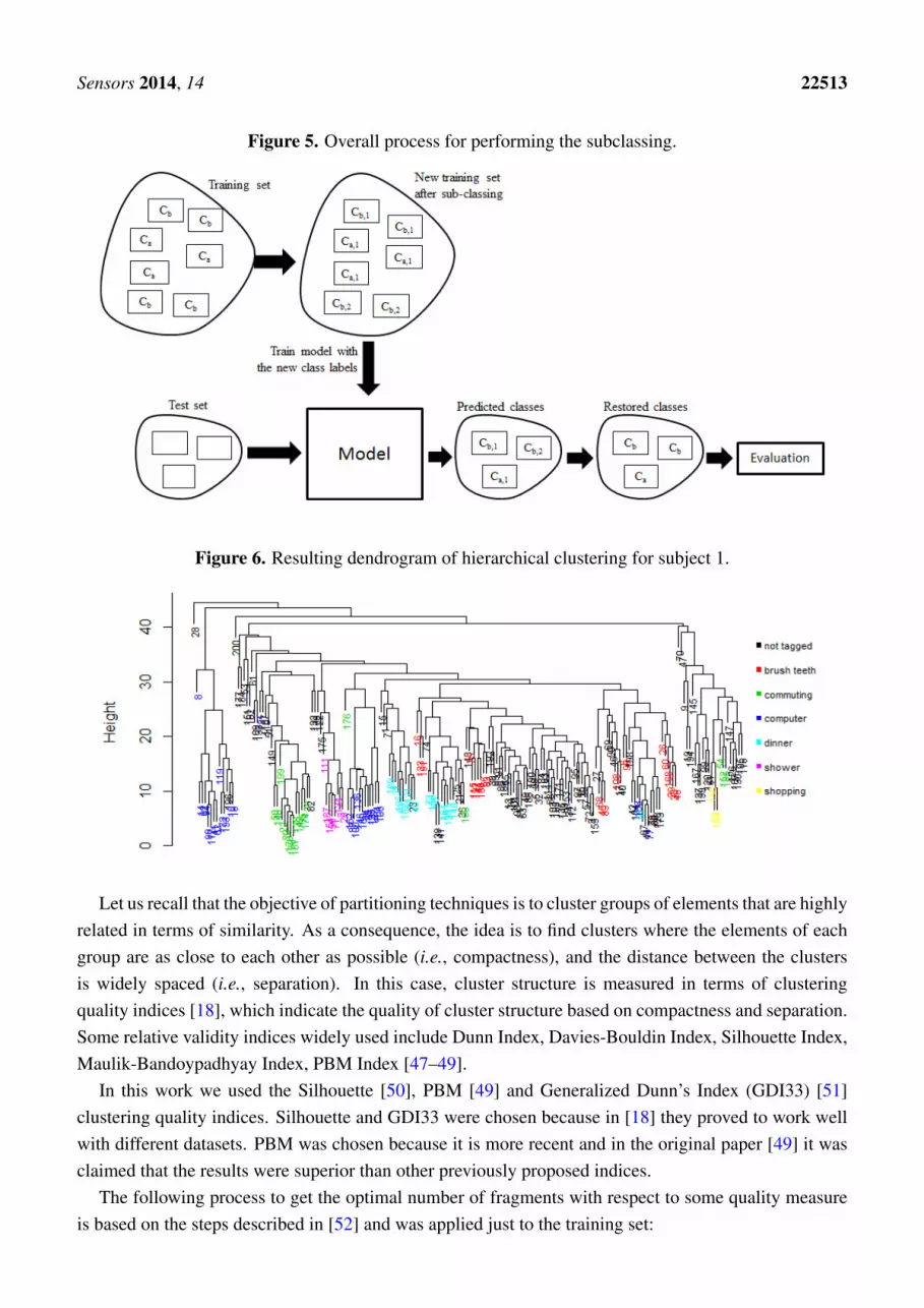
5. Sequence of Primitives Generation
A long-term activity is characterized by a sequence of primitives. These primitives are automaticallydiscovered from the data. In the context of HMMs and CRFs they will be the observations. To obtainthe sequence of primitives, the data is divided into windows of fixed length l (we used l = 60, which
Sensors 2014, 14 22510
is ≈ 3 s) with an overlap of 33%, because in [25] it was shown that small window sizes lead to betterresults than using longer window sizes. For each window segment, the next set of 12 features werecomputed: mean and variance for each of the x,y and z axes; the correlation between every pair of axes;and the mean, variance and average derivative of the magnitude. The resulting feature vectors do nothave a label or class. The task consists of categorizing the feature vectors into different groups such thatinstances that are very similar to each other belong to the same group. For this step we used the k-meansclustering method, where k represents the number of clusters we want. Next, the center or the centroidof each cluster will correspond to a primitive with a unique ID. This clustering step is just performed onthe training set. To assign a label/class to an instance, we get the ID of the closest centroid and assign itas the label of the instance. Figure 4 depicts the overall process of vector quantization.
Figure 4. The acceleration signals are transformed into sequences of primitives usingvector quantization.
6. CRF Feature Functions and Training
In this section we describe each of the three feature functions that were included in the model andhow they were estimated from the training data.
6.1. f1 Observation Symbol Probability Distribution
This feature function is equivalent to Equation (2) for HMMs and defines the probability of observingan specific symbol (primitive) given some state (activity).
f1(qt−1, qt,O, t) = log (P (ot | qt)) . (9)

Sensors 2014, 14 22511
These probabilities are estimated from the training data as:
P (ok | q) =number of primitives of class k in q
total number of primitives in q, 1≤q≤N1≤k≤M
The reason for the log() function is to make this feature equivalent to the symbol probabilitydistribution of an HMM.
6.2. f2 State Transition Probability Distribution
This is equivalent to the state transition probability distribution of an HMM (Equation 1).
f2(qt−1, qt,O, t) =
log (πqt) if t = 1
log (P (qt | qt−1)) otherwise(10)
where πi are the initial probabilities that were set to be uniform. The probability of transitioning from onestate to another P (qt | qt−1) is estimated by computing the transition frequency for every pair of states.Generally, the probability of transitioning from a state to itself will be much higher than transitioning toanother state.
6.3. f3 Sequence Patterns (k-Mers)
The purpose of this function is to include information about the sequence structure, i.e., to findoverlapping sequences of primitives that occur together. In bioinformatics a k-mer (also called n-grams,n-mers, l-tuples) ([45], p. 308) is a string of length k and Count(Text, Pattern) is the number of timesa k-mer Pattern appears as a substring of Text. For example:Count(ACACTACTGCATACTACTACCT,CTAC) = 3 Note that the patterns can be overlapped.
Usually, k-mers are used in DNA sequence analysis [45]. In text processing they are usually calledn-grams [46]. The total number of different k-mers is Mk; recall that M is the number of distinctobservation symbols. The feature function f3 is defined as:
f3(qt−1, qt,O, t) = log (P (ot, ..., ot+k−1 | qt)) (11)
which is the probability of finding a specific k-mer given an activity. This feature function is based on oneof the implications of Zipf’s law and is described in [46] in the context of document classification as:“if we are comparing documents from the same category they should have similar N-gram frequencydistributions”. Note that this feature function is similar to f2 when k = 2 but instead of activitytransitions, it defines primitives transitions, i.e., the probability of some primitive vi occurring aftersome primitive vj given an activity. In the training phase we estimate these probabilities as:
P (ot, ..., ot+k−1 | q) =Count(PrimSeqi, k-mer)| PrimSeqi | −k + 1
, 1≤i≤N
for all Mk possible k-mers. PrimSeqi is the concatenation of the primitives sequence for all long-termactivities of type i from the training set.

Sensors 2014, 14 22512
7. Subclassing Fragmented Classes
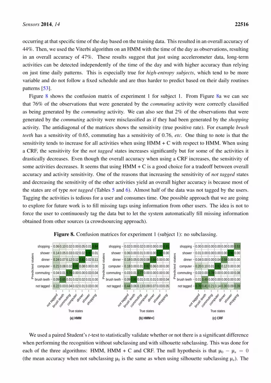
One of the problems when tagging the activities in the training phase is the intra-class fragmentation.This means that several observations may belong to the same class even though they are completelydifferent. For example, a user may tag an activity as commuting but sometimes he may commute mainlyby bus and other times by walking, which are very different from the acceleration point of view. This willproduce noise in the models since the training will take into account all observations of the same classin conjunction, but in the recognition phase an observation may belong to just one subclass (commutingby bus or walking). Of course the user could create two different classes at training time (bus commuteand walk commute) but this would be a tedious task and the subclasses may not be obvious. What wepropose is the following sequence of steps:
(1) For each class Ci in the training set, find if it is fragmented.(2) If it is fragmented, assign each of its observations to their corresponding subclass Ci,j for j = 1...F
where F is the total number of fragments.(3) If it is not fragmented, assign all observations to a single subclass Ci,1.(4) Build/train the models with the subclasses as if they were independent classes.(5) Predict the subclass of the observations in the test set.(6) For the test set, replace each predicted subclass Ci,j with the original class Ci.(7) Validate the results with the ground truth (original class labels).
Figure 5 shows the overall process. One way to find if a class is fragmented is by visual inspection.One approach to perform the visual inspection is to cluster the observations using a method that does notrequire specifying the number of groups a priori, e.g., using hierarchical clustering and then plotting theresulting dendrogram. Figure 6 shows the resulting dendrogram when applying hierarchical clusteringto the observations of subject 1. From this dendrogram, we can see that the working with computer classis fragmented roughly into two, the shopping activity looks uniform, the commuting activity looks likeit is fragmented into two, etc. In some cases it is not obvious in how many fragments a class is dividedinto. For example, the brush teeth activity could be divided into three or maybe four subclasses so thisapproach is subjective and may just work well when the number of classes is small and the separation ofthe fragments is more or less clear.
To perform the clustering, each long-term activity is represented as a sequence of primitives and willbe characterized with a feature vector of size M, where M is the total number of different primitives, i.e.,the alphabet size. The feature vector stores the frequencies of each of the primitives so each long-termactivity is characterized by a distribution of primitives (a histogram).
The visual approach for finding the fragments of a class is feasible when (1) we deal with a small setof activities, and (2) when we have predefined knowledge about the subclasses, i.e., an expert is able tovalidate from human experience. In the case of external validity, that is, when the user knows the classlabels or the number of subclasses, good cluster structure is accomplished when the predicted classes arethe same as the predefined labels of the dataset. When either of the two characteristics mentioned beforeis not fulfilled, a more flexible approach must be used. In the absence of prior knowledge, the use ofrelative validity metrics [47] may offer a good approximation to the real segmentation.
Sensors 2014, 14 22513
Figure 5. Overall process for performing the subclassing.
Figure 6. Resulting dendrogram of hierarchical clustering for subject 1.
Let us recall that the objective of partitioning techniques is to cluster groups of elements that are highlyrelated in terms of similarity. As a consequence, the idea is to find clusters where the elements of eachgroup are as close to each other as possible (i.e., compactness), and the distance between the clustersis widely spaced (i.e., separation). In this case, cluster structure is measured in terms of clusteringquality indices [18], which indicate the quality of cluster structure based on compactness and separation.Some relative validity indices widely used include Dunn Index, Davies-Bouldin Index, Silhouette Index,Maulik-Bandoypadhyay Index, PBM Index [47–49].
In this work we used the Silhouette [50], PBM [49] and Generalized Dunn’s Index (GDI33) [51]clustering quality indices. Silhouette and GDI33 were chosen because in [18] they proved to work wellwith different datasets. PBM was chosen because it is more recent and in the original paper [49] it wasclaimed that the results were superior than other previously proposed indices.
The following process to get the optimal number of fragments with respect to some quality measureis based on the steps described in [52] and was applied just to the training set:

Sensors 2014, 14 22514
(1) Cross-validate the training set.(2) For each class Ci, cluster the observations that belong to Ci into k groups, for k = 2...maxK.
maxK is a predefined upper bound on the allowed number of fragments. Compute the qualityindex of the clustering result for each k.
(3) Subclass Ci into k subclasses where k is the number of groups that yielded the optimalquality index.
(4) Cross-validate the training set with the new subclasses.(5) If the resulting accuracy improves the result of step 1, keep the new subclassing for Ci.
For our experiments, in the cross-validation step, instead of building the HMMs and CRFs, weused the Naive Bayes classifier with the activities histograms as input. The reason of validating thesubclassing step with a simpler classifier is because it is much faster than building the HMMs and CRFmodels and this step has to be done maxK times for each class. For the clustering step, we used thek-means algorithm. One of the advantages of finding the fragments using a quality index is that it canbe done automatically without user intervention as opposed to the visual approach described earlier.It is worth noting that the discovered sub-activities may not correspond to “real activities” since theclustering process is based in kinematic features and, as a consequence, activities are split according totheir qualities rather than their real sub-type. However, for the purposes of this work this is not relevantsince the subclassing is exploited to increase the overall accuracy rather than used to understand whatthese sub-activities are.
8. Experiments and Results
Recall that a long-term activity is represented as a sequence of primitives. A run will be defined asa concatenation of long-term activities that occur consecutively, i.e., an entire day. We performed fiveexperiments: (1) without subclassing; (2) with fixed subclassing; (3) with silhouette subclassing (4) withPBM subclassing; (5) with GDI33 subclassing. Fixed subclassing means that the number of subclassesfor each class were set manually by visual inspection of the dendrogram. In each of the experiments wecompared three different methods to perform the activity segmentation:
(1) HMM: Viterbi algorithm on an HMM without constraint.(2) HMM + C: Viterbi algorithm on an HMM with the k-minimum-consecutive-states constraint.(3) CRF: Viterbi algorithm on a CRF with the k-minimum-consecutive-states constraint and adding
information about sequence patterns.
Since long-term activities are user-dependent, i.e., for one person, the working activity may involvedoing office work and for another person the working activity may be more physically demanding,individual models with the same parameters were built for each subject. Leave-one-day-out crossvalidation was used to validate the results. This means that for each day i, all other days j, j 6= i
are used as training set and day i is used as the test set. The accuracy was computed as the percentageof correct state predictions. Due to computational limitations, the k for k-mers was set to be a smallnumber (in this case, 2) because the number of k-mers grows exponentially (Mk = 3002 = 90, 000
possible different patterns). The number of primitives was set to 300 because the accuracy does not

Sensors 2014, 14 22515
have a significant increase for values greater than 250 (Figure 7). The number of primitives parameterdepends on the sensor data and the features extracted. In our previous work [9] we collected data from acellphone located on the user’s belt and used a different set of features. In that case, a parameter valuegreater or equal to 15 gave the best results. In [11] they used a MotionNode sensor to detect simpleactivities. In that case, an alphabet size of around 150 gave the best results. The number of primitiveswill depend on each application and is determined empirically as stated in [11]. The overall results foreach of the five experiments are listed in Table 4.
Figure 7. Accuracy as number of primitives increase.
Table 4. Overall accuracies for the five experiments for the two subjects.
HMM HMM + C CRF
Experiment 1: no subclassing 60.7% 68.8% 75.1%Experiment 2: fixed 64.7% 71.9% 77.1%Experiment 3: silhouette 64.1% 71.0% 76.3%Experiment 4: PBM 63.9% 70.8% 76.2%Experiment 5: GDI33 64.1% 71.0% 76.3%
From Table 4 it can be seen that for the five experiments the accuracy increases as more informationis added to the model—first adding the minimum activities lifespan (HMM + C) and then addingboth the minimum lifespan and the sequence patterns (CRF). To assess the influence of the transitionsbetween activities, instead of learning the transition matrix from the data we set it to have a uniformdistribution between any two possible transitions (to represent a lack of information). In this case,the overall accuracy (no subclassing) was 52.0%, 67.9%, and 75.5% for HMM, HMM + C and CRF,respectively. This suggests that the transitions between activities had a considerable influence in the firstmodel (HMM), but HMM + C and CRF were more robust to the choice of the transition matrix. Thetype of activities considered in this work may have strong predictable diurnal patterns. As a baseline,we performed the activity recognition with no accelerometer data by just using information of the timeof the day. First, the predicted activity at a given time was set as the activity with highest probability of
Sensors 2014, 14 22516
occurring at that specific time of the day based on the training data. This resulted in an overall accuracy of44%. Then, we used the Viterbi algorithm on an HMM with the time of the day as observations, resultingin an overall accuracy of 47%. These results suggest that just using accelerometer data, long-termactivities can be detected independently of the time of the day and with higher accuracy than relyingon just time daily patterns. This is especially true for high-entropy subjects, which tend to be morevariable and do not follow a fixed schedule and are thus harder to predict based on their daily routinespatterns [53].
Figure 8 shows the confusion matrix of experiment 1 for subject 1. From Figure 8a we can seethat 76% of the observations that were generated by the commuting activity were correctly classifiedas being generated by the commuting activity. We can also see that 2% of the observations that weregenerated by the commuting activity were misclassified as if they had been generated by the shoppingactivity. The antidiagonal of the matrices shows the sensitivity (true positive rate). For example brushteeth has a sensitivity of 0.65, commuting has a sensitivity of 0.76, etc. One thing to note is that thesensitivity tends to increase for all activities when using HMM + C with respect to HMM. When usinga CRF, the sensitivity for the not tagged states increases significantly but for some of the activities itdrastically decreases. Even though the overall accuracy when using a CRF increases, the sensitivity ofsome activities decreases. It seems that using HMM + C is a good choice for a tradeoff between overallaccuracy and activity sensitivity. One of the reasons that increasing the sensitivity of not tagged statesand decreasing the sensitivity of the other activities yield an overall higher accuracy is because most ofthe states are of type not tagged (Tables 5 and 6). Almost half of the data was not tagged by the users.Tagging the activities is tedious for a user and consumes time. One possible approach that we are goingto explore for future work is to fill missing tags using information from other users. The idea is not toforce the user to continuously tag the data but to let the system automatically fill missing informationobtained from other sources (a crowdsourcing approach).
Figure 8. Confusion matrices for experiment 1 (subject 1): no subclassing.
0.22 0.03 0.04 0.02 0.01 0.03 0.00
0.09 0.65 0.01 0.02 0.02 0.01 0.00
0.04 0.01 0.76 0.00 0.00 0.03 0.04
0.21 0.08 0.02 0.81 0.08 0.00 0.00
0.24 0.07 0.12 0.12 0.82 0.02 0.11
0.14 0.05 0.03 0.02 0.02 0.90 0.01
0.06 0.10 0.02 0.00 0.05 0.01 0.84
not tagged
brush teeth
commuting
computer
dinner
shower
shopping
not tag
ged
brus
h teeth
commuting
compu
ter
dinn
er
show
er
shop
ping
True states
(a) HMM
Pre
dic
ted
sta
tes
0.22 0.03 0.04 0.02 0.01 0.03 0.00
0.09 0.65 0.01 0.02 0.02 0.01 0.00
0.04 0.01 0.76 0.00 0.00 0.03 0.04
0.21 0.08 0.02 0.81 0.08 0.00 0.00
0.24 0.07 0.12 0.12 0.82 0.02 0.11
0.14 0.05 0.03 0.02 0.02 0.90 0.01
0.06 0.10 0.02 0.00 0.05 0.01 0.84
0.44 0.06 0.13 0.09 0.07 0.03 0.05
0.09 0.88 0.01 0.01 0.01 0.00 0.04
0.03 0.01 0.77 0.00 0.00 0.00 0.00
0.18 0.00 0.01 0.82 0.06 0.00 0.00
0.18 0.05 0.05 0.08 0.86 0.00 0.00
0.06 0.00 0.01 0.00 0.00 0.97 0.00
0.02 0.00 0.02 0.00 0.00 0.00 0.91
not tagged
brush teeth
commuting
computer
dinner
shower
shopping
not tag
ged
brus
h teeth
commuting
compu
ter
dinn
er
show
er
shop
ping
True states
(b) HMM+C
Pre
dic
ted
sta
tes
0.22 0.03 0.04 0.02 0.01 0.03 0.00
0.09 0.65 0.01 0.02 0.02 0.01 0.00
0.04 0.01 0.76 0.00 0.00 0.03 0.04
0.21 0.08 0.02 0.81 0.08 0.00 0.00
0.24 0.07 0.12 0.12 0.82 0.02 0.11
0.14 0.05 0.03 0.02 0.02 0.90 0.01
0.06 0.10 0.02 0.00 0.05 0.01 0.84
0.70 0.41 0.21 0.14 0.30 0.09 0.39
0.01 0.49 0.00 0.00 0.00 0.00 0.00
0.03 0.00 0.78 0.00 0.00 0.00 0.08
0.20 0.10 0.01 0.82 0.12 0.00 0.00
0.04 0.00 0.00 0.04 0.58 0.00 0.00
0.01 0.00 0.00 0.00 0.00 0.90 0.00
0.00 0.00 0.00 0.00 0.00 0.00 0.53
not tagged
brush teeth
commuting
computer
dinner
shower
shopping
not tag
ged
brus
h teeth
commuting
compu
ter
dinn
er
show
er
shop
ping
True states
(c) CRF
Pre
dic
ted
sta
tes
We used a paired Student’s t-test to statistically validate whether or not there is a significant differencewhen performing the recognition without subclassing and with silhouette subclassing. This was done foreach of the three algorithms: HMM, HMM + C and CRF. The null hypothesis is that µ0 − µs = 0
(the mean accuracy when not subclassing µ0 is the same as when using silhouette subclassing µs). The
Sensors 2014, 14 22517
alternative hypothesis is that µs − µ0 > 0, i.e., there is a significant increase in the overall accuracy whenusing silhouette subclassing. The significance level for the tests was set at α = 0.05.
Table 5. Percent of states of each class (subject 1).
Brush Teeth Commuting Computer Dinner Not Tagged Shopping Shower
(%) 2.8 9.0 30.9 4.8 47.9 1.0 3.4
Table 6. Percent of states of each class (subject 2).
Commuting Exercise Lunch Not Tagged Work
(%) 13.1 0.9 5.8 46.1 33.8
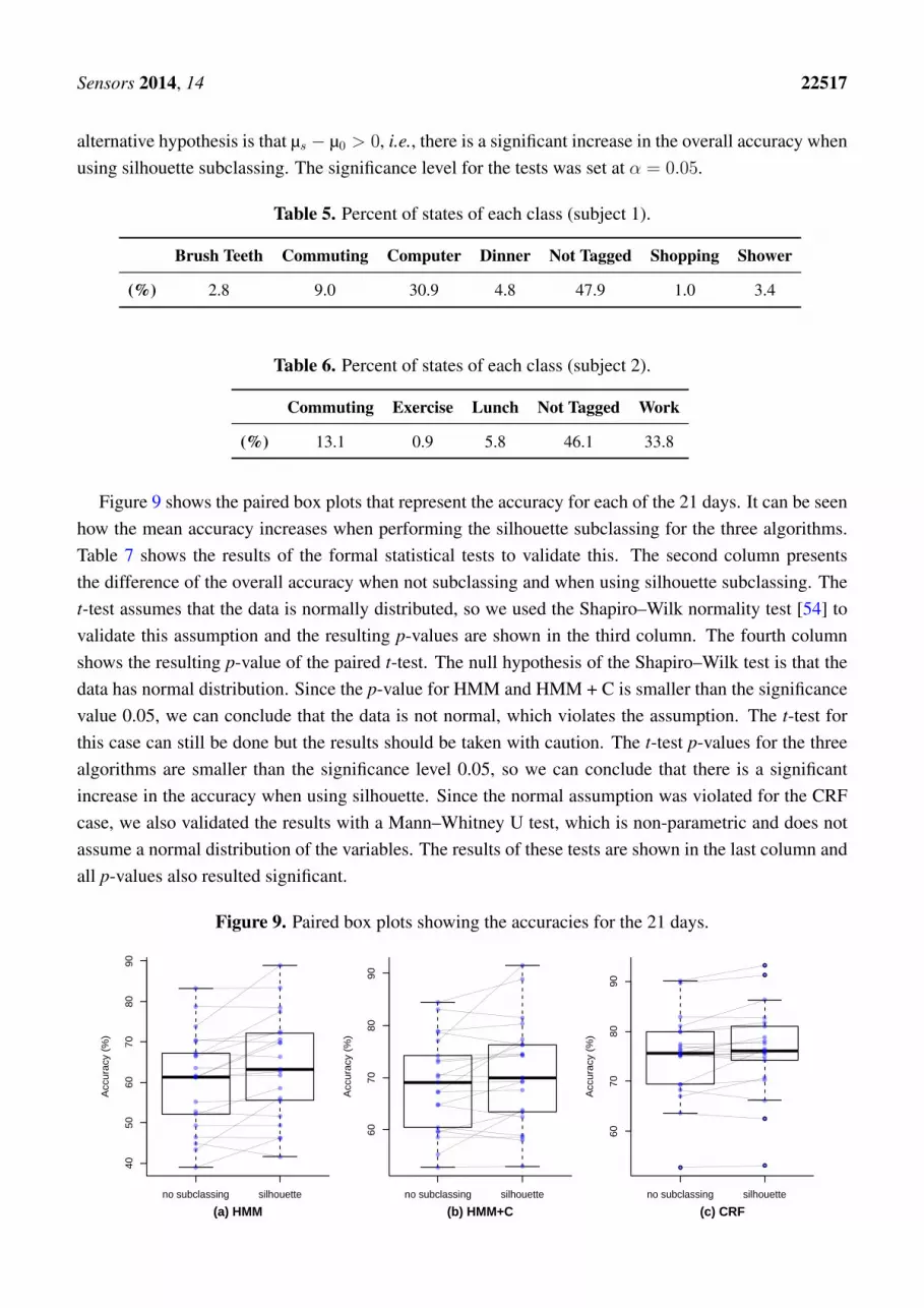
Figure 9 shows the paired box plots that represent the accuracy for each of the 21 days. It can be seenhow the mean accuracy increases when performing the silhouette subclassing for the three algorithms.Table 7 shows the results of the formal statistical tests to validate this. The second column presentsthe difference of the overall accuracy when not subclassing and when using silhouette subclassing. Thet-test assumes that the data is normally distributed, so we used the Shapiro–Wilk normality test [54] tovalidate this assumption and the resulting p-values are shown in the third column. The fourth columnshows the resulting p-value of the paired t-test. The null hypothesis of the Shapiro–Wilk test is that thedata has normal distribution. Since the p-value for HMM and HMM + C is smaller than the significancevalue 0.05, we can conclude that the data is not normal, which violates the assumption. The t-test forthis case can still be done but the results should be taken with caution. The t-test p-values for the threealgorithms are smaller than the significance level 0.05, so we can conclude that there is a significantincrease in the accuracy when using silhouette. Since the normal assumption was violated for the CRFcase, we also validated the results with a Mann–Whitney U test, which is non-parametric and does notassume a normal distribution of the variables. The results of these tests are shown in the last column andall p-values also resulted significant.
Figure 9. Paired box plots showing the accuracies for the 21 days.
no subclassing silhouette
4050
6070
8090
Acc
urac
y (%
)
(a) HMMno subclassing silhouette
6070
8090
Acc
urac
y (%
)
(b) HMM+C
●
●
●
●
●
no subclassing silhouette
6070
8090
Acc
urac
y (%
)
(c) CRF
Sensors 2014, 14 22518
Table 7. Resulting p-values of the statistical tests (µ0: mean accuracy with no subclassing,µs: mean accuracy with silhouette subclassing).
Algorithm µ0− µs Shapiro–Wilk p-Value t-Test p-Value Mann–Whitney p-Value
HMM −3.5 p << 0.05 p << 0.05 p << 0.05
HMM + C −2.2 p << 0.05 p << 0.05 p << 0.05
CRF −1.1 p >> 0.05 p << 0.05 p << 0.05
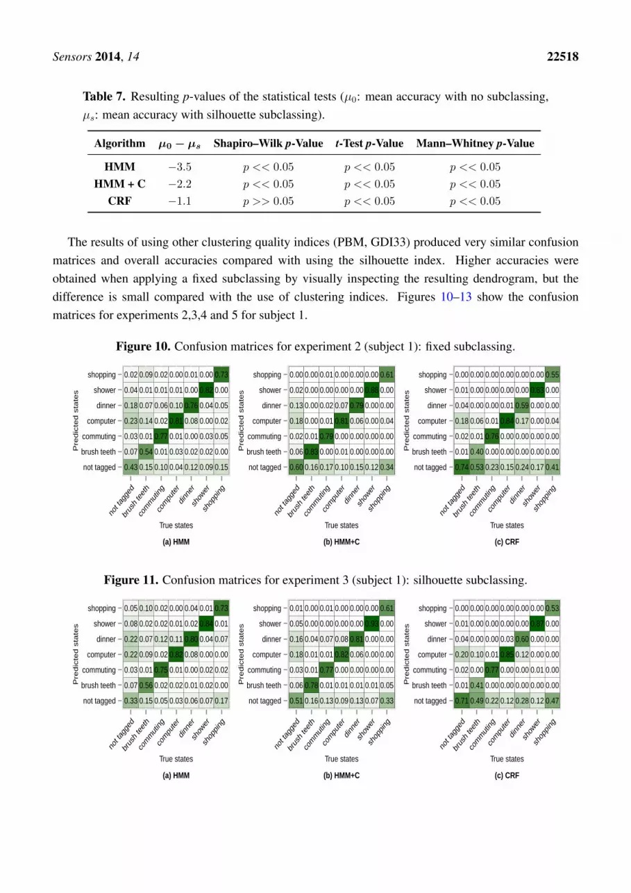
The results of using other clustering quality indices (PBM, GDI33) produced very similar confusionmatrices and overall accuracies compared with using the silhouette index. Higher accuracies wereobtained when applying a fixed subclassing by visually inspecting the resulting dendrogram, but thedifference is small compared with the use of clustering indices. Figures 10–13 show the confusionmatrices for experiments 2,3,4 and 5 for subject 1.
Figure 10. Confusion matrices for experiment 2 (subject 1): fixed subclassing.
0.43 0.15 0.10 0.04 0.12 0.09 0.15
0.07 0.54 0.01 0.03 0.02 0.02 0.00
0.03 0.01 0.77 0.01 0.00 0.03 0.05
0.23 0.14 0.02 0.81 0.08 0.00 0.02
0.18 0.07 0.06 0.10 0.76 0.04 0.05
0.04 0.01 0.01 0.01 0.00 0.82 0.00
0.02 0.09 0.02 0.00 0.01 0.00 0.73
not tagged
brush teeth
commuting
computer
dinner
shower
shopping
not tag
ged
brus
h teeth
commuting
compu
ter
dinn
er
show
er
shop
ping
True states
(a) HMM
Pre
dic
ted
sta
tes
0.43 0.15 0.10 0.04 0.12 0.09 0.15
0.07 0.54 0.01 0.03 0.02 0.02 0.00
0.03 0.01 0.77 0.01 0.00 0.03 0.05
0.23 0.14 0.02 0.81 0.08 0.00 0.02
0.18 0.07 0.06 0.10 0.76 0.04 0.05
0.04 0.01 0.01 0.01 0.00 0.82 0.00
0.02 0.09 0.02 0.00 0.01 0.00 0.73
0.60 0.16 0.17 0.10 0.15 0.12 0.34
0.06 0.83 0.00 0.01 0.00 0.00 0.00
0.02 0.01 0.79 0.00 0.00 0.00 0.00
0.18 0.00 0.01 0.81 0.06 0.00 0.04
0.13 0.00 0.02 0.07 0.79 0.00 0.00
0.02 0.00 0.00 0.00 0.00 0.88 0.00
0.00 0.00 0.01 0.00 0.00 0.00 0.61
not tagged
brush teeth
commuting
computer
dinner
shower
shopping
not tag
ged
brus
h teeth
commuting
compu
ter
dinn
er
show
er
shop
ping
True states
(b) HMM+C
Pre
dic
ted
sta
tes
0.43 0.15 0.10 0.04 0.12 0.09 0.15
0.07 0.54 0.01 0.03 0.02 0.02 0.00
0.03 0.01 0.77 0.01 0.00 0.03 0.05
0.23 0.14 0.02 0.81 0.08 0.00 0.02
0.18 0.07 0.06 0.10 0.76 0.04 0.05
0.04 0.01 0.01 0.01 0.00 0.82 0.00
0.02 0.09 0.02 0.00 0.01 0.00 0.73
0.74 0.53 0.23 0.15 0.24 0.17 0.41
0.01 0.40 0.00 0.00 0.00 0.00 0.00
0.02 0.01 0.76 0.00 0.00 0.00 0.00
0.18 0.06 0.01 0.84 0.17 0.00 0.04
0.04 0.00 0.00 0.01 0.59 0.00 0.00
0.01 0.00 0.00 0.00 0.00 0.83 0.00
0.00 0.00 0.00 0.00 0.00 0.00 0.55
not tagged
brush teeth
commuting
computer
dinner
shower
shopping
not tag
ged
brus
h teeth
commuting
compu
ter
dinn
er
show
er
shop
ping
True states
(c) CRF
Pre
dic
ted
sta
tes
Figure 11. Confusion matrices for experiment 3 (subject 1): silhouette subclassing.
0.33 0.15 0.05 0.03 0.06 0.07 0.17
0.07 0.56 0.02 0.02 0.01 0.02 0.00
0.03 0.01 0.75 0.01 0.00 0.02 0.02
0.22 0.09 0.02 0.82 0.08 0.00 0.00
0.22 0.07 0.12 0.11 0.80 0.04 0.07
0.08 0.02 0.02 0.01 0.02 0.84 0.01
0.05 0.10 0.02 0.00 0.04 0.01 0.73
not tagged
brush teeth
commuting
computer
dinner
shower
shopping
not tag
ged
brus
h teeth
commuting
compu
ter
dinn
er
show
er
shop
ping
True states
(a) HMM
Pre
dic
ted
sta
tes
0.33 0.15 0.05 0.03 0.06 0.07 0.17
0.07 0.56 0.02 0.02 0.01 0.02 0.00
0.03 0.01 0.75 0.01 0.00 0.02 0.02
0.22 0.09 0.02 0.82 0.08 0.00 0.00
0.22 0.07 0.12 0.11 0.80 0.04 0.07
0.08 0.02 0.02 0.01 0.02 0.84 0.01
0.05 0.10 0.02 0.00 0.04 0.01 0.73
0.51 0.16 0.13 0.09 0.13 0.07 0.33
0.06 0.78 0.01 0.01 0.01 0.01 0.05
0.03 0.01 0.77 0.00 0.00 0.00 0.00
0.18 0.01 0.01 0.82 0.06 0.00 0.00
0.16 0.04 0.07 0.08 0.81 0.00 0.00
0.05 0.00 0.00 0.00 0.00 0.93 0.00
0.01 0.00 0.01 0.00 0.00 0.00 0.61
not tagged
brush teeth
commuting
computer
dinner
shower
shopping
not tag
ged
brus
h teeth
commuting
compu
ter
dinn
er
show
er
shop
ping
True states
(b) HMM+C
Pre
dic
ted
sta
tes
0.33 0.15 0.05 0.03 0.06 0.07 0.17
0.07 0.56 0.02 0.02 0.01 0.02 0.00
0.03 0.01 0.75 0.01 0.00 0.02 0.02
0.22 0.09 0.02 0.82 0.08 0.00 0.00
0.22 0.07 0.12 0.11 0.80 0.04 0.07
0.08 0.02 0.02 0.01 0.02 0.84 0.01
0.05 0.10 0.02 0.00 0.04 0.01 0.73
0.71 0.49 0.22 0.12 0.28 0.12 0.47
0.01 0.41 0.00 0.00 0.00 0.00 0.00
0.02 0.00 0.77 0.00 0.00 0.01 0.00
0.20 0.10 0.01 0.85 0.12 0.00 0.00
0.04 0.00 0.00 0.03 0.60 0.00 0.00
0.01 0.00 0.00 0.00 0.00 0.87 0.00
0.00 0.00 0.00 0.00 0.00 0.00 0.53
not tagged
brush teeth
commuting
computer
dinner
shower
shopping
not tag
ged
brus
h teeth
commuting
compu
ter
dinn
er
show
er
shop
ping
True states
(c) CRF
Pre
dic
ted
sta
tes

Sensors 2014, 14 22519
Figure 12. Confusion matrices for experiment 4 (subject 1): PBM subclassing.
0.33 0.15 0.05 0.03 0.06 0.07 0.17
0.07 0.56 0.02 0.02 0.01 0.02 0.00
0.03 0.01 0.75 0.01 0.00 0.02 0.02
0.22 0.09 0.02 0.82 0.08 0.00 0.00
0.24 0.08 0.12 0.11 0.80 0.04 0.07
0.07 0.02 0.02 0.01 0.02 0.84 0.01
0.05 0.10 0.02 0.00 0.04 0.01 0.73
not tagged
brush teeth
commuting
computer
dinner
shower
shopping
not tag
ged
brus
h teeth
commuting
compu
ter
dinn
er
show
er
shop
ping
True states
(a) HMM
Pre
dic
ted
sta
tes
0.33 0.15 0.05 0.03 0.06 0.07 0.17
0.07 0.56 0.02 0.02 0.01 0.02 0.00
0.03 0.01 0.75 0.01 0.00 0.02 0.02
0.22 0.09 0.02 0.82 0.08 0.00 0.00
0.24 0.08 0.12 0.11 0.80 0.04 0.07
0.07 0.02 0.02 0.01 0.02 0.84 0.01
0.05 0.10 0.02 0.00 0.04 0.01 0.73
0.50 0.15 0.13 0.09 0.12 0.06 0.33
0.06 0.79 0.01 0.01 0.01 0.01 0.05
0.03 0.01 0.77 0.00 0.00 0.00 0.00
0.18 0.01 0.01 0.82 0.06 0.00 0.00
0.18 0.04 0.07 0.08 0.81 0.00 0.00
0.03 0.00 0.00 0.00 0.00 0.93 0.00
0.01 0.00 0.01 0.00 0.00 0.00 0.61
not tagged
brush teeth
commuting
computer
dinner
shower
shopping
not tag
ged
brus
h teeth
commuting
compu
ter
dinn
er
show
er
shop
ping
True states
(b) HMM+C
Pre
dic
ted
sta
tes
0.33 0.15 0.05 0.03 0.06 0.07 0.17
0.07 0.56 0.02 0.02 0.01 0.02 0.00
0.03 0.01 0.75 0.01 0.00 0.02 0.02
0.22 0.09 0.02 0.82 0.08 0.00 0.00
0.24 0.08 0.12 0.11 0.80 0.04 0.07
0.07 0.02 0.02 0.01 0.02 0.84 0.01
0.05 0.10 0.02 0.00 0.04 0.01 0.73
0.71 0.49 0.22 0.12 0.31 0.12 0.47
0.01 0.41 0.00 0.00 0.00 0.00 0.00
0.02 0.00 0.77 0.00 0.00 0.01 0.00
0.20 0.10 0.01 0.85 0.12 0.00 0.00
0.04 0.00 0.00 0.03 0.57 0.00 0.00
0.01 0.00 0.00 0.00 0.00 0.87 0.00
0.00 0.00 0.00 0.00 0.00 0.00 0.53
not tagged
brush teeth
commuting
computer
dinner
shower
shopping
not tag
ged
brus
h teeth
commuting
compu
ter
dinn
er
show
er
shop
ping
True states
(c) CRF
Pre
dic
ted
sta
tes
Figure 13. Confusion matrices for experiment 5 (subject 1): GDI33 subclassing.
0.32 0.15 0.04 0.03 0.06 0.07 0.17
0.06 0.56 0.02 0.02 0.01 0.02 0.00
0.06 0.01 0.79 0.01 0.00 0.03 0.02
0.22 0.09 0.02 0.82 0.08 0.00 0.00
0.22 0.08 0.10 0.11 0.80 0.03 0.07
0.07 0.02 0.02 0.01 0.02 0.84 0.01
0.04 0.10 0.02 0.00 0.04 0.01 0.73
not tagged
brush teeth
commuting
computer
dinner
shower
shopping
not tag
ged
brus
h teeth
commuting
compu
ter
dinn
er
show
er
shop
ping
True states
(a) HMM
Pre
dic
ted
sta
tes
0.32 0.15 0.04 0.03 0.06 0.07 0.17
0.06 0.56 0.02 0.02 0.01 0.02 0.00
0.06 0.01 0.79 0.01 0.00 0.03 0.02
0.22 0.09 0.02 0.82 0.08 0.00 0.00
0.22 0.08 0.10 0.11 0.80 0.03 0.07
0.07 0.02 0.02 0.01 0.02 0.84 0.01
0.04 0.10 0.02 0.00 0.04 0.01 0.73
0.49 0.17 0.10 0.09 0.12 0.06 0.33
0.06 0.76 0.00 0.01 0.01 0.01 0.05
0.06 0.01 0.82 0.00 0.00 0.00 0.00
0.18 0.03 0.01 0.82 0.06 0.00 0.00
0.16 0.04 0.06 0.08 0.82 0.00 0.00
0.04 0.00 0.00 0.00 0.00 0.93 0.00
0.01 0.00 0.01 0.00 0.00 0.00 0.61
not tagged
brush teeth
commuting
computer
dinner
shower
shopping
not tag
ged
brus
h teeth
commuting
compu
ter
dinn
er
show
er
shop
ping
True states
(b) HMM+C
Pre
dic
ted
sta
tes
0.32 0.15 0.04 0.03 0.06 0.07 0.17
0.06 0.56 0.02 0.02 0.01 0.02 0.00
0.06 0.01 0.79 0.01 0.00 0.03 0.02
0.22 0.09 0.02 0.82 0.08 0.00 0.00
0.22 0.08 0.10 0.11 0.80 0.03 0.07
0.07 0.02 0.02 0.01 0.02 0.84 0.01
0.04 0.10 0.02 0.00 0.04 0.01 0.73
0.71 0.49 0.22 0.12 0.30 0.12 0.47
0.01 0.41 0.00 0.00 0.00 0.00 0.00
0.02 0.00 0.78 0.00 0.00 0.01 0.00
0.20 0.10 0.01 0.85 0.12 0.00 0.00
0.04 0.00 0.00 0.03 0.58 0.00 0.00
0.01 0.00 0.00 0.00 0.00 0.87 0.00
0.00 0.00 0.00 0.00 0.00 0.00 0.53
not tagged
brush teeth
commuting
computer
dinner
shower
shopping
not tag
ged
brus
h teeth
commuting
compu
ter
dinn
er
show
er
shop
ping
True states
(c) CRF
Pre
dic
ted
sta
tes
9. Reproducibility
In order to make the results reproducible, we made the data and code available for download [55,56].The implementation was coded in R and Java programming languages. The code uses theHMM R package [57] and a modified version of its Viterbi function in order to include thek-minimum-consecutive states constraint. Both the data and the code files include a description of thedata and the instructions to run the code.
10. Conclusions
In this work, we performed long-term activity segmentation from accelerometer data collected witha wristwatch. The long-term activities were transformed into sequences of simple activities by usingvector quantization. HMMs and CRFs were used to perform the segmentation. It was shown how addingadditional information to the models helped to increase the overall accuracy of the tested approaches.The additional information consisted of the minimum lifespan of each of the activities and sequencepatterns (k-mers). Most of the works on complex activity recognition use a fixed infrastructure of

Sensors 2014, 14 22520
sensors. There are also works that perform the recognition using different types of wearable sensors asdescribed in Section 2. In this work, we explored the use of a single accelerometer to segment differentlong-term activities, which may be used as an indicator of how independent a person is and as a sourceof information to healthcare intervention applications. Most of the works also assume that a complexactivity has always the same distribution of simple activities that compose it, which may not be the casesince the same conceptual activity can be performed in very different ways. To deal with this issue, weintroduced the idea of subclassing and described how to reduce the impact of intra-class fragmentationby subclassing the activities using visual inspection and clustering quality indices. The most similarworks are [30,36], which achieved an accuracy of 91.8% and a precision of 88.47%, respectively. Theformer collected 10 h of data from one user and the latter used a dataset consisting of 7 days of datafrom one user. In this work, we achieved accuracies between 70.0% and 77% when using subclassingwith HMM + C and CRFs for two different users (total 21 days of data) and 7 different activities usingjust one sensor. One of the limitations is that both users reported similar activities and in both cases theworking activity involved office work, thus further evaluation with a wider range of users and activitiesis still needed to test the generalization of the method to other possible scenarios and types of users.Another limitation is that the difference between simple and long-term activities was explained to thevolunteer subject before the data collection process, hence only long-term activities were tagged. Asa consequence, the system assumes that the tagged data consist of just long-term activities but in realworld scenarios the users should be allowed to personalize an activity recognition system with any typeof activity regardless of its type. In addition, further evaluation needs to be done to see how well thisapproach could be applied to detecting activities in real time rather than doing the computations offline.This is important in order to provide direct support to individuals while the activity is taking place ratherthan waiting after the data has been collected.
In our experiments, most of the data was not labeled by the user, which can cause several problems.For example, the user may not have labeled a known activity i but at test time it may be correctlyclassified as i. Since it does not initially have a label, it will be marked as misclassified. To overcomethis, for future work we will use a crowdsourcing approach to complete missing information. The idea ofusing crowdsourcing for activity recognition from video data is already being explored [58,59]. However,for accelerometer data it presents several challenges because it is hard to classify an activity based onvisual inspection.
Acknowledgments
Enrique would like to thank Juan P. García-Vázquez for his suggestions and comments andConsejo Nacional de Ciencia y Tecnología (CONACYT) and the AAAmI research group at Tecnológicode Monterrey for the financial support in his Ph.D. studies.
Author Contributions
Enrique Garcia-Ceja is the main author of this research work and manuscript, with Ramon Brena asadvisor. The main contribution of Jose C. Carrasco-Jimenez was in Section 7 of this work but also in the

Sensors 2014, 14 22521
revision of each of the other sections. Leonardo Garrido contributed to the revision of the overall workand manuscript and provided insightful comments and suggestions.
Conflicts of Interest
The authors declare no conflict of interest.
References
1. Martínez-Pérez, F.E.; González-Fraga, J.A.; Cuevas-Tello, J.C.; Rodríguez, M.D. ActivityInference for Ambient Intelligence through Handling Artifacts in a Healthcare Environment.Sensors 2012, 12, 1072–1099.
2. Han, Y.; Han, M.; Lee, S.; Sarkar, A.M.J.; Lee, Y.K. A Framework for Supervising LifestyleDiseases Using Long-Term Activity Monitoring. Sensors 2012, 12, 5363–5379.
3. Jawbone UP. Available online: https://jawbone.com/up (accessed on 24 November 2014).4. Pebble. Available online: https://getpebble.com/ (accessed on 24 November 2014).5. Lawton, M.; Brody, E. Instrumental Activities of Daily Living Scale (IADL). Available online:
http://ciir.cs.umass.edu/ dfisher/cs320/tablet/Surveys.pdf (accessed on 24 November 2014).6. Lane, N.D.; Mohammod, M.; Lin, M.; Yang, X.; Lu, H.; Ali, S.; Doryab, A.; Berke, E.; Choudhury,
T.; Campbell, A. Bewell: A smartphone application to monitor, model and promote wellbeing. InProceedings of the 5th International ICST Conference on Pervasive Computing Technologies forHealthcare, Dublin, Ireland, 23–26 May 2011; pp. 23–26.
7. Aung, M.; Bianchi-Berthouze, N.; Watson, P.; Williams, A.D.C. Automatic Recognitionof Fear-Avoidance Behavior in Chronic Pain Physical Rehabilitation. In Proceedings ofthe International Conference on Pervasive Computing Technologies for Healthcare, Oldenburg,Germany, 20–23 May 2014.
8. Singh, A.; Klapper, A.; Jia, J.; Fidalgo, A.; Tajadura-Jiménez, A.; Kanakam, N.;Bianchi-Berthouze, N.; Williams, A. Motivating People with Chronic Pain to Do Physical Activity:Opportunities for Technology Design. In Proceedings of the SIGCHI Conference on HumanFactors in Computing Systems (CHI’14), Toronto, ON, Canada, 21 May 2014.
9. Garcia-Ceja, E.; Brena, R. Long-Term Activity Recognition from Accelerometer Data. ProcediaTech. 2013, 7, 248–256.
10. Rabiner, L.; Juang, B.H. Fundamentals of Speech Recognition; Prentice Hall: Upper Saddle River,NJ, USA, 1993.
11. Zhang, M.; Sawchuk, A.A. Motion Primitive-Based Human Activity Recognition Using aBag-of-Features Approach. In Proceedings of the ACM SIGHIT International Health InformaticsSymposium (IHI), Miami, FL, USA, 28–30 January 2012; pp. 631–640.
12. Fatima, I.; Fahim, M.; Lee, Y.K.; Lee, S. A Unified Framework for Activity Recognition-BasedBehavior Analysis and Action Prediction in Smart Homes. Sensors 2013, 13, 2682–2699.
13. Viterbi, A. Error bounds for convolutional codes and an asymptotically optimum decodingalgorithm. IEEE Trans. Inf. Theory 1967, 13, 260–269.
14. Forney, G.D., Jr. The viterbi algorithm. Proc. IEEE 1973, 61, 268–278.

Sensors 2014, 14 22522
15. Lafferty, J.D.; McCallum, A.; Pereira, F.C.N. Conditional Random Fields: Probabilistic Modelsfor Segmenting and Labeling Sequence Data. In Proceedings of the Eighteenth InternationalConference on Machine Learning, (ICML’01), Williamstown, MA, USA, 28 June–1 July 2001.
16. Garcia-Ceja, E.; Brena, R. Long-Term Activities Segmentation Using Viterbi Algorithm with ak-Minimum-Consecutive-States Constraint. Procedia Comput. Sci. 2014, 32, 553–560.
17. Sutton, C.; McCallum, A. An introduction to conditional random fields for relational learning.In Introduction to Statistical Relational Learning; MIT Press: Cambridge, MA, USA, 2007;pp. 93–129.
18. Arbelaitz, O.; Gurrutxaga, I.; Muguerza, J.; Pérez, J.M.; Perona, I. An extensive comparative studyof cluster validity indices. Pattern Recognit. 2013, 46, 243–256.
19. Shoaib, M.; Bosch, S.; Incel, O.D.; Scholten, H.; Havinga, P.J.M. Fusion of Smartphone MotionSensors for Physical Activity Recognition. Sensors 2014, 14, 10146–10176.
20. Romera-Paredes, B.; Aung, M.S.H.; Bianchi-Berthouze, N. A One-vs-One Classifier EnsembleWith Majority Voting for Activity Recognition. In Proceedings of the 21st European Symposiumon Artificial Neural Networks, (ESANN 2013), Bruges, Belgium, 24–26 April 2013.
21. Lee, S.W.; Mase, K. Activity and location recognition using wearable sensors. IEEE PervasiveComput. 2002, 1, 24–32.
22. Karantonis, D.; Narayanan, M.; Mathie, M.; Lovell, N.; Celler, B. Implementation of a real-timehuman movement classifier using a triaxial accelerometer for ambulatory monitoring. IEEE Trans.Inf. Technol. Biomed. 2006, 10, 156–167.
23. Mannini, A.; Sabatini, A.M. Machine Learning Methods for Classifying Human Physical Activityfrom on-Body Accelerometers. Sensors 2010, 10, 1154–1175.
24. Kwapisz, J.R.; Weiss, G.M.; Moore, S.A. Activity recognition using cell phone accelerometers.SIGKDD Explor. Newsl. 2011, 12, 74–82.
25. Banos, O.; Galvez, J.M.; Damas, M.; Pomares, H.; Rojas, I. Window Size Impact in HumanActivity Recognition. Sensors 2014, 14, 6474–6499.
26. Lara, O.; Labrador, M. A Survey on Human Activity Recognition Using Wearable Sensors.IEEE Commun. Surv. Tutor. 2013, 15, 1192–1209.
27. Witten, I.; Frank, E.; Hall, M. Data Mining: Practical Machine Learning Tools andTechniques, 3rd ed.; The Morgan Kaufmann Series in Data Management Systems; Elsevier Science:Amsterdam, The Netherlands, 2011.
28. Gu, T.; Wu, Z.; Tao, X.; Pung, H.K.; Lu, J. epSICAR: An Emerging Patterns Based Approachto Sequential, Interleaved and Concurrent Activity Recognition. In Proceedings of the IEEEInternational Conference on Pervasive Computing and Communications, Galveston, TX, USA,9–13 March 2009; pp. 1–9.
29. Cook, D.; Krishnan, N.; Rashidi, P. Activity Discovery and Activity Recognition: A NewPartnership. IEEE Trans. Cybern. 2013, 43, 820–828.
30. Huynh, T.; Blanke, U.; Schiele, B. Scalable Recognition of Daily Activities with WearableSensors. In Location- and Context-Awareness; Hightower, J., Schiele, B., Strang, T., Eds.; Springer:Berlin/Heidelberg, Germany, 2007; Volume 4718, pp. 50–67.

Sensors 2014, 14 22523
31. Mitchell, E.; Monaghan, D.; O’Connor, N.E. Classification of sporting activities using smartphoneaccelerometers. Sensors 2013, 13, 5317–5337.
32. Ugolotti, R.; Sassi, F.; Mordonini, M.; Cagnoni, S. Multi-sensor system for detection andclassification of human activities. J. Ambient Intell. Humaniz. Comput. 2013, 4, 27–41.
33. Lee, Y.S.; Cho, S.B. Activity Recognition Using Hierarchical Hidden Markov Models on aSmartphone with 3D Accelerometer. In Hybrid Artificial Intelligent Systems; Corchado, E.,Kurzynski, M., Wozniak, M., Eds.; Springer: Berlin/Heidelberg, Germany, 2011; Volume 6678,pp. 460–467.
34. Guenterberg, E.; Ghasemzadeh, H.; Jafari, R. Automatic Segmentation and Recognition in BodySensor Networks Using a Hidden Markov Model. ACM Trans. Embed. Comput. Syst. 2012,11, 46:1–46:19.
35. Van Kasteren, T.L.; Englebienne, G.; Kröse, B.J. An Activity Monitoring System for Elderly CareUsing Generative and Discriminative Models. Pers. Ubiquitous Comput. 2010, 14, 489–498.
36. Vinh, L.; Lee, S.; Le, H.; Ngo, H.; Kim, H.; Han, M.; Lee, Y.K. Semi-Markov conditional randomfields for accelerometer-based activity recognition. Appl. Intell. 2011, 35, 226–241.
37. Huynh, T.; Fritz, M.; Schiele, B. Discovery of activity patterns using topic models. In Proceedingsof the 10th International Conference on Ubiquitous Computing, (UbiComp’08), Seoul, Korea,21–24 September 2008; pp. 10–19.
38. Tolstikov, A.; Hong, X.; Biswas, J.; Nugent, C.; Chen, L.; Parente, G. Comparison of fusionmethods based on DST and DBN in human activity recognition. J. Control Theory Appl. 2011,9, 18–27.
39. Sung, J.; Ponce, C.; Selman, B.; Saxena, A. Human Activity Detection from RGBD Images.Available online: http://www.aaai.org/ocs/index.php/WS/AAAIW11/paper/viewFile/4000/4315(accessed on 24 November 2014).
40. Gordon, D.; Hanne, J.H.; Berchtold, M.; Shirehjini, A.; Beigl, M. Towards Collaborative GroupActivity Recognition Using Mobile Devices. Mob. Netw. Appl. 2013, 18, 326–340.
41. Wallach, H.M. Conditional Random Fields: An Introduction; Technical Report MS-CIS-04-21;University of Pennsylvania: Philadelphia, PA, USA, 2004.
42. Ratnaparkhi, A. A maximum entropy model for part-of-speech tagging. In Proceedings of theConference on Empirical Methods in Natural Language Processing, Philadelphia, PA, USA, 17–18May 1996; Volume 1, pp. 133–142.
43. GENEActiv Available online: http://www.geneactiv.org/ (accessed on 24 November 2014).44. Zhang, S.; Murray, P.; Zillmer, R.; Eston, R.G.; Catt, M.; Rowlands, A.V. Activity classification
using the GENEA: Optimum sampling frequency and number of axes. Med. Sci. Sports Exerc.2012, 44, 2228–2234.
45. Kriete, A.; Eils, R. Computational Systems Biology: From Molecular Mechanisms to Disease;Elsevier Science: Amsterdam, The Netherlands, 2013.
46. Cavnar, W.B.; Trenkle, J.M. N-gram based text categorization. In Proceedings of the 3rd AnnualSymposium on Document Analysis and Information Retrieval (SDAIR-94), Las Vegas, NV, USA,11–13 April 1994.

Sensors 2014, 14 22524
47. Sivogolovko, E.; Novikov, B. Validating Cluster Structures in Data Mining Tasks. In Proceedingsof the 2012 Joint EDBT/ICDT Workshops (EDBT-ICDT’12), Berlin, Germany, 26–30 March 2012;pp. 245–250.
48. Xu, R.; Xu, J.; Wunsch, D. A Comparison Study of Validity Indices on Swarm-Intelligence-BasedClustering. IEEE Trans. Syst. Man Cybern. Part B Cybern. 2012, 42, 1243–1256.
49. Pakhira, M.K.; Bandyopadhyay, S.; Maulik, U. Validity index for crisp and fuzzy clusters.Pattern Recognit. 2004, 37, 487–501.
50. Rousseeuw, P.J. Silhouettes: A graphical aid to the interpretation and validation of cluster analysis.J. Comput. Appl. Math. 1987, 20, 53–65.
51. Bezdek, J.; Pal, N. Some new indexes of cluster validity. IEEE Trans. Syst. Man Cybern.Part B Cybern. 1998, 28, 301–315.
52. Liu, Y.; Li, Z.; Xiong, H.; Gao, X.; Wu, J. Understanding of internal clustering validation measures.In Proceedings of the 2010 IEEE 10th International Conference on Data Mining (ICDM), Sydney,Australia, 13–17 December 2010; pp. 911–916.
53. Eagle, N.; Pentland, A. Reality mining: Sensing complex social systems. Pers. UbiquitousComput. 2006, 10, 255–268.
54. Shapiro, S.S.; Wilk, M.B. An analysis of variance test for normality (complete samples).Biometrika 1965, 52, 591–611.
55. Garcia-Ceja, E. Dataset Long-Term Activities. Figshare. Available online: http://dx.doi.org/10.6084/m9.figshare.1029775 (accessed on 24 November 2014).
56. Garcia-Ceja, E. Source Code Long-Term Activities. Figshare. Available online: http://dx.doi.org/10.6084/m9.figshare.1250121 (accessed on 24 November 2014).
57. Himmelmann, L. HMM R Package. Available online: http://cran.r-project.org/web/packages/HMM/index.html (accessed on 1 July 2014).
58. Heilbron, F.C.; Niebles, J.C. Collecting and Annotating Human Activities in Web Videos.In Proceedings of the International Conference on Multimedia Retrieval (ICMR’14), Glasgow, UK,1–4 April 2014; pp. 377–384.
59. Lasecki, W.S.; Weingard, L.; Ferguson, G.; Bigham, J.P. Finding Dependencies between ActionsUsing the Crowd. In Proceedings of the SIGCHI Conference on Human Factors in ComputingSystems (CHI’14), Toronto, ON, Canada, 26 April–1 May 2014; pp. 3095–3098.
© 2014 by the authors; licensee MDPI, Basel, Switzerland. This article is an open access articledistributed under the terms and conditions of the Creative Commons Attribution license(http://creativecommons.org/licenses/by/4.0/).


