Locating Texture Boundaries Using a Fast Unsupervised Approach Based on Clustering

Algorithms Fusion and Level Set Mehryar Emambakhsh #1, Mohammad Hossein Sedaaghi *2, Hossein Ebrahimnezhad #3

#Computer Vision Lab, Department of Electrical Engineering, Sahand University of Technology

Sahand New City, Tabriz, Iran 1 m_emambakhsh@sut.ac.ir 3 ebrahimnezhad@sut.ac.ir

*Department of Electrical Engineering, Sahand University of Technology

Sahand new city, Tabriz, Iran 2 sedaaghi@sut.ac.ir

Abstract—Image segmentation deals with partitioning an

input image into disjoint/non-overlapping regions. Among

different segmentation algorithms, level set methods have been

very popular. Less sensitivity to initialization, ability to split and

merge the contour, and also, involving statistical inference have

made level set even more accepted than similar methods like

snakes. However, it is very time-consuming. To solve this

problem, in this paper a fast variational approach is presented

for texture segmentation. For this purpose, first a feature space

based on non-linear diffusion is set up from CIE L*a*b* colour

components. Then, this feature space is clustered by fusion of

clustering algorithms. Finally, the produced cluster map is used

in level set for contour evolution. As it is shown in the simulation

results, our algorithm is robust in segmenting noisy texture. Also,

it is faster than previous level set approaches for texture

segmentation.

I. INTRODUCTION

Image segmentation is the art of automatically partitioning

an input image into non-overlapping regions, where each

region has uniformity in its pre-defined features. These

features can be simply pixels intensity, colour, texture, motion

(in a video sequence), or an integration of them.

Different methods have been proposed for image

segmentation. One of the most popular algorithms is energy

minimization methods. In these approaches, first, an energy

function based on image features is defined. After that, this function is minimized by a contour evolution. Evolving the

contour is usually performed by active contour methods,

which are either snakes or level set. Level set has some

superiority compared to snakes [1 and 2]. Its implicit contour

evolution results in changing the topology of the contour, i.e.,

the contour can split and merge. Therefore disjoint regions,

with the same properties can be segmented. More than that,

considering statistical inference is much easier in level set

approaches. Furthermore, it is less-sensitive to contour

initialization. Finally, level set methods are much more

suitable for region-based segmentation approaches which are

more robust for noisy images than edge-based approaches.

In [1], a level set method is proposed that integrates colour,

texture, and motion features. Also, in [2] a level set method is

presented for texture segmentation. In both [1] and [2]

approaches, a multi-dimensional feature vector is established.

Then, it is supposed that the feature distribution is accorded with a Gaussian Probability Density Function (PDF). After

that, the mean vector and the covariance matrix are computed

for the Gaussian distribution and are used in a Bayesian

inference. That is, an energy function based on the posterior

probability is maximized through level set evolution. In [3],

level set is utilized in medical image analysis for segmenting

the thalamus in Diffusion Tensor Magnetic Resonance

Imaging (DT-MRI). In [4] another level set utilization, in the

field of medical image segmentation, is proposed. In [5],

supervised texture segmentation is performed by level set, and

in [6] structure tensors are used with level set to perform the

segmentation.

Despite all of the mentioned interesting features of level

set, its computational complexity is very high. To solve this

problem, in this paper, instead of setting up a multi-

dimensional feature vector as the input for level set, this

feature vector is first clustered by clustering algorithms fusion. Fuzzy C-Means (FCM), Self-Organizing Map (SOM),

Gaussian Mixture Model (GMM), and K-means are

considered as the clustering methods in our work. Using these

clustering algorithms with level set, significantly improves the

segmentation speed. To be more specific, in this paper, a fast

variational framework is presented for locating texture

boundaries. For this purpose, first the colour space of the input

image is transformed into CIE L*a*b*. Then, non-linear

diffusion of L*, a*, and b* colour components are computed.

This results in a feature space with 3 dimensions. After that,

clustering algorithms are used on the feature space leading to

4 cluster maps and then, they are fused. Finally, the fusion

result is used to evolve the contour in level set. After the

contour convergence, the inner part locates the texture. As it

will be shown in the simulation results, our algorithm shows

robustness in segmenting noisy images.

2009 IEEE International Conference on Signal and Image Processing Applications

978-1-4244-5561-4/09/$26.00 ©2009 129

This paper is organized as follows. In Section II, the

proposed method is presented, where in subsection II-A the feature extraction method from texture is explained. Then, in

subsection II-B clustering algorithms fusion is demonstrated.

Level set is explained in subsection II-C. The simulation

results are presented in Section III. Finally, Section IV is

dedicated to our conclusion.

II. THE PROPOSED METHOD

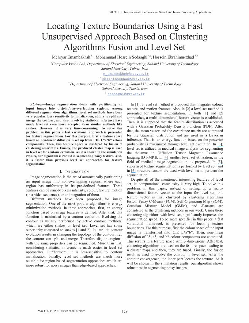
Our proposed method is illustrated in Fig. 1, in a block

diagram. Each block is explained in the next sub-sections.

Fig. 1 The proposed algorithm in a block diagram

A. Feature extraction

In this section, feature extraction from the texture image, is

explained. First of all, a color transformation is utilized, i.e.

the color space of the input image is transformed from RGB to

CIE L*a*b*. After that, non-linear diffusion of L*a*b* color

components is computed.

1) RGB to CIE L*a*b*

It can be understood from McAdams ellipses [7] that RGB

colour domain is not a good choice for processing colour

images. Moreover, if RGB colour components are used as

feature vectors, it can be verified that there will be a big

overlap between feature channels. On the other hand, feature

vectors calculated from CIE L*a*b* colour space have much

more detachability compared to RGB colour space. Therefore,

CIE L*a*b* colour space is utilized instead of RGB.

Consequently, first, the input RGB image is transformed into

CIEXYZ colour space using the following equation:

úúú

û

ù

êêê

ë

é

úúú

û

ù

êêê

ë

é=

úúú

û

ù

êêê

ë

é

B

G

R

Z

Y

X

116.1066.0000.0

114.0587.00299

200.0174.0607.0 (1)

Then, the components of L*a*b* colour domain are

computed using the subsequent equations, i.e.

ïïî

ïïí

ì

³-

<=

008856.016)100(25

008856.0)(3.903

00

00*

Y

Yif

Y

Y

Y

Yif

Y

Y

L

)(13

)(13

/

0

/**

/

0

/**

vvLb

vuLa

-=

-= (2)

While we have,

)315(

4/

ZYX

Xu

++= (3)

460900.0,0200953.0,255

)315(

9

/0

/00

/

===

++=

vuY

ZYX

Xv (4)

The produced colour components are used in the next sub-

section as inputs for non-linear diffusion.

2) Non-linear diffusion

Non-linear diffusion is a method for image de-noising and

simplification. It was initially proposed by Perona and Malik

in [8] for edge detection. At first it was only used for grey

scale (scalar) images. But after G. Gerig et al in [9], proposed

the vector-value version of diffusion equation, it became

applicable for processing colour images, texture feature vectors, and also hyper-spectral images. Also, preserving

image edges, processing on only one scale of the image and

therefore less redundant information production, have made

non-linear diffusion a more popular method for image

segmentation than structure tensors [10 and 11] and Gabor

filters [12, 13, and 14].

Therefore, due to these interesting features, it is employed

in our work to establish the feature space. As it has been seen

in the results, this feature space helps the segmentation

algorithm robust against noise.

The input vector for non-linear diffusion is the L*a*b*

colour components, i.e,

*

*,

*,

2

1

0

bu

au

Lu

=

=

= (5)

The non-linear diffusion equation for vector-valued images

is [2],

))||((1

0

2

i

N

k kit uugdivu ÑÑ=¢¶ å -

= (6)

Where iu¢ is the result of non-linear diffusion when the

input vector is iu . N equals to the dimension of the vector-

valued image. In our wok, it is 3. g(.) is a decreasing function

of the image gradient. In this study, the following function is

employed:

ïî

ïíì

£

>--=

01

0))/(

exp(1)(

s

ss

C

sg m

m

l (7)

Cm is put in the equation to have the S*g(s) flux increasing

for l<g and decreasing for l³g . Also l is a parameter for

controlling image contrast. In comparison with the suggested

functions in [1] and [2] for g(.), our proposed function in (8) has more free parameters, and has more flexibility for wider

range of images.

Solving (6) results in a (3)-dimensional feature vector, i.e.:

),,( 210 uuuu ¢¢¢=¢ (8)

This feature vector will be used in the clustering algorithm.

B. Clustering algorithms fusion

1) Clustering algorithms

Clustering

algorithms

fusion

Feature

extraction

RGB to CIE

L*a*b*

Non-linear

diffusion

SOM

K-means

FCM

GMM

Fusion

Input

imageSegmented

image

Level

set

130

In this study, SOM, K-means, GMM, and FCM methods

are used to cluster the feature space in (8).

· SOM Kohonen’s SOM is an unsupervised competitive neural

network. It uses the neighbourhood interaction set to

approximate lateral neural interaction and discovers the

topological structure hidden in the data for visual display in

one or two dimensional space ([16 and 17]). After finishing

the training step, trained SOM network can be used in the test

phase to cluster test images.

In this work, a two stage SOM network is used. The first

stage, maps the feature space from 3-dimension to 4-

dimension. The second stage performs the unsupervised

classification. Batch unsupervised weight/bias training method

is used to train the neural network. The structure of SOM

neural network is plotted in Fig. 2.

Fig. 2. The SOM structure.

· K-means

K-means is another well-known clustering algorithm that

we utilize. It assigns each point to the cluster whose center

(also called centroid) is nearest. The center is the average of

all the points in the cluster — that is, its coordinates are the

arithmetic mean for each dimension separately over all the

points in the cluster.

It must be mentioned that Euclidean distance is used as

distance criterion for K-means. This distance criterion is much

faster than Mahalanobis, and produces better results than city-block and Hamming distances.

· GMMIn GMM, each mass of features is modelled as a multi-

variate normal density function. These models are fit to data

using expectation maximization (EM) algorithm, which

assigns posterior probabilities to each observation. The fitting

method uses an iterative algorithm that converges to a local

optimum. Actually in the test phase, the a posterioriprobability is computed for each model. The dependency of

each pixel to a specific cluster is determined by examining the

greatness of the probability.

· FCM FCM is the final clustering method we use. FCM provides a

method that shows how to group data points that populate

some multidimensional space into a specific number of

different clusters ([18]). It is a data clustering technique

wherein each data point belongs to a cluster to some degree that is specified by a membership grade. In K-means a data

point, is assumed to be in exactly one cluster. However, this

condition can be relaxed and we can assume that each

sampleju¢ , has some graded or fuzzy cluster membership

( )ji u¢m in clusteriw , where ( ) 10 £¢£ ji um . Basically, this

membership is equivalent to the probability ( )q,|ˆji uwP ¢ , i.e.

([15]),

( )

å

å

=

--

--

=

úû

ùêë

é -¢S-¢-S

úû

ùêë

é -¢S-¢-S=

¢

¢=¢

C

c

ccjc

t

cjc

iiji

t

iji

C

c

cccj

iiij

ji

wPuu

wPuu

wPwup

wPwupuwP

1

12

1

12

1

1

)(ˆ)ˆ(ˆ)ˆ(2

1exp|ˆ|

)(ˆ)ˆ(ˆ)ˆ(2

1exp|ˆ|

)(ˆ)ˆ,|(

)(ˆ)ˆ,|(ˆ,|ˆ

mm

mm

q

qq

(9)

C is the number of clusters where it is equal to 2 in our

work. )(ˆiwP (the a priori probability) is the fraction of

samples from iw ,

im is the mean of the samples, and iS is the

corresponding sample covariance matrix. The a posterioriprobability in (9), is between 0.0 and 1.0. In FCM, a minimum

of the following global cost function is sought [15],

( )[ ]åå= =

-¢¢=C

c

n

j

ij

b

ji uuwPL1 1

2||||ˆ,|ˆ mq (10)

Where b>1 is a free parameter chosen to adjust the

"blending" of different clusters.

2) Fusion

Each clustering method has its own benefits. The

performance of the clustering algorithm significantly depends

on the input feature space distribution. A clustering method

maybe suitable for an image, but for another image it may

produce poor results. It is seen in our work that for a non-

overlapping feature space, GMM produces desirable results.

While for small amount of overlap, FCM and K-means are

more suitable. For highly overlapped feature spaces, SOM

seems to be a good clustering method. Considering these

problems, as it is depicted in our simulation results, clustering

algorithms fusion produces the best generalization for wider ranges of images. For this purpose, the following equation is

considered for each clustering result, i.e.

14

1

4321

=

+++=

å=

-

i

i

GMMSOMFCMmeansK CCCCD

a

aaaa (11)

meansKC -,

FCMC ,SOMC , and

GMMC are binary images each

represent for K-means, FCM, SOM, and GMM clustering

results, respectively. ia ( 4,,1L=i ) is the weight factor for

each clustering algorithm. Finally, D is the decision map. The

final result can be found by a simple thresholding,

îíì

£

>=

0

0

0

1

TD

TDV

(12)

C. Level set

In this section, the variational framework used for level set

evolution is explained. For this purpose, the cluster map is

used to find the internal energy. The level set equation is [1

and 2],

1st stage 2nd stage

0u¢Background

Foreground

1u¢

2u¢

131

÷÷ø

öççè

æ++

ÑÑ

Ñ=¶

¶21)

||.())((

),(mm

ff

fdf

e r

rr

vxt

tx (13)

f is the level set function, which is made by Signed

Distance Functions (SDF), ( ).ed is the smoothed Dirac impulse

function, and v is a scalar that determines the level set

evolution rate. 1m and

2m are the mean of inner and outer

parts of the contour, i.e.,

2,1, ==ò

ò

W

W idx

dxI

i

i

c

ic

cm (14)

W is the image domain and ic is allocated to the inner and

outer part of the contour, i.e. 1c is for the inner, and 2c is for

the outer part,

)(1)(),()( 11 zHzzHz ee cc -==

)(zHe is the regularized Heaviside function. cI is the

cluster map. As it was mentioned earlier, f is calculated from

a SDF, i.e. ®W:f where,

îíì

WÎW¶-

WÎW¶=

2

1

),(

),()(

xifxD

xifxDxf (15)

),( W¶xD is the distance function between x , each image

pixels, and W¶ , the contour ( 0»f ). After initializing the

level set function, the level set equation (13) is solved using the gradient descent algorithm iteratively. It converges when

there is not a major change in 1m and

2m .

III. SIMULATION RESULTS

In this section, the simulation results of our algorithm are presented. The results have been evaluated on an Intel Core 2

Due CPU (T7250). The algorithm has been tested on 59

images from Corel texture dataset [19] and the following

average values have been found for 4,,1, L=iia :

2819.01 =a , 3176.02 =a , 2462.03 =a , and 1543.04 =a .

Also 589.00 =T is considered in (12). Moreover, for training

SOM, 120 and 80 epochs are used for the first and the second

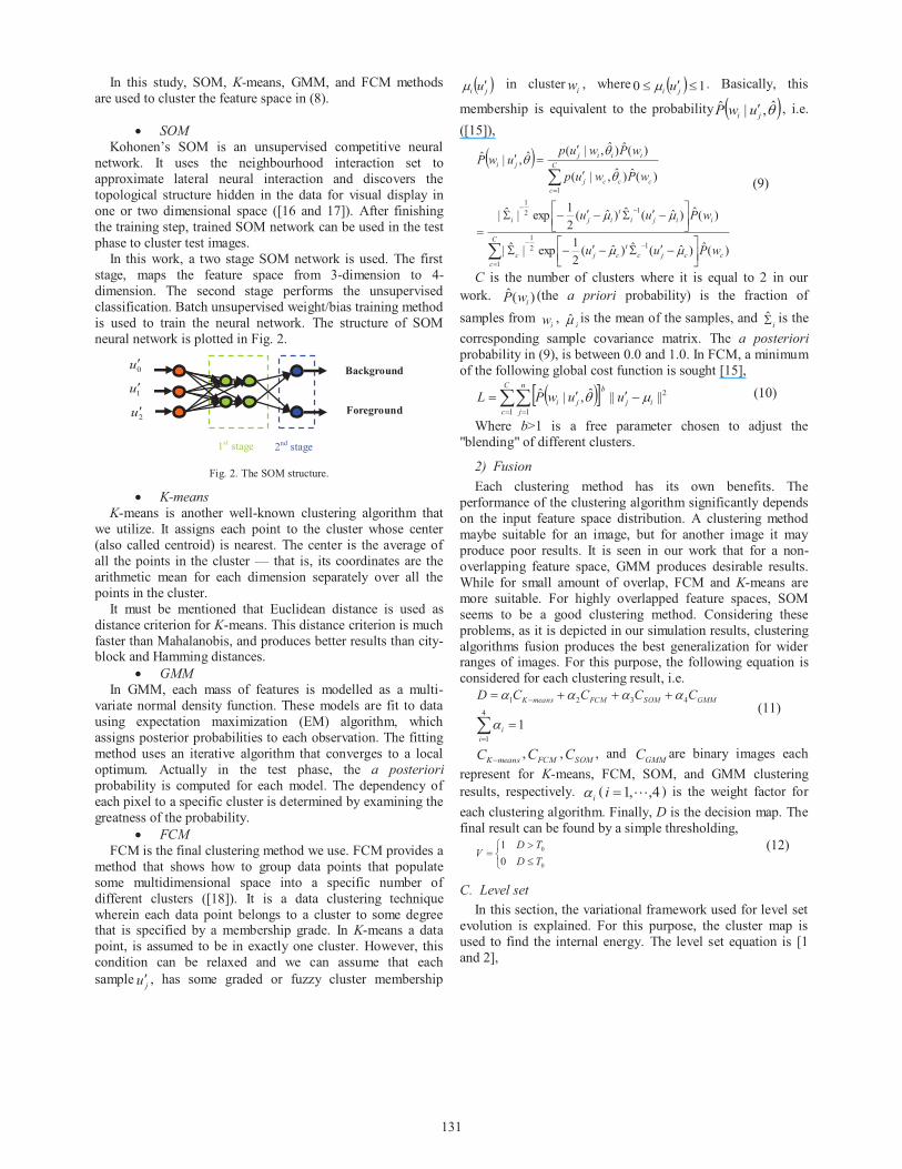
stages, respectively. Fig. 3-a is utilized as the input image.

Also the ground truth is plotted in Fig. 3-b.

(a) (b)

Fig. 3: (a) The input image (b) The corresponding ground truth

(a) (b) (c)

Fig. 4: Colour components (a) L*, (b) a*, and (c) b*

It is initially in RGB colour space. According to our

algorithm, it is first transformed into CIE L*a*b* colour space. The result of this colour transformation is plotted in

Fig. 4. The non-linear diffusion result for each colour channel

is demonstrated in Fig. 5. These diffusion results are

considered as the feature vectors in (8). The feature space is

then clustered according to the mentioned algorithms

explained in Section 2.2.1. The clustering results are plotted in

Table 1.

(a) (b) (c)

Fig. 5: The diffusion result for (a) channel L*, (b) channel a*, and (c) channel b*

In the first column, the clustering algorithm is mentioned,

and in the second, third, and fourth columns, the elapsed time

for clustering in seconds, the Percentage of Correct

Segmentation (PCS) in percent, and the clustering result, is

demonstrated. It must be mentioned that PCS has been

computed according to the ground truth in Fig. 2-b. Finally the

level set evolution is plotted in Fig. 6.

Table 1: The clustering results

Clustering

algorithmElapsed

time

PCS Cluster

maps

K-means 3.24

(sec)

95.96

FCM 8.18

(sec)

95.96

SOM 53.18(sec)

94.53

GMM 12.47(sec)

87.51

Fusion 0.90(sec)

96.10

(a) (b)

(c) (d)

132

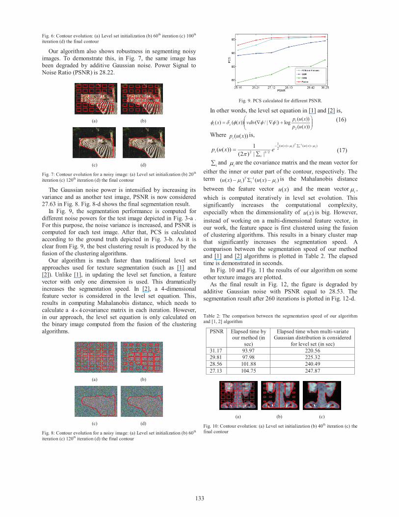
Fig. 6: Contour evolution: (a) Level set initialization (b) 60th iteration (c) 100th

iteration (d) the final contour

Our algorithm also shows robustness in segmenting noisy

images. To demonstrate this, in Fig. 7, the same image has

been degraded by additive Gaussian noise. Power Signal to

Noise Ratio (PSNR) is 28.22.

(a) (b)

(c) (d)

Fig. 7: Contour evolution for a noisy image: (a) Level set initialization (b) 20th

iteration (c) 120th iteration (d) the final contour

The Gaussian noise power is intensified by increasing its

variance and as another test image, PSNR is now considered

27.63 in Fig. 8. Fig. 8-d shows the final segmentation result.

In Fig. 9, the segmentation performance is computed for

different noise powers for the test image depicted in Fig. 3-a .For this purpose, the noise variance is increased, and PSNR is

computed for each test image. After that, PCS is calculated

according to the ground truth depicted in Fig. 3-b. As it is

clear from Fig. 9, the best clustering result is produced by the

fusion of the clustering algorithms.

Our algorithm is much faster than traditional level set

approaches used for texture segmentation (such as [1] and

[2]). Unlike [1], in updating the level set function, a feature

vector with only one dimension is used. This dramatically

increases the segmentation speed. In [2], a 4-dimensional

feature vector is considered in the level set equation. This,

results in computing Mahalanobis distance, which needs to

calculate a 44´ covariance matrix in each iteration. However,

in our approach, the level set equation is only calculated on

the binary image computed from the fusion of the clustering

algorithms.

(a) (b)

(c) (d)

Fig. 8: Contour evolution for a noisy image: (a) Level set initialization (b) 60th

iteration (c) 120th iteration (d) the final contour

Fig. 9. PCS calculated for different PSNR.

In other words, the level set equation in [1] and [2] is,

÷÷ø

öççè

æ+ÑÑ=

))((

))((log|)|/())(()(

2

1

xup

xupvdivxxt fffdf e

(16)

Where ))(( xupiis,

))(())((2

1

2/12

1

||)2(

1))((

iiT

i xuxu

i

i exupmm

p

-å-- -

å= (17)

iå and im are the covariance matrix and the mean vector for

either the inner or outer part of the contour, respectively. The

term ))(())(( 1

ii

T

i xuxu mm -S- - is the Mahalanobis distance

between the feature vector )(xu and the mean vectorim ,

which is computed iteratively in level set evolution. This

significantly increases the computational complexity,

especially when the dimensionality of )(xu is big. However,

instead of working on a multi-dimensional feature vector, in

our work, the feature space is first clustered using the fusion

of clustering algorithms. This results in a binary cluster map

that significantly increases the segmentation speed. A

comparison between the segmentation speed of our method

and [1] and [2] algorithms is plotted in Table 2. The elapsed

time is demonstrated in seconds.

In Fig. 10 and Fig. 11 the results of our algorithm on some

other texture images are plotted.

As the final result in Fig. 12, the figure is degraded by

additive Gaussian noise with PSNR equal to 28.53. The

segmentation result after 260 iterations is plotted in Fig. 12-d.

Table 2: The comparison between the segmentation speed of our algorithm and [1, 2] algorithm

PSNR Elapsed time by our method (in

sec)

Elapsed time when multi-variate Gaussian distribution is considered

for level set (in sec)

31.17 93.97 220.56

29.81 97.98 225.32

28.56 101.88 240.49

27.13 104.75 247.87

(a) (b) (c)

Fig. 10: Contour evolution: (a) Level set initialization (b) 40th iteration (c) the final contour

133

(a) (b) (c)

Fig. 11: Contour evolution: (a) Level set initialization (b) 20th iteration (c) the

final contour

(a) (b)

(c) (d)

Fig. 12: (a) The input image (b) level set initialization (c) 60th iteration (d) the final result

Noise power is increased in Fig. 13 for the same image.

PSNR is 26.72 for this figure. The segmentation result is plotted in Fig. 13-d.

(a) (b)

(c) (d)

Fig. 13: (a) The input image (b) level set initialization (c) 60th iteration (d) the

final result

IV. CONCLUSION

In this paper a fast algorithm is presented for texture

segmentation. Traditional level set methods that calculate

energy functions based on a multi-dimensional feature space

are so time-consuming. To solve this problem, in our work, a

feature space, which is established upon non-linear diffusion

of the CIE L*a*b* colour components, is first clustered with

the fusion of clustering algorithms. This leads to a cluster map

that is used to evolve level set in a variational framework.

The advantages of our algorithm are:

(1) Our approach is much faster than previous level set

methods proposed in [1 and 2].

(2) Due to non-linear diffusion computation and also the

intrinsic region-based nature of our approach, the proposed

method shows robustness in segmenting noisy images.

(3) Unlike the method presented in [1], image gradients are

not calculated for texture images. For noisy images,

derivatives computation intensifies noise, and reduces the performance of the segmentation.

(4) Clustering algorithms fusion has much more

generalization than using an algorithm solely. The fusion

significantly improves the segmentation result.

REFERENCES

[1] S. Daniel Cremers, M. Rousson, and R. Deriche, "A Review of Statistical Approaches to level sets Segmentation: Integrating Colour,

Texture, Motion and Shape", 2007, International Journal of Computer

Vision 72(2), 195–215 [2] M. Rousson, T. Brox, and R. Deriche, "Active Unsupervised Texture

Segmentation on a Diffusion Based Feature Space", 2003, Proceedings of the 2003 IEEE Computer Society Conference on Computer Vision

and Pattern Recognition (CVPR’03)

[3] L. Jonasson, P. Hagmann, C. Pollo, X. Bresson, C. R. Wilson, R.

Meuli, and J. Thiran. A level set method for segmentation of the thalamus and its nuclei in DT-MRI. Signal Processing, Tensor Signal

Processing, 87(2):309–321, February 2007. [4] K. Seongjai and Lim. Hyeona. A hybrid level set segmentation for

medical imagery. In IEEE Nuclear Science Symposium Conference

Record, volume 3, page 5, October 2005. [5] N. Paragios and R. Deriche. "Geodesic active regions and level sets

methods for supervised texture segmentation", International Journal of Computer Vision, 46(3):223, 2002.

[6] C. Feddern, J.Weickert and B. Burgeth, "Level-set methods for tensor-valued images", In Proc. of the IEEE 2nd Workshop on VLSM, pages

65–72, 2003. [7] Forsyth and Ponce, Computer Vision: A Modern Approach, pages: 71-

73, Prentice-Hall, 2002.

[8] P. Perona and J. Malik. "Scale space and edge detection using anisotropic diffusion". IEEE Transactions on Pattern Analysis and

Machine Intelligence, 12:629–639, 1990. [9] G. Gerig, O. Kubler, R. Kikinis, and F. A. Jolesz. "Nonlinear

anisotropic filtering of MRI data", IEEE Transactions on Medical Imaging, 11:221–232, 1992.

[10] Zhizhou Wang and Baba C. Vemuri, "An Affine Invariant Tensor Dissimilarity Measure and its Applications to Tensor-valued Image

Segmentation", Proceedings of the 2004 IEEE Computer Society

Conference on Computer Vision and Pattern Recognition (CVPR’04)

[11] C. Chefd’hotel, O. Faugeras, D. Tschumperl and R. Deriche.

"Constrained flows of matrix-valued functions: Application to diffusion tensor regularization", In ECCV, pages 251–265, 2002.

[12] Roman Sandler and Michael Lindenbaum, "Gabor Filter Analysis for Texture Segmentation", Proceedings of the 2006 Conference on

Computer Vision and Pattern Recognition Workshop (CVPRW’06)

[13] Chen Sagiv Sochen, N.A. Zeevi, Y.Y. , "Integrated active contours

for texture segmentation", June 2006, Volume:15,Issue:6 On page(s):

1633-1646 [14] Kamarainen, J.-K. Kyrki, V. Kalviainen, H. "Invariance properties of

Gabor filter-based features-overview and applications", Volume: 15, Issue: 5, 1088-1099, 2006

[15] R. O. Duda, P. E. Hart, and D. G. Stork. Pattern classification. John Wiley and Sons, 2nd. Edition, 2001.

[16] Z. Dokur, Z. Iscan, and T. Olmez. Segmentation of medical images by using wavelet transform and incremental self-organizing map, volume

4293/2006 of Lecture Notes in Computer Science, pages 800–809.

Springer, Berlin, Heidelberg, 2006 [17] W. Kuo, C. Lin, and Y. Sun. Brain MR images segmentation using

statistical ratio: Mapping between watershed and competitive Hopfield clustering network algorithms. Computer Methods and Programs in

Biomedicine, 91(3):191 – 198, 2008. [18] J.Wang, J. Kong, Y. Lu, M. Qi, and B. Zhang, 2008. A modified FCM

algorithm for MRI brain image segmentation using both local and non-local spatial constraints, Computerized Medical Imaging and Graphics

(PMID: 18818051)

[19] www.corel.com, access time: 2009-05-21

134