Linking objective and subjective modelling for landuse decision-making

Linking objective and subjective modelling

for landuse decision-making

Nathaniel C. Bantayana,*, Ian D. Bishopb

a Institute of Renewable Natural Resources, College of Forestry and Natural Resources, University of the Philippines,

Los BanÄos College, Laguna, Philippinesb Centre for GIS and Modelling, The University of Melbourne, Parkville, Vic., Australia

Received 22 May 1998; received in revised form 16 July 1998; accepted 16 July 1998

Abstract

This paper describes a landuse modelling approach developed for the Makiling Forest Reserve in the Philippines. The process

includes application of the analytical hierarchy process (AHP) but extends this approach to include objective process based

modelling ± in the form of the universal soil loss equation (USLE) ± in the subjectively oriented framework of AHP. A

geographic information system was used for data assembly and to de®ne decision zones and a PC based interface developed to

accommodate interactive application of the AHP and USLE models. Having successfully combined the objective and

subjective elements for evaluation of landuse alternatives, the paper explores the options for landuse allocation based on the

suitability assessments of a participating decision group. # 1998 Elsevier Science B.V. All rights reserved.

Keywords: Landuse; GIS; Analytical hierarchy process (AHP)

1. Introduction

Decision-making is a complex process. It usually

involves multiple objectives, multiple alternatives and

multiple social interests and preferences. Since the

early 1970s, researchers have focused their attention

on multi-objective situations and their simultaneous

treatment. This period saw the emergence of multi-

objective programming models applied to landuse

planning problems. One example is the interactive

linear multi-objective programming model by Nij-

kamp and Rietveld (1976). The model allowed the

decision-maker to express his/her relative preference

with respect to certain provisional ef®cient solutions.

The speci®cation of preference is repeated a number

of times until a best compromise solution is deter-

mined. Similar works include those by Barber (1976),

Dane et al. (1977), Ridgley (1984), Ridgley and

Giambelluca (1992) and Rehman and Romero (1993).

Likewise, decision-making involves multiple alter-

natives. Several alternatives exist that will satisfy the

objectives of the problem to varying degrees (Batty,

1979). The decision-maker has to choose the best

alternative without having a ®rm knowledge of the

effect of each alternative on the objectives. It is

important, in the ®rst instance, to generate a complete

set of alternatives and to use appropriate models to

predict the probable effect of each choice. These

models may be either wholly quantitative and objec-

Landscape and Urban Planning 43 (1998) 35±48

*Corresponding author. Tel.: +63-049-536-2557; fax: +63-049-

536-3206; e-mail: [email protected]

0169-2046/98/$19.00 # 1998 Elsevier Science B.V. All rights reserved.

P I I : S 0 1 6 9 - 2 0 4 6 ( 9 8 ) 0 0 1 0 1 - 7

tive (for example the Universal Soil Loss Equation

(USLE)) or they may involve subjectivity and expert

judgment (e.g. the analytical hierarchy process

(AHP)).

Finally, any landuse planning activity involves

multiple social interests and preferences. Usually,

the ®nal decision on an alternative depends on the

consensus of a group of decision-makers. Saaty (1980)

de®nes consensus as `̀ improving con®dence in the

priority values by using several judges to bring the

results in line with majority preferences.'' Thus, the

decision model must be able to accommodate these

varied and often con¯icting points of view. More

importantly, an aggregation procedure that gives

results which are representative of group opinion is

desirable.

There is considerable work reported in the literature

dealing with the several aspects of the decision process

and systems and procedures for decision support. This

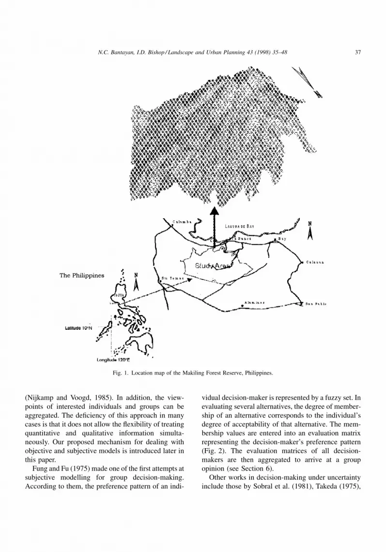
paper reports a case study in the Makiling Forest

Reserve, Philippines which combines the work of

several authors (Fig. 1). Most importantly it presents

an approach to the combination of objective and

subjective modelling. Seldom has the use of both

approaches been reported in combination. There has

been little attempt to develop a systematic procedure

for combination such that an objective/quantitative

model may be used when available and considered

reliable while fuzzier/subjective/expert judgments are

employed to important decision parameters for which

no objective model exists (Bantayan, 1996).

2. A systematic approach to the decision-makingprocess

Complexity necessitates a systematic approach to

the decision-making process to accommodate the

multiplicity and multi-dimensionality of the problem.

A systematic approach is also useful to gain a thor-

ough understanding of the issues affecting the problem

(Jankowski, 1989, 1995). An example of a systems

approach to solving a complex landuse planning

problem is multi-criteria evaluation (MCE). MCE

techniques try to investigate a number of alternatives

(or choice possibilities) in the light of multiple objec-

tives (or criteria) and con¯icting preferences (or prio-

rities) (Voogd, 1983). An extension of MCE is multi-

criteria decision-making (MCDM). MCDM models

go beyond MCE techniques in seeking to establish

preferences and trade-offs among competing objec-

tives which may have been separately evaluated using

MCE (Bantayan and Bishop, 1993a, b).

Engendering preferences presents uncertainties.

These uncertainties point to the fuzziness or the

imprecision of human decisions (Xiang et al.,

1992). Until recently, the exclusion of intangible

information from planning exercises has been com-

mon practice because, `̀ . . . knowledge of human

beings involves the apprehension of qualities, which

in their very nature escape the net of numbers''

(Leitner et al., 1985). But as the same authors argue,

`̀ . . . a reduction of some phenomenon to a set of

measurable variables, to the exclusion of `unmeasur-

ables', provides a necessarily biased representation of

the phenomena at issue and often falls short of depict-

ing what is really important.'' In addition, Blin and

Whinston (1973) point out that problems which

involve expressions of preferences of individuals or

groups are more appropriately solved through the

theory of fuzzy sets. This realisation led to the devel-

opment of models integrating fuzzy set theory into the

decision-making process. Such models are referred to

collectively as subjective models.

Fuzzy set theory ®nds application in systems where

human judgment, perceptions and emotions play a

central role (Zadeh, 1977). It is a `̀ body of concepts

and techniques aimed at providing a systematic frame-

work for dealing with the vagueness and imprecision

inherent in human thought processes'' (Gupta, 1977).

The theory extends the classical two-valued logic (true

and false) of set membership towards a third region ±

between true and false (Brule, 1992). For more details

about fuzzy set theory, numerous references are avail-

able. Notable are those by Gupta (1977), Kaufmann

and Gupta (1985), Zimmermann (1991) or the tutorial

by Brule (1985) which is available on the Internet.

3. Subjective modelling for decision-making

Subjective models for decision-making can be

described as integrating the theory of fuzzy sets with

the concepts of multi-criteria decision-making mod-

els. This provides a coherent process for incorporating

subjective views into an explicit decision process

36 N.C. Bantayan, I.D. Bishop / Landscape and Urban Planning 43 (1998) 35±48

https://www.researchgate.net/publication/220649805_Integrating_Geographical_Information_Systems_and_Multiple_Criteria_Decision-Making_Methods?el=1_x_8&enrichId=rgreq-a5842ad1-4cc1-4ab2-a228-429aebbbdc05&enrichSource=Y292ZXJQYWdlOzIyMjUwMDM5MztBUzoxMDMyOTEwNDAwNDMwMTRAMTQwMTYzNzkxMTk3Nw==

https://www.researchgate.net/publication/37415529_Multi-Criteria_Evaluation_for_Urban_and_Regional_Planning?el=1_x_8&enrichId=rgreq-a5842ad1-4cc1-4ab2-a228-429aebbbdc05&enrichSource=Y292ZXJQYWdlOzIyMjUwMDM5MztBUzoxMDMyOTEwNDAwNDMwMTRAMTQwMTYzNzkxMTk3Nw==

(Nijkamp and Voogd, 1985). In addition, the view-

points of interested individuals and groups can be

aggregated. The de®ciency of this approach in many

cases is that it does not allow the ¯exibility of treating

quantitative and qualitative information simulta-

neously. Our proposed mechanism for dealing with

objective and subjective models is introduced later in

this paper.

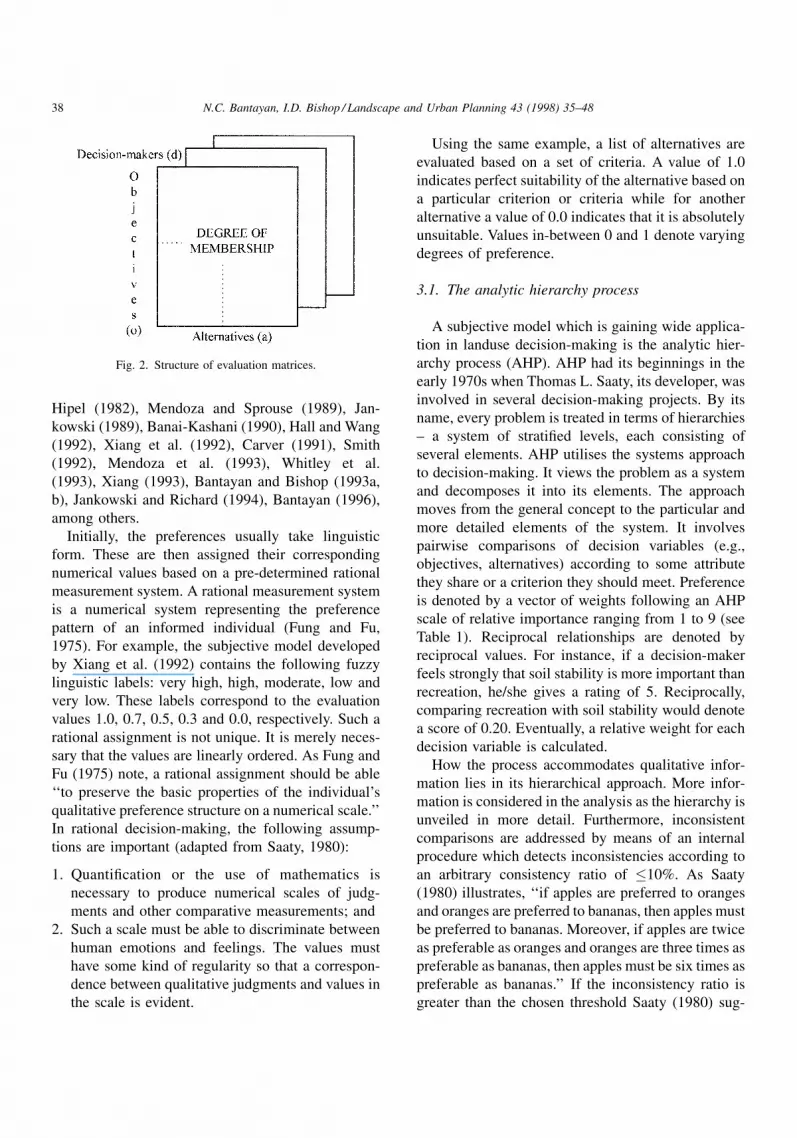
Fung and Fu (1975) made one of the ®rst attempts at

subjective modelling for group decision-making.

According to them, the preference pattern of an indi-

vidual decision-maker is represented by a fuzzy set. In

evaluating several alternatives, the degree of member-

ship of an alternative corresponds to the individual's

degree of acceptability of that alternative. The mem-

bership values are entered into an evaluation matrix

representing the decision-maker's preference pattern

(Fig. 2). The evaluation matrices of all decision-

makers are then aggregated to arrive at a group

opinion (see Section 6).

Other works in decision-making under uncertainty

include those by Sobral et al. (1981), Takeda (1975),

Fig. 1. Location map of the Makiling Forest Reserve, Philippines.

N.C. Bantayan, I.D. Bishop / Landscape and Urban Planning 43 (1998) 35±48 37

Hipel (1982), Mendoza and Sprouse (1989), Jan-

kowski (1989), Banai-Kashani (1990), Hall and Wang

(1992), Xiang et al. (1992), Carver (1991), Smith

(1992), Mendoza et al. (1993), Whitley et al.

(1993), Xiang (1993), Bantayan and Bishop (1993a,

b), Jankowski and Richard (1994), Bantayan (1996),

among others.

Initially, the preferences usually take linguistic

form. These are then assigned their corresponding

numerical values based on a pre-determined rational

measurement system. A rational measurement system

is a numerical system representing the preference

pattern of an informed individual (Fung and Fu,

1975). For example, the subjective model developed

by Xiang et al. (1992) contains the following fuzzy

linguistic labels: very high, high, moderate, low and

very low. These labels correspond to the evaluation

values 1.0, 0.7, 0.5, 0.3 and 0.0, respectively. Such a

rational assignment is not unique. It is merely neces-

sary that the values are linearly ordered. As Fung and

Fu (1975) note, a rational assignment should be able

`̀ to preserve the basic properties of the individual's

qualitative preference structure on a numerical scale.''

In rational decision-making, the following assump-

tions are important (adapted from Saaty, 1980):

1. Quanti®cation or the use of mathematics is

necessary to produce numerical scales of judg-

ments and other comparative measurements; and

2. Such a scale must be able to discriminate between

human emotions and feelings. The values must

have some kind of regularity so that a correspon-

dence between qualitative judgments and values in

the scale is evident.

Using the same example, a list of alternatives are

evaluated based on a set of criteria. A value of 1.0

indicates perfect suitability of the alternative based on

a particular criterion or criteria while for another

alternative a value of 0.0 indicates that it is absolutely

unsuitable. Values in-between 0 and 1 denote varying

degrees of preference.

3.1. The analytic hierarchy process

A subjective model which is gaining wide applica-

tion in landuse decision-making is the analytic hier-

archy process (AHP). AHP had its beginnings in the

early 1970s when Thomas L. Saaty, its developer, was

involved in several decision-making projects. By its

name, every problem is treated in terms of hierarchies

± a system of strati®ed levels, each consisting of

several elements. AHP utilises the systems approach

to decision-making. It views the problem as a system

and decomposes it into its elements. The approach

moves from the general concept to the particular and

more detailed elements of the system. It involves

pairwise comparisons of decision variables (e.g.,

objectives, alternatives) according to some attribute

they share or a criterion they should meet. Preference

is denoted by a vector of weights following an AHP

scale of relative importance ranging from 1 to 9 (see

Table 1). Reciprocal relationships are denoted by

reciprocal values. For instance, if a decision-maker

feels strongly that soil stability is more important than

recreation, he/she gives a rating of 5. Reciprocally,

comparing recreation with soil stability would denote

a score of 0.20. Eventually, a relative weight for each

decision variable is calculated.

How the process accommodates qualitative infor-

mation lies in its hierarchical approach. More infor-

mation is considered in the analysis as the hierarchy is

unveiled in more detail. Furthermore, inconsistent

comparisons are addressed by means of an internal

procedure which detects inconsistencies according to

an arbitrary consistency ratio of �10%. As Saaty

(1980) illustrates, `̀ if apples are preferred to oranges

and oranges are preferred to bananas, then apples must

be preferred to bananas. Moreover, if apples are twice

as preferable as oranges and oranges are three times as

preferable as bananas, then apples must be six times as

preferable as bananas.'' If the inconsistency ratio is

greater than the chosen threshold Saaty (1980) sug-

Fig. 2. Structure of evaluation matrices.


https://www.researchgate.net/publication/23540752_A_fuzzy-group_multicriteria_decisionmaking_model_and_its_application_to_land-use_planning?el=1_x_8&enrichId=rgreq-a5842ad1-4cc1-4ab2-a228-429aebbbdc05&enrichSource=Y292ZXJQYWdlOzIyMjUwMDM5MztBUzoxMDMyOTEwNDAwNDMwMTRAMTQwMTYzNzkxMTk3Nw==

gests re-evaluation of the comparisons. The proce-

dure, however, is limited by the number of factors

which can be compared. An individual cannot simul-

taneously compare more than nine objects without

being confused (Saaty, 1980; Banai-Kashani, 1989).

Thus, comparison of objects beyond nine will not give

reliable results.

3.2. Generating the subjective measure

The ®rst step in the analytic hierarchy process

(AHP) is to de®ne the hierarchy, each representing

a level in the system. Illustrated below are the three

identi®ed levels of hierarchy for landuse decision-

making in our case study area in the Mt Makiling

Forest Reserve, Philippines (Table 2).

Consider the goal as choosing the landuse that is

most suited for the Reserve. This is based initially on a

comparison of the importance of the objectives. This

assessment can be based in consideration of the

Reserve as a whole. However, as the Reserve is not

uniform in its bio-physical characteristics it would be

inappropriate for a decision-maker to determine the

relationship between alternatives and objectives holi-

stically. In order to make informed and valid assess-

ments, the area should be divided into zones with

relatively homogenous characteristics. To this end, the

study area was divided into ten decision zones based

on similarities of slope and soil type. This classi®ca-

tion was deemed appropriate for the purpose. While it

was possible to include more factors in the homo-

genization process, these decision factors were

assumed to come into play in the application of the

subjective model. This was done using the SAGE

raster GIS (Itami and Raulings, 1993a, b) into a

number of pertinent map layers (elevation, soils,

existing land cover, rainfall, roads).

A computer program to assist in the application of

AHP to the Makiling reserve has been developed for

PC using VISUAL BASIC. Each stage of the analysis is

presented to the decision-maker as a series of prompts

seeking a comparison ratio. The program also com-

putes the consistency ratios and returns to the appro-

priate point in the AHP if a consistency threshold is

exceeded. The user may also display the GIS-based

maps at any time to check on the location of a decision

zone or some aspect of the underlying data.

3.3. Pairwise comparison of objectives

The analysis proceeds by conducting a pairwise

comparison of the objectives ± considered for the

reserve as a whole. The assumption taken is that

Table 1

Ratio scale of comparison (from Saaty (1980), p. 54)

Intensity of importance Definition Explanation

1 Equal importance Equal importance or indifference

3 Weak importance of one over another Experience and judgment slightly favour one activity

over another

5 Essential or strong importance Experience and judgment strongly favour one activity

over another

7 Very strong or demonstrated importance An activity is favoured very strongly over another; its

dominance is demonstrated in practice

9 Absolute importance The evidence favouring one activity over another is of

the highest possible order of affirmation

2, 4, 6, 8 Intermediate values between adjacent scale values

Table 2

Hierarchical classification of the study

Level 1 Goal Choose best landuse

Level 2 Objectives 1. Soil stability (SS)

2. Recreation (RV)

3. Employment (EO)

4. Sustainable/potable water (PW)

5. Food production (FP)

6. Education and research (ER)

7. Pollution abatement (PA)

Level 3 Alternatives 1. Cultivated areas (C)

2. Forested areas (F)

3. Built-up areas (B)

4. Park and botanic garden areas (P)


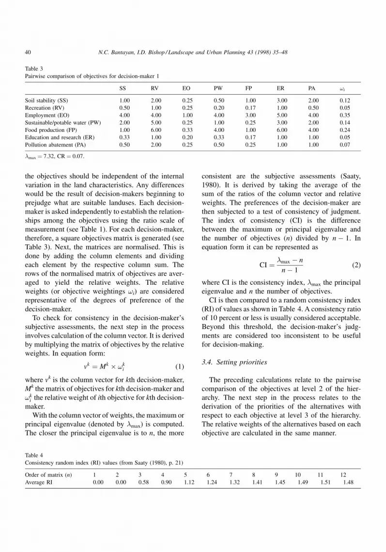
the objectives should be independent of the internal

variation in the land characteristics. Any differences

would be the result of decision-makers beginning to

prejudge what are suitable landuses. Each decision-

maker is asked independently to establish the relation-

ships among the objectives using the ratio scale of

measurement (see Table 1). For each decision-maker,

therefore, a square objectives matrix is generated (see

Table 3). Next, the matrices are normalised. This is

done by adding the column elements and dividing

each element by the respective column sum. The

rows of the normalised matrix of objectives are aver-

aged to yield the relative weights. The relative

weights (or objective weightings !i) are considered

representative of the degrees of preference of the

decision-maker.

To check for consistency in the decision-maker's

subjective assessments, the next step in the process

involves calculation of the column vector. It is derived

by multiplying the matrix of objectives by the relative

weights. In equation form:

vk � Mk � !ki (1)

where vk is the column vector for kth decision-maker,

Mk the matrix of objectives for kth decision-maker and

!ki the relative weight of ith objective for kth decision-

maker.

With the column vector of weights, the maximum or

principal eigenvalue (denoted by �max) is computed.

The closer the principal eigenvalue is to n, the more

consistent are the subjective assessments (Saaty,

1980). It is derived by taking the average of the

sum of the ratios of the column vector and relative

weights. The preferences of the decision-maker are

then subjected to a test of consistency of judgment.

The index of consistency (CI) is the difference

between the maximum or principal eigenvalue and

the number of objectives (n) divided by n ÿ 1. In

equation form it can be represented as

CI � �max ÿ n

nÿ 1(2)

where CI is the consistency index, �max the principal

eigenvalue and n the number of objectives.

CI is then compared to a random consistency index

(RI) of values as shown in Table 4. A consistency ratio

of 10 percent or less is usually considered acceptable.

Beyond this threshold, the decision-maker's judg-

ments are considered too inconsistent to be useful

for decision-making.

3.4. Setting priorities

The preceding calculations relate to the pairwise

comparison of the objectives at level 2 of the hier-

archy. The next step in the process relates to the

derivation of the priorities of the alternatives with

respect to each objective at level 3 of the hierarchy.

The relative weights of the alternatives based on each

objective are calculated in the same manner.

Table 3

Pairwise comparison of objectives for decision-maker 1

SS RV EO PW FP ER PA !i

Soil stability (SS) 1.00 2.00 0.25 0.50 1.00 3.00 2.00 0.12

Recreation (RV) 0.50 1.00 0.25 0.20 0.17 1.00 0.50 0.05

Employment (EO) 4.00 4.00 1.00 4.00 3.00 5.00 4.00 0.35

Sustainable/potable water (PW) 2.00 5.00 0.25 1.00 0.25 3.00 2.00 0.14

Food production (FP) 1.00 6.00 0.33 4.00 1.00 6.00 4.00 0.24

Education and research (ER) 0.33 1.00 0.20 0.33 0.17 1.00 1.00 0.05

Pollution abatement (PA) 0.50 2.00 0.25 0.50 0.25 1.00 1.00 0.07

�max � 7.32, CR � 0.07.

Table 4

Consistency random index (RI) values (from Saaty (1980), p. 21)

Order of matrix (n) 1 2 3 4 5 6 7 8 9 10 11 12

Average RI 0.00 0.00 0.58 0.90 1.12 1.24 1.32 1.41 1.45 1.49 1.51 1.48


The ®nal ranking of the alternatives (denoted by !i)

is calculated by performing a matrix multiplication of

the relative weights of the alternatives per objective

(denoted by Mij) and the relative weights of the

objectives (denoted by !i). It is calculated using the

equation:

!j � Mij � !i (3)

where Mij takes the form

Mij �!11 : !1p

: : :!n1 : !np

24 35 (4)

and !11 is the relative weight of alternative 1 for

objective 1, p is the number of alternatives and n is

the number of objectives.

The procedure is repeated in each decision zone,

until all decision zones are evaluated. Accordingly,

each decision zone will have its own set of relative

weights. From the standpoint of the decision-maker,

making all these assessments becomes very tiring as

the number of decision zones increase. The PC-based

computer model makes it easier for the decision-

maker to input all these subjective assessments.

4. Merging objective and subjective modelling

There is no accepted term for a procedure combin-

ing objective and subjective models in a single para-

digm. As the objective models relating to landuse are

typically physical models we have adopted the term

physico-subjective modelling. The approach uses

AHP subjective modelling process as its starting

point. The difference is that whenever an objective

approach to the estimation of matrix values is possible,

and deemed reliable, that approach is adopted and

replaces the subjective relationship between alterna-

tive and objective which would otherwise have been

used.

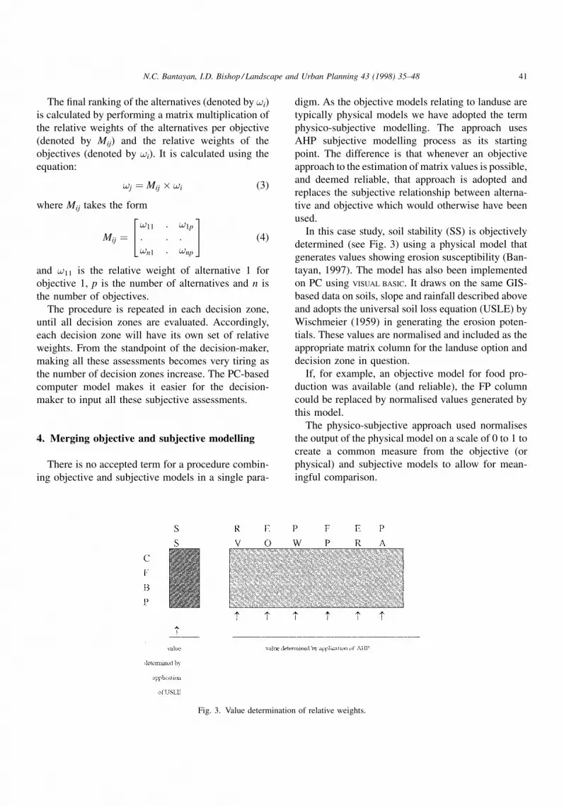
In this case study, soil stability (SS) is objectively

determined (see Fig. 3) using a physical model that

generates values showing erosion susceptibility (Ban-

tayan, 1997). The model has also been implemented

on PC using VISUAL BASIC. It draws on the same GIS-

based data on soils, slope and rainfall described above

and adopts the universal soil loss equation (USLE) by

Wischmeier (1959) in generating the erosion poten-

tials. These values are normalised and included as the

appropriate matrix column for the landuse option and

decision zone in question.

If, for example, an objective model for food pro-

duction was available (and reliable), the FP column

could be replaced by normalised values generated by

this model.

The physico-subjective approach used normalises

the output of the physical model on a scale of 0 to 1 to

create a common measure from the objective (or

physical) and subjective models to allow for mean-

ingful comparison.

Fig. 3. Value determination of relative weights.


In the case of one decision-maker, the analysis is

straightforward and no aggregation is necessary. But,

in this case, where a group of decision-makers is

involved, an aggregate set of objective and alternative

weightings needs to be established. Thus, for kth

decision-maker (d � k, . . . , q) and jth objective

(o � i, . . . , n), a mapping of the relative weights

for all Aj alternatives (a � j, . . . , p) is established.

These weights represent the preference pattern of the

individual decision-maker (or interest group). The

®nal ranking of the alternatives is calculated by per-

forming a matrix multiplication of the relative weights

for all Aj alternatives per objective (denoted by!kij) and

the relative weights for all Oi objectives (denoted by

!i).

A procedure is necessary to test the variation in

response of the decision-making group. It may be that

variability is due to distinct variation in viewpoints

among the members of the group or it may be simply

that scaling process has been applied in slightly

different ways. One available procedure is a non-

parametric test called the Friedman (Q) statistic (Leh-

mann and D'Abrera, 1975). This test rests on the

assumption that there is no difference among the

objective weightings for the individual members of

the group.

The procedure starts with an ordering (ranking) of

the objective weightings. Responses which differ

widely among each other will be re¯ected in large

differences among the average ranking. If this is the

case, the statistic will be large. Otherwise, when the

average ranking are all equal, the statistic is zero.

Friedman's statistic is given by:

Q � 12

Ns�s� 1�Xs

i�1

R2i ÿ 3N�s� 1� (5)

where N is the number of decision-makers, s the

number of objectives and R2i the square of the rank

sum associated with the ith objective.

This equation is used in situations where there are

no ties among the responses for any objective. A more

complex variation on the equation exists to deal with

equal rankings and generates a statistic Q*.

If the hypothesis of no intra-group difference in

weightings is accepted, the median may be used to

represent group response. An aggregate set of objec-

tive weightings is derived to represent group judgment

for the study area. Table 5 is a summary of the

objective weightings for the eight decision-makers

who participated in this study.

The result of the difference analysis for these

weights was:

Q � 7.28, d.f. � 6, p � 0.297.

Q* � 7.35, d.f. � 6, p � 0.290 (adjusted for ties).

Thus, the probability P(Q* � 7.35) that a �2-vari-

able with 6 degrees of freedom exceeds 7.35 is seen to

be 0.290. It can be concluded that the variation in

weightings is not signi®cant at the 5% con®dence

level. Table 6 shows the consequent aggregate objec-

tive weightings (estimated median).

Table 5

Summary of objective weightings for all decision-makers (dk)

Objective d1 d2 d3 d4 d5 d6 d7 d8

SS 0.12 0.25 0.22 0.14 0.023 0.26 0.16 0.08

RV 0.05 0.03 0.11 0.09 0.05 0.09 0.33 0.15

EO 0.35 0.04 0.02 0.08 0.25 0.03 0.08 0.20

PW 0.14 0.25 0.19 0.22 0.13 0.23 0.19 0.12

FP 0.24 0.03 0.06 0.11 0.14 0.03 0.04 0.21

ER 0.05 0.14 0.22 0.13 0.12 0.19 0.09 0.19

PA 0.07 0.26 0.18 0.23 0.08 0.17 0.11 0.05

Table 6

Aggregate objective weightings

Objective Estimated median

Soil stability 0.19

Recreation value 0.10

Employment opportunities 0.09

Sustainable/potable water 0.20

Food production 0.09

Education and research 0.14

Pollution abatement 0.16


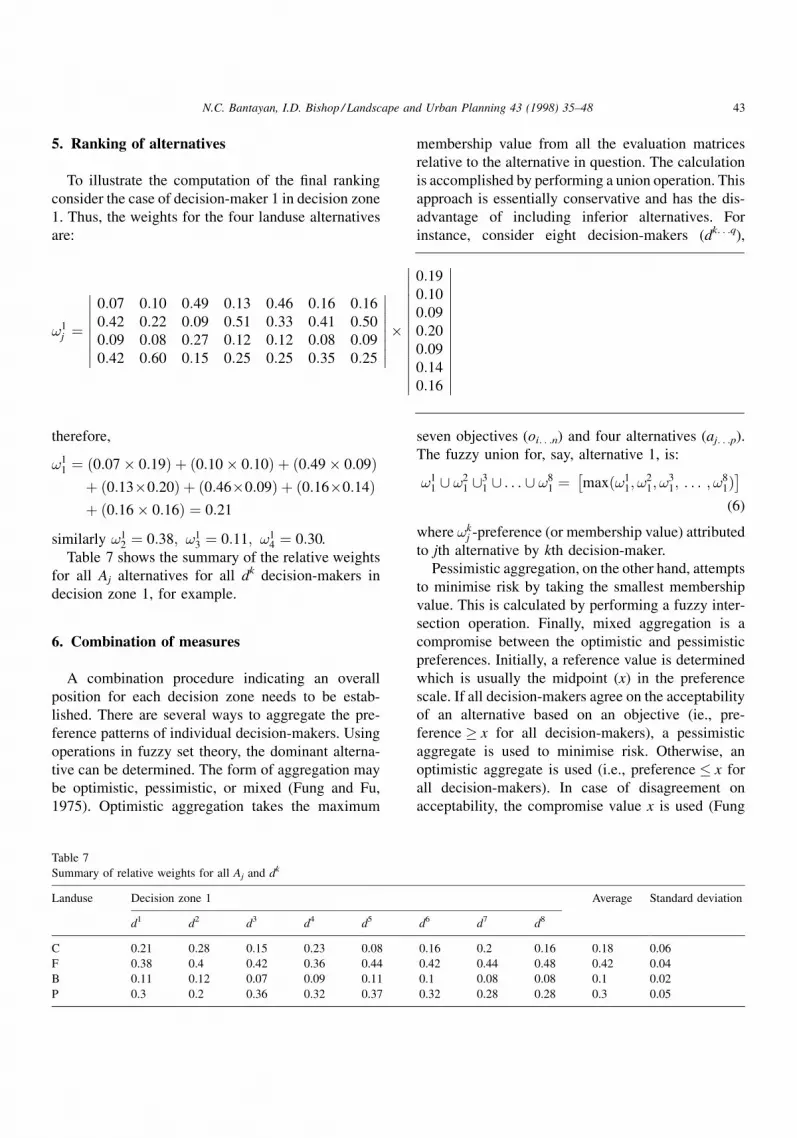
5. Ranking of alternatives

To illustrate the computation of the ®nal ranking

consider the case of decision-maker 1 in decision zone

1. Thus, the weights for the four landuse alternatives

are:

therefore,

!11 � �0:07� 0:19� � �0:10� 0:10� � �0:49� 0:09�� 0:13�0:20� � �0:46�0:09� � �0:16�0:14�� 0:16� 0:16� � 0:21

similarly !12 � 0:38; !1

3 � 0:11; !14 � 0:30.

Table 7 shows the summary of the relative weights

for all Aj alternatives for all dk decision-makers in

decision zone 1, for example.

6. Combination of measures

A combination procedure indicating an overall

position for each decision zone needs to be estab-

lished. There are several ways to aggregate the pre-

ference patterns of individual decision-makers. Using

operations in fuzzy set theory, the dominant alterna-

tive can be determined. The form of aggregation may

be optimistic, pessimistic, or mixed (Fung and Fu,

1975). Optimistic aggregation takes the maximum

membership value from all the evaluation matrices

relative to the alternative in question. The calculation

is accomplished by performing a union operation. This

approach is essentially conservative and has the dis-

advantage of including inferior alternatives. For

instance, consider eight decision-makers (dk. . .q),

seven objectives (oi. . .n) and four alternatives (aj. . .p).

The fuzzy union for, say, alternative 1, is:

!11 [ !2

1 [31 [ . . . [ !8

1 � max�!11; !

21; !

31; . . . ; !8

1��

(6)

where !kj -preference (or membership value) attributed

to jth alternative by kth decision-maker.

Pessimistic aggregation, on the other hand, attempts

to minimise risk by taking the smallest membership

value. This is calculated by performing a fuzzy inter-

section operation. Finally, mixed aggregation is a

compromise between the optimistic and pessimistic

preferences. Initially, a reference value is determined

which is usually the midpoint (x) in the preference

scale. If all decision-makers agree on the acceptability

of an alternative based on an objective (ie., pre-

ference � x for all decision-makers), a pessimistic

aggregate is used to minimise risk. Otherwise, an

optimistic aggregate is used (i.e., preference � x for

all decision-makers). In case of disagreement on

acceptability, the compromise value x is used (Fung

!1j �

0:07 0:10 0:49 0:13 0:46 0:16 0:16

0:42 0:22 0:09 0:51 0:33 0:41 0:50

0:09 0:08 0:27 0:12 0:12 0:08 0:09

0:42 0:60 0:15 0:25 0:25 0:35 0:25

��

0:19

0:10

0:09

0:20

0:09

0:14

0:16

��

��

Table 7

Summary of relative weights for all Aj and dk

Landuse Decision zone 1 Average Standard deviation

d1 d2 d3 d4 d5 d6 d7 d8

C 0.21 0.28 0.15 0.23 0.08 0.16 0.2 0.16 0.18 0.06

F 0.38 0.4 0.42 0.36 0.44 0.42 0.44 0.48 0.42 0.04

B 0.11 0.12 0.07 0.09 0.11 0.1 0.08 0.08 0.1 0.02

P 0.3 0.2 0.36 0.32 0.37 0.32 0.28 0.28 0.3 0.05


and Fu, 1975; Znotinas and Hipel, 1979; Hipel, 1982;

Xiang et al., 1992). The method is more likely to be

generally satisfying in the sense that it takes the

middle ground between the conservatism of the pes-

simistic approach and the looseness of the optimistic

approach. In cases where the judgments are too limit-

ing, it takes the maximum. In cases where the judg-

ments are too generous, it takes the minimum.

In cases where at least one is limiting and at least

one is generous, a value x (typically the median) is

used. The advantage of using median, rather than the

mean, is that it is less affected by polarised viewpoints.

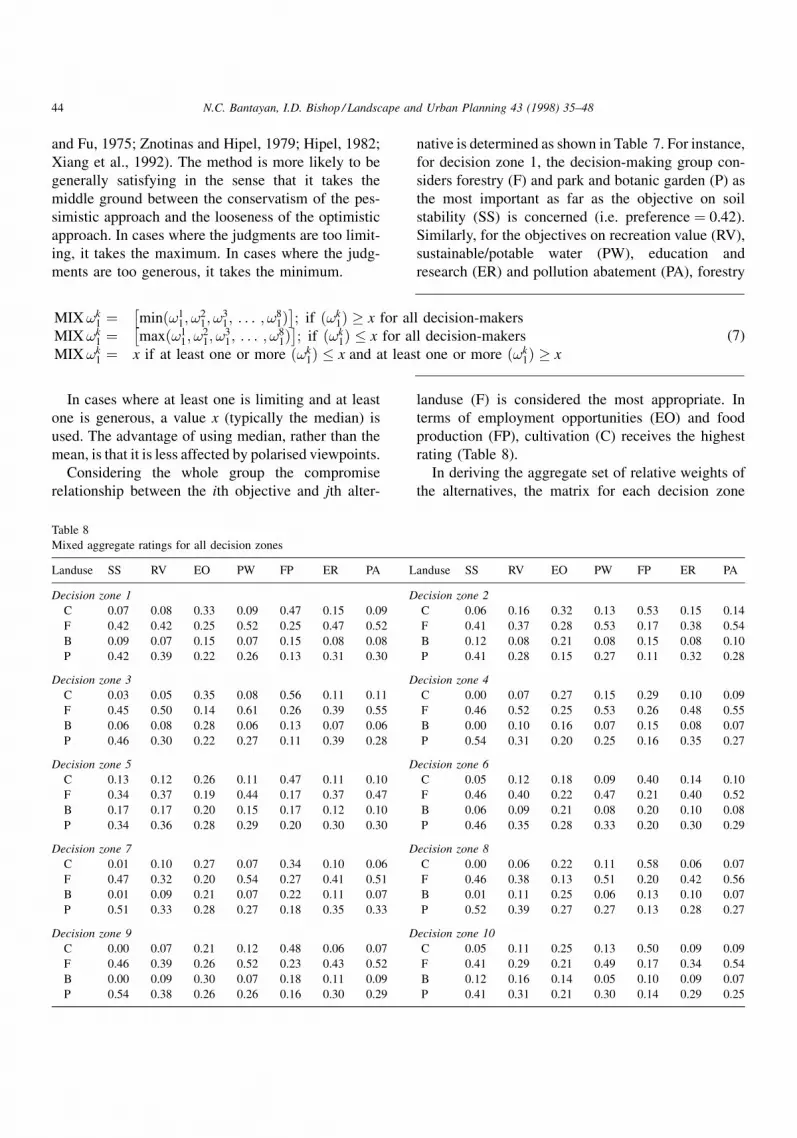
Considering the whole group the compromise

relationship between the ith objective and jth alter-

native is determined as shown in Table 7. For instance,

for decision zone 1, the decision-making group con-

siders forestry (F) and park and botanic garden (P) as

the most important as far as the objective on soil

stability (SS) is concerned (i.e. preference � 0.42).

Similarly, for the objectives on recreation value (RV),

sustainable/potable water (PW), education and

research (ER) and pollution abatement (PA), forestry

landuse (F) is considered the most appropriate. In

terms of employment opportunities (EO) and food

production (FP), cultivation (C) receives the highest

rating (Table 8).

In deriving the aggregate set of relative weights of

the alternatives, the matrix for each decision zone

MIX!k1 � min�!1

1; !21; !

31; . . . ; !8

1��

; if �!k1� � x for all decision-makers

MIX!k1 � max�!1

1; !21; !

31; . . . ; !8

1��

; if �!k1� � x for all decision-makers

MIX!k1 � x if at least one or more �!k

1� � x and at least one or more �!k1� � x

(7)

Table 8

Mixed aggregate ratings for all decision zones

Landuse SS RV EO PW FP ER PA Landuse SS RV EO PW FP ER PA

Decision zone 1 Decision zone 2

C 0.07 0.08 0.33 0.09 0.47 0.15 0.09 C 0.06 0.16 0.32 0.13 0.53 0.15 0.14

F 0.42 0.42 0.25 0.52 0.25 0.47 0.52 F 0.41 0.37 0.28 0.53 0.17 0.38 0.54

B 0.09 0.07 0.15 0.07 0.15 0.08 0.08 B 0.12 0.08 0.21 0.08 0.15 0.08 0.10

P 0.42 0.39 0.22 0.26 0.13 0.31 0.30 P 0.41 0.28 0.15 0.27 0.11 0.32 0.28


C 0.03 0.05 0.35 0.08 0.56 0.11 0.11 C 0.00 0.07 0.27 0.15 0.29 0.10 0.09

F 0.45 0.50 0.14 0.61 0.26 0.39 0.55 F 0.46 0.52 0.25 0.53 0.26 0.48 0.55

B 0.06 0.08 0.28 0.06 0.13 0.07 0.06 B 0.00 0.10 0.16 0.07 0.15 0.08 0.07

P 0.46 0.30 0.22 0.27 0.11 0.39 0.28 P 0.54 0.31 0.20 0.25 0.16 0.35 0.27


C 0.13 0.12 0.26 0.11 0.47 0.11 0.10 C 0.05 0.12 0.18 0.09 0.40 0.14 0.10

F 0.34 0.37 0.19 0.44 0.17 0.37 0.47 F 0.46 0.40 0.22 0.47 0.21 0.40 0.52

B 0.17 0.17 0.20 0.15 0.17 0.12 0.10 B 0.06 0.09 0.21 0.08 0.20 0.10 0.08

P 0.34 0.36 0.28 0.29 0.20 0.30 0.30 P 0.46 0.35 0.28 0.33 0.20 0.30 0.29


C 0.01 0.10 0.27 0.07 0.34 0.10 0.06 C 0.00 0.06 0.22 0.11 0.58 0.06 0.07

F 0.47 0.32 0.20 0.54 0.27 0.41 0.51 F 0.46 0.38 0.13 0.51 0.20 0.42 0.56

B 0.01 0.09 0.21 0.07 0.22 0.11 0.07 B 0.01 0.11 0.25 0.06 0.13 0.10 0.07

P 0.51 0.33 0.28 0.27 0.18 0.35 0.33 P 0.52 0.39 0.27 0.27 0.13 0.28 0.27


C 0.00 0.07 0.21 0.12 0.48 0.06 0.07 C 0.05 0.11 0.25 0.13 0.50 0.09 0.09

F 0.46 0.39 0.26 0.52 0.23 0.43 0.52 F 0.41 0.29 0.21 0.49 0.17 0.34 0.54

B 0.00 0.09 0.30 0.07 0.18 0.11 0.09 B 0.12 0.16 0.14 0.05 0.10 0.09 0.07

P 0.54 0.38 0.26 0.26 0.16 0.30 0.29 P 0.41 0.31 0.21 0.30 0.14 0.29 0.25


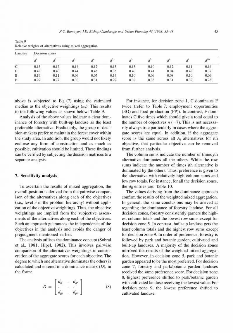
above is subjected to Eq. (7) using the estimated

median as the objective weightings (!i). This results

to the following values as shown below: Table 9.

Analysis of the above values indicate a clear dom-

inance of forestry with built-up landuse as the least

preferable alternative. Predictably, the group of deci-

sion-makers prefer to maintain the forest cover within

the study area. In addition, the group would not likely

endorse any form of construction and as much as

possible, cultivation should be limited. These ®ndings

can be veri®ed by subjecting the decision matrices to a

separate analysis.

7. Sensitivity analysis

To ascertain the results of mixed aggregation, the

overall position is derived from the pairwise compar-

ison of the alternatives along each of the objectives

(i.e., level 3 in the problem hierarchy) without appli-

cation of the objective weightings. Thus, the objective

weightings are implied from the subjective assess-

ments of the alternatives along each of the objectives.

Such an approach guarantees the independence of the

objectives in the analysis and avoids the danger of

prejudgment mentioned earlier.

The analysis utilises the dominance concept (Sobral

et al., 1981; Hipel, 1982). This involves pairwise

comparison of the alternatives weightings in consid-

eration of the aggregate scores for each objective. The

degree to which one alternative dominates the others is

calculated and entered in a dominance matrix (D), in

the form:

D �djj : djp

: : :dpj : dpp

24 35 (8)

For instance, for decision zone 1, C dominates F

twice (refer to Table 7; employment opportunities

(EO) and food production (FP)). In contrast, F dom-

inates C ®ve times which should give a total equal to

the number of objectives n (�7). This is not necessa-

rily always true particularly in cases where the aggre-

gate scores are equal. In addition, if the aggregate

score is the same across all Aj alternatives for ith

objective, that particular objective can be removed

from further analysis.

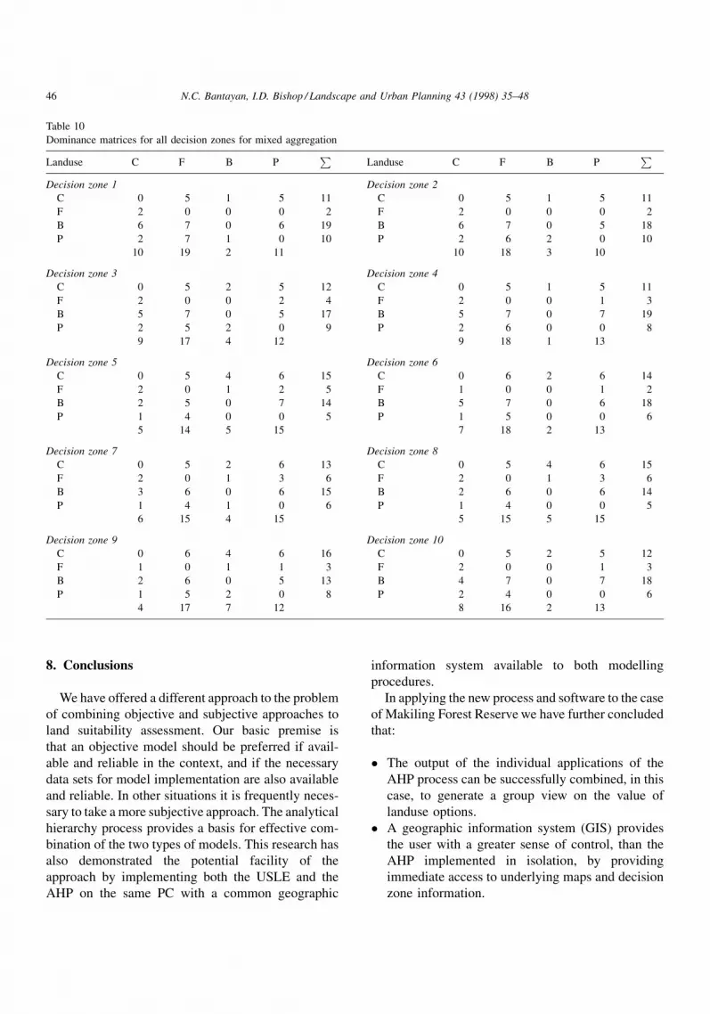
The column sums indicate the number of times jth

alternative dominates all the others. While the row

sums indicate the number of times jth alternative is

dominated by the others. Thus, preference is given to

the alternative with relatively high column sums and

low row totals. For instance, for all the decision zones,

the djj entries are: Table 10.

The values deriving from the dominance approach

con®rm the results of the weighted mixed aggregation.

In general, the same conclusions may be arrived at

regarding the dominance of forestry landuse. For all

decision zones, forestry consistently garners the high-

est column totals and the lowest row sums except for

decision zone 5. In contrast, built-up landuse gets the

least column totals and the highest row sums except

for decision zone 9. In order of preference, forestry is

followed by park and botanic garden, cultivated and

built-up landuses. A majority of the decision zones

mirrored the results of the weighted mixed aggrega-

tion. However, in decision zone 5, park and botanic

garden appeared to be the most preferred. For decision

zone 7, forestry and park/botanic garden landuses

received the same preference score. For decision zone

8, highest preference shifted to park/botanic garden

with cultivated landuse receiving the lowest value. For

decision zone 9, the lowest preference shifted to

cultivated landuse.

Table 9

Relative weights of alternatives using mixed aggregation

Landuse Decision zones

d1 d2 d3 d4 d5 d6 d7 d8 d9 d10

C 0.15 0.17 0.14 0.12 0.13 0.13 0.10 0.12 0.11 0.14

F 0.42 0.40 0.44 0.45 0.35 0.40 0.41 0.04 0.42 0.37

B 0.19 0.11 0.09 0.07 0.14 0.10 0.09 0.08 0.10 0.09

P 0.29 0.27 0.30 0.31 0.29 0.32 0.33 0.31 0.32 0.28


8. Conclusions

We have offered a different approach to the problem

of combining objective and subjective approaches to

land suitability assessment. Our basic premise is

that an objective model should be preferred if avail-

able and reliable in the context, and if the necessary

data sets for model implementation are also available

and reliable. In other situations it is frequently neces-

sary to take a more subjective approach. The analytical

hierarchy process provides a basis for effective com-

bination of the two types of models. This research has

also demonstrated the potential facility of the

approach by implementing both the USLE and the

AHP on the same PC with a common geographic

information system available to both modelling

procedures.

In applying the new process and software to the case

of Makiling Forest Reserve we have further concluded

that:

� The output of the individual applications of the

AHP process can be successfully combined, in this

case, to generate a group view on the value of

landuse options.

� A geographic information system (GIS) provides

the user with a greater sense of control, than the

AHP implemented in isolation, by providing

immediate access to underlying maps and decision

zone information.

Table 10

Dominance matrices for all decision zones for mixed aggregation

Landuse C F B PP

Landuse C F B PP


C 0 5 1 5 11 C 0 5 1 5 11

F 2 0 0 0 2 F 2 0 0 0 2

B 6 7 0 6 19 B 6 7 0 5 18

P 2 7 1 0 10 P 2 6 2 0 10

10 19 2 11 10 18 3 10


C 0 5 2 5 12 C 0 5 1 5 11

F 2 0 0 2 4 F 2 0 0 1 3

B 5 7 0 5 17 B 5 7 0 7 19

P 2 5 2 0 9 P 2 6 0 0 8

9 17 4 12 9 18 1 13


C 0 5 4 6 15 C 0 6 2 6 14

F 2 0 1 2 5 F 1 0 0 1 2

B 2 5 0 7 14 B 5 7 0 6 18

P 1 4 0 0 5 P 1 5 0 0 6

5 14 5 15 7 18 2 13


C 0 5 2 6 13 C 0 5 4 6 15

F 2 0 1 3 6 F 2 0 1 3 6

B 3 6 0 6 15 B 2 6 0 6 14

P 1 4 1 0 6 P 1 4 0 0 5

6 15 4 15 5 15 5 15


C 0 6 4 6 16 C 0 5 2 5 12

F 1 0 1 1 3 F 2 0 0 1 3

B 2 6 0 5 13 B 4 7 0 7 18

P 1 5 2 0 8 P 2 4 0 0 6

4 17 7 12 8 16 2 13


Acknowledgements

We wish to thank the staff of the University of the

Philippines, Los BanÄos College of Forestry and Nat-

ural Resources who supplied the data for this research.

Special thanks are due those who participated in the

workshop.

References

Banai-Kashani, A.R., 1990. Dealing with uncertainty and fuzziness

in development planning: a simulation of hightech industrial

location decision-making by the analytic hierarchy process.

Environment and Planning A 22, 1183±1203.

Banai-Kashani, R., 1989. A new method for site suitability

analysis: the analytic hierarchy process. Environ. Manage.

13(6), 685±693.

Bantayan, N.C., 1997. GIS-based estimation of soil loss. In: The

Pterocarpus, vol. 9. pp. 1, 24±35.

Bantayan, N.C., 1996. Participatory Decision Support Systems:

The Case of the Makiling Forest Reserve. Ph.D. Thesis, The

University of Melbourne, Australia.

Bantayan, N.C., Bishop, I.D., 1993a. The role of GIS in

integrating fuzziness and modelling in landuse planning. In:

Proceedings of the 21st Annual International Conference and

Technical Exhibition, AURISA 93. Aurisa, Adelaide, South

Australia.

Bantayan, N.C., Bishop, I.D., 1993b. An approach to combine

fuzziness with a physical model for landuse planning using

GIS. In: Proceedings of the Land Information Management and

Geographic Information Systems (LIM & GIS) Conference.

University of New South Wales, Sydney, Australia.

Barber, G.M., 1976. Land-use plan design via interactive multi-

objective programming. Environment and Planning A 8, 625±

636.

Batty, M., 1979. On planning processes. In: Goodall, B., Kirby, A.

(Eds.), Resources and Planning. Pergamon Press, Oxford, pp.

17±45.

Blin, J.M., Whinston, A.B., 1973. Fuzzy sets and social choice. J.

Cybernetics 3(4), 28±36.

Brule, J.F., 1992. Fuzzy systems ± a tutorial. From baechte-

[email protected] Newsgroup: comp.ai. 11 pp.

Carver, S.J., 1991. Integrating multi-criteria evaluation with

geographical information systems. Int. J. Geographical Infor-

mation Syst. 5(3), 321±339.

Dane, C.W., Meador, N.C., White, J.B., 1977. Goal programming

in land-use planning. J. Forestry (June), 75(6) 325±329.

Fung, L.W., Fu, K.S., 1975. An axiomatic approach to rational

decision-making in a fuzzy environment. In: Fuzzy Sets and

Their Applications To Cognitive and Decision Processes.

University of California, Berkeley, California, pp. 227±257.

Gupta, M.M., 1977. `Fuzzy-ism', the first decade. In: Gupta, M.,

Saridis, G., Gaines, B. (Eds.), Fuzzy Automata and Decision

Processes, Elsevier North-Holland, New York, pp. 5±10.

Hall, G.B., Wang, F., et al.1992. Comparison of Boolean and fuzzy

classification methods in land suitability analysis by using

geographical information systems. Environment and Planning

A 24, 497±516.

Hipel, K.W., 1982. Fuzzy set methodologies in multicriteria

modelling. In: Gupta, M.M., Sanchez, E. (Eds.), Fuzzy

Information and Decision Processes. North-Holland, Amster-

dam, pp. 279±287.

Itami, R.M., Raulings, R.J., 1993a. SAGE Introductory Guidebook.

Digital Land Systems Research, Melbourne, 106 pp.

Itami, R.M., Raulings, R.J., 1993b. SAGE Reference Manual.

Digital Land Systems Research, Melbourne, 113 pp.

Jankowski, P., 1995. Integrating geographical information systems

and multiple criteria decision-making methods. Int. J. Geo-

graphical Information Syst. 9(3), 251±273.

Jankowski, P., Richard, L., 1994. Integration of GIS-based

suitability analysis and multicriteria evaluation in a spatial

decision support system for route selection. Environment and

Planning B: Planning and Design 21, 323±340.

Jankowski, P., 1989. Mixed-data multicriteria evaluation for

regional planning: a systematic approach to the decision-

making process. Environment and Planning A 21, 349±362.

Kaufmann, A., Gupta, M.M., 1985. Introduction to Fuzzy

Arithmetic ± Theory and Applications. Van Nostrand Reinhold,

New York, 351 pp.

Lehmann, E.L., D'Abrera, H.J.M., 1975. Nonparametrics: Statis-

tical Methods Based on Ranks. Holden-Day, San Francisco,

CA, 458 pp.

Leitner, H., Nijkamp, P., Wrigley, N., 1985. Qualitative spatial data

analysis: a compendium of approaches. In: Nijkamp, P.,

Leitner, H., Wrigley, N. (Eds.), Measuring the Unmeasurable.

Nijhoff (Martinus), Dordrecht, pp. 1±28.

Mendoza, G.A., Sprouse, W., 1989. Forest planning and decision-

making under fuzzy environments: an overview and illustration.

For. Sci. 35(2), 481±502.

Mendoza, G.A., Bruce Bare, B., Zhou, Z., 1993. A fuzzy multiple

objective linear programming approach to forest planning

under uncertainty. Agric. Syst. 41, 257±274.

Nijkamp, P., Voogd, H., 1985. A survey of qualitative multiple

criteria choice models. In: Nijkamp, P., Leitner, H., Wrigley, N.

(Eds.), Measuring the Unmeasurable. Dordrecht, Martinus

Nijhoff Publishers, 425±427.

Nijkamp, P., Rietveld, P., 1976. Multi-objective programming

models. Regional Science and Urban Economics 6, 253±274.

Rehman, T., Romero, C., 1993. The application of the MCDM

paradigm to the management of agricultural systems: some

basic considerations. Agric. Syst. 41, 239±255.

Ridgley, M.A., Giambelluca, T.W., 1992. Linking water-balance

simulation and multiobjective programming: land-use plan

design in Hawaii. Environment and Planning B: Planning and

Design 19, 317±336.

Ridgley, M.A., 1984. Water and urban land-use planning in the

developing world: a linked simulation-multiobjective approach.

Environment and Planning B: Planning and Design 11, 229±242.

Saaty, T.L., 1980. The Analytic Hierarchy Process ± Planning,

Priority Setting, Resource Allocation. McGraw-Hill, New York,

287 pp.


Smith, P.N., 1992. Fuzzy evaluation of land-use and transportation

options. Environment and Planning B: Planning and Design 19,

525±544.

Sobral, M.M., Hipel, K.W., Farquhar, G.J., 1981. A multi-criteria

model for solid waste management. J. Environ. Manage. 12,

97±110.

Takeda, E., 1975. Interactive identification of fuzzy outranking

relations in a multicriteria decision problem. Paper read at

Fuzzy information and decision processes.

Voogd, H., 1983. Multiple Criteria Evaluation for Urban and

Regional Planning. Pion, London, 367 pp.

Whitley, D.L., Xiang, W.-N., Young, J.J., 1993. Use a GIS `Melting

Pot' to assess land use suitability. GIS World 6 (7).

Wischmeier, W.H., 1959. A rainfall erosion index for a universal

soil loss equation. Soil Sci. Soc. Am. 23, 246±249.

Xiang, W.-N., Gross, M., Gy Fabos, J., MacDougall, E.B., 1992. A

fuzzy-group multicriteria decision-making model and its

application to land-use planning. Environment and Planning

B: Planning and Design 19, 61±84.

Xiang, W.-N., 1993. A GIS/MMP-based coordination model and its

application to distributed environmental planning. Environment

and Planning B: Planning and Design 20, 195±220.

Zadeh, L.A., 1977. Fuzzy set theory: a perspective. In: Gupta, M.,

Saridis, G., Gaines, B. (Eds.), Fuzzy Automata and Decision

Processes. Elsevier North-Holland, New York, pp. 3±4.

Zimmermann, H.J., 1991. Fuzzy set theory and its applications.

Norwell, Massachusetts, Kluwer Academic Press.

Znotinas, N.M., Hipel, K.W., 1979. Comparison of alternative

engineering designs. Water Resources Bull. 15(1), 44±59.


Documents

Linking objective and subjective modelling for landuse decision-making