Learning Co-Sparse Analysis Operators with Separable ... - HAL-Inria

HAL Id: hal-01130411https://hal.inria.fr/hal-01130411

Submitted on 5 Oct 2015

HAL is a multi-disciplinary open accessarchive for the deposit and dissemination of sci-entific research documents, whether they are pub-lished or not. The documents may come fromteaching and research institutions in France orabroad, or from public or private research centers.

L’archive ouverte pluridisciplinaire HAL, estdestinée au dépôt et à la diffusion de documentsscientifiques de niveau recherche, publiés ou non,émanant des établissements d’enseignement et derecherche français ou étrangers, des laboratoirespublics ou privés.

Learning Co-Sparse Analysis Operators with SeparableStructures

Matthias Seibert, Julian Wörmann, Rémi Gribonval, Martin Kleinsteuber

To cite this version:Matthias Seibert, Julian Wörmann, Rémi Gribonval, Martin Kleinsteuber. Learning Co-Sparse Analy-sis Operators with Separable Structures. IEEE Transactions on Signal Processing, Institute of Electri-cal and Electronics Engineers, 2015, 64 (1), pp.120-130. 10.1109/TSP.2015.2481875. hal-01130411

https://hal.inria.fr/hal-01130411

https://hal.archives-ouvertes.fr

IEEE TRANSACTIONS ON SIGNAL PROCESSING 1

Learning Co-Sparse Analysis Operators withSeparable Structures

Matthias Seibert, Student Member, IEEE, Julian Wormann, Student Member, IEEE,Remi Gribonval, Fellow, IEEE, and Martin Kleinsteuber, Member, IEEE

Abstract—In the co-sparse analysis model a set of filters isapplied to a signal out of the signal class of interest yieldingsparse filter responses. As such, it may serve as a prior in inverseproblems, or for structural analysis of signals that are known tobelong to the signal class. The more the model is adapted tothe class, the more reliable it is for these purposes. The task oflearning such operators for a given class is therefore a crucialproblem. In many applications, it is also required that the filterresponses are obtained in a timely manner, which can be achievedby filters with a separable structure.

Not only can operators of this sort be efficiently used forcomputing the filter responses, but they also have the advantagethat less training samples are required to obtain a reliableestimate of the operator.

The first contribution of this work is to give theoreticalevidence for this claim by providing an upper bound for thesample complexity of the learning process. The second is astochastic gradient descent (SGD) method designed to learn ananalysis operator with separable structures, which includes anovel and efficient step size selection rule. Numerical experimentsare provided that link the sample complexity to the convergencespeed of the SGD algorithm.

Index Terms—Co-sparsity, separable filters, sample complexity,stochastic gradient descent

I. INTRODUCTION

THE ability to sparsely represent signals has become stan-dard practice in signal processing over the last decade.

The commonly used synthesis approach has been extensivelyinvestigated and has proven its validity in many applications.Its closely related counterpart, the co-sparse analysis approach,was at first not treated with as much interest. In recentyears this has changed and more and more work regardingthe application and the theoretical validity of the co-sparseanalysis model has been published. Both models assume thatthe signals s of a certain class are (approximately) containedin a union of subspaces. In the synthesis model, this reads as

s ≈ Dx, x is sparse. (1)

In other words, the signal is a linear combination of a few

Copyright (c) 2015 IEEE. Personal use of this material is permitted.However, permission to use this material for any other purposes must beobtained from the IEEE by sending a request to [email protected].

The first two authors contributed equally to this work. This paper waspresented in part at SPARS 2015, Cambridge, UK.

M. Seibert, J. Wormann, and M. Kleinsteuber are with the Department ofElectrical and Computer Engineering, TU Munchen, Munich, Germany.E-mail: m.seibert,julian.woermann,[email protected]: http://www.gol.ei.tum.de/

R. Gribonval heads the PANAMA project-team (Inria & CNRS), Rennes,France. E-mail: [email protected]

columns of the synthesis dictionary D. The subspace isdetermined by the indices of the non-zero coefficients of x.

Opposed to that is the co-sparse analysis model

Ωs ≈ α, α is sparse. (2)

Ω is called the analysis operator and its rows representfilters that provide sparse responses. Here, the indices of thefilters with zero response determine the subspace to whichthe signal belongs. This subspace is in fact the intersectionof all hyperplanes to which these filters are normal vectors.Therefore, the information of a signal is encoded in its zeroresponses. In the following, α is referred to as the analyzedsignal.

While analytic analysis operators like the fused Lasso [1]and the finite differences operator, a close relative to the totalvariation [2], are frequently used, it is a well known factthat a concatenation of filters which is adapted to a specificclass of signals produces sparser signal responses. Learningalgorithms aim at finding such an optimal analysis operatorby minimizing the average sparsity over a representative set oftraining samples. An overview of recently developed analysisoperator learning schemes is provided in Section III.

Once an appropriate operator has been chosen there is aplethora of applications that it can be used for. Among theseapplications are regularizing inverse problems in imaging,cf. [3]–[6], where the co-sparsity is used to perform standardtasks such as image denoising or inpainting, bimodal super-resolution and image registration as presented in [7], where thejoint sparsity of analyzed signals from different modalities isminimized, image segmentation as investigated in [8], wherestructural similarity is measured via the co-sparsity of the ana-lyzed signals, classification as proposed in [9], where an SVMis trained on the co-sparse coefficient vectors of a training set,blind compressive sensing, cf. [10], where a co-sparse analysisoperator is learned adaptively during the reconstruction ofa compressively sensed signal, and finally applications inmedical imaging, e.g., for structured representation of EEGsignals [11] and tomographic reconstruction [12]. All theseapplications rely on the sparsity of the analyzed signal, andthus their success depends on how well the learned operatoris adapted to the signal class.

An issue commonly faced by learning algorithms is thattheir performance rapidly decreases as the signal dimensionincreases. To overcome this issue some of the authors proposedseparable approaches for both dictionary learning, cf. [13], andco-sparse analysis operator learning, cf. [14]. These separableapproaches offer the advantage of a noticeably reduced nu-


merical complexity. For example, for a separable operator forimage patches of size p×p the computational burden for bothlearning and applying the filters is reduced from O(p2) toO(p). We refer the reader to our previous work in [14] for adetailed introduction of separable co-sparse analysis operatorlearning.

In the paper at hand we show that separable analysis oper-ators provide the additional benefit of requiring less samplesduring the training phase in order to learn a reliable operator.This is expressed via the sample complexity for which weprovide a result for analysis operator learning, i.e., an upperbound η on the deviation of the expected co-sparsity w.r.t. thesample distribution and the average co-sparsity of a trainingset. Our main result presented in Theorem 9 in Section IVstates that η ∝ C/

√N , where N is the number of training

samples. The constant C depends on the constraints imposedon Ω and we show that it is considerably smaller in theseparable case. As a consequence, we are able to providea generalization bound of an empirically learned analysisoperator.

This generalization bound has a close relation to stochas-tic gradient descent methods. In Section V we introduce ageometric Stochastic Gradient Descent learning scheme forseparable co-sparse analysis operators with a new variable stepsize selection that is based on the Armijo condition. The novellearning scheme is evaluated in Section VI. Our experimentsconfirm the theoretical results on sample complexity in thesense that separable analysis operator learning shows an im-proved convergence rate in the test scenarios.

II. NOTATION

Scalars are denoted by lower-case and upper-case lettersα, n,N , column vectors are written as small bold-face lettersα, s, matrices correspond to bold-face capital letters A,S, andtensors are written as calligraphic letters A,S. This notationis consistently used for the lower parts of the structures. Forexample, the ith column of the matrix X is denoted by xi, theentry in the ith row and the jth column of X is symbolizedby xij , and for tensors xi1i2...iT denotes the entry in X withthe indices ij indicating the position in the respective mode.Sets are denoted by blackletter script C,F,X.

For the discussion of multidimensional signals, we make useof the operations introduced in [15]. In particular, to define theway in which we apply the separable analysis operator to asignal in tensor form we require the k-mode product.

Definition 1. Given the T -tensor S ∈ RI1×I2×...×IT and thematrix Ω ∈ RJk×Ik , their k-mode product is denoted by

S ×k Ω.

The resulting tensor is of the size I1× I2× . . .× Ik−1×Jk×Ik+1 × . . .× IT and its entries are defined as

(S ×k Ω)i1i2...ik−1jkik+1...iT =

Ik∑ik=1

si1i2...iT · ωjkik

for jk = 1, . . . , Jk.

The k-mode product can be rewritten as a matrix-vector

product using the Kronecker product ⊗ and the vec-operatorthat rearranges a tensor into a column vector such that

A = S ×1 Ω(1) ×2 Ω(2) . . .×T Ω(T )

⇔ vec(A) = (Ω(1) ⊗Ω(2) ⊗ . . .⊗Ω(T )) · vec(S).(3)

We also make use of the mapping

ι : RJ1×I1 × . . .× RJT×IT → R∏

k Jk×∏

k Ik

(Ω(1), . . . ,Ω(T )) 7→ Ω(1) ⊗ . . .⊗Ω(T ).(4)

The remainder of notational comments, in particular thoserequired for the discussion of the sample complexity, will beprovided in the corresponding sections.

III. RELATED WORK

As we have pointed out, learning an operator adaptedto a class of signals yields a sparser representation thanthose provided by analytic filter banks. It thus comes as nosurprise that there exists a variety of analysis operator learningalgorithms, which we briefly review in the following.

In [16] the authors present an adaptation of the well knownK-SVD dictionary learning algorithm to the co-sparse analysisoperator setting. The training phase consists of two stages.In the first stage the rows of the operator that determine thesubspace that each signal resides in are determined. In thesubsequent stage each row of the operator is updated to bethe vector that is “most orthogonal” to the signals associatedwith it. These two stages are repeated until a convergencecriterion is met.

In [4] it is postulated that the analysis operator is auniformly normalized tight frame, i.e., the columns of theoperator are orthogonal to each other while all rows havethe same `2-norm. Given noise contaminated training samples,an algorithm is proposed that outputs an analysis operator aswell as noise free approximations of the training data. This isachieved by an alternating two stage optimization algorithm.In the first stage the operator is updated using a projectedsubgradient algorithm, while in the second stage the signalestimation is updated using alternating direction method ofmultipliers (ADMM).

A concept very similar to that of analysis operator learningis called sparsifying transform learning. In [17] a frameworkfor learning overcomplete sparsifying transforms is presented.This algorithm consists of two steps, a sparse coding stepwhere the sparse coefficient is updated by only retainingthe largest coefficients, and a transform update step where astandard conjugate gradient method is used and the resultingoperator is obtained by normalizing the rows.

The authors of [6] propose a method specialized on imageprocessing. Instead of a patch-based approach, an image-basedmodel is proposed with the goal of enforcing coherence acrossoverlapping patches. In this framework, which is based onhigher-order filter-based Markov Random Field models, allpossible patches in the entire image are considered at onceduring the learning phase. A bi-level optimization scheme isproposed that has at its heart an unconstrained optimizationproblem w.r.t. the operator, which is solved using a quasi-Newton method.


Dong et al. [18] propose a method that alternates betweena hard thresholding operation of the co-sparse representationand an operator update stage where all rows of the operatorare simultaneously updated using a gradient method on thesphere. Their target function has the form ‖A−ΩS‖2F , whereA is the co-sparse representation of the signal S.

Finally, Hawe et al. [3] propose a geometric conjugategradient algorithm on the product of spheres, where analysisoperator properties like low coherence and full rank areincorporated as penalty functions in the learning process.

Except for our previous work [14], to our knowledge theonly other analysis operator learning approach that offers aseparable structure is proposed in [19] for the two-dimensionalsetting. Therein, an algorithm is developed that takes as aninput noisy 2D patches Si, i = 1, . . . , N and then attemptsto find Si,Ω1,Ω2 that minimize

∑Ni=1 ‖Si − Si‖2F such that

‖Ω1SiΩ>2 ‖0 ≤ l, where l is a positive integer that serves as

an upper bound on the number of non-zero entries, and therows of Ω1 and Ω2 have unit norm. This problem is solvedby alternating between a sparse coding stage and an operatorupdate stage that is inspired by the work in [16] and relies onsingular value decompositions.

While, to our knowledge, there are no sample complexity re-sults for separable co-sparse analysis operator learning, resultsfor many other matrix factorization schemes exist. Examplesfor this can be found in [20]–[22], among others. Specifically,[22] provides a broad overview of sample complexity resultsfor various matrix factorizations. It is also of particular in-terest to our work since the sample complexity of separabledictionary learning is discussed. The bound derived thereinhas the form c

√β log(N)/N where the driving constant β

behaves proportional to∑i pidi for multidimensional data

in Rp1×...×pT and dictionaries D(i) ∈ Rpi×di . This is animprovement over the non-separable result where the driv-ing constant is proportional to the product over all i, i.e.,β ∝

∏i pidi. The argumentation used to derive the results

in [22] is different from the one we employ throughout thispaper. While the results in [22] are derived by determininga Lipschitz constant and then using an argument based oncovering numbers and concentration of measure, we followa different approach. Following the work in [20], we employMcDiarmid’s inequality in combination with a symmetrizationargument and Rademacher averages. This approach offersbetter results when discussing tall matrices as in the case ofco-sparse analysis operator learning.

IV. SAMPLE COMPLEXITY

Co-sparse analysis operator learning aims at finding a setof filters concatenated in an operator Ω which generates anoptimal sparse representation A = ΩS of a set of trainingsamples S = [s1, . . . , sN ]. This is achieved by solving theoptimization problem

arg minΩ∈C

1N

N∑j=1

f(Ω, sj) (5)

where f(Ω, s) = g(Ωs) + p(Ω) with the sparsity promotingfunction g and the penalty function p. By restricting Ω to the

constraint set C it is ensured that certain trivial solutions areavoided, see e.g. [4]. The additional penalty function is used toenforce more specific constraints. We will discuss appropriatechoices of constraint sets at a later point in this section whilethe penalty function will be concretized in Section V.

Before we can provide our main theoretical result, we firstintroduce several concepts from the field of statistics in orderto make this work self-contained.

A. Rademacher & Gaussian Complexity

In the following, we consider the set of samples S =[s1, . . . , sN ], si ∈ X, where each sample is drawn accordingto an underlying distribution P over X. Furthermore, given theabove defined function f : C× X→ R, we consider the classF = f(Ω, ·) : Ω ∈ C of functions that map the samplespace X to R. We are interested in finding the function f ∈ Ffor which the expected value

E[f ] := Es∼P[f(Ω, s)]

is minimal. However, due to the fact that the distribution P ofthe data samples is not known, in general, it is not possibleto determine the optimal solution to this problem and we arelimited to finding a minimizer of the empirical mean for agiven set of N samples S drawn according to the underlyingdistribution. The empirical mean is defined as

ES[f ] := 1N

N∑i=1

f(Ω, si).

In order to evaluate how well the empirical problem approx-imates the expectation we pursue an approach that relies onthe Rademacher complexity. We use the definition introducedin [23].

Definition 2. Let F ⊂ f(Ω, ·) : Ω ∈ C be a family of realvalued functions defined on the set X. Furthermore, let S =[s1, . . . , sN ] be a set of samples with si ∈ X. The empiricalRademacher complexity of F with respect to the set of samplesS is defined as

RS(F) := Eσ

[supf∈F

1N

N∑i=1

σif(Ω, si)

]where σ1, . . . , σN are independent Rademacher variables, i.e.,random variables with Pr(σi = +1) = Pr(σi = −1) = 1/2for i = 1, . . . , N .

This definition differs slightly from the standard one, wherethe absolute value of the argument within the supremum istaken, cf. [24]. Both definitions coincide when F is closedunder negation, i.e., when f ∈ F implies −f ∈ F. Asproposed in [23], the definition of the empirical Rademachercomplexity as above has the property that it is dominated bythe standard empirical Rademacher complexity. Furthermore,RS(F) vanishes when the function class F consists of a singleconstant function.

Definition 2 is based on a fixed set of training samples S.However, we are generally interested in the correlation of Fwith respect to a distribution P over X. This encourages thefollowing definition.


Definition 3. Let F be as before and S = [s1, . . . , sN ] bea set of samples si, i = 1, . . . , N drawn i.i.d. according toa predefined probability distribution P. Then the Rademachercomplexity of F is defined as

RN (F) := ES[RS(F)].

With these definitions it is possible to provide generalizationbounds for general function classes. Examples for this canbe found in [24]. In addition to the Rademacher complexity,another measure of complexity is required to obtain boundsfor our concrete case at hand. As before, the definition usedhere slightly differs from the standard definition, which canbe found in [24].

Definition 4. Let F ⊂ f(Ω, ·) : Ω ∈ C be a family ofreal valued functions defined on the set X. Furthermore, letS = [s1, . . . , sN ] be a set of samples with si ∈ X. Thenthe empirical Gaussian complexity of the function class F isdefined as

GS(F) = Eγ

[supf∈F

1N

N∑i=1

γif(Ω, si)

]where γ1, . . . , γN are independent Gaussian N (0, 1) randomvariables. The Gaussian complexity of F is defined as

GN (F) = ES

[GS(F)

].

Based on the similar construction of Rademacher and Gaus-sian complexity it is not surprising that it is possible to provethat they fulfill a similarity condition. For us, it is only ofinterest to upper bound the Rademacher complexity with theGaussian complexity.

Lemma 5. Let F be a class of functions mapping from Xto R. For any set of samples S, the empirical Rademachercomplexity can be upper bounded with the empirical Gaussiancomplexity via

RS(F) ≤√π/2 · GS(F).

This can be seen by noting that E[|γi|] =√

2/π and byusing Jensen’s inequality, cf. [25].

B. Generalization Bound for Co-Sparse Analysis OperatorLearning

In this section we provide the concrete bounds for thesample complexity of co-sparse analysis operator learning. Atthe beginning of Section IV we briefly mentioned that the keyrole of constraint sets is to avoid trivial solutions [4]. A verysimple constraint, that achieves this goal is to require that eachrow of the learned operator has unit `2-norm, cf. [3], [4]. Theset of all matrices that fulfills this property has a manifoldstructure and is often referred to as the oblique manifold

Ob(m, p) = Ω ∈ Rm×p : (ΩΩ>)ii = 1, i = 1, . . . ,m.(6)

This is the constraint set we employ for non-separable op-erator learning, which we want to distinguish from learningoperators with separable structure.

A separable structure on the operator is enforced by furtherrestricting the constraint set to the subset Ω ∈ Ob(m, p) :

Ω = ι(Ω(1), . . . ,Ω(T )), Ω(i) ∈ Ob(mi, pi) with the appro-priate dimensions m =

∏imi and p =

∏i pi. The mapping

ι is defined in Equation (4). The fact that ι(Ω(1), . . . ,Ω(T ))is an element of Ob(m, p) is readily checked. While ι is notbijective onto Ob(m, p), this does not pose a problem for ourscenario. This way of expressing separable operators is relatedto signals S in tensor form via

ι(Ω(1), . . . ,Ω(T ))s = vec−1(s)×1 Ω(1) . . .×T Ω(T )

with vec−1(s) = S.To provide concrete results we will require the ability to

bound the absolute value of the realization of a function toits expectation. We use McDiarmid’s inequality, cf. [26], totackle this task.

Theorem 6 (McDiarmid’s Inequality). Suppose X1, . . . , XN

are independent random variables taking values in a set Xand assume that f : XN → R satisfies

supx1,...,xN ,xi

|f(x1, . . . , xN )− f(x1, . . . , xi−1, xi, xi+1, . . . , xN )|

≤ ci for 1 ≤ i ≤ N.It follows that for any ε > 0

Pr(E[f(X1, . . . , XN )]− f(X1, . . . , XN ) ≥ ε)

≤ exp

(− 2ε2∑N

i=1 c2i

).

We are now ready to state a preliminary result.

Lemma 7. Let S = [s1, . . . , sN ] be a set of samples indepen-dently drawn according to a distribution within the unit `2-ball in Rp. Let f(Ω, s) = g(Ωs)+p(Ω) as previously definedwhere the sparsity promoting function g is λ-Lipschitz. Finally,let the function class F be defined as F = f(Ω, ·) : Ω ∈Ob(m, p). Then the inequality

E[f ]− ES[f ] ≤√

2π GS(F) + 3

√2λ2m ln(2/δ)

N, (7)

holds with probability greater than 1− δ.

Proof. When considering the difference E[f ] − ES[f ] thepenalty function p can be omitted since it is independent ofthe samples and therefore cancels out. Now, in order to boundthe difference E[f ] − ES[f ] for all f ∈ F, we consider theequivalent problem of bounding supf∈F(E[f ]− ES[f ]). To dothis we introduce the random variable

Φ(S) = supf∈F

(E[f ]− ES[f ]).

The next step is to use McDiarmid’s inequality to boundΦ(S). Since Ω is an element of the constraint set Ob(m, p),its largest singular value is bounded by

√m. Furthermore, due

to the assumptions that g is λ-Lipschitz and ‖si‖2 ≤ 1, thefunction value of f(Ω, s) changes by at most 2λ

√m when

varying s. Since f appears within the empirical average inΦ, we get the result that the function value of Φ varies byat most 2λ

√m/N when changing a single sample in the set

S. Thus, McDiarmid’s inequality stated in Theorem 6 with a


target probability of δ yields the bound

Φ(S) ≤ ES[Φ(S)] +

√2λ2m ln(1/δ)

N(8)

with probability greater than 1− δ. By using a standard sym-metrization argument, cf. [27], and another instance of McDi-armid’s inequality we can then first upper bound ES[Φ(S)] by2RN (F) and then by 2RS(F), yielding

supf∈F

(E[f ]− ES[f ]) ≤ 2RS(F) + 3

√2λ2m ln(2/δ)

N

with probability greater than 1−δ. A more detailed derivationof these bounds can be found in the appendix. Lemma 5 thenprovides the proposed bound.

The last ingredient for the proof of our main theoremis Slepian’s Lemma, cf. [28], which is used to provide anestimate for the expectation of the supremum of a Gaussianprocess.

Lemma 8 (Slepian’s Lemma). Let X and Y be two centeredGaussian random vectors in RN such that

E[|Yi − Yj |2] ≤ E[|Xi −Xj |2] for i 6= j.

Then

E[

sup1≤1≤N

Yi

]≤ E

[sup

1≤i≤NXi

].

With all the preliminary work taken care of we are nowable to state and prove our main results.

Theorem 9. Let S = [s1, . . . , sN ] be a set of samples inde-pendently drawn according to a distribution within the unit `2-ball in Rp. Let f(Ω, s) = g(Ωs)+p(Ω) as previously definedwhere the sparsity promoting function g is λ-Lipschitz. Finally,let the function class F be defined as F = f(Ω, ·) : Ω ∈ C,where C is either Ob(m, p) for the non-separable case or thesubset Ω ∈ Ob(m, p) : Ω = ι(Ω(1), . . . ,Ω(T )), Ω(i) ∈Ob(mi, pi) for the separable case. Then we have

E[f ]− ES[f ] ≤√

2πλCC√N

+ 3

√2λ2m ln(2/δ)

N(9)

with probability at least 1 − δ, where CC is a constant thatdepends on the constraint set. In the non-separable case theconstant is defined as CC = m

√p, whereas in the separable

case it is given as CC =∑imi√pi.

Proof. Given the results of Lemma 7 it remains to upperbound the empirical Gaussian complexity. We discuss the twoconsidered constraint sets separately in the following.

Non-Separable Operator: In order to find a boundfor GS(F) we define the two Gaussian processesGΩ = 1

N

∑Ni=1 γif(Ω, si) and HΩ = λ√

N〈Ξ,Ω〉F =

λ√N

∑i,j ξijωij with γi and ξij i.i.d. Gaussian random

variables. These two processes fulfill the condition

Eγ [|GΩ −GΩ′ |2] ≤ λ2

N ‖Ω−Ω′‖2F = Eξ[|HΩ −HΩ′ |2],

where the inequality holds since f(Ω, si) is λ-Lipschitz w.r.t.the Frobenius norm in its first component when omitting the

penalty term, i.e.,

|f(Ω, si)− f(Ω′, si)| = |g(Ωsi)− g(Ω′si)| ≤ λ‖Ω−Ω′‖Ffor all Ω,Ω′ ∈ C. Thus, we can apply Slepian’s Lemma,cf. Lemma 8, which provides the inequality

Eγ [supΩ∈C

GΩ] ≤ Eξ[supΩ∈C

HΩ]. (10)

Note, that the left-hand side of this inequality is the empiricalGaussian complexity of our learning problem. Considering theconstraint set C the expression on the right-hand side can bebounded via

Eξ[supHΩ] = λ√NEξ[supΩ∈C〈Ξ,Ω〉F ]

= λ√NEξ[

m∑j=1

‖ξj‖2] ≤ λ√Nm√p.

Here, ξj ∈ Rp, j = 1, . . . ,m denotes the transposed of thej-th row of Ξ.

Separable Operator: To consider the separable analysisoperator in the sense of our previous work [14], we definethe set of functions

f : C× Rp → R,Ω 7→ g(ι(Ω)s).

The function f operates on the direct product of manifoldsC = Ob1×Ob2× . . . × ObT and utilizes the function ι asdefined in Equation (4). The signals si ∈ Rp can be interpretedas vectorized versions of tensorial signals Si ∈ Rp1×...×pTwhere p =

∏pi. Above, we showed that f is λ-Lipschitz

w.r.t. the Frobenius norm on its first variable Ω. As C is asubset of a large oblique manifold, the same holds true for f .

Similar to before, we define two Gaussian processesGΩ = 1

N

∑Ni=1 γif(Ω, si) with Ω ∈ C, and HΩ =

λ√N

∑Ti=1〈Ξ

(i),Ω(i)〉F . The expected value E[|HΩ −HΩ′ |2]

can be equivalently written as λ2

N E[(∑Ti=1 tr((Ξ(i))>Ω(i)))2]

and the inequality

Eγ [|GΩ −GΩ′ |2] ≤ λ2

N ‖Ω−Ω′‖2F = Eξ[|HΩ −HΩ′ |2]

holds, just as in the non-separable case. Hence, we areable to apply Slepian’s lemma which yields the inequalityE[supΩ∈CGΩ] ≤ E[supΩ∈CHΩ]. It only remains to providean upper bound for the right-hand side.

Using the fact that C is now the direct product of obliquemanifolds we get

Eξ [supΩ∈CHΩ] = Eξ

[supΩ∈C

λ√N

T∑i=1

tr(

(Ξ(i))>Ω(i))]

= λ√N

T∑i=1

Eξ[supΩ(i)∈Obi

tr(

(Ξ(i))>Ω(i))]

= λ√N

T∑i=1

Eξ

mi∑j=1

‖ξ(i)j ‖2

≤ λ√N

T∑i=1

mi√pi,

where ξ(i)j denotes the transposed of the j-th row of Ξ(i).The last inequality holds due to Jensen’s inequality and thefact that all ξij are N (0, 1) random variables.


Remark 1. Theorem 9 can be extended to the absolute value|E[f ]−ES[f ]| of the deviation by redefining the function classas F ∪ (−F).

V. STOCHASTIC GRADIENT DESCENT FOR ANALYSISOPERATOR LEARNING

Stochastic Gradient Descent (SGD) is particularly suited forlarge scale optimization and thus a natural choice for manymachine learning problems.

Before we describe a geometric SGD method that respectsthe underlying constraints on the analysis operator, we followthe discussion of SGD methods provided by Bottou in [29]in order to establish a connection of the excess error andthe sample complexity result derived in the previous section.Let f? = arg minf∈F E[f ] be the best possible predictionfunction, let f?S = arg minf∈F ES[f ] be the best possibleprediction function for a set of training samples S, and letfS be the solution found by an optimization method withrespect to the provided set of samples S. Bottou proposesthat the so-called excess error E = E[fS] − E[f?] can bedecomposed as the sum E = Eest + Eopt. Here, the estimationerror Eest = E[f?S] − E[f?] measures the distance betweenthe optimal solution for the expectation and the optimalsolution for the empirical average while the optimization errorEopt = E[fS] − E[f?S] quantifies the distance between theoptimal solution for the empirical average and the solutionobtained via an optimization algorithm.

While Eopt is dependent on the optimization strategy, the es-timation error Eest is closely related to the previously discussedsample complexity. Lower bounds on the sample complexityalso apply to the estimation error as specified in the followingCorollary.

Corollary 10. Under the same conditions as in Theorem 9the estimation error is upper bounded by

Eest ≤ 2√

2πλCC√N

+ 6

√2λ2m ln(2/δ)

N(11)

with probability at least 1− δ.

Proof. The estimation error can be bounded via

Eest = E[f?S]− E[f?] ≤ E[f?S]− E[f?]− ES[f?S] + ES[f?]

≤ |E[f?S]− ES[f?S]|+ |ES[f?]− E[f?]|,where the first inequality holds since f?S is the minimizer ofES, and therefore ES[f?S] ≤ ES[f?] and the final result followsfrom Theorem 9 and its subsequent remark.

A. Geometric Stochastic Gradient Descent

Ongoing from the seminal work of [30], SGD type op-timization methods have attracted attention to solve large-scale machine learning problems [31], [32]. In contrast to fullgradient methods that in each iteration require the computationof the gradient with respect to all the N training samplesS = [s1, . . . , sN ] in SGD the gradient computation onlyinvolves a small batch randomly drawn from the training setin order to find the Ω ∈ C which minimizes the expectationEs∼P[f(Ω, s)]. Accordingly, the cost of each iteration is

independent of N (assuming the cost of accessing each sampleis independent of N ).

In the following we use the notation sk(i) to denote asignal batch of cardinality |k(i)|, where k(i) represents anindex set randomly drawn from 1, 2, . . . , N at iteration i.

In order to account for the constraint set C we follow[33] and propose a geometric SGD optimization scheme. Thisrequires some modifications to classic SGD. The subsequentdiscussion provides a concise introduction to line searchoptimization methods on manifolds. For more insights intooptimization on manifolds in general we refer the reader to[34] and to [33] for optimization on manifolds using SGD inparticular.

In Euclidean space the direction of steepest descent ata point Ω is given by the negative (Euclidean) gradient.For optimization on an embedded manifold C this role istaken over by the negative Riemannian gradient, which is aprojection of the gradient onto the respective tangent space TΩ.To keep notation simple, we denote the Riemannian gradientw.r.t. Ω at a point (Ω, s) by G(Ω, s) = ΠTΩC(∇Ωf(Ω, s)).Optimization methods on manifolds find a new iteration pointby searching along geodesics instead of following a straightpath. We denote a geodesic emanating from point Ω in direc-tion H by Γ(Ω,H, ·). Following this geodesic for distancet then results in the new point Γ(Ω,H, t) ∈ C. Finally,an appropriate step size t has to be computed. A detaileddiscussion on this topic is provided in Section V-B.

Using these definitions, an update step of geometric SGDreads as

Ωi+1 = Γ(Ωi,−G(Ωi, sk(i)), ti). (12)

Since the SGD framework only provides a noisy estimate ofthe objective function in each iteration, a stopping criterionbased on the average over previous iterations is chosen toterminate the optimization scheme. First, let f(Ωi, sk(i))denote the mean over all signals in the batch sk(i) as-sociated to Ωi at iteration i. That is, f(Ωi, sk(i)) =

1|k(i)|

∑|k(i)|j=1 f(Ωi, sj), for sj ∈ sk(i). With the mean cost

for a single batch at hand we are able to calculate thetotal average including all previous iterations. This reads asφi = 1

i

∑i−1j=0 f(Ωi−j , sk(i−j)). Furthermore, let φi denote

the mean over the last l values of φi. Finally, we are able tostate our stopping criterion. The optimization terminates if therelative variation of φi, which is denoted as

v =(|φi − φi|

)/φi, (13)

falls below a certain threshold δ. In our implementation, weset l = 200 with a threshold δ = 5 · 10−5.

B. Step size selection

Regarding the convergence rate, a crucial factor of SGDoptimization is the selection of the step size (often also referredto as learning rate). For convex problems, the step size istypically based on the Lipschitz continuity property. If theLipschitz constant is not known in advance, an appropriatelearning rate is often chosen by using approximation tech-niques. In [35], the authors propose a basic line search that


Algorithm 1 SGD Backtracking Line SearchRequire: a0i > 0, b ∈ (0, 1), c ∈ (0, 1), Ωi,f(Ωi, sk(i−1)), G(Ωi, sk(i)), kmax = 40

Set: a← a0i , k ← 1while f(Γ(Ωi,−G(Ωi, sk(i)), a), sk(i)) >f(Ωi, sk(i−1))−a ·c ·‖G(Ωi, sk(i))‖2F ∧ k < kmax doa← b · ak ← k + 1

end whileOutput: ti ← a

sequentially halves the step size if the current estimate does notminimize the cost. Other approaches involve some predefinedheuristics to iteratively shrink the step size [36] which hasthe disadvantage of requiring the estimation of an additionalhyper-parameter. We suggest a more variable approach byproposing a variation of a backtracking line search algorithmadapted to SGD optimization.

As already stated in Section IV-A, our goal is to find aset of separable filters such that the empirical sparsity overall N samples from our training set is minimal. Now, recallthat instead of computing the gradient with respect to thefull training set, the SGD framework approximates the truegradient by means of a small signal batch or even a singlesignal sample. That is, the reduced computational complexitycomes at the cost of updates that do not minimize the overallobjective. However, it is assumed that on average the SGDupdates approach the minimum of the optimization problemstated in (5), i.e., the empirical mean over all training samples.We utilize this proposition to automatically find an appropriatestep size such that for the next iterate an averaging Armijocondition is fulfilled.

To be precise, starting from an initial step size a0i the steplength ai is successively shrunk until the next iterate fulfillsthe Armijo condition. That is, we have

f(Ωi+1, sk(i)) ≤ f(Ωi, sk(i−1))

− ai · c · ‖G(Ωi, sk(i))‖2F ,(14)

with some constant c ∈ (0, 1). Here, f denotes the average costover a predefined number of previous iterations. The averageis calculated over the function values f(Ωi+1, sk(i)), i.e.,over the cost of the optimized operator with respect to therespective signal batch. This is achieved via a sliding windowimplementation that reads

f(Ωi+1, sk(i)) = 1w

w−1∑j=0

f(Ωi+1−j , sk(i−j)), (15)

with w denoting the window size.

If (14) is not fulfilled, i.e., if the average including the newsample is not at least as low as the previous average, the stepsize ai goes to zero. To avoid needless line search iterations westop the execution after a predefined number of trials kmax andproceed with the next sample without updating the filters andwith resetting ai+1 to its initial value a0i . The complete stepsize selection approach is summarized in Algorithm 1. In ourexperiments we set the parameters to b = 0.9 and c = 10−4.

C. Cost Function and Constraints

An appropriate sparsity measure for our purposes is pro-vided by

g(α) :=∑m

j=1log(1 + να2

j

). (16)

This function serves as a smooth approximation to the `0-quasi-norm, cf. [7], but other smooth sparsity promotingfunctions are also conceivable.

In the section on sample complexity we introduced theoblique manifold as a suitable constraint set. Additionally,there are two properties we wish to enforce on the learnedoperator as motivated in [3]. (i) Full rank of the operator and(ii) No identical filters. This is achieved by incorporating twopenalty functions into the cost function, namely

h(Ω) = − 1p log(p) log det

(1m (Ω)>Ω

),

r(Ω) = −∑k<l

log(

1−((ωk)>(ωl)

)2).

The function h promotes (i) whereas r enforces (ii). Hence,the final optimization problem for a set of training samples si(vectorized versions of signals Si in tensor form) is given as

arg minΩ

1N

N∑j=1

f(Ω, sj)

subject to Ω = (Ω(1), . . . ,Ω(T )),

Ω(i) ∈ Ob(mi, pi), i = 1, . . . , T,

(17)

with the function

f(Ω, s) = g (ι(Ω)s) + κh(ι(Ω)) + µr(ι(Ω)). (18)

The parameters κ and µ are weights that control the impact ofthe full rank and incoherence condition. With this formulationof the optimization problem both separable as well as non-separable learning can be handled with the same cost functionallowing for a direct comparison of these scenarios.

VI. EXPERIMENTS

The purpose of the experiments presented in this section is,on the one side, to give some numerical evidence of the samplecomplexity results from Section IV, and on the other side, todemonstrate the efficiency and performance of our proposedlearning approach from Section V.

A. Learning from natural image patches

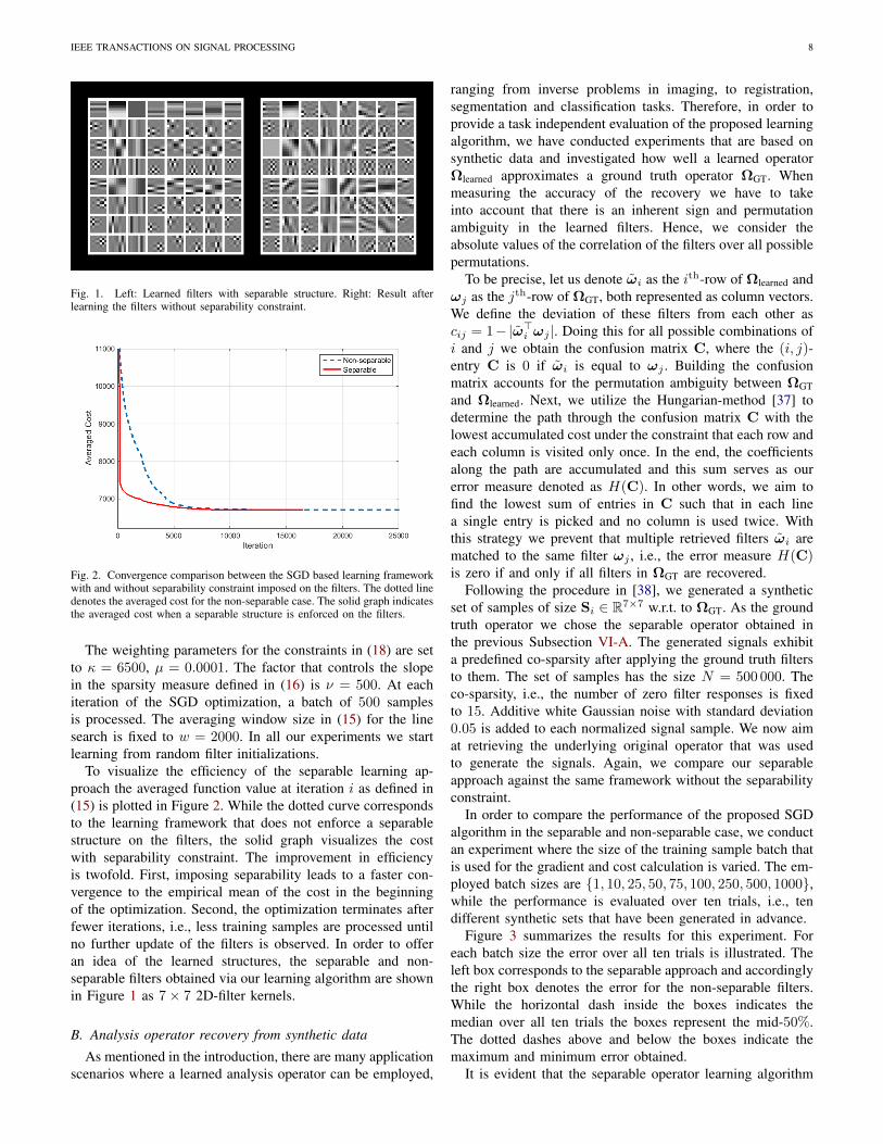
The task of our first experiment is to demonstrate thatseparable filters can be learned from less training samplescompared to learning a set of unstructured filters. We generateda training set that consists of N = 500 000 two-dimensionalnormalized samples of size Si ∈ R7×7 extracted at randomfrom natural images. The learning algorithm then providestwo operators Ω(1),Ω(2) ∈ R8×7 resulting in 64 separablefilters. We compare our proposed separable approach witha version of the same algorithm, that does not enforce aseparable structure on the filters and thus outputs a non-separable analysis operator Ω ∈ R64×49.


Fig. 1. Left: Learned filters with separable structure. Right: Result afterlearning the filters without separability constraint.

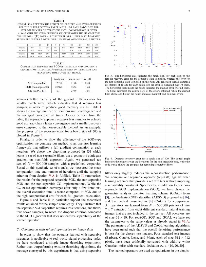
Fig. 2. Convergence comparison between the SGD based learning frameworkwith and without separability constraint imposed on the filters. The dotted linedenotes the averaged cost for the non-separable case. The solid graph indicatesthe averaged cost when a separable structure is enforced on the filters.

The weighting parameters for the constraints in (18) are setto κ = 6500, µ = 0.0001. The factor that controls the slopein the sparsity measure defined in (16) is ν = 500. At eachiteration of the SGD optimization, a batch of 500 samplesis processed. The averaging window size in (15) for the linesearch is fixed to w = 2000. In all our experiments we startlearning from random filter initializations.

To visualize the efficiency of the separable learning ap-proach the averaged function value at iteration i as defined in(15) is plotted in Figure 2. While the dotted curve correspondsto the learning framework that does not enforce a separablestructure on the filters, the solid graph visualizes the costwith separability constraint. The improvement in efficiencyis twofold. First, imposing separability leads to a faster con-vergence to the empirical mean of the cost in the beginningof the optimization. Second, the optimization terminates afterfewer iterations, i.e., less training samples are processed untilno further update of the filters is observed. In order to offeran idea of the learned structures, the separable and non-separable filters obtained via our learning algorithm are shownin Figure 1 as 7× 7 2D-filter kernels.

B. Analysis operator recovery from synthetic data

As mentioned in the introduction, there are many applicationscenarios where a learned analysis operator can be employed,

ranging from inverse problems in imaging, to registration,segmentation and classification tasks. Therefore, in order toprovide a task independent evaluation of the proposed learningalgorithm, we have conducted experiments that are based onsynthetic data and investigated how well a learned operatorΩlearned approximates a ground truth operator ΩGT. Whenmeasuring the accuracy of the recovery we have to takeinto account that there is an inherent sign and permutationambiguity in the learned filters. Hence, we consider theabsolute values of the correlation of the filters over all possiblepermutations.

To be precise, let us denote ωi as the ith-row of Ωlearned andωj as the jth-row of ΩGT, both represented as column vectors.We define the deviation of these filters from each other ascij = 1−|ω>i ωj |. Doing this for all possible combinations ofi and j we obtain the confusion matrix C, where the (i, j)-entry C is 0 if ωi is equal to ωj . Building the confusionmatrix accounts for the permutation ambiguity between ΩGTand Ωlearned. Next, we utilize the Hungarian-method [37] todetermine the path through the confusion matrix C with thelowest accumulated cost under the constraint that each row andeach column is visited only once. In the end, the coefficientsalong the path are accumulated and this sum serves as ourerror measure denoted as H(C). In other words, we aim tofind the lowest sum of entries in C such that in each linea single entry is picked and no column is used twice. Withthis strategy we prevent that multiple retrieved filters ωi arematched to the same filter ωj , i.e., the error measure H(C)is zero if and only if all filters in ΩGT are recovered.

Following the procedure in [38], we generated a syntheticset of samples of size Si ∈ R7×7 w.r.t. to ΩGT. As the groundtruth operator we chose the separable operator obtained inthe previous Subsection VI-A. The generated signals exhibita predefined co-sparsity after applying the ground truth filtersto them. The set of samples has the size N = 500 000. Theco-sparsity, i.e., the number of zero filter responses is fixedto 15. Additive white Gaussian noise with standard deviation0.05 is added to each normalized signal sample. We now aimat retrieving the underlying original operator that was usedto generate the signals. Again, we compare our separableapproach against the same framework without the separabilityconstraint.

In order to compare the performance of the proposed SGDalgorithm in the separable and non-separable case, we conductan experiment where the size of the training sample batch thatis used for the gradient and cost calculation is varied. The em-ployed batch sizes are 1, 10, 25, 50, 75, 100, 250, 500, 1000,while the performance is evaluated over ten trials, i.e., tendifferent synthetic sets that have been generated in advance.

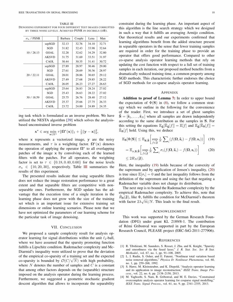
Figure 3 summarizes the results for this experiment. Foreach batch size the error over all ten trials is illustrated. Theleft box corresponds to the separable approach and accordinglythe right box denotes the error for the non-separable filters.While the horizontal dash inside the boxes indicates themedian over all ten trials the boxes represent the mid-50%.The dotted dashes above and below the boxes indicate themaximum and minimum error obtained.

It is evident that the separable operator learning algorithm


TABLE ICOMPARISON BETWEEN THE CONVERGENCE SPEED AND AVERAGE ERROR

FOR THE FILTER RECOVERY EXPERIMENT. FOR EACH BATCH SIZE THEAVERAGE NUMBER OF ITERATIONS UNTIL CONVERGENCE IS GIVEN

ALONG WITH THE AVERAGE ERROR WHICH DENOTES THE MEAN OF THEVALUES FOR H(C) OVER ALL THE TEN TRIALS. UPPER PART: LEARNINGSEPARABLE FILTERS. LOWER PART: LEARNING NON-SEPARABLE FILTERS.

1 10 25 50 75 100 250 500 1000

Iterations 450 422 2573 3721 4595 5780 9673 13637 15198

Avg. error 37.22 33.28 1.39 1.08 0.75 0.56 0.31 0.24 0.14

Iterations 1812 1800 2786 3866 10147 13595 19679 21087 20611

Avg. error 41.21 40.73 38.68 27.74 9.67 1.89 1.38 1.23 1.14

TABLE IICOMPARISON BETWEEN THE SGD OPTIMIZATION AND CONJUGATEGRADIENT OPTIMIZATION. AVERAGE NUMBER OF ITERATIONS AND

PROCESSING TIMES OVER TEN TRIALS.

Iterations time in sec H(C)

SGD (separable) 12358 1176 0.48SGD (non-separable) 21660 1554 1.24

CG (GOAL [3]) 601 2759 1.01

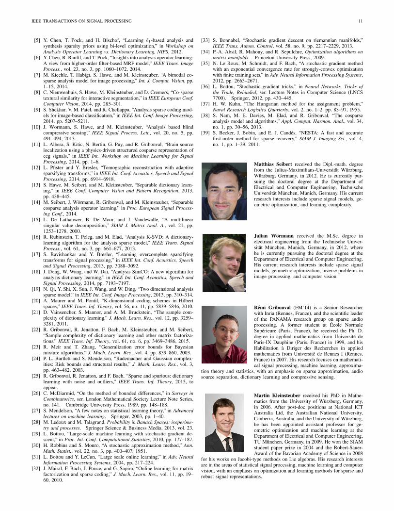
achieves better recovery of the ground truth operator forsmaller batch sizes, which indicates that it requires lesssamples in order to produce good recovery results. Table Ishows the average number of iterations until convergence andthe averaged error over all trials. As can be seen from thetable, the separable approach requires less samples to achievegood accuracy, has a faster convergence and a smaller recoveryerror compared to the non-separable method. As an example,the progress of the recovery error for a batch size of 500 isplotted in Figure 4.

Finally, in order to show the efficiency of the SGD-typeoptimization we compare our method to an operator learningframework that utilizes a full gradient computation at eachiteration. We chose the algorithm proposed in [3] whichlearns a set of non-separable filters via a geometric conjugategradient on manifolds approach. Again, we generated tensets of N = 500 000 samples with a predefined cosparsity.Based on this synthetic set of signals, we measured the meancomputation time and number of iterations until the stoppingcriterion from Section V-A is fulfilled. Table II summarizesthe results for the proposed separable SGD, the non-separableSGD and the non-separable CG implementations. While theCG based optimization converges after only a few iterations,the overall execution time is worse compared to SGD due tothe high computational cost for each full gradient calculation.

Figure 4 and Table II in particular support the theoreticalresults obtained for the sample complexity. They illustrate thatthe separable SGD algorithm requires less iterations, and there-fore fewer samples, to reach the dropout criterion comparedto the SGD algorithm that does not enforce separability of thelearned operator.

C. Comparison with related approaches on image data

In order to show that the operator learned with separablestructures is applicable to real world signal processing tasks,we have conducted a simple image denoising experiment.Rather than outperforming existing denoising algorithms, themessage conveyed by this experiment is that using separable

Fig. 3. The horizontal axis indicates the batch size. For each size, on theleft the recovery error for the separable case is plotted, whereas the error forthe non-separable case is plotted on the right. All generated signals exhibit aco-sparsity of 15 and for each batch size the error is evaluated over 10 trials.The horizontal dash inside the boxes indicates the median error over all trials.The boxes represent the central 50% of the errors obtained, while the dashedlines above and below the boxes indicate maximal and minimal errors.

Fig. 4. Operator recovery error for a batch size of 500. The dotted graphindicates the progress over the iterations for the non-separable case, while thesolid curve shows the progress for retrieving separable filters.

filters only slightly reduces the reconstruction performance.We compare our separable operator (sepSGD) against otherlearning schemes that provide a set of filters without imposinga separability constraint. Specifically, in addition to our non-separable SGD implementation (SGD), we have chosen thegeometric analysis operator learning scheme (GOAL) from[3], the Analysis-KSVD algorithm (AKSVD) proposed in [16],and the method presented in [4] (CAOL) for comparison.All operators are learned from N = 500 000 patches of size7 × 7 extracted from eight different standard natural trainingimages that are not included in the test set. All operators areof size 64 × 49. For sepSGD, SGD and GOAL we have setthe parameters to the same values as already stated in VI-A.The parameters of the AKSVD and CAOL learning algorithmshave been tuned such that the overall denoising performanceis best for the chosen test images. Four standard test images(Barbara, Couple, Lena, and Man), each of size 512 × 512pixels, have been artificially corrupted with additive whiteGaussian noise with standard deviation σn ∈ 10, 20, 30.

The learned operators are used as regularizers in the denois-


TABLE IIIDENOISING EXPERIMENT FOR FOUR DIFFERENT TEST IMAGES CORRUPTED

BY THREE NOISE LEVELS. ACHIEVED PSNR IN DECIBELS (DB).

σn / PSNR Barbara Couple Lena Man

sepSGD 32.13 32.76 34.10 32.71SGD 31.82 32.43 33.98 32.64

10 / 28.13 GOAL 32.28 32.62 34.29 32.80AKSVD 31.75 31.69 33.51 31.97CAOL 30.44 30.35 31.41 30.72

sepSGD 27.89 28.97 30.46 29.00SGD 27.61 28.69 30.36 28.97

20 / 22.11 GOAL 28.01 28.86 30.65 29.12AKSVD 27.49 27.68 29.85 28.22CAOL 26.05 26.23 27.27 26.63

sepSGD 25.64 26.83 28.24 27.02SGD 25.43 26.63 28.22 27.02

30 / 18.59 GOAL 25.75 26.76 28.40 27.12AKSVD 25.37 25.66 27.75 26.33CAOL 23.72 24.00 24.89 24.35

ing task which is formulated as an inverse problem. We haveutilized the NESTA algorithm [39] which solves the analysis-based unconstrained inverse problem

x? ∈ arg minx∈Rn

τ‖Ω∗(x)‖1 + 12‖y − x‖22,

where x represents a vectorized image, y are the noisymeasurements, and τ is a weighting factor. Ω∗(x) denotesthe operation of applying the operator Ω∗ to all overlappingpatches of the image x by convolving each of the learnedfilters with the patches. For all operators, the weightingfactor is set to τ ∈ 0.18, 0.40, 0.60 for the noise levelsσn ∈ 10, 20, 30, respectively. Table III summarizes theresults of this experiment.

The presented results indicate that using separable filtersdoes not reduce the image restoration performance to a greatextent and that separable filters are competitive with non-separable ones. Furthermore, the SGD update has the ad-vantage that the execution time of a single iteration in thelearning phase does not grow with the size of the trainingset which is an important issue for extensive training setdimensions or online learning scenarios. Please note that wehave not optimized the parameters of our learning scheme forthe particular task of image denoising.

VII. CONCLUSION

We proposed a sample complexity result for analysis op-erator learning for signal distributions within the unit `2-ball,where we have assumed that the sparsity promoting functionfulfills a Lipschitz condition. Rademacher complexity and Mc-Diarmid’s inequality were utilized to prove that the deviationof the empirical co-sparsity of a training set and the expectedco-sparsity is bounded by O(C/

√N) with high probability,

where N denotes the number of samples and C is a constantthat among other factors depends on the (separable) structureimposed on the analysis operator during the learning process.Furthermore, we suggested a geometric stochastic gradientdescent algorithm that allows to incorporate the separability

constraint during the learning phase. An important aspect ofthis algorithm is the line search strategy which we designedin such a way that it fulfills an averaging Armijo condition.Our theoretical results and our experiments confirmed thatlearning algorithms benefit from the added structure presentin separable operators in the sense that fewer training samplesare required in order for the training phase to provide anoperator that offers good performance. Compared to otherco-sparse analysis operator learning methods that rely onupdating the cost function with respect to a full set of trainingsamples in each iteration, our proposed method benefits from adramatically reduced training time, a common property amongSGD methods. This characteristic further endorses the choiceof SGD methods for co-sparse analysis operator learning.

APPENDIX

Addition to proof of Lemma 7: In order to upper boundthe expectation of Φ(S) in (8), we follow a common strat-egy which we outline in the following for the convenienceof the reader. First, we introduce a set of ghost samplesS = [s1, . . . , sN ] where all samples are drawn independentlyaccording to the same distribution as the samples in S. Forthis setting the equations ES[ES[f ]] = E[f ] and ES[ES[f ]] =

ES[f ] hold. Using this, we deduce

ES[Φ(S)] ≤ ES,S

[supf∈F

1N

∑i(f(Ω, si)− f(Ω, si))

](19)

= Eσ,S,S

[supf∈F

1N

∑iσi(f(Ω, si)− f(Ω, si))

](20)

≤ 2RN (F).

Here, the inequality (19) holds because of the convexity ofthe supremum and by application of Jensen’s inequality, (20)is true since E[σi] = 0 and the last inequality follows from thedefinition of the supremum and using the fact that negating aRademacher variable does not change its distribution.

The next step is to bound the Rademacher complexity by theempirical Rademacher complexity. To achieve this, note thatRS(F), like Φ, fulfills the condition for McDiarmid’s theoremwith factor 2λ

√m/N . This leads to the final result.

ACKNOWLEDGMENT

This work was supported by the German Research Foun-dation (DFG) under grant KL 2189/8-1. The contributionof Remi Gribonval was supported in part by the EuropeanResearch Council, PLEASE project (ERC-StG-2011-277906).

REFERENCES

[1] R. Tibshirani, M. Saunders, S. Rosset, J. Zhu, and K. Knight, “Sparsityand smoothness via the fused lasso,” J. R. Stat. Soc. Ser. B Stat.Methodol., vol. 67, no. 1, pp. 91–108, 2005.

[2] L. I. Rudin, S. Osher, and E. Fatemi, “Nonlinear total variation basednoise removal algorithms,” Physica D: Nonlinear Phenomena, vol. 60,no. 1, pp. 259–268, 1992.

[3] S. Hawe, M. Kleinsteuber, and K. Diepold, “Analysis operator learningand its application to image reconstruction,” IEEE Trans. Image Pro-cess., vol. 22, no. 6, pp. 2138–2150, 2013.

[4] M. Yaghoobi, S. Nam, R. Gribonval, and M. E. Davies, “Constrainedovercomplete analysis operator learning for cosparse signal modelling,”IEEE Trans. Signal Process., vol. 61, no. 9, pp. 2341–2355, 2013.


[5] Y. Chen, T. Pock, and H. Bischof, “Learning `1-based analysis andsynthesis sparsity priors using bi-level optimization,” in Workshop onAnalysis Operator Learning vs. Dictionary Learning, NIPS, 2012.

[6] Y. Chen, R. Ranftl, and T. Pock, “Insights into analysis operator learning:A view from higher-order filter-based MRF model,” IEEE Trans. ImageProcess., vol. 23, no. 3, pp. 1060–1072, 2014.

[7] M. Kiechle, T. Habigt, S. Hawe, and M. Kleinsteuber, “A bimodal co-sparse analysis model for image processing,” Int. J. Comput. Vision, pp.1–15, 2014.

[8] C. Nieuwenhuis, S. Hawe, M. Kleinsteuber, and D. Cremers, “Co-sparsetextural similarity for interactive segmentation,” in IEEE European Conf.Computer Vision, 2014, pp. 285–301.

[9] S. Shekhar, V. M. Patel, and R. Chellappa, “Analysis sparse coding mod-els for image-based classification,” in IEEE Int. Conf. Image Processing,2014, pp. 5207–5211.

[10] J. Wormann, S. Hawe, and M. Kleinsteuber, “Analysis based blindcompressive sensing,” IEEE Signal Process. Lett., vol. 20, no. 5, pp.491–494, 2013.

[11] L. Albera, S. Kitic, N. Bertin, G. Puy, and R. Gribonval, “Brain sourcelocalization using a physics-driven structured cosparse representation ofeeg signals,” in IEEE Int. Workshop on Machine Learning for SignalProcessing, 2014, pp. 1–6.

[12] L. Pfister and Y. Bresler, “Tomographic reconstruction with adaptivesparsifying transforms,” in IEEE Int. Conf. Acoustics, Speech and SignalProcessing, 2014, pp. 6914–6918.

[13] S. Hawe, M. Seibert, and M. Kleinsteuber, “Separable dictionary learn-ing,” in IEEE Conf. Computer Vision and Pattern Recognition, 2013,pp. 438–445.

[14] M. Seibert, J. Wormann, R. Gribonval, and M. Kleinsteuber, “Separablecosparse analysis operator learning,” in Proc. European Signal Process-ing Conf., 2014.

[15] L. De Lathauwer, B. De Moor, and J. Vandewalle, “A multilinearsingular value decomposition,” SIAM J. Matrix Anal. A., vol. 21, pp.1253–1278, 2000.

[16] R. Rubinstein, T. Peleg, and M. Elad, “Analysis K-SVD: A dictionary-learning algorithm for the analysis sparse model,” IEEE Trans. SignalProcess., vol. 61, no. 3, pp. 661–677, 2013.

[17] S. Ravishankar and Y. Bresler, “Learning overcomplete sparsifyingtransforms for signal processing,” in IEEE Int. Conf. Acoustics, Speechand Signal Processing, 2013, pp. 3088–3092.

[18] J. Dong, W. Wang, and W. Dai, “Analysis SimCO: A new algorithm foranalysis dictionary learning,” in IEEE Int. Conf. Acoustics, Speech andSignal Processing, 2014, pp. 7193–7197.

[19] N. Qi, Y. Shi, X. Sun, J. Wang, and W. Ding, “Two dimensional analysissparse model,” in IEEE Int. Conf. Image Processing, 2013, pp. 310–314.

[20] A. Maurer and M. Pontil, “K-dimensional coding schemes in Hilbertspaces,” IEEE Trans. Inf. Theory, vol. 56, no. 11, pp. 5839–5846, 2010.

[21] D. Vainsencher, S. Mannor, and A. M. Bruckstein, “The sample com-plexity of dictionary learning,” J. Mach. Learn. Res., vol. 12, pp. 3259–3281, 2011.

[22] R. Gribonval, R. Jenatton, F. Bach, M. Kleinsteuber, and M. Seibert,“Sample complexity of dictionary learning and other matrix factoriza-tions,” IEEE Trans. Inf. Theory, vol. 61, no. 6, pp. 3469–3486, 2015.

[23] R. Meir and T. Zhang, “Generalization error bounds for Bayesianmixture algorithms,” J. Mach. Learn. Res., vol. 4, pp. 839–860, 2003.

[24] P. L. Bartlett and S. Mendelson, “Rademacher and Gaussian complex-ities: Risk bounds and structural results,” J. Mach. Learn. Res., vol. 3,pp. 463–482, 2003.

[25] R. Gribonval, R. Jenatton, and F. Bach, “Sparse and spurious: dictionarylearning with noise and outliers,” IEEE Trans. Inf. Theory, 2015, toappear.

[26] C. McDiarmid, “On the method of bounded differences,” in Surveys inCombinatorics, ser. London Mathematical Society Lecture Note Series,no. 141. Cambridge University Press, 1989, pp. 148–188.

[27] S. Mendelson, “A few notes on statistical learning theory,” in Advancedlectures on machine learning. Springer, 2003, pp. 1–40.

[28] M. Ledoux and M. Talagrand, Probability in Banach Spaces: isoperime-try and processes. Springer Science & Business Media, 2013, vol. 23.

[29] L. Bottou, “Large-scale machine learning with stochastic gradient de-scent,” in Proc. Int. Conf. Computational Statistics, 2010, pp. 177–187.

[30] H. Robbins and S. Monro, “A stochastic approximation method,” Ann.Math. Statist., vol. 22, no. 3, pp. 400–407, 1951.

[31] L. Bottou and Y. LeCun, “Large scale online learning,” in Adv. NeuralInformation Processing Systems, 2004, pp. 217–224.

[32] J. Mairal, F. Bach, J. Ponce, and G. Sapiro, “Online learning for matrixfactorization and sparse coding,” J. Mach. Learn. Res., vol. 11, pp. 19–60, 2010.

[33] S. Bonnabel, “Stochastic gradient descent on riemannian manifolds,”IEEE Trans. Autom. Control, vol. 58, no. 9, pp. 2217–2229, 2013.

[34] P.-A. Absil, R. Mahony, and R. Sepulchre, Optimization algorithms onmatrix manifolds. Princeton University Press, 2009.

[35] N. Le Roux, M. Schmidt, and F. Bach, “A stochastic gradient methodwith an exponential convergence rate for strongly-convex optimizationwith finite training sets,” in Adv. Neural Information Processing Systems,2012, pp. 2663–2671.

[36] L. Bottou, “Stochastic gradient tricks,” in Neural Networks, Tricks ofthe Trade, Reloaded, ser. Lecture Notes in Computer Science (LNCS7700). Springer, 2012, pp. 430–445.

[37] H. W. Kuhn, “The Hungarian method for the assignment problem,”Naval Research Logistics Quarterly, vol. 2, no. 1–2, pp. 83–97, 1955.

[38] S. Nam, M. E. Davies, M. Elad, and R. Gribonval, “The cosparseanalysis model and algorithms,” Appl. Comput. Harmon. Anal., vol. 34,no. 1, pp. 30–56, 2013.

[39] S. Becker, J. Bobin, and E. J. Candes, “NESTA: A fast and accuratefirst-order method for sparse recovery,” SIAM J. Imaging Sci., vol. 4,no. 1, pp. 1–39, 2011.

Matthias Seibert received the Dipl.-math. degreefrom the Julius-Maximilians-Universitat Wurzburg,Wurzburg, Germany, in 2012. He is currently pur-suing the doctoral degree at the Department ofElectrical and Computer Engineering, TechnischeUniversitat Munchen, Munich, Germany. His currentresearch interests include sparse signal models, ge-ometric optimization, and learning complexity.

Julian Wormann received the M.Sc. degree inelectrical engineering from the Technische Univer-sitat Munchen, Munich, Germany, in 2012, wherehe is currently pursuing the doctoral degree at theDepartment of Electrical and Computer Engineering.His current research interests include sparse signalmodels, geometric optimization, inverse problems inimage processing, and computer vision.

Remi Gribonval (FM’14) is a Senior Researcherwith Inria (Rennes, France), and the scientific leaderof the PANAMA research group on sparse audioprocessing. A former student at Ecole NormaleSuperieure (Paris, France), he received the Ph. D.degree in applied mathematics from Universite deParis-IX Dauphine (Paris, France) in 1999, and hisHabilitation a Diriger des Recherches in appliedmathematics from Universite de Rennes I (Rennes,France) in 2007. His research focuses on mathemati-cal signal processing, machine learning, approxima-

tion theory and statistics, with an emphasis on sparse approximation, audiosource separation, dictionary learning and compressive sensing.

Martin Kleinsteuber received his PhD in Mathe-matics from the University of Wurzburg, Germany,in 2006. After post-doc positions at National ICTAustralia Ltd, the Australian National University,Canberra, Australia, and the University of Wurzburg,he has been appointed assistant professor for ge-ometric optimization and machine learning at theDepartment of Electrical and Computer Engineering,TU Munchen, Germany, in 2009. He won the SIAMstudent paper prize in 2004 and the Robert-Sauer-Award of the Bavarian Academy of Science in 2008

for his works on Jacobi-type methods on Lie algebras. His research interestsare in the areas of statistical signal processing, machine learning and computervision, with an emphasis on optimization and learning methods for sparse androbust signal representations.

Documents

Learning Co-Sparse Analysis Operators with Separable ... - HAL-Inria