-- .1,1

j" • •. r .... _

:LBL~24131

Lawrence Berkeley Laboratory UNIVERSITY OF CALIFORNIA

ENERGY & ENVIRONMENT DIVISION

Presented at the 1990 Winter ASHRAE Meeting, Atlanta, GA, February 10-14, 1990, and to be published in the Proceedings

The Wind-Shielding and Shading Effects of Trees on Residential Heating and Cooling Requirements

YJ. Huang, H. Akbari, and H. Taha

November 1989

ENERGY & ENVIRONMENT DIVISION

Prepared for the U.S. Department of Energy under Contract Number DE-AC03-76SF00098

.-I N' ('I') >0 .-I ' >01-1 <:jt 0. ro N 0 1-1 ') I (.).0

H . .-1 co H H

III :>tlll~ Il.I ell ell O.f.lell (.) ro ~

r-I Z=,,,,, ~o 01-11-1 Ho.-10

(.)11-1

DISCLAIMER

This document was prepared as an account of work sponsored by the United States Government. While this document is believed to contain correct information, neither the United States Government nor any agency thereof, nor the Regents of the University of California, nor any of their employees, makes any warranty, express or implied, or assumes any legal responsibility for the accuracy, completeness, or usefulness of any information, apparatus, product, or process disclosed, or represents that its use would not infringe privately owned rights. Reference herein to any specific commercial product, process, or service by its trade name, trademark, manufacturer, or otherwise, does not necessarily constitute or imply its endorsement, recommendation, or favoring by the United States Government or any agency thereof, or the Regents of the University of California. The views and opinions of authors expressed herein do not necessarily state or reflect those of the United States Government or any agency thereof or the Regents of the University of California.

LBL-24131

·THE WIND-SHIELDING AND SHADING EFFECTS OF TREES

ON RESIDENTIAL HEATING AND COOLING REQUIREMENTS

Y. J. Huang, H. Akbari, and H. Taha

Energy Analysis Program Applied Science Division

Lawrence Berkeley Laboratory University of California

Berkeley, California 94720

January 1989

*This work was supported by the Assistant Secretary for Conservation and Renewable Energy, '. Office . of Building and Community Systems, Building System Division of theU. S. Department of Energy under contract No. DE-AC0376SF00098. This work was in part funded by a grant from the Univ,ersity-Wide Energy Research Group, University of California-Berkeley.

'\

AT -90-2tl.-4 ' ~----~--~------------------------~------------------~---

,,191990 American Society of Heating, Refrigerating and Air-Conditioning Engineers, Inc., Atlanta, GA. Used by permission from!' ASHRAE Transactions, Vol. 96, Part 1."· .

THE WI'ND·SHIELDING AND SHADING EFFECTS OF TREES ON RESIDENTIAL

HEATING AND COOL_NG REQUIREMENTS

Y.J. Huang ~ ~k~ari ~ ~JM)~ fltot- Ylf ABSTRACT . ~ ene consumption simulated using a . eather modifi-

The U.S. Department of Ene" 'DO£) has funded Ion pr?gr~ in conjunction with the D.' E-2.1 D building several research projects, incl fiing this study, to ener~ slmul~tIon pr?gram. DOE~2. DIs a doc~mented assess the effects of site desi on building space-con- publlc-domaln budding energy f?r. • gram that simulates ,ditioning energy use. An img (tant strategy being inve _ the e~ergy p~rforr;nance Of~. ~ ding hour by h<?ur de-tigated is the use ofveget on for shading, wind co '01, pending on ItS climate, bud g envelope, equipment and temperature modi tion. The study desc . ed in use, and occupant schedu, s (U.S. Dept. of Commerce this report has be conducted concurren wfth a 1980). . closely related,., ea(!Ch project at the rtheastem Th~ base case nual ~nergy con~umptlon of the Forest experim nt Station of the USDA rest Service prototypical ~o~ses as first simulated With no tre~ cC?ver in Pennsylv. ia. The objective of t project is to ~d uSing eXlstl~g eather tapes .. The ener9Y savln~ or measure . d-speed reductions an olar obstructions In~reases re~ult g from the sha~ln~ and Wind re ~tion Caused y trees around represe ative houses wfthin (ilia to trees re then analyzed In Incremental shlon .

. typi neighborhoods and to ~evelop an' empirical metiel for estimating these em ts based on the physical ' characteristics of differe neighborhoods (Heisler 1989).

. The objective of is work is to combine the results 'of the on-site micfl 'Climatic measurements from the 1989 Heisler stud with work in building. energy simula­

. tion to calculat the energy impacts of the observed. microclimatic anges due to trees.

any horticulturalists and landscape architects hay noted,that, in addition to their aestheti alue, trees, s bs, and lawns also have an added ue for saving nergy, both in heating and cooling cf ates. Case stu- I

dies in recent years have docume dramatic differ -. ences in cooting energy use betw houses on unland-scaped and landscaped sites ( echelt 1976; Buffington 1979; Parker 1983). A good scussion of the microcli­matic effects of urban vege tion is given in Hutchison al. (1983). This report ' forego a general litera re survey and describe Iy the microclimate m we have developed to si late the effects of trees. report then discusses the alculated energy saving hen this model, is combin with a whole-house bui Ing simula­tion for various ee conditions in differen limates.

The ob' ctives of this study are to simulate the impact of tr es on heating and cooli energy consump­tion and to assess the conservation potential of trees in seve I representative climates in the U. S. Fourteen proto ical buildings in seven representative U. S. cli­mat were selected and their heating and cooling

rees affect the heating and c in through several processes: n windows, walls, and roofs shading, (2) changing .

the long-wave heat balance a building by lowering the temperatures of the surr nding surfaces through shad­ing and changing the b ding-sky radiation exchange, ,(3) reducing conductiv nd convective heat gain by lower­ing. dry-bulb te eratures through evapotranspiration during the su er, (4) increasing latent cooling loads by adding moi re to the air through evapotranspiration, and (5) re cing the natural ventilation potential, c~g­ing the nvective heat balance of a house, and r~ucing the i tration rate by lowering ambient winds e6ds. This s has concentrated only on the wind- ielding and

ing effects of trees.

The wind-shielding e be both beneficial and detriment to a building's heating and cooling load, Wind aff s a building's energy balance in three ways.

1. A lower tndspeed on a building shell will result in lower conv tive heat transfer from the building sur­faces. This In turn, produces higher surface. tempera­tures an ore conductive heat gain through the building shell! is phenomenon is beneficial in the heating sea-

ut detrimental in the cooting season. 2. A lower windspeed will result in a lower infiltra­

tion. This phenomenon is beneficial in both heating and cooli!1g seasons. The reduction in infiltration has a major

J. Huang and H. Akbari are staff scientists in the Applied Sciences Division of Lawrence Berkeley Laboratory, University of California. 'H. Taha is a graduate student of architecture at the University of California, Berkeley. ,THIS PREPRINT IS FOR DISCUSSION PURPOSES ONLY. FOR INCLUSION IN ASHRAE TRANSAcnONS 1990. V. 96, Pt. 1. Not to be reprinted in wt10Ie 04' in ;part without written permission of the American Society of Heating. Refrigerating and Air-Conditioning Engineers. Inc .• 1791 Tulia Circle. NE. Allanta. GA 30329, Opinions. findings. conclusions, 04' recommendations expressed in this papet' are lhose of the author(sl and do nOI necessarily reflect the views of ASHRAE.

AT-90-24-4

THE WIND-SHIELDING AND SHADING EFFECTS OF TREES ON RESIDENTIAL

HEATING AND COOLING REQUIREMENTS

Y.J. Huang H. Akbari

ABSTRACT The U.S. Department of Energy (DOE) has funded

several research projects, including this study, to assess the effects of site design on building space-con­ditioning energy use. An important strategy being inves­tigated is the use of vegetation for shading, Wind control, and temperature modification. The study described in this report has been conducted concurrently with a closely related research project at the Northeastern Forest Experiment Station of the USDA Forest Service in Pennsylvania. The objective of that project is to measure wind-speed reductions and solar obstructions caused by trees around representative houses within typical neighborhoods and to develop an empirical model for estimating these effects based on the physical characteristics of different neighborhoods (Heisler 1990).

The objective of this work is to combine the results of the on-site microclimatic measurements from the 1990 Heisler study with work in building energy simula­tion to calculate the energy impacts of the observed microclimatic changes due to trees.

INTRODUCTION Many horticulturalists and landscape architects

have noted that, in addition to their aesthetic value, trees, shrubs, and lawns also have an added value for saving energy, both in heating and cooling climates. Case stu­dies in recent years have documented dramatic differ­ences in COOling energy use between houses on unland­scaped and landscaped sites (Laechelt 1976; Buffington 1979; Parker 1983). A good discussion of the microcli­matic effects of urban vegetation is given in Hutchison et al. (1983). This report will forego a general literature survey and describe only the microclimate model we have developed to simulate the effects of trees. The report then discusses the calculated energy savings when this model is combined with a whole-house building simula­tion for various tree conditions in different climates.

The objectives of this study are (1) to simulate the impact of trees on heating and cooling energy consump­tion and (2) to assess the conservation potential of trees in several representative climates in the U. S. Fourteen prototypical buildings in seven representi3.tive U. S. cli­mates were selected and their heating and COOling energy consumption simulated using a weather modifi-

H.Taha

cation program in conjunction with the DOE-2.1 D building energy simulation program. DOE-2.1 D is a documented public-domain building energy program that simulates the energy performance of a building hour by hou~ de­pending on its climate, building envelope, equipment use, and occupant schedules (U,S. Dept. of Commerce 1980). -

The base case annual energy consumption of the prototypical houses was first simulated with no tree cover and using existing weather tapes. The energy savings or increases resulting from the shading and wind reduction due to trees were then analyzed in incremental fashion.

SIMULATING THE MICROCLIMATIC EFFECTS OF TREES

Trees affect the heating and cooling loads of build­ings through several processes: (1) reducing solar gain on windows, walls, and roofs by shading, (2) changing the long-wave heat balance of a building by lowering the temperatures of the surrounding surfaces through-shad­ing and changing the building-sky radiation exchange, (3) reducing conductive and convective heat gain by lower­ing dry-bulb temperatures through evapotranspiration during the summer, (4) increasing latent cooling loads by adding moisture to the air through evapotranspiration, and (5) reducing the natural ventilation potential, chang­ing the convective heat balance of a house, and reducing the infiltration rate by lowering ambient windspeeds. This study has concentrated only on the wind-shielding and shading effects of trees.

Wind Shielding

The wind-shielding effect of trees can be both beneficial and detrimental to a building's heating and cooling load. Wind affects a building's energy balance in three ways.

1. A lower windspeed on a building shell will result in lower convective heat transfer from the building sur­faces. This, in turn, produces higher surface tempera­tures and more conductive heat gain through the building shell. This phenomenon is beneficial in the heating sea­son but detrimental in the cooling season.

2. A lower windspeed will result in a lower infiltra­tion. This phenomenon is beneficial in both heating and cooling seasons. The reduction in infiltration has a major impact on reducing heating energy requirements for old

J. f:fua~g and H. A~bari are staff scientists in the Applied Sciences Division of Lawrence Berkeley Laboratory, University of California. H. Taha IS a graduate student of architecture at the University of California, Berkeley: _ .

1403

and .Ieaky houses. During peak cooling hours, when ambIent temperatures are very high, reduction in the amount of wind-driven infiltration may slightly reduce cooling loads. . .

3. Reductions in windspeed are detrimental during those hours in the cooling season when natural ventilation can be used to extend the comfort zone. This will result in increased reliance on mechanical cooling.

All of the above-mentioned phenomena can be modeled using the DOE-2.1D program.

For houses in open terrain, reductions in windspeed due to shelterbelts can be estimated from the density and height of the trees, their orientation relative to the wind and their distance from the house (Nageli 1946; Heisle~ and DeWall~ 1988). For houses in typical suburban areas, however, wlndspeed reductions at the building height (0-15 feet above ground) depend on a large number of parameters, including the roughness, density, and height of the urban canopy, as well as the location of nearby buildings and trees. Therefore, data from shelterbelt stu­dies cannot be used to study windspeed effects in sub­urban conditions.

The 1990 Heisler study was a detailed effort to gather concurrent windspeed measurements in four sub­urban neighborhoods and to correlate the observed var­iations in windspeeds to differences in urban charac­teristics, such as the amount, location, and height of nearby trees and buildings, as well to ambient air condi­tions (Heisler 1990). The tree canopies of the four neigh­borhoods varied from very dense in what had been a forest to very low.i~ a new development with practically no trees. In addItIon to the four neighborhood sites simultaneous measurements were also made at a control site in an open field and at a nearby airport. Measure­ments were made in both summer and winter to discern changes in wind-shielding effects due to the loss of tree foliage.

The project report produced complex regression equations with up to 22 terms for various urban and ~uilding parameters. For this prototypical study, however, It was most appropriate to use a simplified formulation that related windspeed reductions to the total canopy denSity, defined as the percentage of surface area covered by either buildings or tree crowns (Heisler 1989 private communication). The estimated average wind~ speed reduction during the summer is given in Equation 1.

U = Uo (.292 +.728e-·0424C) (1 )

where

U= windspeed at site uo = windspeed on open urban field C = total canopy density (trees plus buildings)

.The estimated average windspeed reduction during the wInter when the trees are bare is given in Equation 2.

U = Uo (.356 + .644e-·0397C) (2)

1404

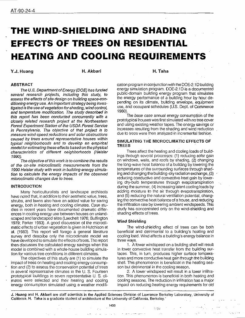
100, _____________ --.

~

c o

10

= .0 u

" " 1!

" co " 0. .. '0

" c: ~

20

/ ,r . 'I If

f

e/ /'

/-

o o

•

• ---o ___ --

~--

Legend

• Winter

o McGinn (Summer)

o+-~--~~-~~-~~-~~~ o U 10 10 40 10 "0 10 10 10 100 Canopy denalty, % (trees + buildings)

Figure 1 Vjind speed reductions for different canopy densi­ties as compared to a control site with no trees or buildings

Figure 1 is a plot of the windspeed reductions from these two equations as a function of the total canopy density. For comparison, the figure also shows the ob­served windspeed reductions from a similar monitoring effort. done in Davis, CA, in 1977 (McGinn 1982). The McGInn study was less comprehensive and included only summer days. Moreover, data from residential areas were mixed with .th?se from an or.chard with a high tree density but no bUIldIngs, an atYPIcal condition for residential areas.

Shading

The shading effects of trees can be simulated in DOE-2.1 D as exterior building shades, once the geometry and transmissivity of the trees have been de­termined. Tree transmissivities vary by species, ranging from 6% to 30% during summer months and 10% to 80% durin~ winter months (Thayer 1983; McPherson 1984). For thIS study, trees were assumed to have transmissivi­ties of 10% during the summer, 70% during the winter, and were placed for shading on the west or south side of the house.

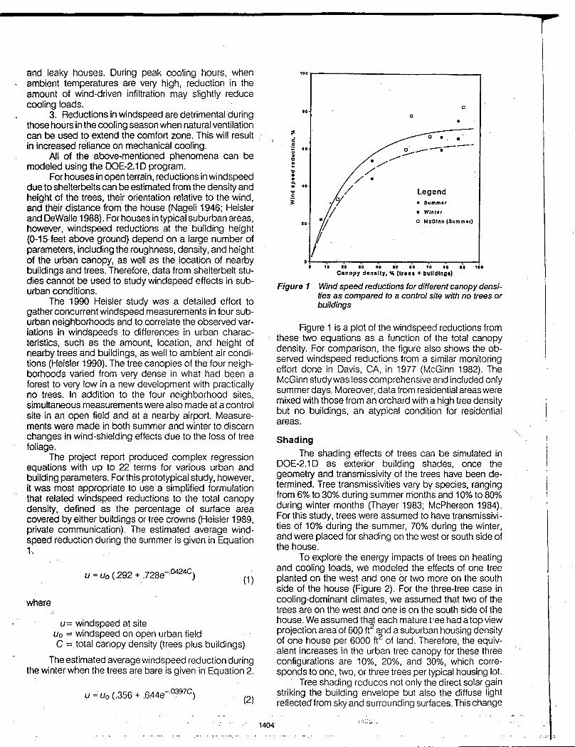
To explore the energy impacts of trees on heating and cooling loads, we modeled the effects of one tree planted on the west and one or two more on the south side of the house (Figure 2). For the three-tree case in cooling-dominant climates, we assumed that two of the trees are on the west and one is on the south side of the ho~se .. We assumed th~t each mature tree had a top view projectIon area of 60P ft ~nd a suburban housing density of one house per 6000 ft of land. Therefore, the equiv­alent increases in the urban tree canopy for these three configurations are 10%, 20%, and 30%, which corre­sponds to one, two, or three trees per typical housing lot.

. Tree shading reduces not only the direct solar gain striking the building envelope but' also the diffuse light reflected from sky and surrounding surfaces. This change

r

Figure 2 Tree canopy shade modeling used for DOE-2. 1 D simulations

is approximated in DOE-2.1 D by modifying the inputs for sky- and ground-form-factors, which define the amount of each visible from a building surface.

Tree shading also alters the exchange of long-wave radiation between the building and its surroundings. During the day, tree shading reduces long-wave heat gain to the house by keeping the surface temperatures of the sidewalks and street lower. At night, trees reduce radia­tive cooling by blocking the amount of night sky visible from the walls and roof. The impact of these changes on building heating and cooling loads cannot be modeled by the DOE-2.1 D program, but a simple calculation shows that the effects are small compared to those due to reductions in direct solar gain (Myrup and Morgan 1972).

Evapotranspiration

A major microclimatic impact of trees that is frequently overlooked is their capability to affect daily temperature swings through the evaporation and tran­spiration of moisture through leaves, a phenomenon agriculturalists call "evapotranspiration."

. From the point of view of energy conservation, dUring the summer a tree can be regarded as a natural "evaporative cooler," using up to 100 gallons of water a day (Kramer 1960). This rate of evapotranspiration trans­late~ into a c?oling potential of 230,000 kcal/day. This cooling effect IS the primary cause for the go F differences in peak noontime temperatures observed between for­ests and open terrain and the 60 F difference found in

1405

noontime air temperatures over irrigated millet fields as compared to bare ground (Geiger 1957, p. 294). Temperature measurements in suburban areas recorded similar but smaller variations in daytime peaks of 40 F to 60 F between neighborhoods under mature tree canopies and newer areas with no trees (McGinn, 1982 p. 59).

Th~ effect of evapotranspiration is minimal during the heating season. This reduction can be attributed to the absence of leaves on deciduous trees, lower ambient temperatures, and lower solar gain.

We have developed a quantitative model for micro­climate modifications due to evapotranspiration as a function of time, ambient conditions, and the amount of added moisture (Huang et al. 1987a). The model has been applied to several U.S. cities to estimate the cooling potentials of evapotranspiration. The study has con­cluded that the conservation potentials of evapotran­spiration during the summer are much larger than the effects of wind-shielding and shading. This study; how­ever, has focused on the wind-shielding and shading effects of trees and has not modeled the effects of evapotranspi ration.

BUILDING ENERGY SIMULATION

To assess the impact of tree canopies on the energy use of typical residential buildings in different cities simu­lations were done using the DOE-2.1 D program for'seven locations, three heating-dominant (Chicago, Min­neapolis, and Pittsburgh), two mixed heating-cooling (Washington and Sacramento), and two cooling-domi­nant (Miami and Phoenix).

Building Physical Characteristics

For each location, two building prototypes were developed based on available survey data and existing '" residential prototype description efforts. The assumed size and conservation level for the prototypes are listed in Table 1.

The first set of prototypes, labeled in Table 1 as "pre-1973 houses," represents houses built between 1950 and the early 1970s with conservation levels that are at the m~a~ of the current building stock. The physical characteristics for these prototypes are based primarily

TABLE 1 Prototype Building Character.lstlcs

Fborarea Found. Wal R-vakJet No.ol- infiltration •

I.DcalIon (It') Type SurllCO c.mng wla Found. P ..... ELF ICh

pno-lmHou .. ChIcago,II. 1400 Basemen( Siding 19 0 0 .. 1 .007 .89

MIaMI, FL 1400 Slob Stucco 0 0 0 1 .007 .59 Mmoapolls, MN 1400 - Sieling 19 11 0 1 .005 .63

PhoeIU.~ 1400 Slab Stucco 0 0 0 1 .007 .55 -PlIsburgt1,PA 1600 llalemen( Siding 19 0 0 1 .005 .58

Sacromonlo. CA 1400 Slob Stucco '1 0 0 1 .007 .58

WaaNngton, DC 2000 B ... men( Siding 11 0 0 1 .007 .79

1~_

ChII:ago, L 2000 Basemen( Sieling 22 " 54ft 3 .005 .64

MIaMI, FL 1600 Slob Stucco 19 7 0 1 .005 .42 Mloinoopolla,MN 2000 Basemen! SIelIng 38 19 54ft 3 .003 .39

~nIx,~ 1600 SlOb Stucco 22 11 52ft 2 .005 .39

PIIsburgt1, PA 1600 _men( Siding 30 " 54ft 2 .003 .35

I SacnmonlO. CA 1600 Slob Stucco 30 11 52ft 1- .005 .42 Washington, DC 2200 Basemen! SIelIng 30 11 54ft 2 .005 .56

.ELF reter_ to the "effective-leakage-fraction" used in the Sherman-Grimsrud model to describe .the tightness of a house to infiltration (Sherman and Grimsrud 1980); "ach" reler. to the average winter infiltration in airchangea per hour.

on a study that analyzed residential energy consumption surveys (RECS) for 1980 and 1981 to define prototypical house descriptions for ten geographical regions

, (Bluestein 1987). For some regions, the average floor areas given in the study seemed too small (e.g., 750 ft2 in Minnea?oliS) and were revised upward to a minimum of 1400 ft . The "pre-1973 houses" all have single-pane windows, minimal ceiling insulation, no wall insulation except in Minneapolis, and are moderately leaky. Tighter constructions were assumed for the colder cities, so that the net infiltration rates were similar for the different cities, ranging from 0.89 ach (air changes per hour) in Chicago to 0.55 ach in Phoenix.

The second set of prototypes, labeled in Table 1 as "1980s houses," represent typical current construction as reported in the 1981 National Association of Home Builders Annual Surveys of New Construction (NAHB 1981). The houses tend to be larger than the pre-1973 houses and have significantly higher conservation levels. The ceilings are insulated up to R-38 in the colder loca­tions, the walls to R-19, and the windows are at least double-glazed except in Miami and Sacramento. Al­though average infiltration rates are not available in the survey data, studies have shown that new houses are Significantly tighter, with air change rates averaging 0.4 per hour (Sherman 1984). Consequently, the prototypes for the 1980s houses were modeled with lower infiltration rates than the pre-1973 houses.

The prototypes represent statistical averages of the building stock in each city. Building geometries that could not be defined using statistical averages were estimated based on typical construction practices. For each build­ing size, wall areas and perimeter lengths were calculated assuming a standard truss width of 28 ft and a wall height of 8 ft. The total window area for each prototype was kept at 12% of the floor area, which. is the average of current construction practices. The assumed building geometries for the four building sizes are given in Table 2.

TABLE 2 Prototype Building Geometries

Prototype Pertmeter House Walt areas" Window Door Floor area length volume Gross Net area area

(n') (~) (Il') (n') (n') (n') (n') 1400 156.0 11200 1248 1052 168 27.5 1600 170.3 12800 1362 1143 192 27.5 2000 198.9 16000 1591 1323 240 27.5 2200 213.1 17600 1705 1413 264 27.5

*The qross wall area 1s that ot the entire vertical surface Includinq the windows and doors. The net vall area is that ot only the walls.

Building Operating Conditions

The assumed building operating conditions were based on earlier studies to define typical operating con­ditions in U.S. homes based on survey data and other studies (Huang 1987b).

The heating thermostat was set at 70° F, with a night setback to 60° F between 11 p.m. and 7 a.m. The cooling thermostat was set at 78° F all day. During the heating season, window venting was assumed when indoor temperatures rose above 78° F: while in the cooling sea-

1406

son, venting was assumed down to 72° F if the following criteria were met: (1) the outdoor temperature was lower than that indoors and not higher than 78° F, (2) the en­thalpy of the outdoor air was lower than that of the indoors, and (3) the cooling load that hour could be met totally through natural ventilation. However, window con­ditions were kept fixed between 11 p.m. and 7 a.m, unless indoor temperatures dropped below the heating setpoint, on the assumption that occupants would not open or close windows after having gone to bed.

To model heat gains from people, equipment, and lights, daily internal loads of 43,100 Btu sensible and 12,150 Btu latent due to 3.2 persons and typical residen­tial appliance use and 8.4 Btu/ft2 due to lights were modeled for each house. This internal loads level is based on analysis of end-use survey data and is explained in Huang (1987b). The hour-by-hour internal loads profile was taken from a schedule developed by the California Energy Commission (CEC 1984).

The building was simulated with a central space­conditioning system consisting of a gas furnace and an air conditioner. For prototypes smaller than 2000 ft2, the rated capacities modeled were 75,000 Btu/h for the gas furnace and 36,000 Btu/h for the air conditioner. For prototype houses of 2000 ft2 and above, the rated capaci­ties modeled were 100,000 Btu/h for the gas furnace and 48,000 Btu/hr for the air conditioner. For the pre-1973 houses, the furnace was assumed to have a system efficiency of 60% and the air conditioner a system COP of 2.17. For the 1980s houses, the furnace was assumed to have a system efficiency of 70% and the air conditioner a system COP of 2.41. Default curves in DOE-2.1 D were used to simulate the hourly performance of the air condi­tioner as a function of temperature, humidity, and part­load ratios (Building Energy Simulation Group 1984).

WEATHER DATA

The DOE-2.1 D program uses as its weather input hourly weather tapes available from sources such as the U.S. National Oceanic and AtmospheriC Administration (NOAA) or the American Society of Heating, Refrigerat­ing, and Air-Conditioning Engineers (ASHRAE). For the base case conditions, Weather Year for Energy Calcula­tions (WYEC) tapes developed by ASHRAEwere used for five of the seven cities (Crow 1981). Typical Meteorologi­cal Year (TMY) weather tapes were used for Chicago and Sacramento.

The seven cities chosen for the DOE-2.1 D simula­tions represent the range of climatic conditions found in the U.S., with heating degree-days ranging from 220 to 8000 and cooling-degree days from 600 to nearly 4000 (Table 3).

In addition to covering temperature variations, a distinction was also made between hot-arid and hot­humid climates. A useful climatic variable for indicating latent cooling loads is latent enthalpydays (Huang et a!. 1986). This variable is similar in concept to degree-days, except that it tabulates the cumulative change in enthalpy over the year to bring ambient conditions down to ~ defined temperature and humidity ratio. This base cond~­tion is generally set to the re.quired indoor comfort condl-

.. ",1\-, .'-TV'

-----------------------------------~~~~~~==~~--

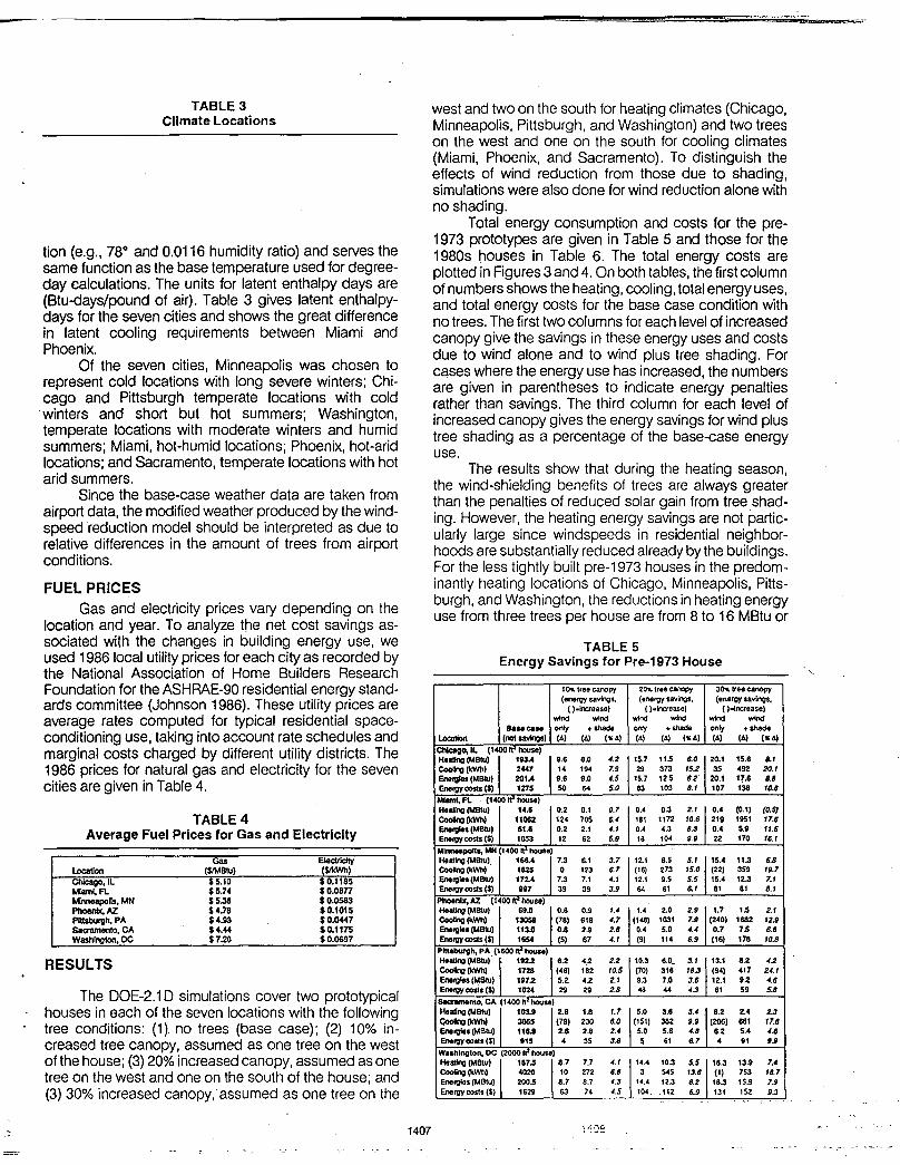
TABLE 3 Climate locations

tion (e.g., 78° and 0.Q116 humidity ratio) and serves the same function as the base temperature used for degree­day calculations. The units for latent enthalpy days are (Btu-days/pound of air). Table 3 gives latent enthalpy­days for the seven cities. and shows the great ?iff~rence in latent cooling requirements between Miami and Phoenix.

Of the seven cities, Minneapolis was chosen to represent cold locations with long severe winters; Chi­cago and Pittsburgh temperate locations with cold winters and short but hot summers; Washington, temperate locations with moderate winters and humid summers; Miami, hot-humid locations; Phoenix, hot-arid locations; and Sacramento, temperate locations with hot arid summers.

Since the base-case weather data are taken from airport data, the modified weather produced by the wind­speed reduction model should be interpreted as d~e to relative differences in the amount of trees from airport conditions.

FUEL PRICES Gas and electricity prices vary depending on the

location and year. To analyze the net cost savings as­sociated with the changes in building energy use, we used 1986 local utility prices for each city as recorded by the National Association of Home Builders Research Foundation for the ASHRAE-90 residential energy stand­ards committee (Johnson 1986). These utility prices are average rates computed for typical residential space­conditioning use, taking into account rate schedules and marginal costs charged by different utility districts. The 1986 prices for natural gas and electricity for the seven cities are given in Table 4.

TABLE 4 Average Fuel Prices for Gas and Electricity

LocatIon Chlcago.IL MIam~FL MiMeapolls, IAN Phoenix, AZ. PIttsburgh. PA Sac:tamenlo. CA Washlnglon. DC

RESULTS

Gas (SIMBtu) n.lo $5.74 $5.36 $4.78 $4.93 $4.44 $7.20

Electricity ($/kWh) $ 0.1185 $o.oan $0.0583 $0.1015 $0.0447 $0.1175 $0.0697

The DOE-2.1D simulations cover two prototypical houses in each of the seven locations with the following tree conditions: (1) no trees (base case); (2) 10% in­creased tree canopy, assumed as one tree on the west of the house; (3) 20% increased canopy, assumed as one tree on the west and one on the south of the house; and (3) 30% increased canopy, assumed as one tree on the

1407

west and two on the south for heating climates (Chicago, Minneapolis, Pittsburgh, and Washington) and two trees on the west and one on the south for cooling climates (Miami, Phoenix, and Sacramento). To distinguish .the effects of wind reduction from those due to shading, simulations were also done for wind reduction alone with no shading.

Total energy consumption and costs for the pre-1973 prototypes are given in Table 5 and those for the 1980s houses in Table 6. The total energy costs are plotted in Figures 3 and 4. On both tables, the first column of numbers shows the heating, cooling, total energy uses, and total energy costs for the base case condition with no trees. The first two columns for each level of increased canopy give the savings in these energy uses and costs due to wind alone and to wind plus tree shading. For cases where the energy use has increased, the numbers are given in parentheses to indicate energy penalties rather than savings. The third column for each level of increased canopy gives the energy savings for wind plus tree shading as a percentage of the base-case energy use.

The results show that during the heating season, the wind-shielding benefits of trees are always greater than the penalties of reduced solar gain from tree shad­ing. However, the heating energy savings are not partic­ularly large since windspeeds in residential neighbor­hoods are substantially reduced already by the buildings. For the less tightly built pre-1973 houses in the predom­inantly heating locations of Chicago, Minneapolis, Pitts­burgh, and Washington, the reductions in heating energy use from three trees per house are from 8 to 16 MBtu or

TABLE 5 Energy Savings for Pre-1973 House

10% tree canopy 20% tfee canopy 30% tree canopy (energy savings. (enerqy savings. (enerqy savings.

( )-lnere.se) ()_lnct8ase) ( )-Increase) wind wind wind wind wind wind

only only • shade l.ocaIIon (4) (4) (6) ("A)

15.8 B.1 .92 20.1 17.6 B.S 138 10.8

0 .• (0.1) (O.S) 219 1951 17.6 0 .• 5.9 11.5 22 170 16.1

15.4 11.3 6.8 (22) 359 19.7 15 .• 12.3 7.1 81 81 B.I

1.7 15 2.1 (240) 1682 12.9 0.7 75 6.6 (16) 178 lO.S

13.1 8.2 4.2 (~) 417 24.1 12.1 92 4.6 61 59 5.8

8.2 2 .• 2.3 (206) 681 11.8 8.2 5 .• 4.6 4 VI U

18.3 13.9 7.4 (I) 753 18.7 18.3 15.9 7.9 131 152 9.3

:~'Je

Chicago Miami Mlnneapoll. Phoenix

.. II .. • •• II II II - ... - --~-.. .. .. ..

S' '---.... a - .. _----- --.... e ll .. .. .. ----· ;; :: to ~~ ___ -....I to 1-~ - ... ___ .... to - _ .. __ -..- _ _ "

~ ~~--~--i· · ~~ • 1i j •

~-_s __ ..... -_.;

• • ~--e-- ..... __

+--..-----.--~ 0 Oi----,..------.--~ • to 10 10. to 10 '" 10 10 10. to " 10 ll-oo canopy don."y (%), Tr .. canopy donllty (%) Troo .onopy donlllY (%) Tro. canopy d .... lty (%)

PIttsburgh Sacramento Washington

.. .,-------, "-r------, -.,-------,

..

.. g eta i .. ... eo ~ I · .. ~ . ~

11 tI .... _ .. _____ _

" " .. ..

--.--_e- __ 10 to

--~-- ... --

~ -.g.., -- •

Legend • Hullng

o Q.!!!!'!L • !!.lol_

.r-..... ---e-__

r-..... --..... --o Ol+--.----.-~

• M " H. to " ". • " H ll-.. canopy d.nolly (%) ll-•• canopy don.lty (%) Tr •• canopy d.noUy (%)

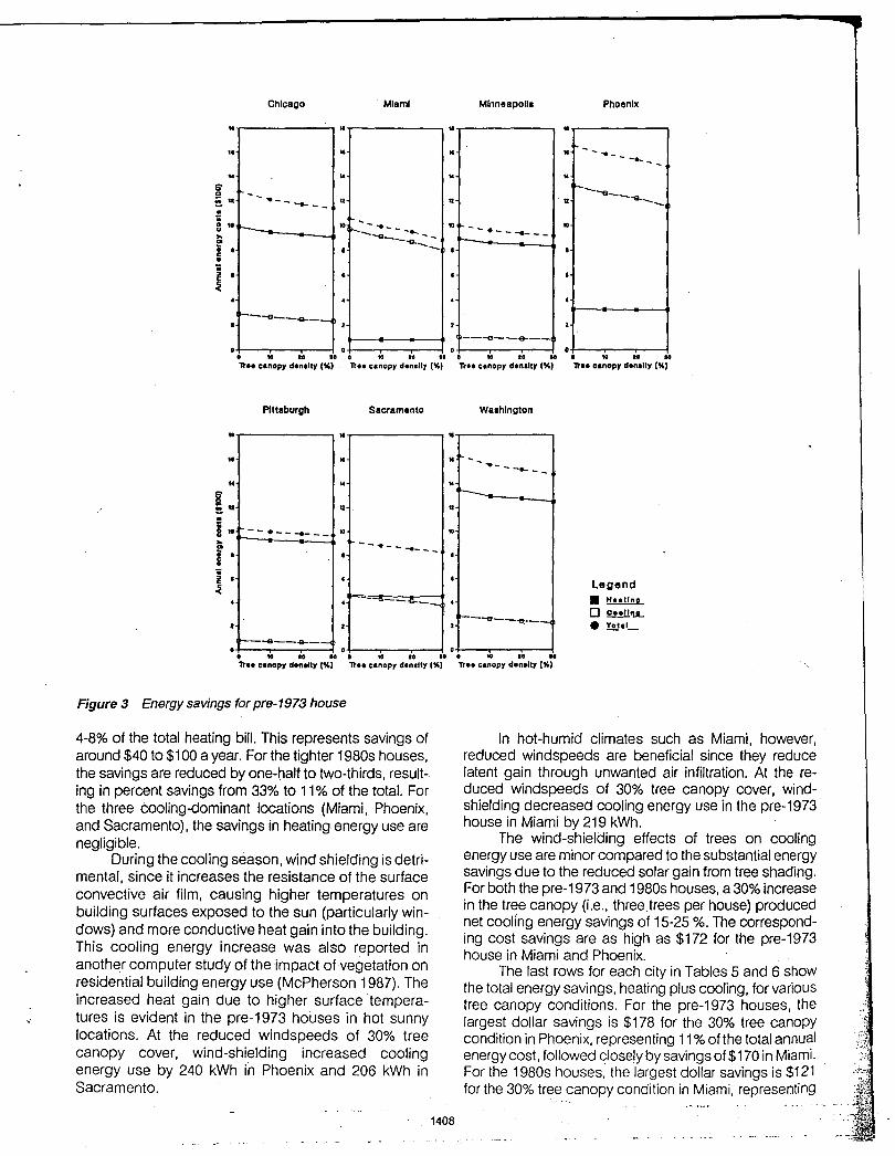
Figure 3 Energy savings for pre-1973 house

4-8% of the total heating bill. This represents savings of around $40 to $100 a year. For the tighter 1980s houses, the savings are reduced by one-half to two-thirds, result­ing in percent savings from 33% to 11% of the total. For the three cooling-dominant locations (Miami, Phoenix, and Sacramento), the savings in heating energy use are negligible.

During the cooling season, wind shielding is detri­mental, since it increases the resistance of the surface convective air film, causing higher temperatures on building surfaces exposed to the sun (particularly win­dows) and more conductive heat gain into the building. This cooling energy increase was also reported in another computer study of the impact of vegetation on residential building energy use (McPherson 1987). The increased heat gain due to higher surface tempera­tures is evident in the pre-1973 houses in hot sunny locations. At the reduced wlndspeeds of 30% tree canopy cover, wind-shielding increased cooling energy use by 240 kWh in Phoenix and 206 kWh in Sacramento.

1408

In hot-humid climates such as Miami, however, reduced windspeeds are beneficial since they reduce latent gain through unwanted air infiltration. At the re­duced windspeeds of 30% tree canopy cover, wind­shielding decreased cooling energy use in the pre-1973 house in Miami by 219 kWh.

The wind-shielding effects of trees on cooling energy use are minor compared to the substantial energy savings due to the reduced solar gain from tree shading. For both the pre-1973 and 1980s houses, a 30% increase in the tree canopy (i.e., three trees per house) produced net cooling energy savings of 15-25 %. The correspond­ing cost savings are as high as $172 for the pre-1973 house in Miami and Phoenix.

The last rows for each city in Tables 5 and 6 show the total energy savings, heating plus cooling, for various tree canopy conditions. For the pre-1973 houses, the largest dollar savings is $178 for the 30% tree canopy condition in Phoenix, representing 11 % of the total annual energy cost, followed closelybysavingsof$170 in Miami. For the 1980s houses, the largest dollar savings is $121 for the 30% tree canopy condition in Miami, representing

Chicago

.... ---~ 0' o

E • i r-------_ .. f' ! • · ;; " c:

~ ~--s J ---e-__ 2

Miami Mlnneapoll. Phoenix

.. -• P--__ - - ... - _ -s-.. ..... -..........

. -- .. -------

• 0 0-1---,.----,.--1 • to 10 JOO to 10 ,01 to to 1011 10 10)0

Tr .. canopy donllty (%) Troo canopy donllty (%) Tro, canopy d.nllty (%) Tr .. canopy donalty (%)

o o

e • · · o u

Pittsburgh

~ -- .. -:.....-.--­• • ~ t--tlf----____ --4

~ ~

Sacramento . Washington

... - -- .... -

"r-..... ---_-..1 --"---.-.-

f--..... ____ _

*----.0-_-4 z ~-.... ____ ~

Legend • Hutlno

o ~.JL • T.ul

~- ..... --..... --• 0 o+-~~~--~

• U " '0. • " H. • " H 'It .. oanopy don.lty (%) 'It .. ca.opy dO.llty (%) 'It •• canopy donolty (%)

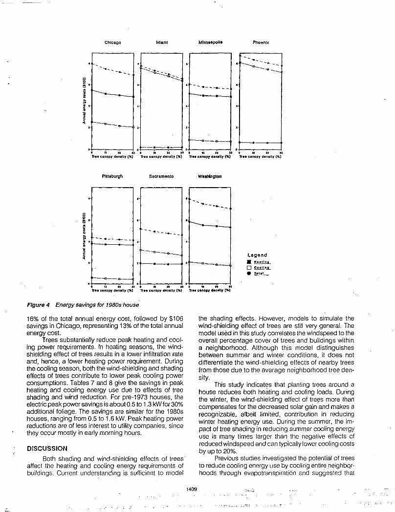
Figure 4 Energy savings for 1980s·house

16% of the total annual energy cost, followed by $106 savings in Chicago, representing 13% of the total annual energy cost.

Trees substantially reduce peak heating and cool­ing power requirements. In heating seasons, the wind­shielding effect of trees results in a lower infiltration rate and, hence, a lower heating power requirement. During the cooling season, both the wind-shielding and shading effects of trees contribute to lower peak cooling power consumptions. Tables 7 and 8 give the savings in peak heating and cooling energy use due to effects of tree shading and wind reduction. For pre-1973 houses, the electric peak power savings is about 0.5 to 1.3 kW for 30% additional foliage. The savings are similar for the 1980s houses, ranging from 0.5 to 1.6 kW. Peak heating power reductions are of less interest to utility companies, since they occur mostly in early morning hours.

DISCUSSION

Both shading and wind-shielding effects of trees' affect the heating and cooling energy requirements of buildings. Current understanding is sufficient to model

1409

the shading effects. However, models to simulate the wind-shielding effect of trees are still very general. The model used in this study correlates the windspeed to the overall percentage cover of trees and buildings within a neighborhood. Although this model distinguishes between summer and winter conditions, it does not differentiate the wind-shielding effects of nearby trees from those due to the average neighborhood tree den­sity.

This study indicates that planting trees around a house reduces both heating and cooling loads. During the winter, the wind-shielding effect of tre~s more than compensates for the decreased solar gain and makes a recognizable, albeit limited, contribution in reducing winter heating energy use. During the summer, the im­pact of tree shading in reducing summer cooling energy use is many times larger than the negative effects of reduced windspeed and can typically lower cooling costs by up to 20%.

Previous studies investigated the potential of trees to reduce cooling energy use by cooling entire _neighbor­hoods through evapotranspiration and suggested that

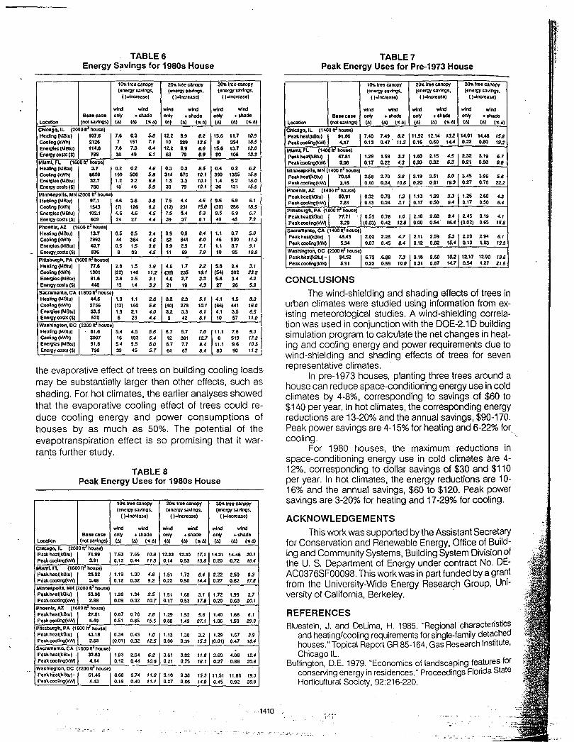
TABLE 6 Energy S~vlngs for 1980s House

1 (h(, Iree canopy 20% tree canopy 3O'f, lreecanopy (e",,1lIY .avlngs. (_IllY .avlngs. (en,1lIY savings.

( )-increase) ( ).Inerease) ()';ncrease)

wind wind wind wind wind Basocase only + shade

locaUon (not savings) (6) (4) ("4)

Chlcago.1l (2000 Heating (MBlu) 15.6 11.7 10.9 COolng(1<Wh) 9 394 18.5 Energtes (MBM 15.6 13.7 12.0 EnelllY costs ($) 80 106 13.3

Mlaml,Fl (1600 Heating (MBIU) 0.4 0.2 6.2 CooIng (kWh) 390 1365 15.8 Energies (MBiIJ) 1.4 5.2 16.0 Ene'llY costs ($) 36 121 15.5

9.5 5.9 6.1 (30) 266 18.5' 9.5 6.9 6.7 49 48 7.9

1.1 0.7 5.0 46 900 fI.3 1.1 3.7 9.1 10 95 10.8

5.8 2.4 3.1 (54) 302 23.2 5.8 3.4 4.2 27 26 5.9

4.1 1.5 3.3 (66) 441 16.0 4.1 3.5 6.5 10 57 fI.O

11.1 7.6 9.3 8 519 17.3

11.1 9.6 10.5 80 90 11.3

the evaporative effect of trees on building cooling loads may be substantially larger than other effects, such as shading. For hot climates, the earlier analyses showed that the evaporative cooling effect of trees could re­duce cooling energy and power consumptions of houses by as much as 50%. The potential of the evapotranspiration effect is so promising that it war­ran~s further study.

TABLE 8 Peak Energy Uses for 1980s House

10% tree canopy 20% Iroe canopy 30% lree canopy (energy savinos, (energy savtngs. (enelllY savings.

( )-inaease) ()-tnctease) ()-tncrease)

wind wind wind wind wind wind BaseC8se only + shade only + shade only + shade

Location (nol savings) (A) (A) ("4) (4) (4) ("4) (6) (4) (,,6)

Chicago, Il (2000 It' house)

P.ak heal(kBlU) I I 71.99 I 7.63 7.66 10.61 '2.22 12.30 ,7"1 '4.21 14.48 20.1 Peakcoofing(1<W) 3.91 0.12 0.44 1103 0.14 0.53 13.6 0.20 o.n 18.4 MIamI.I'l (1600 It' house)

Peak hea~kBlU) I I 26.92 J 1.19 1.30 4.8 11.51 1.72 6.4,1 2.22 2.50 9.3 Pea~cooftng(1<W) :U8 0.12 0.32 9.2 0.22 0.50 14.4 0.27 0.62 17.8 Mlnn •• poll .. MN (2000 ft house)

Peak ""at(kBIU) 1\ 53.96 J 1.26 1.34 2.5 1,.5' 1.68 3·',I,·n 1.99 3.7 Pea~cootIng(kW) 2.98 0.09 0.32 10.7 0.17 0.53 17.8 0.20 0.60 20.1

phOenix, AZ (1600 It' house)

Peak heal(kBlU) I I 27.01 I 0.67 0.76 2.8 1,.29 1.52 5.61,

.40 1.66 6.1 PeakcooUng(1<W) 5.49 0.51 0.85 15.5 O.es 1.49 27.1 1.06 1.59 29.0

Phl.burgh, PA (1600 It' house) .

Peak heal(1<Btu) I I 43.18 I 0.34 0.45 1.0 1,.,3 1.38 3.2 L 1.29 1.67 3.9 Peakcoollng(kW) 2.55 (0.01) 0.32 12.5 0.00 0.39 15.3 (0.01) 0.47 1M

Sacramento, CA (1600 n' hous.)

Peak heat(kBlU) ):1 32.83 1,.93 2.04 6.2 J 3.61 3.82 11.81 3.69 4.06 IZ.4 Peak COOUng(kW) 4.14 0.12 0.44 10.6 0.21 0.75 18.1 0.27 0.86 20.8 W.shlnglon, DC (2200 It' house)

I'.ak ""al(kBlU) ~ ! 61.461 6.68 .6.7. 11.0 19.,8 9.38 15.31"

.5' 11.86 19.3 PeakcooUng(kW) 4.43 0.19 0.49 11.1 0.27 0.66 14.9 0.45 0.92 ZO.8

-.1410 .

TABLE 7 Peak Energy Uses for Pre·1973 House

10% It .. canopy 2Ch< tr .. canopy 3O'f, lree canopy (eMIlIY savings. (e/101lIY savings, (energy savings.

( )-ina .... ) ( )-incr.ase) ()-increas.)

wind wind wind wind wind wind saM case only + shad. only + shade only + shade

LocaUon (not savings) (4) (6) ("4) (4) (4) ("A) (6) (A) ("4)

Chicago, tl (1400 It' hou .. ) 7.49 8.2.1'1.92 12.14 13~ \'4.01 14.48 15.8 Peak heal(1<Bl1J) I I .1.116 I 7.40

Peakcootlng(1<W) 4.17 0.13 0.47 11.3 0.16 0.60 14.4 0.22 0.80 19.2

MIam~ FL (1400 It' house)

3.3 1,.60 2.15 4.5 I 2.32 3.19 P.akhea1(1<BIU) II 47.81 1'.29 1.59 6.7

Peak'cooUng(1<w) 5.08 0.17 0.22 4.3 0.20 0.32 6.3 0.21 0.50 U Mlnneapotls, MN (1400 ft house)

P.ak heat(1<BIU) II 70.551 2.58 2.70 3.8 13.,9 3.51 5.0,1 3.45 3.96 5.6 P •• kcooftng(kWl 3.16 0.10 0.34. 10.8 0.20 0.61 19.3 0.27 0.70 2Z.2

PhOenix, AZ (1400 It' house)

3.31,.25 2.60 Peak heal(1<BIU) J 60.91 1 0.32 0.78 1.3 1,.,3 1.99 4.3

Peak cooUng(kW) 7.81 0.13 0.24 3.1 0.17 0.50 6.4 0.17 0.50 6.4

Pittsburgh, PI. (1600 It' houS.)

3.4, I 2.45 Peakhe~lU) J n.71 10.55 0.78 1.0 \2.,8 2.68 3.19 4.1 P.ak coo6ng(kW) 3.29 (0.03) 0.42 IZ.B 0.00 0,54' 16.4 (0.02) 0.65 19.8

sacramento, CA (1400 ft hOUS.)

Peak h.at(kBlU) 1'1 48.43 i 2.00 2.28 4.7 12." 2.59 5.3 , \ 2.20 .2.94 6.1 Peak coo&ng(kW) 5.34 0.07 0.45 8.4 0.12 0.82 15.4 0.13 1.03 19.3

W.'hl~IOn, DC (2000 It' house) 9.80 10~ \'2.17 12.90 Peak he.1(1<B1u) -,I 84.52 ! 6.73 .6.88 7.3 19.,8 13.6

Pe.k coofing(1<W) 5.91 0.22 0.59 10.0 0.31 0.87 14.7 0.54 1.27 21.5

CONCLUSIONS

The wind-shielding and shading effects of trees in urban climates were studied using information from ex­isting meteorological studies, A wind-shielding correla­tion was used in conjunction with the DOE-2.1 D building simulation program to calculate the net changes in heat­ing and cooling energy and power requirements due to wind-shielding and shading effects of trees for seven representative climates.

In pre-1973 houses, planting three trees around a house can reduce space-conditioning energy use in cold climates by 4-8%, corresponding to savings of $60 to $140 per year. In hot climates, the corresponding energy reductions are 13-20% and the annual savings, $90-170. Peak power savings are 4-15% for heating and 6-22% for cooling. .

For 1980 houses, the maximum reductions in space-conditioning energy use in cold climates are 4-12%, corresponding to dollar savings of $30 and $110 per year. In hot climates, the energy reductions are 10-16% and the annual savings, $60 to $120. Peak power savings are 3-20% for heating and 17-29% for cooling.

ACKNOWLEDGEMENTS

This work was supported by the Assistant Secretary for Conservation and Renewable Energy, Office of Build­ing and Community Systems, Building System Division of the U. S. Department of Energy under contract No. DE­AC0376SF00098. This work was in part funded by a grant from the University-Wide Energy Researqh Group, Uni­versity of California, Berkeley.

REFERENCES Bluestein, J. and DeUma, H. 1985. "Regional characteristics

and heating/cooling requirements for single-family deta?hed houses." Topical Report GR 85-164, Gas Research Institute, Chicago IL.

Buffington, D.E. 1979. "Economics of landscaping features for conserving energy in residences." Proceedings Florida State Horticultural Society, 92:216-220.

.., .... ;~, ,

'.'!

I " '!

Building Energy Simulation Group. 1989. "DOE-2 BDL Sum­mary, Version 2.10." Lawrence Berkeley Laboratory Report LBL-8688, RevA, Berkeley CA.

California Energy Commission .(CEC) 1980. "Assumptions used with energy performance computer programs." Project Re­port No.7, Buildings and Appliance Standards Office, Cal­ifornia Energy Commission, Sacramento CA.

Crow, l.W. 1980. "Development of hourly data for weather year for energy calculations (wyEC), including solar data, at 21 stations throughout the United States." ASHRAE RP 239, American Society of Heating, Refrigerating, and Air-condi­tioning Engineers.

Energy Information Administration (EIA). 1982. "Residential energy consumption survey." U. S. Department of Energy, Washington DC.

Geiger, R. 1957. The climate near the ground, Boston: Harvard University Press.

Heisler, G.M., and DeWalle, D.R. 1988. "Effects of windbreak structure on wind flow." In Agriculture, Ecosystems and En­vironment, Vol. 22, No. 13. pp. 41-67.

Heisler, G.M. 1990. "Mean windspeed below building height in residential neighborhoods with different tree density." ASHRAf Transactions, Vol. 96, Part 1.

Huang, Y.J.; Akbari, H.; Taha, H.; and Rosenfeld, A. 1987a. "The potential of vegetation in reducing summer cooling loads in residential buildings. " Lawrence Berkeley Laboratory Report LBL-21291, Berkeley CA.

Huang, Y.J., et aI. 1987b. "Methodology and assumptions for evaluating heating and cooling energy requirements in new single-family residential buildings (Technical support docu­ment for the· PEAR microcomputer program)." Lawrence Berkeley Laboratory Report LBL-19128, Berkeley CA.

Huang, Y.J.; Ritschard, R.; Bull, J.; and Chang, l. 1986. " "Climate indicators for estimating residential heating and cooling loads. " Lawrence Berkeley Laboratory Report LBL-19128, Berkeley CA. .

Hutchison, B.A., et al. 1983. "Energy conservation mechanisms and potentials of landscape design to ameliorate building microclimates." Landscape Journal, 2: 1, University of Wis­consin.

1411

Johnson, A. 1987. Unpublished report. American Society of Heating, Refrigerating, and Air-conditioning Engineers (ASHRAE) 90.R Residential Building Standards Committee.

Kramer, P.J., and Kozlowski, T. 1960. Physiology of trees, New York: McGraw Hill.

Laechelt, R.L, and Williams, B.M. 1976. "Value of tree shade to homeowners.", Alabama Forestry Commission, Montgom­ery, Al.

McGinn, C. 1982. "Microclimate and energy use in suburban tree canopies," Ph.D. thesis, Univ. of California. Davis

McPherson, E.G. ed. 1984. "Energy-conserving site design" American Society of Landscape Architects, Washington.

McPherson, E.G., Herrington, l.P.; and Heisler, G.M. 1987. " Impacts of vegetation of residential heating and cooling", University of Arizona, Tucson.

Myrup, l.O., and Morgan, D.l. 1972. "Numerical model of the urban atmosphere," Dept. of Agricultural Engineering and Dept. of Water Science and Engineering, Contributions in Atmospheric Science No.4, UC Davis.

Nageli, W. 1946. "Untersuchungen uber die Windverhaltnisse im Bereich von Schilfrohr wanden," pp. 213-266. Ebenda 29.

National Association of Home Builders (NAHB) Research Foun­dation, Inc. 1981. "Single-family attached construction prac­tices." Rockville, MD.

Parker, J.H. 1981. "Uses of landscaping for energy conserva­tion," STAR Project 78-012. Florida State University System, Tallahassee.

Sherman, M.H. and Grimsrud, D.T. 1980. "Measurement of Infiltration Using Fan Pressurization and Weather Data," la­wrence Berkeley Laboratory Report LBL-10892, Berkeley, CA.

Sherman, M.H.; Wilson, D.J.; and Kiel, D.E. 1984. "Variability in residential air leakage." Lawrence Berkeley Laboratory Re­port LBL-17587, Berkeley CA.

Thayer, R.l.; Zanetto, J.; and Maeda, B. 1983. "Modeling the effects of street trees on the performance of solar and conventional houses in Sacramento, California," Landscape Journal, 2:2, University of Wisconsin.

U.S. Department of Commerce 1980. DOE-2 reference manual, Parts 1 & 2 (Version 2.1). Springfield, VA: National Technical Information Service.

!. "'

LA~NCEBERKELEYLABORATORY

UNIVERSITY OF CALIFORNIA TECHNICAL INFORMATION DEPARTMENT

BERKELEY, CALIFORNIA 94720

. ~""

~ .... --

~ o ";:: C\I= ro = .... '¢-.o I :.J CO_....J « en

....J