Embed Size (px)
Citation preview

Lattice-Modelling of Nuclear Graphite for
Improved Understanding of Fracture Processes
A thesis submitted to The University of Manchester
for the degree of Doctor of Philosophy
in the Faculty of Engineering and Physical Sciences
By
Craig N Morrison
2015
School of Mechanical, Aerospace and Civil Engineering


Contents
I Introduction and Background 16
1 Nuclear graphite 17
1.1 Introduction to graphite . . . . . . . . . . . . . . . . . . . . . . . . . . . . 17
1.2 The use of graphite in the nuclear industry . . . . . . . . . . . . . . . . . . 18
1.3 Characterising the global behaviour of graphite . . . . . . . . . . . . . . . 20
1.4 Fracture Process Zone (FPZ) . . . . . . . . . . . . . . . . . . . . . . . . . 21
2 Modelling quasi-brittle material behaviour 24
2.1 Global approach to modelling material failure . . . . . . . . . . . . . . . . 24
2.1.1 Limitations of global fracture mechanics . . . . . . . . . . . . . . 25
2.2 Local approach to fracture . . . . . . . . . . . . . . . . . . . . . . . . . . 26
2.2.1 Discrete models . . . . . . . . . . . . . . . . . . . . . . . . . . . . 27
2.3 Generalised continuum . . . . . . . . . . . . . . . . . . . . . . . . . . . . 28
3 Project outline 29
3.1 Aims and objectives . . . . . . . . . . . . . . . . . . . . . . . . . . . . . . 29
3.2 Report structure . . . . . . . . . . . . . . . . . . . . . . . . . . . . . . . . 29
II Review of Literature 31
4 Manufacture and microstructure of graphite 32
4.1 Manufacturing process . . . . . . . . . . . . . . . . . . . . . . . . . . . . 32
4.2 Resulting microstructure . . . . . . . . . . . . . . . . . . . . . . . . . . . 34
4.2.1 Nuclear graphite grades . . . . . . . . . . . . . . . . . . . . . . . 35
4.2.2 Mechanical properties . . . . . . . . . . . . . . . . . . . . . . . . 36
4.2.3 Fracture mechanisms . . . . . . . . . . . . . . . . . . . . . . . . . 37
4.2.4 Characterising the Fracture Process Zone . . . . . . . . . . . . . . 38
3
CONTENTS CONTENTS
4.3 Effects of radiation damage . . . . . . . . . . . . . . . . . . . . . . . . . . 39
4.3.1 Fast neutron irradiation . . . . . . . . . . . . . . . . . . . . . . . . 39
4.3.2 Radiolytic oxidation . . . . . . . . . . . . . . . . . . . . . . . . . 40
5 Size effect of quasi-brittle structures 42
5.1 Statistical Size Effect . . . . . . . . . . . . . . . . . . . . . . . . . . . . . 42
5.1.1 Power laws . . . . . . . . . . . . . . . . . . . . . . . . . . . . . . 42
5.1.2 Weakest Link Theory . . . . . . . . . . . . . . . . . . . . . . . . . 44
5.2 Deterministic Size Effect . . . . . . . . . . . . . . . . . . . . . . . . . . . 47
6 Non-linear fracture mechanics 50
6.1 Cohesive zone/Discrete crack models . . . . . . . . . . . . . . . . . . . . 51
6.2 Smeared crack models . . . . . . . . . . . . . . . . . . . . . . . . . . . . 53
7 Local approach to material failure 56
7.1 Failure criterion . . . . . . . . . . . . . . . . . . . . . . . . . . . . . . . . 56
7.1.1 Global failure criterion . . . . . . . . . . . . . . . . . . . . . . . . 56
7.1.2 Statistical failure criterion . . . . . . . . . . . . . . . . . . . . . . 59
7.2 Local constitutive equations . . . . . . . . . . . . . . . . . . . . . . . . . 61
7.3 Modelling approaches for graphite . . . . . . . . . . . . . . . . . . . . . . 63
8 Discrete local approaches - lattice models 65
8.1 Background . . . . . . . . . . . . . . . . . . . . . . . . . . . . . . . . . . 66
8.2 Variations of lattice model . . . . . . . . . . . . . . . . . . . . . . . . . . 67
8.2.1 Calibration . . . . . . . . . . . . . . . . . . . . . . . . . . . . . . 67
8.2.2 Lattice network arrangement and choice of element . . . . . . . . . 68
8.2.3 Method for generating and incorporating heterogeneity . . . . . . . 69
8.2.4 Constitutive law and failure criterion . . . . . . . . . . . . . . . . . 71
8.3 Lattice models of note . . . . . . . . . . . . . . . . . . . . . . . . . . . . 72
8.4 Site-Bond lattice model . . . . . . . . . . . . . . . . . . . . . . . . . . . . 75
9 Generalised Continuum 77
9.1 Couple stress theory . . . . . . . . . . . . . . . . . . . . . . . . . . . . . . 77
4

CONTENTS CONTENTS
III Contribution to the field 80
10 Modelling and published work 81
10.1 Model calibration . . . . . . . . . . . . . . . . . . . . . . . . . . . . . . . 83
10.2 Microstructure-informed model . . . . . . . . . . . . . . . . . . . . . . . . 85
11 Conclusions 88
12 Further work 89
12.1 Model calibration . . . . . . . . . . . . . . . . . . . . . . . . . . . . . . . 89
12.1.1 Improved relationship between bond deformation and energy . . . . 89
12.1.2 Couple with dual graph . . . . . . . . . . . . . . . . . . . . . . . . 92
12.2 Explore the effect of porosity on graphite failure energy at grain level . . . 92
12.3 Inclusions and validation of physical phenomena . . . . . . . . . . . . . . 93
12.4 Structural integrity assessment . . . . . . . . . . . . . . . . . . . . . . . . 94
IV Appendices 118
A Linear Elastic Fracture Mechanics (LEFM) 119
A.1 Energy approach . . . . . . . . . . . . . . . . . . . . . . . . . . . . . . . 119
A.1.1 Stress concentration factor (Inglis) . . . . . . . . . . . . . . . . . . 119
A.1.2 Griffith approach . . . . . . . . . . . . . . . . . . . . . . . . . . . 120
A.1.3 Modified Griffith approach . . . . . . . . . . . . . . . . . . . . . . 122
A.1.4 Energy release rate . . . . . . . . . . . . . . . . . . . . . . . . . . 123
A.1.5 The R curve . . . . . . . . . . . . . . . . . . . . . . . . . . . . . . 124
A.2 Stress intensity approach . . . . . . . . . . . . . . . . . . . . . . . . . . . 125
A.3 Crack tip yielding . . . . . . . . . . . . . . . . . . . . . . . . . . . . . . . 127
A.3.1 Irwin’s plastic zone correction . . . . . . . . . . . . . . . . . . . . 127
A.3.2 Dugdale-Barenblatt cohesive zone/strip concept . . . . . . . . . . . 128
A.3.2.1 Dugdale strip yield model . . . . . . . . . . . . . . . . . 129
A.3.2.2 Barenblatt cohesive force model . . . . . . . . . . . . . 130
B Continuum Damage Mechanics (CDM) 132
B.1 Damage parameters . . . . . . . . . . . . . . . . . . . . . . . . . . . . . . 132
B.2 Damage evolution and constitutive laws . . . . . . . . . . . . . . . . . . . 134
5
CONTENTS CONTENTS
C Meso-scale features and couple stresses in fracture process zone 136
D A meso-scale site-bond model for elasticity: Theory and calibration 147
E Lattice-spring model of graphite accounting for pore size distribution 153
F A discrete lattice model of quasi-brittle fracture in porous graphite 158
G Fracture energy of graphite from microstructure-informed lattice model 175
H Site-bond lattice modelling of damage process in nuclear graphite under bend-
ing 183
I Multi-scale modelling of nuclear graphite tensile strength using the Site-Bond
lattice model 194
6

List of Figures
1.1 The crystal structure of graphite . . . . . . . . . . . . . . . . . . . . . . . 17
1.2 A scaled-down AGR core consisting of graphite moderator bricks . . . . . 18
1.3 High temperature reactor; (a) prismatic reflector; (b) graphite pebbles . . . 19
1.4 The stress-displacement graph for; (a) brittle (b) perfectly plastic/ductile
and (c) quasi-brittle materials under uniaxial tension . . . . . . . . . . . . . 20
1.5 A fracture process zone at the tip of a crack . . . . . . . . . . . . . . . . . 21
1.6 Zones of non-linear behaviour for; (a) linear elastic (b) non-linear plastic
(c) non-linear quasi-brittle materials . . . . . . . . . . . . . . . . . . . . . 22
1.7 A typical stress-displacement curve of concrete under uniaxial tension . . . 23
2.1 The global approach to modelling material failure . . . . . . . . . . . . . . 24
2.2 The local approach to fracture considering local material behavior . . . . . 27
4.1 Nuclear graphite production flow sheet . . . . . . . . . . . . . . . . . . . 33
4.2 A CCD image of the microstructure of Gilsocarbon. . . . . . . . . . . . . . 36
4.3 The turn-around for Gilsocarbon at varying temperatures for dimensional
change and relative Youngs Modulus . . . . . . . . . . . . . . . . . . . . . 40
5.1 (a) Geometrically similar structures of different sizes; (b) power scaling laws 43
5.2 Geometrically similar flaws in two components . . . . . . . . . . . . . . . 44
5.3 (a) A chain with links of distributed strength; (b) failure probability of a
given element; (c) a strucutre with a population of micro-cracks . . . . . . 45
5.4 An example of a Weibull plot for graphite; (a) tensile specimens (b) bend
specimens . . . . . . . . . . . . . . . . . . . . . . . . . . . . . . . . . . . 48
5.5 Size effect relations produced from elastic and plastic yield criteria, LEFM
and NLFM . . . . . . . . . . . . . . . . . . . . . . . . . . . . . . . . . . 48
7

LIST OF FIGURES LIST OF FIGURES
6.1 The fictitious crack model for quasi-brittle materials; (a) the stress-displacement
response (b) the crack opening displacement at the ficticious crack tip . . . 52
6.2 Example softening curves . . . . . . . . . . . . . . . . . . . . . . . . . . . 52
6.3 (a) Smeared micro-cracking in a band of width h; (b) The inelasitc deform-
ation in the FPZ represented by an equivalent inelastic strain . . . . . . . . 54
7.1 A simple failure criteria where the bond fails at the tensile stress/strain con-
ditions, σt , εt . . . . . . . . . . . . . . . . . . . . . . . . . . . . . . . . . 57
7.2 (a) The Rankine failure envelope; (b) The Von-Mises and Maximum Shear
failure envelopes . . . . . . . . . . . . . . . . . . . . . . . . . . . . . . . 57
7.3 The Mohr-Coulomb failure envelope. . . . . . . . . . . . . . . . . . . . . 58
7.4 An LEFM approximation (a) of a material with microstructure (b) . . . . . 60
7.5 The Rose-Tucker graphite failure model . . . . . . . . . . . . . . . . . . . 60
7.6 The Burchell graphite failure model . . . . . . . . . . . . . . . . . . . . . 61
7.7 An uncoupled local approach to fracture . . . . . . . . . . . . . . . . . . . 62
7.8 An uncoupled local approach to fracture with a continuous representation
of a crack . . . . . . . . . . . . . . . . . . . . . . . . . . . . . . . . . . . 63
7.9 A coupled local approach to fracture . . . . . . . . . . . . . . . . . . . . . 64
8.1 Different lattice arrangements . . . . . . . . . . . . . . . . . . . . . . . . 67
8.2 A lattice superimposed onto a synthetic concrete microstructure . . . . . . 70
8.3 A centre particle lattice configuration . . . . . . . . . . . . . . . . . . . . . 70
8.4 A failure criterion accounting for tension softening with modified secant
elastic modulus for unloading . . . . . . . . . . . . . . . . . . . . . . . . . 72
8.5 (a) Cellular representation of material; (b) the skeletal bond structure . . . 76
9.1 The stresses present on a 2D couple stress element under static load . . . . 78
10.1 Completed works during 0-12 months of the project . . . . . . . . . . . . . 82
10.2 Completed works during 12-24 months of the project . . . . . . . . . . . . 82
10.3 Completed works during months 24-36 months of the project . . . . . . . . 83
10.4 The 6 degrees of freedom represented by springs in the Site-Bond model . . 84
10.5 The displacement of a cantilever beam in the y-direction along the beam
length (z-direction) . . . . . . . . . . . . . . . . . . . . . . . . . . . . . . 87
A.1 An elliptical hole in a flat plate . . . . . . . . . . . . . . . . . . . . . . . . 120
A.2 The strain energy released around a crack of length 2a . . . . . . . . . . . 121
8
LIST OF FIGURES LIST OF FIGURES
A.3 The prediction of the Griffith energy balance for energetically favourable
fracture . . . . . . . . . . . . . . . . . . . . . . . . . . . . . . . . . . . . 122
A.4 (a) Flat R curve (b) rising R curve . . . . . . . . . . . . . . . . . . . . . . 125
A.5 Coordinate and element definition ahead of a crack tip . . . . . . . . . . . 125
A.6 The 3 modes of loading for a crack . . . . . . . . . . . . . . . . . . . . . . 126
A.7 Estimates of the plastic zone size for small-scale yielding . . . . . . . . . . 128
A.8 The strip-yield model . . . . . . . . . . . . . . . . . . . . . . . . . . . . . 129
A.9 The crack-opening force, P, acting at a distance x from the crack’s centre-line129
A.10 The cohesive force model . . . . . . . . . . . . . . . . . . . . . . . . . . . 131
B.1 The concept of a fictitious undamaged state, on which the effective stress
principle is based . . . . . . . . . . . . . . . . . . . . . . . . . . . . . . . 133
9

Abstract
University of Manchester
Craig Morrison
Doctor of Philosophy
Lattice-Modelling of Nuclear Graphite for Improved Understanding of Fracture
Processes
September 2015
The integrity of graphite components is critical for their fitness for purpose. Since
graphite is a quasi-brittle material the dominant mechanism for loss of integrity is crack-
ing, most specifically the interaction and coalescence of micro-cracks into a critically sized
flaw. Including mechanistic understanding at the length scale of local features (meso-scale)
can help capture the dependence on microstructure of graphites macro-scale integrity. Lat-
tice models are a branch of discrete, local approach models consisting of nodes connected
into a lattice through discrete elements, including springs and beams. Element properties
allow the construction of a micro-mechanically based material constitutive law, which will
generate the expected non-linear quasi-brittle response.
This research focuses on the development of the Site-Bond lattice model, which is con-
structed from a regular tessellation of truncated octahedral cells. The aim of this research
is to explore the Site-Bond model with a view to increasing understanding of deformation
and fracture behaviour of nuclear graphite at the length scale of micro-structural features.
The methodology (choice of element, appropriate meso length-scale, calibration of bond
stiffness constants, microstructure mapping) and results, which include studies on fracture
energy and damage evolution, are presented through a portfolio of published work.
10
Declaration
University of Manchester
PhD by published work Candidate Declaration
Craig Morrison
Faculty of Engineering and Physical Sciences
Lattice-Modelling of Nuclear Graphite for Improved Understanding of Fracture
Processes
Authorship for the presented published works is assigned according to size and significance
of contribution.
All work presented has been completed whilst registered at the University of Manchester.
No portion of the work referred to in this thesis has been submitted in support of an applic-
ation for another degree or qualification of this or any other university or other institute of
learning.
I can confirm that this a true statement and that, subject to any comments above, the sub-
mission is my own original work.
Signed: ......................................... Date: .........................................
11

Acknowledgements
Firstly I would like to thank my entire supervisory team; Dr Andrey Jivkov, Prof John Yates
(prior to retirement), Dr Chris Race, Prof James Marrow and Dr Andy Hodgkins. Particu-
lar thanks are directed to Dr Jivkov whose guidance, infectious enthusiasm and seemingly
boundless knowledge have made this endeavour both productive and enjoyable. I would
also like to thank the academics and researchers working on the QUBE project, in partic-
ular Mingzhong Zhang for useful discussion and collaborations. Further thanks go to my
fellow students based in the School of MACE for creating a vibrant working environment.
There are quite simply too many of them to name all here but special thanks go to Huw,
Tom, Andy, Dean, Alan, Adrian, Umair and Sophia who have been present throughout
the duration of my project. Moreover, I would like to acknowledge the Nuclear FiRST
Doctoral Training Centre and the EPSRC for project funding and general support provided
to me throughout this PhD. I would also like to thank the graphite team at AMEC Foster
Wheeler, Andy Hodgkins, Chris Jones and Owen Booler who allowed me to experience
the industrial context of my research while on a short placement. Finally, I am indebted to
Becky for her understanding especially during the final months of this project in addition to
my family and friends.
12

Copyright
i. The author of this thesis (including any appendices and/or schedules to this thesis)
owns certain copyright or related rights in it (the “Copyright”) and s/he has given
The University of Manchester certain rights to use such Copyright, including for
administrative purposes.
ii. Copies of this thesis, either in full or in extracts and whether in hard or electronic
copy, may be made only in accordance with the Copyright, Designs and Patents Act
1988 (as amended) and regulations issued under it or, where appropriate, in accord-
ance with licensing agreements which the University has from time to time. This
page must form part of any such copies made.
iii. The ownership of certain Copyright, patents, designs, trade marks and other intellec-
tual property (the “Intellectual Property”) and any reproductions of copyright works
in the thesis, for example graphs and tables (“Reproductions”), which may be de-
scribed in this thesis, may not be owned by the author and may be owned by third
parties. Such Intellectual Property and Reproductions cannot and must not be made
available for use without the prior written permission of the owner(s) of the relevant
Intellectual Property and/or Reproductions.
iv. Further information on the conditions under which disclosure, publication and com-
mercialisation of this thesis, the Copyright and any Intellectual Property and/or Re-
productions described in it may take place is available in the University IP Policy
(see http://documents.manchester.ac.uk/DocuInfo.aspx? DocID=487), in any relev-
ant Thesis restriction declarations deposited in the University Library, The University
Library’s regulations (see http://www.manchester.ac.uk/library/aboutus/regulations)
and in The University’s policy on Presentation of Theses.
13
Published Works
1. Meso-scale features and couple stresses in fracture process zone
Craig N Morrison, Andrey P Jivkov, John R Yates
Proceedings of the 13th International Conference on Fracture (ICF13), June
2013, Beijing, China
2. A meso-scale site-bond model for elasticity: Theory and calibration
Mingzhong Zhang, Craig N Morrison, Andrey P Jivkov
Materials Research Innovations, vol 18, 2014, pp 982-986
3. Lattice-spring model of graphite accounting for pore size distribution
Craig N Morrison, Andrey P Jivkov, Gillian Smith, John R Yates
Key Engineering Materials, vol 592-593, 2014, pp 92-95
4. Discrete lattice model of quasi-brittle fracture in porous graphite
Craig N Morrison, Mingzhng Zhang, Andrey P Jivkov, John R Yates
Materials Performance and Characterization, vol 3(3), 2014, pp 414-428
5. Fracture energy of graphite from microstructure-informed lattice model
Craig N Morrison, Mingzhong Zhang, Andrey P Jivkov
Procedia Materials Science, vol 3, 2014, pp 1848-1853
6. Site-bond lattice modelling of damage process in nuclear graphite under bending
Craig N Morrison, Mingzhong Zhang, Dong Liu, Andrey P Jivkov
Proceedings of the 23rd Conference on Structural Mechanics in Reactor Tech-
nology (SMiRT23), August 2015, Manchester, UK
7. Multi-scale modelling of nuclear graphite tensile strength using the Site-Bond lattice
model
14

LIST OF FIGURES
Craig N Morrison, Andrey P Jivkov, Yelena Vertyagina, T James Marrow
Carbon, vol 100, 2016, pp 273-282
15

Part I
Introduction and Background
16
Chapter 1
Nuclear graphite
1.1 Introduction to graphite
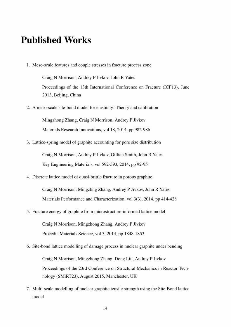
Graphite is an allotrope of carbon which occurs naturally in a variety of states [1, 2]. At
the atomic scale, Figure 1.1, graphite is composed of single atom thick layers of carbon
(namely graphene sheets), where each carbon atom is covalently bonded to its three nearest
neighbours [3]. This creates a regular lattice arrangement of hexagonal carbon atom rings.
These layers form basal planes, with successive planes held weakly together by Van-der-
Waals forces to form a graphite crystallite, in an ABAB sequence (where the atoms in a
given layer are situated directly above/below the centre point of the hexagonal ring in the
below/above layer) although an ABCABC sequence is also possible [4].
a
c
a
Figure 1.1: The crystal structure of graphite [5]
Many of the properties of naturally occurring graphite, such as its inert nature and high
thermal and electrical conductivity, have led to a synthetic counterpart being manufactured
for many nuclear, aerospace and electromechanical applications. Synthetic graphite is man-
ufactured from suitable carbon-based constituents, generally petroleum cokes and a suitable
binder material. The features of the resulting polycrystalline microstructure - grain size,
pore size/density, are strongly influenced by the manufacturing process and the structure of
17
CHAPTER 1. NUCLEAR GRAPHITE
the coke and binder particles used [2]. The manufacturing process and subsequent micro-
structure will be described in more detail in Chapter 4.
1.2 The use of graphite in the nuclear industry
Graphite is an important material in the nuclear industry, having featured in over 100 nuc-
lear power plants, both commercial and research (comprehensive lists of graphite-moderated
reactors are given in [6, 7]). Its main functions within current and past reactors are to
thermalize (moderate) and reflect fast neutrons to sustain fission within the reactor core but
also act as a structural material, a notable advantage over other moderators such as water
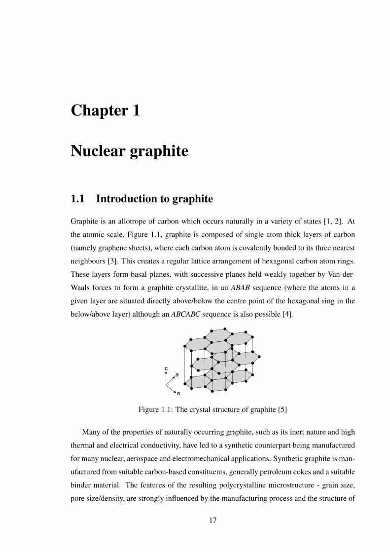
or heavy water [2]. Examples of such reactors are the UK’s current fleet of Advanced Gas-
cooled Reactors (AGR), which were preceded by the Magnox reactors. In such designs the
reactor comprises of a construction of interlocking graphite moderator bricks with holes for
fuel element and control rod insertion and coolant flow, Figure 1.2.
Figure 1.2: A scaled-down AGR core consisting of graphite moderator bricks (Figure from[8] courtesy of British Energy)
Furthermore graphite’s high resistance to thermal shock, low coefficient of thermal ex-
pansion and increasing strength with temperatures up to 2500oC (assuming a non-oxidising
environment) have made it an important material in the design of a Generation IV Very
High Temperature Reactor (VHTR) and the predecessing High Temperature Gas Cooled
Reactors (HTGR). In such reactors, graphite is again used as a moderator and core struc-
18

CHAPTER 1. NUCLEAR GRAPHITE
tural material, such as the prismatic core of the High Temperature Test Reactor (HTTR) in
Japan, but can also be incorporated into the fuel itself, in the form of graphite pebbles, such
as the Thorium High Temperature Reactor (THTR) in Germany or the High Temperature
Reactor 10 (HTR-10) in China, Figure 1.3.
Figure 1.3: High temperature reactor; (a) prismatic reflector blocks undergoing machining[9]; (b) graphite pebbles with tennis ball to gauge scale [10]
The integrity of graphite, as with all structural reactor components, is critical for their
fitness for purpose. As a result, understanding the fracture behaviour of graphite is essential
for a number of reasons:
• Approving plant life extensions of the current UK AGRs. The loss of integrity in the
graphite bricks and other irreplaceable graphite components, such as the fuel sleeves,
could lead to disrupted coolant flow or control rod deployment, both of which can
lead to the overheating of fuel elements.
• Predicting in-service performance of current and future reactors. Typical graphite
bricks are subject to complex thermal and mechanical loading, the response to which
is time-dependent due to radiation damage. Component testing during service can be
complex so increasing the confidence in analytical and numerical models can reduce
required factors of safety and allow more structured maintenance planning.
• Deciding the best course of action for graphite legacy waste. The use of graph-
ite in UK and global reactors has left a significant irradiated graphite waste legacy,
currently over 230,000 tonnes worldwide [6]. Knowledge of the integrity of used-
graphite is essential for planning its recovery from reactors.
This task requires an understanding of the unirradiated (virgin) mechanical properties of
graphite, its response to complex structural loads and a grasp of how the properties change
with time when subject to the severe environment within the reactor, through fast neutron
19

CHAPTER 1. NUCLEAR GRAPHITE
irradiation and radiolytic oxidation. An extensive review of graphite and its use in the
nuclear industry is given by Burchell [7].
1.3 Characterising the global behaviour of graphite
The global response of brittle materials to an applied tensile or bending load is believed to
follow linear elasticity (LE), where a linear increase in load (stress) creates a linear exten-
sion (strain) before a sudden fracture, with very little plastic deformation (Figure 1.4(a)).
Unirradiated (or virgin) graphite’s similar fracture behaviour, with an initially linear re-
sponse and fracture occurring suddenly at low strains led to the assumption, that it too could
be fully described by LE [11]. There are however significant differences between graph-
ite’s response and that of a classically brittle material, such as an observable non-linearity
prior to peak load [12]. This bears similarities to that of an elastic-plastic or ductile mater-
ial (Figure 1.4(b)) where the response is linear elastic up to a point, defined as the elastic
limit or yield point. From this point onwards the response is non-linear with the material
yielding and undergoing plastic deformation prior to failure. This reduced stiffness, along
with other apsects of graphite’s global response, such as tension softening between the peak
load and fracture and a distinct size effect when considering strength and its relation to spe-
cimen size, are better understood when its behaviour is considered at a more local scale.
Distributed micro-cracking within an area ahead of the tip of the macro-crack, defined as
the fracture process zone (FPZ), have led to its characterisation as a quasi-brittle mater-
ial [12, 13], with ultimate failure occurring when distributed micro-cracks coalesce into a
critically sized flaw.
nonlinear
crack localization
(b)
l l
nonlinear
crack localization
(c)
l
crack localizationσ
σ
Δ Δ Δ
σ
nonlinear
(a)
Figure 1.4: The stress-displacement graph for; (a) brittle (b) perfectly plastic/ductile and(c) quasi-brittle materials under uniaxial tension [14]
20
CHAPTER 1. NUCLEAR GRAPHITE
Quasi-brittle is a term which has been used to describe many materials of heterogeneous
microstructure, e.g. concrete, rocks, sea ice, several ceramics, polymers [15], with much
work done on the behaviour of quasi-brittle materials coming from a desire to understand
the behaviour of concrete. Quasi-brittle materials appear to have a mixed response with
characteristics of both elastic and elastic-plastic materials (Figure 1.4(c)) with an initial
linear response corresponding to LE followed by a post-elastic limit non-linearity similar
to that from plasticity [16]. In fact quasi-brittle materials exhibit very little plasticity, with
the macro non-linear response that resembles plasticity being (most prominantly) due to the
formation and accumulation of distributed micro-cracks, prior to the ultimate failure point
of the material. These micro-cracks dissipate the elastic strain energy within the system
causing a local reduction in stiffness as this energy is no longer available to allow the crack
to propagate [16]. The response of the material at the micro-scale remains true to linear
elasticity throughout this region (i.e. the material still remains fundamentally brittle), but
the aggregate based, heterogeneous microstructure prevents sudden fracture. Instead cracks
are allowed to propogate progressively, along a microstructure-dependent fracture path [12].
The affect of graphites microstructure on its mechanical properties and fracture behaviour
are discussed in more detail in Chapter 4.
1.4 Fracture Process Zone (FPZ)
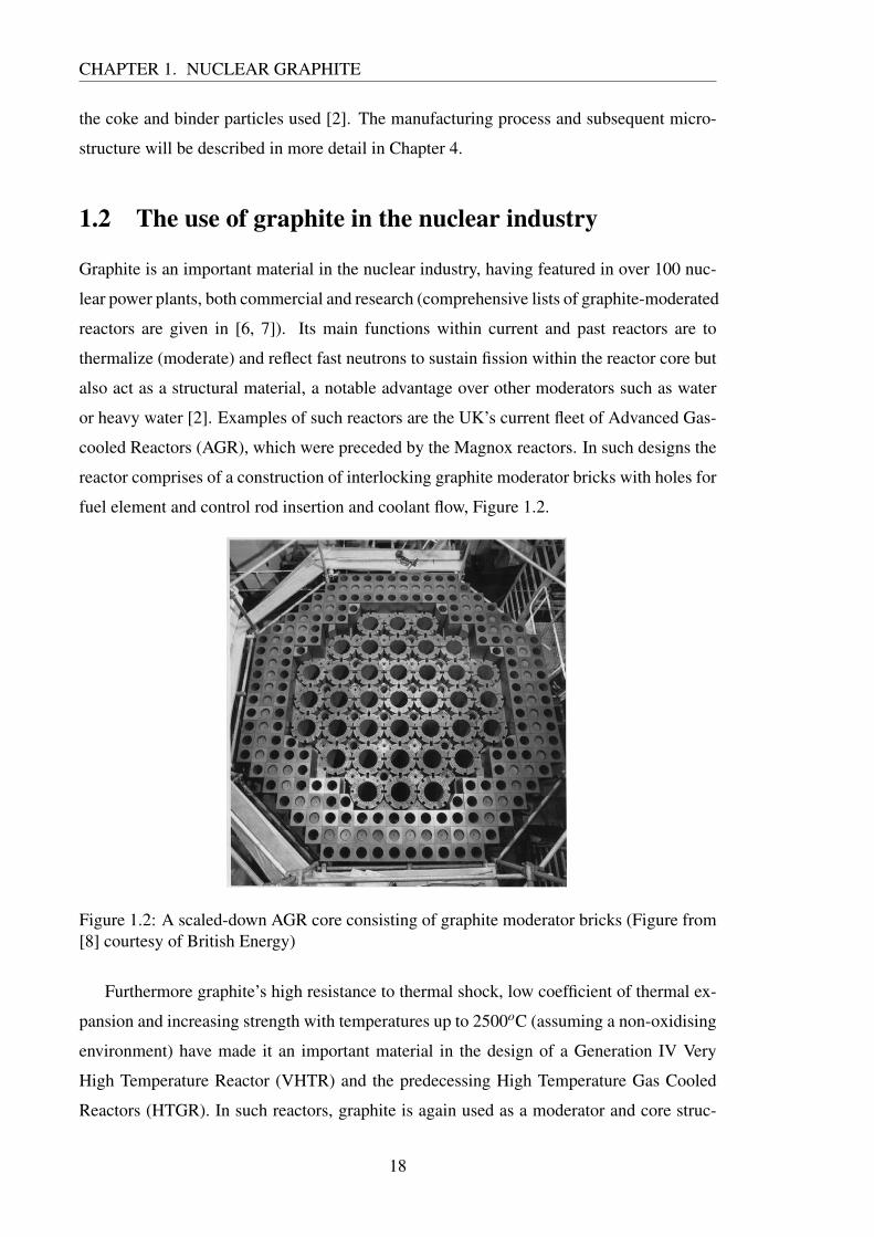
The FPZ is an important concept for modelling fracture of many varieties of materials, with
its size allowing insight into the type of material [16]. Figure 1.5(a) gives a basic example
of an FPZ, with the mechanistic processes at the micro-scale occurring over a distance xc.
Figure 1.5: A fracture process zone at the tip of a crack; (a) shown schematically (top); (b)shown mechanistically (bottom) [17]
21

CHAPTER 1. NUCLEAR GRAPHITE
The FPZ has not been clearly defined but the general definition given by Cottrell [18]
of an identified regime where the specific dissipated energy under steady state propagation
is constant, allows it to be distinguished from the plastic zone in relevant materials. Brittle
materials, are deemed to fail according to Linear Elastic Fracture Mechanics (LEFM - Ap-
pendix A), with fracture occurring suddenly, due to the existing flaws within the material
before the development of a significant damage zone, Figure 1.6(a). In such materials any
plastic zone at the crack tip will be due to small-scale yielding (Appendix A.3). This re-
gion can be defined as the FPZ, the size of which is negligible (of the order of micrometers
[12]) in comparison to the crack. Ductile materials cannot be described by LEFM, with
dislocations, void interaction and coalescence creating a significant damage zone around
crack tips. The failure is instead predicted using the yield strength criteria and a branch
of fracture mechanics corresponding to elastic-plastic behaviour (EPFM). Such materials
will exhibit a small FPZ (although 10− 100 times larger than LEFM [12]) surrounded by
a much larger zone of plastic deformation, Figure 1.6(b). In a quasi-brittle material there
is negligible plasticity, instead the FPZ occupies the entire region subject to non-linearity,
Figure 1.6(c).
F
N
L
F
N
L
F
N
L
Figure 1.6: Zones of non-linear behaviour for linear elastic (left), non-linear plastic(middle) and non-linear quasi-brittle materials (right) (adapted from [14] and [19]). Thecross hatched area, L denotes linear elastic material. N denotes the material subject tonon-linear behaviour in the form of plasticity. F denotes the material subject to non-linearbehaviour that does not include plasticity, i.e. the fracture process zone.
As mentioned, within this process zone are distributed micro-cracks, which individually
behave according to LEFM but prevent the storage of elastic strain energy expected of an
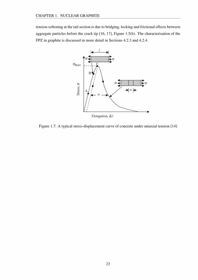
LEFM material at the macroscale. Figure 1.7 shows the typical stress-displacement curve
for a concrete specimen under uniaxial tension, where concrete’s ability to carry a residual
load after the material strength has been reached is evident. The pre-peak load non-linearity
and initial post-peak tension softening are considered to be due to micro-cracking, whereas
22
CHAPTER 1. NUCLEAR GRAPHITE
tension softening at the tail section is due to bridging, locking and frictional effects between
aggregate particles before the crack tip [16, 17], Figure 1.5(b). The characterisation of the
FPZ in graphite is discussed in more detail in Sections 4.2.3 and 4.2.4.
w
l
max
Str
ess,
σ
w
Elongation, Δ l
A
B
C
σ
σ
σ
σ σ
Figure 1.7: A typical stress-displacement curve of concrete under uniaxial tension [14]
23
Chapter 2
Modelling quasi-brittle material
behaviour
2.1 Global approach to modelling material failure
Strain constitutive
equations
Method of
calculation
Stress and strain
field histories
Critical
conditionsStructure
Loading
Initial conditions
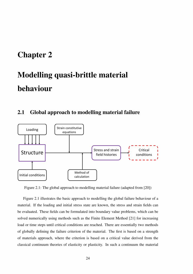
Figure 2.1: The global approach to modelling material failure (adapted from [20])
Figure 2.1 illustrates the basic approach to modelling the global failure behaviour of a
material. If the loading and initial stress state are known, the stress and strain fields can
be evaluated. These fields can be formulated into boundary value problems, which can be
solved numerically using methods such as the Finite Element Method [21] for increasing
load or time steps until critical conditions are reached. There are essentially two methods
of globally defining the failure criterion of the material. The first is based on a strength
of materials approach, where the criterion is based on a critical value derived from the
classical continuum theories of elasticity or plasticity. In such a continuum the material
24

CHAPTER 2. MODELLING QUASI-BRITTLE MATERIAL BEHAVIOUR
is assumed to consist of one continuously distributed mass. Any point within this mass
are considered to have only 3 degrees of freedom (DOF), whereby their movement is fully
described by 3 components of displacement, ux1, ux2 and ux3 in a 3 dimensional x1, x2, x3
coordinate system. The displacement of these points leads to a symmetric stress tensor, and
the loads are described completely by a force vector. The second method is an extension of
these continuum theories into specifically derived failure theories, based on damage - Con-
tinuum Damage Mechanics (CDM), or the presence of a flaw - Fracture Mechanics, either
Linear-Elastic (LEFM), Elastic-Plastic (EPFM) or Non-Linear (NLFM). Fracture mechan-
ics is generally considered the preferred method for assessing and designing engineering
materials throughout academia and in many sectors of industry, with significant advances
since the seminal papers of Griffith [22] and Irwin [23]. Classical global fracture mechanics
essentially models the effect of introducing a discontinuity, in the form of a crack or flaw,
on a material under the assumption of a classical continuum. This assumption is generally
accurate and valid for component/macro scale behaviour predictions but there are several
limitations under other conditions.
Readers with no prior knowledge of LEFM and CDM are referred to Appendices A and
B respectively. NLFM aims to introduce into the continuum failure model the non-linear
processes occurring ahead of a crack that are evident in quasi-brittle materials. This will be
discussed more in Chapter 6. EPFM will not be covered in this thesis, but readers can refer
to [17] for more details.
2.1.1 Limitations of global fracture mechanics
Historically the assumption of a classical continuum has proved accurate and reliable in
cases which consider materials at their macro-scale. However, when exploring smaller
length scales, such as stress concentrations and discontinuities around cracks, notches,
micro-cracks and voids, material microstructure begins to have an effect on behaviour so
materials no longer behave according to classic continuum predictions [24]. The reasons
for this are the limitations to classical global fracture mechanics, both fundamentally and
when specifically applied to quasi-brittle materials. LEFM and EPFM can only be used in
the presence of an initial crack or flaw, which remains sufficiently far away from any bound-
ary, with the size effect relationship between failure load and component size described by
a power-law. Furthermore both follow the assumption that the structure lacks any charac-
teristic length, i.e. any fracture processes occurring ahead of the crack are located within
an insignificantly small region in comparison to the crack length, Figure 1.6. The signific-
25

CHAPTER 2. MODELLING QUASI-BRITTLE MATERIAL BEHAVIOUR
ant “local” damage within a FPZ during quasi-brittle fracture renders such assumptions of
purely global behaviour invalid. Hence LEFM and EPFM can be used with a degree of con-
fidence for very large structures, but fail at smaller component sizes. Non-Linear Fracture
models, Chapter 6, have been developed to account for a non-negligible FPZ but even so
when the size becomes significant it is necessary to account for the actual processes which
dissipate energy in a local approach. An approximate guideline to the suitability of such
models for an FPZ length l, and specimen width D, given by Bažant [25], is shown in Table
2.1.
Length scale Most suitable approachD/l ≥ 100 LEFM
5≤ D/l < 100 NLFMD/l < 5 Local approaches
Table 2.1: Suitable analysis procedures for varying fracture process size
2.2 Local approach to fracture
Predicting the macro-response based on the processes occurring at the length scale of the
micro-structural features (meso-scale) in a so-called “local approach” could potentially be
more representative of the actual material response, rather than just material geometry as
in the “global approach” [20]. Understanding the mechanisms within the fracture process
zone of quasi-brittle materials and how these dissipate the strain energy ahead of the crack
tip is neccesary before these responses can be linked to the macroscopic properties of such
materials. Experimental techniques such as X-ray tomography and digital image/volume
correlation have allowed significant progress in this area [26].
There is no definitive way of introducing representative local behaviour into a frac-
ture model. Different approaches tend to involve either constructing constitutive equations
to account for such behaviour, e.g. accounting for accumulative damage by coupling the
strain constitutive equations with the aforementioned CDM, or assigning a local failure cri-
terion as a post-processing procedure. Developing the constitutive laws has tended to be
phenomenological with macroscopic experimental data used as a basis for parameter curve
fitting for individual loading cases and geometries [27, 28]. Basing the constitutive laws
on micro-structural mechanisms would provide a more realistic representation, with cur-
rent methods being developed including discrete models. A promising approach involves
finding a length scale at which a representative volume element (RVE) can be used to rep-
26
CHAPTER 2. MODELLING QUASI-BRITTLE MATERIAL BEHAVIOUR
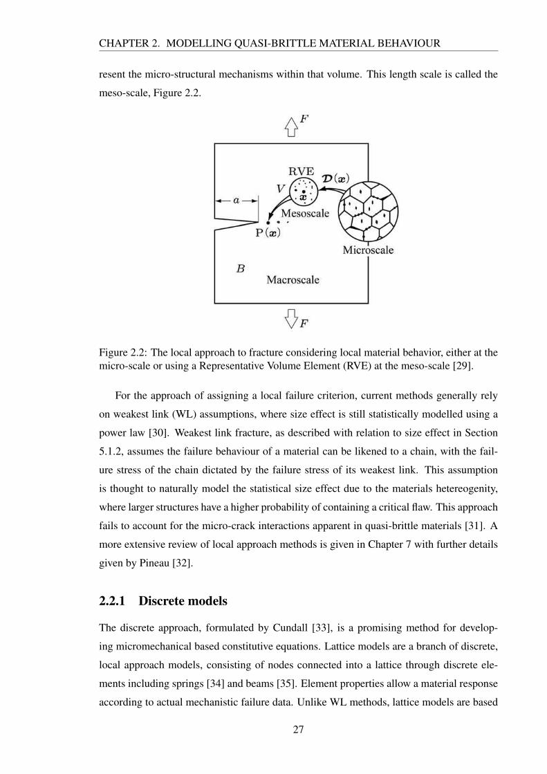
resent the micro-structural mechanisms within that volume. This length scale is called the
meso-scale, Figure 2.2.
Figure 2.2: The local approach to fracture considering local material behavior, either at themicro-scale or using a Representative Volume Element (RVE) at the meso-scale [29].
For the approach of assigning a local failure criterion, current methods generally rely
on weakest link (WL) assumptions, where size effect is still statistically modelled using a
power law [30]. Weakest link fracture, as described with relation to size effect in Section
5.1.2, assumes the failure behaviour of a material can be likened to a chain, with the fail-
ure stress of the chain dictated by the failure stress of its weakest link. This assumption
is thought to naturally model the statistical size effect due to the materials hetereogenity,
where larger structures have a higher probability of containing a critical flaw. This approach
fails to account for the micro-crack interactions apparent in quasi-brittle materials [31]. A
more extensive review of local approach methods is given in Chapter 7 with further details
given by Pineau [32].
2.2.1 Discrete models
The discrete approach, formulated by Cundall [33], is a promising method for develop-
ing micromechanical based constitutive equations. Lattice models are a branch of discrete,
local approach models, consisting of nodes connected into a lattice through discrete ele-
ments including springs [34] and beams [35]. Element properties allow a material response
according to actual mechanistic failure data. Unlike WL methods, lattice models are based
27
CHAPTER 2. MODELLING QUASI-BRITTLE MATERIAL BEHAVIOUR
around a parallel statistical system, with load redistribution amongst remaining bonds once
a bond is broken. Such models have been developed for graphite [36–38] after initial de-
velopment for concrete and cementitious materials [35, 39, 40]. The focus of this work is
the development of the Site-Bond lattice model proposed by Jivkov and Yates [41]. A full
overview of lattice models is given in Chapter 8.
2.3 Generalised continuum
Local approaches attempt to use micro-structural mechanistic understanding to improve
predictions of fracture where the global approach and hence classical continuum assump-
tions break down. Further understanding of the microstructure-fracture relation can be
gained by considering generalized continuum theories [42]. Generalized continua essen-
tially form a local approach to continuum modelling, but strive to maintain continuity
whereas local approaches to fracture model the actual mechanisms of the discontinuities.
One such theory, couple stress theory [43] of which micropolar theory is a branch, uses ad-
ditional deformation measures to describe this relation such as the curvature tensor, defined
as the relative rotation between micro-structural features within the continuum with re-
spect to the distance between them. Within these theories the classical deformation energy,
arising from symmetric strains, is amended with curvature energy, naturally introducing a
microstructure-related length scale that is missing in classical fracture mechanics and study
of size effect. Including such length related terms requires the inclusion of the previously
ignored couple stress component of the stress tensor into the continuum theory. Although
generalised continua and couple stress theory offer a stand-alone approach to modifiying
a classical continuum to account for micro-structural affects, initial work in this project
aimed to use generalized continuum theory as complimentary to local fracture models, in
order to benefit from this internal length scale. In particular a micropolar continuum has
been used in lattice models where both displacements and rotations between lattice nodes
are allowed [44–47] as this allows for rotational invariance. In this manner realistic calib-
ration requires consideration of couple stress theory. An overview of couple stress theory
and other generalised continuum theories are given in Chapter 9.
28

Chapter 3
Project outline
3.1 Aims and objectives
The purpose of this project is to use microstructure-informed lattice-models to improve un-
derstanding of the fracture processes of graphite and hence its behaviour at an engineering
scale. The project has 2 main aims:
• Increase understanding of deformation and fracture behaviour of nuclear graphite
through application of lattice-models.
• Propose an improved methodology of graphite integrity assessment.
These aims are to be achieved through 3 objectives:
1. Develop a micro-structurally informed lattice model at the length scale of graphites
micro-structural features (meso-scale).
2. Validate the model against experimental data in its ability to reproduce elastic con-
stants, material properties and general quasi-brittle behaviour.
3. Use the comparison of model and experiment to explore methods for integrating
micro-structure informed models into engineering integrity assessment procedures.
3.2 Report structure
The thesis is structured as follows; in Part II a review of the literature is undertaken. The
literature surrounding the manufacture, microstructure and fracture properties of nuclear
29
CHAPTER 3. PROJECT OUTLINE
graphite is explored in Chapter 4. The variation of size effect and non-linear fracture mech-
anics are discussed with relation to quasi-brittle materials in Chapters 5 and 6 respectively.
A more comprehensive review is given of the local approach to fracture in Chapter 7 with
specific considerations of constitutive models and failure criterion for concrete, cement and
graphite. An overview of discrete local approaches is given in Chapter 8 with emphasis on
lattice models. The concept of generalised continuum theory is explored in Chapter 9.
This thesis is presented in the form of published or submitted work. The portfolio of
published works can be found in Appendices C-I. Part III outlines the published works
with a brief overview of each paper with accompanying discussion, Chapter 10, before
presenting overall conclusions, Chapter 11, and possible extensions with relation to the
Site-Bond model, Chapter 12.
30
Part II
Review of Literature
31

Chapter 4
Manufacture and microstructure of
graphite
4.1 Manufacturing process
The process of producing synthetic graphite was established in the late 19th Century, fol-
lowing the discovery by Edward Acheson that graphitic carbon, rather than amorphous
carbon, was left behind upon heating silicon carbide in a furnace [2]. The raw constituents
of synthetic graphite can be any graphitizing source of carbon with the general basis of
particulate filler material held together using a binder [1, 48]. Coke particles are used as
filler material due to their high carbon content. These are generally either petroleum cokes,
produced by delayed coking from by-products of petroleum oil distillation, or pitch cokes,
which are produced from coal-tar pitch [2, 4]. The resulting cokes vary in shape depending
on the initial feedstock, ranging in the extremes from high-aspect ratio needle cokes to more
spherical shot cokes [49]. Binder materials are usually distillation products from coal, such
as coal-tar pitch, which soften upon heating, allowing forming of the raw carbon article to
take place before hardening once cooled [4]. The choice of raw materials and the manu-
facturing route taken, particularly with regards to the method of forming, has a significant
effect on the microstructure and hence properties of the resulting grade of graphite.
The manufacturing process, as shown in Figure 4.1, begins with the preparation of the
filler particles. These are calcined in order to reduce the amount of volatile matter from
approximately 15% to below 0.5% [2, 4]. In addition this step serves to pre-shrink the
particles prior to a latter baking stage. Failure to do so may result in poor cohesion between
the filler and binder phases. The filler particles are then subject to milling/grinding before
32

CHAPTER 4. MANUFACTURE AND MICROSTRUCTURE OF GRAPHITE
Coke
Calcined coke
Coke flour Coke particlesBinder material
Green article
Baked article
Impregnated
Calcination
Milled & sized
Mixed
Formed
Cooled
Baked
Nuclear Graphite
Graphitized
Purified
Figure 4.1: Nuclear graphite production flow sheet
being sieved and graded into varying sizes. It is necessary to have a range of sizes from large
filler particles to small fragments, called flour, to allow tighter packing and hence higher
density in the final product [2, 4]. The binder material is then added to the preferred mixture
of particles of varying sizes. The mixture is used to form a solid billet through extrusion or
moulding (either block moulding, isostatic pressing or vibration moulding). The forming
method can introduce a directional bias into the resulting microstructure, depending on the
shape of the initial coke filler particles used. Extrusion tends to cause an alignment of
the long axes of filler particles, if present, to the direction parallel to that of the extrusion.
Moreover moulding can align the particles perpendicular to the direction of the moulding
force [2]. The formed “green article” is then baked at around 800oC to further remove
volatile substances and to carbonize the pitch. This results in a reduction in density and
increase in porosity to 25−35% in the baked article, which is combated by an impregnation
of molten pitch prior to the graphitization stage [2]. Graphitization involves heating the
33
CHAPTER 4. MANUFACTURE AND MICROSTRUCTURE OF GRAPHITE
carbon product at temperatures ranging from 2200− 3000oC, in order to restructure the
carbon article to form regions of crystallite graphite.
The baking and graphitization stages are effective at removing a large number of im-
purities, producing a final product suitable for many industrial applications. Nuclear-grade
graphite however, requires a further purification step to remove impurities which remain
due to their high boiling points [2, 4]. Boron is of particular concern in nuclear applications
due to its high neutron capture cross-section which is inhibitive to the moderating proper-
ties of graphite. A low boron content can be ensured with careful selection of raw materials
and the introduction of an additive into the graphitizing furnace which reacts with the boron
and allows it to be removed along with other volatile elements.
4.2 Resulting microstructure
The resulting product from this manufacturing process is a high purity graphite, the micro-
structure of which is three phase; relatively large filler particles (graphitized coke particles),
a matrix of graphitized binder (sometimes only partially so [50]) and various populations
of porosity. The structure varies significantly depending on the raw materials and manu-
facturing process used. In this section some comments will be made regarding the general
structure of graphite and resulting mechanical properties before considering the specific
structures of a selection of nuclear-grade graphites.
During the graphitization process the underlying structure within the filler particles will
change to form mosaic regions of small graphitic crystallites which can grow, reorientate
and coalesce into domains of longer-range order [51]. This longer-range order within the
filler particles is aligned predominantly in the direction of any bias of the particles, i.e. the
basal planes of the graphitic crystallite will become parallel to the direction of extrusion
[48, 52]. The binder or matrix phase consists of a continous mosaic of randomly orientated
graphitic crystallites [52], although studies have shown that this phase itself can consist of
a combination of graphite crystallites, quinoline insoluble (QI) particles (resulting from the
fractionation process which produced the pitch) and ungraphitized carbon [50].
The three main porosity/initial crack populations, ranging from nm to mm in size, total
approximately 20% of virgin graphite volume [52]. Gas evolution cracking occurs within
the matrix during the impregnation stage of manufacture as gas bubbles form when liquid
pitch boils during baking. As such these are found predominantly in the matrix phase [52].
Calcination and Mrozowski cracks form throughout the graphite due to uneven thermal ex-
34

CHAPTER 4. MANUFACTURE AND MICROSTRUCTURE OF GRAPHITE
pansion and shrinkage as the graphite heats and cools during calcination and graphitization
respectively. The produced cracks are the result of the differing thermal expansion coeffi-
cients of the a and c axis within graphites atomic structure, Figure 1.1, where upon cooling
the graphite shrinks at different rates in the two directions [53]. The porosity phase results
in a density of approximately 1.6−1.8g/cm3, a significant reduction from 2.26g/cm3, the
theoretical density of a perfect graphite crystal. Porosity and associated micro-cracking can
interact and coalesce [54], forming interconnected networks throughout the structure which
are both open and closed to the external environment.
4.2.1 Nuclear graphite grades
The many applications of graphite has led to the development of different varieties, with
different average grain sizes, ranging from coarse grained graphite with grains larger than
4mm to microfine grained graphite with grains smaller than 2µm. In nuclear graphite these
typically range from ultrafine (< 10µm) to medium grains (< 4mm) [37]. The variation in
grain size, alongside other micro-structural differences can result in different mechanical
properties [55]
Past and current reactors in the UK employ a selection of graphites grades. The earliest
generation of gas-cooled reactor in the UK, Magnox reactors, used Pile Grade A (PGA)
as moderator, an extruded graphite distinguishable by its coarse needle coke filler particles
with length in the region of 0.1−1mm [12]. Gilsocarbon, or IM1-24, is used as the mod-
erator and reflector in the UK Advanced Gas-cooled Reactors (AGRs) with VFT and later
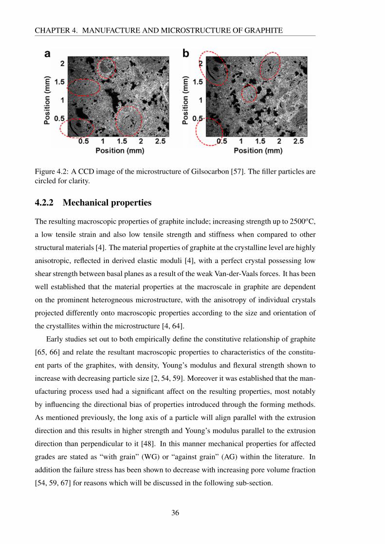
Nittetsi graphites used as fuel element sleeves [56]. In Gilsocarbon the spherical filler
particles are derived from Gilsonite pitch coke and range from 0.3− 1.5mm in size with
layers analagous to those in an onion [57]. The microstructures of both Gilsocarbon [12, 58]
and PGA [12, 58, 59] have been well characterised.
Outside of the UK, there are different graphite grades in use. In particular grade IG110,
an ultrafine historical grade of graphite currently used in the Japanese High Temperature
Test Reactor (HTTR) [60], has attracted considerable research interest [61–63]. Further-
more several graphite grades are currently under consideration for possible future Genera-
tion IV high temperature reactor designs, such as PGX, PCEA and NBG-18 [61, 62]. A list
of candidate grades for the Generation IV reactor designs can be found in the NGNP graph-
ite selection report [9] in addition to the extensive list of current nuclear grade graphites
complete with origin, forming method and mechanical properties given by Burchell [7].
35
CHAPTER 4. MANUFACTURE AND MICROSTRUCTURE OF GRAPHITE
Figure 4.2: A CCD image of the microstructure of Gilsocarbon [57]. The filler particles arecircled for clarity.
4.2.2 Mechanical properties
The resulting macroscopic properties of graphite include; increasing strength up to 2500oC,
a low tensile strain and also low tensile strength and stiffness when compared to other
structural materials [4]. The material properties of graphite at the crystalline level are highly
anisotropic, reflected in derived elastic moduli [4], with a perfect crystal possessing low
shear strength between basal planes as a result of the weak Van-der-Vaals forces. It has been
well established that the material properties at the macroscale in graphite are dependent
on the prominent heterogneous microstructure, with the anisotropy of individual crystals
projected differently onto macroscopic properties according to the size and orientation of
the crystallites within the microstructure [4, 64].
Early studies set out to both empirically define the constitutive relationship of graphite
[65, 66] and relate the resultant macroscopic properties to characteristics of the constitu-
ent parts of the graphites, with density, Young’s modulus and flexural strength shown to
increase with decreasing particle size [2, 54, 59]. Moreover it was established that the man-
ufacturing process used had a significant affect on the resulting properties, most notably
by influencing the directional bias of properties introduced through the forming methods.
As mentioned previously, the long axis of a particle will align parallel with the extrusion
direction and this results in higher strength and Young’s modulus parallel to the extrusion
direction than perpendicular to it [48]. In this manner mechanical properties for affected
grades are stated as “with grain” (WG) or “against grain” (AG) within the literature. In
addition the failure stress has been shown to decrease with increasing pore volume fraction
[54, 59, 67] for reasons which will be discussed in the following sub-section.
36
CHAPTER 4. MANUFACTURE AND MICROSTRUCTURE OF GRAPHITE
With regard to specific graphite grades, the needle-like coke particles in extruded PGA
graphite strongly project the materials anisotropy onto the macroscopic properties such that
the WG Young’s modulus can be double the AG value [68]. Gilsocarbon, shows minimal
directional dependence, with the individual crystallites within the spherical filler particles
having a tendency to align circumferentially. This results in near isotropic mechanical prop-
erties [7], a preferred property of graphite. The high dependence of macroscopic proper-
ties on distributed micro-scale features means these properties can vary between measured
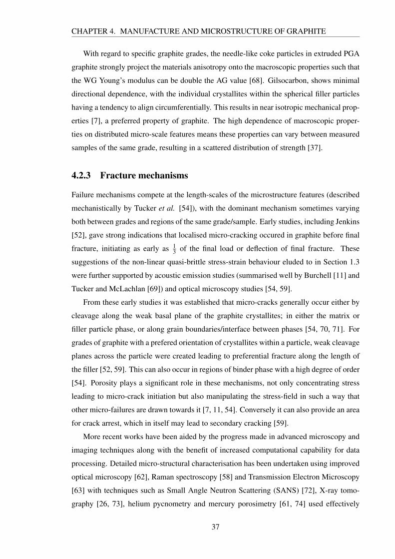
samples of the same grade, resulting in a scattered distribution of strength [37].
4.2.3 Fracture mechanisms
Failure mechanisms compete at the length-scales of the microstructure features (described
mechanistically by Tucker et al. [54]), with the dominant mechanism sometimes varying
both between grades and regions of the same grade/sample. Early studies, including Jenkins
[52], gave strong indications that localised micro-cracking occured in graphite before final
fracture, initiating as early as 13 of the final load or deflection of final fracture. These
suggestions of the non-linear quasi-brittle stress-strain behaviour eluded to in Section 1.3
were further supported by acoustic emission studies (summarised well by Burchell [11] and
Tucker and McLachlan [69]) and optical microscopy studies [54, 59].
From these early studies it was established that micro-cracks generally occur either by
cleavage along the weak basal plane of the graphite crystallites; in either the matrix or
filler particle phase, or along grain boundaries/interface between phases [54, 70, 71]. For
grades of graphite with a prefered orientation of crystallites within a particle, weak cleavage
planes across the particle were created leading to preferential fracture along the length of
the filler [52, 59]. This can also occur in regions of binder phase with a high degree of order
[54]. Porosity plays a significant role in these mechanisms, not only concentrating stress
leading to micro-crack initiation but also manipulating the stress-field in such a way that
other micro-failures are drawn towards it [7, 11, 54]. Conversely it can also provide an area
for crack arrest, which in itself may lead to secondary cracking [59].
More recent works have been aided by the progress made in advanced microscopy and
imaging techniques along with the benefit of increased computational capability for data
processing. Detailed micro-structural characterisation has been undertaken using improved
optical microscopy [62], Raman spectroscopy [58] and Transmission Electron Microscopy
[63] with techniques such as Small Angle Neutron Scattering (SANS) [72], X-ray tomo-
graphy [26, 73], helium pycnometry and mercury porosimetry [61, 74] used effectively
37

CHAPTER 4. MANUFACTURE AND MICROSTRUCTURE OF GRAPHITE
to measure pore size/shape distributions. There has also been focus on in-situ character-
isation of the microstructure, progressive damage and fracture characteristics [75], using
techniques such as strain mapping [57, 73], X-ray tomography [26, 73] and digital im-
age/volume correlation [26, 68, 76], with several techniques sometimes used in parallel.
The combined outcome of these works is a better understanding of the fracture mechan-
isms and how the microfailures interact and accumulate to form the fracture process zone
(FPZ) discussed previously in Section 1.4. Work by Joyce et al. [57] further supported the
view that damage initiates at porosity by showing that the initiating sites of strain localisa-
tions coincided with porosity in a diametral compression sample. Mostafavi and Marrow
[13] showed the same phenomena under flexural loading. Moreover Marrow et al. [73]
showed that the propagation of a crack occurs as a result of the coalescence of microfail-
ures in the FPZ, with Becker et al. [77] observing the same process using the double torsion
technique for stable crack propagation. Furthermore both of these works suggest mechan-
isms that may be increasing the resistance to propagation as the crack extends (R-curve
behaviour, see Appendix A), including micro-cracking and wakes effects such as crack
bridging.
4.2.4 Characterising the Fracture Process Zone
As discussed by Hodgkins et al. [12], the FPZ size and the resultant affect on global re-
sponse is dependent on geometry and applied load. In plain specimens (Hodgkins uses the
example of a beam) microfailures are generally initiated at areas of high stress, due to fea-
tures such as pores, or the loading. As such, damage is distributed over a relatively large
region. This large FPZ allows an increased amount of energy dissipating damage to occur
and hence increases the strain at which global failure occurs, i.e. a larger FPZ increases the
failure strain. When the specimen is notched, the region of high stress is intensified around
the notch reducing the FPZ size, restricting the volume in which damage can occur and
hence reduces energy dissipation and nonlinearity. Furthermore as the component volume
decreases, the considered length scale approaches that at which the microfailures occur and
there will be a size affect, with properties changing for geometrically identical specimens
of differing size. This is discussed further in Chapter 5.
Many attempts to characterise the FPZ size as a material property have been made,
beginning with Hillerborg et al. [78] who termed it the characteristic length, with more
recent attempts including Saucedo et al. [79, 80]. Hillerborg’s characteristic length is
discussed in relation to cohesive zone models in Section 6.1. Although some of these
38

CHAPTER 4. MANUFACTURE AND MICROSTRUCTURE OF GRAPHITE
characterisation attempts include reference to microstructure, the parameters controlling
the size of the FPZ are still not clearly understood. According to Aliha and Ayatollahi [81],
Awaji et al. [82] and Claussen et al. [83], the size of the FPZ for ceramics scales as a
function of the fracture toughness and tensile strength, according to variations of Equation
4.1.
r = A(
Kσc
B)2
(4.1)
where K is fracture toughness, A is a constant and B can be a constant or a function of
another parameter (e.g. a function of crack angle [83]). Conversely Ayatollah and Aliha
[84] have shown empirically that the FPZ size in ceramics is approximately 100 times
greater than the average grain size alone, while Bažant and Oh showed that FPZ width is 3
times the maximum aggregate size [19].
4.3 Effects of radiation damage
The demanding environment within a nuclear reactor can lead to considerable radiation
damage of structural components including graphite. In the following section the two main
mechanisms, fast neutron irradiation and radiolytic oxidation, and their effect on the micro-
structure and mechanical properties of graphite will be briefly discussed.
4.3.1 Fast neutron irradiation
Fast energetic neutrons can collide with carbon atoms within the graphite crystallite, displa-
cing the atom and hence damaging the lattice [2, 48]. This results in significant changes in
the dimensions of the graphite component and its mechanical properties, with these changes
being highly dependent on the temperature and the microstructure, specifically the dire-
citonal bias of crystallites [6].
In general as carbon atoms are displaced, the basal plane from which the atoms ori-
ginated suffers shrinkage. The displaced atoms can cluster between planes, which leads
to swelling in the c-direction (with reference to Figure 1.1) [48, 85]. However porosity
between basal planes can accommodate the swelling, resulting in a net volume shrinkage.
This porosity is termed “accommodation porosity” and includes Mrozowski cracks between
the basal planes. Eventually this porosity is filled so there is expansion in the c-direction,
occurring at a greater rate than the in-plane shrinkage, leading to a net-volume increase and
39

CHAPTER 4. MANUFACTURE AND MICROSTRUCTURE OF GRAPHITE
density decrease. The point at which this occurs is termed the “turn-around” as shown in
Figure 4.3. The changes in mechanical properties with neutron dose is strongly linked to
the corresponding change in volume [11]. Initially the net shrinkage and increase in density
results in an increase in strength and modulus [2, 86] coupled with linear elastic behaviour
as potentially energy dissipating pores are removed. Following turn-around the decrease in
density causes a reduction of strength as pores are created.
Figure 4.3: The turn-around for Gilsocarbon at varying temperatures for; dimensionalchange (left) and relative Youngs modulus (right) [87]
4.3.2 Radiolytic oxidation
Radiolytic oxidation is a concern for some gas cooled reactors, specifically those cooled
by a non-inert gas such as CO2 in the UK’s Magnox and AGR reactors. The CO2 within
the coolant can, when irradiated, split into CO and an oxidising species. This oxidising
species, as with the rest of the coolant can move into “open-porosity” where it can react with
carbon atoms on the graphitic pore surface, increasing the pore size (and hence porosity)
and producing CO [48, 88, 89]. This can result in significant weight-loss, particularly in the
40

CHAPTER 4. MANUFACTURE AND MICROSTRUCTURE OF GRAPHITE
matrix phase [12], to the graphite without any noticable change to the external component
dimensions.
It has been established that the change of mechanical properties, such as tensile or
compressive strength σ or Young’s modulus E, resulting from the fractional weight loss,
x, follows an exponential decay law according to the relationship proposed by Duckworth
[90], Ryshkevitch [91] and expanded by Knudsen [92] for porous materials:
σ = σ0 e−aθ (4.2)
E = E0 e−bθ (4.3)
where σ0 and E0 denote the pore-free values of tensile or compressive strength and Youngs
modulus respectively. θ is the pore volume fraction/porosity and a and b are dimensionless
constants. Alternatively, as outlined by Burchell et al. [93] and Berre et al. [94], the
relationship can be given in terms of fractional weight loss:
σ = σ0 e−Ax (4.4)
E = E0 e−Bx (4.5)
Kelly et al. [95] measured the constants A and B for Gilsocarbon as 4.0 and 3.6 respectively.
Buch [70] derived an expression relating the constants to the pore aspect ratio, Ar:
b = 1+0.594Ar (4.6)
41

Chapter 5
Size effect of quasi-brittle structures
Size effect in materials and structures has been evident since the times of Leonardo da Vinci
[96] who speculated that the strength of a rope is inversely proportional to its length. It is
of particular importance for quasi-brittle materials, where the typical engineering structure
size can vary significantly in length scale from those that can be appropriately tested [97].
The concept of size effect was developed by Mariotte in 1686 to form the basis of what
is now commonly known as the weakest link theory (WLT). Mariotte suggested that the
reason for this inverse proportionality was the increased probability of a failure-inducing
defect in a long rope. Without this defect the failure strength of both ropes would be
equal. Griffith’s work, which became the basis for LEFM, experimentally demonstrated
this strength increase on decreasing glass fibre diameters [22]. A historical overview of
such developments is given by Timoshenko [98].
5.1 Statistical Size Effect
5.1.1 Power laws
It is commonly known that physical systems involving no characteristic length will scale
through a power law [97]. The reasons behind this can be understood by considering the
response to loading, Y and Y ′ of two geometrically similar components of size D and D′
respectively:
Y = f (D), Y ′ = f (D′) (5.1)
Work by Bažant [99] showed that without a characteristic size the following relation must
be true:
42

CHAPTER 5. SIZE EFFECT OF QUASI-BRITTLE STRUCTURES
f (D′)f (D)
= f(
D′
D
)(5.2)
Which can be solved only by the power-law given in Equation 5.3 as only then will the con-
stant, c1, relating to some characteristic length, cancel out when substituted into Equation
5.2. The term s also represents a constant.
f (D) =
(Dc1
)−s
(5.3)
Figure 5.1: (a) Geometrically similar structures of different sizes; (b) power scaling laws[97]
Figure 5.1 illustrates the power-law scaling of nominal strength, σN , with compon-
ent size for elastic, elastic-plastic materials and LEFM. It has been shown that for both
strength/yield criteria for elastic/elastic-plastic materials respectively there is no size effect
with components of geometrically similar dimensions failing under the same value of σN in
the absence of a characteristic length [99]. This result corresponds to a value of s equal to 0.
Also shown in Figure 5.1 is the Weibull distribution, a distribution based upon WLT which
produces a power-law size effect [99]. The value of s shown, 16 [100], is considered typical
for concrete, deriving from an empirically fit Weibull modulus. WLT and specifically the
Weibull distribution will be described more in the following sections.
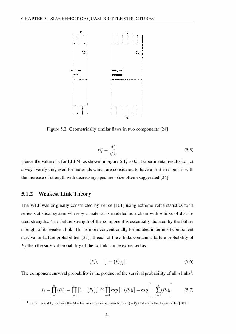
Geometric size effect in LEFM The geometric size effect predicted in LEFM can be
shown by equating the stress intensity factors of two geometrically similar cracks or flaws,
Figure 5.2 [24]:
KI = σ∗1√
πa f( a
W
)= σ
∗2
√πλa f
(λaλW
)(5.4)
43
CHAPTER 5. SIZE EFFECT OF QUASI-BRITTLE STRUCTURES
Figure 5.2: Geometrically similar flaws in two components [24]
σ∗2 =
σ∗1√λ
(5.5)
Hence the value of s for LEFM, as shown in Figure 5.1, is 0.5. Experimental results do not
always verify this, even for materials which are considered to have a brittle response, with
the increase of strength with decreasing specimen size often exaggerated [24].
5.1.2 Weakest Link Theory
The WLT was originally constructed by Peirce [101] using extreme value statistics for a
series statistical system whereby a material is modeled as a chain with n links of distrib-
uted strengths. The failure strength of the component is essentially dictated by the failure
strength of its weakest link. This is more conventionally formulated in terms of component
survival or failure probabilities [37]. If each of the n links contains a failure probability of
P f then the survival probability of the ith link can be expressed as:
(Ps)i =[1−(Pf)
i
](5.6)
The component survival probability is the product of the survival probability of all n links1.
Ps =n
∏i=1
(Ps)i =n
∏i=1
[1−(Pf)
i
]∼= n
∏i=1
exp[−(Pf )i
]= exp
[−
n
∑i=1
(Pf )i
](5.7)
1the 3rd equality follows the Maclaurin series expansion for exp(−Pf
)taken to the linear order [102].
44

CHAPTER 5. SIZE EFFECT OF QUASI-BRITTLE STRUCTURES
Equation 5.7 suggests that as the number of links, n, increases under a constant load the
probability of survival, Ps will decrease as the probability of a weak link increases, illus-
trating a clear size effect. This concept is shown in Figure 5.3.
Figure 5.3: (a) A chain with links of distributed strength; (b) failure probability of a givenelement; (c) a structure with a population of micro-cracks, each with a differing probabilityof becoming critical [97]
Extreme Value Statistics Statistically modelling brittle failure where fracture propagates
from one of many existing microscopic flaws falls into the bracket of extreme value statist-
ics. There are considered to be three types of extreme value distribution, whereby if several
sets of values are sampled from a distribution and the maxima (or minima in the case of
the Weibull distribution) from each set are collated into a new set, than this set will be rep-
resented by one of only three distributions; Gumbel, Fretchet and Weibull. For the sake
of brevity only Weibull will be considered here. For information on Gumbel and Fretchet
distributions please refer to Nemeth and Bratton [37].
Weibull distribution There are many variations on the weakest link theory with the
Weibull distribution being the most commonly referenced [103, 104]. The overview of
the Weibull derivation expressed here follows that presented by Nemeth and Bratton [37].
Weibulls distribution assumes that within a volume, V , of brittle material there exists a
critical stress, σ , which when present at a flaw of size l will lead to catastrophic crack
propagation. If there exists a distribution of flaw sizes, the critical strength, σc of a flaw of
length L can be generalised as follows:
L≥ l σc ≤ σ (5.8)
45
CHAPTER 5. SIZE EFFECT OF QUASI-BRITTLE STRUCTURES
L < l σc > σ (5.9)
A crack density function can be defined, η(σ), describing the amount of flaws in a unit
volume which satisfy σc ≤ σ . For an incremental volume4Vi, the probability of failure of
the ith link, where the critical strength is σi becomes:
Pf (σi) = [η(σi)4Vi] (5.10)
Substituting this into Equation 5.7 gives the survival probabilty of the entire volume as a
function of the failure probabilities of the individual incremental volumes:
Ps(σi) = exp
[−
n
∑i=1
η(σi)4Vi
](5.11)
If a stress of σ is applied to the entire volume where σi = σ for all increments then the
global survival probability of V is:
Ps(σ) = exp [−η(σ)V ] (5.12)
Again using Equation 5.7, the entire component failure probability can be evaluated:
Pf (σ) = 1−Ps(σ) = 1− exp [−η(σ)V ] (5.13)
Or accounting for differing stresses throughout the volume:
Pf (σ) = 1−Ps(σ) = 1− exp[ˆ−η(σ)dV
](5.14)
The Weibull distribution is obtained if a power law is used to describe the crack density
function, η(σ). The Weibull three-parameter function is shown in Equation 5.15:
η(σ) =1
V0
(σ −σu
σ0
)m
=
(σ −σu
σ0V
)m
(5.15)
The three parameters in the model are defined as followed:
σu is the value of σ below which the probability of component failure is zero. Equat-
ing this parameter to zero will produce the two parameter Weibull distribution.
σ0V is the scale parameter which incorporates the characteristic volume, V0, and the
stress value at which 37% of samples under tensile load would not fail.
46

CHAPTER 5. SIZE EFFECT OF QUASI-BRITTLE STRUCTURES
m is the Weibull modulus. This parameter is a dimensionless representation of the
variation of strength in the material. This is evaluated using the best fit to empirical
data.
From Equation 5.14, the two parameter Weibull equation can be decomposed to include an
effective volume, V e:
Pf = 1− exp[ˆ
V−(
σ
σ0V
)m
dV ] = 1− exp[−Ve
(σ f
σ0V
)m
] (5.16)
where Ve =´
V
(σaσ f
)mdV with σa denoting the level of stress at position a(x,y,z) and σ f is
the maximum stress within the effective volume. This implies that for two components (de-
noted with subscripts 1 and 2) of identical relative dimensions but different size, Equation
5.16 can be used to equate their failure probabilites to give a relation between component
volume and the maximum stress at a given point for a given failure probability [37]:
σ f 2
σ f 1=
(Ve1
Ve2
) 1m
(5.17)
Equation 5.17 shows that strength will reduce with increasing component size, with the
reduction related to the Weibull modulus, m.
Aside from its use in describing size effect, much work has been done on using the
Weibull distribution as a failure criterion for graphite to explain the spread of experimental
results, with an extensive review given in Nemeth and Bratton [37]. An example of an
analysis of graphite strength using the Weibull distribution is shown in Figure 5.4, where S
is the probability of fracture. This will be discussed more in Section 7.1.
5.2 Deterministic Size Effect
As mentioned, the power law distribution relating failure strength to size is strongly re-
liant on the absence of a characteristic length. As discussed in Sections 1.4 and 4.2.4,
a characteristic length exists in quasi-brittle materials in the form of the significant FPZ
size. Nemeth and Bratton [37] present evidence from several works which suggest that the
Weibull approach, as a method of modelling size effect purely statistically, is insufficient
for modelling graphite, with similar works drawing the same conclusions for cement-based
materials [31, 100].
At the length scale of a single micro-crack the behaviour can be described as LEFM,
however at the scale that flaws interact the component will exhibit what appears to be plastic
47
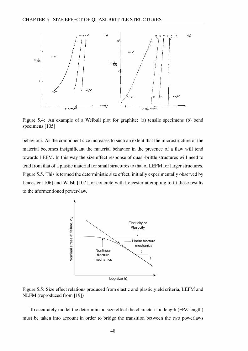
CHAPTER 5. SIZE EFFECT OF QUASI-BRITTLE STRUCTURES
Figure 5.4: An example of a Weibull plot for graphite; (a) tensile specimens (b) bendspecimens [105]
behaviour. As the component size increases to such an extent that the microstructure of the
material becomes insignificant the material behavior in the presence of a flaw will tend
towards LEFM. In this way the size effect response of quasi-brittle structures will need to
tend from that of a plastic material for small structures to that of LEFM for larger structures,
Figure 5.5. This is termed the deterministic size effect, initially experimentally observed by
Leicester [106] and Walsh [107] for concrete with Leicester attempting to fit these results
to the aformentioned power-law.
Nonlinear
fracture
mechanics
Elasticity or
Plasticity
Linear fracture
mechanics
Log(size h)
Nom
inal str
ess a
t fa
ilure
, N
2
1
Figure 5.5: Size effect relations produced from elastic and plastic yield criteria, LEFM andNLFM (reproduced from [19])
To accurately model the deterministic size effect the characteristic length (FPZ length)
must be taken into account in order to bridge the transition between the two powerlaws
48

CHAPTER 5. SIZE EFFECT OF QUASI-BRITTLE STRUCTURES
which describe the distinct statistical size effect behaviour of quasi-brittle materials above
and below the characteristic length [16]. One way of doing this is through the application
of Non-Linear Fracture Mechanics (NLFM), Figure 5.5, which will be discussed further in
the following chapter.
49
Chapter 6
Non-linear fracture mechanics
NLFM aims to introduce the non-linear energy dissipation processes found in the non-
negligible process zone ahead of a crack in a continuum-based failure model. These fracture
models have mainly been developed for concrete and extensive reviews can be found in the
following references [14, 16, 25]. Such models can be generally classified into two types;
• Models which implicitly represent the non-linear zone, mainly for numerical imple-
mentation in Finite Element analysis methods [21]. These include the cohesive or
smeared crack models.
• Models which modify LEFM, replacing the flaw with one of “effective” properties
which represent the non-linearity. These include the two-parameter fracture model,
size-effect model and the effective crack model.
For brevity only the first type, which is of more direct relevance to the presented work,
is considered here. The reader is referred to the aforementioned texts for an overview of
modified LEFM methods. The derivations provided are based around those found in the
cited papers and other standard texts [16, 17].
The first attempt to model the behaviour in an FPZ was the Dugdale-Barenblatt (cohesive-
zone) approach to correct for small-scale yielding in a linear-elastic material. The concept
behind such models originates from Dugdale’s Strip-Yield Model [108] and Barenblatt’s
Cohesive force model [109], which were originally proposed as alternatives to Irwin’s
modification of Griffith’s energy balance criterion (i.e. a correction for plastic flow in
LEFM), Appendix A.3.2. This concept has been extended and developed as the basis for
two of the most significant FPZ models, mainly in application to concrete and cement:
• Fictitious crack model (FCM)
50
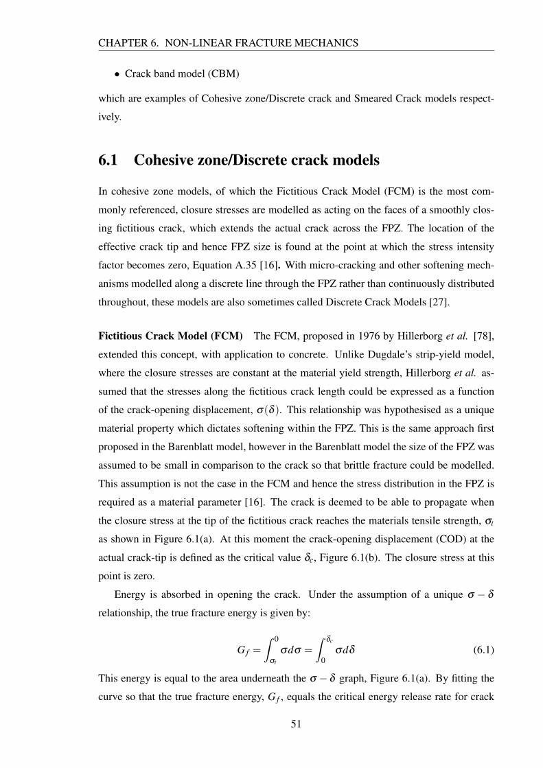
CHAPTER 6. NON-LINEAR FRACTURE MECHANICS
• Crack band model (CBM)
which are examples of Cohesive zone/Discrete crack and Smeared Crack models respect-
ively.
6.1 Cohesive zone/Discrete crack models
In cohesive zone models, of which the Fictitious Crack Model (FCM) is the most com-
monly referenced, closure stresses are modelled as acting on the faces of a smoothly clos-
ing fictitious crack, which extends the actual crack across the FPZ. The location of the
effective crack tip and hence FPZ size is found at the point at which the stress intensity
factor becomes zero, Equation A.35 [16]. With micro-cracking and other softening mech-
anisms modelled along a discrete line through the FPZ rather than continuously distributed
throughout, these models are also sometimes called Discrete Crack Models [27].
Fictitious Crack Model (FCM) The FCM, proposed in 1976 by Hillerborg et al. [78],
extended this concept, with application to concrete. Unlike Dugdale’s strip-yield model,
where the closure stresses are constant at the material yield strength, Hillerborg et al. as-
sumed that the stresses along the fictitious crack length could be expressed as a function
of the crack-opening displacement, σ(δ ). This relationship was hypothesised as a unique
material property which dictates softening within the FPZ. This is the same approach first
proposed in the Barenblatt model, however in the Barenblatt model the size of the FPZ was
assumed to be small in comparison to the crack so that brittle fracture could be modelled.
This assumption is not the case in the FCM and hence the stress distribution in the FPZ is
required as a material parameter [16]. The crack is deemed to be able to propagate when
the closure stress at the tip of the fictitious crack reaches the materials tensile strength, σt
as shown in Figure 6.1(a). At this moment the crack-opening displacement (COD) at the
actual crack-tip is defined as the critical value δc, Figure 6.1(b). The closure stress at this
point is zero.
Energy is absorbed in opening the crack. Under the assumption of a unique σ − δ
relationship, the true fracture energy is given by:
G f =
ˆ 0
σt
σdσ =
ˆδc
0σdδ (6.1)
This energy is equal to the area underneath the σ − δ graph, Figure 6.1(a). By fitting the
curve so that the true fracture energy, G f , equals the critical energy release rate for crack
51

CHAPTER 6. NON-LINEAR FRACTURE MECHANICS
Figure 6.1: The fictitious crack model for quasi-brittle materials; (a) the stress-displacementresponse (left); (b) the crack opening displacement at the ficticious crack tip (right) [17]
propagation, Gc the LEFM energy balance approach is modelled. The choice of a suitable
softening curve to match the energy rates is critical in replicating material behavior. Many
softening curves have been proposed, such as linear, bilinear, power-law and exponential,
Figure 6.2. In (incorrectly) assuming that all the material along the length of FPZ has
reached the tensile strength of the material, σt with a toughness of G f , the same approach as
Irwin in his plastic zone correction (Appendix A.3.1 - Equations A.23 and A.27), Hillerborg
et al. were able to derive a characteristic length expression which roughly approximates the
FPZ length [16]:
lp 'E ′G f
σ2t
(6.2)
0
0.1
0.2
0.3
0.4
0.5
0.6
0.7
0.8
0.9
1
0 0.2 0.4 0.6 0.8 1
σσt
δ δ
linear
bilinear
exponential
Figure 6.2: Example softening curves
Cohesive zone models require two material parameters to describe fracture behaviour.
In the FCM these parameters are the fitted softening relationship, σ(w), in the FPZ and
specific fracture energy G f . In reality, any two independent parameters can be used, includ-
ing lp [16]. There are limitations to the FCM, including the assumption of a unique σ −δ
52
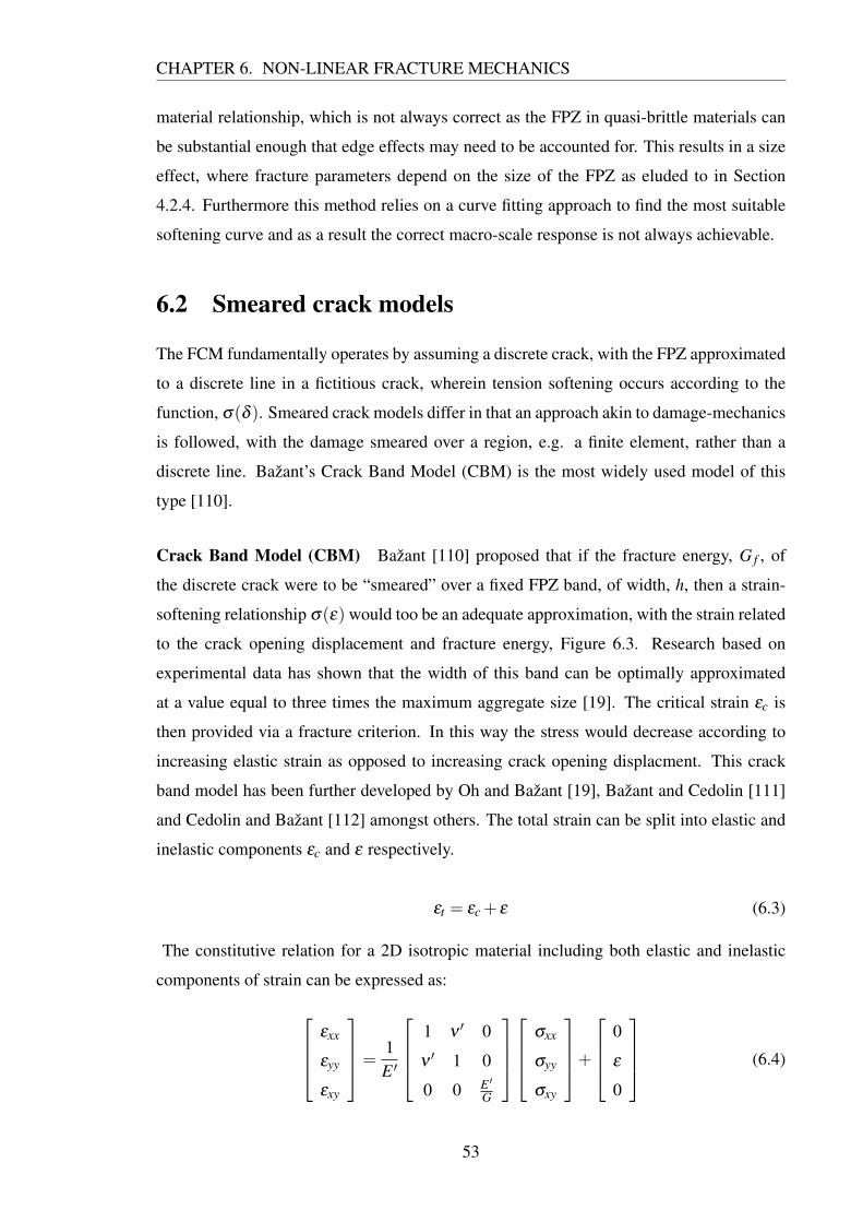
CHAPTER 6. NON-LINEAR FRACTURE MECHANICS
material relationship, which is not always correct as the FPZ in quasi-brittle materials can
be substantial enough that edge effects may need to be accounted for. This results in a size
effect, where fracture parameters depend on the size of the FPZ as eluded to in Section
4.2.4. Furthermore this method relies on a curve fitting approach to find the most suitable
softening curve and as a result the correct macro-scale response is not always achievable.
6.2 Smeared crack models
The FCM fundamentally operates by assuming a discrete crack, with the FPZ approximated
to a discrete line in a fictitious crack, wherein tension softening occurs according to the
function, σ(δ ). Smeared crack models differ in that an approach akin to damage-mechanics
is followed, with the damage smeared over a region, e.g. a finite element, rather than a
discrete line. Bažant’s Crack Band Model (CBM) is the most widely used model of this
type [110].
Crack Band Model (CBM) Bažant [110] proposed that if the fracture energy, G f , of
the discrete crack were to be “smeared” over a fixed FPZ band, of width, h, then a strain-
softening relationship σ(ε) would too be an adequate approximation, with the strain related
to the crack opening displacement and fracture energy, Figure 6.3. Research based on
experimental data has shown that the width of this band can be optimally approximated
at a value equal to three times the maximum aggregate size [19]. The critical strain εc is
then provided via a fracture criterion. In this way the stress would decrease according to
increasing elastic strain as opposed to increasing crack opening displacment. This crack
band model has been further developed by Oh and Bažant [19], Bažant and Cedolin [111]
and Cedolin and Bažant [112] amongst others. The total strain can be split into elastic and
inelastic components εc and ε respectively.
εt = εc + ε (6.3)
The constitutive relation for a 2D isotropic material including both elastic and inelastic
components of strain can be expressed as:
εxx
εyy
εxy
=1E ′
1 ν ′ 0
ν ′ 1 0
0 0 E ′G
σxx
σyy
σxy
+
0
ε
0
(6.4)
53

CHAPTER 6. NON-LINEAR FRACTURE MECHANICS
h
f't
(a) (b)
f't
c
t
E
Figure 6.3: (a) Smeared micro-cracking in a band of width h; (b) The inelasitc deformationin the FPZ represented by an equivalent inelastic strain (reproduced from [16])
where E ′ = E1−ν2 and ν ′ = v
1−νfor plane strain and E ′ = E and ν ′ = ν for plane stress. It is
initially assumed that the micro-cracks within the crack band zone all begin parallel to the
stress applied normal to the crack faces, σyy, as shown in Figure 6.3. In this way the inelastic
strain ε only increases strain in the direction normal to crack faces. Work by Phillips and
Zienkiewicz [113] introduced a shear-retention, or aggregate interlocking factors factor, β :
σxy
εxy= βG (6.5)
where 0< β ≤ 1. This factor was introduced to allow for the physically realistic restrictions
shearing movement due to crack surface roughness and aggregate interlocking [16]. With
this factor the constitutive relations become:
εxx
εyy
εxy
=1E ′
1 ν ′ 0
ν ′ 1 0
0 0 E ′βG
σxx
σyy
σxy
+
0
ε
0
(6.6)
A further improvement to increase physical realism can be introduced by including a scalar
damage parameter, ω , ranging from 0 to 1 for the undamaged and complete failure states
respectively [114]. The reduced stiffness, E ′s = E ′(1−ω), of the crack band zone with
progressive damage in the direction of loading can then be accounted for in the constitutive
relations in a coupled approach to damage using a secant stiffness matrix:
εxx
εyy
εxy
=1E ′
1 ν ′ 0
ν ′ 11−ω
0
0 0 E ′G
σxx
σyy
σxy
+
0
ε
0
(6.7)
54

CHAPTER 6. NON-LINEAR FRACTURE MECHANICS
This progressive damage will produce the tension softening response of concrete, however
this response will be dictated by the choice of softening curve used to evolve the damage
ω = f (εyy). This is a similar scenario to the FCM method with different proposed softening
curve approximations. The fracture energy can be expressed as:
G f =
ˆ h
0
ˆεc
0σyy (ε)dεdx (6.8)
which, assuming the strains do not change over the crack band, equals:
G f = hˆ
εc
0σyy (ε)dε (6.9)
where εc =δch corresponds to the critical crack opening displacement δc in the FCM [19].
Equation 6.9 reduces to Equation 6.1 as h tends to 0.
55
Chapter 7
Local approach to material failure
The limitations to global material failure modelling and fracture mechanics and the limited
applicability of NLFM, as discussed in Chapters 2 and 6, led to the development of more
locally based approaches to failure. Local approaches aim to predict micro failure initiation
and development through into the initiation of a macro sized flaw in areas where global
approaches are unreliable, i.e. in the FPZ. Such models have been previously developed
for fracture of ductile [115–117], brittle [30] and quasi-brittle materials. Introducing local
behavior can essentially be done in two ways (which can be used in combination):
• Definition of a failure criterion that accounts for local fracture mechanisms.
• Incorporation of local behaviour into the global constitutive relations.
A brief review of literature will be undertaken for local approaches to fracture. For further
details, the reader is referred to Pineau [32].
7.1 Failure criterion
7.1.1 Global failure criterion
Criterion for global material failure are classically based around the global material stress
state for an elastic continuum. The simplest failure criterion involves material failure occur-
ring when a critical value of stress or strain is reached. This is shown for a brittle specimen
under uniaxial tension in Figure 7.1, where failure occurs when the material reaches its
tensile strength, σt at a critical value of strain, εt .
This is more formally extended to two (and three) dimensions as the Rankine, or max-
imum stress, failure criteria, Figure 7.2(a), where failure occurs when the maximum prin-
56
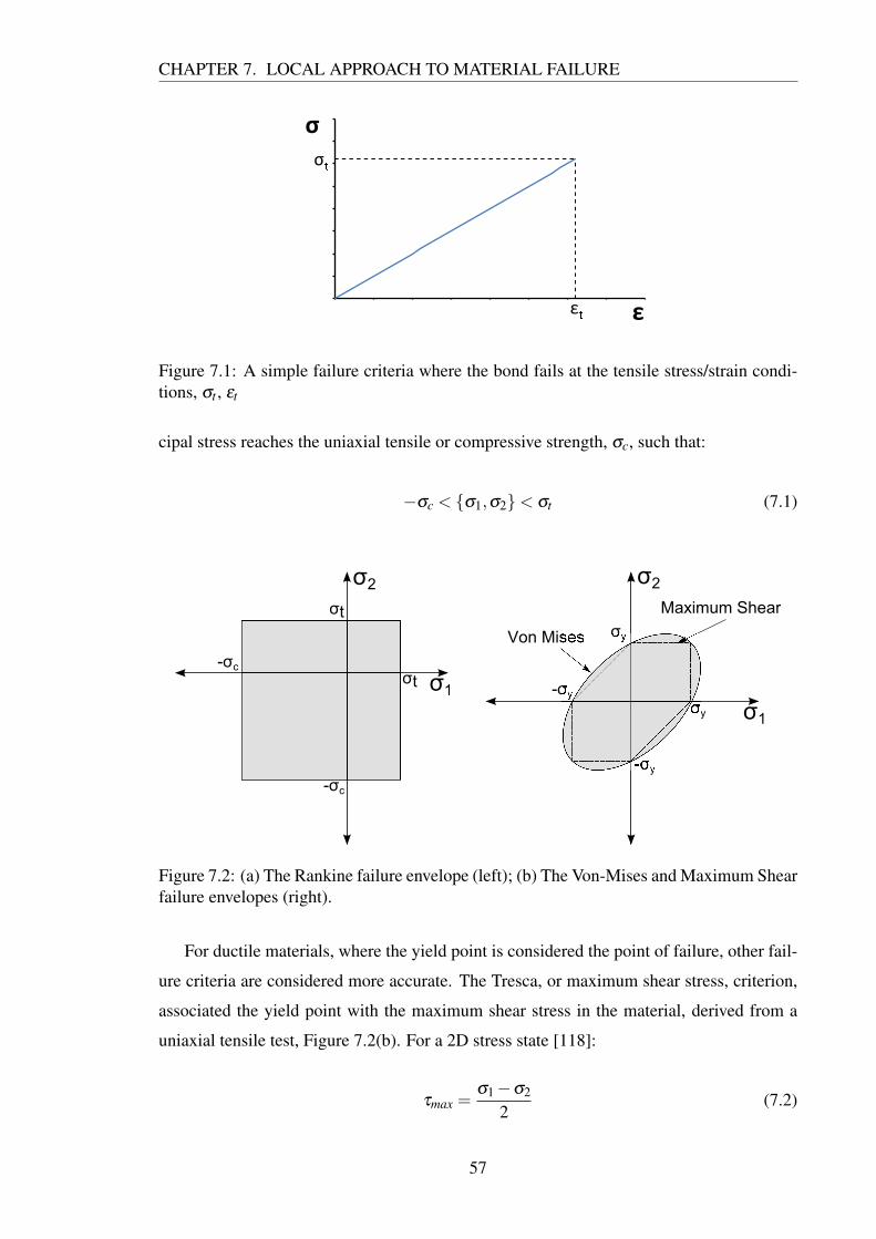
CHAPTER 7. LOCAL APPROACH TO MATERIAL FAILURE
σ
ε
σ
ε
Figure 7.1: A simple failure criteria where the bond fails at the tensile stress/strain condi-tions, σt , εt
cipal stress reaches the uniaxial tensile or compressive strength, σc, such that:
−σc < {σ1,σ2}< σt (7.1)
σ2
σ1
σt
σt
-σc
-σc
σ2
σ1
σy
σy
-σy
-σy
Von Mises
Maximum Shear
Figure 7.2: (a) The Rankine failure envelope (left); (b) The Von-Mises and Maximum Shearfailure envelopes (right).
For ductile materials, where the yield point is considered the point of failure, other fail-
ure criteria are considered more accurate. The Tresca, or maximum shear stress, criterion,
associated the yield point with the maximum shear stress in the material, derived from a
uniaxial tensile test, Figure 7.2(b). For a 2D stress state [118]:
τmax =σ1−σ2
2(7.2)
57

CHAPTER 7. LOCAL APPROACH TO MATERIAL FAILURE
For uniaxial tension at the yield point σ1 = σY and σ2 = 0. This implies at the yield point:
σ1−σ2 = σY (7.3)
Another failure criterion for materials at yield is the Von-Mises, or shear-strain energy,
criterion, Figure 7.2(b). This is also known as the octahedral shear stress, or distortion
energy criterion. This was derived by splitting the principal stresses into volumetric, σV ,
and deviatoric components, σD:
σi = σV +σ
Di (7.4)
where i = 1,2,3 and σV =σ1+σ2+σ33 .
Using these components the strain energy stored in the material upon deformation can
be decomposed into strain energy due to a volume change, i.e. from σV , and due to distor-
tion or shear, i.e. from σDi . The strain energy due to change in shape can be used to derive
the Von-Mises yield criterion (full derivation can be found in Benham et al. [118]):
(σ1−σ2)2 +(σ2−σ3)
2 +(σ3−σ1)2 = 2σ
2Y (7.5)
σ2
σ1
σt
σt
-σc
-σc
Mohr-Coulomb
Max stress
Figure 7.3: The Mohr-Coulomb failure envelope.
A further failure criterion, the Mohr-Coulomb criterion, for brittle materials can be de-
scribed by combining the Rankine and Tresca failure criterion, Figure 7.3(a). This criteria,
derived from the Mohrs circle concept, allowed the material to fail differently under purely
tensile and compressive loads, and incorporated the affect of shear stress from the Tresca
58

CHAPTER 7. LOCAL APPROACH TO MATERIAL FAILURE
criteria.
Much work has been developed for finding a suitable failure criterion for quasi-brittle
materials in a triaxial stress state, in particular concrete. This has included the use of all the
aforementioned brittle and yield criteria. Some more significant works include [119–121]
as well as the use of the Drucker-Prager yield criterion, an extension of Von-Mises [122].
However most of these are phenomenologically based, with parameters found from curve
fitting procedures from experimental results [123] and also fail to replicate variations of
strength over repeated tests [37], a phenomena dictated largely by distributions of micro-
structural features. For graphite it has been shown that modelling failure behaviour accord-
ing to a strength of material approach, with failure occurring at a critical value of stress,
strain or elastic strain energy density, is insufficient for tensile loading as a result of ignor-
ing the underlying microstructure [54].
7.1.2 Statistical failure criterion
Attempts have been made to model the implications of micro-structural defects and the
corresponding mechanisms of graphite, described in Section 4.2.3, using statistical failure
criterion, such as Weibull analysis [37, 54], as discussed with relation to the size effect in
Chapter 5.1.2. In this approach the micro-structural model is implied through the weakest
link assumption, rather than modelled. The use of the Weibull distribution as a local failure
criterion was introduced by Beremin for the application of cleavage fracture [30]. This
statistical model has been questioned in cleavage fracture [124] and quasi-brittle fracture
[31] due to the failure to explicitly account for actual mechanistic failure at the micro-scale.
Other early methods attempted to base graphite’s failure behaviour on the Griffith failure
model. Such an approach is termed the “fracture mechanics model” by Tucker et al. [54],
where the defected microstructure of the graphite, Figure 7.4(b), is represented by a crack
which fails according to Griffith criteria, Figure 7.4(a) located at the area of maximum
stress. Although such an approach aims to represent the microstructure, again it cannot
represent the actual failure mechanisms occurring at the micro-scale, especially using the
simplified crack conditions and geometries assumed in LEFM.
Further improvements, beginning with the work of Buch [70], developed a micro-
structural based failure criterion to define the conditions at which a cleavage flaw will be
generated large enough to fail according to LEFM, using input parameters such as distribu-
tions of particle size and porosity. The failure probability of each individual grain is used
to evaluate the probability that a flaw of critical size in accordance to the Griffith criterion
59

CHAPTER 7. LOCAL APPROACH TO MATERIAL FAILURE
Figure 7.4: An LEFM approximation (a) of a material with microstructure (b) [54]
will develop.
Rose and Tucker extended Buch’s work [71] to generate the Rose-Tucker model, where
the material is discretized into cubes, the size of which is representative of the particle size
within the graphite. Each particle, and hence each cube, is deemed to have a random orient-
ation which will cleave at a prescribed tensile stress. The presence of porosity is included
through the designation of cleavage strength of 0. The failure of sufficient adjacent cubes to
create a critically sized Griffith flaw represents specimen failure, Figure 7.5. One downfall
of this model is the uncoupled affect of the creation of a microflaw with the surrounding
stress field. Essentially as a new pore is created the stress around this pore will remain in
the same state, despite the clear stress raising affects.
Figure 7.5: The Rose-Tucker graphite failure model [54].
A further development of the Rose-Tucker model was developed by Burchell over sev-
eral works [7, 11, 67]. This followed the same discretisation procedure as the Rose-Tucker
model but the onset of cleavage was only considered in areas of concentrated stress, i.e.
around porosity. Initial pores within the model are treated as micro-cracks with cleavage
planes perpendicular to the applied tensile stress on the cube by which they are represented.
60

CHAPTER 7. LOCAL APPROACH TO MATERIAL FAILURE
In this way the stress in surrounding cubes is concentrated. The total failure probability of
a row of particles is dictated by the probability of the concentrated stress from the initial
pore being sufficient to fail each successive particle once the stress is resolved onto the
corresponding cleavage planes, Figure 7.6.
Figure 7.6: The crack front in the Burchell model can extend through an successive particlesif the stress resolved onto the cleavage plane is large enough to cause cleavage [37].
McLachlan and Tucker [69, 125] extended the Burchell model, introducing a reliance
on the stress concentrating capacity of pores on their shape. In this manner pores were
deemed as “active”, or essentially micro-cracks, where the stress around is concentrated, or
“passive”, where the pore shape incurs little stress concentration and hence is less likely to
intiate cleavage.
A review of these statistical failure criterion models was undertaken in Tucker et al.
[54], Tucker and McLachlan [69], and Nemeth and Bratton [37]. These papers concluded
that the models which aim to explicitly model the affects of microstructure, Rose-Tucker,
Burchell, McLachlan-Tucker, performed better than those which implicitly suggest the
presence of microstructure, Weibull, and those which involve microstructure without con-
sideration of the interactions at this scale, fracture mechanics model. However all these
methods are based around a weakest link assumption so are inherently unable to fully model
the interaction processes at the micro-scale.
7.2 Local constitutive equations
A local continuum approach to material failure can rely on both Fracture Mechanics and
Continuum Damage Mechanics (CDM). Introducing damage mechanics allows the damage
to be evolved to the point of macro-crack initiation, after which the critical conditions for
component failure are defined by a failure criterion [20] dictated by fracture mechanics or
61
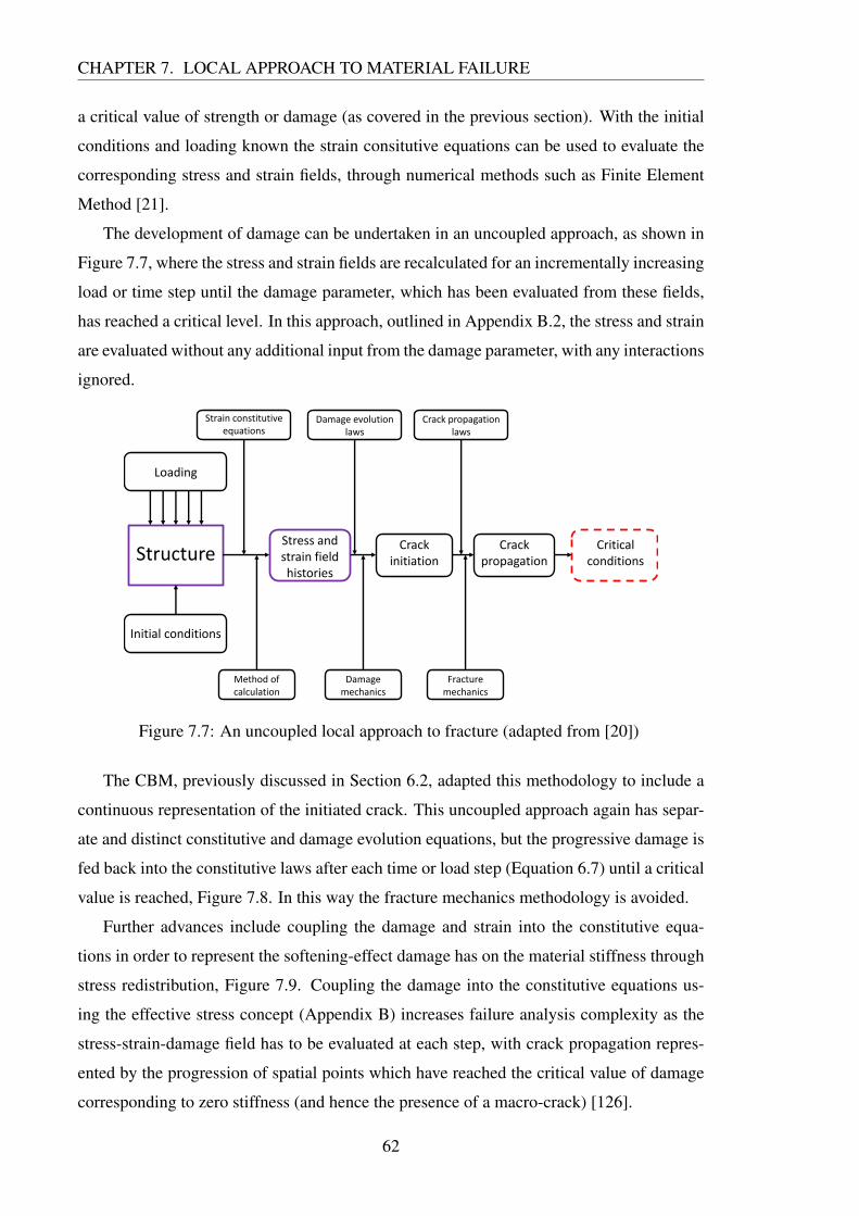
CHAPTER 7. LOCAL APPROACH TO MATERIAL FAILURE
a critical value of strength or damage (as covered in the previous section). With the initial
conditions and loading known the strain consitutive equations can be used to evaluate the
corresponding stress and strain fields, through numerical methods such as Finite Element
Method [21].
The development of damage can be undertaken in an uncoupled approach, as shown in
Figure 7.7, where the stress and strain fields are recalculated for an incrementally increasing
load or time step until the damage parameter, which has been evaluated from these fields,
has reached a critical level. In this approach, outlined in Appendix B.2, the stress and strain
are evaluated without any additional input from the damage parameter, with any interactions
ignored.
Strain constitutive
equations
Method of
calculation
Stress and
strain field
histories
Critical
conditionsStructure
Loading
Initial conditions
Crack
initiation
Crack
propagation
Damage evolution
laws
Crack propagation
laws
Damage
mechanics
Fracture
mechanics
Figure 7.7: An uncoupled local approach to fracture (adapted from [20])
The CBM, previously discussed in Section 6.2, adapted this methodology to include a
continuous representation of the initiated crack. This uncoupled approach again has separ-
ate and distinct constitutive and damage evolution equations, but the progressive damage is
fed back into the constitutive laws after each time or load step (Equation 6.7) until a critical
value is reached, Figure 7.8. In this way the fracture mechanics methodology is avoided.
Further advances include coupling the damage and strain into the constitutive equa-
tions in order to represent the softening-effect damage has on the material stiffness through
stress redistribution, Figure 7.9. Coupling the damage into the constitutive equations us-
ing the effective stress concept (Appendix B) increases failure analysis complexity as the
stress-strain-damage field has to be evaluated at each step, with crack propagation repres-
ented by the progression of spatial points which have reached the critical value of damage
corresponding to zero stiffness (and hence the presence of a macro-crack) [126].
62
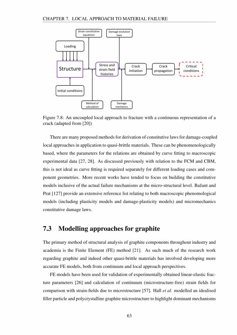
CHAPTER 7. LOCAL APPROACH TO MATERIAL FAILURE
Strain constitutive
equations
Method of
calculation
Stress and
strain field
histories
Critical
conditionsStructure
Loading
Initial conditions
Crack
initiation
Crack
propagation
Damage evolution
laws
Damage
mechanics
Figure 7.8: An uncoupled local approach to fracture with a continuous representation of acrack (adapted from [20])
There are many proposed methods for derivation of constitutive laws for damage-coupled
local approaches in application to quasi-brittle materials. These can be phenomenologically
based, where the parameters for the relations are obtained by curve fitting to macroscopic
experimental data [27, 28]. As discussed previously with relation to the FCM and CBM,
this is not ideal as curve fitting is required separately for different loading cases and com-
ponent geometries. More recent works have tended to focus on building the constitutive
models inclusive of the actual failure mechanisms at the micro-structural level. Bažant and
Prat [127] provide an extensive reference list relating to both macroscopic phenomological
models (including plasticity models and damage-plasticity models) and micromechanics
constitutive damage laws.
7.3 Modelling approaches for graphite
The primary method of structural analysis of graphite components throughout industry and
academia is the Finite Element (FE) method [21]. As such much of the research work
regarding graphite and indeed other quasi-brittle materials has involved developing more
accurate FE models, both from continuum and local approach perspectives.
FE models have been used for validation of experimentally obtained linear-elastic frac-
ture parameters [26] and calculation of continuum (microstructure-free) strain fields for
comparison with strain-fields due to microstructure [57]. Hall et al. modelled an idealised
filler particle and polycrystalline graphite microstructure to highlight dominant mechanisms
63
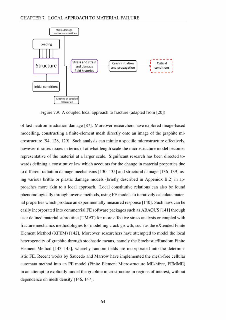
CHAPTER 7. LOCAL APPROACH TO MATERIAL FAILURE
Strain-damage
constitutive equations
Method of coupled
calculation
Stress and strain
and damage
field histories
Critical
conditionsStructure
Loading
Initial conditions
Crack initiation
and propagation
Figure 7.9: A coupled local approach to fracture (adapted from [20])
of fast neutron irradiation damage [87]. Moreover researchers have explored image-based
modelling, constructing a finite-element mesh directly onto an image of the graphite mi-
crostructure [94, 128, 129]. Such analysis can mimic a specific microstructure effectively,
however it raises issues in terms of at what length scale the microstructure model becomes
representative of the material at a larger scale. Significant research has been directed to-
wards defining a constitutive law which accounts for the change in material properties due
to different radiation damage mechanisms [130–135] and structural damage [136–139] us-
ing various brittle or plastic damage models (briefly described in Appenidx B.2) in ap-
proaches more akin to a local approach. Local constitutive relations can also be found
phenomologically through inverse methods, using FE models to iteratively calculate mater-
ial properties which produce an experimentally measured response [140]. Such laws can be
easily incorporated into commercial FE software packages such as ABAQUS [141] through
user defined material subroutine (UMAT) for more effective stress analysis or coupled with
fracture mechanics methodologies for modelling crack growth, such as the eXtended Finite
Element Method (XFEM) [142]. Moreover, researchers have attempted to model the local
heterogeneity of graphite through stochastic means, namely the Stochastic/Random Finite
Element Method [143–145], whereby random fields are incorporated into the determin-
istic FE. Recent works by Saucedo and Marrow have implemented the mesh-free cellular
automata method into an FE model (Finite Element Microstructure MEshfree, FEMME)
in an attempt to explicitly model the graphite microstructure in regions of interest, without
dependence on mesh density [146, 147].
64
Chapter 8
Discrete local approaches - lattice models
Discrete methods show promise in allowing the development of micromechanical based
constitutive equations. Cundall [148] originally developed the Discrete Element Method
(DEM) as a numerical framework to simulate discontinuous problems found in geological
and rock mechanics. This approach was further developed by Cundall and Strack [33] in
application to the flow and interaction of granular media. Such Discrete Element Methods
consider the physical system as a composition of discrete particles, with a node at the centre
of each particle. These particles are free to move according to Newton’s second law upon an
applied force. Upon contact with another particle, the affect of the frictional and interaction
forces on the particle’s motion is calculated. As a result, the important variables for this
method, once the initial position of the particles are specified, are the applied force and
displacement, as opposed to the stress and strain as used in the Finite Element method
[28, 149]. Cundall’s method was extended to study fracture at the micro-structural scale of
rocks [150] and aggregate based composites [151].
More modern developments of particle methods include peridynamics [152] and Smoot-
hed Particle Applied Mechanics (SPAM) [153], the latter of which is equivalent to Smoothed
Particle Hydrodynamics (SPH) [154] but for solids applications. These have been applied
to the study of quasi-brittle structures [155, 156]. These approaches offer a promising
alternative to standard continuum models, where extra constitutive relations are required
for defect interaction and coalescence. Although these particle methods can model damage
progression, there remains no method (to the author’s knowledge) to distribute a initial state
of damage such as porosity and hence explicitly represent the actual mechanisms involved
in failure at the micro-structural scales.
A second branch of discrete method is the lattice models. Lattice models treat the ma-
terial as a parallel system (unlike the weakest link methods, which are essentially statistical
65
CHAPTER 8. DISCRETE LOCAL APPROACHES - LATTICE MODELS
systems based in series), with nodes at cell centres formed into a network through bond
connections to neighbouring nodes, or nodes within a region of influence. These bond con-
nections, represented by discrete elements, in the form of elastic beams [157], springs [34],
fuses [158] or custom elements, are capable of transfering elastic tensile or compressive
forces. Connecting bonds can break due to overextension, removing the ability to transfer
forces between particles. Failure of a bond results in the redistribution of the load, rather
than instantaneously failing the whole system. This is considered to provide a closer repres-
entation of micro-crack interaction and accumulation of damage in quasi-brittle materials,
with the local heterogeneity represented by the failure properties assigned to the discrete
elements.
The parallel basis of lattice models can prove computationally intensive [37] suggesting
engineering scale component models are impractical. However such models can be benefi-
cial in areas where it is necessary to model local behaviour, e.g. in the FPZ. Furthermore,
lattice models have the same advantages over continuum modelling as particle methods,
in that no additional assumptions for crack development or propagation are necessary, but
offer a further advantage in that an initial state of damage can be introduced. The literature
review presented in this chapter will focus on models of a lattice framework although there
is significant overlap in theory and naming conventions between lattice and particle models.
8.1 Background
Development of lattice models, actually predates that of the discrete element method, hav-
ing been used in the field of elasticity since the 1940s [159]. Burt and Dougill [160] are
considered the first to have applied this to model materials of a heterogeneous nature, when
they constructed a random truss joint system with distributed truss strength and stiffness.
The main application of such models, as is generally the trend with all quasi-brittle stud-
ies, has been directed at cementitious and aggregate based materials, stemming from initial
models by Bažant and Tabbara [40] and Schlangen and Van Mier [157].
Bažant et al. [40] proposed a Random Particle Model, generalising previous work from
Zubelewicz and Bažant [151], based on Cundall’s DEM formulation. In his model Bažant
considered only axial forces between particles. In such a way this is considered similar
to the truss network developed by Burt and Dougill [160] although based on a network
of particles, hence bridging the concepts of discrete particle and lattice models. Until this
model, development of discrete element models and lattice models had been in parallel.
66
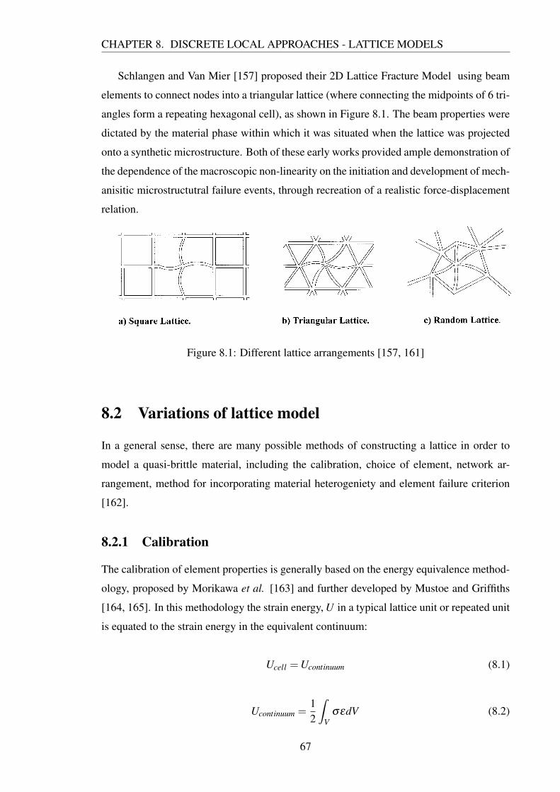
CHAPTER 8. DISCRETE LOCAL APPROACHES - LATTICE MODELS
Schlangen and Van Mier [157] proposed their 2D Lattice Fracture Model using beam
elements to connect nodes into a triangular lattice (where connecting the midpoints of 6 tri-
angles form a repeating hexagonal cell), as shown in Figure 8.1. The beam properties were
dictated by the material phase within which it was situated when the lattice was projected
onto a synthetic microstructure. Both of these early works provided ample demonstration of
the dependence of the macroscopic non-linearity on the initiation and development of mech-
anisitic microstructutral failure events, through recreation of a realistic force-displacement
relation.
Figure 8.1: Different lattice arrangements [157, 161]
8.2 Variations of lattice model
In a general sense, there are many possible methods of constructing a lattice in order to
model a quasi-brittle material, including the calibration, choice of element, network ar-
rangement, method for incorporating material heterogeniety and element failure criterion
[162].
8.2.1 Calibration
The calibration of element properties is generally based on the energy equivalence method-
ology, proposed by Morikawa et al. [163] and further developed by Mustoe and Griffiths
[164, 165]. In this methodology the strain energy, U in a typical lattice unit or repeated unit
is equated to the strain energy in the equivalent continuum:
Ucell =Ucontinuum (8.1)
Ucontinuum =12
ˆV
σεdV (8.2)
67

CHAPTER 8. DISCRETE LOCAL APPROACHES - LATTICE MODELS
For the simplest case of a spring bond with a single DOF the strain energy is given by the
standard relationship:
Ubond =12
ku2 (8.3)
where k is the spring stiffness and u is relative displacement between the ends of the spring.
The strain energy within the cell is given by the total strain energy of each bond within it:
Ucell = ∑bond
Ubond (8.4)
The equivalent procedure for a triangular and square lattice of beam elements (of both
Euler-Bernoulli and Timoshenko formulation) can be found in [44].
The methodology of energy equivalence is analagous to the Cauchy-Born rule, whereby
continuum constitutive relations are derived from the atomistic scale [166]. This procedure
is by no means the exclusive method of calibration, with differing methods discussed with
regards to specific lattice models in Section 8.3.
8.2.2 Lattice network arrangement and choice of element
Many arrangements have been used for lattice models as shown in Figure 8.1. These can
be regularly arranged in 2D; e.g. triangular [161], square [167] or rhombic configuration,
or 3D; cubic [168] or more complex FCC or HCC arrangements [169]; using a variety
of different elements including fuses [158], truss [40] or beams [157] and springs [34].
It can be argued that simple configurations, such as 2D and cubic lattice, do not provide
a physical representation of the actual arrangement and coordination of grains and will
inherently fail to model materials with the correct elastic properties. There is evidence that
the regularity in the aformentioned lattices introduces bias in the propagation direction of
a macro-crack [35, 170]. As a result irregular/random configurations have been proposed,
including configurations obtained through Voronoi tessellation and Delaunay triangulation
procedure [34, 171–173]. However, these random arrangements only directly represent the
unique configuration being modeled.
One of the constraints of lattice models is the ability to reproduce a range of Poisson’s
ratio values suitable for an isotropic linear elastic material. This has been shown to result
from both the network arrangement and choice of element within the model. Studies using
truss or spring elements which transmit only normal forces were shown to be limited to a
fixed value for the Poisson’s ratio, ν = 0.33 for the 2D Random Particle Model by Bažant
68

CHAPTER 8. DISCRETE LOCAL APPROACHES - LATTICE MODELS
and Tabbara [40] and ν = 0.25 for the FCC arrangement by Donze and Magnier [174].
To overcome this restriction many researchers attempted to model non-axial degrees
of freedom between neighbouring particles or sites. This can be done either by using
beam elements, although such structural elements are deemed to be physically unrealistic in
modelling the actual microstructure interactions [175], or by introducing additional shear
springs. The latter was used by Griffiths and Mustoe, who showed that a triangular lat-
tice can be used to represent a material with a Poisson’s ratio, ν < 0.25 (plane strain) and
ν < 0.33 (plane stress) [165]. 3D models still exhibit problems; the cubic and FCC and
HCC arrangements are only representative of a linear elastic isotropic material when ν = 0
[168, 169]. The Distinct Lattice Spring Model (DLSM), described in Section 8.3 overcame
this problem by introducing negative spring stiffness, although the physical meaning of this
is in question [176]. Furthermore there remains the issue with such models that they fail to
remain rotationally invariant when introducing extra degrees of freedom between particles.
8.2.3 Method for generating and incorporating heterogeneity
There are considered to be 2 ways of generating representative heteregeneous material prop-
erties [157]:
• Random distribution of bond properties, according to a given distribution [177, 178].
The distribution can reflect the degree of heterogeneity present in the material in
comparison to the structure size being modelled.
• Generation of a synthetic microstructure, either directly from imaging techniques or
as a statistical representation of the random nature of the material microstructure.
If a synthetic microstructure is generated then there are considered to be 3 general meth-
odolgies for projecting/incorporating the material heterogeneity onto the lattice [179]; the
particle overlay lattice, centre particle lattice and long range interaction lattice.
Lattice with particle overlay This approach involves superimposing a lattice onto the
synthetic microstructure [157, 178], Figure 8.2. The properties of the lattice bonds are
dictated by the micro-structural phase onto which it is projected. In the case of concrete the
are 3 different bonds properties - matrix, aggregate and interface.
Centre particle lattice The centre particle lattice, such as in [169] is constructed by con-
necting the centre points of neighbouring features, e.g. particles or aggregates, with bonds,
69

CHAPTER 8. DISCRETE LOCAL APPROACHES - LATTICE MODELS
Figure 8.2: A lattice superimposed onto a synthetic concrete microstructure (adapted from[161]).
Figure 8.3: A centre particle lattice configuration (adapted from [179]).
Figure 8.3. In this way the interactions between features is included through the calibra-
tion of bond properties. This method provides an advantage that only nodes that represent
particles are generated; a possible computational benefit. However this method provides
calibration issues as each bond represents a multiphase system and provided this issue can
be overcome, each calibration is phenomenlogical and specific to the material composition
for which it was undertaken [179]. This model approach stems from the generation of a
lattice framework from particle methods as mentioned previously [40, 151].
Long range interaction Both of these main types of lattice exist with only short range
interaction, i.e. to the nearest nodal neighbours, however longer range interaction may be
introduced, as in the work of Burt and Dougill [160] and Bažant and Tabbara [40].
70

CHAPTER 8. DISCRETE LOCAL APPROACHES - LATTICE MODELS
8.2.4 Constitutive law and failure criterion
As mentioned in Section 7.1, there have been many failure criteria proposed to model the
global behaviour of brittle, ductile and quasi-brittle materials. The failure criterion for
individual elements in a lattice need to represent either the material phase within which it is
situated for a particle overlay lattice, or the interaction between particles in a centre particle
lattice. Generally the failure criteria is integrated within the constitutive behaviour of the
element itself.
For a spring or truss model, where each spring supports a single degree of freedom
corresponding to a simple uniaxial stress-strain relationship, the simplest criteria is the
elasto-brittle failure seen previously in Figure 7.1, wherein a critical value of stress, strain
or strain energy results in failure. Beam elements capable of representing more complic-
ated stress fields can carry failure criterion derived from the Rankine, Tresca or Von-Mises
failure/yield criterion [161, 167].
It has been suggested that using such failure criterion, where after a critical value of
load or displacement the element is failed and the load redistributed around the remaining
bonds, can give an overly brittle response and without the inclusion of tension softening
at the element level a reliance on element size is introduced [178]. Although Bažant et
al. [40] proposed a softening relationship for the truss bonds between particles, this is
only a representation of the multiphase system in a centre particle lattice configuration as
opposed to the actual behaviour of the matrix phase. It was in fact Arslan et al. [161]
and subsequently Karihaloo et al. [44] who implemented the tension softening relation in
beam elements exclusively for the matrix phase only in a particle overlay lattice, keeping
the elements representative of aggregate and interface elasto-brittle. Both models showed
an improved representation of the tension softening response over early lattice models [40,
157]. A simple brittle tension softening criteria is shown in Figure 8.4. Both Arslan et
al. and Karihaloo et al. implemented the tension softening relation using a secant elastic
modulus, Es to represent the unloading of the bond without residual damage after the peak
load.
Van Mier discussed the use of an energy potential to dictate the 1D force-displacement
between nodes [180]. This is akin to the pair-potential used to represent the relationship
between two atoms in Molecular Dynamics studies whereby energy associated with a pair
of atoms derives exclusively from the separation of the atoms. Such potentials could be
used directly as a lower-scale foundation from which to derive the constitutive relationship
at the length-scale of interest [181]. Conversely the potentials could be used as a framework
71

CHAPTER 8. DISCRETE LOCAL APPROACHES - LATTICE MODELS
σbond)
ε(bond)
σ
ε εf
E
Es
Figure 8.4: A failure criterion accounting for tension softening with modified secant elasticmodulus for unloading
from which to semi-empirically fit a relationship, in essence creating an analogue between
the interaction between atoms and that of lattice nodes.
8.3 Lattice models of note
In addition to the historical perspective in the preceding sections, it is worth briefly men-
tioning here the different lattice models (and closely related lattice-particle models) which
have undergone significant development over recent years and their features.
Lattice Discrete Particle Model (LDPM) Cusatis et al. [175, 182] originally developed
a 3D model they named the Confinement Shear Lattice (CSL) for simulation of concrete, ex-
tending the principles of random spatial distributions of discrete physical particles laid out
by Bažant and Tabbara [40]. Particles, representing aggregates, were joined by bonds cap-
able of transferring axial and shear stresses which simulated deformation and subsequent
failure of the matrix phase. Rather than the energetic calibration described in Section 8.2.2
the CSL relates strains and tractions on a series of microplanes to the stresses in a con-
tinuum cell in a methodology based on that described in the microplane models [183, 184].
The CSL was succesfully coupled to a Finite Element model and demonstrated good pre-
diction of crack paths [173] with other extensions involving random material property fields
[185, 186].
Later works by Cusatis et al. [187–189] introduced a new model, entitled the Lattice
72
CHAPTER 8. DISCRETE LOCAL APPROACHES - LATTICE MODELS
Discrete Particle Model (LDPM) which closely followed the CSL framework but combined
principles and numerical solving methods from the Discrete Particle Method [190]. Both
the LDPM and its predecessors require phenomological calibration from experimental data.
Virtual Internal Bond Model (VIB) Gao and Klein [191] and Klein and Gao [192] de-
veloped the Virtual Internal Bond Model (VIB) utilizing the Cauchy-Born rule of crystal
elasticity. The Cauchy-Born rule is a homogenization technique generally used to provide
continuum constitutive laws from atomistic properties using an energetic calibration. In-
stead of homogenizing at the atomistic scale, the VIB generated a random-lattice of “ma-
terial particles” which were phenomonologically calibrated according to the material of
interest.
Extensions to the VIB include the Virtual Internal Pair-Bond Model (VIPB) [193] and
the Virtual Multi-Dimensional Internal Bond Model (VMIB) [194]. In the VIPB each bond
is replaced by two separate bonds. In this manner the fracture energy can be split into
a specimen size-independent initial fracture energy and a specimen size-dependent total
fracture energy, used with short and long range potentials respectively in order to recreate
the size-effect. In the VMIB the axial bond present in the VIB is complemented by shear
bonds in order to overcome restrictions on Poisson’s ratio (in VIB, maximum ν = 0.25
for plane strain and ν = 0.33 for plane stress). The random nature of the “particles” and
resulting bonds within the VIB model make it inherently non-physical.
Distinct Lattice Spring Model (DLSM) In the thesis of Zhao [176] the virtual non-
physical structure of the VMIB was further extended in an attempt to better approximate a
real microstructure. Spherical particles were distributed randomly with connectivity set by
joining overlapping particles by normal and shear bonds through their centres. In this man-
ner the new model was named the Real Multi-Dimensional Internal Bond Model (RMIB). In
Zhao’s thesis and the published works taken from it [195–198] the numerical implement-
ation of the RMIB with springs for bonds was referred to as the Distinct Lattice Spring
Model (DLSM). The developed solver was based on the Discrete Element Method.
The DLSM (inclusive of the RMIB), which can operate on regular or irregular geometry,
allows the calibration of spring properties from macroscopic elastic properties as opposed
to the reverse for VIB. As mentioned previously, the negative shear stiffness, which oc-
curs when ν > 0.25, allows a full range of Poissons ratio of elastic solids to be simulated.
Moreover the deformation of the shear springs are evaluated from local strain using a least
squares method as opposed to particle displacements, which Zhao argues allows the model
73

CHAPTER 8. DISCRETE LOCAL APPROACHES - LATTICE MODELS
to remain rotationally invariant unlike other lattice models with shear bonds [176].
The model was intended for application on dynamic fracture of rocks [195, 196] with
additional theoretical and numerical works including wave propagation validation [199],
coupling with Numerical Manifold Method [200] and code parallelization [197, 198]. Rate
dependency has also been introduced into bond properties for PMMA [201] and sandstone
[202] with the latter work constructing the model directly from tomography data.
Lattice Solid Model (LSM) The Lattice Solid Model (LSM), also called LSMearth and
ESyS_Particle, has been in development since the late 1990s. Based on molecular dynam-
ics principles, and treated as a lattice of discrete physical particles, it was originally de-
veloped to simulate dynamic response of rocks during earthquakes [203, 204]. More recent
works have highlighted the need to include 6 degrees of freedom between particles (axial,
2× shear, twist and 2×bending) an extension on the axial and shear degrees of freedom
allowed in many other models. Spring constants were initially approximated [205, 206]
and then derived for different lattice arrangements [169]. Further applications of the LSM
have included a parallel implementation of the model for simulating fault gorge [207] and
coupling with Lattice-Boltzmann method to link fluid flow in fractured systems [208].
Rigid Body Spring Network (RBSN) The Rigid-Body Spring Network (RBSN) was
originally proposed by Kawai in 1978 as a more computationally-efficient alternative to
the conventional elements used in the Finite Element Method [209]. The model consisted
of rigid sections which interacted with one another via a system of springs that controlled
behaviour over mutual surfaces. This concept was extended by Bolander and Saito [34] for
modelling crack paths in concrete beams, whereby the geometry was discretized using a
Voronoi tesselation of randomly distributed points, with spring stiffness uniquely defined
by the resultant geometry. The model was extended to 3D and given a fracture criterion
which reflects a cohesive law over cell facet areas by Bolander and Burton [210]. In this
case 6 degrees of freedom were represented by springs between boundaries.
Other researchers who have implemented the RBSN methodology in various forms in-
clude Nagai et al. [211], Vorechovský and Eliáš [212], Eliáš and Vorechovský [213], Grassl
and Jirásek [214], Grassl et al. [39] and Xenos et al. [215].
Volume Compensated Particle Model (VCPM) The Volume Compensated Particle Model
is a relatively new model. Although current studies are limited to 2D, with planned work for
an extension into 3D, the model builds upon concepts from molecular dynamics [216, 217]
74
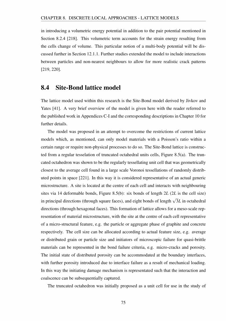
CHAPTER 8. DISCRETE LOCAL APPROACHES - LATTICE MODELS
in introducing a volumetric energy potential in addition to the pair potential mentioned in
Section 8.2.4 [218]. This volumetric term accounts for the strain energy resulting from
the cells change of volume. This particular notion of a multi-body potential will be dis-
cussed further in Section 12.1.1. Further studies extended the model to include interactions
between particles and non-nearest neighbours to allow for more realistic crack patterns
[219, 220].
8.4 Site-Bond lattice model
The lattice model used within this research is the Site-Bond model derived by Jivkov and
Yates [41]. A very brief overview of the model is given here with the reader referred to
the published work in Appendices C-I and the corresponding descriptions in Chapter 10 for
further details.
The model was proposed in an attempt to overcome the restrictions of current lattice
models which, as mentioned, can only model materials with a Poisson’s ratio within a
certain range or require non-physical processes to do so. The Site-Bond lattice is construc-
ted from a regular tesselation of truncated octahedral units cells, Figure 8.5(a). The trun-
cated octahedron was shown to be the regularly tessellating unit cell that was geometrically
closest to the average cell found in a large scale Voronoi tessellations of randomly distrib-
uted points in space [221]. In this way it is considered representative of an actual generic
microstructure. A site is located at the centre of each cell and interacts with neighbouring
sites via 14 deformable bonds, Figure 8.5(b): six bonds of length 2L (2L is the cell size)
in principal directions (through square faces), and eight bonds of length√
3L in octahedral
directions (through hexagonal faces). This formation of lattice allows for a meso-scale rep-
resentation of material microstructure, with the site at the centre of each cell representative
of a micro-structural feature, e.g. the particle or aggregate phase of graphite and concrete
respectively. The cell size can be allocated according to actual feature size, e.g. average
or distributed grain or particle size and initiators of microscopic failure for quasi-brittle
materials can be represented in the bond failure criteria, e.g. micro-cracks and porosity.
The initial state of distributed porosity can be accommodated at the boundary interfaces,
with further porosity introduced due to interface failure as a result of mechanical loading.
In this way the initiating damage mechanism is representated such that the interaction and
coalscence can be subsequentially captured.
The truncated octahedron was initially proposed as a unit cell for use in the study of
75

CHAPTER 8. DISCRETE LOCAL APPROACHES - LATTICE MODELS
Figure 8.5: (a) Cellular representation of material; (b) the skeletal bond structure
stress corrosion cracks between grains [222, 223]. Not until later was the capability of such
a model to recreate macroscopic elastic behaviour of any isotropic material explored [41].
In this work, beam elements were used as bonds between sites in a numerical study. The
model was demonstrated to be capable of reproducing elastic behaviour upto a Poisson’s
ratio of 0.5. It was shown by Jivkov et al. [224] that it was possible to use such a model
for the study of progressive damage evolution, without further constitutive assumptions
regarding crack path direction and flaw coalescence. In this work it was shown that such a
framework could represent the accumulative damage process from initiation through to the
interaction and coalescence of flaws in cement under tensile and compressive loading. This
work was applied to more complex compressive loading conditions for concrete, using a
porosity distribution obtained from X-ray tomography, in [225] and extended in [226].
76

Chapter 9
Generalised Continuum
Generalised continuum theories (sometimes called enriched continuum theories [227]) have
been developed to deal with materials for which the continuum approximation is insuffi-
cient due to the presence of non-negligible micro-structural features, such as quasi-brittle
materials. There are considered to be 3 types of generalised continuum theory [228]:
• “Weak” non-local/strain-gradient theories, whereby the 3 degrees of freedom in the
form of displacements are enriched by including the gradient of strain into the con-
stitutive laws [229].
• “Strong” non-local/non-local integral theories, whereby the stress at any point is re-
lated to the state of the whole body [229].
• Couple stress or micropolar theories, where the rotations of continuum points are
considered as extra degrees of freedom. Such theories are of interest in areas of this
research.
The common ground in such theories is the introduction of a length scale. In couple stress
theory, unlike the non-local theories, it is possible to directly link this length scale to the
micro-structural features of the material to provide a physical basis [42]. As referred to in
Chapter 2, the naturally introduced length scale and rotational invariance in couple stress
theories may prove useful in discrete models [44–47]. As such an outline of a consistent
couple stress theory is given here.
9.1 Couple stress theory
In couple stress theory the continuum is modelled as a set of rigid points within the con-
tinuous mass. Each point has 3 additional degrees of freedom in comparison to the classical
77
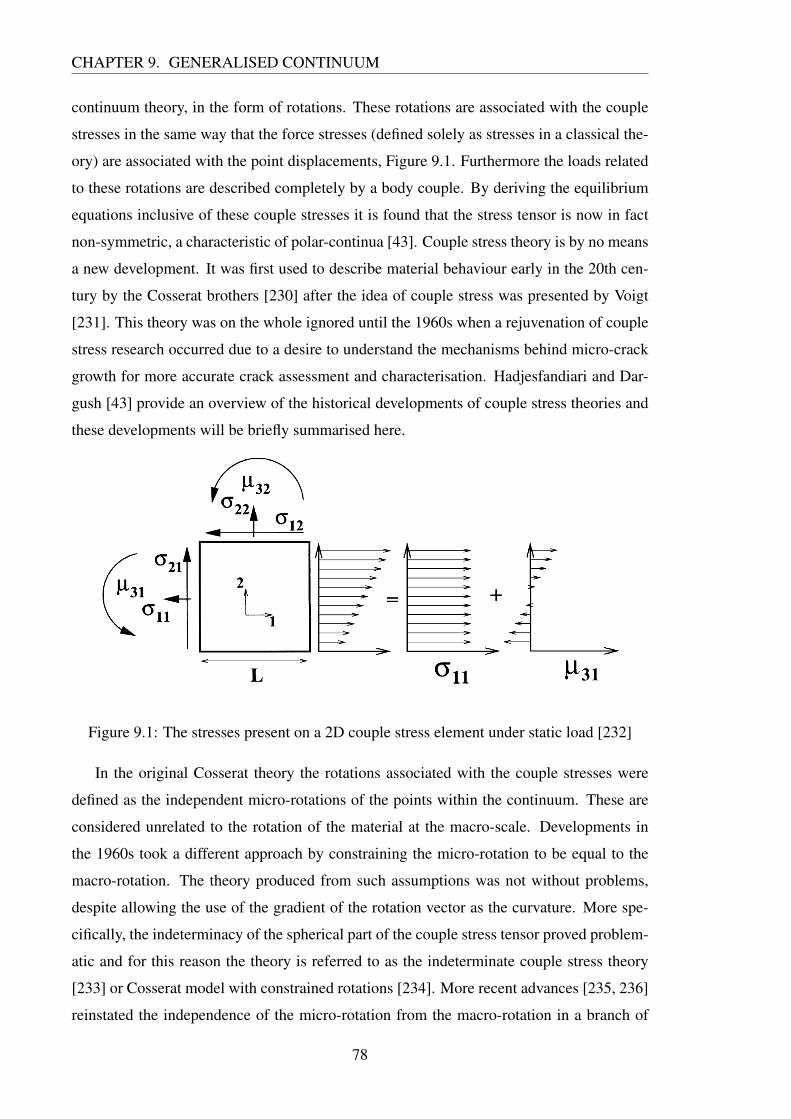
CHAPTER 9. GENERALISED CONTINUUM
continuum theory, in the form of rotations. These rotations are associated with the couple
stresses in the same way that the force stresses (defined solely as stresses in a classical the-
ory) are associated with the point displacements, Figure 9.1. Furthermore the loads related
to these rotations are described completely by a body couple. By deriving the equilibrium
equations inclusive of these couple stresses it is found that the stress tensor is now in fact
non-symmetric, a characteristic of polar-continua [43]. Couple stress theory is by no means
a new development. It was first used to describe material behaviour early in the 20th cen-
tury by the Cosserat brothers [230] after the idea of couple stress was presented by Voigt
[231]. This theory was on the whole ignored until the 1960s when a rejuvenation of couple
stress research occurred due to a desire to understand the mechanisms behind micro-crack
growth for more accurate crack assessment and characterisation. Hadjesfandiari and Dar-
gush [43] provide an overview of the historical developments of couple stress theories and
these developments will be briefly summarised here.
Figure 9.1: The stresses present on a 2D couple stress element under static load [232]
In the original Cosserat theory the rotations associated with the couple stresses were
defined as the independent micro-rotations of the points within the continuum. These are
considered unrelated to the rotation of the material at the macro-scale. Developments in
the 1960s took a different approach by constraining the micro-rotation to be equal to the
macro-rotation. The theory produced from such assumptions was not without problems,
despite allowing the use of the gradient of the rotation vector as the curvature. More spe-
cifically, the indeterminacy of the spherical part of the couple stress tensor proved problem-
atic and for this reason the theory is referred to as the indeterminate couple stress theory
[233] or Cosserat model with constrained rotations [234]. More recent advances [235, 236]
reinstated the independence of the micro-rotation from the macro-rotation in a branch of
78
CHAPTER 9. GENERALISED CONTINUUM
couple stress theory called micropolar theories (sometimes referred to as Cosserat model
with free rotations [237]). This effectively models the material as a collection of discrete
particles, raising concerns about whether this can actually represent a continuum at all. The
most recent development was developed by Hadjesfandiari and Dargush [43], wherein a
consistent couple stress theory is derived using only true kinematical quantities, effectively
introducing natural size dependence into the continuum theory. An outline of the consistent
couple stress theory developed by Hadjesfandiari and Dargush is included in the published
work presented in Appendix C.
Cosserat theory and the developing micropolar elasticity have established themselves
with many applications. For example, the structure of bone [238, 239], cellular and granu-
lar materials [240] provide varying length scales associated with micro-structural features.
Furthermore, discrete materials such as jointed rocks have found that the discrete nature of
the continuum models in micropolar theory provide accurate and useful insight into their be-
haviour [241]. Despite the promise of micropolar elasticity, there are problems which limit
its acceptance as an additional improvement on classical continuum mechanics. Boundary
conditions and material moduli have proved difficult to prescribe and measure respectively,
providing difficulty in model characterization [42].
79
Part III
Contribution to the field
80

Chapter 10
Modelling and published work
This thesis is presented in the form of published or submitted work. The portfolio of work
described by published works can be found in Appendices C-I1. In this Chapter each pub-
lished work will be outlined with a brief overview including context and discussion. Works
during the first 12 months of the project focused on model calibration, Section 10.1, and
initial studies on early iterations of the Site-Bond model, Figure 10.1. Later works, from
12-24 months and 24-36 months as shown in Figures 10.2 and 10.3 respectively, focused
on more complete validated studies of the microstructure-informed Site-Bond model, Sec-
tion 10.2. It should be mentioned that the author has featured as a named author on other
publications although the relevence of the work or the magnitude of contribution from the
author is not deemed significant enough to warrant discussion [242–244].
1Please note that although the content of published works remains unchanged from the published form,the paper itself may be presented in its unpublished format or with changes made to formatting (namely pagemargins) to provide continuity with the rest of this thesis.
81
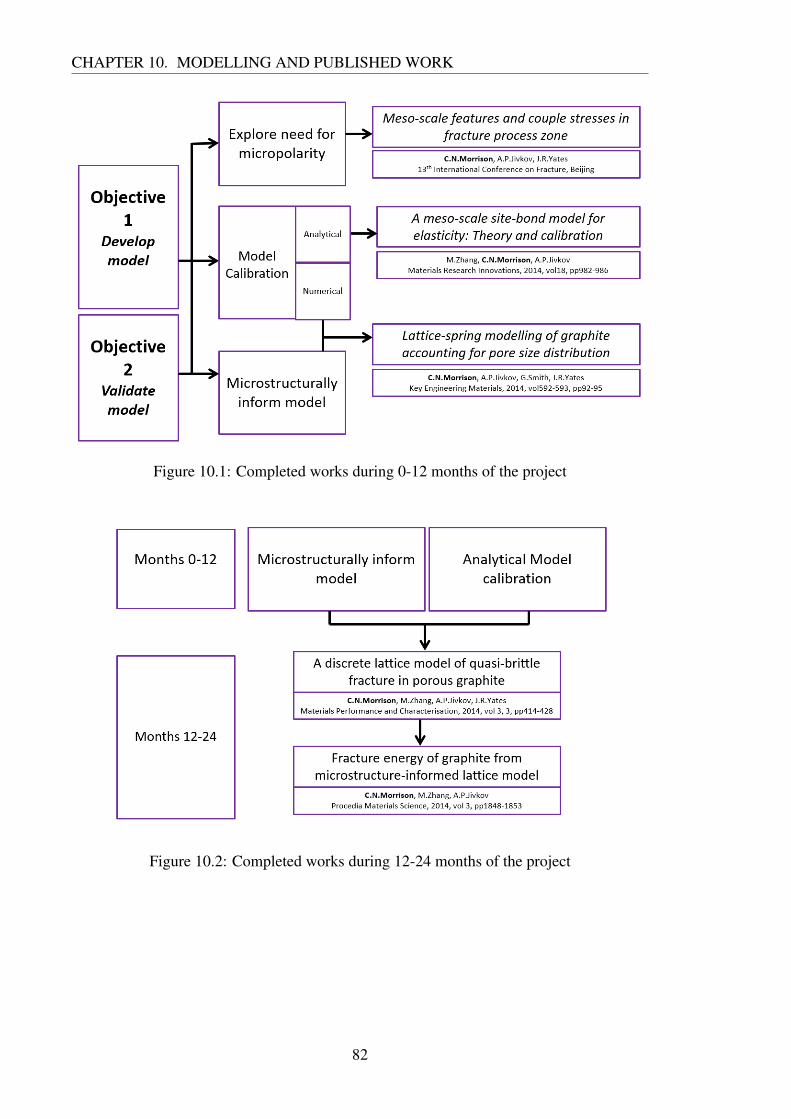
CHAPTER 10. MODELLING AND PUBLISHED WORK
Figure 10.1: Completed works during 0-12 months of the project
Figure 10.2: Completed works during 12-24 months of the project
82

CHAPTER 10. MODELLING AND PUBLISHED WORK
Figure 10.3: Completed works during months 24-36 months of the project
10.1 Model calibration
Meso-scale features and couple stresses in fracture process zone Calibration of the
micro-structurally informed lattice model which forms the initial project objective may
require the inclusion of micropolarity and couple stress theory to obtain the required six
degrees of freedom between each lattice node. Prior to calibration it must be determined
whether the inclusion of couple stresses is beneficial to the calibration procedure and can in-
deed naturally introduce a length scale into local material behaviour modelling. Hence, this
work was a pre-requisite to calibration of the Site-Bond model with spring-bonds. This was
done by constructing a simple finite element model consisting of rigid particles within a de-
formable matrix. The relative rotations and displacements between particles were measured
for 3 different loading cases, with varying degrees of couple stress; hydrostatic compres-
sion, pure twist and pure bending, and were related to the energy within the unit cell. The
energy within the unit cell was used as an indication of size effect. The magnitude of rota-
tions between particles was used to suggest a reduction of springs within each bond prior
to calibration.
This work was presented at the 13th International Conference of Fracture in Beijing,
China. The corresponding conference paper can be found in Appendix C. Further work
towards verifying the physical realism of couple stress theory was planned in the form of
experimental validation, although it was never undertaken due to project time-constraints.
83

CHAPTER 10. MODELLING AND PUBLISHED WORK
A meso-scale site-bond model for elasticity: Theory and calibration This paper, for
which Dr Mingzhong Zhang is the main author, derives analytically the spring constants
for the Site-Bond model in terms of the macroscopic elastic constants of the material. The
version of the Site-Bond model around which this publication focuses, involves the repres-
entation of bonds with six independent elastic springs resisting three relative displacements
and three relative rotations between sites, Figure 10.4. This yields four spring types [169]
with axial, kn, shear, ks, twisting, kt , and bending, kb, stiffness, which could, in general, be
different for principal and octahedral directions.
Figure 10.4: The 6 degrees of freedom represented by springs in the Site-Bond model
The model is calibrated by equating the strain energy in the unit cell and corresponding
continuum for typical global elastic properties of graphite under a homogeneous displace-
ment field. The lattice arrangement has been shown to generate macroscopic cubic elasti-
city. In this branch of elasticity 3 independent elastic constants are required to describe the
material behaviour as demonstrated in Equation 10.1 where W is strain energy density and
E, ν and µ are Youngs modulus, Poission’s ratio and shear modulus respectively.
Wcontinuum = f (E,ν ,µ) (10.1)
Under the initial assumption of a classical continuum (i.e. without micropolarity), relative
angular motion is ignored and the Site-Bond model will be composed of only axial and
shear spring types, the stiffnesses of which are different for the principal and octahedral
directions. The strain energy density within such a unit cell is shown in Equation 10.2.
Wdiscretecell = f((kn,ks)
principal ,(kn,ks)octahedral
)(10.2)
84

CHAPTER 10. MODELLING AND PUBLISHED WORK
This creates an indeterminate problem when calibrating the stiffness values [169], with an
infinite number of stiffness constant combinations that will generate the cubic elasticity
constants. As such, the calibration is over determined. Without micropolarity (or another
suitable method) to make the calibration procedure determinant, the shear stiffnesses in the
principal and octahedral directions are considered to be related, i.e. there are three spring
constants to determine from the three cubic elasticitity constants.
This work was presented at the 2nd Global Conference on Materials Science and En-
gineering, Xianning, China with the corresponding paper published in Materials Research
Innovations, Appendix D.
10.2 Microstructure-informed model
Lattice-spring modelling of graphite accounting for pore size distribution This con-
ference paper presents an initial iteration of the completed first objective - a micro-structura-
lly informed lattice model. The model is developed using an initial numerical calibration
assumption (which was later improved on analytically in the previously described paper).
In the same manner as the analytical calibration, strain energy in the continuum was equated
to the strain energy in the discrete cell, the latter given in terms of stiffnesses and displace-
ments. Rather than a more rigorous derivation the spring constants were calculated by
equating the continuum and discrete energies for several loading cases and then solving for
the spring constants simultaneously. A population of porosity, produced statistically from
experimental data, was introduced onto the model with the constraint of a single pore per
cell face used to scale the cell size. Progressive damage was modeled for several loading
cases representative of the region ahead of a crack tip. This work provides an initial step
towards deriving a load independent damage evolution law which could be implemented in
a continuum model and utilised as part of a structural integrity assessment.
This work was presented at the 7th International Conference on Materials Structure
and Micromechanics of Fracture in Brno, Czech Republic. The corresponding paper was
published in Key Engineering Materials2, Appendix E.
2Two minor issues regarding the Introduction were brought to the attention of the author following pub-lication. Firstly, it is stated that “Synthetic graphite is manufactured from petroleum cokes”. Although this istrue of some graphites. Secondly, it is stated that Gilsocarbon is “a relatively fine-grained graphite”. Gilso-carbon is in fact a medium grained graphite. This information is presented correctly throughout the rest of thethesis.
85
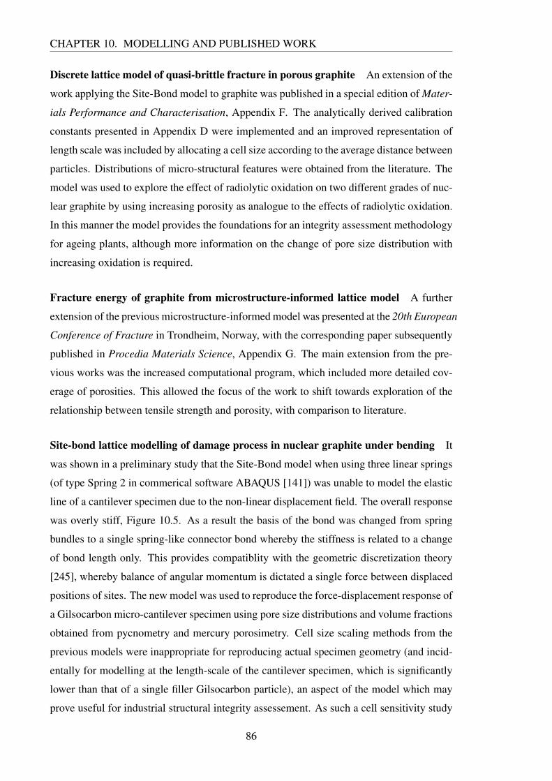
CHAPTER 10. MODELLING AND PUBLISHED WORK
Discrete lattice model of quasi-brittle fracture in porous graphite An extension of the
work applying the Site-Bond model to graphite was published in a special edition of Mater-
ials Performance and Characterisation, Appendix F. The analytically derived calibration
constants presented in Appendix D were implemented and an improved representation of
length scale was included by allocating a cell size according to the average distance between
particles. Distributions of micro-structural features were obtained from the literature. The
model was used to explore the effect of radiolytic oxidation on two different grades of nuc-
lear graphite by using increasing porosity as analogue to the effects of radiolytic oxidation.
In this manner the model provides the foundations for an integrity assessment methodology
for ageing plants, although more information on the change of pore size distribution with
increasing oxidation is required.
Fracture energy of graphite from microstructure-informed lattice model A further
extension of the previous microstructure-informed model was presented at the 20th European
Conference of Fracture in Trondheim, Norway, with the corresponding paper subsequently
published in Procedia Materials Science, Appendix G. The main extension from the pre-
vious works was the increased computational program, which included more detailed cov-
erage of porosities. This allowed the focus of the work to shift towards exploration of the
relationship between tensile strength and porosity, with comparison to literature.
Site-bond lattice modelling of damage process in nuclear graphite under bending It
was shown in a preliminary study that the Site-Bond model when using three linear springs
(of type Spring 2 in commerical software ABAQUS [141]) was unable to model the elastic
line of a cantilever specimen due to the non-linear displacement field. The overall response
was overly stiff, Figure 10.5. As a result the basis of the bond was changed from spring
bundles to a single spring-like connector bond whereby the stiffness is related to a change
of bond length only. This provides compatiblity with the geometric discretization theory
[245], whereby balance of angular momentum is dictated a single force between displaced
positions of sites. The new model was used to reproduce the force-displacement response of
a Gilsocarbon micro-cantilever specimen using pore size distributions and volume fractions
obtained from pycnometry and mercury porosimetry. Cell size scaling methods from the
previous models were inappropriate for reproducing actual specimen geometry (and incid-
entally for modelling at the length-scale of the cantilever specimen, which is significantly
lower than that of a single filler Gilsocarbon particle), an aspect of the model which may
prove useful for industrial structural integrity assessement. As such a cell sensitivity study
86
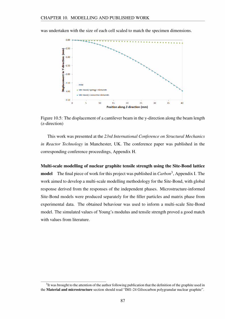
CHAPTER 10. MODELLING AND PUBLISHED WORK
was undertaken with the size of each cell scaled to match the specimen dimensions.
Figure 10.5: The displacement of a cantilever beam in the y-direction along the beam length(z-direction)
This work was presented at the 23rd International Conference on Structural Mechanics
in Reactor Technology in Manchester, UK. The conference paper was published in the
corresponding conference proceedings, Appendix H.
Multi-scale modelling of nuclear graphite tensile strength using the Site-Bond lattice
model The final piece of work for this project was published in Carbon3, Appendix I. The
work aimed to develop a multi-scale modelling methodology for the Site-Bond, with global
response derived from the responses of the independent phases. Microstructure-informed
Site-Bond models were produced separately for the filler particles and matrix phase from
experimental data. The obtained behaviour was used to inform a multi-scale Site-Bond
model. The simulated values of Young’s modulus and tensile strength proved a good match
with values from literature.
3It was brought to the attention of the author following publication that the definition of the graphite used inthe Material and microstructure section should read “IM1-24 Gilsocarbon polygranular nuclear graphite”.
87
Chapter 11
Conclusions
• Lattice models are a branch of discrete, local approach models which allow the con-
struction of a micro-mechanically based material constitutive law capable of gener-
ating the expected non-linear quasi-brittle response of nuclear graphite.
• A methodology for informing a lattice model with microstructure information has
been developed over several published works with a view to increasing the under-
standing of deformation and fracture behaviour of nuclear graphite. Studies have
explored choice of bond element, appropriate meso length-scale, calibration of bond
stiffness constants and microstructure mapping.
• Models produced using this methodology have been validated against experimental
data in the form of elastic constants, material properties and general quasi-brittle
behaviour to good effect.
• The model has been used to explore damage evolution in an initial attempt to develop
a load-independent damage law for possible uses in the continuum models used for
structural integrity assessment.
• The effect of porosity, as an analogue to radiolytic oxidation, on mechanical response
has been explored, providing a platform for the assessment of ageing AGR plants.
• More advanced studies have included reproducing the force-displacement response
of a micro-cantilever specimen and a multi-scale model, whereby a global model is
built up from the response of models of the individual phases.
88
Chapter 12
Further work
The results from this research have been generally positive, justifying further research into
the Site-Bond model. In this chapter several areas of potential future work are discussed.
12.1 Model calibration
The analytical calibration procedure used throughout this research can be improved upon,
refining the model’s capability to discretely represent a continuum volume. The inclusion
of micropolarity described in Appendix C was an attempt to do so, incorporating the effect
of local behaviour at an appropriate length scale into the calibration. Although the conclu-
sions drawn from the work were useful in justifiying assumptions made in the analytical
calibration, the failure to isolate a couple stress constant restricted the impact. As such,
further work may include the exploration of other theories neccessary for derivation of an
improved constitutive relationship between bond deformation and energy within a cell. Two
possible routes will be described here.
12.1.1 Improved relationship between bond deformation and energy
A calibration procedure may draw inspiration from Molecular Dynamics (MD), the origin
of most discrete models for solid mechanics applications, in particular the multi-body po-
tential theories of Finnis and Sinclair [216] and Daw and Baskes [217]. Discrete models
generally work on the same principle whereby energy is derived from a change in spatial
position of a set of discrete points given a constitutive link between force and displace-
ment (in a static sense). In the Site-Bond model discrete points represent micro-structural
features (filler particles in the case of graphite) whereas in MD they represent atoms.
89
CHAPTER 12. FURTHER WORK
In MD the interaction of atoms is approximated by a potential function [246]. Many
potential functions are defined as two-body or pair potentials where the energy between two
atoms is linked exclusively to the relative positions between the atoms. For a system of two
atoms, the resulting potential takes the form Ui j = f(ri j)
where ri j is the distance between
the atoms. Examples of such empirical potentials include the Lennard-Jones potential,
Equation 12.1 and Morse potential, Equation 12.2. In these potentials ε and α are constants
used for curve fitting. Potentials are selected depending on their suitability for a specific
application.
Ui j = 4ε
[(σ
ri j
)12
−(
σ
ri j
)6]
(12.1)
Ui j = ε
[e−2α(ri j−r0)−2e−α(ri j−r0)
](12.2)
Using only pair-potentials to describe atom interactions has significant disadvantages, such
as an inability to fully reproduce elastic constants. Independent works in the 1980s by
Finnis and Sinclair [216] and Daw and Baskes [217] explored the use of a semi-empirical
multi-body potential where an additional term is introduced to account for the local dens-
ity of atomic sites in BCC and FCC crystals respectively. The Finnis-Sinclair multi-body
potential is especially relevant to the site-bond model, which is also constructed in a BCC
arrangement. In multi-body potentials the energy per atom can be split into the pair poten-
tial energy, un and the multi-body term, or cohesive potential, up:
utot = un +uP (12.3)
un and up are given by Equations 12.4 and 12.5 respectively where A is a constant, ri is the
distance from an atom at the BCC crystal origin to the ith atom.
uP =12 ∑
i 6=0V (ri) (12.4)
un =−A f (ρ) (12.5)
The Finnis-Sinclair model introduced the function f (ρ) =√
ρ , where the density function,
ρ , defined in Equation 12.6 is based on a tight-bonding technique and density functional
theory.
90
CHAPTER 12. FURTHER WORK
ρ = ∑i 6=0
φ (ri) (12.6)
Put simply, the pair potential is dependent solely on the distance between two atomic sites.
For each pair-potential between sites the cohesive potential introduces an energy which is
summed over all the sites within a specified radius. In this sense, the force between two
sites then depends on the density of sites around them as well as their separation. From
these definitions it may be seen that the pair-potential is an analogue to the constitutive law
currently used in the Site-Bond model. By using this energy in isolation the relative spatial
changes of sites are considered but it may be that the deformation of the local cell around
each site is unaccounted for. In the Site-Bond model the local density of sites around
a central site defines the local volume around that particular site. As such the cohesive
potential which incorporates this local density can then be interpreted as a volumetric term
whereby it accounts for an energetic change resulting from a deformation of a local volume,
or unit cell, around a central site. The use of such volumetric terms is not entirely new in
lattice models having recently been introduced in the Volume Compensated Particle Model
discussed in Section 8.3 and introduced to an extent in the multi-scale study described in
Appendix I.
The Finnis-Sinclair model and similar models are semi-empirical with curve fit exper-
imental constants used to reproduce experimental observations for different elements. For
the purposes of the Site-Bond model it is appropriate to find a more general link between
changes in geometry and energy. The pair potential used in such a relationship may follow
the form:
up =12 ∑CA f
(4AA0
)(12.7)
where CA is a constant. It may be noted that Equation 12.7 uses a function of the relative
change of area rather than displacement (as is currently used). This is for two reasons. The
first is to conserve angular momentum, which must be followed as a result of a discretization
of elasticity [245]. The second is to be able to include a true representation of stress,
whereby the reduction in area due to bond extension is explicitly incorporated into the
constitutive law. At this stage it is unclear as to whether there is a definitive link between
a relative increase in bond length and the change in the corresponding change in area of
the cell face. If a link is found then it is deemed suitable to use either the change of area
explicitly or implicitly through the change of bond length within the constitutive law. In a
91
CHAPTER 12. FURTHER WORK
similar manner the volumetric, cohesive potential term may follow the form:
un =CV f(4VV0
)(12.8)
where CV is a constant.
12.1.2 Couple with dual graph
The Site-Bond model, and indeed any lattice based model, can be formulated as a mathem-
atical graph, where sites (or lattice nodes) and connecting bonds are represented as vertices
and edges respectively in a cell complex. Such formulations can be expressed as matrices
and implement the field of discrete exterior calculus as an analysis tool. Following the
terminology outlined in [242] where a more complete graph-based formulation of the Site-
Bond model is presented, the geometry of the model can be defined as a 3−complex. As
such the vertices, edges, faces and cell volumes in a graph are referred to as 0−, 1−, 2−and 3−cells respectively. When described in this fashion each graph has an associated dual
space/dual graph, whereby each geometric entity within a graph has a corresponding entity
in the associated dual. Taking the example of a graph A and its dual graph B, each vertice
in graph A corresponds to a cell volume in graph B. In the same manner each edge in graph
A corresponds to a face in graph B and so on.
The dual-graph concept may be used to describe a discretised volume more rigorously.
At present, the Site-Bond model calculates material response according to two variables,
namely lengths and areas or lengths and volumes (the discussion regarding multibody po-
tentials essentially proposes using areas and volumes). This is a means of modelling the
initial graph with little consideration of the influence of the dual graph. By simulating the
graph and its dual simulatenously, calculating equilibrium for both at each increment, al-
lows the material response to be calculated using lengths (and the relative change thereof)
exclusively. This is a topic for further consideration.
12.2 Explore the effect of porosity on graphite failure energy
at grain level
Exploring the effect of porosity on graphite failure energy at the grain level using lower
scale modelling would allow the development of a physically representative failure criteria
when accounting for porosity, which could be implemented within the Site-Bond model.
92
CHAPTER 12. FURTHER WORK
The failure criteria used in the model presented in this thesis (with the exception of the
multi-scale model presented in Appendix I) consists of a linear softening constitutive law
with an energetic failure criteria whereby the failure energy is calculated as the product
of the corresponding face area and the separation energy of graphite. Pores are represen-
ted on bonds through the reduction of the bond failure energy. This approach has given
promising results in reproducing the “graceful” pre-peak softening of quasi-brittle mater-
ials and matching experimentally measured tensile strength values. However, this failure
criteria and the changes under the influence of porosity is somewhat arbritary and it may be
beneficial to derive the affect of porosity on bond energy directly from lower scale models.
12.3 Inclusions and validation of physical phenomena
Although attempts have been made to validate the model at every opportunity, further proof
of concept for different grades of graphite in different component geometries and under
different loading conditions or environments will be beneficial. The hinderance in many
cases of validation is finding consistent data, either microstructure information from which
to populate the model or global response data for comparison. Taking the data used for the
paper outlined Section 10.2 as an example, although all data was obtained from reputable
sources, the values of elastic moduli are dynamic measurements which may differ from
static values and the porosity and filler volume fraction disclosed are lower than some val-
ues used in industry. Such discrepencies may introduce discrepencies between simulation
results and the physical response of graphite specimens. Extensions to the Site-Bond model
may include:
• Directional bias in certain graphite grades. As discussed in Chapter 4 many grades of
graphite have acicular particles with preferential alignment. This could be introduced
into the model either by stretching the cell dimensions along the axis of maximum
particle length or introducing a cleavage direction of particle to simulate the cleavage
directional bias along the particle aligned axis.
• Irradiation in nuclear graphite. Modelling irradiation effectively in the Site-Bond
model is dependent on suitable characterisation of progressive changes to the micro-
structure due to irradiation [11].
• Creep. Although not covered in particular detail in the review of literature, irradiation
creep and the fundamental understanding of the underlying mechanisms, is a signific-
93
CHAPTER 12. FURTHER WORK
ant challenge when considering nuclear graphite. Inclusion of viscoelastic behaviour
into the constitutive relationships of bonds may have potential with relations to such
an application [247].
• Multi-physics phenomena. A long-term goal of the Site-Bond model would be to
couple different physical phenomena to produce a multiphysics model in a similar
manner to other lattice models [208]. Of particular interest would be the coupling
of the site-bond model developed for solid mechanics applications here and that de-
veloped for diffusive reactive transport in porous media [248]. This would be of
particular interest for geological materials.
12.4 Structural integrity assessment
Although the research in this thesis provides a solid platform, further work is needed to
help the Site-Bond model meet the needs of industry with regards to structual integrity
assessment. The damage evolution study presented in Appendix E could be extended to
allow for direct input into an industry standard continuum model. Moreover the studies
related to radiolytic oxidation and ageing plant assessment described in Appendices F and
G may be built upon, incorporating the change of both porosity and pore size distribution
over time which results from radiolytic oxidation. Finally, once further proof of concept is
achieved the numerical stability and computational efficiency of the model maybe refined
to produce a user-friendly tool.
94

Bibliography
[1] P. Mukhopadhyay and R.K. Gupta, editors. Graphite, graphene and their polymer
nanocomposites. CRC Press, 2012.
[2] C.L. Mantell. Carbon and Graphite Handbook. Interscience Publishers, 1968.
[3] W.D. Callister. Materials Science and Engineering: An Introduction (5th Edition).
Wiley, 2000.
[4] L.C.F Blackman, editor. Modern Aspects of Graphite Technology. Academic Press:
London and New York, 1970.
[5] B.J. Marsden, G.N. Hall, O. Wouters, J.A. Vreeling, and J. van der Laan. Dimen-
sional and material property changes to irradiated Gilsocarbon graphite irradiated
between 650 and 750C. Journal of Nuclear Materials, 381(1-2):62–67, 2008.
[6] IAEA. IAEA-TECDOC-1521: Characterization, Treatment and Conditioning of Ra-
dioactive Graphite from Decommissioning of Nuclear Reactors. Technical Report
September, 2006.
[7] T.D. Burchell. Carbon Materials for Advanced Technologies. Elsevier, 1999.
[8] M. Holt. Issues of scale in nuclear graphite components. PhD thesis, The University
of Hull, 2008.
[9] T.D. Burchell, R. Bratton, and W. Windes. NGNP Graphite Selection and Acquisi-
tion Strategy. ORNL/TM-2007/153, (September), 2007.
[10] T. Allen, J. Busby, M. Meyer, and D. Petti. Materials challenges for nuclear systems.
Materials Today, 13(12):14–23, 2010.
[11] T.D. Burchell. A microstructurally based fracture model for polygranular graphites.
Carbon, 34(3):297–316, 1996.
95

BIBLIOGRAPHY
[12] A. Hodgkins, T.J. Marrow, M.R. Wootton, R. Moskovic, and P.E.J. Flewitt. Fracture
behaviour of radiolytically oxidised reactor core graphites: a view. Materials Science
and Technology, 26(8):899–907, 2010.
[13] M. Mostafavi and T.J. Marrow. Quantitative in situ study of short crack propaga-
tion in polygranular graphite by digital image correlation. Fatigue & Fracture of
Engineering Materials & Structures, 35(8):695–707, 2012.
[14] S. Kumar and S.V. Barai. Concrete Fracture Models and Applications. Springer
Berlin Heidelberg, Berlin, Heidelberg, 2011.
[15] E.J. Pique, L. Dortmans, and G. de With. A model material approach to the study
of fracture process zone of quasi-brittle materials. Journal of Materials Scienceals
science, 8:4003–4011, 2003.
[16] B.L. Karihaloo. Fracture mechanics and structural concrete. Longmans Scientific
and Technical, 1995.
[17] T.L. Anderson. Fracture Mechanics: Fundamentals and Applications. CRC Press,
2005.
[18] B. Cotterell. The past, present, and future of fracture mechanics. Engineering Frac-
ture Mechanics, 69(5):533–553, 2002.
[19] B.H. Oh and Z.P. Bažant. Crack band theory for fracture of concrete. Materials and
Structures, 16:155–177, 1983.
[20] J. Lemaitre. Local approach of fracture. Engineering Fracture Mechanics, 23:523–
537, 1986.
[21] M.J. Turner, R.W. Clough, H.C. Martin, and L.J. Topp. Stiffness and Deflection
Analysis of Complex Structures. Journal of the Aeronautical Sciences (Institute of
the Aeronautical Sciences), 23(9):805–823, 1956.
[22] A.A. Griffith. The phenomena of rupture and flow in solids. Philosophical Transac-
tions of the Royal Society of London. Series A, Containing Papers of a Mathematical
or Physical Characterons, 221:163–198, 1921.
[23] G.R. Irwin. Fracture Dynamics. In Fracturing of Metals, pages 147–166, Cleveland,
1948. American Society for Metals.
96

BIBLIOGRAPHY
[24] G.B. Sinclair and A.E. Chambers. Strength size effects and fracture mechanics: What
does the physical evidence say? Engineering fracture mechanics, 26(2), 1987.
[25] Z.P. Bažant. Concrete fracture models: testing and practice. Engineering fracture
mechanics, 69:165–205, 2002.
[26] M. Mostafavi, S.A. McDonald, P.M. Mummery, and T.J. Marrow. Observation and
quantification of three-dimensional crack propagation in poly-granular graphite. En-
gineering Fracture Mechanics, 44:1–11, 2013.
[27] R de Borst. Fracture in quasi-brittle materials: a review of continuum damage-based
approaches. Engineering fracture mechanics, 69:95–112, 2002.
[28] L. Jing. A review of techniques, advances and outstanding issues in numerical mod-
elling for rock mechanics and rock engineering. International Journal of Rock Mech-
anics and Mining Sciences, 40(3):283–353, 2003.
[29] S. Murakami. Continuum Damage Mechanics. Springer Netherlands, Dordrecht,
2012.
[30] F.M. Beremin. A local criterion for cleavage fracture of a nuclear pressure vessel
steel. Metallurgical Transactions A, 14(11):2277–2287, 1983.
[31] Z.P. Bažant and S. Pang. Activation energy based extreme value statistics and size
effect in brittle and quasibrittle fracture. Journal of the Mechanics and Physics of
Solids, 55(1):91–131, 2007.
[32] A. Pineau. Development of the local approach to fracture over the past 25 years:
theory and applications. Advances in Fracture Research, 1:9–24, 2006.
[33] P.A. Cundall and O.D.L. Strack. A discrete numerical model for granular assemblies.
Géotechnique, 29(1):47–65, 1979.
[34] J.E. Bolander and S. Saito. Fracture analyses using spring networks with random
geometry. Engineering Fracture Mechanics, 61:569–591, 1998.
[35] E. Schlangen and E.J. Garboczi. Fracture simulations of concrete using lattice mod-
els: computational aspects. Engineering Fracture Mechanics, 57(2):319–332, 1997.
[36] M.R. Bradford and A.G. Steer. A structurally-based model of irradiated graphite
properties. Journal of Nuclear Materials, 381(1-2):137–144, 2008.
97
BIBLIOGRAPHY
[37] N.N. Nemeth and R.L. Bratton. Overview of statistical models of fracture for nonir-
radiated nuclear-graphite components. Nuclear Engineering and Design, 240(1):1–
29, 2010.
[38] E. Schlangen, P.E.J. Flewitt, G.E. Smith, A.G. Crocker, and A. Hodgkins. Computer
Modelling of Crack Propagation in Porous Reactor Core Graphite. Key Engineering
Materials, 452-453:729–732, 2010.
[39] P. Grassl, D. Grégoire, L. Rojas Solano, and G. Pijaudier-Cabot. Meso-scale model-
ling of the size effect on the fracture process zone of concrete. International Journal
of Solids and Structures, 49(13):1818–1827, 2012.
[40] Z.P. Bažant and M.R. Tabbara. Random particle model for fracture of aggregate or
fiber composites. Journal of Engineering Mechanics, 116(8):1686–1705, 1990.
[41] A.P. Jivkov and J.R. Yates. Elastic behaviour of a regular lattice for meso-scale
modelling of solids. International Journal of Solids and Structures, 49(22):3089–
3099, 2012.
[42] R. Lakes. Experimental methods for study of Cosserat elastic solids and other gen-
eralized elastic continua. In H. Mühlhaus, editor, Continuum models for materials
with Microstructure, number 1, pages 1–22. Wiley, 1995.
[43] A.R. Hadjesfandiari and G.F. Dargush. Couple stress theory for solids. International
Journal of Solids and Structures, 48(18):2496–2510, 2011.
[44] B.L. Karihaloo, P.F. Shao, and Q.Z. Xiao. Lattice modelling of the failure of particle
composites. Engineering Fracture Mechanics, 70(17):2385–2406, 2003.
[45] R.S. Kumar and D.L. McDowell. Generalized continuum modeling of 2-D periodic
cellular solids. International Journal of Solids and Structures, 41(26):7399–7422,
2004.
[46] Z.P. Bažant. Micropolar medium as a model for buckling of grid frameworks. In
Developments in Mechanics, Vol 6, Proceedings of the 12th Midwestern Mechanics
Conference, pages 587–593, 1971.
[47] Z.P. Bažant and M. Christensen. Analogy between micropolar continuum and grid
frameworks under initial stress. International Journal of Solids and Structures,
8(3):327–346, 1972.
98
BIBLIOGRAPHY
[48] R.E. Nightingale, editor. Nuclear Graphite. Academic Press: London and New York,
1962.
[49] H. Marsh, C. Calvert, and J. Bacha. Structure and formation of shot coke - a micro-
scopy study. Journal of Materials Science, 20(1):289–302, 1985.
[50] K.Y. Wen, T.J. Marrow, and B.J. Marsden. The microstructure of nuclear graphite
binders. Carbon, 46(1):62–71, 2008.
[51] J. Abrahamson. The surface energies of graphite. Carbon, 11(4), 1973.
[52] G.M. Jenkins. Fracture in reactor graphite. Journal of Nuclear Materials, 3(3):280–
286, 1962.
[53] S. Mrozowski. Mechanical Strength, Thermal Expansion and Structure of Cokes and
Carbons. Proceedings of the Conferences on Carbon, page 31, 1954.
[54] M.O. Tucker, A.P.G. Rose, and T.D. Burchell. The fracture of polygranular graphites.
Carbon, 5:581–602, 1986.
[55] W.N. Reynolds. Physcial properties of graphite. Elsevier, 1968.
[56] F.J. Brown, J.D. Palmer, and P. Wood. Derivation of a Radionuclide Inventory for
Irradiated Graphite-Chlorine-36 Inventory Determination. In Technical committee
meeting on nuclear graphite waste management, pages 1–10, 1996.
[57] M.R. Joyce, T.J. Marrow, P. Mummery, and B.J. Marsden. Observation of micro-
structure deformation and damage in nuclear graphite. Engineering Fracture Mech-
anics, 75(12):3633–3645, 2008.
[58] B.E. Mironov, A.V.K Westwood, A.J. Scott, R. Brydson, and A.N. Jones. Struc-
ture of different grades of nuclear graphite. Journal of Physics: Conference Series,
371:012017, 2012.
[59] R.H. Knibbs. Fracture in polycrystalline graphite. Journal of Nuclear Materials,
24(2):174–187, 1967.
[60] M. Ogawa and T. Nishihara. Present status of energy in Japan and HTTR project.
Nuclear Engineering and Design, 233(1-3):5–10, 2004.
[61] C.I. Contescu, T. Guldan, P. Wang, and T.D. Burchell. The effect of microstructure
on air oxidation resistance of nuclear graphite. Carbon, 50(9):3354–3366, 2012.
99

BIBLIOGRAPHY
[62] J. Kane, C. Karthik, D.P. Butt, W.E. Windes, and R. Ubic. Microstructural character-
ization and pore structure analysis of nuclear graphite. Journal of Nuclear Materials,
415(2):189–197, 2011.
[63] C. Karthik, J. Kane, D.P. Butt, W.E. Windes, and R. Ubic. Microstructural char-
acterization of next generation nuclear graphites. Microscopy and microanalysis :
the official journal of Microscopy Society of America, Microbeam Analysis Society,
Microscopical Society of Canada, 18(2):272–8, 2012.
[64] P. Delhaes, editor. Graphite and Precursors, World of Carbon; Vol. 1. Gordon and
Breach Publishers: Amsterdam, 2000.
[65] G.M. Jenkins. Analysis of the stress-strain relationships in reactor grade graphite.
British Journal of Applied Physics, 30, 1962.
[66] R.L. Woolley. The yield curve and the compressive strength of polycrystalline graph-
ite. Philosophical Magazine, 11(112):799–807, 1965.
[67] T.D. Burchell. Studies of Fracture in Nuclear Graphite. PhD thesis, The University
of Bath, 1986.
[68] M. Mostafavi, M.J.J. Schmidt, B.J. Marsden, and T.J. Marrow. Fracture behaviour
of an anisotropic polygranular graphite (PGA). Materials Science and Engineering:
A, pages 1–13, 2012.
[69] M.O. Tucker and N. McLachlan. Fracture and microstructure of graphites. Journal
of Physics D: Applied Physics, 26:893–907, 1993.
[70] J.D. Buch. Mechanical Behaviour Model for Graphites. In Properties related to
Fracture Toughness, page 124. 1976.
[71] A.P.G. Rose and M.O. Tucker. A fracture criterion for nuclear graphite. Journal of
Nuclear Materials, Cl:186–195, 1982.
[72] Z. Mileeva, D.K. Ross, and S.M. King. A study of the porosity of nuclear graphite
using small-angle neutron scattering. Carbon, 64:20–26, 2013.
[73] T.J. Marrow, A. Hodgkins, M. Joyce, and B.J. Marsden. Damage nucleation in nuc-
lear graphite. Energy Materials: Materials Science and Engineering for Energy
Systems, 1(3):167–170, 2006.
100

BIBLIOGRAPHY
[74] G.M. Laudone, C.M. Gribble, and G.P. Matthews. Characterisation of the porous
structure of Gilsocarbon graphite using pycnometry, cyclic porosimetry and void-
network modeling. Carbon, 73:61–70, 2014.
[75] T.H. Becker. Understanding and Modelling Damage and Fracture in Nuclear Grade
Graphite. PhD thesis, 2011.
[76] M. Mostafavi, S.A. McDonald, and H. Çetinel. Flexural strength and defect beha-
viour of polygranular graphite under different states of stress. Carbon, 44(0):1–45,
2013.
[77] T.H. Becker, T.J. Marrow, and R.B. Tait. Damage, crack growth and fracture char-
acteristics of nuclear grade graphite using the Double Torsion technique. Journal of
Nuclear Materials, 414(1):32–43, 2011.
[78] A. Hillerborg, M. Modeer, and P.E. Petersson. Analysis of crack formation and crack
growth in concrete by means of fracture mechanics and finite elements. Cement and
concrete research, 1976.
[79] L. Saucedo, C.Y. Rena, and G. Ruiz. Fully-developed fracture process zone as a
material parameter. Anales de Mecanica de la Fracture, 1:89–94, 2011.
[80] L. Saucedo, R.C. Yu, and G. Ruiz. Fully-developed FPZ length in quasi-brittle ma-
terials. International Journal of Fracture, 178(1-2):97–112, 2012.
[81] M.R.M. Aliha and M.R. Ayatollahi. Analysis of fracture initiation angle in some
cracked ceramics using the generalized maximum tangential stress criterion. Inter-
national Journal of Solids and Structures, 49(13):1877–1883, 2012.
[82] H. Awaji, T. Matsunaga, and S. Choi. Relation between Strength, Fracture Tough-
ness, and Critical Frontal Process Zone Size in Ceramics. Materials Transactions,
47(6):1532–1539, 2006.
[83] N. Claussen, B. Mussler, and M.V. Swain. Grain-Size Dependence of Fracture En-
ergy in Ceramics. Communications of the American Ceramic Society, 65(1):C14–16,
1982.
[84] M.R. Ayatollahi and M.R.M Aliha. Fracture Analysis of Some Ceramics Under
Mixed Mode Loading. Journal of the American Ceramic Society, 94(2):561–569,
2011.
101

BIBLIOGRAPHY
[85] P.A. Thrower and W.N. Reynolds. Microstructural changes in neutron-irradiated
graphite. Journal of Nuclear Materials, 8(2):221–226, 1963.
[86] B.J. Marsden, S.L. Fok, T.J. Marrow, and P.M. Mummery. The Relationship Between
Strength and Modulus in Nuclear Graphite. 2nd International Topical Meeting on
High Temperature Reactor Technology, 1(2):1–9, 2004.
[87] G. Hall, B.J. Marsden, and S.L. Fok. The microstructural modelling of nuclear grade
graphite. Journal of Nuclear Materials, 353(1-2):12–18, 2006.
[88] J. Standring and B.W. Ashton. The effect of radiolytic oxidation by carbon dioxide
on the porosity of graphite. Carbon, 3(2):157–165, 1965.
[89] J.V. Best, W.J. Stephen, and A.J. Wickham. Radiolytic graphite oxidation. Progress
in Nuclear Energy, 16(2):127–178, 1985.
[90] W. Duckworth. Discussion of Ryshkewitch Paper. Journal of the American Ceramic
Society, 36(2):68, 1953.
[91] R. Ryshkevitch. Compression strength of porous sintered alumina and zirconia. J
Am Ceram Soc, 36(2):65–8, 1953.
[92] F.P. Knudsen. Dependence of Mechanical Strength of Brittle Polycrystalline Spe-
cimens on Porosity and Grain Size. Journal of the American Ceramic Society,
42(8):376–387, 1959.
[93] T.D. Burchell, I.M. Pickup, B. McEnaney, and R.G. Cooke. The relationship between
microstructure and the reduction of elastic modulus in thermally and radiolytically
corroded nuclear graphites. Carbon, 24(5):545–549, 1986.
[94] C. Berre, S.L. Fok, B.J. Marsden, P.M. Mummery, T.J. Marrow, and G.B. Neighbour.
Microstructural modelling of nuclear graphite using multi-phase models. Journal of
Nuclear Materials, 380(1-3):46–58, 2008.
[95] B.T. Kelly, P.A.V. Johnson, P. Schofield, J.E. Brocklehurst, and M. Birch.
U.K.A.E.A. northern division studies of the radiolytic oxidation of graphite in carbon
dioxide. Carbon, 21(4):441–449, 1983.
[96] L da Vinci. The notebooks of Leonardo da Vinci.
102
BIBLIOGRAPHY
[97] Z.P. Bažant. Size effect on structural strength: a review. Archive of applied mechan-
ics, 69:703–725, 1999.
[98] S. Timoshenko. History of Strength of Materials: With a Brief Account of the History
of Theory of Elasticity and Theory of Structures. Courier Dover Publications, 1983.
[99] Z.P. Bažant. Scaling laws in mechanics of failure. Journal of Engineering Mechan-
ics, 119(9):1828–1844, 1993.
[100] Z.P. Bažant. Probability distribution of energetic-statistical size effect in quasibrittle
fracture. Probabilistic Engineering Mechanics, 19(4):307–319, 2004.
[101] F.T. Peirce. Tensile Tests for Cotton Yarns - ”The Weakest Link”. Theorems on
the Strength of Long and of Composite Specimens. Journal of the Textile Institute
Transactions, 17(7):T355–T368, 1926.
[102] K.A. Stroud and D.J. Booth. Engineering Mathematics. Industrial Press, fifth edition,
2001.
[103] W. Weibull. A statistical representation of fatigue failures in solids. Transactions of
the Royal Institute of Technology Stockholm, Sweden, (27), 1949.
[104] W. Weibull. A statistical distribution function of wide applicability. Journal of
applied mechanics, 1951.
[105] J.E. Brocklehurst and M.I. Darby. Concerning the fracture of graphite under different
test conditions. Materials Science and Engineering, 16(1-2):91–106, 1974.
[106] R.H. Leicester. The size effect of notches. In Proceedings of 2nd Austrailian Con-
ference on Mechanics of Structural. Materials, pages 4.1–4.20, 1969.
[107] P.F. Walsh. Fracture of plain concrete. Indian Concrete Journal, 46(11), 1972.
[108] D.S. Dugdale. Yielding of steel sheets containing slits. Journal of the Mechanics
and Physics of Solids, D:100–104, 1960.
[109] G.N. Barenblatt. The mathematical theory of equilibrium cracks formed in brittle
fracture. Advances in applied mechanics, VII:55–129, 1962.
[110] Z.P. Bažant. Instability, Ductility, and Size Effect in Strain-Softening Concrete.
Journal of the Engineering Mechanics Division, 102(2):331–344.
103
BIBLIOGRAPHY
[111] Z.P. Bažant and L. Cedolin. Finite element modeling of crack band propagation.
Journal of Structural Engineering, 109(17618):69–92, 1983.
[112] L. Cedolin and Z.P Bažant. Effect of finite element choice in blunt crack band ana-
lysis. Computer Methods in Applied Mechanics and Engineering, 24:305–316, 1980.
[113] D.V. Phillips and O.C. Zienkiewicz. Finite element non-linear analysis of concrete
structures. ICE Proceedings, pages 59–88, 1976.
[114] L.M. Kachanov. Rupture time under creep conditions. International Journal of
Fracture, (97), 1958.
[115] V. Tvergaard and A. Needleman. Analysis of the cup-cone fracture in a round tensile
bar. Acta metallurgica, 32(I):157–169, 1984.
[116] G. Rousselier. Ductile fracture models and their potential in local approach of frac-
ture. Nuclear engineering and design, 105:97–111, 1987.
[117] A.L. Gurson. Continuum theory of ductile rupture by void nucleation and growth.
Part I. Yield criteria and flow rules for porous ductile media. Journal of Engineering
Materials and Technology, 1975.
[118] P.P. Benham, R.J. Crawford, and C.G. Armstrong. Mechanics of Engineering Ma-
terials. Pearson, second edition, 1996.
[119] P. Menetrey and K. Willam. Triaxial Failure Criterion for Concrete and its General-
ization. ACI Structural Journal, 92(3):311–318, 1995.
[120] L.F. Boswell and Z. Chen. A general failure criterion for plain concrete. Interna-
tional Journal of Solids and Structures, 23(5):621–630, 1987.
[121] L. Li and T.G. Harmon. Three-parameter failure criterion for concrete. Journal of
Materials in Civil Engineering, 2(4):215–222, 1990.
[122] J.G.M. van Mier and R de Borst. 2-D representation of 3-D limit surfaces. Journal
of engineering mechanics, 1986.
[123] J. Wastiels. Behaviour of concrete under multiaxial stresses - a review. Cement and
Concrete Research, 0(c):35–44, 1979.
104

BIBLIOGRAPHY
[124] A.P. Jivkov, D.P.G. Lidbury, and P. James. Assessment of Local Approach Methods
for Predicting End-of-Life Toughness of RPV Steels. In Proceedings of the ASME
2011 Pressure Vessels & Piping Division Conference, pages 1–10, Baltimore, 2011.
[125] N. McLachlan. The Modelling of Polycrystalline Graphite Fracture and Deformation
Properties. PhD thesis, University of Exeter, 1992.
[126] J. Lemaitre. How to use damage mechanics. Nuclear Engineering and Design,
80:233–245, 1984.
[127] Z.P. Bažant and P.C. Prat. Microplane model for brittle-plastic material: I. Theory.
Journal of Engineering Mechanics, 114(10):1672–1688, 1988.
[128] C. Berre, S.L. Fok, B.J. Marsden, L. Babout, A. Hodgkins, T.J. Marrow, and P.M.
Mummery. Numerical modelling of the effects of porosity changes on the mechanical
properties of nuclear graphite. Journal of Nuclear Materials, 352(1-3):1–5, 2006.
[129] C. Berre, S.L. Fok, P.M. Mummery, J. Ali, B.J. Marsden, T.J. Marrow, and G.B.
Neighbour. Failure analysis of the effects of porosity in thermally oxidised nuclear
graphite using finite element modelling. Journal of Nuclear Materials, 381(1-2):1–8,
October 2008.
[130] H. Li, B.J. Marsden, and S.L. Fok. Relationship between nuclear graphite mod-
erator brick bore profile measurement and irradiation-induced dimensional change.
Nuclear Engineering and Design, 232(3):237–247, 2004.
[131] D.K.L. Tsang and B.J. Marsden. A mathematical stress analysis model for isotropic
nuclear graphite under irradiation condition. Journal of Applied Mathematics and
Mechanics, 4:1–19, 2005.
[132] D.K.L. Tsang and B.J. Marsden. The development of a stress analysis code for
nuclear graphite components in gas-cooled reactors. Journal of Nuclear Materials,
350(3):208–220, 2006.
[133] D.K.L. Tsang and B.J. Marsden. Effects of dimensional change strain in nuclear
graphite component stress analysis. Nuclear Engineering and Design, 237(9):897–
904, 2007.
105
BIBLIOGRAPHY
[134] D.K.L. Tsang and B.J. Marsden. Constitutive material model for the prediction of
stresses in irradiated anisotropic graphite components. Journal of Nuclear Materials,
381(1-2):129–136, 2008.
[135] T. Iyoku, M. Ishimara, and H. Shirai. Development of Thermal/Irradiation Stress
Analytical Code" VIENUS" for HTTR Graphite Block. Journal of Nuclear Science
and Technology, 28(10):921–931, 1991.
[136] T.H. Becker and T.J. Marrow. Modelling Damage in Nuclear Graphite. In 13th
International Conference on Fracture, Beijing, China, pages 1–9, 2013.
[137] Z. Zou, S.L. Fok, S.O. Oyadiji, and B.J. Marsden. Failure predictions for nuclear
graphite using a continuum damage mechanics model. Journal of Nuclear Materials,
324(2-3):116–124, 2004.
[138] Z. Zou, S. L. Fok, B. J. Marsden, and S. O. Oyadiji. Numerical simulation of strength
test on graphite moderator bricks using a continuum damage mechanics model. En-
gineering Fracture Mechanics, 73(3):318–330, 2006.
[139] Y. Kaji, W. Gu, M. Ishihara, T. Arai, and H. Nakamura. Development of structural
analysis program for non-linear elasticity by continuum damage mechanics. Nuclear
Engineering and Design, 206(1):1–12, 2001.
[140] L. Lin, H. Li, A.S.L. Fok, M. Joyce, and J. Marrow. Characterization of heterogeneity
and nonlinearity in material properties of nuclear graphite using an inverse method.
Journal of Nuclear Materials, 381(1-2):158–164, 2008.
[141] Dassault systemes Simulia. Abaqus Version 6.13 Documentation. 2013.
[142] S.T. Kyaw, D.W.J. Tanner, A.A. Becker, W. Sun, and D.K.L. Tsang. Modelling
Crack Growth within Graphite Bricks due to Irradiation and Radiolytic Oxidation.
Procedia Materials Science, 3:39–44, 2014.
[143] J.D. Arregui-Mena, L. Margetts, L. Lever, G.N. Hall, and P.M. Mummery. Stochastic
Thermomechanical Analysis of Nuclear Graphite using ParaFEM. In Proceedings of
the 22nd UK Conference of the Association for Computational Mechanics in Engin-
eering, pages 2–5, Exeter, 2014.
[144] J.D. Arregui-Mena, L. Margetts, D.V. Griffiths, L. Lever, G.N. Hall, and P.M. Mum-
mery. Studies of the Material Properties of Nuclear Graphite using Random Finite
106

BIBLIOGRAPHY
Element Method. In The 4th EDF Energy Nuclear Graphite Symposium. Engineer-
ing Challenges with the Life of Graphite Reactor Cores, pages 1–13, 2014.
[145] J.D. Arregui-Mena, L. Margetts, and P.M. Mummery. Practical Application of the
Stochastic Finite Element Method. Archives of Computational Methods in Engineer-
ing, 2014.
[146] L. Saucedo and T.J. Marrow. FEMME: A multi-scale Finite Element Microstructure
MEshfree fracture model for quasi-brittle materials with complex microstructures.
Engineering Fracture Mechanics, In press, 2015.
[147] L. Saucedo and T.J. Marrow. 3D Cellular Automata Finite Element Method to Model
Quasi-Brittle Fracture. In Engineering Structural Integrity Assessment: where are
we today, pages 1–10, 2013.
[148] P.A. Cundall. A computer model for simulating progressive, large-scale movements
in blocky rock systems. 2(8), 1971.
[149] F.V. Donzé, V. Richefeu, and S.A. Magnier. Advances in discrete element method
applied to soil, rock and concrete mechanics. Electronic Journal of Geotechnical
Engineering, page 44, 2009.
[150] M.E. Plesha and E.C. Aifantis. On the modeling of rocks with microstructure. In
The 24th US Symposium on Rock Mechanics, 1983.
[151] A. Zubelewicz and Z.P. Bažant. Interface element modeling of fracture in aggregate
composites. Journal of Engineering Mechanics, (1):2–7, 1987.
[152] S.A. Silling. Reformulation of elasticity theory for discontinuities and long-range
forces. Journal of the Mechanics and Physics of Solids, 48(1):175–209, 2000.
[153] W.G. Hoover and C.G. Hoover. SPAM-based recipes for continuum simulations.
Computing in Science & Engineering, 2001.
[154] J.J. Monaghan. Smoothed particle hydrodynamics. Reports on Progress in Physics,
68(8):1703–1759, 2005.
[155] W.H. Gerstle, N. Sau, and N. Sakhavand. On peridynamic computational simulation
of concrete structures. ACI Special Publication, 2009.
107

BIBLIOGRAPHY
[156] R. Das and P.W. Cleary. Effect of rock shapes on brittle fracture using Smoothed
Particle Hydrodynamics. Theoretical and Applied Fracture Mechanics, 53(1):47–
60, 2010.
[157] E. Schlangen and J.G.M. van Mier. Experimental and numerical analysis of mi-
cromechanisms of fracture of cement-based composites. Cement and Concrete Com-
posites, 14(2):105–118, 1992.
[158] L. de Arcangelis. A random fuse model for breaking processes. Journal de Physique,
46(1985):585–590, 1985.
[159] A. Hrennikoff. Solution of Problems of Elasticity by the Framework Method.
Journal of Applied Mechanics, 8(4), 1941.
[160] N.J. Burt and J.W. Dougill. Progressive Failure in a Model Heterogeneous Medium.
Journal of the Engineering Mechanics Division, 103(3):365–376.
[161] A. Arslan, R. Ince, and B.L. Karihaloo. Improved lattice model for concrete fracture.
Journal of Engineering Mechanics, 128:57–65, 2002.
[162] Z Qian. Multiscale Modeling of Fracture Processes in Cementitious Materials. PhD
thesis, Delft Univesrity of Technology, 2012.
[163] H. Morikawa, Y. Sawamota, and N. Kobayashi. Local fracture analysis of a rein-
forced concrete slab by the discrete element method. In Proceedings of the 2nd
International Conference on the Discrete Element Method, MIT, 1993.
[164] G.G.W. Mustoe and D.V. Griffiths. An equivalent continuum model using the dis-
crete element method. In Proceedings of the 12th ASCE Engineering Mechanics
Conference, pages 989–992, 1998.
[165] D.V. Griffiths and G.G.W. Mustoe. Modelling of elastic continua using a grillage
of structural elements based on discrete element concepts. International Journal for
Numerical Methods in Engineering, 50:1759–1775, 2001.
[166] P. Steinmann, A. Elizondo, and R. Sunyk. Studies of validity of the Cauchy-Born
rule by direct comparison of continuum and atomistic modelling. Modelling and
Simulation in Materials Science and Engineering, 15(1):S271–S281, 2006.
[167] H.J. Herrmann, A. Hansen, and S. Roux. Fracture of disordered, elastic lattices in
two dimensions. Physical Review B, 39(1):637–648, 1989.
108

BIBLIOGRAPHY
[168] E. Schlangen. Crack Development in Concrete, Part 2: Modelling of Fracture Pro-
cess. Key Engineering Materials, 385-387:73–76, 2008.
[169] Y. Wang and P. Mora. Macroscopic elastic properties of regular lattices. Journal of
the Mechanics and Physics of Solids, 56(12):3459–3474, 2008.
[170] M. Jirásek and Z.P. Bažant. Particle model for quasibrittle fracture and application
to sea ice. Journal of Engineering Mechanics, 1995.
[171] J.E. Bolander and N. Sukumar. Irregular lattice model for quasistatic crack propaga-
tion. Physical Review B, 71(9):094106, 2005.
[172] M. Yip, Z. Li, B. Liao, and J.E. Bolander. Irregular lattice models of fracture of
multiphase particulate materials. International Journal of Fracture, 140(1-4):113–
124, 2006.
[173] G. Cusatis, Z.P. Bažant, and L. Cedolin. Confinement-shear lattice CSL model for
fracture propagation in concrete. Computer Methods in Applied Mechanics and En-
gineering, 195(52):7154–7171, 2006.
[174] F. Donze and S. Magnier. Formulation of a 3-D numerical model of brittle behaviour.
Geophysical Journal International, 122(1):790–802, 1995.
[175] G. Cusatis, Z.P. Bažant, and L. Cedolin. Confinement-Shear Lattice Model for Con-
crete Damage in Tension and Compression: I. Theory. Journal of Engineering Mech-
anics, 129(12):1439–1448, 2003.
[176] G. Zhao. Development of Micro-Macro Continuum-Discontinuum Coupled Numer-
ical Method. PhD thesis, École Polytechnique Fédérale de Lausanne, 2010.
[177] P. Rossi and S. Richer. Numerical modelling of concrete cracking based on a
stochastic approach. Materials and Structures, 20(5):334–337, 1987.
[178] E. Schlangen and J.G.M. van Mier. Simple lattice model for numerical simulation of
fracture of concrete materials and structures. Materials and Structures, 25(9):534–
542, 1992.
[179] M.R.A. van Vliet and J.G.M. van Mier. Comparison of lattice type fracture models
for concrete under biaxial loading regimes. In Alberto Carpinteri, editor, Size-Scale
Effects in the Failure Mechanisms of Materials and Structures. Taylor & Francis,
2002.
109

BIBLIOGRAPHY
[180] J.G.M. van Mier. Multi-scale interaction potentials (F - r) for describing fracture
of brittle disordered materials like cement and concrete. International Journal of
Fracture, 143(1):41–78, 2007.
[181] J.G.M. van Mier. A solution to the parameter-identification conundrum: Multi-scale
interaction potentials. International Journal of Fracture, 184(1-2):171–183, 2013.
[182] G. Cusatis, Z.P. Bažant, and L. Cedolin. Confinement-Shear Lattice Model for Con-
crete Damage in Tension and Compression: II. Computation and Validation. Journal
of Engineering Mechanics, 129(12):1449–1458, 2003.
[183] Z.P. Bažant and Y. Xiang. Microplane model for concrete. Journal of Engineering
Mechanics, 122(3):245–254, 1996.
[184] Z.P. Bažant, F.C. Caner, and I. Carol. Microplane model M4 for concrete. I: For-
mulation with work-conjugate deviatoric stress. Journal of Engineering Mechanics,
126(9):944–953, 2000.
[185] J. Eliáš, M. Vorechovský, and J. Le. Lattice Modeling of Concrete Fracture Including
Material Spatial Randomness. Engineering Mechanics, 20(5):413–426, 2013.
[186] J. Eliáš, M. Vorechovský, and Z.P. Bažant. Stochastic lattice simulations of flexural
failure in concrete beams. VIII International Conference on Fracture Mechanics of
Concrete and Concrete Structures, 2013.
[187] G. Cusatis, D. Pelessone, and A. Mencarelli. Lattice Discrete Particle Model
(LDPM) for failure behavior of concrete. I: Theory. Cement and Concrete Com-
posites, 33(9):881–890, 2011.
[188] G. Cusatis, A. Mencarelli, D. Pelessone, and J. Baylot. Lattice Discrete Particle
Model (LDPM) for failure behavior of concrete. II: Calibration and validation. Ce-
ment and Concrete Composites, 33(9):891–905, 2011.
[189] G. Cusatis and D. Pelessone. Lattice Discrete Particle Model (LPDM): Formulation,
Calibration, and Validation. In Electronic Proceedings of the International Sym-
posium on the Interaction of the Effects of Munitions with Structures (ISIEMS) 12,
pages 1–8, Orlando, 2007.
110

BIBLIOGRAPHY
[190] D. Pelessone, J.D. Baum, R. Löhner, C.M. Charman, and J.T. Baylot. Convergence
study for the discrete particle method. In Proceedings Second MIT Conference on
Computational Fluid and Solid Mechanics, pages 2093–2096, 2003.
[191] H. Gao and P. Klein. Numerical simulation of crack growth in an isotropic solid
with randomized internal cohesive bonds. Journal of the Mechanics and Physics of
Solids, 46(2):187–218, 1998.
[192] P. Klein and H. Gao. Crack nucleation and growth as strain localization in a virtual-
bond continuum. Engineering Fracture Mechanics, 61(1):21–48, 1998.
[193] K. Park, G.H. Paulino, and J.R. Roesler. Virtual Internal Pair-Bond Model for Quasi-
Brittle Materials. Journal of Engineering Mechanics, 134(10):856–866, 2008.
[194] Z. Zhennan and G. Xiurun. Micromechanical modelling of elastic continuum with
virtual multi-dimensional internal bonds. International Journal for Numerical Meth-
ods in Engineering, 65(1):135–146, 2006.
[195] G.F. Zhao, J. Fang, and J. Zhao. A 3D distinct lattice spring model for elasticity
and dynamic failure. International Journal for Numerical and Analytical Methods
in Geomechanics, 35(8):859–885, 2011.
[196] G.F. Zhao, N. Khalili, J. Fang, and J. Zhao. A coupled distinct lattice spring model
for rock failure under dynamic loads. Computers and Geotechnics, 42:1–20, 2012.
[197] G.F. Zhao, J. Fang, L. Sun, and J. Zhao. Parallelization of the distinct lattice spring
model. International Journal for Numerical and Analytical Methods in Geomechan-
ics, 37(1):51–74, 2013.
[198] G.F. Zhao and N. Khalili. Graphics processing unit based parallelization of the dis-
tinct lattice spring model. Computers and Geotechnics, 42:109–117, 2012.
[199] J.B. Zhu, G.F. Zhao, X.B. Zhao, and J. Zhao. Validation study of the distinct lat-
tice spring model (DLSM) on P-wave propagation across multiple parallel joints.
Computers and Geotechnics, 38(2):298–304, 2011.
[200] G.F. Zhao, J. Fang, and J. Zhao. A MLS-based lattice spring model for simulating
elasticity of materials. International journal of computational methods, 9(3), 2012.
111

BIBLIOGRAPHY
[201] T. Kazerani, G.F. Zhao, and J. Zhao. Dynamic fracturing simulation of brittle mater-
ial using the distinct lattice spring method with a full rate-dependent cohesive law.
Rock Mechanics and Rock Engineering, 43(6):717–726, 2010.
[202] G.F. Zhao, A.R. Russell, Xi. Zhao, and N. Khalili. Strain rate dependency of uniaxial
tensile strength in Gosford sandstone by the Distinct Lattice Spring Model with X-
ray micro CT. International Journal of Solids and Structures, 51(7-8):1587–1600,
2014.
[203] P. Mora, Y. Wang, C. Yin, D. Place, and X.C. Yin. Simulation of the Load-Unload
Response Ratio and critical sensitivity in the lattice solid model. Pure and Applied
Geophysics, 159(10):2525–2536, 2002.
[204] Y. Wang, P. Mora, C. Yin, and D. Place. Statistical tests of Load-Unload Response
Ratio signals by Lattice Solid Model: Implication to tidal triggering and earthquake
prediction. Pure and Applied Geophysics, 161(9-10):1829–1839, 2004.
[205] Y. Wang, S. Abe, S. Latham, and P. Mora. Implementation of Particle-scale Rotation
in the 3-D Lattice Solid Model. Pure and Applied Geophysics, 163(9):1769–1785,
2006.
[206] Y. Wang. A new algorithm to model the dynamics of 3-D bonded rigid bodies with
rotations. Acta Geotechnica, 4(2):117–127, 2008.
[207] S. Latham, S. Abe, and P. Mora. Parallel 3-D simulation of a fault gouge using the
Lattice Solid Model. Pure and Applied Geophysics, 163(9):1949–1964, 2006.
[208] P. Mora, Y. Wang, and F. Alonso-Marroquin. Lattice solid/Boltzmann microscopic
model to simulate solid/fluid systems - A tool to study creation of fluid flow networks
for viable deep geothermal energy. Journal of Earth Science, 26(1):11–19, 2015.
[209] T. Kawai. New Discrete Models and their Application to Seismic Response Analysis
of Structures. Nuclear Engineering and Design, 48:207–229, 1978.
[210] J.E. Bolander and S. Berton. Cohesive zone modeling of fracture in irregular lattices.
In Fracture Mechanics of Concrete and Concrete Structures, Ia-FraMCos 5, 2004.
[211] K. Nagai, Y. Sato, and T. Ueda. Mesoscopic Simulation of Failure of Mortar and
Concrete by 3D RBSM. Journal of Advanced Concrete Technology, 3(3):385–402,
2005.
112

BIBLIOGRAPHY
[212] M. Vorechovský and J Eliáš. Relations between structure size, mesh density, and
elemental strength of lattice models. In Computational Modelling of Concrete Struc-
tures, pages 419–428. 2010.
[213] J. Eliáš and M. Vorechovský. The Effect of Mesh Density in Lattice Models for
Concrete with Incorporated Mesostructure. Key Engineering Materials, 488-489:29–
32, 2011.
[214] P. Grassl and M. Jirásek. Meso-scale approach to modelling the fracture process
zone of concrete subjected to uniaxial tension. International Journal of Solids and
Structures, 47(7-8):957–968, 2010.
[215] D. Xenos, D. Grégoire, S. Morel, and P. Grassl. Calibration of nonlocal models for
tensile fracture in quasi-brittle heterogeneous materials. Journal of the Mechanics
and Physics of Solids, 82:48–60, 2015.
[216] M.W. Finnis and J.E. Sinclair. A simple empirical N -body potential for transition
metals. Philosophical Magazine A, 50(1):45–55, 1984.
[217] M.S. Daw and M.I. Baskes. Embedded-atom method: Derivation and application to
impurities, surfaces, and other defects in metals. Physical Review B, 1984.
[218] H. Chen, E. Lin, and Y. Liu. A novel Volume-Compensated Particle method for
2D elasticity and plasticity analysis. International Journal of Solids and Structures,
51(9):1819–1833, 2014.
[219] H. Chen, E. Lin, Y. Jiao, and Y. Liu. A generalized 2D non-local lattice spring model
for fracture simulation. Computational Mechanics, 54(6):1541–1558, 2014.
[220] H. Chen, Y. Jiao, and Y. Liu. Investigating the microstructural effect on elastic and
fracture behavior of polycrystals using a Nonlocal lattice particle model. Materials
Science and Engineering: A, 631:173–180, 2015.
[221] S. Kumar, S.K. Kurtz, J.R. Banavar, and M.G. Sharma. Properties of a three-
dimensional Poisson-Voronoi tesselation: A Monte Carlo study. Journal of Stat-
istical Physics, 67(3-4):523–551, 1992.
[222] A.P. Jivkov, N.P.C. Stevens, and T.J. Marrow. A three-dimensional computational
model for intergranular cracking. Computational Materials Science, 38(2):442–453,
2006.
113
BIBLIOGRAPHY
[223] A.P. Jivkov and T.J. Marrow. Rates of intergranular environment assisted cracking in
three-dimensional model microstructures. Theoretical and Applied Fracture Mech-
anics, 48(3):187–202, 2007.
[224] A.P. Jivkov, M. Gunther, and K.P. Travis. Site-bond modelling of porous quasi-brittle
media. Mineralogical Magazine, 76(8):2969–2974, 2012.
[225] A.P. Jivkov, D.L. Engelberg, R. Stein, and M. Petkovski. Pore space and brittle
damage evolution in concrete. Engineering Fracture Mechanics, 2013.
[226] A.P. Jivkov. Structure of micro-crack population and damage evolution in concrete.
In 13th International Conference on Fracture, pages 1–10, Beijing, China, 2013.
[227] M. Jirásek. Nonlocal Theories in Continuum Mechanics. Acta Polytechnica, 44(5),
2004.
[228] G.A. Maugin. Mechanics of Generalized Continua. In Gérard A. Maugin and An-
drei V. Metrikine, editors, Mechanics of Generalized Continua: One Hundred Years
after the Cosserats, volume 21 of Advances in Mechanics and Mathematics, pages
3–13. Springer New York, New York, NY, 2010.
[229] Z.P. Bažant and M. Jirásek. Nonlocal integral formulations of plasticity and damage:
survey of progress. Journal of Engineering Mechanics, 2002.
[230] E. Cosserat and F. Cosserat. Theory of Deformable Bodies. A. Hermann et Fils,
Paris, 1909.
[231] W. Voigt. Theoretical studies of the elastic behaviour of crystals. Abh Gesch Wis-
senshaften, 34, 1887.
[232] S. Forest. Cosserat media. In K.H.J Buschow, R.W Cahn, M.C Flemings, B Ilschner,
E.J Kramer, and S Mahajan, editors, Encyclopedia of Materials: Science and Tech-
nology, number 9, pages 1–3. Elsevier, 2001.
[233] R.D. Mindlin and H.F. Tiersten. Effects of couple-stresses in linear elasticity. Archive
for Rational Mechanics and Analysis, 11:415–488, 1962.
[234] R.A. Toupin. Theories of elasticity with couple-stress. Archive for Rational Mech-
anics and Analysis, 17(2), 1964.
114

BIBLIOGRAPHY
[235] R.D. Mindlin. Micro-structure in linear elasticity. Archive for Rational Mechanics
and Analysis, 16:51–78, 1964.
[236] W. Nowacki. Theory of Asymmetric Elasticity. Pergamon Press, Oxford, 1986.
[237] M. Garajeu and E. Soos. Cosserat Models Versus Crack Propagation. Mathematics
and Mechanics of Solids, 8(2):189–218, 2003.
[238] H.C. Park and R.S. Lakes. Cosserat micromechanics of human bone: strain redistri-
bution by a hydration sensitive constituent. Journal of biomechanics, 19(5):385–97,
1986.
[239] J.F.C. Yang and R.S. Lakes. Experimental study of micropolar and couple stress
elasticity in compact bone in bending. Journal of biomechanics, (1972):2–9, 1982.
[240] C.S. Chang and L. Ma. A micromechanical-based micropolar theory for deformation
of granular solids. International Journal of Solids and Structures, 28(1):67–86, 1991.
[241] A. Riahi and J.H. Curran. Comparison of the Cosserat Continuum Approach with
Finite Element Interface Models in a Simulation of Layered Materials. Scientia
Iranica Transaction A: Civil Engineering, 17(1), 2010.
[242] A.P. Jivkov, T.S. Todorov, C.N. Morrison, and M. Zhang. Application of analysis on
graphs to site-bond models for damage evolution in heterogeneous materials. In 11th
World Congress on Computational Mechanics 5th European Conference on Compu-
tational Mechanics, 2014.
[243] A.P. Jivkov, C.N. Morrison, and M. Zhang. Site-bond modelling of structure-failure
relations in quasi-brittle media. In 20th European Conference on Fracture, Trond-
heim, Norway, pages 1872–1877, 2014.
[244] M. Zhang, C.N. Morrison, and A.P. Jivkov. A Lattice-spring Model for Damage
Evolution in Cement Paste. Procedia Materials Science, 3(0):1854–1859, 2014.
[245] A. Yavari. On geometric discretization of elasticity. Journal of Mathematical Phys-
ics, 49(2):022901, 2008.
[246] I.M. Torrens. Interatomic Potentials. Elsevier Science, 1972.
[247] L.I. Slepyan, M.V. Ayzenberg-Stepanenko, and J.P. Dempsey. Lattice model for
viscoelastic fracture. Mechanics Time-Dependent Materials, 3(2):159–203, 1999.
115

BIBLIOGRAPHY
[248] Q. Xiong and A.P. Jivkov. Analysis of Pore Structure Effects on Diffusive React-
ive Transport in Bentonite via Pore Network Models. In Waste Management 2015,
Arizona, 2015.
[249] H.L. Ewalds and R.J.H Wanhill. Fracture mechanics. Edward Arnold, 1st edition,
1984.
[250] C.E. Inglis. Stresses in a plate due to the presence of cracks and sharp corners.
Transactions of the Institute of Naval Architects, 55:163–198, 1913.
[251] E. Orowan. Notch Brittleness and the Strength of Metals. Institution of Engineers
and Shipbuilders in Scotland, 1945.
[252] E. Orowan. Fracture and strength of solids. Reports on Progress in Physics, XII:148,
1949.
[253] G.R. Irwin. Onset of Fast Crack Propagation in High Strength Steel and Aluminum
Alloys. In Sagamore Research Conference Proceedings, pages 289–305, 1956.
[254] G.R. Irwin. Analysis of Stresses and Strains Near the End of a Crack Traversing a
Plate. Journal of Applied Mechanics, Transactions of ASME, 24:361–364, 1957.
[255] H.M. Westergaard. Bearing Pressure and Cracks. Journal of Applied Mechanics,
6:49–53, 1939.
[256] G.R. Irwin. Plastic Zone Near a Crack and Fracture Toughness. In Sagamore Re-
search Conference Proceedings, 1961.
[257] F.M. Burdekin and D.E.W. Stone. The crack opening displacement approach to frac-
ture mechanics in yielding materials. The Journal of Strain Analysis for Engineering
Design, 1(2):145–153, 1966.
[258] J.L. Chaboche. Continuum damage mechanics: present state and future trends. Nuc-
lear Engineering and Design, 105:19–33, 1987.
[259] J.L. Chaboche. Continuum Damage Mechanics: Part I - General Concepts. Journal
of Applied Mechanics, 55/59, 1988.
[260] S. Yazdani and H.L. Schreyer. Combined Plasticity and Damage Mechanics Model
for Plain Concrete. Journal of Engineering Mechanics, 116(7):1435–1450, 1990.
116

BIBLIOGRAPHY
[261] A. Benallal, R. Billardon, and J. Lemaitre. Continuum damage mechanics and local
approach to fracture: numerical procedures. Computer Methods in Applied Mechan-
ics and Engineering, 92:141–155, 1991.
[262] D. Krajcinovic. Continuous damage mechanics revisited- Basic concepts and defin-
itions. ASME, Transactions, Journal of Applied Mechanics, 1985.
[263] J.H. Lee and G.L. Fenves. Plastic-damage model for cyclic loading of concrete
structures. Journal of Engineering Mechanics, 124(8):892–900, 1998.
117

Part IV
Appendices
118
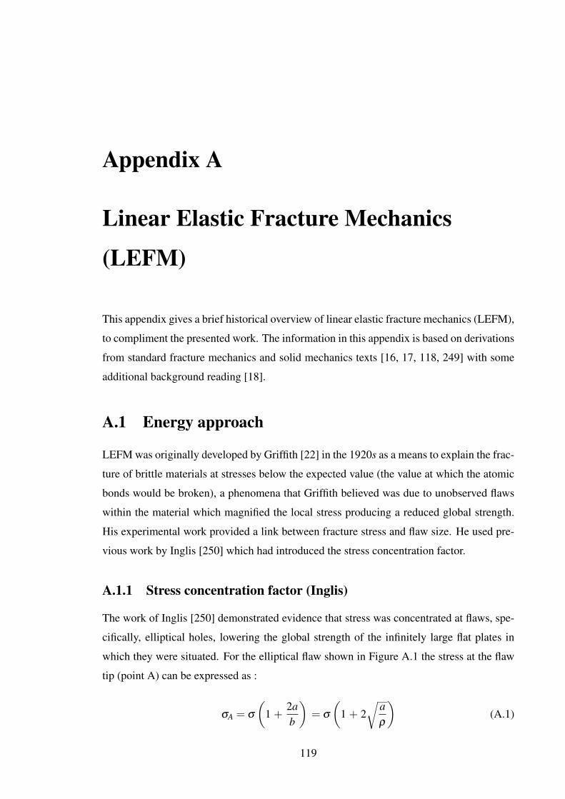
Appendix A
Linear Elastic Fracture Mechanics
(LEFM)
This appendix gives a brief historical overview of linear elastic fracture mechanics (LEFM),
to compliment the presented work. The information in this appendix is based on derivations
from standard fracture mechanics and solid mechanics texts [16, 17, 118, 249] with some
additional background reading [18].
A.1 Energy approach
LEFM was originally developed by Griffith [22] in the 1920s as a means to explain the frac-
ture of brittle materials at stresses below the expected value (the value at which the atomic
bonds would be broken), a phenomena that Griffith believed was due to unobserved flaws
within the material which magnified the local stress producing a reduced global strength.
His experimental work provided a link between fracture stress and flaw size. He used pre-
vious work by Inglis [250] which had introduced the stress concentration factor.
A.1.1 Stress concentration factor (Inglis)
The work of Inglis [250] demonstrated evidence that stress was concentrated at flaws, spe-
cifically, elliptical holes, lowering the global strength of the infinitely large flat plates in
which they were situated. For the elliptical flaw shown in Figure A.1 the stress at the flaw
tip (point A) can be expressed as :
σA = σ
(1 +
2ab
)= σ
(1 + 2
√aρ
)(A.1)
119

APPENDIX A. LINEAR ELASTIC FRACTURE MECHANICS (LEFM)
Figure A.1: An elliptical hole in a flat plate [17]
The stress concentration factor, K, was defined as the ratio between σA and σ . The termaρ
indicates a significant reliance on flaw shape. K varies between 3 for a circular flaw
(a = b) to infinitely large when the flaw develops into a crack (radius of curvature ρ =
0, b→ 0). This is suggestive that any sharp crack should concentrate stress to an infinite
level that guarantees failure upon any non-zero load. This is clearly a physically unrealistic
prediction. In all materials the stress levels ahead of a defect are reduced to various extents
by processes dissipating strain energy, e.g. plasticity, micro-cracking, void formation and
growth, crazing etc.
A.1.2 Griffith approach
Griffith employed the first law of thermodynamics to perform an energy balance, rather
than focusing on the apparently infinite stress at the crack tip. He proposed that crack
propagation will only become energetically favourable if the elastic strain energy released
is in excess of the energy required to produce a new crack surface (surface energy). He
defined the total energy within a cracked plate, U , as:
U =U0 +Ue +Us−F (A.2)
where:
U0 is the elastic energy of the loaded uncracked plate, which is a constant,
Ue is the change in energy due to the introduction of a crack into the plate,
U s is the change in energy due to the creation of two new crack surfaces,
120

APPENDIX A. LINEAR ELASTIC FRACTURE MECHANICS (LEFM)
F is the external work on the plate, which is equal to U0 under displacement control
conditions, i.e. the derivative of F with respect to crack extension equals 0.
For an incrementally increasing crack area dA, the equilibrium condition for crack growth
is achieved when:
d(Us +Ue)
dA= 0 (A.3)
The elastic strain energy released by crack formation can be evaluated from:
Ue =12
ˆa
σ(x)4(x,a)dx (A.4)
where σ(x) is the stress distribution around the crack and 4(x,a) is the vertical crack
opening.
Figure A.2: The strain energy released around a crack of length 2a (reproduced from [118])
Griffith used the work of Inglis [250] to show that for a through thickness crack of
length 2a in an infinite plate, where B is the plate thickness, Figure A.2:
Ue =πσ2a2B
E(A.5)
where E is the Young’s modulus of the material. This can be shown to be:
Ue =πσ2a2k
E(A.6)
where k = 1− v2 for plane strain and k = 1 for plane stress. ν is Poissons ratio. For the
above crack, the surface energy U s is given by:
121
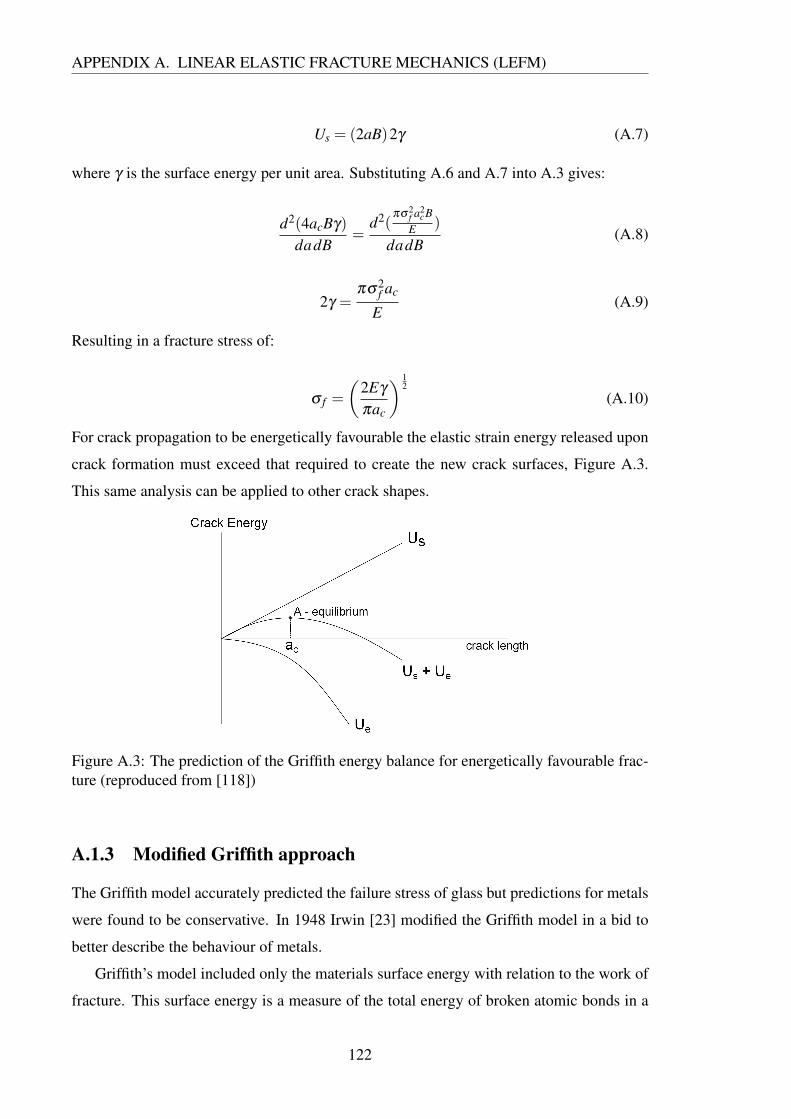
APPENDIX A. LINEAR ELASTIC FRACTURE MECHANICS (LEFM)
Us = (2aB)2γ (A.7)
where γ is the surface energy per unit area. Substituting A.6 and A.7 into A.3 gives:
d2(4acBγ)
dadB=
d2(πσ2
f a2cB
E )
dadB(A.8)
2γ =πσ2
f ac
E(A.9)
Resulting in a fracture stress of:
σ f =
(2Eγ
πac
) 12
(A.10)
For crack propagation to be energetically favourable the elastic strain energy released upon
crack formation must exceed that required to create the new crack surfaces, Figure A.3.
This same analysis can be applied to other crack shapes.
Crack Energy
Us
Ue
Us + Ue
ac
A - equilibrium
Figure A.3: The prediction of the Griffith energy balance for energetically favourable frac-ture (reproduced from [118])
A.1.3 Modified Griffith approach
The Griffith model accurately predicted the failure stress of glass but predictions for metals
were found to be conservative. In 1948 Irwin [23] modified the Griffith model in a bid to
better describe the behaviour of metals.
Griffith’s model included only the materials surface energy with relation to the work of
fracture. This surface energy is a measure of the total energy of broken atomic bonds in a
122
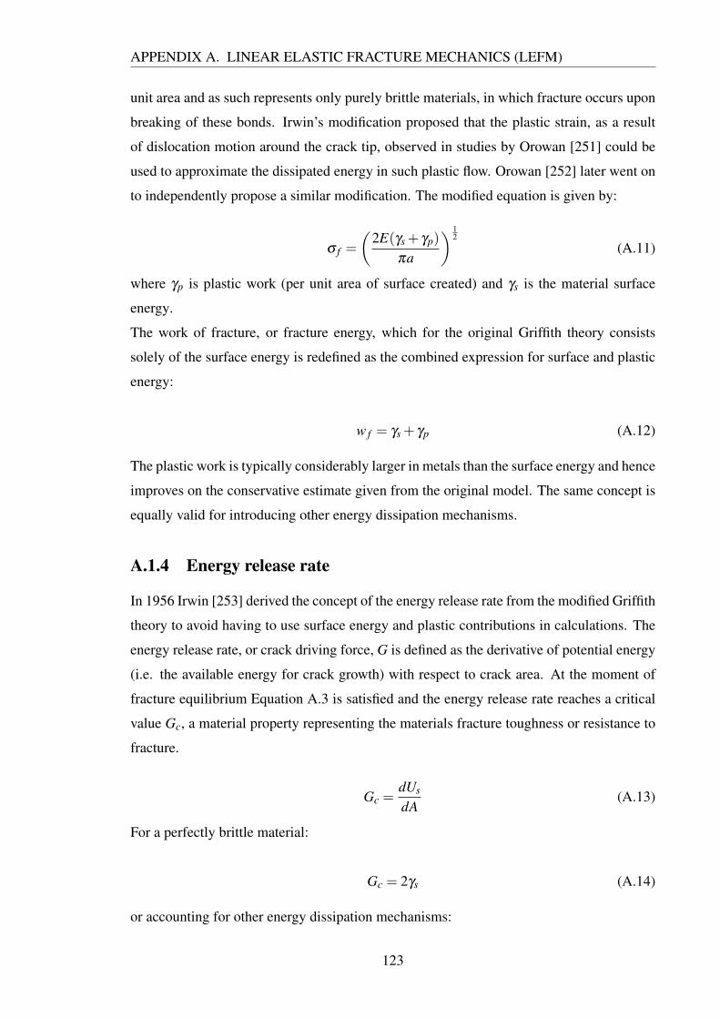
APPENDIX A. LINEAR ELASTIC FRACTURE MECHANICS (LEFM)
unit area and as such represents only purely brittle materials, in which fracture occurs upon
breaking of these bonds. Irwin’s modification proposed that the plastic strain, as a result
of dislocation motion around the crack tip, observed in studies by Orowan [251] could be
used to approximate the dissipated energy in such plastic flow. Orowan [252] later went on
to independently propose a similar modification. The modified equation is given by:
σ f =
(2E(γs + γp)
πa
) 12
(A.11)
where γp is plastic work (per unit area of surface created) and γs is the material surface
energy.
The work of fracture, or fracture energy, which for the original Griffith theory consists
solely of the surface energy is redefined as the combined expression for surface and plastic
energy:
w f = γs + γp (A.12)
The plastic work is typically considerably larger in metals than the surface energy and hence
improves on the conservative estimate given from the original model. The same concept is
equally valid for introducing other energy dissipation mechanisms.
A.1.4 Energy release rate
In 1956 Irwin [253] derived the concept of the energy release rate from the modified Griffith
theory to avoid having to use surface energy and plastic contributions in calculations. The
energy release rate, or crack driving force, G is defined as the derivative of potential energy
(i.e. the available energy for crack growth) with respect to crack area. At the moment of
fracture equilibrium Equation A.3 is satisfied and the energy release rate reaches a critical
value Gc, a material property representing the materials fracture toughness or resistance to
fracture.
Gc =dUs
dA(A.13)
For a perfectly brittle material:
Gc = 2γs (A.14)
or accounting for other energy dissipation mechanisms:
123

APPENDIX A. LINEAR ELASTIC FRACTURE MECHANICS (LEFM)
Gc = 2w f (A.15)
So using the previous cracked example, the energy release rate and hence critical energy
release rate can be expressed as:
G =πσ2a
E(A.16)
Gc =πσ2
f ac
E(A.17)
which is clearly the same as Equation A.9. The crack energy release rate can be shown to
be equal for both load controlled and displacement controlled loading, another advantage
over the modified Griffith approach where load is assumed constant during crack extension.
A.1.5 The R curve
The R curve is a graphical representation of the stability of the crack growth for a given
crack energy release rate. The value of G at which crack extension occurs, Gc, is deemed
equal to a term R, a material property defining its resistance to crack extension.
To determine the state of crack stability, both G and R are plotted against crack size,
a. These are simply called the driving force and resistance curves respectively. When the
crack energy release rate increases with crack length at a lower rate than the material’s
resistance, the crack is deemed stable:
dGda
<dRda
(A.18)
When the crack energy release rate increases with crack length at the same rate as the
material’s resistance, the crack is deemed stable, the crack is on the point of instability:
dGda
=dRda
(A.19)
When the crack energy release rate increases with crack length at a greater rate than the
material’s resistance, the crack is deemed unstable:
dGda
>dRda
(A.20)
For a flat R curve, Figure A.4(a), the material’s resistance to crack extension remains con-
stant so there is a unique value for Gc. This is not so simple for a rising R curve, Figure
124
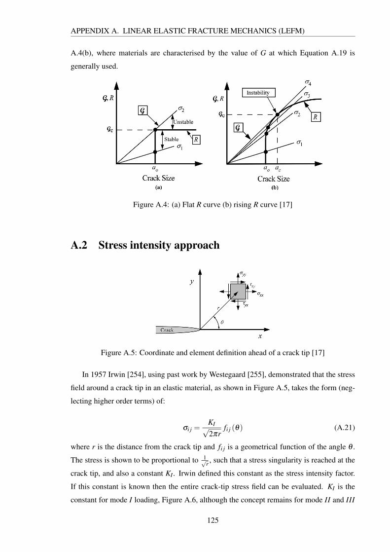
APPENDIX A. LINEAR ELASTIC FRACTURE MECHANICS (LEFM)
A.4(b), where materials are characterised by the value of G at which Equation A.19 is
generally used.
Figure A.4: (a) Flat R curve (b) rising R curve [17]
A.2 Stress intensity approach
Figure A.5: Coordinate and element definition ahead of a crack tip [17]
In 1957 Irwin [254], using past work by Westegaard [255], demonstrated that the stress
field around a crack tip in an elastic material, as shown in Figure A.5, takes the form (neg-
lecting higher order terms) of:
σi j =KI√2πr
fi j (θ) (A.21)
where r is the distance from the crack tip and fi j is a geometrical function of the angle θ .
The stress is shown to be proportional to 1√r , such that a stress singularity is reached at the
crack tip, and also a constant KI . Irwin defined this constant as the stress intensity factor.
If this constant is known then the entire crack-tip stress field can be evaluated. KI is the
constant for mode I loading, Figure A.6, although the concept remains for mode II and III
125

APPENDIX A. LINEAR ELASTIC FRACTURE MECHANICS (LEFM)
loading. Derivations of standard results for these modes can found in the cited texts for
these Appendices. In mixed mode loading the total stress tensor is found from summing
the stress tensors from individual loading modes.
Figure A.6: The 3 modes of loading for a crack [17]
Irwin noted that the stresses appear proportional to√
πa and as such a general expres-
sion for the stress intensity factor for different geometries can be expressed as:
KI = σ√
πa f( a
W
)(A.22)
where W is the width of the cracked plate and as before 2a is the crack width.
The value of the stress intensity factor at fracture, KIc, may be used as an alternative to
the energy release rate as a material property which measures fracture toughness. Despite
the stress intensity factor providing a locally characterising material description through
stress analysis as opposed to the global energy change which quantifies the Griffith method,
both provide an identical approach to fracture mechanics. Although both approaches are
equivalent, the use of the stress intensity factor provides consistency across geometries
through f( a
W
). By combining Equation A.16 and Equation A.22, considering fracture
mode I, G can be expressed as a function of KI for linear elastic materials, such that:
G =K2
IE ′
(A.23)
where E ′ = E for plane stress and E ′ = E1−ν2 . This can be proved for all crack geometries
under each mode of fracture (for full derivation see [17]).
126
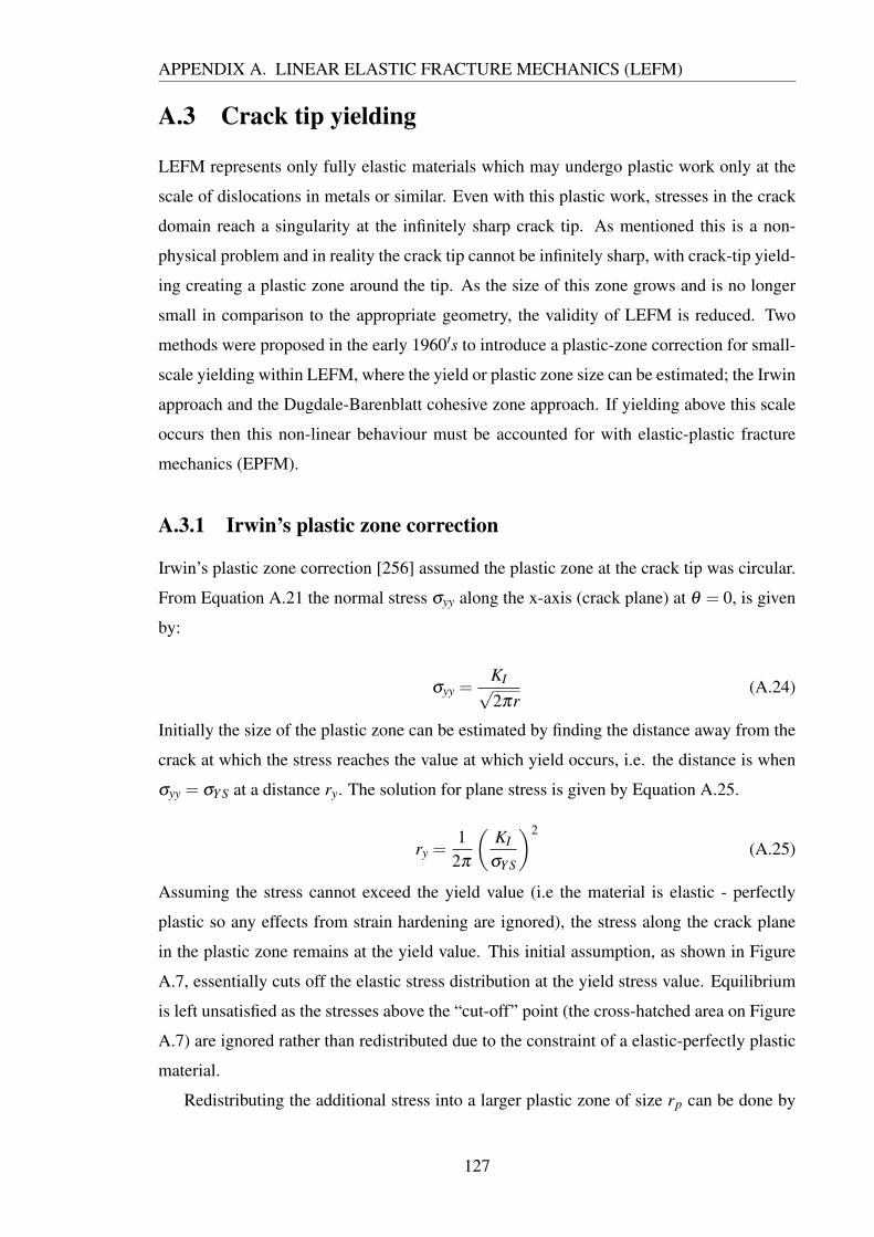
APPENDIX A. LINEAR ELASTIC FRACTURE MECHANICS (LEFM)
A.3 Crack tip yielding
LEFM represents only fully elastic materials which may undergo plastic work only at the
scale of dislocations in metals or similar. Even with this plastic work, stresses in the crack
domain reach a singularity at the infinitely sharp crack tip. As mentioned this is a non-
physical problem and in reality the crack tip cannot be infinitely sharp, with crack-tip yield-
ing creating a plastic zone around the tip. As the size of this zone grows and is no longer
small in comparison to the appropriate geometry, the validity of LEFM is reduced. Two
methods were proposed in the early 1960′s to introduce a plastic-zone correction for small-
scale yielding within LEFM, where the yield or plastic zone size can be estimated; the Irwin
approach and the Dugdale-Barenblatt cohesive zone approach. If yielding above this scale
occurs then this non-linear behaviour must be accounted for with elastic-plastic fracture
mechanics (EPFM).
A.3.1 Irwin’s plastic zone correction
Irwin’s plastic zone correction [256] assumed the plastic zone at the crack tip was circular.
From Equation A.21 the normal stress σyy along the x-axis (crack plane) at θ = 0, is given
by:
σyy =KI√2πr
(A.24)
Initially the size of the plastic zone can be estimated by finding the distance away from the
crack at which the stress reaches the value at which yield occurs, i.e. the distance is when
σyy = σY S at a distance ry. The solution for plane stress is given by Equation A.25.
ry =1
2π
(KI
σY S
)2
(A.25)
Assuming the stress cannot exceed the yield value (i.e the material is elastic - perfectly
plastic so any effects from strain hardening are ignored), the stress along the crack plane
in the plastic zone remains at the yield value. This initial assumption, as shown in Figure
A.7, essentially cuts off the elastic stress distribution at the yield stress value. Equilibrium
is left unsatisfied as the stresses above the “cut-off” point (the cross-hatched area on Figure
A.7) are ignored rather than redistributed due to the constraint of a elastic-perfectly plastic
material.
Redistributing the additional stress into a larger plastic zone of size rp can be done by
127
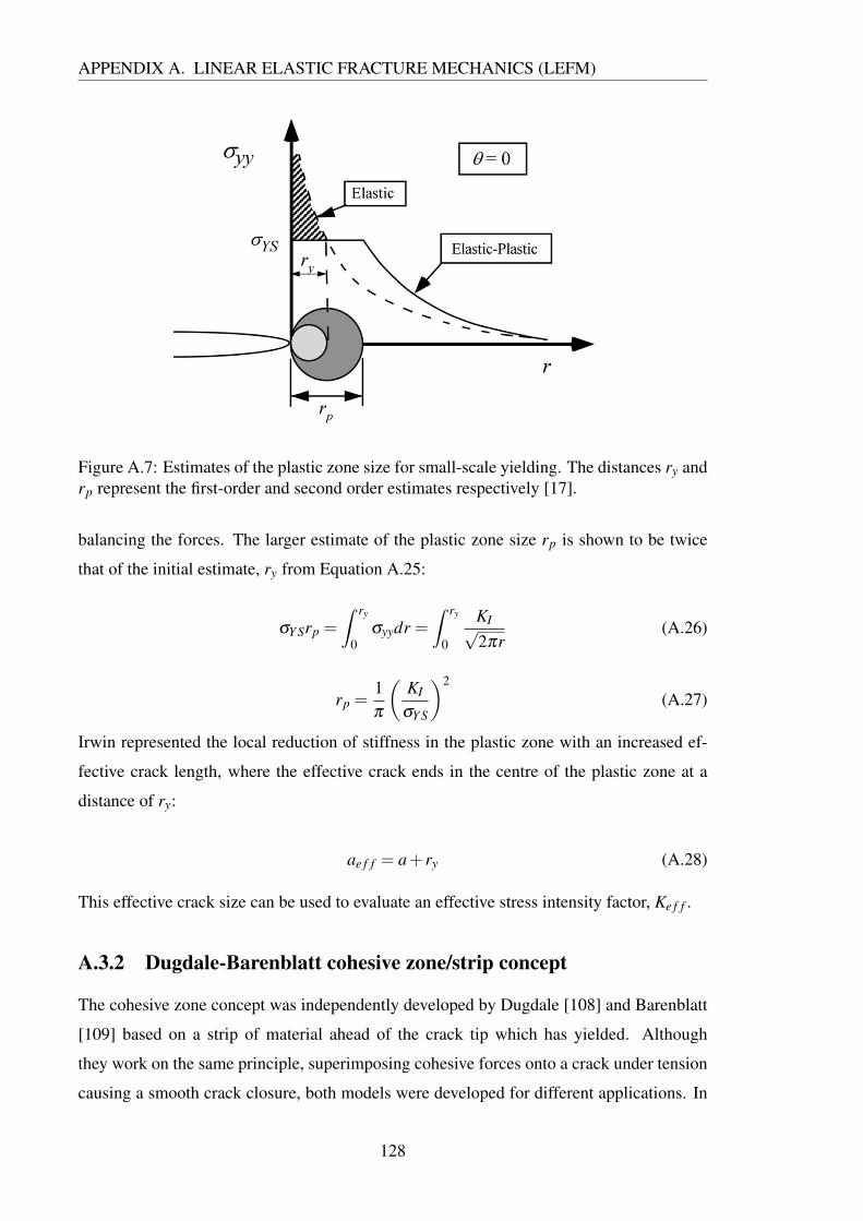
APPENDIX A. LINEAR ELASTIC FRACTURE MECHANICS (LEFM)
Figure A.7: Estimates of the plastic zone size for small-scale yielding. The distances ry andrp represent the first-order and second order estimates respectively [17].
balancing the forces. The larger estimate of the plastic zone size rp is shown to be twice
that of the initial estimate, ry from Equation A.25:
σY Srp =
ˆ ry
0σyydr =
ˆ ry
0
KI√2πr
(A.26)
rp =1π
(KI
σY S
)2
(A.27)
Irwin represented the local reduction of stiffness in the plastic zone with an increased ef-
fective crack length, where the effective crack ends in the centre of the plastic zone at a
distance of ry:
ae f f = a+ ry (A.28)
This effective crack size can be used to evaluate an effective stress intensity factor, Ke f f .
A.3.2 Dugdale-Barenblatt cohesive zone/strip concept
The cohesive zone concept was independently developed by Dugdale [108] and Barenblatt
[109] based on a strip of material ahead of the crack tip which has yielded. Although
they work on the same principle, superimposing cohesive forces onto a crack under tension
causing a smooth crack closure, both models were developed for different applications. In
128

APPENDIX A. LINEAR ELASTIC FRACTURE MECHANICS (LEFM)
essence only Dugdale’s strip yield model was developed to correct for small-scale yielding
in LEFM. Barenblatt’s “cohesive force” model was developed for brittle materials by mod-
elling forces between atoms at the crack tip. The conceptual similarities in the models has
led to both being referred to as Dugdale-Barenblatt or cohesive zone/strip models.
A.3.2.1 Dugdale strip yield model
In Dugdale’s strip yield model, Figure A.8, the plastic work is situated along a strip ahead
of the crack. This model is similar to Irwin’s approach in that the crack is given an effective
length, which exceeds its actual length. However in this model the crack faces within the
plastic zone of length ρ , ahead of a crack of half length a, where ρ � a, are deemed to be
subject to a constant closure stress the magnitude of which equals the yield stress, σY S. For
this model the strip yield is treated as the cohesive zone.
Figure A.8: The strip-yield model [17].
Figure A.9: The crack-opening force, P, acting at a distance x from the crack’s centre-line[17].
For the actual crack distance as shown in Figure A.9, the stress due to the tensile load,
P applied to the crack face is:
σ (x) = σ 0≤ |x|< a (A.29)
For the plastic zone, the distance between the effective and actual crack length, this tensile
load is counteracted by the closure stress:
σ (x) = σ −σY S a≤ |x|< a+ρ (A.30)
129

APPENDIX A. LINEAR ELASTIC FRACTURE MECHANICS (LEFM)
So the stress intensity factor at the effective crack tip due to the tensile load which is applied
over the entire crack length is given by (using Equation A.22):
Kσ = σ√
π(a+ρ) (A.31)
The stress intensity factor at the effective crack tip due to the closure stress over the plastic
zone can be expressed as:
Kclosure =σY S√
π(a+ρ)
ˆ a+ρ
a
√(a+ρ)+ x(a+ρ)− x
dx (A.32)
Kclosure =σY S√
π(a+ρ)
ˆ a+ρ
a
√(a+ρ)− x(a+ρ)+ x
dx (A.33)
for the crack tips in the positive and negative x direction respectively. Solving the sum of
these integrals gives:
Kclosure =−2σY S
√a+ρ
πarccos
(a
a+ρ
)(A.34)
The plastic zone length ρ is evaluated by equating the stress intensity factors from the
remote tension and closure stress. This gives:
aa+ρ
= cos(
πσ
2σY S
)(A.35)
Ke f f can then be estimated using the sum of a and ρ as the effective crack length. This
estimate was improved by Burdekin and Stone [257] who used a Westergaard complex
stress function [255] to derive an expression for the crack-opening displacement from the
strip-yield model. This was used to used calculate the J-integral and hence Ke f f . Both the
concepts of crack-opening displacement (COD) and the J-integral are used more extens-
ively for yielding which exceeds small scale (Elastic-Plastic Fracture Mechanics) and is not
explained here.
A.3.2.2 Barenblatt cohesive force model
Barenblatts cohesive force model worked on the same concept but stresses varied with
deformation rather than remaining constant at the yield stress, Figure A.10. As a result
Equations A.29 and A.30 become:
130
APPENDIX A. LINEAR ELASTIC FRACTURE MECHANICS (LEFM)
q(x)
Figure A.10: The cohesive force model (adapted from [17])
σ (x) = σ 0≤ |x|< a (A.36)
σ (x) = σ −q(x) a≤ |x|< a+ρ (A.37)
A simple comparison between pure LEFM and its plastic zone corrections can be found in
[17].
131

Appendix B
Continuum Damage Mechanics (CDM)
This section gives a brief overview of the background and theory of Continuum Damage
Mechanics. The information presented is sourced from the cited papers, standard text books
[29] and review papers [27, 258].
Continuum damage mechanics (CDM), initially developed by Kachanov [114] to model
creep in metals, provides a complimenting approach to fracture mechanics framework in
modelling material failure. In a purely fracture mechanics approach the effect of the dis-
continuity created by a single crack within a continuum is modelled analytically. For the
FPZ of quasi-brittle materials, the high-volume of cracks and discontinuities and their dy-
namic interaction processes, creates difficulties with this approach.
For quasi-brittle materials, CDM indirectly quantifies the accumulated damage by con-
sidering the degrading effect of the micro-crack population on the macroscopic material
properties such as strength, stiffness and toughness. In this way the high volume of cracks
is essentially “smeared out” within the FPZ continuously. As CDM maintains the classical
continuum assumption, numerical implementation in commercial finite element software
proves relatively simple, in comparison to fracture mechanics where the discontinuities in
the mesh neccesitate remeshing unless mesh-less methods can be sufficiently developed.
B.1 Damage parameters
The CDM framework begins by representing a materials state of damage with one or more
damage variables, which can be of scalar or tensorial form. The continuum damage concept
dictates that the final stage of damage will be when the continuum assumption is broken,
i.e. the development of a discontinuity or macro-crack. A scalar damage variable, D can
be defined with a value of 0 corresponding to an undamaged state and a value of 1 cor-
132

APPENDIX B. CONTINUUM DAMAGE MECHANICS (CDM)
responding to final fracture. A scalar variable is suitable for isotropic loading, i.e. when
the microflaws are randomly distributed or are small enough to assume so. If a scalar vari-
able is unsuitable, i.e for a combination of damage mechanisms or material anisotropy, then
multiple scalar parameters or a tensor may be used.
Damage can be directly measured, through micro-structural observations and a change
in net cross sectional area, or indirectly through the change in physical material macro-
scopic properties as a result of the micro-structural changes [259]. Such properties include
a change in density due to void fraction increase, acoustic emission and most commonly a
change in the mechanical behaviour, characterised by the effective stress. This is an exten-
sion of the effective area concept, Figure B.1, proposed by Kachanov [114]. In this concept
the effective area of the fictitious undamaged state, dA, of a bar under tensile load, dF can
be expressed as a function of the scalar damage parameter D and the area of the damaged
state, dA:
dA = (1−D)dA (B.1)
This can be used to evaluate the effective stress:
σ =dFdA
=1
(1−D)
dFdA
=σ
1−D(B.2)
and hence:
D = 1− σ
σ(B.3)
Figure B.1: The concept of a fictitious undamaged state, on which the effective stress prin-ciple is based [29].
The effective stress concept (and similarly the effective strain concept) equates the re-
133
APPENDIX B. CONTINUUM DAMAGE MECHANICS (CDM)
sponse of a damaged material under an stress, σ , to the response of a fictitious undamaged
volume of the same material under an effective stress, σ . This assumption forms the hypo-
thesis of strain equivalence [29]. In this way:
ε =σ
E (D)(B.4)
ε =σ
E0(B.5)
where E0 is the Young’s modulus of the undamaged and fictitious undamaged volumes of
material and E (D) is the Young’s modulus of the damaged material (either secant or tangent
modulus). Introducing these expressions into Equation B.3 yields:
D = 1− E (D)
E0(B.6)
Without the assumption of isotropic damage, a scalar parameter becomes insufficient to
describe the damage behaviour. In such cases tensorial parameters are required [260].
B.2 Damage evolution and constitutive laws
Once the initial state of damage is known (from the effective stress concept), a descriptive
law mapping the progression of the damage variable as time or load increases is necessary.
This can be derived on a thermodynamic basis, the details of which are out of the scope
of this brief review. For more details consult one of the given references for this appendix.
Once the damage parameter and evolution law are known, the damage can be progressed
until the initiation of failure in terms of a macro-crack. There are two basic approaches to
the damage analysis:
• Uncoupled approach. The uncoupled analysis assumes that the stress and strain
fields are not reliant on the damage within the material. Under initial loading condi-
tions the constitutive laws allow evaluation of the stress and strain field. If the initial
damage state is also known (or assumed to be 0), then the damage evolution law can
be used to evaluate the progression of damage in a given time or load step and hence
determine the resulting damage field. This damage field is used as a failure prediction
for the structure, but has no affect on the subsequent failure analysis for increasing
time or load. This neglect of the interaction between damage and constitutive laws
introduces error but also provides simplicity.
134

APPENDIX B. CONTINUUM DAMAGE MECHANICS (CDM)
• Coupled approach. Coupled analysis recognises the interaction between stress,
strain and damage. In this way the material constitutive laws are derived to take into
account damage and the effect on the material deformation as time or load progresses.
As a result, unlike in the uncoupled approach, the stress, strain and damage can be
evaluated simultaneously. However such procedures require the full field history of
damage and hence increase complexity.
Examples of both types of model can be found in the literature [29, 126, 261, 262]. Moreover
the formulation of different damage models differs depending on the type of material, with
a general distinction evident between elastic and plastic materials:
• Elastic/Elastic-Brittle damage models. In such models damage applies to the elastic
response of an elastic material [139].
• Damage-Plasticity/Elastic-Plastic damage models. In such models damage applies
to elastic-plastic materials. This can incorporate the elastic response exclusively,
leaving the plastic response “undamaged” (uncoupled), or both elastic and plastic
regimes (coupled) [263].
135
Appendix C
Meso-scale features and couple stresses
in fracture process zone
136
13th International Conference on Fracture June 16–21, 2013, Beijing, China
-1-
Meso-scale features and couple stresses in fracture process zone
Craig N Morrison1, 3,*, Andrey P Jivkov2, 3, John R Yates3
1 Nuclear FiRST Doctoral Training Centre
2 Research Centre for Radwaste and Decommissioning 3 Modelling and Simulation Centre
Dalton Nuclear Institute, The University of Manchester, Manchester, M13 9PL, UK
* Corresponding author: [email protected]
Abstract Generalized continuum theories such as couple stress theory have the potential to improve
our understanding of material deformation and fracture behaviour in areas where classical continuum
theory breaks down at, for example, the length scale of meso-scale features within the fracture process
zone. The couple stress theory considers not only relative displacements between these features but
also relative rotations, introducing a natural length scale. A model has been developed of a low
stiffness matrix containing suitably situated high stiffness particles to simulate the presence of defects
at the meso-scale. This has been used to assess the descriptive potential of a novel consistent couple
stress theory. The model has been subjected to a set of displacement fields selected to produce strain
energies with varying contributions from the coupled stresses. The results demonstrate the effect of
particle size to spacing ratio on the elastic energies. These can be used to evaluate the couple stress
constant as well as validate the constant experimentally for specific materials.
Keywords: generalized continuum; meso-scale defects; FE analysis; strain-curvature energy; size
effect
1. Introduction
Analysis of materials at engineering length scales is based upon assumptions of classical
continuum behaviour. This is adequate for most macro-scale analyses but, when considering
smaller length scales where cracks, notches and defects introduce stress concentrations, the
material microstructure is known to have a significant impact on material behaviour [1]. Local
approaches, which incorporate mechanistic understanding of material failure behaviour at the
length scale of their relevant features, are beneficial for linking microstructures to
macroscopic responses [2]. However, the widely used weakest link (WL) assumption has been
challenged as a realistic method of modelling size effects in cleavage [3] and quasi-brittle
fracture [4] as a result of failing to account for the interaction processes during failure.
Discrete methods have shown promise for modelling materials undergoing such fracture.
Lattice models consist of nodes connected into a lattice via springs [5], beams [6] or other
discrete elements with the properties of these connections allowing a micro structurally
informed response. Lattice modelling differs in principle from previous local approach
models by using a statistically parallel system, where loads are redistributed upon the
breaking of a single bond, rather than the ultimate failure seen in WL systems. This is
considered to be a closer representation of the interaction and coalescence of micro-cracks
and flaws, which characterize quasi-brittle materials such as graphite [7] and cement-based
materials [8]. The work presented here explores aspects of the site-bond model developed by
Jivkov and Yates [9] and used for studies of damage evolution from distributed porosity in
cements [10]. Work on this model has shown that evaluating the stiffness coefficients of the
bonds using strain energy equivalence between the discrete model and a classical continuum
creates an indeterminate problem. Use of a generalized continuum theory, such as couple
stress theory, offers a possible solution to this indeterminacy.
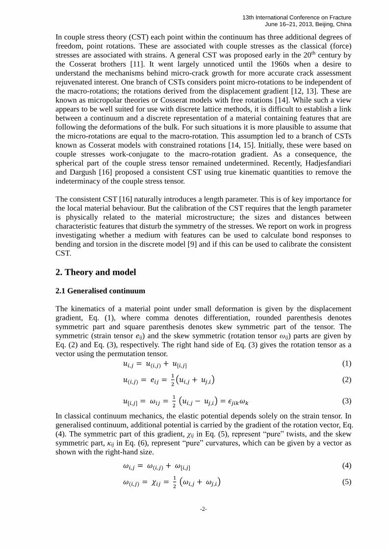
13th International Conference on Fracture June 16–21, 2013, Beijing, China
-2-
In couple stress theory (CST) each point within the continuum has three additional degrees of
freedom, point rotations. These are associated with couple stresses as the classical (force)
stresses are associated with strains. A general CST was proposed early in the 20th century by
the Cosserat brothers [11]. It went largely unnoticed until the 1960s when a desire to
understand the mechanisms behind micro-crack growth for more accurate crack assessment
rejuvenated interest. One branch of CSTs considers point micro-rotations to be independent of
the macro-rotations; the rotations derived from the displacement gradient [12, 13]. These are
known as micropolar theories or Cosserat models with free rotations [14]. While such a view
appears to be well suited for use with discrete lattice methods, it is difficult to establish a link
between a continuum and a discrete representation of a material containing features that are
following the deformations of the bulk. For such situations it is more plausible to assume that
the micro-rotations are equal to the macro-rotation. This assumption led to a branch of CSTs
known as Cosserat models with constrained rotations [14, 15]. Initially, these were based on
couple stresses work-conjugate to the macro-rotation gradient. As a consequence, the
spherical part of the couple stress tensor remained undetermined. Recently, Hadjesfandiari
and Dargush [16] proposed a consistent CST using true kinematic quantities to remove the
indeterminacy of the couple stress tensor.
The consistent CST [16] naturally introduces a length parameter. This is of key importance for
the local material behaviour. But the calibration of the CST requires that the length parameter
is physically related to the material microstructure; the sizes and distances between
characteristic features that disturb the symmetry of the stresses. We report on work in progress
investigating whether a medium with features can be used to calculate bond responses to
bending and torsion in the discrete model [9] and if this can be used to calibrate the consistent
CST.
2. Theory and model
2.1 Generalised continuum
The kinematics of a material point under small deformation is given by the displacement
gradient, Eq. (1), where comma denotes differentiation, rounded parenthesis denotes
symmetric part and square parenthesis denotes skew symmetric part of the tensor. The
symmetric (strain tensor eij) and the skew symmetric (rotation tensor ωij) parts are given by
Eq. (2) and Eq. (3), respectively. The right hand side of Eq. (3) gives the rotation tensor as a
vector using the permutation tensor.
𝑢𝑖,𝑗 = 𝑢(𝑖,𝑗) + 𝑢[𝑖,𝑗] (1)
𝑢(𝑖,𝑗) = 𝑒𝑖𝑗 = 1
2(𝑢𝑖,𝑗 + 𝑢𝑗,𝑖) (2)
𝑢[𝑖,𝑗] = 𝜔𝑖𝑗 = 1
2 (𝑢𝑖,𝑗 − 𝑢𝑗,𝑖) = 𝜖𝑗𝑖𝑘𝜔𝑘 (3)
In classical continuum mechanics, the elastic potential depends solely on the strain tensor. In
generalised continuum, additional potential is carried by the gradient of the rotation vector, Eq.
(4). The symmetric part of this gradient, χij in Eq. (5), represent “pure” twists, and the skew
symmetric part, κij in Eq. (6), represent “pure” curvatures, which can be given by a vector as
shown with the right-hand size.
𝜔𝑖,𝑗 = 𝜔(𝑖,𝑗) + 𝜔[𝑖,𝑗] (4)
𝜔(𝑖,𝑗) = 𝜒𝑖𝑗 = 1
2 (𝜔𝑖,𝑗 + 𝜔𝑗,𝑖) (5)
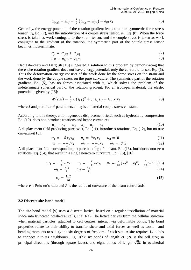
13th International Conference on Fracture June 16–21, 2013, Beijing, China
-3-
𝜔[𝑖,𝑗] = 𝜅𝑖𝑗 = 1
2 (𝜔𝑖,𝑗 − 𝜔𝑗,𝑖) = 𝜖𝑗𝑖𝑘𝜅𝑘 (6)
Generally, the energy potential of the rotation gradient leads to a non-symmetric force stress
tensor, σji, Eq. (7), and the introduction of a couple stress tensor, μji, Eq. (8). When the force
stress is taken as work conjugate to the strain tensor, and the couple stress is taken as work
conjugate to the gradient of the rotation, the symmetric part of the couple stress tensor
becomes indeterminate.
𝜎𝑗𝑖 = 𝜎(𝑗𝑖) + 𝜎[𝑗𝑖] (7)
𝜇𝑗𝑖 = 𝜇(𝑗𝑖) + 𝜇[𝑗𝑖] (8)
Hadjesfandiari and Dargush [16] suggested a solution to this problem by demonstrating that
the entire rotation gradient does not have energy potential, only the curvature tensor, Eq. (6).
Thus the deformation energy consists of the work done by the force stress on the strain and
the work done by the couple stress on the pure curvature. The symmetric part of the rotation
gradient, Eq. (5), has no forces associated with it, which solves the problem of the
indeterminate spherical part of the rotation gradient. For an isotropic material, the elastic
potential is given by [16]:
𝑊(𝜀, 𝜅) = 1
2 𝜆 (𝜀𝑘𝑘)2 + 𝜇 𝜀𝑖𝑗𝜀𝑖𝑗 + 8𝜂 𝜅𝑖𝜅𝑖 (9)
where λ and μ are Lamé parameters and η is a material couple stress constant.
According to this theory, a homogeneous displacement field, such as hydrostatic compression
Eq. (10), does not introduce rotations and hence curvatures.
𝑢1 = 𝑥1 𝑢2 = 𝑥2 𝑢3 = 𝑥3 (10)
A displacement field producing pure twist, Eq. (11), introduces rotations, Eq. (12), but no true
curvatures[16]:
𝑢1 = −𝜃𝑥2𝑥3 𝑢2 = 𝜃𝑥1𝑥3 𝑢3 = 0 (11)
𝜔1 = −1
2𝜃𝑥1 𝜔2 = −
1
2𝜃𝑥2 𝜔3 = 𝜃𝑥3 (12)
A displacement field corresponding to pure bending of a beam, Eq. (13), introduces non-zero
rotations, Eq. (14), that result in a single non-zero curvature, Eq. (15), [16]:
𝑢1 = −1
𝑅𝑥1𝑥3 𝑢2 = −
𝜈
𝑅𝑥2𝑥3 𝑢3 =
𝜈
2𝑅(𝑥2
2 − 𝑥32) −
1
2𝑅𝑥1
2 (13)
𝜔1 = 𝜈𝑥2
𝑅 𝜔2 =
𝑥1
𝑅 (14)
𝜅3 = 1−𝜈
2𝑅 (15)
where is Poisson’s ratio and R is the radius of curvature of the beam central axis.
2.2 Discrete site-bond model
The site-bond model [9] uses a discrete lattice, based on a regular tessellation of material
space into truncated octahedral cells, Fig. 1(a). The lattice derives from the cellular structure
when material particles, attached to cell centres, interact via deformable bonds. The bond
properties relate to their ability to transfer shear and axial forces as well as torsion and
bending moments to satisfy the six degrees of freedom of each site. A site requires 14 bonds
to connect it to its neighbours, Fig. 1(b): six bonds of length 2L (2L is the cell size) in
principal directions (through square faces), and eight bonds of length √3L in octahedral

13th International Conference on Fracture June 16–21, 2013, Beijing, China
-4-
directions (through hexagonal faces). Development of this model involves bond
representations with six independent elastic springs resisting three relative displacements and
three relative rotations between sites. This yields four spring types with axial, Kn, shear, Ks,
twisting, Kt, and bending, Kb, stiffness [17], which could, in general, be different for
principal and octahedral directions.
Figure 1. Cellular representation of material (a); and unit cell with bonds (b).
2.3 FE model of elastic continuum with rigid particles
For our investigation, we use a finite element model of a cube of an elastic material
surrounding a truncated octahedral cell of size 2L. The material has a unit modulus of
elasticity and Poisson’s ratio = 0.375. Rigid cubic particles are introduced in the cube, so
that one particle, P0, is positioned in the centre of the cell, while others are positioned outside
the cell in the principal and octahedral directions as shown in Fig. 2. Three different loading
conditions are used: (H) hydrostatic compression; (T) pure twist; and (B) pure bending. These
are applied via displacement fields on the cube surfaces; examples for pure twist and pure
bending are given in Fig. 3. In all cases we calculate elastic energies, , within the unit cell
surrounding the central particle. With no particles present, the cell elastic energy is given by
the classical continuum solution, since no features exist to disturb stress symmetry. The
displacement magnitudes for the three loading cases are selected so that without particles is
the same, 0.
Figure 2. Particle additions in the principal (left) and octahedral (right) directions.
Figure 3. Displacement maps for the loading cases of pure twist (left) and pure bending (right).

13th International Conference on Fracture June 16–21, 2013, Beijing, China
-5-
To link the cell energies to kinematic quantities we calculate particle translations and rotations
using three unit vectors, n1, n2 and n3 normal to three orthogonal faces of a particle, see Fig. 4.
After deformation these vectors remain orthogonal as the particles are rigid, given with t1, t2
and t3 in Fig. 4. The coordinates of these, arranged in columns, form the transformation
matrix, T, for the particle. The particle motion can be represented by a single rotation, θ given
by Eq. (16), around a normalized axis, α given by Eq. (17). The components of the rotation
vector for a particle are calculated by Eq. (18). The relative rotations between central and any
other particle are expressed in the coordinate system defined by the particular pair using the
corresponding transformation.
𝜃 = 𝑐𝑜𝑠−1 (𝑡𝑟𝑎𝑐𝑒 (𝐓)−1
2) (16)
𝛼 =1
2 sin (𝜃) [
𝑇32 − 𝑇23
𝑇13 − 𝑇31
𝑇21 − 𝑇12
] (17)
𝜔𝑖 = 𝜃 × 𝛼𝑖 , 𝑖 = 1, 2, 3 (18)
Figure 4. Orthogonal vectors, (n1, n2, n3) and (t1, t2, t3) describing the orientation of P0 before and
after deformation respectively.
3. Results and Discussion
For the particle arrangement used (a central particle and all 14 particles of the site-bond model)
we have used four different particle sizes relative to the cell size in order to investigate the
effect of cell to particle size ratio, . The ratios are 3 (large particles), 4, 6, and 12 (small
particles).
In the case of hydrostatic loading no rotations of particles were observed and the relative
displacements between P0 and any principal or octahedral particle were only axial,
conforming to Eq. (10). In the site-bond model these relative displacements should be resisted
by axial springs with stiffness coefficients Knp and Kn
o, respectively. The relative axial
displacements were found independent of , scaling with the applied displacements. The cell
energies were found to be dependent on , as shown in Figure 5. For small particles, = 12,
the cell energy approached 0; the presence of particles has negligible effect. The cell energy
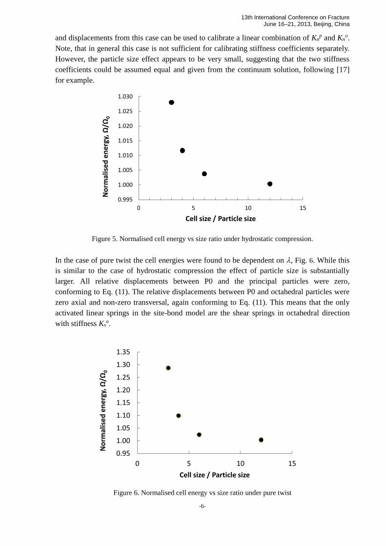
13th International Conference on Fracture June 16–21, 2013, Beijing, China
-6-
and displacements from this case can be used to calibrate a linear combination of Knp and Kn
o.
Note, that in general this case is not sufficient for calibrating stiffness coefficients separately.
However, the particle size effect appears to be very small, suggesting that the two stiffness
coefficients could be assumed equal and given from the continuum solution, following [17]
for example.
Figure 5. Normalised cell energy vs size ratio under hydrostatic compression.
In the case of pure twist the cell energies were found to be dependent on , Fig. 6. While this
is similar to the case of hydrostatic compression the effect of particle size is substantially
larger. All relative displacements between P0 and the principal particles were zero,
conforming to Eq. (11). The relative displacements between P0 and octahedral particles were
zero axial and non-zero transversal, again conforming to Eq. (11). This means that the only
activated linear springs in the site-bond model are the shear springs in octahedral direction
with stiffness Kso.
Figure 6. Normalised cell energy vs size ratio under pure twist
0.995
1.000
1.005
1.010
1.015
1.020
1.025
1.030
0 5 10 15
No
rmal
ise
d e
ner
gy, Ω
/Ω0
Cell size / Particle size
0.95
1.00
1.05
1.10
1.15
1.20
1.25
1.30
1.35
0 5 10 15
No
rmal
ise
d e
ner
gy, Ω
/Ω0
Cell size / Particle size

13th International Conference on Fracture June 16–21, 2013, Beijing, China
-7-
The calculated relative rotations between P0 and the particles in the two directions are shown
in Fig. 7. The non-zero relative rotations between P0 and principal particles were twists as
expected from Eq. (12) and the magnitude shown in Fig. 7 is the twist of the particle in
direction X1. It is seen that this is 3-4 orders of magnitude smaller that the relative rotations
between P0 and octahedral particles. The latter were found to be bend-type rotations only,
conforming to Eq. (12), and suggesting that the only moment springs activated are the
bending springs in the octahedral direction with stiffness Kbo. The magnitudes of the
bend-rotations of octahedral particles were found nearly independent of particle size. These
results suggest that for the case of pure twist, the elastic strain energy is accumulated in the
shear and bending springs in the octahedral direction only, and one can calibrate a linear
combination of Kso and Kb
o, which should depend on the cell to particle size ratio. From this
perspective the results support the analytical derivations in [16], where pure twists do not
contribute to the elastic energy. From here, it can be speculated that the torsion springs in the
principal directions could be omitted from the site-bond model, i.e. Ktp = 0. This should be
supported by considering other cases with curvature-free displacement fields which introduce
twists of principal particles according to the theory.
Figure 7. Relative rotation vs size ratio under pure twist
The cell energy dependence on for the case of pure bending is shown in Fig. 8. The effect of
particle size is smaller than in the case of pure twist, but not negligible. The relative
displacements between P0 and the octahedral particles were non-zero axial and tangential,
conforming to Eq. (13). The relative displacements between P0 and the principal particles also
conform to theory with non-zero axial for particles in X2, non-zero tangential for particles in
X1 and zero displacements of particles in X3. This means that the activated linear springs in
the site-bond model would be axial and shear springs in all octahedral directions with stiffness
coefficients Kno and Ks
o, and axial and shear springs in two principal directions with stiffness
coefficients Knp and Ks
p.
1.E-07
1.E-06
1.E-05
1.E-04
1.E-03
1.E-02
0 5 10 15
Mag
nit
ud
e o
f re
lati
ve r
ota
tio
ns
Cell size / Particle size
Principal
Octahedral
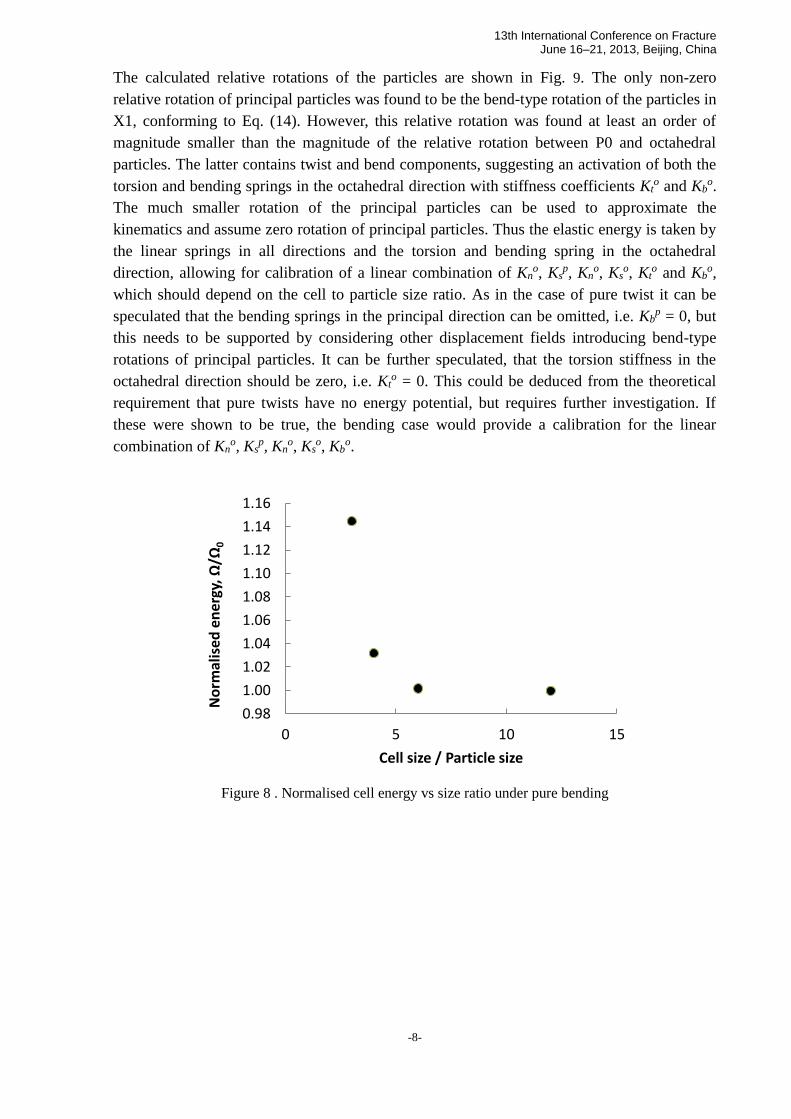
13th International Conference on Fracture June 16–21, 2013, Beijing, China
-8-
The calculated relative rotations of the particles are shown in Fig. 9. The only non-zero
relative rotation of principal particles was found to be the bend-type rotation of the particles in
X1, conforming to Eq. (14). However, this relative rotation was found at least an order of
magnitude smaller than the magnitude of the relative rotation between P0 and octahedral
particles. The latter contains twist and bend components, suggesting an activation of both the
torsion and bending springs in the octahedral direction with stiffness coefficients Kto and Kb
o.
The much smaller rotation of the principal particles can be used to approximate the
kinematics and assume zero rotation of principal particles. Thus the elastic energy is taken by
the linear springs in all directions and the torsion and bending spring in the octahedral
direction, allowing for calibration of a linear combination of Kno, Ks
p, Kno, Ks
o, Kto and Kb
o,
which should depend on the cell to particle size ratio. As in the case of pure twist it can be
speculated that the bending springs in the principal direction can be omitted, i.e. Kbp = 0, but
this needs to be supported by considering other displacement fields introducing bend-type
rotations of principal particles. It can be further speculated, that the torsion stiffness in the
octahedral direction should be zero, i.e. Kto = 0. This could be deduced from the theoretical
requirement that pure twists have no energy potential, but requires further investigation. If
these were shown to be true, the bending case would provide a calibration for the linear
combination of Kno, Ks
p, Kno, Ks
o, Kbo.
Figure 8 . Normalised cell energy vs size ratio under pure bending
0.98
1.00
1.02
1.04
1.06
1.08
1.10
1.12
1.14
1.16
0 5 10 15
No
rmal
ised
en
erg
y, Ω
/Ω0
Cell size / Particle size

13th International Conference on Fracture June 16–21, 2013, Beijing, China
-9-
Figure 9. Relative rotation vs size ratio under pure bending
From the three cases considered in this work, it is clear that a separation between all required
stiffness coefficients is not possible. However, there is a good indication that the site-bond
model should not contain torsion springs and possibly bending springs in the principal
directions. One way to check this is pure twist along the octahedral axis, which theoretically
should provide twist and bend rotations of all particles. If this proves to be the case, the elastic
energy of the continuum with features should be taken by the deformations of the remaining
springs. Additional loading cases are necessary to determine the stiffness coefficients of these
springs. If these are determined from curvature-free loading cases alone, a good strategy for
the calculation of the coupled-stress constant can be proposed. The site-bond model with
constants calibrated from curvature-free loading cases can be subjected to a case introducing
curvature energy according to theory, for example pure bending, and any excess of energy
between the site-bond model and classical continuum should be attributed to curvature energy.
4. Conclusions
We have proposed a methodology for calibrating the spring constants of a special lattice
model using a micromechanical model of a material containing features.
The comparison of the results with the consistent couple-stress theory suggests that
some of the possible moment springs in the lattice could be omitted, reducing the
complexity and increasing the correspondence between continuum couple-stress theory
and discrete representation.
We have demonstrated that in all loading cases considered there is an effect of the
distance to size ratio of the features, which must be taken into account when calibrating
the constants. This suggests that actual microstructure data needs to be used for
calibrating the site-bond model.
The loading cases considered were not sufficient for complete determination of the
spring constants of the discrete model. Further work is necessary with loading cases that
provide different linear combinations of activated springs’ kinematics.
There is the potential that the lattice model, if fully calibrated with curvature-free
loading cases, can provide a means of determining the couple-stress constant for a
material with given microstructure properties such as average particle size and distance.
1.E-07
1.E-06
1.E-05
1.E-04
1.E-03
1.E-02
0 5 10 15
Mag
nit
ud
e o
f re
lati
ve r
ota
tio
ns
Cell size / Particle size
Principal
Octahedral
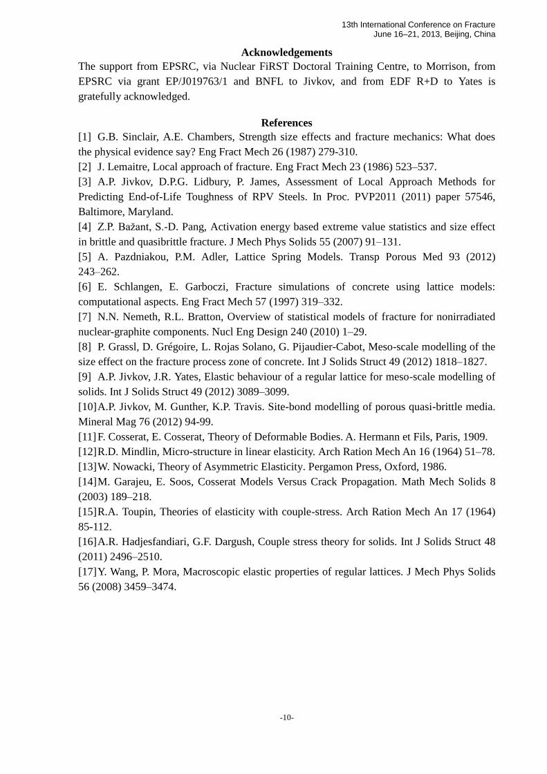
13th International Conference on Fracture June 16–21, 2013, Beijing, China
-10-
Acknowledgements
The support from EPSRC, via Nuclear FiRST Doctoral Training Centre, to Morrison, from
EPSRC via grant EP/J019763/1 and BNFL to Jivkov, and from EDF R+D to Yates is
gratefully acknowledged.
References
[1] G.B. Sinclair, A.E. Chambers, Strength size effects and fracture mechanics: What does
the physical evidence say? Eng Fract Mech 26 (1987) 279-310.
[2] J. Lemaitre, Local approach of fracture. Eng Fract Mech 23 (1986) 523–537.
[3] A.P. Jivkov, D.P.G. Lidbury, P. James, Assessment of Local Approach Methods for
Predicting End-of-Life Toughness of RPV Steels. In Proc. PVP2011 (2011) paper 57546,
Baltimore, Maryland.
[4] Z.P. Bažant, S.-D. Pang, Activation energy based extreme value statistics and size effect
in brittle and quasibrittle fracture. J Mech Phys Solids 55 (2007) 91–131.
[5] A. Pazdniakou, P.M. Adler, Lattice Spring Models. Transp Porous Med 93 (2012)
243–262.
[6] E. Schlangen, E. Garboczi, Fracture simulations of concrete using lattice models:
computational aspects. Eng Fract Mech 57 (1997) 319–332.
[7] N.N. Nemeth, R.L. Bratton, Overview of statistical models of fracture for nonirradiated
nuclear-graphite components. Nucl Eng Design 240 (2010) 1–29.
[8] P. Grassl, D. Grégoire, L. Rojas Solano, G. Pijaudier-Cabot, Meso-scale modelling of the
size effect on the fracture process zone of concrete. Int J Solids Struct 49 (2012) 1818–1827.
[9] A.P. Jivkov, J.R. Yates, Elastic behaviour of a regular lattice for meso-scale modelling of
solids. Int J Solids Struct 49 (2012) 3089–3099.
[10] A.P. Jivkov, M. Gunther, K.P. Travis. Site-bond modelling of porous quasi-brittle media.
Mineral Mag 76 (2012) 94-99.
[11] F. Cosserat, E. Cosserat, Theory of Deformable Bodies. A. Hermann et Fils, Paris, 1909.
[12] R.D. Mindlin, Micro-structure in linear elasticity. Arch Ration Mech An 16 (1964) 51–78.
[13] W. Nowacki, Theory of Asymmetric Elasticity. Pergamon Press, Oxford, 1986.
[14] M. Garajeu, E. Soos, Cosserat Models Versus Crack Propagation. Math Mech Solids 8
(2003) 189–218.
[15] R.A. Toupin, Theories of elasticity with couple-stress. Arch Ration Mech An 17 (1964)
85-112.
[16] A.R. Hadjesfandiari, G.F. Dargush, Couple stress theory for solids. Int J Solids Struct 48
(2011) 2496–2510.
[17] Y. Wang, P. Mora, Macroscopic elastic properties of regular lattices. J Mech Phys Solids
56 (2008) 3459–3474.

Appendix D
A meso-scale site-bond model for
elasticity: Theory and calibration
147

Meso-scale site-bond model for elasticity:theory and calibration
M. Zhang*1, C. N. Morrison1,2 and A. P. Jivkov1
A meso-scale site-bond model is proposed to simulate the macroscopic elastic properties of
isotropic materials. The microstructure of solids is represented by an assembly of truncated
octahedral cells with sites at the cell centres and bonds linking the nearest neighbouring sites.
Based on the equivalence of strain energy stored in a unit cell to strain energy stored in a
continuum of identical volume, the normal and shear stiffness coefficients of bonds are derived
from the given macroscopic elastic constants: Young’s modulus and Poisson’s ratio. To validate
the obtained spring constants, benchmark tests including uniaxial tension and plane strain are
performed. The simulated macroscopic elastic constants are in excellent agreement with the
theoretical values. As a result, the proposed site-bond model can be used to simulate the
macroscopic elastic behaviour of solids with Poisson’s ratios in the range from 21 up to 1/2.
Keywords: Site-bond model, Elasticity, Lattice spring, Discrete2continuum equivalence, Isotropy
IntroductionThe classical homogeneous elasticity is widely used todescribe the macroscopic linear mechanical behaviour ofmost materials, even though they are actually hetero-geneous from a microscopic point of view. However, themechanical response of heterogeneous quasi-brittlematerials, such as concrete, rock, graphite or ceramics,cannot be modelled realistically without explicit con-siderations of their underlying microstructures. Thisrequires numerical approaches which are able to accountfor not only the elastic stage, but also the initiation,growth, interaction and coalescence of micro-cracks. Thediscrete lattice approach, usually called the meso-scaleapproach, shows potential to meet this requirement.1 Inlattice models,1–10 the microstructures of materials arerepresented by an assemblage of unit cells or particles.The lattice sites are placed at the centres of the cells. Thedeformation of the represented continuum arises from theinteractions between the lattice sites. The neighbouringcells are linked through interface bonds, which can berepresented by lattice beam elements or lattice springs.Compared to the continuum finite element modelling,lattice models have been shown to be more suitable forfracture simulation because of their discrete nature.
The lattice models have been successfully applied to themodelling of quasi-brittle materials. The macroscopicstress–strain curve for concrete is obtained by using alattice beam model based on a two-dimensional regularlattice with hexagonal unit cells.2,3 However, this lattice
cannot be used for isotropic elastic materials withPoisson’s ratio larger than 1/3 in plane stress and 1/4 inplane strain.4 Based on the simplest regular lattice withcubic cells, a three-dimensional (3D) lattice beam modelhas been proposed by Schlangen5 to simulate the crackdevelopment in concrete. It has been shown that thislattice is only suitable for materials with zero Poisson’sratio.6 With respect to lattice spring models, Wang andMora7 developed two 3D lattices using face-centred cubicand hexagonal closely-packed arrangements. Each pair ofsites in the lattice network is connected by spring. It wasfound that only isotropic elastic material with Poisson’sratio of zero can be represented by these lattices, which isthe same as cubic lattices. To overcome these limitations,a site-bond based on a bi-regular lattice of truncatedoctahedron cells has been recently proposed by Jivkovand Yates1 for meso-scale modelling of solids. The bondsof the site-bond assembly are modelled with structuralbeam elements. It has been demonstrated that this site-bond model is able to represent isotropic elastic materialswith Poisson’s ratios up to 1/2.
The main purpose of this work is to reformulate thesite-bond assembly presented in Ref. 1 by modelling thebonds with two types of elastic springs instead ofstructural beam elements to further study the capabilityof this lattice arrangement for the macroscopic elasticbehaviour of practical interest. The stiffness coefficientsof springs are analytically determined by equating thestrain energy stored in the discrete and continuum cell.The derived spring constants are validated throughnumerical analyses.
Site-bond modelIn the site-bond model, the microstructure of a realmaterial is represented by tessellating the space intotruncated octahedral cells, as shown in Fig. 1a. The
1Modelling & Simulation Centre and Research Centre for Radwaste &Decommissioning, The University of Manchester, Manchester M13 9PL,UK2Nuclear FiRST Doctoral Training Centre, The University of Manchester,Manchester M13 9PL, UK
*Corresponding author, email [email protected]
S2-982
� W. S. Maney & Son Ltd. 2014Received 15 September 2013; accepted 12 December 2013DOI 10.1179/1432891714Z.000000000537 Materials Research Innovations 2014 VOL 18 SUPPL 2

truncated octahedron was found to be the best choicefor a regular representation of real materials comparedto the cube, the regular hexagonal prism or the rhombicdodecahedron.1,6 Each cell has six equal square facesand eight equal hexagonal faces. The cell centre isconsidered as a site, which is connected with itsneighbouring sites by 14 bonds, six bonds B1 in principaldirections through square faces and eight bonds B2 inoctahedral directions through hexagonal faces, asillustrated in Fig. 1b.
In this study, the bonds are modelled with elasticsprings. The sites have six independent degrees offreedom: three translational and three rotational. Inprinciple, each bond should contain six springs: onenormal, two shear, one twisting, and two bending springsin order to resist the relative displacement and relativerotations between the two adjacent cells. However, it waspresented that the twisting stiffness kt and bendingstiffness kb are related to the shear stiffness ks andnormal stiffness kn, respectively, with the contribution ofkt and kb to the macroscopic elasticity effectivelynegligible in comparison to ks and kn.7 Therefore, onlythe normal and shear springs in principal and octahedraldirections are considered herein, as shown in Fig. 1c.
Derivation of spring constants for site-bond modelIn this section, the spring constants are derived from themacroscopic elastic parameters by equating the strainenergy stored in a unit cell Ucell to the associated strainenergy in the equivalent continuum system Ucont
Ucell~Ucont (1)
The strain energy of the continuum system is given by
Ucont~1
2
ðV
sedV~1
2CijkleijeklV (2)
where C represents the stiffness tensor of the material, eis the strain field and V is the system volume. The strainenergy stored in a unit cell can be expressed as a sum ofthe strain energies stored in each internal bond Ub
Ucell~X
b
Ub~1
4
XNb
b
k(b)n u(b)
n u(b)n zk(b)
s u(b)s u(b)
s
� �(3)
in which u(b)n and u(b)
s stand for the relative displacements
in the normal direction and transverse direction of the
bond, respectively. Let us assume that the bond b linkstwo sites A and B, then the relative normal and sheardisplacements in the 3D global system X1X2X3 can bewritten as
u(b)n ~Du
(b)i j
(b)i (4)
u(b)s ~Du
(b)i {u(b)
n j(b)i (5)
in which
Du(b)i ~eijDxj~eij(xjB{xjA) (6)
The direction vector of the bond j(b)i is given as
j(b)i ~
(xiB{xiA)
LAB
(7)
where xiA and xiB are the positions of the sites, LAB isthe length of the bond. By substituting equations (4)–(7)into equation (3) and performing tensor and vectormanipulations, equation (3) can be expressed as
Ucell~
1
4
XNb
b
L(b)� �2
k(b)n j(b)
i eijj(b)j j(b)
k eklj(b)l zk(b)
s eklj(b)l {j(b)
i eijj(b)j j(b)
k
� �ekmj(b)
m {j(b)n enmj(b)
m j(b)k
� �h i (8)
in which L(b) is the length of a bond b. Then by equatingthe total strain energy stored per unit volume V, thestrain energy density rcont, to that in the unit cellrcell~Ucell=V and by using Cauchy’s formula,8–10 thestress tensor of the continuum system can be obtained as
sij~Lrcont
Leij
~1
2V
XNb
b
L(b)� �2
k(b)s eilj
(b)l j(b)
j z k(b)n {k(b)
s
� �eklj
(b)i j(b)
j j(b)k j(b)
l
h i
(9)
Finally, the elastic stiffness tensor can be given as
Cijkl~Lsij
Lekl
~1
2V
XNb
b
L(b)� �2
k(b)s dikj(b)
j j(b)l z k(b)
n {k(b)s
� �j(b)
i j(b)j j(b)
k j(b)l
h i
(10)
where dik is the Kroecker’s delta.Considering the site-bond assembly shown in Fig. 1
and assuming that the unit cell size in the principaldirections is L, the lengths of bonds B1 and B2 are L and31/2L/2, respectively. The volume of the unit cell V is L3/2. For each bond, k(b)
n and k(b)s are the normal and shear
spring constants for bonds B1 and B2, which are denotedas kp
n and kps , ko
n and kos , respectively in the following
1 Cellular lattice: a site-bond assembly; b unit cell with bonds; c normal and shear springs
(8)
(9)
(10)
Zhang et al. Meso-scale site-bond model for elasticity: theory and calibration
Materials Research Innovations 2014 VOL 18 SUPPL 2 S2-983

sections. The direction vectors of bonds B1 and B2 aregiven in Table 1.
Hence, by using equation (10) and assuming the twoshearing spring stiffness coefficients are equal within eachbond type but different between the two bond types, B1
and B2, we get the components of the stiffness tensor
C1111~2
3L3kp
nzkonz2ko
s
� �~C2222~C3333 (11)
C1122~2
3Lko
n{kos
� �~C1133~
C2233~C2211~C3311~C3322 (12)
C1212~2
3L3kp
s zkonz2ko
s
� �~
C1313~C2323~C2121~C3131~C3232 (13)
Other Cijkl~0 (14)
It can be seen from equations (11)–(14) that there are onlythree independent elastic constants. This indicates that thesite-bond assembly generates macroscopic cubic elasticity.With the Voigt notation, which is the standard mapping fortensor indices, the spring constants can be expressed as
kpn~{ko
nzL
2C11z2C12ð Þ (15)
kps ~{ko
nzL
22C12zC44ð Þ (16)
kos ~ko
n{3L
2C12 (17)
Meanwhile, from equations (11)–(14), we find thatonly when 3kp
n{6kps {2ko
n{kos ~0, the site-bond assem-
bly is able to yield macroscopic isotropic elasticity. Forisotropic materials, Hooke’s law in terms of matrix formcan be written as
s1
s2
s3
s4
s5
s6
2666666664
3777777775~
C11 C12 C12 0 0 0
C21 C11 C12 0 0 0
C21 C21 C11 0 0 0
0 0 0 C44 0 0
0 0 0 0 C55 0
0 0 0 0 0 C66
2666666664
3777777775
e1
e2
e3
2e4
2e5
2e6
2666666664
3777777775
~E
(1zn)(1{2n)
1{n n n 0 0 0
n 1{n n 0 0 0
n n 1{n 0 0 0
0 0 0 (1{2n)=2 0 0
0 0 0 0 (1{2n)=2 0
0 0 0 0 0 (1{2n)=2
2666666664
3777777775
e1
e2
e3
2e4
2e5
2e6
2666666664
3777777775
(18)
where E and n are Young’s modulus and Poisson’s ratio,respectively.
Combining equation (18) and equations (15)–(17), therelationship between the linear stiffness coefficients ofthe bonds and the macroscopic material constants canbe established. However, the four spring stiffness cannotbe uniquely determined because there are only threeequations of equilibrium. To solve this over-determinedproblem, the shear stiffness kp
s of bond B1 in principaldirections is assumed to be zero, since the shear stiffnessko
s has components in principal directions and thecontribution of kp
s to macroscopic elasticity can berepresented in terms of ko
s , as seen in equation (13).Thus, the other spring constants kp
n, kon and ko
s can bedetermined as follows
kpn~
EL
4(1zn)(1{2n)
kon~
(1z2n)EL
4(1zn)(1{2n)
kos ~
(1{4n)EL
4(1zn)(1{2n)
(19)
It can be seen that the shear stiffness kos will become
negative when the Poisson’s ratio n exceeds 1/4. Thisindicates that the physical Poisson’s ratio range resultingfrom the site-bond model is{1vnƒ1=4, since thenegative spring constant seems non-physical. However,it is proved by molecular dynamics simulations that thenegative stiffness still has a physical explanation at themolecular level.10 Therefore, the shear spring withnegative stiffness can be added in order to model amaterial with a Poisson’s ratio higher than 1/4 but lowerthan 1/2.
Benchmark testsNumerical benchmark tests are carried to validate thederived spring stiffness coefficients. The macroscopicYoung’s modulus and Poisson’s ratio are selected asE511 000 MPa and n50?2. The stiffness coefficients ofsprings are calculated from equation (19). A cubic site-bond arrangement with size of 10L by 10L by 10L isused for simulations. This means that there are 10 unitcells in each principal direction; illustration given inFig. 2. The assembly is subjected to various loadingconditions, i.e. uniaxial tension and plane strain, toestimate the macroscopic Young’s modulus, Poisson’sratio and modulus of rigidity independently.
For uniaxial tension, the sites X150, X250 and X350are fixed in the X1, X2 and X3 direction, respectively. Adisplacement of L in the X3 direction is applied at sitesX3510L and other sites are free, which induces amacroscopic tensile strain et~e3~L=10L~0:1. Themacroscopic Poisson’s ratio n for tension and compres-sion is calculated according to n~{e1=e3 or n~{e2=e3,in which e1~u1=10L and e2~u2=10L are identical. Here,
Table 1 Direction vectors of bonds B1 and B2 in the site-bond assembly
Bond type Bond no. b j(b)i
B1 1 (1, 0, 0)2 (0, 1, 0)3 (0, 0, 1)4 (21, 0, 0)5 (0, 21, 0)6 (0, 0, 21)
B2 7 (1/31/2, 21/31/2, 21/31/2)8 (1/31/2, 1/31/2, 21/31/2)9 (1/31/2, 21/31/2, 1/31/2)10 (1/31/2, 1/31/2, 1/31/2)11 (21/31/2, 1/31/2, 1/31/2)12 (21/31/2, 21/31/2, 1/31/2)13 (21/31/2, 1/31/2, 21/31/2)14 (21/31/2, 21/31/2, 21/31/2)
(18)
Zhang et al. Meso-scale site-bond model for elasticity: theory and calibration
S2-984 Materials Research Innovations 2014 VOL 18 SUPPL 2
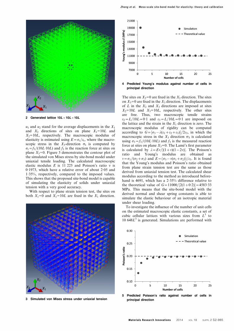
u1 and u2 stand for the average displacements in the X1
and X2 directions of sites on plane X1510L andX2510L, respectively. The macroscopic modulus ofelasticity is estimated using E~st=et, where the macro-scopic stress in the X3-direction st is computed byst~f3=(10L:10L) and f3 is the reaction force at sites onplane X350. Figure 3 demonstrates the contour plot ofthe simulated von Mises stress by site-bond model underuniaxial tensile loading. The calculated macroscopicelastic modulus E is 11 225 and Poisson’s ratio n is0?1973, which have a relative error of about 2?05 and1?35%, respectively, compared to the imposed values.This shows that the proposed site-bond model is capableof simulating the elasticity of solids under uniaxialtension with a very good accuracy.
With respect to plane strain tension test, the sites onboth X150 and X1510L are fixed in the X1 direction.
The sites on X250 are fixed in the X2 direction. The siteson X350 are fixed in the X3 direction. The displacementsof L in the X2 and X3 directions are imposed at sitesX2510L and X3510L, respectively. The other sitesare free. Thus, two macroscopic tensile strainse2~L=10L~0:1 and e3~L=10L~0:1 are imposed onthe lattice and the strain in the X1 direction is zero. Themacroscopic modulus of rigidity can be computedaccording to G~ s3{l(e1ze2ze3)½ �=2e3, in which themacroscopic stress in the X3 direction s3 is calculatedusing s3~f3=(10L:10L) and f3 is the measured reactionforce at sites on plane X350. The Lame’s first parameteris calculated by l~En= (1zn)(1{2n)½ �. The Poisson’sratio and Young’s modulus are obtained asn~s1=(s2zs3) and E~ s3{n(s1zs2)ð Þ=e3. It is foundthat the Young’s modulus and Poisson’s ratio obtainedfrom plane strain tension test are the same as thosederived from uniaxial tension test. The calculated shearmodulus according to the method as introduced before-hand is 4691, which has a 2?35% difference relative tothe theoretical value of G~11000= 2(1z0:2)½ �~4583:33MPa. This means that the site-bond model with thederived normal and shear spring constants is able tosimulate the elastic behaviour of an isotropic materialunder shear loading.
To investigate the influence of the number of unit cellson the estimated macroscopic elastic constants, a set ofcubic cellular lattices with various sizes from L3 to10 648L3 is generated. Simulations are performed with
3 Simulated von Mises stress under uniaxial tension
4 Predicted Young’s modulus against number of cells in
principal direction
5 Predicted Poisson’s ratio against number of cells in
principal direction
2 Generated lattice 10L610L610L
Zhang et al. Meso-scale site-bond model for elasticity: theory and calibration
Materials Research Innovations 2014 VOL 18 SUPPL 2 S2-985

the plane strain boundary conditions. The predictedmacroscopic Young’s modulus, Poisson’s ratio andshear modulus against the number of unit cells in eachprincipal direction of a cubic region are plotted inFigs. 4–6.
It can be seen that the simulated macroscopic Young’smodulus and shear modulus decrease with the increasein the number of cells in principal direction. On thecontrary, the estimated Poisson’s ratio increases withthe increasing size of cellular lattice. Eventually, thesimulated elastic constants tend to their correspondingtheoretical values with the increase in the size of cellularlattice. This is attributed to the smaller boundary effectwhen the size of region is larger. When the number ofcells in principal direction is higher than 20, theestimated results are close enough to the theoreticalvalues.
The generated site-bond model can be considered as avalid representation of isotropic elastic material. Basedon the definition of criterion for bond failure andrelevant implementation as presented in a previous studyby Jivkov et al.,6 the fracture process and damageevolution in quasi-brittle materials can be simulated byusing the proposed site-bond model. This is a subject ofongoing work. In addition, the effects of microstructureparameters, such as porosity, pore size distribution andconnectivity of solid phase, on the macroscopic beha-viour, stress–strain response of quasi-brittle materialswill be investigated. The results of these aspects will bereported in future publications.
ConclusionThis work presents a meso-scale model for macroscopicelasticity of solids. The model is based on a cellularlattice of truncated octahedrons, filling the spacecompactly. The cellular architecture is transformed intodiscrete site-bond lattice with bonds containing normaland shear springs. The spring stiffness coefficients areobtained as functions of macroscopic elastic constants.
From the findings of the present study, the followingconclusions can be drawn.
1. The site-bond assembly represents generally amacroscopic cubic elasticity and is able to deliver anymacroscopic isotropic elasticity.
2. The physical Poisson’s ratio range results from thesite-bond model is {1vnv1=2.
3. For uniaxial tension test, the estimated macro-scopic Young’s modulus and Poisson’s ratio show a verygood agreement with the theoretical ones.
4. For plane strain test, the measured macroscopicmodulus of rigidity fit very well with the theoreticalvalue.
5. The size of cellular lattice plays an important rolein the accuracy of simulation due to boundary effect.When the number of cells in principal direction is higherthan 20, the obtained simulation results are close enoughto the theoretical data.
6. The proposed site-bond model is regarded as a verygood representation of isotropic elastic materials, andwill be applied to simulate the fracture process anddamage evolution in quasi-brittle materials.
Acknowledgements
M. Zhang and A. P. Jivkov acknowledge the supportfrom EPSRC via grant no. EP/J019763/1, ‘QUBE:Quasi-Brittle fracture: a 3D experimentally-validatedapproach’, and from BNFL for the Research Centre forRadwaste & Decommissioning. C. N. Morrison greatlyappreciates the support from EPSRC via NuclearFiRST Doctoral Training Centre.
References1. A. P. Jivkov and J. R. Yates: ‘Elastic behaviour of a regular lattice
for meso-scale modelling of solids’, Int. J. Solids. Struct., 2012, 49,
3089–3099.
2. E. Schlangen and J. G. M. van Mier: ‘Experimental and numerical
analysis of micromechanisms of fracture of cement-based compo-
sites’, Cem. Concr. Compos., 1992, 14, 105–118.
3. C. S. Chang, T. K. Wang, L. J. Sluys and J. G. M. van Mier:
‘Fracture modelling using a micro structural mechanics approach.
I: Theory and formation’, Eng. Fract. Mech., 2002, 69, 1941–1958.
4. D. V. Griffiths and G. G. W. Mustoe: ‘Modelling of elastic
continua using a grillage of structural elements based on discrete
element concepts’, Int. J. Numer. Meth. Eng., 2001, 50, 1759–1775.
5. E. Schlangen: ‘Crack development in concrete. Part 2: Modelling of
fracture process’, Key Eng. Mater., 2008, 73–76, 385–387.
6. A. P. Jivkov, D. L. Engelberg, R. Stein and M. Petkovski: ‘Pore
space and brittle damage evolution in concrete’, Eng. Fract. Mech.,
2013, 110, 378–395.
7. Y. Wang and P. Mora: ‘Macroscopic elastic properties of regular
lattices’, J. Mech. Phys. Solids, 2008, 56, 3459–3474.
8. M. Ostoja-Starzewski: ‘Lattice models in micromechanics’, Appl.
Mech. Rev., 2002, 55, 35–60.
9. G. Wang, A. Al-Ostaz, A. H.-D. Cheng and P. R. Mantena:
‘Hybrid lattice particle modelling: Theoretical considerations for a
2D elastic spring network for dynamic fracture simulations’,
Comput. Mater. Sci., 2009, 44, 1126–1134.
10. S. Zhao and G. Zhao: ‘Implementation of a high order lattice
spring model for elasticity’, Int. J. Solids. Struct., 2012, 49, 2568–
2581.
6 Predicted shear modulus against number of cells in
principal direction
Zhang et al. Meso-scale site-bond model for elasticity: theory and calibration
S2-986 Materials Research Innovations 2014 VOL 18 SUPPL 2

Appendix E
Lattice-spring model of graphite
accounting for pore size distribution
153

Lattice-spring modeling of graphite accounting for pore size distribution
Craig N Morrison1,a, Andrey P Jivkov1,b, Gillian Smith2,c and John R Yates1,d 1School of MACE, The University of Manchester, Oxford Road, Manchester M13 9PL, UK
2Interface Analysis Centre, University of Bristol, Tyndall Avenue, Bristol BS8 1TL, UK
[email protected], [email protected], [email protected], [email protected]
Keywords: Nuclear graphite; Porosity; Meso-scale deformation; Micro-cracks; Macroscopic behaviour
Abstract. Lattice models allow length scale dependent micro-structural features and damage
mechanisms to be incorporated into analyses of mechanical behaviour. They are particularly
suitable for modelling the fracture of nuclear graphite, where porosity generates local failures upon
mechanical and thermal loading. Our recent 3D site-bond model is extended here by representing
bonds with spring groups. Experimentally measured distributions of pore sizes in graphite are used
to generate models with pores assigned to the bonds. Microscopic damage is represented by failure
of normal and shear springs with different criteria based on force and pore size. Macroscopic
damage is analysed for several loading cases. It is shown that, apart from uniaxial loading, the
development of micro-failures yields damage-induced anisotropy in the material. This needs to be
accounted for in constitutive laws for graphite behaviour in FEA of cracked reactor structures.
Introduction
Nuclear-grade graphite has featured in over 100 reactors [1] with its main functions being a fast
neutron moderator and structural material. It also forms an integral part of a potential Generation
IV Very High Temperature Reactor (VHTR). The integrity of graphite, as with all structural reactor
components, is critical for their fitness for purpose. Understanding graphite’s fracture behaviour is
essential for approving plant life extensions and predicting in-service performance.
Synthetic graphite is manufactured from petroleum cokes and a binder material; usually coal-tar
pitch. The resulting micro-structural features – grain size, pore size/density, are strongly influenced
by the manufacturing process and the structure of the coke and binder particles used. The work in
this paper focuses on Gilsocarbon, a relatively fine-grained graphite, used in the UK Advanced
Gas-cooled Reactors (AGRs). Graphite microstructure consists of 3 phases; a matrix of graphitized
binder particles, relatively large filler particles (derived from coke) and porosity [2]. In Gilsocarbon
the spherical filler particles, ranging from 0.3-1.5mm in size, result in near isotropic mechanical
properties [3]. The 3 main porosity populations [4], ranging from nm to mm in size, total
approximately 20% of virgin graphite volume. Gas evolution cracking occurs within the matrix as
gas bubbles form when liquid pitch, impregnated to increase density, boils during baking [3].
Calcination and Mrozowski cracks form within filler particles due to uneven thermal expansion and
shrinkage as the graphite heats and cools during calcination and graphitization respectively [2,5].
Graphite, alongside rock, concrete and cement, is considered a quasi-brittle material [6], with
failure occurring when distributed micro-cracks coalesce into a critically sized flaw. As a result,
graphite exhibits a reduced stiffness upon loading (similar to plasticity) prior to failure [2] despite
remaining brittle. Using local approaches to model graphite failure can capture the dependence of
macro-scale integrity on meso-scale features by incorporating mechanistic understanding of failure
at the length scale of features [7]. However current methods rely on weakest link (WL)
assumptions and fail to account for the micro-crack interactions apparent in quasi-brittle materials
[8]. Lattice models are a branch of discrete, local approach models, consisting of nodes connected
into a lattice through discrete elements including springs [9] and beams [10]. Element properties
allow a material response according to actual mechanistic failure data. Unlike WL methods, lattice
models are based around a parallel statistical system, with load redistribution amongst remaining
bonds once a bond is broken. Such models have been developed for graphite [4,10,11] and cement

[12]. The work presented here furthers the site-bond lattice model developed by Jivkov and Yates
[13]. The model has been calibrated using a generalized continuum theory, with bond stiffness
constants evaluated through strain energy equivalence of a discrete unit cell and classical
continuum [14].
Theory and model
The site-bond model is based upon a tessellation of space into truncated octahedral cells, Fig 1a.
Particles, attached to cell centres, interact via deformable bonds, with 14 bonds connecting a
particle to its neighbours, Fig 1b. The 6 bonds in the principal directions and 8 bonds in the
octahedral directions can have different mechanical responses. The energetic calibration for this
model [14] suggested that as a first assumption particle rotations could be ignored, with bonds
represented only by normal and shear springs. Spring elastic constants Kaxprinc
, Kaxoct
, Kshprinc
and
Kshoct
were calibrated for plane stress and plane strain for a graphite of typical properties E=11Gpa,
v=0.2 [15] with values 4.041 x10⁴, 4.939 x10
4, 2.245 x10
3 and 4.49 x10
3 respectively.
The behaviour of shear springs is illustrated in Fig 2a, where the shaded area represents energy
dissipated in spring failure. For axial springs, failure in compression is not permitted and the
behaviour is shown in Fig 2b.
Gilsocarbon microstructure was modeled, assuming porosity occurs exclusively within the
matrix phase, with calcination and Mrozowski cracks ignored. Filler particles with normally
distributed sizes were randomly located with total volume fraction of 20%. Pores with normally
distributed sizes were located in the matrix with a constraint preventing coalescence and 5%
volume fraction. This porosity was distributed to the faces of the cellular structure. The ratio
between pore and face areas determined the failure energy of the corresponding springs, so that Gc
varied between zero for very large pores and one for very small pores. The model was subject to
uniaxial tension; u1 = u, (x2 and x3 directions remain unconstrained), as well as to fields experienced
ahead a crack: high-constraint plane strain (u1 = u2 = u, u3 = 0) and lower-constraint plane strain (u1
= 0.5u2 = u, u3 = 0). For uniaxial tension the damage can be characterized by the parameter DE, Eq.
(1), as principal stresses σ2 = σ3 = 0.
. (1)
For the plane strain cases, 4 damage parameters are required, Eq. (4-5), evaluated from a
decomposition of nominal stress/strain into deviatoric and volumetric components of sα, eα and σh,
εv respectively, Eq. (2-3), where σh is hydrostatic stress and εv is volumetric strain.
Fig 1. Cellular representation of material
(a); and unit cell with bonds (b).
Fig 2. Spring
failure criteria
for shear
springs(a);
and normal
springs (b).
Displacement -2(uc)sh
Load
(a) (b) (Fc)
sh
(uc)sh
Displacement -10(uc)ax
Load
(Fc)ax
2(uc)sh
-(uc)sh
-(Fc)sh
(uc)ax 2(uc)
ax
Shaded area
= (Gc)sh
Shaded area
= (Gc)ax
-10(Fc)ax

. (2)
where . (3)
. (4)
. (5)
Where K and μ are the bulk and shear moduli respectively.
Results
Uniaxial tension exhibits quasi-brittle behaviour with softening before failure as expected, Fig 3.
The similarity of damage parameters, DE and Dμ suggests that the material remains isotropic, Fig 4.
Upon loading in plane strain under both high and low constraint the damage parameter Dμ
becomes dependent on direction suggesting anisotropy is introduced, Fig 5b and Fig 6b.
Fig 4. The
damage
parameters for
uniaxial tension,
DE (a); Dμ (b).
Fig 5. The
damage
parameters for
plane strain
high constraint
DK (a); Dμ (b).
Fig 3. The stress/strain
response of the model
under uniaxial tension.
(a) (b)
(a) (b)

Discussion and conclusions
The results show that the development of micro-damage in porous graphite is strongly dependent
on the loading. Uniaxial loading seems to be the only case where the material remains isotropic
with damage evolution. This suggests that a macroscopic damage evolution law based on a single
damage parameter is appropriate only for uniaxial states. For material ahead of a macroscopic
crack, high-constraint, Fig 5, and low constraint, Fig 6, damage evolves differently in different
loading directions. Negative damage parameter observed in Fig 5, is not surprising; it merely
shows that the transverse shear modulus in y-direction increased above the initial isotropic value as
the transverse shear modulus in x-direction decreased. It is also clear that damage of shear moduli
is larger than the damage of bulk modulus. The results suggest that damage evolution laws for
complex loading cases need to be based on three independent invariant of the stress tensor.
Presently, it is not clear whether a load-independent evolution law can be developed for materials
with given pore space structures with the strategy presented here. This is a subject of ongoing
work.
References
[1] IAEA report (2006).
[2] A. Hodgkins, T. J. Marrow, M. R. Wootton, R. Moskovic, and P. E. J. Flewitt: Mater. Sci.
Tech. Vol. 26 (2010), p. 899.
[3] M. R. Joyce, T. J. Marrow, P. Mummery, and B. J. Marsden: Eng. Fract. Mech. Vol. 75
(2008), p. 3633.
[4] M. R. Bradford and A. G. Steer: J. Nucl. Mater. Vol. 381 (2008), p. 137.
[5] E. Schlangen, P. E. J. Flewitt, G. E. Smith, a. G. Crocker, and A. Hodgkins: Key Eng.
Mater. Vol. 452–453 (2010), p. 729.
[6] M. Mostafavi and T. J. Marrow: Fatigue Fract. Eng. Mater. Struct. Vol. 35 (2012), p. 695.
[7] J. Lemaitre: Eng. Fract. Mech. Vol. 23 (1986), p. 523.
[8] Z. P. Bažant and S.D. Pang: J. Mech. Phys. Solids Vol. 55 (2007), p. 91.
[9] A. Pazdniakou and P. M. Adler: Tran. Porous Med. Vol. 93 (2012), p. 243.
[10] E. Schlangen and E. Garboczi: Eng. Fract. Mech. Vol. 57 (1997), p. 319.
[11] N. N. Nemeth and R. L. Bratton: Nucl. Eng. Design Vol. 240 (2010), p. 1.
[12] P. Grassl, D. Grégoire, L. Rojas Solano, and G. Pijaudier-Cabot: Int. J. Solids Struct. Vol. 49
(2012), p. 1818.
[13] A.P. Jivkov and J.R. Yates: Int. J. Solids Struct. Vol. 49 (2012), p. 3089.
[14] C. N. Morrison, A. P. Jivkov, and J. R. Yates: Proc. ICF13 (Beijing, China, 2013), p. S31-
016.
[15] M. Holt: Issues of scale in nuclear graphite components (PhD Thesis, University of Hull,
2008).
Fig 6. The
damage
parameters for
plane strain
low constraint,
DK (a); Dμ (b).
(a) (b)

Appendix F
A discrete lattice model of quasi-brittle
fracture in porous graphite
158
Materials Performance andCharacterization
Craig N. Morrison,1 Mingzhong Zhang,2 Andrey P. Jivkov,2 and John
R. Yates2
DOI: 10.1520/MPC20130077
Discrete Lattice Model ofQuasi-Brittle Fracture inPorous Graphite
VOL. 3 / NO. 3 / 2014

Craig N. Morrison,1 Mingzhong Zhang,2 Andrey P. Jivkov,2 and John R. Yates2
Discrete Lattice Model of Quasi-BrittleFracture in Porous Graphite
Reference
Morrison, Craig N., Zhang, Mingzhong, Jivkov, Andrey P., and Yates, John R., “Discrete
Lattice Model of Quasi-Brittle Fracture in Porous Graphite,” Materials Performance and
Characterization, Vol. 3, No. 3, 2014, pp. 414–428, doi:10.1520/MPC20130077.
ISSN 2165-39923
ABSTRACT
Lattice models allow the incorporation of length-scale-dependent
microstructural features and damage mechanisms into analyses of the
mechanical behavior of materials. We describe our 3D lattice implementation
and its use in fracture simulations. The method is particularly suitable for
modeling fractures of nuclear graphite. This is a quasi-brittle material in which
there is considerable non-linearity prior to final fracture caused by the inherent
porosity, which triggers a field of local distributed failures upon mechanical
and thermal loading. Microstructure representative models are generated with
experimentally measured particle and pore size distributions and volume
densities in two graphite grades. The results illustrate the effect of distributed
porosity on the emerging stress–strain response and damage evolution. It is
shown how the failure mode shifts from graceful, plastic-like behavior
associated with substantial energy dissipation via distributed damage at lower
porosities, to glass-like behavior with negligible energy dissipation at higher
porosities. Thus, the work proposes a microstructure-informed methodology
for integrity assessment of aging structures, where porosity increase is driven
by environmental factors, such as radiation of nuclear graphite components.
Keywords
nuclear graphite, porosity, brittle-ligament lattice, damage evolution, quasi-brittle behavior
Manuscript received October 17,
2013; accepted for publication
January 20, 2014; published online
June 18, 2014.
1
Mechanics and Physics of Solids
Research Group, Modelling and
Simulation Centre, The Univ. of
Manchester, Oxford Rd.,
Manchester M13 9PL, United
Kingdom; and Nuclear FiRST
Doctoral Training Centre,
Manchester M13 9PL,
United Kingdom, e-mail:
2
Mechanics and Physics of Solids
Research Group, Modelling and
Simulation Centre, The Univ. of
Manchester, Oxford Rd.,
Manchester M13 9PL,
United Kingdom.
3
This paper is a contribution to a
Special Issue of Materials
Performance and Characterization
on “Fracture Toughness,” Guest
Editors, Bojan Podgornik and
Votjeh Leskovsek, Institute of
Metals and Technology, Ljubljana,
Slovenia.
Copyright VC 2014 by ASTM International, 100 Barr Harbor Drive, P.O. Box C700, West Conshohocken, PA 19428-2959 414
Materials Performance and Characterization
doi:10.1520/MPC20130077 / Vol. 3 / No. 3 / 2014 / available online at www.astm.org
Introduction
Nuclear-grade graphite has been used as a fast neutron moderator in over 100
reactors throughout the world [1], with planned use in the generation IV very-high-
temperature reactor. A main advantage of graphite over other moderator materials,
such as light and heavy water, is its suitability for use as a structural material. As a
result, developing a means of predicting the structural integrity of graphite under
complex loading and in demanding environments, such as a nuclear reactor core, is
critical for predicting plant lifetime and in-service performance.
Nuclear graphite has a feature-rich multiphase microstructure consisting of
petroleum or pitch coke filler particles distributed within a matrix of binder material,
usually coal-tar pitch. Distributed within both the matrix and filler phases is a popu-
lation of porosity. This population can be broadly grouped into three main catego-
ries [2]:
• Gas evolution cracking—During manufacture, liquid pitch is impregnated intothe graphite to increase density. In the subsequent baking of the green article,the pitch boils resulting in the evolution of gas through the matrix phase [3].
• Calcination cracks—During the heating and cooling procedures involved incalcinations, the variation of the thermal expansion/shrinkage of the two solidphases of graphite’s microstructure induces cracks [2,4].
• Mrozowski cracks—These form for similar reasons to calcination cracks dur-ing the graphitization process [2,4].
These flaws can vary in length scale, ranging from the nm scale to mm scale
depending on the grade of graphite in question. The variation of input materials and
manufacturing processes strongly influences the resulting microstructure so that dif-
ferent grades of graphite can have widely different properties.
The work in this paper focuses on two grades of graphite for potential use in
future generations of high-temperature reactors. IG110 is a fine-grained graphite of
isotropic macroscopic properties currently in use in the Japanese high-temperature
test reactor (HTTR), which first reached criticality in November 1998 [5]. It also
remains a possibility for generation IV high-temperature reactors. Another possibil-
ity for high-temperature reactors is PGX, a medium-grained semi-isotropic graphite.
The use of these two grades allows an effective comparison of the proposed method-
ology for grades of varying pore and particle sizes.
Component-scale failure of graphite has been shown to be dependent on its
discrete multiphase microstructure, with the primary failure mechanism being the
coalescence of micro-cracks into a critically sized flaw [6]. Such a response is consid-
ered to be a property of the class of quasi-brittle materials, allowing graphite to be
considered alongside rock, concrete, and cement in its failure behavior. Distinctive
properties of quasi-brittle materials include a reduced stiffness upon loading prior to
failure and a residual load-carrying capacity beyond the peak load [7]. The initial
softening appears similar to plasticity although the individual phases remain brittle.
Failure modeling of quasi-brittle materials has led to the development of a num-
ber of local fracture models, whereby mechanistic understanding at the length scale
of microstructural features—referred to as the meso-scale in this context—can be
incorporated into component scale models [8]. In this way, the macro-scale depend-
ence on these microstructural failure mechanisms can be recreated in a physically
MORRISON ET AL. ON DISCRETE LATTICE MODEL 415
Materials Performance and Characterization
realistic manner. Most current local approaches, such as weakest link (WL) assump-
tions, are phenomenological, with parameters calculated by curve fitting to macro-
scopic experimental data [9]. Such approaches do not account for the chain of
events leading to macroscopic failure, from micro-crack nucleation, through micro-
crack interaction, and, to coalescence, observable at the microscale of quasi-brittle
materials [10].
A continuum-based approach, intended to account for micro-crack nucleation
and growth, is the cohesive zone modeling [9,11], where the failure initiation and
local softening in the quasi-brittle materials are represented by special cohesive
elements. The advantage of this approach is that it is easily incorporated into the
existing finite element formulations, and indeed cohesive elements are offered as
standard in most finite element packages. However, the cohesive zone modeling
relies on the introduction of cohesive elements; hence, the modeling predefines the
potential crack paths. Further, the formulation of the constitutive behavior of the
cohesive elements is phenomenological, involving calibration against observed
macroscopic behavior. Microstructure-informed models, such as the one offered in
this work, have the potential to assist in deriving mechanistic constitutive laws for
cohesive zone modeling.
Discrete approaches offer a promising method of developing material constitu-
tive equations based on the actual micromechanical processes occurring. Lattice
models form a branch of local discrete models, wherein a lattice is formed through
the connection of nodes via discrete elements including springs [12] and beams [13].
The designation of element properties as representative of the micromechanical
failure mechanisms can allow a realistic macro-mechanical response. Unlike WL
methods, where bond failure signals total sample failure, lattice models form a statis-
tically parallel system. This allows redistribution of load once a bond is broken
among the remaining bonds.
Lattice models have been successfully developed for graphite [4,14] and concrete
[13,15]. Previous models have been limited in their ability to reproduce a full range
of Poisson’s ratio for elastic materials. Regular two-dimensional (2D) beam-lattices
using hexagonal unit cells, such as [10], can only be used for an isotropic elastic
material with Poisson’s ratio below 1/3 and 1/4 in plane stress and plane strain,
respectively [15]. This is sufficient for most of the materials classified as quasi-
brittle. However, the evolution of damage via micro-crack formation and growth is
intrinsically a 3D phenomenon, and physically realistic studies require 3D lattices.
Regular 3D lattices, essential for realistic fracture modeling, suffer the same prob-
lems. Simple cubic lattices [16] and more complex face-centered cubic (FCC) and
hexagonal closely-packed (HCP) lattice arrangements [17] have been demonstrated
to be suitable only for materials with a Poisson’s ratio of 0 [18]. The 3D lattice used
in this work offers a significant improvement, as it can represent any isotropic mate-
rial with a Poisson’s ratio of up to 1/4, similar to 2D lattices in plane strain, as shown
in the next section.
The work extends the site-bond 3D lattice model developed by Jivkov and Yates
[19]. Sites at the center of unit cells are connected to neighboring sites by bonds.
Previous work on this model using beam elements as bonds have demonstrated its
ability to represent isotropic elastic materials with Poisson’s ratio between �1 and
0.5 [19]. One of the issues with using beam elements is that no unique
MORRISON ET AL. ON DISCRETE LATTICE MODEL 416
Materials Performance and Characterization

correspondence between the discrete and the continuum response of a cell can be
established without the use of generalized continuum theory [19]. Therefore, in the
current work, bundles of linear springs are used to replace the beam elements as
bonds.
This paper presents a methodology for construction of a meso-scale site-bond
3D lattice accounting for experimentally measured particle and pore size distribu-
tions as an extension on previous work [20]. A parametric study between a surface-
based damage parameter and a standard mechanical damage parameter under
uni-axial tension is used to establish a relationship between the volume fraction of
distributed pores and progressive mechanical damage. It is demonstrated how the
increase of porosity because, for example, of radiation-induced microstructure
changes, embrittles the material, which can provide a scientific underpinning for
integrity assessment of aging graphite components.
Theory and Model
The site-bond model uses a regular tessellation of space into truncated octahedral
cells as a representation of the material microstructure (Fig. 1(a)). This choice is dic-
tated by the observation that the truncated octahedron is the regular shape closest to
the average cell in Voronoi tessellations of real microstructures, in terms of faces,
edges, and vertices [21]. Hence, our cellular representation of the microstructure can
be considered as an initial topological homogenization. The truncated octahedron
comprises of six square faces, normal to principal axes, and eight hexagonal faces,
normal to the octahedral axes. The cellular lattice is used to maintain a link to the
microstructure features to be accounted for in the model. In addition, a discrete
lattice of sites located at cell centers, and bonds connecting neighboring sites, is
generated for computational purposes. As a result, each site is connected to its
neighbors by 14 bonds, six in the principal directions, B1, with lengths equal to the
cell size in principal direction, L, and eight in the octahedral directions, B2, with
lengths equal to H3/2 L (Fig. 1(b)).
In this site-bond model, the bonds between sites are modeled as bundles of
elastic springs. Generally, a bundle should contain six springs to represent the six
possible degrees of freedom between sites, three translational/linear springs (one
normal/axial and two shear), and three rotational/angular springs (one twist/axial
FIG. 1 (a) The cellular site-bond lattice with a single highlighted unit cell; (b) unit cell with bonds; and (c) normal and shear
springs.
MORRISON ET AL. ON DISCRETE LATTICE MODEL 417
Materials Performance and Characterization
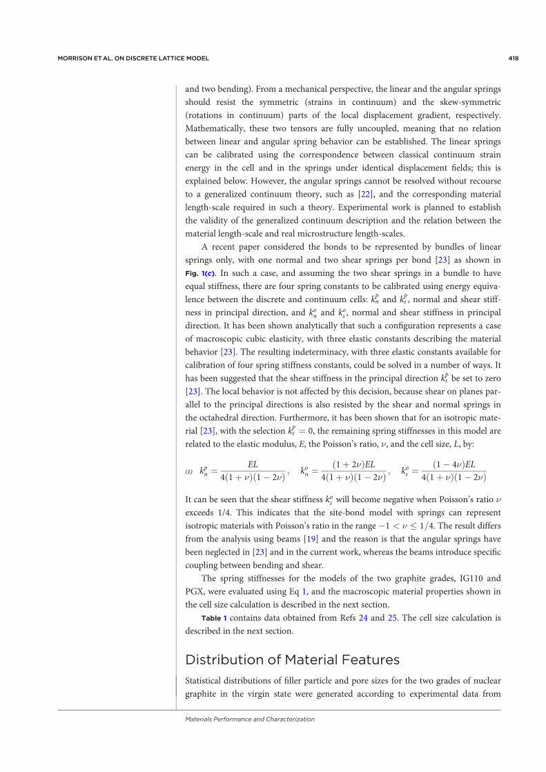
and two bending). From a mechanical perspective, the linear and the angular springs
should resist the symmetric (strains in continuum) and the skew-symmetric
(rotations in continuum) parts of the local displacement gradient, respectively.
Mathematically, these two tensors are fully uncoupled, meaning that no relation
between linear and angular spring behavior can be established. The linear springs
can be calibrated using the correspondence between classical continuum strain
energy in the cell and in the springs under identical displacement fields; this is
explained below. However, the angular springs cannot be resolved without recourse
to a generalized continuum theory, such as [22], and the corresponding material
length-scale required in such a theory. Experimental work is planned to establish
the validity of the generalized continuum description and the relation between the
material length-scale and real microstructure length-scales.
A recent paper considered the bonds to be represented by bundles of linear
springs only, with one normal and two shear springs per bond [23] as shown in
Fig. 1(c). In such a case, and assuming the two shear springs in a bundle to have
equal stiffness, there are four spring constants to be calibrated using energy equiva-
lence between the discrete and continuum cells: kpn and kps , normal and shear stiff-
ness in principal direction, and kon and kos , normal and shear stiffness in principal
direction. It has been shown analytically that such a configuration represents a case
of macroscopic cubic elasticity, with three elastic constants describing the material
behavior [23]. The resulting indeterminacy, with three elastic constants available for
calibration of four spring stiffness constants, could be solved in a number of ways. It
has been suggested that the shear stiffness in the principal direction kps be set to zero
[23]. The local behavior is not affected by this decision, because shear on planes par-
allel to the principal directions is also resisted by the shear and normal springs in
the octahedral direction. Furthermore, it has been shown that for an isotropic mate-
rial [23], with the selection kps ¼ 0, the remaining spring stiffnesses in this model are
related to the elastic modulus, E, the Poisson’s ratio, �, and the cell size, L, by:
kpn ¼EL
4 1þ �ð Þ 1� 2�ð Þ ; kon ¼1þ 2�ð ÞEL
4 1þ �ð Þ 1� 2�ð Þ ; kos ¼1� 4�ð ÞEL
4 1þ �ð Þ 1� 2�ð Þ(1)
It can be seen that the shear stiffness kos will become negative when Poisson’s ratio �
exceeds 1/4. This indicates that the site-bond model with springs can represent
isotropic materials with Poisson’s ratio in the range �1 < � � 1=4. The result differs
from the analysis using beams [19] and the reason is that the angular springs have
been neglected in [23] and in the current work, whereas the beams introduce specific
coupling between bending and shear.
The spring stiffnesses for the models of the two graphite grades, IG110 and
PGX, were evaluated using Eq 1, and the macroscopic material properties shown in
the cell size calculation is described in the next section.
Table 1 contains data obtained from Refs 24 and 25. The cell size calculation is
described in the next section.
Distribution of Material Features
Statistical distributions of filler particle and pore sizes for the two grades of nuclear
graphite in the virgin state were generated according to experimental data from
MORRISON ET AL. ON DISCRETE LATTICE MODEL 418
Materials Performance and Characterization
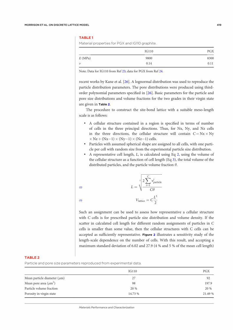
recent works by Kane et al. [26]. A lognormal distribution was used to reproduce the
particle distribution parameters. The pore distributions were produced using third-
order polynomial parameters specified in [26]. Basic parameters for the particle and
pore size distributions and volume fractions for the two grades in their virgin state
are given in Table 2.
The procedure to construct the site-bond lattice with a suitable meso-length
scale is as follows:
• A cellular structure contained in a region is specified in terms of numberof cells in the three principal directions. Thus, for Nx, Ny, and Nz cellsin the three directions, the cellular structure will contain C¼Nx�Ny�Nzþ (Nx�1)� (Ny�1)� (Nz�1) cells.
• Particles with assumed spherical shape are assigned to all cells, with one parti-cle per cell with random size from the experimental particle size distribution.
• A representative cell length, L, is calculated using Eq 2, using the volume ofthe cellular structure as a function of cell length (Eq 3), the total volume of thedistributed particles, and the particle volume fraction h.
L ¼
ffiffiffiffiffiffiffiffiffiffiffiffiffiffiffiffiffiffiffiffiffiffiffiffi2XCi¼1
viparticle
Ch
3
vuuut(2)
Vlattice ¼ CL3
2(3)
Such an assignment can be used to assess how representative a cellular structure
with C cells is for prescribed particle size distribution and volume density. If the
scatter in calculated cell length for different random assignments of particles in C
cells is smaller than some value, then the cellular structures with C cells can be
accepted as sufficiently representative. Figure 2 illustrates a sensitivity study of the
length-scale dependence on the number of cells. With this result, and accepting a
maximum standard deviation of 6.02 and 27.9 (4 % and 5 % of the mean cell length)
TABLE 1
Material properties for PGX and IG110 graphite.
IG110 PGX
E (MPa) 9800 8300
� 0.14 0.11
Note: Data for IG110 from Ref 23; data for PGX from Ref 24.
TABLE 2
Particle and pore size parameters reproduced from experimental data.
IG110 PGX
Mean particle diameter (lm) 27 92
Mean pore area (lm2) 98 197.9
Particle volume fraction 20 % 20 %
Porosity in virgin state 14.73 % 21.49 %
MORRISON ET AL. ON DISCRETE LATTICE MODEL 419
Materials Performance and Characterization
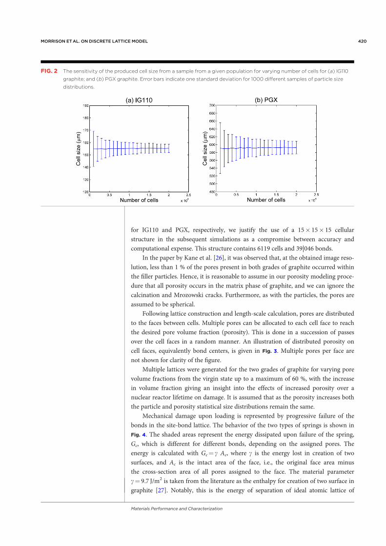
for IG110 and PGX, respectively, we justify the use of a 15� 15� 15 cellular
structure in the subsequent simulations as a compromise between accuracy and
computational expense. This structure contains 6119 cells and 39|046 bonds.
In the paper by Kane et al. [26], it was observed that, at the obtained image reso-
lution, less than 1 % of the pores present in both grades of graphite occurred within
the filler particles. Hence, it is reasonable to assume in our porosity modeling proce-
dure that all porosity occurs in the matrix phase of graphite, and we can ignore the
calcination and Mrozowski cracks. Furthermore, as with the particles, the pores are
assumed to be spherical.
Following lattice construction and length-scale calculation, pores are distributed
to the faces between cells. Multiple pores can be allocated to each cell face to reach
the desired pore volume fraction (porosity). This is done in a succession of passes
over the cell faces in a random manner. An illustration of distributed porosity on
cell faces, equivalently bond centers, is given in Fig. 3. Multiple pores per face are
not shown for clarity of the figure.
Multiple lattices were generated for the two grades of graphite for varying pore
volume fractions from the virgin state up to a maximum of 60 %, with the increase
in volume fraction giving an insight into the effects of increased porosity over a
nuclear reactor lifetime on damage. It is assumed that as the porosity increases both
the particle and porosity statistical size distributions remain the same.
Mechanical damage upon loading is represented by progressive failure of the
bonds in the site-bond lattice. The behavior of the two types of springs is shown in
Fig. 4. The shaded areas represent the energy dissipated upon failure of the spring,
Gc, which is different for different bonds, depending on the assigned pores. The
energy is calculated with Gc¼ c Ac, where c is the energy lost in creation of two
surfaces, and Ac is the intact area of the face, i.e., the original face area minus
the cross-section area of all pores assigned to the face. The material parameter
c¼ 9.7 J/m2 is taken from the literature as the enthalpy for creation of two surface in
graphite [27]. Notably, this is the energy of separation of ideal atomic lattice of
FIG. 2 The sensitivity of the produced cell size from a sample from a given population for varying number of cells for (a) IG110
graphite; and (b) PGX graphite. Error bars indicate one standard deviation for 1000 different samples of particle size
distributions.
MORRISON ET AL. ON DISCRETE LATTICE MODEL 420
Materials Performance and Characterization

graphite and should not be compared to fracture energy directly. Therefore, this
value is identical for the two graphite grades analyzed here. The fracture energy of a
particular grade is an emergent property from the underlying energy of separation
and its microstructure features and distribution. It can be represented by the area
under the simulated stress–strain curve and will be different for different failure
modes, e.g., normal or shear failure. The pore areas allocated to each face are the
maximum pore cross-sectional areas. This is justified to a large extent in the context
of the discrete computational model where the pore can be placed anywhere between
the sites and have the same failure effect on the spring bundle. Thus, Gc tends
toward the maximum spring failure energy (material surface energy) for pore size
approaching zero, and tends toward zero for pore size approaching face area. Bonds
are removed prior to simulations if the initial pore area exceeds the area of the face
on which it is situated.
The assumption used for these criteria is that if the spring damage initiates at a
critical relative displacement, then the damage evolution is linear (softening branch)
FIG. 4 Failure criteria for (a) shear springs; and (b) axial springs.
FIG. 3
A visual representation of the
site bond model with pores
distributed on faces between
cells.
MORRISON ET AL. ON DISCRETE LATTICE MODEL 421
Materials Performance and Characterization

and terminates with spring failure at two times the critical displacement. This is a
reasonable assumption for local brittle failure and allows for direct calculation of the
critical displacement and force from knowledge of the failure energy and initial
spring stiffness. Notably, the axial springs are not allowed to fail in compression,
and the behaviors of the two types of springs are uncoupled in the current model.
Equal failure energies for the axial and shear springs in a bond have been used.
Results and Discussion
Sample site-bond lattices with distributed porosity, with a range of volume fractions,
for each grade of graphite were loaded under displacement control in uni-axial ten-
sion. The simulations were performed in steps of increasing boundary displacements
until the final rupture of the samples. This was an automated solution, such that
multiple spring failures could potentially occur within a loading increment. Whereas
this differs from previous works [17,27], where the load increment was driven by
individual failures, it represents the behavior that would be observed when testing
real samples. At each increment end, the macroscopic stress was determined from
the reaction forces on the boundary with prescribed displacements and the physical
area of this boundary; the macroscopic strain was determined from the current dis-
placement level and the length of the sample. As the strains and stresses are small
within the loading range to failure for this material, the obtained engineering strain
and stress are approximately equal to the true values.
Data for the models analyzed is given in Table 3. This includes the model length
scale derived from each specific particle distribution to cells, the fraction of initially
removed bonds because of excessive pore size on corresponding faces, and the initial
elastic moduli determined prior to damage initiation in the lattice. Notably, the elas-
tic moduli, given in Table 1 and used for the spring stiffness calibration, were derived
with specimens containing virgin state porosities. This is the reason for the differ-
ence between the virgin state elastic moduli in Tables 1 and 3. In principle, the model
can be calibrated without difficulties to account for given porosity (missing bonds)
and provide required macroscopic elastic modulus. However, the initial calibration
of the full lattice is preferable here to facilitate comparison between cases with
increasing porosity. It also helps to note that the porosity effect on the elastic modu-
lus is not linear and arises from the specific combination of a particle size
TABLE 3
Basic parameters of the analyzed models.
Pore Volume Fraction (porosity) Cell Size (lm) Fraction of Bonds Removed Initial Young’s Modulus (MPa)
IG110 0.1473 (virgin) 148.4 0.026 9474.6
0.3 159.1 0.086 8417.6
0.6 148.8 0.319 5083.0
PGX 0.2149 (virgin) 607.0 0.002 8377.4
0.4 547.0 0.268 4938.7
0.6 628.1 0.352 4226.5
Note: Cell size derived from particle distribution to cells; fraction of removed bonds because of large pores on faces; elastic modulus ofvoided model prior to damage.
MORRISON ET AL. ON DISCRETE LATTICE MODEL 422
Materials Performance and Characterization

distribution (via the length scale) and a pore size distribution. For example, compare
the difference between the virgin states of the two grades where the higher porosity
grade, PGX, is stiffer than the lower porosity grade, IG110, relative to the benchmark
values in Table 1, because of the different relation between the cell size (particle sizes)
and the pore sizes.
Figure 5 illustrates the emergent stress–strain curves for both grades of graphite
with different porosities. The initial linear behavior in all cases is governed by corre-
sponding macroscopic elastic modulus, listed in Table 3. Beyond the linear response,
clear quasi-brittle non-linearity prior to the fracture point is observed in Fig. 5 for
cases with low porosities (below 30 %). For higher pore volume fractions, very
little non-linearity is exhibited; the samples failed in a strictly brittle manner at mar-
ginally higher strains than for the cases with lower porosity. The last points of each
stress–strain curve correspond to final failure, i.e., the separation of the modeled vol-
ume into disjoint regions. Further insight into these behaviors is gained by consider-
ing the evolution of the mechanical damage.
FIG. 6 The variation of the mechanical damage parameter DE with applied strain.
FIG. 5 The stress–strain response under of uni-axial tension of (a) IG110 graphite; and (b) PGX graphite.
MORRISON ET AL. ON DISCRETE LATTICE MODEL 423
Materials Performance and Characterization
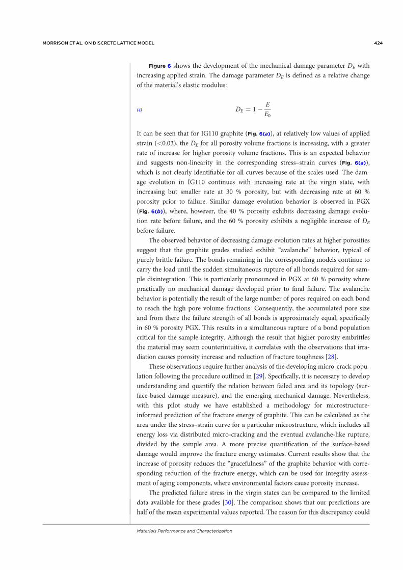
Figure 6 shows the development of the mechanical damage parameter DE with
increasing applied strain. The damage parameter DE is defined as a relative change
of the material’s elastic modulus:
DE ¼ 1� EE0
(4)
It can be seen that for IG110 graphite (Fig. 6(a)), at relatively low values of applied
strain (<0.03), the DE for all porosity volume fractions is increasing, with a greater
rate of increase for higher porosity volume fractions. This is an expected behavior
and suggests non-linearity in the corresponding stress–strain curves (Fig. 6(a)),
which is not clearly identifiable for all curves because of the scales used. The dam-
age evolution in IG110 continues with increasing rate at the virgin state, with
increasing but smaller rate at 30 % porosity, but with decreasing rate at 60 %
porosity prior to failure. Similar damage evolution behavior is observed in PGX
(Fig. 6(b)), where, however, the 40 % porosity exhibits decreasing damage evolu-
tion rate before failure, and the 60 % porosity exhibits a negligible increase of DE
before failure.
The observed behavior of decreasing damage evolution rates at higher porosities
suggest that the graphite grades studied exhibit “avalanche” behavior, typical of
purely brittle failure. The bonds remaining in the corresponding models continue to
carry the load until the sudden simultaneous rupture of all bonds required for sam-
ple disintegration. This is particularly pronounced in PGX at 60 % porosity where
practically no mechanical damage developed prior to final failure. The avalanche
behavior is potentially the result of the large number of pores required on each bond
to reach the high pore volume fractions. Consequently, the accumulated pore size
and from there the failure strength of all bonds is approximately equal, specifically
in 60 % porosity PGX. This results in a simultaneous rapture of a bond population
critical for the sample integrity. Although the result that higher porosity embrittles
the material may seem counterintuitive, it correlates with the observations that irra-
diation causes porosity increase and reduction of fracture toughness [28].
These observations require further analysis of the developing micro-crack popu-
lation following the procedure outlined in [29]. Specifically, it is necessary to develop
understanding and quantify the relation between failed area and its topology (sur-
face-based damage measure), and the emerging mechanical damage. Nevertheless,
with this pilot study we have established a methodology for microstructure-
informed prediction of the fracture energy of graphite. This can be calculated as the
area under the stress–strain curve for a particular microstructure, which includes all
energy loss via distributed micro-cracking and the eventual avalanche-like rupture,
divided by the sample area. A more precise quantification of the surface-based
damage would improve the fracture energy estimates. Current results show that the
increase of porosity reduces the “gracefulness” of the graphite behavior with corre-
sponding reduction of the fracture energy, which can be used for integrity assess-
ment of aging components, where environmental factors cause porosity increase.
The predicted failure stress in the virgin states can be compared to the limited
data available for these grades [30]. The comparison shows that our predictions are
half of the mean experimental values reported. The reason for this discrepancy could
MORRISON ET AL. ON DISCRETE LATTICE MODEL 424
Materials Performance and Characterization

be the assumption for the spring behavior shown in Fig. 4, where a large softening
branch has been introduced. This was done by considering that the graphite matrix
contains a system of nano-pores, which could act as a lower-scale softening mecha-
nism. On the other side the selected separation energy of the matrix does not include
the presence of nano-porosity. These options require further consideration. With
the current separation energy the results suggest that the spring behavior should be
assumed with negligible softening, in which case the stress values shown in Fig. 5
would roughly double.
One point to be noted is that in the present work the increase of porosity has
not been accompanied by any change in the statistical pore size distribution. In
some cases, this could be unrealistic. However, the model provides the means to
calculate the failure energy should changes in size distribution and volume density
of pores be measured experimentally. In addition, the results presented here are spe-
cific to uniaxial loading and hence useful for prediction of fracture energy. The
methodology, however, can be used to derive damage evolution laws for incorpora-
tion in continuum-base finite element analysis of cracked components. It has been
previously shown that under more complex stress states, such plane stress existing
ahead of a crack front, the evolution of damage results in an elastic anisotropy [29].
Derivation of a damage tensor for such loading cases under the proposed methodol-
ogy will be a subject of further publications.
The presented model for elastic-brittle local behavior can be extended to
elastic–plastic or visco-elastic behavior prior to spring failure initiation with the use
of non-linear springs and dampers. This has been done for other lattice models [31]
and is a subject of ongoing work for the lattice proposed here.
The approach developed here is aimed at linking microstructure features
to macroscopic response. It is demonstrated how a macroscopic property, e.g.,
stress–strain curve or damage, emerges from the underlying microstructure and the
separation energy of defect-free graphite atomic lattice. The presented results are
specific to the uniaxial tension of a volume element of a limited size. These allow for
derivation of cohesive zone behavior and fracture toughness associated with the
particular loading considered. One important extension of the work will consider
different deformation conditions, specifically those present ahead of a macroscopic
crack. This way, the model could be used for the analysis of the fracture process
zone size. The parameters controlling this size are still not clearly understood.
According to Aliha and Ayatollahi [32], Awaji et al. [33], and Claussen et al. [34],
the size of the fracture process zone scales with the squared ration of the fracture
toughness and tensile strength. However, Ayatollahi and Aliha [35] have pointed
out that the size is related to the average grain size alone. The modeling of the entire
macro-crack tip region with microstructure-informed lattice will require a signifi-
cant computational effort. As a first step into understanding the different damage
evolutions within the macro-crack tip region, we have planned simulations with rep-
resentative volume elements subjected to the deformation conditions at a number of
spatial positions. The results of such simulations will be analyzed to estimate the
need for large-size lattice covering the entire macro-crack tip region and reported in
future communications. Before completing the planned program, it is difficult to
estimate the effects of grain, pore, and cell sizes on the macroscopic fracture behav-
ior of graphite.
MORRISON ET AL. ON DISCRETE LATTICE MODEL 425
Materials Performance and Characterization

Conclusions
A procedure to construct a meso-scale site-bond lattice model is described that
accounts for experimentally measured particle and pore size distributions and vol-
ume fractions. The procedure is particularly suitable for the analysis of the collective
behavior of micro-cracks, which is the precursor for the non-linear behavior in
quasi-brittle materials, such as graphite.
For the graphite grades investigated, the predicted stress–strain behavior at low
porosities, in virgin state and up to 30 %, is typical of a quasi-brittle material. The
failure is preceded by a significant dissipation of energy by distributed micro-
cracking. This is reflected in the growth of the macroscopic mechanical damage.
At higher porosities, the predicted stress–strain behavior shifts to a typical brit-
tle, characterized by sudden failure with reduced or negligible energy dissipation
from distributed micro-cracking. The failure is an avalanche-like event, whereas a
population of bonds critical to the component integrity fail simultaneously.
The procedure can therefore be used to estimate the changes in material fracture
energy as a function of the changes in the microstructure with aging. Three areas
requiring further investigation are identified: (1) provision of experimental evidence
for the behavior of graphite as a generalized continuum at the particle length scale
and the corresponding calibration of angular springs in bond bundles; (2) quantita-
tive analysis of micro-crack population to relate surface-based damage to mechanical
damage for prediction of fracture energy; and (3) analysis of complex stress states to
derive damage evolution laws for continuum finite element analysis.
ACKNOWLEDGMENTS
C.N.M. greatly appreciates support from EPSRC via Nuclear FiRST Doctoral
Training Centre. M.Z. and A.P.J. acknowledge support from EPSRC via grant
EP/J019763/1, “QUBE: Quasi-Brittle Fracture: A 3D Experimentally Validated
Approach,” and from BNFL for the Research Centre for Radwaste & Decommission-
ing. J.R.Y. acknowledges support from EDF R&D.
References
[1] IAEA, “Characterization, Treatment and Conditioning of Radioactive Graphite
from Decommissioning of Nuclear Reactors,” International Atomic Energy
Agency, Vienna, Austria, 2006.
[2] Bradford, M. R. and Steer, A. G., “A Structurally-Based Model of Irradiated
Graphite Properties,” J. Nucl. Mater., Vol. 381, Nos. 1–2, 2008, pp. 137–144.
[3] Joyce, M. R., Marrow, T. J., Mummery, P., and Marsden, B. J., “Observation of
Microstructure Deformation and Damage in Nuclear Graphite,” Eng. Fract.
Mech., Vol. 75, No. 12, 2008, pp. 3633–3645.
[4] Schlangen, E., Flewitt, P. E. J., Smith, G. E., Crocker, A. G., and Hodgkins, A.,
“Computer Modelling of Crack Propagation in Porous Reactor Core Graphite,”
Key Eng. Mater., Vols. 452–453, 2010, pp. 729–732.
[5] Ogawa, M. and Nishihara, T., “Present Status of Energy in Japan and HTTR
Project,” Nucl. Eng. Des., Vol. 233, Nos. 1–3, 2004, pp. 5–10.
MORRISON ET AL. ON DISCRETE LATTICE MODEL 426
Materials Performance and Characterization

[6] Mostafavi, M. and Marrow, T. J., “Quantitative In Situ Study of Short Crack
Propagation in Polygranular Graphite by Digital Image Correlation,” Fatigue
Fract. Eng. Mater. Struct., Vol. 35, No. 8, 2012, pp. 695–707.
[7] Hodgkins, A., Marrow, T. J., Wootton, M. R., Moskovic, R., and Flewitt, P. E. J.,
“Fracture Behaviour of Radiolytically Oxidised Reactor Core Graphites:
A View,” Mater. Sci. Technol., Vol. 26, No. 8, 2010, pp. 899–907.
[8] Lemaitre, J., “Local Approach of Fracture,” Eng. Fract. Mech., Vol. 25, Nos.
5–6, 1986, pp. 523–537.
[9] de Borst, R., “Fracture in Quasi-Brittle Materials: A Review of Continuum
Damage-Based Approaches,” Eng. Fract. Mech., Vol. 69, 2002, pp. 95–112.
[10] Bazant, Z. P. and Pang, S., “Activation Energy Based Extreme Value Statistics
and Size Effect in Brittle and Quasibrittle Fracture,” J. Mech. Phys. Solids, Vol.
55, No. 1, 2007, pp. 91–131.
[11] Bazant, Z., “Concrete Fracture Models: Testing and Practice,” Eng. Fract.
Mech., Vol. 69, 2002, pp. 165–205.
[12] Pazdniakou, A. and Adler, P. M., “Lattice Spring Models,” Transport Porous
Med., Vol. 93, No. 2, 2012, pp. 243–262.
[13] Schlangen, E. and Garboczi, E., “Fracture Simulations of Concrete Using Lattice
Models: Computational Aspects,” Eng. Fract. Mech., Vol. 57, No. 2, 1997, pp.
319–332.
[14] Nemeth, N. N. and Bratton, R. L., “Overview of Statistical Models of Fracture
for Nonirradiated Nuclear-Graphite Components,” Nucl. Eng. Des., Vol. 240,
No. 1, 2010, pp. 1–29.
[15] Griffiths, D. and Mustoe, G., “Modelling of Elastic Continua Using a Grillage of
Structural Elements Based on Discrete Element Concepts,” Int. J. Numer. Meth-
ods Eng., Vol. 50, 2001, pp. 1759–1775.
[16] Schlangen, E., “Crack Development in Concrete: Part 2. Modelling of Fracture
Process,” Key Eng. Mater., Vols. 385–387, 2008, pp. 73–76.
[17] Wang, Y. and Mora, P., “Macroscopic Elastic Properties of Regular Lattices,”
J. Mech. Phys. Solids, Vol. 56, No. 12, 2008, pp. 3459–3474.
[18] Jivkov, A. P., Engelberg, D. L., Stein, R., and Petkovski, M., “Pore Space and
Brittle Damage Evolution in Concrete,” Eng. Fract. Mech., Vol. 110, 2012, pp.
378–395.
[19] Jivkov, A. P. and Yates, J. R., “Elastic Behaviour of a Regular Lattice for
Meso-Scale Modelling of Solids,” Int. J. Solids Struct., Vol. 49, No. 22, 2012,
pp. 3089–3099.
[20] Morrison, C. N., Jivkov, A. P., Smith, G., and Yates, J. R., “Lattice-Spring
Modeling of Graphite Accounting for Pore Size Distribution,” Key Eng. Mater.,
Vols. 592–593, 2013, pp. 92–95.
[21] Kumar, S., Kurtz, S. K., Banavar, J. R., and Sharma, M. G., “Properties of a
Three-Dimensional Poisson-Voronoi Tesselation: A Monte Carlo Study,”
J. Stat. Phys., Vol. 67, Nos. 3–4, 1992, pp. 523–551.
[22] Hadjesfandiari, A. R. and Dargush, G. F., “Couple Stress Theory for Solids,”
Int. J. Solids Struct., Vol. 48, No. 18, 2011, pp. 2496–2510.
[23] Zhang, M., Morrison, C. N., and Jivkov, A. P., “A Meso-Scale Site-Bond
Model for Elasticity: Theory and Calibration,” Mater. Res. Innov. (in
press).
MORRISON ET AL. ON DISCRETE LATTICE MODEL 427
Materials Performance and Characterization

[24] Kaji, Y., Gu, W., Ishihara, M., Arai, T., and Nakamura, H., “Development of
Structural Analysis Program for Non-Linear Elasticity by Continuum Damage
Mechanics,” Nucl. Eng. Des., Vol. 206, No. 1, 2001, pp. 1–12.
[25] T.T.C. Products, “Special Graphite and Compound Material Products,” Toyo
Tanso Group, Osaka, Japan.
[26] Kane, J., Karthik, C., Butt, D. P., Windes, W. E., and Ubic, R., “Microstructural
Characterization and Pore Structure Analysis of Nuclear Graphite,” J. Nucl.
Mater., Vol. 415, No. 2, 2011, pp. 189–197.
[27] Abrahamson, J., “The Surface Energies of Graphite,” Carbon, Vol. 11, No. 4,
1973, pp. 337–362.
[28] Berre, C., Fok, S. L., Marsden, B. J., Mummery, P. M., Marrow, T. J., and
Neighbour, G. B., “Microstructural Modelling of Nuclear Graphite Using
Multi-Phase Models,” J. Nucl. Mater., Vol. 380, Nos. 1–3, 2008, pp. 46–58.
[29] Jivkov, A. P., “Structure of Micro-Crack Population and Damage Evolution in
Concrete,” 13th International Conference on Fracture, Beijing, China, June
16–21, 2013, pp. 1–10.
[30] Ishihara, M., Sumita, J., Shibata, T., Iyoku, T., and Oku, T., “Principle Design
and Data of Graphite Components,” Nucl. Eng. Des., Vol. 233, Nos. 1–3, 2004,
pp. 251–260.
[31] O’Brien, G. S., “Discrete Visco-Elastic Lattice Methods for Seismic Wave Prop-
agation,” Geophys. Res. Lett., Vol. 35, No. 2, 2008, p. L02302.
[32] Aliha, M. R. M. and Ayatollahi, M. R., “Analysis of Fracture Initiation Angle in
Some Cracked Ceramics Using the Generalized Maximum Tangential Stress
Criterion,” Int. J. Solids Struct., Vol. 49, No. 13, 2012, pp. 1877–1883.
[33] Awaji, H., Matsunaga, T., and Choi, S.-M., “Relation between Strength,
Fracture Toughness, and Critical Frontal Process Zone Size in Ceramics,”
Mater. Trans., Vol. 47, No. 6, 2006, pp. 1532–1539.
[34] Claussen, N., Mussler, B., and Swain, M. V., “Grain-Size Dependence of
Fracture Energy in Ceramics,” Commun. Am. Ceram. Soc., Vol. 65, No. 1, 1982,
pp. C14–C16.
[35] Ayatollahi, M. R. and Aliha, M. R. M., “Fracture Analysis of Some Ceramics
Under Mixed Mode Loading,” J. Am. Ceram. Soc., Vol. 94, No. 2, 2011, pp.
561–569.
MORRISON ET AL. ON DISCRETE LATTICE MODEL 428
Materials Performance and Characterization
Copyright by ASTM Int’l (all rights reserved); Mon Sep 8 7:25:12 EDT 2014Downloaded/printed byCraig Neil Morrison (The University of Manchester, Mechanics and Physics of Solids Research Group, Modelling and Simulation Centre, Manchester, United Kingdom)Pursuant to License Agreement. No further reproduction authorized.

Appendix G
Fracture energy of graphite from
microstructure-informed lattice model
175
Available online at www.sciencedirect.com
ScienceDirect
Procedia Materials Science 3 (2014) 1848-1853
www.elsevier.com/locate/procedia
2211-8128 © 2014 The Authors. Published by Elsevier Ltd.
Selection and peer-review under responsibility of the Norwegian University of Science and Technology (NTNU),
Department of Structural Engineering.
20th European Conference on Fracture (ECF20)
Fracture energy of graphite from microstructure-informed
lattice model
Craig N Morrison*, Mingzhong Zhang, Andrey P Jivkov
Mechanics and Physics of Solids Research Team, School of Mechanical, Aerospace and Civil Engineering, The University
of Manchester, Manchester, M13 9PL, UK
Abstract
Graphite remains a key structural material in the nuclear industry, the integrity assessment of which in
demanding reactor environments is critical for safe operation of plant. Fracture of graphite is preceded by
growth and coalescence of distributed micro-cracks within a process zone, classifying it as a quasi-brittle
material alongside cement-based and ceramic materials. The evolution of a micro-crack population to failure is
well represented by discrete lattice models, e.g. (Wang and Mora 2008). Here, a recently developed 3D lattice
(Jivkov and Yates 2012), with elastic spring elements and brittle-damage behaviour is used to generate
microstructure representative models of two graphite grades at a representative meso length scale. Micro-
cracks are represented by spring failures and the macroscopic damage results from their collective behaviour.
Presented results capture a transition from graceful, plastic-like failure at lower porosities, with energy
dissipation via micro-cracking, to glass-like behaviour with negligible energy dissipation at higher porosities.
The results are in good agreement with experimental data. Thus, the proposed methodology can calculate
fracture energy from the stress-strain curve, or formulate cohesive and damage evolution laws for continuum
models, based exclusively on microstructural features.
© 2014 The Authors. Published by Elsevier Ltd.
Selection and peer-review under responsibility of the Norwegian University of Science and Technology
(NTNU), Department of Structural Engineering.
Keywords: Nuclear graphite; Porosity; Meso-scale model; Quasi-brittle behaviour; Damage evolution
* Corresponding author.
E-mail address: [email protected]
2
1. Introduction
Nuclear-grade graphite has been used as both a fast neutron moderator and structural material in
over 100 reactors worldwide. The ability to fulfill both purposes gives it a distinct advantage over
water-based reactors and has lead to its inclusion in the design of the Generation IV Very High
Temperature Reactor. Consequently both future reactor core designs and life extensions of existing
plants require a suitable means of predicting the structural integrity of graphite in the demanding
environment and complex loading states found in a reactor core.
Graphite has a feature-rich microstructure consisting of multiple phases, the size and structure of
which are dependent upon the raw materials and manufacturing process used. This has allowed for
the development of a broad range of graphite grades, with properties tailored to a specific purpose.
The microstructure consists of filler particles, derived from petroleum or pitch cokes distributed
within a matrix of graphitized binder material; usually coal-tar pitch. Distributed throughout both
of these phases are 3 main populations of porosity formed at different stages of the manufacturing
process; gas evolution cracks, calcinations cracks and Mrozowski cracks (Bradford and Steer 2008;
Joyce et al. 2008), the length scale of which ranges from nm to mm scale depending on the grade in
question.
Current preferred modeling procedures used to investigate component scale integrity are based
on a classical continuum, such as the finite element method. These inherently fail to model the
effect of microstructure on macroscopic behavior, assuming all points in an element behave
homogeneously. This is problematic when modeling graphite components where failure has been
shown to be dependent on its discrete multiphase microstructure (Mostafavi and Marrow 2012),
primarily the result of micro-crack coalescence into a critically sized flaw. Such a response suggests
graphite falls into the class of quasi-brittle materials alongside rock, concrete and ceramics. Upon
loading quasi-brittle materials typically exhibit a reduction of stiffness prior to failure, similar to
plasticity. Moreover, a residual load carrying capacity beyond the peak load is demonstrated
(Hodgkins et al. 2010).
Attempts have been made at developing continuum-based approaches which account implicitly
for microstructural affects, notably in the fracture process zone (FPZ) ahead of an existing crack.
One approach of note, easily implemented in the finite element method is cohesive zone modeling
(Borst 2002; Elices et al. 2002). This method represents the local softening found in quasi-brittle
materials ahead of a crack in the properties of cohesive elements. However problems arise from the
pre-definition of a crack path and the phenomenological calibration and curve fitting of parameters
required from observed macroscopic behavior for different loading cases.
Such failings of continuum approaches have led to the development of a number of local fracture
models for quasi-brittle materials. These ‘meso-scale’ models aim to capture the dependence of
macro- or component scale failure on microstructural features by representing the corresponding
failure mechanisms at the feature length scale in a physically realistic manner (Lemaitre 1986).
However, most current local approaches are again phenomenological (Borst 2002) and as such
inherently ignore the actual failure mechanisms observed at the microscale of quasi-brittle materials
(Bažant and Pang 2007). Microstructure-informed models, such as the one offered in this work,
have the potential to assist in deriving mechanistic constitutive laws suitable for use in the
aforementioned continuum approaches such as cohesive zone modeling.
Lattice models, such as the model described in this paper, are a category of local discrete models,
where discrete elements, including springs (Pazdniakou and Adler 2012) and beams (Schlangen and
Garboczi 1997) are used as connections between nodes to form a parallel network. The response
and failure of elements can incorporate actual mechanisms at the length scale of microstructure
features, allowing a physically realistic macro-mechanical response. Global failure is the result of
cumulative micro-failures into a macro-sized flaw, with load redistribution occurring upon failure

3
of single bonds. Previous lattice models for graphite (Nemeth and Bratton 2010) and concrete
(Schlangen and Garboczi 1997) have either been 2D models, questionable in their ability to
simulate the intrinsically 3D phenomenon of micro-crack damage evolution, or limited in their
ability to reproduce a full range of Poisson’s ratio for elastic materials (Wang and Mora 2008).
This work extends the site-bond 3D lattice model developed by Jivkov and Yates (Jivkov and
Yates 2012) with application to nuclear graphite using bundles of springs as discrete bonds
connecting sites at the centre of unit cells. Previous construction methodology accounting for
experimentally measured particle and pore size distributions is improved (Morrison et al. 2014b;
Morrison et al. 2014a) and used to investigate the effects of increasing porosity on tensile strength
and damage evolution with a view to understanding graphite’s response to radiation damage.
2. Theory and Model
The theory behind the site-bond model is briefly presented here. Details are given in another
contribution to this volume (Jivkov et al. 2014) and in previous works (Jivkov and Yates 2012;
Morrison et al. 2014a; Morrison et al. 2014b). The model consists of a regular tessellation of
truncated octahedral cells – the regular shape considered the closest representation of a generic
microstructure (Kumar et al. 1992). The truncated octahedron has six square faces, normal to the
principle axes, and eight hexagonal faces, normal to the octahedral axes. Sites at cell centers are
connected to neighboring sites by bonds, with bond lengths varying for principal and octahedral
directions.
Fig. 1. Cellular lattice: (a) site-bond assembly; (b) unit cell with bonds; (c) normal and shear springs.
In this work each bond is represented as a bundle of elastic-brittle normal and shear spring. The
need for further angular springs to represent all degrees of freedom between sites is a subject of
ongoing work. Spring constants, given in Eq.1, are calibrated by equating the strain energy in a
single discrete cell to the energy in the equivalent continuum (Zhang et al. 2013).
(1 2 ) (1 4 ); 0; ;
4(1 )(1 2 ) 4(1 )(1 2 ) 4(1 )(1 2 )
p p o o
n s n s
EL v EL v ELk k k k
v v v v v v
(1)
where E and are Young’s modulus and Poisson’s ratio of the material respectively,
and
represent the stiffness of normal and shear springs in principal directions and and
represent
the stiffness of normal and shear springs in octahedral directions. L is the cell size, i.e. distance
between sites in the principal directions.
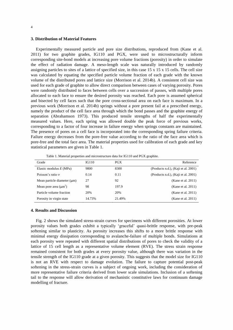
4
3. Distribution of Material Features
Experimentally measured particle and pore size distributions, reproduced from (Kane et al.
2011) for two graphite grades, IG110 and PGX, were used to microstructurally inform
corresponding site-bond models at increasing pore volume fractions (porosity) in order to simulate
the effect of radiation damage. A meso-length scale was naturally introduced by randomly
assigning particles to sites of a lattice of specified size, in this case 15 x 15 x 15 cells. The cell size
was calculated by equating the specified particle volume fraction of each grade with the known
volume of the distributed pores and lattice size (Morrison et al. 2014b). A consistent cell size was
used for each grade of graphite to allow direct comparison between cases of varying porosity. Pores
were randomly distributed to faces between cells over a succession of passes, with multiple pores
allocated to each face to ensure the desired porosity was reached. Each pore is assumed spherical
and bisected by cell faces such that the pore cross-sectional area on each face is maximum. In a
previous work (Morrison et al. 2014b) springs without a pore present fail at a prescribed energy,
namely the product of the cell face area through which the bond passes and the graphite energy of
separation (Abrahamson 1973). This produced tensile strengths of half the experimentally
measured values. Here, each spring was allowed double the peak force of previous works,
corresponding to a factor of four increase in failure energy when springs constants are maintained.
The presence of pores on a cell face is incorporated into the corresponding spring failure criteria.
Failure energy decreases from the pore-free value according to the ratio of the face area which is
pore-free and the total face area. The material properties used for calibration of each grade and key
statistical parameters are given in Table 1.
Table 1. Material properties and microstructure data for IG110 and PGX graphite.
Grade IG110 PGX Reference
Elastic modulus E (MPa) 9800 8300 (Products n.d.), (Kaji et al. 2001)
Poisson’s ratio 0.14 0.11 (Products n.d.), (Kaji et al. 2001)
Mean particle diameter (μm) 27 92 (Kane et al. 2011)
Mean pore area (μm2) 98 197.9 (Kane et al. 2011)
Particle volume fraction 20% 20% (Kane et al. 2011)
Porosity in virgin state 14.73% 21.49% (Kane et al. 2011)
4. Results and Discussion
Fig. 2 shows the simulated stress-strain curves for specimens with different porosities. At lower
porosity values both grades exhibit a typically ‘graceful’ quasi-brittle response, with pre-peak
softening similar to plasticity. As porosity increases this shifts to a more brittle response with
minimal energy dissipation corresponding to avalanche-failure of multiple bonds. Simulations at
each porosity were repeated with different spatial distributions of pores to check the validity of a
lattice of 15 cell length as a representative volume element (RVE). The stress strain response
remained consistent for both grades at every porosity value, although there was variation in the
tensile strength of the IG110 grade at a given porosity. This suggests that the model size for IG110
is not an RVE with respect to damage evolution. The failure to capture potential post-peak
softening in the stress-strain curves is a subject of ongoing work, including the consideration of
more representative failure criteria derived from lower scale simulations. Inclusion of a softening
tail to the response will allow derivation of mechanistic constitutive laws for continuum damage
modelling of fracture.
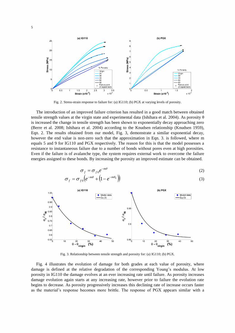
5
Fig. 2. Stress-strain response to failure for: (a) IG110; (b) PGX at varying levels of porosity.
The introduction of an improved failure criterion has resulted in a good match between obtained
tensile strength values at the virgin state and experimental data (Ishihara et al. 2004). As porosity θ
is increased the change in tensile strength has been shown to exponentially decay approaching zero
(Berre et al. 2008; Ishihara et al. 2004) according to the Knudsen relationship (Knudsen 1959),
Eqn. 2. The results obtained from our model, Fig. 3, demonstrate a similar exponential decay,
however the end value is non-zero such that the approximation in Eqn. 3. is followed, where m
equals 5 and 9 for IG110 and PGX respectively. The reason for this is that the model possesses a
resistance to instantaneous failure due to a number of bonds without pores even at high porosities.
Even if the failure is of avalanche type, the system requires external work to overcome the failure
energies assigned to these bonds. By increasing the porosity an improved estimate can be obtained.
m
ff e 0 (2)
010
mm
ff ee (3)
Fig. 3. Relationship between tensile strength and porosity for: (a) IG110; (b) PGX.
Fig. 4 illustrates the evolution of damage for both grades at each value of porosity, where
damage is defined at the relative degradation of the corresponding Young’s modulus. At low
porosity in IG110 the damage evolves at an ever increasing rate until failure. As porosity increases
damage evolution again starts at any increasing rate, however prior to failure the evolution rate
begins to decrease. As porosity progressively increases this declining rate of increase occurs faster
as the material’s response becomes more brittle. The response of PGX appears similar with a

6
quicker decline to a brittle response. The results suggest this model can be used to analyse and
further understand damage evolution ahead of a macroscopic crack for a material of known
microstructure with a possibility to aid in the prediction of FPZ size – a phenomenon not yet fully
understood in quasi-brittle materials (Awaji et al. 2006).
Fig. 4. Damage evolution for: (a) IG110; (b) PGX; at various porosities
5. Conclusions
This work describes a method of constructing a site-bond model to account for experimentally
measured pore and particle size distributions and volume fractions, such that a suitable meso-scale
length scale is achieved. We have demonstrated its potential to derive material constitutive
behavior emerging from micro-crack growth and coalescence – the prominent microstructural
failure mechanism for quasi-brittle materials, such as graphite. Two graphite grades have been
investigated, with ‘graceful’ quasi-brittle found at lower porosities whereby energy is dissipated
with distributed micro-failures and hence an increasing rate of damage evolution prior to global
failure. Increase of porosity leads to a more brittle response where final failure is sudden with
avalanche-like failure of numerous bonds simultaneously. In this case, rate of damage evolution is
constantly decreasing. Tensile strength is shown to exponentially decay with increased porosity,
although the decay relationship differs from literature data.
The method has potential for use in exploring phenomena which are not currently well
understood, e.g. the FPZ size, and deriving constitutive and damage evolution behavior for a
microstructure under aging processes for use in continuum methods. Further work includes;
additional consideration of angular spring inclusion on receipt of experimental evidence exhibiting
graphite’s characteristics as a generalized continuum and exploration of the correct surface energy
of graphite required for deriving spring failure criteria.
Acknowledgements
Morrison appreciates the support from EPSRC via Nuclear FiRST Doctoral Training Centre.
Zhang and Jivkov acknowledge the support from EPSRC via grant EP/J019763/1, “QUBE: Quasi-
Brittle fracture: a 3D experimentally-validated approach”, and from BNFL for the Research Centre
for Radwaste & Decommissioning.
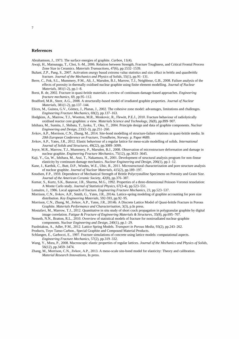
7
References
Abrahamson, J., 1973. The surface energies of graphite. Carbon, 11(4).
Awaji, H., Matsunaga, T., Choi, S.-M., 2006. Relation between Strength, Fracture Toughness, and Critical Frontal Process Zone Size in Ceramics. Materials Transactions, 47(6), pp.1532–1539.
Bažant, Z.P., Pang, S., 2007. Activation energy based extreme value statistics and size effect in brittle and quasibrittle
fracture. Journal of the Mechanics and Physics of Solids, 55(1), pp.91–131. Berre, C., Fok, S.L., Mummery, P.M., Ali, J., Marsden, B.J., Marrow, T.J., Neighbour, G.B., 2008. Failure analysis of the
effects of porosity in thermally oxidised nuclear graphite using finite element modelling. Journal of Nuclear
Materials, 381(1-2), pp.1–8. Borst, R. de, 2002. Fracture in quasi-brittle materials: a review of continuum damage-based approaches. Engineering
fracture mechanics, 69, pp.95–112.
Bradford, M.R., Steer, A.G., 2008. A structurally-based model of irradiated graphite properties. Journal of Nuclear Materials, 381(1-2), pp.137–144.
Elices, M., Guinea, G.V., Gómez, J., Planas, J., 2002. The cohesive zone model: advantages, limitations and challenges.
Engineering Fracture Mechanics, 69(2), pp.137–163. Hodgkins, A., Marrow, T.J., Wootton, M.R., Moskovic, R., Flewitt, P.E.J., 2010. Fracture behaviour of radiolytically
oxidised reactor core graphites: a view. Materials Science and Technology, 26(8), pp.899–907.
Ishihara, M., Sumita, J., Shibata, T., Iyoku, T., Oku, T., 2004. Principle design and data of graphite components. Nuclear Engineering and Design, 233(1-3), pp.251–260.
Jivkov, A.P., Morrison, C.N., Zhang, M., 2014. Site-bond modelling of structure-failure relations in quasi-brittle media. In
20th European Conference on Fracture, Trondheim, Norway. p. Paper #689. Jivkov, A.P., Yates, J.R., 2012. Elastic behaviour of a regular lattice for meso-scale modelling of solids. International
Journal of Solids and Structures, 49(22), pp.3089–3099.
Joyce, M.R., Marrow, T.J., Mummery, P., Marsden, B.J., 2008. Observation of microstructure deformation and damage in nuclear graphite. Engineering Fracture Mechanics, 75(12), pp.3633–3645.
Kaji, Y., Gu, W., Ishihara, M., Arai, T., Nakamura, H., 2001. Development of structural analysis program for non-linear
elasticity by continuum damage mechanics. Nuclear Engineering and Design, 206(1), pp.1–12. Kane, J., Karthik, C., Butt, D.P., Windes, W.E., Ubic, R., 2011. Microstructural characterization and pore structure analysis
of nuclear graphite. Journal of Nuclear Materials, 415(2), pp.189–197. Knudsen, F.P., 1959. Dependence of Mechanical Strength of Brittle Polycrystalline Specimens on Porosity and Grain Size.
Journal of the American Ceramic Society, 42(8), pp.376–387.
Kumar, S., Kurtz, S.K., Banavar, J.R., Sharma, M.G., 1992. Properties of a three-dimensional Poisson-Voronoi tesselation: A Monte Carlo study. Journal of Statistical Physics, 67(3-4), pp.523–551.
Lemaitre, J., 1986. Local approach of fracture. Engineering Fracture Mechanics, 23, pp.523–537.
Morrison, C.N., Jivkov, A.P., Smith, G., Yates, J.R., 2014a. Lattice-spring modeling of graphite accounting for pore size distribution. Key Engineering Materials, 592-593, pp.92–95.
Morrison, C.N., Zhang, M., Jivkov, A.P., Yates, J.R., 2014b. A Discrete Lattice Model of Quasi-brittle Fracture in Porous
Graphite. Materials Performance and Characterisation, 3(3), p.In press. Mostafavi, M., Marrow, T.J., 2012. Quantitative in situ study of short crack propagation in polygranular graphite by digital
image correlation. Fatigue & Fracture of Engineering Materials & Structures, 35(8), pp.695–707.
Nemeth, N.N., Bratton, R.L., 2010. Overview of statistical models of fracture for nonirradiated nuclear-graphite components. Nuclear Engineering and Design, 240(1), pp.1–29.
Pazdniakou, A., Adler, P.M., 2012. Lattice Spring Models. Transport in Porous Media, 93(2), pp.243–262.
Products, Toyo Tanso Carbon., Special Graphite and Compound Material Products. Schlangen, E., Garboczi, E., 1997. Fracture simulations of concrete using lattice models: computational aspects.
Engineering Fracture Mechanics, 57(2), pp.319–332.
Wang, Y., Mora, P., 2008. Macroscopic elastic properties of regular lattices. Journal of the Mechanics and Physics of Solids, 56(12), pp.3459–3474.
Zhang, M., Morrison, C.N., Jivkov, A.P., 2013. A meso-scale site-bond model for elasticity: Theory and calibration.
Material Research Innovations, In press.

Appendix H
Site-bond lattice modelling of damage
process in nuclear graphite under
bending
183

Transactions, SMiRT-23
Manchester, United Kingdom - August 10-14, 2015
Division II
SITE-BOND LATTICE MODELLING OF DAMAGE PROCESS IN
NUCLEAR GRAPHITE UNDER BENDING
Craig N Morrison1, Mingzhong Zhang2, Dong Liu3 and Andrey P Jivkov1
1 Modelling and Simulation Centre, School of Mechanical, Aerospace and Civil Engineering, The
University of Manchester, Manchester, UK 2 Advanced & Innovative Materials Group, Department of Civil, Environmental and Geomatic
Engineering, University College London, London, UK 3 Interface Analysis Centre, School of Physics, University of Bristol, Bristol, UK
ABSTRACT
Graphite is used as neutron moderator and structural material in the core of the UK's fleet of Magnox and
Advanced Gas-cooled Reactors (AGRs). The graphite cores are non-replaceable in these two designs and therefore potentially life-limiting. Graphite is a multi-phase, aggregated and porous material which could
have a non-linear stress-strain response because of distributed damage accumulation within the material
prior to rupture: quasi-brittle characteristics. Lattice models provide a way of capturing the resulting non-
linear behaviour by incorporating microstructural features and damage mechanisms within the discrete
system. Here, the 3D site-bond model (Jivkov and Yates 2012) is used to simulate a near-isotropic nuclear
reactor core Gilsocarbon graphite under bending in a micro-cantilever test (Liu et al 2014).
Experimentally measured pore-size distributions and volume densities are used for model construction. Previous work on graphite site-bond modelling (Morrison et al 2014b) is further developed to consider
pore effect on the deformation and failure behaviour of the bonds. Damage evolution and accumulation
with increasing load is simulated by the consecutive removal of bonds subject to failure criterion. The simulated mechanical properties and force-deflection relationship were validated by experimental results.
Keywords: Site-bond model; Nuclear graphite; Micro-cantilever bending; Local damage; Microstructure
INTRODUCTION
Graphite has been used in the nuclear industry as a fast neutron moderator since the first demonstration of a chain nuclear reaction in the 1940s. Moreover, its high strength at elevated temperatures within reactors
has allowed it to be coupled as a structural component in some reactor designs (Mantell 1968). The three-
phase microstructure of graphite varies depending on the raw materials and the manufacturing process
used. Filler particles, deriving from petroleum or pitch coke, are dispersed within a binder material
matrix, usually consisting of graphitised coal-tar pitch. Both of these solid phases host various
populations of pores covering different length scales (Jenkins 1962). Graphite is believed to belong to the
quasi-brittle class of materials (Hodgkins et al 2010), with structural integrity considered to be dependent on material failures at the length scales of its prominent microstructure features. The initiation of brittle
micro-cracks, considered to be at pores, dissipates energy resulting in a reduction in the global stiffness
prior to peak stress in a similar manner to plasticity; and this is followed by a post peak softening. Ultimate failure is considered to be the result of micro-crack growth and coalescence into a flaw of
critical size.
Global modelling strategies, such as the finite element method (Turner et al 1956), assume scale-
independent homogeneous behaviour within model elements and as such fail to account for the effects of
microstructure failure mechanisms in the material response. This is considered to be inappropriate in
certain cases particularly when modelling situations at length scales where the material response is
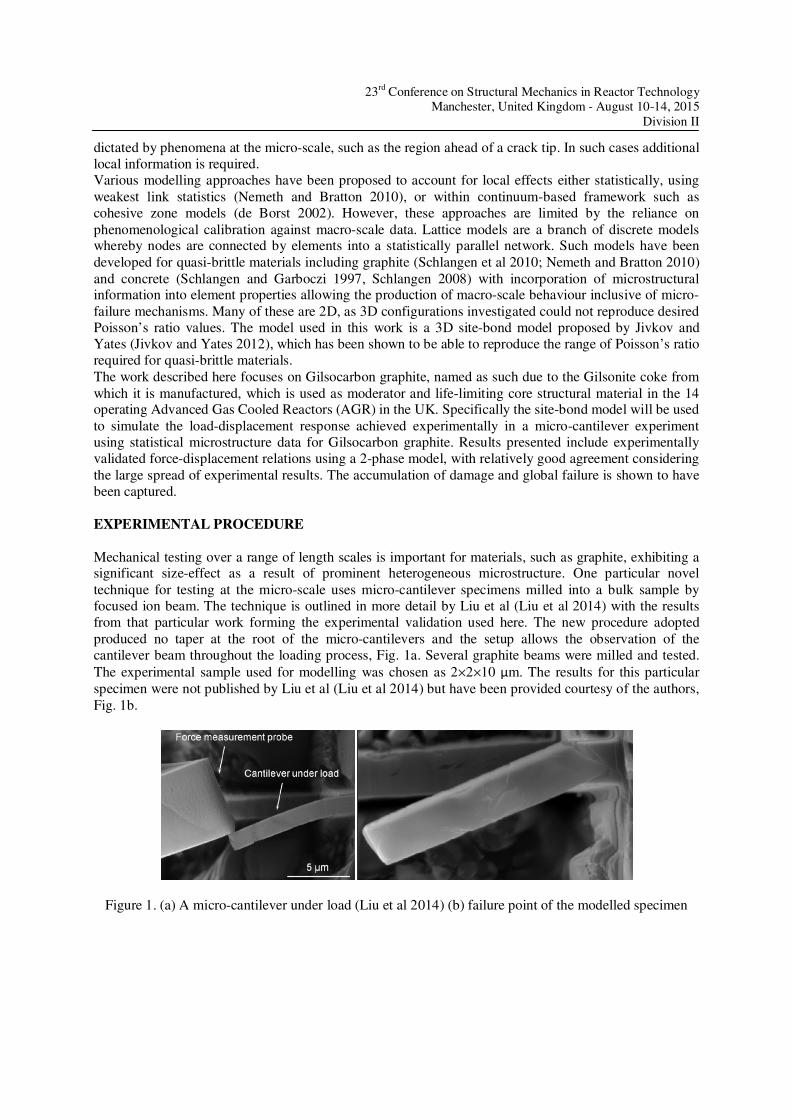
23rd
Conference on Structural Mechanics in Reactor Technology Manchester, United Kingdom - August 10-14, 2015
Division II
dictated by phenomena at the micro-scale, such as the region ahead of a crack tip. In such cases additional
local information is required.
Various modelling approaches have been proposed to account for local effects either statistically, using
weakest link statistics (Nemeth and Bratton 2010), or within continuum-based framework such as
cohesive zone models (de Borst 2002). However, these approaches are limited by the reliance on
phenomenological calibration against macro-scale data. Lattice models are a branch of discrete models whereby nodes are connected by elements into a statistically parallel network. Such models have been
developed for quasi-brittle materials including graphite (Schlangen et al 2010; Nemeth and Bratton 2010)
and concrete (Schlangen and Garboczi 1997, Schlangen 2008) with incorporation of microstructural information into element properties allowing the production of macro-scale behaviour inclusive of micro-
failure mechanisms. Many of these are 2D, as 3D configurations investigated could not reproduce desired
Poisson’s ratio values. The model used in this work is a 3D site-bond model proposed by Jivkov and
Yates (Jivkov and Yates 2012), which has been shown to be able to reproduce the range of Poisson’s ratio
required for quasi-brittle materials.
The work described here focuses on Gilsocarbon graphite, named as such due to the Gilsonite coke from
which it is manufactured, which is used as moderator and life-limiting core structural material in the 14 operating Advanced Gas Cooled Reactors (AGR) in the UK. Specifically the site-bond model will be used
to simulate the load-displacement response achieved experimentally in a micro-cantilever experiment
using statistical microstructure data for Gilsocarbon graphite. Results presented include experimentally
validated force-displacement relations using a 2-phase model, with relatively good agreement considering
the large spread of experimental results. The accumulation of damage and global failure is shown to have
been captured.
EXPERIMENTAL PROCEDURE
Mechanical testing over a range of length scales is important for materials, such as graphite, exhibiting a significant size-effect as a result of prominent heterogeneous microstructure. One particular novel
technique for testing at the micro-scale uses micro-cantilever specimens milled into a bulk sample by
focused ion beam. The technique is outlined in more detail by Liu et al (Liu et al 2014) with the results
from that particular work forming the experimental validation used here. The new procedure adopted
produced no taper at the root of the micro-cantilevers and the setup allows the observation of the
cantilever beam throughout the loading process, Fig. 1a. Several graphite beams were milled and tested.
The experimental sample used for modelling was chosen as 2×2×10 μm. The results for this particular
specimen were not published by Liu et al (Liu et al 2014) but have been provided courtesy of the authors,
Fig. 1b.
Figure 1. (a) A micro-cantilever under load (Liu et al 2014) (b) failure point of the modelled specimen

23rd
Conference on Structural Mechanics in Reactor Technology Manchester, United Kingdom - August 10-14, 2015
Division II
THEORY AND METHOD
The site-bond model represents material volume through the use of a regular lattice of truncated
octahedral cells, Figure 2a. This shape is considered the regularly tessellating shape most capable of
representing a generic microstructure (Kumar et al 1992), and as such the lattice can be considered a
topological homogenization of a microstructure. Sites are located at the centres of cells with each site connected to its 14 nearest neighbours by bonds. In this manner, the sites and bonds are considered the
dual complex of the cell volumes and face areas respectively (Jivkov 2014a; Jivkov 2014b). Of the 14
bonds extending from a site, 6 bonds will pass through square faces in the principal directions and 8 bonds will pass through hexagonal bonds in the octahedral directions, yielding two geometrically distinct
bond types, labelled B1 and B2 in Figure 2b. Principal bonds, B1, and octahedral bonds, B2, have lengths
of L and √3L/2 respectively, where L is the cell length. The proportion of the cell volume directly
associated with each bond is termed the support volume, Figure 2c.
Figure 2. (a) The cellular structure of the site-bond model; (b) unit cell with bonds; (c) support volume,
highlighted in red, for a bond through a principal face
The topology of the site-bond model represents the aggregate microstructure of quasi-brittle materials by
allocating a filler particle/aggregate, the size of which is chosen from a distribution, to each site. As such
the bonds between sites represent the brittle micro-failures which occur both within and between the
particles. First models for concrete (Jivkov et al, 2012; Jivkov, 2014) used beam elements for bonds which introduced micro-polarity not amenable to analytic calibration. Later models for graphite
(Morrison et al 2014a, Morrison et al 2014b) and cement-paste (Zhang et al 2014a) represented the bonds
with spring bundles, where each spring resisted separate translational degree of freedom. Spring
behaviour was calibrated by equating energy within a cell to that of a continuum (Zhang et al 2014b).
This methodology enabled a good representation of isotropic elastic materials with Poisson’s ratio
ranging from -1 to 0.5. However, it was not compatible with the geometric discretization theory (Yavari
2008), whereby balance of angular momentum dictated a single force between displaced positions of sites. As a result the model failed to capture deformations in non-linear displacement fields, such as
bending. To overcome this, bonds are represented in this work by connector elements, which come as
standard in the commercial finite element software ABAQUS (Simulia 2013), and the behaviour is calculated as geometrically non-linear. Connectors allow damage, failure and subsequent energy
dissipation to be readily introduced. The 1D connector element which represents each bond has a single
stiffness value representing the resistance to a length change. The stiffness values of the axial springs
from the previous calibration methodology (Zhang et al 2014b) are given in Equations 1a and 1b. These
are used as a first approximation in the present work; a calibration procedure more suitable for this model
is a subject of ongoing work.
(c)
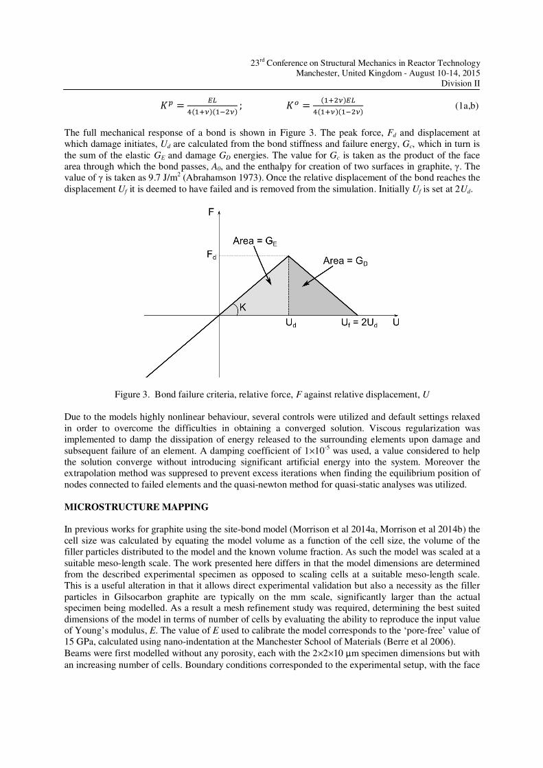
23rd
Conference on Structural Mechanics in Reactor Technology Manchester, United Kingdom - August 10-14, 2015
Division II
�� � ����� ��� ; �
� � ��� ����� ��� (1a,b)
The full mechanical response of a bond is shown in Figure 3. The peak force, Fd and displacement at
which damage initiates, Ud are calculated from the bond stiffness and failure energy, Gc, which in turn is
the sum of the elastic GE and damage GD energies. The value for Gc is taken as the product of the face
area through which the bond passes, A0, and the enthalpy for creation of two surfaces in graphite, γ. The
value of γ is taken as 9.7 J/m2 (Abrahamson 1973). Once the relative displacement of the bond reaches the
displacement Uf it is deemed to have failed and is removed from the simulation. Initially Uf is set at 2Ud.
Figure 3. Bond failure criteria, relative force, F against relative displacement, U
Due to the models highly nonlinear behaviour, several controls were utilized and default settings relaxed
in order to overcome the difficulties in obtaining a converged solution. Viscous regularization was
implemented to damp the dissipation of energy released to the surrounding elements upon damage and
subsequent failure of an element. A damping coefficient of 1×10⁻⁵ was used, a value considered to help
the solution converge without introducing significant artificial energy into the system. Moreover the
extrapolation method was suppresed to prevent excess iterations when finding the equilibrium position of
nodes connected to failed elements and the quasi-newton method for quasi-static analyses was utilized.
MICROSTRUCTURE MAPPING
In previous works for graphite using the site-bond model (Morrison et al 2014a, Morrison et al 2014b) the
cell size was calculated by equating the model volume as a function of the cell size, the volume of the
filler particles distributed to the model and the known volume fraction. As such the model was scaled at a
suitable meso-length scale. The work presented here differs in that the model dimensions are determined
from the described experimental specimen as opposed to scaling cells at a suitable meso-length scale.
This is a useful alteration in that it allows direct experimental validation but also a necessity as the filler
particles in Gilsocarbon graphite are typically on the mm scale, significantly larger than the actual specimen being modelled. As a result a mesh refinement study was required, determining the best suited
dimensions of the model in terms of number of cells by evaluating the ability to reproduce the input value
of Young’s modulus, E. The value of E used to calibrate the model corresponds to the ‘pore-free’ value of
15 GPa, calculated using nano-indentation at the Manchester School of Materials (Berre et al 2006).
Beams were first modelled without any porosity, each with the 2×2×10 μm specimen dimensions but with
an increasing number of cells. Boundary conditions corresponded to the experimental setup, with the face
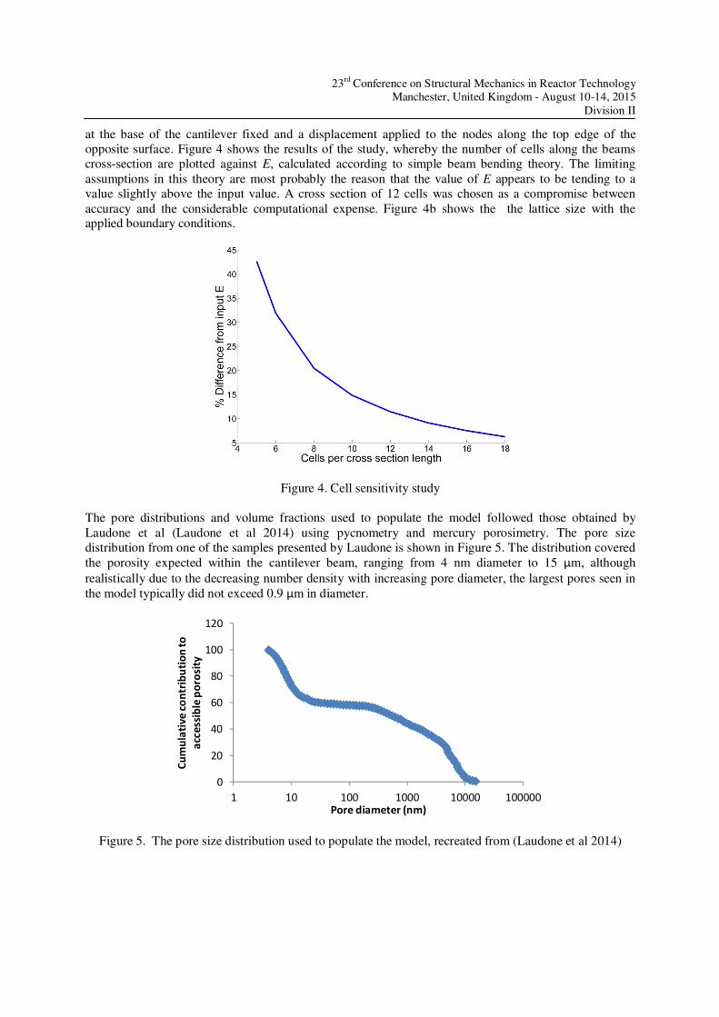
23rd
Conference on Structural Mechanics in Reactor Technology Manchester, United Kingdom - August 10-14, 2015
Division II
at the base of the cantilever fixed and a displacement applied to the nodes along the top edge of the
opposite surface. Figure 4 shows the results of the study, whereby the number of cells along the beams
cross-section are plotted against E, calculated according to simple beam bending theory. The limiting
assumptions in this theory are most probably the reason that the value of E appears to be tending to a
value slightly above the input value. A cross section of 12 cells was chosen as a compromise between
accuracy and the considerable computational expense. Figure 4b shows the the lattice size with the applied boundary conditions.
Figure 4. Cell sensitivity study
The pore distributions and volume fractions used to populate the model followed those obtained by
Laudone et al (Laudone et al 2014) using pycnometry and mercury porosimetry. The pore size
distribution from one of the samples presented by Laudone is shown in Figure 5. The distribution covered
the porosity expected within the cantilever beam, ranging from 4 nm diameter to 15 μm, although
realistically due to the decreasing number density with increasing pore diameter, the largest pores seen in
the model typically did not exceed 0.9 μm in diameter.
Figure 5. The pore size distribution used to populate the model, recreated from (Laudone et al 2014)
0
20
40
60
80
100
120
1 10 100 1000 10000 100000
Cu
mu
lati
ve
co
ntr
ibu
tio
n t
o
acc
ess
ible
po
rosi
ty
Pore diameter (nm)

23rd
Conference on Structural Mechanics in Reactor Technology Manchester, United Kingdom - August 10-14, 2015
Division II
The distributions presented by Laudone accounted only for pore volume accessible to the mercury
intrusion, with the closed pore volume calculated separately from the density of the samples. The pore volume fraction used as input to the model was the average minimum total porosity (i.e. both open and
closed) across all the samples under the assumption that the closed porosity would follow the same size
distribution as the open porosity. This value was 19.14%.
Pores were selected randomly from the distribution before being assigned to a randomly selected bond.
This process was repeated until the desired pore volume fraction was achieved. This process was found to
be time-consuming and largely unnecessary when considering the smaller pores which made up the
majority of those selected. The mismatch between the cell size and the size of the smaller pores meant that many pores were assigned to each face when populating the model. This essentially smeared out the
effect of the smaller pores with the minority of larger pores selected from the tail-end of the distribution
dictating when the model reached the target porosity. In response to this an arbitrary cut-off point
(significantly lower than the critical pore size for a cell face) was chosen, whereby the cumulative volume
fraction of the pores beneath this point and thence the cumulative volume could be divided by the total
number of bonds and assigned to every face as a single effective-pore. A volume bias was implemented
so octahedral bonds received a greater share of this porosity than principal bonds in accordance with its greater associated support volume. This allowed a simple treatment of approximately 75% of the bonds
and resulted in each bond being 15% failed (i.e. 15% of its volume was occupied by pores) before larger
pores were assigned. Micro-cracks are considered to initiate at pores and as such pores are represented in the model by a
change in bond mechanical response. The pore-free response, Figure 3, was scaled according to the size
of the pore present on the particular face, as shown in Figure 6. The change of peak force from the pore-
free value, Fd, to the new value, F’d, is related to the change of an effective area, Equation 2:
�����
� ������ ��
(2)
where V is the support volume of the face and V’ is the support volume remaining after the corresponding pore volume is removed, Equation 3:
�� � �������� �!�"# − ����# (3)
In the same manner, the displacement at which damage initiates, Ud, scales to the new value, U’d
according to the change an effective length, Equation 4:
%��%�
� ����� ��
(4)
The stored elastic energy, GE, thus scales with the change of support volume, Equation 5:
%�����%���
� ��� (5)
Differently, the damage energy, GD, is considered to scale with the real face area, Equation 6:
&%�'�%��(���&%'�%�(��
� )�) (6)
where A’ is the face area remaining after the corresponding pore area is removed, Equation 7:
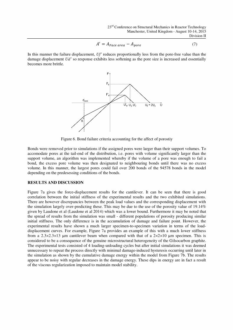
23rd
Conference on Structural Mechanics in Reactor Technology Manchester, United Kingdom - August 10-14, 2015
Division II
*� � *�+,#+�#+ − *���# (7)
In this manner the failure displacement, Uf’ reduces proportionally less from the pore-free value than the
damage displacement Ud’ so response exhibits less softening as the pore size is increased and essentially
becomes more brittle.
Figure 6. Bond failure criteria accounting for the affect of porostiy
Bonds were removed prior to simulations if the assigned pores were larger than their support volumes. To
accomodate pores at the tail-end of the distribution, i.e. pores with volume significantly larger than the
support volume, an algorithm was implemented whereby if the volume of a pore was enough to fail a
bond, the excess pore volume was then designated to neighbouring bonds until there was no excess
volume. In this manner, the largest pores could fail over 200 bonds of the 94578 bonds in the model
depending on the predesessing conditions of the bonds.
RESULTS AND DISCUSSION
Figure 7a gives the force-displacement results for the cantilever. It can be seen that there is good
correlation between the initial stiffness of the experimental results and the two exhibited simulations.
There are however discrepancies between the peak load values and the corresponding displacement with
the simulation largely over-predicting these. This may be due to the use of the porosity value of 19.14%
given by Laudone et al (Laudone et al 2014) which was a lower bound. Furthermore it may be noted that
the spread of results from the simulation was small - different populations of porosity producing similar
initial stiffness. The only difference is in the accumulation of damage and failure point. However, the
experimental results have shown a much larger specimen-to-specimen variation in terms of the load-
displacement curves. For example, Figure 7a provides an example of this with a much lower stiffness
from a 2.3×2.3×13 μm cantilever beam when compared with that of a 2×2×10 μm specimen. This is
considered to be a consequence of the genuine microstructural heterogeneity of the Gilsocarbon graphite.
The experimental tests consisted of 4 loading-unloading cycles but after initial simulations it was deemed
unnecessary to repeat the process directly with minimal damage-induced hysteresis occurring until later in
the simulation as shown by the cumulative damage energy within the model from Figure 7b. The results
appear to be noisy with regular decreases in the damage energy. These dips in energy are in fact a result
of the viscous regularization imposed to maintain model stability.

23rd
Conference on Structural Mechanics in Reactor Technology Manchester, United Kingdom - August 10-14, 2015
Division II
Figure 7. Experimental and computational (a) force-displacement; and (b) damage energy results for the
2×2×10 μm cantilever beam.
The open-source software ParaView was used to visualise damage within the model. Figure 8 shows the initial porosity for simulation 2, where the clusters of failed bonds representing large pores are clearly
visible. Figures 9a and 9b show the development of failed bonds within the model - at an intermediate
load increment corresponding to a displacement of 2.2 μm and the final increment before final failure,
respectively. These represents the distributed damage within the deformed volume prior to the fracture at
peak load, which is consistent with the observation of other workers (Hodgkins 2010) It can be seen from
Figures 9a and 9b that damage occurs at the root of the beam leading to shearing at the wall. It appears
that failed bonds are primarily principal bonds and the damage progresses from the bonds loaded in tension along the top surface, vertically down through the sample as the load is increased and the tension
bearing bonds fail. This crack development from top to bottom, as seen in Figure 9c, is largely to be
expected, although it differs slightly from that seen experimentally, Figure 1b, where the crack begins on
the top surface but away from the root before progressing towards the root. This discrepancy suggests
there may be additional complexity of the local microstructure of that particular beam has not been
experimentally determined, hence not considered in the modelling.
Figure 8. Initial porosity for simulation 2
(a) (b)

23rd
Conference on Structural Mechanics in Reactor Technology Manchester, United Kingdom - August 10-14, 2015
Division II
Figure 9. Failed bonds after: (a) 3000 increments; (b) final increment. (c) Relative displacement in the
failed model
CONCLUSION
The site-bond technology has been adapted to consider a two-phase (matrix and pores) graphite micro-
cantilever beam. Results are promising and physically realistic, but slight discrepancy between
experimental and simulated force-displacement results has been observed. This can be attributed to the
large spread seen from sample to sample in the physical tests. The failure of the beam occurs after accumulation of damage at its root with the distributed porosity throughout the rest of the beam having
apparently negligible effect to the point of global failure. Further work will involve implementation of the
site-bond methodology to graphite under different loading conditions with a view to visualisation of damage accumulation and derivation of a damage evolution law. Furthermore, it is necessary to explore
new avenues for model calibration that are consistent with discretized elasticity theories (Yavari 2008).
ACKNOWLEDGEMENTS
Craig N Morrison acknowledges the support from EPSRC via Nuclear FiRST Doctoral Training Centre.
Mingzhong Zhang, Dong Liu and Andrey P Jivkov acknowledge the support from EPSRC via grants EP/J019763/1 and EP/J019801/1, “QUBE: Quasi-Brittle fracture: a 3D experimentally-validated
approach”. Moreover Mingzhong Zhang and Andrey P Jivkov acknowledge BNFL through the Research
Centre for Radwaste & Decommissioning.
REFERENCES
Abrahamson, J. (1973). “The surface energies of graphite”. Carbon, 11, 337-362. Berre, C., Fok, S.L., Marsden, B.J., Babout, L., Hodgkins, A., Marrow, T.J., Mummery, P.M. (2006).
“Numerical modelling of the effects of porosity changes on the mechanical properties of nuclear
graphite”. Journal of Nuclear Materials, 352, 1-5.
(a) (b)
(c)

23rd
Conference on Structural Mechanics in Reactor Technology Manchester, United Kingdom - August 10-14, 2015
Division II
de Borst, R. (2002). “Fracture in quasi-brittle materials: a review of continuum damage-based
approaches”. Engineering Fracture Mechanics, 69, 95-112. Hodgkins, A., Marrow, T.J., Wootton, M.R., Moskovic, R., Flewitt, P.E.J. (2010). “Fracture behaviour of
radiolytically oxidised reactor core graphites: a view”. Materials Science and Technology, 26(8),
899-907.
Jenkins, G. (1962). “Fracture in reactor graphite”. Journal of Nuclear Materials, 3(3), 280-286.
Jivkov, A.P. (2014). “Structure of micro-crack population and damage evolution in quasi-brittle media”.
Theoretical and Applied Fracture Mechanics, 70, 1-9.
Jivkov, A.P., Gunther M, Travis KP (2012). “Site-bond modelling of porous quasi-brittle media”. Mineralogical Magazine, 76(8), 2969-2974.
Jivkov, A.P., Morrison, C.N., Zhang, M. (2014a) “Site-bond modelling of structure-failure relations in
quasi-brittle media”, Procedia Materials Science, 3, 1872-1877.
Jivkov, A.P., Todorov, T., Morrison, C.N., Zhang, M. (2014b) “Application of analysis on graphs to site-
bond models for damage evolution in heterogeneous materials”, Proc. 11th World Congress on
Computational Mechanics and 5th European Conference on Computational Mechanics.
Jivkov, A.P. and Yates, J.R. (2012). “Elastic behaviour of a regular lattice for meso-scale modelling of solids”. International Journal of Solids and Structures, 49(22), 3089-3099.
Kumar, S., Kurtz, S.K., Banavar, J.R., Sharma, M.G. (1992), “Properties of a three-dimensional Poisson-
Voronoi tessellation: A Monte Carlo study”, Journal of Statistical Physics, 67(3-4), 523-551. Liu, D., Heard, P.J., Nakhodchi, S., Flewitt, P.E.J. (2014), “Small-Scale Approaches to Evaluate the
Mechanical Properties of Quasi-Brittle Reactor Core Graphite”. ASTM symposium, Graphite
Testing for Nuclear Applications: The Significance of Test Specimen Volume and Geometry and the
Statistical Significance of Test Specimen Population, ASTM International, 1-21.
Laudone, G.M., Gribble, C. M., Matthews, G. P. (2014). “Characterisation of the porous structure of
Gilsocarbon graphite using pycnometry, cyclic porosimetry and void-network modeling”. Carbon,
73, 61-70. Mantell, C.L. (1968). Carbon and Graphite Handbook, Interscience Publishers
Morrison, C.N., Zhang, M. Jivkov, A.P. (2014a). “Discrete lattice model of quasi-brittle fracture in
porous graphite”. Materials Performance and Characterization, 3, 414-429, ASTM International Morrison, C.N., Zhang, M., Jivkov, A.P. (2014b). “Fracture energy of graphite from microstructure-
informed lattice model”. Procedia Materials Science, 3, 1848-1853.
Nemeth, N. Bratton, R. (2010). “Overview of statistical models of fracture for nonirradiated nuclear-
graphite”. Nuclear Engineering and Design, 240, 1-29.
Schlangen, E. (2008). “Crack development in Concrete, Part 2: Modelling of Fracture Process”. Key
Engineering Materials, 385-387, 73-76.
Schlangen, E., Flewitt, P.E.J., Smith, G.E., Crocker, A.G., Hodgkins, A. (2010). “Computer Modelling of Crack Propagation in Porous Reactor Core Graphite”. Key Engineering Materials, 452-453, 729-
732.
Schlangen, E. and Garboczi, E. (1997). “Fracture simulations of concrete using lattice models: computational aspects”. Engineering Fracture Mechanics, 57(2), 319-332.
Simulia, Abaqus Version 6.13 Documentation, Dassault systemes, 2013.
Turner, M.J., Clough, R.W., Martin, H.C., Topp, L.J. (1956). “Stiffness and Deflection Analysis of
Complex Structures”, Journal of Aeronautical Sciences, 23(9), 805-824.
Yavari, A. (2008). “On geometric discretization of elasticity”, Journal of Mathematical Physics, 49(2),
022901.
Zhang, M., Morrison, C.N., Jivkov, A.P. (2014a). “A lattice-spring model for damage evolution in cement paste”, Procedia Materials Science, 3, 1854-1859.
Zhang, M., Morrison, C.N., Jivkov, A.P. (2014b). “A meso-scale site-bond model for elasticity: Theory
and calibration”. Materials Research Innovations, 18, 982-986.

Appendix I
Multi-scale modelling of nuclear
graphite tensile strength using the
Site-Bond lattice model
194
Multi-scale modelling of nuclear graphite tensile strength using thesite-bond lattice model
C.N. Morrison a, *, A.P. Jivkov a, Ye. Vertyagina b, T.J. Marrow b
a Modelling and Simulation Centre, School of Mechanical, Aerospace and Civil Engineering, The University of Manchester, UKb Department of Materials, The University of Oxford, UK
a r t i c l e i n f o
Article history:Received 22 September 2015Received in revised form8 December 2015Accepted 30 December 2015Available online 2 January 2016
a b s t r a c t
Failure behaviour of graphite is non-linear with global failure occurring when local micro-failures,initiated at stress-raising pores, coalesce into a critically sized crack. This behaviour can be reproducedby discrete lattices that simulate larger scale constitutive responses, derived from knowledge ofmicrostructure features and failure mechanisms. A multi-scale modelling methodology is presentedusing a 3D Site-Bond lattice model. Microstructure-informed lattices of both filler and matrix constitu-ents or ‘phases’ in Gilsocarbon nuclear graphite are used to derive their individual responses. These arebased on common elastic modulus of “pore-free” graphite, with individual responses emerging frompore distributions in the two phases. The obtained strains compare well with experimentally obtaineddata and the stress-strain behaviour give insight into the deformation and damage behaviour of eachphase. The responses of the filler and matrix are used as inputs to a larger scale composite lattice modelof the macroscopic graphite. The calculated stress-strain composite behaviour, including modulus ofelasticity and tensile strength, is in acceptable agreement with experimental data reported in theliterature, considering the limited microstructure data used for model's construction. The outcomesupports the applicability of the proposed deductive approach to the derivation of macroscopicproperties.© 2016 The Authors. Published by Elsevier Ltd. This is an open access article under the CC BY license
(http://creativecommons.org/licenses/by/4.0/).
1. Introduction
Synthetic graphite has been used in the nuclear industry as afast neutron moderator since the first demonstration of a chainnuclear reaction in the 1940s. Its retention of strength at elevatedtemperatures has allowed it to be used as a structural component inhigh temperature gasecooled reactor designs [1]. Nuclear graphitecan be regarded as having a three-phase microstructure, whichdepends on the rawmaterials and the manufacturing process used.Filler particles, which derive from calcined petroleum or pitch coke,are dispersed within a matrix of binder material, usually consistingof graphitised coal-tar pitch mixed with finely ground filler parti-cles. Both of these solid phases host populations of pores, with sizesthat cover the length scale from a few nm upwards to mm [2].Graphite belongs to the class of quasi-brittle materials, whichexhibit limited non-linear stress/strain response prior to maximumor peak stress, with a macroscopic effect akin to plasticity [3]. This
non-linearity is partly attributed to the generation and growth ofmicro-cracks, which occur at length scales dictated by the promi-nent microstructure features. As tensile strain is applied, micro-cracks initiate around the larger pores due to local stress amplifi-cation, and their effect leads to a reduction in graphite's stiffness[4]. Ultimate tensile failure results from crack growth and coales-cence into a flaw of critical size [4]. The continued evolution ofthese processes determines the behaviour beyond the peak stress;graphite may exhibit a limited post-peak softening or fail at peak-stress, depending on its microstructure and the loading condi-tions [3]. Therefore, the structural integrity of nuclear graphite iscontrolled by the organisation of the three phases (filler, matrix andpores) and the component's service conditions.
Conventional modelling strategies, such as the finite elementmethod [5], assume the behaviour within model elements is ho-mogeneous and scale-independent, which inherently fails to ac-count for the effects of microstructure failure mechanisms in thematerial response. This might be inappropriate in certain cases,particularly when modelling the graphite responses at lengthscales close to its microstructure features. If fracturemechanics is to* Corresponding author.
E-mail address: [email protected] (C.N. Morrison).
Contents lists available at ScienceDirect
Carbon
journal homepage: www.elsevier .com/locate/carbon
http://dx.doi.org/10.1016/j.carbon.2015.12.1000008-6223/© 2016 The Authors. Published by Elsevier Ltd. This is an open access article under the CC BY license (http://creativecommons.org/licenses/by/4.0/).
Carbon 100 (2016) 273e282

be used in the structural integrity assessment of nuclear graphite,the fracture process zone ahead of a macroscopic crack is of specificinterest, as this is influenced by microstructure features and spec-imen size [3], [6]. Integrity assessment requires local information insuch cases.
Local effects have been incorporated into various modellingapproaches. This can be done either statistically, using the weakestlink assumption [7], or within a continuum framework extended bycohesive zonemodels [8]. However, these approaches are restrictedby a dependence on phenomenological calibration against macro-scale data. Lattice models are a branch of discrete modelswhereby nodes are connected by elements into a statistically par-allel network. Such models have been developed for quasi-brittlematerials including graphite [7] [9], and concrete [10e11], incor-porating microstructure information into the element properties toallow the simulation of macro-scale behaviour as a consequence ofmicro-failure mechanisms. Lattice models can be constructed asirregular, representing specific, usually imaged, microstructures, orregular. Irregular models present a substantial problem, as thecalibration of lattice element properties with measured continuumproperties becomes a trial and error process. Regular models can becalibrated in many cases analytically and allow for up-scaling topotentially representative volume elements, although one issuewith most 3D regular lattices has been that they could not be tunedto reproduce desired Poisson's ratio values [12]. The regular 3D site-bond model proposed by Jivkov and Yates [13] is capable ofreproducing the range of Poisson's ratio required for quasi-brittlematerials, and this model has been further extended in thisresearch.
The original model, using beams as lattice elements, was firstlyapplied to study damage evolution in concrete in tension [14] andunder complex loads [15]. One problem with that formulation isthat the structural beams between nodes introduce local micro-polar behaviour in the lattice, i.e. rotation-dependent energy con-servation. That behaviour has not been confirmed experimentallyand consequently the calibration of beam properties remainsincomplete. To avoid this, the site-bond model has been reformu-lated with spring bundles, the stiffness coefficients of which havebeen calibrated analytically [16]. The work presented here makes asubstantial step in the development of the site-bond model with anew approach to represent lattice elements and their behaviour.Experimentally-derived distributions of microstructure features[17] are used to inform separate site-bond lattice models for fillerand matrix constituents (i.e. phases) in the microstructure of near-isotropic Gilsocarbon graphite. The results are compared withexperimental data of the tensile deformation of the individualconstituents, obtained recently by strain imaging of the micro-structure during a mechanical test of the same graphite [18]. Briefdetails of that experiment and the data obtained are provided here.The experimentally measured response of the separate micro-structure constituents is then used to inform a multi-scale site-bond methodology. Such a model may complement and scientifi-cally underpin the conservatism of structural integrity assessmentmethodologies for graphite, providing size estimates for areas ofsignificant local damage ahead of macroscopic cracks, or damageevolution laws for use in continuum scale models.
2. Theory and method
Within the site-bond methodology [13], material volume isrepresented with a discrete assembly of truncated octahedral cellsillustrated in Fig. 1(a). This choice of shape is in accordance withstatistical studies that demonstrate its suitability for representing atopologically averaged microstructure [19]. The computationalcounterpart of the regular assembly is a 3D lattice, or mathematical
graph, consisting of sites at cell centres, connected by bonds to 14neighbouring sites. This yields two distinct bond types, B1 and B2,which emanate from sites in the 6 principal (normal to squarefaces) and 8 octahedral (normal to hexagonal faces) directions,respectively, as illustrated in Fig. 1(b). The bond types have lengthsL and
ffiffiffi3
pL/2, with L representing the cell extension in the principal
directions. The bonds' behaviour is associated with an inter-cellvolume, called the support volume, formed by the two pyramidswith common base at the face normal to the bond; Fig. 1(c) showsthe support volume of a principal bond. An example of a site-bondmodel is given in Fig. 1(d).
Previously the site-bond model has been applied to the three-phase graphite microstructure, i.e. matrix, filler particles andpores, with filler particles considered to be located at sites and tooccupy fractions of cell volumes, pores considered to be located insome support volumes, and the remaining volume occupied bymatrix [20]. In this manner, the network of bonds, modelled asbundles of independent springs, one axial and two transversal,represent the potential micro-failures both within and betweenparticles. With the mapping of particles to sites, the model lengthscale, L, has been determined from experimentally measured par-ticle size distribution and volume fraction. With known L, thesprings' stiffness coefficients have been calculated from the energyequivalence between discrete and continuum cells under homo-geneous strain fields according to the procedure outlined by Zhanget al. [16]. This methodology, derived specifically for the site-bondgeometry, allows for accurate representation of isotropic elasticmaterials with Poisson's ratio ranging from �1 to 0.5, animprovement on previous lattice arrangements where only zeroPoisson's ratio has been allowed [12].
However, when the observable microstructure cannot beconsidered as a three-phase composite, but rather a two-phasecomposite with pores dispersed in a solid, the model length scalecannot be calculated in the same manner. In such a case (e.g.Ref. [21]), the model length scale is arbitrary, and similarly to thefinite element analysis, improved accuracy is achieved by reducing
Fig. 1. The site-bond lattice model; (a) cellular tessellation; (b) sites and bonds in atruncated octahedral cell; (c) bond support volume; (d) site-bond model representedas a network of sites and bonds. (A color version of this figure can be viewed online.)
C.N. Morrison et al. / Carbon 100 (2016) 273e282274
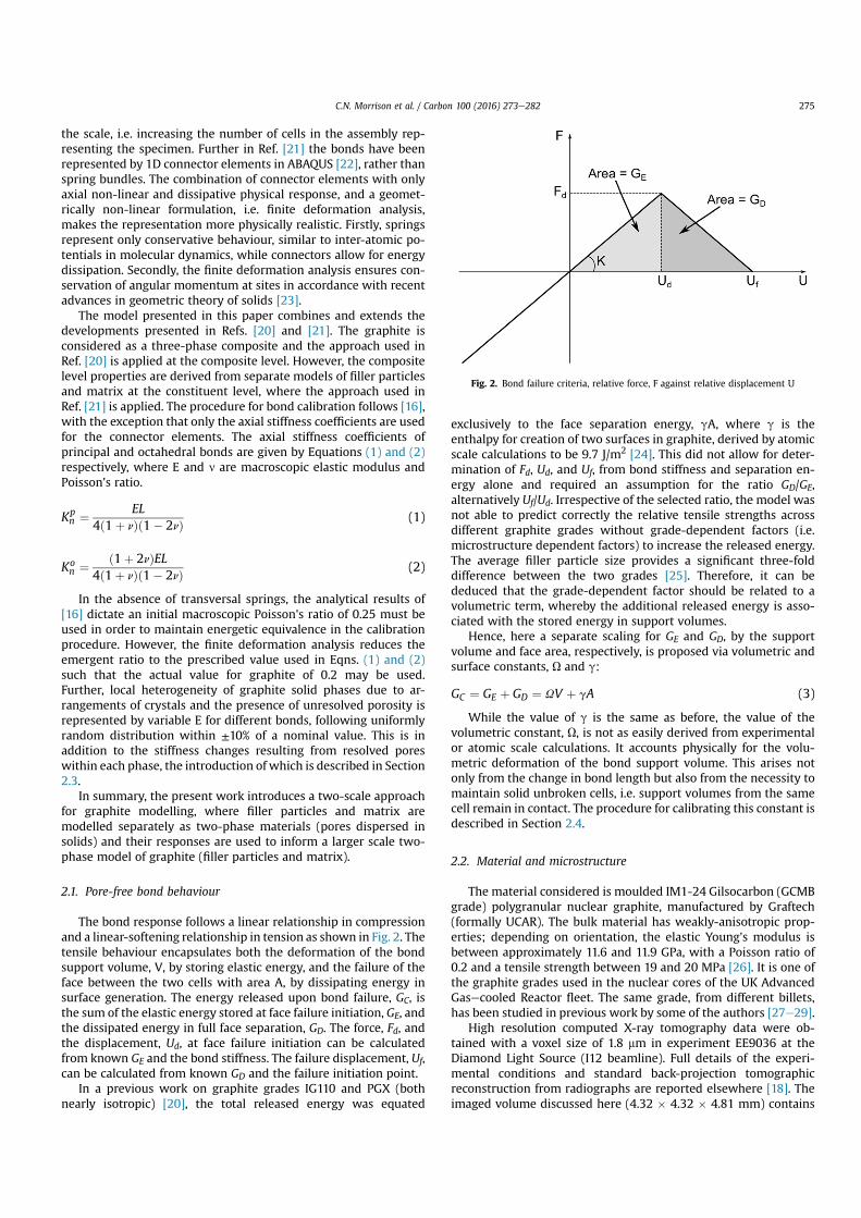
the scale, i.e. increasing the number of cells in the assembly rep-resenting the specimen. Further in Ref. [21] the bonds have beenrepresented by 1D connector elements in ABAQUS [22], rather thanspring bundles. The combination of connector elements with onlyaxial non-linear and dissipative physical response, and a geomet-rically non-linear formulation, i.e. finite deformation analysis,makes the representation more physically realistic. Firstly, springsrepresent only conservative behaviour, similar to inter-atomic po-tentials in molecular dynamics, while connectors allow for energydissipation. Secondly, the finite deformation analysis ensures con-servation of angular momentum at sites in accordance with recentadvances in geometric theory of solids [23].
The model presented in this paper combines and extends thedevelopments presented in Refs. [20] and [21]. The graphite isconsidered as a three-phase composite and the approach used inRef. [20] is applied at the composite level. However, the compositelevel properties are derived from separate models of filler particlesand matrix at the constituent level, where the approach used inRef. [21] is applied. The procedure for bond calibration follows [16],with the exception that only the axial stiffness coefficients are usedfor the connector elements. The axial stiffness coefficients ofprincipal and octahedral bonds are given by Equations (1) and (2)respectively, where E and n are macroscopic elastic modulus andPoisson's ratio.
Kpn ¼ EL
4ð1þ nÞð1� 2nÞ (1)
Kon ¼ ð1þ 2nÞEL
4ð1þ nÞð1� 2nÞ (2)
In the absence of transversal springs, the analytical results of[16] dictate an initial macroscopic Poisson's ratio of 0.25 must beused in order to maintain energetic equivalence in the calibrationprocedure. However, the finite deformation analysis reduces theemergent ratio to the prescribed value used in Eqns. (1) and (2)such that the actual value for graphite of 0.2 may be used.Further, local heterogeneity of graphite solid phases due to ar-rangements of crystals and the presence of unresolved porosity isrepresented by variable E for different bonds, following uniformlyrandom distribution within ±10% of a nominal value. This is inaddition to the stiffness changes resulting from resolved poreswithin each phase, the introduction of which is described in Section2.3.
In summary, the present work introduces a two-scale approachfor graphite modelling, where filler particles and matrix aremodelled separately as two-phase materials (pores dispersed insolids) and their responses are used to inform a larger scale two-phase model of graphite (filler particles and matrix).
2.1. Pore-free bond behaviour
The bond response follows a linear relationship in compressionand a linear-softening relationship in tension as shown in Fig. 2. Thetensile behaviour encapsulates both the deformation of the bondsupport volume, V, by storing elastic energy, and the failure of theface between the two cells with area A, by dissipating energy insurface generation. The energy released upon bond failure, GC, isthe sum of the elastic energy stored at face failure initiation, GE, andthe dissipated energy in full face separation, GD. The force, Fd, andthe displacement, Ud, at face failure initiation can be calculatedfrom known GE and the bond stiffness. The failure displacement, Uf,can be calculated from known GD and the failure initiation point.
In a previous work on graphite grades IG110 and PGX (bothnearly isotropic) [20], the total released energy was equated
exclusively to the face separation energy, gA, where g is theenthalpy for creation of two surfaces in graphite, derived by atomicscale calculations to be 9.7 J/m2 [24]. This did not allow for deter-mination of Fd, Ud, and Uf, from bond stiffness and separation en-ergy alone and required an assumption for the ratio GD/GE,alternatively Uf/Ud. Irrespective of the selected ratio, the model wasnot able to predict correctly the relative tensile strengths acrossdifferent graphite grades without grade-dependent factors (i.e.microstructure dependent factors) to increase the released energy.The average filler particle size provides a significant three-folddifference between the two grades [25]. Therefore, it can bededuced that the grade-dependent factor should be related to avolumetric term, whereby the additional released energy is asso-ciated with the stored energy in support volumes.
Hence, here a separate scaling for GE and GD, by the supportvolume and face area, respectively, is proposed via volumetric andsurface constants, U and g:
GC ¼ GE þ GD ¼ UV þ gA (3)
While the value of g is the same as before, the value of thevolumetric constant, U, is not as easily derived from experimentalor atomic scale calculations. It accounts physically for the volu-metric deformation of the bond support volume. This arises notonly from the change in bond length but also from the necessity tomaintain solid unbroken cells, i.e. support volumes from the samecell remain in contact. The procedure for calibrating this constant isdescribed in Section 2.4.
2.2. Material and microstructure
The material considered is moulded IM1-24 Gilsocarbon (GCMBgrade) polygranular nuclear graphite, manufactured by Graftech(formally UCAR). The bulk material has weakly-anisotropic prop-erties; depending on orientation, the elastic Young's modulus isbetween approximately 11.6 and 11.9 GPa, with a Poisson ratio of0.2 and a tensile strength between 19 and 20 MPa [26]. It is one ofthe graphite grades used in the nuclear cores of the UK AdvancedGasecooled Reactor fleet. The same grade, from different billets,has been studied in previous work by some of the authors [27e29].
High resolution computed X-ray tomography data were ob-tained with a voxel size of 1.8 mm in experiment EE9036 at theDiamond Light Source (I12 beamline). Full details of the experi-mental conditions and standard back-projection tomographicreconstruction from radiographs are reported elsewhere [18]. Theimaged volume discussed here (4.32 � 4.32 � 4.81 mm) contains
Fig. 2. Bond failure criteria, relative force, F against relative displacement U
C.N. Morrison et al. / Carbon 100 (2016) 273e282 275

filler, matrix and pores. The pores have lower X-ray attenuation;there is also some incidental phase contrast due to the imagingconditions, which aids the detection of pores. The regions of fillerandmatrix can then be identified by themorphology of their pores;filler particles exhibit a characteristic onion-skin structure oflenticular pores, and the matrix has a less organised structure,Fig. 3.
A total of 55 filler particles and 25 matrix sub-volumes ofdifferent sizes were extracted from the dataset. The smallest vol-ume of a selected filler particle is 0.05 mm3, and the largest volumeis 4.4 mm3. The matrix volumes vary from 0.16 to 1.16 mm3. Theresults for both phases are shown in Fig. 4.
The microstructures may be segmented using an image in-tensity threshold to define the pores and solid graphite. All X-raytomography images were converted to 8-bit datasets before thesegmentation. It was not possible to apply a single threshold for thegrey-scale dataset, so the segmentation procedure was performedin ImageJ software using a multi-step thresholding with the cor-responding smoothing and binarisation steps for pore boundarydetermination and large pore filling. The thresholds were verifiedvisually by comparisonwith the original grey-scale image. The fillerparticle boundaries have been manually identified by using thevisible matrix pores, which surrounded a particle. These pores arequite large and have a well distinguishable structure that isdifferent from the lenticular pores of the particle. Parts of theparticle boundary connected with solid matrix were restored thenassuming the ellipsoidal shape of the particle. The shape of theunbroken Gilsocarbon filler particles is typically ellipsoidal, oftenclose to a spherical shape. Analyses of tomographic data from thesame graphite billet found that the fraction of filler particles varieswithin 14e29%; the fraction in the volume from Ref. [18] is 29%.
Within both phases the smallest pore volume that could beresolved was restricted by the resolution of the tomography data.The mean filler pore volume throughout the imaged volume is15080 mm3 (standard deviation 6320 mm3). The pores in the matrixhave very different shapes and cover a wide range of volumes from6 to 105 mm3; the most frequent pore volume is approximately100 mm3. The largest individual pores observed occupy a volume ofabout 106 mm3 in the filler and 105 mm3 in the matrix; more than90% of the total pore volume in a subset may be spatially combinedinto one large pore. It is important to note that the selection of
matrix volumes excluded regions that contained larger pores(>100 mm), which occur due to gas porosity. These pores have beenquantified using laboratory tomography data of lower resolution(Skyscan 1272) (10 mm/voxel), their fraction has been estimated as6.3% of the total volume of the sample.
The porosity fraction in the different phases was extracted for arandomly selected subset of 20 filler particles and 7matrix volumesfrom tomographed volumes of the same graphite billet [17]. Theobserved porosity fraction in the filler is typically lower than in thematrix; the mean porosity of the filler subsets is 12.2% with astandard deviation of 3.6%, while the matrix has average porosity of16% and a standard deviation of 3.1%. The cumulative probability forporosity observed in both filler and matrix phases are shown inFig. 5(a). A region was chosen at random for each phase, so that itspore size distribution could be used for the subsequent simulations.The pore size distribution from the selected region for both phasesis shown in Fig. 5(b) with the filler and matrix samples containing1204 and 24394 pores respectively.
The deformation of filler and matrix, up to an applied tensilestress of 7.5 MPa, has been studied by digital volume correlation(DVC) of X-ray computed tomography images, obtained during atensile test. Full details of test and the image correlation analysisare reported elsewhere [18]. Briefly, the DVC analysis of sub-volumes that contained filler and matrix was used to calculatethe axial strains in each xy-plane as the gradient of the averagevertical displacements in the z-direction, which corresponded tothe tensile axis. Only those displacements contained inside theellipsoidal volume that defined the filler particle have beenconsidered for the filler. In the studied volumes, the axial strain at250 MPa applied stress varies from 0.0003 to 0.001 in the filler andfrom 0.0005 to 0.0013 in the matrix; the average axial strain islarger in the matrix (774 mε ± 178 mε) than for the filler particles(667 mε ± 197 mε), which suggests the elastic modulus of the matrixmay be lower. The mean strain of the tomographed volume of thetensile sample at 250 MPa was measured to be 730 mε.
2.3. Pore-affected bond behaviour
The mapping of microstructure to the model follows the pro-cedure outlined in a previous work [21] whereby micro-cracks areconsidered to initiate at pores. Pores, with sizes selected at randomfrom an experimental pore size distribution, are assigned to faces of
Fig. 3. A reconstructed X-ray computed tomographic image of Gilsocarbon micro-structure. Coarse filler particles can be seen dispersed within a matrix of graphitizedpitch and finer (ground) filler particles. Pores can be seen as dark regions as a result oflow X-ray attenuation. Blue inserts show segmented structures of the pores within thematrix (top) and filler (bottom) sub-volumes. (A color version of this figure can beviewed online.)
Fig. 4. Filler particle and matrix sample volumes. (A color version of this figure can beviewed online.)
C.N. Morrison et al. / Carbon 100 (2016) 273e282276

cells until the desired porosity is reached. The presence of porosityis reflected in changes of the tensile response of correspondingbonds, Fig. 6. The peak force changes from the pore-free value, Fd, toa new value, F'd, according to
F 0dFd
¼�V 0
V
�2=3
(4)
where V is the support volume of the bond and V0 is the supportvolume remaining after the corresponding pore volume isremoved, i.e.
V0 ¼ VSupport volume � Vpore (5)
In the same manner, the displacement at face failure initiation,Ud, changes to a new value, U'd, according to
U0d
Ud¼
�V 0
V
�1=3
(6)
Equations (4) and (6) represent pore-corrected force anddisplacement parameters via pore-corrected (or effective) areasand lengths, respectively.
The stored elastic energy at face failure initiation, GE, scales withthe change of support volume:
U0dF
0d
UdFd¼ V 0
V(7)
Differently, the damage energy, GD, scales with the face area:
�U0f � U0
d
�F 0d�
Uf � Ud
�Fd
¼ A0
A(8)
where A0 is the face area remaining after the corresponding porearea is removed:
A0 ¼ AFace area � Apore (9)
In this manner, the failure displacement, Uf’, reduces propor-tionally less from the pore-free value than the initiation displace-ment, Ud’, so the amount of softening is reduced as the pore size isincreased, resulting in an increasingly brittle response. The bondstiffness is also reduced.
Similarly to tensile behaviour, the presence of porosity also al-ters the compressive response of the bond. Compressive stiffness isreduced by the same factor as tensile stiffness according to poresize, although this decrease is only maintained for a relativedisplacement equivalent to the diameter of the pore present, afterwhich time the stiffness increases back to the original value.
In the process of random pore allocation to faces, some porevolumes may exceed the corresponding bond support volumes.Such bonds are removed from the model and the excess pore vol-ume, i.e. the difference between the allocated pore volume and theremoved support volume, is distributed to neighbouring bonds inthe same manner until all the volume is allocated. In this mannerthe size distribution of pores distributed to faces will be a repre-sentative sample of the experimental distribution, although thespatial distribution of pores will be entirely random.
2.4. Calibration of the volumetric constant
Preliminary studies using the pore representation outlined inSub-section 2.3 were undertaken to calibrate the volumetric con-stant. Four different grades of nuclear graphite, IG110, NBG-18, PGXand Gilsocarbon, were simulated with models scaled according tothe size and volume fraction of the corresponding filler particlesfollowing [20]. The microstructure information used for gradesIG110, NBG-18 and PGX, including pore size distributions, porosityand filler particle sizes was taken from the microscopy studies byKane et al. [25]. The filler particle size distribution used for the IM1-24 Gilsocarbon was that shown in Fig. 4. The microstructure dataused for all grades and the corresponding references are
Fig. 5. (a) Porosity distributions for the filler and matrix sub-volumes [17]; (b) poresize distributions for the randomly selected filler and matrix regions [17]. (A colorversion of this figure can be viewed online.)
Fig. 6. Bond failure criteria accounting for the affect of porosity
C.N. Morrison et al. / Carbon 100 (2016) 273e282 277

summarised in Table 1. A filler particle volume fraction may varywithin graphite grades. The value used was 0.2, an average of thetwo values obtained of 0.144 and 0.252 presented in Ref. [17].Although these values were specific to Gilsocarbon, the same fillerparticle volume fraction of 0.2 was used for all grades. The poredistributions taken from Ref. [25] do not differentiate betweenpores found in the matrix and filler phases. Hence, for simplicityonly the pore size distribution for the matrix phase, shown in Fig. 5,was used to calibrate the volumetric constant of the IM1-24 Gil-socarbon. It is not necessary to repeat the process for the fillerphase, because for a prescribed porosity its larger pores can beconsidered as represented in the model by the coalescence ofnumerous smaller pores assigned to one and the same lattice bond.
Measured Young's moduli, tensile strength and typical poros-ities for each grade in its virgin (i.e. as supplied, without any effectsof fast neutron irradiation or radiolytic oxidation) are shown inTable 1. To calculate the pore-free, axial stiffness coefficients ofbonds, pore-free values of the Young's moduli are required. Thesewere calculated with a series of normalised simulations withYoung's modulus equal to one, without porosity and with virginstate porosity. Several realizations with the latter were analysed,differing in the spatial distribution of pores but identical size dis-tributions. The simulations were performed without failure ofbonds, i.e. in the elastic regime of bond behaviour. From thesesimulations the ratios between the (unit) pore-free and the simu-lated average virgin-porosity moduli were calculated. The ratioswere used to scale the experimental virgin-porosity moduli topore-free moduli, reported in row 3, from where pore-free axialstiffness coefficients were calculated by Eqns. (1) and (2). The closeproximity of the calibrated pore-free modulus of Gilsocarbon,14955 MPa, to a pore-free value of 15 GPa, derived from nano-indentation experiments [30], gives confidence in the calibrationprocedure. In the absence of equivalent data (to the knowledge ofthe authors') for the other grades this is considered an adequatevalidation.
Models with calibrated coefficients were subject to displace-ment controlled uniaxial tension until failure, using the assumptionthat energy released at bond failure equals the energy of faceseparation, gA, specifically assuming as previously [20] [21].
GprelimE ¼ Gprelim
D ¼ 12Ag
�Uf ¼ 2Ud
�(10)
Failure was considered to be the point at which the simulationfailed to find equilibrium using a time increment size less than athreshold value (1 � 10�25 was deemed suitably small). Severalcontrol parameters were adapted to improve convergence in thehighly non-linear model. Viscous regularization was utilized toimprove the dissipation of energy from damaged bonds to thesurrounding bonds. A damping coefficient of 1 � 10�5 was chosenafter initial studies showed it gave the best compromise betweenaiding convergence and producing a consistent peak stress. Thequasi-Newton method was used for the analysis and the method ofextrapolation was suppressed, preventing excess iterations.
The difference in simulated and experimental values of tensile
strength, sSimT and sExpT , as a function of model cell size (volume), for
a model that does not include the proposed volumetric correction,is shown in Fig. 7 with red marks. Here, the cell size, shown inTable 1, reflects the different structures of the four graphite gradesin terms of particle size distribution. It is apparent that, when usingthe cell size as a representation of the average filler volume, therelationship between strength discrepancy and size is approxi-mately linear, i.e. the larger the average filler particle size the largerthe difference between simulated and expected tensile strength.
This relation between strength discrepancy and cell size occursfrom using the energy of face separation as a sole measure of en-ergy released upon bond failure, failing to account for the energeticseparation into area, GD ¼ gA, and volumetric terms, GE ¼ UV, asproposed in Section 2.1. As such the volumetric constant can becalibrated from the linear trend.
The peak bond force in the preliminary studies (without volu-metric term) and the proposed model can be expressed as:
FprelimD ¼ffiffiffiffiffiffiffiffiffiffiAgK
p(11)
FD ¼ffiffiffiffiffiffiffiffiffiffiffiffiffi2UVK
p(12)
with stiffness coefficient, K, being the same for both models. Thelinear trend shown in Fig. 7 can be expressed as:
sExpT
sSimT
� 1 ¼ mS (13)
where m is the gradient of the linear trend and S is the cell size.From comparison between simulations and experiment, one canwrite:
Table 1Comparisons between grades for model inputs (Young's modulus, virgin porosity), the resulting model cell size and literature values of tensile strength and mean particle size.
Graphite grade Gilsocarbon (IM1-24) IG110 NBG-18 PGX
Typical young's modulus (MPa) 11600 [26] 9800 [31] 11500 [32] 8300 [33]Calibrated pore-free young's modulus (MPa) 14955 11327 12446 9717Virgin porosity (%) 19.14 [34] 14.73 [25] 13.97 [25] 21.49 [25]Tensile strength (MPa) 19e20 [26] 25.3 [35] 20 [32] 8.1 [35]Mean particle size (major axis length) (mm) 914 [17] 27 ± 2 [25] 360 ± 25 [25] 92 ± 7 [25]Cell size (mm) 1591 79.7 854 297
Fig. 7. Calibration of the volumetric term. (A color version of this figure can be viewedonline.)
C.N. Morrison et al. / Carbon 100 (2016) 273e282278
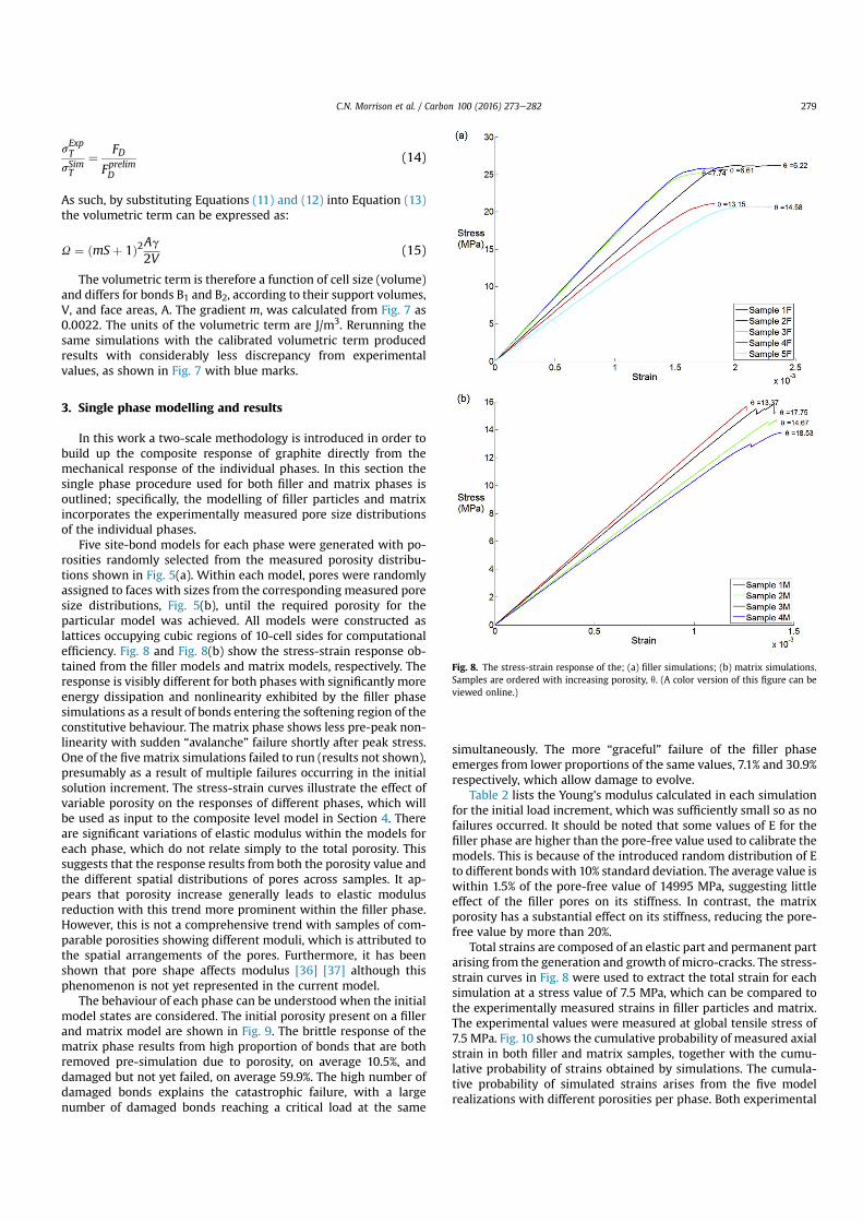
sExpT
sSimT
¼ FDFprelimD
(14)
As such, by substituting Equations (11) and (12) into Equation (13)the volumetric term can be expressed as:
U ¼ ðmSþ 1Þ2Ag2V
(15)
The volumetric term is therefore a function of cell size (volume)and differs for bonds B1 and B2, according to their support volumes,V, and face areas, A. The gradient m, was calculated from Fig. 7 as0.0022. The units of the volumetric term are J/m3. Rerunning thesame simulations with the calibrated volumetric term producedresults with considerably less discrepancy from experimentalvalues, as shown in Fig. 7 with blue marks.
3. Single phase modelling and results
In this work a two-scale methodology is introduced in order tobuild up the composite response of graphite directly from themechanical response of the individual phases. In this section thesingle phase procedure used for both filler and matrix phases isoutlined; specifically, the modelling of filler particles and matrixincorporates the experimentally measured pore size distributionsof the individual phases.
Five site-bond models for each phase were generated with po-rosities randomly selected from the measured porosity distribu-tions shown in Fig. 5(a). Within each model, pores were randomlyassigned to faces with sizes from the corresponding measured poresize distributions, Fig. 5(b), until the required porosity for theparticular model was achieved. All models were constructed aslattices occupying cubic regions of 10-cell sides for computationalefficiency. Fig. 8 and Fig. 8(b) show the stress-strain response ob-tained from the filler models and matrix models, respectively. Theresponse is visibly different for both phases with significantly moreenergy dissipation and nonlinearity exhibited by the filler phasesimulations as a result of bonds entering the softening region of theconstitutive behaviour. The matrix phase shows less pre-peak non-linearity with sudden “avalanche” failure shortly after peak stress.One of the five matrix simulations failed to run (results not shown),presumably as a result of multiple failures occurring in the initialsolution increment. The stress-strain curves illustrate the effect ofvariable porosity on the responses of different phases, which willbe used as input to the composite level model in Section 4. Thereare significant variations of elastic modulus within the models foreach phase, which do not relate simply to the total porosity. Thissuggests that the response results from both the porosity value andthe different spatial distributions of pores across samples. It ap-pears that porosity increase generally leads to elastic modulusreduction with this trend more prominent within the filler phase.However, this is not a comprehensive trend with samples of com-parable porosities showing different moduli, which is attributed tothe spatial arrangements of the pores. Furthermore, it has beenshown that pore shape affects modulus [36] [37] although thisphenomenon is not yet represented in the current model.
The behaviour of each phase can be understood when the initialmodel states are considered. The initial porosity present on a fillerand matrix model are shown in Fig. 9. The brittle response of thematrix phase results from high proportion of bonds that are bothremoved pre-simulation due to porosity, on average 10.5%, anddamaged but not yet failed, on average 59.9%. The high number ofdamaged bonds explains the catastrophic failure, with a largenumber of damaged bonds reaching a critical load at the same
simultaneously. The more “graceful” failure of the filler phaseemerges from lower proportions of the same values, 7.1% and 30.9%respectively, which allow damage to evolve.
Table 2 lists the Young's modulus calculated in each simulationfor the initial load increment, which was sufficiently small so as nofailures occurred. It should be noted that some values of E for thefiller phase are higher than the pore-free value used to calibrate themodels. This is because of the introduced random distribution of Eto different bondswith 10% standard deviation. The average value iswithin 1.5% of the pore-free value of 14995 MPa, suggesting littleeffect of the filler pores on its stiffness. In contrast, the matrixporosity has a substantial effect on its stiffness, reducing the pore-free value by more than 20%.
Total strains are composed of an elastic part and permanent partarising from the generation and growth of micro-cracks. The stress-strain curves in Fig. 8 were used to extract the total strain for eachsimulation at a stress value of 7.5 MPa, which can be compared tothe experimentally measured strains in filler particles and matrix.The experimental values were measured at global tensile stress of7.5 MPa. Fig. 10 shows the cumulative probability of measured axialstrain in both filler and matrix samples, together with the cumu-lative probability of strains obtained by simulations. The cumula-tive probability of simulated strains arises from the five modelrealizations with different porosities per phase. Both experimental
Fig. 8. The stress-strain response of the; (a) filler simulations; (b) matrix simulations.Samples are ordered with increasing porosity, q. (A color version of this figure can beviewed online.)
C.N. Morrison et al. / Carbon 100 (2016) 273e282 279
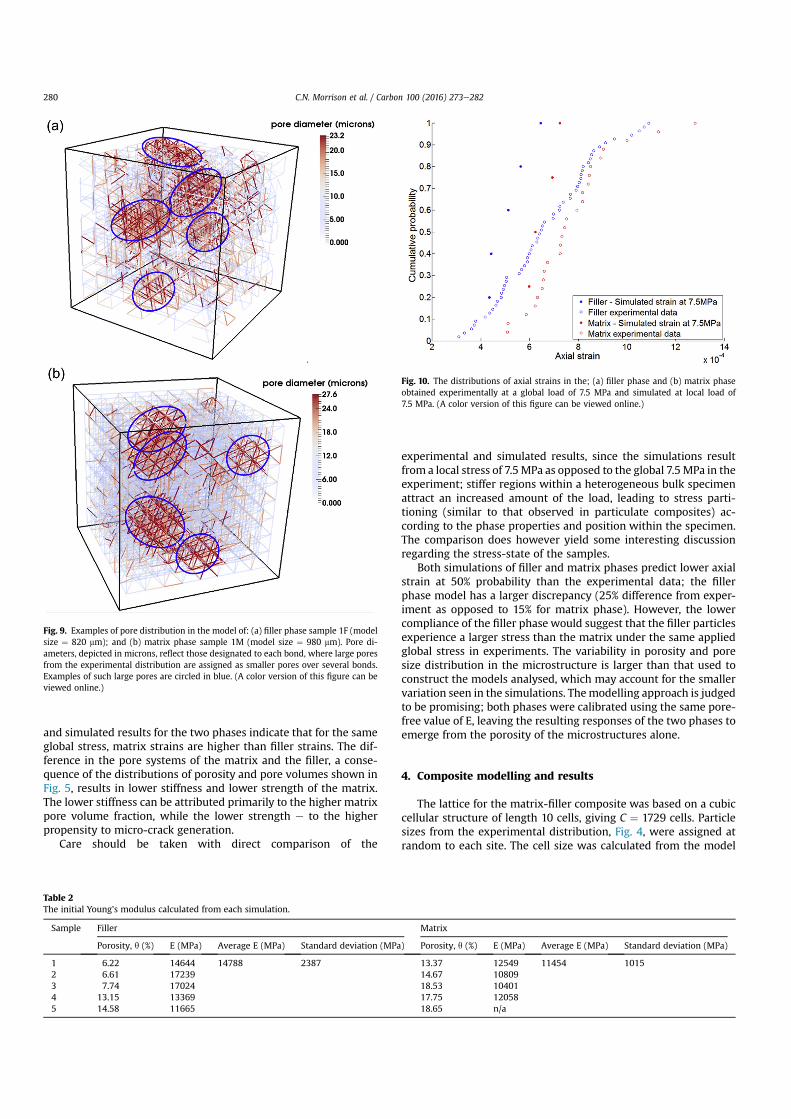
and simulated results for the two phases indicate that for the sameglobal stress, matrix strains are higher than filler strains. The dif-ference in the pore systems of the matrix and the filler, a conse-quence of the distributions of porosity and pore volumes shown inFig. 5, results in lower stiffness and lower strength of the matrix.The lower stiffness can be attributed primarily to the higher matrixpore volume fraction, while the lower strength e to the higherpropensity to micro-crack generation.
Care should be taken with direct comparison of the
experimental and simulated results, since the simulations resultfrom a local stress of 7.5MPa as opposed to the global 7.5MPa in theexperiment; stiffer regions within a heterogeneous bulk specimenattract an increased amount of the load, leading to stress parti-tioning (similar to that observed in particulate composites) ac-cording to the phase properties and position within the specimen.The comparison does however yield some interesting discussionregarding the stress-state of the samples.
Both simulations of filler and matrix phases predict lower axialstrain at 50% probability than the experimental data; the fillerphase model has a larger discrepancy (25% difference from exper-iment as opposed to 15% for matrix phase). However, the lowercompliance of the filler phase would suggest that the filler particlesexperience a larger stress than the matrix under the same appliedglobal stress in experiments. The variability in porosity and poresize distribution in the microstructure is larger than that used toconstruct the models analysed, which may account for the smallervariation seen in the simulations. Themodelling approach is judgedto be promising; both phases were calibrated using the same pore-free value of E, leaving the resulting responses of the two phases toemerge from the porosity of the microstructures alone.
4. Composite modelling and results
The lattice for the matrix-filler composite was based on a cubiccellular structure of length 10 cells, giving C ¼ 1729 cells. Particlesizes from the experimental distribution, Fig. 4, were assigned atrandom to each site. The cell size was calculated from the model
Fig. 9. Examples of pore distribution in the model of: (a) filler phase sample 1F (modelsize ¼ 820 mm); and (b) matrix phase sample 1M (model size ¼ 980 mm). Pore di-ameters, depicted in microns, reflect those designated to each bond, where large poresfrom the experimental distribution are assigned as smaller pores over several bonds.Examples of such large pores are circled in blue. (A color version of this figure can beviewed online.)
Table 2The initial Young's modulus calculated from each simulation.
Sample Filler Matrix
Porosity, q (%) E (MPa) Average E (MPa) Standard deviation (MPa) Porosity, q (%) E (MPa) Average E (MPa) Standard deviation (MPa)
1 6.22 14644 14788 2387 13.37 12549 11454 10152 6.61 17239 14.67 108093 7.74 17024 18.53 104014 13.15 13369 17.75 120585 14.58 11665 18.65 n/a
Fig. 10. The distributions of axial strains in the; (a) filler phase and (b) matrix phaseobtained experimentally at a global load of 7.5 MPa and simulated at local load of7.5 MPa. (A color version of this figure can be viewed online.)
C.N. Morrison et al. / Carbon 100 (2016) 273e282280

volume as a function of cell length L, Equation (16), the cumulativeassigned filler particle volume and the desired filler volume frac-tion, qF, according to Equation (17). The value of qF was taken as 0.2,an average of the two values obtained of 0.144 and 0.252 presentedin Ref. [17].
Vlattice ¼ CL3
2(16)
L ¼
ffiffiffiffiffiffiffiffiffiffiffiffiffiffiffiffiffiffiffiffiffiffiffiffiffiffiffiffiffi2PC
i¼1viparticle
CqF
3
vuut(17)
Bonds, chosen at random, were assigned random properties ofthe filler samples, derived in Section 4. This process continued untilthe cumulative total of the bond support volumes matched thedesired particle volume fraction. The remaining bonds wereassigned random properties of the matrix samples, also derived inSection 4. Specifically, the stress-strain behaviour of the differentfiller and matrix samples (i.e. Fig. 8) were used to inform bondbehaviour. The local gradient of the non-linear stress-strainbehaviour (i.e. from Fig. 8) was used as input to the stiffness cali-bration used for the single phasemodels, Equations (1) and (2). Thisstiffness and the corresponding strain from the sample behaviourwere used to calculate the force-displacement relationship of eachbond.
The results of the composite simulations are shown in Fig. 11.The initial Young's modulus value of 12900 MPa is higher thantypical literature values for virgin Gilsocarbon. This may be a resultof failing to simulate the largest pores in the matrix phase (withsize >100 mm); these occupy 6.3% of the total volume and wereexcluded in the distributions of porosity in filler and matrix, re-ported in Vertyagina and Marrow [17], that were used in the sim-ulations. This extra porosity, which could be included in futuremodels either in the matrix phase models themselves, or as addi-tional porosity applied to the composite model, would slightlydecrease the elastic modulus. The tensile strength value obtained of13.6 MPa is lower than the value of 19e20 MPa quoted in theliterature [26]. The simulated tensile strength would be expected todecrease with inclusion of the larger pores, so this suggests that themodel does need further refinement, particularly with regards tothe peak stress values. Nonetheless, the comparison betweensimulation and experiment is encouraging at this stage of themodel development.
5. General discussion
It was found that the multi-scale model was more numericallystable and less computationally expensive than the single phasemodels. This is because the multi-scale model does not require thepores to be modelled explicitly. Instead the effects of pores arehomogenised within the models of the individual phases, whichare represented by a small number of possible stress-strain be-haviours that are reasonably consistent with experimental behav-iour (i.e. Fig. 10). In doing so there is no need to remove bonds priorto simulation as a result of porosity. This makes finding an initialequilibrium less expensive and hence improves the numericalstability of the model.
Despite these promising results there are still limitations withthe model, mainly linked to limited data and numerical controls.Firstly, in addition to the large pores that are currently neglected,there is finer scale porosity in the graphite microstructure [38] thatis unresolved using the experimental techniques described inSection 2.2. Its effect should be included in the pore-free modulus,however. Furthermore no consideration has been taken of residualstresses, which exist following manufacturing [39] and so affect onthe stress-state of each phase. With respect to numerical stability,the controls required to obtain convergence, including viscousregularization, and their impact on the model response need to befurther understood to increase confidence in the results and henceallow for reduced conservatism in safety assessments of graphitecomponents.
Further work includes an improved calibration procedurecompatible with theories of discrete elasticity [23]. Following this,more rigorous studies may be undertaken using the Site-Bondmethodology, deriving damage evolution laws and characterisingthe size of the fracture process zone for use in continuum scaleanalyses for structural integrity assessment of graphite.
6. Conclusions
A multi-scale modelling methodology is presented, wherebymicrostructure-informed Site-Bond lattice models of both fillerand matrix phases are used to construct a larger scale compositeSite-Bond model of the nuclear grade graphite Gilsocarbon. A keyfeature of the proposed model is that it requires a single cali-bration of the elastic properties of “pore-free” graphite, fromwhere it can predict the elastic properties of real graphite fromthe knowledge of microstructure characteristics, such as particleand pore density and size distribution. The single-phase modelresults suggest that the evolution of damage is more prevalent inthe filler phase than the matrix phase with filler modelsdemonstrating “graceful” stress-strain behaviour resulting frommicro-failures as opposed to the brittle failure seen in the matrixphase. Filler particles are shown to be stiffer than the matrixphase.
� The modulus and tensile strength value calculated from a multi-scale composite model, 12.9 GPa and 13.6 MPa respectively,informed with the responses of the single-phase models, areencouraging when compared to the values found in the litera-ture, 11.6 GPa and 19e20 MPa respectively. The proposed semi-empirical approach, using a calibrated pore-free stiffness andderiving longer scale behaviour from microstructure informa-tion, has the potential to develop into a deductive methodologyfor calculating emergent behaviour, when combined with richermicrostructure information and validated by damage charac-terisation experiments.Fig. 11. The stress-strain response of the multi-scale simulation
C.N. Morrison et al. / Carbon 100 (2016) 273e282 281
Acknowledgements
C.N.M acknowledges the support from EPSRC via Nuclear FiRSTDoctoral Training Centre. A.P.J acknowledges the support fromEPSRC via grant EP/J019801, “QUBE: Quasi-Brittle fracture: a 3Dexperimentally-validated approach”. Moreover A.P.J acknowledgesBNFL through the Research Centre for Radwaste & Decom-missioning. T.J.M. gratefully acknowledges the support of OxfordMartin School, and Ye.V. acknowledges the support of EDF EnergyGeneration.
References
[1] C. Mantell, Carbon and Graphite Handbook, Interscience Publishers, 1968.[2] G. Jenkins, Fracture in reactor graphite, J. Nucl. Mater. 3 (3) (1962) 280e286.[3] A. Hodgkins, T.J. Marrow, M.R. Wootton, R. Moskovic, P.E.J. Flewitt, Fracture
behaviour of radiolytically oxidised reactor core graphites: a view, Mater. Sci.Technol. 26 (8) (2010) 899e907.
[4] M.R. Joyce, T.J. Marrow, P. Mummery, B.J. Marsden, Observation of micro-structure deformation and damage in nuclear graphite, Eng. Fract. Mech. 75(12) (2008) 3633e3645.
[5] M.J. Turner, R.W. Clough, H.C. Martin, L.J. Topp, Stiffness and deflectionanalysis of complex structures, J. Aeronaut. Sci. Inst. Aeronaut. Sci. 23 (9)(1956) 805e823.
[6] S. Nakhodchi, A. Hodgkins, R. Moskovic, D.J. Smith, P.E.J. Flewitt, Fractureprocess zones in polygranular graphite in bending, Key Eng. Mater. 452e453(2011) 93e96.
[7] N.N. Nemeth, R.L. Bratton, Overview of statistical models of fracture fornonirradiated nuclear-graphite components, Nucl. Eng. Des. 240 (1) (2010)1e29.
[8] R. Borst, Fracture in quasi-brittle materials: a review of continuum damage-based approaches, Eng. Fract. Mech. 69 (2002) 95e112.
[9] E. Schlangen, P.E.J. Flewitt, G. Smith, A. Crocker, A. Hodgkins, Computermodelling of crack propagation in porous reactor core graphite, Key Eng.Mater. 452e453 (2011) 729e732.
[10] E. Schlangen, E.J. Garboczi, Fracture simulations of concrete using latticemodels: computational aspects, Eng. Fract. Mech. 57 (2) (1997) 319e332.
[11] E. Schlangen, Crack development in concrete, Part 2: modelling of fractureprocess, Key Eng. Mater. 385e387 (2008) 73e76.
[12] Y. Wang, P. Mora, Macroscopic elastic properties of regular lattices, J. Mech.Phys. Solids 56 (2008) 3459e3474.
[13] A.P. Jivkov, J.R. Yates, Elastic behaviour of a regular lattice for meso-scalemodelling of solids, Int. J. Solids Struct. 49 (22) (2012) 3089e3099.
[14] A.P. Jivkov, M. Gunther, K.P. Travis, Site-bond modelling of porous quasi-brittle media, Mineral. Mag. 76 (8) (2013) 378e395.
[15] A.P. Jivkov, D.L. Engelberg, R. Stein, M. Petkowski, Pore space and brittledamage evolution in concrete, Eng. Fract. Mech. 110 (2013) 378e395.
[16] M. Zhang, C.N. Morrison, A.P. Jivkov, A meso-scale site-bond model for elas-ticity: theory and calibration, Mater. Res. Innovations 18 (2014) 982e986.
[17] Y. Vertyagina, T.J. Marrow, 3D Cellular Automata fracture model for porousgraphite microstructures, in: SMiRT 23-Structural Mechanics in ReactorTechnology, Manchester, UK, 2015.
[18] T.J. Marrow, D. Liu, S.M. Barhli, L. Saucedo-Mora, Y. Vertyagina, D.M. Collins,C. Reinhard, S. Kabra, P.E. Flewitt, D.J. Smith, “In situ observation of the strainswithin a mechanically loaded polygranular graphite,” Carbon 96 (2016)285e302.
[19] S. Kumar, S.K. Kurtz, J.R. Banavar, M.G. Sharma, Properties of a three-dimensional PoissoneVoronoi tessellation: a Monte Carlo study, J. Stat.Phys. 67 (3e4) (1992) 523e551.
[20] C.N. Morrison, M. Zhang, A.P. Jivkov, Discrete lattice model of quasi-brittlefracture in porous graphite, Mater. Perform. Charact. 3 (2014) 1848e1853.
[21] C.N. Morrison, M. Zhang, D. Liu, A.P. Jivkov, Site-bond lattice modelling ofdamage process in nuclear graphite under bending, in: SMiRT 23-StructuralMechanics in Reactor Technology, Manchester, UK, 2015.
[22] Simulia, Abaqus Version 6.13 Documentation, Dassault systemes, 2013.[23] A. Yavari, On geometric discretization of elasticity, J. Math. Phys. 49 (2) (2008)
022901.[24] J. Abrahamson, The surface energies of graphite, Carbon (1973) 337e362.[25] J. Kane, C. Karthik, D.P. Butt, W.E. Windes, R. Ubic, Microstructural charac-
terization and pore structure analysis of nuclear graphite, J. Nucl. Mater. 415(2) (2011) 189e197.
[26] S.D. Preston, B.J. Marsden, Changes in the coefficient of thermal expansion instressed gilsocarbon graphite, Carbon 44 (2006) 1250e1257.
[27] M. Mostafavi, T.J. Marrow, Quantitative in situ study of short crack propaga-tion in polygranular graphite by digital image correlation, Fatigue Fract. Eng.Mater. Struct. 35 (8) (2012) 695e707.
[28] M. Mostafavi, N. Baimpas, E. Tarleton, R.C. Atwood, S.A. McDonald,A.M. Korsunsky, T.J. Marrow, Three-dimensional crack observation, quantifi-cation and simulation in a quasi-brittle material, Acta Mater. 61 (2013)6276e6289.
[29] M. Mostafavi, S.A. McDonald, P.M. Mummery, T.J. Marrow, Observation andquantification of three-dimensional crack propagation in poly-granulargraphite, Eng. Fract. Mech. 110 (2013) 410e420.
[30] C. Berre, S.L. Fok, B.J. Marsden, A. Hodgkins, T.J. Marrow, P.M. Mummery,Numerical modelling of the effects of porosity changes on the mechanicalproperties of nuclear graphite, J. Nucl. Mater. 352 (1e3) (2006) 1e5.
[31] T. T. C. Products, “Special Graphite and Compound Material Products”.[32] P. Beghein, G. Berlioux, B. Mesnildot, F. Hiltmann, M. Melin, NBG-17-An
improved graphite grade for HTRs and VHTRs, Nucl. Eng. Des. 251 (2012)146e149.
[33] Y. Kaji, W. Gu, M. Ishihara, T. Arai, H. Nakamura, Development of structuralanalysis program for non-linear elasticity by continuum damage mechanics,Nucl. Eng. Des. 206 (1) (2001) 1e12.
[34] G.M. Laudone, C.M. Gribble, G.P. Matthews, Characterisation of the porousstructure of Gilsocarbon graphite using pycnometry, cyclic porosimetry andvoid-network modeling, Carbon 73 (2014) 61e70.
[35] M. Ishihara, J. Sumita, T. Shibata, T. Iyoku, T. Oku, Principle design and data ofgraphite components, Nucl. Eng. Des. 233 (1e3) (2004) 251e260.
[36] K.K. Phani, S.K. Niyogi, Young's modulus of porous brittle solids, J. Mater. Sci.22 (1987) 257e263.
[37] C.T. Herakovich, S.C. Baxter, Influence of pore geometry on the effectiveresponse of porous media, J. Mater. Sci. 34 (1999) 1595e1609.
[38] S. Mrozowski, Mechanical strength, thermal expansion and structure of cokesand carbons, in: Proceedings of the Conferences on Carbon, 1954.
[39] R. Krishna, A.N. Jones, R. Edge, B.J. Marsden, Residual stress measurements inpolycrystalline graphite with micro-Raman spectroscopy, Radiat. Phys. Chem.111 (2015) 14e23.
C.N. Morrison et al. / Carbon 100 (2016) 273e282282


