1

Large sea-ice volume anomalies simulated ina coupled climate model

Hugues Goosse1

Université Catholique de Louvain, Institut d'Astronomie et de Géophysique G. Lemaître

Chemin du Cyclotron, 2, B-1348 Louvain-la-Neuve, BelgiumPhone : 32-10-47-32-98, Fax : 32-10-47-47-22, e-mail : hgs@astr.ucl.ac.be

F.M. Selten, R. J. Haarsma, J.D. Opsteegh

KNMIPO Box 201, 3730, AE De Bilt, The Netherlands

Phone : 31-30-220-6911, Fax : 31-30-221-0407, e-mail : selten@knmi.nl

Submitted to Climate Dynamics: December 2001In revised form April 2001

1 corresponding author

2

Abstract

The processes leading to the formation of a large anomaly of sea-ice volume

integrated over the Northern Hemisphere have been investigated in a coarse-

resolution three-dimensional atmosphere-ocean-sea-ice model. This anomaly lasts

for about 20 years and reaches 8.6 x 103 km3, i.e. 6 standard deviations. It is associated

with a maximum surface cooling of more than 5° C in annual mean close to Spitzbergen.

The trigger of the large event in the model is a sequence of years presenting an

atmospheric circulation characterised by negative geopotential height anomalies over

Greenland and positive ones in the Barents and Norwegian Seas. This atmospheric

anomaly induces an increase in the ice volume as well as of the ice extent. Sea ice

survives in the area located close to Spitzbergen where deep convection occurs during

normal years. This is associated with a shut down of convection in that area and thus by a

strong reduction of the upward heat flux from the ocean to the atmosphere that strongly

amplifies the initial cooling. The long sequence of following years presenting the same

type of anomaly in the atmosphere is not just a rare realisation of the intrinsic

atmospheric variability. A positive feedback between the modification of surface

conditions and the atmospheric circulation reinforces the initial atmospheric anomaly.

Finally, the large event stops when convection increases again as a result of an increase

in ocean surface density close to Spitzbergen. This density increase is due to both the

advection of a positive salinity anomaly created in the Arctic because of brine rejection

and to local ice formation southward of Spitzbergen during the cold event. Sensitivity

experiments performed with the model have shown that the frequency of the events is

very sensitive to the mean climate simulated by the model, the frequency being higher in

a colder climate.

3

Introduction

Although numerous uncertainties remain, our understanding of interannual and

decadal variability in the high northern latitudes has considerably increased in recent

years. The dominant mode seems related to the North Atlantic Oscillation (NAO) and the

Arctic Oscillation (AO). The AO and the NAO are the leading modes of variability of the

atmospheric circulation in the North Atlantic and the Northern Hemisphere, respectively,

and are highly correlated (e.g., Hurrel 1995; Thomson and Wallace 1998; Deser 2000).

The response of the high latitudes to the NAO exhibits out of phase variations of ice

concentration between the Labrador and Greenland-Barents Seas (Walsh and Johnson

1979; Slonisky et al. 1997; Deser et al. 2000) as well as modifications of atmospheric and

oceanic circulation (for a review see Dickson et al. 2000). In addition to the response of

the ocean-ice system to atmospheric conditions associated with the NAO, Mysak and

Venegas (1998) have proposed that modifications of ice extent could influence the

atmospheric circulation and thus might play a role in the shift between different phases of

the NAO.

Proshutinsky and Johnson (1997) have described another mode of decadal variability

in the Arctic. Following their analysis, the sea ice and ocean surface motion alternates

between an Anticyclonic Circulation Regime (ACCR) and a Cyclonic Circulation

Regime (CCR), each regime persisting about 5 to 7 years. The atmospheric pattern

associated with the shift between ACCR and CCR displays opposite surface pressure

anomalies between the Central Arctic and Greenland (Johnson et al. 1999).

The instrumental records of the Arctic climate generally start in the second half of the

20th century, a few of them extending back to the beginning of the 20th century (e.g.,

Hanssen-Bauer and Førland 1998). This makes a comprehensive description of

interdecadal to century-scale variability a difficult task. Nevertheless, based on ship

observations from explorers, whalers, sealers and fishermen, Vinje (2001) was able to

reconstruct the sea ice extent in the Nordic Seas back to 1864. In the Barents Sea, his

reconstruction covers the last 400 years (Vinje 1999), although the data coverage is very

4

sparse before 1750. Furthermore, the ice conditions around Iceland have been compiled

from various documentary sources, providing a record back to the 16th century (e.g.

Ogilvie 1992). These reconstructions display significant decadal variability superimposed

on variability on longer time-scales. In particular, the ice extent in the Nordic Seas in

April has decreased by 33% over the past 135 years. Nearly half of this decrease occurred

during the period 1860-1900. This reduction of the ice extent is consistent with the

warming observed in the reconstructions of Overpeck et al. (1997), based on a

compilation of various paleoclimate records covering the last four centuries. The results

of Overpeck et al. (1997) also indicate that the recent warming marks the end of a

relatively cold period in the whole Arctic that started before 1600.

In the North Atlantic, multidecadal variability with a preferred time-scales between

50 and 100 years has been described on the basis of observations by various authors (e.g.,

Mann and Park 1994; Tourre et al. 1999). Using a Coupled General Circulation Model

(CGCM), Delworth and Mann (2001) have recently suggested that those multidecadal

fluctuations could be associated with oscillations of the thermohaline circulation in the

Atlantic. This mode of variability could have an influence on the Arctic climate system

as suggested by model studies (Delworth et al. 1997; Polyakov and Johnson 2000), but

strong observational evidence is still lacking. Holland et al. (2001) have also described a

mode of variability which involves the thermohaline circulation and sea ice in the Arctic.

In their model, the approximate time-scale of the oscillation is 20 years.

In addition to the types of variability described above that seem relatively regular in

time, one spectacular event has occurred during the second half of the 20th century: the

Great Salinity Anomaly or GSA (see Dickson et al. 1988 for a review). The GSA is

characterised by a strong salinity decrease in the Greenland Sea in the late 1960’s,

probably caused by a large inflow of freshwater and sea ice from the Arctic (Aagaard and

Carmack 1989; Häkkinen 1993). The salinity anomaly propagates around the subpolar

gyre until it comes back to the Greenland Sea, significantly attenuated, in 1981-82. The

negative salinity anomaly is associated with a decrease in oceanic convection, both in the

Greenland Sea and in the Labrador Sea, as well as with an increase in the ice

5

concentration in winter (e.g., Mysak and Manak 1989). It has been suggested that other

salinity anomalies have occurred in the area, but probably with a much smaller

magnitude than the GSA (e.g., Belkin et al 1998; Mysak 1999).

A large event of about 30-40 years duration has also been reported in a multi-millenia

simulation performed with a CGCM simulation without any variability in the external

forcing (Hall and Stouffer 2001). During this cold event, the annual mean temperature

near Southern Greenland was about 3°C colder than the mean. This event shares a lot of

characteristics with the interdecadal variability simulated in the same model (Delworth et

al. 1997). But the extreme cooling is triggered by unusually intense and persisting

northerly winds in the Greenland Sea that bring fresh water to the area, stop oceanic

convection there, strongly amplifying the temperature decrease.

In a previous study (Goosse et al. 2002, hereafter GSHO02), we have proposed a

mechanism to explain the decadal variability of the sea-ice volume in a coupled

atmosphere-ocean-sea-ice model. This mechanism has been deduced by performing both

correlation analyses between the simulated variables and a series of additional sensitivity

experiments. This has allowed us to show that the modifications of the sea-ice volume

are driven by a geopotential height pattern characterised by centres of action of opposite

signs over Greenland and over the Barents-Kara-Central Arctic area. This pattern has

thus interesting similarities with the one described by Johnson et al. (1999) to explain the

transitions between ACCR and CCR. In the Arctic, the increase of sea-ice volume

induces an increase in salinity. This salinity anomaly is transported to the Greenland Sea

where it promotes convective activity. This warms up the surface oceanic layer and the

atmosphere in winter and induces a decrease of the ice volume, completing half a cycle.

In addition to this decadal variability, the simulation performed in GSHO02 displays a

large event characterised by a sea-ice volume in the Northern Hemisphere more than 6

standard deviation higher than the mean. The goal of the present paper is to analyse this

large event and to compare it to observations and results of other models. The model and

its climatology are briefly described in section 2. In section 3, the processes leading to

the formation of a large ice volume anomaly are discussed. In this framework, the

6

comparison with the mechanism associated with the decadal variability in the model is of

particular interest. Section 4 deals with the factors that influences the frequency of the

large events. The model results are then compared to the variability observed in the

Arctic in section 5, followed by concluding remarks.

2 Model description

ECBILT-CLIO is a three-dimensional coupled atmosphere–ocean–sea ice model

(Goosse et al. 2001; Renssen et al. 2001; Goosse et al. 2002). The atmospheric

component is ECBILT2 (Opsteegh et al. 1998; Selten et al. 1999), a global spectral

quasi-geostrophic model, truncated at T21, with simple parameterizations for the diabatic

heating due to radiative fluxes, the release of latent heat and the exchange of sensible

heat with the surface. The model contains a full hydrological cycle which is closed over

land by a bucket model for soil moisture. Each bucket is connected to a nearby ocean

grid point to define the river runoff. Accumulation of snow over land occurs in case of

precipitation when the land temperature is below zero. Cloud cover is prescribed

following a seasonally and geographically distributed climatology (D2 monthly data set

of the International Satellite Cloud Climatology Project, ISCCP, Rossow et al 1996).

The CLIO model (Goosse et al. 1999; Goosse and Fichefet 1999) comprises a

primitive equation, free-surface ocean general circulation model coupled to a

thermodynamic-dynamic sea ice model. The ocean component includes a relatively

sophisticated parameterization of vertical mixing (Goosse et al. 1999). The equations are

solved using a mode splitting technique. The time step for temperature and salinity is 24

hours while barotropic and baroclinic modes of the velocity are solved using time steps

of 3 hours and 5 minutes, respectively (Campin and Goosse 1999). The representation of

the vertical growth and decay of sea ice is based an improved version of the 3-layer

model of Semtner (1976) (Fichefet and Morales Maqueda 1997). In the computation of

ice dynamics, sea ice is considered to behave as a viscous-plastic continuum. The

horizontal resolution of CLIO is 3 degrees in latitude and longitude and there are 20

unevenly spaced vertical levels in the ocean.

7

ECBILT and CLIO are coupled every day using the OASIS software (Terray et al.

1998). There is no local flux correction in ECBILT-CLIO. However, the model

systematically overestimates the precipitation over the Atlantic and Arctic oceans

(Opsteegh et al. 1998) with potential consequences for the stability of the thermohaline

circulation as well as on the mass balance of the Arctic snow/sea-ice system. As a

consequence, it has been necessary to artificially reduce the precipitation by 10 % over

the Atlantic and by 50% over the Arctic basins (defined here as the oceanic area north of

68°N). The corresponding water is redistributed homogeneously over the North Pacific, a

region where the model precipitation is underestimated.

The control simulation analysed here is a 3000 year-long integration performed using

a constant solar forcing and atmospheric concentration of greenhouse gases. The

equilibrium state obtained reproduces reasonably well the observed climate. The globally

averaged annual mean sea surface temperature simulated by the model is 0.8°C higher

than Levitus’ (1982) observations but locally the error can be greater than 4°C, in

particular in the Southern Ocean. The oceanic thermohaline circulation is close to the one

derived from observations with, for instance, 15 Sv of North Atlantic Deep Water

(NADW) exported out of the Atlantic Ocean at 30°S. The model also reproduces the

shape and position of Icelandic and Aleutian lows, although the extent of the latter is

overestimated. This results in winds in direction opposite to observations in the Central

Arctic that induce ice velocities pointing towards the East Siberian Sea. This implies a

strong accumulation of sea-ice there in the model (Goosse et al. 2001). This is contrary to

the observed ice thickness distribution that shows a maximum north of the Canadian

Archipelago. It should be noticed that similar problems have been observed in other

coupled atmosphere-ocean-sea-ice models

Integrated over the Northern Hemisphere, the ice area varies in the model from 6.4 x

106 km2 in summer to 13.7 x 106 km2 in winter, close to the observed values of 6.2 and

13.9 x 106 km2, respectively (Gloersen et al. 1992). The position of the ice edge

simulated by the model in both summer and winter is in good agreement with the

observations of Gloersen et al. (1992) (Fig 1). Nevertheless, the model underestimates

8

the ice extent in the Labrador Sea and Greenland Sea in winter and in the Beaufort Sea in

summer. In Barents Sea, sea-ice concentration is too high all year long in the model. The

latter disagreement is largely due to the oceanic model since the same problem has been

observed in the model CLIO alone driven by observed atmospheric fields (e.g., Goosse

and Fichefet 1999). The cause of this discrepancy lies in the wrong path of the ocean

surface currents in these regions: rather than flowing along the Norwegian coast toward

the Barents Sea, as observed, the simulated Norwegian Current flows directly northward

and enters the Arctic Ocean east of Spitzbergen. This current carries warm Atlantic

waters inducing strong ice melting south and east of Spitzbergen in the model. On the

contrary, the heat transport to the Barents Sea is too weak, allowing ice to be maintained

there.

There is no precise estimate of the sea-ice volume in the northern hemisphere based

on observation because of the sparseness of ice-thickness measurements. Nevertheless,

the climatological value simulated (24.2 x 103 km3) is in good agreement with the results

obtained by Hilmer and Lemke (2000), using a dynamic-thermodynamic sea-ice model

driven by NCEP-NCAR reanalysis over the period 1958-1998 (Kalnay et al. 1996). In

ECBILT-CLIO, the standard deviation of the annual mean volume is 1.6 x 103 km3,

which represents 7% of the mean over the whole period. In the simulation of Hilmer and

Lemke (2000), the standard deviation reaches 1.9 x 103 km3 (i.e 6 % of the mean).

Furthermore, in the ice-ocean model CLIO driven by an atmospheric forcing similar to

the one of Hilmer and Lemke (2000), the standard deviation of the annual mean sea-ice

volume is 2.0 103 km3, which corresponds to 7% of the mean over the years 1958-1999

(B. Tartinville 2001, personal communication).

3 The mechanism that leads to the large anomaly

3 1 Description of the large event

The large event starting around model year 2465 and ending about 25 years later

clearly emerges from the time series of the simulated sea-ice volume. It reaches more

than 35 x 103 km3, i.e. 6 standard deviations above the mean value (Fig. 2). Another

9

event around year 2820 presents an anomaly larger than 3 standard deviations while the

ice volume anomalies are smaller than 3 standard deviations in absolute value during the

remaining part of the time series.

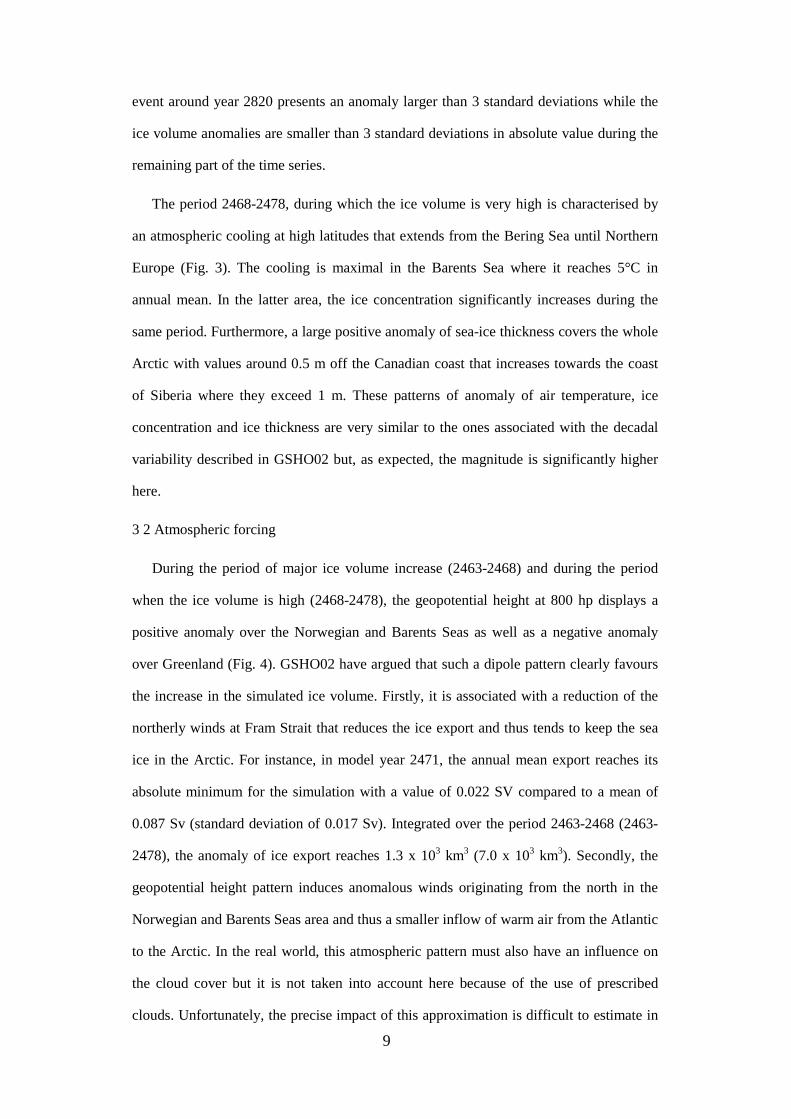
The period 2468-2478, during which the ice volume is very high is characterised by

an atmospheric cooling at high latitudes that extends from the Bering Sea until Northern

Europe (Fig. 3). The cooling is maximal in the Barents Sea where it reaches 5°C in

annual mean. In the latter area, the ice concentration significantly increases during the

same period. Furthermore, a large positive anomaly of sea-ice thickness covers the whole

Arctic with values around 0.5 m off the Canadian coast that increases towards the coast

of Siberia where they exceed 1 m. These patterns of anomaly of air temperature, ice

concentration and ice thickness are very similar to the ones associated with the decadal

variability described in GSHO02 but, as expected, the magnitude is significantly higher

here.

3 2 Atmospheric forcing

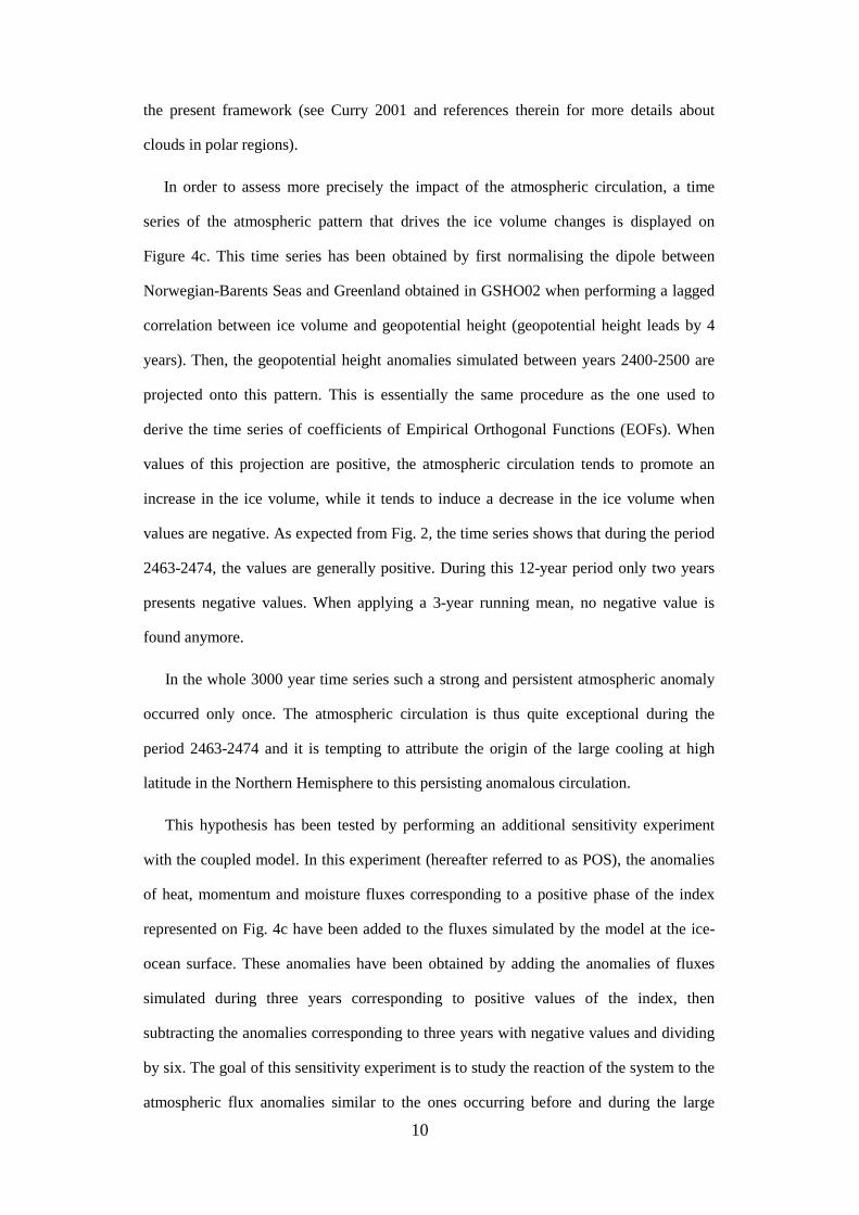
During the period of major ice volume increase (2463-2468) and during the period

when the ice volume is high (2468-2478), the geopotential height at 800 hp displays a

positive anomaly over the Norwegian and Barents Seas as well as a negative anomaly

over Greenland (Fig. 4). GSHO02 have argued that such a dipole pattern clearly favours

the increase in the simulated ice volume. Firstly, it is associated with a reduction of the

northerly winds at Fram Strait that reduces the ice export and thus tends to keep the sea

ice in the Arctic. For instance, in model year 2471, the annual mean export reaches its

absolute minimum for the simulation with a value of 0.022 SV compared to a mean of

0.087 Sv (standard deviation of 0.017 Sv). Integrated over the period 2463-2468 (2463-

2478), the anomaly of ice export reaches 1.3 x 103 km3 (7.0 x 103 km3). Secondly, the

geopotential height pattern induces anomalous winds originating from the north in the

Norwegian and Barents Seas area and thus a smaller inflow of warm air from the Atlantic

to the Arctic. In the real world, this atmospheric pattern must also have an influence on

the cloud cover but it is not taken into account here because of the use of prescribed

clouds. Unfortunately, the precise impact of this approximation is difficult to estimate in

10

the present framework (see Curry 2001 and references therein for more details about

clouds in polar regions).

In order to assess more precisely the impact of the atmospheric circulation, a time

series of the atmospheric pattern that drives the ice volume changes is displayed on

Figure 4c. This time series has been obtained by first normalising the dipole between

Norwegian-Barents Seas and Greenland obtained in GSHO02 when performing a lagged

correlation between ice volume and geopotential height (geopotential height leads by 4

years). Then, the geopotential height anomalies simulated between years 2400-2500 are

projected onto this pattern. This is essentially the same procedure as the one used to

derive the time series of coefficients of Empirical Orthogonal Functions (EOFs). When

values of this projection are positive, the atmospheric circulation tends to promote an

increase in the ice volume, while it tends to induce a decrease in the ice volume when

values are negative. As expected from Fig. 2, the time series shows that during the period

2463-2474, the values are generally positive. During this 12-year period only two years

presents negative values. When applying a 3-year running mean, no negative value is

found anymore.

In the whole 3000 year time series such a strong and persistent atmospheric anomaly

occurred only once. The atmospheric circulation is thus quite exceptional during the

period 2463-2474 and it is tempting to attribute the origin of the large cooling at high

latitude in the Northern Hemisphere to this persisting anomalous circulation.

This hypothesis has been tested by performing an additional sensitivity experiment

with the coupled model. In this experiment (hereafter referred to as POS), the anomalies

of heat, momentum and moisture fluxes corresponding to a positive phase of the index

represented on Fig. 4c have been added to the fluxes simulated by the model at the ice-

ocean surface. These anomalies have been obtained by adding the anomalies of fluxes

simulated during three years corresponding to positive values of the index, then

subtracting the anomalies corresponding to three years with negative values and dividing

by six. The goal of this sensitivity experiment is to study the reaction of the system to the

atmospheric flux anomalies similar to the ones occurring before and during the large

11

event. A similar technique has been used by Delworth and Dixon (2000) to analyse the

impact of an increase of the NAO index in a climate change scenario performed with a

coupled climate model.

The simulation starts from the state of the coupled system in model year 3000. During

the first 5 years of the experiment, the annual mean ice volume increases, reaching values

higher than 30 x 103 km3 (Fig. 5), which are of the same order of magnitude than during

the large anomaly created in the control experiment. After this period, the ice volume

remains more or less stable, keeping values higher than 30 x 103 km3 . This increase of

ice volume in POS is associated with a decrease of convection close to Spitzbergen. If the

anomalies of fluxes imposed in experiment POS are removed, the coupled system comes

back to its previous state in less than 10 years (Fig. 5). This time-scale is also consistent

with the evolution of the large event in the control simulation.

The latter simulation shows that the persistent anomalous atmospheric circulation can

force the large sea ice volume anomaly. Now the question remains whether the long

persistence of the atmospheric anomaly occurred purely by chance or whether there is a

positive feedback by the ice cover that helps to maintain the anomalous circulation. By

performing sensitivity experiments with the atmosphere-only model driven by various

surface conditions, GSHO02 have suggested that such a positive feedback could occur.

But, its role in the decadal variability simulated by the model seems less important than

other feedbacks such as the thermodynamic one between the air temperature and the ice

cover. In the latter feedback, an atmospheric cooling induces an increase in the ice

concentration and ice extent that amplifies the initial decrease in air temperature because

of an increase in surface albedo and of a decrease in the upward heat flux from the ocean

to the atmosphere.

For the large event, the response of the atmospheric circulation to the anomalous ice

cover might be more important, since the anomaly is so much larger than in the decadal

variability of GSHO02. To test this, additional 30-year long experiments have been

performed with the atmospheric model in stand-alone mode. In the control simulation,

the boundary conditions at the ice-ocean surface (sea-surface temperature, ice

12

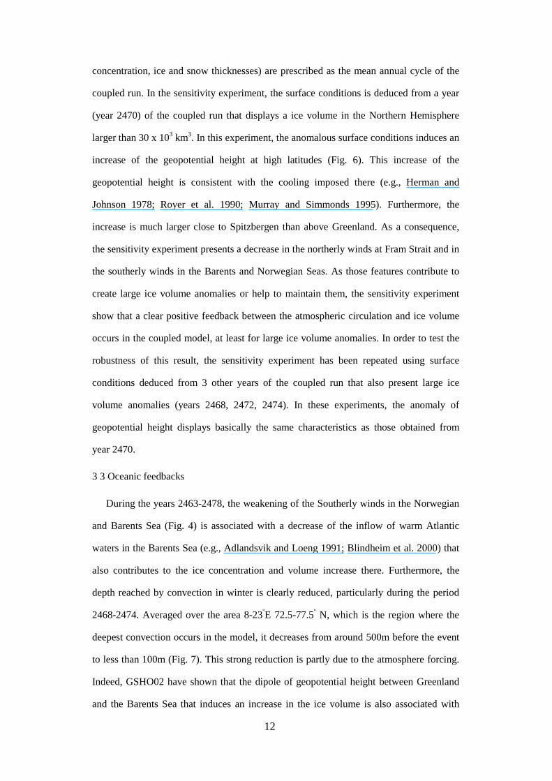
concentration, ice and snow thicknesses) are prescribed as the mean annual cycle of the

coupled run. In the sensitivity experiment, the surface conditions is deduced from a year

(year 2470) of the coupled run that displays a ice volume in the Northern Hemisphere

larger than 30 x 103 km3. In this experiment, the anomalous surface conditions induces an

increase of the geopotential height at high latitudes (Fig. 6). This increase of the

geopotential height is consistent with the cooling imposed there (e.g., Herman and

Johnson 1978; Royer et al. 1990; Murray and Simmonds 1995). Furthermore, the

increase is much larger close to Spitzbergen than above Greenland. As a consequence,

the sensitivity experiment presents a decrease in the northerly winds at Fram Strait and in

the southerly winds in the Barents and Norwegian Seas. As those features contribute to

create large ice volume anomalies or help to maintain them, the sensitivity experiment

show that a clear positive feedback between the atmospheric circulation and ice volume

occurs in the coupled model, at least for large ice volume anomalies. In order to test the

robustness of this result, the sensitivity experiment has been repeated using surface

conditions deduced from 3 other years of the coupled run that also present large ice

volume anomalies (years 2468, 2472, 2474). In these experiments, the anomaly of

geopotential height displays basically the same characteristics as those obtained from

year 2470.

3 3 Oceanic feedbacks

During the years 2463-2478, the weakening of the Southerly winds in the Norwegian

and Barents Sea (Fig. 4) is associated with a decrease of the inflow of warm Atlantic

waters in the Barents Sea (e.g., Adlandsvik and Loeng 1991; Blindheim et al. 2000) that

also contributes to the ice concentration and volume increase there. Furthermore, the

depth reached by convection in winter is clearly reduced, particularly during the period

2468-2474. Averaged over the area 8-23ºE 72.5-77.5º N, which is the region where the

deepest convection occurs in the model, it decreases from around 500m before the event

to less than 100m (Fig. 7). This strong reduction is partly due to the atmosphere forcing.

Indeed, GSHO02 have shown that the dipole of geopotential height between Greenland

and the Barents Sea that induces an increase in the ice volume is also associated with

13

reduced convection. In addition, during the period when the ice volume is large, the

export of ice from the Barents Sea to the Norwegian Sea is very intense. It reaches a

value of 6.4 x 10-2 Sv in 2467 whereas the long-term annual mean of this transport is very

close to zero and its standard deviation is 1.0 x 10-2 Sv. Integrated over the period 2463-

2478, the anomaly of transport amounts to 8.9 x 103 km3 of sea ice. This particularly

large ice mass export is due both to the more northerly winds that prevail during this

period in the Barents Sea (Fig. 4) as well as to the large ice thickness increase in this

region (Fig. 3). In our simulation, this ice export out of the Barents Sea brings ice directly

to the convection sites. As a consequence, it tends to isolate the ocean from the cold

atmosphere in winter thanks to the low conductivity of the ice and to transport freshwater

that efficiently damps the deep convection.

The collapse of convection is associated with a reduction of the upward heat flux in

the ocean of more than 100 W m-2 in annual mean (Fig. 7). This huge reduction implies a

significant local cooling that allows ice to be maintained in the area. Furthermore, it has

an effect at larger scale since the reduction of the upward heat flux in the ocean tends to

cool the air that is transported from Atlantic regions to the Arctic inducing a temperature

decrease there. A simple integration of the upward heat transport in the area 8-23ºE 72.5-

77.5º N leads to a value of about 7.5 1020 J per year for a reduction of 100 W m-2. This is

enough to form 2.5 km3 of sea ice each year. This estimation is quite crude because it

does not take into account any feedback. Furthermore, all the heat released in the Nordic

Seas is not transported to the ice-covered area. Anyway, this estimate shows that the

strong reduction of convection, which is largely due to the increase of ice volume and to

the transport of ice to the convection sites, significantly contributes in turn to the

formation of the large ice volume anomalies simulated by the model.

This decrease of convection in the Nordic Seas is associated with a reduction of the

intensity of the thermohaline circulation in the North Atlantic. The maximum of the

overturning streamfunction in the Nordic Seas decreases from 17 Sv to a minimum of 12

Sv in year 2471, which corresponds to a reduction of more than 4 standard deviations.

The maximum of the overturning over the whole Atlantic reaches its minimum 4 years

14

later and corresponds to a reduction of 3 standard deviations. The signal in the export of

North Atlantic Deep water out of the Atlantic seems less clear, probably because of the

too short duration of the event.

The increase of ice cover and the surface cooling observed in the area 8-23ºE 72.5-

77.5º N completely modify the freshwater balance there. Before the event, the region

received between 0.3 and 0.6 m of freshwater per year, mainly because of the ice melting

induced by the strong upward oceanic heat flux. When convection ceases, the area

produces large amounts of ice. The brine released during ice formation results in a

change of sign of the equivalent freshwater flux that reaches nearly –2 m yr-1 at its

minimum.

The consequences of the ice volume increase are also apparent in the Central Arctic.

Because of 5.4 103 km3 of local ice production over the period 2463-2468, a large

positive anomaly of more than 0.2 psu develops (Fig. 8a). Since the inflow of Atlantic

waters in the Arctic is reduced, the salinity tend to decrease in the Barents, Kara and

Laptev Seas during the years 2469-2479 (Fig. 8b). During this period, the positive

anomaly formed in the Central Arctic is advected to the GIN Seas, where, in addition to

the local ice formation, it contributes to increase the surface density. It thus tends to

precondition the water column for convection that is triggered in model year 2474 when

suitable atmospheric conditions are taking place (Fig. 4). As in the mechanism described

in GSHO02, this brings large amount of heat to the surface that induces ice melting and a

decrease of the ice volume to values prevailing before the event.

4 What determines the frequency of the events ?

In the previous section it was argued that a large enough ice anomaly in the Nordic

Seas is necessary to completely shut down convection there, a prerequisite for the

generation of a large ice volume anomaly in the Arctic. Such an ice anomaly can be

created by a long period of persistent atmospheric forcing, which occurs purely by

chance. The probability of such an event is hard to determine since it would require

prohibitively long integrations with the coupled system. But, under the hypothesis that

15

the atmospheric forcing (Fig. 4c) is adequately described by a first order autoregressive

process (AR1), the frequency of the occurrence of a persistent period of positive

amplitudes lasting at least 12 years can be assessed. The parameters of the AR1 process

are deduced from the autocorrelation coefficient and total variance of the time series of

the projection in Fig. 4c. Using these parameters, 104 AR1 time series of 3000 years

duration each are produced. In those synthetic time series, after performing a 3-year

running mean, a period of 12 consecutive positive values is found every 652 years, on

average. When the test is performed for 12 consecutive years displaying values higher

than 1, as in the model experiment between years 2463-2474 (Fig. 4c), the occurrence is

now every 4863 years on average (or one event every 1.621 time series of 3000 years

duration). This result is not inconsistent with the 1 in 3000 year event observed in the

model. However, much longer model data time series are needed to verify if the AR1

estimate is consistent with the probability of the event in the coupled model. It might be

that the positive feedback between the anomalous ice cover and the atmospheric anomaly

is strong enough to make these persistent events more likely in the coupled integration.

Evidence for this is presented at the end of this section.

It can also not be ruled out beforehand that the large ice anomaly is connected to slow

changes in the ice-ocean system, pacing the occurrence of the events, just needing the

right atmospheric trigger to start and through a positive feedback sustaining the initial

atmospheric anomaly. We were not able to find a variable in the system that clearly

displays such a slow evolution prior to the event. Nevertheless, to test the hypothesis, a

simulation has been restarted from the state obtained in model year 2450, 13 years before

the large ice anomaly. During the first time step (1st January), the heat, freshwater and

momentum fluxes at the atmosphere-ocean interface have been obtained from the values

simulated the 1st January of the preceding year in order to perturb slightly the system.

This simulation has been continued for 100 years. No large event occurred. Thus a very

weak perturbation is able to significantly modify the time evolution of the system. The

timing of the event is thus not set by slow, robust changes in the ocean, but occurs purely

by chance.

16

The frequency of the large events might be increased if the atmospheric forcing

pattern induces larger ice anomalies in the Nordic Seas. This is likely the case in a colder

climate with a larger ice pack in the Arctic. To check this, two additional sensitivity

experiments have been launched. In the experiment described in GSHO02, the

concentration of greenhouse gases is set equal to the value observed in 2000. In the first

sensitivity experiment (PRE), the greenhouse gases concentration that prevailed in pre-

industrial times is applied (1750), resulting in a colder climate (Goosse and Renssen

2001). In experiment SOL, the pre-industrial concentrations are still used but, in addition,

the solar constant has been reduced by 5 W m-2, which roughly corresponds to a mean

forcing at the surface of 1 W m-2. Averaged over the model years 2000-4000, the long-

term mean and standard deviation of the total ice volume in experiment PRE are 40.4 x

103 km3 and 3.3 x 103 km3, respectively. The corresponding values in experiment SOL

are 46.1 x 103 km3 and 4.5 x 103 km3, respectively. As expected, the mean ice volume

increases in these colder simulations. The standard deviation of the ice volume is also

higher, in agreement with previous modelling studies (e.g., Bitz et al. 1996; Holland and

Curry 1999).

In the two sensitivity experiments, the number of events characterised by large ice

volume anomalies is indeed larger than in the control experiment (Fig. 9). In the control

experiment 2 anomalies larger than 3 standard deviations are found, against 13 in PRE

and 5 in SOL. At first sight, it appears strange that the latter value is lower than in PRE

but the standard deviation in SOL is much larger than in PRE. If we take into account all

anomalies larger than 10 x 103 km3, which are already large anomalies, 11 events are

obtained in SOL. This gives a value close to the one in PRE.

This higher frequency of large events in the sensitivity experiments confirms the

picture that the probability of large ice volume anomalies in the Arctic is related to the

probability of ice anomalies in the Nordic Seas large enough to completely cover the

convection sites and stop convection. In colder climates with thicker ice and higher ice

volume variability the probability of creating a large ice anomaly, for instance by

anomalous ice transport, is significantly higher. In these sensitivity experiments, the

17

probability of long persistent atmospheric circulation anomalies has also increased. In

PRE and SOL, a minimum of 4 events characterised by 12 consecutive years with an

index higher than one is found in every 1000 year series analysed, compared to one such

an event in the whole standard experiment. The positive feedback between ice cover and

atmospheric circulation is thus apparently strong enough to change the probability of

occurrence of those long persistent atmospheric circulation anomalies.

In none of the experiments a negative anomaly larger than 3 standard deviation is

found. This is again due to the positive feedback associated with convection. In all our

simulations, convection is generally active in the Nordic Seas. If convection stops, this

induces a strong reduction of the upward heat flux and this strongly contributes to the

formation of a large ice volume anomaly. On the other hand, if convection reaches deeper

levels, it only induces a moderate increase in the upward heat flux and thus a moderate

reduction of the ice volume.

Because of the sensitivity of the large events to the mean climate described above, it

would be useful to assess the influence of the discrepancies between simulated and

observed climate. Furthermore, the role of correction of precipitation applied in the

Arctic should also be investigated. Testing precisely the impact of model errors is always

difficult. The best way is probably to compare the model results and the mechanism

deduced from them to observations (see section 5) and to simulations performed with

other models when available. Nevertheless, analysing some additional experiment

performed with the model can provide complementary information.

The most important problems underlined in section 2 are the wrong distribution of ice

thickness in the Arctic and the too extensive ice cover in the Barents Sea. In order to cure

the first one, a simulation has been performed in which the wind stress above sea ice has

been “corrected”: at each time step, we have added to the simulated value the

climatology derived from the NCEP-NCAR reanalysis for the years 1973-1998 (Kalnay

et al. 1996) and subtracted the climatological value derived for the coupled model.

Because of the realistic wind stresses climatology in this experiment, the ice thickness

distribution is close to the observed one with the maximum located north of the Canadian

18

Archipelago and Greenland. Nevertheless, in this experiment large events are still

simulated demonstrating that their occurrence is not conditioned by the ice thickness

distribution of the coupled model.

In the latter experiment, the ice thickness in the Barents Sea is reduced by nearly a

factor 2 compared to the standard experiment while the ice concentration is only

marginally smaller. ECBILT-CLIO has also been used to simulate early Holocene

climate (Renssen et al 2001). In this simulation, ice thickness and extent are reduced

compared to present-day conditions, in particular in the Barents Sea. Nevertheless, large

events are also simulated. These additional experiments do not prove that the differences

between model and observations have no influence on the occurrence of the large events

and on their characteristics. But, they show that, in the model, they are taking place in a

variety of conditions, increasing our confidence about their occurrence in the real world.

5 Comparison with observations

Ideally, the frequency, the duration, the spatial structure as well as the magnitude of

the simulated cold event should be compared with observations. But this is quite difficult,

particularly in Polar Regions where long time series are very rare. Furthermore, it has

been shown in section 4 that in the model, the frequency of occurrence of the large events

is clearly dependent on the mean state. As a consequence, it is hopeless to try to make a

valuable comparison with a frequency of observed cold event, even if precise time series

were available. The duration of the event is not at odds with data since cold periods of 20

years duration have been observed at high latitudes (e.g., Ogilvie 1992). But studying the

link with sea-ice volume or with the mechanism presented here is impossible because of

the lack of data.

As far as the spatial structure of the simulated event is concerned, it appears possible

to compare with available observational data for a particularly cold year. In normal years,

the south coast of Spitzbergen remains ice-free all year long in the model as observed

(Fig. 10). During the period 2468-2478, a large anomaly of ice concentration is found in

this region and in the Barents Sea (Fig. 3). As a consequence, Spitzbergen is surrounded

19

by ice during the large event. This situation can be compared to the year 1866, which is

the one that displays the largest ice extent anomaly in the Nordic Seas in the compilation

of Vinje (2001) (although this period can not be considered as an exceptionally cold

event in the time series presented by Vinje). During this year, the observed ice edge in

April is located south of Spitzbergen and extents well outside the continental shelf area.

The ice cover is significantly higher in the Barents Sea while the changes appear more

modest in the Greenland Sea. This observed increase in the ice cover must have had a

large impact on the upward oceanic heat flux because of the insulating effect of the sea

ice. This observational picture is broadly similar to the one obtained in the model

indicating that the sequence of events deduced from model results provides a reasonable

hypothesis to explain observed variations. Furthermore, the magnitude of the simulated

anomaly is not out of the range of the observed one.

In summer, a large part of the Barents Sea is still ice covered during the model years

2468-2478. This situation has not been observed over the last 400 years (Vinje 1999).

However, it should be recalled that the model already overestimates the ice cover in the

Barents Sea during the entire simulation.

The cooling during the large event is particularly strong in the Barents Sea and close

to Spitzbergen in the model. So it seems useful to compare the magnitude of the

simulated temperature anomaly to the one estimated from ice cores obtained in

Spitzbergen (Tarussov 1992). The period around year 2470 is very cold in the model over

Spitzbergen, but it does not stand out as clearly in the time series as was the case for the

ice volume (Fig. 11). The simulated minimum of temperature is not inconsistent with

observed time series although a thorough comparison is not easy. In particular, the years

1850-1865 appear quite cold in summer. The data presented in Fig. 11 have been divided

by their standard deviation (Overpeck et al. 1997) but Tarussov (1992) estimates that the

maximum summer cooling was of the order of 1ºC is his smoothed time-series. This is

the same order of magnitude as in the simulation. In addition, Hansen-Bauer and Førland

(1998) have shown, on the basis of the instrumental record at Svalbard Airport during the

20

20th century, that the winter mean temperature anomaly can reach –5° C, a value which is

also in agreement with the simulation.

The large cold event simulated by the model is quite different from the GSA because

the simulated event is characterised by a positive salinity anomaly formed in the Central

Arctic (Fig. 8) while the GSA is characterised by a negative salinity anomaly. The

simulated salinity anomaly propagates in the East Greenland Current and then towards

the Labrador Sea as the GSA. This was expected since the model resolves relatively well

the large-scale currents in the North Atlantic. In the Labrador Sea, the simulated anomaly

coming from the East Greenland Current mixes with an anomaly coming from the Arctic

trough the Canadian Archipelago, which is open in our model (Goosse et al. 1997). Such

anomalies in the Labrador originating from the north have also been observed in recent

years (e.g., Belkin et al. 1998).

During the years 2479-2485, a negative salinity anomaly is formed in the Arctic,

mainly because of ice melting (Fig. 8). This anomaly exits the Arctic both through Fram

Strait and through the Canadian Archipelago towards the Labrador Sea. This behaviour

bears much more similarities with the GSA than the cold event itself. Furthermore,

Walsh and Chapman (1990) have shown that the pressure over the Arctic and Barents

Sea was lower during the year that preceded the GSA. The same type of situation tends to

prevail in the model during the decrease of ice volume (Fig. 4). Unfortunately, the impact

of the salinity anomalies on convection in the Labrador Sea could not be investigated in

the present framework as no deep mixing takes place there in the model (Goosse et al.

2002).

6 Conclusions

The processes leading to the large event bear a lot of similarities with the ones that

govern the decadal variability of the ice volume simulated by the model. In both cases,

the atmospheric pattern that contributes to the formation of a positive ice volume

anomaly is characterised by a strong modification of meridional exchanges in the Nordic

Seas. Furthermore, a reduction of convection, through its effect on the upward oceanic

21

heat flux, plays a significant role in the increase of the ice volume. Finally, when sea-ice

volume is high, convection increases, leading to a reduction of the ice volume. The

advection of a positive salinity anomaly created in the Arctic because of the brine

rejection associated with ice formation seems to contribute to this increase in convective

activity.

The trigger of the large event around model year 2470 is a sequence of years

presenting anomalous atmospheric circulation that favours the ice volume increase. This

occurs purely by chance since a very small perturbation of the model state in year 2450 is

sufficient to forbid the formation of the event. Nevertheless, this does not mean that the

large event is simply a particular example of the mode of decadal variability that would

occur randomly at a very low frequency. Indeed, because of the particularly large sea ice

anomalies, some positive feedbacks that play a smaller role in the decadal variability turn

out to be very important for the large event. Firstly, the modification of surface

conditions associated with the large ice volume anomaly induces a response of the

atmospheric circulation that reinforces the ice volume anomaly. This atmospheric

circulation response is strong enough to change the probability of persistent atmospheric

circulation anomalies in a sensitivity integration with more large ice volume events.

Secondly, the increase in the ice extent is such that ice covers the convection sites. This

induces a collapse of convection close to Spitzbergen while only modest changes of

convection depth are associated with the mode of decadal variability. This collapse of

convection is associated with a strong reduction of the oceanic heat flux and thus strongly

contributes to the formation of the large event. The large event also causes the

amplification of some negative feedbacks. In particular, because of the increase in the ice

extent, strong ice production and brine rejection occurs in the northern part of the Nordic

Seas, contributing significantly to the restart of convection.

Another difference between the large event and the mode of decadal variability is the

time-scale. The ice volume remains roughly 20 years above the mean during the large

event while half a cycle of the decadal mode is about 10 years. A first cause of this

difference is the anomalous atmospheric circulation that persists a particularly long time.

22

Furthermore, as convection collapses, a strong salinity input is needed to restart it. This is

achieved both by the continuous advection of positive anomalies from the Arctic and by

local surface fluxes. Finally, as the ice volume anomaly is large, a longer time is needed

to melt the ice when convection has restarted.

Hall and Stouffer (2001) have also presented a large event that displays strong

similarities with a preferred mode of variability of their atmosphere-ocean-sea-ice model.

The origin of the event was an anomalous atmospheric circulation that persists a

particularly long time. In addition, the response of the convection in the North Atlantic

was responsible in their case too for a strong amplification of the anomaly. This event

shares thus interesting characteristics with the one presented here.

A qualitative comparison has shown that the spatial structure and the magnitude of the

large event simulated by the model seems realistic with regard to the position of the ice

edge and temperatures above Spitzbergen observed during particularly cold years.

Nevertheless, a deeper investigation is difficult because of the lack of very long time

series of sea-ice observations. Furthermore, the sensitivity experiments performed with

the model have shown that the frequency of the events is very sensitive to the mean

climate simulated by the model, the frequency being higher in a colder climate. Because

of the discrepancies between simulated and observed climate, it is thus impossible to

provide a reasonable estimate of the frequency of occurrence of those events in the real

world on the basis of model results alone.

The higher frequency of events in cold climates might have an influence on our

interpretation of the past evolution of climate. It is difficult to assess on the basis of data

if large events are more frequent during cold periods. But, the so-called little ice age,

which is a relatively cold period that roughly covers the years 1550-1900, was not

uniformly cold. It was rather characterised by cold decades separated by relatively mild

ones (e.g., Ogilvie 1992; Overpeck at al., 1997). One hypothesis is that this is simply be

due to high-frequency variations of the forcing (e.g. of solar or volcanic origin). But an

alternative hypothesis is that a relatively low-frequency change in the forcing could

23

trigger large events as the one described here. Testing this hypothesis is a natural next

step of this study.

Acknowledgements

We wish to thank, R. Gerdes, E. Isaksson, H. Renssen, M.A. Morales Maqueda, L.Mysak, B. Tartinville and three anonymous referees for their constructive criticism. T.Vinje kindly provides us with the data necessary to draw Fig. 10. This study was

done within the scope of the Second Multiannual Scientific Support Plan for aSustainable Development Policy (Belgian State, Prime Minister's Services, FederalOffice for Scientific, Technical, and Cultural Affairs, Contract EV/10/9A) and theConcerted Research Action 097/02-208 (French Community of Belgium, Department ofEducation, Research, and Formation). The numerical simulations were performed thanksto the help of the FNRS Belgium (Fonds de la recherche fondamentale collective-:FRFCproject N°2.4556.99 "Simulations numériques et traitement des données"). All support isgratefully acknowledged.

References

Aagaard K, Carmack E (1989) The role of sea ice and other fresh water in the Arcticcirculation. J Geophys Res 94: 14485-14498

Adlandsvik B, Loeng H (1991) A study of the climatic system in the Barents Sea. PolarResearch 10: 45-49

Belkin IM, Levitus S, Antonov J, Malmberg SA (1998) “Great Salinity Anomalies” inthe North Atlantic. Prog Oceanog 41:1-68

Bitz CM, Batisti DS, Moritz RE, Beesley JA (1996) Low-frequency variability in theArctic atmosphere, sea ice, and upper-ocean climate system. J Clim 12: 3319-3330

Blindheim J, Borovkov V, Hansen B, Malmberg S-Aa, Turell WR, Østerhus S (2000)Upper layer cooling and freshening in the Norwegian Sea in relation to atmosphericforcing. Deep-Sea Res I 47:655-680

Campin JM and H Goosse (1999) A parameterization of density drivendownsloping flow for coarse resolution model in z-coordinate. Tellus 51A: 412-430

Curry JA (2001) Introduction to special section: FIRE Arctic Clouds Experiment. J.Geophys. Res.106: 14985-14987

24

Delworth TL, Manabe S, Stouffer R (1997) Multidecadal climate variability in theGreenland Sea and surrounding regions: a coupled model simulation. Geophys Res Let24: 257-260

Delworth TL, Dixon KW (2000) Implications of the recent trend in the Arctic/NorthAtlantic Oscillation for the North Atlantic thermohaline circulation. J. Clim. 13:3721-3727

Delworth TL, Mann ME (2000) Observed and simulated multidecadal variability in theNorthern Hemisphere. Clim. Dyn 16:661-676

Deser C, Walsh JE, Timlin MS (2000) Arctic sea ice variability in the context of recentatmopsheric circulation trends. J Clim 13: 617-633

Deser C (2000) On the teleconnectivity of the Arctic Oscillation. Geophys Res Let 27:779-782

Dickson RR, Meincke J, Malmberg SA, Lee AJ (1988) The “Great Salinity Anomaly” inthe northern North Atlantic 1968-1982. Prog Oceanog 20:103-151

Dickson RR, Osborn TJ, Hurrell JW, Meincke J, Blindheim J, Adlandsvik B, Vinje T,Alekseev G, Maslowski W (2000) The Arctic Ocean response to the North AtlanticOscillation. J Clim 13: 2671-2696

Fichefet T, Morales Maqueda MA (1997) Sensitivity of a global sea ice model to thetreatment of ice thermodynamics and dynamics. J Geophys Res 102: 12609-12646

Gloersen P, Campbell WJ, Cavalieri DJ, Comiso JC, Parkinson CL, Zwally HJ (1992)Arctic and Antarctic sea ice, 1978-1987: satellite passive-microwave observations andanalysis. National Aeronautics and Space Administration, Washington, DC, NASA SP-511, 290pp

Goosse H, Fichefet T, Campin JM (1997) The effects of the water flow through theCanadian Archipelago in a global ice-ocean model. Geophys. Res. Lett., 24: 1507-1510

Goosse H, Deleersnijder E, Fichefet T, England MH (1999). Sensitivity of a globalcoupled ocean-sea ice model to the parameterization of vertical mixing. J. Geophys. Res.104: 13,681-13,695

Goosse H, Fichefet T (1999) Importance of ice-ocean interactions for the global oceancirculation: a model study. J. Geophys. Res. 104: 23,337 23,355

Goosse H, Renssen H (2001) On the delayed response of sea ice in the Southern Ocean toan increase in greenhouse gas concentrations. Geophys Res Let 28: 3469-3473

Goosse H, Selten FM, Haarsma RJ, Opsteegh JD (2001) Decadal variability in highnorthern latitudes as simulated by an intermediate complexity climate model. AnnGlaciol 33, 525-532

25

Goosse H, Selten FM, Haarsma RJ, Opsteegh JD (2002) A mechanism of decadalvariability of the sea-ice volume in the Northern Hemisphere. Clim Dyn, DOI10.1007/s00382-001-0209-5

Häkkinen S (1993) An Arctic source for the great salinity anomaly: a simulation of theArctic ice-ocean system for 1955-1975. J Geophys Res 98: 16,397-16,410

Hall A, Stouffer RJ (2001) An abrupt climate event in a coupled ocean-atmospheresimulation without external forcing. Nature 409:171-174

Hanssen-Bauer I, Førland EJ (1998) Long-term trends in precipitation and temperature inthe Norwegian Arctic: can they be explained by changes in atmospheric circulationpatterns? Clim Res 10:143-153

Herman GF, Johnson WT (1978) The sensitivity of the general circulation to Arctic seaice boundaries: a numerical experiment. Mon Wea Rev 106: 1649-1664

Hilmer M and Lemke P (2000) On the decrease of Arctic sea ice volume. Geophys ResLet 27:3751-3754

Holland MM, Curry JA (1999) The role of physical processes in determining theinterdecadal variability of Central Arctic sea ice. J Clim 12: 3319-3330

Holland MM, Bitz CM, Eby M, Weaver AJ (2001) The role of ice-ocean interactions inthe variability of the North Atlantic thermohaline circulation. J Clim 14: 656-675

Hurrel JW (1995) Decadal trends in the North Atlantic oscillation: regional temperaturesand precipitation. Science 269: 676-679

Johnson MA, Proshutinsky AY, Polyakov IV (1999) Atmospheric patterns forcing tworegimes of Arctic circulation: A return to anticyclonic conditions? Geophys Res. Let. 26:1621-1624

Kalnay, E. and 21 others (1996). The NCEP/NCAR 40-year reanalysis project. Bull.Amer Meteor Soc 77: 437-471

Levitus S (1982) Climatological atlas of the World Ocean. Nat Ocean Atmos Adm ProfPap 13, US Gov Printing Office, Washington DC

Mann ME, Park J (1994) Global-scale modes of surface-temperature variability oninterannual to century time-scales. J Geophys Res 99: 25819-25833.

Murray RJ, Simmonds I (1995) Responses of climate and cyclones to reductions inArctic winter sea ice. J Geophys Res 100: 4791-4806

Mysak LA, Manak DK (1989) Arctic sea-ice extent and anomalies, 1953-84. Atmos.Ocean 27:376-405

Mysak LA, Venegas SA (1998) Decadal climate oscillations in the Arctic: a newfeedback loop for atmosphere-ice-ocean interactions. Geophys Res Let 25, 3607-3610

26

Mysak LA (1999) Interdecadal variability at northern high latitudes. In Navarra A (ed)Beyond El Niño: decadal and interdecadal climate variability. Springer, Berlin, pp 1-24

Ogilvie AEJ (1992) Documentary evidence for changes in the climate of Iceland, A.D.1500 to 1800. In Bradley RS, Jones PD(eds) Climate since A.D. 1500. Routledge,London, pp 92-117

Opsteegh JD, Haarsma RJ, Selten FM, Kattenberg A (1998) ECBILT: A dynamicalternative to mixed boundary conditions in ocean models. Tellus 50A: 348-367

Overpeck J, Hughen K, Hardy D, Bradley R, Case R, Douglas M, Finney B, Gajewski K,Jacoby G, Jennings A, Lamoureux S, Lasca A, MacDonald G, Moore J, Retelle M, SmithS, Wolfe A, Zielinski G (1997) Arctic environmental change of the last four centuries.Science, 278: 1251-1256

Proshutinsky AY, Johnson MA (1997) Two circulation regimes of the wind-driven ArcticOcean. J Geophys Res, 102: 12,493-12,514

Polyakov IV, Johnson MA (2000) Arctic decadal and interdecadal variability. GeophysRes. Let. 27: 4097-4100

Renssen H, Goosse H, Fichefet T, Campin JM (2001) The 8.2 kyr BP event simulated bya global atmosphere-sea-ice-ocean model. Geophys Res Let 28: 1567-1570

Rossow WB, Walker AW, Beuschel DE, Roiter MD (1996) International satellite cloudclimatology project (ISCCP) documentation of new cloud datasets. WMO/TD-No 737,World Meteorological Organisation.

Royer JF, Planton S, Déqué M (1990) A sensitivity experiment for the removal of Arcticsea ice with the French spectral general circulation model. Clim Dyn 5: 1-17

Semtner AJ (1976) A model for the thermodynamic growth of sea ice in numericalinvestigations of climate. J Phys Oceanogr 6: 379-389

Selten FM, Haarsma RJ, Opsteegh JD (1999) On the mechanism of North Atlanticdecadal variability. J Clim 12: 1956-1973

Slonosky VC, Mysak LA, Derome J (1997) Linking Arctic sea-ice and atmosphericcirculation anomalies on interannual and decadal timescales. Atmos Ocean 35: 333-366

Tarussov A (1992) The Arctic from Svalbard to Severnaya Zemlya: climaticreconstruction form ice cores. In Bradley RS, Jones PD(eds) Climate since A.D. 1500.Routledge, London, pp 505-516

Terray L, Valcke S, Piacentini A (1998) OASIS 2.2, Ocean Atmosphere Sea Ice Soiluser’s guide and reference manuel. Centre Européen de Recherche et de Formation enCalcul Scientifique Avancé (CERFACS) Tech. Rep. TR/CGMC/98-05, Toulouse, France

27

Thompson D, Wallace JM (1998) The Arctic Oscillation signature in the wintertimegeopotential height and temperature fields. Geophys Res Let 25: 1297-1300

Tourre YM, Rajagopalan B, Kushnir Y (1999) Dominant patterns of climate variability inthe Atlantic Ocean during the last 136 years. J Clim 12 :2285-2299

Vinje T (1999) Barents Sea ice edge variation over the past 400 years. ExtendedAbstracts, Workshop on Sea-Ice Charts of the Arctic. WMO/TD No 949, WorldMeteorological Organisation, Geneva, pp 4-6

Vinje T (2001) Anomalies of sea-ice extent and atmospheric circulation in the NordicSeas during the period 1864-1998. J Clim 14:255-267

Walsh JE, Johnson CM (1979) An analysis of arctic sea ice fluctuations, 1953-77. J PhysOceanogr 9 :580-591

Walsh JE, Chapman WL (1990) Arctic contribution to upper-ocean variability in theNorth Atlantic. J. Clim. 3: 1462-1471

28

Figures captionFig. 1. Position of the simulated climatological ice edge averaged over the period 2000-2400 (solid) and the observed one (dashed, Gloersen et al. 1992) a in winter(JFM) b insummer (JAS). The position of the ice edge is defined as the 40% concentration level.

Fig. 2. Time series of the simulated sea-ice volume between a model years 1000-3000and b a zoom over model years 2350-2600 (in 103 km3). The horizontal lines representthe mean of the time series plus and minus 3 standard deviations.

Fig. 3. Anomaly of annual mean a air temperature (contour interval is 0.5 K), b sea- iceconcentration (contour interval is 0.1) and c sea-ice thickness (contour interval is 0.25m)during the period 2468-2478.

Fig. 4. Anomaly of winter mean geopotential height at 800 hpa in dam for the period a2463-2468 (contour interval is 0.5 dam) and b 2468-2478 (contour interval is 0.3 dam) cTime series of the projection of the geopotential height on the pattern that drives the icevolume anomalies (in dam). The thick line represents a 3-year running-mean.

Fig. 5. Time series of the simulated sea-ice volume (in 103 km3) in the sensitivityexperiment POS (solid line) in which anomalies of flux corresponding to a situation withhigh index on Fig. 4c have been added to the value computed by the coupled model. Thedashed line represents an additional experiment starting form year 3020 in experimentPOS, in which no anomaly of flux is imposed.

Fig. 6. Difference of winter mean 800 hpa geopotential height between a sensitivityexperiments performed using surface conditions deduced from a year of the coupledexperiment that displays a large ice volume anomaly (year 2470) and a controlexperiment. Those experiments are performed with the stand-alone atmospheric model.The values are averaged over the lest 20 years of a 30-year experiment. Contour intervalis 1 dam.

Fig. 7. Time series of a the winter mean (DJFMA) depth reached by convection in m. bthe upward oceanic heat flux at surface in W m-2. The value are averages over the area 8-23°E, 67 72.5-77.5°N.

Fig. 8. Anomaly of annual mean salinity averaged over the top 500 m of the ocean for theperiod a 2463-2468 (contour interval is 0.05 psu) and b 2469-2478 (contour interval is0.1 psu) c 2479-2485 (contour interval is 0.1 psu).

Fig. 9. Time series of the simulated sea-ice volume (in 103 km3) in two sensitivityexperiments. a pre-industrial conditions and b pre-industrial conditions with a decreaseof the solar constant by 5 Wm-2. The horizontal lines represent the mean of the timeseries plus 3 standard deviations.

Fig. 10. Position of the simulated ice edge averaged over period 2468-2478 in the controlexperiment (solid) a in winter(JFM). The position of the ice edge is defined as the 40%concentration level. The dashed line represents the climatological position of the ice edgesimulated in the model. b Observed position of the ice edge in April 1866 (thin solid) inthe Nordic Seas (data from T. Vinje). The thick line represents climatological position ofthe ice edge observed during the period 1978-1987 (Gloersen et al. 1992).

29

Fig. 11. Anomaly of air temperature (K) over Spitzbergen in the standard experiment aannual mean. b summer mean (JJA). The thick grey curve is a 5-year running mean. cReconstructed summer temperature above Spitzbergen (Tarussov 1992) (Data fromOverpeck et al. 1997). The time series has been divided by its standard deviation. Onedata point is shown every 5 years.