Large deviations of empirical measures under symmetric interaction

935

0894-9840/03/1000-0935/0 © 2004 Plenum Publishing Corporation

Journal of Theoretical Probability, Vol. 16, No. 4, October 2003 (© 2004)

Large Deviations of Empirical Measures underSymmetric Interaction

Włodzimierz Bryc1

1 Department of Mathematics, University of Cincinnati, P.O. Box 210025, Cincinnati, Ohio45221-0025. Email: [email protected]

Received May 22, 2002; revised June 30, 2003

We prove the large deviation principle for the joint empirical measure of pairsof random variables which are coupled by a ‘‘totally symmetric’’ interaction.The rate function is given by an explicit bilinear expression, which is finite onlyon product measures and hence is non-convex.

KEY WORDS: Large deviations; symmetric interaction; non-convex ratefunction.

1. INTRODUCTION

1.1. Large deviations of empirical measures have been widely studied in theliterature since the celebrated Sanov’s theorem, which gives the largedeviations principle in the scale of n of the empirical measures of i.i.d.random variables with the relative entropy H(m | n)=> log dm

dndm as the rate

function. Another entropy, Voiculescu’s non-commutative entropy S(m)=>> log |x − y| m(dx) m(dy), arises in the study of fluctuations of eigenvaluesof random matrices, see Hiai and Petz (8) and the references therein. Chan (4)

interprets empirical measures of eigenvalues of random matrices as asystem of interacting diffusions with singular interactions.

1.2. In this paper we study empirical measures which can be thought ofas a decoupled version of the empirical measures generated by randommatrices. We are interested in empirical measures on R2 generated by pairsof random variables that are tied together by a totally symmetric, and

hence non-local, interaction, see formula (1) for the (unnormalized) jointdensity. Under certain assumptions, we prove that the large deviationprinciple in the scale n2 holds for the joint empirical measures, and the ratefunction is non-convex. As a corollary, we derive a large deviationsprinciple for the univariate average empirical measures with a rate functionthat superficially resembles the rate function of random matrices, seeCorollary 1; an interesting feature here is the emergence of concave ratefunctions, see Remark 3. (Eigenvalues of random matrices are exchange-able and the large deviation rate function for their empirical measures isconvex; infinite exchangeable sequences often lead to non-convex ratefunctions, see Dinwoodie and Zabell (7) and Ref. 3, Example 3.)

1.3. Let g: R2Q R be a continuous function which satisfies the following

conditions.

Assumption 1. g(x, y) \ 0 for all x, y ¥ R.

Assumption 2. For every 0 < a [ 1, Ma :=>> ga(x, y) dx dy < ..

Assumption 3. g(x, y) is bounded, g(x, y) [ eC.

In the following statements we use the convention that −log 0=..

Assumption 4. The function k(x, y) := − log g(x, y) has compactlevel sets: for every a > 0 the set {(x, y): g(x, y) \ e−a} … R2 is compact.

The purpose of the next assumption is to allow singular interactions,where g(x, x)=0; this assumption is automatically satisfied with b=0 ifg(x, y) > 0 for all x, y.

Assumption 5. There is a b \ 0 such that (x, y) W b log |x − y| −log g(x, y) extends from {(x, y): x ] y} to the continuous function on R2.

Examples of functions that satisfy these assumptions are: the Gaussiankernel

g(x, y)=e−x2 − y2+2hxy

for |h| < 1, see the proof of Proposition 1; and a singular kernel

g(x, y)=|x − y|b e−x2 − y2

for b \ 0, see the proof of Proposition 2.

936 Bryc

Define

f(x1,..., xn, y1,..., yn)= Dn

i, j=1g(xi, yj). (1)

Clearly, f depends on n; we will suppress this dependence in our nota-tion and we will further write f(x, y) as a convenient shorthand forf(x1,..., xn, y1,..., yn).

Assumptions 1, 2, and 3 imply that f is integrable. Indeed, sinceg(x, y) [ eC,

Zn :=FR

2nf(x1,..., xn, y1,..., yn) dx1 · · · dxn dy1 · · · dyn

[ FR

2nD

n

i=1(g(xi, yi) eC(n − 1)) dx1 · · · dxn dy1 · · · dyn=eC(n2 − n)Mn

1 < ..

We are interested in joint empirical measures

mn=1n2 C

n

i, j=1dxi, yj

, (2)

considered as random variables with values in the Polish space of proba-bility measures P(R2) (equipped with the topology of weak convergence),with the distribution induced on P(R2) by the probability measure Pr=Prn ¥ P(R2n) defined by

Pr(dx, dy) :=1

Znf(x, y) dx dy. (3)

Theorem 1. If g(x, y) satisfies Assumptions 1, 2, 3, 4, and 5, then thejoint empirical measures {mn} satisfy the large deviation principle in thescale n2 with the rate function I: P(R2) Q [0, .] given by

I(m)=˛FF k(x, y) n1(dx) n2(dy) − I0 if m=n1 é n2 is a productmeasure and k is m-integrable;

. otherwise, (4)

where k(x, y)=−log g(x, y) and I0=infx, y ¥ R k(x, y).

Large Deviations of Empirical Measures under Symmetric Interaction 937

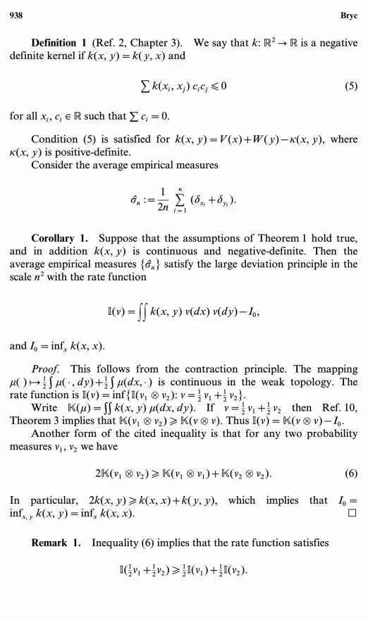
Definition 1 (Ref. 2, Chapter 3). We say that k: R2Q R is a negative

definite kernel if k(x, y)=k(y, x) and

C k(xi, xj) cicj [ 0 (5)

for all xi, ci ¥ R such that ; ci=0.

Condition (5) is satisfied for k(x, y)=V(x)+W(y) − o(x, y), whereo(x, y) is positive-definite.

Consider the average empirical measures

sn :=12n

Cn

i=1(dxi

+dyi).

Corollary 1. Suppose that the assumptions of Theorem 1 hold true,and in addition k(x, y) is continuous and negative-definite. Then theaverage empirical measures {sn} satisfy the large deviation principle in thescale n2 with the rate function

I(n)=FF k(x, y) n(dx) n(dy) − I0,

and I0=infx k(x, x).

Proof. This follows from the contraction principle. The mappingm( ) W 1

2 > m( · , dy)+12 > m(dx, · ) is continuous in the weak topology. The

rate function is I(n)=inf{I(n1 é n2): n=12 n1+1

2 n2}.Write K(m)=>> k(x, y) m(dx, dy). If n=1

2 n1+12 n2 then Ref. 10,

Theorem 3 implies that K(n1 é n2) \ K(n é n). Thus I(n)=K(n é n) − I0.Another form of the cited inequality is that for any two probability

measures n1, n2 we have

2K(n1 é n2) \ K(n1 é n1)+K(n2 é n2). (6)

In particular, 2k(x, y) \ k(x, x)+k(y, y), which implies that I0=infx, y k(x, y)=infx k(x, x). i

Remark 1. Inequality (6) implies that the rate function satisfies

I(12n1+1

2n2) \ 12I(n1)+1

2I(n2).

938 Bryc

2. APPLICATIONS

2.1. Let g(x, y)=e−x2 − y2+2hxy. Then

f(x, y)=exp 1− n Cn

i=1x2

i − n Cn

j=1y2

j +2h Cn

i, j=1xi yj

2

and k(x, y)=x2+y2 − 2hxy.Denote by mr(n)=>x rn(dx) the r-th moment of a measure n.

Proposition 1.

(i) If |h| < 1 then the empirical measures

nn :=1n

Cn

i=1dxj

satisfy the large deviation principle in the scale n2 with the rate function

I(n)=(m2(n) − h2m21(n)).

(ii) If 0 [ h < 1 then the average empirical measures

sn :=12n

Cn

i=1(dxi

+dyi)

satisfy the large deviation principle in the scale n2 with the rate function

I(n)=2(m2(n) − hm21(n)).

(In the formulas above, use I(n)=. if m2(n)=..)

Remark 2. The marginal density relevant in Proposition 1(i) is

f1(x)=C(n, h) exp 1− n2 11n

Cn

i=1x2

i − h2 1 1n

Cn

i=1xi2222 .

Remark 3. Both rate functions in Proposition 1 are concave.

Proof. (i) It is easy to see that the assumptions of Theorem 1 aresatisfied. Indeed, k(x, y)=(x − hy)2+(1 − h2)y2 is continuous, boundedfrom below. Furthermore

{k(x, y) [ a2} … {|y| [ |a|/(1 − h2)} 5 {|x| [ |a|/(1 − h2)}


so k(x, y) has compact level sets. Finally, for a > 0 by a change of variableswe see that >> e−ak(x, y) dx dy=1

a >> e−k(x, y) dx dy < . so Assumption 2 issatisfied, too.

The result follows by the contraction principle: taking a marginalof a measure in P(R2) is a continuous mapping. The rate function isinf{I(m): n(A)=m(A × R)}. But since I is infinite on non-product measures,this is the same as infn2

{>> k(x, y) n(dx) n2(dy) − I0}. Since I0=0 here, itremains to notice that infn2

{>> k(x, y) n(dx) n2(dy)}=infy{> k(x, y) n(dx)}=infy{m2(n)+y2 − 2hym1(n)}=m2(n) − h2m2

1(n).(ii) This follows from Corollary 1: if h \ 0 then 2hxy is positive-

definite. Thus k(x, y)=x2+y2 − 2hxy is a negative definite kernel. i

2.2. Next, we consider a model which can be interpreted as a ‘‘decoupled’’version of a model studied in relation to eigenvalue fluctuations of randommatrices, where one encounters xj instead of our yj, compare Ref. 1, Sec-tion 5 and Ref. 9, formula (1.9). We consider here a slightly more generalsituation when

g(x, y)=|x − y|b e−V(x) − W(y).

Then

f(x, y)= Dn

i, j=1|xi − yj |b D

n

i=1e−nV(xi) D

n

j=1e−nW(yj),

and k(x, y)=V(x)+W(y) − b log |x − y|. We assume that functions V(x),W(y) are continuous, b \ 0, and that

lim|x| Q .

V(|x|)

log `1+x2= lim

|y| Q .

W(|y|)

log `1+y2=.. (7)

Proposition 2. The bivariate empirical measures mn defined by (2)satisfy the large deviation principle in the scale n2 with the rate function Igiven by (4).

In particular, if V(u)=W(u)=u2, then the rate function is

I(n1 é n2)=m2(n1)+m2(n2) − b FF log |x − y| n1(dx) n2(dy)+12b(log b − 1).

Proof. We verify that the hypotheses of Theorem 1 are satisfied.Assumption 1 holds trivially. Assumption 5 holds trivially since V(x)+W(y) is continuous.

940 Bryc

To verify Assumption 3 notice that

k(x, y) \ V(x)+W(y) − b log `1+x2 − b log `1+y2 . (8)

Since V(x) − b log `1+x2 is a continuous function which by (7) tendsto infinity as x Q ± ., it is bounded from below, V(x) − b log `1+x2 \

− c for some c. Similarly, W(y) − b log `1+y2 \ − c.We now verify Assumption 4. The set Ka :={k(x, y) [ a} is closed

since k is lower semicontinuous. Furthermore, (8) implies that Ka is con-tained in a level set of the continuous function V(x)+W(y) − b log `1+x2

− b log `1+y2. The latter set is bounded since V(x) − b log `1+x2 > a+cfor all large enough |x| and similarly W(y) − b log `1+y2 > a+c for alllarge enough |y|.

To verify Assumption 2 we use inequality (8) again. It implies

FF g(x, y)a dx dy [ F e−a(V(x) − b log `1+x2 ) dx F e−a(W(y) − b log `1+y2 ) dy.

By assumption (7), there is N > 0 such that for |x| > N we haveV(x) > (b+2/a) log `1+x2. By the previous argument the integrandis bounded; thus > e−a(V(x) − b log `1+x2) dx [ >

N

−Ne−a(V(x) − b log `1+x2) dx+

>|x| > N e−a(2/a log `1+x2) dx [ 2Neac+>|x| > N1

1+x2 dx < ..Therefore, by Theorem 1 the empirical measures mn satisfy the large

deviation principle with the rate function I(n1 é n2)=> V(x) n1(dx)+> W(y) n2(dy) − b >> log |x − y| n1(dx) n2(dy) − I0. If W(u)=V(u)=u2 thenI0=infx, y{x2+y2 − b log |x − y|}=b/2(1 − log b) by calculus. i

3. AUXILIARY RESULTS AND PROOF OF THEOREM 1The proof relies on Varadhan’s functional method (see Ref. 3,

Theorem T.1.3 and Ref. 6, Theorem 4.4.10). It consists of two steps: verifi-cation that the Varadhan functional

F W L(F) := limn Q .

1n2 log E exp(F(mn))

is well defined for a large enough class of bounded continuous functionsF: PQ R, and the proof of exponential tightness of {mn}.

3.1. Varadhan FunctionalLet F1, ..., Fm: R2

Q R be bounded continuous functions. Consider thebounded continuous function F: P(R2) Q R given by

F(m) := min1 [ r [ m

F Fr dm. (9)


We will show the following.

Theorem 2. Under the assumptions of Theorem 1,

limn Q .

1n2 log F exp(n2F(mn)) f(x, y) dx dy

=sup 3F(m) − F k(x, y) dm : m=n1 é n2 ¥ P(R2)4 . (10)

Denote K(m)=> k(x, y) dm. Notice that by Assumption 3 we haveF(m) − K(m) [ maxr ||Fr ||.+C. In particular,

sup{F(m) − K(m): m ¥ P(R2)} < .. (11)

We prove (10) as two separate inequalities. It will be convenient toprove the upper bound for a larger class of functions F.

Lemma 1. If Assumptions 2 and 3 hold true, then for every boundedcontinuous function F : P(R2) Q R we have

lim supn Q .


[ sup{F(m) − K(m): m=n1 é n2 ¥ P(R2)}. (12)

Proof. Notice that for 0 < h < 1

F exp(n2F(mn)) f(x, y) dx dy

=F exp(n2(F(mn) − hK(mn)) − (1 − h) Cn

i, j=1k(xi, yj)) dx dy

[ exp(n2 supn1, n2

(F(n1 é n2) − hK(n1 é n2)))

× F exp 1−(1 − h) Cn

i, j=1k(xi, yj)2 dx dy.

942 Bryc

Since

Cn

i, j=1k(xi, yj) \ − n2C+ C

n

j=1k(xj, yj),

therefore


[ supn1, n2

{F(n1 é n2) − hK(n1 é n2)}+(1 − h) C+1n

log M1 − h.

Thus

lim supn Q .


[ supn1, n2

{h(F(n1 é n2) − K(n1 é n2))+(1 − h) F(n1 é n2)}+2(1 − h)C

[ h supn1, n2

{F(n1 é n2) − K(n1 é n2)}+(1 − h) ||F||.+2(1 − h)C.

Passing to the limit as h Q 1 we get (12). i

The proof of the lower bound is a combination of the discretizationargument in Ref. 1, pp. 532–535 with the entropy estimate from Ref. 9,pp. 191–192.

Denote by P0 the set of absolutely continuous probability measuresn(dx)=f(x) dx on R with compact support supp(n), and continuousdensity f. Let us first record the well-known fact.

Lemma 2. If n ¥ P0 then n has finite entropy

Hf :=F log f(x) n(dx) < ..

We first establish a weaker version of the lower bound.

Lemma 3. If F is given by (9), then

lim infn Q .


\ sup{F(n1 é n2) − K(n1 é n2): n1, n2 ¥ P0}. (13)


Proof. Fix n1, n2 ¥ P0. Since k(x, y) \ − C is bounded from below,K(n1 é n2) ¥ (−., .], so without loss of generality we may assume thatk(x, y) is n1 é n2-integrable.

Since measures n1, n2 are absolutely continuous and have compactsupports, for every integer n > 0 we can find partitions P1(n)={a0 < a1 < · · · < an} and P2(n)={b0 < b1 < · · · < bn} of supp(n1),supp(n2) respectively such that

n1(ai − 1, ai)=n2(bj − 1, bj)=1n

for i, j=1, 2,..., n.

Then, denoting A=[a0, a1] × [a1, a2] × · · · × [an − 1, an] and B=[b0, b1] ×[b1, b2] × · · · × [bn − 1, bn], we have

F exp(n2F(mn)) f(x, y) dx dy

\ FA × B

exp 1minr

Cn

i, j=1Fr(xi, yj) − C

n

i, j=1k(xi, yj)2 dx dy. (14)

Write n1=f(x) dx, n2=g(y) dy. By our choice of the partitions,functions

fi(x) :=nf(x) I[ai − 1, ai]

and

gj(x) :=ng(x) I[bj − 1, bj]

are probability densities. Let

S(x, y)=minr

Cn

i, j=1Fr(xi, yj) − C

n

i, j=1k(xi, yj) − C

n

i=1log f(xi) − C

n

j=1log g(yj).

Integrating over a smaller set {f1(x1) > 0,..., fn(xn) > 0, g1(y1) > 0,...,gn(yn) > 0} on the right hand side of (14) we get

F exp(n2F(mn)) f(x, y) dx dy \1

n2n F exp(S(x, y)) Dn

i=1fi(xi) D

n

j=1gj(yj) dx dy.

Using Jensen’s inequality, applied to the convex exponential functionin the last integral, we get


n2n exp(S1 − S2 − S3 − S4),

944 Bryc

where

S1=FR

2n1min

rCn

i, j=1Fr(xi, yj)2 D

n

i=1fi(xi) D

n

j=1gj(xj) dx dy,

S2=FR

2nCn

i, j=1k(xi, yj) D

n

i=1fi(xi) D

n

j=1gj(yj) dx dy,

S3=FR

nCn

i=1log f(xi) D

n

i=1fi(xi) dx,

S4=FR

nCn

j=1log g(yj) D

n

j=1gj(yj) dy.

We need the following identities. (Proofs of all Claims are postponeduntil the end of this proof.)

Claim 1. For a n1 é n2-integrable function h, we have

FR

nCn

j=1h(yj) D

n

j=1gj(yj) dy=n F

Rh(y) g(y) dy,

FR

nCn

i=1h(xi) D

n

i=1fi(xi) dx=n F

Rh(x) f(x) dx,

FR

2nCn

i, j=1h(xi, yj) D

n

i=1fi(xi) D

n

j=1gj(yj) dx dy=n2 FF h(x, y) f(x) g(y) dx dy.

Lemma 2 says that the entropies Hf=> log f(x) f(x) dx, Hg=> log g(y) g(y) dy are finite. Thus the functions k(x, y), log f(x), andlog g(y) are n1 é n2-integrable. Applying Claim 1, we get S2=n2K(n1 é n2),S3=nHf, and S4=nHg. Therefore,


n2n exp(S1 − n2K(n1 é n2) − nHf − nHg).

We need the following lower bound for S1.

Claim 2.

F 1minr

Cn

i, j=1Fr(xi, yj)2 D fi(xi) D gj(yj) dx dy \ min

rCn

i, j=1Fr, (i, j),

(16)


where

Fr, (i, j)=min{Fr(x, y): ai − 1 [ x [ ai, bj − 1 [ y [ bj}.

Combining inequalities (15) and (16), we get


\1n2 min

rCn

i, j=1Fr, (i, j) − K(n1 é n2) −

1n

Hf −1n

Hg −2n

log n. (17)

Since functions Fr(x, y) are continuous and n1, n2 have compact sup-port, n1 é n2-almost surely ;n

i, j=1 Fr, (i, j) I(ai − 1, ai)(x) I(bj − 1, bj)(y) Q Fr(x, y),and the functions are bounded. Since 1 [ r [ m ranges over a finite set ofvalues only we have

limn Q .

1n2 min

rCn

i, j=1Fr, (i, j)

=minr

limn Q .

Cn

i, j=1Fr, (i, j)n1(ai − 1, ai) n2(bj − 1bj)=F(n1 é n2).

Letting n Q . in (17) we obtain (13).To conclude the proof, it remains to prove Claims 1 and 2.

Proof of Claim 1. Switching the order of integration and summation,we get

F Cn

j=1h(yj) D gj(yj) dy= C

n

j=1F h(yj) gj(yj) dyj D

i ] jF gi(yi) dyi

= Cn

j=1F h(yj) gj(yj) dyj

=n Cn

j=1F

bj

bj − 1

h(y) g(y) dy=n Fbn

b0

h(y) g(y) dy.

The other two identities follow by a similar argument. i

Proof of Claim 2. Fix 0 [ k [ n, x1,..., xk ¥ R and y1,..., yn ¥ R. Let

Gr, k(x1,..., xk) := Ck

i=1Cn

j=1Fr(xi, yj)+ C

n

i=k+1Cn

j=1min

ai − 1 [ x [ ai

Fr(x, yj).

946 Bryc

If ak − 1 < xk < ak, we have

minr

Gr, k(x1,..., xk)

=minr

1 Ck − 1

i=1C

jFr(xi, yj)+C

jFr(xk, yj)+ C

n

i=k+1C

jmin

ai − 1 [ x [ ai

Fr(x, yj)2

\ minr

Gr, k − 1(x1,..., xk − 1).

Therefore,

Fak

ak − 1

minr

Gr, k(x) fk(xk) dxk \ minr

Gr, k − 1(x).

Recurrently,

F minr

1 Cn

i=1Cn

j=1Fr(xi, yj)2 D fi(xi) dx

=F minr

Gr, n(x) D fi(xi) dx \ minr

Gr, 0(x)

=minr

1 Cn

i=1Cn

j=1min

ai − 1 [ x [ ai

Fr(x, yj)2 .

Applying the same reasoning to variables y1,..., yn and

Gr, k(y1,..., yk) := Ck

j=1Cn

i=1min

ai − 1 [ x [ ai

Fr(x, yj)+ Cn

j=k+1Cn

i=1Fr, (i, j)

we get (16). i

This concludes the proof. i

The next lemmas show that the right hand sides of (12) and (13)coincide.

Let Pc denote compactly supported probability measures.

Lemma 4. If Assumption 3 holds true, then

sup{F(n1 é n2) − K(n1 é n2): n1, n2 ¥ Pc}

=sup{F(n1 é n2) − K(n1 é n2): n1, n2 ¥ P}. (18)


Proof. Clearly the left-hand side of (18) cannot exceed the right handside. To show the converse inequality, fix g > 0 and n1, n2 ¥ P such that

F(n1 é n2) − K(n1 é n2) \ supn1, n2 ¥ P

{F(n1 é n2) − K(n1 é n2)} − g. (19)

Since the supremum is finite, see (11), and k(x, y) is bounded from below,therefore >> |k(x, y)| dn1 dn2 < ..

For L > 0 large enough, define probability measures nj, L by

nj, L(A) :=nj(A 5 [−L, L])

nj([−L, L]), j=1, 2.

By definition, measures nj, L ¥ Pc have compact support. Since −C [

k(x, y) I|x| < L, |y| < L [ |k(x, y)| and k is n1 é n2-integrable, by Lebesgue’sdominated convergence theorem

limL Q .

K(n1, L é n2, L)=limL Q . >L

−L >L−L k(x, y) n1(dx) n2(dy)

limL Q . n1([−L, L]) n2([−L, L])=K(n1 é n2).

Similarly,

limL Q .

F(n1, L é n2, L)=F(n1 é n2).

Thus (18) follows. i

Lemma 5. If Assumptions 3 and 5 hold true, then

sup{F(n1 é n2) − K(n1 é n2): n1, n2 ¥ P0}

=sup{F(n1 é n2) − K(n1 é n2): n1, n2 ¥ P}. (20)

Proof. Trivially,

supn1, n2 ¥ P0

{F(n1 é n2) − K(n1 é n2)} [ supn1, n2 ¥ P

{F(n1 é n2) − K(n1 é n2)}.

To show the converse inequality, fix g > 0 and compactly supportedn1, n2 ¥ Pc such that

F(n1 é n2) − K(n1 é n2) \ supn1, n2 ¥ P

{F(n1 é n2) − K(n1 é n2)} − g, (21)

see Lemma 4. As previously, k(x, y) is n1 é n2-integrable, see (11).

948 Bryc

Consider the convolution nEj (A) := 1

2E >E−E nj(A − x) dx, where j=1, 2

and 0 < E [ 1. Measures nE1, nE

2 have continuous densities, and since n1, n2

have compact supports, nE1, nE

2 also have compact support. Thus nE1, nE

2 ¥ P0

and

supn1, n2 ¥ P0

{F(n1 é n2) − K(n1 é n2)} \ F(nE1 é nE

2) − K(nE1 é nE

2). (22)

As E Q 0 measure nEj converges weakly to nj. Hence

limE Q 0

F(nE1 é nE

2)=F(n1 é n2). (23)

Assumption 5 asserts that V(x, y) :=b log |x − y|+k(x, y) is acontinuous function. Thus |V(x, y)| is bounded on the compact setsupp(n1

1 é n12). Since the supports of nE

1 é nE2 are contained in supp(n1

1 é n12),

and nEj Q nj, we get

FF V(x, y) nE1(dx) nE

2(dy) Q FF V(x, y) n1(dx) n2(dy). (24)

This concludes the proof if b=0. If b > 0, then log |x − y| isn1 é n2-integrable as a linear combination of integrable functions,log |x − y|=(V(x, y) − k(x, y))/b. Therefore we have

F(nE1 é nE

2) − K(nE1 é nE

2)

=F(nE1 é nE

2) − FF V(x, y) nE1(dx) nE

2(dy)+b FF log |x − y| n1(dx) n2(dy)

− b 1FF log |x − y| n1(dx) n2(dy) − FF log |x − y| nE1(dx) nE

2(dy)2 .

Taking the lim sup as E Q 0, from (22), (23), (24), and (21) we get

supn1, n2 ¥ P0

{F(n1 é n2) − K(n1 é n2)}

\ supn1, n2 ¥ P

{F(n1 é n2) − K(n1 é n2)} − g

− lim supE Q 0

1FF log |x − y| n1(dx) n2(dy) − FF log |x − y| nE1(dx) nE

2(dy)2 .

Since g > 0 is arbitrary, to end the proof we use the following.


Claim 3.

lim supE Q 0

1FF log |x − y| n1(dx) n2(dy) − FF log |x − y| nE1(dx) nE

2(dy)2 [ 0. i

Proof of Claim 3. Claim 3 is established by the argument in Ref. 9,pp. 192–193. For completeness, we repeat it here. Let X, Y be independentrandom variables with distributions n1, n2 respectively and let Z=X − Y.Since log |Z| is integrable, Pr(Z=0)=0. Let U ¥ [−2, 2] be a r.v. inde-pendent of Z with the density f(u)=(2 − |u|)/4. It is easy to see that>> log |x − y| nE

1(dx) nE2(dy)=E log |Z+EU|, and the inequality to prove

reads

lim supE Q 0

E 1 log+ 1|1+E(U/Z)|

2 [ 0.

For fixed z ] 0 we have

E 1 log+ 1|1+E(U/z)|

2 [1

log 2log 11+

2E

|z|2 . (25)

Indeed, since (2 − |u|)/4 [ 1/2 we get

E 1 log+ 1|1+E(U/z)|

2 [|z|4E

F1+2E/|z|

1 − 2E/|z|log+ 1

|x|dx.

Therefore,

E 1 log+ 1|1+E(U/z)|

2 [ ˛ |z|4E

F1

1 − 2E/|z|log

1x

dx if |z| > 2E

|z|4E1F

1

0log

1x

dx+F2E/|z| − 1

0log+ 1

xdx2 if |z| [ 2E .

If |z| > 2E we get E(log+ 1|1+E(U/z)|) [ 1

2 log 11−2E/|z| < 1

2 log(1+2E|z|) [ 1

log 2 log(1+2E|z|).

If |z| [ 2E, then E(log+ 1|1+E(U/z)|) [ |z|

2E >10 log 1

x dx [ 1 [ 1log 2 log(1+2E

|z|). Thus inboth cases, (25) holds true.

To finish the proof we integrate inequality (25) and get

lim supE Q 0

E 1 log+ 1|1+E(U/Z)|

2 [1

log 2lim sup

E Q 0E(log(1+2E/|Z|)).

950 Bryc

For E < 1/2 we have log(1+2E/|Z|) [ log 2+log+ 1|Z| and log+ 1

|Z| is inte-grable. Lebesgue’s dominated convergence theorem yields

lim supE Q 0

E(log(1+2E/|Z|))=0. i

Proof of Theorem 2. Combining Lemmas 1 and 3 we have

sup{F(n1 é n2) − K(n1 é n2): n1, n2 ¥ P0}

[ lim infn Q .


[ lim infn Q .


[ sup{F(n1 é n2) − K(n1 é n2): n1, n2 ¥ P}.

By (20), all of the above inequalities are in fact equalities. Thus (10) holdstrue. i

3.2. Exponential Tightness

Recall that {mn} is exponentially tight if for every m > 0 there is acompact subset K … P such that

supn

1n2 log Pr(mn ¨ K) < − m.

Our proof of exponential tightness is a concrete implementation of deAcosta. (5)

Assumption 3 implies that k(x, y)+C \ 0. Let q: P(R2) Q [0, .] begiven by

q(m)=FR

2(k(x, y)+C) dm.

Lemma 6. If Assumptions 3 and 4 hold true, then q has pre-compactlevel sets: for every t > 0, q−1[0, t] is a pre-compact set in P.

Proof. Fix t > 0 and denote K :={m ¥ P(R2): q(m) [ t}. We willshow that K is pre-compact.


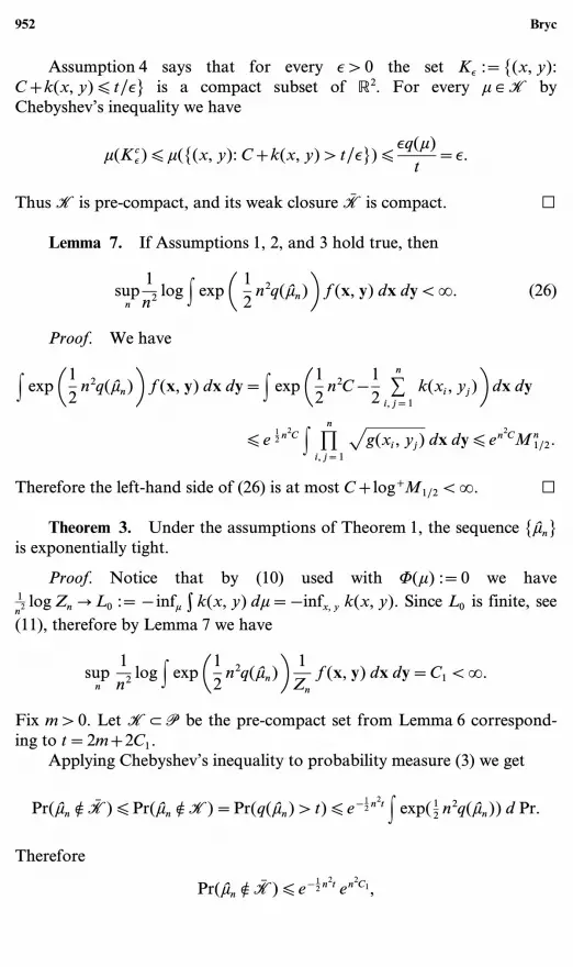
Assumption 4 says that for every E > 0 the set KE :={(x, y):C+k(x, y) [ t/E} is a compact subset of R2. For every m ¥ K byChebyshev’s inequality we have

m(KcE) [ m({(x, y): C+k(x, y) > t/E}) [

Eq(m)t

=E.

Thus K is pre-compact, and its weak closure K is compact. i

Lemma 7. If Assumptions 1, 2, and 3 hold true, then

supn

1n2 log F exp 1 1

2n2q(mn)2 f(x, y) dx dy < .. (26)

Proof. We have

F exp 112

n2q(mn)2 f(x, y) dx dy=F exp 112

n2C −12

Cn

i, j=1k(xi, yj)2 dx dy

[ e12 n2C F D

n

i, j=1`g(xi, yj) dx dy [ en2CMn

1/2.

Therefore the left-hand side of (26) is at most C+log+M1/2 < .. i

Theorem 3. Under the assumptions of Theorem 1, the sequence {mn}is exponentially tight.

Proof. Notice that by (10) used with F(m) :=0 we have1n2 log Zn Q L0 := − infm > k(x, y) dm=−infx, y k(x, y). Since L0 is finite, see(11), therefore by Lemma 7 we have

supn

1n2 log F exp 11

2n2q(mn)2 1

Znf(x, y) dx dy=C1 < ..

Fix m > 0. Let K … P be the pre-compact set from Lemma 6 correspond-ing to t=2m+2C1.

Applying Chebyshev’s inequality to probability measure (3) we get

Pr(mn ¨ K) [ Pr(mn ¨ K)=Pr(q(mn) > t) [ e−12 n2t F exp( 1

2 n2q(mn)) d Pr.

Therefore

Pr(mn ¨ K) [ e−12 n2t en2C1,

952 Bryc

and

1n2 log Pr(mn ¨ K) [ −t/2+C1=−m

for all n. i

Proof of Theorem 1. Recall that the space P=P(R2) of probabilitymeasures on R2 with the topology of weak convergence is a Polish space.By Theorem 3, {mn} is exponentially tight. Theorem 2 says that theVaradhan functional

L(F) := limn Q .

1n2 log E(exp n2F(mn))

is defined on all functions F given by (9), and

L(F)=supn1, n2

{F(n1 é n2) − K(n1 é n2)} − limn Q .

1n2 log Zn

=supn1, n2

{F(n1 é n2) − K(n1 é n2)}+infx, y

k(x, y).

Thus

L(F)=supn1, n2

{F(n1 é n2) − K(n1 é n2)}+I0. (27)

Functions F defined by (9) form a subset of Cb(P(R2)) which sepa-rates points of P(R2) and is closed under the operation of taking pointwiseminima. Thus by Ref. 3, Theorem T.1.3 or Ref. 6, Theorem 4.4.10, theempirical measures {mn} satisfy the large deviation principle with the ratefunction

I(m) :=sup{F(m) − L(F)}; (28)

here, the supremum is taken over all F1,..., Fm ¥ Cb(R2) and F(m) is definedby (9).

It remains to prove formula (4). Fix n1, n2 ¥ P. From (27), for F givenby (9) we have L(F) \ F(n1 é n2) − K(n1 é n2)+I0. Thus formula (28)implies that

I(n1 é n2) [ K(n1 é n2) − I0. (29)


To prove the converse inequality we use the fact that we already knowthat the large deviations principle holds. The large deviations principleimplies that

I(n1 é n2)= supF ¥ Cb(P)

{F(n1 é n2) − L(F)}. (30)

Now consider FM(m)=> (M N k(x, y)) dm. Assumptions 3 and 5 implythat (x, y) W M N k(x, y) is a bounded continuous function for every realM. Thus FM is given by (9). Since M N k(x, y) [ k(x, y), from (27) we getL(FM) [ I0. Thus

I(n1 é n2) \ supM

{FM(n1 é n2) − L(FM)} \ lim supM Q .

F M N k(x, y) dm − I0.

This together with (29) proves (4) for product measures.It remains to verify that if m0 is not a product measure, then

I(m0)=.. To this end, take bounded continuous functions F(x), G(y)such that

d :=F F(x) G(y) m0(dx, dy) − F F(x) m0(dx, dy) F G(y) m0(dx, dy) > 0.

For b > 0, let

Fb(m) :=b 1F F(x) G(y) m(dx, dy) − F F(x) m(dx, dy) F G(y) m(dx, dy)2 .

Clearly, Fb : PQ R is a bounded continuous function, which vanisheson product measures. By the upper bound (12) we therefore haveL(Fb) [ I0. So I(m0) \ Fb(m0) − L(Fb) \ bd − I0. Since b can be arbitrarilylarge, I(m0)=.. i

ACKNOWLEDGMENTS

I would like to thank P. Dupuis for a conversation on non-convex ratefunctions.

REFERENCES

1. Ben Arous, G., and Guionnet, A. (1997). Large deviations for Wigner’s law andVoiculescu’s non-commutative entropy. Probab. Theory Related Fields 108(4), 517–542.

2. Berg, C., Christensen, J. P. R., and Ressel, P. (1984). Harmonic Analysis on Semigroups,Springer-Verlag, New York.

954 Bryc

3. Bryc, W. (1990). On the large deviation principle by the asymptotic value method. InPinsky, M., (ed.), Diffusion Processes and Related Problems in Analysis, Birkhäuser, Vol. I,pp. 447–472.

4. Chan, T. (1993). Large deviations for empirical measures with degenerate limiting distri-bution. Probab. Theory Related Fields 97(1–2), 179–193.

5. de Acosta, A. (1985). Upper bounds for large deviations of dependent random vectors.Z. Wahrsch. Verw. Gebiete 69(4), 551–565.

6. Dembo, A., and Zeitouni, O. (1998). Large Deviations Techniques and Applications (2nded.), Springer-Verlag, New York.

7. Dinwoodie, I. H., and Zabell, S. L. (1992). Large deviations for exchangeable randomvectors. Ann. Probab. 20(3), 1147–1166.

8. Hiai, F., and Petz, D. (2000). The Semicircle Law, Free Random Variables and Entropy,American Mathematical Society, Providence.

9. Johansson, K. (1998). On fluctuations of eigenvalues of random Hermitian matrices. DukeMath. J. 91(1), 151–204.

10. Ressel, P. (1982). A general Hoeffding type inequality. Z. Wahrsch. Verw. Gebiete 61(2),223–235.


Documents

Large deviations of empirical measures under symmetric interaction