Embed Size (px)
Citation preview
To appear: Math. Comp. 2001
LANDEN TRANSFORMATIONS AND THE INTEGRATION OFRATIONAL FUNCTIONS
GEORGE BOROS AND VICTOR H. MOLL
Abstract. We present a rational version of the classical Landen transfor-
mation for elliptic integrals. This is employed to obtain explicit closed-formexpressions for a large class of integrals of even rational functions and to de-velop an algorithm for numerical integration of these functions.
1. Introduction
We consider the space of even rational functions of degree 2p
E2p :=
{R(z) =
P (z)Q(z)
∣∣∣ P (z) :=p−1∑k=0
bkz2(p−1−k) and Q(z) :=
p∑k=0
akz2(p−k)
}with positive real coefficients ak, bk ∈ R+ normalized by the condition a0 = ap = 1,the space
E∞ :=∞⋃p=1
E2p
of normalized even rational functions, and the set of 2p− 1 parameters
P2p := {a1, · · · , ap−1; b0, · · · , bp−1}.
We describe an algorithm to determine, as a function of the parameter set P2p, aclosed-form expression of the integral
I :=∫ ∞
0
R(z) dz(1.1)
for a large class of functions R ∈ E∞. The function R is called symmetric if itsdenominator Q satisfies Q(1/z) = z−2pQ(z). This is equivalent to its coefficientsbeing palindromic, i.e. aj = ap−j for 1 ≤ j ≤ p.
The class of symmetric functions plays a crucial role in this algorithm. Define
Es2p := {R ∈ E2p
∣∣∣ den(R) is symmetric}
(where den(R) denotes the denominator of R), the class of rational functions withsymmetric denominators of degree 2p, and
Es∞ :=∞⋃p=1
Es2p.
Date: April 25, 2001.1991 Mathematics Subject Classification. Primary 33.Key words and phrases. Rational functions, Landen transformation, Integrals.
The second author was supported in part by NSF Grant DMS-0070567.
1
2 GEORGE BOROS AND VICTOR H. MOLL
For m ∈ N define
Em2p := {R ∈ E∞
∣∣∣ (den(R))1/(m+1) is even, symmetric of degree 2p}
and Em,s2p := Em2p ∩ Es2p, so a function R ∈ Em,s2p can be written in the form
R(z) =P (z)
Qm+1(z),
where P (z) is an even polynomial and Q(z) is an even symmetric polynomial ofdegree 2p.
The method of partial fractions gives (in principle) the value of I in terms ofthe roots of Q. Symbolic computations yield either a closed-form answer, an ex-pression in terms of the roots of an associated polynomial, or the integral returnedunevaluated.
The algorithm described here allows only algebraic operations on elementaryfunctions and changes of variables of the same type. In particular, we exclude thesolution of algebraic equations of degree higher than 2. We say that a rationalfunction R ∈ E∞ is computable if its integral can be evaluated by our algorithm.
The first step in the algorithm is to consider symmetric rational functions. InSection 2 we prove a reduction formula, i.e. a map Fp : Es2p → Rp that reduces thecomputability of the integral of the symmetric function R to that of one of degree12deg(R). Here Rp is the space of rational functions with denominator of degree p.These new functions are not necessarily symmetric, and this is the main limitationof our algorithm. The details of Fp require the evaluation of some binomial sumswhich are presented in Appendix A. The classical Wallis’ formula∫ ∞
0
dz
(z2 + 1)m+1=
π
22m+1
(2mm
)shows that every R ∈ Em2 is computable. The reduction formula now implies thatevery R ∈ Em4 is computable. This is described in Section 3. The computability ofR ∈ E4 is also a consequence of the classical theory of hypergeometric functions;the details are given in [2]. In Section 4 we compute the integral of every functionin Em,s8 , where the reduction method expresses these integrals in terms of functionsin Em4 . The algorithm does not, in general, provide a value for the integral of anonsymmetric function of degree 8.
The final piece of the algorithm is described in Section 5: for R ∈ E2p, thesymmetrization of its denominator produces a (symmetric) rational function in E4p
with the same integral as R. The reduction formula now yields a new function inE2p with the same integral as R. We thus obtain a map T2p : E2p → E2p such that∫ ∞
0
R(z) dz =∫ ∞
0
T2p(R(z)) dz.(1.2)
In particular, the class of computable rational functions of degree 2p is invariantunder forward and backward iteration of T2p. This map is the rational analog ofthe original Landen transformation for elliptic integrals described in [4, 13]. Themap T2p can also be interpreted as a map on the coefficients Φ2p : O+
2p → O+2p
where O+2p = R+
p−1 × R+p.
LANDEN TRANSFORMATIONS AND THE INTEGRATION OF RATIONAL FUNCTIONS 3
The case of Φ6 is described in detail in Section 6 and is given explicitly by
a1 → 9 + 5a1 + 5a2 + a1a2
(a1 + a2 + 2)4/3(1.3)
a2 → a1 + a2 + 6(a1 + a2 + 2)2/3
b0 → b0 + b1 + b2(a1 + a2 + 2)2/3
b1 → b0(a2 + 2) + 2b1 + b2(a1 + 3)a1 + a2 + 2
b2 → b0 + b2(a1 + a2 + 2)1/3
.
Let x0 := (a1, a2; b0, b1, b2). Then Φ6 : O+6 → O+
6 is iterated to produce a sequencexn+1 := Φ6(xn) of points in O+
6 that yield a sequence of rational functions withconstant integral. We have proved in [3] the existence of L ∈ R+, depending uponthe initial point x0 = (a1, a2; b0, b1, b2), such that xn → (3, 3;L, 2L,L). Thus∫ ∞
0
b0z4 + b1z
2 + b2z6 + a1z4 + a2z2 + 1
dz = L(x0)× π
2.(1.4)
This establishes a numerical method to compute the integral in (1.4).Numerical studies on integrals of even degree 2p suggest the existence of a lim-
iting value L = L(x0) such that the sequence xn := Φ2p(xn) satisfies
xn →((
p
1
),
(p
2
), · · · ,
(p
p− 1
);(p− 1
0
)L,
(p− 1
1
)L, · · · ,
(p− 1p− 1
)L
).
The integral of the original rational function is thus π2 × L(x0). The proof of
convergence remains open for p ≥ 4. Examples are given in Section 7.The most important issues left unresolved in this paper are the convergence of
the iteration of the map Φ2p discussed above and the geometric interpretation of theLanden transformation T2p. Finally, the question of integration of odd functionshas not been addressed at all.
Some history. The problem of integration of rational functions R(z) = P (z)/Q(z)was considered by J. Bernoulli in the 18th century. He completed the originalattempt by Leibniz of a general partial fraction decomposition of R(z). The maindifficulty associated with this procedure is to obtain a complete factorization ofQ(z) over R. Once this is known the partial fraction decomposition of R(z) can becomputed. The fact is that the primitive of a rational function is always elementary:it consists of a new rational function (its rational part) and the logarithm of a secondrational function (its transcendental part). In his classic monograph [9] G. H. Hardystates: The solution of the problem (of definite integration) in the case of rationalfunctions may therefore be said to be complete; for the difficulty with regard to theexplicit solution of algebraical equations is one not of inadequate knowledge but ofproved impossibility. He goes on to add: It appears from the preceding paragraphsthat we can always find the rational part of the integral, and can find the completeintegral if we can find the roots of Q(z) = 0.
4 GEORGE BOROS AND VICTOR H. MOLL
In the middle of the last century Hermite [10] and Ostrogradsky [15] developedalgorithms to compute the rational part of the primitive of R(z) without factor-ing Q(z). More recently Horowitz [11] rediscovered this method and discussed itscomplexity. The problem of computing the transcendental part of the primitivewas finally solved by Lazard and Rioboo [12], Rothstein [17] and Trager [18]. Fordetailed descriptions and proofs of these algorithms the reader is referred to [5] and[6].
2. The reduction formula
In this section we present a map Fp : Em,s2p → Emp that is the basis of theintegration algorithm described in Section 5. The proof is elementary and thebinomial sums discussed in the Appendix are employed.
Let Dp(z) be the general symmetric polynomial of degree 4p. We express theintegral of z2n/Dm+1
p as a linear combination of integrals of z2j/Em+1p where Ep is
a polynomial of degree 2p whose coefficients are determined by those of Dp.
Theorem 2.1. Let m,n, p ∈ N. Define
Dp(d1, d2, · · · , dp; z) =p∑k=0
dp+1−k(z2k + z4p−2k)(2.1)
and
Ep(d1, d2, · · · , dp; z) =
p+1∑j=1
dj
z2p +
+p∑i=1
22i−1z2(p−i)p−i+1∑j=1
j + i− 1i
(j + 2i− 2j − 1
)dj+i,
(2.2)
for di ∈ R+. Then for 0 ≤ n ≤ (m+ 1)p− 1,∫ ∞0
z2n dz
(Dp(d1, · · · , dp; z))m+1 =
2−m(m+1)p−n−1∑
j=0
4j(
(m+ 1)p− n− 1 + j
2j
)∫ ∞0
z2((m+1)p−1−j)
(Ep(d1, · · · , dp; z) )m+1 dz,
(2.3)
and for (m+ 1)p− 1 < n < 2p(m+ 1)− 1 we employ the symmetry rule
Nn,p = N2p(m+1)−1−n,p.(2.4)
Proof. First observe that (2.4) follows from the change of variable z → 1/z. Nowconsider
Nn,p(d1, · · · , dp;m) :=∫ ∞
0
z2n dz
(∑pk=0 dp+1−k(z4p−2k + z2k) )m+1(2.5)
for 0 ≤ n ≤ (m+ 1)p− 1. The substitution z = tan θ yields
Nn,p =∫ π/2
0
(1− C2)nC4(m+1)p−2n−2 dθ
(∑pk=0 dp+1−k {(1− C2)2p−kC2k + (1− C2)kC4p−2k} )m+1 ,
LANDEN TRANSFORMATIONS AND THE INTEGRATION OF RATIONAL FUNCTIONS 5
where C = cos θ. Letting ψ = 2 θ and D = cosψ = 2C2 − 1 then gives
Nn,p =∫ π
0
(1−D2)n(1 +D)2(m+1)p−2n−1 dψ
(∑pk=0 dp+1−k(1−D2)k {(1−D)2p−2k + (1 +D)2p−2k} )m+1 .
Now observe that the integrals of the odd powers of cosine vanish when we expand(1 +D)2(m+1)p−2n−1, producing
Nn,p = 2−m∫ π/2
0
(1−D2)n∑(m+1)p−n−1j=0
(2(m+1)p−2n−1
2j
)D2j dθ{∑p
k=0 dp+1−k(1−D2)k∑p−kj=0
(2p−2k
2j
)D2j
}m+1 .
A second double angle substitution ϕ = 2ψ gives
Nn,p = 2−m∫ π
0
(1− E)n∑(m+1)p−n−1j=0
(2(m+1)p−2n−1
2j
)2p(m+1)−n−j−1(1 + E)j dϕ{∑p
k=0 dp+1−k(1− E)k∑p−kj=0
(2p−2k
2j
)2p−k−j(1 + E)j
}m+1 ,
where E = cosϕ = 2D2 − 1. The change of variable z = tan(ϕ/2) then yields
Nn,p = 2−m∫ ∞
0
z2n∑(m+1)p−n−1j=0
(2(m+1)p−2n−1
2j
)(1 + z2)(m+1)p−n−j−1 dz{∑p
k=0 dp+1−kz2k(∑p−k
j=0
(2p−2k
2j
)(1 + z2)p−k−j
)}m+1 .
(2.6)
Finally, we modify (2.6) using Lemma A.2 and Lemma A.4 with N = (m+1)p−n−1to produce (2.3).
Note that the previous theorem associates to each rational function of symmetricdenominator
R1(z) =bsz
2s + bs−1z2(s−1) + · · ·+ b0
( z4p + dpz4p−2 + · · ·+ 2d1z2p + · · ·+ 1 )m+1
a new rational function
R2(z) = 2−m(m+1)p−1∑
n=0
bn
(m+1)p−n−1∑j=0
4j(
(m+ 1)p− n− 1 + j
2j
)z2((m+1)p−1−j)
(Ep(d1, · · · , dp; z))m+1
such that ∫ ∞0
R1(z) dz =∫ ∞
0
R2(z) dz.
3. The quartic case
In this section we describe the computability of rational functions R ∈ Em4 .These are functions of the form
R(z) =P (z)
(z4 + 2az2 + 1)m+1
where P (z) is an even polynomial of degree 4m+2. Observe that the normalizationa0 = a2 = 1 makes the denominator of R automatically symmetric. It suffices toevaluate
Nn,4(d1;m) :=∫ ∞
0
z2n dz
(z4 + 2d1z2 + 1)m+1(3.1)
6 GEORGE BOROS AND VICTOR H. MOLL
where 0 ≤ n ≤ 2m+1 is required for convergence. From (2.4) we haveNn,4(d1;m) =N2m−1−n,4(d1;m), so we may assume 0 ≤ n ≤ m. We now employ Theorem 2.1 toobtain a closed form expression for Nn,4(d1;m).
Theorem 3.1. Let m ∈ N and assume 0 ≤ n ≤ m. Then
Nn,4(d1;m) :=∫ ∞
0
z2n dz
(z4 + 2d1z2 + 1)m+1 =(3.2)
π
23m+3/2(1 + a)m+1/2×m−n∑j=0
2j(1 + d1)j ×(
2m− 2j − 1m− j
)(m− n+ j
2j
)(2jj
)(m
j
)−1
.
For m+ 1 ≤ n ≤ 2m+ 1 we have∫ ∞0
z2n dz
(z4 + 2d1z2 + 1)m+1 =(3.3)
π
23m+3/2(1 + d1)m+1/2×n−m−1∑j=0
2j(1 + d1)j ×(
2m− 2j − 1m− j
)(m− n+ j
2j
)(2jj
)(m
j
)−1
.
Proof. We apply the result of the Theorem 2.1 with D1(d1; z) = z4 + 2d1z2 + 1 and
E1(d1; z) = (1 + d1)z2 + 2, so that∫ ∞0
z2n dz
(z4 + 2d1z2 + 1)m+1= 2−m
m−n∑j=0
4j(m− n+ j
2j
)∫ ∞0
z2(m−j) dz
((1 + d1)z2 + 2)m+1.
The change of variable u = (1 + d1)z2/2 then yields∫ ∞0
z2(m−j) dz
( (1 + d1)z2 + 2 )m+1= 2−(j+3/2)(1 + d1)−m+j−1/2
∫ ∞0
um−j−1/2 du
(1 + u)m+1
= π
(2m− 2jm− j
)(2jj
)(m
j
)−1
2−(2m+j+3/2)(1 + d1)−(m−j+1/2),
where we have used∫ ∞0
ur−1/2
(1 + u)sdu =
π
22(s−1)
(2rr
)(2(s− r − 1)s− r − 1
)(s− 1r
)−1
.
The algorithm also requires a scaled version of N0,4(d1;m).
Corollary 3.2. Let b > 0, c > 0, a > −√bc, m ∈ N, and 0 ≤ n ≤ m. Define
Nn,4(a, b, c;m) :=∫ ∞
0
z2n dz
(bz4 + 2az2 + c)m+1 .
Then for 0 ≤ n ≤ m,
Nn,4(a, b, c;m) = π
(c(c/b)m−n
{8(a+
√bc)}2m+1
)−1/2
×
×m−n∑k=0
2k(
2m− 2km− k
)(m− n+ k
2k
)(2kk
)(m
k
)−1(a√bc
+ 1)k
,
(3.4)
LANDEN TRANSFORMATIONS AND THE INTEGRATION OF RATIONAL FUNCTIONS 7
and for m+ 1 ≤ n ≤ 2m+ 1,
Nn,4(a, b, c;m) = π
(c(c/b)m−n
{8(a+
√bc)}2m+1
)−1/2
×
×n−m−1∑k=0
2k(
2m− 2km− k
)(m− n+ k
2k
)(2kk
)(m
k
)−1(a√bc
+ 1)k
.
(3.5)
Proof. Let 0 ≤ n ≤ m. The substitution u = z(b/c)1/4 yields
Nn,4(a, b, c;m) =1
cm−n/2+3/4bn/2+1/4Nn,4
(a√bc
;m),(3.6)
so (3.4) then follows from Theorem 3.1. From (2.4) we have Nn,4(a, b, c;m) =N2m+1−n,4(c, b, a;m) for m+ 1 ≤ n ≤ 2m+ 1, giving (3.5).
4. The symmetric case of degree 8
In this section we prove the computability of the set Em,s8 of symmetric rationalfunctions with denominator of degree 8 and establish an explicit formula for theintegral
Nn,8(a1, a2;m) =∫ ∞
0
z2n dz
(z8 + a2z6 + 2a1z4 + a2z2 + 1)m+1
where 0 ≤ n ≤ 4m+ 3 is required for convergence. Observe that (2.4) reduces thediscussion to the case 0 ≤ n ≤ 2m+ 1. The expression (2.2), with p = 2, producesE2(a1, a2; z) = (1 + a1 + a2)z4 + 2(a2 + 4)z2 + 8.
Theorem 4.1. Every function in Em,s8 is computable. More specifically, definec1 := a2 + 4, c2 := 1 + a1 + a2, and
tk,j(m,n; a1, a2) := π2−(3m+2+k+j)/2c(m−k−j)/22 (c1 +
√8c2)j−m−1/2 ×
×(
4m− n− k + 2k − n
)(2m− 2jm− j
)(m− k + j
2j
)(2jj
)(m
j
)−1
.
Then for m+ 1 ≤ n ≤ 2m+ 1, 1 + a1 + a2 > 0 and a2 + 4 > −8√
8(1 + a1 + a2),∫ ∞0
z2n dz
(z8 + a2z6 + 2a1z4 + a2z2 + 1)m+1=
2m+1∑k=n
k−m−1∑j=0
tk,j(m,n; a1, a2),
and for 0 ≤ n ≤ m, ∫ ∞0
z2n dz
(z8 + a2z6 + 2a1z4 + a2z2 + 1)m+1=
m∑k=n
m−k∑j=0
tk,j(m,n; a1, a2) +2m+1∑k=m+1
k−m−1∑j=0
tk,j(m,n; a1, a2).
Proof. The reduction formula yields∫ ∞0
z2n dz
(z8 + a2z6 + 2a1z4 + a2z2 + 1)m+1=
23m+22m+1∑k=n
2−2k
(4m− n− k + 2
k − n
)∫ ∞0
z2k dz
(c2z4 + 2c1z2 + 8)m+1.(4.1)
8 GEORGE BOROS AND VICTOR H. MOLL
We then use Corollary 3.2 to evaluate (4.1).
5. A sequence of Landen transformations
The transformation theory of elliptic integrals was initiated by Landen in 1771.He proved the invariance of the function
G(a, b) :=∫ π/2
0
d θ√a2 cos2 θ + b2 sin2 θ
(5.1)
under the transformation
a1 = (a+ b)/2 b1 =√ab,(5.2)
i.e. that
G(a1, b1) = G(a, b).(5.3)
Gauss [7] rediscovered this invariance while numerically calculating the length of alemniscate. An elegant proof of (5.3) is given by Newman in [14]. Here, the sub-stitution x = b tan θ converts 2G(a, b) into the integral of
[(a2 + x2)(b2 + x2)
]−1/2
over R; the change of variable t = (x− ab/x)/2 then completes the proof.The Gauss-Landen transformation can be iterated to produce a double sequence
(an, bn) such that 0 ≤ an − bn < 2−n. It follows that an and bn converge toa common limit, the so-called arithmetic-geometric mean of a and b, denoted byAGM(a, b). Passing to the limit in G(a, b) = G(an, bn) produces
π
2AGM(a, b)=
∫ π/2
0
d θ√a2 cos2 θ + b2 sin2 θ
.(5.4)
The reader is referred to [4] and [13] for details.The goal of this section is to produce a map T2p : E2p → E2p that preserves the
integral, i.e. ∫ ∞0
R(z) dz =∫ ∞
0
T2p(R(z)) dz.(5.5)
This map is the rational analog of the original Landen transformation (5.2).
Theorem 5.1. Let R(z) = P (z)/Q(z) with
P (z) =p−1∑j=0
bjz2(p−1−j) and Q(z) =
p∑j=0
ajz2(p−j).(5.6)
Define aj = 0 for j > p, bj = 0 for j > p− 1,
dp+1−j =j∑
k=0
ap−kaj−k(5.7)
for 0 ≤ k ≤ p− 1,
d1 =12
p∑k=0
a2p−k,(5.8)
cj =2p−1∑k=0
ajbp−1−j+k(5.9)
LANDEN TRANSFORMATIONS AND THE INTEGRATION OF RATIONAL FUNCTIONS 9
for 0 ≤ j ≤ 2p− 1, and also
αp(i) =
{22i−1
∑p+1−ik=1
k+i−1i
(k+2i−2k−1
)dk+i if 1 ≤ i ≤ p
1 +∑pk=1 dk if i = 0.
(5.10)
Let
a+i =
αp(i)22iQ(1)2(1−i/p)(5.11)
for 1 ≤ i ≤ p− 1, and
b+i = Q(1)2i/p+1/p−2 ×
[p−1−i∑k=0
(ck + c2p−1−k)(p− 1− k + i
2i
)](5.12)
for 0 ≤ i ≤ p− 1. Finally, define the polynomials
P+(z) =p−1∑k=0
b+i z2(p−1−i) and Q+(z) =
p∑k=0
a+i z
2(p−i).(5.13)
Then T2p(R(z)) := P+(z)/Q+(z) satisfies (5.5), i.e.∫ ∞0
P (z)Q(z)
dz =∫ ∞
0
P+(z)Q+(z)
dz.(5.14)
Proof. The first step is to convert the polynomial Q(z) to its symmetric form:
I :=∫ ∞
0
P (z)Q(z)
dz =∫ ∞
0
C(z)D(z)
dz
with
C(z) = P (z)× z2pQ(1/z) :=2p−1∑k=0
ckz2k
D(z) = Q(z)× z2pQ(1/z) :=p∑k=0
dp+1−k(z2k + z2(2p−k)).
Then
I =2p−1∑k=0
ck
∫ ∞0
z2k dz
Qs(z).
Now employ the reduction formula in Section 2 to evaluate
Lk :=∫ ∞
0
z2k dz
Qs(z).
Observe that one needs to evaluate Lk only for 0 ≤ k ≤ p − 1. Indeed, the usualsymmetry rule yields Lk = L2p−1−k. The reduction formula now gives
Lk =p−1−k∑j=0
22j
(p− 1− k + j
2j
)∫ ∞0
z2(p−1−j) dz∑pi=0 αp(i)z2(p−i)
=1
αp(p)
p−k∑j=1
22(j−1)
(p− k + j − 2
2j − 2
)λ2p−2j+1
∫ ∞0
z2(p−j) dz∑pi=0 b
+i z
2(p−i)
with αp(i) as in (5.10) and λ = [αp(p)/αp(0)]1/2p.
10 GEORGE BOROS AND VICTOR H. MOLL
Note. The extension of this transformation to the case of∫ ∞0
P (z)Qm+1(z)
dz
requires explicit formulae for the coefficients of P (z)×(z2pQ(1/z)
)m+1 andQm+1(z)×(z2pQ(1/z)
)m+1.
An algorithm for integration. Let x = (a,b) with a = (a1, · · · , ap−1), b =(b0, · · · , bp−1), and let O+
2p = R+p−1 × R+
p. We then have a map
Φ2p : O+2p → O+
2p
x := (a,b) → x+ := (a+,b+)
where a+i and b+i are given in (5.11, 5.12). Iteration of this map, starting at x0,
produces a sequence xn+1 := Φ2p(xn) of points in O+2p. The rational functions
formed with these parameters have integrals that remain constant along this orbit.Numerical studies suggest the existence of a number L = L(x0) ∈ R+ such that
xn →((
p
1
),
(p
2
), · · · ,
(p
p− 1
);(p− 1
0
)L,
(p− 1
1
)L, · · · ,
(p− 1p− 1
)L
).
Thus the integral of the original rational function is π2 × L.
6. The sixth degree case
We discuss the map T2p : E2p → E2p for the case p = 3. The effect of T6 onthe coefficients P6 = {b0, b1, b2, a1, a2} is denoted by Φ6 : O+
6 → O+6 and is given
explicitly by
a1 → 9 + 5a1 + 5a2 + a1a2
(a1 + a2 + 2)4/3(6.1)
a2 → a1 + a2 + 6(a1 + a2 + 2)2/3
b0 → b0 + b1 + b2(a1 + a2 + 2)2/3
b1 → b0(a2 + 2) + 2b1 + b2(a1 + 3)a1 + a2 + 2
b2 → b0 + b2(a1 + a2 + 2)1/3
using Theorem 5.1. The map Φ6 preserves the integral
U6(a1, a2, b0; b1, b2) :=∫ ∞
0
b0z4 + b1z
2 + b2z6 + a1z4 + a2x2 + 1
dz(6.2)
and the convergence of its iterations has been proved in [3], the main result of whichis the following theorem.
Theorem 6.1. Let x0 := (a01, a
02; b00, b
01, b
02) ∈ R+
5. Define xn+1 := Φ6(xn). ThenU6 is invariant under Φ6. Moreover, the sequence {(an1 , an2 )} converges to (3, 3) and
LANDEN TRANSFORMATIONS AND THE INTEGRATION OF RATIONAL FUNCTIONS 11
{(bn0 , bn1 , bn2 )} converges to (L, 2L,L), where the limit L is a function of the initialdata x0. Therefore∫ ∞
0
b0z4 + b1z
2 + b2z6 + a1z4 + a2z2 + 1
dz = L(x0)× π
2.
This iteration is similar to Landen’s transformation for elliptic integrals that hasbeen employed in [4] in the efficient calculation of π. Numerical data indicate thatthe convergence of xn is quadratic. The proof of convergence is based on the factthat Φ6 cuts the distance from (a1, a2) to (3, 3) by at least half.
A sequence of algebraic curves. The complete characterization of parameters(a1, a2) in the first quadrant that yield computable rational functions
R(z) :=b0z
4 + b1z2 + b2
z6 + a1z4 + a2z2 + 1.
of degree 6 remains open. The polynomial z6 + a1z4 + a2z
2 + 1 factors whena1 = a2 so the diagonal ∆ := {(a1, a2) ∈ R+ ×R+ : a1 = a2} produces computablefunctions. In view of the invariance of the class of computable functions underiterations by Φ6, the curves Xn := Φ(−n)
6 (∆), with n ∈ Z, are also computable.The curve X1 has equation
(9 + 5a1 + 5a2 + a1a2)3 = (a1 + a2 + 2)2(a1 + a2 + 6)3
and consists of two branches meeting at the cusp (3, 3). In terms of the coordinatesx = a1 − 3 and y = a2 − 3 the leading order term is T1(x, y) = 1728(x− y)2. Thiscurve is rational and can be parametrized by
a1(t) = t−2(t5 − t4 + 2t3 − t2 + t+ 1)(6.3)a2(t) = t−3(t5 + t4 − t3 + 2t2 − t+ 1).
The rationality of Xn for n 6= 1 and its significance for the integration algorithmremains open. The complexity of these curves increases with n. For example, thecurve X2 := Φ(−2)
3 (∆) is of total degree 90 in x = a1−3 and y = a2−3 with leadingterm
T2(x, y) := 2121335(x− y)18[−163(x4 + y4) + 668xy(x2 + y2)− 1074x2y2
].
The diagonal ∆ can be replaced by a 2-parameter family of computable curvesX(c, d) that are produced from the factorization of the sextic with a1 = c + d anda2 = cd+ 1/d. All the images Φ(−n)
6 X(c, d) with n ∈ Z are computable curves. Thequestion of whether these are all the computable parameters remains open.
7. Examples
In this section we present a variety of closed-form evaluations of integrals of ra-tional functions.
Example 1. The integral∫ ∞0
z2
(z4 + 4z2 + 1)9dz =
23698523π12230590464
√6
is computed by Mathematica 3.0 using (3.2) in .01 seconds. The direct calculationtook 12.27 seconds and 6.4 extra seconds to simplify the answer.
12 GEORGE BOROS AND VICTOR H. MOLL
Example 2. The integral of any even rational function with denominator a powerof an even quartic polynomial can be computed directly by using Corollary 3.2. Forexample: ∫ ∞
0
z6 dz
(2z4 + 2z2 + 3)11=
11π(14229567 + 4937288√
6)440301256704 (1 +
√6 )21/2
.
Example 3. The case n = 0 in (3.2) deserves special attention:
N0,4(a;m) =π
2m+3/2(a+ 1)m+1/2Pm(a)(7.1)
where
Pm(a) = 2−2mm∑k=0
2k(
2m− 2km− k
)(m+ k
m
)(a+ 1)k.(7.2)
The polynomial Pm(a) has been studied in [1] and [2].
Example 4. The case n = m in (3.2) yields
Nm,4(a;m) =∫ ∞
0
z2m dz
(z4 + 2az2 + 1)m+1=
π
23m+3/2(1 + a)m+1/2×(
2mm
).
The change of variable z →√z converts this integral to
Nm,4(a;m) =12
∫ ∞0
zm−1/2 dz
(z2 + 2az + 1)m+1,
which is [8] 3.257.9.
Example 5. A symmetric function of degree 6. The integral
I =∫ ∞
0
x8
(x6 + 4x4 + 4x2 + 1)5dx =
∫ ∞0
x8
[(x2 + 1)(x4 + 3x2 + 1)]5dx
can be computed by decomposing the integrand into partial fractions as
− 1(x2 + 1)5
− 1(x2 + 1)4
− 6(x2 + 1)3
− 11(x2 + 1)2
− 31(x2 + 1)
+1
(x4 + 3x2 + 1)5+
2x2
(x4 + 3x2 + 1)5− 4
(x4 + 3x2 + 1)4− 3x2
(x4 + 3x2 + 1)4+
12(x4 + 3x2 + 1)3
+6x2
(x4 + 3x2 + 1)3− 32
(x4 + 3x2 + 1)2− 14x2
(x4 + 3x2 + 1)2
+73
(x4 + 3x2 + 1)+
31x2
(x4 + 3x2 + 1).
Each of these terms is now computable yielding
I =1407326
√5− 3146875
160000× π.
Example 6. Non-symmetric functions of degree 6. In this case we can use thescheme (6.1) to produce numerical approximations to the integral. For example,
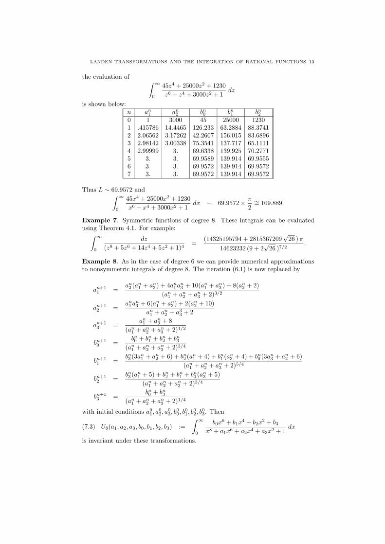
LANDEN TRANSFORMATIONS AND THE INTEGRATION OF RATIONAL FUNCTIONS 13
the evaluation of ∫ ∞0
45z4 + 25000z2 + 1230z6 + z4 + 3000z2 + 1
dz
is shown below:n an1 an2 bn0 bn1 bn20 1 3000 45 25000 12301 .415786 14.4465 126.233 63.2884 88.37412 2.06562 3.17262 42.2607 156.015 83.68963 2.98142 3.00338 75.3541 137.717 65.11114 2.99999 3. 69.6338 139.925 70.27715 3. 3. 69.9589 139.914 69.95556 3. 3. 69.9572 139.914 69.95727 3. 3. 69.9572 139.914 69.9572
Thus L ∼ 69.9572 and∫ ∞0
45x4 + 25000x2 + 1230x6 + x4 + 3000x2 + 1
dx ∼ 69.9572× π
2∼= 109.889.
Example 7. Symmetric functions of degree 8. These integrals can be evaluatedusing Theorem 4.1. For example:∫ ∞
0
dz
(z8 + 5z6 + 14z4 + 5z2 + 1)4=
(14325195794 + 2815367209√
26 )π14623232 (9 + 2
√26 )7/2
.
Example 8. As in the case of degree 6 we can provide numerical approximationsto nonsymmetric integrals of degree 8. The iteration (6.1) is now replaced by
an+11 =
an2 (an1 + an3 ) + 4an1an3 + 10(an1 + an3 ) + 8(an2 + 2)
(an1 + an2 + an3 + 2)3/2
an+12 =
an1an3 + 6(an1 + an3 ) + 2(an2 + 10)
an1 + an2 + a33 + 2
an+13 =
an1 + an3 + 8(an1 + an2 + an3 + 2)1/2
bn+10 =
bn0 + bn1 + bn2 + bn3(an1 + an2 + an3 + 2)3/4
bn+11 =
bn3 (3an1 + an2 + 6) + bn2 (an1 + 4) + bn1 (an3 + 4) + bn0 (3an3 + an2 + 6)(an1 + an2 + an3 + 2)5/4
bn+12 =
bn3 (an1 + 5) + bn2 + bn1 + bn0 (an3 + 5)(an1 + an2 + an3 + 2)3/4
bn+13 =
bn0 + bn3(an1 + an2 + an3 + 2)1/4
with initial conditions a01, a
02, a
03, b
00, b
01, b
02, b
03. Then
U8(a1, a2, a3, b0, b1, b2, b3) :=∫ ∞
0
b0x6 + b1x
4 + b2x2 + b3
x8 + a1x6 + a2x4 + a3x2 + 1dx(7.3)
is invariant under these transformations.
14 GEORGE BOROS AND VICTOR H. MOLL
Note. Numerical calculations show that (an1 , an2 , a
n3 )→ (4, 6, 4) and that (bn0 , b
n1 , b
n2 , b
n3 )→
(1, 3, 3, 1)L for some L depending upon the initial conditions.
Example 9. A symmetric function of degree 12. We use Theorem 2.1 to evaluate
I :=∫ ∞
0
z18 dz
(z12 + 14z10 + 15z8 + 4z6 + 15z4 + 14z2 + 1)3
as
I =25π(25
√56− 54)
301989888.(7.4)
Here p = 3, n = 9, and m = 2, so n > (m + 1)p − 1 and we need to apply thetransformation z → 1/z to reduce the value of n. Indeed, we have
I =∫ ∞
0
z16 dz
(z12 + 14z10 + 15z8 + 4z6 + 15z4 + 14z2 + 1)3,
and Theorem 2.1 now yields
I = 2−17
∫ ∞0
z16 dz
131072(1 + z2)3(1 + 4z2 + z4)3.
The new integrand is expanded in partial fractions in the variable t = z2 to produce(7.4).
Example 10. We use Theorem 2.1 to evaluate
I :=∫ ∞
0
z10 dz
Q2(z)
where
Q(z) = z20 + 6z18 + 93z16 − 24z14 + 162z12 + 548z10 + 162z8 − 24z6 + 93z4 + 6z2 + 1.
The factorization
Q(z) = (1 + z2)2T (z)T (−z)
with
T (z) = z8 − 2z7 + 4z6 + 14z5 + 6z4 − 14z3 + 4z2 + 2z + 1
leads to a partial fraction expansion containing the term
72− 501z + 1994z2 − 2617z3 + 1228z4 − 43z5 + 34z6 − 55z7
8388608(1− 2z + 4z2 + 14z3 + 6z4 − 14z5 + 4z6 + 2z7 + z8)2,
which we were unable to integrate; furthemore, the roots of T (z) = 0 cannot beevaluated by radicals. The procedure described in Theorem 2.1, however, showsthat
I =∫ ∞
0
z10(4 + z2)(z6 + 36z4 + 96z2 + 64) dz524288(z2 + 1)2 (z8 + 3z6 + 8z4 + 3z2 + 1)2
,
LANDEN TRANSFORMATIONS AND THE INTEGRATION OF RATIONAL FUNCTIONS 15
the integrand of which can be expanded to yield
I = − 98388608
∫ ∞0
dz
(z2 + 1)2− 75
8388608
∫ ∞0
dz
z2 + 1
+∫ ∞
0
1921z6 + 10815z4 + 4111z2 + 14622097152 (z8 + 3z6 + 8z4 + 3z2 + 1)2
dz
+∫ ∞
0
91z6 + 719z4 + 1259z2 − 57648388608(z8 + 3z6 + 8z4 + 3z2 + 1)
dz.
Every piece is now computable, with the final result
I =(6480− 509
√15)π
24159191040.
Example 11. The symmetric functions of degree 16 have denominator
D4(d1, d2, d3, d4; z) = z16 + d4z14 + d3z
12 + d2z10 + 2d1z
8 + d2z6 + d3z
4 + d4z2 + 1,
the integral of which is computed in terms of
E4(d1, d2, d3, d4; z) = (1 + d1 + d2 + d3 + d4)z8 + 2(16 + d2 + 4d3 + 9d4)z6
+ 8(20 + d3 + 6d4)z4 + 32(8 + d4)z2 + 128.
This new integral is symmetric provided[d1
d2
]=
[15112
]+[
3−4
]d3 +
[−87
]d4.(7.5)
Introduce the new parameters
ej = dj −(
85− j
)for 2 ≤ j ≤ 4 and e1 = d1 − 1
2
(84
).
Then (7.5) yields [e1
e2
]=
[3−4
]e3 +
[−87
]e4.(7.6)
Thus, if the original denominator has the form
D4(z) = (z16 + 1) + d4(z14 + z2) + d3(z12 + z4) + (112− 4d3 + 7d4)(z10 + z6)+2(15 + 3d3 − 8d4)z8,
the integral ∫ ∞0
P (z)( D4(z) )m+1 dz
is reduced to an integral with symmetric denominator of degree 8 and these arecomputable. We can thus evaluate a 2-parameter family of symmetric integrals ofdegree 16.
For example, take d3 = d4 = 1 to obtain
R1(z) =z4
(z16 + z14 + z12 + 115z10 + 20z8 + 115z6 + z4 + z2 + 1)2.(7.7)
The main theorem yields
R2(z) =1024z4 + 2304z6 + 1792z8 + 560z10 + 60z12 + z14
27(16z8 + 36z6 + 27z4 + 36z2 + 16)2(7.8)
16 GEORGE BOROS AND VICTOR H. MOLL
so that ∫ ∞0
R1(z) dz =∫ ∞
0
R2(z) dz.
Letting f [n] := Nn,8[1, n, 27/32, 9/4] we obtain∫ ∞0
R1(z) dz = 2−15 (f [0] + 60f [1] + 1584f [2] + 4096f [3])
and conclude that∫ ∞0
z4 dz
(z16 + z14 + z12 + 115z10 + 20z8 + 115z6 + z4 + z2 + 1)2=
=(149288517 + 12947003
√131)π
1124663296√
54925 + 4798√
131.
Example 12. We classify the symmetric denominators of degree 32 that yieldcomputable integrals. These functions depend on 8 parameters
D8(d1, · · · , d8; z) =8∑k=0
d9−k(z2k + z2(16−k))(7.9)
and the main theorem expresses the integral in terms of E8. The conditions for E8
to be symmetric yield
d1 = −3441 + 35d5 + 64d6 − 312d7 − 3264d8
d2 = 34720− 56d5 − 110d6 + 560d7 + 4565d8
d3 = −3472 + 28d5 + 64d6 − 329d7 − 2240d8
d4 = 4960− 8d5 − 19d6 + 80d7 + 938d8
and the symmetric E8 is
E8(d5, d6, d7, d8; z) = 32768(1 + z16) + (131072 + 8192d8)(z2 + z14)+
(212992 + 2048d7 + 28672d8)(z4 + z12) + (180224 + 512d6 + 6144d7 + 39424d8)(z6 + z10)+
+(84480 + 128d5 + 1280d6 + 6912d7 + 26880d8)z8.
The symmetry of E8 now determines d5, d6 in terms of d7, d8 and we obtaind1
d2
d3
d4
d5
d6
= −31
63475−100800
47936−13664
2220−224
+
9166−14392
6895−1964
322−28
d7 +
54640−8664541664−11471
2000−189
d8.(7.10)
The function (z2 + 1)16 is a symmetric polynomial of degree 32 and yields a par-ticular solution to (7.10).
As before let
ej = dj −(
169− j
)for 2 ≤ j ≤ 8 and e1 = d1 − 1
2
(168
).
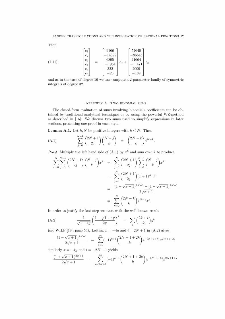
LANDEN TRANSFORMATIONS AND THE INTEGRATION OF RATIONAL FUNCTIONS 17
Then e1
e2
e3
e4
e5
e6
=
9166−14392
6895−1964
322−28
e7 +
54640−8664541664−11471
2000−189
e8(7.11)
and as in the case of degree 16 we can compute a 2-parameter family of symmetricintegrals of degree 32.
Appendix A. Two binomial sums
The closed-form evaluation of sums involving binomials coefficients can be ob-tained by traditional analytical techniques or by using the powerful WZ-methodas described in [16]. We discuss two sums used to simplify expressions in latersections, presenting one proof in each style.
Lemma A.1. Let k,N be positive integers with k ≤ N . ThenN−k∑j=0
(2N + 1
2j
)(N − jk
)=
(2N − k
k
)4N−k.(A.1)
Proof. Multiply the left hand side of (A.1) by xk and sum over k to produceN∑k=0
N−k∑j=0
(2N + 1
2j
)(N − jk
)xk =
N∑j=0
(2N + 1
2j
)N−j∑k=0
(N − jk
)xk
=N∑j=0
(2N + 1
2j
)(x+ 1)N−j
=(1 +
√x+ 1)2N+1 − (1−
√x+ 1)2N+1
2√x+ 1
=N∑k=0
(2N − k
k
)4N−kxk.
In order to justify the last step we start with the well known result
1√1− 4y
(1−√
1− 4y2y
)i=
∑k
(2k + i
k
)yk(A.2)
(see WILF [19], page 54). Letting x = −4y and i = 2N + 1 in (A.2) gives
(1−√x+ 1 )2N+1
2√x+ 1
=∞∑k=0
(−1)k+1
(2N + 1 + 2k
k
)4−(N+1+k)x2N+1+k;
similarly x = −4y and i = −2N − 1 yields
(1 +√x+ 1 )2N+1
2√x+ 1
=∞∑
k=2N+1
(−1)k+1
(2N + 1 + 2k
k
)4−(N+1+k)x2N+1+k.
18 GEORGE BOROS AND VICTOR H. MOLL
Thus
(1 +√x+ 1 )2N+1 − (1−
√x+ 1 )2N+1
2√x+ 1
=2N∑k=0
(−1)k(−(2N + 1− 2k)
k
)4N−kxk
=N∑k=0
(2N − k
k
)4N−kxk.
Lemma A.2. Let N ∈ N. ThenN∑j=0
(2N + 1
2j
)(1 + z2)N−j =
N∑j=0
(N + j
2j
)4jz2(N−j).
Proof. The coefficient of z2k on the left hand side isN−k∑j=0
(2N + 1
2j
)(N − jk
),
and the corresponding coefficient on the right hand side is(
2N−kk
)4N−k. The result
then follows from Lemma A.1.
Lemma A.3. Let k,N ∈ N with k ≤ N . Thenk∑j=0
(2N2j
)(N − jN − k
)=
22k−1N
k
(k +N − 1N − k
).
Proof. This lemma could be proven in the same style as Lemma A.1. Instead weuse the WZ-method as explained in [16]. Indeed, let
F (k; j) =k(
2N2j
)(N−jN−k
)N22k−1
(k+N−1N−k
) ,and define, with the package EKHAD, the function
G(k; j) = F (k; j)× j(2j − 1)2(N + k)(k − j + 1)
.
Then F (k; j)−F (k+ 1; j) = G(k; j+ 1)−G(k; j), and summing over j we see thatthe sum of F (k; j) over j is independent of k. The case k = N produces 1 as thecommon value.
Lemma A.4. Let p ∈ N, d1, d2, · · · , dp be parameters, and define dp+1 := 1. Thenp∑k=0
dp+1−kz2k
p−k∑j=0
(2p− 2k
2j
)(1 + z2)p−k−j =(A.3)
p+1∑j=1
dj
z2p +p∑i=1
22i−1z2(p−i)
p+1−i∑j=1
j + i− 1i
(j + 2i− 2j − 1
)dj+i
.
LANDEN TRANSFORMATIONS AND THE INTEGRATION OF RATIONAL FUNCTIONS 19
Proof. For fixed 0 ≤ i ≤ p− 1 the coefficient of z2i on the right hand side of (A.3)is
[RHS] (2i) =22(p−i)−1
p− i
p+1∑r=p−i+1
(r − 1)(r + p− i− 2r − p+ i− 1
)dr,
and for i = p we have [RHS] (2p) = 1 +∑pj=1 dj . Similarly, for the left hand side
of (A.3),
[LHS] (2i) =p+1∑
r=p+1−idr
p−i∑j=0
(2r − 2
2j
)(r − j − 1
r − j − 1 + i
) .
It is easy to check that the coefficients of z2p match. It suffices to show that foreach i such that 0 ≤ i ≤ p − 1 and for each r such that p + 1 − i ≤ r ≤ p + 1 wehave
p−i∑j=0
(2r − 2
2j
)(r − 1− j
r − 1− p+ i
)=
22(p−i)−1
p− i(r − 1)
(r + p− i− 2r − p+ i− 1
).
This follows from Lemma A.1 with k = p− i and N = r − 1.
The suggestions of the referrees and the editor are gratefully acknowledged.
References
[1] BOROS, G. - MOLL, V.: A criterion for unimodality. Elec. Jour. of Combinatorics, 6 (1999),
#R10.[2] BOROS, G. - MOLL, V.: An integral hidden in Gradshteyn and Ryzhik. Jour. Comp. Appl.
Math. 106, 361-368, 1999.[3] BOROS, G. - MOLL, V.: A rational Landen transformation. Contemporary Mathematics
251, 83-91, 2000.[4] BORWEIN, J. - BORWEIN, P.: Pi and the AGM. Canadian Mathematical Society. Wiley-
Interscience Publication.[5] BRONSTEIN, M.: Symbolic Integration I. Transcendental functions. Algorithms and Com-
putation in Mathematics, 1. Springer-Verlag, 1997.
[6] GEDDES, K. - CZAPOR, S.R. - LABAHN, G.: Algorithms for Computer Algebra. Kluwer,Dordrecht. The Netherlands, 1992.
[7] GAUSS, K.F.: Arithmetische Geometrisches Mittel, 1799. In Werke, 3, 361-432. Konigliche
Gesellschaft der Wissenschaft, Gottingen. Reprinted by Olms, Hildescheim, 1981.[8] GRADSHTEYN, I.S. - RYZHIK, I.M.: Table of Integrals, Series and Products. Fifth Edition,
ed. Alan Jeffrey. Academic Press, 1994.
[9] HARDY, G.H.: The Integration of Functions of a Single Variable. Cambridge Tracts inMathematics and Mathematical Physics, 2, Second Edition, Cambridge University Press,
1958.[10] HERMITE, C.: Sur l’integration des fractions rationelles. Nouvelles Annales de Mathema-
tiques ( 2eme serie) 11, 145-148, 1872.
[11] HOROWITZ, E.: Algorithms for partial fraction decomposition and rational function inte-gration. Proc. of SYMSAM’71, ACM Press, 441-457, 1971.
[12] LAZARD, D. - RIOBOO, R.: Integration of Rational Functions: Rational Computation ofthe Logarithmic Part. Journal of Symbolic Computation 9, 113-116, 1990.
[13] MCKEAN, H. - MOLL, V.: Elliptic Curves: Function Theory, Geometry, Arithmetic. Cam-
bridge University Press, 1997.[14] NEWMAN, D.: A simplified version of the fast algorithm of Brent and Salamin. Math.
Comp. 44, 207-210, 1985.[15] OSTROGRADSKY, M.W.: De l’integration des fractions rationelles. Bulletin de la Classe
Physico-Mathematiques de l’Academie Imperieriale des Sciences de St. Petersbourgh, IV,
145-167, 286-300. 1845.
20 GEORGE BOROS AND VICTOR H. MOLL
[16] PETKOVSEK, M. - WILF, H.S. - ZEILBERGER, D.: A=B. A. K. Peters, Wellesley, Mas-
sachusetts. 1996.
[17] ROTHSTEIN, M.: A new algorithm for the integration of Exponential and LogarithmicFunctions, Proc. of the 1977 MACSYMA Users Conference, NASA Pub., CP-2012, 263-274.
[18] TRAGER, B.M.: Algebraic factoring and rational function integration. Proc. SYMSAC 76,219-226.
[19] WILF, H.S.: generatingfunctionology. Academic Press, 1990.
Department of Mathematics, Xavier University, New Orleans, Louisiana 70125
E-mail address: [email protected]
Department of Mathematics, Tulane University, New Orleans, LA 70118
E-mail address: [email protected]


