arX

iv:c

ond-

mat

/040

9593

v1 [

cond

-mat

.mes

-hal

l] 2

2 Se

p 20

04

Landau-Zener quantum tunneling in disordered nanomagnets

V.G. Benza

Dipartimento di Fisica e Matematica, Universita’ dell’Insubria,

Como, I.N.F.M., sezione di Como, Italy

C.M. Canali

Division of Physics, Department of Chemistry and Biomedical Sciences,

Kalmar University, 391 82 Kalmar, Sweden

G. Strini

Dipartimento di Fisica, Universita’ di Milano, Milano, Italy

(Dated: February 2, 2008)

Abstract

We study Landau-Zener macroscopic quantum transitions in ferromagnetic metal nanoparticles

containing on the order of 100 atoms. The model that we consider is described by an effective

giant-spin Hamiltonian, with a coupling to a random transverse magnetic field mimicking the

effect of quasiparticle excitations and structural disorder on the gap structure of the spin collective

modes. We find different types of time evolutions depending on the interplay between the disorder

in the transverse field and the initial conditions of the system. In the absence of disorder, if

the system starts from a low-energy state, there is one main coherent quantum tunneling event

where the initial-state amplitude is completely depleted in favor of a few discrete states, with

nearby spin quantum numbers; when starting from the highest excited state, we observe complete

inversion of the magnetization through a peculiar “backward cascade evolution”. In the random

case, the disorder-averaged transition probability for a low-energy initial state becomes a smooth

distribution, which is nevertheless still sharply peaked around one of the transitions present in the

disorder-free case. On the other hand, the coherent backward cascade phenomenon turns into a

damped cascade with frustrated magnetic inversion.

1

I. INTRODUCTION

Ferromagnetic transition metal nanoparticles[1, 2, 3] and molecular nanomagnets [4, 5]

have been actively studied over the past decade and are presently the subject of strong inter-

est and intense investigation. So far, interest in ferromagnetic transition metal nanoparticles

has been mainly motivated by their relevance to high-performance information storage tech-

nology and spin electronics[6, 7]. Recently a lot of progress has been made in characterizing

the physical properties of individual ferromagnetic nanoparticles, such as their magnetic

anisotropy[8]. However, reproducible and controlled fabrication is still difficult and the

understanding of their classical dynamics is still not a fully solved problem[9]. Molecular

magnets, on the other hand, are relatively simple and well characterized magnetic systems

that offer the possibility of studying a rich interplay of classical and quantum magnetic

phenomena[5]. Among the latter, the coherent quantum tunneling of the magnetization in

molecular magnets is one of the most fascinating phenomena[10, 11] [45]. Thermally acti-

vated quantum tunneling of the magnetization (QTM) has been observed experimentally

in molecular magnets such as Mn12[12, 13] and Fe8[14]. In these experiments, a sequence

of discrete steps in the magnetic hysteresis curve provides a direct evidence of resonant co-

herent quantum tunneling between collective spin quantum states. For Fe8, there is strong

evidence that at low temperatures (below 360 mK) the system enters a quantum regime

where the reversal of the magnetization is caused by a pure tunneling mechanism[14, 15].

The occurrence of macroscopic QTM has also been investigated in ferromagnetic nanopar-

ticles. Despite the effective spin of a few nanometer particle is typically several orders of

magnitude larger than the spin of a molecular magnet (where S = 10) earlier theoretical

work[10] predicts that QTM in these systems should be possible by applying an external field

close to the classical switching field in the direction opposite to the magnetization. On the

experimental front, some evidence of quantum effects was found in switching field measure-

ments in ferrimagnetic BaFeO nanoparticles[16]. However, it is fair to say that experimental

proof for QTM in single-domain nanoparticles is still a controversial issue. Unambiguous

evidence of QTM can only be provided by the observation of level quantization of the col-

lective spin states like in the case of molecular magnets. For BaFeO nanoparticles with

S = 105, the magnetic field steps associated with such quantizations should be of the order

of a ∆H = Ha/2S ≈ 0.002 mT (where Ha is the anisotropy field), which is too small even

2

for the most sensitive and sophisticated magnetic measurement techniques, such as the new

microSQUID set-up used in Ref. 8. It seems clear that new experiments in this direction,

presently underway, should focus on nanoparticles containing on the order of a few hundred

atoms. In discussing ferromagnetic nanoparticles it is important to draw a clear distinction

between insulating particles, for which the only low-energy degree of freedom is the collec-

tive spin-orientation, and metal nanoparticles, which have discrete particle-hole excitations

in addition. The common practice of modeling a magnetic particle by a spin Hamiltonian,

completely misses this aspect of metal physics. In general for nanoparticles containing a few

thousand atoms, both types of excitations are present in the low-energy quantum spectrum

of transition metal ferromagnetic nanoparticles.

Recently the low-energy quantum states of individual ferromagnetic metal nanoparticles

have been directly probed by means of single-electron-transistor (SET) spectroscopy[17, 18,

19]. These experiments have indeed demonstrated the existence of a complex pattern of

excitation spectra and spurred the elaboration of adequate theoretical models[20, 21, 22, 23]

that include particle-hole and collective excitations on the same footing. It is clear that the

quasiparticle states will change when the collective magnetization orientation is manipulated

with an external field. Thus itinerant quasiparticle excitations can give rise to dissipation in

the dynamics of the collective magnetization[24]. These important and interesting features

represent a considerable complication that cannot be avoided in a theoretical treatment

of macroscopic QTM in ferromagnetic metal nanoparticles. Dissipation from particle-hole

excitations might be one of the reasons why preliminary experiments[5] on 3 nm Fe nanopar-

ticles with S ≈ 800 yield broad switching-field distribution widths that completely smear the

expected field-separation steps coming from level quantization. There is, however, a regime

where the quantum description of small transition metal clusters simplifies considerably, and

their low-energy physics can be described by an effective Hamiltonian with a single giant

spin degree of freedom, like that of a molecular magnet. Indeed, in Ref. 25 it was argued

that a transition metal nanoparticle will behave like a molecular magnet when the energy

scale associated with the collective magnetization, the magnetic anisotropy, is smaller than

the typical energy scale associated with the quasiparticle degree of freedom, δ. This is the

case for transition metal nanoparticles when the number of atoms is on the order of 100.

In this paper we study Landau-Zener macroscopic QTM in transition metal nanopar-

ticles, in the regime where they behave like molecular magnets. In Ref. 25 it was shown

3

that in this case the total spin of the effective Hamiltonian describing the nanoparticle is

specified by a Berry curvature Chern number that characterizes the topologically nontrivial

dependence of the many-electron wavefunction on magnetization orientation. A prescrip-

tion was given to derive microscopically the effective spin Hamiltonian by integrating out the

quasiparticle degrees of freedom in the quantum action constructed within an approximate

spin-density-functional theory framework. Here, however, we take a more pragmatic view,

and we assume that the effect of the quasiparticle degrees of freedom, when integrated out, is

to reshuffle randomly the pattern of avoided crossing gaps in the excitation spectrum of the

collective-magnetization orientation degree of freedom used to describe uniaxial molecular

magnets. Although this procedure might appear ad hoc, we believe that such a “random

matrix theory” should capture part of the complicated interleaved excitation spectra in real

systems, including those features due to surface-imperfections-induced randomness that are

likely to be important in these very small grains. Our goal is to examine the effect of this

randomness on the coherent macroscopic quantum transitions triggered by a magnetic field

swept in the direction of the magnetization. We neglect in the present analysis every effect

arising from decoherence and dissipation. We find different time evolutions depending on

the presence or absence of disorder and on the initial conditions of the system. In the ab-

sence of disorder, if the initial state is close to the ground state, the system undergoes a few

coherent transitions, corresponding to macroscopic tunneling of the collective spin between

quasi-degenerate states. The asymptotic transition probability displays a small number of

discrete peaks, with one dominant contribution. In general we find that the shift of the

magnetization associated with the dominant transition is not large but still significant. A

spectacular effect takes place if the system is prepared initially in a state of high-energy.

In this case, during its time evolution, the system displays complete magnetization inver-

sion, through a peculiar phenomenon that we call “backward cascade”. When disorder is

added in the form of a random static transverse field, the average transition probability for

a low-energy initial state acquires a continuous lineshape. Although the dominant delta-like

peak found in the ordered case is now absent, the distribution is still sharply peaked around

one of the transitions present before. Therefore we conclude that in this case disorder does

not obliterate the occurrence of sharp features in the transition probability distribution that

could be important for the observability of macroscopic quantum coherence. On the other

hand, disorder may suppress the backward cascade effect occurring in the ordered case when

4

the initial state is a highly excited state. In this case at the end of the time evolution, the

original wavepacket is spread essentially over all the eigenstates of the system.

The paper is organized as follows. In Sec. II we introduce a giant spin model describing

a transition-metal nanoparticle in the molecular-magnet limit, and we illustrate some of

its spectral properties. In Sec. III we discuss some paradigmatic features of the dynamical

evolution of the collective magnetization under the effect of a time-dependent magnetic field.

Disorder-averaged evolution of magnetization from the point of view of quantum diffusion is

discussed in Sec. IV. In Sec. V we interpret our results in the context of a simplified network

model, which offers an intuitive and possibly more generic picture of the magnetization

reversal problem. Our conclusions are presented in Sec. VI, where we comment on the

relevance of this work for the observation of QTM in ultrasmall ferromagnetic metal grains.

II. GIANT-SPIN MODEL FOR A FERROMAGNETIC METAL GRAIN

We consider an effective “spin” Hamiltonian aimed at modeling a ferromagnetic transition

metal nanoparticle containing on the order of Na ≈ 100 atoms, in such a way that the

total anisotropy energy KNa is smaller than the single-particle mean-level spacing. Here

K is the bulk anisotropy energy/atom. In this regime the nanoparticle behaves like a

molecular magnet described by a collective quantum “spin” degree of freedom, S [46]. It

is important to emphasize that this collective “spin” is an effective variable representing

coupled quasiparticle spin and orbital degrees of freedom of the original electron system.

This coupling is non-trivial when spin-orbit interaction is included. The “spin” S can be

specified by a Berry curvature Chern number that characterizes the topologically nontrivial

dependence of the many-electron wavefunction on magnetization orientation[25]. The model

that we consider has a uniaxial anisotropy term, augmented by a “transverse magnetic field”,

which can be randomly distributed to mimic the combined remnant effect of quasiparticle

excitations and structural disorder on the gap structure of the spin collective modes[47]. We

will use matrix representations of the (dimensionless) operators (Sx, Sy, Sz) in the basis of

the eigenstates {|S, m >, −S ≤ m ≤ S} of (S2, Sz), where z is aligned along the easy axis.

The components of the “transverse field” are

< S, m|Bx|S, m′ >= δm,m′rx(m)∆x; < S, m|By|S, m′ >= δm,m′ry(m)∆y . (1)

5

Here ∆x, ∆y are given amplitudes, with dimensions of energy, and rx(m), ry(m) are uni-

formly distributed dimensionless random variables having width 1/2 and zero average. The

resulting random coupling is described by the symmetrized operators

(BkSk)(R) = (1/2)(BkSk + SkBk), k = x, y , (2)

having matrix elements:

< S, m|(BkSk)(R)|S, m − 1 >= iǫ(k)∆k(1/2)r′k(m)[(S + m)(S − m + 1)]1/2 , (3)

where r′k(m) = [rk(m) + rk(m− 1)]/2 and ǫ(k) = 0, 1(k = x, y). The effective spin Hamilto-

nian is then:

H = −Bz(t)Sz − KS2z − (BxSx)(R) − (BySy)(R) , (4)

where K is an effective anisotropy energy/spin. In Eq. (4) we have introduced the coupling to

a time-dependent longitudinal field Bz(t), which we will use to manipulate the collective spin

spectrum and induce Landau-Zener type transitions at its avoided-crossing gaps. It is trivial

to verify that S2 commutes with the operators in Eq. (2) and therefore the Hamiltonian of

Eq. (4) remains within a given spin multiplet S. The size of the Hilbert space is 2S + 1

and we will label the energy levels E(m, t) with the discrete index m, running from −S

to S. We discuss some properties of the spectrum when Bz(t) is linearly dependent on

time: Bz(t) = gt. In Fig. 1 we plot the energy levels E(m, t) as a function of time, for a

generic disorder realization of the Hamiltonian given in Eq. (4) when S = 50. (The values

of the other parameters of the Hamiltonian are specified in Sec. III.) It turns out that the

density of states is higher in the upper part of the spectrum; the avoided crossings there

predominantly involve channels associated with nearby sites along the m−chain. At lower

energies the crossings involve channels associated with distant sites m, m′ and the gaps are

accordingly much smaller, as one can see by simple perturbative arguments. To lowest order

the coupling is the product of l nearest neighbor amplitudes (l = |m′ −m|). These features

are clearly visible in Fig. 1. It was argued [21] that the peculiar diamond-like structure of

the spectrum can be a signature of ferromagnetic metals. One can further notice that in

the presence of a constant transverse magnetic field the nearest neighbor amplitudes favor

backward (forward) motion in the region m < 0, (m > 0). This is due to the angular

momentum matrix elements: the amplitude of the process m → m − 1 is larger than the

one relative to m → m + 1 for m < 0, the asymmetry becoming stronger as m approaches

6

-50 0 50Time (w)

-1000

0En

ergy

leve

ls (K

)

-50 0 50Time (w)

-1000

0En

ergy

leve

ls (K

)

-50 0 50Time (w)

-1000

0En

ergy

leve

ls (K

)

-50 0 50Time (w)

-1000

0En

ergy

leve

ls (K

)

FIG. 1: Energy levels E(m, t) vs. time of the random spin Hamiltonian defined in Eq.4, with total

spin S = 50. The time unit is w ≃ K/h, where K is the anisotropy energy/spin.

the ground state. In the classical limit S >> 1 one has a potential barrier separating the

two extremal states m = ±S [9].

III. SPIN DYNAMICS

The deterministic evolution of spin systems under the action of a time-dependent bias has

been considered by various authors, mainly in the context of molecular magnets. Different

situations have been considered, ranging from the case of a large, conserved spin multiplet

S, to that of a general system of interacting spins [26, 27, 28]. The Landau-Zener theory

provides a natural background for this class of problems [29, 30, 31]. The effect of noise

on the Landau-Zener transitions has also been examined at length, in order to obtain a

better understanding of the influence of the phonon and spin baths on macroscopic quantum

coherence[33, 34, 35]. Here, the time evolution of a giant spin with time-independent disorder

is supposed to represent the coherent dynamics of the magnetic moment of a monodomain

ferromagnetic metal nanoparticle in a regime characterized by a large energy gap between

the single-particle excitations and the collective “spin” modes. Our analysis will focus on

the effect of quenched disorder.

7

The wave function |Ψ(t)〉 satisfies the time-dependent Schrodinger equation:

ihd |Ψ(t)〉

d t= H(t)|Ψ(t)〉 (5)

By expanding |Ψ(t)〉 =∑

m cm(t)|S, m > on the basis {|S, m〉}, we obtain the following set

of coupled differential equations for the coefficients cm(t)

ihcm(t) = (−gtm − Km2)cm(t)

−[(∆x/2)r′x(m) + i(∆y/2)r′y(m)][(S + m)(S − m + 1)]1/2cm−1(t) (6)

−[(∆x/2)r′x(m + 1) + i(∆y/2)r′y(m + 1)][(S − m)(S + m + 1)]1/2cm+1(t) .

The Schrodinger equation is integrated over a time interval −T < t < +T such that at

its extrema t = ±T the eigenvalues E(m, t) are well separated: the diagonal part of the

Hamiltonian being linear in t, and the coupling with the transverse field being bounded,

the eigenvalues approach −gtm for large enough |t|. More specifically, under the condition

|∆x|, |∆y| ≪ S, it is sufficient to fix the value of T as follows: T > 4(KS)/g. The eigenvalues

then identify isolated channels and the time evolution can be studied as a scattering problem.

In the present case, the ground state at t = −T is m = −S and turns into m = +S at t = +T .

One would like to integrate the Schrodinger equation over the interval (−T , +T ), with S on

the order of 50 and realistic values of the other parameters, such as an anisotropy energy/spin

on the order of 10−4eV , and a velocity of the bias Bz(t) on the order of mTesla/sec. It is

readily verified that this requires astronomical computation times. The situation is worse if

one needs averaging over a large set of disordered configurations. We would like to emphasize

here that in solving the time dependent Schrodinger equation, we don’t want to make the

frequently used approximation of reducing the full Hamiltonian into an effective two-level

model. While this procedure is perhaps a justified approximation in the case of simpler

models describing molecular magnets with small spins, the level intricacies present in our

spectrum, which are at the heart of the problem we want to study, make this approximation

completely meaningless.

As an example, we studied the case of the evolution from the channel m = −46, close

to the ground state, with K = 10−4eV and ∆x/µB = ∆y/µB = 0.02 Tesla, µB being the

Bohr magneton. In a series of runs we progressively reduced the sweep velocity down to 1

Tesla per second. Further examination of this case for, say, a sweep velocity of 10−1 Tesla

per second requires a few days of computation time. At 1 Tesla per second, we obtained

8

that the system hops from m = −46 to m = −43. The question arises then: what can one

expect at smaller sweep velocities? Could one obtain a much larger hopping range at, say,

1 mTesla per second? The Landau-Zener theory gives a negative answer to this question

and a way out of the computation time problem. Let ∆eff(m, m′) be the (time-dependent)

gap between two channels m, m′; as long as this gap is reasonably large, wave packets

carrying quantum numbers m and m′ practically do not interfere. In the small transient

at the crossing time (where the gap reaches a minimum) the two channels do interfere,

and their scattering is determined by the Landau-Zener matrix S(m, m′) [36]. As is well

known, the transition probability P (m → m′) depends on the adimensional parameter

ν(m, m′) = [∆eff(m, m′)]2/(gh|m − m′|):

P (m → m′) = 1 − exp[−πν(m, m′)/2]. (7)

Notice that g scales as the square of the gap. Since, as already noticed, the gap corresponding

to an hopping event of range l scales as the l-th power of a perturbative parameter, it is

clear that upon reducing g by few orders of magnitude one will not detect hoppings of

significantly larger range. This answers the question we made above. On the other hand,

one can exploit the scaling between the gap and the sweep velocity in order to infer the

behavior in the physical region from the results corresponding to numerically affordable

values of the parameters. In a sequence of runs, we detected the transitions m → m + 1 ,

m → m + 2, m → m + 3, and so on. We then compared the crossing times resulting from

time integration with the ones extracted by direct inspection of the spectrum E(m, t), and

found full agreement. As the crossing behavior appears to be scale invariant, one can argue

that indeed the dynamics can be described as a sequence of L-Z transitions. This argument

works provided that the hopping events involve two channels at a time. In the upper part of

the spectrum, in particular in a region around t = 0, the channels are always close in energy

and tend to hybridize. The resulting motion is a sequence of short range hoppings, as we

will discuss in the sequel.

Based on the above considerations, in the remaining part of this Section we will consider a

value for the sweeping speed that yields reasonable calculation times, although it lies beyond

the experimentally meaningful range. Specifically, we introduce the time unit

w = h/K , (8)

9

where the anisotropy energy K will be taken as our energy unit. The sweeping speed is

chosen in such a way that g · w2/h ≈ 1. As for the values of the transverse amplitudes,

we will take ∆x = ∆y ≈ 2K; an accurate estimate of these parameters should be based on

microscopic derivations similar to the one suggested in Ref. [25], which is a task beyond the

goal of this work. Our choice here is an educated guess based on the fact that if the gaps of

the collective modes of a ferromagnetic metal nanoparticle are due in part to their coupling

with quasi-particle excitations, in the regime where the mean-level spacing of the latter is

larger than the total anisotropy energy, the values of the fictitious transverse field should

lie within a range not smaller than K. Below we discuss the time evolution of the system

both in the disordered and ordered case. In the ordered case the values of the transverse

field B0x, B0

y have been chosen equal to the mean square roots of the random amplitudes:

B0x = (< B2

x >)1/2 = ∆x/(2. · 3.1/2) ≈ ∆x · 0.28867.

We start by examining two paradigmatic behaviors enabling to reconstruct the generic

case. The first is found when the initial state is in the low energy region m ≥ −50. Generally

the system undergoes a major hopping event toward a channel m′ > m, but the hopping

range l = m′ − m, even if significant, is always far from what one would need for magnetic

inversion. This is clearly due to the presence of gaps of almost insurmountable smallness:

these, as it is well known, do occur in the ordered case as well. It must be recalled that

magnetic inversion in molecular magnets, in spite of a smaller spin, is generally observed

with the essential contribution of relaxation and decoherence processes, which are not taken

into account here. From our results it appears that in general the disorder reduces the size

of the gaps: more precisely some of the gaps that in the ordered case are large enough to

give rise to hopping, with disorder are no longer “seen”, so that the state keeps its quantum

number. We also found that as the initial channel m, (m < 0) is closer to the ground state,

the hopping range becomes shorter. The reason for this has been discussed in Section II.

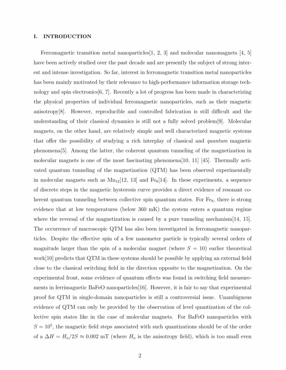
In Fig. 2 we plot the probability distribution

P (m, t) ≡ |〈S, m|Ψ(t)〉|2 (9)

as a function of time and channel index m, for the disordered [Fig. 2(a)] and the ordered

[Fig. 2(b)] case, respectively. Only one disorder realization is considered here. In both

cases the initial wavefunction |Ψ(t = −T )〉 is a state of sharp z-component of the collective

spin, taken in the low-energy part of the spectrum (eigenvalue index m = −25), where the

10

FIG. 2: Probability distribution P (m, t) ≡ |cm(t)|2 = |〈S,m|Ψ(t)〉|2 as a function of time and the

index m. The initial wavefunction is prepared in a state of low energy, m + S = 25. (a) Random

case. (b) Deterministic case.

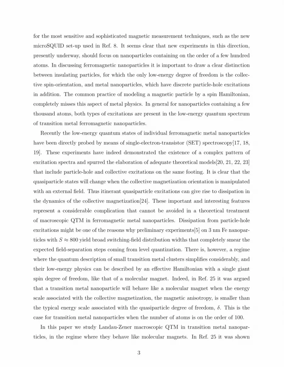
FIG. 3: The same as in Fig. 2 but for an initial wavefunction prepared in an excited state of high

energy, m + S = 100. (a) Deterministic case. (b) Random case.

magnetization 〈Sz〉 is large and negative. As shown in Fig. 2(a), in the disordered case the

system undergoes a single major hopping event at large positive times. The result is a rather

small magnetization shift ∆Sz = 〈Sz(+T )〉 − 〈Sz(−T )〉, smaller than what one observes in

the deterministic case, shown in Fig. 2(b).

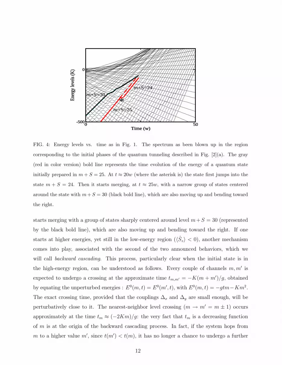
In order to better see how this transition comes about, in Fig.4 we plot, as a function of

time, the part of the spectrum blown up around the region where the quantum tunneling

for the disordered case described in Fig. [2](a) occurs. The gray (red in color version) bold

line moving up-right represents the time evolution of the energy of the initial state, labeled

by m + S = 25. As shown in the figure, at time t ≈ 20w, the level starts to encounter large

gaps. The first transition is a jump down into a state of lower m; at t ≈ 25w, the level

11

0 50Time (w)

-500

0En

ergy

leve

ls (K

)

0 50Time (w)

-500

0En

ergy

leve

ls (K

)

0 50Time (w)

-500

0En

ergy

leve

ls (K

)

0 50Time (w)

-500

0En

ergy

leve

ls (K

)

*m+S=25

m+S=24

m+S=30

FIG. 4: Energy levels vs. time as in Fig. 1. The spectrum as been blown up in the region

corresponding to the initial phases of the quantum tunneling described in Fig. [2](a). The gray

(red in color version) bold line represents the time evolution of the energy of a quantum state

initially prepared in m + S = 25. At t ≈ 20w (where the asterisk is) the state first jumps into the

state m + S = 24. Then it starts merging, at t ≈ 25w, with a narrow group of states centered

around the state with m + S = 30 (black bold line), which are also moving up and bending toward

the right.

starts merging with a group of states sharply centered around level m+S = 30 (represented

by the black bold line), which are also moving up and bending toward the right. If one

starts at higher energies, yet still in the low-energy region (〈Sz〉 < 0), another mechanism

comes into play, associated with the second of the two announced behaviors, which we

will call backward cascading. This process, particularly clear when the initial state is in

the high-energy region, can be understood as follows. Every couple of channels m, m′ is

expected to undergo a crossing at the approximate time tm,m′ = −K(m + m′)/g, obtained

by equating the unperturbed energies : E0(m, t) = E0(m′, t), with E0(m, t) = −gtm−Km2.

The exact crossing time, provided that the couplings ∆x and ∆y are small enough, will be

perturbatively close to it. The nearest-neighbor level crossing (m → m′ = m ± 1) occurs

approximately at the time tm ≈ (−2Km)/g: the very fact that tm is a decreasing function

of m is at the origin of the backward cascading process. In fact, if the system hops from

m to a higher value m′, since t(m′) < t(m), it has no longer a chance to undergo a further

12

nearest-neighbor transition. If on the contrary m′ < m, the next hopping time has still to

come, so that backward motion can be iterated. One can then expect, upon starting from

the highest energy state m = S, a ballistic backward motion ending at m = −S. This is

in fact found in the deterministic case, as shown in Fig. 3(a). We have complete magnetic

inversion, connecting energy maxima, similar to the pendulum kink, with no dispersion.

The hopping terms in the Hamiltonian drive the wave packet down from the local maximum

along the energy profile, but the ballistic velocity equals the time variation of the energy,

so that the wave packet stays on the maximum. Disorder inhibits the coherent sequence

of nearest neighbor hoppings; portions of the wavepacket are then trapped at intermediate

channels; the result is a damped backward avalanche, undergoing fragmentations along the

way. Accordingly, the final variance is extremely large, and complete magnetic inversion is

frustrated, as shown in Fig. 3(b).

In conclusion, when the initial state of the system is in the low-energy region, the main

feature of its time-evolution is the quantum tunneling of the collective spin, associated with

a small but not negligible shift of the magnetization. When the system starts from an

highly excited state, the backward cascading is the salient event of the dynamics. The

time evolution of the magnetic system when starting from a generic state appears to be a

combination of the two behaviors described above.

IV. DISORDER-AVERAGED TRANSITION PROBABILITY

So far we illustrated data originating from single samples. We will now discuss the

disorder-averaged transition probability from the initial state m to the final state m′, defined

as

<< gm′,m >>=<< |〈m′|U(+T ;−T )|m〉|2 >> .

Here, with obvious notation, U(t′; t) is the evolution operator from t to t′ and the double

bracket denotes the ensemble average. In Fig. 5 we plot << gm′,m >> (black solid lines)

for the initial conditions (a)-(d) marked by the vertical dashed lines. The function gm′,m

for the corresponding deterministic case (gray solid lines–red in color version), with the

same initial conditions, is also plotted for comparison. The disorder-averaged probability

displays a single broad peak at a value mmax = mmax(m), a smooth decay in the region

m′ < mmax and a very steep decay on the opposite side of the peak. One can notice that

13

0 25 50 75 100

m’ + S

0

0.1

0.2

0.3

0.4<<

gm

’m >

>

0 50 1000

0.1

0.2

0.3

0.4

0 25 50 75 100

m’ + S

0

0.1

0.2

0.3

0.4

<< g

m’m

>>

0 50 1000

0.1

0.2

0.3

0.4

0 25 50 75 100

m’ + S

0

0.1

0.2

0.3

0.4

0.5

<< g

m’m

>>

0 50 1000

0.1

0.2

0.3

0.4

0.5

0 50 100

m’ + S

0

0.05

0.1

0.15

0.2

<< g

m’m

>>

0 50 1000

0.2

(a)

(b)

(c)

(d)

FIG. 5: Disorder-averaged transition probability << gm′,m >> (black solid lines). For comparison,

the transition probability gm′,m for the deterministic case (gray solid lines–red in color version) is

also included. (a)-(d) represent four different initial conditions. The vertical dashed line marks

the spin quantum number m of the initial state. Note in (d) the complete “backward cascade”

behavior, which turns into a “cascade with traps” in the disordered case.

mmax > m, so that it can be identified with the main hopping event discussed above. The

sensitive asymmetry of the distribution can be explained in terms of the time ordering of

the scattering times: in fact, after the main hopping event has taken place, the backward

cascading is definitely favored with respect to further forward hoppings. We also determined

the disorder-averaged variance of Sz as a function of time

<< (∆Sz)2 >>≡<< 〈Ψ(t)|(Sz− < 〈Sz〉 >)2|Ψ(t)〉 >> (10)

for various initial conditions. This is shown in Fig. 6.

In summary, when starting from low energy channels (see Fig. 6(a)) there is a peak at the

14

-200 -50 100 250 400time(w)

0

1

2

3

4

5

6

7<<

(∆S z)2 >

>

-200 -50 100 250 400time(w)

0

10

20

30

40

50

<< (∆

S z)2 >>

(b)(a)

FIG. 6: Variance of Sz(t) averaged over disorder, as a function of time. (a) Initial state of low

energy (m + S = 5); (b) initial state of higher energy (m + S = 25).

hopping event, then the function rapidly decays to a constant value: in fact during the main

transition to mmax, portions of the wave packet undergo hoppings of shorter range, and no

longer move afterwards. The picture changes when the initial state has higher energy (see

Fig. 6(b)): then, following the main hopping event, a cascading process is always present.

This process is a frustrated ballistic motion: the variance displays a linear time dependence,

as in quantum diffusion, clearly visible in the time region laying between the initial transient

and the final saturation. Notice that the saturation value is almost one order of magnitude

larger than in case (a).

V. NETWORK OF LANDAU-ZENER CROSSINGS

We now give a qualitative interpretation of our results, in terms of a simple network

model representing the time evolution of the energy levels. The nodes of the network are

associated with the m, m′ crossings. Coherently with this interpretation, we will use a ter-

minology commonly employed in studying quantum transport in lattice models, when this

is viewed as an inter-channel scattering problem described by the Landauer-Buttiker for-

malism. Landau-Zener grids were originally introduced in studying the incoherent mixing

of Rydberg manifolds [37]. In the approach suggested below the coherent quantum evolu-

15

-3 -2 -1 0 1 2 3Time (arb. units)

0.7

0.8

0.9

1

Ene

rgy

Lev

els

(arb

. uni

ts)

2

1

0

-1

-2

-2

-1

0

1

2

**

**

**

* * ** * *

* * ** *

** *

**

**

∆∆

∆∆

∆∆

∆∆

∆∆

∆∆

∆∆

∆∆

FIG. 7: Network model in the (t,E) plane, mimicking the time dependence of the level structure

of Fig.1. The path marked by the triangles represents the evolution of the system undergoing

quantum tunneling of the magnetization. The path marked by asterisks represents backward

cascade evolution that occurs when the system starts from a high-energy state.

tion is instead taken into account. Due to the presence of the ferromagnetic S2z term in

the Hamiltonian, the present network has a peculiar topology, which can be schematically

represented as a family of parallel lines in the presence of a boundary acting as a mirror

plane. We display this network in Fig. 1, where the energies are plotted as a function of

time. All the lines are equally oriented with increasing times; in the simplest situation the

avoided crossings involve no more than two lines at a time, although, as stated in Sec. III,

the detailed structure of the spectrum is much more complicated than this and deserves

particular care. A simplified version of this pattern is a lattice where the crossing times are

fixed at their unperturbed values tm,m′ = −K(m + m′)/g, as depicted in Fig. 7. Using an

optics analogy, each lattice node acts as a beam splitter, where the field amplitude trans-

mission corresponds to channel conservation (m → m) and the reflection to inter-channel

hopping (m → m′). At the turning points laying on the horizontal line (E = 1) the channel

is conserved. The time coordinate is oriented from left to right, as in Fig. 1. The transfer

matrix T for the network of Fig. 7 is the time-ordered product of single step matrices acting

on the space of wave functions cm. It is convenient to enumerate the channels with the index

16

n = m + S + 1, (n = 1, N ; N = 2 · S + 1). A generic single step matrix, labeled by the

“scattering time” index k, (k = 3, 2 ·N − 1), is the product of Landau-Zener U(2) operators

, one for each crossing (n → n′) occurring at time k. The crossings are determined by the

equation n + n′ = k; (0 < n < n′ ≤ k).

Let us discuss the deterministic case first. One easily realizes that as the distance from

the “mirror’ line increases, the hopping probability decreases; in fact this distance goes as

|m − m′|, hence nodes laying far from the “mirror” line involve long range hoppings and

small gaps, i.e. small Landau-Zener hopping probabilities. The network can be separated

in two regions, respectively dominated by channel conservation (i.e.localization) and by

hopping (i.e. delocalization). The boundary between the two regions, i.e. the ideal curve

where the hopping probability is 1/2, is approximately parallel to the ”mirror” line. It is

natural to call this boundary “mobility curve”, although it is not a mobility edge in the

usual sense. If, e.g., the particle is initially in the upper energy level, it never leaves the

delocalized region: its most probable path is a sequence of nearest neighbor hoppings, ending

in the final upper level. This explains the ballistic backward cascade. This type of time

evolution is represented schematically on Fig. 7 by the path labeled by asterisks. When

starting from a low energy state, the particle first propagates in the localized region; at

some time it will cross the mobility curve and only at this point it will start hopping, giving

rise typically to one quantum tunneling event only. This second time evolution is marked

on Fig. 7 by the path of triangles. The above analysis can be extended to the disordered

case. One can expect that the boundary between localized and delocalized regions has then

a rather intricate shape; furthermore, since disorder on average lowers the number of “large

gaps” the delocalized region accordingly reduces its size. The backwards ballistic motion

described above is possible provided that a delocalized strip of almost constant width exists.

If the mobility “curve” undergoes fluctuations, and on average approaches the mirror line,

at the narrowings of the delocalized strip some portions of the wave packet must enter

the localized region. The result is a frustrated motion, where various portions of the wave

packet get trapped at intermediate states. If the particle starts evolving from a low energy

channel, its representative line will reach the mobility curve at a later time as compared

with the deterministic case: this also implies a smaller range |m − m′| of the main hopping

event m → m′, (m′ > m). The plots of the transition probability, exhibited in Fig. 5 are

consistent with this description; qualitatively the peaks of these plots identify the average

17

location of the mobility boundary.

VI. CONCLUSIONS

In this article we have investigated the occurrence of Landau-Zener macroscopic quantum

tunneling of the magnetization in a giant-spin model (S = 50 ) in the presence of random

anisotropy. The model is intended to provide a phenomenological description of the low-

energy spin dynamics of a ultra-small ferromagnetic metal nanograin, in a regime where the

quasi-particle mean level spacing is larger than the total anisotropy energy and the metal

grain behaves like a molecular magnet. We have focused, in particular, on the effects of the

disorder on the gap structure of the spin collective modes. The microscopic origin of this

randomness is ultimately related to the non-trivial physics of the itinerant quasiparticles of

the underlaying electronic system.

We find that the time evolution of the system under the action of a Landau-Zener time-

dependent magnetic field depends on the interplay between disorder and initial conditions.

For a disorder-free model starting from a low-energy state, there is one main coherent quan-

tum transition event, with a non-negligible shift in the magnetization. In correspondence of

this transition the occupation amplitude of the original state is essentially totally depleted.

The final (large-time) transition probability distribution is characterized by a few discrete

peaks, with one dominant contribution. Disorder does not obliterate these signatures of

macroscopic quantum coherence: the disorder-averaged transition probability distribution

is smooth, sharply peaked and strongly asymmetric. The resulting shift in magnetization,

at a sweep velocity of the order of mTesla/sec, is estimated in a few percents of the spin

S. When the system is initially prepared in the high-energy excited state, it is subject to

multiple tunneling giving rise to a ballistic motion ending in a final state with complete mag-

netization reversal. This curious coherent time evolution is made possible by the hopping

probability being equal to one during the whole process. On the other hand, when disorder

is present, at each step the wave packet finds a non zero probability of being trapped: as a

result the amplitude of the ballistic wave packet gets damped along the way.

Our results provide some indications about the observability of macroscopic quantum co-

herence in ferromagnetic nanoparticles containing approximately 100 atoms. Specifically the

sharp features in the transition probability, which are robust against disorder, can perhaps

18

be observed in detailed Landau-Zener SQUID magnetometry experiments on single particles

or ensemble of particles, similar to the ones performed by Wernsdorfer and colleagues[5, 16].

The scenario presented above excludes macroscopic magnetic inversion at affordably slow

sweep velocities, as well as hysteresis; by considering decoherence i.e. the decay of the non

diagonal elements of the density matrix, and dissipation, i.e. the damping of its diagonal

part[32, 38], these effects should obviously come into play. In the analysis done in Ref.

[39, 40], where the L-Z theory with one level crossing has been generalized to include deco-

herence and dissipation, it was found that the decoherence does not completely destroy the

quantum nature of the evolution. The main features of the Landau-Zener model are thus

preserved in the pure decoherence (non dissipative) case and survive to a limited amount of

dissipation. For the large-spin system considered in this paper the Hamiltonian dynamics

can be described in terms of a sequence of L-Z level crossings. An important remaining

question which we have not investigated here is whether or not this picture survives in an

open system. The problem of the non-Hamiltonian spin dynamics, already addressed in the

in the past for small quantum spins (see below), is still the object of intense investigation.

A possible source of dephasing and dissipation is the coupling of the nanoparticle magnetic

moment to a particle-hole continuum, such as a metallic substrate and the electron system

of the particle itself. As we have explained above, the latter should not be important in

the molecular magnet regime that we have considered in this work. The coupling to the

substrate, on the other hand, can be controlled by changing the thickness of the insulating

barrier between the nanoparticle and substrate.

Another cause of decoherence comes from the coupling to the phonon bath. Interest-

ingly enough, the possibility of controlling part of phonon-induced phenomena has been

demonstrated in the case of the low-spin molecular system V15 [41]

At low temperatures the dominant cause of decoherence arises from the unavoidable cou-

pling to nuclear spins. The central spin model considered in Ref. 42, where the microsystem

is a single S = 1/2 spin, is the best known description of the spin bath effects; within that

theory, deviations from the Landau-Zener behavior have been pointed out [35]. An anal-

ysis of spin bath effects on metallic ferromagnetic nanoparticles goes beyond the scope of

the present work. We recognize that the coupling to nuclear spin baths can considerably

affect the macroscopic quantum coherence studied here. It is reasonable to assume that this

coupling can influence to a larger degree the decoherence rather than the dissipation, since

19

the phases of the macroscopic spin are sensitive to the nuclear spin precessions, while its

energies are merely perturbed by the spin bath.

As mentioned in the introduction, so far the only experimental attempts to detect di-

rectly MQT in single ferromagnetic nanoparticles has been done by Wernsdorfer et al.[5, 16]

through magnetization measurements. An idea that we would like to propose here is to

search for evidence of MQT in transport experiments on magnetic SETs similar to the ones

performed by D. Ralph’s group[17, 18], but in the presence of a L-Z time-dependent field[48].

In SET experiments with a magnetic nanoparticle as the central island, the coupling between

the nanoparticle electronic states and its magnetic moment causes abrupt changes in the en-

ergy of conductance resonances at the classical switching field. This effect was investigated

theoretically in recent papers[22, 43]. An interesting question to ask is how the coherent

QTM between two degenerate quantum states affects the conductance. From the analysis

carried out in this work, we know that for a large spin (S ≈ 100) MQT might be observable

only at fields close to the classical switching field. Thus SET transport experiments should

give us a clear landmark of the surroundings of where MQT should be looked for. How

macroscopic quantum coherence would affect the tunneling resonances is however not obvi-

ous and deserves to be further investigated. Conversely, if MQT in single magnetic particles

could be detected by means of ordinary magnetization measurements, one very interesting

question is to what extent current flow will influence dephasing of the magnetic macroscopic

quantum coherence. Work along these lines is presently underway[49]. As for the coupling

of the nanoparticle to a metallic substrate, the level of decoherence and dissipation coming

from the tunneling current might be controlled by changing the tunnel barriers of the SET.

VII. ACKNOWLEDGMENTS

We would like to thank W. Wernsdorfer, D. Ralph and A. H. MacDonald for interesting

discussions. This work was supported in part by the Swedish Research Council under Grant

No:621-2001-2357 and by the Faculty of Natural Science of Kalmar University. Support from

the Office of Naval Research under Grant N00014-02-1-0813 is also gratefully acknowledged.

[1] I. M. L. Billas, A. Chatelain, and W. A. de Heer, Science 265, 1682 (1994).

20

[2] M. Lederman, S. Shultz, and M. Ozachi, Phys. Rev. Lett. 73, 1986 (1994).

[3] R. H. Kodama, J. Magn. Magn. Mater. 200, 359 (1999).

[4] R. Sessoli, D. Gatteschi, A. Caneschi, and M. A. Novak, Nature 365, 141 (1993).

[5] W. Wernsdorfer, Adv. Chem. Phys. 118, 99 (2001).

[6] S. A. Majetich and Y. Jin, Science 284, 470 (1999).

[7] S. Sun, C. B. Murray, D. Weller, L. Folks, and A. Moser, Science 287, 1989 (2000).

[8] M. Jamet, W. Wernsdorfer, C. Thirion, D. Mailly, V. Dupuis, P. Melinon, and A. Peres, Phys.

Rev. Lett. 86, 4676 (2001).

[9] A. Garg, cond-mat/0012157.

[10] L. Gunther and B. Barbara, eds., Quantum Tunneling of Magnetization, QTM94 (Kluwer,

Dordrecht, 1995).

[11] E. Chudnovsky and J. Tejada, Macroscopic Quantum Tunneling of the Magnetic Moment

(Cambridge University Press, Cambridge, 1998).

[12] L. Thomas, F. Lionti, R. Ballou, D. Gatteschi, R. Sessoli, and B. Barbara, Nature 383, 145

(1996).

[13] J. R. Friedman, M. P. Sarachik, and J. Tejada, Phys. Rev. Lett. 76, 3830 (1996).

[14] C. Sangregorio, T. Ohm, C. Paulsen, R. Sessoli, and D. Gatteschi, Phys. Rev. Lett. 78, 4645

(1997).

[15] W. Wernsdorfer and R. Sessoli, Science 284, 133 (1999).

[16] W. Wernsdorfer, E. B. Orozco, A. Benoit, D. Mailly, O. Kubo, H. Nakamo, and B. Barbara,

Phys. Rev. Lett. 79, 4014 (1997).

[17] S. Gueron, M. M. Deshmukh, E. B. Myers, and D. C. Ralph, Phys. Rev. Lett. 83, 4148 (1999).

[18] M. M. Deshmukh, S. Kleff, S. Gueron, E. Bonnet, A. N. Pasupathy, J. von Delft, and D. C.

Ralph, Phys. Rev. Lett. 87, 226801 (2001).

[19] M. M. Deshmukh (2002), ph. D. thesis, Cornell University 2002.

http://www.ccmr.cornell.edu∼mandar/mandar-thesis.ps.gz.

[20] C. M. Canali and A. H. MacDonald, Phys. Rev. Lett. 85, 5623 (2000).

[21] A. H. MacDonald and C. M. Canali, Solid State Comm. 119, 253 (2001).

[22] S. Kleff, J. von Delft, M. M. Deshmukh, and D. C. Ralph, Phys. Rev. B 64, 220401 (2001).

[23] A. Cehovin, C. M. Canali, and A. H. MacDonald, Phys. Rev. B 68, 014423 (2003).

[24] G. Tatara and H. Fufuyama, Phys. Rev. Lett. 72, 772 (1994).

21

[25] C. M. Canali, A. Cehovin, and A. H. MacDonald, Phys. Rev. Lett. 91, 046805 (2003).

[26] D. A. Garanin and R. Schilling, cond-mat/0307371.

[27] S. Miyashita and N. Nagaosa, cond-mat/0108063.

[28] D. A. Garanin, cond-mat/0302107.

[29] L. D. Landau, Phys. Z. Sowietunion 2, 46 (1932).

[30] C. Zener, Proc. Roy. Soc. Lond. A 137, 696 (1932).

[31] E. C. G. Stuckelberg, Helv. Phys. Acta 5, 369 (1932).

[32] M. N. Leuenberger and D. Loss, cond-mat/9911065.

[33] K. Saito and Y. Kayanuma, cond-mat/0111420.

[34] V. L. Pokrovsky and S.Scheidl, cond-mat/0312202.

[35] N. A. Sinitsyn and N.Prokofef, Phys Rev B 67, 134403 (1997).

[36] V. Pokrovsky and N. Sinitsyn, cond-mat/0012303.

[37] D. A. Harmin and P. N. Price, Phys Rev A 49, 1933 (1994).

[38] V. V. Dobrovitski, M. I. Katznelson, and B. N. Harmon, Phys. Rev. Lett 84, 3458 (2000).

[39] V.G.Benza and G.Strini, quant-ph/0203110.

[40] V.G.Benza and G.Strini, Fortschr. Phys. 51, 14 (2003).

[41] I. Chiorescu, W. Wernsdorfer, A. Muller, S. Miyashita, and B. Barbara, cond-mat/0212181.

[42] N. Prokofef and P. Stamp, cond-mat/0001080.

[43] A. Cehovin, C. M. Canali, and A. H. MacDonald, Phys. Rev. B 66, 094430 (2002).

[44] G.-H. Kim and T.-S. Kim, Phys. Rev. Lett. 92, 137203 (2004).

[45] In discussing quantum tunneling phenomena involving macroscopic variables it is important

to distinguish between incoherent tunneling of the system out of a classically metastable

potential well and coherent tunneling between two classically degenerate minima separated by

an impenetrable barrier[10]. In the second case, coherent tunneling removes the degeneracy of

the two original ground states causing a level splitting. In this paper we will loosely use the

expression macroscopic quantum tunneling to indicate macroscopic quantum coherence, that

is coherent tunneling.

[46] When the bulk density of states is used to evaluate δ, one finds[25] that a transition metal

nanoparticle will behave like a molecular magnet when Na < 120 in Co and Na < 750 in Fe.

[47] It is important to point out that this random Hamiltonian does not include the coupling of

the nanoparticle magnetic moment with other types of excitations, e.g. the ones related to the

22

degrees of freedom of the nuclear spin bath. Such coupling is likely to be an important source

of decoherence. We will comment on this point in Sec. VI.

[48] While we were completing this work we became aware of a recent paper[44], where a similar

suggestion for the study of MQT in molecular magnets was put forward.

[49] D. Ralph, private communication.

23