Embed Size (px)
Citation preview

Knowing One’s Limits
Logical Analysis of Inductive Inference
Nina Gierasimczuk


Knowing One’s Limits
Logical Analysis of Inductive Inference
ILLC Dissertation Series DS-2010-11
For further information about ILLC-publications, please contact
Institute for Logic, Language and ComputationUniversiteit van Amsterdam
Science Park 9041098 XH Amsterdam
phone: +31-20-525 6051fax: +31-20-525 5206e-mail: [email protected]
homepage: http://www.illc.uva.nl/

Knowing One’s Limits
Logical Analysis of Inductive Inference
Academisch Proefschrift
ter verkrijging van de graad van doctor aan deUniversiteit van Amsterdam
op gezag van de Rector Magnificusprof. dr. D. van den Boom
ten overstaan van een door het college voorpromoties ingestelde commissie, in het openbaar
te verdedigen in de Agnietenkapelop vrijdag 17 december 2010, te 14.00 uur
door
Nina Gierasimczuk
geboren te Brussel, Belgie.
Promotiecommissie:
Promotores:Prof. dr. J. F. A. K. van BenthemProf. dr. D. H. J. de Jongh
Overige leden:Prof. dr. P. W. AdriaansProf. dr. R. ClarkProf. dr. V. F. HendricksProf. dr. R. SchaDr. S. SmetsProf. dr. R. Verbrugge
Faculteit der Natuurwetenschappen, Wiskunde en InformaticaUniversiteit van AmsterdamScience Park 9041098 XH Amsterdam
Copyright c© 2010 by Nina Gierasimczuk
Cover design by Nina Gierasimczuk.Printed and bound by Ipskamp Drukkers.
ISBN: 978–90–5776–220–8
Contents
Acknowledgments ix
I Setting and Motivation 1
1 Introduction 3
2 Mathematical Prerequisites 112.1 Learning Theory . . . . . . . . . . . . . . . . . . . . . . . . . . . 11
2.1.1 Finite Identification . . . . . . . . . . . . . . . . . . . . . . 132.1.2 Identification in the Limit . . . . . . . . . . . . . . . . . . 142.1.3 Other Paradigms . . . . . . . . . . . . . . . . . . . . . . . 16
2.2 Logics of Knowledge and Belief . . . . . . . . . . . . . . . . . . . 182.2.1 Epistemic Logic . . . . . . . . . . . . . . . . . . . . . . . . 182.2.2 Doxastic Logic . . . . . . . . . . . . . . . . . . . . . . . . 23
3 Learning and Epistemic Change 273.1 Identification as an Epistemic Process . . . . . . . . . . . . . . . . 273.2 Learning via Updates and Upgrades . . . . . . . . . . . . . . . . . 31
3.2.1 Learning via Update . . . . . . . . . . . . . . . . . . . . . 333.2.2 Learning via Plausibility Upgrades . . . . . . . . . . . . . 35
3.3 Learning as a Temporal Process . . . . . . . . . . . . . . . . . . . 363.4 Summary . . . . . . . . . . . . . . . . . . . . . . . . . . . . . . . 37
II Learning and Definability 39
4 Learning and Belief Revision 414.1 Iterated Belief Revision . . . . . . . . . . . . . . . . . . . . . . . . 454.2 Iterated DEL-AGM Belief Revision . . . . . . . . . . . . . . . . . 49
v
4.2.1 Conditioning . . . . . . . . . . . . . . . . . . . . . . . . . 504.2.2 Lexicographic Revision . . . . . . . . . . . . . . . . . . . . 514.2.3 Minimal Revision . . . . . . . . . . . . . . . . . . . . . . . 53
4.3 Learning Methods . . . . . . . . . . . . . . . . . . . . . . . . . . . 544.4 Belief-Revision-Based Learning Methods . . . . . . . . . . . . . . 564.5 Convergence . . . . . . . . . . . . . . . . . . . . . . . . . . . . . . 594.6 Learning from Positive and Negative Data . . . . . . . . . . . . . 67
4.6.1 Erroneous Information . . . . . . . . . . . . . . . . . . . . 684.7 Conclusions and Perspectives . . . . . . . . . . . . . . . . . . . . 71
5 Epistemic Characterizations of Identifiability 735.1 Learning and Dynamic Epistemic Logic . . . . . . . . . . . . . . . 74
5.1.1 Dynamic Epistemic Learning Scenarios . . . . . . . . . . . 745.1.2 Finite Identification in DEL . . . . . . . . . . . . . . . . . 755.1.3 Identification in the Limit and DDL . . . . . . . . . . . . . 78
5.2 Learning and Temporal Logic . . . . . . . . . . . . . . . . . . . . 785.2.1 Event Models and Product Update . . . . . . . . . . . . . 795.2.2 Dynamic Epistemic Logic Protocols . . . . . . . . . . . . . 805.2.3 Dynamic Epistemic and Epistemic Temporal Logic . . . . 805.2.4 Learning in a Temporal Perspective . . . . . . . . . . . . . 835.2.5 Finite Identifiability in ETL . . . . . . . . . . . . . . . . . 855.2.6 Identification in the Limit and DETL . . . . . . . . . . . . 875.2.7 Further Questions on Protocols . . . . . . . . . . . . . . . 89
5.3 Conclusions and Perspectives . . . . . . . . . . . . . . . . . . . . 90
III Learning and Computation 93
6 On the Complexity of Conclusive Update 956.1 Basic Definitions and Characterization . . . . . . . . . . . . . . . 976.2 Preset Learning . . . . . . . . . . . . . . . . . . . . . . . . . . . . 1006.3 Eliminative Power and Complexity . . . . . . . . . . . . . . . . . 104
6.3.1 The Complexity of Finite Identifiability Checking . . . . . 1056.3.2 Minimal Definite Finite Tell-Tale . . . . . . . . . . . . . . 1056.3.3 Minimal-Size Definite Finite Tell-Tale . . . . . . . . . . . . 108
6.4 Preset Learning and Fastest Learning . . . . . . . . . . . . . . . . 1106.4.1 Strict Preset Learning . . . . . . . . . . . . . . . . . . . . 1136.4.2 Finite Learning and Fastest Learning . . . . . . . . . . . . 115
6.5 Conclusions and Perspectives . . . . . . . . . . . . . . . . . . . . 117
7 Supervision and Learning Attitudes 1197.1 Sabotage Games . . . . . . . . . . . . . . . . . . . . . . . . . . . 1207.2 Sabotage Modal Logic . . . . . . . . . . . . . . . . . . . . . . . . 124
vi
7.3 Sabotage Learning Games . . . . . . . . . . . . . . . . . . . . . . 1257.3.1 Three Variations . . . . . . . . . . . . . . . . . . . . . . . 1257.3.2 Sabotage Learning Games in Sabotage Modal Logic . . . . 1267.3.3 Complexity of Sabotage Learning Games . . . . . . . . . . 129
7.4 Relaxing Strict Alternation . . . . . . . . . . . . . . . . . . . . . . 1337.5 Conclusions and Perspectives . . . . . . . . . . . . . . . . . . . . 136
8 The Muddy Scientists 1398.1 The Muddy Children Puzzle . . . . . . . . . . . . . . . . . . . . . 1408.2 Muddy Children Generalized . . . . . . . . . . . . . . . . . . . . . 141
8.2.1 Generalized Quantifiers . . . . . . . . . . . . . . . . . . . . 1428.3 Quantifiers as Background Assumptions . . . . . . . . . . . . . . 146
8.3.1 Increasing Quantifiers . . . . . . . . . . . . . . . . . . . . 1468.3.2 Decreasing Quantifiers . . . . . . . . . . . . . . . . . . . . 1478.3.3 Cardinal and Parity Quantifiers . . . . . . . . . . . . . . . 1488.3.4 Proportional Quantifiers . . . . . . . . . . . . . . . . . . . 150
8.4 Iterated Epistemic Reasoning . . . . . . . . . . . . . . . . . . . . 1518.4.1 An Epistemic Model Based on the Number Triangle . . . . 154
8.5 Muddy Children Solvability . . . . . . . . . . . . . . . . . . . . . 1568.6 Discussion . . . . . . . . . . . . . . . . . . . . . . . . . . . . . . . 1588.7 Conclusions and Perspectives . . . . . . . . . . . . . . . . . . . . 161
IV Conclusions 163
9 Conclusions and Outlook 165
Bibliography 169
Index 179
Abstract 181
Samenvatting 183
vii

Acknowledgments
I am very grateful to my supervisors for their help and guidance. In particular, Iwould like to thank Prof. Dick de Jongh for showing me the value of patience andskepticism in scientific research, and for encouraging my interests in formal learningtheory. To Prof. Johan van Benthem I am especially grateful for providing mewith interesting challenges and opportunities, and for indicating the importanceof the balance between setting boundaries and pursuing new ideas.
I am indebted to my co-authors. For the fruitful and inspiring collaboration,and all that I have gained through it I would like to thank: Dr. Alexandru Baltag,Dr. Cedric Degremont, Prof. Dick de Jongh, Lena Kurzen, Dr. Sonja Smets,Dr. Jakub Szymanik, and Fernando Velazquez-Quesada.
There are also others that contributed to the shape of this book through discus-sions about various formal and philosophical issues, among them: Dr. Joel Uckel-man (he also patiently proofread the dissertation), Umberto Grandi, Prof. RinekeVerbrugge, Yurii Khomski, Dr. Joanna Golinska-Pilarek, and Theodora Achourioti.
I would like to thank all members of faculty and staff, associates, and friendsof the Institute of Logic, Language and Computation for creating a greatlyexceptional academic and social environment.
To my closest family: my parents, Dr. Iwona and Dariusz, my sisters, Nataliaand Marta and my godfather, Ryszard Peryt: I am grateful for recognizing myscientific interests, and for all other forms of appreciation and support. And thankyou, Jakub, for being a great companion!
Nina GierasimczukAmsterdam, November 2010
ix


Part I
Setting and Motivation


Chapter 1
Introduction
This book is about change. Change of mind, revision of beliefs, formation ofconjectures, and strategies for learning. We compare two major paradigms offormal epistemology that deal with the dynamics of informational states: formallearning theory and dynamic epistemic logic. Formal learning theory gives a com-putational framework for investigating the process of conjecture change (see, e.g.,Jain, Osherson, Royer, & Sharma, 1999). With its central notion of identificationin the limit (Gold, 1967), it provides direct implications for the analysis of languageacquisition (see, e.g., Angluin & Smith, 1983) and scientific discovery (see, e.g.,Kelly, 1996). On the other hand, directions that explicitly involve notions ofknowledge and belief have been developed in the area of philosophical logic. AfterHintikka (1962) established a precise language to discuss epistemic states, theneed of formalizing dynamics of knowledge emerged. The belief-revision AGMframework (Alchourron, Gardenfors, & Makinson, 1985) constitutes an attempt totalk about the dynamics of epistemic states. Belief-revision policies thus explainedhave been successfully modeled in dynamic epistemic logic (see Van Benthem,2007), which investigates the change in the context of multi-agent systems. Recentattempts to accommodate iterated knowledge and belief change is where epistemiclogic meets learning theory.
Although the two paradigms are interested in similar and interrelated questions,the communication between formal learning theory and dynamic epistemic logicis difficult, mostly because of the differences in their methodologies. Learningtheory is concerned with the global process of convergence in the context ofcomputability. Belief-revision focuses on single steps of revision and constructivemanners of obtaining new states, and the perspective here is more logic- andlanguage-oriented.
Learning theory has been formed as an attempt to formalize and understandthe process of language acquisition. In accordance with his nativist theory oflanguage and his mathematical approach to linguistics, Chomsky (1965) proposedthe existence of what he called a language acquisition device, a module thathumans are born with, an ‘innate facility’ for acquiring language. This turned out
3
4 Chapter 1. Introduction
to be only a step away from the formal definition of language learners as functions,that on ever larger and larger finite samples of a language keep outputtingconjectures—grammars (supposedly) corresponding to the language in question.The generalization of this concept in the context of computability theory has takenthe learners to be number-theoretic functions that on finite samples of a recursiveset output indices that encode Turing machines, in an attempt to find an indexof a machine that generates the set. In analogy to a child, who on the basis offinite samples learns to creatively use a language, by inferring an appropriate setof rules, learning functions are supposed to stabilize on a value that encodes afinite set of rules for generating the language.
Learning theory poses computational constraints. Learning functions are mostoften identified with computational devices, and this leads to assuming theirrecursivity. There are at least three mutually related reasons why learning theoryhas been developed in this direction. One comes from cognitive science: Church’sThesis in its psychological version; one is practical: the need of implementinglearning algorithms; and finally there is a theoretical one: limiting recursion isin itself a mathematically interesting subject for logic and theoretical computerscience.
Church’s Thesis says that the human mind can only deal with computableproblems. This statement underlies the very popular view about the analogybetween minds and Turing machines (for an extensive discussion see Szymanik,2009). This assumption is compatible with investigations into the implementa-tions of learning procedures as effective algorithms. For similar reasons also thestructures that are being learned are often considered to be computable—indeed,they are handled by minds which compute, or by algorithms. However restrictivethese computability conditions might seem, learning remains a phenomenon ofhigh complexity. Identification in the limit (Gold, 1967), the classical definition ofsuccessful learning, requires that the conjectures of learning functions, after someinitial mind-changes, stabilize on the correct hypothesis. This exceeds computableresources, in fact it is an uncomputable, recursive in the limit, condition: there isa step k such that for all steps n > k the computable learning function L outputsthe correct hypothesis. Therefore, the question whether a structure is learnablefalls outside the range of computable problems. Classes of sets for which suchlearning functions exist, i.e., learnable classes, constitute the domain of limitingrecursion theory, an autonomous topic of research in theoretical computer science.
Summing up, the motivation of language acquisition initially directed learningconsiderations towards a recursive framework, with agents represented as certaintype of number-theoretic functions. The discipline has been restricted to thefunctions that satisfy the limiting conditions of convergence on certain datastructures. One might say that the domain has been taken over by successful,ultimately reliable functions (for learning theory in terms of reliability see, e.g.,Kelly, 1998a). The observation that reliability is the feature that distinguishessuccessful learning functions from other possible mind-change policies led to
5
relaxing the recursive paradigm. Learning theory has been re-interpreted as theframework for analyzing the procedural aspects of science, and became a study ofinformation flow and general inquiry. This resulted in the treatment of formallearning theory as the mathematical embodiment of a normative epistemology.1
In philosophy of science and general epistemology there is no need to assume thattheory change is governed by a computable function. Immediately after droppingthe heavy machinery of computability, learning theory linked to the problematicsof knowledge and belief revision (see, e.g., Hendricks, 1995; Jain et al., 1999; Kelly,1996), with attempts to plug the ready-to-use framework of successful convergenceinto the considerations of iterated belief-revision.
On the other side, a logical approach to belief-revision has been proposed inthe so-called AGM framework (Alchourron et al., 1985), where the beliefs of anagent are represented as a logically closed set of sentences of a particular language.A (new) belief-representing sentence gets introduced to the set and causes a beliefchange, which often leads to the necessity of removals to keep the beliefs consistent.AGM theory provides a set of axioms that put some rationality constraints on suchrevisions and allow the evaluation of various belief-revision policies. Presently, avery promising direction of combining the belief-revision framework with modallogics of knowledge and belief gives us a way to investigate revisions in a morelinguistically-detached way. In this thesis we will look at these problems from arecently developed perspective of dynamic epistemic logic.
The framework of dynamic epistemic logic comprises a family of logics ofexplicit informational actions and corresponding knowledge and belief changes inagents. The information flow consisting of update actions performed in a stepwisemanner can be defined as transformations of models. Those transformations can bestudied and analyzed explicitly by combining techniques from epistemic, doxastic,and dynamic logic. Being logics, dynamic epistemic systems come with a semantics,but also with syntax: a formal language and a proof theory. Interestingly, likein learning theory, one of the sources is natural language and communication,but others include epistemology, and theories of agency in computer science (inparticular Baltag, Moss, & Solecki, 1998; Gerbrandy, 1999a, developed basicupdate mechanisms that will be used in this thesis). By now many authors seedynamic epistemic logic as a general theory of social information- and preference-driven agency, which has led to growing links with temporal logics, game theory,and other formal theories of interaction (see Van Benthem, 2010). All these morerecent themes will return at places in this dissertation.
This thesis brings learning theory and dynamic epistemic logic together ontwo levels. The first link is semantic. We combine local update mechanismsof dynamic epistemic logic, that constitute constructive step-by-step changesof current epistemic states, with the long-term temporal modeling offered by
1For the characteristics and history of this line of research see, e.g., the Stanford Encyclopediaof Philosophy entry Formal Learning Theory by Oliver Schulte.

6 Chapter 1. Introduction
learning theory. In terms of benefits of the paradigms, learning theory receivesthe fine-structure of well-motivated local learning actions2, and dynamic epistemiclogic gets a long-term ‘horizon’ which it missed (this approach is developed inChapters 3 and 4). The second link is syntactic. Dynamic epistemic logic has itssyntax and proof theory, learning theory does not. We show how basic notionsof learning theory can be given simple perspicuous qualitative formulations indynamic epistemic languages (the syntactic link is developed in Chapter 5). Inthe long run this perspective offers a chance of generic reasoning calculi aboutinductive learning.
***
The content of this thesis is organized in three parts. Let us give a brief overviewof the chapters.
In Part I we introduce the setting and the motivation of the thesis. Chapter 2gives mathematical preliminaries to the basic frameworks of formal learning theoryand logics of knowledge and belief. Chapter 3 is intended to methodologicallycompare the two frameworks and provide a conceptual ‘warming up’ for the nextpart.
Part II is concerned with generally understood definability notions: expressinglearnability conditions in the language of epistemic and doxastic logic. Chap-ter 4 gives a dynamic epistemic logic account of iterated belief-revision. Byreinterpreting belief-revision policies as learning methods, we evaluate update,lexicographic and minimal upgrades with respect to their reliability on differentkinds of incoming information. We are mainly concerned with identifiabilityin the limit. In the first part we restrict ourselves to learning from sound andcomplete streams of positive data. We show that learning methods based on beliefrevision via conditioning (update) and lexicographic revision are universal, i.e.,provided certain prior conditions, those methods are as powerful as identificationin the limit. We show that in some cases, these priors cannot be modeled usingstandard belief-revision models (as based on well-founded preorders), but onlyusing generalized models (as simple preorders). Furthermore, we draw conclu-sions about the existence of tension between conservatism and learning power byshowing that the very popular, most ‘conservative’ belief-revision method failsto be universal. In the second part we turn to the case of learning from bothpositive and negative data, and we draw conclusions about iterated belief revisiongoverned by such streams. This enriched framework allows us to consider theoccurrence of erroneous information. Provided that errors occur finitely often andare always eventually corrected we show that the lexicographic revision method isstill reliable, but more conservative methods fail.
2One approach to learning theory, learning by erasing (see Section 2.1), uses update-likeactions of hypotheses deletion.
7
In Chapter 5 we are again concerned with learnability properties analyzed inthe context of epistemic and doxastic logic. We study both finite identification andidentification in the limit. We represent the initial uncertainty of the learner as anepistemic model and characterize the conditions of the emergence of irrevocableknowledge in epistemic and dynamic epistemic logic. Then, we move to the caseof identifiability in the limit and we give a doxastic logic characterization of theconditions required for converging to true stable belief. Following recent resultson the correspondence between dynamic epistemic and temporal epistemic logics,we also give a characterization of learnability in terms of temporal protocols. Weuse the fact that the identification of sets can be performed by means of epistemicupdate. In the general context of learnability of protocols we characterize finite andlimiting identification in an epistemic temporal and doxastic temporal language.Our temporal logic based approach to inductive inference gives a straightforwardframework for analyzing various domains of learning on a common ground.
Part III consists of concrete case studies developing the general bridge that webuilt further, while also adding new themes. In Chapter 6 we are concerned withthe problem of obtaining and using minimal samples of information that allowreaching certainty (i.e., allow finite identification). With the notion of eliminativepower of incoming information, we analyze the computational complexity of findingsuch minimal samples. The problem of finding minimal-sized samples turns outto be NP-complete. Moreover, in the general case, we show that if we assumelearners to be recursive, there are situations in which full certainty can be obtainedin a computable way, but it cannot be computably realized by the learner at thefirst possible moment, i.e., as soon as the objective ambiguity between possibilitiesdisappears. We also investigate different types of preset learners, that are tailoredto use the knowledge of such minimal samples in their identification procedure.Differences in computational complexity between reaching certainty and reachingit in the optimal way give a motivation for explicitly introducing a new agent, ateacher, and provide a computational analysis of teachability.
In Chapter 7 we abstract away from the cooperativeness of the learner and theteacher, the property that is uniformly assumed in learning theory. We investigatethe interaction between them in a particular kind of supervision learning gamesbased on sabotage games. We are interested in the complexity of teaching, whichwe interpret in a similar way as in Chapter 6. Assuming the global perspective ofthe teacher, we treat the teachability problem as deciding whether the learningprocess can possibly be successful. We interpret learning as a game and hence weidentify learnability and teachability with the existence of winning strategies inthose games. In this context, we analyze different learning and teaching attitudes,varying the level of the teacher’s helpfulness and the learner’s willingness to learn.We use sabotage modal logic to reason about these games and, in particular,we identify formulae of the language that characterize the existence of winningstrategies in each of the scenarios. We provide the complexity results for the

8 Chapter 1. Introduction
related model-checking problems. They support the intuition that the cooperationof agents facilitates learning. Additionally, we observe the asymmetric nature ofthe moves of the two players and investigate a version without strict alternationof moves.
Finally, in Chapter 8 we consider another type of inductive inference thatconsists of iterated epistemic reasoning in multi-agent scenarios. We generalize theMuddy Children puzzle to treat arbitrary quantifiers in Father’s announcement.Each child in the puzzle is viewed as a scientist who tries to inductively decide ahypothesis. The interconnection with other scientists can influence the discovery ina positive way. We characterize the property that makes quantifier announcementsrelevant in an epistemic context. In particular, we show what makes themprone to the occurrence of iteration of epistemic reasoning. The most immediatecontribution to dynamic epistemic logic is a concise, linear representation of theepistemic situation of the Muddy Children. Moreover, we give a characterizationof the solvability of the Muddy Children puzzle and a uniform way of decidinghow many steps of iterated epistemic reasoning are needed for reaching thesolution. This explicit, step by step analysis brings us closer to investigating theinternal complexity of epistemic problems that the agents are facing and allows acomparison with computational complexity results from the domain of naturallanguage quantifier processing.
Chapter 9 concludes the thesis by giving an overview of results and openquestions.
As the reader may have observed from the above overview, the topics ofthis dissertation are drawn mainly from the domain of logic and theoreticalcomputer science, at points reaching out to game theory and cognitive science.The approach is highly interdisciplinary. Even though the author’s goal was tomake this thesis self-contained, the reader is still assumed to be acquainted withbasics of mathematical logic, computability and complexity theory.
9
Sources of the chapters
Chapter 3 is based on:
Gierasimczuk, N. (2009). Bridging learning theory and dynamic epistemiclogic. Synthese, 169 (2), 371–384.
Gierasimczuk, N. (2009). Learning by erasing in dynamic epistemic logic.In LATA’09: Proceedings of 3rd International Conference on Language andAutomata Theory and Applications, vol. 5457 of LNCS , (pp. 362–373).Springer.
Chapter 4 is based on:
Baltag, A., Gierasimczuk, N., & Smets, S. (2010). Truth tracking and beliefrevision. Manuscript. Presented at NASSLLI’10, Bloomington.
Chapter 5 is based on:
Degremont, C., & Gierasimczuk, N. (2009). Can doxastic agents learn? Onthe temporal structure of learning. In X. He, J. F. Horty, & E. Pacuit (Eds.)LORI’09: Proceedings of 2nd International Workshop on Logic, Rationality,and Interaction, vol. 5834 of LNCS , (pp. 90–104). Springer.
Degremont, C., & Gierasimczuk, N. (2010). Finite identification from theviewpoint of epistemic update. To appear in Information and Computation.
Chapter 6 is based on:
Gierasimczuk, N., & de Jongh, D. (2010). On the minimality of definitefinite tell-tale sets in finite identification of languages. The Yearbook of Logicand Interactive Rationality, (pp. 26–41). Institute for Logic, Language andComputation, Universiteit van Amsterdam.
Chapter 7 is based on:
Gierasimczuk, N., Kurzen, L., & Velazquez-Quesada, F. R. (2009). Learningand teaching as a game: A sabotage approach. In X. He, J. F. Horty,& E. Pacuit (Eds.) LORI’09: Proceedings of 2nd International Workshopon Logic, Rationality, and Interaction, vol. 5834 of LNCS , (pp. 119–132).Springer.
Gierasimczuk, N., Kurzen, L., & Velazquez-Quesada, F. R. (2010). Gamesfor learning: A sabotage approach. Submitted to Logic Journal of theInterest Group in Pure and Applied Logic.
Chapter 8 is based on:
Gierasimczuk, N., & Szymanik, J. (2010). Muddy Children Playground:Number Triangle, Internal Complexity, and Quantifiers. Presented at Logic,Rationality and Intelligent Interaction Workshop, ESSLLI’10, Copenhagen.

Chapter 2
Mathematical Prerequisites
This chapter gathers background information on the two major paradigms discussedand linked in this thesis. First, preliminaries of formal learning theory are given.Then we discuss the basics of dynamic epistemic logic approaches to informationand belief change. In both cases the existing literature varies in basic notionsand notation. The decisions taken in this chapter should be viewed as definingthe framework and laying the grounds for this thesis, rather than restrictingthe paradigms or indicating a general preference. For exhaustive overviews andreferences the reader is advised to consult respectively (Jain et al., 1999) and (VanDitmarsch, Van der Hoek, & Kooi, 2007).
2.1 Learning Theory
Learning theory is concerned with sequences of outputs of recursive functions,focusing on those that stabilize on an appropriate value (Gold, 1967; Putnam, 1965;Solomonoff, 1964a,b). As mentioned in the introduction, the general motivationhere is the possibility of inferring general conclusions from partial, inductively giveninformation, as in the case of language learning (inferring grammars from sentences)and scientific inquiry (drawing general conclusions from partial experiments).These processes can be thought of as games between Scientist (Learner) andNature (Teacher). At the start there is a class of possible worlds, or a classof hypotheses. It is assumed that both Scientist and Nature know what thosepossibilities are, i.e., they both have access to the initial class. Nature chooses oneof those possible worlds to be the actual one. Scientist’s aim is to guess whichone it is. He receives information about the world in an inductive manner. Thestream of data is infinite and contains only and all the elements from the chosenreality. Each time Scientist receives a piece of information he answers with oneof the hypotheses from the initial class. We say that Scientist identifies Nature’schoice in the limit if after some finite number of guesses his answers stabilize ona correct hypothesis. Moreover, it is required that the same is true for all the
11
12 Chapter 2. Mathematical Prerequisites
possible worlds from the initial class, i.e., regardless of which element from theclass is chosen by Nature to be true, Scientist can identify it in the limit. In whatfollows, the possibilities are taken to be sets of integers, and they will be oftencalled languages.
Let U ⊆ N be an infinite recursive set; we call any S ⊆ U a language. Inthe general case, we will be interested in indexed families of recursive languages,i.e., classes C for which a computable function f : N × U → {0, 1} exists thatuniformly decides C, i.e.,
f(i, w) =
{1 if w ∈ Si,0 if w /∈ Si.
In large parts of this thesis we will also consider C to be {S1, S2, . . . , Sn}, a finiteclass of finite sets, in which case we will use IC for the set containing indices of setsin C, i.e., IC = {1, . . . , n}. We will often refer to the setting in which the possiblerealities are taken to be sets using the terms language learning or set learning .
The global input for Scientist is given as an infinite stream of data. In learningtheory, such streams are often called texts (positive presentations).1
Definition 2.1.1. By a text (positive presentation) ε of S we mean an infinitesequence of elements from S enumerating all and only the elements from S(allowing repetitions).
Definition 2.1.2. We will use the following notation:
• εn is the n-th element of ε;
• ε�n is the sequence (ε1, ε2, . . . , εn);
• set(ε) is the set of elements that occur in ε;
• Let U∗ be the set of all finite sequences over U . If α, β ∈ U∗, then by α @ βwe mean that α is a proper initial segment of β.
• L is a learning function—a recursive map from finite data sequences toindices of hypotheses, L : U∗ → N. We will sometimes take the learningfunction to be L : U∗ → N ∪ {↑}. Then the function is allowed to refrainfrom giving a natural number answer, in which case the output is marked by↑, but the function remains recursive.2 We sometimes relax the condition ofrecursivity of L to discuss some cases of non-effective finite identifiability.
1We will be mainly concerned with sequences of positive information, texts. They aresometimes also known under the name of environments (see, e.g., Jain et al., 1999). The typeof information that, besides positive, includes also negative information is usually called aninformant.
2The symbol ↑ in the context of learning functions should not be read as a calculation thatdoes not stop.
2.1. Learning Theory 13
• Let T ⊆ N be a finite set. Then T is the finite sequence such that set(T ) = Tand length(T ) = |T |, where | · | stands for the cardinality of a set, and Tenumerates the integers from T in increasing order.
2.1.1 Finite Identification
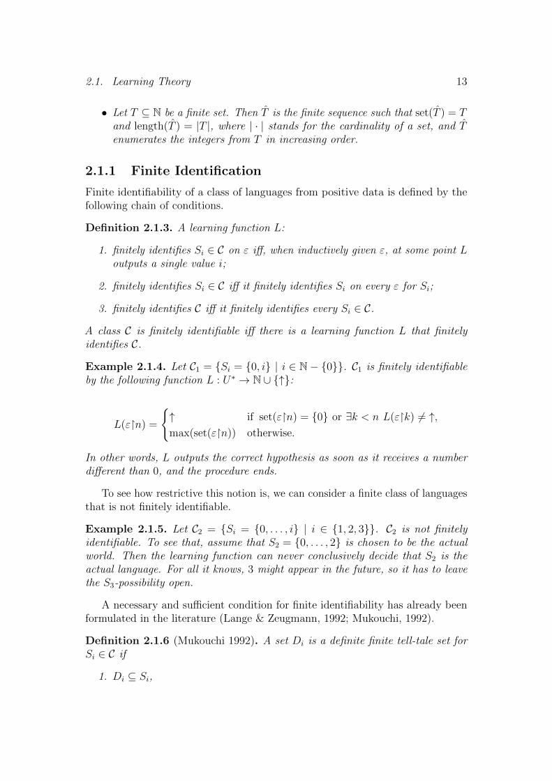
Finite identifiability of a class of languages from positive data is defined by thefollowing chain of conditions.
Definition 2.1.3. A learning function L:
1. finitely identifies Si ∈ C on ε iff, when inductively given ε, at some point Loutputs a single value i;
2. finitely identifies Si ∈ C iff it finitely identifies Si on every ε for Si;
3. finitely identifies C iff it finitely identifies every Si ∈ C.
A class C is finitely identifiable iff there is a learning function L that finitelyidentifies C.
Example 2.1.4. Let C1 = {Si = {0, i} | i ∈ N− {0}}. C1 is finitely identifiableby the following function L : U∗ → N ∪ {↑}:
L(ε�n) =
{↑ if set(ε�n) = {0} or ∃k < n L(ε�k) 6= ↑,max(set(ε�n)) otherwise.
In other words, L outputs the correct hypothesis as soon as it receives a numberdifferent than 0, and the procedure ends.
To see how restrictive this notion is, we can consider a finite class of languagesthat is not finitely identifiable.
Example 2.1.5. Let C2 = {Si = {0, . . . , i} | i ∈ {1, 2, 3}}. C2 is not finitelyidentifiable. To see that, assume that S2 = {0, . . . , 2} is chosen to be the actualworld. Then the learning function can never conclusively decide that S2 is theactual language. For all it knows, 3 might appear in the future, so it has to leavethe S3-possibility open.
A necessary and sufficient condition for finite identifiability has already beenformulated in the literature (Lange & Zeugmann, 1992; Mukouchi, 1992).
Definition 2.1.6 (Mukouchi 1992). A set Di is a definite finite tell-tale set forSi ∈ C if
1. Di ⊆ Si,
14 Chapter 2. Mathematical Prerequisites
2. Di is finite, and
3. for any index j, if Di ⊆ Sj then Si = Sj.
On the basis of this notion, finite identifiability can be then characterized inthe following way.
Theorem 2.1.7 (Mukouchi 1992). A class C is finitely identifiable from positivedata iff there is an effective procedure D : N→ P<ω(N), given by n 7→ Dn, thaton input i produces a definite finite tell-tale of Si.
In other words, each set in a finitely identifiable class contains a finite subsetthat distinguishes it from all other sets in the class. Moreover, for the effectiveidentification it is required that there is a recursive procedure that provides suchdefinite finite tell tale-set.
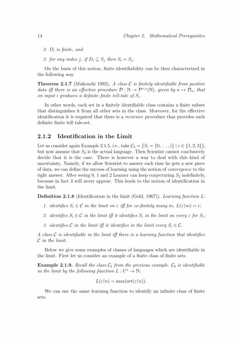
2.1.2 Identification in the Limit
Let us consider again Example 2.1.5, i.e., take C2 = {Si = {0, . . . , i} | i ∈ {1, 2, 3}},but now assume that S2 is the actual language. Then Scientist cannot conclusivelydecide that it is the case. There is however a way to deal with this kind ofuncertainty. Namely, if we allow Scientist to answer each time he gets a new pieceof data, we can define the success of learning using the notion of convergence to theright answer. After seeing 0, 1 and 2 Learner can keep conjecturing S2 indefinitely,because in fact 3 will never appear. This leads to the notion of identification inthe limit.
Definition 2.1.8 (Identification in the limit (Gold, 1967)). Learning function L:
1. identifies Si ∈ C in the limit on ε iff for co-finitely many m, L(ε�m) = i;
2. identifies Si ∈ C in the limit iff it identifies Si in the limit on every ε for Si;
3. identifies C in the limit iff it identifies in the limit every Si ∈ C.
A class C is identifiable in the limit iff there is a learning function that identifiesC in the limit.
Below we give some examples of classes of languages which are identifiable inthe limit. First let us consider an example of a finite class of finite sets.
Example 2.1.9. Recall the class C2 from the previous example. C2 is identifiablein the limit by the following function L : U∗ → N:
L(ε�n) = max(set(ε�n)).
We can use the same learning function to identify an infinite class of finitesets.
2.1. Learning Theory 15
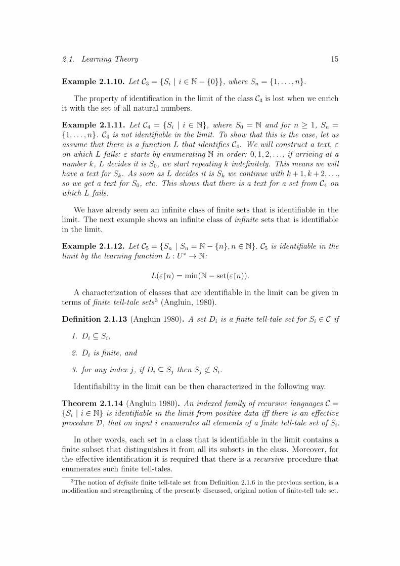
Example 2.1.10. Let C3 = {Si | i ∈ N− {0}}, where Sn = {1, . . . , n}.
The property of identification in the limit of the class C3 is lost when we enrichit with the set of all natural numbers.
Example 2.1.11. Let C4 = {Si | i ∈ N}, where S0 = N and for n ≥ 1, Sn ={1, . . . , n}. C4 is not identifiable in the limit. To show that this is the case, let usassume that there is a function L that identifies C4. We will construct a text, εon which L fails: ε starts by enumerating N in order: 0, 1, 2, . . ., if arriving at anumber k, L decides it is S0, we start repeating k indefinitely. This means we willhave a text for Sk. As soon as L decides it is Sk we continue with k+ 1, k+ 2, . . .,so we get a text for S0, etc. This shows that there is a text for a set from C4 onwhich L fails.
We have already seen an infinite class of finite sets that is identifiable in thelimit. The next example shows an infinite class of infinite sets that is identifiablein the limit.
Example 2.1.12. Let C5 = {Sn | Sn = N− {n}, n ∈ N}. C5 is identifiable in thelimit by the learning function L : U∗ → N:
L(ε�n) = min(N− set(ε�n)).
A characterization of classes that are identifiable in the limit can be given interms of finite tell-tale sets3 (Angluin, 1980).
Definition 2.1.13 (Angluin 1980). A set Di is a finite tell-tale set for Si ∈ C if
1. Di ⊆ Si,
2. Di is finite, and
3. for any index j, if Di ⊆ Sj then Sj 6⊂ Si.
Identifiability in the limit can be then characterized in the following way.
Theorem 2.1.14 (Angluin 1980). An indexed family of recursive languages C ={Si | i ∈ N} is identifiable in the limit from positive data iff there is an effectiveprocedure D, that on input i enumerates all elements of a finite tell-tale set of Si.
In other words, each set in a class that is identifiable in the limit contains afinite subset that distinguishes it from all its subsets in the class. Moreover, forthe effective identification it is required that there is a recursive procedure thatenumerates such finite tell-tales.
3The notion of definite finite tell-tale set from Definition 2.1.6 in the previous section, is amodification and strengthening of the presently discussed, original notion of finite-tell tale set.
16 Chapter 2. Mathematical Prerequisites
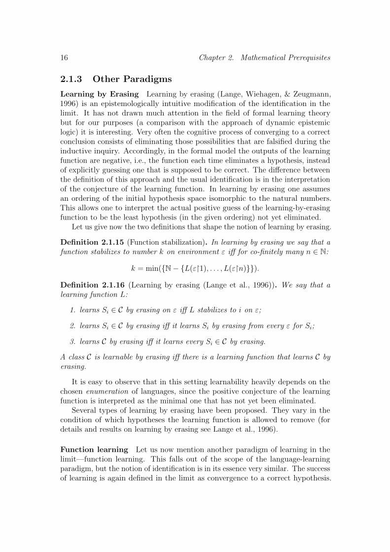
2.1.3 Other Paradigms
Learning by Erasing Learning by erasing (Lange, Wiehagen, & Zeugmann,1996) is an epistemologically intuitive modification of the identification in thelimit. It has not drawn much attention in the field of formal learning theorybut for our purposes (a comparison with the approach of dynamic epistemiclogic) it is interesting. Very often the cognitive process of converging to a correctconclusion consists of eliminating those possibilities that are falsified during theinductive inquiry. Accordingly, in the formal model the outputs of the learningfunction are negative, i.e., the function each time eliminates a hypothesis, insteadof explicitly guessing one that is supposed to be correct. The difference betweenthe definition of this approach and the usual identification is in the interpretationof the conjecture of the learning function. In learning by erasing one assumesan ordering of the initial hypothesis space isomorphic to the natural numbers.This allows one to interpret the actual positive guess of the learning-by-erasingfunction to be the least hypothesis (in the given ordering) not yet eliminated.
Let us give now the two definitions that shape the notion of learning by erasing.
Definition 2.1.15 (Function stabilization). In learning by erasing we say that afunction stabilizes to number k on environment ε iff for co-finitely many n ∈ N:
k = min({N− {L(ε�1), . . . , L(ε�n)}}).
Definition 2.1.16 (Learning by erasing (Lange et al., 1996)). We say that alearning function L:
1. learns Si ∈ C by erasing on ε iff L stabilizes to i on ε;
2. learns Si ∈ C by erasing iff it learns Si by erasing from every ε for Si;
3. learns C by erasing iff it learns every Si ∈ C by erasing.
A class C is learnable by erasing iff there is a learning function that learns C byerasing.
It is easy to observe that in this setting learnability heavily depends on thechosen enumeration of languages, since the positive conjecture of the learningfunction is interpreted as the minimal one that has not yet been eliminated.
Several types of learning by erasing have been proposed. They vary in thecondition of which hypotheses the learning function is allowed to remove (fordetails and results on learning by erasing see Lange et al., 1996).
Function learning Let us now mention another paradigm of learning in thelimit—function learning. This falls out of the scope of the language-learningparadigm, but the notion of identification is in its essence very similar. The successof learning is again defined in the limit as convergence to a correct hypothesis.
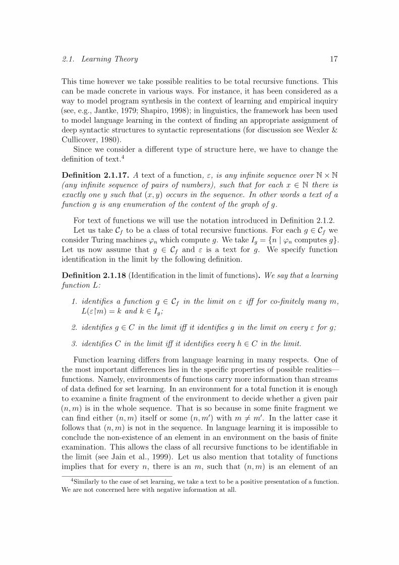
2.1. Learning Theory 17
This time however we take possible realities to be total recursive functions. Thiscan be made concrete in various ways. For instance, it has been considered as away to model program synthesis in the context of learning and empirical inquiry(see, e.g., Jantke, 1979; Shapiro, 1998); in linguistics, the framework has been usedto model language learning in the context of finding an appropriate assignment ofdeep syntactic structures to syntactic representations (for discussion see Wexler &Cullicover, 1980).
Since we consider a different type of structure here, we have to change thedefinition of text.4
Definition 2.1.17. A text of a function, ε, is any infinite sequence over N× N(any infinite sequence of pairs of numbers), such that for each x ∈ N there isexactly one y such that (x, y) occurs in the sequence. In other words a text of afunction g is any enumeration of the content of the graph of g.
For text of functions we will use the notation introduced in Definition 2.1.2.Let us take Cf to be a class of total recursive functions. For each g ∈ Cf we
consider Turing machines ϕn which compute g. We take Ig = {n | ϕn computes g}.Let us now assume that g ∈ Cf and ε is a text for g. We specify functionidentification in the limit by the following definition.
Definition 2.1.18 (Identification in the limit of functions). We say that a learningfunction L:
1. identifies a function g ∈ Cf in the limit on ε iff for co-finitely many m,L(ε�m) = k and k ∈ Ig;
2. identifies g ∈ C in the limit iff it identifies g in the limit on every ε for g;
3. identifies C in the limit iff it identifies every h ∈ C in the limit.
Function learning differs from language learning in many respects. One ofthe most important differences lies in the specific properties of possible realities—functions. Namely, environments of functions carry more information than streamsof data defined for set learning. In an environment for a total function it is enoughto examine a finite fragment of the environment to decide whether a given pair(n,m) is in the whole sequence. That is so because in some finite fragment wecan find either (n,m) itself or some (n,m′) with m 6= m′. In the latter case itfollows that (n,m) is not in the sequence. In language learning it is impossible toconclude the non-existence of an element in an environment on the basis of finiteexamination. This allows the class of all recursive functions to be identifiable inthe limit (see Jain et al., 1999). Let us also mention that totality of functionsimplies that for every n, there is an m, such that (n,m) is an element of an
4Similarly to the case of set learning, we take a text to be a positive presentation of a function.We are not concerned here with negative information at all.
18 Chapter 2. Mathematical Prerequisites
environment. Therefore, it makes little difference to the learning if the functionis enumerated in order (g(0), g(1), . . .). In that case learning is equivalent to theability to guess the next value of the function after a certain time.
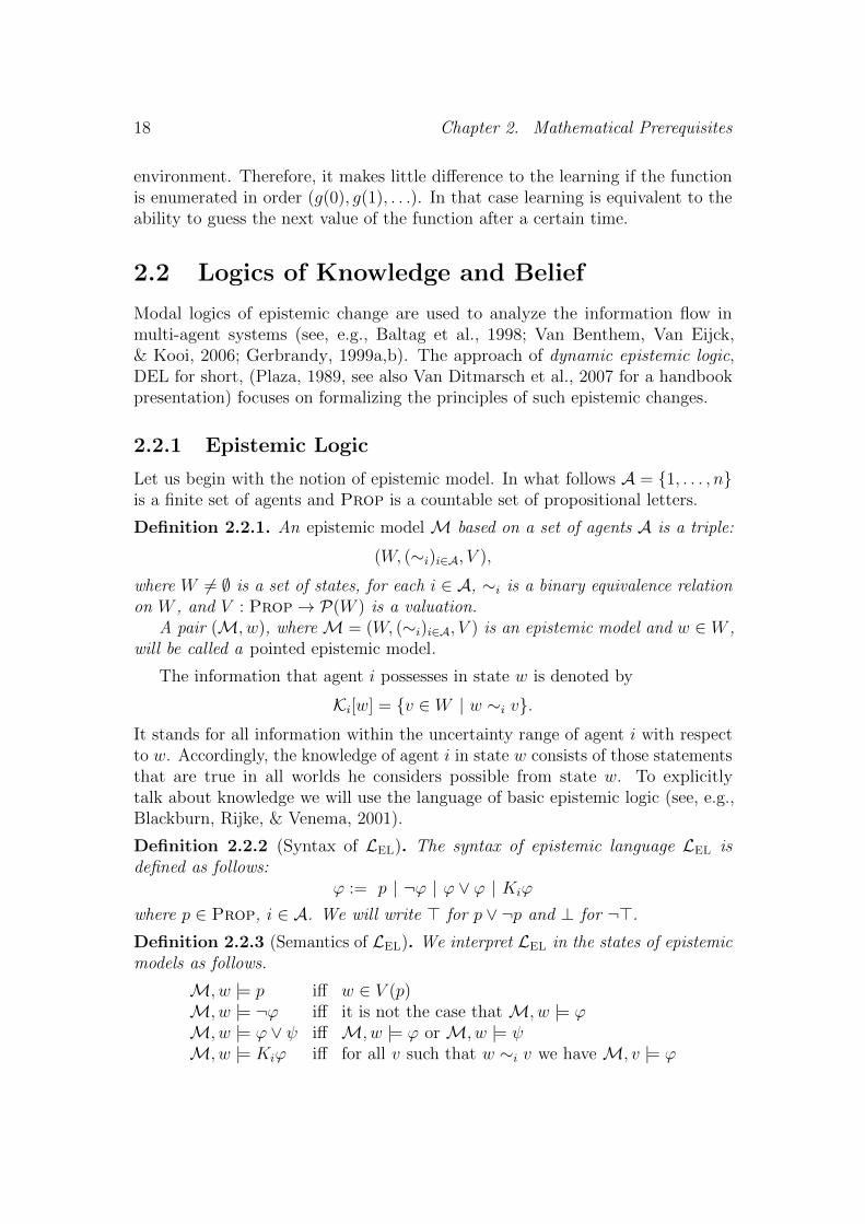
2.2 Logics of Knowledge and Belief
Modal logics of epistemic change are used to analyze the information flow inmulti-agent systems (see, e.g., Baltag et al., 1998; Van Benthem, Van Eijck,& Kooi, 2006; Gerbrandy, 1999a,b). The approach of dynamic epistemic logic,DEL for short, (Plaza, 1989, see also Van Ditmarsch et al., 2007 for a handbookpresentation) focuses on formalizing the principles of such epistemic changes.
2.2.1 Epistemic Logic
Let us begin with the notion of epistemic model. In what follows A = {1, . . . , n}is a finite set of agents and Prop is a countable set of propositional letters.
Definition 2.2.1. An epistemic model M based on a set of agents A is a triple:
(W, (∼i)i∈A, V ),
where W 6= ∅ is a set of states, for each i ∈ A, ∼i is a binary equivalence relationon W , and V : Prop→ P(W ) is a valuation.
A pair (M, w), where M = (W, (∼i)i∈A, V ) is an epistemic model and w ∈ W ,will be called a pointed epistemic model.
The information that agent i possesses in state w is denoted by
Ki[w] = {v ∈ W | w ∼i v}.It stands for all information within the uncertainty range of agent i with respectto w. Accordingly, the knowledge of agent i in state w consists of those statementsthat are true in all worlds he considers possible from state w. To explicitlytalk about knowledge we will use the language of basic epistemic logic (see, e.g.,Blackburn, Rijke, & Venema, 2001).
Definition 2.2.2 (Syntax of LEL). The syntax of epistemic language LEL isdefined as follows:
ϕ := p | ¬ϕ | ϕ ∨ ϕ | Kiϕ
where p ∈ Prop, i ∈ A. We will write > for p ∨ ¬p and ⊥ for ¬>.
Definition 2.2.3 (Semantics of LEL). We interpret LEL in the states of epistemicmodels as follows.
M, w |= p iff w ∈ V (p)M, w |= ¬ϕ iff it is not the case that M, w |= ϕM, w |= ϕ ∨ ψ iff M, w |= ϕ or M, w |= ψM, w |= Kiϕ iff for all v such that w ∼i v we have M, v |= ϕ
2.2. Logics of Knowledge and Belief 19
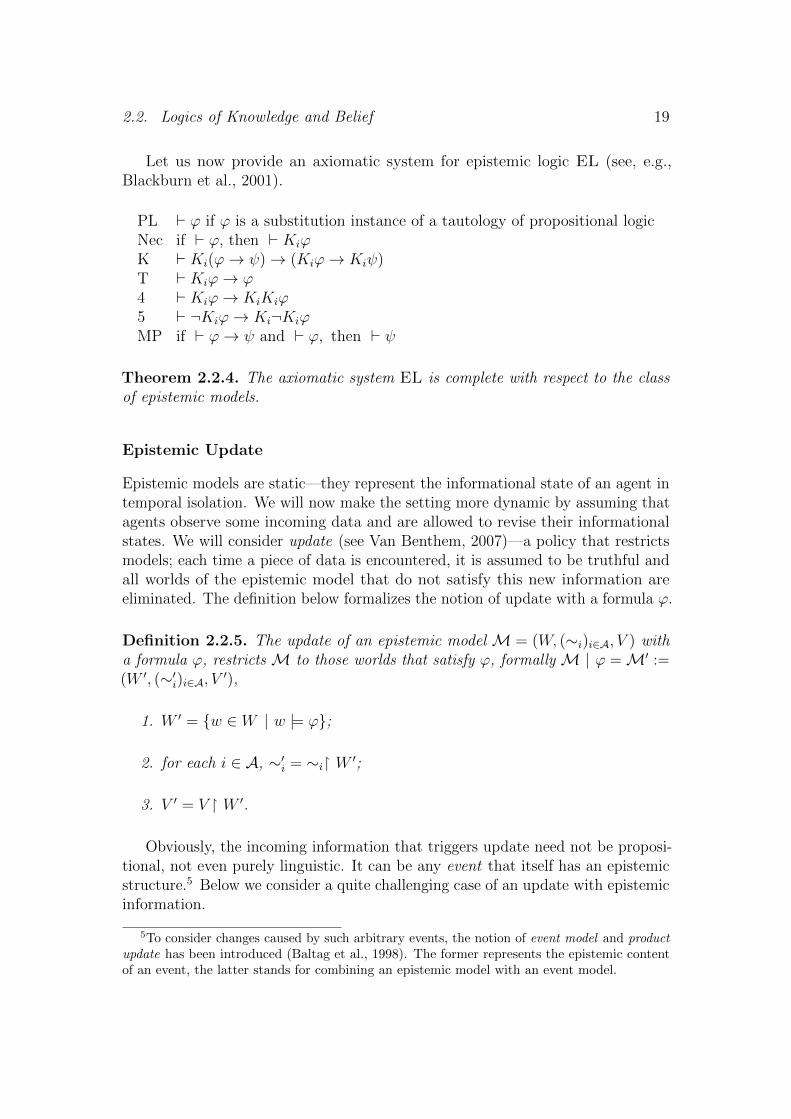
Let us now provide an axiomatic system for epistemic logic EL (see, e.g.,Blackburn et al., 2001).
PL ` ϕ if ϕ is a substitution instance of a tautology of propositional logicNec if ` ϕ, then ` KiϕK ` Ki(ϕ→ ψ)→ (Kiϕ→ Kiψ)T ` Kiϕ→ ϕ4 ` Kiϕ→ KiKiϕ5 ` ¬Kiϕ→ Ki¬KiϕMP if ` ϕ→ ψ and ` ϕ, then ` ψ
Theorem 2.2.4. The axiomatic system EL is complete with respect to the classof epistemic models.
Epistemic Update
Epistemic models are static—they represent the informational state of an agent intemporal isolation. We will now make the setting more dynamic by assuming thatagents observe some incoming data and are allowed to revise their informationalstates. We will consider update (see Van Benthem, 2007)—a policy that restrictsmodels; each time a piece of data is encountered, it is assumed to be truthful andall worlds of the epistemic model that do not satisfy this new information areeliminated. The definition below formalizes the notion of update with a formula ϕ.
Definition 2.2.5. The update of an epistemic model M = (W, (∼i)i∈A, V ) witha formula ϕ, restricts M to those worlds that satisfy ϕ, formally M | ϕ =M′ :=(W ′, (∼′i)i∈A, V ′),
1. W ′ = {w ∈ W | w |= ϕ};
2. for each i ∈ A, ∼′i = ∼i� W ′;
3. V ′ = V � W ′.
Obviously, the incoming information that triggers update need not be proposi-tional, not even purely linguistic. It can be any event that itself has an epistemicstructure.5 Below we consider a quite challenging case of an update with epistemicinformation.
5To consider changes caused by such arbitrary events, the notion of event model and productupdate has been introduced (Baltag et al., 1998). The former represents the epistemic contentof an event, the latter stands for combining an epistemic model with an event model.

20 Chapter 2. Mathematical Prerequisites
Muddy Children We want to devote some space to the classical logical puzzlewhich received a considerable amount of attention in dynamic epistemic logic (see,e.g., Van Ditmarsch et al., 2007; Gerbrandy, 1999a; Moses, Dolev, & Halpern,1986). We discuss it here to give a flavor of complicated epistemic reasoning thatcan be successfully analyzed within DEL framework. We will return to the puzzlein the last chapter of this thesis, where we also propose a novel representation ofthis problem.
Example 2.2.6 (Muddy Children Puzzle). The children, who were playing outsidefor a while, are called back in by their father. Some of them are dirty, in particularthey have mud on their foreheads. The father decides to play with them and says:
(1) At least one of you has mud on your forehead.
And immediately after, he asks:
(I) Can you tell for sure whether or not you have mud on your forehead? If yes,step forward and announce your status.
Each child can see the mud on others but cannot see his or her own forehead.Nothing happens. After that the father repeats I. Still nothing. But after he repeatsthe question three times suddenly all children know whether or not they have mudon their forehead. How is that possible?
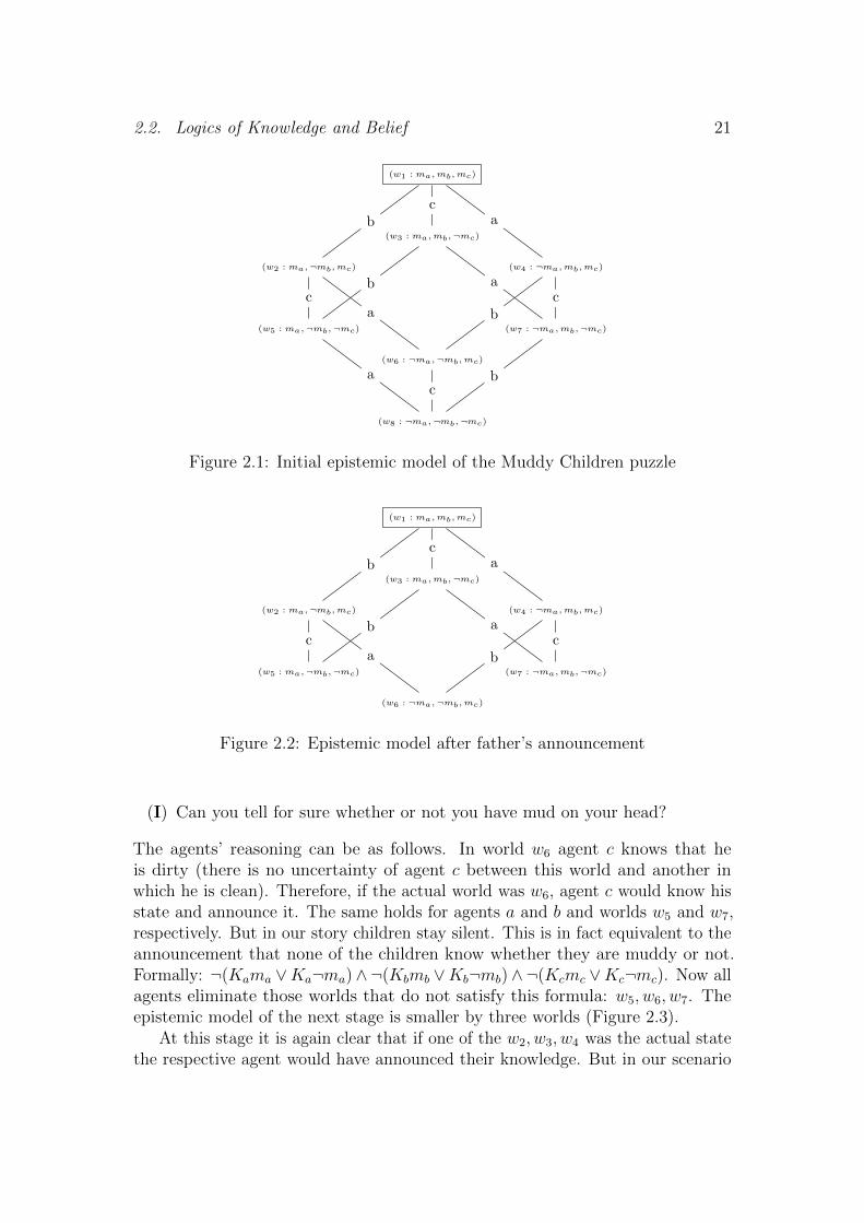
The framework of dynamic epistemic logic allows a clear and comprehensiveexplanation of the underlying phenomena. Let us briefly explain the classicalmodeling. Assume there are three children, let us call them a, b and c, and assumethat, in fact, all of them are muddy. We will take three propositional lettersma, mb and mc that express that the corresponding child is muddy. The initialepistemic model of the situation is depicted in Figure 2.1.
In the model, possible worlds correspond to the ‘distribution of mud’ onchildren’s foreheads, e.g., ma,¬mb,¬mc stands for a being muddy and b and cbeing clean. Two worlds are joined with an edge labeled with x, if the two worldsare in the uncertainty range of agent x (i.e., if agent x cannot distinguish betweenthe two worlds). We drop the reflexive arrows for each state for clarity of thepresentation. The boxed state stands for the actual world. Now, let us see whathappens after the first announcement is made.
(1) At least one of you has mud on your forehead.
In propositional logic, this statement has the following form: (1’) ma ∨mb ∨mc.Since the children trust their father, they all eliminate world w8 in which (1’) isfalse: none of the children is muddy. In other words, they perform an update withformula (1’). The result is depicted in Figure 2.2.
Now the father asks for the first time:
2.2. Logics of Knowledge and Belief 21
(w1 : ma,mb,mc)
(w3 : ma,mb,¬mc)
(w2 : ma,¬mb,mc)
(w5 : ma,¬mb,¬mc)
(w4 : ¬ma,mb,mc)
(w7 : ¬ma,mb,¬mc)
(w6 : ¬ma,¬mb,mc)
(w8 : ¬ma,¬mb,¬mc)
cb a
bcc
a
b
a bc
a
Figure 2.1: Initial epistemic model of the Muddy Children puzzle
(w1 : ma,mb,mc)
(w3 : ma,mb,¬mc)
(w2 : ma,¬mb,mc)
(w5 : ma,¬mb,¬mc)
(w4 : ¬ma,mb,mc)
(w7 : ¬ma,mb,¬mc)
(w6 : ¬ma,¬mb,mc)
cb a
bcc
a
b a
Figure 2.2: Epistemic model after father’s announcement
(I) Can you tell for sure whether or not you have mud on your head?
The agents’ reasoning can be as follows. In world w6 agent c knows that heis dirty (there is no uncertainty of agent c between this world and another inwhich he is clean). Therefore, if the actual world was w6, agent c would know hisstate and announce it. The same holds for agents a and b and worlds w5 and w7,respectively. But in our story children stay silent. This is in fact equivalent to theannouncement that none of the children know whether they are muddy or not.Formally: ¬(Kama ∨Ka¬ma)∧¬(Kbmb ∨Kb¬mb)∧¬(Kcmc ∨Kc¬mc). Now allagents eliminate those worlds that do not satisfy this formula: w5, w6, w7. Theepistemic model of the next stage is smaller by three worlds (Figure 2.3).
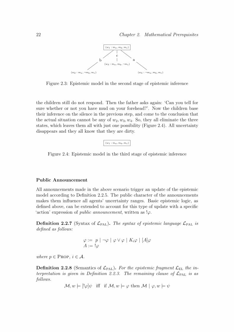
At this stage it is again clear that if one of the w2, w3, w4 was the actual statethe respective agent would have announced their knowledge. But in our scenario
22 Chapter 2. Mathematical Prerequisites
(w1 : ma,mb,mc)
(w3 : ma,mb,¬mc)
(w2 : ma,¬mb,mc) (w4 : ¬ma,mb,mc)
cb a
Figure 2.3: Epistemic model in the second stage of epistemic inference
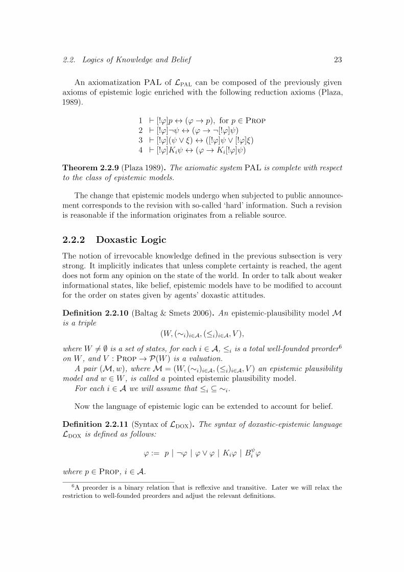
the children still do not respond. Then the father asks again: ‘Can you tell forsure whether or not you have mud on your forehead?’. Now the children basetheir inference on the silence in the previous step, and come to the conclusion thatthe actual situation cannot be any of w2, w3, w4. So, they all eliminate the threestates, which leaves them all with just one possibility (Figure 2.4). All uncertaintydisappears and they all know that they are dirty.
(w1 : ma,mb,mc)
Figure 2.4: Epistemic model in the third stage of epistemic inference
Public Announcement
All announcements made in the above scenario trigger an update of the epistemicmodel according to Definition 2.2.5. The public character of the announcementsmakes them influence all agents’ uncertainty ranges. Basic epistemic logic, asdefined above, can be extended to account for this type of update with a specific‘action’ expression of public announcement, written as !ϕ.
Definition 2.2.7 (Syntax of LPAL). The syntax of epistemic language LPAL isdefined as follows:
ϕ := p | ¬ϕ | ϕ ∨ ϕ | Kiϕ | [A]ϕA := !ϕ
where p ∈ Prop, i ∈ A.
Definition 2.2.8 (Semantics of LPAL). For the epistemic fragment LEL the in-terpretation is given in Definition 2.2.3. The remaining clause of LPAL is asfollows.
M, w |= [!ϕ]ψ iff if M, w |= ϕ then M | ϕ,w |= ψ
2.2. Logics of Knowledge and Belief 23
An axiomatization PAL of LPAL can be composed of the previously givenaxioms of epistemic logic enriched with the following reduction axioms (Plaza,1989).
1 ` [!ϕ]p↔ (ϕ→ p), for p ∈ Prop2 ` [!ϕ]¬ψ ↔ (ϕ→ ¬[!ϕ]ψ)3 ` [!ϕ](ψ ∨ ξ)↔ ([!ϕ]ψ ∨ [!ϕ]ξ)4 ` [!ϕ]Kiψ ↔ (ϕ→ Ki[!ϕ]ψ)
Theorem 2.2.9 (Plaza 1989). The axiomatic system PAL is complete with respectto the class of epistemic models.
The change that epistemic models undergo when subjected to public announce-ment corresponds to the revision with so-called ‘hard’ information. Such a revisionis reasonable if the information originates from a reliable source.
2.2.2 Doxastic Logic
The notion of irrevocable knowledge defined in the previous subsection is verystrong. It implicitly indicates that unless complete certainty is reached, the agentdoes not form any opinion on the state of the world. In order to talk about weakerinformational states, like belief, epistemic models have to be modified to accountfor the order on states given by agents’ doxastic attitudes.
Definition 2.2.10 (Baltag & Smets 2006). An epistemic-plausibility model Mis a triple
(W, (∼i)i∈A, (≤i)i∈A, V ),
where W 6= ∅ is a set of states, for each i ∈ A, ≤i is a total well-founded preorder6
on W , and V : Prop→ P(W ) is a valuation.A pair (M, w), where M = (W, (∼i)i∈A, (≤i)i∈A, V ) an epistemic plausibility
model and w ∈ W , is called a pointed epistemic plausibility model.For each i ∈ A we will assume that ≤i ⊆ ∼i.
Now the language of epistemic logic can be extended to account for belief.
Definition 2.2.11 (Syntax of LDOX). The syntax of doxastic-epistemic languageLDOX is defined as follows:
ϕ := p | ¬ϕ | ϕ ∨ ϕ | Kiϕ | Bψi ϕ
where p ∈ Prop, i ∈ A.
6A preorder is a binary relation that is reflexive and transitive. Later we will relax therestriction to well-founded preorders and adjust the relevant definitions.
24 Chapter 2. Mathematical Prerequisites
Definition 2.2.12 (Semantics of LDOX). We interpret LDOX in the states ofdoxastic-epistemic models in the following way.
M, w |= p iff w ∈ V (p)M, w |= ¬ϕ iff it is not the case that M, w |= ϕM, w |= ϕ ∨ ψ iff M, w |= ϕ or M, w |= ψM, w |= Kiϕ iff for all v such that w∼iv we have M, v |= ϕ
M, w |= Bψi ϕ iff for all v ∈ Ki[w] if v ∈ min≤i(Ki[w] ∩ ‖ψ‖) then v |= ϕ
We define ‖ϕ‖ such that ‖ϕ‖ = {w ∈ W | w |= ϕ}.
The last clause defines the semantics of the conditional belief operator. Anagent is defined to believe ϕ in state w conditionally on ψ if ϕ is true in all statesthat are minimal in the part of the uncertainty range of the agent restricted tothose states that make ψ true.
For axiomatizations of LDOX the reader is advised to consult (Board, 2004)and (Baltag & Smets, 2008b).
Plausibility Upgrade
Epistemic plausibility models can accommodate public announcements of hardinformation. Performing update on those structures has an effect analogous torestriction of simple epistemic models. Such a change can of course result in beliefchange. However, plausibility ordering gives an opportunity to define different,more sophisticated operations on beliefs, operations that do not require statedeletion. As we will see in Chapter 4, such revisions are useful if the source ofinformation is not completely trustworthy.
Lexicographic Upgrade The lexicographic upgrade of an epistemic plausibilitymodel M = (W, (∼i)i∈A, (≤i)i∈A, V ) with a formula ϕ, rearranges the preordersby putting all states satisfying ϕ to be more plausible then others. Let us take≤ϕi = ≤i� ‖ϕ‖, and ≤ϕi = ≤i� ‖¬ϕ‖.
Definition 2.2.13. The lexicographic upgrade of an epistemic plausibility modelM = (W, (∼i)i∈A, (≤i)i∈A, V ) with a formula ϕ is defined as follows:
M ⇑ ϕ := (W, (∼i)i∈A, (≤′i)i∈A, V ),
where for each i ∈ A and for all v, w ∈ Ki[w]:
v ≤′i w iff (v ≤ϕi w or v ≤ϕi w or (v |= ϕ and w |= ¬ϕ)).
The language of announcements that trigger lexicographic upgrade is given inthe following way.
2.2. Logics of Knowledge and Belief 25
Definition 2.2.14 (Syntax of L⇑). The syntax of the doxastic-epistemic languageL⇑ is defined as follows:
ϕ := p | ¬ϕ | ϕ ∨ ϕ | Kiϕ | Bψi ϕ | [A]ϕ
A := ⇑ϕwhere p ∈ Prop, i ∈ A.
Definition 2.2.15 (Semantics of L⇑). For the doxastic-epistemic fragment LDOX
the interpretation is given in Definition 2.2.12. The remaining clause of L⇑ is asfollows.
M, w |= [⇑ϕ]ψ iff M ⇑ ϕ,w |= ψ
Conservative Upgrade The conservative upgrade (also known as minimalupgrade or elite change, see Van Benthem, 2007) of an epistemic plausibilitymodel M = (W, (∼i)i∈A, (≤i)i∈A, V ) with a formula ϕ, rearranges the preordersby making only the most plausible states satisfying ϕ more plausible than allothers, leaving the rest of the preorder the same. Let ≤restϕ
i = ≤i � {t ∈ S | t /∈min≤i ‖ϕ‖}.Definition 2.2.16. The conservative upgrade of an epistemic plausibility modelM = (W, (∼i)i∈A, (≤i)i∈A, V ) with a formula ϕ is defined as follows:
M↑ϕ := (W, (∼i)i∈A, (≤′i)i∈A, V ),
where for each i ∈ A and for all v, w ∈ Ki[w]:
v ≤′i w iff (v ≤restϕi w or v ∈ min≤i‖ϕ‖).
Definition 2.2.17 (Syntax of L↑). The syntax of the doxastic-epistemic languageL↑ is defined as follows:
ϕ := p | ¬ϕ | ϕ ∨ ϕ | Kiϕ | Bψi ϕ | [A]ϕ
A := ↑ϕwhere p ∈ Prop, i ∈ A.
Definition 2.2.18 (Semantics of L↑). For the doxastic-epistemic fragment LDOX
the interpretation is given in Definition 2.2.12. The remaining clause of L↑ is asfollows.
M, w |= [↑ϕ]ψ iff M↑ϕ,w |= ψ
Complete axiomatization for the logics of the two types of upgrades can begiven by a complete axiomatic system for conditional belief complemented withreduction axioms. Van Benthem (2007) gives a detailed discussion on the subject,together with explicitly formulated axioms.
In Chapter 4 we will cover these upgrade methods again in a systematic way.We will compare their reliability in the context of single-agent belief-revision.In this, we will follow other attempts to analyze some classical belief-revisionproblems within the framework of dynamic epistemic and doxastic logic.


Chapter 3
Learning and Epistemic Change
In the present chapter we show how the paradigms of learning theory and dynamicepistemic logic can be linked. We will discuss the interface between learning theoryand dynamic epistemic logic in the context of iterated information change andbelief revision.
3.1 Identification as an Epistemic Process
In Chapter 2 we gave the prerequisites of formal learning theory with its centralnotion of identification. Assuming the reader’s familiarity with those standardtools, we will now discuss the epistemology behind finite and limiting identification.
What are the epistemic components of identification in the limit? The entan-glement of the notions of knowledge, certainty and belief in limiting learning iswidely used in explanations of the paradigm. We quote Gold (1967) in his seminalpaper Language identification in the limit :
In the case of identifiability in the limit the learner does not necessarilyknow 1 when his guess is correct. He must go on processing the infor-mation forever because there is always the possibility that informationwill appear which will force him to change his guess.
With time the epistemic metaphor in identification in the limit became even moreexplicit, involving notions of certainty, justification, possible worlds, etc.:
[...] Thus the Scientist is never justified in feeling certain that her lastconjecture will be her last.
On the other hand, [identifiability in the limit] does warrant a differentkind of confidence, namely that systematic application of guessing rulewill eventually lead to an accurate, last conjecture [...]. If we know
1The emphasis is mine.
27

28 Chapter 3. Learning and Epistemic Change
that the actual world is drawn from [a class identifiable in the limit],then we can be certain that our inquiry will ultimately succeed [...].(Jain et al., 1999, pp. 11–12)
Later, even notions of introspection of knowledge, belief and reliability wereintroduced:
This does not entail that [the learner] knows he knows the answer, since[...] [the learner] may lack any reason to believe that his hypotheseshave begun to converge. Nonetheless, to the extent that the reliabilityperspective on knowledge can be sustained, our paradigms concernscientific discovery in the sense of acquiring knowledge. (Martin &Osherson, 1998, p. 13)
Finally, the epistemic dominance of limiting identification over certainty has beenonce summed up in the following way:
True, there are good reasons for preferring the computable way ofderiving knowledge. We know the results of computations, and onlythink we know the results of trial and error procedures [viz. limitingcomputation]. There are many reasons for preferring knowing tothinking (as Popper, 1966, observed). But that does not change thefact that sometimes thinking may be more appropriate. (Kugel, 1986,p. 155)
Our aim is to expose the epistemology that runs the limiting learning process frombehind the scenes. Let us start by overviewing the components of identification anddiscussing their correspondence with the approach of epistemic logic as describedin Chapter 2.
Class of hypotheses The procedure of learning starts with a class of hypotheses,a class of possible states of the world. It can be interpreted as the backgroundknowledge of Scientist, his uncertainty range (see, e.g., Martin & Osherson, 1997).Scientist expects that one of the possibilities is true, and in the framework it isguaranteed that he is right—Nature indeed chooses one from the class fixed in thebeginning. Among the consequences of such a treatment of background knowledgeis that the actual world is always one of the options Scientist considers possible.Another implication is that learning is not simply verifying or falsifying a singlehypothesis, although those two processes can be viewed as important componentsof identification (Gierasimczuk, 2009b). The fact of picking one from a class is animportant factor in learnability analysis. It allows considering learnability as aproperty of classes of hypotheses determined by some external properties.
3.1. Identification as an Epistemic Process 29
Different nature of data and conclusions The key word “learning” is oftenused in the context of belief revision and dynamic epistemic logic. There ittakes the form of one-step “learning that ϕ”, followed by a modification of theinformational state of the agent—usually by various ways of simply accepting ϕ asit is. In other words, the agent “learned that ϕ” means that the agent “got to knowthat ϕ”. In the setting of formal learning theory it requires more effort than thatto be declared to have learned something. First of all, the incoming information isby default spread over more than one step. The inductive, step-by-step nature ofthis inference is essential; the incoming pieces of data are of a different nature thanthe actual ‘thing’ being learned. Typically, at each finite step the environmentgives only partial information about a potentially infinite set. The relationshipbetween data and hypothesis is like the one between sentences and grammars,natural numbers as such and Turing machines. Namely, if we know the hypothesis,we can infer what kind of possible data are going to appear, but in principle wewill not be able to make a conclusive inference from data to hypotheses. Therefore,in learning theory we say that an agent “learned that a hypothesis holds” if heconverged to this hypothesis on data that are consistent with the actual world.
Positive, true, and readable data There are three important assumptionsthat the incoming data can satisfy:
1. Truthfulness (soundness). Scientist receives only true data, no false infor-mation is included. This assumption leads to, e.g., the priority of incomingdata over the current conjecture and background preferences of Scientist.
2. Positiveness. Scientist receives only elements of positive presentation (text)of the object being learned. Alternatively, together with positive also allnegative information could be included (informant), e.g., for set learningthe graph of the characteristic function of the set could be enumerated.
3. Readability. Scientist has a complete clarity about what information hereceives. A further step would be to analyze the situation of uncertaintyabout the incoming information.
4. Completeness. The data that are consistent with the actual world are alleventually enumerated.
In formal learning theory it is usually assumed that the incoming information isreadable and complete. The source of data is also taken to be truthful. Occasionalerrors are rarely taken into account, and in more applied disciplines are interpretedas noise (see, e.g., Grabowski, 1987). In contrast, the general epistemic frameworkallows erroneous information in form both of mistakes and intentional lies. Inthis respect the original learning theory conforms more to the assumptions of thephilosophy of scientific inquiry (Nature never lies) than to, e.g., conversational
30 Chapter 3. Learning and Epistemic Change
situations (see, e.g., Grice, 1975). Another classic requirement put on data isthat it is positive, i.e., data enumerates only elements of the language. Thisassumption is often challenged by involving negative information, data indicatingwhich elements are not in the set. This setting boosts the power of learningimmensely (see Gold, 1967). It should be noted here that data including bothpositive and negative samples gives remedy to errors. There is enough expressivepower so that any information inconsistent with the actual world can be accountedfor truthfully later on in the process.
Inductive, step-by-step process As briefly mentioned in the previous points,the process of restricting the hypothesis space to only those hypotheses thatare consistent with the incoming data resembles update or public announcement(Baltag et al., 1998). Can learning in the limit of hypothesis h be viewed as theresult of announcing the conjunction of data that lead to stabilization on h? Firstlet us observe that the point of convergence to a correct hypothesis is unknownand in general uncomputable, which makes it also uncomputable to discoverwhich finite sequence resulted in the success of the learning process. Even moreimportantly, finite sequences of data cannot be seen as a single announcement ofa given hypothesis, because which hypothesis is in fact announced by the dataheavily depends on the initial hypothesis space. For instance, let us considertwo classes: C1 = {{1}, {2}} and C2 = {{1}, {1, 2}}, and let h1 be a hypothesiscorresponding to the set {1}. In this case the single event of updating with 1is equivalent to announcing h1 in case C1 had been the initial set of hypotheses,but it does not announce h1 when Scientist has to pick from C2, since the otherhypothesis is still possible.
Infinite procedures The learning theory framework is defined for potentiallyinfinite universes, but even for finite worlds the sequences of data are infinite.The reason for this is that we want to account for situations when Scientist doesnot know the finiteness or size of the entity he investigates. If the initial classof hypotheses is not drastically restrictive, Scientist can never know whether allthe elements have already been enumerated. This leads to infinite proceduresand conditions defined in the limit. Our epistemic setting should reflect theseproperties. It should allow talking about epistemic states as invariant from somepoint onwards, without specifying when this happens. Such an approach tolearning is not unheard of in epistemic logic and belief-revision. There is anongoing philosophical debate about iterated belief revision, iterated epistemicupdate, stability of knowledge, etc. (see, e.g., Stalnaker, 2009). As we will showthey directly correspond to our limiting processes.
Non-introspective knowledge The success of limiting learning can be definedas reaching an epistemic state that can be called ‘knowledge’. What kind of

3.2. Learning via Updates and Upgrades 31
knowledge is it? On the surface it seems to be pretty close to the classical justifiedtrue belief (see, e.g., Chisholm, 1982), the definition ascribed to Plato. Indeed,eventually Scientist puts forward a hypothesis that is true, he believes that it istrue, and moreover he has some reasons to choose it and those reasons can beviewed as a (often very limited) justification. However, from the perspective ofthe agent this ‘knowledge’, preceded by a sequence of belief changes, is strictlyoperational, the work is always in progress. There seems to be some issue withintrospection here—Scientist is not able to point out the successful guess, he doesnot know whether he will not be forced to change his guess again in the lightof future data (for the discussion of the introspection of knowledge in inductiveinference see Hendricks, 2003). On the other hand it is more than just a truebelief—it is immune to change under new true information.
Single agent As mentioned before, in learning theory the data are assumedto be complete and true. In our view, this is the reason why learners are prettylonely in this paradigm. Although in principle, science as well as learning seemto be at least a two-player game that includes a teacher and a learner (a senderof the information and a receiver), for many algorithmic reasons the role of theformer has been minimized. As a result we are concerned here only with the roleof Scientist. Nature can be viewed as an objective, uninvolved source of data.In a sense this constitutes an assumption of fairness. Nature does not intendto help or disturb the process. As a result, learning theory is predominantly aone-agent business. A hint of multi-agency can be associated with team-learning,a framework suggested by Blum & Blum (1975), explicitly introduced by Smith(1982) and since then extensively studied (for an overview see Jain & Sharma,1996). However, multi-agency understood in this way can be summed up aslearners working on their own contributing to some common, bigger goal. Thetopic of communication and (non-)cooperativeness of the learners is marginalhere. Dynamic epistemic and dynamic doxastic logics study these notions ofmulti-agency explicitly, and this is in fact their main focus (for the benefits of amulti-agent approach to epistemic issues see Van Benthem, 2006).
3.2 Learning via Updates and Upgrades
With the above discussion in mind we can now turn to the question of howlearning-theoretic notions can be approached from the perspective of the epistemicframework.2
Let us fix C = {S1, S2, . . .} to be a class of sets. It can be interpreted asthe initial epistemic model, representing the background knowledge of Scientist
2Our considerations are of semantic nature and therefore differ from the computable frameworkof learning theory. E.g., one of the consequences is that we assume the property of consistencyof learning, which in formal learning theory is optional.

32 Chapter 3. Learning and Epistemic Change
together with his uncertainty about which world is the actual one. Let us takethe initial epistemic model to be formally defined as
M = (C,∼),
where C is the set of worlds and ∼ ⊆ C × C is an uncertainty relation for Scientist.For now we do not require any particular preference of the scientist over C—allpossibilities are equally plausible. Hence, we can for now assume that ∼ is auniversal equivalence relation over C. The initial epistemic state of the Scientistis depicted in Figure 3.1. This model corresponds to the starting point of thescientific discovery process. In the beginning Scientist considers all of thempossible. Scientist is given the class of hypotheses C, i.e., he knows what thealternatives are.
S1 S2 S3 S4. . .∼ ∼ ∼ ∼
Figure 3.1: Initial epistemic model
Next, Nature decides on some state of the world by choosing one possibilityfrom C. Let us assume that, as a result, S4 is the chosen world. Then, she decideson some particular environment ε, consistent with S4. We picture this enumerationin Figure 3.2 below.
...
ε1
ε2
ε3
ε4
Figure 3.2: Environment ε consistent with S4
The sequence ε is successively given to Scientist. Let us focus now on the firststep of the procedure. A piece of data ε1 is given to the scientist. In Figure 3.3Scientist’s confrontation with ε1 is depicted. Scientist can react to this newinformation by adjusting his epistemic state in different ways.
3.2. Learning via Updates and Upgrades 33
3.2.1 Learning via Update
Epistemic Update
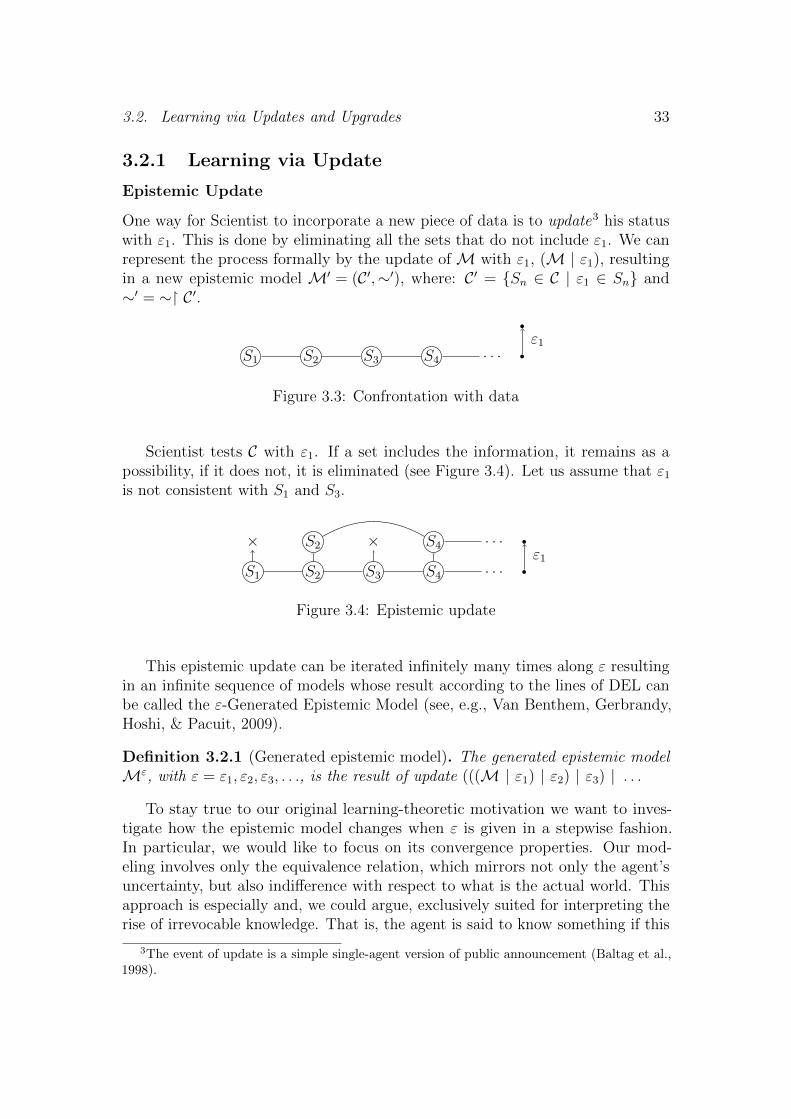
One way for Scientist to incorporate a new piece of data is to update3 his statuswith ε1. This is done by eliminating all the sets that do not include ε1. We canrepresent the process formally by the update of M with ε1, (M | ε1), resultingin a new epistemic model M′ = (C ′,∼′), where: C ′ = {Sn ∈ C | ε1 ∈ Sn} and∼′ = ∼� C ′.
S1 S2 S3 S4. . .
ε1
Figure 3.3: Confrontation with data
Scientist tests C with ε1. If a set includes the information, it remains as apossibility, if it does not, it is eliminated (see Figure 3.4). Let us assume that ε1
is not consistent with S1 and S3.
S1 S2 S3 S4. . .
× S2 × S4. . .
ε1
Figure 3.4: Epistemic update
This epistemic update can be iterated infinitely many times along ε resultingin an infinite sequence of models whose result according to the lines of DEL canbe called the ε-Generated Epistemic Model (see, e.g., Van Benthem, Gerbrandy,Hoshi, & Pacuit, 2009).
Definition 3.2.1 (Generated epistemic model). The generated epistemic modelMε, with ε = ε1, ε2, ε3, . . ., is the result of update (((M | ε1) | ε2) | ε3) | . . .
To stay true to our original learning-theoretic motivation we want to inves-tigate how the epistemic model changes when ε is given in a stepwise fashion.In particular, we would like to focus on its convergence properties. Our mod-eling involves only the equivalence relation, which mirrors not only the agent’suncertainty, but also indifference with respect to what is the actual world. Thisapproach is especially and, we could argue, exclusively suited for interpreting therise of irrevocable knowledge. That is, the agent is said to know something if this
3The event of update is a simple single-agent version of public announcement (Baltag et al.,1998).
34 Chapter 3. Learning and Epistemic Change
something is true in all worlds in his uncertainty range defined by the equivalencerelation. Therefore, we will be particularly interested in the convergence to thestate of such knowledge, i.e., in our case in convergence to the situation in whichonly one, true set is left. Then we will say that the scientist learned with certaintywhat is the actual world. The possibility of reaching certainty in an epistemicmodel by the use of updates resembles the setting of finite identifiability. To recallthe latter let us give a short example.
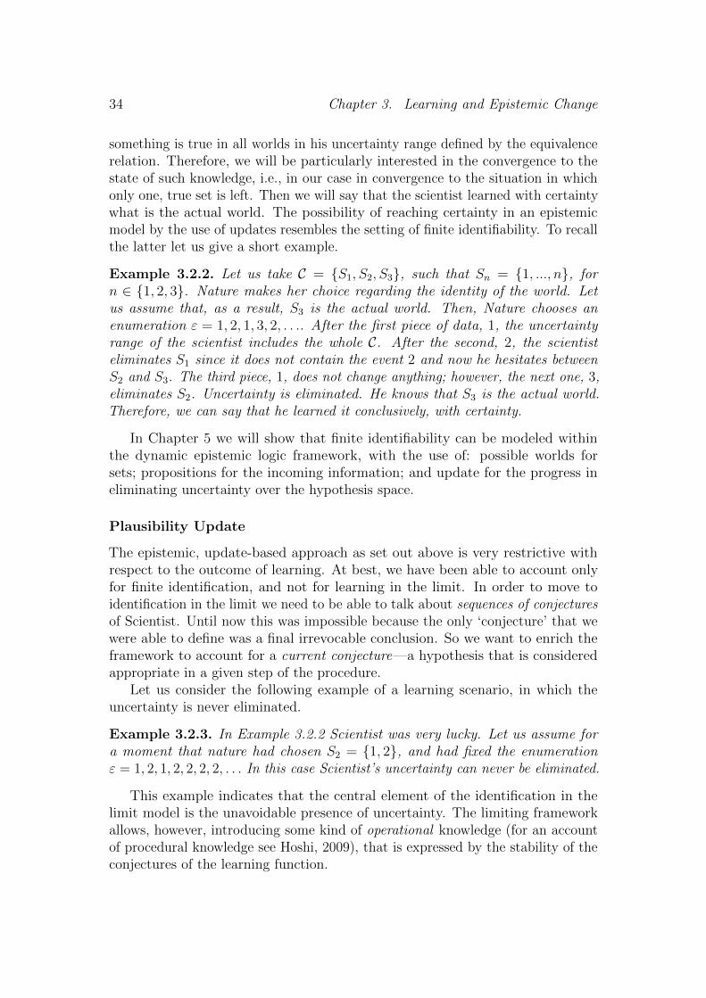
Example 3.2.2. Let us take C = {S1, S2, S3}, such that Sn = {1, ..., n}, forn ∈ {1, 2, 3}. Nature makes her choice regarding the identity of the world. Letus assume that, as a result, S3 is the actual world. Then, Nature chooses anenumeration ε = 1, 2, 1, 3, 2, . . .. After the first piece of data, 1, the uncertaintyrange of the scientist includes the whole C. After the second, 2, the scientisteliminates S1 since it does not contain the event 2 and now he hesitates betweenS2 and S3. The third piece, 1, does not change anything; however, the next one, 3,eliminates S2. Uncertainty is eliminated. He knows that S3 is the actual world.Therefore, we can say that he learned it conclusively, with certainty.
In Chapter 5 we will show that finite identifiability can be modeled withinthe dynamic epistemic logic framework, with the use of: possible worlds forsets; propositions for the incoming information; and update for the progress ineliminating uncertainty over the hypothesis space.
Plausibility Update
The epistemic, update-based approach as set out above is very restrictive withrespect to the outcome of learning. At best, we have been able to account onlyfor finite identification, and not for learning in the limit. In order to move toidentification in the limit we need to be able to talk about sequences of conjecturesof Scientist. Until now this was impossible because the only ‘conjecture’ that wewere able to define was a final irrevocable conclusion. So we want to enrich theframework to account for a current conjecture—a hypothesis that is consideredappropriate in a given step of the procedure.
Let us consider the following example of a learning scenario, in which theuncertainty is never eliminated.
Example 3.2.3. In Example 3.2.2 Scientist was very lucky. Let us assume fora moment that nature had chosen S2 = {1, 2}, and had fixed the enumerationε = 1, 2, 1, 2, 2, 2, 2, . . . In this case Scientist’s uncertainty can never be eliminated.
This example indicates that the central element of the identification in thelimit model is the unavoidable presence of uncertainty. The limiting frameworkallows, however, introducing some kind of operational knowledge (for an accountof procedural knowledge see Hoshi, 2009), that is expressed by the stability of theconjectures of the learning function.
3.2. Learning via Updates and Upgrades 35
To model an algorithmic nature of the learning process that includes the actualguess and other not-yet-eliminated possibilities, we can enrich the epistemic modelwith some plausibility relation. The relation ≤ represents some preference overthe set of hypotheses. E.g., if Scientist is an Occamist, the preference would bedefined according to the simplicity of hypotheses. In the initial epistemic state theuncertainty of the scientist again ranges over the whole of C. This time howeverthe class is ordered and Scientist’s current belief is the most preferred hypothesis.4
Therefore, we consider the initial epistemic plausibility state of Scientist to be:
M = (C,∼,≤).
The procedure of erasing worlds that are inconsistent with successively incomingdata is the same as in the previous section. This time however let us introduce thecurrent-guess state which is interpreted as the actual conjecture of the Scientist.It is always the one that is most preferred—the smallest one according to ≤. Indoxastic logic a set of most preferred hypotheses is almost invariably interpreted asthe ones that the agent believes in. Let us go back to Example 3.2.3, where Naturechose world S2. After seeing 2 and eliminating S1, Scientist’s attention focuses onS2; then S2 is his current belief. It is the most preferred hypothesis, and as suchcan be repeated as long as it is consistent with ε. In this particular case, sinceNature chose a world consistent with S2, it will never be contradicted, so Scientistwill always be uncertain between S2 and S3. However, his preference directs himto believe in the correct hypothesis, without his being aware of the correctness.The belief in a hypothesis may become safe—whatever true information is given,it will not force the scientist to change his mind. And this state of safety whilemaintaining uncertainty is intuitively the one that occurs in identification in thelimit. According to the picture sketched here, we will show (in Chapter 4) thatlearning in the limit can be modeled within the dynamic doxastic logic framework,using: possible worlds for sets; propositions for incoming information; update forthe progress in eliminating uncertainty over the hypothesis space; a plausibilityrelation for the underlying hypothesis space; in each step of the procedure, themost preferred hypothesis as the actual positive guess of the learning function.
3.2.2 Learning via Plausibility Upgrades
Extending this approach we will also investigate different ways of reacting to theincoming information: except for update we will also consider ways of upgradingthe preference relation as a reaction to new data. Upgrades are useful when updateis too strong—in the situations in which the source of information is not entirely
4For now we do not pose any restriction on the plausibility ordering. The conditions ofwell-foundedness or connectedness of the plausibility ordering are often assumed of such doxasticsituations. As we will see later, in our setting, the well-foundedness of the initial plausibilitypreorder might not always be possible.
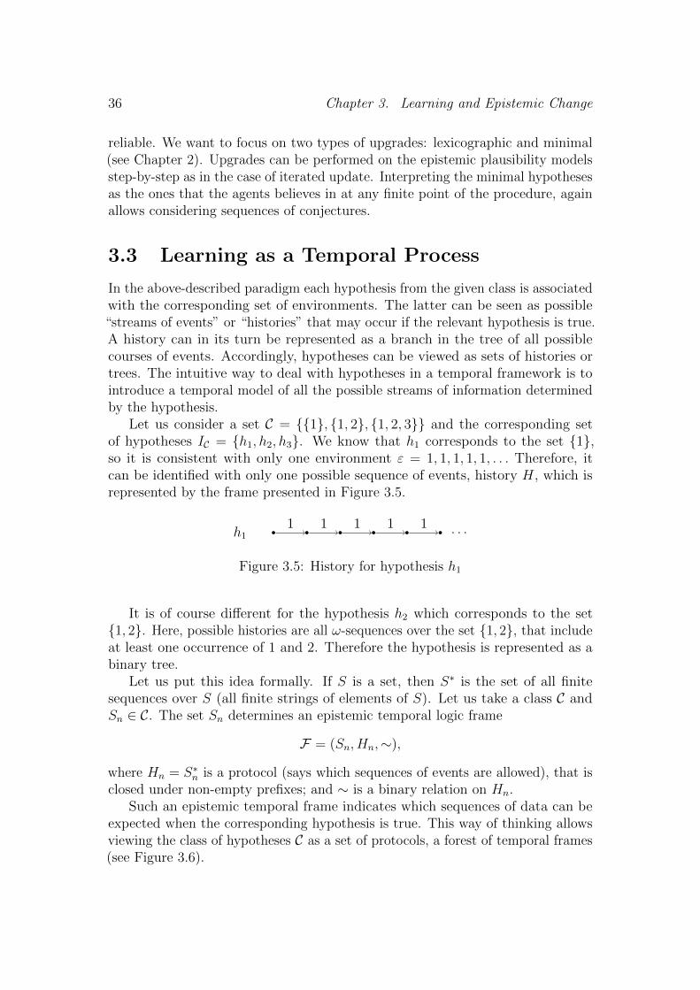
36 Chapter 3. Learning and Epistemic Change
reliable. We want to focus on two types of upgrades: lexicographic and minimal(see Chapter 2). Upgrades can be performed on the epistemic plausibility modelsstep-by-step as in the case of iterated update. Interpreting the minimal hypothesesas the ones that the agents believes in at any finite point of the procedure, againallows considering sequences of conjectures.
3.3 Learning as a Temporal Process
In the above-described paradigm each hypothesis from the given class is associatedwith the corresponding set of environments. The latter can be seen as possible“streams of events” or “histories” that may occur if the relevant hypothesis is true.A history can in its turn be represented as a branch in the tree of all possiblecourses of events. Accordingly, hypotheses can be viewed as sets of histories ortrees. The intuitive way to deal with hypotheses in a temporal framework is tointroduce a temporal model of all the possible streams of information determinedby the hypothesis.
Let us consider a set C = {{1}, {1, 2}, {1, 2, 3}} and the corresponding setof hypotheses IC = {h1, h2, h3}. We know that h1 corresponds to the set {1},so it is consistent with only one environment ε = 1, 1, 1, 1, 1, . . . Therefore, itcan be identified with only one possible sequence of events, history H, which isrepresented by the frame presented in Figure 3.5.
h1. . .1 1 1 1 1
Figure 3.5: History for hypothesis h1
It is of course different for the hypothesis h2 which corresponds to the set{1, 2}. Here, possible histories are all ω-sequences over the set {1, 2}, that includeat least one occurrence of 1 and 2. Therefore the hypothesis is represented as abinary tree.
Let us put this idea formally. If S is a set, then S∗ is the set of all finitesequences over S (all finite strings of elements of S). Let us take a class C andSn ∈ C. The set Sn determines an epistemic temporal logic frame
F = (Sn, Hn,∼),
where Hn = S∗n is a protocol (says which sequences of events are allowed), that isclosed under non-empty prefixes; and ∼ is a binary relation on Hn.
Such an epistemic temporal frame indicates which sequences of data can beexpected when the corresponding hypothesis is true. This way of thinking allowsviewing the class of hypotheses C as a set of protocols, a forest of temporal frames(see Figure 3.6).

3.4. Summary 37
...S3
. . .. . .
S2
. . .
. . .. . .
S1. . .
. . . . . .
Figure 3.6: Epistemic temporal forest F
To sum up, we interpret hypotheses to be sets of histories, i.e., sets of sequencesenumerating events. Therefore, we can reinterpret the possible realities as sets offunctions. This approach leads to a generalized, uniform view of learnability ofvarious structures. Function learning and set learning become analyzable on acommon ground.
To account for identification in the limit, following the argumentation ofprevious sections it seems to be necessary to enrich the temporal models withplausibility ordering that will account for the beliefs at each level of the temporalforest. The latter can be generated from the initial class as in the previous case.Then the temporal epistemic plausibility frame is given as follows:
F≤ = (Sn, Hn,∼,≤).
Our aim in all the above described semantic interpretations is to give anepistemic (temporal) characterization of learnability.
3.4 Summary
In this chapter we gave an introduction to our modeling of the process of inductiveinference in dynamic epistemic logic and dynamic doxastic logic. For now weavoided formalism in order to first provide motivation and basics of the transitionfrom one framework to another. In particular, we indicated that update is appro-priate to analyze the notion of finite identifiability as convergence to knowledge.Learning in the limit, on the other hand, has to be supported by an underlyingordering of the hypothesis space. This indicates that it should be formalized indoxastic logic, where the preference or plausibility relation is a standard elementof any model, and identification in the limit is viewed as reaching safe belief. Wealso proposed to view one component of the learning paradigm, hypotheses andhypothesis spaces, as temporal models. This allows investigating properties ofthe epistemic revision that requires certain sequences of events, conforming tosome temporal protocols. We postulate that identifiability can be expressed intemporal logic interpreted over the corresponding epistemic temporal forests.

Part II
Learning and Definability

Chapter 4
Learning and Belief Revision
Learning can be described as a process of acquiring new information. Thisacquisition can take forms as different as things are that can be learned. Wesay: ‘He learned that she cheated on him’ or ‘She learned about his disease’, butalso: ‘She learned a language’ or ‘He finally learned how to behave’. The first twosentences are about a change in informational state induced by accepting a fact,getting to know something. The latter two are different, they describe a situationin which an inductive acquisition process came to a successful end.
The first kind of learning—getting to know about facts—is formalized andanalyzed in the domain of belief revision and the diverse frameworks of epistemicand doxastic logics. The main aim here is to formalize the elementary dynamicsof knowledge and epistemic attitudes towards incoming information.
The second kind—learning as a process—is studied within the framework offormal learning theory. In this framework a general concept (language, grammar,theory) gets to be identified by an agent on the basis of some elementary data(sentences, results of experiments) over a long period of time. The learning agentis allowed to change his mind on the way, and the process is successful if it resultsin convergence to an appropriate hypothesis. In a sense this kind of learning isbuilt on top of the first kind, it consists of an iteration of simple getting-to-knowevents.
In this chapter we propose a way to use the framework of learning theory toevaluate belief-revision policies. Our interest is shared by at least two existinglines of research. Kelly, Schulte, & Hendricks (1995) and Kelly (1998a,b, 2004,2008) focus on bringing together some classical belief-revision policies (amongothers those proposed by Boutilier, 1996; Darwiche & Pearl, 1997; Grove, 1988;Spohn, 1988) with the framework of function learning (see Chapter 2, Section2.1.3, and for more details Blum & Blum, 1975). In this attempt the possibleconcepts to be learned or discovered are the possible sequential histories. Theproblem of prediction which seems to be at the heart of this approach is obviouslyuseful for modeling certain kind of scientific inquiry. However in general, changesof epistemic states do not have to happen according to some prescribed sequence.
41
42 Chapter 4. Learning and Belief Revision
They are often governed by sequences of facts that are closed under permutationwith respect to their informational content.
Martin & Osherson (1997, 1998) have also worked on establishing the connectionbetween learning theory and belief revision. Their attempt has its roots in theclassical AGM framework (Alchourron et al., 1985) and treats belief revision as atwo step process: the shrinking of the current belief state to accommodate the newinformation (belief contraction) and the incorporation of the data (see Levi, 1980).In this approach, the dominant features of modeling inductive learning as iteratedbelief revision are that the belief state is treated syntactically, as a set of sentencesof a given language, and is assumed to be a full-blown theory (closed under theoperation of consequence), incoming data get a fully trusted welcome, and last butnot least, the agent does not explicitly consider other, perhaps counter-factual,possibilities.
Following Gierasimczuk (2009a,c) and Degremont & Gierasimczuk (2009) weadvance a different line of research. On the inductive inference side, we areinterested in the paradigm of language learning which is more general than theaforementioned function learning approach. We assume that the data are observedin a random manner, so that in general predicting the future sequence is notfeasible, or even relevant. As possible concepts that are inferred we take setsof atomic propositions. Therefore, receiving new data corresponds to getting toknow about facts. On the side of belief revision we follow the lines of dynamicepistemic logic (see Van Benthem, 2007). Hence, we interpret current beliefs ofthe agent (hypothesis) as the content of those possible worlds that he considersmost plausible. The revision does not only result in the change of the currenthypothesis, but can also induce modification of the agent’s plausibility order.
We are mainly concerned with identifiability in the limit (Gold, 1967). Inthe first part we restrict ourselves to learning from sound and complete streamsof positive data. We show that learning methods based on belief revision viaconditioning (update) and lexicographic revision are universal, i.e., provided certainprior conditions, those methods are as powerful as identification in the limit. Thoseprior conditions, the agent’s prior dispositions for belief revision, play a crucialrole here. We show that in some cases, these priors cannot be modeled usingstandard belief-revision models (as based on well-founded preorders), but onlyusing generalized models (as simple preorders). Furthermore, we draw conclusionsabout the existence of tension between conservatism and learning power by showingthat the very popular, most ‘conservative’ belief-revision methods, like Boutilier’sminimal revision, fail to be universal. In the second part we turn to the case oflearning from both positive and negative data. Here, along with information aboutfacts the agent receives negative data about things that do not hold of the actualworld. We again assume these streams to be truthful and we draw conclusionsabout iterated belief revision governed by such streams. This enriched frameworkallows us to consider the occurrence of erroneous information. Provided thaterrors occur finitely often and are always eventually corrected we show that the
43
lexicographic revision method is still reliable, but more conservative methods fail.Before we get to the formal content of this chapter, let us first give two additionalphilosophical motivations for our work.
Evaluation of Belief-Revision Policies The traditional approach to the prob-lem of belief revision (Alchourron et al., 1985) can be summed up in the followingway. The belief is taken to be a set of sentences, often assumed to be closed undersome operation of consequence. Then, confronted with an incoming sentencethe belief set has to undergo some transformation. If the sentence is consistentwith the belief set, it is simply set-theoretically added, and the set is extendedto include all consequences. If the sentence contradicts information contained inthe set, the latter has to be modified by first removing inconsistency, and onlythen performing the addition. In general the belief-revision procedure takes thefollowing form:
〈belief set, proposition〉 → revised belief set;
in other words:〈S, α〉 → S ∗ α.
Intuitively, belief revision, in order to be rational, has to conform to certain generalrules. An intuitive set of rules of this kind, or axiomatization, if one prefers, ofbelief revision has been proposed by Alchourron et al. (1985). Investigations intothe properties of this type of revision led to the following difficulty: often there ismore than one way to make a set consistent with some initially inconsistent input.For instance, if the belief set S = {ϕ, ϕ→ ψ}, and the incoming information is¬ψ then dropping either of the sentences in S would make the set S consistentwith ¬ψ. How do we decide which one should be chosen? This problem indicatesthe need for some preference order that underlies beliefs and governs the orderof potential elimination (Alchourron et al., 1985). The postulate of ordering thebeliefs according to their entrenchment has essentially enriched the framework.The results indicating the necessity of orders led to involving them explicitly asparts of belief states. A system that accounts for the ordering has been providedby Grove (1988), who represented AGM postulates in terms of systems of spheres.This modeling is a direct predecessor of the modal logic based approach to belief,as it presupposes a total well-founded preorder on the initial uncertainty range.The framework then conformed to a new scheme:
〈(belief set,≤), proposition〉 → (revised belief set, revised ≤);
in other words:〈(S,≤), α〉 → (S ∗ α,≤α).
This approach led to many new questions, among others: the origin andjustification of ≤; possible ways of transforming ≤ and the ways in which they
44 Chapter 4. Learning and Belief Revision
are (or should be) chosen.Although this approach has been shown to be quite powerful, it is also very
controversial in the fact that it is very syntactic. Dependence on the specificlanguage and closing off under a consequence relation present problems whencomparing it to linguistic and cognitive reality. In the meantime an alternative,more semantic approach to belief change has been developed, in which modal logicturns out to be very useful (see Stalnaker, 2009). Despite those developmentsthe old uneasiness remains. How are we supposed to judge and choose betweendifferent belief-revision policies? Perhaps, by introducing another level in whichsome new preference relation will order different policies and this preferenceordering itself should become a matter of taste or character? Rott (2008) expectsthat this question will eventually lead to some sort of circularity in the domainof belief-revision theory. It can be argued that this problem could ultimately besolved only by psychological research in human cognitive tendencies. He posesthe following two options as answers to this difficulty:
One option is to insist on divide-and-conquer strategy: Researchers inbelief revision should put their efforts into finding out which methodsare best in which contexts. [...] [A] second option. This optionassumes that there is some level in the belief state hierarchy up towhich constraints of rationality reside, but above which, at all higherlevels, we are just describing, in an idealized way, various ways thatpeople happen to be. [...] In this perspective, there are no objectivestandards for rationality beyond the first level as characterized byAGM.
In the present chapter of this book we will challenge this position by showingthat applying certain types of rules in certain contexts can be analyzed in termsof whether they can be relied upon in the ‘quest for the truth’ (the analysis ofinductive inference in terms of reliability has been for the first time provided byKelly, 1996). We will analyze certain belief-revision policies in terms of theirdependability and show differences in their learning power. In our framework wecan naturally treat the procedural aspect of iterated belief revision, address someintermediate stages of such iterations and relate them to the ultimate success ofa belief-revision policy. Hence, belief-revision methods can get evaluated on thebasis of their learning power. Finally, it can be argued that the above-mentioned‘different ways that people happen to be’ can be traced as evolutionary equilibriathat correspond to effectiveness and reliability of methods.
Safety and Stability of Beliefs The classical definition characterizes knowl-edge as true justified belief (see, e.g., Chisholm, 1982). In a modern setting thishas been formalized as the state of certainty, because a decent justification ofa theory should eliminate all other possibilities. Such definition is difficult to
4.1. Iterated Belief Revision 45
accept from a philosophical standpoint, and many arguments against it can be(and have been) formulated (see, e.g., Gettier, 1963). One of them is that in factknowledge is a dynamic phenomenon and it rarely occurs in the form of irrevocablestates of certainty. Alternatives oscillate around the concept of knowledge assafe belief. The strength of safety is in the guarantee it gives: the safe belief isnot endangered by the occurrence of true data. If we restrict our considerationsto truthful information, or at least assume that mistakes happen rarely, safetycan be reformulated in terms of stability. In other words, knowledge emergeswhen stability is reached. The need for such a notion appeared in many differentframeworks: from reaching an agreement in a conversational situation (see, e.g.,Lehrer, 1965, 1990) to the considerations in the domain of philosophy of science(see, e.g., Hendricks, 2001).
In this work we account for and characterize the emergence of both: therestrictive kind of knowledge (certainty) and stable belief. We explicitly formulatethe conditions under which certain belief states give raise to the emergence ofsuch epistemic and doxastic states.
Finally, inspired by Nozick (1981), Rott (2004) puts forward that perhaps:
[...] knowledge [should] be made of still sterner stuff—stuff that alsosurvives (a modest amount of) misinformation.
In the following sections we will show that under the requirement of convergenceto stable belief some policies are still reliable if a finite number of errors occurand they are all corrected later in the process.
4.1 Iterated Belief Revision
In our analysis of single agent information-update and belief revision we willredefine the framework of dynamic epistemic logic in order to simplify things.As we are here concerned with the single-agent case and moreover, we take theincoming information to be propositional, we will focus on the notion of epistemicstate, i.e., a set of possible worlds.
Definition 4.1.1. A possible world is a valuation over Prop, and it can beidentified with a set s ⊆ Prop. We say that p is true in s (write s |= p) if andonly if p ∈ s.
The uncertainty range of an agent is represented as a set of worlds that theagent considers possible.
Definition 4.1.2. An epistemic state is a set S ⊆ P(Prop) of possible worlds.A pair (S, s), where S is an epistemic state and s ∈ S is called a pointed epistemicstate.
46 Chapter 4. Learning and Belief Revision
With respect to the setting defined in Chapter 2, epistemic states of the agenti associated to the epistemic modelM = (W, (∼i)i∈A, V ) are given by equivalenceclasses in W/∼, in other words, a pointed epistemic state of an agent i is a pair(Ki[w], w).
In accordance with the semantics of basic epistemic logic, we will interpret theknowledge operator in the usual way.
Definition 4.1.3 (Semantics of LEL in epistemic states). We interpret the single-agent LEL in the epistemic states in the following way.
S, s |= p iff p ∈ sS, s |= ¬ϕ iff it is not the case that s |= ϕS, s |= ϕ ∨ ψ iff s |= ϕ or s |= ψS, s |= Kϕ iff S ⊆ ‖ϕ‖
Accordingly, our simplified approach will be extended to the doxastic framework.By enriching the epistemic state with a plausibility relation we consider epistemicplausibility states. To model beliefs, we need to specify some subset S0 ⊆ S ofthe epistemic state, consisting of the possible worlds that are consistent with theagent’s beliefs. The intuition here is that although the agent considers all worldsin his epistemic state possible, some of them are seen as more ‘desirable’, thosewill be given as the minimal ones according to the plausibility order.
Definition 4.1.4. A prior plausibility assignment S 7→ ≤S assigns to any epis-temic state some plausibility order based on the original epistemic state.
Definition 4.1.5. A plausibility state is a pair (S,≤) of an epistemic state Sand a total preorder ≤ on S, called a plausibility relation.
An epistemic state together with some prior plausibility assignment constitutea plausibility state. Here as in the case of plausibility models we will assume theplausibility relations to be arbitrary total preorders. We will sometimes essentiallyrequire their non-well-foundedness.
The language LDOX is interpreted on plausibility states in the same way asLEL. The missing clause of belief is given in the following way:
S,≤, s |= Bϕ iff ∃w ≤ s ∀u ≤ w u |= ϕ.
In the case when ≤ is well-founded, the usual definition of ‘belief as truth in allthe most plausible worlds’ holds, i.e., if (S,≤) is a plausibility state, then for alls ∈ S:
S,≤, s |= Bϕ iff min≤S ⊆ ‖ϕ‖.
Our aim now is to reconstruct iterated belief revision in a strict correspondencewith identifiability in the limit. We will analyze the epistemic and doxasticproperties of limiting learning and the influence of various epistemic attitudes on
4.1. Iterated Belief Revision 47
the process of convergence. Later we will compare the power of learning in thelimit with the capabilities of various belief-revision policies. Before we get to them,we need to set some basic notions of incoming data. As mentioned before, we areinterested in (possibly indefinite) iterations—to get the kind of full generality weneed to consider infinite streams of information.
Our streams of data consist of chunks of information—every such chunk is afinite set of atomic propositions.
Definition 4.1.6. A positive non-deterministic data stream is an infinite sequenceε = (ε1, ε2, . . .) of finite sets εi of propositions from Prop.
The intuition is that, at stage i, the agent observes the data in εi. The dataset ∅ corresponds to making no observation. For clarity, we will call finite parts ofsuch data streams data sequences.
Definition 4.1.7. A data sequence is a finite sequence σ = (σ1, . . . , σn), wherefor every 0 < i ≤ n, σi is a finite subset of Prop.
Besides the usual notation given for texts in Definition 2.1.2, we will also usethe concatenation of data sequences.
Definition 4.1.8. Let σ and π be data sequences. We write σ ∗ π to denote theconcatenation of the two strings, i.e., if σ = (σ1, . . . , σn) and π = (π1, . . . πk), thenσ ∗ π = (σ1, . . . , σn, π1, . . . πk). For simplicity, if ρ is a finite set of propositions,then σ ∗ ρ = (σ1, . . . , σn, ρ).
As explained in Section 2.1, data streams are not entirely arbitrary, they shouldreflect reality, be consistent with the actual world. The analogy with scientificinquiry can be used here: one can base theories on the results of experimentsif the results are assumed to be consistent with reality. This property of datastreams will be called ‘soundness’.
Definition 4.1.9. A positive data stream ε is sound with respect to world s iffall data in ε are true in s, i.e., set(ε) ⊆ s.
Another restriction on data streams is that, since they are infinite, they shouldenumerate all elements that are true in the actual world. In other words, if wewait long enough we will see it all. This property of data streams will be called‘completeness’.
Definition 4.1.10. A positive data stream ε is complete with respect to world siff all the true atomic propositions in s are in ε, i.e., if s ⊆ set(ε).
Throughout the most of this chapter we will assume the data streams for someworld s to be sound and complete with respect to s, i.e., we will assume thats = set(ε).
48 Chapter 4. Learning and Belief Revision
In standard learning theory such positive, sound and complete data streamsare called ‘texts’ (see Chapter 2). They are restricted only to the streams in whichall the observed data εi are either singletons {p} (consisting of a positive atomp ∈ Prop) or ∅ (‘no observation’). The above definitions allow observing morethan one atomic fact at a time. In our formalism each piece of information rangesover finite εi, and therefore the classical learning theory setting is equivalent toours.
Until now learning methods have been described generally as ways of convertingepistemic states into belief sets in a way dependent on the incoming information.In order to approach the subject of learning as an iterated belief-revision process,we will now turn to the more constructive part of our paradigm—the belief-revisionmethods themselves. The long-term aim that we have in mind is to define andinvestigate learning methods that are governed by belief-revision policies.
We define a belief-revision method as a function that, given some data sequence,transforms plausibility states.
Definition 4.1.11. A belief-revision method is a function R that given anyplausibility state (S,≤) and a data sequence σ = (σ1, . . . , σn) (of any finite lengthn), outputs a new plausibility state
R((S,≤), σ) := (Sσ,≤σ).
Our notion of belief-revision method is more general than the one of classicalbelief-revision policies. The latter are memory-free, can account by default onlyfor one step of revision. Hence, each time they take only one piece of incominginformation. The above definition makes our methods dependent on a finite historyof events, but obviously it accounts for the classical policies as a special case.
As in the case of learning methods there are some basic requirements that belief-revision methods might be expected to fulfill. This time most of the propertieswill be defined in terms of belief operator B, as given in Section 4.1. First we givetwo versions of data-retention, the property that states that beliefs are expectedto reflect the incoming information.
Definition 4.1.12. A belief-revision method is weakly data-retentive if after therevision the most recent piece of data is believed, i.e., for σ = (σ1, . . . , σn), wehave
if p ∈ σn then (Sσ,≤σ) |= Bp.
Definition 4.1.13. A belief-revision method is strongly data-retentive if all theobserved data are believed, i.e., if σ = (σ1, . . . , σn) then for every 1 ≤ i ≤ n:
if p ∈ σi then (Sσ,≤σ) |= Bp.
In the case of belief-revision methods we can define two types of conservatism.Unlike general learning methods, belief-revision methods output the whole revised
4.2. Iterated DEL-AGM Belief Revision 49
plausibility state. So, conservatism can take a weak form in which the belief itselfdoes not change if the new piece of data has already been believed, or a strongform in which the whole plausibility state does not change under new information,that has been already believed.
Definition 4.1.14. A belief-revision method is weakly conservative if it keepsthe same belief when it is confirmed by the new information, i.e., for every finiteρ ⊆ Prop such that (Sσ,≤σ) |= B(
∧ρ) and for every formula θ, we have that:
(Sσ,≤σ) |= Bθ iff (Sσ∗ρ,≤σ∗ρ) |= Bθ.
Definition 4.1.15. A belief-revision method is strongly conservative if it doesnot change the plausibility state when the new data has already been believed, i.e.,for every finite ρ ⊆ Prop s.t. (Sσ,≤σ) |= B(
∧ρ), we have
(Sσ,≤σ) = (Sσ∗ρ,≤σ∗ρ).
We define the notion of data-drivenness as in the case of learning methods:
Definition 4.1.16. A belief-revision method is data-driven if it is both weaklydata-retentive and weakly conservative.
As mentioned before, belief-revision methods work on whole plausibility states.This allows a refined notion of keeping track of past events. History-independentbelief-revision methods do not distinguish between the same plausibility statesthat have different pasts.
Definition 4.1.17. A belief-revision method is history-independent if its outputat any stage depends only on the previous output and the most recently observeddata, i.e., for every finite ρ ⊆ Prop and all finite data sequences σ, π, we have
if (Sσ,≤σ) = (Sπ,≤π) then (Sσ∗ρ,≤σ∗ρ) = (Sπ∗ρ,≤π∗ρ).
4.2 Iterated DEL-AGM Belief Revision
All revision methods satisfying the AGM postulates are data-driven. This followsfrom the second AGM postulate: If S is a belief state and S ∗ ϕ represents theset of beliefs resulting from revising S with new belief ϕ, then ϕ belongs to S ∗ ϕ(Alchourron et al., 1985). However, as we will see below, AGM methods arenot necessarily strongly data-retentive, nor strongly conservative. Below we willconsider three basic qualitative belief-revision methods that met considerableattention within dynamic epistemic logic research: conditioning (update), lexico-graphic revision (radical upgrade) and minimal revision (conservative upgrade) (fordetails see Chapter 2). We will investigate the properties of homogeneous iterated
50 Chapter 4. Learning and Belief Revision
revision, i.e., sequences of revisions governed by one particular belief-revisionpolicy.1
4.2.1 Conditioning
We want to focus now on the conditioning revision method, which correspondsto update in dynamic epistemic logic (see Van Benthem, 2007, and Chapter 2).To briefly recall the notion, update operates by deleting those worlds that donot satisfy all the new data. The minimal requirement for rational application ofupdate is that the incoming information is truthful. We redefine the notion ofupdate for our epistemic states in the following way.
Definition 4.2.1. Conditioning is a belief-revision method Cond that takes anepistemic state S together with a prior plausibility assignment ≤S, i.e., a plausi-bility state, and a finite set of propositions ρ and outputs a new plausibility statein the following way:
Cond((S,≤S), ρ) = (Sρ,≤ρS),
where Sρ = {s ∈ S|s |=∧ρ}, and ≤ρS = ≤S�Sρ.
The conditioning revision method is obviously weakly data-retentive. Moreover,one can say that it treats the incoming information very seriously—it deletesall worlds inconsistent with it. The deletion cannot be reversed—in this senseconditioning is the ultimate way to memorize things. Below we prove thatconditioning is strongly data-retentive.
Proposition 4.2.2. Conditioning revision method on (S,≤S) is strongly data-retentive.
Proof. Let us take σ = (σ1, . . . , σn) and assume that Cond((S,≤), σ) = (Sσ,≤σ).We have to show that the conditioning revision method Cond is strongly data-retentive, i.e., if , for every 1 ≤ i ≤ n:
if p ∈ σi then (Sσ,≤σ) |= Bp.
Each time the new information σi comes in all worlds that do not satisfy it areeliminated, therefore Sσ = ‖
∧⋃σ‖. Hence for every world s ∈ Sσ, we have that
s |=∧⋃
σ. So in the resulting model every proposition that ever occurred in σ isbelieved.
Conditioning, being an AGM revision method, is weakly conservative. We willshow that it is not strongly conservative.
1An alternative, complementary view is to alternate belief-revision policies depending on thestatus of the incoming information. In such a case the level of doubt (or conservatism) withwhich one can accept the incoming data depends on the level of the reliability of the incominginformation (see Baltag & Smets, 2008a; Van Benthem, 2007). We will not be concerned withsuch heterogeneous policies, but we view them as an interesting topic for future work.
4.2. Iterated DEL-AGM Belief Revision 51
Proposition 4.2.3. Conditioning is not strongly conservative.
Proof. Let us take a sequence of data σ and assume that Cond((S,≤), σ) =(Sσ,≤σ). We have to show that the conditioning revision method Cond is notstrongly conservative, i.e., it is not necessarily the case that it keeps the sameplausibility state when the new data is already believed. In other words for everyfinite ρ ⊆ Prop such that (Sσ,≤σ) |= B(
∧ρ), we have
(Sσ,≤σ) = (Sσ∗ρ,≤σ∗ρ).
Let us consider the following example. Assume that Sσ = {{p, q}, {p}},ρ = {q}, and the plausibility gives the following order: {p, q}≤σ{p}. Then clearly
(Sσ,≤σ) |= B(∧
ρ).
However, after receiving ρ, the revision method Cond will eliminate world {p} andtherefore:
(Sσ,≤σ) 6= (Sσ∗ρ,≤σ∗ρ).
We have shown that apart from being data-driven (weakly data-retentiveand weakly conservative) conditioning is strongly data-retentive but not stronglyconservative.
Conditioning on Epistemic States Conditioning can change the underlyingplausibility order only by deletion of possible worlds. If update is performed onepistemic states that lack plausibility structure, in some cases, while the range ofuncertainty of the agent shrinks upon new data, the emergence of full certaintycan occur. Conditioning can be considered successful if the actual guess is finitelyidentified (see Chapter 5 and Degremont & Gierasimczuk, 2009). In this casethe iteration on any data stream consistent with any world s allows eliminatinguncertainty in a finite number of steps.
4.2.2 Lexicographic Revision
Lexicographic revision corresponds to radical upgrade in dynamic epistemic logic.When facing new information, it does not delete states, it just makes all the worldssatisfying the new piece of data more plausible than all the worlds that do notsatisfy it and within the two parts, the old order is kept.
Definition 4.2.4. Lexicographic revision is a belief-revision method Lex thattakes an epistemic state S together with a prior plausibility assignment ≤S, i.e., aplausibility state, and a finite set of propositions ρ and outputs a new plausibilitystate in the following way:
Lex((S,≤S), ρ) = (S,≤ρS),
52 Chapter 4. Learning and Belief Revision
where for all t, w ∈ S:
t ≤ρS w iff (t ≤ρS w or t ≤ρS w or (t ∈ ‖∧
ρ‖ ∧ w ∈ ‖¬∧
ρ‖)),
where: ≤ρS = ≤S�‖∧ρ‖, and ≤ρS = ≤S�‖¬
∧ρ‖.
Lexicographic revision is not strongly data-retentive on arbitrary sequencesof data. However, if the data sequence is sound with respect to a world in theepistemic state, strong data retention holds. Moreover, this type of revision is notstrongly conservative. Let us go through the arguments for each case.
Proposition 4.2.5. Lexicographic revision is not strongly data-retentive on arbi-trary data streams.
Proof. Let us take a finite sequence of data σ = (σ1, . . . , σn) and assume thatLex((S,≤), σ) = (S,≤σ). We have to show that the lexicographic revision methodis not strongly data-retentive, i.e. it is not the case that for every 1 ≤ i ≤ n:
if p ∈ σi then (S,≤σ) |= Bp.
Let us take S = {{p}, {q}}, σ = ({p}, {q}), and assume any initial ordering onS, e.g., {p} ≤ {q}. First σ1 = {p} comes in, and p starts to be believed. Afterreceiving σ2 = {q} the most plausible state becomes {q}, so p is no longer believed,i.e., ¬B
∧σ1.
Observe that σ in the above proof is not sound and complete with respectto any possible world in S. Therefore, in the learning-theoretic setting that wedescribed in Chapter 2, σ cannot possibly appear in the first place. In this sensethe lexicographic revision is especially well suited to learning and scientific inquiry—it’s behaviour improves on data streams that are assumed to be consistent withreality. Let us see that it is so.
Proposition 4.2.6. Lexicographic revision method on (S,≤S) is strongly data-retentive on data sequences that are sound with respect to some s ∈ S.
Proof. We have to show that the lexicographic revision method Lex is stronglydata-retentive on sound data sequences. Let us take a plausibility state (S,≤S),s ∈ S and σ—a data sequence that is sound with respect to s, i.e., set(σ) ⊆ s.After reading σ, for all the worlds t that are most plausible with respect to ≤S inS it is the case that ‖
∧⋃σ‖ ⊆ t, t |= B
∧⋃σ. It is so because by assumption
there is at least one such world, s.
While adhering to the desired form of strong data-retention, lexicographicrevision is not strongly conservative.
4.2. Iterated DEL-AGM Belief Revision 53
Proposition 4.2.7. The lexicographic revision is not strongly conservative.
Proof. Let us take a sequence of data σ and assume that Lex((S,≤), σ) = (S,≤σ).We have to show that the lexicographic revision method Lex is not stronglyconservative, i.e., it is not necessarily the case that it keeps the same plausibilitystate when the new data is already believed. Formally, for every finite ρ ⊆ Propsuch that (Sσ,≤σ) |= B(
∧ρ), we have
(S,≤σ) = (S,≤σ∗ρ).
Let us consider the following example. Assume that S = {{p, q}, {p}, {q}},ρ = {q}, and the plausibility gives the following order: {p, q} ≤σ {p} ≤σ {q}.Then clearly (S,≤σ) |= B(
∧ρ). However, after getting ρ, the revision method
will put world {q} to be more plausible than {p}, and therefore
(S,≤σ) 6= (S,≤σ∗ρ).
Summary Lexicographic revision is strongly data-retentive on streams that aresound with respect to some possible world. On the other hand, it is not stronglyconservative.
4.2.3 Minimal Revision
The minimal revision method corresponds to conservative upgrade in dynamicepistemic logic (see Van Benthem, 2007). The most plausible worlds satisfyingthe new data become the most plausible overall. In the remaining part the oldorder is kept.
Definition 4.2.8. Minimal revision is a belief-revision method Mini that takesan epistemic state S together with a prior plausibility assignment ≤S (i.e., aplausibility state) and a finite set of propositions ρ and outputs a new plausibilitystate in the following way:
Mini((S,≤S), ρ) = (S,≤ρS),
where for all t, w ∈ S:
t ≤ρS w iff t ≤restρS w or t ∈ min≤S(S,≤S)
where: ≤restρS = ≤S�{t ∈ S | t /∈ min≤S‖
∧ρ‖}.
The minimal revision method is not strongly data-retentive (not even on sounddata streams). But, on the other hand, it is strongly conservative.
54 Chapter 4. Learning and Belief Revision
Proposition 4.2.9. Minimal revision on (S,≤S) is not strongly data-retentiveon all data sequences that are sound with respect to some s ∈ S.
Proof. Let us take a sequence of data σ = (σ1, . . . , σn) and assume thatMini((S,≤), σ) = (S,≤σ). We have to show that Mini is not strongly data-retentive, i.e., is not the case that for every 1 ≤ i ≤ n:
if p ∈ σi then (S,≤σ) |= Bp.
Let us take S = {{p}, {q}, {p, q}}, σ = ({p}, {q}) a data sequence consistent withworld {p, q}, and assume that the initial ordering on S is {q} ≤ {p} ≤ {p, q}. Afterreceiving σ1 = {p} the plausibility ordering becomes {p} ≤σ1 {q} ≤σ1 {p, q}. Thenσ2 = {q} comes in—now our method gives the ordering {q} ≤(σ1,σ2) {p} ≤(σ1,σ2)
{p, q}. So p is no longer believed although it was included in σ1, i.e., after thesecond piece of data ¬B(
∧σ1).
Proposition 4.2.10. Minimal revision is strongly conservative.
Proof. Let us take a sequence of data σ and assume that Mini((S,≤), σ) = (S,≤σ).We have to show that the minimal revision method is strongly conservative, i.e., itkeeps the same plausibility state when the new data is already believed. Formally,for every finite ρ ⊆ Prop such that (S,≤σ) |= B(
∧ρ), we have
(S,≤σ) = (S,≤σ∗ρ).
Let us take ρ ⊆ Prop such that (S,≤σ) |= B(∧ρ), we have to show that
(S,≤σ) = (S,≤σ∗ρ).
Let us assume that (S,≤σ) 6= (S,≤σ∗ρ). This means that after receiving ρ theplausibility order has been rearranged. By the definition of Mini, this couldhappen only in the case when among the most plausible in (S,≤σ) there was noworld t such that t ∈ ‖ρ‖. But then also (S,≤σ) 6|= B(
∧ρ). Contradiction.
The precise relation between the minimal revision method and the notion ofconservatism is an interesting subject of further investigation. Our definition ofstrong conservatism indicates that minimal revision is the only strongly conserva-tive belief-revision method. Hence, the concepts of minimal revision and stronglyconservative revision are equivalent.
4.3 Learning Methods
In learning theory the learner is taken to be a function that on each finitesequence of data outputs a conjecture—a hypothesis from the initially given setof possibilities. We will follow this intuition here—our learning is performed by a
4.3. Learning Methods 55
function that, given some initial uncertainty range and a data sequence outputsa belief set. The latter contains worlds that are in some way consistent withthe received sequence. In other words, a learning method is a way of convertingany epistemic state, S, into a belief set S0 ⊆ S on the basis of any given datasequence.2
Definition 4.3.1. A learning method is a function L that assigns some belief setL(S, (σ1, . . . , σn)) ⊆ S to an epistemic state S (of any epistemic model) and adata sequence σ = (σ1, . . . , σn) (of any finite length n).
In contrast to our setting, in learning theory the learning functions are assumedto be deterministic, i.e., L(S, σ1, . . . , σn) ⊆ S is either a singleton {h} (for someh ∈ S, called the current hypothesis) or ∅ (when no conjecture is made).
In principle learning methods can be completely arbitrary. However, (to keeplearners reasonable) we might well want them to satisfy certain requirements. Letus now define and briefly describe such basic properties of learning methods.
The first feature of learning methods is their data-retention. It formalizesthe intuition that new beliefs should be consistent with the information received.Minimal requirement of this kind is that the belief set accounts for the most recentpiece of data.
Definition 4.3.2. A learning method is weakly data-retentive if for all datasequences σ = (σ1, . . . , σn), we have that if L(S, σ) 6= ∅ then:
σn ⊆⋂
L(S, σ).
The maximal requirement of data-retention is that the current conjecturealways accounts for all data that have been encountered.
Definition 4.3.3. A learning method is strongly data-retentive if for all datasequences σ = (σ1, . . . , σn) and for every 1 ≤ i ≤ n, we have that if L(S, σ) 6= ∅,then:
σi ⊆⋂
L(S, σ).
In formal learning theory the corresponding property is known under the nameof consistent learning.
Another quite intuitive assumption is that agents change their beliefs onlywhen the observed information clearly contradicts their current beliefs. In otherwords, unless the agent is forced to, he does not change his mind.
2Learning functions output ‘absolute beliefs’. In this respect they seem to be closer to theAGM-style belief revision than to DEL operations which account for ‘conditional beliefs’. Infact, this analogy is not full, because learning functions are allowed to base their conjectures onwhole sequences of events.
56 Chapter 4. Learning and Belief Revision
Definition 4.3.4. A learning method is weakly conservative if for all data se-quences σ = (σ1, . . . , σn) and a finite ρ ⊆ Prop, we have:
if ρ ⊆⋂
L(S, σ) then L(S, σ) = L(S, σ ∗ ρ).
The analogous concepts: conservatism, in learning theory has been shown torestrict the class of languages identifiable in the limit, as has been consistency(see, e.g., Jain et al., 1999). We will not go into details of these arguments here.Let us just mention that our concept of learning method is different from thatof the learning function in formal learning theory. These are assumed to outputintegers that are indices of sets in the initial class. Our learning methods areworking directly on sets and output the entire set corresponding to current beliefs.In this respect our approach is more ‘semantic’ and accordingly learning methodsmay turn out to be more powerful.
For brevity’s sake we will sometimes combine the two weak conditions ofconservatism and data-retention together under the name of data-drivenness.
Definition 4.3.5. A learning method is data-driven if it is both weakly data-retentive and weakly conservative.
Last but not least, an important aspect of learning methods is their memoryconcerning past conjectures. Below we define the limit case of a memory-freelearning method.
Definition 4.3.6. A learning method is memory-free if, at each stage, the newbelief set depends only on the previous belief set and the new data, i.e., for anyfinite ρ ⊆ Prop:
if L(S, σ) = L(S ′, σ′) then L(S, σ ∗ ρ) = L(S ′, σ′ ∗ ρ).
A condition analogous to this in Definition 4.3.6 has been considered in formallearning theory and is known under the name of memory limitations (see, e.g.,Jain et al., 1999).
4.4 Belief-Revision-Based Learning Methods
Finally, we are ready to put all the pieces together and describe learning that isbased on belief-revision methods. We build a learning method from a belief-revisionstrategy in the following way. We take an epistemic state, put some plausibilityorder on it, and simulate a certain belief-revision method while receiving newinformation. The answer of the learning method each time consists of the mostplausible worlds in the plausibility state. Such a learning method still outputs justthe belief states but it bases its conjectures on the constructive work executed inthe background by the belief-revision method.
4.4. Belief-Revision-Based Learning Methods 57
Definition 4.4.1. A belief-revision method R, together with a prior plausibilityassignment S 7→ ≤S, generates a learning method LR, called a belief-revision-basedlearning method, and given by:
LR(S, σ) := min≤SR(S,≤S, σ),
where min≤′(S′,≤′) is the set of all the least elements of S ′ with respect to ≤′ (if
such least elements exist) or ∅ (otherwise).
Now, an interesting set of questions arises. Is it the case that data-retentionand conservatism of belief-revision method is inherited by the correspondingbelief-revision-based learning methods? Do history-independent belief-revisionmethods generate memory-free learning methods? Below we list and discuss severaldependencies between belief-revision methods and learning methods generatedfrom them.
Proposition 4.4.2. If a belief-revision method R is weakly data-retentive thenthe generated learning method LR is weakly data-retentive.
Proof. Let us take a belief-revision method R and some epistemic state togetherwith a prior plausibility assignment (S,≤S). Assume that R is weakly data-retentive, i.e., if σ = (σ1, . . . , σn) is a data sequence then:
∀p ∈ σn (Sσ,≤σS) |= Bp.
We need to show that if LR(S, σ) 6= ∅, then σn ⊆⋂LR(S, σ). Let us then assume
that LR(S, σ) 6= ∅, i.e., there is a ≤σS minimal element in Sσ. Then in every worldminimal with respect to ≤S every p from σn holds:
∀p ∈ σn min≤σS(Sσ,≤σS) ⊆ ‖p‖,
where ‖p‖ stands for the set of possible worlds that include p. Therefore, in everyminimal world the conjunction of the σn holds:
min≤σS(Sσ,≤σS) ⊆ ‖∧
σn‖,
or equivalently:
σn ⊆⋂
min≤σS(Sσ,≤σS).
Since (Sσ,≤σS) = R((S,≤S), σ) = LR(S, σ), we have that
σn ⊆⋂
LR(S, σ).
The next two propositions are proved in a similar way.
58 Chapter 4. Learning and Belief Revision
Proposition 4.4.3. If R is data-retentive then the induced learning method LRis data-retentive.
Proposition 4.4.4. If a belief-revision method R is weakly conservative then theinduced learning method LR is weakly conservative.
It remains to show how belief-revision and learning methods relate to eachother with respect to their memory limitations.
Proposition 4.4.5. A learning method generated from a history-independentbelief-revision method does not have to be memory-free.
Proof. We prove this proposition by showing an example—a belief-revision methodthat is history-independent but the learning method that it induces is not memory-free. Let R be the lexicographic revision method (that corresponds to lexicographicupgrade in DEL, see Chapter 2), all the worlds satisfying the new data becomemore plausible than all the worlds not satisfying them; and within the two zones,the old order is kept. R is clearly history-independent. Each time the revisiontakes into account only the last output in the form of an epistemic plausibility stateand the new incoming information. To see that LR is not memory-free considerthe following two plausibility orders on S = S ′ = {{p}, {q}, {p, q}}. Assume thatfor some σ and σ′:
1. R((S,≤S), σ) gives the plausibility order: {p} <S {p, q} <S {q};
2. R((S ′,≤′S), σ′) gives the plausibility order: {p} <S′ {q} <S′ {p, q}.
It is easy to observe that LR(S, σ) = LR(S ′, σ′). Assume now that the nextobservation ρ = {q}. Then clearly LR(S, σ ∗ρ) = {p, q}, while LR(S ′, σ′ ∗ρ) = {q}.Therefore, for the belief-revision method R there is a data sequence ρ such that:
LR(S, σ) = LR(S ′, σ′), but LR(S, σ ∗ ρ) 6= LR(S ′, σ′ ∗ ρ).
Summary Let us briefly summarize the results we have obtained so far. Data-retention and weak conservatism are preserved when a learning method is generatedfrom a belief-revision method. However history-free belief-revision methods arestill able to remember more than just the last conjecture of the generated learningmethod. This is so, because they ‘keep’ the whole plausibility order for ‘furtheruse’.
4.5. Convergence 59
4.5 Convergence
What does it mean for a learning method to be reliable with respect to the initialepistemic state S? It means that it is possible to rely upon it to find the realworld in finite time, no matter what the real world is, as long as it belongs tothe given initial epistemic state S and as long as the data stream is sound andcomplete (for a discussion of reliability in belief-revision see Kelly et al., 1995). Inthis section we investigate reliability with respect to convergence to the correctbelief. The expected result is not knowledge understood as full certainty, butrather a kind of belief that is guaranteed to persist under true information. In thissetting, an agent can be right in believing something but he might not know it.
Identification in the limit guarantees the convergence to the right hypothesis,i.e., at a finite stage the answers of the learning method stabilize on the correctconjecture.3
Definition 4.5.1. An epistemic state S is identified in the limit on positive databy learning method L if and only if for every world s ∈ S and every sound andcomplete positive data stream for s, there exists a finite stage after which L outputsthe singleton {s} from then on.4
In general we can attribute identifiability to the epistemic states by requiringthat there is a learning method that identifies the state.
Definition 4.5.2. An epistemic state is identifiable in the limit (resp. finitelyidentifiable) on positive data if there exists a learning method that can identify itin the limit (resp. finitely identify it) on positive data.
Particular learning methods differ in their power. The most powerful amongthem are those that are universal, i.e., they can identify in the limit every classidentifiable in the limit.
Definition 4.5.3. A learning method L is universal on positive data if and only ifit can identify in the limit on positive data every epistemic state that is identifiablein the limit.
We are especially interested in learning methods that are generated frombelief-revision policies. For brevity’s sake we will use the notion of identification inthe limit while talking about belief-revision policies. By a belief-revision methodidentifying S in the limit, we mean that the belief-revision method together withsome prior plausibility assignment generates a learning method that identifies Sin the limit (as given in Definition 4.5.1).
3In this chapter we will focus on identification in the limit. Finite identification is investigatedin the context of epistemic logic in Chapter 5.
4In terms of belief, it means that the agent’s conjectures stabilize to the complete true beliefabout the actual world.
60 Chapter 4. Learning and Belief Revision
Definition 4.5.4. An epistemic state S is identified in the limit on positive databy a belief-revision method R if there exists a prior plausibility assignment S 7→ ≤Ssuch that the generated belief-revision-based learning method LR identifies S inthe limit on positive data.
The above definition requires the existence of an appropriate initial plausibilityassignment. In principle it can be a completely arbitrary preorder. However, wemight want this prior plausibility assignment to satisfy certain assumptions ofcognitive realism or rationality. The properties that are often required of suchpriors are well-foundedness and totality. Well-foundedness assures that a minimalstate is always exists and it is possible to point to it as to the current belief. Totalityguarantees that whenever two possibilities are considered, they are comparablewith respect to the plausibility assignment. With respect to identifiability in thelimit one can accordingly demand a prior plausibility assignment to satisfy thoseas standard assumptions of preference relations in doxastic epistemic logic (see,e.g., Degremont, 2010).
Definition 4.5.5. An epistemic state S is standardly identified in the limit onpositive data by a belief-revision method R if there exists a (total) well-foundedprior plausibility assignment S 7→ ≤S such that the induced belief-revision-basedlearning method L identifies S in the limit on positive data.
We define the analogous notion of universality for standard identifiability.
Definition 4.5.6. A revision method is standardly universal on positive data ifit can standardly identify in the limit on positive data every epistemic state thatis identifiable.
Our aim now is to show that some of the DEL-AGM revision methods generatea universal learning methods. The main technical difficulty of this part is theconstruction of the appropriate prior plausibility order. To define it we will usethe concepts of locking sequences introduced by Blum & Blum (1975) and finitetell-tale sets proposed by Angluin (1980). For the latter we will use the simplenon-computable version. We will refine the classical notion of finite tell-talesand use it in the construction of the suitable prior plausibility assignment that,together with conditioning and lexicographic revision, will generate universallearning method.
The first observation is that if convergence occurs, then there is a finite sequenceof data that ‘locks’ the corresponding sequence of conjectures on a correct answer.This finite sequence is called a ‘locking sequence’.
Definition 4.5.7 (Blum & Blum 1975). Let an epistemic state S, a possible worlds ∈ S, a learning method L and a finite data sequence of propositions, σ, be given.The sequence σ is called a locking sequence for s and L if:
1. set(σ) ⊆ s;
4.5. Convergence 61
2. L(S, σ) = {s};
3. for any data sequence α, if set(α) ⊆ s, then L(S, σ) = L(S, σ ∗ α).
Lemma 4.5.8 (Blum & Blum 1975). If a learning method L identifies possibleworld s in the limit then there exists a locking sequence for L on s.
The characterization of identifiability in the limit (see Theorem 2.1.14) canbe generalized to account for arbitrary classes, by dropping the assumptionof computability. It requires the existence of finite sets that allow drawing aconclusion without the risk of overgeneralization.
Lemma 4.5.9 (Angluin 1980). Let S be an epistemic state over a set Prop ofatomic sentences, such that Prop and S are at most countable. If S is identifiablein the limit on positive data, then there exists a total map D : S → P<ω(Prop),given by s 7→ Ds, such that Ds is a finite tell-tale for s, i.e.,
1. Ds is finite,
2. Ds ⊆ s,
3. if Ds ⊆ t ⊆ s then t = s.
Proof. Let S be an epistemic state over a set Prop of atomic sentences, such thatProp and S are at most countable. Let us also assume that S is identifiable inthe limit on positive data by the learning method L, i.e., for every world s ∈ Sand every sound and complete positive data stream for s, there exists a finitestage after which L outputs the singleton {s} from then on. By Lemma 4.5.8,for every s ∈ S we can take a locking sequence σs for L on s. For any s ∈ S wedefine Ds := set(σs).
1. Ds is finite because locking sequences are finite.
2. Ds ⊆ s, because set(σs) ⊆ S.
3. if Ds ⊆ t ⊆ s then t = s. Assume that there are s, t ∈ S, such that s 6= tand Ds ⊆ t ⊆ s. Let us take a positive sound and complete data stream εfor t, such that for some n ∈ N, ε�n = σs. Because σs is a locking sequencefor L on s and set(ε) = t ⊆ s, L converges to s on ε. Therefore, L does notidentify t, a state from S. Contradiction.
This concludes the proof.
We will use the notion of finite ‘tell-tale’ to construct an ordering of S. Theaim is to find a way of assigning the prior plausibility order that allows reliablebelief revision. We will base the construction on finite tell-tales, but we willintroduce one additional condition (see point 4 of Definition 4.5.10, below).

62 Chapter 4. Learning and Belief Revision
Definition 4.5.10. Let S be a countable epistemic state with an injective mapi : S → N, and D′ be a total map such that D′ : S → P<ω(Prop), given bys 7→ D′s having the following properties:
1. D′s is finite,
2. D′s ⊆ s,
3. if D′s ⊆ t ⊆ s then t = s,
4. if D′s ⊆ t but s 6⊆ t then i(s) < i(t).
We call D′ an ordering tell-tale map, and D′s an ordering tell-tale set of s.
Definition 4.5.11. For s, t ∈ S, we put
s �D′ t if and only if D′s ⊆ t.
We take ≤D′ to be the transitive closure of the relation �D′.
Lemma 4.5.12. For any identifiable epistemic state S and any ordering tell-tale map D′, the relation ≤D′ is an order, i.e., ≤D′ is reflexive, transitive andantisymmetric.5
Before we give the proof let us introduce the notion of a proper cycle in ≤D′ .
Definition 4.5.13. A proper cycle in ≤D′ is a sequence of worlds s1, . . . , sn, withn ≥ 2, and such that:
1. D′si is included in si+1 (for all i = 1, . . . , n− 1).
2. s1 = sn, but
3. s1 6= s2.
Proof. The fact that ≤D′ is a preorder is trivial: reflexivity follows from the factthat D′s is always included in s, and transitivity is imposed by construction (bytaking the transitive closure). We need to prove that ≤D′ is antisymmetric. Inorder to do that we will show (by induction on n) that ≤D′ does not containproper cycles of any length n ≥ 2.
1. For the initial step (n = 2): Suppose we have a proper cycle of length 2. Aswe saw, this means that there exist two states s1, s2 such that s1 6= s2, D′s1is included in s2 and D′s2 is included in s1. There are three cases:
5We use D′, to distinguish from the original tell-tale function D (satisfying only the conditionsof Angluin’s Theorem).

4.5. Convergence 63
Case 1: s1 is included in s2. In this case, D′s2 is included in s1, and s1 is includedin s2, so (by Condition 3 of Definition 4.5.10), we have that s1 = s2.Contradiction.
Case 2: s2 is included in s1. This case is similar: D′s1 is included in s2 and s2
is included in s1, so (by Condition 3 of Definition 4.5.10), we have thats2 = s1. Contradiction.
Case 3: s1 is not included in s2, and s2 is not included in s1. In this case, fromthe assumption that D′s1 is included in s2, and that s1 is not included ins2, we can infer (by Condition 4 of Definition 4.5.10), that i(s1) < i(s2).But, in a completely similar manner (from D′s2 included in s1, and s2
not included in s1), we can also infer that i(s2) < i(s1). Putting thesetogether, we get i(s1) < i(s2) < i(s1). Contradiction.
2. For the inductive step (n+ 1): Suppose s1, s2, ..., sn+1 is a proper cycle oflength n+ 1. We consider two cases:
Case 1: There exists k with 1 ≤ k < n such that sk is included in sk+1. If 1 < k,then it is easy to see that the sequence s1, . . . , sk−1, sk+1, . . . (obtainedby deleting sk from the above proper cycle of length n + 1) is also aproper cycle, but of smaller length (n). Contradiction. Similarly, ifk = 1, it is easy to see that the sequence s1, s3, ..., sn+1 (obtained bydeleting s2) is a proper cycle of smaller length (n). Contradiction.
Case 2: sk is not included in sk+1 for any 1 ≤ k < n. In this case, we havethat for all 1 ≤ k < n, D′sk is included in sk+1 but sk is not includedin sk+1. By Condition 4 of Definition 4.5.10, it follows that we haveisk < isk+1
, for all k = 1, . . . , n. By the transitivity of ≤D′ , it followsthat is1 < isn+1 . But by Condition 2 of Definition 4.5.10, s1 = sn+1,hence is1 > isn+1 . Contradiction.
We will now show that ≤D′ , used by the conditioning revision method, guar-antees convergence to the right belief whenever the underlaying epistemic state isidentifiable in the limit.
Theorem 4.5.14. The conditioning-based learning method is universal on positivedata.
Proof. We have to show that an epistemic model S is identifiable in the limit iff Sis identifiable in the limit by the conditioning-based learning method. Obviously,if S is identifiable in the limit by the conditioning-based learning method, then Sis identifiable in the limit. We will therefore focus on the other direction, i.e., wewill show that if S is identifiable in the limit by any learning method, then it isidentifiable in the limit by the conditioning-based learning method.
64 Chapter 4. Learning and Belief Revision
First let us assume that S, an epistemic state, is identifiable in the limit andhence it is at most countable. Let us then take an injective map i : S → N. ByLemma 4.5.9 we can assume the map D that gives tell-tales for any s ∈ S. Onthe basis of D we will now construct a new map D′ : S → P≤ω(Prop). We willproceed step by step according to the enumeration of S given by i.
1. For s1 we set D′(s1) := D(s1).
2. For sn: For every k < n such that Dsn ⊆ sk and sn 6⊆ sk, we choose anatomic proposition pk such that pk ∈ sn and pk 6∈ sk. We define Rest in thefollowing way.
Rest := {pk | k < n & pk ∈ sn & pk 6∈ sk & Dsn ⊆ sk & sn 6⊆ sk}.
Then, we set D′sn = Dsn ∪ Rest .
We have to check if D′ satisfies conditions of Definition 4.5.10.
1. D′s is finite, because Ds and Rest are both finite.
2. D′s ⊆ s, because Ds and Rest are subsets of s.
3. If D′s ⊆ t ⊆ s then t = s, because then Ds ⊆ D′s ⊆ t ⊆ s, and hence, by thedefinition the finite tell-tale set t = s.
What remains is to check the condition 4: If D′(s) ⊆ t and s * t then i(s) < i(t).Let us assume the contrary: D′(s) ⊆ t and s * t and i(t) ≤ i(s). There are twopossibilities:
1. i(t) = i(s), but then s = t and hence s ⊆ t. Contradiction.
2. i(t) < i(s). Then, there is a proposition p ∈ D′(s) such that p ∈ s andp /∈ t. Therefore, by the inductive step of the construction of D′, D′(s) * t.Contradiction.
We now have that D′ satisfies all conditions of Definition 4.5.10, and thereforeit is an ordering tell-tale map. Hence, by Lemma 4.5.12, the corresponding ≤D′ isan order.
It remains to show that S is identifiable in the limit by the learning methodgenerated from the conditioning belief-revision method and the prior plausibilityassignment ≤D′ . Let us then take any s ∈ S and the corresponding D′(s). SinceD′(s) ⊆ s for every ε—a sound and complete positive data stream for s, thereis n ∈ N for which D′(s) ⊆ set(ε�n). Our aim is now to demonstrate that afterreceiving the elements of ε�n, s is the minimal element in Sε�n with respect to≤D′ . Let us assume for contradiction that it is not, i.e., there is t ∈ Sε�n such thatt 6= s and t ≤D′ s. Since t ∈ Sε�n, we get that D′(s) ⊆ t, but then, by Definition

4.5. Convergence 65
4.5.10, s ≤D′ t. And because by Lemma 4.5.12, ≤D′ is antisymmetric we get thats = t. Contradiction.
To see that the conditioning process stabilizes on {s}, it is enough to observethat ε is sound with respect to s, and therefore no further information from εcan eliminate s (because conditioning is weakly conservative). So for any k > n,min≤D′Cond((S,≤′D), ε�k) = {s}.
Theorem 4.5.15. The lexicographic belief-revision method is universal on positivedata streams.
The proof is analogous to the proof of Theorem 4.5.14. As far as simple beliefsare concerned, radical upgrades with true information do exactly what updates do.The only difference is that the rest of the doxastic structure might not stabilize,but only the minimal elements stabilize (on worlds indistinguishable from the realone).
The preorder defined in the proof of Theorem 4.5.14 is not necessarily well-founded. It is impossible to improve on this without losing the universalityproperty. This is why as background setting we need generalized plausibilitymodels, in which the plausibility is a preorder, without assuming well-foundedness.Belief can still be defined as ‘truth in all the states that are plausible enough’ (thisrequires three quantifiers: For every state s there exists some state t ≤ s suchthat ϕ is true in all states w ≤ t). This is equivalent to the standard definition inthe case that there exist minimal states (i.e., states ≤ than all others).
Let us now turn to the negative result concerning the minimal revision method.
Proposition 4.5.16. Minimal revision is not universal.
Proof. Let us give a counter-example, an epistemic state that is identifiable in thelimit, but is not identifiable by the minimal revision method:
S = {{p}, {q}, {p, q}}.
The epistemic state S is identifiable in the limit by the conditioning revisionmethod: just assume the ordering {p} < {q} < {p, q}. However, there is noordering that will allow identification in the limit of S by the minimal revisionmethod. If {p, q} occurs in the ordering before {p} (or before {q}), then theminimal revision method fails to identify {p} ({q}, respectively). If both {p}and {q} precede {p, q} in the ordering then the minimal revision method fails toidentify {p, q} on any data stream consisting of singletons of propositions from{p, q}. On all such data streams for {p, q} the minimal state will alternate between{p} and {q}, or stabilize on one of them. The last case is that at least one of{p} and {q} is equiplausibile to {p, q}. In such case {p, q} is not identifiablebecause for any single proposition from {p, q} there is more than one possibleworld consistent with it.
66 Chapter 4. Learning and Belief Revision
Proposition 4.5.17. There is no standardly universal belief-revision method.
Proof. There is an epistemic state S that is identifiable in the limit by a learningmethod, but is not standardly identified in the limit by any belief-revision method,i.e., there is no belief-revision method that would, together with a well-foundedorder ≤ generate a learning method that identifies S in the limit. The followingepistemic state constitutes such counter-example:
S = {sn = {pk | k ≥ n} | n ∈ N}.
S is identifiable in the limit by learning method L, that is defined in the followingway:
L(S, σ) = sn iff n is the smallest such that set(σ) ⊆ sn.
Moreover, S is identifiable in the limit by a revision-based learning method.We take the conditioning revision method and ≤ ⊆ S × S defined in the followingway: For any sn, sm ∈ S, sn ≤ sm iff n ≥ m. It is easy to observe that ≤ is notwell-founded.
Let us now assume that S is standardly identifiable in the limit, i.e., there is abelief-revision method R and a well-founded order ≤ on S, such that the learningmethod generated from R and ≤ identifies S in the limit. If ≤ is well-founded wecan choose the ≤-minimal element. Let as assume that it is sk for some k ∈ N.Obviously, for all n > k, sn ⊆ sk, in fact there are infinitely many n ∈ N such thatsk ≤ sn and sn ⊆ sk. Therefore, all positive, sound and complete data steams forsuch sn are also sound with respect to sk. If we accept the minimal assumptionof data-drivenness of belief-revision methods, we can easily see that R will notchange the ≤-minimal state from sk to any of sn, for any sound and completedata streams for sn. Therefore R fails to identify in the limit sn, for all n > k.
Summary In this section we considered a notion of reliability of a belief-revisionmethod. We used the concept of identifiability in the limit to define success of aniterated belief-revision process. We have shown that some belief-revision methodsare universal, i.e., they identify in the limit all epistemic states that are identifiableby arbitrary learning methods. Such very powerful learning methods are generatedfrom conditioning and lexicographic revision (update and conservative (radical)upgrade in dynamic epistemic logic). More conservative methods turn out not tobe universal. This indicates the existence of a tension between learning power andconservatism. We can see that the weakness of the minimal revision method liesin ignoring information that is already believed. Universal belief-revision methodsperform operations on plausibility states even if they do not influence the currentbeliefs immediately. These operations pay off as the process continues.

4.6. Learning from Positive and Negative Data 67
4.6 Learning from Positive and Negative Data
We will now extend our framework to account for revising with negation. Let usconsider the stream ε that consists of both positive and negative data:6
set(ε) ⊆ Prop ∪ {p | p ∈ Prop}.
All notions defined in Sections 4.1 and 4.5 (soundness and completeness of astream, identifiability in the limit, universality, etc.) are analogous for this case.
Let us recall the definition of the epistemic state, together with the additionalexplanation how to interpret the negative information.
Definition 4.6.1. Let Prop be the a (possibly infinite) set of atomic propositions.A possible world is a valuation over Prop, and it can be identified with a sets ⊆ Prop. We say that p is true in s (write s |= p) iff p ∈ s, we say that p istrue in s (write s |= p) iff p /∈ s.
Proposition 4.6.2. Conditioning and lexicographic revision generate standardlyuniversal learning methods for positive and negative data.
Proof. In fact, any ω-type order on S gives a suitable prior plausibility assignment.Let us take s ∈ S. Since ≤ is ω-type it is well-founded, there are only finitelymany more plausible worlds. For each such world t ∈ S we collect a pn ∈ t suchthat pn ∈ s .− t ( .− stands for the symmetric difference of two sets). Then weconstruct a finite data sequence σ enumerating the all the information obtainedin this manner, including pn if pn ∈ s or pn if pn /∈ s. Obviously σ is an initialsegment of some data stream ε for s, hence set(σ) is enumerated in finite timeby every data stream ε for s. After set(σ) has been observed all worlds that aremore plausible than s will be deleted (in the case of conditioning) or will becomeless plausible than s. Hence, conditioning and lexicographic revision generateuniversal learning methods.
Proposition 4.6.3. Minimal revision is not universal for positive and negativedata.
Proof. We will give a counterexample, an epistemic state that is identifiable in thelimit on positive and negative data streams, but is not identifiable in the limit bythe minimal revision method. Let us first introduce the sets crucial for constructingthe counterexample. Let SN := {pi | i ∈ N}, Spos := {Si = {p0, . . . , pi} | i ∈ N},Sneg := {Ti = SN − {p0 . . . pi} | i ∈ N}. Now we define our epistemic state in thefollowing way:
S := {SN, ∅} ∪ Spos ∪ Sneg.First let us observe that S is countable, and hence it is identifiable in the limit
from positive and negative data (from the proof of Proposition 4.6.2). We will now
6In learning theory such streams are called ‘informants’, see Jain et al., 1999.

68 Chapter 4. Learning and Belief Revision
show that for any total preorder ≤ on S there is a set in S that is not identifiablein the limit by the minimal revision method. We will consider three basic cases:∅ < SN, SN < ∅ and SN ∼ ∅.
1. ∅ < SN. Let B ⊂ S be the set of all C such that SN < C. There are twocases:
(a) B 6= ∅. Then there is a set C such that ∅ < SN < C and C ∈ Spos∪Sneg.Then C is not identifiable in the limit by the minimal revision method.
(b) B = ∅. Then all sets from Spos are at least as plausible as SN. ThenSN is not identifiable in the limit.
2. SN < ∅. Again, let B ⊂ S be the set of all C such that ∅ < C. Let us againconsider two cases.
(a) B 6= ∅. Then there is a set C such that SN < ∅ < C and C ∈ Spos∪Sneg.Then C is not identifiable in the limit by the minimal revision method.
(b) B = ∅. Then all sets from Sneg are at least as plausible as ∅. Then ∅ isnot identifiable in the limit.
3. ∅ ∼ SN. With this assumption the elements of Spos∪Sneg can find themselvesin one of the three parts of the preorder. We can have elements that aremore plausible than ∅ (we will call the set of such sets B1), equally plausibleas ∅ (set of those will be called B2) or less plausible than ∅ (B3). Since ourepistemic set is infinite, one of B1, B2 and B3 has to be infinite. Let usagain consider three cases:
(a) B1 is infinite. Then B1 has to contain infinitely many sets from Spos,in which case SN is not identifiable, or infinitely many sets from Sneg,in which case ∅ is not identifiable.
(b) B2 is infinite. Then the argument from the above case holds, here forB2.
(c) B3 is infinite. Then B3 has to contain infinitely many sets from Spos, inwhich case all sets from Spos∩B3 are not identifiable, or infinitely manysets from Sneg, in which case all sets from Sneg ∩B3 are not identifiable.
4.6.1 Erroneous Information
If data streams are known to be sound and complete with respect to the actualworld, the most economical strategy is to shrink the uncertainty range by deletingthose possibilities that contradict the data. This strategy is based on total trustof the information source. However, in belief revision errors might be encountered
4.6. Learning from Positive and Negative Data 69
(in the form of mistakes or lies). Eliminating worlds that contradict the incominginformation is then risky and irrational. It is better to change beliefs via someupgrade method, that does not have any built-in mechanism of deletion. Let uscompare the performance of upgrading strategies on erroneous data.
To consider errors, we will give up the soundness of data streams, i.e., wewill allow data that are false in the real world. To still keep the identification ofthe real world possible, the data streams are required to be ‘fair’: there are onlyfinitely many errors, and every error is eventually corrected.
Definition 4.6.4. A stream ε of positive and negative data is fair with respect tothe world s iff:
• ε is complete with respect to s,
• there is n ∈ N such that for all k ≥ n, all the data in s |=∧εk , and
• for every i ∈ N and for every ϕ ∈ εi such that s 2 ϕ, there exists somek ≥ i, such that ϕ ∈ εk.
Notions defined in Subsection 4.5 (identifiability in the limit, universality, etc.)are defined analogously for fair data streams.
We will now demonstrate that lexicographic revision deals with errors in askillful manner. Before we get to that we will introduce and discuss the notion ofpropositional upgrade (which is a special case of generalized upgrade, see Baltag &Smets, 2009b). Such an upgrade is a transformation of an epistemic-plausibilitystate that can be given by any finite sequence of mutually disjoint propositionalsentences x1, . . . , xn. The corresponding propositional upgrade (x1, . . . , xn) actson an epistemic-plausibility state (S,≤S) by changing the preorder ≤S as follows:all worlds that satisfy x1 become less plausible than all satisfying x2, all the worldssatisfying x2 become less plausible than all x3 worlds, etc., up to the worlds whichsatisfy xn. Moreover, for any k such that 1 ≤ k ≤ n, among the worlds satisfyingxk the old order ≤S is kept. In particular, our lexicographic revision is a specialcase of such propositional upgrade, namely in these terms lexicographic revisionwith ϕ can be identified with the propositional upgrade (¬ϕ, ϕ).
Lemma 4.6.5. The class of propositional upgrades is closed under sequentialcomposition.
Proof. We need to show that the sequential composition of any two propositionalupgrades gives a propositional upgrade. Let us take X := (x1, . . . , xn) andY := (y1, . . . , ym). The sequential composition XY is equivalent to the followingpropositional upgrade:
(x1 ∧ y1, . . . , x1 ∧ yn, x1 ∧ y2, . . . , xn ∧ y2, . . . , x1 ∧ ym, . . . , xn ∧ ym).
To show this let us take an arbitrary epistemic-plausibility state (S,≤S) andapply upgrades X and Y successively. First, we apply to (S,≤S) the upgrade X.
70 Chapter 4. Learning and Belief Revision
We obtain the new preorder ≤XS , in which all worlds satisfying x1 are less plausiblethan all x2-worlds, etc., and within each such partition the old order ≤S is kept.Now, to this new epistemic-plausibility state we apply the second upgrade, Y ,obtaining the new preorder ≤XYS , in which all y1-worlds are less plausible than ally2-worlds, etc. However, since the upgrade Y has been applied to the preorder ≤XSwe also know that the new preorder ≤XYS has the following property: for each j,such that 1 ≤ j ≤ m, within the partition given by yj, we have that all x1-worldsare less plausible than all x2-worlds, etc. At the same time in each j and k, suchthat 1 ≤ j ≤ m and 1 ≤ k ≤ n, in the partition (yj ∧ xk) the preorder ≤S ismaintained.
Putting this together, we get that ≤XYS has the following structure:
‖(x1 ∧ y1)‖ ≥XYS . . . ≥XYS ‖(xn ∧ y1)‖ ≥XYS
‖(x1 ∧ y2)‖ ≥XYS . . . ≥XYS ‖(xn ∧ y2)‖ ≥XYS . . . ≥XYS ‖(xn ∧ ym)‖.
Moreover, within each such partition, the old preorder ≤S is kept.The final observation is that the above setting can be obtained directly by the
propositional upgrade of the following form:
(x1 ∧ y1, . . . , x1 ∧ yn, x1 ∧ y2, . . . , xn ∧ y2, . . . , x1 ∧ ym, . . . , xn ∧ ym).
Now we are ready to show that lexicographic revision is well-behaved on fairstreams.
Proposition 4.6.6. Lexicographic revision generates a standardly universal belief-revision-based learning method for fair streams of positive and negative data.
Proof. First let us recall that lexicographic revision, Lex, is standardly universalon positive and negative data. For the above conjecture it is left to be shownthat it retains its power on fair streams. It is sufficient to show that lexicographicrevision is ‘error-correcting’: the effect of revising with the stream ϕ, σ, ϕ is exactlythe same as with the stream σ, ϕ, where σ is a sequence of propositions. Theproof uses the properties of sequential composition for propositional upgrade.
Let us assume that length(σ) = n. In terms of generalized upgrade we need todemonstrate that the sequential composition (¬ϕ, ϕ)(¬σ1, σ1) . . . (¬σn, σn)(ϕ,¬ϕ)is equivalent to (¬σ1, σ1) . . . (¬σn, σn)(ϕ,¬ϕ).
From Lemma 4.6.5 we know that propositional upgrade is closed under se-quential composition. Hence, in the equivalence to be shown, we can replace thecomposition (¬σ1, σ1) . . . (¬σn, σn) by only one generalized upgrade, which we willdenote by (x1, . . . , xm). Now, we have to show that: (¬ϕ, ϕ)(x1, . . . , xm)(ϕ,¬ϕ)is equivalent to: (x1, . . . , xm)(ϕ,¬ϕ).
By the proof of Lemma 4.6.5, the composition (x1, . . . , xn)(ϕ,¬ϕ) has thefollowing form:
(x1 ∧ ϕ, . . . , xn ∧ ϕ, x1 ∧ ¬ϕ, . . . , xn ∧ ¬ϕ).
4.7. Conclusions and Perspectives 71
Accordingly, the other upgrade, (¬ϕ, ϕ)(x1, . . . , xn)(ϕ,¬ϕ), has the followingform:
(¬ϕ ∧ x1 ∧ ϕ,ϕ ∧ x1 ∧ ϕ, . . . ,¬ϕ ∧ xn ∧ ϕ,ϕ ∧ xn ∧ ϕ,¬ϕ ∧ x1 ∧ ¬ϕ,ϕ ∧ x1 ∧ ¬ϕ, . . . ,
¬ϕ ∧ xn ∧ ¬ϕ,ϕ ∧ xn ∧ ¬ϕ).
Let us observe that some of the terms in the above upgrade are inconsistent.We can eliminate them since they correspond to empty subsets of the epistemic-plausibility state. We obtain:
(x1 ∧ ϕ, . . . , xn ∧ ϕ, x1 ∧ ¬ϕ, . . . , xn ∧ ¬ϕ).
The observation that the two propositional upgrades turn out to be the sameconcludes the proof.
Proposition 4.6.7. Conditioning and minimal revision are not universal for fairstreams.
Proof. Conditioning does not tolerate errors at all. On any εi such that εi * sconditioning will remove s and it does not provide a way to revive it. Minimalrevision, as it has been shown, is not universal on regular positive and negativedata streams, which are a special case of fair streams.
Summary In this section we have shown how the framework of iterated beliefrevision can be enriched by the use of negative information. First, we investigatedpositive and negative information that is sound and complete. In this case,both conditioning and lexicographic revision are standardly universal, i.e., thereare well-founded total orders that, together with either of the two mentionedbelief-revision methods, generate universal learning methods. Minimal revisionagain turns out to be insufficient. Secondly, we define fair data streams thatuse both positive and negative information. Such fair streams contain a finitenumber of errors and every error is eventually corrected later in the stream. Theconditioning revision method again proves to be universal on fair streams, becauseit overrides inconsistent information. Conditioning and minimal revision lack thiserror-correcting property.
4.7 Conclusions and Perspectives
We have considered iterated belief-revision policies of conditioning, lexicographicand minimal revision. We have identified certain features of those methodsrelevant in the context of iterated revision: data-retention, conservatism, andhistory-independence. We defined learning methods based on those revisionpolicies and we have shown how the aforementioned properties influence the
72 Chapter 4. Learning and Belief Revision
learning process. Throughout this chapter we have been mainly interested inconvergence to the actual world on the basis of infinite data streams. In the settingof positive, sound, and complete data streams we have exhibited that conditioningand lexicographic revision generate universal learning methods. Minimal revisionfails to be universal, and the crucial property that makes it weaker is its strongconservatism. Moreover, we have shown that the full power of learning cannotbe achieved when the underlying prior plausibility assignment is assumed to bewell-founded. In the case of positive and negative information, both conditioningand lexicographic revision are universal. Minimal revision again is not. Finally,in the setting of fair streams (containing a finite number of errors that all getcorrected later in the stream) lexicographic revision again turns out to be universal.Both conditioning and minimal revision lack the ‘error-correcting’ property.
Future work consists in multi-level investigation of the relationship betweenlearning theory, belief revision, and dynamic epistemic logic. There surely aremany links still to be found, with interesting results for everyone involved. Whatseems to be especially interesting is the multi-agent extension of our results. Interms of the efficiency of convergence it would enrich the multi-agent approachto information flow, an interesting subject for epistemic and doxastic logic. Theinteractive aspect would probably be appreciated in formal learning theory, wherethe single-agent perspective is clearly dominating. Another way to extend theframework is to allow revision with more complex formulae. This would perhapslink to the AGM approach, and to the philosophical investigation into the processof scientific inquiry, where possible realities have a more ‘theoretical’ character.
Chapter 5
Epistemic Characterizations of Identifiability
In this chapter we will further investigate the connection between formal learningtheory and modal-temporal logics of belief change. We will again focus on thelanguage-learning paradigm, in which languages are treated as sets of positive inte-gers.1 In the previous chapter we focused on the semantic analysis of identifiabilityin the limit. Now, we will devote more attention to the syntactic counterparts ofour logical approach to identifiability, focusing on both finite identifiability andidentifiability in the limit. We will show how the previously chosen semantics canbe reflected in an appropriate syntax for knowledge, belief, and their changes overtime. The corresponding notions of learning theory and dynamic epistemic logicare given in Chapter 2.
Our approach to inductive learning in the context of dynamic epistemic andepistemic temporal logic is as follows. As in the previous chapter, we take the initialclass of sets to be possible worlds in an epistemic model, which mirrors Learner’sinitial uncertainty over the range of sets. The incoming pieces of informationare taken to be events that modify the initial model. We will show that iteratedupdate on epistemic models based on finitely identifiable classes of sets is boundto lead to the emergence of irrevocable knowledge. In a similar way identifiabilityin the limit leads to the emergence of stable belief. Next, we observe that thestructure resulting from updating the model with a sequence of events can beviewed as an epistemic temporal forest. We explicitly focus on protocols that areassigned to worlds in set-learning scenarios. We give a temporal characterizationof forests that are generated from learning situations of finite identifiability andidentifiability in the limit. We observe that a special case of this protocol-basedsetting, in which only one stream of events is allowed in each state, can be usedto model the function-learning paradigm. We show that the simple setting ofiterated epistemic update cannot account for all possible learning situations. In
1In this chapter we are concerned with logical characterizations of learning, hence we willoften refer to languages of certain logics. To avoid confusion for the time being we will replacethe name language learning with set learning (see Section 2.1).
73
74 Chapter 5. Epistemic Characterizations of Identifiability
the end we conclude our considerations and present possible directions of furtherwork.
5.1 Learning and Dynamic Epistemic Logic
Following our observations about the power of the conditioning revision method(Chapter 4) we will still be concerned with epistemic update. To recall the idealet us consider some simple examples of single-agent propositional update.
Example 5.1.1. Let us take a single-agent epistemic model M = 〈W,∼, V 〉,where W = {w1, w2, w3}, ∼ = W ×W , Prop = {p1, p2, p3, p4} and the valuationV : Prop→ P(W ) is defined in the following way V (p1) = {w1, w2, w3}, V (p2) ={w1, w2}, V (p3) = {w2, w3}, V (p4) = {w3}, in other words: w1 |= p1 ∧ p2 ∧ ¬p3 ∧¬p4, w2 |= p1 ∧ p2 ∧ p3 ∧ ¬p4, and w3 |= p1 ∧ p3 ∧ p4 ∧ ¬p2. Let us assume thatw2 is the actual world, and that the agent receives propositional information thatis consistent with w2 in the following order: p1, p2, p3. Receiving p1 does notchange anything—every world satisfies p1. Then p2 comes in, eliminating w3,since w3 6|= p2. The agent is now uncertain only between w1 and w2. The lastinformation p3 allows deleting w1 because w1 6|= p3. The uncertainty of the agentnow disappears—the only possibility left is w2. Moreover, whatever true (consistentwith the actual world w2) information comes in, w2 cannot be eliminated.
In fact, if any of the worlds is the actual one, and the agent will receive truthfuland complete propositional information about it, he will be able to eventuallyeliminate all other worlds, and therefore gain full certainty about his situation.
Example 5.1.2. Let us again take a similar epistemic model, this time with thefollowing valuation V (p1) = {w1, w2, w3}, V (p2) = {w1, w2}, V (p3) = {w1}. Now,only one world, namely w1, can get identified by receiving truthful and completepropositional information. In case w2 (or w3) is the actual world, the agent willnever be able to eliminate w1 (or w1 and w2), and therefore the uncertainty willalways remain.
5.1.1 Dynamic Epistemic Learning Scenarios
In Examples 5.1.1 and 5.1.2, the uncertainty range of the agent is revised as newpieces of data (in the form of propositions) are received. The information comesfrom a completely trusted source, and as such causes the agents to eliminatethe worlds that do not satisfy it. In learning theory it is common to assumethe truthfulness of incoming data, and therefore, in principle, it is justified touse epistemic update as a way to perform the inquiry (for such interpretation ofupdate see Van Benthem, 2006). It is important to note that public announcementis not the main notion of dynamic epistemic logic. Our update-based approach to

5.1. Learning and Dynamic Epistemic Logic 75
learning gives the first connection, but dynamic epistemic logic can typically alsodeal with varieties of ‘soft information’ that is less trusted (see Section 2.2).
In this section we will present single-agent learning scenarios in the frameworkof doxastic epistemic logic. We base our investigations on the learning-theoreticframework defined in Section 2.1.
First, the initial learning model is a simple epistemic model whose worldscorrespond to the initial class of sets.
Definition 5.1.3. Let C = {S1, S2, . . .} be a class of sets such that for all i ∈ N,Si ⊆ N. Our initial learning model MC is a triple:
〈WC,∼, VC〉,
where WC = C, ∼ = WC ×WC, VC : Prop∪nom→ P(WC), such that Si ∈ VC(pn)iff n ∈ Si and for each set Si ∈ C, we take a nominal i ∈ nom and we setVC(i) = {Si}.
In words, we identify states of the model with sets, we also assume that ouragent does not have any particular initial information or preference over thepossibilities. The interpretation of the propositional letters is as follows. LetC = {S1, S2, . . .} be a class of sets, and let U =
⋃C be the universal set of C.
For every piece of data n ∈ U we take a propositional letter pn. The nominalscorrespond to indices of sets. They can be interpreted as finite descriptions of setsor as theories that describe possible sequences of events.
In the previous chapter we analyzed our central topic of iterated update. Thedefinitions of data streams, data sequences and related notions remain the samefor this chapter. We will be concerned with sound and complete data streams (seeSection 4.1).
5.1.2 Finite Identification in DEL
The research in dynamic epistemic and dynamic doxastic logic often touches thesubject of converging to some desired states: (common) knowledge or (joint)true belief (see, e.g., Baltag & Smets, 2009a). In this respect it is concernedwith multi-agent versions of the belief-revision problem. In this section we willshow how to use the notion of finite identification to characterize convergence toirrevocable knowledge. To establish the first connection we will restrict ourselvesto the single-agent case.
Definition 5.1.4. Iterated epistemic update of model M with an infinite datastream ε stabilizes to M′ iff there is an n ∈ N, such that for all m ≥ n, Mε�m =M′. In such cases we will sometimes write that the generated epistemic modelMε stabilizes to M′.
76 Chapter 5. Epistemic Characterizations of Identifiability
In our considerations we will use the characterization of finite identifiability ofsets from positive data (Mukouchi, 1992). First we recall the notion of the finitedefinite tell-tale set.
Definition 5.1.5 (Mukouchi 1992). A set Di is a definite finite tell-tale set ofSi ∈ C if
1. Di ⊆ Si,
2. Di is finite, and
3. for any index j, if Di ⊆ Sj then Si = Sj.
The non-computable case of finite identifiability can be then characterized inthe following way.
Theorem 5.1.6 (Mukouchi 1992). A class C is finitely identifiable from positivedata if and only if for every set Si ∈ C there is a definite finite tell-tale set Di.
We are now ready to show that epistemic update performed on finitely identi-fiable class of sets leads to irrevocable knowledge.
Theorem 5.1.7. The following are equivalent:
1. C is finitely identifiable.
2. For every Si ∈ WC and every data stream ε for Si the generated epistemicmodel Mε
C stabilizes to M′C = 〈W ′
C,∼′, VC〉, where W ′C = {Si} and ∼′ =
{(Si, Si)}.
Proof. The proof of this assertion consists mainly in understanding our earliersemantic definitions and arguments, and seeing that they conform to a simplesyntactic pattern definable in epistemic logic. Nevertheless, for once, we add someexplicit formal detail to show how this works.
(1⇒ 2) Let us assume that C is finitely identifiable. Then, by Theorem 5.1.6,for every set Si ∈ C there is a finite definite tell-tale set Di ⊆ Si such that Di isnot a subset of any other set in C. Let us then take one Si and the correspondingfinite definite tell-tale set Di. For every data stream ε for Si there is a finite initialsegment, ε�m, such that Di ⊆ set(ε�m). Then by stage m every Sj such thati 6= j has been eliminated by the update.
(2⇒ 1) Let us assume that for every Si ∈ WC and a data stream ε for Si, thegenerated epistemic model Mε
C stabilizes to M′C = 〈W ′
C,∼′, VC〉, where W ′C = Si
and ∼′ = {(Si, Si)}. Assume that C is not finitely identifiable. Therefore, byTheorem 5.1.6, there is a set Si ∈ C such that every finite subset of Si is includedin some Sj ∈ C such that i 6= j. Then for all n, if Mε�n
C = 〈W ε�nC ,∼ε�n, V ε�n
C 〉 then
{Si, Sj} ⊆ W ε�nC , so Mε
C clearly does not stabilize to M′C = 〈W ′
C,∼′, VC〉, whereW ′C = {Si} and ∼′ = {(Si, Si)}. Contradiction.
5.1. Learning and Dynamic Epistemic Logic 77
With respect to the language of epistemic logic LEL given in Definition 2.2.3,the following corollary corresponds to the semantic characterization in Theorem5.1.7.
Corollary 5.1.8. The following are equivalent:
1. C is finitely identifiable.
2. For every Si ∈ WC and every data stream ε for Si the generated epistemicmodel Mε
C stabilizes to M′C = 〈W ′
C,∼′, VC〉, where W ′C = {Si} and M′
C, Si |=K i.
Proof. From Theorem 5.1.7 we know that 1 is equivalent to:
# For all Si ∈ WC and every data stream ε for Si the generated epistemic modelMεC stabilizes to M′
C = 〈W ′C,∼′, VC〉, where W ′
C = {Si} and ∼′= {(Si, Si)}.
(#⇒ 2) Let us take Si ∈ WC and data stream ε for Si and assume that thegenerated epistemic modelMε
C stabilizes toM′C = 〈W ′
C,∼′, VC〉, where W ′C = {Si}
and ∼′= {(Si, Si)}. Then, by definition of the semantics of LEL, M′, Si |= K i,since it is true that for all Sj ∈ K[Si], we have that M′
C, Sj |= i.
(2 ⇒ #) Let us assume that for every Si ∈ WC and every data stream ε forSi the generated epistemic model Mε
C stabilizes to M′C = 〈W ′
C,∼′, VC〉, whereW ′C = {Si} and M′
C, Si |= K i. This means that for all Sj ∈ K[Si] we have thatM′C, Sj |= i. But from definition of the valuation VC we know that Si is the only
state in WC that validates i. Therefore ∼′ = {(Si, Si)}.
The above results provide a characterization of the outcome of finite identifica-tion in the simple language of epistemic logic. To incorporate more dynamics intothe syntactic counterpart of finite learning we can use the language LPAL.2
Corollary 5.1.9. The following are equivalent:
1. C is finitely identifiable.
2. For every Si ∈ WC and every data stream ε for Si there is an n ∈ N suchthat for all m ≥ n, MC, Si |= [!(
∧set(ε�m))]K i.
Proof. This equivalence follows directly from Corollary 5.1.8 and the semantics ofLPAL, Definition 2.2.8.
2To bring out the future behavior more explicitly in our syntax, we could also formulate thisresult in terms of repeated announcement, in a version of public announcement logic that alsoallows Kleene star. We forego such extensions here.
78 Chapter 5. Epistemic Characterizations of Identifiability
5.1.3 Identification in the Limit and DDL
In Chapter 4 we extensively discussed the interrelation between identifiability inthe limit, update (conditioning), and the notion of belief. Now, on the basis ofthose results we can give the following corollary.
Corollary 5.1.10. The following are equivalent:
1. C is identifiable in the limit.
2. There is a plausibility preorder ≤ ⊆ WC×WC such that for every Si ∈ WC andevery data stream ε for Si in the generated epistemic model Mε
C, min≤WεC
stabilizes to {Si}.
3. There exists a plausibility preorder ≤ ⊆ WC × WC such that for everySi ∈ WC and every data stream ε for Si there is n ∈ N such that for allm ≥ n, (MC,≤), Si |= [!(
∧set(ε�m))]B i.
Clause 3 gives a characterization in public announcement logic with the operatorof absolute belief.3 The plausibility order used in the above corollary is definedand discussed in Section 4.5. It is based on the characterization of identificationin the limit and the concept of the finite tell-tale set (see Section 2.1).
Let us additionally note that the last clauses of Corollaries 5.1.8, 5.1.9, and5.1.10 describe the persistence of the relevant doxastic-epistemic states. In fact,under the conditions of update, it is the case that as soon as the desired doxastic-epistemic state is reached it cannot be lost later in the process.
Until now we have shown how to model learning scenarios in dynamic epistemicand doxastic logic. In order to explicitly express the possibility of convergence asa temporal property, we will view the structure generated by iterated epistemicupdate as a temporal branching model. In this we follow the recently establishedbridge between dynamic epistemic and epistemic temporal logic (see Van Benthemet al., 2009).
5.2 Learning and Temporal Logic
We have shown how basic results connecting dynamic epistemic logic and learningtheory can be given syntactic formulations in terms of the K and B operators.However, we are still missing a crucial dimension, the temporal one. Implicitly,we already considered the temporal aspects, since in fact the knowledge andbeliefs stabilized only after some finite sequences of announcements or other
3Given the reduction axioms of dynamic doxastic logic for ‘factual formulae’, such as thenominal i, an equivalent formulation would be: There is a plausibility preorder ≤ ⊆WC ×WCsuch that for every Si ∈ WC and every data stream ε for Si there is n ∈ N such that for allm ≥ n, (MC ,≤), Si |= B(
∧set(ε�m)) i.

5.2. Learning and Temporal Logic 79
informative events. This long-term aspect could be formalized in extensions ofpublic announcement logic with program operations, in particular, Kleene iteration.While this seems an interesting line to pursue, we feel that this still does not dojustice to another striking logical feature of learning theory: its resemblance totemporal logics. In what follows, we will show how to establish the connection,taking advantage of some recent developments that have linked dynamic epistemiclogic to epistemic temporal logics, via the crucial notion of a protocol.
To make this connection, we need to turn to the more general version of DELbased on event models and product update (Baltag et al., 1998). We will just givethe absolute basics here, referring mainly to the literature.
5.2.1 Event Models and Product Update
Iterated update can be placed in a more general perspective. Obviously, theincoming information does not have to be propositional. It does not even have tobe purely linguistic. It can be any event that itself has an epistemic structure.To consider changes caused by such arbitrary events, we will now introduce thenotion of event model, which represents the epistemic and informational contentof what ‘happens’.
Definition 5.2.1. An event model is a triple:
E = 〈E, (∼Ea)a∈A, pre〉,
where E 6= ∅ is a set of events; for every agent a ∈ A, ∼Ea is a binary equivalencerelation on E, and pre : E → LEL, is a precondition function where LEL is a setof formulae of some epistemic language. A pair (E , e), where e ∈ E is called apointed event model.
For every agent a ∈ A, the relation ∼Ea encodes that agent’s epistemic informa-tion about the event taking place. The precondition function pre maps events toepistemic formulae. An event will be executable in some state only if that statesatisfies the precondition of this event.
The effect of updating an epistemic model M with an event model E can becomputed according to the product update.
Definition 5.2.2. Let M = 〈W, (∼a)a∈A, V 〉 be an epistemic model and E =〈E, (∼Ea)a∈A, pre〉 be an event model. The product update of M with E gives anew epistemic model M⊗E = 〈W ′, (∼′a)a∈A, V ′〉}, where:
1. W ′ = {(w, e) | w ∈ W & e ∈ E & w |= pre(e)};
2. (w, e) ∼′a (w′, e′) iff w ∼a w′ and e ∼Ea e′;
3. and the valuation is as follows: (w, e) ∈ V ′(p) iff w ∈ V (p).
Illustrations of the strength of product update can be found in (Baltag & Moss,2004; Van Benthem, 2010; Van Benthem & Degremont, 2010; Degremont, 2010).
80 Chapter 5. Epistemic Characterizations of Identifiability
5.2.2 Dynamic Epistemic Logic Protocols
By making a step from dynamic epistemic logic into epistemic temporal logic wecan analyze the temporal structure of update. Redefining the iterated epistemicupdate in terms of protocols (see Fagin, Halpern, Moses, & Vardi, 1995; Parikh& Ramanujam, 2003) will bring us closer to the temporal setting. A protocolspecifies sequences of events that are admissible in certain epistemic situations.In this section, following Van Benthem et al. (2009), we will give the definition oflocal protocols and epistemic models generated with respect to a protocol. Bydoing this we prepare the grounds for our learning-theoretic setting.
A protocol P maps states in an epistemic model to sets of finite and infinitesequences of event models closed under taking prefixes. It defines the admissibleruns of some informational process: In general, not every sequence of events maybe possible at a given state.
Let E be the class of all event models. Every state of the epistemic modelis assigned a set of sequences (infinite and finite) of event models closed undertaking finite prefixes, an element of the set
Prot(E) = {P ⊆ P(E∗ ∪ Eω) | P is closed under finite prefixes}.
Definition 5.2.3. Let us take an epistemic model M = 〈W, (∼a)a∈A, V 〉. A localprotocol for M is a function P : W → Prot(E).
Until now we have been concerned with the ε�n-generated epistemic modelM,where ε�n is some sequence of propositions. We will now provide an analogousnotion of a model generated from a sequence of event models but according tosome specific local protocol.
Definition 5.2.4. Let M = 〈W, (∼a)a∈A, V 〉 be an epistemic model. We definethe (P, ε�n)-generated epistemic model MP,ε�n inductively, as follows:
MP,ε�0 = MMP,ε�n+1 = 〈W P,ε�n+1,∼P,ε�n+1, V P,ε�n+1〉, where:
W P,ε�n+1 := {s | s ∈ W P,ε�n; s |= pre(εn+1) & ε�n+ 1 ∈ P (s)};∼P,ε�n+1 := ∼P,ε�n�W P,ε�n+1;V P,ε�n+1 := V P,ε�n�W P,ε�n+1.
The protocol-based approach to update has a straightforward temporal in-terpretation. The question is how iterated product update can be interpretedin epistemic temporal logics, which are widely used to study the evolution ofa system over time focusing on the information that agents possess. And thisperspective is exactly what we need.
5.2.3 Dynamic Epistemic and Epistemic Temporal Logic
Epistemic temporal logics are interpreted on epistemic temporal forests (see, e.g.,Parikh & Ramanujam, 2003).
5.2. Learning and Temporal Logic 81
Definition 5.2.5. An epistemic temporal model H is a tuple:
〈W,Σ, H, (∼a)a∈A, V 〉,
where W 6= ∅ is a countable set of initial states; Σ is a countable set of events;H ⊆ WΣ∗ is a set of histories (sequences of events starting at states from W )closed under non-empty finite prefixes; for each a ∈ A, ∼a ⊆ H × H is anequivalence relation; and V : Prop → P(H) is a valuation. We write wh todenote some finite history starting in the state w.
We sometimes refer to the 〈W,Σ, H〉-part of an ETL model as the temporalprotocol this model is based on. We refer to the information of an agent a at hwith Ka[wh] = {vh′ ∈ H | wh ∼a vh′}.
The question is now how to make the step from dynamic epistemic logic toepistemic temporal logic. The relation between the two frameworks has alreadybeen studied (see, e.g., Van Benthem & Liu, 2004; Van Benthem & Pacuit, 2006).In particular, it has been observed that iterated epistemic update in dynamicepistemic logic generates epistemic temporal forests satisfying certain properties(see Van Benthem et al., 2009). We will refer to this construction by For(M, P )and define it below.
We construct the forest by induction, starting with the epistemic model andand then checking which events can be executed according to the preconditionfunction and to the protocol. Finally, the new information partition is updatedat each stage according to the product update. Since product update describespurely epistemic change, the valuation stays the same as in the initial model.
Definition 5.2.6 (ETL forest generated by a DEL protocol). Each epistemicmodel M = 〈W, (∼Ma )a∈A, V
M〉 and a local protocol P : W → Prot(E) generatesan ETL forest For(M, P ) of the form:
H = 〈WH,E, H, (∼a)a∈A, V 〉, where:
1. WH := W ;
2. H is defined inductively as follows:
H0 := WH;Hn+1 := {(we1 . . . en+1) | (we1 . . . en) ∈ Hn;Mε�n, w |= pre(en+1)and (e1 . . . en+1) ∈ P (w)};H :=
⋃0≤k<ωHk;
3. If w, v ∈ WH, then w ∼a v iff w ∼Ma v;
4. whe ∼a vh′e′ iff whe, vh′e′ ∈ Hk, wh ∼a vh′, e and e′ are states in an eventmodel E and e ∼Ea e′;
82 Chapter 5. Epistemic Characterizations of Identifiability
5. Finally, wh ∈ V (p) iff w ∈ VM(p).
The correspondence between the iterated product update and an epistemictemporal forest relies on some properties of epistemic temporal agents. To beprecise, it has been shown that the structures of iterated DEL update are in factepistemic temporal forests that satisfy the following conditions: perfect recall,synchronicity, uniform no miracles and propositional stability. Let us introducethose epistemic multi-agent assumptions.
Definition 5.2.7. Let us take H = 〈W,Σ, H, (∼a)a∈A, V 〉 to be an epistemictemporal model.
Perfect Recall H satisfies perfect recall iff
for all whe, vh′f ∈ H if Ka[whe] = Ka[vh′f ], then Ka[wh] = Ka[vh′].
The condition of perfect recall expresses that agents do not forget pastinformation as further events take place.
Synchronicity H satisfies synchronicity iff
for all wh, vh′ ∈ H if Ka[wh] = Kb[vh′], then length[wh] = length[vh′].
Synchronicity is satisfied if the agents have access to some external discreteclock and thus can keep track of the time.
Uniform-No-Miracles H satisfies uniform no miracles iff
for all wh, vh′ ∈ H such that wh ∼a vh′
and for all e1, e2 ∈ Σ with whe1, vh′e2 ∈ H
if there are sh′′, th′′′ ∈ H such that sh′′e1 ∼a th′′′e2, then whe1 ∼a vh′e2.
Uniform-No-Miracles means that if an agent cannot distinguish between ahistory terminating with e1 and a history whose last event is e2, then atany time if he is unable to distinguish between two histories wh and vh′
then he is still unable to distinguish between whe1 and vhe2. This propertycharacterizes local ‘updaters’ that do not take into account the whole historybut that proceed in a step-by-step manner.
Propositional Stability H satisfies propositional stability iff for all wh,whe ∈H we have p ∈ V (whe) iff p ∈ V (wh).
The following result says that the iterated product update of an epistemicmodel M according to a protocol P generates an epistemic temporal forest thatvalidates the above-mentioned epistemic properties.
Theorem 5.2.8 (Van Benthem et al. 2009). An ETL-model H is isomorphic to theforest generated by the sequential product update of an epistemic model accordingto some state-dependent DEL-protocol iff it satisfies perfect recall, synchronicity,uniform-no-miracles and propositional stability.
5.2. Learning and Temporal Logic 83
5.2.4 Learning in a Temporal Perspective
Let us now see how the above construction can be used to analyze learningscenarios.
Learning Event Models In our learning setting the incoming information hasa purely propositional character. A simple event learning model can be obviouslyassociated with every such piece of data in the following way.
Definition 5.2.9. Let C = {S1, S2, . . .} be a class of sets and, as before, U =⋃C
is the universal set of C. Let E : N→ E be a function that transforms an integer intoan event model in the following way: for each n ∈ N, E(n) = En = 〈{e},∼En , preE〉,where ∼ = {(e, e)} and preE(e) = pn. Similarly, if S ⊆ N, E(S) = {E(n) | n ∈ S}.
In other words, for every piece of data n from U we take a propositional letterpn. Then for each pn we take a simple public announcement event model. Bymaking the conceptual transition from the simple propositional update to theevent models we want to show that our framework conforms to the general settingdescribed in the previous section.
Local Set-Learning Protocol Intuitively, given a state Si ∈ WC, our protocolP should authorize at Si any ω-sequence that enumerates Si and nothing more.Our set-learning scenarios allow any enumeration of elements of a given set.Therefore, the corresponding local protocol can be defined in the following way.
Definition 5.2.10. Let C = {S1, S2, . . .} be a class of sets and U =⋃C be the
universal set of C. For every Si ∈ WC, the set-learning local protocol, P (Si), isthe smallest subset of (E(U))ω that contains:
{f : ω → E(Si) | f is surjective},
and that is closed under non-empty finite prefixes.
Set-learning local protocols restrict the admissible sequences of events only interms of content and not in terms of ordering. It is easy to observe that such alocal protocol can replace the sets in learning scenarios. In principle we can thenskip the precondition check and instead decide whether an event can take placejust on the basis of the protocols. We will return to this issue in the end of thischapter.
To sum up we will now complement our definition of the initial learning model(Definition 5.1.3) with the local set-learning protocol.
Definition 5.2.11. Let C = {S1, S2, . . .} be a class of sets such that for all i ∈ N,Si ⊆ N. The initial learning model with local protocol consists of:
84 Chapter 5. Epistemic Characterizations of Identifiability
1. an epistemic model MC = 〈WC,∼, VC〉, where WC = C, ∼ = WC × WC,VC : Prop ∪ nom→ P(WC), such that Si ∈ VC(pn) iff n ∈ Si and for eachset Si ∈ C, we take a nominal i and we set VC(i) = {Si}.
2. for each Si ∈ WC, a set-learning local protocol P (Si).
Now we are ready to define how our initial learning model and the local set-learning protocol generate an epistemic temporal forest. We define the additionalset of designated propositional letters based on the previously used set of nominalsnom, Propnom := {qi | i ∈ nom}, and we assume that Propnom ⊆ Prop.
Definition 5.2.12 (Epistemic Temporal Learning Forest). A learning modelMC = 〈WC,∼M, VMC 〉 together with the local set-learning protocol P : W →Prot(E) generates an ETL forest For(M, P ) of the form:
H = 〈WH,E, H,∼, V 〉, where:
1. WH := WC,
2. H is defined inductively as follows:
H0 := WH;
Hn+1 := {(we1 . . . en+1) | (we1 . . . en) ∈ Hn; MP,ε�nC , w |= pre(en+1)
and (e1 . . . en+1) ∈ P (w)};H :=
⋃0≤k<ωHk;
3. If w, v ∈ WH, then w ∼ v iff w ∼M v;
4. whe ∼a vh′e′ iff whe, vh′e′ ∈ Hk, wh ∼ vh′, and e = e′;
5. Finally, the valuation V : Prop ∪ Propnom → P(H) is defined in thefollowing way:
• for every p ∈ Prop, wh ∈ V (p) iff w ∈ VMC (p);
• for every qi ∈ Propnom, wh ∈ V (qi) iff w ∈ VMC (i).
The above construction is in strict correspondence with the general case ofgenerated epistemic temporal forest of Definition 5.2.6. Our concept allows aslight simplification in point 4 because of the very simple structure of our publicannouncement events.
At this point we have the temporal structures that correspond to the learningsituation. The next step is to give a temporal characterization of forests thatsatisfy the identifiability condition.
5.2. Learning and Temporal Logic 85
5.2.5 Finite Identifiability in ETL
In this section we will give a general characterization of finite identification inthe language of an epistemic temporal logic (see Emerson & Halpern, 1986; Faginet al., 1995; Parikh & Ramanujam, 2003). The aim of this section is to give aformula of epistemic temporal logic that characterizes learnable classes of sets.
Epistemic Temporal Language
Syntax The syntax of our epistemic temporal language LETL∗ is defined in thefollowing way.
ϕ := p | ¬ϕ | ϕ ∨ ϕ | Kϕ | Fϕ | Aϕ
where p ranges over a countable set of proposition letters Prop. Kϕ reads: ‘theagent knows that ϕ’. Symbol F stands for future, and we define G to mean ¬F¬.Aϕ means: ‘in all infinite continuations conforming to the protocol, ϕ holds’.
Semantics LETL∗ is interpreted over epistemic temporal frames, H, and pairsof the form (ε, h), the former being a maximal, infinite history in our trees, andthe latter a finite prefix of ε (see Van der Meyden & Wong, 2003; Parikh &Ramanujam, 2003).
Definition 5.2.13. We give the semantics of LETL∗. We skip the boolean clauses.We take h v h′ to mean that h is an initial segment of h′, and p ∈ Prop.
H, ε, wh |= p iff wh ∈ V (p)H, ε, wh |= Kϕ iff for all ε′, vh′ if vh′ ∈ K[wh] then H, ε′, vh′ |= ϕH, ε, wh |= Fϕ iff there is σ ∈ Σ∗ s.t. wh′ = whσ and H, ε, wh′ |= ϕH, ε, wh |= Aϕ iff for all ε′ ∈ P (w) such that wh @ ε′ we have H, ε′, wh |= ϕ
The modality ‘A’ refers to the particular infinite sequences that belong to thechosen protocol associated to w. It can be viewed as an operator that performs aglobal update on the overall temporal structure, ‘accepting’ only those infinitehistories that conform to the protocol.
To give a temporal characterization of finite identifiability we need to expressthe following idea. In our epistemic temporal forest, for any starting, bottom nodeSi it is the case that for all branches in the future there will be a point after whichthe agent will know that he started in Si, which means that he will remain certainabout the partition of the tree he is in. The designated propositional letters fromPropnom correspond to the partitions, which can also be viewed as underlyingtheories that allow predicting further events.4 Formally, with respect to finiteidentifiability of sets, the following theorem holds.
4The characterization involving designated propositional letters can be replaced with one thatuses nominals as markers of bottom nodes. For such an approach see Degremont & Gierasimczuk,2009.
86 Chapter 5. Epistemic Characterizations of Identifiability
Theorem 5.2.14. The following are equivalent:
1. C is finitely identifiable.
2. For all Si ∈ WC and ε ∈ P (Si) the learner’s knowledge about the initial statestabilizes to Si on ε in the generated forest For(MC, P ).
3. For(MC, P ) |= qi → AFGKqi.
Proof. (1 ⇔ 2) This equivalence restates the earlier result (Theorem 5.1.7) interms of epistemic temporal forests.
(2⇔ 3) Let us first observe that in our generated epistemic temporal forestFor(MC, P ) the following holds:
Sih ∼ Sjh′ iff Si ∼ Sj and h = h′. (5.1)
Now let us analyze the structure of Clause 3. For(MC, P ) |= qi stands for a choiceof the partition of the forest, and hence, implicitly, for the initial node Si; then,the temporal prefix AF stands for: ‘on every infinite continuation of Si consistentwith the protocol there is a point’. Hence, it expresses that for all ε for Si thereis a special finite point, a point in which the epistemic temporal fragment of theformula GKqi holds. Following this observation, to conclude the proof it sufficesto show the following proposition:
Proposition 5.2.15. Let Si ∈ WH and Sih ∈ H. The following are equivalent:
1. For all σ ∈ Σ∗, such that Sihσ ∈ H, K[Sihσ] = {Sihσ};
2. For(MC, P ), Sih |= GKqi.
(1⇒ 2) Assume that K[Sih] = {Sih}. By the definition of the valuation V , weget that For(MC, P ), Sih |= qi. Then, by the assumption and the semantics of K,we get that For(MC, P ), Sih |= Kqi. Finally, since For(MC, P ) satisfies PerfectRecall and by the definition of protocol P , we get that For(MC, P ), Sih |= GKqi.
(2⇒ 1) Now, assume that For(MC, P ), Sih |= GKqi. Then, by the semanticsof K and by (5.1) we get that for all σ ∈ Σ∗, such that Sihσ ∈ H, K[Sihσ] ={Sihσ}.
In Chapter 4 we mentioned the adequacy of epistemic models and update withrespect to the modeling of finite identification. However, we have been mostlyconcerned with identification in the limit. In the next section we will explore thelanguage of a temporal logic that can express the condition of identifiability inthe limit.
5.2. Learning and Temporal Logic 87
5.2.6 Identification in the Limit and DETL
In order to give a temporal characterization of identifiability in the limit we needto be able to express beliefs of the learner. Therefore, our temporal forests shouldinclude a plausibility ordering. In Chapter 4 we have shown that conditioning(update) is a universal learning method from truthful data. In other words, in thecase of identifiability in the limit, eliminating the worlds of an epistemic plausibilitymodel is enough to reach stable and true belief. This allows considering veryspecific temporal structures that result from updating a doxastic epistemic modelwith purely propositional information.5
Definition 5.2.16. An epistemic plausibility temporal forest H is a tuple:
〈W,Σ, H, (∼a)a∈A, (≤a)a∈A, V 〉,
where W 6= ∅ is a countable set of initial states; Σ is a countable set of events;H ⊆ WΣ∗ is a set of histories (sequences of events starting at states from W ) closedunder non-empty finite prefixes; for each a ∈ A, ∼a ⊆ H ×H is an equivalencerelation, ≤a ⊆ H × H is a plausibility preorder; and V : Prop → P(H) is avaluation. We write wh to denote some finite history starting in the state w.
Doxastic Epistemic Temporal Language
Syntax Our doxastic epistemic temporal language of LDETL∗ is defined by thefollowing inductive syntax.
ϕ := p | ¬ϕ | ϕ ∨ ϕ | Kϕ | Bϕ | Fϕ | Aϕ
where p ranges over a countable set of proposition letters Prop. Kϕ reads: ‘theagent knows that ϕ’, and Bϕ: ‘the agent believes that ϕ’. Symbol F stands forfuture, G is defined as ¬F¬. Aϕ means: ‘in all continuations ϕ’.LDETL∗ is interpreted over epistemic plausibility temporal forests, its semantics
is for the most part the same as LETL∗ . Below we give the semantics of the missingclause, the belief operator B.
Definition 5.2.17.
H, wh |= Bϕ iff for all vh′, if vh′ ∈ min≤K[wh], then H, vh′ |= ϕ
We again start with an initial learning epistemic model that corresponds toa class of sets and a local set-learning protocol. This time we want to add aplausibility ordering to generate an epistemic plausibility temporal forest. Theconstruction is defined in the following way:
5For more complex actions performed on plausibility models in the context of the comparisonbetween dynamic doxastic and doxastic temporal logic see Van Benthem & Degremont, 2010.

88 Chapter 5. Epistemic Characterizations of Identifiability
Definition 5.2.18 (Learning Forest). A learning model MC = 〈WC,∼M, VMC 〉together with the local set-learning protocol P : W → Prot(E) and a plausibilitypreorder ≤M ⊆ WC ×WC generates an DETL forest For(M, P,≤) of the form:
H = 〈WH,E, H,∼,≤, V 〉, where:
1. WH, E, H, ∼ and V are defined as in the generated epistemic temporalforest, Definition 5.2.12;
2. If w, v ∈ WH and wh, vh′ ∈ H, then wh ≤ vh′ iff wh ∼ vh′ and w ≤M v.
As in the case of finite identifiability we will now provide a formula of doxasticepistemic temporal logic that characterizes identifiability in the limit.
Theorem 5.2.19. The following are equivalent:
1. C is identifiable in the limit.
2. There exists a plausibility preorder ≤ ⊆ WC ×WC such that for all Si ∈ WCand ε ∈ P (Si) the learner’s belief about the initial state stabilizes to Si on εin the generated forest For(MC, P,≤).
3. There exists a plausibility preorder ≤ ⊆ WC×WC such that For(MC, P,≤) |=qi → AFGBqi.
Proof. (1 ⇔ 2) This equivalence follows from the existence of an appropriatepreorder, defined in Section 4.5, and its adaptation to the notion of epistemictemporal forest.
(2 ⇔ 3) The proof has a strategy similar to the proof of Theorem 5.2.14.This time the crucial observation is that in For(MC, P,≤), Sih ≤ Sjh
′ iff Si ≤Sj and h = h′.
Let us observe that the last clauses of Theorems 5.2.14 and 5.2.19 can bestrengthened to exclude the condition of persistence of the doxastic-epistemicstates. In our setting, once such a state is reached, it cannot disappear. In theabove characterizations this can be reflected by dropping the temporal operatorG.
The above theorems give simple syntactic temporal characterizations of finiteand limiting learning in doxastic epistemic temporal logic. We do not provide anyproof theory for these notions, any ‘logic of learning’. However, we do perceive thisas an interesting direction for future work. Moreover, we are especially interestedin giving temporal characterizations of various learning-theoretic facts, e.g., theexistence of tell-tale sets or the locking-sequence lemma (see Chapter 4). Furtherquestions concern modifications of our syntactic temporal characterization andobserving what notions of learning can be obtained this way.
5.2. Learning and Temporal Logic 89
5.2.7 Further Questions on Protocols
Uniform-No-Miracles states that any two histories that are not distinguishablefrom an agent’s perspective cannot get distinguished by extending them with thesame event (or two indistinguishable event states). In our learnability context astrengthening of this rule seems interesting.
Let us consider the problem of identification in a more general perspective.Objects to be learned do not have to be sets, in particular their protocols donot have to be order-independent. Except for sets, formal learning theory is alsoconcerned, for example, with learnability of functions (see Section 2.1.3). Possiblerealities can even be more general, they can be classes of functions (scenarios ofthis kind are at the heart of many inductive inference games, as the card gameEleusis, see, e.g., Romesburg, 1978). Then the worlds can be identified withprotocols that allow certain sequences of events that can be defined by somelogical formula. In particular, events might be assumed to occur in a certain order.Let us consider the following example.
Example 5.2.20. Let us take two possible worlds: w1 and w2 such that:
1. the protocol for w1 allows all infinite sequences that contain all even numbers,and additionally require that whenever a number is 8 then the successorshould be 10;
2. the protocol for w2 allows all infinite sequences that contain all even numbers,and additionally require that whenever a number is 8 then the successorshould be 6.
As long as the learner receives even numbers different than 10 he cannot distinguishbetween the two states, e.g., the two sequences, h, h′, are in both protocols:
• h : 2, 4, 6, 8
• h′ : 4, 2, 6, 8
Therefore, we can say that whichever of the two is enumerated, w1 ∼ w2. However,complementing both of them with the same event, 10, leads to ‘a miracle’—twohypotheses get to be distinguished.
In principle, there is no reason why such ‘miraculous’ classes of hypothesesshould be excluded from learnability considerations. Such cases show a strength ofthe protocol based temporal approach over the one-step simple DEL update. Thelatter is well-suited for set learning, because set-learning protocols are permutationclosed and in this sense they are reducible to the precondition check. This iswhy we turned to a more liberal setting of epistemic temporal logic in whichthe ‘miracle’ of order-dependence is possible. What we observed is that with aprotocol we can obtain not only factual, but also genuine ‘procedural information’
90 Chapter 5. Epistemic Characterizations of Identifiability
in the model. Therefore, sometimes we can distinguish between hypotheses notbecause a new fact comes in, but because of the way in which it comes in.
In general, thinking about learnability in terms of protocols leads to a settingin which the possible realities are identified with sets of scenarios of what shouldbe expected to happen in the future. In this sense, the most general realities aresets—they allow any possible enumeration of their content. Functions allow onlyone particular sequence of events. In between there are a variety of possibilitiesfor defining protocols that can be characterized in an arbitrary way. In general,our results in the previous sections are only the beginning of the logical study ofthe richness of possible learning protocols.
5.3 Conclusions and Perspectives
Our work provides a translation of scenarios from formal learning theory into thedomain of dynamic epistemic logic and epistemic temporal logic. In particular,we characterized the process of identification in the syntax of dynamic doxasticepistemic logic. Moreover, in the more general context of learnability of protocols,we characterized learning in the syntax of a doxastic epistemic temporal language.Hence, we showed that the proposal of expressing learnability in languages ofmodal-temporal logics of knowledge and belief (see Van Benthem, 2010) can bemade precise.
Our results again show that the two prominent approaches, learning theoryand epistemic modal-temporal logics, can be joined together in order to describethe notions of belief and knowledge involved in inductive inference. We believethat bridging the two approaches benefits both sides. For formal learning theory,to create a logic for it is to provide additional syntactic insight into the process ofinductive learning. For logics of epistemic and doxastic change, it enriches theirpresent scope with different learning scenarios, i.e., not only those based on theincorporation of new data but also on generalization.
Moreover, as we indicated in the last section of this chapter the temporallogic based approach to inductive inference gives a straightforward framework foranalyzing various domains of learning on a common ground. In terms of protocols,sets can be seen as classes of specific histories—their permutation-closed completeenumerations. Functions, on the other hand, can be seen as ‘realities’ that allowonly one particular infinite sequence of events. We can think of many intermediateconcepts that may be the object of learning. Interestingly, the identification ofprotocols, that seems to be a generalization of the set-learning paradigm provideswhat has been the original motivation for epistemic temporal logic from the start:identifying the current history that the agent is in, including its order of events,repetitions, and other constraints.
Further directions include extending our approach to other types of identifi-cation, e.g., identification of functions; finding a modal framework for learning

5.3. Conclusions and Perspectives 91
from both positive and negative information; studying systematically the effects ofdifferent restrictions on protocols. We are also interested in investigating variousconstraints one can enforce on learning functions (e.g., consistency, conservatismor set-drivenness) and comparing them to those of epistemic and doxastic agentsin doxastic epistemic temporal logics. Modal logics of belief change are a naturalframework to study a variety of notions that underly such concepts of learnability.Another important restriction on learning functions is computability. In the nextchapter we will be concerned with computable learning functions in the case offinite identification—the convergence to irrevocable knowledge.

Part III
Learning and Computation

Chapter 6
On the Complexity of Conclusive Update
To finitely identify a language means to be able to recognize it with certaintyafter receiving some (specific) finite sample of the language. Such a finite samplethat suffices for finite identification is called definite finite tell-tale set (DFTT,for short, see Lange & Zeugmann, 1992; Mukouchi, 1992). One can interpretsuch a DFTT as the collection of the most characteristic (from a certain point ofview) elements of the set. It has also a different connotation that is based on theeliminative power of its elements. We can think of the information that is carriedby a particular sample of the language in a negative way, as showing which of thehypotheses are inconsistent with the information that has arrived, and therebyeliminating them. A set S is finitely identifiable if its finite subset has the powerof eliminating all possibilities under consideration which are different from S.
From the characterization of finite identifiability (Mukouchi, 1992), we knowthat if a class of languages is finitely identifiable, then the identification can bedone on the basis of corresponding DFTTs, i.e., finite subsets of the originallanguages that contain a sample sufficient for finite identifiability. We will call alearner that explicitly uses some DFTTs in the process of identification a presetlearner. The name derives from the fact that such a learner is equipped with extrainformation about the DFTTs prior to the identification. A number of issuesemerge when analyzing computational properties of the definite finite tell-talesused in identification. Since DFTTs are by no means unique, it can obviouslybe useful to obtain small definite tell-tales. In this context we distinguish twonotions of minimality for DFTTs. A minimal DFTT is a DFTT that cannotbe further reduced without losing its eliminative power with respect to a classof languages. A minimal-size DFTT of a set S, is a DFTT that is one of thosewhich are smallest among all possible DFTTs of S. In order to investigate thecomputational complexity of finding such minimal DFTTs, we will have to restrictourselves to finite classes of languages. Even though it is a very heavy restriction,it creates the possibility of grasping important aspects of the complexity of finiteidentification. We will next move back to more general cases and investigatehow the use of the class of all (minimal) DFTTs can influence the speed of finite
95
96 Chapter 6. On the Complexity of Conclusive Update
identification.In the previous chapters we linked the notion of finite identification with the
convergence to irrevocable knowledge. The idea of eliminating possibilities thatare inconsistent with the incoming data is essentially the same as in the concept ofupdate in dynamic epistemic logic (see, e.g., Van Ditmarsch et al., 2007). Presentlywe discuss, given the epistemic state S, the computational complexity of:
1. deciding whether convergence to irrevocable knowledge via update is possible(whether S is finitely identifiable);
2. given that the class is finitely identifiable, finding minimal samples thatallow eliminating uncertainty (finding minimal DFTTs);
3. given that the class is finitely identifiable, finding minimal-size samples thatallow eliminating uncertainty (finding minimal-size DFTTs).
We argue that the investigations into the complexity of finite identification give anew perspective on the complexity of the emergence of the resulting state, the stateof full certainty, that corresponds to the K operator in S5 systems of epistemiclogic (see Chapter 2).
The computational tasks can also be interpreted as a motivation for explicitlyintroducing a new actor, a teacher. Her role is to decide whether learning (given acertain learnability condition) can be successful, and if it can be, to find and provideto the learner minimal samples that will lead to the emergence of knowledge.The analysis of complexity of those tasks assumes a number of conditions on theteacher and the learner: helpfulness of the teacher and eagerness to learn of thelearner. Those are not controversial, however they constitute only one of manypossible learning and teaching attitudes (other profiles are discussed, in a differentsetting, in Chapter 7).
The plan of this chapter is as follows. We first recall some relevant learnabilitynotions and the definition and characterization of finite identifiability. We willintroduce the notion of preset learner that performs identification on the basisof some DFTTs, and characterize the notion using the concept of subset-drivenlearning. Then we will ask the question of how difficult it is to find DFTTs ofvarious kinds. We present the refined notions of minimal DFTT, and minimal-sizeDFTT. We show that the problem of finding a minimal-size DFTT is NP-complete,while the problem of finding any minimal DFTT is PTIME computable. Therefore,it can be argued that it is harder for a teacher to provide a minimal-size optimalsample, than just any minimal sufficient information. Then we analyze thepossibility of a recursive function that explicitly provides all minimal DFTTsof a finite language. We call the type of finite identification that requires theexistence of such a function strict preset finite identification. For the case of finiteclasses of finite languages we apply a computational complexity analysis—herefinding the set of all minimal DFTTs turns out to be NP-hard. In the more
6.1. Basic Definitions and Characterization 97
general case of infinite classes of finite languages, we also show that there arerecursively finitely identifiable classes which are not recursively strict preset finitelyidentifiable. In the end we compare finite identification with the concept of fastestfinite identification and show classes for which recursive finite identifiers exist,but which cannot be recursively finitely identified in the fastest way. That isso because for those classes no recursive function exists that gives access to allminimal DFTTs for each language in the class.
6.1 Basic Definitions and Characterization
Let U ⊆ N be an infinite recursive set, we call any S ⊆ U a language. In thegeneral case, we will be interested in any class of languages that forms an indexedfamily of recursive languages, i.e., a class C for which a computable functionf : N× U → {0, 1} exists that uniformly decides C, i.e.:
f(i, w) =
{1 if w ∈ Si,0 if w /∈ Si.
In large parts of this chapter we will also consider C to be {S1, S2, . . . , Sn}, a finiteclass of finite sets, in which case we will use IC for the set containing indices ofsets in C, i.e., IC = {1, . . . , n}.
The notation and basic definition are as introduced in Chapter 2. We recallthose that are most important for the content of the present chapter.
Finite identifiability of a class of languages from positive data is defined bythe following chain of conditions.
Definition 6.1.1. A learning function L:
1. finitely identifies Si ∈ C on ε iff, when inductively given ε, at some point Lgives a single output i;
2. finitely identifies Si ∈ C iff it finitely identifies Si on every ε for Si;
3. finitely identifies C iff it finitely identifies every Si ∈ C.
A class C is finitely identifiable iff there is a learning function L that finitelyidentifies C.
The correspondence between the learning-theoretical setting and the epistemicframework is set to be as in Chapter 4. Namely we take U := Prop an infinite,countable set of propositions, we call any s ⊆ Prop a possible world. A set ofpossible worlds S = {s1, s2, . . .} is an epistemic state. Throughout a large partof this chapter the epistemic states are taken to be finite. Otherwise we assumethem to be indexed families of recursive sets of propositions. Accordingly, the
98 Chapter 6. On the Complexity of Conclusive Update
text (positive presentation) ε of si is a sound and complete infinite sequence ofpropositions from Prop allowing repetitions, that are satisfied in si. For simplicitywe will continue here with the number-theoretical framework, but we would likethe reader to bear in mind that the epistemic interpretation of these results isstraightforward.
Let us recall the necessary and sufficient condition for finite identifiability(Lange & Zeugmann, 1992; Mukouchi, 1992). It involves a modified, strongernotion of finite tell-tale (Angluin, 1980), namely the definite finite tell-tale set.
Definition 6.1.2 (Mukouchi 1992). A set Di is a definite finite tell-tale set forSi ∈ C if
1. Di ⊆ Si,
2. Di is finite, and
3. for any index j, if Di ⊆ Sj then Si = Sj.
Finite identifiability can be then characterized in the following way.
Theorem 6.1.3 (Mukouchi 1992). A class C is finitely identifiable from positivedata iff there is an effective procedure D : N→ P<ω(N), given by n 7→ Dn, thaton input i produces a definite finite tell-tale of Si.
In other words, each set in a finitely identifiable class contains a finite subsetthat distinguishes it from all other sets in the class. Moreover, for the effectiveidentification it is required that there is a recursive procedure that provides suchDFTTs.
Let us first observe that if a language Si contains a DFTT, then every text forSi enumerates all elements of this DFTT in finite time.
Proposition 6.1.4. If ε is a text for Si ∈ C and S is a finite subset of Si (inparticular a DFTT of Si), then there is an n ∈ N, such that set(ε�n) is a supersetof S.
Proof. Let us take a finite S ⊆ Si, and ε—a text for Si. Assume for contradictionthere is no n ∈ N such that set(ε�n) is a superset of S. Then that means thatthere is k ∈ N such that k ∈ S ⊆ Si and for all n, εn 6= k. This contradicts thedefinition of text.
Theorem 6.1.3 gives the characterization of finite identification in terms ofa recursive procedure that generates DFTTs. Below we present a new way oftell-tale sets being given—by a decision procedure. We will call such a procedurea dftt-function.
Definition 6.1.5. Let C be an indexed family of recursive sets. The dftt-functionfor C is a recursive function fdftt : P<ω(N)× N→ {0, 1}, such that:

6.1. Basic Definitions and Characterization 99
1. if fdftt(S, i) = 1, then S is a DFTT of Si;
2. for every i ∈ N there is a finite S ⊆ N, such that fdftt(S, i) = 1.
A first observation about the dftt-function is that it cannot attribute twoi, j ∈ N, such that i 6= j to one finite set S .
Proposition 6.1.6. Let C be a class of languages and fdftt be a dftt-function forC. Then there is no finite S ⊆ N such that for some i, j ∈ N, such that i 6= j andfdftt(S, i) = 1 and fdftt(S, j) = 1.
Proof. Assume that there is a finite S ⊆ N and i, j ∈ N such that fdftt(S, j) = 1and fdftt(S, i) = 1. Then, by definition of fdftt, S is a DFTT of both Si and Sj.By the definition of DFTT, i = j.
Now we will show that in fact the condition given in Theorem 6.1.3 is equivalentto the existence of such dftt-function.
Theorem 6.1.7. A class C is finitely identifiable from positive data iff there is adftt-function for C.
Proof. (⇒) Let us assume that C is finitely identifiable. Then, by Theorem 6.1.3there is an effective procedure D : N→ P<ω(N), given by n 7→ Dn, that on inputi produces all elements of a definite finite tell-tale of Si. Let S ⊆ N be a finite setand i ∈ N. We define f : P<ω(N)× N→ {0, 1} in the following way:
f(S, i) =
{1 if Di = S;
0 otherwise.
Let us observe that f is a dftt-function for C:
1. f is recursive: given S and i the function f uses D to produce a DFTT ofSi, and then compares the obtained Di with S. Such a Di always exists bythe definition of D;
2. if f(S, i) = 1 then S is obviously a DFTT of Si;
3. for all i ∈ N there is a finite S ⊆ N such that f(S, i) = 1, by the definitionof D.
(⇐) Let us take a class C and assume that there is a dftt-function for C. Letus take Si ∈ C. The standard text εst for Si is defined in the following way:
εst0 = µn(n ∈ Si), and
εstn =
{n if n ∈ Si;εstn−1 otherwise.
100 Chapter 6. On the Complexity of Conclusive Update
We define D : N → P<ω(N) in the following way: On input i, D constructsthe standard text for Si in a step by step manner. At each step n, D performsa search for a S ⊆ set(εst�n) such that fdftt(S, i) = 1. The first one found inthis manner is taken to be Di. By Definition of fdftt and Proposition 6.1.4, D isrecursive and Di is a DFTT of Si.
We have shown that DFTTs for a finitely identifiable class can be given intwo equivalent ways. It is important to remember that fdftt may not recognize allDFTTs of a given language, but it is guaranteed to ‘know about’ at least one.
6.2 Preset Learning
Let us now turn to our central notion of preset learning. Intuitively, a presetlearning function uses a recursive decision function, such as the dftt-functiondefined in the previous section, as a guide in the process of identification.
Definition 6.2.1. Let C = {Si | i ∈ N} be a class of languages, ε—a text forsome Si ∈ C, and f : P<ω(N) × N → {0, 1} be a recursive function. A presetlearning function L based on f is defined in the following way:
L(ε�n) =
µj set(ε�n) ⊆ Sj if for that j ∃S ⊆ set(ε�n) f(S, j) = 1
& ∀k < n L(ε�k) = ↑;↑ otherwise.
It is easy to see that on any text for a language in the class such a functionhas at most one integer value. In general we will call such learning functions (atmost) once defined.
Definition 6.2.2. A learning function L is (at most) once defined on C iff forany text ε for a language from C and n, k ∈ N such that n 6= k: L(ε�n) = ↑ orL(ε�k) = ↑.
Proposition 6.2.3. Every preset learning function is (at most) once defined.
Proof. Let C be a class of languages. Assume that L is a preset learning functionbased on recursive f , and, for contradiction, that L is not (at most) once definedon C. Then, there is ε—a text for some Si ∈ C and `, n ∈ N such that ` 6= n,L(ε�`) 6= ↑ and L(ε�n) 6= ↑. Assume that ` < n. Since L is total, there is an isuch that L(ε�n) = i, and so, by the definition of L, ∃S ⊆ set(ε�n) f(S, i) = 1and ∀k < n L(ε�k) = ↑. The latter gives a contradiction with the assumptionthat L(ε�`) 6= ↑.
Moreover, we can show that if for every i ∈ N, f judges at least one finiteS ⊆ Si positively then the preset learning function based on f is recursive.
6.2. Preset Learning 101
Proposition 6.2.4. Let L be a preset learning function based on f . If f satisfiesCondition 2 of Definition 6.1.5, i.e., for all i ∈ N there is a finite S ⊆ N such thatf(S, i) = 1, then L is recursive on any finitely identifiable class.
We will now show that preset learners can identify every finitely identifiableclass.
Proposition 6.2.5. If a class C is finitely identifiable then it is finitely identifiedby a preset learner.
Proof. Assume that C is finitely identifiable, then by the Theorem 6.1.7, thereis a dftt-function fdftt for C. We will show that L, the recursive preset learnerbased on fdftt finitely identifies C. First, let us observe that by Proposition 6.2.4,L is recursive. By Proposition 6.2.3 we have that for any ε text for some Si ∈ C,L is (at most) once defined. Let us take ε a text for Si ∈ C. By the definitionof text and DFTT for all j 6= i, there is no n ∈ N and no S such that S ⊆set(ε�n) & f(S, j) = 1. By the definition of fdftt we get that ∃S ⊆ Si f(S, i) = 1,and by Proposition 6.1.4 there ∃n, S (S ⊆ set(ε�n) & f(S, i) = 1). Take thesmallest such n. Then L(ε�n) = i.
We have shown that a preset learning function based on a dftt-function canidentify any finitely identifiable class. In the next section we will discuss somefurther properties of preset learning.
Set-Drivenness and Subset-Drivenness The fact that the preset learnerbased on a dftt-function is universal with respect to finite identification indicatesthat for finite learning it is enough to care at each step only about the content ofthe finite sequence presented so far. In particular, a preset learner only checkswhether the sequence includes a subset with certain properties. It does not payattention to the order of elements and repetitions. Learning functions that workthis way are called set-driven.
Definition 6.2.6 (Wexler & Cullicover 1980). Let C be an indexed family ofrecursive sets. A learning function L is said to be set-driven with respect to Ciff for any two texts ε1 and ε2 for some languages in C and any two n, k ∈ N, ifset(ε1�n) = set(ε2�k), L(ε1�n) 6= ↑ and L(ε2�k) 6= ↑ (i.e., they both have a naturalnumber value), then L(ε1�n) = L(ε2�k).
It has been shown that set-drivenness does not restrict the power of finiteidentification.1 This is different from the general case of identification in the limit,where set-drivenness does restrict the power of identification.
1In their proof of Theorem 6.2.7, Lange & Zeugmann construct a learner very similar to ourpreset learning function. We would like to thank the anonymous reviewer of The 23rd AnnualConference of Learning Theory 2010 for pointing us in this direction.
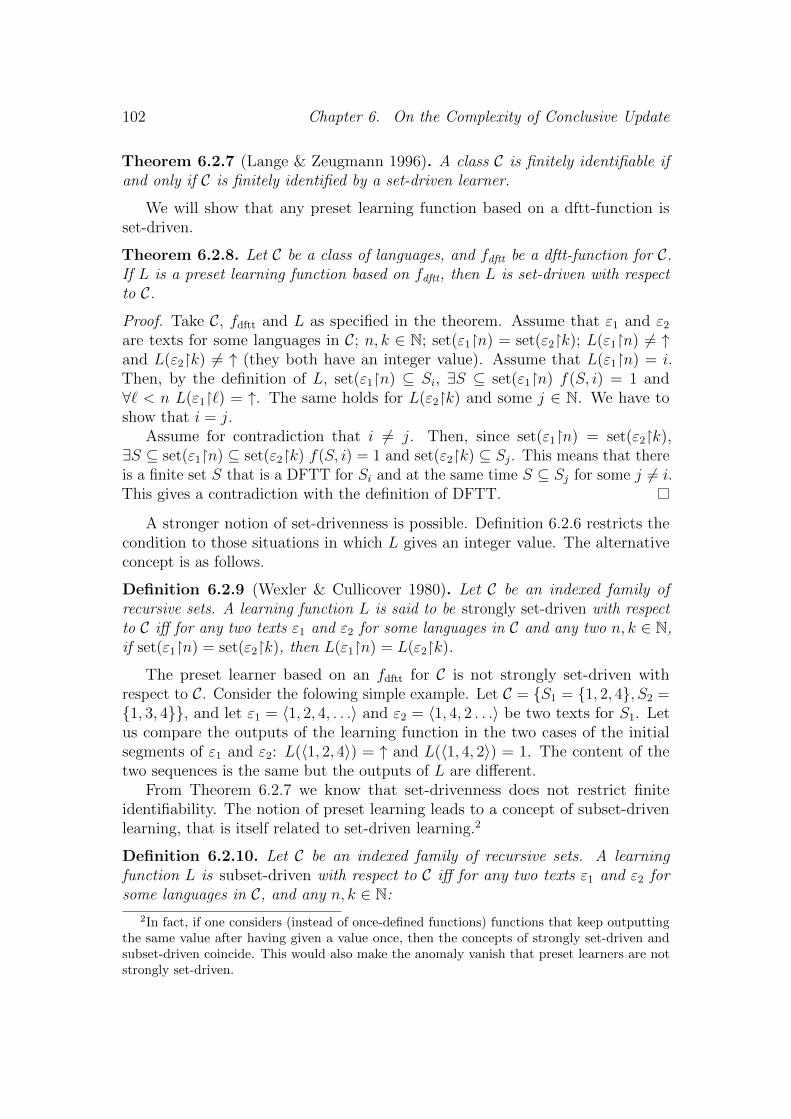
102 Chapter 6. On the Complexity of Conclusive Update
Theorem 6.2.7 (Lange & Zeugmann 1996). A class C is finitely identifiable ifand only if C is finitely identified by a set-driven learner.
We will show that any preset learning function based on a dftt-function isset-driven.
Theorem 6.2.8. Let C be a class of languages, and fdftt be a dftt-function for C.If L is a preset learning function based on fdftt, then L is set-driven with respectto C.
Proof. Take C, fdftt and L as specified in the theorem. Assume that ε1 and ε2
are texts for some languages in C; n, k ∈ N; set(ε1�n) = set(ε2�k); L(ε1�n) 6= ↑and L(ε2�k) 6= ↑ (they both have an integer value). Assume that L(ε1�n) = i.Then, by the definition of L, set(ε1�n) ⊆ Si, ∃S ⊆ set(ε1�n) f(S, i) = 1 and∀` < n L(ε1�`) = ↑. The same holds for L(ε2�k) and some j ∈ N. We have toshow that i = j.
Assume for contradiction that i 6= j. Then, since set(ε1�n) = set(ε2�k),∃S ⊆ set(ε1�n) ⊆ set(ε2�k) f(S, i) = 1 and set(ε2�k) ⊆ Sj . This means that thereis a finite set S that is a DFTT for Si and at the same time S ⊆ Sj for some j 6= i.This gives a contradiction with the definition of DFTT.
A stronger notion of set-drivenness is possible. Definition 6.2.6 restricts thecondition to those situations in which L gives an integer value. The alternativeconcept is as follows.
Definition 6.2.9 (Wexler & Cullicover 1980). Let C be an indexed family ofrecursive sets. A learning function L is said to be strongly set-driven with respectto C iff for any two texts ε1 and ε2 for some languages in C and any two n, k ∈ N,if set(ε1�n) = set(ε2�k), then L(ε1�n) = L(ε2�k).
The preset learner based on an fdftt for C is not strongly set-driven withrespect to C. Consider the folowing simple example. Let C = {S1 = {1, 2, 4}, S2 ={1, 3, 4}}, and let ε1 = 〈1, 2, 4, . . .〉 and ε2 = 〈1, 4, 2 . . .〉 be two texts for S1. Letus compare the outputs of the learning function in the two cases of the initialsegments of ε1 and ε2: L(〈1, 2, 4〉) = ↑ and L(〈1, 4, 2〉) = 1. The content of thetwo sequences is the same but the outputs of L are different.
From Theorem 6.2.7 we know that set-drivenness does not restrict finiteidentifiability. The notion of preset learning leads to a concept of subset-drivenlearning, that is itself related to set-driven learning.2
Definition 6.2.10. Let C be an indexed family of recursive sets. A learningfunction L is subset-driven with respect to C iff for any two texts ε1 and ε2 forsome languages in C, and any n, k ∈ N:
2In fact, if one considers (instead of once-defined functions) functions that keep outputtingthe same value after having given a value once, then the concepts of strongly set-driven andsubset-driven coincide. This would also make the anomaly vanish that preset learners are notstrongly set-driven.
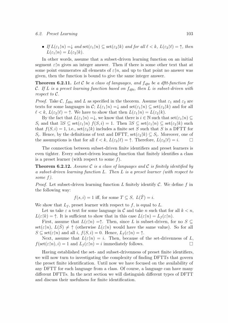
6.2. Preset Learning 103
• If L(ε1�n) =↓ and set(ε1�n) ⊆ set(ε2�k) and for all ` < k, L(ε2�`) = ↑, thenL(ε1�n) = L(ε2�k).
In other words, assume that a subset-driven learning function on an initialsegment ε�n gives an integer answer. Then if there is some other text that atsome point enumerates all elements of ε�n, and up to that point no answer wasgiven, then the function is bound to give the same integer answer.
Theorem 6.2.11. Let C be a class of languages, and fdftt be a dftt-function forC. If L is a preset learning function based on fdftt, then L is subset-driven withrespect to C.
Proof. Take C, fdftt and L as specified in the theorem. Assume that ε1 and ε2 aretexts for some languages in C; L(ε1�n) =↓ and set(ε1�n) ⊆ set(ε2�k) and for all` < k, L(ε2�`) = ↑. We have to show that then L(ε1�n) = L(ε2�k).
By the fact that L(ε1�n) =↓, we know that there is i ∈ N such that set(ε1�n) ⊆Si and that ∃S ⊆ set(ε1�n) f(S, i) = 1. Then ∃S ⊆ set(ε1�n) ⊆ set(ε2�k) suchthat f(S, i) = 1, i.e., set(ε2�k) includes a finite set S such that S is a DFTT forSi. Hence, by the definitions of text and DFTT, set(ε2�k) ⊆ Si. Moreover, one ofthe assumptions is that for all ` < k, L(ε2�`) = ↑. Therefore, L(ε2�`) = i.
The connection between subset-driven finite identifiers and preset learners iseven tighter. Every subset-driven learning function that finitely identifies a classis a preset learner (with respect to some f).
Theorem 6.2.12. Assume C is a class of languages and C is finitely identified bya subset-driven learning function L. Then L is a preset learner (with respect tosome f).
Proof. Let subset-driven learning function L finitely identify C. We define f inthe following way:
f(s, i) = 1 iff, for some T ⊆ S, L(T ) = i.
We show that Lf , preset learner with respect to f , is equal to L.Let us take ε a text for some language in C and take n such that for all k < n,
L(ε�k) = ↑. It is sufficient to show that in this case L(ε�n) = Lf (ε�n).First, assume that L(ε�n) =↑. Then, since L is subset-driven, for no S ⊆
set(ε�n), L(S) 6= ↑ (otherwise L(ε�n) would have the same value). So for allS ⊆ set(ε�n) and all i, f(S, i) = 0. Hence, Lf (ε�n) = ↑.
Next, assume that L(ε�n) = i. Then, because of the set-drivenness of L,f(set(ε�n), i) = 1 and Lf (ε�n) = i immediately follows.
Having established the set- and subset-drivenness of preset finite identifiers,we will now turn to investigating the complexity of finding DFTTs that governthe preset finite identification. Until now we have focused on the availability ofany DFTT for each language from a class. Of course, a language can have manydifferent DFTTs. In the next section we will distinguish different types of DFTTand discuss their usefulness for finite identification.
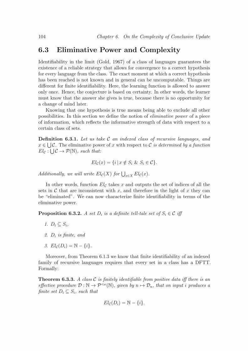
104 Chapter 6. On the Complexity of Conclusive Update
6.3 Eliminative Power and Complexity
Identifiability in the limit (Gold, 1967) of a class of languages guarantees theexistence of a reliable strategy that allows for convergence to a correct hypothesisfor every language from the class. The exact moment at which a correct hypothesishas been reached is not known and in general can be uncomputable. Things aredifferent for finite identifiability. Here, the learning function is allowed to answeronly once. Hence, the conjecture is based on certainty. In other words, the learnermust know that the answer she gives is true, because there is no opportunity fora change of mind later.
Knowing that one hypothesis is true means being able to exclude all otherpossibilities. In this section we define the notion of eliminative power of a pieceof information, which reflects the informative strength of data with respect to acertain class of sets.
Definition 6.3.1. Let us take C an indexed class of recursive languages, andx ∈
⋃C. The eliminative power of x with respect to C is determined by a function
ElC :⋃C → P(N), such that:
ElC(x) = {i |x /∈ Si & Si ∈ C}.
Additionally, we will write ElC(X) for⋃x∈X ElC(x).
In other words, function ElC takes x and outputs the set of indices of all thesets in C that are inconsistent with x, and therefore in the light of x they canbe “eliminated”. We can now characterize finite identifiability in terms of theeliminative power.
Proposition 6.3.2. A set Di is a definite tell-tale set of Si ∈ C iff
1. Di ⊆ Si,
2. Di is finite, and
3. ElC(Di) = N− {i}.
Moreover, from Theorem 6.1.3 we know that finite identifiability of an indexedfamily of recursive languages requires that every set in a class has a DFTT.Formally:
Theorem 6.3.3. A class C is finitely identifiable from positive data iff there is aneffective procedure D : N→ P<ω(N), given by n 7→ Dn, that on input i produces afinite set Di ⊆ Si, such that
ElC(Di) = N− {i}.

6.3. Eliminative Power and Complexity 105
6.3.1 The Complexity of Finite Identifiability Checking
As has already been mentioned in the introduction to this chapter, we aim toanalyze the computational complexity of finding DFTTs. In order to do that werestrict ourselves to finite classes of finite sets. One may ask about the purpose offurther reduction of sets that are already finite. In fact, if a finite class of finitesets is finitely identifiable, then each element of the class is already its own DFTT.However, finite sets can be much larger than their DFTTs. For example, we cantake a class of the following form:
C = {Si = {2i, 2i first odd natural numbers} | i = 1, . . . , n}.
In this case reduction to the minimal information that suffices for finite identifica-tion, 2i, makes a significant difference in the complexity of the process of learning.The learner can simply disregard all odd numbers and wait for an even number.
Theorem 6.3.4. Checking whether a finite class of finite sets is finitely identifiableis polynomial with respect to the number of sets in the class and the maximalcardinality of sets in the class.
Proof. The procedure consists of computing ElC(x) and checking whether for eachSi ∈ C, El(Si) = IC − {i}, where IC = {i | Si ∈ C}.
Let us first focus on computing ElC(x) for x ∈⋃C. We take a class C and
assume that |C| = m, and that the largest set in C has n elements.In the first steps we have to obtain
⋃C. After this, we list for each element of⋃
C the indices of the sets to which the element does not belong. In this step wehave computed ElC(x) for each x ∈
⋃C. All components of this procedure can
clearly be performed in polynomial time with respect to m and n. It remains tocheck whether for all Si ∈ C,
⋃x∈Si ElC(x) = IC − {i}. This involves essentially
only the operation of sum.
From this analysis we conclude that checking whether a finite class of finitesets is finitely identifiable is a quite easy, polynomial task. Nevertheless, as wesaw in the example in the beginning of this section, it can be time consuming if nand m are large numbers.
6.3.2 Minimal Definite Finite Tell-Tale
We are now ready to introduce one of the two nonequivalent notions of minimalityof the DFTTs. We will call Di a minimal DFTT of Si in C if and only if allthe elements of the sets in Di are essential for finite identification of Si in C, i.e.,taking an element out of the set Di will decrease its eliminative power with respectto C, and hence it will no longer be a DFTT. We will observe that a language canhave many minimal DFTTs of different cardinalities. This will give us a cause tointroduce another notion of minimality—minimal-size DFTT.
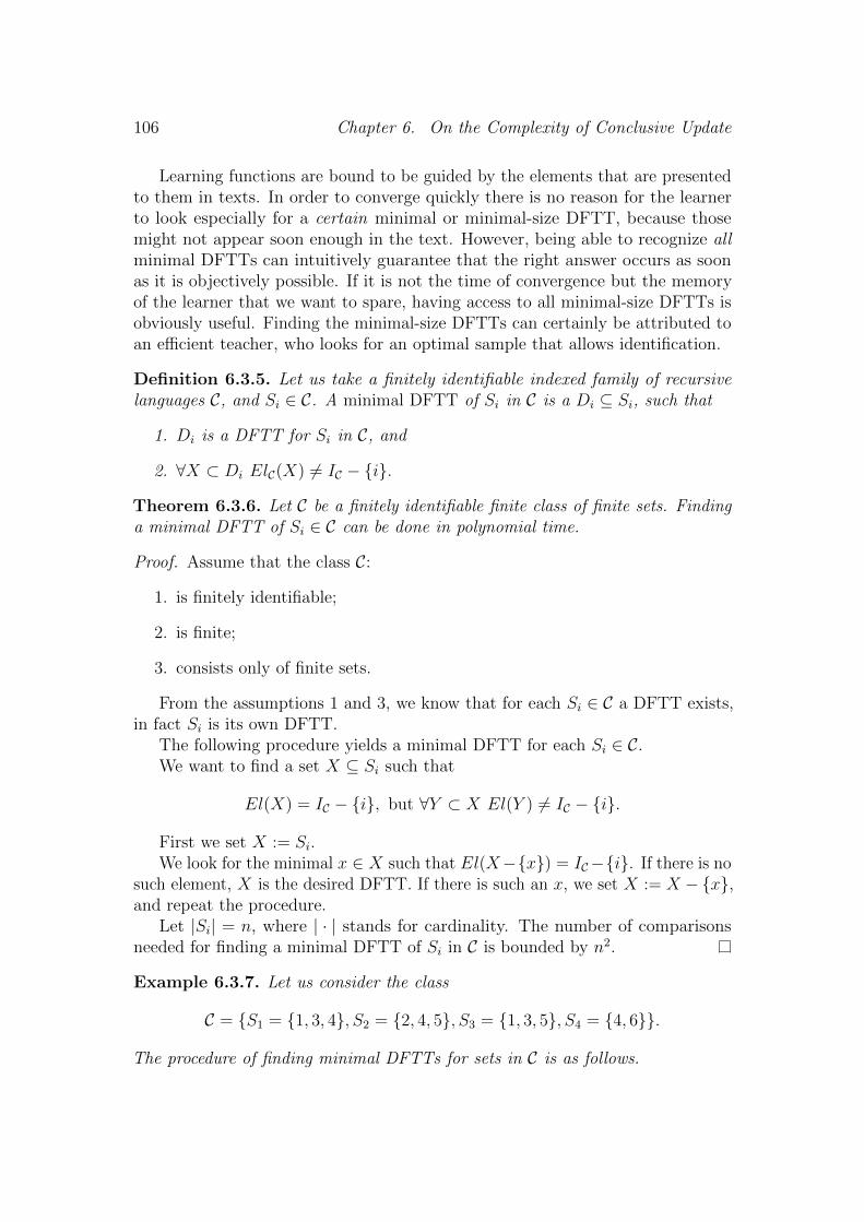
106 Chapter 6. On the Complexity of Conclusive Update
Learning functions are bound to be guided by the elements that are presentedto them in texts. In order to converge quickly there is no reason for the learnerto look especially for a certain minimal or minimal-size DFTT, because thosemight not appear soon enough in the text. However, being able to recognize allminimal DFTTs can intuitively guarantee that the right answer occurs as soonas it is objectively possible. If it is not the time of convergence but the memoryof the learner that we want to spare, having access to all minimal-size DFTTs isobviously useful. Finding the minimal-size DFTTs can certainly be attributed toan efficient teacher, who looks for an optimal sample that allows identification.
Definition 6.3.5. Let us take a finitely identifiable indexed family of recursivelanguages C, and Si ∈ C. A minimal DFTT of Si in C is a Di ⊆ Si, such that
1. Di is a DFTT for Si in C, and
2. ∀X ⊂ Di ElC(X) 6= IC − {i}.
Theorem 6.3.6. Let C be a finitely identifiable finite class of finite sets. Findinga minimal DFTT of Si ∈ C can be done in polynomial time.
Proof. Assume that the class C:
1. is finitely identifiable;
2. is finite;
3. consists only of finite sets.
From the assumptions 1 and 3, we know that for each Si ∈ C a DFTT exists,in fact Si is its own DFTT.
The following procedure yields a minimal DFTT for each Si ∈ C.We want to find a set X ⊆ Si such that
El(X) = IC − {i}, but ∀Y ⊂ X El(Y ) 6= IC − {i}.
First we set X := Si.We look for the minimal x ∈ X such that El(X−{x}) = IC−{i}. If there is no
such element, X is the desired DFTT. If there is such an x, we set X := X − {x},and repeat the procedure.
Let |Si| = n, where | · | stands for cardinality. The number of comparisonsneeded for finding a minimal DFTT of Si in C is bounded by n2.
Example 6.3.7. Let us consider the class
C = {S1 = {1, 3, 4}, S2 = {2, 4, 5}, S3 = {1, 3, 5}, S4 = {4, 6}}.
The procedure of finding minimal DFTTs for sets in C is as follows.
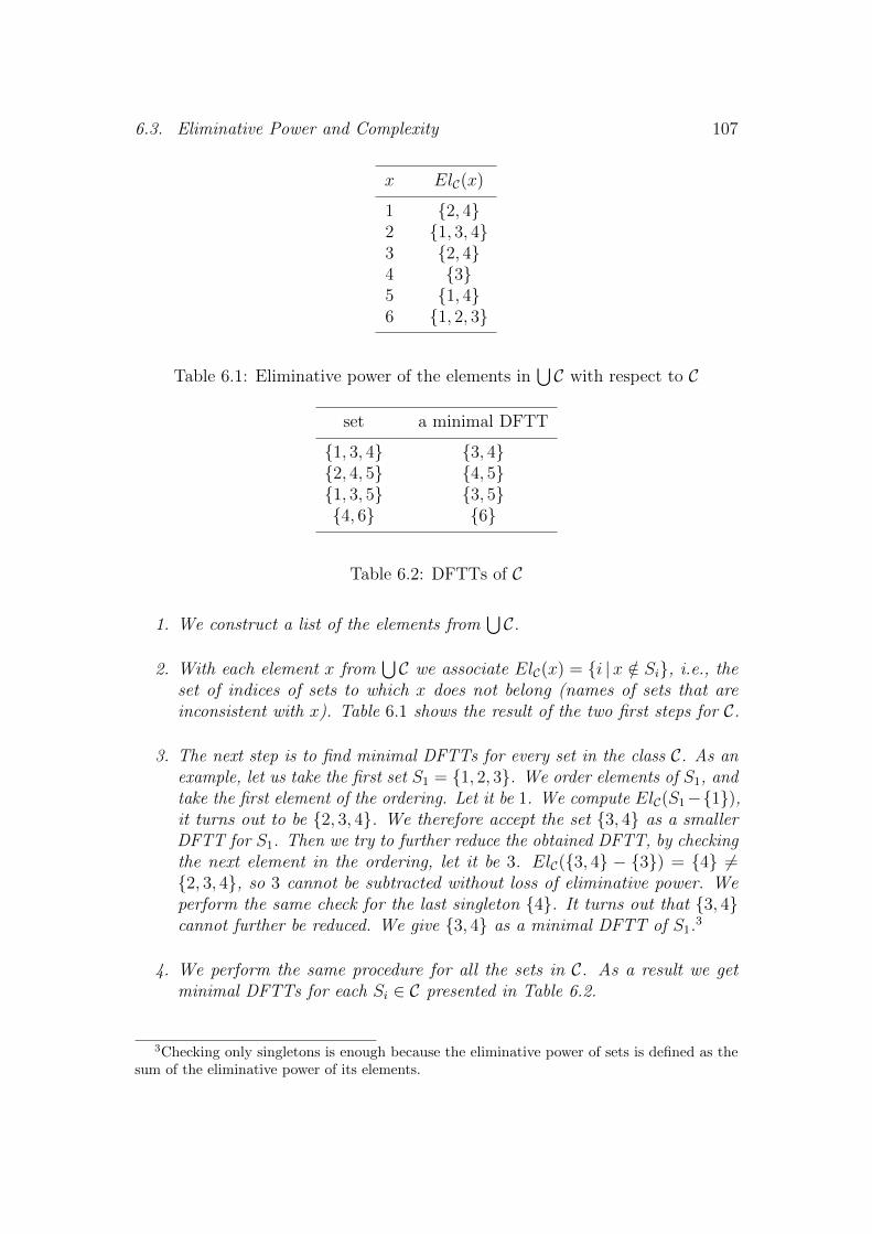
6.3. Eliminative Power and Complexity 107
x ElC(x)
1 {2, 4}2 {1, 3, 4}3 {2, 4}4 {3}5 {1, 4}6 {1, 2, 3}
Table 6.1: Eliminative power of the elements in⋃C with respect to C
set a minimal DFTT
{1, 3, 4} {3, 4}{2, 4, 5} {4, 5}{1, 3, 5} {3, 5}{4, 6} {6}
Table 6.2: DFTTs of C
1. We construct a list of the elements from⋃C.
2. With each element x from⋃C we associate ElC(x) = {i |x /∈ Si}, i.e., the
set of indices of sets to which x does not belong (names of sets that areinconsistent with x). Table 6.1 shows the result of the two first steps for C.
3. The next step is to find minimal DFTTs for every set in the class C. As anexample, let us take the first set S1 = {1, 2, 3}. We order elements of S1, andtake the first element of the ordering. Let it be 1. We compute ElC(S1−{1}),it turns out to be {2, 3, 4}. We therefore accept the set {3, 4} as a smallerDFTT for S1. Then we try to further reduce the obtained DFTT, by checkingthe next element in the ordering, let it be 3. ElC({3, 4} − {3}) = {4} 6={2, 3, 4}, so 3 cannot be subtracted without loss of eliminative power. Weperform the same check for the last singleton {4}. It turns out that {3, 4}cannot further be reduced. We give {3, 4} as a minimal DFTT of S1.3
4. We perform the same procedure for all the sets in C. As a result we getminimal DFTTs for each Si ∈ C presented in Table 6.2.
3Checking only singletons is enough because the eliminative power of sets is defined as thesum of the eliminative power of its elements.
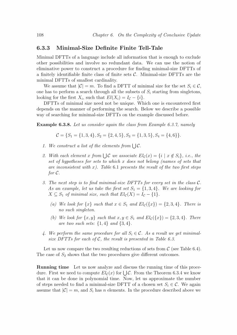
108 Chapter 6. On the Complexity of Conclusive Update
6.3.3 Minimal-Size Definite Finite Tell-Tale
Minimal DFTTs of a language include all information that is enough to excludeother possibilities and involve no redundant data. We can use the notion ofeliminative power to construct a procedure for finding minimal-size DFTTs ofa finitely identifiable finite class of finite sets C. Minimal-size DFTTs are theminimal DFTTs of smallest cardinality.
We assume that |C| = m. To find a DFTT of minimal size for the set Si ∈ C,one has to perform a search through all the subsets of Si starting from singletons,looking for the first Xi, such that El(Xi) = IC − {i}.
DFTTs of minimal size need not be unique. Which one is encountered firstdepends on the manner of performing the search. Below we describe a possibleway of searching for minimal-size DFTTs on the example discussed before.
Example 6.3.8. Let us consider again the class from Example 6.3.7, namely
C = {S1 = {1, 3, 4}, S2 = {2, 4, 5}, S3 = {1, 3, 5}, S4 = {4, 6}}.
1. We construct a list of the elements from⋃C.
2. With each element x from⋃C we associate ElC(x) = {i | x /∈ Si}, i.e., the
set of hypotheses for sets to which x does not belong (names of sets thatare inconsistent with x). Table 6.1 presents the result of the two first stepsfor C.
3. The next step is to find minimal-size DFTTs for every set in the class C.As an example, let us take the first set S1 = {1, 3, 4}. We are looking forX ⊆ S1 of minimal size, such that ElC(X) = IC − {1}.
(a) We look for {x} such that x ∈ S1 and ElC({x}) = {2, 3, 4}. There isno such singleton.
(b) We look for {x, y} such that x, y ∈ S1 and ElC({x}) = {2, 3, 4}. Thereare two such sets: {1, 4} and {3, 4}.
4. We perform the same procedure for all Si ∈ C. As a result we get minimal-size DFTTs for each of C, the result is presented in Table 6.3.
Let us now compare the two resulting reductions of sets from C (see Table 6.4).The case of S2 shows that the two procedures give different outcomes.
Running time Let us now analyze and discuss the running time of this proce-dure. First we need to compute ElC(x) for
⋃C. From the Theorem 6.3.4 we know
that it can be done in polynomial time. Now, let us approximate the numberof steps needed to find a minimal-size DFTT of a chosen set Si ∈ C. We againassume that |C| = m, and Si has n elements. In the procedure described above we
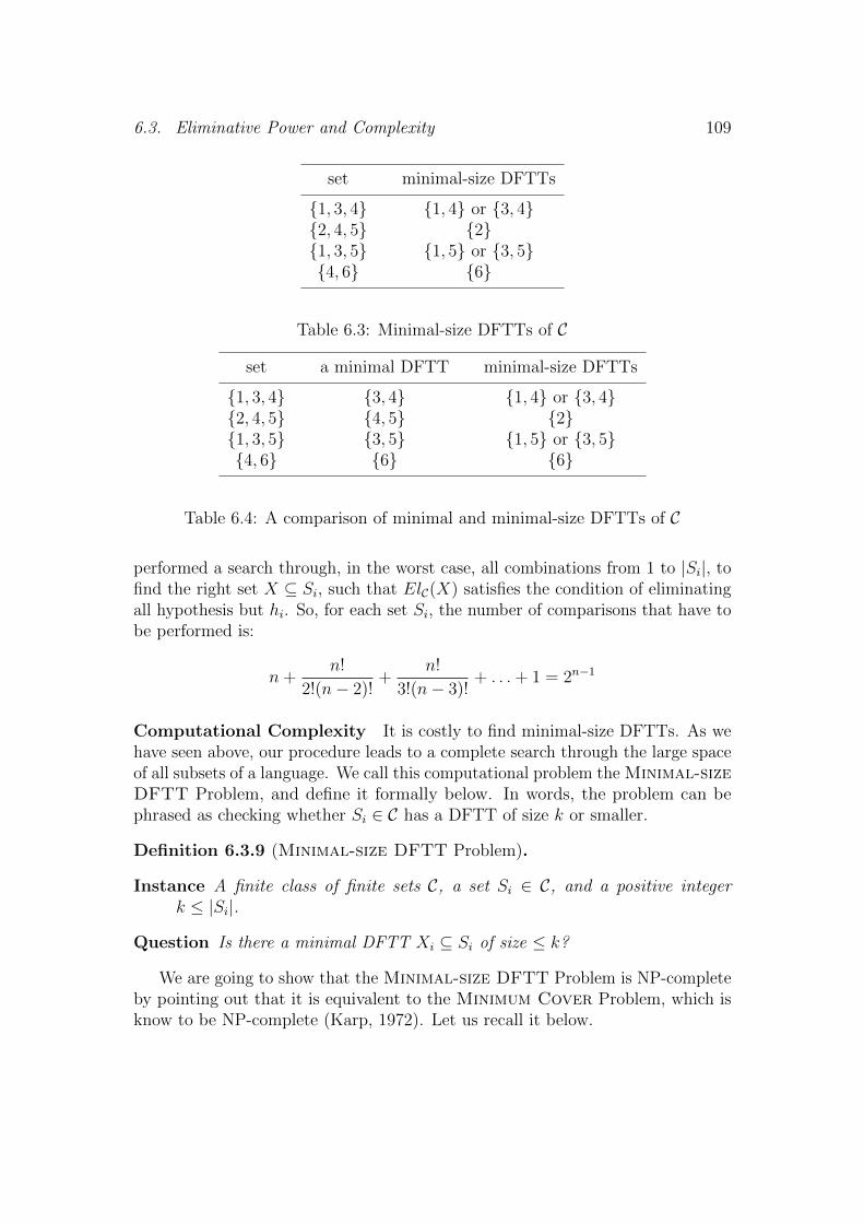
6.3. Eliminative Power and Complexity 109
set minimal-size DFTTs
{1, 3, 4} {1, 4} or {3, 4}{2, 4, 5} {2}{1, 3, 5} {1, 5} or {3, 5}{4, 6} {6}
Table 6.3: Minimal-size DFTTs of C
set a minimal DFTT minimal-size DFTTs
{1, 3, 4} {3, 4} {1, 4} or {3, 4}{2, 4, 5} {4, 5} {2}{1, 3, 5} {3, 5} {1, 5} or {3, 5}{4, 6} {6} {6}
Table 6.4: A comparison of minimal and minimal-size DFTTs of C
performed a search through, in the worst case, all combinations from 1 to |Si|, tofind the right set X ⊆ Si, such that ElC(X) satisfies the condition of eliminatingall hypothesis but hi. So, for each set Si, the number of comparisons that have tobe performed is:
n+n!
2!(n− 2)!+
n!
3!(n− 3)!+ . . .+ 1 = 2n−1
Computational Complexity It is costly to find minimal-size DFTTs. As wehave seen above, our procedure leads to a complete search through the large spaceof all subsets of a language. We call this computational problem the Minimal-sizeDFTT Problem, and define it formally below. In words, the problem can bephrased as checking whether Si ∈ C has a DFTT of size k or smaller.
Definition 6.3.9 (Minimal-size DFTT Problem).
Instance A finite class of finite sets C, a set Si ∈ C, and a positive integerk ≤ |Si|.
Question Is there a minimal DFTT Xi ⊆ Si of size ≤ k?
We are going to show that the Minimal-size DFTT Problem is NP-completeby pointing out that it is equivalent to the Minimum Cover Problem, which isknow to be NP-complete (Karp, 1972). Let us recall it below.
110 Chapter 6. On the Complexity of Conclusive Update
Definition 6.3.10 (Minimal Cover Problem).
Instance: Collection P of subsets of a finite set F , positive integer k ≤ |P |.
Question: Does P contain a cover for X of size k or less, i.e., a subset P ′ ⊆ Pwith |P ′| ≤ k such that every element of X belongs to at least one memberof P ′?
Theorem 6.3.11. The Minimal-size DFTT Problem is NP-complete.
Proof. First, let us observe that by Theorem 6.3.3, Minimal-size DFTT Problemis equivalent to the following Problem:
Definition 6.3.12 (Minimal-size DFTT′ Problem).
Instance: Collection {El(x) | x ∈ Si}, positive integer k ≤ |Si|.
Question: Does {El(x) | x ∈ Si} contain a cover for IC − {i} of size k or less,i.e., a subset Yi ⊆ {El(x) | x ∈ Si} with |Yi| ≤ k such that every element of{El(x) | x ∈ Si} belongs to at least one member of Yi?
It is easy to observe that Minimal-size DFTT′ Problem is a notationalvariant of Minimum Cover Problem, i.e., we take F = IC, P = {El(x) | x ∈ Si}(and therefore |P | = |Si|), and X = IC − {i}. Therefore Minimal-size DFTT′
Problem is NP-complete. Since the Minimal-size DFTT′ Problem is equivalentto the Minimal-size DFTT Problem, we conclude that the Minimal-sizeDFTT Problem is also NP-complete.
According the our previous considerations, the Minimal-size DFTT Problemmay have to be solved by an optimal (‘good’) teacher, who is expected to giveonly relevant information to guarantee fast learning. In this sense our result showsthat the task of providing the most useful information for finite identification isNP-complete.
6.4 Preset Learning and Fastest Learning
Let us now return to the concept of the preset learner. This concept is based onthe intuition that it is easier to identify a complicated, large finite structure oran infinite language solely on the basis of their DFTTs, treating those as finitesymptoms of the underlying structure. In particular, the use of minimal DFTTsand their influence on the speed of finite identification gives rise to an interestingset of questions. A very natural one is how DFTTs can be used by such presetlearning functions. In this section we introduce the notion of fastest learner thatfinitely identifies a language Si as soon as objective ‘ambiguity’ between languageshas been lifted. In other words, we will define the extreme case of a finite learnerwho decides on the right language as soon as any DFTT has been enumerated.
6.4. Preset Learning and Fastest Learning 111
Let us again take a finitely identifiable class C, and Si ∈ C. Now, consider thecollection Di of all DFTTs of Si ∈ C.
Definition 6.4.1. Let C be an indexed family of recursive sets. C is finitelyidentifiable in the fastest way if and only if there is a learning function L s.t.:
L(ε�n) = i iff ∃Dji ∈ Di D
ji ⊆ set(ε�n) &
¬∃Dki ∈ Di D
ki ⊆ set(ε�n− 1).
We will call such L a fastest learning function.
Intuitively, the fastest learner has to explicitly store all DFTTs of all languagesin the given class. Then he makes his conjectures on the basis of the occurrenceof the DFTTs in the given text. However, we do not have to provide a set of allDFTTs of all languages explicitly. Rather, we will define them to be accessiblevia a decision procedure.
Definition 6.4.2. Let C be an indexed family of recursive sets. The completedftt-function for C is a recursive function fc-dftt : P<ω(N)×N→ {0, 1}, such that:
1. fc-dftt(S, i) = 1 if and only if S is a DFTT of Si;
2. for every i ∈ N there is a finite S ⊆ N, such that fc-dftt(S, i) = 1.
Theorem 6.4.3. A class C is finitely identifiable in the fastest way if and only ifthere is a complete dftt-function for C.
Proof. (⇒) Let us take a class C and assume that it is finitely identifiable inthe fastest way, i.e., there is a learning function L that finitely identifies C, andsatisfies the condition of Definition 6.4.1. We define f : P<ω(N)× N→ {0, 1} inthe following way:
f(S, i) =
{1 if ∃T ⊆ S L(T ) = i,
0 otherwise.
First, let us observe that f is recursive because L is recursive and there are onlyfinitely many T ⊆ S.
Now we have to show that f is a complete dftt-function for C. Let us observethat for every i ∈ N there is a finite S ⊆ N, such that f(S, i) = 1. This is sobecause L finitely identifies C, and so, it finitely identifies an Si ∈ C on a textthat enumerates Si in increasing order. It remains to show that:
f(S, i) = 1 iff S is a DFTT for Si.
(⇒) Assume that f(S, i) = 1, then ∃T ⊆ S L(T ) = i. By the definition offastest learner L we have that ∃Dj
i ∈ Di Dji ⊆ set(T ), i.e., there is a DFTT
of Si included in T and hence also in S. Since S ⊆ Si, S then has to be aDFTT for Si as well.

112 Chapter 6. On the Complexity of Conclusive Update
(⇐) Assume that S is a DFTT for Si and, for contradiction, that f(S, i) = 0.Then it means that ∀T ⊆ S L(T ) 6= i. Take ε any text for Si and letε′ := S ∗ ε. ε′ is clearly a text for Si, but L is not the fastest learner on ε′.Contradiction.
(⇐) Assume that there is a complete dftt-function, fc-dftt, for C. We define Lto be the preset learning function based on fc-dftt. Then, by Proposition 6.2.5 Lfinitely identifies C. We have to show that L is the fastest learner, i.e., for anySi ∈ C and any text ε for Si:
L(ε�n) = i iff ∃Dji ∈ Di D
ji ⊆ set(ε�n) &
¬∃Dki ∈ Di D
ki ⊆ set(ε�n− 1).
(⇒) Assume that L(ε�n) = i and, for contradiction, that the right-handside of the above equivalence does not hold. Then there are two possibilities.
1. ∀Dji ∈ Di D
ji * set(ε�n). But then from the assumption that L(ε�n) = i,
by the definition of L we have also that set(ε�n) ⊆ Si and ∃S ⊆ set(ε�n)such that fc-dftt(S, i) = 1. Hence, by the definition of fc-dftt, S is a DFTT ofSi and S ⊆ set(ε�n). Contradiction.
2. ∃Dki ∈ Di D
ki ⊆ set(ε�n − 1). Since L(ε�n) = i, by the definition of L we
have that ∀` < n L(ε�`) = ↑ and hence (a) ∀` < n−1 L(ε�`) = ↑. Moreover,by the definition of fc-dftt, (b) fc-dftt(set(ε�n−1), i) = 1 and by the definitionof DFTT, (c) set(ε�n− 1) ⊆ Si. From (a), (b) and (c) we can conclude thatL(ε�n− 1) = i. This contradicts the fact that L is (at most) once defined.
(⇐) Assume that for ε a text for Si ∈ C and n ∈ N the following holds:
∃Dji ∈ Di Dj
i ⊆ set(ε�n) & (1)
¬∃Dki ∈ Di Dk
i ⊆ set(ε�n− 1) (2)
Then, by (2), for all k < n there is no S such that S ⊆ set(ε�k) andf(S, i) = 1. Hence, by the definition of L for all k < n, L(ε�k) 6= i. Since εis a text for Si it can not enumerate any DFTT of some different set in C,hence we have that for all k < n, L(ε�k) = ↑. By (1) and the definition offc-dftt we get that ∃S ⊆ set(ε�n) fc-dftt(S, i) = 1. So, L(ε�n) = i.
This completes the proof.
The above theorem gives a condition of fastest finite identifiability. For anyfinite set and i ∈ N, the function f decides whether S is a DFTT of Si. In otherwords, the class of all DFTTs of C, {Di | Si ∈ C}, is uniformly decidable. Infact, the function that the fastest preset learner uses does not have to give apositive answer every time it sees a DFTT, it is enough if the function signals theoccurrence of every minimal DFTT.
6.4. Preset Learning and Fastest Learning 113
Definition 6.4.4. Let C be an indexed family of recursive sets. The min dftt-function for C is a recursive function fmin-dftt : P<ω(N)× N→ {0, 1}, such that:
1. fmin-dftt(S, i) = 1 if and only if S is a minimal DFTT of Si;
2. for every i ∈ N there is a finite S ⊆ N, such that fmin-dftt(S, i) = 1.
Theorem 6.4.5. A class C is finitely identifiable in the fastest way iff there is amin-dftt-function for C.
Proof. (⇒) Assume that a class C is finitely identifiable in the fastest way. Then,by Theorem 6.4.3, there is an effective function fc-dftt : P<ω(N)×N→ {0, 1} suchthat fc-dftt(S, i) = 1 iff S is a DFTT for Si and for every i ∈ N there is a finite setS ⊆ N such that fc-dftt(S, i) = 1.
We define fmin-dftt : P<ω(N)× N→ {0, 1} in the following way:
fmin-dftt(S, i) =
{1 if fc-dftt(S, i) = 1 & ¬∃T ⊂ S fc-dftt(T, i) = 1,
0 otherwise.
The function fmin-dftt is recursive, because S is finite and fc-dftt is recursive.(⇒) Assume that there is an effective function fmin-dftt : P<ω(N) × N → {0, 1}such that fmin-dftt(S, i) = 1 iff S is a minimal DFTT for Si and for every i ∈ Nthere is a finite set S ⊆ N such that fmin-dftt(S, i) = 1.
We define fc-dftt : P<ω(N)× N→ {0, 1} in the following way:
fc-dftt(S, i) =
{1 if ∃T ⊆ S fmin-dftt(T, i) = 1,
0 otherwise.
The function fc-dftt is recursive, because S is finite and fmin-dftt is recursive.
6.4.1 Strict Preset Learning
The reader may have expected a stronger notion of preset learner for which arecursive function F exists such that that for each Si, F (i) is a finite set of DFTTsfor Si. As announced before we will now be interested in learners that haveat their direct disposal all minimal DFTTs of languages from the given class.Obviously, such a situation is only generally possible in the case of classes of finitelanguages. We will consider both possibilities: the one of finite classes of finitelanguages and that of infinite classes of finite languages. We define strict presetfinite identifiability in the following way.
Definition 6.4.6. A finitely identifiable class C is strict preset finitely identifiableiff there is a recursive function F : N→ P<ω(N) such that F (i) outputs the set ofall minimal DFTTs of Si.

114 Chapter 6. On the Complexity of Conclusive Update
Computational Complexity of Strict Preset Learning Let us again goback to the case of a finite class of finite sets. To compute the set min-Di of allminimal DFTTs of Si ∈ C we need to perform the procedure for finding a minimalDFTT for all possible orderings of elements in Si. Therefore the simple proceduredescribed earlier (in Section 6.3.2) has to be performed n! times. This indicatesthat finding the set of all minimal DFTTs is in general quite costly. We show thatin fact the problem is NP-hard.
Proposition 6.4.7. Finding min-Di of Si ∈ C is NP-hard.
Proof. It is easy to observe that once we enumerate Di of Si, we can find aminimal-size DFTT of Si in polynomial time by simply picking one of the smallestsets in Di. This means that the Minimal-size DFTT Problem for Si can bepolynomially reduced to the problem of finding Di for Si.
We will now move to the case of infinite classes of finite sets. We will comparethe two notions: strict preset learning and fastest learning in the more generalsetting of recursive sets. We will proceed with a number of examples. First wewill show that there are classes that are finitely identifiable both in the fastestand in the preset way, but that are not strict preset finitely identifiable.
In the following we will use the manner of speech where we will say that e is aTuring machine if we mean that e is an integer that codes a Turing machine andf(a) = {b, c} will mean that f(a) codes the finite set containing just b and c. Letus recall the notion of Kleene’s T -predicate.
Definition 6.4.8 (T -predicate (Kleene, 1943)). T (e, x, y) holds iff e is a Turingmachine that on input x performs computation y.
Let us recall that with the use of the T -predicate the Halting Problem can bedefined in the following way:
∃yT (e, e, y) ⇐⇒ ϕe(e) ↓ .
In other words, the question of whether Turing machine e stops on the input eis equivalent to the question of existence of a computation y performed by e oninput e.
Let us start with an example of a finitely identifiable class for which a recursivepreset learner exists, but which is not strict preset finitely identifiable.
Theorem 6.4.9. There exists a class C that is finitely identifiable, but for whichno recursive function F exists such that for each i, F (i) is the set of all minimalDFTTs for Si.
Proof. Let us consider the following class of finite sets C = {Si | i ∈ N}:
Si = {2i, 2(µyT (i, i, y)) + 1}.
6.4. Preset Learning and Fastest Learning 115
Obviously, the class C is finitely identifiable. Moreover there exists a recursivefastest learner L that finitely identifies C and can be defined in the following way:
L(ε�n) =
{i if 2i ∈ set(ε�n),
µ` T (`, `, k) if 2k + 1 ∈ set(ε�n).
We can easily observe that |Si| = 2 ⇐⇒ ϕi(i) ↓. Minimal DFTTs of Si are{2i}, and, in case ϕi(i) ↓, also {2(µyT (i, i, y)) + 1}}. It is clear that no totalrecursive function F such that
g(i) = {{2i}, {2(µyT (i, i, y)) + 1}}
can be given, because its existence would solve the Halting Problem.
Therefore, the strict preset learner for the above class cannot be recursive.Since the recursive fastest learner exists (defined in the proof above), the fastestlearner cannot be strict preset. Hence, we can conclude that even in the case ofclasses of finite languages strict preset finite identification is properly includedin finite identification and in fastest finite identification. A similar result can beshown for the minimal-size strict preset finite identifiability, i.e., when the learningfunction requires the set of all the minimal-size DFTTs.
Proposition 6.4.10. There exists a class C that is finitely identifiable, but forwhich no recursive function F exists such that for each i, F (i) is the set of allminimal-size DFTTs for Si.
Proof. The argument is analogous to the one given in the proof of Theorem 6.4.9.Let j : N2 → N be a recursive pairing function (bijection) with inverses j1 and j2.We now consider the class C = {Si | i ∈ C}:
Si = {3j1(i), 3j2(i) + 1, 3(µyT (i, i, y)) + 2}.
The set of all minimal-size DFTTs of Si is {{3(µyT (i, i, y)) + 2}} in case ϕi(i) ↓and {{3j1(i)}, {3j2(i) + 1}} in case ϕi(i)↑. Therefore the minimal-size DFTTs ofSi cannot be given by a total recursive function, because its existence would solvethe Halting Problem.
6.4.2 Finite Learning and Fastest Learning
We have established that recursive fastest identifiability does not require strictpreset learnability even in the finite cases. We will now turn to the more generalquestion whether every finitely identifiable class has a fastest learner. The answeris negative—there are finitely identifiable classes of languages which cannot befinitely identified in the fastest way.
116 Chapter 6. On the Complexity of Conclusive Update
Definition 6.4.11 (Smullyan 1958). Let A,B ⊂ N. A separating set is C ⊂ Nsuch that A ⊂ C and B ∩ C = ∅. In particular, if A and B are disjoint then Aitself is a separating set for the pair, as is B. If a pair of disjoint sets A and Bhas no computable separating set, then the two sets are recursively inseparable.
The following theorem says that there are effectively finitely identifiable classesof languages for which there is no effective fastest learner and no recursive functionthat could enumerate a minimal DFTT for each language.
Theorem 6.4.12. There exists a class C that is finitely identifiable but is notfinitely identifiable in the fastest way (and moreover there is no recursive functionthat gives a minimal-size DFTT for each language).
Proof. Let A and B be two disjoint r.e. recursively inseparable sets. Let x ∈ Abe equivalent to ∃y Rxy with R recursive and let x ∈ B be equivalent to ∃y Sxywith S recursive. We assume that for each x there is at most one y such that Rxyand at most one y such that Sxy.
The class of languages {Si | i ∈ N} is defined as follows:
Si = {2i, 2i+ 1} ∪ {2j | Rji} ∪ {2j + 1 | Sji}.
The idea is that {2i, 2i+ 1} is the exclusive domain of Si except that, for someusually much larger m, Rim or Sim may be true, and then 2i ∈ Sm or 2i+1 ∈ Sm,respectively. There can be at most one such m, and for that m only one of Rimor Sim can be true. However, since A and B are recursively inseparable there canbe no recursive function f that makes this latter choice for each i.
It is clear that to decide definitely that the language is Si it suffices to encounter2i and 2i + 1, so {2i, 2i + 1} is a DFTT for Si. But, if i ∈ A, then {2i + 1} isa DFTT for Si, and if i ∈ B, then {2i} is a DFTT for Si. To be more precise,{2i + 1} is a DFTT for Si if i 6∈ B and {2i} is a DFTT for Si if i 6∈ A. But norecursive learner can decide on this, so there cannot be a recursive fastest learner,or a function that gives, for each i, a minimal DFTT for Si.
In general there is no reason for preset learners to use only minimal DFTTs.They can have a set of DFTTs for each Si and only use those. The class given inthe proof of Theorem 6.4.12, for which no recursive fastest learner is possible canobviously have a preset learner but the DFTTs do not include the minimal ones.
The above theorem shows that fastest finite identifiability is properly includedin finite identification and hence also in preset finite identification. Hence, we haveshown the existence of yet another kind of learning, even more demanding thanfinite identification. Speaking in terms of conclusive update, our considerationsshow that in some cases, even if computable convergence to certainty is possible,it is not computable to conclude that at the first moment in which objectiveambiguity disappears.
6.5. Conclusions and Perspectives 117
In the light of these discoveries about preset learning, we can give a compu-tational justification for introducing multi-agency to this setting. It seems tobe justifiable to switch the perspective from the single agent, learning-orientedview, to the two agent game of learner and teacher. The responsibility of effectivelearning, in the line with natural intuitions, is in the hands of the teacher, whosecomputational task is to find samples of information that guarantee optimallearning. Intuitively, it is not very surprising that the task of finding such minimalsamples can be more difficult than the complexity of the actual learning. Assuch, computing the minimal(-size) DFTTs seems to go beyond the abilities ofthe learner and is not necessary in order to be rational or successful. However,such a task is natural to be performed by a teacher.
6.5 Conclusions and Perspectives
We used the characterization of finite identification of languages from positivedata to discuss the complexity of optimal learning and teaching strategies infinite identification. We introduced two notions: minimal DFTT and minimal-sizeDFTT. By viewing the informativeness of examples as their power to eliminatecertain conjectures, we have checked the computational complexity of ‘finiteteachability’ from minimal DFTT and minimal-size DFTT. In the former casethe problem turns out to be PTIME computable, while the latter falls into theNP-complete class of problems. This suggests that it is easy to teach in a waythat avoids irrelevant information but it is potentially difficult to teach in themost effective way. We also conceptually extended the characterization of finiteidentification and introduced the notion of preset learner. We compared variationsof the latter with the idea of fastest finite identification. In particular, we focusedon the notion of strict preset finite identifiers that have at their disposal all minimalDFTTs of every language in the class. Even in the setting of classes of finite setsthis type of learning turns out to be restrictive with respect to finite identifiability.We have exhibited a recursively finitely identifiable class that cannot be recursivelyfinitely identifiable in the fastest way. Hence we have established a new morerestrictive kind of finite identification.
Links between finite identification and dynamic epistemic logic have alreadybeen established and described in Chapters 3–5. For dynamic epistemic logic therestriction to finite sets of finite languages is very natural, so our analysis of itscomplexity can be applied to strengthen this connection. The complexity of fastestfinite identification corresponds to the complexity of fastest conclusive update indynamic epistemic logic. It gives a new measure of computational complexity ofcertainty— a measure that corresponds to the question of how difficult it is toreach the state of irrevocable knowledge.
The main assumptions of learning theory and hence also of the present chapteris the cooperative nature of the interaction between the learner and the teacher.In the next chapter we will reflect upon other possible learning attitudes.

Chapter 7
Supervision and Learning Attitudes
In philosophy, logic and psychology the word ‘learning’ is used to denote a varietyof phenomena. In this chapter, as in the previous ones, we take the phrase ‘tolearn’ to mean ‘to acquire information in order to arrive at a certain (correct)conclusion’. In this we follow the lines of learning theory (see, e.g., Jain et al.,1999) where learning consists of a sequence of mind changes that should lead toa correct conclusion. All belief states visited on the way there, together withthe correct one, are drawn from some given set of possibilities that constitutesthe initial uncertainty range. To be more specific, let us try to describe in thoseterms the process of language learning. Agent L’s (Learner’s) aim is to ‘arrive’at a grammar that correctly describes his native language. This scenario can berepresented by a graph in which the vertices represent possible grammars andan edge from vertex s1 to vertex s2 labeled with α stands for a possibility of amind change from grammar s1 to s2 that is triggered by the incoming informationα. The properties of such a graph are determined by features of the initial rangeof possibilities, the language being learned, and the nature of agent’s learningstrategy. Then, the process of learning can be represented simply as a ‘journey’of L through the graph until he finally reaches the correct grammar. Obviously,other inductive inference processes can also be described in this way.
The setting can be enriched by the presence of another agent, let us callher Teacher, T , who decides which data are presented to L, in which order, etc.In other words, we can introduce another player who supervises the process oflearning and manipulates the data in order to influence the speed and accuracy ofconvergence. The analysis of the role of the teacher has been increasingly presentin formal learning theory (e.g., see Angluin, 1987 for the minimally adequateteacher in learning from queries and counterexamples, and Balbach & Zeugmann,2009 for recent developments in teachability theory).
In this chapter, we investigate the interaction between Learner and Teacher ina particular kind of supervision learning game that is played on a graph. Learner’sinformation state changes while he moves around the graph, from one conjectureto another. Teacher, having a global perspective, knows the structure of the
119
120 Chapter 7. Supervision and Learning Attitudes
graph, and by providing certain information eliminates some initially possiblemind changes of L. We are interested in the complexity of teaching, which weinterpret in a similar way as in Chapter 6. Assuming the global perspective ofTeacher, we identify the teachability problem with deciding whether the successof the learning process is possible. We interpret learning as a game and hence weidentify learnability and teachability with the existence of winning strategies in acertain type of game. In this context, we analyze different Learner and Teacherattitudes, varying the level of Teacher’s helpfulness and Learner’s willingness tolearn.
We interpret our learning game within the existing framework of sabotage games(Van Benthem, 2005). We start by recalling sabotage games and sabotage modallogic. Then, we explore variations of the winning condition of the game, providingsabotage modal logic formulae that characterize the existence of a winning strategyand their model-checking complexity (in other words: the complexity of decidingwhether a player has a winning strategy in the game) in each case. Then weobserve the asymmetry of the players’ roles, and we allow Teacher to skip movesand we analyze how such removal of strict alternation of the moves affects ourprevious results. Finally, we recapitulate the work and discuss possible extensions.
With respect to the previous chapter, which also deals with computationalcomplexity of teaching, we will now, in a way, take a step back. We will lose thedetailed view on the content of epistemic states. Instead, we will gain the globalpicture of the process on conjecture change, and will be able to see the influenceof intentional attitudes on the complexity of teaching.
7.1 Sabotage Games
As we already mentioned, our perspective on learning leads naturally to the frame-work of sabotage games. Sabotage games are useful for reasoning about variousinteractive processes involving random breakdowns or intentional obstruction in asystem, from the failures of server networks to the logistics of traveling by publictransport. We argue that it can also be interpreted positively, as some form oflearning. But before we get to that, we first introduce the general, basic frameworkof sabotage games.
A sabotage game is played in a directed multi-graph, with two players, Runnerand Blocker, moving in alternation, with Runner moving first. Runner moves bymaking a single transition from the current vertex. Blocker moves by deleting anyedge from the graph. Runner wins the game if he is able to reach a designatedgoal vertex; otherwise Blocker wins.
To define the game formally let us first introduce the structure in whichsabotage games take place, a directed multi-graph (see, e.g., Balakrishnan, 1997).
7.1. Sabotage Games 121
Definition 7.1.1. A directed multi-graph is a pair G = (V,E) where V is aset of vertices and E : V × V → N is a function indicating the number of edgesbetween any two vertices.
The sabotage game is defined in the following way.
Definition 7.1.2 (Loding & Rohde 2003a). A sabotage game
SG = 〈V,E, v, vg〉
is given by a directed multi-graph (V,E) and two vertices v, vg ∈ V . Vertex vrepresents the initial position of Runner and vg represents the goal state (the aimof Runner).
Each match consists of a sequence of positions and is played as follows:
1. the initial position 〈E0, v0〉 is given by 〈E, v〉;
2. round k + 1 from position 〈Ek, vk〉 consists of:
(a) Runner moving to some vk+1 such that E(vk, vk+1) > 0, and then
(b) Blocker removing an edge (v, v′) such that Ek(v, v′) > 0.
The new position is 〈Ek+1, vk+1〉, where Ek+1(v, v′) := Ek(v, v′)− 1 and, for
every (u, u′) 6= (v, v′), Ek+1(u, u′) := Ek(u, u′);
3. the match ends if a player cannot make a move or if Learner reaches thegoal state, which is the only case in which he wins.
In other words, Blocker removes an edge between two states v, v′ by decreasingthe value of E(v, v′) by 1. As we will see later, this description of the game basedon the above definition of multi-graphs can lead to some technical problems whenwe want to interpret modal logic over these structures. Therefore, we will nowpresent an alternative definition, which we later show to be equivalent with respectto the existence of a winning strategy1.
Definition 7.1.3. Let Σ = {a1, . . . an} be a finite set of labels. A directedlabeled multi-graph is a tuple GΣ = (V, E) where V is a set of vertices andE = (Ea1 , . . . , Ean) is a collection of binary relations Eai ⊆ V × V for each ai ∈ Σ.
In the above definition, the labels from Σ are used to represent multiple edgesbetween two vertices; E is simply an ordered collection of binary relations on Vwith labels drawn from Σ. Accordingly, the modified definition of sabotage gameis as follows.
1In what follows we take the size of any multi-graph G = (V,E) to be bounded by: |V |+max{E(v, w) | v, w ∈ V } · |V 2|.
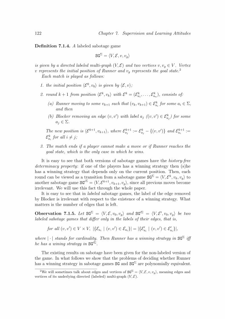
122 Chapter 7. Supervision and Learning Attitudes
Definition 7.1.4. A labeled sabotage game
SGΣ = 〈V, E , v, vg〉
is given by a directed labeled multi-graph (V, E) and two vertices v, vg ∈ V . Vertexv represents the initial position of Runner and vg represents the goal state.2
Each match is played as follows:
1. the initial position 〈E0, v0〉 is given by 〈E , v〉;
2. round k + 1 from position 〈Ek, vk〉 with Ek = (Eka1 , . . . , Ekan), consists of:
(a) Runner moving to some vk+1 such that (vk, vk+1) ∈ Ekai for some ai ∈ Σ,and then
(b) Blocker removing an edge (v, v′) with label aj ((v, v′) ∈ Ekaj) for someaj ∈ Σ.
The new position is 〈Ek+1, vk+1〉, where Ek+1aj
:= Ekaj − {(v, v′)} and Ek+1
ai:=
Ekai for all i 6= j;
3. The match ends if a player cannot make a move or if Runner reaches thegoal state, which is the only case in which he wins.
It is easy to see that both versions of sabotage games have the history-freedeterminacy property : if one of the players has a winning strategy then (s)hehas a winning strategy that depends only on the current position. Then, eachround can be viewed as a transition from a sabotage game SGΣ = 〈V, Ek, vk, vg〉 toanother sabotage game SG′
Σ = 〈V, Ek+1, vk+1, vg〉, since all previous moves becomeirrelevant. We will use this fact through the whole paper.
It is easy to see that in labeled sabotage games, the label of the edge removedby Blocker is irrelevant with respect to the existence of a winning strategy. Whatmatters is the number of edges that is left.
Observation 7.1.5. Let SGΣ = 〈V, E , v0, vg〉 and SG′Σ = 〈V, E ′, v0, vg〉 be twolabeled sabotage games that differ only in the labels of their edges, that is,
for all (v, v′) ∈ V × V, |{Eai | (v, v′) ∈ Eai}| = |{E ′ai | (v, v′) ∈ E ′ai}|,
where | · | stands for cardinality. Then Runner has a winning strategy in SGΣ iffhe has a wining strategy in SG′Σ.
The existing results on sabotage have been given for the non-labeled version ofthe game. In what follows we show that the problems of deciding whether Runnerhas a winning strategy in sabotage games SG and SGΣ are polynomially equivalent.
2We will sometimes talk about edges and vertices of SGΣ = 〈V, E , v, vg〉, meaning edges andvertices of its underlying directed (labeled) multi-graph (V, E).
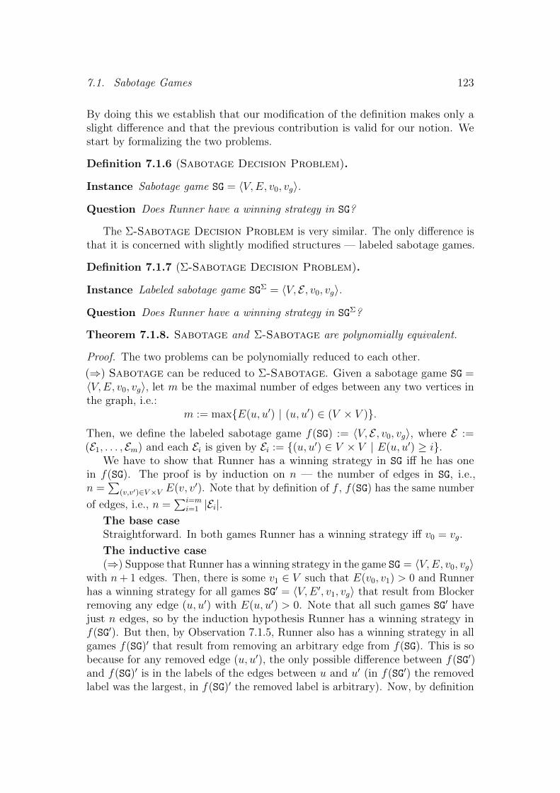
7.1. Sabotage Games 123
By doing this we establish that our modification of the definition makes only aslight difference and that the previous contribution is valid for our notion. Westart by formalizing the two problems.
Definition 7.1.6 (Sabotage Decision Problem).
Instance Sabotage game SG = 〈V,E, v0, vg〉.
Question Does Runner have a winning strategy in SG?
The Σ-Sabotage Decision Problem is very similar. The only difference isthat it is concerned with slightly modified structures — labeled sabotage games.
Definition 7.1.7 (Σ-Sabotage Decision Problem).
Instance Labeled sabotage game SGΣ = 〈V, E , v0, vg〉.
Question Does Runner have a winning strategy in SGΣ?
Theorem 7.1.8. Sabotage and Σ-Sabotage are polynomially equivalent.
Proof. The two problems can be polynomially reduced to each other.
(⇒) Sabotage can be reduced to Σ-Sabotage. Given a sabotage game SG =〈V,E, v0, vg〉, let m be the maximal number of edges between any two vertices inthe graph, i.e.:
m := max{E(u, u′) | (u, u′) ∈ (V × V )}.
Then, we define the labeled sabotage game f(SG) := 〈V, E , v0, vg〉, where E :=(E1, . . . , Em) and each Ei is given by Ei := {(u, u′) ∈ V × V | E(u, u′) ≥ i}.
We have to show that Runner has a winning strategy in SG iff he has onein f(SG). The proof is by induction on n — the number of edges in SG, i.e.,n =
∑(v,v′)∈V×V E(v, v′). Note that by definition of f , f(SG) has the same number
of edges, i.e., n =∑i=m
i=1 |Ei|.The base caseStraightforward. In both games Runner has a winning strategy iff v0 = vg.
The inductive case(⇒) Suppose that Runner has a winning strategy in the game SG = 〈V,E, v0, vg〉
with n+ 1 edges. Then, there is some v1 ∈ V such that E(v0, v1) > 0 and Runnerhas a winning strategy for all games SG′ = 〈V,E ′, v1, vg〉 that result from Blockerremoving any edge (u, u′) with E(u, u′) > 0. Note that all such games SG′ havejust n edges, so by the induction hypothesis Runner has a winning strategy inf(SG′). But then, by Observation 7.1.5, Runner also has a winning strategy in allgames f(SG)′ that result from removing an arbitrary edge from f(SG). This is sobecause for any removed edge (u, u′), the only possible difference between f(SG′)and f(SG)′ is in the labels of the edges between u and u′ (in f(SG′) the removedlabel was the largest, in f(SG)′ the removed label is arbitrary). Now, by definition
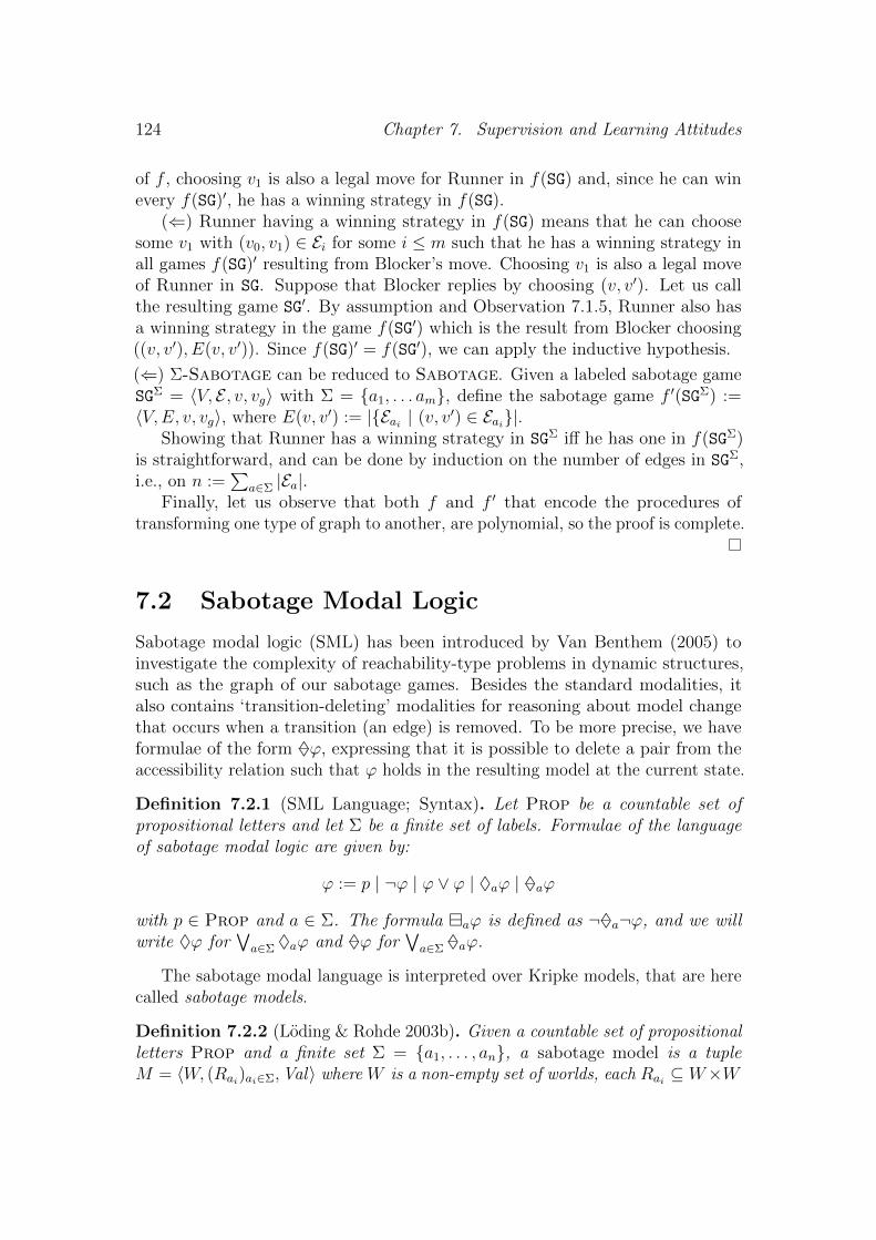
124 Chapter 7. Supervision and Learning Attitudes
of f , choosing v1 is also a legal move for Runner in f(SG) and, since he can winevery f(SG)′, he has a winning strategy in f(SG).
(⇐) Runner having a winning strategy in f(SG) means that he can choosesome v1 with (v0, v1) ∈ Ei for some i ≤ m such that he has a winning strategy inall games f(SG)′ resulting from Blocker’s move. Choosing v1 is also a legal moveof Runner in SG. Suppose that Blocker replies by choosing (v, v′). Let us callthe resulting game SG′. By assumption and Observation 7.1.5, Runner also hasa winning strategy in the game f(SG′) which is the result from Blocker choosing((v, v′), E(v, v′)). Since f(SG)′ = f(SG′), we can apply the inductive hypothesis.
(⇐) Σ-Sabotage can be reduced to Sabotage. Given a labeled sabotage gameSGΣ = 〈V, E , v, vg〉 with Σ = {a1, . . . am}, define the sabotage game f ′(SGΣ) :=〈V,E, v, vg〉, where E(v, v′) := |{Eai | (v, v′) ∈ Eai}|.
Showing that Runner has a winning strategy in SGΣ iff he has one in f(SGΣ)is straightforward, and can be done by induction on the number of edges in SGΣ,i.e., on n :=
∑a∈Σ |Ea|.
Finally, let us observe that both f and f ′ that encode the procedures oftransforming one type of graph to another, are polynomial, so the proof is complete.
7.2 Sabotage Modal Logic
Sabotage modal logic (SML) has been introduced by Van Benthem (2005) toinvestigate the complexity of reachability-type problems in dynamic structures,such as the graph of our sabotage games. Besides the standard modalities, italso contains ‘transition-deleting’ modalities for reasoning about model changethat occurs when a transition (an edge) is removed. To be more precise, we haveformulae of the form ♦ϕ, expressing that it is possible to delete a pair from theaccessibility relation such that ϕ holds in the resulting model at the current state.
Definition 7.2.1 (SML Language; Syntax). Let Prop be a countable set ofpropositional letters and let Σ be a finite set of labels. Formulae of the languageof sabotage modal logic are given by:
ϕ := p | ¬ϕ | ϕ ∨ ϕ | ♦aϕ | ♦aϕ
with p ∈ Prop and a ∈ Σ. The formula �aϕ is defined as ¬♦a¬ϕ, and we willwrite ♦ϕ for
∨a∈Σ ♦aϕ and ♦ϕ for
∨a∈Σ ♦aϕ.
The sabotage modal language is interpreted over Kripke models, that are herecalled sabotage models.
Definition 7.2.2 (Loding & Rohde 2003b). Given a countable set of propositionalletters Prop and a finite set Σ = {a1, . . . , an}, a sabotage model is a tupleM = 〈W, (Rai)ai∈Σ,Val〉 where W is a non-empty set of worlds, each Rai ⊆ W×W
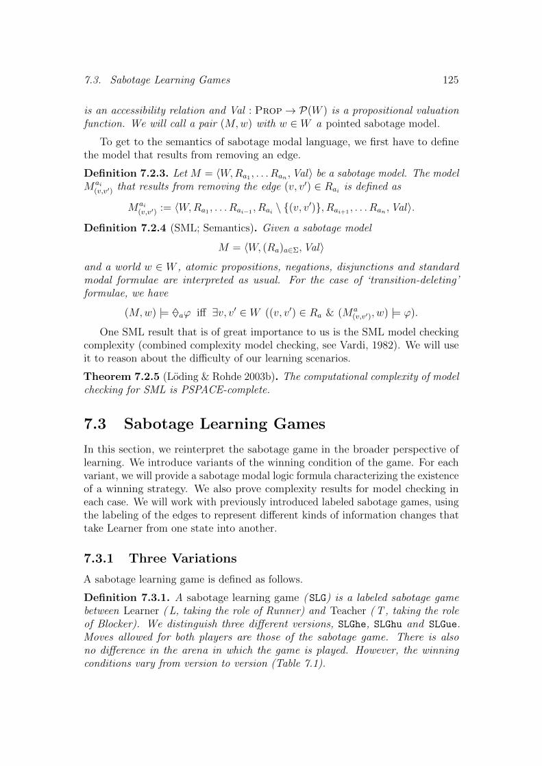
7.3. Sabotage Learning Games 125
is an accessibility relation and Val : Prop→ P(W ) is a propositional valuationfunction. We will call a pair (M,w) with w ∈ W a pointed sabotage model.
To get to the semantics of sabotage modal language, we first have to definethe model that results from removing an edge.
Definition 7.2.3. Let M = 〈W,Ra1 , . . . Ran ,Val〉 be a sabotage model. The modelMai
(v,v′) that results from removing the edge (v, v′) ∈ Rai is defined as
Mai(v,v′) := 〈W,Ra1 , . . . Rai−1
, Rai \ {(v, v′)}, Rai+1, . . . Ran ,Val〉.
Definition 7.2.4 (SML; Semantics). Given a sabotage model
M = 〈W, (Ra)a∈Σ,Val〉
and a world w ∈ W , atomic propositions, negations, disjunctions and standardmodal formulae are interpreted as usual. For the case of ‘transition-deleting’formulae, we have
(M,w) |= ♦aϕ iff ∃v, v′ ∈ W ((v, v′) ∈ Ra & (Ma(v,v′), w) |= ϕ).
One SML result that is of great importance to us is the SML model checkingcomplexity (combined complexity model checking, see Vardi, 1982). We will useit to reason about the difficulty of our learning scenarios.
Theorem 7.2.5 (Loding & Rohde 2003b). The computational complexity of modelchecking for SML is PSPACE-complete.
7.3 Sabotage Learning Games
In this section, we reinterpret the sabotage game in the broader perspective oflearning. We introduce variants of the winning condition of the game. For eachvariant, we will provide a sabotage modal logic formula characterizing the existenceof a winning strategy. We also prove complexity results for model checking ineach case. We will work with previously introduced labeled sabotage games, usingthe labeling of the edges to represent different kinds of information changes thattake Learner from one state into another.
7.3.1 Three Variations
A sabotage learning game is defined as follows.
Definition 7.3.1. A sabotage learning game ( SLG) is a labeled sabotage gamebetween Learner ( L, taking the role of Runner) and Teacher ( T , taking the roleof Blocker). We distinguish three different versions, SLGhe, SLGhu and SLGue.Moves allowed for both players are those of the sabotage game. There is alsono difference in the arena in which the game is played. However, the winningconditions vary from version to version (Table 7.1).
126 Chapter 7. Supervision and Learning Attitudes
Game Winning Condition
SLGue L wins iff L reaches the goal state, T wins otherwise.
SLGhu T wins iff L reaches the goal state, L wins otherwise.
SLGhe L and T win iff L reaches the goal state. Both lose otherwise.
Table 7.1: Sabotage Learning Games
The different winning conditions correspond to different levels of Teacher’shelpfulness and Learner’s willingness to learn. We can then have the cooperativecase with helpful Teacher and eager Learner (SLGhe). But there are two otherpossibilities that we will be interested in: unhelpful Teacher with eager Learner(SLGue), and helpful Teacher with unwilling Learner (SLGhu).
Having defined the games representing various types of Teacher and Learnerattitudes, we now show how sabotage modal logic can be used for reasoning aboutplayers’ strategic powers in these games.
7.3.2 Sabotage Learning Games in Sabotage Modal Logic
Sabotage modal logic turns out to be useful for reasoning about graph-like struc-tures where edges can disappear; in particular, it is useful for reasoning aboutsabotage learning games. In order to interpret the logic on our graphs we need totransform the arena of a labeled sabotage game into a sabotage model in whichformulae of the logic can be interpreted. In fact, for each SLG we can construct apointed sabotage model in the following straightforward way.
Definition 7.3.2. Let SGΣ = 〈V, E , v0, vg〉 be a sabotage game and E = (Ea)a∈Σ.The pointed sabotage model (M(SGΣ), v0) over the set of atomic propositionsProp := {goal} is given by
M(SGΣ) := 〈V, E ,Val〉,
where Val(goal) := {vg}.
In the light of this construction, sabotage modal logic becomes useful forreasoning about players’ strategic powers in sabotage learning games. Eachwinning condition in Table 7.1 can be expressed by a formula of SML thatcharacterizes the existence of a winning strategy, that is, the formula is true ina given pointed sabotage model if and only if the corresponding player has awinning strategy in the game represented by the model.

7.3. Sabotage Learning Games 127
Unhelpful Teacher and Eager Learner (SLGue) Let us first consider SLGue,the original sabotage game (Van Benthem, 2005). For any n ∈ N, we define theformula γuen inductively as follows:
γue0 := goal , γuen+1 := goal ∨ ♦ � γuen .The following result is Theorem 7 of Loding & Rohde (2003b) rephrased for labeledsabotage games. We provide a detailed proof to show how our labeled definitionavoids a technical issue present in the original proof.
Theorem 7.3.3. Learner has a winning strategy in the SLGue
SGΣ = 〈V, E0, v0, vg〉if and only if (M(SGΣ), v0) |= γuen , where n is the number of edges of SGΣ.
Proof. The proof is by induction on n.
The base case(⇒) If L has a winning strategy in a game SGΣ with no edges, then he should
be already in the winning state, that is v0 = vg. Thus, (M(SGΣ), v0) |= goal andhence, (M(SGΣ), v0) |= γue0 .
(⇐) If (M(SGΣ), v0) |= γue0 then (M(SGΣ), v0) |= goal . Since vg is the only statewhere goal holds, then we have v0 = vg, and therefore L wins SGΣ immediately.
The inductive case(⇒) Suppose that SGΣ has n+ 1 edges, and assume L has a winning strategy.
There are two possibilities: L’s current state is the goal state (that is, v0 = vg), orit is not.
In the first case, we get (M(SGΣ), v0) |= goal and hence (M(SGΣ), v0) |= γuen+1.In the second case, since L has a winning strategy in SGΣ, there is some statev1 ∈ V reachable from v0, i.e., for some ai ∈ Σ (that is, (v0, v1) ∈ E0
ai) such that
in all games SGΣ(u,u′),aj
= 〈V, E1(u,u′),aj
, v1, vg〉 that result from removing edge (u, u′)
from the relation labeled aj, L as a winning strategy.3
All such games have n edges, so by inductive hypothesis we have
(M(SGΣ(u,u′),aj
), v1) |= γuen .
for every edge (u, u′) and label aj . Now, the key observation is that each M -imageof the game that results from L moving to v1 and T removing edge (u, u′) withlabel aj , is exactly the model that results from removing edge (u, u′) with aj fromthe model M(SGΣ).4 Then, for all such (u, u′) and aj, we have
(M(SGΣ)aj(u,u′), v1) |= γuen .
3The collection E1(u,u′),aj
is given by (E0a1, . . . , E0
aj− {u, u′}, . . . , E0
a|Σ|).
4In the original definition of a sabotage game this is not the case. In the game, the edges areimplicitly ordered by numbers (the existence of an edge labeled with k implies the existence ofedges labeled with 1, . . . , k − 1); in the model, this is not the case. When we remove an edgefrom a game we always remove the one with the highest label, but when we remove an edgefrom a model we remove an arbitrary one: the operations of removing an edge and turning agame into a model do not commute.

128 Chapter 7. Supervision and Learning Attitudes
It follows that (M(SGΣ), v1) |= �γuen and therefore (M(SGΣ), v0) |= ♦ � γuen , thatis, (M(SGΣ), v0) |= γuen+1.
(⇐) Suppose that (M(SGΣ), v0) |= goal ∨♦� γuen . Then, v0 is the goal state orelse there is a state v1 accessible from v0 such that (M(SGΣ), v1) |= �γuen , that is,(M(SGΣ)ai(u,u′), v1) |= γuen , for all edges (u, u′) and labels aj . By inductive hypothesis,L has a winning strategy in each game that correspond to each pointed model(M(SGΣ)ai(u,u′), v1). But these games are exactly those that result from removing
any edge from the game 〈V, E0, v0, vg〉 after L moves from v0 to v1. Hence, L hasa winning strategy in 〈V, E0, v0, vg〉, the game that corresponds to the pointedmodel (M(SGΣ), v0), as required.
Helpful Teacher and unwilling Learner (SLGhu) Now consider SLGhu, thegame with helpful Teacher and unwilling Learner. We define γhun inductively, as
γhu0 := goal , γhun+1 := goal ∨ (♦> ∧�♦γhun ).
In this case, Teacher has to be sure that Learner does not get stuck before he hasreached the goal state — this is why the conjunct ♦> is needed in the definitionof γhun+1. We show that this formula corresponds to the existence of a winningstrategy for Teacher.
Theorem 7.3.4. Teacher has a winning strategy in the SLGhu
SGΣ = 〈V, E0, v0, vg〉if and only if (M(SGΣ), v0) |= γhun , where n is the number of edges of SGΣ.
Proof. Similar to the proof of Theorem 7.3.3.
Helpful Teacher and eager Learner (SLGhe) Finally, for SLGhe, the corre-sponding formula is defined as
γhe0 := goal , γhen+1 := goal ∨ ♦♦γhen .Theorem 7.3.5. Teacher and Learner have a joint winning strategy in SLGhe
SGΣ = 〈V, E0, v0, vg〉if and only if (M(SGΣ), v0) |= γhen , where n is the number of edges of SGΣ.
Proof. L and T have a joint winning strategy if and only if there is a path fromv0 to vg. From left to right this is obvious. From right to left, if there is such apath, then there is also one without cycles5, and a joint winning strategy is theone that follows the path and at each step removes the edge that has just beenused (it is essential that L moves first). The theorem follows by observing thatγhen expresses the existence of such path.
The above results for the three scenarios are summarized in Table 7.2.5If this is not the case, i.e., if it is essential that L uses a path twice, removing used edges
could cause L to be stuck somewhere away from the goal.
7.3. Sabotage Learning Games 129
Game Winning Condition in SML Winner
SLGue γue0 := goal , γuen+1 := goal ∨ ♦ � γuen Learner
SLGhu γhu0 := goal , γhun+1 := goal ∨ (♦> ∧ (�♦γhun )) Teacher
SLGhe γhe0 := goal , γhen+1 := goal ∨ ♦♦γhen Both
Table 7.2: Winning Conditions for SLG in SML
7.3.3 Complexity of Sabotage Learning Games
We have characterized the existence of a winning strategy in our three versions ofSLGs by means of sabotage modal logic formulae. In this section, we investigatethe complexity of deciding whether such formulae are true in a given pointedmodel, i.e., the complexity of checking whether there is a winning strategy in thecorresponding game.
By Theorem 7.2.5, the model checking problem of sabotage modal logic isPSPACE-complete. This gives us PSPACE upper bounds for the complexity ofdeciding whether a player can win a given game. In the three cases, we can alsogive tight lower bounds.
Unhelpful Teacher and eager Learner (SLGue) For SLGue, which can beidentified with the standard sabotage game, PSPACE-hardness is shown byreduction from Quantified Boolean Formula (Loding & Rohde, 2003b).
Theorem 7.3.6 (Loding & Rohde 2003b). SLGue is PSPACE-complete.
Helpful Teacher and unwilling Learner (SLGhu) Whereas at first sight,SLGhu and SLGue might seem to be duals of each other, the relationship betweenthem is more complex due to the different nature of the players’ moves: Learnermoves locally by choosing an state accessible from the current one, while Teachermoves globally by removing an arbitrary edge. Nevertheless, we can show PSPACE-hardness for SLGhu. In the proof we will use the Quantified Boolean Formula(QBF) problem, known to be PSPACE-complete.
Definition 7.3.7 (Quantified Boolean Formula Problem).
Instance Let ϕ be an instance of QBF, i.e., a formula:
ϕ := ∃x1∀x2∃x3 . . . Qxnψ
where Q is ∃ for n odd, and ∀ for n even, and ψ is a quantifier-free formulain conjunctive normal form.
Question Is ϕ satisfiable?
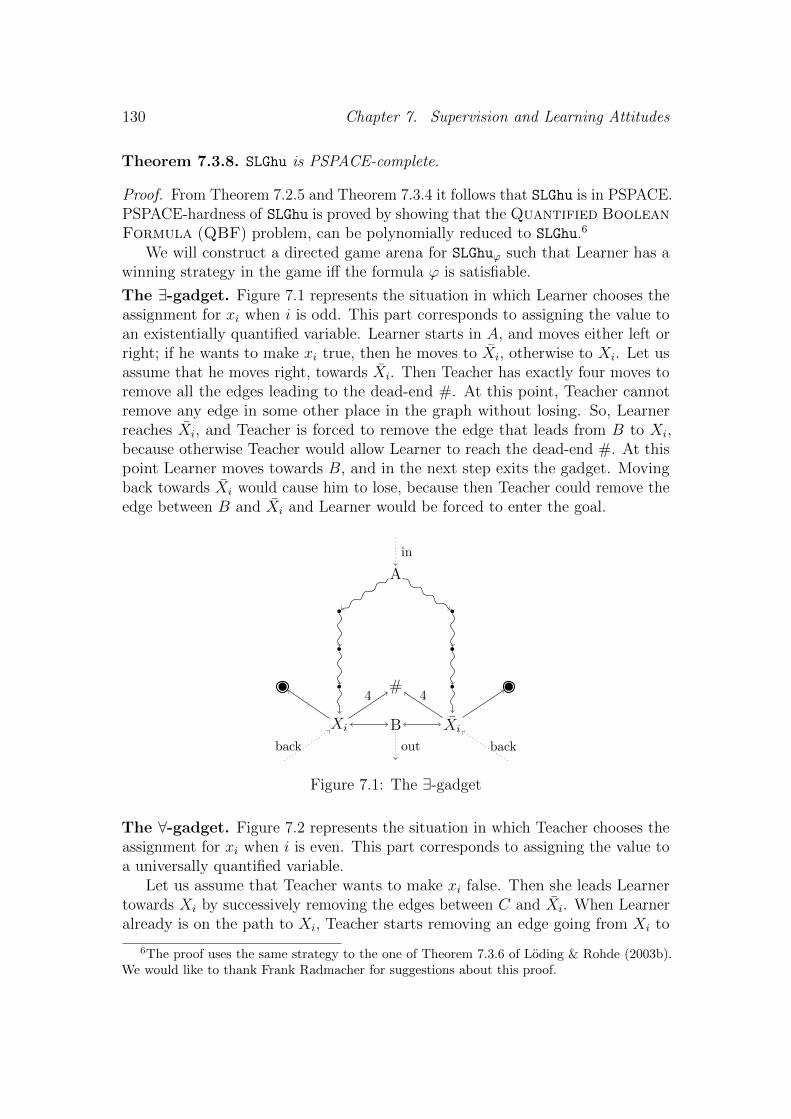
130 Chapter 7. Supervision and Learning Attitudes
Theorem 7.3.8. SLGhu is PSPACE-complete.
Proof. From Theorem 7.2.5 and Theorem 7.3.4 it follows that SLGhu is in PSPACE.PSPACE-hardness of SLGhu is proved by showing that the Quantified BooleanFormula (QBF) problem, can be polynomially reduced to SLGhu.6
We will construct a directed game arena for SLGhuϕ such that Learner has awinning strategy in the game iff the formula ϕ is satisfiable.
The ∃-gadget. Figure 7.1 represents the situation in which Learner chooses theassignment for xi when i is odd. This part corresponds to assigning the value toan existentially quantified variable. Learner starts in A, and moves either left orright; if he wants to make xi true, then he moves to Xi, otherwise to Xi. Let usassume that he moves right, towards Xi. Then Teacher has exactly four moves toremove all the edges leading to the dead-end #. At this point, Teacher cannotremove any edge in some other place in the graph without losing. So, Learnerreaches Xi, and Teacher is forced to remove the edge that leads from B to Xi,because otherwise Teacher would allow Learner to reach the dead-end #. At thispoint Learner moves towards B, and in the next step exits the gadget. Movingback towards Xi would cause him to lose, because then Teacher could remove theedge between B and Xi and Learner would be forced to enter the goal.
A
Xi Xi
#
B
·· ··
in
4 4
outback back
Figure 7.1: The ∃-gadget
The ∀-gadget. Figure 7.2 represents the situation in which Teacher chooses theassignment for xi when i is even. This part corresponds to assigning the value toa universally quantified variable.
Let us assume that Teacher wants to make xi false. Then she leads Learnertowards Xi by successively removing the edges between C and Xi. When Learneralready is on the path to Xi, Teacher starts removing an edge going from Xi to
6The proof uses the same strategy to the one of Theorem 7.3.6 of Loding & Rohde (2003b).We would like to thank Frank Radmacher for suggestions about this proof.
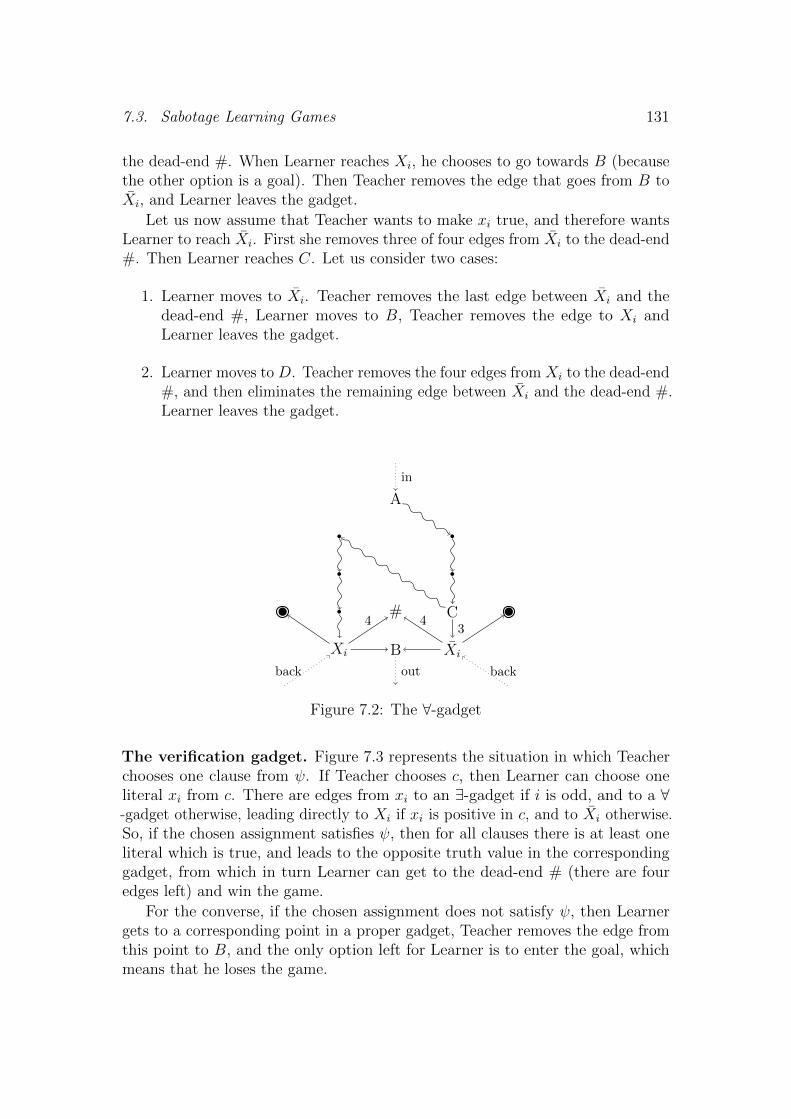
7.3. Sabotage Learning Games 131
the dead-end #. When Learner reaches Xi, he chooses to go towards B (becausethe other option is a goal). Then Teacher removes the edge that goes from B toXi, and Learner leaves the gadget.
Let us now assume that Teacher wants to make xi true, and therefore wantsLearner to reach Xi. First she removes three of four edges from Xi to the dead-end#. Then Learner reaches C. Let us consider two cases:
1. Learner moves to Xi. Teacher removes the last edge between Xi and thedead-end #, Learner moves to B, Teacher removes the edge to Xi andLearner leaves the gadget.
2. Learner moves to D. Teacher removes the four edges from Xi to the dead-end#, and then eliminates the remaining edge between Xi and the dead-end #.Learner leaves the gadget.
A
Xi
C
Xi
#
B
·· ··
in
34 4
outback back
Figure 7.2: The ∀-gadget
The verification gadget. Figure 7.3 represents the situation in which Teacherchooses one clause from ψ. If Teacher chooses c, then Learner can choose oneliteral xi from c. There are edges from xi to an ∃-gadget if i is odd, and to a ∀-gadget otherwise, leading directly to Xi if xi is positive in c, and to Xi otherwise.So, if the chosen assignment satisfies ψ, then for all clauses there is at least oneliteral which is true, and leads to the opposite truth value in the correspondinggadget, from which in turn Learner can get to the dead-end # (there are fouredges left) and win the game.
For the converse, if the chosen assignment does not satisfy ψ, then Learnergets to a corresponding point in a proper gadget, Teacher removes the edge fromthis point to B, and the only option left for Learner is to enter the goal, whichmeans that he loses the game.

132 Chapter 7. Supervision and Learning Attitudes
A1 A2 A3 A4 #
C1 # C2 # C3 # C4 #
in
Figure 7.3: The verification gadget
With the above considerations, we can observe that Learner has a winningstrategy in SLGhuϕ iff ϕ is satisfiable. Moreover, the representation can clearly bedone in polynomial time with respect to the size of ϕ. This finishes the proof.
Helpful Teacher and eager Learner (SLGhe) Finally, let us have a look atSLGhe. This game is different from the two previous ones: L and T win or losetogether. Then, a winning strategy for each of them need not take into accountall possible moves of the other. This suggests that this version should be lesscomplex than SLGue and SLGhu.
As mentioned in the proof of Theorem 7.3.5, L and T have a joint winningstrategy if and only if the goal vertex is reachable from L’s position. Thus, deter-mining whether they can win SLGhe is equivalent to solving the Reachability(st-Connectivity) problem, which is known to be non-deterministic logarithmicspace complete (NL-complete) (Papadimitriou, 1994).
Theorem 7.3.9. SLGhe is NL-complete.
Proof. Polynomial equivalence of SLGhe and REACHABILITY follows from theargument given in the proof of Theorem 7.3.5.
Table 7.3 summarizes the complexity results for the different versions of SLG.The complexity of these problems can be interpreted as the difficulty of decidingwhether certain aims of Teacher can be fulfilled. We can attribute the question ofthe existence of the winning strategy to Teacher, as she already has the globalperspective on the situation anyway. Our results say how difficult it is for her todecide whether there is a chance of success. The results agree with our intuition,as coming up with a strategy to teach is easier if Learner and Teacher cooperate.Following our interpretation it is the easiest for Teacher to check whether theteaching will work out if Teacher assumes eagerness of Learner and she herselfdoes her best to ensure that he succeeds. Moreover, the remaining two cases turnout to be equally difficult — it is as difficult to decide whether Teacher can force
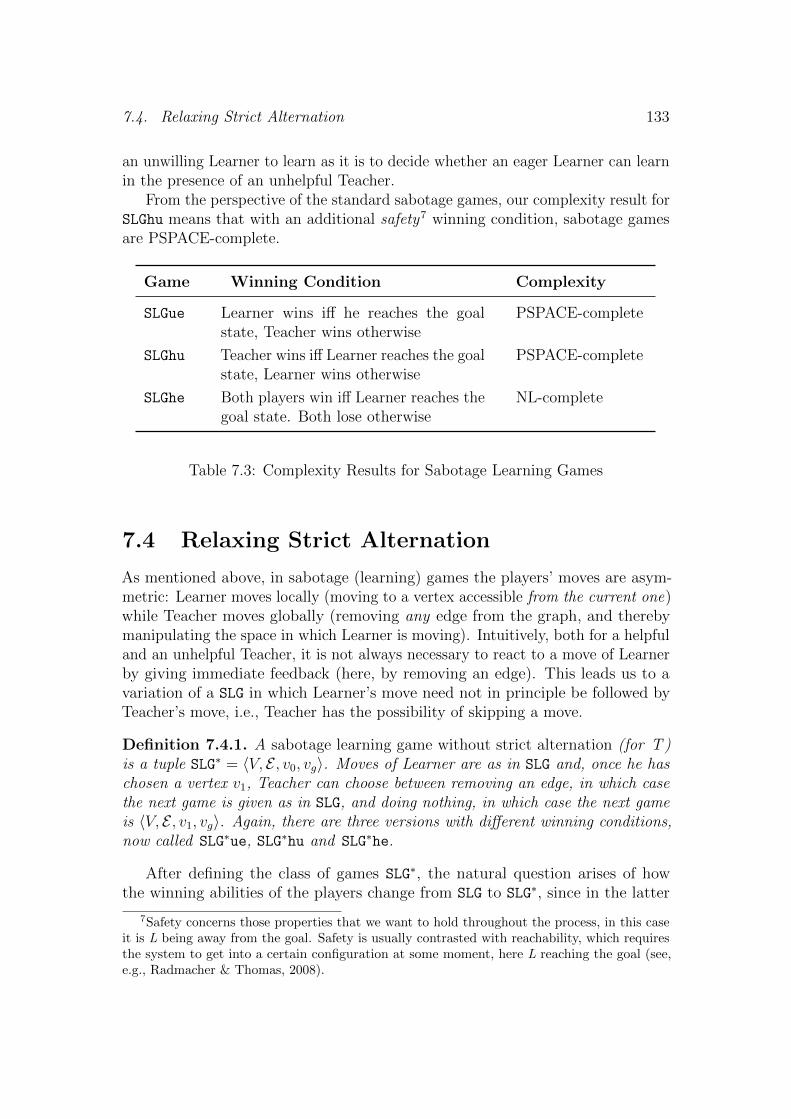
7.4. Relaxing Strict Alternation 133
an unwilling Learner to learn as it is to decide whether an eager Learner can learnin the presence of an unhelpful Teacher.
From the perspective of the standard sabotage games, our complexity result forSLGhu means that with an additional safety7 winning condition, sabotage gamesare PSPACE-complete.
Game Winning Condition Complexity
SLGue Learner wins iff he reaches the goalstate, Teacher wins otherwise
PSPACE-complete
SLGhu Teacher wins iff Learner reaches the goalstate, Learner wins otherwise
PSPACE-complete
SLGhe Both players win iff Learner reaches thegoal state. Both lose otherwise
NL-complete
Table 7.3: Complexity Results for Sabotage Learning Games
7.4 Relaxing Strict Alternation
As mentioned above, in sabotage (learning) games the players’ moves are asym-metric: Learner moves locally (moving to a vertex accessible from the current one)while Teacher moves globally (removing any edge from the graph, and therebymanipulating the space in which Learner is moving). Intuitively, both for a helpfuland an unhelpful Teacher, it is not always necessary to react to a move of Learnerby giving immediate feedback (here, by removing an edge). This leads us to avariation of a SLG in which Learner’s move need not in principle be followed byTeacher’s move, i.e., Teacher has the possibility of skipping a move.
Definition 7.4.1. A sabotage learning game without strict alternation (for T )is a tuple SLG∗ = 〈V, E , v0, vg〉. Moves of Learner are as in SLG and, once he haschosen a vertex v1, Teacher can choose between removing an edge, in which casethe next game is given as in SLG, and doing nothing, in which case the next gameis 〈V, E , v1, vg〉. Again, there are three versions with different winning conditions,now called SLG∗ue, SLG∗hu and SLG∗he.
After defining the class of games SLG∗, the natural question arises of howthe winning abilities of the players change from SLG to SLG∗, since in the latter
7Safety concerns those properties that we want to hold throughout the process, in this caseit is L being away from the goal. Safety is usually contrasted with reachability, which requiresthe system to get into a certain configuration at some moment, here L reaching the goal (see,e.g., Radmacher & Thomas, 2008).
134 Chapter 7. Supervision and Learning Attitudes
Teacher can choose between removing an edge or doing nothing. In the restof this section, we show that for all three winning conditions (SLG∗ue, SLG∗hu,SLG∗he), the winning abilities of the players remain the same as in the case inwhich players move in strict alternation. This is surprising in the SLGhu case. It isby no means obvious that if Teacher has a winning strategy in the game withoutstrict alternation then she also has one in the regular version of the game, becausewe might expect that removing an edge instead of skipping the move could resultin blocking the way to the goal.
We start with the case of an unhelpful Teacher and an eager Learner, SLG∗ue.Note that although in this new setting matches can be infinite, e.g., in the gamewith unwilling L, if T skips her moves indefinitely, L will just keep moving, andhence the game will not be finished in finite time. However, in fact if Learner canwin the game, he can do so in a finite number of rounds. We start with a lemmastating that if Learner can win some SLGue in some number of rounds, then hecan do so also if the underlying multi-graph has additional edges.
Definition 7.4.2. Let Σ = {a1, . . . an} be a finite set of labels. For directed labeledmulti-graphs, GΣ = (V, E) and G′Σ = (V ′, E ′), we say that GΣ is a subgraph ofG′Σ if V ⊆ V ′ and Eai ⊆ E ′ai for all labels ai ∈ Σ.
Lemma 7.4.3. If Learner has a strategy for winning the SLGue 〈V, E , v0, vg〉 in atmost n rounds, then he can also win any SLGue 〈V, E ′, v0, vg〉 in at most n rounds,where (V, E) is a subgraph of (V, E ′).
Proof. The proof is by induction on n. In the inductive step, for the case thatT removes an edge which was not in the original multi-graph, note that theresulting graph is a supergraph of the original one. Then we can use the inductivehypothesis.
Theorem 7.4.4. Let us consider the SLG 〈V, E , v0, vg〉 with (V, E) being a di-rected labeled multi-graph and v, vg ∈ V . Learner has a winning strategy in thecorresponding SLGue iff he has a wining strategy in the corresponding SLG∗ue.
Proof. From left to right, we show by induction on n that if L can win the SLGue
in at most n rounds, then he can also win the SLG∗ue in at most n rounds. In theinductive step, in the case that T responds by not removing any edge, we firstuse Lemma 7.4.3 and then can apply the inductive hypothesis.
The direction from right to left is immediate: if L has a winning strategyfor SLG∗ue, then he can also win the corresponding SLGue by using the samestrategy.
The case of helpful Teacher and unwilling Learner is more interesting. Onemight expect that the additional possibility of skipping a move gives more power toTeacher, since she could avoid removals that would have made the goal unreachablefrom the current vertex. However, we can show that this is not the case. First,we state the following lemmas.

7.4. Relaxing Strict Alternation 135
Lemma 7.4.5. Consider the SLG∗hu 〈V, E , v0, vg〉. If there is a path from v0 tovg and there is no path from v0 to a state from where vg is not reachable, thenTeacher has a winning strategy.
Proof. Let us assume that all states reachable from v0 are on paths to vg. Then,even if T refrains from removing any edge, L will be on a path to the goal. Now,either the path to the goal does not include a loop or it does. If it does not thenT can simply wait until L arrives at the goal. If it does, T can remove the edgesthat lead to the loops in such a way that vg is still reachable from any vertex.
Lemma 7.4.6. For all SLG∗hu 〈V, E , v0, vg〉, if Teacher has a winning strategyand there is an edge (v, v′) ∈ Ea for some a ∈ Σ such that no path from v0 to vguses (v, v′), then Teacher also has a winning strategy in 〈V, E ′, v0, vg〉, where E ′results from removing (v, v′) from Ea.
Proof. If v is not reachable from v0, it is easy to see that the claim holds. Assumethat v is reachable from v0. T ’s winning strategy should prevent L from movingfrom v to v′ (otherwise L wins). Hence, T can also win if (v, v′) is not there.
Theorem 7.4.7. If Teacher has a winning strategy in the SLG∗hu 〈V, E , v0, vg〉,then she also has a winning strategy in which she removes an edge in each round.
Proof. The proof is by induction on the number of edges n =∑
a∈Σ |Ea|.The base caseStraightforward: there is no round because L cannot move.
The inductive caseAssume that T has a winning strategy in SLG∗hu 〈V, E , v0, vg〉 with
∑a∈Σ |Ea| =
n+ 1.If v0 = vg, it is obvious. Otherwise, since T can win, there is some v1 ∈ V
such that (v0, v1) ∈ Ea for some a ∈ Σ and for all such v1 we have:
1. There is a path from v1 to vg, and
2. (a) T can win 〈V, E , v1, vg〉, or
(b) there is a ((v, v′), a) ∈ (V × V )× Σ such that (v, v′) ∈ Ea and T canwin 〈V, E ′, v1, vg〉 where E ′ is the result from removing (v, v′) from Ea.
If 2b holds, since∑
a∈Σ |E ′a| = n, we are done — we use the inductive hypothesisto conclude that T has a winning strategy in which she removes an edge in eachround (in particular, her first choice is ((v, v′), a)). Let us show that 2b holds.
If there is some (v, v′) ∈ V × V such that (v, v′) ∈ Ea for some a ∈ Σ and thisedge is not part of any path from v1 to vg then by Lemma 7.4.6, T can removethis edge and 2b holds, so we are done.
If all edges in (V, E) belong to a path from v1 to vg, from 1, there are two cases:either there is only one, or there is more than one path from v1 to vg.

136 Chapter 7. Supervision and Learning Attitudes
In the first case (only one path) (v0, v1) can be chosen since it cannot be partof the unique path from v1 to vg. Assume now that there is more than one pathfrom v1 to vg. Let p = (v1, v2, . . . , vg) be the/a shortest path from v1 to vg. Thispath cannot contain any loops. Then, from this path take vi such that i is thesmallest index for which it holds that from vi there is a path (vi, v
′i+1, . . . vg) to
vg that is at least as long as the path following p from vi (i.e., (vi, vi+1, . . . , vg)).Intuitively, when following path p from v1 to vg, vi is the first point at which onecan deviate from p in order to take another path to vg (recall that we considerthe case where every vertex in the graph is part of a path from v1 to vg). Nowit is possible for T to choose (vi, v
′i+1) ∈ Ea. Let E ′ be the resulting set of edges
after removing (vi, v′i+1) from Ea. Then we are in the game 〈V, E ′, v1, vg〉. Note
that due to the way we chose the edge to be removed, in the new graph it stillholds that from v0 there is no path to a vertex from which vg is not reachable(this holds because from vi the goal vg is still reachable). Then by Lemma 7.4.5,T can win 〈V, E ′, v1, vg〉, which then implies 2b.
Hence, we conclude that 2b is the case and thus using the inductive hypothesis,T can win 〈V, E , v0, vg〉 also by removing an edge in every round.
Corollary 7.4.8. Teacher has a SLG∗hu-winning strategy in 〈V, E , v0, vg〉 iff shehas a SLGhu-winning strategy.
As the reader might have noticed, the result that if Teacher can win a SLG∗hu,then she can also win the corresponding SLGhu, relies on the fact that Learner isthe first to move. For instance, in a graph with two vertices and and one edge —leading from the initial vertex to the goal vertex — if Teacher was to move first,she can win the SLG∗hu only by skipping the move.
Finally, let us consider the case of helpful Teacher and eager Learner.
Theorem 7.4.9. If Learner and Teacher have a joint SLG∗he-winning strategy in〈V, E , v0, vg〉, then they have a joint SLGhe-winning strategy
Proof. If the players have a joint SLG∗he-winning strategy, then there is an acyclicpath from v0 to vg, which L can follow. At each round, T has to remove the edgethat has just been used by L.
Let us briefly conclude this section. We have shown that allowing Teacherto skip moves does not change the winning abilities of the players. Using theseresults, both the complexity and definability results from the previous section alsoapply to their versions without strict alternation, in which Teacher can skip amove.
7.5 Conclusions and Perspectives
We have provided a game theoretical approach to learning that takes into accountdifferent levels of cooperativeness between Learner and Teacher in a game of
7.5. Conclusions and Perspectives 137
perfect information based on sabotage games. Because of our new interpretationwe were able to define sabotage learning games with three different winningconditions. Then, following the strategy of Loding & Rohde (2003b), we haveshown how sabotage modal logic can be used to reason about these games and,in particular, we have identified formulae of the language that characterize theexistence of winning strategies in each of the two remaining cases. We alsoprovided complexity results for the model-checking problem of these formulae.Our complexity results support the intuitive claim that cooperation of agentsfacilitates learning. Moreover, in our framework it turns out to be as difficult todecide whether a Teacher can force an unwilling Learner to learn as it is to decidewhether an eager Learner can learn in the presence of an unhelpful Teacher.
Viewed from the perspective of the standard sabotage games, our complexityresult for the game between a helpful Teacher and an unwilling Learner meansthat also with a safety winning condition, sabotage games are PSPACE-complete.
From the game-theoretical perspective, sabotage learning games can be ex-tended to more general scenarios by relaxing the strict alternation. The moves ofthe players are of a different nature. Learner’s moves can be seen as internal ones,moving to a state that is reachable from the current one, while Teacher’s moves canbe interpreted externally, removing any edge of the underlying graph. Once thisasymmetry is observed, it becomes natural to ask what happens if from time totime Learner’s move is not followed by Teacher’s move (e.g., Learner can performseveral changes of his information state before Teacher makes a restriction). Ourresults of Section 7.4 show that if we allow Teacher to skip a move, the winningabilities of the players do not change with respect to the original versions of thegames. In the case of helpful Teacher and unwilling Learner, the result is quitesurprising since it says that if Teacher can force Learner to learn in the game withnon-strict alternation, then she can also do it when she is forced to remove edgesin each round. This result crucially depends on the fact that Learner is the firstto move, and does not hold in case Teacher starts the game.
In this chapter, we have described the learning process purely as changes ininformation states, without going further into their epistemic and/or doxasticinterpretation.
We understand successful learning as the ability to reach an appropriateinformation state, not taking into account what happens afterwards. Formallearning theory that treats the inductive inference type of learning situates our workclose to the concept of finite identification (Mukouchi, 1992) treated extensivelyin previous chapters. In particular, we are not concerned with the stability of theresulting state. Identification in the limit (Gold, 1967) extends finite identificationby looking beyond reachability in order to describe ‘ongoing behavior’. Fixed-pointlogics, such as the modal µ-calculus (Kozen, 1983; Scott & Bakker, 1969), canprovide us with tools to express this notion of learnability. Further work involvesinvestigating how fixed points can enrich sabotage-based learning analysis.
Moreover, in natural learning scenarios, e.g., language learning, the goal of

138 Chapter 7. Supervision and Learning Attitudes
the learning process is concealed from Learner. An extension of the framework ofrandomized sabotage games (Klein, Radmacher, & Thomas, 2009) could then beused to model the interaction between Learner and Teacher.

Chapter 8
The Muddy Scientists
Imagine you are one of ten prisoners locked up for extensive use of logic. To makeyou even more miserable, the guard comes up with a puzzle. He gathers all ten ofyou and says: ‘Each of you will be assigned a random hat, either black or white.You will be lined up single file where each can see the hats in front of him but notbehind. Starting with the prisoner in the back of the line and moving forward,you must each, in turn, say only one word which must be ‘black’ or ‘white’. If theword you uttered matches your hat color you are released, if not, you are killedon the spot. You have half an hour to pray for your life.’ Then he leaves. Oneof the prisoners says: ‘I have a plan! If you agree on it, 9 of us 10 will definitelysurvive, and the remaining one has a 50/50 chance of survival.’ What does hehave in mind?
Most probably the strategy that he wants to implement is as follows. First,the prisoners have to agree on the following meaning of the utterance of the onewho is the last in the line. If he says ‘white’, it means that he sees an even numberof white hats in front of him. If he says ‘black’ it means that he sees an oddnumber of white hats in front of him. Hence, his utterance has nothing to dowith what he thinks his own hat is. There is a 50/50 chance of the total numberblack hats being odd or even, and a 50/50 chance of his hat being black or white,so his chance of survival is the same. However, after this utterance the prisonerthat stands in front of him knows for sure the color of his hat—he compares theutterance of his predecessor with the number of white hats he sees in front of him.If the parity is the same, he concludes that his hat is black, otherwise it is white.He makes his guess aloud. Now the person in front of her takes into account thefirst announcement and the second utterance, sees the number of white hats infront of her, and now she is also certain about her hat’s color, etc.
This epistemic scenario shows the power of multi-agent information exchange.A very simple quantitative public announcement carries powerful qualitativeinformation. Agents can easily deduce nontrivial facts from implicit and indirectinformation. Obviously, the information has to be relevant to make certaindeductions possible. For example, in the above scenario announcing ‘At least 5
139

140 Chapter 8. The Muddy Scientists
hats are white’ is not as effective as announcing the parity.In this chapter we deal with the question of what makes such announcements
relevant in epistemic context. We will be concerned with the simpler multi-agentscenario of the so-called Muddy Children puzzle, where, in contrast to the above-described Top-Hat puzzle, each agent has information about the state of all otheragents.
8.1 The Muddy Children Puzzle
Yet another thought experiment—you are now out of prison, visiting a relative,who has three children1. While you are having coffee in the living-room, the kidsare playing outside. When they come back home, their father says:
(1) At least one of you has mud on your forehead.
Then he asks them:
(I) Can you tell for sure whether you have mud on your forehead? If yes, stepforward and announce your status.
Each child can see the mud on others but cannot see his or her own forehead.Nothing happens. The father insists—he repeats (I). Still nothing. But after herepeats the question for the third time suddenly all muddy children know thatthey have mud on their forehead. You are quite amazed by their telepathic skills.You ask yourself—how is that possible?
A considerable amount of philosophical and logical literature has been devotedto describe the epistemic phenomena that make such ‘miraculous’ inferences work.The framework of dynamic epistemic logic allows a clear and comprehensive expla-nation of the underlying phenomena (see Van Ditmarsch et al., 2007; Gerbrandy,1999a; Moses et al., 1986). The classical modeling of the Muddy Children puzzlehas been explained in Chapter 2. The DEL representation is extensive—the sizeof the epistemic model is exponential with respect to the number of children. Thisseems to be essential, as children are in fact asked whether or not they themselvesare muddy. Therefore, even the worlds in which the same number of children ismuddy, e.g., (w2 : ma,¬mb,mc) and (w3 : ma,mb,¬mc) have to be distinguished.
The similarity between the Muddy Children puzzle and the Top-Hats problemis striking: in both cases agents need to reason about their properties on thebasis of some general quantitative statement; the settings differ with respect tothe observational power of the agents. It looks like the possibility of convergenceto knowledge in such problems depends on the trade-off between the internalstructure of epistemic information and the amount of information provided by
1We assume that it is commonly know among them that they are truthful and that they areperfect logical reasoners.
8.2. Muddy Children Generalized 141
the public announcement. To see these differences in full light let us consider thefollowing two cases:
• The Top-Hats puzzle: announcing ‘an even number of hats are white’ allowsepistemic reasoning that solves the puzzle for any configuration; announcing‘at least one hat is black’ allows solving the problem only in a very limitednumber of cases.
• The Muddy Children puzzle: announcing ‘at least one of you has mud onyour forehead’ allows epistemic reasoning that solves the puzzle for anyconfiguration (see Van Ditmarsch et al., 2007), while announcing parityleads to an immediate one-step solution that does not involve any epistemicreasoning.
Hence, it is fair to say that in some sense parity announcements bring moreinformation than existential announcements, at least with respect to the above-mentioned epistemic frameworks. In this chapter we study the informationalcontent of various announcements in an epistemic context. We will generalize theMuddy Children problem and consider the ‘muddy inferences’ as depending onthis kind of background information (public announcement).
8.2 Muddy Children Generalized
Let us recall the first announcement made by the father:
1. At least one of you has mud on your forehead.
Sentence (1) can be seen as a background assumption that makes the epistemicmulti-agent inferential process possible. Unlike other assumptions of the puzzle(e.g., truthfulness of the agents, their perfect reasoning skills, etc.), it is factual, ex-ternal with respect to the agents and, as such, explicitly present in the formulationof the puzzle. It also has a different status than the events taking place after theannouncement. In the modeling explained in Chapter 2 the first announcementand next epistemic updates have the same status. The implicit idea is that theagents first construct the exhaustive representation of the situation, then theymodify the model according to the background assumption and after that proceedto performing the updates of their epistemic reasoning. In fact the question aboutthe epistemic states of the agents is asked after the background assumption hasbeen introduced. The quantifier announcement prepares the ground for epistemicreasoning, and enforces some structure on the situation.
The background information has the form of a simple quantifier sentence, withthe quantifier ‘At least one’. However, as we have already seen the backgroundassumption can be altered with the use of different quantifiers, e.g., ‘at mostthree’, ‘an even number of’, etc. We will have a look at various quantifiers in the
142 Chapter 8. The Muddy Scientists
background assumption of the Muddy Children puzzle, investigate their multi-agent inferential power and associate the latter with some properties of generalizedquantifiers.
8.2.1 Generalized Quantifiers
The information provided by the father in the Muddy Children scenario has thefollowing form:
Q of you have mud on your forehead.
As a matter of fact, Q may be substituted by various quantifiers, like ‘At leastone’, ‘An even number’, ‘One third’ and so on. Of course not all quantifiersguarantee the convergence to knowledge. As we said before, the informationalpower of an announcement depends on the quantifier. This is not very surprising—it is well understood in linguistics that expressivity of a language is to a hugeextent determined by the employed quantifier constructions (see, e.g., Peters &Westerstahl, 2006). In principle, the Muddy Children situation can be modeled asM = (U,A), where U is the set of children and A ⊆ U is the set of children thatare muddy. Of course after father’s announcement some models are no longerpossible. Only those satisfying the quantifier sentence, i.e., M |= QU(A), shouldbe considered. Therefore, the model of a given Muddy Children scenario consistsof structures satisfying the quantifier sentence. The agent’s goal is to pinpointone of them—the actual world. To explain this idea in more detail let us startwith introducing the notion of generalized quantifiers.
Definition 8.2.1 (Mostowski 1957). A generalized quantifier Q of type (1) is aclass of structures of the form M = (U,A), where A is a subset of U . Additionally,Q is closed under isomorphism, i.e., if M and M ′ are isomorphic2, then (M ∈Q ⇐⇒ M ′ ∈ Q).
Let us give some examples of generalized quantifiers in the context of MuddyChildren scenarios. The classical Muddy Children puzzle with the father saying‘At least one of you has mud on your forehead’ involves the existential generalizedquantifier:
∃ = {(U,A) : A ⊆ U & A 6= ∅}.
The variation with the father using the cardinal quantifier ‘Exactly m of you. . . ’gives rise to the following class of models:
∃=m = {(U,A) : A ⊆ U & |A| = m}.
Furthermore, the father may know the Top-Hat puzzle and use a divisibilityannouncement of the form ‘A number divisible by k of you. . . ’. This situation
2Two models M and M ′ are isomorphic iff there is a bijective map f between M and M ′
that preserves their structure.
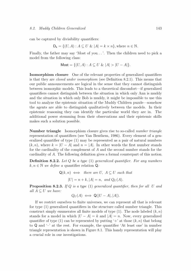
8.2. Muddy Children Generalized 143
can be captured by divisibility quantifiers:
Dk = {(U,A) : A ⊆ U & |A| = k × n},where n ∈ N.
Finally, the father may say ‘Most of you. . . ’. Then the children need to pick amodel from the following class:
Most = {(U,A) : A ⊆ U & |A| > |U − A|}.
Isomorphism closure One of the relevant properties of generalized quantifiersis that they are closed under isomorphism (see Definition 8.2.1). This means thatour public announcements are logical in the sense that they cannot distinguishbetween isomorphic models. This leads to a theoretical discomfort—if generalizedquantifiers cannot distinguish between the situation in which only Ann is muddyand the situation in which only Bob is muddy, it might be impossible to use thistool to analyze the epistemic situation of the Muddy Children puzzle—somehowthe agents are able to distinguish qualitatively between the models. In theirepistemic reasoning they can identify the particular world they are in. Theadditional power stemming from their observations and their epistemic skillsmakes such a solution possible.
Number triangle Isomorphism closure gives rise to so-called number trianglerepresentation of quantifiers (see Van Benthem, 1986). Every element of a gen-eralized quantifier of type (1) may be represented as a pair of natural numbers(k, n), where k = |U − A| and n = |A|. In other words the first number standsfor the cardinality of the complement of A and the second number stands for thecardinality of A. The following definition gives a formal counterpart of this notion.
Definition 8.2.2. Let Q be a type (1) generalized quantifier. For any numbersk, n ∈ N we define a quantifier relation Q:
Q(k, n) ⇐⇒ there are U, A ⊆ U such that
|U | = n+ k, |A| = n, and QU(A).
Proposition 8.2.3. If Q is a type (1) generalized quantifier, then for all U andall A ⊆ U we have:
QU(A) ⇐⇒ Q(|U − A|, |A|).
If we restrict ourselves to finite universes, we can represent all that is relevantfor type (1) generalized quantifiers in the structure called number triangle. Thisconstruct simply enumerates all finite models of type (1). The node labeled (k, n)stands for a model in which |U − A| = k and |A| = n. Now, every generalizedquantifier of type (1) can be represented by putting ‘+’ at those (k, n) that belongto Q and ‘–’ at the rest. For example, the quantifier ‘At least one’ in numbertriangle representation is shown in Figure 8.1. This handy representation will playa crucial role in our investigations.
144 Chapter 8. The Muddy Scientists
(0,0)
(1,0) (0,1)
(2,0) (1,1) (0,2)
(3,0) (2,1) (1,2) (0,3)
(4,0) (3,1) (2,2) (1,3) (0,4)
—– +
– + +– + + +
– + + + +
Figure 8.1: Number triangle and the representation of ‘At least 1’
Monotonicity An important intuition about some natural language quantifiersis that they say that some sets are ‘large enough’. We would expect that quantifiersare closed under some operations that change the size of those sets. The simplestamong such operations is the one of taking subsets and supersets. Intuitively,monotonicity is about quantifiers being closed under these operations. The possibleannouncements of the father may differ with respect to this factor.
Definition 8.2.4. A generalized quantifier Q of type (1) is said to be upwardmonotone (increasing), just in case for any two sets X and Y , if X is a subset ofY , then QU(X) entails QU(Y ) for every U .
For example, the quantifier ‘every child’ is monotone increasing. For example,the first sentence below entails the second as the set of children that have mud onthe forehead is a subset of children that are dirty.
1. Every child has mud on the forehead.
2. Every child is dirty.
Definition 8.2.5. A generalized quantifier Q of type (1) is said to be downwardmonotone (decreasing), just in case for any two sets X and Y , if X is a subset ofY , then QU(Y ) entails QU(X) for every U .
A quantifier Q is said to be downward monotone (decreasing) if the entailmentholds in the other direction. An example of a monotone decreasing quantifier is‘no child’ as the first sentence below entails the second:
1. No child is dirty.
2. No child has mud on the forehead.
Similarly a kind of monotonicity can be defined for the complement of thepredicate. This property is called extension and guarantees that if a given finitemodel satisfies a quantifier, then extending U − A cannot change this.
Definition 8.2.6. A quantifier Q of type (1) satisfies extension iff for all modelsM and M ′, with the universes U and U ′, respectively: A ⊆ U ⊆ U ′ impliesQU(A)⇒ QU ′(A).
8.2. Muddy Children Generalized 145
It is not surprising that monotonicity is one of the key properties of quantifiers,both in logic and linguistics. In model theory it contributes to definability (see,e.g., Vaananen, 2002); in linguistics it is used, among other applications, to explainthe phenomenon of negative polarity items (see, e.g., Ladusaw, 1979). Moreover,there are good reasons to believe that it is a crucial feature for processing naturallanguage quantifiers, as has already been suggested by psychologists, e.g., Johnson-Laird (1983) as well as linguists and logicians, e.g., Barwise & Cooper (1981),and empirically supported by Geurts (2003). There are also strong links withlearnability of quantifiers (see Clark, 2010; Gierasimczuk, 2007, 2009b; Tiede,1999).
CE quantifiers It is relevant in the context of Muddy Children puzzle tointroduce the notion of such a quantifiers.
Definition 8.2.7 (Mostowski 1957). A generalized quantifier Q of type (1,1) isa class of structures of the form M = (U,A,B), where A,B are subsets of U .Additionally, Q is closed under isomorphism, i.e., if M and M ′ are isomorphic,then (M ∈ Q ⇐⇒ M ′ ∈ Q).
One may argue that the quantifiers used in the puzzle, as many other naturallanguage quantifiers, are in fact of type (1,1) as they bind the two predicates‘children’ and ‘muddy’. This leads to the formalization of the form ‘Q of thechildren are muddy’. We would have then two sets A and B—the first standsfor the set of children, the second for the set of muddy objects. Our considerationsin this chapter explicitly concern quantifiers of type (1), but they also accountfor (1,1) quantifiers that satisfy certain additional restrictions. So-called CE-quantifiers (Vaananen, 2002) are those quantifiers of type (1,1) that, in additionto the isomorphism closure, satisfy the properties of extension and conservativity:
Definition 8.2.8. Let M = (U,A,B) and M ′ = (U ′, A′, B′) be finite models, andA,B ⊆ U ⊆ U ′:
1. Q of type (1, 1) satisfies extension iff QU(A,B) implies QU ′(A,B).
2. Q of type (1, 1) is conservative iff QU(A,B) iff QU(A,A ∩B).
Those properties quite intuitively capture natural language quantifier construc-tions, and have been even proposed as natural language universals (Barwise &Cooper, 1981). Also, they reduce quantifiers to being dependent only on twocardinalities: |A−B| and |A∩B|. Therefore, the relevant finite models can againbe represented as pairs of integers, and such quantifiers can be depicted in thenumber triangle (see Vaananen, 2002).

146 Chapter 8. The Muddy Scientists
8.3 Quantifiers as Background Assumptions
In this section we will investigate the behavior of various generalized quantifiersin the multi-agent inferential situation of the Muddy Children puzzle. We willinvestigate its solvability. We will say that a Muddy Children situation is ‘solvable’if it entails the possibility of all agents converging to knowledge about their ownstatus in a finite number of steps.
8.3.1 Increasing Quantifiers
Let us first consider a class of quantifiers that is closest to the classical version ofthe Muddy Children puzzle, namely: ‘At least m’, where m ∈ N. In the puzzlethis takes the form of the announcement:
At least k of you have mud on your foreheads.
Quantifiers of this form are monotone increasing and satisfy extension—once thequantifier is true in a model, adding new elements to A or U − A will not changeits logical value.3 The number triangle representation gives us always a downwardtriangle starting in a point (0,m).
How do those quantifiers behave in the Muddy Children situation? In Table 8.1rows are labeled with the total number of children and columns with the numberof muddy children. The number at the coordinates (c,m) says how many steps areneeded to solve the Muddy Children puzzle for the muddy children (immediatelyafter all children know their status).
0 1 2 3 4 51 x 1 x x x x2 x 1 2 x x x3 x 1 2 3 x x4 x 1 2 3 4 x5 x 1 2 3 4 56 x 1 2 3 4 5 . . .
0 1 2 3 4 51 x x x x x x2 x x 1 x x x3 x x 1 2 x x4 x x 1 2 3 x5 x x 1 2 3 46 x x 1 2 3 4 . . .
Table 8.1: ‘At least one’ and ‘At least two’
The numbers of steps needed to solve the puzzle form a triangle, with thevalues increasing horizontally to the right. When increasing the parameter kin the quantifier ‘At least k’ the whole triangle simply moves to the right anddownwards.
3In the case of (1,1) quantifiers this property corresponds to upward monotonicity in the leftargument, which is also called persistence (see Peters & Westerstahl, 2006).

8.3. Quantifiers as Background Assumptions 147
From the conceptual analysis we can extract some more information aboutthe structure of the solutions. In Table 8.2 a number is superscripted by ‘+’if in the final step of the reasoning some children infer their status from otherchildren’s epistemic announcements (from other children saying that they alreadyknow). The lack of the plus means that the final step of the reasoning is drawnsimultaneously by all agents.
0 1 2 3 4 51 x 1 x x x x2 x 1+ 2 x x x3 x 1+ 2+ 3 x x4 x 1+ 2+ 3+ 4 x5 x 1+ 2+ 3+ 4+ 56 x 1+ 2+ 3+ 4+ 5+
. . .
0 1 2 3 4 51 x x x x x x2 x x 1 x x x3 x x 1+ 2 x x4 x x 1+ 2+ 3 x5 x x 1+ 2+ 3+ 46 x x 1+ 2+ 3+ 4+
. . .
Table 8.2: ‘At least one’ and ‘At least two’
Now we are ready to give a general fact about this type of backgroundassumption.
Proposition 8.3.1. Let us take a Muddy Children situation, with n the numberof children, m ≤ n the number of muddy children. The Muddy Children puzzlewith the background assumption ‘At least k of you have mud on your forehead’can be solved in m− (k − 1) steps, where k ≤ m.
Using a similar background assumption with inner negation
At least k of you do not have mud on your foreheads
also makes the puzzle solvable. ‘At least k not’ behaves as ‘At least k’, but dependson the number of clean children. In general, inner negation works this way forother quantifiers.
A simplifying observation about a similar class of upward monotone quantifiersthat satisfy extension is as follows:
Observation 8.3.2. Let us take a Muddy Children situation, with n the numberof children, m ≤ n the number of muddy children. The Muddy Children puzzlewith the background assumption ‘More than k of you have mud on your forehead’can be solved in m− k steps, where k ≤ m.
8.3.2 Decreasing Quantifiers
Let us now consider another natural class, downward monotone quantifiers thatsatisfy extension: ‘At most k’, where k ∈ N. In the puzzle this takes form of theannouncement:
At most k of you have mud on your foreheads.

148 Chapter 8. The Muddy Scientists
Like in the case of increasing quantifiers we provide a table with the numbers ofsteps needed for solving the puzzle in respective cases. By doing this we indicatehow the situation changes with the parameter k. In Table 8.3 we can observe
0 1 2 3 41 ? ? x x x2 2 1+ x x x3 2 1+ x x x4 2 1+ x x x5 2 1+ x x x . . .
0 1 2 3 41 ? ? x x x2 ? ? ? x x3 3 2+ 1+ x x4 3 2+ 1+ x x5 3 2+ 1+ x x . . .
Table 8.3: ‘At most one’ and ‘At most two’
that the numbers of steps needed to solve the puzzle form a block, with thevalues increasing horizontally to the left. When increasing the parameter k inthe quantifier ‘At least k’ the whole blocks moves to the right and downwardsrevealing the next column on the left. Also, in case when the parameter k in thequantifiers is larger or equal to the number of muddy children, the puzzle is notsolvable! When the block of numbers moves downward together with k, it leavesa trace consisting of question marks behind that correspond to the unsolvablesituations.
We can characterize the solvability of Muddy Children situations with thequantifier ‘At most k’ in the following way.
Proposition 8.3.3. Let us take a Muddy Children scenario, with n the numberof children, m ≤ n the number of muddy children. If n > k then the MuddyChildren puzzle with the background assumption ‘At most k of you have mud onyour forehead’ can be solved in (k + 1)−m steps. If n ≤ k the situation is notsolvable.
Like in the previous case we give a simplifying observation about a similarclass of downward monotone quantifiers that satisfy extension:
Observation 8.3.4. Let us take a Muddy Children situation, with n the numberof children, m ≤ n the number of muddy children. The Muddy Children puzzlewith the background assumption ‘Less than k of you have mud on your forehead’can be solved in k −m steps, where k ≤ m. If m < k the situation is not solvable.
8.3.3 Cardinal and Parity Quantifiers
Some kinds of quantifiers allow one-step immediate solvability for all agents.Taking into consideration what they already know, the announcement gives themfull certainty about their state. This takes place for example when the number of

8.3. Quantifiers as Background Assumptions 149
muddy children is explicitly announced with the use of the quantifier ‘Exactly k’,where k ∈ N. The announcement of:
Exactly k of you have mud on your foreheads
always leads to immediate answers (see Table 8.4).
0 . . . k k+1 . . .1 x x 1 x x2 x x 1 x x3 x x 1 x x4 x x 1 x x5 x x 1 x x . . .
Table 8.4: ‘Exactly k’
Proposition 8.3.5. Every Muddy Children scenario with a background assumptionof the form ‘Exactly k’ is solvable in 1 step.
There are other, more interesting quantifiers with this property, e.g., divisibilityquantifiers: ‘A number divisible by k’, where k ∈ N. An example of such anannouncement for k = 2 is:
An even number of you have mud on your foreheads.
In Table 8.5 you can see that the columns that include solvable scenarios areisolated and consists only of 1s. Moreover, if the number k in the quantifier‘Divisible by k’ increases the gaps between the columns.
0 1 2 3 41 1 x 1 x 12 1 x 1 x 13 1 x 1 x 14 1 x 1 x 15 1 x 1 x 1 . . .
0 1 2 3 4 5 61 1 x x 1 x x 12 1 x x 1 x x 13 1 x x 1 x x 14 1 x x 1 x x 15 1 x x 1 x x 1 . . .
Table 8.5: ‘Even’ and ‘Divisible by 3’
A relevant fact is as follows.
Proposition 8.3.6. Let us take a Muddy Children scenario. The Muddy Childrenpuzzle with the background assumption ‘The number of you that have mud on yourforehead is ` mod k’, for any `, k ∈ N, can be solved in 1 step.
Additionally, it is worth noting that provided that every agent sees all otheragents, and in fact the number of muddy children is k ×m, the announcement ofquantifier ‘A number divisible by k’ is equivalent to announcing ‘Exactly k ×m’.

150 Chapter 8. The Muddy Scientists
All and No There are two simple natural language quantifiers that also allowone step immediate solvability for all agents. Quantifiers ‘All’ and ‘No’ informall the agents directly about the status of all agents, and therefore their own.Trivially, the announcement of:
All of you have mud on your foreheads
orNone of you have mud on your foreheads
always leads to immediate answers (see Table 8.6).
0 1 2 3 41 x 1 x x x2 x x 1 x x3 x x x 1 x4 x x x x 15 x x x x x . . .
0 1 2 3 4 51 1 x x x x x2 1 x x x x x3 1 x x x x x4 1 x x x x x5 1 x x x x x . . .
Table 8.6: ‘All’ and ‘No’
Proposition 8.3.7. Every Muddy Children scenario with a background assumptionof the form ‘All’ and ‘No’ is solvable in 1 step.
8.3.4 Proportional Quantifiers
Proportional quantifiers indicate the ratio between the number of elements inthe predicate and the total number of elements. The first that comes to mindis ‘Exactly 1
k’, where k ∈ N. Update with this information will be survived by
cardinalities that are divisible by k. In those situations, where |A| = k × `, forsome ` ∈ N, it is equivalent to the cardinal quantifier ‘Exactly `’ (see previoussection). However, there are also more interesting cases of upward monotoneproportional quantifiers. Such class is, e.g., ‘More than 1
k’, where k ∈ N. An
example of such announcement could be:
Most of you have mud on your foreheads.
If we agree to interpret ‘Most’ as ‘More than half’, then the solvability of theMuddy Children puzzle with this quantifier is depicted in on the left in Table 8.7.The table on the right shows the pattern for the quantifier ‘More than one third’.
The patterns in Table 8.7 might at first sight seem complex, but as a matter offact it is quite easy to observe that the pattern consists of smaller parts resemblingsimple increasing quantifiers that satisfy extension (see Section 8.3.1). In factthese muddy situations are reducible to those given by quantifiers ‘More than k’.

8.4. Iterated Epistemic Reasoning 151
0 1 2 3 4 51 x 1 x x x x2 x x 1 x x x3 x x 1+ 2 x x4 x x x 1+ 2 x5 x x x 1+ 2+ 36 x x x x 1+ 2+
. . .
0 1 2 3 4 51 x 1 x x x x2 x 1 2 x x x3 x x 1+ 2 x x4 x x 1+ 2+ 3 x5 x x 1+ 2+ 3+ 46 x x x 1+ 2+ 3+
. . .
Table 8.7: ‘More than half’ and ‘More than one third’
In a given situation, when |U | = n, ‘More than 1k’ is of course equivalent to ‘More
than nk’. This can be also observed in Table 8.7, the examples of ‘intervals’ of the
kind described in the proposition are printed bold.
Observation 8.3.8. The Muddy Quantifier ‘More than 1k’ consists of intervals
q0, q1, . . . such that:
1. q0 consists of k − 1 rows in the table, and for i > 0, qi consists of k rows.
2. qi is the segment of size k of the table for ‘More than i’ starting in the i-throw.
The number of steps needed to solve this puzzle is then characterized in thefollowing way.
Proposition 8.3.9. Let us take a Muddy Children situation, with n the numberof children, m ≤ n number of muddy children. The Muddy Children puzzle withthe background assumption ‘More than 1
kof you have mud on your forehead’ can
be solved in dm− nke steps.
All above-mentioned propositions lead to a uniform perspective on quantifierannouncements in the Muddy Children puzzle. In the next sections we will describethe epistemic reasoning using the tools of generalized quantifier theory.
8.4 Iterated Epistemic Reasoning
The number of steps needed to solve the puzzle seems to be pretty arbitrary. Itis, however, clearly determined by the epistemic structures that can be definedon the basis of the number triangle. In order to understand how this works, letus have a look at a concrete Muddy Children scenario. Let us assume that wehave three agents a, b, and c. All possibilities with respect to the size of the set ofmuddy children are enumerated in the third level of the number triangle. Let usalso assume at this point that the actual situation is that agents a, b are muddyand c is clean. Therefore, with respect to our representation the real world is(1, 2), one child is clean and two are muddy:
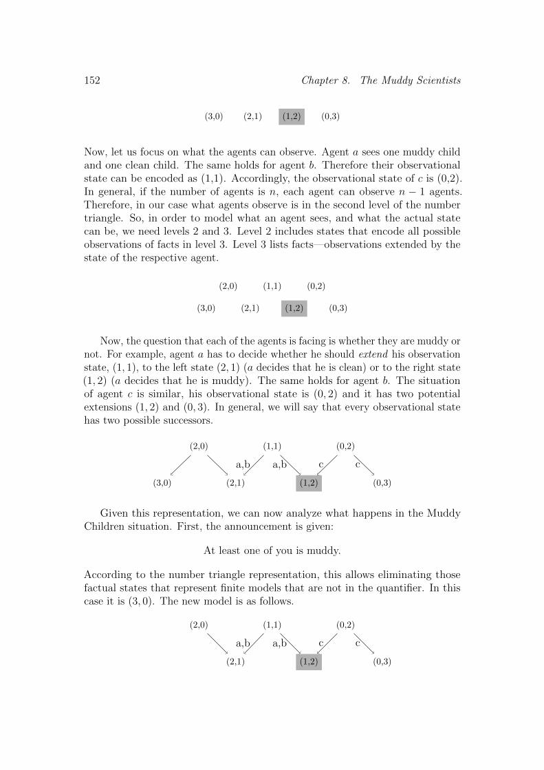
152 Chapter 8. The Muddy Scientists
(3,0) (2,1) (1,2) (0,3)
Now, let us focus on what the agents can observe. Agent a sees one muddy childand one clean child. The same holds for agent b. Therefore their observationalstate can be encoded as (1,1). Accordingly, the observational state of c is (0,2).In general, if the number of agents is n, each agent can observe n − 1 agents.Therefore, in our case what agents observe is in the second level of the numbertriangle. So, in order to model what an agent sees, and what the actual statecan be, we need levels 2 and 3. Level 2 includes states that encode all possibleobservations of facts in level 3. Level 3 lists facts—observations extended by thestate of the respective agent.
(3,0)
(2,0)
(2,1)
(1,1)
(1,2)
(0,2)
(0,3)
Now, the question that each of the agents is facing is whether they are muddy ornot. For example, agent a has to decide whether he should extend his observationstate, (1, 1), to the left state (2, 1) (a decides that he is clean) or to the right state(1, 2) (a decides that he is muddy). The same holds for agent b. The situationof agent c is similar, his observational state is (0, 2) and it has two potentialextensions (1, 2) and (0, 3). In general, we will say that every observational statehas two possible successors.
(3,0)
(2,0)
(2,1)
(1,1)
(1,2)
(0,2)
(0,3)
a,b a,b c c
Given this representation, we can now analyze what happens in the MuddyChildren situation. First, the announcement is given:
At least one of you is muddy.
According to the number triangle representation, this allows eliminating thosefactual states that represent finite models that are not in the quantifier. In thiscase it is (3, 0). The new model is as follows.
(3,0)
(2,0)
(2,1)
(1,1)
(1,2)
(0,2)
(0,3)
a,b a,b c c
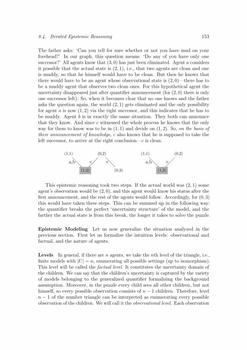
8.4. Iterated Epistemic Reasoning 153
The father asks: ‘Can you tell for sure whether or not you have mud on yourforehead?’ In our graph, this question means: ‘Do any of you have only onesuccessor?’ All agents know that (3, 0) has just been eliminated. Agent a considersit possible that the actual state is (2, 1), i.e., that two agents are clean and oneis muddy, so that he himself would have to be clean. But then he knows thatthere would have to be an agent whose observational state is (2, 0)—there has tobe a muddy agent that observes two clean ones. For this hypothetical agent theuncertainty disappeared just after quantifier announcement (for (2, 0) there is onlyone successor left). So, when it becomes clear that no one knows and the fatherasks the question again, the world (2, 1) gets eliminated and the only possibilityfor agent a is now (1, 2) via the right successor, and this indicates that he has tobe muddy. Agent b is in exactly the same situation. They both can announcethat they know. And since c witnessed the whole process he knows that the onlyway for them to know was to be in (1, 1) and decide on (1, 2). So, on the basis oftheir announcement of knowledge, c also knows that he is supposed to take theleft successor, to arrive at the right conclusion—c is clean.
(1,1)
(1,2)
(0,2)
(0,3)
a,b c c
(1,1)
(1,2)
(0,2)
a,b c
This epistemic reasoning took two steps. If the actual world was (2, 1) someagent’s observation would be (2, 0), and this agent would know his status after thefirst announcement, and the rest of the agents would follow. Accordingly, for (0, 3)this would have taken three steps. This can be summed up in the following way:the quantifier breaks the perfect ‘uncertainty structure’ of the model, and thefarther the actual state is from this break, the longer it takes to solve the puzzle.
Epistemic Modeling Let us now generalize the situation analyzed in theprevious section. First let us formalize the intuition levels: observational andfactual, and the nature of agents.
Levels In general, if there are n agents, we take the nth level of the triangle, i.e.,finite models with |U | = n, enumerating all possible settings (up to isomorphism).This level will be called the factual level. It constitutes the uncertainty domain ofthe children. We can say that the children’s uncertainty is captured by the varietyof models belonging to the generalized quantifier formalizing the backgroundassumption. Moreover, in the puzzle every child sees all other children, but nothimself, so every possible observation consists of n− 1 children. Therefore, leveln − 1 of the number triangle can be interpreted as enumerating every possibleobservation of the children. We will call it the observational level. Each observation

154 Chapter 8. The Muddy Scientists
can be extended to one of the two factual states that are the closest below—tothe left if the observer in question is clean or to the right if he is muddy.
Agents There can be any number of Muddy Children—the puzzle is a realmulti -agent scenario. This is why it is so surprising to realize that it can becollapsed to two agents, i.e., two local states. Obviously every agent is in one ofthe two groups: either among the muddy children or among the clean ones. Butthis gives much more—in fact there are at most two possible observational statesthat the agents might be in. Every clean child observes the same as all other cleanchildren, and every muddy child observes the same as all other muddy children.
Proposition 8.4.1. Every agent’s observation is encoded by one of at most twostates in the observational level. Those two are neighboring states.
Proof. For the first part. Assume that the total number of children is n, thenumber of muddy children is m. Let us pick an agent and call him a. There aretwo possibilities:
1. a is muddy, then a’s observational state is (n−m,m− 1).
2. a is clean, then a’s observational state is ((n−m)− 1,m).
The two relevant observational states neighbor each other in the model becausethey are the only two states that can be extended to the actual state (n−m,m).
Moreover, the actual world clearly determines the number of agents perceivingthe same situation.
Proposition 8.4.2. Given a certain situation (c,m) there are c children that arein the observational state (c− 1,m) and m children in the observational state of(c,m− 1). In case m = 0 all children are in the observational state (c− 1, 0). Incase c = 0 all children are in the observational state (0,m− 1).
8.4.1 An Epistemic Model Based on the Number Triangle
In this section we will link our modeling of the Muddy Children puzzle to theexisting approaches based on dynamic epistemic logic. The correspondence is notstraightforward. However, it is possible to formalize our models in a similar way.
Definition 8.4.3. The Muddy Children model for n children is a quadrupleMMC
n = (So, Sf , Rm, Rm), where
• So = {(c,m) | c+m = n− 1} (the observational states),
• Sf = {(c,m) | c+m = n} (the factual states),
• Rm ⊆ So × Sf , such that Rm((c1,m1), (c2,m2)) iff m2 = m1 + 1,
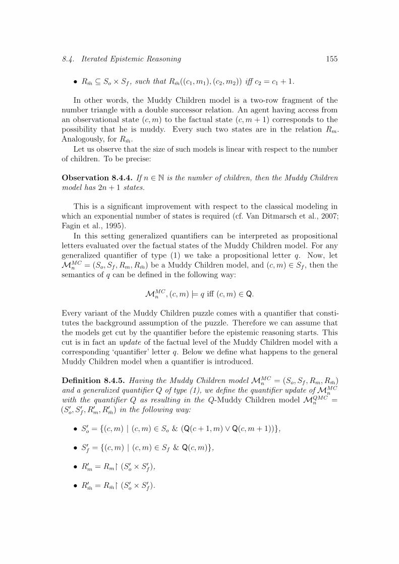
8.4. Iterated Epistemic Reasoning 155
• Rm ⊆ So × Sf , such that Rm((c1,m1), (c2,m2)) iff c2 = c1 + 1.
In other words, the Muddy Children model is a two-row fragment of thenumber triangle with a double successor relation. An agent having access froman observational state (c,m) to the factual state (c,m + 1) corresponds to thepossibility that he is muddy. Every such two states are in the relation Rm.Analogously, for Rm.
Let us observe that the size of such models is linear with respect to the numberof children. To be precise:
Observation 8.4.4. If n ∈ N is the number of children, then the Muddy Childrenmodel has 2n+ 1 states.
This is a significant improvement with respect to the classical modeling inwhich an exponential number of states is required (cf. Van Ditmarsch et al., 2007;Fagin et al., 1995).
In this setting generalized quantifiers can be interpreted as propositionalletters evaluated over the factual states of the Muddy Children model. For anygeneralized quantifier of type (1) we take a propositional letter q. Now, letMMC
n = (So, Sf , Rm, Rm) be a Muddy Children model, and (c,m) ∈ Sf , then thesemantics of q can be defined in the following way:
MMCn , (c,m) |= q iff (c,m) ∈ Q.
Every variant of the Muddy Children puzzle comes with a quantifier that consti-tutes the background assumption of the puzzle. Therefore we can assume thatthe models get cut by the quantifier before the epistemic reasoning starts. Thiscut is in fact an update of the factual level of the Muddy Children model with acorresponding ‘quantifier’ letter q. Below we define what happens to the generalMuddy Children model when a quantifier is introduced.
Definition 8.4.5. Having the Muddy Children model MMCn = (So, Sf , Rm, Rm)
and a generalized quantifier Q of type (1), we define the quantifier update ofMMCn
with the quantifier Q as resulting in the Q-Muddy Children model MQMCn =
(S ′o, S′f , R
′m, R
′m) in the following way:
• S ′o = {(c,m) | (c,m) ∈ So & (Q(c+ 1,m) ∨ Q(c,m+ 1))},
• S ′f = {(c,m) | (c,m) ∈ Sf & Q(c,m)},
• R′m = Rm� (S ′o × S ′f ),
• R′m = Rm� (S ′o × S ′f ).

156 Chapter 8. The Muddy Scientists
At this point let us observe that for some quantifiers Q the Q-Muddy Childrenmodels have a fixed size, independent of the number of children. Such a quantifieris for example ‘At most k’. In all situations in which the number of children nis larger than k the puzzle is solvable. If fact, in this situation for any n > k,|S ′f | = k. This shows that some quantifier announcements leave behind them afixed number of possible worlds.
The epistemic information can be expressed with formulae evaluated in theobservational states. We can say that an agent in an observational state (c,m)knows that ϕm (that he is muddy) if and only if the only successor of (c,m) is(c,m+ 1). Moreover, if an epistemic announcement eliminates an observationalstate it also eliminates all its successors. As our modeling is Muddy-Childrenspecific, we do not give here a full epistemic language. The semantic analysis of theannouncements is aimed at emphasizing the analogy with so-called unsuccessfulannouncements in DEL (see Van Ditmarsch et al., 2007).
8.5 Muddy Children Solvability
By reinterpreting the Muddy Children puzzle within the semantics of quantifierswe can associate every finite model with the number of steps needed to solve thepuzzle, if it is solvable at all.
Definition 8.5.1. A muddy quantifier is a pair QMC = (Q, fQ), where Q isa quantifier and fQ : Q → N is a function that assigns to a pair of numbersrepresenting M ∈ Q the number of steps needed to solve the Muddy Childrenpuzzle with the background assumption containing quantifier Q.
Below we list some examples of muddy quantifiers in the number trianglerepresentation according to the previously given enumeration of interesting cases.4
First let us consider the quantifier ‘At least k’. It is easy to observe thatincreasing k causes the downward triangle to move down along the (0, 0)–(0, n)axis.
This quantifier allows solving the Muddy Children puzzle for any configurationof ‘muddiness’. However, within a certain level, the farther from a minus thelonger it takes.
Now let us have a look at the quantifier ‘At most k’.The question-marks occur in place of models that satisfy the quantifier, but
for which it is impossible to solve the Muddy Children puzzle. For example, ifone child is clean and one child is muddy (the actual world is (1, 1)) the MuddyChildren situation does not lead to a solution if the announcement is:
At most two of you are muddy.
4As before, the index + marks the solutions in which at least one agent infers his status fromthe announcement of knowledge of other agents. The lack of + marks the situations in whichthe agents discover their status simultaneously.

8.5. Muddy Children Solvability 157
—– 1
– 1+ 2– 1+ 2+ 3
– 1+ 2+ 3+ 4
—– –
– – 1– – 1+ 2
– – 1+ 2+ 3
Figure 8.2: Increasing muddy-quantifiers ‘At least 1’ and ‘At least 2’
—
? ?2 1+ –
2 1+ – –
2 1+ – – –
—
? ?? ? ?
3 2+ 1+ –
3 2+ 1+ – –
Figure 8.3: Decreasing muddy-quantifiers ‘At most 1’ and ‘At most 2’
Again, the farther from a minus the longer it takes to solve the puzzle.Divisibility quantifiers in the Muddy Children setting do not involve much
inference—every situation is solvable in one step (see Figure 8.4). Moreover, there
—1 –
1 – 11 – 1 –
1 – 1 – 11 – 1 – 1 –
—1 –
1 – –1 – – 1
1 – – 1 –1 – – 1 – –
Figure 8.4: Muddy-quantifiers ‘Divisible by 2’ and ‘Divisible by 3’
is no ‘+’ superscript anywhere. This indicates that the answers are simultaneouslygiven by all the agents.
Finally, let us have a look at upward monotone proportional quantifiers. Theycreate more complicated patterns (see Figure 8.5).
Notice the similarity between these patterns and those of Figure 8.5. Thenumber of steps increases to the right, together with the distance from a minus.
Function fQ in Definition 8.5.1 gives the number of steps needed to solve thepuzzle. It follows from the structure of the epistemic models that underlie thereasoning:
Proposition 8.5.2. Let Q be a generalized quantifier, and n be the number ofchildren. Then the corresponding muddy quantifier is QMC = (Q, fQ), where the
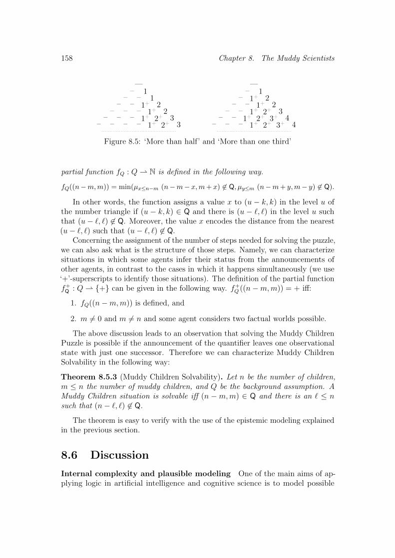
158 Chapter 8. The Muddy Scientists
—– 1
– – 1– – 1+ 2
– – – 1+ 2– – – 1+ 2+ 3
– – – – 1+ 2+ 3
—– 1
– 1+ 2– – 1+ 2
– – 1+ 2+ 3– – 1+ 2+ 3+ 4
– – – 1+ 2+ 3+ 4
Figure 8.5: ‘More than half’ and ‘More than one third’
partial function fQ : Q ⇀ N is defined in the following way.
fQ((n−m,m)) = min(µx≤n−m (n−m− x,m+ x) 6∈ Q, µy≤m (n−m+ y,m− y) 6∈ Q).
In other words, the function assigns a value x to (u − k, k) in the level u ofthe number triangle if (u − k, k) ∈ Q and there is (u − `, `) in the level u suchthat (u− `, `) 6∈ Q. Moreover, the value x encodes the distance from the nearest(u− `, `) such that (u− `, `) 6∈ Q.
Concerning the assignment of the number of steps needed for solving the puzzle,we can also ask what is the structure of those steps. Namely, we can characterizesituations in which some agents infer their status from the announcements ofother agents, in contrast to the cases in which it happens simultaneously (we use‘+’-superscripts to identify those situations). The definition of the partial functionf+Q : Q ⇀ {+} can be given in the following way. f+
Q ((n−m,m)) = + iff:
1. fQ((n−m,m)) is defined, and
2. m 6= 0 and m 6= n and some agent considers two factual worlds possible.
The above discussion leads to an observation that solving the Muddy ChildrenPuzzle is possible if the announcement of the quantifier leaves one observationalstate with just one successor. Therefore we can characterize Muddy ChildrenSolvability in the following way:
Theorem 8.5.3 (Muddy Children Solvability). Let n be the number of children,m ≤ n the number of muddy children, and Q be the background assumption. AMuddy Children situation is solvable iff (n −m,m) ∈ Q and there is an ` ≤ nsuch that (n− `, `) 6∈ Q.
The theorem is easy to verify with the use of the epistemic modeling explainedin the previous section.
8.6 Discussion
Internal complexity and plausible modeling One of the main aims of ap-plying logic in artificial intelligence and cognitive science is to model possible
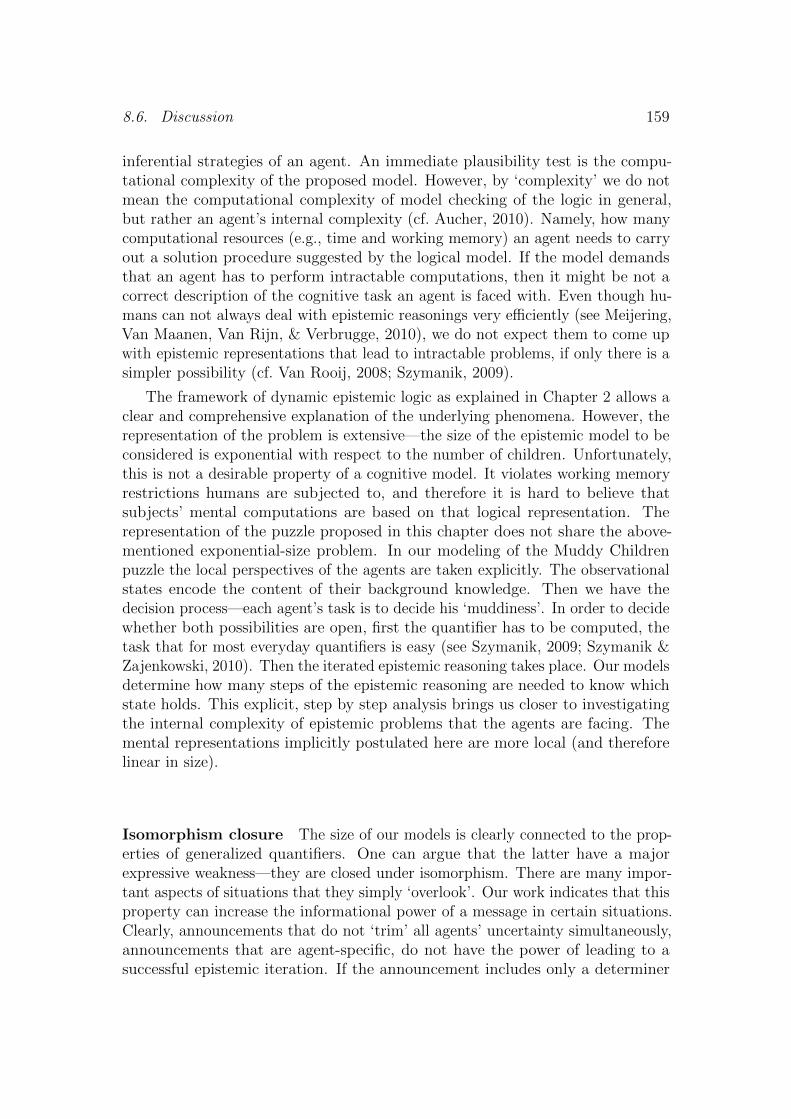
8.6. Discussion 159
inferential strategies of an agent. An immediate plausibility test is the compu-tational complexity of the proposed model. However, by ‘complexity’ we do notmean the computational complexity of model checking of the logic in general,but rather an agent’s internal complexity (cf. Aucher, 2010). Namely, how manycomputational resources (e.g., time and working memory) an agent needs to carryout a solution procedure suggested by the logical model. If the model demandsthat an agent has to perform intractable computations, then it might be not acorrect description of the cognitive task an agent is faced with. Even though hu-mans can not always deal with epistemic reasonings very efficiently (see Meijering,Van Maanen, Van Rijn, & Verbrugge, 2010), we do not expect them to come upwith epistemic representations that lead to intractable problems, if only there is asimpler possibility (cf. Van Rooij, 2008; Szymanik, 2009).
The framework of dynamic epistemic logic as explained in Chapter 2 allows aclear and comprehensive explanation of the underlying phenomena. However, therepresentation of the problem is extensive—the size of the epistemic model to beconsidered is exponential with respect to the number of children. Unfortunately,this is not a desirable property of a cognitive model. It violates working memoryrestrictions humans are subjected to, and therefore it is hard to believe thatsubjects’ mental computations are based on that logical representation. Therepresentation of the puzzle proposed in this chapter does not share the above-mentioned exponential-size problem. In our modeling of the Muddy Childrenpuzzle the local perspectives of the agents are taken explicitly. The observationalstates encode the content of their background knowledge. Then we have thedecision process—each agent’s task is to decide his ‘muddiness’. In order to decidewhether both possibilities are open, first the quantifier has to be computed, thetask that for most everyday quantifiers is easy (see Szymanik, 2009; Szymanik &Zajenkowski, 2010). Then the iterated epistemic reasoning takes place. Our modelsdetermine how many steps of the epistemic reasoning are needed to know whichstate holds. This explicit, step by step analysis brings us closer to investigatingthe internal complexity of epistemic problems that the agents are facing. Themental representations implicitly postulated here are more local (and thereforelinear in size).
Isomorphism closure The size of our models is clearly connected to the prop-erties of generalized quantifiers. One can argue that the latter have a majorexpressive weakness—they are closed under isomorphism. There are many impor-tant aspects of situations that they simply ‘overlook’. Our work indicates that thisproperty can increase the informational power of a message in certain situations.Clearly, announcements that do not ‘trim’ all agents’ uncertainty simultaneously,announcements that are agent-specific, do not have the power of leading to asuccessful epistemic iteration. If the announcement includes only a determiner
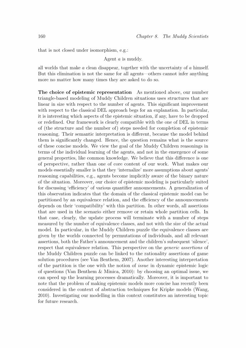
160 Chapter 8. The Muddy Scientists
that is not closed under isomorphism, e.g.:
Agent a is muddy.
all worlds that make a clean disappear, together with the uncertainty of a himself.But this elimination is not the same for all agents—others cannot infer anythingmore no matter how many times they are asked to do so.
The choice of epistemic representation As mentioned above, our numbertriangle-based modeling of Muddy Children situations uses structures that arelinear in size with respect to the number of agents. This significant improvementwith respect to the classical DEL approach begs for an explanation. In particular,it is interesting which aspects of the epistemic situation, if any, have to be droppedor redefined. Our framework is clearly compatible with the one of DEL in termsof (the structure and the number of) steps needed for completion of epistemicreasoning. Their semantic interpretation is different, because the model behindthem is significantly changed. Hence, the question remains what is the sourceof these concise models. We view the goal of the Muddy Children reasonings interms of the individual learning of the agents, and not in the emergence of somegeneral properties, like common knowledge. We believe that this difference is oneof perspective, rather than one of core content of our work. What makes ourmodels essentially smaller is that they ‘internalize’ more assumptions about agents’reasoning capabilities, e.g., agents become implicitly aware of the binary natureof the situation. Moreover, our choice of epistemic modeling is particularly suitedfor discussing ‘efficiency’ of various quantifier announcements. A generalization ofthis observation indicates that the domain of the classical epistemic model can bepartitioned by an equivalence relation, and the efficiency of the announcementsdepends on their ‘compatibility’ with this partition. In other words, all assertionsthat are used in the scenario either remove or retain whole partition cells. Inthat case, clearly, the update process will terminate with a number of stepsmeasured by the number of equivalence classes, and not with the size of the actualmodel. In particular, in the Muddy Children puzzle the equivalence classes aregiven by the worlds connected by permutations of individuals, and all relevantassertions, both the Father’s announcement and the children’s subsequent ‘silence’,respect that equivalence relation. This perspective on the generic assertions ofthe Muddy Children puzzle can be linked to the rationality assertions of gamesolution procedures (see Van Benthem, 2007). Another interesting interpretationof the partition is the one with the notion of issue in dynamic epistemic logicof questions (Van Benthem & Minica, 2010): by choosing an optimal issue, wecan speed up the learning processes dramatically. Moreover, it is important tonote that the problem of making epistemic models more concise has recently beenconsidered in the context of abstraction techniques for Kripke models (Wang,2010). Investigating our modelling in this context constitutes an interesting topicfor future research.
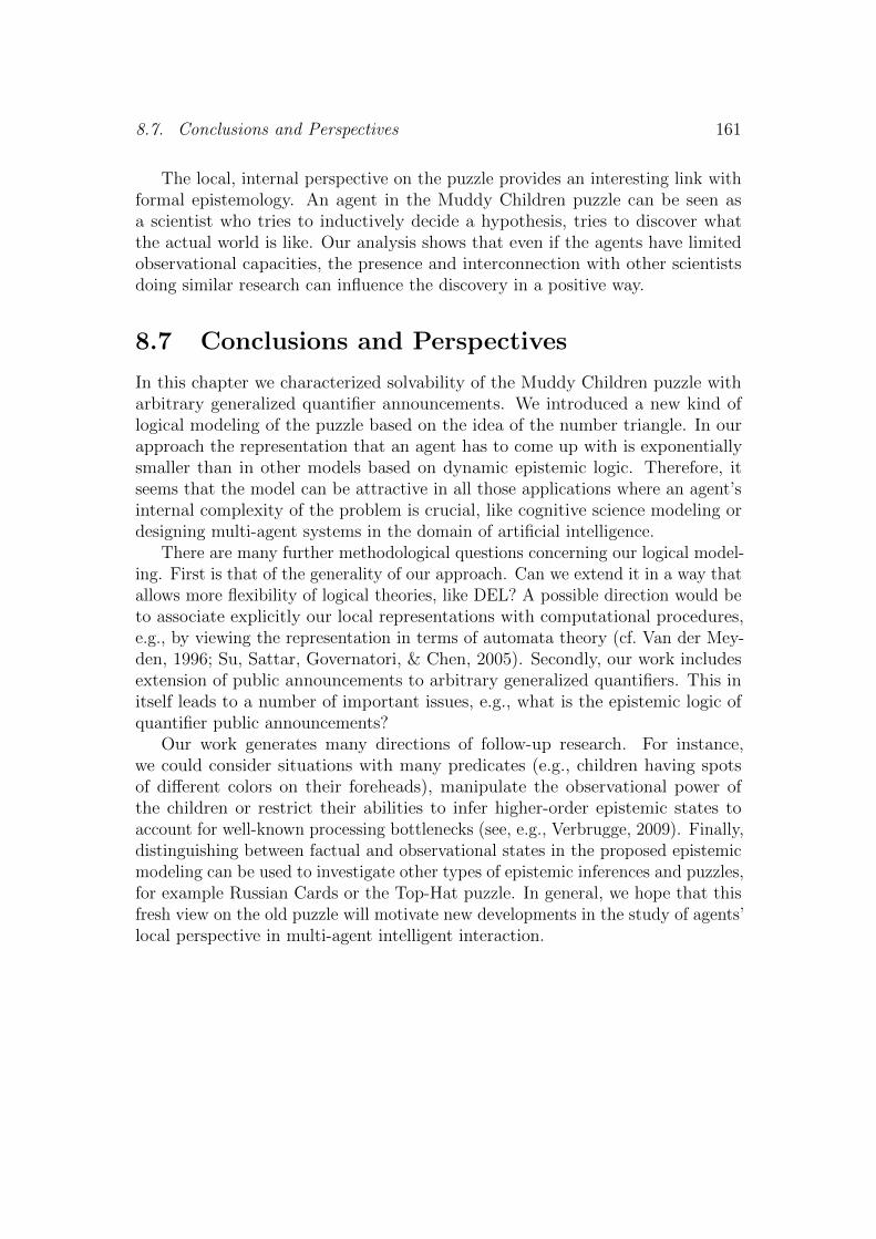
8.7. Conclusions and Perspectives 161
The local, internal perspective on the puzzle provides an interesting link withformal epistemology. An agent in the Muddy Children puzzle can be seen asa scientist who tries to inductively decide a hypothesis, tries to discover whatthe actual world is like. Our analysis shows that even if the agents have limitedobservational capacities, the presence and interconnection with other scientistsdoing similar research can influence the discovery in a positive way.
8.7 Conclusions and Perspectives
In this chapter we characterized solvability of the Muddy Children puzzle witharbitrary generalized quantifier announcements. We introduced a new kind oflogical modeling of the puzzle based on the idea of the number triangle. In ourapproach the representation that an agent has to come up with is exponentiallysmaller than in other models based on dynamic epistemic logic. Therefore, itseems that the model can be attractive in all those applications where an agent’sinternal complexity of the problem is crucial, like cognitive science modeling ordesigning multi-agent systems in the domain of artificial intelligence.
There are many further methodological questions concerning our logical model-ing. First is that of the generality of our approach. Can we extend it in a way thatallows more flexibility of logical theories, like DEL? A possible direction would beto associate explicitly our local representations with computational procedures,e.g., by viewing the representation in terms of automata theory (cf. Van der Mey-den, 1996; Su, Sattar, Governatori, & Chen, 2005). Secondly, our work includesextension of public announcements to arbitrary generalized quantifiers. This initself leads to a number of important issues, e.g., what is the epistemic logic ofquantifier public announcements?
Our work generates many directions of follow-up research. For instance,we could consider situations with many predicates (e.g., children having spotsof different colors on their foreheads), manipulate the observational power ofthe children or restrict their abilities to infer higher-order epistemic states toaccount for well-known processing bottlenecks (see, e.g., Verbrugge, 2009). Finally,distinguishing between factual and observational states in the proposed epistemicmodeling can be used to investigate other types of epistemic inferences and puzzles,for example Russian Cards or the Top-Hat puzzle. In general, we hope that thisfresh view on the old puzzle will motivate new developments in the study of agents’local perspective in multi-agent intelligent interaction.


Part IV
Conclusions

Chapter 9
Conclusions and Outlook
In Chapter 1 we defined as the aim of this thesis “to link learning theory withlogics of knowledge and belief”. Let us now look back to see to what extent wehave fulfilled this goal.
We started off (in Chapter 3) with a methodological analysis of both frameworks,in particular with analyzing the basic learning-theoretic setting in terms of dynamicepistemic logic. We observed a compatibility with respect to basic epistemologicalassumptions, but we also pointed out some difficulties, in particular the differencein the perspective on the mind-change process. Learning theory focuses oncomputational problems and on a global picture of sequences of conjectures.Dynamic epistemic logic zooms in on particular steps of revision, providing amore constructive, logical approach. We built on what the two have in common,i.e., on the initial uncertainty of the agent. The translation of the basic learningtheory setting into the semantics of modal logic exposes the epistemic groundsof inductive inference. It also shows the restrictions of the domain of epistemicproblems covered by learning theory. In particular, the learning theory setting isconceptually limited to the single agent case.
Part II of this thesis is directly concerned with the problem of translationbetween the paradigms. The idea is to express learnability in epistemic anddoxastic logic, accounting for the temporal aspects of learning as well. In Chapter4 we approached the problem from the perspective of identifiability in the limit, thedominant notion of learning theory. Learning in the limit is the kind of learning ofwhich success does not depend on reaching certainty. It does not concern the stateof irrevocable knowledge, but rather stable true belief. Hence, we linked it withthe belief-revision problem and with doxastic logic. Using a characterization ofidentifiability in the limit we defined learnability as the reachability of safe belief.We also showed the properties of various belief-revision policies with respect to theirability to converge to the true belief. First, we restricted ourselves to learning fromsound and complete streams of positive data. We showed that learning methodsbased on belief revision via conditioning (update) and lexicographic revision areuniversal, i.e., provided certain prior conditions, those methods are as powerful as
165
166 Chapter 9. Conclusions and Outlook
identification in the limit. Those prior conditions, the agent’s prior dispositionsfor belief revision, play a crucial role here. We showed that in some cases, thesepriors cannot be modeled using standard belief-revision models (as those are basedon well-founded preorders), but only using generalized models (based on simplepreorders). Furthermore, we drew conclusions about the existence of a tensionbetween conservatism and learning power by showing that the very popular, most‘conservative’ belief-revision method fails to be universal. In the second part weturned to the case of learning from both positive and negative data. Here, alongwith positive information the agent receives negative data about facts that do nothold of the actual world. We again assumed these streams to be truthful and wedrew conclusions about iterated belief revision governed by such streams. Thisenriched framework allows us to consider the occurrence of erroneous information.Provided that errors occur finitely often and are always eventually corrected weshow that the lexicographic revision method is still reliable, but more conservativemethods fail.
In Chapter 5 we were also concerned with expressing learnability in theepistemic framework, this time focusing only on update. We advanced a differentapproach—we investigated both finite identifiability and identifiability in the limitas properties of epistemic and doxastic models. We characterized the outcomeof finite identification in the language of epistemic logic and dynamic epistemiclogic. As a corollary from our results obtained in Chapter 4, we also characterizedthe outcome of identification in the limit in doxastic logic. Then, focusing onthe procedural aspect of learning we observed that the iterated update of finiteidentification generates an epistemic temporal forest. We used the latter tocharacterize finite identifiability in epistemic temporal logic. Then, we againextended our results to the case of identifiability in the limit, indicating thetemporal conditions for the success of this type of learning. As a result, weshow what properties the initial uncertainty range needs to have, to guaranteereaching the state of irrevocable knowledge and true stable belief. Both irrevocableknowledge and true stable belief concern the complete description of the actualworld. Finally, we mentioned that our temporal setting accounts for more thanjust language learning. All other types of learning, e.g., function-learning, can beanalyzed in this temporal setting.
In Part II our aim was to establish a connection between the two frameworks.As we all know, well-established relationships are usually based on mutual profit,motivation and inspiration exchange. The research presented in Part III of thisbook was meant to live up to this kind of expectation. In Chapter 6, inspiredby the dynamic epistemic logic interpretation of certainty, we investigated it inthe learning-theoretic setting. We focused on the distinction between objectivecertainty (the objective lack of alternatives to the actual world) and subjective,introspective certainty (with the agent being aware of the unambiguity). Assumingthe computability of agents, we showed that there are classes of languages that arefinitely identifiable, i.e., the agent can always eventually conclude certainty; but no
167
computable agent can always conclude it as soon as it is objectively possible, i.e.,as soon as the data exclude all other possibilities. For learning theory this meansthat the domain of finite identifiability properly contains the domain of fastestfinite identification—a well-motivated new kind of finite identification. In the samechapter, on the basis of learning theory, we also investigated the complexity ofobtaining minimal conclusive samples of information, the minimal descriptions thatinclude enough information to eliminate uncertainty. Our results may, for instance,find applications in the analysis of efficient communication in epistemic games.In particular, the task of finding a minimal-size sample eliminating uncertaintyturned out to be NP-complete and hence, most probably, more difficult thanfinding any minimal sample, which can be done in polynomial time. As the task offinding a minimal-size sample could be delegated to a helpful teacher, our resultsprovide an indirect computational motivation for introducing another agent, ateacher, to the simple setting of finite identification. Therefore, computationalanalysis shows that teaching in the most efficient way is very demanding.
The aim of Chapter 7 was to enrich both learning theory and dynamic epistemiclogic with new learning-related concepts. We questioned the learning-theoreticdogma of learner-teacher cooperativeness by analyzing the computational com-plexity of various learning and teaching attitudes. It turned out that the questionof teachability of a concept (the possibility to direct the learner to the desiredstate in a graph) is NP-complete under the assumption of non-cooperativenessof the learner. Our epistemic interpretation of Sabotage Games provided in thatchapter, is based on deletion, as are epistemic update and the framework oflearning by erasing, discussed in Chapter 2, but it gives an account of the progressof mind-change that differs from both. It allows thinking of incoming informationin a more local way—as the removal of possible mind-changes, rather than thehypotheses themselves. This is a step towards modeling a learner to have limitedaccess to the whole range of possibilities.
In Chapter 7 we explicitly enriched learning situations with a second agent,the teacher. In Chapter 8 we considered a multi-agent scenario of the MuddyChildren puzzle. Inspired by results on the learnability of generalized quantifiers,we reinterpreted the agents of the puzzle as scientists. They are supposed to decidea hypothesis on the basis of a background assumption (a generalized quantifier)and inductive epistemic inference. The most immediate contribution to dynamicepistemic logic is a concise, linear representation of the epistemic situation ofMuddy Children and a characterization of the solvability of the generalized versionof the Muddy Children puzzle (with arbitrary quantifiers). Viewing the puzzlefrom the perspective of learning theory, leads one to extend the incoming factual,propositional information by some epistemic, indirect information. It sheds lighton a different kind of learning performed by a team of learners with interconnectedobservational power. Moreover, our approach gives additional insights into theefficiency of learning.
168 Chapter 9. Conclusions and Outlook
Overall, in this thesis we focused on building a connection between formal learn-ing theory and dynamic epistemic logic. The semantic link provided dynamicepistemic logic with a uniform framework for considering iterated actions. Thesemantic analysis underlying this logical view on inductive inference led us to givesyntactic chracterizations of learnability in doxastic epistemic modal-temporal log-ics. Further topics of the thesis, taken from the domains of computability, games,and multi-agency, strengthen the connection by providing additional insights intothe process of epistemic and doxastic change.
There are many open questions and directions for further work. They are alldiscussed in detail in the corresponding chapters of the thesis. Let us here un-derline some of them that seem especially interesting from the perspective of theinterrelation between learning theory and logics of knowledge and belief.
The first open problem concerns the transfer of the computational aspects oflearning theory to the frameworks of belief revision and epistemic change. Thetask of revising beliefs has a direct psychological interpretation. This cognitive linkleads us towards the computational framework. Hence, a theoretically interestingand an empirically inspiring direction is to establish a broad learning-theory-like computational platform for investigating the restriction to computable (andperhaps also tractable, cf. Chapter 8) belief-revision. Chapter 4 gives a generalsetting that could be adapted to such considerations.
The second direction is to incorporate non-trivial epistemic multi-agency intothe framework of learning theory. Such multi-agency is the very central conceptof game theory and epistemic logic. In learning theory, team learning has beenconsidered in the context of improving learnability, but these considerations havebeen limited by conditions of true information and perfect observation. From ourconsiderations in Chapter 8 we can see that there are very simple scenarios inwhich quite substantial observational limitations of the agents can still lead tosuccessful learning.
The third further direction concerns a generalization of learning-theoreticapproach to account for a great variety of input information. As we showed (e.g.,in Chapter 4) the character of the incoming information can heavily influence con-vergence. Hence, it is reasonable to account for different levels of trustworthinessin formal learning models, by linking different kinds of incoming information withdifferent operations on models.
The fourth topic of further work concerns analyzing particular learning al-gorithms, properties of learning functions, and properties of learnable classes inepistemic and doxastic temporal logic. In particular, we would like to get thetemporal characterizations of protocols that govern certain types of learning orlead to particular learning effects. The topic is especially interesting, because thetemporal treatment of hypotheses gives a framework for analyzing different typesof structures on a common ground, as we argued in Chapter 5.

Bibliography
Alchourron, C. E., Gardenfors, P., & Makinson, D. (1985). On the logic oftheory change: Partial meet contraction and revision functions. The Journal ofSymbolic Logic, 50 (2), 510–530.
Angluin, D. (1980). Inductive inference of formal languages from positive data.Information and Control , 45(2), 117–135.
Angluin, D. (1987). Learning regular sets from queries and counterexamples.Information and Computation, 75 (2), 87–106.
Angluin, D., & Smith, C. H. (1983). Inductive inference: Theory and methods.ACM Computing Surveys , 15 (3), 237–269.
Aucher, G. (2010). An internal version of epistemic logic. Studia Logica, 94 (1),1–22.
Balakrishnan, V. K. (1997). Graph Theory . McGraw-Hill.
Balbach, F. J., & Zeugmann, T. (2009). Recent developments in algorithmicteaching. In A. H. Dediu, A.-M. Ionescu, & C. Martın-Vide (Eds.) LATA’09:Proceedings of 3rd International Conference on Language and Automata Theoryand Applications , vol. 5457 of Lecture Notes in Computer Science, (pp. 1–18).Springer.
Baltag, A., & Moss, L. (2004). Logics for epistemic programs. Synthese, 139 (2),165–224.
Baltag, A., Moss, L. S., & Solecki, S. (1998). The logic of public announcements,common knowledge, and private suspicions. In I. Gilboa (Ed.) TARK’98:Proceedings of the 7th Conference on Theoretical Aspects of Rationality andKnowledge, (pp. 43–56). San Francisco, CA, USA: Morgan Kaufmann PublishersInc.
169
170 BIBLIOGRAPHY
Baltag, A., & Smets, S. (2006). Dynamic belief revision over multi-agent plausibilitymodels. In G. Bonanno, W. van der Hoek, & M. Wooldridge (Eds.) LOFT’06:Proceedings of 7th Conference on Logic and the Foundations of Game andDecision Theory , (pp. 11–24). University of Liverpool.
Baltag, A., & Smets, S. (2008a). The logic of conditional doxastic actions. InR. van Rooij, & K. Apt (Eds.) New Perspectives on Games and Interaction.Texts in Logic and Games . Amsterdam University Press.
Baltag, A., & Smets, S. (2008b). A qualitative theory of dynamic interactive beliefrevision. In G. Bonanno, W. van der Hoek, & M. Wooldridge (Eds.) LOFT’08:Proceedings of 8th Conference on Logic and the Foundations of Game andDecision Theory , no. 3 in Texts in Logic and Games, (pp. 9–58). AmsterdamUniversity Press.
Baltag, A., & Smets, S. (2009a). Group belief dynamics under iterated revision:fixed points and cycles of joint upgrades. In TARK’09: Proceedings of the 12thConference on Theoretical Aspects of Rationality and Knowledge, (pp. 41–50).ACM.
Baltag, A., & Smets, S. (2009b). Learning by questions and answers: Frombelief-revision cycles to doxastic fixed points. In H. Ono, M. Kanazawa, &R. de Queiroz (Eds.) Logic, Language, Information and Computation, vol. 5514of Lecture Notes in Computer Science, (pp. 124–139). Springer.
Barwise, J., & Cooper, R. (1981). Generalized quantifiers and natural language.Linguistics and Philosophy , 4 , 159–219.
Van Benthem, J. (1986). Essays in Logical Semantics . Dordrecht: D. Reidel.
Van Benthem, J. (2005). An essay on sabotage and obstruction. In D. Hutter, &W. Stephan (Eds.) Mechanizing Mathematical Reasoning, Essays in Honor ofJorg H. Siekmann on the Occasion of His 60th Birthday , vol. 2605 of LectureNotes in Computer Science, (pp. 268–276). Springer.
Van Benthem, J. (2006). One is a lonely number: on the logic of communication.In Z. Chatzidakis, P. Koepke, & W. Pohlers (Eds.) LC’02: Proceedings of LogicColloquium 2002 , vol. 27 of Lecture Notes in Logic, (pp. 96–129). Cergy-Pontoise:ASL & A.K. Peters.
Van Benthem, J. (2007). Dynamic logic for belief revision. Journal of AppliedNon-Classical Logics , 2 , 129–155.
Van Benthem, J. (2007). Rational dynamics and epistemic logic in games. In-ternational Game Theory Review , 9:1 , 13–45. Erratum reprint, Volume 9:2,377–409.
BIBLIOGRAPHY 171
Van Benthem, J. (2010). Logical Dynamics of Information and Interaction.Cambridge: Cambridge University Press.
Van Benthem, J., & Degremont, C. (2010). Bridges between dynamic doxasticand doxastic temporal logics. In G. Bonanno, B. Lowe, & W. van der Hoek(Eds.) LOFT’08: Revised Selected Papers of 8th Conference on Logic andthe Foundations of Game and Decision Theory , vol. 6006 of Lecture Notes inComputer Science, (pp. 151–173). Springer.
Van Benthem, J., Van Eijck, J., & Kooi, B. (2006). Logics of communication andchange. Information and Computation, 204 (11), 1620–1662.
Van Benthem, J., Gerbrandy, J., Hoshi, T., & Pacuit, E. (2009). Mergingframeworks for interaction: DEL and ETL. Journal of Philosophical Logic,38 (5), 491–526.
Van Benthem, J., & Liu, F. (2004). Diversity of logical agents in games. PhilosophiaScientiae, 8(2), 163–178.
Van Benthem, J., & Minica, S. (2010). Questions and issue management. Towarda dynamic logic of questions. To appear in the Journal of Philosophical Logic.
Van Benthem, J., & Pacuit, E. (2006). The tree of knowledge in action: Towardsa common perspective. In G. Governatori, I. Hodkinson, & Y. Venema (Eds.)AiML’06: Proceedings of Advances in Modal Logic 2006 , vol. 6, (pp. 87–106).Edmonton: King’s College.
Blackburn, P., Rijke, M. D., & Venema, Y. (2001). Modal Logic. No. 53 inCambridge Tracts in Theoretical Computer Science. Cambridge UniversityPress.
Blum, L., & Blum, M. (1975). Toward a mathematical theory of inductive inference.Information and Control , 28 , 125–155.
Board, O. (2004). Dynamic interactive epistemology. Games and EconomicBehavior , 49 (1), 49–80.
Boutilier, C. (1996). Iterated revision and minimal change of conditional beliefs.Journal of Philosophical Logic, 25 , 263–305.
Chisholm, R. (1982). Knowledge as Justified True Belief. The Foundations ofKnowing . Minneapolis: University of Minnesota Press.
Chomsky, N. (1965). Aspects of the Theory of Syntax . MIT Press.
Clark, R. (2010). On the learnability of quantifiers. In J. van Benthem, & A. terMeulen (Eds.) Handbook of Logic and Language, (pp. 909–922). Elsevier. 2ndedition.
172 BIBLIOGRAPHY
Darwiche, A., & Pearl, J. (1997). On the logic of iterated belief revision. ArtificialIntelligence, 89 , 1–29.
Degremont, C. (2010). The temporal mind. Observations on the logic of beliefchange in interactive systems . Ph.D. thesis, Universiteit van Amsterdam.
Degremont, C., & Gierasimczuk, N. (2009). Can doxastic agents learn? Onthe temporal structure of learning. In X. He, J. F. Horty, & E. Pacuit (Eds.)LORI’09: Proceedings of 2nd International Workshop on Logic, Rationality,and Interaction, vol. 5834 of Lecture Notes in Computer Science, (pp. 90–104).Springer.
Van Ditmarsch, H., Van der Hoek, W., & Kooi, B. (2007). Dynamic EpistemicLogic. Springer Netherlands.
Emerson, E. A., & Halpern, J. Y. (1986). “Sometimes” and “not never” revisited:on branching versus linear time temporal logic. Journal of ACM , 33 (1), 151–178.
Fagin, R., Halpern, J. Y., Moses, Y., & Vardi, M. Y. (1995). Reasoning AboutKnowledge. MIT Press.
Gerbrandy, J. (1999a). Bisimulations on planet Kripke. Ph.D. thesis, Universiteitvan Amsterdam.
Gerbrandy, J. (1999b). Dynamic epistemic logic. In L. Moss, J. Ginzburg, &M. De Rijke (Eds.) Logic, Language, and Computation, vol. 2. CSLI Publications.
Gettier, E. L. (1963). Is justified true belief knowledge? Analysis , 23 (6), 121–123.
Geurts, B. (2003). Reasoning with quantifiers. Cognition, 86 , 223–251.
Gierasimczuk, N. (2007). The problem of learning the semantics of quantifiers.In TBiLLC’05: 6th International Tbilisi Symposium on Logic, Language, andComputation. Revised Selected Papers , vol. 4363 of Lecture Notes in ArtificialIntelligence, (pp. 117–126). Springer.
Gierasimczuk, N. (2009a). Bridging learning theory and dynamic epistemic logic.Synthese, 169 (2), 371–384.
Gierasimczuk, N. (2009b). Identification through inductive verification. InTBiLLC’07: 7th International Tbilisi Symposium on Logic, Language, andComputation. Revised Selected Papers , vol. 5422 of Lecture Notes in ComputerScience, (pp. 193–205). Berlin, Heidelberg: Springer-Verlag.
Gierasimczuk, N. (2009c). Learning by erasing in dynamic epistemic logic. InLATA’09: Proceedings of 3rd International Conference on Language and Au-tomata Theory and Applications , vol. 5457 of Lecture Notes in Computer Science,(pp. 362–373). Springer.
BIBLIOGRAPHY 173
Gold, E. (1967). Language identification in the limit. Information and Control ,10 , 447–474.
Grabowski, J. (1987). Inductive inference of functions from noised observations.In K. Jantke (Ed.) Analogical and Inductive Inference, vol. 265 of Lecture Notesin Computer Science, (pp. 55–60). Springer Berlin/Heidelberg.
Grice, H. P. (1975). Logic and conversation. In P. Cole, & J. Morgan (Eds.)Syntax and semantics , vol. 3. New York: Academic Press.
Grove, A. (1988). Two modellings for theory change. Journal of PhilosophicalLogic, 17 , 157–170.
Hendricks, V. (1995). AGM-identification of first order structures. Tech. rep.,Department of Philosophy, Carnegie Mellon University, PA, USA.
Hendricks, V. (2001). The Convergence of Scientific Knowledge: A View fromThe Limit . Dordrecht: Kluwer Academic Publishers.
Hendricks, V. (2003). Active agents. Journal of Logic, Language and Information,12 (4), 469–495.
Hintikka, J. (1962). Knowledge and Belief. An Introduction to the Logic of theTwo Notions . Cornell University Press.
Hoshi, T. (2009). Epistemic Dynamics and Protocol Information. Ph.D. thesis,Stanford University.
Jain, S., Osherson, D., Royer, J. S., & Sharma, A. (1999). Systems that Learn.Chicago: MIT Press.
Jain, S., & Sharma, A. (1996). Team learning of recursive languages. In PRICAI’96:Proceedings of the 4th Pacific Rim International Conference on Artificial Intel-ligence, (pp. 324–335). London, UK: Springer-Verlag.
Jantke, K. P. (1979). Natural properties of strategies identifying recursive functions.Elektronische Informationverarbeitung und Kybernetik , 15 , 487–496.
Johnson-Laird, P. N. (1983). Mental Models: Toward a Cognitive Science ofLanguage, Inference and Consciousness . Harvard University Press.
Karp, R. M. (1972). Reducibility among combinatorial problems. In R. E. Miller,& J. W. Thatcher (Eds.) Complexity of Computer Computations , (pp. 85–103).Plenum Press.
Kelly, K. (1996). The Logic of Reliable Inquiry . Oxford: Oxford University Press.
174 BIBLIOGRAPHY
Kelly, K., Schulte, O., & Hendricks, V. (1995). Reliable belief revision. InProceedings of the 10th International Congress of Logic, Methodology, andPhilosophy of Science, (pp. 383–398). Kluwer Academic Publishers.
Kelly, K. T. (1998a). Iterated belief revision, reliability, and inductive amnesia.Erkenntnis , 50 , 11–58.
Kelly, K. T. (1998b). The learning power of belief revision. In TARK’98: Proceed-ings of the 7th Conference on Theoretical Aspects of Rationality and Knowledge,(pp. 111–124). San Francisco, CA, USA: Morgan Kaufmann Publishers Inc.
Kelly, K. T. (2004). Learning theory and epistemology. In I. Niiniluoto, M. Sinto-nen, & J. Smolenski (Eds.) Handbook of Epistemology . Dordrecht: Kluwer.
Kelly, K. T. (2008). Ockham’s razor, truth, and information. In P. Adriaans, &J. van Benthem (Eds.) Handbook of the Philosophy of Information. Elsevier.
Kleene, S. C. (1943). Recursive predicates and quantifiers. Transactions of theAmerican Mathematical Society , 53 (1), 41–73.
Klein, D., Radmacher, F. G., & Thomas, W. (2009). The complexity of reachabil-ity in randomized sabotage games. In F. Arbab, & M. Sirjani (Eds.) FSEN’09:Proceedings of 3rd International Conference on Fundamentals of Software Engi-neering , vol. 5961 of Lecture Notes in Computer Science.
Kozen, D. (1983). Results on the propositional µ-calculus. Theoretical ComputerScience, 27 , 333–354.
Kugel, P. (1986). Thinking may be more than computing. Cognition, 22 (2),137–198.
Ladusaw, W. (1979). Polarity Sensitivity as Inherent Scope Relations . Phd thesis,University of Texas.
Lange, S., Wiehagen, R., & Zeugmann, T. (1996). Learning by erasing. InALT’96: Proceeding of 7th International Workshop on Algorithmic LearningTheory , Lecture Notes in Artificial Intelligence, (pp. 228–241). Springer-Verlag.
Lange, S., & Zeugmann, T. (1992). Types of monotonic language learning and theircharacterization. In COLT’92: Proceedings of the 5th Annual ACM Conferenceon Computational Learning Theory , (pp. 377–390). ACM.
Lange, S., & Zeugmann, T. (1996). Set-driven and rearrangement-independentlearning of recursive languages. Mathematical Systems Theory , 29 (6), 599–634.
Lehrer, K. (1965). Knowledge, truth and evidence. Analysis , 25 (5), 168–175.
BIBLIOGRAPHY 175
Lehrer, K. (1990). Theory of Knowledge. Routledge, London.
Levi, I. (1980). The Enterprise of Knowledge. Cambridge, MA: MIT Press.
Loding, C., & Rohde, P. (2003a). Solving the sabotage game is PSPACE-hard. InMFCS’03: Proceedings of the 28th International Symposium on MathematicalFoundations of Computer Science, vol. 2474 of Lecture Notes in ComputerScience, (pp. 531–540). Springer.
Loding, C., & Rohde, P. (2003b). Solving the sabotage game is PSPACE-hard.Tech. rep., Aachener Informatik Berichte, RWTH Aachen.
Martin, E., & Osherson, D. (1997). Scientific discovery based on belief revision.The Journal of Symbolic Logic, 62 (4), 1352–1370.
Martin, E., & Osherson, D. (1998). Elements of Scientific Inquiry . Cambridge:MIT Press.
Meijering, B., Van Maanen, L., Van Rijn, H., & Verbrugge, R. (2010). Thefacilitative effect of context on second order social reasoning. In R. Catrambone,& S. Ohlsson (Eds.) CogSci’10: Proceedings of the 32nd Annual Conference ofthe Cognitive Science Society .
Van der Meyden, R. (1996). Finite state implementations of knowledge-basedprograms. In FSTTCS’96: Proceedings of the Annual Conference on Foundationsof Software Technology and Theoretical Computer Science 1996 , (pp. 262–273).
Van der Meyden, R., & Wong, K. (2003). Complete axiomatizations for reasoningabout knowledge and branching time. Studia Logica, 75 (1), 93–123.
Moses, Y., Dolev, D., & Halpern, J. Y. (1986). Cheating husbands and otherstories: A case study of knowledge, action, and communication. DistributedComputing , 1 (3), 167–176.
Mostowski, A. (1957). On a generalization of quantifiers. Fundamenta Mathemat-icae, 44 , 12–36.
Mukouchi, Y. (1992). Characterization of finite identification. In AII’92: Proceed-ings of the International Workshop on Analogical and Inductive Inference, (pp.260–267). Springer-Verlag.
Nozick, R. (1981). Philosophical Explanations . Harvard University Press.
Papadimitriou, C. M. (1994). Computational Complexity . Reading, MA: Addison-Wesley.
Parikh, R., & Ramanujam, R. (2003). A knowledge based semantics of messages.Journal of Logic, Language and Information, 12 (4), 453–467.
176 BIBLIOGRAPHY
Peters, S., & Westerstahl, D. (2006). Quantifiers in Language and Logic. Oxford:Oxford University Press.
Plato (360 B.C.). Theaetetus .
Plaza, J. (1989). Logics of public communications. In M. Emrich, M. Pfeifer,M. Hadzikadic, & Z. Ras (Eds.) Proceedings of the 4th International Symposiumon Methodologies for Intelligent Systems , (pp. 201–216).
Popper, K. (1966). The Open Society and its Enemies. Princeton UniversityPress.
Putnam, H. (1965). Trial and error predicates and the solution to a problem ofMostowski. The Journal of Symbolic Logic, 30 (1), 49–57.
Radmacher, F. G., & Thomas, W. (2008). A game theoretic approach to theanalysis of dynamic networks. Electronic Notes in Theoretical Computer Science,200 (2), 21–37.
Romesburg, C. H. (1978). Simulating scientific inquiry with the card game eleusis.Science Education, 5 (63), 599–608.
Van Rooij, I. (2008). The tractable cognition thesis. Cognitive Science: AMultidisciplinary Journal , 32 (6), 939–984.
Rott, H. (2004). Stability, strength and sensitivity: Converting belief into knowl-edge. Erkenntnis , 61 (2-3).
Rott, H. (2008). A new psychologism in logic? Reflections from the point of viewof belief revision. Studia Logica, 88 (1), 113–136.
Scott, D., & Bakker, W. D. (1969). A theory of programs. Unpublished manuscript,IBM, Vienna.
Shapiro, E. (1998). Algorithmic Program Debugging . Cambridge, MA: MIT Press.
Smith, C. H. (1982). The power of pluralism for automatic program synthesis.Journal of ACM , 29 (4), 1144–1165.
Smullyan, R. M. (1958). Undecidability and recursive inseparability. Zeitschriftfur Mathematische Logik und Grundlagen der Mathematik , 4 (7–11), 143–147.
Solomonoff, R. (1964a). A formal theory of inductive inference. Part I. Informationand Control , 7 (1), 1–22.
Solomonoff, R. (1964b). A formal theory of inductive inference. Part II. Informationand Control , 7 (2), 224–254.
BIBLIOGRAPHY 177
Spohn, W. (1988). A general non-probabilisistic theory of inductive reasoning.Uncertainty in Artificial Intelligence, 4 , 149–159.
Stalnaker, R. (2009). Iterated belief revision. Erkenntnis , 70 (2), 189–209.
Su, K., Sattar, A., Governatori, G., & Chen, Q. (2005). A computationallygrounded logic of knowledge, belief and certainty. In AAMAS’05: Proceedings ofthe 4th International Joint Conference on Autonomous Agents and MultiagentSystems , (pp. 149–156).
Szymanik, J. (2009). Quantifiers in TIME and SPACE. Computational Complexityof Generalized Quantifiers in Natural Language. Ph.D. thesis, Universiteit vanAmsterdam.
Szymanik, J., & Zajenkowski, M. (2010). Comprehension of simple quantifiers.Empirical evaluation of a computational model. Cognitive Science, 34 (3),521–532.
Tiede, H.-J. (1999). Identifiability in the limit of context-free generalized quantifiers.Journal of Language and Computation, 1 , 93–102.
Vaananen, J. (2002). On the expressive power of monotone natural languagequantifiers over finite models. Journal of Philosophical Logic, 31 , 327–358.
Vardi, M. Y. (1982). The complexity of relational query languages. In STOC’82:Proceedings of the 14th Annual ACM Symposium on Theory of Computing , (pp.137–146). New York, NY, USA: ACM Press.
Verbrugge, R. (2009). Logic and social cognition. Journal of Philosophical Logic,38 (6), 649–680.
Wang, Y. (2010). Epistemic Modelling and Protocol Dynamics. Ph.D. thesis,Universiteit van Amsterdam.
Wexler, K., & Cullicover, P. (1980). Formal Principles of Language Acquisition.Cambridge, MA: MIT Press.

Index
belief revision, 41conditioning, 50iterated, 45lexicographic, 51method, 48
conservative, 49data-driven, 49data-retentive, 48history-independent, 49
minimal, 53
class of hypotheses, 28
data sequence, 47data stream, 47
complete, 47fair, 69positive, 47positive and negative, 67sound, 47
definite finite tell-tale set, 13minimal, 105minimal-size, 108
DEL, see dynamic epistemic logicDFTT, see definite finite tell-tale setdirected multi-graph, 120
labeled, 121doxastic logic, 23dynamic epistemic logic, 20, 74
eliminative power, 104
epistemic logic, 18epistemic model, 18
based on number triangle, 154temporal, 81
epistemic state, 45epistemic update, 19, 31epistemic-plausibility model, 23erroneous information, 68event model, 79
finite identification, 13fastest, 110
finite tell-tale set, 15function stabilization, 16function-learning, 16
generalized quantifier, 142CE, 145extension, 144isomorphism closure, 143monotonicity, 144
generated ETL forest, 81
identification in the limit, 14initial learning model, 75
language learning, see set learninglearning by erasing, 16learning function, 12
once defined, 100set-driven, 101
179

180 Index
subset-driven, 102learning method, 54
belief-revision based, 56conservative, 56data-driven, 56data-retentive, 55memory-free, 56reliable, 59standardly universal, 60universal, 59
local protocol, 80locking sequence, 60
Muddy Children, 20, 140generalized, 141solvability, 156
number triangle, 143
perfect recall, 82plausibility state, 46plausibility upgrade, 24, 31
conservative, 25lexicographic, 24
possible world, 45preset learning, 100
strict, 113prior plausibility assignment, 46product update, 79propositional stability, 82public announcement, 22
recursively inseparable sets, 116
sabotage game, 120decision problem, 123labeled, 122
Sabotage Learning Game, 125Sabotage Modal Logic, 124safe belief, 44set learning, 12synchronicity, 82
T-predicate, 114text, 12
of a function, 17
uniform-no-miracles, 82
Abstract
The thesis links learning theory with logics of knowledge and belief.
Following the introduction and mathematical preliminaries, Chapter 3 containsa methodological analysis of both frameworks, in particular it analyzes the basiclearning-theoretic setting in terms of dynamic epistemic logic.
In Chapter 4 we use learning theory to evaluate dynamic epistemic logic-based belief-revision policies. We investigate them with respect to their abilityto converge to the true belief for sound and complete streams of positive data,streams of positive and negative data, and erroneous fair information. We showthat some belief-revision methods are universal on certain types of data, i.e., theyhave full learning power.
Chapter 5 is concerned with expressing identification in the limit and finiteidentifiability in the languages of modal and temporal logics of epistemic anddoxastic change. We characterize learnability by formulas of various logics ofknowledge and belief.
In Chapter 6 we investigate the notion of definite finite tell-tale set in finiteidentifiability of languages, in particular the computational complexity of findingvarious kinds of minimal DFTTs. Assuming the computability of learning functionswe show that there are classes of languages that are finitely identifiable, but nocomputable agent can always conclude it as soon as it is objectively possible.
In Chapter 7 we analyze different levels of cooperativeness between the learnerand the teacher in a game of perfect information based on sabotage games. Wegive formulas of sabotage modal logic that characterize the existence of winningstrategies in such games. We show that non-cooperative case is PSPACE-complete,and that relaxing the strict alternation of the moves of the two players does notinfluence the winning conditions.
In Chapter 8 we generalize the Muddy Children puzzle, to account for arbitraryquantifier announcements. We characterize the solvability of the generalizedversion of the Muddy Children puzzle and we propose a new representation ofthe epistemic situation of Muddy Children scenarios. Our modeling is linear with
181

182 Abstract
respect to the number of agents, and is more concise than the one used in theclassical dynamic epistemic approach.
Overall, we focus on building a connection between formal learning theoryand dynamic epistemic logic. We provide dynamic epistemic logic with a uniformframework for considering iterated actions. On the other hand, this leads to alogical view on inductive inference and to syntactic characterizations of learnabilityin modal and temporal logics. Further topics of the thesis, taken from the domainsof computability, games, and multi-agency, strengthen the connection by providingadditional computational, logical and philosophical insights into the process ofepistemic and doxastic change.

Samenvatting
Deze dissertatie verbindt leertheorie met logica’s van kennis en geloof.
Na de inleiding en het wiskundige voorwerk volgt Hoofdstuk 3 met een method-ologische analyse van beide gebieden. Daarbij analyseert dit hoofdstuk de leerthe-oretische werkwijze in termen van de dynamisch-epistemische logica.
In Hoofdstuk 4 gebruiken we leertheorie om strategieen voor geloofsrevisie teevalueren die gebaseerd zijn op dynamisch-episteische logica. We beoordelen dezestrategien op hun mogelijkheden om naar waar geloof te convergeren op correcteen volledige stromen van positieve gegevens, op stromen van positieve en negatievegegevens, en op beperkt foutenbevattende informatie. We laten zien dat geschiktegeloofsrevisiemethoden universeel zijn op bepaalde soorten gegevens, d.w.z. dat zedan volledige leerkracht hebben.
Hoofdstuk 5 houdt zich bezig met het uitdrukken van identificatie in de limieten eindige identificeerbaarheid in modaal-logische en tijdslogische talen voorepistemische en doxastische verandering. We karakteriseren leerbaarheid daarbijdoor middel van formules van verschillende logica’s van kennis en geloof.
In Hoofdstuk 6 onderzoeken we het begrip (eindige telltale-verzameling) uit detheorie van eindige identificeerbaarheid van talen. In het bijzonder onderzoeken wede computationele complexiteit van het vinden van diverse soorten van minimaleDFTTs. Onder de aanname van de berekenbaarheid van de leerfuncties latenwe zien dat er klassen van talen zijn die eindig identificeerbaar zijn, terwijl tochgeen berekenbare agent altijd de juiste identificatie kan maken zodra dat objectiefmogelijk is.
In Hoofdstuk 7 onderzoeken we verschillende niveaus van samenwerkingsberei-dheid tussen leerling en leraar in een spel van perfecte informatie gebaseerd opsabotage-spelen. We geven formules van de sabotage-modale logica aan die hetbestaan van winnende strategien in dergelijke spelen karakteriseren. We latenzien dat het niet-samenwerkingsgeval PSPACE-volledig is, en dat verzwakkingvan de eis dat de zetten van de twee spelers strikt alternerend zijn de conditiesvoor winnen niet benvloeden.
183

184 Samenvatting
In Hoofdstuk 8 generaliseren we de informatie-puzzel van de modderige kinderendoor aankondigingen met willekeurige kwantoren toe te laten. We karakteriserende gevallen waarin de gegeneraliseerde puzzel oplosbaar is en we stellen een nieuwerepresentatie voor van scenario’s met modderige kinderen. Onze modelleermethodeis lineair met betrekking tot het aantal agenten en is compacter dan die van deklassieke dynamisch-epistemische benadering.
Door het proefschrift heen zijn we er steeds op gericht een verbinding aante brengen tussen formele leertheorie en dynamisch-epistemische logica. Wegeven aldus aan de dynamisch-epistemische logica een uniform kader voor hetbeschouwen van herhaalde handelingen. Aan de andere zijde leidt dit verband toteen logische visie op inductieve inferentie en tot syntactische karakteriseringen vanleerbaarheid in modale en temporele logica’s. De verdere thema’s uit de dissertatie,afkomstig uit de gebieden van berekenbaarheid, speltheorie, en de theorie van meer-agentsystemen, versterken de verbinding door additionele computationele, logischeen filosofische inzichten te geven in processen van epistemische en doxastischeverandering.
Titles in the ILLC Dissertation Series:
ILLC DS-2001-01: Maria AloniQuantification under Conceptual Covers
ILLC DS-2001-02: Alexander van den BoschRationality in Discovery - a study of Logic, Cognition, Computation andNeuropharmacology
ILLC DS-2001-03: Erik de HaasLogics For OO Information Systems: a Semantic Study of Object Orientationfrom a Categorial Substructural Perspective
ILLC DS-2001-04: Rosalie IemhoffProvability Logic and Admissible Rules
ILLC DS-2001-05: Eva HooglandDefinability and Interpolation: Model-theoretic investigations
ILLC DS-2001-06: Ronald de WolfQuantum Computing and Communication Complexity
ILLC DS-2001-07: Katsumi SasakiLogics and Provability
ILLC DS-2001-08: Allard TammingaBelief Dynamics. (Epistemo)logical Investigations
ILLC DS-2001-09: Gwen KerdilesSaying It with Pictures: a Logical Landscape of Conceptual Graphs
ILLC DS-2001-10: Marc PaulyLogic for Social Software
ILLC DS-2002-01: Nikos MassiosDecision-Theoretic Robotic Surveillance
ILLC DS-2002-02: Marco AielloSpatial Reasoning: Theory and Practice
ILLC DS-2002-03: Yuri EngelhardtThe Language of Graphics
ILLC DS-2002-04: Willem Klaas van DamOn Quantum Computation Theory
ILLC DS-2002-05: Rosella GennariMapping Inferences: Constraint Propagation and Diamond Satisfaction
ILLC DS-2002-06: Ivar VermeulenA Logical Approach to Competition in Industries
ILLC DS-2003-01: Barteld KooiKnowledge, chance, and change
ILLC DS-2003-02: Elisabeth Catherine BrouwerImagining Metaphors: Cognitive Representation in Interpretation and Under-standing
ILLC DS-2003-03: Juan HeguiabehereBuilding Logic Toolboxes
ILLC DS-2003-04: Christof MonzFrom Document Retrieval to Question Answering
ILLC DS-2004-01: Hein Philipp RohrigQuantum Query Complexity and Distributed Computing
ILLC DS-2004-02: Sebastian BrandRule-based Constraint Propagation: Theory and Applications
ILLC DS-2004-03: Boudewijn de BruinExplaining Games. On the Logic of Game Theoretic Explanations
ILLC DS-2005-01: Balder David ten CateModel theory for extended modal languages
ILLC DS-2005-02: Willem-Jan van HoeveOperations Research Techniques in Constraint Programming
ILLC DS-2005-03: Rosja MastopWhat can you do? Imperative mood in Semantic Theory
ILLC DS-2005-04: Anna PilatovaA User’s Guide to Proper names: Their Pragmatics and Semanics
ILLC DS-2005-05: Sieuwert van OtterlooA Strategic Analysis of Multi-agent Protocols
ILLC DS-2006-01: Troy LeeKolmogorov complexity and formula size lower bounds
ILLC DS-2006-02: Nick BezhanishviliLattices of intermediate and cylindric modal logics
ILLC DS-2006-03: Clemens KupkeFinitary coalgebraic logics
ILLC DS-2006-04: Robert SpalekQuantum Algorithms, Lower Bounds, and Time-Space Tradeoffs
ILLC DS-2006-05: Aline HoninghThe Origin and Well-Formedness of Tonal Pitch Structures
ILLC DS-2006-06: Merlijn SevensterBranches of imperfect information: logic, games, and computation
ILLC DS-2006-07: Marie NilsenovaRises and Falls. Studies in the Semantics and Pragmatics of Intonation
ILLC DS-2006-08: Darko SarenacProducts of Topological Modal Logics
ILLC DS-2007-01: Rudi CilibrasiStatistical Inference Through Data Compression
ILLC DS-2007-02: Neta SpiroWhat contributes to the perception of musical phrases in western classicalmusic?
ILLC DS-2007-03: Darrin HindsillIt’s a Process and an Event: Perspectives in Event Semantics
ILLC DS-2007-04: Katrin SchulzMinimal Models in Semantics and Pragmatics: Free Choice, Exhaustivity, andConditionals
ILLC DS-2007-05: Yoav SeginerLearning Syntactic Structure
ILLC DS-2008-01: Stephanie WehnerCryptography in a Quantum World
ILLC DS-2008-02: Fenrong LiuChanging for the Better: Preference Dynamics and Agent Diversity
ILLC DS-2008-03: Olivier RoyThinking before Acting: Intentions, Logic, Rational Choice
ILLC DS-2008-04: Patrick GirardModal Logic for Belief and Preference Change
ILLC DS-2008-05: Erik RietveldUnreflective Action: A Philosophical Contribution to Integrative Neuroscience
ILLC DS-2008-06: Falk UngerNoise in Quantum and Classical Computation and Non-locality
ILLC DS-2008-07: Steven de RooijMinimum Description Length Model Selection: Problems and Extensions
ILLC DS-2008-08: Fabrice NauzeModality in Typological Perspective
ILLC DS-2008-09: Floris RoelofsenAnaphora Resolved
ILLC DS-2008-10: Marian CounihanLooking for logic in all the wrong places: an investigation of language, literacyand logic in reasoning
ILLC DS-2009-01: Jakub SzymanikQuantifiers in TIME and SPACE. Computational Complexity of GeneralizedQuantifiers in Natural Language
ILLC DS-2009-02: Hartmut FitzNeural Syntax
ILLC DS-2009-03: Brian Thomas SemmesA Game for the Borel Functions
ILLC DS-2009-04: Sara L. UckelmanModalities in Medieval Logic
ILLC DS-2009-05: Andreas WitzelKnowledge and Games: Theory and Implementation
ILLC DS-2009-06: Chantal BaxSubjectivity after Wittgenstein. Wittgenstein’s embodied and embedded subjectand the debate about the death of man.
ILLC DS-2009-07: Kata BaloghTheme with Variations. A Context-based Analysis of Focus
ILLC DS-2009-08: Tomohiro HoshiEpistemic Dynamics and Protocol Information
ILLC DS-2009-09: Olivia LadinigTemporal expectations and their violations
ILLC DS-2009-10: Tikitu de Jager“Now that you mention it, I wonder. . . ”: Awareness, Attention, Assumption
ILLC DS-2009-11: Michael FrankeSignal to Act: Game Theory in Pragmatics
ILLC DS-2009-12: Joel UckelmanMore Than the Sum of Its Parts: Compact Preference Representation OverCombinatorial Domains
ILLC DS-2009-13: Stefan BoldCardinals as Ultrapowers. A Canonical Measure Analysis under the Axiom ofDeterminacy.
ILLC DS-2010-01: Reut TsarfatyRelational-Realizational Parsing
ILLC DS-2010-02: Jonathan ZvesperPlaying with Information
ILLC DS-2010-03: Cedric DegremontThe Temporal Mind. Observations on the logic of belief change in interactivesystems
ILLC DS-2010-04: Daisuke IkegamiGames in Set Theory and Logic
ILLC DS-2010-05: Jarmo KontinenCoherence and Complexity in Fragments of Dependence Logic
ILLC DS-2010-06: Yanjing WangEpistemic Modelling and Protocol Dynamics
ILLC DS-2010-07: Marc StaudacherUse theories of meaning between conventions and social norms
ILLC DS-2010-08: Amelie GheerbrantFixed-Point Logics on Trees
ILLC DS-2010-09: Gaelle FontaineModal Fixpoint Logic: Some Model Theoretic Questions
ILLC DS-2010-10: Jacob VosmaerLogic, Algebra and Topology. Investigations into canonical extensions, dualitytheory and point-free topology.


