Knots and Seifert surfaces

GRAU DE MATEMÀTIQUES

Treball final de grau

Knots and Seifert surfaces

Autor: Eric Vallespí Rodríguez

Director: Dr. Javier José Gutiérrez Marín

Realitzat a: Departament de

Matemàtiques i Informàtica

Barcelona, 21 de juny de 2020

Agraïments

Voldria agraïr primer de tot al Dr. Javier Gutiérrez Marín per la seva ajuda,dedicació i respostes immediates durant el transcurs de tot aquest treball. Al Dr.Ricardo García per tot i no haver pogut tutoritzar aquest treball, haver-me recomanatal Dr. Javier com a tutor d’aquest. A la meva família i als meus amics i amigues quem’han fet costat en tot moment (i sobretot en aquests últims mesos força complicats).I finalment a aquelles persones que "m’han descobert" aquest curs i que han fetd’aquest un de molt especial.

3

Abstract

Since the beginning of the degree that I think that everyone should have theoportunity to know mathematics as they are and not as they are presented (or werepresented) at a high school level. In my opinion, the answer to the question "whydo we do this?" that a student asks, shouldn’t be "because is useful", it shouldbe "because it’s interesting" or "because we are curious". To study mathematics(in every level) should be like solving an enormous puzzle. It should be a playfulexperience and satisfactory (which doesn’t mean effortless nor without dedication).

It is this idea that brought me to choose knot theory as the main focus of myproject. I wanted a theme that generated me curiosity and that it could be attrac-tive to other people with less mathematical background, in order to spread whatmathematics are to me. It is because of this that i have dedicated quite some timeto explain the intuitive idea behind every proof and definition, and it is because ofthis that the great majority of proofs and definitions are paired up with an image(created by me).

In regards to the technical part of the project I have had as main objectives: tointroduce myself to knot theory, to comprehend the idea of genus of a knot and knowthe propeties we could derive to study knots.

Resum

Des que vaig començar la carrera que penso que tothom hauria de tenir la opor-tunitat de conèixer les matemàtiques tal i com són i no com són (o almenys eren)presentades a nivell de secundària. En la meva opinió, la resposta a la pregunta "perquè fem això?" que formula un alumne no hauria de ser "perquè és útil", si no mésaviat "perquè ens interessa" o "perquè tenim curiositat". Estudiar matemàtiques(en tots els nivells) hauria de ser com resoldre un trencaclosques gegant. Hauria deser una experiència juganera i satifactoria (que no vol dir que no requereixi esforç nidedicació).

És aquesta idea la que m’ha portat a escollir la teoria de nusos com a brancaprincipal del meu treball. Volia una temàtica que em despertés curiositat i que ala vegada pogués ser atractiva per a gent sense gaire coneixement matemàtic, peraixí poder difondre al màxim el què són per a mi les matemàtiques. És per aixòque he dedicat força temps a explicar la idea intuïtiva darrera de cada definició idemostració, i és per això que la gran majoria d’aquestes va acompanyada d’unaimatge (fetes per mi).

Pel que fa a la part tècnica del treball, com a principals objectius he tingut:introduïr-me en la teoria de nusos, comprendre la idea del gènere d’un nus i veurequines propietats ens proporcionava per a estudiar nusos.

4

2010 Mathematics Subject Classification. 57M25, 57N05

Contents

1 Basic concepts 11.1 Knots and diagrams . . . . . . . . . . . . . . . . . . . . . . . . . . . 11.2 Equivalence of knots . . . . . . . . . . . . . . . . . . . . . . . . . . . 31.3 Connected sum . . . . . . . . . . . . . . . . . . . . . . . . . . . . . . 5

2 Seifert surfaces and genus 92.1 Topological surfaces . . . . . . . . . . . . . . . . . . . . . . . . . . . 92.2 Seifert surfaces . . . . . . . . . . . . . . . . . . . . . . . . . . . . . . 142.3 Genus . . . . . . . . . . . . . . . . . . . . . . . . . . . . . . . . . . . 16

3 Minimal genus theorem for alternating knots 193.1 The theorem . . . . . . . . . . . . . . . . . . . . . . . . . . . . . . . 193.2 Examples . . . . . . . . . . . . . . . . . . . . . . . . . . . . . . . . . 21

4 Genus additivity and aplications 254.1 Additivity . . . . . . . . . . . . . . . . . . . . . . . . . . . . . . . . . 254.2 Aplications . . . . . . . . . . . . . . . . . . . . . . . . . . . . . . . . 28

Appendices 31

A 33

Bibliography 35

i

Chapter 1

Basic concepts

In this chapter we will give the necessary definitions to work with knots, wewill define the equivalence between knots, we will give a brief explanation why is itnatural to consider such definition of equivalence and not others and we will definethe connected sum of two knots.

1.1 Knots and diagrams

Loosely speaking, a mathematical knot is a piece of string entangled with itself,with no ends, inside a three dimensional space. The easiest way to imagine this isto take a piece of string, tie a knot, and glue the ends together.

Of course, this is not a rigorous definition and we cannot work whit it. Themathematical definition is as follows.

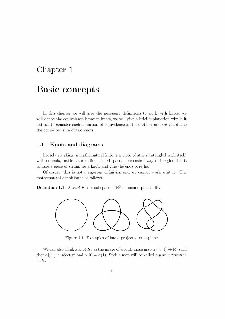
Definition 1.1. A knot K is a subspace of R3 homeomorphic to S1.

Figure 1.1: Examples of knots projected on a plane

We can also think a knotK, as the image of a continuous map α : [0, 1]→ R3 suchthat α|[0,1) is injective and α(0) = α(1). Such a map will be called a parametrizationof K.

1

2 Basic concepts

The examples in Figure 1.1 are not knots, in rigorus terms, they are what we willcall knot diagrams.

Definition 1.2. Let K be a knot, α a parametrization of K and π : R3 → R2 aprojection. Supose there exists t0, t1 ∈ [0, 1) such that π ◦ α(t0) = π ◦ α(t1) (that is,the plane curve π ◦ α has a self intersection). We say that such self intersection istransversal if π ◦α is differentiable at t0 and t1, and the tangent vectors are linearlyindependent.

Definition 1.3. Given a knot K, a projection π : R3 → R2 is a regular projection ofK if:

i) For every point p ∈ π(K), we have |π−1(p)| ≤ 2.

ii) Every self intersection of π(K) is transversal.

The points p ∈ π(K) where |π−1(p)| = 2 are called crossing points.

|A| denotes the cardinality of the set A.For us, a projection of a knot will always be regular unless is otherwise indicated.

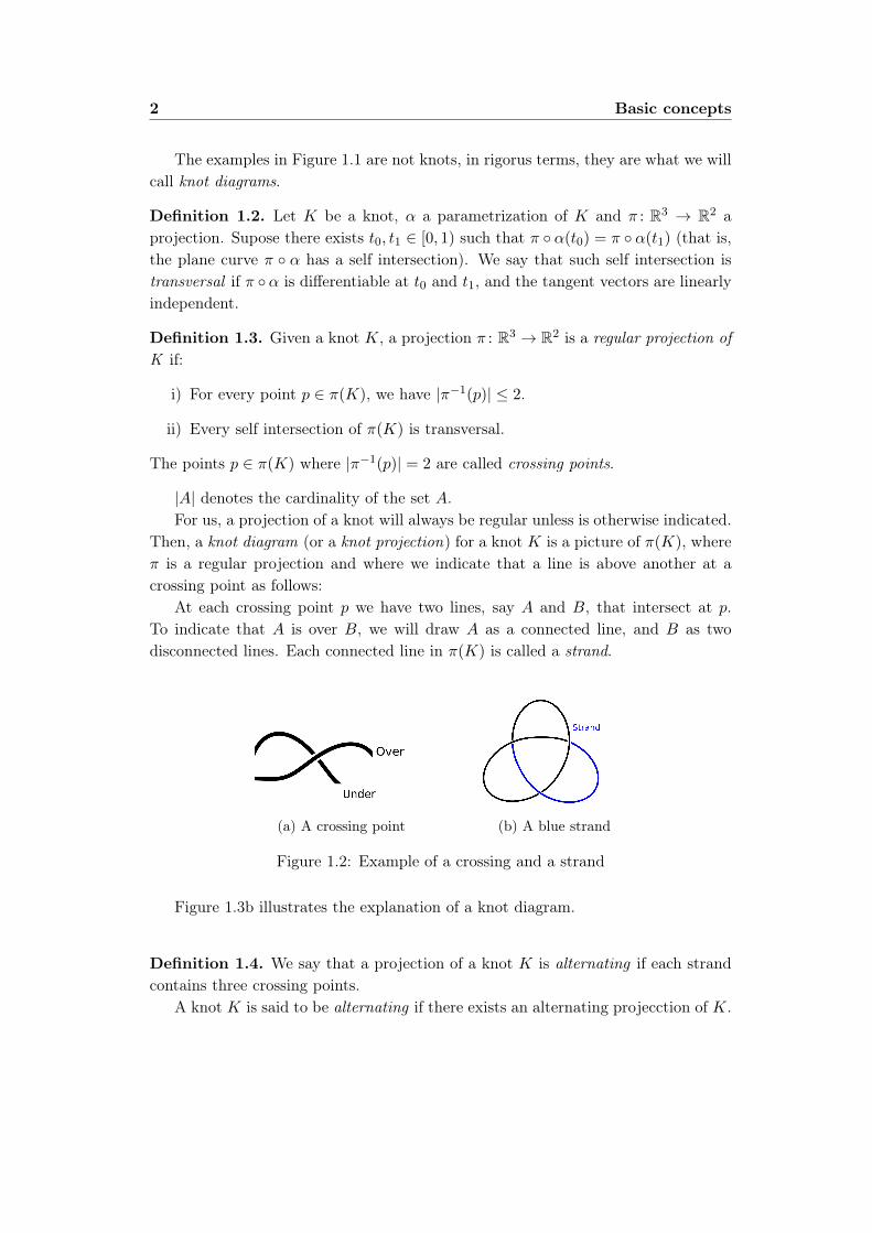
Then, a knot diagram (or a knot projection) for a knot K is a picture of π(K), whereπ is a regular projection and where we indicate that a line is above another at acrossing point as follows:

At each crossing point p we have two lines, say A and B, that intersect at p.To indicate that A is over B, we will draw A as a connected line, and B as twodisconnected lines. Each connected line in π(K) is called a strand.

(a) A crossing point (b) A blue strand

Figure 1.2: Example of a crossing and a strand

Figure 1.3b illustrates the explanation of a knot diagram.

Definition 1.4. We say that a projection of a knot K is alternating if each strandcontains three crossing points.

A knot K is said to be alternating if there exists an alternating projecction of K.

1.2 Equivalence of knots 3

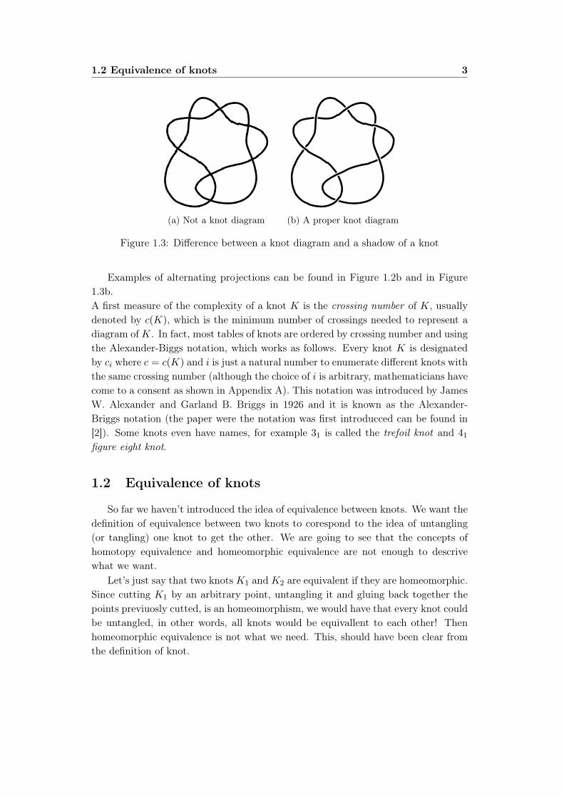
(a) Not a knot diagram (b) A proper knot diagram

Figure 1.3: Difference between a knot diagram and a shadow of a knot

Examples of alternating projections can be found in Figure 1.2b and in Figure1.3b.A first measure of the complexity of a knot K is the crossing number of K, usuallydenoted by c(K), which is the minimum number of crossings needed to represent adiagram ofK. In fact, most tables of knots are ordered by crossing number and usingthe Alexander-Biggs notation, which works as follows. Every knot K is designatedby ci where c = c(K) and i is just a natural number to enumerate different knots withthe same crossing number (although the choice of i is arbitrary, mathematicians havecome to a consent as shown in Appendix A). This notation was introduced by JamesW. Alexander and Garland B. Briggs in 1926 and it is known as the Alexander-Briggs notation (the paper were the notation was first introducced can be found in[2]). Some knots even have names, for example 31 is called the trefoil knot and 41figure eight knot.

1.2 Equivalence of knots

So far we haven’t introduced the idea of equivalence between knots. We want thedefinition of equivalence between two knots to corespond to the idea of untangling(or tangling) one knot to get the other. We are going to see that the concepts ofhomotopy equivalence and homeomorphic equivalence are not enough to descrivewhat we want.

Let’s just say that two knots K1 and K2 are equivalent if they are homeomorphic.Since cutting K1 by an arbitrary point, untangling it and gluing back together thepoints previuosly cutted, is an homeomorphism, we would have that every knot couldbe untangled, in other words, all knots would be equivallent to each other! Thenhomeomorphic equivalence is not what we need. This, should have been clear fromthe definition of knot.

4 Basic concepts

Now, since all knots are homeomorphic to each other, they are also homotopyequivalent. Therefore homotopy equivalence is not good enough either.

What we want is a definition that takes into account what happens to the spacearound the knot while we deform it. This fact of taking into account how the spacearound is deformed is encapsulated with the concept of ambient isotopy.

Definition 1.5. Let X,Y be topological spaces, I = [0, 1], and f, g embeddings fromX to Y . Then, f and g are said to be ambient isotopic if there exists a continuousmap H : Y × I → Y such that:

i) For all t ∈ I, H(·, t) is an homeomorphism from Y to itself.

ii) H(·, 0) = idY .

iii) For all x ∈ X, H(f(x), 1) = g(x).

We say that H is an ambient isotopy between f and g.Here idY denotes the identity map in Y .

With this in mind the definition of eqivalence between knots is the following.

Definition 1.6. Given two knots K1 and K2, we say that K1 and K2 are equivalentand we will write K1 ∼ K2, if there exists an ambient isotopy H : R3 × I → R3

between idR3 : R3 → R3 and an homeomorphismH1 : R3 → R3 such that,H(K1, 1) =

H1(K1) = K2

It is common to write Ht(x) instead of H(x, t).

We are now ready to define the unknot, also known as the trivial knot.

Definition 1.7. We say that a knot K is the unknot (or the trivial knot) if it isequivalent to the subspace {(x, y, z) ∈ R3| x2 + y2 = 1, z = 0}. We will denote theunknot by O

A diagram of the unknot can be found in the first picture of Figure 1.1.We are not interested in all possible knots, we want to avoid knots with rather

complicated structures like those with infinite crossings. To avoid these type of knotswe will work only with tame knots.

Definition 1.8. A polygonal knot K is the union of a finite collection of line seg-ments that are disjoint or that intersect at their end points in such a way that K ishomeomorphic to S1

Definition 1.9. A knot is tame if it is equivalent to a polygonal knot. A knot iswild if it’s not tame.

From now on, all knots considered will be tame unless is otherwise indicated.

1.3 Connected sum 5

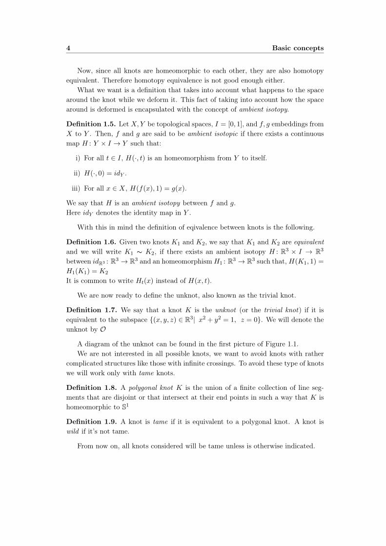
Figure 1.4: A picture of a wild knot

1.3 Connected sum

The idea behind the connected sum of two knots is that of cutting two knots andgluing the ends so that from two knots we get a new one. But, to rigorously definethis operation we first need to define what an oriented knot is.

Definition 1.10. Given a knot K and two homeomorphisms f, g : S1 → K, we saythat an oriented knot is a class of equivalence of the pair

(K, f

), where[(

K, f)]

=[(K, g

)]if and only if deg(f−1 ◦ g) = 1,

where [a] denotes the equivalence class of a and deg(h) denotes the degree of thecontinuous map h : S1 → S1

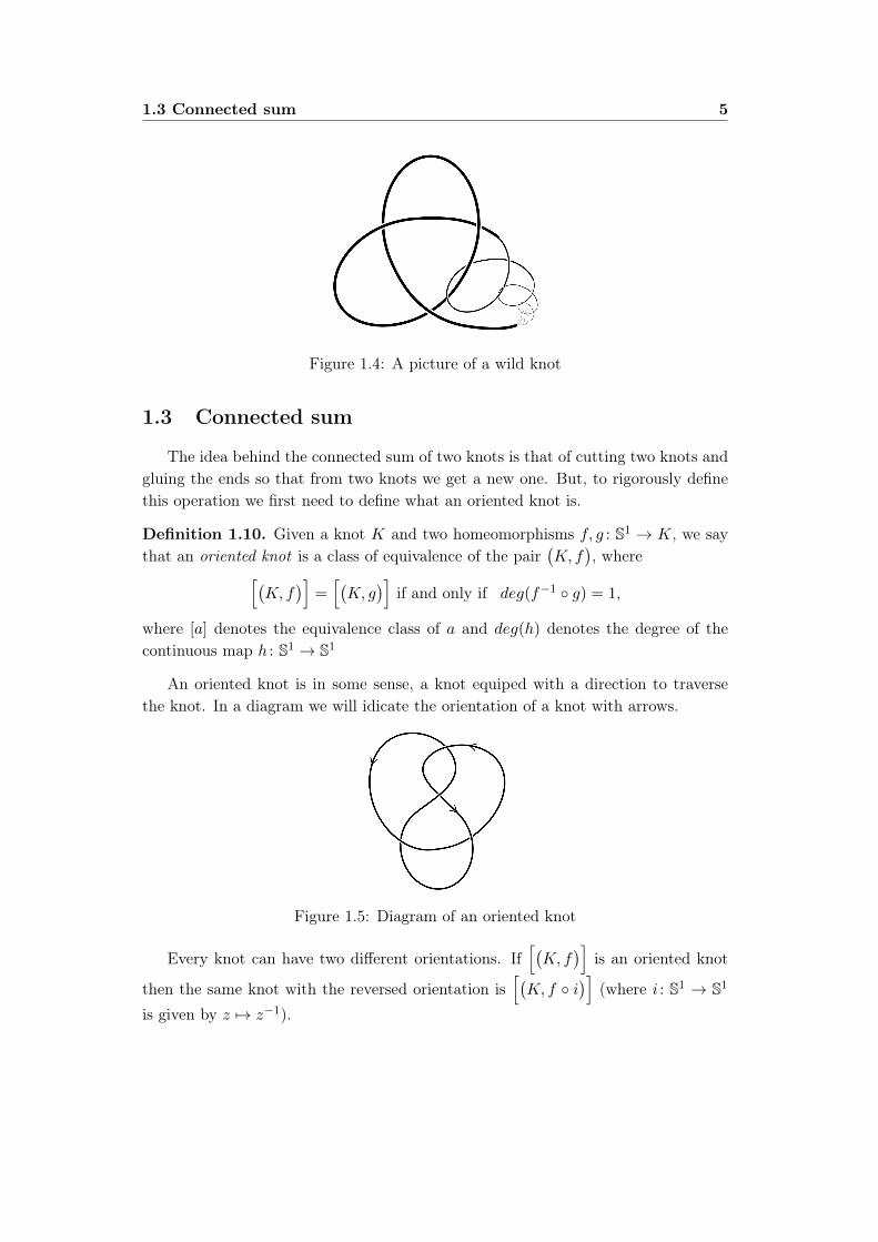
An oriented knot is in some sense, a knot equiped with a direction to traversethe knot. In a diagram we will idicate the orientation of a knot with arrows.

Figure 1.5: Diagram of an oriented knot

Every knot can have two different orientations. If[(K, f

)]is an oriented knot

then the same knot with the reversed orientation is[(K, f ◦ i

)](where i : S1 → S1

is given by z 7→ z−1).

6 Basic concepts

Let’s see that they are in fact two different orientations. What we need to see is thatdeg(f−1 ◦ f ◦ i) 6= 1, but that is clear since

deg(f−1 ◦ f ◦ i) = deg(i) = −1

If K denotes a knot, K+ will denote the same knot with a fixed orientation andwe will denote the same knot with the other orientation by K−. Ocasionally we willnot use the superscript to indicate the orientation, whether we are talking about aknot or an oriented knot will be clear from context.

Equivalence of knots translates to equivalence of oriented knots as follows:

Definition 1.11. Let K+1 and K+

2 be two oriented knots given by the classes[(K1, f1

)],[(K2, f2

)]. Then we say that the oriented knots are equivalent, and

we will write K+1 ∼ K+

2 if there is an ambient isotopy between the two that respectsthe orientation. That is K1 ∼ K2 via the ambient isotopy H, and

[(K2, f2

)]=[(

K2, H1 ◦ f1)], i.e, deg(f−12 ◦ H1 ◦ f1) = 1. We say that a knot K is invertible if

K+ ∼ K−.

As an example, the unknot is invertible. An ambient isotopy Ht between O+

and O− is the one that for every t ∈ I, Ht is a rotation around the x axis of angleπt radians, that is

Ht(x, y, z) = (x, cos(πt)y + sin(πt)z,−sin(πt)y + cos(πt)z) (x, y, z) ∈ R3

We are now ready to define the connected sum of two knots.

Definition 1.12. Let K1,K2 be two oriented knots, and consider their diagrams(given by regular projections π1, π2, respectively) in such a way that they do notintersect. Consider a closed disk D such that:

i) D ∩ π1(K1) and D ∩ π2(K2) have no crossing points and are connected.

ii) |∂D ∩ π1(K1)| = |∂D ∩ π2(K2)| = 2

If needed bring π1(K1) and π2(K2) closer or further apart via an ambient isotopyso that the conditions are satisfied (keeping in mind they cannot intersect!). Thenremove Int(D) from both K1 and K2. Finally, identify each point of ∂D ∩ π1(K1)

with a point of ∂D ∩ π2(K2) in such a way that orientations match up.This process gives us a new diagram. The connected sum of K1 and K2, denotedK1#K2, is an oriented knot with that diagram.

1.3 Connected sum 7

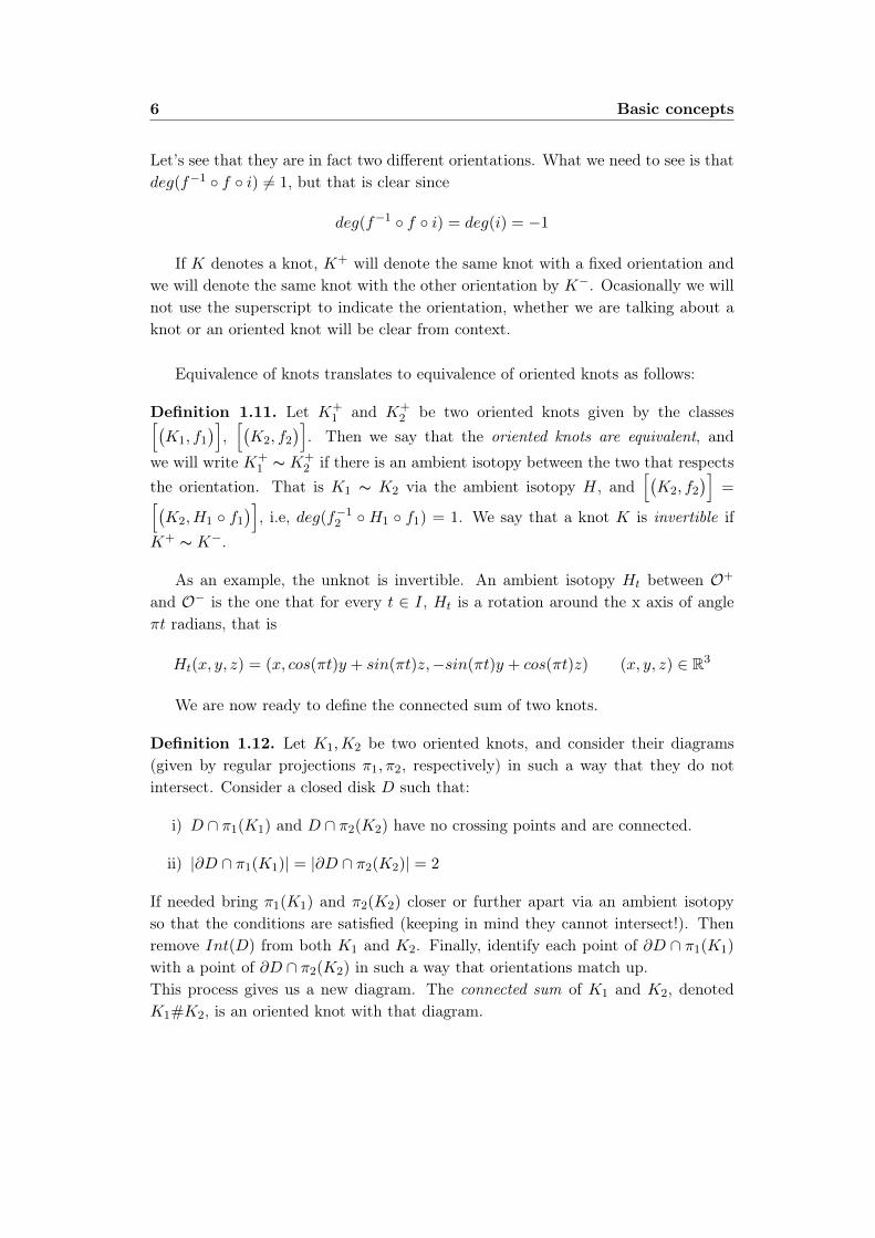
(a) π(K1) ∪ π(K2) ∪D (b)(π(K1) ∪ π(K2)

)\D

(c) K1#K2

Figure 1.6: Connected sum of 51 and 41

The pictures in Figure 1.6 help to understand the process.It is important to notice that if we had not required the knots to be oriented,

then there would be two possible diagrams of K1#K2 that could end up beeing notequivalent!Although the connected sum is a well defined operation between oriented knots, theresult does depend on the orientation of both K1 and K2. But if one of the knots isinvertible, say K1 then K+

1 #K2 ∼ K−1 #K2.

The name connected sum suggests there must be some connection between thisnew operation and the sum of numbers as we know it. The next result shows us theconnection between the two.

Proposition 1.13. The following staments are true:

i) The connected sum is commutative.

ii) The connected sum is associative.

iii) For every oriented knot K, K#O ∼ K. That is, O is the neutral element ofthe connected sum.

Proof.

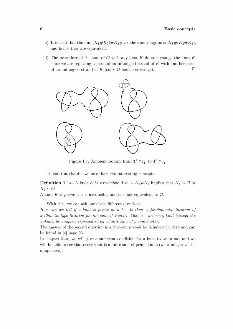
i) Given the sumK1#K2, we can get toK2#K1 via an ambient isotopy by slidingone knot through the other (see an example in Figure 1.7).

8 Basic concepts

ii) It is clear that the sum (K1#K2)#K3 gives the same diagram asK1#(K2#K3),and hence they are equivalent.

iii) The procedure of the sum of O with any knot K doesn’t change the knot Ksince we are replacing a piece of an untangled strand of K with another pieceof an untangled strand of K (since O has no crossings).

Figure 1.7: Ambient isotopy from 3+1 #4+1 to 4+1 #3+1

To end this chapter we introduce two interesting concepts.

Definition 1.14. A knot K is irreducible if K ∼ K1#K2 implies that K1 ∼ O orK2 ∼ O.A knot K is prime if it is irreducible and it is not equivalent to O.

With this, we can ask ourselves different questions:How can we tell if a knot is prime or not? Is there a fundamental theorem ofarithmetic-type theorem for the sum of knots?. That is, can every knot (except theunknot) be uniquely represented by a finite sum of prime knots?.The answer of the second question is a theorem proved by Schubert in 1949 and canbe found in [4] page 96.In chapter four, we will give a sufficient condition for a knot to be prime, and wewill be able to see that every knot is a finite sum of prime knots (we won’t prove theuniqueness).

Chapter 2

Seifert surfaces and genus

In this chapter we first recall some notions regarding surfaces and we will intro-duce the concept of Seifert surfaces of a knot in order to define a knot invariant, thegenus of a knot.

2.1 Topological surfaces

We first recall some definitions about topological surfaces

Definition 2.1. A topological surface is a topological space S such that:

i) S is a Hausdorff space.

ii) S is a second countable space i.e, S has a countable base.

iii) For every p ∈ S, there exists an open neighborhood Up of p, and an homeo-morphism ϕp : Up −→ ϕ(Up) ⊆ R2 where ϕ(Up) is open in R2.

The pair(Up, ϕp

)is called a chart of S. And a family of charts A =

{(Ui, ϕi

)}i∈I

is called an atlas of S if S =⋃

i∈I Ui.

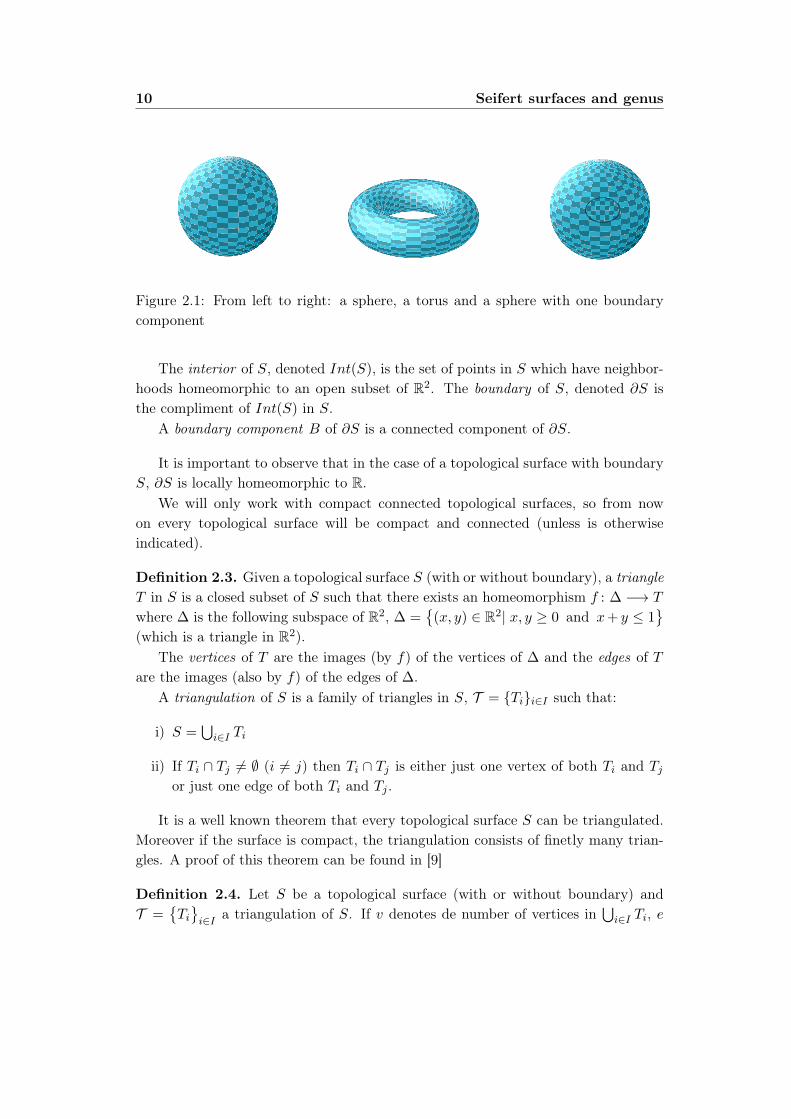
In Figure 2.1 there are two examples of surfaces.

Definition 2.2. A topological surface with boundary is a topological space S suchthat:

i) S is a Hausdorff space.

ii) S is a second countable space i.e, S has a countable base.

iii) For every p ∈ S, there exists an open neighborhood Up of p, and an homeo-morphism ϕp : Up −→ ϕ(Up) ⊆ R2

+ = {(x, y) ∈ R2|y ≥ 0} where ϕ(Up) is openin R2

+.

9

10 Seifert surfaces and genus

Figure 2.1: From left to right: a sphere, a torus and a sphere with one boundarycomponent

The interior of S, denoted Int(S), is the set of points in S which have neighbor-hoods homeomorphic to an open subset of R2. The boundary of S, denoted ∂S isthe compliment of Int(S) in S.

A boundary component B of ∂S is a connected component of ∂S.

It is important to observe that in the case of a topological surface with boundaryS, ∂S is locally homeomorphic to R.

We will only work with compact connected topological surfaces, so from nowon every topological surface will be compact and connected (unless is otherwiseindicated).

Definition 2.3. Given a topological surface S (with or without boundary), a triangleT in S is a closed subset of S such that there exists an homeomorphism f : ∆ −→ T

where ∆ is the following subspace of R2, ∆ ={

(x, y) ∈ R2| x, y ≥ 0 and x+ y ≤ 1}

(which is a triangle in R2).The vertices of T are the images (by f) of the vertices of ∆ and the edges of T

are the images (also by f) of the edges of ∆.A triangulation of S is a family of triangles in S, T = {Ti}i∈I such that:

i) S =⋃

i∈I Ti

ii) If Ti ∩ Tj 6= ∅ (i 6= j) then Ti ∩ Tj is either just one vertex of both Ti and Tjor just one edge of both Ti and Tj .

It is a well known theorem that every topological surface S can be triangulated.Moreover if the surface is compact, the triangulation consists of finetly many trian-gles. A proof of this theorem can be found in [9]

Definition 2.4. Let S be a topological surface (with or without boundary) andT =

{Ti}i∈I a triangulation of S. If v denotes de number of vertices in

⋃i∈I Ti, e

2.1 Topological surfaces 11

the number of edges in⋃

i∈I Ti and f the number of triangles of T (also known asfaces), then the Euler-Poincaré characteristic of T is

χ(T ) = v − e+ f.

It can be proved (using homology groups) that the Euler-Poincaré characteristicis a topological invariant and therefore does not depend on the triangulation, so itis common to talk about the Euler-Poincaré characteristic of a topological surfaceinstead of the characteristic of a triangulation of that surface. We will write χ(S) todenote the Euler-Poincaré characteristic of the surface S.

In the same way that there is a notion of connected sum for knots, there is alsoa notion of connected sum of topological surfaces.

Definition 2.5. Given two surfaces S1 and S2. Let D1 be a closed disk in a chart ofS1 and D2 a closed disk in a chart of S2. Let h : ∂D1 −→ ∂D2 be a homeomorphism.

Then the connected sum of S1 and S2 is another topological surface defined as

S1#S2 = (S1 \◦D1) t (S2 \

◦D2)/ ∼

where for all x ∈ ∂D1 and all y ∈ ∂D2, x ∼ y if and only if y = h(x)

Proposition 2.6. Let S1 and S2 be two topological surfaces (with or without bound-ary) then the following equation holds:

χ(S1#S2) = χ(S1) + χ(S2)− 2

Proof. Let T1 and T2 be two triangulations of S1 and S2 (respectively) and vi, ei andfi the number vertices, edges and faces of Ti respectively (with i = 1, 2).

We can think of S1#S2 as the surface resulting of removing a face of a triangleT1 of S1 and a face of a triangle T2 of S2 and then identifying each edge of T1 with anedge of T2 (we can do this because every closed triangle is homeomorphic to a closeddisk). From this, it is clear that there is a triangulation T of S1#S2 such that thenumber vertices of T are v1 + v2 − 3, the number of edges of T are e1 + e2 − 3 andthe number of faces of T are f1 + f2− 2. Therefore the Euler-Poincaré characteristicof S1#S2 is:

χ(S1#S2) = v1 + v2 − 3− e1 − e2 + 3 + f1 + f2 − 2 = χ(S1) + χ(S2)− 2.

We now recall the calssification theorem of compact connected surfaces.


Theorem 2.7 (Classification of compact connected surfaces). Every compact con-nected topological surface is homeomorphic to one and only one of the followingsurfaces:

i) S2

ii) gT2 = T2#g· · ·#T2

iii) #gP2R = #P2

R#g· · ·#P2

R

Where g ∈ N \ {0}. S2 denotes the two dimensional sphere, T2 the two dimensionaltorus and P2

R the real projective plane.

A proof of this theorem can be found in [6]

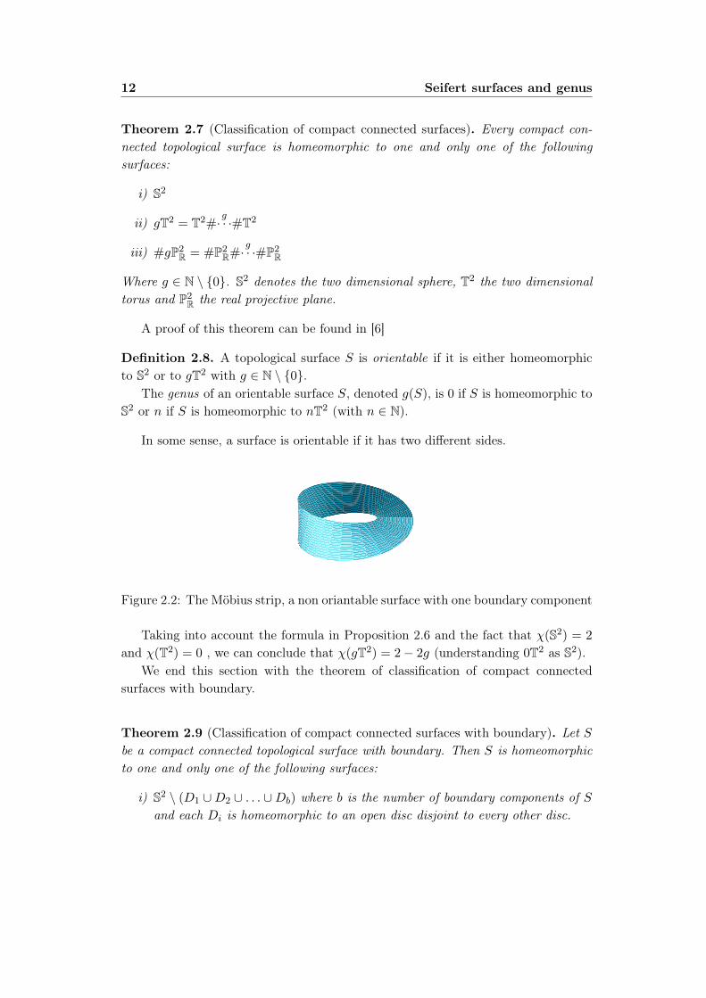
Definition 2.8. A topological surface S is orientable if it is either homeomorphicto S2 or to gT2 with g ∈ N \ {0}.

The genus of an orientable surface S, denoted g(S), is 0 if S is homeomorphic toS2 or n if S is homeomorphic to nT2 (with n ∈ N).

In some sense, a surface is orientable if it has two different sides.

Figure 2.2: The Möbius strip, a non oriantable surface with one boundary component

Taking into account the formula in Proposition 2.6 and the fact that χ(S2) = 2

and χ(T2) = 0 , we can conclude that χ(gT2) = 2− 2g (understanding 0T2 as S2).We end this section with the theorem of classification of compact connected

surfaces with boundary.

Theorem 2.9 (Classification of compact connected surfaces with boundary). Let Sbe a compact connected topological surface with boundary. Then S is homeomorphicto one and only one of the following surfaces:

i) S2 \ (D1 ∪D2 ∪ . . . ∪Db) where b is the number of boundary components of Sand each Di is homeomorphic to an open disc disjoint to every other disc.

2.1 Topological surfaces 13

ii) gT2 \ (D1 ∪D2 ∪ . . .∪Db) where b is the number of boundary components of Sand each Di is homeomorphic to an open disc disjoint to every other disc.

iii) nP2R \ (D1 ∪D2 ∪ . . . ∪Db) where b is the number of boundary components of

S and each Di is homeomorphic to an open disc disjoint to every other disc.

Proof. Let S be a compact connected topological surface with boundary. Since ∂Sis closed in S and S is both Hausdorff and compact, it follows that ∂S is compact.From this, we know that ∂S has a finite number of boundary components, say b.Each boundary component is closed and therefore also compact. And since everyboundary component is compact, connected and locally homeomorphic to R it followsthat every boundary component is homeomorphic to S1.

Now for every boundary component Ci consider a closed disk Di and considera homeomorphism hi : Ci −→ ∂Di (i = 1, . . . , b). Finally consider the topologicalspace S = S tD1 t . . . tDb/ ∼ where for every pair of points x ∈ Ci and y ∈ ∂Di,x ∼ y if and only if y = hi(x). It is clear from the construction that S is Hausdorff,has a countable base, is compact and connected. What it may not be obvious at firstglance is that it is locally homeomorphic to an open set of R2. Let us see that it isindeed the case.

Take a point p ∈ S. If p ∈ Int(S)∪Int(D1)∪. . .∪Int(Db) then by definition p hasan open neighborhood homeomorphic to an open set of R2. Supose then that p ∈ Ci

for a particular i ≤ b. Since Ci is identyfied with ∂Di we can think of p as beeingboth in Ci and ∂Di. Because p ∈ Ci and p ∈ ∂Di there exist two open neighborhoodsU, V of p with U ⊆ S and V ⊆ Di and two homeomorphism f : U −→ f(U) ⊆ R2

+

and g : V −→ g(V ) ⊆ R2+. Without loss of generality we can supose that f(p) = g(p)

(if nedded bring g(p) to f(p) with a translation). Choose a neighborhood I of p inCi such that I ⊆ U and I ⊆ V . Consider now U ′ = f(Int(U)) ∪ f(I) and V ′ =

g(Int(V ))∪g(I), then f−1(U ′) and g−1(V ′) are open in S and Di (respectively) andthey overlap only in I. Therefore W = f−1(U ′) ∪ g−1(V ′) is an open neighborhoodof p homeomorphic to an open subset of R2.

With all of this, S is a compact connected topological surface and by Theorem2.7 we have that S is homeomorphic to either S2, gT2 or nP2

R via H. So S ishomeomorphic to either S2 \ (H(D1) ∪ H(D2) ∪ . . . ∪ H(Db)) , gT2 \ (H(D1) ∪H(D2) ∪ . . . ∪H(Db)) or nP2

R \ (H(D1) ∪H(D2) ∪ . . . ∪H(Db)).

With the previous theorem in mind it is easy to see that for every surface S withboundary, χ(S) = χ(S) + b where b is the number of boundary components of S.

Definition 2.10. Given a surface with boundary S, we say that S is orientable if Sis orientable.

The genus of S (denoted g(S)) is the genus of S.


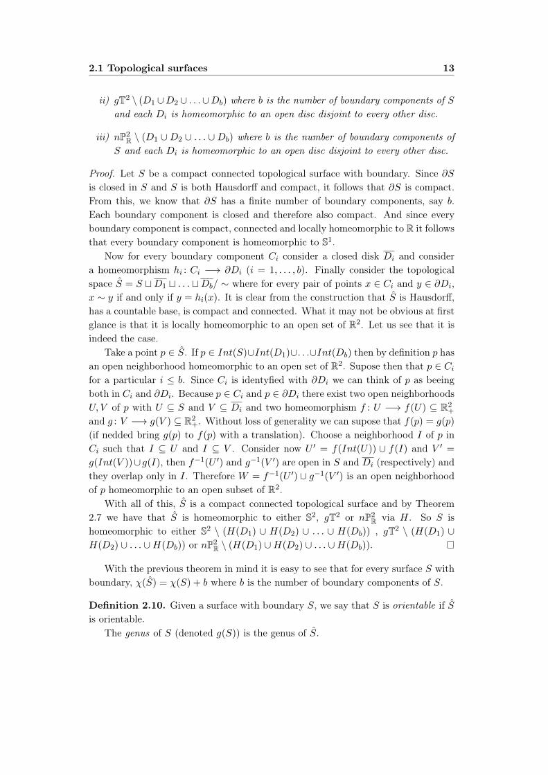
Figure 2.3: A torus with two boundary components

In the end, for every orientable surface with boundary S we have the followingformula (which will be of use later on)

χ(S) = 2− 2g(S)− b (2.1)

2.2 Seifert surfaces

Now that we are familiarized with orientable surfaces with boundary we are readyto define the concept of Seifert surface.

Definition 2.11. Given a knot K, a Seifert surface for K is an orientable compactconnected surface S ⊂ R3 such that ∂S = K. We will also say that S is a Seifertsurface spanning K.

It is not clear from the definition that such surfaces must exist, even less clear ishow to construct them (if they even exist of course). The next theorem proves theexistence of Seifert surfaces and gives a way to construct them.

Theorem 2.12. Given a knot K, there exists a Seifert surface S spanning K.

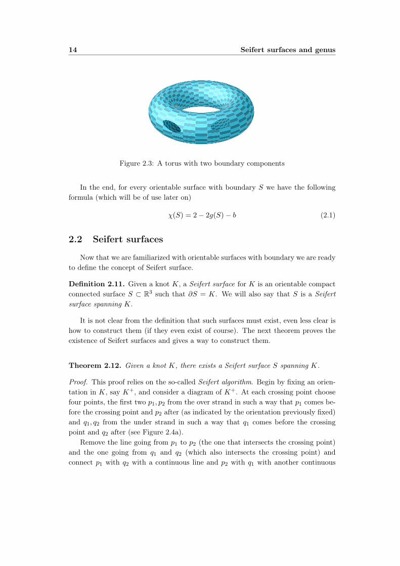
Proof. This proof relies on the so-called Seifert algorithm. Begin by fixing an orien-tation in K, say K+, and consider a diagram of K+. At each crossing point choosefour points, the first two p1, p2 from the over strand in such a way that p1 comes be-fore the crossing point and p2 after (as indicated by the orientation previously fixed)and q1, q2 from the under strand in such a way that q1 comes before the crossingpoint and q2 after (see Figure 2.4a).

Remove the line going from p1 to p2 (the one that intersects the crossing point)and the one going from q1 and q2 (which also intersects the crossing point) andconnect p1 with q2 with a continuous line and p2 with q1 with another continuous

2.2 Seifert surfaces 15

(a) (b)

Figure 2.4: Choosing points in a crossing to create Seifert circles

line that does not intersect the previus one (see Figure 2.4b). The result is a diagramof disjoint loops with an induced orientation, these loops are called Seifert circles.

Now consider each Seifert circle c contained in a plane z = zc in R3, where zcis different for every Seifert circle (thus every Seifert circle is at a different height).Continue by considering, for each Seifert circle c, a disc (or subset homeomorphic toa disc) in z = zc whose boundary is c (the process is similar to that of the proof ofTheorem 2.9). Finally connect each disc with a twisted band begining in the linepreviosly attached to p1 and q2 and ending in the line previously attached to p2 andq1. Connect it in such a way that the orientations on the boundries of the discsmatch up, that is p1 must be connected with a line (an "edge" of the band) to p2that does not contain q1 and q2 (and the same must happen with q1 and q2).

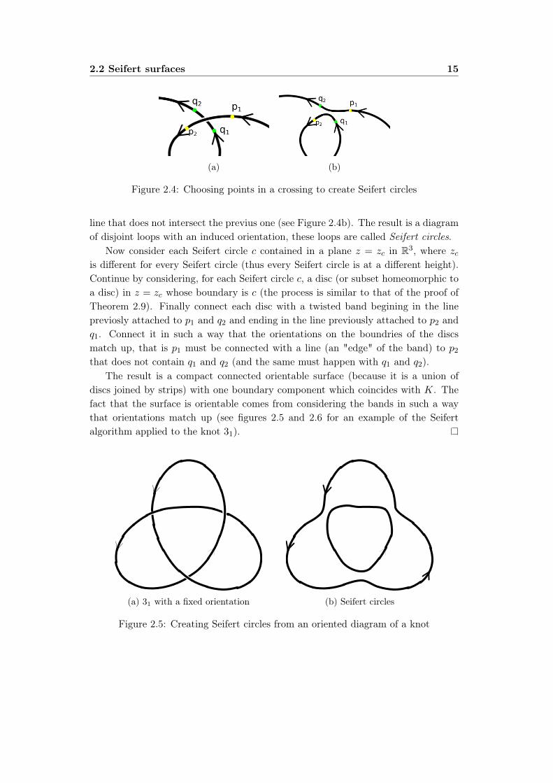
The result is a compact connected orientable surface (because it is a union ofdiscs joined by strips) with one boundary component which coincides with K. Thefact that the surface is orientable comes from considering the bands in such a waythat orientations match up (see figures 2.5 and 2.6 for an example of the Seifertalgorithm applied to the knot 31).

(a) 31 with a fixed orientation (b) Seifert circles

Figure 2.5: Creating Seifert circles from an oriented diagram of a knot


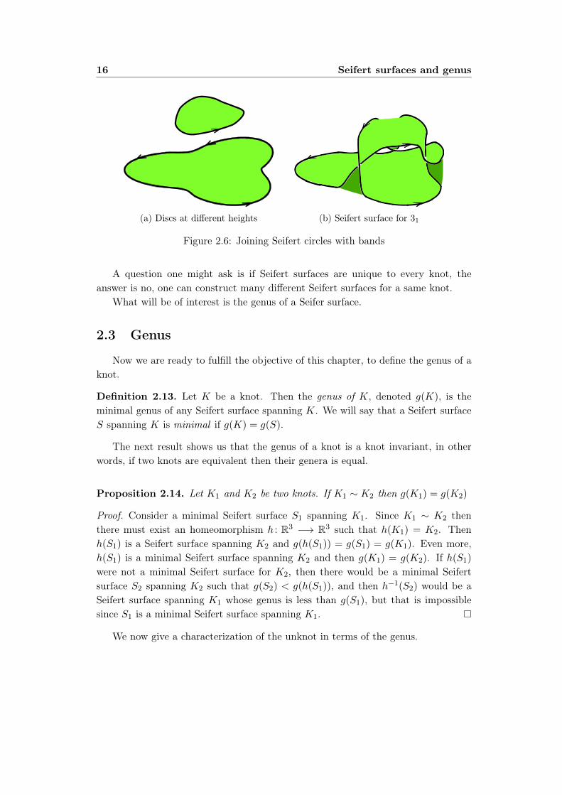
(a) Discs at different heights (b) Seifert surface for 31

Figure 2.6: Joining Seifert circles with bands

A question one might ask is if Seifert surfaces are unique to every knot, theanswer is no, one can construct many different Seifert surfaces for a same knot.

What will be of interest is the genus of a Seifer surface.

2.3 Genus

Now we are ready to fulfill the objective of this chapter, to define the genus of aknot.

Definition 2.13. Let K be a knot. Then the genus of K, denoted g(K), is theminimal genus of any Seifert surface spanning K. We will say that a Seifert surfaceS spanning K is minimal if g(K) = g(S).

The next result shows us that the genus of a knot is a knot invariant, in otherwords, if two knots are equivalent then their genera is equal.

Proposition 2.14. Let K1 and K2 be two knots. If K1 ∼ K2 then g(K1) = g(K2)

Proof. Consider a minimal Seifert surface S1 spanning K1. Since K1 ∼ K2 thenthere must exist an homeomorphism h : R3 −→ R3 such that h(K1) = K2. Thenh(S1) is a Seifert surface spanning K2 and g(h(S1)) = g(S1) = g(K1). Even more,h(S1) is a minimal Seifert surface spanning K2 and then g(K1) = g(K2). If h(S1)

were not a minimal Seifert surface for K2, then there would be a minimal Seifertsurface S2 spanning K2 such that g(S2) < g(h(S1)), and then h−1(S2) would be aSeifert surface spanning K1 whose genus is less than g(S1), but that is impossiblesince S1 is a minimal Seifert surface spanning K1.

We now give a characterization of the unknot in terms of the genus.

2.3 Genus 17

Theorem 2.15. Let K be a knot. Then K is the unknot if and only if g(K) = 0.

Proof. If K is the unknot, then a disc with boundary K is clearly a minimal Seifertsurface spanning K. And since a disc is a sphere with one boundary component itfollows that g(K) = g(S2) = 0.

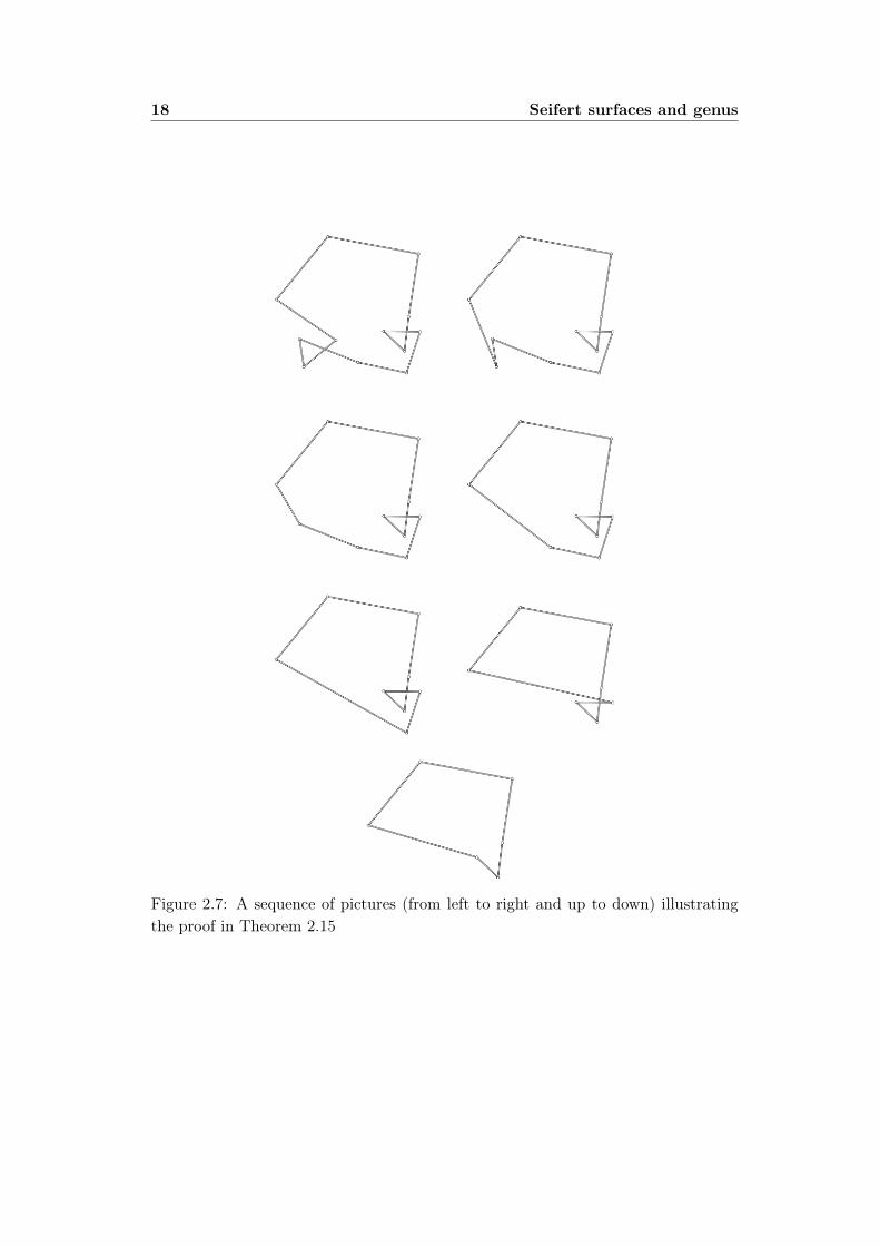
Conversely, if K is a knot with g(K) = 0, then there is a minimal Seifert surfaceS of K with g(S) = 0, and so S is a sphere with one boundary component, i.e, adisc. We can view K in S as a poligonal knot and the vertices of K as verticesof a triangulation T of S. Now for each vertex in the boundary of S if the vertexis attatched to only two edges, we remove those two edges and end up with theremaining edge of the triangle (this can be viewed as pushing the vertex inside thetriangle along with its edges, which is an ambient isotopy). This process is doneuntil we end up with just on triangle (the fact that we can do that is because T is infact a triangulation of a disc). Since the boundary of a triangle and O are ambientisotopic we have that K ∼ O (see an example in Figure 2.7).


Figure 2.7: A sequence of pictures (from left to right and up to down) illustratingthe proof in Theorem 2.15

Chapter 3

Minimal genus theorem for alter-nating knots

In Chapter 2 we have seen that the genus of a knot is a knot invariant. But if wetry to calculate the genus of a knot K from a Seifert surface obtained using Seifert’salgorithm, we end up with an upper bound for g(K) and not necessarily g(K). Thenhow do we actually calculate the genus of a knot?

In this chapter we will prove that applying Seifert’s algorithm to an alternatingprojection of a knot K does in fact yield a minimal Seifert surface for K.

3.1 The theorem

The proof we are presenting is an adaptation of a proof presented by David Gabai(a mathematician at Princeton University) in an article of the Duke MathematicalJournal. In his article, David Gabai proves the result for alternating links (linksessentially are finite collection of knots tangled between each other). Since we areonly interested in knots, we have adapted the proof to our case. The complete proofcan be found in [5].

To prove the theorem we first need the following result:

Lemma 3.1. Let K be a knot. If S is a Seifert surface for K, which is not minimal,then there exists a Seifert surface T for K such that Int(S) ∩ Int(T ) = ∅ andg(T ) < g(S).

It is important to remark that in his article David Gabai writes χ(S′) > χ(S)

instead of g(S′) < g(S). The two facts are equivalent if one considers formula (2.1)from Section 1 Chapter 2.

We are not going to prove this lemma here since it relies on the notions of tubularneighborhoods, intersection numbers and how these concepts are related to homology

19

20 Minimal genus theorem for alternating knots

groups, and this falls out of the scope of our project.

Theorem 3.2. Let K be an alternating knot. If S is a Seifert surface for K obtainedby applying Seifert’s algorithm to an alternating projection of K then S is a minimalSeifert surface for K.

Proof. Let K be an alternating knot. Consider an alternating projection of K (givenby a regular projection π) with n crossings and the Seifert surface S obtained throughSeifert’s algorithm. We are going to prove the theorem by induction on n.

Base case: n = 1

On one hand, since the projection has only one crossing, by applying an ambientisotopy to K we can remove the crossing (by twisting the knot) then K ∼ O, and sog(K) = 0.

On the other hand, S is two discs joined by a twisted band. By performing anhomeomorphism (the one induced by the ambient isotopy above is enough) we havethat S is homeomorphic to a disc, and thus g(S) = 0.

So in the case n = 1 Seifert’s algorithm applied to an alternating knot yields aminimal Seifert surface.

Induction stepBegin by considering an alternating projection of K with n+ 1 crossings, and let

S be the Seifert surface obtained by applying Seifert’s algorithm to that projection.Suppose S is not minimal.

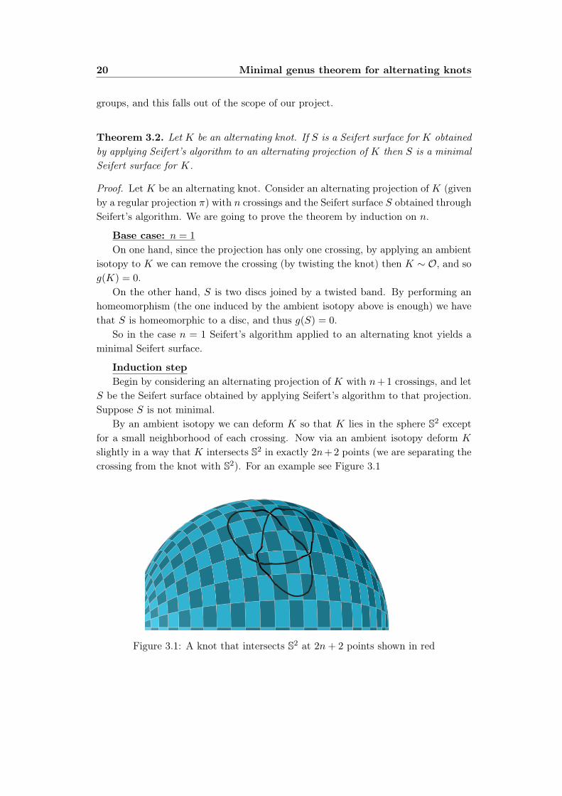
By an ambient isotopy we can deform K so that K lies in the sphere S2 exceptfor a small neighborhood of each crossing. Now via an ambient isotopy deform K

slightly in a way that K intersects S2 in exactly 2n+ 2 points (we are separating thecrossing from the knot with S2). For an example see Figure 3.1

Figure 3.1: A knot that intersects S2 at 2n+ 2 points shown in red

3.2 Examples 21

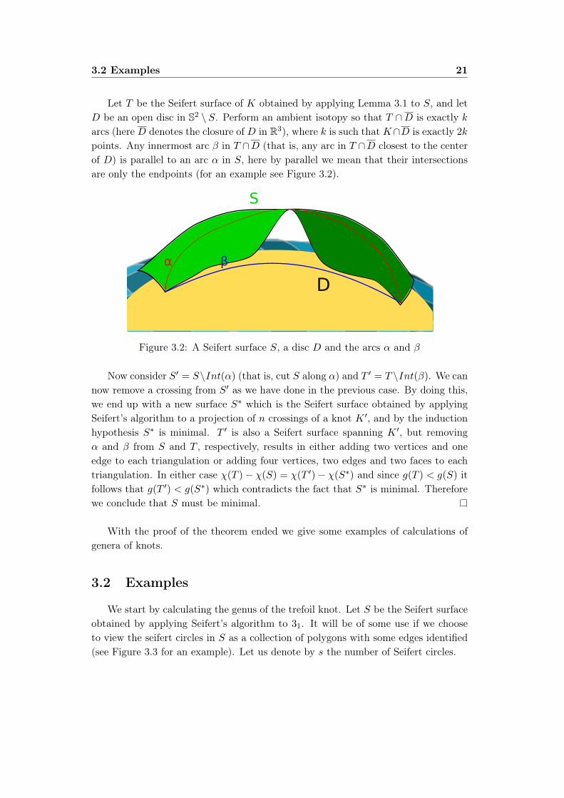
Let T be the Seifert surface of K obtained by applying Lemma 3.1 to S, and letD be an open disc in S2 \ S. Perform an ambient isotopy so that T ∩D is exactly karcs (here D denotes the closure of D in R3), where k is such that K∩D is exactly 2k

points. Any innermost arc β in T ∩D (that is, any arc in T ∩D closest to the centerof D) is parallel to an arc α in S, here by parallel we mean that their intersectionsare only the endpoints (for an example see Figure 3.2).

S

βα

D

Figure 3.2: A Seifert surface S, a disc D and the arcs α and β

Now consider S′ = S\Int(α) (that is, cut S along α) and T ′ = T \Int(β). We cannow remove a crossing from S′ as we have done in the previous case. By doing this,we end up with a new surface S∗ which is the Seifert surface obtained by applyingSeifert’s algorithm to a projection of n crossings of a knot K ′, and by the inductionhypothesis S∗ is minimal. T ′ is also a Seifert surface spanning K ′, but removingα and β from S and T , respectively, results in either adding two vertices and oneedge to each triangulation or adding four vertices, two edges and two faces to eachtriangulation. In either case χ(T )− χ(S) = χ(T ′)− χ(S∗) and since g(T ) < g(S) itfollows that g(T ′) < g(S∗) which contradicts the fact that S∗ is minimal. Thereforewe conclude that S must be minimal.

With the proof of the theorem ended we give some examples of calculations ofgenera of knots.

3.2 Examples

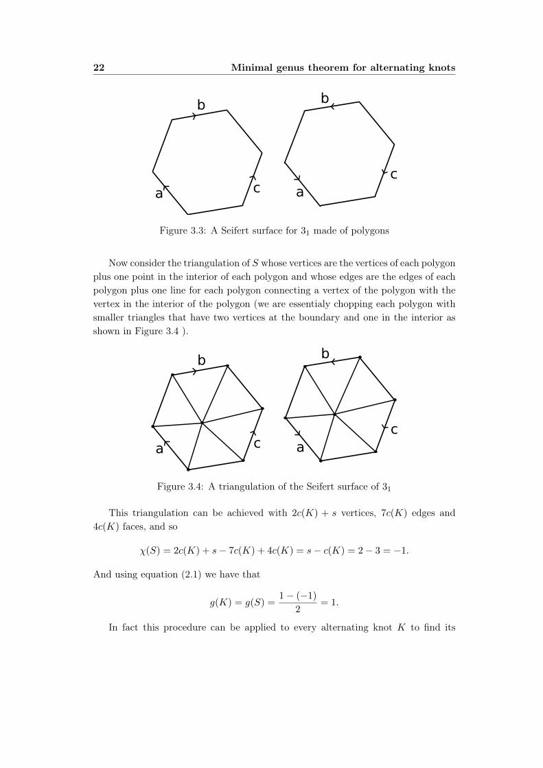
We start by calculating the genus of the trefoil knot. Let S be the Seifert surfaceobtained by applying Seifert’s algorithm to 31. It will be of some use if we chooseto view the seifert circles in S as a collection of polygons with some edges identified(see Figure 3.3 for an example). Let us denote by s the number of Seifert circles.


a

b

c a

b

c

Figure 3.3: A Seifert surface for 31 made of polygons

Now consider the triangulation of S whose vertices are the vertices of each polygonplus one point in the interior of each polygon and whose edges are the edges of eachpolygon plus one line for each polygon connecting a vertex of the polygon with thevertex in the interior of the polygon (we are essentialy chopping each polygon withsmaller triangles that have two vertices at the boundary and one in the interior asshown in Figure 3.4 ).

a

b

c a

b

c

Figure 3.4: A triangulation of the Seifert surface of 31

This triangulation can be achieved with 2c(K) + s vertices, 7c(K) edges and4c(K) faces, and so

χ(S) = 2c(K) + s− 7c(K) + 4c(K) = s− c(K) = 2− 3 = −1.

And using equation (2.1) we have that

g(K) = g(S) =1− (−1)

2= 1.

In fact this procedure can be applied to every alternating knot K to find its

3.2 Examples 23

genus, giving the following formula:

g(K) = g(S) =1− χ(S)

2=

1 + c(K)− s2

, (3.1)

where s is the number of Seifert circles. Moreover for any knot K we have thefollowing inequality:

g(K) ≤ 1 + c(K)− s2

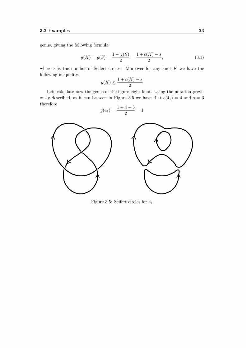
Lets calculate now the genus of the figure eight knot. Using the notation previ-ously described, as it can be seen in Figure 3.5 we have that c(41) = 4 and s = 3

thereforeg(41) =

1 + 4− 3

2= 1

Figure 3.5: Seifert circles for 41


Chapter 4

Genus additivity and aplications

In this chapter we are going to see that the genus of a knot is additive withrespect to the connected sum of knots. This property will allow us to answer thequestions asked in Chapter 1 and thus conclude with one of the objectives of theproject.

4.1 Additivity

Theorem 4.1. For any two knots K1 and K2, g(K1#K2) = g(K1) + g(K2)

Proof. We will prove the theorem in two parts, the first one will prove g(K1#K2) ≤g(K1) + g(K2) and the second one g(K1#K2) ≥ g(K1) + g(K2).

Part 1: g(K1#K2) ≤ g(K1) + g(K2)

Consider K1 and K2 in such a way that there is a plane that separetes them andconsider S1 and S2 two minimal Seifert surfaces spanning K1 and K2 respectively(S1 and S2 also separeted by the plane). Give orientations to both K1 and K2 andconsider K1#K2 making sure that K1#K2 does not intersect Int(S1) nor Int(S2).

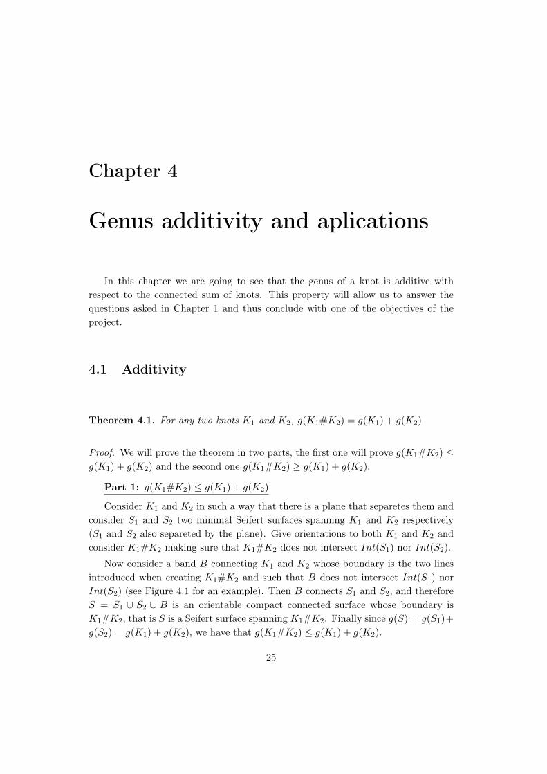
Now consider a band B connecting K1 and K2 whose boundary is the two linesintroduced when creating K1#K2 and such that B does not intersect Int(S1) norInt(S2) (see Figure 4.1 for an example). Then B connects S1 and S2, and thereforeS = S1 ∪ S2 ∪ B is an orientable compact connected surface whose boundary isK1#K2, that is S is a Seifert surface spanning K1#K2. Finally since g(S) = g(S1)+

g(S2) = g(K1) + g(K2), we have that g(K1#K2) ≤ g(K1) + g(K2).

25

26 Genus additivity and aplications

(a) Disjoint seifert surfaces of 31 (b) Seifert surface for 31#31

Figure 4.1: Connecting two Seifert surfaces with a band

Part 2: g(K1) + g(K2) ≤ g(K1#K2)

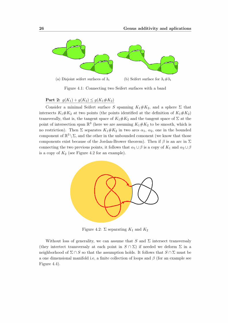
Consider a minimal Seifert surface S spanning K1#K2, and a sphere Σ thatintersects K1#K2 at two points (the points identified at the definition of K1#K2)transverally, that is, the tangent space of K1#K2 and the tangent space of Σ at thepoint of intersection span R3 (here we are assuming K1#K2 to be smooth, which isno restriction). Then Σ separates K1#K2 in two arcs α1, α2, one in the boundedcomponent of R3 \Σ, and the other in the unbounded comonent (we know that thosecomponents exist because of the Jordan-Brower theorem). Then if β is an arc in Σ

connecting the two previous points, it follows that α1 ∪ β is a copy of K1 and α2 ∪ βis a copy of K2 (see Figure 4.2 for an example).

Figure 4.2: Σ separating K1 and K2

Without loss of generality, we can assume that S and Σ intersect transversaly(they intertect transversaly at each point in S ∩ Σ) if needed we deform Σ in aneighborhood of Σ ∩ S so that the assumption holds. It follows that S ∩ Σ must bea one dimensional manifold i.e, a finite collection of loops and β (for an example seeFigure 4.4).

4.1 Additivity 27

Figure 4.3: Σ ∩ S a collection of loops (in green) and β (in blue)

The idea now is to do a sequence of deformations of S for each loop in a way thatthe genus does not change but at each step S ∩Σ has fewer loops to finally concludethat S ∩ Σ = β.

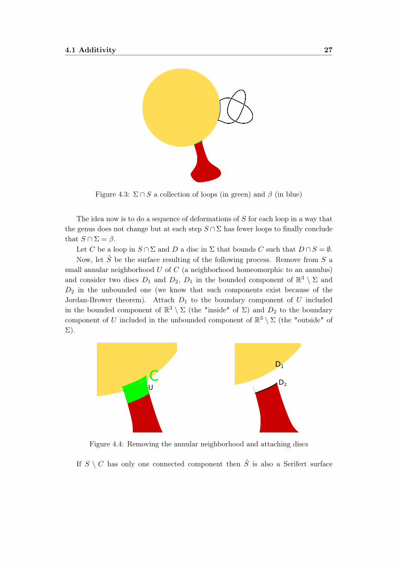
Let C be a loop in S ∩Σ and D a disc in Σ that bounds C such that D ∩ S = ∅.Now, let S be the surface resulting of the following process. Remove from S a

small annular neighborhood U of C (a neighborhood homeomorphic to an annulus)and consider two discs D1 and D2, D1 in the bounded component of R3 \ Σ andD2 in the unbounded one (we know that such components exist because of theJordan-Brower theorem). Attach D1 to the boundary component of U includedin the bounded component of R3 \ Σ (the "inside" of Σ) and D2 to the boundarycomponent of U included in the unbounded component of R3 \ Σ (the "outside" ofΣ).

D1

D2CU

Figure 4.4: Removing the annular neighborhood and attaching discs

If S \ C has only one connected component then S is also a Serifert surface


spanning K1#K2 whose genus is less than the genus of S, but that is impossiblesince S is minimal. Then S \ C has more than one connected component. Considerthe connected component fo S that containsK1#K2, this is a Seifert surface spanningK1#K2 whose genus is the same as S and that intersects Σ in fewer loops (at leastwe have eliminated C).

By repeating this process a finite number of times (because the number of loopsis finite), we end up with a Seifert surface S∗ for K1#K2 that intersects at Σ only atβ. Then if we denote B1 the bounded component of R3 \ Σ and B2 the unboundedone, we have that S∗1 = (B1∩S∗)∪β is a Seifert surface for K1 and S∗2 = (B2∩S∗)∪βis a Seifert surface for K2 and so we have

g(K1) + g(K2) ≤ g(S∗1) + g(S∗2) = g(S∗) = g(K1#K2)

and thus we complete the proof.

4.2 Aplications

Theorem 4.1 has a good amount of impications which we now state and prove.

Corollary 4.2. Given any two knots K1 and K2, then if K1#K2 ∼ O then K1 ∼K2 ∼ O.

Proof. By Theorem 4.1 we have that 0 = g(K1#K2) = g(K1) + g(K2) and sinceg(K) ≥ 0 for any knot K, it must be that g(K1) = g(K2) = 0 and by Theorem 2.15we have that K1 ∼ K2 ∼ O.

This tells us that the unknot is not a connected sum of two non trivial knots(intuitively a rope with two knots tied in it where the ends are joined, will onlyuntangle if the rope is cutted).

Corollary 4.3. For every knot K if g(K) = 1 then K is a prime knot

Proof. If K = K1#K2 then by Theorem 4.1 either g(K1) = 0 or g(K2) = 0 and theneither K1 ∼ O or K2 ∼ O.

Corollary 4.4. Every knot K is a sum of at least g(K) prime knots, and thus afinite sum of prime knots.

Proof. IfK is prime then the result is obvious. Suppose then thatK is not prime. Bydefinition there exist K1,K2 both different from the unknot such that K = K1#K2

and from Theorem 4.1 it follows that g(K1), g(K2) < g(K). Now we do the sameprocess for K1 and K2 in order to end up with new knots (assuming K1 and K2

4.2 Aplications 29

are no both prime knots) whose connected sum is K. By repeating this process weconclude that K is a sum of prime knots. The fact that the number of prime knotsis at most g(K) is immediate from the additivity of the genus and the fact that allprime knots have genus greater or equal than 1.

Corollary 4.5. There are non trivial knots with arbitrarily large crossing number.

Proof. For any knot K, by equation (3.1), since the number of seifert circles willalways be at least 1 we have that

g(K) ≤ c(K)

2.

Let K be a non trivial knot, and Kn the sum of n copies of K. Then

n ≤ g(Kn) ≤ c(Kn)

2

and as n approaches infinity so does c(Kn).


Appendices

31

Appendix A

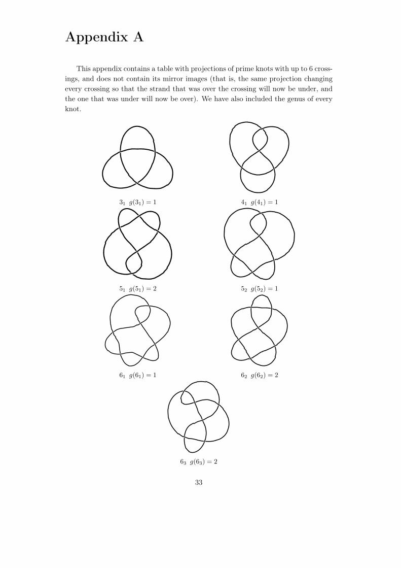
This appendix contains a table with projections of prime knots with up to 6 cross-ings, and does not contain its mirror images (that is, the same projection changingevery crossing so that the strand that was over the crossing will now be under, andthe one that was under will now be over). We have also included the genus of everyknot.

31 g(31) = 1 41 g(41) = 1

51 g(51) = 2 52 g(52) = 1

61 g(61) = 1 62 g(62) = 2

63 g(63) = 2

33

34

Bibliography

[1] Colin C. Adams, The Knot Book: An Elementary Introduction to the Mathe-matical Theory of Knots. W.H. Freeman and Company, New York, 1994.

[2] J. W. Alexander, G. B. Briggs, On Types of Knotted Curves, Annals of Math-ematics.

[3] M.A: Armstrong, Basic Topology, Undergraduate Texts in Mathematics,Springer-Verlag, 1983.

[4] G. Burde, H. Zieschang, Knots, Walter de Gruyter & Co., Berlin, 1985.

[5] Gabai, David. Genera of the alternating links, Duke Mathematical Journal. J.53 (1986), no. 3, 677–681. doi:10.1215/S0012-7094-86-05336-6.

[6] Kosniowski, C. (1980). A First Course in Algebraic Topology. Cambridge: Cam-bridge University Press.

[7] The KnotPlot Site, http://knotplot.com/

[8] W.B.R. Lickorish, An Introduction to Knot Theory, Springer-Verlag New York,1997.

[9] Edwin E. Moise Geometric Topology in Dimensions 2 and 3. Springer Sci-ene+Busines Medis, LLC.

[10] J. Roberts, Knots Knotes, unpublished lecture notes, 2010, http://math.ucsd.edu/ justin/papers.html.

[11] D. Rolfsen, Knots and Links, AMS Chelsea Publishing, 2003.

35

Documents

Knots and Seifert surfaces