KAM theory without action-angle variables

INSTITUTE OF PHYSICS PUBLISHING NONLINEARITY

Nonlinearity 18 (2005) 855–895 doi:10.1088/0951-7715/18/2/020

KAM theory without action-angle variables

R de la Llave1, A Gonzalez1, A Jorba2 and J Villanueva3

1 Department of Mathematics, University of Texas at Austin, University Station C1200, Austin,TX 78712-0257, USA2 Dept. de Matematica Aplicada i Analisi, Universitat de Barcelona, Barcelona, Spain3 Dept. de Matematica Aplicada I, Universitat Politecnica de Catalunya, Barcelona, Spain

Received 19 July 2004, in final form 23 November 2004Published 21 January 2005Online at stacks.iop.org/Non/18/855

Recommended by V Baladi

AbstractWe give a proof of a KAM theorem on existence of invariant tori with aDiophantine rotation vector for Hamiltonian systems. The method of proof isbased on the use of the geometric properties of Hamiltonian systems which, inparticular, do not require the Hamiltonian system either to be written in action-angle variables or to be a perturbation of an integrable one. The proposedmethod is also useful to compute numerically invariant tori for Hamiltoniansystems. We also prove a translated torus theorem in any number of degrees offreedom.

Mathematics Subject Classification: 37J40

1. Introduction

The goal of this paper is to present a proof of a KAM theorem on existence of invariant toriwith a Diophantine rotation vector for Hamiltonian systems (symplectic maps and Hamiltonianvector fields).

What we show is that, given an approximately invariant torus which is not too degenerate,there is a true invariant torus nearby. We will refer to such proofs as ‘polishing’.

The proof is constructive and the KAM method presented here leads to an algorithm thatcan be implemented numerically and which uses very small requirements of memory andoperation.

The methodology presented here does not require the system either to be a perturbationof an integrable system or to be written in action-angle variables. This is due to the fact thatthe method is based on the geometric properties of Hamiltonian systems which do not requiresuch assumptions.

Of course, action-angle variables always exist in a neighbourhood of an invariant torus.However, a change of coordinates bringing the system to action-angle variables in generalcannot be explicitly computed.

0951-7715/05/020855+41$30.00 © 2005 IOP Publishing Ltd and London Mathematical Society Printed in the UK 855

http://dx.doi.org/10.1088/0951-7715/18/2/020

http://stacks.iop.org/no/18/855

856 R de la Llave et al

The guiding principle for the proof given here is the observation that the geometry of theproblem implies that KAM tori are reducible and approximately invariant tori are approximatelyreducible—see sections 4.2 and 8. This leads to a solution of the linearized equations withouttransformation theory. Moreover, the reducing transformation is given explicitly in terms ofthe approximately invariant torus, which forms the basis of an efficient numerical algorithm.

The use of the geometry makes the method applicable to other situations where geometricconditions imply automatic reducibility. For example, in [HdlL04b] similar ideas in spirithave been developed to prove existence of normally hyperbolic manifolds of quasi-periodicmappings. The numerical results, obtained by the implementation of the algorithm yielded bythe method of the proof, are presented in [HdlL04a].

The customary KAM statements for nearly integrable systems follow taking the invarianttori for the integrable system as approximately invariant tori for the perturbed system.

Presenting the KAM theory in a polished way—as is done in [Mos66a, Mos66b, Rus76a,Zeh75, Zeh76, SZ89, Ran87, CC97]—has certain advantages. We mention just a few, whichwe will develop in future papers.

• In many practical applications, one has to consider systems that are not close to integrablebut nevertheless one has some approximately invariant tori with small enough error—obtained, for example, by using a non-rigorous numerical method, some asymptoticexpansion etc. Then, the results presented here imply that close to these approximatelyinvariant tori there is a true invariant torus. That is, the existence of invariant tori isvalidated. In numerical analysis, theorems of this type are often called ‘a posterioriestimates’.

• From a more theoretical point of view, by approximating differentiable functions byanalytic ones [Mos67,Zeh75,Sal04], the results presented here more or less automaticallylead to results for finitely differentiable Hamiltonian systems.

• By taking the results of formal expansions as approximately invariant tori, one obtainsdifferentiability with respect to parameters or with respect to the frequency. In particular,the families of tori are Whitney differentiable. A general discussion of this can be foundin [Van02, dlLV00].

By a similar method, one can also obtain results on the abundance of tori near a torus(this is sometimes called ‘condensation’).

• The smooth dependence on parameters leads to several other results such as estimates onthe measure occupied by the invariant tori and the persistence of tori in near-integrablesystems with weak conditions of non-degeneracy.

A novelty of our approach compared with other approaches to KAM theory is that themethod does not require action-angle variables at all. This seems to be useful in severalsituations. We just mention the following:

• In practical—numerical—applications, it is often not easy to work with action-anglevariables. Hence, from the point of view of using the result as a validation tool fornumerics the requirement of using action-angle variables is unduly restrictive.

• On several occasions the action-angle variables are much more singular than the originalsystem (a recent remarkable example of a very smooth integrable system with complicatedaction-angle variables is [RC95, RC97]).

Two important examples of this situation, from a theoretical point of view, are:– Tori near a separatrix in a perturbed pendulum. Near a separatrix, the orbits

change from rotation to libration, which are topologically different. Hence, action-angle coordinates on each side are discontinuous. There are several applicationsin which it is useful to have tori close to a separatrix. In one degree of freedom,

KAM theory without action-angle variables 857

see [Neı84,Her83]. The paper [DdlLS03] contains a detailed study of the singularityof the action-angle variables and shows that tori near a separatrix play an importantrole in mechanisms of instability.

– Tori close to an elliptic point. The action-angle variables are singular near an ellipticcritical point. Since in the vicinity of an elliptic point, the approximation of invarianttori is related to the size of the actions, the methods based on action-angle variablescannot deal with regions in which one of the actions is much smaller than someof the others. Similar phenomena occur in the proof of the Nekhoroshev theorem.The papers [FGB98, GFB98] overcome the problem of degeneracy of action-angledeveloping a Nekhoroshev theory not based on action-angle. Other proofs based onother methods are [Nie98, Pos99].

We hope to come to the problem of tori in the vicinity of an elliptic point in thenear future.

Let us give a general picture of the results for symplectic maps—the Hamiltonian vectorfields case is similar.

The results for an exact symplectic map f of a 2n-dimensional manifold U are based onthe study of the equation

(f ◦ K)(θ) = K(θ + ω), (1)

where K : Tn = (R/Z)n → U is the function to be determined and ω ∈ R

n satisfies aDiophantine condition.

We will assume that U is either Tn × U with U ⊂ R

n or U ⊂ R2n, so that we can use a

system of coordinates. In the case that U = Tn × U , we note that the embedding K could be

non-trivial.Note that (1) implies that the range of K is invariant under f . The map K gives a

parametrization of the invariant torus which makes the dynamics of f restricted to the torusinto a rigid rotation.

What we show is that, given a K which solves equation (1) approximately and which isnot too degenerate (see definition 2), then, there is a true solution nearby.

Remark 1. It is a general fact that the results on invariant tori for maps imply the results forvector fields if we have local uniqueness.

If we denote the flow by St , if S1 ◦ K(θ) = K(θ + ω), then, for all t

S1 ◦ (St ◦ K)(θ) = St ◦ S1 ◦ K(θ) = (St ◦ K)(θ + ω).

By the local uniqueness, we conclude that, for small t , we have St ◦ K(θ) = K(θ + ϕt ),where ϕt is a differentiable function. From St+s = St ◦ Ss , we conclude that ϕt+s = ϕt + ϕs

and, since ϕ is differentiable, ϕt = ηt for some vector η. Since ϕ1 = ω, we conclude thatη = ω. Hence, from the equation of invariance for the time one map and the uniqueness weobtain that

St ◦ K(θ) = K(θ + tω)

for all t .A different argument to show that invariant tori theorems for maps imply results for flows

(and vice versa) can be found in [Dou82]. Note that the argument presented above applies toother types of invariant objects.

Nevertheless, in section 8, we will present a direct proof for flows along the same line asthe proof for maps. This has a certain interest since the direct proofs presented here can beconverted into algorithms. Moreover, we also formulate the results for vector fields preciselyin section 2.4.


K(θ)

u(θ)v(θ)

K(θ + ω)

u(θ + ω)v(θ + ω)

Df(K(θ))v(θ)

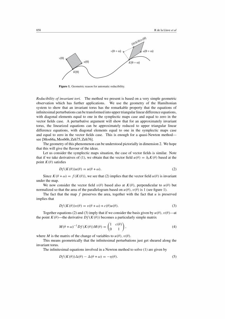
Figure 1. Geometric reason for automatic reducibility.

Reducibility of invariant tori. The method we present is based on a very simple geometricobservation which has further applications. We use the geometry of the Hamiltoniansystem to show that an invariant torus has the remarkable property that the equations ofinfinitesimal perturbations can be transformed into upper triangular linear difference equations,with diagonal elements equal to one in the symplectic maps case and equal to zero in thevector fields case. A perturbative argument will show that for an approximately invarianttorus, the linearized equations can be approximately reduced to upper triangular lineardifference equations, with diagonal elements equal to one in the symplectic maps caseand equal to zero in the vector fields case. This is enough for a quasi-Newton method—see [Mos66a, Mos66b, Zeh75, Zeh76].

The geometry of this phenomenon can be understood pictorially in dimension 2. We hopethat this will give the flavour of the ideas.

Let us consider the symplectic maps situation, the case of vector fields is similar. Notethat if we take derivatives of (1), we obtain that the vector field u(θ) = ∂θK(θ) based at thepoint K(θ) satisfies

Df (K(θ))u(θ) = u(θ + ω). (2)

Since K(θ + ω) = f (K(θ)), we see that (2) implies that the vector field u(θ) is invariantunder the map.

We now consider the vector field v(θ) based also at K(θ), perpendicular to u(θ) butnormalized so that the area of the parallelogram based on u(θ), v(θ) is 1 (see figure 1).

The fact that the map f preserves the area, together with the fact that u is preservedimplies that

Df (K(θ))v(θ) = v(θ + ω) + c(θ)u(θ). (3)

Together equations (2) and (3) imply that if we consider the basis given by u(θ), v(θ)—atthe point K(θ)—the derivative Df (K(θ)) becomes a particularly simple matrix

M(θ + ω)−1Df (K(θ))M(θ) =(

1 c(θ)

0 1

), (4)

where M is the matrix of the change of variables to u(θ), v(θ).This means geometrically that the infinitesimal perturbations just get sheared along the

invariant torus.The infinitesimal equations involved in a Newton method to solve (1) are given by

Df (K(θ))�(θ) − �(θ + ω) = −η(θ). (5)


Using equation (4) they become

(1 c(θ)

0 1

)M(θ)�(θ) − (M�)(θ + ω) = −M(θ + ω)−1η(θ). (6)

Equation (6) can be studied using the usual techniques for difference equations. It is wellknown that one can solve equations of the form (6), provided that certain averages vanish. Asit turns out, the vanishing of the averages can be guaranteed by a geometric condition and anon-degeneracy condition on c(θ). As a possible alternative, we will also propose the use ofthe method of the translated curve theorem and solve problems with extra parameters whichmake the averages zero.

Of course, there is little point in applying a linearized equation to something that is alreadya solution, but it turns out that if the K is not an exact solution but an approximate solutionof (1), it is possible to construct a matrix which approximately satisfies (4). This is enough toget a quasi-Newton method.

Note that (2) is a feature of all conjugacy problems (it plays a prominent role in thediscussions of [Mos66b]). On the other hand, (3) uses the geometric properties of the map f .

The automatic ‘approximate reducibility’—an analogue of equation (3)—is guaranteed byquite a number of geometric properties. For example, in this paper we will discuss the situationfor symplectic maps and Hamiltonian vector fields. In such cases the fact that invariant toriare Lagrangian plays an important role.

There are, however, quite a number of other contexts. We just mention that thesame phenomenon happens for conformally symplectic mappings in the sense of [WL98]—those are mappings in which the symplectic form gets multiplied by a constant—as well asvolume preserving maps.

We point out that automatic reducibility has been considered in the case of Lagrangiansystems. For example, it appears in [Koz83, Mos88]. The Lagrangian automatic reducibilityhas the advantage that it also applies to systems with more independent variables. On the otherhand, there seems to be no straightforward variational context for several situations such asconformally symplectic or volume preserving.

Besides the Lagrangian context, reducibility has also been used in the Hamiltonian contextin [Bos86], where the author uses reducibility to prove the theorem of persistence of invarianttori in Hamiltonian systems close to integrable. In [Rus76b] the author presents a geometricmethod, using reducibility, to prove existence of invariant tori for twist mappings. In [CC97],the authors use the automatic reducibility for tori which are graphs in mechanical systems(action-angle coordinates and Hamiltonians of the form kinetic plus potential energy) to obtainthe existence of invariant tori in rotations of the three body problem with parameters close tothose of the Ceres asteroid.

This paper is organized as follows: in section 2 we formulate the results of this paper. Insection 3 we explain briefly the general idea of the proofs. Section 4 contains the main step onthe construction of the polishing method for symplectic maps and proves that the linearizedequation of (1) can be transformed into an upper triangular linear equation which can besolved approximately. In section 5 we use the results from section 4 to construct a quadraticconvergent Newton-like method for solving equation (1). In section 6 we prove that solutionsof equation (1) are locally unique. In section 7 we will see how, with the use of parameters,the non-degenerate condition can be avoided. More concretely, we will describe a polishingmethod to prove the existence of an invariant torus for an element of a given parametric familyof symplectic maps fλ. Finally, in section 8 we sketch the procedure from Hamiltonian vectorfields.


2. Statement of results

2.1. Notation and preliminaries

Before we formulate the results of this paper, we introduce some notation. Let � = dα be anexact symplectic structure on U, and let a : U → R

2n be defined by

αz = a(z) dz, ∀z ∈ U. (7)

For each z ∈ U let J (z) : TzU → TzU be a linear isomorphism satisfying

�z(ξ, η) = 〈ξ, J (z)η〉, (8)

where 〈·, ·〉 is the Euclidean scalar product on R2n. It is well known that J satisfies

J (z)� = −J (z).

Remark 2. Although it is possible to assume (by changing the metric on U, cf [Wei77]), thatJ is an almost complex structure, i.e. J 2 = −Id, we will not make this assumption. Indeed,we have striven to deal with the problem in whatever coordinates it is presented.

Definition 1. Given γ > 0 and σ � n, we define D(γ, σ ) as the set of frequency vectorsω ∈ R

n satisfying the Diophantine condition:

| · ω − m| � γ | |−σ1 , ∀ ∈ Z

n\{0}, m ∈ Z,

where | |1 = | 1| + · · · + | n|.Similarly, given γ > 0 and σ > n − 1, we define Dh(γ, σ ) as the set of frequency vectors

ω ∈ Rn satisfying

|k · ω| � γ

|k|σ1, ∀k ∈ Z

n − {0}. (9)

Let Uρ denote the complex strip of width ρ > 0 : Uρ = {θ ∈ Cn : |Im θ | � ρ}. (Pρ, ‖ ‖ρ)

will denote the Banach space set of functions K : Uρ → U which are one-periodic in all itsvariables, real analytic on the interior of Uρ , continuous on the boundary of Uρ , and such that

‖K‖ρdef= sup

θ∈Uρ

|K(θ)| < ∞,

where |·| represents the maximum norm on the spaces Rm and C

m, i.e. if x = (x1, . . . , xm) ∈C

m, then

|x| def= maxj=1,...,m

|xj |.

Similar notation for the norm will also be used for real or complex matrices of arbitrarydimension, and it will refer to the matrix norm induced by the vectorial one.

Similarly, we will consider the set Pρ of functions K : Uρ → U real analytic on theinterior of Uρ and continuous on the boundary of Uρ , and satisfying

K(θ + k) = K(θ) + (k, 0), k ∈ Zn. (10)

Note that it is equivalent to saying that K satisfies (10) as to say that K(θ)− (θ, 0) is periodic.Hence, we can consider Pρ as an affine space modelled on Pρ .

Given a function g, analytic on a complex set B, for m ∈ Z+def= N ∪ {0} denote the

Cm-norm of g on B by |g|Cm,B, i.e.

|g|Cm,Bdef= sup

0�|k|�m

supz∈B

|Dkg(z)|.


Given a function g : B ⊂ Rd → R

m, Dg(z) will denote the m×d matrix with i, j coordinates(∂gi/∂xj ). For h : U → R, ∇h will represent the gradient of h.

We denote the Fourier expansion of a periodic mapping K : Tn → U by

K(θ) =∑ ∈Zn

K( ) exp(2π i · θ),

where · is the Euclidean scalar product in Rn and the Fourier coefficients K( ) can be

computed by

K( ) def=∫

Tn

K(θ) exp(−2π i · θ) dθ.

The average of K is the 0-Fourier coefficient, and we denote the average of K on Tn by

avg{K}θ def=∫

Tn

K(θ) dθ = K(0).

Definition 2. Given a symplectic map f and ω ∈ D(γ, σ ), a mapping K ∈ Pρ is said to benon-degenerate if it satisfies the following conditions:

N1. There exists an n × n matrix-valued function N(θ), such that

N(θ)(DK(θ)�DK(θ)) = In,

where In is the n-dimensional identity matrix.N2. The average of the matrix-valued function

S(θ)def= P(θ + ω)�[Df (K(θ))J (K(θ))−1P(θ) − J (K(θ + ω))−1P(θ + ω)]

with

P(θ)def= DK(θ)N(θ) (11)

is non-singular.

We will denote the set of functions in Pρ satisfying conditions N1, N2 by ND(ρ).

By the rank theorem, condition N1 guarantees that dim K(Tn) = n. For the KAMtheorem, the main non-degeneracy condition is N2, which is a twist condition. Its role willbecome clear in section 4.3. Note that N1 depends only on K whereas N2 depends on K and f .

2.2. Existence of an invariant torus for symplectic maps

Now we are ready to state the sufficient conditions to guarantee the existence of a true invarianttorus with Diophantine frequency vector ω near an approximately invariant torus.

Theorem 1. Let f : U → U be an exact symplectic map, and ω ∈ D(γ, σ ), for some γ > 0and σ > n. Assume that the following hypotheses hold:

H1. K0 ∈ ND(ρ0) (i.e. K0 satisfies definition 2).H2. The map f is real analytic and it can be holomorphically extended to some complex

neighbourhood of the image under K0 of Uρ0 :

Br = {z ∈ C2n : sup

|Im θ |<ρ0

|z − K0(θ)| < r}

for some r > 0, satisfying |f |C2,Br< ∞.

H3. If a and J are as in (7) and (8), respectively,

|a|C2,Br< ∞, |J |C1,Br

< ∞, |J−1|C1,Br< ∞.


Define the error function e0 by

e0def= f ◦ K0 − K0 ◦ Tω. (12)

There exists a constant c > 0 depending on σ , n, r , ρ0, |f |C2,Br, |a|C2,Br

, |J |C1,Br,

|J−1|C1,Br, ‖DK0‖ρ0 , ‖N0‖ρ0 , |(avg{S0}θ )−1| (where N0 and S0 are as in definition 2, replacing

K with K0) such that, if ‖e0‖ρ0 , defined in (12), verifies the following inequalities:

cγ −4δ−4σ0 ‖e0‖ρ0 < 1 (13)

and

cγ −2δ−2σ0 ‖e0‖ρ0 < r,

where 0 < δ0 � min(1, ρ0/12) is fixed, then there exists K∞ ∈ ND(ρ0 − 6δ0) such that

f ◦ K∞ − K∞ ◦ Tω = 0.

Moreover,

‖K∞ − K0‖ρ∞ � cγ −2 δ−2σ0 ‖e0‖ρ0 .

Remark 3. We emphasize that theorem 1 does not assume either that the system is given inaction-angle variables or that the maps are close to integrable.

The only smallness conditions needed are on the size of e0.

Remark 4. The geometric method we present here enables us to construct a quadraticconvergent sequence of approximate solutions of (1) (see lemma 11).

The quadratic estimates (see inequality (68)) contain the term γ −4, this is the reason forthe coefficient γ −4 in (13) which is the same as that obtained in some classical papers onKAM theory (e.g. [Mos66a, Mos66b, Zeh76]), but it is worse than the γ −2 obtained in someclassical KAM theorems (e.g. [Pos01, Sal04]). This estimation results in worse estimation ofthe measure of the invariant tori than what is possible.

Similarly, the exponent of δ0 in the conditions is similar to that of [Mos66a,Mos66b,Zeh76]since it is proportional to 4σ but is different from that of [Pos01, Sal04] which contains only2σ + A. This leads to different losses in differentiability.

We hope to come back to these problems in future research.

Remark 5. Note that given a mapping K satisfying equation (1), for any ϕ ∈ Tn the mapping

K(θ + ϕ) is also a solution of (1). We will adopt the criterion that two parametrizations, K

and K , of an embedded torus such that K(θ) = K(θ + ϕ), for some ϕ ∈ Tn, are equivalent

since they only differ in the arbitrary choice of the origin of the phases.

The following result states that the solutions obtained in theorem 1 are locally unique up tothe irrelevant choice of origin of the phase. As we mentioned, remark 1 is a general argumentthat allows results for flows to be obtained from results for maps with local uniqueness.

Theorem 2. Assume that ω ∈ D(γ, σ ). Let K1, K2 ∈ ND(ρ) (see definition 2) be twosolutions of (1), such that: K1(Uρ) ⊂ Br , and K2(Uρ) ⊂ Br .

There exists a constant c > 0 depending on n, σ , γ , ρ, ρ−1, |f |C2,Br, |J |Br

, |J−1|Br

‖K2‖C2,ρ , ‖N‖ρ , |(avg{S}θ )−1| (with N and S as in definition 2, replacing K with K2), suchthat if ‖K1 − K2‖ρ satisfies

cγ −2δ−2σ‖K1 − K2‖ρ < 1,

where δ = ρ/8, then there exists an initial phase τ ∈ Rn, such that K1 ◦ Tτ = K2 in Uρ/2.


2.3. A translated torus theorem

Let us assume that U = Tn ×U where U ⊂ R

n is an open set, and let � be an exact symplecticstructure on U. In this section we will assume that K is a non-trivial embedding of the torusin the annulus rather than just a periodic function. We say that fλ is a d-parametric familyof symplectic maps if there is a function f : U × B → U, with B ⊂ R

d , such that for eachx ∈ U the map f (x, ·) is C2, and such that for each λ ∈ B, the map fλ

def= f (·, λ) : U → U issymplectic and real analytic.

Definition 3. Given a 2n-parametric family of symplectic maps fλ and ω ∈ D(γ, σ ), the pairfλ, K ∈ Pρ is said to be non-degenerate if it satisfies the following conditions:

T1. There exists an n × n matrix-valued function N(θ), such that

N(θ)(DK(θ)� DK(θ)) = In.

T2. Let P be as in (11) and

T (θ) = P(θ)�[In − J (K(θ))−1P(θ)DK(θ)�J (K(θ))],

then the 2n × 2n matrix

�(θ) =(

T (θ + ω)

DK(θ + ω)�J (K(θ + ω))

) (∂fλ

∂λ

∣∣∣∣λ=λ

(K(θ))

)is such that avg{�}θ has a range of dimension 2n.

Let fλ : U → U be a 2n-parametric family of symplectic maps, and let K0 be anapproximate solution of (1), with f = f0. That is, K(θ + k) = K(θ) + (k, 0) for k ∈ Z

n.Assume that the pair f0, K0 satisfies definition 3, then we prove that there exists a solution of

fλ ◦ K = K ◦ Tω, (14)

where ω ∈ D(γ, σ ) is fixed.In the simplest case—which gives the name to the theorem—the family fλ consists just

in fλ(x, y) = f0(x, y) + (0, λ).This translated curve theorem is a technical tool in the study of invariant circles when the

non-degeneracy assumptions are not met.The main result of this section is the following:

Theorem 3. Let ω ∈ D(γ, σ ) be a frequency vector and let fλ be a 2n-parametric family ofsymplectic maps. Assume that the following hypotheses hold:

H1′. f0 and K0 ∈ Pρ0 satisfy conditions T1 and T2 (see definition 3).H2′. fλ is a family of real analytic symplectic maps that can be holomorphically extended to

some complex neighbourhood


θ∈Uρ0

|z − K0(θ)| < r}

for some r > 0, such that |fλ|C2,Br< ∞.

Define the error function

e0(θ) = f0(K0(θ)) − K0(θ + ω).

There exists a constant c > 0, depending on σ , n, ρ0, r , |f0|C2,Br, ‖DK0‖ρ0 ,

‖(∂fλ/∂λ)|λ=0K0‖ρ0 , ‖N0‖ρ0 and |(avg{�0(θ)}θ )−1| (where N0 and �0 are as in definition 3,replacing K with K0), such that if ‖e0‖ρ0 verifies the following inequalities:

cγ −4δ−4σ0 ‖e0‖ρ0 < 1


and

cγ −2δ−2σ0 ‖e0‖ρ0 < r,

where 0 < δ0 � min(1, ρ0/12), then there exists a mapping K∞ ∈ Pρ0−6δ0 and a vectorλ∞ ∈ R

2n, satisfying

fλ∞ ◦ K∞ = K∞ ◦ Tω.

Moreover, the following inequalities hold:

‖K∞ − K0‖ρ0−6δ0 < cγ 2δ−2σ0 ‖e0‖ρ0 ,

|λ∞| < cγ 2δ−2σ0 ‖e0‖ρ0 .

Remark 6. The same result holds if we consider ad-parametric family of symplectic maps withd � 2n. Moreover, if the elements of the family are exact symplectic we can consider d � n.

In this case we also have local uniqueness.

Theorem 4. Assume that ω ∈ D(γ, σ ). Let K1, K2 ∈ ND(ρ) be solutions of

fλ ◦ K = K ◦ Tω,

satisfying the hypotheses of theorem 3, and such that: K1(Uρ) ⊂ Br and K2(Uρ) ⊂ Br .There exists a constant c > 0 depending on n, σ , γ , ρ, ρ−1, |fλ|C2,Br

, |J |Br, |J−1|Br

,‖(∂fλ/∂λ)|λ=0K2‖ρ , ‖K2‖C2,ρ , ‖N2‖ρ and |(avg{�2}θ )−1| (with N2 and �2 as in definition 3,replacing K with K2), such that if ‖K1 − K2‖ρ satisfies

c‖K1 − K2‖ρ < 1,

where δ = ρ/8, then there exists an initial phase τ ∈ Rn, such that K1 ◦ Tτ = K2 in Uρ/2.

2.4. Existence of an invariant torus for vector fields

The results for a Hamiltonian vector field with Hamiltonian function H : U → R are basedon the study of the equation

∂ωK(θ) = J∇H(K(θ)), (15)

where J is defined in (8) and ∂ω is the derivative in direction ω:

∂ωKdef=

n∑i=1

ωi

∂

∂θi

K,

where K : Tn → U is the function to be determined and ω ∈ Dh(γ, σ ) ⊂ R

n (see definition 1).Note that (15) implies that the range of K is invariant under the Hamiltonian vector field

with Hamiltonian function H , XH. The map K gives a parametrization of the invariant toruswhich makes the dynamics of the vector field XH restricted to the torus into a rigid rotation.

In order to simplify the notation we assume that � = dx ∧ dy. This is not restrictivebecause the proof of theorem 5 follows from theorem 1 (see [Dou82]). Moreover, the directconstruction given in section 8 works for a general exact symplectic structure � = dα.

Definition 4. Given a Hamiltonian function H and a frequency vector ω, the mappingK : T

n → U is said to be non-degenerate (for the Hamiltonian vector field XH) if it satisfiesthe following conditions:

– K is real analytic on the set Uρ .– There exists a matrix N satisfying

N(θ)DK(θ)�DK(θ) = In.


– avg{S}θ is invertible, with

S(θ) = N(θ)DK(θ)�[A(θ)J − JA(θ)]DK(θ)N(θ),

where

A(θ) =(

Dx∇yH(K(θ)) Dy∇yH(K(θ))

−Dx∇xH(K(θ)) −Dy∇xH(K(θ))

).

Theorem 5. Let ω satisfy the Diophantine condition (9). Assume that K0 is non-degenerate(i.e. satisfies definition 4). Assume that H is real analytic and that it can be holomorphicallyextended to some complex neighbourhood of the image of Uρ under K0:


θ∈Uρ

|z − K0(θ)| < r}.


e0def= J ∇H(K0(θ)) − ∂ωK0(θ).

There exists a constant c > 0, depending on σ , n, r , ρ, |H |C3,Br, ‖DK0‖ρ , ‖N0‖ρ and

|(avg{S0}θ )−1| (with N0 and S0 given by definition 4, replacing K with K0), such that if

cγ −4δ−4σ0 ‖e0‖ρ < 1

and

cγ −2δ−2σ0 ‖e0‖ρ0 < r

with δ0 = ρ/12, then there exists a solution for (15), K∞, which is real analytic on Uρ/2 andsatisfies the non-degenerate conditions in definition 4. Moreover,

‖K∞ − K0‖ρ/2 � cγ −2δ−2σ0 ‖e0‖ρ.

Remark 7. There is a local uniqueness statement for vector fields which follows by thereduction to the time one map (see [Dou82]). We do not formulate such a theorem.

We will say that Hλ is a d-parametric family of Hamiltonian functions if there is a functionH : U × B → R, with B ⊂ R

d , such that for each x ∈ U the map H(x, ·) is C2 and such that

for each λ ∈ B, the map Hλdef= H(·, λ) : U → R is a real analytic Hamiltonian function.

There is an analogue of the translated torus theorem (theorem 3) in which we study theequation

∂ωK(θ) = J∇Hλ(K(θ)), (16)

where Hλ is a 2n-parametric family of Hamiltonian functions, and K ∈ Pρ (see equation (10)).

Theorem 6. Let ω satisfy the Diophantine condition (9). Assume that K0 ∈ Pρ satisfies thefollowing properties:

– There exists a matrix N0 satisfying

N0(θ)DK0(θ)�DK0(θ) = In.

– avg{�0}θ has maximum range, with

�0(θ) =

N0(θ)DK0(θ)�J

(∂

∂λ∇Hλ(K0(θ))

∣∣∣∣λ=0

)

DK0(θ)�J

(∂

∂λ∇Hλ(K0(θ))

∣∣∣∣λ=0

) .



e0def= ∂ωK0(θ) − J∇H0(K0(θ)).

There exists a constant c > 0, depending on σ , n, r , ρ, |H |C3,Br, ‖DK0‖ρ , ‖N0‖ρ , ‖�0‖ρ and

|(avg{�0}θ )−1|, such that if

cγ −4δ−4σ0 ‖e0‖ρ < 1

and

cγ −2δ−2σ0 ‖e0‖ρ0 < r

with δ0 = ρ/12, then there exist λ∞ ∈ R2n and K∞ ∈ Pρ/2 satisfying

∂ωK∞(θ) = J∇Hλ∞(K∞(θ)).

Moreover,

‖K∞ − K0‖ρ/2 � cγ −2δ−2σ0 ‖e0‖ρ

and

|λ∞| < cγ 2δ−2σ0 ‖e0‖ρ0 .

2.5. The perturbative case

Even if one of the strong points of the proof presented here is that it does not require thatthe problem is in action-angle coordinates or close to integrable, we will present how theresults here apply to the quasi-integrable case. We hope that this can help in understandingthe meaning of the non-degeneracy conditions.

We consider Tn × U endowed with the usual symplectic structure.

If we consider a map

f (ϕ, I ) = (ϕ + A(I), I ) + �(ϕ, I),

where � is small, we can take as K(θ) = (θ, I ∗) where I ∗ is chosen in such a way thatA(I ∗) = ω.

Then, we see that the size of the error function can be controlled by the size of �.The non-degeneracy condition N1 on the embedding is satisfied clearly since N(θ) = In.We have that in this case P is the constant matrix

P(θ) =(

In

0

).

Since � is assumed to be small, we will verify the hypothesis on the main part of the mapconsidering � as a small perturbation.

Note that

Df (K(θ)) =(

In DA(I ∗)0 In

)+ O(�).

Performing the calculation in the definition of S, we obtain that, in this perturbative case,S = DA(I ∗) + O(�).

Hence, in this perturbative case, the non-degeneracy condition we assume is precisely thetwist condition.

We leave to the reader the verification that in the other quasi-integrable cases, the non-degeneracy conditions we assume reduce to the standard ones.


3. Sketch of the procedure

Equations (1), (14)–(16) are functional equations for the unknown functionK (and the unknownparameter λ in the case of (14) and (16)). As shown in [Mos66a, Zeh75], in order to provethe existence of a solution of a nonlinear problem by using a modified Newton method it isenough to have an approximate solution of the corresponding linearized equation such that thenew error is quadratic with respect to the original one.

The main idea is to use the geometric properties of the problem to prove that thecorresponding linearized equations can be transformed into a simpler linear equation thatis approximately solvable by using Fourier series.

We emphasize that, at each step of the iterative procedure, the reduction of the erroris accomplished by adding a small function rather than composing with a near identitytransformation (as is customary in many proofs of the KAM theorem). This leads to simplerand more efficient estimates, which are closer to those obtained in numerical procedures. Itis also interesting to note that the procedure presented here can be implemented to computenumerical approximations of invariant tori.

3.1. Maps

The key point in finding a solution for (1) and (14) is to solve the corresponding linearizedequation approximately. The main part of both linearized equations is the linear operator:

Tf,K,ω� = Df (K(θ))� − � ◦ Tω. (17)

Indeed, equations (1) and (14) can be formulated as finding zeros of

F(K)def= f ◦ K − K ◦ Tω (18)

and

G(K, λ)def= fλ ◦ K − K ◦ Tω, (19)

respectively. Therefore, at least formally we have

DF(K)� = Tf,K,ω�,

DG(K, λ)(�K, �λ) = Tfλ,K,ω(�K) +∂fλ(K)

∂λ�λ.

In section 4 we prove that, under certain hypotheses, the corresponding linear operator DF(K)

is approximately invertible in the sense of [Zeh75]. First of all we prove that the Lagrangiancharacter of an invariant torus, for a symplectic map, is slightly modified if the torus isonly approximately invariant (see section 4.1). The approximate Lagrangian character ofan approximately invariant torus enables us to define a change of variables such that in the newvariables the linear operator DF(K) is, except for quadratic terms, an upper triangular lineardifferential equation. In section 4.3 we show that, if some non-degeneracy conditions hold, inthe new variables the linearized equation

DF(K)� = −F(K)

can be solved approximately.Similarly, in section 7 we prove (with different non-degeneracy conditions) that

DG(K, λ)(�K, δλ) = −G(K, λ)

can be solved approximately.


4. The linearized operator DF(K)

In order to construct a modified Newton method for the functional equation (18) we have tostudy the invertibility properties of the corresponding linear operatorDF(K). More concretely,we are interested in the solvability properties of the linearized equation

DF(K)�(θ) = Df (K(θ))�(θ) − �(θ + ω) = −e(θ), (20)

where K is an approximate solution of (1) with error function

e(θ) = F(K)(θ), θ ∈ Rn. (21)

By using the geometric properties of the problem we will prove that (20) can be transformedinto another equation that can be solved approximately by using Fourier series. To be moreprecise, by using the symplectic properties of f and the algebraic properties of ω we will showthat, if the error e defined in (21) is small enough, then for any θ ∈ T

n the set{∂K(θ)

∂θj

, J (K(θ))∂K(θ)

∂θj

}n

j=1

forms a basis of TK(θ)U ∼ R2n (the tangent space to U at the point K(θ)). We use this basis

to transform the linearized equation (20) into a convenient linear equation for which we canconstruct an approximate solution.

4.1. Approximate Lagrangian character

In this section we formulate the well-known result that a torus supporting an irrational rotationis Lagrangian.

Let L be the linear application defined by

(K∗�)θ(ξ, η) = 〈ξ, L(θ)η〉, for any ξ, η ∈ R2n, θ ∈ T

n,

then

L(θ) = DK(θ)�J (K(θ))DK(θ), (22)

where J is defined by (8). With the previous notation the Lagrangian character of K isequivalent to the following equality:

L(θ) = 0, ∀θ ∈ Tn.

Therefore, it is natural to say that an approximately invariant torus is approximately Lagrangianif the norm of L is ‘small’. We will show that if a parametrization K satisfies (1) approximately,then the norm of L can be estimated by the norm of the error given in (21), e.

4.1.1. Exact solutions. In order to make the proof of the approximately Lagrangian characterof an approximate solution of (1) clearer, we present a proof of the Lagrangian character of anexact solution of (1).

Lemma 1. Assume that K is a solution of (1) then K∗� (equivalently, L defined in (22)) isidentically zero.

Proof. Since K satisfies (1) and f is symplectic we have

f ◦ K = K ◦ Tω and f ∗� = �.

Then,

K∗� = K∗(f ∗�) = (f ◦ K)∗� = (K ◦ Tω)∗�


and so we have

K∗� − (K ◦ Tω)∗� = 0.

Moreover, since ω is rationally independent, rotations on the torus are ergodic, this impliesthat K∗�, equivalently L, is constant.

Also, since � is exact with � = dα, then if K = (K1, . . . , K2n)� and if in (7)

a = (a1, . . . , a2n)�, then

(K∗α)θ =n∑

j=1

cj (θ) dθj ,

where for s = 1, . . . , n, cs has the following expression:

cs(θ) = (DK(θ)�a(K(θ)))s =2n∑

j=1

∂Kj (θ)

∂θs

aj (K(θ)).

This implies L(θ) = Dc(θ)� − Dc(θ), and since the average of Dc(θ) is equal to zero oneobtains that the average of L is equal to zero. �

4.1.2. Approximate solutions. We need the following result; for a proof see [Rus75,Rus76b,Rus76c] (see also [dlL01]).

Proposition 2. Let ω ∈ D(γ, σ ), assume that the mapping h : Tn → R

2n is analytic on Uρ ,and has zero average, avg{h}θ = 0. Then for any 0 < δ < ρ, the difference equation

v(θ) − v(θ + ω) = h(θ) (23)

has a unique zero average solution v : Tn → R

2n, real analytic on Uρ−δ , for any 0 < δ < ρ.Moreover, the following estimate holds:

‖v‖ρ−δ � c0γ−1δ−σ‖h‖ρ,

where c0 is a constant depending on n and σ .

The approximate Lagrangian character of an approximate solution of (1) follows becauseK∗� satisfies a small divisors equation, similar to (23), with the right-hand side expressed interms of derivatives of the error function e defined in (21). We make this more precise in thefollowing statement.

Lemma 3. Let e be the error function defined in (21), then K∗� satisfies the following lineardifference equation:

K∗� − (K ◦ Tω)∗� = �e, (24)

where

(�e)θ =n∑

i=1

n∑j=1

gi j (θ) dθi dθj ,

where gij are the coordinates of the n × n matrix g given in (25). In particular, the average ofg is equal to zero.

Moreover, if K is real analytic on the complex strip of width ρ, then there exists a constantc > 0, depending on n, σ , ρ, ‖DK‖ρ , |f |C1,Br

, |J |C1,Br, such that, for 0 < δ < ρ/2

‖L‖ρ−2δ � c1γ−1δ−(σ+1)‖e‖ρ,

where L is given in (22).


Proof. Define �e = K∗� − (K ◦ Tω)∗�, then

�e = (f ◦ K)∗� − (K ◦ Tω)∗�

and

g(θ) = DK(θ)�Df (K(θ))�J (f (K(θ)))Df (K(θ))DK(θ) − L(θ + ω),

where L is defined in (22). Using the equality

Df (K(θ))DK(θ) = DK(θ + ω) + De(θ),

which follows from (21), and performing some computations, one obtains

g(θ) = DK(θ + ω)�ϕ(θ)DK(θ + ω) − ψ(θ)� + (Df (K(θ))DK(θ))�J (f (K(θ)))De(θ),

(25)

where

ϕ(θ) = J (f (K(θ))) − J (K(θ + ω))

and

ψ(θ) = DK(θ + ω)�J (f (K(θ)))De(θ).

Note that if K is real analytic on the complex strip of width ρ, then

‖ϕ‖ρ � |J |C1,Br‖e‖ρ,

‖ψ‖ρ−δ � cδ−1‖e‖ρ,

where c is a constant depending on n, ‖DK‖ρ and |f |C1,Br. Therefore, from (25) we have

‖g‖ρ−δ � cδ−1‖e‖ρ.

Applying the last inequality and proposition 2 we obtain an estimation for the norm of L.Indeed, equation (24) is equivalent to

L − L ◦ Tω = g.

Proposition 2 implies

‖L‖ρ−2δ � c0γ−1δ−σ‖g‖ρ−δ � c0γ

−1cδ−(σ+1)‖e‖ρ,

where c0 is the constant of proposition 2. �

4.2. Approximate reducibility

In this section we will use the results of section 4.1 to prove that there exists a change ofvariables �(θ) = M(θ) ξ(θ) such that in the variable ξ equation (20) takes the form

(C + B)ξ − ξ ◦ Tω = −(M ◦ Tω)−1e, (26)

where C(θ) is an upper triangular matrix with diagonal terms equal to 1.We will see that, in the invariant case (i.e. K is a solution for (1)) M can be chosen in such

a way that B is identically equal to zero.In the invariant case the change of variables is obtained by using the fact that Df (K(θ))

is a linear symplectic transformation taking the tangent vector (∂K(θ)/∂θj ) into the tangentvector (∂K(θ + ω)/∂θj ), and the Lagrangian character of an invariant torus. In the case that Kis an approximate solution for (1) we will use the change of variables defined in the invariantcase. The fact that Df (K(θ)) takes (∂K(θ)/∂θj ) into (∂K(θ + ω)/∂θj ) + (∂e(θ)/∂θj ) andthat K is approximately Lagrangian will produce the following estimate:

‖B‖ρ−2δ � γ −1δ−(σ+1)c‖e‖ρ.


4.2.1. Exact solutions. Let us look for a matrix-valued function M such that

Df (K(θ))M(θ) = M(θ + ω)C(θ),

where C(θ) is an upper triangular matrix with diagonal terms equal to 1.If K satisfies (1), taking derivatives we obtain

Df (K(θ))DK(θ) = DK(θ + ω), (27)

hence M(θ) and C(θ) can be chosen to have the following form:

M(θ) = (DK(θ) M1(θ)) and C(θ) =(

In S(θ)

0 H(θ)

),

where S and H are n×n matrix-valued functions, and M1 is a 2n×n matrix-valued function,that has to be determined.

Define

N(θ)def= (DK(θ)�DK(θ))−1. (28)

If we take M1 to be

M1(θ) = J (K(θ))−1DK(θ)N(θ),

some simple algebraic calculations show that H is the identity matrix and

S(θ) = P(θ + ω)�[Df (K(θ))J (K(θ))−1P(θ) − J (K(θ + ω))−1P(θ + ω)] (29)

with

P(θ)def= DK(θ)N(θ). (30)

Therefore, we have proved the following result.

Proposition 4. Assume that K satisfies (1). If

M(θ)def= (DK(θ) J (K(θ))−1DK(θ)N(θ)) (31)

and

C(θ)def=

(In S(θ)

0 In

)(32)

with S defined in (29), then

Df (K(θ))M(θ) = M(θ + ω)C(θ). (33)

Remark 8. If the symplectic linear transformation satisfies J−1 = −J , then

P(θ + ω)�J (K(θ + ω))−1P(θ + ω) = 0.

Therefore, S takes the following form:

S(θ) = −P(θ + ω)�Df (K(θ))J (K(θ))P (θ).

Remark 9. It is possible to make further transformations that make C a constant. Nevertheless,since the present form is good enough for our purposes, we do not pursue it here.

Let M be defined by (31), in what follows we show that M is invertible. A directcomputation yields

M(θ)�J (K(θ))M(θ) = V (θ) + R(θ), (34)


where

V (θ)def=

(0 In

−In −P(θ)�J (K(θ))−1P(θ)

)(35)

and

R(θ) =(

L(θ) 00 0

)(36)

with P , L and N defined in (30), (22) and (28), respectively.Note that V is invertible, with its inverse given by

V (θ)−1 =(−P(θ)�J (K(θ))−1P(θ) −In

In 0

). (37)

If K satisfies (1), then lemma 1 implies L = 0, this implies R = 0. Hence, equality (34)implies that M is invertible and its inverse is given by

M(θ)−1 = V (θ)−1M(θ)�J (K(θ)) =(

T (θ)

DK(θ)�J (K(θ))

)

with V −1 given in (37) and

T (θ)def= P(θ)�[In − J (K(θ))−1P(θ)DK(θ)�J (K(θ))], (38)

where P(θ) is given in (30).Since M and C satisfy equality (33), we have that M(θ + ω)−1Df (K(θ))M(θ) = C(θ).

Therefore, if we substitute �(θ) = M(θ)ξ(θ) in the linear equation (20) we have

C(θ)ξ(θ) − ξ(θ + ω) = p(θ)

with

p(θ) = −M(θ + ω)−1e(θ) =( −T (θ + ω)e(θ)

−DK(θ + ω)�J (K(θ + ω))e(θ)

), (39)

where P(θ) = DK(θ)N(θ) (see (30)), and T is defined in (38).

Remark 10. If J−1 = −J , then

V (θ) =(

0 In

−In N(θ)L(θ)N(θ)

),

where L is defined in (22). Then

M(θ)�J (K(θ))M(θ) = J0 +

(L(θ) 0

0 N(θ)L(θ)N(θ)

),

where

J0 =(

0 In

−In 0

).

In particular, if K is a parametrization of an invariant torus and � is the canonical symplecticform in R

2n, then M is symplectic:

M�J0M = J0.


4.2.2. Approximate solutions. Assume that K is an approximate solution of (1) with errorgiven by (21), and let M be defined by (31). We will show that, with the change of variables� = Mξ , equation (20) takes the form of (26).

In order to guarantee that M defines a change of variables we need M to be invertible.From equality (34) one sees that if the matrix V (θ) + R(θ) is invertible, then M(θ) is alsoinvertible. The invertibility of V (θ) + R(θ) depends on the size of ‖e‖ρ , in order to show thatwe first bound the norm of V (θ)−1R(θ) in terms of ‖e‖ρ . Using expressions (36) and (37) thefollowing lemma is immediate.

Lemma 5. Assume that the hypotheses of lemma 3 hold. Then there exists a constant c3

depending on n, σ , ρ, |f |C1,Br, |J |C1,Br

, |J−1|Br, ‖N‖ρ , ‖DK‖ρ and the constant c1 of lemma 3

such that for any 0 < δ < ρ/2 the following inequality holds:

‖V (θ)−1R(θ)‖ρ−2δ < c3γ−1δ−(σ+1)‖e‖ρ.

As a consequence of lemma 5 we have:

Lemma 6. Assume that the hypotheses of lemma 3 hold, and let c3 be the constant of lemma 5.If e satisfies

c3γ−1δ−(σ+1)‖e‖ρ � 1

2 , (40)

then M is invertible and its inverse is given by

M(θ)−1 = V (θ)−1M(θ)�J (K(θ)) + Me(θ), (41)

where

Me(θ)def= −[I2n + V (θ)−1R(θ)]−1V (θ)−1R(θ)V (θ)−1M(θ)�J (K(θ)).

In particular, Me = 0 if e = 0. Moreover,

‖Me‖ρ−2δ � c4γ−1δ−(σ+1)‖e‖ρ,

where c4 is a constant depending on n, c3, |J−1|Br, |J |Br

, ‖DK‖ρ , ‖N‖ρ .

Proof. From lemma 5 and the assumption on ‖e‖ρ one obtains

‖V (θ)−1R(θ)‖ρ−2δ � c3γ−1δ−(σ+1)‖e‖ρ � 1

2 .

Then I2n + V (θ)−1R(θ) is invertible with

‖(I2n + V (θ)−1R(θ))−1‖ρ−2δ � 1

1 − ‖V (θ)−1R(θ)‖ρ−2δ

� 2

and using equality (34) we have

M(θ)−1 = (V (θ) + R(θ))−1M(θ)�J (K(θ))

= V (θ)−1M(θ)�J (K(θ)) + Me(θ). �

Proposition 7. Assume that ω ∈ D(γ, σ ), and that ‖e‖ρ satisfies inequality (40), where c3 isthe constant of lemma 5.

The change of variables �(θ) = M(θ)ξ(θ), transforms (20) into[(In S(θ)

0 In

)+ B(θ)

]ξ(θ) − ξ(θ + ω) = p(θ) + w(θ), (42)

where S is defined in (29), p is given in (39), and

B(θ)def= M(θ + ω)−1E(θ), w(θ)

def= −Me(θ + ω)e(θ) (43)


with

E(θ)def= Df (K(θ))M(θ) − M(θ + ω)C(θ). (44)

Moreover, the following estimates hold:

‖B(θ)‖ρ−2δ < c5γ−1δ−(σ+1)‖e‖ρ, (45)

‖w‖ρ−2δ < c4γ−1δ−(σ+1)‖e‖2

ρ, (46)

where c5 is a constant which depends on n, ρ, |f |C1,Br, |J |C1,Br

, |J−1|Br, ‖DK‖ρ , ‖N‖ρ , and

c1 and c4 are constants of lemma 6.

Proof. In the variable ξ , equation (20) takes the form

Df (K(θ))M(θ)ξ(θ) − M(θ + ω)ξ(θ + ω) = −e(θ).

Multiplying by M(θ + ω)−1 we obtain

M(θ + ω)−1Df (K(θ))M(θ)ξ(θ) − ξ(θ + ω) = −M(θ + ω)−1e(θ).

Using equality (44) and the definition of B we have

M(θ + ω)−1Df (K(θ))M(θ) = C(θ) + B(θ).

Moreover, from (41) we have

−M(θ + ω)−1e(θ) = −V (θ + ω)−1M(θ + ω)J (K(θ + ω))e(θ) − Me(θ + ω)e(θ),

defining p and w as in (39) and (43), respectively, we have (42).Estimate (46) follows from lemma 6.Let us prove estimate (45). From lemma 6 one obtains

‖B‖ρ−2δ � ‖V −1‖ρ‖M(θ + ω)�J (K(θ + ω))E(θ)‖ρ−2δ + ‖MeE‖ρ−2δ

×c‖M(θ + ω)�J (K(θ + ω))E(θ)‖ρ−2δ + cγ −1δ−(σ+1)|e|ρ (47)

for some constant c.We claim that there exists a constant c2, depending on n, ρ, |f |C1,Br

, |J |C1,Br, |J−1|Br

,‖DK‖ρ , ‖N‖ρ and c1 such that, for any 0 < δ < ρ/2, the following estimate holds:

‖M(θ + ω)�J (K(θ + ω))E(θ)‖ρ−2δ � c2γ−1δ−(σ+1)‖e‖ρ. (48)

Indeed, using the following equality:

Df (K(θ))DK(θ) − DK(θ + ω) = De(θ)

we have

E(θ) = (De(θ) E1(θ)),

where

E1(θ) = Df (K(θ))J (K(θ))−1DK(θ)N(θ) − DK(θ + ω)S(θ)

−J (K(θ + ω))−1DK(θ + ω)N(θ + ω).

On the other hand, performing some simple computations, we have

M(θ)�J (K(θ)) =(

Q(θ)�

−P(θ)�

),

where P is defined by equation (30), and Q(θ) = −J (K(θ))DK(θ). Then, we have

M(θ + ω)�J (K(θ + ω))E(θ) =(

Q(θ + ω)�De(θ) Q(θ + ω)�E1(θ)

−P(θ + ω)�De(θ) −P(θ + ω)�E1(θ)

).


Moreover, E1 satisfies

P(θ + ω)�E1(θ) = 0 (49)

and

Q(θ + ω)�E1(θ) = φ(θ) − ψ(θ) − L(θ + ω)S(θ), (50)

where L(θ), defined in (22), is bounded in lemma 3,

φ(θ) = (Df (K(θ))DK(θ))�ϕ(θ)Df (K(θ))J (K(θ))−1DK(θ)N(θ)

with ϕ(θ) = J (K(θ + ω)) − J (f (K(θ))), and

ψ(θ) = De(θ)�J (K(θ + ω))Df (K(θ))J (K(θ))−1DK(θ)N(θ).

Then inequality (48) follows from equalities (49), (50) and lemma 3. Therefore, estimate (45)follows from (47) and (48). �

Remark 11. Note that in proposition 7, we have w = 0 and B = 0 in the case that K

parametrizes an invariant torus.

4.3. Approximate solvability of the linearized equation

Proposition 7 guarantees the existence of a change of variables which takes (20) into (42). Weemphasize that proposition 7 holds for any real analytic symplectic map f for which there is areal analytic approximate solution of (1), K , with small enough error function and frequencyvector ω ∈ D(γ, σ ). In this section we prove that if f is an exact symplectic map, andK satisfies the non-degeneracy condition N2, then equation (20) can be solved approximatelyin the customary sense of Nash–Moser theory. In order to do that we study the approximatesolvability of (42).

Let us consider the following linear operator:

Lωξ(θ) =(

In S(θ)

0 In

)ξ(θ) − ξ(θ + ω),

where S is defined in (29). Note that (42) can be written as follows:

Lωξ(θ) + B(θ)ξ(θ) = p(θ) + w(θ).

The approximate solutions of (42) will be the solutions of

Lωξ(θ) = p(θ) −(

0avg{py}θ

), (51)

where (px, py) are the symplectically conjugate variables of p. The exactness property of f

will enable us to prove that |avg{py}θ | is quadratic with respect to the norm of the error. Thena solution of (51) will satisfy (42) up to errors which are ‘quadratic’ in the errors, which doesnot affect the ‘quadratic’ convergence of the methods [Zeh75].

The non-degeneracy condition N2 in definition 2 guarantees the solvability of (51), as weprove in the following result.

Proposition 8. Assume that ω ∈ D(γ, σ ) and that the following hypotheses hold:

(a) The average of S, avg{S}θ , is non-singular.(b) v = (vx, vy) : R

n → Rn × R

n is real analytic on Uρ , one-periodic in all its arguments,with vy : R

n → Rn a zero average function.


There exists a unique function ξ = (ξx, ξy) : Rn → R

n × Rn real analytic on Uρ−2δ , for any

0 < δ < min(1, ρ/2), satisfying

Lωξ = v

with avg{ξx}θ = 0 and

avg{ξy}θ = (avg{S}θ )−1(avg{vx}θ − avg{S(θ)ξy}θ ), (52)

where ξy = ξy − avg{ξy}θ .Moreover, there exists a constant c depending on σ , ρ, n, ‖N‖ρ , ‖K‖ρ and

|(avg{S}θ )−1|, s.t.

‖ξ‖ρ−2δ < cγ −2δ−2σ‖v‖ρ.

Proof. The linear difference equation Lωξ = (vx, vy)� is written as follows

ξx(θ) − ξx(θ + ω) = vx(θ) − S(θ)ξy(θ),

ξy(θ) − ξy(θ + ω) = vy(θ).

First we consider the n-dimensional equation

ξy(θ) − ξy(θ + ω) = vy. (53)

Since ω ∈ D(γ, σ ) and avg{vy}θ = 0, proposition 2 implies the existence of a solution ξy ofequation (53) which has arbitrary average and is analytic on Uρ−δ , for any 0 < δ < ρ/2, andsatisfies the following estimate:

‖ξy‖ρ−δ � c0γ−1δ−σ‖vy‖ρ + |avg{ξy}θ |,

where c0 is the constant given in proposition 2.Moreover, if avg{ξy}θ is defined by (52), then the following equality holds:

avg{vx(θ) − S(θ)ξy(θ)}θ = 0.

Thus, there exists a unique zero average solution ξx of

ξx(θ) − ξx(θ + ω) = vx(θ) − S(θ)ξy(θ), (54)

satisfying

‖ξx‖ρ−2δ � c0γ−1δ−σ‖vx(θ) − S(θ)ξy(θ)‖ρ−δ.

Finally, using the bound for ‖ξy‖ρ−δ and assuming 0 < δ < min(ρ, 1), one obtains the desiredestimate. �

Remark 12. We remark that proposition 8 is the justification for our definition of the non-degeneracy condition N2 (see definition 2).

Remark 13. The uniqueness property of the solution ξ in proposition 8 implies that for anyother mapping ξ = (ξx, ξy) satisfying Lω ξ = v will also satisfy

ξ = ξ +

(avg{ξx}θ

0

).

Let ξ be the solution of (51), with avg{ξ}θ as in proposition 8, and define �(θ) =M(θ)ξ(θ), then

F(K)�(θ) = −e(θ) + M(θ + ω)

[B(θ)ξ(θ) − w(θ) −

(0

avg{py}θ

)], (55)

B and w are defined in equation (43).


Note that if we want to obtain an approximate solution of (20) with quadratic error withrespect to the norm of e, because of (45), (46) and the estimates given in proposition 8, it isenough to prove that the norm of avg{py}θ is quadratic with respect to the norm ‖e‖ρ .

Lemma 9. If f is exact symplectic, then the following equality holds:

avg{py}θ = −avg{ϕ(θ) + De(θ)�Da(K(θ + ω))e(θ)}θ ,where e is defined in (21), a is defined by α = a dz, and

ϕ(θ) = (Df (K(θ))DK(θ))�φ(θ),

φ(θ) = a(f (K(θ))) − a(K(θ + ω)) − Da(K(θ + ω))e(θ). (56)

Moreover, the following estimate holds:

|avg{py}θ | � c5ρ−1‖e‖2

ρ, (57)

where c5 is a constant depending on n, ρ, ‖DK‖ρ , |f |C1,Brand |a|C2,Br

.

Proof. First of all note that

px(θ) = −T (θ + ω)e(θ), py(θ) = −DK(θ + ω)�J (K(θ + ω))e(θ), (58)

where T is defined in (38). Moreover, from (8) we have

�z(ζ, η) =2n∑i=1

2n∑j=1

Ji,j (z)ζiηj , ∀ζ, η ∈ R2n.

Then, if � = dα, with α = a dz, for i, j = 1, . . . , 2n, we have

Ji,j (z) = ∂aj (z)

∂zi

− ∂ai(z)

∂zj

,

equivalently

J (z) = Da(z)� − Da(z). (59)

Using equality (59) we obtain

DK(θ + ω)�J (K(θ + ω))e(θ) = DK(θ + ω)�Da(K(θ + ω))�f (K(θ))︸︷︷︸(1)

− DK(θ + ω)�Da(K(θ + ω))�K(θ + ω)︸︷︷︸(2)

− DK(θ + ω)�Da(K(θ + ω))e(θ)︸︷︷︸(3)

.

Note that

(1) = ∇[a(K(θ + ω)) · f (K(θ))] − DK(θ)�Df (K(θ))�a(K(θ + ω))

and

(2) = ∇[a(K(θ + ω)) · K(θ + ω)] − DK(θ + ω)�a(K(θ + ω)).

Then

avg{(1) − (2)}θ = −avg{DK(θ)�Df (K(θ))�a(K(θ + ω)) − DK(θ)�a(K(θ))}θ .Moreover, if f is exact symplectic the following equality holds:

(f ◦ K)∗α = K∗α + d(b ◦ K).

Expressing this in coordinates and integrating we have

avg{DK(θ)�a(K(θ))}θ = avg{(Df (K(θ))DK(θ))�a(f (K(θ)))}θ , (60)


Equality (60) implies (see (56))

avg{(1) − (2)}θ = avg{(Df (K(θ))DK(θ))�(a(f (K(θ))) − a(K(θ + ω)))}θ= avg{(Df (K(θ))DK(θ))�Da(K(θ + ω))e(θ)}θ

+ avg{(Df (K(θ))DK(θ))�φ(θ)}θ .Therefore,

avg{(1) − (2) − (3)}θ = avg{(Df (K(θ))DK(θ))�φ(θ)}θ+avg{De(θ)�Da(K(θ + ω))e(θ)}θ ,

where we have used that Df (K(θ))DK(θ) − DK(θ + ω) = De(θ).By Cauchy’s inequalities and the properties of the norms, we have the following estimate

for |avg{py}θ |:|avg{py}θ | � c5ρ

−1‖e‖2ρ,

where c5 is a constant depending on n, ρ, ‖DK‖ρ , |f |C1,Brand |a|C2,Br

. �From propositions 7, 8 and equation (57), we have that the linearized equation

[DF(K)�](θ) = −e(θ)

is approximately solvable in the following sense.

Lemma 10. Assume that ω ∈ D(γ, σ ), f is an exact symplectic map, S (defined in (29))satisfies that avg{S}θ is non-singular, and that ‖e‖ρ is small enough such that proposition 7applies.

Let M be defined by (31), and ξ be the solution of (51). The mapping �(θ) = M(θ)ξ(θ)

satisfies (55). Moreover, the following estimates hold:

‖�‖ρ−2δ � cγ −2δ−2σ‖e‖ρ (61)

and

‖DF(K)� + e‖ρ−2δ � cγ −3δ−(3σ+1)‖e‖2ρ, (62)

where c is a constant depending on σ , n, ρ, |a|C2,Br, |J |C1,Br

, |J−1|Br, |f |C1,Br

, ‖DK‖ρ , ‖N‖ρ ,|(avg{S}θ )−1|.Proof. Estimate (61) follows from proposition 8. Equality (55) follows from proposition 7and the definition of �. From inequality (45) and proposition 8 one obtains

‖M(θ + ω)B(θ)ξ(θ)‖ρ−2δ � cγ −3δ−(3σ+1)‖e‖2ρ

for some constant c. Inequality (46) implies

‖M(θ + ω)w(θ)‖ρ−2δ � cγ −1δ−(σ+1)‖e‖2ρ

and from inequality (57) we obtain∥∥∥∥M(θ + ω)

(0

avg{py}θ

)∥∥∥∥ρ−2δ

� cγ −1ρ−1‖e‖2ρ.

Applying these estimates to (55) we obtain (62). �

5. A modified Newton method

In this section we will assume that f , K0, ω and ρ0 satisfy the hypotheses of theorem 1. Weapply the results of section 4 to construct a modified Newton method. We will show that if


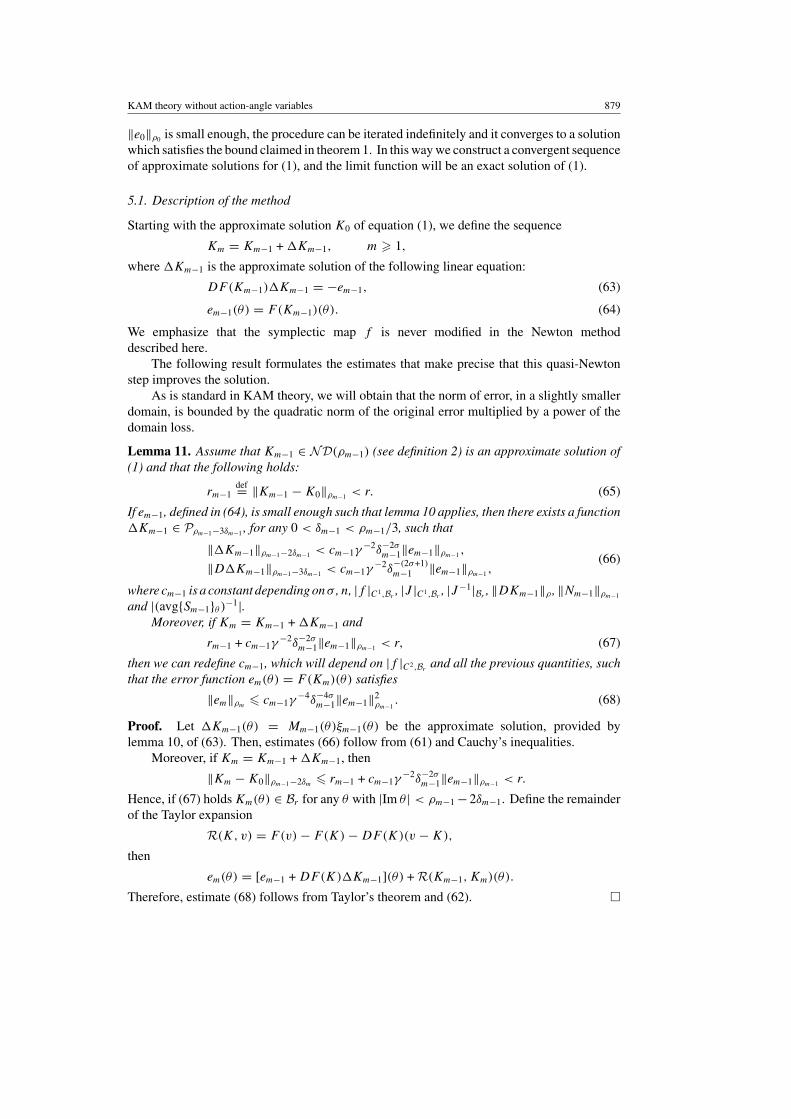
‖e0‖ρ0 is small enough, the procedure can be iterated indefinitely and it converges to a solutionwhich satisfies the bound claimed in theorem 1. In this way we construct a convergent sequenceof approximate solutions for (1), and the limit function will be an exact solution of (1).

5.1. Description of the method

Starting with the approximate solution K0 of equation (1), we define the sequence

Km = Km−1 + �Km−1, m � 1,

where �Km−1 is the approximate solution of the following linear equation:

DF(Km−1)�Km−1 = −em−1, (63)

em−1(θ) = F(Km−1)(θ). (64)

We emphasize that the symplectic map f is never modified in the Newton methoddescribed here.

The following result formulates the estimates that make precise that this quasi-Newtonstep improves the solution.

As is standard in KAM theory, we will obtain that the norm of error, in a slightly smallerdomain, is bounded by the quadratic norm of the original error multiplied by a power of thedomain loss.

Lemma 11. Assume that Km−1 ∈ ND(ρm−1) (see definition 2) is an approximate solution of(1) and that the following holds:

rm−1def= ‖Km−1 − K0‖ρm−1 < r. (65)

If em−1, defined in (64), is small enough such that lemma 10 applies, then there exists a function�Km−1 ∈ Pρm−1−3δm−1 , for any 0 < δm−1 < ρm−1/3, such that

‖�Km−1‖ρm−1−2δm−1 < cm−1γ−2δ−2σ

m−1‖em−1‖ρm−1 ,

‖D�Km−1‖ρm−1−3δm−1 < cm−1γ−2δ

−(2σ+1)m−1 ‖em−1‖ρm−1 ,

(66)

where cm−1 is a constant depending onσ , n, |f |C1,Br, |J |C1,Br

, |J−1|Br, ‖DKm−1‖ρ , ‖Nm−1‖ρm−1

and |(avg{Sm−1}θ )−1|.Moreover, if Km = Km−1 + �Km−1 and

rm−1 + cm−1γ−2δ−2σ

m−1‖em−1‖ρm−1 < r, (67)

then we can redefine cm−1, which will depend on |f |C2,Brand all the previous quantities, such

that the error function em(θ) = F(Km)(θ) satisfies

‖em‖ρm� cm−1γ

−4δ−4σm−1‖em−1‖2

ρm−1. (68)

Proof. Let �Km−1(θ) = Mm−1(θ)ξm−1(θ) be the approximate solution, provided bylemma 10, of (63). Then, estimates (66) follow from (61) and Cauchy’s inequalities.

Moreover, if Km = Km−1 + �Km−1, then

‖Km − K0‖ρm−1−2δm� rm−1 + cm−1γ

−2δ−2σm−1‖em−1‖ρm−1 < r.

Hence, if (67) holds Km(θ) ∈ Br for any θ with |Im θ | < ρm−1 − 2δm−1. Define the remainderof the Taylor expansion

R(K, v) = F(v) − F(K) − DF(K)(v − K),

then

em(θ) = [em−1 + DF(K)�Km−1](θ) + R(Km−1, Km)(θ).

Therefore, estimate (68) follows from Taylor’s theorem and (62). �


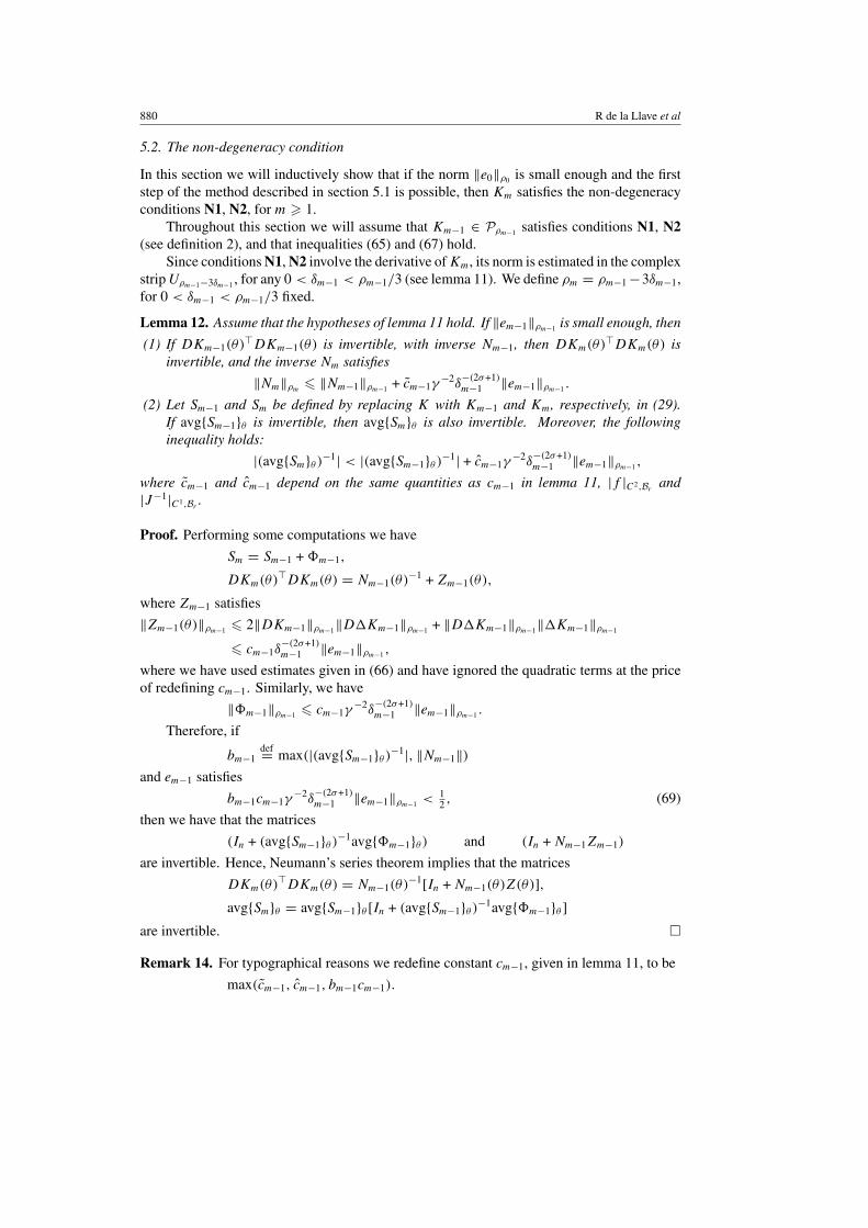
5.2. The non-degeneracy condition

In this section we will inductively show that if the norm ‖e0‖ρ0 is small enough and the firststep of the method described in section 5.1 is possible, then Km satisfies the non-degeneracyconditions N1, N2, for m � 1.

Throughout this section we will assume that Km−1 ∈ Pρm−1 satisfies conditions N1, N2(see definition 2), and that inequalities (65) and (67) hold.

Since conditions N1, N2 involve the derivative of Km, its norm is estimated in the complexstrip Uρm−1−3δm−1 , for any 0 < δm−1 < ρm−1/3 (see lemma 11). We define ρm = ρm−1 −3δm−1,for 0 < δm−1 < ρm−1/3 fixed.

Lemma 12. Assume that the hypotheses of lemma 11 hold. If ‖em−1‖ρm−1 is small enough, then

(1) If DKm−1(θ)�DKm−1(θ) is invertible, with inverse Nm−1, then DKm(θ)�DKm(θ) isinvertible, and the inverse Nm satisfies

‖Nm‖ρm� ‖Nm−1‖ρm−1 + cm−1γ

−2δ−(2σ+1)m−1 ‖em−1‖ρm−1 .

(2) Let Sm−1 and Sm be defined by replacing K with Km−1 and Km, respectively, in (29).If avg{Sm−1}θ is invertible, then avg{Sm}θ is also invertible. Moreover, the followinginequality holds:

|(avg{Sm}θ )−1| < |(avg{Sm−1}θ )−1| + cm−1γ−2δ

−(2σ+1)m−1 ‖em−1‖ρm−1 ,

where cm−1 and cm−1 depend on the same quantities as cm−1 in lemma 11, |f |C2,Brand

|J−1|C1,Br.

Proof. Performing some computations we have

Sm = Sm−1 + �m−1,

DKm(θ)�DKm(θ) = Nm−1(θ)−1 + Zm−1(θ),

where Zm−1 satisfies

‖Zm−1(θ)‖ρm−1 � 2‖DKm−1‖ρm−1‖D�Km−1‖ρm−1 + ‖D�Km−1‖ρm−1‖�Km−1‖ρm−1

� cm−1δ−(2σ+1)m−1 ‖em−1‖ρm−1 ,

where we have used estimates given in (66) and have ignored the quadratic terms at the priceof redefining cm−1. Similarly, we have

‖�m−1‖ρm−1 � cm−1γ−2δ

−(2σ+1)m−1 ‖em−1‖ρm−1 .

Therefore, if

bm−1def= max(|(avg{Sm−1}θ )−1|, ‖Nm−1‖)

and em−1 satisfies

bm−1cm−1γ−2δ

−(2σ+1)m−1 ‖em−1‖ρm−1 < 1

2 , (69)

then we have that the matrices

(In + (avg{Sm−1}θ )−1avg{�m−1}θ ) and (In + Nm−1Zm−1)

are invertible. Hence, Neumann’s series theorem implies that the matrices

DKm(θ)�DKm(θ) = Nm−1(θ)−1[In + Nm−1(θ)Z(θ)],

avg{Sm}θ = avg{Sm−1}θ [In + (avg{Sm−1}θ )−1avg{�m−1}θ ]

are invertible. �

Remark 14. For typographical reasons we redefine constant cm−1, given in lemma 11, to be

max(cm−1, cm−1, bm−1cm−1).


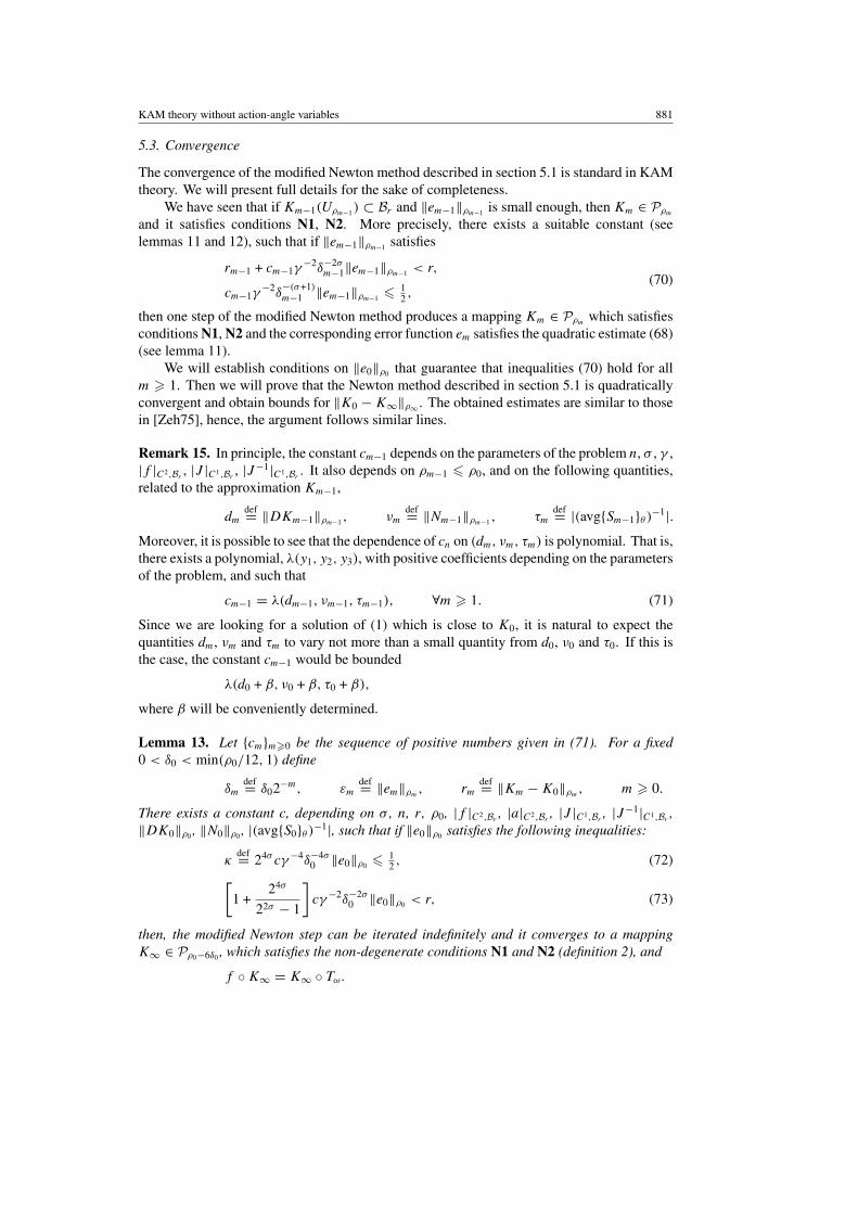
5.3. Convergence

The convergence of the modified Newton method described in section 5.1 is standard in KAMtheory. We will present full details for the sake of completeness.

We have seen that if Km−1(Uρm−1) ⊂ Br and ‖em−1‖ρm−1 is small enough, then Km ∈ Pρm

and it satisfies conditions N1, N2. More precisely, there exists a suitable constant (seelemmas 11 and 12), such that if ‖em−1‖ρm−1 satisfies

rm−1 + cm−1γ−2δ−2σ

m−1‖em−1‖ρm−1 < r,

cm−1γ−2δ

−(σ+1)m−1 ‖em−1‖ρm−1 � 1

2 ,(70)

then one step of the modified Newton method produces a mapping Km ∈ Pρmwhich satisfies

conditions N1, N2 and the corresponding error function em satisfies the quadratic estimate (68)(see lemma 11).

We will establish conditions on ‖e0‖ρ0 that guarantee that inequalities (70) hold for allm � 1. Then we will prove that the Newton method described in section 5.1 is quadraticallyconvergent and obtain bounds for ‖K0 − K∞‖ρ∞ . The obtained estimates are similar to thosein [Zeh75], hence, the argument follows similar lines.

Remark 15. In principle, the constant cm−1 depends on the parameters of the problem n, σ , γ ,|f |C2,Br

, |J |C1,Br, |J−1|C1,Br

. It also depends on ρm−1 � ρ0, and on the following quantities,related to the approximation Km−1,

dmdef= ‖DKm−1‖ρm−1 , νm

def= ‖Nm−1‖ρm−1 , τmdef= |(avg{Sm−1}θ )−1|.

Moreover, it is possible to see that the dependence of cn on (dm, νm, τm) is polynomial. That is,there exists a polynomial, λ(y1, y2, y3), with positive coefficients depending on the parametersof the problem, and such that

cm−1 = λ(dm−1, νm−1, τm−1), ∀m � 1. (71)

Since we are looking for a solution of (1) which is close to K0, it is natural to expect thequantities dm, νm and τm to vary not more than a small quantity from d0, ν0 and τ0. If this isthe case, the constant cm−1 would be bounded

λ(d0 + β, ν0 + β, τ0 + β),

where β will be conveniently determined.

Lemma 13. Let {cm}m�0 be the sequence of positive numbers given in (71). For a fixed0 < δ0 < min(ρ0/12, 1) define

δmdef= δ02−m, εm

def= ‖em‖ρm, rm

def= ‖Km − K0‖ρm, m � 0.

There exists a constant c, depending on σ , n, r , ρ0, |f |C2,Br, |a|C2,Br

, |J |C1,Br, |J−1|C1,Br

,‖DK0‖ρ0 , ‖N0‖ρ0 , |(avg{S0}θ )−1|, such that if ‖e0‖ρ0 satisfies the following inequalities:

κdef= 24σ cγ −4δ−4σ

0 ‖e0‖ρ0 � 12 , (72)[

1 +24σ

22σ − 1

]cγ −2δ−2σ

0 ‖e0‖ρ0 < r, (73)

then, the modified Newton step can be iterated indefinitely and it converges to a mappingK∞ ∈ Pρ0−6δ0 , which satisfies the non-degenerate conditions N1 and N2 (definition 2), and

f ◦ K∞ = K∞ ◦ Tω.


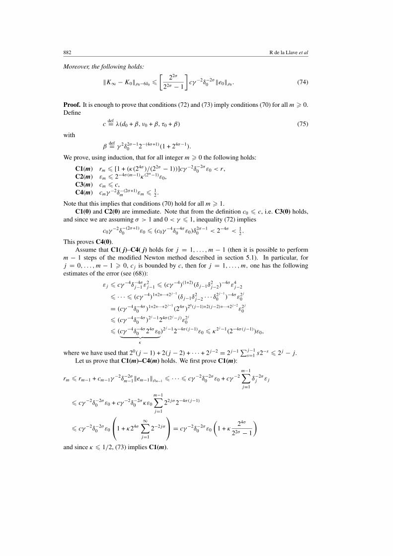
Moreover, the following holds:

‖K∞ − K0‖ρ0−6δ0 �[

22σ

22σ − 1

]cγ −2δ−2σ

0 ‖e0‖ρ0 . (74)

Proof. It is enough to prove that conditions (72) and (73) imply conditions (70) for all m � 0.Define

cdef= λ(d0 + β, ν0 + β, τ0 + β) (75)

with

βdef= γ 2δ2σ−1

0 2−(4σ+1)(1 + 24σ−1).

We prove, using induction, that for all integer m � 0 the following holds:

C1(m) rm � [1 + (κ(24σ )/(22σ − 1))]cγ −2δ−2σ0 ε0 < r ,

C2(m) εm � 2−4σ(m−1)κ(2m−1)ε0,C3(m) cm � c,C4(m) cmγ −2δ−(2σ+1)

m εm � 12 .

Note that this implies that conditions (70) hold for all m � 1.C1(0) and C2(0) are immediate. Note that from the definition c0 � c, i.e. C3(0) holds,

and since we are assuming σ > 1 and 0 < γ � 1, inequality (72) implies

c0γ−2δ

−(2σ+1)0 ε0 � (c0γ

−4δ−4σ0 ε0)δ

2σ−10 < 2−4σ < 1

2 .

This proves C4(0).Assume that C1( j)–C4( j) holds for j = 1, . . . , m − 1 (then it is possible to perform

m − 1 steps of the modified Newton method described in section 5.1). In particular, forj = 0, . . . , m − 1 � 0, cj is bounded by c, then for j = 1, . . . , m, one has the followingestimates of the error (see (68)):

εj � cγ −4δ−4σj−1 ε2

j−1 � (cγ −4)(1+2)(δj−1δ2j−2)

−4σ ε4j−2

� · · · � (cγ −4)1+2+···+2j−1(δj−1δ

2j−2 · · · δ2j−1

0 )−4σ ε2j

0

= (cγ −4δ−4σ0 )1+2+···+2j−1

(24σ )20(j−1)+2(j−2)+···+2j−2ε2j

0

� (cγ −4δ−4σ0 )2j −124σ(2j −j)ε2j

0

� (cγ −4δ−4σ0 24σ ε0︸︷︷︸κ

)2j −12−4σ(j−1)ε0 � κ2j −1(2−4σ(j−1))ε0,

where we have used that 20(j − 1) + 2(j − 2) + · · · + 2j−2 = 2j−1 ∑j−1s=1 s2−s � 2j − j.

Let us prove that C1(m)–C4(m) holds. We first prove C1(m):

rm � rm−1 + cm−1γ−2δ−2σ

m−1‖em−1‖ρm−1 � · · · � cγ −2δ−2σ0 ε0 + cγ −2

m−1∑j=1

δ−2σj εj

� cγ −2δ−2σ0 ε0 + cγ −2δ−2σ

0 κε0

m−1∑j=1

22jσ 2−4σ(j−1)

� cγ −2δ−2σ0 ε0

1 + κ24σ

∞∑j=1

2−2jσ

= cγ −2δ−2σ

0 ε0

(1 + κ

24σ

22σ − 1

)

and since κ � 1/2, (73) implies C1(m).


Therefore, inequalities (68) and (72) imply

εj < κ2j −1ε02−4σ(j−1), for j = 1, . . . , m, (76)

this proves C2(m).We now prove C3(m). The first inequality in (66) and lemma 12 imply

dm � dm−1 + cm−1γ−2δ

−(2σ+1)m−1 εm−1 � d0 + sm−1,

νm � νm−1 + cm−1γ−2δ

−(2σ+1)m−1 εm−1 � ν0 + sm−1,

τm � τm−1 + cm−1γ−2δ

−(2σ+1)m−1 εm−1 � τ0 + sm−1,

where

sm−1def=

m−1∑j=0

cjγ−2δ

−(2σ+1)j εj .

Let us estimate sm−1. Inequality (76) and C3( j) imply, for j = 1, . . . , m − 1,

cj γ−2δ

−(2σ+1)j εj � (cγ −2δ

−(2σ+1)0 ε0)2

4σ κ2j −12−j (2σ−1),

then, using inequality (72) one has

sm−1 � cγ −2δ−(2σ+1)0 ε0

(1 + κ24σ

∞∑j=1

2−j (2σ−1)

)

= κγ 2δ2σ−10 2−4σ

(1 + κ

24σ

22σ−1 − 1

)� γ 2δ2σ−1

0 2−(4σ+1)(1 + 24σ−1) = κ1.

Then

dm � d0 + β, νm � ν0 + β, τm � τ0 + β,

this implies cm � c, i.e. C3(m) holds. From (76) and (72) we have

cmγ −2δ−(2σ+1)m εm � (cγ −2δ

−(2σ+1)0 ε0)2

4σ κ(2m−1)2−m(2σ−1)

� κγ 2δ2σ−10 κ2m−12−m(2σ−1) � 1

2 .

Hence, we have proved C j(m) for j = 1, 2, 3, 4.Therefore, the modified Newton method described in section 5 produces a sequence of

mappings Km satisfying lemma 11. In particular, from the first inequality in (66) we have that{Km}m�0 is a Cauchy sequence in the scale of Banach spaces Pρm

. Let K∞ = limm→∞ Km, then

K∞ ∈ Pρ∞ (see definition 2), with ρ∞def= limm→∞ ρm = ρ0 − 6δ0. Moreover, inequality (68)

implies that K∞ satisfies (1). Finally, estimate (74) follows from the first inequality in (66) and

‖K∞ − K0‖ρ∞ �∞∑

m=0

‖�Km‖ρ∞ �∞∑

m=0

‖�Km‖ρm.

�

6. Local uniqueness

In this section, we prove theorem 2. The proof is rather standard. It suffices to show that theoperator DF(K) has an approximate left inverse (see [Zeh75]).

In our context the existence of the approximate left inverse amounts to the uniquenessstatement of proposition 8 and remark 13. The uniqueness up to additive constants in theseresults amounts to the uniqueness of re-parametrization of K (see remark 5).


From now on we assume that K1 and K2 satisfy the hypotheses of theorem 2. We notethat if F(K1) = F(K2) = 0, by Taylor’s theorem we have

0 = F(K1) − F(K2) = DF(K2)(K1 − K2) + R(K1, K2), (77)

where

‖R‖ρ � c‖K1 − K2‖2ρ.

Since K2 is an exact solution of (1), the results of section 4.2 apply and proposition 7 impliesthat equation (77) can be transformed into(

In S(θ)

0 In

)�(θ) − �(θ + ω) = −M−1(θ + ω)R(K1, K2)(θ),

where S is defined by (29), replacing K with K2, and

� = M(θ)−1(K1 − K2)(θ) =(

T (θ)

DK2(θ)�J (K2(θ))

)(K1 − K2)(θ)

with T defined in (38) (replacing K with K2).By the uniqueness statement in proposition 8 and remark 13 we obtain

‖� − (avg{�x}θ , 0)�‖ρ−2δ � cγ −2δ−2σ‖R‖2ρ � cγ −2δ−2σ‖K1 − K2‖2

ρ,

where

avg{�x}θ = avg{T (θ)[K1 − K2](θ)}θ .

Lemma 14. There exists a constant c, depending on n, ρ−1, |J |Br, |J−1|Br

, ‖N‖ρ , ‖K1‖C2,ρ ,such that if

c‖K1 − K2‖ρ � 1,

then there exists an initial phase τ1 ∈ �def= {τ ∈ R

n : |τ | < ‖K1 − K2‖ρ} such that,

avg{T (θ)[K1 ◦ Tτ1 − K2](θ)}θ = 0. (78)

Therefore, for any 0 < δ < ρ/2 we have

‖K1 ◦ Tτ1 − K2‖ρ−2δ < cγ −2δ−2σ‖K1 − K2‖2ρ (79)

for some constant c depending on n, σ , γ , ρ, ρ−1, |f |C2,Br, |J |Br

, |J−1|Br‖DK2‖ρ , ‖N‖ρ ,

|(avg{S}θ )−1|, with N and S as in definition 2, replacing K with K2.

Proof. Some direct computations (see (38)) show that

T (θ)DK2(θ) = In.

Then, for x ∈ Rn

T (θ)[K1(θ + x) − K2(θ)] = T (θ)[K1(θ + x) − K2(θ)] − T (θ)DK2(θ)x + x.

Therefore, a solution τ1 of (78) is a fixed point of

�(x)def= −avg{T (θ)[K1(θ + x) − K2(θ)] − T (θ)DK2(θ)x}θ .

Performing some computations we see that for any |x|, |y| < ‖K1 − K2‖ρ (i.e. x, y ∈ �), thefollowing holds:

|�(y) − �(x)| � c1|y − x|2 + c2|x||y − x| + c3‖D(K1 − K2)‖0|y − x|� c4‖K1 − K2‖ρ |y − x|,


where the constant c4 depends on n, ρ−1, ‖K2‖C2,ρ and ‖T ‖ρ (i.e. |J |Br, |J−1|Br

, ‖DK2‖ρ and‖N‖ρ , see (38)). Therefore, if c = c4, and

c‖K1 − K2‖ρ < 1,

then the mapping � : � → � is a contraction.Let |τ1| < ‖K1 − K2‖ρ satisfy (78), then K1 ◦ Tτ1 is a solution of (1) such that if

�(θ) = M(θ)−1(K1 ◦ Tτ1 − K2)(θ),

then the uniqueness statement in proposition 8, remark 13 and equality (78) imply

‖�‖ρ−2δ � cγ −2δ−2σ‖R‖2ρ � cγ −2δ−2σ‖K1 − K2‖2

ρ.

Therefore, we have

‖K1 ◦ Tτ1 − K2‖ρ−2δ � ‖M‖ρ‖�‖ρ−2δ

� cγ −2δ−2σ‖K1 − K2‖2ρ

for any 0 < δ, ρ/2. �Let τ1 be as in lemma 14, since K1 ◦ Tτ1 is also a solution of (1), we can apply lemma 14

to the solutions K1 ◦ Tτ1 and K2 (note that we do not change K2, this implies, in particular,that c and c do not change). Hence, we obtain a sequence {τm}m�1 such that

|τm − τm−1| < ‖K1 ◦ Tτm−1 − K2‖ρm−1

and

‖K1 ◦ Tτm− K2‖ρm

� cγ −2δ−2σm ‖K1 ◦ Tτm−1 − K2‖2

ρm−1· · ·

� (cγ −2)2m

[δmδ2m−1δ

22

m−2 . . . δ2m−1

1 ]−2σ‖K1 − K2‖2m

ρ

� (cγ −2δ−2σ1 22σ‖K1 − K2‖ρ)

2m

2−2σ(j−1),

where δ1 = ρ/8, δm+1 = δm/2 and ρm = ρ − ∑mj=1 δj for m � 1.

Therefore, if

c = max(c, c22σ )

and

γ −2δ−2σ1 c‖K1 − K2‖ρ < 1,

then the sequence {τm} converges, and its limit τ∞ satisfies

‖K1 ◦ Tτ∞ − K2‖ρ/2 = 0.

7. Proof of theorem 3

We formulate a general step of the procedure, the iterative procedure and the argument for theconvergence are identical to those presented in section 5.

7.1. A general step of a modified Newton method

Let K ∈ Pρ be an approximate solution of (14) with error function

e = fλ ◦ K − K ◦ Tω (80)

and assume that K and fλ satisfy definition 3. In order to construct a new approximate solutionby using a modified Newton method, we look for an increment of the parameter �λ and anincrement function �K which is one-periodic in each variable and such that the elements of


order 1 of G(K + �K, λ + �λ) are equal to zero, with G defined in (19). This leads to a studyof the solvability properties of the linearized equation:(

∂fλ(K(θ))

∂λ

)�λ + Df (K(θ))�K(θ) − �K(θ + ω) = −e(θ). (81)

Note that, except for the term (∂fλ(K(θ))/∂λ)�λ, the left-hand part of (81) has the same formas the linear operator DF(K). Hence, the geometric procedure described in section 4 willwork in this case with small modifications.

We emphasize that the geometric properties of an approximate solution of (1) and theresults on the reducibility of the linearized equation in section 4.2 follow from the symplecticproperties of f and the size of the error function, then the results of sections 4.1 and 4.2 alsohold for the symplectic map fλ. The main difference is that in section 4.3 the approximatesolvability was achieved using the exactness character of f and the non-degeneracy conditionN2 (see proposition 8 and lemma 9). In this case this will be achieved by using the incrementof the parameter �λ.

The approximate solution of the transformed equation will produce an approximatesolution of the linear equation (81) with quadratic error.

In order to ensure that the procedure can be iterated, we have to verify that the correctionobtained by adding to K the approximate solution of the linearized equation (81) and thesymplectic map fλ+�λ satisfy the same conditions as K and fλ (this part is identical tosection 5.2).

Proposition 7, applied to the map fλ and K , implies that if M is defined by (31), replacingf with fλ, then the change of variables �(θ) = M(θ)ξ(θ) transforms (81) into[(

In S(θ)

0 In

)+ B(θ)

]ξ(θ) − ξ(θ + ω) = p(θ) + w(θ) + M(θ + ω)−1

(∂fλ(K(θ))

∂λ

)�λ,

(82)

where S is defined in (29) replacing f with fλ,

p(θ) = −V (θ + ω)−1M(θ + ω)�J (K(θ + ω))e(θ), (83)

where V −1 is given in (37), and B and w satisfy estimates

‖B(θ)‖ρ−2δ � cγ −1δ−(σ+1)‖e‖ρ,

‖w‖ρ−2δ � cγ −1δ−(σ+1)‖e‖2ρ

for some constant c > 0.Moreover, lemma 6 implies

M(θ + ω)−1

(∂fλ(K(θ))

∂λ

)�λ = �(θ)�λ + q(θ)

with

�(θ)def= V (θ + ω)−1M(θ + ω)�J (K(θ + ω))

(∂fλ(K(θ))

∂λ

)(84)

and

‖q‖ρ−2δ � cγ −1δ−(σ+1)

∥∥∥∥∂fλ(K(θ))

∂λ

∥∥∥∥ρ

|�λ| ‖e‖ρ.

Let us prove that the reduced equation obtained by removing the terms B, w and q fromequation (82) can be solved for (ξ, �λ).


Proposition 15. Assume that ω ∈ D(γ, σ ) and that K and fλ satisfy definition 3. If ‖e‖ρ

is small enough then there exists a mapping ξ , analytic on Uρ−2δ , and a vector �λ ∈ R2n,

satisfying (In S(θ)

0 In

)ξ(θ) − ξ(θ + ω) = R(θ), (85)

where

R(θ)def= −V (θ + ω)−1M(θ + ω)�J (K(θ + ω))

[e(θ) +

(∂fλ(K(θ))

∂λ

)�λ

]. (86)

Moreover, there exists a constant c, depending on n, σ , ρ, r , |f |C2,Br, ‖DK‖ρ , ‖N(θ)‖ρ ,

‖(∂fλ(K(θ))/∂λ)‖ρ and |(avg{�}θ )−1| (see (84)) such that the following inequalities hold:

‖ξ‖ρ−2δ � cγ −2δ−2σ‖e‖ρ, (87)

|�λ| � c|(avg{�(θ)}θ )−1|‖e‖ρ. (88)

Proof. Consider the symplectically conjugated coordinates R = (Rx, Ry) and ξ = (ξx, ξy),then equation (85) can be written as

ξx(θ) − ξx(θ + ω) = Rx(θ) − S(θ)ξy(θ),

ξy(θ) − ξy(θ + ω) = Ry(θ).

From (86) one can see that

R(θ) =( −T (θ + ω)e(θ)

−DK(θ + ω)�J (K(θ + ω))e(θ)

)+ �(θ)�λ (89)

with � given in (84).Since fλ and K satisfy definition 3 we have that avg{�}θ has range of dimension 2n.

Therefore, we can fix the last n-coordinates of �λ ∈ R2n such that

avg{Ry}θ = 0.

Proposition 2 implies that there exists a unique zero-average analytic mapping on Uρ−δ

satisfying

ξy(θ) − ξy(θ + ω) = Ry(θ)

and

‖ξy‖ρ−δ � cγ −1δ−σ‖Ry‖ρ. (90)

Now, we let �λ be completely determined by the equation

avg{Rx(θ) − S(θ)ξy(θ)}θ = 0.

By proposition 2 there exists a unique mapping ξx satisfying

ξx(θ) − ξx(θ + ω) = px(θ) − S(θ)ξy(θ)

with

‖ξx‖ρ−2δ � cγ −1δ−σ‖Rx(θ) − S(θ)ξy(θ)‖ρ−δ. (91)

Note that �λ ∈ R2n was defined to be the unique solution of

avg{�(θ)}θ�λ =(

avg{−T (θ + ω)e(θ) − S(θ)ξy(θ)}θavg{−DK(θ + ω)�J (K(θ + ω))e(θ)}θ

). (92)


Let (ϕx, ϕy)� = avg{�(θ)}θ�λ, then from (89) and (92) we have the following estimates:

‖Ry‖ρ � c

(‖e‖ρ +

∥∥∥∥(

∂fλ(K(θ))

∂λ

)∥∥∥∥ρ

|ϕy |)

� c‖e‖ρ (93)

and

‖Rx‖ρ � c

(‖e‖ρ +

∥∥∥∥(

∂fλ(K(θ))

∂λ

)∥∥∥∥ρ

|ϕx |)

� c(‖e‖ρ + |avg{S(θ)ξy(θ)}θ |)� c(‖e‖ρ + c′γ −1ρ−1‖Ry‖ρ). (94)

Inequalities (90), (91), (93), (94) and equality (92) imply estimates (87) and (88). �The construction of an approximate solution of the linearized equation (81) is now clear,

and we establish this in the following result, the proof follows from the previous constructionand is very similar to the proof of lemma 10.

Proposition 16. Assume that the hypotheses of proposition 15 hold. Let ξ and �λ be as in

proposition 15, define �K(θ)def= M(θ)ξ(θ). The pair (�K, �λ) is an approximate solution

of the linearized equation (81) satisfying

‖DG(K, λ)(�K, �λ) + G(u, λ)‖ρ−2δ � cδ−3σ+1‖e‖2ρ

for some constant c, depending on n, σ , r , |f |C1,Br, ‖DK‖ρ , ‖N(θ)‖ρ , |(avg{�}θ )−1| (see (84))

and ‖(∂fλ(K(θ))/∂λ)‖ρ .

Remark 16. In the case that fλ is exact symplectic we have proved in section 4.3 that(see lemma 9)

|avg{DK(θ + ω)�J (K(θ + ω))e(θ)}θ | � cρ−1‖e‖2ρ,

then, if �λ = (�λx, �λy)�, we have

|�λy | � c′|(avg{�}θ )−1||avg{DK(θ + ω)�J (K(θ + ω))e(θ)}θ | � c′′‖e‖2ρ.

Moreover, if K satisfies the non-degeneracy condition N2 stated in definition (29), i.e. then × n matrix avg{S(θ)}θ , with S defined by (29), replacing f with fλ, is non-singular, thenwe can choose avg{ξy}θ in proposition 15 such that

avg{−T (θ + ω)e(θ) − S(θ)ξ}θ ,then �λy = 0 (see (92)).

7.1.1. The iterative procedure. Let �K and �λ be as in proposition 16, we consider K +�K

as an approximate solution of the equation

fλ+�λ ◦ Z = Z ◦ Tω.

Since K is analytic on Uρ and the solution of (85) is analytic on Uρ−2δ for any 0 < δ < ρ/2,K + �K is analytic on Uρ−2δ . Moreover, inequalities (87) and (88) imply

‖�K‖ρ−2δ � cδ−2σ‖e‖ρ, |�λ| � c‖e‖ρ (95)

and by using Cauchy’s inequality one has

‖D�K‖ρ−3δ � cδ−(2σ+1)‖e‖ρ. (96)

One step of the modified Newton method is obtained by proving that K +�K and fλ+�λ satisfythe same conditions as K and fλ.


Lemma 17. Assume that λ ∈ Rn, K ∈ P , and that fλ and K satisfy definition 3. If ‖e‖ρ is

small enough, then K +�K and fλ+� satisfy definition (84). Moreover, if � is defined by (84),then the following inequality holds:

|avg{�1(θ)}θ | � |avg{�(θ)}θ | + cγ −2δ−(2σ+1)‖e‖ρ,

where �1 is defined by (84) by replacing fλ and K with fλ+�λ and K + �K , respectively, andc is a constant depending on n, σ , r , |f |C2,Br

, ‖DK‖ρ , ‖N(θ)‖ρ , ‖(∂2fλ(K(θ))/∂2λ)‖ρ and|(avg{�}θ )−1|.

Proof. The proof is very similar to the proof of lemma 12 in section 5.2, it follows theassumption that the family fλ is twice differentiable with respect to λ, the estimations givenin (95) and (96) and Neumann’s series theorem. �

Since the estimate and the induction hypotheses have the same structure as those insection 5, the convergence argument and the final estimates do not need any modifications.

8. The linear equation for vector fields

Let ω be a fixed frequency vector satisfying the Diophantine condition (9), and let K be anapproximate solution of (15). We study the invertibility properties of the linear operator

JD(∇H(K))� − ∂ω�. (97)

8.1. Lagrangian character

We need the version of proposition 2 for vector fields.

Proposition 18. Assume that ω satisfies the Diophantine condition

|k · ω| � γ

|k|σ1, ∀ k ∈ Z

n − {0},

for some constants γ > 0 and σ > n − 1.Let h be a real analytic function with zero average. There exists a unique analytic solution

v with zero average, of the linear equation

n∑j=1

ωj

∂v

∂θi

= h.

Moreover, if h ∈ Pρ , the solution v satisfies the following estimate:

‖v‖ρ−δ � cδ−σ γ −1‖v‖ρ,

where c is a constant depending on n and σ .

It is known that if K is a solution of (15) with ω rationally independent, then the torusK(Tn) is a Lagrangian manifold. In the case that K satisfies (15) only approximately, we willprove that K(Tn) is approximate Lagrangian.

Lemma 19. Let K : Tn → U be a real analytic mapping on the complex strip of width ρ > 0.


e(θ) = J∇H(K(θ)) − ∂ωK(θ). (98)


The following holds:

(a) The components of the vector DK(θ)�Je(θ) are zero average functions.(b) If e = 0, i.e. K satisfies

∂ωK = J∇H ◦ K, (99)

then there exists a function b : Tn → R and a constant vector a0 ∈ R

n such that

K∗α = db + a0 dθ,

where α = −y dx.(c) There exist two functions b : T

n → R and g : Tn → R

n and a constant vector a0 ∈ Rn

such that

K∗α = db + a0 dθ +n∑

j=1

gj (θ) dθj .

Moreover, the function g satisfies

∂ωg(θ) = DK(θ)�Je(θ). (100)

(d) Let L(θ) be defined by (22). There exists a constant c, depending on n, σ and |DK|ρ ,such that

|L|ρ−2δ � cγ −1δ−(σ+1)‖e‖ρ. (101)

In particular, L = 0 if e = 0.

Proof. The pull-back of α = −y dx under K = (w, v)� is given by

K∗α = −v dw = −n∑

j=1

∂w(θ)

∂θj

�v(θ) dθj .

For j = 1, . . . , n, define aj (θ) = (∂w(θ)/∂θj )�v(θ), then

∂ωaj (θ) =(

∂ω

∂w(θ)

∂θj

)�v(θ) +

∂w(θ)

∂θj

�∂ωv(θ)

=[ex(θ) · ∂v(θ)

∂θj

− ey(θ) · ∂w(θ)

∂θj

]

+∂

∂θj

DyH(K(θ))v(θ) + (H ◦ K)(θ)︸︷︷︸

h1

− ex(θ) · v(θ)︸︷︷︸h2

.

Note that since ∂ωaj (θ), (∂/∂θj )h1 and (∂/∂θj )h2 have average equal to zero, then

avg

{ex(θ) · ∂v(θ)

∂θj

− ey(θ) · ∂w(θ)

∂θj

}θ

= 0,

which proves part (a) of lemma 19. Moreover (cf [Rus75]), since ω is Diophantine there existfunctions g : T

n → Rn and b1, b2 : T

n → R such that g satisfies (100) and

∂ωb1 = h1 − avg{h1}θ , ∂ωb2 = h2 − avg{h2}θ .If K is a solution of (99), then g and b2 are constants. Setting g = 0 and b2 = 0, we have

K∗α = −n∑

j=1

aj (θ) dθj = −∑

j

∂

∂θj

b1,j (θ) dθj − avg{aj }θ dθj ,

this proves part (b) of lemma 19. Taking b = −(b1 − b2) part (c) of lemma 19 follows.


Let us prove part (d). From part (c) we have

K∗� = dK∗α = d(−g dθ)

in coordinate representation one has

L(θ) = Dg(θ) − Dg(θ)�,

therefore, part (d) of lemma 19 follows from equality (100). �

8.2. Change of variables in the linearized equation

As in the case of analytic exact symplectic maps, the geometric structure of K makes it possibleto define a change of variables which transforms the linear operator (97) into a simpler one(compare with the case of maps in section 4.2). Let A be defined by

A(θ)def=

(Dx∇yH(K(θ)) Dy∇yH(K(θ))

−Dx∇xH(K(θ)) −Dy∇xH(K(θ))

)= JD(∇H)(K(θ)). (102)

Then the linearized equation

JD(∇H(K))� − ∂ω� = −e,

takes the form

A(θ)�(θ) − ∂ω�(θ) = −e(θ). (103)

If we perform the change of variables �(θ) = M(θ)ξ(θ), in the variables ξ the linearizedequation (103) has the following expression:

[A(θ)M(θ) − ∂ωM(θ)]ξ(θ) − M(θ)∂ωξ(θ) = −e(θ),

where A(θ) is defined in (102). Similar to the case of exact symplectic maps, we give a changeof variables M such that the matrix

M(θ)−1[A(θ)M(θ) − ∂ωM(θ)] (104)

is an upper triangular matrix with diagonal terms equal to zero.Assume that there exists a matrix N such that

N(θ) = (DK(θ)�DK(θ))−1 (105)

and consider the 2n × 2n matrix valued function

M(θ) = (DK(θ) JDK(θ)N(θ)). (106)

Lemma 20. If K is an approximate solution of (99), with error e, then if M is defined by (106)we have

A(θ)M(θ) − ∂ωM(θ) = M(θ)

(0 S(θ)

0 0

)+ E(θ) (107)

with

S(θ) = N(θ)DK(θ)�[A(θ)J − JA(θ)]DK(θ)N(θ) (108)

and

‖JM(θ)�JE‖ρ−2δ � cγ −1δ−(σ+1)‖e‖ρ, (109)

where 0 < δ < ρ/2 and c is a constant depending on n, ρ, ‖A‖ρ , ‖K‖ρ and ‖N‖ρ .


Proof. This is an analogue to the results for maps presented in section 4.2. Since the casewhen K is an approximate solution of (15) involves a lot of (but simple) computations whichcould hide the main idea we only consider the case when K is a solution of (15).

Let us compute W(θ) = A(θ)M(θ) − ∂ωM(θ) in two steps: (a) compute the firstn-columns, (b) compute the last n-columns.

First note that since K satisfies (15)

A(θ)DK(θ) = ∂ωDK(θ), (110)

this gives that the first n columns of W(θ) are equal to zero.The last n columns of W(θ) are given by

W1(θ) = A(θ)JDK(θ)N(θ) − ∂ω(JDK(θ)N(θ)).

The Hamiltonian character A(θ)J = −JA(θ)� and equality (110) implies

W1(θ) = −J [A(θ)� + A(θ)]DK(θ)N(θ) − JDK(θ)∂ωN(θ).

Moreover, by using equality (110), it is not difficult to see that

∂ωN(θ) = −N(θ)DK(θ)�[A(θ)� + A(θ)]DK(θ)N(θ).

Since K satisfies (15) the vectors {∂K(θ)/∂θj , J (∂K(θ)/∂θj )}nj=1 form a basis of TθU ∼ R2n,

then we can find n × n matrix-valued functions S(θ) and T (θ), such that

W1(θ) = DK(θ)S(θ) + JDK(θ)N(θ)T (θ). (111)

Multiplying the last inequality by −DK(θ)�J and performing some simple substitutions oneobtains

T (θ) = −DK(θ)�JW1(θ) = 0.

Moreover, multiplying equality (111) by N(θ)DK(θ)� we have

S(θ) = N(θ)DK(θ)�[A(θ)JDK(θ)N(θ) − J∂ω(DK(θ)N(θ))]

= N(θ)DK(θ)�[A(θ)J − JA(θ)]DK(θ)N(θ),

where we have used the two following equalities:

DK(θ)�JDK(θ) = 0, ∂ωDK(θ) = A(θ)DK(θ).

Therefore, if S has the expression given in (108), and K is a solution of (15), we have

A(θ)M(θ) − ∂ωM(θ) = M(θ)

(0 S(θ)

0 0

).

The case when K is an approximate solution of (15) with error e follows defining

E(θ) = A(θ)M(θ) − ∂ωM(θ) − M(θ)

(0 S(θ)

0 0

).

Performing some computations and using the equality

A(θ)DK(θ) − ∂ωDK(θ) = De(θ),

we obtain equality (107) and estimate (109). �Now we prove that the matrix M defined in (106) is invertible. From the definition of M

it follows that

M(θ)�JM(θ) = −J + R(θ)

with

R(θ) =(

L(θ) 00 N�L(θ)N(θ)

),

where L = DK(θ)�JDK(θ).


The norm of matrix R is controlled by the approximate Lagrangian character of the torus K .In fact, from inequality (101), the norm of R verifies the following inequality:

‖R‖ρ−2δ � cγ −1δ−(σ+1)‖e‖ρ.

Lemma 21. If the error function e is small enough, the matrix M , given by (106), is invertibleand the inverse is given by

M(θ)−1 = JM(θ)�J + Me(θ)

with

‖Me‖ρ−2δ � cγ −1δ−(σ+1)‖e‖ρ

for some constant c and any 0 < δ < ρ. In particular, if e = 0, Me = 0.

When K solves equation (15) approximately, matrix M defined by (106) reduces (104)into a simple form, and the change of variables �(θ) = M(θ)ξ(θ) will transform the linearizedequation (97) into a more simple one (see (112)). The result can be summarized as follows.

Proposition 22. The change of variables �(θ) = M(θ)ξ(θ), with M defined in (106),transforms the linearized equation (103) into[(

0 S(θ)

0 0

)+ B(θ)

]ξ(θ) − ∂ωξ(θ) = p(θ) + w(θ), (112)

where S is defined in (108),

p(θ) = −JM(θ)�Je(θ) =(

−N(θ)�DK(θ)�e(θ)

DK(θ)�Je(θ)

)(113)

and B and w satisfy

‖B‖ρ−2δ � cγ −1δ−(σ+1)‖e‖ρ,

‖w‖ρ−δ � cγ −1δ−(σ+1)‖e‖2ρ

(114)

for any 0 < δ < ρ/2, where c is a constant depending on n, ‖DK‖ρ and ‖N‖ρ .

Proof. Since M is invertible, we have

A(θ)M(θ)ξ(θ) − ∂ω(M(θ)ξ(θ)) = M(θ)[M(θ)−1W(θ)ξ(θ) − ∂ωξ(θ)]

= M(θ)[JM(θ)�JW(θ)ξ(θ) + MeW(θ)ξ(θ) − ∂ωξ(θ)],

with W(θ) = A(θ)M(θ) − ∂ωM(θ). From lemma 20 we have

M(θ)−1W(θ) =(

0 S(θ)

0 0

)+ M(θ)−1E(θ).

Therefore, if we define

B(θ) = M(θ)−1E(θ) = JM(θ)�JE(θ) + Me(θ)E(θ)

the estimate (109) and the estimate for the norm of Me imply the first inequality of (114).Therefore, in the variables ξ , the linear equation (103) is written

[C(θ) + B(θ)]ξ(θ) − ∂ωξ(θ) = −M(θ)−1e(θ) = −JM(θ)�Je(θ) − Mee(θ). �


8.3. Solvability of the reduced equation

Let us consider the reduced equation

S(θ)ξy − ∂ωξx = −N(θ)�DK(θ)�e(θ),

∂ωξy = DK(θ)�Je(θ),(115)

The conditions guaranteeing the existence of a solution (ξx, ξy) of equation (115) are providedby the following result:

Lemma 23. There exists a solution (ξx, ξy) of equation (115) satisfying the following estimate:

‖ξy‖ρ−δ � c1γ−1δ−σ‖e‖ρ,

‖ξx‖ρ−2δ � c2γ−2δ−2σ‖e‖ρ

for any 0 < δ < ρ/2, where c1 and c2 are constants depending on n, σ , ‖N‖ρ , ‖K‖ρ and|(avg{S}θ )−1|.

Proof. From part (c) of lemma 19 avg{DK(θ)�Je(θ)}θ = 0, then the small divisors equation

∂ωξy = DK(θ)�Je(θ)

has a solution ξy with average equal to zero (cf [Rus75]). Let ξy ∈ Rn such that the function

ξy = ξy + ξy satisfies

avg{S(θ)ξy + N(θ)�DK(θ)�e(θ)}θ = 0.

Then, the small divisors equation

∂ωξx = S(θ)ξy + N(θ)�DK(θ)�e(θ)

has a unique solution ξx with average equal to zero. The estimations for ξx and ξy followfrom [Rus75]. �

Acknowledgments

The authors are grateful to Professor Niederman for his careful reading of this paper and for hisvaluable suggestions. The work of RL has been supported by NSF grants, a Deans Fellowshipat U.T. Austin Spring 03. Visits of RL to Barcelona have been supported by ICREA. AG wassupported by a US–Spain Science & Technology Programme 2000, Project 96. AJ and JV havealso been supported by the Catalan grant 2001SGR-70, the Spanish grant MCyT/FEDER,no BFM2003-07521-C02-01, the INTAS grant 00-221 and DURSI.

References

[Bos86] Bost J-B 1986 Tores invariants des systemes dynamiques hamiltoniens (d’apres Kolmogorov, Arnold,Moser, Russmann, Zehnder, Herman, Poschel, . . .) Asterisque 133–134 113–57 Seminar Bourbakivol 1984/85

[CC97] Celletti A and Chierchia L 1997 On the stability of realistic three-body problems Commun. Math. Phys.186 413–49

[DdlLS03] Delshams A, de la Llave R and Seara T M 2003 A geometric mechanism for diffusion in hamiltoniansystems overcoming the large gap problem: heuristics and rigorous verification on a model Preprintmp arc 03-182

[dlL01] de la Llave R 2001 A tutorial on KAM theory Smooth Ergodic Theory and its Applications (Seattle, WA,1999) (Providence, RI: American Mathematical Society) pp 175–292

[dlLV00] de la Llave R and Vano J 2000 A Whitney–Zehnder implicit function theorem Manuscript


[Dou82] Douady R 1982 Une demonstration directe de l’equivalence des theoremes de tores invariants pourdiffeomorphismes et champs de vecteurs C. R. Acad. Sci. Paris Ser. I Math. 295 201–4

[FGB98] Fasso F, Guzzo M and Benettin G 1998 Nekhoroshev-stability of elliptic equilibria of Hamiltonian systemsCommun. Math. Phys. 197 347–60

[GFB98] Guzzo M, Fasso F and Benettin G 1998 On the stability of elliptic equilibria Math. Phys. Electron. J. 4Paper 1, p 16 (electronic)

[HdlL04a] Haro A and de la Llave R 2004 A parameterization method for the computation of whiskers in quasiperiodic maps: numerical implementation Preprint mp arc 04-350

[HdlL04b] Haro A and de la Llave R 2004 A parameterization method for the computation of whiskers in quasiperiodic maps: rigorous results Preprint mp arc 04-348

[Her83] Herman M-R 1983 Sur les courbes invariantes par les diffeomorphismes de l’anneau vol 1 (Paris: SocieteMathematique de France) Asterisque 103

[Koz83] Kozlov S M 1983 Reducibility of quasiperiodic differential operators and averaging Tr. Moskov. Mat.Obshch. 46 99–123

Kozlov S M 1984 Trans. Moscow Math. Soc. 2 101–26 (Engl. Transl.)[Mos66a] Moser J 1966 A rapidly convergent iteration method and non-linear differential equations. II Ann. Scuola

Norm. Sup. Pisa (3) 20 499–535[Mos66b] Moser J 1966 A rapidly convergent iteration method and non-linear partial differential equations. I Ann.

Scuola Norm. Sup. Pisa (3) 20 265–315[Mos67] Moser J 1967 Convergent series expansions for quasi-periodic motions Math. Ann. 169 136–76[Mos88] Moser J 1988 A stability theorem for minimal foliations on a torus Ergodic Theory Dyn. Syst. 8∗ (Charles

Conley Memorial Issue) 251–81[Neı84] Neıshtadt A I 1984 The separation of motions in systems with rapidly rotating phase Prikl. Mat. Mekh.

48 197–204[Nie98] Niederman L 1998 Nonlinear stability around an elliptic equilibrium point in a Hamiltonian system

Nonlinearity 11 1465–79[Pos99] Poschel J 1999 On Nekhoroshev’s estimate at an elliptic equilibrium Internat. Math. Res. Notices 203–15[Pos01] Poschel J 2001 A lecture on the classical KAM theorem Smooth Ergodic Theory and its Applications

(Seattle, WA, 1999) (Providence, RI: American Mathematical Society) pp 707–32[Ran87] Rana D 1987 Proof of accurate upper and lower bounds to stability domains in small denominator problems

PhD Thesis Princeton University[RC95] Rakovic M J and Shih-I Chu 1995 New integrable systems: hydrogen atom in external fields Physica D

81 271–9[RC97] Rakovic M J and Shih-I Chu 1997 Phase-space structure of a new integrable system related to hydrogen

atoms in external fields J. Phys. A: Math. Gen. 30 733–53[Rus75] Russmann H 1975 On optimal estimates for the solutions of linear partial differential equations of first

order with constant coefficients on the torus Dynamical Systems, Theory and Applications (BattelleRencontres, Seattle, WA, 1974) (Lecture Notes in Physics vol 38) (Berlin: Springer) pp 598–624

[Rus76a] Russmann H 1976 On a new proof of Moser’s twist mapping theorem Proc. 5th Conf. on MathematicalMethods in Celestial Mechanics (Oberwolfach, 1975) vol 14 (part I) pp 19–31

[Rus76b] Russmann H 1976 On optimal estimates for the solutions of linear difference equations on the circleCelestial Mech. 14 33–7

[Rus76c] Russmann H 1976 Note on sums containing small divisors Commun. Pure Appl. Math. 29 755–8[Sal04] Salamon D 2004 The Kolmogorov–Arnold–Moser theorem Math. Phys. Electron. J. (3) 1–37[SZ89] Salamon D and Zehnder E 1989 KAM theory in configuration space Comment. Math. Helv. 64 84–132[Van02] Vano J 2002 A Whitney–Zehnder implicit function theorem PhD Thesis University of Texas at Austin[Wei77] Weinstein A 1977 Lectures on Symplectic Manifolds (Regional Conference Series in Mathematics No 29)

(Providence, RI: American Mathematical Society) (Expository lectures from the CBMS Regional Conf.held at the University of North Carolina, 8–12 March, 1976)

[WL98] Wojtkowski M P and Liverani C 1998 Conformally symplectic dynamics and symmetry of the Lyapunovspectrum Commun. Math. Phys. 194 47–60

[Zeh75] Zehnder E 1975 Generalized implicit function theorems with applications to some small divisorproblems. I Commun. Pure Appl. Math. 28 91–140

[Zeh76] Zehnder E 1976 Generalized implicit function theorems with applications to some small divisorproblems. II Commun. Pure Appl. Math. 29 49–111

Documents

KAM theory without action-angle variables