Embed Size (px)
Citation preview

Computational Study of
Multiple Hydrokinetic Turbine Performance
By
Joseph David Jonas
A Thesis
Presented to the Graduate and Research Committee
Of Lehigh University
in Candidacy for the Degree of Master of Science
in
Mechanical Engineering
Lehigh University
August 2014

ii
iii
This thesis is accepted and approved in partial fulfillment of the requirements for the
Master of Science degree in Mechanical Engineering
__________________________________________
Date Approved
________________________________________
Dr. Alparslan Oztekin
Thesis Advisor
________________________________________
Dr. D. Gary Harlow, Chairperson
Mechanical Engineering and Mechanics

iv
Table of Contents
List of Figures ..................................................................................................................... v
Acknowledgements ........................................................................................................... vii
Nomenclature ....................................................................................................................... i
Abstract ............................................................................................................................... 1
1. Introduction ................................................................................................................. 2
1.2 Motivation for Present Research .......................................................................... 3
1.3 Limits of Hydrokinetic Turbine Efficiency .......................................................... 5
1.4 Introduction to Turbulence Modeling .................................................................. 8
1.5 Introduction to Computational Fluid Dynamics ................................................ 10
1.6 Opportunity for Present Research ...................................................................... 12
2. Simulation Setup........................................................................................................ 13
2.1 Geometry Selection and Generation .................................................................. 13
2.2 Mesh Generation ................................................................................................ 20
2.3 Approximations of Turbine Rotation ................................................................. 24
2.4 Turbulence Model Selection .............................................................................. 26
2.5 Boundary and Initial Conditions ........................................................................ 30
2.7 Solver Selection.................................................................................................. 34
3. Simulation Quality and Results ................................................................................. 35
3.1 Turbine Performance Metrics............................................................................. 35
3.2 Turbine Performance Outputs ............................................................................ 36
3.3 Simulation Quality Metrics ................................................................................ 40
3.4 Simulation Quality ............................................................................................. 42
4. Conclusion ................................................................................................................. 55
4.1 Results Summary and Turbine Placement Recommendations ................................ 55
4.2 Physical Explanation of Simulation Results ........................................................... 56
4.3 Methods of Simulation Validation .......................................................................... 57
4.4 Areas of Further Research ....................................................................................... 59
Bibliography ..................................................................................................................... 61
Vita .................................................................................................................................... 63

v
List of Figures
Figure 1: Cross section of a conventional hydroelectric power plant [1] .......................... 3
Figure 2: Horizontal Axis vs Vertical Axis Turbines [5] .................................................. 5
Figure 3: Perspective view of Turbine Geometry ............................................................ 14
Figure 4: View of Turbine from Flow Direction ............................................................. 14
Figure 5: Definition of Separation Distance .................................................................... 15
Figure 6: Front View of nonrotating domains for a) d = 3R, b) d = 5R, c) d = 7R ......... 18
Figure 7: Perspective View of Simulation Space (d = 5R) .............................................. 19
Figure 8: Inlet View of Simulation Space (d = 5R) ......................................................... 19
Figure 9: Blade Surface Mesh Viewed from Flow Direction (d = 5R) ........................... 21
Figure 10: Mesh extending upstream and downstream of blade tip (d = 5R) ................. 21
Figure 11: Coarse Mesh Front View (d = 5R) ................................................................. 22
Figure 12: Fine Mesh Front View (d = 5R) ..................................................................... 23
Figure 13: a) Left Turbine Power vs Separation distance b) Right Turbine Power vs
Separation Distance .......................................................................................................... 37
Figure 14: a) Left Turbine Drag vs Separation Distance b) Right Turbine Drag vs
Separation Distance .......................................................................................................... 38
Figure 15: Percentage different between left Turbine and Right Turbine power ............ 39
Figure 16: Velocity Downstream of Turbines for a) Fine Mesh and b) Coarse Mesh at d =
5R ...................................................................................................................................... 44
Figure 17: Surface Pressure Contours for d = 5R separation distance on a) Fine Mesh and
b) Coarse Mesh ................................................................................................................. 45
Figure 18: Surface of Constant Vorticity (25.25 s^-1) for d=5R on the a) Fine Mesh and
b) Coarse Mesh ................................................................................................................. 47
Figure 19: Highest Residual for each Simulation ............................................................ 48
Figure 20: Velocity Contours on Coarse mesh for the a) d = 3R b) d = 5R and c) d = 7R
simulations ........................................................................................................................ 51
Figure 21: Surfaces of Constant Vorticity on the coarse mesh for a) d = 3R b) d = 5R and
c) d = 7R simulations ........................................................................................................ 53
Figure 22: 𝒚 + values for the coarse mesh d = 5R simulation ........................................ 54

vi
Figure 23: Typical river flow cross-section [23] ............................................................ 55

vii
Acknowledgements
The author would first like to thank his thesis advisor, Professor Alparslan Oztekin
for his guidance, insight and enthusiasm through every step of this research process. Chris
Schleicher and Jake Riglin, with their extensive knowledge of Computational Fluid
Dynamics tools, were invaluable in assisting with simulation setup and troubleshooting,
and the author would extend his gratitude to them as well. Additionally, the author would
like to express his sincerest appreciation and thanks towards his parents and Lehigh
University alumni Cynthia Ellsworth Jonas, BSME ’82 and Gordon M Jonas, BSME ’81
for all of their encouragement and wisdom over the last twenty-three years. Finally, the
author would like to thank the myriad of other family, friends, teachers and mentors who
have helped and continue to help him achieve his dreams.

Nomenclature
𝐾�� Rate of Kinetic Energy
entering Turbine [J s-1]
�� Mass Flow rate entering
Turbine [kg s-1]
𝑉𝑖 Velocity at Turbine Inlet [m s-
1]
𝜌 Fluid Density [kg m-3]
𝐴 Swept Area of Turbine [m2]
𝐶𝑇 Ideal Turbine Power
Coefficient [-]
𝑉𝑜 Velocity at Turbine Exit [m s-
1]
𝑃𝑖𝑑𝑒𝑎𝑙 Power Generated by Ideal
Turbine [W]
𝑇𝑆𝑅 Tip Speed Ratio [-]
𝑅 Turbine Radius [m]
𝛺 Magnitude of Rotation Rate of
Turbine [rad s-1]
𝜎 Solidity Ratio [-]
𝐵 Number of Turbine Blades [-]
𝑐 Chord length of turbine at
blade tip [m]
𝑅𝑒𝑥 Reynolds Number based on
characteristic length 𝑥 [-]
𝑥 Characteristic length of system
[m]
𝜇 Dynamic Viscosity of Fluid
[Pa s]
∇ Vector Differential Operator
[m-1]
∙ Vector Dot Product Operator [-
]
𝒗 Absolute Velocity Vector [m s-
1]
𝑡 Time [s]
𝑝 Static Pressure [Pa]
𝒇 Net body force per Unit
Volume Vector [N m-3]
𝑑 Turbine Separation Distance
[m]
𝒗𝑟 Velocity Vector relative to
rotating frame [m s-1]
𝜴 Vector of Revolution of the
Rotating Domain [s-1]
× Vector Cross Product [-]
𝒓
Displacement Vector from point
in Rotating domain to origin of
rotating domain (m)
𝑘 Specific Turbulent Kinetic
Energy [m2 s2]
𝑢𝑖 The i-th component of vector 𝒗
[m s-1]
𝑢𝑖′ The fluctuating component of
𝑢𝑖 [m s-1]
𝜖 Specific Turbulent Dissipation
[m2 s3]
𝜈 Kinematic Viscosity (equal to
𝜇/𝜌) [m2 s-1]
𝑥𝑘 k-th component of the
coordinate frame [m]
𝜔 Specific Dissipation Rate [s-1]
𝛽∗ Constant [0.09]
𝜏𝑖𝑗 Reynolds Stress Tensor [Pa]
𝛿𝑖𝑗 Kronecker delta function [-]
𝜇𝑡 Turbulent Dynamic Viscosity
[Pa s]
𝐹1 Blending Function [-]
𝐹2 Blending Function [-]
ii
𝐶𝐷𝑘𝜔
Positive portion off-diagonal
Cross Diffusion terms from 𝜔
equation [kg m-3 s-2]
𝛺∗ Absolute value of Vorticity
Vector [s-1]
𝜎𝑘1 Constant [0.85]
𝜎𝑘2 Constant [1.0]
𝜎𝜔1 Constant [0.5]
𝜎𝜔2 Constant [0.856]
𝛽1 Constant [0.0750]
𝛽2 Constant [0.0828]
𝜅 Constant [0.41]
𝑎1 Constant [0.31]
𝛾1 Function of 𝛽1, 𝛽∗, 𝜎𝜔1, and 𝜅
[0.533166]
𝛾2 Function of 𝛽2, 𝛽∗, 𝜎𝜔2, and 𝜅
[0.44035]
𝜎𝑘 Function of 𝐹1, 𝜎𝑘1, and 𝜎𝑘2 [-]
𝜎𝜔 Function of 𝐹1, 𝜎𝜔2 and 𝜎𝜔2 [-]
𝛽 Function of 𝐹1, 𝛽1, and 𝛽2 [-]
𝛾 Function of 𝐹1, 𝛾1, and 𝛾2 [-]
𝑈 Free Stream Velocity [m s-1]
𝑘𝑖𝑜 Value of 𝑘 at the domain inlet
and outlet [m2 s2]
𝜔𝑖𝑜 Value of 𝜔 at the domain inlet
and outlet [s-1]
𝐼 Turbulent Intensity [-]
𝑙 Turbulent Length Scale [-]
𝐷ℎ Hydraulic Diameter of River
Domain [m]
𝑅𝑒𝐷ℎ
Reynolds Number using 𝐷ℎ as
the characteristic length [-]
𝑘𝑤𝑎𝑙𝑙 Value of 𝑘 at the solid walls of
domain [m2 s2]
𝜔𝑤𝑎𝑙𝑙 Value of 𝜔 at the solid walls of
domain [s-1]
∆𝑦1
Distance from the wall to the
nearest point in the discretized
domain[m]
𝑦+ Dimensionless wall distance [-]
𝑢∗ Friction Velocity [m s-1]
𝜏𝑤 Wall shear stress [Pa]
𝐶𝑃 Coefficient of Performance [-]
𝑃 Simulation Power Output [W]
𝐶𝐷 Coefficient of Drag [-]
𝐹𝐷 Simulation Drag [N]

1
Abstract
The k-ω Shear Stress Transport turbulence model was used to determine the
performance of a pair of horizontal-axis hydrokinetic turbines. By varying the separation
distance perpendicular to the flow direction between these turbines and computing both
power and drag coefficients, the relationship between these outputs and the separation
distance as an input was discovered. This study used a rotating reference frame, steady
state approximation over three separation distances and two different mesh sizes to verify
mesh independence. Once this meshing methodology was verified, two more separation
distances were run using the same steady-state approximations at the coarse mesh size to
better understand turbine performance at greater separation distances. The results of these
simulations show that, at a given separation distance, the left and right turbines have very
similar performance. The power and drag coefficients were both found to decrease on the
order of 8% as the turbines are brought closer together, which means that, in an infinite
and uniform flow field, turbines should be placed as far apart as is feasible to maximize
resultant combined power output.
2
1. Introduction
1.1 History of Hydro Power
The potential for the movement of water to do useful work was realized thousands
of years ago by farmers in Mesopotamia and ancient Egypt, whose advances in controlled
irrigation allowed their civilizations to thrive in even harsh environments. Centuries later,
water wheels were used to extract mechanical work from rivers to perform a variety of
tasks much more efficiently than could be done by hand, such as crushing grain, spinning
pottery wheels, or operating machinery in textile mills. With the invention of the electric
generator in the late nineteenth century, it was not long before hydroelectric power
established itself as a reliable and inexpensive method of power generation.
As technology has progressed over the last two centuries, the conventional method
of generating hydroelectricity that has arisen involves creating a dam which obstructs the
water’s flow. As the water upstream continues to flow and hit the dam, the water level
around the dam rises and creates an artificial lake where massive amounts of water builds
up. The water at the bottom of this lake is now under high pressure due to the weight of all
of the water above it, which creates an enormous amount of potential energy. By releasing
some of the water at the bottom of the lake and forcing it through a turbine, this potential
energy is converted into mechanical energy. This mechanical energy is converted into
electrical power using a series of massive electric generators, which can then be distributed
to the power grid with the help of transformers. A cross section of a typical hydroelectric
power plant is shown in Figure 1.

3
Figure 1: Cross section of a conventional hydroelectric power plant [1]
As of 2011, hydroelectric power produces 3.5 trillion kilowatt-hours of electricity
annually (which represents 16% of global electricity generation), and almost all of this
power is produced by the world’s 45,000+ large hydroelectric dams. The total amount of
power generated via hydroelectricity is expected to grow by an average of 3% annually,
which it has averaged every year for the past four decades [2].
1.2 Motivation for Present Research
Conventional hydroelectric power has many advantages, the most notable of which
is that it is a renewable energy, and one that has two orders of magnitude lower carbon
footprint per kilowatt-hour than coal, oil, or natural gas [3]. Additionally, once the power
station is already running, it is one of the cheapest forms of electricity, at 3 to 5 US cents
per kilowatt-hour for plants that have over a 10 megawatt capacity [4].
One major feature of conventional hydropower is that it necessitates the creation of
a large body of water to extract power from. Region-dependent, the lake that the dam

4
creates can be a popular tourist attraction and bring in a lot of revenue for the surrounding
community. However, the creation of this lake also means that the natural habitat of many
different forms of wildlife will be disrupted, which can involve preventing the migration
of fish in the river as well as displacing any land-based animals (humans included) that
might live along the river’s shore. Another issue is that, often times, the ability of the
hydroelectric plant to generate power can be compromised during long draught periods or,
climate-dependent, during the wintertime, when the river flowing into the dam can freeze.
Dams and the lakes that they create also require substantial space, often taking up
dozens of square miles of surface area and hundreds of thousands or even millions of cubic
meters of water volume. But in some communities the biggest issue is that building a dam
can be prohibitively expensive and take years of planning and construction time before any
power can be generated. These properties can make conventional hydroelectric dams ill-
suited to providing the power needs of certain groups of people, who are likely to turn to
fossil fuels to fulfill their power needs even despite the presence of powerful rivers that
flow through their communities. People living in areas that do fit this description, as well
as any other organizations which could utilize highly mobile and quiet power generation
create the potential market for a source of hydroelectric power that shares many of the
benefits of conventional hydropower, but without severely disrupting the environment in
which they are installed or requiring a long and expensive setup.
The most simple of such a device is the Hydrokinetic Turbine (HKT), which is
capable of generating mechanical energy from a stream using only the kinetic energy that

5
the moving water already has. This mechanical energy can then be used to make electrical
power via a generator, similar to how wind turbines generate power from moving air.
Hydrokinetic Turbines can be classified into two main categories: vertical axis
turbines and horizontal axis turbines. The difference between them is that, in horizontal
axis turbines, the axis of rotation of the turbine is parallel with the flow direction, whereas
in vertical-axis turbines the rotation axis of the turbines is perpendicular to the flow
direction (usually such that the axis of rotation is in the same plane as the river’s surface,
or in a manner that is perpendicular to that surface). The different turbine types are shown
in Figure 2 for Wind Turbines, although the concept is the same for Hydrokinetic Turbines.
Figure 2: Horizontal Axis vs Vertical Axis Turbines [5]
1.3 Limits of Hydrokinetic Turbine Efficiency
Without having the luxury of utilizing a large static head, the total power output of
hydrokinetic turbines can be expected to be much lower than that of conventional

6
hydroelectric dams. To quantify the available energy for extraction, it is important to
remember that the total rate of kinetic energy (KE) entering the turbine is given by
𝐾�� =1
2��𝑉𝑖
2 (1)
where �� in this case is the mass flow rate into the turbine, and 𝑉𝑖 is the velocity at the
turbine inlet (which we can assume is equal to the free stream velocity). Keeping in mind
that �� = 𝜌𝐴𝑉𝑖 then the flow of KE into the turbine is given by
𝐾�� =1
2𝜌𝐴𝑉𝑖
3 (2)
where ρ is the density of the water, and A is the swept area of the turbine.
If all of this energy in the water were extracted, then the water at the turbine outlet
would not be moving and therefore block the flow upstream. If this were the case, then this
water would prevent the flow from entering the turbine and halt any future power
generation. This means that the theoretical maximum power that can be generated by an
ideal hydrokinetic turbine (i.e. a turbine with an infinite number of blades, no drag, zero
hub diameter, and other unrealistic assumptions) is only a fraction of this total kinetic
energy. This fraction is called the Ideal Turbine Power Coefficient (𝐶𝑇) and is given by the
equation
𝐶𝑇 =1
2(1 +
𝑉𝑜
𝑉𝑖) (1 − (
𝑉𝑜
𝑉𝑖)
2
) (3)
where Vi is the same as before and Vo is the velocity at the turbine outlet. This equation for
the power coefficient is maximized at 𝑉𝑜
𝑉𝑖= 1/3, which makes CT= 16/27 ≅ 0.5926. This
7
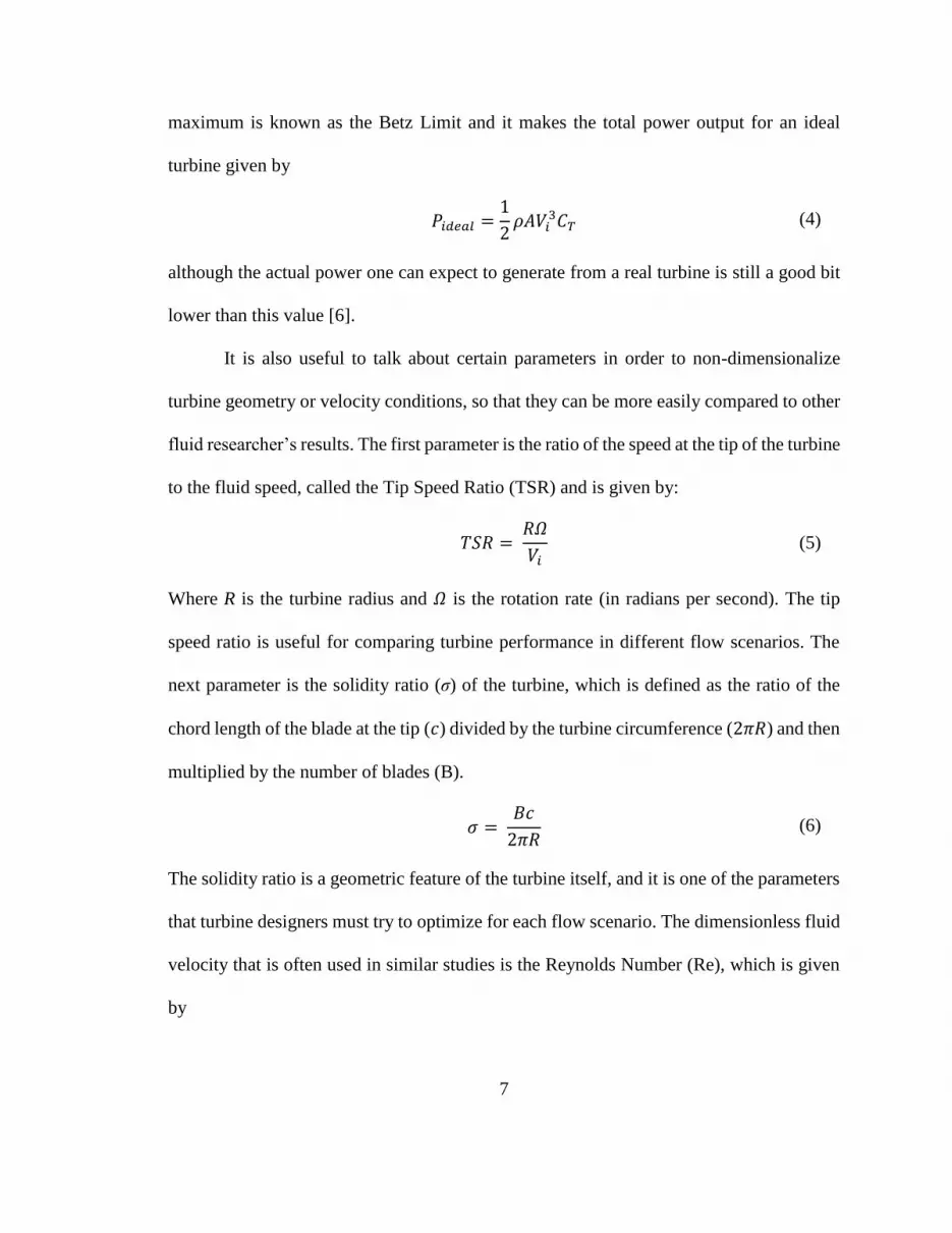
maximum is known as the Betz Limit and it makes the total power output for an ideal
turbine given by
𝑃𝑖𝑑𝑒𝑎𝑙 =1
2𝜌𝐴𝑉𝑖
3𝐶𝑇 (4)
although the actual power one can expect to generate from a real turbine is still a good bit
lower than this value [6].
It is also useful to talk about certain parameters in order to non-dimensionalize
turbine geometry or velocity conditions, so that they can be more easily compared to other
fluid researcher’s results. The first parameter is the ratio of the speed at the tip of the turbine
to the fluid speed, called the Tip Speed Ratio (TSR) and is given by:
𝑇𝑆𝑅 = 𝑅𝛺
𝑉𝑖 (5)
Where R is the turbine radius and 𝛺 is the rotation rate (in radians per second). The tip
speed ratio is useful for comparing turbine performance in different flow scenarios. The
next parameter is the solidity ratio (σ) of the turbine, which is defined as the ratio of the
chord length of the blade at the tip (𝑐) divided by the turbine circumference (2𝜋𝑅) and then
multiplied by the number of blades (B).
𝜎 = 𝐵𝑐
2𝜋𝑅 (6)
The solidity ratio is a geometric feature of the turbine itself, and it is one of the parameters
that turbine designers must try to optimize for each flow scenario. The dimensionless fluid
velocity that is often used in similar studies is the Reynolds Number (Re), which is given
by

8
𝑅𝑒𝑥 =𝜌𝑉𝑖𝑥
𝜇 (7)
where 𝑥 is some characteristic length of the system and µ is the dynamic viscosity of the
fluid.
1.4 Introduction to Turbulence Modeling
For the past couple of decades, the issue of modeling the performance of rotating
turbines was done with blade-element momentum (BEM) approximations. These methods
use the angle of attack of the blades with respect to the incoming flow, the speed of the
water coming into contact with the blades, the rotation rate of the blades, and other
relatively simple geometric properties to find the resulting forces on a differential element
of the blade. Integrating these quantities over the length of the blade and multiplying the
result by the number of blades allows for the calculation of turbine power, thrust, and a few
other useful quantities.
The BEM models are still in use today due to their reasonable accuracy and relative
simplicity, but they fail to take into account many of the complexities of the flow around a
hydrokinetic turbine. For instance, the BEM model assumes that the flow is largely 2D
with respect to the blade surface, which means that it cannot take into account interaction
between adjacent blade elements nor can it predict the effects of the vortex shedding at the
blade tip, blade trailing edge, and turbine hub [7]. This vorticity affects how the incoming
flow interacts with the blade and thus must also impact turbine performance. Therefore, to
find more accurate results using numerical methods, a way of taking these effects into
account is needed.

9
To come up with a method of resolving these issues, it is important to remember
that the motion of any Newtonian fluid is governed by the famous Navier-Stokes equations.
The equations are derived from conservation of mass and momentum for a differential
element of a Newtonian fluid, and whose form for incompressible flow with constant
viscosity is expressed below in vector form.
∇ ∙ 𝒗 = 0 (8)
𝜌 (𝜕𝒗
𝜕𝑡+ 𝒗 ∙ ∇𝒗) = −∇𝑝 + 𝜇∇2𝒗 + 𝒇 (9)
where ∇ is the vector differential operator, ∙ represents the vector dot product, 𝒗 is the
velocity vector of the fluid, 𝜌 is the fluid density (which through the incompressibility
assumption is a constant), 𝑡 is time, 𝑝 is pressure, 𝜇 is the fluid’s viscosity, and 𝒇 is the net
body force per unit volume vector.
Finding an analytical solution to the Navier-Stokes equations in an arbitrarily
shaped domain with specific boundary and initial conditions remains one of the greatest
challenges of modern mathematics [8]; even using direct numerical simulation to “brute
force” a solution to the Navier-Stokes equations remains an impossibility for all but the
simplest of flow scenarios [9]. However through the process of Reynolds decomposition,
which breaks down each of the four unknowns of the Navier-stokes equations (the velocity
in three-dimensions as well as the static pressure) into an average quantity and a fluctuating
quantity, the resulting problem becomes more tractable. Keep in mind that this Reynolds-
Average Navier-Stokes (RANS) process creates more unknowns than there are equations
to solve, so more equations must be found in order for the number of equations to match
the number of unknowns. These equations that are introduced have to describe the flow in

10
the best way at a minimal computational cost, and the entire field of RANS Turbulence
Modeling has been dedicated to finding the equations which accomplish this goal the best.
Luckily, a great deal of research in turbulence modeling has already been done, but
even so using RANS solvers to analyze designs for rotating turbines in 3D is a problem
that until recently remained computationally unfeasible to solve. Recent advances in
turbulence models (such as the k-𝜖 model, k-ω model, and their more modern variations)
retain relative computational simplicity yet are able to capture many complicated features
of turbulent flows. Massive leaps in computing technology allow simulations with orders
of magnitude more complexity than those that could be run just a decade ago, which means
that using fully three-dimensional RANS analysis of a rotating turbine is well within the
capacity of many modern high-end desktop computers.
1.5 Introduction to Computational Fluid Dynamics
Computational Fluid Dynamics (CFD) is a relatively new branch of fluid mechanics
that utilizes numerical methods and powerful computers to find approximate solutions to
complicated fluid flows. From these solutions important quantities which are relevant to
the researcher or designer can be subsequently determined. CFD lets its practitioners model
how their product or concept will interact with fluids in a way that is often much quicker,
cheaper and more practical than building a prototype and conducting the relevant
experiments.
The main motivation of applying CFD is modeling the behavior of turbulent flows,
as virtually all flows of practical interest involve turbulence [10]. In order to do this, there
are several steps that need to occur. First, the geometry of the simulation must be created

11
using Computer-Aided Design (CAD) software such as AutoCAD, Solidworks, or, as was
the case for this study, ANSYS DesignModeler (v13.0). Next, the domain needs to be
discretized into many smaller, simply-shaped chunks called elements.
This is discretization is done by importing the CAD file into a meshing program,
where the user can specify many various parameters to create a desirable mesh. This step
is very important, as the accuracy of the approximate solution that a numerical simulation
will generate is extremely dependent on the nature, quality and fineness of the mesh that is
being used. Creating a mesh that is detailed enough to capture all relevant flow
characteristics is essential for high-quality solutions, however there are naturally
limitations that the available computing resources place on how fine of a mesh can be
created.
After creating a satisfactory mesh, an appropriate turbulence model must be
selected which performs well under the flow conditions that could be reasonably expected
for the present simulation. From there, boundary conditions are applied to the walls of the
domain (and, for the case of a time-dependent simulation, initial conditions must also be
applied) which best represent the situation that is being modeled. Additionally for the
present study, modeling the rotating turbine blades in a HKT require the creation of a
rotating zone, where various approximations to account for this rotation must be done.
Finally, an interface linking the rotating zone and the non-rotating zone must be created in
order to formalize the connectivity between these domains, as well as selecting a series of
solvers which are capable of finding a converged solution in a reasonable amount of time.

12
After the simulation is run, the various quantities that are important for each
simulation can be extracted. In order to be sure that the results are not significantly affected
by the truncation errors inherent in all numerical methods, other simulations of varying
grid sizes with the same geometry, turbulence model, and boundary conditions must be run
to verify mesh independence or mesh convergence [11].
1.6 Opportunity for Present Research
Thus far, there has been in-depth CFD research in the wind turbine field, and as a
result the relationship of many different input and design conditions to the important
outputs is relatively well understood in this application. Likely due to comparably fewer
opportunities for funding, these relationships in hydrokinetic turbines are arguably less
well understood. And while many similar phenomena occur in hydrokinetic turbines as
they do in wind turbines, it is disingenuous to assume that wild turbine theory and design
practices can be directly applied to hydrokinetic turbines [6].
Horizontal-Axis Hydrokinetic Turbines (HAKHT) were chosen for this study due
to their higher efficiency, which is a result of lower incidence loss due to more of the fluid
hitting the turbine blades of HAHKT’s at an optimal angle than comparable vertical-axis
HKT’s [12]. Due to the relatively low power output of a single HKT, it is a natural
progression that multiple units will be needed to fulfill most customers’ energy needs.
The issue of the optimal location to place these turbines relative to each-other then
becomes apparent. It is intuitively clear (and can be shown via experimental evidence and
using CFD tools) that these turbines should not be placed directly downstream of one-
another, as trying to extract energy from fluid that has already had a large percentage of its

13
energy extracted from it is not particularly wise. In fact, according to experimental studies
done by [13], it takes 35 turbine diameters downstream of an axial HKT for the averaged
longitudinal velocity to reach 97% of the turbine inflow averaged velocity. However, the
problem of how far away perpendicular to the flow direction these turbines should be
placed in order to maximize power output is not well understood.
The research in this paper is intended to analyze the effect that separation distance
perpendicular to the flow direction has in a pair of horizontal axis hydrokinetic turbines
using Reynolds-Average Navier-Stokes Computational Fluid Dynamics modeling.
2. Simulation Setup
2.1 Geometry Selection and Generation
The geometry of the two turbines used in this study was taken from [14], which has
a turbine diameter of 21 inches (0.5334 m), a hub diameter of 2.5 inches
(0.0635 m), hub length of 15 inches (0.381 m), a uniform blade thickness of 0.5 inches
(0.0127 m), a “leading edge to trailing edge” of blade axial displacement of 5.8584 inches
(0.1488 m), and two blades, with each blade spanning an angle of 142.3 degrees with
respect to the hub. A perspective view of one of these turbines and a view from the flow
direction are shown in Figure 3 and Figure 4.

14
Figure 3: Perspective view of Turbine Geometry
Figure 4: View of Turbine from Flow Direction
The turbine is designed to rotate at 150 RPM clockwise when viewed from the flow
direction; this design was optimized to maximize the power generation on a relatively
shallow (hence the small turbine diameter) yet fast-moving river with an average fluid
speed of 2.25 m/s. These geometry and flow conditions make the TSR for these simulations
equal to approximately 1.8619, while the solidity ratio is approximately 0.79055. However
it is important to keep in mind that, for the purposes of this study, the geometry of the
turbines themselves is not as important as the separation distance between them.
To determine the effect that separation distance (𝑑) has on turbine performance,
several different river geometries must be created with different turbine separation

15
distances in each one. The separation distance for the purposes of this paper is expressed
as the distance between the axes of rotations of each of the turbines, as shown in Figure 5.
Figure 5: Definition of Separation Distance
Defining separation distance in this manner means that, with a turbine diameter of
21 inches, a separation distance of 21 inches means that the tips of the turbine blades will
be just barely touching. With that definition in mind, five different geometries were
created, with 𝑑 equal to three, four, five, six and seven turbine radii (31.5 inches, 42 inches,
52.5 inches, 63 inches, and 73.5 inches respectively).
The computational domain that was constructed for all of these simulations is 30
feet (9.144 m) wide and 10 feet (3.048 m) tall. It is important in the geometry setup that
the turbines are placed sufficiently far away from the river bed in order to prevent any wall
effects from interfering with the results. This would also represent expected operating
conditions; as such a hydrokinetic turbine would need to be placed a far away from the
river bed to maximize the energy of the water that is passing through the turbine as well as
minimize the chances that the turbine is damaged by any heavy debris traveling along the
river bed. As such, the turbines are placed 74 inches (1.8796 m) away from the bottom of
the river bed, as well as 46 inches (1.1684 m) beneath the free surface of the water.

16
The computational domain in these types of simulations needs to be long enough
so that the inlet and outlet pressure/gradient boundary conditions do not interfere with the
true nature of the flow around the turbines. In order to meet this goal, the river geometry
created for this study is 30 feet (9.144 m) in depth, with 10 feet (3.048 m) upstream and 20
feet (6.096 m) downstream of the turbine leading edge in order to capture the turbine’s
wake and thus the effect that that wake will have on turbine performance.
A very important but not often discussed part of the geometry generation in
Hydrokinetic Turbine CFD simulations is how large the cylindrical rotating domain that
encloses the turbines should be. It has been shown by [15] that a larger rotating domain
radius more accurately reflects experimental results, however because the present study
involves simulating two turbines that are close together instead of one, creating large
rotating domains for these turbines is not possible. This is because the generation of a
rotating domain with a large diameter in this scenario would cause the domains to intersect
and create nonsensical results. Therefore the nature of the present simulations places a hard
restriction on the allowable size of the rotating domain for the present study based upon
their separation distance. Even further constraints on the rotating domain size become
apparent when attempting to mesh the river geometry and avoid the generation of high
aspect ratio elements in between the rotating turbine domains.
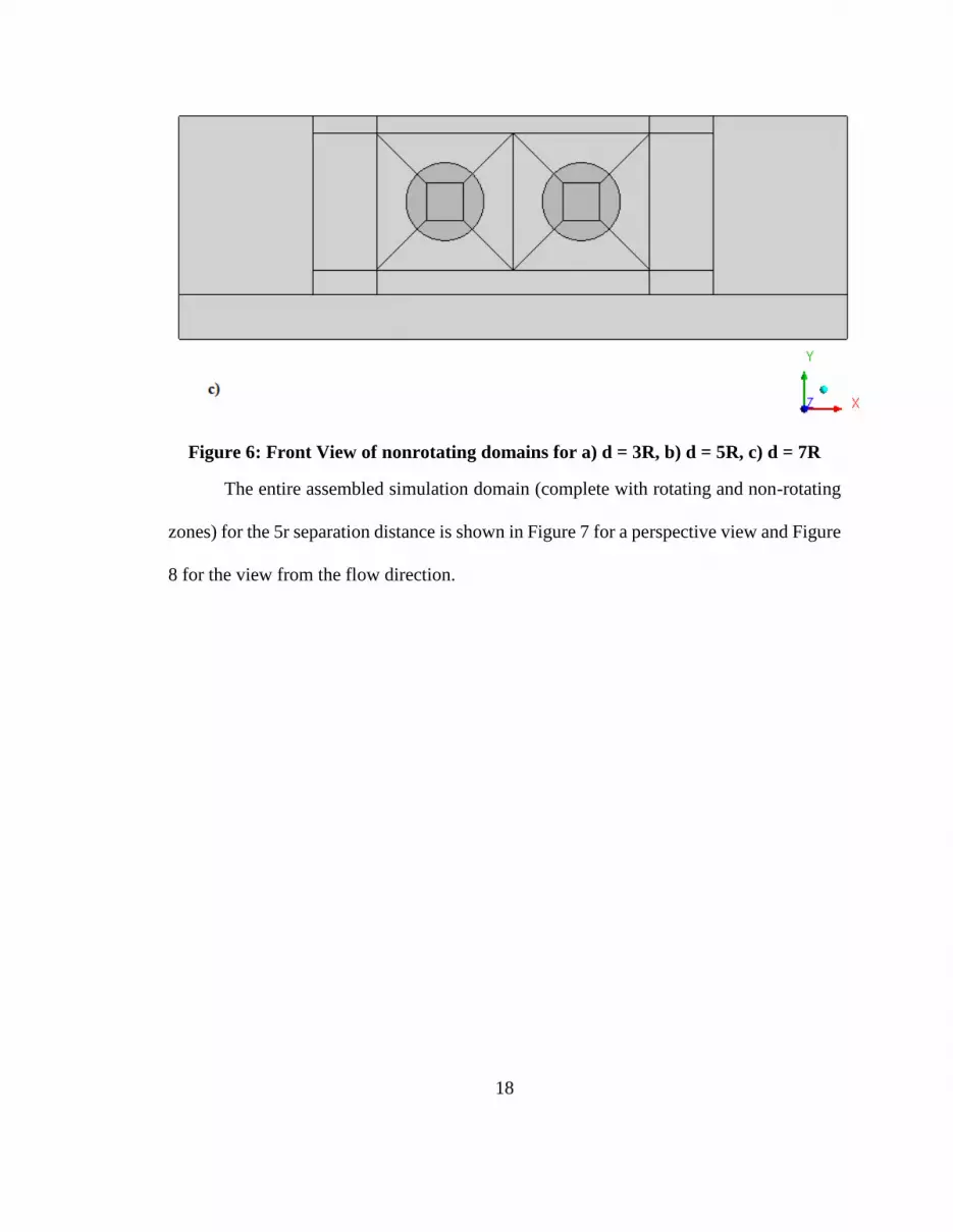
With all of these constraints in mind, the radii of the rotating domains for this study
are 1.25R (26.25 inches) for d= 3R, 1.5R (31.5 inches) for d= 4R, 1.75R (36.75 inches) for
d= 5R, 2R (42 inches) for d = 6R, and 2R (42 inches) for d = 7R. The non-rotating river

17
domain for the d =3R, d = 5R and d = 7R separation distances are shown in Figure 6a,
Figure 6b, and Figure 6c.
18
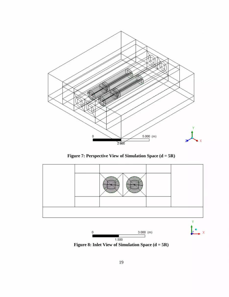
Figure 6: Front View of nonrotating domains for a) d = 3R, b) d = 5R, c) d = 7R
The entire assembled simulation domain (complete with rotating and non-rotating
zones) for the 5r separation distance is shown in Figure 7 for a perspective view and Figure
8 for the view from the flow direction.
19
Figure 7: Perspective View of Simulation Space (d = 5R)
Figure 8: Inlet View of Simulation Space (d = 5R)

20
In both figures, the river region is shown with transparent faces, whereas the left
and right turbine regions are shown at 75% transparency in order to highlight the
boundaries of the different regions as well as show the locations of the turbines themselves.
For each simulation, the cylindrical rotating domains extend 60 inches (1.524 m)
upstream and 126 inches (3.2004 m) downstream from the leading edge of the turbine
blades.
2.2 Mesh Generation
The turbine domain geometry, turbine hub, and river geometries were all created
and meshed separately and then combined in order to use different software to model each
domain. The river domain and hub domains were solid modeled in a manner that makes
each solid body in those regions have four sides. This procedure allowed for the creation
of a structured hexahedral mesh throughout all domains, which has a number of advantages
over the comparatively simpler to setup unstructured meshes that many other CFD
practitioners use.
The use of a fully structured mesh allowed for the creation of elements with very
high quality even in the region close to and surrounding the turbine blades; usually in these
types of simulations a minimum meshing quality of above 0.30 is desired, but for all
simulations in this computational study a minimum mesh quality of 0.40 was achieved. A
similarly lofty goal of an aspect ratio below 4 for all elements was also achieved for all
simulations. These outcomes are possible because the structured mesh creates a very well-
organized geometry discretization on the blade surface (as seen in Figure 9) as well as
creates a smooth inflation layer from the surface of the blades to the free stream (as

21
demonstrated in Figure 10), which is intended to capture the complex turbulent effects
originating on the blade surface, blade leading edge and blade tips.
Figure 9: Blade Surface Mesh Viewed from Flow Direction (d = 5R)
Figure 10: Mesh extending upstream and downstream of blade tip (d = 5R)

22
Another advantage to the fully structured nature of the mesh is that it allows for the
creation of a river domain mesh that is symmetric about the midplane between the two
turbines, which means that any differences in calculated performance between the left and
right turbine cannot be attributed to meshing asymmetries.
In order to map the solution from one of these domains to the other, mesh interfaces
that link each exterior surface in the turbine domains to its counterpart in the interior of the
river domain must be created. Similar grid interfaces are used for the fluid upstream and
downstream of the turbine hubs, as well as for the General Grid Interface (GGI)
surrounding the turbine blades in each rotating domain.
For the d=3R, d=4R, and d=5R separation distances, two simulations with different
mesh sizes were run in order to verify mesh independence of the results. These two mesh
sizes are shown for the 5R separation distance in Figure 11 and Figure 12 as viewed from
the inlet of the domain.
Figure 11: Coarse Mesh Front View (d = 5R)

23
Figure 12: Fine Mesh Front View (d = 5R)
It is worth noting that there is no inflation layer in the mesh at the walls of the river
bed; this was a conscious decision intended to reduce the number of elements involved in
each simulation. This comes at the cost of not accurately representing the flow near walls
of the simulation, but because the turbines are placed far enough away from the walls then
that would not dramatically affect the calculated flow around the turbine nor calculated
turbine performance.
For the coarse meshes at every separation distance, approximately 650 thousand
structured elements were used to discretize the river domain, approximately 1 million
elements each in both the rotating left and right turbine regions, as well as around 700
thousand elements to capture the upstream and downstream hub region of the river. For the
fine meshes, approximately 2.6 million elements were used to discretize the river, 1.5
million elements each for the rotating domain around the left and right turbine, and 700
thousand elements for the upstream and downstream hub regions. Altogether, that makes
approximately 3.5 million elements for each of the coarse mesh simulations and
approximately 6.1 million elements for the fine mesh simulations.

24
The hub and river domains were meshed in hexahedral elements using ANSYS
ICEM CFD’s mapped face meshing feature, whereas the domains around the two turbines
were meshed with hexahedral elements using the Turbogrid extension for ANSYS
Workbench v13.0.
2.3 Approximations of Turbine Rotation
The nature of vortex shedding on solid bodies makes even a relatively simple flow,
such as 2D flow past a cylinder, have an oscillatory solution. It should come as no surprise,
then, that the flow past a rotating turbine (with a much more complicated geometry than a
simple cylinder) will also have an innately unsteady resulting flow. The importance of
incorporating this turbine rotation and inherent flow fluctuations in our numerical
simulations becomes paramount.
One approach to taking these fluctuations into account is to run a fully transient
simulation, where initial conditions are assumed, and from those initial conditions the
solution moves forward in time, calculating the flow state at every time step. To describe
the turbine rotation accurately, the time step that the simulation uses must be small in
relation to the rotation rate of the turbines, and the mesh around both turbine regions must
rotate a small increment after each time step. After enough time steps have been run so that
the initial flow assumptions have been “dampened out” there is a periodic flow pattern that
will result. From there, expected turbine performance is derived via time-averaging
operations over all of the generated data files.
Although potentially able to find very accurate solutions, there are a few major
downsides to the fully transient solution method that make it very unwieldy to use. Firstly,

25
the simulation needs to run for often times several thousand time steps or more, which
means that it can take weeks of computation time for a single simulation. This method also
generates a ton of data files as results, and storing all of that data can be a challenge of its
own. It is possible to save the data files after a every “X” number of time steps to cut down
on the quantity of data stored, but it is difficult to know a priori how big of a number “X”
should be in order to capture all of the fluctuations in the flow.
As an alternative to modeling all of these turbulent variations directly, it is possible
to average-out all of these fluctuating effects to get an approximate steady-state solution.
The so-called rotating reference frame models do just that; instead of rotating the mesh for
each turbine a small angle during every time step, the movement of the turbine is instead
incorporated into the governing equations which are solved around the turbine regions.
These modified Navier-Stokes equations shown below represent conservation of mass and
momentum in a rotating domain for incompressible flow with constant viscosity.
∇ ∙ 𝒗𝒓 = 0 (10)
𝜌 (𝜕𝒗𝒓
𝜕𝑡+ 𝒗𝒓 ∙ ∇𝒗𝒓 + 𝜴 × (𝜴 × 𝒓) + 2𝜴 × 𝒗𝒓) = −∇𝑝 + 𝜇∇2𝒗𝒓 (11)
In these equations, 𝒗𝒓 is the velocity vector in the rotating reference frame, 𝜴 is the vector
of revolution of the rotating domain (where the direction of 𝜴 is the direction the axis of
revolution of the rotating domain, and the magnitude of 𝜴 represents how quickly the
domain is rotating), and 𝒓 is the vectored distance from the origin of the moving frame to
an arbitrary point in the rotating domain, × represents the vector cross product, while ∇,
𝑝, 𝑡 , 𝜌, ∙,and 𝜇 refer to the same quantities and operations as they do in the non-rotating
Navier-Stokes equations. The extra terms that result from this rotating reference frame

26
formulation, namely the 𝜴 × (𝜴 × 𝒓) and 2𝜴 × 𝒗𝒓 terms in the momentum equations,
represent the inertial centrifugal and Coriolis forces, respectively [16].
The benefits to this steady-state approach over a fully transient simulation are
numerous; firstly, because there is no time stepping when using the rotating reference
frame approach, it has much friendlier computation times. The data is also much easier to
store and interpret, because the output of these simulations is often a single data file from
which all important turbine performance parameters can be derived. Although strictly
speaking not as accurate as the fully transient simulations, the rotating reference frame
approximations are used in the vast majority of wind and hydrokinetic turbine CFD studies
because of these benefits (and because most of the time the results of the transient and
steady-state simulations end up being very similar anyways).
This study utilized the steady-state, rotating reference frame approach for all
separation distances and both mesh sizes.
2.4 Turbulence Model Selection
As stated in the introduction, a turbulence model that accurately describes the flow
conditions of our present situation must be selected. The model used for this study is the
k-ω Shear-Stress Transport (SST) Model, developed by Menter [17] in 1994, due to its
good behavior describing separating flows and flows with an adverse pressure gradient.
This model is a combination of the k-ω model, which does well modeling turbulence at
regions close to the walls, and the k-𝜖 model, which better models free-stream turbulent
behavior.

27
The k-𝜖 and k-ω models have been used heavily in the turbulence modeling and
CFD communities to great success; both models use two differential equations to keep
track of the properties of the turbulent flow, making them fall under a more general
category of two-equation turbulence models. The k-𝜖 model keeps track of the Specific
Turbulent Kinetic Energy (k) and the Specific Turbulent Dissipation (𝜖), which are defined
using Einstein summation notation below.
𝑘 = 1
2𝑢𝑖′𝑢𝑖′ (12)
𝜖 = 𝜈𝜕𝑢𝑖′
𝜕𝑥𝑘
𝜕𝑢𝑖′
𝜕𝑥𝑘
(13)
In the above equations, 𝑢𝑖′ represents the fluctuating portion of the Reynolds
decomposition of 𝑢𝑖 (which is itself a component of the velocity vector 𝒗), 𝜈 is the
kinematic viscosity of the fluid (given by μ/ρ), 𝑥𝑘 is one of the three components of the
direction vector, and the bar over certain quantities represents a time-averaging operation.
In a physical sense, 𝑘 represents the kinetic energy of the turbulent fluctuations per
unit mass (and hence has the units of (length)^2/(time)^2). 𝜖 in this model represents the
rate at which the turbulence kinetic energy is converted into thermal energy (and has units
of (length)^2/(time)^3); or, an alternative way of thinking about this quantity is that it is
equal to the mean rate at which work is done by the fluctuating component of the strain
rate against the fluctuating viscous stresses [10].
The k-ω model uses the same definition for the turbulent kinetic energy, but no
longer explicitly solves for 𝜖, instead choosing to utilize differential equations for the
Specific Dissipation rate (ω) of the turbulent flow. The quantity ω does not have a strict

28
physical meaning, as it was derived entirely through dimensional analysis, but it can be
thought of as the mean frequency of the turbulence (as it has units of 1/(time)). ω is often
defined implicitly using the simple relationship
𝜔 =𝜖
𝑘𝛽∗ (14)
where 𝜖 and 𝑘 are the same as before, and 𝛽∗ is a dimensionless constant that depends on
the model being used.
The k-ω SST model utilizes blending functions to transition from the k-ω model
close to the walls into the k-𝜖 model in the free stream; this approach avoids the downsides
of either model at a comparatively small computational cost. These equations, shown
below in their most general form using Einstein summation notation, are coupled
differential equations with (as you might expect from the name of the model) k and ω as
the unknowns.
𝜕(𝜌𝑘)
𝜕𝑡+
𝜕(𝜌𝑢𝑗𝑘)
𝜕𝑥𝑗= 𝜏𝑖𝑗
𝜕𝑢𝑖
𝜕𝑥𝑗− 𝛽∗𝜌𝜔𝑘 +
𝜕
𝜕𝑥𝑗[(𝜇 + 𝜎𝑘𝜇𝑡)
𝜕𝑘
𝜕𝑥𝑗] (15)
𝜕(𝜌𝜔)
𝜕𝑡+
𝜕(𝜌𝑢𝑗𝜔)
𝜕𝑥𝑗=
𝜌𝛾
𝜇𝑡𝜏𝑖𝑗
𝜕𝑢𝑖
𝜕𝑥𝑗− 𝛽𝜌𝜔2 +
𝜕
𝜕𝑥𝑗[(𝜇 + 𝜎𝜔𝜇𝑡)
𝜕𝜔
𝜕𝑥𝑗] …
+ 2(1 − 𝐹1)𝜌𝜎𝜔2
𝜔
𝜕𝑘
𝜕𝑥𝑗
𝜕𝜔
𝜕𝑥𝑗
(16)
These are the two differential equations that need to be solved in the k-ω SST model, but
in these equations there are a plethora of constants and plenty of shorthand notations. The
explicit definitions of these quantities are shown below.

29
𝜏𝑖𝑗 = 𝜇𝑡 (𝜕𝑢𝑖
𝜕𝑥𝑗+
𝜕𝑢𝑗
𝜕𝑥𝑖−
2
3
𝜕𝑢𝑘
𝜕𝑥𝑘𝛿𝑖𝑗) −
2
3𝜌𝑘𝛿𝑖𝑗 (17)
𝜇𝑡 =𝜌𝑎1𝑘
max (𝑎1𝜔; 𝐹2𝛺∗) (18)
𝐹1 = tanh (min [max (√𝑘
𝛽∗𝜔𝑦;500𝜈
𝑦2𝜔) ;
4𝜌𝜎𝜔2𝑘
𝐶𝐷𝑘𝜔𝑦2]
4
) (19)
𝐹2 = tanh (max [2√𝑘
𝛽∗𝜔𝑦;
500𝜈
𝑦2𝜔]
2
) (20)
𝐶𝐷𝑘𝜔 = max (2𝜌𝜎𝜔2
𝜔
𝜕𝑘
𝜕𝑥𝑗
𝜕𝜔
𝜕𝑥𝑗; 10 −20) (21)
In the above relationships, 𝜏𝑖𝑗 represents the Reynold’s Stress Tensor (the k-ω SST model
uses the Boussinesq eddy-viscosity Approximation to make this quantity a product of the
eddy viscosity and the mean strain-rate tensor, therefore adding closure to the RANS
equations [10]), 𝛿𝑖𝑗 is the Kronecker delta function (𝛿𝑖𝑗 = 1 if i = j, and 𝛿𝑖𝑗= 0 if i ≠ j), 𝜇𝑡
is the turbulent dynamic viscosity, 𝐹1 and 𝐹2 are blending functions, 𝐶𝐷𝑘𝜔 is the positive
portion of the Cross Diffusion term of Equation (16), y is the distance in the domain away
from any solid surfaces, 𝛺∗ is the absolute value of the vorticity, and 𝛽∗, 𝜎𝑘, 𝛾, 𝛽, 𝜎𝜔, 𝑎1,
and 𝜎𝜔2 are all model constants.
It is important to remember that the value of many of the constants shown in the
above equations actually dependent upon the distance in the domain away from solid
surfaces (𝑦) as well as on the values of values of k, ω, and their spatial derivatives that the
equations (15) and (16) are being evaluated at. The blending functions that take these

30
factors into account are what make the k-ω SST model distinct in comparison to most other
two-equation models.
The value of these constants change according to the following relationship:
𝜙 = 𝐹1𝜙1 + (1 − 𝐹1)𝜙2 (22)
where 𝐹1 represents the same blending function as before, 𝜙 represents the value of one of
the constants that is used in the above equations (i.e. either 𝜎𝜔, 𝜎𝑘, 𝛾, or 𝛽), while 𝜙1
and 𝜙2are given by the following set of values:
𝜙1: 𝜎𝑘1 = 0.85 𝜎𝜔1 = 0.5 𝛽1 = 0.0750 𝛾1 = 𝛽1 𝛽∗ − ⁄ 𝜎𝜔1𝜅2 √𝛽∗⁄
𝜙2: 𝜎𝑘2 = 1.0 𝜎𝜔2 = 0.856 𝛽2 = 0.0828 𝛾2 = 𝛽2 𝛽∗ − ⁄ 𝜎𝜔2𝜅2 √𝛽∗⁄
The constants that do not change based upon the value of 𝐹1 are
𝛽∗ = 0.09 𝜅 = 0.41 𝑎1 = 0.31
2.5 Boundary and Initial Conditions
The after selecting the turbulence model, the final step of the simulation setup is
defining our boundary conditions and (in the case of the fully transient simulation) initial
conditions. The boundary conditions must specify a value or a gradient of that value for all
quantities that are to be found inside of that boundary. Put more explicitly: the value of
the velocity in three dimensions, the pressure, the turbulent kinetic energy and the turbulent
frequency (or a gradient of those quantities) at all boundaries in the computational domain
must be found before any meaningful simulations can be run.
When looking at the river domain from the flow direction, the domain can be
thought of as a “box.” The left, right and bottom of the box just represent the river bed, so

31
these surfaces are given the simple boundary conditions that the velocity is zero and that
the pressure gradient perpendicular to these walls are also zero. The top of this box
represents the surface of the river, which is safe to assume has zero shear stress. This zero
shear stress assumption means that the gradient of the velocity and gradient of the pressure
normal to this so-called free surface (or symmetry boundary condition) are both zero.
The front of the river domain is given a uniform inlet velocity normal to that
surface, 𝑈, of 2.25 m/s, while the pressure is assumed to be at a zero gradient here as well.
In reality, rivers do not have a uniform velocity distribution throughout a cross-section of
flow, but for the purposes of these simulations generating a uniform velocity distribution
at the inlet guarantees that the flow entering both turbines will be the same flow that the
turbine was optimized for. Additionally, uniform flow ensures that the same kinetic energy
is entering both turbines, which means that any difference in power output between the left
and right turbines cannot be attributed to variations in flow conditions surrounding each
turbine. In fact, because the turbines are placed sufficiently far away from the walls of the
simulation, 𝑈 is also the velocity that can be assumed to be entering the turbine. The exit
of the river domain (which is the “back” of the computational box) is a pressure outlet
condition set equal to zero, and the velocity is assumed to be a zero gradient (which means
that the turbulent flow has stopped developing downstream).
The boundary conditions for the two turbines themselves are both moving walls,
which means that the velocity is specified and the pressure gradient normal to the turbine
surface is zero. In our steady state simulations, the velocity of the walls of the turbine in
the stationary frame is given by 𝜴 × 𝒓, but it is important to remember that the domain

32
surrounding both turbines utilizes the rotating reference frame approach. In the frame of
reference for the rotating turbine the walls of that turbine are stationary; thus relative to
their respective rotating frames the velocity on the surface of each turbine is zero in the
steady-state simulations. This zero-velocity boundary condition is also true for a transient
simulation, as the velocity of the turbine blades with respect to the rotating mesh is still
zero.
The boundary conditions for k and ω in the k-ω SST model are more complicated
to determine, at least in comparison to the ones for the pressure and velocity. As might be
expected from a symmetry boundary condition, the gradient of k and ω at the free surface
is zero. However, for both the inlet and the outlet, the turbulent kinetic energy and specific
dissipation rate boundary conditions are given by the following relationships:
𝑘𝑖𝑜 =3
2 (𝑈 𝐼)2 𝜔𝑖𝑜 =
√𝑘𝑖𝑜
𝑙(𝛽∗)
−14 (23)
Where 𝑘𝑖𝑜 and 𝜔𝑖𝑜 are the values of the turbulent kinetic energy and turbulent frequency,
respectively, at the inlet and outlet, 𝐼 is the Turbulent Intensity, 𝑙 is the Turbulent Length
Scale, and 𝑈 and 𝛽∗ are the same as before [18].
It therefore becomes necessary to determine what, exactly the turbulent intensity
and turbulent length scales are for this simulation. The turbulent intensity is defined as the
ratio of the magnitude of fluctuating component of the flow to the magnitude of the steady
component of the flow. The value of 𝐼 at the inlet and outlet is calculated using the formula
for a fully developed flow in a duct, which is given by
𝐼 = 0.16 𝑅𝑒𝐷ℎ
−1 8⁄ (24)

33
where 𝑅𝑒𝐷ℎis the Reynold’s number of the flow based upon the Hydraulic Diameter (𝐷ℎ)
of the duct [19]. Using the formula that the hydraulic diameter is equal to four times the
duct area divided by the wetted perimeter, it can be easily found that for this river geometry
𝐷ℎ = 7.3152 m. Remembering Equation (7) for the Reynolds number and using the
properties of water at 20oC, 𝑅𝑒𝐷ℎ is found to be 1.638 ∙ 107. Plugging this in to Equation
(24), the Turbulent Intensity at the Inlet and Outlet is found to be 0.02006 for all
simulations.
The turbulent length scale (𝑙) for fully developed pipe flow is given by
𝑙 = 0.07 𝐷ℎ (25)
so using the hydraulic diameter of the river geometry it is found that 𝑙 = 0.51206 m [20].
Now that the turbulent intensity and turbulent length scales are known, the values of 𝑘𝑖𝑜
and 𝜔𝑖𝑜 can be determined, although these values are calculated automatically in FLUENT
and are not important parameters for the purpose of this study.
In a similar fashion, the values of k and ω at the solid walls of the domain (which
in our simulations refers to the river bed and the turbine blades) are given by the following
relationships:
𝑘𝑤𝑎𝑙𝑙 = 0 𝜔𝑤𝑎𝑙𝑙 = 106𝜈
𝛽1(∆𝑦1)2 (26)
where 𝜈 is the kinematic viscosity, 𝛽1 is a constant, and ∆𝑦1 is the distance to the next point
away from the wall [17].
For a transient simulation, the “zeroth” time step is usually initialized based upon
the steady state solution. As the solution moves forward in time, the time-dependent
features of the flow will start to manifest themselves in the simulation. In order to allow

34
time for this to occur, it has become common practice in transient CFD simulations to
discard the data from the first several turbine revolutions before any post-processing
operations are performed.
2.7 Solver Selection
The last bit of information that must be specified before any simulation can be run
are the solvers that FLUENT will use in order to find the best numerical solution for the
discretized geometry, boundary conditions, governing equations, and surface interfaces
that it is given. Namely the Pressure-Velocity Coupling, Time Stepping and Spatial
Discretization Schemes must ideally be chosen in a way that lets the solution converge as
rapidly and with as much accuracy as possible.
With those objectives in mind, the “Coupled” scheme was used for the Pressure-
Velocity coupling, while the “least squares cell based” and “standard” schemes were used
for the gradient and pressure solvers, respectively. For the momentum, turbulent kinetic
energy, and specific dissipation rate equations, a “second order upwind” scheme was
selected. Although all simulations in this study were steady state, a “Pseudo-Transient”
time step option was utilized. More information about how each of these solvers work as
well as their advantages and drawbacks can be found in the FLUENT 14.0 User’s Guide
[22].

35
3. Simulation Quality and Results
3.1 Turbine Performance Metrics
When attempting to optimize turbine performance, it is necessary to define which
parameter(s) of the turbine should be optimized. For the purposes of this study, the
separation distance that maximizes the total power that the turbine is generating needs to
be discovered. Or, if such a distance is found not to exist, then the objective would be to
find a correlation between the separation distance and the power output.
Power is not the only important output parameter; naturally, the turbine drag force
will want to be minimized in order to reduce the strain on the supports that hold the turbines
in place. The drag force can be thought of as the “cost” that generating power has on the
mechanical and electrical machinery used to create that power. Thus, minimizing that drag
force will correlate with an increase in the lifespan of the equipment used; therefore, a
similar relationship between resultant drag forces and separation distance would also be
very valuable.
It is also useful to nondimensionalize both the drag and the power output, so that
other CFD practitioners can more readily compare their results to these. The coefficient of
drag (𝐶𝐷) and coefficient of performance (𝐶𝑝) do just that and are, respectively, defined
according to the following relationships
𝐶𝐷 = 𝐹𝐷
12 𝜌𝑈2𝐴
(27)
𝐶𝑝 = 𝑃
12 𝜌𝑈2𝐴𝛺
(28)

36
where 𝐹𝐷 is the resultant drag force and P is the resultant power output from one of the
turbines in the simulations.
The objective of these CFD simulations are to discover the relationship between
the separation distance of the turbines and the coefficient of performance and coefficient
of drag from both turbines.
3.2 Turbine Performance Outputs
After running the simulations as described above, the following relationships
between turbine power vs separation distance were observed as shown in figure 13.
440
460
480
500
520
540
560
3R 4R 5R 6R 7R
Wat
ts
Fig 13a) Left Turbine Power
Fine Mesh
Coarse Mesh

37
Figure 13: a) Left Turbine Power vs Separation distance b) Right Turbine Power vs
Separation Distance
The turbine drag vs separation distance graph obeyed a similar relationship, as shown in
figure 14.
440
460
480
500
520
540
560
3R 4R 5R 6R 7R
Wat
ts
Fig 13b) Right Turbine Power
Fine Mesh
Coarse Mesh
520
540
560
580
600
620
640
3R 4R 5R 6R 7R
Ne
wto
ns
Fig 14a) Left Turbine Drag
Fine Mesh
Coarse Mesh

38
Figure 14: a) Left Turbine Drag vs Separation Distance b) Right Turbine Drag vs
Separation Distance
It is worth mentioning that the simulation for the d=7R geometry was unable to be
meshed to the same quality as the other simulations in this study. This is for two separate
reasons. The first is an artificial limitation of twice the turbine radius that Turbogrid places
on how large the rotating domain can be in relation to the turbine; this means that the
rotating domain size to separation distance ratio is smaller for the d=7R simulation than it
was for the other simulations in this study. The other limitation has to do with how the
mesh is structured which forces high aspect ratio elements upstream of the rotating domain
inlet and downstream of the rotating domain outlet. These two factors help to explain why
the drag and power outputs for the d=7R separation distance do not match up as neatly with
the results of the other simulations.
It is also valuable to look at the percent difference between the left turbine and the
right turbine power when separation distance is held constant. Doing this in figure 15, the
following relationship is observed.
500
520
540
560
580
600
620
640
660
3R 4R 5R 6R 7R
Ne
wto
ns
Fig 14b) Right Turbine Drag
Fine Mesh
Coarse Mesh

39
Mesh d=3R d=4R d=5R d=6R d=7R Units
% Power Difference
Fine 0.032311 0.53658 -0.56709 - - %
Coarse -0.02081 -0.5715 -0.14763 -0.14678 -3.85579 % Figure 15: Percentage different between left Turbine and Right Turbine power
A positive value of this quantity indicates that the left turbine is generating that
much more power than the right, whereas a negative value would represent that the right
turbine is generating more power than the left.
From these figures, we can see three very important relationships:
1) Holding separation distance constant, there seems to be a negligible difference in
both resultant drag and power output between the left turbine and the right turbine.
This is good news for customers who are looking to apply this research, because
that means that the left generator and the right generator will be subject to
approximately identical power loads, and will thus “wear out” at the same rates.
2) The Turbine Power and Drag both appear to asymptotically approach a constant
value when they are brought further and further apart. One could intuitively guess
that the turbines will cease interacting if they are brought infinitely far apart, so
these results do make sense.
3) Both the left and the right turbine appear to generate in the order of 10% less power
and 10% less drag when the turbines are close together in comparison to when they
are far apart. This suggests that, in order to maximize the power output of these
turbines when placed in a uniform flow field, the turbines should be separated as
far away as possible.
40
Expanding on the third point: The rivers in which these turbines will be placed are, in
general, not uniform flow fields. When this is the case, all turbines should be placed in an
area of the flow that maximizes the kinetic energy of the water that will be entering those
turbines. However, even in non-uniform flow conditions there will still exist a large, fast-
moving region of the flow that will have an almost uniform flow distribution (i.e. the
gradient of the velocity field will be near zero). The results of this study suggest that the
turbines should be placed far apart from each other within that high-velocity region.
3.3 Simulation Quality Metrics
In order to ensure that the results of the CFD simulations that were generated by
this study are representative of reality, three different approaches were utilized to verify
simulation accuracy.
The first method of investigating the accuracy of the simulations involves plugging
in the results (for static pressure, the three velocities, and k and omega) that are obtained
numerically back into the governing equations that are being solved in the first place.
Because there are six governing equations (one for continuity, x-momentum, y-
momentum, z-momentum, k and 𝜔), then six so-called “Residuals” are generated after
every iteration. Each residual can be thought of as a “grade” for how well the results satisfy
the given differential equation after it has been discretized by the mesh, with a better grade
corresponding to lower residual values. For a steady-state simulation, the residuals start off
near 1 and quickly drop down and eventually level off and fluctuate around a certain value
after several hundred to a few thousand iterations; the value that the residuals fluctuation
around is known as the converged residual. For the steady-state simulations, the solution
41
is generally not considered converged until all of the converged residuals fall below a
certain value. For a transient simulation, a maximum number of iterations per time step as
well as minimum residual criteria are specified; the simulation moves forward a time step
after either of these two conditions are satisfied.
The second method of verifying numerical accuracy is by looking at the pressure,
velocity, turbulent kinetic energy, specific dissipation rate, and other contours of the flow
solution. When viewing the contours of these quantities using planes to get 2D slices of the
results, there should not exist many “sharp” edges on the contours (i.e. they should be
relatively smooth). If the contours show these sharp edges in an area where it would not
make sense for these edges to exist in reality, then it is likely that the mesh is not accurately
capturing the complicated flow conditions in that area. It is entirely possible that a solution
is found which satisfies the discretized governing differential equations very well (and
would therefore have a low residual), but because the mesh could discretize the domain in
a manner that does not capture all characteristics of the flow, that simulation could still
generate results which do not optimally reflect reality. Viewing these slices of the flow to
discover if this is the case is a simple yet valuable tool for any CFD practitioner, and if the
discretization is found to not represent the flow very well, then the mesh needs to be refined
in that area and the simulation re-run. This method of investigating the solution quality is
a “dummy check” in the sense that there are no quantities that are being measured, which
makes this a subjective and purely qualitative method of determining how confident a
researcher should be in their results.
42
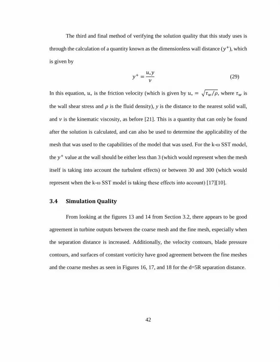
The third and final method of verifying the solution quality that this study uses is
through the calculation of a quantity known as the dimensionless wall distance (𝑦+), which
is given by
𝑦+ =𝑢∗𝑦
𝜈 (29)
In this equation, 𝑢∗ is the friction velocity (which is given by 𝑢∗ = √𝜏𝑤 𝜌⁄ , where 𝜏𝑤 is
the wall shear stress and 𝜌 is the fluid density), y is the distance to the nearest solid wall,
and 𝜈 is the kinematic viscosity, as before [21]. This is a quantity that can only be found
after the solution is calculated, and can also be used to determine the applicability of the
mesh that was used to the capabilities of the model that was used. For the k-ω SST model,
the 𝑦+ value at the wall should be either less than 3 (which would represent when the mesh
itself is taking into account the turbulent effects) or between 30 and 300 (which would
represent when the k-ω SST model is taking these effects into account) [17][10].
3.4 Simulation Quality
From looking at the figures 13 and 14 from Section 3.2, there appears to be good
agreement in turbine outputs between the coarse mesh and the fine mesh, especially when
the separation distance is increased. Additionally, the velocity contours, blade pressure
contours, and surfaces of constant vorticity have good agreement between the fine meshes
and the coarse meshes as seen in Figures 16, 17, and 18 for the d=5R separation distance.
43

44
Figure 16: Velocity Downstream of Turbines for a) Fine Mesh and b) Coarse Mesh
at d = 5R

45
Figure 17: Surface Pressure Contours for d = 5R separation distance on a) Fine
Mesh and b) Coarse Mesh

46

47
Figure 18: Surface of Constant Vorticity (25.25 s^-1) for d=5R on the a) Fine Mesh
and b) Coarse Mesh
Notice in these plots several features of the flow that should be expected. In figures
16 and 18, the vortex shedding effects at the blade tips and blade hub are well defined for
both mesh sizes. Likewise in Figure 17 the upstream side of the blade leading edge is seen
to have the highest pressure, and (although not shown in these plots) the downstream side
of the blade leading edge has the lowest pressure. All of these flow characteristics are
clearly defined in both the coarse mesh and fine mesh simulations, which provides
evidence that any relationship between the power/drag and the separation distance is not

48
due to a meshing anomaly. This can help to provide confidence that the trends found in this
study between the relevant parameters are accurate.
The residuals for each simulation are shown below in figure 19; these numbers
represent the highest converged residual around which the discretized mesh and specified
solver converged to and fluctuated around.
3R 4R 5R 6R 7R
Highest Residual
Fine Mesh 7.53E-05 2.95E-04 4.62E-05 - -
Coarse Mesh 1.72E-04 2.29E-04 7.94E-05 6.04E-05 1.81E-05
Figure 19: Highest Residual for each Simulation
For HAHKT’s, a convergence criterion for the residuals of less than 10-4 can be
used [12]. Unfortunately, not all simulations in the present study were able to meet this
goal due a combination of mesh size/aspect ratio limitations. However, even though some
simulations were unable to meet this maximum allowable residual criterion, the power and
drag coefficients can be shown to converge for a given mesh well before any residual
criterion is met. This confirms that even though the residuals might not be where they
ideally should be, the drag and moment coefficients that are found are not changing with
any noticeable precision after a certain point in the residual convergence. Therefore, the
solutions found can be expected to accurately represent expected turbine performance at
that separation distance even without satisfying these residual criteria.
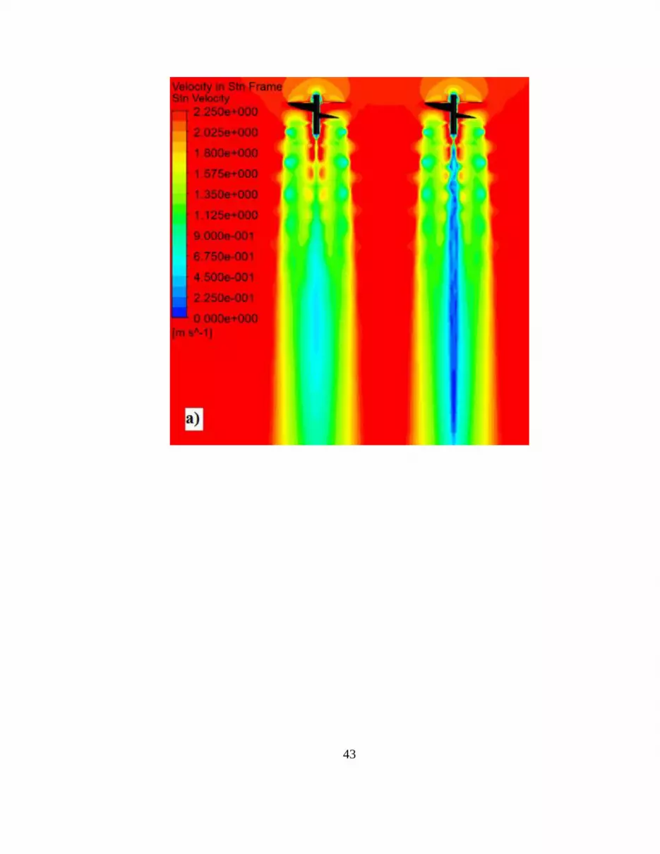
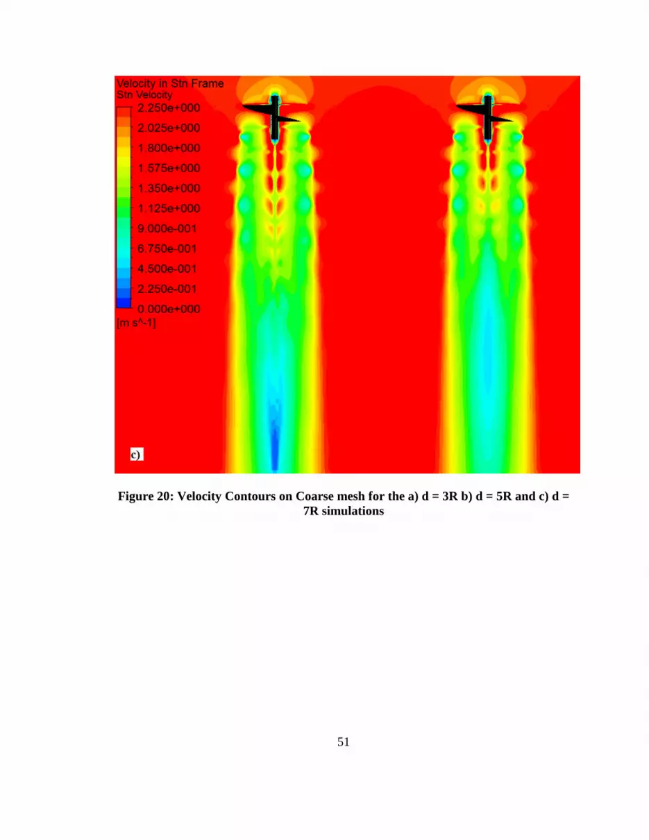
As discussed in the previous section, it is also valuable to investigate the velocity
and pressure contours of the results that are generated. There were a total of eight different
simulations run in this study, so it would be impractical to list all of those contours for
every simulation. Shown in figures 20 and 21 are the velocity contours and a surface of
constant vorticity for the coarse d = 3R, d = 5R, and d=7R simulations.

49

50
51
Figure 20: Velocity Contours on Coarse mesh for the a) d = 3R b) d = 5R and c) d =
7R simulations

52

53
Figure 21: Surfaces of Constant Vorticity on the coarse mesh for a) d = 3R b) d = 5R
and c) d = 7R simulations
From these plots, it can be seen that the wakes behind the turbines in each
simulation look very similar at each separation distance. This is to be expected, as the
turbines used in all simulations and the free stream velocity/boundary conditions are the
same. Because of this similarity, these plots only serve to provide more confidence in this
computational study’s results.
The final method of verifying solution accuracy is to make sure that the blades of
the turbines are undergoing flow conditions that the turbulence model that was selected is
suitable for. As discussed in the previous section, this is done by investigating the 𝑦+ values
on the blade surface. Plotting that value over the 30 to 300 range on the turbines, as shown
in figure 22 for the d=5R separation distance, shows smooth 𝑦+value contours.

54
Figure 22: 𝒚+ values for the coarse mesh d = 5R simulation
The 𝑦+ contours on the turbine surface shown in Figure 22 show that the flow
conditions around each turbine are captured very well by the k-ω SST turbulence model
and by the mesh that was used at each surface. This means that this turbulence model has
been experimentally verified for flow conditions similar to those in the present study,
providing even more confidence in the accuracy of the predicted results.
The 𝑦+ contours for the other mesh sizes and other separation distances look
essentially identical to the ones shown in figure 22, and are not attached in this paper to
avoid pictorial redundancy.

55
4. Conclusion
4.1 Results Summary and Turbine Placement Recommendations
The effects of separation distance between two turbines on each turbine’s drag
coefficients, performance coefficients, and on the resulting flow characteristics were
studied. In order to maximize both combined turbine power output and resultant drag for
both turbines, the simulation results
suggest that, in a uniform flow field,
the turbines should be placed as far
apart as is feasible. At every
separation distance, the drag and
performance coefficients of the left
and the right turbines are shown to be
very similar.
In reality a river will not have
a uniform flow distribution; in fact,
the flow of many rivers has been
measured by geologists and they tend
to have a velocity distribution similar to what is shown in Figure 23. For those in the field
who wish to maximize turbine power output, the turbines should be placed in the river
cross section in a manner that maximizes the kinetic energy of the water that enters those
turbines. As seen in Figure 23, the maximum kinetic energy of the river will be found in a
region close to the river’s surface, so it makes sense to place the turbines in that region.
Figure 23: Typical river flow cross-section
[23]

56
However it is also important to realize that, inside of this high-velocity region, the
gradient of the velocity vector will be near zero and the flow can therefore be considered
approximately uniform. If this is the case, then the results of this study would still hold as
long as the turbines are placed within that high fluid velocity and near-zero gradient region.
Additional restrictions on turbine placement become apparent due to the realization
that, if the turbines are placed too close to the surface, there will be two-phase air and water
interaction. The single-phase simulations done in this study are unable to take into account
the mixing of air and water that occurs in the form of periodic surface waves, generated air
bubbles in the fluid, and water droplets which can be expelled momentarily from the river’s
surface. In addition to being much more difficult to model, the air-water interaction is also
not something that the eventual customers of these turbines will want, as it will almost
assuredly increase turbine wear and decrease turbine performance. Therefore, the turbines
should be placed sufficiently beneath the river’s surface so that this detrimental air-water
interaction never manifests itself.
The results of this study therefore suggest that the turbines should be placed far
apart from each other within the high-velocity region near the top-center of the river’s cross
section. But, because of air-water interactions, the author recommends that the turbines
also be placed sufficiently far below the free surface of the river in order to maximize the
system’s power output.
4.2 Physical Explanation of Simulation Results
From a purely fluid mechanics intuition standpoint, if two turbines are put very
close together, it can be expected that their flows would interact downstream. This

57
interaction is a result of the turbines interfering with the development of each other’s wake,
and would make the turbine’s flow develop less “easily” in comparison to how they would
behave in the free stream. Therefore, it makes sense that the presence of two turbines
adjacent to one-another in a stream would negatively impact the drag and performance
coefficients of each other. Looking back at figures 13 and 14, it can be shown that the
power and drag coefficients done in this study at the smaller separation distances match up
nicely with this intuition.
Using this as a starting point, then it can be deduced that, as the turbines are
separated further and further, the degree of interaction between the two turbines wakes
would be reduced. This suggests that the power and drag of each turbine should
asymptotically approach some maximum value as this separation distance in increased.
The results from this study do show the power and drag coefficients beginning to level off
at a larger separation distance, which confirms this intuition.
It can then be concluded that many of the trends discovered through this study do
match up neatly with what those with a strong fluid mechanics background should expect
them to be. This provides further evidence that, although certainly not without its
imperfections, the results presented in this study can be assumed to be of reasonable
accuracy.
4.3 Methods of Simulation Validation
The limited computational and temporal resources at the author’s disposal leave
plenty of opportunity for further study on this problem. In order to validate the results
presented in this thesis, the author recommends the use of fully transient simulations to

58
verify that the steady-state assumptions used in the present study are succeeding in
capturing all important flow characteristics. The inherently unsteady nature of the flow as
well as the extent of turbulent interaction between each turbine means that this problem
should benefit greatly from the improved accuracy associated with a transient simulation.
However, even the use of a transient simulation cannot correct for the limitations
that this particular experiment places on the size of the rotating domains around each
turbine. As of the conclusion of this study, the affect that the changing size of the rotating
domain has on the results of the present simulations is unknown. This can be rectified by
performing a study on the effect of the rotating domain size on the predicted turbine
performance, and then by comparing those results to the ones in this study.
A way to circumvent dealing with the unknown effect of the rotating domain is to
get rid of the cylindrical rotating domains entirely and instead model the rotation of each
turbine via an adaptive meshing scheme. Instead of rotating the cylindrical mesh a small
amount with each time step, the turbine geometry itself is rotated within a larger body
during each time step, and the domain around both turbines would need to be meshed again
at every time step. This is only possible through the creation of an unstructured adaptive
meshes near the turbine blades, which creates several computational hurtles that the present
study was able to go around addressing. Naturally, the researcher would need to have
extensive computational resources at their disposal in order to make such a study feasible.
Alternatively, experimental studies should be done in water tunnels to provide
further validation for the results presented in this study. Nonetheless, this study should

59
prove to be a worthwhile foundation for further research in this area, as well as provide a
guide to those who seek to maximize turbine performance in a real river.
4.4 Areas of Further Research
As stated in earlier sections, the present study only modeled a single fluid, the
water, in order to determine turbine performance. This is a valid assumption as long as the
turbines are placed well beneath the river surface, but when the turbine is rotating near the
river’s surface this may not be the case due to air and water mixing. This is a phenomenon
that the present simulations have not even attempted to model, but the presence of air
hitting the turbine blades instead of water would almost assuredly negatively affect turbine
performance and increase turbine wear. In a more academic sense, the scale of how large
this decrease in performance will be as a function of the turbine’s distance beneath the
river’s surface is still unstudied. Therefore, further research on this subject could include
modeling both the air and the water in order to discover this relationship as well as shed
light on just how far beneath the surface the turbines should be placed.
More research could also be done to further optimize turbine performance over a
wider range of tip speed ratios. Such research may include changing the blade pitch and/or
blade rotation rate, increasing the number of blades, varying the thickness of the blades to
a more streamlined cross-section, or even creating adjustable-pitch turbine blades (similar
in concept to Kaplan turbines used in many modern hydroelectric dams).
Alternative areas of research could involve including more of the turbine system
into the CFD simulations. The present study used only the turbine blades and turbine hub
geometry to derive system performance, but did not attempt to model the nacelle that will

60
be attached to the turbine (in order to house the gear box and generator) or model the
mooring of the turbine system (to hold the system in place in the river). Naturally, taking
these factors into account would simultaneously increase the complexity of the simulations,
but could also better represent the conditions in which the turbines will be deployed.

61
Bibliography
[1] Hydroelectric Power. Tennessee Valley Authority. [Online]
http://www.tva.gov/power/hydroart.htm (Accessed Mar 14, 2014).
[2] Hayley Moller, Data Highlights. Earth Policy Institute. Published: Jun 14, 2012.
[Online] http://www.earth-policy.org/data_highlights/2012/highlights29 (Accessed
March 18, 2014)
[3] Environmental Costs of Electricity, Pace University Center for Environmental and
Legal Studies (Oceana Publications, 1990) [Online]
http://www.stewartmarion.com/carbon-footprint/html/carbon-footprint-kilowatt-
hour.html#carbon-dioxide-from-one-kilowatt-hour (Accessed April 2, 2014).
[4] Use and Capacity of Global Hydropower Increases. Worldwatch Institute.
[Online] http://www.worldwatch.org/node/9527 (Accessed April 2, 2014).
[5] About Wind Energy. Continental Wind Power. [Online]
http://mstudioblackboard.tudelft.nl/duwind/Wind%20energy%20online%20reader
/figures/horizontal_vertical.gif (Accessed April 9, 2014).
[6] V.B. Miller, L.A. Schaefer. Computational Fluid Dynamics for Hydrokinetic
Turbines. Proceedings of the ASME 2009 International Mechanical Engineering
Congress and Exposition. IMECE2009-11115. November 13-19, Lake Buena Vista,
Florida, USA.
[7] N. Kolekar, Z. Hu, A. Banerjee, X. Du. Hydrodynamic Design and Optimization
of Hydro-kinetic Turbines using a Robust Design Method. Proceedings of the 1st Marine
Energy Technology Symposium. April 10-11, 2013, Washington, D.C. pp 8
[8] Millennium Problems. Clay Mathematics Institute. [Online]
http://www.claymath.org/millennium-problems (Accessed April 15, 2014).
[9] Direct Numerical Simulation. CFD Online. [Online] http://www.cfd-
online.com/Wiki/Direct_numerical_simulation_%28DNS%29 (Accessed April 15, 2014)
[10] D.C. Wilcox. Turbulence Modeling for CFD. Third Edition (DCW Industries,
Inc., La Canada, CA 2010) pp. 4, 108-109, 16.
[11] Statement on the Control of Numerical Accuracy. ASME Journal of Fluids
Engineering. http://journaltool.asme.org/templates/JFENumAccuracy.pdf
[12] S.S. Mukherji, N. Kolekar, A. Banerjee, and R. Mishra. Numerical Investigation
and evaluation of optimum hydrodynamic performance of a horizontal axis hydrokinetic
turbine. Journal of Renewable and Sustainable energy 3, 06315 (2011); doi:
10.1063/1.3662100
[13] B. Gunawan, V.S. Neary, C. Hill, and L.P. Chamorro. “Measurement of velocity
deficit at the downstream of a 1:10 axial hydrokinetic turbine model.” Energy-Water-
Ecosystems Engineering, Wind and Power Technologies, Environmental Sciences
Division, Oak Ridge National Laboratory. http://energy.sandia.gov/wp/wp-
content/gallery/uploads/velocitydeficit_neary.pdf
[14] W. C. Schleicher, J. D. Riglin, Z. A. Kraybill, A. Oztekin and R. C. Klein, Jr.,
"Design and Simulation of a Micro Hydrokinetic Turbine," in Proceedings of the 1st
Marine Energy Technology Symposium, Washington, D.C., 2013.
[15] M. Zadravec, S. Basic, M. Hribersek. “The Influence of Rotating Domain Size in
a Rotating Frame of Reference Approach for Simulation of rotating Impeller in a Mixing

62
Vessel” in Journal of Engineering Science and Technology. Vol. 2, No. 2 (2007) 126 –
138 © School of Engineering, Taylor’s University College
[16] Navier-Stokes Equations – Rotational. Wolfram Research. [Online]
http://scienceworld.wolfram.com/physics/Navier-StokesEquationsRotational.html
(Accessed May 1, 2014)
[17] F.R. Menter, “Two-equation Eddy-Viscosity Turbulence Models for Engineering
Applications,” AIAA Journal, Vol. 32, no. 8, pp. 1598-1605, August 1994.
[18] Turbulence Free-stream Boundary Conditions. CFD Online. [Online].
http://www.cfd-online.com/Wiki/Turbulence_free-stream_boundary_conditions
(Accessed May 3, 2014)
[19] Turbulence Intensity. CFD Online. [Online]. http://www.cfd-
online.com/Wiki/Turbulence_intensity (Accessed May 3, 2014)
[20] Turbulent Length Scale. CFD Online. [Online] http://www.cfd-
online.com/Wiki/Turbulent_length_scale (Accessed May 3, 2014)
[21] Dimensionless Wall Distance. CFD Online. [Online] http://www.cfd-
online.com/Wiki/Dimensionless_wall_distance_%28y_plus%29 (Accessed May 3, 2014)
[22] FLUENT 14.0 User’s Guide. ANSYS
http://cdlab2.fluid.tuwien.ac.at/LEHRE/TURB/Fluent.Inc/v140/flu_ug.pdf
[23] Environmental Techniques – Stream Discharge Measurement. University of
Colorado, Department of Geography. [Online]. http://www.colorado.edu/geography/
courses/geog_2043_f01/lab01_2.html (Accessed Jun 6, 2014)
63
Vita
Joseph David Jonas was born on February 23, 1991 to Gordon M and Cynthia J
Jonas in Fairfield, Connecticut. Since then he has had the fortune of living in many different
places early in his life, which in addition to his place of birth include the outskirts of
Knoxville, Tennessee; Charlotte, North Carolina; Corning, New York; and Allentown,
New Jersey, where he graduated from Allentown High School class of 2009. Since then,
he attended Lehigh University for his Bachelor of Science degree in Mechanical
Engineering, a degree which he received with high honors in January of 2013. Upon the
completion of his B.S. and with the aid of Lehigh's Presidential Scholar program, Joseph
started pursuing his Masters of Science degree in Mechanical Engineering, of which this
Thesis is the final requirement.


