Joint Scalar versus Joint Velocity-Scalar PDF Simulations of Bluff-Body Stabilized Flames with REDIM

Flow Turbulence Combust (2009) 82:185–209DOI 10.1007/s10494-008-9162-2

Joint Scalar versus Joint Velocity-Scalar PDFSimulations of Bluff-Body StabilizedFlames with REDIM

B. Merci · B. Naud · D. Roekaerts · U. Maas

Received: 13 December 2007 / Accepted: 22 May 2008 / Published online: 3 July 2008© Springer Science + Business Media B.V. 2008

Abstract Two transported PDF strategies, joint velocity-scalar PDF (JVSPDF) andjoint scalar PDF (JSPDF), are investigated for bluff-body stabilized jet-type tur-bulent diffusion flames with a variable degree of turbulence–chemistry interaction.Chemistry is modeled by means of the novel reaction-diffusion manifold (REDIM)technique. A detailed chemistry mechanism is reduced, including diffusion effects,with N2 and CO2 mass fractions as reduced coordinates. The second-moment closureRANS turbulence model and the modified Curl’s micro-mixing model are not varied.Radiative heat loss effects are ignored. The results for mean velocity and velocityfluctuations in physical space are very similar for both PDF methods. They agree wellwith experimental data up to the neck zone. Each of the two PDF approaches impliesa different closure for the velocity-scalar correlation. This leads to differences in theradial profiles in physical space of mean scalars and mixture fraction variance, due todifferent scalar flux modeling. Differences are visible in mean mixture fraction and

B. MerciPostdoctoral Fellow of the Fund of Scientific Research, FWO-Vlaanderen, Flanders, Belgium

B. Merci (B)UGent, Department of Flow, Heat and Combustion Mechanics, Ghent University,Sint-Pietersnieuwstraat 41, 9000 Ghent, Belgiume-mail: [email protected]

B. NaudEnergy Department, Modeling and Numerical Simulation Group, Ciemat, Madrid, Spain

D. RoekaertsDepartment of Multi-Scale Physics, Delft University of Technology, Delft, The Netherlands

U. MaasInstitute for Technical Thermodynamics, Karlsruhe University (TH), Germany

186 Flow Turbulence Combust (2009) 82:185–209

mean temperature, as well as in mixture fraction variance. In principle, the JVSPDFsimulations can be closer to physical reality, as a differential model is implied forthe scalar fluxes, whereas the gradient diffusion hypothesis is implied in JSPDFsimulations. Yet, in JSPDF simulations, turbulent diffusion can be tuned by meansof the turbulent Schmidt number. In the neck zone, where the turbulent flow fieldresults deteriorate, the joint scalar PDF results are in somewhat better agreementwith experimental data, for the test cases considered. In composition space, whereresults are reported as scatter plots, differences between the two PDF strategies aresmall in the calculations at hand, with a little more local extinction in the joint scalarPDF results.

Keywords CFD · Transported PDF · REDIM · Bluff body stablised flames

1 Introduction

In turbulent non-premixed flames, non-linear interaction between turbulence andfinite-rate chemistry is often important. Turbulence–chemistry interaction is thusa central issue in non-premixed turbulent flame modeling and simulations. Stronginteraction may lead to local extinction or incomplete combustion. Under suchcircumstances, pre-assumed PDF modeling is typically not suitable. Given a certainchemistry model, an exact treatment of the chemical reaction source term is achievedin the framework of the computationally much more expensive transported proba-bility density function (PDF) technique, be it joint scalar or joint velocity-scalar [1].The conditional molecular flux is left as a modeling issue.

In this study, we apply transported PDF methods, based on stochastic Lagrangianmodeling. We compare the results of joint scalar PDF (JSPDF) and joint velocity-scalar PDF (JVSPDF) simulations. Following [1], a mass density function (MDF)transport equation is modeled and solved using a particle stochastic method. Thethree major modeling ingredients are: the turbulence model, the chemistry modeland the micro-mixing model. Several recent comparative studies focus on the influ-ence of these different sub-models on numerical simulation results of turbulent non-premixed flames. In [2] e.g., three widely used micro-mixing models are compared,considering stochastic simulations of partially stirred reactors (PaSR). In the contextof transported scalar PDF modeling, the same micro-mixing models are comparedin [3] for the piloted jet diffusion flame Delft flame III, and in [4] for the bluff-body stabilized flames ‘Sydney HM1–3’ [5–7]. In [8], seven combustion mechanismsfor methane/air are compared for joint velocity-scalar-turbulence frequency PDFcalculations of the non-premixed piloted jet flames ‘Sandia D-F’. In [9], the influenceof three C1 chemistry models on two micro-mixing models is studied for Delftflame III and the bluff-body flames HM1–3. In [10], detailed models, containingC2 chemistry, are applied to the same bluff-body test cases. In [11], an algebraicextension of the modified Curl’s coalescence/dispersion (CD) mixing model [12] isapplied to HM2 and HM3, with systematically reduced C2 chemistry.

In the present paper, we focus on the Sydney flames HM1 and HM3. The fuelis a mixture of 50%H2/50%CH4 by volume. It is a target test case of the TNF

Flow Turbulence Combust (2009) 82:185–209 187

workshop series on turbulent non-premixed flames [13]. Recently, a few papers onthese flames appeared, employing transported PDF [10, 11] and conditional momentclosure (CMC) [14]. With respect to chemistry modeling, the present work is animprovement over [4]. Instead of a C1 skeletal mechanism, the novel reaction-diffusion manifold (REDIM) technique [15] is applied, reducing a detailed reactionmechanism, consisting of 34 species and 302 reactions [16]. Recently, there hasbeen much research activity in the field of reduced chemistry, in combination withchemistry–transport coupling. A comprehensive review is provided by Ren and Pope[18, 19], which argues in favor of the ‘close-parallel’ assumption for chemistry-basedslow manifolds. This basically reduces to the assumption that the system evolves ona manifold, close and parallel to a manifold that is solely based on chemistry. Thedistance from the ‘chemical’ manifold is governed by diffusion processes. We applythe REDIM technique of [15], leading to an invariant low-dimensional manifold,directly accounting for the coupling of chemistry and diffusion (and convection). Theobtained, invariant, manifold need not be parallel to a manifold that is solely basedon chemistry.

In order to achieve good agreement to experimental data for the turbulent flowfield, in terms of radial profiles in physical space of mean velocities and velocity fluc-tuations, a second moment closure model is applied with modified model constants[4, 20]. Good quality of the results is obtained up to the neck zone. The modifiedCurl’s coalescence/dispersion (CD) [21] is used as micro-mixing model. In [4], acomparative study is presented to the Euclidean Minimum Spanning Tree (EMST)model [22], in the framework of transported scalar PDF, revealing that EMST is notsuperior to CD for the test cases considered. We confirmed this with the currentchemistry approach or REDIM (not discussed here). In [4], we reported it was notpossible to obtain a stationary solution for HM3 with the CD mixing model. This wasattributed to the use of C1 chemistry in [4]. Applying reduced chemistry, with theREDIM technique, a stationary solution is obtained and profiles of major and minorchemical species in physical space are in good agreement to experimental data. Weremark that Gkagkas et al. [11] report that, in line with our previous findings [4], nostatistically stationary solution could be found for HM3 with their C/D type micro-mixing model, starting from a steady laminar flamelet solution.

The choice of the PDF description itself has direct consequences on the modelingof the scalar flux and higher order velocity-scalar correlations. With the joint scalarMDF, the gradient diffusion assumption for closure of the conditional fluctuatingvelocity term in the MDF transport equation, leads to a simple algebraic model forthe scalar flux. In this case, good agreement in physical space for mean mixture frac-tion and mixture fraction variance can be obtained by tuning the turbulent Schmidtnumber. When the velocity components are included in the PDF description, thetransport equation for the joint velocity-scalar MDF is modeled and solved usinga particle method. In this case, the combination of the model for particle velocityevolution and the micro-mixing model implies a modeled transport equation for thescalar flux and higher order velocity-scalar correlations. In the present study, we com-pare results of JSPDF and JVSPDF simulations, using hybrid finite volume/particlemethods, implemented in the same in-house computer program ‘PDFD’, describedby Naud et al. in [23]. The same turbulence, chemistry and micro-mixing models areused in all simulations.


2 PDF Approach

2.1 Statistical description

The statistical description of the flow is in terms of the joint one-point PDF fφ :fφ (ψ; x, t) . dψ is the probability that Φ is in the interval [ψ,ψ+dψ[at point (x, t).When JSPDF is considered, Φ is the composition vector φ. For JVSPDF, Φ = (U, φ),with U the velocity vector. The joint PDF is defined as in [1, 4]:

fφ (ψ; x, t) = ⟨δ[φ (x, t) − ψ

]⟩(1)

where δ[] is the Dirac delta function and where the brackets 〈〉 refer to ex-pected values [1]. Using the conditional expected value 〈Q (x, t) |ψ 〉 fφ (ψ; x, t) =⟨Q (x, t) .δ

[φ (x, t) − ψ

]⟩, mean (or ‘expected’) values are defined as:

〈Q (x, t)〉 =∫

[ψ]〈Q (x, t) |ψ 〉 fφ (ψ; x, t) dψ (2)

Fluctuations are defined as: q′ (x, t) = Q (x, t) − 〈Q (x, t)〉.For variable density flows, it is useful to consider the joint MDF Fφ (ψ) =

ρ (ψ) fφ (ψ). Density weighted averages (Favre averages) are:

Q (x, t) = 〈ρ (x, t) Q (x, t)〉〈ρ (x, t)〉 =

∫[ψ] 〈Q (x, t) |ψ 〉 F� (ψ; x, t) dψ

∫[ψ] F� (ψ; x, t) dψ

. (3)

Fluctuations with respect to the Favre average are defined as: q′′ (x, t) =Q (x, t) − Q (x, t).

2.2 Joint scalar PDF transport equation

When the joints scalar MDF is considered, the following transport equation ismodeled and solved [1]:

∂ Fφ

∂t+ ∂U jFφ

∂x j+ ∂

∂ψα

[Sα (ψ) Fφ

] = − ∂

∂xi

[⟨u′′

i |ψ ⟩Fφ

]− ∂

∂ψα

[〈θα |ψ 〉 Fφ

](4)

with the mixing term θα (φ) = − 1

ρ (φ)

∂ Jαj

∂x j, and where Sα is the reaction source term

for scalar φα and Jα its molecular flux. The first term on the right hand side ismodeled using a gradient diffusion assumption:

∂

∂xi

[⟨u′′

i |ψ ⟩Fφ

] = − ∂

∂xi

[

T∂(Fφ

/ρ)

∂xi

]

(5)

where T is the turbulent diffusivity, modeled as T = μT/ScT , with μT the eddyviscosity. The turbulent Schmidt number is taken as ScT = 0.7 or ScT = 0.85(see below).


2.3 Joint velocity-scalar PDF transport equation

When velocity is included in the PDF description, the transport equation for the

joint velocity-scalar MDF can be written(

neglecting the mean viscous stress tensor

gradient ∂〈τij〉∂x j

):

∂ FUφ

∂t+ V j

∂ FUφ

∂x j+(

− 1

〈ρ〉∂ 〈p〉∂x j

+ g j

)∂ FUφ

∂x j+ ∂

∂ψα

[Sα (ψ) FUφ

]

= − ∂

∂V j

[a jFUφ

]− ∂

∂ψα

[1

ρ (ψ)

⟨−∂ Jα

j

∂x j

∣∣∣∣V, ψ

⟩FUφ

](6)

The term a j denotes:

a j =(

1

〈ρ〉 − 1

ρ (ψ)

)∂ 〈p〉∂x j

+ 1

ρ (ψ)

⟨

− ∂p′

∂x j+ ∂τ ′

ij

∂xi

∣∣∣∣∣V, ψ

⟩

. (7)

A Langevin model is used to close this term, as mentioned below, in the sectionon turbulence modeling. The terms on the left hand side of (6) are in closed form.Compared to (4), effects of convection and mean pressure gradient are now exactlytaken into account.

2.4 Hybrid finite volume/particle method

Equations (4) and (6) are solved using the consistent hybrid finite-volume/particlemethod presented in [23]. Mean velocity ˜U, mean pressure gradient ∂〈p〉/∂xi,

Reynolds stresses⟨pu′′

i u′′j

⟩and turbulent dissipation rate ε, which is not included

in the PDF representation, are obtained by a standard finite-volume (FV) methodbased on a pressure-correction algorithm.

A particle method is applied for the solution of the MDF transport equation. Aset of uniformly distributed computational particles evolves according to stochasticdifferential equations. Each particle has a set of properties {w*, m*, X*,φ*} (scalarMDF) or {w*, m*, X*, u*, φ*} (velocity-scalar MDF), where w* is a numericalweight, m* is the particle mass, X* its position, u* its fluctuating velocity and φ*the particle’s composition. The superscript * denotes that the quantity is a particleproperty. Particle mass m* is constant in time. The particle joint scalar MDF is:

F Pφ (x, ψ; t) =

⟨∑

∗w∗m∗ · δ

(X∗ (t) − x

) · δ(φ∗ (t) − ψ

)⟩

(8)

Additional properties can be deduced for each stochastic particle from the primaryproperties listed above. As an example, the particle density is obtained as: ρ∗ (t) =ρ[φ∗ (t)

].


Increments of particle position X* and composition φ* over a small time step dtare given by:

dX∗i = (

U∗i + [

Uci

]∗)dt (9)

dφ∗α = θ∗

αdt + Sα

(φ∗)dt (10)

The correction velocity Uc results from a position correction algorithm [24], ensuringthat the volume represented by the particles in a computational cell, equals the cellgeometric volume. The values of the position correction algorithm parameters areset to: k f = 0.5, kb = 1 and Nc

T A = 100, as in [23]. θ∗α represents the model for the

conditional scalar flux (micro-mixing model).With the scalar MDF, U* results from a random walk model for particle position

evolution:

U∗i dt =

[Ui + 1

〈ρ〉∂T

∂xi

]∗dt +

[(2T

〈ρ〉)1/2

]∗

dWi , (11)

with dWi an increment over dt of the Wiener process Wi.With the joint velocity-scalar MDF, the equations read:

U∗i = [

Ui]∗ + u∗

i (12)

du∗i = −u∗

j

[∂Ui

∂x j

]∗dt +

⎡

⎣ 1

〈ρ〉∂ 〈ρ〉 ˜u′′

i u′′j

∂x j

⎤

⎦

∗

dt + a∗i dt (13)

In the above equations, the quantities between brackets []* are FV properties inter-polated at the particle location using bilinear basis functions as in [25]. The modelfor a∗

i is specified below in the section on turbulence modeling.The method of fractional steps [1] is used to integrate the system of equations.

In order to ensure second-order accuracy, the ‘midpoint rule’ is used [24, 25]. Alocal time-stepping algorithm, developed in the framework of statistically stationaryproblems [3, 26], is applied.

2.5 Consistency and coupling

The turbulent dissipation rate is not included in the PDF representation. Thetransport equation solved for ε in the FV method, provides additional information,required to model the unclosed term ai and the micro-mixing model. The otherFV equations are consistent with the modeled MDF transport equation [23]. Themean density <ρ> in the FV method is directly obtained from the iteration averagedmean density in the particle method, applying the iteration averaging procedure aspresented in [23]. We remark that the global convergence of the method is improvedin comparison to the latter reference, where density relaxation was used.

An outer iteration consists of a number of FV iterations and particle time steps.We use a fixed number of particle time steps (typically five), while the FV methodis iterated until the residuals of all equations are decreasing and the global mean


pressure correction is below a specified threshold (with a maximum of 1000 FViterations per outer iteration).

3 Modeling

3.1 Turbulence model

Turbulence is modeled using the second-moment closure RANS model of [20].This is the isotropization of production model of [27], with modified constant valueCε1 = 1.6, instead of the standard value Cε1 = 1.44. Consistently, the Lagrangianisotropization of production model (LIPM) is used in the velocity-scalar PDFapproach to describe velocity evolution ai [28, 29].

3.2 Reduced chemistry model: REDIM

The REDIM concept, described in detail in [15], is used to reduce a detailedCH4/H2/air detailed reaction mechanism of 34 species and 302 reactions [16]. Thisconcept is based on a relaxation process, where an initial guess for a low-dimensionalmanifold evolves in such a manner that an invariant slow reaction/diffusion manifoldis obtained. One major advantage of the REDIM technique over the ILDM conceptis the fact that a REDIM exists in the whole accessed domain, even at low tempera-tures (close to the unburned mixture), where chemistry is slow and ILDM does notyield an existing manifold. Close to equilibrium the REDIM is typically close to theILDM. It has been shown in [15] that, if chemistry governs the overall process, i.e.,gradients tend to zero, the REDIM concept yields slow manifolds or, equivalently,iteratively refined ILDMs as a limiting case [17].

The m-dimensional vector of reduced coordinates represents the compositionvector φ. The evolution equation, solved to obtain the low-dimensional manifolds(see below), is formulated in generalized coordinates. In order to simplify thesubsequent use of the tables, suitable simple progress variables are identified afterthe calculation of the REDIM. They are used as the reduced coordinates. For thetest case under study, it is possible to use mixture fraction (or mass fraction of N2)

and one reaction progress variable (mass fraction of CO2), because the result of theREDIM calculations show that they are suitable coordinates. Thus, in the presentwork, m = 2. Equal diffusivities and unity Lewis number are assumed in the presentapplication of REDIM, although it is possible to extend the REDIM concept tosystems with non-equal diffusivities.

In the following, we describe only the specific implementation details for the con-sidered system. LetΦdenote the thermo-kinetic state

(Φ=(h, p, Y1/M1,. . .,YS/MS)

T),

where h is the specific enthalpy, p the pressure, Y the mass fractions, M the molarmasses, and S the number of species. For the two-dimensional REDIM, this statevector is assumed to be a function of the two mentioned reduced coordinates. Asinitial guess for the REDIM, we build up a tensor product mesh covering the entiredomain from the un-burnt mixing line to the line of complete reaction to H2 O andCO2. Values inside the domain are estimated, based on an interpolation between


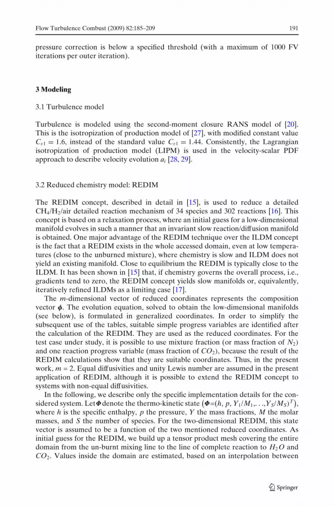
Fig. 1 Initial guess for theREDIM; blue: completereaction to CO2 and H2 O;magenta: unburned mixture;red and green: two laminardiffusion flamelets fortangential pressure gradientequal to 104N/m4 and106N/m4; axes: mass fractions,divided by molar mass(mol/kg)

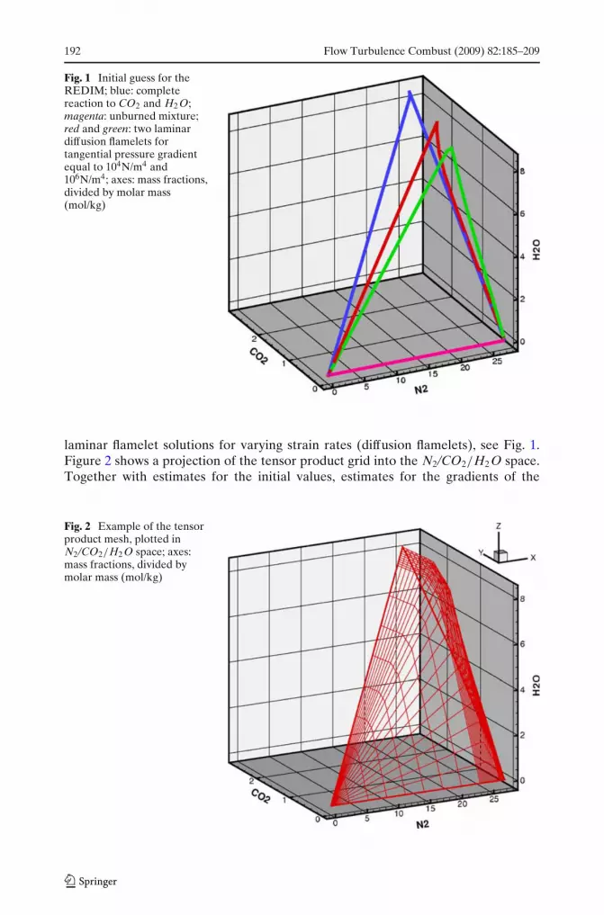
laminar flamelet solutions for varying strain rates (diffusion flamelets), see Fig. 1.Figure 2 shows a projection of the tensor product grid into the N2/CO2/H2 O space.Together with estimates for the initial values, estimates for the gradients of the

Fig. 2 Example of the tensorproduct mesh, plotted inN2/CO2/H2 O space; axes:mass fractions, divided bymolar mass (mol/kg)


progress variables are obtained by a linear interpolation (gradients are also tabulatedin terms of the tensor product mesh).

In this way we obtain Φ0 = Φ0 (φ), where φ is the two-dimensional vector ofreduced coordinates. This starting solution then evolves according to the REDIMequation:

∂Φ

∂τ=(

I − ΦφΦ+φ

)·{

F (Φ) +∑

ij

dρ

iΦφiφ j j

}(14)

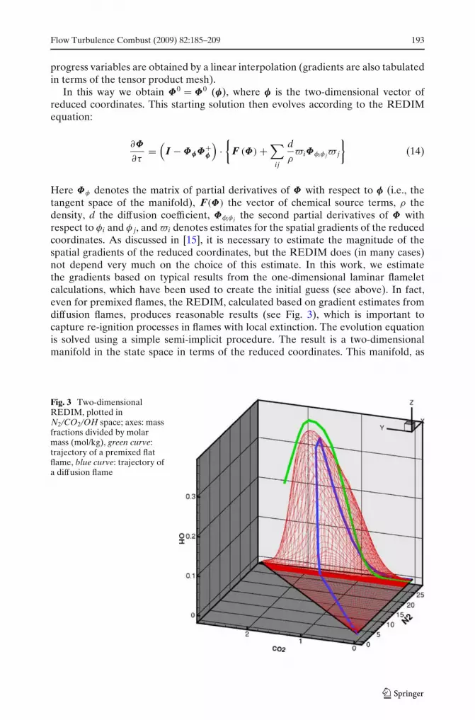
Here Φφ denotes the matrix of partial derivatives of Φ with respect to φ (i.e., thetangent space of the manifold), F(Φ) the vector of chemical source terms, ρ thedensity, d the diffusion coefficient, Φφiφ j the second partial derivatives of Φ withrespect to φi and φ j, and i denotes estimates for the spatial gradients of the reducedcoordinates. As discussed in [15], it is necessary to estimate the magnitude of thespatial gradients of the reduced coordinates, but the REDIM does (in many cases)not depend very much on the choice of this estimate. In this work, we estimatethe gradients based on typical results from the one-dimensional laminar flameletcalculations, which have been used to create the initial guess (see above). In fact,even for premixed flames, the REDIM, calculated based on gradient estimates fromdiffusion flames, produces reasonable results (see Fig. 3), which is important tocapture re-ignition processes in flames with local extinction. The evolution equationis solved using a simple semi-implicit procedure. The result is a two-dimensionalmanifold in the state space in terms of the reduced coordinates. This manifold, as

Fig. 3 Two-dimensionalREDIM, plotted inN2/CO2/OH space; axes: massfractions divided by molarmass (mol/kg), green curve:trajectory of a premixed flatflame, blue curve: trajectory ofa diffusion flame


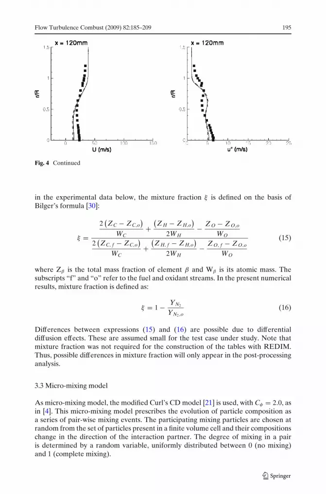
Fig. 4 Mean axial velocity component (left) and axial velocity fluctuations (right) for HM1

well as additional information such as chemical rates of the progress variable andtemperature, is tabulated using the tensor product mesh.

In Eqs. 4 and 6, the composition vector is thus reduced to φ = (ξ ,YCO2) and thechemical source term SCO2(φ) is given by the REDIM reduced chemistry. Note that


Fig. 4 Continued

in the experimental data below, the mixture fraction ξ is defined on the basis ofBilger’s formula [30]:

ξ =2(ZC − ZC,o

)

WC+(Z H − Z H,o

)

2WH− Z O − Z O,o

WO

2(ZC, f − ZC,o

)

WC+(Z H, f − Z H,o

)

2WH− Z O, f − Z O,o

WO

(15)

where Zβ is the total mass fraction of element β and Wβ is its atomic mass. Thesubscripts “f” and “o” refer to the fuel and oxidant streams. In the present numericalresults, mixture fraction is defined as:

ξ = 1 − YN2

YN2,o(16)

Differences between expressions (15) and (16) are possible due to differentialdiffusion effects. These are assumed small for the test case under study. Note thatmixture fraction was not required for the construction of the tables with REDIM.Thus, possible differences in mixture fraction will only appear in the post-processinganalysis.

3.3 Micro-mixing model

As micro-mixing model, the modified Curl’s CD model [21] is used, with Cφ = 2.0, asin [4]. This micro-mixing model prescribes the evolution of particle composition asa series of pair-wise mixing events. The participating mixing particles are chosen atrandom from the set of particles present in a finite volume cell and their compositionschange in the direction of the interaction partner. The degree of mixing in a pairis determined by a random variable, uniformly distributed between 0 (no mixing)and 1 (complete mixing).


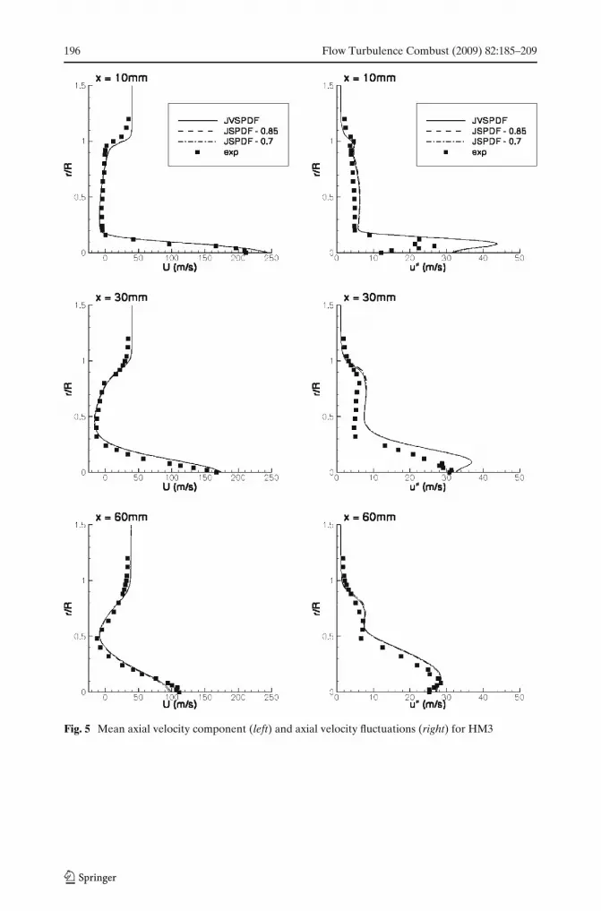
Fig. 5 Mean axial velocity component (left) and axial velocity fluctuations (right) for HM3


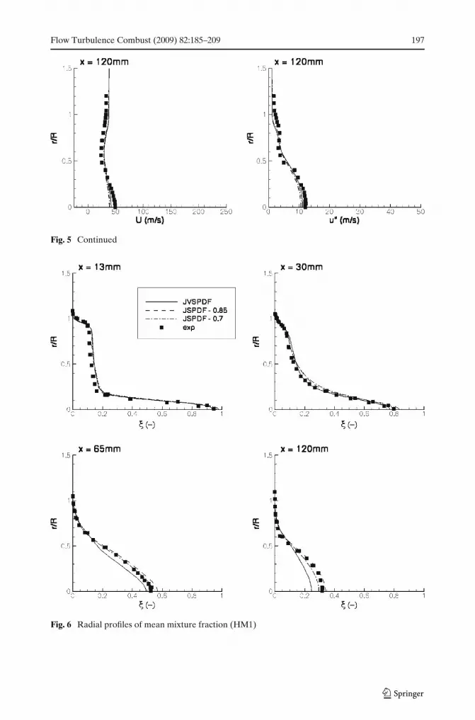
Fig. 5 Continued

Fig. 6 Radial profiles of mean mixture fraction (HM1)


Fig. 7 Radial profiles of CO2 mass fraction (HM1)

3.4 Implications for modeled equations for mean scalar, scalar varianceand scalar flux

In the simulations, Eqs. 4 and 6 are solved with a Monte Carlo method. IntegrationEq. 4 or 6 over the sample space yields the same mean scalar and scalar variancetransport equations:

∂ 〈ρ〉 φα

∂t+ ∂ 〈ρ〉 φαU j

∂x j= −∂ 〈ρ〉 ˜u′′

jφ′′α

∂x j+ 〈ρ〉 Sα, (17)

∂ 〈ρ〉 φ′′2α

∂t+ ∂ 〈ρ〉 U jφ′′2

α

∂x j+ 2 〈ρ〉 ˜u′′

jφ′′α

∂φα

∂x j= −

∂⟨ρu′′

jφ′′2α

⟩

∂x j− 2 〈ρ〉 ˜φ′′

α Sα − 2⟨ρφ′′

αθα

⟩.

(18)

There is no implicit summation over index α. The observation that there is no micro-mixing term in Eq. 17 is a direct consequence of the conservation of the mean bythe mixing model. The final term in Eq. 18, concerning the modeling of the scalar


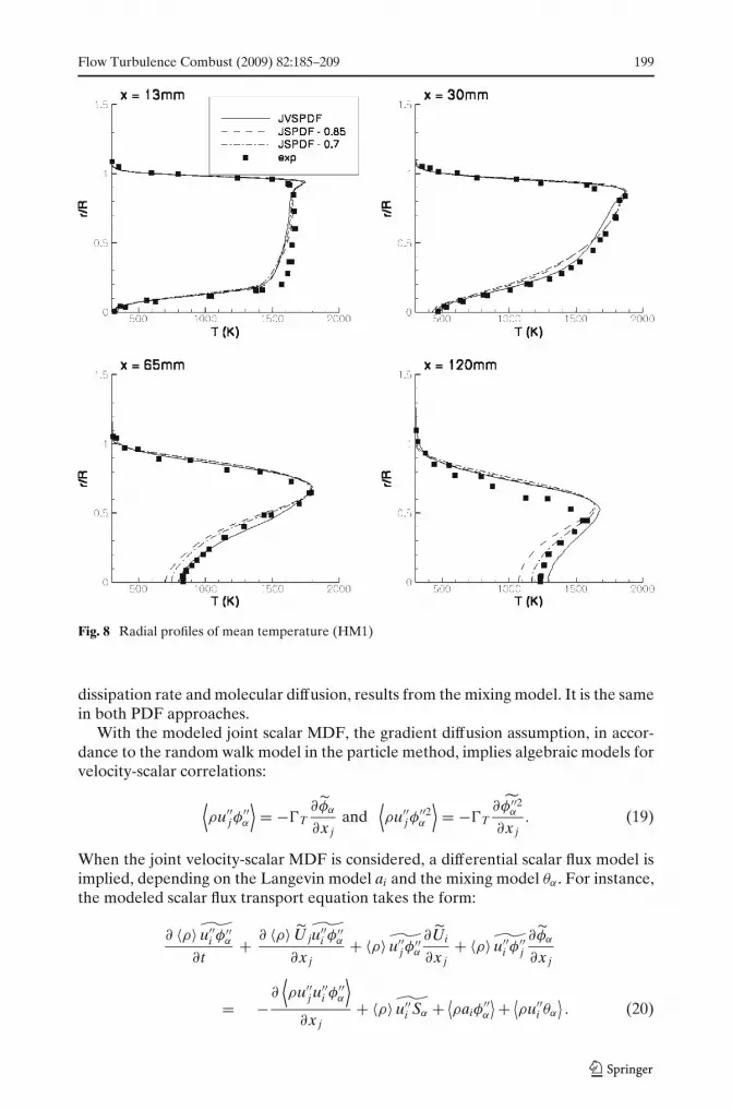
Fig. 8 Radial profiles of mean temperature (HM1)

dissipation rate and molecular diffusion, results from the mixing model. It is the samein both PDF approaches.

With the modeled joint scalar MDF, the gradient diffusion assumption, in accor-dance to the random walk model in the particle method, implies algebraic models forvelocity-scalar correlations:

⟨ρu′′

jφ′′α

⟩= −T

∂φα

∂x jand

⟨ρu′′

jφ′′2α

⟩= −T

∂φ′′2α

∂x j. (19)

When the joint velocity-scalar MDF is considered, a differential scalar flux model isimplied, depending on the Langevin model ai and the mixing model θα . For instance,the modeled scalar flux transport equation takes the form:

∂ 〈ρ〉 ˜u′′i φ

′′α

∂t+ ∂ 〈ρ〉 U j

˜u′′i φ

′′α

∂x j+ 〈ρ〉 ˜u′′

jφ′′α

∂Ui

∂x j+ 〈ρ〉 ˜u′′

i φ′′j∂φα

∂x j

= −∂⟨ρu′′

j u′′i φ

′′α

⟩

∂x j+ 〈ρ〉 ˜u′′

i Sα + ⟨ρaiφ

′′α

⟩+ ⟨ρu′′

i θα

⟩. (20)


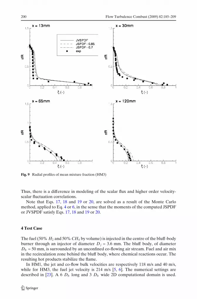
Fig. 9 Radial profiles of mean mixture fraction (HM3)

Thus, there is a difference in modeling of the scalar flux and higher order velocity-scalar fluctuation correlations.

Note that Eqs. 17, 18 and 19 or 20, are solved as a result of the Monte Carlomethod, applied to Eq. 4 or 6, in the sense that the moments of the computed JSPDFor JVSPDF satisfy Eqs. 17, 18 and 19 or 20.

4 Test Case

The fuel (50% H2 and 50% CH4 by volume) is injected in the centre of the bluff-bodyburner through an injector of diameter Dj = 3.6 mm. The bluff body, of diameterDb = 50 mm, is surrounded by an unconfined co-flowing air stream. Fuel and air mixin the recirculation zone behind the bluff body, where chemical reactions occur. Theresulting hot products stabilize the flame.

In HM1, the jet and co-flow bulk velocities are respectively 118 m/s and 40 m/s,while for HM3, the fuel jet velocity is 214 m/s [5, 6]. The numerical settings aredescribed in [23]. A 6 Db long and 3 Db wide 2D computational domain is used.


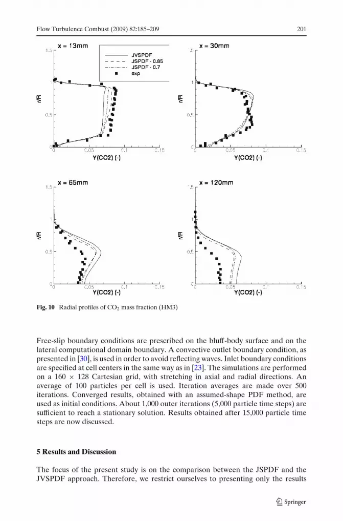
Fig. 10 Radial profiles of CO2 mass fraction (HM3)

Free-slip boundary conditions are prescribed on the bluff-body surface and on thelateral computational domain boundary. A convective outlet boundary condition, aspresented in [30], is used in order to avoid reflecting waves. Inlet boundary conditionsare specified at cell centers in the same way as in [23]. The simulations are performedon a 160 × 128 Cartesian grid, with stretching in axial and radial directions. Anaverage of 100 particles per cell is used. Iteration averages are made over 500iterations. Converged results, obtained with an assumed-shape PDF method, areused as initial conditions. About 1,000 outer iterations (5,000 particle time steps) aresufficient to reach a stationary solution. Results obtained after 15,000 particle timesteps are now discussed.

5 Results and Discussion

The focus of the present study is on the comparison between the JSPDF and theJVSPDF approach. Therefore, we restrict ourselves to presenting only the results


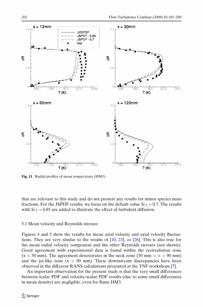
Fig. 11 Radial profiles of mean temperature (HM3)

that are relevant to this study and do not present any results for minor species massfractions. For the JSPDF results, we focus on the default value ScT = 0.7. The resultswith ScT = 0.85 are added to illustrate the effect of turbulent diffusion.

5.1 Mean velocity and Reynolds stresses

Figures 4 and 5 show the results for mean axial velocity and axial velocity fluctua-tions. They are very similar to the results of [10, 23], or [26]. This is also true forthe mean radial velocity component and the other Reynolds stresses (not shown).Good agreement with experimental data is found within the recirculation zone(x < 50 mm). The agreement deteriorates in the neck zone (50 mm < × < 90 mm)and the jet-like zone (x > 90 mm). These downstream discrepancies have beenobserved in the different RANS calculations presented at the TNF workshops [7].

An important observation for the present study is that the very small differencesbetween scalar PDF and velocity-scalar PDF results (due to some small differencesin mean density) are negligible, even for flame HM3.


Fig. 12 Radial profiles of mixture fraction variance (HM1)

5.2 Mean composition

Figures 6, 7, 8 show radial profiles for mean mixture fraction, CO2 mass fraction andtemperature for flame HM1. Significant differences between JSPDF and JVSPDFresults are observed. Within the recirculation region, where good agreement isobtained for the mean velocity and turbulent velocity fluctuations, the quality ofthe JVSPDF mean mixture fraction results is better than the JSPDF results. Indeed,excessive radial turbulent diffusion is observed with JSPDF in this region, whereradial gradients of mean velocity and mixture fraction are large. Differences in CO2

mass fractions are small in this region. The differences in mean mixture fractionpredictions are reflected in better mean temperature predictions with JVSPDF thanwith JSPDF. In the neck zone, mean mixture fraction is in general under-predictedwith the JVSPDF approach, though. This is in line with the under-prediction of meanaxial velocity in this region. In the JSPDF results, agreement with experimentaldata seems better, despite the under-prediction of mean axial velocity (and thusconvection). As the convective terms in the modeled transport equations are verysimilar and the turbulence level is practically the same, too, the differences between


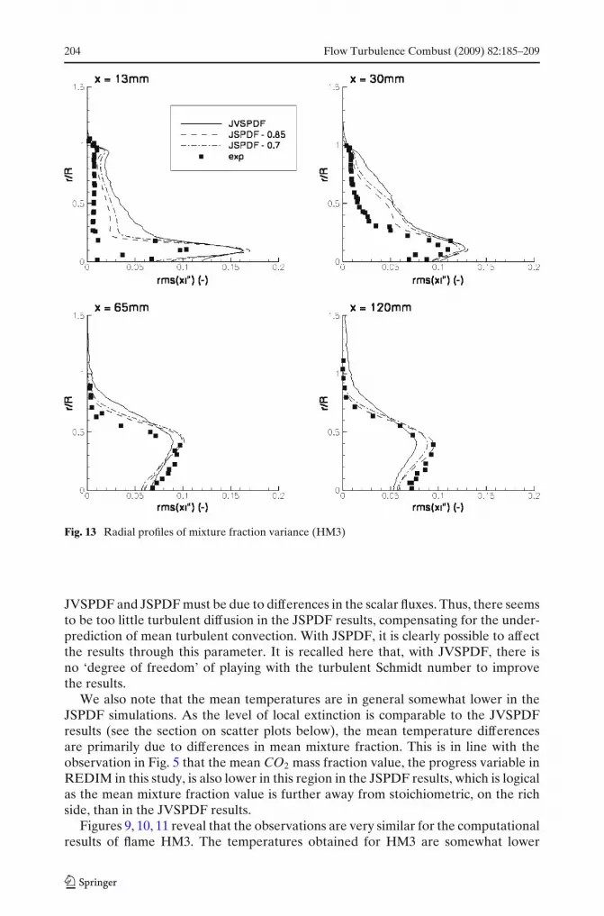
Fig. 13 Radial profiles of mixture fraction variance (HM3)

JVSPDF and JSPDF must be due to differences in the scalar fluxes. Thus, there seemsto be too little turbulent diffusion in the JSPDF results, compensating for the under-prediction of mean turbulent convection. With JSPDF, it is clearly possible to affectthe results through this parameter. It is recalled here that, with JVSPDF, there isno ‘degree of freedom’ of playing with the turbulent Schmidt number to improvethe results.

We also note that the mean temperatures are in general somewhat lower in theJSPDF simulations. As the level of local extinction is comparable to the JVSPDFresults (see the section on scatter plots below), the mean temperature differencesare primarily due to differences in mean mixture fraction. This is in line with theobservation in Fig. 5 that the mean CO2 mass fraction value, the progress variable inREDIM in this study, is also lower in this region in the JSPDF results, which is logicalas the mean mixture fraction value is further away from stoichiometric, on the richside, than in the JVSPDF results.

Figures 9, 10, 11 reveal that the observations are very similar for the computationalresults of flame HM3. The temperatures obtained for HM3 are somewhat lower


Fig. 14 Scatter plots for temperature (HM1). Experimental plots [7] reveal the ‘raw’ data (scatterplots) as well as the conditional ‘Reynolds’ and ‘Favre’ averages (not discussed here). Results forJSPDF are with ScT = 0.7. Results with ScT = 0.85 are almost identical

than for HM1, due to the occurrence of more local extinction (see below). Thereis no excellent agreement with experimental data, though: neither the JVSPDFresults nor the JSPDF results capture the experimental observation that the reactionregion shifts from the outer side of the recirculation region (as in HM1) to the innerside. Note that, in [4], it is reported that, in contrast to experimental observations,


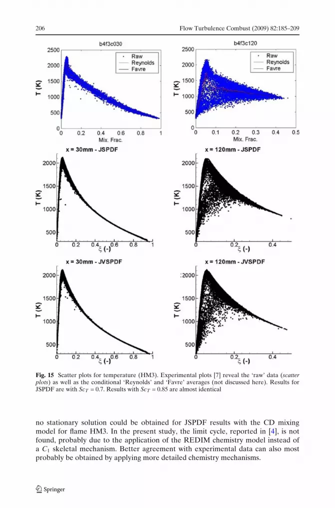
Fig. 15 Scatter plots for temperature (HM3). Experimental plots [7] reveal the ‘raw’ data (scatterplots) as well as the conditional ‘Reynolds’ and ‘Favre’ averages (not discussed here). Results forJSPDF are with ScT = 0.7. Results with ScT = 0.85 are almost identical

no stationary solution could be obtained for JSPDF results with the CD mixingmodel for flame HM3. In the present study, the limit cycle, reported in [4], is notfound, probably due to the application of the REDIM chemistry model instead ofa C1 skeletal mechanism. Better agreement with experimental data can also mostprobably be obtained by applying more detailed chemistry mechanisms.


5.3 Mixture fraction variance

In Figs. 12 and 13, differences are observed in the radial profiles of mixture fractionvariance. In general, the JSPDF results are in better correspondence with theexperimental data. The results are slightly better than reported in [4]. It is clear thatthe observed differences between JVSPDF and JSPDF are related to differences inmean mixture fraction, as well as to the modeling of velocity-scalar correlations: the

scalar flux u′′jξ

′′, appearing in the production term, and the triple correlation ˜u′′jξ

′′2,appearing in the turbulent diffusion term in Eq. 18. The under-prediction of mixturefraction variance with JVSPDF in the neck zone is mainly due to the lower meanmixture fraction values in this region.

5.4 Results in composition space: scatter plots

Figures 14 and 15 reveal that, in composition space, differences between JSPDF andJVSPDF results are small, with the turbulence, chemistry and micro-mixing modelsapplied. There is slightly more local extinction with JSPDF.

This indicates that the effect of differences in particle evolution in physical spacedue to mean convection and turbulent mixing, is small in composition space. Conse-quently, after further evolution due to the chemical source term, as retrieved fromthe REDIM table as constructed for the chemistry mechanism under consideration,the global scatter plots are very similar for JSPDF and JVSPDF simulations.

6 Conclusions

A comparison of scalar PDF and velocity-scalar PDF modeling has been conductedfor the bluff-body flames HM1 and HM3. Differences in the predicted turbulent flowfields are negligible. We applied one turbulence (LRR-IPM), chemistry (REDIM)and micro-mixing (CD) model.

Significant differences are observed in results for mean mixture fraction (andmean CO2 mass fraction). Consequently, there are also strong deviations in meantemperature and mixture fraction variance. These are attributed to implied modelingdifferences in the scalar fluxes (and higher order correlations). In general, jointvelocity-scalar PDF results, potentially closer to physical reality due to a differentialscalar flux model, are in line with the turbulent flow field results. In the recirculationregion, with strong radial gradients of mean velocity and mean mixture fraction, theJVSPDF results are somewhat better, as excessive turbulent diffusion occurs in theJSPDF simulations, in which a gradient diffusion assumption is implied. In the neckzone, however, the JVSPDF results are not better than joint scalar PDF results, dueto poorer agreement to experimental data for the turbulent flow field. Local tuning ofthe turbulent Schmidt number in JSPDF simulations, which is impossible in JVSPDFsimulations, can compensate for this for the test case under study.

The impact of the choice, JSPDF vs. JVSPDF, on scatter plots is small for the testcases under study, with a slightly higher level of local extinction in the JSPDF results.The scatter plots are in general in good agreement with experimental data.


Acknowledgements This collaborative research is supported by the COMLIMANS program, bythe Spanish MEC under Project ENE 2005–09190-C04–04/CON, by the Deutsche Forschungsge-meinschaft and by the Fund of Scientific Research–Flanders (Belgium) (FWO-Vlaanderen) throughFWO-project G.0079.07.

References

1. Pope, S.B.: PDF methods for turbulent reactive flows. Prog. En. Combust. Sci. 11, 119–192 (1985)2. Ren, Z., Pope, S.B.: An investigation of the performance of turbulent mixing models. Combust.

Flame. 136, 208–216 (2004)3. Merci, B., Roekaerts, D., Naud, B.: Study of the performance of three micromixing models in

transported scalar PDF simulations of a piloted jet diffusion flame (“Delft Flame III”). Combust.Flame. 144, 476–493 (2006)

4. Merci, B., Roekaerts, D., Naud, B., Pope, S.B.: Comparative study of micromixing modelsin transported scalar PDF simulations of turbulent nonpremixed bluff body flames. Combust.Flame. 146, 109–130 (2006)

5. Dally, B.B., Masri, A.R.: Flow and mixing fields of turbulent bluff-body jets and flames. Combust.Theory Mod. 2, 193–219 (1998)

6. Dally, B.B., Masri, A.R., Barlow, R.S., Fiechtner, G.J.: Instantaneous and mean compositionalstructure of bluff-body stabilized nonpremixed flames. Combust. Flame. 114, 119–148 (1998)

7. http://www.aeromech.usyd.edu.au/thermofluids/main_frame.htm8. Cao, R.R., Pope, S.B.: The influence of chemical mechanisms on PDF calculations of non-

premixed piloted jet flames. Combust. Flame. 143, 450–470 (2005)9. Merci, B., Naud, B., Roekaerts, D.: Interaction between chemistry and micro-mixing modeling

in transported pdf simulations of turbulent non-premixed flames. Combust. Sci. Technol. 179,153–172 (2007)

10. Liu, K., Pope, S.B., Caughey, D.A.: Calculations of bluff-body stabilized flames using a jointprobability density function model with detailed chemistry. Combust. Flame. 141, 89–117 (2005)

11. Gkagkas, K., Lindstedt, R.P., Kuan, T.S.: Proceedings 2nd ECCOMAS thematic conference oncomputational combustion. In: Roekaerts, D., Coelho, P., Boersma, B.J., Claramunt, K. (eds.)Delft, 2007, pp. 16 (2007). [ISBN: 978–90–811768–1–1]

12. Lindstedt, R.P., Ozarovsky, H.C., Barlow, R.S., Karpetis, A.N.: Progression of local-ized extinction in high Reynolds number turbulent jet flames. Proc. Combust. Inst. 31,1551–1558 (2007)

13. Barlow, R.S.: International workshop on measurement and computation of turbulent non-premixed flames. http://www.ca.sandia.gov/TNF

14. Sreedhara, S., Huh, K.Y.: Modeling of turbulent, two-dimensional nonpremixed CH4/H-2 flameover a bluffbody using first- and second-order elliptic conditional moment closures. Combust.Flame. 143, 119–134 (2005)

15. Bykov, V., Maas, U.: The extension of the ILDM concept to reaction-diffusion manifolds.Combust. Theory Mod. 11(6), 839–862 (2007)

16. Warnatz, J., Maas U., Dibble, R.W.: Combustion. Springer (1996) [ISBN:3-540-60730-7]17. Nafe, J., Maas, U.: A general algorithm for improving ILDMs. Combust. Theory Mod. 6, 697–709

(2002)18. Ren, Z., Pope, S.B.: The use of slow manifolds in reactive flows. Combust. Flame. 147, 243–261

(2006)19. Ren, Z., Pope, S.B.: Transport-chemistry coupling in the reduced description of reactive flows.

Combust. Theory Mod. 11(5), 715–739 (2007)20. Li, G., Naud, B., Roekaerts, D.: Numerical investigation of a bluff-body stabilised nonpremixed

flame with differential Reynolds-stress models. Flow, Turbul. Combust. 70, 211–240 (2003)21. Janicka, J., Kolbe, W., Kollmann, W.: Closure of the transport-equation for the probability

density-function of turbulent scalar fields. J. Non-Equil. Thermod. 4, 47–66 (1979)22. Subramaniam, S., Pope, S.B.: A mixing model for turbulent reactive flows based on Euclidean

minimum spanning trees. Combust. Flame. 115, 487–514 (1998)23. Naud, B., Jiménez, C., Roekaerts, D.: A consistent hybrid PDF method: implementation details

and application to the simulation of a bluff-body stabilised flame. Prog. Comp.l Fluid Dyn. 6,146–157 (2006)

http://www.aeromech.usyd.edu.au/thermofluids/main_frame.htm

http://www.ca.sandia.gov/TNF


24. Muradoglu, M., Pope, S.B., Caughey, D.A.: The hybrid method for the PDF equations ofturbulent reactive flows: consistency conditions and correction algorithms. J. Comp. Phys. 172,841–878 (2001)

25. Jenny, P., Pope, S.B., Muradoglu, M., Caughey, D.A.: A hybrid algorithm for the joint PDFequation of turbulent reactive flows. J. Comp. Phys. 166, 218–252 (2001)

26. Muradoglu, M., Pope, S.B.: Local time-stepping algorithm for solving probability density func-tion turbulence model equations. AIAA J. 40, 1755–1763 (2002)

27. Launder, B.E., Reece, G.J., Rodi, W.: Progress in development of a reynolds-stress turbulenceclosure. J. Fluid Mech. 68, 537–566 (1975)

28. Wouters, H.A., Peeters, T.W.J., Roekaerts, D.: On the existence of a generalized Langevinmodel representation for second-moment closures. Phys. Fluids. 8, 1702–1704 (1996)

29. Pope, S.B.: On the relationship between stochastic Lagrangian models of turbulence and 2nd-moment closures. Phys. Fluids. 6, 973–985 (1994)

30. Bilger, R.W., Starner, S.H., Kee, R.J.: On reduced mechanisms for methane air combustion innonpremixed flames. Combust. Flame. 80, 135–149 (1990)

Documents

Joint Scalar versus Joint Velocity-Scalar PDF Simulations of Bluff-Body Stabilized Flames with REDIM